Concepts, Techniques, and Models of Computer Programming
939
Concepts, Techniques, and Models of Computer Programming PETER VAN ROY 1 Universit´ e catholique de Louvain (at Louvain-la-Neuve) Swedish Institute of Computer Science SEIF HARIDI 2 Royal Institute of Technology (KTH) Swedish Institute of Computer Science June 5, 2003 1 Email: [email protected], Web: http://www.info.ucl.ac.be/~pvr 2 Email: [email protected], Web: http://www.it.kth.se/~seif
-
Upload
khangminh22 -
Category
Documents
-
view
6 -
download
0
Transcript of Concepts, Techniques, and Models of Computer Programming

Concepts, Techniques, and Modelsof Computer Programming
PETER VAN ROY1
Universite catholique de Louvain (at Louvain-la-Neuve)Swedish Institute of Computer Science
SEIF HARIDI2
Royal Institute of Technology (KTH)Swedish Institute of Computer Science
June 5, 2003
1Email: [email protected], Web: http://www.info.ucl.ac.be/~pvr2Email: [email protected], Web: http://www.it.kth.se/~seif

ii
Copyright c© 2001-3 by P. Van Roy and S. Haridi. All rights reserved.

Contents
List of Figures xvi
List of Tables xxiv
Preface xxvii
Running the example programs xliii
I Introduction 1
1 Introduction to Programming Concepts 31.1 A calculator . . . . . . . . . . . . . . . . . . . . . . . . . . . . . . 31.2 Variables . . . . . . . . . . . . . . . . . . . . . . . . . . . . . . . . 41.3 Functions . . . . . . . . . . . . . . . . . . . . . . . . . . . . . . . 41.4 Lists . . . . . . . . . . . . . . . . . . . . . . . . . . . . . . . . . . 61.5 Functions over lists . . . . . . . . . . . . . . . . . . . . . . . . . . 91.6 Correctness . . . . . . . . . . . . . . . . . . . . . . . . . . . . . . 111.7 Complexity . . . . . . . . . . . . . . . . . . . . . . . . . . . . . . 121.8 Lazy evaluation . . . . . . . . . . . . . . . . . . . . . . . . . . . . 131.9 Higher-order programming . . . . . . . . . . . . . . . . . . . . . . 151.10 Concurrency . . . . . . . . . . . . . . . . . . . . . . . . . . . . . . 161.11 Dataflow . . . . . . . . . . . . . . . . . . . . . . . . . . . . . . . . 171.12 State . . . . . . . . . . . . . . . . . . . . . . . . . . . . . . . . . . 181.13 Objects . . . . . . . . . . . . . . . . . . . . . . . . . . . . . . . . 191.14 Classes . . . . . . . . . . . . . . . . . . . . . . . . . . . . . . . . . 201.15 Nondeterminism and time . . . . . . . . . . . . . . . . . . . . . . 211.16 Atomicity . . . . . . . . . . . . . . . . . . . . . . . . . . . . . . . 231.17 Where do we go from here . . . . . . . . . . . . . . . . . . . . . . 241.18 Exercises . . . . . . . . . . . . . . . . . . . . . . . . . . . . . . . . 24
II General Computation Models 29
2 Declarative Computation Model 31
Copyright c© 2001-3 by P. Van Roy and S. Haridi. All rights reserved.
iv CONTENTS
2.1 Defining practical programming languages . . . . . . . . . . . . . 33
2.1.1 Language syntax . . . . . . . . . . . . . . . . . . . . . . . 33
2.1.2 Language semantics . . . . . . . . . . . . . . . . . . . . . . 38
2.2 The single-assignment store . . . . . . . . . . . . . . . . . . . . . 44
2.2.1 Declarative variables . . . . . . . . . . . . . . . . . . . . . 44
2.2.2 Value store . . . . . . . . . . . . . . . . . . . . . . . . . . 44
2.2.3 Value creation . . . . . . . . . . . . . . . . . . . . . . . . . 45
2.2.4 Variable identifiers . . . . . . . . . . . . . . . . . . . . . . 46
2.2.5 Value creation with identifiers . . . . . . . . . . . . . . . . 47
2.2.6 Partial values . . . . . . . . . . . . . . . . . . . . . . . . . 47
2.2.7 Variable-variable binding . . . . . . . . . . . . . . . . . . . 48
2.2.8 Dataflow variables . . . . . . . . . . . . . . . . . . . . . . 49
2.3 Kernel language . . . . . . . . . . . . . . . . . . . . . . . . . . . . 50
2.3.1 Syntax . . . . . . . . . . . . . . . . . . . . . . . . . . . . . 50
2.3.2 Values and types . . . . . . . . . . . . . . . . . . . . . . . 51
2.3.3 Basic types . . . . . . . . . . . . . . . . . . . . . . . . . . 53
2.3.4 Records and procedures . . . . . . . . . . . . . . . . . . . 54
2.3.5 Basic operations . . . . . . . . . . . . . . . . . . . . . . . 56
2.4 Kernel language semantics . . . . . . . . . . . . . . . . . . . . . . 57
2.4.1 Basic concepts . . . . . . . . . . . . . . . . . . . . . . . . . 57
2.4.2 The abstract machine . . . . . . . . . . . . . . . . . . . . . 61
2.4.3 Non-suspendable statements . . . . . . . . . . . . . . . . . 64
2.4.4 Suspendable statements . . . . . . . . . . . . . . . . . . . 67
2.4.5 Basic concepts revisited . . . . . . . . . . . . . . . . . . . 69
2.4.6 Last call optimization . . . . . . . . . . . . . . . . . . . . 74
2.4.7 Active memory and memory management . . . . . . . . . 75
2.5 From kernel language to practical language . . . . . . . . . . . . . 80
2.5.1 Syntactic conveniences . . . . . . . . . . . . . . . . . . . . 80
2.5.2 Functions (the fun statement) . . . . . . . . . . . . . . . . 85
2.5.3 Interactive interface (the declare statement) . . . . . . . 88
2.6 Exceptions . . . . . . . . . . . . . . . . . . . . . . . . . . . . . . . 91
2.6.1 Motivation and basic concepts . . . . . . . . . . . . . . . . 91
2.6.2 The declarative model with exceptions . . . . . . . . . . . 93
2.6.3 Full syntax . . . . . . . . . . . . . . . . . . . . . . . . . . 95
2.6.4 System exceptions . . . . . . . . . . . . . . . . . . . . . . 97
2.7 Advanced topics . . . . . . . . . . . . . . . . . . . . . . . . . . . . 98
2.7.1 Functional programming languages . . . . . . . . . . . . . 98
2.7.2 Unification and entailment . . . . . . . . . . . . . . . . . . 100
2.7.3 Dynamic and static typing . . . . . . . . . . . . . . . . . . 106
2.8 Exercises . . . . . . . . . . . . . . . . . . . . . . . . . . . . . . . . 108
Copyright c© 2001-3 by P. Van Roy and S. Haridi. All rights reserved.

CONTENTS v
3 Declarative Programming Techniques 1133.1 What is declarativeness? . . . . . . . . . . . . . . . . . . . . . . . 117
3.1.1 A classification of declarative programming . . . . . . . . . 1173.1.2 Specification languages . . . . . . . . . . . . . . . . . . . . 1193.1.3 Implementing components in the declarative model . . . . 119
3.2 Iterative computation . . . . . . . . . . . . . . . . . . . . . . . . . 1203.2.1 A general schema . . . . . . . . . . . . . . . . . . . . . . . 1203.2.2 Iteration with numbers . . . . . . . . . . . . . . . . . . . . 1223.2.3 Using local procedures . . . . . . . . . . . . . . . . . . . . 1223.2.4 From general schema to control abstraction . . . . . . . . 125
3.3 Recursive computation . . . . . . . . . . . . . . . . . . . . . . . . 1263.3.1 Growing stack size . . . . . . . . . . . . . . . . . . . . . . 1273.3.2 Substitution-based abstract machine . . . . . . . . . . . . 1283.3.3 Converting a recursive to an iterative computation . . . . 129
3.4 Programming with recursion . . . . . . . . . . . . . . . . . . . . . 1303.4.1 Type notation . . . . . . . . . . . . . . . . . . . . . . . . . 1313.4.2 Programming with lists . . . . . . . . . . . . . . . . . . . . 1323.4.3 Accumulators . . . . . . . . . . . . . . . . . . . . . . . . . 1423.4.4 Difference lists . . . . . . . . . . . . . . . . . . . . . . . . 1443.4.5 Queues . . . . . . . . . . . . . . . . . . . . . . . . . . . . . 1493.4.6 Trees . . . . . . . . . . . . . . . . . . . . . . . . . . . . . . 1533.4.7 Drawing trees . . . . . . . . . . . . . . . . . . . . . . . . . 1613.4.8 Parsing . . . . . . . . . . . . . . . . . . . . . . . . . . . . 163
3.5 Time and space efficiency . . . . . . . . . . . . . . . . . . . . . . 1693.5.1 Execution time . . . . . . . . . . . . . . . . . . . . . . . . 1693.5.2 Memory usage . . . . . . . . . . . . . . . . . . . . . . . . . 1753.5.3 Amortized complexity . . . . . . . . . . . . . . . . . . . . 1773.5.4 Reflections on performance . . . . . . . . . . . . . . . . . . 178
3.6 Higher-order programming . . . . . . . . . . . . . . . . . . . . . . 1803.6.1 Basic operations . . . . . . . . . . . . . . . . . . . . . . . 1803.6.2 Loop abstractions . . . . . . . . . . . . . . . . . . . . . . . 1863.6.3 Linguistic support for loops . . . . . . . . . . . . . . . . . 1903.6.4 Data-driven techniques . . . . . . . . . . . . . . . . . . . . 1933.6.5 Explicit lazy evaluation . . . . . . . . . . . . . . . . . . . . 1963.6.6 Currying . . . . . . . . . . . . . . . . . . . . . . . . . . . . 196
3.7 Abstract data types . . . . . . . . . . . . . . . . . . . . . . . . . . 1973.7.1 A declarative stack . . . . . . . . . . . . . . . . . . . . . . 1983.7.2 A declarative dictionary . . . . . . . . . . . . . . . . . . . 1993.7.3 A word frequency application . . . . . . . . . . . . . . . . 2013.7.4 Secure abstract data types . . . . . . . . . . . . . . . . . . 2043.7.5 The declarative model with secure types . . . . . . . . . . 2053.7.6 A secure declarative dictionary . . . . . . . . . . . . . . . 2103.7.7 Capabilities and security . . . . . . . . . . . . . . . . . . . 210
3.8 Nondeclarative needs . . . . . . . . . . . . . . . . . . . . . . . . . 213
Copyright c© 2001-3 by P. Van Roy and S. Haridi. All rights reserved.

vi CONTENTS
3.8.1 Text input/output with a file . . . . . . . . . . . . . . . . 2133.8.2 Text input/output with a graphical user interface . . . . . 2163.8.3 Stateless data I/O with files . . . . . . . . . . . . . . . . . 219
3.9 Program design in the small . . . . . . . . . . . . . . . . . . . . . 2213.9.1 Design methodology . . . . . . . . . . . . . . . . . . . . . 2213.9.2 Example of program design . . . . . . . . . . . . . . . . . 2223.9.3 Software components . . . . . . . . . . . . . . . . . . . . . 2233.9.4 Example of a standalone program . . . . . . . . . . . . . . 228
3.10 Exercises . . . . . . . . . . . . . . . . . . . . . . . . . . . . . . . . 233
4 Declarative Concurrency 2374.1 The data-driven concurrent model . . . . . . . . . . . . . . . . . . 239
4.1.1 Basic concepts . . . . . . . . . . . . . . . . . . . . . . . . . 2414.1.2 Semantics of threads . . . . . . . . . . . . . . . . . . . . . 2434.1.3 Example execution . . . . . . . . . . . . . . . . . . . . . . 2464.1.4 What is declarative concurrency? . . . . . . . . . . . . . . 247
4.2 Basic thread programming techniques . . . . . . . . . . . . . . . . 2514.2.1 Creating threads . . . . . . . . . . . . . . . . . . . . . . . 2514.2.2 Threads and the browser . . . . . . . . . . . . . . . . . . . 2514.2.3 Dataflow computation with threads . . . . . . . . . . . . . 2524.2.4 Thread scheduling . . . . . . . . . . . . . . . . . . . . . . 2564.2.5 Cooperative and competitive concurrency . . . . . . . . . . 2594.2.6 Thread operations . . . . . . . . . . . . . . . . . . . . . . 260
4.3 Streams . . . . . . . . . . . . . . . . . . . . . . . . . . . . . . . . 2614.3.1 Basic producer/consumer . . . . . . . . . . . . . . . . . . 2614.3.2 Transducers and pipelines . . . . . . . . . . . . . . . . . . 2634.3.3 Managing resources and improving throughput . . . . . . . 2654.3.4 Stream objects . . . . . . . . . . . . . . . . . . . . . . . . 2704.3.5 Digital logic simulation . . . . . . . . . . . . . . . . . . . . 271
4.4 Using the declarative concurrent model directly . . . . . . . . . . 2774.4.1 Order-determining concurrency . . . . . . . . . . . . . . . 2774.4.2 Coroutines . . . . . . . . . . . . . . . . . . . . . . . . . . . 2794.4.3 Concurrent composition . . . . . . . . . . . . . . . . . . . 281
4.5 Lazy execution . . . . . . . . . . . . . . . . . . . . . . . . . . . . 2834.5.1 The demand-driven concurrent model . . . . . . . . . . . . 2864.5.2 Declarative computation models . . . . . . . . . . . . . . . 2904.5.3 Lazy streams . . . . . . . . . . . . . . . . . . . . . . . . . 2934.5.4 Bounded buffer . . . . . . . . . . . . . . . . . . . . . . . . 2954.5.5 Reading a file lazily . . . . . . . . . . . . . . . . . . . . . . 2974.5.6 The Hamming problem . . . . . . . . . . . . . . . . . . . . 2984.5.7 Lazy list operations . . . . . . . . . . . . . . . . . . . . . . 2994.5.8 Persistent queues and algorithm design . . . . . . . . . . . 3034.5.9 List comprehensions . . . . . . . . . . . . . . . . . . . . . 307
4.6 Soft real-time programming . . . . . . . . . . . . . . . . . . . . . 309
Copyright c© 2001-3 by P. Van Roy and S. Haridi. All rights reserved.

CONTENTS vii
4.6.1 Basic operations . . . . . . . . . . . . . . . . . . . . . . . 3094.6.2 Ticking . . . . . . . . . . . . . . . . . . . . . . . . . . . . 311
4.7 Limitations and extensions of declarative programming . . . . . . 3144.7.1 Efficiency . . . . . . . . . . . . . . . . . . . . . . . . . . . 3144.7.2 Modularity . . . . . . . . . . . . . . . . . . . . . . . . . . 3154.7.3 Nondeterminism . . . . . . . . . . . . . . . . . . . . . . . 3194.7.4 The real world . . . . . . . . . . . . . . . . . . . . . . . . 3224.7.5 Picking the right model . . . . . . . . . . . . . . . . . . . 3234.7.6 Extended models . . . . . . . . . . . . . . . . . . . . . . . 3234.7.7 Using different models together . . . . . . . . . . . . . . . 325
4.8 The Haskell language . . . . . . . . . . . . . . . . . . . . . . . . . 3274.8.1 Computation model . . . . . . . . . . . . . . . . . . . . . . 3284.8.2 Lazy evaluation . . . . . . . . . . . . . . . . . . . . . . . . 3284.8.3 Currying . . . . . . . . . . . . . . . . . . . . . . . . . . . . 3294.8.4 Polymorphic types . . . . . . . . . . . . . . . . . . . . . . 3304.8.5 Type classes . . . . . . . . . . . . . . . . . . . . . . . . . . 331
4.9 Advanced topics . . . . . . . . . . . . . . . . . . . . . . . . . . . . 3324.9.1 The declarative concurrent model with exceptions . . . . . 3324.9.2 More on lazy execution . . . . . . . . . . . . . . . . . . . . 3344.9.3 Dataflow variables as communication channels . . . . . . . 3374.9.4 More on synchronization . . . . . . . . . . . . . . . . . . . 3394.9.5 Usefulness of dataflow variables . . . . . . . . . . . . . . . 340
4.10 Historical notes . . . . . . . . . . . . . . . . . . . . . . . . . . . . 3434.11 Exercises . . . . . . . . . . . . . . . . . . . . . . . . . . . . . . . . 344
5 Message-Passing Concurrency 3535.1 The message-passing concurrent model . . . . . . . . . . . . . . . 354
5.1.1 Ports . . . . . . . . . . . . . . . . . . . . . . . . . . . . . . 3545.1.2 Semantics of ports . . . . . . . . . . . . . . . . . . . . . . 355
5.2 Port objects . . . . . . . . . . . . . . . . . . . . . . . . . . . . . . 3575.2.1 The NewPortObject abstraction . . . . . . . . . . . . . . 3585.2.2 An example . . . . . . . . . . . . . . . . . . . . . . . . . . 3595.2.3 Reasoning with port objects . . . . . . . . . . . . . . . . . 360
5.3 Simple message protocols . . . . . . . . . . . . . . . . . . . . . . . 3615.3.1 RMI (Remote Method Invocation) . . . . . . . . . . . . . 3615.3.2 Asynchronous RMI . . . . . . . . . . . . . . . . . . . . . . 3645.3.3 RMI with callback (using thread) . . . . . . . . . . . . . . 3645.3.4 RMI with callback (using record continuation) . . . . . . . 3665.3.5 RMI with callback (using procedure continuation) . . . . . 3675.3.6 Error reporting . . . . . . . . . . . . . . . . . . . . . . . . 3675.3.7 Asynchronous RMI with callback . . . . . . . . . . . . . . 3685.3.8 Double callbacks . . . . . . . . . . . . . . . . . . . . . . . 369
5.4 Program design for concurrency . . . . . . . . . . . . . . . . . . . 3705.4.1 Programming with concurrent components . . . . . . . . . 370
Copyright c© 2001-3 by P. Van Roy and S. Haridi. All rights reserved.

viii CONTENTS
5.4.2 Design methodology . . . . . . . . . . . . . . . . . . . . . 3725.4.3 List operations as concurrency patterns . . . . . . . . . . . 3735.4.4 Lift control system . . . . . . . . . . . . . . . . . . . . . . 3745.4.5 Improvements to the lift control system . . . . . . . . . . . 383
5.5 Using the message-passing concurrent model directly . . . . . . . 3855.5.1 Port objects that share one thread . . . . . . . . . . . . . 3855.5.2 A concurrent queue with ports . . . . . . . . . . . . . . . . 3875.5.3 A thread abstraction with termination detection . . . . . . 3905.5.4 Eliminating sequential dependencies . . . . . . . . . . . . . 393
5.6 The Erlang language . . . . . . . . . . . . . . . . . . . . . . . . . 3945.6.1 Computation model . . . . . . . . . . . . . . . . . . . . . . 3945.6.2 Introduction to Erlang programming . . . . . . . . . . . . 3955.6.3 The receive operation . . . . . . . . . . . . . . . . . . . . 398
5.7 Advanced topics . . . . . . . . . . . . . . . . . . . . . . . . . . . . 4025.7.1 The nondeterministic concurrent model . . . . . . . . . . . 402
5.8 Exercises . . . . . . . . . . . . . . . . . . . . . . . . . . . . . . . . 407
6 Explicit State 4136.1 What is state? . . . . . . . . . . . . . . . . . . . . . . . . . . . . . 416
6.1.1 Implicit (declarative) state . . . . . . . . . . . . . . . . . . 4166.1.2 Explicit state . . . . . . . . . . . . . . . . . . . . . . . . . 417
6.2 State and system building . . . . . . . . . . . . . . . . . . . . . . 4186.2.1 System properties . . . . . . . . . . . . . . . . . . . . . . . 4196.2.2 Component-based programming . . . . . . . . . . . . . . . 4206.2.3 Object-oriented programming . . . . . . . . . . . . . . . . 421
6.3 The declarative model with explicit state . . . . . . . . . . . . . . 4216.3.1 Cells . . . . . . . . . . . . . . . . . . . . . . . . . . . . . . 4226.3.2 Semantics of cells . . . . . . . . . . . . . . . . . . . . . . . 4246.3.3 Relation to declarative programming . . . . . . . . . . . . 4256.3.4 Sharing and equality . . . . . . . . . . . . . . . . . . . . . 426
6.4 Abstract data types . . . . . . . . . . . . . . . . . . . . . . . . . . 4276.4.1 Eight ways to organize ADTs . . . . . . . . . . . . . . . . 4276.4.2 Variations on a stack . . . . . . . . . . . . . . . . . . . . . 4296.4.3 Revocable capabilities . . . . . . . . . . . . . . . . . . . . 4336.4.4 Parameter passing . . . . . . . . . . . . . . . . . . . . . . 434
6.5 Stateful collections . . . . . . . . . . . . . . . . . . . . . . . . . . 4386.5.1 Indexed collections . . . . . . . . . . . . . . . . . . . . . . 4396.5.2 Choosing an indexed collection . . . . . . . . . . . . . . . 4416.5.3 Other collections . . . . . . . . . . . . . . . . . . . . . . . 442
6.6 Reasoning with state . . . . . . . . . . . . . . . . . . . . . . . . . 4446.6.1 Invariant assertions . . . . . . . . . . . . . . . . . . . . . . 4446.6.2 An example . . . . . . . . . . . . . . . . . . . . . . . . . . 4456.6.3 Assertions . . . . . . . . . . . . . . . . . . . . . . . . . . . 4486.6.4 Proof rules . . . . . . . . . . . . . . . . . . . . . . . . . . . 449
Copyright c© 2001-3 by P. Van Roy and S. Haridi. All rights reserved.

CONTENTS ix
6.6.5 Normal termination . . . . . . . . . . . . . . . . . . . . . . 4526.7 Program design in the large . . . . . . . . . . . . . . . . . . . . . 453
6.7.1 Design methodology . . . . . . . . . . . . . . . . . . . . . 4546.7.2 Hierarchical system structure . . . . . . . . . . . . . . . . 4566.7.3 Maintainability . . . . . . . . . . . . . . . . . . . . . . . . 4616.7.4 Future developments . . . . . . . . . . . . . . . . . . . . . 4646.7.5 Further reading . . . . . . . . . . . . . . . . . . . . . . . . 466
6.8 Case studies . . . . . . . . . . . . . . . . . . . . . . . . . . . . . . 4676.8.1 Transitive closure . . . . . . . . . . . . . . . . . . . . . . . 4676.8.2 Word frequencies (with stateful dictionary) . . . . . . . . . 4756.8.3 Generating random numbers . . . . . . . . . . . . . . . . . 4766.8.4 “Word of Mouth” simulation . . . . . . . . . . . . . . . . . 481
6.9 Advanced topics . . . . . . . . . . . . . . . . . . . . . . . . . . . . 4846.9.1 Limitations of stateful programming . . . . . . . . . . . . 4846.9.2 Memory management and external references . . . . . . . 485
6.10 Exercises . . . . . . . . . . . . . . . . . . . . . . . . . . . . . . . . 487
7 Object-Oriented Programming 4937.1 Motivations . . . . . . . . . . . . . . . . . . . . . . . . . . . . . . 495
7.1.1 Inheritance . . . . . . . . . . . . . . . . . . . . . . . . . . 4957.1.2 Encapsulated state and inheritance . . . . . . . . . . . . . 4977.1.3 Objects and classes . . . . . . . . . . . . . . . . . . . . . . 497
7.2 Classes as complete ADTs . . . . . . . . . . . . . . . . . . . . . . 4987.2.1 An example . . . . . . . . . . . . . . . . . . . . . . . . . . 4997.2.2 Semantics of the example . . . . . . . . . . . . . . . . . . 5007.2.3 Defining classes . . . . . . . . . . . . . . . . . . . . . . . . 5017.2.4 Initializing attributes . . . . . . . . . . . . . . . . . . . . . 5037.2.5 First-class messages . . . . . . . . . . . . . . . . . . . . . . 5047.2.6 First-class attributes . . . . . . . . . . . . . . . . . . . . . 5077.2.7 Programming techniques . . . . . . . . . . . . . . . . . . . 507
7.3 Classes as incremental ADTs . . . . . . . . . . . . . . . . . . . . . 5077.3.1 Inheritance . . . . . . . . . . . . . . . . . . . . . . . . . . 5087.3.2 Static and dynamic binding . . . . . . . . . . . . . . . . . 5117.3.3 Controlling encapsulation . . . . . . . . . . . . . . . . . . 5127.3.4 Forwarding and delegation . . . . . . . . . . . . . . . . . . 5177.3.5 Reflection . . . . . . . . . . . . . . . . . . . . . . . . . . . 522
7.4 Programming with inheritance . . . . . . . . . . . . . . . . . . . . 5247.4.1 The correct use of inheritance . . . . . . . . . . . . . . . . 5247.4.2 Constructing a hierarchy by following the type . . . . . . . 5287.4.3 Generic classes . . . . . . . . . . . . . . . . . . . . . . . . 5317.4.4 Multiple inheritance . . . . . . . . . . . . . . . . . . . . . 5337.4.5 Rules of thumb for multiple inheritance . . . . . . . . . . . 5397.4.6 The purpose of class diagrams . . . . . . . . . . . . . . . . 5397.4.7 Design patterns . . . . . . . . . . . . . . . . . . . . . . . . 540
Copyright c© 2001-3 by P. Van Roy and S. Haridi. All rights reserved.

x CONTENTS
7.5 Relation to other computation models . . . . . . . . . . . . . . . 5437.5.1 Object-based and component-based programming . . . . . 5437.5.2 Higher-order programming . . . . . . . . . . . . . . . . . . 5447.5.3 Functional decomposition versus type decomposition . . . 5477.5.4 Should everything be an object? . . . . . . . . . . . . . . . 548
7.6 Implementing the object system . . . . . . . . . . . . . . . . . . . 5527.6.1 Abstraction diagram . . . . . . . . . . . . . . . . . . . . . 5527.6.2 Implementing classes . . . . . . . . . . . . . . . . . . . . . 5547.6.3 Implementing objects . . . . . . . . . . . . . . . . . . . . . 5557.6.4 Implementing inheritance . . . . . . . . . . . . . . . . . . 556
7.7 The Java language (sequential part) . . . . . . . . . . . . . . . . . 5567.7.1 Computation model . . . . . . . . . . . . . . . . . . . . . . 5577.7.2 Introduction to Java programming . . . . . . . . . . . . . 558
7.8 Active objects . . . . . . . . . . . . . . . . . . . . . . . . . . . . . 5637.8.1 An example . . . . . . . . . . . . . . . . . . . . . . . . . . 5647.8.2 The NewActive abstraction . . . . . . . . . . . . . . . . . 5647.8.3 The Flavius Josephus problem . . . . . . . . . . . . . . . . 5657.8.4 Other active object abstractions . . . . . . . . . . . . . . . 5687.8.5 Event manager with active objects . . . . . . . . . . . . . 569
7.9 Exercises . . . . . . . . . . . . . . . . . . . . . . . . . . . . . . . . 574
8 Shared-State Concurrency 5778.1 The shared-state concurrent model . . . . . . . . . . . . . . . . . 5818.2 Programming with concurrency . . . . . . . . . . . . . . . . . . . 581
8.2.1 Overview of the different approaches . . . . . . . . . . . . 5818.2.2 Using the shared-state model directly . . . . . . . . . . . . 5858.2.3 Programming with atomic actions . . . . . . . . . . . . . . 5888.2.4 Further reading . . . . . . . . . . . . . . . . . . . . . . . . 589
8.3 Locks . . . . . . . . . . . . . . . . . . . . . . . . . . . . . . . . . . 5908.3.1 Building stateful concurrent ADTs . . . . . . . . . . . . . 5928.3.2 Tuple spaces (“Linda”) . . . . . . . . . . . . . . . . . . . . 5948.3.3 Implementing locks . . . . . . . . . . . . . . . . . . . . . . 599
8.4 Monitors . . . . . . . . . . . . . . . . . . . . . . . . . . . . . . . . 6008.4.1 Bounded buffer . . . . . . . . . . . . . . . . . . . . . . . . 6028.4.2 Programming with monitors . . . . . . . . . . . . . . . . . 6058.4.3 Implementing monitors . . . . . . . . . . . . . . . . . . . . 6058.4.4 Another semantics for monitors . . . . . . . . . . . . . . . 607
8.5 Transactions . . . . . . . . . . . . . . . . . . . . . . . . . . . . . . 6088.5.1 Concurrency control . . . . . . . . . . . . . . . . . . . . . 6108.5.2 A simple transaction manager . . . . . . . . . . . . . . . . 6138.5.3 Transactions on cells . . . . . . . . . . . . . . . . . . . . . 6168.5.4 Implementing transactions on cells . . . . . . . . . . . . . 6198.5.5 More on transactions . . . . . . . . . . . . . . . . . . . . . 623
8.6 The Java language (concurrent part) . . . . . . . . . . . . . . . . 625
Copyright c© 2001-3 by P. Van Roy and S. Haridi. All rights reserved.

CONTENTS xi
8.6.1 Locks . . . . . . . . . . . . . . . . . . . . . . . . . . . . . 626
8.6.2 Monitors . . . . . . . . . . . . . . . . . . . . . . . . . . . . 626
8.7 Exercises . . . . . . . . . . . . . . . . . . . . . . . . . . . . . . . . 626
9 Relational Programming 633
9.1 The relational computation model . . . . . . . . . . . . . . . . . . 635
9.1.1 The choice and fail statements . . . . . . . . . . . . . . 635
9.1.2 Search tree . . . . . . . . . . . . . . . . . . . . . . . . . . 636
9.1.3 Encapsulated search . . . . . . . . . . . . . . . . . . . . . 637
9.1.4 The Solve function . . . . . . . . . . . . . . . . . . . . . . 638
9.2 Further examples . . . . . . . . . . . . . . . . . . . . . . . . . . . 639
9.2.1 Numeric examples . . . . . . . . . . . . . . . . . . . . . . 639
9.2.2 Puzzles and the n-queens problem . . . . . . . . . . . . . . 641
9.3 Relation to logic programming . . . . . . . . . . . . . . . . . . . . 644
9.3.1 Logic and logic programming . . . . . . . . . . . . . . . . 644
9.3.2 Operational and logical semantics . . . . . . . . . . . . . . 647
9.3.3 Nondeterministic logic programming . . . . . . . . . . . . 650
9.3.4 Relation to pure Prolog . . . . . . . . . . . . . . . . . . . 652
9.3.5 Logic programming in other models . . . . . . . . . . . . . 653
9.4 Natural language parsing . . . . . . . . . . . . . . . . . . . . . . . 654
9.4.1 A simple grammar . . . . . . . . . . . . . . . . . . . . . . 655
9.4.2 Parsing with the grammar . . . . . . . . . . . . . . . . . . 656
9.4.3 Generating a parse tree . . . . . . . . . . . . . . . . . . . . 656
9.4.4 Generating quantifiers . . . . . . . . . . . . . . . . . . . . 657
9.4.5 Running the parser . . . . . . . . . . . . . . . . . . . . . . 660
9.4.6 Running the parser “backwards” . . . . . . . . . . . . . . 660
9.4.7 Unification grammars . . . . . . . . . . . . . . . . . . . . . 661
9.5 A grammar interpreter . . . . . . . . . . . . . . . . . . . . . . . . 662
9.5.1 A simple grammar . . . . . . . . . . . . . . . . . . . . . . 663
9.5.2 Encoding the grammar . . . . . . . . . . . . . . . . . . . . 663
9.5.3 Running the grammar interpreter . . . . . . . . . . . . . . 664
9.5.4 Implementing the grammar interpreter . . . . . . . . . . . 665
9.6 Databases . . . . . . . . . . . . . . . . . . . . . . . . . . . . . . . 667
9.6.1 Defining a relation . . . . . . . . . . . . . . . . . . . . . . 668
9.6.2 Calculating with relations . . . . . . . . . . . . . . . . . . 669
9.6.3 Implementing relations . . . . . . . . . . . . . . . . . . . . 671
9.7 The Prolog language . . . . . . . . . . . . . . . . . . . . . . . . . 673
9.7.1 Computation model . . . . . . . . . . . . . . . . . . . . . . 674
9.7.2 Introduction to Prolog programming . . . . . . . . . . . . 676
9.7.3 Translating Prolog into a relational program . . . . . . . . 681
9.8 Exercises . . . . . . . . . . . . . . . . . . . . . . . . . . . . . . . . 684
Copyright c© 2001-3 by P. Van Roy and S. Haridi. All rights reserved.

xii CONTENTS
III Specialized Computation Models 687
10 Graphical User Interface Programming 68910.1 Basic concepts . . . . . . . . . . . . . . . . . . . . . . . . . . . . . 69110.2 Using the declarative/procedural approach . . . . . . . . . . . . . 692
10.2.1 Basic user interface elements . . . . . . . . . . . . . . . . . 69310.2.2 Building the graphical user interface . . . . . . . . . . . . 69410.2.3 Declarative geometry . . . . . . . . . . . . . . . . . . . . . 69610.2.4 Declarative resize behavior . . . . . . . . . . . . . . . . . . 69710.2.5 Dynamic behavior of widgets . . . . . . . . . . . . . . . . 698
10.3 Case studies . . . . . . . . . . . . . . . . . . . . . . . . . . . . . . 69910.3.1 A simple progress monitor . . . . . . . . . . . . . . . . . . 69910.3.2 A simple calendar widget . . . . . . . . . . . . . . . . . . . 70010.3.3 Automatic generation of a user interface . . . . . . . . . . 70310.3.4 A context-sensitive clock . . . . . . . . . . . . . . . . . . . 707
10.4 Implementing the GUI tool . . . . . . . . . . . . . . . . . . . . . 71210.5 Exercises . . . . . . . . . . . . . . . . . . . . . . . . . . . . . . . . 712
11 Distributed Programming 71311.1 Taxonomy of distributed systems . . . . . . . . . . . . . . . . . . 71611.2 The distribution model . . . . . . . . . . . . . . . . . . . . . . . . 71811.3 Distribution of declarative data . . . . . . . . . . . . . . . . . . . 720
11.3.1 Open distribution and global naming . . . . . . . . . . . . 72011.3.2 Sharing declarative data . . . . . . . . . . . . . . . . . . . 72211.3.3 Ticket distribution . . . . . . . . . . . . . . . . . . . . . . 72311.3.4 Stream communication . . . . . . . . . . . . . . . . . . . . 725
11.4 Distribution of state . . . . . . . . . . . . . . . . . . . . . . . . . 72611.4.1 Simple state sharing . . . . . . . . . . . . . . . . . . . . . 72611.4.2 Distributed lexical scoping . . . . . . . . . . . . . . . . . . 728
11.5 Network awareness . . . . . . . . . . . . . . . . . . . . . . . . . . 72911.6 Common distributed programming patterns . . . . . . . . . . . . 730
11.6.1 Stationary and mobile objects . . . . . . . . . . . . . . . . 73011.6.2 Asynchronous objects and dataflow . . . . . . . . . . . . . 73211.6.3 Servers . . . . . . . . . . . . . . . . . . . . . . . . . . . . . 73411.6.4 Closed distribution . . . . . . . . . . . . . . . . . . . . . . 737
11.7 Distribution protocols . . . . . . . . . . . . . . . . . . . . . . . . 73811.7.1 Language entities . . . . . . . . . . . . . . . . . . . . . . . 73811.7.2 Mobile state protocol . . . . . . . . . . . . . . . . . . . . . 74011.7.3 Distributed binding protocol . . . . . . . . . . . . . . . . . 74211.7.4 Memory management . . . . . . . . . . . . . . . . . . . . . 743
11.8 Partial failure . . . . . . . . . . . . . . . . . . . . . . . . . . . . . 74411.8.1 Fault model . . . . . . . . . . . . . . . . . . . . . . . . . . 74511.8.2 Simple cases of failure handling . . . . . . . . . . . . . . . 74711.8.3 A resilient server . . . . . . . . . . . . . . . . . . . . . . . 748
Copyright c© 2001-3 by P. Van Roy and S. Haridi. All rights reserved.

CONTENTS xiii
11.8.4 Active fault tolerance . . . . . . . . . . . . . . . . . . . . . 74911.9 Security . . . . . . . . . . . . . . . . . . . . . . . . . . . . . . . . 74911.10Building applications . . . . . . . . . . . . . . . . . . . . . . . . . 751
11.10.1Centralized first, distributed later . . . . . . . . . . . . . . 75111.10.2Handling partial failure . . . . . . . . . . . . . . . . . . . . 75111.10.3Distributed components . . . . . . . . . . . . . . . . . . . 752
11.11Exercises . . . . . . . . . . . . . . . . . . . . . . . . . . . . . . . . 752
12 Constraint Programming 75512.1 Propagate and search . . . . . . . . . . . . . . . . . . . . . . . . . 756
12.1.1 Basic ideas . . . . . . . . . . . . . . . . . . . . . . . . . . 75612.1.2 Calculating with partial information . . . . . . . . . . . . 75712.1.3 An example . . . . . . . . . . . . . . . . . . . . . . . . . . 75812.1.4 Executing the example . . . . . . . . . . . . . . . . . . . . 76012.1.5 Summary . . . . . . . . . . . . . . . . . . . . . . . . . . . 761
12.2 Programming techniques . . . . . . . . . . . . . . . . . . . . . . . 76112.2.1 A cryptarithmetic problem . . . . . . . . . . . . . . . . . . 76112.2.2 Palindrome products revisited . . . . . . . . . . . . . . . . 763
12.3 The constraint-based computation model . . . . . . . . . . . . . . 76412.3.1 Basic constraints and propagators . . . . . . . . . . . . . . 766
12.4 Computation spaces . . . . . . . . . . . . . . . . . . . . . . . . . 76612.4.1 Programming search with computation spaces . . . . . . . 76712.4.2 Definition . . . . . . . . . . . . . . . . . . . . . . . . . . . 767
12.5 Implementing the relational computation model . . . . . . . . . . 77712.5.1 The choice statement . . . . . . . . . . . . . . . . . . . . 77812.5.2 Implementing the Solve function . . . . . . . . . . . . . . 778
12.6 Exercises . . . . . . . . . . . . . . . . . . . . . . . . . . . . . . . . 778
IV Semantics 781
13 Language Semantics 78313.1 The shared-state concurrent model . . . . . . . . . . . . . . . . . 784
13.1.1 The store . . . . . . . . . . . . . . . . . . . . . . . . . . . 78513.1.2 The single-assignment (constraint) store . . . . . . . . . . 78513.1.3 Abstract syntax . . . . . . . . . . . . . . . . . . . . . . . . 78613.1.4 Structural rules . . . . . . . . . . . . . . . . . . . . . . . . 78713.1.5 Sequential and concurrent execution . . . . . . . . . . . . 78913.1.6 Comparison with the abstract machine semantics . . . . . 78913.1.7 Variable introduction . . . . . . . . . . . . . . . . . . . . . 79013.1.8 Imposing equality (tell) . . . . . . . . . . . . . . . . . . . . 79113.1.9 Conditional statements (ask) . . . . . . . . . . . . . . . . . 79313.1.10Names . . . . . . . . . . . . . . . . . . . . . . . . . . . . . 79513.1.11Procedural abstraction . . . . . . . . . . . . . . . . . . . . 795
Copyright c© 2001-3 by P. Van Roy and S. Haridi. All rights reserved.

xiv CONTENTS
13.1.12Explicit state . . . . . . . . . . . . . . . . . . . . . . . . . 79713.1.13By-need triggers . . . . . . . . . . . . . . . . . . . . . . . . 79813.1.14Read-only variables . . . . . . . . . . . . . . . . . . . . . . 80013.1.15Exception handling . . . . . . . . . . . . . . . . . . . . . . 80113.1.16Failed values . . . . . . . . . . . . . . . . . . . . . . . . . . 80413.1.17Variable substitution . . . . . . . . . . . . . . . . . . . . . 805
13.2 Declarative concurrency . . . . . . . . . . . . . . . . . . . . . . . 80613.3 Eight computation models . . . . . . . . . . . . . . . . . . . . . . 80813.4 Semantics of common abstractions . . . . . . . . . . . . . . . . . 80913.5 Historical notes . . . . . . . . . . . . . . . . . . . . . . . . . . . . 81013.6 Exercises . . . . . . . . . . . . . . . . . . . . . . . . . . . . . . . . 811
V Appendices 815
A Mozart System Development Environment 817A.1 Interactive interface . . . . . . . . . . . . . . . . . . . . . . . . . . 817
A.1.1 Interface commands . . . . . . . . . . . . . . . . . . . . . . 817A.1.2 Using functors interactively . . . . . . . . . . . . . . . . . 818
A.2 Batch interface . . . . . . . . . . . . . . . . . . . . . . . . . . . . 819
B Basic Data Types 821B.1 Numbers (integers, floats, and characters) . . . . . . . . . . . . . 821
B.1.1 Operations on numbers . . . . . . . . . . . . . . . . . . . . 823B.1.2 Operations on characters . . . . . . . . . . . . . . . . . . . 824
B.2 Literals (atoms and names) . . . . . . . . . . . . . . . . . . . . . 825B.2.1 Operations on atoms . . . . . . . . . . . . . . . . . . . . . 826
B.3 Records and tuples . . . . . . . . . . . . . . . . . . . . . . . . . . 826B.3.1 Tuples . . . . . . . . . . . . . . . . . . . . . . . . . . . . . 827B.3.2 Operations on records . . . . . . . . . . . . . . . . . . . . 828B.3.3 Operations on tuples . . . . . . . . . . . . . . . . . . . . . 829
B.4 Chunks (limited records) . . . . . . . . . . . . . . . . . . . . . . . 829B.5 Lists . . . . . . . . . . . . . . . . . . . . . . . . . . . . . . . . . . 830
B.5.1 Operations on lists . . . . . . . . . . . . . . . . . . . . . . 831B.6 Strings . . . . . . . . . . . . . . . . . . . . . . . . . . . . . . . . . 832B.7 Virtual strings . . . . . . . . . . . . . . . . . . . . . . . . . . . . . 833
C Language Syntax 835C.1 Interactive statements . . . . . . . . . . . . . . . . . . . . . . . . 836C.2 Statements and expressions . . . . . . . . . . . . . . . . . . . . . 836C.3 Nonterminals for statements and expressions . . . . . . . . . . . . 838C.4 Operators . . . . . . . . . . . . . . . . . . . . . . . . . . . . . . . 838
C.4.1 Ternary operator . . . . . . . . . . . . . . . . . . . . . . . 841C.5 Keywords . . . . . . . . . . . . . . . . . . . . . . . . . . . . . . . 841C.6 Lexical syntax . . . . . . . . . . . . . . . . . . . . . . . . . . . . . 843
Copyright c© 2001-3 by P. Van Roy and S. Haridi. All rights reserved.

CONTENTS xv
C.6.1 Tokens . . . . . . . . . . . . . . . . . . . . . . . . . . . . . 843C.6.2 Blank space and comments . . . . . . . . . . . . . . . . . . 843
D General Computation Model 845D.1 Creative extension principle . . . . . . . . . . . . . . . . . . . . . 846D.2 Kernel language . . . . . . . . . . . . . . . . . . . . . . . . . . . . 847D.3 Concepts . . . . . . . . . . . . . . . . . . . . . . . . . . . . . . . . 848
D.3.1 Declarative models . . . . . . . . . . . . . . . . . . . . . . 848D.3.2 Security . . . . . . . . . . . . . . . . . . . . . . . . . . . . 849D.3.3 Exceptions . . . . . . . . . . . . . . . . . . . . . . . . . . . 849D.3.4 Explicit state . . . . . . . . . . . . . . . . . . . . . . . . . 850
D.4 Different forms of state . . . . . . . . . . . . . . . . . . . . . . . . 850D.5 Other concepts . . . . . . . . . . . . . . . . . . . . . . . . . . . . 851
D.5.1 What’s next? . . . . . . . . . . . . . . . . . . . . . . . . . 851D.5.2 Domain-specific concepts . . . . . . . . . . . . . . . . . . . 851
D.6 Layered language design . . . . . . . . . . . . . . . . . . . . . . . 852
Bibliography 853
Index 869
Copyright c© 2001-3 by P. Van Roy and S. Haridi. All rights reserved.

xvi
Copyright c© 2001-3 by P. Van Roy and S. Haridi. All rights reserved.

List of Figures
1.1 Taking apart the list [5 6 7 8] . . . . . . . . . . . . . . . . . . 71.2 Calculating the fifth row of Pascal’s triangle . . . . . . . . . . . . 81.3 A simple example of dataflow execution . . . . . . . . . . . . . . . 171.4 All possible executions of the first nondeterministic example . . . 211.5 One possible execution of the second nondeterministic example . . 23
2.1 From characters to statements . . . . . . . . . . . . . . . . . . . . 332.2 The context-free approach to language syntax . . . . . . . . . . . 352.3 Ambiguity in a context-free grammar . . . . . . . . . . . . . . . . 362.4 The kernel language approach to semantics . . . . . . . . . . . . . 392.5 Translation approaches to language semantics . . . . . . . . . . . 422.6 A single-assignment store with three unbound variables . . . . . . 442.7 Two of the variables are bound to values . . . . . . . . . . . . . . 442.8 A value store: all variables are bound to values . . . . . . . . . . 452.9 A variable identifier referring to an unbound variable . . . . . . . 462.10 A variable identifier referring to a bound variable . . . . . . . . . 462.11 A variable identifier referring to a value . . . . . . . . . . . . . . . 472.12 A partial value . . . . . . . . . . . . . . . . . . . . . . . . . . . . 472.13 A partial value with no unbound variables, i.e., a complete value . 482.14 Two variables bound together . . . . . . . . . . . . . . . . . . . . 482.15 The store after binding one of the variables . . . . . . . . . . . . . 492.16 The type hierarchy of the declarative model . . . . . . . . . . . . 532.17 The declarative computation model . . . . . . . . . . . . . . . . . 622.18 Lifecycle of a memory block . . . . . . . . . . . . . . . . . . . . . 762.19 Declaring global variables . . . . . . . . . . . . . . . . . . . . . . 882.20 The Browser . . . . . . . . . . . . . . . . . . . . . . . . . . . . . . 902.21 Exception handling . . . . . . . . . . . . . . . . . . . . . . . . . . 922.22 Unification of cyclic structures . . . . . . . . . . . . . . . . . . . . 102
3.1 A declarative operation inside a general computation . . . . . . . 1143.2 Structure of the chapter . . . . . . . . . . . . . . . . . . . . . . . 1153.3 A classification of declarative programming . . . . . . . . . . . . . 1163.4 Finding roots using Newton’s method (first version) . . . . . . . . 1213.5 Finding roots using Newton’s method (second version) . . . . . . 123
Copyright c© 2001-3 by P. Van Roy and S. Haridi. All rights reserved.

xviii LIST OF FIGURES
3.6 Finding roots using Newton’s method (third version) . . . . . . . 1243.7 Finding roots using Newton’s method (fourth version) . . . . . . . 1243.8 Finding roots using Newton’s method (fifth version) . . . . . . . . 1253.9 Sorting with mergesort . . . . . . . . . . . . . . . . . . . . . . . . 1403.10 Control flow with threaded state . . . . . . . . . . . . . . . . . . . 1413.11 Deleting node Y when one subtree is a leaf (easy case) . . . . . . . 1563.12 Deleting node Y when neither subtree is a leaf (hard case) . . . . 1573.13 Breadth-first traversal . . . . . . . . . . . . . . . . . . . . . . . . 1593.14 Breadth-first traversal with accumulator . . . . . . . . . . . . . . 1603.15 Depth-first traversal with explicit stack . . . . . . . . . . . . . . . 1603.16 The tree drawing constraints . . . . . . . . . . . . . . . . . . . . . 1623.17 An example tree . . . . . . . . . . . . . . . . . . . . . . . . . . . . 1623.18 Tree drawing algorithm . . . . . . . . . . . . . . . . . . . . . . . . 1643.19 The example tree displayed with the tree drawing algorithm . . . 1653.20 Delayed execution of a procedure value . . . . . . . . . . . . . . . 1813.21 Defining an integer loop . . . . . . . . . . . . . . . . . . . . . . . 1863.22 Defining a list loop . . . . . . . . . . . . . . . . . . . . . . . . . . 1863.23 Simple loops over integers and lists . . . . . . . . . . . . . . . . . 1873.24 Defining accumulator loops . . . . . . . . . . . . . . . . . . . . . . 1883.25 Accumulator loops over integers and lists . . . . . . . . . . . . . . 1893.26 Folding a list . . . . . . . . . . . . . . . . . . . . . . . . . . . . . 1903.27 Declarative dictionary (with linear list) . . . . . . . . . . . . . . . 1993.28 Declarative dictionary (with ordered binary tree) . . . . . . . . . 2013.29 Word frequencies (with declarative dictionary) . . . . . . . . . . . 2023.30 Internal structure of binary tree dictionary in WordFreq (in part) 2033.31 Doing S1={Pop S X} with a secure stack . . . . . . . . . . . . . 2083.32 A simple graphical I/O interface for text . . . . . . . . . . . . . . 2173.33 Screen shot of the word frequency application . . . . . . . . . . . 2283.34 Standalone dictionary library (file Dict.oz) . . . . . . . . . . . . 2293.35 Standalone word frequency application (file WordApp.oz) . . . . . 2303.36 Component dependencies for the word frequency application . . . 231
4.1 The declarative concurrent model . . . . . . . . . . . . . . . . . . 2404.2 Causal orders of sequential and concurrent executions . . . . . . . 2424.3 Relationship between causal order and interleaving executions . . 2424.4 Execution of the thread statement . . . . . . . . . . . . . . . . . 2454.5 Thread creations for the call {Fib 6} . . . . . . . . . . . . . . . 2544.6 The Oz Panel showing thread creation in {Fib 26 X} . . . . . . 2554.7 Dataflow and rubber bands . . . . . . . . . . . . . . . . . . . . . 2564.8 Cooperative and competitive concurrency . . . . . . . . . . . . . . 2594.9 Operations on threads . . . . . . . . . . . . . . . . . . . . . . . . 2604.10 Producer-consumer stream communication . . . . . . . . . . . . . 2614.11 Filtering a stream . . . . . . . . . . . . . . . . . . . . . . . . . . . 2644.12 A prime-number sieve with streams . . . . . . . . . . . . . . . . . 264
Copyright c© 2001-3 by P. Van Roy and S. Haridi. All rights reserved.

LIST OF FIGURES xix
4.13 Pipeline of filters generated by {Sieve Xs 316} . . . . . . . . . 2664.14 Bounded buffer . . . . . . . . . . . . . . . . . . . . . . . . . . . . 2674.15 Bounded buffer (data-driven concurrent version) . . . . . . . . . . 2674.16 Digital logic gates . . . . . . . . . . . . . . . . . . . . . . . . . . . 2724.17 A full adder . . . . . . . . . . . . . . . . . . . . . . . . . . . . . . 2734.18 A latch . . . . . . . . . . . . . . . . . . . . . . . . . . . . . . . . . 2754.19 A linguistic abstraction for logic gates . . . . . . . . . . . . . . . . 2764.20 Tree drawing algorithm with order-determining concurrency . . . 2784.21 Procedures, coroutines, and threads . . . . . . . . . . . . . . . . . 2804.22 Implementing coroutines using the Thread module . . . . . . . . 2814.23 Concurrent composition . . . . . . . . . . . . . . . . . . . . . . . 2824.24 The by-need protocol . . . . . . . . . . . . . . . . . . . . . . . . . 2874.25 Stages in a variable’s lifetime . . . . . . . . . . . . . . . . . . . . 2894.26 Practical declarative computation models . . . . . . . . . . . . . . 2914.27 Bounded buffer (naive lazy version) . . . . . . . . . . . . . . . . . 2964.28 Bounded buffer (correct lazy version) . . . . . . . . . . . . . . . . 2964.29 Lazy solution to the Hamming problem . . . . . . . . . . . . . . . 2984.30 A simple ‘Ping Pong’ program . . . . . . . . . . . . . . . . . . . . 3104.31 A standalone ‘Ping Pong’ program . . . . . . . . . . . . . . . . . 3114.32 A standalone ‘Ping Pong’ program that exits cleanly . . . . . . . 3124.33 Changes needed for instrumenting procedure P1 . . . . . . . . . . 3174.34 How can two clients send to the same server? They cannot! . . . . 3194.35 Impedance matching: example of a serializer . . . . . . . . . . . . 326
5.1 The message-passing concurrent model . . . . . . . . . . . . . . . 3565.2 Three port objects playing ball . . . . . . . . . . . . . . . . . . . 3595.3 Message diagrams of simple protocols . . . . . . . . . . . . . . . . 3625.4 Schematic overview of a building with lifts . . . . . . . . . . . . . 3745.5 Component diagram of the lift control system . . . . . . . . . . . 3755.6 Notation for state diagrams . . . . . . . . . . . . . . . . . . . . . 3755.7 State diagram of a lift controller . . . . . . . . . . . . . . . . . . . 3775.8 Implementation of the timer and controller components . . . . . . 3785.9 State diagram of a floor . . . . . . . . . . . . . . . . . . . . . . . 3795.10 Implementation of the floor component . . . . . . . . . . . . . . . 3805.11 State diagram of a lift . . . . . . . . . . . . . . . . . . . . . . . . 3815.12 Implementation of the lift component . . . . . . . . . . . . . . . . 3825.13 Hierarchical component diagram of the lift control system . . . . . 3835.14 Defining port objects that share one thread . . . . . . . . . . . . . 3865.15 Screenshot of the ‘Ping-Pong’ program . . . . . . . . . . . . . . . 3865.16 The ‘Ping-Pong’ program: using port objects that share one thread 3875.17 Queue (naive version with ports) . . . . . . . . . . . . . . . . . . 3885.18 Queue (correct version with ports) . . . . . . . . . . . . . . . . . 3895.19 A thread abstraction with termination detection . . . . . . . . . . 3915.20 A concurrent filter without sequential dependencies . . . . . . . . 392
Copyright c© 2001-3 by P. Van Roy and S. Haridi. All rights reserved.

xx LIST OF FIGURES
5.21 Translation of receive without time out . . . . . . . . . . . . . . 4005.22 Translation of receive with time out . . . . . . . . . . . . . . . . 4015.23 Translation of receive with zero time out . . . . . . . . . . . . . 4025.24 Connecting two clients using a stream merger . . . . . . . . . . . 4045.25 Symmetric nondeterministic choice (using exceptions) . . . . . . . 4075.26 Asymmetric nondeterministic choice (using IsDet ) . . . . . . . . 407
6.1 The declarative model with explicit state . . . . . . . . . . . . . . 4226.2 Five ways to package a stack . . . . . . . . . . . . . . . . . . . . . 4296.3 Four versions of a secure stack . . . . . . . . . . . . . . . . . . . . 4306.4 Different varieties of indexed collections . . . . . . . . . . . . . . . 4396.5 Extensible array (stateful implementation) . . . . . . . . . . . . . 4436.6 A system structured as a hierarchical graph . . . . . . . . . . . . 4566.7 System structure – static and dynamic . . . . . . . . . . . . . . . 4586.8 A directed graph and its transitive closure . . . . . . . . . . . . . 4666.9 One step in the transitive closure algorithm . . . . . . . . . . . . 4676.10 Transitive closure (first declarative version) . . . . . . . . . . . . . 4696.11 Transitive closure (stateful version) . . . . . . . . . . . . . . . . . 4716.12 Transitive closure (second declarative version) . . . . . . . . . . . 4726.13 Transitive closure (concurrent/parallel version) . . . . . . . . . . . 4746.14 Word frequencies (with stateful dictionary) . . . . . . . . . . . . . 476
7.1 An example class Counter (with class syntax) . . . . . . . . . . 4987.2 Defining the Counter class (without syntactic support) . . . . . . 4997.3 Creating a Counter object . . . . . . . . . . . . . . . . . . . . . . 5007.4 Illegal and legal class hierarchies . . . . . . . . . . . . . . . . . . . 5087.5 A class declaration is an executable statement . . . . . . . . . . . 5097.6 An example class Account . . . . . . . . . . . . . . . . . . . . . . 5107.7 The meaning of “private” . . . . . . . . . . . . . . . . . . . . . . 5137.8 Different ways to extend functionality . . . . . . . . . . . . . . . . 5177.9 Implementing delegation . . . . . . . . . . . . . . . . . . . . . . . 5197.10 An example of delegation . . . . . . . . . . . . . . . . . . . . . . . 5217.11 A simple hierarchy with three classes . . . . . . . . . . . . . . . . 5257.12 Constructing a hierarchy by following the type . . . . . . . . . . . 5277.13 Lists in object-oriented style . . . . . . . . . . . . . . . . . . . . . 5287.14 A generic sorting class (with inheritance) . . . . . . . . . . . . . . 5297.15 Making it concrete (with inheritance) . . . . . . . . . . . . . . . . 5307.16 A class hierarchy for genericity . . . . . . . . . . . . . . . . . . . . 5307.17 A generic sorting class (with higher-order programming) . . . . . 5317.18 Making it concrete (with higher-order programming) . . . . . . . 5327.19 Class diagram of the graphics package . . . . . . . . . . . . . . . 5347.20 Drawing in the graphics package . . . . . . . . . . . . . . . . . . . 5367.21 Class diagram with an association . . . . . . . . . . . . . . . . . . 5377.22 The Composite pattern . . . . . . . . . . . . . . . . . . . . . . . . 541
Copyright c© 2001-3 by P. Van Roy and S. Haridi. All rights reserved.

LIST OF FIGURES xxi
7.23 Functional decomposition versus type decomposition . . . . . . . 5487.24 Abstractions in object-oriented programming . . . . . . . . . . . . 5537.25 An example class Counter (again) . . . . . . . . . . . . . . . . . 5547.26 An example of class construction . . . . . . . . . . . . . . . . . . 5557.27 An example of object construction . . . . . . . . . . . . . . . . . . 5567.28 Implementing inheritance . . . . . . . . . . . . . . . . . . . . . . . 5577.29 Parameter passing in Java . . . . . . . . . . . . . . . . . . . . . . 5627.30 Two active objects playing ball (definition) . . . . . . . . . . . . . 5637.31 Two active objects playing ball (illustration) . . . . . . . . . . . . 5647.32 The Flavius Josephus problem . . . . . . . . . . . . . . . . . . . . 5657.33 The Flavius Josephus problem (active object version) . . . . . . . 5667.34 The Flavius Josephus problem (data-driven concurrent version) . 5687.35 Event manager with active objects . . . . . . . . . . . . . . . . . 5707.36 Adding functionality with inheritance . . . . . . . . . . . . . . . . 5717.37 Batching a list of messages and procedures . . . . . . . . . . . . . 572
8.1 The shared-state concurrent model . . . . . . . . . . . . . . . . . 5808.2 Different approaches to concurrent programming . . . . . . . . . . 5828.3 Concurrent stack . . . . . . . . . . . . . . . . . . . . . . . . . . . 5868.4 The hierarchy of atomic actions . . . . . . . . . . . . . . . . . . . 5888.5 Differences between atomic actions . . . . . . . . . . . . . . . . . 5898.6 Queue (declarative version) . . . . . . . . . . . . . . . . . . . . . 5918.7 Queue (sequential stateful version) . . . . . . . . . . . . . . . . . 5928.8 Queue (concurrent stateful version with lock) . . . . . . . . . . . 5938.9 Queue (concurrent object-oriented version with lock) . . . . . . . 5948.10 Queue (concurrent stateful version with exchange) . . . . . . . . . 5958.11 Queue (concurrent version with tuple space) . . . . . . . . . . . . 5968.12 Tuple space (object-oriented version) . . . . . . . . . . . . . . . . 5978.13 Lock (non-reentrant version without exception handling) . . . . . 5988.14 Lock (non-reentrant version with exception handling) . . . . . . . 5988.15 Lock (reentrant version with exception handling) . . . . . . . . . 5998.16 Bounded buffer (monitor version) . . . . . . . . . . . . . . . . . . 6048.17 Queue (extended concurrent stateful version) . . . . . . . . . . . . 6068.18 Lock (reentrant get-release version) . . . . . . . . . . . . . . . . . 6078.19 Monitor implementation . . . . . . . . . . . . . . . . . . . . . . . 6088.20 State diagram of one incarnation of a transaction . . . . . . . . . 6158.21 Architecture of the transaction system . . . . . . . . . . . . . . . 6198.22 Implementation of the transaction system (part 1) . . . . . . . . . 6218.23 Implementation of the transaction system (part 2) . . . . . . . . . 6228.24 Priority queue . . . . . . . . . . . . . . . . . . . . . . . . . . . . . 6248.25 Bounded buffer (Java version) . . . . . . . . . . . . . . . . . . . . 627
9.1 Search tree for the clothing design example . . . . . . . . . . . . . 6379.2 Two digit counting with depth-first search . . . . . . . . . . . . . 640
Copyright c© 2001-3 by P. Van Roy and S. Haridi. All rights reserved.

xxii LIST OF FIGURES
9.3 The n-queens problem (when n = 4) . . . . . . . . . . . . . . . . 6429.4 Solving the n-queens problem with relational programming . . . . 6439.5 Natural language parsing (simple nonterminals) . . . . . . . . . . 6589.6 Natural language parsing (compound nonterminals) . . . . . . . . 6599.7 Encoding of a grammar . . . . . . . . . . . . . . . . . . . . . . . . 6649.8 Implementing the grammar interpreter . . . . . . . . . . . . . . . 6669.9 A simple graph . . . . . . . . . . . . . . . . . . . . . . . . . . . . 6699.10 Paths in a graph . . . . . . . . . . . . . . . . . . . . . . . . . . . 6719.11 Implementing relations (with first-argument indexing) . . . . . . . 672
10.1 Building the graphical user interface . . . . . . . . . . . . . . . . 69310.2 Simple text entry window . . . . . . . . . . . . . . . . . . . . . . 69410.3 Function for doing text entry . . . . . . . . . . . . . . . . . . . . 69510.4 Windows generated with the lr and td widgets . . . . . . . . . . 69510.5 Window generated with newline and continue codes . . . . . . 69610.6 Declarative resize behavior . . . . . . . . . . . . . . . . . . . . . . 69710.7 Window generated with the glue parameter . . . . . . . . . . . . 69810.8 A simple progress monitor . . . . . . . . . . . . . . . . . . . . . . 70010.9 A simple calendar widget . . . . . . . . . . . . . . . . . . . . . . . 70110.10Automatic generation of a user interface . . . . . . . . . . . . . . 70310.11From the original data to the user interface . . . . . . . . . . . . . 70410.12Defining the read-only presentation . . . . . . . . . . . . . . . . . 70510.13Defining the editable presentation . . . . . . . . . . . . . . . . . . 70510.14Three views of FlexClock, a context-sensitive clock . . . . . . . . 70710.15Architecture of the context-sensitive clock . . . . . . . . . . . . . 70710.16View definitions for the context-sensitive clock . . . . . . . . . . . 71010.17The best view for any size clock window . . . . . . . . . . . . . . 711
11.1 A simple taxonomy of distributed systems . . . . . . . . . . . . . 71711.2 The distributed computation model . . . . . . . . . . . . . . . . . 71811.3 Process-oriented view of the distribution model . . . . . . . . . . 72011.4 Distributed locking . . . . . . . . . . . . . . . . . . . . . . . . . . 72711.5 The advantages of asynchronous objects with dataflow . . . . . . 73311.6 Graph notation for a distributed cell . . . . . . . . . . . . . . . . 74111.7 Moving the state pointer . . . . . . . . . . . . . . . . . . . . . . . 74111.8 Graph notation for a distributed dataflow variable . . . . . . . . . 74211.9 Binding a distributed dataflow variable . . . . . . . . . . . . . . . 74211.10A resilient server . . . . . . . . . . . . . . . . . . . . . . . . . . . 748
12.1 Constraint definition of Send-More-Money puzzle . . . . . . . . . 76212.2 Constraint-based computation model . . . . . . . . . . . . . . . . 76512.3 Depth-first single solution search . . . . . . . . . . . . . . . . . . 76812.4 Visibility of variables and bindings in nested spaces . . . . . . . . 77012.5 Communication between a space and its distribution strategy . . . 77512.6 Lazy all-solution search engine Solve . . . . . . . . . . . . . . . . 779
Copyright c© 2001-3 by P. Van Roy and S. Haridi. All rights reserved.

LIST OF FIGURES xxiii
13.1 The kernel language with shared-state concurrency . . . . . . . . 787
B.1 Graph representation of the infinite list C1=a|b|C1 . . . . . . . . 832
C.1 The ternary operator “. := ” . . . . . . . . . . . . . . . . . . . . 840
Copyright c© 2001-3 by P. Van Roy and S. Haridi. All rights reserved.

xxiv
Copyright c© 2001-3 by P. Van Roy and S. Haridi. All rights reserved.

List of Tables
2.1 The declarative kernel language . . . . . . . . . . . . . . . . . . . 50
2.2 Value expressions in the declarative kernel language . . . . . . . . 51
2.3 Examples of basic operations . . . . . . . . . . . . . . . . . . . . . 56
2.4 Expressions for calculating with numbers . . . . . . . . . . . . . . 82
2.5 The if statement . . . . . . . . . . . . . . . . . . . . . . . . . . . 83
2.6 The case statement . . . . . . . . . . . . . . . . . . . . . . . . . 83
2.7 Function syntax . . . . . . . . . . . . . . . . . . . . . . . . . . . . 85
2.8 Interactive statement syntax . . . . . . . . . . . . . . . . . . . . . 88
2.9 The declarative kernel language with exceptions . . . . . . . . . . 94
2.10 Exception syntax . . . . . . . . . . . . . . . . . . . . . . . . . . . 95
2.11 Equality (unification) and equality test (entailment check) . . . . 100
3.1 The descriptive declarative kernel language . . . . . . . . . . . . . 117
3.2 The parser’s input language (which is a token sequence) . . . . . . 166
3.3 The parser’s output language (which is a tree) . . . . . . . . . . . 167
3.4 Execution times of kernel instructions . . . . . . . . . . . . . . . . 170
3.5 Memory consumption of kernel instructions . . . . . . . . . . . . . 176
3.6 The declarative kernel language with secure types . . . . . . . . . 206
3.7 Functor syntax . . . . . . . . . . . . . . . . . . . . . . . . . . . . 224
4.1 The data-driven concurrent kernel language . . . . . . . . . . . . 240
4.2 The demand-driven concurrent kernel language . . . . . . . . . . . 285
4.3 The declarative concurrent kernel language with exceptions . . . . 332
4.4 Dataflow variable as communication channel . . . . . . . . . . . . 337
4.5 Classifying synchronization . . . . . . . . . . . . . . . . . . . . . . 340
5.1 The kernel language with message-passing concurrency . . . . . . 355
5.2 The nondeterministic concurrent kernel language . . . . . . . . . . 403
6.1 The kernel language with explicit state . . . . . . . . . . . . . . . 423
6.2 Cell operations . . . . . . . . . . . . . . . . . . . . . . . . . . . . 423
7.1 Class syntax . . . . . . . . . . . . . . . . . . . . . . . . . . . . . . 501
8.1 The kernel language with shared-state concurrency . . . . . . . . 580
Copyright c© 2001-3 by P. Van Roy and S. Haridi. All rights reserved.

xxvi
9.1 The relational kernel language . . . . . . . . . . . . . . . . . . . . 6359.2 Translating a relational program to logic . . . . . . . . . . . . . . 6499.3 The extended relational kernel language . . . . . . . . . . . . . . 673
11.1 Distributed algorithms . . . . . . . . . . . . . . . . . . . . . . . . 740
12.1 Primitive operations for computation spaces . . . . . . . . . . . . 768
13.1 Eight computation models . . . . . . . . . . . . . . . . . . . . . . 809
B.1 Character lexical syntax . . . . . . . . . . . . . . . . . . . . . . . 822B.2 Some number operations . . . . . . . . . . . . . . . . . . . . . . . 823B.3 Some character operations . . . . . . . . . . . . . . . . . . . . . . 824B.4 Literal syntax (in part) . . . . . . . . . . . . . . . . . . . . . . . . 825B.5 Atom lexical syntax . . . . . . . . . . . . . . . . . . . . . . . . . . 825B.6 Some atom operations . . . . . . . . . . . . . . . . . . . . . . . . 826B.7 Record and tuple syntax (in part) . . . . . . . . . . . . . . . . . . 826B.8 Some record operations . . . . . . . . . . . . . . . . . . . . . . . . 828B.9 Some tuple operations . . . . . . . . . . . . . . . . . . . . . . . . 829B.10 List syntax (in part) . . . . . . . . . . . . . . . . . . . . . . . . . 829B.11 Some list operations . . . . . . . . . . . . . . . . . . . . . . . . . 831B.12 String lexical syntax . . . . . . . . . . . . . . . . . . . . . . . . . 832B.13 Some virtual string operations . . . . . . . . . . . . . . . . . . . . 833
C.1 Interactive statements . . . . . . . . . . . . . . . . . . . . . . . . 836C.2 Statements and expressions . . . . . . . . . . . . . . . . . . . . . 836C.3 Nestable constructs (no declarations) . . . . . . . . . . . . . . . . 837C.4 Nestable declarations . . . . . . . . . . . . . . . . . . . . . . . . . 837C.5 Terms and patterns . . . . . . . . . . . . . . . . . . . . . . . . . . 838C.6 Other nonterminals needed for statements and expressions . . . . 839C.7 Operators with their precedence and associativity . . . . . . . . . 840C.8 Keywords . . . . . . . . . . . . . . . . . . . . . . . . . . . . . . . 841C.9 Lexical syntax of variables, atoms, strings, and characters . . . . . 842C.10 Nonterminals needed for lexical syntax . . . . . . . . . . . . . . . 842C.11 Lexical syntax of integers and floating point numbers . . . . . . . 842
D.1 The general kernel language . . . . . . . . . . . . . . . . . . . . . 847
Copyright c© 2001-3 by P. Van Roy and S. Haridi. All rights reserved.

Preface
Six blind sages were shown an elephant and met to discuss their ex-perience. “It’s wonderful,” said the first, “an elephant is like a rope:slender and flexible.” “No, no, not at all,” said the second, “an ele-phant is like a tree: sturdily planted on the ground.” “Marvelous,”said the third, “an elephant is like a wall.” “Incredible,” said thefourth, “an elephant is a tube filled with water.” “What a strangepiecemeal beast this is,” said the fifth. “Strange indeed,” said thesixth, “but there must be some underlying harmony. Let us investi-gate the matter further.”– Freely adapted from a traditional Indian fable.
“A programming language is like a natural, human language in thatit favors certain metaphors, images, and ways of thinking.”– Mindstorms: Children, Computers, and Powerful Ideas [141], Sey-mour Papert (1980)
One approach to study computer programming is to study programming lan-guages. But there are a tremendously large number of languages, so large that itis impractical to study them all. How can we tackle this immensity? We couldpick a small number of languages that are representative of different programmingparadigms. But this gives little insight into programming as a unified discipline.This book uses another approach.
We focus on programming concepts and the techniques to use them, not onprogramming languages. The concepts are organized in terms of computationmodels. A computation model is a formal system that defines how computationsare done. There are many ways to define computation models. Since this book isintended to be practical, it is important that the computation model should bedirectly useful to the programmer. We will therefore define it in terms of conceptsthat are important to programmers: data types, operations, and a programminglanguage. The term computation model makes precise the imprecise notion of“programming paradigm”. The rest of the book talks about computation modelsand not programming paradigms. Sometimes we will use the phrase programmingmodel. This refers to what the programmer needs: the programming techniquesand design principles made possible by the computation model.
Each computation model has its own set of techniques for programming and
Copyright c© 2001-3 by P. Van Roy and S. Haridi. All rights reserved.

xxviii PREFACE
reasoning about programs. The number of different computation models that areknown to be useful is much smaller than the number of programming languages.This book covers many well-known models as well as some less-known models.The main criterium for presenting a model is whether it is useful in practice.
Each computation model is based on a simple core language called its kernellanguage. The kernel languages are introduced in a progressive way, by addingconcepts one by one. This lets us show the deep relationships between the dif-ferent models. Often, just adding one new concept makes a world of differencein programming. For example, adding destructive assignment (explicit state) tofunctional programming allows us to do object-oriented programming.
When stepping from one model to the next, how do we decide on what con-cepts to add? We will touch on this question many times in the book. The maincriterium is the creative extension principle. Roughly, a new concept is addedwhen programs become complicated for technical reasons unrelated to the prob-lem being solved. Adding a concept to the kernel language can keep programssimple, if the concept is chosen carefully. This is explained further in Appendix D.This principle underlies the progression of kernel languages presented in the book.
A nice property of the kernel language approach is that it lets us use differ-ent models together in the same program. This is usually called multiparadigmprogramming. It is quite natural, since it means simply to use the right conceptsfor the problem, independent of what computation model they originate from.Multiparadigm programming is an old idea. For example, the designers of Lispand Scheme have long advocated a similar view. However, this book applies it ina much broader and deeper way than was previously done.
From the vantage point of computation models, the book also sheds newlight on important problems in informatics. We present three such areas, namelygraphical user interface design, robust distributed programming, and constraintprogramming. We show how the judicious combined use of several computationmodels can help solve some of the problems of these areas.
Languages mentioned
We mention many programming languages in the book and relate them to par-ticular computation models. For example, Java and Smalltalk are based on anobject-oriented model. Haskell and Standard ML are based on a functional mod-el. Prolog and Mercury are based on a logic model. Not all interesting languagescan be so classified. We mention some other languages for their own merits. Forexample, Lisp and Scheme pioneered many of the concepts presented here. Er-lang is functional, inherently concurrent, and supports fault tolerant distributedprogramming.
We single out four languages as representatives of important computationmodels: Erlang, Haskell, Java, and Prolog. We identify the computation modelof each language in terms of the book’s uniform framework. For more informationabout them we refer readers to other books. Because of space limitations, we are
Copyright c© 2001-3 by P. Van Roy and S. Haridi. All rights reserved.

PREFACE xxix
not able to mention all interesting languages. Omission of a language does notimply any kind of value judgement.
Goals of the book
Teaching programming
The main goal of the book is to teach programming as a unified discipline witha scientific foundation that is useful to the practicing programmer. Let us lookcloser at what this means.
What is programming?
We define programming, as a general human activity, to mean the act of extend-ing or changing a system’s functionality. Programming is a widespread activitythat is done both by nonspecialists (e.g., consumers who change the settings oftheir alarm clock or cellular phone) and specialists (computer programmers, theaudience of this book).
This book focuses on the construction of software systems. In that setting,programming is the step between the system’s specification and a running pro-gram that implements it. The step consists in designing the program’s archi-tecture and abstractions and coding them into a programming language. Thisis a broad view, perhaps broader than the usual connotation attached to theword programming. It covers both programming “in the small” and “in thelarge”. It covers both (language-independent) architectural issues and (language-dependent) coding issues. It is based more on concepts and their use rather thanon any one programming language. We find that this general view is natural forteaching programming. It allows to look at many issues in a way unbiased bylimitations of any particular language or design methodology. When used in aspecific situation, the general view is adapted to the tools used, taking accounttheir abilities and limitations.
Both science and technology
Programming as defined above has two essential parts: a technology and its sci-entific foundation. The technology consists of tools, practical techniques, andstandards, allowing us to do programming. The science consists of a broad anddeep theory with predictive power, allowing us to understand programming. Ide-ally, the science should explain the technology in a way that is as direct and usefulas possible.
If either part is left out, we are no longer doing programming. Without thetechnology, we are doing pure mathematics. Without the science, we are doing acraft, i.e., we lack deep understanding. Teaching programming correctly thereforemeans teaching both the technology (current tools) and the science (fundamental
Copyright c© 2001-3 by P. Van Roy and S. Haridi. All rights reserved.

xxx PREFACE
concepts). Knowing the tools prepares the student for the present. Knowing theconcepts prepares the student for future developments.
More than a craft
Despite many efforts to introduce a scientific foundation, programming is almostalways taught as a craft. It is usually taught in the context of one (or a few)programming languages (e.g., Java, complemented with Haskell, Scheme, or Pro-log). The historical accidents of the particular languages chosen are interwoventogether so closely with the fundamental concepts that the two cannot be sepa-rated. There is a confusion between tools and concepts. What’s more, differentschools of thought have developed, based on different ways of viewing program-ming, called “paradigms”: object-oriented, logic, functional, etc. Each school ofthought has its own science. The unity of programming as a single discipline hasbeen lost.
Teaching programming in this fashion is like having separate schools of bridgebuilding: one school teaches how to build wooden bridges and another schoolteaches how to build iron bridges. Graduates of either school would implicitlyconsider the restriction to wood or iron as fundamental and would not think ofusing wood and iron together.
The result is that programs suffer from poor design. We give an examplebased on Java, but the problem exists in all existing languages to some degree.Concurrency in Java is complex to use and expensive in computational resources.Because of these difficulties, Java-taught programmers conclude that concurrencyis a fundamentally complex and expensive concept. Program specifications aredesigned around the difficulties, often in a contorted way. But these difficultiesare not fundamental at all. There are forms of concurrency that are quite usefuland yet as easy to program with as sequential programs (for example, streamprogramming as exemplified by Unix pipes). Furthermore, it is possible to imple-ment threads, the basic unit of concurrency, almost as cheaply as procedure calls.If the programmer were taught about concurrency in the correct way, then heor she would be able to specify for and program in systems without concurrencyrestrictions (including improved versions of Java).
The kernel language approach
Practical programming languages scale up to programs of millions of lines of code.They provide a rich set of abstractions and syntax. How can we separate the lan-guages’ fundamental concepts, which underlie their success, from their historicalaccidents? The kernel language approach shows one way. In this approach, apractical language is translated into a kernel language that consists of a smallnumber of programmer-significant elements. The rich set of abstractions andsyntax is encoded into the small kernel language. This gives both programmerand student a clear insight into what the language does. The kernel language hasa simple formal semantics that allows reasoning about program correctness and
Copyright c© 2001-3 by P. Van Roy and S. Haridi. All rights reserved.

PREFACE xxxi
complexity. This gives a solid foundation to the programmer’s intuition and theprogramming techniques built on top of it.
A wide variety of languages and programming paradigms can be modeled bya small set of closely-related kernel languages. It follows that the kernel languageapproach is a truly language-independent way to study programming. Since anygiven language translates into a kernel language that is a subset of a larger, morecomplete kernel language, the underlying unity of programming is regained.
Reducing a complex phenomenon to its primitive elements is characteristic ofthe scientific method. It is a successful approach that is used in all the exactsciences. It gives a deep understanding that has predictive power. For example,structural science lets one design all bridges (whether made of wood, iron, both,or anything else) and predict their behavior in terms of simple concepts such asforce, energy, stress, and strain, and the laws they obey [62].
Comparison with other approaches
Let us compare the kernel language approach with three other ways to give pro-gramming a broad scientific basis:
• A foundational calculus, like the λ calculus or π calculus, reduces program-ming to a minimal number of elements. The elements are chosen to simplifymathematical analysis, not to aid programmer intuition. This helps theo-reticians, but is not particularly useful to practicing programmers. Founda-tional calculi are useful for studying the fundamental properties and limitsof programming a computer, not for writing or reasoning about generalapplications.
• A virtual machine defines a language in terms of an implementation on anidealized machine. A virtual machine gives a kind of operational semantics,with concepts that are close to hardware. This is useful for designing com-puters, implementing languages, or doing simulations. It is not useful forreasoning about programs and their abstractions.
• A multiparadigm language is a language that encompasses several program-ming paradigms. For example, Scheme is both functional and imperative([38]) and Leda has elements that are functional, object-oriented, and logi-cal ([27]). The usefulness of a multiparadigm language depends on how wellthe different paradigms are integrated.
The kernel language approach combines features of all these approaches. A well-designed kernel language covers a wide range of concepts, like a well-designedmultiparadigm language. If the concepts are independent, then the kernel lan-guage can be given a simple formal semantics, like a foundational calculus. Final-ly, the formal semantics can be a virtual machine at a high level of abstraction.This makes it easy for programmers to reason about programs.
Copyright c© 2001-3 by P. Van Roy and S. Haridi. All rights reserved.

xxxii PREFACE
Designing abstractions
The second goal of the book is to teach how to design programming abstractions.The most difficult work of programmers, and also the most rewarding, is notwriting programs but rather designing abstractions. Programming a computer isprimarily designing and using abstractions to achieve new goals. We define anabstraction loosely as a tool or device that solves a particular problem. Usually thesame abstraction can be used to solve many different problems. This versatilityis one of the key properties of abstractions.
Abstractions are so deeply part of our daily life that we often forget aboutthem. Some typical abstractions are books, chairs, screwdrivers, and automo-biles.1 Abstractions can be classified into a hierarchy depending on how special-ized they are (e.g., “pencil” is more specialized than “writing instrument”, butboth are abstractions).
Abstractions are particularly numerous inside computer systems. Moderncomputers are highly complex systems consisting of hardware, operating sys-tem, middleware, and application layers, each of which is based on the work ofthousands of people over several decades. They contain an enormous number ofabstractions, working together in a highly organized manner.
Designing abstractions is not always easy. It can be a long and painful process,as different approaches are tried, discarded, and improved. But the rewards arevery great. It is not too much of an exaggeration to say that civilization is builton successful abstractions [134]. New ones are being designed every day. Someancient ones, like the wheel and the arch, are still with us. Some modern ones,like the cellular phone, quickly become part of our daily life.
We use the following approach to achieve the second goal. We start with pro-gramming concepts, which are the raw materials for building abstractions. Weintroduce most of the relevant concepts known today, in particular lexical scoping,higher-order programming, compositionality, encapsulation, concurrency, excep-tions, lazy execution, security, explicit state, inheritance, and nondeterministicchoice. For each concept, we give techniques for building abstractions with it.We give many examples of sequential, concurrent, and distributed abstractions.We give some general laws for building abstractions. Many of these general lawshave counterparts in other applied sciences, so that books like [69], [55], and [62]can be an inspiration to programmers.
Main features
Pedagogical approach
There are two complementary approaches to teaching programming as a rigorousdiscipline:
1Also, pencils, nuts and bolts, wires, transistors, corporations, songs, and differential equa-tions. They do not have to be material entities!
Copyright c© 2001-3 by P. Van Roy and S. Haridi. All rights reserved.

PREFACE xxxiii
• The computation-based approach presents programming as a way to defineexecutions on machines. It grounds the student’s intuition in the real worldby means of actual executions on real systems. This is especially effectivewith an interactive system: the student can create program fragments andimmediately see what they do. Reducing the time between thinking “whatif” and seeing the result is an enormous aid to understanding. Precisionis not sacrificed, since the formal semantics of a program can be given interms of an abstract machine.
• The logic-based approach presents programming as a branch of mathemat-ical logic. Logic does not speak of execution but of program properties,which is a higher level of abstraction. Programs are mathematical con-structions that obey logical laws. The formal semantics of a program isgiven in terms of a mathematical logic. Reasoning is done with logical as-sertions. The logic-based approach is harder for students to grasp yet it isessential for defining precise specifications of what programs do.
Like Structure and Interpretation of Computer Programs, by Abelson, Sussman,& Sussman [1, 2], our book mostly uses the computation-based approach. Con-cepts are illustrated with program fragments that can be run interactively on anaccompanying software package, the Mozart Programming System [129]. Pro-grams are constructed with a building-block approach, bringing together basicconcepts to build more complex ones. A small amount of logical reasoning is in-troduced in later chapters, e.g., for defining specifications and for using invariantsto reason about programs with state.
Formalism used
This book uses a single formalism for presenting all computation models andprograms, namely the Oz language and its computation model. To be precise, thecomputation models of this book are all carefully-chosen subsets of Oz. Why didwe choose Oz? The main reason is that it supports the kernel language approachwell. Another reason is the existence of the Mozart Programming System.
Panorama of computation models
This book presents a broad overview of many of the most useful computation mod-els. The models are designed not just with formal simplicity in mind (although itis important), but on the basis of how a programmer can express himself/herselfand reason within the model. There are many different practical computationmodels, with different levels of expressiveness, different programming techniques,and different ways of reasoning about them. We find that each model has itsdomain of application. This book explains many of these models, how they arerelated, how to program in them, and how to combine them to greatest advantage.
Copyright c© 2001-3 by P. Van Roy and S. Haridi. All rights reserved.

xxxiv PREFACE
More is not better (or worse), just different
All computation models have their place. It is not true that models with moreconcepts are better or worse. This is because a new concept is like a two-edgedsword. Adding a concept to a computation model introduces new forms of expres-sion, making some programs simpler, but it also makes reasoning about programsharder. For example, by adding explicit state (mutable variables) to a functionalprogramming model we can express the full range of object-oriented programmingtechniques. However, reasoning about object-oriented programs is harder thanreasoning about functional programs. Functional programming is about calcu-lating values with mathematical functions. Neither the values nor the functionschange over time. Explicit state is one way to model things that change overtime: it provides a container whose content can be updated. The very power ofthis concept makes it harder to reason about.
The importance of using models together
Each computation model was originally designed to be used in isolation. It mighttherefore seem like an aberration to use several of them together in the sameprogram. We find that this is not at all the case. This is because models arenot just monolithic blocks with nothing in common. On the contrary, they havemuch in common. For example, the differences between declarative & imperativemodels and concurrent & sequential models are very small compared to whatthey have in common. Because of this, it is easy to use several models together.
But even though it is technically possible, why would one want to use severalmodels in the same program? The deep answer to this question is simple: becauseone does not program with models, but with programming concepts and ways tocombine them. Depending on which concepts one uses, it is possible to considerthat one is programming in a particular model. The model appears as a kind ofepiphenomenon. Certain things become easy, other things become harder, andreasoning about the program is done in a particular way. It is quite natural fora well-written program to use different models. At this early point this answermay seem cryptic. It will become clear later in the book.
An important principle we will see in this book is that concepts traditionallyassociated with one model can be used to great effect in more general models. Forexample, the concepts of lexical scoping and higher-order programming, which areusually associated with functional programming, are useful in all models. Thisis well-known in the functional programming community. Functional languageshave long been extended with explicit state (e.g., Scheme [38] and StandardML [126, 192]) and more recently with concurrency (e.g., Concurrent ML [158]and Concurrent Haskell [149, 147]).
Copyright c© 2001-3 by P. Van Roy and S. Haridi. All rights reserved.

PREFACE xxxv
The limits of single models
We find that a good programming style requires using programming conceptsthat are usually associated with different computation models. Languages thatimplement just one computation model make this difficult:
• Object-oriented languages encourage the overuse of state and inheritance.Objects are stateful by default. While this seems simple and intuitive, itactually complicates programming, e.g., it makes concurrency difficult (seeSection 8.2). Design patterns, which define a common terminology for de-scribing good programming techniques, are usually explained in terms of in-heritance [58]. In many cases, simpler higher-order programming techniqueswould suffice (see Section 7.4.7). In addition, inheritance is often misused.For example, object-oriented graphical user interfaces often recommend us-ing inheritance to extend generic widget classes with application-specificfunctionality (e.g., in the Swing components for Java). This is counter toseparation of concerns.
• Functional languages encourage the overuse of higher-order programming.Typical examples are monads and currying. Monads are used to encodestate by threading it throughout the program. This makes programs moreintricate but does not achieve the modularity properties of true explicitstate (see Section 4.7). Currying lets you apply a function partially bygiving only some of its arguments. This returns a new function that expectsthe remaining arguments. The function body will not execute until allarguments are there. The flipside is that it is not clear by inspection whetherthe function has all its arguments or is still curried (“waiting” for the rest).
• Logic languages in the Prolog tradition encourage the overuse of Horn clausesyntax and search. These languages define all programs as collections ofHorn clauses, which resemble simple logical axioms in an “if-then” style.Many algorithms are obfuscated when written in this style. Backtracking-based search must always be used even though it is almost never needed(see [196]).
These examples are to some extent subjective; it is difficult to be completely ob-jective regarding good programming style and language expressiveness. Thereforethey should not be read as passing any judgement on these models. Rather, theyare hints that none of these models is a panacea when used alone. Each modelis well-adapted to some problems but less to others. This book tries to presenta balanced approach, sometimes using a single model in isolation but not shyingaway from using several models together when it is appropriate.
Copyright c© 2001-3 by P. Van Roy and S. Haridi. All rights reserved.

xxxvi PREFACE
Teaching from the book
We explain how the book fits in an informatics curriculum and what coursescan be taught with it. By informatics we mean the whole field of informationtechnology, including computer science, computer engineering, and informationsystems. Informatics is sometimes called computing.
Role in informatics curriculum
Let us consider the discipline of programming independent of any other domainin informatics. In our experience, it divides naturally into three core topics:
1. Concepts and techniques.
2. Algorithms and data structures.
3. Program design and software engineering.
The book gives a thorough treatment of topic (1) and an introduction to (2) and(3). In which order should the topics be given? There is a strong interdependencybetween (1) and (3). Experience shows that program design should be taughtearly on, so that students avoid bad habits. However, this is only part of the storysince students need to know about concepts to express their designs. Parnas hasused an approach that starts with topic (3) and uses an imperative computationmodel [143]. Because this book uses many computation models, we recommendusing it to teach (1) and (3) concurrently, introducing new concepts and designprinciples gradually. In the informatics program at UCL, we attribute eightsemester-hours to each topic. This includes lectures and lab sessions. Togetherthe three topics comprise one sixth of the full informatics curriculum for licentiateand engineering degrees.
There is another point we would like to make, which concerns how to teachconcurrent programming. In a traditional informatics curriculum, concurrencyis taught by extending a stateful model, just as Chapter 8 extends Chapter 6.This is rightly considered to be complex and difficult to program with. There areother, simpler forms of concurrent programming. The declarative concurrency ofChapter 4 is much simpler to program with and can often be used in place ofstateful concurrency (see the quote that starts Chapter 4). Stream concurrency,a simple form of declarative concurrency, has been taught in first-year courses atMIT and other institutions. Another simple form of concurrency, message passingbetween threads, is explained in Chapter 5. We suggest that both declarativeconcurrency and message-passing concurrency be part of the standard curriculumand be taught before stateful concurrency.
Courses
We have used the book as a textbook for several courses ranging from second-year undergraduate to graduate courses [200, 199, 157]. In its present form,
Copyright c© 2001-3 by P. Van Roy and S. Haridi. All rights reserved.

PREFACE xxxvii
this book is not intended as a first programming course, but the approach couldlikely be adapted for such a course.2 Students should have a small amount ofprevious programming experience (e.g., a practical introduction to programmingand knowledge of simple data structures such as sequences, sets, stacks, trees,and graphs) and a small amount of mathematical maturity (e.g., a first course onanalysis, discrete mathematics, or algebra). The book has enough material forat least four semester-hours worth of lectures and as many lab sessions. Some ofthe possible courses are:
• An undergraduate course on programming concepts and techniques. Chap-ter 1 gives a light introduction. The course continues with Chapters 2–8.Depending on the desired depth of coverage, more or less emphasis can beput on algorithms (to teach algorithms along with programming), concur-rency (which can be left out completely, if so desired), or formal semantics(to make intuitions precise).
• An undergraduate course on applied programming models. This includesrelational programming (Chapter 9), specific programming languages (espe-cially Erlang, Haskell, Java, and Prolog), graphical user interface program-ming (Chapter 10), distributed programming (Chapter 11), and constraintprogramming (Chapter 12). This course is a natural sequel to the previousone.
• An undergraduate course on concurrent and distributed programming (Chap-ters 4, 5, 8, and 11). Students should have some programming experience.The course can start with small parts of Chapters 2, 3, 6, and 7 to introducedeclarative and stateful programming.
• A graduate course on computation models (the whole book, including thesemantics in Chapter 13). The course can concentrate on the relationshipsbetween the models and on their semantics.
The book’s Web site has more information on courses including transparenciesand lab assignments for some of them. The Web site has an animated interpreterdone by Christian Schulte that shows how the kernel languages execute accordingto the abstract machine semantics. The book can be used as a complement toother courses:
• Part of an undergraduate course on constraint programming (Chapters 4, 9,and 12).
• Part of a graduate course on intelligent collaborative applications (parts ofthe whole book, with emphasis on Part III). If desired, the book can becomplemented by texts on artificial intelligence (e.g., [160]) or multi-agentsystems (e.g., [205]).
2We will gladly help anyone willing to tackle this adaptation.
Copyright c© 2001-3 by P. Van Roy and S. Haridi. All rights reserved.

xxxviii PREFACE
• Part of an undergraduate course on semantics. All the models are formallydefined in the chapters that introduce them, and this semantics is sharpenedin Chapter 13. This gives a real-sized case study of how to define thesemantics of a complete modern programming language.
The book, while it has a solid theoretical underpinning, is intended to give a prac-tical education in these subjects. Each chapter has many program fragments, allof which can be executed on the Mozart system (see below). With these frag-ments, course lectures can have live interactive demonstrations of the concepts.We find that students very much appreciate this style of lecture.
Each chapter ends with a set of exercises that usually involve some program-ming. They can be solved on the Mozart system. To best learn the material inthe chapter, we encourage students to do as many exercises as possible. Exer-cises marked (advanced exercise) can take from several days up to several weeks.Exercises marked (research project) are open ended and can result in significantresearch contributions.
Software
A useful feature of the book is that all program fragments can be run on asoftware platform, the Mozart Programming System. Mozart is a full-featuredproduction-quality programming system that comes with an interactive incremen-tal development environment and a full set of tools. It compiles to an efficientplatform-independent bytecode that runs on many varieties of Unix and Win-dows, and on Mac OS X. Distributed programs can be spread out over all thesesystems. The Mozart Web site, http://www.mozart-oz.org, has complete infor-mation including downloadable binaries, documentation, scientific publications,source code, and mailing lists.
The Mozart system efficiently implements all the computation models coveredin the book. This makes it ideal for using models together in the same programand for comparing models by writing programs to solve a problem in differentmodels. Because each model is implemented efficiently, whole programs can bewritten in just one model. Other models can be brought in later, if needed, in apedagogically justified way. For example, programs can be completely written inan object-oriented style, complemented by small declarative components wherethey are most useful.
The Mozart system is the result of a long-term development effort by theMozart Consortium, an informal research and development collaboration of threelaboratories. It has been under continuing development since 1991. The system isreleased with full source code under an Open Source license agreement. The firstpublic release was in 1995. The first public release with distribution support wasin 1999. The book is based on an ideal implementation that is close to Mozartversion 1.3.0, released in 2003. The differences between the ideal implementationand Mozart are listed on the book’s Web site.
Copyright c© 2001-3 by P. Van Roy and S. Haridi. All rights reserved.

PREFACE xxxix
History and acknowledgements
The ideas in this book did not come easily. They came after more than a decadeof discussion, programming, evaluation, throwing out the bad, and bringing inthe good and convincing others that it is good. Many people contributed ideas,implementations, tools, and applications. We are lucky to have had a coherentvision among our colleagues for such a long period. Thanks to this, we have beenable to make progress.
Our main research vehicle and “testbed” of new ideas is the Mozart system,which implements the Oz language. The system’s main designers and developersare and were (in alphabetic order): Per Brand, Thorsten Brunklaus, Denys Duchi-er, Donatien Grolaux, Seif Haridi, Dragan Havelka, Martin Henz, Erik Klintskog,Leif Kornstaedt, Michael Mehl, Martin Muller, Tobias Muller, Anna Neiderud,Konstantin Popov, Ralf Scheidhauer, Christian Schulte, Gert Smolka, Peter VanRoy, and Jorg Wurtz. Other important contributors are and were (in alphabet-ic order): Ilies Alouini, Thorsten Brunklaus, Raphael Collet, Frej Drejhammer,Sameh El-Ansary, Nils Franzen, Kevin Glynn, Martin Homik, Simon Lindblom,Benjamin Lorenz, Valentin Mesaros, and Andreas Simon.
We would also like to thank the following researchers and indirect contributors:Hassan Aıt-Kaci, Joe Armstrong, Joachim Durchholz, Andreas Franke, ClaireGardent, Fredrik Holmgren, Sverker Janson, Torbjorn Lager, Elie Milgrom, JohanMontelius, Al-Metwally Mostafa, Joachim Niehren, Luc Onana, Marc-AntoineParent, Dave Parnas, Mathias Picker, Andreas Podelski, Christophe Ponsard,Mahmoud Rafea, Juris Reinfelds, Thomas Sjoland, Fred Spiessens, Joe Turner,and Jean Vanderdonckt.
We give a special thanks to the following people for their help with materi-al related to the book. We thank Raphael Collet for co-authoring Chapters 12and 13 and for his work on the practical part of LINF1251, a course taughtat UCL. We thank Donatien Grolaux for three GUI case studies (used in Sec-tions 10.3.2–10.3.4). We thank Kevin Glynn for writing the Haskell introduction(Section 4.8). We thank Frej Drejhammar, Sameh El-Ansary, and Dragan Havel-ka for their work on the practical part of DatalogiII, a course taught at KTH. Wethank Christian Schulte who was responsible for completely rethinking and rede-veloping a subsequent edition of DatalogiII and for his comments on a draft ofthe book. We thank Ali Ghodsi, Johan Montelius, and the other three assistantsfor their work on the practical part of this edition. We thank Luis Quesada andKevin Glynn for their work on the practical part of INGI2131, a course taughtat UCL. We thank Bruno Carton, Raphael Collet, Kevin Glynn, Donatien Gro-laux, Stefano Gualandi, Valentin Mesaros, Al-Metwally Mostafa, Luis Quesada,and Fred Spiessens for their efforts in proofreading and testing the example pro-grams. Finally, we thank the members of the Department of Computing Scienceand Engineering at UCL, the Swedish Institute of Computer Science, and the De-partment of Microelectronics and Information Technology at KTH. We apologizeto anyone we may have inadvertently omitted.
Copyright c© 2001-3 by P. Van Roy and S. Haridi. All rights reserved.

xl PREFACE
How did we manage to keep the result so simple with such a large crowd ofdevelopers working together? No miracle, but the consequence of a strong vi-sion and a carefully crafted design methodology that took more than a decade tocreate and polish (see [196] for a summary; we can summarize it as “a design iseither simple or wrong”). Around 1990, some of us came together with alreadystrong systems building and theoretical backgrounds. These people initiated theACCLAIM project, funded by the European Union (1991–1994). For some rea-son, this project became a focal point. Three important milestones among manywere the papers by Sverker Janson & Seif Haridi in 1991 [93] (multiple paradigmsin AKL), by Gert Smolka in 1995 [180] (building abstractions in Oz), and by SeifHaridi et al in 1998 [72] (dependable open distribution in Oz). The first paperon Oz was published in 1993 and already had many important ideas [80]. Af-ter ACCLAIM, two laboratories continued working together on the Oz ideas: theProgramming Systems Lab (DFKI, Universitat des Saarlandes, and CollaborativeResearch Center SFB 378) in Saarbrucken, Germany, and the Intelligent SystemsLaboratory (Swedish Institute of Computer Science), in Stockholm, Sweden.
The Oz language was originally designed by Gert Smolka and his studentsin the Programming Systems Lab [79, 173, 179, 81, 180, 74, 172]. The well-factorized design of the language and the high quality of its implementation aredue in large part to Smolka’s inspired leadership and his lab’s system-buildingexpertise. Among the developers, we mention Christian Schulte for his role incoordinating general development, Denys Duchier for his active support of users,and Per Brand for his role in coordinating development of the distributed im-plementation. In 1996, the German and Swedish labs were joined by the De-partment of Computing Science and Engineering (Universite catholique de Lou-vain), in Louvain-la-Neuve, Belgium, when the first author moved there. Togetherthe three laboratories formed the Mozart Consortium with its neutral Web sitehttp://www.mozart-oz.org so that the work would not be tied down to a singleinstitution.
This book was written using LaTeX 2ε, flex, xfig, xv, vi/vim, emacs, andMozart, first on a Dell Latitude with Red Hat Linux and KDE, and then onan Apple Macintosh PowerBook G4 with Mac OS X and X11. The first au-thor thanks the Walloon Region of Belgium for their generous support of theOz/Mozart work at UCL in the PIRATES project.
What’s missing
There are two main topics missing from the book:
• Static typing. The formalism used in this book is dynamically typed. De-spite the advantages of static typing for program verification, security, andimplementation efficiency, we barely mention it. The main reason is thatthe book focuses on expressing computations with programming concepts,
Copyright c© 2001-3 by P. Van Roy and S. Haridi. All rights reserved.

PREFACE xli
with as few restrictions as possible. There is already plenty to say evenwithin this limited scope, as witness the size of the book.
• Specialized programming techniques. The set of programming techniquesis too vast to explain in one book. In addition to the general techniquesexplained in this book, each problem domain has its own particular tech-niques. This book does not cover all of them; attempting to do so woulddouble or triple its size. To make up for this lack, we point the reader tosome good books that treat particular problem domains: artificial intel-ligence techniques [160, 136], algorithms [41], object-oriented design pat-terns [58], multi-agent programming [205], databases [42], and numericaltechniques [153].
Final comments
We have tried to make this book useful both as a textbook and as a reference.It is up to you to judge how well it succeeds in this. Because of its size, it islikely that some errors remain. If you find any, we would appreciate hearing fromyou. Please send them and all other constructive comments you may have to thefollowing address:
Concepts, Techniques, and Models of Computer ProgrammingDepartment of Computing Science and EngineeringUniversite catholique de LouvainB-1348 Louvain-la-Neuve, Belgium
As a final word, we would like to thank our families and friends for their supportand encouragement during the more than three years it took us to write this book.Seif Haridi would like to give a special thanks to his parents Ali and Amina andto his family Eeva, Rebecca, and Alexander. Peter Van Roy would like to give aspecial thanks to his parents Frans and Hendrika and to his family Marie-Therese,Johan, and Lucile.
Louvain-la-Neuve, Belgium Peter Van RoyKista, Sweden Seif HaridiJune 2003
Copyright c© 2001-3 by P. Van Roy and S. Haridi. All rights reserved.

xlii PREFACE
Copyright c© 2001-3 by P. Van Roy and S. Haridi. All rights reserved.

Running the example programs
This book gives many example programs and program fragments, All of these canbe run on the Mozart Programming System. To make this as easy as possible,please keep the following points in mind:
• The Mozart system can be downloaded without charge from the MozartConsortium Web site http://www.mozart-oz.org. Releases exist for var-ious flavors of Windows and Unix and for Mac OS X.
• All examples, except those intended for standalone applications, can be runin Mozart’s interactive development environment. Appendix A gives anintroduction to this environment.
• New variables in the interactive examples must be declared with the declare
statement. The examples of Chapter 1 show how to do it. Forgetting todo this can result in strange errors if older versions of the variables exist.Starting with Chapter 2 and for all succeeding chapters, the declare state-ment is omitted in the text when it is obvious what the new variables are.It should be added to run the examples.
• Some chapters use operations that are not part of the standard Mozart re-lease. The source code for these additional operations (along with muchother useful material) is given on the book’s Web site. We recommendputting these definitions into your .ozrc file, so they will be loaded auto-matically when the system starts up.
• There are a few differences between the ideal implementation of this bookand the Mozart system. They are explained on the book’s Web site.
Copyright c© 2001-3 by P. Van Roy and S. Haridi. All rights reserved.
Part I
Introduction
Copyright c© 2001-3 by P. Van Roy and S. Haridi. All rights reserved.


Chapter 1
Introduction to ProgrammingConcepts
“There is no royal road to geometry.”– Euclid’s reply to Ptolemy, Euclid (c. 300 BC)
“Just follow the yellow brick road.”– The Wonderful Wizard of Oz, L. Frank Baum (1856–1919)
Programming is telling a computer how it should do its job. This chapter givesa gentle, hands-on introduction to many of the most important concepts in pro-gramming. We assume you have had some previous exposure to computers. Weuse the interactive interface of Mozart to introduce programming concepts in aprogressive way. We encourage you to try the examples in this chapter on arunning Mozart system.
This introduction only scratches the surface of the programming concepts wewill see in this book. Later chapters give a deep understanding of these conceptsand add many other concepts and techniques.
1.1 A calculator
Let us start by using the system to do calculations. Start the Mozart system bytyping:
oz
or by double-clicking a Mozart icon. This opens an editor window with twoframes. In the top frame, type the following line:
{Browse 9999*9999}
Use the mouse to select this line. Now go to the Oz menu and select Feed Region.This feeds the selected text to the system. The system then does the calculation
Copyright c© 2001-3 by P. Van Roy and S. Haridi. All rights reserved.
4 Introduction to Programming Concepts
9999*9999 and displays the result, 99980001 , in a special window called thebrowser. The curly braces { ... } are used for a procedure or function call.Browse is a procedure with one argument, which is called as {Browse X} . Thisopens the browser window, if it is not already open, and displays X in it.
1.2 Variables
While working with the calculator, we would like to remember an old result,so that we can use it later without retyping it. We can do this by declaring avariable:
declareV=9999*9999
This declares V and binds it to 99980001 . We can use this variable later on:
{Browse V*V}
This displays the answer 9996000599960001 .Variables are just short-cuts for values. That is, they cannot be assigned
more than once. But you can declare another variable with the same name as aprevious one. This means that the old one is no longer accessible. But previouscalculations, which used the old variable, are not changed. This is because thereare in fact two concepts hiding behind the word “variable”:
• The identifier. This is what you type in. Variables start with a capitalletter and can be followed by any letters or digits. For example, the capitalletter “V” can be a variable identifier.
• The store variable. This is what the system uses to calculate with. It ispart of the system’s memory, which we call its store.
The declare statement creates a new store variable and makes the variableidentifier refer to it. Old calculations using the same identifier V are not changedbecause the identifier refers to another store variable.
1.3 Functions
Let us do a more involved calculation. Assume we want to calculate the factorialfunction n!, which is defined as 1× 2× · · · × (n− 1)× n. This gives the numberof permutations of n items, that is, the number of different ways these items canbe put in a row. Factorial of 10 is:
{Browse 1*2*3*4*5*6*7*8*9*10}
This displays 3628800 . What if we want to calculate the factorial of 100? Wewould like the system to do the tedious work of typing in all the integers from 1to 100. We will do more: we will tell the system how to calculate the factorial ofany n. We do this by defining a function:
Copyright c© 2001-3 by P. Van Roy and S. Haridi. All rights reserved.

1.3 Functions 5
declarefun {Fact N}
if N==0 then 1 else N*{Fact N-1} endend
The keyword declare says we want to define something new. The keyword fun
starts a new function. The function is called Fact and has one argument N. Theargument is a local variable, i.e., it is known only inside the function body. Eachtime we call the function a new variable is declared.
Recursion
The function body is an instruction called an if expression. When the functionis called then the if expression does the following steps:
• It first checks whether N is equal to 0 by doing the test N==0.
• If the test succeeds, then the expression after the then is calculated. Thisjust returns the number 1. This is because the factorial of 0 is 1.
• If the test fails, then the expression after the else is calculated. That is,if N is not 0, then the expression N*{Fact N-1} is done. This expressionuses Fact , the very function we are defining! This is called recursion. Itis perfectly normal and no cause for alarm. Fact is recursive because thefactorial of N is simply N times the factorial of N-1 . Fact uses the followingmathematical definition of factorial:
0! = 1
n! = n× (n− 1)! if n > 0
which is recursive.
Now we can try out the function:
{Browse {Fact 10}}
This should display 3628800 as before. This gives us confidence that Fact isdoing the right calculation. Let us try a bigger input:
{Browse {Fact 100}}
This will display a huge number:
933 26215 44394 41526 81699 23885 62667 0049071596 82643 81621 46859 29638 95217 59999 3229915608 94146 39761 56518 28625 36979 20827 2237582511 85210 91686 40000 00000 00000 00000 00000
Copyright c© 2001-3 by P. Van Roy and S. Haridi. All rights reserved.

6 Introduction to Programming Concepts
This is an example of arbitrary precision arithmetic, sometimes called “infiniteprecision” although it is not infinite. The precision is limited by how muchmemory your system has. A typical low-cost personal computer with 64 MB ofmemory can handle hundreds of thousands of digits. The skeptical reader willask: is this huge number really the factorial of 100? How can we tell? Doing thecalculation by hand would take a long time and probably be incorrect. We willsee later on how to gain confidence that the system is doing the right thing.
Combinations
Let us write a function to calculate the number of combinations of r items takenfrom n. This is equal to the number of subsets of size r that can be made from
a set of size n. This is written
(nr
)in mathematical notation and pronounced
“n choose r”. It can be defined as follows using the factorial:(nr
)=
n!r! (n− r)!
which leads naturally to the following function:
declarefun {Comb N R}
{Fact N} div ({Fact R}*{Fact N-R})end
For example, {Comb 10 3} is 120, which is the number of ways that 3 items canbe taken from 10. This is not the most efficient way to write Comb, but it isprobably the simplest.
Functional abstraction
The function Combcalls Fact three times. It is always possible to use existingfunctions to help define new functions. This principle is called functional abstrac-tion because it uses functions to build abstractions. In this way, large programsare like onions, with layers upon layers of functions calling functions.
1.4 Lists
Now we can calculate functions of integers. But an integer is really not very muchto look at. Say we want to calculate with lots of integers. For example, we wouldlike to calculate Pascal’s triangle:
1
1 1
1 2 1
1 3 3 1
Copyright c© 2001-3 by P. Van Roy and S. Haridi. All rights reserved.

1.4 Lists 7
1 2
1 2
1 2
1 2
1 2
1 2
1 2
5
|
L = [5 6 7 8]
L =
L.2 =
L.1 = 5
L.2 = [6 7 8]
|
6 |
7 |
8
|
6 |
7 |
8 nilnil
Figure 1.1: Taking apart the list [5 6 7 8]
1 4 6 4 1
. . . . . . . . . .
This triangle is named after scientist and mystic Blaise Pascal. It starts with 1in the first row. Each element is the sum of two other elements: the ones aboveit and just to the left and right. (If there is no element, like on the edges, thenzero is taken.) We would like to define one function that calculates the whole nthrow in one swoop. The nth row has n integers in it. We can do it by using listsof integers.
A list is just a sequence of elements, bracketed at the left and right, like [5
6 7 8] . For historical reasons, the empty list is written nil (and not [] ). Listscan be displayed just like numbers:
{Browse [ 5 6 7 8]}
The notation [5 6 7 8] is a short-cut. A list is actually a chain of links, whereeach link contains two things: one list element and a reference to the rest of thechain. Lists are always created one element a time, starting with nil and addinglinks one by one. A new link is written H|T , where H is the new element and T
is the old part of the chain. Let us build a list. We start with Z=nil . We add afirst link Y=7|Z and then a second link X=6|Y . Now X references a list with twolinks, a list that can also be written as [6 7] .
The link H|T is often called a cons, a term that comes from Lisp.1 We alsocall it a list pair. Creating a new link is called consing. If T is a list, then consingH and T together makes a new list H|T :
1Much list terminology was introduced with the Lisp language in the late 1950’s and hasstuck ever since [120]. Our use of the vertical bar comes from Prolog, a logic programminglanguage that was invented in the early 1970’s [40, 182]. Lisp itself writes the cons as (H . T),which it calls a dotted pair.
Copyright c© 2001-3 by P. Van Roy and S. Haridi. All rights reserved.

8 Introduction to Programming Concepts
1 2 1 Third row
11 Second row
1 First row
(0) 1 3 3 1 (0)
1 4 6 4 1
+ + + + +
Fourth row
Fifth row
Figure 1.2: Calculating the fifth row of Pascal’s triangle
declareH=5T=[6 7 8]{Browse H|T}
The list H|T can be written [5 6 7 8] . It has head 5 and tail [6 7 8] . Thecons H|T can be taken apart, to get back the head and tail:
declareL=[5 6 7 8]{Browse L.1}{Browse L.2}
This uses the dot operator “. ”, which is used to select the first or second argumentof a list pair. Doing L.1 gives the head of L, the integer 5. Doing L.2 gives thetail of L, the list [6 7 8] . Figure 1.1 gives a picture: L is a chain in which eachlink has one list element and the nil marks the end. Doing L.1 gets the firstelement and doing L.2 gets the rest of the chain.
Pattern matching
A more compact way to take apart a list is by using the case instruction, whichgets both head and tail in one step:
declareL=[5 6 7 8]case L of H|T then {Browse H} {Browse T} end
This displays 5 and [6 7 8] , just like before. The case instruction declares twolocal variables, H and T, and binds them to the head and tail of the list L. We saythe case instruction does pattern matching, because it decomposes L accordingto the “pattern” H|T . Local variables declared with a case are just like variablesdeclared with declare , except that the variable exists only in the body of thecase statement, that is, between the then and the end .
Copyright c© 2001-3 by P. Van Roy and S. Haridi. All rights reserved.

1.5 Functions over lists 9
1.5 Functions over lists
Now that we can calculate with lists, let us define a function, {Pascal N} , tocalculate the nth row of Pascal’s triangle. Let us first understand how to do thecalculation by hand. Figure 1.2 shows how to calculate the fifth row from thefourth. Let us see how this works if each row is a list of integers. To calculate arow, we start from the previous row. We shift it left by one position and shift itright by one position. We then add the two shifted rows together. For example,take the fourth row:
[1 3 3 1]
We shift this row left and right and then add them together:
[1 3 3 1 0]
+ [0 1 3 3 1]
Note that shifting left adds a zero to the right and shifting right adds a zero tothe left. Doing the addition gives:
[1 4 6 4 1]
which is the fifth row.
The main function
Now that we understand how to solve the problem, we can write a function to dothe same operations. Here it is:
declare Pascal AddList ShiftLeft ShiftRightfun {Pascal N}
if N==1 then [1]else
{AddList {ShiftLeft {Pascal N-1}}{ShiftRight {Pascal N-1}}}
endend
In addition to defining Pascal , we declare the variables for the three auxiliaryfunctions that remain to be defined.
The auxiliary functions
This does not completely solve the problem. We have to define three more func-tions: ShiftLeft , which shifts left by one position, ShiftRight , which shiftsright by one position, and AddList , which adds two lists. Here are ShiftLeft
and ShiftRight :
Copyright c© 2001-3 by P. Van Roy and S. Haridi. All rights reserved.

10 Introduction to Programming Concepts
fun {ShiftLeft L}case L of H|T then
H|{ShiftLeft T}else [0] end
end
fun {ShiftRight L} 0|L end
ShiftRight just adds a zero to the left. ShiftLeft traverses L one element ata time and builds the output one element at a time. We have added an else tothe case instruction. This is similar to an else in an if : it is executed if thepattern of the case does not match. That is, when L is empty then the outputis [0] , i.e., a list with just zero inside.
Here is AddList :
fun {AddList L1 L2}case L1 of H1|T1 then
case L2 of H2|T2 thenH1+H2|{AddList T1 T2}
endelse nil end
end
This is the most complicated function we have seen so far. It uses two case
instructions, one inside another, because we have to take apart two lists, L1 andL2 . Now that we have the complete definition of Pascal , we can calculate anyrow of Pascal’s triangle. For example, calling {Pascal 20} returns the 20th row:
[1 19 171 969 3876 11628 27132 50388 75582 9237892378 75582 50388 27132 11628 3876 969 171 19 1]
Is this answer correct? How can you tell? It looks right: it is symmetric (reversingthe list gives the same list) and the first and second arguments are 1 and 19, whichare right. Looking at Figure 1.2, it is easy to see that the second element of thenth row is always n−1 (it is always one more than the previous row and it startsout zero for the first row). In the next section, we will see how to reason aboutcorrectness.
Top-down software development
Let us summarize the technique we used to write Pascal :
• The first step is to understand how to do the calculation by hand.
• The second step writes a main function to solve the problem, assuming thatsome auxiliary functions (here, ShiftLeft , ShiftRight , and AddList )are known.
• The third step completes the solution by writing the auxiliary functions.
Copyright c© 2001-3 by P. Van Roy and S. Haridi. All rights reserved.

1.6 Correctness 11
The technique of first writing the main function and filling in the blanks af-terwards is known as top-down software development. It is one of the mostwell-known approaches, but it gives only part of the story.
1.6 Correctness
A program is correct if it does what we would like it to do. How can we tellwhether a program is correct? Usually it is impossible to duplicate the program’scalculation by hand. We need other ways. One simple way, which we used before,is to verify that the program is correct for outputs that we know. This increasesconfidence in the program. But it does not go very far. To prove correctness ingeneral, we have to reason about the program. This means three things:
• We need a mathematical model of the operations of the programming lan-guage, defining what they should do. This model is called the semantics ofthe language.
• We need to define what we would like the program to do. Usually, thisis a mathematical definition of the inputs that the program needs and theoutput that it calculates. This is called the program’s specification.
• We use mathematical techniques to reason about the program, using thesemantics. We would like to demonstrate that the program satisfies thespecification.
A program that is proved correct can still give incorrect results, if the systemon which it runs is incorrectly implemented. How can we be confident that thesystem satisfies the semantics? Verifying this is a major task: it means verifyingthe compiler, the run-time system, the operating system, and the hardware! Thisis an important topic, but it is beyond the scope of the present book. For thisbook, we place our trust in the Mozart developers, software companies, andhardware manufacturers.2
Mathematical induction
One very useful technique is mathematical induction. This proceeds in two steps.We first show that the program is correct for the simplest cases. Then we showthat, if the program is correct for a given case, then it is correct for the next case.From these two steps, mathematical induction lets us conclude that the programis always correct. This technique can be applied for integers and lists:
• For integers, the base case is 0 or 1, and for a given integer n the next caseis n + 1.
2Some would say that this is foolish. Paraphrasing Thomas Jefferson, they would say thatthe price of correctness is eternal vigilance.
Copyright c© 2001-3 by P. Van Roy and S. Haridi. All rights reserved.

12 Introduction to Programming Concepts
• For lists, the base case is nil (the empty list) or a list with one or a fewelements, and for a given list T the next case is H|T (with no conditions onH).
Let us see how induction works for the factorial function:
• {Fact 0} returns the correct answer, namely 1.
• Assume that {Fact N-1} is correct. Then look at the call {Fact N} . Wesee that the if instruction takes the else case, and calculates N*{Fact
N-1} . By hypothesis, {Fact N-1} returns the right answer. Therefore,assuming that the multiplication is correct, {Fact N} also returns the rightanswer.
This reasoning uses the mathematical definition of factorial, namely n! = n ×(n − 1)! if n > 0, and 0! = 1. Later in the book we will see more sophisticatedreasoning techniques. But the basic approach is always the same: start with thelanguage semantics and problem specification, and use mathematical reasoningto show that the program correctly implements the specification.
1.7 Complexity
The Pascal function we defined above gets very slow if we try to calculate higher-numbered rows. Row 20 takes a second or two. Row 30 takes many minutes. Ifyou try it, wait patiently for the result. How come it takes this much time? Letus look again at the function Pascal :
fun {Pascal N}if N==1 then [1]else
{AddList {ShiftLeft {Pascal N-1}}{ShiftRight {Pascal N-1}}}
endend
Calling {Pascal N} will call {Pascal N-1} two times. Therefore, calling {Pascal
30} will call {Pascal 29} twice, giving four calls to {Pascal 28} , eight to{Pascal 27} , and so forth, doubling with each lower row. This gives 229 callsto {Pascal 1} , which is about half a billion. No wonder that {Pascal 30} isslow. Can we speed it up? Yes, there is an easy way: just call {Pascal N-1}
once instead of twice. The second call gives the same result as the first, so if wecould just remember it then one call would be enough. We can remember it byusing a local variable. Here is a new function, FastPascal , that uses a localvariable:
fun {FastPascal N}if N==1 then [1]else L in
Copyright c© 2001-3 by P. Van Roy and S. Haridi. All rights reserved.

1.8 Lazy evaluation 13
L={FastPascal N-1}{AddList {ShiftLeft L} {ShiftRight L}}
endend
We declare the local variable L by adding “L in ” to the else part. This is justlike using declare , except that the variable exists only between the else and theend . We bind L to the result of {FastPascal N-1} . Now we can use L whereverwe need it. How fast is FastPascal ? Try calculating row 30. This takes minuteswith Pascal , but is done practically instantaneously with FastPascal . A lessonwe can learn from this example is that using a good algorithm is more importantthan having the best possible compiler or fastest machine.
Run-time guarantees of execution time
As this example shows, it is important to know something about a program’sexecution time. Knowing the exact time is less important than knowing thatthe time will not blow up with input size. The execution time of a program asa function of input size, up to a constant factor, is called the program’s timecomplexity. What this function is depends on how the input size is measured.We assume that it is measured in a way that makes sense for how the programis used. For example, we take the input size of {Pascal N} to be simply theinteger N (and not, e.g., the amount of memory needed to store N).
The time complexity of {Pascal N} is proportional to 2n. This is an ex-ponential function in n, which grows very quickly as n increases. What is thetime complexity of {FastPascal N} ? There are n recursive calls, and each callprocesses a list of average size n/2. Therefore its time complexity is proportionalto n2. This is a polynomial function in n, which grows at a much slower ratethan an exponential function. Programs whose time complexity is exponentialare impractical except for very small inputs. Programs whose time complexity isa low-order polynomial are practical.
1.8 Lazy evaluation
The functions we have written so far will do their calculation as soon as theyare called. This is called eager evaluation. Another way to evaluate functions iscalled lazy evaluation.3 In lazy evaluation, a calculation is done only when theresult is needed. Here is a simple lazy function that calculates a list of integers:
fun lazy {Ints N}N|{Ints N+1}
end
Calling {Ints 0} calculates the infinite list 0|1|2|3|4|5|... . This looks likeit is an infinite loop, but it is not. The lazy annotation ensures that the function
3These are sometimes called data-driven and demand-driven evaluation, respectively.
Copyright c© 2001-3 by P. Van Roy and S. Haridi. All rights reserved.
14 Introduction to Programming Concepts
will only be evaluated when it is needed. This is one of the advantages of lazyevaluation: we can calculate with potentially infinite data structures without anyloop boundary conditions. For example:
L={Ints 0}{Browse L}
This displays the following, i.e., nothing at all:
L<Future>
(The browser displays values but does not affect their calculation.) The “Future ”annotation means that L has a lazy function attached to it. If the value of L isneeded, then this function will be automatically called. Therefore to get moreresults, we have to do something that needs the list. For example:
{Browse L.1}
This displays the first element, namely 0. We can calculate with the list as if itwere completely there:
case L of A|B|C|_ then {Browse A+B+C} end
This causes the first three elements of L to be calculated, and no more. Whatdoes it display?
Lazy calculation of Pascal’s triangle
Let us do something useful with lazy evaluation. We would like to write a functionthat calculates as many rows of Pascal’s triangle as are needed, but we do notknow beforehand how many. That is, we have to look at the rows to decide whenthere are enough. Here is a lazy function that generates an infinite list of rows:
fun lazy {PascalList Row}Row|{PascalList
{AddList {ShiftLeft Row}{ShiftRight Row}}}
end
Calling this function and browsing it will display nothing:
declareL={PascalList [1]}{Browse L}
(The argument [1] is the first row of the triangle.) To display more results, theyhave to be needed:
{Browse L.1}{Browse L.2.1}
This displays the first and second rows.Instead of writing a lazy function, we could write a function that takes N,
the number of rows we need, and directly calculates those rows starting from aninitial row:
Copyright c© 2001-3 by P. Van Roy and S. Haridi. All rights reserved.

1.9 Higher-order programming 15
fun {PascalList2 N Row}if N==1 then [Row]else
Row|{PascalList2 N-1{AddList {ShiftLeft Row}
{ShiftRight Row}}}end
end
We can display 10 rows by calling {Browse {PascalList2 10 [1]}} . Butwhat if later on we decide that we need 11 rows? We would have to call PascalList2
again, with argument 11. This would redo all the work of defining the first 10rows. The lazy version avoids redoing all this work. It is always ready to continuewhere it left off.
1.9 Higher-order programming
We have written an efficient function, FastPascal , that calculates rows of Pas-cal’s triangle. Now we would like to experiment with variations on Pascal’s tri-angle. For example, instead of adding numbers to get each row, we would liketo subtract them, exclusive-or them (to calculate just whether they are odd oreven), or many other possibilities. One way to do this is to write a new ver-sion of FastPascal for each variation. But this quickly becomes tiresome. Canwe somehow just have one generic version? This is indeed possible. Let us callit GenericPascal . Whenever we call it, we pass it the customizing function(adding, exclusive-oring, etc.) as an argument. The ability to pass functions asarguments is known as higher-order programming.
Here is the definition of GenericPascal . It has one extra argument Op tohold the function that calculates each number:
fun {GenericPascal Op N}if N==1 then [1]else L in
L={GenericPascal Op N-1}{OpList Op {ShiftLeft L} {ShiftRight L}}
endend
AddList is replaced by OpList . The extra argument Op is passed to OpList .ShiftLeft and ShiftRight do not need to know Op, so we can use the oldversions. Here is the definition of OpList :
fun {OpList Op L1 L2}case L1 of H1|T1 then
case L2 of H2|T2 then{Op H1 H2}|{OpList Op T1 T2}
end
Copyright c© 2001-3 by P. Van Roy and S. Haridi. All rights reserved.

16 Introduction to Programming Concepts
else nil endend
Instead of doing an addition H1+H2, this version does {Op H1 H2} .
Variations on Pascal’s triangle
Let us define some functions to try out GenericPascal . To get the originalPascal’s triangle, we can define the addition function:
fun {Add X Y} X+Y end
Now we can run {GenericPascal Add 5} .4 This gives the fifth row exactly asbefore. We can define FastPascal using GenericPascal :
fun {FastPascal N} {GenericPascal Add N} end
Let us define another function:
fun {Xor X Y} if X==Y then 0 else 1 end end
This does an exclusive-or operation, which is defined as follows:
X Y {Xor X Y}
0 0 00 1 11 0 11 1 0
Exclusive-or lets us calculate the parity of each number in Pascal’s triangle, i.e.,whether the number is odd or even. The numbers themselves are not calculated.Calling {GenericPascal Xor N} gives the result:
1
1 1
1 0 1
1 1 1 1
1 0 0 0 1
1 1 0 0 1 1
1 0 1 0 1 0 1
. . . . . . . . . . . . . .
Some other functions are given in the exercises.
1.10 Concurrency
We would like our program to have several independent activities, each of whichexecutes at its own pace. This is called concurrency. There should be no inter-ference between the activities, unless the programmer decides that they need to
4We can also call {GenericPascal Number. ´ +´ 5} , since the addition operation´ +´ is part of the module Number. But modules are not introduced in this chapter.
Copyright c© 2001-3 by P. Van Roy and S. Haridi. All rights reserved.

1.11 Dataflow 17
X Y Z U
* *
+
Figure 1.3: A simple example of dataflow execution
communicate. This is how the real world works outside of the system. We wouldlike to be able to do this inside the system as well.
We introduce concurrency by creating threads. A thread is simply an executingprogram like the functions we saw before. The difference is that a program canhave more than one thread. Threads are created with the thread instruction. Doyou remember how slow the original Pascal function was? We can call Pascal
inside its own thread. This means that it will not keep other calculations fromcontinuing. They may slow down, if Pascal really has a lot of work to do. Thisis because the threads share the same underlying computer. But none of thethreads will stop. Here is an example:
thread P inP={Pascal 30}{Browse P}
end{Browse 99*99}
This creates a new thread. Inside this new thread, we call {Pascal 30} andthen call Browse to display the result. The new thread has a lot of work to do.But this does not keep the system from displaying 99*99 immediately.
1.11 Dataflow
What happens if an operation tries to use a variable that is not yet bound? Froma purely aesthetic point of view, it would be nice if the operation would simplywait. Perhaps some other thread will bind the variable, and then the operationcan continue. This civilized behavior is known as dataflow. Figure 1.3 gives asimple example: the two multiplications wait until their arguments are boundand the addition waits until the multiplications complete. As we will see later inthe book, there are many good reasons to have dataflow behavior. For now, letus see how dataflow and concurrency work together. Take for example:
declare X inthread {Delay 10000} X=99 end{Browse start} {Browse X*X}
Copyright c© 2001-3 by P. Van Roy and S. Haridi. All rights reserved.

18 Introduction to Programming Concepts
The multiplication X*X waits until X is bound. The first Browse immediatelydisplays start . The second Browse waits for the multiplication, so it displaysnothing yet. The {Delay 10000} call pauses for 10000 milliseconds (i.e., 10seconds). X is bound only after the delay continues. When X is bound, then themultiplication continues and the second browse displays 9801. The two operationsX=99 and X*X can be done in any order with any kind of delay; dataflow executionwill always give the same result. The only effect a delay can have is to slow thingsdown. For example:
declare X inthread {Browse start} {Browse X*X} end{Delay 10000} X=99
This behaves exactly as before: the browser displays 9801 after 10 seconds. Thisillustrates two nice properties of dataflow. First, calculations work correctlyindependent of how they are partitioned between threads. Second, calculationsare patient: they do not signal errors, but simply wait.
Adding threads and delays to a program can radically change a program’sappearance. But as long as the same operations are invoked with the same argu-ments, it does not change the program’s results at all. This is the key propertyof dataflow concurrency. This is why dataflow concurrency gives most of theadvantages of concurrency without the complexities that are usually associatedwith it.
1.12 State
How can we let a function learn from its past? That is, we would like the functionto have some kind of internal memory, which helps it do its job. Memory is neededfor functions that can change their behavior and learn from their past. This kindof memory is called explicit state. Just like for concurrency, explicit state modelsan essential aspect of how the real world works. We would like to be able to dothis in the system as well. Later in the book we will see deeper reasons for havingexplicit state. For now, let us just see how it works.
For example, we would like to see how often the FastPascal function is used.Is there some way FastPascal can remember how many times it was called? Wecan do this by adding explicit state.
A memory cell
There are lots of ways to define explicit state. The simplest way is to define asingle memory cell. This is a kind of box in which you can put any content.Many programming languages call this a “variable”. We call it a “cell” to avoidconfusion with the variables we used before, which are more like mathemati-cal variables, i.e., just short-cuts for values. There are three functions on cells:NewCell creates a new cell, := (assignment) puts a new value in a cell, and @
Copyright c© 2001-3 by P. Van Roy and S. Haridi. All rights reserved.

1.13 Objects 19
(access) gets the current value stored in the cell. Access and assignment are alsocalled read and write. For example:
declareC={NewCell 0}C:=@C+1{Browse @C}
This creates a cell C with initial content 0, adds one to the content, and thendisplays it.
Adding memory to FastPascal
With a memory cell, we can let FastPascal count how many times it is called.First we create a cell outside of FastPascal . Then, inside of FastPascal , weadd one to the cell’s content. This gives the following:
declareC={NewCell 0}fun {FastPascal N}
C:=@C+1{GenericPascal Add N}
end
(To keep it short, this definition uses GenericPascal .)
1.13 Objects
Functions with internal memory are usually called objects. The extended versionof FastPascal we defined in the previous section is an object. It turns out thatobjects are very useful beasts. Let us give another example. We will define acounter object. The counter has a cell that keeps track of the current count. Thecounter has two operations, Bumpand Read. Bumpadds one and then returns theresulting count. Read just returns the count. Here is the definition:
declarelocal C in
C={NewCell 0}fun {Bump}
C:=@C+1@C
endfun {Read}
@Cend
end
There is something special going on here: the cell is referenced by a local variable,so it is completely invisible from the outside. This property is called encapsu-
Copyright c© 2001-3 by P. Van Roy and S. Haridi. All rights reserved.

20 Introduction to Programming Concepts
lation. It means that nobody can mess with the counter’s internals. We canguarantee that the counter will always work correctly no matter how it is used.This was not true for the extended FastPascal because anyone could look atand modify the cell.
We can bump the counter up:
{Browse {Bump}}{Browse {Bump}}
What does this display? Bumpcan be used anywhere in a program to count howmany times something happens. For example, FastPascal could use Bump:
declarefun {FastPascal N}
{Browse {Bump}}{GenericPascal Add N}
end
1.14 Classes
The last section defined one counter object. What do we do if we need morethan one counter? It would be nice to have a “factory” that can make as manycounters as we need. Such a factory is called a class. Here is one way to defineit:
declarefun {NewCounter}C Bump Read in
C={NewCell 0}fun {Bump}
C:=@C+1@C
endfun {Read}
@Cendcounter(bump:Bump read:Read)
end
NewCounter is a function that creates a new cell and returns new Bumpand Read
functions for it. Returning functions as results of functions is another form ofhigher-order programming.
We group the Bump and Read functions together into one compound datastructure called a record. The record counter(bump:Bump read:Read) is char-acterized by its label counter and by its two fields, called bump and read . Letus create two counters:
declareCtr1={NewCounter}
Copyright c© 2001-3 by P. Van Roy and S. Haridi. All rights reserved.

1.15 Nondeterminism and time 21
C={NewCell 0} C:=2 C:=1
C={NewCell 0} C:=1 C:=2
time
final content of C is 1
final content of C is 2First execution:
Second execution:
Figure 1.4: All possible executions of the first nondeterministic example
Ctr2={NewCounter}
Each counter has its own internal memory and its own Bumpand Read functions.We can access these functions by using the “. ” (dot) operator. Ctr1.bump
accesses the Bumpfunction of the first counter. Let us bump the first counter anddisplay its result:
{Browse {Ctr1.bump}}
Towards object-oriented programming
We have given an example of a simple class, NewCounter , that defines two op-erations, Bump and Read. Operations defined inside classes are usually calledmethods. The class can be used to make as many counter objects as we need.All these objects share the same methods, but each has its own separate internalmemory. Programming with classes and objects is called object-based program-ming.
Adding one new idea, inheritance, to object-based programming gives object-oriented programming. Inheritance means that a new class can be defined interms of existing classes by specifying just how the new class is different. We saythe new class inherits from the existing classes. Inheritance is a powerful conceptfor structuring programs. It lets a class be defined incrementally, in differentparts of the program. Inheritance is quite a tricky concept to use correctly. Tomake inheritance easy to use, object-oriented languages add special syntax for it.Chapter 7 covers object-oriented programming and shows how to program withinheritance.
1.15 Nondeterminism and time
We have seen how to add concurrency and state to a program separately. Whathappens when a program has both? It turns out that having both at the sametime is a tricky business, because the same program can give different resultsfrom one execution to the next. This is because the order in which threads accessthe state can change from one execution to the next. This variability is called
Copyright c© 2001-3 by P. Van Roy and S. Haridi. All rights reserved.

22 Introduction to Programming Concepts
nondeterminism. Nondeterminism exists because we lack knowledge of the exacttime when each basic operation executes. If we would know the exact time,then there would be no nondeterminism. But we cannot know this time, simplybecause threads are independent. Since they know nothing of each other, theyalso do not know which instructions each has executed.
Nondeterminism by itself is not a problem; we already have it with concur-rency. The difficulties occur if the nondeterminism shows up in the program,i.e., if it is observable. (An observable nondeterminism is sometimes called a racecondition.) Here is an example:
declareC={NewCell 0}thread
C:=1endthread
C:=2end
What is the content of C after this program executes? Figure 1.4 shows the twopossible executions of this program. Depending on which one is done, the finalcell content can be either 1 or 2. The problem is that we cannot say which. Thisis a simple case of observable nondeterminism. Things can get much trickier. Forexample, let us use a cell to hold a counter that can be incremented by severalthreads:
declareC={NewCell 0}thread I in
I=@CC:=I+1
endthread J in
J=@CC:=J+1
end
What is the content of C after this program executes? It looks like each threadjust adds 1 to the content, making it 2. But there is a surprise lurking: thefinal content can also be 1! How is this possible? Try to figure out why beforecontinuing.
Interleaving
The content can be 1 because thread execution is interleaved. That is, threadstake turns each executing a little. We have to assume that any possible interleav-ing can occur. For example, consider the execution of Figure 1.5. Both I and
Copyright c© 2001-3 by P. Van Roy and S. Haridi. All rights reserved.

1.16 Atomicity 23
time
C={NewCell 0} I=@C J=@C C:=I+1
(C contains 1) (C contains 1)(I equals 0) (J equals 0)(C contains 0)
C:=J+1
Figure 1.5: One possible execution of the second nondeterministic example
J are bound to 0. Then, since I+1 and J+1 are both 1, the cell gets assigned 1twice. The final result is that the cell content is 1.
This is a simple example. More complicated programs have many more pos-sible interleavings. Programming with concurrency and state together is largelya question of mastering the interleavings. In the history of computer technol-ogy, many famous and dangerous bugs were due to designers not realizing howdifficult this really is. The Therac-25 radiation therapy machine is an infamousexample. It sometimes gave its patients radiation doses that were thousands oftimes greater than normal, resulting in death or serious injury [112].
This leads us to a first lesson for programming with state and concurrency: ifat all possible, do not use them together! It turns out that we often do not needboth together. When a program does need to have both, it can almost always bedesigned so that their interaction is limited to a very small part of the program.
1.16 Atomicity
Let us think some more about how to program with concurrency and state. Oneway to make it easier is to use atomic operations. An operation is atomic if nointermediate states can be observed. It seems to jump directly from the initialstate to the result state.
With atomic operations we can solve the interleaving problem of the cellcounter. The idea is to make sure that each thread body is atomic. To do this,we need a way to build atomic operations. We introduce a new language entity,called lock, for this. A lock has an inside and an outside. The programmer definesthe instructions that are inside. A lock has the property that only one thread ata time can be executing inside. If a second thread tries to get in, then it will waituntil the first gets out. Therefore what happens inside the lock is atomic.
We need two operations on locks. First, we create a new lock by calling thefunction NewLock . Second, we define the lock’s inside with the instruction lock
L then ... end , where L is a lock. Now we can fix the cell counter:
declareC={NewCell 0}L={NewLock}thread
lock L then I in
Copyright c© 2001-3 by P. Van Roy and S. Haridi. All rights reserved.

24 Introduction to Programming Concepts
I=@CC:=I+1
endendthread
lock L then J inJ=@CC:=J+1
endend
In this version, the final result is always 2. Both thread bodies have to be guardedby the same lock, otherwise the undesirable interleaving can still occur. Do yousee why?
1.17 Where do we go from here
This chapter has given a quick overview of many of the most important conceptsin programming. The intuitions given here will serve you well in the chapters tocome, when we define in a precise way the concepts and the computation modelsthey are part of.
1.18 Exercises
1. Section 1.1 uses the system as a calculator. Let us explore the possibilities:
(a) Calculate the exact value of 2100 without using any new functions. Tryto think of short-cuts to do it without having to type 2*2*2*...*2
with one hundred 2’s. Hint: use variables to store intermediate results.
(b) Calculate the exact value of 100! without using any new functions. Arethere any possible short-cuts in this case?
2. Section 1.3 defines the function Combto calculate combinations. This func-tion is not very efficient because it might require calculating very largefactorials. The purpose of this exercise is to write a more efficient versionof Comb.
(a) As a first step, use the following alternative definition to write a moreefficient function:(
nr
)=
n× (n− 1)× · · · × (n− r + 1)r × (r − 1)× · · · × 1
Calculate the numerator and denominator separately and then dividethem. Make sure that the result is 1 when r = 0.
Copyright c© 2001-3 by P. Van Roy and S. Haridi. All rights reserved.

1.18 Exercises 25
(b) As a second step, use the following identity:
(nr
)=
(n
n− r
)
to increase efficiency even more. That is, if r > n/2 then do thecalculation with n− r instead of with r.
3. Section 1.6 explains the basic ideas of program correctness and applies themto show that the factorial function defined in Section 1.3 is correct. In thisexercise, apply the same ideas to the function Pascal of Section 1.5 to showthat it is correct.
4. What does Section 1.7 say about programs whose time complexity is ahigh-order polynomial? Are they practical or not? What do you think?
5. Section 1.8 defines the lazy function Ints that lazily calculates an infinitelist of integers. Let us define a function that calculates the sum of a list ofintegers:
fun {SumList L}case L of X|L1 then X+{SumList L1}else 0 end
end
What happens if we call {SumList {Ints 0}} ? Is this a good idea?
6. Section 1.9 explains how to use higher-order programming to calculate vari-ations on Pascal’s triangle. The purpose of this exercise is to explore thesevariations.
(a) Calculate individual rows using subtraction, multiplication, and otheroperations. Why does using multiplication give a triangle with allzeroes? Try the following kind of multiplication instead:
fun {Mul1 X Y} (X+1)*(Y+1) end
What does the 10th row look like when calculated with Mul1 ?
(b) The following loop instruction will calculate and display 10 rows at atime:
for I in 1..10 do {Browse {GenericPascal Op I}} end
Use this loop instruction to make it easier to explore the variations.
7. This exercise compares variables and cells. We give two code fragments.The first uses variables:
Copyright c© 2001-3 by P. Van Roy and S. Haridi. All rights reserved.

26 Introduction to Programming Concepts
local X inX=23local X in
X=44end{Browse X}
end
The second uses a cell:
local X inX={NewCell 23}X:=44{Browse @X}
end
In the first, the identifier X refers to two different variables. In the second,X refers to a cell. What does Browse display in each fragment? Explain.
8. This exercise investigates how to use cells together with functions. Let usdefine a function {Accumulate N} that accumulates all its inputs, i.e., itadds together all the arguments of all calls. Here is an example:
{Browse {Accumulate 5}}{Browse {Accumulate 100}}{Browse {Accumulate 45}}
This should display 5, 105, and 150, assuming that the accumulator containszero at the start. Here is a wrong way to write Accumulate :
declarefun {Accumulate N}Acc in
Acc={NewCell 0}Acc:=@Acc+N@Acc
end
What is wrong with this definition? How would you correct it?
9. This exercise investigates another way of introducing state: a memory store.The memory store can be used to make an improved version of FastPascal
that remembers previously-calculated rows.
(a) A memory store is similar to the memory of a computer. It has aseries of memory cells, numbered from 1 up to the maximum used sofar. There are four functions on memory stores: NewStore creates anew store, Put puts a new value in a memory cell, Get gets the current
Copyright c© 2001-3 by P. Van Roy and S. Haridi. All rights reserved.

1.18 Exercises 27
value stored in a memory cell, and Size gives the highest-numberedcell used so far. For example:
declareS={NewStore}{Put S 2 [22 33]}{Browse {Get S 2}}{Browse {Size S}}
This stores [22 33] in memory cell 2, displays [22 33] , and thendisplays 2. Load into the Mozart system the memory store as definedin the supplements file on the book’s Web site. Then use the interactiveinterface to understand how the store works.
(b) Now use the memory store to write an improved version of FastPascal ,called FasterPascal , that remembers previously-calculated rows. Ifa call asks for one of these rows, then the function can return it directlywithout having to recalculate it. This technique is sometimes calledmemoization since the function makes a “memo” of its previous work.This improves its performance. Here’s how it works:
• First make a store S available to FasterPascal .
• For the call {FasterPascal N} , let M be the number of rowsstored in S, i.e., rows 1 up to M are in S.
• If N>M then compute rows M+1 up to N and store them in S.
• Return the Nth row by looking it up in S.
Viewed from the outside, FasterPascal behaves identically to FastPascal
except that it is faster.
(c) We have given the memory store as a library. It turns out that thememory store can be defined by using a memory cell. We outline howit can be done and you can write the definitions. The cell holds thestore contents as a list of the form [N1|X1 ... Nn|Xn] , where thecons Ni|Xi means that cell number Ni has content Xi . This meansthat memory stores, while they are convenient, do not introduce anyadditional expressive power over memory cells.
(d) Section 1.13 defines a counter with just one operation, Bump. Thismeans that it is not possible to read the counter without adding oneto it. This makes it awkward to use the counter. A practical counterwould have at least two operations, say Bump and Read, where Read
returns the current count without changing it. The practical counterlooks like this:
declarelocal C in
C={NewCell 0}fun {Bump}
Copyright c© 2001-3 by P. Van Roy and S. Haridi. All rights reserved.

28 Introduction to Programming Concepts
C:=@C+1@C
endfun {Read}
@Cend
end
Change your implementation of the memory store so that it uses thiscounter to keep track of the store’s size.
10. Section 1.15 gives an example using a cell to store a counter that is incre-mented by two threads.
(a) Try executing this example several times. What results do you get?Do you ever get the result 1? Why could this be?
(b) Modify the example by adding calls to Delay in each thread. Thischanges the thread interleaving without changing what calculationsthe thread does. Can you devise a scheme that always results in 1?
(c) Section 1.16 gives a version of the counter that never gives the result 1.What happens if you use the delay technique to try to get a 1 anyway?
Copyright c© 2001-3 by P. Van Roy and S. Haridi. All rights reserved.

Part II
General Computation Models
Copyright c© 2001-3 by P. Van Roy and S. Haridi. All rights reserved.


Chapter 2
Declarative Computation Model
“Non sunt multiplicanda entia praeter necessitatem.”“Do not multiply entities beyond necessity.”– Ockham’s Razor, William of Ockham (1285–1349?)
Programming encompasses three things:
• First, a computation model, which is a formal system that defines a lan-guage and how sentences of the language (e.g., expressions and statements)are executed by an abstract machine. For this book, we are interested incomputation models that are useful and intuitive for programmers. Thiswill become clearer when we define the first one later in this chapter.
• Second, a set of programming techniques and design principles used to writeprograms in the language of the computation model. We will sometimescall this a programming model. A programming model is always built ontop of a computation model.
• Third, a set of reasoning techniques to let you reason about programs,to increase confidence that they behave correctly and to calculate theirefficiency.
The above definition of computation model is very general. Not all computationmodels defined in this way will be useful for programmers. What is a reasonablecomputation model? Intuitively, we will say that a reasonable model is one thatcan be used to solve many problems, that has straightforward and practical rea-soning techniques, and that can be implemented efficiently. We will have moreto say about this question later on. The first and simplest computation modelwe will study is declarative programming. For now, we define this as evaluatingfunctions over partial data structures. This is sometimes called stateless program-ming, as opposed to stateful programming (also called imperative programming)which is explained in Chapter 6.
The declarative model of this chapter is one of the most fundamental com-putation models. It encompasses the core ideas of the two main declarative
Copyright c© 2001-3 by P. Van Roy and S. Haridi. All rights reserved.
32 Declarative Computation Model
paradigms, namely functional and logic programming. It encompasses program-ming with functions over complete values, as in Scheme and Standard ML. Italso encompasses deterministic logic programming, as in Prolog when search isnot used. And finally, it can be made concurrent without losing its good proper-ties (see Chapter 4).
Declarative programming is a rich area – most of the ideas of the more ex-pressive computation models are already there, at least in embryonic form. Wetherefore present it in two chapters. This chapter defines the computation modeland a practical language based on it. The next chapter, Chapter 3, gives theprogramming techniques of this language. Later chapters enrich the basic mod-el with many concepts. Some of the most important are exception handling,concurrency, components (for programming in the large), capabilities (for encap-sulation and security), and state (leading to objects and classes). In the context ofconcurrency, we will talk about dataflow, lazy execution, message passing, activeobjects, monitors, and transactions. We will also talk about user interface design,distribution (including fault tolerance), and constraints (including search).
Structure of the chapter
The chapter consists of seven sections:
• Section 2.1 explains how to define the syntax and semantics of practical pro-gramming languages. Syntax is defined by a context-free grammar extendedwith language constraints. Semantics is defined in two steps: by translat-ing a practical language into a simple kernel language and then giving thesemantics of the kernel language. These techniques will be used throughoutthe book. This chapter uses them to define the declarative computationmodel.
• The next three sections define the syntax and semantics of the declarativemodel:
– Section 2.2 gives the data structures: the single-assignment store andits contents, partial values and dataflow variables.
– Section 2.3 defines the kernel language syntax.
– Section 2.4 defines the kernel language semantics in terms of a simpleabstract machine. The semantics is designed to be intuitive and topermit straightforward reasoning about correctness and complexity.
• Section 2.5 defines a practical programming language on top of the kernellanguage.
• Section 2.6 extends the declarative model with exception handling, whichallows programs to handle unpredictable and exceptional situations.
• Section 2.7 gives a few advanced topics to let interested readers deepen theirunderstanding of the model.
Copyright c© 2001-3 by P. Van Roy and S. Haridi. All rights reserved.

2.1 Defining practical programming languages 33
’N’ ’=’ ’=’ 0 ’ ’ t h e n ’ ’ 1 ’\n’ ’ ’ e l s e
fun
ifNFact
1 *==
N 0 FactN
−
1N
a statementrepresentingparse tree
sequence oftokens
Parser
Tokenizer
[’fun’ ’{’ ’Fact’ ’N’ ’}’ ’if’ ’N’ ’==’ ’0’ ’then’
’end’]
[f u n ’{’ ’F’ a c t ’ ’ ’N’ ’}’ ’\n’ ’ ’ i f ’ ’
d ’\n’ e n d]
sequence ofcharacters
’else’ ’N’ ’*’ ’{’ ’Fact’ ’N’ ’−’ ’1’ ’}’ ’end’
’ ’ N ’*’ ’{’ ’F’ a c t ’ ’ ’N’ ’−’ 1 ’}’ ’ ’ e n
Figure 2.1: From characters to statements
2.1 Defining practical programming languages
Programming languages are much simpler than natural languages, but they canstill have a surprisingly rich syntax, set of abstractions, and libraries. This isespecially true for languages that are used to solve real-world problems, which wecall practical languages. A practical language is like the toolbox of an experiencedmechanic: there are many different tools for many different purposes and all toolsare there for a reason.
This section sets the stage for the rest of the book by explaining how wewill present the syntax (“grammar”) and semantics (“meaning”) of practical pro-gramming languages. With this foundation we will be ready to present the firstcomputation model of the book, namely the declarative computation model. Wewill continue to use these techniques throughout the book to define computationmodels.
2.1.1 Language syntax
The syntax of a language defines what are the legal programs, i.e., programs thatcan be successfully executed. At this stage we do not care what the programs areactually doing. That is semantics and will be handled in the next section.
Copyright c© 2001-3 by P. Van Roy and S. Haridi. All rights reserved.

34 Declarative Computation Model
Grammars
A grammar is a set of rules that defines how to make ‘sentences’ out of ‘words’.Grammars can be used for natural languages, like English or Swedish, as well asfor artificial languages, like programming languages. For programming languages,‘sentences’ are usually called ‘statements’ and ‘words’ are usually called ‘tokens’.Just as words are made of letters, tokens are made of characters. This gives ustwo levels of structure:
statement (‘sentence’) = sequence of tokens (‘words’)token (‘word’) = sequence of characters (‘letters’)
Grammars are useful both for defining statements and tokens. Figure 2.1 givesan example to show how character input is transformed into a statement. Theexample in the figure is the definition of Fact :
fun {Fact N}if N==0 then 1else N*{Fact N-1} end
end
The input is a sequence of characters, where ´ ´ represents the space and ´ \n ´
represents the newline. This is first transformed into a sequence of tokens andsubsequently into a parse tree. The syntax of both sequences in the figure is com-patible with the list syntax we use throughout the book. Whereas the sequencesare “flat”, the parse tree shows the structure of the statement. A program thataccepts a sequence of characters and returns a sequence of tokens is called a to-kenizer or lexical analyzer. A program that accepts a sequence of tokens andreturns a parse tree is called a parser.
Extended Backus-Naur Form
One of the most common notations for defining grammars is called ExtendedBackus-Naur Form (EBNF for short), after its inventors John Backus and Pe-ter Naur. The EBNF notation distinguishes terminal symbols and nonterminalsymbols. A terminal symbol is simply a token. A nonterminal symbol representsa sequence of tokens. The nonterminal is defined by means of a grammar rule,which shows how to expand it into tokens. For example, the following rule definesthe nonterminal 〈digit〉:
〈digit〉 ::= 0 | 1 | 2 | 3 | 4 | 5 | 6 | 7 | 8 | 9
It says that 〈digit〉 represents one of the ten tokens 0, 1, ..., 9. The symbol“|” is read as “or”; it means to pick one of the alternatives. Grammar rules canthemselves refer to other nonterminals. For example, we can define a nonterminal〈int〉 that defines how to write positive integers:
〈int〉 ::= 〈digit〉 { 〈digit〉 }
Copyright c© 2001-3 by P. Van Roy and S. Haridi. All rights reserved.

2.1 Defining practical programming languages 35
Context-free grammar
Expresses restrictions imposed by the language-(e.g., variables must be declared before use)
Makes the grammar context-sensitive-
(e.g., with EBNF)
Set of extra conditions
Is easy to read and understand-
Defines a superset of the language-
+
Figure 2.2: The context-free approach to language syntax
This rule says that an integer is a digit followed by zero or more digits. Thebraces “{ ... }” mean to repeat whatever is inside any number of times, includingzero.
How to read grammars
To read a grammar, start with any nonterminal symbol, say 〈int〉. Reading thecorresponding grammar rule from left to right gives a sequence of tokens accordingto the following scheme:
• Each terminal symbol encountered is added to the sequence.
• For each nonterminal symbol encountered, read its grammar rule and re-place the nonterminal by the sequence of tokens that it expands into.
• Each time there is a choice (with |), pick any of the alternatives.
The grammar can be used both to verify that a statement is legal and to generatestatements.
Context-free and context-sensitive grammars
Any well-defined set of statements is called a formal language, or language forshort. For example, the set of all possible statements generated by a grammarand one nonterminal symbol is a language. Techniques to define grammars canbe classified according to how expressive they are, i.e., what kinds of languagesthey can generate. For example, the EBNF notation given above defines a class ofgrammars called context-free grammars. They are so-called because the expansionof a nonterminal, e.g., 〈digit〉, is always the same no matter where it is used.
For most practical programming languages, there is usually no context-freegrammar that generates all legal programs and no others. For example, in manylanguages a variable has to be declared before it is used. This condition cannotbe expressed in a context-free grammar because the nonterminal that uses the
Copyright c© 2001-3 by P. Van Roy and S. Haridi. All rights reserved.
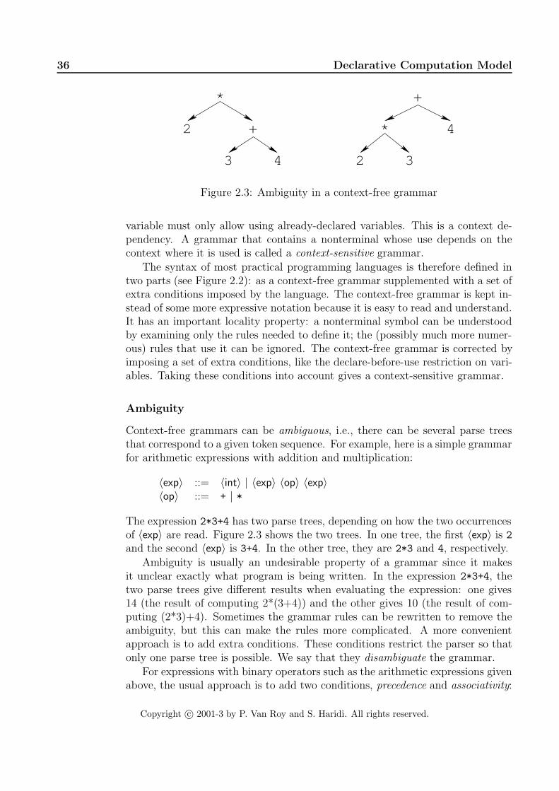
36 Declarative Computation Model
*
+
3 4
+
*
2 3
2 4
Figure 2.3: Ambiguity in a context-free grammar
variable must only allow using already-declared variables. This is a context de-pendency. A grammar that contains a nonterminal whose use depends on thecontext where it is used is called a context-sensitive grammar.
The syntax of most practical programming languages is therefore defined intwo parts (see Figure 2.2): as a context-free grammar supplemented with a set ofextra conditions imposed by the language. The context-free grammar is kept in-stead of some more expressive notation because it is easy to read and understand.It has an important locality property: a nonterminal symbol can be understoodby examining only the rules needed to define it; the (possibly much more numer-ous) rules that use it can be ignored. The context-free grammar is corrected byimposing a set of extra conditions, like the declare-before-use restriction on vari-ables. Taking these conditions into account gives a context-sensitive grammar.
Ambiguity
Context-free grammars can be ambiguous, i.e., there can be several parse treesthat correspond to a given token sequence. For example, here is a simple grammarfor arithmetic expressions with addition and multiplication:
〈exp〉 ::= 〈int〉 | 〈exp〉 〈op〉 〈exp〉〈op〉 ::= + | *
The expression 2*3+4 has two parse trees, depending on how the two occurrencesof 〈exp〉 are read. Figure 2.3 shows the two trees. In one tree, the first 〈exp〉 is 2and the second 〈exp〉 is 3+4. In the other tree, they are 2*3 and 4, respectively.
Ambiguity is usually an undesirable property of a grammar since it makesit unclear exactly what program is being written. In the expression 2*3+4, thetwo parse trees give different results when evaluating the expression: one gives14 (the result of computing 2*(3+4)) and the other gives 10 (the result of com-puting (2*3)+4). Sometimes the grammar rules can be rewritten to remove theambiguity, but this can make the rules more complicated. A more convenientapproach is to add extra conditions. These conditions restrict the parser so thatonly one parse tree is possible. We say that they disambiguate the grammar.
For expressions with binary operators such as the arithmetic expressions givenabove, the usual approach is to add two conditions, precedence and associativity:
Copyright c© 2001-3 by P. Van Roy and S. Haridi. All rights reserved.

2.1 Defining practical programming languages 37
• Precedence is a condition on an expression with different operators, like2*3+4. Each operator is given a precedence level. Operators with highprecedences are put as deep in the parse tree as possible, i.e., as far awayfrom the root as possible. If * has higher precedence than +, then the parsetree (2*3)+4 is chosen over the alternative 2*(3+4). If * is deeper in thetree than +, then we say that * binds tighter than +.
• Associativity is a condition on an expression with the same operator, like2-3-4. In this case, precedence is not enough to disambiguate because alloperators have the same precedence. We have to choose between the trees(2-3)-4 and 2-(3-4). Associativity determines whether the leftmost orthe rightmost operator binds tighter. If the associativity of - is left, thenthe tree (2-3)-4 is chosen. If the associativity of - is right, then the othertree 2-(3-4) is chosen.
Precedence and associativity are enough to disambiguate all expressions definedwith operators. Appendix C gives the precedence and associativity of all theoperators used in this book.
Syntax notation used in this book
In this chapter and the rest of the book, each new data type and language con-struct is introduced together with a small syntax diagram that shows how it fitsin the whole language. The syntax diagram gives grammar rules for a simplecontext-free grammar of tokens. The notation is carefully designed to satisfy twobasic principles:
• All grammar rules can stand on their own. No later information will everinvalidate a grammar rule. That is, we never give an incorrect grammarrule just to “simplify” the presentation.
• It is always clear by inspection when a grammar rule completely defines anonterminal symbol or when it gives only a partial definition. A partialdefinition always ends in three dots “...”.
All syntax diagrams used in the book are summarized in Appendix C. Thisappendix also gives the lexical syntax of tokens, i.e., the syntax of tokens interms of characters. Here is an example of a syntax diagram with two grammarrules that illustrates our notation:
〈statement〉 ::= skip | 〈expression〉 ´ =´ 〈expression〉 | ...〈expression〉 ::= 〈variable〉 | 〈int〉 | ...
These rules give partial definitions of two nonterminals, 〈statement〉 and 〈expression〉.The first rule says that a statement can be the keyword skip , or two expressionsseparated by the equals symbol =, or something else. The second rule says thatan expression can be a variable, an integer, or something else. To avoid confusion
Copyright c© 2001-3 by P. Van Roy and S. Haridi. All rights reserved.

38 Declarative Computation Model
with the grammar rule’s own syntax, a symbol that occurs literally in the textis always quoted with single quotes. For example, the equals symbol is shown as´ =´ . Keywords are not quoted, since for them no confusion is possible. A choicebetween different possibilities in the grammar rule is given by a vertical bar |.
Here is a second example to give the remaining notation:
〈statement〉 ::= if 〈expression〉 then 〈statement〉{ elseif 〈expression〉 then 〈statement〉 }[ else 〈statement〉 ] end | ...
〈expression〉 ::= ´ [ ´ { 〈expression〉 }+ ´ ] ´ | ...〈label〉 ::= unit | true | false | 〈variable〉 | 〈atom〉
The first rule defines the if statement. There is an optional sequence of elseif
clauses, i.e., there can be any number of occurrences including zero. This isdenoted by the braces { ... }. This is followed by an optional else clause, i.e., itcan occur zero or one times. This is denoted by the brackets [ ... ]. The secondrule defines the syntax of explicit lists. They must have at least one element, e.g.,[5 6 7] is valid but [ ] is not (note the space that separates the [ and the ] ).This is denoted by { ... }+. The third rule defines the syntax of record labels.This is a complete definition. There are five possibilities and no more will everbe given.
2.1.2 Language semantics
The semantics of a language defines what a program does when it executes.Ideally, the semantics should be defined in a simple mathematical structure thatlets us reason about the program (including its correctness, execution time, andmemory use) without introducing any irrelevant details. Can we achieve this for apractical language without making the semantics too complicated? The techniquewe use, which we call the kernel language approach, gives an affirmative answerto this question.
Modern programming languages have evolved through more than five decadesof experience in constructing programmed solutions to complex, real-world prob-lems.1 Modern programs can be quite complex, reaching sizes measured in mil-lions of lines of code, written by large teams of human programmers over manyyears. In our view, languages that scale to this level of complexity are successfulin part because they model some essential aspects of how to construct complexprograms. In this sense, these languages are not just arbitrary constructions ofthe human mind. We would therefore like to understand them in a scientific way,i.e., by explaining their behavior in terms of a simple underlying model. This isthe deep motivation behind the kernel language approach.
1The figure of five decades is somewhat arbitrary. We measure it from the first workingstored-program computer, the Manchester Mark I. According to lab documents, it ran its firstprogram on June 21, 1948 [178].
Copyright c© 2001-3 by P. Van Roy and S. Haridi. All rights reserved.

2.1 Defining practical programming languages 39
Practical language
Kernel language
Translation
proc {Sqr X Y}
fun {Sqr X} X*X endB={Sqr {Sqr A}}
{’*’ X X Y}end
end {Sqr T B} {Sqr A T}local T in - Has a formal semantics (e.g.,
an operational, axiomatic, ordenotational semantics)
-intuitive conceptsContains a minimal set of
Is easy for the programmerto understand and reason in
-
for the programmerProvides useful abstractions-
Can be extended withlinguistic abstractions
-
Figure 2.4: The kernel language approach to semantics
The kernel language approach
This book uses the kernel language approach to define the semantics of program-ming languages. In this approach, all language constructs are defined in termsof translations into a core language known as the kernel language. The kernellanguage approach consists of two parts (see Figure 2.4):
• First, define a very simple language, called the kernel language. This lan-guage should be easy to reason in and be faithful to the space and timeefficiency of the implementation. The kernel language and the data struc-tures it manipulates together form the kernel computation model.
• Second, define a translation scheme from the full programming languageto the kernel language. Each grammatical construct in the full language istranslated into the kernel language. The translation should be as simple aspossible. There are two kinds of translation, namely linguistic abstractionand syntactic sugar. Both are explained below.
The kernel language approach is used throughout the book. Each computationmodel has its kernel language, which builds on its predecessor by adding one newconcept. The first kernel language, which is presented in this chapter, is calledthe declarative kernel language. Many other kernel languages are presented lateron in the book.
Formal semantics
The kernel language approach lets us define the semantics of the kernel language inany way we want. There are four widely-used approaches to language semantics:
Copyright c© 2001-3 by P. Van Roy and S. Haridi. All rights reserved.

40 Declarative Computation Model
• An operational semantics shows how a statement executes in terms of anabstract machine. This approach always works well, since at the end of theday all languages execute on a computer.
• An axiomatic semantics defines a statement’s semantics as the relation be-tween the input state (the situation before executing the statement) andthe output state (the situation after executing the statement). This relationis given as a logical assertion. This is a good way to reason about state-ment sequences, since the output assertion of each statement is the inputassertion of the next. It therefore works well with stateful models, since astate is a sequence of values. Section 6.6 gives an axiomatic semantics ofChapter 6’s stateful model.
• A denotational semantics defines a statement as a function over an ab-stract domain. This works well for declarative models, but can be appliedto other models as well. It gets complicated when applied to concurrentlanguages. Sections 2.7.1 and 4.9.2 explain functional programming, whichis particularly close to denotational semantics.
• A logical semantics defines a statement as a model of a logical theory. Thisworks well for declarative and relational computation models, but is hardto apply to other models. Section 9.3 gives a logical semantics of the declar-ative and relational computation models.
Much of the theory underlying these different semantics is of interest primarily tomathematicians, not to programmers. It is outside the scope of the book to givethis theory. The principal formal semantics we give in this book is an operationalsemantics. We define it for each computation model. It is detailed enough tobe useful for reasoning about correctness and complexity yet abstract enough toavoid irrelevant clutter. Chapter 13 collects all these operational semantics intoa single formalism with a compact and readable notation.
Throughout the book, we give an informal semantics for every new languageconstruct and we often reason informally about programs. These informal pre-sentations are always based on the operational semantics.
Linguistic abstraction
Both programming languages and natural languages can evolve to meet theirneeds. When using a programming language, at some point we may feel the needto extend the language, i.e., to add a new linguistic construct. For example, thedeclarative model of this chapter has no looping constructs. Section 3.6.3 definesa for construct to express certain kinds of loops that are useful for writingdeclarative programs. The new construct is both an abstraction and an additionto the language syntax. We therefore call it a linguistic abstraction. A practicalprogramming language consists of a set of linguistic abstractions.
Copyright c© 2001-3 by P. Van Roy and S. Haridi. All rights reserved.

2.1 Defining practical programming languages 41
There are two phases to defining a linguistic abstraction. First, define a newgrammatical construct. Second, define its translation into the kernel language.The kernel language is not changed. This book gives many examples of usefullinguistic abstractions, e.g., functions (fun ), loops (for ), lazy functions (fun
lazy ), classes (class ), reentrant locks (lock ), and others.2 Some of these arepart of the Mozart system. The others can be added to Mozart with the gump
parser-generator tool [104]. Using this tool is beyond the scope of this book.A simple example of a linguistic abstraction is the function syntax, which
uses the keyword fun . This is explained in Section 2.5.2. We have alreadyprogrammed with functions in Chapter 1. But the declarative kernel languageof this chapter only has procedure syntax. Procedure syntax is chosen for thekernel since all arguments are explicit and there can be multiple outputs. Thereare other, deeper reasons for choosing procedure syntax which are explained laterin this chapter. Because function syntax is so useful, though, we add it as alinguistic abstraction.
We define a syntax for both function definitions and function calls, and atranslation into procedure definitions and procedure calls. The translation letsus answer all questions about function calls. For example, what does {F1 {F2
X} {F3 Y}} mean exactly (nested function calls)? Is the order of these functioncalls defined? If so, what is the order? There are many possibilities. Somelanguages leave the order of argument evaluation unspecified, but assume that afunction’s arguments are evaluated before the function. Other languages assumethat an argument is evaluated when and if its result is needed, not before. So evenas simple a thing as nested function calls does not necessarily have an obvioussemantics. The translation makes it clear what the semantics is.
Linguistic abstractions are useful for more than just increasing the expressive-ness of a program. They can also improve other properties such as correctness,security, and efficiency. By hiding the abstraction’s implementation from the pro-grammer, the linguistic support makes it impossible to use the abstraction in thewrong way. The compiler can use this information to give more efficient code.
Syntactic sugar
It is often convenient to provide a short-cut notation for frequently-occurringidioms. This notation is part of the language syntax and is defined by grammarrules. This notation is called syntactic sugar. Syntactic sugar is analogous tolinguistic abstraction in that its meaning is defined precisely by translating itinto the full language. But it should not be confused with linguistic abstraction:it does not provide a new abstraction, but just reduces program size and improvesprogram readability.
We give an example of syntactic sugar that is based on the local statement.
2Logic gates (gate ) for circuit descriptions, mailboxes (receive ) for message-passingconcurrency, and currying and list comprehensions as in modern functional languages, cf.,Haskell.
Copyright c© 2001-3 by P. Van Roy and S. Haridi. All rights reserved.

42 Declarative Computation Model
Programming language
Mathematical studyof programming
Foundational calculusKernel language Abstract machine
Efficient executionon a real machine
Aid the programmerin reasoning andunderstanding
Translations
Figure 2.5: Translation approaches to language semantics
Local variables can always be defined by using the statement local X in ...
end . When this statement is used inside another, it is convenient to have syntacticsugar that lets us leave out the keywords local and end . Instead of:
if N==1 then [1]else
local L in...
endend
we can write:
if N==1 then [1]else L in
...end
which is both shorter and more readable than the full notation. Other examplesof syntactic sugar are given in Section 2.5.1.
Language design
Linguistic abstractions are a basic tool for language design. Any abstraction thatwe define has three phases in its lifecycle. When first we define it, it has no lin-guistic support, i.e., there is no syntax in the language designed to make it easyto use. If at some point, we suspect that it is especially basic and useful, we candecide to give it linguistic support. It then becomes a linguistic abstraction. Thisis an exploratory phase, i.e., there is no commitment that the linguistic abstrac-tion will become part of the language. If the linguistic abstraction is successful,i.e., it simplifies programs and is useful to programmers, then it becomes part ofthe language.
Copyright c© 2001-3 by P. Van Roy and S. Haridi. All rights reserved.

2.1 Defining practical programming languages 43
Other translation approaches
The kernel language approach is an example of a translation approach to seman-tics, i.e., it is based on a translation from one language to another. Figure 2.5shows the three ways that the translation approach has been used for definingprogramming languages:
• The kernel language approach, used throughout the book, is intended for theprogrammer. Its concepts correspond directly to programming concepts.
• The foundational approach is intended for the mathematician. Examplesare the Turing machine, the λ calculus (underlying functional program-ming), first-order logic (underlying logic programming), and the π calculus(to model concurrency). Because these calculi are intended for formal math-ematical study, they have as few elements as possible.
• The machine approach is intended for the implementor. Programs are trans-lated into an idealized machine, which is traditionally called an abstractmachine or a virtual machine.3 It is relatively easy to translate idealizedmachine code into real machine code.
Because we focus on practical programming techniques, this book uses only thekernel language approach.
The interpreter approach
An alternative to the translation approach is the interpreter approach. The lan-guage semantics is defined by giving an interpreter for the language. New lan-guage features are defined by extending the interpreter. An interpreter is a pro-gram written in language L1 that accepts programs written in another languageL2 and executes them. This approach is used by Abelson & Sussman [2]. In theircase, the interpreter is metacircular, i.e., L1 and L2 are the same language L.Adding new language features, e.g., for concurrency and lazy evaluation, gives anew language L′ which is implemented by extending the interpreter for L.
The interpreter approach has the advantage that it shows a self-containedimplementation of the linguistic abstractions. We do not use the interpreterapproach in this book because it does not in general preserve the execution-timecomplexity of programs (the number of operations needed as a function of inputsize). A second difficulty is that the basic concepts interact with each other inthe interpreter, which makes them harder to understand.
3Strictly speaking, a virtual machine is a software emulation of a real machine, running onthe real machine, that is almost as efficient as the real machine. It achieves this efficiency byexecuting most virtual instructions directly as real instructions. The concept was pioneered byIBM in the early 1960’s in the VM operating system. Because of the success of Java, whichuses the term “virtual machine”, modern usage tends to blur the distinction between abstractand virtual machines.
Copyright c© 2001-3 by P. Van Roy and S. Haridi. All rights reserved.

44 Declarative Computation Model
unbound
unbound
unbound
x
x
x3
2
1
Figure 2.6: A single-assignment store with three unbound variables
unbound
x
x
x3
2
1314
nil1 2 3
Figure 2.7: Two of the variables are bound to values
2.2 The single-assignment store
We introduce the declarative model by first explaining its data structures. Themodel uses a single-assignment store, which is a set of variables that are initiallyunbound and that can be bound to one value. Figure 2.6 shows a store with threeunbound variables x1, x2, and x3. We can write this store as {x1, x2, x3}. Fornow, let us assume we can use integers, lists, and records as values. Figure 2.7shows the store where x1 is bound to the integer 314 and x2 is bound to the list[1 2 3] . We write this as {x1 = 314, x2 = [1 2 3] , x3}.
2.2.1 Declarative variables
Variables in the single-assignment store are called declarative variables. We usethis term whenever there is a possible confusion with other kinds of variables.Later on in the book, we will also call these variables dataflow variables becauseof their role in dataflow execution.
Once bound, a declarative variable stays bound throughout the computationand is indistinguishable from its value. What this means is that it can be usedin calculations as if it were the value. Doing the operation x + y is the same asdoing 11 + 22, if the store is {x = 11, y = 22}.
2.2.2 Value store
A store where all variables are bound to values is called a value store. Anotherway to say this is that a value store is a persistent mapping from variables to
Copyright c© 2001-3 by P. Van Roy and S. Haridi. All rights reserved.

2.2 The single-assignment store 45
"George" 25
x
x
x3
2
1314
nil1 2 3
person
name age
Figure 2.8: A value store: all variables are bound to values
values. A value is a mathematical constant. For example, the integer 314 isa value. Values can also be compound entities. For example, the list [1 2
3] and the record person(name:"George" age:25) are values. Figure 2.8shows a value store where x1 is bound to the integer 314, x2 is bound to thelist [1 2 3] , and x3 is bound to the record person(name:"George" age:25) .Functional languages such as Standard ML, Haskell, and Scheme get by with avalue store since they compute functions on values. (Object-oriented languagessuch as Smalltalk, C++, and Java need a cell store, which consists of cells whosecontent can be modified.)
At this point, a reader with some programming experience may wonder whywe are introducing a single-assignment store, when other languages get by witha value store or a cell store. There are many reasons. The first reason is thatwe want to compute with partial values. For example, a procedure can return anoutput by binding an unbound variable argument. The second reason is declara-tive concurrency, which is the subject of Chapter 4. It is possible because of thesingle-assignment store. The third reason is that it is essential when we extend themodel to deal with relational (logic) programming and constraint programming.Other reasons having to do with efficiency (e.g., tail recursion and difference lists)will become clear in the next chapter.
2.2.3 Value creation
The basic operation on a store is binding a variable to a newly-created value. Wewill write this as xi=value. Here xi refers directly to a variable in the store (andis not the variable’s textual name in a program!) and value refers to a value, e.g.,314 or [1 2 3] . For example, Figure 2.7 shows the store of Figure 2.6 after thetwo bindings:
x1 = 314x2 = [1 2 3]
Copyright c© 2001-3 by P. Van Roy and S. Haridi. All rights reserved.

46 Declarative Computation Model
x1
unbound"X"
Inside the storeIn statement
Figure 2.9: A variable identifier referring to an unbound variable
nil1 2 3
x1
"X"
Inside the store
Figure 2.10: A variable identifier referring to a bound variable
The single-assignment operation xi=value constructs value in the store and thenbinds the variable xi to this value. If the variable is already bound, the operationwill test whether the two values are compatible. If they are not compatible, anerror is signaled (using the exception-handling mechanism, see Section 2.6).
2.2.4 Variable identifiers
So far, we have looked at a store that contains variables and values, i.e., storeentities, with which calculations can be done. It would be nice if we could referto a store entity from outside the store. This is the role of variable identifiers.A variable identifier is a textual name that refers to a store entity from outsidethe store. The mapping from variable identifiers to store entities is called anenvironment.
The variable names in program source code are in fact variable identifiers.For example, Figure 2.9 has an identifier “X” (the capital letter X) that refers tothe store variable x1. This corresponds to the environment {X → x1}. To talkabout any identifier, we will use the notation 〈x〉. The environment {〈x〉 → x1}is the same as before, if 〈x〉 represents X. As we will see later, variable identifiersand their corresponding store entities are added to the environment by the local
and declare statements.
Copyright c© 2001-3 by P. Van Roy and S. Haridi. All rights reserved.

2.2 The single-assignment store 47
x1
nil1 2 3"X"
Inside the store
Figure 2.11: A variable identifier referring to a value
x1
x2
person
unbound"George"
name age
"X"
"Y"
Inside the store
Figure 2.12: A partial value
2.2.5 Value creation with identifiers
Once bound, a variable is indistinguishable from its value. Figure 2.10 shows whathappens when x1 is bound to [1 2 3] in Figure 2.9. With the variable identifierX, we can write the binding as X=[1 2 3] . This is the text a programmer wouldwrite to express the binding. We can also use the notation 〈x〉=[1 2 3] if wewant to be able to talk about any identifier. To make this notation legal in aprogram, 〈x〉 has to be replaced by an identifier.
The equality sign “=” refers to the bind operation. After the bind completes,the identifier “X” still refers to x1, which is now bound to [1 2 3] . This isindistinguishable from Figure 2.11, where X refers directly to [1 2 3] . Followingthe links of bound variables to get the value is called dereferencing. It is invisibleto the programmer.
2.2.6 Partial values
A partial value is a data structure that may contain unbound variables. Fig-ure 2.12 shows the record person(name:"George" age: x2) , referred to by theidentifier X. This is a partial value because it contains the unbound variable x2.The identifier Y refers to x2. Figure 2.13 shows the situation after x2 is boundto 25 (through the bind operation Y=25). Now x1 is a partial value with nounbound variables, which we call a complete value. A declarative variable can
Copyright c© 2001-3 by P. Van Roy and S. Haridi. All rights reserved.
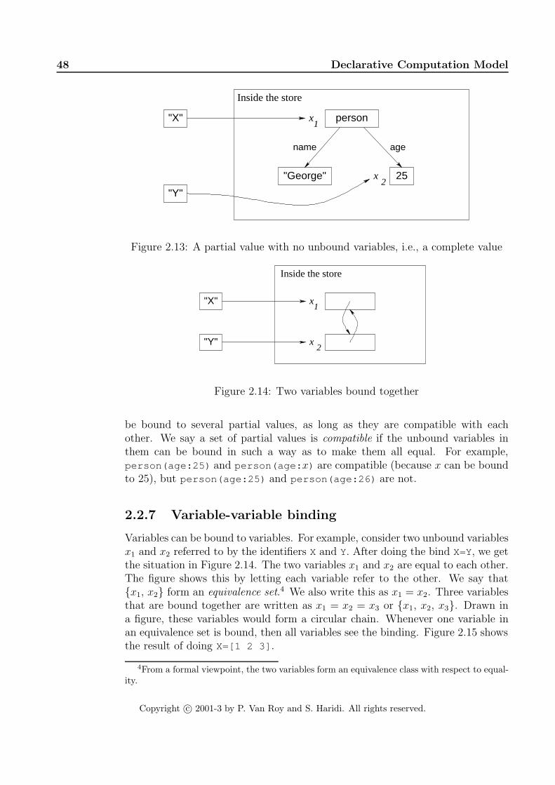
48 Declarative Computation Model
x1
x2
person
25"George"
name age
"X"
"Y"
Inside the store
Figure 2.13: A partial value with no unbound variables, i.e., a complete value
x1
"X"
"Y" x2
Inside the store
Figure 2.14: Two variables bound together
be bound to several partial values, as long as they are compatible with eachother. We say a set of partial values is compatible if the unbound variables inthem can be bound in such a way as to make them all equal. For example,person(age:25) and person(age: x) are compatible (because x can be boundto 25), but person(age:25) and person(age:26) are not.
2.2.7 Variable-variable binding
Variables can be bound to variables. For example, consider two unbound variablesx1 and x2 referred to by the identifiers X and Y. After doing the bind X=Y, we getthe situation in Figure 2.14. The two variables x1 and x2 are equal to each other.The figure shows this by letting each variable refer to the other. We say that{x1, x2} form an equivalence set.4 We also write this as x1 = x2. Three variablesthat are bound together are written as x1 = x2 = x3 or {x1, x2, x3}. Drawn ina figure, these variables would form a circular chain. Whenever one variable inan equivalence set is bound, then all variables see the binding. Figure 2.15 showsthe result of doing X=[1 2 3] .
4From a formal viewpoint, the two variables form an equivalence class with respect to equal-ity.
Copyright c© 2001-3 by P. Van Roy and S. Haridi. All rights reserved.

2.2 The single-assignment store 49
x1
1 2 3 nil
Inside the store
"X"
"Y" x2
Figure 2.15: The store after binding one of the variables
2.2.8 Dataflow variables
In the declarative model, creating a variable and binding it are done separately.What happens if we try to use the variable before it is bound? We call this avariable use error. Some languages create and bind variables in one step, so thatuse errors cannot occur. This is the case for functional programming languages.Other languages allow creating and binding to be separate. Then we have thefollowing possibilities when there is a use error:
1. Execution continues and no error message is given. The variable’s contentis undefined, i.e. it is “garbage”: whatever is found in memory. This iswhat C++ does.
2. Execution continues and no error message is given. The variable is initial-ized to a default value when it is declared, e.g., to 0 for an integer. This iswhat Java does.
3. Execution stops with an error message (or an exception is raised). This iswhat Prolog does for arithmetic operations.
4. Execution waits until the variable is bound and then continues.
These cases are listed in increasing order of niceness. The first case is very bad,since different executions of the same program can give different results. What’smore, since the existence of the error is not signaled, the programmer is not evenaware when this happens. The second is somewhat better. If the program has ause error, then at least it will always give the same result, even if it is a wrongone. Again the programmer is not made aware of the error’s existence.
The third and fourth cases are reasonable in certain situations. In the third,a program with a use error will signal this fact, instead of silently continuing.This is reasonable in a sequential system, since there really is an error. It isunreasonable in a concurrent system, since the result becomes nondeterministic:depending on the timing, sometimes an error is signaled and sometimes not. Inthe fourth, the program will wait until the variable is bound, and then continue.This is unreasonable in a sequential system, since the program will wait forever.
Copyright c© 2001-3 by P. Van Roy and S. Haridi. All rights reserved.
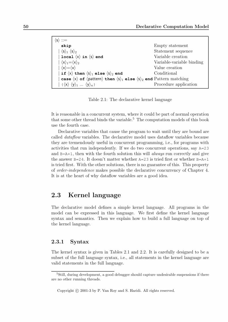
50 Declarative Computation Model
〈s〉 ::=skip Empty statement| 〈s〉1 〈s〉2 Statement sequence| local 〈x〉 in 〈s〉 end Variable creation| 〈x〉1=〈x〉2 Variable-variable binding| 〈x〉=〈v〉 Value creation| if 〈x〉 then 〈s〉1 else 〈s〉2 end Conditional| case 〈x〉 of 〈pattern〉 then 〈s〉1 else 〈s〉2 end Pattern matching| { 〈x〉 〈y〉1 ... 〈y〉n} Procedure application
Table 2.1: The declarative kernel language
It is reasonable in a concurrent system, where it could be part of normal operationthat some other thread binds the variable.5 The computation models of this bookuse the fourth case.
Declarative variables that cause the program to wait until they are bound arecalled dataflow variables. The declarative model uses dataflow variables becausethey are tremendously useful in concurrent programming, i.e., for programs withactivities that run independently. If we do two concurrent operations, say A=23
and B=A+1, then with the fourth solution this will always run correctly and givethe answer B=24. It doesn’t matter whether A=23 is tried first or whether B=A+1
is tried first. With the other solutions, there is no guarantee of this. This propertyof order-independence makes possible the declarative concurrency of Chapter 4.It is at the heart of why dataflow variables are a good idea.
2.3 Kernel language
The declarative model defines a simple kernel language. All programs in themodel can be expressed in this language. We first define the kernel languagesyntax and semantics. Then we explain how to build a full language on top ofthe kernel language.
2.3.1 Syntax
The kernel syntax is given in Tables 2.1 and 2.2. It is carefully designed to be asubset of the full language syntax, i.e., all statements in the kernel language arevalid statements in the full language.
5Still, during development, a good debugger should capture undesirable suspensions if thereare no other running threads.
Copyright c© 2001-3 by P. Van Roy and S. Haridi. All rights reserved.

2.3 Kernel language 51
〈v〉 ::= 〈number〉 | 〈record〉 | 〈procedure〉〈number〉 ::= 〈int〉 | 〈float〉〈record〉, 〈pattern〉 ::= 〈literal〉
| 〈literal〉(〈feature〉1: 〈x〉1 ... 〈feature〉n: 〈x〉n)〈procedure〉 ::= proc { $ 〈x〉1 ... 〈x〉n} 〈s〉 end
〈literal〉 ::= 〈atom〉 | 〈bool〉〈feature〉 ::= 〈atom〉 | 〈bool〉 | 〈int〉〈bool〉 ::= true | false
Table 2.2: Value expressions in the declarative kernel language
Statement syntax
Table 2.1 defines the syntax of 〈s〉, which denotes a statement. There are eightstatements in all, which we will explain later.
Value syntax
Table 2.2 defines the syntax of 〈v〉, which denotes a value. There are three kindsof value expressions, denoting numbers, records, and procedures. For records andpatterns, the arguments 〈x〉1, ..., 〈x〉n must all be distinct identifiers. This ensuresthat all variable-variable bindings are written as explicit kernel operations.
Variable identifier syntax
Table 2.1 uses the nonterminals 〈x〉 and 〈y〉 to denote a variable identifier. Wewill also use 〈z〉 to denote identifiers. There are two ways to write a variableidentifier:
• An uppercase letter followed by zero or more alphanumeric characters (let-ters or digits or underscores), for example X, X1, or ThisIsALongVariable_IsntIt .
• Any sequence of printable characters enclosed within ‘ (back-quote) char-acters, e.g., ` this is a 25$\variable! ` .
A precise definition of identifier syntax is given in Appendix C. All newly-declaredvariables are unbound before any statement is executed. All variable identifiersmust be declared explicitly.
2.3.2 Values and types
A type or data type is a set of values together with a set of operations on thosevalues. A value is “of a type” if it is in the type’s set. The declarative modelis typed in the sense that it has a well-defined set of types, called basic types.For example, programs can calculate with integers or with records, which are all
Copyright c© 2001-3 by P. Van Roy and S. Haridi. All rights reserved.

52 Declarative Computation Model
of integer type or record type, respectively. Any attempt to use an operationwith values of the wrong type is detected by the system and will raise an errorcondition (see Section 2.6). The model imposes no other restrictions on the useof types.
Because all uses of types are checked, it is not possible for a program to behaveoutside of the model, e.g., to crash because of undefined operations on its internaldata structures. It is still possible for a program to raise an error condition, forexample by dividing by zero. In the declarative model, a program that raisesan error condition will terminate immediately. There is nothing in the model tohandle errors. In Section 2.6 we extend the declarative model with a new concept,exceptions, to handle errors. In the extended model, type errors can be handledwithin the model.
In addition to basic types, programs can define their own types, which arecalled abstract data types, ADT for short. Chapter 3 and later chapters showhow to define ADTs.
Basic types
The basic types of the declarative model are numbers (integers and floats), records(including atoms, booleans, tuples, lists, and strings), and procedures. Table 2.2gives their syntax. The nonterminal 〈v〉 denotes a partially constructed value.Later in the book we will see other basic types, including chunks, functors, cells,dictionaries, arrays, ports, classes, and objects. Some of these are explained inAppendix B.
Dynamic typing
There are two basic approaches to typing, namely dynamic and static typing. Instatic typing, all variable types are known at compile time. In dynamic typing,the variable type is known only when the variable is bound. The declarativemodel is dynamically typed. The compiler tries to verify that all operations usevalues of the correct type. But because of dynamic typing, some type checks arenecessarily left for run time.
The type hierarchy
The basic types of the declarative model can be classified into a hierarchy. Fig-ure 2.16 shows this hierarchy, where each node denotes a type. The hierarchyis ordered by set inclusion, i.e., all values of a node’s type are also values of theparent node’s type. For example, all tuples are records and all lists are tuples.This implies that all operations of a type are also legal for a subtype, e.g., alllist operations work also for strings. Later on in the book we will extend thishierarchy. For example, literals can be either atoms (explained below) or anotherkind of constant called names (see Section 3.7.5). The parts where the hierarchyis incomplete are given as “...”.
Copyright c© 2001-3 by P. Van Roy and S. Haridi. All rights reserved.

2.3 Kernel language 53
Literal
...
...Int Float
Number Record
Tuple
Value
Procedure
AtomBool
True False
Char List
String...
...
Figure 2.16: The type hierarchy of the declarative model
2.3.3 Basic types
We give some examples of the basic types and how to write them. See Appendix Bfor more complete information.
• Numbers. Numbers are either integers or floating point numbers. Exam-ples of integers are 314 , 0, and ˜10 (minus 10). Note that the minus signis written with a tilde “˜ ”. Examples of floating point numbers are 1.0 ,3.4 , 2.0e2 , and ˜2.0E˜2 .
• Atoms. An atom is a kind of symbolic constant that can be used as asingle element in calculations. There are several different ways to writeatoms. An atom can be written as a sequence of characters starting witha lowercase letter followed by any number of alphanumeric characters. Anatom can also be written as any sequence of printable characters enclosedin single quotes. Examples of atoms are a_person , donkeyKong3 , and´ #### hello #### ´ .
• Booleans. A boolean is either the symbol true or the symbol false .
• Records. A record is a compound data structure. It consists of a labelfollowed by a set of pairs of features and variable identifiers. Features canbe atoms, integers, or booleans. Examples of records are person(age:X1
name:X2) (with features age and name), person(1:X1 2:X2) , ´ | ´ (1:H
2:T) , ´ #´ (1:H 2:T) , nil , and person . An atom is a record with nofeatures.
• Tuples. A tuple is a record whose features are consecutive integers startingfrom 1. The features do not have to be written in this case. Examples of
Copyright c© 2001-3 by P. Van Roy and S. Haridi. All rights reserved.

54 Declarative Computation Model
tuples are person(1:X1 2:X2) and person(X1 X2) , both of which meanthe same.
• Lists. A list is either the atom nil or the tuple ´ | ´ (H T) (label is verticalbar), where T is either unbound or bound to a list. This tuple is called alist pair or a cons. There is syntactic sugar for lists:
– The ´ | ´ label can be written as an infix operator, so that H|T meansthe same as ´ | ´ (H T) .
– The ´ | ´ operator associates to the right, so that 1|2|3|nil meansthe same as 1|(2|(3|nil)) .
– Lists that end in nil can be written with brackets [ ... ] , so that [1
2 3] means the same as 1|2|3|nil . These lists are called completelists.
• Strings. A string is a list of character codes. Strings can be written withdouble quotes, so that "E=mcˆ2" means the same as [69 61 109 99 94
50] .
• Procedures. A procedure is a value of the procedure type. The statement:
〈x〉=proc {$ 〈y〉1 ... 〈y〉n } 〈s〉 end
binds 〈x〉 to a new procedure value. That is, it simply declares a newprocedure. The $ indicates that the procedure value is anonymous, i.e.,created without being bound to an identifier. There is a syntactic short-cutthat is more familiar:
proc { 〈x〉 〈y〉1 ... 〈y〉n } 〈s〉 end
The $ is replaced by an identifier. This creates the procedure value andimmediately tries to bind it to 〈x〉. This short-cut is perhaps easier to read,but it blurs the distinction between creating the value and binding it to anidentifier.
2.3.4 Records and procedures
We explain why chose records and procedures as basic concepts in the kernellanguage. This section is intended for readers with some programming experiencewho wonder why we designed the kernel language the way we did.
The power of records
Records are the basic way to structure data. They are the building blocks ofmost data structures, including lists, trees, queues, graphs, etc., as we will see inChapter 3. Records play this role to some degree in most programming languages.
Copyright c© 2001-3 by P. Van Roy and S. Haridi. All rights reserved.

2.3 Kernel language 55
But we shall see that their power can go much beyond this role. The extra powerappears in greater or lesser degree depending on how well or how poorly thelanguage supports them. For maximum power, the language should make it easyto create them, take them apart, and manipulate them. In the declarative model,a record is created by simply writing it down, with a compact syntax. A recordis taken apart by simply writing down a pattern, also with a compact syntax.Finally, there are many operations to manipulate records: to add, remove, orselect fields, to convert to a list and back, etc. In general, languages that providethis level of support for records are called symbolic languages.
When records are strongly supported, they can be used to increase the ef-fectiveness of many other techniques. This book focuses on three in particu-lar: object-oriented programming, graphical user interface (GUI) design, andcomponent-based programming. In object-oriented programming, Chapter 7shows how records can represent messages and method heads, which are whatobjects use to communicate. In GUI design, Chapter 10 shows how records canrepresent “widgets”, the basic building blocks of a user interface. In component-based programming, Section 3.9 shows how records can represent modules, whichgroup together related operations.
Why procedures?
A reader with some programming experience may wonder why our kernel languagehas procedures as a basic construct. Fans of object-oriented programming maywonder why we do not use objects instead. Fans of functional programming maywonder why we do not use functions. We could have chosen either possibility,but we did not. The reasons are quite straightforward.
Procedures are more appropriate than objects because they are simpler. Ob-jects are actually quite complicated, as Chapter 7 explains. Procedures are moreappropriate than functions because they do not necessarily define entities thatbehave like mathematical functions.6 For example, we define both componentsand objects as abstractions based on procedures. In addition, procedures are flex-ible because they do not make any assumptions about the number of inputs andoutputs. A function always has exactly one output. A procedure can have anynumber of inputs and outputs, including zero. We will see that procedures are ex-tremely powerful building blocks, when we talk about higher-order programmingin Section 3.6.
6From a theoretical point of view, procedures are “processes” as used in concurrent calculisuch as the π calculus. The arguments are channels. In this chapter we use processes thatare composed sequentially with single-shot channels. Chapters 4 and 5 show other types ofchannels (with sequences of messages) and do concurrent composition of processes.
Copyright c© 2001-3 by P. Van Roy and S. Haridi. All rights reserved.

56 Declarative Computation Model
Operation Description Argument typeA==B Equality comparison ValueA\=B Nonequality comparison Value{IsProcedure P} Test if procedure ValueA=<B Less than or equal comparison Number or AtomA<B Less than comparison Number or AtomA>=B Greater than or equal comparison Number or AtomA>B Greater than comparison Number or AtomA+B Addition NumberA-B Subtraction NumberA*B Multiplication NumberA div B Division IntA mod B Modulo IntA/B Division Float{Arity R} Arity Record{Label R} Label RecordR.F Field selection Record
Table 2.3: Examples of basic operations
2.3.5 Basic operations
Table 2.3 gives the basic operations that we will use in this chapter and the next.There is syntactic sugar for many of these operations so that they can be writtenconcisely as expressions. For example, X=A*B is syntactic sugar for {Number. ´ * ´
A B X}, where Number. ´ * ´ is a procedure associated with the type Number.7
All operations can be denoted in some long way, e.g., Value. ´ ==´ , Value. ´ <´ ,Int. ´ div ´ , Float. ´ / ´ . The table uses the syntactic sugar when it exists.
• Arithmetic. Floating point numbers have the four basic operations, +, - ,* , and / , with the usual meanings. Integers have the basic operations +,- , * , div , and mod, where div is integer division (truncate the fractionalpart) and mod is the integer modulo, i.e., the remainder after a division.For example, 10 mod 3=1.
• Record operations. Three basic operations on records are Arity , Label ,and “. ” (dot, which means field selection). For example, given:
X=person(name:"George" age:25)
then {Arity X} =[age name] , {Label X} =person , and X.age =25 . Thecall to Arity returns a list that contains first the integer features in ascend-ing order and then the atom features in ascending lexicographic order.
7To be precise, Number is a module that groups the operations of the Number type andNumber. ´ * ´ selects the multiplication operation.
Copyright c© 2001-3 by P. Van Roy and S. Haridi. All rights reserved.
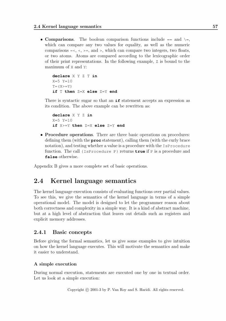
2.4 Kernel language semantics 57
• Comparisons. The boolean comparison functions include == and \= ,which can compare any two values for equality, as well as the numericcomparisons =<, <, >=, and >, which can compare two integers, two floats,or two atoms. Atoms are compared according to the lexicographic orderof their print representations. In the following example, Z is bound to themaximum of X and Y:
declare X Y Z T inX=5 Y=10T=(X>=Y)if T then Z=X else Z=Y end
There is syntactic sugar so that an if statement accepts an expression asits condition. The above example can be rewritten as:
declare X Y Z inX=5 Y=10if X>=Y then Z=X else Z=Y end
• Procedure operations. There are three basic operations on procedures:defining them (with the proc statement), calling them (with the curly bracenotation), and testing whether a value is a procedure with the IsProcedure
function. The call {IsProcedure P} returns true if P is a procedure andfalse otherwise.
Appendix B gives a more complete set of basic operations.
2.4 Kernel language semantics
The kernel language execution consists of evaluating functions over partial values.To see this, we give the semantics of the kernel language in terms of a simpleoperational model. The model is designed to let the programmer reason aboutboth correctness and complexity in a simple way. It is a kind of abstract machine,but at a high level of abstraction that leaves out details such as registers andexplicit memory addresses.
2.4.1 Basic concepts
Before giving the formal semantics, let us give some examples to give intuitionon how the kernel language executes. This will motivate the semantics and makeit easier to understand.
A simple execution
During normal execution, statements are executed one by one in textual order.Let us look at a simple execution:
Copyright c© 2001-3 by P. Van Roy and S. Haridi. All rights reserved.

58 Declarative Computation Model
local A B C D inA=11B=2C=A+BD=C*C
end
This looks simple enough; it will bind D to 169. Let us look more closely at whatit does. The local statement creates four new variables in the store, and makesthe four identifiers A, B, C, D refer to them. (For convenience, this extends slightlythe local statement of Table 2.1.) This is followed by two bindings, A=11 andB=2. The addition C=A+Badds the values of A and B and binds C to the result 13.The multiplication D multiples the value of C by itself and binds D to the result169. This is quite simple.
Variable identifiers and static scoping
We saw that the local statement does two things: it creates a new variableand it sets up an identifier to refer to the variable. The identifier only refers tothe variable inside the local statement, i.e., between the local and the end .We call this the scope of the identifier. Outside of the scope, the identifier doesnot mean the same thing. Let us look closer at what this implies. Consider thefollowing fragment:
local X inX=1local X in
X=2{Browse X}
end{Browse X}
end
What does it display? It displays first 2 and then 1. There is just one identifier,X, but at different points during the execution, it refers to different variables.
Let us summarize this idea. The meaning of an identifier like X is determinedby the innermost local statement that declares X. The area of the programwhere X keeps this meaning is called the scope of X. We can find out the scope ofan identifier by simply inspecting the text of the program; we do not have to doanything complicated like execute or analyze the program. This scoping rule iscalled lexical scoping or static scoping. Later we will see another kind of scopingrule, dynamic scoping, that is sometimes useful. But lexical scoping is by far themost important kind of scoping rule because it is localized, i.e., the meaning ofan identifier can be determined by looking at a small part of the program.
Copyright c© 2001-3 by P. Van Roy and S. Haridi. All rights reserved.

2.4 Kernel language semantics 59
Procedures
Procedures are one of the most important basic building blocks of any language.We give a simple example that shows how to define and call a procedure. Hereis a procedure that binds Z to the maximum of X and Y:
proc {Max X Y ?Z}if X>=Y then Z=X else Z=Y end
end
To make the definition easier to read, we mark the output argument with a ques-tion mark “?”. This has absolutely no effect on execution; it is just a comment.Calling {Max 3 5 C} binds Cto 5. How does the procedure work, exactly? WhenMax is called, the identifiers X, Y, and Z are bound to 3, 5, and the unbound vari-able referenced by C. When Max binds Z, then it binds this variable. Since C
also references this variable, this also binds C. This way of passing parametersis called call by reference. Procedures output results by being passed referencesto unbound variables, which are bound inside the procedure. This book most-ly uses call by reference, both for dataflow variables and for mutable variables.Section 6.4.4 explains some other parameter passing mechanisms.
Procedures with external references
Let us examine the body of Max. It is just an if statement:
if X>=Y then Z=X else Z=Y end
This statement has one particularity, though: it cannot be executed! This isbecause it does not define the identifiers X, Y, and Z. These undefined identifiersare called free identifiers. Sometimes these are called free variables, althoughstrictly speaking they are not variables. When put inside the procedure Max,the statement can be executed, because all the free identifiers are declared asprocedure arguments.
What happens if we define a procedure that only declares some of the freeidentifiers as arguments? For example, let’s define the procedure LB with thesame procedure body as Max, but only two arguments:
proc {LB X ?Z}if X>=Y then Z=X else Z=Y end
end
What does this procedure do when executed? Apparently, it takes any numberX and binds Z to X if X>=Y, but to Y otherwise. That is, Z is always at leastY. What is the value of Y? It is not one of the procedure arguments. It has tobe the value of Y when the procedure is defined. This is a consequence of staticscoping. If Y=9 when the procedure is defined, then calling {LB 3 Z} binds Z to9. Consider the following program fragment:
local Y LB inY=10
Copyright c© 2001-3 by P. Van Roy and S. Haridi. All rights reserved.

60 Declarative Computation Model
proc {LB X ?Z}if X>=Y then Z=X else Z=Y end
endlocal Y=15 Z in
{LB 5 Z}end
end
What does the call {LB 5 Z} bind Z to? It will be bound to 10. The binding Y=15
when LB is called is ignored; it is the binding Y=10 at the procedure definitionthat is important.
Dynamic scoping versus static scoping
Consider the following simple example:
local P Q inproc {Q X} {Browse stat(X)} endproc {P X} {Q X} endlocal Q in
proc {Q X} {Browse dyn(X)} end{P hello}
endend
What should this display, stat(hello) or dyn(hello) ? Static scoping saysthat it will display stat(hello) . In other words, P uses the version of Q thatexists at P’s definition. But there is another solution: P could use the version of Q
that exists at P’s call. This is called dynamic scoping. Both have been used as thedefault scoping rule in programming languages. The original Lisp language wasdynamically scoped. Common Lisp and Scheme, which are descended from Lisp,are statically scoped by default. Common Lisp still allows to declare dynamically-scoped variables, which it calls special variables [181]. Which default is better?The correct default is procedure values with static scoping. This is because aprocedure that works when it is defined will continue to work, independent ofthe environment where it is called. This is an important software engineeringproperty.
Dynamic scoping remains useful in some well-defined areas. For example,consider the case of a procedure whose code is transferred across a network fromone computer to another. Some of this procedure’s external references, for exam-ple calls to common library operations, can use dynamic scoping. This way, theprocedure will use local code for these operations instead of remote code. This ismuch more efficient.8
8However, there is no guarantee that the operation will behave in the same way on the targetmachine. So even for distributed programs the default should be static scoping.
Copyright c© 2001-3 by P. Van Roy and S. Haridi. All rights reserved.

2.4 Kernel language semantics 61
Procedural abstraction
Let us summarize what we learned from Max and LB. Three concepts play animportant role:
• Procedural abstraction. Any statement can be made into a procedure byputting it inside a procedure declaration. This is called procedural abstrac-tion. We also say that the statement is abstracted into a procedure.
• Free identifiers. A free identifier in a statement is an identifier that is notdefined in that statement. It might be defined in an enclosing statement.
• Static scoping. A procedure can have external references, which are freeidentifiers in the procedure body that are not declared as arguments. LB
has one external reference. Max has none. The value of an external referenceis its value when the procedure is defined. This is a consequence of staticscoping.
Procedural abstraction and static scoping together form one of the most powerfultools presented in this book. In the semantics, we will see that they can beimplemented in a simple way.
Dataflow behavior
In the single-assignment store, variables can be unbound. On the other hand,some statements need bound variables, otherwise they cannot execute. For ex-ample, what happens when we execute:
local X Y Z inX=10if X>=Y then Z=X else Z=Y end
end
The comparison X>=Y returns true or false , if it can decide which is the case.If Y is unbound, it cannot decide, strictly speaking. What does it do? Continu-ing with either true or false would be incorrect. Raising an error would be adrastic measure, since the program has done nothing wrong (it has done nothingright either). We decide that the program will simply stop its execution, with-out signaling any kind of error. If some other activity (to be determined later)binds Y then the stopped execution can continue as if nothing had perturbed thenormal flow of execution. This is called dataflow behavior. Dataflow behaviorunderlies a second powerful tool presented in this book, namely concurrency. Inthe semantics, we will see that dataflow behavior can be implemented in a simpleway.
2.4.2 The abstract machine
We will define the kernel semantics as an operational semantics, i.e., it defines themeaning of the kernel language through its execution on an abstract machine. We
Copyright c© 2001-3 by P. Van Roy and S. Haridi. All rights reserved.

62 Declarative Computation Model
U=Z.age X=U+1 if X<2 then ...
Single-assignment store
with dataflow variables)
Semantic stack(statement in execution)
(value store extended
W=atom
Y=42
XZ=person(age: Y)
U
Figure 2.17: The declarative computation model
first define the basic concepts of the abstract machine: environments, semanticstatement, statement stack, execution state, and computation. We then show howto execute a program. Finally, we explain how to calculate with environments,which is a common semantic operation.
Overview of concepts
A running program is defined in terms of a computation, which is a sequence ofexecution states. Let us define exactly what this means. We need the followingconcepts:
• A single-assignment store σ is a set of store variables. These variables arepartitioned into (1) sets of variables that are equal but unbound and (2)variables that are bound to a number, record, or procedure. For example,in the store {x1, x2 = x3, x4 = a| x2}, x1 is unbound, x2 and x3 are equaland unbound, and x4 is bound to the partial value a| x2. A store variablebound to a value is indistinguishable from that value. This is why a storevariable is sometimes called a store entity.
• An environment E is a mapping from variable identifiers to entities in σ.This is explained in Section 2.2. We will write E as a set of pairs, e.g.,{X→ x, Y→ y}, where X, Y are identifiers and x, y refer to store entities.
• A semantic statement is a pair (〈s〉, E) where 〈s〉 is a statement and Eis an environment. The semantic statement relates a statement to what itreferences in the store. The set of possible statements is given in Section 2.3.
• An execution state is a pair (ST, σ) where ST is a stack of semantic state-ments and σ is a single-assignment store. Figure 2.17 gives a picture of theexecution state.
Copyright c© 2001-3 by P. Van Roy and S. Haridi. All rights reserved.

2.4 Kernel language semantics 63
• A computation is a sequence of execution states starting from an initialstate: (ST0, σ0)→ (ST1, σ1)→ (ST2, σ2)→ ....
A single transition in a computation is called a computation step. A computationstep is atomic, i.e., there are no visible intermediate states. It is as if the stepis done “all at once”. In this chapter, all computations are sequential, i.e., theexecution state contains exactly one statement stack, which is transformed by alinear sequence of computation steps.
Program execution
Let us execute a program in this semantics. A program is simply a statement 〈s〉.Here is how to execute the program:
• The initial execution state is:
([(〈s〉, φ)], φ)
That is, the initial store is empty (no variables, empty set φ) and the initialexecution state has just one semantic statement (〈s〉, φ) in the stack ST.The semantic statement contains 〈s〉 and an empty environment (φ). Weuse brackets [...] to denote the stack.
• At each step, the first element of ST is popped and execution proceedsaccording to the form of the element.
• The final execution state (if there is one) is a state in which the semanticstack is empty.
A semantic stack ST can be in one of three run-time states:
• Runnable: ST can do a computation step.
• Terminated: ST is empty.
• Suspended: ST is not empty, but it cannot do any computation step.
Calculating with environments
A program execution often does calculations with environments. An environmentE is a function that maps variable identifiers 〈x〉 to store entities (both unboundvariables and values). The notation E(〈x〉) retrieves the entity associated with theidentifier 〈x〉 from the store. To define the semantics of the abstract machine in-structions, we need two common operations on environments, namely adjunctionand restriction.
Adjunction defines a new environment by adding a mapping to an existingone. The notation:
E + {〈x〉 → x}
Copyright c© 2001-3 by P. Van Roy and S. Haridi. All rights reserved.

64 Declarative Computation Model
denotes a new environment E ′ constructed from E by adding the mapping {〈x〉 →x}. This mapping overrides any other mapping from the identifier 〈x〉. That is,E ′(〈x〉) is equal to x, and E ′(〈y〉) is equal to E(〈y〉) for all identifiers 〈y〉 differentfrom 〈x〉. When we need to add more than one mapping at once, we writeE + {〈x〉1 → x1, ..., 〈x〉n → xn}.
Restriction defines a new environment whose domain is a subset of an existingone. The notation:
E|{〈x〉1,...,〈x〉n}
denotes a new environment E ′ such that dom(E ′) = dom(E)∩{〈x〉1, ..., 〈x〉n} andE′(〈x〉) = E(〈x〉) for all 〈x〉 ∈ dom(E ′). That is, the new environment does notcontain any identifiers other than those mentioned in the set.
2.4.3 Non-suspendable statements
We first give the semantics of the statements that can never suspend.
The skip statement
The semantic statement is:
(skip , E)
Execution is complete after this pair is popped from the semantic stack.
Sequential composition
The semantic statement is:
(〈s〉1 〈s〉2, E)
Execution consists of the following actions:
• Push (〈s〉2, E) on the stack.
• Push (〈s〉1, E) on the stack.
Variable declaration (the local statement)
The semantic statement is:
(local 〈x〉 in 〈s〉 end , E)
Execution consists of the following actions:
• Create a new variable x in the store.
• Let E ′ be E + {〈x〉 → x}, i.e., E ′ is the same as E except that it adds amapping from 〈x〉 to x.
• Push (〈s〉, E′) on the stack.
Copyright c© 2001-3 by P. Van Roy and S. Haridi. All rights reserved.

2.4 Kernel language semantics 65
Variable-variable binding
The semantic statement is:
(〈x〉1 = 〈x〉2, E)
Execution consists of the following action:
• Bind E(〈x〉1) and E(〈x〉2) in the store.
Value creation
The semantic statement is:
(〈x〉 = 〈v〉, E)
where 〈v〉 is a partially constructed value that is either a record, number, orprocedure. Execution consists of the following actions:
• Create a new variable x in the store.
• Construct the value represented by 〈v〉 in the store and let x refer to it. Allidentifiers in 〈v〉 are replaced by their store contents as given by E.
• Bind E(〈x〉) and x in the store.
We have seen how to construct record and number values, but what about pro-cedure values? In order to explain them, we have first to explain the concept oflexical scoping.
Lexical scoping revisited
A statement 〈s〉 can contain many occurrences of variable identifiers. For eachidentifier occurrence, we can ask the question: where was this identifier declared?If the declaration is in some statement (part of 〈s〉 or not) that textually surrounds(i.e., encloses) the occurrence, then we say that the declaration obeys lexicalscoping. Because the scope is determined by the source code text, this is alsocalled static scoping.
Identifier occurrences in a statement can be bound or free with respect to thatstatement. An identifier occurrence X is bound with respect to a statement 〈s〉if it is declared inside 〈s〉, i.e., in a local statement, in the pattern of a case
statement, or as argument of a procedure declaration. An identifier occurrencethat is not bound is free. Free occurrences can only exist in incomplete programfragments, i.e., statements that cannot run. In a running program, it is alwaystrue that every identifier occurrence is bound.
Copyright c© 2001-3 by P. Van Roy and S. Haridi. All rights reserved.

66 Declarative Computation Model
Bound identifier occurrences and bound variables
Do not confuse a bound identifier occurrence with abound variable! A bound identifier occurrence does notexist at run time; it is a textual variable name that tex-tually occurs inside a construct that declares it (e.g., aprocedure or variable declaration). A bound variable ex-ists at run time; it is a dataflow variable that is boundto a partial value.
Here is an example with both free and bound occurrences:
local Arg1 Arg2 inArg1=111*111Arg2=999*999Res=Arg1+Arg2
end
In this statement, all variable identifiers are declared with lexical scoping. Theidentifier occurrences Arg1 and Arg2 are bound and the occurrence Res is free.This statement cannot be run. To make it runnable, it has to be part of a biggerstatement that declares Res. Here is an extension that can run:
local Res inlocal Arg1 Arg2 in
Arg1=111*111Arg2=999*999Res=Arg1+Arg2
end{Browse Res}
end
This can run since it has no free identifier occurrences.
Procedure values (closures)
Let us see how to construct a procedure value in the store. It is not as simple asone might imagine because procedures can have external references. For example:
proc {LowerBound X ?Z}if X>=Y then Z=X else Z=Y end
end
In this example, the if statement has three free variables, X, Y, and Z. Twoof them, X and Z, are also formal parameters. The third, Y, is not a formalparameter. It has to be defined by the environment where the procedure isdeclared. The procedure value itself must have a mapping from Y to the store.Otherwise, we could not call the procedure since Y would be a kind of danglingreference.
Let us see what happens in the general case. A procedure expression is writtenas:
Copyright c© 2001-3 by P. Van Roy and S. Haridi. All rights reserved.

2.4 Kernel language semantics 67
proc { $ 〈y〉1 ... 〈y〉n} 〈s〉 end
The statement 〈s〉 can have free variable identifiers. Each free identifer is either aformal parameter or not. The first kind are defined anew each time the procedureis called. They form a subset of the formal parameters {〈y〉1, ..., 〈y〉n}. The secondkind are defined once and for all when the procedure is declared. We call themthe external references of the procedure. Let us write them as {〈z〉1, ..., 〈z〉k}.Then the procedure value is a pair:
( proc { $ 〈y〉1 ... 〈y〉n} 〈s〉 end , CE )
Here CE (the contextual environment) is E|{〈z〉1,...,〈z〉n}, where E is the environ-ment when the procedure is declared. This pair is put in the store just like anyother value.
Because it contains an environment as well as a procedure definition, a pro-cedure value is often called a closure or a lexically-scoped closure. This is becauseit “closes” (i.e., packages up) the environment at procedure definition time. Thisis also called environment capture. When the procedure is called, the contextu-al environment is used to construct the environment of the executing procedurebody.
2.4.4 Suspendable statements
There are three statements remaining in the kernel language:
〈s〉 ::= ...| if 〈x〉 then 〈s〉1 else 〈s〉2 end
| case 〈x〉 of 〈pattern〉 then 〈s〉1 else 〈s〉2 end
| { 〈x〉 〈y〉1 ... 〈y〉n}
What should happen with these statements if 〈x〉 is unbound? From the discussionin Section 2.2.8, we know what should happen. The statements should simplywait until 〈x〉 is bound. We say that they are suspendable statements. They havean activation condition, which is a condition that must be true for executionto continue. The condition is that E(〈x〉) must be determined, i.e., bound to anumber, record, or procedure.
In the declarative model of this chapter, once a statement suspends it willnever continue, because there is no other execution that could make the activationcondition true. The program simply stops executing. In Chapter 4, when weintroduce concurrent programming, we will have executions with more than onesemantic stack. A suspended stack ST can become runnable again if another stackdoes an operation that makes ST’s activation condition true. In that chapter weshall see that communication from one stack to another through the activationcondition is the basis of dataflow execution. For now, let us stick with just onesemantic stack.
Copyright c© 2001-3 by P. Van Roy and S. Haridi. All rights reserved.

68 Declarative Computation Model
Conditional (the if statement)
The semantic statement is:
(if 〈x〉 then 〈s〉1 else 〈s〉2 end , E)
Execution consists of the following actions:
• If the activation condition is true (E(〈x〉) is determined), then do the fol-lowing actions:
– If E(〈x〉) is not a boolean (true or false ) then raise an error condi-tion.
– If E(〈x〉) is true , then push (〈s〉1, E) on the stack.
– If E(〈x〉) is false , then push (〈s〉2, E) on the stack.
• If the activation condition is false, then execution does not continue. Theexecution state is kept as is. We say that execution suspends. The stop canbe temporary. If some other activity in the system makes the activationcondition true, then execution can resume.
Procedure application
The semantic statement is:
({ 〈x〉 〈y〉1 ... 〈y〉n} , E)
Execution consists of the following actions:
• If the activation condition is true (E(〈x〉) is determined), then do the fol-lowing actions:
– If E(〈x〉) is not a procedure value or is a procedure with a number ofarguments different from n, then raise an error condition.
– If E(〈x〉) has the form (proc { $ 〈z〉1 ... 〈z〉n} 〈s〉 end , CE) then push(〈s〉, CE + {〈z〉1 → E(〈y〉1), ..., 〈z〉n → E(〈y〉n)}) on the stack.
• If the activation condition is false, then suspend execution.
Pattern matching (the case statement)
The semantic statement is:
(case 〈x〉 of 〈lit〉(〈feat〉1: 〈x〉1 ... 〈feat〉n: 〈x〉n) then 〈s〉1 else 〈s〉2 end , E)
(Here 〈lit〉 and 〈feat〉 are synonyms for 〈literal〉 and 〈feature〉.) Execution consistsof the following actions:
Copyright c© 2001-3 by P. Van Roy and S. Haridi. All rights reserved.

2.4 Kernel language semantics 69
• If the activation condition is true (E(〈x〉) is determined), then do the fol-lowing actions:
– If the label of E(〈x〉) is 〈lit〉 and its arity is [〈feat〉1 · · · 〈feat〉n], thenpush (〈s〉1, E + {〈x〉1 → E(〈x〉).〈feat〉1, ..., 〈x〉n → E(〈x〉).〈feat〉n}) onthe stack.
– Otherwise push (〈s〉2, E) on the stack.
• If the activation condition is false, then suspend execution.
2.4.5 Basic concepts revisited
Now that we have seen the kernel semantics, let us look again at the examples ofSection 2.4.1 to see exactly what they are doing. We look at three examples; wesuggest you do the others as exercises.
Variable identifiers and static scoping
We saw before that the following statement 〈s〉 displays first 2 and then 1:
〈s〉 ≡
local X in
X=1
〈s〉1 ≡
local X in
X=2
{Browse X}
end
〈s〉2 ≡ {Browse X}
end
The same identifier X first refers to 2 and then refers to 1. We can understandbetter what happens by executing 〈s〉 in our abstract machine.
1. The initial execution state is:
( [(〈s〉, φ)], φ )
Both the environment and the store are empty (E = φ and σ = φ).
2. After executing the outermost local statement and the binding X=1, weget:
( [(〈s〉1〈s〉2, {X→ x})],{x = 1} )
The identifier X refers to the store variable x, which is bound to 1. Thenext statement to be executed is the sequential composition 〈s〉1〈s〉2.
3. After executing the sequential composition, we get:
Copyright c© 2001-3 by P. Van Roy and S. Haridi. All rights reserved.

70 Declarative Computation Model
( [(〈s〉1, {X→ x}), (〈s〉2, {X→ x})],{x = 1} )
Each of the statements 〈s〉1 and 〈s〉2 has its own environment. At this point,the two environments have identical values.
4. Let us start executing 〈s〉1. The first statement in 〈s〉1 is a local statement.Executing it gives:
( [(X=2 {Browse X} , {X→ x′}), (〈s〉2, {X→ x})],{x′, x = 1} )
This creates the new variable x′ and calculates the new environment {X→x}+ {X→ x′}, which is {X→ x′}. The second mapping of X overrides thefirst.
5. After the binding X=2 we get:
( [({Browse X} , {X→ x′}), ({Browse X} , {X→ x})],{x′ = 2, x = 1} )
(Remember that 〈s〉2 is a Browse .) Now we see why the two Browse callsdisplay different values. It is because they have different environments. Theinner local statement is given its own environment, in which X refers toanother variable. This does not affect the outer local statement, whichkeeps its environment no matter what happens in any other instruction.
Procedure definition and call
Our next example defines and calls the procedure Max, which calculates the max-imum of two numbers. With the semantics we can see precisely what happens
Copyright c© 2001-3 by P. Van Roy and S. Haridi. All rights reserved.

2.4 Kernel language semantics 71
during the definition and execution of Max. Here is the example in kernel syntax:
〈s〉 ≡
local Max in
local A in
local B in
local C in
〈s〉1 ≡
Max=proc {$ X Y Z}
〈s〉3 ≡
local T in
T=(X>=Y)
〈s〉4 ≡ if T then Z=X else Z=Y end
end
end
A=3
B=5
〈s〉2 ≡ {Max A B C}
end
end
end
end
This statement is in the kernel language syntax. We can see it as the expandedform of:
local Max C inproc {Max X Y ?Z}
if X>=Y then Z=X else Z=Y endend{Max 3 5 C}
end
This is much more readable but it means exactly the same as the verbose version.We have added the following three short-cuts:
• Declaring more than one variable in a local declaration. This is translatedinto nested local declarations.
• Using “in-line” values instead of variables, e.g., {P 3} is a short-cut forlocal X in X=3 {P X} end .
• Using nested operations, e.g., putting the operation X>=Y in place of theboolean in the if statement.
We will use these short-cuts in all examples from now on.Let us now execute statement 〈s〉. For clarity, we omit some of the interme-
diate steps.
1. The initial execution state is:
( [(〈s〉, φ)], φ )
Copyright c© 2001-3 by P. Van Roy and S. Haridi. All rights reserved.

72 Declarative Computation Model
Both the environment and the store are empty (E = φ and σ = φ).
2. After executing the four local declarations, we get:
( [(〈s〉1, {Max→ m, A→ a, B→ b, C→ c})],{m, a, b, c} )
The store contains the four variables m, a, b, and c. The environment of〈s〉1 has mappings to these variables.
3. After executing the bindings of Max, A, and B, we get:
( [({Max A B C} , {Max→ m, A→ a, B→ b, C→ c})],{m = (proc {$ X Y Z} 〈s〉3 end , φ), a = 3, b = 5, c} )
The variables m, a, and b are now bound to values. The procedure isready to be called. Notice that the contextual environment of Max is emptybecause it has no free identifiers.
4. After executing the procedure application, we get:
( [(〈s〉3, {X→ a, Y→ b, Z→ c})],{m = (proc {$ X Y Z} 〈s〉3 end , φ), a = 3, b = 5, c} )
The environment of 〈s〉3 now has mappings from the new identifiers X, Y,and Z.
5. After executing the comparison X>=Y, we get:
( [(〈s〉4, {X→ a, Y→ b, Z→ c, T→ t})],{m = (proc {$ X Y Z} 〈s〉3 end , φ), a = 3, b = 5, c, t = false } )
This adds the new identifier T and its variable t bound to false .
6. Execution is complete after statement 〈s〉4 (the conditional):
( [], {m = (proc {$ X Y Z} 〈s〉3 end , φ), a = 3, b = 5, c = 5, t = false } )
The statement stack is empty and c is bound to 5.
Procedure with external references (part 1)
The second example defines and calls the procedure LowerBound , which ensuresthat a number will never go below a given lower bound. The example is interestingbecause LowerBound has an external reference. Let us see how the following codeexecutes:
Copyright c© 2001-3 by P. Van Roy and S. Haridi. All rights reserved.

2.4 Kernel language semantics 73
local LowerBound Y C inY=5proc {LowerBound X ?Z}
if X>=Y then Z=X else Z=Y endend{LowerBound 3 C}
end
This is very close to the Max example. The body of LowerBound is identicalto the body of Max. The only difference is that LowerBound has an externalreference. The procedure value is:
( proc {$ X Z} if X>=Y then Z=X else Z=Y end end , {Y→ y} )
where the store contains:
y = 5
When the procedure is defined, i.e., when the procedure value is created, theenvironment has to contain a mapping of Y. Now let us apply this procedure. Weassume that the procedure is called as {LowerBound A C} , where A is bound to3. Before the application we have:
( [({LowerBound A C} , {Y→ y, LowerBound → lb, A→ a, C→ c})],{ lb = (proc {$ X Z} if X>=Y then Z=X else Z=Y end end , {Y→ y}),
y = 5, a = 3, c} )
After the application we get:
( [(if X>=Y then Z=X else Z=Y end , {Y→ y, X→ a, Z→ c})],{ lb = (proc {$ X Z} if X>=Y then Z=X else Z=Y end end , {Y→ y}),
y = 5, a = 3, c} )
The new environment is calculated by starting with the contextual environment({Y → y} in the procedure value) and adding mappings from the formal argu-ments X and Z to the actual arguments a and c.
Procedure with external references (part 2)
In the above execution, the identifier Y refers to y in both the calling environmentas well as the contextual environment of LowerBound . How would the executionchange if the following statement were executed instead of {LowerBound 3 C} :
local Y inY=10{LowerBound 3 C}
end
Here Y no longer refers to y in the calling environment. Before looking at theanswer, please put down the book, take a piece of paper, and work it out. Justbefore the application we have almost the same situation as before:
Copyright c© 2001-3 by P. Van Roy and S. Haridi. All rights reserved.

74 Declarative Computation Model
( [({LowerBound A C} , {Y→ y′, LowerBound → lb, A→ a, C→ c})],{ lb = (proc {$ X Z} if X>=Y then Z=X else Z=Y end end , {Y→ y}),
y′ = 10, y = 5, a = 3, c} )
The calling environment has changed slightly: Y refers to a new variable y′, whichis bound to 10. When doing the application, the new environment is calculatedin exactly the same way as before, starting from the contextual environment andadding the formal arguments. This means that the y′ is ignored! We get exactlythe same situation as before in the semantic stack:
( [(if X>=Y then Z=X else Z=Y end , {Y→ y, X→ a, Z→ c})],{ lb = (proc {$ X Z} if X>=Y then Z=X else Z=Y end end , {Y→ y}),
y′ = 10, y = 5, a = 3, c} )
The store still has the binding y′ = 10. But y′ is not referenced by the semanticstack, so this binding makes no difference to the execution.
2.4.6 Last call optimization
Consider a recursive procedure with just one recursive call which happens tobe the last call in the procedure body. We call such a procedure tail-recursive.Our abstract machine executes a tail-recursive procedure with a constant stacksize. This is because our abstract machine does last call optimization. This issometimes called tail recursion optimization, but the latter terminology is lessprecise since the optimization works for any last call, not just tail-recursive calls(see Exercises). Consider the following procedure:
proc {Loop10 I}if I==10 then skipelse
{Browse I}{Loop10 I+1}
endend
Calling {Loop10 0} displays successive integers from 0 up to 9. Let us see howthis procedure executes.
• The initial execution state is:
( [({Loop10 0} , E0)],σ )
where E0 is the environment at the call.
• After executing the if statement, this becomes:
( [({Browse I} , {I → i0}) ({Loop10 I+1} , {I → i0})],{i0 = 0} ∪ σ )
Copyright c© 2001-3 by P. Van Roy and S. Haridi. All rights reserved.

2.4 Kernel language semantics 75
• After executing the Browse , we get to the first recursive call:
( [({Loop10 I+1} , {I → i0})],{i0 = 0} ∪ σ )
• After executing the if statement in the recursive call, this becomes:
( [({Browse I} , {I → i1}) ({Loop10 I+1} , {I → i1})],{i0 = 0, i1 = 1} ∪ σ )
• After executing the Browse again, we get to the second recursive call:
( [({Loop10 I+1} , {I → i1})],{i0 = 0, i1 = 1} ∪ σ )
It is clear that the stack at the kth recursive call is always of the form:
[({Loop10 I+1} , {I → ik−1})]
There is just one semantic statement and its environment is of constant size. Thisis the last call optimization. This shows the efficient way to program loops in thedeclarative model: the loop should be invoked through a last call.
2.4.7 Active memory and memory management
In the Loop10 example, the semantic stack and the store have very differentbehaviors. The semantic stack is bounded by a constant size. On the other hand,the store grows bigger at each call. At the kth recursive call, the store has theform:
{i0 = 0, i1 = 1, ..., ik−1 = k − 1} ∪ σ
Let us see why this growth is not a problem in practice. Look carefully at thesemantic stack. The variables {i0, i1, ..., ik−2} are not needed for executing thiscall. The only variable needed is ik−1. Removing the not-needed variables givesa smaller store:
{ik−1 = k − 1} ∪ σ
Executing with this smaller store gives exactly the same results as before!From the semantics it follows that a running program needs only the infor-
mation in the semantic stack and in the part of the store reachable from thesemantic stack. A partial value is reachable if it is referenced by a statement onthe semantic stack or by another reachable partial value. The semantic stack andthe reachable part of the store are together called the active memory. The restof the store can safely be reclaimed, i.e., the memory it uses can be reused forother purposes. Since the active memory size of the Loop10 example is boundedby a small constant, it can loop indefinitely without exhausting system memory.
Copyright c© 2001-3 by P. Van Roy and S. Haridi. All rights reserved.

76 Declarative Computation Model
(either manually or byReclaim
(program execution)Become inactive
Deallocate
Allocate
Active
Inactive
Free
garbage collection)
Figure 2.18: Lifecycle of a memory block
Memory use cycle
Memory consists of a sequence of words. This sequence is divided up into blocks,where a block consists of a sequence of one or more words used to store a lan-guage entity or part of a language entity. Blocks are the basic unit of memoryallocation. Figure 2.18 shows the lifecycle of a memory block. Each block of mem-ory continuously cycles through three states: active, inactive, and free. Memorymanagement is the task of making sure that memory circulates correctly alongthis cycle. A running program that needs a block of memory will allocate it froma pool of free memory blocks. During its execution, a running program may nolonger need some of the memory it allocated:
• If it can determine this directly, then it deallocates this memory. Thismakes it immediately become free again. This is what happens with thesemantic stack in the Loop10 example.
• If it cannot determine this directly, then the memory becomes inactive. It issimply no longer reachable by the running program. This is what happenswith the store in the Loop10 example.
Usually, memory used for managing control flow (the semantic stack) can bedeallocated and memory used for data structures (the store) becomes inactive.
Inactive memory must eventually be reclaimed, i.e., the system must recognizethat it is inactive and put it back in the pool of free memory. Otherwise, thesystem has a memory leak and will soon run out of memory. Reclaiming inactivememory is the hardest part of memory management, because recognizing thatmemory is unreachable is a global condition. It depends on the whole executionstate of the running program. Low-level languages like C or C++ often leavereclaiming to the programmer, which is a major source of program errors. Thereare two kinds of program error that can occur:
• Dangling reference. This happens when a block is reclaimed even though itis still reachable. The system will eventually reuse this block. This means
Copyright c© 2001-3 by P. Van Roy and S. Haridi. All rights reserved.

2.4 Kernel language semantics 77
that data structures will be corrupted in unpredictable ways, causing theprogram to crash. This error is especially pernicious since the effect (thecrash) is usually very far away from the cause (the incorrect reclaiming).This makes dangling references hard to debug.
• Memory leak. This happens when an unreachable block is considered as stillreachable, and so is not reclaimed. The effect is that active memory sizekeeps growing indefinitely until eventually the system’s memory resourcesare exhausted. Memory leaks are less dangerous than dangling referencesbecause programs can continue running for some time before the error forcesthem to stop. Long-lived programs, such as operating systems and servers,must not have any memory leaks.
Garbage collection
Many high-level languages, such as Erlang, Haskell, Java, Lisp, Prolog, Smalltalk,and so forth, do automatic reclaiming. That is, reclaiming is done by the sys-tem independently of the running program. This completely eliminates danglingreferences and greatly reduces memory leaks. This relieves the programmer ofmost of the difficulties of manual memory management. Automatic reclaimingis called garbage collection. Garbage collection is a well-known technique thathas been used for a long time. It was used in the 1960’s for early Lisp systems.Until the 1990’s, mainstream languages did not use it because it was incorrectlyjudged as being too inefficient. It has finally become acceptable in mainstreamprogramming because of the popularity of the Java language.
A typical garbage collector has two phases. In the first phase, it determineswhat the active memory is. It does this finding all data structures that arereachable starting from an initial set of pointers called the root set. The root setis the set of pointers that are always needed by the program. In the abstractmachine defined so far, the root set is simply the semantic stack. In general, theroot set includes all pointers in ready threads and all pointers in operating systemdata structures. We will see this when we extend the machine to implementthe new concepts introduced in later chapters. The root set also includes somepointers related to distributed programming (namely references from remote sites;see Chapter 11).
In the second phase, the garbage collector compacts the memory. That is, itcollects all the active memory blocks into one contiguous block (a block withoutholes) and the free memory blocks into one contiguous block.
Modern garbage collection algorithms are efficient enough that most applica-tions can use them with only small memory and time penalties [95]. The mostwidely-used garbage collectors run in a “batch” mode, i.e., they are dormant mostof the time and run only when the total amount of active and inactive memoryreaches a predefined threshold. While the garbage collector runs, the programdoes not fulfill its task. This is perceived as an occasional pause in programexecution. Usually this pause is small enough not to be disruptive.
Copyright c© 2001-3 by P. Van Roy and S. Haridi. All rights reserved.

78 Declarative Computation Model
There exist garbage collection algorithms, called real-time garbage collectors,that can run continuously, interleaved with the program execution. They can beused in cases, such as hard real-time programming, in which there must not beany pauses.
Garbage collection is not magic
Having garbage collection lightens the burden of memory management for thedeveloper, but it does not eliminate it completely. There are two cases that remainthe developer’s responsibility: avoiding memory leaks and managing externalresources.
Avoiding memory leaks It is the programmer’s responsibility to avoid mem-ory leaks. If the program continues to reference a data structure that it no longerneeds, then that data structure’s memory will never be recovered. The programshould be careful to lose all references to data structures no longer needed.
For example, take a recursive function that traverses a list. If the list’s headis passed to the recursive call, then list memory will not be recovered during thefunction’s execution. Here is an example:
L=[1 2 3 ... 1000000]
fun {Sum X L1 L}case L1 of Y|L2 then {Sum X+Y L2 L}else X end
end
{Browse {Sum 0 L L}}
Sumsums the elements of a list. But it also keeps a reference to L, the originallist, even though it does not need L. This means L will stay in memory duringthe whole execution of Sum. A better definition is as follows:
fun {Sum X L1}case L1 of Y|L2 then {Sum X+Y L2}else X end
end
{Browse {Sum 0 L}}
Here the reference to L is lost immediately. This example is trivial. But things canbe more subtle. For example, consider an active data structure S that containsa list of other data structures D1, D2, ..., Dn. If one of these, say Di , is no longerneeded by the program, then it should be removed from the list. Otherwise itsmemory will never be recovered.
A well-written program therefore has to do some “cleanup” after itself: makingsure that it no longer references data structures that it no longer needs. The
Copyright c© 2001-3 by P. Van Roy and S. Haridi. All rights reserved.

2.4 Kernel language semantics 79
cleanup can be done in the declarative model, but it is cumbersome.9
Managing external resources A Mozart program often needs data structuresthat are external to its operating system process. We call such a data structurean external resource. External resources affect memory management in two ways.An internal Mozart data structure can refer to an external resource and vice versa.Both possibilities need some programmer intervention. Let us consider each caseseparately.
The first case is when a Mozart data structure refers to an external resource.For example, a record can correspond to a graphic entity in a graphics display orto an open file in a file system. If the record is no longer needed, then the graphicentity has to be removed or the file has to be closed. Otherwise, the graphicsdisplay or the file system will have a memory leak. This is done with a techniquecalled finalization, which defines actions to be taken when data structures becomeunreachable. Finalization is explained in Section 6.9.2.
The second case is when an external resource needs a Mozart data structure.This is often straightforward to handle. For example, consider a scenario wherethe Mozart program implements a database server that is accessed by externalclients. This scenario has a simple solution: never do automatic reclaiming ofthe database storage. Other scenarios may not be so simple. A general solutionis to set aside a part of the Mozart program to represent the external resource.This part should be active (i.e., have its own thread) so that it is not reclaimedhaphazardly. It can be seen as a “proxy” for the resource. The proxy keeps a ref-erence to the Mozart data structure as long as the resource needs it. The resourceinforms the proxy when it no longer needs the data structure. Section 6.9.2 givesanother technique.
The Mozart garbage collector
The Mozart system does automatic memory management. It has both a localgarbage collector and a distributed garbage collector. The latter is used fordistributed programming and is explained in Chapter 11. The local garbagecollector uses a copying dual-space algorithm.
The garbage collector divides memory into two spaces, which each takes uphalf of available memory space. At any instant, the running program sits com-pletely in one half. Garbage collection is done when there is no more free memoryin that half. The garbage collector finds all data structures that are reachablefrom the root set and copies them to the other half of memory. Since they arecopied to one contiguous memory block this also does compaction.
The advantage of a copying garbage collector is that its execution time isproportional to the active memory size, not to the total memory size. Smallprograms will garbage collect quickly, even if they are running in a large memoryspace. The two disadvantages of a copying garbage collector are that half the
9It is more efficiently done with explicit state (see Chapter 6).
Copyright c© 2001-3 by P. Van Roy and S. Haridi. All rights reserved.

80 Declarative Computation Model
memory is unusable at any given time and that long-lived data structures (likesystem tables) have to be copied at each garbage collection. Let us see howto remove these two disadvantages. Copying long-lived data can be avoided byusing a modified algorithm called a generational garbage collector. This partitionsactive memory into generations. Long-lived data structures are put in oldergenerations, which are collected less often.
The memory disadvantage is only important if the active memory size ap-proaches the maximum addressable memory size of the underlying architecture.Mainstream computer technology is currently in a transition period from 32-bitto 64-bit addressing. In a computer with 32-bit addresses, the limit is reachedwhen active memory size is 1000 MB or more. (The limit is usually not 4000MB due to limitations in the operating system.) At the time of writing, thislimit is reached by large programs in high-end personal computers. For suchprograms, we recommend to use a computer with 64-bit addresses, which has nosuch problem.
2.5 From kernel language to practical language
The kernel language has all the concepts needed for declarative programming.But trying to use it for practical declarative programming shows that it is toominimal. Kernel programs are just too verbose. It turns out that most of thisverbosity can be eliminated by judiciously adding syntactic sugar and linguisticabstractions. This section does just that:
• It defines a set of syntactic conveniences that give a more concise and read-able full syntax.
• It defines an important linguistic abstraction, namely functions, that isuseful for concise and readable programming.
• It explains the interactive interface of the Mozart system and shows howit relates to the declarative model. This brings in the declare statement,which is a variant of the local statement designed for interactive use.
The resulting language is used in Chapter 3 to explain the programming tech-niques of the declarative model.
2.5.1 Syntactic conveniences
The kernel language defines a simple syntax for all its constructs and types. Thefull language has the following conveniences to make this syntax more usable:
• Nested partial values can be written in a concise way.
• Variables can be both declared and initialized in one step.
Copyright c© 2001-3 by P. Van Roy and S. Haridi. All rights reserved.

2.5 From kernel language to practical language 81
• Expressions can be written in a concise way.
• The if and case statements can be nested in a concise way.
• The new operators andthen and orelse are defined as conveniences fornested if statements.
• Statements can be converted into expressions by using a nesting marker.
The nonterminal symbols used in the kernel syntax and semantics correspond asfollows to those in the full syntax:
Kernel syntax Full syntax〈x〉, 〈y〉, 〈z〉 〈variable〉〈s〉 〈statement〉, 〈stmt〉
Nested partial values
In Table 2.2, the syntax of records and patterns implies that their arguments arevariables. In practice, many partial values are nested deeper than this. Becausenested values are so often used, we give syntactic sugar for them. For example,we extend the syntax to let us write person(name:"George" age:25) insteadof the more cumbersome version:
local A B in A="George" B=25 X=person(name:A age:B) end
where X is bound to the nested record.
Implicit variable initialization
To make programs shorter and easier to read, there is syntactic sugar to bind avariable immediately when it is declared. The idea is to put a bind operationbetween local and in . Instead of local X in X=10 {Browse X} end , inwhich X is mentioned three times, the short-cut lets one write local X=10 in
{Browse X} end , which mentions X only twice. A simple case is the following:
local X=〈expression〉 in 〈statement〉 end
This declares X and binds it to the result of 〈expression〉. The general case is:
local 〈pattern〉=〈expression〉 in 〈statement〉 end
where 〈pattern〉 is any partial value. This declares all the variables in 〈pattern〉and then binds 〈pattern〉 to the result of 〈expression〉. In both cases, the variablesoccurring on the left-hand side of the equality, i.e., X or the variables in 〈pattern〉,are the ones declared.
Implicit variable initialization is convenient for taking apart a complex da-ta structure. For example, if T is bound to the record tree(key:a left:L
right:R value:1) , then just one equality is enough to extract all four fields:
Copyright c© 2001-3 by P. Van Roy and S. Haridi. All rights reserved.

82 Declarative Computation Model
〈expression〉 ::= 〈variable〉 | 〈int〉 | 〈float〉 || 〈expression〉 〈evalBinOp〉 〈expression〉| ´ ( ´ 〈expression〉 〈evalBinOp〉 〈expression〉 ´ ) ´
| ´ { ´ 〈expression〉 { 〈expression〉 } ´ } ´
| ...〈evalBinOp〉 ::= ´ +´ | ´ - ´ | ´ * ´ | ´ / ´ | div | mod |
| ´ ==´ | ´ \= ´ | ´ <´ | ´ =<´ | ´ >´ | ´ >=´ | ...
Table 2.4: Expressions for calculating with numbers
localtree(key:A left:B right:C value:D)=T
in〈statement〉
end
This is a kind of pattern matching. T must have the right structure, otherwisean exception is raised. This does part of the work of the case statement, whichgeneralizes this so that the programmer decides what to do if the pattern is notmatched. Without the short-cut, the following is needed:
local A B C D in{Label T}=treeA=T.keyB=T.leftC=T.rightD=T.value〈statement〉
end
which is both longer and harder to read. What if T has more than four fields,but we want to extract just four? Then we can use the following notation:
localtree(key:A left:B right:C value:D ...)=T
in〈statement〉
end
The “... ” means that there may be other fields in T.
Expressions
An expression is syntactic sugar for a sequence of operations that returns a value.It is different from a statement, which is also a sequence of operations but doesnot return a value. An expression can be used inside a statement whenever avalue is needed. For example, 11*11 is an expression and X=11*11 is a statement.Semantically, an expression is defined by a straightforward translation into kernel
Copyright c© 2001-3 by P. Van Roy and S. Haridi. All rights reserved.

2.5 From kernel language to practical language 83
〈statement〉 ::= if 〈expression〉 then 〈inStatement〉{ elseif 〈expression〉 then 〈inStatement〉 }[ else 〈inStatement〉 ] end
| ...〈inStatement〉 ::= [ { 〈declarationPart〉 }+ in ] 〈statement〉
Table 2.5: The if statement
〈statement〉 ::= case 〈expression〉of 〈pattern〉 [ andthen 〈expression〉 ] then 〈inStatement〉{ ´ [] ´ 〈pattern〉 [ andthen 〈expression〉 ] then 〈inStatement〉 }[ else 〈inStatement〉 ] end
| ...〈pattern〉 ::= 〈variable〉 | 〈atom〉 | 〈int〉 | 〈float〉
| 〈string〉 | unit | true | false
| 〈label〉 ´ ( ´ { [ 〈feature〉 ´ : ´ ] 〈pattern〉 } [ ´ ... ´ ] ´ ) ´
| 〈pattern〉 〈consBinOp〉 〈pattern〉| ´ [ ´ { 〈pattern〉 }+ ´ ] ´
〈consBinOp〉 ::= ´ #´ | ´ | ´
Table 2.6: The case statement
syntax. So X=11*11 is translated into {Mul 11 11 X} , where Mul is a three-argument procedure that does multiplication.10
Table 2.4 shows the syntax of expressions that calculate with numbers. Lateron we will see expressions for calculating with other data types. Expressions arebuilt hierarchically, starting from basic expressions (e.g., variables and numbers)and combining them together. There are two ways to combine them: usingoperators (e.g., the addition 1+2+3+4 ) or using function calls (e.g., the squareroot {Sqrt 5.0} ).
Nested if and case statements
We add syntactic sugar to make it easy to write if and case statements withmultiple alternatives and complicated conditions. Table 2.5 gives the syntax ofthe full if statement. Table 2.6 gives the syntax of the full case statement and itspatterns. (Some of the nonterminals in these tables are defined in Appendix C.)These statements are translated into the primitive if and case statements ofthe kernel language. Here is an example of a full case statement:
case Xs#Ysof nil#Ys then 〈s〉1
10Its real name is Number. ´ * ´ , since it is part of the Number module.
Copyright c© 2001-3 by P. Van Roy and S. Haridi. All rights reserved.

84 Declarative Computation Model
[] Xs#nil then 〈s〉2[] (X|Xr)#(Y|Yr) andthen X=<Y then 〈s〉3else 〈s〉4 end
It consists of a sequence of alternative cases delimited with the “[] ” symbol. Thealternatives are often called clauses. This statement translates into the followingkernel syntax:
case Xs of nil then 〈s〉1else
case Ys of nil then 〈s〉2else
case Xs of X|Xr thencase Ys of Y|Yr then
if X=<Y then 〈s〉3 else 〈s〉4 endelse 〈s〉4 end
else 〈s〉4 endend
end
The translation illustrates an important property of the full case statement:clauses are tested sequentially starting with the first clause. Execution continuespast a clause only if the clause’s pattern is inconsistent with the input argument.
Nested patterns are handled by looking first at the outermost pattern and thenworking inwards. The nested pattern (X|Xr)#(Y|Yr) has one outer pattern ofthe form A#B and two inner patterns of the form A|B . All three patterns are tuplesthat are written with infix syntax, using the infix operators ´ #´ and ´ | ´ . Theycould have been written with the usual syntax as ´ #´ (A B) and ´ | ´ (A B) . Eachinner pattern (X|Xr) and (Y|Yr) is put in its own primitive case statement.The outer pattern using ´ #´ disappears from the translation because it occursalso in the case ’s input argument. The matching with ´ #´ can therefore be doneat translation time.
The operators andthen and orelse
The operators andthen and orelse are used in calculations with boolean values.The expression:
〈expression〉1 andthen 〈expression〉2translates into:
if 〈expression〉1 then 〈expression〉2 else false end
The advantage of using andthen is that 〈expression〉2 is not evaluated if 〈expression〉1is false . There is an analogous operator orelse . The expression:
〈expression〉1 orelse 〈expression〉2translates into:
if 〈expression〉1 then true else 〈expression〉2 end
Copyright c© 2001-3 by P. Van Roy and S. Haridi. All rights reserved.

2.5 From kernel language to practical language 85
〈statement〉 ::= fun ´ { ´ 〈variable〉 { 〈pattern〉 } ´ } ´ 〈inExpression〉 end
| ...〈expression〉 ::= fun ´ { ´ ´ $´ { 〈pattern〉 } ´ } ´ 〈inExpression〉 end
| proc ´ { ´ ´ $´ { 〈pattern〉 } ´ } ´ 〈inStatement〉 end
| ´ { ´ 〈expression〉 { 〈expression〉 } ´ } ´
| local { 〈declarationPart〉 }+ in 〈expression〉 end
| if 〈expression〉 then 〈inExpression〉{ elseif 〈expression〉 then 〈inExpression〉 }[ else 〈inExpression〉 ] end
| case 〈expression〉of 〈pattern〉 [ andthen 〈expression〉 ] then 〈inExpression〉{ ´ [] ´ 〈pattern〉 [ andthen 〈expression〉 ] then 〈inExpression〉 }[ else 〈inExpression〉 ] end
| ...〈inStatement〉 ::= [ { 〈declarationPart〉 }+ in ] 〈statement〉〈inExpression〉 ::= [ { 〈declarationPart〉 }+ in ] [ 〈statement〉 ] 〈expression〉
Table 2.7: Function syntax
That is, 〈expression〉2 is not evaluated if 〈expression〉1 is true .
Nesting markers
The nesting marker “$” turns any statement into an expression. The expression’svalue is what is at the position indicated by the nesting marker. For example, thestatement {P X1 X2 X3} can be written as {P X1 $ X3} , which is an expressionwhose value is X2. This makes the source code more concise, since it avoids havingto declare and use the identifier X2. The variable corresponding to X2 is hiddenfrom the source code.
Nesting markers can make source code more readable to a proficient program-mer, while making it harder for a beginner to see how the code translates to thekernel language. We will use them only when they greatly increase readability.For example, instead of writing:
local X in {Obj get(X)} {Browse X} end
we will instead write {Browse {Obj get($)}} . Once you get used to nestingmarkers, they are both concise and clear. Note that the syntax of procedurevalues as explained in Section 2.3.3 is consistent with the nesting marker syntax.
2.5.2 Functions (the fun statement)
The declarative model provides a linguistic abstraction for programming withfunctions. This is our first example of a linguistic abstraction, as defined in
Copyright c© 2001-3 by P. Van Roy and S. Haridi. All rights reserved.

86 Declarative Computation Model
Section 2.1.2. We define the new syntax for function definitions and functioncalls and show how they are translated into the kernel language.
Function definitions
A function definition differs from a procedure definition in two ways: it is intro-duced with the keyword fun and the body must end with an expression. Forexample, a simple definition is:
fun {F X1 ... XN} 〈statement〉 〈expression〉 end
This translates to the following procedure definition:
proc {F X1 ... XN ?R} 〈statement〉 R=〈expression〉 end
The extra argument R is bound to the expression in the procedure body. If thefunction body is an if statement, then each alternative of the if can end in anexpression:
fun {Max X Y}if X>=Y then X else Y end
end
This translates to:
proc {Max X Y ?R}R = if X>=Y then X else Y end
end
We can further translate this by transforming the if from an expression to astatement. This gives the final result:
proc {Max X Y ?R}if X>=Y then R=X else R=Y end
end
Similar rules apply for the local and case statements, and for other statementswe will see later. Each statement can be used as an expression. Roughly speak-ing, whenever an execution sequence in a procedure ends in a statement, thecorresponding sequence in a function ends in an expression. Table 2.7 gives thecomplete syntax of expressions. This table takes all the statements we have seenso far and shows how to use them as expressions. In particular, there are alsofunction values, which are simply procedure values written in functional syntax.
Function calls
A function call {F X1 ... XN} translates to the procedure call {F X1 ... XN
R} , where R replaces the function call where it is used. For example, the followingnested call of F:
{Q {F X1 ... XN} ... }
is translated to:
Copyright c© 2001-3 by P. Van Roy and S. Haridi. All rights reserved.

2.5 From kernel language to practical language 87
local R in{F X1 ... XN R}{Q R ... }
end
In general, nested functions are evaluated before the function in which they arenested. If there are several, then they are evaluated in the order they appear inthe program.
Function calls in data structures
There is one more rule to remember for function calls. It has to do with a callinside a data structure (record, tuple, or list). Here is an example:
Ys={F X}|{Map Xr F}
In this case, the translation puts the nested calls after the bind operation:
local Y Yr inYs=Y|Yr{F X Y}{Map Xr F Yr}
end
This ensures that the recursive call is last. Section 2.4.6 explains why this isimportant for execution efficiency. The full Map function is defined as follows:
fun {Map Xs F}case Xsof nil then nil[] X|Xr then {F X}|{Map Xr F}end
end
Map applies the function F to all elements of a list and returns the result. Hereis an example call:
{Browse {Map [1 2 3 4] fun {$ X} X*X end }}
This displays [1 4 9 16] . The definition of Map translates as follows to thekernel language:
proc {Map Xs F ?Ys}case Xs of nil then Ys=nilelse case Xs of X|Xr then
local Y Yr inYs=Y|Yr{F X Y}{Map Xr F Yr}
endend end
end
Copyright c© 2001-3 by P. Van Roy and S. Haridi. All rights reserved.

88 Declarative Computation Model
〈interStatement〉 ::= 〈statement〉| declare { 〈declarationPart〉 }+ [ 〈interStatement〉 ]| declare { 〈declarationPart〉 }+ in 〈interStatement〉
〈declarationPart〉 ::= 〈variable〉 | 〈pattern〉 ´ =´ 〈expression〉 | 〈statement〉
Table 2.8: Interactive statement syntax
"Browse" procedure value
x1
"Browse" procedure value
x1
unbound
unboundx2
unboundx4
unboundx3
"X"
"Y"
unbound"X"
"Y" x2
unbound
Result of second declare X YResult of first declare X Y
Figure 2.19: Declaring global variables
The dataflow variable Yr is used as a “placeholder” for the result in the recursivecall {Map Xr F Yr} . This lets the recursive call be the last call. In our model,this means that the recursion executes with the same space and time efficiencyas an iterative construct like a while loop.
2.5.3 Interactive interface (the declare statement)
The Mozart system has an interactive interface that allows to introduce programfragments incrementally and execute them as they are introduced. The fragmentshave to respect the syntax of interactive statements, which is given in Table 2.8.An interactive statement is either any legal statement or a new form, the declare
statement. We assume that the user feeds interactive statements to the systemone by one. (In the examples given throughout this book, the declare statementis often left out. It should be added if the example declares new variables.)
The interactive interface allows to do much more than just feed statements.It has all the functionality needed for software development. Appendix A givesa summary of some of this functionality. For now, we assume that the user justknows how to feed statements.
The interactive interface has a single, global environment. The declare
statement adds new mappings to this environment. It follows that declare can
Copyright c© 2001-3 by P. Van Roy and S. Haridi. All rights reserved.

2.5 From kernel language to practical language 89
only be used interactively, not in standalone programs. Feeding the followingdeclaration:
declare X Y
creates two new variables in the store, x1 and x2. and adds mappings from X andY to them. Because the mappings are in the global environment we say that X
and Y are global variables or interactive variables. Feeding the same declarationa second time will cause X and Y to map to two other new variables, x3 and x4.Figure 2.19 shows what happens. The original variables, x1 and x2, are still in thestore, but they are no longer referred to by X and Y. In the figure, Browse mapsto a procedure value that implements the browser. The declare statement addsnew variables and mappings, but leaves existing variables in the store unchanged.
Adding a new mapping to an identifier that already maps to a variable maycause the variable to become inaccessible, if there are no other references to it.If the variable is part of a calculation, then it is still accessible from within thecalculation. For example:
declare X YX=25declare AA=person(age:X)declare X Y
Just after the binding X=25, X maps to 25, but after the second declare X
Y it maps to a new unbound variable. The 25 is still accessible through theglobal variable A, which is bound to the record person(age:25) . The recordcontains 25 because X mapped to 25 when the binding A=person(age:X) wasexecuted. The second declare X Ychanges the mapping of X, but not the recordperson(age:25) since the record already exists in the store. This behavior ofdeclare is designed to support a modular programming style. Executing aprogram fragment will not cause the results of any previously-executed fragmentto change.
There is a second form of declare :
declare X Y in 〈stmt〉which declares two global variables, as before, and then executes 〈stmt〉. Thedifference with the first form is that 〈stmt〉 declares no variables (unless it containsa declare ).
The Browser
The interactive interface has a tool, called the Browser, which allows to look intothe store. This tool is available to the programmer as a procedure called Browse .The procedure Browse has one argument. It is called as {Browse 〈expr〉} , where〈expr〉 is any expression. It can display partial values and it will update thedisplay whenever the partial values are bound more. Feeding the following:
{Browse 1}
Copyright c© 2001-3 by P. Van Roy and S. Haridi. All rights reserved.

90 Declarative Computation Model
Figure 2.20: The Browser
displays the integer 1. Feeding:
declare Y in{Browse Y}
displays just the name of the variable, namely Y. No value is displayed. Thismeans that Y is currently unbound. Figure 2.20 shows the browser window afterthese two operations. If Y is bound, e.g., by doing Y=2, then the browser willupdate its display to show this binding.
Dataflow execution
We saw earlier that declarative variables support dataflow execution, i.e., anoperation waits until all arguments are bound before executing. For sequentialprograms this is not very useful, since the program will wait forever. On theother hand, it is useful for concurrent programs, in which more than one instruc-tion sequence can be executing at the same time. An independently-executinginstruction sequence is called a thread. Programming with more than one threadis called concurrent programming; it is introduced in Chapter 4.
All examples in this chapter execute in a single thread. To be precise, eachprogram fragment fed into the interactive interface executes in its own thread.This lets us give simple examples of dataflow execution in this chapter. Forexample, feed the following statement:
declare A B C inC=A+B{Browse C}
This will display nothing, since the instruction C=A+B blocks (both of its argu-ments are unbound). Now, feed the following statement:
A=10
This will bind A, but the instruction C=A+B still blocks since B is still unbound.Finally, feed the following:
Copyright c© 2001-3 by P. Van Roy and S. Haridi. All rights reserved.

2.6 Exceptions 91
B=200
This displays 210 in the browser. Any operation, not just addition, will blockif it does not get enough input information to calculate its result. For example,comparisons can block. The equality comparison X==Y will block if it cannotdecide whether or not X is equal to or different from Y. This happens, e.g., if oneor both of the variables are unbound.
Programming errors often result in dataflow suspensions. If you feed a state-ment that should display a result and nothing is displayed, then the probablecause of the problem is a blocked operation. Carefully check all operations tomake sure that their arguments are bound. Ideally, the system’s debugger shoulddetect when a program has blocked operations that cannot continue.
2.6 Exceptions
How do we handle exceptional situations within a program? For example, dividingby zero, opening a nonexistent file, or selecting a nonexistent field of a record?These errors do not occur in a correct program, so they should not encumbernormal programming style. On the other hand, they do occur sometimes. Itshould be possible for programs to manage these errors in a simple way. Thedeclarative model cannot do this without adding cumbersome checks throughoutthe program. A more elegant way is to extend the model with an exception-handling mechanism. This section does exactly that. We give the syntax andsemantics of the extended model and explain what exceptions look like in the fulllanguage.
2.6.1 Motivation and basic concepts
In the semantics of Section 2.4, we speak of “raising an error” when a statementcannot continue correctly. For example, a conditional raises an error when itsargument is a non-boolean value. Up to now, we have been deliberately vagueabout exactly what happens next. Let us now be more precise. We would like tobe able to detect these errors and handle them from within a running program.The program should not stop when they occur. Rather, it should in a controlledway transfer execution to another part, called the exception handler, and passthe exception handler a value that describes the error.
What should the exception-handling mechanism look like? We can make twoobservations. First, it should be able to confine the error, i.e., quarantine it so thatit does not contaminate the whole program. We call this the error confinementprinciple:
Assume that the program is made up of interacting “components”organized in hierarchical fashion. Each component is built of smallercomponents. We put “component” in quotes because the languagedoes not need to have a component concept. It just needs to be
Copyright c© 2001-3 by P. Van Roy and S. Haridi. All rights reserved.

92 Declarative Computation Model
= raise exception
= exception-catchingexecution context
execution context=jump
Figure 2.21: Exception handling
compositional, i.e., programs are built in layered fasion. Then theerror confinement principle states that an error in a component shouldbe catchable at the component boundary. Outside the component, theerror is either invisible or reported in a nice way.
Therefore, the mechanism causes a “jump” from inside the component to itsboundary. The second observation is that this jump should be a single operation.The mechanism should be able, in a single operation, to exit from arbitrarilymany levels of nested context. Figure 2.21 illustrates this. In our semantics, acontext is simply an entry on the semantic stack, i.e., an instruction that has tobe executed later. Nested contexts are created by procedure calls and sequentialcompositions.
The declarative model cannot jump out in a single operation. The jump hasto be coded explicitly as little hops, one per context, using boolean variables andconditionals. This makes programs more cumbersome, especially since the extracoding has to be added everywhere that an error can possibly occur. It can beshown theoretically that the only way to keep programs simple is to extend themodel [103, 105].
We propose a simple extension to the model that satisfies these conditions. Weadd two statements: the try statement and the raise statement. The try state-ment creates an exception-catching context together with an exception handler.The raise statement jumps to the boundary of the innermost exception-catchingcontext and invokes the exception handler there. Nested try statements createnested contexts. Executing try 〈s〉 catch 〈x〉 then 〈s〉1 end is equivalent to ex-ecuting 〈s〉, if 〈s〉 does not raise an exception. On the other hand, if 〈s〉 raises anexception, i.e., by executing a raise statement, then the (still ongoing) execu-tion of 〈s〉 is aborted. All information related to 〈s〉 is popped from the semanticstack. Control is transferred to 〈s〉1, passing it a reference to the exception in 〈x〉.
Copyright c© 2001-3 by P. Van Roy and S. Haridi. All rights reserved.

2.6 Exceptions 93
Any partial value can be an exception. This means that the exception-handling mechanism is extensible by the programmer, i.e., new exceptions can bedefined as they are needed by the program. This lets the programmer foresee newexceptional situations. Because an exception can be an unbound variable, raisingan exception and determining what the exception is can be done concurrently. Inother words, an exception can be raised (and caught) before it is known whichexception it is! This is quite reasonable in a language with dataflow variables:we may at some point know that there exists a problem but not know yet whichproblem.
An example
Let us give a simple example of exception handling. Consider the following func-tion, which evaluates simple arithmetic expressions and returns the result:
fun {Eval E}if {IsNumber E} then Eelse
case Eof plus(X Y) then {Eval X}+{Eval Y}[] times(X Y) then {Eval X}*{Eval Y}else raise illFormedExpr(E) endend
endend
For this example, we say an expression is ill-formed if it is not recognized byEval , i.e., if it contains other values than numbers, plus , and times . Tryingto evaluate an ill-formed expression E will raise an exception. The exception isa tuple, illFormedExpr(E) , that contains the ill-formed expression. Here is anexample of using Eval :
try{Browse {Eval plus(plus(5 5) 10)}}{Browse {Eval times(6 11)}}{Browse {Eval minus(7 10)}}
catch illFormedExpr(E) then{Browse ´ *** Illegal expression ´ #E#´ *** ´ }
end
If any call to Eval raises an exception, then control transfers to the catch clause,which displays an error message.
2.6.2 The declarative model with exceptions
We extend the declarative computation model with exceptions. Table 2.9 givesthe syntax of the extended kernel language. Programs can use two new state-ments, try and raise . In addition, there is a third statement, catch 〈x〉 then
Copyright c© 2001-3 by P. Van Roy and S. Haridi. All rights reserved.

94 Declarative Computation Model
〈s〉 ::=skip Empty statement| 〈s〉1 〈s〉2 Statement sequence| local 〈x〉 in 〈s〉 end Variable creation| 〈x〉1=〈x〉2 Variable-variable binding| 〈x〉=〈v〉 Value creation| if 〈x〉 then 〈s〉1 else 〈s〉2 end Conditional| case 〈x〉 of 〈pattern〉 then 〈s〉1 else 〈s〉2 end Pattern matching| { 〈x〉 〈y〉1 ... 〈y〉n} Procedure application| try 〈s〉1 catch 〈x〉 then 〈s〉2 end Exception context| raise 〈x〉 end Raise exception
Table 2.9: The declarative kernel language with exceptions
〈s〉 end , that is needed internally for the semantics and is not allowed in pro-grams. The catch statement is a “marker” on the semantic stack that definesthe boundary of the exception-catching context. We now give the semantics ofthese statements.
The try statement
The semantic statement is:
(try 〈s〉1 catch 〈x〉 then 〈s〉2 end , E)
Execution consists of the following actions:
• Push the semantic statement (catch 〈x〉 then 〈s〉2 end , E) on the stack.
• Push (〈s〉1, E) on the stack.
The raise statement
The semantic statement is:
(raise 〈x〉 end , E)
Execution consists of the following actions:
• Pop elements off the stack looking for a catch statement.
– If a catch statement is found, pop it from the stack.
– If the stack is emptied and no catch is found, then stop executionwith the error message “Uncaught exception”.
• Let (catch 〈y〉 then 〈s〉 end , Ec) be the catch statement that is found.
Copyright c© 2001-3 by P. Van Roy and S. Haridi. All rights reserved.
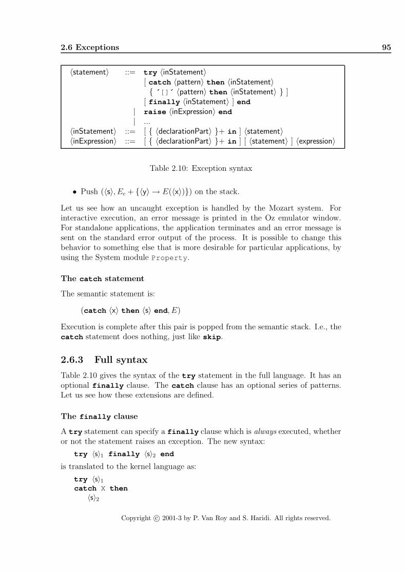
2.6 Exceptions 95
〈statement〉 ::= try 〈inStatement〉[ catch 〈pattern〉 then 〈inStatement〉{ ´ [] ´ 〈pattern〉 then 〈inStatement〉 } ]
[ finally 〈inStatement〉 ] end
| raise 〈inExpression〉 end
| ...〈inStatement〉 ::= [ { 〈declarationPart〉 }+ in ] 〈statement〉〈inExpression〉 ::= [ { 〈declarationPart〉 }+ in ] [ 〈statement〉 ] 〈expression〉
Table 2.10: Exception syntax
• Push (〈s〉, Ec + {〈y〉 → E(〈x〉)}) on the stack.
Let us see how an uncaught exception is handled by the Mozart system. Forinteractive execution, an error message is printed in the Oz emulator window.For standalone applications, the application terminates and an error message issent on the standard error output of the process. It is possible to change thisbehavior to something else that is more desirable for particular applications, byusing the System module Property .
The catch statement
The semantic statement is:
(catch 〈x〉 then 〈s〉 end , E)
Execution is complete after this pair is popped from the semantic stack. I.e., thecatch statement does nothing, just like skip .
2.6.3 Full syntax
Table 2.10 gives the syntax of the try statement in the full language. It has anoptional finally clause. The catch clause has an optional series of patterns.Let us see how these extensions are defined.
The finally clause
A try statement can specify a finally clause which is always executed, whetheror not the statement raises an exception. The new syntax:
try 〈s〉1 finally 〈s〉2 end
is translated to the kernel language as:
try 〈s〉1catch X then〈s〉2
Copyright c© 2001-3 by P. Van Roy and S. Haridi. All rights reserved.

96 Declarative Computation Model
raise X endend〈s〉2
(where an identifier X is chosen that is not free in 〈s〉2). It is possible to define atranslation in which 〈s〉2 only occurs once; we leave this to the reader.
The finally clause is useful when dealing with entities that are external tothe computation model. With finally , we can guarantee that some “cleanup”action gets performed on the entity, whether or not an exception occurs. A typicalexample is reading a file. Assume F is an open file11, the procedure ProcessFile
manipulates the file in some way, and the procedure CloseFile closes the file.Then the following program ensures that F is always closed after ProcessFile
completes, whether or not an exception was raised:
try{ProcessFile F}
finally {CloseFile F} end
Note that this try statement does not catch the exception; it just executesCloseFile whenever ProcessFile completes. We can combine both catchingthe exception and executing a final statement:
try{ProcessFile F}
catch X then{Browse ´ *** Exception ´ #X#´ when processing file *** ´ }
finally {CloseFile F} end
This behaves like two nested try statements: the innermost with just a catch
clause and the outermost with just a finally clause.
Pattern matching
A try statement can use pattern matching to catch only exceptions that match agiven pattern. Other exceptions are passed to the next enclosing try statement.The new syntax:
try 〈s〉catch 〈p〉1 then 〈s〉1
[] 〈p〉2 then 〈s〉2...[] 〈p〉n then 〈s〉n
end
is translated to the kernel language as:
try 〈s〉catch X then
case X
11We will see later how file input/output is handled.
Copyright c© 2001-3 by P. Van Roy and S. Haridi. All rights reserved.

2.6 Exceptions 97
of 〈p〉1 then 〈s〉1[] 〈p〉2 then 〈s〉2...[] 〈p〉n then 〈s〉nelse raise X endend
end
If the exception does not match any of the patterns, then it is simply raised again.
2.6.4 System exceptions
The Mozart system itself raises a few exceptions. They are called system ex-ceptions. They are all records with one of the three labels failure , error , orsystem :
• failure : indicates an attempt to perform an inconsistent bind operation(e.g., 1=2) in the store (see Section 2.7.2).
• error : indicates a runtime error in the program, i.e., a situation that shouldnot occur during normal operation. These errors are either type or domainerrors. A type error occurs when invoking an operation with an argument ofincorrect type, e.g., applying a nonprocedure to some argument ({foo 1} ,where foo is an atom), or adding an integer to an atom (e.g., X=1+a). Adomain error occurs when invoking an operation with an argument that isoutside of its domain (even if it has the right type), e.g., taking the squareroot of a negative number, dividing by zero, or selecting a nonexistent fieldof a record.
• system : indicates a runtime condition occurring in the environment of theMozart operating system process, e.g., an unforeseeable situation like aclosed file or window or a failure to open a connection between two Mozartprocesses in distributed programming (see Chapter 11).
What is stored inside the exception record depends on the Mozart system version.Therefore programmers should rely only on the label. For example:
fun {One} 1 endfun {Two} 2 endtry {One}={Two}catch
failure(...) then {Browse caughtFailure}end
The pattern failure(...) catches any record whose label is failure .
Copyright c© 2001-3 by P. Van Roy and S. Haridi. All rights reserved.

98 Declarative Computation Model
2.7 Advanced topics
This section gives additional information for deeper understanding of the declar-ative model, its trade-offs, and possible variations.
2.7.1 Functional programming languages
Functional programming consists of defining functions on complete values, wherethe functions are true functions in the mathematical sense. A language in whichthis is the only possible way to calculate is called a pure functional language.Let us examine how the declarative model relates to pure functional program-ming. For further reading on the history, formal foundations, and motivationsfor functional programming we recommend the survey article by Hudak [85].
The λ calculus
Pure functional languages are based on a formalism called the λ calculus. Thereare many variants of the λ calculus. All of these variants have in common twobasic operations, namely defining and evaluating functions. For example, thefunction value fun {$ X} X*X end is identical to the λ expression λx. x ∗ x.This expression consists of two parts: the x before the dot, which is the function’sargument, and the expression x ∗ x, which is the function’s result. The Append
function, which appends two lists together, can be defined as a function value:
Append= fun {$ Xs Ys}if {IsNil Xs} then Xselse {Cons {Car Xs} {Append {Cdr Xs} Ys}}end
end
This is equivalent to the following λ expression:
append = λxs, ys . if isNil(xs) then yselse cons(car(xs), append(cdr(xs), ys))
The definition of Append uses the following helper functions:
fun {IsNil X} X==nil endfun {IsCons X} case X of _|_ then true else false end endfun {Car H|T} H endfun {Cdr H|T} T endfun {Cons H T} H|T end
Restricting the declarative model
The declarative model is more general than the λ calculus in two ways. First,it defines functions on partial values, i.e., with unbound variables. Second, ituses a procedural syntax. We can define a pure functional language by putting
Copyright c© 2001-3 by P. Van Roy and S. Haridi. All rights reserved.

2.7 Advanced topics 99
two syntactic restrictions on the declarative model so that it always calculatesfunctions on complete values:
• Always bind a variable to a value immediately when it is declared. That is,the local statement always has one of the following two forms:
local 〈x〉=〈v〉 in 〈s〉 endlocal 〈x〉={ 〈y〉 〈y〉1 ... 〈y〉n} in 〈s〉 end
• Use only the function syntax, not the procedure syntax. For function callsinside data structures, do the nested call before creating the data structure(instead of after, as in Section 2.5.2). This avoids putting unbound variablesin data structures.
With these restrictions, the model no longer needs unbound variables. The declar-ative model with these restrictions is called the (strict) functional model. Thismodel is close to well-known functional programming languages such as Schemeand Standard ML. The full range of higher-order programming techniques is pos-sible. Pattern matching is possible using the case statement.
Varieties of functional programming
Let us explore some variations on the theme of functional programming:12
• The functional model of this chapter is dynamically typed like Scheme.Many functional languages are statically typed. Section 2.7.3 explains thedifferences between the two approaches. Furthermore, many statically-typed languages, e.g., Haskell and Standard ML, do type inferencing, whichallows the compiler to infer the types of all functions.
• Thanks to dataflow variables and the single-assignment store, the declar-ative model allows programming techniques that are not found in mostfunctional languages, including Scheme, Standard ML, Haskell, and Er-lang. This includes certain forms of last call optimization and techniquesto compute with partial values as shown in Chapter 3.
• The declarative concurrent model of Chapter 4 adds concurrency while stillkeeping all the good properties of functional programming. This is possiblebecause of dataflow variables and the single-assignment store.
• In the declarative model, functions are eager by default, i.e., function argu-ments are evaluated before the function body is executed. This is also calledstrict evaluation. The functional languages Scheme and Standard ML arestrict. There is another useful execution order, lazy evaluation, in which
12In addition to what is listed here, the functional model does not have any special syntacticor implementation support for currying. Currying is a higher-order programming techniquethat is explained in Section 3.6.6.
Copyright c© 2001-3 by P. Van Roy and S. Haridi. All rights reserved.

100 Declarative Computation Model
〈statement〉 ::= 〈expression〉 ´ =´ 〈expression〉 | ...〈expression〉 ::= 〈expression〉 ´ ==´ 〈expression〉
| 〈expression〉 ´ \= ´ 〈expression〉 | ...〈binaryOp〉 ::= ´ =´ | ´ ==´ | ´ \= ´ | ...
Table 2.11: Equality (unification) and equality test (entailment check)
function arguments are evaluated only if their result is needed. Haskell isa lazy functional language.13 Lazy evaluation is a powerful flow controltechnique in functional programming [87]. It allows to program with po-tentially infinite data structures without giving explicit bounds. Section 4.5explains this in detail. An eager declarative program can evaluate functionsand then never use them, thus doing superfluous work. A lazy declarativeprogram, on the other hand, does the absolute minimum amount of workto get its result.
2.7.2 Unification and entailment
In Section 2.2 we have seen how to bind dataflow variables to partial valuesand to each other, using the equality (´ =´ ) operation as shown in Table 2.11.In Section 2.3.5 we have seen how to compare values, using the equality test(´ ==´ and ´ \= ´ ) operations. So far, we have seen only the simple cases of theseoperations. Let us now examine the general cases.
Binding a variable to a value is a special case of an operation called unification.The unification 〈Term1〉=〈Term2〉 makes the partial values 〈Term1〉 and 〈Term2〉equal, if possible, by adding zero or more bindings to the store. For example, f(X
Y)=f(1 2) does two bindings: X=1 and Y=2. If the two terms cannot be madeequal, then an exception is raised. Unification exists because of partial values; ifthere would be only complete values then it would have no meaning.
Testing whether a variable is equal to a value is a special case of the entailmentcheck and disentailment check operations. The entailment check 〈Term1〉==〈Term2〉(and its opposite, the disentailment check 〈Term1〉\= 〈Term2〉) is a two-argumentboolean function that blocks until it is known whether 〈Term1〉 and 〈Term2〉 areequal or not equal.14 Entailment and disentailment checks never do any binding.
13To be precise, Haskell is a non-strict language. This is identical to laziness for most practicalpurposes. The difference is explained in Section 4.9.2.
14The word “entailment” comes from logic. It is a form of logical implication. This is becausethe equality 〈Term1〉==〈Term2〉 is true if the store, considered as a conjunction of equalities,“logically implies” 〈Term1〉==〈Term2〉.
Copyright c© 2001-3 by P. Van Roy and S. Haridi. All rights reserved.

2.7 Advanced topics 101
Unification (the = operation)
A good way to conceptualize unification is as an operation that adds informationto the single-assignment store. The store is a set of dataflow variables, whereeach variable is either unbound or bound to some other store entity. The store’sinformation is just the set of all its bindings. Doing a new binding, for exampleX=Y, will add the information that X and Y are equal. If X and Y are alreadybound when doing X=Y, then some other bindings may be added to the store. Forexample, if the store already has X=foo(A) and Y=foo(25) , then doing X=Y willbind A to 25. Unification is a kind of “compiler” that is given new informationand “compiles it into the store”, taking account the bindings that are alreadythere. To understand how this works, let us look at some possibilities.
• The simplest cases are bindings to values, e.g., X=person(name:X1 age:X2) ,and variable-variable bindings, e.g., X=Y. If X and Y are unbound, then theseoperations each add one binding to the store.
• Unification is symmetric. For example, person(name:X1 age:X2)=X meansthe same as X=person(name:X1 age:X2) .
• Any two partial values can be unified. For example, unifying the tworecords:
person(name:X1 age:X2)person(name:"George" age:25)
This binds X1 to "George" and X2 to 25.
• If the partial values are already equal, then unification does nothing. Forexample, unifying X and Y where the store contains the two records:
X=person(name:"George" age:25)Y=person(name:"George" age:25)
This does nothing.
• If the partial values are incompatible then they cannot be unified. Forexample, unifying the two records:
person(name:X1 age:26)person(name:"George" age:25)
The records have different values for their age fields, namely 25 and 26,so they cannot be unified. This unification will raise a failure exception,which can be caught by a try statement. The unification might or mightnot bind X1 to "George" ; it depends on exactly when it finds out thatthere is an incompatibility. Another way to get a unification failure is byexecuting the statement fail .
Copyright c© 2001-3 by P. Van Roy and S. Haridi. All rights reserved.

102 Declarative Computation Model
f a b
f a b
Y=f(a:_ b:Y)
X=f(a:X b:X)
X=f(a:X b:_)
Y
X
f a bXX=Y
Figure 2.22: Unification of cyclic structures
• Unification is symmetric in the arguments. For example, unifying the tworecords:
person(name:"George" age:X2)person(name:X1 age:25)
This binds X1 to "George" and X2 to 25, just like before.
• Unification can create cyclic structures, i.e., structures that refer to them-selves. For example, the unification X=person(grandfather:X) . Thiscreates a record whose grandfather field refers to itself. This situationhappens in some crazy time-travel stories.
• Unification can bind cyclic structures. For example, let’s create two cyclicstructures, in X and Y, by doing X=f(a:X b:_) and Y=f(a:_ b:Y) . Now,doing the unification X=Y creates a structure with two cycles, which we canwrite as X=f(a:X b:X) . This example is illustrated in Figure 2.22.
The unification algorithm
Let us give a precise definition of unification. We will define the operationunify(x, y) that unifies two partial values x and y in the store σ. Unificationis a basic operation of logic programming. When used in the context of unifica-tion, store variables are called logic variables. Logic programming, which is alsocalled relational programming, is discussed in Chapter 9.
The store The store consists of a set of k variables, x1, ..., xk, that are parti-tioned as follows:
Copyright c© 2001-3 by P. Van Roy and S. Haridi. All rights reserved.

2.7 Advanced topics 103
• Sets of unbound variables that are equal (also called equivalence sets ofvariables). The variables in each set are equal to each other but not to anyother variables.
• Variables bound to a number, record, or procedure (also called determinedvariables).
An example is the store {x1 = foo(a: x2) , x2 = 25, x3 = x4 = x5, x6, x7 = x8}that has eight variables. It has three equivalence sets, namely {x3, x4, x5}, {x6},and {x7, x8}. It has two determined variables, namely x1 and x2.
The primitive bind operation We define unification in terms of a primitivebind operation on the store σ. The operation binds all variables in an equivalenceset:
• bind(ES, 〈v〉) binds all variables in the equivalence set ES to the number orrecord 〈v〉. For example, the operation bind({x7, x8}, foo(a: x2) ) modifiesthe example store so that x7 and x8 are no longer in an equivalence set butboth become bound to foo(a: x2) .
• bind(ES1, ES2) merges the equivalence set ES1 with the equivalence setES2. For example, the operation bind({x3, x4, x5}, {x6}) modifies the ex-ample store so that x3, x4, x5, and x6 are in a single equivalence set, namely{x3, x4, x5, x6}.
The algorithm We now define the operation unify(x, y) as follows:
1. If x is in the equivalence set ESx and y is in the equivalence set ESy, thendo bind(ESx, ESy). If x and y are in the same equivalence set, this is thesame as doing nothing.
2. If x is in the equivalence set ESx and y is determined, then do bind(ESx, y).
3. If y is in the equivalence set ESy and x is determined, then do bind(ESy, x).
4. If x is bound to l(l1 : x1, ..., ln : xn) and y is bound to l′(l′1 : y1, ..., l′m : ym)
with l 6= l′ or {l1, ..., ln} 6= {l′1, ..., l′m}, then raise a failure exception.
5. If x is bound to l(l1 : x1, ..., ln : xn) and y is bound to l(l1 : y1, ..., ln : yn),then for i from 1 to n do unify(xi, yi).
Handling cycles The above algorithm does not handle unification of partialvalues with cycles. For example, assume the store contains x = f(a: x) andy = f(a: y) . Calling unify(x, y) results in the recursive call unify(x, y), whichis identical to the original call. The algorithm loops forever! Yet it is clearthat x and y have exactly the same structure: what the unification should do is
Copyright c© 2001-3 by P. Van Roy and S. Haridi. All rights reserved.

104 Declarative Computation Model
add exactly zero bindings to the store and then terminate. How can we fix thisproblem?
A simple fix is to make sure that unify(x, y) is called at most once for eachpossible pair of two variables (x, y). Since any attempt to call it again will notdo anything new, it can return immediately. With k variables in the store, thismeans at most k2 unify calls, so the algorithm is guaranteed to terminate. Inpractice, the number of unify calls is much less than this. We can implementthe fix with a table that stores all called pairs. This gives the new algorithmunify′(x, y):
• Let M be a new, empty table.
• Call unify′′(x, y).
This needs the definition of unify′′(x, y):
• If (x, y) ∈M then we are done.
• Otherwise, insert (x, y) in M and then do the original algorithm for unify(x, y),in which the recursive calls to unify are replaced by calls to unify′′.
This algorithm can be written in the declarative model by passing M as two extraarguments to unify′′. A table that remembers previous calls so that they can beavoided in the future is called a memoization table.
Displaying cyclic structures
We have seen that unification can create cyclic structures. To display these inthe browser, it has to be configured right. In the browser’s Options menu, pickthe Representation entry and choose the Graph mode. There are three displaymodes, namely Tree (the default), Graph, and Minimal Graph. Tree does nottake sharing or cycles into account. Graph correctly handles sharing and cycles bydisplaying a graph. Minimal Graph shows the smallest graph that is consistentwith the data. We give some examples. Consider the following two unifications:
local X Y Z inf(X b)=f(a Y)f(Z a)=Z{Browse [X Y Z]}
end
This shows the list [a b R14=f(R14 a)] in the browser, if the browser is setup to show the Graph representation. The term R14=f(R14 a) is the textualrepresentation of a cyclic graph. The variable name R14 is introduced by thebrowser; different versions of Mozart might introduce different variable names.As a second example, feed the following unification when the browser is set upfor Graph, as before:
Copyright c© 2001-3 by P. Van Roy and S. Haridi. All rights reserved.

2.7 Advanced topics 105
declare X Y Z ina(X c(Z) Z)=a(b(Y) Y d(X)){Browse X#Y#Z}
Now set up the browser for the Minimal Graph mode and display the term again.How do you explain the difference?
Entailment and disentailment checks (the == and \= operations)
The entailment check X==Y is a boolean function that tests whether X and Y areequal or not. The opposite check, X\=Y , is called a disentailment check. Bothchecks use essentially the same algorithm.15 The entailment check returns true
if the store implies the information X=Y in a way that is verifiable (the store“entails” X=Y) and false if the store will never imply X=Y, again in a way thatis verifiable (the store “disentails” X=Y). The check blocks if it cannot determinewhether X and Y are equal or will never be equal. It is defined as follows:
• It returns the value true if the graphs starting from the nodes of X and Y
have the same structure, i.e., all pairwise corresponding nodes have identicalvalues or are the same node. We call this structure equality.
• It returns the value false if the graphs have different structure, or somepairwise corresponding nodes have different values.
• It blocks when it arrives at pairwise corresponding nodes that are different,but at least one of them is unbound.
Here is an example:
declare L1 L2 L3 Head Tail inL1=Head|TailHead=1Tail=2|nil
L2=[1 2]{Browse L1==L2}
L3= ´ | ´ (1:1 2: ´ | ´ (2 nil)){Browse L1==L3}
All three lists L1 , L2 , and L3 are identical. Here is an example where the entail-ment check cannot decide:
declare L1 L2 X inL1=[1]L2=[X]{Browse L1==L2}
15Strictly speaking, there is a single algorithm that does both the entailment and disen-tailment checks simultaneously. It returns true or false depending on which check callsit.
Copyright c© 2001-3 by P. Van Roy and S. Haridi. All rights reserved.

106 Declarative Computation Model
Feeding this example will not display anything, since the entailment check cannotdecide whether L1 and L2 are equal or not. In fact, both are possible: if X isbound to 1 then they are equal and if X is bound to 2 then they are not. Tryfeeding X=1 or X=2 to see what happens. What about the following example:
declare L1 L2 X inL1=[X]L2=[X]{Browse L1==L2}
Both lists contain the same unbound variable X. What will happen? Think aboutit before reading the answer in the footnote.16 Here is a final example:
declare L1 L2 X inL1=[1 a]L2=[X b]{Browse L1==L2}
This will display false . While the comparison 1==X blocks, further inspection ofthe two graphs shows that there is a definite difference, so the full check returnsfalse .
2.7.3 Dynamic and static typing
“The only way of discovering the limits of the possible is to venturea little way past them into the impossible.”– Clarke’s Second Law, Arthur C. Clarke (1917–)
It is important for a language to be strongly-typed, i.e., to have a type systemthat is enforced by the language. (This is contrast to a weakly-typed language,in which the internal representation of a type can be manipulated by a program.We will not speak further of weakly-typed languages in this book.) There aretwo major families of strong typing: dynamic typing and static typing. We haveintroduced the declarative model as being dynamically typed, but we have notyet explained the motivation for this design decision, nor the differences betweenstatic and dynamic typing that underlie it. In a dynamically-typed language,variables can be bound to entities of any type, so in general their type is knownonly at run time. In a statically-typed language, on the other hand, all variabletypes are known at compile time. The type can be declared by the programmer orinferred by the compiler. When designing a language, one of the major decisionsto make is whether the language is to be dynamically typed, statically typed, orsome mixture of both. What are the advantages and disadvantages of dynamicand static typing? The basic principle is that static typing puts restrictions onwhat programs one can write, reducing expressiveness of the language in returnfor giving advantages such as improved error catching ability, efficiency, security,and partial program verification. Let us examine this closer:
16The browser will display true , since L1 and L2 are equal no matter what X might bebound to.
Copyright c© 2001-3 by P. Van Roy and S. Haridi. All rights reserved.
2.7 Advanced topics 107
• Dynamic typing puts no restrictions on what programs one can write. To beprecise, all syntactically-legal programs can be run. Some of these programswill raise exceptions, possibly due to type errors, which can be caught byan exception handler. Dynamic typing gives the widest possible variety ofprogramming techniques. The increased flexibility is felt quite strongly inpractice. The programmer spends much less time adjusting the program tofit the type system.
• Dynamic typing makes it a trivial matter to do separate compilation, i.e.,modules can be compiled without knowing anything about each other. Thisallows truly open programming, in which independently-written modulescan come together at run time and interact with each other. It also makesprogram development scalable, i.e., extremely large programs can be dividedinto modules that can be compiled individually without recompiling othermodules. This is harder to do with static typing because the type disciplinemust be enforced across module boundaries.
• Dynamic typing shortens the turnaround time between an idea and itsimplementation. It enables an incremental development environment thatis part of the run-time system. It allows to test programs or programfragments even when they are in an incomplete or inconsistent state.
• Static typing allows to catch more program errors at compile time. Thestatic type declarations are a partial specification of the program, i.e., theyspecify part of the program’s behavior. The compiler’s type checker veri-fies that the program satisfies this partial specification. This can be quitepowerful. Modern static type systems can catch a surprising number ofsemantic errors.
• Static typing allows a more efficient implementation. Since the compiler hasmore information about what values a variable can contain, it can choose amore efficient representation. For example, if a variable is of boolean type,the compile can implement it with a single bit. In a dynamically-typedlanguage, the compiler cannot always deduce the type of a variable. Whenit cannot, then it usually has to allocate a full memory word, so that anypossible value (or a pointer to a value) can be accommodated.
• Static typing can improve the security of a program. Secure ADTs can beconstructed based solely on the protection offered by the type system.
Unfortunately, the choice between dynamic and static typing is most often basedon emotional (“gut”) reactions, not on rational argument. Adherents of dynamictyping relish the expressive freedom and rapid turnaround it gives them andcriticize the reduced expressiveness of static typing. On the other hand, adherentsof static typing emphasize the aid it gives them for writing correct and efficientprograms and point out that it finds many program errors at compile time. Little
Copyright c© 2001-3 by P. Van Roy and S. Haridi. All rights reserved.
108 Declarative Computation Model
hard data exists to quantify these differences. In our experience, the differencesare not great. Programming with static typing is like word processing with aspelling checker: a good writer can get along without it, but it can improve thequality of a text.
Each approach has a role in practical application development. Static typ-ing is recommended when the programming techniques are well-understood andwhen efficiency and correctness are paramount. Dynamic typing is recommendedfor rapid development and when programs must be as flexible as possible, suchas application prototypes, operating systems, and some artificial intelligence ap-plications.
The choice between static or dynamic typing does not have to be all or noth-ing. In each approach, a bit of the other can be added, gaining some of its ad-vantages. For example, different kinds of polymorphism (where a variable mighthave values of several different types) add flexibility to statically-typed function-al and object-oriented languages. It is an active research area to design statictype systems that capture as much as possible of the flexibility of dynamic typesystems, while encouraging good programming style and still permitting compiletime verification.
The computation models given in this book are all subsets of the Oz lan-guage, which is dynamically typed. One research goal of the Oz project is toexplore what programming techniques are possible in a computation model thatintegrates several programming paradigms. The only way to achieve this goal iswith dynamic typing.
When the programming techniques are known, then a possible next step is todesign a static type system. While research in increasing the functionality andexpressiveness of Oz is still ongoing in the Mozart Consortium, the Alice projectat Saarland University in Saarbrucken, Germany, has chosen to add a static typesystem. Alice is a statically-typed language that has much of the expressivenessof Oz. At the time of writing, Alice is interoperable with Oz (programs canbe written partly in Alice and partly in Oz) since it is based on the Mozartimplementation.
2.8 Exercises
1. Consider the following statement:
proc {P X}if X>0 then {P X-1} end
end
Is the identifier occurrence of P in the procedure body free or bound? Justifyyour answer. Hint: this is easy to answer if you first translate to kernelsyntax.
Copyright c© 2001-3 by P. Van Roy and S. Haridi. All rights reserved.

2.8 Exercises 109
2. Section 2.4 explains how a procedure call is executed. Consider the followingprocedure MulByN :
declare MulByN N inN=3proc {MulByN X ?Y}
Y=N*Xend
together with the call {MulByN A B} . Assume that the environment at thecall contains {A→ 10, B→ x1}. When the procedure body is executed, themapping N→ 3 is added to the environment. Why is this a necessary step?In particular, would not N→ 3 already exist somewhere in the environmentat the call? Would not this be enough to ensure that the identifier Nalreadymaps to 3? Give an example where N does not exist in the environmentat the call. Then give a second example where N does exist there, but isbound to a different value than 3.
3. If a function body has an if statement with a missing else case, then anexception is raised if the if condition is false. Explain why this behavioris correct. This situation does not occur for procedures. Explain why not.
4. This exercise explores the relationship between the if statement and thecase statement.
(a) Define the if statement in terms of the case statement. This showsthat the conditional does not add any expressiveness over patternmatching. It could have been added as a linguistic abstraction.
(b) Define the case statement in terms of the if statement, using theoperations Label , Arity , and ´ . ´ (feature selection).
This shows that the if statement is essentially a more primitive version ofthe case statement.
5. This exercise tests your understanding of the full case statement. Giventhe following procedure:
proc {Test X}case Xof a|Z then {Browse ´ case ´ (1)}[] f(a) then {Browse ´ case ´ (2)}[] Y|Z andthen Y==Z then {Browse ´ case ´ (3)}[] Y|Z then {Browse ´ case ´ (4)}[] f(Y) then {Browse ´ case ´ (5)}else {Browse ´ case ´ (6)} end
end
Copyright c© 2001-3 by P. Van Roy and S. Haridi. All rights reserved.

110 Declarative Computation Model
Without executing any code, predict what will happen when you feed {Test
[b c a]} , {Test f(b(3))} , {Test f(a)} , {Test f(a(3))} , {Test f(d)} ,{Test [a b c]} , {Test [c a b]} , {Test a|a} , and {Test ´ | ´ (a b
c)} . Use the kernel translation and the semantics if necessary to make thepredictions. After making the predictions, check your understanding byrunning the examples in Mozart.
6. Given the following procedure:
proc {Test X}case X of f(a Y c) then {Browse ´ case ´ (1)}else {Browse ´ case ´ (2)} end
end
Without executing any code, predict what will happen when you feed:
declare X Y {Test f(X b Y)}
Same for:
declare X Y {Test f(a Y d)}
Same for:
declare X Y {Test f(X Y d)}
Use the kernel translation and the semantics if necessary to make the predic-tions. After making the predictions, check your understanding by runningthe examples in Mozart. Now run the following example:
declare X Yif f(X Y d)==f(a Y c) then {Browse ´ case ´ (1)}else {Browse ´ case ´ (2)} end
Does this give the same result or a different result than the previous exam-ple? Explain the result.
7. Given the following code:
declare Max3 Max5proc {SpecialMax Value ?SMax}
fun {SMax X}if X>Value then X else Value end
endend{SpecialMax 3 Max3}{SpecialMax 5 Max5}
Without executing any code, predict what will happen when you feed:
{Browse [{Max3 4} {Max5 4}]}
Copyright c© 2001-3 by P. Van Roy and S. Haridi. All rights reserved.
2.8 Exercises 111
Check your understanding by running this example in Mozart.
8. This exercise explores the relationship between linguistic abstractions andhigher-order programming.
(a) Define the function AndThen as follows:
fun {AndThen BP1 BP2}if {BP1} then {BP2} else false end
end
Does the following call:
{AndThen fun {$} 〈expression〉1 endfun {$} 〈expression〉2 end }
give the same result as 〈expression〉1 andthen 〈expression〉2? Does itavoid the evaluation of 〈expression〉2 in the same situations?
(b) Write a function OrElse that is to orelse as AndThen is to andthen .Explain its behavior.
9. This exercise examines the importance of tail recursion, in the light of thesemantics given in the chapter. Consider the following two functions:
fun {Sum1 N}if N==0 then 0 else N+{Sum1 N-1} end
end
fun {Sum2 N S}if N==0 then S else {Sum2 N-1 N+S} end
end
(a) Expand the two definitions into kernel syntax. It should be clear thatSum2 is tail recursive and Sum1 is not.
(b) Execute the two calls {Sum1 10} and {Sum2 10 0} by hand, usingthe semantics of this chapter to follow what happens to the stack andthe store. How large does the stack become in either case?
(c) What would happen in the Mozart system if you would call {Sum1
100000000} or {Sum2 100000000 0} ? Which one is likely to work?Which one is not? Try both on Mozart to verify your reasoning.
10. Consider the following function SMerge that merges two sorted lists:
fun {SMerge Xs Ys}case Xs#Ysof nil#Ys then Ys[] Xs#nil then Xs[] (X|Xr)#(Y|Yr) then
Copyright c© 2001-3 by P. Van Roy and S. Haridi. All rights reserved.

112 Declarative Computation Model
if X=<Y thenX|{SMerge Xr Ys}
elseY|{SMerge Xs Yr}
endend
end
Expand SMerge into the kernel syntax. Note that X#Y is a tuple of twoarguments that can also be written ´ #´ (X Y) . The resulting procedureshould be tail recursive, if the rules of Section 2.5.2 are followed correctly.
11. Last call optimization is important for much more than just recursive calls.Consider the following mutually recursive definition of the functions IsOdd
and IsEven :
fun {IsEven X}if X==0 then true else {IsOdd X-1} end
end
fun {IsOdd X}if X==0 then false else {IsEven X-1} end
end
We say that these functions are mutually recursive since each function callsthe other. Mutual recursion can be generalized to any number of functions.A set of functions is mutually recursive if they can be put in a sequencesuch that each function calls the next and the last calls the first. For thisexercise, show that the calls {IsOdd N} and {IsEven N} execute withconstant stack size for all nonnegative N. In general, if each function ina mutually-recursive set has just one function call in its body, and thisfunction call is a last call, then all functions in the set will execute withtheir stack size bounded by a constant.
12. Section 2.7.2 explains that the bind operation is actually much more gen-eral than just binding variables: it makes two partial values equal (if theyare compatible). This operation is called unification. The purpose of thisexercise is to explore why unification is interesting. Consider the three uni-fications X=[a Z] , Y=[W b] , and X=Y. Show that the variables X, Y, Z, andWare bound to the same values, no matter in which order the three unifi-cations are done. In Chapter 4 we will see that this order-independence isimportant for declarative concurrency.
Copyright c© 2001-3 by P. Van Roy and S. Haridi. All rights reserved.

Chapter 3
Declarative ProgrammingTechniques
“S’il vous plaıt... dessine-moi un arbre!”“If you please – draw me a tree!”– Freely adapted from Le Petit Prince, Antoine de Saint-Exupery(1900–1944)
“The nice thing about declarative programming is that you can writea specification and run it as a program. The nasty thing about declar-ative programming is that some clear specifications make incrediblybad programs. The hope of declarative programming is that you canmove from a specification to a reasonable program without leavingthe language.”– The Craft of Prolog, Richard O’Keefe (?–)
Consider any computational operation, i.e., a program fragment with inputs andoutputs. We say the operation is declarative if, whenever called with the samearguments, it returns the same results independent of any other computationstate. Figure 3.1 illustrates the concept. A declarative operation is independent(does not depend on any execution state outside of itself), stateless1 (has nointernal execution state that is remembered between calls), and deterministic(always gives the same results when given the same arguments). We will showthat all programs written using the computation model of the last chapter aredeclarative.
Why declarative programming is important
Declarative programming is important because of two properties:
• Declarative programs are compositional. A declarative program con-sists of components that can each be written, tested, and proved correct
1The concept of “stateless” is sometimes called “immutable”.
Copyright c© 2001-3 by P. Van Roy and S. Haridi. All rights reserved.

114 Declarative Programming Techniques
Rest of computation
operationDeclarative
Results
Arguments
Figure 3.1: A declarative operation inside a general computation
independently of other components and of its own past history (previouscalls).
• Reasoning about declarative programs is simple. Programs writtenin the declarative model are easier to reason about than programs written inmore expressive models. Since declarative programs compute only values,simple algebraic and logical reasoning techniques can be used.
These two properties are important both for programming in the large and in thesmall, respectively. It would be nice if all programs could easily be written in thedeclarative model. Unfortunately, this is not the case. The declarative model isa good fit for certain kinds of programs and a bad fit for others. This chapterand the next examine the programming techniques of the declarative model andexplain what kinds of programs can and cannot be easily written in it.
We start by looking more closely at the first property. Let us define a com-ponent as a precisely delimited program fragment with well-defined inputs andoutputs. A component can be defined in terms of a set of simpler components. Forexample, in the declarative model a procedure is one kind of component. Theapplication program is the topmost component in a hierarchy of components.The hierarchy bottoms out in primitive components which are provided by thesystem.
In a declarative program, the interaction between components is determinedsolely by each component’s inputs and outputs. Consider a program with adeclarative component. This component can be understood on its own, withouthaving to understand the rest of the program. The effort needed to understandthe whole program is the sum of the efforts needed for the declarative componentand for the rest.
Copyright c© 2001-3 by P. Van Roy and S. Haridi. All rights reserved.

115
Large−scale program structureTime and space efficiency
Nondeclarative needs
Limitations and extensionsRelation to other declarative models
What is declarativeness?
Iterative and recursive computationProgramming with lists and trees
Definition
The model
with recursionProgramming
Higher−order programmingControl abstractions Abstract data types
Secure abstract data types
Procedural Data
The real world
Abstraction
Figure 3.2: Structure of the chapter
If there would be a more intimate interaction between the component andthe rest of the program, then they could not be understood independently. Theywould have to be understood together, and the effort needed would be much big-ger. For example, it might be (roughly) proportional to the product of the effortsneeded for each part. For a program with many components that interact inti-mately, this very quickly explodes, making understanding difficult or impossible.An example of such an intimate interaction is a concurrent program with sharedstate, as explained in Chapter 8.
Intimate interactions are often necessary. They cannot be “legislated away”by programming in a model that does not directly support them (as Section 4.7clearly explains). But an important principle is that they should only be usedwhen necessary and not otherwise. To support this principle, as many componentsas possible should be declarative.
Writing declarative programs
The simplest way to write a declarative program is to use the declarative mod-el of the last chapter. The basic operations on data types are declarative, e.g.,the arithmetic, list, and record operations. It is possible to combine declara-tive operations to make new declarative operations, if certain rules are followed.Combining declarative operations according to the operations of the declarativemodel will result in a declarative operation. This is explained in Section 3.1.3.
The standard rule in algebra that “equals can be replaced by equals” is anotherexample of a declarative combination. In programming languages, this property
Copyright c© 2001-3 by P. Van Roy and S. Haridi. All rights reserved.

116 Declarative Programming Techniques
Declarativeprogramming
Descriptive
Programmable
Definitional
Observational
Declarative model
Functional programming
Logic programming
Figure 3.3: A classification of declarative programming
is called referential transparency. It greatly simplifies reasoning about programs.For example, if we know that f(a) = a2, then we can replace f(a) by a2 in anyother place where it occurs. The equation b = 7f(a)2 then becomes b = 7a4. Thisis possible because f(a) is declarative: it depends only on its arguments and noton any other computation state.
The basic technique for writing declarative programs is to consider the pro-gram as a set of recursive function definitions, using higher-orderness to simplifythe program structure. A recursive function is one whose definition body refersto the function itself, either directly or indirectly. Direct recursion means thatthe function itself is used in the body. Indirect recursion means that the functionrefers to another function that directly or indirectly refers to the original function.Higher-orderness means that functions can have other functions as arguments andresults. This ability underlies all the techniques for building abstractions that wewill show in the book. Higher-orderness can compensate somewhat for the lackof expressiveness of the declarative model, i.e., it makes it easy to code limitedforms of concurrency and state in the declarative model.
Structure of the chapter
This chapter explains how to write practical declarative programs. The chap-ter is roughly organized into the six parts shown in Figure 3.2. The first partdefines “declarativeness”. The second part gives an overview of programmingtechniques. The third and fourth parts explain procedural and data abstraction.The fifth part shows how declarative programming interacts with the rest of thecomputing environment. The sixth part steps back to reflect on the usefulness ofthe declarative model and situate it with respect to other models.
Copyright c© 2001-3 by P. Van Roy and S. Haridi. All rights reserved.

3.1 What is declarativeness? 117
〈s〉 ::=skip Empty statement
| 〈s〉1 〈s〉2 Statement sequence| local 〈x〉 in 〈s〉 end Variable creation| 〈x〉1=〈x〉2 Variable-variable binding| 〈x〉=〈v〉 Value creation
Table 3.1: The descriptive declarative kernel language
3.1 What is declarativeness?
The declarative model of Chapter 2 is an especially powerful way of writing declar-ative programs, since all programs written in it will be declarative by this factalone. But it is still only one way out of many for doing declarative programming.Before explaining how to program in the declarative model, let us situate it withrespect to the other ways of being declarative. Let us also explain why programswritten in it are always declarative.
3.1.1 A classification of declarative programming
We have defined declarativeness in one particular way, so that reasoning aboutprograms is simplified. But this is not the only way to make precise what declar-ative programming is. Intuitively, it is programming by defining the what (theresults we want to achieve) without explaining the how (the algorithms, etc., need-ed to achieve the results). This vague intuition covers many different ideas. Letus try to explain them. Figure 3.3 classifies the most important ones. The firstlevel of classification is based on the expressiveness. There are two possibilities:
• A descriptive declarativeness. This is the least expressive. The declarative“program” just defines a data structure. Table 3.1 defines a language atthis level. This language can only define records! It contains just the firstfive statements of the kernel language in Table 2.1. Section 3.8.2 shows howto use this language to define graphical user interfaces. Other examples area formatting language like HTML, which gives the structure of a documentwithout telling how to do the formatting, or an information exchange lan-guage like XML, which is used to exchange information in an open formatthat is easily readable by all. The descriptive level is too weak to writegeneral programs. So why is it interesting? Because it consists of datastructures that are easy to calculate with. The records of Table 3.1, HTMLand XML documents, and the declarative user interfaces of Section 3.8.2can all be created and transformed easily by a program.
• A programmable declarativeness. This is as expressive as a Turing machine.2
2A Turing machine is a simple formal model of computation that is as powerful as any
Copyright c© 2001-3 by P. Van Roy and S. Haridi. All rights reserved.

118 Declarative Programming Techniques
For example, Table 2.1 defines a language at this level. See the introduc-tion to Chapter 6 for more on the relationship between the descriptive andprogrammable levels.
There are two fundamentally different ways to view programmable declarative-ness:
• A definitional view, where declarativeness is a property of the componentimplementation. For example, programs written in the declarative modelare guaranteed to be declarative, because of properties of the model.
• An observational view, where declarativeness is a property of the componentinterface. The observational view follows the principle of abstraction: thatto use a component it is enough to know its specification without knowingits implementation. The component just has to behave declaratively, i.e.,as if it were independent, stateless, and deterministic, without necessarilybeing written in a declarative computation model.
This book uses both the definitional and observational views. When we areinterested in looking inside a component, we will use the definitional view. Whenwe are interested in how a component behaves, we will use the observational view.
Two styles of definitional declarative programming have become particularlypopular: the functional and the logical. In the functional style, we say that acomponent defined as a mathematical function is declarative. Functional lan-guages such as Haskell and Standard ML follow this approach. In the logicalstyle, we say that a component defined as a logical relation is declarative. Log-ic languages such as Prolog and Mercury follow this approach. It is harder toformally manipulate functional or logical programs than descriptive programs,but they still follow simple algebraic laws.3 The declarative model used in thischapter encompasses both functional and logic styles.
The observational view lets us use declarative components in a declarativeprogram even if they are written in a nondeclarative model. For example, adatabase interface can be a valuable addition to a declarative language. Yet,the implementation of this interface is almost certainly not going to be logicalor functional. It suffices that it could have been defined declaratively. Some-times a declarative component will be written in a functional or logical style, andsometimes it will not be. In later chapters we will build declarative componentsin nondeclarative models. We will not be dogmatic about the matter; we willconsider the component to be declarative if it behaves declaratively.
computer that can be built, as far as is known in the current state of computer science. Thatis, any computation that can be programmed on any computer can also be programmed on aTuring machine.
3For programs that do not use the nondeclarative abilities of these languages.
Copyright c© 2001-3 by P. Van Roy and S. Haridi. All rights reserved.

3.1 What is declarativeness? 119
3.1.2 Specification languages
Proponents of declarative programming sometimes claim that it allows to dispensewith the implementation, since the specification is all there is. That is, thespecification is the program. This is true in a formal sense, but not in a practicalsense. Practically, declarative programs are very much like other programs: theyrequire algorithms, data structures, structuring, and reasoning about the order ofoperations. This is because declarative languages can only use mathematics thatcan be implemented efficiently. There is a trade-off between expressiveness andefficiency. Declarative programs are usually a lot longer than what a specificationcould be. So the distinction between specification and implementation still makessense, even for declarative programs.
It is possible to define a declarative language that is much more expressivethan what we use in this book. Such a language is called a specification language.It is usually impossible to implement specification languages efficiently. This doesnot mean that they are impractical; on the contrary. They are an important toolfor thinking about programs. They can be used together with a theorem prover,i.e., a program that can do certain kinds of mathematical reasoning. Practicaltheorem provers are not completely automatic; they need human help. But theycan take over much of the drudgery of reasoning about programs, i.e., the tediousmanipulation of mathematical formulas. With the aid of the theorem prover,a developer can often prove very strong properties about his or her program.Using a theorem prover in this way is called proof engineering. Up to now, proofengineering is only practical for small programs. But this is enough for it to beused successfully when safety is of critical importance, e.g., when lives are atstake, such as in medical apparatus or public transportation.
Specification languages are outside the scope of this book.
3.1.3 Implementing components in the declarative model
Combining declarative operations according to the operations of the declarativemodel always results in a declarative operation. This section explains why thisis so. We first define more precisely what it means for a statement to be declar-ative. Given any statement in the declarative model. Partition the free variableidentifiers in the statement into inputs and outputs. Then, given any bindingof the input identifiers to partial values and the output identifiers to unboundvariables, executing the statement will give one of three results: (1) some bindingof the output variables, (2) suspension, or (3) an exception. If the statement isdeclarative, then for the same bindings of the inputs, the result is always thesame.
For example, consider the statement Z=X. Assume that X is the input and Z
is the output. For any binding of X to a partial value, executing this statementwill bind Z to the same partial value. Therefore the statement is declarative.
We can use this result to prove that the statement
Copyright c© 2001-3 by P. Van Roy and S. Haridi. All rights reserved.

120 Declarative Programming Techniques
if X>Y then Z=X else Z=Y end
is declarative. Partition the statement’s three free identifiers, X, Y, Z, into twoinput identifiers X and Y and one output identifier Z. Then, if X and Y are boundto any partial values, the statement’s execution will either block or bind Z to thesame partial value. Therefore the statement is declarative.
We can do this reasoning for all operations in the declarative model:
• First, all basic operations in the declarative model are declarative. Thisincludes all operations on basic types, which are explained in Chapter 2.
• Second, combining declarative operations with the constructs of the declar-ative model gives a declarative operation. The following five compoundstatements exist in the declarative model:
– The statement sequence.
– The local statement.
– The if statement.
– The case statement.
– Procedure declaration, i.e., the statement 〈x〉=〈v〉 where 〈v〉 is a pro-cedure value.
They allow building statements out of other statements. All these ways ofcombining statements are deterministic (if their component statements aredeterministic, then so are they) and they do not depend on any context.
3.2 Iterative computation
We will now look at how to program in the declarative model. We start bylooking at a very simple kind of program, the iterative computation. An iterativecomputation is a loop whose stack size is bounded by a constant, independentof the number of iterations. This kind of computation is a basic programmingtool. There are many ways to write iterative programs. It is not always obviouswhen a program is iterative. Therefore, we start by giving a general schema thatshows how to construct many interesting iterative computations in the declarativemodel.
3.2.1 A general schema
An important class of iterative computations starts with an initial state S0 andtransforms the state in successive steps until reaching a final state Sfinal:
S0 → S1 → · · · → Sfinal
An iterative computation of this class can be written as a general schema:
Copyright c© 2001-3 by P. Van Roy and S. Haridi. All rights reserved.

3.2 Iterative computation 121
fun {Sqrt X}Guess=1.0
in{SqrtIter Guess X}
endfun {SqrtIter Guess X}
if {GoodEnough Guess X} then Guesselse
{SqrtIter {Improve Guess X} X}end
endfun {Improve Guess X}
(Guess + X/Guess) / 2.0endfun {GoodEnough Guess X}
{Abs X-Guess*Guess}/X < 0.00001endfun {Abs X} if X<0.0 then ˜X else X end end
Figure 3.4: Finding roots using Newton’s method (first version)
fun {Iterate Si}if { IsDone Si} then Si
else Si+1 inSi+1={ Transform Si}{Iterate Si+1}
endend
In this schema, the functions IsDone and Transform are problem dependent.Let us prove that any program that follows this schema is iterative. We will showthat the stack size does not grow when executing Iterate . For clarity, we givejust the statements on the semantic stack, leaving out the environments and thestore:
• Assume the initial semantic stack is [R={Iterate S0} ].
• Assume that { IsDone S0} returns false . Just after executing the if , thesemantic stack is [S1={ Transform S0} , R={Iterate S1} ].
• After executing { Transform S1} , the semantic stack is [R={Iterate S1} ].
We see that the semantic stack has just one element at every recursive call, namely[R={Iterate Si+1} ].
Copyright c© 2001-3 by P. Van Roy and S. Haridi. All rights reserved.

122 Declarative Programming Techniques
3.2.2 Iteration with numbers
A good example of iterative computation is Newton’s method for calculating thesquare root of a positive real number x. The idea is to start with a guess g ofthe square root, and to improve this guess iteratively until it is accurate enough.The improved guess g′ is the average of g and x/g:
g′ = (g + x/g)/2.
To see that the improved guess is beter, let us study the difference between theguess and
√x:
ε = g −√
x
Then the difference between g′ and√
x is:
ε′ = g′ −√
x = (g + x/g)/2−√
x = ε2/2g
For convergence, ε′ should be smaller than ε. Let us see what conditions that thisimposes on x and g. The condition ε′ < ε is the same as ε2/2g < ε, which is thesame as ε < 2g. (Assuming that ε > 0, since if it is not, we start with ε′, whichis always greater than 0.) Substituting the definition of ε, we get the condition√
x + g > 0. If x > 0 and the initial guess g > 0, then this is always true. Thealgorithm therefore always converges.
Figure 3.4 shows one way of defining Newton’s method as an iterative compu-tation. The function {SqrtIter Guess X} calls {SqrtIter {Improve Guess
X} X} until Guess satisfies the condition {GoodEnough Guess X} . It is clearthat this is an instance of the general schema, so it is an iterative computation.The improved guess is calculated according to the formula given above. The“good enough” check is |x − g2|/x < 0.00001, i.e., the square root has to beaccurate to five decimal places. This check is relative, i.e., the error is divided byx. We could also use an absolute check, e.g., something like |x − g2| < 0.00001,where the magnitude of the error has to be less than some constant. Why is usinga relative check better when calculating square roots?
3.2.3 Using local procedures
In the Newton’s method program of Figure 3.4, several “helper” routines aredefined: SqrtIter , Improve , GoodEnough , and Abs. These routines are used asbuilding blocks for the main function Sqrt . In this section, we will discuss whereto define helper routines. The basic principle is that a helper routine defined onlyas an aid to define another routine should not be visible elsewhere. (We use theword “routine” for both functions and procedures.)
In the Newton example, SqrtIter is only needed inside Sqrt , Improve andGoodEnough are only needed inside SqrtIter , and Abs is a utility function thatcould be used elsewhere. There are two basic ways to express this visibility, withsomewhat different semantics. The first way is shown in Figure 3.5: the helper
Copyright c© 2001-3 by P. Van Roy and S. Haridi. All rights reserved.

3.2 Iterative computation 123
localfun {Improve Guess X}
(Guess + X/Guess) / 2.0endfun {GoodEnough Guess X}
{Abs X-Guess*Guess}/X < 0.00001endfun {SqrtIter Guess X}
if {GoodEnough Guess X} then Guesselse
{SqrtIter {Improve Guess X} X}end
endin
fun {Sqrt X}Guess=1.0
in{SqrtIter Guess X}
endend
Figure 3.5: Finding roots using Newton’s method (second version)
routines are defined outside of Sqrt in a local statement. The second way isshown in Figure 3.6: each helper routine is defined inside of the routine thatneeds it.4
In Figure 3.5, there is a trade-off between readability and visibility: Improve
and GoodEnough could be defined local to SqrtIter only. This would result intwo levels of local declarations, which is harder to read. We have decided to putall three helper routines in the same local declaration.
In Figure 3.6, each helper routine sees the arguments of its enclosing routineas external references. These arguments are precisely those with which the helperroutines are called. This means we could simplify the definition by removing thesearguments from the helper routines. This gives Figure 3.7.
There is a trade-off between putting the helper definitions outside the routinethat needs them or putting them inside:
• Putting them inside (Figures 3.6 and 3.7) lets them see the arguments ofthe main routines as external references, according to the lexical scopingrule (see Section 2.4.3). Therefore, they need fewer arguments. But eachtime the main routine is invoked, new helper routines are created. Thismeans that new procedure values are created.
• Putting them outside (Figures 3.4 and 3.5) means that the procedure valuesare created once and for all, for all calls to the main routine. But then the
4We leave out the definition of Abs to avoid needless repetition.
Copyright c© 2001-3 by P. Van Roy and S. Haridi. All rights reserved.

124 Declarative Programming Techniques
fun {Sqrt X}fun {SqrtIter Guess X}
fun {Improve Guess X}(Guess + X/Guess) / 2.0
endfun {GoodEnough Guess X}
{Abs X-Guess*Guess}/X < 0.00001end
inif {GoodEnough Guess X} then Guesselse
{SqrtIter {Improve Guess X} X}end
endGuess=1.0
in{SqrtIter Guess X}
end
Figure 3.6: Finding roots using Newton’s method (third version)
fun {Sqrt X}fun {SqrtIter Guess}
fun {Improve}(Guess + X/Guess) / 2.0
endfun {GoodEnough}
{Abs X-Guess*Guess}/X < 0.00001end
inif {GoodEnough} then Guesselse
{SqrtIter {Improve}}end
endGuess=1.0
in{SqrtIter Guess}
end
Figure 3.7: Finding roots using Newton’s method (fourth version)
Copyright c© 2001-3 by P. Van Roy and S. Haridi. All rights reserved.
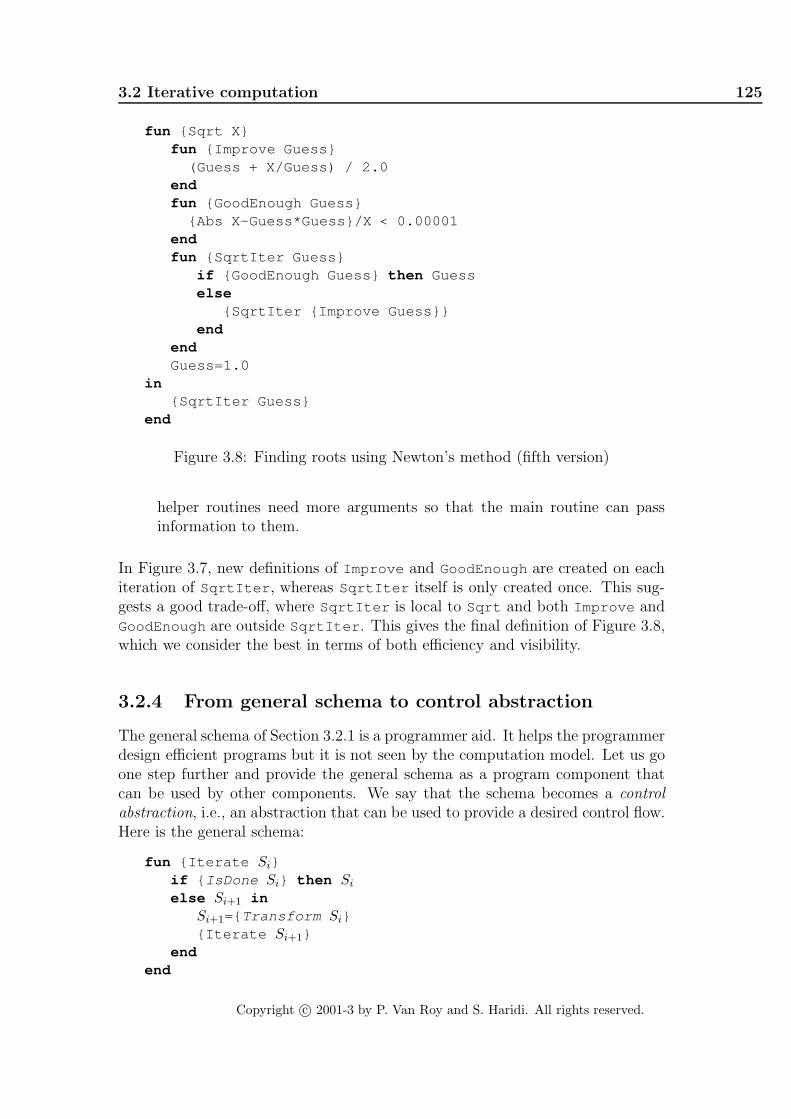
3.2 Iterative computation 125
fun {Sqrt X}fun {Improve Guess}
(Guess + X/Guess) / 2.0endfun {GoodEnough Guess}
{Abs X-Guess*Guess}/X < 0.00001endfun {SqrtIter Guess}
if {GoodEnough Guess} then Guesselse
{SqrtIter {Improve Guess}}end
endGuess=1.0
in{SqrtIter Guess}
end
Figure 3.8: Finding roots using Newton’s method (fifth version)
helper routines need more arguments so that the main routine can passinformation to them.
In Figure 3.7, new definitions of Improve and GoodEnough are created on eachiteration of SqrtIter , whereas SqrtIter itself is only created once. This sug-gests a good trade-off, where SqrtIter is local to Sqrt and both Improve andGoodEnough are outside SqrtIter . This gives the final definition of Figure 3.8,which we consider the best in terms of both efficiency and visibility.
3.2.4 From general schema to control abstraction
The general schema of Section 3.2.1 is a programmer aid. It helps the programmerdesign efficient programs but it is not seen by the computation model. Let us goone step further and provide the general schema as a program component thatcan be used by other components. We say that the schema becomes a controlabstraction, i.e., an abstraction that can be used to provide a desired control flow.Here is the general schema:
fun {Iterate Si}if { IsDone Si} then Si
else Si+1 inSi+1={ Transform Si}{Iterate Si+1}
endend
Copyright c© 2001-3 by P. Van Roy and S. Haridi. All rights reserved.

126 Declarative Programming Techniques
This schema implements a general while loop with a calculated result. To makethe schema into a control abstraction, we have to parameterize it by extractingthe parts that vary from one use to another. There are two such parts: thefunctions IsDone and Transform . We make these two parts into parameters ofIterate :
fun {Iterate S IsDone Transform}if {IsDone S} then Selse S1 in
S1={Transform S}{Iterate S1 IsDone Transform}
endend
To use this control abstraction, the arguments IsDone and Transform are givenone-argument functions. Passing functions as arguments to functions is partof a range of programming techniques called higher-order programming. Thesetechniques are further explained in Section 3.6. We can make Iterate behaveexactly like SqrtIter by passing it the functions GoodEnough and Improve .This can be written as follows:
fun {Sqrt X}{Iterate
1.0fun {$ G} {Abs X-G*G}/X<0.00001 endfun {$ G} (G+X/G)/2.0 end }
end
This uses two function values as arguments to the control abstraction. This isa powerful way to structure a program because it separates the general controlflow from this particular use. Higher-order programming is especially helpful forstructuring programs in this way. If this control abstraction is used often, thenext step could be to provide it as a linguistic abstraction.
3.3 Recursive computation
Iterative computations are a special case of a more general kind of computation,called recursive computation. Let us see the difference between the two. Recallthat an iterative computation can be considered as simply a loop in which acertain action is repeated some number of times. Section 3.2 implements this inthe declarative model by introducing a control abstraction, the function Iterate .The function first tests a condition. If the condition is false, it does an actionand then calls itself.
Recursion is more general than this. A recursive function can call itself any-where in the body and can call itself more than once. In programming, recursionoccurs in two major ways: in functions and in data types. A function is recur-sive if its definition has at least one call to itself. The iteration abstraction of
Copyright c© 2001-3 by P. Van Roy and S. Haridi. All rights reserved.

3.3 Recursive computation 127
Section 3.2 is a simple case. A data type is recursive if it is defined in terms ofitself. For example, a list is defined in terms of a smaller list. The two forms ofrecursion are strongly related since recursive functions can be used to calculatewith recursive data types.
We saw that an iterative computation has a constant stack size. This is notalways the case for a recursive computation. Its stack size may grow as the inputgrows. Sometimes this is unavoidable, e.g., when doing calculations with trees,as we will see later. In other cases, it can be avoided. An important part ofdeclarative programming is to avoid a growing stack size whenever possible. Thissection gives an example of how this is done. We start with a typical case ofa recursive computation that is not iterative, namely the naive definition of thefactorial function. The mathematical definition is:
0! = 1n! = n · (n− 1)! if n > 0
This is a recurrence equation, i.e., the factorial n! is defined in terms of a factorialwith a smaller argument, namely (n−1)!. The naive program follows this mathe-matical definition. To calculate {Fact N} there are two possibilities, namely N=0
or N>0. In the first case, return 1. In the second case, calculate {Fact N-1} ,multiply by N, and return the result. This gives the following program:
fun {Fact N}if N==0 then 1elseif N>0 then N*{Fact N-1}else raise domainError endend
end
This defines the factorial of a big number in terms of the factorial of a smallernumber. Since all numbers are nonnegative, they will bottom out at zero and theexecution will finish.
Note that factorial is a partial function. It is not defined for negative N. Theprogram reflects this by raising an exception for negative N. The definition inChapter 1 has an error since for negative N it goes into an infinite loop.
We have done two things when writing Fact . First, we followed the mathe-matical definition to get a correct implementation. Second, we reasoned abouttermination, i.e., we showed that the program terminates for all legal arguments,i.e., arguments inside the function’s domain.
3.3.1 Growing stack size
This definition of factorial gives a computation whose maximum stack size isproportional to the function argument N. We can see this by using the semantics.First translate Fact into the kernel language:
proc {Fact N ?R}
Copyright c© 2001-3 by P. Van Roy and S. Haridi. All rights reserved.

128 Declarative Programming Techniques
if N==0 then R=1elseif N>0 then N1 R1 in
N1=N-1{Fact N1 R1}R=N*R1
else raise domainError endend
end
Already we can guess that the stack size might grow, since the multiplicationcomes after the recursive call. That is, during the recursive call the stack has tokeep information about the multiplication for when the recursive call returns. Letus follow the semantics and calculate by hand what happens when executing thecall {Fact 5 R} . For clarity, we simplify slightly the presentation of the abstractmachine by substituting the value of a store variable into the environment. Thatis, the environment {..., N → n, ...} is written as {..., N → 5, ...} if the store is{..., n = 5, ...}.
• The initial semantic stack is [({Fact N R} , {N→ 5, R→ r0})].
• At the first call:
[ ({Fact N1 R1} , {N1→ 4, R1→ r1, ...}),(R=N*R1, {R→ r0, R1→ r1N→ 5, ...})]
• At the second call:
[ ({Fact N1 R1} , {N1→ 3, R1→ r2, ...}),(R=N*R1, {R→ r1, R1→ r2, N→ 4, ...}),(R=N*R1, {R→ r0, R1→ r1, N→ 5, ...})]
• At the third call:
[ ({Fact N1 R1} , {N1→ 2, R1→ r3, ...}),(R=N*R1, {R→ r2, R1→ r3, N→ 3, ...}),(R=N*R1, {R→ r1, R1→ r2, N→ 4, ...}),(R=N*R1, {R→ r0, R1→ r1, N→ 5, ...})]
It is clear that the stack grows bigger by one statement per call. The last recursivecall is the fifth, which returns immediately with r5 = 1. Then five multiplicationsare done to get the final result r0 = 120.
3.3.2 Substitution-based abstract machine
This example shows that the abstract machine of Chapter 2 can be rather cum-bersome for hand calculation. This is because it keeps both variable identifiersand store variables, using environments to map from one to the other. This is
Copyright c© 2001-3 by P. Van Roy and S. Haridi. All rights reserved.

3.3 Recursive computation 129
realistic; it is how the abstract machine is implemented on a real computer. Butit is not so nice for hand calculation.
We can make a simple change to the abstract machine that makes it mucheasier to use for hand calculation. The idea is to replace the identifiers in thestatements by the store entities that they refer to. This is called doing a substi-tution. For example, the statement R=N*R1 becomes r2 = 3∗ r3 when substitutedaccording to {R→ r2, N→ 3, R1→ r3}.
The substitution-based abstract machine has no environments. It directlysubstitutes identifiers by store entities in statements. For the recursive factorialexample, this gives the following:
• The initial semantic stack is [{Fact 5 r0} ].
• At the first call: [{Fact 4 r1} , r0=5* r1].
• At the second call: [{Fact 3 r2} , r1=4* r2, r0=5* r1].
• At the third call: [{Fact 2 r3} , r2=3* r3, r1=4* r2, r0=5* r1].
As before, we see that the stack grows by one statement per call. We summarizethe differences between the two versions of the abstract machine:
• The environment-based abstract machine, defined in Chapter 2, is faithfulto the implementation on a real computer, which uses environments. How-ever, environments introduce an extra level of indirection, so they are hardto use for hand calculation.
• The substitution-based abstract machine is easier to use for hand calcu-lation, because there are many fewer symbols to manipulate. However,substitutions are costly to implement, so they are generally not used in areal implementation.
Both versions do the same store bindings and the same manipulations of thesemantic stack.
3.3.3 Converting a recursive to an iterative computation
Factorial is simple enough that is can be rearranged to become iterative. Let ussee how this is done. Later on, we will give a systematic way of making iterativecomputations. For now, we just give a hint. In the previous calculation:
R=(5*(4*(3*(2*(1*1)))))
it is enough to rearrange the numbers:
R=(((((1*5)*4)*3)*2)*1)
Then the calculation can be done incrementally, starting with 1*5 . This gives 5,then 20 , then 60 , then 120 , and finally 120 . The iterative definition of factorialthat does things this way is:
Copyright c© 2001-3 by P. Van Roy and S. Haridi. All rights reserved.

130 Declarative Programming Techniques
fun {Fact N}fun {FactIter N A}
if N==0 then Aelseif N>0 then {FactIter N-1 A*N}else raise domainError endend
endin
{FactIter N 1}end
The function that does the iteration, FactIter , has a second argument A. Thisargument is crucial; without it an iterative factorial is impossible. The secondargument is not apparent in the simple mathematical definition of factorial weused first. We had to do some reasoning to bring it in.
3.4 Programming with recursion
Recursive computations are at the heart of declarative programming. This sectionshows how to write in this style. We show the basic techniques for programmingwith lists, trees, and other recursive data types. We show how to make thecomputation iterative when possible. The section is organized as follows:
• The first step is defining recursive data types. Section 3.4.1 gives a simplenotation that lets us define the most important recursive data types.
• The most important recursive data type is the list. Section 3.4.2 presentsthe basic programming techniques for lists.
• Efficient declarative programs have to define iterative computations. Sec-tion 3.4.3 presents accumulators, a systematic technique to achieve this.
• Computations often build data structures incrementally. Section 3.4.4 presentsdifference lists, an efficient technique to achieve this while keeping thecomputation iterative.
• An important data type related to the list is the queue. Section 3.4.5shows how to implement queues efficiently. It also introduces the basic ideaof amortized efficiency.
• The second most important recursive data type, next to linear structuressuch as lists and queues, is the tree. Section 3.4.6 gives the basic program-ming techniques for trees.
• Sections 3.4.7 and 3.4.8 give two realistic case studies, a tree drawingalgorithm and a parser, that between them use many of the techniques ofthis section.
Copyright c© 2001-3 by P. Van Roy and S. Haridi. All rights reserved.
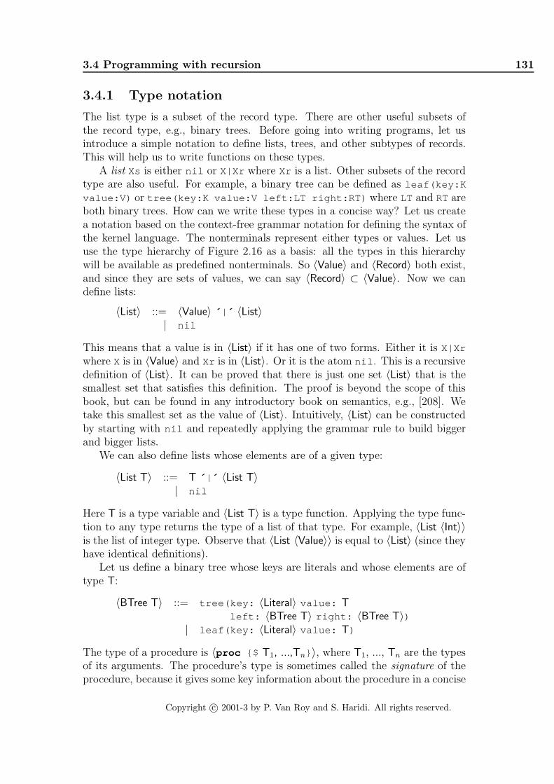
3.4 Programming with recursion 131
3.4.1 Type notation
The list type is a subset of the record type. There are other useful subsets ofthe record type, e.g., binary trees. Before going into writing programs, let usintroduce a simple notation to define lists, trees, and other subtypes of records.This will help us to write functions on these types.
A list Xs is either nil or X|Xr where Xr is a list. Other subsets of the recordtype are also useful. For example, a binary tree can be defined as leaf(key:K
value:V) or tree(key:K value:V left:LT right:RT) where LT and RTareboth binary trees. How can we write these types in a concise way? Let us createa notation based on the context-free grammar notation for defining the syntax ofthe kernel language. The nonterminals represent either types or values. Let ususe the type hierarchy of Figure 2.16 as a basis: all the types in this hierarchywill be available as predefined nonterminals. So 〈Value〉 and 〈Record〉 both exist,and since they are sets of values, we can say 〈Record〉 ⊂ 〈Value〉. Now we candefine lists:
〈List〉 ::= 〈Value〉 ´ | ´ 〈List〉| nil
This means that a value is in 〈List〉 if it has one of two forms. Either it is X|Xr
where X is in 〈Value〉 and Xr is in 〈List〉. Or it is the atom nil . This is a recursivedefinition of 〈List〉. It can be proved that there is just one set 〈List〉 that is thesmallest set that satisfies this definition. The proof is beyond the scope of thisbook, but can be found in any introductory book on semantics, e.g., [208]. Wetake this smallest set as the value of 〈List〉. Intuitively, 〈List〉 can be constructedby starting with nil and repeatedly applying the grammar rule to build biggerand bigger lists.
We can also define lists whose elements are of a given type:
〈List T〉 ::= T ´ | ´ 〈List T〉| nil
Here T is a type variable and 〈List T〉 is a type function. Applying the type func-tion to any type returns the type of a list of that type. For example, 〈List 〈Int〉〉is the list of integer type. Observe that 〈List 〈Value〉〉 is equal to 〈List〉 (since theyhave identical definitions).
Let us define a binary tree whose keys are literals and whose elements are oftype T:
〈BTree T〉 ::= tree(key: 〈Literal〉 value: Tleft: 〈BTree T〉 right: 〈BTree T〉)
| leaf(key: 〈Literal〉 value: T)
The type of a procedure is 〈proc {$ T1, ...,Tn} 〉, where T1, ..., Tn are the typesof its arguments. The procedure’s type is sometimes called the signature of theprocedure, because it gives some key information about the procedure in a concise
Copyright c© 2001-3 by P. Van Roy and S. Haridi. All rights reserved.

132 Declarative Programming Techniques
form. The type of a function is 〈fun {$ T1, ...,Tn}: T〉, which is equivalent to〈proc {$ T1, ...,Tn, T} 〉. For example, the type 〈fun {$ 〈List〉 〈List〉}: 〈List〉 〉is a function with two list arguments that returns a list.
Limits of the notation
This type notation can define many useful sets of values, but its expressivenessis definitely limited. Here are some cases where the notation is not good enough:
• The notation cannot define the positive integers, i.e., the subset of 〈Int〉whose elements are all greater than zero.
• The notation cannot define sets of partial values. For example, differencelists cannot be defined.
We can extend the notation to handle the first case, e.g., by adding booleanconditions.5 In the examples that follow, we will add these conditions in thetext when they are needed. This means that the type notation is descriptive: itgives logical assertions about the set of values that a variable may take. Thereis no claim that the types could be checkable by a compiler. On the contrary,they often cannot be checked. Even types that are simple to specify, such as thepositive integers, cannot in general be checked by a compiler.
3.4.2 Programming with lists
List values are very concise to create and to take apart, yet they are powerfulenough to encode any kind of complex data structure. The original Lisp languagegot much of its power from this idea [120]. Because of lists’ simple structure,declarative programming with them is easy and powerful. This section gives thebasic techniques of programming with lists:
• Thinking recursively: the basic approach is to solve a problem in terms ofsmaller versions of the problem.
• Converting recursive to iterative computations: naive list programs are oftenwasteful because their stack size grows with the input size. We show howto use state transformations to make them practical.
• Correctness of iterative computations: a simple and powerful way to reasonabout iterative computations is by using state invariants.
• Constructing programs by following the type: a function that calculates witha given type almost always has a recursive structure that closely mirrorsthe type definition.
5This is similar to the way we define language syntax in Section 2.1.1: a context-free notationwith extra conditions when they are needed.
Copyright c© 2001-3 by P. Van Roy and S. Haridi. All rights reserved.

3.4 Programming with recursion 133
We end up this section with a bigger example, the mergesort algorithm. Latersections show how to make the writing of iterative functions more systematicby introducing accumulators and difference lists. This lets us write iterativefunctions from the start. We find that these techniques “scale up”, i.e., theywork well even for large declarative programs.
Thinking recursively
A list is a recursive data structure: it is defined in terms of a smaller version ofitself. To write a function that calculates on lists we have to follow this recursivestructure. The function consists of two parts:
• A base case. For small lists (say, of zero, one, or two elements), the functioncomputes the answer directly.
• A recursive case. For bigger lists, the function computes the result in termsof the results of one or more smaller lists.
As our first example, we take a simple recursive function that calculates the lengthof a list according to this technique:
fun {Length Ls}case Lsof nil then 0[] _|Lr then 1+{Length Lr}end
end{Browse {Length [a b c]}}
Its type signature is 〈fun {$ 〈List〉}: 〈Int〉〉, a function of one list that returnsan integer. The base case is the empty list nil , for which the function returns 0.The recursive case is any other list. If the list has length n, then its tail has lengthn− 1. The tail is smaller than the original list, so the program will terminate.
Our second example is a function that appends two lists Ls and Ms togetherto make a third list. The question is, on which list do we use induction? Is it thefirst or the second? We claim that the induction has to be done on the first list.Here is the function:
fun {Append Ls Ms}case Lsof nil then Ms[] X|Lr then X|{Append Lr Ms}end
end
Its type signature is 〈fun {$ 〈List〉 〈List〉}: 〈List〉〉. This function follows exactlythe following two properties of append:
• append(nil , m) = m
Copyright c© 2001-3 by P. Van Roy and S. Haridi. All rights reserved.

134 Declarative Programming Techniques
• append(x| l, m) = x | append(l, m)
The recursive case always calls Append with a smaller first argument, so theprogram terminates.
Recursive functions and their domains
Let us define the function Nth to get the nth element of a list.
fun {Nth Xs N}if N==1 then Xs.1elseif N>1 then {Nth Xs.2 N-1}end
end
Its type is 〈fun {$ 〈List〉 〈Int〉}: 〈Value〉〉. Remember that a list Xs is eithernil or a tuple X|Y with two arguments. Xs.1 gives X and Xs.2 gives Y. Whathappens when we feed the following:
{Browse {Nth [ a b c d] 5}}
The list has only four elements. Trying to ask for the fifth element means tryingto do Xs.1 or Xs.2 when Xs=nil . This will raise an exception. An exception isalso raised if N is not a positive integer, e.g., when N=0. This is because there isno else clause in the if statement.
This is an example of a general technique to define functions: always usestatements that raise exceptions when values are given outside their domains.This will maximize the chances that the function as a whole will raise an exceptionwhen called with an input outside its domain. We cannot guarantee that anexception will always be raised in this case, e.g., {Nth 1|2|3 2} returns 2 while1|2|3 is not a list. Such guarantees are hard to come by. They can sometimesbe obtained in statically-typed languages.
The case statement also behaves correctly in this regard. Using a case
statement to recurse over a list will raise an exception when its argument is nota list. For example, let us define a function that sums all the elements of a listof integers:
fun {SumList Xs}case Xsof nil then 0[] X|Xr then X+{SumList Xr}end
end
Its type is 〈fun {$ 〈List 〈Int〉〉}: 〈Int〉〉. The input must be a list of integersbecause SumList internally uses the integer 0. The following call:
{Browse {SumList [1 2 3]}}
displays 6. Since Xs can be one of two values, namely nil or X|Xr , it is naturalto use a case statement. As in the Nth example, not using an else in the case
Copyright c© 2001-3 by P. Van Roy and S. Haridi. All rights reserved.

3.4 Programming with recursion 135
will raise an exception if the argument is outside the domain of the function. Forexample:
{Browse {SumList 1|foo}}
raises an exception because 1|foo is not a list, and the definition of SumList
assumes that its input is a list.
Naive definitions are often slow
Let us define a function to reverse the elements of a list. Start with a recursivedefinition of list reversal:
• Reverse of nil is nil .
• Reverse of X|Xs is Z, wherereverse of Xs is Ys, andappend Ys and [X] to get Z.
This works because X is moved from the front to the back. Following this recursivedefinition, we can immediately write a function:
fun {Reverse Xs}case Xsof nil then nil[] X|Xr then
{Append {Reverse Xr} [X]}end
end
Its type is 〈fun {$ 〈List〉}: 〈List〉〉. Is this function efficient? To find out, wehave to calculate its execution time given an input list of length n. We can do thisrigorously with the techniques of Section 3.5. But even without these techniques,we can see intuitively what happens. There will be n recursive calls followed byn calls to Append . Each Append call will have a list of length n/2 on average.The total execution time is therefore proportional to n · n/2, namely n2. Thisis rather slow. We would expect that reversing a list, which is not exactly acomplex calculation, would take time proportional to the input length and notto its square.
This program has a second defect: the stack size grows with the input listlength, i.e., it defines a recursive computation that is not iterative. Naivelyfollowing the recursive definition of reverse has given us a rather inefficient result!Luckily, there are simple techniques for getting around both these inefficiencies.They will let us define linear-time iterative computations whenever possible. Wewill see two useful techniques: state transformations and difference lists.
Converting recursive to iterative computations
Let us see how to convert recursive computations into iterative ones. Instead ofusing Reverse , we take a simpler function that calculates the length of a list:
Copyright c© 2001-3 by P. Van Roy and S. Haridi. All rights reserved.

136 Declarative Programming Techniques
fun {Length Xs}case Xs of nil then 0[] _|Xr then 1+{Length Xr}end
end
Note that the SumList function has the same structure. This function is linear-time but the stack size is proportional to the recursion depth, which is equalto the length of Xs. Why does this problem occur? It is because the addition1+{Length Xr} happens after the recursive call. The recursive call is not last,so the function’s environment cannot be recovered before it.
How can we calculate the list length with an iterative computation, which hasbounded stack size? To do this, we have to formulate the problem as a sequenceof state transformations. That is, we start with a state S0 and we transform itsuccessively, giving S1, S2, ..., until we reach the final state Sfinal, which containsthe answer. To calculate the list length, we can take the length i of the part ofthe list already seen as the state. Actually, this is only part of the state. The restof the state is the part Ys of the list not yet seen. The complete state Si is thenthe pair (i, Ys). The general intermediate case is as follows for state Si (wherethe full list Xs is [e1 e2 · · · en]):
Xs︷ ︸︸ ︷e1 e2 · · · ei ei+1 · · · en︸ ︷︷ ︸
Ys
At each recursive call, i will be incremented by 1 and Ys reduced by one element.This gives us the function:
fun {IterLength I Ys}case Ysof nil then I[] _|Yr then {IterLength I+1 Yr}end
end
Its type is 〈fun {$ 〈Int〉 〈List〉}: 〈Int〉〉. Note the difference with the previousdefinition. Here the addition I+1 is done before the recursive call to IterLength ,which is the last call. We have defined an iterative computation.
In the call {IterLength I Ys} , the initial value of I is 0. We can hide thisinitialization by defining IterLength as a local procedure. The final definitionof Length is therefore:
localfun {IterLength I Ys}
case Ysof nil then I[] _|Yr then {IterLength I+1 Yr}end
end
Copyright c© 2001-3 by P. Van Roy and S. Haridi. All rights reserved.

3.4 Programming with recursion 137
infun {Length Xs}
{IterLength 0 Xs}end
end
This defines an iterative computation to calculate the list length. Note that wedefine IterLength outside of Length . This avoids creating a new procedurevalue each time Length is called. There is no advantage to defining IterLength
inside Length , since it does not use Length ’s argument Xs.We can use the same technique on Reverse as we used for Length . In the
case of Reverse , the state uses the reverse of the part of the list already seeninstead of its length. Updating the state is easy: we just put a new list elementin front. The initial state is nil . This gives the following version of Reverse :
localfun {IterReverse Rs Ys}
case Ysof nil then Rs[] Y|Yr then {IterReverse Y|Rs Yr}end
endin
fun {Reverse Xs}{IterReverse nil Xs}
endend
This version of Reverse is both a linear-time and an iterative computation.
Correctness with state invariants
Let us prove that IterLength is correct. We will use a general technique thatworks well for IterReverse and other iterative computations. The idea is todefine a property P (Si) of the state that we can prove is always true, i.e., it isa state invariant. If P is chosen well, then the correctness of the computationfollows from P (Sfinal). For IterLength we define P as follows:
P ((i, Ys)) ≡ (length(Xs) = i + length(Ys))
where length(L) gives the length of the list L. This combines i and Ys in such away that we suspect it is a state invariant. We use induction to prove this:
• First prove P (S0). This follows directly from S0 = (0, Xs).
• Assuming P (Si) and Si is not the final state, prove P (Si+1). This followsfrom the semantics of the case statement and the function call. WriteSi = (i, Ys). We are not in the final state, so Ys is of nonzero length. Fromthe semantics, I+1 adds 1 to i and the case statement removes one elementfrom Ys. Therefore P (Si+1) holds.
Copyright c© 2001-3 by P. Van Roy and S. Haridi. All rights reserved.

138 Declarative Programming Techniques
Since Ys is reduced by one element at each call, we eventually arrive at the finalstate Sfinal = (i, nil ), and the function returns i. Since length(nil ) = 0, fromP (Sfinal) it follows that i = length(Xs).
The difficult step in this proof is to choose the property P . It has to satisfy twoconstraints. First, it has to combine the arguments of the iterative computationsuch that the result does not change as the computation progresses. Second, ithas to be strong enough that the correctness follows from P (Sfinal). A rule ofthumb for finding a good P is to execute the program by hand in a few smallcases, and from them to picture what the general intermediate case is.
Constructing programs by following the type
The above examples of list functions all have a curious property. They all have alist argument, 〈List T〉, which is defined as:
〈List T〉 ::= nil
| T ´ | ´ 〈List T〉
and they all use a case statement which has the form:
case Xsof nil then 〈expr〉 % Base case[] X|Xr then 〈expr〉 % Recursive callend
What is going on here? The recursive structure of the list functions exactlyfollows the recursive structure of the type definition. We find that this propertyis almost always true of list functions.
We can use this property to help us write list functions. This can be a tremen-dous help when type definitions become complicated. For example, let us write afunction that counts the elements of a nested list. A nested list is a list in whicheach element can itself be a list, e.g., [[1 2] 4 nil [[5] 10]] . We define thetype 〈NestedList T〉 as follows:
〈NestedList T〉 ::= nil
| 〈NestedList T〉 ´ | ´ 〈NestedList T〉| T ´ | ´ 〈NestedList T〉
To avoid ambiguity, we have to add a condition on T, namely that T is neither nil
nor a cons. Now let us write the function {LengthL 〈NestedList T〉}: 〈Int〉 whichcounts the number of elements in a nested list. Following the type definition givesthis skeleton:
fun {LengthL Xs}case Xsof nil then 〈expr〉[] X|Xr andthen {IsList X} then〈expr〉 % Recursive calls for X and Xr
[] X|Xr then
Copyright c© 2001-3 by P. Van Roy and S. Haridi. All rights reserved.

3.4 Programming with recursion 139
〈expr〉 % Recursive call for Xrend
end
(The third case does not have to mention {Not {IsList X}} since it followsfrom the negation of the second case.) Here {IsList X} is a function thatchecks whether X is nil or a cons:
fun {IsCons X} case X of _|_ then true else false end endfun {IsList X} X==nil orelse {IsCons X} end
Fleshing out the skeleton gives the following function:
fun {LengthL Xs}case Xsof nil then 0[] X|Xr andthen {IsList X} then
{LengthL X}+{LengthL Xr}[] X|Xr then
1+{LengthL Xr}end
end
Here are two example calls:
X=[[1 2] 4 nil [[5] 10]]{Browse {LengthL X}}{Browse {LengthL [X X]}}
What do these calls display?Using a different type definition for nested lists gives a different length func-
tion. For example, let us define the type 〈NestedList2 T〉 as follows:
〈NestedList2 T〉 ::= nil
| 〈NestedList2 T〉 ´ | ´ 〈NestedList2 T〉| T
Again, we have to add the condition that T is neither nil nor a cons. Notethe subtle difference between 〈NestedList T〉 and 〈NestedList2 T〉! Following thedefinition of 〈NestedList2 T〉 gives a different and simpler function LengthL2 :
fun {LengthL2 Xs}case Xsof nil then 0[] X|Xr then
{LengthL2 X}+{LengthL2 Xr}else 1 end
end
What is the difference between LengthL and LengthL2 ? We can deduce it bycomparing the types 〈NestedList T〉 and 〈NestedList2 T〉. A 〈NestedList T〉 alwayshas to be a list, whereas a 〈NestedList2 T〉 can also be of type T. Therefore the
Copyright c© 2001-3 by P. Van Roy and S. Haridi. All rights reserved.

140 Declarative Programming Techniques
L
L1
L2
S1
S2
S
L11
L12
L21
L22 S22
S21
S12
S11
Split
Split Merge
Merge
Split Merge
Inputlist list
Sorted
Figure 3.9: Sorting with mergesort
call {LengthL2 foo} is legal (it returns 1), wherease {LengthL foo} is illegal(it raises an exception). It is reasonable to consider this as an error in LengthL2 .
There is an important lesson to be learned here. It is important to define arecursive type before writing the recursive function that uses it. Otherwise it iseasy to be misled by an apparently simple function that is incorrect. This is trueeven in functional languages that do type inference, such as Standard ML andHaskell. Type inference can verify that a recursive type is used correctly, but thedesign of a recursive type remains the programmer’s responsibility.
Sorting with mergesort
We define a function that takes a list of numbers or atoms and returns a new listsorted in ascending order. It uses the comparison operator <, so all elements haveto be of the same type (all integers, all floats, or all atoms). We use the mergesortalgorithm, which is efficient and can be programmed easily in a declarative model.The mergesort algorithm is based on a simple strategy called divide-and-conquer:
• Split the list into two smaller lists of approximately equal length.
• Use mergesort recursively to sort the two smaller lists.
• Merge the two sorted lists together to get the final result.
Figure 3.9 shows the recursive structure. Mergesort is efficient because the splitand merge operations are both linear-time iterative computations. We first definethe merge and split operations and then mergesort itself:
fun {Merge Xs Ys}case Xs # Ysof nil # Ys then Ys[] Xs # nil then Xs[] (X|Xr) # (Y|Yr) then
if X<Y then X|{Merge Xr Ys}else Y|{Merge Xs Yr}end
Copyright c© 2001-3 by P. Van Roy and S. Haridi. All rights reserved.

3.4 Programming with recursion 141
S1 S2 S3 SnP1 P2 P3
S1
P
ifSnBase case
Recursive case
Figure 3.10: Control flow with threaded state
endend
The type is 〈fun {$ 〈List T〉 〈List T〉}: 〈List T〉〉, where T is either 〈Int〉, 〈Float〉,or 〈Atom〉. We define split as a procedure because it has two outputs. It couldalso be defined as a function returning a pair as a single output.
proc {Split Xs ?Ys ?Zs}case Xsof nil then Ys=nil Zs=nil[] [X] then Ys=[X] Zs=nil[] X1|X2|Xr then Yr Zr in
Ys=X1|YrZs=X2|Zr{Split Xr Yr Zr}
endend
The type is 〈proc {$ 〈List T〉 〈List T〉 〈List T〉} 〉. Here is the definition of merge-sort itself:
fun {MergeSort Xs}case Xsof nil then nil[] [X] then [X]else Ys Zs in
{Split Xs Ys Zs}{Merge {MergeSort Ys} {MergeSort Zs}}
endend
Its type is 〈fun {$ 〈List T〉}: 〈List T〉〉 with the same restriction on T as inMerge . The splitting up of the input list bottoms out at lists of length zero andone, which can be sorted immediately.
Copyright c© 2001-3 by P. Van Roy and S. Haridi. All rights reserved.

142 Declarative Programming Techniques
3.4.3 Accumulators
We have seen how to program simple list functions and how to make them itera-tive. Realistic declarative programming is usually done in a different way, namelyby writing functions that are iterative from the start. The idea is to carry stateforward at all times and never do a return calculation. A state S is representedby adding a pair of arguments, S1 and Sn, to each procedure. This pair is calledan accumulator. S1 represents the input state and Sn represents the output state.Each procedure definition is then written in a style that looks like this:
proc {P X S1 ?Sn}if {BaseCase X} then Sn=S1else
{P1 S1 S2}{P2 S2 S3}{P3 S3 Sn}
endend
The base case does no calculation, so the output state is the same as the inputstate (Sn=S1). The recursive case threads the state through each recursive call(P1, P2, and P3) and eventually returns it to P. Figure 3.10 gives an illustration.Each arrow represents one state variable. The state value is given at the arrow’stail and passed to the arrow’s head. By state threading we mean that each proce-dure’s output is the next procedure’s input. The technique of threading a statethrough nested procedure calls is called accumulator programming.
Accumulator programming is used in the IterLength and IterReverse
functions we saw before. In these functions the accumulator structure is not soclear, because they are functions. What is happening is that the input state ispassed to the function and the output state is what the function returns.
Multiple accumulators
Consider the following procedure, which takes an expression containing identifiers,integers, and addition operations (using label plus ). It calculates two results:it translates the expression into machine code for a simple stack machine and itcalculates the number of instructions in the resulting code.
proc {ExprCode E C1 ?Cn S1 ?Sn}case Eof plus(A B) then C2 C3 S2 S3 in
C2=plus|C1S2=S1+1{ExprCode B C2 C3 S2 S3}{ExprCode A C3 Cn S3 Sn}
[] I thenCn=push(I)|C1Sn=S1+1
Copyright c© 2001-3 by P. Van Roy and S. Haridi. All rights reserved.

3.4 Programming with recursion 143
endend
This procedure has two accumulators: one to build the list of machine instructionsand another to hold the number of instructions. Here is a sample execution:
declare Code Size in{ExprCode plus(plus(a 3) b) nil Code 0 Size}{Browse Size#Code}
This displays:
5#[push(a) push(3) plus push(b) plus]
More complicated programs usually need more accumulators. When writing largedeclarative programs, we have typically used around half a dozen accumulatorssimultaneously. The Aquarius Prolog compiler was written in this style [198,194]. Some of its procedures have as many as 12 accumulators. This means 24additional arguments! This is difficult to do without mechanical aid. We used anextended DCG preprocessor6 that takes declarations of accumulators and addsthe arguments automatically [96].
We no longer program in this style; we find that programming with explicitstate is simpler and more efficient (see Chapter 6). It is reasonable to use a fewaccumulators in a declarative program; it is actually quite rare that a declarativeprogram does not need a few. On the other hand, using many is a sign that someof them would probably be better written with explicit state.
Mergesort with an accumulator
In the previous definition of mergesort, we first called the function Split todivide the input list into two halves. There is a simpler way to do the mergesort,by using an accumulator. The parameter represents “the part of the list still tobe sorted”. The specification of MergeSortAcc is:
• S#L2={MergeSortAcc L1 N} takes an input list L1 and an integer N. Itreturns two results: S, the sorted list of the first N elements of L1 , and L2 ,the remaining elements of L1 . The two results are paired together with the# tupling constructor.
The accumulator is defined by L1 and L2 . This gives the following definition:
fun {MergeSort Xs}fun {MergeSortAcc L1 N}
if N==0 thennil # L1
elseif N==1 then[L1.1] # L1.2
elseif N>1 then
6DCG (Definite Clause Grammar) is a grammar notation that is used to hide the explicitthreading of accumulators.
Copyright c© 2001-3 by P. Van Roy and S. Haridi. All rights reserved.

144 Declarative Programming Techniques
NL=N div 2NR=N-NLYs # L2 = {MergeSortAcc L1 NL}Zs # L3 = {MergeSortAcc L2 NR}
in{Merge Ys Zs} # L3
endend
in{MergeSortAcc Xs {Length Xs}}.1
end
The Merge function is unchanged. Remark that this mergesort does a differentsplit than the previous one. In this version, the split separates the first half ofthe input list from the second half. In the previous version, split separates theodd-numbered list elements from the even-numbered elements.
This version has the same time complexity as the previous version. It uses lessmemory because it does not create the two split lists. They are defined implicitlyby the combination of the accumulating parameter and the number of elements.
3.4.4 Difference lists
A difference list is a pair of two lists, each of which might have an unbound tail.The two lists have a special relationship: it must be possible to get the secondlist from the first by removing zero or more elements from the front. Here aresome examples:
X#X % Represents the empty listnil#nil % idem[a]#[a] % idem(a|b|c|X)#X % Represents [a b c](a|b|c|d|X)#(d|X) % idem[a b c d]#[d] % idem
A difference list is a representation of a standard list. We will talk of the differencelist sometimes as a data structure by itself, and sometimes as representing astandard list. Be careful not to confuse these two viewpoints. The difference list[a b c d]#[d] might contain the lists [a b c d] and [d] , but it representsneither of these. It represents the list [a b c] .
Difference lists are a special case of difference structures. A difference struc-ture is a pair of two partial values where the second value is embedded in the first.The difference structure represents a value that is the first structure minus thesecond structure. Using difference structures makes it easy to construct iterativecomputations on many recursive datatypes, e.g., lists or trees. Difference listsand difference structures are special cases of accumulators in which one of theaccumulator arguments can be an unbound variable.
Copyright c© 2001-3 by P. Van Roy and S. Haridi. All rights reserved.

3.4 Programming with recursion 145
The advantage of using difference lists is that when the second list is anunbound variable, another difference list can be appended to it in constant time.To append (a|b|c|X)#X and (d|e|f|Y)#Y , just bind X to (d|e|f|Y) . Thiscreates the difference list (a|b|c|d|e|f|Y)#Y . We have just appended the lists[a b c] and [d e f] with a single binding. Here is a function that appendsany two difference lists:
fun {AppendD D1 D2}S1#E1=D1S2#E2=D2
inE1=S2S1#E2
end
It can be used like a list append:
local X Y in {Browse {AppendD (1|2|3|X)#X (4|5|Y)#Y}} end
This displays (1|2|3|4|5|Y)#Y . The standard list append function, defined asfollows:
fun {Append L1 L2}case L1of X|T then X|{Append T L2}[] nil then L2end
end
iterates on its first argument, and therefore takes time proportional to the lengthof the first argument. The difference list append is much more efficient: it takesconstant time.
The limitation of using difference lists is that they can be appended only once.This property means that difference lists can only be used in special circum-stances. For example, they are a natural way to write programs that constructbig lists in terms of lots of little lists that must be appended together.
Difference lists as defined here originated from Prolog and logic program-ming [182]. They are the basis of many advanced Prolog programming tech-niques. As a concept, a difference list lives somewhere between the concept ofvalue and the concept of state. It has the good properties of a value (programsusing them are declarative), but it also has some of the power of state because itcan be appended once in constant time.
Flattening a nested list
Consider the problem of flattening a nested list, i.e., calculating a list that hasall the elements of the nested list but is no longer nested. We first give a solutionusing lists and then we show that a much better solution is possible with differencelists. For the list solution, let us reason with mathematical induction based on the
Copyright c© 2001-3 by P. Van Roy and S. Haridi. All rights reserved.

146 Declarative Programming Techniques
type 〈NestedList〉 we defined earlier, in the same way we did with the LengthL
function:
• Flatten of nil is nil .
• Flatten of X|Xr where X is a nested list, is Z whereflatten of X is Y,flatten of Xr is Yr , andappend Y and Yr to get Z.
• Flatten of X|Xr where X is not a list, is Z whereflatten of Xr is Yr , andZ is X|Yr .
Following this reasoning, we get the following definition:
fun {Flatten Xs}case Xsof nil then nil[] X|Xr andthen {IsList X} then
{Append {Flatten X} {Flatten Xr}}[] X|Xr then
X|{Flatten Xr}end
end
Calling:
{Browse {Flatten [[a b] [[c] [d]] nil [e [f]]]}}
displays [a b c d e f] . This program is very inefficient because it needs to domany append operations (see Exercises). Now let us reason again in the sameway, but with difference lists instead of standard lists:
• Flatten of nil is X#X (empty difference list).
• Flatten of X|Xr where X is a nested list, is Y1#Y4 whereflatten of X is Y1#Y2,flatten of Xr is Y3#Y4, andequate Y2 and Y3 to append the difference lists.
• Flatten of X|Xr where X is not a list, is (X|Y1)#Y2 whereflatten of Xr is Y1#Y2.
We can write the second case as follows:
• Flatten of X|Xr where X is a nested list, is Y1#Y4 whereflatten of X is Y1#Y2 andflatten of Xr is Y2#Y4.
This gives the following program:
Copyright c© 2001-3 by P. Van Roy and S. Haridi. All rights reserved.

3.4 Programming with recursion 147
fun {Flatten Xs}proc {FlattenD Xs ?Ds}
case Xsof nil then Y in Ds=Y#Y[] X|Xr andthen {IsList X} then Y1 Y2 Y4 in
Ds=Y1#Y4{FlattenD X Y1#Y2}{FlattenD Xr Y2#Y4}
[] X|Xr then Y1 Y2 inDs=(X|Y1)#Y2{FlattenD Xr Y1#Y2}
endend Ys
in{FlattenD Xs Ys#nil} Ys
end
This program is efficient: it does a single cons operation for each non-list in theinput. We convert the difference list returned by FlattenD into a regular list bybinding its second argument to nil . We write FlattenD as a procedure becauseits output is part of its last argument, not the whole argument (see Section 2.5.2).It is common style to write a difference list in two arguments:
fun {Flatten Xs}proc {FlattenD Xs ?S E}
case Xsof nil then S=E[] X|Xr andthen {IsList X} then Y2 in
{FlattenD X S Y2}{FlattenD Xr Y2 E}
[] X|Xr then Y1 inS=X|Y1{FlattenD Xr Y1 E}
endend Ys
in{FlattenD Xs Ys nil} Ys
end
As a further simplification, we can write FlattenD as a function. To do this, weuse the fact that S is the output:
fun {Flatten Xs}fun {FlattenD Xs E}
case Xsof nil then E[] X|Xr andthen {IsList X} then
{FlattenD X {FlattenD Xr E}}[] X|Xr then
Copyright c© 2001-3 by P. Van Roy and S. Haridi. All rights reserved.

148 Declarative Programming Techniques
X|{FlattenD Xr E}end
endin
{FlattenD Xs nil}end
What is the role of E? It gives the “rest” of the output, i.e., when the FlattenD
call exhausts its own contribution to the output.
Reversing a list
Let us look again at the naive list reverse of the last section. The problem withnaive reverse is that it uses a costly append function. Perhaps it will be moreefficient with the constant-time append of difference lists? Let us do the naivereverse with difference lists:
• Reverse of nil is X#X (empty difference list).
• Reverse of X|Xs is Z, wherereverse of Xs is Y1#Y2 andappend Y1#Y2 and (X|Y)#Y together to get Z.
Rewrite the last case as follows, by doing the append:
• Reverse of X|Xs is Y1#Y, wherereverse of Xs is Y1#Y2 andequate Y2 and X|Y .
It is perfectly allowable to move the equate before the reverse (why?). This gives:
• Reverse of X|Xs is Y1#Y, wherereverse of Xs is Y1#(X|Y) .
Here is the final definition:
fun {Reverse Xs}proc {ReverseD Xs ?Y1 Y}
case Xsof nil then Y1=Y[] X|Xr then
{ReverseD Xr Y1 X|Y}end
end Y1in
{ReverseD Xs Y1 nil} Y1end
Copyright c© 2001-3 by P. Van Roy and S. Haridi. All rights reserved.

3.4 Programming with recursion 149
Look carefully and you will see that this is almost exactly the same iterativesolution as in the last section. The only difference between IterReverse andReverseD is the argument order: the output of IterReverse is the secondargument of ReverseD . So what’s the advantage of using difference lists? Withthem, we derived ReverseD without thinking, whereas to derive IterReverse
we had to guess an intermediate state that could be updated.
3.4.5 Queues
An important basic data structure is the queue. A queue is a sequence of elementswith an insert and a delete operation. The insert operation adds an element toone end of the queue and the delete operation removes an element from the otherend. We say the queue has FIFO (First-In-First-Out) behavior. Let us investigatehow to program queues in the declarative model.
A naive queue
An obvious way to implement queues is by using lists. If L represents the queuecontent, then inserting X gives the new queue X|L and deleting X is done bycalling {ButLast L X L1} , which binds X to the deleted element and returnsthe new queue in L1 . ButLast returns the last element of L in X and all elementsbut the last in L1 . It can be defined as:
proc {ButLast L ?X ?L1}case Lof [Y] then X=Y L1=nil[] Y|L2 then L3 in
L1=Y|L3{ButLast L2 X L3}
endend
The problem with this implementation is that ButLast is slow: it takes timeproportional to the number of elements in the queue. On the contrary, we wouldlike both the insert and delete operations to be constant-time. That is, doing anoperation on a given implementation and machine always takes time less thansome constant number of seconds. The value of the constant depends on theimplementation and machine. Whether or not we can achieve the constant-timegoal depends on the expressiveness of the computation model:
• In a strict functional programming language, i.e., the declarative modelwithout dataflow variables (see Section 2.7.1), we cannot achieve it. Thebest we can do is to get amortized constant-time operations [138]. Thatis, any sequence of n insert and delete operations takes a total time thatis proportional to some constant times n. Any individual operation mightnot be constant-time, however.
Copyright c© 2001-3 by P. Van Roy and S. Haridi. All rights reserved.

150 Declarative Programming Techniques
• In the declarative model, which extends the strict functional model withdataflow variables, we can achieve the constant-time goal.
We will show how to define both solutions. In both definitions, each operationtakes a queue as input and returns a new queue as output. As soon as a queueis used by the program as input to an operation, then it can no longer be usedas input to another operation. In other words, there can be only one version ofthe queue in use at any time. We say that the queue is ephemeral.7 Each versionexists from the moment it is created to the moment it can no longer be used.
Amortized constant-time ephemeral queue
Here is the definition of a queue whose insert and delete operations have constantamortized time bounds. The definition is taken from Okasaki [138]:
fun {NewQueue} q(nil nil) end
fun {Check Q}case Q of q(nil R) then q({Reverse R} nil) else Q end
end
fun {Insert Q X}case Q of q(F R) then {Check q(F X|R)} end
end
fun {Delete Q X}case Q of q(F R) then F1 in F=X|F1 {Check q(F1 R)} end
end
fun {IsEmpty Q}case Q of q(F R) then F==nil end
end
This uses the pair q(F R) to represent the queue. F and R are lists. F representsthe front of the queue and R represents the back of the queue in reversed form.At any instant, the queue content is given by {Append F {Reverse R}} . Anelement can be inserted by adding it to the front of R and deleted by removing itfrom the front of F. For example, say that F=[a b] and R=[d c] . Deleting thefirst element returns a and makes F=[b] . Inserting the element e makes R=[e d
c] . Both operations are constant-time.To make this representation work, each element in R has to be moved to F
sooner or later. When should the move be done? Doing it element by element isinefficient, since it means replacing F by {Append F {Reverse R}} each time,which takes time at least proportional to the length of F. The trick is to do it onlyoccasionally. We do it when F becomes empty, so that F is non-nil if and only
7Queues implemented with explicit state (see Chapters 6 and 7) are also usually ephemeral.
Copyright c© 2001-3 by P. Van Roy and S. Haridi. All rights reserved.

3.4 Programming with recursion 151
if the queue is non-empty. This invariant is maintained by the Check function,which moves the content of R to F whenever F is nil.
The Check function does a list reverse operation on R. The reverse takes timeproportional to the length of R, i.e., to the number of elements it reverses. Eachelement that goes through the queue is passed exactly once from R to F. Allocatingthe reverse’s execution time to each element therefore gives a constant time perelement. This is why the queue is amortized.
Worst-case constant-time ephemeral queue
We can use difference lists to implement queues whose insert and delete operationshave constant worst-case execution times. We use a difference list that ends inan unbound dataflow variable. This lets us insert elements in constant time bybinding the dataflow variable. Here is the definition:
fun {NewQueue} X in q(0 X X) end
fun {Insert Q X}case Q of q(N S E) then E1 in E=X|E1 q(N+1 S E1) end
end
fun {Delete Q X}case Q of q(N S E) then S1 in S=X|S1 q(N-1 S1 E) end
end
fun {IsEmpty Q}case Q of q(N S E) then N==0 end
end
This uses the triple q(N S E) to represent the queue. At any instant, the queuecontent is given by the difference list S#E. N is the number of elements in thequeue. Why is N needed? Without it, we would not know how many elementswere in the queue.
Example use
The following example works with either of the above definitions:
declare Q1 Q2 Q3 Q4 Q5 Q6 Q7inQ1={NewQueue}Q2={Insert Q1 peter}Q3={Insert Q2 paul}local X in Q4={Delete Q3 X} {Browse X} endQ5={Insert Q4 mary}local X in Q6={Delete Q5 X} {Browse X} endlocal X in Q7={Delete Q6 X} {Browse X} end
This inserts three elements and deletes them. Each element is inserted before itis deleted. Now let us see what each definition can do that the other cannot.
Copyright c© 2001-3 by P. Van Roy and S. Haridi. All rights reserved.

152 Declarative Programming Techniques
With the second definition, we can delete an element before it is inserted.Doing such a delete returns an unbound variable that will be bound to the cor-responding inserted element. So the last four calls in the above example can bechanged as follows:
local X in Q4={Delete Q3 X} {Browse X} endlocal X in Q5={Delete Q4 X} {Browse X} endlocal X in Q6={Delete Q5 X} {Browse X} endQ7={Insert Q6 mary}
This works because the bind operation of dataflow variables, which is used bothto insert and delete elements, is symmetric.
With the first definition, maintaining multiple versions of the queue simul-taneously gives correct results, although the amortized time bounds no longerhold.8 Here is an example with two versions:
declare Q1 Q2 Q3 Q4 Q5 Q6inQ1={NewQueue}Q2={Insert Q1 peter}Q3={Insert Q2 paul}Q4={Insert Q2 mary}local X in Q5={Delete Q3 X} {Browse X} endlocal X in Q6={Delete Q4 X} {Browse X} end
Both Q3 and Q4 are calculated from their common ancestor Q2. Q3 containspeter and paul . Q4 contains peter and mary . What do the two Browse callsdisplay?
Persistent queues
Both definitions given above are ephemeral. What can we do if we need touse multiple versions and still require constant-time execution? A queue thatsupports multiple simultaneous versions is called persistent.9 Some applicationsneed persistent queues. For example, if during a calculation we pass a queuevalue to another routine:
...{SomeProc Qa}Qb={Insert Qa x}Qc={Insert Qb y}...
8To see why not, consider any sequence of n queue operations. For the amortized constant-time bound to hold, the total time for all operations in the sequence must be proportional ton. But what happens if the sequence repeats an “expensive” operation in many versions? Thisis possible, since we are talking of any sequence. Since the time for an expensive operation andthe number of versions can both be proportional to n, the total time bound grows as n2.
9This meaning of persistence should not be confused with persistence as used in transactionsand databases (Sections 8.5 and 9.6), which is a completely different concept.
Copyright c© 2001-3 by P. Van Roy and S. Haridi. All rights reserved.

3.4 Programming with recursion 153
We assume that SomeProc can do queue operations but that the caller does notwant to see their effects. It follows that we may have two versions of the queue.Can we write queues that keep the time bounds for this case? It can be done ifwe extend the declarative model with lazy execution. Then both the amortizedand worst-case queues can be made persistent. We defer this solution until wepresent lazy execution in Section 4.5.
For now, let us propose a simple workaround that is often sufficient to make theworst-case queue persistent. It depends on there not being too many simultaneousversions. We define an operation ForkQ that takes a queue Q and creates twoidentical versions Q1 and Q2. As a preliminary, we first define a procedure ForkD
that creates two versions of a difference list:
proc {ForkD D ?E ?F}D1#nil=DE1#E0=E {Append D1 E0 E1}F1#F0=F {Append D1 F0 F1}
in skip end
The call {ForkD D E F} takes a difference list D and returns two fresh copiesof it, E and F. Append is used to convert a list into a fresh difference list. Notethat ForkD consumes D, i.e., D can no longer be used afterwards since its tail isbound. Now we can define ForkQ , which uses ForkD to make two versions of aqueue:
proc {ForkQ Q ?Q1 ?Q2}q(N S E)=Qq(N S1 E1)=Q1q(N S2 E2)=Q2
in{ForkD S#E S1#E1 S2#E2}
end
ForkQ consumes Q and takes time proportional to the size of the queue. We canrewrite the example as follows using ForkQ :
...{ForkQ Qa Qa1 Qa2}{SomeProc Qa1}Qb={Insert Qa2 x}Qc={Insert Qb y}...
This works well if it is acceptable for ForkQ to be an expensive operation.
3.4.6 Trees
Next to linear data structures such as lists and queues, trees are the most im-portant recursive data structure in a programmer’s repertory. A tree is either a
Copyright c© 2001-3 by P. Van Roy and S. Haridi. All rights reserved.

154 Declarative Programming Techniques
leaf node or a node that contains one or more trees. Nodes can carry additionalinformation. Here is one possible definition:
〈Tree〉 ::= leaf( 〈Value〉)| tree( 〈Value〉 〈Tree〉1 ... 〈Tree〉n)
The basic difference between a list and a tree is that a list always has a linearstructure whereas a tree can have a branching structure. A list always has anelement followed by exactly one smaller list. A tree has an element followed bysome number of smaller trees. This number can be any natural number, i.e., zerofor leaf nodes and any positive number for non-leaf nodes.
There exist an enormous number of different kinds of trees, with differentconditions imposed on their structure. For example, a list is a tree in whichnon-leaf nodes always have exactly one subtree. In a binary tree the non-leafnodes always have exactly two subtrees. In a ternary tree they have exactly threesubtrees. In a balanced tree, all subtrees of the same node have the same size(i.e., the same number of nodes) or approximately the same size.
Each kind of tree has its own class of algorithms to construct trees, traversetrees, and look up information in trees. This chapter uses several different kindsof trees. We give an algorithm for drawing binary trees in a pleasing way, we showhow to use higher-order techniques for calculating with trees, and we implementdictionaries with ordered binary trees.
This section sets the stage for these developments. We will give the basicalgorithms that underlie many of these more sophisticated variations. We defineordered binary trees and show how to insert information, look up information,and delete information from them.
Ordered binary tree
An ordered binary tree 〈OBTree〉 is a binary tree in which each node includes apair of values:
〈OBTree〉 ::= leaf
| tree( 〈OValue〉 〈Value〉 〈OBTree〉1 〈OBTree〉2)
Each non-leaf node includes the values 〈OValue〉 and 〈Value〉. The first value〈OValue〉 is any subtype of 〈Value〉 that is totally ordered, i.e., it has booleancomparison functions. For example, 〈Int〉 (the integer type) is one possibility.The second value 〈Value〉 is carried along for the ride. No particular condition isimposed on it.
Let us call the ordered value the key and the second value the information.Then a binary tree is ordered if for each non-leaf node, all the keys in the firstsubtree are less than the node key, and all the keys in the second subtree aregreater than the node key.
Copyright c© 2001-3 by P. Van Roy and S. Haridi. All rights reserved.

3.4 Programming with recursion 155
Storing information in trees
An ordered binary tree can be used as a repository of information, if we definethree operations: looking up, inserting, and deleting entries.
To look up information in an ordered binary tree means to search whether agiven key is present in one of the tree nodes, and if so, to return the informationpresent at that node. With the orderedness condition, the search algorithm caneliminate half the remaining nodes at each step. This is called binary search. Thenumber of operations it needs is proportional to the depth of the tree, i.e., thelength of the longest path from the root to a leaf. The look up can be programmedas follows:
fun {Lookup X T}case Tof leaf then notfound[] tree(Y V T1 T2) then
if X<Y then {Lookup X T1}elseif X>Y then {Lookup X T2}else found(V) end
endend
Calling {Lookup X T} returns found(V) if a node with X is found, and notfound
otherwise. Another way to write Lookup is by using andthen in the case state-ment:
fun {Lookup X T}case Tof leaf then notfound[] tree(Y V T1 T2) andthen X==Y then found(V)[] tree(Y V T1 T2) andthen X<Y then {Lookup X T1}[] tree(Y V T1 T2) andthen X>Y then {Lookup X T2}end
end
Many developers find the second way more readable because it is more visual, i.e.,it gives patterns that show what the tree looks like instead of giving instructionsto decompose the tree. In a word, it is more declarative. This makes it easier toverify that it is correct, i.e., to make sure that no cases have been overlooked. Inmore complicated tree algorithms, pattern matching with andthen is a definiteadvantage over explicit if statements.
To insert or delete information in an ordered binary tree, we construct a newtree that is identical to the original except that it has more or less information.Here is the insertion operation:
fun {Insert X V T}case Tof leaf then tree(X V leaf leaf)[] tree(Y W T1 T2) andthen X==Y then
Copyright c© 2001-3 by P. Van Roy and S. Haridi. All rights reserved.

156 Declarative Programming Techniques
T1
T1
Y
leaf
Figure 3.11: Deleting node Y when one subtree is a leaf (easy case)
tree(X V T1 T2)[] tree(Y W T1 T2) andthen X<Y then
tree(Y W {Insert X V T1} T2)[] tree(Y W T1 T2) andthen X>Y then
tree(Y W T1 {Insert X V T2})end
end
Calling {Insert X V T} returns a new tree that has the pair (X V) insertedin the right place. If T already contains X, then the new tree replaces the oldinformation with V.
Deletion and tree reorganizing
The deletion operation holds a surprise in store. Here is a first try at it:
fun {Delete X T}case Tof leaf then leaf[] tree(Y W T1 T2) andthen X==Y then leaf[] tree(Y W T1 T2) andthen X<Y then
tree(Y W {Delete X T1} T2)[] tree(Y W T1 T2) andthen X>Y then
tree(Y W T1 {Delete X T2})end
end
Calling {Delete X T} should return a new tree that has no node with key X.If T does not contain X, then T is returned unchanged. Deletion seems simpleenough, but the above definition is incorrect. Can you see why?
It turns out that Delete is not as simple as Lookup or Insert . The error inthe above definition is that when X==Y, the whole subtree is removed instead ofjust a single node. This is only correct if the subtree is degenerate, i.e., if bothT1 and T2 are leaf nodes. The fix is not completely obvious: when X==Y, we haveto reorganize the subtree so that it no longer has the key Y but is still an orderedbinary tree. There are two cases, illustrated in Figures 3.11 and 3.12.
Copyright c© 2001-3 by P. Van Roy and S. Haridi. All rights reserved.

3.4 Programming with recursion 157
Remove Y Move up Yp
T1
Y
T2 T1Yp
T2
?
T1
Ypkey of T2Smallest
TpT2 minus Yp
Figure 3.12: Deleting node Y when neither subtree is a leaf (hard case)
Figure 3.11 is the easy case, when one subtree is a leaf. The reorganized treeis simply the other subtree. Figure 3.12 is the hard case, when both subtrees arenot leaves. How do we fill the gap after removing Y? Another key has to take theplace of Y, “percolating up” from inside one of the subtrees. The idea is to pickthe smallest key of T2, call it Yp, and make it the root of the reorganized tree.The remaining nodes of T2 make a smaller subtree, call it Tp, which is put in thereorganized tree. This ensures that the reorganized tree is still ordered, since byconstruction all keys of T1 are less than Yp, which is less than all keys of Tp.
It is interesting to see what happens when we repeatedly delete a tree’s roots.This will “hollow out” the tree from the inside, removing more and more of theleft-hand part of T2. Eventually, T2’s left subtree is removed completely and theright subtree takes its place. Continuing in this way, T2 shrinks more and more,passing through intermediate stages in which it is a complete, but smaller orderedbinary tree. Finally, it disappears completely.
To implement the fix, we use a function {RemoveSmallest T2} that returnsthe smallest key of T2, its associated value, and a new tree that lacks this key.With this function, we can write a correct version of Delete as follows:
fun {Delete X T}case Tof leaf then leaf[] tree(Y W T1 T2) andthen X==Y then
case {RemoveSmallest T2}of none then T1[] Yp#Vp#Tp then tree(Yp Vp T1 Tp)end
[] tree(Y W T1 T2) andthen X<Y thentree(Y W {Delete X T1} T2)
[] tree(Y W T1 T2) andthen X>Y thentree(Y W T1 {Delete X T2})
endend
The function RemoveSmallest returns either a triple Yp#Vp#Tp or the atomnone . We define it recursively as follows:
fun {RemoveSmallest T}case T
Copyright c© 2001-3 by P. Van Roy and S. Haridi. All rights reserved.

158 Declarative Programming Techniques
of leaf then none[] tree(Y V T1 T2) then
case {RemoveSmallest T1}of none then Y#V#T2[] Yp#Vp#Tp then Yp#Vp#tree(Y V Tp T2)end
endend
One could also pick the largest element of T1 instead of the smallest element ofT2. This gives much the same result.
The extra difficulty of Delete compared to Insert or Lookup occurs fre-quently with tree algorithms. The difficulty occurs because an ordered tree sat-isfies a global condition, namely being ordered. Many kinds of trees are definedby global conditions. Algorithms for these trees are complex because they haveto maintain the global condition. In addition, tree algorithms are harder to writethan list algorithms because the recursion has to combine results from severalsmaller problems, not just one.
Tree traversal
Traversing a tree means to perform an operation on its nodes in some well-definedorder. There are many ways to traverse a tree. Many of these are derived fromone of two basic traversals, called depth-first and breadth-first traversal. Let uslook at these traversals.
Depth-first is the simplest traversal. For each node, it visits first the left-mostsubtree, then the node itself, and then the right-most subtree. This makes it easyto program since it closely follows how nested procedure calls execute. Here is atraversal that displays each node’s key and information:
proc {DFS T}case Tof leaf then skip[] tree(Key Val L R) then
{DFS L}{Browse Key#Val}{DFS R}
endend
The astute reader will realize that this depth-first traversal does not make muchsense in the declarative model, because it does not calculate any result.10 We canfix this by adding an accumulator. Here is a traversal that calculates a list of allkey/value pairs:
proc {DFSAcc T S1 Sn}case T
10Browse cannot be defined in the declarative model.
Copyright c© 2001-3 by P. Van Roy and S. Haridi. All rights reserved.

3.4 Programming with recursion 159
proc {BFS T}fun {TreeInsert Q T}
if T\=leaf then {Insert Q T} else Q endend
proc {BFSQueue Q1}if {IsEmpty Q1} then skipelse
X Q2={Delete Q1 X}tree(Key Val L R)=X
in{Browse Key#Val}{BFSQueue {TreeInsert {TreeInsert Q2 L} R}}
endend
in{BFSQueue {TreeInsert {NewQueue} T}}
end
Figure 3.13: Breadth-first traversal
of leaf then Sn=S1[] tree(Key Val L R) then S2 S3 in
{DFSAcc L S1 S2}S3=Key#Val|S2{DFSAcc R S3 Sn}
endend
Breadth-first is a second basic traversal. It first traverses all nodes at depth 0,then all nodes at depth 1, and so forth, going one level deeper at a time. At eachlevel, it traverses the nodes from left to right. The depth of a node is the lengthof the path from the root to the current node, not including the current node. Toimplement breadth-first traversal, we need a queue to keep track of all the nodesat a given depth. Figure 3.13 shows how it is done. It uses the queue data typewe defined in the previous section. The next node to visit comes from the headof the queue. The node’s two subtrees are added to the tail of the queue. Thetraversal will get around to visiting them when all the other nodes of the queuehave been visited, i.e., all the nodes at the current depth.
Just like for the depth-first traversal, breadth-first traversal is only useful inthe declarative model if supplemented by an accumulator. Figure 3.14 gives anexample that calculates a list of all key/value pairs in a tree.
Depth-first traveral can be implemented in a similar way as breadth-firsttraversal, by using an explicit data structure to keep track of the nodes to vis-it. To make the traversal depth-first, we simply use a stack instead of a queue.Figure 3.15 defines the traversal, using a list to implement the stack.
Copyright c© 2001-3 by P. Van Roy and S. Haridi. All rights reserved.
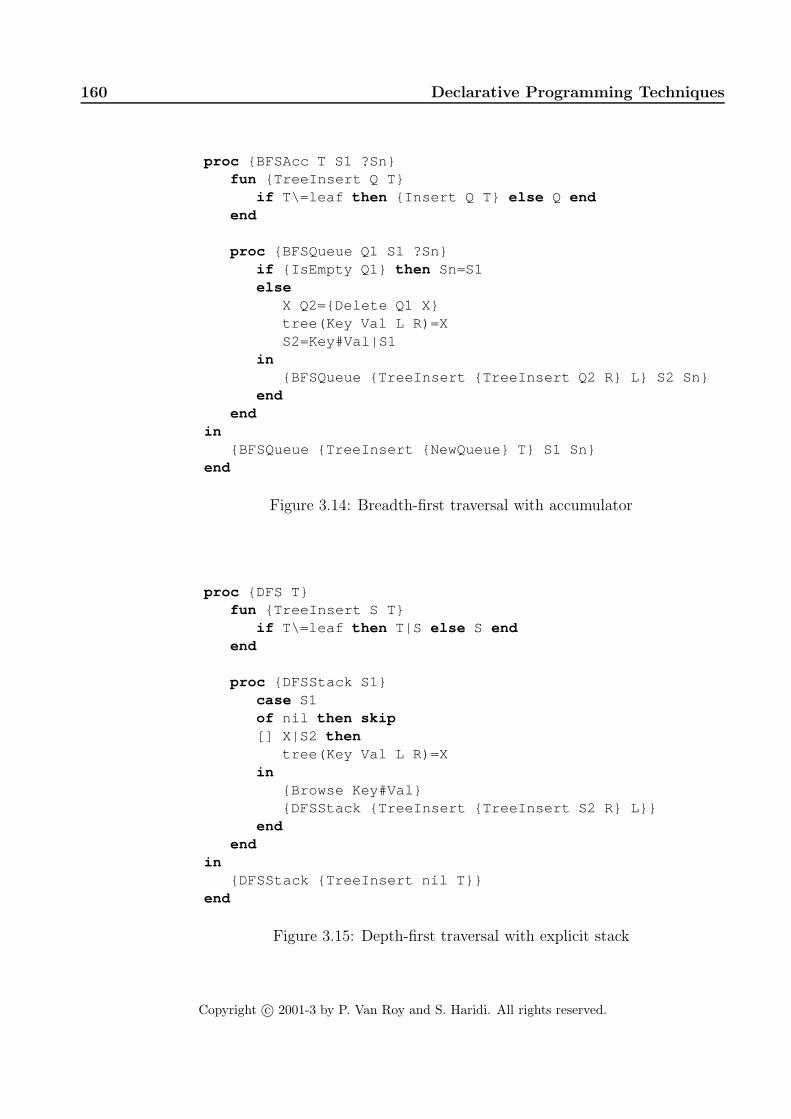
160 Declarative Programming Techniques
proc {BFSAcc T S1 ?Sn}fun {TreeInsert Q T}
if T\=leaf then {Insert Q T} else Q endend
proc {BFSQueue Q1 S1 ?Sn}if {IsEmpty Q1} then Sn=S1else
X Q2={Delete Q1 X}tree(Key Val L R)=XS2=Key#Val|S1
in{BFSQueue {TreeInsert {TreeInsert Q2 R} L} S2 Sn}
endend
in{BFSQueue {TreeInsert {NewQueue} T} S1 Sn}
end
Figure 3.14: Breadth-first traversal with accumulator
proc {DFS T}fun {TreeInsert S T}
if T\=leaf then T|S else S endend
proc {DFSStack S1}case S1of nil then skip[] X|S2 then
tree(Key Val L R)=Xin
{Browse Key#Val}{DFSStack {TreeInsert {TreeInsert S2 R} L}}
endend
in{DFSStack {TreeInsert nil T}}
end
Figure 3.15: Depth-first traversal with explicit stack
Copyright c© 2001-3 by P. Van Roy and S. Haridi. All rights reserved.
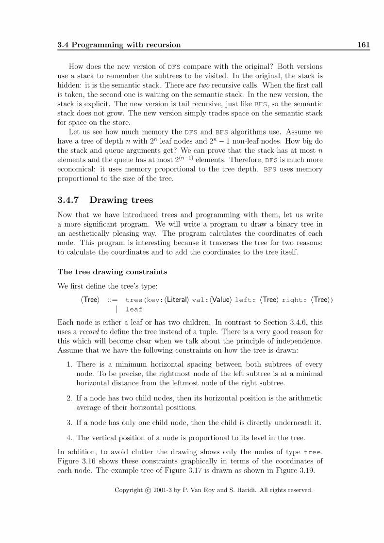
3.4 Programming with recursion 161
How does the new version of DFS compare with the original? Both versionsuse a stack to remember the subtrees to be visited. In the original, the stack ishidden: it is the semantic stack. There are two recursive calls. When the first callis taken, the second one is waiting on the semantic stack. In the new version, thestack is explicit. The new version is tail recursive, just like BFS, so the semanticstack does not grow. The new version simply trades space on the semantic stackfor space on the store.
Let us see how much memory the DFS and BFS algorithms use. Assume wehave a tree of depth n with 2n leaf nodes and 2n − 1 non-leaf nodes. How big dothe stack and queue arguments get? We can prove that the stack has at most nelements and the queue has at most 2(n−1) elements. Therefore, DFSis much moreeconomical: it uses memory proportional to the tree depth. BFS uses memoryproportional to the size of the tree.
3.4.7 Drawing trees
Now that we have introduced trees and programming with them, let us writea more significant program. We will write a program to draw a binary tree inan aesthetically pleasing way. The program calculates the coordinates of eachnode. This program is interesting because it traverses the tree for two reasons:to calculate the coordinates and to add the coordinates to the tree itself.
The tree drawing constraints
We first define the tree’s type:
〈Tree〉 ::= tree(key: 〈Literal〉 val: 〈Value〉 left: 〈Tree〉 right: 〈Tree〉)| leaf
Each node is either a leaf or has two children. In contrast to Section 3.4.6, thisuses a record to define the tree instead of a tuple. There is a very good reason forthis which will become clear when we talk about the principle of independence.Assume that we have the following constraints on how the tree is drawn:
1. There is a minimum horizontal spacing between both subtrees of everynode. To be precise, the rightmost node of the left subtree is at a minimalhorizontal distance from the leftmost node of the right subtree.
2. If a node has two child nodes, then its horizontal position is the arithmeticaverage of their horizontal positions.
3. If a node has only one child node, then the child is directly underneath it.
4. The vertical position of a node is proportional to its level in the tree.
In addition, to avoid clutter the drawing shows only the nodes of type tree .Figure 3.16 shows these constraints graphically in terms of the coordinates ofeach node. The example tree of Figure 3.17 is drawn as shown in Figure 3.19.
Copyright c© 2001-3 by P. Van Roy and S. Haridi. All rights reserved.

162 Declarative Programming Techniques
(c,y’)
(a,y)
(b,y’)
d
(a,y)
1. Distance d between subtrees has minimum value
2. If two children exist, a is average of b and c(a,y’)
4. Vertical position y is proportional to level in the tree
3. If only one child exists, it is directly below parent
Figure 3.16: The tree drawing constraints
tree(key:a val:111left:tree(key:b val:55
left:tree(key:x val:100left:tree(key:z val:56 left:leaf right:leaf)right:tree(key:w val:23 left:leaf right:leaf))
right:tree(key:y val:105 left:leafright:tree(key:r val:77 left:leaf right:leaf)))
right:tree(key:c val:123left:tree(key:d val:119
left:tree(key:g val:44 left:leaf right:leaf)right:tree(key:h val:50
left:tree(key:i val:5 left:leaf right:leaf)right:tree(key:j val:6 left:leaf right:leaf)))
right:tree(key:e val:133 left:leaf right:leaf)))
Figure 3.17: An example tree
Calculating the node positions
The tree drawing algorithm calculates node positions by traversing the tree, pass-ing information between nodes, and calculating values at each node. The traversalhas to be done carefully so that all the information is available at the right time.Exactly what traversal is the right one depends on what the constraints are. Forthe above four constraints, it is sufficient to traverse the tree in a depth-first order.In this order, each left subtree of a node is visited before the right subtree. Abasic depth-first traversal looks like this:
proc {DepthFirst Tree}case Treeof tree(left:L right:R ...) then
{DepthFirst L}{DepthFirst R}
[] leaf thenskip
endend
Copyright c© 2001-3 by P. Van Roy and S. Haridi. All rights reserved.

3.4 Programming with recursion 163
The tree drawing algorithm does a depth-first traversal and calculates the (x,y)coordinates of each node during the traversal. As a preliminary to running thealgorithm, we extend the tree nodes with the fields x and y at each node:
fun {AddXY Tree}case Treeof tree(left:L right:R ...) then
{Adjoin Treetree(x:_ y:_ left:{AddXY L} right:{AddXY R})}
[] leaf thenleaf
endend
The function AddXY returns a new tree with the two fields x and y added toall nodes. It uses the Adjoin function which can add new fields to recordsand override old ones. This is explained in Appendix B.3.2. The tree drawingalgorithm will fill in these two fields with the coordinates of each node. If the twofields exist nowhere else in the record, then there is no conflict with any otherinformation in the record.
To implement the tree drawing algorithm, we extend the depth-first traversalby passing two arguments down (namely, level in the tree and limit on leftmostposition of subtree) and two arguments up (namely, horizontal position of thesubtree’s root and rightmost position of subtree). Downward-passed argumentsare sometimes called inherited arguments. Upward-passed arguments are some-times called synthesized arguments. With these extra arguments, we have enoughinformation to calculate the positions of all nodes. Figure 3.18 gives the com-plete tree drawing algorithm. The Scale parameter gives the basic size unit ofthe drawn tree, i.e., the minimum distance between nodes. The initial argumentsare Level =1 and LeftLim =Scale . There are four cases, depending on whethera node has two subtrees, one subtree (left or right), or zero subtrees. Patternmatching in the case statement picks the right case. This takes advantage of thefact that the tests are done in sequential order.
3.4.8 Parsing
As a second case study of declarative programming, let us write a parser for asmall imperative language with syntax similar to Pascal. This uses many of thetechniques we have seen, in particular, it uses an accumulator and builds a tree.
What is a parser
A parser is part of a compiler. A compiler is a program that translates a sequenceof characters, which represents a program, into a sequence of low-level instructionsthat can be executed on a machine. In its most basic form, a compiler consistsof three parts:
Copyright c© 2001-3 by P. Van Roy and S. Haridi. All rights reserved.

164 Declarative Programming Techniques
Scale=30
proc {DepthFirst Tree Level LeftLim ?RootX ?RightLim}case Treeof tree(x:X y:Y left:leaf right:leaf ...) then
X=RootX=RightLim=LeftLimY=Scale*Level
[] tree(x:X y:Y left:L right:leaf ...) thenX=RootXY=Scale*Level{DepthFirst L Level+1 LeftLim RootX RightLim}
[] tree(x:X y:Y left:leaf right:R ...) thenX=RootXY=Scale*Level{DepthFirst R Level+1 LeftLim RootX RightLim}
[] tree(x:X y:Y left:L right:R ...) thenLRootX LRightLim RRootX RLeftLim
inY=Scale*Level{DepthFirst L Level+1 LeftLim LRootX LRightLim}RLeftLim=LRightLim+Scale{DepthFirst R Level+1 RLeftLim RRootX RightLim}X=RootX=(LRootX+RRootX) div 2
endend
Figure 3.18: Tree drawing algorithm
• Tokenizer. The tokenizer reads a sequence of characters and outputs asequence of tokens.
• Parser. The parser reads a sequence of tokens and outputs an abstractsyntax tree. This is sometimes called a parse tree.
• Code generator. The code generator traverses the syntax tree and gen-erates low-level instructions for a real machine or an abstract machine.
Usually this structure is extended by optimizers to improve the generated code.In this section, we will just write the parser. We first define the input and outputformats of the parser.
The parser’s input and output languages
The parser accepts a sequence of tokens according to the grammar given in Ta-ble 3.2 and outputs an abstract syntax tree. The grammar is carefully designedto be right recursive and deterministic. This means that the choice of grammar
Copyright c© 2001-3 by P. Van Roy and S. Haridi. All rights reserved.

3.4 Programming with recursion 165
Figure 3.19: The example tree displayed with the tree drawing algorithm
rule is completely determined by the next token. This makes it possible to writea top down, left to right parser with only one token lookahead.
For example, say we want to parse a 〈Term〉. It consists of a non-empty seriesof 〈Fact〉 separated by 〈TOP〉 tokens. To parse it, we first parse a 〈Fact〉. Then weexamine the next token. If it is a 〈TOP〉, then we know the series continues. If itis not a 〈TOP〉, then we know the series has ended, i.e., the 〈Term〉 has ended. Forthis parsing strategy to work, there must be no overlap between 〈TOP〉 tokens andthe other possible tokens that come after a 〈Fact〉. By inspecting the grammarrules, we see that the other tokens must be taken from {〈EOP〉, 〈COP〉, ;, end,then, do, else, )}. We confirm that all the tokens defined by this set are differentfrom the tokens defined by 〈TOP〉.
There are two kinds of symbols in Table 3.2: nonterminals and terminals.A nonterminal symbol is one that is further expanded according to a grammarrule. A terminal symbol corresponds directly to a token in the input. It isnot expanded. The nonterminal symbols are 〈Prog〉 (complete program), 〈Stat〉(statement), 〈Comp〉 (comparison), 〈Expr〉 (expression), 〈Term〉 (term), 〈Fact〉(factor), 〈COP〉 (comparison operator), 〈EOP〉 (expression operator), and 〈TOP〉(term operator). To parse a program, start with 〈Prog〉 and expand until findinga sequence of tokens that matches the input.
The parser output is a tree (i.e., a nested record) with syntax given in Ta-ble 3.3. Superficially, Tables 3.2 and 3.3 have very similar content, but they areactually quite different: the first defines a sequence of tokens and the seconddefines a tree. The first does not show the structure of the input program–wesay it is flat. The second exposes this structure–we say it is nested. Becauseit exposes the program’s structure, we call the nested record an abstract syntax
Copyright c© 2001-3 by P. Van Roy and S. Haridi. All rights reserved.

166 Declarative Programming Techniques
〈Prog〉 ::= program 〈Id〉 ; 〈Stat〉 end〈Stat〉 ::= begin { 〈Stat〉 ; } 〈Stat〉 end
| 〈Id〉 := 〈Expr〉| if 〈Comp〉 then 〈Stat〉 else 〈Stat〉| while 〈Comp〉 do 〈Stat〉| read 〈Id〉| write 〈Expr〉
〈Comp〉 ::= { 〈Expr〉 〈COP〉 } 〈Expr〉〈Expr〉 ::= { 〈Term〉 〈EOP〉 } 〈Term〉〈Term〉 ::= { 〈Fact〉 〈TOP〉 } 〈Fact〉〈Fact〉 ::= 〈Integer〉 | 〈Id〉 | ( 〈Expr〉 )〈COP〉 ::= ´ ==´ | ´ != ´ | ´ >´ | ´ <´ | ´ =<´ | ´ >=´
〈EOP〉 ::= ´ +´ | ´ - ´
〈TOP〉 ::= ´ * ´ | ´ / ´
〈Integer〉 ::= (integer)〈Id〉 ::= (atom)
Table 3.2: The parser’s input language (which is a token sequence)
tree. It is abstract because it is encoded as a data structure in the language, andno longer in terms of tokens. The parser’s role is to extract the structure fromthe flat input. Without this structure, it is extremely difficult to write the codegenerator and code optimizers.
The parser program
The main parser call is the function {Prog S1 Sn} , where S1 is an input list oftokens and Sn is the rest of the list after parsing. This call returns the parsedoutput. For example:
declare A Sn inA={Prog
[program foo ´ ; ´ while a ´ +´ 3 ´ <´ b ´ do´ b ´ := ´ b ´ +´ 1 ´ end ´ ]Sn}
{Browse A}
displays:
prog(foo while( ´ <´ ( ´ +´ (a 3) b) assign(b ´ +´ (b 1))))
We give commented program code for the complete parser. Prog is written asfollows:
fun {Prog S1 Sn}Y Z S2 S3 S4 S5
inS1=program|S2
Copyright c© 2001-3 by P. Van Roy and S. Haridi. All rights reserved.

3.4 Programming with recursion 167
〈Prog〉 ::= prog( 〈Id〉 〈Stat〉 )
〈Stat〉 ::= ´ ; ´ ( 〈Stat〉 〈Stat〉 )
| assign( 〈Id〉 〈Expr〉 )
| ´ if ´ ( 〈Comp〉 〈Stat〉 〈Stat〉 )
| while( 〈Comp〉 〈Stat〉 )
| read( 〈Id〉 )
| write( 〈Expr〉 )
〈Comp〉 ::= 〈COP〉( 〈Expr〉 〈Expr〉 )
〈Expr〉 ::= 〈Id〉 | 〈Integer〉 | 〈OP〉( 〈Expr〉 〈Expr〉 )
〈COP〉 ::= ´ ==´ | ´ != ´ | ´ >´ | ´ <´ | ´ =<´ | ´ >=´
〈OP〉 ::= ´ +´ | ´ - ´ | ´ * ´ | ´ / ´
〈Integer〉 ::= (integer)〈Id〉 ::= (atom)
Table 3.3: The parser’s output language (which is a tree)
Y={Id S2 S3}S3=´ ; ´ |S4Z={Stat S4 S5}S5=´ end ´ |Snprog(Y Z)
end
The accumulator is threaded through all terminal and nonterminal symbols. Eachnonterminal symbol has a procedure to parse it. Statements are parsed with Stat ,which is written as follows:
fun {Stat S1 Sn}T|S2=S1
incase Tof begin then
{Sequence Stat fun {$ X} X== ´ ; ´ end S2 ´ end ´ |Sn}[] ´ if ´ then C X1 X2 S3 S4 S5 S6 in
{Comp C S2 S3}S3=´ then ´ |S4X1={Stat S4 S5}S5=´ else ´ |S6X2={Stat S6 Sn}´ if ´ (C X1 X2)
[] while then C X S3 S4 inC={Comp S2 S3}S3=´ do´ |S4X={Stat S4 Sn}while(C X)
Copyright c© 2001-3 by P. Van Roy and S. Haridi. All rights reserved.

168 Declarative Programming Techniques
[] read then I inI={Id S2 Sn}read(I)
[] write then E inE={Expr S2 Sn}write(E)
elseif {IsIdent T} then E S3 inS2=´ := ´ |S3E={Expr S3 Sn}assign(T E)
elseS1=Snraise error(S1) end
endend
The one-token lookahead is put in T. With a case statement, the correct branchof the Stat grammar rule is found. Statement sequences (surrounded by begin
– end) are parsed by the procedure Sequence . This is a generic procedure thatalso handles comparison sequences, expression sequences, and term sequences. Itis written as follows:
fun {Sequence NonTerm Sep S1 Sn}X1 S2 T S3
inX1={NonTerm S1 S2}S2=T|S3if {Sep T} then X2 in
X2={Sequence NonTerm Sep S3 Sn}T(X1 X2) % Dynamic record creation
elseS2=SnX1
endend
This takes two input functions, NonTerm, which is passed any nonterminal, andSep, which detects the separator symbol in a sequence. Comparisons, expressions,and terms are parsed as follows with Sequence :
fun {Comp S1 Sn} {Sequence Expr COP S1 Sn} endfun {Expr S1 Sn} {Sequence Term EOP S1 Sn} endfun {Term S1 Sn} {Sequence Fact TOP S1 Sn} end
Each of these three functions has its corresponding function for detecting sepa-rators:
fun {COP Y}Y==´ <´ orelse Y==´ >´ orelse Y==´ =<´ orelseY==´ >=´ orelse Y==´ ==´ orelse Y==´ != ´
Copyright c© 2001-3 by P. Van Roy and S. Haridi. All rights reserved.

3.5 Time and space efficiency 169
endfun {EOP Y} Y== ´ +´ orelse Y==´ - ´ endfun {TOP Y} Y== ´ * ´ orelse Y==´ / ´ end
Finally, factors and identifiers are parsed as follows:
fun {Fact S1 Sn}T|S2=S1
inif {IsInt T} orelse {IsIdent T} then
S2=SnT
else E S2 S3 inS1=´ ( ´ |S2E={Expr S2 S3}S3=´ ) ´ |SnE
endend
fun {Id S1 Sn} X in S1=X|Sn true ={IsIdent X} X endfun {IsIdent X} {IsAtom X} end
Integers are represented as built-in integer values and detected using the built-inIsInt function.
This parsing technique works for grammars where one-token lookahead isenough. Some grammars, called ambiguous grammars, require to look at morethan one token to decide which grammar rule is needed. A simple way to parsethem is with nondeterministic choice, as explained in Chapter 9.
3.5 Time and space efficiency
Declarative programming is still programming; even though it has strong math-ematical properties it still results in real programs that run on real computers.Therefore, it is important to think about computational efficiency. There are twoparts to efficiency: execution time (e.g., in seconds) and memory usage (e.g., inbytes). We will show how to calculate both of these.
3.5.1 Execution time
Using the kernel language and its semantics, we can calculate the execution timeup to a constant factor. For example, for a mergesort algorithm we will be ableto say that the execution time is proportional to n log n, given an input list oflength n. The asymptotic time complexity of an algorithm is the tightest upperbound on its execution time as a function of the input size, up to a constantfactor. This is sometimes called the worst-case time complexity.
Copyright c© 2001-3 by P. Van Roy and S. Haridi. All rights reserved.

170 Declarative Programming Techniques
〈s〉 ::=skip k| 〈x〉1=〈x〉2 k| 〈x〉=〈v〉 k| 〈s〉1 〈s〉2 T (s1) + T (s2)| local 〈x〉 in 〈s〉 end k + T (s)| proc { 〈x〉 〈y〉1 ... 〈y〉n} 〈s〉 end k| if 〈x〉 then 〈s〉1 else 〈s〉2 end k + max(T (s1), T (s2))| case 〈x〉 of 〈pattern〉 then 〈s〉1 else 〈s〉2 end k + max(T (s1), T (s2))| { 〈x〉 〈y〉1 ... 〈y〉n} Tx(sizex(Ix({y1, ..., yn}))
Table 3.4: Execution times of kernel instructions
To find the constant factor, it is necessary to measure actual runs of the pro-gram on its implementation. Calculating the constant factor a priori is extremelydifficult. This is because modern computer systems have a complex hardware andsoftware structure that introduces much unpredictability in the execution time:they do memory management (see Section 3.5.2), they have complex memorysystems (with virtual memory and several levels of caches), they have complexpipelined and superscalar architectures (many instructions are simultaneously invarious stages of execution; an instruction’s execution time often depends on theother instructions present), and the operating system does context switches at un-predictable times. This unpredictability improves the average performance at theprice of increasing performance fluctuations. For more information on measuringperformance and its pitfalls, we recommend [91].
Big-oh notation
We will give the execution time of the program in terms of the “big-oh” notationO(f(n)). This notation lets us talk about the execution time without havingto specify the constant factor. Let T (n) be a function that gives the executiontime of some program, measured in the size of the input n. Let f(n) be someother function defined on nonnegative integers. Then we say T (n) is of O(f(n))(pronounced T (n) is of order f(n)) if T (n) ≤ c.f(n) for some positive constantc, for all n except for some small values n ≤ n0. That is, as n grows there is apoint after which T (n) never gets bigger than c.f(n).
Sometimes this is written T (n) = O(f(n)). Be careful! This use of equalsis an abuse of notation, since there is no equality involved. If g(n) = O(f(n))and h(n) = O(f(n)), then it is not true that g(n) = h(n). A better way tounderstand the big-oh notation is in terms of sets and membership: O(f(n)) isa set of functions, and saying T (n) is of O(f(n)) means simply that T (n) is amember of the set.
Copyright c© 2001-3 by P. Van Roy and S. Haridi. All rights reserved.

3.5 Time and space efficiency 171
Calculating the execution time
We use the kernel language as a guide. Each kernel instruction has a well-definedexecution time, which may be a function of the size of its arguments. Assumewe have a program that consists of the p functions F1, ..., Fp. We would like tocalculate the p functions TF1, ..., TFp. This is done in three steps:
1. Translate the program into the kernel language.
2. Use the kernel execution times to set up a collection of equations thatcontain TF1, ..., TFp. We call these equations recurrence equations sincethey define the result for n in terms of results for values smaller than n.
3. Solve the recurrence equations for TF1, ..., TFp.
Table 3.4 gives the execution time T (s) for each kernel statement 〈s〉. In thistable, s is an integer and the arguments yi = E(〈y〉i) for 1 ≤ i ≤ n, for the ap-propriate environment E. Each instance of k is a different positive real constant.The function Ix({y1, ..., yn}) returns the subset of a procedure’s arguments thatare used as inputs.11 The function sizex({y1, ..., yk}) is the “size” of the inputarguments for the procedure x. We are free to define size in any way we like; ifit is defined badly then the recurrence equations will have no solution. For theinstructions 〈x〉=〈y〉 and 〈x〉=〈v〉 there is a rare case when they can take morethan constant time, namely, when the two arguments are bound to large partialvalues. In that case, the time is proportional to the size of the common part ofthe two partial values.
Example: Append function
Let us give a simple example to show how this works. Consider the Append
function:
fun {Append Xs Ys}case Xsof nil then Ys[] X|Xr then X|{Append Xr Ys}end
end
This has the following translation into the kernel language:
proc {Append Xs Ys ?Zs}case Xsof nil then Zs=Ys[] X|Xr then Zr in
Zs=X|Zr{Append Xr Ys Zr}
11This can sometimes differ from call to call. For example, when a procedure is used toperform different tasks at different calls.
Copyright c© 2001-3 by P. Van Roy and S. Haridi. All rights reserved.

172 Declarative Programming Techniques
endend
Using Table 3.4, we get the following recurrence equation for the recursive call:
TAppend (size(I({Xs, Ys, Zs}))) = k1+max(k2, k3+TAppend (size(I({Xr , Ys, Zr })))
(The subscripts for size and I are not needed here.) Let us simplify this. Weknow that I({Xs, Ys, Zs}) = {Xs} and we assume that size({Xs}) = n, where nis the length of Xs. This gives:
TAppend (n) = k1 + max(k2, k3 + TAppend (n− 1))
Further simplifying gives:
TAppend (n) = k4 + TAppend (n− 1)
We handle the base case by picking a particular value of Xs for which we candirectly calculate the result. Let us pick Xs=nil . This gives:
TAppend (0) = k5
Solving the two equations gives:
TAppend (n) = k4.n + k5
Therefore TAppend (n) is of O(n).
Recurrence equations
Before looking at more examples, let us take a step back and look at recurrenceequations in general. A recurrence equation has one of two forms:
• An equation that defines a function T (n) in terms of T (m1), ..., T (mk),where m1, ..., mk < n.
• An equation that gives T (n) directly for certain values of n, e.g., T (0) orT (1).
When calculating execution times, recurrence equations of many different kindspop up. Here is a table of some frequently occurring equations and their solutions:
Equation SolutionT (n) = k + T (n− 1) O(n)T (n) = k1 + k2.n + T (n− 1) O(n2)T (n) = k + T (n/2) O(logn)T (n) = k1 + k2.n + T (n/2) O(n)T (n) = k + 2.T (n/2) O(n)T (n) = k1 + k2.n + 2.T (n/2) O(n logn)
There are many techniques to derive these solutions. We will see a few in theexamples that follow. The box explains two of the most generally useful ones.
Copyright c© 2001-3 by P. Van Roy and S. Haridi. All rights reserved.

3.5 Time and space efficiency 173
Solving recurrence equations
The following techniques are often useful:
• A simple three-step technique that almost always works inpractice. First, get exact numbers for some small inputs(for example: T (0) = k, T (1) = k + 3, T (2) = k + 6).Second, guess the form of the result (for example: T (n) =an + b, for some as yet unknown a and b). Third, plugthe guessed form into the equations. In our example thisgives b = k and (an + b) = 3 + (a.(n− 1) + b). This givesa = 3, for a final result of T (n) = 3n + k. The three-steptechnique works if the guessed form is correct.
• A much more powerful technique, called generating func-tions, that gives closed-form or asymptotic results in awide variety of cases without having to guess the form. Itrequires some technical knowledge of infinite series and cal-culus, but not more than is seen in a first university-levelcourse on these subjects. See Knuth [102] and Wilf [207]for good introductions to generating functions.
Example: FastPascal
In Chapter 1, we introduced the function FastPascal and claimed with a bit ofhandwaving that {FastPascal N} is of O(n2). Let us see if we can derive thismore rigorously. Here is the definition again:
fun {FastPascal N}if N==1 then [1]else L in
L={FastPascal N-1}{AddList {ShiftLeft L} {ShiftRight L}}
endend
We can derive the equations directly from looking at this definition, withouttranslating functions into procedures. Looking at the definition, it is easy to seethat ShiftRight is of O(1), i.e., it is constant time. Using similar reasoning asfor Append , we can derive that AddList and ShiftLeft are of O(n) where n isthe length of L. This gives us the following recurrence equation for the recursivecall:
TFastPascal (n) = k1 + max(k2, k3 + TFastPascal (n− 1) + k4.n)
Copyright c© 2001-3 by P. Van Roy and S. Haridi. All rights reserved.

174 Declarative Programming Techniques
where n is the value of the argument N. Simplifying gives:
TFastPascal (n) = k5 + k4.n + TFastPascal (n− 1)
For the base case, we pick N=1. This gives:
TFastPascal (1) = k6
To solve these two equations, we first “guess” that the solution is of the form:
TFastPascal (n) = a.n2 + b.n + c
This guess comes from an intuitive argument like the one given in Chapter 1. Wethen insert this form into the two equations. If we can successfully solve for a,b, and c, then this means that our guess was correct. Inserting the form into thetwo equations gives the following three equations in a, b, and c:
k4 − 2a = 0
k5 + a− b = 0
a + b + c− k6 = 0
We do not have to solve this system completely; it suffices to verify that a 6= 0.12
Therefore TFastPascal (n) is of O(n2).
Example: MergeSort
In the previous section we saw three mergesort algorithms. They all have the sameexecution time, with different constant factors. Let us calculate the executiontime of the first algorithm. Here is the main function again:
fun {MergeSort Xs}case Xsof nil then nil[] [X] then [X]else Ys Zs in
{Split Xs Ys Zs}{Merge {MergeSort Ys} {MergeSort Zs}}
endend
Let T (n) be the execution time of {MergeSort Xs} , where n is the length ofXs. Assume that Split and Merge are of O(n) in the length of their inputs.We know that Split outputs two lists of lengths dn/2e and bn/2c, From thedefinition of MergeSort , this lets us define the following recurrence equations:
• T (0) = k1
12If we guess a.n2 + b.n + c and the actual solution is of the form b.n + c, then we will geta = 0.
Copyright c© 2001-3 by P. Van Roy and S. Haridi. All rights reserved.

3.5 Time and space efficiency 175
• T (1) = k2
• T (n) = k3 + k4n + T (dn/2e) + T (bn/2c) if n ≥ 2
This uses the ceiling and floor functions, which are a bit tricky. To get rid ofthem, assume that n is a power of 2, i.e., n = 2k for some k. Then the equationsbecome:
• T (0) = k1
• T (1) = k2
• T (n) = k3 + k4n + 2T (n/2) if n ≥ 2
Expanding the last equation gives (where L(n) = k3 + k4n):
• T (n) =
k︷ ︸︸ ︷L(n) + 2L(n/2) + 4L(n/4) + ... + (n/2)L(2) + 2T (1)
Replacing L(n) and T (1) by their values gives:
• T (n) =
k︷ ︸︸ ︷(k4n + k3) + (k4n + 2k3) + (k4n + 4k3) + ... + (k4n + (n/2)k3) + k2
Doing the sum gives:
• T (n) = k4kn + (n− 1)k3 + k2
We conclude that T (n) = O(n log n). For values of n that are not powers of 2, weuse the easily-proved fact that n ≤ m ⇒ T (n) ≤ T (m) to show that the big-ohbound still holds. The bound is independent of the content of the input list. Thismeans that the O(n log n) bound is also a worst-case bound.
3.5.2 Memory usage
Memory usage is not a single figure like execution time. It consists of two quitedifferent concepts:
• The instantaneous active memory size ma(t), in memory words. Thisnumber gives how much memory the program needs to continue to exe-cute successfully. A related number is the maximum active memory size,Ma(t) = max0≤u≤t ma(u). This number is useful for calculating how muchphysical memory your computer needs to execute the program successfully.
• The instantaneous memory consumption mc(t), in memory words/second.This number gives how much memory the program allocates during itsexecution. A large value for this number means that memory managementhas more work to do, e.g., the garbage collector will be invoked more often.This will increase execution time. A related number is the total memoryconsumption, Mc(t) =
∫ t
0mc(u)du, which is a measure for how much total
work memory management has to do to run the program.
Copyright c© 2001-3 by P. Van Roy and S. Haridi. All rights reserved.

176 Declarative Programming Techniques
〈s〉 ::=skip 0| 〈x〉1=〈x〉2 0| 〈x〉=〈v〉 memsize(v)| 〈s〉1 〈s〉2 M(s1) + M(s2)| local 〈x〉 in 〈s〉 end 1 + T (s)| if 〈x〉 then 〈s〉1 else 〈s〉2 end max(M(s1), M(s2))| case 〈x〉 of 〈pattern〉 then 〈s〉1 else 〈s〉2 end max(M(s1), M(s2))| { 〈x〉 〈y〉1 ... 〈y〉n} Mx(sizex(Ix({y1, ..., yn}))
Table 3.5: Memory consumption of kernel instructions
These two numbers should not be confused. The first is much more important.A program can allocate memory very slowly (e.g., 1 KB/s) and yet have a largeactive memory (e.g., 100 MB). For example, a large in-memory database that han-dles only simple queries. The opposite is also possible. A program can consumememory at a high rate (e.g., 100 MB/s) and yet have a quite small active memo-ry (e.g., 10 KB). For example, a simulation algorithm running in the declarativemodel.13
Instantaneous active memory size
The active memory size can be calculated at any point during execution by fol-lowing all the references from the semantic stack into the store and totaling thesize of all the reachable variables and partial values. It is roughly equal to thesize of all the data structures needed by the program during its execution.
Total memory consumption
The total memory consumption can be calculated with a technique similar tothat used for execution time. Each kernel language operation has a well-definedmemory consumption. Table 3.5 gives the memory consumption M(s) for eachkernel statement 〈s〉. Using this table, recurrence equations can be set up forthe program, from which the total memory consumption of the program can becalculated as a function of the input size. To this number should be added thememory consumption of the semantic stack. For the instruction 〈x〉=〈v〉 thereis a rare case in which memory consumption is less than memsize(v), namelywhen 〈x〉 is partly instantiated. In that case, only the memory of the new entitiesshould be counted. The function memsize(v) is defined as follows, according tothe type and value of v:
13Because of this behavior, the declarative model is not good for running simulations unlessit has an excellent garbage collector!
Copyright c© 2001-3 by P. Van Roy and S. Haridi. All rights reserved.

3.5 Time and space efficiency 177
• For an integer: 0 for small integers, otherwise proportional to integer size.Calculate the number of bits needed to represent the integer in two’s com-plement form. If this number is less than 28, then 0. Else divide by 32 andround up to the nearest integer.
• For a float: 2.
• For a list pair: 2.
• For a tuple or record: 1 + n, where n = length(arity(v)).
• For a procedure value: k+n, where n is the number of external references ofthe procedure body and k is a constant that depends on the implementation.
All figures are in number of 32-bit memory words, correct for Mozart 1.3.0. Fornested values, take the sum of all the values. For records and procedure valuesthere is an additional one-time cost. For each distinct record arity the additionalcost is roughly proportional to n (because the arity is stored once in a symboltable). For each distinct procedure in the source code, the additional cost dependson the size of the compiled code, which is roughly proportional to the total numberof statements and identifiers in the procedure body. In most cases, these one-timecosts add a constant to the total memory consumption; for the calculation theycan usually be ignored.
3.5.3 Amortized complexity
Sometimes we are not interested in the complexity of single operations, but ratherin the total complexity of a sequence of operations. As long as the total complex-ity is reasonable, we might not care whether individual operations are sometimesmore expensive. Section 3.4.5 gives an example with queues: as long as a se-quence of n insert and delete operations has a total execution time that is O(n),we might not care whether individual operations are always O(1). They are al-lowed occasionally to be more expensive, as long as this does not happen toofrequently. In general, if a sequence of n operations has a total execution timeO(f(n)), then we say that it has an amortized complexity of O(f(n)/n).
Amortized versus worst-case complexity
For many application domains, having a good amortized complexity is goodenough. However, there are three application domains that need guarantees onthe execution time of individual operations. They are hard real-time systems,parallel systems, and interactive systems.
A hard real-time system has to satisfy strict deadlines on the completion ofcalculations. Missing such a deadline can have dire consequences including lossof lives. Such systems exist, e.g., in pacemakers and train collision avoidance (seealso Section 4.6.1).
Copyright c© 2001-3 by P. Van Roy and S. Haridi. All rights reserved.

178 Declarative Programming Techniques
A parallel system executes several calculations simultaneously to achieve speedupof the whole computation. Often, the whole computation can only advance afterall the simultaneous calculations complete. If one of these calculations occasion-ally takes much more time, then the whole computation slows down.
An interactive system, such as a computer game, should have a uniform reac-tion time. For example, if a multi-user action game sometimes delays its reactionto a player’s input then the player’s satisfaction is much reduced.
The banker’s method and the physicist’s method
Calculating the amortized complexity is a little harder than calculating the worst-case complexity. (And it will get harder still when we introduce lazy executionin Section 4.5.) There are basically two methods, called the banker’s method andthe physicist’s method.
The banker’s method counts credits, where a “credit” represents a unit ofexecution time or memory space. Each operation puts aside some credits. Anexpensive operation is allowed when enough credits have been put aside to coverits execution.
The physicist’s method is based on finding a potential function. This is akind of “height above sea level”. Each operation changes the potential, i.e., itclimbs or descends a bit. The cost of each operation is the change in potential,namely, how much it climbs or descends. The total complexity is a function ofthe difference between the initial and final potentials. As long as this differenceremains small, large variations are allowed in between.
For more information on these methods and many examples of their use withdeclarative algorithms, we recommend the book by Okasaki [138].
3.5.4 Reflections on performance
Ever since the beginning of the computer era in the 1940’s, both space and timehave been becoming cheaper at an exponential rate (a constant factor improve-ment each year). They are currently very cheap, both in absolute terms and inperceived terms: a low-cost personal computer of the year 2000 typically has atleast 64MB of random-access memory and 4 GB of persistent storage on disk,with a performance of several hundred million instructions per second, whereeach instruction can perform a full 64-bit operation including floating point. Itis comparable to or faster than a Cray-1, the world’s fastest supercomputer in1975. A supercomputer is defined to be one of the fastest computers existing ata particular time. The first Cray-1 had a clock frequency of 80 MHz and couldperform several 64-bit floating point operations per cycle [178]. At constant cost,personal computer performance is still improving according to Moore’s Law (thatis, doubling every two years), and this is predicted to continue at least throughoutthe first decade of the 21st century.
Because of this situation, performance is usually not a critical issue. If your
Copyright c© 2001-3 by P. Van Roy and S. Haridi. All rights reserved.

3.5 Time and space efficiency 179
problem is tractable, i.e., there exists an efficient algorithm for it, then if you usegood techniques for algorithm design, the actual time and space that the algo-rithm takes will almost always be acceptable. In other words, given a reasonableasymptotic complexity of a program, the constant factor is almost never critical.This is even true for most multimedia applications (which use video and audio)because of the excellent graphics libraries that exist.
Not all problems are tractable, though. There are problems that are com-putationally expensive, for example in the areas of combinatorial optimization,operational research, scientific computation and simulation, machine learning,speech and vision recognition, and computer graphics. Some of these problemsare expensive simply because they have to do a lot of work. For example, gameswith realistic graphics, which by definition are always at the edge of what is pos-sible. Other problems are expensive for more fundamental reasons. For example,NP-complete problems. These problems are in NP, i.e., it is easy to check a solu-tion, if you are given a candidate.14 But finding a solution may be much harder. Asimple example is the circuit satisfiability problem. Given a combinational digitalcircuit that consists of And, Or , and Not gates. Does there exist a set of input val-ues that makes the output 1? This problem is NP-complete [41]. An NP-completeproblem is a special kind of NP problem with the property that if you can solveone in polynomial time, then you can solve all in polynomial time. Many com-puter scientists have tried over several decades to find polynomial-time solutionsto NP-complete problems, and none have succeeded. Therefore, most comput-er scientists suspect that NP-complete problems cannot be solved in polynomialtime. In this book, we will not talk any more about computationally-expensiveproblems. Since our purpose is to show how to program, we limit ourselves totractable problems.
In some cases, the performance of a program can be insufficient, even if theproblem is theoretically tractable. Then the program has to be rewritten to im-prove performance. Rewriting a program to improve some characteristic is calledoptimizing it, although it is never “optimal” in any mathematical sense. Usually,the program can easily be improved up to a point, after which diminishing returnsset in and the program rapidly becomes more complex for ever smaller improve-ments. Optimization should therefore not be done unless necessary. Prematureoptimization is the bane of computing.
Optimization has a good side and a bad side. The good side is that the overallexecution time of most applications is largely determined by a very small part ofthe program text. Therefore performance optimization, if necessary, can almostalways be done by rewriting just this small part (sometimes a few lines suffice).The bad side is that it is usually not obvious, even to experienced programmers,where this part is a priori. Therefore, this part should be identified after theapplication is running and only if a performance problem is noticed. If no suchproblem exists, then no performance optimization should be done. The best
14NP stands for “nondeterministic polynomial time”.
Copyright c© 2001-3 by P. Van Roy and S. Haridi. All rights reserved.

180 Declarative Programming Techniques
technique to identify the “hotspots” is profiling, which instruments the applicationto measure its run-time characteristics.
Reducing a program’s space use is easier than reducing its execution time.The overall space use of a program depends on the data representation chosen. Ifspace is a critical issue, then a good technique is to use a compression algorithmon the data when it is not part of an immediate computation. This trades spacefor time.
3.6 Higher-order programming
Higher-order programming is the collection of programming techniques that be-come available when using procedure values in programs. Procedure values arealso known as lexically-scoped closures. The term higher-order comes from theconcept of order of a procedure. A procedure all of whose arguments are not pro-cedures is of order zero. A procedure that has at least one zero-order procedurein an argument is of order one. And so forth: a procedure is of order n + 1 ifit has at least one argument of order n and none of higher order. Higher-orderprogramming means simply that procedures can be of any order, not just orderzero.
3.6.1 Basic operations
There are four basic operations that underlie all the techniques of higher-orderprogramming:
• Procedural abstraction: the ability to convert any statement into a pro-cedure value.
• Genericity: the ability to pass procedure values as arguments to a proce-dure call.
• Instantiation: the ability to return procedure values as results from aprocedure call.
• Embedding: the ability to put procedure values in data structures.
Let us first examine each of these operations in turn. Subsequently, we will seemore sophisticated techniques, such as loop abstractions, that use these basicoperations.
Procedural abstraction
We have already introduced procedural abstraction. Let us briefly recall thebasic idea. Any statement 〈stmt〉 can be “packaged” into a procedure by writingit as proc {$} 〈stmt〉 end . This does not execute the statement, but insteadcreates a procedure value (a closure). Because the procedure value contains a
Copyright c© 2001-3 by P. Van Roy and S. Haridi. All rights reserved.

3.6 Higher-order programming 181
{X}
<stmt> proc {$}<stmt>
end
X=
Normal execution Delayed execution
Execute astatement
‘‘Package’’a statement
Execute thestatement
time time
Figure 3.20: Delayed execution of a procedure value
contextual environment, executing it gives exactly the same result as executing〈stmt〉. The decision whether or not to execute the statement is not made wherethe statement is defined, but somewhere else in the program. Figure 3.20 showsthe two possibilities: either executing 〈stmt〉 immediately or with a delay.
Procedure values allow more than just delaying execution of a statement.They can have arguments, which allows some of their behavior to be influencedby the call. As we will see throughout the book, procedural abstraction is enor-mously powerful. It underlies higher-order programming and object-oriented pro-gramming, and is extremely useful for building abstractions. Let us give anotherexample of procedural abstraction. Consider the statement:
local A=1.0 B=3.0 C=2.0 D RealSol X1 X2 inD=B*B-4.0*A*Cif D>=0.0 then
RealSol= trueX1=(˜B+{Sqrt D})/(2.0*A)X2=(˜B-{Sqrt D})/(2.0*A)
elseRealSol= falseX1=˜B/(2.0*A)X2={Sqrt ˜D}/(2.0*A)
end{Browse RealSol#X1#X2}
end
This calculates the solutions of the quadratic equation x2 + 3x + 2 = 0. It uses
the quadratic formula−b±
√b2 − 4ac
2a, which gives the two solutions of the
equation ax2 + bx+ c = 0. The value d = b2− 4ac is called the discriminant: if itis positive or zero, then there are two real solutions. Otherwise, the two solutions
Copyright c© 2001-3 by P. Van Roy and S. Haridi. All rights reserved.

182 Declarative Programming Techniques
are conjugate complex numbers. The above statement can be converted into aprocedure by using it as the body of a procedure definition and passing the freevariables as arguments:
declareproc {QuadraticEquation A B C ?RealSol ?X1 ?X2}
D=B*B-4.0*A*Cin
if D>=0.0 thenRealSol= trueX1=(˜B+{Sqrt D})/(2.0*A)X2=(˜B-{Sqrt D})/(2.0*A)
elseRealSol= falseX1=˜B/(2.0*A)X2={Sqrt ˜D}/(2.0*A)
endend
This procedure will solve any quadratic equation. Just call it with the equation’scoefficients as arguments:
declare RS X1 X2 in{QuadraticEquation 1.0 3.0 2.0 RS X1 X2}{Browse RS#X1#X2}
A common limitation
Many older imperative languages have a restricted form of procedural abstraction.To understand this, let us look at Pascal and C [94, 99]. In C, all procedure def-initions are global (they cannot be nested). This means that only one procedurevalue can exist corresponding to each procedure definition. In Pascal, proceduredefinitions can be nested, but procedure values can only be used in the samescope as the procedure definition, and then only while the program is executingin that scope. These restrictions make it impossible in general to “package up”a statement and execute it somewhere else.
This means that many higher-order programming techniques are impossible.For example, it is impossible to program new control abstractions. Instead, eachlanguage provides a predefined set of control abstractions (such as loops, condi-tionals, and exceptions). A few higher-order techniques are still possible. Forexample, the quadratic equation example works because it has no external refer-ences: it can be defined as a global procedure in C and Pascal. Generic operationsalso often work for the same reason (see below).
The restrictions of C and Pascal are a consequence of the way these languagesdo memory management. In both languages, the implementation puts part of thestore on the semantic stack. This part of the store is usually called local variables.Allocation is done using a stack discipline. E.g., some local variables are allocated
Copyright c© 2001-3 by P. Van Roy and S. Haridi. All rights reserved.

3.6 Higher-order programming 183
at each procedure entry and deallocated at the corresponding exit. This is aform of automatic memory management that is much simpler to implement thangarbage collection. Unfortunately, it is easy to create dangling references. It isextremely difficult to debug a large program that occasionally behaves incorrectlybecause of a dangling reference.
Now we can explain the restrictions. In both C and Pascal, creating a proce-dure value is restricted so that the contextual environment never has any danglingreferences. There are some language-specific techniques that can be used to light-en this restriction. For example, in object-oriented languages such as C++ orJava it is possible for objects to play the role of procedure values. This techniqueis explained in Chapter 7.
Genericity
We have already seen an example of higher-order programming in an earliersection. It was introduced so gently that perhaps you have not noticed thatit is doing higher-order programming. It is the control abstraction Iterate ofSection 3.2.4, which uses two procedure arguments, Transform and IsDone .
To make a function generic is to let any specific entity (i.e., any operationor value) in the function body become an argument of the function. We say theentity is abstracted out of the function body. The specific entity is given when thefunction is called. Each time the function is called another entity can be given.
Let us look at a second example of a generic function. Consider the functionSumList :
fun {SumList L}case Lof nil then 0[] X|L1 then X+{SumList L1}end
end
This function has two specific entities: the number zero (0) and the operationplus (+). The zero is a neutral element for the plus operation. These two entitiescan be abstracted out. Any neutral element and any operation are possible. Wegive them as parameters. This gives the following generic function:
fun {FoldR L F U}case Lof nil then U[] X|L1 then {F X {FoldR L1 F U}}end
end
This function is usually called FoldR because it associates to the right. We candefine SumList as a special case of FoldR :
fun {SumList L}{FoldR L fun {$ X Y} X+Y end 0}
Copyright c© 2001-3 by P. Van Roy and S. Haridi. All rights reserved.

184 Declarative Programming Techniques
end
We can use FoldR to define other functions on lists. Here is function that calcu-lates the product:
fun {ProductList L}{FoldR L fun {$ X Y} X*Y end 1}
end
Here is another that returns true if there is at least one true in the list:
fun {Some L}{FoldR L fun {$ X Y} X orelse Y end false }
end
FoldR is an example of a loop abstraction. Section 3.6.2 looks at other kinds ofloop abstraction.
Mergesort made generic
The mergesort algorithm we saw in Section 3.4.2 is hardwired to use the ´ <´
comparison function. Let us make mergesort generic by passing the comparisonfunction as an argument. We change the Merge function to reference the functionargument F and the MergeSort function to reference the new Merge :
fun {GenericMergeSort F Xs}fun {Merge Xs Ys}
case Xs # Ysof nil # Ys then Ys[] Xs # nil then Xs[] (X|Xr) # (Y|Yr) then
if {F X Y} then X|{Merge Xr Ys}else Y|{Merge Xs Yr} end
endendfun {MergeSort Xs}
case Xsof nil then nil[] [X] then [X]else Ys Zs in
{Split Xs Ys Zs}{Merge {MergeSort Ys} {MergeSort Zs}}
endend
in{MergeSort Xs}
end
This uses the old definition of Split . We put the definitions of Merge andMergeSort inside the new function GenericMergeSort . This avoids passingthe function F as an argument to Merge and MergeSort . Instead, the two
Copyright c© 2001-3 by P. Van Roy and S. Haridi. All rights reserved.

3.6 Higher-order programming 185
procedures are defined once per call of GenericMergeSort . We can define theoriginal mergesort in terms of GenericMergeSort :
fun {MergeSort Xs}{GenericMergeSort fun {$ A B} A<B end Xs}
end
Instead of fun {$ A B} A<B end , we could have written Number. ´ <´ becausethe comparison ´ <´ is part of the module Number.
Instantiation
An example of instantiation is a function MakeSort that returns a sorting func-tion. Functions like MakeSort are sometimes called “factories” or “generators”.MakeSort takes a boolean comparison function F and returns a sorting routinethat uses F as comparison function. Let us see how to build MakeSort using ageneric sorting routine Sort . Assume that Sort takes two inputs, a list L and aboolean function F, and returns a sorted list. Now we can define MakeSort :
fun {MakeSort F}fun {$ L}
{Sort L F}end
end
We can see MakeSort as specifying a set of possible sorting routines. CallingMakeSort instantiates the specification. It returns an element of the set, whichwe call an instance of the specification.
Embedding
Procedure values can be put in data structures. This has many uses:
• Explicit lazy evaluation, also called delayed evaluation. The ideais not to build a complete data structure in one go, but to build it ondemand. Build only a small part of the data structure with procedures atthe extremities that can be called to build more. For example, the consumerof a data structure is given a pair: part of the data structure and a newfunction to calculate another pair. This means the consumer can controlexplicitly how much of the data structure is evaluated.
• Modules. A module is a record that groups together a set of related oper-ations.
• Software component. A software component is a generic procedure thattakes a set of modules as input arguments and returns a new module. Itcan be seen as specifying a module in terms of the modules it needs (seeSection 6.7).
Copyright c© 2001-3 by P. Van Roy and S. Haridi. All rights reserved.

186 Declarative Programming Techniques
proc {For A B S P}proc {LoopUp C}
if C=<B then {P C} {LoopUp C+S} endendproc {LoopDown C}
if C>=B then {P C} {LoopDown C+S} endend
inif S>0 then {LoopUp A} endif S<0 then {LoopDown A} end
end
Figure 3.21: Defining an integer loop
proc {ForAll L P}case Lof nil then skip[] X|L2 then
{P X}{ForAll L2 P}
endend
Figure 3.22: Defining a list loop
3.6.2 Loop abstractions
As the examples in the previous sections show, loops in the declarative modeltend to be verbose because they need explicit recursive calls. Loops can be mademore concise by defining them as control abstractions. There are many differentkinds of loops that we can define. In this section, we first define simple for-loopsover integers and lists and then we add accumulators to them to make them moreuseful.
Integer loop
Let us define an integer loop, i.e., a loop that repeats an operation with a sequenceof integers. The procedure {For A B S P} calls {P I} for integers I that startwith A and continue to B, in steps of S. For example, executing {For 1 10 1
Browse} displays the integers 1, 2, ..., 10. Executing {For 10 1 ˜2 Browse}
displays 10, 8, 6, 4, 2. The For loop is defined in Figure 3.21. This definitionworks for both positive and negative steps. It uses LoopUp for positive S andLoopDown for negative S. Because of lexical scoping, LoopUp and LoopDown eachneeds only one argument. They see B, S, and P as external references.
Copyright c© 2001-3 by P. Van Roy and S. Haridi. All rights reserved.

3.6 Higher-order programming 187
..
. ...
{P X1}
{P X2}
{P X3}
{ForAll L P}
List loop
{P A }
{P A+S }
{P A+2*S}
{For A B S P}
Integer loop
{P A+n*S} {P Xn}
(where L=[X1 X2 ... Xn])(if S>0: as long as A+n*S=<B)
(if S<0: as long as A+n*S>=B)
Figure 3.23: Simple loops over integers and lists
List loop
Let us define a list loop, i.e., a loop that repeats an operation for all elements ofa list. The procedure {ForAll L P} calls {P X} for all elements X of the list L.For example, {ForAll [a b c] Browse} displays a, b, c . The ForAll loop isdefined in Figure 3.21. Figure 3.23 compares For and ForAll in a graphic way.
Accumulator loops
The For and ForAll loops just repeat an action on different arguments, butthey do not calculate any result. This makes them quite useless in the declara-tive model. They will show their worth only in the stateful model of Chapter 6.To be useful in the declarative model, the loops can be extended with an accu-mulator. In this way, they can calculate a result. Figure 3.24 defines ForAcc andForAllAcc , which extend For and ForAll with an accumulator.15 ForAcc andForAllAcc are the workhorses of the declarative model. They are both definedwith a variable Mid that is used to pass the current state of the accumulator tothe rest of the loop. Figure 3.25 compares ForAcc and ForAllAcc in a graphicway.
Folding a list
There is another way to look at accumulator loops over lists. They can be seenas a “folding” operation on a list, where folding means to insert an infix operatorbetween elements of the list. Consider the list l = [x1 x2 x3 ... xn]. Then foldingl with the infix operator f gives:
x1 f x2 f x3 f ... f xn
15In the Mozart system, ForAcc and ForAllAcc are called ForThread and FoldL ,respectively.
Copyright c© 2001-3 by P. Van Roy and S. Haridi. All rights reserved.

188 Declarative Programming Techniques
proc {ForAcc A B S P In ?Out}proc {LoopUp C In ?Out}Mid in
if C=<B then {P In C Mid} {LoopUp C+S Mid Out}else In=Out end
endproc {LoopDown C In ?Out}Mid in
if C>=B then {P In C Mid} {LoopDown C+S Mid Out}else In=Out end
endin
if S>0 then {LoopUp A In Out} endif S<0 then {LoopDown A In Out} end
end
proc {ForAllAcc L P In ?Out}case Lof nil then In=Out[] X|L2 then Mid in
{P In X Mid}{ForAllAcc L2 P Mid Out}
endend
Figure 3.24: Defining accumulator loops
To calculate this expression unambiguously we have to add parentheses. Thereare two possibilities. We can do the left-most operations first (associate to theleft):
((...((x1 f x2) f x3) f ... xn−1) f xn)
or do the right-most operations first (associate to the right):
(x1 f (x2 f (x3 f ... (xn−1 f xn)...)))
As a finishing touch, we slightly modify these expressions so that each applicationof f involves just one new element of l. This makes them easier to calculate andreason with. To do this, we add a neutral element u. This gives the followingtwo expressions:
((...(((u f x1) f x2) f x3) f ... xn−1) f xn)
(x1 f (x2 f (x3 f ... (xn−1 f (xn f u))...)))
To calculate these expressions we define the two functions {FoldL L F U} and{FoldR L F U} . The function {FoldL L F U} does the following:
Copyright c© 2001-3 by P. Van Roy and S. Haridi. All rights reserved.

3.6 Higher-order programming 189
Accumulator loop over integers
{ForAcc A B S P In Out}
Accumulator loop over list
{ForAllAcc L P In Out}
(if S<0: as long as A+n*S>=B)
(if S>0: as long as A+n*S=<B)(where L=[X1 X2 ... Xn])
In
. .
In
{P X1 }
{P X2 }
{P X3 }
{P Xn }
.
{P A }
{P A+S }
{P A+2*S }
{P A+n*S }
..
Out
.
Out
Figure 3.25: Accumulator loops over integers and lists
{F ... {F {F {F U X1} X2} X3} ... Xn}
The function {FoldR L F U} does the following:
{F X1 {F X2 {F X3 ... {F Xn U} ... }}}
Figure 3.26 shows FoldL and FoldR in a graphic way. We can relate FoldL
and FoldR to the accumulator loops we saw before. Comparing Figure 3.25 andFigure 3.26, we can see that FoldL is just another name for ForAllAcc .
Iterative definitions of folding
Figure 3.24 defines ForAllAcc iteratively, and therefore also FoldL . Here is thesame definition in functional notation:
fun {FoldL L F U}case Lof nil then U[] X|L2 then
{FoldL L2 F {F U X}}end
end
This is compacter than the procedural definition but it hides the accumulator,which obscures its relationship with the other kinds of loops. Compactness is notalways a good thing.
What about FoldR ? The discussion on genericity in Section 3.6.1 gives arecursive definition, not an iterative one. At first glance, it does not seem soeasy to define FoldR iteratively. Can you give an iterative definition of FoldR ?The way to do it is to define an intermediate state and a state transformation
Copyright c© 2001-3 by P. Van Roy and S. Haridi. All rights reserved.

190 Declarative Programming Techniques
U
{P X1 }
{P X2 }
{P X3 }
{P Xn }
.
Out
.
Out
{P Xn }
{P X3 }
{P X1 }
{P X2 }
U
..
Folding from the left Folding from the right
{FoldL L P U Out} {FoldR L P U Out}
Figure 3.26: Folding a list
function. Look at the expression given above: what is the intermediate state?How do you get to the next state? Before peeking at the answer, we suggest youput down the book and try to define an iterative FoldR . Here is one possibledefinition:
fun {FoldR L F U}fun {Loop L U}
case Lof nil then U[] X|L2 then
{Loop L2 {F X U}}end
endin
{Loop {Reverse L} U}end
Since FoldR starts by calculating with Xn, the last element of L, the idea isto iterate over the reverse of L. We have seen before how to define an iterativereverse.
3.6.3 Linguistic support for loops
Because loops are so useful, they are a perfect candidate for a linguistic abstrac-tion. This section defines the declarative for loop, which is one way to do this.The for loop is defined as part of the Mozart system [47]. The for loop is closelyrelated to the loop abstractions of the previous section. Using for loops is ofteneasier than using loop abstractions. When writing loops we recommend to trythem first.
Copyright c© 2001-3 by P. Van Roy and S. Haridi. All rights reserved.

3.6 Higher-order programming 191
Iterating over integers
A common operation is iterating for successive integers from a lower bound I toa higher bound J . Without loop syntax, the standard declarative way to do thisuses the {For A B S P} abstraction:
{For A B S proc {$ I} 〈stmt〉 end }
This is equivalent to the following for loop:
for I in A..B do 〈stmt〉 end
when the step S is 1, or:
for I in A..B;S do 〈stmt〉 end
when S is different from 1. The for loop declares the loop counter I , which is avariable whose scope extends over the loop body 〈stmt〉.
Declarative versus imperative loops
There is a fundamental difference between a declarative loop and an imperativeloop, i.e., a loop in an imperative language such as C or Java. In the latter, theloop counter is an assignable variable which is assigned a different value on eachiteration. The declarative loop is quite different: on each iteration it declares anew variable. All these variables are referred to by the same identifier. There isno destructive assignment at all. This difference can have major consequences.For example, the iterations of a declarative loop are completely independent ofeach other. Therefore, it is possible to run them concurrently without changingthe loop’s final result. For example:
for I in A..B do thread 〈stmt〉 end end
runs all iterations concurrently but each of them still accesses the right value of I .Putting 〈stmt〉 inside the statement thread ... end runs it as an independentactivity. This is an example of declarative concurrency, which is the subject ofChapter 4. Doing this in an imperative loop would raise havoc since each iterationwould no longer be sure it accesses the right value of I . The increments of theloop counter would no longer be synchronized with the iterations.
Iterating over lists
The for loop can be extended to iterate over lists as well as over integer intervals.For example, the call:
{ForAll L proc {$ X} 〈stmt〉 end end }
is equivalent to:
for X in L do 〈stmt〉 end
Just as with ForAll , the list can be a stream of elements.
Copyright c© 2001-3 by P. Van Roy and S. Haridi. All rights reserved.

192 Declarative Programming Techniques
Patterns
The for loop can be extended to contain patterns that implicitly declare vari-ables. For example, if the elements of L are triplets of the form obj(name:N
price:P coordinates:C) , then we can loop over them as follows:
for obj(name:N price:P coordinates:C) in L doif P<1000 then {Show N} end
end
This declares and binds the new variables N, P, and C for each iteration. Theirscope ranges over the loop body.
Collecting results
A useful extension of the for loop is to collect results. For example, let us makea list of all integers from 1 to 1000 that are not multiples of either 2 or 3:
L=for I in 1..1000 collect:C doif I mod 2 \= 0 andthen I mod 3 \= 0 then {C I} end
end
The for loop is an expression that returns a list. The “collect:C ” declarationdefines a collection procedure C that can be used anywhere in the loop body.The collection procedure uses an accumulator to collect the elements. The aboveexample is equivalent to:
{ForAcc 1 1000 1proc {$ ?L1 I L2}
if I mod 2 \= 0 andthen I mod 3 \= 0 then L1=I|L2else L1=L2 end
endL nil}
In general, the for loop is more expressive than this, since the collection proce-dure can be called deep inside nested loops and other procedures without havingto thread the accumulator explicitly. Here is an example with two nested loops:
L=for I in 1..1000 collect:C doif I mod 2 \= 0 andthen I mod 3 \= 0 then
for J in 2..10 doif I mod J == 0 then {C I#J} end
endend
end
How does the for loop achieve this without threading the accumulator? It usesexplicit state, as we will see in Chapter 6.
Copyright c© 2001-3 by P. Van Roy and S. Haridi. All rights reserved.

3.6 Higher-order programming 193
Other useful extensions
The above examples give some of the most-used looping idioms in a declarativeloop syntax. Many more looping idioms are possible. For example: immediatelyexiting the loop (break ), immediately exiting and returning an explicit result(return ), immediately continuing with the next iteration (continue ), multipleiterators that advance in lockstep, and other collection procedures (e.g., append
and prepend for lists and sum and maximize for integers). For other exampledesigns of declarative loops we recommend studying the loop macro of CommonLisp [181] and the state threads package of SICStus Prolog [96].
3.6.4 Data-driven techniques
A common task is to do some operation over a big data structure, traversing thedata structure and calculating some other data structure based on this traversal.This idea is used most often with lists and trees.
List-based techniques
Higher-order programming is often used together with lists. Some of the loopabstractions can be seen in this way, e.g., FoldL and FoldR . Let us look at someother list-based techniques.
A common list operation is Map, which calculates a new list from an old listby applying a function to each element. For example, {Map [1 2 3] fun {$
I} I*I end } returns [1 4 9] . It is defined as follows:
fun {Map Xs F}case Xsof nil then nil[] X|Xr then {F X}|{Map Xr F}end
end
Its type is 〈fun {$ 〈List T〉 〈fun {$ T}: U〉}: 〈List U〉〉. Map can be definedwith FoldR . The output list is constructed using FoldR ’s accumulator:
fun {Map Xs F}{FoldR Xs fun {$ I A} {F I}|A end nil}
end
What would happen if we would use FoldL instead of FoldR ? Another commonlist operation is Filter , which applies a boolean function to each list elementand outputs the list of all elements that give true . For example, {Filter [1 2
3 4] fun {$ A B} A<3 end } returns [1 2] . It is defined as follows:
fun {Filter Xs F}case Xsof nil then nil[] X|Xr andthen {F X} then X|{Filter Xr F}
Copyright c© 2001-3 by P. Van Roy and S. Haridi. All rights reserved.

194 Declarative Programming Techniques
[] X|Xr then {Filter Xr F}end
end
Its type is 〈fun {$ 〈List T〉 〈fun {$ T T}: 〈bool〉〉}: 〈List T〉〉. Filter canalso be defined with FoldR :
fun {Filter Xs F}{FoldR Xs fun {$ I A} if {F I} then I|A else A end end nil}
end
It seems that FoldR is a surprisingly versatile function. This should not be asurprise, since FoldR is simply a for-loop with an accumulator! FoldR itself canbe implemented in terms of the generic iterator Iterate of Section 3.2:
fun {FoldR Xs F U}{Iterate
{Reverse Xs}#Ufun {$ S} Xr#A=S in Xr==nil endfun {$ S} Xr#A=S in Xr.2#{F Xr.1 A} end }.2
end
Since Iterate is a while-loop with accumulator, it is the most versatile loopabstraction of them all. All other loop abstractions can be programmed in termsof Iterate . For example, to program FoldR we only have to encode the statein the right way with the right termination function. Here we encode the stateas a pair Xr#A , where Xr is the not-yet-used part of the input list and A is theaccumulated result of the FoldR . Watch out for the details: the initial Reverse
call and the .2 at the end to get the final accumulated result.
Tree-based techniques
As we saw in Section 3.4.6 and elsewhere, a common operation on a tree is tovisit all its nodes in some particular order and do certain operations while visitingthe nodes. For example, the code generator mentioned in Section 3.4.8 has totraverse the nodes of the abstract syntax tree to generate machine code. The treedrawing program of Section 3.4.7, after it calculates the node’s positions, has totraverse the nodes in order to draw them. Higher-order techniques can be usedto help in these traversals.
Let us consider n-ary trees, which are more general than the binary trees welooked at so far. An n-ary tree can be defined as follows:
〈Tree T〉 ::= tree(node: T sons: 〈List 〈Tree T〉〉)
In this tree, each node can have any number of sons. Depth-first traversal of thistree is just as simple as for binary trees:
proc {DFS Tree}tree(sons:Sons ...)=Tree
in
Copyright c© 2001-3 by P. Van Roy and S. Haridi. All rights reserved.

3.6 Higher-order programming 195
for T in Sons do {DFS T} endend
We can “decorate” this routine to do something at each node it visits. For exam-ple, let us call {P T} at each node T. This gives the following generic procedure:
proc {VisitNodes Tree P}tree(sons:Sons ...)=Tree
in{P Tree}for T in Sons do {VisitNodes T P} end
end
An slightly more involved traversal is to call {P Tree T} for each father-son linkbetween a father node Tree and one of its sons T:
proc {VisitLinks Tree P}tree(sons:Sons ...)=Tree
infor T in Sons do {P Tree T} {VisitLinks T P} end
end
These two generic procedures were used to draw the trees of Section 3.4.7 afterthe node positions were calculated. VisitLinks drew the lines between nodesand VisitNodes drew the nodes themselves.
Following the development of Section 3.4.6, we extend these traversals withan accumulator. There are as many ways to accumulate as there are possibletraversals. Accumulation techniques can be top-down (the result is calculated bypropagating from a father to its sons), bottom-up (from the sons to the father),or use some other order (e.g., across the breadth of the tree, for a breadth-firsttraversal). Comparing with lists, top-down is like FoldL and bottom-up is likeFoldR . Let us do a bottom-up accumulation. We first calculate a folded value foreach node. Then the folded value for a father is a function of the father’s nodeand the values for the sons. There are two functions: LF to fold together all sonsof a given father, and TF to fold their result together with the father. This givesthe following generic function with accumulator:
localfun {FoldTreeR Sons TF LF U}
case Sonsof nil then U[] S|Sons2 then
{LF {FoldTree S TF LF U} {FoldTreeR Sons2 TF LF U}}end
endin
fun {FoldTree Tree TF LF U}tree(node:N sons:Sons ...)=Tree
in{TF N {FoldTreeR Sons TF LF U}}
Copyright c© 2001-3 by P. Van Roy and S. Haridi. All rights reserved.

196 Declarative Programming Techniques
endend
Here is an example call:
fun {Add A B} A+B endT=tree(node:1
[tree(node:2 sons:nil)tree(node:3 sons:[tree(node:4 sons:nil)])])
{Browse {FoldTree T Add Add 0}}
This displays 10, the sum of the values at all nodes.
3.6.5 Explicit lazy evaluation
Modern functional languages have a built-in execution strategy called lazy eval-uation or lazy execution. Here we show how to program lazy execution explicitlywith higher-order programming. Section 4.5 shows how to make lazy executionimplicit, i.e., where the mechanics of triggering the execution are handled by thesystem. As we shall see in Chapter 4, implicit lazy execution is closely connectedto concurrency.
In lazy execution, a data structure (such as a list) is constructed incrementally.The consumer of the list structure asks for new list elements when they are needed.This is an example of demand-driven execution. It is very different from the usual,supply-driven evaluation, where the list is completely calculated independent ofwhether the elements are needed or not.
To implement lazy execution, the consumer should have a mechanism to askfor new elements. We call such a mechanism a trigger. There are two natural waysto express triggers in the declarative model: as a dataflow variable or with higher-order programming. Section 4.3.3 explains how with a dataflow variable. Herewe explain how with higher-order programming. The consumer has a functionthat it calls when it needs a new list element. The function call returns a pair:the list element and a new function. The new function is the new trigger: callingit returns the next data item and another new function. And so forth.
3.6.6 Currying
Currying is a technique that can simplify programs that heavily use higher-orderprogramming. The idea is to write functions of n arguments as n nested functionsof one argument. For example, the maximum function:
fun {Max X Y}if X>=Y then X else Y end
end
is rewritten as follows:
fun {Max X}fun {$ Y}
Copyright c© 2001-3 by P. Van Roy and S. Haridi. All rights reserved.

3.7 Abstract data types 197
if X>=Y then X else Y endend
end
This keeps the same function body. It is called as {{Max 10} 20} , giving 20 .The advantage of using currying is that the intermediate functions can be usefulin themselves. For example, the function {Max 10} returns a result that is neverless than 10 . It is called a partially-applied function. We can give it the nameLowerBound10 :
LowerBound10={Max 10}
In many functional programming languages, in particular, Standard ML andHaskell, all functions are implicitly curried. To use currying to maximum ad-vantage, these languages give it a simple syntax and an efficient implementation.They define the syntax so that curried functions can be defined without nestingany keywords and called without parentheses. If the function call max 10 20
is possible, then max 10 is also possible. The implementation makes curryingas cheap as possible. It costs nothing when not used and the construction ofpartially-applied functions is avoided whenever possible.
The declarative computation model of this chapter does not have any specialsupport for currying. Neither does the Mozart system have any syntactic or im-plementation support for it. Most uses of currying in Mozart are simple ones.However, intensive use of higher-order programming as is done in functional lan-guages may justify currying support for them. In Mozart, the partially-appliedfunctions have to be defined explicitly. For example, the max 10 function can bedefined as:
fun {LowerBound10 Y}{Max 10 Y}
end
The original function definition does not change, which is efficient in the declara-tive model. Only the partially-applied functions themselves become more expen-sive.
3.7 Abstract data types
A data type, or simply type, is a set of values together with a set of operationson these values. The declarative model comes with a predefined set of types,called the basic types (see Section 2.3). In addition to these, the user is free todefine new types. We say a type is abstract if it is completely defined by its setof operations, regardless of the implementation. This is abbreviated as ADT.This means that it is possible to change the implementation of the type withoutchanging its use. Let us investigate how the user can define new abstract types.
Copyright c© 2001-3 by P. Van Roy and S. Haridi. All rights reserved.

198 Declarative Programming Techniques
3.7.1 A declarative stack
To start this section, let us give a simple example of an abstract data type, a stack〈Stack T〉 whose elements are of type T. Assume the stack has four operations,with the following types:
〈fun {NewStack}: 〈Stack T〉〉〈fun {Push 〈Stack T〉 T}: 〈Stack T〉〉〈fun {Pop 〈Stack T〉 T}: 〈Stack T〉〉〈fun {IsEmpty 〈Stack T〉}: 〈Bool〉〉
This set of operations and their types defines the interface of the abstract datatype. These operations satisfy certain laws:
• {IsEmpty {NewStack}} =true . A new stack is always empty.
• For any E and S0, S1={Push S0 E} and S0={Pop S1 E} hold. Pushingan element and then popping gives the same element back.
• {Pop {EmptyStack}} raises an error. No elements can be popped off anempty stack.
These laws are independent of any particular implementation, or said differently,all implementations have to satisfy these laws. Here is an implementation of thestack that satisfies the laws:
fun {NewStack} nil endfun {Push S E} E|S endfun {Pop S E} case S of X|S1 then E=X S1 end endfun {IsEmpty S} S==nil end
Here is another implementation that satisfies the laws:
fun {NewStack} stackEmpty endfun {Push S E} stack(E S) endfun {Pop S E} case S of stack(X S1) then E=X S1 end endfun {IsEmpty S} S==stackEmpty end
A program that uses the stack will work with either implementation. This iswhat we mean by saying that stack is an abstract data type.
A functional programming look
Attentive readers will notice an unusual aspect of these two definitions: Pop iswritten using a functional syntax, but one of its arguments is an output! Wecould have written Pop as follows:
fun {Pop S} case S of X|S1 then X#S1 end end
which returns the two outputs as a pair, but we chose not to. Writing {Pop S E}
is an example of programming with a functional look, which uses functional syntaxfor operations that are not necessarily mathematical functions. We consider that
Copyright c© 2001-3 by P. Van Roy and S. Haridi. All rights reserved.

3.7 Abstract data types 199
fun {NewDictionary} nil endfun {Put Ds Key Value}
case Dsof nil then [Key#Value][] (K#V)|Dr andthen Key==K then
(Key#Value) | Dr[] (K#V)|Dr andthen K>Key then
(Key#Value)|(K#V)|Dr[] (K#V)|Dr andthen K<Key then
(K#V)|{Put Dr Key Value}end
endfun {CondGet Ds Key Default}
case Dsof nil then Default[] (K#V)|Dr andthen Key==K then
V[] (K#V)|Dr andthen K>Key then
Default[] (K#V)|Dr andthen K<Key then
{CondGet Dr Key Default}end
endfun {Domain Ds}
{Map Ds fun {$ K#_} K end }end
Figure 3.27: Declarative dictionary (with linear list)
this is justified for programs that have a clear directionality in the flow of data.It can be interesting to highlight this directionality even if the program is notfunctional. In some cases this can make the program more concise and morereadable. The functional look should be used sparingly, though, and only incases where it is clear that the operation is not a mathematical function. Wewill use the functional look occasionally throughout the book, when we judge itappropriate.
For the stack, the functional look lets us highlight the symmetry betweenPush and Pop. It makes it clear syntactically that both operations take a stackand return a stack. Then, for example, the output of Pop can be immediatelypassed as input to a Push , without needing an intermediate case statement.
3.7.2 A declarative dictionary
Let us give another example, an extremely useful abstract data type called adictionary. A dictionary is a finite mapping from a set of simple constants to
Copyright c© 2001-3 by P. Van Roy and S. Haridi. All rights reserved.

200 Declarative Programming Techniques
a set of language entities. Each constant maps to one language entity. Theconstants are called keys because they unlock the path to the entity, in someintuitive sense. We will use atoms or integers as constants. We would like tobe able to create the mapping dynamically, i.e., by adding new keys during theexecution. This gives the following set of basic functions on the new type 〈Dict〉:
• 〈fun {NewDictionary}: 〈Dict〉〉 returns a new empty dictionary.
• 〈fun {Put 〈Dict〉 〈Feature〉 〈Value〉}: 〈Dict〉〉 takes a dictionary and returnsa new dictionary that adds the mapping 〈Feature〉→〈Value〉. If 〈Feature〉 al-ready exists, then the new dictionary replaces it with 〈Value〉.
• 〈fun {Get 〈Dict〉 〈Feature〉}: 〈Value〉〉 returns the value corresponding to〈Feature〉. If there is none, an exception is raised.
• 〈fun {Domain 〈Dict〉}: 〈List 〈Feature〉〉〉 returns a list of the keys in 〈Dict〉.
For this example we define the 〈Feature〉 type as 〈Atom〉 | 〈Int〉.
List-based implementation
Figure 3.27 shows an implementation in which the dictionary is represented as alist of pairs Key#Value that are sorted on the key. Instead of Get , we define aslightly more general access operation, CondGet :
• 〈fun {CondGet 〈Dict〉 〈Feature〉 〈Value〉1}: 〈Value〉2〉 returns the value cor-responding to 〈Feature〉. If 〈Feature〉 is not present, then it returns 〈Value〉1.
CondGet is almost as easy to implement as Get and is very useful, as we will seein the next example.
This implementation is extremely slow for large dictionaries. Given a uniformdistribution of keys, Put needs on average to look at half the list. CondGet needson average to look at half the list, whether the element is present or not. We seethat the number of operations is O(n) for dictionaries with n keys. We say thatthe implementation does a linear search.
Tree-based implementation
A more efficient implementation of dictionaries is possible by using an orderedbinary tree, as defined in Section 3.4.6. Put is simply Insert and CondGet
is very similar to Lookup . This gives the definitions of Figure 3.28. In thisimplementation, the Put and CondGet operations take O(log n) time and spacefor a tree with n nodes, given that the tree is “reasonably balanced”. That is, foreach node, the sizes of the left and right subtrees should not be “too different”.
Copyright c© 2001-3 by P. Van Roy and S. Haridi. All rights reserved.

3.7 Abstract data types 201
fun {NewDictionary} leaf endfun {Put Ds Key Value}
% ... similar to Insertendfun {CondGet Ds Key Default}
% ... similar to Lookupendfun {Domain Ds}
proc {DomainD Ds ?S1 Sn}case Dsof leaf then
S1=Sn[] tree(K _ L R) then S2 S3 in
{DomainD L S1 S2}S2=K|S3{DomainD R S3 Sn}
endend D
in{DomainD Ds D nil} D
end
Figure 3.28: Declarative dictionary (with ordered binary tree)
State-based implementation
We can do even better than the tree-based implementation by leaving the declara-tive model behind and using explicit state (see Section 6.5.1). This gives a statefuldictionary, which is a slightly different type than the declarative dictionary. Butit gives the same functionality. Using state is an advantage because it reducesthe execution time of Put and CondGet operations to amortized constant time.
3.7.3 A word frequency application
To compare our four dictionary implementations, let us use them in a simpleapplication. Let us write a program to count word frequencies in a string. Lateron, we will see how to use this to count words in a file. Figure 3.29 defines thefunction WordFreq , which is given a list of characters Cs and returns a list ofpairs W#N, where Wis a word (a maximal sequence of letters and digits) and N isthe number of times the word occurs in Cs. The function WordFreq is defined interms of the following functions:
• {WordChar C} returns true iff C is a letter or digit.
• {WordToAtom PW} converts a reversed list of word characters into an atomcontaining those characters. The function StringToAtom is used to createthe atom.
Copyright c© 2001-3 by P. Van Roy and S. Haridi. All rights reserved.

202 Declarative Programming Techniques
fun {WordChar C}(&a=<C andthen C=<&z) orelse(&A=<C andthen C=<&Z) orelse (&0=<C andthen C=<&9)
end
fun {WordToAtom PW}{StringToAtom {Reverse PW}}
end
fun {IncWord D W}{Put D W {CondGet D W 0}+1}
end
fun {CharsToWords PW Cs}case Csof nil andthen PW==nil then
nil[] nil then
[{WordToAtom PW}][] C|Cr andthen {WordChar C} then
{CharsToWords {Char.toLower C}|PW Cr}[] C|Cr andthen PW==nil then
{CharsToWords nil Cr}[] C|Cr then
{WordToAtom PW}|{CharsToWords nil Cr}end
end
fun {CountWords D Ws}case Wsof W|Wr then {CountWords {IncWord D W} Wr}[] nil then Dend
end
fun {WordFreq Cs}{CountWords {NewDictionary} {CharsToWords nil Cs}}
end
Figure 3.29: Word frequencies (with declarative dictionary)
Copyright c© 2001-3 by P. Van Roy and S. Haridi. All rights reserved.

3.7 Abstract data types 203
Figure 3.30: Internal structure of binary tree dictionary in WordFreq (in part)
• {IncWord D W} takes a dictionary D and an atom W. Returns a new dic-tionary in which the Wfield is incremented by 1. Remark how easy this isto write with CondGet , which takes care of the case when Wis not yet inthe dictionary.
• {CharsToWords nil Cs} takes a list of characters Cs and returns a listof atoms, where the characters in each atom’s print name form a word inCs. The function Char.toLower is used to convert uppercase letters tolowercase, so that “The” and “the” are considered the same word.
• {CountWords D Ws} takes an empty dictionary and the output of CharsToWords .It returns a dictionary in which each key maps to the number of times theword occurs.
Here is a sample execution. The following input:
declareT="Oh my darling, oh my darling, oh my darling Clementine.
She is lost and gone forever, oh my darling Clementine."{Browse {WordFreq T}}
displays this word frequency count:
[she#1 is#1 clementine#2 lost#1 my#4 darling#4 gone#1 and#1oh#4 forever#1]
We have run WordFreq on a more substantial text, namely an early draft ofthis book. The text contains 712626 characters, giving a total of 110457 wordsof which 5561 are different. We have run WordFreq with three implementa-tions of dictionaries: using lists (see previous example), using binary trees (seeSection 3.7.2), and using state (the built-in implementation of dictionaries; seeSection 6.8.2). Figure 3.30 shows part of the internal structure of the binary tree
Copyright c© 2001-3 by P. Van Roy and S. Haridi. All rights reserved.

204 Declarative Programming Techniques
dictionary, drawn with the algorithm of Section 3.4.7. The code we measured isin Section 3.8.1. Running it gives the following times (accurate to 10%):16
Dictionary implementation Execution time Time complexityUsing lists 620 seconds O(n)Using ordered binary trees 8 seconds O(log n)Using state 2 seconds O(1)
The time is the wall-clock time to do everything, i.e., read the text file, runWordFreq , and write a file containing the word counts. The difference betweenthe three times is due completely to the different dictionary implementations.Comparing the times gives a good example of the practical effect of using differentimplementations of an important data type. The complexity shows how the timeto insert or look up one item depends on the size of the dictionary.
3.7.4 Secure abstract data types
In both the stack and dictionary data types, the internal representation of valuesis visible to users of the type. If the users are disciplined programmers then thismight not be a problem. But this is not always the case. A user can be temptedto look at a representation or even to construct new values of the representation.
For example, a user of the stack type can use Length to see how many ele-ments are on the stack, if the stack is implemented as a list. The temptation todo this can be very strong if there is no other way to find out what the size of thestack is. Another temptation is to fiddle with the stack contents. Since any listis also a legal stack value, the user can build new stack values, e.g., by removingor adding elements.
In short, any user can add new stack operations anywhere in the program.This means that the stack’s implementation is potentially spread out over thewhole program instead of being limited to a small part. This is a disastrous stateof affairs, for two reasons:
• The program is much harder to maintain. For example, say we want toimprove the efficiency of a dictionary by replacing the list-based implemen-tation by a tree-based implementation. We would have to scour the wholeprogram to find out which parts depend on the list-based implementation.There is also a problem of error confinement: if the program has bugs inone part then this can spill over into the abstract data types, making thembuggy as well, which then contaminates other parts of the program.
• The program is susceptible to malicious interference. This is a more subtleproblem that has to do with security. It does not occur with programs writ-ten by people who trust each other. It occurs rather with open programs.
16Using Mozart 1.1.0 under Red Hat Linux release 6.1 on a Dell Latitude CPx notebookcomputer with Pentium III processor at 500 MHz.
Copyright c© 2001-3 by P. Van Roy and S. Haridi. All rights reserved.

3.7 Abstract data types 205
An open program is one that can interact with other programs that are onlyknown at run-time. What if the other program is malicious and wants todisrupt the execution of the open program? Because of the evolution of theInternet, the proportion of open programs is increasing.
How do we solve these problems? The basic idea is to protect the internal repre-sentation of the abstract datatype’s values, e.g., the stack values, from unautho-rized interference. The value to be protected is put inside a protection boundary.There are two ways to use this boundary:
• Stationary value. The value never leaves the boundary. A well-defined setof operations can enter the boundary to calculate with the value. The resultof the calculation stays inside the boundary.
• Mobile value. The value can leave and reenter the boundary. When it isoutside, operations can be done on it. Operations with proper authorizationcan take the value out of the boundary and calculate with it. The result isput back inside the boundary.
With either of these solutions, reasoning about the type’s implementation is muchsimplified. Instead of looking at the whole program, we need only look at howthe type’s operations are implemented.
The first solution is like computerized banking. Each client has an accountwith some amount of money. A client can do a transaction that transfers moneyfrom his or her account to another account. But since clients never actually goto the bank, the money never actually leaves the bank. The second solution islike a safe. It stores money and can be opened by clients who have the key. Eachclient can take money out of the safe or put money in. Once out, the client cangive the money to another client. But when the money is in the safe, it is safe.
In the next section we build a secure ADT using the second solution. Thisway is the easiest to understand for the declarative model. The authorization weneed to enter the protection boundary is a kind of “key”. We add it as a newconcept to the declarative model, called name. Section 3.7.7 then explains that akey is an example of a very general security idea, called a capability. In Chapter 6,Section 6.4 completes the story on secure ADTs by showing how to implementthe first solution and by explaining the effect of explicit state on security.
3.7.5 The declarative model with secure types
The declarative model defined so far does not let us construct a protection bound-ary. To do it, we need to extend the model. We need two extensions, one toprotect values and one to protect unbound variables. Table 3.6 shows the re-sulting kernel language with its two new operations. We now explain these twooperations.
Copyright c© 2001-3 by P. Van Roy and S. Haridi. All rights reserved.

206 Declarative Programming Techniques
〈s〉 ::=skip Empty statement| 〈s〉1 〈s〉2 Statement sequence| local 〈x〉 in 〈s〉 end Variable creation| 〈x〉1=〈x〉2 Variable-variable binding| 〈x〉=〈v〉 Value creation| if 〈x〉 then 〈s〉1 else 〈s〉2 end Conditional| case 〈x〉 of 〈pattern〉 then 〈s〉1 else 〈s〉2 end Pattern matching| { 〈x〉 〈y〉1 ... 〈y〉n} Procedure application| try 〈s〉1 catch 〈x〉 then 〈s〉2 end Exception context| raise 〈x〉 end Raise exception| {NewName〈x〉} Name creation| 〈y〉=!! 〈x〉 Read-only view
Table 3.6: The declarative kernel language with secure types
Protecting values
One way to make values secure is by adding a “wrapping” operation with a“key”. That is, the internal representation is put inside a data structure that isinaccessible except to those that know a special value, the key. Knowing the keyallows to create new wrappings and to look inside existing wrappings made withthe same key.
We implement this with a new basic type called a name. A name is a constantlike an atom except that it has a much more restricted set of operations. Inparticular, names do not have a textual representation: they cannot be printedor typed in at the keyboard. Unlike for atoms, it is not possible to convertbetween names and strings. The only way to know a name is by being passed areference to it within a program. The name type comes with just two operations:
Operation Description{NewName} Return a fresh nameN1==N2 Compare names N1 and N2
A fresh name is one that is guaranteed to be different from all other names in thesystem. Alert readers will notice that NewNameis not declarative because callingit twice returns different results. In fact, the creation of fresh names is a statefuloperation. The guarantee of uniqueness means that NewNamehas some internalmemory. However, if we use NewNamejust for making declarative ADTs securethen this is not a problem. The resulting secure ADT is still declarative.
To make a data type secure, it suffices to put it inside a function that has anexternal reference to the name. For example, take the value S:
S=[a b c]
Copyright c© 2001-3 by P. Van Roy and S. Haridi. All rights reserved.

3.7 Abstract data types 207
This value is an internal state of the stack type we defined before. We can makeit secure as follows:
Key={NewName}SS=fun {$ K} if K==Key then S end end
This first creates a new name in Key. Then it makes a function that can returnS, but only if the correct argument is given. We say that this “wraps” the valueS inside SS. If one knows Key, then accessing S from SS is easy:
S={SS Key}
We say this “unwraps” the value S from SS. If one does not know Key, unwrappingis impossible. There is no way to know Key except for being passed it explicitly inthe program. Calling SS with a wrong argument will simply raise an exception.
A wrapper
We can define an abstract data type to do the wrapping and unwrapping. Thetype defines two operations, Wrap and Unwrap . Wrap takes any value and returnsa protected value. Unwrap takes any protected value and returns the originalvalue. The Wrap and Unwrap operations come in pairs. The only way to unwrapa wrapped value is by using the corresponding unwrap operation. With nameswe can define a procedure NewWrapper that returns new Wrap/Unwrap pairs:
proc {NewWrapper ?Wrap ?Unwrap}Key={NewName}
infun {Wrap X}
fun {$ K} if K==Key then X end endendfun {Unwrap W}
{W Key}end
end
For maximum protection, each abstract data type can use its own Wrap/Unwrap
pair. Then they are protected from each other as well as from the main program.Given the value S as before:
S=[a b c]
we protect it as follows:
SS={Wrap S}
We can get the original value back as follows:
S={Unwrap SS}
Copyright c© 2001-3 by P. Van Roy and S. Haridi. All rights reserved.

208 Declarative Programming Techniques
[a b c]
[a b c]
[b c]
Pop X=a
Secure stack implementationS
S1
Wrap with
Unwrap with
[b c]
Protected value
Figure 3.31: Doing S1={Pop S X} with a secure stack
A secure stack
Now we can make the stack secure. The idea is to unwrap incoming valuesand wrap outgoing values. To perform a legal operation on a secure type value,the routine unwraps the secure value, performs the intended operation to get anew value, and then wraps the new value to guarantee security. This gives thefollowing implementation:
local Wrap Unwrap in{NewWrapper Wrap Unwrap}fun {NewStack} {Wrap nil} endfun {Push S E} {Wrap E|{Unwrap S}} endfun {Pop S E}
case {Unwrap S} of X|S1 then E=X {Wrap S1} endendfun {IsEmpty S} {Unwrap S}==nil end
end
Figure 3.31 illustrates the Pop operation. The box with keyhole represents aprotected value. The key represents the name, which is used internally by Wrap
and Unwrap to lock and unlock a box. Lexical scoping guarantees that wrappingand unwrapping are only possible inside the stack implementation. Namely, theidentifiers Wrap and Unwrap are only visible inside the local statement. Outsidethis scope, they are hidden. Because Unwrap is hidden, there is absolutely noway to see inside a stack value. Because Wrap is hidden, there is absolutely noway to “forge” stack values.
Copyright c© 2001-3 by P. Van Roy and S. Haridi. All rights reserved.

3.7 Abstract data types 209
Protecting unbound variables
Sometimes it is useful for a data type to output an unbound variable. For exam-ple, a stream is a list with an unbound tail. We would like anyone to be able toread the stream but only the data type implementation to be able to extend it.Using standard unbound variables this does not work, for example:
S=a|b|c|X
The variable X is not secure since anyone who knows S can bind X.The problem is that anyone who has a reference to an unbound variable can
bind the variable. One solution is to have a restricted version of the variable thatcan only be read, not bound. We call this a read-only view of a variable. Weextend the declarative model with one function:
Operation Description!!X Return a read-only view of X
Any attempt to bind a read-only view will block. Any binding of X will betransferred to the read-only view. To protect a stream, its tail should be a read-only view.
In the abstract machine, read-only views sit in a new store called the read-only store. We modify the bind operation so that before binding a variable toa determined value, it checks whether the variable is in the read-only store. Ifso, the bind suspends. When the variable becomes determined, then the bindoperation can continue.
Creating fresh names
To conclude this section, let us see how to create fresh names in the implemen-tation of the declarative model. How can we guarantee that a name is globallyunique? This is easy for programs running in one process: names can be im-plemented as successive integers. But this approach fails miserably for openprograms. For them, globally potentially means among all running programs inall the world’s computers. There are basically two approaches to create namesthat are globally unique:
• The centralized approach. There is a name factory somewhere in the world.To get a fresh name, you need to send a message to this factory and the replycontains a fresh name. The name factory does not have to be physicallyin one place; it can be spread out over many computers. For example,the IP protocol supposes a unique IP address for every computer in theworld that is connected to the Internet. IP addresses can change over time,though, e.g., if network address translation is done or dynamic allocation ofIP addresses is done using the DHCP protocol. We therefore complementthe IP address with a high-resolution timestamp giving the creation timeof NewName. This gives a unique constant that can be used to implement alocal name factory on each computer.
Copyright c© 2001-3 by P. Van Roy and S. Haridi. All rights reserved.

210 Declarative Programming Techniques
• The decentralized approach. A fresh name is just a vector of random bits.The random bits are generated by an algorithm that depends on enoughexternal information so that different computers will not generate the samevector. If the vector is long enough, then the that names are not uniquewill be arbitrarily small. Theoretically, the probability is always nonzero,but in practice this technique works well.
Now that we have a unique name, how do we make sure that it is unforge-able? This requires cryptographic techniques that are beyond the scope of thisbook [166].
3.7.6 A secure declarative dictionary
Now let us see how to make the declarative dictionary secure. It is quite easy.We can use the same technique as for the stack, namely by using a wrapper andan unwrapper. Here is the new definition:
localWrap Unwrap{NewWrapper Wrap Unwrap}% Previous definitions:fun {NewDictionary2} ... endfun {Put2 Ds K Value} ... endfun {CondGet2 Ds K Default} ... endfun {Domain2 Ds} ... end
infun {NewDictionary}
{Wrap {NewDictionary2}}endfun {Put Ds K Value}
{Wrap {Put2 {Unwrap Ds} K Value}}endfun {CondGet Ds K Default}
{CondGet2 {Unwrap Ds} K Default}endfun {Domain Ds}
{Domain2 {Unwrap Ds}}end
end
Because Wrap and Unwrap are only known inside the scope of the local , thewrapped dictionary cannot be unwrapped by anyone outside of this scope. Thistechnique works for both the list and tree implementations of dictionaries.
3.7.7 Capabilities and security
We say a computation is secure if it has well-defined and controllable proper-ties, independent of the existence of other (possibly malicious) entities (either
Copyright c© 2001-3 by P. Van Roy and S. Haridi. All rights reserved.

3.7 Abstract data types 211
computations or humans) in the system [4]. We call these entities “adversaries”.Security allows to protect both from malicious computations and innocent (butbuggy) computations. The property of being secure is global; “cracks” in a systemcan occur at any level, from the hardware to software to the human organiza-tion housing the system. Making a computer system secure involves not onlycomputer science but also many aspects of human society [5].
A short, precise, and concrete description of how the system will ensure itssecurity is called its security policy. Designing, implementing, and verifying se-curity policies is crucial for building secure systems, but is outside the scope ofthis book.
In this section, we consider only a small part of the vast discipline of security,namely the programming language viewpoint. To implement a security policy, asystem uses security mechanisms. Throughout this book, we will discuss securitymechanisms that are part of a programming language, such as lexical scopingand names. We will ask ourselves what properties a language must possess inorder to build secure programs, that is, programs that can resist attacks byadversaries that stay within the language.17 We call such a language a securelanguage. Having a secure language is an important requirement for buildingsecure computer programs. Designing and implementing a secure language is animportant topic in programming language research. It involves both semanticproperties and properties of the implementation.
Capabilities
The protection techniques we have introduced to make secure abstract data typesare special cases of a security concept called a capability. Capabilities are at theheart of modern research on secure languages. For example the secure languageE hardens references to language entities so that they behave as capabilities [123,183]. The Wrap/Unwrap pairs we introduced previously are called sealer/unsealerpairs in E. Instead of using external references to protect values, sealer/unsealerpairs encrypt and decrypt the values. In this view, the name is used as anencryption and decryption key.
The capability concept was invented in the 1960’s, in the context of operatingsystem design. Operating systems have always had to protect users from eachother while still allowing them do their work. Since this early work, it has becomeclear that the concept belongs in the programming language and is generally use-ful for building secure programs [124]. Capabilities can be defined in many ways,but the following definition is reasonable for a programming language. A capa-bility is an unforgeable language entity that gives its owner the right to performa given set of actions. The set of actions is defined inside the capability andmay change over time. By unforgeable we mean that it is not possible for anyimplementation, even one that is intimately connected to the hardware architec-
17Staying withing the language can be guaranteed by always running programs within avirtual machine that accepts only binaries of legal programs.
Copyright c© 2001-3 by P. Van Roy and S. Haridi. All rights reserved.

212 Declarative Programming Techniques
ture such as one in assembly language, to create a capability. In the E literaturethis property is summarized by the phrase “connectivity begets connectivity”:the only way to get a new capability is by being passed it explicitly through anexisting capability [125].
All values of data types are capabilities in this sense, since they give theirowners the ability to do all operations of that type, but no more. An ownerof a language entity is any program fragment that references that entity. Forexample, a record R gives its owner the ability to do many operations includingfield selection R.F and arity {Arity R} . A procedure P gives its owner theability to call P. A name gives its owner the ability to compare its value withother values. An unbound variable gives its owner the ability to bind it and toread its value. A read-only variable gives its owner the ability to read its value,but not to bind it.
New capabilities can be defined during a program’s execution as instances ofADTs. For the models of this book, the simplest way is to use procedure values.A reference to a procedure value gives its owner the right to call the procedure,i.e., to do whatever action the procedure was designed to do. Furthermore, aprocedure reference cannot be forged. In a program, the only way to know thereference is if it is passed explicitly. The procedure can hide all its sensitive infor-mation in its external references. For this to work, the language must guaranteethat knowing a procedure does not automatically give one the right to examinethe procedure’s external references!
Principle of least privilege
An important design principle for secure systems is the principle of least privilege:each entity should be given the least authority (or “privilege”) that is necessaryfor it to get its job done. This is also called the principle of least authority (POLA)or the “need to know” principle. Determining exactly what the least authority isin all cases is an undecidable problem: there cannot exist an algorithm to solveit in all cases. This is because the authority depends on what the entity doesduring its execution. If we would have an algorithm, it would be powerful enoughto solve the Halting Problem, which has been proved not to have a solution.
In practice, we do not need to know the exact least authority. Sufficientsecurity can be achieved with approximations to it. The programming languageshould make it easy to do these approximations. Capabilities, as we definedthem above, have this ability. With them, it is easy to make the approximationas precise as is needed. For example, an entity can be given the authority tocreate a file with a given name and maximum size in a given directory. For files,coarser granularities are usually enough, such as the authority to create a file ina given directory. Capabilities can handle both the fine and coarse-grained caseseasily.
Copyright c© 2001-3 by P. Van Roy and S. Haridi. All rights reserved.

3.8 Nondeclarative needs 213
Capabilities and explicit state
Declarative capabilities, i.e., capabilities written in a declarative computationmodel, lack one crucial property to make them useful in practice. The set ofactions they authorize cannot be changed over time. In particular, none of theiractions can be revoked. To make a capability revocable, the computation modelneeds an additional concept, namely explicit state. This is explained in Sec-tion 6.4.3.
3.8 Nondeclarative needs
Declarative programming, because of its “pure functional” view of programming,is somewhat detached from the real world, in which entities have memories (state)and can evolve independently and proactively (concurrency). To connect a declar-ative program to the real world, some nondeclarative operations are needed. Thissection talks about two classes of such operations: file I/O (input/output) andgraphical user interfaces. A third class of operations, standalone compilation, isgiven in Section 3.9.
Later on we will see that the nondeclarative operations of this section fit intomore general computation models than the declarative one, in particular statefuland concurrent models. In a general sense, this section ties in with the discussionon the limits of declarative programming in Section 4.7. Some of the operationsmanipulate state that is external to the program; this is just a special case of thesystem decomposition principle explained in Section 6.7.2.
The new operations introduced by this section are collected in modules. Amodule is simply a record that groups together related operations. For exam-ple, the module List groups many list operations, such as List.append andList.member (which can also be referenced as Append and Member). This sec-tion introduces the three modules File (for file I/O of text), QTk (for graphicaluser interfaces), and Pickle (for file I/O of any values). Some of these modules(like Pickle ) are immediately known by Mozart when it starts up. The othermodules can be loaded by calling Module.link . In what follows, we show howto do this for File and QTk. More information about modules and how to usethem is given later, in Section 3.9.
3.8.1 Text input/output with a file
A simple way to interface declarative programming with the real world is byusing files. A file is a sequence of values that is stored external to the programon a permanent storage medium such as a hard disk. A text file is a sequenceof characters. In this section, we show how to read and write text files. This isenough for using declarative programs in a practical way. The basic pattern ofaccess is simple:
Copyright c© 2001-3 by P. Van Roy and S. Haridi. All rights reserved.
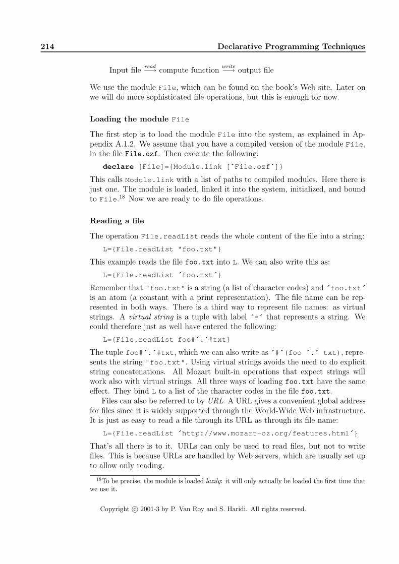
214 Declarative Programming Techniques
Input fileread−→ compute function
write−→ output file
We use the module File , which can be found on the book’s Web site. Later onwe will do more sophisticated file operations, but this is enough for now.
Loading the module File
The first step is to load the module File into the system, as explained in Ap-pendix A.1.2. We assume that you have a compiled version of the module File ,in the file File.ozf. Then execute the following:
declare [File]={Module.link [ ´ File.ozf ´ ]}
This calls Module.link with a list of paths to compiled modules. Here there isjust one. The module is loaded, linked it into the system, initialized, and boundto File .18 Now we are ready to do file operations.
Reading a file
The operation File.readList reads the whole content of the file into a string:
L={File.readList "foo.txt"}
This example reads the file foo.txt into L. We can also write this as:
L={File.readList ´ foo.txt ´ }
Remember that "foo.txt" is a string (a list of character codes) and ´ foo.txt ´
is an atom (a constant with a print representation). The file name can be rep-resented in both ways. There is a third way to represent file names: as virtualstrings. A virtual string is a tuple with label ´ #´ that represents a string. Wecould therefore just as well have entered the following:
L={File.readList foo# ´ . ´ #txt}
The tuple foo# ´ . ´ #txt , which we can also write as ´ #´ (foo ´ . ´ txt) , repre-sents the string "foo.txt" . Using virtual strings avoids the need to do explicitstring concatenations. All Mozart built-in operations that expect strings willwork also with virtual strings. All three ways of loading foo.txt have the sameeffect. They bind L to a list of the character codes in the file foo.txt.
Files can also be referred to by URL. A URL gives a convenient global addressfor files since it is widely supported through the World-Wide Web infrastructure.It is just as easy to read a file through its URL as through its file name:
L={File.readList ´ http://www.mozart-oz.org/features.html ´ }
That’s all there is to it. URLs can only be used to read files, but not to writefiles. This is because URLs are handled by Web servers, which are usually set upto allow only reading.
18To be precise, the module is loaded lazily: it will only actually be loaded the first time thatwe use it.
Copyright c© 2001-3 by P. Van Roy and S. Haridi. All rights reserved.

3.8 Nondeclarative needs 215
Mozart has other operations that allow to read a file either incrementally orlazily, instead of all at once. This is important for very large files that do not fitinto the memory space of the Mozart process. To keep things simple for now, werecommend that you read files all at once. Later on we will see how to read a fileincrementally.
Writing a file
Writing a file is usually done incrementally, by appending one string at a timeto the file. The module File provides three operations: File.writeOpen toopen the file, which must be done first, File.write to append a string to thefile, and File.writeClose to close the file, which must be done last. Here is anexample:
{File.writeOpen ´ foo.txt ´ }{File.write ´ This comes in the file.\n ´ }{File.write ´ The result of 43*43 is ´ #43*43# ´ .\n ´ }{File.write "Strings are ok too.\n"}{File.writeClose}
After these operations, the file ’foo.txt’ has three lines of text, as follows:
This comes in the file.
The result of 43*43 is 1849.
Strings are ok too.
Example execution
In Section 3.7.3 we defined the function WordFreq that calculates the word fre-quencies in a string. We can use this function to calculate word frequencies andstore them in a file:
% 1. Read input fileL={File.readList ´ book.raw ´ }% 2. Compute functionD={WordFreq L}% 3. Write output file{File.writeOpen ´ word.freq ´ }for X in {Domain D} do
{File.write {Get D X}# ´ occurrences of word ´ #X#´ \n ´ }end{File.writeClose}
Section 3.7.3 gives some timing figures of this code using different dictionaryimplementations.
Copyright c© 2001-3 by P. Van Roy and S. Haridi. All rights reserved.

216 Declarative Programming Techniques
3.8.2 Text input/output with a graphical user interface
The most direct way to interface programs with a human user is through a graph-ical user interface. This section shows a simple yet powerful way to define graphi-cal user interfaces, namely by means of concise, mostly declarative specifications.This is an excellent example of a descriptive declarative language, as explainedin Section 3.1. The descriptive language is recognized by the QTk module of theMozart system. The user interface is specified as a nested record, supplementedwith objects and procedures. (Objects are introduced in Chapter 7. For now,you can consider them as procedures with internal state, like the examples ofChapter 1.)
This section shows how to build user interfaces to input and output textualdata to a window. This is enough for many declarative programs. We give a briefoverview of the QTk module, just enough to build these user interfaces. Lateron we will build more sophisticated graphical user interfaces. Chapter 10 gives afuller discussion of declarative user interface programming in general and of itsrealization in QTk.
Declarative specification of widgets
A window on the screen consists of a set of widgets. A widget is a rectangulararea in the window that has a particular interactive behavior. For example, somewidgets can display text or graphic information, and other widgets can acceptuser interaction such as keyboard input and mouse clicks. We specify each widgetdeclaratively with a record whose label and features define the widget type andinitial state. We specify the window declaratively as a nested record (i.e., a tree)that defines the logical structure of the widgets in the window. Here are the fivewidgets we will use for now:
• The label widget can display a text. The widget is specified by the record:
label(text:VS)
where VS is a virtual string.
• The text widget is used to display and enter large quantities of text. It canuse scrollbars to display more text than can fit on screen. With a vertical(i.e., top-down) scrollbar, the widget is specified by the record:
text(handle:H tdscrollbar: true )
When the window is created, the variable H will be bound to an object usedto control the widget. We call such an object a handler. You can considerthe object as a one-argument procedure: {H set(VS)} displays a text and{H get(VS)} reads the text.
• The button widget specifies a button and an action to execute when thebutton is pressed. The widget is specified by the record:
Copyright c© 2001-3 by P. Van Roy and S. Haridi. All rights reserved.

3.8 Nondeclarative needs 217
Figure 3.32: A simple graphical I/O interface for text
button(text:VS action:P)
where VS is a virtual string and P is a zero-argument procedure. {P} iscalled whenever the button is pressed.19 For each window, all its actionsare executed sequentially.
• The td (top-down) and lr (left-right) widgets specify an arrangement ofother widgets in top-down or left-right order:
lr(W1 W2 ... Wn)td(W1 W2 ... Wn)
where W1, W2, ..., Wnare other widget specifications.
Declarative specification of resize behavior
When a window is resized, the widgets inside should behave properly, i.e., eitherchanging size or staying the same size, depending on what the interface should do.We specify each widget’s resize behavior declaratively, by means of an optionalglue feature in the widget’s record. The glue feature indicates whether thewidget’s borders should or should not be “glued” to its enclosing widget. Theglue feature’s argument is an atom consisting of any combination of the fourcharacters n (north), s (south), w (west), e (east), indicating for each directionwhether the border should be glued or not. Here are some examples:
• No glue. The widget keeps its natural size and is centered in the spaceallotted to it, both horizontally and vertically.
• glue:nswe glues to all four borders, stretching to fit both horizontally andvertically.
• glue:we glues horizontally left and right, stretching to fit. Vertically, thewidget is not stretched but centered in the space allotted to it.
19To be precise, whenever the left mouse button is both clicked and released while the mouseis over the button. This allows the user to correct any mistaken click on the button.
Copyright c© 2001-3 by P. Van Roy and S. Haridi. All rights reserved.

218 Declarative Programming Techniques
• glue:w glues to the left edge and does not stretch.
• glue:wns glues vertically top and bottom, stretching to fit vertically, andglues to the left edge, not stretching horizontally.
Loading the module QTk
The first step is to load the QTk module into the system. Since QTk is part of theMozart Standard Library, it suffices to give the right path name:
declare [QTk]={Module.link [ ´ x-oz://system/wp/QTk.ozf ´ ]}
Now that QTk is loaded, we can use it to build interfaces according to the speci-fications of the previous section.
Building the interface
The QTk module has a function QTk.build that takes an interface specification,which is just a nested record of widgets, and builds a window containing thesewidgets. Let us build a simple interface with one button that displays ouch inthe browser whenever the button is clicked:
D=td(button(text:"Press me"action: proc {$} {Browse ouch} end ))
W={QTk.build D}{W show}
The record D always has to start with td or lr , even if the window has just onewidget. QTk.build returns an object Wthat represents the window. The windowstarts out being hidden. It can be displayed or hidden again by calling {W show}
or {W hide} . Here is a bigger example that implements a complete text I/Ointerface:
declareIn OutA1=proc {$} X in {In get(X)} {Out set(X)} endA2=proc {$} {W close} endD=td(title:"Simple text I/O interface"
lr(label(text:"Input:")text(handle:In tdscrollbar: true glue:nswe)glue:nswe)
lr(label(text:"Output:")text(handle:Out tdscrollbar: true glue:nswe)glue:nswe)
lr(button(text:"Do It" action:A1 glue:nswe)button(text:"Quit" action:A2 glue:nswe)glue:we))
W={QTk.build D}{W show}
Copyright c© 2001-3 by P. Van Roy and S. Haridi. All rights reserved.

3.8 Nondeclarative needs 219
At first glance, this may seem complicated, but look again: there are six widgets(two label , two text , two button ) arranged with td and lr widgets. TheQTk.build function takes the description D. It builds the window of Figure 3.32and creates the handler objects In and Out . Compare the record D with Fig-ure 3.32 to see how they correspond.
There are two action procedures, A1 and A2, one for each button. The actionA1 is attached to the “Do It” button. Clicking on the button calls A1, whichtransfers text from the first text widget to the second text widget. This works asfollows. The call {In get(X)} gets the text of the first text widget and bindsit to X. Then {Out set(X)} sets the text in the second text widget to X. Theaction A2 is attached to the “Quit” button. It calls {W close} , which closes thewindow permanently.
Putting nswe glue almost everywhere allows the window to behavior properlywhen resized. The lr widget with the two buttons has we glue only, so that thebuttons do not expand vertically. The label widgets have no glue, so they havefixed sizes. The td widget at the top level needs no glue since we assume it isalways glued to its window.
3.8.3 Stateless data I/O with files
Input/output of a string is simple, since a string consists of characters that canbe stored directly in a file. What about other values? It would be a great help tothe programmer if it would be possible to save any value to a file and to load itback later. The System module Pickle provides exactly this ability. It can saveand load any complete value:
{Pickle.save X FN} % Save X in file FN{Pickle.load FNURL ?X} % Load X from file (or URL) FNURL
All data structures used in declarative programming can be saved and loaded ex-cept for those containing unbound variables. For example, consider this programfragment:
declarefun {Fact N}
if N==0 then 1 else N*{Fact N-1} endendF100={Fact 100}F100Gen1= fun {$} F100 endF100Gen2= fun {$} {Fact 100} endFNGen1=fun {$ N} F={Fact N} in fun {$} F end endFNGen2=fun {$ N} fun {$} {Fact N} end end
F100 is a (rather big) integer; the four other entities are functions. The followingoperation saves the four functions to a file:
{Pickle.save [F100Gen1 F100Gen2 FNGen1 FNGen2] ´ factfile ´ }
Copyright c© 2001-3 by P. Van Roy and S. Haridi. All rights reserved.

220 Declarative Programming Techniques
To be precise, this saves a value consisting of list of four elements in the filefactfile. In this example, all elements are functions. The functions have beenchosen to illustrate various degrees of delayed calculation. The first two returnthe result of calculating 100!. The first, F100Gen1, knows the integer and returnsit directly, and the second, F100Gen2, calculates the value each time it is called.The third and fourth, when called with an integer argument n, return a functionthat when itself called, returns n!. The third, FNGen1, calculates n! when called,so the returned function just returns a known integer. The fourth, FNGen2, doesno calculation but lets the returned function calculate n! when called.
To use the contents of factfile, it must first be loaded:
declare[F1 F2 F3 F4]={Pickle.load ´ factfile ´ }
in{Browse {F1}}{Browse {F2}}{Browse {{F3 100}}}{Browse {{F4 100}}}
This displays 100! four times. Of course, the following is also possible:
declare F1 F2 F3 F4 in{Browse {F1}}{Browse {F2}}{Browse {{F3 100}}}{Browse {{F4 100}}}[F1 F2 F3 F4]={Pickle.load ´ factfile ´ }
After the file is loaded, this displays exactly the same as before. This illustratesyet again how dataflow makes it possible to use a variable before binding it.
We emphasize that the loaded value is exactly the same as the one that wassaved. There is no difference at all between them. This is true for all possiblevalues: numbers, records, procedures, names, atoms, lists, and so on, includingother values that we will see later on in the book. Executing this on one process:
... % First statement (defines X){Pickle.save X ´ myfile ´ }
and then this on a second process:
X={Pickle.load ´ myfile ´ }... % Second statement (uses X)
is rigorously identical to executing the following on a third process:
... % First statement (defines X){Pickle.save X ´ myfile ´ }_={Pickle.load ´ myfile ´ }... % Second statement (uses X)
If the calls to Pickle are removed, like this:
Copyright c© 2001-3 by P. Van Roy and S. Haridi. All rights reserved.

3.9 Program design in the small 221
... % First statement (defines X)
... % Second statement (uses X)
then there are two minor differences:
• The first case creates and reads the file ´ myfile ´ . The second case doesnot.
• The first case raises an exception if there was a problem in creating orreading the file.
3.9 Program design in the small
Now that we have seen many programming techniques, the next logical step isto use them to solve problems. This step is called program design. It startsfrom a problem we want to solve (usually explained in words, sometimes not veryprecisely) gives the high-level structure of the program, i.e., what programmingtechniques we need to use and how they are connected together, and ends upwith a complete program that solves the problem.
For program design, there is an important distinction between “programmingin the small” and “programming in the large”. We will call the resulting pro-grams “small programs” and “large programs”. The distinction has nothing todo with the program’s size, but rather with how many people were involved in itsdevelopment. Small programs are written by one person over a short period oftime. Large programs are written by more than one person or over a long periodof time. The same person now and one year from now should be considered astwo people, since the person will forget many details over a year. This sectiongives an introduction to programming in the small; we leave programming in thelarge to Section 6.7.
3.9.1 Design methodology
Assume we have a problem that can be solved by writing a small program. Let ussee how to design the program. We recommend the following design methodology,which is a mixture of creativity and rigorous thinking:
• Informal specification. We start by writing down as precisely as we canwhat the program should do: what it’s inputs and outputs are and howthe outputs relate to the inputs. This description is called an informalspecification. Even though it is precise, we call it “informal” because it iswritten in English. “Formal” specifications are written in a mathematicalnotation.
• Examples. To make the specification perfectly clear, it is always a goodidea to imagine examples of what the program does in particular cases. The
Copyright c© 2001-3 by P. Van Roy and S. Haridi. All rights reserved.

222 Declarative Programming Techniques
examples should “stress” the program: use it in boundary conditions andin the most unexpected ways we can imagine.
• Exploration. To find out what programming techniques we will need, agood way is to use the interactive interface to experiment with programfragments. The idea is to write small operations that we think might beneeded for the program. We use the operations that the system alreadyprovides as a basis. This step gives us a clearer view of what the program’sstructure should be.
• Structure and coding. Now we can lay out the program’s structure. Wemake a rough outline of the operations needed to calculate the outputs fromthe inputs and how they fit together. We then fill in the blanks by writingthe actual program code. The operations should be simple: each operationshould do just one thing. To improve the structure we can group relatedoperations in modules.
• Testing and reasoning. Finally, we have to verify that our programdoes the right thing. We try it on a series of test cases, including theexamples we came up with before. We correct errors until the programworks well. We can also reason about the program and its complexity, usingthe formal semantics for parts that are not clear. Testing and reasoning arecomplementary: it is important to do both to get a high-quality program.
These steps are not meant to be obligatory, but rather to serve as inspiration.Feel free to adapt them to your own circumstances. For example, when imaginingexamples it can be clear that the specification has to be changed. However, takecare never to forget the most important step, which is testing.
3.9.2 Example of program design
To illustrate these steps, let us retrace the development of the word frequencyapplication of Section 3.7.3. Here is a first attempt at an informal specification:
Given a file name, the application opens a window and displays a listof pairs, where each pair consists of a word and an integer giving thenumber of times the word occurs in the file.
Is this specification precise enough? What about a file containing a word that isnot valid English or a file containing non-Ascii characters? Our specification isnot precise enough: it does not define what a “word” is. To make it more precisewe have to know the purpose of the application. Say that we just want to get ageneral idea of word frequencies, independent of any particular language. Thenwe can define a word simply as:
A “word” is a maximal contiguous sequence of letters and digits.
Copyright c© 2001-3 by P. Van Roy and S. Haridi. All rights reserved.

3.9 Program design in the small 223
This means that words are separated by at least one character that is not a letteror a digit. This accepts a word that is not valid English but does not accept wordscontaining non-Ascii characters. Is this good enough? What about words with ahyphen (such as “true-blue”) or idiomatic expressions that act as units (such as“trial and error”)? In the interest of simplicity, let us reject these for now. Butwe may have to change the specification later to accept them, depending on howwe use the word frequency application.
Now we have arrived at our specification. Note the essential role played byexamples. They are important signposts on the way to a precise specification.The examples were expressly designed to test the limits of the specification.
The next step is to design the program’s structure. The appropriate struc-ture seems to be a pipeline: first read the file into a list of characters and thenconvert the list of characters into a list of words, where a word is represented asa character string. To count the words we need a data structure that is indexedby words. The declarative dictionary of Section 3.7.2 would be ideal, but it isindexed by atoms. Luckily, there is an operation to convert character strings toatoms: StringToAtom (see Appendix B). With this we can write our program.Figure 3.29 gives the heart: a function WordFreq that takes a list of charactersand returns a dictionary. We can test this code on various examples, and espe-cially on the examples we used to write the specification. To this we will add thecode to read the file and display the output in a window; for this we use the fileoperations and graphical user interface operations of Section 3.8. It is importantto package the application cleanly, as a software component. This is explained inthe next two sections.
3.9.3 Software components
What is a good way to organize a program? One could write the program asone big monolithic whole, but this can be confusing. A better way is to partitionthe program into logical units, each of which implements a set of operations thatare related in some way. Each logical unit has two parts, an interface and animplementation. Only the interface is visible from outside the logical unit. Alogical unit may use others as part of its implementation.
A program is then simply a directed graph of logical units, where an edgebetween two logical units means that the first needs the second for its imple-mentation. Popular usage calls these logical units “modules” or “components”,without defining precisely what these words mean. This section introduces thebasic concepts, defines them precisely, and shows how they can be used to helpdesign small declarative programs. Section 6.7 explains how these ideas can beused to help design large programs.
Copyright c© 2001-3 by P. Van Roy and S. Haridi. All rights reserved.

224 Declarative Programming Techniques
〈statement〉 ::= functor 〈variable〉[ import { 〈variable〉 [ at 〈atom〉 ]
| 〈variable〉 ´ ( ´ { (〈atom〉 | 〈int〉) [ ´ : ´ 〈variable〉 ] }+ ´ ) ´
}+ ][ export { [ (〈atom〉 | 〈int〉) ´ : ´ ] 〈variable〉 }+ ]define { 〈declarationPart〉 }+ [ in 〈statement〉 ] end
| ...
Table 3.7: Functor syntax
Modules and functors
We call module a part of a program that groups together related operations intoan entity that has an interface and an implementation. In this book, we willimplement modules in a simple way:
• The module’s interface is a record that groups together related language en-tities (usually procedures, but anything is allowed including classes, objects,etc.).
• The module’s implementation is a set of language entities that are accessibleby the interface operations but hidden from the outside. The implementa-tion is hidden using lexical scoping.
We will consider module specifications as entities separate from modules. Amodule specification is a kind of template that creates a module each time it isinstantiated. A module specification is sometimes called a software component.Unfortunately, the term “software component” is widely used with many differentmeanings [187]. To avoid any confusion in this book, we will call our modulespecifications functors. A functor is a function whose arguments are the modulesit needs and whose result is a new module. (To be precise, the functor takesmodule interfaces as arguments, creates a new module, and returns that module’sinterface!) Because of the functor’s role in structuring programs, we provide itas a linguistic abstraction. A functor has three parts: an import part, whichspecifies what other modules it needs, an export part, which specifies the moduleinterface, and a define parts, which gives the module implementation includingits initialization code. The syntax for functor declarations allows to use them aseither statements or expressions, like the syntax for procedures. Table 3.7 givesthe syntax of functor declarations as statements.
In the terminology of software engineering, a software component is a unit ofindependent deployment, a unit of third-party development, and has no persistentstate (following the definition given in [187]). Functors satisfy this definition andare therefore a kind of software component. With this terminology, a module is acomponent instance; it is the result of installing a functor in a particular module
Copyright c© 2001-3 by P. Van Roy and S. Haridi. All rights reserved.

3.9 Program design in the small 225
environment. The module environment consists of a set of modules, each of whichmay have an execution state.
Functors in the Mozart system are compilation units. That is, the system hassupport for handling functors in files, both as source code (i.e., human-readabletext) and object code (i.e., compiled form). Source code can be compiled, ortranslated, into object code. This makes it easy to use functors to exchangesoftware between developers. For example, the Mozart system has a library, calledMOGUL (for Mozart Global User Library), in which third-party developers canput any kind of information. Usually, they put in functors and applications.
An application is standalone if it can be run without the interactive interface.It consists of a main functor, which is evaluated when the program starts. Itimports the modules it needs, which causes other functors to be evaluated. Themain functor is used for its effect of starting the application and not for itsresulting module, which is silently ignored. Evaluating, or “installing”, a functorcreates a new module in three steps. First, the modules it needs are identified.Second, the initialization code is executed. Third, the module is loaded the firsttime it is needed during execution. This technique is called dynamic linking,as opposed to static linking, in which the modules are loaded when executionstarts. At any time, the set of currently installed modules is called the moduleenvironment.
Implementing modules and functors
Let us see how to construct software components in steps. First we give anexample module. Then we show how to convert this module into a softwarecomponent. Finally, we turn it into a linguistic abstraction.
Example module In general a module is a record, and its interface is accessedthrough the record’s fields. We construct a module called MyList that providesinterface procedures for appending, sorting, and testing membership of lists. Thiscan be written as follows:
declare MyList inlocal
proc {Append ... } ... endproc {MergeSort ...} ... endproc {Sort ... } ... {MergeSort ...} ... endproc {Member ...} ... end
inMyList= ´ export ´ (append: Append
sort: Sortmember: Member...)
end
Copyright c© 2001-3 by P. Van Roy and S. Haridi. All rights reserved.

226 Declarative Programming Techniques
The procedure MergeSort is inaccessible outside of the local statement. Theother procedures cannot be accessed directly, but only through the fields ofthe MyList module, which is a record. For example, Append is accessible asMyList.append . Most of the library modules of Mozart, i.e., the Base andSystem modules, follow this structure.
A software component Using procedural abstraction, we can turn this mod-ule into a software component. The software component is a function that returnsa module:
fun {MyListFunctor}proc {Append ... } ... endproc {MergeSort ...} ... endproc {Sort ... } ... {MergeSort ...} ... endproc {Member ...} ... end
in´ export ´ (append: Append
sort: Sortmember: Member...)
end
Each time MyListFunctor is called, it creates and returns another MyList mod-ule. In general, MyListFunctor could have arguments, which are the othermodules needed for MyList .
From this definition, it is clear that functors are just values in the language.They share the following properties with procedure values:
• A functor definition can be evaluated at run time, giving a functor.
• A functor can have external references to other language entities. For ex-ample, it is easy to make a functor that contains data calculated at runtime. This is useful, for example, to include large tables or image data insource form.
• A functor can be stored in a file by using the Pickle module. This file canbe read by any Mozart process. This makes it easy to create libraries ofthird-party functors, such as MOGUL.
• A functor is lightweight; it can be used to encapsulate a single entity suchas one object or class, in order to make explicit the modules needed by theentity.
Because functors are values, it is possible to manipulate them in sophisticatedways within the language. For example, a software component can be builtthat implements component-based programming, in which components determineat run time which components they need and when to link them. Even moreflexibility is possible when dynamic typing is used. A component can link an
Copyright c© 2001-3 by P. Van Roy and S. Haridi. All rights reserved.

3.9 Program design in the small 227
arbitrary component at run time, by installing any functors and calling themaccording to their needs.
Linguistic support This software component abstraction is a reasonable oneto organize large programs. To make it easier to use, to ensure that it is notused incorrectly, and to make clear the intention of the programmer (avoidingconfusion with other higher-order programming techniques), we turn it into alinguistic abstraction. The function MyListFunctor corresponds to the followingfunctor syntax:
functorexport
append:Appendsort:Sortmember:Member...
defineproc {Append ... } ... endproc {MergeSort ...} ... endproc {Sort ... } ... {MergeSort ...} ... endproc {Member ...} ... end
end
Note that the statement between define and end does implicit variable decla-ration, exactly like the statement between local and in .
Assume that this functor has been compiled and stored in the file MyList.ozf
(we will see below how to compile a functor). Then the module can be createdas follows in the interactive interface:
declare [MyList]={Module.link [ ´ MyList.ozf ´ ]}
The function Module.link is defined in the System module Module . It takesa list of functors, loads them from the file system, links them together (i.e.,evaluates them together, so that each module sees its imported modules), andreturns a corresponding list of modules. The Module module allows doing manyother operations on functors and modules.
Importing modules Software components can depend on other software com-ponents. To be precise, instantiating a software component creates a module.The instantiation might need other modules. In the new syntax, we declare thiswith import declarations. To import a library module it is enough to give thename of its functor. On the other hand, to import a user-defined module requiresstating the file name or URL of the file where the functor is stored.20 This isreasonable, since the system knows where the library modules are stored, but
20Other naming schemes are possible, in which functors have some logical name in a compo-nent management system.
Copyright c© 2001-3 by P. Van Roy and S. Haridi. All rights reserved.

228 Declarative Programming Techniques
Figure 3.33: Screen shot of the word frequency application
does not know where you have stored your own functors. Consider the followingfunctor:
functorimport
BrowserFO at ´ file:///home/mydir/FileOps.ozf ´
define{Browser.browse {FO.countLines ´ /etc/passwd ´ }}
end
The import declaration imports the System module Browser and the user-defined module FOspecified by the functor stored in the file /home/mydir/FileOps.ozf.When this functor is linked, the statement between define ... end is execut-ed. This calls the function FO.countLines , which counts the number of lines ina given file, and then calls the procedure Browser.browse to display the result.This particular functor is defined for its effect, not for the module that it creates.It therefore does not export any interface.
3.9.4 Example of a standalone program
Now let us package the word frequency application using components and makeit into a standalone program. Figure 3.33 gives a screenshot of the program’sexecution. The program consists of two components, Dict and WordApp, whichare functors whose source code is in the files Dict.oz and WordApp.oz. Thecomponents implement the declarative dictionary and the word frequency appli-cation. In addition to importing Dict , the WordApp component also imports themodules File and QTk. It uses these modules to read from the file and create anoutput window.
The complete source code of the Dict and WordApp components is given in
Copyright c© 2001-3 by P. Van Roy and S. Haridi. All rights reserved.

3.9 Program design in the small 229
functorexport new:NewDict put:Put condGet:CondGet entries:Entriesdefine
fun {NewDict} leaf end
fun {Put Ds Key Value}case Dsof leaf then tree(Key Value leaf leaf)[] tree(K _ L R) andthen Key==K then
tree(K Value L R)[] tree(K V L R) andthen K>Key then
tree(K V {Put L Key Value} R)[] tree(K V L R) andthen K<Key then
tree(K V L {Put R Key Value})end
end
fun {CondGet Ds Key Default}case Dsof leaf then Default[] tree(K V _ _) andthen Key==K then V[] tree(K _ L _) andthen K>Key then
{CondGet L Key Default}[] tree(K _ _ R) andthen K<Key then
{CondGet R Key Default}end
end
fun {Entries Ds}proc {EntriesD Ds S1 ?Sn}
case Dsof leaf then
S1=Sn[] tree(K V L R) then S2 S3 in
{EntriesD L S1 S2}S2=K#V|S3{EntriesD R S3 Sn}
endend
in {EntriesD Ds $ nil} endend
Figure 3.34: Standalone dictionary library (file Dict.oz)
Copyright c© 2001-3 by P. Van Roy and S. Haridi. All rights reserved.

230 Declarative Programming Techniques
functorimport
Dict FileQTk at ´ x-oz://system/wp/QTk.ozf ´
definefun {WordChar C}
(&a=<C andthen C=<&z) orelse(&A=<C andthen C=<&Z) orelse (&0=<C andthen C=<&9) end
fun {WordToAtom PW} {StringToAtom {Reverse PW}} end
fun {IncWord D W} {Dict.put D W {Dict.condGet D W 0}+1} end
fun {CharsToWords PW Cs}case Csof nil andthen PW==nil then
nil[] nil then
[{WordToAtom PW}][] C|Cr andthen {WordChar C} then
{CharsToWords {Char.toLower C}|PW Cr}[] _|Cr andthen PW==nil then
{CharsToWords nil Cr}[] _|Cr then
{WordToAtom PW}|{CharsToWords nil Cr}end
end
fun {CountWords D Ws}case Ws of W|Wr then {CountWords {IncWord D W} Wr}[] nil then D end
end
fun {WordFreq Cs}{CountWords {Dict.new} {CharsToWords nil Cs}} end
L={File.readList stdin}E={Dict.entries {WordFreq L}}S={Sort E fun {$ A B} A.2>B.2 end }
H Des=td(title: ´ Word frequency count ´text(handle:H tdscrollbar: true glue:nswe))
W={QTk.build Des} {W show}for X#Y in S do {H insert( ´ end ´ X#´ : ´ #Y#´ times\n ´ )} end
end
Figure 3.35: Standalone word frequency application (file WordApp.oz)
Copyright c© 2001-3 by P. Van Roy and S. Haridi. All rights reserved.

3.9 Program design in the small 231
(Supplements)
A B A imports B
File
WordApp
Open Finalize
(Figure)
(System)
(System)
(System)
QTkDict
(Figure)
Figure 3.36: Component dependencies for the word frequency application
Figures 3.34 and 3.35. The principal difference between these components and thecode of Sections 3.7.3 and 3.7.2 is that the components are enclosed in functor
... end with the right import and export clauses. Figure 3.36 shows thedependencies. The Open and Finalize modules are Mozart System modules.The File component can be found on the book’s Web site. The QTk componentis in the Mozart system’s standard library. The Dict component differs slightlyfrom the declarative dictionary of Section 3.7.2: it replaces Domain by Entries ,which gives a list of pairs Key#Value instead of just a list of keys.
This application can easily be extended in many ways. For example, thewindow display code in WordApp.oz could be replaced by the following:
H1 H2 Des=td(title:"Word frequency count"text(handle:H1 tdscrollbar: true glue:nswe)text(handle:H2 tdscrollbar: true glue:nswe))
W={QTk.build Des} {W show}
E={Dict.entries {WordFreq L}}SE1={Sort E fun {$ A B} A.1<B.1 end }SE2={Sort E fun {$ A B} A.2>B.2 end }for X#Y in SE1 do
{H1 insert( ´ end ´ X#´ : ´ #Y#´ times\n ´ )}endfor X#Y in SE2 do
{H2 insert( ´ end ´ X#´ : ´ #Y#´ times\n ´ )}end
This displays two frames, one in alphabetic order and the other in order of de-creasing word frequency.
Copyright c© 2001-3 by P. Van Roy and S. Haridi. All rights reserved.

232 Declarative Programming Techniques
Standalone compilation and execution
Let us now compile the word frequency application as a standalone program. Afunctor can be used in two ways: as a compiled functor (which is importable byother functors) or as a standalone program (which can be directly executed fromthe command line). Any functor can be compiled to make a standalone program.In that case, no export part is necessary and the initialization part defines theprogram’s effect. Given the file Dict.oz defining a functor, the compiled functorDict.ozf is created with the command ozc from a shell interface:
ozc -c Dict.oz
Given the file WordApp.oz defining a functor to be used as a standalone program,the standalone executable WordApp is created with the following command:
ozc -x WordApp.oz
This can be executed as follows:
WordApp < book.raw
where book.raw is a file containing a text. The text is passed to the program’sstandard input, which is seen inside the program as a file with name stdin. Thiswill dynamically link Dict.ozf when dictionaries are first accessed. It is alsopossible to statically link Dict.ozf in the compiled code of the WordApp appli-cation, so that no dynamic linking is needed. These possibilities are documentedin the Mozart system.
Library modules
The word frequency application uses the QTk module, which is part of the Mozartsystem. Any programming language, to be practically useful, must be accompa-nied by a large set of useful abstractions. These are organized into libraries. Alibrary is a coherent collection of one or more related abstractions that are usefulin a particular problem domain. Depending on the language and the library,the library can be considered as part of the language or as being outside of thelanguage. The dividing line can be quite vague: in almost all cases, many of alanguage’s basic operations are in fact implemented in libraries. For example,higher functions on real numbers (sine, cosine, logarithm, etc.) are usually im-plemented in libraries. Since the number of libraries can be very great, it is agood idea to organize libraries as modules.
The importance of libraries has become increasingly important. It is fueledon the one side by the increasing speed and memory capacity of computers andon the other side by the increasing demands of users. A new language that doesnot come with a significant set of libraries, e.g., for network operations, graphicoperations, database operations, etc., is either a toy, unsuited for real applicationdevelopment, or only useful in a narrow problem domain. Implementing libraries
Copyright c© 2001-3 by P. Van Roy and S. Haridi. All rights reserved.

3.10 Exercises 233
is a major effort. To alleviate this problem, new languages almost always comewith an external language interface. This lets them communicate with programswritten in other languages.
Library modules in Mozart The library modules available in the Mozart sys-tem consist of Base modules and System modules. The Base modules are availableimmediately upon startup. They are part of the language definition, providingbasic operations on the language data types. The number, list, and record op-erations given in this chapter are in the Base modules. The System modulesare not available immediately upon startup but can be imported in functors.They provide additional functionality such as file I/O, graphical user interfaces,distributed programming, logic and constraint programming, operating systemaccess, and so forth.
The Mozart interactive interface can give a full list of the library modules inMozart. In the interactive Oz menu, open the Compiler Panel and click on theEnvironment tab. This shows all the defined variables in the global environmentincluding the modules.
3.10 Exercises
1. Absolute value of real numbers. We would like to define a function Abs
that calculates the absolute value of a real number. The following definitiondoes not work:
fun {Abs X} if X<0 then ˜X else X end end
Why not? How would you correct it? Hint: the problem is trivial.
2. Cube roots. This chapter uses Newton’s method to calculate square roots.The method can be extended to calculate roots of any degree. For example,the following method calculates cube roots. Given a guess g for the cuberoot of x, an improved guess is given by (x/g2 + 2g)/3. Write a declarativeprogram to calculate cube roots using Newton’s method.
3. The half-interval method.21 The half-interval method is a simple butpowerful technique for finding roots of the equation f(x) = 0, where f is acontinuous real function. The idea is that, if we are given points a and bsuch that f(a) < 0 < f(b), then f must have at least one root between aand b. To locate a root, let x = (a + b)/2 and compute f(x). If f(x) > 0then f must have a root between a and x. If f(x) < 0 then f must have aroot between x and b. Repeating this process will define smaller and smallerintervals that converge on a root. Write a declarative program to solve thisproblem using the techniques of iterative computation.
21This example is taken from Abelson & Sussman [1].
Copyright c© 2001-3 by P. Van Roy and S. Haridi. All rights reserved.

234 Declarative Programming Techniques
4. Iterative factorial. This chapter gives a definition of factorial whosemaximum stack depth is proportional to the input argument. Give anotherdefinition of factorial which results in an iterative computation. Use thetechnique of state transformations from an initial state, as shown in theIterLength example.
5. An iterative SumList . Rewrite the function SumList of Section 3.4.2 tobe iterative using the techniques developed for Length .
6. State invariants. Write down a state invariant for the IterReverse
function.
7. Checking if something is a list. Section 3.4.3 defines a function LengthL
that calculates the number of elements in a nested list. To see whether X isa list or not, LengthL uses the function Leaf defined in this way:
fun {Leaf X} case X of _|_ then false else true end end
What happens if we replace this by the following definition:
fun {Leaf X} X\=(_|_) end
What goes wrong if we use this version of Leaf ?
8. Another append function. Section 3.4.2 defines the Append functionby doing recursion on the first argument. What happens if we try to dorecursion on the second argument? Here is a possible solution:
fun {Append Ls Ms}case Msof nil then Ls[] X|Mr then {Append {Append Ls [X]} Mr}end
end
Is this program correct? Does it terminate? Why or why not?
9. An iterative append. This exercises explores the expressive power ofdataflow variables. In the declarative model, the following definition ofappend is iterative:
fun {Append Xs Ys}case Xsof nil then Ys[] X|Xr then X|{Append Xr Ys}end
end
We can see this by looking at the expansion:
Copyright c© 2001-3 by P. Van Roy and S. Haridi. All rights reserved.
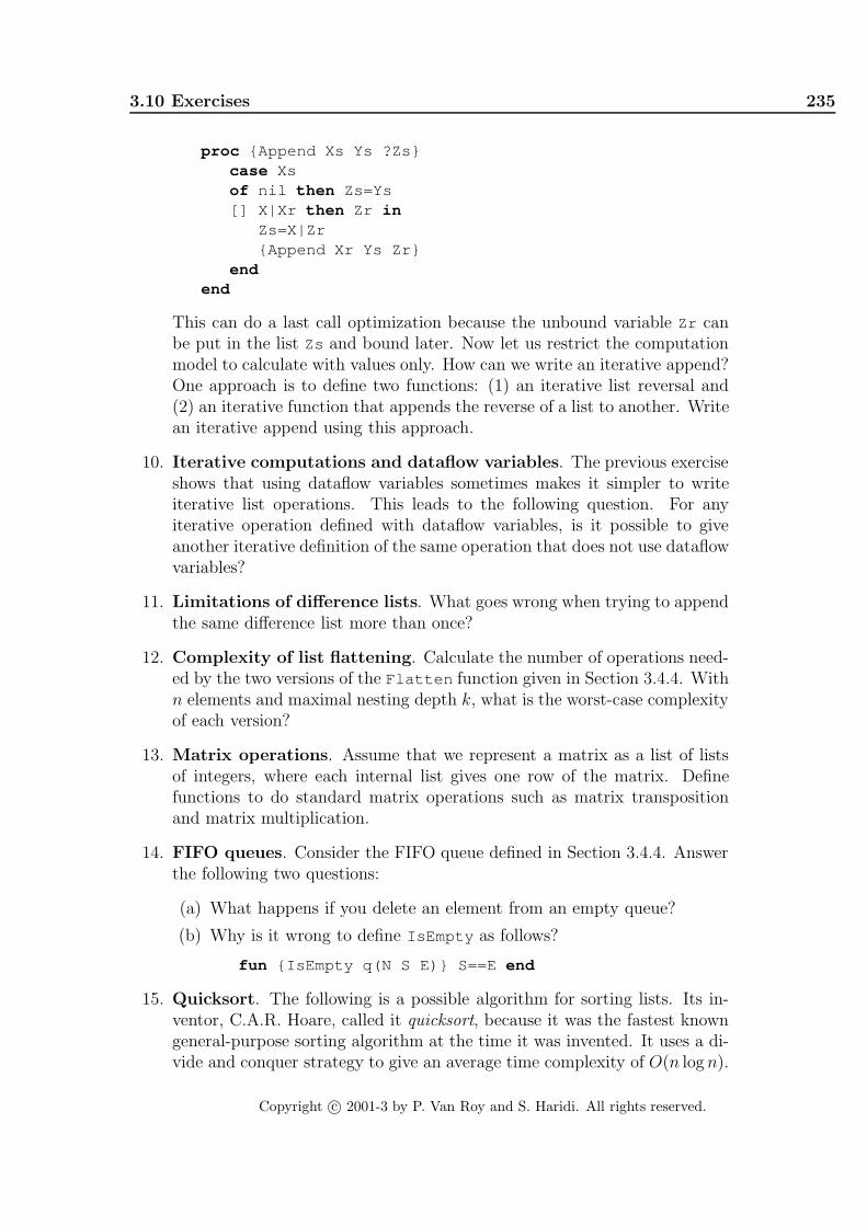
3.10 Exercises 235
proc {Append Xs Ys ?Zs}case Xsof nil then Zs=Ys[] X|Xr then Zr in
Zs=X|Zr{Append Xr Ys Zr}
endend
This can do a last call optimization because the unbound variable Zr canbe put in the list Zs and bound later. Now let us restrict the computationmodel to calculate with values only. How can we write an iterative append?One approach is to define two functions: (1) an iterative list reversal and(2) an iterative function that appends the reverse of a list to another. Writean iterative append using this approach.
10. Iterative computations and dataflow variables. The previous exerciseshows that using dataflow variables sometimes makes it simpler to writeiterative list operations. This leads to the following question. For anyiterative operation defined with dataflow variables, is it possible to giveanother iterative definition of the same operation that does not use dataflowvariables?
11. Limitations of difference lists. What goes wrong when trying to appendthe same difference list more than once?
12. Complexity of list flattening. Calculate the number of operations need-ed by the two versions of the Flatten function given in Section 3.4.4. Withn elements and maximal nesting depth k, what is the worst-case complexityof each version?
13. Matrix operations. Assume that we represent a matrix as a list of listsof integers, where each internal list gives one row of the matrix. Definefunctions to do standard matrix operations such as matrix transpositionand matrix multiplication.
14. FIFO queues. Consider the FIFO queue defined in Section 3.4.4. Answerthe following two questions:
(a) What happens if you delete an element from an empty queue?
(b) Why is it wrong to define IsEmpty as follows?
fun {IsEmpty q(N S E)} S==E end
15. Quicksort. The following is a possible algorithm for sorting lists. Its in-ventor, C.A.R. Hoare, called it quicksort, because it was the fastest knowngeneral-purpose sorting algorithm at the time it was invented. It uses a di-vide and conquer strategy to give an average time complexity of O(n log n).
Copyright c© 2001-3 by P. Van Roy and S. Haridi. All rights reserved.

236 Declarative Programming Techniques
Here is an informal description of the algorithm for the declarative model.Given an input list L. Then do the following operations:
(a) Pick L’s first element, X, to use as a pivot.
(b) Partition L into two lists, L1 and L2 , such that all elements in L1 areless than X and all elements in L2 are greater or equal than X.
(c) Use quicksort to sort L1 giving S1 and to sort L2 giving S2.
(d) Append the lists S1 and S2 to get the answer.
Write this program with difference lists to avoid the linear cost of append.
16. (advanced exercise) Tail-recursive convolution.22 For this exercise, writea function that takes two lists [x1 x2 · · · xn] and [y1 y2 · · · yn] and returnstheir symbolic convolution [x1#yn x2#yn−1 · · · xn#y1]. The function shouldbe tail recursive and do no more than n recursive calls. Hint: the functioncan calculate the reverse of the second list and pass it as an argument toitself. Because unification is order-independent, this works perfectly well.
17. (advanced exercise) Currying. The purpose of this exercise is to define alinguistic abstraction to add currying to Oz. First define a scheme for trans-lating function definitions and calls. Then use the gump parser-generatortool to add the linguistic abstraction to Mozart.
22This exercise is due to Olivier Danvy.
Copyright c© 2001-3 by P. Van Roy and S. Haridi. All rights reserved.

Chapter 4
Declarative Concurrency
“Twenty years ago, parallel skiing was thought to be a skill attain-able only after many years of training and practice. Today, it isroutinely achieved during the course of a single skiing season. [...]All the goals of the parents are achieved by the children: [...] Butthe movements they make in order to produce these results are quitedifferent.”– Mindstorms: Children, Computers, and Powerful Ideas [141], Sey-mour Papert (1980)
The declarative model of Chapter 2 lets us write many programs and usepowerful reasoning techniques on them. But, as Section 4.7 explains, there existuseful programs that cannot be written easily or efficiently in it. For example,some programs are best written as a set of activities that execute independently.Such programs are called concurrent. Concurrency is essential for programs thatinteract with their environment, e.g., for agents, GUI programming, OS interac-tion, and so forth. Concurrency also lets a program be organized into parts thatexecute independently and interact only when needed, i.e., client/server and pro-ducer/consumer programs. This is an important software engineering property.
Concurrency can be simple
This chapter extends the declarative model of Chapter 2 with concurrency whilestill being declarative. That is, all the programming and reasoning techniques fordeclarative programming still apply. This is a remarkable property that deserves tobe more widely known. We will explore it throughout this chapter. The intuitionunderlying it is quite simple. It is based on the fact that a dataflow variable canbe bound to only one value. This gives the following two consequences:
• What stays the same: The result of a program is the same whether or not itis concurrent. Putting any part of the program in a thread does not changethe result.
Copyright c© 2001-3 by P. Van Roy and S. Haridi. All rights reserved.

238 Declarative Concurrency
• What is new: The result of a program can be calculated incrementally. Ifthe input to a concurrent program is given incrementally, then the programwill calculate its output incrementally as well.
Let us give an example to fix this intuition. Consider the following sequential pro-gram that calculates a list of successive squares by generating a list of successiveintegers and then mapping each to its square:
fun {Gen L H}{Delay 100}if L>H then nil else L|{Gen L+1 H} end
end
Xs={Gen 1 10}Ys={Map Xs fun {$ X} X*X end }{Browse Ys}
(The {Delay 100} call waits for 100 milliseconds before continuing.) We canmake this concurrent by doing the generation and mapping in their own threads:
thread Xs={Gen 1 10} endthread Ys={Map Xs fun {$ X} X*X end } end{Browse Ys}
This uses the thread 〈s〉 end statement, which executes 〈s〉 concurrently. Whatis the difference between the concurrent and the sequential versions? The result ofthe calculation is the same in both cases, namely [1 4 9 16 ... 81 100] . Inthe sequential version, Gen calculates the whole list before Map starts. The finalresult is displayed all at once when the calculation is complete, after one second.In the concurrent version, Gen and Map both execute simultaneously. WheneverGen adds an element to its list, Map will immediately calculate its square. Theresult is displayed incrementally, as the elements are generated, one element eachtenth of a second.
We will see that the deep reason why this form of concurrency is so simple isthat programs have no observable nondeterminism. A program in the declarativeconcurrent model always has this property, if the program does not try to bind thesame variable to incompatible values. This is explained in Section 4.1. Anotherway to say it is that there are no race conditions in a declarative concurrentprogram. A race condition is just an observable nondeterministic behavior.
Structure of the chapter
The chapter can be divided into six parts:
• Programming with threads. This part explains the first form of declar-ative concurrency, namely data-driven concurrency, also known as supply-driven concurrency. There are four sections. Section 4.1 defines the data-driven concurrent model, which extends the declarative model with threads.This section also explains what declarative concurrency means. Section 4.2
Copyright c© 2001-3 by P. Van Roy and S. Haridi. All rights reserved.

4.1 The data-driven concurrent model 239
gives the basics of programming with threads. Section 4.3 explains themost popular technique, stream communication. Section 4.4 gives someother techniques, namely order-determining concurrency, coroutines, andconcurrent composition.
• Lazy execution. This part explains the second form of declarative con-currency, namely demand-driven concurrency, also known as lazy execution.Section 4.5 introduces the lazy concurrent model and gives some of the mostimportant programming techniques, including lazy streams and list compre-hensions.
• Soft real-time programming. Section 4.6 explains how to program withtime in the concurrent model.
• Limitations and extensions of declarative programming. How farcan declarative programming go? Section 4.7 explores the limitations ofdeclarative programming and how to overcome them. This section givesthe primary motivations for explicit state, which is the topic of the nextthree chapters.
• The Haskell language. Section 4.8 gives an introduction to Haskell, apurely functional programming language based on lazy evaluation.
• Advanced topics and history. Section 4.9 shows how to extend thedeclarative concurrent model with exceptions. It also goes deeper into var-ious topics including the different kinds of nondeterminism, lazy execution,dataflow variables, and synchronization (both explicit and implicit). Final-ly, Section 4.10 concludes by giving some historical notes on the roots ofdeclarative concurrency.
Concurrency is also a key part of three other chapters. Chapter 5 extends theeager model of the present chapter with a simple kind of communication chan-nel. Chapter 8 explains how to use concurrency together with state, e.g., forconcurrent object-oriented programming. Chapter 11 shows how to do distribut-ed programming, i.e., programming a set of computers that are connected by anetwork. All four chapters taken together give a comprehensive introduction topractical concurrent programming.
4.1 The data-driven concurrent model
In Chapter 2 we presented the declarative computation model. This model issequential, i.e., there is just one statement that executes over a single-assignmentstore. Let us extend the model in two steps, adding just one concept in each step:
• The first step is the most important. We add threads and the single in-struction thread 〈s〉 end . A thread is simply an executing statement, i.e.,
Copyright c© 2001-3 by P. Van Roy and S. Haridi. All rights reserved.

240 Declarative Concurrency
...ST1
Single-assignment store
Multiple semantic stacksST2 STn
(‘‘threads’’)
W=atom
Y=42
XZ=person(age: Y)
U
Figure 4.1: The declarative concurrent model
〈s〉 ::=skip Empty statement| 〈s〉1 〈s〉2 Statement sequence| local 〈x〉 in 〈s〉 end Variable creation| 〈x〉1=〈x〉2 Variable-variable binding| 〈x〉=〈v〉 Value creation| if 〈x〉 then 〈s〉1 else 〈s〉2 end Conditional| case 〈x〉 of 〈pattern〉 then 〈s〉1 else 〈s〉2 end Pattern matching| { 〈x〉 〈y〉1 ... 〈y〉n} Procedure application| thread 〈s〉 end Thread creation
Table 4.1: The data-driven concurrent kernel language
a semantic stack. This is all we need to start programming with declara-tive concurrency. As we will see, adding threads to the declarative modelkeeps all the good properties of the model. We call the resulting model thedata-driven concurrent model.
• The second step extends the model with another execution order. We addtriggers and the single instruction {ByNeed P X} . This adds the possibilityto do demand-driven computation, which is also known as lazy execution.This second extension also keeps the good properties of the declarativemodel. We call the resulting model the demand-driven concurrent modelor the lazy concurrent model. We put off explaining lazy execution untilSection 4.5.
For most of this chapter, we leave out exceptions from the model. This is becausewith exceptions the model is no longer declarative. Section 4.9.1 looks closer atthe interaction of concurrency and exceptions.
Copyright c© 2001-3 by P. Van Roy and S. Haridi. All rights reserved.

4.1 The data-driven concurrent model 241
4.1.1 Basic concepts
Our approach to concurrency is a simple extension to the declarative model thatallows more than one executing statement to reference the store. Roughly, allthese statements are executing “at the same time”. This gives the model illus-trated in Figure 4.1, whose kernel language is in Table 4.1. The kernel languageextends Figure 2.1 with just one new instruction, the thread statement.
Interleaving
Let us pause to consider precisely what “at the same time” means. There aretwo ways to look at the issue, which we call the language viewpoint and theimplementation viewpoint:
• The language viewpoint is the semantics of the language, as seen by theprogrammer. From this viewpoint, the simplest assumption is to let thethreads do an interleaving execution: in the actual execution, threads taketurns doing computation steps. Computation steps do not overlap, or inother words, each computation step is atomic. This makes reasoning aboutprograms easier.
• The implementation viewpoint is how the multiple threads are actuallyimplemented on a real machine. If the system is implemented on a singleprocessor, then the implementation could also do interleaving. However,the system might be implemented on multiple processors, so that threadscan do several computation steps simultaneously. This takes advantage ofparallelism to improve performance.
We will use the interleaving semantics throughout the book. Whatever the par-allel execution is, there is always at least one interleaving that is observationallyequivalent to it. That is, if we observe the store during the execution, we canalways find an interleaving execution that makes the store evolve in the sameway.
Causal order
Another way to see the difference between sequential and concurrent executionis in terms of an order defined among all execution states of a given program:
Causal order of computation steps
For a given program, all computation steps form a par-tial order, called the causal order. A computation stepoccurs before another step, if in all possible executions ofthe program, it happens before the other. Similarly for acomputation step that occurs after another step. Some-times a step is neither before nor after another step. Inthat case, we say that the two steps are concurrent.
Copyright c© 2001-3 by P. Van Roy and S. Haridi. All rights reserved.

242 Declarative Concurrency
Thread T1
T3
T2
T4
T5
order within a thread
order between threads
Concurrent execution
Sequential execution
(partial order)
(total order)
computation step
Figure 4.2: Causal orders of sequential and concurrent executions
2I
1I 2I
1I 2I
1I 2I
1IaI
aI
aI
aI
bI
bI
bI
bI cI
cI
cI
cI
T2
T11I
cI
I 2
bIaI
Some possible executionsCausal order
Figure 4.3: Relationship between causal order and interleaving executions
In a sequential program, all computation steps are totally ordered. There areno concurrent steps. In a concurrent program, all computation steps of a giventhread are totally ordered. The computation steps of the whole program forma partial order. Two steps in this partial order are causally ordered if the firstbinds a dataflow variable X and the second needs the value of X.
Figure 4.2 shows the difference between sequential and concurrent execution.Figure 4.3 gives an example that shows some of the possible executions corre-sponding to a particular causal order. Here the causal order has two threads T1and T2, where T1 has two operations (I1 and I2) and T2 has three operations(Ia, Ib, and Ic). Four possible executions are shown. Each execution respects thecausal order, i.e., all instructions that are related in the causal order are related inthe same way in the execution. How many executions are possible in all? (Hint:there are not so many in this example.)
Copyright c© 2001-3 by P. Van Roy and S. Haridi. All rights reserved.

4.1 The data-driven concurrent model 243
Nondeterminism
An execution is nondeterministic if there is an execution state in which there is achoice of what to do next, i.e., a choice which thread to reduce. Nondeterminismappears naturally when there are concurrent states. If there are several threads,then in each execution state the system has to choose which thread to executenext. For example, in Figure 4.3, after the first step, which always does Ia, thereis a choice of either I1 or Ib for the next step.
In a declarative concurrent model, the nondeterminism is not visible to theprogrammer.1 There are two reasons for this. First, dataflow variables can bebound to only one value. The nondeterminism affects only the exact momentwhen each binding takes place; it does not affect the plain fact that the bindingdoes take place. Second, any operation that needs the value of a variable has nochoice but to wait until the variable is bound. If we allow operations that couldchoose whether to wait or not then the nondeterminism would become visible.
As a consequence, a declarative concurrent model keeps the good propertiesof the declarative model of Chapter 2. The concurrent model removes some butnot all of the limitations of the declarative model, as we will see in this chapter.
Scheduling
The choice of which thread to execute next is done by part of the system calledthe scheduler. At each computation step, the scheduler picks one among all theready threads to execute next. We say a thread is ready, also called runnable, ifits statement has all the information it needs to execute at least one computationstep. Once a thread is ready, it stays ready indefinitely. We say that threadreduction in the declarative concurrent model is monotonic. A ready thread canbe executed at any time.
A thread that is not ready is called suspended. Its first statement cannotcontinue because it does not have all the information it needs. We say the firststatement is blocked. Blocking is an important concept that we will come acrossagain in the book.
We say the system is fair if it does not let any ready thread “starve”, i.e.,all ready threads will eventually execute. This is an important property to makeprogram behavior predictable and to simplify reasoning about programs. It isrelated to modularity: fairness implies that a thread’s execution does not dependon that of any other thread, unless the dependency is programmed explicitly. Inthe rest of the book, we will assume that threads are scheduled fairly.
4.1.2 Semantics of threads
We extend the abstract machine of Section 2.4 by letting it execute with severalsemantic stacks instead of just one. Each semantic stack corresponds to the
1If there are no unification failures, i.e., attempts to bind the same variable to incompatiblepartial values. Usually we consider a unification failure as a consequence of a programmer error.
Copyright c© 2001-3 by P. Van Roy and S. Haridi. All rights reserved.

244 Declarative Concurrency
intuitive concept “thread”. All semantic stacks access the same store. Threadscommunicate through this shared store.
Concepts
We keep the concepts of single-assignment store σ, environment E, semanticstatement (〈s〉, E), and semantic stack ST. We extend the concepts of executionstate and computation to take into account multiple semantic stacks:
• An execution state is a pair (MST, σ) where MST is a multiset of semanticstacks and σ is a single-assignment store. A multiset is a set in which thesame element can occur more than once. MST has to be a multiset becausewe might have two different semantic stacks with identical contents, e.g.,two threads that execute the same statements.
• A computation is a sequence of execution states starting from an initialstate: (MST0, σ0)→ (MST1, σ1)→ (MST2, σ2)→ ....
Program execution
As before, a program is simply a statement 〈s〉. Here is how to execute theprogram:
• The initial execution state is:
({ [
statement︷ ︸︸ ︷(〈s〉, φ) ]︸ ︷︷ ︸stack
}
︸ ︷︷ ︸multiset
, φ)
That is, the initial store is empty (no variables, empty set φ) and the initialexecution state has one semantic stack that has just one semantic statement(〈s〉, φ) on it. The only difference with Chapter 2 is that the semantic stackis in a multiset.
• At each step, one runnable semantic stack ST is selected from MST, leavingMST ′. We can say MST = {ST}]MST ′. (The operator ] denotes multisetunion.) One computation step is then done in ST according to the semanticsof Chapter 2, giving:
(ST, σ)→ (ST ′, σ′)
The computation step of the full computation is then:
({ST} ]MST ′, σ)→ ({ST ′} ]MST ′, σ′)
We call this an interleaving semantics because there is one global sequenceof computation steps. The threads take turns each doing a little bit of work.
Copyright c© 2001-3 by P. Van Roy and S. Haridi. All rights reserved.

4.1 The data-driven concurrent model 245
(thread <s> end, E)ST ST (<s>,E)
...ST1 n 1 STn
...
single-assignment store single-assignment store
Figure 4.4: Execution of the thread statement
• The choice of which ST to select is done by the scheduler according to awell-defined set of rules called the scheduling algorithm. This algorithmis careful to make sure that good properties, e.g., fairness, hold of anycomputation. A real scheduler has to take much more than just fairnessinto account. Section 4.2.4 discusses many of these issues and explains howthe Mozart scheduler works.
• If there are no runnable semantic stacks in MST then the computation cannot continue:
– If all ST in MST are terminated, then we say the computation termi-nates.
– If there exists at least one suspended ST in MST that cannot be re-claimed (see below), then we say the computation blocks.
The thread statement
The semantics of the thread statement is defined in terms of how it alters themultiset MST. A thread statement never blocks. If the selected ST is of the form[(thread 〈s〉 end , E)]+ST ′, then the new multiset is {[(〈s〉, E)]}]{ST ′}]MST ′.In other words, we add a new semantic stack [(〈s〉, E)] that corresponds to thenew thread. Figure 4.4 illustrates this. We can summarize this in the followingcomputation step:
({[(thread 〈s〉 end , E)] + ST ′} ]MST ′, σ)→ ({[(〈s〉, E)]} ] {ST ′} ]MST ′, σ)
Memory management
Memory management is extended to the multiset as follows:
• A terminated semantic stack can be deallocated.
• A blocked semantic stack can be reclaimed if its activation condition de-pends on an unreachable variable. In that case, the semantic stack wouldnever become runnable again, so removing it changes nothing during theexecution.
Copyright c© 2001-3 by P. Van Roy and S. Haridi. All rights reserved.

246 Declarative Concurrency
This means that the simple intuition of Chapter 2, that “control structures aredeallocated and data structures are reclaimed”, is no longer completely true inthe concurrent model.
4.1.3 Example execution
The first example shows how threads are created and how they communicatethrough dataflow synchronization. Consider the following statement:
local B inthread B=true endif B then {Browse yes} end
end
For simplicity, we will use the substitution-based abstract machine introduced inSection 3.3.
• We skip the initial computation steps and go directly to the situation whenthe thread and if statements are each on the semantic stack. This gives:
( {[thread b=true end , if b then {Browse yes} end ]},{b} ∪ σ )
where b is a variable in the store. There is just one semantic stack, whichcontains two statements.
• After executing the thread statement, we get:
( {[b=true ], [if b then {Browse yes} end ]},{b} ∪ σ )
There are now two semantic stacks (“threads”). The first, containingb=true , is ready. The second, containing the if statement, is suspend-ed because the activation condition (b determined) is false.
• The scheduler picks the ready thread. After executing one step, we get:
( {[], [if b then {Browse yes} end ]},{b = true } ∪ σ )
The first thread has terminated (empty semantic stack). The second threadis now ready, since b is determined.
• We remove the empty semantic stack and execute the if statement. Thisgives:
( {[{Browse yes} ]},{b = true } ∪ σ )
One ready thread remains. Further calculation will display yes .
Copyright c© 2001-3 by P. Van Roy and S. Haridi. All rights reserved.

4.1 The data-driven concurrent model 247
4.1.4 What is declarative concurrency?
Let us see why we can consider the data-driven concurrent model as a form ofdeclarative programming. The basic principle of declarative programming is thatthe output of a declarative program should be a mathematical function of itsinput. In functional programming, it is clear what this means: the program exe-cutes with some input values and when it terminates, it has returned some outputvalues. The output values are functions of the input values. But what does thismean in the data-driven concurrent model? There are two important differenceswith functional programming. First, the inputs and outputs are not necessarilyvalues since they can contain unbound variables. And second, execution mightnot terminate since the inputs can be streams that grow indefinitely! Let us lookat these two problems one at a time and then define what we mean by declarativeconcurrency.2
Partial termination
As a first step, let us factor out the indefinite growth. We will present theexecution of a concurrent program as a series of stages, where each stage has anatural ending. Here is a simple example:
fun {Double Xs}case Xs of X|Xr then 2*X|{Double Xr} end
end
Ys={Double Xs}
The output stream Ys contains the elements of the input stream Xs multipliedby 2. As long as Xs grows, then Ys grows too. The program never terminates.However, if the input stream stops growing, then the program will eventuallystop executing too. This is an important insight. We say that the program doesa partial termination. It has not terminated completely yet, since further bindingthe inputs would cause it to execute further (up to the next partial termination!).But if the inputs do not change then the program will execute no further.
Logical equivalence
If the inputs are bound to some partial values, then the program will eventuallyend up in partial termination, and the outputs will be bound to other partialvalues. But in what sense are the outputs “functions” of the inputs? Both inputsand outputs can contain unbound variables! For example, if Xs=1|2|3|Xr thenthe Ys={Double Xs} call returns Ys=2|4|6|Yr , where Xr and Yr are unboundvariables. What does it mean that Ys is a function of Xs?
2Chapter 13 gives a formal definition of declarative concurrency that makes precise the ideasof this section.
Copyright c© 2001-3 by P. Van Roy and S. Haridi. All rights reserved.

248 Declarative Concurrency
To answer this question, we have to understand what it means for store con-tents to be “the same”. Let us give a simple definition from first principles.(Chapters 9 and 13 give a more formal definition based on mathematical logic.)Before giving the definition, we look at two examples to get an understanding ofwhat is going on. The first example can bind X and Y in two different ways:
X=1 Y=X % First caseY=X X=1 % Second case
In the first case, the store ends up with X=1 and Y=X. In the second case, thestore ends up with X=1 and Y=1. In both cases, X and Y end up being bound to1. This means that the store contents are the same for both cases. (We assumethat the identifiers denote the same store variables in both cases.) Let us give asecond example, this time with some unbound variables:
X=foo(Y W) Y=Z % First caseX=foo(Z W) Y=Z % Second case
In both cases, X is bound to the same record, except that the first argument canbe different, Y or Z. Since Y=Z (Y and Z are in the same equivalence set), we againexpect the store contents to be the same for both cases.
Now let us define what logical equivalence means. We will define logicalequivalence in terms of store variables. The above examples used identifiers, butthat was just so that we could execute them. A set of store bindings, like eachof the four cases given above, is called a constraint. For each variable x andconstraint c, we define values(x, c) to be the set of all possible values x can have,given that c holds. Then we define:
Two constraints c1 and c2 are logically equivalent if: (1) they con-tain the same variables, and (2) for each variable x, values(x, c1) =values(x, c2).
For example, the constraint x = foo( y w) ∧ y = z (where x, y, z, and w arestore variables) is logically equivalent to the constraint x = foo( z w) ∧ y = z.This is because y = z forces y and z to have the same set of possible values, sothat foo( y w) defines the same set of values as foo( z w) . Note that variablesin an equivalence set (like {y, z}) always have the same set of possible values.
Declarative concurrency
Now we can define what it means for a concurrent program to be declarative. Ingeneral, a concurrent program can have many possible executions. The threadexample given above has at least two, depending on the order in which the bind-ings X=1 and Y=X are done.3 The key insight is that all these executions have toend up with the same result. But “the same” does not mean that each variable
3In fact, there are more than two, because the binding X=1 can be done either before orafter the second thread is created.
Copyright c© 2001-3 by P. Van Roy and S. Haridi. All rights reserved.

4.1 The data-driven concurrent model 249
has to be bound to the same thing. It just means logical equivalence. This leadsto the following definition:
A concurrent program is declarative if the following holds for all pos-sible inputs. All executions with a given set of inputs have one oftwo results: (1) they all do not terminate or (2) they all eventuallyreach partial termination and give results that are logically equiva-lent. (Different executions may introduce new variables; we assumethat the new variables in corresponding positions are equal.)
Another way to say this is that there is no observable nondeterminism. Thisdefinition is valid for eager as well as lazy execution. What’s more, when weintroduce non-declarative models (e.g., with exceptions or explicit state), we willuse this definition as a criterium: if part of a non-declarative program obeys thedefinition, we can consider it as declarative for the rest of the program.
We can prove that the data-driven concurrent model is declarative accordingto this definition. But even more general declarative models exist. The demand-driven concurrent model of Section 4.5 is also declarative. This model is quitegeneral: it has threads and can do both eager and lazy execution. The fact thatit is declarative is astonishing.
Failure
A failure is an abnormal termination of a declarative program that occurs whenwe attempt to put conflicting information in the store. For example, if we wouldbind X both to 1 and to 2. The declarative program cannot continue becausethere is no correct value for X.
Failure is an all-or-nothing property: if a declarative concurrent program re-sults in failure for a given set of inputs, then all possible executions with thoseinputs will result in failure. This must be so, else the output would not be amathematical function of the input (some executions would lead to failure andothers would not). Take the following example:
thread X=1 endthread Y=2 endthread X=Y end
We see that all executions will eventually reach a conflicting binding and subse-quently terminate.
Most failures are due to programmer errors. It is rather drastic to terminatethe whole program because of a single programmer error. Often we would like tocontinue execution instead of terminating, perhaps to repair the error or simplyto report it. A natural way to do this is by using exceptions. At the point wherea failure would occur, we raise an exception instead of terminating. The programcan catch the exception and continue executing. The store contents are whatthey were just before the failure.
Copyright c© 2001-3 by P. Van Roy and S. Haridi. All rights reserved.

250 Declarative Concurrency
However, it is important to realize that execution after raising the exceptionis no longer declarative! This is because the store contents are not always thesame in all executions. In the above example, just before failure occurs thereare three possibilities for the values of X & Y: 1 & 1, 2 & 2, and 1 & 2. Ifthe program continues execution then we can observe these values. This is anobservable nondeterminism. We say that we have left the declarative model. Fromthe instant when the exception is raised, the execution is no longer part of adeclarative model, but is part of a more general (non-declarative) model.
Failure confinement
If we want execution to become declarative again after a failure, then we have tohide the nondeterminism. This is the responsibility of the programmer. For thereader who is curious as to how to do this, let us get ahead of ourselves a littleand show how to repair the previous example. Assume that X and Y are visibleto the rest of the program. If there is an exception, we arrange for X and Y to bebound to default values. If there is no exception, then they are bound as before.
declare X Ylocal X1 Y1 S1 S2 S3 in
threadtry X1=1 S1=ok catch _ then S1=error end
endthread
try Y1=2 S2=ok catch _ then S2=error endendthread
try X1=Y1 S3=ok catch _ then S3=error endendif S1==error orelse S2==error orelse S3==error then
X=1 % Default for XY=1 % Default for Y
else X=X1 Y=Y1 endend
Two things have to be repaired. First, we catch the failure exceptions with thetry statements, so that execution will not stop with an error. (See Section 4.9.1for more on the declarative concurrent model with exceptions.) A try statementis needed for each binding since each binding could fail. Second, we do the bind-ings in local variables X1 and Y1, which are invisible to the rest of the program.We make the bindings global only when we are sure that there is no failure.4
4This assumes that X=X1 and Y=Y1 will not fail.
Copyright c© 2001-3 by P. Van Roy and S. Haridi. All rights reserved.

4.2 Basic thread programming techniques 251
4.2 Basic thread programming techniques
There are many new programming techniques that become possible in the con-current model with respect to the sequential model. This section examines thesimplest ones, which are based on a simple use of the dataflow property of threadexecution. We also look at the scheduler and see what operations are possible onthreads. Later sections explain more sophisticated techniques, including streamcommunication, order-determining concurrency, and others.
4.2.1 Creating threads
The thread statement creates a new thread:
threadproc {Count N} if N>0 then {Count N-1} end end
in{Count 1000000}
end
This creates a new thread that runs concurrently with the main thread. Thethread ... end notation can also be used as an expression:
declare X inX = thread 10*10 end + 100*100{Browse X}
This is just syntactic sugar for:
declare X inlocal Y in
thread Y=10*10 endX=Y+100*100
end
A new dataflow variable, Y, is created to communicate between the main threadand the new thread. The addition blocks until the calculation 10*10 is finished.
When a thread has no more statements to execute then it terminates. Eachnonterminated thread that is not suspended will eventually be run. We say thatthreads are scheduled fairly. Thread execution is implemented with preemptivescheduling. That is, if more than one thread is ready to execute, then each threadwill get processor time in discrete intervals called time slices. It is not possiblefor one thread to take over all the processor time.
4.2.2 Threads and the browser
The browser is a good example of a program that works well in a concurrentenvironment. For example:
thread {Browse 111} end{Browse 222}
Copyright c© 2001-3 by P. Van Roy and S. Haridi. All rights reserved.
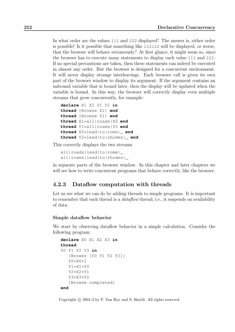
252 Declarative Concurrency
In what order are the values 111 and 222 displayed? The answer is, either orderis possible! Is it possible that something like 112122 will be displayed, or worse,that the browser will behave erroneously? At first glance, it might seem so, sincethe browser has to execute many statements to display each value 111 and 222 .If no special precautions are taken, then these statements can indeed be executedin almost any order. But the browser is designed for a concurrent environment.It will never display strange interleavings. Each browser call is given its ownpart of the browser window to display its argument. If the argument contains anunbound variable that is bound later, then the display will be updated when thevariable is bound. In this way, the browser will correctly display even multiplestreams that grow concurrently, for example:
declare X1 X2 Y1 Y2 inthread {Browse X1} endthread {Browse Y1} endthread X1=all|roads|X2 endthread Y1=all|roams|Y2 endthread X2=lead|to|rome|_ endthread Y2=lead|to|rhodes|_ end
This correctly displays the two streams
all|roads|lead|to|rome|_all|roams|lead|to|rhodes|_
in separate parts of the browser window. In this chapter and later chapters wewill see how to write concurrent programs that behave correctly, like the browser.
4.2.3 Dataflow computation with threads
Let us see what we can do by adding threads to simple programs. It is importantto remember that each thread is a dataflow thread, i.e., it suspends on availabilityof data.
Simple dataflow behavior
We start by observing dataflow behavior in a simple calculation. Consider thefollowing program:
declare X0 X1 X2 X3 inthreadY0 Y1 Y2 Y3 in
{Browse [Y0 Y1 Y2 Y3]}Y0=X0+1Y1=X1+Y0Y2=X2+Y1Y3=X3+Y2{Browse completed}
end
Copyright c© 2001-3 by P. Van Roy and S. Haridi. All rights reserved.

4.2 Basic thread programming techniques 253
{Browse [X0 X1 X2 X3]}
If you feed this program then the browser will display all the variables as beingunbound. Observe what happens when you input the following statements oneat a time:
X0=0X1=1X2=2X3=3
With each statement, the thread resumes, executes one addition, and then sus-pends again. That is, when X0 is bound the thread can execute Y0=X0+1. Itsuspends again because it needs the value of X1 while executing Y1=X1+Y0, andso on.
Using a declarative program in a concurrent setting
Let us take a program from Chapter 3 and see how it behaves when used in aconcurrent setting. Consider the ForAll loop, which is defined as follows:
proc {ForAll L P}case L of nil then skip[] X|L2 then {P X} {ForAll L2 P} end
end
What happens when we execute it in a thread:
declare L inthread {ForAll L Browse} end
If L is unbound, then this will immediately suspend. We can bind L in otherthreads:
declare L1 L2 inthread L=1|L1 endthread L1=2|3|L2 endthread L2=4|nil end
What is the output? Is the result any different from the result of the sequentialcall {ForAll [ 1 2 3 4] Browse} ? What is the effect of using ForAll in aconcurrent setting?
A concurrent map function
Here is a concurrent version of the Map function defined in Section 3.4.3:
fun {Map Xs F}case Xs of nil then nil[] X|Xr then thread {F X} end |{Map Xr F} end
end
Copyright c© 2001-3 by P. Van Roy and S. Haridi. All rights reserved.

254 Declarative Concurrency
F6 F4
F5
F2
F1F3
F2
F2
F2
F1F3
F4
F2
F1F3
Synchronize on result
Running thread
Create new thread
Figure 4.5: Thread creations for the call {Fib 6}
The thread statement is used here as an expression. Let us explore the behaviorof this program. If we enter the following statements:
declare F Xs Ys Zs{Browse thread {Map Xs F} end }
then a new thread executing {Map Xs F} is created. It will suspend immediatelyin the case statement because Xs is unbound. If we enter the following statements(without a declare !):
Xs=1|2|Ysfun {F X} X*X end
then the main thread will traverse the list, creating two threads for the first twoarguments of the list, thread {F 1} end and thread {F 2} end , and then itwill suspend again on the tail of the list Y. Finally, doing
Ys=3|ZsZs=nil
will create a third thread with thread {F 3} end and terminate the computa-tion of the main thread. The three threads will also terminate, resulting in thefinal list [1 4 9] . Remark that the result is the same as the sequential mapfunction, only it can be obtained incrementally if the input is given incremental-ly. The sequential map function executes as a “batch”: the calculation gives noresult until the complete input is given, and then it gives the complete result.
A concurrent Fibonacci function
Here is a concurrent divide-and-conquer program to calculate the Fibonacci func-tion:
Copyright c© 2001-3 by P. Van Roy and S. Haridi. All rights reserved.

4.2 Basic thread programming techniques 255
Figure 4.6: The Oz Panel showing thread creation in {Fib 26 X}
fun {Fib X}if X=<2 then 1else thread {Fib X-1} end + {Fib X-2} end
end
This program is based on the sequential recursive Fibonacci function; the onlydifference is that the first recursive call is done in its own thread. This programcreates an exponential number of threads! Figure 4.5 shows all the thread cre-ations and synchronizations for the call {Fib 6} . A total of eight threads areinvolved in this calculation. You can use this program to test how many threadsyour Mozart installation can create. For example, feed:
{Browse {Fib 25}}
while observing the Oz Panel to see how many threads are running. If {Fib
25} completes too quickly, try a larger argument. The Oz Panel, shown inFigure 4.6, is a Mozart tool that gives information on system behavior (runtime,memory usage, threads, etc.). To start the Oz Panel, select the Oz Panel entryof the Oz menu in the interactive interface.
Dataflow and rubber bands
By now, it is clear that any declarative program of Chapter 3 can be made con-current by putting thread ... end around some of its statements and expressions.Because each dataflow variable will be bound to the same value as before, thefinal result of the concurrent version will be exactly the same as the originalsequential version.
One way to see this intuitively is by means of rubber bands. Each dataflowvariable has its own rubber band. One end of the rubber band is attached to
Copyright c© 2001-3 by P. Van Roy and S. Haridi. All rights reserved.

256 Declarative Concurrency
F = F1 + F2
rubber band stretches
F1 = {Fib X-1}
rigid rubber band
Concurrent modelSequential model
F1 = {Fib X-1} endthread
F1 + F2F =
Figure 4.7: Dataflow and rubber bands
where the variable is bound and the other end to where the variable is used.Figure 4.7 shows what happens in the sequential and concurrent models. In thesequential model, binding and using are usually close to each other, so the rubberbands do not stretch much. In the concurrent model, binding and using can bedone in different threads, so the rubber band is stretched. But it never breaks:the user always sees the right value.
Cheap concurrency and program structure
By using threads, it is often possible to improve the structure of a program, e.g.,to make it more modular. Most large programs have many places in which threadscould be used for this. Ideally, the programming system should support this withthreads that use few computational resources. In this respect the Mozart systemis excellent. Threads are so cheap that one can afford to create them in largenumbers. For example, entry-level personal computers of the year 2000 have atleast 64 MB of active memory, with which they can support more than 100000simultaneous active threads.
If using concurrency lets your program have a simpler structure, then useit without hesitation. But keep in mind that even though threads are cheap,sequential programs are even cheaper. Sequential programs are always fasterthan concurrent programs having the same structure. The Fib program in Sec-tion 4.2.3 is faster if the thread statement is removed. You should create threadsonly when the program needs them. On the other hand, you should not hesitateto create a thread if it improves program structure.
4.2.4 Thread scheduling
We have seen that the scheduler should be fair, i.e., every ready thread willeventually execute. A real scheduler has to do much more than just guaranteefairness. Let us see what other issues arise and how the scheduler takes care ofthem.
Copyright c© 2001-3 by P. Van Roy and S. Haridi. All rights reserved.

4.2 Basic thread programming techniques 257
Time slices
The scheduler puts all ready threads in a queue. At each step, it takes the firstthread out of the queue, lets it execute some number of steps, and then putsit back in the queue. This is called round-robin scheduling. It guarantees thatprocessor time is spread out equitably over the ready threads.
It would be inefficient to let each thread execute only one computation stepbefore putting it back in the queue. The overhead of queue management (takingthreads out and putting them in) relative to the actual computation would bequite high. Therefore, the scheduler lets each thread execute for many computa-tion steps before putting it back in the queue. Each thread has a maximum timethat it is allowed to run before the scheduler stops it. This time interval is calledits time slice or quantum. After a thread’s time slice has run out, the schedulerstops its execution and puts it back in the queue. Stopping a running thread iscalled preemption.
To make sure that each thread gets roughly the same fraction of the processortime, a thread scheduler has two approaches. The first way is to count compu-tation steps and give the same number to each thread. The second way is to usea hardware timer that gives the same time to each thread. Both approaches arepractical. Let us compare the two:
• The counting approach has the advantage that scheduler execution is de-terministic, i.e., running the same program twice will preempt threads atexactly the same instants. A deterministic scheduler is often used for hardreal-time applications, where guarantees must be given on timings.
• The timer approach is more efficient, because the timer is supported byhardware. However, the scheduler is no longer deterministic. Any eventin the operating system, e.g., a disk or network operation, will change theexact instants when preemption occurs.
The Mozart system uses a hardware timer.
Priority levels
For many applications, more control is needed over how processor time is sharedbetween threads. For example, during the course of a computation, an event mayhappen that requires urgent treatment, bypassing the “normal” computation.On the other hand, it should not be possible for urgent computations to starvenormal computations, i.e., to cause them to slow down inordinately.
A compromise that seems to work well in practice is to have priority levels forthreads. Each priority level is given a minimum percentage of the processor time.Within each priority level, threads share the processor time fairly as before. TheMozart system uses this technique. It has three priority levels, high, medium, andlow. There are three queues, one for each priority level. By default, processortime is divided among the priorities in the ratios 100 : 10 : 1 for high : medium
Copyright c© 2001-3 by P. Van Roy and S. Haridi. All rights reserved.

258 Declarative Concurrency
: low priorities. This is implemented in a very simple way: every tenth time sliceof a high priority thread, a medium priority thread is given one slice. Similarly,every tenth time slice of a medium priority thread, a low priority thread is givenone slice. This means that high priority threads, if there are any, divide atleast 100/111 (about 90%) of the processor time amongst themselves. Similarly,medium priority threads, if there are any, divide at least 10/111 (about 9%) ofthe processor time amongst themselves. And last of all, low priority threads, ifthere are any, divide at least 1/111 (about 1%) of the processor time amongstthemselves. These percentages are guaranteed lower bounds. If there are fewerthreads, then they might be higher. For example, if there are no high prioritythreads, then a medium priority thread can get up to 10/11 of the processor time.In Mozart, the ratios high : medium and medium : low are both 10 by default.They can be changed with the Property module.
Priority inheritance
When a thread creates a child thread, then the child is given the same priorityas the parent. This is particularly important for high priority threads. In anapplication, these threads are used for “urgency management”, i.e., to do workthat must be handled in advance of the normal work. The part of the applicationdoing urgency management can be concurrent. If the child of a high prioritythread would have, say, medium priority, then there is a short “window” of timeduring which the child thread is medium priority, until the parent or child canchange the thread’s priority. The existence of this window would be enough tokeep the child thread from being scheduled for many time slices, because thethread is put in the queue of medium priority. This could result in hard-to-tracetiming bugs. Therefore a child thread should never get a lower priority than itsparent.
Time slice duration
What is the effect of the time slice’s duration? A short slice gives very “fine-grained” concurrency: threads react quickly to external events. But if the sliceis too short, then the overhead of switching between threads becomes significant.Another question is how to implement preemption: does the thread itself keeptrack of how long it has run, or is it done externally? Both solutions are viable, butthe second is much easier to implement. Modern multitasking operating systems,such as Unix, Windows 2000, or Mac OS X, have timer interrupts that can beused to trigger preemption. These interrupts arrive at a fairly low frequency, 60or 100 per second. The Mozart system uses this technique.
A time slice of 10 ms may seem short enough, but for some applications it istoo long. For example, assume the application has 100000 active threads. Theneach thread gets one time slice every 1000 seconds. This may be too long a wait.In practice, we find that this is not a problem. In applications with many threads,such as large constraint programs (see Chapter 12), the threads usually depend
Copyright c© 2001-3 by P. Van Roy and S. Haridi. All rights reserved.

4.2 Basic thread programming techniques 259
(competitive concurrency)Processes
(cooperative concurrency)Threads
Figure 4.8: Cooperative and competitive concurrency
strongly on each other and not on the external world. Each thread only uses asmall part of its time slice before yielding to another thread.
On the other hand, it is possible to imagine an application with many threads,each of which interacts with the external world independently of the other threads.For such an application, it is clear that Mozart as well as recent Unix, Windows, orMac OS X operating systems are unsatisfactory. The hardware itself of a personalcomputer is unsatisfactory. What is needed is a hard real-time computing system,which uses a special kind of hardware together with a special kind of operatingsystem. Hard real-time is outside the scope of the book.
4.2.5 Cooperative and competitive concurrency
Threads are intended for cooperative concurrency, not for competitive concur-rency. Cooperative concurrency is for entities that are working together on someglobal goal. Threads support this, e.g., any thread can change the time ratiosbetween the three priorities, as we will see. Threads are intended for applicationsthat run in an environment where all parts trust one another.
On the other hand, competitive concurrency is for entities that have a localgoal, i.e., they are working just for themselves. They are interested only in theirown performance, not in the global performance. Competitive concurrency isusually managed by the operating system in terms of a concept called a process.
This means that computations often have a two-level structure, as shown inFigure 4.8. At the highest level, there is a set of operating system processesinteracting with each other, doing competitive concurrency. Processes are usu-ally owned by different applications, with different, perhaps conflicting goals.Within each process, there is a set of threads interacting with each other, doingcooperative concurrency. Threads in one process are usually owned by the same
Copyright c© 2001-3 by P. Van Roy and S. Haridi. All rights reserved.

260 Declarative Concurrency
Operation Description{Thread.this} Return the current thread’s name{Thread.state T} Return the current state of T
{Thread.suspend T} Suspend T (stop its execution){Thread.resume T} Resume T (undo suspension){Thread.preempt T} Preempt T
{Thread.terminate T} Terminate T immediately{Thread.injectException T E} Raise exception E in T
{Thread.setPriority T P} Set T’s priority to P
{Thread.setThisPriority P} Set current thread’s priority to P
{Property.get priorities} Return the system priority ratios{Property.put Set the system priority ratios
priorities p(high:X medium:Y)}
Figure 4.9: Operations on threads
application.
Competitive concurrency is supported in Mozart by its distributed computa-tion model and by the Remote module. The Remote module creates a separateoperating system process with its own computational resources. A competitivecomputation can then be put in this process. This is relatively easy to programbecause the distributed model is network transparent: the same program can runwith different distribution structures, i.e., on different sets of processes, and itwill always give the same result.5
4.2.6 Thread operations
The modules Thread and Property provide a number of operations pertinentto threads. Some of these operations are summarized in Figure 4.9. The priorityP can have three values, the atoms low , medium, and high . Each thread has aunique name, which refers to the thread when doing operations on it. The threadname is a value of Name type. The only way to get a thread’s name is for thethread itself to call Thread.this . It is not possible for another thread to getthe name without cooperation from the original thread. This makes it possibleto rigorously control access to thread names. The system procedure:
{Property.put priorities p(high:X medium:Y)}
sets the processor time ratio to X:1 between high priority and medium priorityand to Y:1 between medium priority and low-priority. X and Y are integers. Ifwe execute:
{Property.put priorities p(high:10 medium:10)}
5This is true as long as no process fails. See Chapter 11 for examples and more information.
Copyright c© 2001-3 by P. Van Roy and S. Haridi. All rights reserved.

4.3 Streams 261
Xs={Generate 0 150000} S={Sum Xs 0}
ConsumerProducerXs = 0 | 1 | 2 | 3 | 4 | 5 | ...
Figure 4.10: Producer-consumer stream communication
then for each 10 time slices allocated to runnable high priority threads, the systemwill allocate one time slice to medium priority threads, and similarly betweenmedium and low priority threads. This is the default. Within the same prioritylevel, scheduling is fair and round-robin.
4.3 Streams
The most useful technique for concurrent programming in the declarative con-current model is using streams to communicate between threads. A stream is apotentially unbounded list of messages, i.e., it is a list whose tail is an unbounddataflow variable. Sending a message is done by extending the stream by oneelement: bind the tail to a list pair containing the message and a new unboundtail. Receiving a message is reading a stream element. A thread communicatingthrough streams is a kind of “active object” that we will call a stream object. Nolocking or mutual exclusion is necessary since each variable is bound by only onethread.
Stream programming is a quite general approach that can be applied in manydomains. It is the concept underlying Unix pipes. Morrison uses it to good effectin business applications, in an approach he calls “flow-based programming” [127].This chapter looks at a special case of stream programming, namely deterministicstream programming, in which each stream object always knows for each inputwhere the next message will come from. This case is interesting because it isdeclarative. Yet it is already quite useful. We put off looking at nondeterministicstream programming until Chapter 5.
4.3.1 Basic producer/consumer
This section explains how streams work and shows how to program an asyn-chronous producer/consumer with streams. In the declarative concurrent model,a stream is represented by a list whose tail is an unbound variable:
declare Xs Xs2 inXs=0|1|2|3|4|Xs2
Copyright c© 2001-3 by P. Van Roy and S. Haridi. All rights reserved.

262 Declarative Concurrency
A stream is created incrementally by binding the tail to a new list pair and a newtail:
declare Xs3 inXs2=5|6|7|Xs3
One thread, called the producer, creates the stream in this way, and other threads,called the consumers, read the stream. Because the stream’s tail is a dataflowvariable, the consumers will read the stream as it is created. The followingprogram asynchronously generates a stream of integers and sums them:
fun {Generate N Limit}if N<Limit then
N|{Generate N+1 Limit}else nil end
end
fun {Sum Xs A}case Xsof X|Xr then {Sum Xr A+X}[] nil then Aend
end
local Xs S inthread Xs={Generate 0 150000} end % Producer threadthread S={Sum Xs 0} end % Consumer thread{Browse S}
end
Figure 4.10 gives a particularly nice way to define this pattern, using a precisegraphic notation. Each rectangle denotes a recursive function inside a thread,the solid arrow denotes a stream, and the arrow’s direction is from producer toconsumer. After the calculation is finished, this displays 11249925000 . Theproducer, Generate , and the consumer, Sum, run in their own threads. Theycommunicate through the shared variable Xs, which is bound to a stream of inte-gers. The case statement in Sumblocks when Xs is unbound (no more elements),and resumes when Xs is bound (new elements arrive).
In the consumer, dataflow behavior of the case statement blocks executionuntil the arrival of the next stream element. This synchronizes the consumerthread with the producer thread. Waiting on for a dataflow variable to be boundis the basic mechanism for synchronization and communication in the declarativeconcurrent model.
Using a higher-order iterator
The recursive call to Sumhas an argument A that is the sum of all elements seenso far. This argument and the function’s output together make an accumulator,as we saw in Chapter 3. We can get rid of the accumulator by using a loopabstraction:
Copyright c© 2001-3 by P. Van Roy and S. Haridi. All rights reserved.

4.3 Streams 263
local Xs S inthread Xs={Generate 0 150000} endthread S={FoldL Xs fun {$ X Y} X+Y end 0} end{Browse S}
end
Because of dataflow variables, the FoldL function has no problems working in aconcurrent setting. Getting rid of an accumulator by using a higher-order iteratoris a general technique. The accumulator is not really gone, it is just hidden insidethe iterator. But writing the program is simpler since the programmer no longerhas to reason in terms of state. The List module has many loop abstractionsand other higher-order operations that can be used to help implement recursivefunctions.
Multiple readers
We can introduce multiple consumers without changing the program in any way.For example, here are three consumers, reading the same stream:
local Xs S1 S2 S3 inthread Xs={Generate 0 150000} endthread S1={Sum Xs 0} endthread S2={Sum Xs 0} endthread S3={Sum Xs 0} end
end
Each consumer thread will receive stream elements independently of the others.The consumers do not interfere with each other because they do not actually“consume” the stream; they just read it.
4.3.2 Transducers and pipelines
We can put a third stream object in between the producer and consumer. Thisstream object reads the producer’s stream and creates another stream whichis read by the consumer. We call it a transducer. In general, a sequence ofstream objects each of which feeds the next is called a pipeline. The producer issometimes called the source and the consumer is sometimes called the sink. Letus look at some pipelines with different kinds of transducers.
Filtering a stream
One of the simplest transducers is the filter, which outputs only those elementsof the input stream that satisfy a given condition. A simple way to make a filteris to put a call to the function Filter , which we saw in Chapter 3, inside its ownthread. For example, we can pass only those elements that are odd integers:
local Xs Ys S inthread Xs={Generate 0 150000} end
Copyright c© 2001-3 by P. Van Roy and S. Haridi. All rights reserved.

264 Declarative Concurrency
S={Sum Ys 0}Ys={Filter Xs IsOdd}Xs={Generate 0 150000}
IsOdd
Producer Filter ConsumerXs = 0 | 1 | 2 | 3 | ... Ys = 1 | 3 | 5 | ...
Figure 4.11: Filtering a stream
Xs
Xr
X
Ys
ZsSieveFilter
Sieve
X | Zs
Figure 4.12: A prime-number sieve with streams
thread Ys={Filter Xs IsOdd} endthread S={Sum Ys 0} end{Browse S}
end
where IsOdd is a one-argument boolean function that is true only for odd integers:
fun {IsOdd X} X mod 2 \= 0 end
Figure 4.11 shows this pattern. This figure introduces another bit of graphicnotation, the dotted arrow, which denotes a single value (a non-stream argumentto the function).
Sieve of Eratosthenes
As a bigger example, let us define a pipeline that implements the prime-numbersieve of Eratosthenes. The output of the sieve is a stream containing only primenumbers. This program is called a “sieve” since it works by successively filteringout nonprimes from streams, until only primes remain. The filters are createddynamically when they are first needed. The producer generates a stream ofconsecutive integers starting from 2. The sieve peels off an element and createsa filter to remove multiples of that element. It then calls itself recursively on thestream of remaining elements. Filter 4.12 gives a picture. This introduces yetanother bit of graphic notation, the triangle, which denotes either peeling off the
Copyright c© 2001-3 by P. Van Roy and S. Haridi. All rights reserved.

4.3 Streams 265
first element of a stream or prefixing a new first element to a stream. Here is thesieve definition:
fun {Sieve Xs}case Xsof nil then nil[] X|Xr then Ys in
thread Ys={Filter Xr fun {$ Y} Y mod X \= 0 end } endX|{Sieve Ys}
endend
This definition is quite simple, considering that it is dynamically setting up apipeline of concurrent activities. Let us call the sieve:
local Xs Ys inthread Xs={Generate 2 100000} endthread Ys={Sieve Xs} end{Browse Ys}
end
This displays prime numbers up to 100000. This program is a bit simplisticbecause it creates too many threads, namely one per prime number. Such a largenumber of threads is not necessary since it is easy to see that generating primenumbers up to n requires filtering multiples only up to
√n. 6 We can modify the
program to create filters only up to this limit:
fun {Sieve Xs M}case Xsof nil then nil[] X|Xr then Ys in
if X=<M thenthread Ys={Filter Xr fun {$ Y} Y mod X \= 0 end } end
else Ys=Xr endX|{Sieve Ys M}
endend
With a list of 100000 elements, we can call this as {Sieve Xs 316} (since316 = b
√100000c). This dynamically creates the pipeline of filters shown in
Figure 4.13. Since small factors are more common than large factors, most of theactual filtering is done in the early filters.
4.3.3 Managing resources and improving throughput
What happens if the producer generates elements faster than the consumer canconsume them? If this goes on long enough, then unconsumed elements will pileup and monopolize system resources. The examples we saw so far do nothing
6If the factor f is greater than√
n, then there is another factor n/f that is less than√
n.
Copyright c© 2001-3 by P. Van Roy and S. Haridi. All rights reserved.

266 Declarative Concurrency
... FilterFilter
31373 52
{Sieve Xs 316}XsFilter Filter Filter
Figure 4.13: Pipeline of filters generated by {Sieve Xs 316}
to prevent this. One way to solve this problem is to limit the rate at which theproducer generates new elements, so that some global condition (like a maximumresource usage) is satisfied. This is called flow control. It requires that someinformation be sent back from the consumer to the producer. Let us see how toimplement it.
Flow control with demand-driven concurrency
The simplest flow control is called demand-driven concurrency, or lazy execution.In this technique, the producer only generates elements when the consumer ex-plicitly demands them. (The previous technique, where the producer generates anelement whenever it likes, is called supply-driven execution, or eager execution.)Lazy execution requires a mechanism for the consumer to signal the producerwhenever it needs a new element. The simplest way to do this is to use dataflow.For example, the consumer can extend its input stream whenever it needs a newelement. That is, the consumer binds the stream’s end to a list pair X|Xr , whereX is unbound. The producer waits for this list pair and then binds X to the nextelement. Here is how to program it:
proc {DGenerate N Xs}case Xs of X|Xr then
X=N{DGenerate N+1 Xr}
endend
fun {DSum ?Xs A Limit}if Limit>0 then
X|Xr=Xsin
{DSum Xr A+X Limit-1}else A end
end
local Xs S inthread {DGenerate 0 Xs} end % Producer threadthread S={DSum Xs 0 150000} end % Consumer thread{Browse S}
end
Copyright c© 2001-3 by P. Van Roy and S. Haridi. All rights reserved.

4.3 Streams 267
S={Sum Ys 0}{Buffer 4 Xs Ys}
Buffer ConsumerYs = 0 | _
ProducerXs = 0 | 1 | 2 | 3 | 4 | _
4
Xs={Generate 0 150000}
Figure 4.14: Bounded buffer
proc {Buffer N ?Xs Ys}fun {Startup N ?Xs}
if N==0 then Xselse Xr in Xs=_|Xr {Startup N-1 Xr} end
end
proc {AskLoop Ys ?Xs ?End}case Ys of Y|Yr then Xr End2 in
Xs=Y|Xr % Get element from bufferEnd=_|End2 % Replenish the buffer{AskLoop Yr Xr End2}
endend
End={Startup N Xs}in
{AskLoop Ys Xs End}end
Figure 4.15: Bounded buffer (data-driven concurrent version)
It is now the consumer that controls how many elements are needed (150000is an argument of DSum, not DGenerate ). This implements lazy execution byprogramming it explicitly.7
Flow control with a bounded buffer
Up to now we have seen two techniques for managing stream communication,namely eager and lazy execution. In eager execution, the producer is completelyfree: there are no restrictions on how far it can get ahead of the consumer. Inlazy execution, the producer is completely constrained: it can generate nothingwithout an explicit request from the consumer. Both techniques have problems.
7There is another way to implement lazy execution, namely by extending the computationmodel with a new concept, called “trigger”. This is explained in Section 4.5. We will see thatthe trigger approach is easier to program with than explicit laziness.
Copyright c© 2001-3 by P. Van Roy and S. Haridi. All rights reserved.

268 Declarative Concurrency
We have seen that eager execution leads to an explosion in resource usage. Butlazy execution also has a serious problem. It leads to a strong reduction inthroughput. By throughput we mean the number of messages that can be sent perunit of time. (Throughput is usually contrasted with latency, which is defined asthe time taken from the send to the arrival of a single message.) If the consumerrequests a message, then the producer has to calculate it, and meanwhile theconsumer waits. If the producer were allowed to get ahead of the consumer, thenthe consumer would not have to wait.
Is there a way we can get the best of both worlds, i.e., both avoid the resourceproblem and not reduce throughput? Yes, this is indeed possible. It can bedone with a combination of eager and lazy execution called a bounded buffer. Abounded buffer is a transducer that stores elements up to a maximum number, sayn. The producer is allowed to get ahead of the consumer, but only until the bufferis full. This limits the extra resource usage to n elements. The consumer can takeelements from the buffer immediately without waiting. This keeps throughputhigh. When the buffer has less than n elements, the producer is allowed toproduce more elements, until the buffer is full.
Figure 4.15 shows how to program the bounded buffer. Figure 4.14 gives apicture. This picture introduces a further bit of graphic notation, small inversearrows on a stream, which denote requests for new stream elements (i.e., thestream is lazy). To understand how the buffer works, remember that both Xs
and Ys are lazy streams. The buffer executes in two phases:
• The first phase is the initialization. It calls Startup to ask for n elementsfrom the producer. In other words, it extends Xs with n elements that areunbound. The producer detects this and can generate these n elements.
• The second phase is the buffer management. It calls AskLoop to satisfyrequests from the consumer and initiate requests to the producer. Wheneverthe consumer asks for an element, AskLoop does two things: it gives theconsumer an element from the buffer and it asks the producer for anotherelement to replenish the buffer.
Here is a sample execution:
local Xs Ys S inthread {DGenerate 0 Xs} end % Producer threadthread {Buffer 4 Xs Ys} end % Buffer threadthread S={DSum Ys 0 150000} end % Consumer thread{Browse Xs} {Browse Ys}{Browse S}
end
One way to see for yourself how this works is to slow down its execution to ahuman scale. This can be done by adding a {Delay 1000} call inside Sum. Thisway, you can see the buffer: Xs always has four more elements than Ys.
Copyright c© 2001-3 by P. Van Roy and S. Haridi. All rights reserved.

4.3 Streams 269
The bounded buffer program is a bit tricky to understand and write. Thisis because a lot of bookkeeping is needed to implement the lazy execution. Thisbookkeeping is there for technical reasons only; it has no effect on how the pro-ducer and consumer are written. This is a good indication that extending thecomputation model might be a good alternative way to implement laziness. Thisis indeed the case, as we will see in Section 4.5. The implicit laziness introducedthere is much easier to program with than the explicit laziness we use here.
There is one defect of the bounded buffer we give here. It takes up O(n)memory space even if nothing is stored in it (e.g., when the producer is slow).This extra memory space is small: it consists of n unbound list elements, whichare the n requests to the producer. Yet, as sticklers for program frugality, we askif it is possible to avoid this extra memory space. A simple way to avoid it is byusing explicit state, as defined in Chapter 6. This allows us to define an abstractdata type that represents a bounded buffer and that has two operations, Put andGet . Internally, the ADT can save space by using an integer to count producerrequests instead of list elements.
As a final remark, we can see that eager and lazy execution are just extremecases of a bounded buffer. Eager execution is what happens when the buffer hasinfinite size. Lazy execution is what happens when the buffer has zero size. Whenthe buffer has a finite nonzero size, then the behavior is somewhere between thesetwo extremes.
Flow control with thread priorities
Using a bounded buffer is the best way to implement flow control, because it worksfor all relative producer/consumer speeds without twiddling with any “magicnumbers”. A different and inferior way to do flow control is to change the relativepriorities between producer and consumer threads, so that consumers consumefaster than producers can produce. It is inferior because it is fragile: its successdepends on the amount of work needed for an element to be produced wp andconsumed wc. It succeeds only if the speed ratio sc/sw between the consumerthread and the producer thread is greater than wc/wp. The latter depends notonly on thread priorities but also on how many other threads exist.
That said, let us show how to implement it anyway. Let us give the producerlow priority and the consumer high priority. We also set both priority ratioshigh:medium and medium:low to 10:1 and 10:1 . We use the original, data-driven versions of Generate and Sum:
{Property.put priorities p(high:10 medium:10)}local Xs S in
thread{Thread.setThisPriority low}Xs={Generate 0 150000}
endthread
Copyright c© 2001-3 by P. Van Roy and S. Haridi. All rights reserved.

270 Declarative Concurrency
{Thread.setThisPriority high}S={Sum Xs 0}
end{Browse S}
end
This works in our case since the time to consume an element is not 100 timesgreater than the time to produce an element. But it might no longer work for amodified producer or consumer which might take more or less time. The generallesson is that changing thread priorities should never be used to get a program towork correctly. The program should work correctly, no matter what the prioritiesare. Changing thread priorities is then a performance optimization; it can be usedto improve the throughput of a program that is already working.
4.3.4 Stream objects
Let us now step back and reflect on what stream programming is really doing.We have written concurrent programs as networks of threads that communicatethrough streams. This introduces a new concept which we can call a stream ob-ject: a recursive procedure that executes in its own thread and communicateswith other stream objects through input and output streams. The stream ob-ject can maintain an internal state in the arguments of its procedure, which areaccumulators.
We call a stream object an object because it has an internal state that isaccessed in a controlled way (by messages on streams). Throughout the book,we will use the term “object” for several such entities, including port objects,passive objects, and active objects. These entities differ in how the internal stateis stored and how the controlled access is defined. The stream object is the firstand simplest of these entities.
Here is a general way to create stream objects:
proc {StreamObject S1 X1 ?T1}case S1of M|S2 then N X2 T2 in
{NextState M X1 N X2}T1=N|T2{StreamObject S2 X2 T2}
else skip endenddeclare S0 X0 T0 inthread
{StreamObject S0 X0 T0}end
StreamObject is a kind of “template” for creating a stream object. Its behavioris defined by NextState , which takes an input message M and a state X1, andcalculates an output message N and a new state X2. Executing StreamObject in
Copyright c© 2001-3 by P. Van Roy and S. Haridi. All rights reserved.

4.3 Streams 271
a new thread creates a new stream object with input stream S0, output streamT0, and initial state X0. The stream object reads messages from the input stream,does internal calculations, and sends messages on the output stream. In general,an object can have any fixed number of input and output streams.
Stream objects can be linked together in a graph, where each object receivesmessages from one or more other objects and sends messages to one or more otherobjects. For example, here is a pipeline of three stream objects:
declare S0 T0 U0 V0 inthread {StreamObject S0 0 T0} endthread {StreamObject T0 0 U0} endthread {StreamObject U0 0 V0} end
The first object receives from S0 and sends on T0, which is received by the secondobject, and so forth.
4.3.5 Digital logic simulation
Programming with a directed graph of stream objects is called synchronous pro-gramming. This is because a stream object can only perform a calculation afterit reads one element from each input stream. This implies that all the streamobjects in the graph are synchronized with each other. It is possible for a streamobject to get ahead of its successors in the graph, but it cannot get ahead of itspredecessors. (In Chapter 8 we will see how to build active objects which can runcompletely independently of each other.)
All the examples of stream communication we have seen so far are very simplekinds of graphs, namely linear chains. Let us now look at an example wherethe graph is not a linear chain. We will build a digital logic simulator, i.e., aprogram that faithfully models the execution of electronic circuits consisting ofinterconnected logic gates. The gates communicate through time-varying signalsthat can only take discrete values, such as 0 and 1. In synchronous digital logicthe whole circuit executes in lock step. At each step, each logic gate reads itsinput wires, calculates the result, and puts it on the output wires. The steps arecadenced by a circuit called a clock. Most current digital electronic technology issynchronous. Our simulator will be synchronous as well.
How do we model signals on a wire and circuits that read these signals? In asynchronous circuit, a signal varies only in discrete time steps. So we can modela signal as a stream of 0’s and 1’s. A logic gate is then simply a stream object:a recursive procedure, running in its own thread, that reads input streams andcalculates output streams. A clock is a recursive procedure that produces aninitial stream at a fixed rate.
Combinational logic
Let us first see how to build simple logic gates. Figure 4.16 shows some typicalgates with their standard pictorial symbols and the boolean functions that define
Copyright c© 2001-3 by P. Van Roy and S. Haridi. All rights reserved.

272 Declarative Concurrency
000
01
11
1
x
xy
y
xy
z
z
z
x Not
Or
And
Xorz
x Not And Or Xor
z
1
0
0 1 10 0 1 1
1 1 0
0 0 0
y
1
Figure 4.16: Digital logic gates
them. The exclusive-or gate is usually called Xor . Each gate has one or moreinputs and an output. The simplest is the Not gate, whose output is simply thenegation of the input. In terms of streams, we define it as follows:
fun {NotGate Xs}case Xs of X|Xr then (1-X)|{NotGate Xr} end
end
This gate works instantaneously, i.e., the first element of the output stream iscalculated from the first element of the input stream. This is a reasonable wayto model a real gate if the clock period is much longer than the gate delay. Itallows us to model combinational logic, i.e., logic circuits that have no internalmemory. Their outputs are boolean functions of their inputs, and they are totallydependent on the inputs.
How do we connect several gates together? Connecting streams is easy: theoutput stream of one gate can be directly connected to the input stream of an-other. Because all gates can execute simultaneously, each gate needs to executeinside its own thread. This gives the final definition of NotG:
localfun {NotLoop Xs}
case Xs of X|Xr then (1-X)|{NotLoop Xr} endend
infun {NotG Xs}
thread {NotLoop Xs} endend
end
Calling NotG creates a new Not gate in its own thread. We see that a workinglogic gate is much more than just a boolean function; it is actually a concurrententity that communicates with other concurrent entities. Let us build other kindsof gates. Here is a generic function that can build any kind of two-input gate:
fun {GateMaker F}
Copyright c© 2001-3 by P. Van Roy and S. Haridi. All rights reserved.

4.3 Streams 273
x
y
z c
s
Figure 4.17: A full adder
fun {$ Xs Ys}fun {GateLoop Xs Ys}
case Xs#Ys of (X|Xr)#(Y|Yr) then{F X Y}|{GateLoop Xr Yr}
endend
inthread {GateLoop Xs Ys} end
endend
This function is a good example of higher-order programming: it combines gener-icity with instantiation. With it we can build many gates:
AndG ={GateMaker fun {$ X Y} X*Y end }OrG ={GateMaker fun {$ X Y} X+Y-X*Y end }NandG={GateMaker fun {$ X Y} 1-X*Y end }NorG ={GateMaker fun {$ X Y} 1-X-Y+X*Y end }XorG ={GateMaker fun {$ X Y} X+Y-2*X*Y end }
Each of these functions creates a gate whenever it is called. The logical operationsare implemented as arithmetic operations on the integers 0 and 1.
Now we can build combinational circuits. A typical circuit is a full adder,which adds three one-bit numbers, giving a two-bit result. Full adders can bechained together to make adders of any number of bits. A full adder has threeinputs, x, y, z, and two outputs c and s. It satisfies the equation x+y+z = (cs)2.For example, if x = 1, y = 1, and z = 0, then the result is c = 1 and s = 0,which is (10)2 in binary, namely two. Figure 4.17 defines the circuit. Let us seehow it works. c is 1 if at least two inputs are 1. There are three ways that thiscan happen, each of which is covered by an AndG call. s is 1 if the number of1 inputs is odd, which is exactly the definition of exclusive-or. Here is the same
Copyright c© 2001-3 by P. Van Roy and S. Haridi. All rights reserved.

274 Declarative Concurrency
circuit defined in our simulation framework:
proc {FullAdder X Y Z ?C ?S}K L M
inK={AndG X Y}L={AndG Y Z}M={AndG X Z}C={OrG K {OrG L M}}S={XorG Z {XorG X Y}}
end
We use procedural notation for FullAdder because it has two outputs. Here isan example of using the full adder:
declareX=1|1|0|_Y=0|1|0|_Z=1|1|1|_ C S in{FullAdder X Y Z C S}{Browse inp(X Y Z)#sum(C S)}
This adds three sets of input bits.
Sequential logic
Combinational circuits are limited because they cannot store information. Letus be more ambitious in the kinds of circuits we wish to model. Let us modelsequential circuits, i.e., circuits whose behavior depends on their own past output.This means simply that some outputs are fed back as inputs. Using this idea, wecan build bistable circuits, i.e., circuits with two stable states. A bistable circuitis a memory cell that can store one bit of information. Bistable circuits are oftencalled flip flops.
We cannot model sequential circuits with the approach of the previous section.What happens if we try? Let us connect an output to an input. To produce anoutput, the circuit has to read an input. But there is no input, so no outputis produced either. In fact, this is a deadlock situation since there is a cyclicdependency: output waits for input and input waits for output.
To correctly model sequential circuits, we have to introduce some kind of timedelay between the inputs and the outputs. Then the circuit will take its inputfrom the previous output. There is no longer a deadlock. We can model the timedelay by a delay gate, which simply adds one or more elements to the head of thestream:
fun {DelayG Xs}0|Xs
end
For an input a| b| c| d|... , DelayG outputs 0| a| b| c| d|... , which is just adelayed version of the input. With DelayG we can model sequential circuits. Let
Copyright c© 2001-3 by P. Van Roy and S. Haridi. All rights reserved.

4.3 Streams 275
Delay
id
do
c
f
Figure 4.18: A latch
us build a latch, which is a simple kind of bistable circuit that can memorize itsinput. Figure 4.18 defines a simple latch. Here is the program:
fun {Latch C DI}DO X Y Z F
inF={DelayG DO}X={AndG F C}Z={NotG C}Y={AndG Z DI}DO={OrG X Y}DO
end
The latch has two inputs, C and DI , and one output, DO. If C is 0, then the outputtracks DI , i.e., it always has the same value as DI . If C is 1, then the output isfrozen at the last value of DI . The latch is bistable since DOcan be either 0 or 1.The latch works because of the delayed feedback from DOto F.
Clocking
Assume we have modeled a complex circuit. To simulate its execution, we haveto create an initial input stream of values that are discretized over time. Oneway to do it is by defining a clock, which is a timed source of periodic signals.Here is a simple clock:
fun {Clock}fun {Loop B}
B|{Loop B}end
inthread {Loop 1} end
Copyright c© 2001-3 by P. Van Roy and S. Haridi. All rights reserved.

276 Declarative Concurrency
proc {Gate X1 X2 ... Xn Y1 Y2 ... Ym}proc {P S1 S2 ... Sn U1 U2 ... Um}
case S1#S2#...#Snof (X1|T1)#(X2|T2)#...#(Xn|Tn) then
Y1 Y2 ... YmV1 V2 ... Vm
in{GateStep X1 X2 ... Xn Y1 Y2 ... Ym}U1=Y1|V1U2=Y2|V2...Um=Ym|Vm{P T1 T2 ... Tn V1 V2 ... Vm}
endend
inthread {P X1 X2 ... Xn Y1 Y2 ... Ym} end
end
Figure 4.19: A linguistic abstraction for logic gates
end
Calling {Clock} creates a stream that grows very quickly, which makes the sim-ulation go at the maximum rate of the Mozart implementation. We can slowdown the simulation to a human time scale by adding a delay to the clock:
fun {Clock}fun {Loop B}
{Delay 1000} B|{Loop B}end
inthread {Loop 1} end
end
The call {Delay N} causes its thread to suspend for N milliseconds and then tobecome running again.
A linguistic abstraction for logic gates
In most of the above examples, logic gates are programmed with a constructionthat always has the same shape. The construction defines a procedure withstream arguments and at its heart there is a procedure with boolean arguments.Figure 4.19 shows how to make this construction systematic. Given a procedureGateStep , it defines another procedure Gate . The arguments of GateStep arebooleans (or integers) and the arguments of Gate are streams. We distinguishthe gate’s inputs and outputs. The arguments X1, X2, ..., Xn are the gate’sinputs. The arguments Y1, Y2, ..., Ymare the gate’s outputs. GateStep defines
Copyright c© 2001-3 by P. Van Roy and S. Haridi. All rights reserved.

4.4 Using the declarative concurrent model directly 277
the instantaneous behavior of the gate, i.e., it calculates the boolean outputs ofthe gate from its boolean inputs at a given instant. Gate defines the behaviorin terms of streams. We can say that the construction lifts a calculation withbooleans to become a calculation with streams. We could define an abstractionthat implements this construction. This gives the function GateMaker we definedbefore. But we can go further and define a linguistic abstraction, the gate
statement:
gate input 〈x〉1 · · · 〈x〉n output 〈y〉1 · · · 〈y〉m then 〈s〉 end
This statement translates into the construction of Figure 4.19. The body 〈s〉corresponds to the definition of GateStep : it does a boolean calculation withinputs 〈x〉1 · · · 〈x〉n and outputs 〈y〉1 · · · 〈y〉m. With the gate statement, we candefine an And gate as follows:
proc {AndG X1 X2 ?X3}gate input X1 X2 output X3 then X3=X1*X2 end
end
The identifiers X1, X2, and X3 refer to different variables inside and outside thestatement. Inside they refer to booleans and outside to streams. We can embedgate statements in procedures and use them to build large circuits.
We could implement the gate statement using Mozart’s parser-generator toolgump. Many symbolic languages, notably Haskell and Prolog, have the abilityto extend their syntax, which makes this kind of addition easy. This is oftenconvenient for special-purpose applications.
4.4 Using the declarative concurrent model di-
rectly
Stream communication is not the only way to program in the declarative con-current model. This section explores some other techniques. These techniquesuse the declarative concurrent model directly, without taking advantage of anabstraction such as stream objects.
4.4.1 Order-determining concurrency
“In whichever order these twenty-four cards are laid side by side, the resultwill be a perfectly harmonious landscape.”– From “The Endless Landscape”: 24-piece Myriorama, Leipzig (1830s).
A simple use of concurrency in a declarative program is to find the order ofcalculations. That is, we know which calculations have to be done, but becauseof data dependencies, we do not know their order. What’s more, the order maydepend on the values of the data, i.e., there is no one static order that is alwaysright. In this case, we can use dataflow concurrency to find the order automati-cally.
Copyright c© 2001-3 by P. Van Roy and S. Haridi. All rights reserved.

278 Declarative Concurrency
proc {DepthFirst Tree Level LeftLim ?RootX ?RightLim}case Treeof tree(x:X y:Y left:leaf right:leaf ...) then
X=LeftLimRootX=XRightLim=Xthread Y=Scale*Level end
[] tree(x:X y:Y left:L right:leaf ...) thenX=RootXthread Y=Scale*Level end{DepthFirst L Level+1 LeftLim RootX RightLim}
[] tree(x:X y:Y left:leaf right:R ...) thenX=RootXthread Y=Scale*Level end{DepthFirst R Level+1 LeftLim RootX RightLim}
[] tree(x:X y:Y left:L right:R ...) thenLRootX LRightLim RRootX RLeftLim
inRootX=Xthread X=(LRootX+RRootX) div 2 endthread Y=Scale*Level endthread RLeftLim=LRightLim+Scale end{DepthFirst L Level+1 LeftLim LRootX LRightLim}{DepthFirst R Level+1 RLeftLim RRootX RightLim}
endend
Figure 4.20: Tree drawing algorithm with order-determining concurrency
We give an example of order-determining concurrency using the tree drawingalgorithm of Chapter 3. This algorithm is given a tree and calculates the positionsof all the tree’s nodes so that the tree can be drawn in an aesthetically pleasingway. The algorithm traverses the tree in two directions: first from the root tothe leaves and then from the leaves back up to the root. During the traversals,all the node positions are calculated. One of the tricky details in this algorithmis the order in which the node positions are calculated. Consider the algorithmdefinition given in Section 3.4.7. In this definition, Level and LeftLim are inputs(they propagate down towards the leaves), RootX and RightLim are outputs(they propagate up towards the root), and the calculations have to be done inthe correct order to avoid deadlock. There are two ways to find the correct order:
• The first way is for the programmer to deduce the order and to programaccordingly. This is what Section 3.4.7 does. This gives the most efficientcode, but if the programmer makes an error then the program blocks with-out giving a result.
• The second way is for the system to deduce the order dynamically. The
Copyright c© 2001-3 by P. Van Roy and S. Haridi. All rights reserved.

4.4 Using the declarative concurrent model directly 279
simplest way to do this is to put each calculation in a different thread.Dataflow execution then finds the correct order at run time.
Figure 4.20 gives a version of the tree drawing algorithm that uses order-determiningconcurrency to find the correct calculation order at run time. Each calculationthat might block is done in a thread of its own.8 The algorithm’s result is thesame as before. This is true because the concurrency is used only to change thecalculation order, not to change which calculations are done. This is an exampleof how to use concurrency in declarative programming and remain declarative.In the above code, the threads are created before the recursive calls. In fact, thethreads can be created at any time and the algorithm will still work.
Constraint programming
Compared to the sequential algorithm of Section 3.4.7, the algorithm of thissection is simpler to design because it moves part of the design burden from theprogrammer to the system. There is an even simpler way: by using constraintprogramming. This approach is explained in Chapter 12.
Constraint programming lightens the design burden of the programmer evenmore, at the cost of needing fairly sophisticated constraint solving algorithmsthat might need large execution times. Order-determining concurrency does localpropagation, where simple local conditions (e.g., dataflow dependencies) deter-mine when constraints run. Constraint programming is a natural step beyondthis: it extends local propagation by also doing search, which looks at candidatesolutions until it finds one that is a complete solution.
4.4.2 Coroutines
A coroutine is a nonpreemptive thread. To explain this precisely, let us use theterm locus of control, which is defined as an executing sequence of instructions.Figure 4.21 compares coroutines with procedure calls and threads. A procedurecall transfers control once to the procedure body (the call), and then back (thereturn). There is only one locus of control in the program. A coroutine is calledexplicitly like a procedure, but each coroutine has its has its own locus of control,like a thread. The difference with a thread is that the latter is controlled implic-itly: the system automatically switches execution between threads without anyprogrammer intervention.
Coroutines have two operations, Spawn and Resume. The CId={Spawn P}
function creates a new coroutine and returns its identity CId . This is a bit likecreating a new thread. The new coroutine is initially suspended but will executethe zero-argument procedure P when it is resumed. The {Resume CId} operationtransfers control from the current coroutine to the coroutine with identity CId .
8Binding operations are not put in their own threads because they never block. What wouldbe the difference if each binding were put in its own thread?
Copyright c© 2001-3 by P. Van Roy and S. Haridi. All rights reserved.

280 Declarative Concurrency
Explicit transfer by program
(return)
{Resume C1} {Resume C1}
Procedures
Coroutines
Threads
One locus of control
X=unit
thread {P} end {Wait X}
{Resume C2}{Resume C2}C2={Spawn P}
{P}
New locus of control
Implicit transfer by systemNew locus of control
(preemptive scheduling)
Explicit transfer by program
Executing locus of control
Suspended locus of control
Synchronization between loci of control
(nonpreemptive scheduling)
Figure 4.21: Procedures, coroutines, and threads
Each coroutine has the responsibility to transfer control often enough so that theothers have a chance to execute. If this is not done correctly, then a coroutinemight never have a chance to execute. This is called starvation and is usuallydue to programmer error. (Starvation is not possible with threads if they arescheduled fairly.)
Since coroutines do not introduce nondeterminism in the model, programsusing them are still declarative. However, coroutines themselves cannot be imple-mented in the declarative concurrent model because their implementation needsexplicit state. They can be implemented using the shared-state concurrent modelof Chapter 8. Section 8.2.2 explains how to implement simple versions of Spawn
and Resume using this model. Another way to implement them is by using theThread module.
Implementation using the Thread module
Thread scheduling is often made controllable in ways that resemble coroutines.For example, we can introduce an operation similar to Resume that immediatelypreempts a thread, i.e., switches execution to another runnable thread (if oneexists). This is called Thread.preempt in Mozart. We can also introduce op-erations to control whether a thread is allowed to execute or not. In Mozart,these operations are called Thread.suspend and Thread.resume . A threadT can be suspended indefinitely by calling {Thread.suspend T} Here T is the
Copyright c© 2001-3 by P. Van Roy and S. Haridi. All rights reserved.

4.4 Using the declarative concurrent model directly 281
fun {Spawn P}PId in
threadPId={Thread.this}{Thread.suspend PId}{P}
endPId
end
proc {Resume Id}{Thread.resume Id}{Thread.suspend {Thread.this}}
end
Figure 4.22: Implementing coroutines using the Thread module
thread identity, which is obtained by calling T={Thread.this} . The threadcan be resumed by calling {Thread.resume T} . Figure 4.22 shows how to im-plement Spawn and Resume in terms of Thread.this , Thread.suspend , andThread.resume .
4.4.3 Concurrent composition
We have seen how threads are forked using the thread statement. A naturalquestion that arises is how to join back a forked thread into the original threadof control. That is, how can the original thread wait until the forked thread hasterminated? This is a special case of detecting termination of multiple threads,and making another thread wait on that event. The general scheme is quiteeasy when using dataflow execution. Assume that we have n statements 〈S1〉, ...,〈Sn〉. Assume that the statements create no threads while executing.9 Then thefollowing code will execute each statement in a different thread and wait untilthey have all completed:
local X1 X2 X3 ... Xn1 Xn inthread 〈S〉1 X1=unit endthread 〈S〉2 X2=X1 endthread 〈S〉3 X3=X2 end...thread 〈S〉n Xn=Xn1 end{Wait Xn}
end
9The general case in which threads can create new threads, and so forth recursively, ishandled in Section 5.5.3.
Copyright c© 2001-3 by P. Van Roy and S. Haridi. All rights reserved.

282 Declarative Concurrency
proc {Barrier Ps}fun {BarrierLoop Ps L}
case Ps of P|Pr then M inthread {P} M=L end{BarrierLoop Pr M}
[] nil then Lend
endS={BarrierLoop Ps unit }
in{Wait S}
end
Figure 4.23: Concurrent composition
This works by using the unification operation of dataflow variables (see Sec-tion 2.7.2). When thread Ti terminates, it binds the variables Xi−1 and Xi. This“short-circuits” the variables. When all threads have terminated then the vari-ables X1, X2, ..., Xn will be unified (“merged together”) and bound to unit . Theoperation {Wait Xn} blocks until Xn is bound.
There is a different way to detect termination with dataflow variables thatdoes not depend on binding variables to variables, but uses an auxiliary thread:
local X1 X2 X3 ... Xn1 Xn Done inthread 〈S〉1 X1=unit endthread 〈S〉2 X2=unit endthread 〈S〉3 X3=unit end...thread 〈S〉n Xn=unit endthread
{Wait X1} {Wait X2} {Wait X3} ... {Wait Xn}Done=unit
end{Wait Done}
end
Using explicit state gives another set of approaches to detect termination. Forexample, Section 5.5.3 shows an algorithm that works even when threads canthemselves create new threads.
Control abstraction
Figure 4.23 defines the combinator Barrier that implements concurrent composi-tion. A combinator is just a control abstraction. The term combinator emphasizesthat the operation is compositional, i.e., that combinators can be nested. Thisis also true of control abstractions if they are based on lexically-scoped closures,like the procedure values of this book.
Copyright c© 2001-3 by P. Van Roy and S. Haridi. All rights reserved.

4.5 Lazy execution 283
Barrier takes a list of zero-argument procedures, starts each procedure in itsown thread, and terminates after all these threads terminate. It does terminationdetection using the unification scheme of the previous section. Barrier can bethe basis of a linguistic abstraction, the conc statement:
conc〈S〉1 [] 〈S〉2 [] ... [] 〈S〉n
end
defined as:
{Barrier[ proc {$} 〈S〉1 end
proc {$} 〈S〉2 end...proc {$} 〈S〉n end ]}
Barrier is more general than the conc statement since the number of statementsdoes not have to be known at compile time.
4.5 Lazy execution
“All things spring up without a word spoken,and grow without a claim for their production.”– Tao-te Ching, Lao-tzu (6th century BC)
“Necessity is the mother of invention.”“But who is the father?”“Laziness!”– Freely adapted from a traditional proverb.
Up to now, we have always executed statements in order, from left to right.In a statement sequence, we start by executing the first statement. When it isfinished we continue to the next.10 This fact may seem too obvious to requirementioning. Why should it be any other way? But it is a healthy reflex toquestion the obvious! Many significant discoveries have been made by peoplequestioning the obvious: it led Newton to discover the spectrum of light andEinstein to discover the postulate of relativity. Let us therefore question theobvious and see where it leads us.
Are there other execution strategies for declarative programs? It turns outthat there is a second execution strategy fundamentally different from the usualleft-to-right execution. We call this strategy lazy evaluation or demand-drivenevaluation. This in contrast to the usual strategy, which is called eager evaluationor data-driven evaluation. In lazy evaluation, a statement is only executed when
10Statement order may be determined statically by textual sequence or dynamically bydataflow synchronization.
Copyright c© 2001-3 by P. Van Roy and S. Haridi. All rights reserved.

284 Declarative Concurrency
its result is needed somewhere else in the program. For example, take the followingprogram fragment:
fun lazy {F1 X} 1+X*(3+X*(3+X)) endfun lazy {F2 X} Y=X*X in Y*Y endfun lazy {F3 X} (X+1)*(X+1) endA={F1 10}B={F2 20}C={F3 30}D=A+B
The three functions F1, F2, and F3 are lazy functions. This is indicated with theannotation “lazy ” in the syntax. Lazy functions are not executed when they arecalled. They do not block either. What happens is that they create “stoppedexecutions” that will be continued only when their results are needed. In ourexample, the function calls A={F1 10} , B={F2 20} , and C={F3 30} all createstopped executions. When the addition D=A+B is invoked, then the values of A
and B are needed. This triggers the execution of the first two calls. After thecalls finish, the addition can continue. Since C is not needed, the third call is notexecuted.
The importance of lazy evaluation
Lazy evaluation is a powerful concept that can simplify many programming tasks.It was first discovered in functional programming, where it has a long and dis-tinguished history [85]. Lazy evaluation was originally studied as an executionstrategy that is useful only for declarative programs. However, as we will see inthis book, laziness also has a role to play in more expressive computation modelsthat contain declarative models as subsets.
Lazy evaluation has a role both for programming in the large (for modulariza-tion and resource management) and for programming in the small (for algorithmdesign). For programming in the small, it can help in the design of declarative al-gorithms that have good amortized or worst-case time bounds. This is explainedin detail by Chris Okasaki in his book on functional data structures [138]. Sec-tion 4.5.8 gives the main ideas. For programming in the large, it can help mod-ularize programs. This is explained in detail in the article by John Hughes [87].For example, consider an application where a producer sends a stream of data toa consumer. In an eager model, the producer decides when enough data has beensent. With laziness, it is the consumer that decides. Sections 4.5.3-4.5.6 give thisexample and others.
The lazy computation model of this book is slightly different from lazy eval-uation as used in functional languages such as Haskell and Miranda. Since theselanguages are sequential, lazy evaluation does coroutining between the lazy func-tion and the function that needs the result. In this book, we study laziness inthe more general context of concurrent models. To avoid confusion with lazyevaluation, which is sequential, we will use the term lazy execution to cover the
Copyright c© 2001-3 by P. Van Roy and S. Haridi. All rights reserved.

4.5 Lazy execution 285
〈s〉 ::=skip Empty statement| 〈s〉1 〈s〉2 Statement sequence| local 〈x〉 in 〈s〉 end Variable creation| 〈x〉1=〈x〉2 Variable-variable binding| 〈x〉=〈v〉 Value creation| if 〈x〉 then 〈s〉1 else 〈s〉2 end Conditional| case 〈x〉 of 〈pattern〉 then 〈s〉1 else 〈s〉2 end Pattern matching| { 〈x〉 〈y〉1 ... 〈y〉n} Procedure application| thread 〈s〉 end Thread creation| {ByNeed 〈x〉 〈y〉} Trigger creation
Table 4.2: The demand-driven concurrent kernel language
general case which can be concurrent.
Structure of the section
This section defines the concept of lazy execution and surveys the new program-ming techniques that it makes possible. It has the following structure:
• The first two sections give the fundamentals of lazy execution and showhow it interacts with eager execution and concurrency. Section 4.5.1 definesthe demand-driven concurrent model and gives its semantics. This modelextends the data-driven concurrent model with laziness as a new concept.It is an amazing fact that this model is declarative. Section 4.5.2 shows sixdifferent declarative computation models that are possible with differentcombinations of laziness, dataflow variables, and declarative concurrency.All of these models are practical and some of them have been used as thebasis of functional programming languages.
• The next four sections, Sections 4.5.3–4.5.6, give programming techniquesusing lazy streams. Streams are the most common use of laziness.
• The final three sections give more advanced uses of laziness. Section 4.5.7introduces the subject by showing what happens when standard list func-tions are made lazy. Section 4.5.8 shows how to use laziness to designpersistent data structures, with good amortized or worst-case complexities.Section 4.5.9 explains list comprehensions, which are a higher level of ab-straction in which to view to lazy streams.
Copyright c© 2001-3 by P. Van Roy and S. Haridi. All rights reserved.

286 Declarative Concurrency
4.5.1 The demand-driven concurrent model
The demand-driven concurrent model extends the data-driven concurrent modelwith just one new concept, the by-need trigger. The guiding principle in thedesign of this concept was declarative concurrency. The resulting model satisfiesthe definition of declarative concurrency given in Section 4.1.4. This sectiondefines the semantics of by-need triggers and shows how lazy functions can beexpressed with it.
How can both data-driven and demand-driven concurrency coexist in the samecomputation model? The way we have chosen is to make data-driven concurrencythe default and to add an extra operation to introduce a demand-driven part. It isreasonable to make data-driven concurrency the default because it is much easierto reason about time and space complexity and to implement efficiently. We findthat often the best way to structure an application is to build it in data-drivenfashion around a demand-driven core.
By-need triggers
To do demand-driven concurrency, we add one instruction, ByNeed, to the ker-nel language (see Table 4.2). Its operation is extremely simple. The statement{ByNeed P Y} has the same effect as the statement thread {X Y} end . Bothstatements call the procedure P in its own thread with argument Y. The differencebetween the statements is when the procedure call is executed. For thread {P
Y} end , we know that {P Y} will always be executed eventually. For {ByNeed
P Y} , we know that {P Y} will be executed only if the value of Y is needed. Ifthe value of Y is never needed, then {P Y} will never be executed. Here is anexample:
{ByNeed proc {$ A} A=111*111 end Y}{Browse Y}
This displays Y without calculating its value, since the browser does not need thevalue of Y. Invoking an operation that needs the value of Y, for example, Z=Y+1
or {Wait Y} , will trigger the calculation of Y. This causes 12321 to be displayed.
Semantics of by-need triggers
We implement ByNeed in the computation model by adding just one concept,the by-need trigger. In general, a trigger is a pair consisting of an activationcondition, which is a boolean expression, and an action, which is a procedure.When the activation condition becomes true, then the action is executed once.When this happens we say the trigger is activated. For a by-need trigger, theactivation condition is the need for the value of a variable.
We distinguish between programmed triggers, which are written explicitly bythe programmer, and internal triggers, which are part of the computation model.Programmed triggers are illustrated in Section 4.3.3. A by-need trigger is a kindof internal trigger.
Copyright c© 2001-3 by P. Van Roy and S. Haridi. All rights reserved.

4.5 Lazy execution 287
1. Y is neededThread T1
2. Remove trig(X,Y)
Triggered action
Trigger condition
3. Create T2
4. Evaluate {X Y}T2
Figure 4.24: The by-need protocol
We define the semantics of by-need triggers in three steps. We first adda trigger store to the execution state. We then define two operations, triggercreation and activation. Finally, we make precise what we mean by “needing” avariable.
Extension of execution state A by-need trigger is a pair trig(x, y) of adataflow variable y and a one-argument procedure x. Next to the single-assignmentstore σ, we add a new store τ called the trigger store. The trigger store containsall the by-need triggers and is initially empty. The execution state becomes atriple (MST, σ, τ).
Trigger creation The semantic statement is:
({ByNeed 〈x〉 〈y〉} , E)
Execution consists of the following actions:
• If E(〈y〉) is not determined, then add the trigger trig(E(〈x〉), E(〈y〉)) to thetrigger store.
• Otherwise, if E(〈y〉) is determined, then create a new thread with initialsemantic statement ({ 〈x〉 〈y〉} , E) (see Section 4.1 for thread semantics).
Trigger activation If the trigger store contains trig(x, y) and a need for yis detected, i.e., there is either a thread that is suspended waiting for y to bedetermined, or an attempt to bind y to make it determined, then do the following:
• Remove the trigger from the trigger store.
• Create a new thread with initial semantic statement ({ 〈x〉 〈y〉} , {〈x〉 →x, 〈y〉 → y}) (see Section 4.1).
These actions can be done at any point in time after the need is detected, sincethe need will not go away. The semantics of trigger activation is called the by-needprotocol. It is illustrated in Figure 4.24.
Copyright c© 2001-3 by P. Van Roy and S. Haridi. All rights reserved.
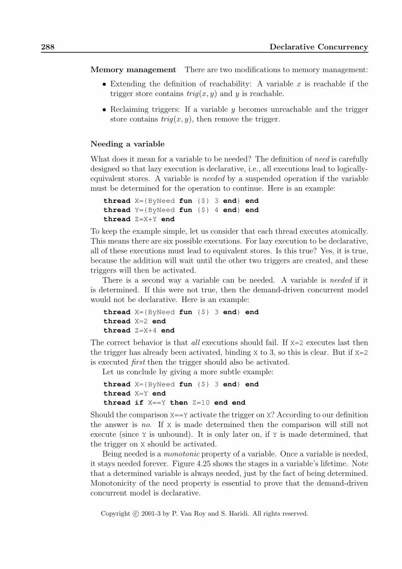
288 Declarative Concurrency
Memory management There are two modifications to memory management:
• Extending the definition of reachability: A variable x is reachable if thetrigger store contains trig(x, y) and y is reachable.
• Reclaiming triggers: If a variable y becomes unreachable and the triggerstore contains trig(x, y), then remove the trigger.
Needing a variable
What does it mean for a variable to be needed? The definition of need is carefullydesigned so that lazy execution is declarative, i.e., all executions lead to logically-equivalent stores. A variable is needed by a suspended operation if the variablemust be determined for the operation to continue. Here is an example:
thread X={ByNeed fun {$} 3 end } endthread Y={ByNeed fun {$} 4 end } endthread Z=X+Y end
To keep the example simple, let us consider that each thread executes atomically.This means there are six possible executions. For lazy execution to be declarative,all of these executions must lead to equivalent stores. Is this true? Yes, it is true,because the addition will wait until the other two triggers are created, and thesetriggers will then be activated.
There is a second way a variable can be needed. A variable is needed if itis determined. If this were not true, then the demand-driven concurrent modelwould not be declarative. Here is an example:
thread X={ByNeed fun {$} 3 end } endthread X=2 endthread Z=X+4 end
The correct behavior is that all executions should fail. If X=2 executes last thenthe trigger has already been activated, binding X to 3, so this is clear. But if X=2
is executed first then the trigger should also be activated.Let us conclude by giving a more subtle example:
thread X={ByNeed fun {$} 3 end } endthread X=Y endthread if X==Y then Z=10 end end
Should the comparison X==Yactivate the trigger on X? According to our definitionthe answer is no. If X is made determined then the comparison will still notexecute (since Y is unbound). It is only later on, if Y is made determined, thatthe trigger on X should be activated.
Being needed is a monotonic property of a variable. Once a variable is needed,it stays needed forever. Figure 4.25 shows the stages in a variable’s lifetime. Notethat a determined variable is always needed, just by the fact of being determined.Monotonicity of the need property is essential to prove that the demand-drivenconcurrent model is declarative.
Copyright c© 2001-3 by P. Van Roy and S. Haridi. All rights reserved.

4.5 Lazy execution 289
Unboundneeded
+Determined
needed+
Unbound
Figure 4.25: Stages in a variable’s lifetime
Using by-need triggers
By-need triggers can be used to implement other concepts that have some “lazy”or “demand-driven” behavior. For example, they underlie lazy functions anddynamic linking. Let us examine each in turn.
Implementing lazy functions with by-need A lazy function is evaluatedonly when its result is needed. For example, the following function generates alazy list of integers:
fun lazy {Generate N} N|{Generate N+1} end
This is a linguistic abstraction that is defined in terms of ByNeed. It is calledlike a regular function:
L={Generate 0}{Browse L}
This will display nothing until L is needed. Let us ask for the third element of L:
{Browse L.2.2.1}
This will calculate the third element, 2, and then display it. The linguistic ab-straction is translated into the following code that uses ByNeed:
fun {Generate N}{ByNeed fun {$} N|{Generate N+1} end }
end
This uses procedural abstraction to delay the execution of the function body.The body is packaged into a zero-argument function which is only called whenthe value of {Generate N} is needed. It is easy to see that this works for alllazy functions. Threads are cheap enough in Mozart that this definition of lazyexecution is practical.
Implementing dynamic linking with by-need We briefly explain what dy-namic linking is all about and the role played by lazy execution. Dynamic link-ing is used to implement a general approach to structuring applications calledcomponent-based programming. This approach was introduced in Section 3.9
Copyright c© 2001-3 by P. Van Roy and S. Haridi. All rights reserved.

290 Declarative Concurrency
and is explained fully in Chapters 5 and 6. Briefly, an application’s source codeconsists of a set of component specifications, called functors. A running applica-tion consists of instantiated components, called modules. A module is representedby a record that groups together the module’s operations. Each record field ref-erences one operation. Components are linked when they are needed, i.e., theirfunctors are loaded into memory and instantiated. As long as the module is notneeded, then the component is not linked. When a program attempts to accessa module field, then the component is needed and by-need execution is used tolink the component.
4.5.2 Declarative computation models
At this point, we have defined a computation model with both laziness and con-currency. It is important to realize that these are independent concepts. Concur-rency can make batch computations incremental. Laziness can reduce the amountof computation needed to get a result. A language can have neither, either, orboth of these concepts. For example, a language with laziness but no concurrencydoes coroutining between a producer and a consumer.
Let us now give an overview of all the declarative computation models weknow. All together, we have added three concepts to strict functional program-ming that preserve declarativeness while increasing expressiveness: dataflow vari-ables, declarative concurrency, and laziness. Adding these concepts in variouscombinations gives six different practical computation models, as summarized inFigure 4.26.11 Dataflow variables are a prerequisite for declarative concurren-cy, since they are the mechanism by which threads synchronize and communi-cate. However, a sequential language, like the model of Chapter 2, can also havedataflow variables and use them to good effect.
Since laziness and dataflow variables are independent concepts, this meansthere are three special moments in a variable’s lifetime:
1. Creation of the variable as an entity in the language, such that it can beplaced inside data structures and passed to or from a function or proce-dure. The variable is not yet bound to its value. We call such a variable a“dataflow variable”.
2. Specification of the function or procedure call that will evaluate the valueof the variable (but the evaluation is not done yet).
3. Evaluation of the function. When the result is available, it is bound to thevariable. The evaluation might be done according to a trigger, which maybe implicit such as a “need” for the value. Lazy execution uses implicitneed.
11This diagram leaves out search, which leads to another kind of declarative programmingcalled relational programming. This is explained in Chapter 9.
Copyright c© 2001-3 by P. Van Roy and S. Haridi. All rights reserved.

4.5 Lazy execution 291
(1), (2), (3): Declaring, specifying, and evaluating are done separately
dataflow variableswith values and
(e.g., Scheme, ML)
(e.g., Haskell) dataflow variableslazy FP with
sequential
dataflow variableswith values and
concurrentsequentialwith values
eager execution
(strictness)
lazy execution
(1)&(2)&(3)
(1)&(2), (3) (1), (2), (3)
(1), (2)&(3) (1), (2)&(3)
(1), (2), (3)
(2): Specify the function to calculate the variable’s value(3): Evaluate the function and bind the variable
programmingstrict functional
programminglazy functional
data−drivenconcurrent model(e.g., Section 4.1)
demand−drivenconcurrent model
(e.g., Section 4.5.1)
(1), (2)&(3): Declaring is done first; specifying and evaluating are done later and coincide
(1): Declare a variable in the store
(1)&(2), (3): Declaring and specifying coincide; evaluating is done later(1)&(2)&(3): Declaring, specifying, and evaluating all coincide
declarative model(e.g., Chapter 2,
Prolog)
Figure 4.26: Practical declarative computation models
These three moments can be done separately or at the same time. Differentlanguages enforce different possibilities. This gives four variant models in all.Figure 4.26 lists these models, as well as the two additional models that resultwhen concurrency is added as well. For each of the variants, we show an examplewith a variable X that will eventually be bound to the result of the computation11*11 . Here are the models:
• In a strict functional language with values, such as Scheme or StandardML, moments (1) & (2) & (3) must always coincide. This is the model ofSection 2.7.1. For example:
declare X=11*11 % (1)+(2)+(3) together
• In a lazy functional language with values, such as Haskell, moments (1) &(2) always coincide, but (3) may be separate. For example (defining first alazy function):
declare fun lazy {LazyMul A B} A*B enddeclare X={LazyMul 11 11} % (1)+(2) together{Wait X} % (3) separate
This can also be written as:
declare X={ fun lazy {$} 11*11 end } % (1)+(2) together{Wait X} % (3) separate
Copyright c© 2001-3 by P. Van Roy and S. Haridi. All rights reserved.

292 Declarative Concurrency
• In a strict language with dataflow variables, moment (1) may be separateand (2) & (3) always coincide. This is the declarative model, which isdefined in Chapter 2. This is also used in logic programming languagessuch as Prolog. For example:
declare X % (1) separateX=11*11 % (2)+(3) together
If concurrency is added, this gives the data-driven concurrent model de-fined at the beginning of this chapter. This is used in concurrent logicprogramming languages. For example:
declare X % (1) separatethread X=11*11 end % (2)+(3) togetherthread if X>100 then {Browse big} end end % Conditional
Because dataflow variables are single-assignment, the conditional alwaysgives the same result.
• In the demand-driven concurrent model of this chapter, moments (1), (2),(3) may all be separate. For example:
declare X % (1) separateX={ fun lazy {$} 11*11 end } % (2) separate{Wait X} % (3) separate
When concurrency is used explicitly, this gives:
declare X % (1)thread X={ fun lazy {$} 11*11 end } end % (2)thread {Wait X} end % (3)
This is the most general variant model. The only connection between thethree moments is that they act on the same variable. The execution of (2)and (3) is concurrent, with an implicit synchronization between (2) and (3):(3) waits until (2) has defined the function.
In all these examples, X is eventually bound to 121 . Allowing the three momentsto be separate gives maximum expressiveness within a declarative framework. Forexample, laziness allows to do declarative calculations with potentially infinitelists. Laziness allows to implement many data structures as efficiently as withexplicit state, yet still declaratively (see, e.g., [138]). Dataflow variables allow towrite concurrent programs that are still declarative. Using both together allows towrite concurrent programs that consist of stream objects communicating throughpotentially infinite streams.
One way to understand the added expressiveness is to realize that dataflowvariables and laziness each add a weak form of state to the model. In both cases,restrictions on using the state ensure the model is still declarative.
Copyright c© 2001-3 by P. Van Roy and S. Haridi. All rights reserved.

4.5 Lazy execution 293
Why laziness with dataflow must be concurrent
In a functional language without dataflow variables, laziness can be sequential.In other words, demand-driven arguments to a lazy function can be evaluatedsequentially (i.e., using coroutining). If dataflow variables are added, this is nolonger the case. A deadlock can occur if the arguments are evaluated sequentially.To solve the problem, the arguments must be evaluated concurrently. Here is anexample:
localZfun lazy {F1 X} X+Z endfun lazy {F2 Y} Z=1 Y+Z end
in{Browse {F1 1}+{F2 2}}
end
This defines F1 and F2 as lazy functions. Executing this fragment displays 5(do you see why?). If {F1 1} and {F2 2} were executed sequentially insteadof concurrently, then this fragment would deadlock. This is because X+Z wouldblock and Z=1 would never be reached. A question for the astute reader: whichof the models in Figure 4.26 has this problem? The binding of Z done by F2 isa kind of “declarative side effect”, since F2 changes its surroundings through ameans separate from its arguments. Declarative side effects are usually benign.
It is important to remember that a language with dataflow variables andconcurrent laziness is still declarative. There is no observable nondeterminism.{F1 1}+{F2 2} always gives the same result.
4.5.3 Lazy streams
In the producer/consumer example of Section 4.3.1, it is the producer that decideshow many list elements to generate, i.e., execution is eager. This is a reasonabletechnique if the total amount of work is finite and does not use many systemresources (e.g., memory or processor time). On the other hand, if the total workpotentially uses many resources, then it may be better to use lazy execution.With lazy execution, the consumer decides how many list elements to generate.If an extremely large or a potentially unbounded number of list elements areneeded, then lazy execution will use many fewer system resources at any givenpoint in time. Problems that are impractical with eager execution can becomepractical with lazy execution. On the other hand, lazy execution may use manymore total resources, because of the cost of its implementation. The need forlaziness must take both of these factors into account.
Lazy execution can be implemented in two ways in the declarative concurrentmodel: with programmed triggers or with internal triggers. Section 4.3.3 givesan example with programmed triggers. Programmed triggers require explicitcommunications from the consumer to the producer. A simpler way is to use
Copyright c© 2001-3 by P. Van Roy and S. Haridi. All rights reserved.

294 Declarative Concurrency
internal triggers, i.e., for the language to support laziness directly. In that casethe language semantics ensures that a function is evaluated only if its result isneeded. This makes the function definition simpler because it does not have todo the “bookkeeping” of the trigger messages. In the demand-driven concurrentmodel we give syntactic support to this technique: the function can be annotatedas “lazy ”. Here is how to do the previous example with a lazy function thatgenerates a potentially infinite list:
fun lazy {Generate N}N|{Generate N+1}
end
fun {Sum Xs A Limit}if Limit>0 then
case Xs of X|Xr then{Sum Xr A+X Limit-1}
endelse A end
end
local Xs S inXs={Generate 0} % ProducerS={Sum Xs 0 150000} % Consumer{Browse S}
end
As before, this displays 11249925000 . Note that the Generate call does notneed to be put in its own thread, in contrast to the eager version. This is becauseGenerate creates a by-need trigger and then completes.
In this example, it is the consumer that decides how many list elements shouldbe generated. With eager execution it was the producer that decided. In the con-sumer, it is the case statement that needs a list pair, so it implicitly triggers thegeneration of a new list element X. To see the difference in resource consumptionbetween this version and the preceding version, try both with 150000 and thenwith 15000000 elements. With 150000 elements, there are no memory problems(on a personal computer with 64MB memory) and the eager version is faster.This is because of the overhead of the lazy version’s implicit triggering mecha-nism. With 15000000 elements, the lazy version needs only a very small memoryspace during execution, while the eager version needs a huge memory space. Lazyexecution is implemented with the ByNeed operation (see Section 4.5.1).
Declaring lazy functions
In lazy functional languages, all functions are lazy by default. In contrast to this,the demand-driven concurrent model requires laziness to be declared explicitly,with the lazy annotation. We find that this makes things simpler both forthe programmer and the compiler, in several ways. The first way has to dowith efficiency and compilation. Eager evaluation is several times more efficient
Copyright c© 2001-3 by P. Van Roy and S. Haridi. All rights reserved.

4.5 Lazy execution 295
than lazy evaluation because there is no triggering mechanism. To get goodperformance in a lazy functional language, this implies that the compiler hasto determine which functions can safely be implemented with eager evaluation.This is called strictness analysis. The second way has to do with language design.An eager language is much easier to extend with non-declarative concepts, e.g.,exceptions and state, than a lazy language.
Multiple readers
The multiple reader example of Section 4.3.1 will also work with lazy execution.For example, here are three lazy consumers using the Generate and Sumfunctionsdefined in the previous section:
local Xs S1 S2 S3 inXs={Generate 0}thread S1={Sum Xs 0 150000} endthread S2={Sum Xs 0 100000} endthread S3={Sum Xs 0 50000} end
end
Each consumer thread asks for stream elements independently of the others. Ifone consumer is faster than the others, then the others may not have to ask forthe stream elements, if they have already been calculated.
4.5.4 Bounded buffer
In the previous section we built a bounded buffer for eager streams by explicitlyprogramming the laziness. Let us now build a bounded buffer using the lazinessof the computation model. Our bounded buffer will take a lazy input stream andreturn a lazy output stream.
Defining a lazy bounded buffer is a good exercise in lazy programming be-cause it shows how lazy execution and data-driven concurrency interact. Let usdo the design in stages. We first specify its behavior. When the buffer is firstcalled, it fills itself with n elements by asking the producer. Afterwards, when-ever the consumer asks for an element, the buffer in its turn asks the producerfor another element. In this way, the buffer always contains up to n elements.Figure 4.27 shows the resulting definition. The call {List.drop In N} skipsover N elements of the stream In , giving the stream End. This means that End
always “looks ahead” N elements with respect to In . The lazy function Loop isiterated whenever a stream element is needed. It returns the next element I butalso asks the producer for one more element, by calling End.2 . In this way, thebuffer always contains up to N elements.
However, the buffer of Figure 4.27 is incorrect. The major problem is due tothe way lazy execution works: the calculation that needs the result will blockwhile the result is being calculated. This means that when the buffer is first
Copyright c© 2001-3 by P. Van Roy and S. Haridi. All rights reserved.
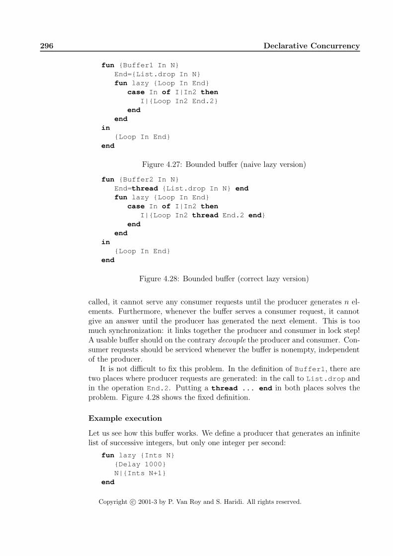
296 Declarative Concurrency
fun {Buffer1 In N}End={List.drop In N}fun lazy {Loop In End}
case In of I|In2 thenI|{Loop In2 End.2}
endend
in{Loop In End}
end
Figure 4.27: Bounded buffer (naive lazy version)
fun {Buffer2 In N}End=thread {List.drop In N} endfun lazy {Loop In End}
case In of I|In2 thenI|{Loop In2 thread End.2 end }
endend
in{Loop In End}
end
Figure 4.28: Bounded buffer (correct lazy version)
called, it cannot serve any consumer requests until the producer generates n el-ements. Furthermore, whenever the buffer serves a consumer request, it cannotgive an answer until the producer has generated the next element. This is toomuch synchronization: it links together the producer and consumer in lock step!A usable buffer should on the contrary decouple the producer and consumer. Con-sumer requests should be serviced whenever the buffer is nonempty, independentof the producer.
It is not difficult to fix this problem. In the definition of Buffer1 , there aretwo places where producer requests are generated: in the call to List.drop andin the operation End.2 . Putting a thread ... end in both places solves theproblem. Figure 4.28 shows the fixed definition.
Example execution
Let us see how this buffer works. We define a producer that generates an infinitelist of successive integers, but only one integer per second:
fun lazy {Ints N}{Delay 1000}N|{Ints N+1}
end
Copyright c© 2001-3 by P. Van Roy and S. Haridi. All rights reserved.

4.5 Lazy execution 297
Now let us create this list and add a buffer of 5 elements:
declareIn={Ints 1}Out={Buffer2 In 5}{Browse Out}{Browse Out.1}
The call Out.1 requests one element. Calculating this element takes one second.Therefore, the browser first displays Out<Future> and one second later addsthe first element, which updates the display to 1|_<Future> . The notation“_<Future> ” denotes a read-only variable. In the case of lazy execution, thisvariable has an internal trigger attached to it. Now wait at least 5 seconds, to letthe buffer fill up. Then enter:
{Browse Out.2.2.2.2.2.2.2.2.2.2}
This requests 10 elements. Because the buffer only has 5 elements, it is immedi-ately emptied, displaying:
1|2|3|4|5|6|_<Future>
One more element is added each second for four seconds. The final result is:
1|2|3|4|5|6|7|8|9|10|_<Future>
At this point, all consumer requests are satisfied and the buffer will start fillingup again at the rate of one element per second.
4.5.5 Reading a file lazily
The simplest way to read a file is as a list of characters. However, if the file isvery large, this uses an enormous amount of memory. This is why files are usuallyread incrementally, a block at a time (where a block is a contiguous piece of thefile). The program is careful to keep in memory only the blocks that are needed.This is memory-efficient, but is cumbersome to program.
Can we have the best of both worlds: to read the file as a list of characters(which keeps programs simple), yet to read in only the parts we need (whichsaves memory)? With lazy execution the answer is yes. Here is the functionReadListLazy that solves the problem:
fun {ReadListLazy FN}{File.readOpen FN}fun lazy {ReadNext}L T I in
{File.readBlock I L T}if I==0 then T=nil {File.readClose} else T={ReadNext} endL
endin
{ReadNext}end
Copyright c© 2001-3 by P. Van Roy and S. Haridi. All rights reserved.

298 Declarative Concurrency
Times 2
Times 3
Times 5
1
Merge
Figure 4.29: Lazy solution to the Hamming problem
It uses three operations in the File module (which is available on the book’s Website): {File.readOpen FN} , which opens file FN for reading, {File.readBlock
I L T} , which reads a block in the difference list L#T and returns its size in I ,and {File.readClose} , which closes the file.
The ReadListLazy function reads a file lazily, a block at a time. Whenevera block is exhausted then another block is read automatically. Reading blocksis much more efficient than reading single characters since only one lazy call isneeded for a whole block. This means that ReadListLazy is practically speakingjust as efficient as the solution in which we read blocks explicitly. When the endof file is reached then the tail of the list is bound to nil and the file is closed.
The ReadListLazy function is acceptable if the program reads all of the file,but if it only reads part of the file, then it is not good enough. Do you see whynot? Think carefully before reading the answer in the footnote!12 Section 6.9.2shows the right way to use laziness together with external resources such as files.
4.5.6 The Hamming problem
The Hamming problem, named after Richard Hamming, is a classic problem ofdemand-driven concurrency. The problem is to generate the first n integers ofthe form 2a3b5c with a, b, c ≥ 0. Hamming actually solved a more general version,which considers products of the first k primes. We leave this one to an exercise!The idea is to generate the integers in increasing order in a potentially infinitestream. At all times, a finite part h of this stream is known. To generate the nextelement of h, we take the least element x of h such that 2x is bigger than the lastelement of h. We do the same for 3 and 5, giving y and z. Then the next element
12It is because the file stays open during the whole execution of the program–this consumesvaluable system resources including a file descriptor and a read buffer.
Copyright c© 2001-3 by P. Van Roy and S. Haridi. All rights reserved.

4.5 Lazy execution 299
of h is min(2x, 3y, 5z). We start the process by initializing h to have the singleelement 1. Figure 4.29 gives a picture of the algorithm. The simplest way toprogram this algorithm is with two lazy functions. The first function multipliesall elements of a list by a constant:
fun lazy {Times N H}case H of X|H2 then N*X|{Times N H2} end
end
The second function takes two lists of integers in increasing order and mergesthem into a single list:
fun lazy {Merge Xs Ys}case Xs#Ys of (X|Xr)#(Y|Yr) then
if X<Y then X|{Merge Xr Ys}elseif X>Y then Y|{Merge Xs Yr}else X|{Merge Xr Yr}end
endend
Each value should appear only once in the output. This means that when X==Y,it is important to skip the value in both lists Xs and Ys. With these two functions,it is easy to solve the Hamming problem:
H=1|{Merge {Times 2 H}{Merge {Times 3 H}
{Times 5 H}}}{Browse H}
This builds a three-argument merge function using two two-argument merge func-tions. If we execute this as is, then it displays very little:
1|_<Future>
No elements are calculated. To get the first n elements of H, we need to ask thatthey be calculated. For example, we can define the procedure Touch :
proc {Touch N H}if N>0 then {Touch N-1 H.2} else skip end
end
This traverses N elements of H, which causes them to be calculated. Now we cancalculate 20 elements by calling Touch :
{Touch 20 H}
This displays:
1|2|3|4|5|6|8|9|10|12|15|16|18|20|24|25|27|30|32|36|_<Future>
4.5.7 Lazy list operations
All the list functions of Section 3.4 can be made lazy. It is insightful to see howthis changes their behavior.
Copyright c© 2001-3 by P. Van Roy and S. Haridi. All rights reserved.

300 Declarative Concurrency
Lazy append
We start with a simple function: a lazy version of Append :
fun lazy {LAppend As Bs}case Asof nil then Bs[] A|Ar then A|{LAppend Ar Bs}end
end
The only difference with the eager version is the “lazy ” annotation. The lazydefinition works because it is recursive: it calculates part of the answer and thencalls itself. Calling LAppend with two lists will append them lazily:
L={LAppend "foo" "bar"}{Browse L}
We say this function is incremental: forcing its evaluation only does enough of thecalculation to generate one additional output element, and then creates anothersuspension. If we “touch” successive elements of L this will successively show f ,o, o, one character at a time. However, after we have exhausted "foo" , thenLAppend is finished, so it will show "bar" all at once. How do we make a listappend that returns a completely lazy list? One way is to give LAppend a lazylist as second argument. First define a function that takes any list and returns alazy version:
fun lazy {MakeLazy Ls}case Lsof X|Lr then X|{MakeLazy Lr}else nil end
end
MakeLazy works by iterating over its input list, i.e., like LAppend , it calculatespart of the answer and then calls itself. This only changes the control flow;considered as a function between lists, MakeLazy is an identity. Now call LAppend
as follows:
L={LAppend "foo" {MakeLazy "bar"}}{Browse L}
This will lazily enumerate both lists, i.e., it successively returns the characters f ,o, o, b, a, and r .
Lazy mapping
We have seen Map in Section 3.6; it evaluates a function on all elements of a list.It is easy to define a lazy version of this function:
fun lazy {LMap Xs F}case Xsof nil then nil
Copyright c© 2001-3 by P. Van Roy and S. Haridi. All rights reserved.

4.5 Lazy execution 301
[] X|Xr then {F X}|{LMap Xr F}end
end
This function takes any list or lazy list Xs and returns a lazy list. Is it incremental?
Lazy integer lists
We define the function {LFrom I J} that generates a lazy list of integers fromI to J :
fun {LFrom I J}fun lazy {LFromLoop I}
if I>J then nil else I|{LFromLoop I+1} endendfun lazy {LFromInf I} I|{LFromInf I+1} end
inif J==inf then {LFromInf I} else {LFromLoop I} end
end
Why is LFrom itself not annotated as lazy?13 This definition allows J=inf , inwhich case an infinite lazy stream of integers is generated.
Lazy flatten
This definition shows that lazy difference lists are as easy to generate as lazylists. As with the other lazy functions, it suffices to annotate as lazy all recursivefunctions that calculate part of the solution on each iteration.
fun {LFlatten Xs}fun lazy {LFlattenD Xs E}
case Xsof nil then E[] X|Xr then
{LFlattenD X {LFlattenD Xr E}}[] X then X|Eend
endin
{LFlattenD Xs nil}end
We remark that this definition has the same asymptotic efficiency as the eagerdefinition, i.e., it takes advantage of the constant-time append property of differ-ence lists.
13Only recursive functions need to be controlled, since they would otherwise do a potentiallyunbounded calculation.
Copyright c© 2001-3 by P. Van Roy and S. Haridi. All rights reserved.

302 Declarative Concurrency
Lazy reverse
Up to now, all the lazy list functions we introduced are incremental, i.e., they areable to produce one element at a time efficiently. Sometimes this is not possible.For some list functions, the work required to produce one element is enough toproduce them all. We call these functions monolithic. A typical example is listreversal. Here is a lazy definition:
fun {LReverse S}fun lazy {Rev S R}
case Sof nil then R[] X|S2 then {Rev S2 X|R} end
endin {Rev S nil} end
Let us call this function:
L={LReverse [a b c]}{Browse L}
What happens if we touch the first element of L? This will calculate and displaythe whole reversed list! Why does this happen? Touching L activates the sus-pension {Rev [a b c] nil} (remember that LReverse itself is not annotatedas lazy). This executes Rev and creates a new suspension for {Rev [b c] [a]}
(the recursive call), but no list pair. Therefore the new suspension is immedi-ately activated. This does another iteration and creates a second suspension,{Rev [c] [b a]} . Again, no list pair is available, so the second suspension isimmediately activated. This continues until Rev returns [c b a] . At this point,there is a list pair so the evaluation completes. The need for one list pair hascaused the whole list reversal to be done. This is what we mean by a monolithicfunction. For list reversal, another way to understand this behavior is to thinkof what list reversal means: the first element of a reversed list is the last elementof the input list. We therefore have to traverse the whole input list, which letsus construct the whole reversed list.
Lazy filter
To complete this section, we give another example of an incremental function,namely filtering an input list according to a condition F:
fun lazy {LFilter L F}case Lof nil then nil[] X|L2 then
if {F X} then X|{LFilter L2 F} else {LFilter L2 F} endend
end
Copyright c© 2001-3 by P. Van Roy and S. Haridi. All rights reserved.
4.5 Lazy execution 303
We give this function because we will need it for list comprehensions in Sec-tion 4.5.9.
4.5.8 Persistent queues and algorithm design
In Section 3.4.5 we saw how to build queues with constant-time insert and deleteoperations. Those queues only work in the ephemeral case, i.e., only one versionexists at a time. It turns out we can use laziness to build persistent queues withthe same time bounds. A persistent queue is one that supports multiple versions.We first show how to make an amortized persistent queue with constant-timeinsert and delete operations. We then show how to achieve worst-case constant-time.
Amortized persistent queue
We first tackle the amortized case. The reason why the amortized queue ofSection 3.4.5 is not persistent is that Delete sometimes does a list reversal,which is not constant time. Each time a Delete is done on the same version,another list reversal is done. This breaks the amortized complexity if there aremultiple versions.
We can regain the amortized complexity by doing the reverse as part of a lazyfunction call. Invoking the lazy function creates a suspension instead of doing thereverse right away. Sometime later, when the result of the reverse is needed, thelazy function does the reverse. With some cleverness, this can solve our problem:
• Between the creation of the suspension and the actual execution of thereverse, we arrange that there are enough operations to pay back the costsincurred by the reverse.
• But the reverse can be paid for only once. What if several versions wantto do the reverse? This is not a problem. Laziness guarantees that thereverse is only done once, even if more than one version triggers it. The firstversion that needs it will activate the trigger and save the result. Subsequentversions will use the result without doing any calculation.
This sounds nice, but it depends on being able to create the suspension far enoughin advance of the actual reverse. Can we do it? In the case of a queue, we can.Let us represent the queue as a 4-tuple:
q(LenF F LenR R)
F and Rare the front and rear lists, like in the ephemeral case. We add the integersLenF and LenR, which give the lengths of F and R. We need these integers to testwhen it is time to create the suspension. At some magic instant, we move theelements of R to F. The queue then becomes:
q(LenF+LenR {LAppend F {Reverse R}} 0 nil)
Copyright c© 2001-3 by P. Van Roy and S. Haridi. All rights reserved.

304 Declarative Concurrency
In Section 3.4.5 we did this (eagerly) when F became empty, so the Append didnot take any time. But this is too late to keep the amortized complexity, sincethe reverse is not paid for (e.g., maybe R is a very big list). We remark that thereverse gets evaluated in any case when the LAppend has finished, i.e., after |F|elements are removed from the queue. Can we arrange that the elements of F
pay for the reverse? We can, if we create the suspension when |R| ≈ |F|. Thenremoving each element of F pays for part of the reverse. By the time we have toevaluate the reverse, it is completely paid for. Using the lazy append makes thepayment incremental. This gives the following implementation:
fun {NewQueue} q(0 nil 0 nil) end
fun {Check Q}case Q of q(LenF F LenR R) then
if LenF>=LenR then Qelse q(LenF+LenR {LAppend F {Reverse R}} 0 nil) end
endend
fun {Insert Q X}case Q of q(LenF F LenR R) then
{Check q(LenF F LenR+1 X|R)}end
end
fun {Delete Q X}case Q of q(LenF F LenR R) then F1 in
F=X|F1 {Check q(LenF-1 F1 LenR R)}end
end
Both Insert and Delete call the function Check , which chooses the moment todo the lazy call. Since Insert increases |R| and Delete decreases |F|, eventually|R| becomes as large as |F|. When |R| = |F|+1, Check does the lazy call {LAppend
F {Reverse R}} . The function LAppend is defined in Section 4.5.7.Let us summarize this technique. We replace the original eager function call
by a lazy function call. The lazy call is partly incremental and partly monolithic.The trick is that the lazy call starts off being incremental. By the time themonolithic part is reached, there have been enough incremental steps so that themonolithic part is paid for. It follows that the result is amortized constant-time.
For a deeper discussion of this technique including its application to otherdata structures and a proof of correctness, we recommend [138].
Worst-case persistent queue
The reason the above definition is not worst-case constant-time is because Reverse
is monolithic. If we could rewrite it to be incremental, then we would have a so-
Copyright c© 2001-3 by P. Van Roy and S. Haridi. All rights reserved.

4.5 Lazy execution 305
lution with constant-time worst-case behavior. But list reversal cannot be madeincremental, so this does not work. Let us try another approach.
Let us look at the context of the call to Reverse . It is called together with alazy append:
{LAppend F {Reverse R}}
This first executes the append incrementally. When all elements of F have beenpassed to the output, then the reverse is executed monolithically. The cost of thereverse is amortized over the steps of the append.
Instead of amortizing the cost of the reverse, perhaps we can actually do thereverse together with the steps of the append. When the append is finished, thereverse will be finished as well. This is the heart of the solution. To implement it,let us compare the definitions of reverse and append. Reverse uses the recursivefunction Rev:
fun {Reverse R}fun {Rev R A}
case Rof nil then A[] X|R2 then {Rev R2 X|A} end
endin {Rev R nil} end
Rev traverses R, accumulates a solution in A, and then returns the solution. Canwe do both Rev and LAppend in a single loop? Here is LAppend :
fun lazy {LAppend F B}case Fof nil then B[] X|F2 then X|{LAppend F2 B}end
end
This traverses F and returns B. The recursive call is passed B unchanged. Letus change this to use B to accumulate the result of the reverse! This gives thefollowing combined function:
fun lazy {LAppRev F R B}case F#Rof nil#[Y] then Y|B[] (X|F2)#(Y|R2) then X|{LAppRev F2 R2 Y|B}end
end
LAppRev traverses both F and R. During each iteration, it calculates one elementof the append and accumulates one element of the reverse. This definition onlyworks if R has exactly one more element than F, which is true for our queue. Theoriginal call:
{LAppend F {Reverse R}}
Copyright c© 2001-3 by P. Van Roy and S. Haridi. All rights reserved.

306 Declarative Concurrency
is replaced by:
{LAppRev F R nil}
which gives exactly the same result except that LAppRev is completely incremen-tal. The definition of Check then becomes:
fun {Check Q}case Q of q(LenF F LenR R) then
if LenR=<LenF then Qelse q(LenF+LenR {LAppRev F R nil} 0 nil) end
endend
Careful analysis shows that the worst-case bound of this queue is O(logn), andnot O(1) as our intuition might expect it to be. The bound is much better thanO(n), but it is not constant. See the Exercises for an explanation and a suggestionon how to achieve a constant bound.
Taking a program with a worst-case bound and adding laziness naively willgive an amortized bound. This is because laziness changes where the function callsare executed, but does not do more of them (the eager case is an upper bound).The definition of this section is remarkable because it does just the opposite: itstarts with an amortized bound and uses laziness to give a worst-case bound.
Lessons for algorithm design
Laziness is able to shuffle calculations around, spreading them out or bunchingthem together without changing the final result. This is a powerful tool fordesigning declarative algorithms. It has to be used carefully, however. Usednaively, laziness can destroy perfectly good worst-case bounds, turning them intoamortized bounds. Used wisely, laziness can improve amortized algorithms: itcan sometimes make the algorithm persistent and it can sometimes transform theamortized bound into a worst-case bound.
We can outline a general scheme. Start with an algorithm A that has anamortized bound O(f(n)) when used ephemerally. For example, the first queueof Section 3.4.5 has an amortized bound of O(1). We can use laziness to movefrom ephemeral to persistent while keeping this time bound. There are twopossibilities:
• Often we can get a modified algorithm A’ that keeps the amortized boundO(f(n)) when used persistently. This is possible when the expensive opera-tions can be spread out to be mostly incremental but with a few remainingmonolithic operations.
• In a few cases, we can go farther and get a modified algorithm A” withworst-case bound O(f(n)) when used persistently. This is possible whenthe expensive operations can be spread out to be completely incremental.
Copyright c© 2001-3 by P. Van Roy and S. Haridi. All rights reserved.

4.5 Lazy execution 307
This section realizes both possibilities with the first queue of Section 3.4.5. Thepersistent algorithms so obtained are often quite efficient, especially if used byapplications that really need the persistence. They compare favorably with algo-rithms in stateful models.
4.5.9 List comprehensions
List comprehensions are a powerful tool for calculating with lazy streams. Theyallow to specify lazy streams in a way that closely resembles the mathematicalnotation of set comprehension. For example, the mathematical notation {x ∗y | 1 ≤ x ≤ 10, 1 ≤ y ≤ x} specifies the set {1∗1, 2∗1, 2∗2, 3∗1, 3∗2, 3∗3, ...10∗10},i.e. {1, 2, 3, 4, 5, ..., 100}. We turn this notation into a practical programming toolby modifying it to specify not sets, but lazy streams. This makes the notationvery efficient to implement, while keeping it at a high level of abstraction. Forexample, the list comprehension [x ∗ y | 1 ≤ x ≤ 10, 1 ≤ y ≤ x] (notice thesquare list brackets!) specifies the list [1*1 2*1 2*2 3*1 3*2 3*3 · · · 10*10]
(in this order), i.e., the list [1 2 4 3 6 9 · · · 100] . The list is calculated lazily.Because of laziness the list comprehension can generate a potentially unboundedstream, not just a finite list.
List comprehensions have the following basic form:
[f(x) | x← generator(a1, ..., an), guard(x, a1, ..., an)]
The generator x← generator(a1, ..., an) calculates a lazy list whose elements aresuccessively assigned to x. The guard guard(x, a1, ..., an) is a boolean function.The list comprehension specifies a lazy list containing the elements f(x), wheref is any function and x takes on values from the generator for which the guard istrue. In the general case, there can be any number of variables, generators, andguards. A typical generator is from:
x← from(a, b)
Here x takes on the integer values a, a+1, ..., b, in that order. Calculation is donefrom left to right. The generators, when taken from left to right, are consideredas nested loops: the rightmost generator is the innermost loop.
There is a close connection between list comprehensions and the relationalprogramming of Section 9. Both provide lazy interfaces to infinitely long se-quences and make it easy to write “generate-and-test” programs. Both allow tospecify the sequences in a declarative way.
While list comprehensions are usually considered to be lazy, they can in factbe programmed in both eager and lazy versions. For example, the list compre-hension:
z = [x#x | x← from(1, 10)]
can be programmed in two ways. An eager version is:
Copyright c© 2001-3 by P. Van Roy and S. Haridi. All rights reserved.

308 Declarative Concurrency
Z = {Map {From 1 10} fun {$ X} X#X end }
For the eager version, the declarative model of Chapter 2 is good enough. It usesthe Map function of Section 3.6.3 and the From function which generates a list ofintegers. A lazy version is:
Z = {LMap {LFrom 1 10} fun {$ X} X#X end }
The lazy version uses the LMap and LFrom functions of the previous section. Thisexample and most examples of this section can be done with either a lazy or eagerversion. Using the lazy version is always correct. Using the eager version is aperformance optimization. It is several times faster if the cost of calculating thelist elements is not counted. The optimization is only possible if the whole listfits in memory. In the rest of this section, we always use the lazy version.
Here is a list comprehension with two variables:
z = [x#y | x← from(1, 10), y ← from(1, x)]
This can be programmed as:
Z = {LFlatten{LMap {LFrom 1 10} fun {$ X}
{LMap {LFrom 1 X} fun {$ Y}X#Y
end }end }}
We have seen LFlatten in the previous section; it converts a list of lists to a“flat” lazy list, i.e., a lazy list that contains all the elements, but no lists. Weneed LFlatten because otherwise we have a list of lists. We can put LFlatten
inside LMap:
fun {FMap L F}{LFlatten {LMap L F}}
end
This simplifies the program:
Z = {FMap {LFrom 1 10} fun {$ X}{LMap {LFrom 1 X} fun {$ Y}
X#Yend }
end }
Here is an example with two variables and a guard:
z = [x#y | x← from(1, 10), y ← from(1, 10), x + y ≤ 10]
This gives the list of all pairs x#y such that the sum x + y is at most 10. It canbe programmed as:
Z = {LFilter{FMap {LFrom 1 10} fun {$ X}
Copyright c© 2001-3 by P. Van Roy and S. Haridi. All rights reserved.

4.6 Soft real-time programming 309
{LMap {LFrom 1 10} fun {$ Y}X#Y
end }end }fun {$ X#Y} X+Y=<10 end }
This uses the function LFilter defined in the previous section. We can refor-mulate this example to be more efficient. The idea is to generate as few elementsas possible. In the above example, 100 (=10*10) elements are generated. From2 ≤ x + y ≤ 10 and 1 ≤ y ≤ 10, we derive that 1 ≤ y ≤ 10 − x. This gives thefollowing solution:
z = [x#y | x← from(1, 10), y ← from(1, 10− x)]
The program then becomes:
Z = {FMap {LFrom 1 10} fun {$ X}{LMap {LFrom 1 10-X} fun {$ Y}
X#Yend }
end }
This gives the same list as before, but only generates about half as many elements.
4.6 Soft real-time programming
4.6.1 Basic operations
The Time module contains a number of useful soft real-time operations. A real-time operation has a set of deadlines (particular times) at which certain calcu-lations must be completed. A soft real-time operation requires only that thereal-time deadlines be respected most of the time. This is opposed to hard real-time, which has hard deadlines, i.e., that must be respected all the time, withoutany exception. Hard real-time is needed when lives are at stake, e.g., in medicalequipment and air traffic control. Soft real-time is used in other cases, e.g., fortelephony and consumer electronics. Hard real-time requires special techniquesfor both hardware and software. Standard personal computers cannot do hardreal-time because they have unpredictable hardware delays (e.g., virtual memory,caching, process scheduling). Soft real-time is much easier to implement and isoften sufficient. Three soft real-time operations provided by Time are:
• {Delay I} : suspends the executing thread for at least I milliseconds andthen continues.
• {Alarm I U} : creates a new thread that binds U to unit after at least I
milliseconds. Alarm can be implemented with Delay .
• {Time.time} : returns the integer number of seconds that have passed sincethe current year started.
Copyright c© 2001-3 by P. Van Roy and S. Haridi. All rights reserved.

310 Declarative Concurrency
localproc {Ping N}
if N==0 then {Browse ´ ping terminated ´ }else {Delay 500} {Browse ping} {Ping N-1} end
endproc {Pong N}
{For 1 N 1proc {$ I} {Delay 600} {Browse pong} end }
{Browse ´ pong terminated ´ }end
in{Browse ´ game started ´ }thread {Ping 50} endthread {Pong 50} end
end
Figure 4.30: A simple ‘Ping Pong’ program
The semantics of Delay is simple: it communicates to the scheduler that thethread is to be considered suspended for a given time period. After this timeis up, the scheduler marks the thread as runnable again. The thread is notnecessarily run immediately. If there are lots of other runnable threads, it maytake some time before the thread actually runs.
We illustrate the use of Delay by means of a simple example that shows theinterleaving execution of two threads. The program is called ´ Ping Pong ´ andis defined in Figure 4.30. It starts two threads. One displays ping periodicallyeach 500 milliseconds and the other displays pong each 600 milliseconds. Becausepongs come out slower than pings, it is possible for two pings to be displayedwithout any pongs in between. Can the same thing happen with two pongs?That is, can two pongs ever be displayed with no pings in between? Assume thatthe Ping thread has not yet terminated, otherwise the question would be tooeasy. Think carefully before reading the answer in the footnote.14
A simple standalone application
Section 3.9 in Chapter 2 shows how to make standalone applications in Oz. Tomake the ´ Ping Pong ´ program standalone, the first step is to make a functorof it, as shown in Figure 4.31. If the source code is stored in file PingPong.oz ,then the program can be compiled with the following command:
ozc -x PingPong.oz
14The language does indeed allow two pongs to be displayed with no intervening pings becausethe definition of Delay only gives the minimum suspension time. The thread suspending for500 milliseconds can occasionally suspend for a longer time, for example for 700 milliseconds.But this is a rare occurrence in practice because it depends on external events in the operatingsystem or in other threads.
Copyright c© 2001-3 by P. Van Roy and S. Haridi. All rights reserved.

4.6 Soft real-time programming 311
functorimport
Browser(browse:Browse)define
proc {Ping N}if N==0 then {Browse ´ ping terminated ´ }else {Delay 500} {Browse ping} {Ping N-1} end
endproc {Pong N}
{For 1 N 1proc {$ I} {Delay 600} {Browse pong} end }
{Browse ´ pong terminated ´ }end
in{Browse ´ game started ´ }thread {Ping 50} endthread {Pong 50} end
end
Figure 4.31: A standalone ‘Ping Pong’ program
Type PingPong in your shell to start the program. To terminate this program ina Unix shell you have to type CTRL-C.
The program of Figure 4.31 does not terminate properly when the Ping andthe Pong threads terminate. It does not detect when the threads terminate. Wecan fix this problem using the techniques of Section 4.4.3. Figure 4.32 adds atermination detection that terminates the main thread only when both the Ping
and the Pong threads terminate. We could also use the Barrier abstractiondirectly. After detecting termination, we use the call {Application.exit 0}
to cleanly exit the application.
4.6.2 Ticking
We would like to invoke an action (e.g., send a message to a stream object, calla procedure, etc.) exactly once per second, giving it the local time as argument.We have three operations at our disposal: {Delay D} , which delays for at least D
milliseconds, {Time.time} , which returns the number of seconds since January1 of the current year, and {OS.localTime} , which returns a record giving localtime accurate to one second. How does the following function measure up:
fun {NewTicker}fun {Loop}
X={OS.localTime}in
{Delay 1000}X|{Loop}
Copyright c© 2001-3 by P. Van Roy and S. Haridi. All rights reserved.

312 Declarative Concurrency
functorimport
Browser(browse:Browse)Application
define...X1 X2
in{Browse ´ game started ´ }thread {Ping 50} X1= unit endthread {Pong 50} X2= unit end{Wait X1} {Wait X2}{Application.exit 0}
end
Figure 4.32: A standalone ‘Ping Pong’ program that exits cleanly
endin
thread {Loop} endend
This function creates a stream that grows by one element per second. To executean action once every second, create a thread that reads the stream and performsthe action:
thread for X in {NewTicker} do {Browse X} end end
Any number of threads can read the same stream. The problem is, this solutionis not quite right. The stream is extended almost exactly once per second. Theproblem is the “almost”. Every once in a while, one second is lost, i.e., successiveelements on the stream show a difference of two seconds. However, there isone good point: the same second cannot be sent twice, since {Delay 1000}
guarantees a delay of at least 1000 milliseconds, to which is added the execution ofthe instructions in Loop . This gives a total delay of at least 1000+ε milliseconds,where ε is a fraction of a microsecond.
How can we correct this problem? A simple way is to compare the currentresult of OS.localTime with the previous result, and to add an element to thestream only when the local time changes. This gives:
fun {NewTicker}fun {Loop T}
T1={OS.localTime}in
{Delay 900}if T1\=T then T1|{Loop T1} else {Loop T1} end
endin
Copyright c© 2001-3 by P. Van Roy and S. Haridi. All rights reserved.

4.6 Soft real-time programming 313
thread {Loop {OS.localTime}} endend
This version guarantees that exactly one tick will be sent per second, if {Delay
900} always delays for less than one second. The latter condition holds if thereare not too many active threads and garbage collection does not take too long.One way to guarantee the first condition is to give the Loop thread high priorityand all other threads medium or low priority. To guarantee the second condition,the program must ensure that there is not too much active data, since garbagecollection time is proportional to the amount of active data.
This version has the minor problem that it “hesitates” every 9 seconds. Thatis, it can happen that {OS.localTime} gives the same result twice in a row,since the two calls are separated by just slightly more than 900 milliseconds.This means that the stream will not be updated for 1800 milliseconds. Anotherway to see this problem is that 10 intervals of 900 milliseconds are needed tocover 9 seconds, which means that nothing happens during one of the intervals.How can we avoid this hesitation? A simple way is to make the delay smaller.With a delay of 100 milliseconds, the hesitation will never be greater than 100milliseconds plus the garbage collection time.
A better way to avoid the hesitation is to use synchronized clocks. That is, wecreate a free-running counter that runs at approximately one second per tick, andwe adjust its speed so that it remains synchronized with the operating systemtime. Here is how it is done:
fun {NewTicker}fun {Loop N}
T={Time.time}in
if T>N then {Delay 900}elseif T<N then {Delay 1100}else {Delay 1000} endN|{Loop N+1}
endin
thread {Loop {Time.time}} endend
The loop has a counter, N, that is always incremented by one. We compare thecounter value to the result of {Time.time} .15 If the counter is slower (T>N),we speed it up. Likewise, if the counter is faster (T<N), we slow it down. Thespeedup and slowdown factors are small (10% in the example), which makes thehesitation unnoticeable.
15How would you fix NewTicker to work correctly when Time.time turns over, i.e., goesback to 0?
Copyright c© 2001-3 by P. Van Roy and S. Haridi. All rights reserved.

314 Declarative Concurrency
4.7 Limitations and extensions of declarative pro-
gramming
Declarative programming has the major advantage that it considerably simplifiessystem building. Declarative components can be built and debugged indepen-dently of each other. The complexity of a system is the sum of the complexitiesof its components. A natural question to ask is how far can declarative pro-gramming go? Can everything be programmed in a declarative way, such thatprograms are both natural and efficient? This would be a major boon for sys-tem building. We say a program is efficient if its performance differs by just aconstant factor from the performance of an assembly language program to solvethe same problem. We say a program is natural if very little code is needed justfor technical reasons unrelated to the problem at hand. Let us consider efficiencyand naturalness issues separately. There are three naturalness issues: modularity,nondeterminism, and interfacing with the real world.
We recommend to use the declarative model of this chapter or the sequentialversion of Chapter 2 except when any of the above issues is critical. This makesit easier to write correct and efficient components.
4.7.1 Efficiency
Is declarative programming efficient? There is a fundamental mismatch betweenthe declarative model and a standard computer, such as presented in [146]. Thecomputer is optimized for modifying data in-place, while the declarative modelnever modifies data but always creates new data. This is not as severe a prob-lem as it seems at first glance. The declarative model may have a large inherentmemory consumption, but its active memory size remains small. The task re-mains, though, to implement the declarative model with in-place assignment.This depends first on the sophistication of the compiler.
Can a compiler map declarative programs effectively to a standard computer?Paraphrasing science fiction author and futurologist Arthur C. Clarke, we can saythat “any sufficiently advanced compiler is indistinguishable from magic” [37].16
That is, it is unrealistic to expect the compiler to rewrite your program. Evenafter several decades of research, no such compiler exists for general-purpose pro-gramming. The farthest we have come is compilers that can rewrite the programin particular cases. Computer scientist Paul Hudak calls them “smart-aleck”compilers. Because of their unpredictable optimizations, they are hard to use.Therefore, for the rest of the discussion, we assume that the compiler does astraightforward mapping from the source program to the target, in the sense thattime and space complexities of compiled code can be derived in a simple wayfrom language semantics.
16Clarke’s Third Law: “Any sufficiently advanced technology is indistinguishable from mag-ic.”
Copyright c© 2001-3 by P. Van Roy and S. Haridi. All rights reserved.

4.7 Limitations and extensions of declarative programming 315
Now we can answer the question whether declarative programming is efficient.Given a straightforward compiler, the pedantic answer to the question is no. Butin fact the practical answer is yes, with one caveat: declarative programming isefficient if one is allowed to rewrite the program to be less natural. Here are threetypical examples:
1. A program that does incremental modifications of large data structures,e.g., a simulation that modifies large graphs (see Section 6.8.4), cannot ingeneral be compiled efficiently. Even after decades of research, there is nostraightforward compiler that can take such a program and implement itefficiently. However, if one is allowed to rewrite the program, then there isa simple trick that is often sufficient in practice. If the state is threaded(e.g., kept in an accumulator) and the program is careful never to accessan old state, then the accumulator can be implemented with destructiveassignment.
2. A function that does memoization cannot be programmed without changingits interface. Assume we have a function that uses many computationalresources. To improve its performance, we would like to add memoizationto it, i.e., an internal cache of previously-calculated results, indexed by thefunction arguments. At each function call, we first check the cache to seeif the result is already there. This internal cache cannot be added withoutrewriting the program by threading an accumulator everywhere that thefunction is called. Section 10.3.2 gives an example.
3. A function that implements a complex algorithm often needs intricate code.That is, even though the program can be written declaratively with the sameefficiency as a stateful program, doing so makes it more complex. Thisfollows because the declarative model is less expressive than the statefulmodel. Section 6.8.1 shows an example: a transitive closure algorithmwritten in both the declarative and the stateful models. Both versions havetime efficiency O(n3). The stateful algorithm is simpler to write than thedeclarative one.
We conclude that declarative programming cannot always be efficient and naturalsimultaneously. Let us now look at the naturalness issues.
4.7.2 Modularity
We say a program is modular with respect to a change in a given part if the changecan be done without changing the rest of the program. Modularity is discussedfurther in Section 6.7.2. Here are two examples where declarative programs arenot modular:
1. The first example is the memoization cache we saw before. Adding thiscache to a function is not modular, since an accumulator must be threadedin many places outside the function.
Copyright c© 2001-3 by P. Van Roy and S. Haridi. All rights reserved.

316 Declarative Concurrency
2. A second example is instrumenting a program. We would like to know howmany times some of its subcomponents are invoked. We would like to addcounters to these subcomponents, preferably without changing either thesubcomponent interfaces or the rest of the program. If program is declar-ative, this is impossible, since the only way is to thread an accumulatorthroughout the program.
Let us look closer at the second example. Assume that we are using the declarativemodel to implement a large declarative component. The component definitionlooks something like this:
fun {SC ...}proc {P1 ...}
...endproc {P2 ...}
...{P1 ...}{P2 ...}
endproc {P3 ...}
...{P2 ...}{P3 ...}
endin
´ export ´ (p1:P1 p2:P2 p3:P3)end
Calling SCinstantiates the component: it returns a module with three operations,P1, P2, and P3. We would like to instrument the component by counting thenumber of times procedure P1 is called. The successive values of the count are astate. We can encode this state as an accumulator, i.e., by adding two argumentsto each procedure. With this added instrumentation, the component definitionlooks something like this:
fun {SC ...}proc {P1 ... S1 ?Sn}
Sn=S1+1...
endproc {P2 ... T1 ?Tn}
...{P1 ... T1 T2}{P2 ... T2 Tn}
endproc {P3 ... U1 ?Un}
...
Copyright c© 2001-3 by P. Van Roy and S. Haridi. All rights reserved.

4.7 Limitations and extensions of declarative programming 317
Maincomponent
Main Main
P3
P1
P2Subcomponent
Using an accumulator Using explicit state
SC
P3
P1
P2
SC
Figure 4.33: Changes needed for instrumenting procedure P1
{P2 ... U1 U2}{P3 ... U2 Un}
endin
´ export ´ (p1:P1 p2:P2 p3:P3)end
Each procedure defined by SChas a changed interface: it has two extra argumentsthat together form an accumulator. The procedure P1 is called as {P1 ...
Sin Sout} , where Sin is the input count and Sout is the output count. Theaccumulator has to be threaded between the procedure calls. This techniquerequires both SCand the calling module to do a fair amount of bookkeeping, butit works.
Another solution is to write the component in a stateful model. One suchmodel is defined in Chapter 6; for now assume that we have a new languageentity, called “cell”, that we can assign and access (with the := and @operators),similar to an assignable variable in imperative programming languages. Cellswere introduced in Chapter 1. Then the component definition looks somethinglike this:
fun {SC ...}Ctr={NewCell 0}proc {P1 ...}
Ctr:=@Ctr+1...
endproc {P2 ...}
...
Copyright c© 2001-3 by P. Van Roy and S. Haridi. All rights reserved.

318 Declarative Concurrency
{P1 ...}{P2 ...}
endproc {P3 ...}
...{P2 ...}{P3 ...}
endfun {Count} @Ctr end
in´ export ´ (p1:P1 p2:P2 p3:P3 count:Count)
end
In this case, the component interface has one extra function, Count , and theinterfaces to P1, P2, and P3 are unchanged. The calling module has no book-keeping to do whatsoever. The count is automatically initialized to zero whenthe component is instantiated. The calling module can call Count at any timeto get the current value of the count. The calling module can also ignore Count
completely, if it likes, in which case the component has exactly the same behavioras before (except for a very slight difference in performance).
Figure 4.33 compares the two approaches. The figure shows the call graphof a program with a component Main that calls subcomponent SC. A call graphis a directed graph where each node represents a procedure and there is an edgefrom each procedure to the procedures it calls. In Figure 4.33, SC is called fromthree places in the main component. Now let us instrument SC. In the declarativeapproach (at left), an accumulator has to be added to each procedure on the pathfrom Main to P1. In the stateful approach (at right), the only changes are theextra operation Count and the body of P1. In both cases, the changes are shownwith thick lines. Let us compare the two approaches:
• The declarative approach is not modular with respect to instrumentingP1, because every procedure definition and call on the path from Main toP1 needs two extra arguments. The interfaces to P1, P2, and P3 are allchanged. This means that other components calling SChave to be changedtoo.
• The stateful approach is modular because the cell is mentioned only where itis needed, in the initialization of SCand in P1. In particular, the interfacesto P1, P2, and P3, remain the same in the stateful approach. Since theextra operation Count can be ignored, other components calling SCdo nothave to be changed.
• The declarative approach is slower because it does much extra argumentpassing. All procedures are slowed down for the sake of one. The statefulapproach is efficient; it only spends time when necessary.
Which approach is simpler: the first or the second? The first has a simpler modelbut a more complex program. The second has a more complex model but a
Copyright c© 2001-3 by P. Van Roy and S. Haridi. All rights reserved.

4.7 Limitations and extensions of declarative programming 319
Cli ent 1
Client 2
Server?
OutS2
OutS1
InS
Figure 4.34: How can two clients send to the same server? They cannot!
simpler program. In our view, the declarative approach is not natural. Becauseit is modular, the stateful approach is clearly the simplest overall.
The fallacy of the preprocessor
Maybe there is a way we can have our cake and eat it too. Let us define apreprocessor to add the arguments so we do not have to write them everywhere.A preprocessor is a program that takes another program’s source code as input,transforms it according to some simple rules, and returns the result. We define apreprocessor that takes the syntax of the stateful approach as input and translatesit into a program that looks like the declarative approach. Voila! It seems thatwe can now program with state in the declarative model. We have overcome alimitation of the declarative model. But have we? In fact, we have done nothingof the sort. All we have succeeded in doing is build an inefficient implementationof a stateful model. Let us see why:
• When using the preprocessor, we see only programs that look like the state-ful version, i.e., stateful programs. This obliges us to reason in the statefulmodel. We have therefore de facto extended the declarative model withexplicit state.
• The preprocessor transforms these stateful programs into programs withthreaded state, which are inefficient because of all the argument passing.
4.7.3 Nondeterminism
The declarative concurrent model seems to be quite powerful for building concur-rent programs. For example, we can easily build a simulator for digital electroniccircuits. However, despite this apparent power, the model has a limitation thatcripples it for many concurrent applications: it always behaves deterministically.If a program has observable nondeterminism, then it is not declarative. This lim-itation is closely related to modularity: components that are truly independent
Copyright c© 2001-3 by P. Van Roy and S. Haridi. All rights reserved.

320 Declarative Concurrency
behave nondeterministically with respect to each other. To show that this is nota purely theoretical limitation, we give two realistic examples: a client/serverapplication and a video display application.
The limitation can be removed by adding a nondeterministic operation tothe model. The extended model is no longer declarative. There are many pos-sible nondeterministic operations we could add. Chapters 5 and 8 explain thepossibilities in detail. Let us briefly go over them here:
• A first solution is to add a nondeterministic wait operation, such as WaitTwo
which waits for one of two variables to become bound, and indicates one ofthe bound ones. Its definition is given in the supplements file on the book’sWeb site. WaitTwo is nice for the client/server application.
• A second solution is to add IsDet , a boolean function that tests imme-diately whether a dataflow variable is bound or not. This allows to usedataflow variables as a weak form of state. IsDet is nice for the videodisplay application.
• A third solution is to add explicit state to the model, for example in theform of ports (communication channels) or cells (mutable variables).
How do these three solutions compare in expressiveness? WaitTwo can be pro-grammed in the declarative concurrent model with explicit state. Therefore, itseems that the most expressive model needs just explicit state and IsDet .
A client/server application
Let us investigate a simple client/server application. Assume that there are twoindependent clients. Being independent implies that they are concurrent. Whathappens if they communicate with the same server? Because they are indepen-dent, the server can receive information in any order from the two clients. Thisis observable nondeterministic behavior.
Let us examine this closer and see why it cannot be expressed in the declarativeconcurrent model. The server has an input stream from which it reads commands.Let us start with one client, which sends commands to the server. This worksperfectly. How can a second client connect to the server? The second client has toobtain a reference to a stream that it can bind and that is read by the server. Theproblem is that such a stream does not exist! There is only one stream, betweenthe first client and the server. The second client cannot bind that stream, sincethis would conflict with the first client’s bindings.
How can we solve this problem? Let us approach it naively and see if we canfind a solution. One approach might be to let the server have two input streams,like this:
fun {Server InS1 InS2}...
end
Copyright c© 2001-3 by P. Van Roy and S. Haridi. All rights reserved.

4.7 Limitations and extensions of declarative programming 321
But how does the server read the streams? Does it first read one element fromInS1 and then one element from InS2 ? Does it simultaneously read one elementfrom both streams? Neither of these solutions is correct. In fact, it is not possibleto write a solution in the declarative concurrent model. The only thing we cando is have two independent servers, one for each client. But these servers cannotcommunicate with each other, since otherwise we would have the same problemall over again.
Figure 4.34 illustrates the problem: InS is the server’s input stream and OutS1
and OutS2 are the two client’s output streams. How can the messages appearingon both client streams be given to the server? The simple answer is that in thedeclarative concurrent model they cannot! In the declarative concurrent model,an active object always has to know from which stream it will read next.
How can we solve this problem? If the clients execute in coordinated fashion,so that the server always knows which client will send the next command, then theprogram is declarative. But this is unrealistic. To write a true solution, we haveto add a nondeterministic operation to the model, like the WaitTwo operationwe mentioned above. With WaitTwo , the server can wait for a command fromeither client. Chapter 5 gives a solution using WaitTwo , in the nondeterministicconcurrent model (see Advanced Topics).
A video display application
Let us look at a simple video display application. It consists of a displayerthat receives a stream of video frames and displays them. The frames arriveat a particular rate, that is, some number of frames arrive per second. Forvarious reasons, this rate can fluctuate: the frames have different resolutions,some processing might be done on them, or the transmission network has varyingbandwidth and latency.
Because of the varying arrival rate, the displayer cannot always display allframes. Sometimes it has to skip over frames. For example, it might want toskip quickly to the latest frame that was sent. This kind of stream managementcannot be done in the declarative concurrent model, because there is no way todetect the end of the stream. It can be done by extending the model with one newoperation, IsDet . The boolean test {IsDet Xs} checks immediately whether Xs
is already bound or not (returning true or false ), and does not wait if it is notbound. Using IsDet , we can define the function Skip that takes a stream andreturns its unbound tail:
fun {Skip Xs}if {IsDet Xs} then
case Xs of _|Xr then {Skip Xr} [] nil then nil endelse Xs end
end
This iterates down the stream until it finds an unbound tail. Here is a slightlydifferent version that always waits until there is at least one element:
Copyright c© 2001-3 by P. Van Roy and S. Haridi. All rights reserved.

322 Declarative Concurrency
fun {Skip1 Xs}case Xs of X|Xr then
if {IsDet Xr} then {Skip1 Xr} else Xs end[] nil then nil end
end
With Skip1 , we can write a video displayer that, after it has displayed a frame,immediately skips to the latest transmitted frame:
proc {Display Xs}case {Skip1 Xs}of X|Xr then
{DisplayFrame X}{Display Xr}
[] nil then skipend
end
This will work well even if there are variations in the frame arrival rate and thetime to display a frame.
4.7.4 The real world
The real world is not declarative. It has both state (entities have an internalmemory) and concurrency (entities evolve independently).17 Since declarativeprograms interact with the real world, either directly or indirectly, they are partof an environment that contains these concepts. This has two consequences:
1. Interfacing problems. Declarative components lack the expressivity to in-terface with non-declarative components. The latter are omnipresent, e.g.,hardware peripherals and user interfaces are both inherently concurrent andstateful (see Section 3.8). Operating systems also use concurrency and statefor their own purposes, because of the reasons mentioned previously. Onemight think that these non-declarative properties could be either maskedor encoded somehow, but somehow this never works. Reality always peeksthrough.
2. Specification problems. Program specifications often mention state and con-currency, because they are targeted for the real world. If the program isdeclarative, then it has to encode this in some way. For example, a specifi-cation for a collaborative tool may require that each user lock what they areworking on to prevent conflicts during concurrent access. In the implemen-tation, the locks have to be encoded in some way. Using locks directly in astateful model gives an implementation that is closer to the specification.
17In fact, the real world is parallel, but this is modeled inside a program with concurrency.Concurrency is a language concept that expresses logically independent computations. Paral-lelism is an implementation concept that expresses activities that happen simultaneously. In acomputer, parallelism is used only to increase performance.
Copyright c© 2001-3 by P. Van Roy and S. Haridi. All rights reserved.

4.7 Limitations and extensions of declarative programming 323
4.7.5 Picking the right model
There exist many computation models that differ in how expressive they are andhow hard it is to reason about programs written in them. The declarative model isone of the simplest of all. However, as we have explained, it has serious limitationsfor some applications. There are more expressive models that overcome theselimitations, at the price of sometimes making reasoning more complicated. Forexample, concurrency is often needed when interacting with the external world.When such interactions are important then a concurrent model should be usedinstead of trying to get by with just the declarative model.
The more expressive models are not “better” than the others, since they donot always give simpler programs and reasoning in them is usually harder.18 Inour experience, all models have their place and can be used together to goodeffect in the same program. For example, in a program with concurrent state,many components can be declarative. Conversely, in a declarative program, somecomponents (e.g., graph algorithms) need state to be implemented well. Wesummarize this experience in the following rule:
Rule of least expressiveness
When programming a component, the right computationmodel for the component is the least expressive modelthat results in a natural program.
The idea is that each component should be programmed in its “natural” model.Using a less expressive model would give a more complex program and usinga more expressive model would not give a simpler program but would makereasoning about it harder.
The problem with this rule is that we have not really defined “natural”. Thisis because to some degree, naturalness is a subjective property. Different peoplemay find different models easier to use, because of their differing knowledge andbackground. The issue is not the precise definition of “natural”, but the factthat such a definition exists for each person, even though it might be different fordifferent people.
4.7.6 Extended models
Now we have some idea of the limitations of the declarative model and a fewintuitions on how extended models with state and concurrency can overcomethese limitations. Let us therefore give a brief overview of the declarative modeland its extensions:
• Declarative sequential model (see Chapters 2–3). This model encom-passes strict functional programming and deterministic logic programming.
18Another reason why they are not better has to do with distributed programming andnetwork-awareness, which is explained in Chapter 11.
Copyright c© 2001-3 by P. Van Roy and S. Haridi. All rights reserved.

324 Declarative Concurrency
It extends the former with partial values (using dataflow variables, whichare also called “logic variables”) and the latter with higher-order proce-dures. Reasoning with this model is based on algebraic calculations withvalues. Equals can be substituted for equals and algebraic identities can beapplied. A component’s behavior is independent of when it is executed orof what happens in the rest of the computation.
• Declarative concurrent model (in this chapter; defined in Sections 4.1and 4.5). This is the declarative model extended with explicit threadsand by-need computation. This model keeps most of the nice propertiesof the declarative model, e.g., reasoning is almost as simple, while beingtruly concurrent. This model can do both data-driven and demand-drivenconcurrency. It subsumes lazy functional programming and deterministicconcurrent logic programming. Components interact by binding and usingsharing dataflow variables.
• Declarative model with exceptions (defined in Sections 2.6.2 and 4.9.1).The concurrent declarative model with exceptions is no longer declarative,since programs can be written that expose nondeterminism.
• Message-passing concurrent model (see Chapter 5). This is the declar-ative model extended with communication channels (ports). This removesthe limitation of the declarative concurrent model that it cannot implementprograms with some nondeterminism, e.g., a client/server where severalclients talk to a server. This is a useful generalization of the declarativeconcurrent model that is easy to program in and allows to restrict the non-determinism to small parts of the program.
• Stateful model (see Chapters 6–7; defined in Section 6.3). This is thedeclarative model extended with explicit state. This model can expresssequential object-oriented programming. A state is a sequence of valuesthat is extended as the computation proceeds. Having explicit state meansthat a component does not always give the same result when called withthe same arguments. The component can “remember” information fromone call to the next. This allows the component to have a “history”, whichlets it interact more meaningfully with its environment by adapting andlearning from its past. Reasoning with this model requires reasoning on thehistory.
• Shared-state concurrent model (see Chapter 8; defined in Section 8.1).This is the declarative model extended with both explicit state and threads.This model contains concurrent object-oriented programming. The concur-rency is more expressive than the declarative concurrent model since it canuse explicit state to wait simultaneously on one of several events occurring(this is called nondeterministic choice). Reasoning with this model is the
Copyright c© 2001-3 by P. Van Roy and S. Haridi. All rights reserved.

4.7 Limitations and extensions of declarative programming 325
most complex since there can be multiple histories interacting in unpre-dictable ways.
• Relational model (in Chapter 9; defined in Section 9.1). This is thedeclarative model extended with search (which is sometimes called “don’tknow” nondeterminism, although the search algorithm is almost always de-terministic). In the program, the search is expressed as sequence of choices.The search space is explored by making different choices until the result issatisfactory. This model allows to program with relations. It encompassesnondeterministic logic programming in the Prolog style. This model is aprecursor to constraint programming, which is introduced in Chapter 12.
Later on, we will devote whole chapters to each of these models to explain whatthey are good for, how to program in them, and how to reason with them.
4.7.7 Using different models together
Typically, any well-written program of reasonable size has different parts writ-ten in different models. There are many ways to use different models together.This section gives an example of a particularly useful technique, which we callimpedance matching, that naturally leads to using different models together inthe same program.
Impedance matching is one of the most powerful and practical ways to imple-ment the general principle of separation of concerns. Consider two computationmodels Big and Small, such that model Big is more expressive than Small, butharder to reason in. For example, model Big could be stateful and model Smalldeclarative. With impedance matching, we can write a program in model Smallthat can live in the computational environment of model Big.
Impedance matching works by building an abstraction in model Big that isparameterized with a program in model Small. The heart of impedance matchingis finding and implementing the right abstraction. This hard work only needs tobe done once; afterwards there is only the easy work of using the abstraction.Perhaps surprisingly, it turns out that it is almost always possible to find andimplement an appropriate abstraction. Here are some typical cases of impedancematching:
• Using a sequential component in a concurrent model. For example, the ab-straction can be a serializer that accepts concurrent requests, passes themsequentially, and returns the replies correctly. Figure 4.35 gives an illustra-tion. Plugging a sequential component into the serializer gives a concurrentcomponent.
• Using a declarative component in a stateful model. For example, the ab-straction can be a storage manager that passes its content to the declarativeprogram and stores the result as its new content.
Copyright c© 2001-3 by P. Van Roy and S. Haridi. All rights reserved.

326 Declarative Concurrency
Serializer
requests and replies
Sequential component
Concurrent componentPlug in the
Sequential
component
Concurrentrequests and replies
Figure 4.35: Impedance matching: example of a serializer
• Using a centralized component in a distributed model. A distributed modelexecutes over more than one operating system process. For example, theabstraction can be a collector that accepts requests from any site and passesthem to a single site.
• Using a component that is intended for a secure model in an insecure mod-el. A insecure model is one that assumes the existence of malicious entitiesthat can disturb programs in well-defined ways. A secure model assumesthat no such entities exist. The abstraction can be a protector that insu-lates a computation by verifying all requests from other computations. Theabstraction handles all the details of coping with the presence of maliciousadversaries. A firewall is a kind of protector.
• Using a component that is intended for a closed model in an open model.An open model is one that lets independent computations find each otherand interact. A closed model assumes that all computations are initiallyknown. The abstraction can be a connector that accepts requests from onecomputation to connect to another, using an open addressing scheme.
• Using a component that assumes a reliable model in a model with par-tial failure. Partial failure occurs in a distributed system when part of thesystem fails. For example, the abstraction can be a replicator that imple-ments fault tolerance by doing active replication between several sites andmanaging recovery when one fails.
These cases are orthogonal. As the examples show, it is often a good idea toimplement several cases in one abstraction. This book has abstractions thatillustrate all these cases and more. Usually, the abstraction puts a minor condition
Copyright c© 2001-3 by P. Van Roy and S. Haridi. All rights reserved.

4.8 The Haskell language 327
on the program written in model Small. For example, a replicator often assumesthat the function it is replicating is deterministic.
Impedance matching is extensively used in the Erlang project at Ericsson [9].A typical Erlang abstraction takes a declarative program written in a functionallanguage and makes it stateful, concurrent, and fault tolerant.
4.8 The Haskell language
We give a brief introduction to Haskell, a popular functional programming lan-guage supported by a number of interpreters and compilers [85, 148].19 It isperhaps the most successful attempt to define a practical, completely declara-tive language. Haskell is a non-strict, strongly-typed functional language thatsupports currying and the monadic programming style. Strongly typed meansthat the types of all expressions are computed at compile time and all functionapplications must be type correct. The monadic style is a set of higher-orderprogramming techniques that can be used to replace explicit state in many cases.The monadic style can do much more than just simulate state; we do not explainit in this brief introduction but we refer to any of the many papers and tutorialswritten about it [86, 209, 135].
Before giving the computation model, let us start with a simple example. Wecan write a factorial function in Haskell as follows:
factorial :: Integer -> Integer
factorial 0 = 1
factorial n | n > 0 = n * factorial (n-1)
The first line is the type signature. It specifies that factorial is a functionthat expects an argument of type Integer and returns a result of type Integer.Haskell does type inferencing, i.e., the compiler is able to automatically infer thetype signatures, for almost all functions.20 This happens even when the typesignature is provided: the compiler then checks that the signature is accurate.Type signatures provide useful documentation.
The next two lines are the code for factorial. In Haskell a function definitioncan consist of many equations. To apply a function to an argument we do patternmatching; we examine the equations one by one from top to bottom until we findthe first one whose pattern matches the argument. The first line of factorial
only matches an argument of 0; in this case the answer is immediate, namely 1.If the argument is nonzero we try to match the second equation. This equationhas a Boolean guard which must be true for the match to succeed. The secondequation matches all arguments that are greater than 0; in that case we evaluaten * factorial (n-1). What happens if we apply factorial to a negative
19The author of this section is Kevin Glynn.20Except in a very few special cases which are beyond the scope of this section, such as
polymorphic recursion.
Copyright c© 2001-3 by P. Van Roy and S. Haridi. All rights reserved.

328 Declarative Concurrency
argument? None of the equations match and the program will give a run-timeerror.
4.8.1 Computation model
A Haskell program consists of a single expression. This expression may containmany reducible subexpressions. In which order should they be evaluated? Haskellis a non-strict language, so no expression should be evaluated unless its result isdefinitely needed. Intuitively then, we should first reduce the leftmost expressionuntil it is a function, substitute arguments in the function body (without evalu-ating them!) and then reduce the resulting expression. This evaluation order iscalled normal order. For example, consider the following expression:
(if n >= 0 then factorial else error) (factorial (factorial n))
This uses n to choose which function, factorial or error, to apply to the ar-gument (factorial (factorial n)). It is pointless evaluating the argumentuntil we have evaluated the if then else statement. Once this is evaluated wecan substitute factorial (factorial n) in the body of factorial or error
as appropriate and continue evaluation.Let us explain in a more precise way how expressions reduce in Haskell. Imag-
ine the expression as a tree.21 Haskell first evaluates the leftmost subexpressionuntil it evaluates to a data constructor or function:
• If it evaluates to a data constructor then evaluation is finished. Any re-maining subexpressions remain unevaluated.
• If it evaluates to a function and it is not applied to any arguments thenevaluation is finished.
• Otherwise, it evaluates to a function and is applied to arguments. Applythe function to the first argument (without evaluating it) by substituting itin the body of the function and re-evaluate.
Built-in functions such as addition and pattern matching cause their arguments tobe evaluated before they can evaluate. For declarative programs this evaluationorder has the nice property that it always terminates if any evaluation ordercould.
4.8.2 Lazy evaluation
Since arguments to functions are not automatically evaluated before functioncalls, we say that function calls in Haskell are non-strict. Although not mandatedby the Haskell language, most Haskell implementations are in fact lazy, that is,
21For efficiency reasons, most Haskell implementations represent expressions as graphs, i.e.,shared expressions are only evaluated once.
Copyright c© 2001-3 by P. Van Roy and S. Haridi. All rights reserved.

4.8 The Haskell language 329
they ensure that expressions are evaluated at most once. The differences betweenlazy and non-strict evaluation are explained in Section 4.9.2.
Optimising Haskell compilers perform an analysis called strictness analysis todetermine when the laziness is not necessary for termination or resource control.Functions that do not need laziness are compiled as eager (“strict”) functions,which is much more efficient.
As an example of laziness we reconsider the calculation of a square root byNewton’s method given in Section 3.2. The idea is that we first create an “infinite”list containing better and better approximations to the square root. We thentraverse the list until we find the first approximation which is accurate enoughand return it. Because of laziness we will only create as much of the list ofapproximations as we need.
sqrt x = head (dropWhile (not . goodEnough) sqrtGuesses)
where
goodEnough guess = (abs (x - guess*guess))/x < 0.00001
improve guess = (guess + x/guess)/2.0
sqrtGuesses = 1:(map improve sqrtGuesses)
The definitions following the where keyword are local definitions, i.e., they areonly visible within sqrt. goodEnough returns true if the current guess is closeenough. improve takes a guess and returns a better guess. sqrtGuesses producesthe infinite list of approximations. The colon : is the list constructor, equivalentto | in Oz. The first approximation is 1. The following approximations arecalculated by applying the improve function to the list of approximations. map isa function that applies a function to all elements of a list, similar to Map in Oz.22
So the second element of sqrtGuesses will be improve 1, the third element willbe improve (improve 1). To calculate the nth element of the list we evaluateimprove on the (n− 1)th element.
The expression dropWhile (not . goodEnough) sqrtGuesses drops theapproximations from the front of the list that are not close enough. (not .
goodEnough) is a function composition. It applies goodEnough to the approx-imation and then applies the boolean function not to the result. So (not .
goodEnough) is a function that returns true if goodEnough returns false.Finally, head returns the first element of the resulting list, which is the first
approximation that was close enough. Notice how we have separated the calcu-lation of the approximations from the calculation that chooses the appropriateanswer.
4.8.3 Currying
From the reduction rules we see that a function that expects multiple arguments isactually applied to its arguments one at a time. In fact, applying an n-argument
22Note that the function and list arguments appear in a different order in the Haskell and Ozversions.
Copyright c© 2001-3 by P. Van Roy and S. Haridi. All rights reserved.

330 Declarative Concurrency
function to a single argument evaluates to an (n−1) argument function specializedto the value of the first argument. This process is called currying (see alsoSection 3.6.6). We can write a function which doubles all the elements in a listby calling map with just one argument:
doubleList = map (\x -> 2*x)
The notation \x -> 2*x is Haskell’s notation for an anonymous function (a λexpression). In Oz the same expression would be written fun {$ X} 2*X end .Let us see how doubleList evaluates:
doubleList [1,2,3,4]
=> map (\x -> 2*x) [1,2,3,4]
=> [2,4,6,8]
Note that list elements are separated by commas in Haskell.
4.8.4 Polymorphic types
All Haskell expressions have a statically-determined type. However, we are notlimited to Haskell’s predefined types. A program can introduce new types. Forexample, we can introduce a new type BinTree for binary trees:
data BinTree a = Empty | Node a (BinTree a) (BinTree a)
A BinTree is either Empty or a Node consisting of an element and two sub-trees. Empty and Node are data constructors: they build data structures of typeBinTree. In the definition a is a type variable and stands for an arbitrary type,the type of elements contained in the tree. BinTree Integer is then the type ofbinary trees of integers. Notice how in a Node the element and the elements insubtrees are restricted to have the same type. We can write a size function thatreturns the number of elements in a binary tree as follows:
size :: BinTree a -> Integer
size Empty = 0
size (Node val lt rt) = 1 + (size lt) + (size rt)
The first line is the type signature. It can be read as “For all types a, size takesan argument of type BinTree a and returns an Integer”. Since size works ontrees containing any type of element it is called a polymorphic function. The codefor the function consists of two lines. The first line matches trees that are empty,their size is 0. The second line matches trees that are non-empty, their size is 1plus the size of the left subtree plus the size of the right subtree.
Let us write a lookup function for an ordered binary tree. The tree con-tains tuples consisting of an integer key and a string value. It has type BinTree
(Integer,String). The lookup function returns a value with type Maybe String.This value will be Nothing if the key does not exist in the tree and Just val if(k,val) is in the tree:
Copyright c© 2001-3 by P. Van Roy and S. Haridi. All rights reserved.

4.8 The Haskell language 331
lookup :: Integer -> BinTree (Integer,String) -> Maybe String
lookup k Empty = Nothing
lookup k (Node (nk,nv) lt rt) | k == nk = Just nv
lookup k (Node (nk,nv) lt rt) | k < nk = lookup k lt
lookup k (Node (nk,nv) lt rt) | k > nk = lookup k rt
At first sight, the type signature of lookup may look strange. Why is there a-> between the Integer and tree arguments? This is due to currying. When weapply lookup to an integer key we get back a new function which when appliedto a binary tree always looks up the same key.
4.8.5 Type classes
A disadvantage of the above definition of lookup is that the given type is veryrestrictive. We would like to make it polymorphic as we did with size. Thenthe same code could be used to search trees containing tuples of almost any type.However, we must restrict the first element of the tuple to be a type that supportsthe comparison operations ==, <, and > (e.g., there is not a computable orderingfor functions, so we do not want to allow functions as keys).
To support this Haskell has type classes. A type class gives a name to a groupof functions. If a type supports those functions we say the type is a member ofthat type class. In Haskell there is a built in type class called Ord which supports==, <, and >. The following type signature specifies that the type of the tree’skeys must be in type class Ord:
lookup :: (Ord a) => a -> BinTree (a,b) -> Maybe b
and indeed this is the type Haskell will infer for lookup. Type classes allowfunction names to be overloaded. The < operator for Integers is not the sameas the < operator for Strings. Since a Haskell compiler knows the types of allexpressions, it can substitute the appropriate type specific operation at each use.Type classes are supported by functional languages such as Clean and Mercury.(Mercury is a logic language with functional programming support.) Other lan-guages, including Standard ML and Oz, can achieve a similar overloading effectby using functors.
Programmers can add their own types to type classes. For example, we couldadd the BinTree type to Ord by providing appropriate definitions for the com-parison operators. If we created a type for complex numbers we could makeit a member of the numeric type class Num by providing appropriate numericaloperators. The most general type signature for factorial is
factorial :: (Num a, Ord a) => a -> a
So factorial can be applied to an argument of any type supporting numericaland comparison operations, returning a value of the same type.
Copyright c© 2001-3 by P. Van Roy and S. Haridi. All rights reserved.

332 Declarative Concurrency
〈s〉 ::=skip Empty statement| 〈s〉1 〈s〉2 Statement sequence| local 〈x〉 in 〈s〉 end Variable creation| 〈x〉1=〈x〉2 Variable-variable binding| 〈x〉=〈v〉 Value creation| if 〈x〉 then 〈s〉1 else 〈s〉2 end Conditional| case 〈x〉 of 〈pattern〉 then 〈s〉1 else 〈s〉2 end Pattern matching| { 〈x〉 〈y〉1 ... 〈y〉n} Procedure application| thread 〈s〉 end Thread creation| {ByNeed 〈x〉 〈y〉} Trigger creation| try 〈s〉1 catch 〈x〉 then 〈s〉2 end Exception context| raise 〈x〉 end Raise exception| {FailedValue 〈x〉 〈y〉} Failed value
Table 4.3: The declarative concurrent kernel language with exceptions
4.9 Advanced topics
4.9.1 The declarative concurrent model with exceptions
In Section 2.6 we added exceptions to sequential declarative programming. Letus now see what happens when we add exceptions to concurrent declarative pro-gramming. We first explain how exceptions interact with concurrency. Then weexplain how exceptions interact with by-need computation.
Exceptions and concurrency
So far, we have ignored exceptions in concurrent declarative programming. Thereis a very simple reason for this: if a component raises an exception in the declar-ative concurrent model then the model is no longer declarative! Let us addexceptions to the declarative concurrent model and see what happens. For thedata-driven model, the resulting kernel language is given in Table 4.3. This tablecontains the thread and ByNeed instructions, the try and raise statements,and also one new operation, FailedValue , which handles the interaction betweenexceptions and by-need computation. We first explain the interaction betweenconcurrency and exceptions; we leave FailedValue to the next section.
Let us investigate how exceptions can make the model nondeclarative. Thereare two basic ways. First, to be declarative, a component has to be deterministic.If the statements X=1 and X=2 are executed concurrently, then execution is nolonger deterministic: one of them will succeed and the other will raise an excep-tion. In the store, X will be bound either to 1 or to 2; both cases are possible.This is a clear case of observable nondeterminism. The exception is a witness to
Copyright c© 2001-3 by P. Van Roy and S. Haridi. All rights reserved.

4.9 Advanced topics 333
this; it is raised on unification failure, which means that there is potentially anobservable nondeterminism. The exception is not a guarantee of this; for exampleexecuting X=1 and X=2 in order in the same thread will raise an exception, yetX is always bound to 1. But if there are no exceptions, then execution is surelydeterministic and hence declarative.
A second way that an exception can be raised is when an operation cannotcomplete normally. This can be due to internal reasons, e.g., the arguments areoutside the operation’s domain (such as dividing by zero), or external reasons,e.g., the external environment has a problem (such as trying to open a file thatdoes not exist). In both cases, the exception indicates that an operation wasattempted outside of its specification. When this happens, all bets are off, so tospeak. From the viewpoint of semantics, there is no guarantee on what the oper-ation has done; it could have done anything. Again, the operation has potentiallybecome nondeterministic.
To summarize, when an exception is raised, this is an indication either of non-deterministic execution or of an execution outside specification. In either case,the component is no longer declarative. We say that the declarative concurrentmodel is declarative modulo exceptions. It turns out that the declarative con-current model with exceptions is similar to the shared-state concurrent model ofChapter 8. This is explained in Section 8.1.
So what do we do when an exception occurs? Are we completely powerless towrite a declarative program? Not at all. In some cases, the component can “fixthings” so that it is still declarative when viewed from the outside. The basicproblem is to make the component deterministic. All sources of nondeterminismhave to be hidden from the outside. For example, if a component executes X=1
and X=2 concurrently, then the minimum it has to do is (1) catch the exceptionby putting a try around each binding, and (2) encapsulate X so its value is notobservable from the outside. See the failure confinement example in Section 4.1.4.
Exceptions and by-need computation
In Section 2.6, we added exceptions to the declarative model as a way to handleabnormal conditions without encumbering the code with error checks. If a bindingfails, it raises a failure exception, which can be caught and handled by anotherpart of the application.
Let us see how to extend this idea to by-need computation. What happensif the execution of a by-need trigger cannot complete normally? In that case itdoes not calculate a value. For example:
X={ByNeed fun {$} A=foo(1) B=foo(2) in A=B A end }
What should happen if a thread needs X? Triggering the calculation causes afailure when attempting the binding A=B. It is clear that X cannot be bound toa value, since the by-need computation is not able to complete. On the otherhand, we cannot simply leave X unbound since the thread that needs X expects avalue. The right solution is for that thread to raise an exception. To ensure this,
Copyright c© 2001-3 by P. Van Roy and S. Haridi. All rights reserved.

334 Declarative Concurrency
we can bind X to a special value called a failed value. Any thread that needs afailed value will raise an exception.
We extend the kernel language with the operation FailedValue , which cre-ates a failed value:
X={FailedValue cannotCalculate}
Its definition is given in the supplements file on the book’s Web site. It createsa failed value that encapsulates the exception cannotCalculate . Any threadthat attempts to use X will raise the exception cannotCalculate . Any partialvalue can be encapsulated inside the failed value.
With FailedValue we can define a “robust” version of ByNeed that auto-matically creates a failed value when a by-need computation raises an exception:
proc {ByNeed2 P X}{ByNeed
proc {$ X}try Y in {P Y} X=Ycatch E then X={FailedValue E} end
end X}end
ByNeed2 is called in the same way as ByNeed. If there is any chance that theby-need computation will raise an exception, then ByNeed2 will encapsulate theexception in a failed value.
Table 4.3 gives the kernel language for the complete declarative concurrentmodel including both by-need computation and exceptions. The kernel languagecontains the operations ByNeed and FailedValue as well as the try and raise
statements. The operation {FailedValue 〈x〉 〈y〉} encapsulates the exception〈x〉 in the failed value 〈y〉. Whenever a thread needs 〈y〉, the statement raise
〈x〉 end is executed in the thread.One important use of failed values is in the implementation of dynamic linking.
Recall that by-need computation is used to load and link modules on need. Ifthe module could not be found, then the module reference is bound to a failedvalue. Then, whenever a thread tries to use the nonexistent module, an exceptionis raised.
4.9.2 More on lazy execution
There is a rich literature on lazy execution. In Section 4.5 we have just touchedthe tip of the iceberg. Let us now continue the discussion of lazy execution. Webring up two topics:
• Language design issues. When designing a new language, what is therole of laziness? We briefly summarize the issues involved.
• Reduction order and parallelism. Modern functional programminglanguages, as exemplified by Haskell, often use a variant of laziness called
Copyright c© 2001-3 by P. Van Roy and S. Haridi. All rights reserved.

4.9 Advanced topics 335
non-strict evaluation. We give a brief overview of this concept and why itis useful.
Language design issues
Should a declarative language be lazy or eager or both? This is part of a largerquestion: should a declarative language be a subset of an extended, nondeclarativelanguage? Limiting a language to one computation model allows to optimize itssyntax and semantics for that model. For programs that “fit” the model, this cangive amazingly concise and readable code. Haskell and Prolog are particularlystriking examples of this approach to language design [17, 182]. Haskell useslazy evaluation throughout and Prolog uses Horn clause resolution throughout.See Section 4.8 and Section 9.7, respectively, for more information on these twolanguages. FP, an early and influential functional language, carried this to anextreme with a special character set, which paradoxically reduces readability [12].However, as we shall see in Section 4.7, many programs require more than onecomputation model. This is true also for lazy versus eager execution. Let us seewhy:
• For programming in the small, e.g., designing algorithms, eagerness is im-portant when execution complexity is an issue. Eagerness makes it easy todesign and reason about algorithms with desired worst-case complexities.Laziness makes this much harder; even experts get confused. On the oth-er hand, laziness is important when designing algorithms with persistence,i.e., that can have multiple coexisting versions. Section 4.5.8 explains whythis is so and gives an example. We find that a good approach is to useeagerness by default and to put in laziness explicitly, exactly where it isneeded. Okasaki does this with a version of the eager functional languageStandard ML extended with explicit laziness [138].
• For programming in the large, eagerness and laziness both have importantroles when interfacing components. For example, consider a pipeline com-munication between a producer and consumer component. There are twobasic ways to control this execution: either the producer decides when tocalculate new elements (“push” style) or the consumer asks for elements asit needs them (“pull” style). A push style implies an eager execution and apull style implies a lazy execution. Both styles can be useful. For example,a bounded buffer enforces a push style when it is not full and a pull stylewhen it is full.
We conclude that a declarative language intended for general-purpose program-ming should support both eager and lazy execution, with eager being the defaultand lazy available through a declaration. If one is left out, it can always beencoded, but this makes programs unnecessarily complex.
Copyright c© 2001-3 by P. Van Roy and S. Haridi. All rights reserved.

336 Declarative Concurrency
Reduction order and parallelism
We saw that lazy evaluation will evaluate a function’s arguments only when theyare needed. Technically speaking, this is called normal order reduction. Whenexecuting a declarative program, normal order reduction will always choose toreduce first the leftmost expression. After doing one reduction step, then againthe leftmost expression is chosen. Let us look at an example to see how thisworks. Consider the function F1 defined as follows:
fun {F1 A B}if B then A else 0 end
end
Let us evaluate the expression {F1 {F2 X} {F3 Y}} . The first reduction stepapplies F1 to its arguments. This substitutes the arguments into the body of F1.This gives if {F3 Y} then {F2 X} else 0 end . The second step starts theevaluation of F3. If this returns false , then F2 is not evaluated at all. We cansee intuitively that normal order reduction only evaluates expressions when theyare needed.
There are many possible reduction orders. This is because every executionstep gives a choice which function to reduce next. With declarative concurrency,many of these orders can appear during execution. This makes no difference inthe result of the calculation: we say that there is no observable nondeterminism.
Besides normal order reduction, there is another interesting order called ap-plicative order reduction. It always evaluates a function’s arguments before eval-uating the function. This is the same as eager evaluation. In the expression {F1
{F2 X} {F3 Y}} , this evaluates both {F2 X} and {F3 Y} before evaluating F1.With applicative order reduction, if either {F2 X} or {F3 Y} goes into an infiniteloop, then the whole computation will go into an infinite loop. This is true eventhough the results of {F2 X} or {F3 Y} might not be needed by the rest of thecomputation. We say that applicative order reduction is strict.
For all declarative programs, we can prove that all reduction orders thatterminate give the same result. This result is a consequence of the Church-Rosser Theorem, which shows that reduction in the λ calculus is confluent, i.e.,reductions that start from the same expression and follow different paths canalways be brought back together again. We can say this another way: changingthe reduction order only affects whether or not the program terminates but doesnot change its result. We can also prove that normal order reduction gives thesmallest number of reduction steps when compared to any other reduction order.
Non-strict evaluation A functional programming language whose computa-tion model terminates when normal order reduction terminates is called a non-strict language. We mention non-strict evaluation because it is used in Haskell, apopular functional language. The difference between non-strict and lazy evalua-tion is subtle. A lazy language does the absolute minimum number of reductionsteps. A non-strict language might do more steps, but it is still guaranteed to
Copyright c© 2001-3 by P. Van Roy and S. Haridi. All rights reserved.

4.9 Advanced topics 337
Asynchronous SynchronousSend bind a variable wait until variable needed
Receive use variable immediately wait until variable bound
Table 4.4: Dataflow variable as communication channel
terminate in those cases when the lazy language terminates. To better see thedifference between lazy and non-strict, consider the following example:
local X={F 4} in X+X end
In a non-strict language {F 4} may be computed twice. In a lazy language {F
4} will be computed exactly once when X is first needed and the result reused foreach subsequent occurrence of X. A lazy language is always non-strict, but notthe other way around.
The difference between non-strict and lazy evaluation becomes important in aparallel processor. For example, during the execution of {F1 {F2 X} {F3 Y}}
we might start executing {F2 X} on an available processor, even before we knowwhether it is really needed or not. This is called speculative execution. If later onwe find out that {F2 X} is needed, then we have a head start in its execution. If{F2 X} is not needed, then we abort it as soon as we know this. This might wastesome work, but since it is on another processor it will not cause a slowdown. Anon-strict language can be implemented with speculative execution.
Non-strictness is problematic when we want to extend a language with explicitstate (as we will do in Chapter 6). A non-strict language is hard to extend withexplicit state because non-strictness introduces a fundamental unpredictabilityin a language’s execution. We can never be sure how many times a function isevaluated. In a declarative model this is not serious since it does not changecomputations’ results. It becomes serious when we add explicit state. Functionswith explicit state can have unpredictable results. Lazy evaluation has the sameproblem but to a lesser degree: evaluation order is data-dependent but at leastwe know that a function is evaluated at most once. The solution used in thedeclarative concurrent model is to make eager evaluation the default and lazyevaluation require an explicit declaration. The solution used in Haskell is morecomplicated: to avoid explicit state and instead use a kind of accumulator calleda monad. The monadic approach uses higher-order programming to make thestate threading implicit. The extra arguments are part of function inputs andoutputs. They are threaded by defining a new function composition operator.
4.9.3 Dataflow variables as communication channels
In the declarative concurrent model, threads communicate through shared dataflowvariables. There is a close correspondence between operations on dataflow vari-ables and operations on a communication channel. We consider a dataflow vari-able as a kind of communication channel and a thread as a kind of object. Then
Copyright c© 2001-3 by P. Van Roy and S. Haridi. All rights reserved.

338 Declarative Concurrency
binding a variable is a kind of send and waiting until a variable is bound is a kindof receive. The channel has the property that only one message can be sent butthe message can be received many times. Let us investigate this analogy further.
On a communication channel, send and receive operations can be asynchronousor synchronous. This gives four possibilities in all. Can we express these possi-bilities with dataflow variables? Two of the possibilities are straightforward sincethey correspond to a standard use of dataflow execution:
• Binding a variable corresponds to an asynchronous send. The binding canbe done independent of whether any threads have received the message.
• Waiting until a variable is bound corresponds to a synchronous receive. Thebinding must exist for the thread to continue execution.
What about asynchronous receive and synchronous send? In fact, they are bothpossible:
• Asynchronous receive means simply to use a variable before it is bound.For example, the variable can be inserted in a data structure before it isbound. Of course, any operation that needs the variable’s value will waituntil the value arrives.
• Synchronous send means to wait with binding until the variable’s value isreceived. Let us consider that a value is received if it is needed by someoperation. Then the synchronous send can be implemented with by-needtriggers:
proc {SyncSend X M}Sync in
{ByNeed proc {$ _} X=M Sync= unit end X}{Wait Sync}
end
Doing {SyncSend X M} sends Mon channel X and waits until it has beenreceived.
Table 4.4 summarizes these four possibilities.Communication channels sometimes have nonblocking send and receive oper-
ations. These are not the same as asynchronous operations. The defining charac-teristic of a nonblocking operation is that it returns immediately with a booleanresult telling whether the operation was successful or not. With dataflow vari-ables, a nonblocking send is trivial since a send is always successful. A nonblockingreceive is more interesting. It consists in checking whether the variable is boundor not, and returning true or false accordingly. This can be implemented withthe IsDet function. {IsDet X} returns immediately with true if X is boundand with false otherwise. To be precise, IsDet returns true if X is determined,i.e., bound to a number, record, or procedure. Needless to say, IsDet is not adeclarative operation.
Copyright c© 2001-3 by P. Van Roy and S. Haridi. All rights reserved.

4.9 Advanced topics 339
4.9.4 More on synchronization
We have seen that threads can communicate through shared dataflow variables.When a thread needs the result of a calculation done by another thread then itwaits until this result is available. We say that it synchronizes on the availabilityof the result. Synchronization is one of the fundamental concepts in concurrentprogramming. Let us now investigate this concept more closely.
We first define precisely the basic concept, called a synchronization point.Consider threads T1 and T2, each doing a sequence of computation steps. T1does α0 → α1 → α2 → ... and T2 does β0 → β1 → β2 → .... The threadsactually execute together in one global computation. This means that there isone global sequence of computation steps that contains the steps of each thread,interleaved: α0 → β0 → β1 → α1 → α2 → .... There are many ways that thetwo computations can be interleaved. But not all interleavings can occur in realcomputations:
• Because of fairness, it is not possible to have an infinite sequence of α stepswithout some β steps. Fairness is a global property that is enforced by thesystem.
• If the threads depend on each other’s results in some way, then there are ad-ditional constraints called synchronization points. A synchronization pointlinks two computation steps βi and αj . We say that βi synchronizes onαj if in every interleaving that can occur in a real computation, βi occursafter αj . Synchronization is a local property that is enforced by operationshappening in the threads.
How does the program specify when to synchronize? There are two broad ap-proaches:
• Implicit synchronization. In this approach, the synchronization opera-tions are not visible in the program text; they are part of the operationalsemantics of the language. For example, using a dataflow variable will syn-chronize on the variable being bound to a value.
• Explicit synchronization. In this approach, the synchronization oper-ations are visible in the program text; they consist of explicit operationsput there by the programmer. For example, Section 4.3.3 shows a demand-driven producer/consumer that uses a programmed trigger. Later on in thebook we will see other ways to do explicit synchronization, for example byusing locks or monitors (see Chapter 8).
There are two directions of synchronization:
• Supply-driven synchronization (eager execution). Attempting to ex-ecute an operation causes the operation to wait until its arguments areavailable. In other words, the operation synchronizes on the availability of
Copyright c© 2001-3 by P. Van Roy and S. Haridi. All rights reserved.

340 Declarative Concurrency
Supply-driven Demand-drivenImplicit dataflow execution lazy executionExplicit locks, monitors, etc. programmed trigger
Table 4.5: Classifying synchronization
its arguments. This waiting has no effect on whether or not the argumentswill be calculated; if some other thread does not calculate them then theoperation will wait indefinitely.
• Demand-driven synchronization (lazy execution). Attempting toexecute an operation causes the calculation of its arguments. In other words,the calculation of the arguments synchronizes on the operation needingthem.
Table 4.5 shows the four possibilities that result. All four are practical and existin real systems. Explicit synchronization is the primary mechanism in most lan-guages that are based on a stateful model, e.g., Java, Smalltalk, and C++. Thismechanism is explained in Chapter 8. Implicit synchronization is the primarymechanism in most languages that are based on a declarative model, e.g., func-tional languages such as Haskell use lazy evaluation and logic languages such asProlog and concurrent logic languages use dataflow execution. This mechanismis presented in this chapter.
All four possibilities can be used efficiently in the computation models ofthis book. This lets us compare their expressiveness and ease of use. We findthat concurrent programming is simpler with implicit synchronization than withexplicit synchronization. In particular, we find that programming with dataflowexecution makes concurrent programs simpler. Even in a stateful model, like theone in Chapter 8, dataflow execution is advantageous. After comparing languageswith explicit and implicit synchronization, Bal et al come to the same conclusion:that dataflow variables are “spectacularly expressive” in concurrent programmingas compared to explicit synchronization, even without explicit state [14]. Thisexpressiveness is one of the reasons why we emphasize implicit synchronization inthe book. Let us now examine more closely the usefulness of dataflow execution.
4.9.5 Usefulness of dataflow variables
Section 4.2.3 shows how dataflow execution is used for synchronization in thedeclarative concurrent model. There are many other uses for dataflow execution.This section summarizes these uses. We give pointers to examples throughoutthe book to illustrate them. Dataflow execution is useful because:
• It is a powerful primitive for concurrent programming (see this chapter andChapter 8). It can be used for synchronizing and communicating between
Copyright c© 2001-3 by P. Van Roy and S. Haridi. All rights reserved.

4.9 Advanced topics 341
concurrent computations. Many concurrent programming techniques be-come simplified and new techniques become possible when using dataflowvariables.
• It removes order dependencies between parts of a program (see this chapterand Chapter 8). To be precise, it replaces static dependencies (decided bythe programmer) by dynamic dependencies (decided by the data). This isthe basic reason why dataflow computation is useful for parallel program-ming. The output of one part can be passed directly as input to the nextpart, independent of the order in which the two parts are executed. Whenthe parts execute, the second one will block only if necessary, i.e., only if itneeds the result of the first and it is not yet available.
• It is a powerful primitive for distributed programming (see Chapter 11). Itimproves latency tolerance and third-party independence. A dataflow vari-able can be passed among sites arbitrarily. At all times, it “remembers itsorigins,” i.e., when the value becomes known then the variable will receiveit. The communication needed to bind the variable is part of the variableand not part of the program manipulating the variable.
• It makes it possible to do declarative calculations with partial information.This was exploited in Chapter 3 with difference lists. One way to look atpartial values is as complete values that are only partially known. This isa powerful idea that is further exploited in constraint programming (seeChapter 12).
• It allows the declarative model to support logic programming (see Sec-tion 9.3). That is, it is possible to give a logical semantics to many declar-ative programs. This allows reasoning about these programs at a very highlevel of abstraction. From a historical viewpoint, dataflow variables wereoriginally discovered in the context of concurrent logic programming, wherethey are called logic variables.
An insightful way to understand dataflow variables is to see them as a middleground between having no state and having state:
• A dataflow variable is stateful, because it can change state (i.e., be bound toa value), but it can be bound to just one value in its lifetime. The statefulaspect can be used to get some of the advantages of programming withstate (as explained in Chapter 6) while staying within a declarative model.For example, difference lists can be appended in constant time, which is notpossible for lists in a pure functional model.
• A dataflow variable is stateless, because binding is monotonic. By mono-tonic we mean that more information can be added to the binding, but noinformation can be changed or removed. Assume the variable is bound to a
Copyright c© 2001-3 by P. Van Roy and S. Haridi. All rights reserved.

342 Declarative Concurrency
partial value. Later on, more and more of the partial value can be bound,which amounts to binding the unbound variables inside the partial value.But these bindings cannot be changed or undone.
The stateless aspect can be used to get some of the advantages of declarativeprogramming within a non-declarative model. For example, it is possibleto add concurrency to the declarative model, giving the declarative concur-rent model of this chapter, precisely because threads communicate throughshared dataflow variables.
Futures and I-structures
The dataflow variables used in this book are but one technique to implementdataflow execution. Another, quite popular technique is based on a slightly dif-ferent concept, the single-assignment variable. This is a mutable variable thatcan be assigned only once. This differs from a dataflow variable in that the lattercan be assigned (perhaps multiple times) to many partial values, as long as thepartial values are compatible with each other.
Two of the best-known instances of the single-assignment variable are futuresand I-structures. The purpose of futures and I-structures is to increase the po-tential parallelism of a program by removing inessential dependencies betweencalculations. They allow concurrency between a computation that calculates avalue and one that uses the value. This concurrency can be exploited on a paral-lel machine. We define futures and I-structures and compare them with dataflowvariables.
Futures were first introduced in Multilisp, a language intended for writingparallel programs [68]. Multilisp introduces the function call (future E) (inLisp syntax), where E is any expression. This does two things: it immediatelyreturns a placeholder for the result of E and it initiates a concurrent evaluationof E. When the value of E is needed, i.e., a computation tries to access theplaceholder, then the computation blocks until the value is available. We modelthis as follows in the declarative concurrent model (where E is a zero-argumentfunction):
fun {Future E}X in
thread X={E} end!!X
end
A future can only be bound by the concurrent computation that is created alongwith it. This is enforced by returning a read-only variable. Multilisp also has adelay construct that does not initiate any evaluation but uses by-need execution.It causes evaluation of its argument only when the result is needed.
An I-structure (for incomplete structure) is an array of single-assignment vari-ables. Individual elements can be accessed before all the elements are computed.I-structures were introduced as a language construct for writing parallel programs
Copyright c© 2001-3 by P. Van Roy and S. Haridi. All rights reserved.

4.10 Historical notes 343
on dataflow machines, for example in the dataflow language Id [11, 202, 88, 131].I-structures are also used in pH (“parallel Haskell”), a recent language designthat extends Haskell for implicit parallelism [132, 133]. An I-structure permitsconcurrency between a computation that calculates the array elements and acomputation that uses their values. When the value of an element is needed,then the computation blocks until it is available. Like a future and a read-onlyvariable, an element of an I-structure can only be bound by the computation thatcalculates it.
There is a fundamental difference between dataflow variables on one side andfutures and I-structures on the other side. The latter can be bound only once,whereas dataflow variables can be bound more than once, as long as the bindingsare consistent with each other. Two partial values are consistent if they areunifiable. A dataflow variable can be bound many times to different partialvalues, as long as the partial values are unifiable. Section 4.3.1 gives an examplewhen doing stream communication with multiple readers. Multiple readers areeach allowed to bind the list’s tail, since they bind it in a consistent way.
4.10 Historical notes
Declarative concurrency has a long and respectable history. We give some ofthe highlights. In 1974, Gilles Kahn defined a simple Algol-like language withthreads that communicate by channels that behave like FIFO queues with block-ing wait and nonblocking send [97]. He called this model determinate parallelprogramming.23 In Kahn’s model, a thread can wait on only one channel at atime, i.e., each thread always knows from what channel the next input will come.Furthermore, only one thread can send on each channel. This last restriction isactually a bit too strong. Kahn’s model could be extended to be like the declar-ative concurrent model. More than one thread could send on a channel, as longas the sends are ordered deterministically. For example, two threads could taketurns sending on the same channel.
In 1977, Kahn and David MacQueen extended Kahn’s original model in sig-nificant ways [98]. The extended model is demand-driven, supports dynamicreconfiguration of the communication structure, and allows multiple readers onthe same channel.
In 1990, Vijay Saraswat et al generalized Kahn’s original model to concurrentconstraints [164]. This adds partial values to the model and reifies communica-tion channels as streams. Saraswat et al define first a determinate concurrentconstraint language, which is essentially the same as the data-driven model ofthis chapter. It generalizes Kahn’s original model to make possible programmingtechniques such as dynamic reconfiguration, channels with multiple readers, in-complete messages, difference structures, and tail-recursive append.
23By “parallelism” he means concurrency. In those days the term parallelism was used tocover both concepts.
Copyright c© 2001-3 by P. Van Roy and S. Haridi. All rights reserved.

344 Declarative Concurrency
Saraswat et al define the concept of resting point, which is closely related topartial termination as defined in Section 13.2. A resting point of a program is astore σ that satisfies the following property. When the program executes with thisstore, no information is ever added (the store is unchanged). The store existingwhen a program is partially terminated is a resting point.
The declarative concurrent models of this book have strong relationships to thepapers cited above. The basic concept of determinate concurrency was defined byKahn. The existence of the data-driven model is implicit in the work of Saraswatet al. The demand-driven model is related to the model of Kahn and MacQueen.The contribution of this book is to place these models in a uniform frameworkthat subsumes all of them. Section 4.5 defines a demand-driven model by addingby-need synchronization to the data-driven model. By-need synchronization isbased on the concept of needing a variable. Because need is defined as a monotonicproperty, this gives a quite general declarative model that has both concurrencyand laziness.
4.11 Exercises
1. Thread semantics. Consider the following variation of the statement usedin Section 4.1.3 to illustrate thread semantics:
local B inthread B=true endthread B=false endif B then {Browse yes} end
end
For this exercise, do the following:
(a) Enumerate all possible executions of this statement.
(b) Some of these executions cause the program to terminate abnormally.Make a small change to the program to avoid these abnormal termi-nations.
2. Threads and garbage collection. This exercise examines how garbagecollection behaves with threads and dataflow variables. Consider the fol-lowing program:
proc {B _}{Wait _}
end
proc {A}Collectible={NewDictionary}
in{B Collectible}
Copyright c© 2001-3 by P. Van Roy and S. Haridi. All rights reserved.

4.11 Exercises 345
end
After the call {A} is done, will Collectible become garbage? That is,will the memory occupied by Collectible be recovered? Give an answerby thinking about the semantics. Verify that the Mozart system behavesin this way.
3. Concurrent Fibonacci. Consider the following sequential definition ofthe Fibonacci function:
fun {Fib X}if X=<2 then 1else
{Fib X-1}+{Fib X-2}end
end
and compare it with the concurrent definition given in Section 4.2.3. Runboth on the Mozart system and compare their performance. How muchfaster is the sequential definition? How many threads are created by theconcurrent call {Fib N} as a function of N?
4. Order-determining concurrency. Explain what happens when execut-ing the following:
declare A B C D inthread D=C+1 endthread C=B+1 endthread A=1 endthread B=A+1 end{Browse D}
In what order are the threads created? In what order are the additionsdone? What is the final result? Compare with the following:
declare A B C D inA=1B=A+1C=B+1D=C+1{Browse D}
Here there is only one thread. In what order are the additions done? Whatis the final result? What do you conclude?
5. The Wait operation. Explain why the {Wait X} operation could bedefined as:
Copyright c© 2001-3 by P. Van Roy and S. Haridi. All rights reserved.

346 Declarative Concurrency
proc {Wait X}if X==unit then skip else skip end
end
Use your understanding of the dataflow behavior of the if statement and== operation.
6. Thread scheduling. Section 4.7.3 shows how to skip over already-calculatedelements of a stream. If we use this technique to sum the elements of the in-teger stream in Section 4.3.1, the result is much smaller than 11249925000,which is the sum of the integers in the stream. Why is it so much smaller?Explain this result in terms of thread scheduling.
7. Programmed triggers using higher-order programming. Programmedtriggers can be implemented by using higher-order programming instead ofconcurrency and dataflow variables. The producer passes a zero-argumentfunction F to the consumer. Whenever the consumer needs an element, itcalls the function. This returns a pair X#F2 where X is the next streamelement and F2 is a function that has the same behavior as F. Modify theexample of Section 4.3.3 to use this technique.
8. Dataflow behavior in a concurrent setting. Consider the function{Filter In F} , which returns the elements of In for which the booleanfunction F returns true . Here is a possible definition of Filter :
fun {Filter In F}case Inof X|In2 then
if {F X} then X|{Filter In2 F}else {Filter In2 F} end
elsenil
endend
Executing the following:
{Show {Filter [ 5 1 2 4 0] fun {$ X} X>2 end }}
displays:
[5 4]
So Filter works as expected in the case of a sequential execution when allthe input values are available. Let us now explore the dataflow behavior ofFilter .
(a) What happens when we execute the following:
Copyright c© 2001-3 by P. Van Roy and S. Haridi. All rights reserved.

4.11 Exercises 347
declare A{Show {Filter [ 5 1 A 4 0] fun {$ X} X>2 end }}
One of the list elements is a variable A that is not yet bound to a value.Remember that the case and if statements will suspend the threadin which they execute, until they can decide which alternative path totake.
(b) What happens when we execute the following:
declare Out Athread Out={Filter [5 1 A 4 0] fun {$ X} X>2 end } end{Show Out}
Remember that calling Show displays its argument as it exists at theinstant of the call. Several possible results can be displayed; whichand why? Is the Filter function deterministic? Why or why not?
(c) What happens when we execute the following:
declare Out Athread Out={Filter [5 1 A 4 0] fun {$ X} X>2 end } end{Delay 1000}{Show Out}
Remember that the call {Delay N} suspends its thread for at least N
milliseconds. During this time, other ready threads can be executed.
(d) What happens when we execute the following:
declare Out Athread Out={Filter [5 1 A 4 0] fun {$ X} X>2 end } endthread A=6 end{Delay 1000}{Show Out}
What is displayed and why?
9. Digital logic simulation. In this exercise we will design a circuit to add n-bit numbers and simulate it using the technique of Section 4.3.5. Given twon-bit binary numbers, (xn−1...x0)2 and (yn−1...y0)2. We will build a circuitto add these numbers by using a chain of full adders, similar to doing longaddition by hand. The idea is to add each pair of bits separately, passingthe carry to the next pair. We start with the low-order bits x0 and y0.Feed them to a full adder with the third input z = 0. This gives a sumbit s0 and a carry c0. Now feed x1, y1, and c0 to a second full adder. Thisgives a new sum s1 and carry c1. Continue this for all n bits. The finalsum is (sn−1...s0)2. For this exercise, program the addition circuit using fulladders. Verify that it works correctly by feeding it several additions.
10. Basics of laziness. Consider the following program fragment:
Copyright c© 2001-3 by P. Van Roy and S. Haridi. All rights reserved.

348 Declarative Concurrency
fun lazy {Three} {Delay 1000} 3 end
Calculating {Three}+0 returns 3 after a 1000 millisecond delay. This is asexpected, since the addition needs the result of {Three} . Now calculate{Three}+0 three times in succession. Each calculation waits 1000 millisec-onds. How can this be, since Three is supposed to be lazy. Shouldn’t itsresult be calculated only once?
11. Laziness and concurrency I. This exercise looks closer at the concurrentbehavior of lazy execution. Execute the following:
fun lazy {MakeX} {Browse x} {Delay 3000} 1 endfun lazy {MakeY} {Browse y} {Delay 6000} 2 endfun lazy {MakeZ} {Browse z} {Delay 9000} 3 end
X={MakeX}Y={MakeY}Z={MakeZ}
{Browse (X+Y)+Z}
This displays x and y immediately, z after 6 seconds, and the result 6 after15 seconds. Explain this behavior. What happens if (X+Y)+Z is replaced byX+(Y+Z) or by thread X+Y end + Z? Which form gives the final resultthe quickest? How would you program the addition of n integers i1, ...,in, given that integer ij only appears after tj milliseconds, so that the finalresult appears the quickest?
12. Laziness and concurrency II. Let us compare the kind of incremental-ity we get from laziness and from concurrency. Section 4.3.1 gives a pro-ducer/consumer example using concurrency. Section 4.5.3 gives the sameproducer/consumer example using laziness. In both cases, it is possible forthe output stream to appear incrementally. What is the difference? Whathappens if you use both concurrency and laziness in the producer/consumerexample?
13. Laziness and monolithic functions. Consider the following two defini-tions of lazy list reversal:
fun lazy {Reverse1 S}fun {Rev S R}
case S of nil then R[] X|S2 then {Rev S2 X|R} end
endin {Rev S nil} end
fun lazy {Reverse2 S}fun lazy {Rev S R}
Copyright c© 2001-3 by P. Van Roy and S. Haridi. All rights reserved.

4.11 Exercises 349
case S of nil then R[] X|S2 then {Rev S2 X|R} end
endin {Rev S nil} end
What is the difference in behavior between {Reverse1 [a b c]} and{Reverse2 [a b c]} ? Do the two definitions calculate the same result?Do they have the same lazy behavior? Explain your answer in each case.Finally, compare the execution efficiency of the two definitions. Whichdefinition would you use in a lazy program?
14. Laziness and iterative computation. In the declarative model, oneadvantage of dataflow variables is that the straightforward definition ofAppend is iterative. For this exercise, consider the straightforward lazyversion of Append without dataflow variables, as defined in Section 4.5.7.Is it iterative? Why or why not?
15. Performance of laziness. For this exercise, take some declarative pro-grams you have written and make them lazy by declaring all routines aslazy. Use lazy versions of all built-in operations, for example addition be-comes Add, which is defined as fun lazy {Add X Y} X+Y end . Comparethe behavior of the original eager programs with the new lazy ones. What isthe difference in efficiency? Some functional languages, such as Haskell andMiranda, implicitly consider all functions as lazy. To achieve reasonableperformance, these languages do strictness analysis, which tries to find asmany functions as possible that can safely be compiled as eager functions.
16. By-need execution. Define an operation that requests the calculation ofX but that does not wait.
17. Hamming problem. The Hamming problem of Section 4.5.6 is actuallya special case of the original problem, which asks for the first n integers ofthe form pa1
1 pa22 ...pak
k with a1, a2, ..., ak ≥ 0 using the first k primes p1, ...,pk. For this exercise, write a program that solves this problem for any nwhen given k.
18. Concurrency and exceptions. Consider the following control abstractionthat implements try –finally :
proc {TryFinally S1 S2}B Y in
try {S1} B= false catch X then B=true Y=X end{S2}if B then raise Y end end
end
Using the abstract machine semantics as a guide, determine the differentpossible results of the following program:
Copyright c© 2001-3 by P. Van Roy and S. Haridi. All rights reserved.

350 Declarative Concurrency
local U=1 V=2 in{TryFinally
proc {$}thread
{TryFinally proc {$} U=V endproc {$} {Browse bing} end }
endendproc {$} {Browse bong} end }
end
How many different results are possible? How many different executionsare possible?
19. Limitations of declarative concurrency. Section 4.7 states that declar-ative concurrency cannot model client/server applications, because the serv-er cannot read commands from more than one client. Yet, the declarativeMerge function of Section 4.5.6 reads from three input streams to generateone output stream. How can this be?
20. (advanced exercise) Worst-case bounds with laziness. Section 4.5.8explains how to design a queue with worst-case time bound of O(log n). Thelogarithm appears because the variable F can have logarithmically manysuspensions attached to it. Let us see how this happens. Consider anempty queue to which we repeatedly add new elements. The tuple (|F|, |R|)starts out as (0, 0). It then becomes (0, 1), which immediately initiates alazy computation that will eventually make it become (1, 0). (Note thatF remains unbound and has one suspension attached.) When two moreelements are added, the tuple becomes (1, 2), and a second lazy computationis initiated that will eventually make it become (3, 0). Each time that R isreversed and appended to F, one new suspension is created on F. The sizeof R that triggers the lazy computation doubles with each iteration. Thedoubling is what causes the logarithmic bound. For this exercise, let usinvestigate how to write a queue with a constant worst-case time bound.One approach that works is to use the idea of schedule, as defined in [138].
21. (advanced exercise) List comprehensions. Define a linguistic abstractionfor list comprehensions (both lazy and eager) and add it to the Mozartsystem. Use the gump parser-generator tool documented in [104].
22. (research project) Controlling concurrency. The declarative concurrentmodel gives three primitive operations that affect execution order withoutchanging the results of a computation: sequential composition (total order,supply-driven), lazy execution (total order, demand-driven), and concur-rency (partial order, determined by data dependencies). These operationscan be used to “tune” the order in which a program accepts input and
Copyright c© 2001-3 by P. Van Roy and S. Haridi. All rights reserved.

4.11 Exercises 351
gives results, for example to be more or less incremental. This is a goodexample of separation of concerns. For this exercise, investigate this topicfurther and answer the following questions. Are these three operations com-plete? That is, can all possible partial execution orders be specified withthem? What is the relationship with reduction strategies in the λ calculus(e.g., applicative order reduction, normal order reduction)? Are dataflowor single-assignment variables essential?
23. (research project) Parallel implementation of functional languages.Section 4.9.2 explains that non-strict evaluation allows to take advantageof speculative execution when implementing a parallel functional language.However, using non-strict evaluation makes it difficult to use explicit state.For this exercise, study this trade-off. Can a parallel functional languagetake advantage of both speculative execution and explicit state? Design,implement, and evaluate a language to verify your ideas.
Copyright c© 2001-3 by P. Van Roy and S. Haridi. All rights reserved.

352 Declarative Concurrency
Copyright c© 2001-3 by P. Van Roy and S. Haridi. All rights reserved.

Chapter 5
Message-Passing Concurrency
“Only then did Atreyu notice that the monster was not a single,solid body, but was made up of innumerable small steel-blue insectswhich buzzed like angry hornets. It was their compact swarm thatkept taking different shapes.”– The Neverending Story, Michael Ende (1929–1995)
In the last chapter we saw how to program with stream objects, which isboth declarative and concurrent. But it has the limitation that it cannot handleobservable nondeterminism. For example, we wrote a digital logic simulator inwhich each stream object knows exactly which object will send it the next mes-sage. We cannot program a client/server where the server does not know whichclient will send it the next message.
We can remove this limitation by extending the model with an asynchronouscommunication channel. Then any client can send messages to the channel andthe server can read them from the channel. We use a simple kind of channelcalled a port that has an associated stream. Sending a message to the port causesthe message to appear on the port’s stream.
The extended model is called the message-passing concurrent model. Since thismodel is nondeterministic, it is no longer declarative. A client/server programcan give different results on different executions because the order of client sendsis not determined.
A useful programming style for this model is to associate a port to each streamobject. The object reads all its messages from the port, and sends messages toother stream objects through their ports. This style keeps most of the advantagesof the declarative model. Each stream object is defined by a recursive procedurethat is declarative.
Another programming style is to use the model directly, programming withports, dataflow variables, threads, and procedures. This style can be useful forbuilding concurrency abstractions, but it is not recommended for large programsbecause it is harder to reason about.
Copyright c© 2001-3 by P. Van Roy and S. Haridi. All rights reserved.

354 Message-Passing Concurrency
Structure of the chapter
The chapter consists of the following parts:
• Section 5.1 defines the message-passing concurrent model. It defines theport concept and the kernel language. It also defines port objects, whichcombine ports with a thread.
• Section 5.2 introduces the concept of port objects, which we get by com-bining ports with stream objects.
• Section 5.3 shows how to do simple kinds of message protocols with portobjects.
• Section 5.4 shows how to design programs with concurrent components. Ituses port objects to build a lift control system.
• Section 5.5 shows how to use the message-passing model directly, withoutusing the port object abstraction. This can be more complex than usingport objects, but it is sometimes useful.
• Section 5.6 gives an introduction to Erlang, a programming language basedon port objects. Erlang is designed for and used in telecommunicationsapplications, where fine-grained concurrency and robustness are important.
• Section 5.7 explains one advanced topic: the nondeterministic concurrentmodel, which is intermediate in expressiveness between the declarative con-current model and the message-passing model of this chapter.
5.1 The message-passing concurrent model
The message-passing concurrent model extends the declarative concurrent modelby adding ports. Table 5.1 shows the kernel language. Ports are a kind of com-munication channel. Ports are no longer declarative since they allow observablenondeterminism: many threads can send a message on a port and their order isnot determined. However, the part of the computation that does not use portscan still be declarative. This means that with care we can still use many of thereasoning techniques of the declarative concurrent model.
5.1.1 Ports
A port is an ADT that has two operations, namely creating a channel and sendingto it:
• {NewPort S P} : create a new port with entry point P and stream S.
Copyright c© 2001-3 by P. Van Roy and S. Haridi. All rights reserved.

5.1 The message-passing concurrent model 355
〈s〉 ::=skip Empty statement| 〈s〉1 〈s〉2 Statement sequence| local 〈x〉 in 〈s〉 end Variable creation| 〈x〉1=〈x〉2 Variable-variable binding| 〈x〉=〈v〉 Value creation| if 〈x〉 then 〈s〉1 else 〈s〉2 end Conditional| case 〈x〉 of 〈pattern〉 then 〈s〉1 else 〈s〉2 end Pattern matching| { 〈x〉 〈y〉1 ... 〈y〉n} Procedure application| thread 〈s〉 end Thread creation| {NewPort 〈y〉 〈x〉} Port creation| {Send 〈x〉 〈y〉} Port send
Table 5.1: The kernel language with message-passing concurrency
• {Send P X} : append X to the stream corresponding to the entry point P.Successive sends from the same thread appear on the stream in the sameorder in which they were executed. This property implies that a port is anasynchronous FIFO communication channel.
For example:
declare S P in{NewPort S P}{Browse S}{Send P a}{Send P b}
This displays the stream a|b|_ . Doing more sends will extend the stream. Saythe current end of the stream is S. Doing the send {Send P a} will bind S toa|S1 , and S1 becomes the new end of the stream. Internally, the port alwaysremembers the current end of the stream. The end of the stream is a read-onlyvariable. This means that a port is a secure ADT.
By asynchronous we mean that a thread that sends a message does not waitfor any reply. As soon as the message is in the communication channel, the objectcan continue with other activities. This means that the communication channelcan contain many pending messages, which are waiting to be handled. By FIFOwe mean that messages sent from any one object arrive in the same order thatthey are sent. This is important for coordination among the threads.
5.1.2 Semantics of ports
The semantics of ports is quite straightforward. To define it, we first extend theexecution state of the declarative model by adding a mutable store. Figure 5.1
Copyright c© 2001-3 by P. Van Roy and S. Haridi. All rights reserved.

356 Message-Passing Concurrency
Immutable store Mutable store(single−assignment)
{Send Q f} ... case Z of a|Z2 then ... Semantic stacks (threads)
(ports)
...
Z
V=B|X
B=2A=1
X p1:Xp2:Z
Q=p2P=p1
W=A|V
Figure 5.1: The message-passing concurrent model
shows the mutable store. Then we define the operations NewPort and Send interms of the mutable store.
Extension of execution state
Next to the single-assignment store σ (and the trigger store τ , if laziness is im-portant) we add a new store µ called the mutable store. This store containsports, which are pairs of the form x : y, where x and y are variables of the single-assignment store. The mutable store is initially empty. The semantics guaranteesthat x is always bound to a name value that represents a port and that y is un-bound. We use name values to identify ports because name values are uniqueunforgeable constants. The execution state becomes a triple (MST, σ, µ) (or aquadruple (MST, σ, µ, τ) if the trigger store is considered).
The NewPort operation
The semantic statement ({NewPort 〈x〉 〈y〉} , E) does the following:
• Create a fresh port name n.
• Bind E(〈y〉) and n in the store.
• If the binding is successful, then add the pair E(〈y〉) : E(〈x〉) to the mutablestore µ.
• If the binding fails, then raise an error condition.
The Send operation
The semantic statement ({Send 〈x〉 〈y〉} , E) does the following:
Copyright c© 2001-3 by P. Van Roy and S. Haridi. All rights reserved.

5.2 Port objects 357
• If the activation condition is true (E(〈x〉) is determined), then do the fol-lowing actions:
– If E(〈x〉) is not bound to the name of a port, then raise an errorcondition.
– If the mutable store contains E(〈x〉) : z then do the following actions:
∗ Create a new variable z′ in the store.
∗ Update the mutable store to be E(〈x〉) : z′.
∗ Create a new list pair E(〈y〉)| z′ and bind z with it in the store.
• If the activation condition is false, then suspend execution.
This semantics is slightly simplified with respect to the complete port semantics.In a correct port, the end of the stream should always be a read-only view. Thisrequires a straightforward extension to the NewPort and Send semantics. Weleave this as an exercise for the reader.
Memory management
Two modifications to memory management are needed because of the mutablestore:
• Extending the definition of reachability: A variable y is reachable if themutable store contains x : y and x is reachable.
• Reclaiming ports: If a variable x becomes unreachable, and the mutablestore contains the pair x : y, then remove this pair.
5.2 Port objects
A port object is a combination of one or more ports and a stream object. Thisextends stream objects in two ways. First, many-to-one communication is possi-ble: many threads can reference a given port object and send to it independently.This is not possible with a stream object because it has to know from whereits next message will come from. Second, port objects can be embedded insidedata structures (including messages). This is not possible with a stream objectbecause it is referenced by a stream that can be extended by just one thread.
The concept of port object has many popular variations. Sometimes the word“agent” is used to cover a similar idea: an active entity with which one canexchange messages. The Erlang system has the “process” concept, which is like aport object except that it adds an attached mailbox that allows to filter incomingmessages by pattern matching. Another often-used term is “active object”. It issimilar to a port object except that it is defined in an object-oriented way, by aclass (as we shall see in Chapter 7). In this chapter we use only port objects.
Copyright c© 2001-3 by P. Van Roy and S. Haridi. All rights reserved.

358 Message-Passing Concurrency
In the message-passing model, a program consists of a set of port objectssending and receiving messages. Port objects can create new port objects. Portobjects can send messages containing references to other port objects. This meansthat the set of port objects forms a graph that can evolve during execution.
Port objects can be used to model distributed systems, where a distributedsystem is a set of computers that can communicate with each other through anetwork. Each computer is modeled as one or more port objects. A distributedalgorithm is simply an algorithm between port objects.
A port object has the following structure:
declare P1 P2 ... Pn inlocal S1 S2 ... Sn in
{NewPort S1 P1}{NewPort S2 P2}...{NewPort Sn Pn}thread {RP S1 S2 ... Sn} end
end
The thread contains a recursive procedure RP that reads the port streams andperforms some action for each message received. Sending a message to the portobject is just sending a message to one of the ports. Here is an example portobject with one port that displays all the messages it receives:
declare P inlocal S in
{NewPort S P}thread {ForAll S proc {$ M} {Browse M} end } end
end
With the for loop syntax, this can be written more concisely as:
declare P inlocal S in
{NewPort S P}thread for M in S do {Browse M} end end
end
Doing {Send P hi} will eventually display hi . We can compare this with thestream objects of Chapter 4. The difference is that port objects allow many-to-one communication, i.e., any thread that references the port can send a messageto the port object at any time. The object does not know from which thread thenext message will come. This is in contrast to stream objects, where the objectalways knows from which thread the next message will come.
5.2.1 The NewPortObject abstraction
We can define an abstraction to make it easier to program with port objects. Letus define an abstraction in the case that the port object has just one port. To
Copyright c© 2001-3 by P. Van Roy and S. Haridi. All rights reserved.

5.2 Port objects 359
ball
ball
ball
ball
ball
ball
Player 3
Player 2Player 1
Figure 5.2: Three port objects playing ball
define the port object, we only have to give the initial state Init and the statetransition function Fun. This function is of type 〈fun {$ Ts Tm}: Ts〉 where Ts
is the state type and Tm is the message type.
fun {NewPortObject Init Fun}proc {MsgLoop S1 State}
case S1 of Msg|S2 then{MsgLoop S2 {Fun Msg State}}
[] nil then skip endendSin
inthread {MsgLoop Sin Init} end{NewPort Sin}
end
Some port objects are purely reactive, i.e., they have no internal state. Theabstraction becomes simpler for them:
fun {NewPortObject2 Proc}Sin in
thread for Msg in Sin do {Proc Msg} end end{NewPort Sin}
end
There is no state transition function, but simply a procedure that is invoked foreach message.
5.2.2 An example
There are three players standing in a circle, tossing a ball amongst themselves.When a player catches the ball, he picks one of the other two randomly to throwthe ball to. We can model this situation with port objects. Consider three portobjects, where each object has a reference to the others. There is a ball that is sent
Copyright c© 2001-3 by P. Van Roy and S. Haridi. All rights reserved.

360 Message-Passing Concurrency
between the objects. When a port object receives the ball, it immediately sendsit to another, picked at random. Figure 5.2 shows the three objects and whatmessages each object can send and where. Such a diagram is called a componentdiagram. To program this, we first define a component that creates a new player:
fun {Player Others}{NewPortObject2
proc {$ Msg}case Msg of ball then
Ran={OS.rand} mod {Width Others} + 1in
{Send Others.Ran ball}end
end }end
Others is a tuple that contains the other players. Now we can set up the game:
P1={Player others(P2 P3)}P2={Player others(P1 P3)}P3={Player others(P1 P2)}
In this program, Player is a component and P1, P2, P3 are its instances. Tostart the game, we toss a ball to one of the players:
{Send P1 ball}
This starts a furiously fast game of tossing the ball. To slow it down, we can adda {Delay 1000} in each player.
5.2.3 Reasoning with port objects
Consider a program that consists of port objects which send each other messages.Proving that the program is correct consists of two parts: proving that each portobject is correct (when considered by itself) and proving that the port objectswork together correctly. The first step is to show that each port object is correct.Each port object defines an ADT. The ADT should have an invariant assertion,i.e., an assertion that is true whenever an ADT operation has completed andbefore the next operation has started. To show that the ADT is correct, it isenough to show that the assertion is an invariant. We showed how to do this forthe declarative model in Chapter 3. Since the inside of a port object is declarative(it is a recursive function reading a stream), we can use the techniques we showedthere.
Because the port object has just one thread, the ADT’s operations are exe-cuted sequentially within it. This means we can use mathematical induction toshow that the assertion is an invariant. We have to prove two things:
• When the port object is first created, the assertion is satisfied.
Copyright c© 2001-3 by P. Van Roy and S. Haridi. All rights reserved.

5.3 Simple message protocols 361
• If the assertion is satisfied before a message is handled, then the assertionis satisfied after the message is handled.
The existence of the invariant shows that the port object itself is correct. Thenext step is to show that the program using the port objects is correct. Thisrequires a whole different set of techniques.
A program in the message-passing model is a set of port objects that sendeach other messages. To show that this is correct, we have to determine what thepossible sequences of messages are that each port object can receive. To determinethis, we start by classifying all the events in the system (there are three kinds:message sends, message receives, and internal events of a port object). We canthen define causality between events (whether an event happens before another).Considering the system of port objects as a state transition system, we can thenreason about the whole program. Explaining this in detail is beyond the scopeof this chapter. We refer interested readers to books on distributed algorithms,such as Lynch [115] or Tel [189].
5.3 Simple message protocols
Port objects work together by exchanging messages in coordinated ways. It isinteresting to study what kinds of coordination are important. This leads us todefine a protocol as a sequence of messages between two or more parties that canbe understood at a higher level of abstraction than just its individual messages.Let us take a closer look at message protocols and see how to realize them withport objects.
Most well-known protocols are rather complicated ones such as the Internetprotocols (TCP/IP, HTTP, FTP, etc.) or LAN (Local Area Network) protocolssuch as Ethernet, DHCP (Dynamic Host Connection Protocol), and so forth [107].In this section we show some of simpler protocols and how to implement themusing port objects. All the examples use NewPortObject2 to create port objects.
Figure 5.3 shows the message diagrams of many of the simple protocols (weleave the other diagrams up to the reader!). These diagrams show the messagespassed between a client (denoted C) and a server (denoted S). Time flows down-wards. The figure is careful to distinguish idle threads (which are available toservice requests) from suspended threads (which are not available).
5.3.1 RMI (Remote Method Invocation)
Perhaps the most popular of the simple protocols is the RMI. It allows an objectto call another object in a different operating system process, either on the samemachine or on another machine connected by a network [119]. Historically, theRMI is a descendant of the RPC (Remote Procedure Call), which was invented inthe early 1980’s, before object-oriented programming became popular [18]. Theterminology RMI became popular once objects started replacing procedures as
Copyright c© 2001-3 by P. Van Roy and S. Haridi. All rights reserved.

362 Message-Passing Concurrency
1. RMI(2 calls)
5. Asynchronous RMI
3. RMI with callback(using thread)
Thread states
with callback
4. RMI with callback(using continuation)
2. Asynchronous RMI(2 calls)
(using threads)(2 calls)
C S C S
C S
SC C S
suspendedidle
active
Figure 5.3: Message diagrams of simple protocols
the remote entities to be called. We apply the term RMI somewhat loosely to portobjects, even though they do not have methods in the sense of object-orientedprogramming (see Chapter 7 for more on methods). For now, we assume that a“method” is simply what a port object does when it receives a particular message.
From the programmer’s viewpoint, the RMI and RPC protocols are quitesimple: a client sends a request to a server and then waits for the server to sendback a reply. (This viewpoint abstracts from implementation details such as howdata structures are passed from one address space to another.) Let us give anexample. We first define the server as a port object:
proc {ServerProc Msg}case Msgof calc(X Y) then
Y=X*X+2.0*X+2.0end
endServer={NewPortObject2 ServerProc}
Copyright c© 2001-3 by P. Van Roy and S. Haridi. All rights reserved.

5.3 Simple message protocols 363
This particular server has no internal state. The second argument Y of calc isbound by the server. We assume the server does a complex calculation, which wemodel by the polynomial X*X+2.0*X+2.0 . We define the client:
proc {ClientProc Msg}case Msgof work(Y) thenY1 Y2 in
{Send Server calc(10.0 Y1)}{Wait Y1}{Send Server calc(20.0 Y2)}{Wait Y2}Y=Y1+Y2
endendClient={NewPortObject2 ClientProc}{Browse {Send Client work($)}}
Note that we are using a nesting marker “$”. We recall that the last line isequivalent to:
local X in {Send Client work(X)} {Browse X} end
Nesting markers are a convenient way to turn statements into expressions. Thereis an interesting difference between the client and server definitions. The clientdefinition references the server directly but the server definition does not knowits clients. The server gets a client reference indirectly, through the argument Y.This is a dataflow variable that is bound to the answer by the server. The clientwaits until receiving the reply before continuing.
In this example, all messages are executed sequentially by the server. In ourexperience, this is the best way to implement RMI. It is simple to program withand reason about. Some RMI implementations do things somewhat differently.They allow multiple calls from different clients to be processed concurrently. Thisis done by allowing multiple threads at the server-side to accept requests for thesame object. The server no longer serves requests sequentially. This is muchharder to program with: it requires the server to protect its internal state data.We will examine this case later, in Chapter 8. When programming in a languagethat provides RMI or RPC, such as C or Java, it is important to know whetheror not messages are executed sequentially by the server.
In this example, the client and server are both written in the same languageand both execute in the same operating system process. This is true for allprograms of this chapter. When the processes are not the same, we speak of adistributed system. This is explained in Chapter 11. This is possible, e.g., inJava RMI, where both processes run Java. The programming techniques of thischapter still hold for this case, with some modifications due to the nature ofdistributed systems.
It can happen that the client and server are written in different languages,but that we still want them to communicate. There exist standards for this, e.g.,
Copyright c© 2001-3 by P. Van Roy and S. Haridi. All rights reserved.

364 Message-Passing Concurrency
the CORBA architecture. This is useful for letting programs communicate evenif their original design did not plan for it.
5.3.2 Asynchronous RMI
Another useful protocol is the asynchronous RMI. This is similar to RMI, exceptthat the client continues execution immediately after sending the request. Theclient is informed when the reply arrives. With this protocol, two requests can bedone in rapid succession. If communications between client and server are slow,then this will give a large performance advantage over RMI. In RMI, we can onlysend the second request after the first is completed, i.e., after one round trip fromclient to server.
proc {ClientProc Msg}case Msgof work(?Y) thenY1 Y2 in
{Send Server calc(10.0 Y1)}{Send Server calc(20.0 Y2)}Y=Y1+Y2
endendClient={NewPortObject2 ClientProc}{Browse {Send Client work($)}}
The message sends overlap. The client waits for both results Y1 and Y2 beforedoing the addition Y1+Y2.
Note that the server sees no difference with standard RMI. It still receivesmessages one by one and executes them sequentially. Requests are handled bythe server in the same order as they are sent and the replies arrive in that order aswell. We say that the requests and replies are sent in First-In-First-Out (FIFO)order.
5.3.3 RMI with callback (using thread)
The RMI with callback is like an RMI except that the server needs to call theclient in order to fulfill the request. Let us see an example. Here is a server thatdoes a callback to find the value of a special parameter called delta , which isknown only by the client:
proc {ServerProc Msg}case Msgof calc(X ?Y Client) thenX1 D in
{Send Client delta(D)}X1=X+DY=X1*X1+2.0*X1+2.0
Copyright c© 2001-3 by P. Van Roy and S. Haridi. All rights reserved.

5.3 Simple message protocols 365
endendServer={NewPortObject2 ServerProc}
The server knows the client reference because it is an argument of the calc
message. We leave out the {Wait D} since it is implicit in the addition X+D.Here is a client that calls the server in the same way as for RMI:
proc {ClientProc Msg}case Msgof work(?Z) thenY in
{Send Server calc(10.0 Y Client)}Z=Y+100.0
[] delta(?D) thenD=1.0
endendClient={NewPortObject2 ClientProc}{Browse {Send Client work($)}}
(As before, the Wait is implicit.) Unfortunately, this solution does not work. Itdeadlocks during the call {Send Client work(Z)} . Do you see why? Draw amessage diagram to see why.1 This shows that a simple RMI is not the rightconcept for doing callbacks.
The solution to this problem is for the client call not to wait for the reply.The client must continue immediately after making its call, so that it is ready toaccept the callback. When the reply comes eventually, the client must handle itcorrectly. Here is one way to write a correct client:
proc {ClientProc Msg}case Msgof work(?Z) thenY in
{Send Server calc(10.0 Y Client)}thread Z=Y+100.0 end
[] delta(?D) thenD=1.0
endendClient={NewPortObject2 ClientProc}{Browse {Send Client work($)}}
Instead of waiting for the server to bind Y, the client creates a new thread to dothe waiting. The new thread’s body is the work to do when Y is bound. Whenthe reply comes eventually, the new thread does the work and binds Z.
1It is because the client suspends when it calls the server, so that the server cannot call theclient.
Copyright c© 2001-3 by P. Van Roy and S. Haridi. All rights reserved.

366 Message-Passing Concurrency
It is interesting to see what happens when we call this client from outside. Forexample, let us do the call {Send Client work(Z)} . When this call returns, Z
will usually not be bound yet. Usually this is not a problem, since the operationthat uses Z will block until Z is bound. If this is undesirable, then the client callcan itself be treated like an RMI:
{Send Client work(Z)}{Wait Z}
This lifts the synchronization from the client to the application that uses theclient. This is the right way to handle the problem. The problem with theoriginal, buggy solution is that the synchronization is done in the wrong place.
5.3.4 RMI with callback (using record continuation)
The solution of the previous example creates a new thread for each client call.This assumes that threads are inexpensive. How do we solve the problem if weare not allowed to create a new thread? The solution is for the client to pass acontinuation to the server. After the server is done, it passes the continuationback to the client so that the client can continue. In that way, the client neverwaits and deadlock is avoided. Here is the server definition:
proc {ServerProc Msg}case Msgof calc(X Client Cont) thenX1 D Y in
{Send Client delta(D)}X1=X+DY=X1*X1+2.0*X1+2.0{Send Client Cont#Y}
endendServer={NewPortObject2 ServerProc}
After finishing its own work, the server passes Cont#Y back to the client. It addsY to the continuation since Y is needed by the client!
proc {ClientProc Msg}case Msgof work(?Z) then
{Send Server calc(10.0 Client cont(Z))}[] cont(Z)#Y then
Z=Y+100.0[] delta(?D) then
D=1.0end
endClient={NewPortObject2 ClientProc}{Browse {Send Client work($)}}
Copyright c© 2001-3 by P. Van Roy and S. Haridi. All rights reserved.

5.3 Simple message protocols 367
The part of work after the server call is put into a new method, cont . The clientpasses the server the continuation cont(Z) . The server calculates Y and then letsthe client continue its work by passing it cont(Z)#Y .
When the client is called from outside, the continuation-based solution tocallbacks behaves in the same way as the thread-based solution. Namely, Z willusually not be bound yet when the client call returns. We handle this in the sameway as the thread-based solution, by lifting the synchronization from the clientto its caller.
5.3.5 RMI with callback (using procedure continuation)
The previous example can be generalized in a powerful way by passing a procedureinstead of a record. We change the client as follows (the server is unchanged):
proc {ClientProc Msg}case Msgof work(?Z) then
C=proc {$ Y} Z=Y+100.0 endin
{Send Server calc(10.0 Client cont(C))}[] cont(C)#Y then
{C Y}[] delta(?D) then
D=1.0end
endClient={NewPortObject2 ClientProc}{Browse {Send Client work($)}}
The continuation contains the work that the client has to do after the server callreturns. Since the continuation is a procedure value, it is self-contained: it canbe executed by anyone without knowing what is inside.
5.3.6 Error reporting
All the protocols we covered so far assume that the server will always do its jobcorrectly. What should we do if this is not the case, that is, if the server canoccasionally make an error? For example, it might be due to a network problembetween the client and server, or the server process is no longer running. In anycase, the client should be notified that an error has occurred. The natural way tonotify the client is by raising an exception. Here is how we can modify the serverto do this:
proc {ServerProc Msg}case Msgof sqrt(X Y E) then
try
Copyright c© 2001-3 by P. Van Roy and S. Haridi. All rights reserved.

368 Message-Passing Concurrency
Y={Sqrt X}E=normal
catch Exc thenE=exception(Exc)
endend
endServer={NewPortObject2 ServerProc}
The extra argument E signals whether execution was normal or not. The servercalculates square roots. If the argument is negative, Sqrt raises an exception,which is caught and passed to the client.
This server can be called by both synchronous and asynchronous protocols.In a synchronous protocol, the client can call it as follows:
{Send Server sqrt(X Y E)}case E of exception(Exc) then raise Exc end end
The case statement blocks the client until E is bound. In this way, the clientsynchronizes on one of two things happening: a normal result or an exception. Ifan exception was raised at the server, then the exception is raised again at theclient. This guarantees that Y is not used unless it is bound to a normal result.In an asynchronous protocol there is no guarantee. It is the client’s responsibilityto check E before using Y.
This example makes the basic assumption that the server can catch the ex-ception and pass it back to the client. What happens when the server fails or thecommunication link between the client and server is cut or too slow for the clientto wait? These cases will be handled in Chapter 11.
5.3.7 Asynchronous RMI with callback
Protocols can be combined to make more sophisticated ones. For example, wemight want to do two asynchronous RMIs where each RMI does a callback. Hereis the server:
proc {ServerProc Msg}case Msgof calc(X ?Y Client) thenX1 D in
{Send Client delta(D)}thread
X1=X+DY=X1*X1+2.0*X1+2.0
endend
end
Here is the client:
Copyright c© 2001-3 by P. Van Roy and S. Haridi. All rights reserved.

5.3 Simple message protocols 369
proc {ClientProc Msg}case Msgof work(?Y) thenY1 Y2 in
{Send Server calc(10.0 Y1 Client)}{Send Server calc(20.0 Y2 Client)}thread Y=Y1+Y2 end
[] delta(?D) thenD=1.0
endend
What is the message diagram for the call {Send Client work(Y)} ? Whatwould happen if the server did not create a thread for doing the work after thecallback?
5.3.8 Double callbacks
Sometimes the server does a first callback to the client, which itself does a secondcallback to the server. To handle this, both the client and the server must continueimmediately and not wait until the result comes back. Here is the server:
proc {ServerProc Msg}case Msgof calc(X ?Y Client) thenX1 D in
{Send Client delta(D)}thread
X1=X+DY=X1*X1+2.0*X1+2.0
end[] serverdelta(?S) then
S=0.01end
end
Here is the client:
proc {ClientProc Msg}case Msgof work(Z) thenY in
{Send Server calc(10.0 Y Client)}thread Z=Y+100.0 end
[] delta(?D) then S in{Send Server serverdelta(S)}thread D=1.0+S end
endend
Copyright c© 2001-3 by P. Van Roy and S. Haridi. All rights reserved.

370 Message-Passing Concurrency
Calling {Send Client work(Z)} calls the server, which calls the client methoddelta(D) , which itself calls the server method serverdelta(S) . A question foran alert reader: why is the last statement D=1.0+S also put in a thread?2
5.4 Program design for concurrency
This section gives an introduction to component-based programming with con-current components.
In Section 4.3.5 we saw how to do digital logic design using the declarativeconcurrent model. We defined a logic gate as the basic circuit component andshowed how to compose them to get bigger and bigger circuits. Each circuit hadinputs and outputs, which were modeled as streams.
This section continues that discussion in a more general setting. We put it inthe larger context of component-based programming. Because of message-passingconcurrency we no longer have the limitations of the synchronous “lock-step”execution of Chapter 4.
We first introduce the basic concepts of concurrent modeling. Then we give apractical example, a lift control system. We show how to design and implementthis system using high-level component diagrams and state diagrams. We startby explaining these concepts.
5.4.1 Programming with concurrent components
To design a concurrent application, the first step is to model it as a set of con-current activities that interact in well-defined ways. Each concurrent activityis modeled by exactly one concurrent component. A concurrent component issometimes known as an “agent”. Agents can be reactive (have no internal state)or have internal state. The science of programming with agents is sometimesknown as multi-agent systems, often abbreviated as MAS. Many different proto-cols of varying complexities have been devised in MAS. This section only brieflytouches on these protocols. In component-based programming, agents are usuallyconsidered as quite simple entities with little intelligence built-in. In the artifi-cial intelligence community, agents are usually considered as doing some kind ofreasoning.
Let us define a simple model for programming with concurrent components.The model has primitive components and ways to combine components. Theprimitive components are used to create port objects.
A concurrent component
Let us define a simple model for component-based programming that is basedon port objects and executes with concurrent message-passing. In this model, a
2Strictly speaking, it is not needed in this example. But in general, the client does not knowwhether the server will do another callback!
Copyright c© 2001-3 by P. Van Roy and S. Haridi. All rights reserved.

5.4 Program design for concurrency 371
concurrent component is a procedure with inputs and outputs. When invoked,the procedure creates a component instance, which is a port object. An input isa port whose stream is read by the component. An output is a port to which thecomponent can send.
Procedures are the right concept to model concurrent components since theyallow to compose components and to provide arbitrary numbers of inputs andoutputs. Inputs and outputs can be local, with visibility restricted to inside thecomponent.
Interface
A concurrent component interacts with its environment through its interface.The interface consists of the set of its inputs and outputs, which are collectivelyknown as its wires. A wire connects one or more outputs to one or more inputs.The message-passing model of this chapter provides two basic kinds of wires:one-shot and many-shot. One-shot wires are implemented by dataflow variables.They are used for values that do not change or for one-time messages (like ac-knowledgements). Only one message can be passed and only one output can beconnected to a given input. Many-shot wires are implemented by ports. Theyare used for message streams. Any number of messages can be passed and anynumber of outputs can write to a given input.
The declarative concurrent model of Chapter 4 also has one-shot and many-shot wires, but the latter are restricted in that only one output can write to agiven input.
Basic operations
There are four basic operations in component-based programming:
• Instantiation: creating an instance of a component. By default, each in-stance is independent of each other instance. In some cases, instances mightall have a dependency on a shared instance.
• Composition: build a new component out of other components. The lat-ter can be called subcomponents to emphasize their relationship with thenew component. We assume that the default is that the components wewish to compose have no dependencies. This means that they are concur-rent! Perhaps surprisingly, compound components in a sequential systemhave dependencies even if they share no arguments. This follows becauseexecution is sequential.
• Linking: combining component instances by connecting inputs and outputs.Different kinds of links: one-shot, many-shot, inputs that can be connectedto one output only or to many outputs, outputs that can be connectedto one input only or to many inputs. Usually, one-shot links go from oneoutput to many inputs. All inputs see the same value when it is available.
Copyright c© 2001-3 by P. Van Roy and S. Haridi. All rights reserved.

372 Message-Passing Concurrency
Many-shot links go from many outputs to many inputs. All inputs see thesame stream of input values.
• Restriction: restricting visibility of inputs or outputs to within a compoundcomponent. Restriction means to limit some of the interface wires of thesubcomponents to the interior of the new component, i.e., they do notappear in the new component’s interface.
Let us give an example to illustrate these concepts. In Section 4.3.5 we showedhow to model digital logic circuits as components. We defined procedures AndG,OrG, NotG, and DelayG to implement logic gates. Executing one of these pro-cedures creates a component instance. These instances are stream objects, butthey could have been port objects. (A simple exercise is to generalize the logicgates to become port objects.) We defined a latch as a compound component asfollows in terms of gates:
proc {Latch C DI ?DO}X Y Z F
in{DelayG DO F}{AndG F C X}{NotG C Z}{AndG Z DI Y}{OrG X Y DO}
end
The latch component has five subcomponents. These are linked together byconnecting outputs and inputs. For example, the output X of the first And gateis given as input to the Or gate. Only the wires DI and DOare visible to theoutside of the latch. The wires X, Y, Z, and F are restricted to the inside of thecomponent.
5.4.2 Design methodology
Designing a concurrent program is more difficult than designing a sequentialprogram, because there are usually many more potential interactions betweenthe different parts. To have confidence that the concurrent program is correct,we need to follow a sequence of unambiguous design rules. From our experience,the design rules of this section give good results if they are followed with somerigor.
• Informal specification. Write down a possibly informal, but precise specifi-cation of what the system should do.
• Components. Enumerate all the different forms of concurrent activity inthe specification. Each activity will become one component. Draw a blockdiagram of the system that shows all component instances.
Copyright c© 2001-3 by P. Van Roy and S. Haridi. All rights reserved.

5.4 Program design for concurrency 373
• Message protocols. Decide on what messages the components will send anddesign the message protocols between them. Draw the component diagramwith all message protocols.
• State diagrams. For each concurrent entity, write down its state diagram.For each state, verify that all the appropriate messages are received andsent with the right conditions and actions.
• Implement and schedule. Code the system in your favorite programminglanguage. Decide on the scheduling algorithm to be used for implementingthe concurrency between the components.
• Test and iterate. Test the system and reiterate until it satisfies the initialspecification.
We will use these rules for designing the lift control system that is presented lateron.
5.4.3 List operations as concurrency patterns
Programming with concurrent components results in many message protocols.Some simple protocols are illustrated in Section 5.3. Much more complicated pro-tocols are possible. Because message-passing concurrency is so close to declarativeconcurrency, many of these can be programmed as simple list operations.
All the standard list operations (e.g., of the List module) can be interpretedas concurrency patterns. We will see that this is a powerful way to write concur-rent programs. For example, the standard Map function can be used as a patternthat broadcasts queries and collects their replies in a list. Consider a list PL ofports, each of which is the input port of a port object. We would like to send themessage query(foo Ans) to each port object, which will eventually bind Ans tothe answer. By using Map we can send all the messages and collect the answersin a single line:
AL={Map PL fun {$ P} Ans in {Send P query(foo Ans)} Ans end }
The queries are sent asynchronously and the answers will eventually appear inthe list AL. We can simplify the notation even more by using the $ nesting markerwith the Send. This completely avoids mentioning the variable Ans:
AL={Map PL fun {$ P} {Send P query(foo $)} end }
We can calculate with AL as if the answers are already there; the calculation willautomatically wait if it needs an answer that is not there. For example, if theanswers are positive integers, we can calculate their maximum by doing the samecall as in a sequential program:
M={FoldL AL Max 0}
Copyright c© 2001-3 by P. Van Roy and S. Haridi. All rights reserved.

374 Message-Passing Concurrency
Lift shaft 1 Lift shaft 2 Lift shaft 3
Floor N
Floor 2
Floor 1 Lift 3
Lift 1
Lift 2
User B
User A User C
...
Controller 1 Controller 2 Controller 3
Figure 5.4: Schematic overview of a building with lifts
5.4.4 Lift control system
Lifts are a part of our everyday life.3 Yet, have you ever wondered how theywork? How do lifts communicate with floors and how does a lift decide whichfloor to go to? There are many ways to program a lift control system.
In this section we will design a simple lift control system as a concurrentprogram. Our first design will be quite simple. Nevertheless, as you will see, theconcurrent program that results will still be fairly complex. Therefore we takecare to follow the design methodology given earlier.
We will model the operation of the hypothetical lift control system of a build-ing, with a fixed number of lifts, a fixed number of floors between which liftstravel, and users. Figure 5.4 gives an abstract view of what our building lookslike. There are floors, lifts, controllers for lift movement, and users that comeand go. We will model what happens when a user calls a lift to go to anotherfloor. Our model will focus on concurrency and timing, to show correctly howthe concurrent activities interact in time. But we will put in enough detail to geta running program.
The first task is the specification. In this case, we will be satisfied with apartial specification of the problem. There are a set of floors and a set of lifts.Each floor has a call button that users can press. The call button does not specifyan up or down direction. The floor randomly chooses the lift that will service itsrequest. Each lift has a series of call(I) buttons numbered for all floors I, to tell
3Lifts are useful for those who live in flats, in the same way that elevators are useful forthose who live in apartments.
Copyright c© 2001-3 by P. Van Roy and S. Haridi. All rights reserved.

5.4 Program design for concurrency 375
Controller signals successful move
arrive(Ack)
call(F)
at(F)
step(D)
UserUser
call call(F)
Controller CLift LAck=unit
Floor F
arrive(Ack)
Ack=unit
step(D)
at(F)
call(F)
call User presses button to call a lift
Floor F calls a lift to itselfUser presses button to go to floor F
Lift signals its arrival at the floor
Floor tells lift it can leave now
Lift asks controller to move one floor
Figure 5.5: Component diagram of the lift control system
Received message &Boolean condition
Sent message& ActionFirst
state state
Second
Figure 5.6: Notation for state diagrams
it to stop at a given floor. Each lift has a schedule, which is the list of floors thatit will visit in order.
The scheduling algorithm we will use is called FCFS (First-Come-First-Served):a new floor is always added at the end of the schedule. This is also known asFIFO (First-In-First-Out) scheduling. Both the call and call(I) buttons do FCFS.When a lift arrives at a scheduled floor, the doors open and stay open for a fixedtime before closing. Moving lifts take a fixed time to go from one floor to thenext.
The lift control system is designed as a set of interacting concurrent compo-nents. Figure 5.5 shows the block diagram of their interactions. Each rectanglerepresents an instance of a concurrent component. In our design, there are fourkinds of components, namely floors, lifts, controllers, and timers. All componentinstances are port objects. Controllers are used to handle lift motion. Timershandle the real-time aspect of the system.
Because of FCFS scheduling, lifts will often move much farther than necessary.If a lift is already at a floor, then calling that floor again may call another lift. Ifa lift is on its way from one floor to another, then calling an intermediate floorwill not cause the lift to stop there. We can avoid these problems by making thescheduler more intelligent. Once we have determined the structure of the wholeapplication, it will become clear how to do this and other improvements.
Copyright c© 2001-3 by P. Van Roy and S. Haridi. All rights reserved.

376 Message-Passing Concurrency
State transition diagrams
A good way to design a port object is to start by enumerating the states it can bein and the messages it can send and receive. This makes it easy to check that allmessages are properly handled in all states. We will go over the state diagramsof each component. First we introduce the notation for state transition diagrams(sometimes called state diagrams for short).
A state transition diagram is a finite state automaton. It consists of a finiteset of states and a set of transitions between states. At each instant, it is ina particular state. It starts in an initial state and evolves by doing transitions.A transition is an atomic operation that does the following. The transition isenabled when the appropriate message is received and a boolean condition on itand the state is true. The transition can then send a message and change thestate. Figure 5.6 shows the graphical notation. Each circle represents a state.Arrows between circles represent transitions.
Messages can be sent in two ways: to a port or by binding a dataflow variable.Messages can be received on the port’s stream or by waiting for the binding.Dataflow variables are used as a lightweight channel on which only one messagecan be sent (a “one-shot wire”). To model time delays, we use a timer protocol:the caller Pid sends the message starttimer(N Pid) to a timer agent to requesta delay of N milliseconds. The caller then continues immediately. When timeis up, the timer agent sends a message stoptimer back to the caller. (Thetimer protocol is similar to the {Delay N} operation, reformulated in the styleof concurrent components.)
Implementation
We present the implementation of the lift control system by showing each partseparately, namely the controller, the floor, and the lift. We will define functionsto create them:
• {Floor Num Init Lifts} returns a floor Fid with number Num, initialstate Init , and lifts Lifts .
• {Lift Num Init Cid Floors} returns a lift Lid with number Num, ini-tial state Init , controller Cid , and floors Floors .
• {Controller Init} returns a controller Cid .
For each function, we explain how it works and give the state diagram and thesource code. We then create a building with a lift control system and show howthe components interact.
The controller The controller is the easiest to explain. It has two states,motor stopped and motor running. At the motor stopped state the controller canreceive a step(Dest) from the lift, where Dest is the destination floor number.
Copyright c© 2001-3 by P. Van Roy and S. Haridi. All rights reserved.
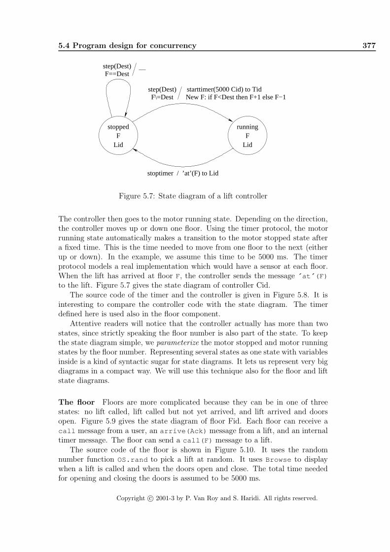
5.4 Program design for concurrency 377
F\=Dest
stopped running
LidFF
step(Dest)F==Dest
Lid
stoptimer / ’at’(F) to Lid
starttimer(5000 Cid) to TidNew F: if F<Dest then F+1 else F−1
step(Dest)
Figure 5.7: State diagram of a lift controller
The controller then goes to the motor running state. Depending on the direction,the controller moves up or down one floor. Using the timer protocol, the motorrunning state automatically makes a transition to the motor stopped state aftera fixed time. This is the time needed to move from one floor to the next (eitherup or down). In the example, we assume this time to be 5000 ms. The timerprotocol models a real implementation which would have a sensor at each floor.When the lift has arrived at floor F, the controller sends the message ´ at ´ (F)
to the lift. Figure 5.7 gives the state diagram of controller Cid.The source code of the timer and the controller is given in Figure 5.8. It is
interesting to compare the controller code with the state diagram. The timerdefined here is used also in the floor component.
Attentive readers will notice that the controller actually has more than twostates, since strictly speaking the floor number is also part of the state. To keepthe state diagram simple, we parameterize the motor stopped and motor runningstates by the floor number. Representing several states as one state with variablesinside is a kind of syntactic sugar for state diagrams. It lets us represent very bigdiagrams in a compact way. We will use this technique also for the floor and liftstate diagrams.
The floor Floors are more complicated because they can be in one of threestates: no lift called, lift called but not yet arrived, and lift arrived and doorsopen. Figure 5.9 gives the state diagram of floor Fid. Each floor can receive acall message from a user, an arrive(Ack) message from a lift, and an internaltimer message. The floor can send a call(F) message to a lift.
The source code of the floor is shown in Figure 5.10. It uses the randomnumber function OS.rand to pick a lift at random. It uses Browse to displaywhen a lift is called and when the doors open and close. The total time neededfor opening and closing the doors is assumed to be 5000 ms.
Copyright c© 2001-3 by P. Van Roy and S. Haridi. All rights reserved.

378 Message-Passing Concurrency
fun {Timer}{NewPortObject2
proc {$ Msg}case Msg of starttimer(T Pid) then
thread {Delay T} {Send Pid stoptimer} endend
end }end
fun {Controller Init}Tid={Timer}Cid={NewPortObject Init
fun {$ Msg state(Motor F Lid)}case Motorof running then
case Msgof stoptimer then
{Send Lid ´ at ´ (F)}state(stopped F Lid)
end[] stopped then
case Msgof step(Dest) then
if F==Dest thenstate(stopped F Lid)
elseif F<Dest then{Send Tid starttimer(5000 Cid)}state(running F+1 Lid)
else % F>Dest{Send Tid starttimer(5000 Cid)}state(running F-1 Lid)
endend
endend }
in Cid end
Figure 5.8: Implementation of the timer and controller components
Copyright c© 2001-3 by P. Van Roy and S. Haridi. All rights reserved.

5.4 Program design for concurrency 379
stoptimer /
notcalled called
doorsopen(Ack) arrive(Ack) /starttimer(5000 Fid) to Tid
arrive(Ack) /
call / call(F) to random Lid
call / −
arrive(A) / A=Ack
call / −
starttimer(5000 Fid) to Tid
Ack=unit
Figure 5.9: State diagram of a floor
The lift Lifts are the most complicated of all. Figure 5.11 gives the statediagram of lift Lid. Each lift can be in one of four states: empty schedule andlift stopped (idle), nonempty schedule and lift moving past a given floor, waitingfor doors when moving past a scheduled floor, and waiting for doors when idleat a called floor. The way to understand this figure is to trace through someexecution scenarios. For example, here is a simple scenario. A user presses thecall button at floor 1. The floor then sends call(1) to a lift. The lift receivesthis and sends step(1) to the controller. Say the lift is currently at floor 3. Thecontroller sends ´ at ´ (2) to the lift, which then sends step(1) to the controlleragain. The controller sends ´ at ´ (1) to the lift, which then sends arrive(Ack)
to floor 1 and waits until the floor acknowledges that it can leave.Each lift can receive a call(N) message and an ´ at ´ (N) message. The lift
can send an arrive(Ack) message to a floor and a step(Dest) message toits controller. After sending the arrive(Ack) message, the lift waits until thefloor acknowledges that the door actions have finished. The acknowledgement isdone by using the dataflow variable Ack as a one-shot wire. The floor sends anacknowledgement by binding Ack= unit and the lift waits with {Wait Ack} .
The source code of the lift component is shown in Figure 5.12. It uses a seriesof if statements to implement the conditions for the different transitions. It usesBrowse to display when a lift will go to a called floor and when the lift arrivesat a called floor. The function {ScheduleLast L N} implements the scheduler:it adds N to the end of the schedule L and returns the new schedule.
The building We have now specified the complete system. It is instructive totrace through the execution by hand, following the flow of control in the floors,lifts, controllers, and timers. For example, say that there are 10 floors and 2 lifts.Both lifts are on floor 1 and floors 9 and 10 each call a lift. What are the possibleexecutions of the system? Let us define a compound component that creates abuilding with FN floors and LN lifts:
Copyright c© 2001-3 by P. Van Roy and S. Haridi. All rights reserved.

380 Message-Passing Concurrency
fun {Floor Num Init Lifts}Tid={Timer}Fid={NewPortObject Init
fun {$ Msg state(Called)}case Calledof notcalled then Lran in
case Msgof arrive(Ack) then
{Browse ´ Lift at floor ´ #Num# : open doors ´ }{Send Tid starttimer(5000 Fid)}state(doorsopen(Ack))
[] call then{Browse ´ Floor ´ #Num# calls a lift! ´ }Lran=Lifts.(1+{OS.rand} mod {Width Lifts}){Send Lran call(Num)}state(called)
end[] called then
case Msgof arrive(Ack) then
{Browse ´ Lift at floor ´ #Num# : open doors ´ }{Send Tid starttimer(5000 Fid)}state(doorsopen(Ack))
[] call thenstate(called)
end[] doorsopen(Ack) then
case Msgof stoptimer then
{Browse ´ Lift at floor ´ #Num# : close doors ´ }Ack= unitstate(notcalled)
[] arrive(A) thenA=Ackstate(doorsopen(Ack))
[] call thenstate(doorsopen(Ack))
endend
end }in Fid end
Figure 5.10: Implementation of the floor component
Copyright c© 2001-3 by P. Van Roy and S. Haridi. All rights reserved.

5.4 Program design for concurrency 381
New Pos: NPos
call(N) & N==Pos
Pos
Sched/=nil
Moving=true
Wait
doorsfor
call(N) &N/=Pos
New Sched: [N]
Sched=nil
Moving=false
Pos
Wait
doorsfor
call(N)
arrive(Ack) to Pos
{Wait Ack} & Sched.2==nil
New Sched: {ScheduleLast Sched N}
at(NPos) & NPos==Sched.1arrive(Ack) to Sched.1
{Wait Ack} / −
{Wait Ack} & Sched.2/=nil
step(Sched.2.1) to CidNew Pos: NPos
New Sched: Sched.2
step(N) to Cid
New Pos: NPos
at(NPos) & NPos/=Sched.1step(Sched.1) to Cid
Figure 5.11: State diagram of a lift
proc {Building FN LN ?Floors ?Lifts}Lifts={MakeTuple lifts LN}for I in 1..LN do Cid in
Cid={Controller state(stopped 1 Lifts.I)}Lifts.I={Lift I state(1 nil false ) Cid Floors}
endFloors={MakeTuple floors FN}for I in 1..FN do
Floors.I={Floor I state(notcalled) Lifts}end
end
This uses MakeTuple to create a new tuple containing unbound variables. Eachcomponent instance will run in its own thread. Here is a sample execution:
declare F L in{Building 2 0 2 F L}{Send F.20 call}{Send F.4 call}{Send F.10 call}{Send L.1 call(4)}
This makes the lifts move around in a building with 20 floors and 2 lifts.
Reasoning about the lift control system To show that the lift works cor-rectly, we can reason about its invariant properties. For example, an ´ at ´ (_)
message can only be received when Sched\=nil . This is a simple invariant thatcan be proved easily from the fact that ´ at ´ and step messages occur in pairs.It is easy to see by inspection that a step message is always done when the liftgoes into a state where Sched\=nil , and that the only transition out of this
Copyright c© 2001-3 by P. Van Roy and S. Haridi. All rights reserved.

382 Message-Passing Concurrency
fun {ScheduleLast L N}if L\=nil andthen {List.last L}==N then Lelse {Append L [N]} end
end
fun {Lift Num Init Cid Floors}{NewPortObject Init
fun {$ Msg state(Pos Sched Moving)}case Msgof call(N) then
{Browse ´ Lift ´ #Num# needed at floor ´ #N}if N==Pos andthen {Not Moving} then
{Wait {Send Floors.Pos arrive($)}}state(Pos Sched false )
else Sched2 inSched2={ScheduleLast Sched N}if {Not Moving} then
{Send Cid step(N)} endstate(Pos Sched2 true )
end[] ´ at ´ (NewPos) then
{Browse ´ Lift ´ #Num# at floor ´ #NewPos}case Schedof S|Sched2 then
if NewPos==S then{Wait {Send Floors.S arrive($)}}if Sched2==nil then
state(NewPos nil false )else
{Send Cid step(Sched2.1)}state(NewPos Sched2 true )
endelse
{Send Cid step(S)}state(NewPos Sched Moving)
endend
endend }
end
Figure 5.12: Implementation of the lift component
Copyright c© 2001-3 by P. Van Roy and S. Haridi. All rights reserved.

5.4 Program design for concurrency 383
Controller C
User
at(F)
step(D)arrive(Ack)
call(F)
User
call
Ack=unit
call(F)
LiftShaft
Floor F Lift L
Figure 5.13: Hierarchical component diagram of the lift control system
state (triggered by a call message) preserves the invariant. Another invariant isthat successive elements of a schedule are always different (can you prove this?).
5.4.5 Improvements to the lift control system
The lift control system of the previous section is somewhat naive. In this sectionwe will indicate five ways in which it can be improved: by using componentcomposition to make it hierarchical, by improving how it opens and closes doors,by using negotiation to find the best lift to call, by improving scheduling to reducethe amount of lift motion, and by handling faults (lifts that stop working). Weleave the last three improvements as exercises for the reader.
Hierarchical organization
Looking at the component diagram of Figure 5.5, we see that each controller talksonly with its corresponding lift. This is visible also in the definition of Building .This means that we can improve the organization by combining controller andlift into a compound component, which we call a lift shaft. Figure 5.13 shows theupdated component diagram with a lift shaft. We implement this by defining thecomponent LiftShaft as follows:
fun {LiftShaft I state(F S M) Floors}Cid={Controller state(stopped F Lid)}Lid={Lift I state(F S M) Cid Floors}
in Lid end
Then the Building procedure can be simplified:
proc {Building FN LN ?Floors ?Lifts}Lifts={MakeTuple lifts LN}for I in 1..LN do Cid in
Lifts.I={LiftShaft I state(1 nil false ) Floors}endFloors={MakeTuple floors FN}
Copyright c© 2001-3 by P. Van Roy and S. Haridi. All rights reserved.

384 Message-Passing Concurrency
for I in 1..FN doFloors.I={Floor I state(notcalled) Lifts}
endend
The encapsulation provided by LiftShaft improves the modularity of the pro-gram. We can change the internal organization of a lift shaft without changingits interface.
Improved door management
Our system opens all doors at a floor when the first lift arrives and closes thema fixed time later. So what happens if a lift arrives at a floor when the doorsare already open? The doors may be just about to close. This behavior isunacceptable for a real lift. We need to improve our lift control system so thateach lift has its own set of doors.
Improved negotiation
We can improve our lift control system so that the floor picks the closest liftinstead of a random lift. The idea is for the floor to send messages to all liftsasking them to give an estimate of the time it would take to reach the floor. Thefloor can then pick the lift with the least time. This is an example of a simplenegotiation protocol.
Improved scheduling
We can improve the lift scheduling. For example, assume the lift is moving fromfloor 1 to floor 5 and is currently at floor 2. Calling floor 3 should cause the liftto stop on its way up, instead of the naive solution where it first goes to floor 5and then down to floor 3. The improved algorithm moves in one direction untilthere are no more floors to stop at and then changes direction. Variations on thisalgorithm, which is called the elevator algorithm for obvious reasons, are used toschedule the head movement of a hard disk. With this scheduler we can have twocall buttons to call upgoing and downgoing lifts separately.
Fault tolerance
What happens if part of the system stops working? For example, a lift can be outof order, either because of maintenance, because it has broken down, or simplybecause someone is blocking open the doors at a particular floor. Floors can alsobe “out of order”, e.g., a lift may be forbidden to stop at a floor for some reason.We can extend the lift control system to handle these cases. The basic ideas areexplained in the Exercises.
Copyright c© 2001-3 by P. Van Roy and S. Haridi. All rights reserved.

5.5 Using the message-passing concurrent model directly 385
5.5 Using the message-passing concurrent mod-
el directly
The message-passing model can be used in other ways rather than just program-ming with port objects. One way is to program directly with threads, procedures,ports, and dataflow variables. Another way is to use other abstractions. Thissection gives some examples.
5.5.1 Port objects that share one thread
It is possible to run many port objects on just one thread, if the thread serializesall their messages. This can be more efficient than using one thread per portobject. According to David Wood of Symbian Ltd., this solution was used in theoperating system of the Psion Series 3 palmtop computers, where memory is at apremium [210]. Execution is efficient since no thread scheduling has to be done.Objects can access shared data without any particular precautions since all theobjects run in the same thread. The main disadvantage is that synchronization isharder. Execution cannot wait inside an object for a calculation done in anotherobject. Attempting this will block the program. This means that programs mustbe written in a particular style. State must be either global or stored in themessage arguments, not in the objects. Messages are a kind of continuation, i.e.,there is no return. Each object execution finishes by sending a message.
Figure 5.14 defines the abstraction NewPortObjects . It sets up the singlethread and returns two procedures, AddPortObject and Call :
• {AddPortObject PO Proc} adds a new port object with name POto thethread. The name should be a literal or a number. Any number of newport objects can be added to the thread.
• {Call PO Msg} asynchronously sends the message Msg to the port objectPO. All message executions of all port objects are executed in the singlethread. Exceptions raised during message execution are simply ignored.
Note that the abstraction stores the port objects’ procedures in a record and usesAdjoinAt to extend this record when a new port object is added.
Figure 5.15 gives a screenshot of a small concurrent program, ‘Ping-Pong’,which uses port objects that share one thread. Figure 5.16 gives the full sourcecode of ‘Ping-Pong’. It uses NewProgWindow , the simple progress monitor definedin Chapter 10. Two objects are created initially, pingobj and pongobj . Eachobject understands two messages, ping(N) and pong(N) . The pingobj objectasynchronously sends a pong(N) message to the pongobj object and vice versa.Each message executes by displaying a text and then continuing execution bysending a message to the other object. The integer argument N counts messagesby being incremented at each call. Execution is started with the initial call {Call
pingobj ping(0)} .
Copyright c© 2001-3 by P. Van Roy and S. Haridi. All rights reserved.

386 Message-Passing Concurrency
proc {NewPortObjects ?AddPortObject ?Call}Sin P={NewPort Sin}
proc {MsgLoop S1 Procs}case S1of msg(I M)|S2 then
try {Procs.I M} catch _ then skip end{MsgLoop S2 Procs}
[] add(I Proc Sync)|S2 then Procs2 inProcs2={AdjoinAt Procs I Proc}Sync= unit{MsgLoop S2 Procs2}
[] nil then skip endend
inproc {AddPortObject I Proc}Sync in
{Send P add(I Proc Sync)}{Wait Sync}
end
proc {Call I M}{Send P msg(I M)}
end
thread {MsgLoop Sin procs} endend
Figure 5.14: Defining port objects that share one thread
Figure 5.15: Screenshot of the ‘Ping-Pong’ program
Copyright c© 2001-3 by P. Van Roy and S. Haridi. All rights reserved.

5.5 Using the message-passing concurrent model directly 387
declare AddPortObject Call{NewPortObjects AddPortObject Call}
InfoMsg={NewProgWindow "See ping-pong"}
fun {PingPongProc Other}proc {$ Msg}
case Msgof ping(N) then
{InfoMsg "ping("#N#")"}{Call Other pong(N+1)}
[] pong(N) then{InfoMsg "pong("#N#")"}{Call Other ping(N+1)}
endend
end
{AddPortObject pingobj {PingPongProc pongobj}}{AddPortObject pongobj {PingPongProc pingobj}}{Call pingobj ping(0)}
Figure 5.16: The ‘Ping-Pong’ program: using port objects that share one thread
When the program starts, it creates a window that displays a term of theform ping(123) or pong(123) , where the integer gives the message count. Thismonitors execution progress. When the checkbutton is enabled, then each termis displayed for 50 ms. When the checkbutton is disabled, then the messages arepassed internally at a much faster rate, limited only by the speed of the Mozartrun-time system.4
5.5.2 A concurrent queue with ports
The program shown in Figure 5.17 defines a thread that acts as a FIFO queue.The function NewQueuereturns a new queue Q, which is a record queue(put:PutProc
get:GetProc) that contains two procedures, one for inserting an element in thequeue and one for fetching an element from the queue. The queue is implement-ed with two ports. The use of dataflow variables makes the queue insensitive tothe relative arrival order of Q.get and Q.put requests. For example, the Q.get
requests can arrive even when the queue is empty. To insert an element X, call{Q.put X} . To fetch an element in Y, call {Q.get Y} .
The program in Figure 5.17 is almost correct, but it does not work becauseport streams are read-only variables. To see this, try the following sequence of
4With Mozart 1.3.0 on a 1 GHz PowerPC processor (PowerBook G4), the rate is about300000 asynchronous method calls per second.
Copyright c© 2001-3 by P. Van Roy and S. Haridi. All rights reserved.

388 Message-Passing Concurrency
fun {NewQueue}Given GivePort={NewPort Given}Taken TakePort={NewPort Taken}
inGiven=Takenqueue(put: proc {$ X} {Send GivePort X} end
get: proc {$ X} {Send TakePort X} end )end
Figure 5.17: Queue (naive version with ports)
statements:
declare Q inthread Q={NewQueue} end{Q.put 1}{Browse {Q.get $}}{Browse {Q.get $}}{Browse {Q.get $}}{Q.put 2}{Q.put 3}
The problem is that Given=Taken tries to impose equality between two read-only variables, i.e., bind them. But a read-only variable can only be read andnot bound. So the thread defining the queue will suspend in the statementGiven=Taken . We can fix the problem by defining a procedure Match and run-ning it in its own thread, as shown in Figure 5.18. You can verify that the abovesequence of statements now works.
Let us look closer to see why the correct version works. Doing a series of putoperations:
{Q.put I0} {Q.put I1} ... {Q.put In}
incrementally adds the elements I0 , I1 , ..., In , to the stream Given , resultingin:
I0|I1|...|In|F1
where F1 is a read-only variable. In the same way, doing a series of get operations:
{Q.get X0} {Q.get X1} ... {Q.get Xn}
adds the elements X0, X1, ..., Xn to the stream Taken , resulting in:
X0|X1|...|Xn|F2
where F2 is another read-only variable. The call {Match Given Taken} bindsthe Xi ’s to Ii ’s and blocks again for F1=F2.
This concurrent queue is completely symmetric with respect to inserting andretrieving elements. That is, Q.put and Q.get are defined in exactly the sameway. Furthermore, because they use dataflow variables to reference queue ele-ments, these operations never block. This gives the queue the remarkable prop-
Copyright c© 2001-3 by P. Van Roy and S. Haridi. All rights reserved.

5.5 Using the message-passing concurrent model directly 389
fun {NewQueue}Given GivePort={NewPort Given}Taken TakePort={NewPort Taken}proc {Match Xs Ys}
case Xs # Ysof (X|Xr) # (Y|Yr) then
X=Y {Match Xr Yr}[] nil # nil then skipend
endin
thread {Match Given Taken} endqueue(put: proc {$ X} {Send GivePort X} end
get: proc {$ X} {Send TakePort X} end )end
Figure 5.18: Queue (correct version with ports)
erty that it can be used to insert and retrieve elements before the elements areknown. For example, if you do a {Q.get X} when there are no elements in thequeue, then an unbound variable is returned in X. The next element that is in-serted will be bound to X. To do a blocking retrieval, i.e., one that waits whenthere are no elements in the queue, the call to Q.get should be followed by aWait :
{Q.get X}{Wait X}
Similarly, if you do {Q.put X} when X is unbound, i.e., when there is no elementto insert, then the unbound variable X will be put in the queue. Binding X willmake the element known. To do an insert only when the element is known, thecall to Q.put should be preceded by a Wait :
{Wait X}{Q.put X}
We have captured the essential asymmetry between put and get: it is in the Wait
operation. Another way to see this is that put and get reserve places in the queue.The reservation can be done independent of whether the values of the elementsare known or not.
Attentive readers will see that there is an even simpler solution to the problemof Figure 5.17. The procedure Match is not really necessary. It is enough to runGiven=Taken in its own thread. This is because the unification algorithm doesexactly what Match does.5
5This FIFO queue design was first given by Denys Duchier.
Copyright c© 2001-3 by P. Van Roy and S. Haridi. All rights reserved.

390 Message-Passing Concurrency
5.5.3 A thread abstraction with termination detection“Ladies and gentlemen, we will be arriving shortly in Brussels Midistation, where this train terminates.”– Announcement, Thalys high-speed train, Paris-Brussels line, Jan-uary 2002
Thread creation with thread 〈stmt〉 end can itself create new threads duringthe execution of 〈stmt〉. We would like to detect when all these new threadshave terminated. This does not seem easy: new threads may themselves createnew threads, and so forth. A termination detection algorithm like the one ofSection 4.4.3 is needed. The algorithm of that section requires explicitly passingvariables between threads. We require a solution that is encapsulated, i.e., it doesnot have this awkwardness. To be precise, we require a procedure NewThread
with the following properties:
• The call {NewThread P SubThread} creates a new thread that executesthe zero-argument procedure P. It also returns a one-argument procedureSubThread .
• During the execution of P, new threads can be created by calling {SubThread
P1} , where the zero-argument procedure P1 is the thread body. We callthese subthreads. SubThread can be called recursively, that is, insidethreads created with SubThread .
• The NewThread call returns after the new thread and all subthreads haveterminated.
That is, there are three ways to create a new thread:
thread 〈stmt〉 end
{NewThread proc {$} 〈stmt〉 end SubThread}
{SubThread proc {$} 〈stmt〉 end }
They have identical behavior except for NewThread , which has a different termi-nation behavior. NewThread can be defined using the message-passing model asshown in Figure 5.19. This definition uses a port. When a subthread is created,then 1 is sent to the port. When a subthread terminates, then −1 is sent. Theprocedure ZeroExit accumulates a running total of these numbers. If the totalever reaches zero, then all subthreads have terminated and ZeroExit returns.
We can prove that this definition is correct by using invariant assertions.Consider the following assertion: “the sum of the elements on the port’s stream isgreater than or equal to the number of active threads.” When the sum is zero, thisimplies that the number of active threads is zero as well. We can use induction toshow that the assertion is true at every part of every possible execution, startingfrom the call to NewThread . It is clearly true when Newthread starts since bothnumbers are zero. During an execution, there are four relevant actions: sending
Copyright c© 2001-3 by P. Van Roy and S. Haridi. All rights reserved.

5.5 Using the message-passing concurrent model directly 391
localproc {ZeroExit N Is}
case Is of I|Ir thenif N+I\=0 then {ZeroExit N+I Ir} end
endend
inproc {NewThread P ?SubThread}
Is Pt={NewPort Is}in
proc {SubThread P}{Send Pt 1}thread
{P} {Send Pt ˜1}end
end{SubThread P}{ZeroExit 0 Is}
endend
Figure 5.19: A thread abstraction with termination detection
+1, sending -1, starting a thread, and terminating a thread. By inspection of theprogram, each of these actions keeps the assertion true. (We can assume withoutloss of generality that thread termination occurs just before sending -1, since thethread then no longer executes any part of the user program.)
This definition of NewThread has two restrictions. First, P and P1 shouldalways call SubThread to create subthreads, never any other operation (suchas thread ... end or a SubThread created elsewhere). Second, SubThread
should not be called anywhere else in the program. The definition can be extendedto relax these restrictions or to check them. We leave these tasks as exercises forthe reader.
An issue about port send semantics
We know that the Send operation is asynchronous, that is, it completes imme-diately. The termination detection algorithm relies on another property of Send:that {Send Pt 1} (in the parent thread) arrives before {Send Pt ˜1} (in thechild thread). Can we assume that sends in different threads behave in this way?Yes we can, if we are sure the Send operation reserves a slot in the port stream.Look back to the semantics we have defined for ports in the beginning of thechapter: the Send operation does indeed put its argument in the port stream.
Copyright c© 2001-3 by P. Van Roy and S. Haridi. All rights reserved.

392 Message-Passing Concurrency
proc {ConcFilter L F ?L2}Send Close
in{NewPortClose L2 Send Close}{Barrier
{Map Lfun {$ X}
proc {$}if {F X} then {Send X} end
endend }}
{Close}end
Figure 5.20: A concurrent filter without sequential dependencies
We call this the slot-reserving semantics of Send.6
Unfortunately, this semantics is not the right one in general. We really wantan eventual slot-reserving semantics, where the Send operation might not imme-diately reserve a slot but we are sure that it will eventually. Why is this semantics“right”? It is because it is the natural behavior of a distributed system, wherea program is spread out over more than one process and processes can be ondifferent machines. A Send can execute on a different process than where theport stream is constructed. Doing a Send does not immediately reserve a slotbecause the slot might be on a different machine (remember that the Send shouldcomplete immediately)! All we can say is that doing a Send will eventually reservea slot.
With the “right” semantics for Send, our termination detection algorithm isincorrect since {Send Pt ˜1} might arrive before {Send Pt 1} . We can fix theproblem by defining a slot-reserving port in terms of an eventual slot-reservingport:
proc {NewSPort ?S ?SSend}S1 P={NewPort S1} in
proc {SSend M} X in {Send P M#X} {Wait X} endthread S={Map S1 fun {$ M#X} X= unit M end } end
end
NewSPort behaves like NewPort . If NewPort defines an eventual slot-reservingport, then NewSPort will define a slot-reserving port. Using NewSPort in thetermination detection algorithm will ensure that it is correct in case we use the“right” port semantics.
6This is sometimes called a synchronous Send, because it only completes when the messageis delivered to the stream. We will avoid this term because the concept of “delivery” is notclear. For example, we might want to talk about delivering a message to an application processinstead of a stream.
Copyright c© 2001-3 by P. Van Roy and S. Haridi. All rights reserved.

5.5 Using the message-passing concurrent model directly 393
5.5.4 Eliminating sequential dependencies
Let us examine how to remove useless sequential dependencies between differentparts of a program. We take as example the procedure {Filter L F L2} , whichtakes a list L and a one-argument boolean function F. It outputs a list L2 thatcontains the elements X of L for which {F X} is true. This is a library function(it is part of the List module) that can be defined declaratively as follows:
fun {Filter L F}case Lof nil then nil[] X|L2 then
if {F X} then X|{Filter L2 F} else {Filter L2 F} endend
end
or equivalently, using the loop syntax:
fun {Filter L F}for X in L collect:C do
if {F X} then {C X} endend
end
This definition is efficient, but it introduces sequential dependencies: {F X} canbe calculated only after it has been calculated for all elements of L before X. Thesedependencies are introduced because all calculations are done sequentially in thesame thread. But these dependencies are not really necessary. For example, inthe call:
{Filter [ A 5 1 B 4 0 6] fun {$ X} X>2 end Out}
it is possible to deduce immediately that 5, 4, and 6 will be in the output, withoutwaiting for A and B to be bound. Later on, if some other thread does A=10, then10 could be added to the result immediately.
We can write a new version of Filter that avoids these dependencies. Itconstructs its output incrementally, as the input information arrives. We use twobuilding blocks:
• Concurrent composition (see Section 4.4.3). The procedure Barrier im-plements concurrent composition: it creates a concurrent task for each listelement and waits until all are finished.
• Asynchronous channels (ports, see earlier in this chapter). The procedureNewPortClose implements a port with a send and a close operation. Itsdefinition is given in the supplements file on the book’s Web site. The closeoperation terminates the port’s stream with nil .
Figure 5.20 gives the definition. It first creates a port whose stream is the outputlist. Then Barrier is called with a list of procedures, each of which adds X to
Copyright c© 2001-3 by P. Van Roy and S. Haridi. All rights reserved.

394 Message-Passing Concurrency
the output list if {F X} is true. Finally, when all list elements are taken care of,the output list is ended by closing the port.
Is ConcFilter declarative? As it is written, certainly not, since the outputlist can appear in any order (an observable nondeterminism). It can be madedeclarative by hiding this nondeterminism, for example by sorting the outputlist. There is another way, using the properties of ADTs. If the rest of theprogram does not depend on the order (e.g., the list is a representation of a setdata structure), then ConcFilter can be treated as if it were declarative. Thisis easy to see: if the list were in fact hidden inside a set ADT, then ConcFilter
would be deterministic and hence declarative.
5.6 The Erlang language
The Erlang language was developed by Ericsson for telecommunications applica-tions, in particular, for telephony [9, 206]. Its implementation, the Ericsson OTP(Open Telecom Platform), features fine-grained concurrency (efficient threads),extreme reliability (high performance software fault tolerance), and hot code re-placement ability (update software while the system is running). It is a high-levellanguage that hides the internal representation of data and does automatic mem-ory management. It has been used successfully in several Ericsson products.
5.6.1 Computation model
The Erlang computation model has an elegant layered structure. We first ex-plain the model and then we show how it is extended for distribution and faulttolerance.
The Erlang computation model consists of entities called processes, similar toport objects, that communicate through message passing. The language can bedivided into two layers:
• Functional core. Port objects are programmed in a dynamically-typedstrict functional language. Each port object contains one thread that runsa recursive function whose arguments are the thread’s state. Functions canbe passed in messages.
• Message passing extension. Threads communicate by sending messagesto other threads asynchronously in FIFO order. Each thread has a uniqueidentifier, its PID, which is a constant that identifies the receiving thread,but can also be embedded in data structures and messages. Messages arevalues in the functional core. They are put in the receiving thread’s mailbox.Receiving can be blocking or nonblocking. The receiving thread uses patternmatching to wait for and then remove messages that have a given formfrom its mailbox, without disturbing the other messages. This means thatmessages are not necessarily treated in the order that they are sent.
Copyright c© 2001-3 by P. Van Roy and S. Haridi. All rights reserved.

5.6 The Erlang language 395
A port object in Erlang consists of a thread associated with one mailbox. Thisis called a process in Erlang terminology. A process that spawns a new processspecifies which function should be initially executed inside it.
Extensions for distribution and fault tolerance
The centralized model is extended for distribution and fault tolerance:
• Transparent distribution. Processes can be on the same machine oron different machines. A single machine environment is called a node inErlang terminology. In a program, communication between local or remoteprocesses is written in exactly the same way. The PID encapsulates thedestination and allows the run-time system to decide whether to do a local orremote operation. Processes are stationary; this means that once a processis created in a node it remains there for its entire lifetime. Sending amessage to a remote process requires exactly one network operation, i.e.,no intermediate nodes are involved. Processes can also be created at remotenodes. Programs are network transparent, i.e., they give the same resultno matter on which nodes the processes are placed. Programs are networkaware since the programmer has complete control of process placement andcan optimize it according to the network characteristics.
• Failure detection. A process can be set up to detect faults in another pro-cess. In Erlang terminology this is called linking the two processes. Whenthe second process fails, a message is sent to the first, which can receive it.This failure detection ability allows many fault-tolerance mechanisms to beprogrammed entirely in Erlang.
• Persistence. The Erlang run-time system comes with a database, calledMnesia, that helps to build highly available applications.
We can summarize by saying that Erlang’s computation model (port objectswithout mutable state) is strongly optimized for building fault-tolerant distribut-ed systems. The Mnesia database compensates for the lack of a general mutablestore. A typical example of a product built using Erlang is Ericsson’s AXD301ATM switch, which provides telephony over an ATM network. The AXD301handles 30-40 million calls per week with a reliability of 99.9999999% (about 30ms downtime per year) and contains 1.7 million lines of Erlang [8].
5.6.2 Introduction to Erlang programming
To give a taste of Erlang, we give some small Erlang programs and show howto do the same thing in the computation models of this book. The programsare mostly taken from the Erlang book [9]. We show how to write functionsand concurrent programs with message passing. For more information on Erlangprogramming, we highly recommend the Erlang book.
Copyright c© 2001-3 by P. Van Roy and S. Haridi. All rights reserved.

396 Message-Passing Concurrency
A simple function
The core of Erlang is a strict functional language with dynamic typing. Here isa simple definition of the factorial function:
factorial(0) -> 1;
factorial(N) when N>0 -> N*factorial(N-1).
This example introduces the basic syntactic conventions of Erlang. Functionnames are in lowercase and variable identifiers are capitalized. Variable identifiersare bound to values when defined, which means that Erlang has a value store.An identifier’s binding cannot be changed; it is single assignment, just as in thedeclarative model. These conventions are inherited from Prolog, in which thefirst Erlang implementation (an interpreter) was written.
Erlang functions are defined by clauses; each clause has a head (with a patternand optional guard) and a body. The patterns are checked in order starting withthe first clause. If a pattern matches, its variables are bound and the clause bodyis executed. The optional guard is a boolean function that has to return true.All the variable identifiers in the pattern must be different. If a pattern does notmatch, then the next clause is tried. We can translate the factorial as follows inthe declarative model:
fun {Factorial N}case Nof 0 then 1[] N andthen N>0 then N*{Factorial N-1}end
end
The case statement does pattern matching exactly as in Erlang, with a differentsyntax.
Pattern matching with tuples
Here is a function that does pattern matching with tuples:
area({square, Side}) ->
Side*Side;
area({rectangle, X, Y}) ->
X*Y;
area({circle, Radius}) ->
3.14159*Radius*Radius;
area({triangle, A, B, C}) ->
S=(A+B+C)/2;
math:sqrt(S*(S-A)*(S-B)*(S-C)).
This uses the square root function sqrt defined in the module math. This functioncalculates the area of a plane shape. It represents the shape by means of a tuple
Copyright c© 2001-3 by P. Van Roy and S. Haridi. All rights reserved.

5.6 The Erlang language 397
that identifies the shape and gives its size. Tuples in Erlang are written with curlybraces: {square, Side} would be written as square(Side) in the declarativemodel. In the declarative model, the function can be written as follows:
fun {Area T}case Tof square(Side) then Side*Side[] rectangle(X Y) then X*Y[] circle(Radius) then 3.14159*Radius*Radius[] triangle(A B C) then S=(A+B+C)/2.0 in
{Sqrt S*(S-A)*(S-B)*(S-C)}end
end
Concurrency and message passing
In Erlang, threads are created together with a mailbox that can be used to sendmessages to the thread. This combination is called a process. There are threeprimitives:
• The spawn operation (written as spawn(M,F,A)) creates a new process andreturns a value (called “process identifier”) that can be used to send mes-sages to it. The arguments of spawn give the initial function call that startsthe process, identified by module M, function name F, and argument list A.
• The send operation (written as Pid!Msg) asynchronously sends the messageMsg to the process, which is identified by its process identifier Pid. Themessages are put in the mailbox, which is a kind of process queue.
• The receive operation receives a message from inside the process. It usespattern matching to pick a message from the mailbox.
Let us take the area function and put it inside a process. This makes it into aserver that can be called from any other process.
-module(areaserver).
-export([start/0, loop/0]).
start() -> spawn(areaserver, loop, []).
loop() ->
receive
{From, Shape} ->
From!area(Shape),
loop()
end.
Copyright c© 2001-3 by P. Van Roy and S. Haridi. All rights reserved.

398 Message-Passing Concurrency
This defines the two operations start and loop in the new module areaserver.These two operations are exported outside the module. We need to define themin a module because the spawn operation requires the module name as an ar-gument. The loop operation repeatedly reads a message (a two-argument tuple{From, Shape}) and responds to it by calling area and sending the reply to theprocess From. Now let us start a new server and call it:
Pid=areaserver:start(),
Pid!{self(), {square, 3.4}},
receive
Ans -> ...
end,
Here self() is a language operation that returns the process identifier of thecurrent process. This allows the server to return a reply. Let us write this in theconcurrent stateful model:
fun {Start}S AreaServer={NewPort S} in
threadfor msg(Ans Shape) in S do
Ans={Area Shape}end
endAreaServer
end
Let us again start a new server and call it:
Pid={Start}local Ans in
{Send Pid msg(Ans square(3.4))}{Wait Ans}...
end
This example uses the dataflow variable Ans to get the reply. This mimics thesend to From done by Erlang. To do exactly what Erlang does, we need totranslate the receive operation into a computation model of the book. This isa little more complicated. It is explained in the next section.
5.6.3 The receive operation
Much of the unique flavor and expressiveness of concurrent programming in Er-lang is due to the mailboxes and how they are managed. Messages are taken outof a mailbox with the receive operation. It uses pattern matching to pick outa desired message, leaving the other messages unchanged. Using receive givesparticularly compact, readable, and efficient code. In this section, we implement
Copyright c© 2001-3 by P. Van Roy and S. Haridi. All rights reserved.

5.6 The Erlang language 399
receive as a linguistic abstraction. We show how to translate it into the com-putation models of this book. There are two reasons for giving the translation.First, it gives a precise semantics for receive, which aids the understanding ofErlang. Second, it shows how to do Erlang-style programming in Oz.
Because of Erlang’s functional core, receive is an expression that returns avalue. The receive expression has the following general form [9]:
receive
Pattern1 [when Guard1] -> Body1;
...
PatternN [when GuardN] -> BodyN;
[ after Expr -> BodyT; ]
end
The guards (when clauses) and the time out (after clause) are optional. Thisexpression blocks until a message matching one of the patterns arrives in thecurrent thread’s mailbox. It then removes this message, binds the correspondingvariables in the pattern, and executes the body. Patterns are very similar to pat-terns in the case statement of this book: they introduce new single-assignmentvariables whose scope ranges over the corresponding body. For example, theErlang pattern {rectangle, [X,Y]} corresponds to the pattern rectangle([X
Y]) . Identifiers starting with lowercase letters correspond to atoms and identi-fiers starting with capital letters correspond to variables, like the notation of thisbook. Compound terms are enclosed in braces { and } and correspond to tuples.
The optional after clause defines a time out; if no matching message arrivesafter a number of milliseconds given by evaluating the expression Expr, then thetime-out body is executed. If zero milliseconds are specified, then the after
clause is executed immediately if there are no messages in the mailbox.
General remarks
Each Erlang process is translated into one thread with one port. Sending tothe process means sending to the port. This adds the message to the port’sstream, which represents the mailbox contents. All forms of receive, when theycomplete, either take exactly one message out of the mailbox or leave the mailboxunchanged. We model this by giving each translation of receive an input streamand an output stream. All translations have two arguments, Sin and Sout , thatreference the input stream and the output stream. These streams do not appearin the Erlang syntax. After executing a receive, there are two possibilities forthe value of the output stream. Either it is the same as the input stream or ithas one less message than the input stream. The latter occurs if the messagematches a pattern.
We distinguish three different forms of receive that result in different trans-lations. In each form the translation can be directly inserted in a program andit will behave like the respective receive. The first form is translated using the
Copyright c© 2001-3 by P. Van Roy and S. Haridi. All rights reserved.

400 Message-Passing Concurrency
T (receive ... end Sin Sout ) ≡local
fun {Loop S T#E Sout}case S of M|S1 then
case Mof T (Pattern1) then E=S1 T (Body1 T Sout )...[] T (PatternN) then E=S1 T (BodyN T Sout )else E1 in E=M|E1 {Loop S1 T#E1 Sout}end
endend T
in{Loop Sin T#T Sout}
end
Figure 5.21: Translation of receive without time out
declarative model. The second form has a time out; it uses the nondeterministicconcurrent model (see Section 8.2). The third form is a special case of the secondwhere the delay is zero, which makes the translation much simpler.
First form (without time out)
The first form of the receive expression is as follows:
receive
Pattern1 -> Body1;
...
PatternN -> BodyN;
end
The receive blocks until a message arrives that matches one of the patterns.The patterns are checked in order from Pattern1 to PatternN. We leave outthe guards to avoid cluttering up the code. Adding them is straightforward. Apattern can be any partial value; in particular an unbound variable will alwayscause a match. Messages that do not match are put in the output stream and donot cause the receive to complete.
Figure 5.21 gives the translation of the first form, which we will write asT (receive ... end Sin Sout ). The output stream contains the messages thatremain after the receive expression has removed the ones it needs. Note that thetranslation T (Body T Sout ) of a body that does not contain a receive expressionmust bind Sout=T .
The Loop function is used to manage out-of-order reception: if a message Misreceived that does not match any pattern, then it is put in the output stream and
Copyright c© 2001-3 by P. Van Roy and S. Haridi. All rights reserved.

5.6 The Erlang language 401
T (receive ... end Sin Sout ) ≡local
Cancel={Alarm T (Expr)}fun {Loop S T#E Sout}
if {WaitTwo S Cancel}==1 thencase S of M|S1 then
case Mof T (Pattern1) then E=S1 T (Body1 T Sout )...[] T (PatternN) then E=S1 T (BodyN T Sout )else E1 in E=M|E1 {Loop S1 T#E1 Sout} end
endelse E=S T (BodyT T Sout )
end Tin
{Loop Sin T#T Sout}end
Figure 5.22: Translation of receive with time out
Loop is called recursively. Loop uses a difference list to manage the case when areceive expression contains a receive expression.
Second form (with time out)
The second form of the receive expression is as follows:
receive
Pattern1 -> Body1;
...
PatternN -> BodyN;
after Expr -> BodyT;
end
When the receive is entered, Expr is evaluated first, giving the integer n. Ifno match is done after n milliseconds, then the time-out action is executed. If amatch is done before n milliseconds, then it is handled as if there were no timeout. Figure 5.22 gives the translation.
The translation uses a timer interrupt implemented by Alarm and WaitTwo .{Alarm N} , explained in Section 4.6, is guaranteed to wait for at least n mil-liseconds and then bind the unbound variable Cancel to unit . {WaitTwo S
Cancel} , which is defined in the supplements file on the book’s Web site, waitssimultaneously for one of two events: a message (S is bound) and a time out(Cancel is bound). It can return 1 if its first argument is bound and 2 if itssecond argument is bound.
Copyright c© 2001-3 by P. Van Roy and S. Haridi. All rights reserved.

402 Message-Passing Concurrency
T (receive ... end Sin Sout ) ≡if {IsDet Sin} then
case Sin of M|S1 thencase Mof T (Pattern1) then T (Body1 S1 Sout )...[] T (PatternN) then T (BodyN) S1 Sout )else T (BodyT Sin Sout ) end
endelse Sout=Sin end
Figure 5.23: Translation of receive with zero time out
The Erlang semantics is slightly more complicated than what is defined inFigure 5.22. It guarantees that the mailbox is checked at least once, even if thetime out is zero or has expired by the time the mailbox is checked. We canimplement this guarantee by stipulating that WaitTwo favors its first argument,i.e., that it always returns 1 if its first argument is determined. The Erlangsemantics also guarantees that the receive is exited quickly after the time outexpires. While this is easily guaranteed by an actual implementation, it is notguaranteed by Figure 5.22 since Loop could go on forever if messages arrivequicker than the loop iterates. We leave it to the reader to modify Figure 5.22 toadd this guarantee.
Third form (with zero time out)
The third form of the receive expression is like the second form except thatthe time-out delay is zero. With zero delay the receive is nonblocking. Asimpler translation is possible when compared to the case of nonzero time out.Figure 5.23 gives the translation. Using IsDet , it first checks whether there is amessage that matches any of the patterns. {IsDet S} , explained in Section 4.9.3,checks immediately whether S is bound or not and returns true or false . Ifthere is no message that matches (for example, if the mail box is empty) thenthe default action BodyT is done.
5.7 Advanced topics
5.7.1 The nondeterministic concurrent model
This section explains the nondeterministic concurrent model, which is intermedi-ate in expressiveness between the declarative concurrent model and the message-passing concurrent model. It is less expressive than the message-passing modelbut in return it has a logical semantics (see Chapter 9).
The nondeterministic concurrent model is the model used by concurrent logic
Copyright c© 2001-3 by P. Van Roy and S. Haridi. All rights reserved.

5.7 Advanced topics 403
〈s〉 ::=skip Empty statement| 〈s〉1 〈s〉2 Statement sequence| local 〈x〉 in 〈s〉 end Variable creation| 〈x〉1=〈x〉2 Variable-variable binding| 〈x〉=〈v〉 Value creation| if 〈x〉 then 〈s〉1 else 〈s〉2 end Conditional| case 〈x〉 of 〈pattern〉 then 〈s〉1 else 〈s〉2 end Pattern matching| { 〈x〉 〈y〉1 ... 〈y〉n} Procedure application| thread 〈s〉 end Thread creation| {WaitTwo 〈x〉 〈y〉 〈z〉} Nondeterministic choice
Table 5.2: The nondeterministic concurrent kernel language
programming [177]. It is sometimes called the process model of logic program-ming, since it models predicates as concurrent computations. It is interestingboth for historical reasons and for the insight it gives into practical concurrentprogramming. We first introduce the nondeterministic concurrent model andshow how it solves the stream communication problem of Section 4.7.3. We thenshow how to implement nondeterministic choice in the declarative concurrentmodel with exceptions, showing that the latter is at least as expressive as thenondeterministic model.
Table 5.2 gives the kernel language of the nondeterministic concurrent model.It adds just one operation to the declarative concurrent model: a nondeterministicchoice that waits for either of two events and nondeterministically returns whenone has happened with an indication of which one.
Limitation of the declarative concurrent model
In Section 4.7.3 we saw a fundamental limitation of the declarative concurrentmodel: stream objects must access input streams in a fixed pattern. Two streamscannot independently feed the same stream object. How can we solve this prob-lem? Consider the case of two client objects and a server object. We can tryto solve it by putting a new stream object, a stream merger, in between the twoclients and the server. The stream merger has two input streams and one outputstream. All the messages appearing on each of the input streams will be put onthe output stream. Figure 5.24 illustrates the solution. This seems to solve ourproblem: each client sends messages to the stream merger, and the stream mergerforwards them to the server. The stream merger is defined as follows:
fun {StreamMerger OutS1 OutS2}case OutS1#OutS2of (M|NewS1)#OutS2 then
M|{StreamMerger NewS1 OutS2}
Copyright c© 2001-3 by P. Van Roy and S. Haridi. All rights reserved.

404 Message-Passing Concurrency
Cli ent 1
Client 2
Server
OutS2
OutS1
InSStream
Merger
Figure 5.24: Connecting two clients using a stream merger
[] OutS1#(M|NewS2) thenM|{StreamMerger OutS1 NewS2}
[] nil#OutS2 thenOutS2
[] OutS1#nil thenOutS1
endend
The stream merger is executed in its own thread. This definition handles the caseof termination, i.e., when either or both clients terminate. Yet, this solution hasa basic difficulty: it does not work! Why not? Think carefully before reading theanswer in the footnote.7
Adding nondeterministic choice
But this abortive solution has the germs of a working solution. The problem isthat the case statement only waits on one condition at a time. A possible solutionis therefore to extend the declarative concurrent model with an operation thatallows to wait concurrently on more than one condition. We call this operationnondeterministic choice. One of the simplest ways is to add an operation thatwaits concurrently on two dataflow variables being bound. We call this operationWaitTwo because it generalizes Wait . The function call {WaitTwo A B} returnswhen either A or B is bound. It returns either 1 or 2. It can return 1 whenA is bound and 2 when B is bound. A simple Mozart definition is given inthe supplements file on the book’s Web site. The declarative concurrent modelextended with WaitTwo is called the nondeterministic concurrent model.
7It is because the case statement tests only one pattern at a time, and only goes to thenext when the previous ones fail. While it is waiting on stream OutS1 , it cannot accept aninput from stream OutS2 , and vice versa.
Copyright c© 2001-3 by P. Van Roy and S. Haridi. All rights reserved.

5.7 Advanced topics 405
Concurrent logic programming
The nondeterministic concurrent model is the basic model of concurrent logicprogramming, as pioneered by IC-Prolog, Parlog, Concurrent Prolog, FCP (FlatConcurrent Prolog), GHC (Guarded Horn Clauses), and Flat GHC [35, 36, 34,175, 176, 191]. It is the principal computation model that was used by theJapanese Fifth Generation Project and many other substantial projects in the1980’s [177, 57, 190]. In the nondeterministic concurrent model, it is possible towrite a stream merger. Its definition looks as follows:
fun {StreamMerger OutS1 OutS2}F={WaitTwo OutS1 OutS2}
incase F#OutS1#OutS2of 1#(M|NewS1)#OutS2 then
M|{StreamMerger OutS2 NewS1}[] 2#OutS1#(M|NewS2) then
M|{StreamMerger NewS2 OutS1}[] 1#nil#OutS2 then
OutS2[] 2#OutS1#nil then
OutS1end
end
This style of programming is exactly what concurrent logic programming does. Atypical syntax for this definition in a Prolog-like concurrent logic language wouldbe as follows:
streamMerger([M|NewS1], OutS2, InS) :- true |
InS=[M|NewS],
streamMerger(OutS2, NewS1, NewS).
streamMerger(OutS1, [M|NewS2], InS) :- true |
InS=[M|NewS],
streamMerger(NewS2, OutS1, NewS).
streamMerger([], OutS2, InS) :- true |
InS=OutS2.
streamMerger(OutS1, [], InS) :- true |
InS=OutS1.
This definition consists of four clauses, each of which defines one nondeterministicchoice. Keep in mind that syntactically Prolog uses [] for nil and [H|T] forH|T . Each clause consists of a guard and a body. The vertical bar | separatesthe guard from the body. A guard does only tests, blocking if a test cannot bedecided. A guard must be true for a clause to be choosable. The body is executedonly if the clause is chosen. The body can bind output variables.
The stream merger first calls WaitTwo to decide which stream to listen to.Only after WaitTwo returns does it enter the case statement. Because of the
Copyright c© 2001-3 by P. Van Roy and S. Haridi. All rights reserved.

406 Message-Passing Concurrency
argument F, alternatives that do not apply are skipped. Note that the recursivecalls reverse the two stream arguments. This helps guarantee fairness betweenboth streams in systems where the WaitTwo statement favors one or the other(which is often the case in an implementation). A message appearing on an inputstream will eventually appear on the output stream, independent of what happensin the other input stream.
Is it practical?
What can we say about practical programming in this model? Assume that newclients arrive during execution. Each client wants to communicate with the server.This means that a new stream merger must be created for each client! The finalresult is a tree of stream mergers feeding the server. Is this a practical solution?It has two problems:
• It is inefficient. Each stream merger executes in its own thread. The tree ofstream mergers is extended at run time each time a new object referencesthe server. Furthermore, the tree is not necessarily balanced. It would takeextra work to balance it.
• It lacks expressiveness. It is not possible to reference the server directly.For example, it is not possible to put a server reference in a data structure.The only way we have to reference the server is by referencing one of itsstreams. We can put this in a data structure, but only one client canuse this reference. (Remember that declarative data structures cannot bemodified.)
How can we solve these two problems? The first problem could hypotheticallybe solved by a very smart compiler that recognizes the tree of stream mergersand replaces it by a direct many-to-one communication in the implementation.However, after two decades of research in this area, such a compiler does notexist [190]. Some systems solve the problem in another way: by adding an ab-straction for multi-way merge whose implementation is done outside the model.This amounts to extending the model with ports. The second problem can bepartially solved (see Exercises), but the solution is still cumbersome.
We seem to have found an inherent limitation of the nondeterministic con-current model. Upon closer examination, the problem seems to be that there isno notion of explicit state in the model, where explicit state associates a namewith a store reference. Both the name and the store reference are immutable;only their association can be changed. There are many equivalent ways to intro-duce explicit state. One way is by adding the concept of cell, as will be shownin Chapter 6. Another way is by adding the concept of port, as we did in thischapter. Ports and cells are equivalent in a concurrent language: there are simpleimplementations of each in terms of the other.
Copyright c© 2001-3 by P. Van Roy and S. Haridi. All rights reserved.

5.8 Exercises 407
fun {WaitTwo A B}X in
thread {Wait A} try X=1 catch _ then skip end endthread {Wait B} try X=2 catch _ then skip end endX
end
Figure 5.25: Symmetric nondeterministic choice (using exceptions)
fun {WaitTwo A B}U in
thread {Wait A} U= unit endthread {Wait B} U= unit end{Wait U}if {IsDet A} then 1 else 2 end
end
Figure 5.26: Asymmetric nondeterministic choice (using IsDet )
Implementing nondeterministic choice
The WaitTwo operation can be defined in the declarative concurrent model ifexceptions are added.8 Figure 5.25 gives a simple definition. This returns 1 or 2,depending on whether A is bound or B is bound. This definition is symmetric; itdoes not favor either A or B. We can write an asymmetric version that favors A
by using IsDet , as shown in Figure 5.26.9
5.8 Exercises
1. Port objects that share one thread. Section 5.5.1 gives a small pro-gram, ‘Ping-Pong’, that has two port objects. Each object executes amethod and then asynchronously calls the other. When one initial messageis inserted into the system, this causes an infinite ping-pong of messages tobounce between the objects. What happens if two (or more) initial mes-sages are inserted? For example, what happens if these two initial calls aredone:
{Call Ping ping(0)}{Call Pong pong(10000000)}
8For practical use, however, we recommend the definition given in the supplements file onthe book’s Web site.
9Both definitions have the minor flaw that they can leave threads “hanging around” foreverif one variable is never bound. The definitions can be corrected to terminate any hangingthreads. We leave these corrections as exercises for the reader.
Copyright c© 2001-3 by P. Van Roy and S. Haridi. All rights reserved.

408 Message-Passing Concurrency
Messages will still ping-pong indefinitely, but how? Which messages will besent and how will the object executions be interleaved? Will the interleavingbe in lock-step (alternating between objects strictly), looser (subject tofluctuations due to thread scheduling), or something in between?
2. Lift control system. Section 5.4.4 gives the design of a simple lift controlsystem. Let us explore it:
• The current design has one controller object per lift. To economize oncosts, the developer decides to change this to keep just one controllerfor the whole system. Each lift then communicates with this controller.The controller’s internal definition stays the same. Is this a good idea?How does it change the behavior of the lift control system?
• In the current design, the controller steps up or down one floor at atime. It stops at all floors that it passes, even if the floor was notrequested. Change the lift and controller objects to avoid this jumpybehavior by stopping only at requested floors.
3. Fault tolerance for the lift control system. There are two kinds offaults that can happen: components can be blocked temporarily or theycan be permanently out of order. Let us see how to handle each case:
• A lift is blocked. Extend the system to continue working when a liftis temporarily blocked at a floor by a malicious user. First extend thefloor to reset the door timer when the floor is called while the doorsare open. Then the lift’s schedule should be given to other lifts and thefloors should no longer call that particular lift. When the lift worksagain, floors should again be able to call the lift. This can be donewith time-outs.
• A lift is out of order. The first step is to add generic primitives forfailure detection. We might need both synchronous and asynchronousdetection. In synchronous detection, when a component goes down, weassume that any message sent to it gets the immediate reply down(Id) ,where Id identifies the component. In asynchronous detection, we“link” a component to another when they are both still working. Then,when the second component crashes, the down message is sent to thefirst one immediately. Now extend the system to continue workingwhen a lift is out of order. The system should reconfigure itself tocontinue working for a building with one less lift.
• A floor is out of order. Extend the system to continue working when afloor is out of order. The system should reconfigure itself to continueworking for a building with one less floor.
• Lift maintenance. Extend the system so that a lift can be broughtdown for maintenance and brought back up again later.
Copyright c© 2001-3 by P. Van Roy and S. Haridi. All rights reserved.

5.8 Exercises 409
• Interactions. What happens if several floors and lifts become out oforder simultaneously? Does your system handle this properly?
4. Termination detection. Replace definition of SubThread in Section 5.5.3by:
proc {SubThread P}thread
{Send Pt 1} {P} {Send Pt ˜1}end
end
Explain why the result is not correct. Give an execution such that thereexists a point where the sum of the elements on the port’s stream is zero,yet all threads have not terminated.
5. Concurrent filter. Section 5.5.4 defines a concurrent version of Filter ,called ConcFilter , that calculates each output element independently, i.e.,without waiting for the previous ones to be calculated.
(a) What happens when the following is executed:
declare Out{ConcFilter [5 1 2 4 0] fun {$ X} X>2 end Out}{Show Out}
How many elements are displayed by the ShowWhat is the order of thedisplayed elements? If several displays are possible, give all of them.Is the execution of ConcFilter deterministic? Why or why not?
(b) What happens when the following is executed:
declare Out{ConcFilter [5 1 2 4 0] fun {$ X} X>2 end Out}{Delay 1000}{Show Out}
What is displayed now by Show? If several displays are possible, giveall of them.
(c) What happens when the following is executed:
declare Out A{ConcFilter [5 1 A 4 0] fun {$ X} X>2 end Out}{Delay 1000}{Show Out}
What is displayed now? What is the order of the displayed elements?If, after the above, A is bound to 3, then what happens to the list Out ?
(d) If the input list has n elements, what is the complexity (in “big-Oh”notation) of the number of operations of ConcFilter ? Discuss thedifference in execution time between Filter and ConcFilter .
Copyright c© 2001-3 by P. Van Roy and S. Haridi. All rights reserved.

410 Message-Passing Concurrency
6. Semantics of Erlang’s receive. Section 5.6.3 shows how to translateErlang’s receive operation. The second form of this operation, with timeout, is the most general one. Let us take a closer look.
(a) Verify that the second form reduces to the third form, when the timeout delay is zero.
(b) Verify that the second form reduces to the first form, when the timeout delay approaches infinity.
(c) Another way to translate the second form would be to insert a uniquemessage (using a name) after n milliseconds. This requires some care tokeep the unique message from appearing in the output stream. Writeanother translation of the third form that uses this technique. Whatare the advantages and disadvantages of this translation with respectto the one in the book?
7. Erlang’s receive as a control abstraction. For this exercise, implementthe Erlang receive operation, which is defined in Section 5.6.3, as thefollowing control abstraction:
• C={Mailbox.new} creates a new mailbox C.
• {Mailbox.send C M} sends message Mto mailbox C.
• {Mailbox.receive C [P1#E1 P2#E2 ... Pn#En] D} performs areceive on mailbox C. Pi is a one-argument boolean function fun {$
M} 〈expr〉 end that represents a pattern and its guard. The functionreturns true if and only if the pattern and guard succeed for messageM. Ei is a one-argument function fun {$ M} 〈expr〉 end that representsa body. It is executed when message M is received and the receivereturns its result. D represents the delay. It is either a nonnegativeinteger giving the delay in milliseconds or the atom infinity , whichrepresents an infinite delay.
8. Limitations of stream communication. In this exercise, we explore thelimits of stream communication in the nondeterministic concurrent model.Section 5.7.1 claims that we can partially solve the problem of putting serverreferences in a data structure. How far can we go? Consider the followingactive object:
declare NSthread {NameServer NS nil} end
where NameServer is defined as follows:
proc {NameServer NS L}case NSof register(A S)|NS1 then
Copyright c© 2001-3 by P. Van Roy and S. Haridi. All rights reserved.

5.8 Exercises 411
{NameServer NS1 A#S|L}[] getstream(A S)|NS1 then L1 OldS NewS in
L1={Replace L A OldS NewS}thread {StreamMerger S NewS OldS} end{NameServer NS1 L1}
[] nil thenskip
endend
fun {Replace InL A OldS NewS}case InLof B#S|L1 andthen A=B then
OldS=SA#NewS|L1
[] E|L1 thenE|{Replace L1 A OldS NewS}
endend
The NameServer object understands two commands. Assume that S is aserver’s input stream and foo is the name we wish to give the server. Givena reference NSto the name server’s input stream, doing NS=register(foo
S)|NS1 will add the pair foo#S to its internal list L. Doing NS=getstream(foo
S1)|NS1 will create a fresh input stream, S1, for the server whose name isfoo , which the name server has stored on its internal list L. Since foo is aconstant, we can put it in a data structure. Therefore, it seems that we canput server references in a data structure, by defining a name server. Is thisa practical solution? Why or why not? Think before reading the answer inthe footnote.10
10It’s not possible to name the name server! It has to be added as an extra argument to allprocedures. Eliminating this argument needs explicit state.
Copyright c© 2001-3 by P. Van Roy and S. Haridi. All rights reserved.

412 Message-Passing Concurrency
Copyright c© 2001-3 by P. Van Roy and S. Haridi. All rights reserved.

Chapter 6
Explicit State
“L’etat c’est moi.”“I am the state.”– Louis XIV (1638–1715)
“If declarative programming is like a crystal, immutable and prac-tically eternal, then stateful programming is organic: it grows andevolves as we watch.”– Inspired by On Growth and Form, D’Arcy Wentworth Thompson(1860–1948)
At first glance, explicit state is just a minor extension to declarative program-ming: in addition to depending on its arguments, the component’s result alsodepends on an internal parameter, which is called its “state”. This parametergives the component a long-term memory, a “sense of history” if you will.1 With-out state, a component has only short-term memory, one that exists during aparticular invocation of the component. State adds a potentially infinite branchto a finitely running program. By this we mean the following. A component thatruns for a finite time can only have gathered a finite amount of information. If thecomponent has state, then to this finite information can be added the informationstored by the state. This “history” can be indefinitely long, since the componentcan have a memory that reaches far into the past.
Oliver Sacks has described the case of people with brain damage who onlyhave a short-term memory [161]. They live in a continuous “present” with nomemory beyond a few seconds into the past. The mechanism to “fix” short-termmemories into the brain’s long-term storage is broken. Strange it must be to livein this way. Perhaps these people use the external world as a kind of long-termmemory? This analogy gives some idea of how important state can be for people.We will see that state is just as important for programming.
1Chapter 5 also introduced a form of long-term memory, the port. It was used to define portobjects, active entities with an internal memory. The main emphasis there was on concurrency.The emphasis of this chapter is on the expressiveness of state without concurrency.
Copyright c© 2001-3 by P. Van Roy and S. Haridi. All rights reserved.

414 Explicit State
Structure of the chapter
This chapter gives the basic ideas and techniques of using state in program design.The chapter is structured as follows:
• We first introduce and define the concept of explicit state in the first threesections.
– Section 6.1 introduces explicit state: it defines the general notion of“state”, which is independent of any computation model, and showsthe different ways that the declarative and stateful models implementthis notion.
– Section 6.2 explains the basic principles of system design and why stateis an essential part of system design. It also gives first definitions ofcomponent-based programming and object-oriented programming.
– Section 6.3 precisely defines the stateful computation model.
• We then introduce ADTs with state in the next two sections.
– Section 6.4 explains how to build abstract data types both with andwithout explicit state. It shows the effect of explicit state on buildingsecure abstract data types.
– Section 6.5 gives an overview of some useful stateful ADTs, namelycollections of items. It explains the trade-offs of expressiveness andefficiency in these ADTs.
• Section 6.6 shows how to reason with state. We present a technique, themethod of invariants, that can make this reasoning almost as simple asreasoning about declarative programs, when it can be applied.
• Section 6.7 explains component-based programming. This is a basic pro-gram structuring technique that is important both for very small and verylarge programs. It is also used in object-oriented programming.
• Section 6.8 gives some case studies of programs that use state, to show moreclearly the differences with declarative programs.
• Section 6.9 introduces some more advanced topics: the limitations of state-ful programming and how to extend memory management for external ref-erences.
Chapter 7 continues the discussion of state by developing a particularly richprogramming style, namely object-oriented programming. Because of the wideapplicability of object-oriented programming, we devote a full chapter to it.
Copyright c© 2001-3 by P. Van Roy and S. Haridi. All rights reserved.

415
A problem of terminology
Stateless and stateful programming are often called declarative and imperativeprogramming, respectively. The latter terms are not quite right, but traditionhas kept their use. Declarative programming, taken literally, means programmingwith declarations, i.e., saying what is required and letting the system determinehow to achieve it. Imperative programming, taken literally, means to give com-mands, i.e., to say how to do something. In this sense, the declarative model ofChapter 2 is imperative too, because it defines sequences of commands.
The real problem is that “declarative” is not an absolute property, but amatter of degree. The language Fortran, developed in the late 1950’s, was thefirst mainstream language that allowed writing arithmetic expressions in a syntaxthat resembles mathematical notation [13]. Compared to assembly language thisis definitely declarative! One could tell the computer that I+J is required with-out specifying where in memory to store I and J and what machine instructionsare needed to retrieve and add them. In this relative sense, languages have beengetting more declarative over the years. Fortran led to Algol-60 and structuredprogramming [46, 45, 130], which led to Simula-67 and object-oriented program-ming [137, 152].2
This book sticks to the traditional usage of declarative as stateless and im-perative as stateful. We call the computation model of Chapter 2 “declarative”,even though later models are arguably more declarative, since they are more ex-pressive. We stick to the traditional usage because there is an important sense inwhich the declarative model really is declarative according to the literal meaning.This sense appears when we look at the declarative model from the viewpoint oflogic and functional programming:
• A logic program can be “read” in two ways: either as a set of logical axioms(the what) or as a set of commands (the how). This is summarized byKowalski’s famous equation Program = Logic + Control [106]. The logicalaxioms, when supplemented by control flow information (either implicit orexplicitly given by the programmer), give a program that can be run on acomputer. Section 9.3.3 explains how this works for the declarative model.
• A functional program can also be “read” in two ways: either as a definitionof a set of functions in the mathematical sense (the what) or as a set ofcommands for evaluating those functions (the how). As a set of commands,the definition is executed in a particular order. The two most popular ordersare eager and lazy evaluation. When the order is known, the mathematicaldefinition can be run on a computer. Section 4.9.2 explains how this worksfor the declarative model.
2It is a remarkable fact that all three languages were designed in one ten-year period, fromapproximately 1957 to 1967. Considering that Lisp and Absys, among other languages, alsodate from this period and that Prolog is from 1972, we can speak of a veritable golden age inprogramming language design.
Copyright c© 2001-3 by P. Van Roy and S. Haridi. All rights reserved.

416 Explicit State
However, in practice, the declarative reading of a logic or functional program canlose much of its “what” aspect because it has to go into a lot of detail on the “how”(see the O’Keefe quote for Chapter 3). For example, a declarative definitionof tree search has to give almost as many orders as an imperative definition.Nevertheless, declarative programming still has three crucial advantages. First, itis easier to build abstractions in a declarative setting, since declarative operationsare by nature compositional. Second, declarative programs are easier to test, sinceit is enough to test single calls (give arguments and check the results). Testingstateful programs is harder because it involves testing sequences of calls (due tothe internal history). Third, reasoning with declarative programming is simplerthan with imperative programming (e.g., algebraic reasoning is possible).
6.1 What is state?
We have already programmed with state in the declarative model of Chapter 3.For example, the accumulators of Section 3.4.3 are state. So why do we need awhole chapter devoted to state? To see why, let us look closely at what statereally is. In its simplest form, we can define state as follows:
A state is a sequence of values in time that contains the intermediateresults of a desired computation.
Let us examine the different ways that state can be present in a program.
6.1.1 Implicit (declarative) state
The sequence need only exist in the mind of the programmer. It does not needany support at all from the computation model. This kind of state is calledimplicit state or declarative state. As an example, look at the declarative functionSumList :
fun {SumList Xs S}case Xsof nil then S[] X|Xr then {SumList Xr X+S}end
end
It is recursive. Each call has two arguments: Xs, the unexamined rest of the inputlist, and S, the sum of the examined part of the input list. While calculating thesum of a list, SumList calls itself many times. Let us take the pair (Xs#S) ateach call, since it gives us all the information we need to know to characterize thecall. For the call {SumList [ 1 2 3 4] 0} this gives the following sequence:
[1 2 3 4] # 0[2 3 4] # 1[3 4] # 3
Copyright c© 2001-3 by P. Van Roy and S. Haridi. All rights reserved.

6.1 What is state? 417
[4] # 6nil # 10
This sequence is a state. When looked at in this way, SumList calculates withstate. Yet neither the program nor the computation model “knows” this. Thestate is completely in the mind of the programmer.
6.1.2 Explicit state
It can be useful for a function to have a state that lives across function callsand that is hidden from the callers. For example, we can extend SumList tocount how many times it is called. There is no reason why the function’s callersneed to know about this extension. Even stronger: for modularity reasons thecallers should not know about the extension. This cannot be programmed in thedeclarative model. The closest we can come is to add two arguments to SumList
(an input and output count) and thread them across all the callers. To do itwithout additional arguments we need an explicit state:
An explicit state in a procedure is a state whose lifetime extends overmore than one procedure call without being present in the procedure’sarguments.
Explicit state cannot be expressed in the declarative model. To have it, weextend the model with a kind of container that we call a cell. A cell has a name,an indefinite lifetime, and a content that can be changed. If the procedure knowsthe name, it can change the content. The declarative model extended with cells iscalled the stateful model. Unlike declarative state, explicit state is not just in themind of the programmer. It is visible in both the program and the computationmodel. We can use a cell to add a long-term memory to SumList . For example,let us keep track of how many times it is called:
localC={NewCell 0}
infun {SumList Xs S}
C:=@C+1case Xsof nil then S[] X|Xr then {SumList Xr X+S}end
endfun {SumCount} @C end
end
This is the same definition as before, except that we define a cell and updateits content in SumList . We also add the function SumCount to make the stateobservable. Let us explain the new operations that act on the explicit state.NewCell creates a new cell with initial content 0. @gets the content and := puts
Copyright c© 2001-3 by P. Van Roy and S. Haridi. All rights reserved.

418 Explicit State
in a new content. If SumCount is not used, then this version of SumList cannotbe distinguished from the previous version: it is called in the same way and givesthe same results.3
The ability to have explicit state is very important. It removes the limitsof declarative programming (see Section 4.7). With explicit state, abstract da-ta types gain tremendously in modularity since it is possible to encapsulate anexplicit state inside them. The access to the state is limited according to theoperations of the abstract data type. This idea is at the heart of object-orientedprogramming, a powerful programming style that is elaborated in Chapter 7. Thepresent chapter and Chapter 7 both explore the ramifications of explicit state.
6.2 State and system building
The principle of abstraction
As far as we know, the most successful system-building principle for intelligentbeings with finite thinking abilities, such as human beings, is the principle ofabstraction. Consider any system. It can be thought of as having two parts: aspecification and an implementation. The specification is a contract, in a math-ematical sense that is stronger than the legal sense. The contract defines howthe rest of the world interacts with the system, as seen from the outside. Theimplementation is how the system is constructed, as seen from the inside. Themiraculous property of the distinction specification/implementation is that thespecification is usually much simpler to understand than the implementation.One does not have to know how to build a watch in order to read time on it.To paraphrase evolutionist Richard Dawkins, it does not matter whether thewatchmaker is blind or not, as long as the watch works.
This means that it is possible to build a system as a concentric series of layers.One can proceed step by step, building layer upon layer. At each layer, build animplementation that takes the next lower specification and provides the nexthigher one. It is not necessary to understand everything at once.
Systems that grow
How is this approach supported by declarative programming? With the declar-ative model of Chapter 2, all that the system “knows” is on the outside, exceptfor the fixed set of knowledge that it was born with. To be precise, because aprocedure is stateless, all its knowledge, its “smarts,” are in its arguments. Thesmarter the procedure gets, the “heavier” and more numerous the arguments get.Declarative programming is like an organism that keeps all its knowledge outsideof itself, in its environment. Despite his claim to the contrary (see the chapterquote), this was exactly the situation of Louis XIV: the state was not in his person
3The only differences are a minor slowdown and a minor increase in memory use. In almostall cases, these differences are irrelevant in practice.
Copyright c© 2001-3 by P. Van Roy and S. Haridi. All rights reserved.

6.2 State and system building 419
but all around him, in 17th century France.4 We conclude that the principle ofabstraction is not well supported by declarative programming, because we cannotput new knowledge inside a component.
Chapter 4 partly alleviated this problem by adding concurrency. Stream ob-jects can accumulate internal knowledge in their internal arguments. Chapter 5enhanced the expressive power dramatically by adding ports, which makes possi-ble port objects. A port object has an identity and can be viewed from the outsideas a stateful entity. But this requires concurrency. In the present chapter, weadd explicit state without concurrency. We shall see that this promotes a verydifferent programming style than the concurrent component style of Chapter 5.There is a total order among all operations in the system. This cements a strongdependency between all parts of the system. Later, in Chapter 8, we will addconcurrency to remove this dependency. The model of that chapter is difficult toprogram in. Let us first see what we can do with state without concurrency.
6.2.1 System properties
What properties should a system have to best support the principle of abstrac-tion? Here are three:
• Encapsulation. It should be possible to hide the internals of a part.
• Compositionality. It should be possible to combine parts to make a newpart.
• Instantiation/invocation. It should be possible to create many instancesof a part based on a single definition. These instances “plug” themselvesinto their environment (the rest of the system in which they will live) whenthey are created.
These properties need support from the programming language, e.g., lexical scop-ing supports encapsulation and higher-order programming supports instantiation.The properties do not require state; they can be used in declarative programmingas well. For example, encapsulation is orthogonal to state. On the one hand, itis possible to use encapsulation in declarative programs without state. We havealready used it many times, for example in higher-order programming and streamobjects. On the other hand, it is also possible to use state without encapsulation,by defining the state globally so all components have free access to it.
Invariants
Encapsulation and explicit state are most useful when used together. Addingstate to declarative programming makes reasoning about the program much hard-
4To be fair to Louis, what he meant was that the decision-making power of the state wasvested in his person.
Copyright c© 2001-3 by P. Van Roy and S. Haridi. All rights reserved.

420 Explicit State
er, because the program’s behavior depends on the state. For example, a pro-cedure can do a side effect, i.e., it modifies state that is visible to the rest ofthe program. Side effects make reasoning about the program extremely difficult.Bringing in encapsulation does much to make reasoning tractable again. This isbecause stateful systems can be designed so that a well-defined property, calledan invariant, is always true when viewed from the outside. This makes reasoningabout the system independent of reasoning about its environment. This part-ly gives us back one of the properties that makes declarative programming soattractive.
Invariants are only part of the story. An invariant just says that the com-ponent is not behaving incorrectly; it does not guarantee that the componentis making progress towards some goal. For that, a second property is neededto mark the progress. This means that even with invariants, programming withstate is not quite as simple as declarative programming. We find that a goodrule of thumb for complex systems is to keep as many components as possibledeclarative. State should not be “smeared out” over many components. It shouldbe concentrated in just a few carefully-selected components.
6.2.2 Component-based programming
The three properties of encapsulation, compositionality, and instantiation definecomponent-based programming (see Section 6.7). A component specifies a pro-gram fragment with an inside and an outside, i.e., with a well-defined interface.The inside is hidden from the outside, except for what the interface permits.Components can be combined to make new components. Components can beinstantiated, making a new instance that is linked into its environment. Compo-nents are a ubiquitous concept. We have already seen them in several guises:
• Procedural abstraction. We have seen a first example of components inthe declarative computation model. The component is called a proceduredefinition and its instance is called a procedure invocation. Procedural ab-straction underlies the more advanced component models that came later.
• Functors (compilation units). A particularly useful kind of component isa compilation unit, i.e., it can be compiled independently of other compo-nents. In this book, we call such components functors and their instancesmodules.
• Concurrent components. A system with independent, interacting enti-ties can be seen as a graph of concurrent components that send each othermessages.
In component-based programming, the natural way to extend a component isby using composition: build a new component that contains the original one.The new component offers a new functionality and uses the old component toimplement the functionality.
Copyright c© 2001-3 by P. Van Roy and S. Haridi. All rights reserved.

6.3 The declarative model with explicit state 421
We give a concrete example from our experience to show the usefulness ofcomponents. Component-based programming was an essential part of the In-formation Cities project, which did extensive multi-agent simulations using theMozart system [155, 162]. The simulations were intended to model evolution andinformation flow in parts of the Internet. Different simulation engines (in a singleprocess or distributed, with different forms of synchronization) were defined asreusable components with identical interfaces. Different agent behaviors were de-fined in the same way. This allowed rapidly setting up many different simulationsand extending the simulator without having to recompile the system. The setupwas done by a program, using the module manager provided by the System mod-ule Module . This is possible because components are values in the Oz language(see Section 3.9.3).
6.2.3 Object-oriented programming
A popular set of techniques for stateful programming is called object-orientedprogramming. We devote the whole of Chapter 7 to these techniques. Object-oriented programming adds a fourth property to component-based programming:
• Inheritance. It is possible to build the system in incremental fashion, asa small extension or modification of another system.
Incrementally-built components are called classes and their instances are calledobjects. Inheritance is a way of structuring programs so that a new implementa-tion extends an existing one.
The advantage of inheritance is that it factors the implementation to avoidredundancy. But inheritance is not an unmixed blessing. It implies that a com-ponent strongly depends on the components it inherits from. This dependencycan be difficult to manage. Much of the literature on object-oriented design, e.g.,on design patterns [58], focuses on the correct use of inheritance. Although com-ponent composition is less flexible than inheritance, it is much simpler to use.We recommend to use it whenever possible and to use inheritance only whencomposition is insufficient (see Chapter 7).
6.3 The declarative model with explicit state
One way to introduce state is to have concurrent components that run indefinitelyand that can communicate with other components, like the stream objects ofChapter 4 or the port objects of Chapter 5. In the present chapter we directlyadd explicit state to the declarative model. Unlike in the two previous chapters,the resulting model is still sequential. We will call it the stateful model.
Explicit state is a pair of two language entities. The first entity is the state’sidentity and the second is the state’s current content. There exists an operationthat when given the state’s identity returns the current content. This operation
Copyright c© 2001-3 by P. Van Roy and S. Haridi. All rights reserved.

422 Explicit State
Immutable store Mutable store (cells)
Semantic stack
V=c2
U=@V X=U.age if @X>=18 then ...
W=34
Z=person(age: Y)
U
c1:Wc2:Z
Y=c1X
Figure 6.1: The declarative model with explicit state
defines a system-wide mapping between state identities and all language entities.What makes it stateful is that the mapping can be modified. Interestingly, neitherof the two language entities themselves is modified. It is only the mapping thatchanges.
6.3.1 Cells
We add explicit state as one new basic type to the computation model. We callthe type a cell. A cell is a pair of a constant, which is a name value, and a referenceinto the single-assignment store. Because names are unforgeable, cells are a trueabstract data type. The set of all cells lives in the mutable store. Figure 6.1shows the resulting computation model. There are two stores: the immutable(single-assignment) store, which contains dataflow variables that can be boundto one value, and the mutable store, which contains pairs of names and references.Table 6.1 shows its kernel language. Compared to the declarative model, it addsjust two new statements, the cell operations NewCell and Exchange . Theseoperations are defined informally in Table 6.2. For convenience, this table addstwo more operations, @(access) and := (assignment). These do not provide anynew functionality since they can be defined in terms of Exchange . Using C:=Y asan expression has the effect of an Exchange : it gives the old value as the result.
Amazingly, adding cells with their two operations is enough to build all thewonderful concepts that state can provide. All the sophisticated concepts of ob-jects, classes, and other abstract data types can be built with the declarativemodel extended with cells. Section 7.6.2 explains how to build classes and Sec-tion 7.6.3 explains how to build objects. In practice, their semantics are definedin this way, but the language has syntactic support to make them easy to useand the implementation has support to make them more efficient [75].
Copyright c© 2001-3 by P. Van Roy and S. Haridi. All rights reserved.

6.3 The declarative model with explicit state 423
〈s〉 ::=skip Empty statement| 〈s〉1 〈s〉2 Statement sequence| local 〈x〉 in 〈s〉 end Variable creation| 〈x〉1=〈x〉2 Variable-variable binding| 〈x〉=〈v〉 Value creation| if 〈x〉 then 〈s〉1 else 〈s〉2 end Conditional| case 〈x〉 of 〈pattern〉 then 〈s〉1 else 〈s〉2 end Pattern matching| { 〈x〉 〈y〉1 ... 〈y〉n} Procedure application| {NewName〈x〉} Name creation| 〈y〉=!! 〈x〉 Read-only view| try 〈s〉1 catch 〈x〉 then 〈s〉2 end Exception context| raise 〈x〉 end Raise exception| {NewCell 〈x〉 〈y〉} Cell creation| {Exchange 〈x〉 〈y〉 〈z〉} Cell exchange
Table 6.1: The kernel language with explicit state
Operation Description{NewCell X C} Create a new cell C with initial content X.{Exchange C X Y} Atomically bind X with the old content of
cell C and set Y to be the new content.X=@C Bind X to the current content of cell C.C:=X Set X to be the new content of cell C.X=C:=Y Another syntax for {Exchange C X Y} .
Table 6.2: Cell operations
Copyright c© 2001-3 by P. Van Roy and S. Haridi. All rights reserved.

424 Explicit State
6.3.2 Semantics of cells
The semantics of cells is quite similar to the semantics of ports given in Sec-tion 5.1.2. It is instructive to compare them. In similar manner to ports, wefirst add a mutable store. The same mutable store can hold both ports and cells.Then we define the operations NewCell and Exchange in terms of the mutablestore.
Extension of execution state
Next to the single-assignment store σ and the trigger store τ , we add a new storeµ called the mutable store. This store contains cells, which are pairs of the formx : y, where x and y are variables of the single-assignment store. The mutablestore is initially empty. The semantics guarantees that x is always bound to aname value that represents a cell. On the other hand, y can be any partial value.The execution state becomes a triple (MST, σ, µ) (or a quadruple (MST, σ, µ, τ)if the trigger store is considered).
The NewCell operation
The semantic statement ({NewCell 〈x〉 〈y〉} , E) does the following:
• Create a fresh cell name n.
• Bind E(〈y〉) and n in the store.
• If the binding is successful, then add the pair E(〈y〉) : E(〈x〉) to the mutablestore µ.
• If the binding fails, then raise an error condition.
Observant readers will notice that this semantics is almost identical to that ofports. The principal difference is the type. Ports are identified by a port nameand cells by a cell name. Because of the type, we can enforce that cells can onlybe used with Exchange and ports can only be used with Send.
The Exchange operation
The semantic statement ({Exchange 〈x〉 〈y〉 〈z〉} , E) does the following:
• If the activation condition is true (E(〈x〉) is determined), then do the fol-lowing actions:
– If E(〈x〉) is not bound to the name of a cell, then raise an error condi-tion.
– If the mutable store contains E(〈x〉) : w then do the following actions:
∗ Update the mutable store to be E(〈x〉) : E(〈z〉).
Copyright c© 2001-3 by P. Van Roy and S. Haridi. All rights reserved.
6.3 The declarative model with explicit state 425
∗ Bind E(〈y〉) and w in the store.
• If the activation condition is false, then suspend execution.
Memory management
Two modifications to memory management are needed because of the mutablestore:
• Extending the definition of reachability: A variable y is reachable if themutable store contains x : y and x is reachable.
• Reclaiming cells: If a variable x becomes unreachable, and the mutablestore contains the pair x : y, then remove this pair.
The same modifications are needed independent of whether the mutable storeholds cells or ports.
6.3.3 Relation to declarative programming
In general, a stateful program is no longer declarative, since running the programseveral times with the same inputs can give different outputs depending on theinternal state. It is possible, though, to write stateful programs that behave asif they were declarative, i.e., to write them so they satisfy the definition of adeclarative operation. It is a good design principle to write stateful componentsso that they behave declaratively.
A simple example of a stateful program that behaves declaratively is theSumList function we gave earlier. Let us show a more interesting example, inwhich the state is used as an intimate part of the function’s calculation. Wedefine a list reversal function by using a cell:
fun {Reverse Xs}Rs={NewCell nil}
infor X in Xs do Rs := X|@Rs end@Rs
end
Since the cell is encapsulated inside the Reverse , there is no way to tell thedifference between this implementation and a declarative implementation. It isoften possible to take a declarative program and convert it to a stateful programwith the same behavior by replacing the declarative state with an explicit state.The reverse direction is often possible as well. We leave it as an exercise for thereader to take a declarative implementation of Reverse and to convert it to astateful implementation.
Another interesting example is memoization, in which a function remembersthe results of previous calls so that future calls can be handled quicker. Chapter 10gives an example using a simple graphical calendar display. It uses memoizationto avoid redrawing the display unless it has changed.
Copyright c© 2001-3 by P. Van Roy and S. Haridi. All rights reserved.

426 Explicit State
6.3.4 Sharing and equality
By introducing cells we have extended the concept of equality. We have to dis-tinguish the equality of cells from the equality of their contents. This leads tothe concepts of sharing and token equality.
Sharing
Sharing, also known as aliasing, happens when two identifiers X and Y refer tothe same cell. We say that the two identifiers are aliases of each other. Changingthe content of X also changes the content of Y. For example, let us create a cell:
X={NewCell 0}
We can create a second reference Y to this cell:
declare Y inY=X
Changing the content of Y will change the content of X:
Y:=10{Browse @X}
This displays 10. In general, when a cell’s content is changed, then all the cell’saliases see the changed content. When reasoning about a program, the program-mer has to be careful to keep track of aliases. This can be difficult, since theycan easily be spread out through the whole program. This problem can be mademanageable by encapsulating the state, i.e., using it in just a small part of a pro-gram and guaranteeing that it cannot escape from there. This is one of the keyreasons why abstract data types are an especially good idea when used togetherwith explicit state.
Token equality and structure equality
Two values are equal if they have the same structure. For example:
X=person(age:25 name:"George")Y=person(age:25 name:"George"){Browse X==Y}
This displays true . We call this structure equality. It is the equality we haveused up to now. With cells, though, we introduce a new notion of equality calledtoken equality. Two cells are not equal if they have the same content, rather theyare equal if they are the same cell! For example, let us create two cells:
X={NewCell 10}Y={NewCell 10}
These are different cells with different identities. The following comparison:
{Browse X==Y}
Copyright c© 2001-3 by P. Van Roy and S. Haridi. All rights reserved.

6.4 Abstract data types 427
displays false . It is logical that the cells are not equal, since changing thecontent of one cell will not change the content of the other. However, our twocells happen to have the same content:
{Browse @X==@Y}
This displays true . This is a pure coincidence; it does not have to stay truethroughout the program. We conclude by remarking that aliases do have thesame identities. The following example:
X={NewCell 10}Y=X{Browse X==Y}
displays true because X and Y are aliases, i.e., they refer to the same cell.
6.4 Abstract data types
As we saw in Section 3.7, an abstract data type is a set of values together witha set of operations on those values. Now that we have added explicit state tothe model, we can complete the discussion started in Section 3.7. That sectionshows the difference between secure and open ADTs in the case of declarativeprogramming. State adds an extra dimension to the possibilities.
6.4.1 Eight ways to organize ADTs
An ADT with the same functionality can be organized in many different ways.For example, in Section 3.7 we saw that a simple ADT like a stack can be eitheropen or secure. Here we will introduce two more axes, state and bundling, eachwith two choices. Because these axes are orthogonal, this gives eight ways in allto organize an ADT! Some are rarely used. Others are common. But each hasits advantages and disadvantages. We briefly explain each axis and give someexamples. In the examples later on in the book, we choose whichever of the eightways that is appropriate in each case.
Openness and security
An open ADT is one in which the internal representation is completely visible tothe whole program. Its implementation can be spread out over the whole program.Different parts of the program can extend the implementation independently ofeach other. This is most useful for small programs in which expressiveness ismore important than security.
A secure ADT is one in which the implementation is concentrated in one partof the program and is inaccessible to the rest of the program. This is usuallywhat is desired for larger programs. It allows the ADT to be implemented andtested independently of the rest of the program. We will see the different waysto define a secure ADT. Perhaps surprisingly, we will see that a secure ADT can
Copyright c© 2001-3 by P. Van Roy and S. Haridi. All rights reserved.

428 Explicit State
be defined completely in the declarative model with higher-order programming.No additional concepts (such as names) are needed.
An ADT can be partially secure, e.g., the rights to look at its internal repre-sentation can be given out in a controlled way. In the stack example of Section 3.7,the Wrap and Unwrap functions can be given out to certain parts of the program,for example to extend the implementation of stacks in a controlled way. This isan example of programming with capabilities.
State
A stateless ADT, also known as a declarative ADT, is written in the declarativemodel. Chapter 3 gives examples: a declarative stack, queue, and dictionary.With this approach, ADT instances cannot be modified, but new ones must becreated. When passing an ADT instance to a procedure, you can be sure aboutexactly what value is being passed. Once created, the instance never changes.On the other hand, this leads to a proliferation of instances that can be difficultto manage. The program is also less modular, since instances must be explicitlypassed around, even through parts that may not need the instance themselves.
A stateful ADT internally uses explicit state. Examples of stateful ADTs arecomponents and objects, which are usually stateful. With this approach, ADTinstances can change as a function of time. One cannot be sure about what valueis encapsulated inside the instance without knowing the history of all procedurecalls at the interface since its creation. In contrast to declarative ADTs, thereis only one instance. Furthermore, this one instance often does not have to bepassed as a parameter; it can be accessed inside procedures by lexical scoping.This makes the program more concise. The program is also potentially moremodular, since parts that do not need the instance do not need to mention it.
Bundling
Next to security and state, a third choice to make is whether the data is keptseparate from the operations (unbundled) or whether they are kept together (bun-dled). Of course, an unbundled ADT can always be bundled in a trivial way byputting the data and operations in a record. But a bundled ADT cannot beunbundled; the language semantics guarantees that it always stays bundled.
An unbundled ADT is one that can separate its data from its operations. It isa remarkable fact that an unbundled ADT can still be secure. To achieve security,each instance is created together with a “key”. The key is an authorization toaccess the internal data of the instance (and update it, if the instance is stateful).All operations of the ADT know the key. The rest of the program does notknow the key. Usually the key is a name, which is an unforgeable constant (seeSection B.2).
An unbundled ADT can be more efficient than a bundled one. For example,a file that stores instances of an ADT can contain just the data, without anyoperations. If the set of operations is very large, then this can take much less
Copyright c© 2001-3 by P. Van Roy and S. Haridi. All rights reserved.

6.4 Abstract data types 429
Open, declarative,and unbundled
Secure, declarative,and unbundled
as it exists in Prolog and SchemeThe usual open declarative style,
secure by using wrappersThe declarative style is made
Secure, stateful,and bundled
Secure, stateful,and unbundled
as it exists in Smalltalk and JavaThe usual object-oriented style,
usual object-oriented style
Secure, declarative,and bundled flavor to the declarative style
Bundling gives an object-oriented
An unbundled variation of the
Figure 6.2: Five ways to package a stack
space than storing both the data and the operations. When the data is reloaded,then it can be used as before as long as the key is available.
A bundled ADT is one that keeps together its data and its operations in sucha way that they cannot be separated by the user. As we will see in Chapter 7,this is what object-oriented programming does. Each object instance is bundledtogether with its operations, which are called “methods”.
6.4.2 Variations on a stack
Let us take the 〈Stack T〉 type from Section 3.7 and see how to adapt it tosome of the eight possibilities. We give five useful possibilities. We start fromthe simplest one, the open declarative version, and then use it to build fourdifferent secure versions. Figure 6.2 summarizes them. Figure 6.3 gives a graphicillustration of the four secure versions and their differences. In this figure, theboxes labeled “Pop” are procedures that can be invoked. Incoming arrows areinputs and outgoing arrows are outputs. The boxes with keyholes are wrappeddata structures that are the inputs and outputs of the Pop procedures. Thewrapped data structures can only be unwrapped inside the Pop procedures. Twoof the Pop procedures (the second and third) themselves wrap data structures.
Open declarative stack
We set the stage for these secure versions by first giving the basic stack function-ality in the simplest way:
fun {NewStack} nil endfun {Push S E} E|S end
Copyright c© 2001-3 by P. Van Roy and S. Haridi. All rights reserved.

430 Explicit State
Pop
[a b c]
Pop
[b c]
Declarative bundled
X=a
Pop
S1={Pop S X}
[b c]S1
S [a b c]
Declarative unbundled
S
S1={S.pop X}
X=a
S1
[b c][a b c]
C
(after)(before)
X=a
Pop
X={S.pop}
Stateful bundled Stateful unbundled
X=a
[a b c][b c]
C
(before)
(after)
Pop
W
X={Pop W}
S
Figure 6.3: Four versions of a secure stack
fun {Pop S ?E}case S of X|S1 then E=X S1 end
endfun {IsEmpty S} S==nil end
This version is open, declarative, and unbundled.
Secure declarative unbundled stack
We make this version secure by using a wrapper/unwrapper pair, as seen inSection 3.7:
local Wrap Unwrap in{NewWrapper Wrap Unwrap}fun {NewStack} {Wrap nil} endfun {Push S E} {Wrap E|{Unwrap S}} endfun {Pop S ?E}
case {Unwrap S} of X|S1 then E=X {Wrap S1} endendfun {IsEmpty S} {Unwrap S}==nil end
end
This version is secure, declarative, and unbundled. The stack is unwrapped whenentering the ADT and wrapped when exiting. Outside the ADT, the stack isalways wrapped.
Copyright c© 2001-3 by P. Van Roy and S. Haridi. All rights reserved.

6.4 Abstract data types 431
Secure declarative bundled stack
Let us now make a bundled version of the declarative stack. The idea is to hidethe stack inside the operations, so that it cannot be separated from them. Hereis how it is programmed:
localfun {StackOps S}
fun {Push X} {StackOps X|S} endfun {Pop ?E}
case S of X|S1 then E=X {StackOps S1} endendfun {IsEmpty} S==nil end
in ops(push:Push pop:Pop isEmpty:IsEmpty) endin
fun {NewStack} {StackOps nil} endend
This version is secure, declarative, and bundled. Note that it does not use wrap-ping, since wrapping is only needed for unbundled ADTs. The function StackOps
takes a list S and returns a record of procedure values, ops(pop:Pop push:Push
isEmpty:IsEmpty) , in which S is hidden by lexical scoping. Using a record letsus group the operations in a nice way. Here is an example use:
declare S1 S2 S3 X inS1={NewStack}{Browse {S1.isEmpty}}S2={S1.push 23}S3={S2.pop X}{Browse X}
It is a remarkable fact that making an ADT secure needs neither explicit statenor names. It can be done with higher-order programming alone. Because thisversion is both bundled and secure, we can consider it as a declarative form ofobject-oriented programming. The stack S1 is a declarative object.
Secure stateful bundled stack
Now let us construct a stateful version of the stack. Calling NewStack creates anew stack with three operations Push , Pop, and IsEmpty :
fun {NewStack}C={NewCell nil}proc {Push X} C:=X|@C endfun {Pop}
case @Cof X|S1 then C:=S1 X endendfun {IsEmpty} @C==nil end
inops(push:Push pop:Pop isEmpty:IsEmpty)
Copyright c© 2001-3 by P. Van Roy and S. Haridi. All rights reserved.

432 Explicit State
end
This version is secure, stateful, and bundled. In like manner to the declarativebundled version, we use a record to group the operations. This version providesthe basic functionality of object-oriented programming, namely a group of opera-tions (“methods”) with a hidden internal state. The result of calling NewStack isan object instance with three methods Push , Pop, and IsEmpty . Since the stackvalue is always kept hidden inside the implementation, this version is alreadysecure even without names.
Comparing two popular versions
Let us compare the simplest secure versions in the declarative and stateful models,namely the declarative unbundled and the stateful bundled versions. Each ofthese two versions is appropriate for secure ADTs in its respective model. It paysto compare them carefully and think about the different styles they represent:
• In the declarative unbundled version, each operation that changes the stackhas two arguments more than the stateful version: an input stack and anoutput stack.
• The implementations of both versions have to do actions when entering andexiting an operation. The calls of Unwrap and Wrap correspond to calls of@and := , respectively.
• The declarative unbundled version needs no higher-order techniques to workwith many stacks, since all stacks work with all operations. On the otherhand, the stateful bundled version needs instantiation to create new versionsof Push , Pop and IsEmpty for each instance of the stack ADT.
Here is the interface of the declarative unbundled version:
〈fun {NewStack}: 〈Stack T〉〉〈fun {Push 〈Stack T〉 T}: 〈Stack T〉〉〈fun {Pop 〈Stack T〉 T}: 〈Stack T〉〉〈fun {IsEmpty 〈Stack T〉}: 〈Bool〉〉
Because it is declarative, the stack type 〈Stack T〉 appears in every operation.Here is the interface of the stateful bundled version:
〈fun {NewStack}: 〈Stack T〉〉〈proc {Push T} 〉〈fun {Pop}: T〉〈fun {IsEmpty}: 〈bool〉〉
In the stateful bundled version, we define the stack type 〈Stack T〉 as〈op(push: 〈proc {$ T} 〉 pop: 〈fun {$}: T〉 isEmpty: 〈fun {$}: 〈Bool〉〉) 〉.
Copyright c© 2001-3 by P. Van Roy and S. Haridi. All rights reserved.

6.4 Abstract data types 433
Secure stateful unbundled stack
It is possible to combine wrapping with cells to make a version that is secure,stateful, and unbundled. This style is little used in object-oriented programming,but deserves to be more widely known. It does not need higher-order program-ming. Each operation has one stack argument instead of two for the declarativeversion:
local Wrap Unwrap in{NewWrapper Wrap Unwrap}fun {NewStack} {Wrap {NewCell nil}} endproc {Push S X} C={Unwrap S} in C:=X|@C endfun {Pop S}C={Unwrap S} in
case @Cof X|S1 then C:=S1 X endendfun {IsEmpty S} @{Unwrap S}==nil end
end
In this version, NewStack only needs Wrap and the other functions only needUnwrap .
6.4.3 Revocable capabilities
Using explicit state, it is possible to build secure ADTs that have controllablesecurity. As an example of this, let us show how to build revocable capabilities.Chapter 3 introduced the concept of a capability, which gives its owner an irre-vocable right to do something. Sometimes we would like to give a revocable rightinstead, i.e., a right that can be removed. We can implement this with explicitstate. Without loss of generality, we assume the capability is represented as aone-argument procedure.5 Here is a generic procedure that takes any capabilityand returns a revocable version of that capability:
proc {Revocable Obj ?R ?RObj}C={NewCell Obj}
inproc {R}
C:= proc {$ M} raise revokedError end endendproc {RObj M}
{@C M}end
end
Given any one-argument procedure Obj , the procedure returns a revoker R anda revocable version RObj . At first, RObj forwards all its messages to Obj . After
5This is an important case because it covers the object system of Chapter 7.
Copyright c© 2001-3 by P. Van Roy and S. Haridi. All rights reserved.

434 Explicit State
executing {R} , calling RObj invariably raises a revokedError exception. Hereis an example:
fun {NewCollector}Lst={NewCell nil}
inproc {$ M}
case Mof add(X) then T in {Exchange Lst T X|T}[] get(L) then L={Reverse @Lst}end
endend
declare C R inC={Revocable {NewCollector} R}
The function NewCollector creates an instance of an ADT that we call a col-lector. It has two operations, add and get . With add , it can collect items intoa list in the order that they are collected. With get , the current value of thelist can be retrieved at any time. We make the collector revocable. When it hasfinished its job, the collector can be made inoperable by calling R.
6.4.4 Parameter passing
Now that we have introduced explicit state, we are at a good point to investigatethe different ways that languages do parameter passing. This book almost alwaysuses call by reference. But many other ways have been devised to pass informationto and from a called procedure. Let us briefly define the most prominent ones.For each mechanism, we give an example in a Pascal-like syntax and we codethe example in the stateful model of this chapter. This coding can be seen as asemantic definition of the mechanism. We use Pascal because of its simplicity.Java is a more popular language, but explaining its more elaborate syntax is notappropriate for this section. Section 7.7 gives an example of Java syntax.
Call by reference
The identity of a language entity is passed to the procedure. The procedure canthen use this language entity freely. This is the primitive mechanism used bythe computation models of this book, for all language entities including dataflowvariables and cells.
Imperative languages often mean something slightly different by call by refer-ence. They assume that the reference is stored in a cell local to the procedure. Inour terminology, this is a call by value where the reference is considered as a value(see below). When studying a language that has call by reference, we recommendlooking carefully at the language definition to see exactly what is meant.
Copyright c© 2001-3 by P. Van Roy and S. Haridi. All rights reserved.

6.4 Abstract data types 435
Call by variable
This is a special case of call by reference. The identity of a cell is passed to theprocedure. Here is an example:
procedure sqr(var a:integer);
begin
a:=a*a
end
var c:integer;
c:=25;
sqr(c);
browse(c);
We code this example as follows:
proc {Sqr A}A:=@A*@A
end
localC={NewCell 0}
inC:=25{Sqr C}{Browse @C}
end
For the call {Sqr C} , the A inside Sqr is a synonym of the C outside.
Call by value
A value is passed to the procedure and put into a cell local to the procedure.The implementation is free either to copy the value or to pass a reference, as longas the procedure cannot change the value in the calling environment. Here is anexample:
procedure sqr(a:integer);
begin
a:=a+1;
browse(a*a)
end;
sqr(25);
We code this example as follows:
Copyright c© 2001-3 by P. Van Roy and S. Haridi. All rights reserved.

436 Explicit State
proc {Sqr D}A={NewCell D}
inA:=@A+1{Browse @A*@A}
end
{Sqr 25}
The cell A is initialized with the argument of Sqr . The Java language uses callby value for both values and object references. This is explained in Section 7.7.
Call by value-result
This is a modification of call by variable. When the procedure is called, thecontent of a cell (i.e., a mutable variable) is put into another mutable variablelocal to the procedure. When the procedure returns, the content of the latter isput into the former. Here is an example:
procedure sqr(inout a:integer);
begin
a:=a*a
end
var c:integer;
c:=25;
sqr(c);
browse(c);
This uses the keyword “inout” to indicate call by value-result, as is used in theAda language. We code this example as follows:
proc {Sqr A}D={NewCell @A}
inD:=@D*@DA:=@D
end
localC={NewCell 0}
inC:=25{Sqr C}{Browse @C}
end
There are two mutable variables: one inside Sqr (namely D) and one outside(namely C). Upon entering Sqr , D is assigned the content of C. Upon exiting, C
Copyright c© 2001-3 by P. Van Roy and S. Haridi. All rights reserved.

6.4 Abstract data types 437
is assigned the content of D. During the execution of Sqr , modifications to D areinvisible from the outside.
Call by name
This mechanism is the most complex. It creates a procedure value for eachargument. A procedure value used in this way is called a thunk. Each time theargument is needed, the procedure value is evaluated. It returns the name of acell, i.e., the address of a mutable variable. Here is an example:
procedure sqr(callbyname a:integer);
begin
a:=a*a
end;
var c:integer;
c:=25;
sqr(c);
browse(c);
This uses the keyword “callbyname” to indicate call by name. We code thisexample as follows:
proc {Sqr A}{A}:=@{A}*@{A}
end
local C={NewCell 0} inC:=25{Sqr fun {$} C end }{Browse @C}
end
The argument A is a function that when evaluated returns the name of a mutablevariable. The function is evaluated each time the argument is needed. Call byname can give unintuitive results if array indices are used in the argument (seeExercise).
Call by need
This is a modification of call by name in which the procedure value is evaluatedonly once. Its result is stored and used for subsequent evaluations. Here is oneway to code call by need for the call by name example:
proc {Sqr A}B={A}
inB:=@B*@B
Copyright c© 2001-3 by P. Van Roy and S. Haridi. All rights reserved.

438 Explicit State
end
local C={NewCell 0} inC:=25{Sqr fun {$} C end }{Browse @C}
end
The argument A is evaluated when the result is needed. The local variable B
stores its result. If the argument is needed again, then B is used. This avoidsreevaluating the function. In the Sqr example this is easy to implement sincethe result is clearly needed three times. If it is not clear from inspection whetherthe result is needed, then lazy evaluation can be used to implement call by needdirectly (see Exercise).
Call by need is exactly the same concept as lazy evaluation. The term “callby need” is more often used in a language with state, where the result of thefunction evaluation can be the name of a cell (a mutable variable). Call by nameis lazy evaluation without memoization. The result of the function evaluation isnot stored, so it is evaluated again each time it is needed.
Discussion
Which of these mechanisms (if any) is “right” or “best”? This has been thesubject of much discussion (see, e.g., [116]). The goal of the kernel languageapproach is to factorize programming languages into a small set of programmer-significant concepts. For parameter passing, this justifies using call by referenceas the primitive mechanism which underlies the other mechanisms. Unlike theothers, call by reference does not depend on additional concepts such as cells orprocedure values. It has a simple formal semantics and is efficient to implement.On the other hand, this does not mean that call by reference is always the rightmechanism for programs. Other parameter passing mechanisms can be codedby combining call by reference with cells and procedure values. Many languagesoffer these mechanisms as linguistic abstractions.
6.5 Stateful collections
An important kind of ADT is the collection, which groups together a set of partialvalues into one compound entity. There are different kinds of collection depend-ing on what operations are provided. Along one axis we distinguish indexedcollections and unindexed collections, depending on whether or not there is rapidaccess to individual elements (through an index). Along another axis we distin-guish extensible or inextensible collections, depending on whether the number ofelements is variable or fixed. We give a brief overview of these different kinds ofcollections, starting with indexed collections.
Copyright c© 2001-3 by P. Van Roy and S. Haridi. All rights reserved.

6.5 Stateful collections 439
Tuple
Dictionary
RecordArray
Add literal indices Add state
Add state Add literal indices
Indices are integers from 1 to N
Cannot be changed
Indices are integers or literals
Cannot be changedContent can be changed
Indices are integers from L to H
Indices are integers or literals
Content and size can be changed
Figure 6.4: Different varieties of indexed collections
6.5.1 Indexed collections
In the context of declarative programming, we have already seen two kinds ofindexed collection, namely tuples and records. We can add state to these twodata types, allowing them to be updated in certain ways. The stateful versionsof tuples and records are called arrays and dictionaries.
In all, this gives four different kinds of indexed collection, each with its partic-ular trade-offs between expressiveness and efficiency (see Figure 6.4). With sucha proliferation, how does one choose which to use? Section 6.5.2 compares thefour and gives advice on how to choose among them.
Arrays
An array is a mapping from integers to partial values. The domain is a set ofconsecutive integers from a lower bound to an upper bound. The domain is givenwhen the array is declared and cannot be changed afterwards. The range of themapping can be changed. Both accessing and changing an array element are donein constant time. If you need to change the domain or if the domain is not knownwhen you declare the array, then you should use a dictionary instead of an array.The Mozart system provides arrays as a predefined ADT in the Array module.Here are some of the more common operations:
• A={NewArray L H I} returns a new array with indices from L to H, inclu-sive, all initialized to I .
• {Array.put A I X} puts in A the mapping of I to X. This can also bewritten A.I:=X .
• X={Array.get A I} returns from A the mapping of I . This can also bewritten as X=A.I .
• L={Array.low A} returns the lower index bound of A.
Copyright c© 2001-3 by P. Van Roy and S. Haridi. All rights reserved.

440 Explicit State
• H={Array.high A} returns the higher index bound of A.
• R={Array.toRecord L A} returns a record with label L and the sameitems as the array A. The record is a tuple only if the lower index bound is1.
• A={Tuple.toArray T} returns an array with bounds between 1 and {Width
T} , where the elements of the array are the elements of T.
• A2={Array.clone A} returns a new array with exactly the same indicesand contents as A.
There is a close relationship between arrays and tuples. Each of them maps oneof a set of consecutive integers to partial values. The essential difference is thattuples are stateless and arrays are stateful. A tuple has fixed contents for itsfields, whereas in an array the contents can be changed. It is possible to create acompletely new tuple differing only on one field from an existing tuple, using theAdjoin and AdjoinAt operations. These take time and memory proportional tothe number of features in the tuple. The put operation of an array is a constanttime operation, and therefore much more efficient.
Dictionaries
A dictionary is a mapping from simple constants (atoms, names, or integers) topartial values. Both the domain and the range of the mapping can be changed.An item is a pair of one simple constant and a partial value. Items can be ac-cessed, changed, added, or removed during execution. All operations are efficient:accessing and changing are done in constant time and adding/removal are done inamortized constant time. By amortized constant time we mean that a sequenceof n add or removal operations is done in total time proportional to n, when nbecomes large. This means that each individual operation may not be constanttime, since occasionally the dictionary has to be reorganized internally, but re-organizations are relatively rare. The active memory needed by a dictionary isalways proportional to the number of items in the mapping. Other than systemmemory, there are no limits to the number of fields in the mapping. Section 3.7.3gives some ballpark measurements comparing stateful dictionaries to declarativedictionaries. The Mozart system provides dictionaries as a predefined ADT inthe Dictionary module. Here are some of the more common operations:
• D={NewDictionary} returns a new empty dictionary.
• {Dictionary.put D LI X} puts in D the mapping of LI to X. This canalso be written D.LI:=X .
• X={Dictionary.get D LI} returns from D the mapping of LI . This canalso be written X=D.LI , i.e., with the same notation as for records.
Copyright c© 2001-3 by P. Van Roy and S. Haridi. All rights reserved.

6.5 Stateful collections 441
• X={Dictionary.condGet D LI Y} returns from D the mapping of LI , ifit exists. Otherwise, it returns Y. This is minor variation of get , but itturns out to be extremely useful in practice.
• {Dictionary.remove D LI} removes from D the mapping of LI .
• {Dictionary.member D LI B} tests in D whether LI exists, and binds B
to the boolean result.
• R={Dictionary.toRecord L D} returns a record with label L and thesame items as the dictionary D. The record is a “snapshot” of the dictio-nary’s state at a given moment in time.
• D={Record.toDictionary R} returns a dictionary with the same itemsas the record R. This operation and the previous one are useful for savingand restoring dictionary state in pickles.
• D2={Dictionary.clone D} returns a new dictionary with exactly thesame keys and items as D.
There is a close relationship between dictionaries and records. Each of themmaps simple constants to partial values. The essential difference is that recordsare stateless and dictionaries are stateful. A record has a fixed set of fields andtheir contents, whereas in a dictionary the set of fields and their contents canbe changed. Like for tuples, new records can be created with the Adjoin andAdjoinAt operations, but these take time proportional to the number of recordfeatures. The put operation of a dictionary is a constant time operation, andtherefore much more efficient.
6.5.2 Choosing an indexed collection
The different indexed collections have different trade-offs in possible operations,memory use, and execution time. It is not always easy to decide which collectiontype is the best one in any given situation. We examine the differences betweenthese collections to make this decision easier.
We have seen four types of indexed collections: tuples, records, arrays, anddictionaries. All provide constant-time access to their elements by means ofindices, which can be calculated at run time. But apart from this commonalitythey are quite different. Figure 6.4 gives a hierarchy that shows how the fourtypes are related to each other. Let us compare them:
• Tuples. Tuples are the most restrictive, but they are fastest and requireleast memory. Their indices are consecutive positive integers from 1 to amaximum N which is specified when the tuple is created. They can be usedas arrays when the contents do not have to be changed. Accessing a tuplefield is extremely efficient because the fields are stored consecutively.
Copyright c© 2001-3 by P. Van Roy and S. Haridi. All rights reserved.

442 Explicit State
• Records. Records are more flexible than tuples because the indices can beany literals (atoms or names) and integers. The integers do not have tobe consecutive. The record type, i.e., the label and arity (set of indices),is specified when the record is created. Accessing record fields is nearlyas efficient as accessing tuple fields. To guarantee this, records fields arestored consecutively, like for tuples. This implies that creating a new recordtype (i.e., one for which no record exists yet) is much more expensive thancreating a new tuple type. A hash table is created when the record typeis created. The hash table maps each index to its offset in the record. Toavoid having to use the hash table on each access, the offset is cached inthe access instruction. Creating new records of an already-existing type isas inexpensive as creating a tuple.
• Arrays. Arrays are more flexible than tuples because the content of eachfield can be changed. Accessing an array field is extremely efficient becausethe fields are stored consecutively. The indices are consecutive integers fromany lower bound to any upper bound. The bounds are specified when thearray is created. The bounds cannot be changed.
• Dictionaries. Dictionaries are the most general. They combine the flexibil-ity of arrays and records. The indices can be any literals and integers andthe content of each field can be changed. Dictionaries are created empty.No indices need to be specified. Indices can be added and removed efficient-ly, in amortized constant time. On the other hand, dictionaries take morememory than the other data types (by a constant factor) and have sloweraccess time (also by a constant factor). Dictionaries are implemented asdynamic hash tables.
Each of these types defines a particular trade-off that is sometimes the right one.Throughout the examples in the book, we select the right indexed collection typewhenever we need one.
6.5.3 Other collections
Unindexed collections
Indexed collections are not always the best choice. Sometimes it is better to use anunindexed collection. We have seen two unindexed collections: lists and streams.Both are declarative data types that collect elements in a linear sequence. Thesequence can be traversed from front to back. Any number of traversals can bedone simultaneously on the same list or stream. Lists are of finite, fixed length.Streams are incomplete lists; their tails are unbound variables. This means theycan always be extended, i.e., they are potentially unbounded. The stream is one ofthe most efficient extensible collections, in both memory use and execution time.Extending a stream is more efficient than adding a new index to a dictionary andmuch more efficient than creating a new record type.
Copyright c© 2001-3 by P. Van Roy and S. Haridi. All rights reserved.

6.5 Stateful collections 443
fun {NewExtensibleArray L H Init}A={NewCell {NewArray L H Init}}#Initproc {CheckOverflow I}
Arr=@(A.1)Low={Array.low Arr}High={Array.high Arr}
inif I>High then
High2=Low+{Max I 2*(High-Low)}Arr2={NewArray Low High2 A.2}
infor K in Low..High do Arr2.K:=Arr.K end(A.1):=Arr2
endendproc {Put I X}
{CheckOverflow I}@(A.1).I:=X
endfun {Get I}
{CheckOverflow I}@(A.1).I
endin extArray(get:Get put:Put)end
Figure 6.5: Extensible array (stateful implementation)
Streams are useful for representing ordered sequences of messages. This is anespecially appropriate representation since the message receiver will automaticallysynchronize on the arrival of new messages. This is the basis of a powerfuldeclarative programming style called stream programming (see Chapter 4) andits generalization to message passing (see Chapter 5).
Extensible arrays
Up to now we have seen two extensible collections: streams and dictionaries.Streams are efficiently extensible but elements cannot be accessed efficiently (lin-ear search is needed). Dictionaries are more costly to extend (but only by aconstant factor) and they can be accessed in constant time. A third extensiblecollection is the extensible array. This is an array that is resized upon overflow.It has the advantages of constant-time access and significantly less memory us-age than dictionaries (by a constant factor). The resize operation is amortizedconstant time, since it is only done when an index is encountered that is greaterthan the current size.
Extensible arrays are not provided as a predefined type by Mozart. We can
Copyright c© 2001-3 by P. Van Roy and S. Haridi. All rights reserved.

444 Explicit State
implement them using standard arrays and cells. Figure 6.5 shows one possibleversion, which allows an array to increase in size but not decrease. The call{NewExtensibleArray L H X} returns a secure extensible array A with initialbounds L and Hand initial content X. The operation {A.put I X} puts X at indexI . The operation {A.get I} returns the content at index I . Both operationsextend the array whenever they encounter an index that is out of bounds. Theresize operation always at least doubles the array’s size. This guarantees thatthe amortized cost of the resize operation is constant. For increased efficiency,one could add “unsafe” put and get operations that do no bounds checking. Inthat case, the responsibility would be on the programmer to ensure that indicesremain in bounds.
6.6 Reasoning with state
Programs that use state in a haphazard way are very difficult to understand.For example, if the state is visible throughout the whole program then it can beassigned anywhere. The only way to reason is to consider the whole programat once. Practically speaking, this is impossible for big programs. This sectionintroduces a method, called invariant assertions, which allows to tame state. Weshow how to use the method for programs that have both stateful and declarativeparts. The declarative part appears as logical expressions inside the assertions.We also explain the role of abstraction (deriving new proof rules for linguisticabstractions) and how to take dataflow execution into account.
The technique of invariant assertions is usually called axiomatic semantics,following Floyd, Hoare, and Dijkstra, who initially developed it in the 1960’s and1970’s. The correctness rules were called “axioms” and the terminology has stuckever since. Manna gave an early but still interesting presentation [118].
6.6.1 Invariant assertions
The method of invariant assertions allows to reason independently about parts ofprograms. This gets back one of the strongest properties of declarative program-ming. However, this property is achieved at the price of a rigorous organization ofthe program. The basic idea is to organize the program as a hierarchy of ADTs.Each ADT can use other ADTs in its implementation. This gives a directedgraph of ADTs.
A hierarchical organization of the program is good for more than just reason-ing. We will see it many times in the book. We find it again in the component-based programming of Section 6.7 and the object-oriented programming of Chap-ter 7.
Each ADT is specified with a series of invariant assertions, also called invari-ants. An invariant is a logical sentence that defines a relation among the ADT’sarguments and its internal state. Each operation of the ADT assumes that some
Copyright c© 2001-3 by P. Van Roy and S. Haridi. All rights reserved.

6.6 Reasoning with state 445
invariant is true and, when it completes, assures the truth of another invariant.The operation’s implementation guarantees this. In this way, using invariantsdecouples an ADT’s implementation from its use. We can reason about eachseparately.
To realize this idea, we use the concept of assertion. An assertion is a logicalsentence that is attached to a given point in the program, between two instruc-tions. An assertion can be considered as a kind of boolean expression (we will seelater exactly how it differs from boolean expressions in the computation model).Assertions can contain variable and cell identifiers from the program as well asvariables and quantifiers that do not occur in the program, but are used just forexpressing a particular relation. For now, consider a quantifier as a symbol, suchas ∀ (“for all”) and ∃ (“there exists”), that is used to express assertions that holdtrue over all values of variables in a domain, not just for one value.
Each operation Oi of the ADT is specified by giving two assertions Ai and Bi.The specification states that, if Ai is true just before Oi, then when Oi completesBi will be true. We denote this by:
{ Ai } Oi { Bi }This specification is sometimes called a partial correctness assertion. It is partialbecause it is only valid if Oi terminates normally. Ai is called the preconditionand Bi is called the postcondition. The specification of the complete ADT thenconsists of partial correctness assertions for each of its operations.
6.6.2 An example
Now that we have some inkling of how to proceed, let us give an example of howto specify a simple ADT and prove it correct. We use the stateful stack ADT weintroduced before. To keep the presentation simple, we will introduce the notationwe need gradually during the example. The notation is not complicated; it is justa way of writing boolean expressions that allows us to express what we need to.Section 6.6.3 defines the notation precisely.
Specifying an ADT
We begin by specifying the ADT independent of its implementation. The firstoperation creates a stateful bundled instance of a stack:
Stack={NewStack}
The function NewStack creates a new cell c, which is hidden inside the stack bylexical scoping. It returns a record of three operations, Push , Pop, and IsEmpty ,which is bound to Stack . So we can say that the following is a specification ofNewStack :
{ true }Stack={NewStack}{ @c = nil ∧ Stack = ops(push:Push pop:Pop isEmpty:IsEmpty) }
Copyright c© 2001-3 by P. Van Roy and S. Haridi. All rights reserved.

446 Explicit State
The precondition is true , which means that there are no special conditions. Thenotation @c denotes the content of the cell c.
This specification is incomplete since it does not define what the referencesPush , Pop, and IsEmpty mean. Let us define each of them separately. We startwith Push . Executing {Stack.push X} is an operation that pushes X on thestack. We specify this as follows:
{ @c = S }{Stack.push X}{ @c = X|S }
The specifications of NewStack and Stack.push both mention the internal cellc. This is reasonable when proving correctness of the stack, but is not reasonablewhen using the stack, since we want the internal representation to be hidden. Wecan avoid this by introducing a predicate stackContent with following definition:
stackContent(Stack , S) ≡ @c = S
where c is the internal cell corresponding to Stack . This hides any mention of theinternal cell from programs using the stack. Then the specifications of NewStack
and Stack.push become:
{ true }Stack={NewStack}{ stackContent(Stack , nil ) ∧
Stack = ops(push:Push pop:Pop isEmpty:IsEmpty) }
{ stackContent(Stack , S) }{Stack.push X}{ stackContent(Stack , X|S ) }
We continue with the specifications of Stack.pop and Stack.isEmpty :
{ stackContent(Stack , X|S ) }Y={Stack.pop}{ stackContent(Stack , S) ∧ Y = X }
{ stackContent(Stack , S) }X={Stack.isEmpty}{ stackContent(Stack , S) ∧ X = (S==nil) }
The full specification of the stack consists of these four partial correctness asser-tions. These assertions do not say what happens if a stack operation raises anexception. We will discuss this later.
Proving an ADT correct
The specification we gave above is how the stack should behave. But does ourimplementation actually behave in this way? To verify this, we have to checkwhether each partial correctness assertion is correct for our implementation. Here
Copyright c© 2001-3 by P. Van Roy and S. Haridi. All rights reserved.

6.6 Reasoning with state 447
is the implementation (to make things easier, we have unnested the nested state-ments):
fun {NewStack}C={NewCell nil}proc {Push X} S in S=@C C:=X|S endfun {Pop} S1 in
S1=@Ccase S1 of X|S then C:=S X end
endfun {IsEmpty} S in S=@C S==nil end
inops(push:Push pop:Pop isEmpty:IsEmpty)
end
With respect to this implementation, we have to verify each of the four partialcorrectness assertions that make up the specification of the stack. Let us focuson the specification of the Push operation. We leave the other three verificationsup to the reader. The definition of Push is:
proc {Push X}S in
S=@CC:=X|S
end
The precondition is { stackContent(Stack , s) }, which we expand to { @C= s },where C refers to the stack’s internal cell. This means we have to prove:
{ @C= s }S=@CC:=X|S{ @C= X| s }
The stack ADT uses the cell ADT in its implementation. To continue the proof,we therefore need to know the specifications of the cell operations @and := . Thespecification of @is:
{ P }〈y〉 = @〈x〉{ P ∧ 〈y〉 = @〈x〉 }
where 〈y〉 is an identifier, 〈x〉 is an identifier bound to a cell, and P is an assertion.The specification of := is:
{ P (〈exp〉) }〈x〉:= 〈exp〉{ P (@〈x〉) }
where 〈x〉 is an identifier bound to a cell, P (@〈x〉) is an assertion that contains @〈x〉,and 〈exp〉 is an expression that is allowed in an assertion. These specificationsare also called proof rules, since they are used as building blocks in a correctness
Copyright c© 2001-3 by P. Van Roy and S. Haridi. All rights reserved.

448 Explicit State
proof. When we apply each rule we are free to choose 〈x〉, 〈y〉, P , and 〈exp〉 tobe what we need.
Let us apply the proof rules to the definition of Push . We start with theassignment statement and work our way backwards: given the postcondition, wedetermine the precondition. (With assignment, it is often easier to reason in thebackwards direction.) In our case, the postcondition is @C= X| s. Matching thisto P (@〈x〉), we see that 〈x〉 is the cell C and P (@C) ≡ @C= X| s. Using the rulefor := , we replace @Cby X|S , giving X|S = X| s as the precondition.
Now let us reason forwards from the cell access. The precondition is @C= s.From the proof rule, we see that the postcondition is (@C= s∧S = @C). Bringingthe two parts together gives:
{ @C= s }S=@C{ @C= s ∧ S = @C}{ X|S = X| s }C:=X|S{ @C= X| s }
This is a valid proof because of two reasons. First, it strictly respects the proofrules for @and := . Second, (@C= s ∧ S = @C) implies (X|S = X| s).
6.6.3 Assertions
An assertion 〈ass〉 is a boolean expression that is attached to a particular place ina program, which we call a program point. The boolean expression is very similarto boolean expressions in the computation model. There are some differencesbecause assertions are mathematical expressions used for reasoning, not programfragments. An assertion can contain identifiers 〈x〉, partial values x, and cellcontents @〈x〉 (with the operator @). For example, we used the assertion @C= X| swhen reasoning about the stack ADT. An assertion can also contain quantifiersand their dummy variables. Finally, it can contain mathematical functions. Thesecan correspond directly to functions written in the declarative model.
To evaluate an assertion it has to be attached to a program point. Programpoints are characterized by the environment that exists there. Evaluating an as-sertion at a program point means evaluating using this environment. We assumethat all dataflow variables are sufficiently bound so that the evaluation gives true
or false .We use the notations ∧ for logical conjunction (and), ∨ for logical disjunction
(or), and ¬ for logical negation (not). We use the quantifiers for all (∀) and thereexists (∃):
∀x.〈type〉: 〈ass〉 〈ass〉 is true when x has any value of type 〈type〉.∃x.〈type〉: 〈ass〉 〈ass〉 is true for at least one value x of type 〈type〉.
In each of these quantified expressions, 〈type〉 is a legal type of the declarativemodel as defined in Section 2.3.2.
Copyright c© 2001-3 by P. Van Roy and S. Haridi. All rights reserved.

6.6 Reasoning with state 449
The reasoning techniques we introduce here can be used in all stateful lan-guages. In many of these languages, e.g., C++ and Java, it is clear from thedeclaration whether an identifier refers to a mutable variable (a cell or attribute)or a value (i.e., a constant). Since there is no ambiguity, the @symbol can safelybe left out for them. In our model, we keep the @because we can distinguishbetween the name of a cell (C) and its content (@C).
6.6.4 Proof rules
For each statement S in the kernel language, we have a proof rule that shows allpossible correct forms of { A } S { B }. This proof rule is just a specification ofS. We can prove the correctness of the rule by using the semantics. Let us seewhat the rules are for the stateful kernel language.
Binding
We have already shown one rule for binding, in the case 〈y〉 = @〈x〉, where theright-hand side is the content of a cell. The general form of a binding is 〈x〉 =〈exp〉, where 〈exp〉 is a declarative expression that evaluates to a partial value.The expression may contain cell accesses (calls to @). This gives the followingproof rule:
{ P }〈x〉 = 〈exp〉{ P ∧ 〈x〉 = 〈exp〉 }
where P is an assertion.
Assignment
The following proof rule holds for assignment:
{ P (〈exp〉) }〈x〉:= 〈exp〉{ P (@〈x〉) }
where 〈x〉 refers to a cell, P (@〈x〉) is an assertion that contains @〈x〉, and 〈exp〉 isa declarative expression.
Conditional (if statement)
The if statement has the form:
if 〈x〉 then 〈stmt〉1 else 〈stmt〉2 end
The behavior depends on whether 〈x〉 is bound to true or false . If we know:
{ P ∧ 〈x〉 = true } 〈stmt〉1 { Q }
and also:
Copyright c© 2001-3 by P. Van Roy and S. Haridi. All rights reserved.

450 Explicit State
{ P ∧ 〈x〉 = false } 〈stmt〉2 { Q }
then we can conclude:
{ P } if 〈x〉 then 〈stmt〉1 else 〈stmt〉2 end { Q }.
Here P and Q are assertions and 〈stmt〉1 and 〈stmt〉2 are statements in the kernellanguage. We summarize this rule with the following notation:
{ P ∧ 〈x〉 = true } 〈stmt〉1 { Q }{ P ∧ 〈x〉 = false } 〈stmt〉2 { Q }
{ P } if 〈x〉 then 〈stmt〉1 else 〈stmt〉2 end { Q }
In this notation, the premises are above the horizontal line and the conclusion isbelow it. To use the rule, we first have to prove the premises.
Procedure without external references
Assume the procedure has the following form:
proc { 〈p〉 〈x〉1 ... 〈x〉n}〈stmt〉
end
where the only external references of 〈stmt〉 are {〈x〉1, ..., 〈x〉n}. Then the follow-ing rule holds:
{ P ( 〈x〉 ) } 〈stmt〉 { Q( 〈x〉 ) }
{ P ( 〈y〉 ) } { 〈p〉 〈y〉1 ... 〈y〉n } { Q( 〈y〉 ) }
where P and Q are assertions and the notation 〈x〉 means 〈x〉1, ..., 〈x〉n.
Procedure with external references
Assume the procedure has the following form:
proc { 〈p〉 〈x〉1 ... 〈x〉n}〈stmt〉
end
where the external references of 〈stmt〉 are {〈x〉1, ..., 〈x〉n, 〈z〉1, ..., 〈z〉k}. Thenthe following rule holds:
{ P ( 〈x〉, 〈z〉 ) } 〈stmt〉 { Q( 〈x〉, 〈z〉 ) }
{ P ( 〈y〉, 〈z〉 ) } { 〈p〉 〈y〉1 ... 〈y〉n } { Q( 〈y〉, 〈z〉 ) }
where P and Q are assertions.
Copyright c© 2001-3 by P. Van Roy and S. Haridi. All rights reserved.

6.6 Reasoning with state 451
While loops
The previous rules are sufficient to reason about programs that use recursion todo looping. For stateful loops it is convenient to add another basic operation: thewhile loop. Since we can define the while loop in terms of the kernel language,it does not add any new expressiveness. Let us therefore define the while loopas a linguistic abstraction. We introduce the new syntax:
while 〈expr〉 do 〈stmt〉 end
We define the semantics of the while loop by translating it into simpler opera-tions:
{While fun {$} 〈expr〉 end proc {$} 〈stmt〉 end }
proc {While Expr Stmt}if {Expr} then {Stmt} {While Expr Stmt} end
end
Let us add a proof rule specifically for the while loop:
{ P ∧ 〈expr〉 } 〈stmt〉 { P }
{ P } while 〈expr〉 do 〈stmt〉 end { P ∧ ¬〈expr〉 }We can prove that the rule is correct by using the definition of the while loopand the method of invariant assertions. It is usually easier to use this rule thanto reason directly with recursive procedures.
For loops
In Section 3.6.3 we saw another loop construct, the for loop. In its simplestform, this loops over integers:
for 〈x〉 in 〈y〉.. 〈z〉 do 〈stmt〉 end
This is also a linguistic abstraction, which we define as follows:
{For 〈y〉 〈z〉 proc {$ 〈x〉} 〈stmt〉 end }
proc {For I H Stmt}if I=<H then {Stmt I} {For I+1 H Stmt} else skip end
end
We add a proof rule specifically for the for loop:
∀i.〈y〉 ≤ i ≤ 〈z〉 : { Pi−1 ∧ 〈x〉 = i } 〈stmt〉 { Pi }
{ P〈y〉−1} for 〈x〉 in 〈y〉.. 〈z〉 do 〈stmt〉 end { P〈z〉 }
Watch out for the initial index of P ! Because a for loop starts with 〈y〉, theinitial index of P has to be 〈y〉 − 1, which expresses that we have not yet startedthe loop. Just like for the while loop, we can prove that this rule is correct byusing the definition of the for loop. Let us see how this rule works with a simpleexample. Consider the following code which sums the elements of an array:
Copyright c© 2001-3 by P. Van Roy and S. Haridi. All rights reserved.

452 Explicit State
local C={NewCell 0} infor I in 1..10 do C:=@C+A.I end
end
where A is an array with indices from 1 to 10. Let us choose an invariant:
Pi ≡ @C=∑i
j=1 Aj
where Aj is the j-th element of A. This invariant simply defines an intermediateresult of the loop calculation. With this invariant we can prove the premise ofthe for rule:
{ @C=∑i−1
j=1 Aj ∧ I = i }C:=@C+A.I{ @C=
∑ij=1 Aj }
This follows immediately from the assignment rule. Since P0 is clearly true justbefore the loop, it follows from the for rule that P10 is true. Therefore C containsthe sum of all array elements.
Reasoning at higher levels of abstraction
The while and for loops are examples of reasoning at a higher level of ab-straction than the kernel language. For each loop, we defined the syntax and itstranslation into the kernel language, and then gave a proof rule. The idea is toverify the proof rule once and for all and then to use it as often as we like. Thisapproach, defining new concepts and their proof rules, is the way to go for prac-tical reasoning about stateful programs. Always staying at the kernel languagelevel is much too verbose for all but toy programs.
Aliasing
The proof rules given above are correct if there is no aliasing. They need tobe modified in obvious ways if aliasing can occur. For example, assume that C
and D both reference the same cell and consider the assignment C:=@C+1. Saythe postcondition is @C= 5 ∧@D= 5 ∧ C = D. The standard proof rule lets uscalculate the precondition by replacing @Cby @C+ 1. This gives an incorrectresult because it does not take into account that D is aliased to C. The proof rulecan be corrected by doing the replacement for @Das well.
6.6.5 Normal termination
Partial correctness reasoning does not say anything about whether or not a pro-gram terminates normally. It just says, if a program terminates normally, thensuch and such is true. This makes reasoning simple, but it is only part of thestory. We also have to prove termination. There are three ways that a programcan fail to terminate normally:
Copyright c© 2001-3 by P. Van Roy and S. Haridi. All rights reserved.

6.7 Program design in the large 453
• Execution goes into an infinite loop. This is a programmer error due to thecalculation not making progress towards its goal.
• Execution blocks because a dataflow variable is not sufficiently bound insidean operation. This is a programmer error due to overlooking a calculationor a deadlock situation.
• Execution raises an exception because of an error. The exception is anabnormal exit. In this section we consider only one kind of error, a typeerror, but similar reasoning can be done for other kinds of errors.
Let us see how to handle each case.
Progress reasoning
Each time there is a loop, there is the danger that it will not terminate. Toshow that a loop terminates, it suffices to show that there is a function that isnonnegative and that always decreases upon successive iterations.
Suspension reasoning
It suffices to show that all variables are sufficiently bound before they are used.For each use of the variable, tracing back all possible execution paths shouldalways come across a binding.
Type checking
To show that there are no type errors, it suffices to show that all variables are ofthe correct type. This is called type checking. Other kinds of errors need otherkinds of checking.
6.7 Program design in the large
“Good software is good in the large and in the small, in its high-levelarchitecture and in its low-level details.”– Object-oriented software construction, 2nd ed., Bertrand Meyer(1997)
“An efficient and a successful administration manifests itself equallyin small as in great matters.”– Memorandum, August 8, 1943, Winston Churchill (1874–1965)
Programming in the large is programming by a team of people. It involvesall aspects of software development that require communication and coordinationbetween people. Managing a team so they work together efficiently is difficultin any area–witness the difficulty of training football teams. For programming,
Copyright c© 2001-3 by P. Van Roy and S. Haridi. All rights reserved.

454 Explicit State
it is especially difficult since programs are generally quite unforgiving of smallerrors. Programs demand an exactness which is hard for human beings to satisfy.Programming in the large is often called software engineering.
This section builds on Section 3.9’s introduction to programming in the small.We explain how to develop software in small teams. We do not explain what todo for larger teams (with hundreds or thousands of members)–that is the topicof another book.
6.7.1 Design methodology
Many things both true and false have been said about the correct design method-ology for programming in the large. Much of the existing literature consists ofextrapolation based on limited experiments, since rigorous validation is so diffi-cult. To validate a new idea, several otherwise identical teams would have to workin identical circumstances. This has rarely been done and we do not attempt iteither.
This section summarizes the lessons we have learned from our own systems-building experience. We have designed and built several large software sys-tems [198, 29, 129]. We have thought quite a bit about how to do good programdesign in a team and looked at how other successful developer teams work. Wetry to isolate the truly useful principles from the others.
Managing the team
The first and most important task is to make sure that the team works togetherin a coordinated fashion. There are three ideas for achieving this:
• Compartmentalize the responsibility of each person. For example, each com-ponent can be assigned to one person, who is responsible for it. We find thatresponsibilities should respect component boundaries and not overlap. Thisavoids interminable discussions about who should have fixed a problem.
• In contrast to responsibility, knowledge should be freely exchanged, not com-partmentalized. Team members should frequently exchange informationabout different parts of the system. Ideally, there should be no teammember who is indispensable. All major changes to the system shouldbe discussed among knowledgeable team members before being implement-ed. This greatly improves the system’s quality. It is important also thata component’s owner have the last word on how the component should bechanged. Junior team members should be apprenticed to more senior mem-bers to learn about the system. Junior members become experienced bybeing given specific tasks to do, which they do in as independent a fashionas possible. This is important for the system’s longevity.
• Carefully document each component interface, since it is also the interfacebetween the component’s owner and other team members. Documentation
Copyright c© 2001-3 by P. Van Roy and S. Haridi. All rights reserved.

6.7 Program design in the large 455
is especially important, much more so than for programming in the small.A good documentation is a pillar of stability that can be consulted by allteam members.
Development methodology
There are many ways to organize software development. The techniques of top-down, bottom-up, and even “middle-out” development have been much discussed.None of these techniques is really satisfactory, and combining them does not helpmuch. The main problem is that they all rely on the system’s requirements andspecification to be fairly complete to start with, i.e., that the designers anticipatedmost of the functional and non-functional requirements. Unless the system isvery well understood, this is almost impossible to achieve. In our experience, anapproach that works well is the thin-to-thick approach:
• Start with a small set of requirements, which is a subset of the complete set,and build a complete system that satisfies them. The system specificationand architecture are “empty shells”: they are just complete enough so thata running program can be built, but they do not solve the user problems.
• Then continuously extend the requirements, extending the other layers asneeded to satisfy them. Using an organic metaphor, we say the applicationis “grown” or “evolved”. This is sometimes called an evolutionary approach.At all times, there is a running system that satisfies its specification andthat can be evaluated by its potential users.
• Do not optimize during the development process. That is, do not make thedesign more complex just to increase performance. Use simple algorithmswith acceptable complexity and keep a simple design with the right abstrac-tions. Do not worry about the overhead of these abstractions. Performanceoptimization can be done near the end of development, but only if there areperformance problems. Profiling should then be used to find those parts ofthe system (usually very small) that should be rewritten.
• Reorganize the design as necessary during development, to keep a goodcomponent organization. Components should encapsulate design decisionsor implement common abstractions. This reorganization is sometimes called“refactoring”. There is a spectrum between the extremes of completelyplanning a design and completely relying on refactoring. The best approachis somewhere in the middle.
The thin-to-thick approach has many advantages:
• Bugs of all sizes are detected early and can be fixed quickly.
• Deadline pressure is much relieved, since there is always a working applica-tion.
Copyright c© 2001-3 by P. Van Roy and S. Haridi. All rights reserved.

456 Explicit State
worldExternal
(with internal structure)Component instance
Interface
Figure 6.6: A system structured as a hierarchical graph
• Developers are more motivated, because they have quick feedback on theirefforts.
• Users are more likely to get what they really need, because they have achance to use the application during the development process.
• The architecture is more likely to be good, since it can be corrected earlyon.
• The user interface is more likely to be good, since it is continuously improvedduring the development process.
For most systems, even very small ones, we find that it is almost impossible todetermine in advance what the real requirements are, what a good architectureis to implement them, and what the user interface should be. The thin-to-thickapproach works well partly because it makes very few assumptions up front. Fora complementary view, we recommend studying extreme programming, which isanother approach that emphasizes the trade-off between planning and refactor-ing [185].
6.7.2 Hierarchical system structure
How should the system be structured to support teamwork and thin-to-thick de-velopment? One way that works in practice is to structure the application asa hierarchical graph with well-defined interfaces at each level (see Figure 6.6).That is, the application consists of a set of nodes where each node interacts withsome other nodes. Each node is a component instance. Each node is itself a
Copyright c© 2001-3 by P. Van Roy and S. Haridi. All rights reserved.

6.7 Program design in the large 457
small application, and can itself be decomposed into a graph. The decomposi-tion bottoms out when we reach primitive components that are provided by theunderlying system.
Component connection
The first task when building the system is to connect the components together.This has both a static and a dynamic aspect:
• Static structure. This consists of the component graph that is knownwhen the application is designed. These components can be linked as soonas the application starts up. Each component instance corresponds roughlyto a bundle of functionality that is sometimes known as a library or apackage. For efficiency, we would like each component instance to existat most once in the system. If a library is needed by different parts ofthe application, then we want the instances to share this same library.For example, a component may implement a graphics package; the wholeapplication can get by with just one instance.
• Dynamic structure. Often, an application will do calculations with com-ponents at run time. It may want to link new components, which are knownonly at run time. Or it may want to calculate a new component and storeit. Component instances need not be shared; perhaps several instancesof a component are needed. For example, a component may implement adatabase interface. Depending on whether there are one or more externaldatabases, one or more instances of the component should be loaded. Thisis determined at run time, whenever a database is added.
Figure 6.7 shows the resulting structure of the application, with some componentslinked statically and others linked dynamically.
Static structure To support the static structure, it is useful to make compo-nents into compilation units stored in files. We call these components functorsand their instances modules. A functor is a component that can be stored in afile. It is a compilation unit because the file can be compiled independently ofother functors. The functor’s dependencies are given as filenames. In order tobe accessible by other functors, the functor must be stored in a file. This allowsother functors to specify that they need it by giving the filename.
A functor has two representations: a source form, which is just a text, and acompiled form, which is a value in the language. If the source form is in a filefoo.oz, whose entire content is of the form functor ... end , then it can becompiled to give another file, foo.ozf, that contains the compiled form. Thecontent of file foo.oz looks like this:
functorimport OtherComp1 at File1
Copyright c© 2001-3 by P. Van Roy and S. Haridi. All rights reserved.

458 Explicit State
Sharing boundary
Dependency
Component instance
Static application structure
Dynamic structure Dynamic structure(call to Module.apply)
Figure 6.7: System structure – static and dynamic
OtherComp2 at File2...OtherCompN at FileN
export op1:X1 op2:X2 ... opK:Xkdefine
% Define X1, ..., Xk...
end
This component depends on the other components OtherComp1 , ..., OtherCompN ,stored respectively in files File1 , ..., FileN . It defines a module with fields op1 ,..., opK, referenced by X1, ..., Xk and defined in the functor body.
An application is just one compiled functor. To run the application, all theother compiled functors that it needs, directly or indirectly, must be broughttogether and instantiated. When the application is run, it loads its componentsand links them. Linking a component means to evaluate it with its importedmodules as arguments and to give the result to the modules that need it. Linkingcan be done when the application starts up (static linking), or by need, i.e., one byone as they are needed (dynamic linking). We have found that dynamic linking isusually preferable, as long as all the compiled functors are quickly accessible (e.g.,exist on the local system). With this default the application starts up quicklyand it takes up only as much memory space as it needs.
Dynamic structure In terms of the language, a functor is just another lan-guage entity. If a program contains a statement of the form X=functor ...
end then X will be bound to the functor value. Like a procedure, the functor
Copyright c© 2001-3 by P. Van Roy and S. Haridi. All rights reserved.
6.7 Program design in the large 459
may have external references. Instantiating a functor gives a module, which isthe set of language entities created by initializing the functor. An interface is arecord giving the externally-visible language entities of the module. In a conve-nient abuse of notation, this record is sometimes called the module. There existsa single operation to instantiate functors:
• Ms={Module.apply Fs} . Given a list Fs of functors (as language entities),this instantiates all the functors and creates a list Ms of modules. Withinthe scope of a Module.apply call, functors are shared. That is, if the samefunctor is mentioned more than once, then it is only linked once.
Each call to Module.apply results in a new, fresh set of modules. This operationis part of the module Module . If the functor is stored in a file it must be loadedfirst before calling Module.apply .
Component communication
Once the components are connected together, they have to communicate witheach other. Here are six of the most popular protocols for component communi-cation. We give them in increasing order of component independence:
1. Procedure. The first organization is where the application is sequentialand where one component calls the other like a procedure. The caller is notnecessarily the only initiator; there can be nested calls where the locus ofcontrol passes back and forth between components. But there is only oneglobal locus of control, which strongly ties together the two components.
2. Coroutine. A second organization is where two components each evolveindependently, but still in a sequential setting. This introduces the conceptof a coroutine (see Section 4.4.2). A component calls another, which contin-ues where it left off. There are several loci of control, one for each coroutine.This organization is looser than the previous one, but the components arestill dependent because they execute in alternation.
3. Concurrent and synchronous. A third organization is one in which eachcomponent evolves independently of the others and can initiate and termi-nate communications with another component, according to some protocolthat both components agree on. The components execute concurrently.There are several loci of control, called threads, which evolve independently(see Chapters 4 and 8). Each component still calls the others synchronously,i.e., each call waits for a response.
4. Concurrent and asynchronous. A fourth organization is a set of concur-rent components that communicate through asynchronous channels. Eachcomponent sends messages to others, but does not have to wait for a re-sponse. The channels can have FIFO order (messages received in order of
Copyright c© 2001-3 by P. Van Roy and S. Haridi. All rights reserved.

460 Explicit State
sending) or be unordered. The channels are called streams in Chapter 4and ports in Chapter 8. In this organization each component still knowsthe identity of the component with which it communicates.
5. Concurrent mailbox. A fifth organization is a variation of the fourth.The asynchronous channels behave like mailboxes. That is, it is possible todo pattern matching to extract messages from the channels, without dis-turbing the messages that remain. This is very useful for many concurrentprograms. It is a basic operation in the Erlang language, which has FIFOmailboxes (see Chapter 5). Unordered mailboxes are also possible.
6. Coordination model. A sixth organization is where the components cancommunicate without the senders and receivers knowing each other’s iden-tities. An abstraction called tuple space lives at the interface. The compo-nents are concurrent and interact solely through the common tuple space.One component can insert a message asynchronously and another can re-trieve the message. Section 8.3.2 defines one form of tuple space abstractionand shows how to implement it.
The model independence principle
Each component of the system is written in a particular computation model.Section 4.7.6 has summarized the most popular computation models used toprogram components. During development, a component’s internal structure maychange drastically. It is not uncommon for its computation model to change. Astateless component can become stateful (or concurrent, or distributed, etc.), orvice versa. If such a change happens inside a component, then it is not necessaryto change its interface. The interface needs to change only if the externally-visible functionality of the component changes. This is an important modularityproperty of the computation models. As long as the interface is the same, thisproperty guarantees that it is not necessary to change anything else in the restof the system. We consider this property as a basic design principle for thecomputation models:
Model independence principle
The interface of a component should be independent ofthe computation model used to implement the compo-nent. The interface should depend only on the externally-visible functionality of the component.
A good example of this principle is memoization. Assume the component is afunction that calculates its result based on one argument. If the calculation istime consuming, then keeping a cache of argument-result pairs can greatly reducethe execution time. When the function is called, check whether the argument isin the cache. If so, return the result directly without doing the calculation.
Copyright c© 2001-3 by P. Van Roy and S. Haridi. All rights reserved.

6.7 Program design in the large 461
If not, do the calculation and add the new argument-result pair to the cache.Section 10.3.2 has an example of memoization. Since the memoization cache isstateful, changing a component to do memoization means that the componentmay change from using the declarative model to using the stateful model. Themodel independence principle implies that this can be done without changinganything else in the program.
Efficient compilation versus efficient execution
A component is a compilation unit. We would like to compile a componentas quickly and efficiently as possible. This means we would like to compile acomponent separately, i.e., without knowing about other components. We wouldalso like the final program, in which all components are assembled, to be asefficient and compact as possible. This means we would like to do compile-timeanalysis, e.g., type checking, Haskell-style type inference, or global optimization.
There is a strong tension between these two desires. If the compilation istruly separate then analysis cannot cross component boundaries. To do a trulyglobal analysis, the compiler must in general be able to look at the whole programat once. This means that for many statically-typed languages, compiling largeprograms (more than, say, a million lines of source code) requires much time andmemory.
There are many clever techniques that try to get the best of both worlds.Ideally, these techniques should not make the compiler too complicated. This isa difficult problem. After five decades of experience in language and compilerdesign, it is still an active research topic.
Commercial-quality systems span the whole spectrum from completely sepa-rate compilation to sophisticated global analysis. Practical application develop-ment can be done at any point of the spectrum. The Mozart system is at oneextreme of the spectrum. Since it is dynamically typed, components can be com-piled without knowing anything about each other. This means that compilationis completely scalable: compiling a component takes the same time, independentof whether it is used in a million-line program or in a thousand-line program. Onthe other hand, there are disadvantages: less optimization is possible and typemismatches can only be detected at run-time. Whether or not these issues arecritical depends on the application and the experience of the developer.
6.7.3 Maintainability
Once the system is built and works well, we have to make sure that it keepsworking well. The process of keeping a system working well after it is deployed iscalled maintenance. What is the best way to structure systems so they are main-tainable? From our experience, here are some of the most important principles.We look at this from the viewpoint of single components and from the viewpointof the system.
Copyright c© 2001-3 by P. Van Roy and S. Haridi. All rights reserved.

462 Explicit State
Component design
There are good ways and bad ways to design components. A bad way is to makea flowchart and carve it up into pieces, where each piece is a component. Muchbetter is to think of a component as an abstraction. For example, assume thatwe are writing a program that uses lists. Then it is almost always a good ideato gather all list operations into a component, which defines the list abstraction.With this design, lists can be implemented, debugged, changed, and extendedwithout touching the rest of the program. For example, say we want to use theprogram with lists that are too big for main memory. It is enough to change thelist component to store them on files instead of in main memory.
Encapsulate design decisions More generally, we can say that a componentshould encapsulate a design decision.6 That way, when the design decision ischanged, only that component has to be changed. This a very powerful formof modularity. The usefulness of a component can be evaluated by seeing whatchanges it accommodates. For example, consider a program that calculates withcharacters, such as the word frequency example of Section 3.9.4. Ideally, thedecision which character format to use (for example, ASCII, Latin-1, or Unicode)should be encapsulated in one component. This makes it simple to change fromone format to another.
Avoid changing component interfaces A component can be changed bychanging its implementation or by changing its interface. Changing the interfaceis problematic since all components that depend on the changed interface have tobe rewritten or recompiled. Therefore, changing the interface should be avoided.But in practice, interface changes cannot be avoided during the design of a com-ponent. All we can do is minimize their frequency. To be precise, the interfacesof often-needed components should be designed as carefully as possible from thestart.
Let us give a simple example to make this clear. Consider a componentthat sorts lists of character strings. It can change its sorting algorithm withoutchanging its interface. This can often be done without recompiling the rest ofthe program, simply by linking in the new component. On the other hand,if the character format is changed then the component might require a differentinterface. For example, characters can change size from one to two bytes (if ASCIIis replaced with Unicode). This requires recompiling all the components that usethe changed component (directly or indirectly), since the compiled code maydepend on the character format. Recompilation can be onerous; changing a 10-line component might require recompiling most of the program, if the componentis used often.
6More romantically, it is sometimes said that the component has a “secret”.
Copyright c© 2001-3 by P. Van Roy and S. Haridi. All rights reserved.

6.7 Program design in the large 463
System design
Fewest possible external dependencies A component that depends on an-other, i.e., it requires the other for its operation, is a source of maintenanceproblems. If the other is changed, then the first must be changed as well. This isa major source of “software rot”, i.e., once-working software that stops working.For example, LaTeX is a popular document preparation system in the scientificcommunity that is noted for its high-quality output [108]. A LaTeX documentcan have links to other files, to customize and extend its abilities. Some of theseother files, called packages, are fairly standardized and stable. Others are simplylocal customizations, called style files. In our experience, it is very bad for LaTeXdocuments to have links to style files in other, perhaps global, directories. If theseare changed, then the documents can often no longer be pageset. To aid main-tenance, it is much preferable to have copies of the style files in each documentdirectory. This satisfies a simple invariant: each document is guaranteed to bepagesettable at all times (“working software keeps working”). This invariant isan enormous advantage that far outweighs the two disadvantages: (1) the extramemory needed for the copies and (2) the possibility that a document may usean older style file. If a style file is updated, the programmer is free to use the newversion in the document, but only if necessary. Meanwhile, the document staysconsistent. A second advantage is that it is easy to send the document from oneperson to another, since it is self-contained.
Fewest possible levels of indirection This is related to the previous rule.When A points to B, then updating B requires updating A. Any indirectionis a kind of “pointer”. The idea is to avoid the pointer becoming dangling,i.e., its destination no longer makes sense to the source. An action at B maycause A’s pointer to become dangling. B doesn’t know about A’s pointer and socannot prevent such a thing. A stop-gap is never to change B, but only to makemodified copies. This can work well if the system does automatic global memorymanagement.
Two typical examples of problematic pointers are symbolic links in a Unix filesystem and URLs. Symbolic links are pernicious for system maintenance. Theyare convenient because they can refer to other mounted directory trees, but in factthey are a big cause of system problems. URLs are known to be extremely flaky.They are often referenced in printed documents, but their lifetime is usually muchless than that of the document. This is both because they can quickly becomedangling and because the Internet has a low quality of service.
Dependencies should be predictable For example, consider a ‘localize’ com-mand that is guaranteed to retrieve a file over a network and make a local copy.It has simple and predictable behavior, unlike the “page caching” done by Webbrowsers. Page caching is a misnomer, because a true cache maintains coherencebetween the original and the copy. For any such “cache”, the replacement policy
Copyright c© 2001-3 by P. Van Roy and S. Haridi. All rights reserved.

464 Explicit State
should be clearly indicated.
Make decisions at the right level For example, time outs are bad. A timeout is an irrevocable decision made at a low level in the system (a deeply-nestedcomponent) that propagates all the way to the top level without any way for theintermediate components to intervene. This behavior short-circuits any effortsthe application designer may do to mask the problem or solve it.
Documented violations Whenever one of the previous principles is violated,perhaps for a good reason (e.g., physical constraints such as memory limitations orgeographic separation force a pointer to exist), then this should be documented!That is, all external dependencies, all levels of indirection, all non-predictabledependencies, and all irrevocable decisions, should be documented.
Simple bundling hierarchy A system should not be stored in a dispersedway in a file system, but should be together in one place as much as possible. Wedefine a simple hierarchy of how to bundle system components. We have foundthis hierarchy to be useful for documents as well as applications. The easiest-to-maintain design is first. For example, if the application is stored in a file systemthen we can define the following order:
1. If possible, put the whole application in one file. The file may be structuredin sections, corresponding to components.
2. If the above is not possible (for example, there are files of different typesor different people are to work on different parts simultaneously), then putthe whole application in one directory.
3. If the above is not possible (for example, the application is to be compiledfor multiple platforms), put the application in a directory hierarchy withone root.
6.7.4 Future developments
Components and the future of programming
The increased use of components is changing the programming profession. Wesee two major ways this change is happening. First, components will make pro-gramming accessible to application users, not just professional developers. Givena set of components at a high level of abstraction and an intuitive graphical userinterface, a user can do many simple programming tasks by himself or herself.This tendency has existed for a long time in niche applications such as statisticspackages, signal processing packages, and packages for control of scientific ex-periments. The tendency will eventually encompass applications for the generalpublic.
Copyright c© 2001-3 by P. Van Roy and S. Haridi. All rights reserved.

6.7 Program design in the large 465
Second, programming will change for professional developers. As more andmore useful components are developed, the granularity of programming will in-crease. That is, the basic elements used by programmers will more often be largecomponents instead of fine-grained language operations. This trend is visible inprogramming tools such as Visual Basic and in component environments such asEnterprise Java Beans. The main bottleneck limiting this evolution is the speci-fication of component behavior. Current components tend to be overcomplicatedand have vague specifications. This limits their possible uses. The solution, inour view, is to make components simpler, better factorize their functionalities,and improve how they can be connected together.
Compositional versus noncompositional design
Hierarchical composition may seem like a very natural way to structure a system.In fact, it’s not “natural” at all! Nature uses a very different approach, whichmight be called noncompositional. Let us compare the two. Let us first comparetheir component graphs. A component graph is one in which each component isa node and there is an edge between components if they know of each other. Ina compositional system, the graph is hierarchical. Each component is connectedonly to its siblings, its children, and its parents. As a result, the system canbe decomposed in many ways into independent parts, such that the interfacebetween the parts is small.
In a noncompositional system, the component graph does not have this struc-ture. The graph tends to be bushy and nonlocal. Bushy means that each com-ponent is connected to many others. Nonlocal means that each component isconnected to widely different parts of the graph. Decomposing the system intoparts is more arbitrary. The interfaces between the parts tend to be larger. Thismakes it harder to understand the components without taking into account theirrelation with the rest of the system. One example of a noncompositional graph isa Small World graph, which has the property that the graph’s diameter is small(each component is within a few hops of any other component).
Let us see why hierarchical composition is suitable for system design by hu-mans. The main constraint for humans is the limited size of human short-termmemory. A human being can only keep a small number of concepts in his or hermind simultaneously. A large design must therefore be chopped up into partsthat is each small enough to be kept in a single individual’s mind. Without ex-ternal aid, this leads humans to build compositional systems. On the other hand,design by nature has no such limitation. It works through the principle of naturalselection. New systems are built by combining and modifying existing systems.Each system is judged as a whole by how well it performs in the natural environ-ment. The most successful systems are those with the most offspring. Thereforenatural systems tend to be noncompositional.
It seems that each approach, in its pure form, is a kind of extreme. Humandesign is goal-oriented and reductionistic. Natural design is exploratory and
Copyright c© 2001-3 by P. Van Roy and S. Haridi. All rights reserved.

466 Explicit State
y z
x
y z
x
Figure 6.8: A directed graph and its transitive closure
holistic. Is it a meaningful question to try to get the best of both worlds? Wecan imagine building tools to let human beings use a more “natural” approach tosystem design. In this book, we do not consider this direction further. We focuson the compositional approach.
6.7.5 Further reading
There are many books on program design and software engineering. We suggest[150, 154] as general texts and [185] for a view on how to balance design andrefactoring. The Mythical Man-Month by Frederick Brooks dates from 1975 butis still good reading [25, 26]. Software Fundamentals is a collection of papers byDave Parnas that spans his career and is also good reading [144]. The Cathedraland the Bazaar by Eric Raymond is an interesting account of how to developopen source software [156].
Component Software: Beyond Object-Oriented Programming
For more information specifically about components, we recommend the bookComponent Software: Beyond Object-Oriented Programming by Clemens Szyper-ski [187]. This book gives an overview of the state-of-the-art in componenttechnology as of 1997. The book combines a discussion of the fundamentalsof components together with an overview of what exists commercially. The fun-damentals include the definition of “component”, the concepts of interface andpolymorphism, the difference between inheritance, delegation, and forwarding,the trade-offs in using composition versus inheritance, and how to connect com-ponents together. The three main commercial platforms discussed are the OMGwith its CORBA standard, Microsoft with COM and its derivatives DCOM, OLE,and ActiveX, and Sun with Java and JavaBeans. The book gives a reasonablywell-balanced technical overview of these platforms.
Copyright c© 2001-3 by P. Van Roy and S. Haridi. All rights reserved.
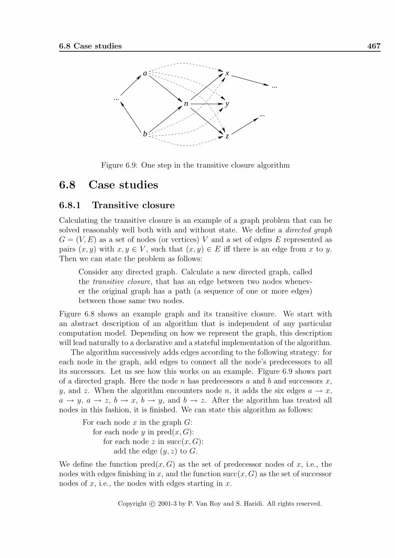
6.8 Case studies 467
z
yn
x
b
a
...
...
...
Figure 6.9: One step in the transitive closure algorithm
6.8 Case studies
6.8.1 Transitive closure
Calculating the transitive closure is an example of a graph problem that can besolved reasonably well both with and without state. We define a directed graphG = (V, E) as a set of nodes (or vertices) V and a set of edges E represented aspairs (x, y) with x, y ∈ V , such that (x, y) ∈ E iff there is an edge from x to y.Then we can state the problem as follows:
Consider any directed graph. Calculate a new directed graph, calledthe transitive closure, that has an edge between two nodes whenev-er the original graph has a path (a sequence of one or more edges)between those same two nodes.
Figure 6.8 shows an example graph and its transitive closure. We start withan abstract description of an algorithm that is independent of any particularcomputation model. Depending on how we represent the graph, this descriptionwill lead naturally to a declarative and a stateful implementation of the algorithm.
The algorithm successively adds edges according to the following strategy: foreach node in the graph, add edges to connect all the node’s predecessors to allits successors. Let us see how this works on an example. Figure 6.9 shows partof a directed graph. Here the node n has predecessors a and b and successors x,y, and z. When the algorithm encounters node n, it adds the six edges a → x,a → y, a → z, b → x, b → y, and b → z. After the algorithm has treated allnodes in this fashion, it is finished. We can state this algorithm as follows:
For each node x in the graph G:for each node y in pred(x, G):
for each node z in succ(x, G):add the edge (y, z) to G.
We define the function pred(x, G) as the set of predecessor nodes of x, i.e., thenodes with edges finishing in x, and the function succ(x, G) as the set of successornodes of x, i.e., the nodes with edges starting in x.
Copyright c© 2001-3 by P. Van Roy and S. Haridi. All rights reserved.

468 Explicit State
Why does this algorithm work? Consider any two nodes a and b with a pathbetween them: a → n1 → n2 → ... → nk → b (where k ≥ 0). We have toshow that the final graph has an edge from a to b. The nodes n1 through nk areencountered in some order by the algorithm. When the algorithm encounters anode ni, it “short circuits” the node, i.e., it creates a new path from a to b thatavoids the node. Therefore when the algorithm has encountered all nodes, it hascreated a path that avoids all of them, i.e., it has an edge directly from a to b.
Representing a graph
To write up the algorithm as a program, we first have to choose a representationfor directed graphs. Let us consider two possible representations:
• The adjacency list representation. The graph is a list with elements ofthe form I#Ns where I identifies a node and Ns is an ordered list of itsimmediate successors. As we will see below, ordered lists of successors aremore efficient to calculate with than unordered lists.
• The matrix representation. The graph is a two-dimensional array. Theelement with coordinates (I ,J) is true if there is an edge from node I tonode J . Otherwise, the element is false.
We find that the choice of representation strongly influences what is the bestcomputation model. In what follows, we assume that all graphs have at leastone node and that the nodes are consecutive integers. We first give a declarativealgorithm that uses the adjacency list representation [139]. We then give an in-place stateful algorithm that uses the matrix representation [41]. We then givea second declarative algorithm that also uses the matrix representation. Finally,we compare the three algorithms.
Converting between representations
To make comparing the two algorithms easier, we first define routines to convertfrom the adjacency list representation to the matrix representation and vice versa.Here is the conversion from adjacency list to matrix:
fun {L2M GL}M={Map GL fun {$ I#_} I end }L={FoldL M Min M.1}H={FoldL M Max M.1}GM={NewArray L H unit }
infor I#Ns in GL do
GM.I:={NewArray L H false }for J in Ns do GM.I.J:= true end
endGM
end
Copyright c© 2001-3 by P. Van Roy and S. Haridi. All rights reserved.

6.8 Case studies 469
fun {DeclTrans G}Xs={Map G fun {$ X#_} X end }
in{FoldL Xs
fun {$ InG X}SX={Succ X InG} in
{Map InGfun {$ Y#SY}
Y#if {Member X SY} then{Union SY SX} else SY end
end }end G}
end
Figure 6.10: Transitive closure (first declarative version)
In this routine, as in all following routines, we use GL for the adjacency listrepresentation and GMfor the matrix representation. Here is the conversion frommatrix to adjacency list:
fun {M2L GM}L={Array.low GM}H={Array.high GM}
infor I in L..H collect:C do
{C I# for J in L..H collect:D doif GM.I.J then {D J} end
end }end
end
This uses the loop syntax including the accumulation procedure collect:C togood advantage.
Declarative algorithm
We first give a declarative algorithm for transitive closure. The graph is repre-sented as an adjacency list. The algorithm needs two utility routines, Succ , whichreturns the succesor list of a given node, and Union , which calculates the unionof two ordered lists. We develop the algorithm by successive transformation ofthe abstract algorithm. This design method is known as stepwise refinement.
The outermost loop in the abstract algorithm transforms the graph in suc-cessive steps. Our declarative algorithm does the same by using FoldL , whichdefines a loop with accumulator. This means we can define the main functionDeclTrans as follows:
Copyright c© 2001-3 by P. Van Roy and S. Haridi. All rights reserved.

470 Explicit State
fun {DeclTrans G}
Xs={Nodes G} in
{FoldL Xs
fun {$ InG X}
SX={Succ X InG} in
for each node Y in pred(X, InG ):for each node Z in SX:
add edge (Y, Z)end G}
end
The next step is to implement the two inner loops:
for each node Y in pred(X, InG ):for each node Z in SX:
add edge (Y, Z)
These loops transform one graph into another, by adding edges. Since our graphis represented by a list, a natural choice is to use Map, which transforms onelist into another. This gives the following code, where Union is used to add thesuccessor list of X to that of Y:
{Map InGfun {$ Y#SY}
Y#if “Y in pred(X, InG )” then{Union SY SX} else SY end
end }
We finish up by noticing that Y is in pred(X, InG ) if and only if X is in succ(Y, InG ).This means we can write the if condition as follows:
{Map InGfun {$ Y#SY}
Y#if {Member X SY} then{Union SY SX} else SY end
end }
Putting everything together we get the final definition in Figure 6.10. This usesMap to calculate {Nodes G} . We conclude by remarking that FoldL , Map, andother routines such as Member, Filter , etc., are basic building blocks that mustbe mastered when writing declarative algorithms.
To finish up our presentation of the declarative algorithm, we give the defini-tions of the two utility routines. Succ returns the list of successors of a node:
fun {Succ X G}case G of Y#SY|G2 then
if X==Y then SY else {Succ X G2} endend
end
Copyright c© 2001-3 by P. Van Roy and S. Haridi. All rights reserved.

6.8 Case studies 471
proc {StateTrans GM}L={Array.low GM}H={Array.high GM}
infor K in L..H do
for I in L..H doif GM.I.K then
for J in L..H doif GM.K.J then GM.I.J:= true end
endend
endend
end
Figure 6.11: Transitive closure (stateful version)
Succ assumes that X is always in the adjacency list, which is true in our case.Union returns the union of two sets, where all sets are represented as orderedlists:
fun {Union A B}case A#Bof nil#B then B[] A#nil then A[] (X|A2)#(Y|B2) then
if X==Y then X|{Union A2 B2}elseif X<Y then X|{Union A2 B}elseif X>Y then Y|{Union A B2}end
endend
Union ’s execution time is proportional to the length of the smallest input listbecause its input lists are ordered. If the lists were not ordered, its executiontime would be proportional to the product of their lengths (why?), which isusually much larger.
Stateful algorithm
We give a stateful algorithm for transitive closure. The graph is represented asa matrix. This algorithm assumes that the matrix contains the initial graph. Itthen calculates the transitive closure in-place, i.e., by updating the input matrixitself. Figure 6.11 gives the algorithm. For each node K, this looks at eachpotential edge (I , J) and adds it if there is both an edge from I to K and from K
to J . We show now the stepwise transformation that leads to this algorithm. Wefirst restate the abstract algorithm with the proper variable names:
Copyright c© 2001-3 by P. Van Roy and S. Haridi. All rights reserved.

472 Explicit State
fun {DeclTrans2 GT}H={Width GT}fun {Loop K InG}
if K=<H thenG={MakeTuple g H} in
for I in 1..H doG.I={MakeTuple g H}for J in 1..H do
G.I.J=InG.I.J orelse (InG.I.K andthen InG.K.J)end
end{Loop K+1 G}
else InG endend
in{Loop 1 GT}
end
Figure 6.12: Transitive closure (second declarative version)
For each node k in the graph G:for each node i in pred(k, G):
for each node j in succ(k, G):add the edge (i, j) to G.
This leads to the following refinement:
proc {StateTrans GM}
L={Array.low GM}
H={Array.high GM}
in
for K in L..H do
for I in L..H do
if GM.I.K then
for each J in succ(K, GM) add GM.I.J:= true
end
end
end
end
We note that J is in succ(K, GM) if GM.K.J is true. This means we can replacethe inner loop by:
for J in L..H doif GM.K.J then GM.I.J:= true end
end
Copyright c© 2001-3 by P. Van Roy and S. Haridi. All rights reserved.

6.8 Case studies 473
Second declarative algorithm
Inspired by the stateful algorithm, we develop a second declarative algorithm.The second algorithm uses a series of tuples to store the successive approximationsof the transitive closure. We use the variable GT instead of GMto emphasize thischange in representation. A tuple is a record with fields numbered consecutivelyfrom 1 to a maximum value. So this algorithm is restricted to nodes whosenumbering starts from 1. Note that MakeTuple creates a tuple with unboundvariables. Figure 6.12 gives the algorithm.
This is somewhat more complicated than the stateful version. Each iterationof the outer loop uses the result of the previous iteration (InG ) as input to cal-culate the next iteration (G). The recursive function Loop passes the result fromone iteration to the next. While this may seem a bit complicated, it has the ad-vantages of the declarative model. For example, it is straightforward to convertit into a concurrent algorithm for transitive closure using the model of Chapter 4.The concurrent algorithm can run efficiently on a parallel processor. We justadd thread ... end to parallelize the two outer loops as shown in Figure 6.13.This gives a parallel dataflow implementation of the algorithm. Synchronizationis done through the tuples which initially contain unbound variables. The tuplesbehave like I-structures in a dataflow machine (see Section 4.9.5). It is an inter-esting exercise to draw a picture of an executing program, with data structuresand threads.
Example executions
Let us calculate the transitive closure of the graph [1#[2 3] 2#[1] 3#nil] .This is the same graph we showed before in Figure 6.8 except that we use integersto represent the nodes. Here is how to use the declarative algorithms:
{Browse {DeclTrans [1#[2 3] 2#[1] 3#nil]}}
Here is how to use the stateful algorithm:
declare GM in{StateTrans GM={L2M [1#[2 3] 2#[1] 3#nil]}}{Browse {M2L GM}}
This is slightly more complicated because of the calls to L2M and M2L, which weuse to give both the input and output as an adjacency list. All three algorithmsgive the result [1#[1 2 3] 2#[1 2 3] 3#nil] .
Discussion
Both the declarative and stateful algorithms are actually variations of the sameconceptual algorithm, which is called the Floyd-Warshall algorithm. All threealgorithms have an asymptotic running time of O(n3) for a graph of n nodes. Sowhich algorithm is better? Let us explore different aspects of this question:
Copyright c© 2001-3 by P. Van Roy and S. Haridi. All rights reserved.

474 Explicit State
fun {DeclTrans2 GT}H={Width GT}fun {Loop K InG}
if K=<H thenG={MakeTuple g H} in
threadfor I in 1..H do
threadG.I={MakeTuple g H}for J in 1..H do
G.I.J=InG.I.J orelse(InG.I.K andthen InG.K.J)
endend
endend{Loop K+1 G}
else InG endend
in{Loop 1 GT}
end
Figure 6.13: Transitive closure (concurrent/parallel version)
• A first aspect is ease of understanding and reasoning. Perhaps surprising-ly, the stateful algorithm has the simplest structure. It consists of threesimple nested loops that update a matrix in a straightforward way. Bothdeclarative algorithms have a more complex structure:
– The first one takes an adjacency list and passes it through a sequenceof stages in pipelined fashion. Each stage takes an input list andincrementally creates an output list.
– The second one has a similar structure as the stateful algorithm, butcreates a sequence of tuples in pipelined fashion.
Programming in the declarative model forces the algorithm to be structuredas a pipeline, written with small, independent components. Programmingin the stateful model encourages (but does not force) the algorithm to bestructured as a monolithic block, which is harder to decompose. The state-ful model gives more freedom in how to write the program. Depending onone’s point of view, this can be a good or bad thing.
• A second aspect is performance: running time and memory use. Bothalgorithms asymptotically have the same running time and active memorysizes. We have measured the running times of both algorithms on several
Copyright c© 2001-3 by P. Van Roy and S. Haridi. All rights reserved.

6.8 Case studies 475
large random graphs. Given a random graph of 200 nodes in which there isan edge between any node pair with probability p. For p greater than about0.05, the first declarative algorithm takes about 10 seconds, the secondabout 12 seconds, and the stateful algorithm about 15 seconds. For ptending to 0, the first declarative algorithm tends towards 0 seconds and theother algorithms increase slightly, to 16 and 20 seconds, respectively.7 Weconclude that the first declarative algorithm always has better performancethan the two others. The adjacency list representation is better than thematrix representation when the graph is sparse.
Of course, the conclusions of this particular comparison are by no means defini-tive. We have chosen simple and clean versions of each style, but many variationsare possible. For example, the first declarative algorithm can be modified to usea stateful Union operation. The stateful algorithm can be modified to stop loop-ing when no more new edges are found. What then can we conclude from thiscomparison?
• Both the declarative and stateful models are reasonable for implementingtransitive closure.
• The choice of representation (adjacency list or matrix) can be more impor-tant than the choice of computation model.
• Declarative programs tend to be less readable than stateful programs, be-cause they must be written in pipelined fashion.
• Stateful programs tend to be more monolithic than declarative programs,because explicit state can be modified in any order.
• It can be easier to parallelize a declarative program, because there are fewerdependencies between its parts.
6.8.2 Word frequencies (with stateful dictionary)
In Section 3.7.3 we showed how to use dictionaries to count the number of dif-ferent words in a text file. We compared the execution times of three versions ofthe word frequency counter, each one with a different implementation of dictio-naries. The first two versions use declarative dictionaries (implemented lists andbinary trees, respectively) and the third uses the built-in definition of dictionaries(implemented with state). The version using stateful dictionaries, shown in Fig-ure 6.14, is slightly different from the one using declarative dictionaries, shownin Figure 3.29:
7All measurements using Mozart 1.1.0 under Red Hat Linux release 6.1 on a Dell LatitudeCPx notebook computer with Pentium III processor at 500 MHz.
Copyright c© 2001-3 by P. Van Roy and S. Haridi. All rights reserved.

476 Explicit State
fun {WordChar C} ... end
fun {WordToAtom PW} ... end
fun {CharsToWords PW Cs} ... end
Put=Dictionary.putCondGet=Dictionary.condGet
proc {IncWord D W}{Put D W {CondGet D W 0}+1}
end
proc {CountWords D Ws}case Wsof W|Wr then
{IncWord D W}{CountWords D Wr}
[] nil then skipend
end
fun {WordFreq Cs}D={NewDictionary}
in{CountWords D {CharsToWords nil Cs}}D
end
Figure 6.14: Word frequencies (with stateful dictionary)
• The stateful version needs to pass just one argument as input to each pro-cedure that uses a dictionary.
• The declarative version has to use two arguments to these procedures: onefor the input dictionary and one for the output dictionary. In Figure 3.29,the second output is realized by using functional notation.
The difference shows up in the operations Put , IncWords , CountWords , andWordFreq . For example, Figure 6.14 uses the stateful {Put D LI X} , whichupdates D. Figure 3.29 uses the declarative {Put D1 LI X D2} , which reads D1
and returns a new dictionary D2.
6.8.3 Generating random numbers
A very useful primitive operation is a random number generator. It lets thecomputer “throw dice”, so to speak. How do we generate random numbers in a
Copyright c© 2001-3 by P. Van Roy and S. Haridi. All rights reserved.

6.8 Case studies 477
computer? Here we give the main insights; see Knuth [101] for a deep discus-sion of the theory underlying random number generators and of the concept ofrandomness itself.
Different approaches
One could imagine the following ways to generate random numbers:
• A first technique would be to use unpredictable events in the computeritself, e.g., related to concurrency, as explained in the previous chapter.Alas, their unpredictability does not follow simple laws. For example, usingthe thread scheduler as a source of randomness will give some fluctuations,but they do not have a useful probability distribution. Furthermore, theyare intimately linked with the computation in nonobvious ways, so even iftheir distribution was known, it would be dependent on the computation.So this is not a good source of random numbers.
• A second technique would be to rely on a source of true randomness. Forexample, electronic circuits generate noise, which is a completely unpre-dictable signal whose approximate probability distribution is known. Thenoise comes from the depths of the quantum world, so for all practical pur-poses it is truly random. But there are two problems. First, the probabilitydistribution is not exactly known: it might vary slightly from one circuit tothe next or with the ambient temperature. The first problem is not serious;there are ways to “normalize” the random numbers so that their distribu-tion is a constant, known one. There is a second, more serious problem:the randomness cannot be reproduced except by storing the random num-bers and replaying them. It might seem strange to ask for reproducibilityfrom a source of randomness, but it is perfectly reasonable. For exam-ple, the randomness might be input to a simulator. We would like to varysome parameter in the simulator such that any variation in the simulatordepends only on the parameter, and not on any variation in the randomnumbers. For this reason, computers are not usually connected to trulyrandom sources.
• It might seem that we have carefully worked ourselves into a tight corner.We would like true randomness and we would like it to be reproducible.How can we resolve this dilemma? The solution is simple: we calculatethe random numbers. How can this generate truly random numbers? Thesimple answer is, it cannot. But the numbers can appear random, for allpractical purposes. They are called pseudorandom numbers. What does thismean? It is not simple to define. Roughly, the generated numbers shouldgive the same behavior as truly random numbers, for the use we make ofthem.
Copyright c© 2001-3 by P. Van Roy and S. Haridi. All rights reserved.

478 Explicit State
The third solution, calculating random numbers, is the one that is almost alwaysimplemented. The question is, what algorithm do we use? Certainly not analgorithm chosen at random! Knuth [101] shows the pitfalls of this approach.It almost always gives bad results. We need an algorithm that has known goodproperties. We cannot guarantee that the random numbers will be good enough,but we can try to get what we can. For example, the generated random numbersshould satisfy strong statistical properties, have the right distribution, and theirperiod should be sufficiently long. The last point is worth expanding on: since arandom number generator does a calculation with finite information, eventuallyit will repeat itself. Clearly, the period of repetition should be very long.
Uniformly distributed random numbers
A random number generator stores an internal state, with which it calculatesthe next random number and the next internal state. The state should be largeenough to allow a long period. The random number is initialized with a numbercalled its seed. Initializing it again with the same seed should give the samesequence of random numbers. If we do not want the same sequence, we caninitialize it with information that will never be the same, such as the currentdate and time. Modern computers almost always have an operation to get thetime information. Now we can define the abstract data type of a random numbergenerator:
• {NewRand ?Rand ?Init ?Max} returns three references: a random numbergenerator Rand, its initialization procedure Init , and its maximum valueMax. Each generator has its own internal state. For best results, Max shouldbe large. This allows the program to reduce the random numbers to thesmaller domains it needs for its own purposes.
• {Init Seed} initializes the generator with integer seed Seed, that shouldbe in the range 0, 1, ..., Max. To give many possible sequences, Max shouldbe large. Initialization can be done at any time.
• X={Rand} generates a new random number X and updates the internal state.X is an integer in the range 0, 1, ..., Max-1 and has a Uniform distribution,i.e., all integers have the same probability of appearing.
How do we calculate a new random number? It turns out that a good simplemethod is the linear congruential generator. If x is the internal state and s is theseed, then the internal state is updated as follows:
x0 = sxn = (axn−1 + b) mod m
The constants a, b, and m have to be carefully chosen so that the sequence x0,x1, x2, ..., has good properties. The internal state xi is a uniformly distributedinteger from 0 to m− 1. It is easy to implement this generator:
Copyright c© 2001-3 by P. Van Roy and S. Haridi. All rights reserved.

6.8 Case studies 479
localA=333667B=213453321M=1000000000
inproc {NewRand ?Rand ?Init ?Max}
X={NewCell 0}in
proc {Init Seed} X:=Seed endfun {Rand} X:=(A*@X+B) mod M in @XendMax=M
endend
This is one of the simplest methods that has reasonably good behavior. Moresophisticated methods are possible that are even better.
Using laziness instead of state
The linear congruential algorithm can be packaged in a completely different way,as a lazy function. To get the next random number, it suffices to read the nextelement of the stream. Here is the definition:
localA=333667B=213453321M=1000000000
infun lazy {RandList S0}
S1=(A*S0+B) mod Min
S1|{RandList S1}end
end
Instead of using a cell, the state is stored in a recursive argument of RandList .Instead of calling Rand explicitly to get the next number, RandList is calledimplicitly when the next number is needed. Laziness acts as a kind of brake,making sure that the computation advances only as rapidly as its results areneeded. A third difference is that higher-order programming is not needed, sinceeach call to RandList generates a new sequence of random numbers.
Nonuniform distributions
A good technique to generate random numbers of any distribution is to start witha uniformly distributed random number. From this, we calculate a number withanother distribution. Using this technique we explain how to generate Gaussianand Exponential distributions. We first define a new generator:
Copyright c© 2001-3 by P. Van Roy and S. Haridi. All rights reserved.

480 Explicit State
declare Rand Init Max in {NewRand Rand Init Max}
Now we define functions to generate a Uniform distribution from 0 to 1 and aUniform integer distribution from A to B inclusive:
FMax={IntToFloat Max}fun {Uniform}
{IntToFloat {Rand}}/FMaxend
fun {UniformI A B}A+{FloatToInt {Floor {Uniform}*{IntToFloat B-A+1}}}
end
We will use Uniform to generate random variables with other distributions. First,let us generate random variables with an Exponential distribution. For this dis-tribution, the probability that X ≤ x is D(x) = 1− e−λx, where λ is a parametercalled the intensity. Since X ≤ x iff D(X) ≤ D(x), it follows that the probabilitythat D(X) ≤ D(x) is D(x). Writing y = D(x), it follows that the probability thatD(X) ≤ y is y. Therefore D(X) is uniformly distributed. Say D(X) = U whereU is a uniformly distributed random variable. Then we have X = − ln(1−U)/λ.This gives the following function:
fun {Exponential Lambda}˜{Log 1.0-{Uniform}}/Lambda
end
Now let us generate a Normal distribution with mean 0 and variance 1. This isalso called a Gaussian distribution. We use the following technique. Given twovariables U1 and U2, uniformly distributed from 0 to 1. Let R =
√−2 ln U1 and
φ = 2πU2. Then X1 = R cos φ and X2 = R sin φ are independent variables witha Gaussian distribution. The proof of this fact is beyond the scope of the book;it can be found in [101]. This gives the following function:
TwoPi=4.0*{Float.acos 0.0}fun {Gauss}
{Sqrt ˜2.0*{Log {Uniform}}} * {Cos TwoPi*{Uniform}}end
Since each call can give us two Gaussian variables, we can use a cell to rememberone result for the next call:
local GaussCell={NewCell nil} infun {Gauss}
Prev={Exchange GaussCell $ nil}in
if Prev\=nil then Prevelse R Phi in
R={Sqrt ˜2.0*{Log {Uniform}}}Phi=TwoPi*{Uniform}GaussCell:=R*{Cos Phi}
Copyright c© 2001-3 by P. Van Roy and S. Haridi. All rights reserved.

6.8 Case studies 481
R*{Sin Phi}end
endend
Each call of Gauss calculates two independent Gaussian variables; we returnone and store the other in a cell. The next call returns it without doing anycalculation.
6.8.4 “Word of Mouth” simulation
Let us simulate how Web users “surf” on the Internet. To “surf” between Websites means to successively load different Web sites. To keep our simulator simple,we will only look at one aspect of a Web site, namely its performance. This canbe reasonable when surfing between Web portals, which each provide a large andsimilar set of services. Assume there are n Web sites with equal content and atotal of m users. Each Web site has constant performance. Each user would liketo get to the Web site with highest performance. But there is no global measureof performance; the only way a user can find out about performance is by askingother users. We say that information passes by “word of mouth”. This gives usthe following simulation rules:
• Each site has a constant performance. Assume the constants are uniformlydistributed.
• Each user knows which site it is on.
• Each site knows how many users are on it.
• Each user tries to step to a site with higher performance. The user asks afew randomly-picked users about the performance at their site. The userthen goes to the site with highest performance. However, the performanceinformation is not exact: it is perturbed by Gaussian noise.
• One round of the simulation consists of all users doing a single step.
With these rules, we might expect users eventually to swarm among the siteswith highest performance. But is it really so? A simulation can give us answer.
Let us write a small simulation program. First, let us set up the globalconstants. We use the functions Init , UniformI , and Gauss defined in theprevious section. There are n sites, m users, and we do t simulation rounds.We initialize the random number generator and write information to the file´ wordofmouth.txt ´ during the simulation. We use the incremental write op-erations defined in the File module on the book’s Web site. With 10000 sites,500000 users, and 200 rounds, this gives the following:
Copyright c© 2001-3 by P. Van Roy and S. Haridi. All rights reserved.

482 Explicit State
declareN=10000 M=500000 T=200{Init 0}{File.writeOpen ´ wordofmouth.txt ´ }proc {Out S}
{File.write {Value.toVirtualString S 10 10}#"\n"}end
Next, we decide how to store the simulation information. We would like to storeit in records or tuples, because they are easy to manipulate. But they cannotbe modified. Therefore, we will store the simulation information in dictionaries.Dictionaries are very similar to records except that they can be changed dynam-ically (see Section 6.5.1). Each site picks its performance randomly. It has adictionary giving its performance and the number of users on it. The followingcode creates the initial site information:
declareSites={MakeTuple sites N}for I in 1..N do
Sites.I={Record.toDictionaryo(hits:0 performance:{IntToFloat {UniformI 1 80000}})}
end
Each user picks its site randomly. It has a dictionary giving its current site.It updates the Sites information. The following code creates the initial userinformation:
declareUsers={MakeTuple users M}for I in 1..M do
S={UniformI 1 N}in
Users.I={Record.toDictionary o(currentSite:S)}Sites.S.hits := Sites.S.hits + 1
end
Now that we have all the data structures, let us do one user step in the simulation.The function {UserStep I} does one step for user I , i.e., the user asks threeother users for the performance of their sites, it calculates its new site, and thenit updates all the site and user information.
proc {UserStep I}U = Users.I% Ask three users for their performance informationL = {List.map [{UniformI 1 M} {UniformI 1 M} {UniformI 1 M}]
fun {$ X}(Users.X.currentSite) #Sites.(Users.X.currentSite).performance
+ {Gauss}*{IntToFloat N}end }
Copyright c© 2001-3 by P. Van Roy and S. Haridi. All rights reserved.

6.8 Case studies 483
% Calculate the best siteMS#MP = {List.foldL L
fun {$ X1 X2} if X2.2>X1.2 then X2 else X1 end endU.currentSite #Sites.(U.currentSite).performance
+ {Abs {Gauss}*{IntToFloat N}}}
inif MS\=U.currentSite then
Sites.(U.currentSite).hits :=Sites.(U.currentSite).hits - 1
U.currentSite := MSSites.MS.hits := Sites.MS.hits + 1
endend
Now we can do the whole simulation:
for J in 1..N do{Out {Record.adjoinAt {Dictionary.toRecord site Sites.J}
name J}}end{Out endOfRound(time:0 nonZeroSites:N)}for I in 1..T do
X = {NewCell 0}in
for U in 1..M do {UserStep U} endfor J in 1..N do
H=Sites.J.hits inif H\=0 then
{Out {Record.adjoinAt{Dictionary.toRecord site Sites.J} name J}}
X:=1+@Xend
end{Out endOfRound(time:I nonZeroSites:@X)}
end{File.writeClose}
To make the simulator self-contained, we put all the above code in one procedurewith parameters N, M, T, and the output filename.
What is the result of the simulation? Will users cluster around the sites withhighest performance, even though they have only a very narrow and inaccurateview of what is going on? Running the above simulation shows that the number ofnonzero sites (with at least one user) decreases smoothly in inverse exponentialfashion from 10000 initially to less than 100 after 83 rounds. Average perfor-mance of user sites increases from about 40000 (half of the maximum) to morethan 75000 (within 6% of maximum) after just 10 rounds. So we can make a pre-
Copyright c© 2001-3 by P. Van Roy and S. Haridi. All rights reserved.

484 Explicit State
liminary conclusion that the best sites will quickly be found and the worst siteswill quickly be abandoned, even by word-of-mouth propagation of very approxi-mate information. Of course, our simulation has some simplifying assumptions.Feel free to change the assumptions and explore. For example, the assumptionthat a user can pick any three other users is unrealistic–it assumes that each userknows all the others. This makes convergence too fast. See the Exercises of thischapter for a more realistic assumption on user knowledge.
6.9 Advanced topics
6.9.1 Limitations of stateful programming
Stateful programming has some strong limitations due to its use of explicit state.Object-oriented programming is a special case of stateful programming, so itsuffers from the same limitations.
The real world is parallel
The main limitation of the stateful model is that programs are sequential. Inthe real world, entities are both stateful and act in parallel. Sequential statefulprogramming does not model the parallel execution.
Sometimes this limitation is appropriate, e.g., when writing simulators whereall events must be coordinated (stepping from one global state to another in acontrolled way). In other cases, e.g., when interacting with the real world, thelimitation is an obstacle. To remove the limitation, the model needs to have bothstate and concurrency. We have seen one simple way to achieve this in Chapter 5.Another way is given in Chapter 8. As Section 4.7.6 explains, concurrency in themodel can model parallelism in the real world.
The real world is distributed
Explicit state is hard to use well in a distributed system. Chapter 11 explains thislimitation in depth. Here we give just the main points. In a distributed system,the store is partitioned into separate parts. Within one part, the store behavesefficiently as we have seen. Between parts, communication is many orders ofmagnitude more expensive. The parts coordinate with one another to maintainthe desired level of global consistency. For cells this can be expensive because cellcontents can change at any time in any part. The programmer has to decide onboth the level of consistency and the coordination algorithm used. This makes ittricky to do distributed programming with state.
The declarative model and its extension to concurrent message passing inChapter 5 are much easier to use. As Chapter 5 explains, a system can be de-composed into independent components that communicate with messages. This
Copyright c© 2001-3 by P. Van Roy and S. Haridi. All rights reserved.

6.9 Advanced topics 485
fits very well with the partitioned store of a distributed system. When program-ming a distributed system, we recommend to use the message-passing modelwhenever possible for coordinating the parts. Chapter 11 explains how to pro-gram a distributed system and when to use the different computation models ina distributed setting.
6.9.2 Memory management and external references
As explained in Section 2.4.7, garbage collection is a technique for automaticmemory management that recovers memory for all entities inside the computationmodel that no longer take part in the computation. This is not good enough forentities outside the computation model. Such entities exist because there is aworld outside of the computation model, which interacts with it. How can we doautomatic memory management for them? There are two cases:
• From inside the computation model, there is a reference to an entity outsideit. We call such a reference a resource pointer. Here are some examples:
– A file descriptor, which points to a data structure held by the operatingsystem. When the file descriptor is no longer referenced, we would liketo close the file.
– A handle to access an external database. When the handle is no longerreferenced, we would like to close the connection to the database.
– A pointer to a block of memory allocated through the Mozart C++interface. When the memory is no longer referenced, we would like itto be freed.
• From the external world, there is a reference to inside the computationmodel. We call such a reference a ticket. Tickets are used in distributedprogramming as a means to connect processes together (see Chapter 11).
In the second case, there is no safe way in general to recover memory. By safewe mean not to release memory as long as external references exist. The externalworld is so big that the computation model cannot know whether any referencestill exists or not. One pragmatic solution is to add the language entity to the rootset for a limited period of time. This is known as a time-lease mechanism. Thetime period can be renewed when the language entity is accessed. If the timeperiod expires without a renewal, we assume that there are no more externalreferences. The application has to be designed to handle the rare case when thisassumption is wrong.
In the first case, there is a simple solution based on parameterizing the garbagecollector. This solution, called finalization, gives the ability to perform a user-defined action when a language entity has become unreachable. This is imple-mented by the System module Finalize . We first explain how the module works.We then give some examples of how it is used.
Copyright c© 2001-3 by P. Van Roy and S. Haridi. All rights reserved.

486 Explicit State
Finalization
Finalization is supported by the Finalize module. The design of this moduleis inspired by the guardian concept of [51]. Finalize has the following twooperations:
• {Finalize.register X P} registers a reference X and a procedure P.When X becomes otherwise unreachable (otherwise than through finaliza-tion), {P X} is eventually executed in its own thread. During this execution,X is reachable again until its reference is no longer accessible.
• {Finalize.everyGC P} registers a procedure P to be invoked eventuallyafter every garbage collection.
In both of these operations, you cannot rely on how soon after the garbage collec-tion the procedure P will be invoked. It is in principle possible that the call mayonly be scheduled several garbage collections late if the system has very manylive threads and generates garbage at a high rate.
There is no limitation on what the procedure P is allowed to do. This isbecause P is not executed during garbage collection, when the system’s internaldata structures can be temporarily inconsistent, but is scheduled for executionafter garbage collection. P can even reference X and itself call Finalize .
An interesting example is the everyGC operation itself, which is defined interms of register :
proc {EveryGC P}proc {DO _} {P} {Finalize.register DO DO} end
in{Finalize.register DO DO}
end
This creates a procedure DOand registers it using itself as its own handler. WhenEveryGC exits, the reference to DO is lost. This means that DOwill be invokedafter the next garbage collection. When invoked, it calls P and registers itselfagain.
Laziness and external resources
To make lazy evaluation practical for external resources like files, we need to usefinalization to release the external resources when they are no longer needed. Forexample, in Section 4.5.5 we defined a function ReadListLazy that reads a filelazily. This function closes the file after it is completely read. But this is not goodenough: even if only part of the file is needed, the file should also be closed. Wecan implement this with finalization. We extend the definition of ReadListLazy
to close the file when it becomes inaccessible:
fun {ReadListLazy FN}{File.readOpen FN}
Copyright c© 2001-3 by P. Van Roy and S. Haridi. All rights reserved.

6.10 Exercises 487
fun lazy {ReadNext}L T I in
{File.readBlock I L T}if I==0 then T=nil {File.readClose} else T={ReadNext} endL
endin
{Finalize.register F proc {$ F} {File.readClose} end }{ReadNext}
end
This requires just one call to Finalize .
6.10 Exercises
1. What is state. Section 6.1 defines the function SumList , which has astate encoded as the successive values of two arguments at recursive calls.For this exercise, rewrite SumList so that the state is no longer encoded inarguments, but by cells.
2. Emulating state with concurrency. This exercise explores whetherconcurrency can be used to obtain explicit state.
(a) First use concurrency to create an updatable container. We create athread that uses a recursive procedure to read a stream. The streamhas two possible commands: access(X) , which binds X to the con-tainer’s current content, and assign(X) , which assigns X as the newcontent. Here is how it is done:
fun {MakeState Init}proc {Loop S V}
case S of access(X)|S2 thenX=V {Loop S2 V}
[] assign(X)|S2 then{Loop S2 X}
else skip endendS
inthread {Loop S Init} endS
end
S={MakeState 0}
The call {MakeState Init} creates a new container with initial con-tent Init . We use the container by putting commands on the stream.
Copyright c© 2001-3 by P. Van Roy and S. Haridi. All rights reserved.

488 Explicit State
For example, here is a sequence of three commands for the containerS:
declare S1 X Y inS=access(X)|assign(3)|access(Y)|S1
This binds X to 0 (the initial content), puts 3 in the container, andthen binds Y to 3.
(b) Now rewrite SumList to use this container to count the number ofcalls. Can this container be encapsulated, i.e., can it be added withoutchanging the arguments of SumList ? Why or why not? What happenswhen we try to add the function SumCount like in Section 6.1.2?
3. Implementing ports. In Chapter 5 we introduced the concept of port,which is a simple communication channel. Ports have the operations {NewPort
S P} , which returns a port P with stream S, and {Send P X} , which sendsmessage X on port P. From these operations, it is clear that ports are astateful unbundled ADT. For this exercise, implement ports in terms ofcells, using the techniques of Section 6.4.
4. Explicit state and security. Section 6.4 gives four ways to constructsecure ADTs. From these constructions, it seems that the ability to makeADTs secure is a consequence of using one or both of the following concepts:procedure values (which provide hiding through lexical scoping) and namevalues (which are unforgeable and unguessable). In particular, explicit stateseems to have no role with respect to security. For this exercise, thinkcarefully about this assertion. Is it true? Why or why not?
5. Declarative objects and identity. Section 6.4.2 shows how to build adeclarative object, which combines value and operations in a secure way.However, the implementation given misses one aspect of objects, namelytheir identity. That is, an object should keep the same identity after statechanges. For this exercise, extend the declarative objects of Section 6.4.2to have an identity.
6. Revocable capabilities. Section 6.4.3 defines the three-argument proce-dure Revocable , which takes a capability and uses explicit state to cre-ate two things: a revocable version of that capability and a revoker. ForRevocable , the capability is represented as a one-argument procedure andthe revoker is a zero-argument procedure. For this exercise, write a versionof Revocable that is a one-argument procedure and where the revoker isalso a one-argument procedure. This allows Revocable to be used recur-sively on all capabilities including revokers and itself. For example, theability to revoke a capability can then be made revocable.
7. Abstractions and memory management. Consider the following ADTwhich allows to collect information together into a list. The ADT has three
Copyright c© 2001-3 by P. Van Roy and S. Haridi. All rights reserved.

6.10 Exercises 489
operations. The call C={NewCollector} creates a new collector C. Thecall {Collect C X} adds X to C’s collection. The call L={EndCollect}
returns the final list containing all collected items in the order they werecollected. Here are two ways to implement collectors that we will compare:
• C is a cell that contains a pair H|T , where H is the head of the collectedlist and T is its unbound tail. Collect is implemented as:
proc {Collect C X}H T in
{Exchange C H|(X|T) H|T}end
Implement the NewCollector and EndCollect operations with thisrepresentation.
• C is a pair H|T , where H is the head of the collected list and T is a cellthat contains its unbound tail. Collect is implemented as:
proc {Collect C X}T in
{Exchange C.2 X|T T}end
Implement the NewCollector and EndCollect operations with thisrepresentation.
• We compare the two implementations with respect to memory man-agement. Use the table of Section 3.5.2 to calculate how many wordsof memory are allocated by each version of Collect . How many ofthese words immediately become inactive in each version? What doesthis imply for garbage collection? Which version is best?
This example is taken from the Mozart system. Collection in the for loopwas originally implemented with one version. It was eventually replaced bythe other. (Note that both versions work correctly in a concurrent setting,i.e., if Collect is called from multiple threads.)
8. Call by name. Section 6.4.4 shows how to code call by name in the statefulcomputation model. For this exercise, consider the following example takenfrom [56]:
procedure swap(callbyname x,y:integer);
var t:integer;
begin
t:=x; x:=y; y:=t
end;
var a:array [1..10] of integer;
Copyright c© 2001-3 by P. Van Roy and S. Haridi. All rights reserved.

490 Explicit State
var i:integer;
i:=1; a[1]:=2; a[2]=1;
swap(i, a[i]);
writeln(a[1], a[2]);
This example shows a curious behavior of call by name. Running the exam-ple does not swap i and a[i], as one might expect. This shows an undesir-able interaction between destructive assignment and the delayed evaluationof an argument.
• Explain the behavior of this example using your understanding of callby name.
• Code the example in the stateful computation model. Use the followingencoding of array[1..10]:
A={MakeTuple array 10}for J in 1..10 do A.J={NewCell 0} end
That is, code the array as a tuple of cells.
• Explain the behavior again in terms of your coding.
9. Call by need. With call by name, the argument is evaluated again eachtime it is needed.
• For this exercise, redo the swap example of the previous exercise withcall by need instead of call by name. Does the counterintuitive be-havior still occur? If not, can similar problems still occur with call byneed by changing the definition of swap?
• In the code that implements call by need, Sqr will always call A. Thisis fine for Sqr , since we can see by inspection that the result is neededthree times. But what if the need cannot be determined by inspection?We do not want to call A unnecessarily. One possibility is to use lazyfunctions. Modify the coding of call by need given in Section 6.4.4so that it uses laziness to call A only when needed, even if that needcannot be determined by inspection. A should be called at most once.
10. Evaluating indexed collections. Section 6.5.1 presents four indexed col-lection types, namely tuples, records, arrays, and dictionaries, with differentperformance/expressiveness trade-offs. For this exercise, compare these fourtypes in various usage scenarios. Evaluate their relative performance andusefulness.
11. Extensible arrays. The extensible array of Section 6.5 only extends thearray upwards. For this exercise, modify the extensible array so it extendsthe array in both directions.
Copyright c© 2001-3 by P. Van Roy and S. Haridi. All rights reserved.

6.10 Exercises 491
12. Generalized dictionaries. The built-in dictionary type only works forliteral keys, i.e., numbers, atoms, or names. For this exercise, implement adictionary that can use any value as a key. One possible solution uses thefact that the == operation can compare any values. Using this operation,the dictionary could store entries as an association list, which is a list ofpairs Key#Value , and do simple linear search.
13. Loops and invariant assertions. Use the method of invariant asser-tions to show that the proof rules for the while and for loops given inSection 6.6.4 are correct.
14. The break statement. A block is a set of statements with a well-definedentry point and exit point. Many modern imperative programming lan-guages, such as Java and C++, are based on the concept of block. Theselanguages allow defining nested blocks and provide an operation to jumpimmediately from within a block to the block’s exit point. This operationis called break. For this exercise, define a block construct with a breakoperation that can be called as follows:
{Block proc {$ Break} 〈stmt〉 end }
This should have exactly the same behavior as executing 〈stmt〉, exceptthat executing {Break} inside 〈stmt〉 should immediately exit the block.Your solution should work correctly for nested blocks and exceptions raisedwithin blocks. If 〈stmt〉 creates threads, then these should not be affectedby the break operation. Hint: use the exception handling mechanism.
15. “Small World” simulation. The “Word of Mouth” simulation of Sec-tion 6.8.4 makes some strong simplifying assumptions. For example, thesimulation assumes that each user can choose any three users at randomto ask them about their performance. This is much too strong an assump-tion. The problem is that the choice ranges over all users. This gives eachuser a potentially unbounded amount of knowledge. In actuality, each userhas bounded knowledge: a small network of acquaintances that changesbut slowly. Each user asks only members of his network of acquaintances.Rewrite the simulation program to take this assumption into account. Thiscan make convergence much slower. With this assumption, the simulationis called a “Small World” simulation [203].
16. Performance effects in “Word of Mouth” simulation. The “Wordof Mouth” simulation of Section 6.8.4 assumes that site performance isconstant. A better way to take performance into account is to assume thatit is constant up to a given threshold number of users, which is fixed for eachsite. Beyond this threshold, performance goes down in inverse proportionto the number of users. This is based on the premise that for small numbersof users, Internet performance is the bottleneck, and for large numbers ofusers, site performance is the bottleneck.
Copyright c© 2001-3 by P. Van Roy and S. Haridi. All rights reserved.

492 Explicit State
17. Word frequency application. Section 6.8.2 gives a version of the wordfrequency algorithm that uses stateful dictionaries. Rewrite the word fre-quency application of Section 3.9.4 to use the stateful version.
Copyright c© 2001-3 by P. Van Roy and S. Haridi. All rights reserved.

Chapter 7
Object-Oriented Programming
“The fruit is too well known to need anydescription of its external characteristics.”– From entry “Apple”, Encyclopaedia Britannica (11th edition)
This chapter introduces a particularly useful way of structuring stateful pro-grams called object-oriented programming. It introduces one new concept overthe last chapter, namely inheritance, which allows to define ADTs in incremen-tal fashion. However, the computation model is the same stateful model as inthe previous chapter. We can loosely define object-oriented programming asprogramming with encapsulation, explicit state, and inheritance. It is often sup-ported by a linguistic abstraction, the concept of class, but it does not have tobe. Object-oriented programs can be written in almost any language.
From a historical viewpoint, the introduction of object-oriented programmingmade two major contributions to the discipline of programming. First, it madeclear that encapsulation is essential. Programs should be organized as collec-tions of ADTs. This was first clearly stated in the classic article on “informationhiding” [142], reprinted in [144]. Each module, component, or object has a “se-cret” known only to itself. Second, it showed the importance of building ADTsincrementally, using inheritance. This avoids duplicated code.
Object-oriented programming is one of the most successful and pervasive ar-eas in informatics. From its timid beginnings in the 1960’s it has invaded everyarea of informatics, both in scientific research and technology development. Thefirst object-oriented language was Simula 67, developed in 1967 as a descendantof Algol 60 [130, 137, 152]. Simula 67 was much ahead of its time and had littleimmediate influence. Much more influential in making object-oriented program-ming popular was Smalltalk-80, released in 1980 as the result of research done inthe 1970’s [60]. The currently most popular programming languages, Java andC++, are object-oriented [186, 184]. The most popular “language-independent”design aids, the Unified Modeling Language (UML) and Design Patterns, bothimplicitly assume that the underlying language is object-oriented [58, 159]. With
Copyright c© 2001-3 by P. Van Roy and S. Haridi. All rights reserved.

494 Object-Oriented Programming
all this exposure, one might feel that object-oriented programming is well under-stood (see the chapter quote). Yet, this is far from being the case.
Structure of the chapter
The purpose of this chapter is not to cover all of object-oriented programmingin 100 pages or less. This is impossible. Instead, we give an introduction thatemphasizes areas where other programming books are weak: the relationship withother computation models, the precise semantics, and the possibilities of dynamictyping. The chapter is structured as follows:
• Motivations (Section 7.1). We give the principal motivation for object-oriented programming, namely to support inheritance, and how its featuresrelate to this.
• An object-oriented computation model (Sections 7.2 and 7.3). Wedefine an object system that takes advantage of dynamic typing to combinesimplicity and flexibility. This allows us to explore better the limits ofthe object-oriented abstraction and situate existing languages within them.We single out three areas: controlling encapsulation, single and multipleinheritance, and higher-order programming techniques. We give the objectsystem syntactic and implementation support to make it easier to use andmore efficient.
• Programming with inheritance (Section 7.4). We explain the basicprinciples and techniques for using inheritance to construct object-orientedprograms. We illustrate them with realistic example programs. We givepointers into the literature on object-oriented design.
• Relation to other computation models (Section 7.5). From the view-point of multiple computation models, we show how and when to use andnot use object-oriented programming. We relate it to component-based pro-gramming, object-based programming, and higher-order programming. Wegive additional design techniques that become possible when it is used to-gether with other models. We explain the pros and cons of the oft-repeatedprinciple stating that every language entity should be an object. This prin-ciple has guided the design of several major object-oriented languages, butis often misunderstood.
• Implementing the object system (Section 7.6). We give a simple andprecise semantics of our object system, by implementing it in terms of thestateful computation model. Because the implementation uses a compu-tation model with a precise semantics, we can consider it as a semanticdefinition.
Copyright c© 2001-3 by P. Van Roy and S. Haridi. All rights reserved.

7.1 Motivations 495
• The Java language (Section 7.7). We give an overview of the sequentialpart of Java, a popular object-oriented programming language. We showhow the concepts of Java fit in the object system of the chapter.
• Active objects (Section 7.8). An active object extends a port object ofChapter 5 by using a class to define its behavior. This combines the abilitiesof object-oriented programming with message-passing concurrency.
After reading this chapter, you will have a better view of what object-orientedprogramming is about, how to situate it among other computation models, andhow to use the expressiveness it offers.
Object-Oriented Software Construction
For more information on object-oriented programming techniques and principles,we recommend the book Object-Oriented Software Construction, Second Edition,by Bertrand Meyer [122]. This book is especially interesting for its detaileddiscussion of inheritance, including multiple inheritance.
7.1 Motivations
7.1.1 Inheritance
As we saw in the previous chapter, stateful abstract data types are a very usefulconcept for organizing a program. In fact, a program can be built in a hierarchicalstructure as ADTs that depend on other ADTs. This is the idea of component-based programming.
Object-oriented programming takes this idea one step further. It is based onthe observation that components frequently have much in common. Take theexample of sequences. There are many different ADTs that are “sequence-like”.Sometimes we want them to behave like stacks (adding and deleting at the sameend). Sometimes we want them to behave like queues (adding and deleting atopposite ends). And so forth, with dozens of possibilities. All of these sequencesshare the basic, linear-order property of the concept of sequence. How can weimplement them without duplicating the common parts?
Object-oriented programming answers this question by introducing the addi-tional concept of inheritance. An ADT can be defined to “inherit” from otherADTs, that is, to have substantially the same functionality as the others, withpossibly some modifications and extensions. Only the differences between theADT and its ancestors have to be specified. Such an incremental definition of anADT is called a class.
Copyright c© 2001-3 by P. Van Roy and S. Haridi. All rights reserved.

496 Object-Oriented Programming
Stateful model with inheritance
Inheritance is the essential difference between object-oriented programming andmost other kinds of stateful programming. It is important to emphasize thatinheritance is a programming technique; the underlying computation model ofobject-oriented programming is simply the stateful model (or the shared-stateconcurrent model, for concurrent object-oriented programming). Object-orientedlanguages provide linguistic support for inheritance by adding classes as a lin-guistic abstraction.
Caveats
It turns out that inheritance is a very rich concept that can be rather tricky.There are many ways that an ADT can be built by modifying other ADTs.The primary approach used in object-oriented programming is syntactic: a newADT is defined by doing simple syntactic manipulations of an existing ADT.Because the resulting changes in semantics are not always easy to infer, thesemanipulations must be done with great care.
The component approach to building systems is much simpler. A componentgroups together any set of entities and treats them as a unit from the viewpointof use dependency. A component is built from subcomponents, respecting theirspecifications.
Potential
Despite the difficulties of using inheritance, it has a great potential: it increasesthe possibilities of factoring an application, i.e., to make sure that each abstrac-tion is implemented just once. Having more than one implementation of anabstraction does not just make the program longer. It is an invitation to dis-aster: if one implementation is changed, then the others must also be changed.What’s more, the different implementations are usually slightly different, whichmakes nonobvious the relationships among all the changes. This “code duplica-tion” of an abstraction is one of the biggest sources of errors. Inheritance has thepotential to remove this duplication.
The potential to factor an application is a two-edged sword. It comes atthe price of “spreading out” an ADT’s implementation over large parts of theprogram. The implementation of an ADT does not exist in one place; all theADTs that are part of it have to be considered together. Even stronger, part ofthe implementation may exist only as compiled code, with no access to the sourcecode.
Early on, it was believed that inheritance would solve the problem of softwarereuse. That is, it would make it easier to build libraries that can be distributedto third parties, for use in other applications. This has not worked out in prac-tice. The failure of inheritance as a reuse technique is clear from the success of
Copyright c© 2001-3 by P. Van Roy and S. Haridi. All rights reserved.

7.1 Motivations 497
other techniques such as components, frameworks, and design patterns. Inheri-tance remains most useful within a single application or closely-related family ofapplications.
Inheritance is not an unmixed blessing, but it takes its place next to higher-order programming as one of the most important techniques for structuring aprogram.
7.1.2 Encapsulated state and inheritance
The combination of encapsulating explicit state and inheritance has led to thefield of object-oriented programming, which is presented in this chapter. Thisfield has developed a rich theory and practice on how to write stateful programswith inheritance. Unfortunately, this theory tends to consider everything as be-ing an object and to mix the notions of state and encapsulation. The advantagesto be gained by considering other entities than objects and by using encapsula-tion without state are often ignored. Chapters 3 and 4 explain well how to usethese two ideas. The present chapter follows the object-oriented philosophy andemphasizes how to build ADTs with both explicit state and inheritance.
Most object-oriented programming languages consider that ADTs should haveexplicit state by default. For example, Smalltalk, C++, and Java all considervariables to be stateful, i.e., mutable, by default. In Java it is possible to makevariables immutable by declaring them as final, but it is not the default. Thisgoes against the rule of thumb given in Section 4.7.6, and in our view it is amistake. Explicit state is a complex notion which should not be the first onethat students are taught. There are simpler ways to program, e.g., using variableidentifiers to refer to values or dataflow variables. These simpler ways should beconsidered first before moving to explicit state.
7.1.3 Objects and classes
An object is an entity that encapsulates a state so that it can only be accessedin a controlled way from outside the object. The access is provided by means ofmethods, which are procedures that are accessible from the outside and that candirectly access the internal state. The only way to modify the state is by callingthe methods. This means that the object can guarantee that the state alwayssatisfies some invariant property.
A class is an entity that specifies an object in an incremental way, by definingthe classes that the object inherits from (its direct ancestors) and defining howthe class is different from the direct ancestors. Most modern languages supportclasses as a linguistic abstraction. We will do the same in this chapter. To makethe concepts precise we will add a simple yet powerful class construct.
This chapter only talks about objects that are used sequentially, i.e., that areused in a single thread. Chapter 8 explains how to use objects in a concurrent
Copyright c© 2001-3 by P. Van Roy and S. Haridi. All rights reserved.

498 Object-Oriented Programming
class Counterattr valmeth init(Value)
val:=Valueendmeth browse
{Browse @val}endmeth inc(Value)
val:=@val+Valueend
end
Figure 7.1: An example class Counter (with class syntax)
setting, when multiple threads use the objects. In particular, object locking isexplained there.
7.2 Classes as complete ADTs
The heart of the object concept is controlled access to encapsulated data. Thebehavior of an object is specified by a class. In the most general case, a classis an incremental definition of an ADT, that defines the ADT as a modificationof other ADTs. There is a rich set of concepts for defining classes. We classifythese concepts into two sets, according as they permit the class to define an ADTcompletely or incrementally:
• Complete ADT definition. These are all the concepts that permit aclass, taken by itself, to define an ADT. There are two sets of concepts:
– Defining the various elements that make up a class (Section 7.2.3),namely methods, attributes, and properties. Attributes can be initial-ized in several ways, per object or per class (Section 7.2.4).
– Taking advantage of dynamic typing. This gives first-class messages(Section 7.2.5) and first-class attributes (Section 7.2.6). This allowspowerful forms of polymorphism that are difficult or impossible to doin statically-typed languages. This increased freedom comes with anincreased responsibility of the programmer to use it correctly.
• Incremental ADT definition. These are all the concepts related to in-heritance, that is, they define how a class is related to existing classes. Theyare given in Section 7.3.
Copyright c© 2001-3 by P. Van Roy and S. Haridi. All rights reserved.

7.2 Classes as complete ADTs 499
localproc {Init M S}
init(Value)=M in (S.val):=Valueendproc {Browse2 M S}
{Browse @(S.val)}endproc {Inc M S}
inc(Value)=M in (S.val):=@(S.val)+Valueend
inCounter=c(attrs:[val]
methods:m(init:Init browse:Browse2 inc:Inc))end
Figure 7.2: Defining the Counter class (without syntactic support)
7.2.1 An example
To see how classes and objects work in the object system, let us define an exampleclass and use it to create an object. We assume that the language has a newconstruct, the class declaration. We assume that classes are first-class valuesin the language. This lets us use a class declaration as either statement orexpression, in similar manner to a proc declaration. Later on in the chapter, wewill see how to define classes in the kernel language of the stateful model. Thiswould let us define class as a linguistic abstraction.
Figure 7.1 defines a class referred to by the variable Counter . This class hasone attribute, val , that holds a counter’s current value, and three methods, init ,browse , and inc , for initializing, displaying, and incrementing the counter. Theattribute is assigned with the := operator and accessed with the @operator. Thisseems quite similar to how other languages would do it, modulo a different syntax.But appearances can be deceiving!
The declaration of Figure 7.1 is actually executed at run time, i.e., it is astatement that creates a class value and binds it to Counter . Replace “Counter ”by “$” and the declaration can be used in an expression. Putting this declarationat the head of a program will declare the class before executing the rest, which isfamiliar behavior. But this is not the only possibility. The declaration can be putanywhere that a statement can be. For example, putting the declaration inside aprocedure will create a new and distinct class each time the procedure is called.Later on we will use this possibility to make parameterized classes.
Let us create an object of class Counter and do some operations with it:
C={New Counter init(0)}{C inc(6)} {C inc(6)}{C browse}
This creates the counter object C with initial value 0, increments it twice by 6,
Copyright c© 2001-3 by P. Van Roy and S. Haridi. All rights reserved.

500 Object-Oriented Programming
fun {New Class Init}Fs={Map Class.attrs fun {$ X} X#{NewCell _} end }S={List.toRecord state Fs}proc {Obj M}
{Class.methods.{Label M} M S}end
in{Obj Init}Obj
end
Figure 7.3: Creating a Counter object
and then displays the counter’s value. The statement {C inc(6)} is called anobject application. The message inc(6) is sent to the object, which invokes thecorresponding method. Now try the following:
local X in {C inc(X)} X=5 end{C browse}
This displays nothing at all! The reason is that the object application
{C inc(X)}
blocks inside the method inc . Can you see exactly where? Now try the followingvariation:
declare S inlocal X in thread {C inc(X)} S= unit end X=5 end{Wait S} {C browse}
Things now work as expected. We see that dataflow execution keeps its familiarbehavior when used with objects.
7.2.2 Semantics of the example
Before going on to describe the additional abilities of classes, let us give thesemantics of the Counter example. It is a simple application of higher-orderprogramming with explicit state. The semantics we give here is slightly simplified;it leaves out the abilities of class that are not used in the example (such asinheritance and self ). Section 7.6 gives the full semantics.
Figure 7.2 shows what Figure 7.1 does by giving the definition of the classCounter in the stateful model without any class syntax. We can see thataccording to this definition, a class is simply a record containing a set of attributenames and a set of methods. An attribute name is a literal. A method is aprocedure that has two arguments, the message and the object state. In eachmethod, assigning to an attribute (“val:= ”) is done with a cell assignment andaccessing an attribute (“@val”) is done with a cell access.
Copyright c© 2001-3 by P. Van Roy and S. Haridi. All rights reserved.

7.2 Classes as complete ADTs 501
〈statement〉 ::= class 〈variable〉 { 〈classDescriptor〉 }{ meth 〈methHead〉 [ ´ =´ 〈variable〉 ]
( 〈inExpression〉 | 〈inStatement〉 ) end }end
| lock [ 〈expression〉 then ] 〈inStatement〉 end
| 〈expression〉 ´ := ´ 〈expression〉| 〈expression〉 ´ , ´ 〈expression〉| ...
〈expression〉 ::= class ´ $´ { 〈classDescriptor〉 }{ meth 〈methHead〉 [ ´ =´ 〈variable〉 ]
( 〈inExpression〉 | 〈inStatement〉 ) end }end
| lock [ 〈expression〉 then ] 〈inExpression〉 end
| 〈expression〉 ´ := ´ 〈expression〉| 〈expression〉 ´ , ´ 〈expression〉| ´ @ 〈expression〉| self
| ...〈classDescriptor〉 ::= from { 〈expression〉 }+ | prop { 〈expression〉 }+
| attr { 〈attrInit〉 }+〈attrInit〉 ::= ( [ ´ ! ´ ] 〈variable〉 | 〈atom〉 | unit | true | false )
[ ´ : ´ 〈expression〉 ]〈methHead〉 ::= ( [ ´ ! ´ ] 〈variable〉 | 〈atom〉 | unit | true | false )
[ ´ ( ´ { 〈methArg〉 } [ ´ ... ´ ] ´ ) ´ ][ ´ =´ 〈variable〉 ]
〈methArg〉 ::= [ 〈feature〉 ´ : ´ ] ( 〈variable〉 | ´ _´ | ´ $´ ) [ ´ <=´ 〈expression〉 ]
Table 7.1: Class syntax
Figure 7.3 defines the function Newwhich is used to create objects from classes.This function creates the object state, defines a one-argument procedure Obj thatis the object, and initializes the object before returning it. The object state S
is a record holding one cell for each attribute. The object state is hidden insideObj by lexical scoping.
7.2.3 Defining classes
A class is a data structure that defines an object’s internal state (attributes), itsbehavior (methods), the classes it inherits from, and several other properties andoperations that we will see later on. More generally, a class is a data structurethat describes an ADT and gives its partial or total implementation. Table 7.1gives the syntax of classes. There can be any number of objects of a given class.They are called instances of the class. These objects have different identities
Copyright c© 2001-3 by P. Van Roy and S. Haridi. All rights reserved.

502 Object-Oriented Programming
and can have different values for their internal state. Otherwise, all objects of agiven class behave according to the class definition. An object Obj is called withthe syntax {Obj M} , where M is a record that defines the message. Calling anobject is also called sending a message to the object. This terminology exists forhistorical reasons; we do not recommend it since it is easily confused with sendinga message on a communication channel. An object invocation is synchronous,like a procedure’s. The invocation returns only when the method has completelyexecuted.
A class defines the constituent parts that each instance will have. In object-oriented terminology, these parts are often called members. There are three kindsof members:
• Attributes (declared with the keyword “attr ”). An attribute, is a cellthat contains part of the instance’s state. In object-oriented terminology, anattribute is often called an instance variable. The attribute can contain anylanguage entity. The attribute is visible only in the class definition and allclasses that inherit from it. Every instance has a separate set of attributes.The instance can update an attribute with the following operations:
– An assignment statement: 〈expr〉1:= 〈expr〉2. This assigns the result ofevaluating 〈expr〉2 to the attribute whose name is obtained by evalu-ating 〈expr〉1.
– An access operation: @〈expr〉. This accesses the attribute whose nameis obtained by evaluating 〈expr〉. The access operation can be used inany expression that is lexically inside the class definition. In particular,it can be used inside of procedures that are defined inside the class.
– An exchange operation. If the assignment 〈expr〉1:= 〈expr〉2 is used asan expression, then it has the effect of an exchange. For example,consider the statement 〈expr〉3=〈expr〉1:= 〈expr〉2. This first evaluatesthe three expressions. Then it it unifies 〈expr〉3 with the content of theattribute 〈expr〉1 and atomically sets the new content to 〈expr〉2.
• Methods (declared with the keyword “meth ”). A method is a kind ofprocedure that is called in the context of a particular object and that canaccess the object’s attributes. The method consists of a head and body.The head consists of a label, which must be an atom or a name, and a setof arguments. The arguments must be distinct variables, otherwise thereis a syntax error. For increased expressiveness, method heads are similarto patterns and messages are similar to records. Section 7.2.5 explains thepossibilities.
• Properties (declared with the keyword “prop ”). A property modifies howan object behaves. For example:
Copyright c© 2001-3 by P. Van Roy and S. Haridi. All rights reserved.

7.2 Classes as complete ADTs 503
– The property locking creates a new lock with each object instance.The lock can be accessed inside the class with the lock ... end con-struct. Locking is explained in Chapter 8.
– The property final makes the class be a final class, i.e., it cannot beextended with inheritance. Inheritance is explained in Section 7.3.
Attributes and methods are literals. If they are defined with atom syntax, thenthey are atoms. If they are defined with identifier syntax (e.g., capitalized), thenthe system will create new names for them. The scope of these names is the classdefinition. Using names gives a fine-grained control over object security, as wewill see. Section 7.2.4 shows how to initialize attributes.
In addition to having these kinds of members, Section 7.3 shows how a classcan inherit members from other classes. An instance of a class is created withthe operation New:
MyObj={New MyClass init}
This creates a new object MyObj of class MyClass and passes init as the firstmessage to the object. This message is used to initialize the object.
7.2.4 Initializing attributes
Attributes can be initialized in two ways: per instance or per class.
• Per instance. An attribute can be given a different initial value per in-stance. This is done by not initializing it in the class definition. For exam-ple:
class OneAptattr streetNamemeth init(X) @streetName=X end
endApt1={New OneApt init(drottninggatan)}Apt2={New OneApt init(rueNeuve)}
Each instance, including Apt1 and Apt2 , will initially reference a differentunbound variable. Each variable can be bound to a different value.
• Per class. An attribute can be given a value that is the same for allinstances of a class. This is done by initializing it with “: ” in the classdefinition. For example:
class YorkAptattr
streetName:yorkstreetNumber:100wallColor:_floorSurface:wood
Copyright c© 2001-3 by P. Van Roy and S. Haridi. All rights reserved.

504 Object-Oriented Programming
meth init skip endendApt3={New YorkApt init}Apt4={New YorkApt init}
All instances, including Apt3 and Apt4 , have the same initial values forall four attributes. This includes wallColor , even though the initial valueis an unbound variable. All instances refer to the same unbound variable. Itcan be bound by binding it in one of the instances, e.g., @wallColor=white .Then all instances will see this value. Be careful not to confuse the two op-erations @wallColor=white and wallColor:=white .
• Per brand. This is another way to use the per-class initialization. A brandis a set of classes that are related in some way, but not by inheritance. Anattribute can be given a value that is the same for all members of a brandby initializing with the same variable for all members. For example:1
L=linuxclass RedHat
attr ostype:Lendclass SuSE
attr ostype:Lendclass Debian
attr ostype:Lend
Each instance of each class will be initialized to the same value.
Since an attribute is stateful, its initial reference can be changed.
7.2.5 First-class messages
The principle is simple: messages are records and method heads are patterns thatmatch a record. As a consequence, the following possibilities exist for object callsand method definitions:
• In the object call {Obj M} , the following is possible:
1. Static record as message. In the simplest case, M is a recordthat is known at compile time, e.g., like in the object call {Counter
inc(X)} .
2. Dynamic record as message. It is possible to call {Obj M} whereM is a variable that references a record that is calculated at run time.
1With apologies to all omitted Linux distributions.
Copyright c© 2001-3 by P. Van Roy and S. Haridi. All rights reserved.

7.2 Classes as complete ADTs 505
Because of dynamic typing, it is possible to create new record typesat run time (e.g., with Adjoin or List.toRecord ).
• In the method definition, the following is possible:
1. Fixed argument list. The method head is a pattern consisting of alabel followed by a series of arguments in parentheses. For example:
meth foo(a:A b:B c:C)% Method body
end
The method head foo(a:A b:B c:C) is a pattern that must matchthe message exactly, i.e., the label foo and arity [a,b,c] must match.The features (a, b, and c) can be given in any order. A class can onlyhave one method definition with a given label, otherwise there is asyntax error.
2. Flexible argument list. The method head is the same as in the fixedargument list except it ends in “... ”. For example:
meth foo(a:A b:B c:C ...)% Method body
end
The “... ” in the method head means that any message is acceptedif it has at least the listed arguments. This means the same as the“... ” in patterns, e.g., in a case statement. The given label mustmatch the message label and the given arity must be a subset of themessage arity.
3. Variable reference to method head. The whole method headis referenced by a variable. This is particularly useful with flexibleargument lists, but it can also be used with a fixed argument list. Forexample:
meth foo(a:A b:B c:C ...)=M% Method body
end
The variable Mreferences the full message as a record. The scope of M
is the method body.
4. Optional argument. A default is given for an argument. The defaultis used if the argument is not in the message. For example:
meth foo(a:A b:B<=V)% Method body
end
The “<=V” in the method head means that the field b is optionalin the object call. That is, the method can be called either with or
Copyright c© 2001-3 by P. Van Roy and S. Haridi. All rights reserved.
506 Object-Oriented Programming
without the field. With the field, an example call is foo(a:1 b:2) ,which ignores the expression V. Without the field, an example call isfoo(a:1) , for which the actual message received is foo(a:1 b:V) .
5. Private method label. We said that method labels can be names.This is denoted by using a variable identifier:
meth A(bar:X)% Method body
end
The method A is bound to a fresh name when the class is defined. A
is initially visible only in the scope of the class definition. If it has tobe used elsewhere in the program, it must be passed explicitly.
6. Dynamic method label. It is possible to calculate a method label atrun time, by using an the escaped variable identifier. This is possiblebecause class definitions are executed at run time. The method labelhas to be known when the class definition is executed. For example:
meth !A(bar:X)% Method body
end
causes the method label to be whatever the variable A was bound to.The variable must be bound to an atom or a name. By using names,this technique can make methods secure (see Section 7.3.3).
7. The otherwise method. The method head with label otherwise isa catchall that accepts any message for which no other method exists.For example:
meth otherwise(M)% Method body
end
A class can only have one method with head otherwise , otherwisethere is a syntax error. This method must have just one argument,otherwise a run-time “arity mismatch” error is given. If this methodexists, then the object accepts any message. If no method is definedfor the message, then the otherwise(M) method is called with thefull message in M as a record. This mechanism allows to implementdelegation, an alternative to inheritance explained in Section 7.3.4.This mechanism also allows making wrappers around method calls.
All these possibilities are covered by the syntax of Table 7.1. In general, forthe call {Obj M} , the compiler tries to determine statically what the object Obj
and the method M are. If it can, then it compiles a very fast specialized callinstruction. If it cannot, then it compiles a general object call instruction. Thegeneral instruction uses caching. The first call is slower, because it looks up the
Copyright c© 2001-3 by P. Van Roy and S. Haridi. All rights reserved.

7.3 Classes as incremental ADTs 507
method and caches the result. Subsequent calls find the method in the cache andare almost as fast as the specialized call.
7.2.6 First-class attributes
Attribute names can be calculated at run time. For example, it is possible towrite methods to access and assign any attributes:
class Inspectormeth get(A ?X)
X=@Aendmeth set(A X)
A:=Xend
end
The get method can access any attribute and the set method can assign anyattribute. Any class that has these methods will open up its attributes for pub-lic use. This ability is dangerous for programming but can be very useful fordebugging.
7.2.7 Programming techniques
The class concept we have introduced so far gives a convenient syntax for definingADTs with encapsulated state and multiple operations. The class statementdefines a class value, which can be instantiated to give objects. In addition tohaving a convenient syntax, class values as defined here keep all the advantages ofprocedure values. All of the programming techniques for procedures also apply forclasses. Classes can have external references just like procedure values. Classesare compositional: classes can be nested within classes. They are compatiblewith procedure values: classes can be nested within procedures and vice versa.Classes are not this flexible in all object-oriented languages; usually some limitsare imposed, as explained in Section 7.5.
7.3 Classes as incremental ADTs
As explained before, the main addition that object-oriented programming addsto component-based programming is inheritance. Object-oriented programmingallows to define a class incrementally, by extending existing classes. It is notenough to say which classes are extended; to properly define a new ADT moreconcepts are needed. Our model includes three sets of concepts:
• The first is inheritance itself (Section 7.3.1), which defines which preexistingclasses are extended.
Copyright c© 2001-3 by P. Van Roy and S. Haridi. All rights reserved.

508 Object-Oriented Programming
A1 B1
BA
C
A1 B1
BA
C
Illegal class hierarchy Legal class hierarchy
m m m
m
(two ‘‘m’’ visible from C) (one ‘‘m’’ visible from C)
Method m
Figure 7.4: Illegal and legal class hierarchies
• The second is method access control (Section 7.3.2), which defines howto access particular methods both in the new class and in the preexistingclasses. It is done with static and dynamic binding and the concept of self .
• The third is encapsulation control (Section 7.3.3), which defines what partof a program can see a classes’ attributes and methods.
In addition, the model can use first-class messages to implement delegation, acompletely different way to define ADTs incrementally (see Section 7.3.4).
7.3.1 Inheritance
Inheritance is a way to construct new classes from existing classes. It defineswhat attributes and methods are available in the new class. We will restrict ourdiscussion of inheritance to methods. The same rules apply to attributes. Themethods available in a class C are defined through a precedence relation on themethods that appear in the class hierarchy. We call this relation the overridingrelation:
• A method in class C overrides any method with the same label in all of C’ssuperclasses.
Classes may inherit from one or more classes, which appear after the keywordfrom in the class declaration. A class that inherits from exactly one class is saidto use single inheritance (sometimes called simple inheritance). Inheriting frommore than one class is called multiple inheritance. A class B is a superclass of aclass A if:
• B appears in the from declaration of A, or
• B is a superclass of a class appearing in the from declaration of A.
Copyright c© 2001-3 by P. Van Roy and S. Haridi. All rights reserved.
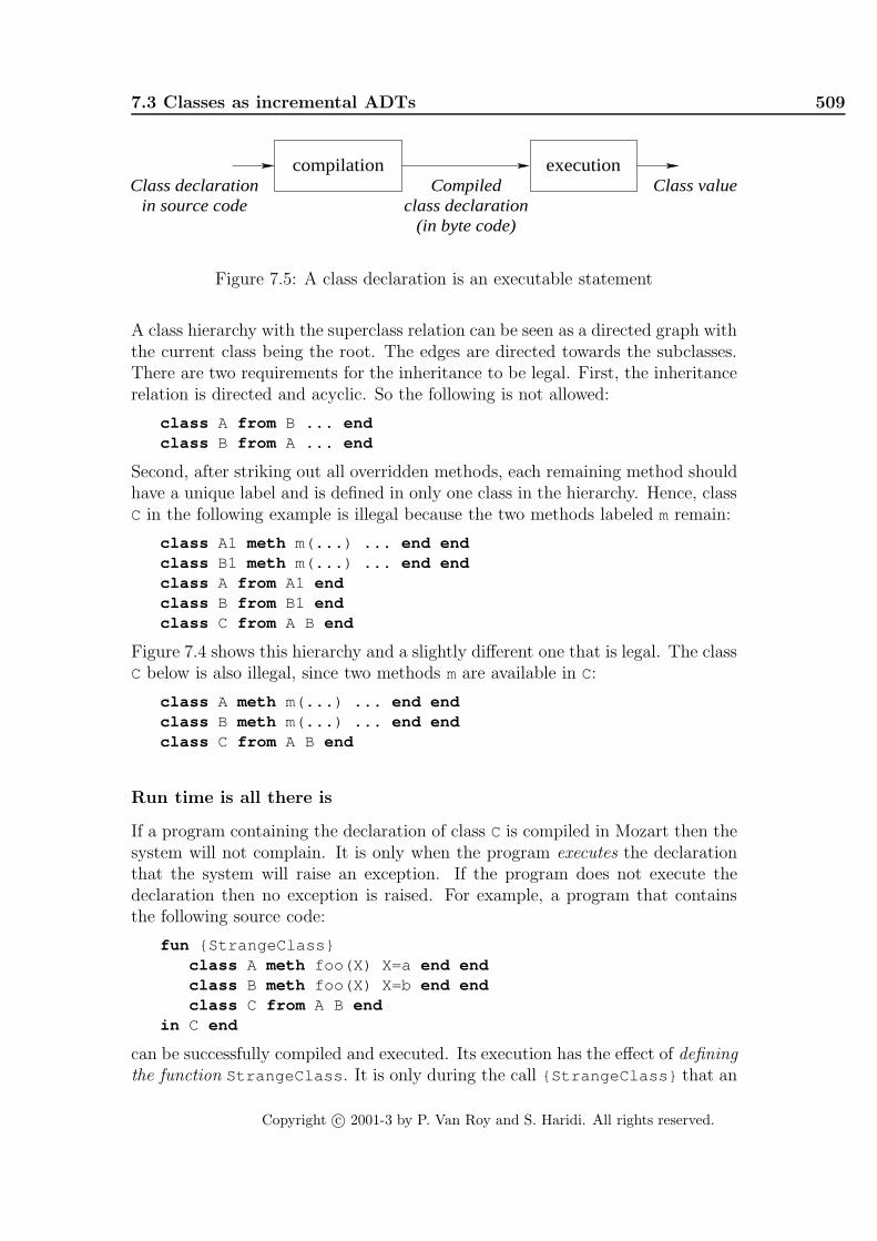
7.3 Classes as incremental ADTs 509
compilation executionClass declaration
in source code class declarationCompiled Class value
(in byte code)
Figure 7.5: A class declaration is an executable statement
A class hierarchy with the superclass relation can be seen as a directed graph withthe current class being the root. The edges are directed towards the subclasses.There are two requirements for the inheritance to be legal. First, the inheritancerelation is directed and acyclic. So the following is not allowed:
class A from B ... endclass B from A ... end
Second, after striking out all overridden methods, each remaining method shouldhave a unique label and is defined in only one class in the hierarchy. Hence, classC in the following example is illegal because the two methods labeled mremain:
class A1 meth m(...) ... end endclass B1 meth m(...) ... end endclass A from A1 endclass B from B1 endclass C from A B end
Figure 7.4 shows this hierarchy and a slightly different one that is legal. The classC below is also illegal, since two methods mare available in C:
class A meth m(...) ... end endclass B meth m(...) ... end endclass C from A B end
Run time is all there is
If a program containing the declaration of class C is compiled in Mozart then thesystem will not complain. It is only when the program executes the declarationthat the system will raise an exception. If the program does not execute thedeclaration then no exception is raised. For example, a program that containsthe following source code:
fun {StrangeClass}class A meth foo(X) X=a end endclass B meth foo(X) X=b end endclass C from A B end
in C end
can be successfully compiled and executed. Its execution has the effect of definingthe function StrangeClass . It is only during the call {StrangeClass} that an
Copyright c© 2001-3 by P. Van Roy and S. Haridi. All rights reserved.

510 Object-Oriented Programming
class Accountattr balance:0meth transfer(Amt)
balance:=@balance+Amtendmeth getBal(Bal)
Bal=@balanceendmeth batchTransfer(AmtList)
for A in AmtList do { self transfer(A)} endend
end
Figure 7.6: An example class Account
exception will be raised. This “late error detection” is not just a property of classdeclarations. It is a general property of the Mozart system that is a consequenceof the dynamic nature of the language. Namely, there is no distinction betweencompile time and run time. The object system shares this dynamic nature. Forexample, it is possible to define classes whose method labels are calculated at runtime (see Section 7.2.5).
The Mozart system blurs the distinction between run time and compile time,to the point where everything is run time. The compiler is part of the run-timesystem. A class declaration is an executable statement. Compiling and executingit creates a class, which is a value in the language (see Figure 7.5). The classvalue can be passed to New to create an object.
A programming system does not strictly need to distinguish between compiletime and run time. The distinction is simply a way to help the compiler performcertain kinds of optimization. Most mainstream languages, including C++ andJava, make this distinction. Typically, a few operations (like declarations) canbe executed only at compile time, and all other operations can be executed onlyat run time. The compiler can then execute all declarations at the same time,without any interference from the program’s execution. This allows it to domore powerful optimizations when generating code. But it greatly reduces theflexibility of the language. For example, genericity and instantiation are no longeravailable to the programmer as general tools.
Because of Mozart’s dynamic nature, the role of the compiler is very small.Since the compiler does not actually execute any declarations (it just convertsthem to executable statements), it needs very little knowledge of the languagesemantics. The compiler does in fact have some knowledge of language semantics,but this is an optimization that allows earlier detection of some errors and moreefficient compiled code. More knowledge could be added to the compiler, forexample to detect class hierarchy errors when it can deduce what the methodlabels are.
Copyright c© 2001-3 by P. Van Roy and S. Haridi. All rights reserved.

7.3 Classes as incremental ADTs 511
7.3.2 Static and dynamic binding
When executing inside an object, we often want to call another method in thesame object, i.e., do a kind of recursive invocation. This seems simple enough, butit becomes slightly more complicated when inheritance is involved. A commonuse of inheritance is to define a new ADT that extends an existing ADT. Toimplement this correctly, it turns out that we need two ways to do a recursivecall. They are called static and dynamic binding. We explain them by means ofan example.
Consider the class Account defined in Figure 7.6. This class models a simplebank account with a balance. We can transfer money to it with transfer , inspectthe balance with getBal , and do a series of transfers with batchTransfer . Notethat batchTransfer calls transfer for each transfer.
Let us extend Account to do logging, i.e., to keep a record of all transactionsit does. One way is to use inheritance, by overriding the transfer method:
class LoggedAccount from Accountmeth transfer(Amt)
{LogObj addentry(transfer(Amt))}...
endend
where LogObj is an object that keeps the log. Let us create a logged accountwith an initial balance of 100:
LogAct={New LoggedAccount transfer(100)}
Now the question is, what happens when we call batchTransfer ? Does it callthe old transfer in Account or the new transfer in LoggedAccount ? Wecan deduce what the answer must be, if we assume that a class is an ADT. EveryADT has a set of methods that define what it does. For LoggedAccount , thisset consists of the getBal and batchTransfer methods defined in Account
as well as the new transfer defined in LoggedAccount itself. Therefore, theanswer is that batchTransfer must call the new transfer in LoggedAccount .This is called dynamic binding. It is written as a call to self , i.e., as { self
transfer(A)} .
When Account was defined, there was no LoggedAccount yet. Using dy-namic binding keeps open the possibility that Account can be extended withinheritance, while ensuring that the new class is an ADT that correctly extendsthe old ADT. That is, it keeps all the functionality of the old ADT while addingsome new functionality.
However, dynamic binding is usually not enough to implement the extendedADT. To see why, let us investigate closer how the new transfer is defined.Here is the full definition:
class LoggedAccount from Accountmeth transfer(Amt)
Copyright c© 2001-3 by P. Van Roy and S. Haridi. All rights reserved.

512 Object-Oriented Programming
{LogObj addentry(transfer(Amt))}Account,transfer(Amt)
endend
Inside the new transfer , we have to call the old transfer . We cannot usedynamic binding, since this would always call the new transfer . Instead, weuse another technique called static binding. In static binding, we call a methodby pinpointing the method’s class. Here the notation Account,transfer(Amt)
pinpoints the method transfer in the class Account .Both static and dynamic binding are needed when using inheritance to over-
ride methods. Dynamic binding allows the new ADT to correctly extend the oldADT by letting old methods call new methods, even though the new method didnot exist when the old method was defined. Static binding allows new methodsto call old methods when they have to. We summarize the two techniques:
• Dynamic binding. This is written { self M}. This chooses the methodmatching Mthat is visible in the current object. This takes into account theoverriding that has been done.
• Static binding. This is written C, M (with a comma), where C is a classthat defines a method matching M. This chooses the method matching M
that is visible in the class C. This takes overriding into account from theroot class up to class C, but no further. If the object is of a subclass of C
that has overridden Magain, then this is not taken into account.
Dynamic binding is the only possible behavior for attributes. Static binding isnot possible for them since the overridden attributes simply do not exist, neitherin a logical sense (the only object that exists is the instance of the final class) norin a practical sense (the implementation allocates no memory for them).
7.3.3 Controlling encapsulation
The principle of controlling encapsulation in an object-oriented language is tolimit access to class members, namely attributes and methods, according to therequirements of the application architecture. Each member is defined with ascope. The scope is that part of the program text in which the member is visible,i.e., can be accessed by mentioning its name. Usually, the scope is staticallydefined, by the structure of the program. It can also be dynamically defined,namely during execution, if names are used (see below).
Programming languages usually give a default scope to each member whenit is declared. This default can be altered with special keywords. Typical key-words used are public, private, and protected. Unfortunately, different languagesuse these terms to define slightly different scopes. Visibility in programming lan-guages is a tricky concept. In the spirit of [54], we will try to bring order to thischaos.
Copyright c© 2001-3 by P. Van Roy and S. Haridi. All rights reserved.

7.3 Classes as incremental ADTs 513
SubSubC
I3I2 ... In
SubC
C
...
I1
to Smalltalk and Oz‘‘private’’ according
Class hierarchy
Instances
Region of visibility forobject I3: all privateattributes in this regionare visible to I3
=
to C++ and Java‘‘private’’ according
Figure 7.7: The meaning of “private”
Private and public scopes (in the ADT sense)
The two most basic scopes are private and public, with the following meanings:
• A private member is one which is only visible in the object instance. Theobject instance can see all members defined in its class and its superclasses.Thus private defines a kind of vertical visibility.
• A public member is one which is visible anywhere in the program.
In both Smalltalk and Oz, attributes are private and methods are public accordingto this definition.
These definitions of private and public are natural if classes are used to con-struct ADTs. Let us see why:
• First of all, a class is not the same thing as the ADT it defines! The classis an increment; it defines an ADT as an incremental modification of itssuperclasses. The class is only needed during the ADT’s construction. TheADT is not an increment; it stands on its own, with all its own attributesand methods. Many of these may come from the superclasses and not fromthe class.
• Second, attributes are internal to the ADT and should be invisible from theoutside. This is exactly the definition of private.
• Finally, methods make up the external interface of the ADT, so they shouldbe visible to all entities that reference the ADT. This is exactly the definitionof public.
Copyright c© 2001-3 by P. Van Roy and S. Haridi. All rights reserved.

514 Object-Oriented Programming
Constructing other scopes
Techniques for writing programs to control encapsulation are based essentially ontwo concepts: lexical scoping and name values. The private and public scopesdefined above can be implemented with these two concepts. However, many otherscopes can also be expressed using name values and lexical scoping. For example,it is possible to express the private and protected scopes of C++ and Java, as wellas write programs that have much more elaborate security policies. The basictechnique is to let method heads be name values instead of atoms. A name isan unforgeable constant; the only way to know a name is if someone gives you areference to it (see Section 3.7.5 and Appendix B.2). In this way, a program canpass the reference in a controlled way, to exactly those areas of the program inwhich it should be visible.
In the examples of the previous sections, we have used atoms as method labels.But atoms are not secure: if a third party finds out the atom’s print representation(either by guessing or by some other way) then he can call the method too. Namesare a simple way to plug this kind of security leak. This is important for a softwaredevelopment project with well-defined interfaces between different components.It is even more important for open distributed programs, where code written atdifferent times by different groups can coexist (see Chapter 11).
Private methods (in the C++ and Java sense)
When a method head is a name value, then its scope is limited to all instancesof the class, but not to subclasses or their instances. This is exactly private inthe sense of C++ and Java. Because of its usefulness, the object system of thischapter gives syntactic support for this technique. There are two ways to writeit, depending on whether the name is defined implicitly inside the class or comesfrom the outside:
• By using a variable identifier as the method head. This implicitly creates aname when the class is defined and binds it to the variable. For example:
class Cmeth A(X)
% Method bodyend
end
Method head A is bound to a name. The variable A is only visible inside theclass definition. An instance of C can call method A in any other instance ofC. Method A is invisible to subclass definitions. This is a kind of horizontalvisibility. It corresponds to the concept of private method as it exists in C++and Java (but not in Smalltalk). As Figure 7.7 shows, private in C++ andJava is very different from private in Smalltalk and Oz. In Smalltalk andOz, private is relative to an object and its classes, e.g., I3 in the figure. In
Copyright c© 2001-3 by P. Van Roy and S. Haridi. All rights reserved.

7.3 Classes as incremental ADTs 515
C++ and Java, private is relative to a class and its instances, e.g., SubSubCin the figure.
• By using an escaped variable identifier as the method head. This syntaxindicates that we will declare and bind the variable identifier outside of theclass. When the class is defined then the method head is bound to whateverthe variable is bound to. This is a very general mechanism that can be usedto protect methods in many ways. It can also be used for other purposesthan security (see Section 7.2.5). Here is an example that does exactly thesame as the previous case:
localA={NewName}
inclass C
meth !A(X)% Method body
endend
end
This creates a name at class definition time, just like in the previous case,and binds the method head to it. In fact, the previous definition is just ashort-hand for this example.
Letting the programmer determine the method label allows to define a securitypolicy at a very fine grain. The program can pass the method label to exactlythose entities who need to know it.
Protected methods (in the C++ sense)
By default, methods in the object system of this chapter are public. Using names,we can construct the concept of a protected method, including both the C++version and the Java version. In C++, a method is protected if it is accessibleonly in the class it is defined or in descendant classes (and all instance objectsof these classes). The protected concept is a combination of the Smalltalk notionof private with the C++/Java notion of private: it has both a horizontal andvertical component. Let us show how to express the C++ notion of protected.The Java notion of protected is somewhat different; we leave it to an exercise. Inthe following class, method A is protected:
class Cattr pa:Ameth A(X) skip endmeth foo(...) { self A(5)} end
end
Copyright c© 2001-3 by P. Van Roy and S. Haridi. All rights reserved.

516 Object-Oriented Programming
It is protected because the attribute pa stores a reference to A. Now create asubclass C1 of C. We can access method A as follows in the subclass:
class C1 from Cmeth b(...) A=@pa in { self A(5)} end
end
Method b accesses the method with label A through the attribute pa , which existsin the subclass. The method label can be stored in the attribute because it isjust a value.
Attribute scopes
Attributes are always private. The only way to make them public is by means ofmethods. Because of dynamic typing, it is possible to define generic methods thatgive read and write access to all attributes. The class Inspector in Section 7.2.6shows one way to do this. Any class that inherits from Inspector will have allits attributes potentially be public. Atom attributes are not secure since theycan be guessed. Name attributes are secure even when using Inspector , sincethey cannot be guessed.
Atoms or names as method heads?
When should one use an atom or a name as a method head? By default, atomsare visible throughout the whole program and names are visible only in the lexicalscope of their creation. We can give a simple rule when implementing ADTs: forinternal methods use names and for external methods use atoms.
Most popular object-oriented programming languages (e.g., Smalltalk, C++,and Java) support only atoms as method heads, not names. These languagesmake atoms usable by adding special operations to restrict their visibility (e.g.,private and protected declarations). On the other hand, names are practicaltoo. Their visibility can be extended by passing around references. But thecapability-based approach exemplified by names has not yet become popular.Let us look more closely at the trade-offs in using names versus atoms.
Atoms are uniquely identified by their print representations. This means theycan be stored in program source files, in emails, on Web pages, etc. In particular,they can be stored in the programmer’s head! When writing a large program, amethod can be called from anywhere by just giving its print representation. Onthe other hand, with names this is more awkward: the program itself has somehowto pass the name to the caller. This adds some complexity to the program aswell as being a burden for the programmer. So atoms win out both for programsimplicity and for the psychological comfort factor during development.
Names have other advantages. First, it is impossible to have conflicts withinheritance (either single or multiple). Second, encapsulation can be better man-aged, since an object reference does not necessarily have the right to call all the
Copyright c© 2001-3 by P. Van Roy and S. Haridi. All rights reserved.

7.3 Classes as incremental ADTs 517
Inheritance
‘‘Static’’ approach:at class definition time
‘‘Dynamic’’ approaches:at object creation time
Loose bindingTight binding between original object/classand derived object/class
common self no common selfcommon self
defined on classes defined on objects defined on objects
ForwardingDelegation
Figure 7.8: Different ways to extend functionality
object’s methods. Therefore, the program as a whole can be made less error-prone and better structured. A final point is that names can be given syntacticsupport to simplify their use. For example, in the object system of this chapterit suffices to capitalize the method head.
7.3.4 Forwarding and delegation
Inheritance is one way to reuse already-defined functionality when defining newfunctionality. Inheritance can be tricky to use well, because it implies a tightbinding between the original class and its extension. Sometimes it is better touse looser approaches. Two such approaches are forwarding and delegation. Bothare defined at the level of objects: if object Obj1 does not understand messageM, then M is passed transparently to object Obj2 . Figure 7.8 compares theseapproaches with inheritance.
Forwarding and delegation differ in how they treat self . In forwarding, Obj1
and Obj2 keep their separate identities. A self call in Obj2 will stay in Obj2 . Indelegation, there is just one identity, namely that of Obj1 . A self call in Obj2
will call Obj1 . We say that delegation, like implementation inheritance, impliesa common self. Forwarding does not imply a common self.
Let us show how to express forwarding and delegation. We define specialobject creation functions, NewF and NewD, for forwarding and delegation. Weare helped in this by the flexibility of our object system: we use the otherwise
method, messages as values, and the dynamic creation of classes. We start withforwarding since it is the simplest.
Copyright c© 2001-3 by P. Van Roy and S. Haridi. All rights reserved.

518 Object-Oriented Programming
Forwarding
An object can forward to any other object. In the object system of this chapter,this can be implemented with the otherwise(M) method (see Section 7.2.5).The argument Mis a first-class message that can be passed to another object. Letus define NewF, a version of New that creates objects that can forward:
localclass ForwardMixin
attr Forward:nonemeth setForward(F) Forward:=F endmeth otherwise(M)
if @Forward==none then raise undefinedMethod endelse {@Forward M} end
endend
infun {NewF Class Init}
{New class $ from Class ForwardMixin end Init}end
end
Objects created with NewF have a method setForward(F) that lets them setdynamically the object to which they will forward messages they do not under-stand. Let us create two objects Obj1 and Obj2 such that Obj2 forwards toObj1 :
class C1meth init skip endmeth cube(A B) B=A*A*A end
end
class C2meth init skip endmeth square(A B) B=A*A end
end
Obj1={NewF C1 init}Obj2={NewF C2 init}{Obj2 setForward(Obj1)}
Doing {Obj2 cube(10 X)} will cause Obj2 to forward the message to Obj1 .
Delegation
Delegation is a powerful way to structure a system dynamically [113]. It lets usbuild a hierarchy among objects instead of among classes. Instead of an objectinheriting from a class (at class definition time), we let an object delegate toanother object (at object creation time). Delegation can achieve the same effects
Copyright c© 2001-3 by P. Van Roy and S. Haridi. All rights reserved.

7.3 Classes as incremental ADTs 519
localSetSelf={NewName}class DelegateMixin
attr this Delegate:nonemeth !SetSelf(S) this:=S endmeth set(A X) A:=X endmeth get(A ?X) X=@A endmeth setDelegate(D) Delegate:=D endmeth Del(M S) SS in
SS=@this this:=Stry { self M} finally this:=SS end
endmeth call(M) SS in
SS=@this this:= selftry { self M} finally this:=SS end
endmeth otherwise(M)
if @Delegate==none thenraise undefinedMethod end
else{@Delegate Del(M @this)}
endend
endin
fun {NewD Class Init}Obj={New class $ from Class DelegateMixin end Init}
in{Obj SetSelf(Obj)}Obj
endend
Figure 7.9: Implementing delegation
Copyright c© 2001-3 by P. Van Roy and S. Haridi. All rights reserved.

520 Object-Oriented Programming
as inheritance, with two main differences: the hierarchy is between objects, notclasses, and it can be changed at any time.
Given any two objects Obj1 and Obj2 , we suppose there exists a methodsetDelegate such that {Obj2 setDelegate(Obj1)} sets Obj2 to delegate toObj1 . In other words, Obj1 behaves as the “superclass” of Obj2 . Whenever amethod is invoked that is not defined in Obj2 , the method call will be retriedat Obj1 . The delegation chain can grow to any length. If there is an Obj3 thatdelegates to Obj2 , then calling Obj3 can climb up the chain all the way to Obj1 .
An important property of the delegation semantics is that self is always pre-served: it is the self of the original object that initiated the delegation chain. Itfollows that the object state (the attributes) is also the state of the original object.In that sense, the other objects play the role of classes: in a first instance, it istheir methods that are important in delegation, not the values of their attributes.
Let us implement delegation using our object system. Figure 7.9 gives theimplementation of NewD, which is used instead of Newto create objects. In orderto use delegation, we impose the following syntactic constraints on how the objectsystem must be used:
Operation Original syntax Delegation syntaxObject call { 〈obj〉 M} { 〈obj〉 call(M)}
Self call { self M} {@this M}
Get attribute @〈attr〉 {@this get( 〈attr〉 $)}
Set attribute 〈attr〉:=X {@this set( 〈attr〉 X)}
Set delegate { 〈obj〉1 setDelegate( 〈obj〉2)}
These syntactic constraints could be eliminated by an appropriate linguistic ab-straction. Now let us give a simple example of how delegation works. We definetwo objects Obj1 and Obj2 and let Obj2 delegate to Obj1 . We give each objectan attribute i and a way to increment it. With inheritance this would look asfollows:
class C1NonDelattr i:0meth init skip endmeth inc(I) i:=@i+I endmeth browse { self inc(10)} {Browse c1#@i} endmeth c { self browse} end
end
class C2NonDel from C1NonDelattr i:0meth init skip endmeth browse { self inc(100)} {Browse c2#@i} end
end
With our delegation implementation we can get the same effect by using the codeof Figure 7.10. It is more verbose, but that is only because the system has no
Copyright c© 2001-3 by P. Van Roy and S. Haridi. All rights reserved.

7.3 Classes as incremental ADTs 521
class C1attr i:0meth init skip endmeth inc(I)
{@this set(i {@this get(i $)}+I)}endmeth browse
{@this inc(10)}{Browse c1#{@this get(i $)}}
endmeth c {@this browse} end
endObj1={NewD C1 init}
class C2attr i:0meth init skip endmeth browse
{@this inc(100)}{Browse c2#{@this get(i $)}}
endendObj2={NewD C2 init}{Obj2 setDelegate(Obj1)}
Figure 7.10: An example of delegation
syntactic support for delegation. It is not due to the concept itself. Note thatthis just scratches the surface of what we could do with delegation. For example,by calling setDelegate again we could change the hierarchy of the program atrun-time. Let us now call Obj1 and Obj2 :
{Obj2 call(c)}{Obj1 call(c)}
Doing these calls several times shows that each object keeps its own local state,that Obj2 “inherits” the inc and c methods from object Obj1 , and that Obj2
“overrides” the browse method. Let us make the delegation chain longer:
class C2battr i:0meth init skip end
endObjX={NewD C2b init}{ObjX setDelegate(Obj2)}
ObjX inherits all its behavior from Obj2 . It is identical to Obj2 except that ithas a different local state. The delegation hierarchy now has three levels: ObjX ,Obj2 , and Obj1 . Let us change the hierarchy by letting ObjX delegate to Obj1 :
Copyright c© 2001-3 by P. Van Roy and S. Haridi. All rights reserved.

522 Object-Oriented Programming
{ObjX setDelegate(Obj1)}{ObjX call(c)}
In the new hierarchy, ObjX inherits its behavior from Obj1 . It uses the browse
method of Obj1 , so it will increment by 10 instead of by 100.
7.3.5 Reflection
A system is reflective if it can inspect part of its execution state while it isrunning. Reflection can be purely introspective (only reading the internal state,without modifying it) or intrusive (both reading and modifying the internal state).Reflection can be done at a high or low level of abstraction. One example ofreflection at a high level would be the ability to see the entries on the semanticstack as closures. It can be explained simply in terms of the abstract machine.On the other hand, the ability to read memory as an array of integers is reflectionat a low level. There is no simple way to explain it in the abstract machine.
Meta-object protocols
Object-oriented programming, because of its richness, is a particularly fertile areafor reflection. For example, the system could make it possible to examine or evenchange the inheritance hierarchy, while a program is running. This is possiblein Smalltalk. The system could make it possible to change how objects executeat a basic level, e.g., how inheritance works (how method lookup is done in theclass hierarchy) and how methods are called. The description of how an objectsystem works at a basic level is called a meta-object protocol. The ability tochange the meta-object protocol is a powerful way to modify an object system.Meta-object protocols are used for many purposes: debugging, customizing, andseparation of concerns (e.g., transparently adding encryption or format changesto method calls). Meta-object protocols were originally invented in the contextof the Common Lisp Object System (CLOS) [100, 140]. They are an active areaof research in object-oriented programming.
Method wrapping
A common use of meta-object protocols is to do method wrapping, that is, tointercept each method call, possibly performing a user-defined operation beforeand after the call and possibly changing the arguments to the call itself. In ourobject system, we can implement this in a simple way by taking advantage ofthe fact that objects are one-argument procedures. For example, let us write atracer to track the behavior of an object-oriented program. The tracer shoulddisplay the method label whenever we enter a method and exit a method. Hereis a version of New that implements this:
fun {TraceNew Class Init}Obj={New Class Init}
Copyright c© 2001-3 by P. Van Roy and S. Haridi. All rights reserved.

7.3 Classes as incremental ADTs 523
proc {TracedObj M}{Browse entering({Label M})}{Obj M}{Browse exiting({Label M})}
endin TracedObj end
An object created with TraceNew behaves identically to an object created withNew, except that method calls (except for calls to self ) are traced. The defi-nition of TraceNew uses higher-order programming: the procedure TracedObj
has the external reference Obj . This definition can easily be extended to do moresophisticated wrapping. For example, the message M could be transformed insome way before being passed to Obj .
A second way to implement TraceNew is to do the wrapping with a classinstead of a procedure. This traces all method calls including calls to self . Thisgives the following definition:
fun {TraceNew2 Class Init}Obj={New Class Init}TInit={NewName}class Tracer
meth !TInit skip endmeth otherwise(M)
{Browse entering({Label M})}{Obj M}{Browse exiting({Label M})}
endend
in {New Tracer TInit} end
This uses dynamic class creation, the otherwise method, and a fresh nameTInit for the initialization method to avoid conflicts with other method labels.
Reflection of object state
Let us show a simple but useful example of reflection in object-oriented program-ming. We would like to be able to read and write the whole state of an object,independent of the object’s class. The Mozart object system provides this abilitythrough the class ObjectSupport.reflect . Inheriting from this class gives thefollowing three additional methods:
• clone(X) creates a clone of self and binds it to X. The clone is a newobject with the same class and the same values of attributes.
• toChunk(X) binds to X a protected value (a “chunk”) that contains thecurrent values of the attributes.
• fromChunk(X) sets the object state to X, where X was obtained from aprevious call of toChunk .
Copyright c© 2001-3 by P. Van Roy and S. Haridi. All rights reserved.
524 Object-Oriented Programming
A chunk is like a record but with a restricted set of operations. It is protected inthe sense that only authorized programs can look inside it (see Appendix B.4).Chunks can be implemented with procedure values and names, as explained inSection 3.7.5. Let us extend the Counter class we saw before to do state reflec-tion:
class Counter from ObjectSupport.reflectattr valmeth init(Value)
val:=Valueendmeth browse
{Browse @val}endmeth inc(Value)
val:=@val+Valueend
end
We can define two objects:
C1={New Counter init(0)}C2={New Counter init(0)}
and then transfer state from one to the other:
{C1 inc(10)}local X in {C1 toChunk(X)} {C2 fromChunk(X)} end
At this point C2 also has the value 10. This is a simplistic example, but statereflection is actually a very powerful tool. It can be used to build generic ab-stractions on objects, i.e., abstractions that work on objects of any class.
7.4 Programming with inheritance
All the programming techniques of stateful programming and declarative pro-gramming are still possible in the object system of this chapter. Particularly use-ful are techniques that are based on encapsulation and state to make programsmodular. See the previous chapter, and especially the discussion of component-based programming, which relies on encapsulation.
This section focuses on the new techniques that are made possible by object-oriented programming. All these techniques center around the use of inheritance:first, using it correctly, and then, taking advantage of its power.
7.4.1 The correct use of inheritance
There are two ways to view inheritance:
Copyright c© 2001-3 by P. Van Roy and S. Haridi. All rights reserved.

7.4 Programming with inheritance 525
VerboseAccount
Account
AccountWithFee
Figure 7.11: A simple hierarchy with three classes
• The type view. In this view, classes are types and subclasses are subtypes.For example, take a LabeledWindow class that inherits from a Window
class. All labeled windows are also windows. The type view is consistentwith the principle that classes should model real-world entities or someabstract versions of them. In the type view, classes satisfy the substitutionproperty: every operation that works for an object of class C also works forobjects of a subclass of C. Most object-oriented languages, such as Java andSmalltalk, are designed for the type view [63, 60]. Section 7.4.1 exploreswhat happens if we do not respect the type view.
• The structure view. In this view, inheritance is just another program-ming tool that is used to structure programs. This view is strongly dis-couraged because classes no longer satisfy the substitution property. Thestructure view is an almost unending source of bugs and bad designs. Ma-jor commercial projects, which shall here remain anonymous, have failed forthis reason. A few object-oriented languages, notably Eiffel, are designedfrom the start to allow both the type and structure views [122].
In the type view, each class stands on its own two feet, so to speak, as a bona fideADT. This is even true for classes that have subclasses; from the viewpoint ofthe subclass, the class is an ADT, with sole access through the methods and itsattributes hidden. In the structure view, classes are sometimes just scaffolding,which exists only for its role in structuring the program.
In the vast majority of cases, inheritance should respect the type view. Doingotherwise gives subtle and pernicious bugs that can poison a whole system. Letus give an example. We take as base class the Account class we saw before,which is defined in Figure 7.6. We will extend it in two ways. The first extensionis conservative, i.e., it respects the type view:
class VerboseAccount from Account
Copyright c© 2001-3 by P. Van Roy and S. Haridi. All rights reserved.

526 Object-Oriented Programming
meth verboseTransfer(Amt){ self transfer(Amt)}{Browse ´ Balance: ´ #@balance}
endend
We simply add a new method verboseTransfer . Since the existing methodsare not changed, this implies that a VerboseAccount object will work correctlyin all cases where an Account object works. Let us now do a second, moredangerous extension:
class AccountWithFee from VerboseAccountattr fee:5meth transfer(Amt)
VerboseAccount,transfer(Amt-@fee)end
end
Figure 7.11 shows the resulting hierarchy. The open arrowhead in this figure isthe usual notation to represent an inheritance link. AccountWithFree overridesthe method transfer . Overriding is not a problem in of itself. The problemis that an AccountWithFee object does not work correctly when viewed as anAccount object. They do not satisfy the same invariant. Consider the sequenceof three calls:
{A getBalance(B)}{A transfer(S)}{A getBalance(B2)}
If A is an Account object, this implies B+S=B2. If A is an AccountWithFee
object, this implies B+S-@fee=B2 . This will break any program that relies onthe behavior of Account objects. Typically, the origin of the break will notbe obvious, since it is carefully hidden inside a method somewhere in a largeapplication. It will appear long after the change was made, as a slight imbalancein the books. Debugging such “slight” problems is amazingly difficult and time-consuming.
The rest of this section primarily considers the type view. Almost all usesof inheritance should respect the type view. However, the structure view is oc-casionally useful. Its main use is in changing the behavior of the object systemitself. For this purpose, it should be used only by expert language implementorswho clearly understand the ramifications of what they are doing. A simple ex-ample is method wrapping (see Section 7.3.5), which requires using the structureview. For more information, we recommend [122] for a deeper discussion of thetype view versus the structure view.
A cautionary tale
We end the discussion on the correct use of inheritance with a cautionary tale.Some years ago, a well-known company initiated an ambitious project based
Copyright c© 2001-3 by P. Van Roy and S. Haridi. All rights reserved.

7.4 Programming with inheritance 527
NilClass ConsClass
ListClass
Figure 7.12: Constructing a hierarchy by following the type
on object-oriented programming. Despite a budget of several billion dollars, theproject failed. Among many reasons for the failure was an incorrect use of object-oriented programming, in particular concerning inheritance. Two major mistakeswere made:
• The substitution property was regularly violated. Routines that workedcorrectly with objects of a given class did not work with objects of a sub-class. This made it much more difficult to use objects: instead of oneroutine being sufficient for many classes, many routines were needed.
• Classes were subclassed to fix small problems. Instead of fixing the classitself, a subclass was defined to patch the class. This was done so frequentlythat it gave layers upon layers of patches. Object invocations were sloweddown by an order of magnitude. The class hierarchy became unnecessarilydeep, which increased complexity of the system.
The lesson to heed is to be careful to use inheritance in a correct way. Respect thesubstitution property whenever possible. Use inheritance to add new functionalityand not to patch a broken class. Study common design patterns to learn thecorrect use of inheritance.
Reengineering At this point, we should mention the discipline of reengineer-ing, which can be used to fix architectural problems like these two incorrect usesof inheritance [44, 15]. The general goal of reengineering is to take an existing sys-tem and attempt to improve some of its properties by changing the source code.Many properties can be improved in this way: system architecture, modularity,performance, portability, quality of documentation, and use of new technology.However, reengineering cannot resurrect a failed project. It is more like curing adisease. If the designer has a choice, the best approach remains to prevent thedisease, i.e., to design a system so that it can be adapted to changing require-ments. In Section 6.7 and throughout the book, we give design principles thatwork towards this goal.
Copyright c© 2001-3 by P. Van Roy and S. Haridi. All rights reserved.

528 Object-Oriented Programming
class ListClassmeth isNil(_) raise undefinedMethod end endmeth append(_ _) raise undefinedMethod end endmeth display raise undefinedMethod end end
end
class NilClass from ListClassmeth init skip endmeth isNil(B) B= true endmeth append(T U) U=T endmeth display {Browse nil} end
end
class ConsClass from ListClassattr head tailmeth init(H T) head:=H tail:=T endmeth isNil(B) B= false endmeth append(T U)
U2={@tail append(T $)}in
U={New ConsClass init(@head U2)}endmeth display {Browse @head} {@tail display} end
end
Figure 7.13: Lists in object-oriented style
7.4.2 Constructing a hierarchy by following the type
When writing programs with recursion, we saw in Section 3.4.2 that it is a goodidea to define first the type of the data structure, and then to construct therecursive program by following the type. We can use a similar idea to constructinheritance hierarchies. For example, consider the list type 〈List T〉, which isdefined as:
〈List T〉 ::= nil
| T ´ | ´ 〈List T〉
This says that a list is either nil or a list pair. Let us implement the list ADTin the class ListClass . Following the type definition means that we define twoother classes that inherit from ListClass , which we can call NilClass andConsClass . Figure 7.12 shows the hierarchy. This hierarchy is a natural designto respect the substitution principle. An instance of NilClass is a list, so it iseasy to use it wherever a list is required. The same holds for ConsClass .
Figure 7.13 defines a list ADT that follows this hierarchy. In this figure,ListClass is an abstract class: a class in which some methods are left unde-fined. Trying to call the methods isNil , append , and display will raise an
Copyright c© 2001-3 by P. Van Roy and S. Haridi. All rights reserved.

7.4 Programming with inheritance 529
class GenericSortmeth init skip endmeth qsort(Xs Ys)
case Xsof nil then Ys = nil[] P|Xr then S L in
{ self partition(Xr P S L)}{Append { self qsort(S $)}
P|{ self qsort(L $)} Ys}end
endmeth partition(Xs P Ss Ls)
case Xsof nil then Ss=nil Ls=nil[] X|Xr then Sr Lr in
if { self less(X P $)} thenSs=X|Sr Ls=Lr
elseSs=Sr Ls=X|Lr
end{ self partition(Xr P Sr Lr)}
endend
end
Figure 7.14: A generic sorting class (with inheritance)
exception. Abstract classes are not intended to be instantiated, since they lacksome methods. The idea is to define another class that inherits from the ab-stract class and that adds the missing methods. This gives a concrete class,which can be instantiated since it defines all the methods it calls. NilClass andConsClass are concrete classes. They define the methods isNil , append , anddisplay . The call {L1 append(L2 L3)} binds L3 to the concatenation of L1
and L2 , without changing L1 or L2 . The call {L display} displays the list. Letus now do some calculations with lists:
L1={New ConsClassinit(1 {New ConsClass
init(2 {New NilClass init})})}L2={New ConsClass init(3 {New NilClass init})}L3={L1 append(L2 $)}{L3 display}
This creates two lists L1 and L2 and concatenates them to form L3 . It thendisplays the contents of L3 in the browser, as 1, 2, 3, nil .
Copyright c© 2001-3 by P. Van Roy and S. Haridi. All rights reserved.

530 Object-Oriented Programming
class IntegerSort from GenericSortmeth less(X Y B)
B=(X<Y)end
end
class RationalSort from GenericSortmeth less(X Y B)
´ / ´ (P Q)=X´ / ´ (R S)=Y
in B=(P*S<Q*R) endend
Figure 7.15: Making it concrete (with inheritance)
IntegerSort RationalSort
GenericSort
Figure 7.16: A class hierarchy for genericity
Copyright c© 2001-3 by P. Van Roy and S. Haridi. All rights reserved.

7.4 Programming with inheritance 531
fun {MakeSort Less}class $
meth init skip endmeth qsort(Xs Ys)
case Xsof nil then Ys = nil[] P|Xr then S L in
{ self partition(Xr P S L)}{Append { self qsort(S $)}
P|{ self qsort(L $)} Ys}end
endmeth partition(Xs P Ss Ls)
case Xsof nil then Ss=nil Ls=nil[] X|Xr then Sr Lr in
if {Less X P} thenSs=X|Sr Ls=Lr
elseSs=Sr Ls=X|Lr
end{ self partition(Xr P Sr Lr)}
endend
endend
Figure 7.17: A generic sorting class (with higher-order programming)
7.4.3 Generic classes
A generic class is one that only defines part of the functionality of an ADT. It hasto be completed before it can be used to create objects. Let us look at two ways todefine generic classes. The first way, often-used in object-oriented programming,uses inheritance. The second way uses higher-order programming. We will seethat the first way is just a syntactic variation of the second. In other words,inheritance can be seen as a programming style that is based on higher-orderprogramming.
Using inheritance
A common way to make classes more generic in object-oriented programmingis to use abstract classes. For example, Figure 7.14 defines an abstract classGenericSort for sorting a list. This class uses the quicksort algorithm, whichneeds a boolean comparison operation. The boolean operation’s definition de-pends on the type of data that is sorted. Other classes can inherit from GenericSort
Copyright c© 2001-3 by P. Van Roy and S. Haridi. All rights reserved.
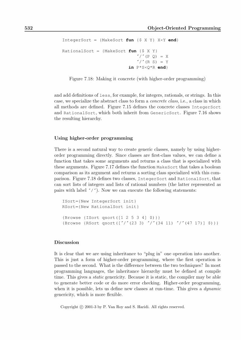
532 Object-Oriented Programming
IntegerSort = {MakeSort fun {$ X Y} X<Y end }
RationalSort = {MakeSort fun {$ X Y}´ / ´ (P Q) = X´ / ´ (R S) = Y
in P*S<Q*R end }
Figure 7.18: Making it concrete (with higher-order programming)
and add definitions of less , for example, for integers, rationals, or strings. In thiscase, we specialize the abstract class to form a concrete class, i.e., a class in whichall methods are defined. Figure 7.15 defines the concrete classes IntegerSort
and RationalSort , which both inherit from GenericSort . Figure 7.16 showsthe resulting hierarchy.
Using higher-order programming
There is a second natural way to create generic classes, namely by using higher-order programming directly. Since classes are first-class values, we can define afunction that takes some arguments and returns a class that is specialized withthese arguments. Figure 7.17 defines the function MakeSort that takes a booleancomparison as its argument and returns a sorting class specialized with this com-parison. Figure 7.18 defines two classes, IntegerSort and RationalSort , thatcan sort lists of integers and lists of rational numbers (the latter represented aspairs with label ´ / ´ ). Now we can execute the following statements:
ISort={New IntegerSort init}RSort={New RationalSort init}
{Browse {ISort qsort([1 2 5 3 4] $)}}{Browse {RSort qsort([ ´ / ´ (23 3) ´ / ´ (34 11) ´ / ´ (47 17)] $)}}
Discussion
It is clear that we are using inheritance to “plug in” one operation into another.This is just a form of higher-order programming, where the first operation ispassed to the second. What is the difference between the two techniques? In mostprogramming languages, the inheritance hierarchy must be defined at compiletime. This gives a static genericity. Because it is static, the compiler may be ableto generate better code or do more error checking. Higher-order programming,when it is possible, lets us define new classes at run-time. This gives a dynamicgenericity, which is more flexible.
Copyright c© 2001-3 by P. Van Roy and S. Haridi. All rights reserved.

7.4 Programming with inheritance 533
7.4.4 Multiple inheritance
Multiple inheritance is useful when an object has to be two different things inthe same program. For example, consider a graphical display that can show avariety of geometrical figures, including circles, lines, and more complex figures.We would like to define a “grouping” operation that can combine any numberof figures into a single, composite figure. How can we model this with object-oriented programming? We will design a simple, fully working program. We willuse multiple inheritance to add the grouping ability to figures. The idea for thisdesign comes from Bertrand Meyer [122]. This program can easily be extendedto a full-fledged graphics package.
Geometric figures
We first define the class Figure to model geometric figures, with methods init
(initialize the figure), move(X Y) (move the figure), and display (display thefigure):
class Figuremeth otherwise(M)
raise undefinedMethod endend
end
This is an abstract class; any attempt to invoke its methods will raise an excep-tion. Actual figures are instances of subclasses of Figure . For example, here isa Line class:
class Line from Figureattr canvas x1 y1 x2 y2meth init(Can X1 Y1 X2 Y2)
canvas:=Canx1:=X1 y1:=Y1x2:=X2 y2:=Y2
endmeth move(X Y)
x1:=@x1+X y1:=@y1+Yx2:=@x2+X y2:=@y2+Y
endmeth display
{@canvas create(line @x1 @y1 @x2 @y2)}end
end
and here is a Circle class:
class Circle from Figureattr canvas x y rmeth init(Can X Y R)
canvas:=Can
Copyright c© 2001-3 by P. Van Roy and S. Haridi. All rights reserved.

534 Object-Oriented Programming
LinkedList
elemnext
initadd(F)
forall(P)
displaymove(X Y)
init
displaymove(X Y)
init
displaymove(X Y)
init
Figure
Methods
Attributes
Inheritance
Line
canvas
x2, y2x1, y1
Circle
canvasx, y
r
CompositeFigure
Figure 7.19: Class diagram of the graphics package
x:=X y:=Y r:=Rendmeth move(X Y)
x:=@x+X y:=@y+Yendmeth display
{@canvas create(oval @x-@r @y-@r @x+@r @y+@r)}end
end
Figure 7.19 shows how Line and Circle inherit from Figure . This kind ofdiagram is called a class diagram. It is a part of UML, the Uniform Model-ing Language, a widely-used set of techniques for modeling object-oriented pro-grams [54]. Class diagrams are a useful way to visualize the class structure ofan object-oriented program. Each class is represented by a rectangle with threeparts, containing the class name, the attributes it defines, and the methods itdefines. These rectangles can be connected with lines representing inheritancelinks.
Linked lists
We define the class LinkedList to group figures together, with methods init
(initialize the linked list), add(F) (add a figure), and forall(M) (execute {F
M} for all figures):
class LinkedListattr elem next
Copyright c© 2001-3 by P. Van Roy and S. Haridi. All rights reserved.

7.4 Programming with inheritance 535
meth init(elem:E<=null next:N<=null)elem:=E next:=N
endmeth add(E)
next:={New LinkedList init(elem:E next:@next)}endmeth forall(M)
if @elem\=null then {@elem M} endif @next\=null then {@next forall(M)} end
endend
The forall(M) method is especially interesting because it uses first-class mes-sages. A linked list is represented as a sequence of instances of this class. Thenext field of each instance refers to the next one in the list. The last elementhas the next field equal to null . There is always at least one element in thelist, called the header. The header is not an element that it seen by users of thelinked list; it is just needed for the implementation, The header always has theelem field equal to null . Therefore an empty linked list corresponds to a headernode with both elem and next fields equal to null .
Composite figures
What is a composite figure? It is both a figure and a linked list of figures. There-fore we define a class CompositeFigure that inherits from both Figure andLinkedList :
class CompositeFigure from Figure LinkedListmeth init
LinkedList,initendmeth move(X Y)
{ self forall(move(X Y))}endmeth display
{ self forall(display)}end
end
Figure 7.19 shows the multiple inheritance. The multiple inheritance is correctbecause the two functionalities are completely different and have no undesir-able interaction. The init method is careful to initialize the linked list. Itdoes not need to initialize the figure. As in all figures, there is a move and adisplay method. The move(X Y) method moves all figures in the linked list.The display method displays all figures in the linked list.
Do you see the beauty of this design? With it, a figure can consist of otherfigures, some of which consist of other figures, and so forth, to any number of
Copyright c© 2001-3 by P. Van Roy and S. Haridi. All rights reserved.

536 Object-Oriented Programming
Figure 7.20: Drawing in the graphics package
levels. The inheritance structure guarantees that moving and displaying willalways work correctly.
Example execution
Let us run this example. First, we set up a window with a graphics display field:
declareW=250 H=150 CanWindow={QTk.build td(canvas(width:W height:H bg:white handle:Can))}{Window show}
This uses the QTk graphics tool, which is explained in Chapter 10. For now justassume that this sets up a canvas, which is the drawing field for our geometricfigures. Next, we define a composite figure F1 containing a triangle and a circle:
declareF1={New CompositeFigure init}{F1 add({New Line init(Can 50 50 150 50)})}{F1 add({New Line init(Can 150 50 100 125)})}{F1 add({New Line init(Can 100 125 50 50)})}{F1 add({New Circle init(Can 100 75 20)})}
We can display this figure as follows:
{F1 display}
This displays the figure once. Let us move the figure around and display it eachtime:
for I in 1..10 do {F1 display} {F1 move(3 ˜2)} end
Figure 7.20 shows the result.
Copyright c© 2001-3 by P. Van Roy and S. Haridi. All rights reserved.

7.4 Programming with inheritance 537
Figure
LinkedList
elemnext
initadd(F)
forall(P)
CompositeFigure
init
figlist
move(X Y)display
add(F)
Association
1 1
Figure 7.21: Class diagram with an association
Composite figures with single inheritance
Instead of defining CompositeFigure with multiple inheritance, we can define itusing single inheritance by putting the list of figures in an attribute. This gives:
class CompositeFigure from Figureattr figlistmeth init
figlist:={New LinkedList init}endmeth add(F)
{@figlist add(F)}endmeth move(X Y)
{@figlist forall(move(X Y))}endmeth display
{@figlist forall(display)}end
end
Figure 7.21 shows the class diagram for this case. The link between CompositeFigure
and LinkedList is called an association. It represents a relationship betweenthe two classes. The numbers attached to the two ends are cardinalities; eachnumber says how many elements there are for a particular instance. The number1 on the linked list side means that there is exactly one linked list per compositefigure, and similarly for the other side. The association link is a specification;it does not say how it is implemented. In our case, each composite figure has afiglist attribute that references a linked list.
The example execution we gave before will also work in the single inheri-tance case. What are the trade-offs in using single or multiple inheritance in this
Copyright c© 2001-3 by P. Van Roy and S. Haridi. All rights reserved.

538 Object-Oriented Programming
example? In both cases, the figures that make up the composite figure are encap-sulated. The main difference is that multiple inheritance brings the operations oflinked lists up to the same level as figures:
• With multiple inheritance, a composite figure is also a linked list. Allthe operations of the LinkedList class can be used directly on compositefigures. This is important if we want to do linked list calculations withcomposite figures.
• With single inheritance, a composite figure completely hides its structure.This is important if we want to protect the composite figure from anycalculations other than those defined in its class.
Scaling it up
It is straightforward to extend this example to be a full-fledged graphics package.Here are some of the changes that should be made:
• Many more figures can be defined to inherit from Figure .
• In the current implementation, figures are tied to their canvas. This hasthe advantage that it allows figures to be spread over multiple canvasses.But usually we will not want this ability. Rather, we would like to be ableto draw the same figure on different canvasses. This means that the canvasshould not be an attribute of figure objects but be passed as argument tothe display method.
• A journaling facility can be added. That is, it should be possible to recordsequences of drawing commands, i.e., sequences of calls to figures, and ma-nipulate the recordings as first-class entities. These recordings representdrawings at a high level of abstraction. They can then be manipulated bythe application, stored on files, passed to other applications, etc.
• The display method should be able to pass arbitrary parameters fromthe application program, through the graphics package, to the underlyinggraphics subsystem. In the Line and Circle classes, we change it asfollows:
meth display(...)=M{@canvas {Adjoin M create(line @x1 @y1 @x2 @y2)}}
end
The Adjoin operation combines two record arguments, where the secondargument overrides the first in the case of conflicts. This allows arbitraryparameters to be passed through display to the canvas drawing command.For example, the call {F display(fill:red width:3)} draws a red fig-ure of width 3.
Copyright c© 2001-3 by P. Van Roy and S. Haridi. All rights reserved.

7.4 Programming with inheritance 539
7.4.5 Rules of thumb for multiple inheritance
Multiple inheritance is a powerful technique that has to be used with care. Werecommend that you use multiple inheritance as follows:
• Multiple inheritance works well when combining two completely indepen-dent abstractions. For example, figures and linked lists have nothing incommon, so they can be combined fruitfully.
• Multiple inheritance is much harder to use correctly when the abstractionshave something in common. For example, creating a WorkStudy class fromStudent and Employee is dubious, because students and employees areboth human beings. They may in fact both inherit from a common Person
class. Even if they do not have a shared ancestor, there can be problems ifthey have some concepts in common.
• What happens when sibling superclasses share (directly or indirectly) acommon ancestor class that specifies a stateful object (i.e., it has attributes)?This is known as the implementation-sharing problem. This can lead to du-plicated operations on the common ancestor. This typically happens wheninitializing an object. The initialization method usually has to initialize itssuperclasses, so the common ancestor is initialized twice. The only remedyis to understand carefully the inheritance hierarchy to avoid such duplica-tion. Alternatively, you should only inherit from multiple classes that donot share a stateful common ancestor.
• When name clashes occur, i.e., the same method label is used for adjacentsuperclasses, then the program must define a local method that overridesthe conflict-causing methods. Otherwise the object system gives an errormessage. A simple way to avoid name clashes is to use name values asmethod heads. This is a useful technique for classes, such as mixin classes,that are often inherited from by multiple inheritance.
7.4.6 The purpose of class diagrams
Class diagrams are excellent tools for visualizing the class structure of an appli-cation. They are at the heart of the UML approach to modeling object-orientedapplications, and as such they enjoy widespread use. This popularity has oftenmasked their limitations. They have three clear limitations:
• They do not specify the functionality of a class. For example, if the methodsof a class enforce an invariant, then this invariant does not show up in theclass diagram.
• They do not model the dynamic behavior of the application, i.e., its evo-lution over time. Dynamic behavior is both large-scale and small-scale.
Copyright c© 2001-3 by P. Van Roy and S. Haridi. All rights reserved.

540 Object-Oriented Programming
Applications often go through different phases, for which different class di-agrams are valid. Application are often concurrent, with independent partsthat interact in coordinated ways.
• They only model one level in the application’s component hierarchy. AsSection 6.7 explains, well-structured applications have a hierarchical de-composition. Classes and objects are near the base of this hierarchy. Aclass diagram explains the decomposition at this level.
The UML approach recognizes these limitations and provides tools that partiallyalleviate them, e.g., the interaction diagram and the package diagram. Inter-action diagrams model part of the dynamic behavior. Package diagrams modelcomponents at a higher level in the hierarchy than classes.
7.4.7 Design patterns
When designing a software system, it is common to encounter the same problemsover and over again. The design pattern approach explicitly recognizes this andproposes solutions to these problems. A design pattern is a technique that solvesone of these common problems. The present book is full of design patterns inthat sense. For example, here are two:
• In declarative programming, Section 3.4.2 introduces the rule of construct-ing a program by following a type. A program that uses a complicatedrecursive data structure can often be written easily by looking at the typeof the data structure. The structure of the program mirrors the type defi-nition.
• Section 6.4.2 introduces a series of techniques for making an ADT secureby wrapping the functionality in a secure layer. These techniques are inde-pendent of what the ADT does; they work for any ADT.
Design patterns were first popularized in an influential book by Gamma, Helm,Johnson, and Vlissides [58], which gives a catalogue of design patterns in object-oriented programming and explains how to use them. The catalogue emphasizespatterns based on inheritance, using the type view. Let us look at a typicaldesign pattern of this catalogue from the viewpoint of a programmer who thinksin terms of computation models.
The Composite pattern
Composite is a typical example of a design pattern. The purpose of Compositeis to build hierarchies of objects. Given a class that defines a leaf, the patternshows how to use inheritance to define trees. Figure 7.22, taken from Gamma etal, shows the inheritance diagram of the Composite pattern. The usual way touse this pattern is to plug in an initial leaf class, Leaf . Then the pattern defines
Copyright c© 2001-3 by P. Van Roy and S. Haridi. All rights reserved.

7.4 Programming with inheritance 541
Leaf Composite
Component
operation
add(Component)operation
children
operationadd(Component)
remove(Component)getChild(Int)
remove(Component)getChild(Int)
Figure 7.22: The Composite pattern
both the Composite and Component classes. Component is an abstract class.The hierarchy is either an instance of Leaf or Composite .
We can use the Composite pattern to define compound graphic figures. Sec-tion 7.4.4 solves the problem by combining a figure and a linked list (either withsingle or multiple inheritance). The Composite pattern is a more abstract solu-tion, in that it does not assume that the grouping is done by a linked list. TheComposite class has add and remove operations but does not say how they areimplemented. They could be implemented as a linked list, but they could also beimplemented differently, e.g., as a dictionary or as a declarative list.
Given a class that defines a leaf of the tree, the Composite pattern returns aclass that defines the tree. When put in this way, this sounds much like higher-order programming: we would like to define a function that accepts a class andreturns another class. Most programming languages, such as C++ and Java, donot allow defining this function, however. There are two reasons for this. First,most languages do not consider classes as first-class values. Second, the functiondefines a new superclass of the input class. Most languages allow defining newsubclasses but not new superclasses. Yet despite these limitations we would stilllike to use the Composite pattern in our programs.
The usual solution to this dilemma is to consider design patterns as primarilya way to organize one’s thoughts, without necessarily being supported by the pro-gramming language. A pattern might exist only in the mind of the programmer.Design patterns can then be used in languages like C++ or Java, even if theycannot be implemented as abstractions in those languages. This can be made
Copyright c© 2001-3 by P. Van Roy and S. Haridi. All rights reserved.

542 Object-Oriented Programming
easier by using a source code preprocessor. The programmer can then programdirectly with design patterns, and the preprocessor generates the source code forthe target language.
Supporting the Composite pattern
The object system of this chapter lets us support a grouping pattern very muchlike Composite from within the computation model. Let us implement a treestructure whose leaves and internal nodes are objects. The leaves are instancesof the Leaf class, which is provided at run-time. The internal nodes forward allmethod invocations to the leaves in their subtree. The simplest way to implementthis is to define a class Composite for the internal nodes. This class contains a listof its children, which may be instances of Composite or Leaf . We assume thatall instances have the initialization method init and that Composite instanceshave the method add for adding a new subtree.
class Compositeattr childrenmeth init
children:=nilendmeth add(E)
children:=E|@nodelistendmeth otherwise(M)
for N in @children do {N M} endend
end
If nodes have many subnodes, then it is inefficient to remove nodes in this imple-mentation. In that situation, using dictionaries instead of lists might be a goodchoice. Here is an example of how to construct a tree:
N0={New Composite init}L1={New Leaf init} {N0 add(L1)}L2={New Leaf init} {N0 add(L2)}N3={New Composite init} {N0 add(N3)}L4={New Leaf init} {N0 add(L4)}
L5={New Leaf init} {N3 add(L5)}L6={New Leaf init} {N3 add(L6)}L7={New Leaf init} {N3 add(L7)}
If Leaf is the Figure class of Section 7.4.4, then Composite defines compositefigures.
Enforcing valid trees This implementation works for any Leaf class becauseof dynamic typing. The disadvantage of this solution is that the system does not
Copyright c© 2001-3 by P. Van Roy and S. Haridi. All rights reserved.

7.5 Relation to other computation models 543
enforce all leaves to be instances of the same class. Let us add such enforcementto Composite :
class Compositeattr children validmeth init(Valid)
children:=nil@valid=Valid
endmeth add(E)
if {Not {@valid E}} then raise invalidNode end endchildren:=E|@children
endmeth otherwise(M)
for N in @children do {N M} endend
end
When an instance of Composite is initialized, it is given a function Valid , whichis bound to the stateless attribute valid . The function Valid is used to checkthe validity of each inserted node.
7.5 Relation to other computation models
“The language does not prevent you from deeply nesting classes,but good taste should. [...] Nesting more than two levels invites areadability disaster and should probably never be attempted.”– The Java Programming Language, Second Edition,Ken Arnold and James Gosling (1998) [10]
Object-oriented programming is one way to structure programs, which is mostoften used together with explicit state. In comparison with other computationmodels, it is characterized primarily by its use of inheritance. From the viewpointof multiple computation models, inheritance is not a new concept in the kernellanguage, but emerges rather from how the class linguistic abstraction is defined.This section examines how inheritance relates to other higher-order techniques.This section also examines the commonly-stated desire that “everything shouldbe an object”, to find out what it means and to what extent it makes sense.
7.5.1 Object-based and component-based programming
Object-based programming is object-oriented programming without inheritance.This is like component-based programming with class syntax. This gives a con-venient notation for encapsulating state and defining multiple operations on it.Without inheritance, the object abstraction becomes much simpler. There are no
Copyright c© 2001-3 by P. Van Roy and S. Haridi. All rights reserved.

544 Object-Oriented Programming
problems of overriding and conflict in multiple inheritance. Static and dynamicbinding are identical.
7.5.2 Higher-order programming
Object-oriented programming and higher-order programming are closely related.For example, let us examine the case of a sorting routine that is parameterizedby an order function. A new sorting routine can be created by giving a particularorder function. In higher-order programming, this can be written as follows:
proc {NewSortRoutine Order ?SortRoutine}proc {SortRoutine InL OutL}
% ... {Order X Y} calculates orderend
end
In object-oriented programming, this can be written as follows:
class SortRoutineClassattr ordmeth init(Order)
ord:=Orderendmeth sort(InL OutL)
% ... {@ord order(X Y $)} calculates orderend
end
The order relation itself is written as follows:
proc {Order X Y ?B}B=(X<Y)
end
or as follows:
class OrderClassmeth init skip endmeth order(X Y B)
B=(X<Y)end
end
Instantiating the sorting routine is then written as follows:
SortRoutine={NewSortRoutine Order}
or as follows:
SortRoutine={New SortRoutineClass init({New OrderClass init})}
Copyright c© 2001-3 by P. Van Roy and S. Haridi. All rights reserved.

7.5 Relation to other computation models 545
Embellishments added by object-oriented programming
It is clear that procedure values and objects are closely related. Let us now com-pare higher-order and object-oriented programming more carefully. The maindifference is that object-oriented programming “embellishes” higher-order pro-gramming. It is a richer abstraction that provides a collection of additionalidioms beyond procedural abstraction:
• Explicit state can be defined and used easily.
• Multiple methods that share the same explicit state can be defined easily.Invoking an object picks one of them.
• Classes are provided, which define a set of methods and can be instantiated.Each instance has a fresh explicit state. If objects are like procedures, thenclasses are like procedures that return procedures.
• Inheritance is provided, to define new sets of methods from existing sets,by extending, modifying, and combining existing ones. Static and dynamicbinding make this ability particulary rich.
• Different degrees of encapsulation can be defined between classes and ob-jects. Attributes and methods can be private, public, protected or havesome other, programmer-defined encapsulation.
It is important to note that these mechanisms do not provide any fundamentallynew ability. They can be completely defined with higher-order programming,explicit state, and name values. On the other hand, the mechanisms are usefulidioms that lead to a programming style that is often convenient.
Object-oriented programming is an abstraction that provides a rich notationto use any or all of these mechanisms together, whenever they are needed. Thisrichness is a double-edged sword. On the one hand, it makes the abstractionparticularly useful for many programming tasks. On the other hand, the ab-straction has a complex semantics and is hard to reason about. For this reason,we recommend to use object orientation only in those cases when it significantlysimplifies program structure, e.g., when there is a clear need for inheritance: theprogram contains a set of closely-related abstract data types. In other cases, werecommend to use simpler programming techniques.
Common limitations
The object system defined in this chapter is particularly close to higher-orderprogramming. Not all object systems are so close. In particular, the followingcharacteristics are often absent or cumbersome to use:
• Classes as values. They can be created at run-time, passed as arguments,and stored in data structures.
Copyright c© 2001-3 by P. Van Roy and S. Haridi. All rights reserved.

546 Object-Oriented Programming
• Full lexical scoping. Full lexical scoping means that the language supportsprocedure values with external references. This allows a class to be definedinside the scope of a procedure or another class. Both Smalltalk-80 andJava support procedure values (with some restrictions). In Java they areinstances of inner classes (i.e., nested classes). They are quite verbose dueto the class syntax (see section quote).
• First-class messages. Usually, the labels of messages and methods bothhave to be known at compile time. The most general way to remove thisrestriction is to allow messages to be values in the language, which can becalculated at run time. Both Smalltalk-80 and Java provide this ability,although it is more verbose than the usual (static) method invocations. Forexample, here is a generic way to add “batching” to a class C:
class Batchermeth nil skip endmeth ´ | ´ (M Ms) { self M} { self Ms} end
end
Mixing in the class Batcher adds batching ability to any other class:
C={New class $ from Counter Batcher end init(0)}{C [inc(2) browse inc(3) inc(4)]}
Section 7.8.5 gives another way to add batching.
Some object-oriented languages, e.g., C++, do not support full higher-order pro-gramming because they cannot define procedure values with lexical scoping atrun time (as explained in Section 3.6.1). In these languages, many of the abil-ities of higher-order programming can be obtained through encapsulation andinheritance, with a little effort from the programmer:
• A procedure value can be encoded as an object. The object’s attributesrepresent the procedure value’s external references and the method argu-ments are the procedure value’s arguments. When the object is created, itsattributes are initialized with the external references. The object can bepassed around and called just like a procedure value. With a little bit of dis-cipline from the programmer, this allows for programming with procedurevalues, thus giving true higher-order programming.
• A generic procedure can be encoded as an abstract class. A generic proce-dure is one that takes procedure arguments and returns a specific procedure.For example a generic sorting routine can take a comparison operation fora given type and return a sorting routine that sorts arrays of that type. Anabstract class is a class with undefined methods. The methods are definedin subclasses.
Copyright c© 2001-3 by P. Van Roy and S. Haridi. All rights reserved.

7.5 Relation to other computation models 547
Encoding procedure values as objects
Let us give an example of how to encode a procedure value in a typical object-oriented language. Assume we have any statement 〈stmt〉. With proceduralabstraction, we can define a procedure with proc {P} 〈stmt〉 end and execute itlater as {P} . To encode this in our object system we have to know the externalreferences of 〈stmt〉. Assume they are X and Y. We define the following class:
class Procattr x ymeth init(X Y) @x=X @y=Y endmeth apply X=@x Y=@y in 〈stmt〉 end
end
The external references are represented by the stateless attributes x and y . Wedefine P by doing P={New Proc init(X Y)} and call it with {P apply} . Thisencoding can be used in any object-oriented language. With it, we can usealmost all the higher-order programming techniques of this book. It has twodisadvantages with respect to procedures: it is more cumbersome to write andthe external references have to be written explicitly.
7.5.3 Functional decomposition versus type decomposi-tion
How do we organize an ADT that is based on a type 〈T〉 with subtypes 〈T〉1, 〈T〉2,〈T〉3 and includes a set of operations 〈F〉1, ..., 〈F〉n? In declarative programming,Section 3.4.2 recommends to construct functions by following the type defini-tion. In object-oriented programming, Section 7.4.2 recommends to constructinheritance hierarchies in similar fashion, also by following the type definition.Both sections give examples based on lists. Figure 7.23 gives a rough schematicoverview comparing the two approaches. They result in very different programstructures, which we call functional decomposition and type decomposition. Infunctional decomposition, each function definition is a self-contained whole, butthe types are spread out over all functions. In type decomposition, each type isa self-contained whole, but the function definitions are spread out over all types.Which approach is better? It turns out that each has its uses:
• In functional decomposition, one can modify a function or add a new func-tion without changing the other function definitions. However, changing oradding a type requires to modify all function definitions.
• In type decomposition, one can modify a type (i.e., a class) or add a newtype (including by inheritance) without changing the other type definitions.However, changing or adding a function requires to modify all class defini-tions.
When designing a program, it is good to ask oneself what kind of modificationis most important. If the type is relatively simple and there are a large number
Copyright c© 2001-3 by P. Van Roy and S. Haridi. All rights reserved.

548 Object-Oriented Programming
Type definition
〈T〉 ::= 〈T〉1 | 〈T〉2 | 〈T〉3
Operations
〈F〉1, 〈F〉2, ..., 〈F〉n
Functional decomposition Type decomposition
fun { 〈F〉1 〈T〉 ...}case 〈T〉of 〈T〉1 then
...[] 〈T〉2 then
...[] 〈T〉3 then
...end
end
fun { 〈F〉2 〈T〉 ...}...
end
...
fun { 〈F〉n 〈T〉 ...}...
end
class 〈T〉 ... end
class 〈T〉1 from 〈T〉...meth 〈F〉1(...)
...endmeth 〈F〉2(...)
...end...meth 〈F〉n(...)
...end
end
class 〈T〉2 from 〈T〉 ... end
class 〈T〉3 from 〈T〉 ... end
Figure 7.23: Functional decomposition versus type decomposition
of operations, then the functional approach is usually clearer. If the type iscomplex, with a relatively small number of operations, then the type approachcan be clearer. There are techniques that combine some of the advantages of bothapproaches. See, e.g., [211], which explains some of these techniques and showshow to use them to build extensible compilers.
7.5.4 Should everything be an object?
In the area of object-oriented programming, the principle is often invoked that“everything should be an object”. Often, it is invoked without a precise under-standing of what it means. For example, we saw someone define it on a mailinglist as “one should send messages to everything” (whatever that means). Let usexamine this principle and try to discover what it is really trying to say.
Copyright c© 2001-3 by P. Van Roy and S. Haridi. All rights reserved.

7.5 Relation to other computation models 549
Strong objects
A sensible way to define the principle is as “all language entities should be in-stances of ADTs with as many generic properties as possible”. In its extremeform, this implies five properties: all language entities should be defined by class-es, be extensible with inheritance, have a unique identity, encapsulate a state,and be accessed with a uniform syntax. The word “object” is sometimes usedfor entities with all these properties. To avoid confusion, we will call them strongobjects. An object-oriented language is called pure if all its entities are strongobjects.
The desire for purity can lead to good things. For example, many languageshave the concept of “exception” to handle abnormal events during execution.It can be quite convenient for exceptions to be objects within an inheritancehierarchy. This allows classifying them into different categories, catching themonly if they are of a given class (or its subclasses), and possibly changing them(adding information) if they are stateful.
Smalltalk-80 is a good example of a language for which purity was an ex-plicit design goal [60, 89]. All data types in Smalltalk, including simple oneslike integers, are objects. However, not everything in Smalltalk is an object;there is a concept called block that is a procedure value used for building controlabstractions.
In most languages, not all entities are strong objects. Let us give some exam-ples in Java. An integer in Java is a pure value; it is not defined by a class anddoes not encapsulate a state. An object in Java can have just final attributes,which means that it is stateless. An array in Java cannot be extended with in-heritance. Arrays behave as if they were defined in a final class. We summarizethis by saying that Java is object-oriented but not pure.
Should a language have only strong objects? It is clear that the answer is no,for many reasons. First, stateless entities can play an important role. With them,the powerful reasoning techniques of declarative programming become possible.For this reason, many language designs allow them. We cite Objective Caml [32],which has a functional core, and Java [10], which has immutable objects. Inaddition, stateless entities are essential for making transparent distributed pro-gramming practical (see Chapter 11). Second, not all entities need a uniqueidentity. For example, structured entities such as tuples in a database are iden-tified by their contents, not by their names. Third, the simplicity of a uniformsyntax is illusory, as we explain below.
We seem to be removing each property one by one. We are left with twoprinciples: all language entities should be instances of ADTs and uniformityamong ADTs should be exploited when it is reasonable. Some ADTs will haveall the properties of strong objects; others will have only some of these propertiesbut also have some other, completely different properties. These principles areconsistent with the use of multiple computation models advocated in this book.Building a system consists primarily in designing abstractions and realizing them
Copyright c© 2001-3 by P. Van Roy and S. Haridi. All rights reserved.

550 Object-Oriented Programming
as ADTs.
Objects and explicit state
Let us elaborate why stateless objects are a good idea. Given a particular object,how can one predict its future behavior? It depends on two factors:
1. Its internal state, which potentially depends on all past calls. These callscan be done from many parts of the program.
2. Its textual definition, which depends on all classes it inherits from. Theseclasses can be defined in many places in the program text.
We see that the semantics of an object is spread out over both time and space.This makes an object harder to understand than a function. The semantics ofa function is all concentrated in one place, namely the textual definition of thefunction. The function does not have a history; it depends only on its definitionand its arguments.
We give an example that shows why objects are harder to program withwhen they have state. Assume that we are doing arithmetic with the IEEEfloating point standard and that we have implemented the standard completely.This means, for example, that we can change the rounding mode of arithmeticoperations during execution (round to nearest even, round up, round down, etc.).If we do not use this ability carefully, then whenever we do an addition X+Y wehave no idea what it will do unless we have followed the whole execution. Anypart of the program could have changed the rounding mode. This can wreakhavoc on numeric methods, which depend on predictable rounding to get goodresults. One solution is for all numeric methods to set the rounding methodinitially and on each external call.
To avoid this problem as much as possible, the language should not favorexplicit state and inheritance. That is, not using them should be easy. Forinheritance, this is almost never a problem, since it is always harder to use itthan to avoid it. For explicit state, it depends on the language. In the object-oriented model of this chapter, defining (stateless) functions is actually slightlyeasier than defining (stateful) objects. Objects need to be defined as instances ofclasses, which themselves are defined with a class –end wrapping one or moremeth –end declarations. Functions just need fun –end .
In popular object-oriented languages, unfortunately, explicit state is almost al-ways the default and functions are usually syntactically cumbersome. In Smalltalk,all attributes are stateful but function values can be defined easily. In Java, thereis no syntactic support for functions and object attributes are stateful unlessdeclared to be final.
Copyright c© 2001-3 by P. Van Roy and S. Haridi. All rights reserved.

7.5 Relation to other computation models 551
Uniform object syntax
A language’s syntax should help and not hinder programmers in designing, writ-ing, and reasoning about programs. An important principle in syntax design isform mirrors content. Differences in semantics should be visible as differences insyntax and vice versa. For example, the while loop as used in many languageshas a syntax similar to while 〈expr〉 do 〈stmt〉. By writing 〈expr〉 before 〈stmt〉,the syntax reflects the fact that the condition 〈expr〉 is evaluated before executing〈stmt〉. If 〈expr〉 is false, then 〈stmt〉 is not executed at all. The Cobol languagedoes things differently. It has the perform loop, which can be written perform
〈stmt〉 until 〈expr〉. This syntax is misleading since 〈expr〉 is tested before 〈stmt〉yet is written after 〈stmt〉. The perform loop’s semantics are while not 〈expr〉 do〈stmt〉.
Should all operations on language entities have the same syntax? This doesnot necessarily improve readability. For example, Scheme has a uniform syntaxwhich does not necessarily make it more readable. We find that a uniform syntaxjust moves the richness of the language away from the syntax and into the namesof objects and classes. This adds a second layer of syntax, making the languagemore verbose. Let us give an example taken from symbolic programming lan-guages. Stateless values can be given a very natural, compact syntax. A listvalue can be created just by mentioning it, e.g.:
LV=[1 2 3]
This is approximately the syntax used by languages that support symbolic pro-gramming, such as Prolog, Haskell, Erlang, and their relatives. This contrastswith the use of a uniform object syntax:
ListClass *lv= new ConsClass(1, new ConsClass(2,
new ConsClass(3, new NilClass())));
This is C++ syntax, which is similar to Java syntax. For decomposing a listvalue, there is another natural notation using pattern matching:
case LV of X|LV2 then ... end
Pattern matching is commonly used in symbolic languages. This is also cumber-some to do in a uniform object syntax. There is a further increase in verbositywhen doing concurrent programming in the object syntax. This is because theuniform syntax requires explicit synchronization. This is not true for the case
syntax above, which is sufficient for concurrent programming if the computationmodel does implicit dataflow synchronization.
Another, more realistic example is the graphical user interface tool of Chap-ter 10. Inspired by this tool, Christophe Ponsard built a Java prototype of asimilar tool. The Java version is more cumbersome to use than the Oz version,primarily because Java has no syntactic support for record values. Unfortunately,this verbosity is an inherent property of Java. There is no simple way around it.
Copyright c© 2001-3 by P. Van Roy and S. Haridi. All rights reserved.
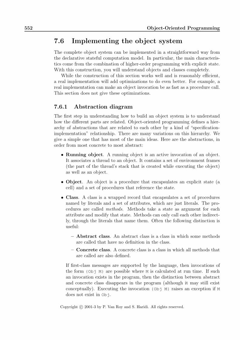
552 Object-Oriented Programming
7.6 Implementing the object system
The complete object system can be implemented in a straightforward way fromthe declarative stateful computation model. In particular, the main characteris-tics come from the combination of higher-order programming with explicit state.With this construction, you will understand objects and classes completely.
While the construction of this section works well and is reasonably efficient,a real implementation will add optimizations to do even better. For example, areal implementation can make an object invocation be as fast as a procedure call.This section does not give these optimizations.
7.6.1 Abstraction diagram
The first step in understanding how to build an object system is to understandhow the different parts are related. Object-oriented programming defines a hier-archy of abstractions that are related to each other by a kind of “specification-implementation” relationship. There are many variations on this hierarchy. Wegive a simple one that has most of the main ideas. Here are the abstractions, inorder from most concrete to most abstract:
• Running object. A running object is an active invocation of an object.It associates a thread to an object. It contains a set of environment frames(the part of the thread’s stack that is created while executing the object)as well as an object.
• Object. An object is a procedure that encapsulates an explicit state (acell) and a set of procedures that reference the state.
• Class. A class is a wrapped record that encapsulates a set of proceduresnamed by literals and a set of attributes, which are just literals. The pro-cedures are called methods. Methods take a state as argument for eachattribute and modify that state. Methods can only call each other indirect-ly, through the literals that name them. Often the following distinction isuseful:
– Abstract class. An abstract class is a class in which some methodsare called that have no definition in the class.
– Concrete class. A concrete class is a class in which all methods thatare called are also defined.
If first-class messages are supported by the language, then invocations ofthe form {Obj M} are possible where M is calculated at run time. If suchan invocation exists in the program, then the distinction between abstractand concrete class disappears in the program (although it may still existconceptually). Executing the invocation {Obj M} raises an exception if M
does not exist in Obj .
Copyright c© 2001-3 by P. Van Roy and S. Haridi. All rights reserved.

7.6 Implementing the object system 553
concreteclass
abstractclass
metaclass
inherits from
inherits from
instance ofinvocation of
inherits from
(object & thread)running object object
instance of
instance of
Figure 7.24: Abstractions in object-oriented programming
• Metaclass. A metaclass is a class with a particular set of methods thatcorrespond to the basic operations of a class, for example: object creation,inheritance policy (which methods to inherit), method call, method return,choice of method to call, attribute assignment, attribute access, self call.Writing these methods allows to customize the semantics of objects.
Figure 7.24 shows how these concepts are related. There are three relationships,“invocation of”, “instance of”, and “inherits from”. These relationships have thefollowing intuitive meanings:
• A running object is created when a thread invokes an object. The runningobject exists until the thread’s execution leaves it. Multiple invocations ofthe same object can exist simultaneously.
• An object can be created as an instance of a class. If the object systemdistinguishes between abstract and concrete classes, then it is usually onlypossible to create instances of concrete classes. The object exists forever.2
The object encapsulates a cell that was created especially for it. Multipleinstances of the same class can exist simultaneously.
• A class can be created that inherits from a list of other classes. The newclass exists forever. Inheritance takes a set of methods and a list of classesand returns a new class with a new set of methods. Multiple classes thatinherit from the same class can exist simultaneously. If one class can inheritfrom several classes, then we have multiple inheritance. Otherwise, if oneclass can inherit only from one class, we have single inheritance.
2In practice, until the actively running program loses all references to it. At that point,garbage collection can reclaim its memory and finalization can perform a last action, if necessary.
Copyright c© 2001-3 by P. Van Roy and S. Haridi. All rights reserved.

554 Object-Oriented Programming
class Counterattr valmeth init(Value)
val:=Valueendmeth inc(Value)
val:=@val+Valueendmeth browse
{Browse @val}end
end
Figure 7.25: An example class Counter (again)
• A class can be created as an instance of a metaclass. The new class existsforever. The basic operations of the class are defined by particular meth-ods of the metaclass. Multiple instances of the same metaclass can existsimultaneously.
7.6.2 Implementing classes
We first explain the class linguistic abstraction. The Counter class of Figure 7.25is translated internally into the definition of Figure 7.26. This figure shows thata class is simply a value, a record, that is protected from snooping because ofthe wrapper Wrap (see Section 3.7.5). (Later, when the class is used to createobjects, it will be unwrapped with the corresponding Unwrap .) The class recordcontains:
• A set of methods in a method table. Each method is a three-argument pro-cedure that takes a message M, which is always a record, an extra parameterS representing the state of the current object, and Self , which referencesthe object itself.
• A set of attribute names, giving the attributes that each class instance(object) will possess. Each attribute is a stateful cell that is accessed bythe attribute name, which is either an atom or an Oz name.
This example is slightly simplified because it does not show how to support staticbinding (see exercises). The Counter class has a single attribute accessed bythe atom val . It has a method table with three methods accessed through thefeatures browse , init , and inc . As we can see, the method init assigns thevalue Value to the attribute val , the method inc increments the attribute val ,and the method browse browses the current value of val .
Copyright c© 2001-3 by P. Van Roy and S. Haridi. All rights reserved.

7.6 Implementing the object system 555
declare Counterlocal
Attrs = [val]MethodTable = m(browse:MyBrowse init:Init inc:Inc)proc {Init M S Self}
init(Value)=Min
(S.val):=Valueendproc {Inc M S Self}
Xinc(Value)=M
inX=@(S.val) (S.val):=X+Value
endproc {MyBrowse M S Self}
browse=M{Browse @(S.val)}
endin
Counter = {Wrap c(methods:MethodTable attrs:Attrs)}end
Figure 7.26: An example of class construction
7.6.3 Implementing objects
We can use the class Counter to create objects. Figure 7.27 shows a genericfunctionw Newthat creates an object from any class. It starts by unwrapping theclass. It then creates an object state, a record, from the attributes of the class. Itinitializes each field of this record to a cell (with an unbound initial value). Thisuses the iterator Record.forAll to iterate over all fields of a record.
The object Obj returned by Newis a one-argument procedure. When called as{Obj M} , it looks up and calls the procedure corresponding to M in the methodtable. Because of lexical scoping, the object state is visible only within Obj . Onecan say that Obj is a procedure that encapsulates the state.
The definition of Figure 7.27 works correctly, but it may not be the mostefficient way to implement objects. An actual system can use a different, moreefficient implementation as long as it behaves in the same way. For example, theMozart system uses an implementation in which object invocations are almost asefficient as procedure calls [74, 76].
The proof of the pudding is in the eating. Let us verify that the class worksas claimed. We now create the Counter class and try out Newas follows:
C={New Counter init(0)}{C inc(6)} {C inc(6)}
Copyright c© 2001-3 by P. Van Roy and S. Haridi. All rights reserved.

556 Object-Oriented Programming
fun {New WClass InitialMethod}State Obj Class={Unwrap WClass}
inState = {MakeRecord s Class.attrs}{Record.forAll State proc {$ A} {NewCell _ A} end }proc {Obj M}
{Class.methods.{Label M} M State Obj}end{Obj InitialMethod}Obj
end
Figure 7.27: An example of object construction
{C browse}
This behaves in exactly the same way as the example of Section 7.2.1.
7.6.4 Implementing inheritance
Inheritance calculates a new class record starting from existing class records,which are combined according to the inheritance rules given in Section 7.3.1.Inheritance can be defined by the function From, where the call C={From C1 C2
C3} returns a new class record whose base definition is C1 and which inheritsfrom C2 and C3. It corresponds to the following class syntax:
class C from C2 C3... % The base class C1
end
Figure 7.28 shows the definition of From. It uses the set operations in the Set
module, which can be found on the book’s Web site. From first checks the methodtables and attribute lists for conflicts. If a duplicate method label or attribute isfound in C2 and C3 that is not overridden by C1, then an exception is raised. ThenFrom constructs the new method table and attribute lists. Overriding is handledproperly by the Adjoin function on the method tables (see Appendix B.3.2).The definition is slightly simplified because it does not handle static binding andbecause it assumes that there are exactly two superclasses.
7.7 The Java language (sequential part)
Java is a concurrent object-oriented language with a syntax that resembles C++.This section gives a brief introduction to the sequential part of Java. We explainhow to write a simple program, how to define classes, and how to use inheritance.We defer talking about concurrency in Java until Chapter 8. We do not talk
Copyright c© 2001-3 by P. Van Roy and S. Haridi. All rights reserved.

7.7 The Java language (sequential part) 557
fun {From C1 C2 C3}c(methods:M1 attrs:A1)={Unwrap C1}c(methods:M2 attrs:A2)={Unwrap C2}c(methods:M3 attrs:A3)={Unwrap C3}MA1={Arity M1}MA2={Arity M2}MA3={Arity M3}ConfMeth={Minus {Inter MA2 MA3} MA1}ConfAttr={Minus {Inter A1 A2} A3}
inif ConfMeth\=nil then
raise illegalInheritance(methConf:ConfMeth) endendif ConfAttr\=nil then
raise illegalInheritance(attrConf:ConfAttr) endend{Wrap c(methods:{Adjoin {Adjoin M2 M3} M1}
attrs:{Union {Union A2 A3} A1})}end
Figure 7.28: Implementing inheritance
about the reflection package, which lets one do much of what the object systemof this chapter can do (although in a more verbose way).
Java is almost a pure object-oriented language, i.e., almost everything is anobject. Only a small set of primitive types, namely integers, floats, booleans, andcharacters, are not objects. Java is a relatively clean language with a relativelysimple semantics. Despite the syntactic similarity, there is a major difference inlanguage philosophy between Java and C++ [184, 10]. C++ gives access to themachine representation of data and a direct translation to machine instructions.It also has manual memory management. Because of these properties, C++ isoften suitable as a replacement for assembly language. In contrast, Java hidesthe representation of data and does automatic memory management. It supportsdistributed computing on multiple platforms. It has a more sophisticated ob-ject system. These properties make Java better for general-purpose applicationdevelopment.
7.7.1 Computation model
Java consists of statically-typed object-oriented programming with classes, pas-sive objects, and threads. The Java computation model is close to the shared-state concurrent model, minus dataflow variables, triggers, and names. Parameterpassing is done by value, both for primitive types and object references. Newly-declared variables are given a default initial value that depends on their type.There is support for single assignment: variables and object attributes can be
Copyright c© 2001-3 by P. Van Roy and S. Haridi. All rights reserved.

558 Object-Oriented Programming
declared as final, which means that the variable can be assigned exactly once.Final variables must be assigned before they are used.
Java introduces its own terminology for some concepts. Classes contain fields(attributes, in our terminology), methods, other classes, or interfaces, which areknown collectively as class members. Variables are either fields, local variables(declared in code blocks local to methods), or method parameters. Variables aredeclared by giving their type, identifier, and an optional set of modifiers (e.g.,final). The self concept is called this.
Interfaces
Java has an elegant solution to the problems of multiple inheritance (Sections 7.4.4and 7.4.5). Java introduces the concept of interface, which syntactically looks likea class with only method declarations. An interface has no implementation. Aclass can implement an interface, which simply means that it defines all the meth-ods in the interface. Java supports single inheritance for classes, thus avoidingthe problems of multiple inheritance. But, to preserve the advantages of multipleinheritance, Java supports multiple inheritance for interfaces.
Java supports higher-order programming in a trivial way by means of theencoding given in Section 7.5.2. In addition to this, Java has more direct supportfor higher-order programming through inner classes. An inner class is a classdefinition that is nested inside another class or inside a code block (such as amethod body). An instance of an inner class can be passed outside of the methodbody or code block. An inner class can have external references, but there is arestriction if it is nested in a code block: in that case it cannot reference non-finalvariables. We could say that an instance of an inner class is almost a procedurevalue. The restriction likely exists because the language designers wanted non-final variables in code blocks to be implementable on a stack, which would bepopped when exiting the method. Without the restriction, this might createdangling references.
7.7.2 Introduction to Java programming
We give a brief introduction to programming in Java. We explain how to write asimple program, how to define classes, how to use inheritance, and how to writeconcurrent programs with locks and monitors. We situate the Java style withrespect to the computation models of this book.
This section only scratches the surface of what is possible in Java. For moreinformation, we refer the reader to one of the many good books on Java program-ming. We especially recommend [10] (on the language) and [111] (on concurrentprogramming).
Copyright c© 2001-3 by P. Van Roy and S. Haridi. All rights reserved.

7.7 The Java language (sequential part) 559
A simple program
We would like to calculate the factorial function. In Java, functions are definedas methods that return a result:
class Factorial {
public long fact(long n) {
long f=1;
for (int i=1; i<=n; i++) f=f*i;
return f;
}
}
Statements are terminated with a semicolon “;” unless they are compound state-ments, which are delimited by braces { ...}. Variable identifiers are declared bypreceding them with their type, as in long f. Assignment is denoted by theequals sign =. In the object system of Chapter 7 this becomes:
class Factorialmeth fact(N ?X)F={NewCell 1} in
for I in 1..N do F:=@F*I endX=@F
endend
Note that i is an assignable variable (a cell) that is updated on each iteration,whereas I is a value that is declared anew on each iteration. Factorial can alsobe defined recursively:
class Factorial {
public long fact(long n) {
if (n==0) return 1;
else return n*this.fact(n-1);
}
}
In our object system this becomes:
class Factorialmeth fact(N ?F)
if N==0 then F=1else F=N*{ self fact(N-1 $)} end
endend
There are a few differences with the object system of Chapter 7. The Javakeyword this is the same as self in our object system. Java is statically typed.The type of all variables is declared at compile time. Our model is dynamicallytyped. A variable can be bound to an entity of any type. In Java, the visibility
Copyright c© 2001-3 by P. Van Roy and S. Haridi. All rights reserved.

560 Object-Oriented Programming
of fact is declared to be public. In our model, fact is public by default; to getanother visibility we would have to declare it as a name.
Input/output
Any realistic Java program has to do I/O. Java has an elaborate I/O subsystembased on the notion of stream, which is an ordered sequence of data that hasa source (for an input stream) or a destination (for an output stream). Do notconfuse this with the concept of stream as used in the rest of this book: a list withunbound tail. The Java stream concept generalizes the Unix concept of standardI/O, i.e., the standard input (stdin) and standard output (stdout) files.
Streams can encode many types, including primitive types, objects, and objectgraphs. (An object graph is an object together with the other objects it refer-ences, directly or indirectly.) Streams can be byte streams or character streams.Characters are not the same as bytes since Java supports Unicode. A byte inJava is an 8-bit unsigned integer. A character in Java is a Unicode 2.0 character,which has a 16-bit code. We do not treat I/O further in this section.
Defining classes
The Factorial class is rather atypical. It has only one method and no attributes.Let us define a more realistic class. Here is a class to define points in two-dimensional space:
class Point {
public double x, y;
}
The attributes x and y are public, which means they are visible from outside theclass. Public attributes are usually not a good idea; it is almost always better tomake them private and use accessor methods:
class Point {
double x, y;
Point(double x1, y1) { x=x1; y=y1; }
public double getX() { return x; }
public double getY() { return y; }
}
The method Point is called a constructor; it is used to initialize new objectscreated with new, as in:
Point p=new Point(10.0, 20.0);
which creates the new Point object p. Let us add some methods to calculatewith points:
Copyright c© 2001-3 by P. Van Roy and S. Haridi. All rights reserved.

7.7 The Java language (sequential part) 561
class Point {
double x, y;
Point(double x1, y1) { x=x1; y=y1; }
public double getX() { return x; }
public double getY() { return y; }
public void origin() { x=0.0; y=0.0; }
public void add(Point p) { x+=p.getX(); y+=p.getY(); }
public void scale(double s) { x*=s; y*=s; }
}
The p argument of add is a local variable whose initial value is a reference to theargument. In our object system we can define Point as follows:
class Pointattr x ymeth init(X Y) x:=X y:=Y endmeth getX(X) X=@x endmeth getY(Y) Y=@y endmeth origin x:=0.0 y:=0.0 endmeth add(P) x:=@x+{P getX($)} y:=@y+{P getY($)} endmeth scale(S) x:=@x*S y:=@y*S end
end
This definition is very similar to the Java definition. There are also some minorsyntactic differences, such as the operators += and *=. Both definitions haveprivate attributes. There is a subtle difference in the visibility of the attributes.In Java, private attributes are visible to all objects of the same class. This meansthe method add could be written differently:
public void add(Point p) { x+=p.x; y+=p.y; }
This is explained further in Section 7.3.3.
Parameter passing and main program
Parameter passing to methods is done with call by value. A copy of the valueis passed to the method and can be modified inside the method without chang-ing the original value. For primitive values, such as integers and floats, this isstraightforward. Java also passes object references (not the objects themselves)by value. So objects can almost be considered as using call by reference. Thedifference is that, inside the method, the field can be modified to refer to anotherobject.
Figure 7.29 gives an example. This example is a complete standalone program;it can be compiled and executed as is. Each Java program has one method, main,that is called when the program is started The object reference c is passed byvalue to the method sqr. Inside sqr, the assignment a=null has no effect on c.
Copyright c© 2001-3 by P. Van Roy and S. Haridi. All rights reserved.

562 Object-Oriented Programming
class MyInteger {
public int val;
MyInteger(int x) { val=x; }
}
class CallExample {
public void sqr(MyInteger a) {
a.val=a.val*a.val;
a=null;
}
public static void main(String[] args) {
int c=new MyInteger(25);
CallExample.sqr(c);
System.out.println(c.val);
}
}
Figure 7.29: Parameter passing in Java
The argument of main is an array of strings that contains the command linearguments of the program when called from the operating system, The methodcall System.out.println prints its argument to the standard output.
Inheritance
We can use inheritance to extend the Point class. For example, it can be extendedto represent a pixel, which is the smallest independently displayable area on atwo-dimensional graphics output device such as a computer screen. Pixels havecoordinates, just like points, but they also have color.
class Pixel extends Point {
Color color;
public void origin() {
super.origin();
color=null;
}
public Color getC() { return color; }
public void setC(Color c) { color=c; }
}
The extend keyword is used to denote inheritance; it corresponds to from in ourobject system. We assume the class Color is defined elsewhere. The class Pixel
overrides the origin method. The new origin initializes both the point and the
Copyright c© 2001-3 by P. Van Roy and S. Haridi. All rights reserved.

7.8 Active objects 563
class BallGameattr other count:0meth init(Other)
other:=Otherendmeth ball
count:=@count+1{@other ball}
endmeth get(X)
X=@countend
end
B1={NewActive BallGame init(B2)}B2={NewActive BallGame init(B1)}
{B1 ball}
Figure 7.30: Two active objects playing ball (definition)
color. It uses super to access the overridden method in the immediate ancestorclass. With respect to the current class, this class is often called the superclass.In our object system, we can define Pixel as follows:
class Pixel from Pointattr colormeth origin
Point,origincolor:=null
endmeth getC(C) C=@color endmeth setC(C) color:=C end
end
7.8 Active objects
An active object is a port object whose behavior is defined by a class. It consistsof a port, a thread that reads messages from the port’s stream, and an object thatis a class instance. Each message that is received will cause one of the object’smethods to be invoked.
Copyright c© 2001-3 by P. Van Roy and S. Haridi. All rights reserved.

564 Object-Oriented Programming
ball
B1 B2
ball
Figure 7.31: Two active objects playing ball (illustration)
7.8.1 An example
Let us start with an example. Consider two active objects, where each objecthas a reference to the other. When each object receives the message ball , itsends the message ball to the other. The ball will be passed back and forthindefinitely between the objects. We define the behavior of the active objectsby means of a class. Figure 7.30 defines the objects and Figure 7.31 illustrateshow the messages pass between them. Each object references the other in theattribute other . We also add an attribute count to count the number of timesthe message ball is received. The initial call {B1 ball} starts the game. Withthe method get(X) we can follow the game’s progress:
declare X in{B1 get(X)}{Browse X}
Doing this several times will show a sequence of numbers that increase rapidly.
7.8.2 The NewActive abstraction
The behavior of active objects is defined with a class. Each method of the classcorresponds to a message that is accepted by the active object. Figure 7.30 givesan example. Sending a message M to an active object A is written as {A M} ,with the same syntax as invoking a standard, passive object. In contrast to theother objects of this chapter, which are called passive objects, the invocation ofan active object is asynchronous: it returns immediately, without waiting untilthe message has been handled. We can define a function NewActive that worksexactly like New except that it creates an active object:
fun {NewActive Class Init}Obj={New Class Init}P
inthread S in
{NewPort S P}for M in S do {Obj M} end
endproc {$ M} {Send P M} end
Copyright c© 2001-3 by P. Van Roy and S. Haridi. All rights reserved.

7.8 Active objects 565
40
23
4
5
6
7
1
..
.
Figure 7.32: The Flavius Josephus problem
end
This makes defining active objects very intuitive.
7.8.3 The Flavius Josephus problem
Let us now tackle a bigger problem. We introduce it with a well-known historicalanecdote. Flavius Josephus was a Roman historian of Jewish origin. During theJewish-Roman wars of the first century AD, he was in a cave with fellow soldiers,40 men in all, surrounded by enemy Roman troops. They decided to commitsuicide by standing in a ring and counting off each third man. Each man sodesignated was to commit suicide. Figure 7.32 illustrates the problem. Josephus,not wanting to die, managed to place himself in the position of the last survivor.
In the general version of this problem, there are n soldiers numbered from 1to n and each k-th soldier will be eliminated. The count starts from the firstsoldier. What is the number of the last survivor? Let us model this problem byrepresenting soldiers with active objects. There is ring of active objects whereeach object knows its two neighbors. Here is one possible message-passing pro-tocol to solve the problem. A message kill(X S) circulates around the ring,where X counts live objects traversed and S is the total number of live objectsremaining. Initially, the message kill(1 N) is given to the first object. Whenobject i receives the message kill(X S) it does the following:
• If it is alive and s = 1, then it is the last survivor. It signals this by bindinga global variable. No more messages are forwarded.
• If it is alive and X mod k = 0, then it becomes dead and it sends themessage kill(X+1 S-1) to the next object in the ring.
Copyright c© 2001-3 by P. Van Roy and S. Haridi. All rights reserved.

566 Object-Oriented Programming
class Victimattr ident step last succ pred alive: truemeth init(I K L) ident:=I step:=K last:=L endmeth setSucc(S) succ:=S endmeth setPred(P) pred:=P endmeth kill(X S)
if @alive thenif S==1 then @last=@identelseif X mod @step==0 then
alive:= false{@pred newsucc(@succ)}{@succ newpred(@pred)}{@succ kill(X+1 S-1)}
else{@succ kill(X+1 S)}
endelse {@succ kill(X S)} end
endmeth newsucc(S)
if @alive then succ:=Selse {@pred newsucc(S)} end
endmeth newpred(P)
if @alive then pred:=Pelse {@succ newpred(P)} end
endend
fun {Josephus N K}A={NewArray 1 N null}Last
infor I in 1..N do
A.I:={NewActive Victim init(I K Last)}endfor I in 2..N do {A.I setPred(A.(I-1))} end{A.1 setPred(A.N)}for I in 1..(N-1) do {A.I setSucc(A.(I+1))} end{A.N setSucc(A.1)} {A.1 kill(1 N)}Last
end
Figure 7.33: The Flavius Josephus problem (active object version)
Copyright c© 2001-3 by P. Van Roy and S. Haridi. All rights reserved.

7.8 Active objects 567
• If it is alive and X mod k 6= 0, then it sends the message kill(X+1 S) tothe next object in the ring.
• If it is dead, then it forwards the message kill(X S) to the next object.3
Figure 7.33 gives a program that implements this protocol. The function Josephus
returns immediately with an unbound variable, which will be bound to the num-ber of the last survivor as soon as it is known.
Short-circuit protocol
The solution of Figure 7.33 removes dead objects from the circle with a short-circuit protocol. If this were not done, the traveling message would eventual-ly spend most of its time being forwarded by dead objects. The short-circuitprotocol uses the newsucc and newpred methods. When an object dies, it sig-nals to both its predecessor and its successor that it should be bypassed. Theshort-circuit protocol is just an optimization to reduce execution time. It can beremoved and the program will still run correctly.
Without the short-circuit protocol, the program is actually sequential sincethere is just a single message circulating. It could have been written as a sequen-tial program. With the short-circuit protocol it is no longer sequential. Morethan one message can be traveling in the network at any given time.
A declarative solution
As alert programmers, we remark that the solution of Figure 7.33 has no ob-servable nondeterminism. We can therefore write it completely in the declarativeconcurrent model of Chapter 4. Let us do this and compare the two programs.Figure 7.34 shows a declarative solution that implements the same protocol as theactive object version. Like the active object version, it does short-circuiting andeventually terminates with the identity of the last survivor. It pays to comparethe two versions carefully. The declarative version is half the size of the activeobject version. One reason is that streams are first-class entities. This makesshort-circuiting very easy: just return the input stream as output.
The declarative program uses a concurrent abstraction, Pipe , that it definesespecially for this program. If l ≤ h, then the function call {Pipe X s L H F}
creates a pipeline of h−l+1 stream objects, numbered from l to h inclusive. Eachstream object is created by the call {F Is I} , which is given an input streamIs and an integer I and returns the output stream. We create a closed ringby feeding the output stream Zs back to the input, with the additional messagekill(1 N) to start the execution.
3The dead object is a kind of zombie.
Copyright c© 2001-3 by P. Van Roy and S. Haridi. All rights reserved.

568 Object-Oriented Programming
fun {Pipe Xs L H F}if L=<H then {Pipe {F Xs L} L+1 H F} else Xs end
end
fun {Josephus2 N K}fun {Victim Xs I}
case Xs of kill(X S)|Xr thenif S==1 then Last=I nilelseif X mod K==0 then
kill(X+1 S-1)|Xrelse
kill(X+1 S)|{Victim Xr I}end
[] nil then nil endendLast Zs
inZs={Pipe kill(1 N)|Zs 1 N
fun {$ Is I} thread {Victim Is I} end end }Last
end
Figure 7.34: The Flavius Josephus problem (data-driven concurrent version)
7.8.4 Other active object abstractions
Section 5.3 shows some of the useful protocols that we can build on top of messagepassing. Let us take two of these protocols and make them into abstractions foractive objects.
Synchronous active objects
It is easy to extend active objects to give them synchronous behavior, like astandard object or an RMI object. A synchronous invocation {Obj M} does notreturn until the method corresponding to M is completely executed. Internal tothe abstraction, we use a dataflow variable to do the synchronization. Here is thedefinition of NewSync, which creates a synchronous active object:
fun {NewSync Class Init}Obj={New Class Init}P
inthread S in
{NewPort S P}for M#X in S do {Obj M} X= unit end
endproc {$ M} X in {Send P M#X} {Wait X} end
Copyright c© 2001-3 by P. Van Roy and S. Haridi. All rights reserved.

7.8 Active objects 569
end
Each message sent to the object contains a synchronization token X, which isbound when the message is completely handled.
Active objects with exception handling
Explicitly doing exception handling for active objects can be cumbersome, sinceit means adding a try in each server method and a case after each call. Letus hide these statements inside an abstraction. The abstraction adds an extraargument that can be used to test whether or not an exception occurred. Insteadof adding the extra argument in the method, we add it to the object invocationitself. In this way, it automatically works for all methods. The extra argumentis bound to normal if the invocation completes normally, and to exception(E)
if the object raises the exception E. Here is the definition of NewActiveExc :
fun {NewActiveExc Class Init}P Obj={New Class Init} in
thread S in{NewPort S P}for M#X in S do
try {Obj M} X=normalcatch E then X=exception(E) end
endendproc {$ M X} {Send P M#X} end
end
The object Obj is called as {Obj M X} , where X is the extra argument. So thesend is still asynchronous and the client can examine at any time whether the callcompleted successfully or not. For the synchronous case, we can put the case
statement inside the abstraction:
proc {$ M}X in
{Send P M#X}case E of normal then skip[] exception(Exc) then raise Exc end end
end
This lets us call the object exactly like a passive object.
7.8.5 Event manager with active objects
We can use active objects to implement a simple concurrent event manager. Theevent manager contains a set of event handlers. Each handler is a triple Id#F#S ,where Id uniquely identifies the handler, F defines the state update function, andS is the handler’s state. When an event E occurs, each triple Id#F#S is replaced
Copyright c© 2001-3 by P. Van Roy and S. Haridi. All rights reserved.

570 Object-Oriented Programming
class EventManagerattr
handlersmeth init handlers:=nil endmeth event(E)
handlers:={Map @handlers fun {$ Id#F#S} Id#F#{F E S} end }
endmeth add(F S ?Id)
Id={NewName}handlers:=Id#F#S|@handlers
endmeth delete(DId ?DS)
handlers:={List.partition@handlers fun {$ Id#F#S} DId==Id end [_#_#DS]}
endend
Figure 7.35: Event manager with active objects
by Id#F#{F E S} . That is, each event handler is a finite state machine, whichdoes a transition from state S to state {F E S} when the event E occurs.
The event manager was originally written in Erlang [7]. The Erlang com-putation model is based on communicating active objects (see Chapter 5). Thetranslation of the original code to the concurrent stateful model was straightfor-ward.
We define the event manager EMas an active object with four methods:
• {EM init} initializes the event manager.
• {EM event(E)} posts the event E at the event manager.
• {EM add(F S Id)} adds a new handler with update function F and initialstate S. Returns a unique identifier Id .
• {EM delete(Id S)} removes the handler with identifier Id , if it exists.Returns the handler’s state in S.
Figure 7.35 shows how to define the event manager as a class. We show how touse the event manager to do error logging. First we define a new event manager:
EM={NewActive EventManager init}
We then install a memory-based handler. It logs every event in an internal list:
MemH=fun {$ E Buf} E|Buf endId={EM add(MemH nil $)}
We can replace the memory-based handler by a disk-based handler during exe-cution, without losing any of the already-logged events. In the following code,
Copyright c© 2001-3 by P. Van Roy and S. Haridi. All rights reserved.

7.8 Active objects 571
class ReplaceEventManager from EventManagermeth replace(NewF NewS OldId NewId
insert:P<= proc {$ _} skip end )Buf=EventManager,delete(OldId $)
in{P Buf}NewId=EventManager,add(NewF NewS $)
endend
Figure 7.36: Adding functionality with inheritance
we remove the memory-based handler, open a log file, write the already-loggedevents to the file, and then define and install the disk-based handler:
DiskH= fun {$ E F} {F write(vs:E)} F endFile={New Open.file init(name: ´ event.log ´ flags:[write create])}Buf={EM delete(Id $)}for E in {Reverse Buf} do {File write(vs:E)} endId2={EM add(DiskH File $)}
This uses the System module Open to write the log. We could use the File
module but then the rest of the program could not use it, since it only supportsone open file at a time for writing.
Adding functionality with inheritance
The event manager of Figure 7.35 has the defect that if events occur during areplacement, i.e., between the delete and add operations, then they will not belogged. How can we remedy this defect? A simple solution is to add a newmethod, replace to EventManager that does both the delete and add. Becauseall methods are executed sequentially in the active object, this ensures no eventwill occur between the delete and add. We have the choice to add the new methoddirectly, to EventManager , or indirectly, to a subclass by inheritance. Whichpossibility is the right solution depends on several factors. First, whether wehave access to the source code of EventManager . If we do not, then inheritanceis the only possibility. If we do have the source code, inheritance may still be theright answer. It depends on how often we need the replace functionality. If wealmost always need it in event managers, then we should modify EventManager
directly and not create a second class. If we rarely need it, then its definitionshould not encumber EventManager , and we can separate it by using inheritance.
Let us use inheritance for this example. Figure 7.36 defines a new classReplaceEventManager that inherits from EventManager and adds a new methodreplace . Instances of ReplaceEventManager have all methods of EventManager
as well as the method replace . The insert field is optional; it can be used toinsert an operation to be done between the delete and add operations. We define
Copyright c© 2001-3 by P. Van Roy and S. Haridi. All rights reserved.

572 Object-Oriented Programming
class Batchermeth batch(L)
for X in L doif {IsProcedure X} then {X} else { self X} end
endend
end
Figure 7.37: Batching a list of messages and procedures
a new event manager:
EM={NewActive ReplaceEventManager init}
Now we can do the replacement as follows:
DiskH= fun {$ E S} {S write(vs:E)} S endFile={New Open.file init(name: ´ event.log ´ flags:[write create])}Id2{EM replace(DiskH File Id Id2
insert:proc {$ S}
for E in {Reverse S} do{File write(vs:E)} end
end )}
Because replace is executed inside the active object, it is serialized with all theother messages to the object. This ensures that no events can arrive between thedelete and add methods.
Batching operations using a mixin class
A second way to remedy the defect is to add a new method that does batching,i.e., it does a list of operations. Figure 7.37 defines a new class Batcher that hasjust one method, batch(L) . The list L can contain messages or zero-argumentprocedures. When batch(L) is called, the messages are passed to self and theprocedures are executed, in the order they occur in L. This is an example of usingfirst-class messages. Since messages are also language entities (they are records),they can be put in a list and passed to Batcher . We define a new class thatinherits from EventManager and brings in the functionality of Batcher :
class BatchingEventManager from EventManager Batcher end
We use multiple inheritance because Batcher can be useful to any class thatneeds batching, not just to event managers. Now we can define a new eventmanager:
EM={NewActive BatchingEventManager init}
All instances of BatchingEventManager have all methods of EventManager aswell as the method batch . The class Batcher is an example of a mixin class: it
Copyright c© 2001-3 by P. Van Roy and S. Haridi. All rights reserved.

7.8 Active objects 573
adds functionality to an existing class without needing to know anything aboutthe class. Now we can replace the memory-based handler by a disk-based handler:
DiskH= fun {$ E S} {S write(vs:E)} S endFile={New Open.file init(name: ´ event.log ´ flags:[write create])}Buf Id2{EM batch([delete(Id Buf)
proc {$}for E in {Reverse Buf} do {File write(vs:E)} end
endadd(DiskH File Id2)])}
The batch method guarantees atomicity in the same way as the replace method,i.e., because it executes inside the active object.
What are the differences between the replacement solution and the batchingsolution? There are two:
• The replacement solution is more efficient because the replace methodis hard-coded. The batch method, on the other hand, adds a layer ofinterpretation.
• The batching solution is more flexible. Batching can be added to any classusing multiple inheritance. No new methods have to be defined. Further-more, any list of messages and procedures can be batched, even a list thatis calculated at run time. However, the batching solution requires that thelanguage support first-class messages.
Combining computation models
The event manager is an interesting combination of the declarative, object-oriented, and stateful concurrent computation models:
• Each event handler is defined declaratively by its state update function.Even stronger, each method of the event manager can be seen as a declara-tive definition. Each method takes the event manager’s internal state fromthe attribute handlers , does a declarative operation on it, and stores theresult in handlers .
• All methods are executed in sequential fashion, as if they were in a statefulmodel with no concurrency. All concurrency is managed by the active objectabstraction, as implemented by NewActive . This abstraction guaranteesthat all object invocations are serialized. Especially, no locking or otherconcurrency control is needed.
• New functionality, for example replacement or batching, is added by usingobject-oriented inheritance. Because the new method executes inside theactive object, it is guaranteed to be atomic.
Copyright c© 2001-3 by P. Van Roy and S. Haridi. All rights reserved.

574 Object-Oriented Programming
The result is that event handlers are defined sequentially and declaratively, andyet can be used in a stateful concurrent environment. This is an example ofimpedance matching, as defined in Section 4.7.7. Impedance matching is a specialcase of the general principle of separation of concerns. The concerns of state andconcurrency are separated from the definition of the event handlers. It is goodprogramming practice to separate concerns as much as possible. Using differentcomputation models together often helps to achieve separation of concerns.
7.9 Exercises
1. Uninitialized objects. The function Newcreates a new object when givena class and an initial message. Write another function New2 that does notrequire an initial message. That is, the call Obj={New2 Class} creates anew object without initializing it. Hint: write New2 in terms of New.
2. Protected methods in the Java sense. A protected method in Java hastwo parts: it is accessible throughout the package that defines the classand also by descendants of the class. For this exercise, define a linguisticabstraction that allows to annotate a method or attribute as protected inthe Java sense. Show how to encode this in the model of Section 7.3.3 byusing name values. Use functors to represent Java packages. For example,one approach might to be to define the name value globally in the functorand also to store it in an attribute called setOfAllProtectedAttributes .Since the attribute is inherited, the method name is visible to all subclasses.Work out the details of this approach.
3. Method wrapping. Section 7.3.5 shows how to do method wrapping. Thedefinition of TraceNew2 given there uses a class Trace that has an externalreference. This is not allowed in some object systems. For this exercise,rewrite TraceNew2 so that it uses a class with no external references.
4. Implementing inheritance and static binding. For this exercise, gen-eralize the implementation of the object system given in Section 7.6 tohandle static binding and to handle inheritance with any number of super-classes (not just two).
5. Message protocols with active objects. For this exercise, redo themessage protocols of Section 5.3 with active objects instead of port objects.
6. The Flavius Josephus problem. Section 7.8.3 solves this problem intwo ways, using active objects and using data-driven concurrency. For thisexercise, do the following:
(a) Use a third model, the sequential stateful model, to solve the problem.Write two programs: the first without short-circuiting and the second
Copyright c© 2001-3 by P. Van Roy and S. Haridi. All rights reserved.

7.9 Exercises 575
with it. Try to make both as concise and natural as possible in themodel. For example, without short-circuiting an array of booleans isa natural data structure to represent the ring. Compare the structureof both programs with the two programs in Section 7.8.3.
(b) Compare the execution times of the different versions. There are twoorthogonal analyses to be done. First, measure the advantages (if any)of using short-circuiting for various values of n and k. This can be donein each of the three computation models. For each model, divide the(n, k) plane into two regions, depending on whether short-circuitingis faster or not. Are these regions the same for each model? Second,compare the three versions with short-circuiting. Do these versionshave the same asymptotic time complexity as a function of n and k?
7. (advanced exercise) Inheritance without explicit state. Inheritancedoes not require explicit state; the two concepts are orthogonal. For thisexercise, design and implement an object system with classes and inheri-tance but without explicit state. One possible starting point is the imple-mentation of declarative objects in Section 6.4.2.
8. (research project) Programming design patterns. For this exercise, de-sign an object-oriented language that allows “upwards” inheritance (defin-ing a new superclass of a given class) as well as higher-order programming.Upwards inheritance is usually called generalization. Implement and eval-uate the usefulness of your language. Show how to program the designpatterns of Gamma et al [58] as abstractions in your language. Do youneed other new operations in addition to generalization?
Copyright c© 2001-3 by P. Van Roy and S. Haridi. All rights reserved.

576 Object-Oriented Programming
Copyright c© 2001-3 by P. Van Roy and S. Haridi. All rights reserved.

Chapter 8
Shared-State Concurrency
The shared-state concurrent model is a simple extension to the declarative con-current model that adds explicit state in the form of cells, which are a kind of mu-table variable. This model is equivalent in expressiveness to the message-passingconcurrent model of Chapter 5, because cells can be efficiently implemented withports and vice versa. In practice, however, the shared-state model is harder toprogram than the message-passing model. Let us see what the problem is andhow we can solve it.
The inherent difficulty of the model
Let us first see exactly why the shared-state model is so difficult. Executionconsists of multiple threads, all executing independently and all accessing sharedcells. At some level, a thread’s execution can be seen as a sequence of atomicinstructions. For a cell, these are @(access), := (assignment), and Exchange .Because of the interleaving semantics, all execution happens as if there was oneglobal order of operations. All operations of all threads are therefore “interleaved”to make this order. There are many possible interleavings; their number is limitedonly by data dependencies (calculations needing results of others). Any particularexecution realizes an interleaving. Because thread scheduling is nondeterministic,there is no way to know which interleaving will be chosen.
But just how many interleavings are possible? Let us consider a simple case:two threads, each doing k cell operations. Thread T1 does the operations a1, a2,..., ak and thread T2 does b1, b2, ..., bk. How many possible executions are there,
interleaving all these operations? It is easy to see that the number is
(2kk
).
Any interleaved execution consists of 2k operations, of which each thread takesk. Consider these operations as integers from 1 to 2k, put in a set. Then T1
takes k integers from this set and T2 gets the others. This number is exponentialin k.1 For three or more threads, the number of interleavings is even bigger (seeExercises).
1Using Stirling’s formula we approximate it as 22k/√
πk.
Copyright c© 2001-3 by P. Van Roy and S. Haridi. All rights reserved.

578 Shared-State Concurrency
It is possible to write algorithms in this model and prove their correctnessby reasoning on all possible interleavings. For example, given that the onlyatomic operations on cells are @and := , then Dekker’s algorithm implementsmutual exclusion. Even though Dekker’s algorithm is short (e.g., 48 lines of codein [43], using a Pascal-like language), the reasoning is already quite difficult. Forbigger programs, this technique rapidly becomes impractical. It is unwieldy andinterleavings are easy to overlook.
Why not use declarative concurrency?
Given the inherent difficulty of programming in the shared-state concurrent mod-el, an obvious question is why not stick with the declarative concurrent model ofChapter 4? It is enormously simpler to program in than the shared-state concur-rent model. It is almost as easy to reason in as the declarative model, which issequential.
Let us briefly examine why the declarative concurrent model is so easy. It isbecause dataflow variables are monotonic: they can be bound to just one value.Once bound, the value does not change. Threads that share a dataflow variable,e.g., a stream, can therefore calculate with the stream as if it were a simple value.This is in contrast to cells, which are nonmonotonic: they can be assigned anynumber of times to values that have no relation to each other. Threads that sharea cell cannot make any assumptions about its content: at any time, the contentcan be completely different from any previous content.
The problem with the declarative concurrent model is that threads must com-municate in a kind of “lock-step” or “systolic” fashion. Two threads communicat-ing with a third thread cannot execute independently; they must coordinate witheach other. This is a consequence of the fact that the model is still declarative,and hence deterministic.
We would like to allow two threads to be completely independent and yetcommunicate with the same third thread. For example, we would like clients tomake independent queries to a common server or to independently increment ashared state. To express this, we have to leave the realm of declarative models.This is because two independent entities communicating with a third introduce anobservable nondeterminism. A simple way to solve the problem is to add explicitstate to the model. Ports and cells are two important ways to add explicit state.This gets us back to the model with both concurrency and state. But reasoningdirectly in this model is impractical. Let us see how we can get around theproblem.
Getting around the difficulty
Programming in the stateful concurrent model is largely a matter of managingthe interleavings. There are two successful approaches:
Copyright c© 2001-3 by P. Van Roy and S. Haridi. All rights reserved.
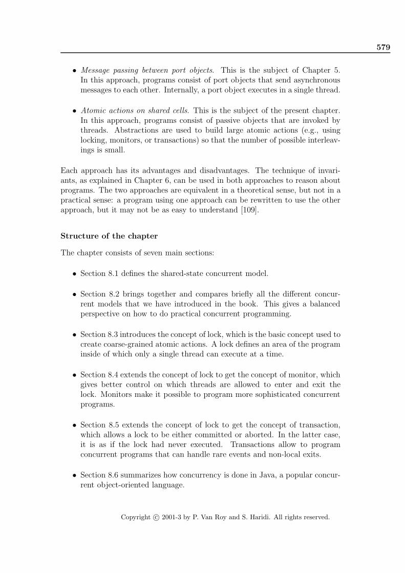
579
• Message passing between port objects. This is the subject of Chapter 5.In this approach, programs consist of port objects that send asynchronousmessages to each other. Internally, a port object executes in a single thread.
• Atomic actions on shared cells. This is the subject of the present chapter.In this approach, programs consist of passive objects that are invoked bythreads. Abstractions are used to build large atomic actions (e.g., usinglocking, monitors, or transactions) so that the number of possible interleav-ings is small.
Each approach has its advantages and disadvantages. The technique of invari-ants, as explained in Chapter 6, can be used in both approaches to reason aboutprograms. The two approaches are equivalent in a theoretical sense, but not in apractical sense: a program using one approach can be rewritten to use the otherapproach, but it may not be as easy to understand [109].
Structure of the chapter
The chapter consists of seven main sections:
• Section 8.1 defines the shared-state concurrent model.
• Section 8.2 brings together and compares briefly all the different concur-rent models that we have introduced in the book. This gives a balancedperspective on how to do practical concurrent programming.
• Section 8.3 introduces the concept of lock, which is the basic concept used tocreate coarse-grained atomic actions. A lock defines an area of the programinside of which only a single thread can execute at a time.
• Section 8.4 extends the concept of lock to get the concept of monitor, whichgives better control on which threads are allowed to enter and exit thelock. Monitors make it possible to program more sophisticated concurrentprograms.
• Section 8.5 extends the concept of lock to get the concept of transaction,which allows a lock to be either committed or aborted. In the latter case,it is as if the lock had never executed. Transactions allow to programconcurrent programs that can handle rare events and non-local exits.
• Section 8.6 summarizes how concurrency is done in Java, a popular concur-rent object-oriented language.
Copyright c© 2001-3 by P. Van Roy and S. Haridi. All rights reserved.

580 Shared-State Concurrency
... Multiple semantic stacks
Immutable store(single-assignment)
Mutable store
ST1 ST2 STn(‘‘threads’’)
W=atom
XZ=person(age: Y)
U=c2
c2:Zc1:W
Y=c1
Figure 8.1: The shared-state concurrent model
〈s〉 ::=skip Empty statement| 〈s〉1 〈s〉2 Statement sequence| local 〈x〉 in 〈s〉 end Variable creation| 〈x〉1=〈x〉2 Variable-variable binding| 〈x〉=〈v〉 Value creation| if 〈x〉 then 〈s〉1 else 〈s〉2 end Conditional| case 〈x〉 of 〈pattern〉 then 〈s〉1 else 〈s〉2 end Pattern matching| { 〈x〉 〈y〉1 ... 〈y〉n} Procedure application| thread 〈s〉 end Thread creation| {ByNeed 〈x〉 〈y〉} Trigger creation| {NewName〈x〉} Name creation| 〈y〉=!! 〈x〉 Read-only view| try 〈s〉1 catch 〈x〉 then 〈s〉2 end Exception context| raise 〈x〉 end Raise exception| {FailedValue 〈x〉 〈y〉} Failed value| {IsDet 〈x〉 〈y〉} Boundness test| {NewCell 〈x〉 〈y〉} Cell creation| {Exchange 〈x〉 〈y〉 〈z〉} Cell exchange
Table 8.1: The kernel language with shared-state concurrency
Copyright c© 2001-3 by P. Van Roy and S. Haridi. All rights reserved.

8.1 The shared-state concurrent model 581
8.1 The shared-state concurrent model
Chapter 6 adds explicit state to the declarative model. This allows to do object-oriented programming. Chapter 4 adds concurrency to the declarative model.This allows to have multiple active entities that evolve independently. The nextstep is to add both explicit state and concurrency to the declarative model. Oneway to do this is given in Chapter 5: by adding ports. This chapter gives analternative way: by adding cells.
The resulting model, called the shared-state concurrent model, is shown inFigure 8.1. Its kernel language is defined in Table 8.1. If we consider the subsetof operations up to ByNeed then we have the declarative concurrent model. Weadd names, read-only variables, exceptions, and explicit state to this model.
8.2 Programming with concurrency
By now, we have seen many different ways to write concurrent programs. Beforediving into programming with shared-state concurrency, let us make a slightdetour and put all these ways into perspective. We first give a brief overview ofthe main approaches. We then examine more closely the new approaches thatbecome possible with shared-state concurrency.
8.2.1 Overview of the different approaches
For the programmer, there are four main practical approaches to writing concur-rent programs:
• Sequential programming (Chapters 3, 6, and 7). This is the baselineapproach that has no concurrency. It can be either eager or lazy.
• Declarative concurrency (Chapter 4). This is concurrency in the declar-ative model, which gives the same results as a sequential program but cangive them incrementally. This model is usable when there is no observablenondeterminism. It can be either eager (data-driven concurrency) or lazy(demand-driven concurrency).
• Message-passing concurrency (Chapter 5 and Section 7.8). This is mes-sage passing between port objects, which are internally sequential. Thislimits the number of interleavings. Active objects (Section 7.8) are a vari-ant of port objects where the object’s behavior is defined by a class.
• Shared-state concurrency (this chapter). This is threads updating sharedpassive objects using coarse-grained atomic actions. This is another ap-proach to limit the number of interleavings.
Copyright c© 2001-3 by P. Van Roy and S. Haridi. All rights reserved.

582 Shared-State Concurrency
Order−determining concurrencyCoroutiningLazy evaluation
Sequential programming
Demand−driven concurrency
Use the model directlyMessage−passing concurrencyShared−state concurrency
Stream objects with merge
Approaches
Sequential
Nondeterministic concurrent
Stateful concurrent
Declarative concurrent
(declarative or stateful)
Model
Data−driven concurrency
Figure 8.2: Different approaches to concurrent programming
Figure 8.2 gives a complete list of these approaches and some others. Previouschapters have already explained sequential programming and concurrent declara-tive programming. In this chapter we look at the others. We first give an overviewof the four main approaches.
Sequential programming
In a sequential model, there is a total order among all operations. This is thestrongest order invariant a program can have. We have seen two ways that thisorder can be relaxed a little, while still keeping a sequential model:
• “Order-determining” concurrency (Section 4.4.1). In this model, alloperations execute in a total order, like with sequential execution, but theorder is unknown to the programmer. Concurrent execution with dataflowfinds the order dynamically.
• Coroutining (Section 4.4.2). In this model, preemption is explicit, i.e., theprogram decides when to pass control to another thread. Lazy evaluation,in which laziness is added to a sequential program, does coroutining.
Both of these variant models are still deterministic.
Declarative concurrency
The declarative concurrent models of Chapter 4 all add threads to the declarativemodel. This does not change the result of a calculation, but only changes theorder in which the result is obtained. For example, the result might be givenincrementally. This allows to build a dynamic network of concurrent stream
Copyright c© 2001-3 by P. Van Roy and S. Haridi. All rights reserved.

8.2 Programming with concurrency 583
objects connected with streams. Because of concurrency, adding an element toits input stream allows a stream object to produce an output immediately.
These models have nondeterminism in the implementation, since the systemchooses how to advance the threads. But, to stay declarative, the nondetermin-ism must not be observable to the program. The declarative concurrent modelsguarantee this as long as no exceptions are raised (since exceptions are witness-es to an observable nondeterminism). In practice, this means that each streamobject must know at all times from which stream its next input will come.
The demand-driven concurrent model, also known as lazy execution (Sec-tion 4.5), is a form of declarative concurrency. It does not change the result ofa calculation, but only affects how much calculation is done to obtain the result.It can sometimes give results in cases where the data-driven model would go intoan infinite loop. This is important for resource management, i.e., controlling howmany computational resources are needed. Calculations are initiated only whentheir results are needed by other calculations. Lazy execution is implementedwith by-need triggers.
Message-passing concurrency
Message passing is a basic programming style of the stateful concurrent model. Itis explained in Chapter 5 and Section 7.8. It extends the declarative concurrentmodel with a simple kind of communication channel, a port. It defines port objects,which extend stream objects to read from ports. A program is then a networkof port objects communicating with each other through asynchronous messagepassing. Each port object decides when to handle each messages. The portobject processes the messages sequentially. This limits the possible interleavingsand allows us to reason using invariants. Sending and receiving messages betweenport objects introduces a causality between events (send, receive, and internal).Reasoning on such systems requires reasoning on the causality chains.
Shared-state concurrency
Shared state is another basic programming style in the stateful concurrent model.It is explained in the present chapter. It consists of a set of threads accessinga set of shared passive objects. The threads coordinate among each other whenaccessing the shared objects. They do this by means of coarse-grained atomicactions, e.g., locks, monitors, or transactions. Again, this limits the possibleinterleavings and allows us to reason using invariants.
Relationship between ports and cells
The message-passing and shared-state models are equivalent in expressiveness.This follows because ports can be implemented with cells and vice versa. (It isan amusing exercise to implement the Send operation using Exchange and viceversa.) It would seem then that we have the choice whether to add ports or cells
Copyright c© 2001-3 by P. Van Roy and S. Haridi. All rights reserved.

584 Shared-State Concurrency
to the declarative concurrent model. However, in practice this is not so. Thetwo computation models emphasize a quite different programming style that isappropriate for different classes of applications. The message-passing style is ofprograms as active entities that coordinate with one another. The shared-statestyle is of programs as passive data repositories that are modified in a coherentway.
Other approaches
In addition to these four approaches, there are two others worth mentioning:
• Using the stateful concurrent model directly. This consists in pro-gramming directly in the stateful concurrent model, either in message-passing style (using threads, ports, and dataflow variables, see Section 5.5),in shared-state style (using threads, cells, and dataflow variables, see Sec-tion 8.2.2), or in a mixed style (using both cells and ports).
• Nondeterministic concurrent model (Section 5.7.1). This model addsa nondeterministic choice operator to the declarative concurrent model. Itis a stepping stone to the stateful concurrent model.
They are less common, but can be useful in some circumstances.
Which concurrent model to use?
How do we decide which approach to use when writing a concurrent program?Here are a few rules of thumb:
• Stick with the least concurrent model that suffices for your program. Forexample, if using concurrency does not simplify the architecture of the pro-gram, then stick with a sequential model. If your program does not have anyobservable nondeterminism, such as independent clients interacting with aserver, then stick with the declarative concurrent model.
• If you absolutely need both state and concurrency, then use either themessage-passing or the shared-state approach. The message-passing ap-proach is often the best for multi-agent programs, i.e., programs that con-sist of autonomous entities (“agents”) that communicate with each other.The shared-state approach is often the best for data-centered programs,i.e., programs that consist of a large repository of data (“database”) that isaccessed and updated concurrently. Both approaches can be used togetherfor different parts of the same application.
• Modularize your program and concentrate the concurrency aspects in asfew places as possible. Most of the time, large parts of the program canbe sequential or use declarative concurrency. One way to implement this
Copyright c© 2001-3 by P. Van Roy and S. Haridi. All rights reserved.

8.2 Programming with concurrency 585
is with impedance matching, which is explained in Section 4.7.7. For ex-ample, active objects can be used as front ends to passive objects. If thepassive objects are all called from the same active object then they can usea sequential model.
Too much concurrency is bad
There is a model, the maximally concurrent model, that has even more concur-rency than the stateful concurrent model. In the maximally concurrent model,each operation executes in its own thread. Execution order is constrained onlyby data dependencies. This has the greatest possible concurrency.
The maximally concurrent model model has been used as the basis for exper-imental parallel programming languages. But it is both hard to program in andhard to implement efficiently (see Exercise). This is because operations tend tobe fine-grained compared to the overhead of scheduling and synchronizing. Theshared-state concurrent model of this chapter does not have this problem becausethread creation is explicit. This allows the programmer to control the granularity.We do not present the maximally concurrent model in more detail in this chapter.A variant of this model is used for constraint programming (see Chapter 12).
8.2.2 Using the shared-state model directly
As we saw in the beginning of this chapter, programming directly in the shared-state model can be tough. This is because there are potentially an enormousnumber of interleavings, and the program has to work correctly for all of them.That is the main reason why more high-level approaches, like active objects andatomic actions, were developed. Yet, it is sometimes useful to use the modeldirectly. Before moving on to using atomic actions, let us see what can be donedirectly in the shared-state concurrent model. Practically, it boils down to pro-gramming with threads, procedures, cells, and dataflow variables. This sectiongives some examples.
Concurrent stack
A concurrent ADT is an ADT where multiple threads can execute the ADToperations simultaneously. The first and simplest concurrent ADT we show is astack. The stack provides nonblocking push and pop operations, i.e., they neverwait, but succeed or fail immediately. Using exchange, its implementation is verycompact, as Figure 8.3 shows. The exchange does two things: it accesses the cell’sold content and it assigns a new content. Because exchange is atomic, it can beused in a concurrent setting. Because the push and pop operations each do justone exchange, they can be interleaved in any way and still work correctly. Anynumber of threads can access the stack concurrently, and it will work correctly.The only restriction is that a pop should not be attempted on an empty stack.An exception can be raised in that case, e.g., as follows:
Copyright c© 2001-3 by P. Van Roy and S. Haridi. All rights reserved.

586 Shared-State Concurrency
fun {NewStack}Stack={NewCell nil}proc {Push X}S in
{Exchange Stack S X|S}endfun {Pop}X S in
{Exchange Stack X|S S}X
endin
stack(push:Push pop:Pop)end
Figure 8.3: Concurrent stack
fun {Pop}X S in
try {Exchange Stack X|S S}catch failure(...) then raise stackEmpty end endX
end
The concurrent stack is simple because each operation does just a single exchange.Things become much more complex when an ADT operation does more than onecell operation. For the ADT operation to be correct in general, these opera-tions would have to be done atomically. To guarantee this in a simple way, werecommend using the active object or atomic action approach.
Simulating a slow network
The object invocation {Obj M} calls Obj immediately and returns when thecall is finished. We would like to modify this to simulate a slow, asynchronousnetwork, where the object is called asynchronously after a delay that representsthe network delay. Here is a simple solution that works for any object:
fun {SlowNet1 Obj D}proc {$ M}
thread{Delay D}{Obj M}
endend
end
The call {SlowNet1 Obj D} returns a “slow” version of Obj . When the slowobject is invoked, it waits at least Dmilliseconds before calling the original object.
Copyright c© 2001-3 by P. Van Roy and S. Haridi. All rights reserved.

8.2 Programming with concurrency 587
Preserving message order with token passing The above solution doesnot preserve message order. That is, if the slow object is invoked several timesfrom within the same thread, then there is no guarantee that the messages willarrive in the same order as they are sent. Moreover, if the object is invokedfrom several threads, different executions of the object can overlap in time whichcould result in an inconsistent object state. Here is a solution that does preservemessage order and guarantees that only one thread at a time can execute insidethe object:
fun {SlowNet2 Obj D}C={NewCell unit }
inproc {$ M}Old New in
{Exchange C Old New}thread
{Delay D}{Wait Old}{Obj M}New=unit
endend
end
This solution uses a general technique, called token passing, to extract an execu-tion order from one part of a program and impose it on another part. The tokenpassing is implemented by creating a sequence of dataflow variables X0, X1, X2, ...,and passing consecutive pairs (X0, X1), (X1, X2), ... to the operations that shouldbe done in the same order. An operation that receives the pair (Xi, Xi+1) doesthe following steps in order:
1. Wait until the token arrives, i.e., until Xi is bound ({Wait X i} ).
2. Do the computation.
3. Send the token to the next pair, i.e., bind Xi+1 (Xi+1=unit ).
In the definition of SlowNet2 , each time the slow object is called, a pair ofvariables (Old , New) is created. This is inserted into the sequence by the call{Exchange C Old New} . Because Exchange is atomic, this works also in aconcurrent setting where many threads call the slow object. Each pair shares onevariable with the previous pair (Old ) and one with the next pair (New). Thiseffectively puts the object call in an ordered queue. Each call is done in a newthread. It first waits until the previous call has terminated ({Wait Old} ), theninvokes the object ({Obj M} ), and finally signals that the next call can continue(New=unit ). The {Delay D} call must be done before {Wait Old} ; otherwiseeach object call would take at least D milliseconds, which is incorrect.
Copyright c© 2001-3 by P. Van Roy and S. Haridi. All rights reserved.

588 Shared-State Concurrency
Simple lock
(gating mechanism) (can be aborted)
(ACID properties)... ...
Reentrant lock
Monitor Light transaction
Full transaction
Figure 8.4: The hierarchy of atomic actions
8.2.3 Programming with atomic actions
Starting with the next section, we give the programming techniques for shared-state concurrency using atomic actions. We introduce the concepts gradually,starting with locks. We refine locks into monitors and transactions. Figure 8.4shows the hierarchical relationships between these three concepts.
• Locks allow to group little atomic operations together into big atomic oper-ations. With a reentrant lock, the same lock can guard discontiguous partsof the program. A thread that is inside one part can reenter the lock at anypart without suspending.
• Monitors refine locks with wait points. A wait point is a pair of an exit anda corresponding entry with no code in between. (Wait points are sometimescalled delay points [6].) Threads can park themselves at a wait point, justoutside the lock. Exiting threads can wake up parked threads.
• Transactions refine locks to have two possible exits: a normal one (calledcommit) and an exceptional one (called abort). The exceptional exit can betaken at any time during the transaction. When it is taken, the transactionleaves the execution state unchanged, i.e., as it was upon entry.
Figure 8.5 summarizes the principal differences between the three concepts. Thereare many variations of these concepts that are designed to solve specific problems.This section only gives a brief introduction to the basic ideas.
Reasoning with atomic actions
Consider a program that uses atomic actions throughout. Proving that the pro-gram is correct consists of two parts: proving that each atomic action is correct(when considered by itself) and proving that the program uses them correctly.The first step is to show that each atomic action, e.g., lock, monitor, or transac-tion, is correct. Each atomic action defines an ADT. The ADT should have an
Copyright c© 2001-3 by P. Van Roy and S. Haridi. All rights reserved.

8.2 Programming with concurrency 589
Lock Transaction
enter
exitcommit abort
Monitor
wait
wait
Figure 8.5: Differences between atomic actions
invariant assertion, i.e., an assertion that is true when there is no thread insidethe ADT. This is similar to reasoning with stateful programs and active objects,except that the ADT can be accessed concurrently. Because only one thread canbe inside the atomic action at a time, we can still use mathematical induction toshow that the assertion is an invariant. We have to prove two things:
• When the ADT is first defined, the assertion is satisfied.
• Whenever a thread exits from the ADT, the assertion is satisfied.
The existence of the invariant shows that the atomic action is correct. The nextstep is to show that the program using the atomic actions is correct.
8.2.4 Further reading
There are many good books on concurrent programming. The following fourare particularly well-suited as companions to this book. They give more practi-cal techniques and theoretical background for the two concurrent paradigms ofmessage-passing and shared-state concurrency. At the time of writing, we know ofno books that deal with the third concurrent paradigm of declarative concurrency.
Concurrent Programming in Java
The first book deals with shared-state concurrency: Concurrent Programmingin Java, Second Edition, by Doug Lea [111]. This book presents a rich set ofpractical programming techniques that are particularly well-suited to Java, apopular concurrent object-oriented language (see Chapters 7 and 8). However,they can be used in many other languages including the shared-state concurrentmodel of this book. The book is targeted towards the shared-state approach;message passing is mentioned only in passing.
The major difference between the Java book and this chapter is that the Javabook assumes threads are expensive. This is true for current Java implementa-tions. Because of this, the Java book adds a conceptual level between threads and
Copyright c© 2001-3 by P. Van Roy and S. Haridi. All rights reserved.
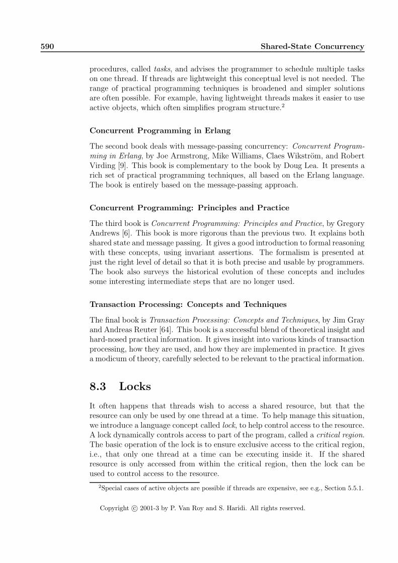
590 Shared-State Concurrency
procedures, called tasks, and advises the programmer to schedule multiple taskson one thread. If threads are lightweight this conceptual level is not needed. Therange of practical programming techniques is broadened and simpler solutionsare often possible. For example, having lightweight threads makes it easier to useactive objects, which often simplifies program structure.2
Concurrent Programming in Erlang
The second book deals with message-passing concurrency: Concurrent Program-ming in Erlang, by Joe Armstrong, Mike Williams, Claes Wikstrom, and RobertVirding [9]. This book is complementary to the book by Doug Lea. It presents arich set of practical programming techniques, all based on the Erlang language.The book is entirely based on the message-passing approach.
Concurrent Programming: Principles and Practice
The third book is Concurrent Programming: Principles and Practice, by GregoryAndrews [6]. This book is more rigorous than the previous two. It explains bothshared state and message passing. It gives a good introduction to formal reasoningwith these concepts, using invariant assertions. The formalism is presented atjust the right level of detail so that it is both precise and usable by programmers.The book also surveys the historical evolution of these concepts and includessome interesting intermediate steps that are no longer used.
Transaction Processing: Concepts and Techniques
The final book is Transaction Processing: Concepts and Techniques, by Jim Grayand Andreas Reuter [64]. This book is a successful blend of theoretical insight andhard-nosed practical information. It gives insight into various kinds of transactionprocessing, how they are used, and how they are implemented in practice. It givesa modicum of theory, carefully selected to be relevant to the practical information.
8.3 Locks
It often happens that threads wish to access a shared resource, but that theresource can only be used by one thread at a time. To help manage this situation,we introduce a language concept called lock, to help control access to the resource.A lock dynamically controls access to part of the program, called a critical region.The basic operation of the lock is to ensure exclusive access to the critical region,i.e., that only one thread at a time can be executing inside it. If the sharedresource is only accessed from within the critical region, then the lock can beused to control access to the resource.
2Special cases of active objects are possible if threads are expensive, see e.g., Section 5.5.1.
Copyright c© 2001-3 by P. Van Roy and S. Haridi. All rights reserved.

8.3 Locks 591
fun {NewQueue}X in
q(0 X X)end
fun {Insert q(N S E) X}E1 in
E=X|E1 q(N+1 S E1)end
fun {Delete q(N S E) X}S1 in
S=X|S1 q(N-1 S1 E)end
Figure 8.6: Queue (declarative version)
The shared resource can be either inside the program (e.g., an object) oroutside it (e.g., an operating system resource). Locks can help in both cases. Ifthe resource is inside the program, then the programmer can guarantee that itcannot be referenced outside the critical region, using lexical scoping. This kindof guarantee can in general not be given for resources outside of the program.For those resources, locks are an aid to the programmer, but he must follow thediscipline of only referencing the resource inside the critical region.
There are many different kinds of locks that provide different kinds of accesscontrol. Most of them can be implemented in Oz using language entities we havealready seen (i.e., cells, threads, and dataflow variables). However, a particu-larly useful kind of lock, the thread-reentrant lock, is directly supported by thelanguage. The following operations are provided:
• {NewLock L} returns a new lock.
• {IsLock X} returns true if and only if X references a lock.
• lock X then 〈S〉 end guards 〈S〉 with lock X. If no thread is currentlyexecuting any statement guarded by lock X, then any thread can enter. Ifa thread is currently executing a guarded statement, then the same threadcan enter again, if it encounters the same lock in a nested execution. Athread suspends if it attempts to enter a guarded statement while there isanother thread in a statement guarded by the same lock.
Note that lock X then ... end can be called many times with the same lockX. That is, the critical section does not have to be contiguous. The lock willensure that at most one thread is inside any of the parts that it guards.
Copyright c© 2001-3 by P. Van Roy and S. Haridi. All rights reserved.

592 Shared-State Concurrency
fun {NewQueue}X C={NewCell q(0 X X)}proc {Insert X}N S E1 in
q(N S X|E1)=@CC:=q(N+1 S E1)
endfun {Delete}N S1 E X in
q(N X|S1 E)=@CC:=q(N-1 S1 E)X
endin
queue(insert:Insert delete:Delete)end
Figure 8.7: Queue (sequential stateful version)
8.3.1 Building stateful concurrent ADTs
Now that we have introduced locks, we are ready to program stateful concurrentADTs. Let us approach this in steps. We give a systematic way to transforma declarative ADT to become a stateful concurrent ADT. We also show how tomodify a sequential stateful ADT to become concurrent.
We illustrate the different techniques by means of a simple example, a queue.This is not a limitation since these techniques work for any ADT. We start froma declarative implementation and show how to convert this to a stateful imple-mentation that can be used in a concurrent setting:
• Figure 8.6 is essentially the declarative queue of Section 3.4.4. (For brevitywe leave out the function IsEmpty .) Delete operations never block: if thequeue is empty when an element is deleted, then a dataflow variable isreturned which will be bound to the next inserted element. The size N ispositive if there are more inserts than deletes and negative otherwise. Allfunctions have the form Qout={QueueOp Qin ...} , taking an input queueQin and returning an output queue Qout . This queue will work correctlyin a concurrent setting, insofar as it can be used there. The problem is thatthe order of the queue operations is explicitly determined by the program.Doing these queue operations in different threads will ipso facto cause thethreads to synchronize. This is almost surely an undesired behavior.
• Figure 8.7 shows the same queue, but in a stateful version that encapsulatesthe queue’s data. This version cannot be used in a concurrent settingwithout some changes. The problem is that encapsulating the state requiresto read the state (@), do the operation, and then to write the new state (:= ).
Copyright c© 2001-3 by P. Van Roy and S. Haridi. All rights reserved.

8.3 Locks 593
fun {NewQueue}X C={NewCell q(0 X X)}L={NewLock}proc {Insert X}N S E1 in
lock L thenq(N S X|E1)=@CC:=q(N+1 S E1)
endendfun {Delete}N S1 E X in
lock L thenq(N X|S1 E)=@CC:=q(N-1 S1 E)
endX
endin
queue(insert:Insert delete:Delete)end
Figure 8.8: Queue (concurrent stateful version with lock)
If two threads each do an insert, then both reads may be done before bothwrites, which is incorrect. A correct concurrent version requires the read-operation-write sequence to be atomic.
• Figure 8.8 shows a concurrent version of the stateful queue, using a lock toensure atomicity of the read-operation-write sequence. Doing queue opera-tions in different threads will not impose any synchronization between thethreads. This property is a consequence of using state.
• Figure 8.9 shows the same version, written with object-oriented syntax. Thecell is replaced by the attribute queue and the lock is implicitly defined bythe locking property.
• Figure 8.10 shows another concurrent version, using an exchange to en-sure atomicity. Since there is only a single state operation (the exchange),no locks are needed. This version is made possible because of the single-assignment property of dataflow variables. An important detail: the arith-metic operations N-1 and N+1 must be done after the exchange (why?).
We discuss the advantages and disadvantages of these solutions:
• The declarative version of Figure 8.6 is the simplest, but it cannot be usedas a shared resource between independent threads.
Copyright c© 2001-3 by P. Van Roy and S. Haridi. All rights reserved.

594 Shared-State Concurrency
class Queueattr queueprop locking
meth initqueue:=q(0 X X)
end
meth insert(X)lock N S E1 in
q(N S X|E1)=@queuequeue:=q(N+1 S E1)
endend
meth delete(X)lock N S1 E in
q(N X|S1 E)=@queuequeue:=q(N-1 S1 E)
endend
end
Figure 8.9: Queue (concurrent object-oriented version with lock)
• Both concurrent versions of Figure 8.8 and 8.10 are reasonable. Figure 8.8’suse of a lock is more general, since a lock can be used to make atomic any setof operations. This version can be written with an object-oriented syntax,as shown in Figure 8.9. Figure 8.10’s version with exchange is compact butless general; it is only possible for operations that manipulate a single datasequence.
8.3.2 Tuple spaces (“Linda”)
Tuple spaces are a popular abstraction for concurrent programming. The firsttuple space abstraction, called Linda, was introduced by David Gelernter in1985 [59, 30, 31]. This abstraction plays two very different roles. From a theoret-ical viewpoint, it is one of the first models of concurrent programming. From apractical viewpoint, it is a useful abstraction for concurrent programs. As such, itcan be added to any language, thus giving a concurrent version of that language(e.g., C with Linda is called C-Linda). A tuple space abstraction is sometimescalled a coordination model and a programming language that contains a tuplespace abstraction is sometimes called a coordination language. In its basic form,the abstraction is simple to define. It consists of a multiset TS of tuples withthree basic operations:
Copyright c© 2001-3 by P. Van Roy and S. Haridi. All rights reserved.

8.3 Locks 595
fun {NewQueue}X C={NewCell q(0 X X)}proc {Insert X}N S E1 N1 in
{Exchange C q(N S X|E1) q(N1 S E1)}N1=N+1
endfun {Delete}N S1 E N1 X in
{Exchange C q(N X|S1 E) q(N1 S1 E)}N1=N-1X
endin
queue(insert:Insert delete:Delete)end
Figure 8.10: Queue (concurrent stateful version with exchange)
• {TS write(T)} adds the tuple T to the tuple space.
• {TS read(L T)} waits until the tuple space contains at least one tuplewith label L. It then removes one such tuple and binds it to T.
• {TS readnonblock(L T B)} does not wait, but immediately returns. Itreturns with B=false if the tuple space contains no tuple with label L.Otherwise, it returns with B=true , removes one tuple with label L andbinds it to T.
This slightly simplifies the usual formulation of Linda, in which the read oper-ation can do pattern matching. This abstraction has two important properties.The first property is that it provides a content-addressable memory: tuples areidentified only by their labels. The second property is that the readers are decou-pled from the writers. The abstraction does no communication between readersand writers other than that defined above.
Example execution
We first create a new tuple space:
TS={New TupleSpace init}
In TS we can read and write any tuples in any order. The final result is alwaysthe same: the reads see the writes in the order they are written. Doing {TS
write(foo(1 2 3))} adds a tuple with label foo and three arguments. Thefollowing code waits until a tuple with label foo exists, and when it does, itremoves and displays it:
thread {Browse {TS read(foo $)}} end
Copyright c© 2001-3 by P. Van Roy and S. Haridi. All rights reserved.

596 Shared-State Concurrency
fun {NewQueue}X TS={New TupleSpace init}proc {Insert X}N S E1 in
{TS read(q q(N S X|E1))}{TS write(q(N+1 S E1))}
endfun {Delete}N S1 E X in
{TS read(q q(N X|S1 E))}{TS write(q(N-1 S1 E))}X
endin
{TS write(q(0 X X))}queue(insert:Insert delete:Delete)
end
Figure 8.11: Queue (concurrent version with tuple space)
The following code immediately checks if a tuple with label foo exists:
local T B in {TS readnonblock(foo T B)} {Browse T#B} end
This does not block, so it does not need to be put in its own thread.
Implementing a concurrent queue
We can show yet another implementation of a concurrent queue, using tuplespaces instead of cells. Figure 8.11 shows how it is done. The tuple space TS
contains a single tuple q(N S E) that represents the state of the queue. The tuplespace is initialized with the tuple q(0 X X) that represents an empty queue. Nolocking is needed because the read operation atomically removes the tuple fromthe tuple space. This means that the tuple can be considered as a unique token,which is passed between the tuple space and the queue operations. If there aretwo concurrent Insert operations, only one will get the tuple and the otherwill wait. This is another example of the token passing technique introduced inSection 8.2.2.
Implementing tuple spaces
A tuple space can be implemented with a lock, a dictionary, and a concurrentqueue. Figure 8.12 shows a simple implementation in object-oriented style. Thisimplementation is completely dynamic; at any moment it can read and writetuples with any labels. The tuples are stored in a dictionary. The key is thetuple’s label and the entry is a queue of tuples with that label. The capitalizedmethods EnsurePresent and Cleanup are private to the TupleSpace class and
Copyright c© 2001-3 by P. Van Roy and S. Haridi. All rights reserved.

8.3 Locks 597
class TupleSpaceprop lockingattr tupledict
meth init tupledict:={NewDictionary} end
meth EnsurePresent(L)if {Not {Dictionary.member @tupledict L}}then @tupledict.L:={NewQueue} end
end
meth Cleanup(L)if {@tupledict.L.size}==0then {Dictionary.remove @tupledict L} end
end
meth write(Tuple)lock L={Label Tuple} in
{ self EnsurePresent(L)}{@tupledict.L.insert Tuple}
endend
meth read(L ?Tuple)lock
{ self EnsurePresent(L)}{@tupledict.L.delete Tuple}{ self Cleanup(L)}
end{Wait Tuple}
end
meth readnonblock(L ?Tuple ?B)lock
{ self EnsurePresent(L)}if {@tupledict.L.size}>0 then
{@tupledict.L.delete Tuple} B= trueelse B=false end{ self Cleanup(L)}
endend
end
Figure 8.12: Tuple space (object-oriented version)
Copyright c© 2001-3 by P. Van Roy and S. Haridi. All rights reserved.

598 Shared-State Concurrency
fun {SimpleLock}Token={NewCell unit }proc {Lock P}Old New in
{Exchange Token Old New}{Wait Old}{P}New=unit
endin
´ lock ´ ( ´ lock ´ :Lock)end
Figure 8.13: Lock (non-reentrant version without exception handling)
fun {CorrectSimpleLock}Token={NewCell unit }proc {Lock P}Old New in
{Exchange Token Old New}{Wait Old}try {P} finally New=unit end
endin
´ lock ´ ( ´ lock ´ :Lock)end
Figure 8.14: Lock (non-reentrant version with exception handling)
invisible to users of tuple space objects (see Section 7.3.3). The implementationdoes correct memory management: a new entry is added upon the first occurrenceof a particular label; and when the queue is empty, the entry is removed.
The tuple space implementation uses a concurrent stateful queue which is aslightly extended version of Figure 8.8. We add just one operation, a functionthat returns the size of the queue, i.e., the number of elements it contains. Ourqueue extends Figure 8.8 like this:
fun {NewQueue}...fun {Size}
lock L then @C.1 endend
inqueue(insert:Insert delete:Delete size:Size)
end
We will extend this queue again for implementing monitors.
Copyright c© 2001-3 by P. Van Roy and S. Haridi. All rights reserved.

8.3 Locks 599
fun {NewLock}Token={NewCell unit }CurThr={NewCell unit }proc {Lock P}
if {Thread.this}==@CurThr then{P}
else Old New in{Exchange Token Old New}{Wait Old}CurThr:={Thread.this}try {P} finally
CurThr:= unitNew=unit
endend
endin
´ lock ´ ( ´ lock ´ :Lock)end
Figure 8.15: Lock (reentrant version with exception handling)
8.3.3 Implementing locks
Locks can be defined in the concurrent stateful model by using cells and dataflowvariables. We first show the definition of a simple lock, then a simple lock thathandles exceptions correctly, and finally a thread-reentrant lock. The built-inlocks provided by the system are thread-reentrant locks with the semantics givenhere, but they have a more efficient low-level implementation.
A simple lock is a procedure {L P} that takes a zero-argument procedure P
as argument and executes P in a critical section. Any thread that attempts toenter the lock while there is still one thread inside will suspend. The lock iscalled simple because a thread that is inside a critical section cannot enter anyother critical section protected by the same lock. It first has to leave the initialcritical section. Simple locks can be created by the function SimpleLock definedin Figure 8.13. If multiple threads attempt to access the lock body, then onlyone is given access and the others are queued. When a thread leaves the criticalsection, access is granted to the next thread in the queue. This uses the tokenpassing technique of in Section 8.2.2.
But what happens if the lock body {P} raises an exception? The lock of Fig-ure 8.13 does not work since New will never be bound. We can fix this problemwith a try statement. Figure 8.14 gives a version of the simple lock that han-dles exceptions. The try 〈stmt〉1 finally 〈stmt〉2 end is syntactic sugar thatensures 〈stmt〉2 is executed in both the normal and exceptional cases, i.e., anexception will not prevent the lock from being released.
Copyright c© 2001-3 by P. Van Roy and S. Haridi. All rights reserved.

600 Shared-State Concurrency
A thread-reentrant lock extends the simple lock to allow the same thread toenter other critical sections protected by the same lock. It is even possible tonest critical sections protected by the same lock. Other threads trying to acquirethe lock will queue until P is completed. When the lock is released, it is grantedto the thread standing first in line. Figure 8.15 shows how to define thread-reentrant locks. This assumes that each thread has a unique identifier T thatis different from the literal unit and that is obtained by calling the procedure{Thread.this T} . The assignments to CurThr have to be done in exactly theplaces shown. What can go wrong if {Wait Old} and CurThr:={Thread.this}
are switched or if CurThr:= unit and New=unit are switched?
8.4 Monitors
Locks are an important tool for building concurrent abstractions in a statefulmodel, but they are not sufficient. For example, consider the simple case of abounded buffer. A thread may want to put an element in the buffer. It is notenough to protect the buffer with a lock. What if the buffer is full: the threadenters and can do nothing! What we really want is a way for the thread to waituntil the buffer is not full, and then continue. This cannot be done with justlocks. It needs a way for threads to coordinate among each other. For example,a thread that puts an element in the buffer can be notified that the buffer is notfull by another thread which removes an element from the buffer.
The standard way for coordinating threads in a stateful model is by usingmonitors. Monitors were introduced by Brinch Hansen [22, 23] and further de-veloped by Hoare [82]. They continue to be widely used; for example they area basic concept in the Java language [111]. A monitor is a lock extended withprogram control over how waiting threads enter and exit the lock. This controlmakes it possible to use the monitor as a resource that is shared among concur-rent activities. There are several ways to give this control. Typically, a monitorhas either one set of waiting threads or several queues of waiting threads. Thesimplest case is when there is one set; let us consider it first.
The monitor adds a wait and a notify operation to the lock entry and exitoperations. (notify is sometimes called signal.) The wait and notify are onlypossible from inside the monitor. When inside a monitor, a thread can explicitlydo a wait; thereupon the thread suspends, is entered in the monitor’s wait set,and releases the monitor lock. When a thread does a notify, it lets one threadin the wait set continue. This thread attempts to get the monitor lock again. Ifit succeeds, it continues running from where it left off.
We first give an informal definition of monitors. We then program someexamples both with monitors and in the declarative concurrent model. Thiswill let us compare both approaches. We conclude the section by giving animplementation of monitors in the shared-state concurrent model.
Copyright c© 2001-3 by P. Van Roy and S. Haridi. All rights reserved.

8.4 Monitors 601
Definition
There exist several varieties of monitors, with slightly different semantics. Wefirst explain the Java version because it is simple and popular. (Section 8.4.4gives an alternative version.) The following definition is taken from [110]. InJava, a monitor is always part of an object. It is an object with an internal lockand wait set. Object methods can be protected by the lock by annotating themas synchronized. There are three operations to manage the lock: wait, notify,and notifyAll. These operations can only be called by threads that hold thelock. They have the following meaning:
• The wait operation does the following:
– The current thread is suspended.
– The thread is placed in the object’s internal wait set.
– The lock for the object is released.
• The notify operation does the following:
– If one exists, an arbitrary thread T is removed from the object’s internalwait set.
– T proceeds to get the lock, just as any other thread. This means that T
will always suspend for a short time, until the notifying thread releasesthe lock.
– T resumes execution at the point it was suspended.
• The notifyAll operation is similar to notify except that it does the abovesteps for all threads in the internal wait set. The wait set is then emptied.
For the examples that follow, we suppose that a function NewMonitor exists withthe following specification:
• M={NewMonitor} creates a monitor with operations {M. ´ lock ´ } (monitorlock procedure), {M.wait} (wait operation), {M.notify} (notify opera-tion), and {M.notifyAll} (notifyAll operation).
In the same way as for locks, we assume that the monitor lock is thread-reentrantand handles exceptions correctly. Section 8.4.3 explains how the monitor is im-plemented.
Monitors were designed for building concurrent ADTs. To make it easier tobuild ADTs with monitors, some languages provide them as a linguistic abstrac-tion. This makes it possible for the compiler to guarantee that the wait and notifyoperations are only executed inside the monitor lock. This can also make it easyfor the compiler to ensure safety properties, e.g., that shared variables are onlyaccessed through the monitor [24].
Copyright c© 2001-3 by P. Van Roy and S. Haridi. All rights reserved.

602 Shared-State Concurrency
8.4.1 Bounded buffer
In Chapter 4, we showed how to implement a bounded buffer declaratively in twoways, with both eager and lazy stream communication. In this section we imple-ment it with a monitor. We then compare this solution with the two declarativeimplementations. The bounded buffer is an ADT with three operations:
• B={New Buffer init(N)} : create a new bounded buffer B of size N.
• {B put(X)} : put the element X in the buffer. If the buffer is full, this willblock until the buffer has room for the element.
• {B get(X)} : remove the element X from the buffer. If the buffer is empty,this will block until there is at least one element.
The idea of the implementation is simple: the put and get operations will eachwait until the buffer is not full and not empty, respectively. This gives the fol-lowing partial definition:
class Bufferattr
buf first last n i
meth init(N)buf:={NewArray 0 N-1 null}first:=0 last:=0 n:=N i:=0
end
meth put(X)... % wait until i<n% now add an element:@buf.@last:=Xlast:=(@last+1) mod @ni:=@i+1
end
meth get(X)... % wait until i>0% now remove an element:X=@buf.@firstfirst:=(@first+1) mod @ni:=@i-1
endend
The buffer uses an array of n elements, indexed by first and last . The arraywraps around: after element n− 1 comes element 0. The buffer’s maximum sizeis n of which i elements are used. Now let’s code it with a monitor. The naivesolution is the following (where M is a monitor record):
Copyright c© 2001-3 by P. Van Roy and S. Haridi. All rights reserved.
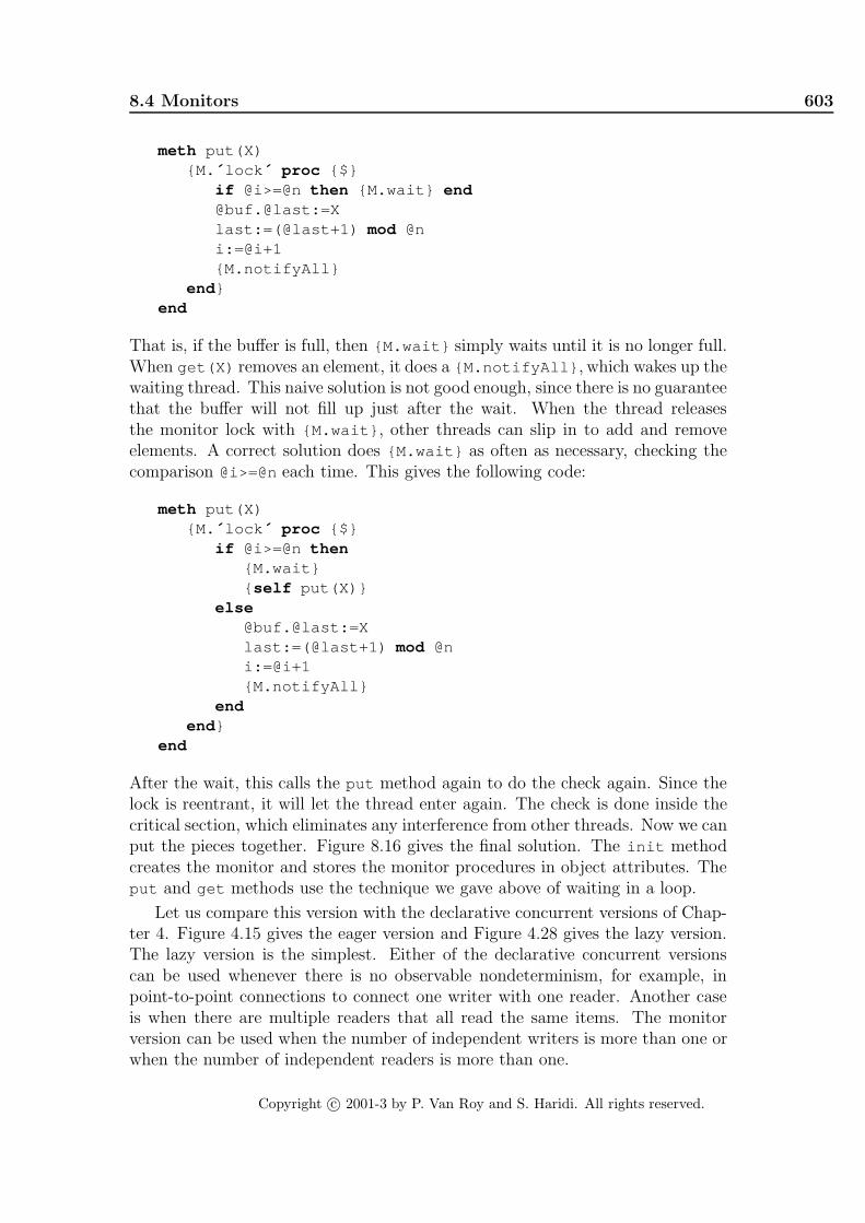
8.4 Monitors 603
meth put(X){M. ´ lock ´ proc {$}
if @i>=@n then {M.wait} end@buf.@last:=Xlast:=(@last+1) mod @ni:=@i+1{M.notifyAll}
end }end
That is, if the buffer is full, then {M.wait} simply waits until it is no longer full.When get(X) removes an element, it does a {M.notifyAll} , which wakes up thewaiting thread. This naive solution is not good enough, since there is no guaranteethat the buffer will not fill up just after the wait. When the thread releasesthe monitor lock with {M.wait} , other threads can slip in to add and removeelements. A correct solution does {M.wait} as often as necessary, checking thecomparison @i>=@neach time. This gives the following code:
meth put(X){M. ´ lock ´ proc {$}
if @i>=@n then{M.wait}{ self put(X)}
else@buf.@last:=Xlast:=(@last+1) mod @ni:=@i+1{M.notifyAll}
endend }
end
After the wait, this calls the put method again to do the check again. Since thelock is reentrant, it will let the thread enter again. The check is done inside thecritical section, which eliminates any interference from other threads. Now we canput the pieces together. Figure 8.16 gives the final solution. The init methodcreates the monitor and stores the monitor procedures in object attributes. Theput and get methods use the technique we gave above of waiting in a loop.
Let us compare this version with the declarative concurrent versions of Chap-ter 4. Figure 4.15 gives the eager version and Figure 4.28 gives the lazy version.The lazy version is the simplest. Either of the declarative concurrent versionscan be used whenever there is no observable nondeterminism, for example, inpoint-to-point connections to connect one writer with one reader. Another caseis when there are multiple readers that all read the same items. The monitorversion can be used when the number of independent writers is more than one orwhen the number of independent readers is more than one.
Copyright c© 2001-3 by P. Van Roy and S. Haridi. All rights reserved.

604 Shared-State Concurrency
class Bufferattr m buf first last n i
meth init(N)m:={NewMonitor}buf:={NewArray 0 N-1 null}n:=N i:=0 first:=0 last:=0
end
meth put(X){@m. lock ´ proc {$}
if @i>=@n then{@m.wait}{ self put(X)}
else@buf.@last:=Xlast:=(@last+1) mod @ni:=@i+1{@m.notifyAll}
endend }
end
meth get(X){@m. lock ´ proc {$}
if @i==0 then{@m.wait}{ self get(X)}
elseX=@buf.@firstfirst:=(@first+1) mod @ni:=@i-1{@m.notifyAll}
endend }
endend
Figure 8.16: Bounded buffer (monitor version)
Copyright c© 2001-3 by P. Van Roy and S. Haridi. All rights reserved.
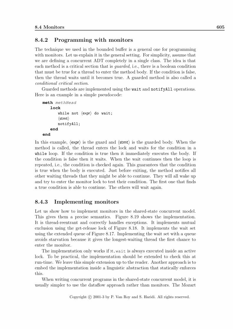
8.4 Monitors 605
8.4.2 Programming with monitors
The technique we used in the bounded buffer is a general one for programmingwith monitors. Let us explain it in the general setting. For simplicity, assume thatwe are defining a concurrent ADT completely in a single class. The idea is thateach method is a critical section that is guarded, i.e., there is a boolean conditionthat must be true for a thread to enter the method body. If the condition is false,then the thread waits until it becomes true. A guarded method is also called aconditional critical section.
Guarded methods are implemented using the wait and notifyAll operations.Here is an example in a simple pseudocode:
meth methHeadlock
while not 〈expr〉 do wait;〈stmt〉notifyAll;
endend
In this example, 〈expr〉 is the guard and 〈stmt〉 is the guarded body. When themethod is called, the thread enters the lock and waits for the condition in awhile loop. If the condition is true then it immediately executes the body. Ifthe condition is false then it waits. When the wait continues then the loop isrepeated, i.e., the condition is checked again. This guarantees that the conditionis true when the body is executed. Just before exiting, the method notifies allother waiting threads that they might be able to continue. They will all wake upand try to enter the monitor lock to test their condition. The first one that findsa true condition is able to continue. The others will wait again.
8.4.3 Implementing monitors
Let us show how to implement monitors in the shared-state concurrent model.This gives them a precise semantics. Figure 8.19 shows the implementation.It is thread-reentrant and correctly handles exceptions. It implements mutualexclusion using the get-release lock of Figure 8.18. It implements the wait setusing the extended queue of Figure 8.17. Implementing the wait set with a queueavoids starvation because it gives the longest-waiting thread the first chance toenter the monitor.
The implementation only works if M.wait is always executed inside an activelock. To be practical, the implementation should be extended to check this atrun-time. We leave this simple extension up to the reader. Another approach is toembed the implementation inside a linguistic abstraction that statically enforcesthis.
When writing concurrent programs in the shared-state concurrent model, it isusually simpler to use the dataflow approach rather than monitors. The Mozart
Copyright c© 2001-3 by P. Van Roy and S. Haridi. All rights reserved.

606 Shared-State Concurrency
fun {NewQueue}...fun {Size}
lock L then @C.1 endendfun {DeleteAll}
lock L thenX q(_ S E)=@C in
C:=q(0 X X)E=nil S
endendfun {DeleteNonBlock}
lock L thenif {Size}>0 then [{Delete}] else nil end
endend
inqueue(insert:Insert delete:Delete size:Size
deleteAll:DeleteAll deleteNonBlock:DeleteNonBlock)end
Figure 8.17: Queue (extended concurrent stateful version)
implementation therefore does no special optimizations to improve monitor per-formance. However, the implementation of Figure 8.19 can be optimized in manyways, which is important if monitor operations are frequent.
Extended concurrent queue
For the monitor implementation, we extend the concurrent queue of Figure 8.8with the three operations Size , DeleteAll , and DeleteNonBlock . This givesthe definition of Figure 8.17.
This queue is a good example of why reentrant locking is useful. Just lookat the definition of DeleteNonBlock : it calls Size and Delete . This will onlywork if the lock is reentrant.
Reentrant get-release lock
For the monitor implementation, we extend the reentrant lock of Figure 8.15 toa get-release lock. This exports the actions of getting and releasing the lock asseparate operations, Get and Release . This gives the definition of Figure 8.18.The operations have to be separate because they are used in both LockM andWaitM .
Copyright c© 2001-3 by P. Van Roy and S. Haridi. All rights reserved.

8.4 Monitors 607
fun {NewGRLock}Token1={NewCell unit }Token2={NewCell unit }CurThr={NewCell unit }
proc {GetLock}if {Thread.this}\=@CurThr then Old New in
{Exchange Token1 Old New}{Wait Old}Token2:=NewCurThr:={Thread.this}
endend
proc {ReleaseLock}CurThr:= unitunit =@Token2
endin
´ lock ´ (get:GetLock release:ReleaseLock)end
Figure 8.18: Lock (reentrant get-release version)
8.4.4 Another semantics for monitors
In the monitor concept we introduced above, notify has just one effect: it causesone waiting thread to leave the wait set. This thread then tries to obtain themonitor lock. The notifying thread does not immediately release the monitorlock. When it does, the notified thread competes with other threads for the lock.This means that an assertion satisfied at the time of the notify might no longerbe satisfied when the notified thread enters the lock. This is why an enteringthread has to check the condition again.
There is a variation that is both more efficient and easier to reason about. Itis for notify to do two operations atomically: it first causes one waiting threadto leave the wait set (as before) and it then immediately passes the monitor lockto that thread. The notifying thread thereby exits from the monitor. This hasthe advantage that an assertion satisfied at the time of the notify will still be truewhen the notified thread continues. The notifyAll operation no longer makesany sense in this variation, so it is left out.
Languages that implement monitors this way usually allow to declare severalwait sets. A wait set is seen by the programmer as an instance of a specialADT called a condition. The programmer can create new instances of conditions,which are called condition variables. Each condition variable c has two operations,c.wait and c.notify.
Copyright c© 2001-3 by P. Van Roy and S. Haridi. All rights reserved.
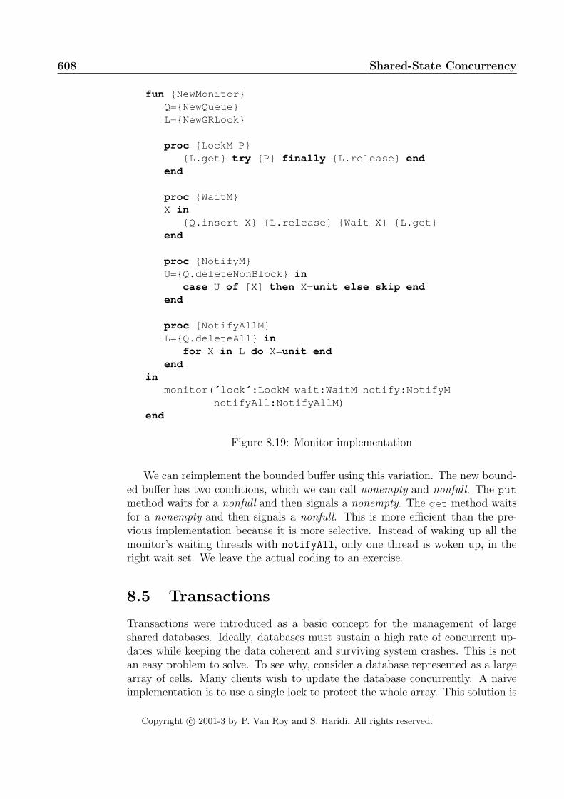
608 Shared-State Concurrency
fun {NewMonitor}Q={NewQueue}L={NewGRLock}
proc {LockM P}{L.get} try {P} finally {L.release} end
end
proc {WaitM}X in
{Q.insert X} {L.release} {Wait X} {L.get}end
proc {NotifyM}U={Q.deleteNonBlock} in
case U of [X] then X=unit else skip endend
proc {NotifyAllM}L={Q.deleteAll} in
for X in L do X=unit endend
inmonitor( ´ lock ´ :LockM wait:WaitM notify:NotifyM
notifyAll:NotifyAllM)end
Figure 8.19: Monitor implementation
We can reimplement the bounded buffer using this variation. The new bound-ed buffer has two conditions, which we can call nonempty and nonfull. The put
method waits for a nonfull and then signals a nonempty. The get method waitsfor a nonempty and then signals a nonfull. This is more efficient than the pre-vious implementation because it is more selective. Instead of waking up all themonitor’s waiting threads with notifyAll, only one thread is woken up, in theright wait set. We leave the actual coding to an exercise.
8.5 Transactions
Transactions were introduced as a basic concept for the management of largeshared databases. Ideally, databases must sustain a high rate of concurrent up-dates while keeping the data coherent and surviving system crashes. This is notan easy problem to solve. To see why, consider a database represented as a largearray of cells. Many clients wish to update the database concurrently. A naiveimplementation is to use a single lock to protect the whole array. This solution is
Copyright c© 2001-3 by P. Van Roy and S. Haridi. All rights reserved.

8.5 Transactions 609
impractical for many reasons. One problem is that a client that takes one minuteto perform an operation will prevent any other operation from taking place duringthat time. This problem can be solved with transactions.
The term “transaction” has acquired a fairly precise meaning: it is any oper-ation that satisfies the four ACID properties [16, 64]. ACID is an acronym:
• A stands for atomic: no intermediate states of a transaction’s execution areobservable. It is as if the transaction happened instantaneously or did nothappen at all. The transaction can complete normally (it commits) or itcan be canceled (it aborts).
• C stands for consistent: observable state changes respect the system in-variants. Consistency is closely related to atomicity. The difference is thatconsistency is the responsibility of the programmer, whereas atomicity isthe responsibility of the implementation of the transaction system.
• I stands for isolation: several transactions can execute concurrently withoutinterfering with each other. They execute as if they were sequential. Thisproperty is also called serializability. It means that the transactions havean interleaving semantics, just like the underlying computation model. Wehave “lifted” the interleaving semantics up from the model to the level ofthe transactions.
• D stands for durability: observable state changes survive across system shut-downs. Durability is often called persistence. Implementing durability re-quires a stable storage (such as a disk) that stores the observable statechanges.
This chapter only gives a brief introduction to transaction systems. The classicreference on transactions is Bernstein et al [16]. This book is clear and preciseand introduces the theory of transactions with just the right amount of formalismto aid intuition. Unfortunately, this book is out of print. Good libraries will oftenhave a copy. Another good book on transactions is Gray & Reuter [64]. An exten-sive and mathematically rigorous treatment is given by Weikum & Vossen [204].
Lightweight (ACI) transactions
Outside of database applications all four ACID properties are not always needed.This section uses the term “transaction” in a narrower sense that is closer to theneeds of general-purpose concurrent programming. Whenever there is a risk ofconfusion, we will call it a light transaction. A lightweight transaction is simplyan abortable atomic action. It has all ACID properties except for D (durability).A lightweight transaction can commit or abort. The abort can be due to a causeinternal to the program (e.g., because of conflicting access to shared data) orexternal to the program (e.g., due to failure of part of the system, like a disk orthe network).
Copyright c© 2001-3 by P. Van Roy and S. Haridi. All rights reserved.

610 Shared-State Concurrency
Motivations
We saw that one motivation for transactions was to increase the throughput ofconcurrent accesses to a database. Let us look at some other motivations. A sec-ond motivation is concurrent programming with exceptions. Most routines havetwo possible ways to exit: either they exit normally or they raise an exception.Usually the routine behaves atomically when it exits normally, i.e., the caller seesthe initial state and the result but nothing in between. When there is an excep-tion this is not the case. The routine might have put part of the system in aninconsistent state. How can we avoid this undesirable situation? There are twosolutions:
• The caller can clean up the called routine’s mess. This means that thecalled routine has to be carefully written so that its mess is always limitedin extent.
• The routine can be inside a transaction. This solution is harder to im-plement, but can make the program much simpler. Raising an exceptioncorresponds to aborting the transaction.
A third motivation is fault tolerance. Lightweight transactions are important forwriting fault-tolerant applications. When a fault occurs, a fault-tolerant applica-tion has to take three steps: (1) detect the fault, (2) contain the fault in a limitedpart of the application, and (3) handle the fault. Lightweight transactions are agood mechanism for fault confinement.
A fourth motivation is resource management. Lightweight transactions allowto acquire multiple resources without causing a concurrent application to stopbecause of an undesirable situation called deadlock. This situation is explainedbelow.
Kernel language viewpoint Let us make a brief detour and examine trans-actions from the viewpoint of computation models. The transactional solutionsatisfies one of our criteria for adding a concept to the computation model, namelythat programs in the extended model are simpler. But what exactly is the con-cept to be added? This is still an open research subject. In our view, it is a veryimportant one. Some day, the solution to this question will be an important partof all general-purpose programming languages. In this section we do not solvethis problem. We will implement transactions as an abstraction in the concurrentstateful model without changing the model.
8.5.1 Concurrency control
Consider a large database accessed by many clients at the same time. What doesthis imply for transactions? It means that they are concurrent yet still satisfyserializability. The implementation should allow concurrent transactions and yet
Copyright c© 2001-3 by P. Van Roy and S. Haridi. All rights reserved.

8.5 Transactions 611
it has to make sure that they are still serializable. There is a strong tensionbetween these two requirements. They are not easy to satisfy simultaneously.The design of transaction systems that satisfy both has led to a rich theory andmany clever algorithms [16, 64].
Concurrency control is the set of techniques used to build and program con-current systems with transactional properties. We introduce these techniques andthe concepts they are based on and we show one practical algorithm. Technicallyspeaking, our algorithm does optimistic concurrency control with strict two-phaselocking and deadlock avoidance. We explain what all these terms mean and whythey are important. Our algorithm is interesting because it is both practical andsimple. A complete working implementation takes just two pages of code.
Locks and timestamps
The two most widely-used approaches to concurrency control are locks and time-stamps:
• Lock-based concurrency control. Each stateful entity has a lock that controlsaccess to the entity. For example, a cell might have a lock that permits onlyone transaction to use it at a time. In order to use a cell, the transactionmust have a lock on it. Locks are important to enforce serializability. Thisis a safety property, i.e., an assertion that is always true during execution.A safety property is simply a system invariant. In general, locks allow torestrict the system’s behavior so that it is safe.
• Timestamp-based concurrency control. Each transaction is given a time-stamp that gives it a priority. The timestamps are taken from an orderedset, something like the numbered tickets used in shops to ensure that cus-tomers are served in order. Timestamps are important to ensure that exe-cution makes progress. For example, that each transaction will eventuallycommit or abort. This is a liveness property, i.e., an assertion that alwayseventually becomes true.
Safety and liveness properties describe how a system behaves as a function oftime. To reason with these properties, it is important to be careful about theexact meanings of the terms “is always true” and “eventually becomes true”.These terms are relative to the current execution step. A property is always trueif it is true at every execution step starting from the current step. A propertyeventually becomes true if there exists at least one execution step in the futurewhere it is true. We can combine always and eventually to make more complicatedproperties. For example, a property that always eventually becomes true meansthat at every step starting from the current step it will eventually become true.The property “an active transaction will eventually abort or commit” is of thistype. This style of reasoning can be given a formal syntax and semantics. Thisresults in a variety of logic called temporal logic.
Copyright c© 2001-3 by P. Van Roy and S. Haridi. All rights reserved.

612 Shared-State Concurrency
Optimistic and pessimistic scheduling
There are many algorithms for concurrency control, which vary on different axes.One of these axes is the degree of optimism or pessimism of the algorithm. Letus introduce this with two examples taken from real life. Both examples concerntraveling, by airplane or by train.
Airlines often overbook flights, that is, sell more tickets than there is roomon the flight. At boarding time, there have usually been enough cancellationsthat this is not a problem (all passengers have a seat). But occasionally somepassengers have no seat, and these have to be accommodated in some way (e.g.,by booking them on a later flight and reimbursing their discomfort). This isan example of optimistic scheduling: a passenger requesting a ticket is given theticket right away even if the flight is already completely booked, as long as theoverbooking is less than some ratio. Occasional problems are tolerated sinceoverbooking allows to increase the average number of filled seats on a flight andbecause problems are easily repaired.
Railways are careful to ensure that there are never two trains traveling towardseach other on the same track segment. A train is only allowed to enter a tracksegment if at that moment there is no other train on the same segment. Protocolsand signaling mechanisms have been devised to ensure this. This is an exampleof pessimistic scheduling: a train requesting to enter a segment may have to waituntil the segment is known to be clear. Unlike the case of overbookings, accidentsare not tolerated because they are extremely costly and usually irreparable interms of people’s lives lost.
Let us see how these approaches apply to transactions. A transaction requestsa lock on a cell. This request is given to a scheduler. The scheduler decides whenand if the request should be fulfilled. It has three possible responses: to satisfythe request immediately, to reject the request (causing a transaction abort), or topostpone its decision. An optimistic scheduler tends to give the lock right away,even if this might cause problems later on (deadlocks and livelocks, see below).A pessimistic scheduler tends to delay giving the lock, until it is sure that noproblems can occur. Depending on how often transactions work on shared data,an optimistic or pessimistic scheduler might be more appropriate. For example,if transactions mostly work on independent data, then an optimistic schedulermay give higher performance. If transactions often work on shared data, then apessimistic scheduler may give higher performance. The algorithm we give belowis an optimistic one; it sometimes has to repair mistakes due to past choices.
Two-phase locking
Two-phase locking is the most popular technique for doing locking. It is usedby almost all commercial transaction processing systems. It can be proved thatdoing two-phase locking guarantees that transactions are serializable. In two-phase locking a transaction has two phases: a growing phase, in which it acquireslocks but does not release them, and a shrinking phase, in which it releases locks
Copyright c© 2001-3 by P. Van Roy and S. Haridi. All rights reserved.

8.5 Transactions 613
but does not acquire them. A transaction is not allowed to release a lock andthen acquire another lock afterwards. This restriction means that a transactionmight hold a lock longer than it needs to. Experience shows that this is not aserious problem.
A popular refinement of two-phase locking used by many systems is calledstrict two-phase locking. In this refinement, all locks are released simultaneouslyat the end of the transaction, after it commits or aborts. This avoids a problemcalled cascading abort. Consider the following scenario. Assume that standardtwo-phase locking is used with two transactions T1 and T2 that share cell C. FirstT1 locks C and changes C’s content. Then T1 releases the lock in its shrinkingphase but continues to be active. Finally T2 locks C, does a calculation withC, and commits. What happens if T1, which is still active, now aborts? If T1aborts then T2 has to abort too, since it has read a value of C modified by T1.T2 could be linked in a similar way to another transaction T3, and so forth. IfT1 aborts then all the others have to abort as well, in cascade, even though theyalready committed. If locks are released only after transactions commit or abortthen this problem does not occur.
8.5.2 A simple transaction manager
Let us design a simple transaction manager. It will do optimistic concurrencycontrol with strict two-phase locking. We first design the algorithm using stepwiserefinement. We then show how to implement a transaction manager that is basedon this algorithm.
A naive algorithm
We start the design with the following simple idea. Whenever a transactionrequests the lock of an unlocked cell, let it acquire the lock immediately withoutany further conditions. If the cell is already locked, then let the transaction waituntil it becomes unlocked. When a transaction commits or aborts, then it releasesall its locks. This algorithm is optimistic because it assumes that getting the lockwill not give problems later on. If problems arise (see next paragraph!) then thealgorithm has to fix them.
Deadlock
Our naive algorithm has a major problem: it suffers from deadlocks. Considertwo concurrent transactions T1 and T2 where each one uses cells C1 and C2. Lettransaction T1 use C1 and C2, in that order, and transaction T2 use C2 and C1,in the reverse order. Because of concurrency, it can happen that T1 has C1’slock and T2 has C2’s lock. When each transaction tries to acquire the other lockit needs, it waits. Both transactions will therefore wait indefinitely. This kindof situation, in which active entities (transactions) wait for resources (cells) in acycle, such that no entity can continue, is called a deadlock.
Copyright c© 2001-3 by P. Van Roy and S. Haridi. All rights reserved.

614 Shared-State Concurrency
How can we ensure that our system never suffers from the consequences ofdeadlock? Like for ailments in general, there are two basic approaches: preventionand cure. The goal of deadlock prevention (also called avoidance) is to prevent adeadlock from ever happening. A transaction is prevented from locking an objectthat might lead to a deadlock. The goal of deadlock cure (also called detection &resolution) is to detect when a deadlock occurs and to take some action to reverseits effects.
Both approaches are based on a concept called the wait-for graph. This is adirected graph that has nodes for active entities (e.g., transactions) and resources(e.g., cells). There is an edge from each active entity to the resource it is waitingfor (if any) but does not yet have. There is an edge from each resource tothe active entity (if any) that has it. A deadlock corresponds to a cycle in thewait-for graph. Deadlock avoidance forbids adding an edge that would make acycle. Deadlock detection detects the existence of a cycle and then removes oneof its edges. The algorithm we give below does deadlock avoidance. It keeps atransaction from getting a lock that might result in a deadlock.
The correct algorithm
We can avoid deadlocks in the naive algorithm by giving earlier transactions high-er priority than later transactions. The basic idea is simple. When a transactiontries to acquire a lock, it compares its priority with the priority of the transactionalready holding the lock. If the latter has lower priority, i.e., it is a more recenttransaction, then it is restarted and the former gets the lock. Let us define analgorithm based on this idea. We assume that transactions perform operations oncells and that each cell comes with a priority queue of waiting transactions, i.e.,the transactions wait in order of their priorities. We use timestamps to implementthe priorities. Here is the complete algorithm:
• A new transaction is given a priority that is lower than all active transac-tions.
• When a transaction tries to acquire a lock on a cell, then it does one of thefollowing:
– If the cell is currently unlocked, then the transaction immediately takesthe lock and continues.
– If the cell is already locked by the transaction, then the transactionjust continues.
– If the cell is locked by a transaction with higher priority, then thecurrent transaction waits, i.e., it enqueues itself on the cell’s queue.
– If the cell is locked by a transaction with lower priority, then restartthe latter and give the lock to the transaction with higher priority.A restart consists of two actions: first to abort the transaction andsecond to start it again with the same priority.
Copyright c© 2001-3 by P. Van Roy and S. Haridi. All rights reserved.

8.5 Transactions 615
Done
already takenAsk for lock
Ask for & obtain lock
Waiting
Running
Restart
ProbationObtain lock
Done
Ask for lock
needs one of my locksHigh priority transaction
High priority transactionneeds one of my locks
StartCommit
orAbort
Figure 8.20: State diagram of one incarnation of a transaction
• When a transaction commits, then it releases all its locks and dequeues onewaiting transaction per released lock (if there is one waiting).
• When a transaction aborts (because it raises an exception or explicitly doesan abort operation) then it unlocks all its locked cells, restores their states,and dequeues one waiting transaction per unlocked cell (if there is onewaiting).
Restarting at a well-defined point
There is a small problem with the above algorithm. It terminates running trans-actions at an arbitrary point during their execution. This can give problems. Itcan lead to inconsistencies in the run-time data structures of the transaction.It can lead to complications in the implementation of the transaction manageritself.
A simple solution to these problems is to terminate the transaction at a well-defined point in its execution. A well-defined point is, for example, the instantwhen a transaction asks the transaction manager for a lock. Let us refine theabove algorithm to restart only at such points. Again, we start with a simplebasic idea: instead of restarting a low priority transaction, we mark it. Later,when it tries to acquire a lock, the transaction manager notices that it is markedand restarts it. To implement this idea, we extend the algorithm as follows:
• Transactions can be in one of three states (the marks):
– running : this is the unmarked state. The transaction is running freelyand is able to acquire locks as before.
– probation : this is the marked state. The transaction still runs freely,but the next time it tries to acquire a lock, it will be restarted. If itasks for no more locks, it will eventually commit.
Copyright c© 2001-3 by P. Van Roy and S. Haridi. All rights reserved.

616 Shared-State Concurrency
– waiting_on(C) : this means that the transaction is waiting for thelock on cell C. It will obtain the lock when it becomes available. How-ever, if a high priority transaction wants a lock held by this one whileit is waiting, it will be restarted.
Figure 8.20 gives the state diagram of one incarnation of a transactionaccording to this scheme. By incarnation we mean part of the lifetime ofa transaction, from its initial start or a restart until it commits, aborts, oragain restarts.
• When a transaction tries to acquire a lock, then it checks its state beforeattempting to acquire locks. If it is in the state probation then it isrestarted immediately. This is fine, since the transaction is at a well-definedpoint.
• When a transaction tries to acquire a lock and the cell is locked by a trans-action with lower priority, then do the following. Enqueue the high prioritytransaction and take action depending on the state of the low priority trans-action:
– running : change the state to probation and continue.
– probation : do nothing.
– waiting_on(C) : remove the low priority transaction from the queueit is waiting on and restart it immediately. This is fine, since it is at awell-defined point.
• When a transaction is enqueued on a cell C, change its state to waiting_on(C) .When a transaction is dequeued, change its state to running .
8.5.3 Transactions on cells
Let us define an ADT for doing transactions on cells that uses the algorithm ofthe previous section.3 We define the ADT as follows:
• {NewTrans ?Trans ?NewCellT} creates a new transaction context andreturns two operations: Trans for creating transactions and NewCellT forcreating new cells.
• A new cell is created by calling NewCellT in the same way as with thestandard NewCell :
{NewCellT X C}
3A similar ADT can be defined for objects, but the implementation is a little more compli-cated since we have to take into account classes and methods. For simplicity we will thereforelimit ourselves to cells.
Copyright c© 2001-3 by P. Van Roy and S. Haridi. All rights reserved.

8.5 Transactions 617
This creates a new cell in the transaction context and binds it to C The cellcan only be used inside transactions of this context. The initial value of thecell is X.
• A new transaction is created by calling the function Trans as follows:
{Trans fun {$ T} 〈expr〉 end B}
The sequential expression 〈expr〉 can interact with its environment in onlythe following ways: it can read values (including procedures and functions)and it can perform operations on cells created with NewCellT . The Trans
call executes 〈expr〉 in a transactional manner and completes when 〈expr〉completes. If 〈expr〉 raises an exception then the transaction will abort andraise the same exception. If the transaction commits, then it has the sameeffect as an atomic execution of 〈expr〉 and it returns the same result. If thetransaction aborts, then it is as if 〈expr〉 were not executed at all (all itsstate changes are undone). B is bound to commit or abort , respectively,depending on whether the transaction commits or aborts.
• There are four operations that can be performed inside 〈expr〉:
– T.access , T.assign , and T.exchange have the same semantics asthe standard three cell operations. They must only use cells createdby NewCellT .
– T.abort is a zero-argument procedure that when called causes thetransaction to abort immediately.
• There are only two ways a transaction can abort: either it raises an excep-tion or it calls T.abort . In all other cases, the transaction will eventuallycommit.
An example
Let us first create a new transaction environment:
declare Trans NewCellT in{NewTrans Trans NewCellT}
We first define two cells in this environment:
C1={NewCellT 0}C2={NewCellT 0}
Now let us increment C1 and decrement C2 in the same transaction:
{Trans proc {$ T _}{T.assign C1 {T.access C1}+1}{T.assign C2 {T.access C2}-1}
end _ _}
Copyright c© 2001-3 by P. Van Roy and S. Haridi. All rights reserved.
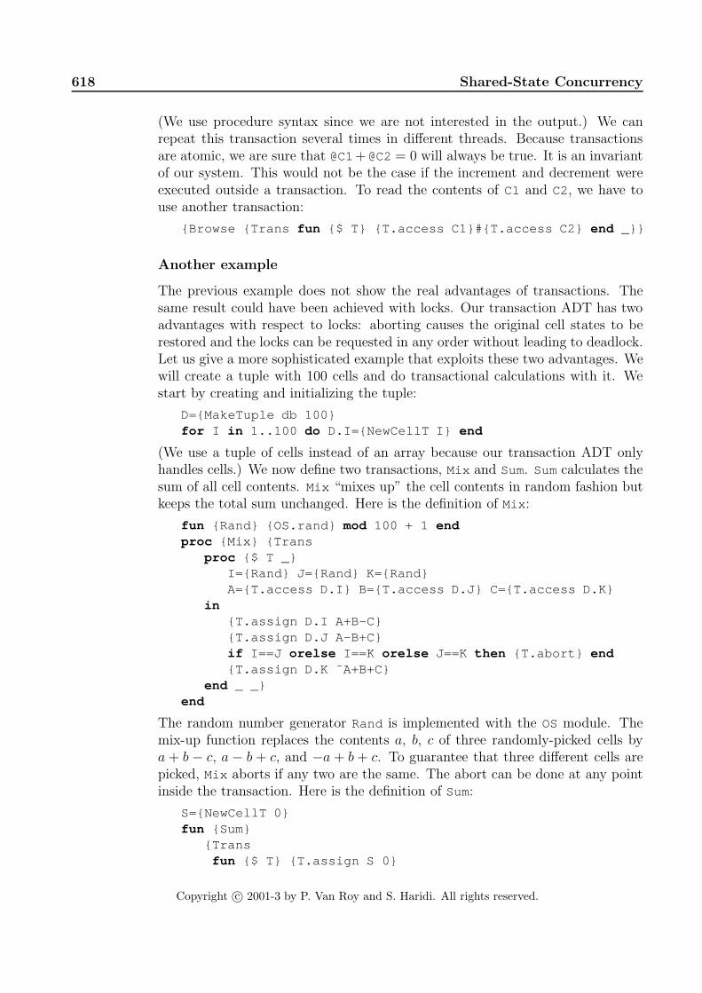
618 Shared-State Concurrency
(We use procedure syntax since we are not interested in the output.) We canrepeat this transaction several times in different threads. Because transactionsare atomic, we are sure that @C1+ @C2= 0 will always be true. It is an invariantof our system. This would not be the case if the increment and decrement wereexecuted outside a transaction. To read the contents of C1 and C2, we have touse another transaction:
{Browse {Trans fun {$ T} {T.access C1}#{T.access C2} end _}}
Another example
The previous example does not show the real advantages of transactions. Thesame result could have been achieved with locks. Our transaction ADT has twoadvantages with respect to locks: aborting causes the original cell states to berestored and the locks can be requested in any order without leading to deadlock.Let us give a more sophisticated example that exploits these two advantages. Wewill create a tuple with 100 cells and do transactional calculations with it. Westart by creating and initializing the tuple:
D={MakeTuple db 100}for I in 1..100 do D.I={NewCellT I} end
(We use a tuple of cells instead of an array because our transaction ADT onlyhandles cells.) We now define two transactions, Mix and Sum. Sumcalculates thesum of all cell contents. Mix “mixes up” the cell contents in random fashion butkeeps the total sum unchanged. Here is the definition of Mix :
fun {Rand} {OS.rand} mod 100 + 1 endproc {Mix} {Trans
proc {$ T _}I={Rand} J={Rand} K={Rand}A={T.access D.I} B={T.access D.J} C={T.access D.K}
in{T.assign D.I A+B-C}{T.assign D.J A-B+C}if I==J orelse I==K orelse J==K then {T.abort} end{T.assign D.K ˜A+B+C}
end _ _}end
The random number generator Rand is implemented with the OS module. Themix-up function replaces the contents a, b, c of three randomly-picked cells bya + b − c, a − b + c, and −a + b + c. To guarantee that three different cells arepicked, Mix aborts if any two are the same. The abort can be done at any pointinside the transaction. Here is the definition of Sum:
S={NewCellT 0}fun {Sum}
{Transfun {$ T} {T.assign S 0}
Copyright c© 2001-3 by P. Van Roy and S. Haridi. All rights reserved.

8.5 Transactions 619
(active object)
TM
T
T
Sync=ok
abort(T)
savestate(T C ?Sync)
commit(T)
getlock(T C ?Sync)
Sync=okSync=halt
..
.
Sequentialtransactions
Asynchronous messages managerTransaction
Figure 8.21: Architecture of the transaction system
for I in 1..100 do{T.assign S {T.access S}+{T.access D.I}} end
{T.access S}end _}
end
Sumuses the cell S to hold the sum. Note that Sum is a big transaction since itsimultaneously locks all cells in the tuple. Now we can do some calculations:
{Browse {Sum}} % Displays 5050for I in 1..1000 do thread {Mix} end end{Browse {Sum}} % Still displays 5050
5050 is the sum of the integers from 1 to 100. You can check that the values ofindividual cells are well and truly mixed:
{Browse {Trans fun {$ T} {T.access D.1}#{T.access D.2} end _}}
This initially displays 1#2 , but will subsequently display very different values.
8.5.4 Implementing transactions on cells
Let us show how to build a transaction system that implements our optimistictwo-phase locking algorithm. The implementation consists of a transaction man-ager and a set of running transactions. (Transaction managers come in manyvarieties and are sometimes called transaction processing monitors [64].) Thetransaction manager and the running transactions each execute in its own thread.This allows terminating a running transaction without affecting the transaction
Copyright c© 2001-3 by P. Van Roy and S. Haridi. All rights reserved.

620 Shared-State Concurrency
manager. A running thread sends four kinds of messages to the transaction man-ager: to get a lock (getlock ), to save a cell’s state (savestate ), to commit(commit ), and to abort (abort ). Figure 8.21 shows the architecture.
The transaction manager is always active and accepts commands from therunning transactions’ threads. When a transaction is restarted, it restarts in anew thread. It keeps the same timestamp, though. We implement the transactionmanager as an active object using the NewActive function of Section 7.8. Theactive object has two internal methods, Unlockall and Trans , and five externalmethods, newtrans , getlock , savestate , commit , and abort . Figures 8.22and 8.23 show the implementation of the transaction system. Together withNewActive and the priority queue, this is a complete working implementation.Each active transaction is represented by a record with five fields:
• stamp : This is the transaction’s timestamp, a unique integer that identifiesthe transaction and its priority. This number is incremented for successivetransactions. High priority therefore means a small timestamp.
• save : This is a dictionary indexed by cell name (see below) that containsentries of the form save(cell:C state:S) , where C is a cell record (asrepresented below) and S is the cell’s original state.
• body : This is the function fun {$ T} 〈expr〉 end that represents the trans-action body.
• state : This is a cell containing running , probation , or waiting_on(C) .If probation , it means that the transaction will be restarted the next timeit tries to obtain a lock. If waiting_on(C) , it means that the transactionwill be restarted immediately if a higher priority transaction needs C.
• result : This is a dataflow variable that will be bound to commit(Res) ,abort(Exc) , or abort when the transaction completes.
Each cell is represented by a record with four fields:
• name: This is a name value that is the cell’s unique identifier.
• owner : This is either unit , if no transaction is currently locking the cell,or the transaction record if a transaction is locking the cell.
• queue : This is a priority queue containing pairs of the form Sync#T , whereT is a transaction record and Sync is the synchronization variable on whichthe transaction is currently blocked. The priority is the transaction’s time-stamp. Sync will always eventually be bound by the transaction managerto ok or halt .
• state : This is a cell that contains the transactional cell’s content.
Copyright c© 2001-3 by P. Van Roy and S. Haridi. All rights reserved.

8.5 Transactions 621
class TMClassattr timestamp tmmeth init(TM) timestamp:=0 tm:=TM end
meth Unlockall(T RestoreFlag)for save(cell:C state:S) in {Dictionary.items T.save} do
(C.owner):= unitif RestoreFlag then (C.state):=S endif {Not {C.queue.isEmpty}} thenSync2#T2={C.queue.dequeue} in
(T2.state):=running(C.owner):=T2 Sync2=ok
endend
end
meth Trans(P ?R TS) /* See next figure */ endmeth getlock(T C ?Sync) /* See next figure */ end
meth newtrans(P ?R)timestamp:=@timestamp+1 { self Trans(P R @timestamp)}
endmeth savestate(T C ?Sync)
if {Not {Dictionary.member T.save C.name}} then(T.save).(C.name):=save(cell:C state:@(C.state))
end Sync=okendmeth commit(T) { self Unlockall(T false )} endmeth abort(T) { self Unlockall(T true )} end
end
proc {NewTrans ?Trans ?NewCellT}TM={NewActive TMClass init(TM)} in
fun {Trans P ?B} R in{TM newtrans(P R)}case R of abort then B=abort unit[] abort(Exc) then B=abort raise Exc end[] commit(Res) then B=commit Res end
endfun {NewCellT X}
cell(name:{NewName} owner:{NewCell unit }queue:{NewPrioQueue} state:{NewCell X})
endend
Figure 8.22: Implementation of the transaction system (part 1)
Copyright c© 2001-3 by P. Van Roy and S. Haridi. All rights reserved.

622 Shared-State Concurrency
meth Trans(P ?R TS)Halt={NewName}T=trans(stamp:TS save:{NewDictionary} body:P
state:{NewCell running} result:R)proc {ExcT C X Y} S1 S2 in
{@tm getlock(T C S1)}if S1==halt then raise Halt end end{@tm savestate(T C S2)} {Wait S2}{Exchange C.state X Y}
endproc {AccT C ?X} {ExcT C X X} endproc {AssT C X} {ExcT C _ X} endproc {AboT} {@tm abort(T)} R=abort raise Halt end end
inthread try Res={T.body t(access:AccT assign:AssT
exchange:ExcT abort:AboT)}in {@tm commit(T)} R=commit(Res)catch E then
if E\=Halt then {@tm abort(T)} R=abort(E) endend end
end
meth getlock(T C ?Sync)if @(T.state)==probation then
{ self Unlockall(T true )}{ self Trans(T.body T.result T.stamp)} Sync=halt
elseif @(C.owner)== unit then(C.owner):=T Sync=ok
elseif T.stamp==@(C.owner).stamp thenSync=ok
else /* T.stamp\=@(C.owner).stamp */ T2=@(C.owner) in{C.queue.enqueue Sync#T T.stamp}(T.state):=waiting_on(C)if T.stamp<T2.stamp then
case @(T2.state) of waiting_on(C2) thenSync2#_={C2.queue.delete T2.stamp} in
{ self Unlockall(T2 true )}{ self Trans(T2.body T2.result T2.stamp)}Sync2=halt
[] running then(T2.state):=probation
[] probation then skip endend
endend
Figure 8.23: Implementation of the transaction system (part 2)
Copyright c© 2001-3 by P. Van Roy and S. Haridi. All rights reserved.

8.5 Transactions 623
When a transaction T does an exchange operation on cell C, it executes theExcT procedure defined in Trans . This first sends getlock(T C Sync1) to thetransaction manager to request a lock on the cell. The transaction manager replieswith Sync1=ok if the transaction successfully gets the lock and Sync1=halt ifthe current thread should be terminated. In the latter case, getlock ensuresthat the transaction is restarted. If the transaction gets the lock, then it callssavestate(T C Sync2) to save the original cell state.
Priority queue
The transaction manager uses priority queues to make sure that high prioritytransactions get the first chance to lock cells. A priority queue is a queue whoseentries are always ordered according to some priority. In our queue, the prioritiesare integers and the lowest value has the highest priority. We define the ADT asfollows:
• Q={NewPrioQueue} creates an empty priority queue.
• {Q.enqueue X P} inserts X with priority P, where P is an integer.
• X={Q.dequeue} returns the entry with the smallest integer value and re-moves it from the queue.
• X={Q.delete P} returns the entry with priority P and removes it from thequeue.
• B={Q.isEmpty} returns true or false depending on whether Q is empty ornot.
Figure 8.24 shows a simple implementation of the priority queue. The priorityqueue is represented internally as a cell containing a list of pairs pair(X P) ,which are ordered according to increasing P. The dequeue operation executes inO(1) time. The enqueue and delete operations execute in O(s) time where sis the size of the queue. More sophisticated implementations are possible withbetter time complexities.
8.5.5 More on transactions
We have just scratched the surface of transaction processing. Let us finish bymentioning some of the most useful extensions [64]:
• Durability. We have not shown how to make a state change persistent.This is done by putting state changes on stable storage, such as a disk.Techniques for doing this are carefully designed to maintain atomicity, nomatter at what instant in time a system crash happens.
Copyright c© 2001-3 by P. Van Roy and S. Haridi. All rights reserved.

624 Shared-State Concurrency
fun {NewPrioQueue}Q={NewCell nil}proc {Enqueue X Prio}
fun {InsertLoop L}case L of pair(Y P)|L2 then
if Prio<P then pair(X Prio)|Lelse pair(Y P)|{InsertLoop L2} end
[] nil then [pair(X Prio)] endend
in Q:={InsertLoop @Q} end
fun {Dequeue}pair(Y _)|L2=@Q
inQ:=L2 Y
end
fun {Delete Prio}fun {DeleteLoop L}
case L of pair(Y P)|L2 thenif P==Prio then X=Y L2else pair(Y P)|{DeleteLoop L2} end
[] nil then nil endend X
inQ:={DeleteLoop @Q}X
end
fun {IsEmpty} @Q==nil endin
queue(enqueue:Enqueue dequeue:Dequeuedelete:Delete isEmpty:IsEmpty)
end
Figure 8.24: Priority queue
Copyright c© 2001-3 by P. Van Roy and S. Haridi. All rights reserved.

8.6 The Java language (concurrent part) 625
• Nested transactions. It often happens that we have a long-lived transactionthat contains a series of smaller transactions. For example, a complex banktransaction might consist of a large series of updates to many accounts.Each of these updates is a transaction. The series itself should also be atransaction: if something goes wrong in the middle, it is canceled. Thereis a strong relationship between nested transactions, encapsulation, andmodularity.
• Distributed transactions. It often happens that a database is spread overseveral physical sites, either for performance or organizational reasons. Wewould still like to perform transactions on the database.
8.6 The Java language (concurrent part)
The introduction of Section 7.7 only talked about the sequential part of Java.We now extend this to the concurrent part. Concurrent programming in Java issupported by two concepts: threads and monitors. Java is designed for shared-state concurrency. Threads are too heavyweight to support an active objectapproach efficiently. Monitors have the semantics of Section 8.4. Monitors arelightweight constructs that are associated to individual objects.
Each program starts with one thread, the one that executes main. New threadscan be created in two ways, by instantiating a subclass of the Thread class or byimplementing the Runnable interface. By default, the program terminates whenall its threads terminate. Since threads tend to be heavyweight in current Ja-va implementations, the programmer is encouraged not to create many of them.Using the Thread class gives more control, but might be overkill for some appli-cations. Using the Runnable interface is lighter. Both techniques assume thatthere is a method run:
public void run();
that defines the thread’s body. The Runnable interface consists of just this singlemethod.
Threads interact by means of shared objects. To control the interaction, anyJava object can be a monitor, as defined in Section 8.4. Methods can executeinside the monitor lock with the keyword synchronized. Methods without thiskeyword are called non-synchronized. They execute outside the monitor lock butcan still see the object attributes. This ability has been strongly criticized becausethe compiler can no longer guarantee that the object attributes are accessedsequentially [24]. Non-synchronized methods can be more efficient, but theyshould be used extremely rarely.
We give two examples. The first example uses synchronized methods justfor locking. The second example uses the full monitor operations. For furtherreading, we recommend [111].
Copyright c© 2001-3 by P. Van Roy and S. Haridi. All rights reserved.

626 Shared-State Concurrency
8.6.1 Locks
The simplest way to do concurrent programming in Java is with multiple threadsthat access shared objects. Let us extend the class Point as an example:
class Point {
double x, y;
Point(double x1, y1) { x=x1; y=y1; }
public double getX() { return x; }
public double getY() { return y; }
public synchronized void origin() { x=0.0; y=0.0; }
public synchronized void add(Point p)
{ x+=p.getX(); y+=p.getY(); }
public synchronized void scale(double s) { x*=s; y*=s; }
public void draw(Graphics g) {
double lx, ly;
synchronized (this) { lx=x; ly=y; }
g.drawPoint(lx, ly);
}
}
Each instance of Point has its own lock. Because of the keyword synchronized,the methods origin, add, and scale all execute within the lock. The methoddraw is only partly synchronized. This is because it calls an external method,g.drawPoint (not defined in the example). Putting the external method insidethe object lock would increase the likelihood of deadlocking the program. Instead,g should have its own lock.
8.6.2 Monitors
Monitors are an extension of locks that give more control over how threads enterand exit. Monitors can be used to do more sophisticated kinds of cooperationbetween threads accessing a shared object. Section 8.4.1 shows how to write abounded buffer using monitors. The solution given there can easily be translatedto Java, giving Figure 8.25. This defines a bounded buffer of integers. It usesan array of integers, buf, which is allocated when the buffer is initialized. Thepercent sign % denotes the modulo operation, i.e., the remainder after integerdivision.
8.7 Exercises
1. Number of interleavings. Generalize the argument used in the chapterintroduction to calculate the number of possible interleavings of n threads,each doing k operations. Using Stirling’s formula for the factorial function,n! ≈
√2πnn+1/2e−n, calculate a closed form approximation to this function.
Copyright c© 2001-3 by P. Van Roy and S. Haridi. All rights reserved.

8.7 Exercises 627
class Buffer
int[] buf;
int first, last, n, i;
public void init(int size) {
buf=new int[size];
n=size; i=0; first=0; last=0;
}
public synchronized void put(int x) {
while (i<n) wait();
buf[last]=x;
last=(last+1)%n;
i=i+1;
notifyAll();
}
public synchronized int get() {
int x;
while (i==0) wait();
x=buf[first];
first=(first+1)%n;
i=i-1;
notifyAll();
return x;
}
}
Figure 8.25: Bounded buffer (Java version)
Copyright c© 2001-3 by P. Van Roy and S. Haridi. All rights reserved.

628 Shared-State Concurrency
2. Concurrent counter. Let us implement a concurrent counter in the sim-plest possible way. The counter has an increment operation. We wouldlike this operation to be callable from any number of threads. Consider thefollowing possible implementation that uses one cell and an Exchange :
local X in {Exchange C X X+1} end
This attempted solution does not work.
• Explain why the above program does not work and propose a simplefix.
• Would your fix still be possible in a language that did not have dataflowvariables? Explain why or why not.
• Give a solution (perhaps the same one as in the previous point) thatworks in a language without dataflow variables.
3. Maximal concurrency and efficiency. In between the shared-state con-current model and the maximally concurrent model, there is an interestingmodel called the job-based concurrent model. The job-based model is identi-cal to the shared-state concurrent model, except that whenever an operationwould block, a new thread is created with only that operation (this is calleda job) and the original thread continues execution.4 Practically speaking,the job-based model has all the concurrency of the maximally concurrentmodel, and in addition it can easily be implemented efficiently. For this ex-ercise, investigate the job-based model. Is it a good choice for a concurrentprogramming language? Why or why not?
4. Simulating slow networks. Section 8.2.2 defines a function SlowNet2
that creates a “slow” version of an object. But this definition imposesa strong order constraint. Each slow object defines a global order of itscalls and guarantees that the original objects are called in this order. Thisconstraint is often too strong. A more refined version would only imposeorder among object calls within the same thread. Between different threads,there is no reason to impose an order. Define a function SlowNet3 thatcreates slow objects with this property.
5. The MVar abstraction. An MVar is a box that can be full or empty. Itcomes with two procedures, Put and Get . Doing {Put X} puts X in thebox if it is empty, thus making it full. If the box is full, Put waits until it isempty. Doing {Get X} binds X to the boxes’ content and empties the box.If the box is empty, Get waits until it is full. For this exercise, implementthe MVar abstraction. Use whatever concurrency approach is most natural.
4The initial Oz language used the job-based model [180].
Copyright c© 2001-3 by P. Van Roy and S. Haridi. All rights reserved.
8.7 Exercises 629
6. Communicating Sequential Processes (CSP). The CSP language con-sists of independent threads (called “processes” in CSP terminology) com-municating through synchronous channels [83, 165]. The channels have twooperations, send and receive, with rendezvous semantics. That is, a sendblocks until a receive is present and vice versa. When send and receive aresimultaneously present, then they both complete atomically, transferringinformation from send to receive. The Ada language also uses rendezvoussemantics. In addition, there is a nondeterministic receive operation whichlistens to several channels simultaneously. As soon as a message is receivedon one of the channels, then the nondeterministic receive completes. Forthis exercise, implement these CSP operations as the following control ab-straction:
• C={Channel.new} creates a new channel C.
• {Channel.send C M} sends message Mon channel C.
• {Channel.mreceive [C1#S1 C2#S2 ... Cn#Sn]} listens nondeter-ministically on channels C1, C2, ..., and Cn. Si is a one-argumentprocedure proc {$ M} 〈stmt〉 end that is executed when message M
is received on channel Ci .
Now extend the Channel.mreceive operation with guards:
• {Channel.mreceive [C1#B1#S1 C2#B2#S2 ... Cn#Bn#Sn]} , whereBi is a one-argument boolean function fun {$ M} 〈expr〉 end thatmust return true for a message to be received on channel Ci .
7. Comparing Linda with Erlang. Linda has a read operation that canselectively retrieve tuples according to a pattern (see Section 8.3.2). Erlanghas a receive operation that can selectively receive messages according toa pattern (see Section 5.6.3). For this exercise, compare and contrast thesetwo operations and the abstractions that they are part of. What do theyhave in common and how do they differ? For what kinds of application iseach best suited?
8. Termination detection with monitors. This exercise is about detectingwhen a group of threads are all terminated. Section 4.4.3 gives an algorithmthat works for a flat thread space, where threads are not allowed to createnew threads. Section 5.5.3 gives an algorithm that works for a hierarchicalthread space, where threads can create new threads to any nesting level.The second algorithm uses a port to collect the termination information.For this exercise, write an algorithm that works for a hierarchical threadspace, like the second algorithm, but that uses a monitor instead of a port.
9. Monitors and conditions. Section 8.4.4 gives an alternative semantics formonitors in which there can be several wait sets, which are called conditions.
Copyright c© 2001-3 by P. Van Roy and S. Haridi. All rights reserved.

630 Shared-State Concurrency
The purpose of this exercise is to study this alternative and compare it withmain approach given in the text.
• Reimplement the bounded buffer example of Figure 8.16 using moni-tors with conditions.
• Modify the monitor implementation of Figure 8.19 to implement mon-itors with conditions. Allow the possibility to create more than onecondition for a monitor.
10. Breaking up big transactions. The second example in Section 8.5.3defines the transaction Sum that locks all the cells in the tuple while itis calculating their sum. While Sum is active, no other transaction cancontinue. For this exercise, rewrite Sum as a series of small transactions.Each small transaction should only lock a few cells. Define a representationfor a partial sum, so that a small transaction can see what has already beendone and determine how to continue. Verify your work by showing that youcan perform transactions while a sum calculation is in progress.
11. Lock caching. In the interest of simplicity, the transaction manager ofSection 8.5.4 has some minor inefficiencies. For example, getlock andsavestate messages are sent on each use of a cell by a transaction. It isclear that they are only really needed the first time. For this exercise, opti-mize the getlock and savestate protocols so they use the least possiblenumber of messages.
12. Read and write locks. The transaction manager of Section 8.5 locks acell upon its first use. If transactions T1 and T2 both want to read thesame cell’s content, then they cannot both lock the cell simultaneously. Wecan relax this behavior by introducing two kinds of locks, read locks andwrite locks. A transaction that holds a read lock is only allowed to read thecell’s content, not change it. A transaction that holds a write lock can doall cell operations. A cell can either be locked with exactly one write lockor with any number of read locks. For this exercise, extend the transactionmanager to use read and write locks.
13. Concurrent transactions. The transaction manager of Section 8.5 cor-rectly handles any number of transactions that execute concurrently, buteach individual transaction must be sequential. For this exercise, extend thetransaction manager so that the individual transactions can themselves beconcurrent. Hint: add the termination detection algorithm of Section 5.5.3.
14. Combining monitors and transactions. Design and implement a con-currency abstraction that combines the abilities of monitors and transac-tions. That is, it has the ability to wait and notify, and also the ability toabort without changing any state. Is this a useful abstraction?
Copyright c© 2001-3 by P. Van Roy and S. Haridi. All rights reserved.

8.7 Exercises 631
15. (research project) Transactional computation model. Extend the shared-state concurrent model of this chapter to allow transactions, as suggestedin Section 8.5. Your extension should satisfy the following properties:
• It should have a simple formal semantics.
• It should be efficient, i.e., only cause overhead when transactions areactually used.
• It should preserve good properties of the model, e.g., compositionality.
This will allow programs to use transactions without needing costly andcumbersome encodings. Implement a programming language that uses yourextension and evaluate it for realistic concurrent programs.
Copyright c© 2001-3 by P. Van Roy and S. Haridi. All rights reserved.

632 Shared-State Concurrency
Copyright c© 2001-3 by P. Van Roy and S. Haridi. All rights reserved.

Chapter 9
Relational Programming
“Toward the end of the thirteenth century, Ramon Llull (RaimundoLulio or Raymond Lully) invented the thinking machine. [...] Thecircumstances and objectives of this machine no longer interest us,but its guiding principle–the methodical application of chance to theresolution of a problem–still does.”– Ramon Llull’s Thinking Machine, Jorge Luis Borges (1899–1986)
“In retrospect it can now be said that the ars magna Lulli was thefirst seed of what is now called “symbolic logic,” but it took a longtime until the seed brought fruit, this particular fruit.”– Postscript to the “Universal Library”, Willy Ley (1957)
A procedure in the declarative model uses its input arguments to calculatethe values of its output arguments. This is a functional calculation, in the math-ematical sense: the outputs are functions of the inputs. For a given set of inputargument values, there is only one set of output argument values. We can gen-eralize this to become relational. A relational procedure is more flexible in twoways than a functional procedure. First, there can be any number of results to acall, either zero (no results), one, or more. Second, which arguments are inputsand which are outputs can be different for each call.
This flexibility makes relational programming well-suited for databases andparsers, in particular for difficult cases such as deductive databases and parsingambiguous grammars. It can also be used to enumerate solutions to complexcombinatoric problems. We have used it to automatically generate diagnosticsfor a RISC microprocessor, the VLSI-BAM [84, 193]. The diagnostics enumerateall possible instruction sequences that use register forwarding. Relational pro-gramming has also been used in artificial intelligence applications such as DavidWarren’s venerable WARPLAN planner [39].
From the programmer’s point of view, relational programming extends declar-ative programming with a new kind of statement called “choice”. Conceptually,the choice statement nondeterministically picks one among a set of alternatives.
Copyright c© 2001-3 by P. Van Roy and S. Haridi. All rights reserved.

634 Relational Programming
During execution, the choice is implemented with search, which enumerates thepossible answers. We call this don’t know nondeterminism, although the searchalgorithm is almost always deterministic.
Introducing a choice statement is an old idea. E. W. Elcock [52] used it in1967 in the Absys language and Floyd [53] used it in the same year. The Prologlanguage uses a choice operation as the heart of its execution model, which wasdefined in 1972 [40]. Floyd gives a lucid account of the choice operation. Hefirst extends a simple Algol-like language with a function called choice(n), whichreturns an integer from 1 to n. He then shows how to implement a depth-firstsearch strategy using flow charts to give the operational semantics of the extendedlanguage.
Watch out for efficiency
The flexibility of relational programming has a reverse side. It can easily leadto highly inefficient programs, if not used properly. This cannot be avoided ingeneral since each new choice operation multiplies the size of the search space bythe number of alternatives. The search space is the set of candidate solutions to aproblem. This means the size is exponential in the number of choice operations.However, relational programming is sometimes practical:
• When the search space is small. This is typically the case for databaseapplications. Another example is the above-mentioned VLSI-BAM diagnos-tics generator, which generated all combinations of instructions for registerforwarding, condition bit forwarding, and branches in branch delay slots.This gave a total of about 70,000 lines of VLSI-BAM assembly languagecode. This was small enough to be used as input to the gate-level simula-tor.
• As an exploratory tool. If used on small examples, relational program-ming can give results even if it is impractical for bigger examples. Theadvantage is that the programs can be much shorter and easier to write:no algorithm has to be devised since search is a brute force technique thatavoids the need for algorithms. This is an example of nonalgorithmic pro-gramming. This kind of exploration gives insight into the problem structure.This insight is often sufficient to design an efficient algorithm.
To use search in other cases, more sophisticated techniques are needed, e.g., pow-erful constraint-solving algorithms, optimizations based on the problem structure,and search heuristics. We leave these until Chapter 12. The present chapterstudies the use of nondeterministic programming as a tool for the two classes ofproblems for which it works well. For more information and techniques, we rec-ommend any good book on Prolog, which has good support for nondeterministicprogramming [182, 39].
Copyright c© 2001-3 by P. Van Roy and S. Haridi. All rights reserved.

9.1 The relational computation model 635
〈s〉 ::=skip Empty statement| 〈s〉1 〈s〉2 Statement sequence| local 〈x〉 in 〈s〉 end Variable creation| 〈x〉1=〈x〉2 Variable-variable binding| 〈x〉=〈v〉 Value creation| if 〈x〉 then 〈s〉1 else 〈s〉2 end Conditional| case 〈x〉 of 〈pattern〉 then 〈s〉1 else 〈s〉2 end Pattern matching| { 〈x〉 〈y〉1 ... 〈y〉n} Procedure application| choice 〈s〉1 [] ... [] 〈s〉n end Choice| fail Failure
Table 9.1: The relational kernel language
Structure of the chapter
The chapter consists of four parts:
• Section 9.1 explains the basic concepts of the relational computation model,namely choice and encapsulated search. Section 9.2 continues with somemore examples to introduce programming in the model.
• Section 9.3 introduces logic and logic programming. It introduces a newkind of semantics for programs, the logical semantics. It then explains howboth the declarative and relational computation models are doing logicprogramming.
• Sections 9.4–9.6 give large examples in three areas that are particularlywell-suited to relational programming, namely natural language parsing,interpreters, and deductive databases.
• Section 9.7 gives an introduction to Prolog, a programming language basedon relational programming. Prolog was originally designed for natural lan-guage processing, but has become one of the main programming languagesin all areas that require symbolic programming.
9.1 The relational computation model
9.1.1 The choice and fail statements
The relational computation model extends the declarative model with two newstatements, choice and fail :
Copyright c© 2001-3 by P. Van Roy and S. Haridi. All rights reserved.
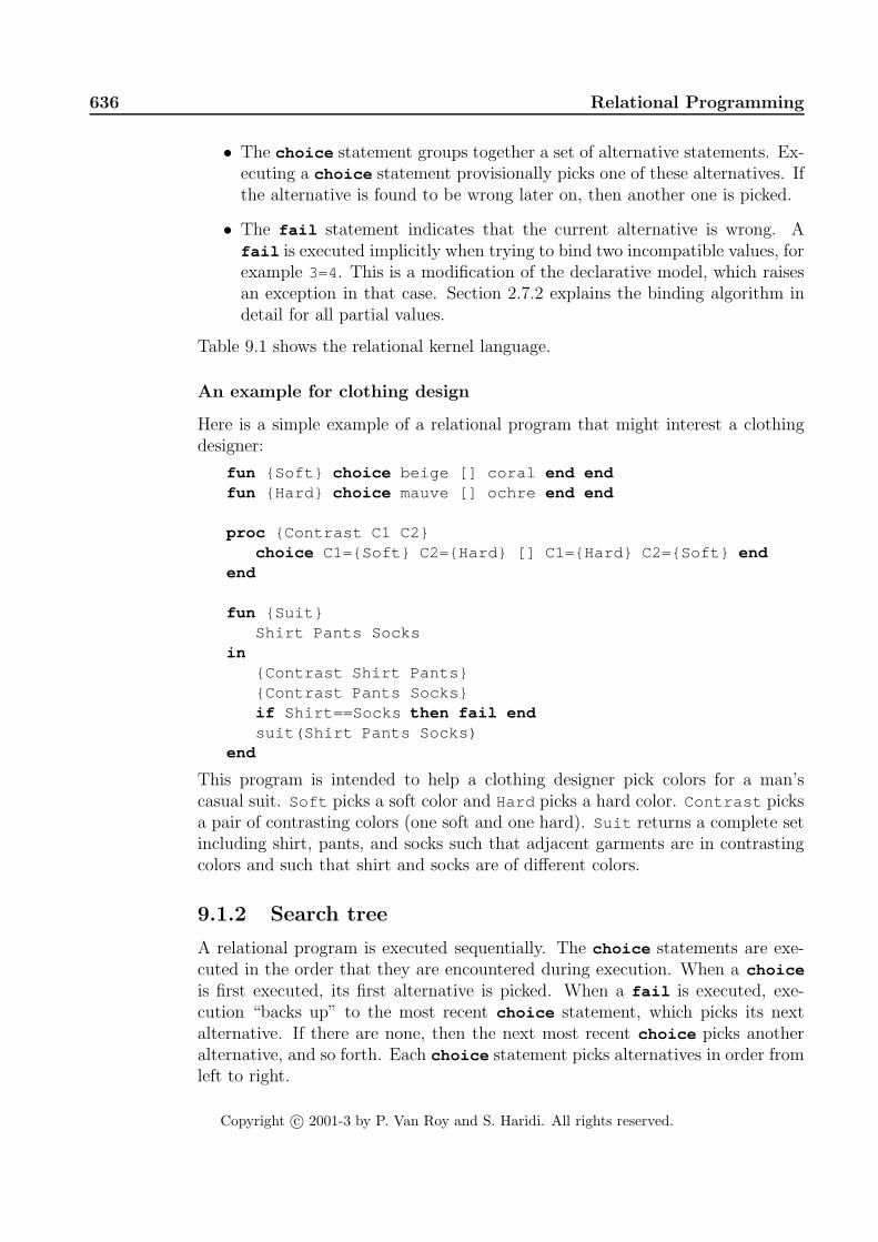
636 Relational Programming
• The choice statement groups together a set of alternative statements. Ex-ecuting a choice statement provisionally picks one of these alternatives. Ifthe alternative is found to be wrong later on, then another one is picked.
• The fail statement indicates that the current alternative is wrong. Afail is executed implicitly when trying to bind two incompatible values, forexample 3=4 . This is a modification of the declarative model, which raisesan exception in that case. Section 2.7.2 explains the binding algorithm indetail for all partial values.
Table 9.1 shows the relational kernel language.
An example for clothing design
Here is a simple example of a relational program that might interest a clothingdesigner:
fun {Soft} choice beige [] coral end endfun {Hard} choice mauve [] ochre end end
proc {Contrast C1 C2}choice C1={Soft} C2={Hard} [] C1={Hard} C2={Soft} end
end
fun {Suit}Shirt Pants Socks
in{Contrast Shirt Pants}{Contrast Pants Socks}if Shirt==Socks then fail endsuit(Shirt Pants Socks)
end
This program is intended to help a clothing designer pick colors for a man’scasual suit. Soft picks a soft color and Hard picks a hard color. Contrast picksa pair of contrasting colors (one soft and one hard). Suit returns a complete setincluding shirt, pants, and socks such that adjacent garments are in contrastingcolors and such that shirt and socks are of different colors.
9.1.2 Search tree
A relational program is executed sequentially. The choice statements are exe-cuted in the order that they are encountered during execution. When a choice
is first executed, its first alternative is picked. When a fail is executed, exe-cution “backs up” to the most recent choice statement, which picks its nextalternative. If there are none, then the next most recent choice picks anotheralternative, and so forth. Each choice statement picks alternatives in order fromleft to right.
Copyright c© 2001-3 by P. Van Roy and S. Haridi. All rights reserved.

9.1 The relational computation model 637
......
...... ......
Shirt=beigePants=ochre
Shirt=beigePants=mauve
Shirt=coralPants=mauve
Shirt=coralPants=ochre
Pants={Hard}Shirt=beige
Pants={Hard}Shirt=coral
Pants={Hard}Shirt={Soft}
{Suit}
Shirt={Hard}Pants={Soft}
Pants={Soft}Socks={Hard}
Pants=mauveShirt=beige
Pants={Hard}Socks={Soft}
Shirt=beigePants=mauve
Shirt=beige Shirt=beigePants=mauve
Shirt=beigePants=mauvePants=beigeSocks={Hard}
Shirt=beigePants=mauvePants=coralSocks={Hard}
(fail) (fail)
Pants=mauvePants=ochrePants=mauve
Socks={Soft} Socks={Soft}
Shirt=beigePants=mauveSocks=coralShirt\=Socks
Shirt=beigePants=mauveSocks=beigeShirt\=Socks
(fail)
(fail) (succeed)
... ...
choice
choice
choice
choice
choice
choice
choice
Figure 9.1: Search tree for the clothing design example
This execution strategy can be illustrated with a tree called the search tree.Each node in the search tree corresponds to a choice statement and each subtreecorresponds to one of the alternatives. Figure 9.1 shows part of the search tree forthe clothing design example. Each path in the tree corresponds to one possibleexecution of the program. The path can lead either to no solution (marked “fail”)or to a solution (marked “succeed”). The search tree shows all paths at a glance,including both the failed and successful ones.
9.1.3 Encapsulated search
A relational program is interesting because it can potentially execute in manydifferent ways, depending on the choices it makes. We would like to controlwhich choices are made and when they are made. For example, we would like tospecify the search strategy: depth-first search, breadth-first search, or some otherstrategy. We would like to specify how many solutions are calculated: just onesolution, all solutions right away, or new solutions on demand. Briefly, we wouldlike the same relational program to be executed in many different ways.
One way to exercise this control is to execute the relational program withencapsulated search. Encapsulation means that the relational program runs insidea kind of “environment”. The environment controls which choices are made bythe relational program and when they are made. The environment also protectsthe rest of the application from the effects of the choices. This is important
Copyright c© 2001-3 by P. Van Roy and S. Haridi. All rights reserved.
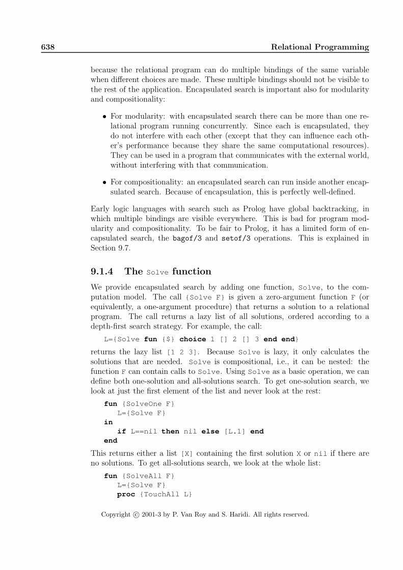
638 Relational Programming
because the relational program can do multiple bindings of the same variablewhen different choices are made. These multiple bindings should not be visible tothe rest of the application. Encapsulated search is important also for modularityand compositionality:
• For modularity: with encapsulated search there can be more than one re-lational program running concurrently. Since each is encapsulated, theydo not interfere with each other (except that they can influence each oth-er’s performance because they share the same computational resources).They can be used in a program that communicates with the external world,without interfering with that communication.
• For compositionality: an encapsulated search can run inside another encap-sulated search. Because of encapsulation, this is perfectly well-defined.
Early logic languages with search such as Prolog have global backtracking, inwhich multiple bindings are visible everywhere. This is bad for program mod-ularity and compositionality. To be fair to Prolog, it has a limited form of en-capsulated search, the bagof/3 and setof/3 operations. This is explained inSection 9.7.
9.1.4 The Solve function
We provide encapsulated search by adding one function, Solve , to the com-putation model. The call {Solve F} is given a zero-argument function F (orequivalently, a one-argument procedure) that returns a solution to a relationalprogram. The call returns a lazy list of all solutions, ordered according to adepth-first search strategy. For example, the call:
L={Solve fun {$} choice 1 [] 2 [] 3 end end }
returns the lazy list [1 2 3] . Because Solve is lazy, it only calculates thesolutions that are needed. Solve is compositional, i.e., it can be nested: thefunction F can contain calls to Solve . Using Solve as a basic operation, we candefine both one-solution and all-solutions search. To get one-solution search, welook at just the first element of the list and never look at the rest:
fun {SolveOne F}L={Solve F}
inif L==nil then nil else [L.1] end
end
This returns either a list [X] containing the first solution X or nil if there areno solutions. To get all-solutions search, we look at the whole list:
fun {SolveAll F}L={Solve F}proc {TouchAll L}
Copyright c© 2001-3 by P. Van Roy and S. Haridi. All rights reserved.

9.2 Further examples 639
if L==nil then skip else {TouchAll L.2} endend
in{TouchAll L}L
end
This returns a list of all solutions.
Computation spaces
We have introduced choice and fail statements and the Solve function. Thesenew operations can be programmed by extending the declarative model with justone new concept, the computation space. Computation spaces are part of theconstraint-based computation model, which is explained in Chapter 12. Theywere originally designed for constraint programming, a powerful generalization ofrelational programming. Chapter 12 explains how to implement choice , fail ,and Solve in terms of computation spaces. The definition of Solve is also givenin the supplements file on the book’s Web site.
Solving the clothing design example
Let us use Solve to find answers to the clothing design example. To find allsolutions, we do the following query:
{Browse {SolveAll Suit}}
This displays a list of the eight solutions:
[suit(beige mauve coral) suit(beige ochre coral)suit(coral mauve beige) suit(coral ochre beige)suit(mauve beige ochre) suit(mauve coral ochre)suit(ochre beige mauve) suit(ochre coral mauve)]
Figure 9.1 gives enough of the search tree to show how the first solution suit(beige
mauve coral) is obtained.
9.2 Further examples
We give some simple examples to show how to program in the relational compu-tation model.
9.2.1 Numeric examples
Let us show some simple examples using numbers, to show how to program withthe relational computation model. Here is a program that uses choice to countfrom 0 to 9:
Copyright c© 2001-3 by P. Van Roy and S. Haridi. All rights reserved.

640 Relational Programming
... 96 97 98 99
{Digit}
{Digit}
(second digit)
(first digit)
0 1 2 3 4 ...
Figure 9.2: Two digit counting with depth-first search
fun {Digit}choice 0 [] 1 [] 2 [] 3 [] 4 [] 5 [] 6 [] 7 [] 8 [] 9 end
end{Browse {SolveAll Digit}}
This displays:
[0 1 2 3 4 5 6 7 8 9]
(Note that the zero-argument function Digit is the same as a one-argumentprocedure.) We can combine calls to Digit to count with more than one digit:
fun {TwoDigit}10*{Digit}+{Digit}
end{Browse {SolveAll TwoDigit}}
This displays:
[0 1 2 3 4 5 6 7 8 9 10 11 12 13 14 ... 98 99]
This shows what it means to do a depth-first search: when two choices are done,the program first makes the first choice and then makes the second. Here the func-tion chooses first the tens digit and then the ones digit. Changing the definitionof TwoDigit to choose digits in the opposite order will give unusual results:
fun {StrangeTwoDigit}{Digit}+10*{Digit}
end{Browse {SolveAll StrangeTwoDigit}}
This displays:
[0 10 20 30 40 50 60 70 80 90 1 11 21 31 41 ... 89 99]
In this case, the tens digit is chosen second and therefore changes quicker thanthe ones digit.
Copyright c© 2001-3 by P. Van Roy and S. Haridi. All rights reserved.

9.2 Further examples 641
Palindrome product problem
Using Digit , we can already solve some interesting puzzles, like the “palindromeproduct” problem. We would like to find all four-digit palindromes that are prod-ucts of two-digit numbers. A palindrome is a number that reads the same forwardsand backwards, when written in decimal notation. The following program solvesthe puzzle:
proc {Palindrome ?X}X=(10*{Digit}+{Digit})*(10*{Digit}+{Digit}) % Generate(X>0)= true % Test 1(X>=1000)= true % Test 2(X div 1000) mod 10 = (X div 1) mod 10 % Test 3(X div 100) mod 10 = (X div 10) mod 10 % Test 4
end
{Browse {SolveAll Palindrome}}
This displays all 118 palindrome products. Why do we have to write the conditionX>0 as (X>0)= true ? If the condition returns false , then the attempted bindingfalse =true will fail. This ensures the relational program will fail when thecondition is false.
Palindrome product is an example of a generate-and-test program: it generatesa set of possibilities and then it uses tests to filter out the bad ones. The tests useunification failure to reject bad alternatives. Generate-and-test is a very naiveway to explore a search space. It generates all the possibilities first and onlyfilters out the bad ones afterwards. In palindrome product, 10000 possibilitiesare generated.
Chapter 12 introduces a much better way to explore a search space, calledpropagate-and-search. This approach does the filtering during the generation, sothat many fewer possibilities are generated. If we extend palindrome productto 6-digit numbers then the naive solution takes 45 seconds.1 The propagate-and-search solution of Chapter 12 takes less than 0.4 second to solve the sameproblem.
9.2.2 Puzzles and the n-queens problem
The n-queens problem is an example of a combinatoric puzzle. This kind of puzzlecan be easily specified in relational programming. The resulting solution is notvery efficient; for more efficiency we recommend using constraint programminginstead, as explained in Chapter 12. Using relational programming is a precursorto constraint programming.
The problem is to place n queens on an n × n chessboard so that no queenattacks another. There are many ways to solve this problem. The solution givenin Figure 9.4 is noteworthy because it uses dataflow variables. We can get the
1On a 500 MHz Pentium III processor running Mozart 1.1.0.
Copyright c© 2001-3 by P. Van Roy and S. Haridi. All rights reserved.

642 Relational Programming
����������������
����������������
��������������������
��������������������
����������������
����������������
����������������
����������������
��������������������
��������������������
����������������
����������������
����������������
����������������
����������������
����������������
�������������������������������������������������������������������������������������������������������������������������������������������������������������������������������������������������������������������������������������������������������������������������������������������������
�������������������������������������������������������������������������������������������������������������������������������������������������������������������������������������������������������������������������������������������������������������������������������������������������
���������������������������������������������������������������������������������������������������������������������������������������������������������������������������������������������������������������������������������
���������������������������������������������������������������������������������������������������������������������������������������������������������������������������������������������������������������������������������
�������������������������������������������������������������������������������������������������������������������������������������������������������������������������
�������������������������������������������������������������������������������������������������������������������������������������������������������������������������
�������������������������������������������������������������������������������������������������������������������������
�������������������������������������������������������������������������������������������������������������������������
�������������������������������������������������������������������������������������������������������������������������������������������������������������������������������������������������������������������������������������������������������������������������������������������������
�������������������������������������������������������������������������������������������������������������������������������������������������������������������������������������������������������������������������������������������������������������������������������������������������
���������������������������������������������������������������������������������������������������������������������������������������������������������������������������������������������������������������������������������
���������������������������������������������������������������������������������������������������������������������������������������������������������������������������������������������������������������������������������
��������������������������������������������������������������������������������������������������������������������������������������������������������������������������������������
��������������������������������������������������������������������������������������������������������������������������������������������������������������������������������������
�������������������������������������������������������������������������������������������������������������������������
�������������������������������������������������������������������������������������������������������������������������
���������������������������������������������������������������������������������������������������������������������������������������������������������������������������������������������������������������������������������
���������������������������������������������������������������������������������������������������������������������������������������������������������������������������������������������������������������������������������
�������������������������������������������������������������������������������������������������������������������������������������������������������������������������
�������������������������������������������������������������������������������������������������������������������������������������������������������������������������
�������������������������������������������������������������������������������������������������������������������������
�������������������������������������������������������������������������������������������������������������������������
�������������������������������������������������������������������������������������������������������������������������
�������������������������������������������������������������������������������������������������������������������������
�������������������������������������������������������������������������������������������������������������������������������������������������������������������������
�������������������������������������������������������������������������������������������������������������������������������������������������������������������������
���������������������������������������������������������������������������������������������������������������������������������������������������������������������������������������������������������������������������������
���������������������������������������������������������������������������������������������������������������������������������������������������������������������������������������������������������������������������������
Cs (columns)
Us Ds(down diagonals)(up diagonals)
Figure 9.3: The n-queens problem (when n = 4)
first solution of an 8-queens problem as follows:
{Browse {SolveOne fun {$} {Queens 8} end }}
This uses higher-order programming to define a zero-argument function from theone-argument function Queens . The answer displayed is:
[[1 7 5 8 2 4 6 3]]
This list gives the placement of the queens on the chessboard. It assumes thereis one queen per column. The solution lists the eight columns and gives for eachcolumn the queen’s position (first square of first column, seventh square of secondcolumn, etc.). How many solutions are there to the 8-queens problem (countingreflections and rotations as separate)? This is easy to calculate:
{Browse {Length {SolveAll fun {$} {Queens 8} end }}}
This displays the number 92, which is the answer. Queens is not the best possibleprogram for solving the n-queens problem. It is not practical for large n. Muchbetter programs can be gotten by using constraint programming or by design-ing specialized algorithms (which amounts almost to the same thing). But thisprogram is simple and elegant.
How does this magical program work? We explain it by means of Figure 9.3.Each column, up diagonal, and down diagonal has one dataflow variable. Thelists Cs, Us, and Ds contain all the column variables, up variables, and downvariables, respectively. Each column variable “guards” a column, and similarly
Copyright c© 2001-3 by P. Van Roy and S. Haridi. All rights reserved.

9.2 Further examples 643
fun {Queens N}fun {MakeList N}
if N==0 then nil else _|{MakeList N-1} endend
proc {PlaceQueens N ?Cs ?Us ?Ds}if N>0 then Ds2
Us2=_|Usin
Ds=_|Ds2{PlaceQueens N-1 Cs Us2 Ds2}{PlaceQueen N Cs Us Ds}
else skip endend
proc {PlaceQueen N ?Cs ?Us ?Ds}choice
Cs=N|_ Us=N|_ Ds=N|_[] _|Cs2=Cs _|Us2=Us _|Ds2=Ds in
{PlaceQueen N Cs2 Us2 Ds2}end
endQs={MakeList N}
in{PlaceQueens N Qs _ _}Qs
end
Figure 9.4: Solving the n-queens problem with relational programming
for the variables of the up and down diagonals. Placing a queen on a squarebinds the three variables to the queen’s number. Once the variables are bound,no other queen can bind the variable of the same column, up diagonal, or downdiagonal. This is because a dataflow variable can only have one value. Trying tobind to another value gives a unification failure, which causes that alternative tobe rejected.
The procedure PlaceQueens traverses a column from top to bottom. It keepsthe same Cs, but “shifts” the Us one place to the right and the Ds one place tothe left. At each iteration, PlaceQueens is at one row. It calls PlaceQueen ,which tries to place a queen in one of the columns of that row, by binding oneentry in Cs, Us, and Ds.
Copyright c© 2001-3 by P. Van Roy and S. Haridi. All rights reserved.

644 Relational Programming
9.3 Relation to logic programming
Both the declarative computation model of Chapter 2 and the relational com-putation model of this chapter are closely related to logic programming. Thissection examines this relationship. Section 9.3.1 first gives a brief introductionto logic and logic programming. Sections 9.3.2 and 9.3.3 then show how theseideas apply to the declarative and relational computation models. Finally, Sec-tion 9.3.4 briefly mentions pure Prolog, which is another implementation of logicprogramming.
The advantage of logic programming is that programs have two semantics,a logical and an operational semantics, which can be studied separately. If theunderlying logic is chosen well, then the logical semantics is much simpler thanthe operational. However, logic programming cannot be used for all computationmodels. For example, there is no good way to design a logic for the statefulmodel. For it we can use the axiomatic semantics of Section 6.6.
9.3.1 Logic and logic programming
A logic program is a statement of logic that is given an operational semantics, i.e.,it can be executed on a computer. If the operational semantics is well-designed,then the execution has two properties: it is correct, i.e., it respects the logicalsemantics (all consequences of the execution are valid logical consequences of theprogram considered as a set of logical axioms) and it is efficient, i.e., it allows towrite programs that execute with the expected time and space complexity. Letus examine more closely the topics of logic and logic programming. Be warnedthat this section gives only a brief introduction to logic and logic programming.For more information we refer interested readers to other books [114, 182].
Propositional logic
What is an appropriate logic in which to write logic programs? There are manydifferent logics. For example, there is propositional logic. Propositional formulasconsist of expressions combining symbols such as p, q, r, and so forth togetherwith the connectors ∧ (“and”), ∨ (“or”), ↔ (“if and only if”), → (“implies”),and ¬ (“not”). The symbols p, q, r, and so forth are called atoms in logic. Anatom in logic is the smallest indivisible part of a logical formula. This shouldnot be confused with an atom in a programming language, which is a constantuniquely determined by its print representation.
Propositional logic allows to express many simple laws. The contrapositivelaw (p→ q) ↔ (¬q → ¬p) is a formula of propositional logic, as is De Morgan’slaw ¬(p∧ q)↔ (¬p∨¬q). To assign a truth value to a propositional formula, wehave to assign a truth value to each of its atoms. We then evaluate the formulausing the usual rules for ∧, ∨, ↔, →, and ¬:
Copyright c© 2001-3 by P. Van Roy and S. Haridi. All rights reserved.

9.3 Relation to logic programming 645
a b a ∧ b a ∨ b a↔ b a→ b ¬afalse false false false true true truefalse true false true false true truetrue false false true false false falsetrue true true true true true false
If the formula is true for all possible assignments of its atoms, then it is calleda tautology. Both the contrapositive law and De Morgan’s law are examples oftautologies. They are true for all four possible truth assignments of p and q.
First-order predicate calculus
Propositional logic is rather weak as a base for logic programming, principally be-cause it does not allow expressing data structures. First-order predicate calculusis much better-suited for this. The predicate calculus generalizes propositionallogic with variables, terms, and quantifiers. A logical formula in the predicatecalculus has the following grammar, where 〈a〉 is an atom and 〈f〉 is a formula:
〈a〉 ::= p(〈x〉1, ..., 〈x〉n)〈f〉 ::= 〈a〉
| 〈x〉 = f(l1 : 〈x〉1, ..., ln : 〈x〉n)| 〈x〉1 = 〈x〉2| 〈f〉1 ∧ 〈f〉2 | 〈f〉1 ∨ 〈f〉2 | 〈f〉1 ↔ 〈f〉2 | 〈f〉1 → 〈f〉2 | ¬〈f〉| ∀〈x〉.〈f〉 | ∃〈x〉.〈f〉
Atoms in predicate calculus are more general than propositional atoms since theycan have arguments. Here 〈x〉 is a variable symbol, p is a predicate symbol, f is aterm label, and the li are term features. The symbols ∀ (“for all”) and ∃ (“thereexists”) are called quantifiers. In like manner as for program statements, wecan define the free identifier occurrences of a logical formula. Sometimes theseare called free variables, although strictly speaking they are not variables. Alogical formula with no free identifier occurrences is called a logical sentence. Forexample, p(x, y) ∧ q(y) is not a logical sentence because it has two free variablesx and y. We can make it a sentence by using quantifiers, giving for instance∀x.∃y.p(x, y) ∧ q(y). The free variables x and y are captured by the quantifiers.
Logical semantics of predicate calculus
To assign a truth value to a sentence of the predicate calculus, we have to do a bitmore work than for the propositional calculus. We have to define a model. Theword “model” here means a logical model, which is a very different beast than acomputation model! A logical model consists of two parts: a domain of discourse(all possible values of the variables) and a set of relations (where a relation is aset of tuples). Each predicate has a relation, which gives the tuples for which thepredicate is true. Among all predicates, equality (=) is particularly important.The equality relation will almost always be part of the model. The quantifiers
Copyright c© 2001-3 by P. Van Roy and S. Haridi. All rights reserved.

646 Relational Programming
∀x (“for all x”) and ∃x (“there exists x”) range over the domain of discourse.Usually the logical model is chosen so that a special set of sentences, called theaxioms, are all true. Such a model is called a logical semantics of the axioms.There can be many models for which the axioms are true.
Let us see how this works with an example. Consider the following two axioms:
∀x, y.grandfather(x, y)↔ ∃z.father(x, z) ∧ father(z, y)∀x, y, z.father(x, z) ∧ father(y, z)→ x = y
There are many possible models of these axioms. Here is one possible model:
Domain of discourse: {george, tom, bill}Father relation: {father(george, tom), father(tom, bill)}Grandfather relation: {grandfather(george, bill)}Equality relation: {george = george, tom = tom, bill = bill}
The relations contain only the true tuples; all other tuples are assumed to be false.With this model, we can give truth values to sentences of predicate calculus. Forexample, the sentence ∃x, y.father(x, y)→ father(y, x) can be evaluated as beingfalse. Note that the equality relation is part of this model, even though theaxioms might not mention it explicitly.
Logic programming
Now we can state more precisely what a logic program is. For our purposes, alogic program consists of a set of axioms in the first-order predicate calculus, asentence called the query, and a theorem prover, i.e., a system that can performdeduction using the axioms in an attempt to prove or disprove the query. Per-forming deductions is called executing the logic program. Can we build a practicalprogramming system based on the idea of executing logic programs? We still needto address three issues:
• Theoretically, a theorem prover is limited in what it can do. It is only guar-anteed to find a proof or disproof for queries that are true in all models. Ifwe are only interested in some particular models, then there might not exista proof or disproof, even though the query is true. We say that the theo-rem prover is incomplete. For example, we might be interested in numbertheory, so we use the model of integers with integer arithmetic. There is afamous result in mathematics called Godel’s Incompleteness Theorem, fromwhich it follows that there exist statements of number theory that cannotbe proved or disproved within any finite set of axioms.
• Even in those cases where the theorem prover could theoretically find aresult, it might be too inefficient. The search for a proof might take expo-nential time. A theorem prover intended for practical programming shouldhave a simple and predictable operational semantics, so that the program-mer can define algorithms and reason about their complexity.
Copyright c© 2001-3 by P. Van Roy and S. Haridi. All rights reserved.

9.3 Relation to logic programming 647
• A final point is that the deduction done by the theorem prover should beconstructive. That is, if the query states that there exists an x that satisfiessome property, then the system should construct a witness to the existence.In other words, it should build a data structure as an output of the logicprogram.
Two approaches are taken to overcome these problems:
• We place restrictions on the form of the axioms so that an efficient con-structive theorem prover is possible. The Prolog language, for example, isbased on Horn clauses, which are axioms of the form:
∀x1, ..., xk . 〈a〉1 ∧ ... ∧ 〈a〉n → 〈a〉,
where {x1, ..., xk} are chosen so that the axiom has no free variables. Hornclauses are interesting because there is an efficient constructive theoremprover for them using an inference rule called resolution [114]. The rela-tional computation model of this chapter also does logic programming, butwithout using resolution. It uses a different set of axioms and theoremprover, which are discussed in the next section.
• We give the programmer the possibility of helping the theorem prover withoperational knowledge. This operational knowledge is essential for writingefficient logic programs. For example, consider a logic program to sorta list of integers. A naive program might consist of axioms defining apermutation of a list and a query that states that there exists a permutationwhose elements are in ascending order. Such a program would be short butinefficient. Much more efficient would be to write axioms that express theproperties of an efficient sorting algorithm, such as mergesort.
A major achievement of computer science is that practical logic programmingsystems have been built by combining these two approaches. The first popularlanguage to achieve this goal was Prolog; it was subsequently followed by manyother languages. High-performance Prolog implementations are amazingly fast;they can even rival the speed of imperative language implementations [195].
9.3.2 Operational and logical semantics
There are two ways to look at a logic program: the logical view and the op-erational view. In the logical view, it is simply a statement of logic. In theoperational view, it defines an execution on a computer. Before looking at therelational model, let us look first at the declarative model of Chapter 2. We willsee that programs in the declarative model have a logical semantics as well as anoperational semantics. It is straightforward to translate a declarative programinto a logical sentence. If the program terminates correctly, i.e., it does not block,go into an infinite loop, or raise an exception, then all the bindings it does are
Copyright c© 2001-3 by P. Van Roy and S. Haridi. All rights reserved.
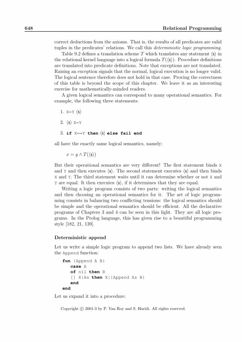
648 Relational Programming
correct deductions from the axioms. That is, the results of all predicates are validtuples in the predicates’ relations. We call this deterministic logic programming.
Table 9.2 defines a translation scheme T which translates any statement 〈s〉 inthe relational kernel language into a logical formula T (〈s〉). Procedure definitionsare translated into predicate definitions. Note that exceptions are not translated.Raising an exception signals that the normal, logical execution is no longer valid.The logical sentence therefore does not hold in that case. Proving the correctnessof this table is beyond the scope of this chapter. We leave it as an interestingexercise for mathematically-minded readers.
A given logical semantics can correspond to many operational semantics. Forexample, the following three statements:
1. X=Y 〈s〉
2. 〈s〉 X=Y
3. if X==Y then 〈s〉 else fail end
all have the exactly same logical semantics, namely:
x = y ∧ T (〈s〉)
But their operational semantics are very different! The first statement binds X
and Y and then executes 〈s〉. The second statement executes 〈s〉 and then bindsX and Y. The third statement waits until it can determine whether or not X andY are equal. It then executes 〈s〉, if it determines that they are equal.
Writing a logic program consists of two parts: writing the logical semanticsand then choosing an operational semantics for it. The art of logic program-ming consists in balancing two conflicting tensions: the logical semantics shouldbe simple and the operational semantics should be efficient. All the declarativeprograms of Chapters 3 and 4 can be seen in this light. They are all logic pro-grams. In the Prolog language, this has given rise to a beautiful programmingstyle [182, 21, 139].
Deterministic append
Let us write a simple logic program to append two lists. We have already seenthe Append function:
fun {Append A B}case Aof nil then B[] X|As then X|{Append As B}end
end
Let us expand it into a procedure:
Copyright c© 2001-3 by P. Van Roy and S. Haridi. All rights reserved.

9.3 Relation to logic programming 649
Relational statement Logical formulaskip truefail false〈s〉1 〈s〉2 T (〈s〉1) ∧ T (〈s〉2)local X in 〈s〉 end ∃x.T (〈s〉)X=Y x = yX=f(l1:X1 ... ln:Xn) x = f(l1 : x1, ..., ln : xn)if X then 〈s〉1 else 〈s〉2 end (x = true ∧ T (〈s〉1)) ∨ (x = false ∧ T (〈s〉2))case X of f(l1:X1 ... ln:Xn) (∃x1, ..., xn.x = f(l1 : x1, ..., ln : xn) ∧ T (〈s〉1))
then 〈s〉1 else 〈s〉2 end ∨(¬∃x1, ..., xn.x = f(l1 : x1, ..., ln : xn) ∧ T (〈s〉2))proc {P X1 ... Xn} 〈s〉 end ∀x1, ..., xn.p(x1, ..., xn)↔ T (〈s〉){P Y1 ... Yn} p(y1, ..., yn)choice 〈s〉1 [] ... [] 〈s〉n end T (〈s〉1) ∨ ... ∨ T (〈s〉n)
Table 9.2: Translating a relational program to logic
proc {Append A B ?C}case Aof nil then C=B[] X|As then Cs in
C=X|Cs{Append As B Cs}
endend
According to Table 9.2, this procedure has the following logical semantics:
∀a, b, c.append(a, b, c)↔(a = nil ∧ c = b) ∨ (∃x, a′, c′.a = x| a′ ∧ c = x| c′ ∧ append(a′, b, c′))
The procedure also has an operational semantics, given by the semantics of thedeclarative model. The call:
{Append [1 2 3] [4 5] X}
executes successfully and returns X=[1 2 3 4 5] . The call’s logical meaning isthe tuple append([1, 2, 3], [4, 5], x). After the execution, the tuple becomes:
append([1, 2, 3], [4, 5], [1, 2, 3, 4, 5])
This tuple is a member of the append relation. We see that Append can be seenas a logic program.
Another deterministic append
The above definition of Append does not always give a solution. For example,the call {Append X [3] [1 2 3]} should return X=[1 2] , which is the logical-ly correct solution, but the program cannot give this solution because it assumes
Copyright c© 2001-3 by P. Van Roy and S. Haridi. All rights reserved.

650 Relational Programming
X is bound to a value on input. The program blocks. This shows that the opera-tional semantics is incomplete. To give a solution, we need to write a version ofAppend with a different operational semantics. To calculate X from the last twoarguments, we change the definition of Append as follows:
proc {Append A B ?C}if B==C then A=nilelse
case C of X|Cs then As inA=X|As{Append As B Cs}
endend
end
This version of Append expects its last two arguments to be inputs and its firstargument to be an output. It has a different operational semantics as the previousversion, but keeps the same logical semantics. To be precise, its logical semanticsaccording to Table 9.2 is:
∀a, b, c.append(a, b, c)↔(b = c ∧ a = nil ) ∨ (∃x, c′, a′.c = x| c′ ∧ a = x| a′ ∧ append(a′, b, c′))
This sentence is logically equivalent to the previous one.
Nondeterministic append
We have seen two versions of Append , with the same logical semantics but differ-ent operational semantics. Both versions return exactly one solution. But whatif we want the solutions of {Append X Y [1 2 3]} ? There are four differentsolutions that satisfy the logical semantics. The declarative model is determinis-tic, so it can only give one solution at most. To give several solutions, we can usethe choice statement to guess the right information and then continue. This isexplained in the next section.
9.3.3 Nondeterministic logic programming
We saw that the Append procedure in the declarative model has a logical se-mantics but the operational semantics is not able to realize this logical semanticsfor all patterns of inputs and outputs. In the declarative model, the operationalsemantics is deterministic (it gives just one solution) and directional (it works foronly one pattern of input and output arguments). With relational programming,we can write programs with a more flexible operational semantics, that can givesolutions when the declarative program would block. We call this nondetermin-istic logic programming. To see how it works, let us look again at the logicalsemantics of append:
Copyright c© 2001-3 by P. Van Roy and S. Haridi. All rights reserved.

9.3 Relation to logic programming 651
∀a, b, c.append(a, b, c)↔(a = nil ∧ c = b) ∨ (∃x, a′, c′.a = x| a′ ∧ c = x| c′ ∧ append(a′, b, c′))
How can we write a program that respects this logical semantics and is able toprovide multiple solutions for the call {Append X Y [1 2 3]} ? Look closely atthe logical semantics. There is a disjunction (∨) with a first alternative (a = nil ∧c = b) and a second alternative (∃x, a′, c′.a = x| a′ ∧ c = x| c′ ∧ append(a′, b, c′)).To get multiple solutions, the program should be able to pick both alternatives.We implement this by using the choice statement. This gives the followingprogram:
proc {Append ?A ?B ?C}choice
A=nil B=C[] As Cs X in
A=X|As C=X|Cs {Append As B Cs}end
end
We can search for all solutions to the call {Append X Y [1 2 3]} :
{Browse {SolveAllproc {$ S} X#Y=S in {Append X Y [1 2 3]} end }}
To get one output, we pair the solutions X and Y together. This displays all foursolutions:
[nil#[1 2 3] [1]#[2 3] [1 2]#[3] [1 2 3]#nil]
This program can also handle the directional cases, for example:
{Browse {SolveAllproc {$ X} {Append [1 2] [3 4 5] X} end }}
displays [[1 2 3 4 5]] (a list of one solution). The program can even handlecases where no arguments are known at all, e.g., {Append X Y Z} . Since in thatcase there are an infinity of solutions, we do not call SolveAll , but just Solve :
L={Solve proc {$ S} X#Y#Z=S in {Append X Y Z} end }
Each solution is a tuple containing all three arguments (X#Y#Z). We can displaysuccessive solutions one by one by touching successive elements of L:
{Touch 1 L}{Touch 2 L}{Touch 3 L}{Touch 4 L}...
({Touch N L} is defined in Section 4.5.6; it simply traverses the first N elementsof L.) This displays successive solutions:
nil#B#B|[X1]#B#(X1|B)|
[X1 X2]#B#(X1|X2|B)|
Copyright c© 2001-3 by P. Van Roy and S. Haridi. All rights reserved.

652 Relational Programming
[X1 X2 X3]#B#(X1|X2|X3|B)|_
All possible solutions are given in order of increasing length of the first argument.This can seem somewhat miraculous. It certainly seemed so to the first logicprogrammers, in the late 1960’s and early 1970’s. Yet it is a simple consequenceof the semantics of the choice statement, which picks its alternatives in order. Bewarned that this style of programming, while it can sometimes perform miracles,is extremely dangerous. It is very easy to get into infinite loops or exponential-time searches, i.e., to generate candidate solutions almost indefinitely withoutever finding a good one. We advise you to write deterministic programs wheneverpossible and to use nondeterminism only in those cases when it is indispensable.Before running the program, verify that the solution you want is one of theenumerated solutions.
9.3.4 Relation to pure Prolog
The relational computation model provides a form of nondeterministic logic pro-gramming that is very close to what Prolog provides. To be precise, it is a subsetof Prolog called “pure Prolog” [182]. The full Prolog language extends pureProlog with operations that lack a logical semantics but that are useful for pro-gramming a desired operational semantics (see the Prolog section in Chapter 9).Programs written in either pure Prolog or the relational computation model canbe translated in a straightforward way to the other. There are three principaldifferences between pure Prolog and the relational computation model:
• Prolog uses a Horn clause syntax with an operational semantics based onresolution. The relational computation model uses a functional syntax withan operational semantics tailored to that syntax.
• The relational computation model allows full higher-order programming.This has no counterpart in first-order predicate calculus but is useful forstructuring programs. Higher-order programming is not supported at all inpure Prolog and only partially in full Prolog.
• The relational computation model distinguishes between deterministic op-erations (which do not use choice ) and nondeterministic operations (whichuse choice ). In pure Prolog, both have the same syntax. Deterministic op-erations efficiently perform functional calculations, i.e., it is known whicharguments are the inputs and which are the outputs. Nondeterministicoperations perform relational calculations, i.e., it is not known which argu-ments are inputs and outputs, and indeed the same relation can be used indifferent ways.
Copyright c© 2001-3 by P. Van Roy and S. Haridi. All rights reserved.

9.3 Relation to logic programming 653
9.3.5 Logic programming in other models
So far we have seen logic programming in the declarative model, possibly extendedwith a choice operation. What about logic programming in other models? Inother words, in how far is it possible to have a logical semantics in other models?To have a logical semantics means that execution corresponds to deduction, i.e.,execution can be seen as performing inference and the results of procedure callsgive valid tuples in a simple logical model, such as a model of the predicatecalculus. The basic principle is to enrich the control: we extend the operationalsemantics, which allows to calculate new tuples in the same logical model. Letus examine some other computation models:
• Adding concurrency to the declarative model gives the data-driven anddemand-driven concurrent models. These models also do logic program-ming, since they only change the order in which valid tuples are calculated.They do not change the content of the tuples.
• The nondeterministic concurrent model of Section 5.7.1 does logic pro-gramming. It adds just one operation, WaitTwo , which can be given alogical semantics. Logically, the call {WaitTwo X Y Z} is equivalent toz = 1∨z = 2, since Z is bound to 1 or 2. Operationally, WaitTwo waits un-til one of its arguments is determined. WaitTwo is used to manage controlin a concurrent program, namely to pick an execution path that does notblock.
The nondeterministic concurrent model is interesting because it combinestwo properties. It has a straightforward logical semantics and it is al-most as expressive as a stateful model. For example, it allows buildinga client/server program with two independent clients and one server, whichis not possible in a declarative model. This is why the model was chosen asthe basis for concurrent logic programming.
• The stateful models are another story. There is no straightforward way togive a logical meaning to a stateful operation. However, stateful models cando logic programming if the state is used in a limited way. For example,it can be encapsulated inside a control abstraction or it can be used as aparameter to part of a program. In the first case we are just enriching thecontrol. In the second case, as long as the state does not change, we canreason as if it were constant.
• The constraint-based computation model of Chapter 12 is the most pow-erful model for doing logic programming that we see in this book. It givestechniques for solving complex combinatoric optimization problems. It isthe most powerful model in the sense that it has the most sophisticatedmechanisms both for specifying and automatically determining the controlflow. From the logic programming viewpoint, it has the strongest deductionabilities.
Copyright c© 2001-3 by P. Van Roy and S. Haridi. All rights reserved.

654 Relational Programming
9.4 Natural language parsing
Section 3.4.8 shows how to do parsing with a difference list. The grammar that itparses is deterministic with a lookahead of one token: it suffices to know the nexttoken to know what grammar rule will apply. This is sometimes a very strongrestriction. Some languages need a much larger lookahead to be parsed. This iscertainly true for natural languages, but can also be true for widely-used formallanguages (like Cobol and Fortran, see below).
The one-token lookahead restriction can be removed by using relational pro-gramming. Relational programs can be written to parse highly ambiguous gram-mars. This is one of the most flexible ways to do parsing. It can parse grammarswith absolutely no restriction on the form of the grammar. The disadvantage isthat if the grammar is highly ambiguous, the parser can be extremely slow. But ifthe ambiguity is localized to small parts of the input, the efficiency is acceptable.
This section gives a simple example of natural language parsing in the rela-tional style. This style was pioneered by the Prolog language in the early 1970’s.It is fair to say that Prolog was originally invented for this purpose [40]. This sec-tion only scratches the surface of what can be done in this area with the relationalcomputation model. For further reading, we recommend [48].
Examples in Cobol and Fortran
Using relational programming to parse ambiguous grammars is quite practical.For example, it is being used successfully by Darius Blasband of Phidani Softwareto build transformation tools for programs written in Fortran and Cobol [19].These two languages are difficult to parse with more traditional tools such as theUnix lex/yacc family. Let us see what the problems are with these two languages.
The problem with parsing Cobol The following fragment is legal Cobolsyntax:
IF IF=THEN THEN THEN=ELSE ELSE ELSE=IF
This IF statement uses variables named IF, THEN, and ELSE. The parser has todecide whether each occurrence of the tokens IF, THEN, and ELSE is a variableidentifier or a keyword. The only way to make the distinction is to continue theparse until only one unambiguous interpretation remains. The problem is thatCobol makes no distinction between keywords and variable identifiers.
The problem with parsing Fortran Fortran is even more difficult to parsethan Cobol. To see why, consider the following fragment, which is legal Fortransyntax:
DO 5 I = 1,10
...
5 CONTINUE
Copyright c© 2001-3 by P. Van Roy and S. Haridi. All rights reserved.

9.4 Natural language parsing 655
This defines a loop that iterates its body 10 times, where I is given consecutivevalues from 1 to 10. Look what happens when the comma in the DO statement isreplaced by a period:
DO 5 I = 1.10
In Fortran, this has the same meaning as:
DO5I = 1.10
where DO5I is a new variable identifier that is assigned the floating point number1.10. In this case, the loop body is executed exactly once with an undefined(garbage) value stored in I. The problem is that Fortran allows whitespace withina variable identifier and does not require that variable identifiers be declared inadvance. This means that the parser has to look far ahead to decide whetherthere is one token, DO5I, or three, DO, 5, and I. The parser cannot parse the DO
statement unambiguously until the . or , is encountered.This is a famous error that caused the failure of at least one satellite launch
worth tens of millions of dollars. An important lesson for designing programminglanguages is that changing the syntax of a legal program slightly should not giveanother legal program.
9.4.1 A simple grammar
We use the following simple grammar for a subset of English:
〈Sentence〉 ::= 〈NounPhrase〉 〈VerbPhrase〉〈NounPhrase〉 ::= 〈Determiner〉 〈Noun〉 〈RelClause〉 | 〈Name〉〈VerbPhrase〉 ::= 〈TransVerb〉 〈NounPhrase〉 | 〈IntransVerb〉〈RelClause〉 ::= who 〈VerbPhrase〉 | ε
〈Determiner〉 ::= every | a
〈Noun〉 ::= man | woman
〈Name〉 ::= john | mary
〈TransVerb〉 ::= loves
〈IntransVerb〉 ::= lives
Here ε means that the alternative is empty (nothing is chosen). Some examplesof sentences in this grammar are:
“john loves mary”“a man lives”“every woman who loves john lives”
Let us write a parser that generates an equivalent sentence in the predicate cal-culus. For example, parsing the sentence “a man lives” will generate the termexists(X and(man(X) lives(X)) in the syntax of the relational computationmodel, which represents ∃x.man(x) ∧ lives(x). The parse tree is a sentence inpredicate calculus that represents the meaning of the natural language sentence.
Copyright c© 2001-3 by P. Van Roy and S. Haridi. All rights reserved.

656 Relational Programming
9.4.2 Parsing with the grammar
The first step is to parse with the grammar, i.e., to accept valid sentences of thegrammar. Let us represent the sentence as a list of atoms. For each nonterminalin the grammar, we write a function that takes an input list, parses part of it,and returns the unparsed remainder of the list. For 〈TransVerb〉 this gives:
proc {TransVerb X0 X}X0=loves|X
end
This can be called as:
{TransVerb [loves a man] X}
which parses “loves” and binds X to [a man] . If the grammar has a choice, thenthe procedure uses the choice statement to represent this. For 〈Name〉 this gives:
proc {Name X0 X}choice X0=john|X [] X0=mary|X end
end
This picks one of the two alternatives. If a nonterminal requires another nonter-minal, then the latter is called as a procedure. For 〈VerbPhrase〉 this gives:
proc {VerbPhrase X0 X}choice X1 in
{TransVerb X0 X1} {NounPhrase X1 X}[] {IntransVerb X0 X}end
end
Note how X1 is passed from TransVerb to NounPhrase . Continuing in this waywe can write a procedure for each of the grammar’s nonterminal symbols.
To do the parse, we execute the grammar with encapsulated search. We wouldlike the execution to succeed for correct sentences and fail for incorrect sentences.This will not always be the case, depending on how the grammar is defined andwhich search we do. For example, if the grammar is left-recursive then doing adepth-first search will go into an infinite loop. A left-recursive grammar has atleast one rule whose first alternative starts with the nonterminal, like this:
〈NounPhrase〉 ::= 〈NounPhrase〉 〈RelPhrase〉 | 〈Noun〉
In this rule, a 〈NounPhrase〉 consists first of a 〈NounPhrase〉! This is not necessarilywrong; it just means that we have to be careful how we parse with the grammar.If we do a breadth-first search or an iterative deepening search instead of a depth-first search, then we are guaranteed to find a successful parse, if one exists.
9.4.3 Generating a parse tree
We would like our parser to do more than just succeed or fail. Let us extend it togenerate a parse tree. We can do this by making our procedures into functions.
Copyright c© 2001-3 by P. Van Roy and S. Haridi. All rights reserved.

9.4 Natural language parsing 657
For example, let us extend 〈Name〉 to output the name it has parsed:
fun {Name X0 X}choice
X0=john|X john[] X0=mary|X maryend
end
When 〈Name〉 parses “john”, it outputs the atom john . Let us extend 〈TransVerb〉to output the predicate loves(x, y), where x is the subject and y is the object.This gives:
fun {TransVerb S O X0 X}X0=loves|Xloves(S O)
end
Note that 〈TransVerb〉 also has two new inputs, S and O. These inputs will befilled in when it is called.
9.4.4 Generating quantifiers
Let us see one more example, to show how our parser generates the quantifiers“for all” and “there exists”. They are generated for determiners:
fun {Determiner S P1 P2 X0 X}choice
X0=every|Xall(S imply(P1 P2))
[] X0=a|Xexists(S and(P1 P2))
endend
The determiner “every” generates a “for all”. The sentence “every man lovesmary” gives the term all(X imply(man(X) loves(X mary))) , which corre-sponds to ∀x.man(x) → loves(x, mary). In the call to 〈Determiner〉, P1 will bebound to man(X) and P2 will be bound to loves(X mary) . These bindings aredone inside 〈NounPhrase〉, which finds out what the 〈Noun〉 and 〈RelClause〉 are,and passes this information to 〈Determiner〉:
fun {NounPhrase N P1 X0 X}choice P P2 P3 X1 X2 in
P={Determiner N P2 P1 X0 X1}P3={Noun N X1 X2}P2={RelClause N P3 X2 X}P
[] N={Name X0 X}P1
end
Copyright c© 2001-3 by P. Van Roy and S. Haridi. All rights reserved.

658 Relational Programming
fun {Determiner S P1 P2 X0 X}choice
X0=every|Xall(S imply(P1 P2))
[] X0=a|Xexists(S and(P1 P2))
endend
fun {Noun N X0 X}choice
X0=man|Xman(N)
[] X0=woman|Xwoman(N)
endend
fun {Name X0 X}choice
X0=john|Xjohn
[] X0=mary|Xmary
endend
fun {TransVerb S O X0 X}X0=loves|Xloves(S O)
end
fun {IntransVerb S X0 X}X0=lives|Xlives(S)
end
Figure 9.5: Natural language parsing (simple nonterminals)
Copyright c© 2001-3 by P. Van Roy and S. Haridi. All rights reserved.

9.4 Natural language parsing 659
fun {Sentence X0 X}P P1 N X1 in
P={NounPhrase N P1 X0 X1}P1={VerbPhrase N X1 X}P
end
fun {NounPhrase N P1 X0 X}choice P P2 P3 X1 X2 in
P={Determiner N P2 P1 X0 X1}P3={Noun N X1 X2}P2={RelClause N P3 X2 X}P
[] N={Name X0 X}P1
endend
fun {VerbPhrase S X0 X}choice O P1 X1 in
P1={TransVerb S O X0 X1}{NounPhrase O P1 X1 X}
[] {IntransVerb S X0 X}end
end
fun {RelClause S P1 X0 X}choice P2 X1 in
X0=who|X1P2={VerbPhrase S X1 X}and(P1 P2)
[] X0=XP1
endend
Figure 9.6: Natural language parsing (compound nonterminals)
Copyright c© 2001-3 by P. Van Roy and S. Haridi. All rights reserved.

660 Relational Programming
end
Since P1 and P2 are single-assignment variables, they can be passed to 〈Determiner〉before they are bound. In this way, each nonterminal brings its piece of the puzzleand the whole grammar fits together.
9.4.5 Running the parser
The complete parser is given in Figures 9.5 and 9.6. Figure 9.5 shows the simplenonterminals, which enumerate atoms directly. Figure 9.6 shows the compoundnonterminals, which call other nonterminals. To run the parser, feed both figuresinto Mozart. Let us start by parsing some simple sentences. For example:
fun {Goal}{Sentence [mary lives] nil}
end{Browse {SolveAll Goal}}
The SolveAll call will calculate all possible parse trees. This displays:
[lives(mary)]
This is a list of one element since there is only a single parse tree. How aboutthe following sentence:
fun {Goal}{Sentence [every man loves mary] nil}
end
Parsing this gives:
[all(X imply(man(X) loves(X mary)))]
To see the unbound variable X, choose the Minimal Graph representation in thebrowser. Let us try a more complicated example:
fun {Goal}{Sentence [every man who lives loves a woman] nil}
end
Parsing this gives:
[all(Ximply(and(man(X) lives(X))
exists(Y and(woman(Y) loves(X Y)))))]
9.4.6 Running the parser “backwards”
So far, we have given sentences and parsed them. This shows only part of whatour parser can do. In general, it can take any input to Sentence that containsunbound variables and find all the parses that are consistent with that input.This shows the power of the choice statement. For example, let us find allsentences of three words:
Copyright c© 2001-3 by P. Van Roy and S. Haridi. All rights reserved.

9.4 Natural language parsing 661
fun {Goal}{Sentence [_ _ _] nil}
end
Executing this goal gives the following eight parse trees:
[all(A imply(man(A) lives(A)))all(B imply(woman(B) lives(B)))exists(C and(man(C) lives(C)))exists(D and(woman(D) lives(D)))loves(john john)loves(john mary)loves(mary john)loves(mary mary)]
See if you can find out which sentence corresponds to each parse tree. For exam-ple, the first tree corresponds to the sentence “every man lives”.
The ability to compute with partial information, which is what our parserdoes, is an important step in the direction of constraint programming. Chapter 12gives an introduction to constraint programming.
9.4.7 Unification grammars
Our parser does more than just parse; it also generates a parse tree. We didthis by extending the code of the parser, “piggybacking” the generation on theactions of the parser. There is another, more concise way to define this: byextending the grammar so that nonterminals have arguments. For example, thenonterminal 〈Name〉 becomes 〈Name〉(N), which means “the current name is N”.When 〈Name〉 calls its definition, N is bound to john or mary , depending onwhich rule is chosen. Other nonterminals are handled in the same way. Forexample, 〈TransVerb〉 becomes 〈TransVerb〉(S O P), which means “the currentverb links subject S and object O to make the phrase P”. When 〈TransVerb〉calls its definition, the corresponding arguments are bound together. If S andO are inputs, 〈TransVerb〉 constructs P, which has the form loves(S O) . Afterextending the whole grammar in similar fashion (following the parser code), weget the following rules:
〈Sentence〉(P) ::= 〈NounPhrase〉(N P1 P) 〈VerbPhrase〉(N P1)〈NounPhrase〉(N P1 P) ::= 〈Determiner〉(N P2 P1 P) 〈Noun〉(N P3)
〈RelClause〉(N P3 P2)〈NounPhrase〉(N P1 P1) ::= 〈Name〉(N)〈VerbPhrase〉(S P) ::= 〈TransVerb〉(S O P1) 〈NounPhrase〉(O P1 P)〈VerbPhrase〉(S P) ::= 〈IntransVerb〉(S P)〈RelClause〉(S P1 and(P1 P2)) ::= who 〈VerbPhrase〉(S P2)〈RelClause〉(S P1 P1) ::= ε
Copyright c© 2001-3 by P. Van Roy and S. Haridi. All rights reserved.

662 Relational Programming
〈Determiner〉(S P1 P2 all(S imply(P1 P2))) ::= every
〈Determiner〉(S P1 P2 exists(S and(P1 P2)) ::= a
〈Noun〉(N man(N)) ::= man
〈Noun〉(N woman(N)) ::= woman
〈Name〉(john) ::= john
〈Name〉(mary) ::= mary
〈TransVerb〉(S O loves(S O)) ::= loves
〈IntransVerb〉(S lives(S)) ::= lives
These rules correspond exactly to the parser program we have written. You cansee the advantage of using the rules: they are more concise and easier to under-stand than the program. They can be automatically translated into a program.This translation is so useful that the Prolog language has a built-in preprocessorto support it.
This kind of grammar is called a definite clause grammar, or DCG, becauseeach rule corresponds to a kind of Horn clause called a definite clause. Eachnonterminal can have arguments. When a nonterminal is matched with a rule,the corresponding arguments are unified together. DCGs are a simple exampleof a very general kind of grammar called unification grammar. Many differentkinds of unification grammar are used in natural language parsing. The practicalones use constraint programming instead of relational programming.
9.5 A grammar interpreter
The previous section shows how to build simple parser and how to extend itto return a parse tree. For each new grammar we want to parse, we have tobuild a new parser. The parser is “hardwired”: its implementation is basedon the grammar it parses. Wouldn’t it be nice to have a generic parser thatwould work for all grammars, simply by passing the grammar definition as anargument? A generic parser is easier to use and more flexible than a hardwiredparser. To represent the grammar in a programming language, we encode it asa data structure. Depending on how flexible the language is, the encoding willlook almost like the grammar’s EBNF definition.
The generic parser is an example of an interpreter. Recall that an interpreteris a program written in language L1 that accepts programs written in anotherlanguage L2 and executes them. For the generic parser, L1 is the relationalcomputation model and L2 is a grammar definition.
The generic parser uses the same execution strategy as the hardwired parser.It keeps track of two extra arguments: the token sequence to be parsed andthe rest of the sequence. It uses a choice operation to choose a rule for eachnonterminal. It is executed with encapsulated search.
Copyright c© 2001-3 by P. Van Roy and S. Haridi. All rights reserved.

9.5 A grammar interpreter 663
9.5.1 A simple grammar
To keep things simple in describing the generic parser, we use a small gram-mar that defines s-expressions. An s-expression starts with a left parenthesis,followed by a possibly empty sequence of atoms or s-expressions, and ends ina right parenthesis. Two examples are (a b c) and (a (b) () (d (c))). S-expressions were originally used in Lisp to represent nested lists. Our grammarwill parse s-expressions and build the list that they represent. Here is the gram-mar’s definition:
〈sexpr〉(s(As)) ::= ’(’ 〈seq〉(As) ’)’〈seq〉(nil) ::= ε〈seq〉(A|As) ::= 〈atom〉(A) 〈seq〉(As)〈seq〉(A|As) ::= 〈sexpr〉(A) 〈seq〉(As)〈atom〉(X) ::= X & (X is an atom different from ’(’ and ’)’)
This definition extends the EBNF notation by allowing terminals to be variablesand by adding a boolean condition to check whether a rule is valid. These exten-sions occur in the definition of 〈atom〉(X). The argument X represents the actualatom that is parsed. To avoid confusion between an atom and the left or rightparenthesis of an s-expression, we check that the atom is not a parenthesis.
9.5.2 Encoding the grammar
Let us encode this grammar as a data structure. We will first encode rules. A ruleis a tuple with two parts, a head and a body. The body is a list of nonterminalsand terminals. For example, the rule defining 〈sexpr〉 could be written as:
local As inrule(sexpr(s(As)) [ ´ ( ´ seq(As) ´ ) ´ ])
end
The unbound variable As will be bound when the rule is used. This representationis not quite right. There should be a fresh variable As each time the rule is used.To implement this, we encode the rule as a function:
fun {$} As inrule(sexpr(s(As)) [ ´ ( ´ seq(As) ´ ) ´ ])
end
Each time the function is called, a tuple is returned containing a fresh variable.This is still not completely right, since we cannot distinguish nonterminals with-out arguments from terminals. To avoid this confusion, we wrap terminals in atuple with label t . (This means that we cannot have a nonterminal with labelt .) This gives the final, correct representation:
fun {$} As inrule(sexpr(s(As)) [t( ´ ( ´ ) seq(As) t( ´ ) ´ )])
end
Copyright c© 2001-3 by P. Van Roy and S. Haridi. All rights reserved.

664 Relational Programming
r(sexpr:[ fun {$} As inrule(sexpr(s(As)) [t( ´ ( ´ ) seq(As) t( ´ ) ´ )])
end ]seq: [ fun {$}
rule(seq(nil) nil)endfun {$} As A in
rule(seq(A|As) [atom(A) seq(As)])endfun {$} As A in
rule(seq(A|As) [sexpr(A) seq(As)])end ]
atom: [ fun {$} X inrule(atom(X)
[t(X)fun {$}
{IsAtom X} andthen X\= ´ ( ´ andthen X\= ´ ) ´end ])
end ])
Figure 9.7: Encoding of a grammar
Now that we can encode rules, let us encode the complete grammar. We representthe grammar as a record where each nonterminal has one field. This field containsa list of the nonterminal’s rules. We have seen that a rule body is a list containingnonterminals and terminals. We add a third kind of entry, a boolean functionthat has to return true for the rule to be valid. This corresponds to the conditionwe used in the definition of 〈atom〉(X).
Figure 9.7 gives the complete grammar for s-expressions encoded as a datastructure. Note how naturally this encoding uses higher-order programming:rules are functions that themselves may contain boolean functions.
9.5.3 Running the grammar interpreter
Let us define an ADT for the grammar interpreter. The function NewParser
takes a grammar definition and returns a parser:
Parse={NewParser Rules}
Rules is a record like the grammar definition in Figure 9.7. Parse takes asinputs a goal to be parsed, Goal , and a list of tokens, S0. It does the parse andreturns the unparsed remainder of S0 in S:
{Parse Goal S0 S}
While doing the parse, it can also build a parse tree because it unifies the argu-ments of the nonterminal with the head of the chosen rule.
The parser is executed with encapsulated search. Here is an example:
Copyright c© 2001-3 by P. Van Roy and S. Haridi. All rights reserved.

9.5 A grammar interpreter 665
{Browse {SolveOnefun {$} E in
{Parse sexpr(E)[ ´ ( ´ hello ´ ( ´ this is an sexpr ´ ) ´ ´ ) ´ ] nil}
Eend }}
This returns a list containing the first solution:
[s([hello s([this is an sexpr])])]
9.5.4 Implementing the grammar interpreter
Figure 9.8 gives the definition of the grammar interpreter. NewParser createsa parser Parse that references the grammar definition in Rules . The parser iswritten as a case statement. It accepts four kinds of goals:
• A list of other goals. The parser is called recursively for all goals in the list.
• A procedure, which should be a zero-argument boolean function. The func-tion is called and its result is unified with true . If the result is false , thenthe parser fails, which causes another alternative to be chosen.
• A terminal, represented as the tuple t(X) . This terminal is unified with thenext element in the input list.
• A nonterminal, represented as a record. Its label is used to look up therule definitions in Rules . Then a rule is chosen nondeterministically withChooseRule and Parse is called recursively.
This structure is typical of interpreters. They examine the input and decide whatto do depending on the input’s syntax. They keep track of extra information(here, the arguments S0 and S) to help do the work.
Dynamic choice points
The parser calls ChooseRule to choose a rule for a nonterminal. Using thechoice statement, we could write ChooseRule as follows:
proc {ChooseRule Rs Goal Body}case Rs of nil then fail[] R|Rs2 then
choicerule(Goal Body)={R}
[]{ChooseRule Rs2 Goal Body}
endend
end
Copyright c© 2001-3 by P. Van Roy and S. Haridi. All rights reserved.

666 Relational Programming
fun {NewParser Rules}proc {Parse Goal S0 S}
case Goalof nil then S0=S[] G|Gs then S1 in
{Parse G S0 S1}{Parse Gs S1 S}
[] t(X) then S0=X|Selse if {IsProcedure Goal} then
{Goal}= trueS0=S
else Body Rs in /* Goal is a nonterminal */Rs=Rules.{Label Goal}{ChooseRule Rs Goal Body}{Parse Body S0 S}
end endendproc {ChooseRule Rs Goal Body}
I={Space.choose {Length Rs}}in
rule(Goal Body)={{List.nth Rs I}}end
inParse
end
Figure 9.8: Implementing the grammar interpreter
This definition creates a series of binary choice points. (Note that it calls therule definition R to create a fresh rule instance.) There is another, more flexibleand efficient way to write ChooseRule . Instead of using the choice statement,which implies a statically fixed number of choices, we use another operation,Space.choose , which works with any number of choices. Space.choose ispart of the Space module, which defines operations on computation spaces. Thecurious reader can skip ahead to Chapter 12 to find out more about them. But itis not necessary to understand computation spaces to understand Space.choose .
The call I={Space.choose N} creates a choice point with N alternatives andreturns I , the alternative that is picked by the search strategy. I ranges from1 to N. The number of alternatives can be calculated at run-time, wherease inthe choice statement it is statically known as part of the program’s syntax. Infact, the choice statement is a linguistic abstraction that is implemented withSpace.choose . The following statement:
choice〈stmt〉1
[] ... []
Copyright c© 2001-3 by P. Van Roy and S. Haridi. All rights reserved.

9.6 Databases 667
〈stmt〉nend
is translated as:
case {Space.choose N}of 1 then 〈stmt〉1...[] N then 〈stmt〉nend
So the Space.choose operation is the real basic concept and the choice state-ment is a derived concept.
Meta-interpreters
Our interpreter is actually a special kind of interpreter called a meta-interpretersince it uses the relational model’s unify operation directly to implement thegrammar’s unify operation. In general, any interpreter of L2 that uses opera-tions of L1 directly to implement the same operations in L2 is called a meta-interpreter. Writing meta-interpreters is a standard programming technique inlanguages whose primitive operations are complex. It avoids having to reimple-ment these operations and it is more efficient. A popular case is Prolog, whichhas unification and search as primitives. It is easy to explore extensions to Prologby writing meta-interpreters.
9.6 Databases
A database is a collection of data that has a well-defined structure. Usually, itis assumed that the data are long-lived, in some loose sense, e.g., they surviveindependently of whether the applications or the computer itself is running. (Thelatter property is often called persistence.)
There are many ways to organize the data in a database. One of the mostpopular ways is to consider the data as a set of relations, where a relation is aset of tuples. A database organized as a set of relations is called a relationaldatabase. For example, a graph can be defined by one relation, which is a set oftuples where each tuple represents one edge (see Figure 9.9):
edge(1 2) edge(2 1) edge(2 3) edge(3 4)edge(2 5) edge(5 6) edge(4 6) edge(6 7)edge(6 8) edge(1 5) edge(5 1)
A relational database explicitly stores these tuples so that we can calculate withthem. We can use the relational computation model of this chapter to do thesecalculations. Typical operations on a relational database are query (reading thedata) and update (modifying the data):
Copyright c© 2001-3 by P. Van Roy and S. Haridi. All rights reserved.

668 Relational Programming
• A query is more than just a simple read, but is a logical formula whosebasic elements are the relations in the database. It is the role of the DBMS(database management system) to find all tuples that satisfy the formula.
• An update means to add information to the database. This informationmust be of the right kind and not disturb the organization of the database.The update is usually implemented as a transaction (see Section 8.5).
This section touches on just a few parts of the area of databases. For moreinformation, we refer the reader to the comprehensive introduction by Date [42].
Relational programming is well-suited for exploring the concepts of relationaldatabases. There are several reasons for this:
• It places no restrictions on the logical form of the query. Even if the query ishighly disjunctive (it has many choices), it will be treated correctly (albeitslowly).
• It allows to experiment with deductive databases. A deductive databaseis a database whose implementation can deduce additional tuples that arenot explicitly stored. Typically, the deductive database allows defining newrelations in terms of existing relations. No tuples are stored for these newrelations, but they can be used just like any other relation.
The deep reason for these properties is that the relational computation model isa form of logic programming.
9.6.1 Defining a relation
Let us first define an abstraction to calculate with relations. For conciseness, weuse object-oriented programming to define the abstraction as a class, RelationClass .
• A new relation is an instance of RelationClass , e.g., Rel={New RelationClass
init} creates the initially empty relation Rel .
• The following operations are possible:
– {Rel assert(T)} adds the tuple T to Rel . Assert can only be doneoutside a relational program.
– {Rel assertall(Ts)} adds the list of tuples Ts to Rel . Assertallcan only be done outside a relational program.
– {Rel query(X)} binds X to one of the tuples in Rel . X can be anypartial value. If more than one tuple is compatible with X, then searchcan enumerate all of them. Query can only be done inside a relationalprogram.
Copyright c© 2001-3 by P. Van Roy and S. Haridi. All rights reserved.

9.6 Databases 669
1 2 3 4 5 6 7 8
Figure 9.9: A simple graph
These operations are similar to what a Prolog system provides. For example,assert is a limited version of Prolog’s assert/1 that can assert facts (i.e., tu-ples), not complete clauses. For the examples that follow, we assume that Rel
has efficiency similar to a good Prolog implementation [29]. That is, the set oftuples is stored in a dictionary that indexes them on their first argument. Thismakes it possible to write efficient programs. Without this indexing, even simplelookups would need to do linear search. More sophisticated indexing is possible,but in practice first-argument indexing is often sufficient. Section 9.6.3 gives animplementation of RelationClass that does first-argument indexing.
9.6.2 Calculating with relations
An example relation
Let us show an example of this abstraction for doing calculations on graphs. Weuse the example graph of Figure 9.9. We define this graph as two relations: a setof nodes and a set of edges. Here is the set of nodes:
NodeRel={New RelationClass init}{NodeRel
assertall([node(1) node(2) node(3) node(4)node(5) node(6) node(7) node(8)])}
The tuple node(1) represents the node 1. Here is the set of edges:
EdgeRel={New RelationClass init}{EdgeRel
assertall([edge(1 2) edge(2 1) edge(2 3) edge(3 4)edge(2 5) edge(5 6) edge(4 6) edge(6 7)edge(6 8) edge(1 5) edge(5 1)])}
The tuple edge(1 2) represents an edge from node 1 to node 2. We can queryNodeRel or EdgeRel with the message query . Let us define the proceduresNodeP and EdgeP to make this more concise:
proc {NodeP A} {NodeRel query(node(A))} endproc {EdgeP A B} {EdgeRel query(edge(A B))} end
With these definitions of NodeP and EdgeP we can write relational programs.
Copyright c© 2001-3 by P. Van Roy and S. Haridi. All rights reserved.

670 Relational Programming
Some queries
Let us start with a very simple query: what edges are connected to node 1? Wedefine the query as a one-argument procedure:
proc {Q ?X} {EdgeP 1 X} end
This calls EdgeP with first argument 1. We calculate the results by using Q asargument to a search operation:
{Browse {SolveAll Q}}
This displays:
[2 5]
Here is another query, which defines paths of length three whose nodes are inincreasing order:
proc {Q2 ?X} A B C D in{EdgeP A B} A<B= true{EdgeP B C} B<C= true{EdgeP C D} C<D=trueX=path(A B C D)
end
We list all paths that satisfy the query:
{Browse {SolveAll Q2}}
This displays:
[path(3 4 6 7) path(3 4 6 8) path(2 3 4 6)path(2 5 6 7) path(2 5 6 8) path(1 2 3 4)path(1 2 5 6) path(1 5 6 7) path(1 5 6 8)]
The query Q2 has two kinds of calls, generators (the calls to EdgeP) and testers(the conditions). Generators can return several results. Testers can only fail. Forefficiency, it is a good idea to call the testers as early as possible, i.e., as soon asall their arguments are bound. In Q2, we put each tester immediately after thegenerator that binds its arguments.
Paths in a graph
Let us do a more realistic calculation. We will calculate the paths in our examplegraph. This is an example of a deductive database calculation, i.e., we will performlogical inferences on the database. We define a path as a sequence of nodes suchthat there is an edge between each node and its successor and no node occurs morethan once. For example, [1 2 5 6] is a path in the graph defined by EdgeP.We can define path as a derived relation PathP , i.e., a new relation defined interms of EdgeP. Figure 9.10 shows the definition.
The relation {PathP A B Path} is true if Path is a path from A to B. PathP
uses an auxiliary definition, Path2P , which has the extra argument Trace , thelist of already-encountered nodes. Trace is used to avoid using the same node
Copyright c© 2001-3 by P. Van Roy and S. Haridi. All rights reserved.

9.6 Databases 671
proc {PathP ?A ?B ?Path}{NodeP A}{Path2P A B [A] Path}
end
proc {Path2P ?A ?B Trace ?Path}choice
A=BPath={Reverse Trace}
[] C in{EdgeP A C}{Member C Trace}= false{Path2P C B C|Trace Path}
endend
Figure 9.10: Paths in a graph
twice and also to accumulate the path. Let us look more closely at Path2P . Ithas two choices, each of which has a logical reading:
• In the first choice, A=B, which means the path is complete. In that case,the path is simply the reverse of Trace .
• In the second choice, we extend the path. We add an edge from A to anothernode C. The path from A to B consists of an edge from A to C and a pathfrom C to B. We verify that the edge C is not in Trace .
The definition of Path2P is an example of logic programming: the logical defi-nition of Path2P is used to perform an algorithmic calculation. Note that thedefinition of Path2P is written completely in the relational computation model.It is an interesting combination of deterministic and nondeterministic calculation:EdgeP and Path2P are both nondeterministic and the list operations Reverse
and Member are both deterministic.
9.6.3 Implementing relations
Figure 9.11 shows the implementation of RelationClass . It is quite simple:it uses a dictionary to store the tuples and the choice statement to enumeratequery results. The choice is done in the procedure Choose , which successivelychooses all elements of a list. First-argument indexing is a performance optimiza-tion. It is implemented by using a new operation, IsDet , to check whether theargument is bound or unbound. If the first argument is unbound, then all tuplesare possible results. If the first argument is bound, then we can use it as an indexinto a much smaller set of possible tuples.
Copyright c© 2001-3 by P. Van Roy and S. Haridi. All rights reserved.

672 Relational Programming
proc {Choose ?X Ys}choice Ys=X|_[] Yr in Ys=_|Yr {Choose X Yr} end
end
class RelationClassattr dmeth init
d:={NewDictionary}endmeth assertall(Is)
for I in Is do { self assert(I)} endendmeth assert(I)
if {IsDet I.1} thenIs={Dictionary.condGet @d I.1 nil} in{Dictionary.put @d I.1 {Append Is [I]}}
elseraise databaseError(nonground(I)) end
endendmeth query(I)
if {IsDet I} andthen {IsDet I.1} then{Choose I {Dictionary.condGet @d I.1 nil}}
else{Choose I {Flatten {Dictionary.items @d}}}
endend
end
Figure 9.11: Implementing relations (with first-argument indexing)
Copyright c© 2001-3 by P. Van Roy and S. Haridi. All rights reserved.

9.7 The Prolog language 673
〈s〉 ::=skip Empty statement| 〈s〉1 〈s〉2 Statement sequence| local 〈x〉 in 〈s〉 end Variable creation| 〈x〉1=〈x〉2 Variable-variable binding| 〈x〉=〈v〉 Value creation| if 〈x〉 then 〈s〉1 else 〈s〉2 end Conditional| case 〈x〉 of 〈pattern〉 then 〈s〉1 else 〈s〉2 end Pattern matching| { 〈x〉 〈y〉1 ... 〈y〉n} Procedure application| choice 〈s〉1 [] ... [] 〈s〉n end Choice| fail Failure| {IsDet 〈x〉 〈y〉} Boundness test| {NewCell 〈x〉 〈y〉} Cell creation| {Exchange 〈x〉 〈y〉 〈z〉} Cell exchange
Table 9.3: The extended relational kernel language
Extended relational computation model
The implementation in Figure 9.11 extends the relational computation modelin two ways: it uses stateful dictionaries (i.e., explicit state) and the operationIsDet .2 This is a general observation: to implement useful relational abstrac-tions, we need state (for modularity) and the ability to detect whether a variableis still unbound or not (for performance optimization). Table 9.3 shows the kernellanguage of this extended computation model. Because of encapsulated search,a running relational program can only read state, not modify it. The booleanfunction {IsDet X} returns true or false depending on whether X is not an un-bound variable or is an unbound variable. A variable that is not unbound is calleddetermined. IsDet corresponds exactly to the Prolog operation nonvar(X).
9.7 The Prolog language
Despite many extensions and new ideas, Prolog is still the most popular languagefor practical logic programming [182]. This is partly because Prolog has a quitesimple operational model that easily accommodates many extensions and partlybecause no consensus has yet been reached on a successor. The computationmodel of the “pure” subset of Prolog, i.e., Prolog minus its extralogical features,is exactly the relational computation model.
Modern implementations of Prolog are efficient and provide rich functionalityfor application development (e.g., [29]). It is possible to compile Prolog withsimilar execution efficiency as C; the Aquarius and Parma systems are construc-
2Leaving aside exceptions, since they are only used for detecting erroneous programs.
Copyright c© 2001-3 by P. Van Roy and S. Haridi. All rights reserved.

674 Relational Programming
tive proof of this [194, 188]. The successful series of conferences on PracticalApplications of Prolog is witness to the usefulness of Prolog in industry.
Prolog is generally used in application areas in which complex symbolic manip-ulations are needed, such as expert systems, specialized language translators, pro-gram generation, data transformation, knowledge processing, deductive databas-es, and theorem proving. There are two application areas in which Prolog is stillpredominant over other languages: natural language processing and constraintprogramming. The latter in particular has matured from being a subfield of log-ic programming into being a field in its own right, with conferences, practicalsystems, and industrial applications.
Prolog has many advantages for such applications. The bulk of programmingcan be done cleanly in its pure declarative subset. Programs are concise due tothe expressiveness of unification and the term notation. Memory management isdynamic and implicit. Powerful primitives exist for useful non-declarative opera-tions. The call/1 provides a form of higher-orderness (first-class procedures, butwithout lexical scoping). The setof/3 provides a form of encapsulated searchthat can be used as a database query language.
The two programming styles
Logic programming languages have traditionally been used in two very differentways:
• For algorithmic problems, i.e., for which efficient algorithms are known.Most applications written in Prolog, including expert systems, are of thiskind.
• For search problems, i.e., for which efficient algorithms are not known, butthat can be solved with search. For example, combinatoric optimization ortheorem proving. Most applications in constraint programming are of thiskind.
Prolog was originally designed as a compromise between these two styles. Itprovides backtracking execution, which is just built-in depth-first search. Thiscompromise is not ideal. For algorithmic problems the search is not necessary. Forsearch problems the search is not good enough. This problem has been recognizedto some extent since the original conception of the language in 1972. The firstsatisfactory solution, encapsulating search with computation spaces, was givenby the AKL language in 1990 [70, 92]. The unified model of this book simplifiesand generalizes the AKL solution (see Chapter 12).
9.7.1 Computation model
The Prolog computation model has a layered structure with three levels:
Copyright c© 2001-3 by P. Van Roy and S. Haridi. All rights reserved.

9.7 The Prolog language 675
• The core consists of a simple theorem prover that uses Horn clauses andthat executes with SLDNF resolution [114]. The acronym SLDNF has a longhistory; it means approximately “Selection in Linear resolution for Definiteclauses, augmented by Negation as Failure”. It defines a theorem proverthat executes like the relational computation model. Negation as failureis a practical technique to deduce some negative information: if trying toprove the atom 〈a〉 fails finitely, then deduce ¬〈a〉. Finite failure meansthat the search tree (defined in Section 9.1.2) has only a finite number ofleaves (no infinite loops) and all are failed. This can easily be detected inthe relational model: it means simply that Solve finds no solutions anddoes not loop. Negation as failure is incomplete: if the theorem prover loopsindefinitely or blocks trying to prove 〈a〉 then we cannot deduce anything.
• The second level consists of a series of extralogical features that are used tomodify and extend the resolution-based theorem prover. These features con-sist of the freeze/2 operation (giving data-driven execution, implementedwith coroutining), the bagof/3 and setof/3 operations (giving aggregateoperations similar to database querying), the call/1 operation (giving alimited form of higher-order programming), the cut operation “!” (used toprune search), and the var/1 and nonvar/1 operations (also used to prunesearch).
• The third level consists of the assert/1 and retract/1 operations, whichprovide explicit state. This is important for program design and modularity.
The Prolog computation model is the heart of a whole family of extensions. Oneof the most important extensions is constraint logic programming. It retains thesequential search strategy of Prolog, but extends it with new data structures andconstraint solving algorithms. See Chapter 12 for more information.
There is a second family of computation models for logic programming, calledconcurrent logic programming. These are centered around the nondeterministicconcurrent model, which is explained in Section 5.7.1. This model allows to writelogic programs for long-lived concurrent calculations that interact amongst eachother and with the real world. This makes it possible to write operating systems.
In the late 1980’s, the first deep synthesis of these two families was done byMaher and Saraswat, resulting in concurrent constraint programming [117, 163].This model was first realized practically by Haridi and Janson [70, 92]. Thegeneral computation model of this book is a concurrent constraint model. Formore information about the history of these ideas, we recommend [196].
Future developments
There are three major directions in the evolution of logic programming languages:
• Mercury. An evolution of Prolog that is completely declarative, staticallytyped and moded, and higher-order. It focuses on the algorithmic program-ming style. It keeps the Horn clause syntax and global backtracking.
Copyright c© 2001-3 by P. Van Roy and S. Haridi. All rights reserved.
676 Relational Programming
• Oz. An evolution of Prolog and concurrent logic programming that cleanlyseparates the algorithmic and search programming styles. It also cleanlyintegrates logic programming with other computation models. It replacesthe Horn clause syntax with a syntax that is closer to functional languages.
• Constraint programming. An evolution of Prolog that consists of a setof constraint algorithms and ways to combine them to solve complex op-timization problems. This focuses on the search programming style. Con-straint techniques can be presented as libraries (e.g., ILOG Solver is a C++library) or language extensions (e.g., SICStus Prolog and Oz).
9.7.2 Introduction to Prolog programming
Let us give a brief introduction to programming in Prolog. We start with a simpleprogram and continue with a more typical program. We briefly explain how towrite good programs, which both have a logical reading and execute efficiently.We conclude with a bigger program that shows Prolog at its best: constructing aKWIC index. For more information on Prolog programming, we recommend oneof many good textbooks, such as [182, 21].
A simple predicate
Let us once again define the factorial function, this time as a Prolog predicate.
factorial(0, 1).
factorial(N, F) :- N>0,
N1 is N-1, factorial(N1, F1), F is N*F1.
A Prolog program consists of a set of predicates, where each predicate consistsof a set of clauses. A predicate corresponds roughly to a function or procedurein other languages. Each clause, when considered by itself, should express aproperty of the predicate. This allows us to do purely logical reasoning about theprogram. The two clauses of factorial/2 satisfy this requirement. Note thatwe identify the predicate by its name and its number of arguments.
A particularity about Prolog is that all arguments are terms, i.e., tuples in ourterminology. This shows up clearly in its treatment of arithmetic. The syntaxN-1 denotes a term with label ’-’ and two arguments N and 1. To consider theterm as a subtraction, we pass it to the predicate is/2, which interprets it anddoes the subtraction.3 This is why we have to use the extra variables N1 and F1.Let us call the predicate with N bound and F unbound:
| ?- factorial(10, F).
3Most Prolog compilers examine the term at compile time and generate a sequence of in-structions that does the arithmetic without constructing the term.
Copyright c© 2001-3 by P. Van Roy and S. Haridi. All rights reserved.

9.7 The Prolog language 677
(The notation | ?- is part of the Prolog system; it means that we are perform-ing an interactive query.) This returns with F bound to 3628800. How is thisanswer obtained? The Prolog system considers the clauses as precise operationalinstructions on how to execute. When calling factorial, the system tries eachclause in turn. If the clause head unifies with the caller, then the system executesthe calls in the clause body from left to right. If the clause head does not unifyor a body call fails, then the system backtracks (i.e., undoes all bindings done inthe clause) and tries the next clause. If the last clause has been tried, then thewhole predicate fails.
Calculating logically with lists
Factorial is a rather atypical Prolog predicate, since it does not use the powerof unification or search. Let us define another predicate that is more in thespirit of the language, namely sublist(L1, L2), which is true for lists L1 andL2 whenever L1 occurs as a contiguous part of L2:
sublist(L1, L2) :- append(V, T, L2), append(H, L1, V).
Logically, this says “L1 is a sublist of L2 if there exist lists H and T such thatappending together H, L1, and T gives L2”. These variables do not need anexplicit declaration; they are declared implicitly with a scope that covers thewhole clause. The order of the append/3 calls might seem strange, but it doesnot change the logical meaning. We will see later why this order is important.We define append/3 as follows:
append([], L2, L2).
append([X|M1], L2, [X|M3]) :- append(M1, L2, M3).
In Prolog syntax, [] denotes the empty list nil and [X|M1] denotes the listpair X|M1. In the relational model of Chapter 9, this program can be written asfollows:
proc {Sublist L1 L2} H V T in{Append V T L2} {Append H L1 V}
end
proc {Append L1 L2 L3}choice
L1=nil L3=L2[] X M1 M3 in
L1=X|M1 L3=X|M3 {Append M1 L2 M3}end
end
Each clause is an alternative in a choice statement. All the local variables inthe clause bodies are declared explicitly.
Copyright c© 2001-3 by P. Van Roy and S. Haridi. All rights reserved.

678 Relational Programming
There are many ways that sublist/2 can execute, depending on which ar-guments are instantiated when it is called. Some of these will be efficient; othersmay go into infinite loops. Let us execute the call:
| ?- sublist(L1, [a,b]).
(Prolog lists are written with commas separating the elements.) We can executethis in the relational model as follows:
{Browse {SolveAllproc {$ X} {Sublist X [a b]} end }}
This displays a list of six solutions:
[nil [a] nil [a b] [b] nil]
These are the same solutions in the same order as would be calculated by a Prologsystem. Why are the solutions returned in this order? Why is nil returned threetimes? Trace through the execution of the program to find out.
The order of the append/3 calls in the definition of sublist/2 might seemstrange. The following definition is more intuitive:
sublist(L1, L2) :- append(H, L1, V), append(V, T, L2).
That is, we first append H and L1 to get V, and then we append V and T to getL2. What happens if we execute sublist(L1, [a,b]) with this definition?
From this example, we can see that programming solely by reasoning aboutthe logic can lead to inefficient programs. To get efficiency, we have to takethe execution order into account. The art of programming in Prolog is to writedefinitions that are both logical and efficient [139, 182]. Let us see how to achievethis.
How to write Prolog programs
One way to write good Prolog programs is to follow these three steps:
• First write the program as if it were a statement in pure logic. The resultingprogram is logically correct but it might be inefficient or go into an infiniteloop as a result of Prolog’s depth-first search strategy.
• Second, rewrite (part of) the program for efficiency, taking care not to breakthe logical semantics. This step introduces algorithmic knowledge into theprogram’s logic. The program remains purely logical, however. In the caseof sublist/2, changing the order of the append/3 calls changes efficiencybut does not change the logical meaning. The best order is the one in whichthe append/3 with fewest solutions comes first.
• Third, add extralogical operations where they are needed. These operationsare needed for various reasons, such as efficiency, adjusting execution order,modularity, or parameterizing the program. They should be used in adisciplined way, so that the logical view holds as much as possible.
Copyright c© 2001-3 by P. Van Roy and S. Haridi. All rights reserved.

9.7 The Prolog language 679
Let us look again at factorial/2 in the light of this methodology. It needsto be rewritten slightly for efficiency reasons. As it stands, if the first clause ischosen, then the system might still store information allowing to backtrack to thesecond clause.4 To avoid this inefficiency, we add a pruning operator called “cut”(written as “!”). Executing a cut commits to the current clause, by discardingthe information needed to backtrack. This gives the following definition:
factorial(0, F) :- !, F=1.
factorial(N, F) :- N>0,
N1 is N-1, factorial(N1, F1), F is N*F1.
Note that the cut is placed exactly at the earliest moment that we know thecurrent clause is correct, and any output variables are bound after it. A cutplaced in this way does not change the logical semantics; it is called a blue cut(see Section 9.7.3 below).
For programs that do complex symbolic manipulations (such as compilers, in-terpreters, database managers, parsers, and other data processors) this method-ology is quite practical. The logical view is usually much easier to understand.Things get complicated only when we try to deduce exactly when the operationsare done.
A bigger program
To finish our introduction to Prolog, let us look at a Prolog program that islogical, efficient, and does useful work. The program takes a list of article titlesand calculates a KWIC (keyword in context) index for them. The program is amodified version of an original from The Art of Prolog [182]. It uses unification,backtracking, and the aggregate operation setof/3.
kwic(T, K) :-
setof(Ys, Xs^(member(Xs,T),rotFilter(Xs,Ys)), K).
rotFilter(Xs, Ys) :-
append(As, [Key|Bs], Xs),
not insignificant(Key),
append([Key|Bs], [’.’|As], Ys).
insignificant(a). insignificant(the).
insignificant(in). insignificant(of).
member(X, [X|_]).
member(X, [_|L]) :- member(X, L).
4Whether or not it does so depends on the sophistication of the compiler. Many Prologcompilers index only on the first argument of a predicate and do not look inside clause bodies.
Copyright c© 2001-3 by P. Van Roy and S. Haridi. All rights reserved.

680 Relational Programming
The predicate rotFilter(Xs,Ys) is true if Ys is a rotated version of Xs whosefirst element is a reasonable candidate to be a keyword (i.e., it is not insignificant).We translate this program as follows into the relational model:
proc {Kwic T K} B in{SolveAll
proc {$ Ys} Xs in {Member Xs T} {RotFilter Xs Ys} end B}{Sort B fun {$ X Y} X.1<Y.1 end K}
end
proc {RotFilter Xs Ys}As Key Bs in
{Append As Key|Bs Xs}{Insignificant Key}= false{Append Key|Bs ´ . ´ |As Ys}
end
fun {Insignificant Key}Key==a orelse Key==the orelse Key== ´ in ´ orelse Key== ´ of ´
end
We translate setof/3 as an all-solutions search followed by a list sort. Thistranslation is explained in Section 9.7.3. We translate insignificant/1 as aboolean function, which is more efficient than choice to express how it is used.We leave the translation of member/2 up to the reader. Here is an exampleexecution:
{Kwic [[the principle ´ of ´ relativity][the design ´ of ´ everyday things]] K}
Browsing K displays:
[[design ´ of ´ everyday things ´ . ´ the][everyday things ´ . ´ the design ´ of ´ ][principle ´ of ´ relativity ´ . ´ the][relativity ´ . ´ the principle ´ of ´ ][things ´ . ´ the design ´ of ´ everyday]]
Given a keyword, scanning this sorted list allows to find the title in which it isused. For more efficiency, we can put the titles in a dictionary indexed by thekeywords:
D={NewDictionary}for Key|Ys in K do D.Key:=Key|Ys end
If the dictionary is stateful, this lets us access the titles in constant time. If weuse a dictionary, we can omit the Sort operation without affecting efficiency.
Copyright c© 2001-3 by P. Van Roy and S. Haridi. All rights reserved.

9.7 The Prolog language 681
9.7.3 Translating Prolog into a relational program
We show how to translate any pure Prolog program into a relational programwith the same logical semantics and operational semantics. The translation is apurely syntactic one. Translating in the opposite direction is not possible becausethe declarative model is higher-order and compositional, which is not true ofpure Prolog. We also show how to translate Prolog programs with cut (if theyare properly written) and with bagof/3 into relational programs. The Queens
program of Section 9.2.2 was originally written in Prolog. We translated it intothe relational computation model using the rules of this section.
Translating pure Prolog
To translate a pure Prolog program to a relational program in the declarativemodel, follow these three rules for each of the program’s predicates:
• Translate deterministic predicates, i.e., those that do not do backtracking,into relational programs using if and case but not choice .
• Translate nondeterministic predicates, i.e., those that are backtracked into,into procedures with choice . Each clause is one alternative of the choice
statement.
• If you have doubts whether the predicate is deterministic or nondeterminis-tic, then your Prolog program may have a memory leak. This is because itmay be accumulating choice points forever. We strongly suggest that yourewrite the predicate so that it is clearly deterministic or nondeterministic.If you do not or cannot do this, then translate it as if it were nondeter-ministic. The resulting relational program will have a memory leak if theProlog program does.
Here are examples of a deterministic and a nondeterministic Prolog predicate,translated according to these rules. Consider the following deterministic Prologpredicate:
place_queens(0, _, _, _) :- !.
place_queens(I, Cs, Us, [_|Ds]) :-
I>0, J is I-1,
place_queens(J, Cs, [_|Us], Ds),
place_queen(I, Cs, Us, Ds).
This predicate has a blue cut according to O’Keefe [139], i.e., the cut is needed toinform naive implementations that the predicate is deterministic, so they can im-prove efficiency, but it does not change the program’s results. The factorial/2
predicate of the previous section uses a blue cut. The predicate is translated as:
Copyright c© 2001-3 by P. Van Roy and S. Haridi. All rights reserved.

682 Relational Programming
proc {PlaceQueens N ?Cs ?Us ?Ds}if N==0 then skipelseif N>0 then Ds2 Us2=_|Us in
Ds=_|Ds2{PlaceQueens N-1 Cs Us2 Ds2}{PlaceQueen N Cs Us Ds}
else fail endend
The following nondeterministic Prolog predicate:
placequeen(N, [N|_], [N|_], [N|_]).
placequeen(N, [_|Cs2], [_|Us2], [_|Ds2]) :-
placequeen(N, Cs2, Us2, Ds2).
is translated as:
proc {PlaceQueen N ?Cs ?Us ?Ds}choice N|_ =Cs N|_ =Us N|_ =Ds[] _|Cs2=Cs _|Us2=Us _|Ds2=Ds in
{PlaceQueen N Cs2 Us2 Ds2}end
end
In both examples, the logical semantics and the operational semantics of theProlog and relational versions are identical.
The cut operation (“!”)
If your Prolog program uses cut “!”, then the translation to a relational programis often simple if the cut is a grue cut, i.e., a blue or green cut, as defined byO’Keefe [139]. A green cut removes irrelevant solutions. Grue cuts do not haveany effect on logical semantics but they improve the program’s efficiency. Let ustranslate the following predicate:
foo(X, Z) :- guard1(X, Y), !, body1(Y, Z).
foo(X, Z) :- guard2(X, Y), !, body2(Y, Z).
The guards must not bind any head variables. We say that the guards are quiet.It is good Prolog style to postpone binding head variables until after the cut. Thetranslation has two cases, depending on whether the guards are deterministic ornot. If a guard is deterministic (it has no choice ), then write it as a deterministicboolean function. This gives the following simple translation:
proc {Foo X ?Z}if Y in {Guard1 X Y} then {Body1 Y Z}elseif Y in {Guard2 X Y} then {Body2 Y Z}else fail end
end
Copyright c© 2001-3 by P. Van Roy and S. Haridi. All rights reserved.

9.7 The Prolog language 683
If a guard is nondeterministic (it uses choice ), then write it so that it has oneinput and one output argument, like this: {Guard1 In Out} . It should not bindthe input argument. This gives the following translation:
proc {Foo X ?Z}case {SolveOne fun {$} {Guard1 X} end } of [Y] then
{Body1 Y Z}elsecase {SolveOne fun {$} {Guard2 X} end } of [Y] then
{Body2 Y Z}else fail then
end
If neither of these two cases apply to your Prolog program, e.g., either your guardsbind head variables or you use cuts in other ways (i.e., as red cuts), then it likelydoes not have a logical semantics. A red cut prunes away logical solutions, i.e.,it changes the logical semantics. A program with red cuts is defined only byits operational semantics. When that happens, the translation is not automatic.You will have to understand the program’s operational semantics and use thisknowledge to translate into an equivalent relational program.
The bagof/3 and setof/3 predicates
Prolog’s bagof/3 predicate corresponds to using SolveAll inside a relationalprogram. Its extension setof/3 sorts the result and removes duplicates. Weshow how to translate bagof/3; for setof/3 it is straightforward to follow thiswith the Sort operation (see Appendix B.5). Consider the following small biblicaldatabase (taken from [182]):
father(terach, abraham).
father(terach, nachor).
father(terach, haran).
father(abraham, isaac).
father(haran, lot).
father(haran, milcah).
father(haran, yiscah).
This can be written as follows as a relational program:
proc {Father ?F ?C}choice F=terach C=abraham[] F=terach C=nachor[] F=terach C=haran[] F=abraham C=isaac[] F=haran C=lot[] F=haran C=milcah[] F=haran C=yiscahend
end
Copyright c© 2001-3 by P. Van Roy and S. Haridi. All rights reserved.

684 Relational Programming
Calling bagof/3 without existential quantification, for example:
children1(X, Kids) :- bagof(K, father(X,K), Kids).
is defined as follows with SolveAll :
proc {Children1 X ?Kids}{SolveAll proc {$ K} {Father X K} end Kids}
end
The Children1 definition is deterministic; it assumes X is known and it returnsKids . To search over different values of X the following definition should be usedinstead:
proc {Children1 ?X ?Kids}{Father X _}{SolveAll proc {$ K} {Father X K} end Kids}
end
The call {Father X _} creates a choice point on X. The “_” is syntactic sugarfor local X in X end , which is just a new variable with a very small scope.
Calling bagof/3 with existential quantification, for example:
children2(Kids) :- bagof(K, X^father(X,K), Kids).
is defined as follows with SolveAll :
proc {Children2 ?Kids}{SolveAll proc {$ K} {Father _ K} end Kids}
end
The relational solution uses _ to add a new existentially-scoped variable. TheProlog solution, on the other hand, introduces a new concept, namely the “exis-tential quantifier” X^, which only has meaning in terms of setof/3 and bagof/3.The fact that this notation denotes an existential quantifier is arbitrary. Therelational solution introduces no new concepts. It really does existential quantifi-cation inside the search query.
In addition to doing all-solutions bagof/3, relational programs can do a lazybagof/3, i.e., where each new solution is calculated on demand. Lazy bagof/3
can be done by using the list returned by Solve .
9.8 Exercises
1. Natural language parsing and databases. For this exercise, combinethe techniques of Sections 9.4 and 9.6 to build a natural language parserwith a large vocabulary that can be updated at run-time. In other words,write a natural language parser that uses a dynamic database.
Copyright c© 2001-3 by P. Van Roy and S. Haridi. All rights reserved.

9.8 Exercises 685
2. Parsing the EBNF syntax. Section 9.5 shows how to write a genericparser that takes any definite clause grammar and returns a parser forthat grammar. Unfortunately, the grammar has to be encoded as a datastructure. This makes it harder to read than the usual EBNF syntax. Forthis exercise, write a parser that takes the grammar written in EBNF syntaxand returns its encoding. In this way, the grammar input to the genericparser can be written in the usual EBNF syntax instead of encoded. As afirst step, give an EBNF definition of the extended EBNF syntax itself.
3. Meta-interpreters and virtual machines. Virtual machines achieveefficiency by executing virtual instructions directly on the underlying hard-ware (see Section 2.1.2). Meta-interpreters achieve simplicity by execut-ing interpreted operations directly by the underlying language (see Sec-tion 9.5.4). For this exercise, compare and contrast these two approaches.
4. (research project) Relational programming with state. In the relation-al computation model of this chapter, explicit state that is created outsideof a relational program can only be read, not modified, during the executionof the relational program. This restriction exists because of encapsulatedsearch (see, e.g., [172, 169]). For this exercise, investigate how to removethis restriction while maintaining the desirable properties of the relationalcomputation model, i.e., its simple logical semantics and efficient imple-mentation.
5. (research project) Relational programming and transactions. A trans-action can do an abort, which cancels the current calculation (see Sec-tion 8.5). In relational programming, one can do a fail, which says thatthe current calculation is wrong (see Section 9.1). For this exercise, exam-ine the relationship between abort and failure. In what cases can you givea transactional meaning to a relational program or a relational meaningto a transactional program? Can you design a computation model thatcombines the abilities of the transactional and relational models?
Copyright c© 2001-3 by P. Van Roy and S. Haridi. All rights reserved.

686 Relational Programming
Copyright c© 2001-3 by P. Van Roy and S. Haridi. All rights reserved.

Part III
Specialized Computation Models
Copyright c© 2001-3 by P. Van Roy and S. Haridi. All rights reserved.


Chapter 10
Graphical User InterfaceProgramming
“Nowadays the growth of a graphic image can be divided into twosharply defined phases. The process begins with the search for avisual form that will interpret as clearly as possible one’s train ofthought. [...] After this, to my great relief, there dawns the secondphase, that is the making of the graphic print; for now the spirit cantake its rest while the work is taken over by the hands.”– The Graphic Work of M.C. Escher, M.C. Escher (1898–1972)
This chapter shows a particularly simple and powerful way to do graphical userinterface (GUI) programming. We combine the declarative model together withthe shared-state concurrent model in an approach that takes advantage of thegood properties of each model. To introduce the approach, let us first summarizethe existing approaches:
• Purely procedural. The user interface is constructed by a sequence of graph-ics commands. These commands can be purely imperative, as in tcl/tk,object-oriented, as in the Java AWT (Abstract Window Toolkit) package orits extension, the Swing components, or even functional, as in Haskell fud-gets. The object-oriented or functional style is preferable to an imperativestyle because it is easier to structure the graphics commands.
• Purely declarative. The user interface is constructed by choosing from a setof predefined possibilities. This is an example of descriptive declarativeness,as explained in Section 3.1. A well-known example is HTML (HyperTextMarkup Language), the formatting language used for Web pages.
• Using an interface builder. The user interface is constructed manually bythe developer, using a direct manipulation interface. A well-known exampleis Microsoft Visual Studio.
Copyright c© 2001-3 by P. Van Roy and S. Haridi. All rights reserved.
690 Graphical User Interface Programming
The procedural approach is expressive (anything at all can be done at run time)but is complex to use. The declarative approach is easy to use (a few simpledeclarations suffice to create an interface) but lacks expressiveness. The interfacebuilder approach is easy to use and gives immediate feedback on the interface,but it lacks expressiveness and the interface is hard to change at run time. Noneof these approaches is satisfactory. In our view, this is because each is limited toa single computation model.
This chapter gives an approach to building graphical user interfaces (GUIs)that combines a declarative base together with a selected set of procedural con-cepts including objects and threads. We provide a user interface toolkit that isboth expressive and easy to use. In the context of the book, this has two goals:
• To present the ideas underlying a practical tool for GUI design that givesthe user a high level of abstraction. It turns out that the combination ofdeclarative and non-declarative (i.e., procedural) techniques is particularlyappropriate for graphical user interface design.
• To give a realistic example that shows the advantages of programming withconcepts instead of programming in models. We start from the declarativeprogramming techniques of Chapter 3 and add state and concurrency ex-actly where it is needed. This is a practical example of combining severalcomputation models.
To a first approximation, our user interface specifications are just data structures,which can be calculated at run time. The declarative model makes it easy tocalculate with symbolic data structures such as records and lists. This meansthat we can easily define and manipulate quite sophisticated user interfaces. Forexample:
• We build a context-sensitive clock widget, that changes its shape and pre-sentation depending on an external parameter, which is the window size.Other widgets and external parameters are just as easily programmed.
• We show how to generate user interfaces quickly starting from programdata. It requires just a few simple data structure manipulations.
The ideas in this chapter are embodied in the QTk module, which is part of theMozart system [65]. QTk (“Quick Tk”) is a full-featured GUI design tool basedon the declarative approach [66, 67]. QTk is implemented as a front end to thetcl/tk graphics package. It has been used to build GUIs for real applications.All the examples we give can be run directly with QTk. This chapter gives mostof the key ideas underlying QTk but only shows a small fraction of the availablewidgets.
Structure of the chapter
The chapter consists of four sections:
Copyright c© 2001-3 by P. Van Roy and S. Haridi. All rights reserved.

10.1 Basic concepts 691
• Section 10.1 introduces the basic concepts underlying declarative and pro-cedural approaches and how we propose to combine them.
• Section 10.2 gives an introduction to the principles of QTk and how to useit to build user interfaces.
• Section 10.3 gives four case studies to progressively illustrate different as-pects of the approach: a simple progress monitor, a calendar widget, theautomatic generation of a user interface from a data set, and a context-sensitive clock.
• Section 10.4 says a few words about how QTk is implemented.
10.1 Basic concepts
What are the relative merits of the declarative and procedural approaches tospecifying user interfaces? The trade-off is between manipulability and expres-siveness:
• The declarative approach defines a set of possibilities for different attributes.The developer chooses among this set and defines a data structure that de-scribes the interface. A purely declarative approach makes it easy to formal-ly manipulate the user interface definitions, e.g., to translate raw data intoa user interface or to change representations. However, the expressivenessis limited because it is only possible to express what the designers initiallythought of.
• The procedural approach gives a set of primitive operations and the abilityto write programs with them. These programs construct the interface. Apurely procedural approach has no limits on expressiveness, since in itsgeneral form it defines a full-fledged programming language. However, thismakes it harder to do formal manipulations on the user interface definitions,i.e., to calculate the user interface.
This trade-off is not a temporary state of affairs, to be solved by some ingeniousnew approach. It is a deep property of computation models. As a languagebecomes more expressive, its programs become less amenable to formal manipu-lation. This is illustrated by the Halting Problem.1
However, this trade-off is not as bad as it seems on first glance. It is stillpossible to define a model that is both manipulable and expressive. We can do itby combining the declarative and procedural approaches. We use the declarative
1Assume a language as expressive as a Turing machine, i.e., it is based on a general-purposecomputer with potentially unbounded memory. Then it is impossible to write a program that,when given an input program, determines in finite time whether or not the input program willhalt.
Copyright c© 2001-3 by P. Van Roy and S. Haridi. All rights reserved.

692 Graphical User Interface Programming
approach in those areas where manipulability is important but a limited expres-siveness is sufficient. We use the procedural approach for those areas whereexpressiveness is essential. To be precise, for each window we define four partsdeclaratively:
• The static structure of the window as a set of nested widgets, where a widgetis a primitive component of a graphical user interface.
• The widget types.
• The initial states of the widgets.
• The resize behavior of the window, i.e., how the widgets change size andrelative position when the window size changes.
We define two parts procedurally:
• Procedures that are executed when external events happen. These proce-dures are called actions. Events are external activities that are detected bythe window.
• Objects that can be called to change the interface in various ways. Theseobjects are called handlers.
The complete definition of the interface is a nested record value with embeddedprocedures and objects. Since it is a record, all the declarative parts can beformally manipulated. Since it has procedures and objects, it can do arbitrarycomputations.
When designing a graphical user interface, we recommend to use the declar-ative approach as the primary approach, and to supplement it with proceduralaspects to increase expressiveness exactly where it is needed. There is a recentstandard for Web design, Dynamic HTML, that also makes it possible to combinethe declarative and procedural approaches [61]. It uses character strings insteadof records for the declarative part. It is not as tightly integrated with a pro-gramming language as the approach of this chapter. At the time this book waswritten, the performance of the declarative part was not yet adequate to supportthe design approach we recommend.
10.2 Using the declarative/procedural approach
As much of the interface as possible is defined declaratively as record values.Records are a good choice for two reasons: they are very general data structuresand it is easy to calculate with them. The GUI consists of a set of widgets, whereeach widget is specified by a record. Specifying a GUI is done not by defining anew mini-language, but by using records in the existing language. Programminga complex GUI then becomes a simple matter of doing calculations with recordsand lists. Since both are strongly supported by the declarative model, thesecalculations are easy to specify and efficient.
Copyright c© 2001-3 by P. Van Roy and S. Haridi. All rights reserved.

10.2 Using the declarative/procedural approach 693
User interface description: recordcontaining action procedures and
unbound variables (for handler objects)
Window on screen
Build user interface
Actions and handler objects
(interpret description to createhandler objects and event thread)
Data to be displayed
Calculate user interface description
ApplicationHuman user
Figure 10.1: Building the graphical user interface
10.2.1 Basic user interface elements
The GUI model of this chapter has five basic elements:
• Windows and widgets. A window is a rectangular area of the screen thatcontains a set of widgets arranged hierarchically according to a particularlayout. A widget is a GUI primitive that is represented visually on the screenand that contains an interaction protocol, which defines its interactions witha human user. A widget is specified by a record, which gives its type, initialstate, a reference to its handler, and some of the actions it can invoke (seebelow). An interaction protocol defines what information is displayed bythe widget and what sequences of user commands and widget actions areacceptable.
• Events and actions. An event is a well-defined discrete interaction by theexternal world on the user interface. An event is defined by its type, thetime at which it occurs, and possibly some additional information (such asthe mouse coordinates). Events are not seen directly by the program, butonly indirectly by means of actions. An event can trigger the invocation ofan action. An action is a procedure that is invoked when a particular eventoccurs.
• Handlers. A handler is an object with which the program can control awidget. Each widget can have a corresponding handler.
Copyright c© 2001-3 by P. Van Roy and S. Haridi. All rights reserved.
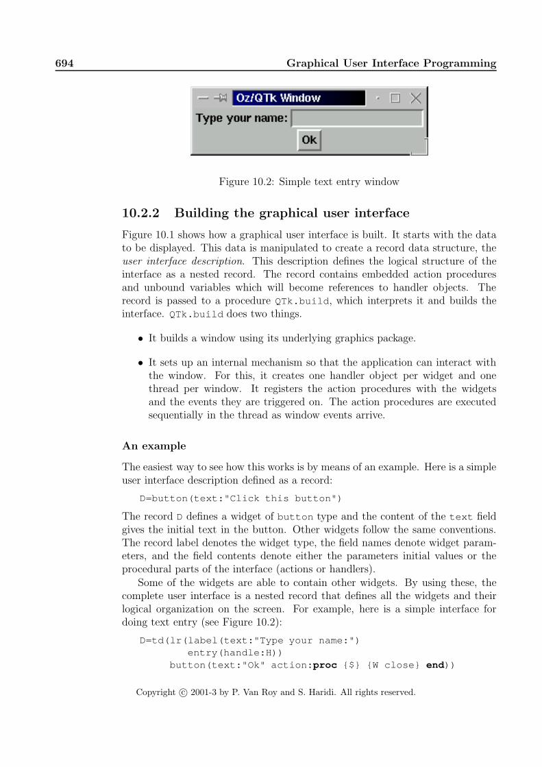
694 Graphical User Interface Programming
Figure 10.2: Simple text entry window
10.2.2 Building the graphical user interface
Figure 10.1 shows how a graphical user interface is built. It starts with the datato be displayed. This data is manipulated to create a record data structure, theuser interface description. This description defines the logical structure of theinterface as a nested record. The record contains embedded action proceduresand unbound variables which will become references to handler objects. Therecord is passed to a procedure QTk.build , which interprets it and builds theinterface. QTk.build does two things.
• It builds a window using its underlying graphics package.
• It sets up an internal mechanism so that the application can interact withthe window. For this, it creates one handler object per widget and onethread per window. It registers the action procedures with the widgetsand the events they are triggered on. The action procedures are executedsequentially in the thread as window events arrive.
An example
The easiest way to see how this works is by means of an example. Here is a simpleuser interface description defined as a record:
D=button(text:"Click this button")
The record D defines a widget of button type and the content of the text fieldgives the initial text in the button. Other widgets follow the same conventions.The record label denotes the widget type, the field names denote widget param-eters, and the field contents denote either the parameters initial values or theprocedural parts of the interface (actions or handlers).
Some of the widgets are able to contain other widgets. By using these, thecomplete user interface is a nested record that defines all the widgets and theirlogical organization on the screen. For example, here is a simple interface fordoing text entry (see Figure 10.2):
D=td(lr(label(text:"Type your name:")entry(handle:H))
button(text:"Ok" action: proc {$} {W close} end ))
Copyright c© 2001-3 by P. Van Roy and S. Haridi. All rights reserved.

10.2 Using the declarative/procedural approach 695
fun {GetText A}H T D Win
D=td(lr(label(text:A) entry(handle:H))button(text:"Ok"
action: proc {$} T={H get($)} {W close} end ))W={QTk.build D}{W show} {W wait}T
end
Figure 10.3: Function for doing text entry
Figure 10.4: Windows generated with the lr and td widgets
The td widget organizes its member widgets in top-down fashion. The lr widgetis similar, but goes left to right. This example has one action, proc {$} {W
close} end , and a handle, H, which we will explain later. At this point, bothH and Ware still unbound variables. Create the window by passing D to theQTk.build procedure:
W={QTk.build D}
This creates a window, a window object Wthat represents it, and a handler objectH. Now we display the window:
{W show}
The user can type text in this window. At any time, the text in the window canbe read by calling the handler H:
T={H get($)}
This is usually done when the window is closed. To make sure it is done whenthe window is closed, we can put it inside the action procedure.
To complete this example, let us encapsulate the whole user interface in afunction called GetText . Figure 10.3 shows the resulting code. Calling GetText
will wait until the user types a line of text and then return the text:
{Browse {GetText "Type your name:"}}
Note that GetText does a {W wait} call to wait until the window is closedbefore returning. Leaving out this call will return immediately with an unboundvariable that is bound later, when the user clicks the button.
Copyright c© 2001-3 by P. Van Roy and S. Haridi. All rights reserved.

696 Graphical User Interface Programming
Figure 10.5: Window generated with newline and continue codes
10.2.3 Declarative geometry
In addition to the widgets themselves, there are two other aspects of a windowthat are defined declaratively: the geometric arrangement of its widgets and thebehavior of its widgets when the window is resized. We describe each in turn. Thegeometric arrangement of widgets is defined by means of three special widgetsthat can contain other widgets:
• The lr and td widgets arrange their member widgets left-right or top-down.Figure 10.4 shows the two windows that are displayed with the followingtwo commands:
D=lr(label(text:"left")label(text:"center")label(text:"right"))
W1={QTk.build D}{W1 show}
E=td(label(text:"top")label(text:"center")label(text:"down"))
W2={QTk.build E}{W2 show}
• The placeholder widget defines a rectangular area in the window that cancontain any other widget as long as the window exists. The placeholder’scontent can be changed at any time during execution. A placeholder may beput inside a placeholder, to any level of recursion. In the following example,the window alternatively contains a label and a pushbutton:
placeholder(handle:P)...{P set(label(text:"Hello"))}...{P set(button(text:"World"))}
Calling {P set(D)} is almost the same as calling {QTk.build D} , i.e., itinterprets the nested record D and creates handler objects, but the visibleeffect is limited to the rectangular area of the placeholder widget.
Copyright c© 2001-3 by P. Van Roy and S. Haridi. All rights reserved.

10.2 Using the declarative/procedural approach 697
Ww e
n
s
Figure 10.6: Declarative resize behavior
• The lr and td widgets support the special codes newline , empty , andcontinue , which allows to organize their member widgets in a grid struc-ture with aligned rows and columns of the same size (see Figure 10.5). Thecode newline makes the subsequent contained widgets jump to a new row(for lr ) or column (for td ). All the widgets in the new row or column arealigned with the widgets in the previous row or column. The empty spe-cial code leaves an empty box the size of a widget. The continue specialcode lets the previous widget span over an additional box. The followingdescription:
lr(button(text:"One" glue:we)button(text:"Two" glue:we)button(text:"Three" glue:we) newlinebutton(text:"Four" glue:we)button(text:"Five" glue:we)button(text:"Six" glue:we) newlinebutton(text:"Seven" glue:we)button(text:"Eight" glue:we)button(text:"Nine" glue:we) newlineempty button(text:"Zero" glue:we) continue)
gives the window of Figure 10.5.
10.2.4 Declarative resize behavior
When the size of a window is changed, the interface has to define how the internalwidgets rearrange themselves. This is called the resize behavior. The resizebehavior is dynamic, i.e., it defines a behavior over time. But it is a sufficientlyrestricted kind of dynamic behavior that we can define it using a descriptivedeclarative model.
Copyright c© 2001-3 by P. Van Roy and S. Haridi. All rights reserved.

698 Graphical User Interface Programming
Figure 10.7: Window generated with the glue parameter
We define the resize behavior of a widget by an optional glue parameter, whosevalue is an atom made up of any combination of the letters n, s , w, and e. Theglue parameter places constraints on how the widget is placed and how it resizes.As Figure 10.6 illustrates, a widget W is always placed inside a rectangular areaand has a “natural” size defined by its contents. One can choose for the widgetto occupy its natural size in either direction (horizontally or vertically) or to beexpanded to take as much space as possible in either direction. For the left-right direction, the w value, when present, will attach the widget to the left side(“west”). The same for the e value (“east”) and the right side. If w and e arepresent simultaneously, then the widget is expanded. Otherwise, it takes up justits natural size. For the top-down direction, the n and s values play the sameroles (“north” and “south”). For example, the description:
lr(label(text:"Name" glue:w) entry(glue:we) glue:nwe)
gives the window of Figure 10.7.
10.2.5 Dynamic behavior of widgets
The dynamic behavior of widgets is defined by means of action procedures andhandler objects. Look again at the example of Section 10.2.2:
declare E D WinD=td(lr(label(text:"Type your name:")
entry(handle:E))button(text:"Ok" action:toplevel#close))
W={QTk.build D}{W show}
The action toplevel#close is part of the button; when the button is clickedthen this causes the window to be closed. Generally, actions are zero-argumentprocedures, except that short-cuts are given for a few common actions such asclosing the window. The handle E is an object that allows to control the textentry widget. For example, here’s how to set the value of the widget’s text entryfield:
Copyright c© 2001-3 by P. Van Roy and S. Haridi. All rights reserved.

10.3 Case studies 699
{E set("Type here")}
Here is how to read and display the value of the field:
{Browse {E get($)}}
Actions can also be attached to events such as mouse clicks:
proc {P} {Browse ´ clicked with third mouse button! ´ } end{E bind(event:"<3>" action:P)}
The event "<3>" means a click of the third mouse button. Attaching it to E
means that the button has to be clicked when the mouse is over E’s widget. Acomplete list of possible events is given in the QTk documentation in the Mozartsystem.
10.3 Case studies
We present four case studies that show different techniques of user interface de-sign:
• The first is a simple progress monitor. This example has no special featuresexcept to show how simple it is to build a custom display for a particularpurpose.
• The second builds a simple calendar widget. It is based on an lr widgetwith gridding ability. It shows the flexibility of the gridding. It also showshow to use a placeholder and how state can be introduced to optimizeexecution of what is originally a purely declarative calculation.
• The third derives two different GUIs by transforming one data model intotwo GUI specifications. The user can switch between the two at any time.This shows the advantage of tightly integrating the GUI tool with the lan-guage, since different data models can be represented with the same datastructures (e.g., records and lists) and transformed with the same opera-tions.
• The fourth defines a clock with an interface that adapts itself according toan external condition. The best view of the clock data is chosen dynamicallydepending on the window size. Because of the mixed declarative/proceduralapproach, each view can be completely defined in just a few lines of code.
The second through fourth case studies were originally written by Donatien Gro-laux.
10.3.1 A simple progress monitor
We start by defining the simple interface that we used in Section 5.5.1 to monitorthe progress of a message-passing program. The interface has a check button
Copyright c© 2001-3 by P. Van Roy and S. Haridi. All rights reserved.

700 Graphical User Interface Programming
fun {NewProgWindow CheckMsg}InfoHdl See={NewCell true }H D=td(label(text:nil handle:InfoHdl)
checkbutton(text:CheckMsg handle:H init: trueaction: proc {$} See:={H get($)} end ))
in{{QTk.build D} show}proc {$ Msg}
if @See then {Delay 50} {InfoHdl set(text:Msg)} endend
end
Figure 10.8: A simple progress monitor
that can be enabled and disabled. Enabling and disabling this button is doneconcurrently with the monitored program. When enabled, the interface displaysa message that can be updated dynamically. The program is slowed down sothat each new message appears for at least 50 ms. When disabled, the inter-face freezes and lets the program run at full speed. This allows to monitor theprogress of a running program without unduly perturbing the program. Fig-ure 10.8 shows the definition. A screenshot is given in Section 5.5.1. CallingInfoMsg={NewProgWindow Msg} creates a new window with checkbutton mes-sage Msg. During program execution, {InfoMsg Msg} can be called as often asdesired to display Msg in the window. With the checkbutton, the user can chooseto track these calls or to freeze the display.
10.3.2 A simple calendar widget
The grid structure of Section 10.2.3 can be used to build widgets with dataarranged in rectangular form. We show how by building a simple calendar widget.Figure 10.9 shows what it looks like. We define the procedure Calendar thatreturns the calendar widget and its display procedure:
proc {Calendar ?Cal ?Redraw}P in
Cal=placeholder(handle:P)proc {Redraw T}
...{P set(...)}
endend
The calendar widget is a placeholder that is updated by calling {Redraw T} witha time argument T. The redraw procedure should be called at least once a day toupdate the calendar. For simplicity, we will redraw the complete calendar eachtime.
Copyright c© 2001-3 by P. Van Roy and S. Haridi. All rights reserved.

10.3 Case studies 701
Figure 10.9: A simple calendar widget
Let us now see what is inside the Redraw procedure. It has a time argumentT. Assume that the time has the format of the {OS.localTime} call, which is arecord that looks like this:
time(hour:11 isDst:0 mDay:12 min:5 mon:11 sec:7wDay:2 yDay:346 year:100)
For the calendar we need only the fields wDay (weekday, 0 to 6, where 0 is Sunday),mDay(day of month, 1 to 31), mon (month, 0 to 11), and year (years since 1900).
The calendar is a rectangular grid of weekday names and day numbers. Redraw
builds this grid by using an lr widget. We first make a list of all the calendarelements and use newline to go to the next line in the calendar. We start bydefining the calendar’s header:
Header=[label newlinelabel(text:"Mo") label(text:"Tu") label(text:"We")label(text:"Th") label(text:"Fr") label(text:"Sa")label(text:"Su") newlinelrline(glue:we) continue continue continuecontinue continue continue newline]
This displays the weekday names and underlines them. We now make a list thatcontains all calendar numbers. First, we calculate the number of days in themonth, taking leap years into account:2
ML={List.nth [31if (T.year div 4)==0 then 29 else 28 end31 30 31 30 31 31 30 31 30 31] T.mon+1}
Second, we calculate the number of blank spots in the grid before the calendarday with number “1”:
2As an exercise, correct the leap year calculation according to the complete rules for theGregorian calendar.
Copyright c© 2001-3 by P. Van Roy and S. Haridi. All rights reserved.

702 Graphical User Interface Programming
SD=(((7-(T.mDay mod 7))+T.wDay) mod 7)
With these two numbers, we can make a list of calendar days, correctly offset inthe month:
fun {Loop Skip Col Nu}if Nu>ML then nilelseif Col==8 then
newline|{Loop Skip 1 Nu}elseif Skip>0 then
label|{Loop Skip-1 Col+1 Nu}elseif Nu==T.mDay then
label(text:Nu bg:black fg:white)|{Loop 0 Col+1 Nu+1}else
label(text:Nu)|{Loop 0 Col+1 Nu+1}end
endR={Append Header {Loop SD 1 1}}
Here, Col gives the column (from 1 to 7) and Nu is today’s day number. Finally,we can update the placeholder:
{P set({List.toTuple lr R})}
This completes the inside of Redraw . Let us now create and display a calendar:
declare Cal Redraw W in{Calendar Cal Redraw}W={QTk.build td(Cal)}{Redraw {OS.localTime}}{W show}
The calendar can be redrawn at any time by calling Redraw .
Memoization: using state to avoid repeating work
This redraw procedure will redraw the whole calendar each time it is called. Formany clocks this will be once per second or once per minute. This is very wastefulof computational resources. We can avoid the repetitive redraw by storing theyDay , year , and mon fields together in a cell, and redrawing only if the contentchanges:
proc {Calendar ?Cal ?Redraw}P Date={NewCell r(yDay:0 year:0 mon:0)}
inCal=placeholder(handle:P)proc {Redraw T}
TOld=@DateTNew=r(yDay:T.yDay year:T.year mon:T.mon)
inif TOld==TNew then skipelse
Copyright c© 2001-3 by P. Van Roy and S. Haridi. All rights reserved.

10.3 Case studies 703
Figure 10.10: Automatic generation of a user interface
Date:=TNew... % Recalculate and redisplay as before
endend
end
If we leave out the final call to P, then the original Redraw procedure has adeclarative implementation and the new Redraw procedure has a stateful im-plementation. Yet, both have identical behavior when viewed from the outside.The state is used just to memorize the previous calendar calculation so that theprocedure can avoid doing the same calculation twice. Paraphrasing philosopherGeorge Santayana, we can say this is remembering the past to avoid repeating it.This technique is called memoization. It is a common use of state. It is particu-larly nice because it is modular: the use of state is hidden inside the procedure(see Section 6.7.2).
10.3.3 Automatic generation of a user interface
Using records to specify the user interface makes it possible to calculate the us-er interface directly from the data. This is a powerful technique that supportsadvanced approaches to GUI design. One such approach is model-based design.In this approach, different aspects of a GUI design are specified in separate for-malisms called models. A running GUI is then obtained from all the models takentogether [145]. Typical models include a domain model, a presentation model, adialog model, a task model, a user model, a platform model, and a help model.These models can be represented within the language as data structures consist-ing of nested records and procedure values. From the records, it is possible tocalculate QTk records. It is particularly easy to translate the domain model intothe presentation and dialog models, because the latter are directly supported byQTk.
The domain model is very similar to the application’s data model. It definesthe data entities that the user can manipulate. The presentation model is arepresentation of the visual, auditive and other elements that the UI offers to
Copyright c© 2001-3 by P. Van Roy and S. Haridi. All rights reserved.

704 Graphical User Interface Programming
EditPresentation
Original data
UIRead−only view Editable view
widget (QTk)Placeholder
UI
ViewPresentation
Figure 10.11: From the original data to the user interface
the users. The dialog model defines how the presentation model interacts withthe user. It represents the actions that a user can initiate via the presentationelements and the responses of the application.
We give an example to show how one domain model can be automaticallymapped to two presentation models: a read-only view and an editable view of thedata. The user can freely switch between the views by clicking a check button (seeFigure 10.10). The mapping from the domain model to the presentation modelsis done in a natural way by means of functions, using declarative programming.There are two functions, ViewPresentation and EditPresentation , each ofwhich calculates the QTk presentation model from the same original data (seeFigure 10.11). The presentation model is encapsulated in a common interfacefor the two views. A placeholder is used to dynamically display one of the twoviews. Because of the common interface, keeping coherence between views isstraightforward.
Let us write a simple example program to illustrate these ideas. We use avery simple domain model: a list of pairs of the form identifier#value , whichrepresents the known information about some entity. The purpose of the GUI isto display or edit this information. Let us take the following information to startwith:
Data=[name#"Roger"surname#"Rabbit"age#14]
Now we define the two functions that translate this domain representation into theview information needed by QTk. The first function, ViewPresentation , buildsthe read-only view. It builds a representation where each pair identifier#value
is mapped to a label widget whose text is the identifier followed by a colon “:”and the corresponding value. Figure 10.12 gives the source code. The functionreturns a record with four fields:
Copyright c© 2001-3 by P. Van Roy and S. Haridi. All rights reserved.

10.3 Case studies 705
fun {ViewPresentation Data}Hdl In={NewCell Data}HR={MakeRecord hr {Map Data fun {$ D#_} D end }}
inr(spec: {Adjoin
{List.toTuple td{Map Data fun {$ D#V}
label(glue:we handle:HR.D text:D#":"#V) end }}td(glue:nswe handle:Hdl)}
handle: Hdlset: proc {$ Ds}
In:=Dsfor D#V in Ds do {HR.D set(text:D#":"#V)} end
endget: fun {$} @In end )
end
Figure 10.12: Defining the read-only presentation
fun {EditPresentation Data}Hdl Feats={Map Data fun {$ D#_} D end }HR={MakeRecord hr Feats}fun {Loop Ds}
case Ds of D#V|Dr thenlabel(glue:e text:D#":") |entry(handle:HR.D init:V glue:we) |newline | {Loop Dr}
else nil endend
inr(spec: {Adjoin
{List.toTuple lr {Loop Data}}lr(glue:nswe handle:Hdl)}
handle: Hdlset: proc {$ Ds}
for D#V in Ds do {HR.D set(V)} end endget: fun {$}
{Map Feats fun {$ D} D#{HR.D get($)} end } end )end
Figure 10.13: Defining the editable presentation
Copyright c© 2001-3 by P. Van Roy and S. Haridi. All rights reserved.

706 Graphical User Interface Programming
• Field spec : the interface specification, which describes the widget in QTk
format.
• Field handle : the widget’s handle, when the interface is created.
• Field set : a one-argument procedure that updates the information dis-played by the widget. During execution, this lets us change the data thatis displayed.
• Field get : a zero-argument function that returns the data that is displayed,in the same format as it was input. Since ViewPresentation does notchange the data, this simply returns the last information that was set. (InEditPresentation it will return the new information that the user hastyped.)
The get and set operations are used to keep coherence of the data when switch-ing between the two views. The HR record collects all the data items’ handles,for the use of the get and set operations.
The second function, EditPresentation , builds the editable view. It buildsa representation where each pair identifier#value is mapped to a label con-taining the identifier followed by ”:” and an entry widget. Figure 10.13 givesthe source code. This function also returns a record with four fields, like theViewPresentation function. This time, the result of the get function is ob-tained from the widgets themselves.
The main application calls both of these functions on the same data. Themain window contains a placeholder widget and a checkbox widget. Oncethe window is built, the specifications of both views are put in the placeholder
widget. Subsequently they can be put back at any time by using just theirhandles. Checking or unchecking the checkbox switches between the two views.Data integrity between the views is maintained by using their associated set andget operations. Here is the source code:
P CV1={ViewPresentation Data}V2={EditPresentation Data}{{QTk.build
td(placeholder(glue:nswe handle:P)checkbutton(text:"Edit" init: false handle:C
action:proc {$}
Old#New= if {C get($)} then V1#V2 else V2#V1 endin {New.set {Old.get}} {P set(New.handle)} end ))}
show}{P set(V2.spec)}{P set(V1.spec)}
This example shows the advantages of tightly integrating an executable model-based GUI with an expressive programming language. The different models can
Copyright c© 2001-3 by P. Van Roy and S. Haridi. All rights reserved.

10.3 Case studies 707
Figure 10.14: Three views of FlexClock, a context-sensitive clock
(uses minimum size)...(refreshes each widgetonce a second)
procedureRefresh Widget
(record)Minimum
size
(each definition has three parts)
Definition of views
PlaceholderselectorView
widget
eventsWindow resize
Clock
Figure 10.15: Architecture of the context-sensitive clock
all be expressed as data structures of the language. The mappings between thedifferent models can then be done easily within the language.
10.3.4 A context-sensitive clock
This section defines a simple clock utility, FlexClock, that dynamically displaysa different view depending on the size of the window. When the window isresized, the “best” view for the new size is chosen. The application defines sixdifferent views and takes about 100 lines of code. It dynamically chooses thebest view among the six. The best view is the one that gives the most detailedtime information in the available window size. Figure 10.14 shows three of thesix views. A more elaborate version with 16 views, an analog clock widget, and
Copyright c© 2001-3 by P. Van Roy and S. Haridi. All rights reserved.

708 Graphical User Interface Programming
a calendar widget, is available as part of the Mozart demos.
Figure 10.15 shows the architecture of the clock. Each view consists of threeparts: a refresh procedure, a widget definition, and a minimum size. A clock callsall the refresh procedures once a second with the current time. A view selectorpicks one of the views and puts it in a placeholder widget to display it. Eachtime the window is resized, i.e., whenever a resize event occurs, then the viewselector chooses the best view and displays it. The refresh procedures and theview selector run concurrently. This is acceptable because there is no interferencebetween them.
Let us implement the clock according to this architecture. We first set up asmall server that periodically calls each procedure in a list of procedures:
NotifyClocklocal
Clocks={NewCell nil}proc {Loop}
T={OS.localTime}in
for I in @Clocks do {I T} end{Delay 1000}{Loop}
endin
proc {NotifyClock P}Clocks:=P|@Clocks
endthread {Loop} end
end
The period is almost exactly once per second.3 Calling {NotifyClock P} addsP to the list of procedures to be notified. The refresh procedure of each viewwill be put in this list. The OS.localTime call returns a record that containsall the time information. To help in calculating the views, we define some utilityfunctions to format the time information in various ways:
fun {TwoPos I} if I<10 then "0"#I else I end endfun {FmtTime T} {TwoPos T.hour}#":"#{TwoPos T.min} endfun {FmtTimeS T} {FmtTime T}#":"#{TwoPos T.sec} endfun {FmtDate T} {TwoPos T.mDay}#"/"#{TwoPos T.mon+1} endfun {FmtDateY T} {FmtDate T}#"/"#(1900+T.year) endfun {FmtDay T}
{List.nth ["Sunday" "Monday" "Tuesday" "Wednesday""Thursday" "Friday" "Saturday"] T.wDay+1}
endfun {FmtMonth T}
{List.nth ["January" "February" "March" "April" "May"
3Section 4.6.2 explains how to do it exactly once per second.
Copyright c© 2001-3 by P. Van Roy and S. Haridi. All rights reserved.

10.3 Case studies 709
"June" "July" "August" "September" "October""November" "December"]
T.mon+1}end
Now we define each view as a record with three elements:
• Field refresh : a procedure that is called with a time argument to updatethe view’s display.
• Field spec : a declarative specification of the widgets comprising the view.
• Field surface : the minimal size (horizontally and vertically) that is re-quired to correctly display the view.
Figure 10.16 defines all six views in one list. Alert readers will notice that thereis a seventh, empty view that will be displayed in case the window is too small todisplay a text. The window that displays a view contains just a single placeholderwidget. A placeholder, as we saw before, is a container that can contain anywidget and that can change the displayed widget at any time as long as thewindow exists. Here is the window:
declare P W inW={QTk.build
td(title:"FlexClock demo"placeholder(handle:P width:1 height:1 glue:nswe))}
To initialize the application, all views are placed once in the placeholder. Afterthis is done, any view can be displayed again in the placeholder by a singlecommand using the view’s handle. We also register each refresh procedure withNotifyClock . The result is a list, Views , that has one triple per view, containingthe minimal width, minimal height, and a handle for the view:
Views={Map ViewListfun {$ R}
Width#Height=R.surfacein
{P set(R.spec)}{NotifyClock R.refresh}Width#Height#(R.spec).handle
end }
Now we have initialized the placeholder and registered all the refresh procedures.The next step is to set up the mechanism to calculate the best view and displayit. We will assume the best view is the one that satisfies the following threeconditions:
• The window size is big enough to display the view, i.e., window width ≥minimal view width and window height ≥ minimal view height.
Copyright c© 2001-3 by P. Van Roy and S. Haridi. All rights reserved.

710 Graphical User Interface Programming
declareH0 H1 H2 H3 H4 H5 H6ViewList=
[r(refresh: proc {$ T} skip endspec:label(handle:H0 glue:nswe bg:white)surface:0#0)
r(refresh: proc {$ T} {H1 set(text:{FmtTime T})} endspec:label(handle:H1 glue:nswe bg:white)surface:40#10)
r(refresh: proc {$ T} {H2 set(text:{FmtTimeS T})} endspec:label(handle:H2 glue:nswe bg:white)surface:80#10)
r(refresh:proc {$ T}
{H3 set(text:{FmtTime T}# ´ \n ´ #{FmtDate T})} endspec:label(handle:H3 glue:nswe bg:white)surface:40#30)
r(refresh:proc {$ T}
{H4 set(text:{FmtTimeS T}# ´ \n ´ #{FmtDateY T})}end
spec:label(handle:H4 glue:nswe bg:white)surface:80#30)
r(refresh:proc {$ T}
{H5 set(text:{FmtTimeS T}# ´ \n ´ #{FmtDay T}#", "#{FmtDateY T})} end
spec:label(handle:H5 glue:nswe bg:white)surface:130#30)
r(refresh:proc {$ T}
{H6 set(text:{FmtTimeS T}# ´ \n ´ #{FmtDay T}#", "#T.mDay#" "#{FmtMonth T}#" "#(1900+T.year))}
endspec:label(handle:H6 glue:nswe bg:white)surface:180#30)]
Figure 10.16: View definitions for the context-sensitive clock
Copyright c© 2001-3 by P. Van Roy and S. Haridi. All rights reserved.

10.3 Case studies 711
Minimal size for view 3
Area in which view 3 is chosen(3)
3
15010000
(1)(0) (2) (2) (2)
(0) (3) (4) (5) (6)
50
50
(0) (0) (0) (0) (0)
Width
Height
30
40 80 130 180
0
1 2
4 5 63
10
Figure 10.17: The best view for any size clock window
• The distance between the bottom right corner of the minimal view and thebottom right corner of the window is minimized. It suffices to minimize thesquare of this distance.
• If no view satisfies the above two conditions, the smallest view is chosen bydefault.
Figure 10.17 shows how this divides up the plane among the seven views. Theprocedure Place does the calculation and displays the best view in the place-holder:
proc {Place}WW={QTk.wInfo width(P)}WH={QTk.wInfo height(P)}_#Handle={List.foldRInd Views
fun {$ I W#H#Handle Min#CH}This=(W-WW)*(W-WW)+(H-WH)*(H-WH)
inif W<WWandthen H<WHandthen
(Min==inf orelse This<Min) then This#Handleelse Min#CH end
endinf# local (_#_#H)|_=Views in H end }
in{P set(Handle)}
end
This starts with a minimum of inf , representing infinity, and is reduced for eachview with a smaller distance. When the window is resized, Place has to be calledto set the correct view according to the new size of the window. This is done bybinding the <Configure> event of QTk:
Copyright c© 2001-3 by P. Van Roy and S. Haridi. All rights reserved.

712 Graphical User Interface Programming
{P bind(event: ´ <Configure> ´ action:Place)}
The window is now completely set up, but it is still hidden. We display it asfollows:
{W show}
10.4 Implementing the GUI tool
The GUI tool is implemented as three layers: a front end, a middle layer, anda back end. The front end is the QTk module, which is an interpreter for thedeclarative specifications. The middle layer is the Tk module, which offers anobject-oriented interface to the underlying graphics package. The back end is thegraphics package, which is tcl/tk.
When a specification is given to the interpreter by calling QTk.build , theinterpreter builds the user interface by giving commands to the graphics packageusing a model that is almost completely procedural. The interpretation overheadis only paid once. The only overhead in the calls to the handler objects is therun-time type checking of their arguments.
The placeholder widget deserves a mention because a new widget can be putin it at any time during execution. When a widget is first put in, it is like callingQTk.build , i.e., there is an interpretation overhead. The placeholder reducesthis overhead by caching the interpretation of each widget that is put in. To puta widget in a placeholder again, it suffices to put in the widget’s handler. This isenough for the placeholder to identify which widget is meant.
10.5 Exercises
1. Calendar widget. Section 10.3.2 gives a formula for calculating the num-ber of blank spots in the grid before day 1. Why is this formula correct?
2. Clock with calendar. Extend the context-sensitive clock of Section 10.3with a calendar and add views so that the calendar is shown only when thewindow is big enough. You can use the calendar widget defined in the samesection.
Copyright c© 2001-3 by P. Van Roy and S. Haridi. All rights reserved.

Chapter 11
Distributed Programming
A distributed system is a set of computers that are linked together by a network.Distributed systems are ubiquitous in modern society. The canonical exampleof such a system, the Internet, has been growing exponentially ever since itsinception in the late 1970’s. The number of host computers that are part ofit has been doubling each year since 1980. The question of how to program adistributed system is therefore of major importance.
This chapter shows one approach to programming a distributed system. Forthe rest of the chapter, we assume that each computer has an operating systemthat supports the concept of process and provides network communication. Pro-gramming a distributed system then means to write a program for each processsuch that all processes taken together implement the desired application. For theoperating system, a process is a unit of concurrency. This means that if we ab-stract away from the fact that the application is spread over different processes,this is just a case of concurrent programming. Ideally, distributed programmingwould be just a kind of concurrent programming, and the techniques we haveseen earlier in the book would still apply.
Distributed programming is complicated
Unfortunately, things are not so simple. Distributed programming is more com-plicated than concurrent programming for the following reasons:
• Each process has its own address space. Data cannot be transferred fromone process to another without some translation.
• The network has limited performance. Typically, the basic network opera-tions are many orders of magnitude slower than the basic operations insideone process. At the time of publication of this book, network transfer timeis measured in milliseconds, whereas computational operations are done innanoseconds or less. This enormous disparity is not projected to change forthe foreseeable future.
Copyright c© 2001-3 by P. Van Roy and S. Haridi. All rights reserved.
714 Distributed Programming
• Some resources are localized. There are many resources that can only beused at one particular computer due to physical constraints. Localizedresources are typically peripherals such as input/output (display screen,keyboard/mouse, file system, printer). They can be more subtle, such asa commercial application that can only be run on a particular computerbecause it is licensed there.
• The distributed system can fail partially. The system consists of manycomponents that are only loosely connected. It might be that part of thenetwork stops working or that some of the computers stop working.
• The distributed system is open. Independent users and computations co-habit the system. They share the system’s resources and they may competeor collaborate. This gives problems of security (protection against maliciousintent) and naming (finding one another).
How do we manage this complexity? Let us attempt to use the principle ofseparation of concerns. According to this principle, we can divide the probleminto an ideal case and a series of non-ideal extensions. We give a solution for theideal case and we show how to modify the solution to handle the extensions.
The network transparency approach
In the ideal case, the network is fast, resources can be used everywhere, all com-puters are up and running, and all users trust one another. In this case thereis a solution to the complexity problem: network transparency. That is, we im-plement the language so that a program will run correctly independently of howit is partitioned across the distributed system. The language has a distributedimplementation to guarantee this property. Each language entity is implementedby one or more distribution protocols, which all are carefully designed to respectthe language semantics. For example, the language could provide the concept ofan object. An object can be implemented as a stationary object, which meansthat it resides on one process and other processes can invoke it with exactly thesame syntax as if it were local. The behavior will be different in the nonlocal case(there will be a round trip of network messages), but this difference is invisiblefrom the programmer’s point of view.
Another possible distribution protocol for an object is the cached object. Inthis protocol, any process invoking the object will first cause the object to becomelocal to it. From then on, all invocations from that process will be local ones (untilsome other process causes the object to move away). The point is that bothstationary and cached objects have exactly the same behavior from the languagepoint of view.
With network transparency, programming a distributed system becomes sim-ple. We can reuse all the techniques of concurrent programming we saw through-out the book. All the complexity is hidden inside the language implementation.
Copyright c© 2001-3 by P. Van Roy and S. Haridi. All rights reserved.

715
This is a real complexity, but given the conditions of the ideal case, it can berealistically implemented. It provides all the distribution protocols. It translatesdata between the address spaces of the processes. Translating to serial form iscalled marshaling and translating back is called unmarshaling. The term serial-ization is also used. It does distributed garbage collection, i.e., not reclaiming alocal entity if there is still some remote reference.
The idea of making a distributed language operation similar to a local lan-guage operation has a long history. The first implementation was the RemoteProcedure Call (RPC), done in the early 1980’s [18]. A call to a remote procedurebehaves in the same way, under ideal conditions, as a local procedure. Recently,the idea has been extended to object-oriented programming by allowing methodsto be invoked remotely. This is called Remote Method Invocation (RMI). Thistechnique has been made popular by the Java programming language [186].
Beyond network transparency
Network transparency solves the problem in the ideal case. The next step is tohandle the non-ideal extensions. Handling all of them at the same time whilekeeping things simple is a research problem that is still unsolved. In this chapterwe only show the tip of the iceberg of how it could be done. We give a practicalintroduction to each of the following extensions:
• Network awareness (i.e., performance). We show how choosing the dis-tribution protocol allows to tune the performance without changing thecorrectness of the program.
• Openness. We show how independent computations can connect togeth-er. In this we are aided because Oz is a dynamically-typed language: alltype information is part of the language entities. This makes connectingindependent computations relatively easy.
• Localized resources. We show how to package a computation into acomponent that knows what localized resources it needs. Installing thiscomponent in a process should connect it to these resources automatically.We already have a way to express this, using the concept of functor. Afunctor has an import declaration that lists what modules it needs. Ifresources are visible as modules, then we can use this to solve the problemof linking to localized resources.
• Failure detection. We show how to detect partial failure in a way usableto the application program. The program can use this information to dofault confinement and possibly to repair the situation and continue work-ing. While failure detection breaks transparency, doing it in the languageallows to build abstractions that hide the faults, e.g., using redundancy toimplement fault tolerance. These abstractions, if desired, could be used toregain transparency.
Copyright c© 2001-3 by P. Van Roy and S. Haridi. All rights reserved.

716 Distributed Programming
This brief introduction leaves out many issues such as security, naming, resourcemanagement, and building fault tolerance abstractions. But it gives a goodoverview of the general issues in the area of distributed programming.
Structure of the chapter
This chapter consists of the following parts:
• Sections 11.1 and 11.2 set the stage by giving a taxonomy of distributedsystems and by explaining our distributed computation model.
• Sections 11.3–11.6 show how to program in this distribution model. Wefirst show how to program with declarative data and then with state. Wehandle state separately because it involves more sophisticated and expensivedistribution protocols. We then explain the concept of network awareness,which is important for performance reasons. Finally, we show some commondistributed programming patterns.
• Section 11.7 explains the distributed protocols in more detail. It singles outtwo particularly interesting protocols, the mobile state protocol and thedistributed binding protocol.
• Section 11.8 introduces partial failure. It explains and motivates the twofailures we detect, permanent process failure and temporary network inac-tivity. It gives some simple programming techniques including an abstrac-tion to create resilient server objects.
• Section 11.9 briefly discusses the issue of security and how it affects writingdistributed applications.
• Section 11.10 summarizes the chapter by giving a methodology how to builddistributed applications.
11.1 Taxonomy of distributed systems
This chapter is mainly about a quite general kind of distributed system, the opencollaborative system. The techniques we give can also be used for other kinds ofdistributed system, such as cluster computing. To explain why this is so, we givea taxonomy of distributed systems that situates the different models. Figure 11.1shows four types of distributed system. For each type, there is a simple diagram toillustrate it. In these diagrams, circles are processors or computers, the rectangleis memory, and connecting lines are communication links (a network). The figurestarts with a shared-memory multiprocessor, which is a computer that consistsof several processors attached to a memory that is shared between all of them.Communication between processors is extremely fast; it suffices for one processor
Copyright c© 2001-3 by P. Van Roy and S. Haridi. All rights reserved.

11.1 Taxonomy of distributed systems 717
(partial failure)?
Distributed memorymultiprocessor
Shared memorymultiprocessor
multiprocessorDistributed memory
with partial failure
Add distribution
Add partial failure
Add openness
Collaboration(‘‘Internet computing’’)
Open distributed system
(naming and security)
High performance(‘‘cluster computing’’)
Figure 11.1: A simple taxonomy of distributed systems
to write a memory cell and another to read it. Coordinating the processors, sothat, e.g., they all agree to do the same operation at the same time, is efficient.
Small shared-memory multiprocessors with one to eight processors are com-modity items. Larger scalable shared-memory cache-coherent multiprocessorsare also available but are relatively expensive. A more popular solution is toconnect a set of independent computers through their I/O channels. Anotherpopular solution is to connect off-the-shelf computers with a high-speed network.The network can be implemented as a shared bus (similar to Ethernet) or bepoint-to-point (separately connecting pairs of processors). It can be custom oruse standard LAN (local-area network) technology. All such machines are usual-ly called clusters or distributed-memory multiprocessors. They usually can havepartial failure, i.e., where one processor fails while the others continue. In thefigure, a failed computer is a circle crossed with a large X. With appropriatehardware and software the cluster can keep running, albeit with degraded perfor-mance, even if some processors are failed. That is, the probability that the clustercontinues to provide its service is close to 1 even if part of the cluster is failed.This property is called high availability. A cluster with the proper hardware andsoftware combines high performance with high availability.
In the last step, the computers are connected through a wide-area network(WAN) such as the Internet. This adds openness, in which independent compu-tations or computers can find each other, connect, and collaborate meaningfully.Openness is the crucial difference between the world of high-performance com-puting and the world of collaborative computing. In addition to partial failure,openness introduces two new issues: naming and security. Naming is how compu-tations or computers find each other. Naming is usually supported by a special
Copyright c© 2001-3 by P. Van Roy and S. Haridi. All rights reserved.
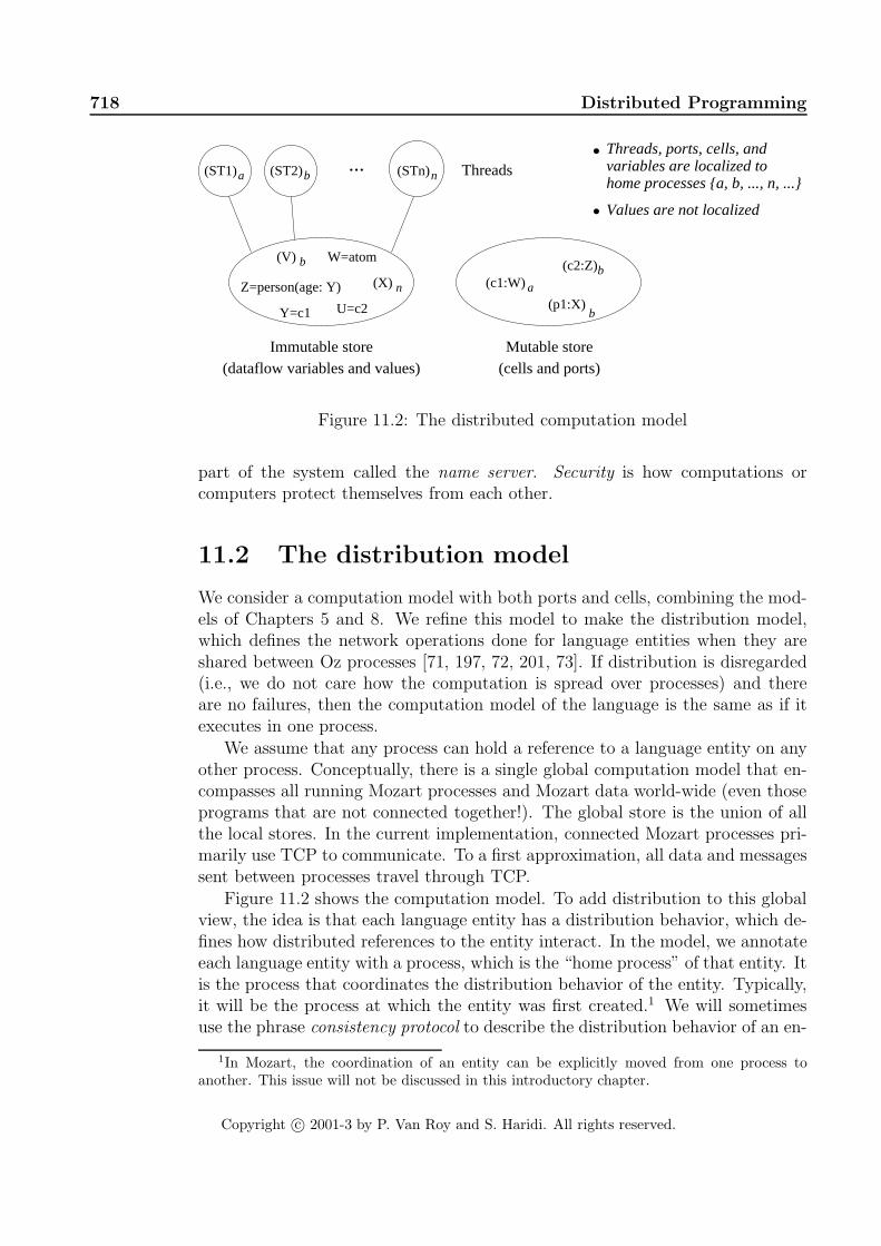
718 Distributed Programming
b
●
● Threads, ports, cells, andvariables are localized tohome processes {a, b, ..., n, ...}
Threads...
b
(ST1) (ST2) (STn)a b n
b
Immutable store Mutable store
a
Values are not localized
(dataflow variables and values) (cells and ports)
n (c1:W)(c2:Z)
(X)
U=c2Y=c1(p1:X)
Z=person(age: Y)
W=atom(V)
Figure 11.2: The distributed computation model
part of the system called the name server. Security is how computations orcomputers protect themselves from each other.
11.2 The distribution model
We consider a computation model with both ports and cells, combining the mod-els of Chapters 5 and 8. We refine this model to make the distribution model,which defines the network operations done for language entities when they areshared between Oz processes [71, 197, 72, 201, 73]. If distribution is disregarded(i.e., we do not care how the computation is spread over processes) and thereare no failures, then the computation model of the language is the same as if itexecutes in one process.
We assume that any process can hold a reference to a language entity on anyother process. Conceptually, there is a single global computation model that en-compasses all running Mozart processes and Mozart data world-wide (even thoseprograms that are not connected together!). The global store is the union of allthe local stores. In the current implementation, connected Mozart processes pri-marily use TCP to communicate. To a first approximation, all data and messagessent between processes travel through TCP.
Figure 11.2 shows the computation model. To add distribution to this globalview, the idea is that each language entity has a distribution behavior, which de-fines how distributed references to the entity interact. In the model, we annotateeach language entity with a process, which is the “home process” of that entity. Itis the process that coordinates the distribution behavior of the entity. Typically,it will be the process at which the entity was first created.1 We will sometimesuse the phrase consistency protocol to describe the distribution behavior of an en-
1In Mozart, the coordination of an entity can be explicitly moved from one process toanother. This issue will not be discussed in this introductory chapter.
Copyright c© 2001-3 by P. Van Roy and S. Haridi. All rights reserved.

11.2 The distribution model 719
tity. The distribution behavior is implemented by exchanging messages betweenMozart processes.
What kinds of distribution behavior are important? To see this, we firstdistinguish between stateful, stateless, and single-assignment language entities.Each of them has a different distribution behavior:
• Stateful entities (threads, cells, ports, objects) have an internal state. Thedistribution behavior has to be careful to maintain a globally coherent viewof the state. This puts major constraints on the kinds of efficient behaviorthat are possible. The simplest kind of behavior is to make them stationary.An operation on a stationary entity will traverse the network from theinvoking process and be performed on the entity’s home process. Otherkinds of behavior are possible.
• Single-assignment entities (dataflow variables, streams) have one essentialoperation, namely binding. Binding a dataflow variable will bind all itsdistributed references to the same value. This operation is coordinatedfrom the process on which the variable is created.
• Stateless entities, i.e., values (procedures, functions, records, classes, func-tors) do not need a process annotation because they are constants. Theycan be copied between processes.
Figure 11.3 shows a set of processes with localized threads, cells, and unbounddataflow variables. In the stateful concurrent model, the other entities can bedefined in terms of these and procedure values. These basic entities have a defaultdistributed behavior. But this behavior can be changed without changing thelanguage semantics. For example, a remote operation on a cell could force thecell to migrate to the calling process, and thereafter perform the operation locally.
For all derived entities except for ports, the distributed behaviors of the de-fined entities can be seen as derived behavior from the distributed behavior oftheir parts. In this respect ports are different. The default distribution behavioris asynchronous (see Section 5.1). This distributed behavior does not follow fromthe definition of ports in terms of cells. This behavior cannot be derived fromthat of a cell. This means that ports are basic entities in the distribution model,just like cells.
The model of this section is sufficient to express useful distributed programs,but it has one limitation: partial failures are not taken into account. In Sec-tion 11.8 we will extend the basic model to overcome this limitation.
Depending on the application’s needs, entities may be given different dis-tributed behaviors. For example “mobile” objects (also known as “cached” ob-jects) move to the process that is using them. These objects have the samelanguage semantics but a different distributed hehavior. This is important fortuning network performance.
Copyright c© 2001-3 by P. Van Roy and S. Haridi. All rights reserved.

720 Distributed Programming
Process b
... SnS2S3
S1X
Threads
Cell
c1:X
Dataflow variable
c2:Z Z
W
SxY
Process a Process n
Figure 11.3: Process-oriented view of the distribution model
11.3 Distribution of declarative data
Let us show how to program with the distribution model. In this section we showhow distribution works for the declarative subset of the stateful concurrent model.We start by explaining how to get different processes to talk to each other.
11.3.1 Open distribution and global naming
We say a distributed computation is open if a process can connect independentlywith other processes running a distributed computation at run time, withoutnecessarily knowing beforehand which process it may connect with nor the typeof information it may exchange. A distributed computation is closed if it isarranged so that a single process starts and then spawns other processes on variouscomputers it has access to. We will talk about closed distribution later.
An important issue in open distributed computing is naming. How do in-dependent computations avoid confusion when communicating with each other?They do so by using globally-unique names for things. For example, insteadof using print representations (character strings) to name procedures, ports, orobjects, we use globally-unique names instead. The uniqueness should be guar-anteed by the system. There are many possible ways to name entities:
• References. A reference is an unforgeable means to access any languageentity. To programs, a reference is transparent, i.e., it is dereferenced whenneeded to access the entity. References can be local, to an entity on thecurrent process, or remote, to an entity on a remote process. For example,a thread can reference an entity that is localized on another process. Thelanguage does not distinguish local from remote references.
• Names. A name is an unforgeable constant that is used to implementabstract data types. Names can be used for different kinds of identityand authentication abilities (see Sections 3.7.5 and 6.4). All language en-tities with token equality, e.g., objects, classes, procedures, functors, etc.,
Copyright c© 2001-3 by P. Van Roy and S. Haridi. All rights reserved.

11.3 Distribution of declarative data 721
implement their identity by means of a name embedded inside them (seeChapter 13).
• Tickets. A ticket, in the terminology of this chapter, is a global means toaccess any language entity. A ticket is similar to a reference, except that it isvalid anywhere including outside a Mozart process. It is represented by anASCII string, it is explicitly created and dereferenced, and it is forgeable. Acomputation can get a reference to an independent computation by gettinga ticket from that computation. The ticket is communicated using anycommunication protocol between the processes (e.g., TCP, IP, SMTP, etc.)or between the users of these processes (e.g., sneakernet, telephone, PostItnotes, etc.). Usually, these protocols can only pass simple datatypes, notarbitrary language references. But in almost all cases they support passinginformation coded in ASCII form. If they do, then they can pass a ticket.
• URLs (Uniform Resource Locators). A URL is a global reference toa file. The file must be accessible by a World-Wide Web server. A URLencodes the hostname of a machine that has aWeb server and a file name onthat machine. URLs are used to exchange persistent information betweenprocesses. A common technique is to store a ticket in a file addressed byURL.
Within a distributed computation, all these four kinds of names can be passed be-tween processes. References and names are pure names, i.e., they do not explicitlyencode any information other than being unique. They can be used only inside adistributed computation. Tickets and URLs are impure names since they explic-itly encode the information needed to dereference them–they are ASCII stringsand can be read as such. Since they are encoded in ASCII, they can be usedboth inside and outside a distributed computation. In our case we will connectdifferent processes together using tickets.
The Connection module
Tickets are created and used with the Connection module. This module hasthree basic operations:
• {Connection.offer X ?T} creates a ticket T for any reference X. Theticket can be taken just once. Attempting to take a ticket more than oncewill raise an exception.
• {Connection.offerUnlimited X ?T} creates a ticket T for any referenceX. The ticket can be taken any number of times.
• {Connection.take T ?X} creates a reference X when given a valid ticket inT. The X refers to exactly the same language entity as the original referencethat was offered when the ticket was created. A ticket can be taken at any
Copyright c© 2001-3 by P. Van Roy and S. Haridi. All rights reserved.

722 Distributed Programming
process. If taken at a different process than where the ticket was offered,then network communication is initiated between the two processes.
With Connection , connecting computations in different processes is extreme-ly simple. The system does a great deal of work to give this simple view. Itimplements the connection protocol, transparent marshaling and unmarshaling,distributed garbage collection, and a carefully-designed distribution protocol foreach language entity.
11.3.2 Sharing declarative data
Sharing records
We start with a simple example. The first process has a big data structure, arecord, that it wants to share. It first creates the ticket:2
X=the_novel(text:"It was a dark and stormy night. ..."author:"E.G.E. Bulwer-Lytton"year:1803)
{Show {Connection.offerUnlimited X}}
This example creates the ticket with Connection.offerUnlimited and displaysit in the Mozart emulator window (with Show). Any other process that wants toget a reference to X just has to know the ticket. Here is what the other processdoes:
X2={Connection.take ´ ...ticket comes here... ´ }
(To make this work, you have to replace the text ´ ....ticket comes here.... ´
by what was displayed by the first process.) That’s it. The operation Connection.take
takes the ticket and returns a language reference, which we put in X2. Becauseof network transparency, both X and X2 behave identically.
Sharing functions
This works for other data types as well. Assume the first process has a functioninstead of a record:
fun {MyEncoder X} (X*4449+1234) mod 33667 end{Show {Connection.offerUnlimited MyEncoder}}
The second process can get the function easily:
E2={Connection.take ´ ...MyEncoders ticket... ´ }{Show {E2 10000}} % Call the function
2Here, as in the subsequent examples, we leave out declare for brevity, but we keepdeclare ... in for clarity.
Copyright c© 2001-3 by P. Van Roy and S. Haridi. All rights reserved.

11.3 Distribution of declarative data 723
Sharing dataflow variables
In addition to records and functions, the ticket can also be used to pass unboundvariables. Any operation that needs the value will wait, even across the network.This is how we do distributed synchronization [71]. The first process creates thevariable and makes it globally accessible:
declare X in{Show {Connection.offerUnlimited X}}
But the process does not bind the variable yet. Other processes can get a referenceto the variable:
declare X inX={Connection.take ´ ...Xs ticket... ´ }{Browse X*X}
The multiplication blocks until X is bound. Try doing X=111 in the first process.The binding will become visible on all processes that reference the variable.
11.3.3 Ticket distribution
In the above examples we copied and pasted tickets between windows of theinteractive environment. A better way to distribute tickets is to store them in afile. To successfully connect with the ticket, the destination process just has toread the file. This not only makes the distribution easier, it also can distributeover a larger part of the network. There are two basic ways:
• Local distribution. This uses the local file system. The destination pro-cess has to be connected to the same file system as the source process. Thisworks well on a LAN where all machines have access to the same file system.
• Global distribution. This uses the global Web infrastructure. The filecan be put in a directory that is published by a Web server, e.g., in a~/public_html directory on Unix. The file can then be accessed by URL.
Using a URL to make connections is a general approach that works well forcollaborative applications on the Internet. To implement these techniques weneed an operation to store and load a ticket from a file or URL. This is alreadyprovided by the Pickle module as described in Chapter 2. Any stateless valuecan be stored on a file and retrieved by other process that has a read access-rightto the file.
The Pickle module We recall that the Pickle module has two operations:
• {Pickle.save X FN} saves any value X in the file whose name is FN.
• {Pickle.load FNURL ?X} loads into X the value stored in FNURL, whichcan be a file name or a URL.
Copyright c© 2001-3 by P. Van Roy and S. Haridi. All rights reserved.

724 Distributed Programming
Pickle can store any stateless entity. For example, it can be used to storerecords, procedures, classes, and even functors, all of which are pure values. Anattempt to save stateful data in a pickle will raise an exception. An attempt tosave a partial value in a pickle will block until the partial value is complete. Thefollowing code:
{Pickle.save MyEncoder ´ ˜/public_html/encoder ´ }
saves the function MyEncoder in a file. Files in the ˜/public_html directory areoften publicly-accessible by means of URLs. Anyone who needs the MyEncoder
function can just load the file by giving the right URL:
MyEnc={Pickle.load ´ http://www.info.ucl.ac.be/˜pvr/encoder ´ }
MyEncoder and MyEnc are absolutely identical from the program’s point of view.There is no way to distinguish them. The ability to store, transfer, and then exe-cute procedure values across a network is the essential property of what nowadaysis known as “applets”. A value saved in a pickle continues to be valid even ifthe process that did the save is no longer running. The pickle itself is a filethat contains complete information about the value. This file can be copied andtransferred at will. It will continue to give the same value when loaded withPickle.load .
The main limitation of pickles is that only values can be saved. One wayto get around this is to make a snapshot of stateful information, i.e., make astateless data structure that contains the instantaneous states of all relevantstateful entities. This is more complex than pickling since the stateful entitiesmust be locked and unlocked, and situations such as deadlock must be avoided.
However, we do not need such a complete solution in this case. There is asimple technique for getting around this limitation that works for any languageentity, as long as the process that did the save is still running. The idea is tostore a ticket in a pickle. This works since tickets are strings, which are values.This is a useful technique for making any language entity accessible worldwide.The URL is the entry point for the entity addressed by the ticket.
The Offer and Take operations Using Pickle and Connection , we de-fine two convenience operations Offer and Take that implement this technique.These operations are available in the module Distribution , which can be foundon the book’s Web site. The procedure Offer makes language entity X availablethrough file FN:
proc {Offer X FN}{Pickle.save {Connection.offerUnlimited X} FN}
end
The function Take gets a reference to the language entity by giving the file FNURL:
fun {Take FNURL}{Connection.take {Pickle.load FNURL}}
end
Copyright c© 2001-3 by P. Van Roy and S. Haridi. All rights reserved.

11.3 Distribution of declarative data 725
This uses Pickle.load , which can load any stateless data from a file. Theargument FNURLcan either be a file name or a URL.
11.3.4 Stream communication
Declarative programming with streams, as in Chapter 4, can be made distributedsimply by starting the producer and consumer in different processes. They onlyhave to share a reference to the stream.
Eager stream communication
Let us first see how this works with an eager stream. First create the consumerin one process and create a ticket for its stream:
declare Xs Sum in{Offer Xs tickfile}fun {Sum Xs A}
case Xs of X|Xr then {Sum Xr A+X} [] nil then A endend{Browse {Sum Xs 0}}
Then create the producer in another process. It takes the ticket to get a referenceto Xs and then creates the stream:
declare Xs Generate inXs={Take tickfile}fun {Generate N Limit}
if N<Limit then N|{Generate N+1 Limit} else nil endendXs={Generate 0 150000}
This creates the stream 0|1|2|3|... and binds it to Xs. This sends the streamacross the network from the producer process to the consumer process. Thisis efficient since stream elements are sent asynchronously across the network.Because of thread scheduling, the stream is created in “batches” and each batchis sent across the network in one message.
Lazy stream communication
We can run the same example with lazy stream communication. Take the exam-ples with programmed triggers (Section 4.3.3) and implicit triggers (Section 4.5)and run them in different processes, as we showed above with eager streams.
Message passing and ports
A port is a basic data type; it is a FIFO channel with an asynchronous sendoperation. Asynchronous means that the send operation completes immediately,without waiting for the network. FIFO means that successive sends in the same
Copyright c© 2001-3 by P. Van Roy and S. Haridi. All rights reserved.

726 Distributed Programming
thread will appear in the same order in the channel’s stream. Ports generalizestreams by allowing many-to-one communication. It is the difference betweenthe declarative concurrent model and the message-passing model. Let us createa port, make it globally accessible, and display the stream contents locally:
declare S P in{NewPort S P}{Offer P tickfile}for X in S do {Browse X} end
The for loop causes dataflow synchronization to take place on elements appearingon the stream S. Each time a new element appears, an iteration of the loop isdone. Now we can let a second process send to the port:
P={Take tickfile}{Send P hello}{Send P ´ keep in touch ´ }
Since the Send operation is asynchronous, it sends just a single message on thenetwork.
11.4 Distribution of state
Stateful entities are more expensive to distribute than stateless entities in anetwork-transparent system. It is because changes in state have to be visibleto all processes that use the entity.
11.4.1 Simple state sharing
Sharing cells
The simplest way to share state between processes is by sharing a cell. This canbe done exactly in the same way as for the other types.
declareC={NewCell unit }{Offer C tickfile}
Any other process can access C by doing:
declareC1={Take tickfile}
C and C1 are indistinguishable in the language. Any process that references thecell in this way can do operations on it. The system guarantees that this isglobally coherent. I.e., if process 1 first puts foo in the cell, and then process 2does an exchange, then process 2 will see foo . Knowing how the system does thisis important for efficiency (e.g., network hops). We will see later how the globalcoherence is maintained and how the programmer can control what the networkoperations are.
Copyright c© 2001-3 by P. Van Roy and S. Haridi. All rights reserved.

11.4 Distribution of state 727
fun {CorrectSimpleLock}Token={NewCell unit }proc {Lock P}Old New in
{Exchange Token Old New}{Wait Old}try {P} finally New=unit end
endin
´ lock ´ ( ´ lock ´ :Lock)end
Figure 11.4: Distributed locking
Distributed locking
Now that we know the distributed behavior of cells, let us it to implement a well-known distributed locking algorithm, also known as distributed mutual exclusionusing token passing.3 When locking a critical section, multiple requests shouldall correctly block and be queued, independent of whether the threads are on thesame process or on another process. We show how to implement this conciselyand efficiently in the language. Figure 11.4, taken from Section 8.3, shows oneway to implement a lock that handles exceptions correctly.4 If multiple threadsattempt to access the lock body, then only one is given access, and the others arequeued. The queue is a sequence of dataflow variables. Each thread suspends onone variable in the sequence, and will bind the next variable after it has executedthe lock body. Each thread desiring the lock therefore references two variables:one to wait for the lock and one to pass the lock to the next thread. Each variableis referenced by two threads.
When the threads are on different processes, the definition of Figure 11.4implements distributed token passing, a well-known distributed locking algo-rithm [33]. We explain how it works. When a thread tries to enter the lockbody, the Exchange gives it access to the previous thread’s New variable. Theprevious thread’s process is New’s owner. When the previous thread binds New,the owner sends the binding to the next thread’s process. This requires a singlemessage.
Sharing objects and other data types
A more sophisticated way to share state is to share objects. In this way, weencapsulate the shared state and control what the possible operations on it are.Here is an example:
class Coder
3The built-in distributed locks of Mozart use this algorithm.4For simplicity, we leave out reentrancy since it does only local execution.
Copyright c© 2001-3 by P. Van Roy and S. Haridi. All rights reserved.

728 Distributed Programming
attr seedmeth init(S) seed:=S endmeth get(X)
X=@seedseed:=(@seed*1234+4449) mod 33667
endendC={New Coder init(100)}{Offer C tickfile}
This defines the class Coder and an object C. Any process that takes the object’sticket will reference it. The Mozart system guarantees that the object will behaveexactly like a centralized object. For example, if the object raises an exception,then the exception will be raised in the thread calling the object.
11.4.2 Distributed lexical scoping
One of the important properties of network transparency is distributed lexicalscoping: a procedure value that references a language entity will continue toreference that entity, independent of where the procedure value is transferredacross the network. This causes remote references to be created implicitly, bythe simple act of copying the procedure value from one process to another. Forexample:
declareC={NewCell 0}fun {Inc X} X+@C end{Offer C tickfile1}{Offer Inc tickfile2}
Inc will always reference C, no matter from which process it is called. A thirdprocess can take C’s ticket and change the content. This will change the behaviorof Inc . The following scenario can happen: (1) process 1 defines C and Inc , (2)process 2 gets a reference to Inc and calls it, and (3) process 3 gets a referenceto C and changes its content. When process 2 calls Inc again it will use the newcontent of C. Semantically, this behavior is nothing special: it is a consequence ofusing procedure values with network transparency. But how is it implemented?In particular, what network operations are done to guarantee it? We would likethe network behavior to be simple and predictable. Fortunately, we can designthe system so that this is indeed the case, as Section 11.7 explains.
Distributed lexical scoping, like lexical scoping, is important for reasons ofsoftware engineering. Entities that are moved or copied between processes willcontinue to behave according to their specification, and not inadvertently changebecause some local entity happens to have the same name as one of their externalreferences. The importance of distributed lexical scoping was first recognized byLuca Cardelli and realized in Obliq, a simple functional language with object-based extensions that was designed for experimenting with network-transparent
Copyright c© 2001-3 by P. Van Roy and S. Haridi. All rights reserved.

11.5 Network awareness 729
distribution [28].
11.5 Network awareness
With these examples it should be clear how network transparency works. Beforegoing further, let us give some insight into the distributed behavior of the variouslanguage entities. The distributed implementation of Mozart does many differentthings. It uses a wide variety of distributed algorithms to provide the illusion ofnetwork transparency (e.g., see Section 11.7). At this point, you may be gettinguneasy about all this activity going on behind the scenes. Can it be understood,and controlled if need be, to do exactly what we want it to do? There are in facttwo related questions:
• What network operations does the system do to implement transparency?
• Are the network operations simple and predictable, i.e., is it possible tobuild applications that communicate in predictable ways?
As we will see, the network operations are both few and predictable; in mostcases exactly what would be achieved by explicit message passing. This propertyof the distribution subsystem is called network awareness.
We now give a quick summary of the network operations done by the most-used language entities; later on in Section 11.7 we will define the distributedalgorithms that implement them in more detail.5 The basic idea is the following:stateless entities are copied, bindings of dataflow variables are multicast, ports arestationary with FIFO sends, and other stateful entities use a consistency protocol.Here is a more detailed description:
• Numbers, records, and literals are stateless entities with structure equal-ity. That is, separately-created copies cannot be distinguished. The valuesare copied immediately whenever a source process sends a message to atarget process. This takes one network hop. Many copies can exist on thetarget process, one for each message sent by the source process.
• Procedures, functions, classes, and functors are stateless entities withtoken equality. That is, each entity when created comes with a globallyunique name. The default protocol needs one message possibly followed byone additional round trip. In the first message, just the name is sent. If thisname already exists in the target process, then the value is already presentand the protocol is finished. If not, then the value is immediately requestedwith a round trip. This means that at most one copy of these entities canexist on each process.
5The distribution behavior we give here is the default behavior. It is possible to change thisdefault behavior by explicit commands to the Mozart implementation; we will not address thisissue in this chapter.
Copyright c© 2001-3 by P. Van Roy and S. Haridi. All rights reserved.

730 Distributed Programming
• Dataflow variables. When binding the variable, one message is sent tothe process coordinating the variable protocol. This process then multicastsone message to each process that references the variable. This means thatthe coordinating process implicitly knows all processes that reference thevariable.
• Objects, cells, and locks. Objects are a particular case of distributedstate. There are many ways to implement distributed state in a networktransparent way. This chapter singles out three protocols in particular:mobile cached objects (the default), stationary objects, and asynchronousobjects. Each protocol gives good network behavior for a particular patternof use. The Coder example we gave before defines a mobile cached object.A mobile cached object is moved to each process that uses it. This requiresa maximum of three messages for each object move. Once the object hasmoved to a process, no further messages are needed for invocations in thatprocess. Later on, we will redo the Coder example with a stationary object(which behaves like a server) and an asynchronous object (which allowsmessage streaming).
• Streams. A stream is a list whose tail is an unbound variable. Sendingon a stream means to add elements by binding the tail. Receiving meansreading the stream’s content. Sending on a stream will send stream elementsasynchronously from a producer process to a consumer processes. Streamelements are batched when possible for best network performance.
• Ports. Sending to a port is both asynchronous and FIFO. Each elementsent causes one message to be sent to the port’s home process. This kind ofsend is not possible with RMI, but it is important to have: in many cases,one can send things without having to wait for a result.
It is clear that the distributed behavior of these entities is both simple and well-defined. To a first approximation, we recommend that a developer just ignore itand assume that the system is being essentially as efficient as a human program-mer doing explicit message passing. There are no hidden inefficiencies.
11.6 Common distributed programming patterns
11.6.1 Stationary and mobile objects
In the Coder example given above, the object is mobile (i.e., cached). Thisgives good performance when the object is shared between processes, e.g., in acollaborative application. The object behaves like a cache. On the other hand, itis often useful to have an object that does not move, i.e., a stationary object. Forexample, the object might depend on some external resources that are localizedto a particular process. Putting the object on that process can give orders of
Copyright c© 2001-3 by P. Van Roy and S. Haridi. All rights reserved.

11.6 Common distributed programming patterns 731
magnitude better performance than putting it elsewhere. A stationary object isa good way to define a server, since servers often use localized resources.
Whether or not an object is mobile or stationary is defined independently ofthe object’s class. It is defined when the object is created. Using New creates amobile cached object and using NewStat creates a stationary object. The systemsupports NewStat in the implementation as a basic primitive, e.g., all objects thatare system resources (such as file descriptor objects) are stationary. NewStat hasactually already been defined, in Chapter 7 when we introduce active objects. Wegive the definition again, because we will use it to understand the distributionbehavior:
fun {NewStat Class Init}P Obj={New Class Init} in
thread S in{NewPort S P}for M#X in S do
try {Obj M} X=normalcatch E then X=exception(E) end
endendproc {$ M}X in
{Send P M#X}case X of normal then skip[] exception(E) then raise E end end
endend
Let us see how the distributed behavior of NewStat is derived from the defaultbehavior of its component parts. Let us make a stationary version of the Coder
object:
C={NewStat Coder init(100)}{Offer C tickfile}
This creates a thread and a port situated on the home process. C is a referenceto a one-argument procedure. Now assume another process gets a reference to C:
C2={Take tickfile}
This will transfer the procedure to the second process. That is, the second processnow has a copy of the procedure C, which it references by C2. Now let the secondprocess call C2:
local A in{C2 get(A)} {Browse A}
end
This creates a dataflow variable A and then calls C2 locally. This does a port send{Send get(A)#X} . The references to A and X are transferred to the first process.At the home process, {Obj get(A)} is executed, where Obj is the actual Coder
Copyright c© 2001-3 by P. Van Roy and S. Haridi. All rights reserved.

732 Distributed Programming
object. If this execution is successful, then A is bound to a result and X is boundto normal . Both bindings are transferred back to the second process. If theexecution would have raised an exception E, then it would be transferred back asthe tuple exception(E) .
What we have described is a general algorithm for remote method invocationof a stationary object. For example, the object on the home process, while servinga request, could call another object at a third process, and so on. Exceptions willbe passed correctly.
We can also see that remote calls to stationary objects are more complexthan calls to mobile cached objects! Mobile objects are simpler, because oncethe object arrives at the caller process, the subsequent execution will be local(including any raised exceptions).
How many network hops does it take to call a remote stationary object? Oncethe caller has a reference to the object, it takes two hops: one to send the tupleM#Xand one to send the results back. We can see the difference in performancebetween mobile and stationary objects. Do the following in a second process,preferably on another machine:
C2={Take tickfile}for I in 1..100000 do {C2 get(_)} end{Show done}
This does 100000 calls to C2. Try doing this for both mobile and stationaryobjects and measure the difference in execution time. How do you explain thedifference?
11.6.2 Asynchronous objects and dataflow
We have seen how to share an object among several processes. Because of networktransparency, these objects are synchronous. That is, each object call waits untilthe method completes before continuing. Both mobile and stationary objects aresynchronous. Calling a stationary object requires two messages: first from thecaller to the object, and then from the object to the caller. If the network is slow,this can take long.
One way to get around the network delay is to do an asynchronous objectcall. First do the send without waiting for the result. Then wait for the resultlater when it is needed. This technique works very well together with dataflowvariables. The result of the send is an unbound variable that is automaticallybound as soon as its value is known. Because of dataflow, the variable can bepassed around, stored in data structures, used in calculations, etc., even beforeits value is known. Let us see how this works with the Coder object. First, createan asynchronous object:
C={NewActive Coder init(100)}{Offer C tickfile}
Copyright c© 2001-3 by P. Van Roy and S. Haridi. All rights reserved.

11.6 Common distributed programming patterns 733
Need values
Use values
Waitingtime
Call objectsynchronously when
results are needed
Need values
Use values
Call objectasynchronously when
results are needed
Need values
Use values
Call objectasynchronously before
results are needed
timeWaiting
Waitingtime
Figure 11.5: The advantages of asynchronous objects with dataflow
(We use the definition of NewActive given in Section 7.8.) This object has exactlythe same behavior as a standard object, except that an object call does not waituntil the method completes. Assume that the second process needs three randomnumbers and calls C three times:
C1={Take tickfile}X={C1 get($)}Y={C1 get($)}Z={C1 get($)}...% use X, Y, and Z as usual
These three calls all return immediately without waiting for the network. Thethree results, X, Y, and Z, are still unbound variables. They can be used as ifthey were the results:
S=X+Y+Z{Show S}
Because of dataflow, this addition will automatically block until the three resultshave arrived. Figure 11.5 shows the three possibilities:
• In the first scenario (using NewStat ), the program does three synchronouscalls at the moment it needs their results. This takes three round-tripmessage delays before it can calculate with the results.
• The second scenario does better by using asynchronous calls. This takesslightly more than one round-trip message delay before the calculation.
Copyright c© 2001-3 by P. Van Roy and S. Haridi. All rights reserved.

734 Distributed Programming
• The third scenario is best of all. Here the asynchronous calls are initiatedbefore we need them. When we need them, their calculation is already inprogress. This can take much less than one round-trip message delay.
The first scenario is standard sequential object-oriented programming. Becauseof dataflow, the second scenario can be done without changing any program codeexcept for using NewActive instead of New to define the object. Again becauseof dataflow, the third scenario is possible without changing any program codeexcept for making the calls earlier. For both the second and third scenarios, thedataflow behavior is automatic and can be ignored by the programmer.
Asynchronous objects with exceptions
The asynchronous objects defined above differ in one crucial aspect from standardsynchronous objects. They never raise exceptions. We can solve this problem byusing NewActiveExc , which is also defined in Section 7.8. The object call thenlooks like {Obj M X} , where the extra argument X is used to inform the callerwhether the execution terminated normally or raised an exception. The callercan then catch the exception at a time that is suitable to it.
Separating timing from functionality
Now we have seen most of what the distributed computation model provides forobject-oriented programming. Let us summarize the possibilities. We have seenthat exactly the same program code can be executed with synchronous objects(either mobile or stationary) or asynchronous objects (either called on need orcalled early). In other words, the distributed model completely separates timingissues from programming techniques. This is a remarkable result. It is madepossible because of implicit synchronization with dataflow variables.
11.6.3 Servers
A compute server
One of the promises of distributed computing is making computations go fasterby exploiting the parallelism inherent in networks of computers. A first step isto create a compute server, which uses its computational resources to do anycomputation that is given it. Here is one way to create a compute server:
class ComputeServermeth init skip endmeth run(P) {P} end
endC={NewStat ComputeServer init}
Assume that a client gets a reference to C as shown before. Here is how the clientcan use the compute server:
Copyright c© 2001-3 by P. Van Roy and S. Haridi. All rights reserved.

11.6 Common distributed programming patterns 735
fun {Fibo N}if N<2 then 1 else {Fibo N-1}+{Fibo N-2} end
end
local F in{C run( proc {$} F={Fibo 30} end )}{Browse F}
end
local F inF={Fibo 30}{Browse F}
end
This first does the computation {Fibo 30} remotely and then repeats it locally.In the remote case, the variable F is shared between the client and server. Whenthe server binds it, its value is immediately sent to the server. This is how theclient gets a result from the server.
This compute server can execute almost any statement 〈stmt〉 remotely. Justmake a zero-argument procedure out of it:
P=proc {$} 〈stmt〉 end
and execute {C run(P)} . Because of network transparency, 〈stmt〉 can be almostany statement in the language. For example, 〈stmt〉 can define new classes inher-iting from client classes. 〈stmt〉 can have references to other language entities atthe client, e.g., variables for passing back results. During the remote execution,these references become distributed.
Access to remote resources
The compute server shown in the previous section cannot use the server’s re-sources. Let us remove this limitation. We define a resource as a module whoseuse is restricted to one process. For example, the Open module (the file system)and the QTk module (the graphics display) are resources.
To remotely execute a statement that contains resources, we first have tospecify which resources it needs. This can be done with functors. A functoris a module specification that defines which resources the module needs. Whilefunctors are the basis for standalone compilation (compiling a file that defines afunctor), they are also first-class data types, i.e., values in the language. For thecompute server, we can define a functor on the fly at the client and pass it to thecompute server. For example, the following statement:
declare T F infunctor F
import OSdefine
T={OS.time}
Copyright c© 2001-3 by P. Van Roy and S. Haridi. All rights reserved.

736 Distributed Programming
end
defines a functor that is referenced by F. It specifies a module that imports theresource OSand binds T to the result of calling OS.time . The resource OScontainsbasic operating system functionality. The function OS.time returns the currenttime in seconds since Jan. 1, 1970. The purpose of functor F is to tell us whattime the compute server thinks it is.
To pass this functor to the compute server, we have to modify the server toaccept functors instead of procedures. That is, the server has to install the functorlocally, i.e., create a module that is connected to all the resources mentioned inthe import clause. As we saw in Section 6.7, the System module Module is ableto do this. The new class ComputeServer looks like this:
class ComputeServermeth init skip endmeth run(F) {Module.apply [F] _} end
end
This compute server is called in exactly the same way as the previous one.Module.apply takes a list of functors, installs them in a shared environment,and returns a list of modules. For this application we are not interested in theresulting module, but just in the computation.
This compute server can execute any statement 〈stmt〉 remotely. Just makea functor out of it, specifying which resources it needs:
F=functor import 〈resourceList〉 define 〈stmt〉 end
where 〈resourceList〉 is a list of resources. Then execute {C run(F)} .The definition we give here allows the computation to access all the serv-
er’s resources. This is because it uses the default module manager provided byModule . We can use Module to create another module manager that allows onlyrestricted access to resources. For example, it might allow the computation todo file operations only to a given directory. This can be important for reasons ofsecurity.
A dynamically-upgradable compute server
Sometimes a server has to be upgraded, for example to add extra functionali-ty or to fix a bug. As a final server example, we show how to write a serverthat can be upgraded without stopping it. The upgrade can even be done in-teractively. A person sits down at a terminal anywhere in the world, starts upan interactive Mozart session, and upgrades the running server. First define ageneric upgradable server:
proc {NewUpgradableStat Class Init ?Upg ?Srv}Obj={New Class Init}C={NewCell Obj}
in
Copyright c© 2001-3 by P. Van Roy and S. Haridi. All rights reserved.

11.6 Common distributed programming patterns 737
Srv={MakeStatproc {$ M} {@C M} end }
Upg={MakeStatproc {$ Class2#Init2} C:={New Class2 Init2} end }
end
(MakeStat is defined in the supplements file on the book’s Web site.) Thisdefinition must be executed on the server process. It returns a server Srv and astationary procedure Upg used for upgrading the server. The server is upgradablebecause it does all object calls indirectly through the cell C.
An upgradable compute server is created almost exactly as a fixed computeserver, namely by executing the following on the server process:
declare Srv Upg inSrv={NewUpgradableStat ComputeServer init Upg}
Now we can upgrade the compute server while it is running. Let us define a newclass CComputeServer . We upgrade the server with an object of the new class:
class CComputeServer from ComputeServermeth run(P Prio<=medium)
thread{Thread.setThisPriority Prio}ComputeServer,run(P)
endend
end{Upg CComputeServer#init}
That’s all there is to it. The upgraded compute server overrides the run methodwith a new method that has a default. The new method supports the originalcall run(P) and adds a new call run(P Prio) , where Prio sets the priority ofthe thread doing the computation P.
The compute server can be upgraded as many times as desired since garbagecollection will remove any unused old compute server code. For example, it wouldbe nice if the client could find out how many active computations there are onthe compute server before deciding whether or not to do a computation there.We leave it to the reader to upgrade the server to add a new method that returnsthe number of active computations at each priority level.
11.6.4 Closed distribution
Closed distribution is when an application completely manages its distributionstructure. For example, a server application that runs on a cluster can itself createall the processes that will run on the cluster machines. Just as the Connection
module provides the basic primitives for open distribution, the Remote moduleprovides the basic primitives for closed distribution. Remote is an extension ofModule . It creates a remote process along with the means to install new functorsthere. Executing the following:
Copyright c© 2001-3 by P. Van Roy and S. Haridi. All rights reserved.

738 Distributed Programming
R={New Remote.manager init}
creates a remote process and a local object R which is the remote process’s “man-ager”. If no arguments are given, then the remote process is created on the samemachine as the caller process. With the right arguments it is possible to createprocesses on other machines. For example, the call:
R={New Remote.manager init(host: ´ norge.info.ucl.ac.be ´ )}
creates a remote process on the host norge.info.ucl.ac.be. By default, theremote process will be created using rsh (remote shell). In order for this to work,the host must have been set up properly beforehand. The remote process canalso be created with ssh (secure shell). For information on this and other aspectsof Remote , please see the Mozart documentation [129].
Once a remote process has been created, it can be controlled through themanager object R. This object has an interface that closely resembles that ofModule , i.e., it controls the instantiation of functors at the remote process. Call-ing the manager with {R apply(F X)} installs functor F on the remote processand returns the module in X.
There is a kind of “master-slave” relationship between the original process andthe new process. The original process can observe the new process’s behavior,for example, to keep track of its resource consumption. The original process canchange the new process’s process priority, put it to sleep, and even terminate it ifnecessary. The original process can give the new process limited versions of somecritical system modules, so that the new process behaves like a sand box.
11.7 Distribution protocols
We now briefly summarize the distribution protocols implemented in Mozart.We first give an overview of all the different protocols for the different languageentities. We then focus on two particularly interesting protocols: the mobile stateprotocol (used for cached cells and objects) and the distributed binding protocol(used for dataflow variables). We end with a quick look at the distributed garbagecollector.
11.7.1 Language entities
Each language entity is implemented by one or more distributed algorithms. Eachalgorithm respects the entity’s semantics if distribution is disregarded. The lan-guage entities have the following protocols:
• Stateful entities are implemented with one of the following three protocols:
– Stationary state. All operations always execute on the processwhere the state resides, called the target process. Remote invocationssend messages to this process. Conceptually, it is as if the invoking
Copyright c© 2001-3 by P. Van Roy and S. Haridi. All rights reserved.

11.7 Distribution protocols 739
thread moves to the target process. When seen in this way, distribut-ed exceptions and reentrant locking work correctly. Operations aresynchronous. Asynchronous operations require explicit programming,e.g., by using thread ... end .
– Mobile state. In this case the invoking thread is stationary. Theright to update the state moves from one process to another. We callthis right the state pointer or content edge. An exchange operation willfirst cause the state pointer to move to the executing process, so thatthe exchange is always local [201, 197]. The mobile state protocol canbe seen as implementing a cache, i.e., it is a cache coherence protocol.
– Invalidation. This protocol optimizes the mobile state protocol whenreading is much more frequent than updating. A process that wantsto read the state sends a message to the target process and gets thestate in reply, thus creating a local replica of the state. A processthat wants to update the state must first explicitly invalidate all thesereplicas by sending them an invalidation message. This guaranteesthat the interleaving semantics of state updates is maintained. Theright to update the state still moves from one process to another.
• Single-assignment entities are implemented with a distributed unificationalgorithm [71]. The key operation of this algorithm is a distributed bindoperation, which replaces the variable by whatever it is bound to, on all theprocesses that know the variable. There are two variants of this algorithm:
– Lazy binding (on demand). The replacement is done on a processonly when the process needs the variable. This variant reduces thenumber of network messages, but increases latency and keeps a depen-dency on the variable’s home process.
– Eager binding (on supply). The replacement is done on a processas soon as the variable is bound, whether or not the process needs thevariable.
The Mozart system currently implements just the eager binding algorithm.
• Stateless entities are implemented with one of the following three proto-cols [3]:
– Lazy copying (on demand). The value is copied to a process onlywhen the process needs it. This reduces the number of network mes-sages, but increases latency and keeps a dependency on the originalprocess.
– Eager copying (on supply, sent if not present). The value is notsent as part of the message, but if upon reception of the message thevalue is not present, then an immediate request is made for it. In most
Copyright c© 2001-3 by P. Van Roy and S. Haridi. All rights reserved.

740 Distributed Programming
Kind of entity Algorithm EntityStateless Eager immediate copying record, integer
Eager copying procedure, class, functorLazy copying object-record
Single assignment Eager binding dataflow variable, streamStateful Stationary state port, thread, object-state
Mobile state cell, object-state
Table 11.1: Distributed algorithms
cases, this is the optimal protocol, since the value will be present onthe receiving process for all except the first message referencing it.
– Eager immediate copying (on supply, always sent). The value issent as part of the message. This has minimum latency, but can over-load the network since values will be repeatedly sent to processes. Itis used to send record structures.
• In addition to these algorithms, there is a distributed garbage collectionalgorithm. This algorithm works alongside the local garbage collection. Thealgorithm does no global operations and is able to remove all garbage exceptfor cross-process cycles between stateful entities. The algorithm consists oftwo parts: a credit mechanism and a time-lease mechanism. The creditmechanism works well when there are no failures. It is a kind of weightedreference counting [151]. Each language entity with remote references has asupply of “credits”. Each remote reference to the entity must have at leastone credit. When a local garbage collection reclaims a remote reference,then its credits are sent back. When the entity has no outstanding remotecredits and no local references, then it can be reclaimed. In the time-leasemechanism, each distributed entity exists only for a limited time unless itis periodically renewed by a message sent from a remote reference. Thishandles the case of partial failure.
Table 11.1 shows the algorithms used by the current system for each languageentity. In this table, an object consists of two parts, the object-record (whichcontains the class) and the object-state (the object’s internal cell). We concludethat network operations6 are predictable for all language entities, which gives theprogrammer the ability to manage network communications.
11.7.2 Mobile state protocol
The mobile state protocol is one of the distributed algorithms used to implementstateful entities. Objects, cells, and locks are implemented with this protocol.This section gives the intuition underlying the protocol and explains the network
6In terms of the number of network hops.
Copyright c© 2001-3 by P. Van Roy and S. Haridi. All rights reserved.

11.7 Distribution protocols 741
state pointer
cell content
T
M
P
X
PP
Figure 11.6: Graph notation for a distributed cell
T
cell content
state pointer(2)
M
PP
X
P
get(1)forward
put(3)
Figure 11.7: Moving the state pointer
operations it does. A formal definition of the protocol and a proof that it respectsthe language semantics are given in [201]. An extension that is well-behaved incase of network and process failure is given together with proof in [20]. TheMozart system implements this extended protocol.
We use a graph notation to describe the protocol. Each (centralized) languageentity, i.e., record, procedure value, dataflow variable, thread, and cell, is repre-sented by a node in the graph. To represent a distributed computation, we addtwo additional nodes, called proxy and manager. Each language entity that hasremote references is represented by a star-like structure, with one manager and aset of proxies. The proxy is the local reference of a remote entity. The managercoordinates the protocol that implements the distribution behavior of the entity.The manager is also called the coordinator.
Figure 11.6 shows a cell that has remote references on three processes. The cellconsists of three proxies P and one manager M. The cell content X is accessiblefrom the first proxy through the state pointer. A thread T on the third processreferences the cell, which means that it references the third proxy.
What happens when T does an exchange operation? The state pointer is on adifferent process from T, so the mobile state protocol is initiated to bring the statepointer to T’s process. Once the state pointer is local to T, then the exchangeis performed. This implies the remarkable property that all cell operations arealways performed locally in the thread that initiates them.
The protocol to move the state pointer consists of three messages: get, put,
Copyright c© 2001-3 by P. Van Roy and S. Haridi. All rights reserved.

742 Distributed Programming
1 2T T
M
P
PP
Figure 11.8: Graph notation for a distributed dataflow variable
1 2T T
P PM
P
requestbinding
binding(2)(2)
binding
(1)(2)
W=V+1 V=10
Figure 11.9: Binding a distributed dataflow variable
and forward. Figure 11.7 shows how they are sent. The third proxy initiates themove by sending a get request to M. The manager M plays the role of a serializer:all requests pass through it. After receiving the get, M sends a forward messageto the first proxy. When the first proxy receives the forward, it sends a put tothe third proxy. This atomically transfers the state pointer from the first to thethird proxy.
11.7.3 Distributed binding protocol
The distributed binding protocol is used to bind dataflow variables that havereferences on several processes. The general binding algorithm is called unifi-cation; the distributed version does distributed unification. A formal definitionof the protocol and a proof that it respects the language semantics are givenin [71]. The Mozart system implements an extended version of this protocol thatis well-behaved in case of network and process failure.
When unification is made distributed it turns out that the whole algorithmremains centralized except for one operation, namely binding a variable. To givethe intuition underlying distributed unification it is therefore sufficient to explaindistributed binding.
Figure 11.8 shows a dataflow variable V that has remote references on threeprocesses. Like the distributed cell, there are three proxies P and one managerM. The manager has references to all proxies. On the first process, thread T1
references V and is suspended on the operation W=V+1. On the third process,
Copyright c© 2001-3 by P. Van Roy and S. Haridi. All rights reserved.

11.7 Distribution protocols 743
thread T2 also references V and is about to do the binding V=10.
The protocol to bind V consists of two messages: request(X) and binding(X).Figure 11.9 shows how they are sent. The third proxy initiates the protocolby sending request(10) to M. The first such request received by M causes abinding(10) to be sent to all proxies. This action is the heart of the algorithm.The rest is details to make it work in all cases. If M is already bound when itreceives the request, then it simply ignores the request. This is correct since theproxy that sent the request will receive a binding in due course. If a new proxy iscreated on a fourth process, then it must register itself with the manager. Thereare a few more such cases; they are all explained in [71].
This algorithm has several good properties. In the common case where thevariable is on just two processes, for example where the binding is used to returnthe result of a computation, the algorithm’s latency is a single round trip. This isthe same as explicit message passing. A binding conflict (an attempt to bind thesame variable to two incompatible values) will cause an exception to be raised onthe process that is responsible for the conflict.
11.7.4 Memory management
When distribution is taken into account, the Mozart system has three levels ofgarbage collection:
• A local garbage collector per process. This collector coordinates its workwith the distributed collectors.
• A distributed garbage collector that uses weighted reference counting.
• A distributed garbage collector based on a time-lease mechanism.
Weighted reference counting The first level of distributed garbage collec-tion uses weighted reference counting [151]. This collector works when there areno failures. It can rapidly remove all distributed garbage except for cross-processcycles between stateful entities on different owner processes. Each remote ref-erence has a nonzero amount of credit, that implies the continued aliveness ofthe entity. When the remote reference is reclaimed, the credit is returned to theowner. When the owner sees there is no longer any outstanding credit, then theentity can be reclaimed if there are no more local references.
Weighted reference counting is efficient and scalable. First, creating a newremote reference requires essentially zero network messages in addition to themessages sent by the application. Second, each remote process does not need toknow any other process except the owner process. Third, the owner process doesnot need to know any remote process.
Copyright c© 2001-3 by P. Van Roy and S. Haridi. All rights reserved.

744 Distributed Programming
Time-lease mechanism The second level of distributed garbage collectionuses a time-lease mechanism. This collector works when there are permanent orlong-lived temporary failures. Each remote reference has only a limited lifetime (a“lease on life”), and must periodically send a “lease renewal” message to the ownerprocess. If the owner process does not receive any lease renewal messages after agiven (long) time period, then it assumes that the reference may be considereddead.
The time-lease mechanism is complementary to weighted reference counting.The latter reclaims garbage rapidly in the case when there are no failures. Theformer is much slower, but it is guaranteed in finite time to reclaim all garbagecreated because of failure. This plugs the memory leaks due to failure.
Programmer responsibility The main problem with distributed garbage col-lection is to collect cycles of data that exist on several processes and that containstateful entities. As far as we know, there does not exist an efficient and simpledistributed garbage collector that can collect these cycles.
This means that distributed memory management is not completely auto-matic; the application has to do a little bit of work. For example, consider aclient/server application. Each client has a reference to the server. Often, theserver has references to the clients. This creates a cycle between each client andthe server. If the client and server are on different processes, they cannot bereclaimed. To reclaim a client or a server, it is necessary to break the cycle. Thishas to be done by the application. There are two ways to do it: either the serverhas to remove the client reference or the client has to remove the server reference.
Creating a ticket with {Connection.offerUnlimited X T} makes X a per-manent reference. That is, X is added to the root set and is never reclaimed.Once-only tickets, i.e., those created with {Connection.offer X T} , can onlybe taken once. As soon as they are taken, X is no longer a permanent referenceand is potentially reclaimable again.
It is possible to use distribution to reduce the time needed by local garbagecollection. With Remote , create a small process that runs the time-critical partof the application. Since the process is small, local garbage collection in it willbe very fast.
11.8 Partial failure
Let us now extend the distribution model with support for partial failure. Wefirst explain the kinds of failures we detect and how we detect them. Then weshow some simple ways to use this detection in applications to handle partialfailure.
Copyright c© 2001-3 by P. Van Roy and S. Haridi. All rights reserved.

11.8 Partial failure 745
11.8.1 Fault model
The fault model defines the kinds of failures that can occur in the system andhow they are reflected in the language by a failure detection mechanism. We havedesigned a simple fault model that captures the most common kinds of failures onthe Internet. The Mozart system can detect just two kinds of failures, permanentprocess failure and network inactivity:
• Permanent process failure is commonly known as fail-silent with failuredetection. It is indicated by the failure mode permFail . That is, a processstops working instantaneously, does not communicate with other processesfrom that point onwards, and the stop can be detected from the outside.Permanent process failure cannot in general be detected on a WAN (e.g.,the Internet), but only on a LAN.
• Network inactivity is a kind of temporary failure. It can be either temporaryor permanent, but even when it is supposedly permanent, one could imaginethe network being repaired. It is different from process failure because thenetwork does not store any state. Network inactivity is indicated by thefailure mode tempFail . The Mozart system assumes that it is alwayspotentially temporary, i.e., it never times out by default.
These failures are reflected in the language in two ways, either synchronously orasynchronously:
• Synchronous (i.e., lazy) detection is done when attempting to do an oper-ation on a language entity. If the entity is affected by a failure, then theoperation is replaced by another, which is predefined by the program. Forexample, the operation can be replaced by a raised exception.
• Asynchronous (i.e., eager) detection is done independent of any operations.A program first posts a “watcher” on an entity, before any problems occur.Later, if the system detects a problem, then it enables the watcher, whichexecutes a predefined operation in a new thread. Watchers use the well-known heart-beat mechanism for failure detection.
The two failure modes, detected either synchronously or asynchronously, are suf-ficient for writing fault-tolerant distributed applications. They are provided byMozart’s primitive failure detection module Fault .
Network inactivity
The network inactivity failure mode allows the application to react quickly totemporary network problems. It is raised by the system as soon as a networkproblem is recognized. It is therefore fundamentally different from a time out. Atime out happens when a part of the system that is waiting for an event abandonsthe wait. The default behavior of TCP is to give a time out after some minutes.
Copyright c© 2001-3 by P. Van Roy and S. Haridi. All rights reserved.

746 Distributed Programming
This duration has been chosen to be very long, approximating infinity from theviewpoint of the network connection. After the time out, one can be sure thatthe connection is no longer working.
The purpose of tempFail is to inform the application of network problems,not to mark the end of a connection. For example, if an application is connectedto a server and if there are problems with the server, then the application wouldlike to be informed quickly so that it can try connecting to another server. AtempFail failure mode can therefore be relatively frequent, much more frequentthan a time out. In most cases, a tempFail fault state will eventually go away.
It is possible for a tempFail state to last forever. For example, if a userdisconnects the network connection of a laptop machine, then only he or sheknows whether the problem is permanent. The application cannot in generalknow this. The decision whether to continue waiting or to stop the wait can cutthrough all levels of abstraction to appear at the top level (i.e., the user). Theapplication might then pop up a window to ask the user whether to continuewaiting or not. The important thing is that the network layer does not make thisdecision; the application is completely free to decide or to let the user decide.
Where to do time outs
A surprisingly large number of existing systems (both programming platformsand applications) incorrectly handle prolonged network inactivity. When thereis a prolonged network inactivity during an operation, they do a time out: theyabort the waiting operation and invoke an error handling routine. Often, thisabort is irrevocable: it is impossible to continue the operation. Many operatingsystem utilities are of this type, e.g., ftp and ssh.
The mistake in this approach is that the decision to time out is made at thewrong level. For example, assume there is a time out in a lower layer, e.g., thetransport layer (TCP protocol) of the network interface. This time out crossesall abstraction boundaries to appear directly at the top level, i.e., to the user.The user is informed in some way: the application stops, or at best a window isopened asking confirmation to abort the application. The user does not have thepossibility to communicate back to the timed-out layer. This limits the flexibilityof the system.
The right approach is not to time out by default but to let the applicationdecide. The application might decide to wait indefinitely (avoiding an abort),to abort immediately without waiting, or to let the user decide what to do.This greatly increases the perceived quality of the system. For example, a hard-mounted resource in the NFS file system offers the first possibility. The Stopbutton in recent Web browsers offers the third possibility.
Copyright c© 2001-3 by P. Van Roy and S. Haridi. All rights reserved.

11.8 Partial failure 747
11.8.2 Simple cases of failure handling
We show how to handle two cases, namely disconnected operation and failuredetection. We show how to use the Fault module in either case.
Disconnected operation
Assume that you are running part of an application locally on your machinethrough a dialup connection. These connections are not meant to last for verylong times; they are made for conversations, which usually are short. There aremany ways a connection can be broken. For example, you might want to hangup to make an urgent phone call, or you are connected in an airport and yourcalling card runs out of cash, or the phone company just drops your connectionunexpectedly.
You would like your application to be impervious to this kind of fickleness.That is, you would like the application to wait patiently until you reconnect andthen continue working as if nothing went wrong. In Mozart, this can be achievedby setting the default failure detection to detect only permanent process failures:
% Each process executes this on startup:{Fault.defaultEnable [permFail] _}
This means that operations will only raise exceptions on permanent process fail-ures; on network inactivity they will wait indefinitely until the network problemgoes away.
Detecting a problem and taking action
On many computers, booting up is an infuriating experience. How many timeshave you turned on a laptop, only to wait several minutes because the oper-ating system expects a network connection, and has to time out before goingon? Mozart cannot fix your operating system, but it can make sure that yourapplication will not have the same brainless behavior.
Assume you want to use a remote port. If the remote port has problems(intermittent or no access) then the application should be informed of this fact.This is easy to set up:
% Get a reference to the port:X={Take tickfile}
% Signal as soon as a problem is detected:{Fault.installWatcher X [tempFail permFail]
proc {$ _ _}{Browse X# ´ has problems! Its use is discouraged. ´ }
end _}
The procedure passed to Fault.installWatcher is called a watcher; it will becalled in its own thread as soon as the system detects a problem. It’s up to you to
Copyright c© 2001-3 by P. Van Roy and S. Haridi. All rights reserved.

748 Distributed Programming
fun {NewStat Class Init}Obj={New Class Init}P
inthread S in
{NewPort S P}for M#X in S do
try {Obj M} X=normalcatch E then
try X=exception(E)catch system(dp(...) ...) then
skip /* client failure detected */end
endend
endproc {$ M}X in
try {Send P M#X} catch system(dp(...) ...) thenraise serverFailure end
endcase X of normal then skip[] exception(E) then raise E end end
endend
Figure 11.10: A resilient server
do what’s necessary, e.g., set an internal flag to indicate that no communicationwill be done.
If the problem was tempFail , then it is possible that communication withX will be restored. If that happens, Mozart allows you to continue using X as ifnothing wrong had happened.
11.8.3 A resilient server
We saw the NewStat operation for creating stationary objects. Let us show howto extend it to be resilient to client failure and at the same time protect the clientagainst server failure. We use the exception-handling mechanism. Attempting toperform an operation on an entity that requires coordination with a remote failedprocess will raise an exception. We use this behavior to protect both the serverand the client from failures. We protect the server by using a try statement:
try {Obj M} X=normal catch ... end
This protects the server against a client that shares a variable with the server (inthis case X). We need a second try statement:
Copyright c© 2001-3 by P. Van Roy and S. Haridi. All rights reserved.

11.9 Security 749
try X=exception(E) catch _ then skip end
since the statement X=exception(E) also binds X. We protect the client:
proc {$ M}X in
try {Send P M#X}catch _ then raise serverFailure end endcase X of normal then skip[] exception(E) then raise E end end
end
The try {Send P M#X} ... end signals to the client that the server has failed.In general, any operation on a distributed entity has to be wrapped in a try . Thecomplete definition of NewStat is given in Figure 11.10. Note that distributionfaults show up as exceptions of the form system(dp(...) ...) .
If tempFail detection is enabled, the stationary server defined here will bewill be slowed down if there are communication problems with the client, i.e., itwill wait until tempFail is raised (for example when try X=exception(E) isexecuted). One way around this problem is to provide mutiple server objects toallow serving multiple clients simultaneously.
11.8.4 Active fault tolerance
Applications sometimes need active fault tolerance, i.e., part of the applicationis replicated on several processes and a replication algorithm is used to keepthe parts coherent with each other. Building ADTs to provide this is an activeresearch topic. For example, in Mozart we have built a replicated transactionalobject store, called GlobalStore [128]. This keeps copies of a set of objects onseveral processes and gives access to them through a transactional protocol. Thecopies are kept coherent through the protocol. As long as at least one process isalive, the GlobalStore will survive.
Because of the failure detection provided by the Fault module, the Mozartsystem lets the GlobalStore and other fault-tolerant ADTs be written complete-ly in Oz without recompiling the system. Ongoing research involves buildingabstractions for active fault tolerance and improved failure detection.
11.9 Security
An application is secure if it can continue to fulfill its specification despite inten-tional (i.e., malicious) failures of its components. Security is a global problem:a weakness in any part of the system can potentially be exploited. Security is arelative concept: no system is absolutely secure since with sufficient effort it canalways be compromised. All we can do is increase the effort required to breakthe security, until it is not cost-effective for an adversary to attempt it. Security
Copyright c© 2001-3 by P. Van Roy and S. Haridi. All rights reserved.

750 Distributed Programming
issues appear at each layer of a distributed system. We identify the followinglayers [72]:
• Application security. This is a property of the application program. Theapplication can continue to fulfill its specification despite adversaries whoseattacks stay within the permitted operations in the application itself.
• Language security. This is a property of the language. In a securelanguage, applications can continue to fulfill their specifications despite ad-versaries whose attacks stay within the language. As we explain in Sec-tion 3.7.7, the kernel languages of this book provide language security be-cause they have a rigorous semantics that permits the construction of secureADTs.
• Implementation security. This is a property of the language implemen-tation in the process. In a secure implementation, applications can continueto fulfill their specifications despite adversaries that attempt to interferewith compiled programs and the language’s run-time system. Providingimplementation security requires cryptographic techniques that are outsidethe scope of this book.
• Operating system security, network security, and hardware secu-rity. We group these three together, although each of them is a big topicthat can be studied separately. The system is secure if applications cancontinue to fulfill their specifications despite adversaries who attempt tointerfere with the operating system, the network, or the hardware. For theoperating system and network, we can rely to some degree on off-the-shelfproducts. Hardware security is another matter entirely. Unless we have aspecial “hardened” computer, giving physical access to the computer alwaysmakes it possible to compromise security.
Each of these layers must be addressed to some degree, or otherwise the applica-tion is not secure. To judge how much effort must be put in making each layersecure, a threat model must be set up and a threat analysis done. Then a securitypolicy must be defined, implemented, and verified. These activities are calledsecurity engineering. They are beyond the scope of this book. We recommendAnderson’s book for an excellent overview [5].
Section 3.7 shows how to build secure abstract data types using languagesecurity. These techniques are necessary for building secure applications on theInternet, but they are not sufficient. We also have to address the other layers. Forimplementation security, we need a secure Mozart implementation. The develop-ment of such an implementation is ongoing research. Building implementation-secure systems is a research area with a long tradition. As an entry point inthis area, we recommend the work on the E language and its secure implementa-tion [123, 183].
Copyright c© 2001-3 by P. Van Roy and S. Haridi. All rights reserved.

11.10 Building applications 751
11.10 Building applications
With the examples given in this chapter, you have enough technical knowledgealready to build fairly sophisticated distributed applications.
11.10.1 Centralized first, distributed later
Developing an application is done in two phases:
• First, write the application without partitioning the computation betweenprocesses. Check the correctness and termination properties of the appli-cation on one process. Most of the debugging is done here.
• Second, place the threads on the right processes and give the objects adistributed semantics to satisfy the geographic constraints (placement ofresources, dependencies between processes) and the performance constraints(network bandwidth and latency, machine memory and speed).
The large-scale structure of an application consists of a graph of threads andobjects. Threads are created on the processes that need them. Objects maybe stationary, mobile, or asynchronous. They exchange messages which mayrefer to objects or other entities. Records and procedures, both stateless entities,are the basic data structures of the application–they are passed automaticallybetween processes when needed. Dataflow variables and locks are used to manageconcurrency and dataflow execution.
11.10.2 Handling partial failure
The application must be able to handle partial failure. A good approach is todesign for fault confinement. That is, to design the application so that failures canbe confined, i.e., their effect will not propagate throughout the whole applicationbut will be limited. Fault confinement has to be part of the initial applicationdesign. Otherwise the number of failure modes can be very large, which makesfault confinement infeasible.
There is a trade-off between the communication mode (synchronous or asyn-chronous) and the fault detection/confinement mechanism. Compared to syn-chronous communication, asynchronous communication improves performancebut makes fault confinement harder. Consider a system with three active objects,T1, T2, and T3. T1 does an asynchronous send to T2 and continues, assumingthat T2 is alive. Later, T1 sends a message to T3 under this assumption. Butthe assumption might have been wrong. T1 might have been executing for a longtime under this wrong assumption. With synchronous sends this problem cannotoccur. T1 does a synchronous send to T2 and is informed that T2 has a problembefore continuing. This confines the fault to an earlier point of the program. Thetrade-off between early fault detection and asynchronous communication is fun-damental, like the choice between optimistic and pessimistic concurrency control.
Copyright c© 2001-3 by P. Van Roy and S. Haridi. All rights reserved.

752 Distributed Programming
With asynchronous communication, the application must be prepared to correctany false assumptions it makes about the rest of the system working correctly.
There are different ways to realize fault confinement. One way is to buildabstractions that do all the fault handling internally. If done well, this can hidecompletely the complexities of handling faults, at the cost of having to use theparticular abstraction. The GlobalStore mentioned before takes this approach.If we cannot hide the faults completely, the next best thing is to have narrowinterfaces (say, just one port) between processes. A final point is that a message-passing programming style is preferable over a shared-state style. Fault handlingof distributed shared state is notoriously difficult.
11.10.3 Distributed components
Functors and resources are the key players in distributed component-based pro-gramming. A functor is stateless, so it can be transparently copied anywhereacross the net and made persistent by pickling it on a file. A functor is linked ona process by evaluating it there with the process resources that it needs (“plug-ging it in” to the process). The result is a new resource, which can be used asis or linked with more functors. Functors can be used as a core technology driv-ing an open community of developers who contribute to a global pool of usefulcomponents.
11.11 Exercises
1. Implementing network awareness. Explain exactly what happens inthe network (what messages are sent and when) during the execution ofthe distributed lexical scoping example given in Section 11.4. Base yourexplanation on the distributed algorithms explained in Section 11.7.
2. Distributed lift control system. Make the lift control system of Chap-ter 5 into a distributed system. Put each component in a separate process.Extend the system to handle partial failure, i.e., when one of the compo-nents fails or has communication problems.
3. A simple chat room. Use the techniques of this chapter to write a simpleserver-based chat application. Clients connect to the server, receive allprevious messages, and can send new messages. Extend your chat roomto handle client failures and server failure. If there is a server failure, theclient should detect this and allow the human user to connect to anotherserver.
4. A replicated server. To make a server resistant to failures, one techniqueis to replicate it on two processes. Client requests are sent to both replicas,each of which does the computation and returns a result. The client needs
Copyright c© 2001-3 by P. Van Roy and S. Haridi. All rights reserved.
11.11 Exercises 753
only to receive one result. This assumes that the server is deterministic. Ifone of the replicas fails, the other replica detects this, starts a new secondreplica using the Remote module, and informs the client. For this exercise,write an abstraction for a replicated server that hides all the fault handlingactivities from the clients.
Copyright c© 2001-3 by P. Van Roy and S. Haridi. All rights reserved.

754 Distributed Programming
Copyright c© 2001-3 by P. Van Roy and S. Haridi. All rights reserved.

Chapter 12
Constraint Programming
“Plans within plans within plans within plans.”– Dune, Frank Herbert (1920–1986)
Constraint programming consists of a set of techniques for solving constraintsatisfaction problems.1 A constraint satisfaction problem, or CSP, consists of a setof constraints on a set of variables. A constraint, in this setting, is simply a logicalrelation, such as “X is less than Y” or “X is a multiple of 3”. The first problem isto find whether there exists a solution, without necessarily constructing it. Thesecond problem is to find one or more solutions.
A CSP can always be solved with brute force search. All possible values ofall variables are enumerated and each is checked to see whether it is a solution.Except in very small problems, the number of candidates is usually too large toenumerate them all. Constraint programming has developed “smart” ways tosolve CSPs which greatly reduce the amount of search needed. This is sufficientto solve many practical problems. For many problems, though, search cannot beentirely eliminated. Solving CSPs is related to deep questions of intractability.Problems that are known to be intractable will always need some search. Thehope of constraint programming is that, for the problems that interest us, thesearch component can be reduced to an acceptable level.
Constraint programming is qualitatively different from the other programmingparadigms that we have seen, such as declarative, object-oriented, and concurrentprogramming. Compared to these paradigms, constraint programming is muchcloser to the ideal of declarative programming: to say what we want withoutsaying how to achieve it.
Structure of the chapter
This chapter introduces a quite general approach for tackling CSPs called propagate-and-search or propagate-and-distribute. The chapter is structured as follows:
1This chapter was co-authored with Raphael Collet.
Copyright c© 2001-3 by P. Van Roy and S. Haridi. All rights reserved.

756 Constraint Programming
• Section 12.1 gives the basic ideas of the propagate-and-search approach bymeans of an example. This introduces the idea of encapsulating constraintsinside a kind of container called a computation space.
• Section 12.2 shows how to specify and solve some example constraint prob-lems using propagate-and-search.
• Section 12.3 introduces the constraint-based computation model and its twoparts: constraints (both basic and propagators) and computation spaces.
• Section 12.4 defines computation spaces and shows how to program propagate-and-search with the computation space ADT.
• Section 12.5 shows how to implement the choice , fail , and Solve oper-ations of the relational computation model with computation spaces.
12.1 Propagate and search
In this section, we introduce the basic ideas underlying the propagate-and-searchapproach by means of a simple example. Sections 12.3 and 12.4 continue this pre-sentation by showing how the stateful computation model is extended to supportthis approach and how to program with the extended model.
12.1.1 Basic ideas
The propagate-and-search approach is based on three important ideas:
1. Keep partial information. During the calculation, we might have partialinformation about a solution (such as, “in any solution, X is greater than100”). We keep as much of this information as possible.
2. Use local deduction. Each of the constraints uses the partial informationto deduce more information. For example, combining the constraint “X isless than Y” and the partial information “X is greater than 100”, we candeduce that ”Y is greater than 101” (assuming Y is an integer).
3. Do controlled search. When no more local deductions can be done, then wehave to search. The idea is to search as little as possible. We will do justa small search step and then we will try to do local deduction again. Asearch step consists in splitting a CSP P into two new problems, (P ∧ C)and (P ∧ ¬C), where C is a new constraint. Since each new problemhas an additional constraint, it can do new local deductions. To find thesolutions of P , it is enough to take the union of the solutions to the twonew problems. The choice of C is extremely important. A well-chosen Cwill lead to a solution in just a few search steps.
Copyright c© 2001-3 by P. Van Roy and S. Haridi. All rights reserved.

12.1 Propagate and search 757
12.1.2 Calculating with partial information
The first part of constraint programming is calculating with partial information,namely keeping partial information and doing local deduction on it. We givean example to show how this works, using intervals of integers. Assume thatx and y measure the sides of a rectangular field of agricultural land in integralmeters. We only have approximations to x and y. Assume that 90 ≤ x ≤ 110and 48 ≤ y ≤ 53. Now we would like to calculate with this partial information.For example, is the area of the field bigger than 4000 square meters? This is easyto do with constraint programming. We first declare what we know about x andy:
declare X Y inX::90#110Y::48#53
The notation X::90#110 means x ∈ {90, 91, ..., 110}. Now let us calculate withthis information. With constraint programming, xy > 4000 will return with trueimmediately:2
declare A inA::0#10000A=:X*Y{Browse A>:4000} % Displays 1
We can also display the area directly:
{Browse A} % Displays A{4320#5830}
From this we know the area must be in the range from 4320 to 5830 square meters.The statement A=:X*Y does a constraint multiplication. Technically, it is calleda propagator: it looks at its arguments a, x, and y, and propagates informationbetween them. In this case, the propagation is simple: the minimal value of ais updated to 90× 48 (which is 4320) and the maximal value of a is updated to110× 53 (which is 5830). Note that we have to give the initial information abouta, for example that it is in the range from 0 to 10000. If we do not give thisinformation, the constraint multiplication A=:X*Y will block.
Now let us add some more information about x and y and see what we candeduce from it. Assume we know that the difference x− 2y is exactly 11 meters.We know this by fitting a rope to the y side. Passing the rope twice on the x sideleaves 11 meters. What can we deduce from this fact? Add the constraint:
X-2*Y=:11
Technically, this new constraint is also a propagator. It does a local deductionwith the information we know about x and y. The browser display is automat-ically updated to A{5136#5341} . This considerably increases the accuracy of
2The program fragment will display the integer 1, which means true. The boolean is givenas an integer because we often need to do calculations with it.
Copyright c© 2001-3 by P. Van Roy and S. Haridi. All rights reserved.

758 Constraint Programming
our measurement: we know the area must be from 5136 to 5341 square meters.What do we know about x and y? We can display them:
{Browse X}{Browse Y}
This displays X{107#109} for x and Y{48#49} for y. This is a very simpleexample of calculating with partial information, but it can already be quite useful.
12.1.3 An example
We now look at an example of a complete constraint program, to see how propagate-and-search actually works. Consider the following problem:
How can I make a rectangle out of 24 unit squares so that the perime-ter is exactly 20?
Say that x and y are the lengths of the rectangle’s sides. This gives two equations:
x · y = 24
2 · (x + y) = 20
We can also add a third equation:
x ≤ y
Strictly speaking, the third equation is not necessary, but including it does noharm (since we can always flip a rectangle over) and it will make the problem’ssolution easier (technically, it reduces the size of the search space). These threeequations are constraints. We call these equations propagators, since we will usethem to make local deductions, i.e., “propagate” partial information about asolution.
To solve the problem, it is useful to start with some information about thevariables. We bound the possible values of the variables. This is not absolutelynecessary, but it is almost always possible and it often makes solving the problemeasier. For our example, assume that X and Y each range from 1 and 9. Thisis reasonable since they are positive and less than 10. This gives two additionalequations:
x ∈ {1, 2, ..., 9}y ∈ {1, 2, ..., 9}
We call these equations basic constraints since they are of the simple form “vari-able in an explicit set”, which can be represented directly in memory.
Copyright c© 2001-3 by P. Van Roy and S. Haridi. All rights reserved.

12.1 Propagate and search 759
The initial problem
Now let us start solving the problem. We have three propagators and two basicconstraints. This gives the following situation:
S1 : X*Y=:24 X+Y=:10 X=<:Y || X::1#9 Y::1#9
which we will call the computation space S1. A computation space contains thepropagators and the basic constraints on the problem variables. As in the previousexample, we use the notation X::1#9 to mean x ∈ {1, 2, ..., 9}. We have the threepropagators X*Y=:24 , X+Y=:10 , and X=<:Y . Syntactically, we show that theseare propagators by adding the colon : to their name.
Local deductions
Each propagator now tries to do local deductions. For example, the propagatorX*Y=:24 notices that since Y is at most 9, that X cannot be 1 or 2. Therefore X isat least 3. It follows that Y is at most 8 (since 3*8=24). The same reasoning can bedone with X and Y reversed. The propagator therefore updates the computationspace:
S1 : X*Y=:24 X+Y=:10 X=<:Y || X::3#8 Y::3#8
Now the propagator X+Y=:10 enters the picture. It notices that since Y cannotbe 2, therefore X cannot be 8. Similarly, Y cannot be 8 either. This gives:
S1 : X*Y=:24 X+Y=:10 X=<:Y || X::3#7 Y::3#7
With this new information, the propagator X*Y=:24 can do more deduction.Since X is at most 7, therefore Y must be at least 4 (because 3*7 is definitely lessthan 24). If Y is at least 4, then X must be at most 6. This gives:
S1 : X*Y=:24 X+Y=:10 X=<:Y || X::4#6 Y::4#6
At this point, none of the propagators sees any opportunities for adding infor-mation. We say that the computation space has become stable. Local deductioncannot add any more information.
Using search
How do we continue? We have to make a guess. Let us guess X=4. To make surethat we do not lose any solutions, we need two computation spaces: one in whichX=4 and another in which X6=4. This gives:
S2 : X*Y=:24 X+Y=:10 X=<:Y || X=4 Y::4#6
S3 : X*Y=:24 X+Y=:10 X=<:Y || X::5#6 Y::4#6
Copyright c© 2001-3 by P. Van Roy and S. Haridi. All rights reserved.

760 Constraint Programming
Each of these computation spaces now has the opportunity to do local deductionsagain. For S2, the local deductions give a value of Y:
S2 : X*Y=:24 X+Y=:10 X=<:Y || X=4 Y=6
At this point, each of the three propagators notices that it is completely solved(it can never add any more information) and therefore removes itself from thecomputation space. We say that the propagators are entailed. This gives:
S2 : (empty) || X=4 Y=6
The result is a solved computation space. It contains the solution X=4 Y=6.Let us see what happens with S3. Propagator X*Y=:24 deduces that X=6
Y=4 is the only possibility consistent with itself (we leave the reasoning to thereader). Then propagator X=<:Y sees that there is no possible solution consistentwith itself. This causes the space to fail:
S3 : (failed)
A failed space has no solution. We conclude that the only solution is X=4 Y=6.
12.1.4 Executing the example
Let us run this example in Mozart. We define the problem by writing a one-argument procedure whose argument is the solution. Running the procedure setsup the basic constraints, the propagators, and selects a distribution strategy. Thedistribution strategy defines the “guess” that splits the search in two. Here is theprocedure definition:
proc {Rectangle ?Sol}sol(X Y)=Sol
inX::1#9 Y::1#9X*Y=:24 X+Y=:10 X=<:Y{FD.distribute naive Sol}
end
The solution is returned as the tuple Sol , which contains the two variables X
and Y. Here X::1#9 and Y::1#9 are the two basic constraints and X*Y=:24 ,X+Y=:10 , and X=<:Y are the three propagators. The FD.distribute call selectsthe distribution strategy. The chosen strategy (naive ) selects the first non-determined variable in Sol , and picks the leftmost element in the domain as aguess. To find the solutions, we pass the procedure to a general search engine:
{Browse {SolveAll Rectangle}}
This displays a list of all solutions, namely [sol(4 6)] since there is only one.All the constraint operations used in this example, namely :: , =: , =<: , and
FD.distribute are predefined in the Mozart system. The full constraint pro-gramming support of Mozart consists of several dozen operations. All of these
Copyright c© 2001-3 by P. Van Roy and S. Haridi. All rights reserved.

12.2 Programming techniques 761
operations are defined in the constraint-based computation model. This modelintroduces just two new concepts to the stateful concurrent model: finite do-main constraints (basic constraints like X::1#9 ) and computation spaces. Allthe richness of constraint programming in Mozart is provided by this model.
12.1.5 Summary
The fundamental concept used to implement propagate-and-search is the compu-tation space, which contains propagators and basic constraints. Solving a problemalternates two phases. A space first does local deductions with the propagators.When no more local deductions are possible, i.e., the space is stable, then a searchstep is done. In this step, two copies of the space are first made. A basic constraintC is then “guessed” according to a heuristic called the distribution strategy. Theconstraint C is then added to the first copy and ¬C is added to the second copy.We then continue with each copy. The process is continued until all spaces areeither solved or failed. This gives us all solutions to the problem.
12.2 Programming techniques
Now that we have seen the basic concepts, let us see how to program with them.A constraint problem is defined by a one-argument procedure. The procedureargument is bound to the solution of the problem. Inside the procedure, next tothe usual language operations, two new kinds of operations are possible:
• Constraints. These specify the relationships between the different parts ofthe problem. They can be either basic constraints or propagators.
• Specification of the distribution strategy. This specifies how the search treeis to be formed, i.e., which constraints C and ¬C are chosen at each nodewhen doing a search step.
In contrast to relational programming (see Chapter 9), there is no explicit creationof choice points (no choice statement). This would be too crude a way to search;what actually happens is that choice points are created dynamically in terms ofthe distribution strategy that is specified.
12.2.1 A cryptarithmetic problem
Now that we have the basic concepts, let us see how we can program with them.As example we take a well-known combinatoric puzzle, the Send+More=Moneyproblem.3 The problem is to assign digits to letters such that the followingaddition makes sense:
3This example is taken from [174].
Copyright c© 2001-3 by P. Van Roy and S. Haridi. All rights reserved.

762 Constraint Programming
proc {SendMoreMoney ?Sol}S E N D M O R Y
inSol=sol(s:S e:E n:N d:D m:M o:O r:R y:Y) %1Sol:::0#9 %2{FD.distinct Sol} %3S\=:0 %4M\=:0
1000*S + 100*E + 10*N + D %5+ 1000*M + 100*O + 10*R + E=: 10000*M + 1000*O + 100*N + 10*E + Y{FD.distribute ff Sol} %6
end
Figure 12.1: Constraint definition of Send-More-Money puzzle
S E N D+ M O R EM O N E Y
There are two conditions: each letter is assigned to a different digit and theleading digits of the numbers are different from zero (S 6= 0 and M 6= 0).
To solve this problem with constraints, the first step is to model the problem,i.e., to set up data structures and constraints that reflect the problem structure.In this problem, it is easy: each digit is a variable and the problem conditions be-come constraints on the variables. There are eight different letters, and thereforeeight variables.
The second step is to define a one-argument procedure that implements thismodel. Figure 12.1 shows one way to define the procedure. The numbered state-ments have the following effects:
1. The solution Sol is a record with one field for every different letter.
2. The fields of Sol are integers in the domain {0, ..., 9}.
3. The fields of Sol are pairwise distinct, i.e., no two have the same value.
4. Since they are leading digits, the values of S and Mare not zero.
5. All the digits satisfy the equation SEND + MORE = MONEY .
6. The distribution strategy tries the letters according to a first-fail strategy(ff ). This means that the strategy tries first the letter with the leastnumber of possibilities, and with this letter it tries the least value first.
The third step is to solve the problem:
{Browse {SolveAll SendMoreMoney}}
Copyright c© 2001-3 by P. Van Roy and S. Haridi. All rights reserved.

12.2 Programming techniques 763
This computes and displays a list of all solutions. Note that this is done in thesame way as search in relational programming (see Chapter 9). This displays:
[sol(d:7 e:5 m:1 n:6 o:0 r:8 s:9 y:2)]
In other words, there is just one solution, which is:
9 5 6 7+ 1 0 8 51 0 6 5 2
That is all there is to it! In practice, things are a bit more complicated:
• Modeling the problem. Modeling the problem is not always easy. Oftenthere are many possible ways to represent the problem in terms of con-straints. It is not always obvious which one is best!
• Constraints and distribution strategies. There are many constraintsand distribution strategies to choose from. Which ones are best dependsstrongly on the problem.
• Understanding the problem. The first solution to a realistic problemis usually too inefficient. There are many techniques to improve it. Somepossibilities are to take advantage of problem structure, to use redundantconstraints, to use different distribution strategies, and to use the Explorer(an interactive graphical search tree exploration tool, see [171]).
12.2.2 Palindrome products revisited
In Section 9.2.1, we saw how to find palindrome products with relational pro-gramming. The technique used there takes 45 seconds to find all solutions for 6digit palindromes. Here is a smarter solution that takes advantage of constraintsand the propagate-and-search approach:
proc {Palindrome ?Sol}sol(A)=SolB C X Y Z
inA::0#999999 B::0#999 C::0#999A=:B*CX::0#9 Y::0#9 Z::0#9A=:X*100000+Y*10000+Z*1000+Z*100+Y*10+X{FD.distribute ff [X Y Z]}
end
This takes slightly less than two seconds. We can do even better by realizingthat a palindrome XY ZZY X is always a multiple of 11. That is, XY ZZY X =X · 100001 + Y · 10010 + Z · 1100, which means XY ZZY X/11 = X · 9091 + Y ·910 + Z · 100. Taking advantage of this, we can specify the problem as follows:
Copyright c© 2001-3 by P. Van Roy and S. Haridi. All rights reserved.

764 Constraint Programming
proc {Palindrome ?Sol}sol(A)=SolB C X Y Z
inA::0#90909 B::0#90 C::0#999A=:B*CX::0#9 Y::0#9 Z::0#9A=:X*9091+Y*910+Z*100{FD.distribute ff [X Y Z]}
end
This takes slightly less than 0.4 seconds to solve the same problem. What canwe conclude from this simple example? Many things:
• A constraint-based formulation of a combinatoric problem can be muchfaster than a generate-and-test formulation. For palindrome product, theconstraint solution is more than 100 times faster than the naive solution.
• To make it fast, you also have to take advantage of the problem structure.A little bit of smarts goes a long way. For palindrome product, takingadvantage of the solution being a multiple of 11 makes the program 5 timesfaster.
• A fast solution is not necessarily more complicated than a slow solution.Compare the slow and fast solutions to palindrome product: they are aboutequal in length and ease of understanding.
• Performance can depend strongly on the exact problem formulation. Chang-ing it a little bit can make it much faster or (usually) much slower.
• To write a good specification, you have to understand the operational mean-ing of the constraints as well as the logical meaning. The latter is enoughfor showing correctness, but the former is essential to get good performance.
12.3 The constraint-based computation model
The propagate-and-search approach is supported by adding two concepts to thestateful concurrent model: basic constraints and computation spaces. Basicconstraints are a simple generalization of declarative variables in the single-assignment store. Computation spaces extend the model as shown in Figure 12.2.
A computation space collects together basic constraints and propagators, aswe saw in the example of Section 12.1.3. The basic constraints are a constraintstore. The propagators are threads. A computation space is always created insidea parent space; it can see the constraints of its parent. In the figure, X is boundto a computation space that is created inside the top-level space.
Copyright c© 2001-3 by P. Van Roy and S. Haridi. All rights reserved.

12.3 The constraint-based computation model 765
...S1 S2 Sn
Mutable store
Threads
Constraint store
...
Mutable store
Threads
X=
Constraint store
ST1 ST2 STn
...S1 S2 Sn
Mutable store
Threads
Constraint store
...
Mutable store
Threads
X=
Constraint store
ST1 ST2 STn
...S1 S2 Sn
Mutable store
Threads
Constraint store
...
Mutable store
Threads
X=
Constraint store
ST1 ST2 STn
Top-levelcomputation space
Child space
Child space
W=atom
c1:WY=c1
W=atom
c1:WY=c1
W=atomc1:WY=c1
W=atom
c1:WY=c1
W=atomc1:WY=c1
W=atom
c1:WY=c1
Figure 12.2: Constraint-based computation model
Copyright c© 2001-3 by P. Van Roy and S. Haridi. All rights reserved.
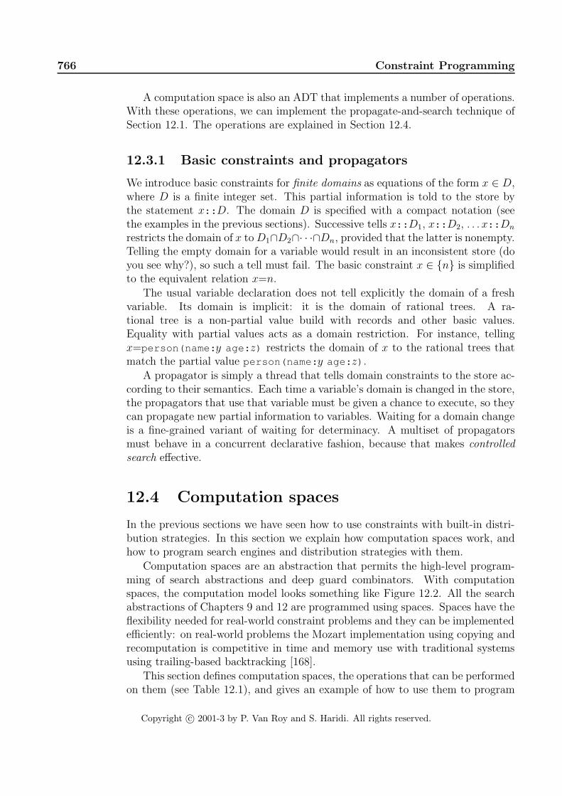
766 Constraint Programming
A computation space is also an ADT that implements a number of operations.With these operations, we can implement the propagate-and-search technique ofSection 12.1. The operations are explained in Section 12.4.
12.3.1 Basic constraints and propagators
We introduce basic constraints for finite domains as equations of the form x ∈ D,where D is a finite integer set. This partial information is told to the store bythe statement x:: D. The domain D is specified with a compact notation (seethe examples in the previous sections). Successive tells x:: D1, x:: D2, . . .x:: Dn
restricts the domain of x to D1∩D2∩· · ·∩Dn, provided that the latter is nonempty.Telling the empty domain for a variable would result in an inconsistent store (doyou see why?), so such a tell must fail. The basic constraint x ∈ {n} is simplifiedto the equivalent relation x=n.
The usual variable declaration does not tell explicitly the domain of a freshvariable. Its domain is implicit: it is the domain of rational trees. A ra-tional tree is a non-partial value build with records and other basic values.Equality with partial values acts as a domain restriction. For instance, tellingx=person(name: y age: z) restricts the domain of x to the rational trees thatmatch the partial value person(name: y age: z) .
A propagator is simply a thread that tells domain constraints to the store ac-cording to their semantics. Each time a variable’s domain is changed in the store,the propagators that use that variable must be given a chance to execute, so theycan propagate new partial information to variables. Waiting for a domain changeis a fine-grained variant of waiting for determinacy. A multiset of propagatorsmust behave in a concurrent declarative fashion, because that makes controlledsearch effective.
12.4 Computation spaces
In the previous sections we have seen how to use constraints with built-in distri-bution strategies. In this section we explain how computation spaces work, andhow to program search engines and distribution strategies with them.
Computation spaces are an abstraction that permits the high-level program-ming of search abstractions and deep guard combinators. With computationspaces, the computation model looks something like Figure 12.2. All the searchabstractions of Chapters 9 and 12 are programmed using spaces. Spaces have theflexibility needed for real-world constraint problems and they can be implementedefficiently: on real-world problems the Mozart implementation using copying andrecomputation is competitive in time and memory use with traditional systemsusing trailing-based backtracking [168].
This section defines computation spaces, the operations that can be performedon them (see Table 12.1), and gives an example of how to use them to program
Copyright c© 2001-3 by P. Van Roy and S. Haridi. All rights reserved.

12.4 Computation spaces 767
search. Actually we use the example as a roadmap throughout the definitions ofconcepts and operations. The discussion in this section follows the model in [172,169]. This model is implemented in the Mozart system [129] and refines the onepresented in the articles [167, 170]. The space abstraction can be made language-independent; [78] describes a C++ implementation of a similar abstraction thatprovides both trailing and copying.
12.4.1 Programming search with computation spaces
A search strategy defines how the search tree is explored, e.g., depth-first searchor breadth-first search. A distribution strategy defines the shape and content ofthe search tree, i.e., how many alternatives exist at a node and what constraint isadded for each alternative. Computation spaces can be used to program searchstrategies and distribution strategies independent of each other. That is, anysearch strategy can be used together with any distribution strategy. Here is howit is done:
• Create the space with the correct program inside. This program defines allthe variables and constraints in the space.
• Let the program run inside the space. Variables and propagators are creat-ed. All propagators execute until no more information can be added to thestore in this manner. The space eventually reaches stability.
• During the space’s execution, the computation inside the space can decideto create a choice point. The decision which constraint to add for eachalternative defines the distribution strategy. One of the space’s threads willsuspend when the choice point is created.
• When the space has become stable, execution continues outside the space,to decide what to do next. There are different possibilities depending onwhether or not a choice point has been created in the space. If there isnone, then execution can stop and return with a solution. If there is one,then the search strategy decides which alternative to choose and commitsto that alternative.
The next section explains the operations we need for this approach, together witha concrete example of a search engine. Section 12.5 gives another example of howto program search with spaces. Many other strategies can be programmed thanare shown here; for more information see [172, 169].
12.4.2 Definition
Our goal is to present computation spaces as a mean for implementing searchstrategies and distribution strategies. We will explain in detail the execution ofa concrete example of a search engine on a small problem. The definitions ofconcepts and operations will be given as they come in the execution.
Copyright c© 2001-3 by P. Van Roy and S. Haridi. All rights reserved.

768 Constraint Programming
fun {DFE S}case {Ask S}of failed then nil[] succeeded then [S][] alternatives(2) then C={Clone S} in
{Commit S 1}case {DFE S} of nil then {Commit C 2} {DFE C}[] [T] then [T]end
endend
% Given {Script Sol}, returns solution [Sol] or nil:fun {DFS Script}
case {DFE {NewSpace Script}} of nil then nil[] [S] then [{Merge S}]end
end
Figure 12.3: Depth-first single solution search
〈statement〉 ::= {NewSpace 〈x〉 〈y〉 }
| {Choose 〈x〉 〈y〉 }
| {Ask 〈x〉 〈y〉 }
| {Commit 〈x〉 〈y〉 }
| {Clone 〈x〉 〈y〉 }
| {Inject 〈x〉 〈y〉 }
| {Merge 〈x〉 〈y〉 }
Table 12.1: Primitive operations for computation spaces
A depth-first search engine
Figure 12.3 shows how to program depth-first single solution search, in the caseof binary choice points. This explores the search tree in depth-first manner andreturns the first solution it finds. The problem is defined as a unary procedure{Script Sol} that gives a reference to the solution Sol , just like the examplesof Section 12.2. The solution is returned in a one-element list as [Sol] . If thereis no solution, then nil is returned. In Script , choice points are defined withthe primitive space operation Choose .
The search function uses the primitive operations on spaces NewSpace, Ask ,Commit , Clone , and Merge . We will explain each operation in detail as it comesin the execution. Table 12.1 lists the complete set of primitive operations.
Copyright c© 2001-3 by P. Van Roy and S. Haridi. All rights reserved.

12.4 Computation spaces 769
A script example
Let us run the search engine on the example given in Section 12.1.3. The problemwas specified by the procedure Rectangle .
proc {Rectangle ?Sol}sol(X Y)=Sol
inX::1#9 Y::1#9X*Y=:24 X+Y=:10 X=<:Y{FD.distribute naive Sol}
end
We start the execution with the statement Sol={DFS Rectangle} , where DFS
and Rectangle are defined as above, and Sol is a fresh variable. If we expandthe body of the function, it should create two variables, say S and L, leading toa configuration like the following. The box represents the thread that executesthe statements, and below it is a representation of the store.
S={NewSpace Rectangle}
L={DFE S}
Sol= case L of ... end
Rectangle=< proc > Sol L S
Space creation
The first primitive space operation we use is NewSpace. In our example, itcreates a new computation space S, with a root variable Root , and one threadthat executes {Rectangle Root} . Both the new thread and the new store areshown inside a box, which delimits the “boundaries” of the space.
L={DFE S}
Sol= case L of ... end
Rectangle=< proc > Sol L S={Rectangle Root}
Root
A precise definition of NewSpace is
• S={NewSpace P} , when given a unary procedure P, creates a new compu-tation space and returns a reference to it. In this space, a fresh variable R,called the root variable, is created and a new thread, and {P R} is invokedin the thread.
Recall that a computation space encapsulates a computation. It is thus an in-stance of the stateful concurrent model, with its three parts: thread store, con-straint store, and mutable store. As it can itself nest a computation space, thespaces naturally form a tree structure:
Copyright c© 2001-3 by P. Van Roy and S. Haridi. All rights reserved.
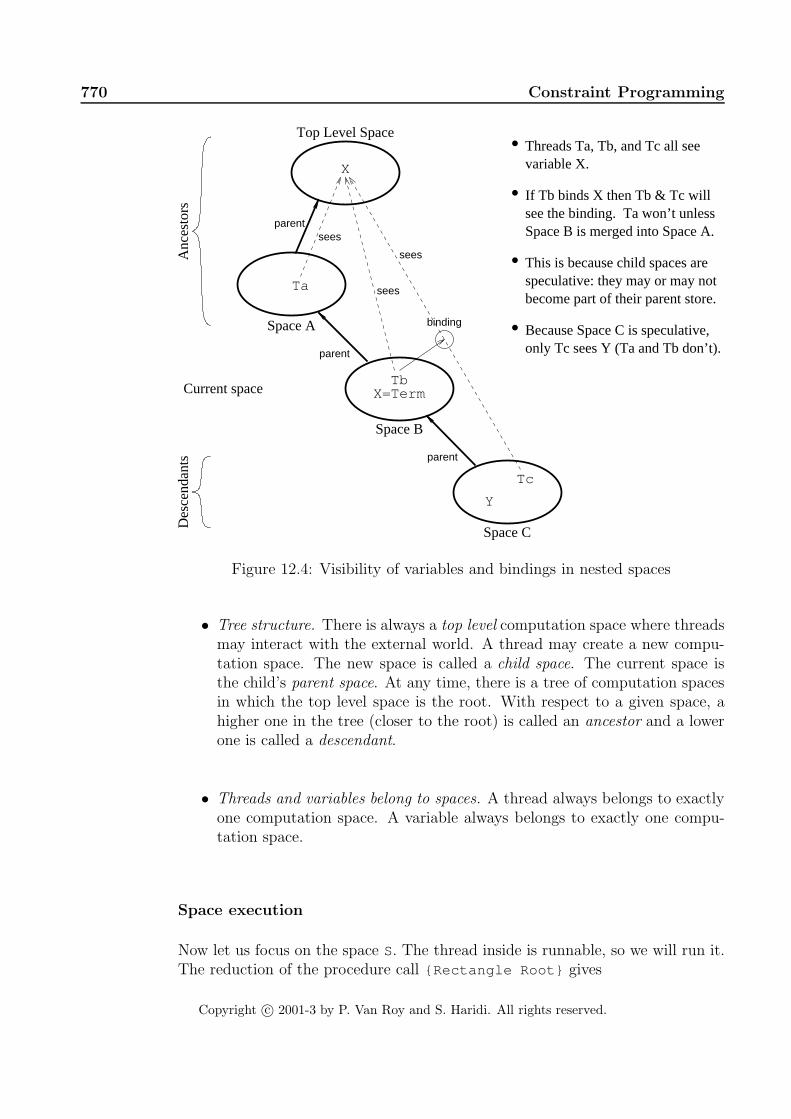
770 Constraint Programming
Space A
Space B
Top Level Space
Anc
esto
rsX
Ta
TbX=Term
Threads Ta, Tb, and Tc all see●
variable X.
If Tb binds X then Tb & Tc willsee the binding. Ta won’t unlessSpace B is merged into Space A.
●
● This is because child spaces are
become part of their parent store.speculative: they may or may not
Because Space C is speculative,●
only Tc sees Y (Ta and Tb don’t).
Space C
Tc
Y
Des
cend
ants parent
parent
binding
sees
sees
Current space
sees
parent
Figure 12.4: Visibility of variables and bindings in nested spaces
• Tree structure. There is always a top level computation space where threadsmay interact with the external world. A thread may create a new compu-tation space. The new space is called a child space. The current space isthe child’s parent space. At any time, there is a tree of computation spacesin which the top level space is the root. With respect to a given space, ahigher one in the tree (closer to the root) is called an ancestor and a lowerone is called a descendant.
• Threads and variables belong to spaces. A thread always belongs to exactlyone computation space. A variable always belongs to exactly one compu-tation space.
Space execution
Now let us focus on the space S. The thread inside is runnable, so we will run it.The reduction of the procedure call {Rectangle Root} gives
Copyright c© 2001-3 by P. Van Roy and S. Haridi. All rights reserved.

12.4 Computation spaces 771
S=
local sol(X Y)=Root in
X::1#9 Y::1#9
X*Y=:24 X+Y=:10 X=<:Y
{FD.distribute naive Root}
end
Root
You might have noticed that the variable Rectangle is bound outside the space,which did not prevent the inner thread to read its value and use it. Computationspaces do respect precise visibility rules. Those rules provide a certain degree ofisolation from the “external” computation.
• Variable visibility. A thread sees and may access variables belonging to itsspace as well as to all ancestor spaces. The thread cannot see the variablesof descendant spaces. Figure 12.4 gives an example with bindings.
• Basic constraint visibility. A thread may add basic constraints to variablesvisible to it. This means that it may constrain variables belonging to itsspace or to its ancestor spaces. The basic constraint will only be visible inthe current space and its descendants. That is, the parent space does notsee the binding unless the current space is merged with it (see later).
Posting constraints
The thread inside the space continues its execution. It creates two new variablesX and Y inside the space, and binds Root to sol(X Y) . This gives
S=
X::1#9 Y::1#9
X*Y=:24 X+Y=:10 X=<:Y
{FD.distribute naive Root}
Root=sol(X Y) X Y
It then tells the basic constraints X::1#9 and Y::1#9 to the constraint store ofthe space, and creates new propagators, each one in its own thread. We have
S=X*Y=:24 X+Y=:10 X=<:Y {FD.distribute naive Root}
Root=sol(X Y) X::1#9 Y::1#9
Concurrent propagation
Now propagators enter the scene. As we have seen in Section 12.1.3, they prop-agate concurrently, reducing the domains to 4#6 . The space becomes
S=X*Y=:24 X+Y=:10 X=<:Y {FD.distribute naive Root}
Root=sol(X Y) X::4#6 Y::4#6
Copyright c© 2001-3 by P. Van Roy and S. Haridi. All rights reserved.

772 Constraint Programming
Execution in a computation space does a variant of the maximally concurrentmodel. It avoids the difficulties usually associated with this model. Let us seewhy this is possible. Each constraint is implemented as a thread (called “propa-gator”) that executes concurrently with the other propagators. Each propagatoradds information to the store until no more information can be added. Con-straint programming avoids the difficulties of the maximally concurrent modelbecause propagator execution is monotonic: they only add information, theynever change or remove information. (This is essentially the same reason whyconcurrent declarative programming is simpler than concurrent stateful program-ming.) Furthermore, propagators have a logical semantics. All the informationthey add is consistent with this semantics. If they are written correctly, then theexact order in which they execute does not matter. When they reach a fixpoint(space stability), i.e., when no propagator can add any more information, theresult is always the same.
Distribution
The propagators in the space are no longer runnable. At this point, FD.distribute
becomes runnable. This procedure implements the distribution strategy. It picksa variable and a value following a heuristic, in this case X and 4, and proposes a“guess”. For this it executes the statement {Choose 2} , which creates a choicepoint with two alternatives, and blocks until a call to Commit unblocks it. Theinteraction between Choose and Commit is explained in detail later. The wholecomputation (including the parent space) now looks like
L={DFE S}
Sol= case L of ... end
Rectangle=< proc > Sol L
S=
X*Y=:24
X+Y=:10
X=<:Y
case {Choose 2}
of 1 then X=4 {FD.distribute [Y]}
[] 2 then X\=:4 {FD.distribute Root}
end
Root=sol(X Y) X::4#6 Y::4#6
The definition of Choose is
• Y={Choose N} is the only operation that is called from inside the space,while the other operations are called from outside the space. It creates achoice point with N alternatives. Then it blocks, waiting for an alternativeto be chosen by a Commit operation on the space. The Choose call definesonly the number of alternatives; it does not specify what to do for any givenalternative. Choose returns with Y=I when alternative 1≤I ≤N is chosen.A maximum of one choice point may exist in a space at any time.
Copyright c© 2001-3 by P. Van Roy and S. Haridi. All rights reserved.

12.4 Computation spaces 773
State of a space
The space was running concurrently with its parent space. The thread of thesearch engine now executes the statement L={DFE S} , which evaluates {Ask S} .This operation asks the space for its status. In this case, it returns alternatives(2) ,meaning that a choice point with two alternatives has been created inside thespace. After reduction of the case statement, the whole computation becomes
local C={Clone S} in
{Commit S 1}
L=case {DFE S} of ... end
end
Sol= case L of ... end
Rectangle=< proc > Sol L S=<space>
Here we give a precise definition of the various states of a space. A space isrunnable if it or a descendant contains a runnable thread, and blocked otherwise.Let us run all threads in the space and its descendants, until the space is blocked.Then the space can be in one of the following further states:
• The space is stable. This means that no additional basic constraints donein an ancestor can make the space runnable. A stable space can be in fourfurther states:
– The space is succeeded. This means that it contains no choice points.A succeeded space contains a solution to the logic program.
– The space is distributable. This means that the space has one threadthat is suspended on a choice point with two or more alternatives. Aspace can have at most one choice point; attempting to create anothergives an error.
– The space is failed. This means that the space attempted to tell in-consistent basic constraints, for instance binding the same variable totwo different values. No further execution happens in the space.
– The space is merged. This means that the space has been discarded andits constraint store has been added to a parent. Any further operationon the space is an error. This state is the end of a space’s lifetime.
• The space is suspended. This means that additional basic constraints donein an ancestor can make the space runnable. Being suspended is usuallya temporary condition due to concurrency. It means that some ancestorspace has not yet transferred all required information to the space. A spacethat stays not stable indefinitely usually indicates a programmer error.
The operation Ask is then defined as
Copyright c© 2001-3 by P. Van Roy and S. Haridi. All rights reserved.

774 Constraint Programming
• A={Ask S} asks the space S for its status. As soon as the space becomesstable, A is bound. If S is failed, merged, or succeeded, then Ask returnsfailed , merged , or succeeded . If S is distributable, then it returnsalternatives(N) , where N is the number of alternatives.
Cloning a space
The next statement of the search engine thread declares a variable C, and createsa copy of the space S. Note that variables and threads belonging to S are copiedtoo, so that both spaces are independent of each other. For the sake of simplicity,we have kept the same identifiers for S and C in the picture below. But theyactually denote different variables in the stores.
{Commit S 1}
L=case {DFE S} of ... end
Sol= case L of ... end
Rectangle=< proc > Sol L
S=
X*Y=:24
X+Y=:10
X=<:Y
case {Choose 2}
of 1 then X=4 {FD.distribute [Y]}
[] 2 then X\=:4 {FD.distribute Root}
end
Root=sol(X Y) X::4#6 Y::4#6
C=
X*Y=:24
X+Y=:10
X=<:Y
case {Choose 2}
of 1 then X=4 {FD.distribute [Y]}
[] 2 then X\=:4 {FD.distribute Root}
end
Root=sol(X Y) X::4#6 Y::4#6
The definition of Clone is
• C={Clone S} , if S is a stable space, creates an identical copy (a clone) of S
and returns a reference to it. This allows both alternatives of a distributablespace to be explored.
Committing to an alternative
The search engine then executes {Commit S 1} . This indicates to the space S
to enter the first alternative. So the call to Choose inside the space unblocks andreturns 1. The distributor thread then binds X to 4, which leads to the space
S=X*Y=:24 X+Y=:10 X=<:Y {FD.distribute [Y]}
Root=sol(X Y) X=4 Y::4#6
We define Commit as
Copyright c© 2001-3 by P. Van Roy and S. Haridi. All rights reserved.

12.4 Computation spaces 775
A={Ask X}case A ofalternatives(N) then
{Commit X I}end
...
I={Choose N}case I of
1. Block
5. Synch on alternative(pass I)
of 1 then ...
end...
6. Run alternative[] 2 then ...
......
(pass N)3. Synch on stability
(in parent space)Search strategy
Computation space X
...
4. Calculate alternative
2. Block
...
Figure 12.5: Communication between a space and its distribution strategy
• {Commit S I} , if S is a distributable space, causes the Choose call in thespace to complete and return I as its result. This may cause the space toresume execution. The integer I must satisfy 1≤I ≤N, where N is the firstargument of the Choose call.
Now we see precisely how to make the search strategy interact with the distri-bution strategy. The basic technique is to use Choose , Ask , and Commit tocommunicate between the inside of a space and the search strategy, which is pro-grammed in the parent space. Figure 12.5 shows how the communication works.Within the space, calling I={Choose N} first informs the search strategy of thetotal number of alternatives (N). Then the search strategy picks one (I ) and in-forms the space. The synchronization condition between the inside of the spaceand the search strategy is stability, i.e., that there are no more local deductionspossible inside the space.
Merging a space
The propagators inside S now run until both variables become determined. Allthe propagators are entailed by the store, they simply disappear from S:
S={FD.distribute [Y]}
Root=sol(X Y) X=4 Y=6
The distributor thread terminates too, because Y is determined, so the wholecomputation becomes
L=case {DFE S} of ... end
Sol= case L of ... end
Rectangle=< proc > Sol L S= Root=sol(X Y) X=4 Y=6
Copyright c© 2001-3 by P. Van Roy and S. Haridi. All rights reserved.

776 Constraint Programming
C=
X*Y=:24
X+Y=:10
X=<:Y
case {Choose 2}
of 1 then X=4 {FD.distribute [Y]}
[] 2 then X\=:4 {FD.distribute Root}
end
Root=sol(X Y) X::4#6 Y::4#6
The search engine calls again {DFE S} , which performs {Ask S} . The returnedvalue is now succeeded , which means that the computation inside S has termi-nated with a consistent store. The search engine continues its execution. Thecall to {DFE S} then returns [S] . The latter matches the second clause in DFS,and the search ends with the statement Sol=[{Merge S}] . The call {Merge
S} merges S with the current space, and returns the root variable of S. Thecomputation becomes
Rectangle=< proc > Sol=Root L=[S] S=<merged>
Root=sol(X Y) X=4 Y=6
C=
X*Y=:24
X+Y=:10
X=<:Y
case {Choose 2}
of 1 then X=4 {FD.distribute [Y]}
[] 2 then X\=:4 {FD.distribute Root}
end
Root=sol(X Y) X::4#6 Y::4#6
Merging a space is necessary to access the solution:
• Access by merging. A thread cannot see the variables of a child space,unless the child space is merged with its parent. Space merging is an explicitprogram operation. It causes the child space to disappear and all the child’scontent to be added to the parent space.
And Merge is defined by
• {Merge S Y} binds Y to the root variable of space S and discards the space.
Space failure
Suppose now that the search would continue. This would be the case if the firstalternative had no solution. The search engine would then execute {Commit C
2} L={DFE C} . The statement {Commit C 2} causes {Choose 2} to return 2,which makes the space C evolve to
C=X*Y=:24 X+Y=:10 X=<:Y {FD.distribute Root}
Root=sol(X Y) X::5#6 Y::4#6
As we have seen, the action of the propagators lead to inconsistencies. For in-stance, X*Y=:24 propagates the constraints X=6 and Y=4. The propagator X=<:Y
cannot be satisfied with those values, which makes the space C fail:
Copyright c© 2001-3 by P. Van Roy and S. Haridi. All rights reserved.

12.5 Implementing the relational computation model 777
C=<failed>
In the search engine, the call to {Ask C} would return failed . This means thatC contains no solution. The search would then return nil in that case.
Failures, stateful operations, and interaction with the external world are en-capsulated in computation spaces in the following way.
• Exceptions and failures. A thread that tries to add an inconsistent ba-sic constraint to its constraint store will raise a failure exception. Whathappens then in the top level space is implementation-dependent. If theexception occurs in a child space and is not caught, then the space fails. Afailure happening in a propagator immediately results in its space’s failure,because propagators are threads by themselves.
• Stateful operations. Operations on stateful entities across spaces are forbid-den. For instance, a thread cannot read or change the value of a cell thatbelongs to its space’s parent. A consequence is that only the top level spacecan interact with the external world.
Injecting a computation into a space
There is one primitive operation that we have not used, namely Inject . Thisoperation is however useful, because it permits to add constraints to an existingspace. For instance, you can constrain the solution of a space to be “better” thanan already known solution. The definition of “better” is problem-dependent, ofcourse. Here is the definition of Inject :
• {Inject S P} is similar to space creation except that it uses an existingspace S. It creates a new thread in the space and invokes {P R} in thethread, where R is the space’s root variable. This makes a stable space notstable again. Adding constraints to an existing space is necessary for somedistribution strategies such as branch-and-bound and saturation [172, 169].
12.5 Implementing the relational computation
model
We end this brief introduction to constraint programming by connecting withthe relational computation model of Chapter 9. The relational model extends thedeclarative model with choice and fail statements and with a Solve operationto do encapsulated search. We can now show how to program these operationswith computation spaces. We have already showed how to do fail ; it remainsto implement choice and Solve . Their implementation is independent of theconstraint domain. It will work for finite domain constraints. It will also workfor the single-assignment store used in the rest of the book, since it is also aconstraint system.
Copyright c© 2001-3 by P. Van Roy and S. Haridi. All rights reserved.

778 Constraint Programming
12.5.1 The choice statement
We can define the choice statement in terms of the Choose operation. Thefollowing statement:
choice 〈s〉1 [] 〈s〉2 [] ... [] 〈s〉n end
is a linguistic abstraction that is defined as follows:
case {Choose N}of 1 then 〈s〉1[] 2 then 〈s〉2...[] N then 〈s〉nend
This creates a choice point and then executes the statement corresponding to thechoice made by the search engine.
12.5.2 Implementing the Solve function
Figure 12.6 shows the implementation of the Solve function. It is an all-solutionsearch engine that uses both computation spaces and laziness. The reader shouldpay attention to where laziness occurs. It is important because of the statefulnature of spaces. For instance, in the else clause of SolveLoop , a clone of S
must be created before any attempt to Commit on S. Because of the lazy natureof SolveLoop , we could actually have declared C and NewTail in reverse order:
...NewTail={SolveLoop S I+1 N SolTail}C={Space.clone S}
...
This works because the value of NewTail is not needed before C is committed.
12.6 Exercises
1. Cryptarithmetic. Write a program to solve all puzzles of the form “Word1plus Word2 equals Word3”. The words should be input interactively. Usethe solution to the Send+More=Money problem given in Section 12.2.1 asa guide. The user should be able to stop the search process if it is takingtoo long. Use the Solve function to enumerate the solutions.
Copyright c© 2001-3 by P. Van Roy and S. Haridi. All rights reserved.

12.6 Exercises 779
% Returns the list of solutions of Script given by a lazy% depth-first explorationfun {Solve Script}
{SolveStep {Space.new Script} nil}end
% Returns the list of solutions of S appended with SolTailfun {SolveStep S SolTail}
case {Space.ask S}of failed then SolTail[] succeeded then {Space.merge S}|SolTail[] alternatives(N) then {SolveLoop S 1 N SolTail}end
end
% Lazily explores the alternatives I through N of space S,% and returns the list of solutions found, appended with% SolTailfun lazy {SolveLoop S I N SolTail}
if I>N thenSolTail
elseif I==N then{Space.commit S I}{SolveStep S SolTail}
elseC={Space.clone S}NewTail={SolveLoop S I+1 N SolTail}
in{Space.commit C I}{SolveStep C NewTail}
endend
Figure 12.6: Lazy all-solution search engine Solve
Copyright c© 2001-3 by P. Van Roy and S. Haridi. All rights reserved.

780 Constraint Programming
Copyright c© 2001-3 by P. Van Roy and S. Haridi. All rights reserved.

Part IV
Semantics
Copyright c© 2001-3 by P. Van Roy and S. Haridi. All rights reserved.


Chapter 13
Language Semantics
“This is the secret meaning of the runes; I hid here magic-runes,undisturbed by evil witchcraft. In misery shall he die by means ofmagic art who destroys this monument.”– Runic inscription, Bjorketorp Stone
For all the computation models of the previous chapters, we gave a formal se-mantics in terms of a simple abstract machine. For the declarative model, thisabstract machine contains two main parts: a single-assignment store and a seman-tic stack. For concurrency, we extended the machine to have multiple semanticstacks. For lazy execution we added a trigger store. For explicit state we addeda mutable store. For read-only views we added a read-only store.
This chapter brings all these pieces together. It defines an operational seman-tics for all the computation models of the previous chapters.1 We use a differentformalism than the abstract machine of the previous chapters. The formalism ofthis chapter is more compact and easier to reason with than the abstract machinedefinitions. It has three principal changes with respect to the abstract machineof Chapter 2:
• It uses a concise notation based on reduction rules. The reduction rulesfollow the abstract syntax, i.e., there are one or more rules for each syntacticconstruct. This approach is called Structural Operational Semantics, orSOS for short. It was pioneered by Gordon Plotkin [208].
• It uses substitutions instead of environments. We saw that statements, inorder to be reducible, must define bindings for their free identifiers. Inthe abstract machine, these bindings are given by the environment in thesemantic statement. In this chapter, the free identifiers are directly substi-tuted by references into the store. We have the invariant that in a reduciblestatement, all free identifiers have been replaced by store references.
1This chapter was co-authored with Raphael Collet.
Copyright c© 2001-3 by P. Van Roy and S. Haridi. All rights reserved.

784 Language Semantics
• It represents the single-assignment store as a logical formula. This formula isa conjunction of basic constraints, each of which represents a single variablebinding. Activation conditions are replaced by logical conditions such asentailment and disentailment.
The chapter is structured as follows:
• Section 13.1 is the main part. It gives the semantics of the shared-stateconcurrent model.
• Section 13.2 gives a formal definition of declarative concurrency, which is animportant property of some subsets of the shared-state concurrent model.
• Section 13.3 explains how subsets of this semantics cover the different com-putation models of the previous chapters.
• Section 13.4 explains how the semantics covers the different programmingabstractions and concepts seen in previous chapters.
• Section 13.5 briefly summarizes the historical development of the shared-state concurrent model and its relative, the message-passing concurrentmodel.
This chapter is intended to be self-contained. It can be understood independentlyof the previous chapters. However, its mathematical content is much higher thanthe previous chapters. To aid understanding, we therefore recommend that youconnect it with the abstract machine that was defined before.
13.1 The shared-state concurrent model
This section gives a structural operational semantics for the shared-state concur-rent model. We also call this the general computation model, since it is the mostgeneral model of the book. It covers all the computation models of the book ex-cept for the relational and constraint-based models. The semantics of each earliermodel, e.g., the declarative, declarative concurrent, and stateful models, can beobtained by taking just the rules for the language constructs that exist in thosemodels. A configuration in the shared-state concurrent model consists of severaltasks connected to a shared store:
task · · · task↘ ↙store
A task, also called thread, is the basic unit of sequential calculation. A compu-tation consists of a sequence of computation steps, each of which transforms aconfiguration into another configuration. At each step, a task is chosen among allreducible tasks. The task then does a single reduction step. The execution of thedifferent tasks is therefore interleaved. We say that the model has an interleavingsemantics. Concurrency is modeled by reasoning about all possible interleavings.
Copyright c© 2001-3 by P. Van Roy and S. Haridi. All rights reserved.

13.1 The shared-state concurrent model 785
13.1.1 The store
The store consists of two parts: a single-assignment store and a predicate store:
• The single-assignment store (also called constraint store) contains variablesand their bindings. The constraint store is monotonic: variables and bind-ings can be added, but never changed or removed.
• The predicate store contains the additional information that is needed forthe execution of certain statements. The predicate store consists of theprocedure store (containing procedure values), the mutable store (contain-ing cells), the trigger store (containing by-need triggers), and the read-onlystore (containing read-only views). Some of these stores are nonmonoton-ic. These stores are introduced in step-by-step fashion as we define thereduction rules that need them.
All reduction rules are carefully designed so that task reduction is monotonic:once a task is reducible, then it stays reducible even if information is added tothe constraint store or the predicate store is changed.
13.1.2 The single-assignment (constraint) store
The constraint store is a repository of information about the program variables.For instance, the store can contain the information “x is bound to 3 and x is equalto y”, which is written x=3 ∧ x=y. Such a set of bindings is called a constraint.It has a logical semantics, which is explained in Chapter 9. This is why we alsocall this store the constraint store. For this chapter we use just a small part ofthe logical semantics, namely logical conjunction (adding new information to thestore, i.e., doing a binding) and entailment (checking whether some informationis in the store).
The constraint store entails information. For example, the store x=3 ∧ x=yentails y=3, even though that information is not directly present as a binding.We denote the store by σ and we write this as σ |= y=3. We also use anotherrelation called disentailment. If β is a constraint, then we say that σ disentails βif σ entails the negation of β, i.e., σ |= ¬β. For example, if σ contains x=3 thenit disentails x=4.
Entailment and disentailment are the general relations we use to query thestore. They are both forms of logical implication. We assume that the implemen-tation uses an efficient algorithm for checking them. Such an algorithm is givenin Section 2.7.2.
The constraint store is monotonic, i.e., information can be added but notchanged or removed. Consequently, both entailment and disentailment are mono-tonic too: when the store entails some information or its negation, this stays trueforever.2 The constraint store provides two primitive operations to the program-
2Note that “σ disentails β” is not the same as “it is not true that σ entails β”. The formeris monotonic while the latter is not.
Copyright c© 2001-3 by P. Van Roy and S. Haridi. All rights reserved.

786 Language Semantics
mer, called tell and ask :
• Tell. The tell operation is a mechanism to add information to the store. Atask telling the information β to store σ updates the store to σ∧β, providedthat the new store is consistent. For instance, a task may not tell y=7 tothe store x=3∧x=y. It may however tell y=3, which is consistent with thestore. An inconsistent tell leaves the store unchanged. It is signaled withsome mechanism, typically by raising an exception.
• Ask. The ask operation is a mechanism to query the store for the presenceof some information. A task asking store σ for information β becomesreducible when σ entails either β or its negation ¬β. For instance, withthe store x=3 ∧ x=y, asking for y=3 will give an affirmative answer (theinformation is present). Asking for y=4 will give a negative answer (theinformation will never be present). An affirmative answer corresponds toan entailment and a negative answer corresponeds to a disentailment. Thetask will not reduce until either an affirmative or negative answer is possible.Therefore the ask operation is a synchronization mechanism. The taskdoing the ask is said to synchronize on β, which is called its guard.
Monotonicity of the store implies a strong property: task reduction is monotonic.Assume that a task waits for the store to contain some information, i.e., the taskbecomes reducible when the store entails some information. Then, once the taskis reducible, it stays reducible even if other tasks are reduced before it. Thisis an excellent basis for dataflow concurrency, where tasks synchronize on theavailability of data.
13.1.3 Abstract syntax
Figure 13.1 defines the abstract syntax for the kernel language of the shared-state concurrent model. Here S denotes a statement, C, P , X, Y denote variableidentifiers, k denotes an integer constant, and n is an integer such that n ≥ 0.In the record f(l1:X1 · · · ln:Xn), the label f denotes an atom, and each one of thefeatures li denotes an atom or integer constant. We use ≡ to denote equalitybetween semantic objects, in order to avoid confusion with = in the equalitystatement.
We assume that in any statement defining a lexical scope for a list of variableidentifiers, the identifiers in the list are pairwise distinct. To be precise, in thethree statements
local X1 · · ·Xn in S end
case X of f(l1:X1 · · · ln:Xn) then S1 else S2 end
proc { P X1 · · ·Xn} S end
we must have Xi 6≡ Xj for i 6= j. We further assume that all identifiers (includingX) are distinct in the record tell X=f(l1:X1 · · · ln:Xn). These conditions on
Copyright c© 2001-3 by P. Van Roy and S. Haridi. All rights reserved.

13.1 The shared-state concurrent model 787
S ::= skip empty statement| S1 S2 sequential composition| thread S end thread introduction
| local X1 · · ·Xn in S end variable introduction (n ≥ 1)
| X=Y imposing equality (tell)| X=k| X=f(l1:X1 · · · ln:Xn)
| if X then S1 else S2 end conditional statements (ask)| case X of f(l1:X1 · · · ln:Xn)
then S1 else S2 end
| {NewNameX} name introduction
| proc { P X1 · · ·Xn} S end procedural abstraction| { P X1 · · ·Xn}
| {IsDet X Y } explicit state| {NewCell X C}
| {Exchange C X Y }
| {ByNeed P X} by-need trigger
| Y =!! X read-only variable
| try S1 catch X then S2 end exception handling| raise X end
| {FailedValue X Y }
Figure 13.1: The kernel language with shared-state concurrency
pairwise distinctness are important to ensure that statements are truly primitive,i.e., that there are no hidden tells of the form X = Y .
13.1.4 Structural rules
The system advances by successive reduction steps. A possible reduction step isdefined by a reduction rule of the form
T T ′
σ σ′ if C
stating that the computation makes a transition from a multiset of tasks T con-nected to a store σ, to a multiset of tasks T ′ connected to a store σ′. We callthe pair T /σ a configuration. The rule can have an optional boolean conditionC, which has to be true for the rule to reduce. In this notation, we assume thatthe left-hand side of a rule (the initial configuration T /σ) may have patterns and
Copyright c© 2001-3 by P. Van Roy and S. Haridi. All rights reserved.

788 Language Semantics
that an empty pattern matches anything. For the rule to reduce, the patternmust be matched in the obvious way.
We use a very light notation for multisets of tasks: the multiset is namedby a letter in calligraphic style, disjoint union is denoted by a white space, andsingletons are written without curly braces. This allows to write “T1 T T2” for{T1}]T ]{T2}. Any confusion with a sequence of statements is avoided becauseof the thread syntax (see later). We generally write “σ” to denote a store, leavingimplicit the set of its variables, say V. If need be, we can make the set explicitby writing the store with V as a subscript: σV .
We use two equivalent notations to express that a rule has the entailmentcondition σ |= β. The condition can be written as a pattern on the left-hand sideor as an explicit condition:
T T ′
σ ∧ β σ ∧ βor
T T ′
σ σif σ |= β
In the definitions that follow, we use whichever notation is the most convenient.We assume the semantics has the following two rules, which express model
properties that are independent of the kernel language.
T U T ′ Uσ σ′ if
T T ′
σ σ′T Tσ σ′ if σ and σ′ are equivalent
The first rule expresses concurrency: a subset of the threads can reduce withoutdirectly affecting or depending on the others. The second rule states that thestore can be replaced by an equivalent one. The second rule can also be writtenas
σ σ′ if σ and σ′ are equivalent
(using an empty pattern instead of T ).
Equivalent stores
A store σ consists of a constraint store σc and a predicate store σp. We denotethis as σ = σc ∧ σp. We say that two stores σ and σ′ are equivalent if (1) theirconstraint stores entail one another, that is, σc |= σ′
c and σ′c |= σc, and (2) their
stores entail the other’s predicate store, that is, σ |= σ′p and σ′ |= σp.
We define entailment for the predicate store σp as follows. We consider σp asa multiset of items called predicates. A predicate can be considered as a tuple ofvariables, e.g., trig(x, y) is a predicate. We say that σ |= p′1 ∧ · · · ∧ p′n if thereexists a subset {p1, . . . , pn} of σp such that for all i, pi and p′i have the samelabels and number of arguments, and the corresponding arguments of pi and p′iare equal in σc. For example, if σ ≡ x=x′ ∧ trig(x, y) then σ |= trig(x′, y).
This definition of equivalence is a form of logical equivalence. It is possiblebecause entailment makes the store independent of its representation: if σ andσ′ are equivalent, then σ |= γ if and only if σ′ |= γ.
Copyright c© 2001-3 by P. Van Roy and S. Haridi. All rights reserved.

13.1 The shared-state concurrent model 789
13.1.5 Sequential and concurrent execution
A thread is a sequence of statements S1 S2 · · ·Sn that we write in a head-tailfashion with angle brackets, i.e., 〈S1 〈S2 〈· · · 〈Sn 〈〉〉 · · · 〉〉〉. The abstract syntaxof threads is
T ::= 〈〉 | 〈S T 〉.A terminated thread has the form 〈〉. Its reduction simply leads to an empty setof threads. A non-terminated thread has the form 〈S T 〉. Its reduction replacesits topmost statement S by its reduction S ′:
〈〉σ σ
〈S T 〉 〈S ′ T 〉σ σ′ if
S S ′
σ σ′
(We extend the reduction rule notation to allow statements in addition to mul-tisets of tasks.) The empty statement, sequential composition, and thread intro-duction are intimately tied to the notion of thread. Their reduction needs a morespecific definition than the one given above for S:
〈skip T 〉 Tσ σ
〈(S1 S2) T 〉 〈S1 〈S2 T 〉〉σ σ
〈thread S end T 〉 〈T 〉 〈S 〈〉〉σ σ
The empty statement skip is removed from the thread’s statement sequence. Asequence S1 S2 makes S1 the thread’s first statement, while thread S end createsa new thread with statement S, that is, 〈S 〈〉〉.
13.1.6 Comparison with the abstract machine semantics
Now that we have introduced some reduction rules, let us briefly compare themwith the abstract machine. For example, let us consider the semantics of sequen-tial composition. The abstract machine semantics defines sequential compositionas follows (taken from Section 2.4):
The semantic statement is
(〈s〉1 〈s〉2, E)
Execution consists of the following actions:
• Push (〈s〉2, E) on the stack.
• Push (〈s〉1, E) on the stack.
The reduction rule semantics of this chapter defines sequential composition asfollows (taken from the previous section):
〈(S1 S2) T 〉 〈S1 〈S2 T 〉〉σ σ
Copyright c© 2001-3 by P. Van Roy and S. Haridi. All rights reserved.

790 Language Semantics
It pays dividends to compare carefully these two definitions. They say exactlythe same thing. Do you see why this is? Let us go over it systematically. Inthe reduction rule semantics, a thread is given as a sequence of statements. Thissequence corresponds exactly to the semantic stack of the abstract machine. Therule for sequential composition transforms the list from 〈(S1 S2) T 〉 to 〈S1 〈S2 T 〉〉.This transformation can be read operationally: first pop (S1 S2) from the list,then push S2, and finally push S1.
The reduction rule semantics is nothing other than a precise and compactnotation for the English-language definition of the abstract machine with substi-tutions.
13.1.7 Variable introduction
The local statement does variable introduction: it creates new variables in thestore and replaces the free identifiers by these variables. We give an example tounderstand how the local statement executes. In the following statement, theidentifier Foo in S2 refers to a different variable from the one referred to by Foo
in S1 and S3:local Foo Bar in
S1
local Foo in S2 end
S3
≡ S4
end
The outermost local replaces the occurrences of Foo in S1 and S3 but not thosein S2. This gives the following reduction rule:
local X1 · · ·Xn in S end S{X1→x1, . . . , Xn→xn}σV σV∪{x1,...,xn}
if x1, . . . , xn fresh variables
In this rule, as in subsequent rules, we use “x” to denote a variable and “X” todenote an identifier. A variable is fresh if it is different from all existing variablesin the store. So the condition of the rule states that all the variables xi aredistinct and not in V.
The notation S{X1→x1, . . . , Xn→xn} stands for the simultaneous substitu-tion of the free occurrences of X1 by x1, X2 by x2, . . . , Xn by xn. For instance,the substitution of Foo by x and Bar by y in the statement S4 defined abovegives
S4{Foo→x, Bar→y} ≡ S1{Foo→x, Bar→y}local Foo in S2{Bar→y} end
S3{Foo→x, Bar→y}A substitution is actually an environment that is used as a function. Since vari-ables and identifiers are in disjoint sets, the substitution S{X1→x1, . . . , Xn→xn}is equivalent to the composition of single substitutions S{X1→x1} · · · {Xn→xn}.The substitution operation S{X→x} is defined formally in Section 13.1.17.
Copyright c© 2001-3 by P. Van Roy and S. Haridi. All rights reserved.

13.1 The shared-state concurrent model 791
13.1.8 Imposing equality (tell)
According to Section 13.1.7, a variable introduced by local has no initial value.The variable exists but the store simply has no information about it. Addinginformation about the variable is done by the tell operation. Let β denote astatement imposing equality. This statement has three possible forms:
β ::= x=y | x=z | x=f(l1:x1 · · · ln:xn).
This states that x is equal to either another variable y, an integer or name z, ora record with label f , features (i.e., field names) li, and fields xi. Doing a telloperation adds the information in β to the store, provided that it does not leadto an inconsistent store. This is also called binding the variable x.
It is possible that the new information in β conflicts with what the storealready knows about x. We say that β is inconsistent with σ. This happenswhenever β ∧ σ ↔ false . For example, take β ≡ x=10 and σ ≡ x=20. Insteadof adding β to the store, we signal this as an error, e.g., by raising an exception.Therefore the store is always consistent.
In practice, most tell operations are very simple: telling β just binds onevariable, x, without binding any others. For example, telling x=23 where σ hasno binding for x. But the tell operation is actually much more general. It cancause many bindings to be done. For example, take σ ≡ x=f(x1 x2)∧y=f(y1 y2).Then telling x = y does three bindings: x=y, x1=y1, and x2=y2.
Naive semantics of tell
The following two rules decide whether to add β to the store.
β skip
σ σ ∧ βif σ ∧ β is consistent
β fail
σ σif σ ∧ β is inconsistent
(Note that β is used to denote both a statement and a constraint.) We couldimplement tell to follow these rules. However, such an implementation wouldbe complicated and hard to make efficient. The Mozart system uses a slightlymore elaborate semantics that can be implemented efficiently. The tell opera-tion is a good example of the trade-off between simple semantics and efficientimplementation.
Realistic semantics of tell
We have seen that one tell operation can potentially add many bindings to thestore. This generality has an important consequence for inconsistent tells. Forexample, take β ≡ x=y and σ ≡ x=f(x1 x2)∧y=f(y1 y2)∧x2=a∧y2=b. The tell
Copyright c© 2001-3 by P. Van Roy and S. Haridi. All rights reserved.

792 Language Semantics
is inconsistent. Does the tell add x1=y1 to the store? It would be nice if the telldid nothing at all, i.e., σ is unchanged afterwards. This is the naive semantics.But this is very expensive to implement: it means the tell operation would be atransaction, which is rolled back if an inconsistency is detected. The system wouldhave to do a transaction for each variable binding. It turns out that implementingtell as a transaction is not necessary. If β ∧σ is inconsistent, practical experienceshows that it is perfectly reasonable that some bindings remain in place after theinconsistency is detected.
For the semantics of a tell operation we therefore need to distinguish a bindingthat implies no other bindings (which we call a basic binding) and a binding thatimplies other bindings (which we call a nonbasic binding). In the above example,x=y is nonbasic and x1=y1 is basic.
Bindings implied by β
To see whether β is a basic binding, we need to determine the extra bindings thathappen as part of a tell operation, i.e., the bindings of other variables than x. Fora store σ, we write β
σ→ γ to say that the binding β involves the extra bindingγ. The relation
σ→ is defined as the least reflexive transitive relation satisfying
x=f(l1:y1 · · · ln:yn)σ→ xi=yi if σ |= x=f(l1:x1 · · · ln:xn)
x=yσ→ xi=yi if σ |= x=f(l1:x1 · · · ln:xn) ∧ y=f(l1:y1 · · · ln:yn)
We can now define subbindingsσ(β), the set of bindings strictly involved by β andnot yet entailed by σ, as
subbindingsσ(β) ={
γ∣∣∣ β
σ→ γ and γ 6 σ→ β and σ 6|= γ}
.
Rules for basic bindings
We refine the naive semantics to allow some nonbasic bindings to remain whenthe tell is inconsistent. We first give the rules for the basic bindings. They decidewhether to add β to the store, in the simple case where β just binds one variable.
β skip
σ σ ∧ βif subbindingsσ(β) = ∅ and σ ∧ β is consistent
β fail
σ σif subbindingsσ(β) = ∅ and σ ∧ β is inconsistent
If only basic bindings are done, then these rules are sufficient. In that case, thenaive semantics and the realistic semantics coincide. On the other hand, if thereare nonbasic bindings, we need one more rule, which is explained next.
Copyright c© 2001-3 by P. Van Roy and S. Haridi. All rights reserved.

13.1 The shared-state concurrent model 793
Rule for nonbasic bindings
The following rule applies when β involves other bindings. It allows β to bedecomposed into basic bindings, which can be told first.
β γ βσ σ
if γ ∈ subbindingsσ(β)
With the three binding rules, we can now completely explain how a realistic telloperation works. Telling β consists of two parts. If β is basic, then the two basicbinding rules explain everything. If β is nonbasic, then the nonbasic binding ruleis used to “peel off” basic bindings, until the tell is reduced to basic bindings only.The rule allows basic bindings to be peeled off in any order, so the implementationis free to choose an order that it can handle efficiently.
This rule handles the fact that some bindings may be done even if β is incon-sistent with the store. The inconsistency will eventually be noticed by a basicbinding, but some previously peeled-off basic bindings may have already beendone by then.
13.1.9 Conditional statements (ask)
There is a single conditional statement that does an ask operation, namely the if
statement. The reduction of an if statement depends on its condition variable:
if x then S1 else S2 end S1
σ ∧ x=true σ ∧ x=true
if x then S1 else S2 end S2
σ ∧ x=false σ ∧ x=false
This statement synchronizes on the value of the variable x. The first rule applieswhen the store entails x=true and the second rule applies when the store entailsx=false . The value of x can be determined by a boolean function, as in x=(y<z)(Section 13.1.11). What happens if x is different from the atoms true and false
is explained later.The if statement only becomes reducible when the store entails sufficient
information to decide whether x is true or false . If there is not enough infor-mation in the store, then neither rule can reduce. The if statement is said todo dataflow synchronization. Because store variables are the basis for dataflowexecution, they are called dataflow variables.
The case statement
The case statement is a linguistic abstraction for pattern matching that is builton top of if . Its semantics can be derived from the semantics of if , local , andthe record operations Arity and Label . Because pattern matching is such an
Copyright c© 2001-3 by P. Van Roy and S. Haridi. All rights reserved.

794 Language Semantics
interesting concept, though, we prefer to give the semantics of case directly asreduction rules:
case x of f(l1:X1 · · · ln:Xn)then S1 else S2 end
S1{X1→x1, . . . , Xn→xn}
σ ∧ x=f(l1:x1 · · · ln:xn) σ ∧ x=f(l1:x1 · · · ln:xn)
case x of f(l1:X1 · · · ln:Xn)then S1 else S2 end
S2
σ σ
if σ |= x6=f(l1:x1 · · · ln:xn)for any variables x1, . . . , xn
The semantics of pattern matching uses entailment. We say that x matches thepattern f(l1:X1 · · · ln:Xn) if there exist x1, . . . , xn such that the store entailsx=f(l1:x1 · · · ln:xn). If the match is successful, then the case statement reducesto S1 where the identifiers Xi are replaced by the corresponding xi. This impliesthat the lexical scope of the Xi covers the whole statement S1. Otherwise, if wecan deduce that the match will never succeed, the case reduces to S2. If thereis not enough information to decide one way or another, then neither rule canreduce. This is the dataflow behavior of case .
Determined variables and the Wait statement
We say that a variable is determined if it is bound to an integer, a name, ora record. We say an equality determines a variable if it results in the variablebecoming determined. We define the predicate det(x) which is entailed by thestore when the given variable x is determined.
σ |= det(x) iff σ |= x=z for some integer or name zor σ |= x=f(l1:x1 . . . ln:xn) for some f, li, xi with n ≥ 0
It is useful to introduce a statement that blocks until a variable is determined.We call this the Wait statement. Its semantics is extremely simple: it reduces toskip when its argument is determined.
{Wait x} skip
σ σif σ |= det(x)
Wait is a form of ask; like the case statement it can be defined in terms of if :
proc {Wait X}if X==unit then skip else skip end
end
That is, {Wait X} waits until it can be decided whether X is the same as ordifferent from unit . This reduces when anything definite, no matter what, isknown about X.
Copyright c© 2001-3 by P. Van Roy and S. Haridi. All rights reserved.

13.1 The shared-state concurrent model 795
13.1.10 Names
Names are unforgeable constants, similar to atoms but without a print represen-tation. They are used in the semantics to give a unique identity to proceduresand cells (see Sections 13.1.11 and 13.1.12). But their usefulness goes much be-yond this semantic role. They behave as first-class rights, because they do nothave a concrete representation and cannot be forged. A thread cannot guess aname value: a thread can know a name only if it references it via one of its vari-ables. We therefore provide names to the programmer as well as using them inthe semantics.
There are just two operations on a name: creation and equality test. A nameis equal only to itself. New names can be created at will. We use the metavariableξ to denote a name, and we extend the equality statement for names:
β ::= · · · | x=ξ.
This statement cannot be typed directly by the programmer, but only createdindirectly through the NewNameoperation, which creates a new name:
{NewNamex} x=ξσ σ
if ξ fresh name
The NewNameoperation is not needed for the semantics of procedures and cells.
13.1.11 Procedural abstraction
A procedure is created by the execution of a proc statement. This puts a proce-dure value proc {$ X1 · · ·Xn} S end in the procedure store. This value is almostthe same as a λ-expression in the λ-calculus. The difference is a matter of detail:a true λ expression returns a result when applied, whereas a procedure value bindsits arguments when applied. This means that a procedure value can return anynumber of results including none. When the procedure is applied, its procedurevalue is pushed on the semantic stack and its argument identifiers Xi referenceits effective arguments. The procedure value must of course contain no free oc-currence of any identifier. This can be proved as a property of the reduction rulesemantics.
We associate a procedure to a variable by giving the procedure a name. Namesare globally unique constants; they were introduced in the previous section. Wepair the name ξ with the procedure value, giving ξ:proc {$ X1 · · ·Xn} S end ,which is put in the procedure store. The procedure store consists of pairs name:valuewhich define a mapping from names to procedure values. A variable that refersto the procedure is bound to ξ in the constraint store.
proc { xp X1 · · ·Xn} S end xp=ξσ σ ∧ ξ:proc {$ X1 · · ·Xn} S end
if ξ fresh name
Copyright c© 2001-3 by P. Van Roy and S. Haridi. All rights reserved.

796 Language Semantics
{ xp x1 · · ·xn} S{X1→x1, . . . , Xn→xn}σ ∧ xp=ξ ∧ ξ:proc {$ X1 · · ·Xn} S end σ ∧ xp=ξ ∧ ξ:proc {$ X1 · · ·Xn} S end
It is interesting to see the dataflow behavior of the procedure call. The invocationstatement { xp x1 · · ·xn} synchronizes on the value of xp. So the procedure canbe created in a concurrent thread, provided that no other thread binds xp to avalue.
Where is the contextual environment?
In the abstract machine, a procedure value consists of two parts: the proce-dure’s source definition and a contextual environment that gives its external ref-erences. Where does the contextual environment appear in the procedure valueξ:proc {$ X1 · · ·Xn} S end? It is very simple: the contextual environment ap-pears in the procedure body S. When a local statement (or another statementthat creates variables) executes, it substitutes identifiers by variables in all thestatements that it encompasses, including procedure bodies. Take for example:
local Add N inN=3proc {Add A B} B=A+N end
end
When the procedure is defined, it creates the value ξ:proc {$ A B} B=A+ n end ,where n is the variable that was substituted for N. The contextual environmentis {n}.
Built-in procedures
A practical implementation of the shared-state concurrent model has to definebuilt-in procedures, such as arithmetic operators, comparisons, etc. For instance,the sum operation can be written as x=x1 +x2, which is actually a shorthand forthe procedure call {Add x1 x2 x} that is defined by
{Add x1 x2 x} x=kσ ∧ x1=k1 ∧ x2=k2 σ ∧ x1=k1 ∧ x2=k2
if k = k1 + k2
Another built-in procedure is the equality test, which is often used in conjunctionwith an if statement. Equality test is the general form of the ask operationdefined in Section 13.1.2. It is usually written as a boolean function in infixnotation, as in x=(x1==x2) which is shorthand for {Equal x1 x2 x} .
{Equal x1 x2 x} x=true
σ σif σ |= x1=x2
{Equal x1 x2 x} x=false
σ σif σ |= x1 6=x2
An algorithm to implement the Equal operation is given in Section 2.7.2. Noticethat both Add and Equal have dataflow behavior.
Copyright c© 2001-3 by P. Van Roy and S. Haridi. All rights reserved.

13.1 The shared-state concurrent model 797
13.1.12 Explicit state
There are two forms of explicit state in the model. First, there is the boundnesscheck of dataflow variables, which is a weak form of state. Then there are cells,which is a true explicit state. We explain them in turn. The relationship betweenthe two is explored in an exercise.
Boundness check
The boundness check IsDet lets us examine whether variables are determined ornot, without waiting. This lets us examine the instantaneous status of a dataflowvariable. It can be defined with the following rules:
{IsDet x y} y=true
σ σif σ |= det(x)
{IsDet x y} y=false
σ σif σ |= ¬det(x)
The first rule, checking whether x is determined, is similar to the rule for Wait .It is the second rule that introduces something new: it allows to give a definiteresult, y = false , for a negative test. This was not possible up to now. Thisis the first rule in our semantics that has a nonmonotonic condition, i.e., if therule is reducible then adding more information to the store can make the rule nolonger reducible.
Cells
All the statements introduced up to now define a language that calculates with theconstraint store and procedure store, both of which are monotonic. We have nowarrived at a point where we need a nonmonotonic store, which we call the mutablestore. The mutable store contains entities called cells, which implement explicitstate. This is important for reasons of modularity (see Section 4.7). It greatlyincreases the model’s expressive power, allowing object-oriented programming,for instance. The reverse side of the coin is that reasoning about programs andtesting them become harder.
A cell is named in the same way as a procedure: when the cell is created, afresh name ξ is associated with it. A pair ξ:x is put in the mutable store, wherethe variable x defines the current value of the cell. One changes a cell’s value toy by replacing the pair ξ:y in the mutable store by ξ:y. Cells need two primitiveoperations only, namely cell creation and exchange:
{NewCell x xc} xc=ξσ σ ∧ ξ:x
if ξ fresh name
{Exchange xc xold xnew} xold=xσ ∧ xc=ξ ∧ ξ:x σ ∧ xc=ξ ∧ ξ:xnew
Copyright c© 2001-3 by P. Van Roy and S. Haridi. All rights reserved.

798 Language Semantics
Having just one operation to use cells, Exchange , is rather minimal. It is oftenconvenient to assume that two other operations exist, namely xc:= x (assignment)and x=@xc (access). Since we can define them in terms of Exchange , no additionalrules are needed for them.
It is interesting to see the dataflow behavior of Exchange . It blocks until itsfirst argument references a cell. It never blocks on the second or third arguments.This allows it to manipulate the cell’s contents even before they are determined.
Example of a stream
Using cells and dataflow variables together permits some remarkable program-ming techniques. We give a small example that uses a stream. Assume that thecell C contains the tail of a stream. Then the following statement adds the atomone to the stream:
local X Old New in{Exchange C Old New}X=oneOld=X|New
end
The three instructions inside this local statement can be executed in any orderand the final result is exactly the same. What’s more, several threads can inde-pendently add elements to the stream by each executing this local statement.The order of the elements on the stream is determined by the order in which theExchange statements are executed.
13.1.13 By-need triggers
The by-need trigger is the basic concept used to define demand-driven execution.Its semantics is carefully designed so that the demand-driven concurrent modelis still declarative. We define the semantics in two steps. We first define theneedσ(S, x) relation that says when statement S “needs” variable x. We thendefine the semantics of the ByNeed operation. For this, we add two predicates tothe store, namely need(x) and trig(p, x). We can view these as sitting in a newstore called the trigger store.
The semantics of Section 4.5.1 is correct according to this section, but thesemantics of this section is more general (it allows more executions). Section 4.5.1is more restricted to make it easier to implement.
The by-need semantics of this section is designed so that the demand-drivenconcurrent model of Chapter 4 is declarative. In particular, the semantics isdesigned so that the need(x) predicate is monotonic, reduction rules for by-needtriggers introduce no nondeterminism, and unification never blocks because ofby-need execution.
Copyright c© 2001-3 by P. Van Roy and S. Haridi. All rights reserved.

13.1 The shared-state concurrent model 799
The needσ(S, x) relation
The relation needσ(S, x) holds between a statement S, a store σ, and a variablex if and only if three conditions hold:
• No reduction is possible for S with store σ.
• There exists a constraint c (a set of variable bindings) such that σ ∧ c isconsistent and a reduction is possible for S with store σ ∧ c.
• It is true that σ |= ¬det(x) and for all constraints c that satisfy the previouscondition, we have σ ∧ c |= det(x).
The first condition says that S is suspended. The second condition says that Scan be made reducible by adding bindings to the store. The third condition saysthat these added bindings also make x determined, i.e., making x determined isa necessary condition on the added bindings.
Rules for need(x)
We use the needσ(S, x) relation to decide when to add the need(x) predicate tothe trigger store. The first rule implements this idea:
S Sσ σ ∧ need(x)
if needσ(S, x) and σ 6|= need(x)
We need a second rule:
σ σ ∧ need(x)if σ |= det(x) and σ 6|= need(x)
This rules says that even if no statement needs x, the mere fact of x beingdetermined is enough to make it needed. This ensures that the need(x) predicateis monotonic. We can use this fact to show that the demand-driven model isdeclarative.
Rules for by-need trigger
The following rule defines the creation of a by-need trigger:
{ByNeed xp x} skip
σ σ ∧ trig(xp, x)
The following rule defines the activation of a by-need trigger:
〈{ xp x} 〈〉〉σ ∧ trig(xp, x) σ
if σ |= need(x)
These two rules can be seen as a variation of the semantics of thread { xp x} end ,where the existence of need(x) is used to decide whether or not to execute { xp x} .The predicate trig(xp, x) can be seen as a kind of suspended thread.
Copyright c© 2001-3 by P. Van Roy and S. Haridi. All rights reserved.

800 Language Semantics
Lazy functions
A lazy function is implemented by attaching a by-need trigger to the variable thatwill contain the function result. The “lazy ” annotation is a syntactic short-cutfor this technique. Any lazy function, e.g.,
fun lazy {F X1 ... Xn} 〈expr〉 end
behaves as if it were defined by:
fun {F X1 ... Xn}
{ByNeed fun {$} 〈expr〉 end }
end
When written in full, this becomes:
proc {F X1 ... Xn X}
local P in
proc {P X} X= 〈expr〉 end
{ByNeed P X}
end
end
The WaitQuiet statement
It is possible to define a variation of Wait , called WaitQuiet , that has a differentbehavior with by-need execution:
{WaitQuiet x} skip
σ σif σ |= det(x)
This rule is identical with the rule for Wait . The difference between the twoappears when the variable’s value is computed by need. By definition, we stipulatethat arguments of WaitQuiet are not recognized by the needσ(S, x) relation. Thismeans that Wait requests the computation of the value, while WaitQuiet doesnot. WaitQuiet is used in the Mozart system to implement the Browser.
13.1.14 Read-only variables
A read-only variable is a restricted version of a dataflow variable that cannotbe made determined by binding it. Any such attempt will block. A read-onlyvariable y is always linked to another variable x that does not have this restriction.When x becomes determined then y is bound to the same partial value. Anyblocked bindings of y can then continue.
To define the semantics of read-only variables, we first add the predicatefuture(x, y) to the store. This states that y is a read-only view of x. We can viewthese predicates as sitting in a new store called the read-only store. Once x is
Copyright c© 2001-3 by P. Van Roy and S. Haridi. All rights reserved.

13.1 The shared-state concurrent model 801
determined, the predicate is removed from the store and replaced by the bindingx=y.
Four rules are needed: one each for the creation and removal of the read-only view, one to block any attempted bindings, and one to handle by-needsynchronization. A read-only view is created by the procedure {ReadOnly x xr} ,which binds xr to a read-only view of x. To be compatible with Mozart syntax,which uses the prefix operator “!! ”, we will always write this procedure as afunction call xr=!! x,
xr=!! x xr=yσ σ ∧ future(x, y)
if x fresh variable
This creates y, a read-only variable for x, and a future predicate that associatesthem. The second rule removes the future predicate when x is determined.
σ ∧ future(x, y) σ ∧ x=yif σ |= det(x)
A third rule is needed to block any attempt to make y determined by binding it.This rule replaces the first basic binding rule given in Section 13.1.8. It adds onenew condition to the basic binding rule.
β skip
σ σ ∧ βif subbindingsσ(β) = ∅ and σ ∧ β is consistent and ¬preventσ(β)
Here preventσ(β) prevents a binding in two cases: (1) the variable to be bound isread-only and would be made determined, and (2) two read-only variables wouldbe bound together. We define it as follows:
preventσ(β) ≡ pre1 σ(β) ∨ pre2 σ(β)pre1 σ(β) ≡ ∃y. σ |= future( , y) and σ ∧ β |= det(y)pre2 σ(β) ≡ ∃y, y′. σ |= future( , y) ∧ future( , y′) and β ≡ y=y′
A final rule is needed for by-need synchronization. Read-only views are used toprotect dataflow variables used in abstractions, but the dataflow variables shouldstill be effective in lazy calculations. This implies that if y is needed, the needshould be propagated to x.
σ σ ∧ need(x)if σ |= need(y) ∧ future(x, y) and σ 6|= need(x)
It is possible to add a “quiet” version of the !! operation which is opaque to theneed condition. The quiet version would not need this final rule.
13.1.15 Exception handling
The exception mechanism is closely bound to sequential composition. Indeed,raising an exception modifies the sequence of statements in the thread where it
Copyright c© 2001-3 by P. Van Roy and S. Haridi. All rights reserved.

802 Language Semantics
has been thrown. It skips every statement inside the scope defined by the mostenclosing try /catch block.
The following rule for the try /catch statement is a first attempt towards itssemantics:
try S1 catch X then S2 end try S ′1 catch X then S2 end
σ σ′ ifS S ′
σ σ′
It defines the reduction of the nested statement. We then just need to add tworules for the cases where S1 is skip and raise x end . But this definition is notcomplete: it does not handle thread creation inside the try /catch block.
So let us try another approach. We “unfold” the try /catch statement, inorder to match the reduction of the nested statement with the usual rules forsequence and thread creation. We say that the statement
try S1 catch X then S2 end
unfolds to a sequence of two statements, the first one being S1, and the secondone a “catch ” statement:
S1 (catch X then S2 end )
The new catch statement is for semantic use only: it is a marker that stops araise statement exactly at the place it must. The unfolding technique workseven when try /catch blocks are nested. For instance, the statement:
try
try S1
catch X then S2 end
S3
≡ scope of outer
try /catch
catch Y then S4 end
S5
when put in a thread unfolds to:
〈
scope of outertry /catch︷ ︸︸ ︷
S1︸︷︷︸scope of nested
try /catch
〈catch X then S2 end 〈S3 〈catch Y then S4 end 〈S5 〈〉〉〉〉〉〉
The following two rules define the unfolding of a try /catch statement and thesimplification of a catch statement when no exception is raised:
try S1 catch X then S2 end S1 (catch X then S2 end )σ σ
catch X then S2 end skip
σ σ
Copyright c© 2001-3 by P. Van Roy and S. Haridi. All rights reserved.

13.1 The shared-state concurrent model 803
We now define the behavior of a raise statement. As we said earlier, it shouldskip every statement following it, except a catch statement. As the followingstatements reside in the current thread’s tail, we must use a “thread-level” re-duction:
〈raise x end 〈S T 〉〉 〈raise x end T 〉σ σ
if S 6≡ catch . . . end
〈raise x end 〈S T 〉〉 〈S2{X→x} T 〉σ σ
if S ≡ catch X then S2 end
What happens if the thread’s statement sequence is done (i.e., there is only thetermination symbol)? The behavior in this case is implementation dependent.The implementation should have a rule like this one:
〈raise x end 〈〉〉 . . .σ . . .
The Mozart system has a rule that halts the process with an error message(“Uncaught exception”).
Sources of exceptions
Exceptions can have three origins: explicitly by executing a raise , implicitlythrough a language operation that is impossible, and implicitly through an eventexternal to the system. This section defines the implicit exceptions that comefrom language operations. Several statements can raise an exception when theirreduction will never be possible. The first case is imposing an equality that wouldlead to an inconsistent store. This means that fail is replaced by raise in thesecond basic binding rule:
β raise failure(...) end
σ σif subbindingsσ(β) = ∅ and σ∧β is inconsistent
where the ... stands for some debugging information that is not specified here.3
The second case is a type inconsistency. This is defined with the followingrules. An exception is raised when the condition variable of an if statement isnot a boolean:
if x then S1 else S2 end raise error(...) end
σ σif σ |= det(x) ∧ x /∈ {true , false }
3The raise statement in this rule is shorthand for local X in X=failure(...)raise X end end .
Copyright c© 2001-3 by P. Van Roy and S. Haridi. All rights reserved.

804 Language Semantics
An exception is raised if a procedure application is invoked on something that isnot a procedure or is a procedure with a wrong number of arguments:
{ xp x1 · · ·xn} raise error(...) end
σ σif σ |= det(xp) ∧ (xp is not a procedure)
{ xp x1 · · ·xn} raise error(...) end
σ σif σ |= xp=ξ ∧ ξ:λX1 · · ·Xm.S and m 6= n
An exception is raised if Exchange is executed on something that is not a cell:
{Exchange xc xold xnew} raise error(...) end
σ σif σ |= det(xc) ∧ (xc is not a cell)
We can add analogous rules for the built-in procedures.
13.1.16 Failed values
The semantics of failed values is defined by four rules. The first rule creates afailed value:
{FailedValue x xf } xf=yσ σ ∧ y=failed(x)
if y fresh variable
The entity failed(x) represents a failed value that encapsulates the variable x. Afailed value is not a value, i.e., it is not a member of the set of possible values.It follows that a rule that needs a value to reduce will not reduce with a failedvalue. However, we allow a failed value to be bound to an unbound variable.This means it can be passed to and from a procedure and it can be embedded ina data structure. The second rule ensures that needing a failed value raises anexception:
S raise x end
σ σif needσy(S, y) and σ |= y=failed(x)
Here σy = σ \ {y=failed(x)}, i.e., y is unbound in σy. This allows correct calcu-lation of the needσ relation. The third rule handles the case of IsDet . This caseis not handled correctly by the second rule because it does a test on a variablebeing not determined. We therefore have to handle it separately:
{IsDet xf y} raise x end
σ σif σ |= xf=failed(x)
This assumes that neither of the rules of Section 13.1.12 will reduce for a failedvalue. The fourth rule ensures that attempting to bind a failed value to a nonva-riable raises an exception:
β raise x end
σ σif subbindingsσ(β) = ∅ and failconflictσ(β, x)
Copyright c© 2001-3 by P. Van Roy and S. Haridi. All rights reserved.

13.1 The shared-state concurrent model 805
This rule is added to the two basic binding rules. We define the conditionfailconflictσ(β, x) to be true in two cases. First, if β |= det(y) and σ |= y=failed(x).Second, if β ≡ y=y′ and at least one of y or y′ is bound to a failed value of theform failed(x) and the other is a failed value or determined.
13.1.17 Variable substitution
This section defines the substitution of identifiers by variables in a statement.The notation Sθ, where θ = {X1→x1, . . . , Xn→xn}, stands for the substitutionof X1 by x1, . . . , Xn by xn in the statement S. For convenience, we first definesubstitutions for variables and identifiers. Let χ denote an identifier or a variable,i.e., χ ::= X | x.
χθ =
{θ(χ) if χ ∈ dom(θ)χ otherwise
The following substitutions do not involve lexical scoping, so their definition iseasy.
(skip )θ ≡ skip
(S1 S2)θ ≡ S1θ S2θ
(thread S end )θ ≡ thread Sθ end
(χ1=χ2)θ ≡ χ1θ = χ2θ
(χ=z)θ ≡ χθ = z
(χ=f(l1:χ1 · · · ln:χn))θ ≡ χθ = f(l1:χ1θ · · · ln:χnθ)
(if χ then S1 else S2 end )θ ≡ if χθ then S1θ else S2θ end
({ χ χ1 · · ·χn} )θ ≡ { χθ χ1θ · · ·χnθ}
(raise χ end )θ ≡ raise χθ end
We assume that NewName, IsDet , NewCell , Exchange , ByNeed, ReadOnly , andFailedValue are handled by the procedure application case. The remainingsubstitutions deal with lexical scoping. The notation θ{X1,...,Xn} stands for theremoval of the mappings of X1, . . . , Xn from θ, i.e.,
θ{X1,...,Xn} ={X→x ∈ θ
∣∣∣ X /∈ {X1, . . . , Xn}}
.
(local X1 · · ·Xn in S end )θ ≡ local X1 · · ·Xn in Sθ{X1,...,Xn} end(case χ of f(l1:X1 . . . ln:Xn)
then S1 else S2 end
)θ ≡ case χθ of f(l1:X1 . . . ln:Xn)
then S1θ{X1,...,Xn} else S2θ end
(proc { χ X1 · · ·Xn} S end )θ ≡ proc { χθ X1 · · ·Xn} Sθ{X1,...,Xn} end
(try S1 catch X then S2 end )θ ≡ try S1θ catch X then S2θ{X} end
Copyright c© 2001-3 by P. Van Roy and S. Haridi. All rights reserved.

806 Language Semantics
13.2 Declarative concurrency
In Section 4.1.4 we gave an informal definition of the concept of declarative con-currency. Let us now make this definition formal. Recall how we define a reduc-tion step:
T T ′
σ σ′
Here T is a multiset of threads in execution (i.e., statement sequences) and σ isa set of bindings (a store). Let us assume for this section that σ has no cells.We call T a program in execution, or program, for short, if there is no risk ofconfusion with the meaning of program as a source text.
Partial and total termination
We say that the configuration T /σ is partially terminated if it cannot be furtherreduced (no reduction rule applies). The termination is partial since adding bind-ings to σ might allow some rules to apply and execution to continue. Althoughit is not needed for defining declarative concurrency, we can also define total ter-mination: no matter what bindings are added to σ, the configuration cannot bereduced further.
We can also consider failed computations as partially terminated if we intro-duce the following two reduction rules.
〈raise x end 〈〉〉σ false
Tfalse false
With those rules, any uncaught exception eventually lead to the failure configu-ration ∅/false .
Logical equivalence
We define logical equivalence between stores as we did in the beginning of thechapter. We extend this to logical equivalence between configurations. Let V bea set of variables. Two configurations T /σ and T ′/σ′ are logically equivalent withrespect to V if there exists a bijection r on variables and names such that
• for all x in V, r(x) = x,
• r(σ) ≡ σ′ and σ ≡ r−1(σ′),
• r(T ) = T ′ and T = r−1(T ′), where r and r−1 are used as substitutions.
The mapping r makes the correspondence between variables and names that arenot in a common set V.
Copyright c© 2001-3 by P. Van Roy and S. Haridi. All rights reserved.

13.2 Declarative concurrency 807
Declarative concurrency
We say that a program T is declarative concurrent if for all σV ,
• T /σ always reduces after a finite number of reduction steps to a partiallyterminated configuration and all these configurations are logically equiva-lent with respect to V ;
• for every partial termination T ′/σ′ of T /σ, σ′ entails σ (monotonicity).
Those two statements also hold for failure configurations. The failed store false
entails all the other stores.In general, we say that a computation model is declarative concurrent if all its
programs are declarative concurrent. Intuitively, we can consider a declarativeconcurrent program as calculating a partial function b = fT (a), where a = σ andb = σ′. The function is determined by the program T .
The execution of a declarative concurrent program can always be separatedinto a sequence of alternating input and output “phases”: adding a set of bindings(input phase) and executing until partial termination (output phase).
We can prove that all the declarative concurrent models of Chapter 4 aredeclarative concurrent according to the above definition. In particular, the mostgeneral model (which contains both threads and by-need triggers) is declarativeconcurrent.
From the viewpoint of foundational calculi, this result means that the declar-ative concurrent model can be seen as an interesting intermediate step betweenfunctional calculi such as the λ calculus and process calculi such as the π calculus.The λ calculus is a model of functional programming. This has nice propertiessuch as confluence (see Section 4.9.2). The π calculus is a model of concurrentprogramming: it is not functional but it is able to express many concurrent com-putations. The declarative concurrent model is both functional and concurrent.It restricts the expressiveness of concurrency compared to the π calculus in sucha way that computations become functional again like in the λ calculus.
Confluence property
The above definition of declarative concurrency only considers partial termina-tions. Nothing is said about infinite executions. Here we propose another wayto express declarative concurrency which takes all kinds of computations intoaccount. We use the notation T /σ −→ T ′/σ′ to say that there exists a finiteexecution that begins with configuration T /σ and ends with configuration T ′/σ′.Partial termination is not required for T ′/σ′.
A program T is declarative concurrent if for all σV , and for all executionsT /σ −→ T1/σ1 and T /σ −→ T2/σ2, there exist two further executions T1/σ1 −→T ′
1/σ′1 and T2/σ2 −→ T ′
2/σ′2 such that the configurations T ′
1/σ′1 and T ′
2/σ′2 are
equivalent with respect to V.
Copyright c© 2001-3 by P. Van Roy and S. Haridi. All rights reserved.

808 Language Semantics
The property can be depicted by the following diagram, where the configura-tion T ′/σ′ is given “up to equivalence with respect to V.”
T /σ↙ ↘
T1/σ1 T2/σ2
↘ ↙T ′/σ′
This property is useful for infinite executions. It states that all finite executionsof a neverending declarative program must be consistent with each other. Forinstance, consider a program T that binds x to an infinite list. If x is bound to1|2|3|... during one execution, and to 2|4|6|... during another execution,then the program is not declarative.
13.3 Eight computation models
The previous section gives the semantics of the shared-state concurrent model,which is the most expressive general-purpose model of the book. This semanticsis factorized so that the semantics of most of the earlier models are subsets ofit. To make these subsets easy to understand, we distinguish three properties:concurrency, state, and laziness. Each of these properties is defined by a part ofthe semantics:
• Concurrency is introduced by the thread statement. Having concurrencyimplies that there is a multiset of tasks.
• State is introduced by the NewCell operation and handled by the Exchange
operation. Having state implies that there is a mutable store. We assumethat having ports is equivalent to having state.
• Laziness is introduced by the ByNeed operation. Having laziness impliesthat there is a trigger store.
Each of the three properties can be left out of the model by removing its state-ments. This gives eight useful models of varying degrees of expressiveness (!).Table 13.1 lists these eight models. All of these models are practical and mosthave been used in real programming languages. Table 13.1 also situates a num-ber of real languages with respect to the model that in our opinion best fits theintended use of each language. In this table, C means concurrency, L meanslaziness, and S means state. An × means the property is in the model, a blankmeans it is not.
In the shared-state concurrent model, the three properties are all explicit.That is, the programmer controls whether or not they are used by means ofexplicit commands. This is not true of all the languages mentioned. For example,
Copyright c© 2001-3 by P. Van Roy and S. Haridi. All rights reserved.
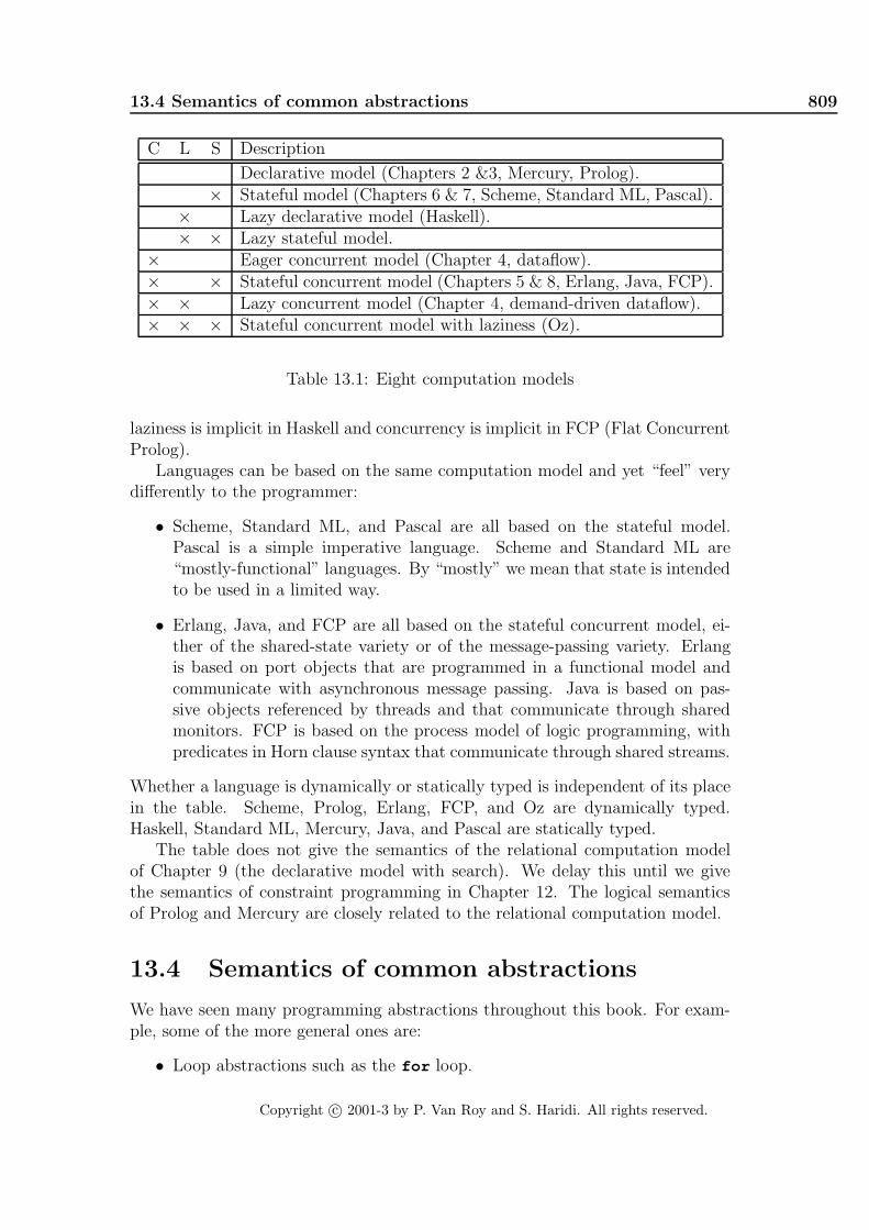
13.4 Semantics of common abstractions 809
C L S Description
Declarative model (Chapters 2 &3, Mercury, Prolog).× Stateful model (Chapters 6 & 7, Scheme, Standard ML, Pascal).
× Lazy declarative model (Haskell).× × Lazy stateful model.
× Eager concurrent model (Chapter 4, dataflow).× × Stateful concurrent model (Chapters 5 & 8, Erlang, Java, FCP).× × Lazy concurrent model (Chapter 4, demand-driven dataflow).× × × Stateful concurrent model with laziness (Oz).
Table 13.1: Eight computation models
laziness is implicit in Haskell and concurrency is implicit in FCP (Flat ConcurrentProlog).
Languages can be based on the same computation model and yet “feel” verydifferently to the programmer:
• Scheme, Standard ML, and Pascal are all based on the stateful model.Pascal is a simple imperative language. Scheme and Standard ML are“mostly-functional” languages. By “mostly” we mean that state is intendedto be used in a limited way.
• Erlang, Java, and FCP are all based on the stateful concurrent model, ei-ther of the shared-state variety or of the message-passing variety. Erlangis based on port objects that are programmed in a functional model andcommunicate with asynchronous message passing. Java is based on pas-sive objects referenced by threads and that communicate through sharedmonitors. FCP is based on the process model of logic programming, withpredicates in Horn clause syntax that communicate through shared streams.
Whether a language is dynamically or statically typed is independent of its placein the table. Scheme, Prolog, Erlang, FCP, and Oz are dynamically typed.Haskell, Standard ML, Mercury, Java, and Pascal are statically typed.
The table does not give the semantics of the relational computation modelof Chapter 9 (the declarative model with search). We delay this until we givethe semantics of constraint programming in Chapter 12. The logical semanticsof Prolog and Mercury are closely related to the relational computation model.
13.4 Semantics of common abstractions
We have seen many programming abstractions throughout this book. For exam-ple, some of the more general ones are:
• Loop abstractions such as the for loop.
Copyright c© 2001-3 by P. Van Roy and S. Haridi. All rights reserved.

810 Language Semantics
• Software components (functors) and their instances (modules).
• Stream objects and declarative concurrency.
• Coroutines (non-preemptive threads).
• Lazy functions and list comprehensions.
• Secure abstract data types, wrappers, and revocable capabilities.
• Incremental definition of abstract data types (classes) and their instances(objects).
• Ports (communication channels) and port objects.
• Concurrent components (port objects and their compositions).
• Active objects, both asynchronous and synchronous.
• Active objects with mailboxes (as used in Erlang).
• Locks, reentrant locks, monitors, and transactions.
• Tuple spaces (similar to the Linda concept).
We showed how to implement these abstractions using the shared-state concurrentmodel or a subset of this model. When taken together with this chapter, theseimplementations can be seen as formal semantic definitions of the abstractions.The choice of which concepts are primitive and which are derived is often a matterof judgement. For example, Chapter 5 defines a port as a primitive concept andgives its semantics directly.
For some of the abstractions, we have defined new syntax, thus making theminto linguistic abstractions. For the semantics, it is almost irrelevant whether ornot an abstraction has syntactic support. We say “almost” because the syntaxcan guarantee that the abstraction is not used in an incorrect way, which isimportant when reasoning about programs.
13.5 Historical notes
The computation model of this chapter was developed over many years. Webriefly summarize its history. In the late 1980’s, a new model of computationknown as the concurrent constraint model was developed by Michael Maher andVijay Saraswat out of concurrent logic programming and constraint logic pro-gramming [163, 117, 90]. All computation models of the book are ultimatelybased on this model.
The concurrent constraint model led to the AKL language [93, 92] and sub-sequently to Oz 1 [179, 180], a precursor of the language used in this book. AKL
Copyright c© 2001-3 by P. Van Roy and S. Haridi. All rights reserved.

13.6 Exercises 811
adds stateful data (in the form of ports) and encapsulated search to the ba-sic concurrent constraint model. Oz 1 further adds higher-order procedures, acompositional syntax (instead of the Horn clause syntax of AKL), stateful ab-stractions including an object system, and computation spaces for encapsulatedsearch. Like AKL, Oz 1 has implicit concurrency: when a statement blocks it isput into its own thread that contains only that statement. The direct successor ofOz 1, called Oz 2, replaces implicit concurrency by explicit thread creation, whichallows an improved object system and makes it easier to reason about programs.
The kernel languages used in this book are subsets of Oz 3, which this bookcalls simply Oz. Oz 3 extends and simplifies Oz 2 in many ways. It adds by-need execution (an early version is given in [121]), first-class software componentscalled functors [50], and a distributed computation model [72]. It has a simpleformal semantics that can be implemented efficiently. The formal semantics ofthis chapter completes and corrects the semantics given in earlier publications,notably regarding by-need execution and read-only variables.
13.6 Exercises
1. The case statement. Let us investigate the case statement, whose se-mantics is defined in Section 13.1.9.
(a) Show how the semantic rules of case can be derived from the rulesfor local and if .
(b) In the first rule for the case , we could have explicitly introducedvariables for the Xi by:
case x of f(l1:X1 . . . ln:Xn)then S1 else S2 end
local X1 · · ·Xn in
X1=x1 · · · Xn=xn S1 end
σ ∧ x=f(l1:x1 . . . ln:xn) σ ∧ x=f(l1:x1 . . . ln:xn)
Do the rules lead to the same possible executions? What are thedifferences (if any)?
(c) It is possible to write an if statement in terms of a case statement.How? This implies that case could have been put in the kernel lan-guage instead of if , and if could have been defined as a linguisticabstraction.
2. Lexically-scoped closures. The rules for procedural abstraction in Sec-tion 13.1.11 are designed to follow lexical scoping, i.e., procedure introduc-tion creates a lexically-scoped closure. Let us look more closely to see howthis works:
• Write the consecutive computation steps (rule reductions) for the ex-ecution of the ForAll and MakeAdder definitions in Section 13.1.11.
Copyright c© 2001-3 by P. Van Roy and S. Haridi. All rights reserved.
812 Language Semantics
• Procedure introduction creates the λ expression ξ:λX1 · · ·Xn.S in thestore. Explain how the contextual environment is stored in this λexpression.
3. Implementing cells with IsDet . Section 13.1.12 explains the IsDet
operation, which can be used to check the status of a dataflow variable. Forthis exercise, let us examine the expressive power of IsDet .
• Define the operations NewCell and Exchange in the declarative modelextended with IsDet . The semantics of these operations should beidentical to their semantics with cells, as given in this chapter. Itis straightforward to define a solution, albeit an inefficient one, thatworks in a sequential model. Hint: use the function LastCons , definedas:
fun {LastCons Xs}case Xs of X|Xr then
if {IsDet Xr} then {LastCons Xr} else Xs end[] nil then nil end
end
Using LastCons let us gets around the monotonicity of the store. Theidea is to build incrementally a list with unbound tail and use IsDet
to get its latest known element.
• Does the above solution work in a concurrent model, i.e., when ex-changes on the same cell are done concurrently? Is such a solutionpossible? In the light of this result, comment on the relationship be-tween IsDet and explicit state.
4. Reading and writing a cell. Section 13.1.12 mentions that two more celloperations can be added for programming convenience, namely xold=@xc toread the content and xc:= xnew to update the content. Define the semanticsof these two operations.
5. Dataflow streams. Section 13.1.12 gives an example of a local state-ment that adds an element to a stream. Prove that executing two of thesestatements in different threads always gives exactly the same final resultas if they were executed sequentially in the same thread in one order oranother.
6. Stateful streams. Define a stream datatype that does not use dataflowvariables. That is, it is a list in which each tail is a cell whose content pointsto the rest of the list. The last cell contains a marker saying that the streamis not yet complete, e.g., the atom incomplete . (This is not the same as theatom nil which means that the stream is complete.) There is a global cellC whose contents is always the last cell in the stream. Write an operationthat adds an element to the stream and that works in a concurrent setting.
Copyright c© 2001-3 by P. Van Roy and S. Haridi. All rights reserved.

13.6 Exercises 813
Hint: assume that there exists a statement lock S end such that only onethread at a time can be executing S; all others suspend if needed to makethis true. Can you do it without using a lock statement? Compare yoursolution to that of the previous exercise. Which is simpler?
7. Needing a variable. Section 13.1.13 gives a definition of what it meansto need a variable. Because this need relation is monotonic, we can showthat the demand-driven concurrent model is declarative. However, thereare other ways to define the need relation that also result in declarativemodels. For this exercise, try to find at least one such definition.
8. Exceptions with a finally clause. Section 13.1.15 defines the try /catch
statement:
try S1 catch X then S2 end
which executes S2 if an exception is raised in S1. Another, very usefulstatement relating to exceptions is the try /finally statement:
try S1 finally S2 end
which always executes S2, whether or not S1 raises an exception. If S1 raisesan exception, then this exception is raised again after executing S2. Definethe try /finally statement in terms of the try /catch statement.
9. (advanced exercise) Lambda calculus. The book claims that the declar-ative model and the declarative concurrent model both do functional pro-gramming. For this exercise, prove this claim formally. First show that anyexecution in the declarative model corresponds to an execution in a versionof the λ calculus. How do dataflow variables show up? Then show thatadding concurrency and laziness do not change this result.
10. (research project) Trade-offs in language design. When designing a lan-guage, there are often trade-offs between the programmer’s mental model,the language semantics, and the implementation. One would like all threeto be simple, but that is often impossible. One of the delicate matters isto find the right balance. To make this concrete, let us see how to providethe concept of binding in a dataflow language. Section 13.1.8 defines twosemantics for binding, which it calls the naive semantics and the realisticsemantics. There is also a third possibility. Let us summarize all three:
• The naive semantics does binding atomically, as a transaction. Ifadding β would be inconsistent, then the store is unchanged. Thisgives a simple mental model and a simple semantics, but the imple-mentation is complex. This semantics was much discussed in the con-text of concurrent logic programming, but was dropped because ofproblems implementing it efficiently [177, 190].
Copyright c© 2001-3 by P. Van Roy and S. Haridi. All rights reserved.

814 Language Semantics
• The realistic semantics does binding as an incremental tell. That is, ifβ is inconsistent, then the store might still be changed. This makes theimplementation simple, but the semantics somewhat more complex.Experience shows that the mental model is acceptable. This semanticsis chosen for the computation models of this book.
• The third semantics is more in line with mainstream programminglanguages. It jettisons unification in favor of simple bindings only. Itallows binding only unbound variables with terms. Variable-variablebindings block and term-term bindings raise an exception. This makesboth the implementation and the semantics simple. However, it is lessexpressive for the programmer. This approach was pioneered, e.g., indataflow languages with I-structures such as Id and pH [131, 132, 133]and in Multilisp [68] (see Section 4.9.4).
For this exercise, reexamine the trade-offs between these three approaches.Which would you recommend?
Copyright c© 2001-3 by P. Van Roy and S. Haridi. All rights reserved.

Part V
Appendices
Copyright c© 2001-3 by P. Van Roy and S. Haridi. All rights reserved.


Appendix A
Mozart System DevelopmentEnvironment
“Beware the ides of March.”– Soothsayer to Julius Caesar, William Shakespeare (1564–1616)
The Mozart system used in this book has a complete IDE (Interactive De-velopment Environment). To get you started, we give a brief overview of thisenvironment here. We refer you to the system documentation for additional in-formation.
A.1 Interactive interface
The Mozart system has an interactive interface that is based on the Emacs texteditor. The interfactive interface is sometimes called the OPI, which stands forOz Programming Interface. The OPI is split into several buffers: scratch pad,Oz emulator, Oz compiler, and one buffer for each open file. This interface givesaccess to several tools: incremental compiler (which can compile any legal pro-gram fragment), Browser (visualize the single-assignment store), Panel (resourceusage), Compiler Panel (compiler settings and environment), Distribution Panel(distribution subsystem including message traffic), and the Explorer (interactivegraphical resolution of constraint problems). These tools can also be manipulatedfrom within programs, e.g., the Compiler module allows to compile strings fromwithin programs.
A.1.1 Interface commands
You can access all the important OPI commands through the menus at the topof the window. Most of these commands have keyboard equivalents. We give themost important ones:
Copyright c© 2001-3 by P. Van Roy and S. Haridi. All rights reserved.

818 Mozart System Development Environment
Command EffectCTRL-x CTRL-f Read a file into a new editor bufferCTRL-x CTRL-s Save current buffer into its fileCTRL-x i Insert file into the current bufferCTRL-. CTRL-l Feed current line into MozartCTRL-. CTRL-r Feed current selected region into MozartCTRL-. CTRL-p Feed current paragraph into MozartCTRL-. CTRL-b Feed current buffer into MozartCTRL-. h Halt the run-time system (but keep the editor)CTRL-x CTRL-c Halt the complete systemCTRL-. e Toggle the emulator windowCTRL-. c Toggle the compiler windowCTRL-x 1 Make current buffer fill the whole windowCTRL-g Cancel current command
The notation “CTRL-x” means to hold down the Control key and then press thekey x once. The CTRL-g command is especially useful if you get lost. To feed atext means to compile and execute it. A region is a contiguous part of the buffer.It can be selected by dragging over it while holding the first mouse button down.A paragraph is a set of non-empty text lines delimited by empty lines or by thebeginning or end of the buffer.
The emulator window gives messages from the emulator. It gives the outputof Show and run-time error messages, e.g., uncaught exceptions. The compilerwindow gives messages from the compiler. It says whether fed source code isaccepted by the system and gives compile-time error messages otherwise.
A.1.2 Using functors interactively
Functors are software component specifications that aid in building well-structuredprograms. A functor can be instantiated, which creates a module. A module isa run-time entity that groups together any other run-time entities. Modulescan contain records, procedures, objects, classes, running threads, and any otherentity that exists at run-time.
Functors are compilation units, i.e., their source code can be put in a file andcompiled as one unit. Functors can also be used in the interactive interface. Thisfollows the Mozart principle that everything can be done interactively.
• A compiled functor can be loaded interactively. For example, assume thatthe Set module, which can be found on the book’s Web site, is compiled infile Set.ozf. It will be loaded interactively with the following code:
declare[Set]={Module.link ["Set.ozf"]}
This creates the module Set . Other functor manipulations are possible byusing the module Module .
Copyright c© 2001-3 by P. Van Roy and S. Haridi. All rights reserved.

A.2 Batch interface 819
• A functor is simply a value, like a class. It can be defined interactively witha syntax similar to classes:
F=functor $ define skip end
This defines a functor and binds F to it.
A.2 Batch interface
The Mozart system can be used from a command line. Oz source files can becompiled and linked. Source files to compile should contain functors, i.e., startwith the keyword functor . For example, assume that we have the source fileSet.oz, which is available on the book’s Web site. We create the compiled functorSet.ozf by typing the following command from a command line interface:
ozc -c Set.oz
We can create a standalone executable Set by typing the following:
ozc -x Set.oz
(In the case of Set.oz, the standalone executable does very little: it just definesthe set operations.) The Mozart default is to use dynamic linking, i.e., neededmodules are loaded and linked at the moment they are needed in an application.This keeps compiled files small. But it is possible to link all imported modulesduring compilation (static linking) so that no dynamic linking is needed.
Copyright c© 2001-3 by P. Van Roy and S. Haridi. All rights reserved.

820 Mozart System Development Environment
Copyright c© 2001-3 by P. Van Roy and S. Haridi. All rights reserved.

Appendix B
Basic Data Types
“Wie het kleine niet eert is het grote niet weert.”“He who does not honor small things is not worthy of great things.”– Traditional Dutch proverb.
This appendix explains the most common basic data types in Oz together withsome common operations. The types explained are numbers (including integersand floating point numbers), characters (which are represented as small integers),literals (constants of two types, either atoms or names), records, tuples, chunks(records with a limited set of operations), lists, strings (which are represented aslists of characters), and virtual strings (strings represented as tuples).
For each data type discussed in this appendix, there is a corresponding Basemodule in the Mozart system that defines all operations on the data type. Thisappendix gives some but not all of these operations. See the Mozart systemdocumentation for complete information [49].
B.1 Numbers (integers, floats, and characters)
The following code fragment introduces four variables I , H, F and C. It binds I
to an integer, H to an integer in hexadecimal notation, F to a float, and C to thecharacter t in this order. It then displays I , H, F, and C:
declare I H F C inI = ˜5H = 0xDadBeddedABadBadBabeF = 5.5C = &t{Browse I} {Browse H} {Browse F} {Browse C}
Note that ˜ (tilde) is the unary minus symbol. This displays the following:
˜510335328705954529514441585.5
Copyright c© 2001-3 by P. Van Roy and S. Haridi. All rights reserved.

822 Basic Data Types
〈character〉 ::= (any integer in the range 0 ... 255)| ´ &´ 〈charChar〉| ´ &´ 〈pseudoChar〉
〈charChar〉 ::= (any inline character except \ and NUL)〈pseudoChar〉 ::= (’\’ followed by three octal digits)
| (´ \x ´ or ´ \X ´ followed by two hexadecimal digits)| ´ \a ´ | ´ \b ´ | ´ \f ´ | ´ \n ´ | ´ \r ´ | ´ \t ´
| ´ \v ´ | ´ \\ ´ | ´ \ ´´ | ´ \" ´ | ´ \ `´ | ´ \& ´
Table B.1: Character lexical syntax
116
Oz supports binary, octal, decimal, and hexadecimal notation for integers, whichcan have any number of digits. An octal integer starts with a leading 0 (zero),followed by any number of digits from 0 to 7. A binary integer starts with aleading 0b or 0B (zero followed by the letter b or B) followed by any number ofbinary digits, i.e., 0 or 1. A hexadecimal integer starts with a leading 0x or 0X
(zero followed by the letter x or X). The hexadecimal digits from 10 to 15 aredenoted by the letters a through f and A through F.
Floats are different from integers in that they approximate real numbers. Hereare some examples of floats:
˜3.14159265359 3.5E3 ˜12.0e˜2 163.
Note that Mozart uses ˜ (tilde) as the unary minus symbol for floats as well asintegers. Floats are internally represented in double precision (64 bits) using theIEEE floating point standard. A float must be written with a decimal point andat least one digit before the decimal point. There may be zero or more digitsafter the decimal point. Floats can be scaled by powers of ten by appending theletter e or E followed by a decimal integer (which can be negative with a ´ ˜ ´ ).
Characters are a subtype of integers that range from 0 to 255 . The standardISO 8859-1 coding is used. This code extends the ASCII code to include the lettersand accented letters of most languages whose alphabets are based on the Romanalphabet. Unicode is a 16-bit code that extends the ASCII code to include thecharacters and writing specifics (like writing direction) of most of the alphabetsused in the world. It is not currently used, but may be in the future. There arefive ways to write characters:
• A character can be written as an integer in the range 0, 1, ..., 255 , in accordwith the integer syntax given before.
• A character can be written as an ampersand & followed by a specific char-acter representation. There are four such representations:
– Any inline character except for \ (backslash) and the NUL character.
Copyright c© 2001-3 by P. Van Roy and S. Haridi. All rights reserved.

B.1 Numbers (integers, floats, and characters) 823
〈expression〉 ::= 〈expression〉 〈binaryOp〉 〈expression〉| ´ { ´ 〈expression〉 { 〈expression〉 } ´ } ´
| ...〈binaryOp〉 ::= ´ +´ | ´ - ´ | ´ * ´ | ´ / ´ | div | mod | ...
Table B.2: Some number operations
Some examples are &t , & (note the space), and &+. Inline controlcharacters are acceptable.
– A backslash \ followed by three octal digits, e.g., &\215 is a character.The first digit should not be greater than 3.
– A backslash \ followed by the letter x or X, followed by two hexadecimaldigits, e.g., &\x3f is a character.
– A backslash \ followed by one of the following characters: a (= \007 ,bell), b (= \010 , backspace), f (= \014 , formfeed), n (= \012 , new-line), r (= \015 , carriage return), t (= \011 , horizontal tab), v (=\013 , vertical tab), \ (= \134 , backslash), ’ (= \047 , single quote)," (= \042 , double quote), ‘ (= \140 , backquote), and & (= \046 ,ampersand). For example, &\\ is the backslash character, i.e., theinteger 92 (the ASCII code for \ ) .
Table B.1 summarizes these possibilities.There is no automatic type conversion in Oz, so 5.0 = 5 will raise an excep-
tion. The next section explains the basic operations on numbers, including theprimitive procedures for explicit type conversion. The complete set of operationsfor characters, integers, and floats are given in the Base modules Char , Float ,and Int . Additional generic operations on all numbers are given in the Basemodule Number. See the documentation for more information.
B.1.1 Operations on numbers
To express a calculation with numbers, we use two kinds of operations: binaryoperations, such as addition and subtraction, and function applications, such astype conversions. Table B.2 gives the syntax of these expressions. All numbers,i.e., both integers and floats, support addition, subtraction, and multiplication:
declare I Pi Radius Circumference inI = 7 * 11 * 13 + 27 * 37Pi = 3.1415926536Radius = 10.Circumference = 2.0 * Pi * Radius
Integer arithmetic is to arbitrary precision. Float arithmetic has a fixed precision.Integers support integer division (div symbol) and modulo (mod symbol). Floats
Copyright c© 2001-3 by P. Van Roy and S. Haridi. All rights reserved.
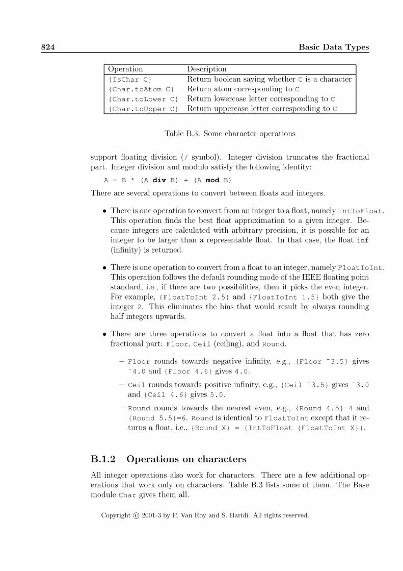
824 Basic Data Types
Operation Description{IsChar C} Return boolean saying whether C is a character{Char.toAtom C} Return atom corresponding to C
{Char.toLower C} Return lowercase letter corresponding to C
{Char.toUpper C} Return uppercase letter corresponding to C
Table B.3: Some character operations
support floating division (/ symbol). Integer division truncates the fractionalpart. Integer division and modulo satisfy the following identity:
A = B * (A div B) + (A mod B)
There are several operations to convert between floats and integers.
• There is one operation to convert from an integer to a float, namely IntToFloat .This operation finds the best float approximation to a given integer. Be-cause integers are calculated with arbitrary precision, it is possible for aninteger to be larger than a representable float. In that case, the float inf
(infinity) is returned.
• There is one operation to convert from a float to an integer, namely FloatToInt .This operation follows the default rounding mode of the IEEE floating pointstandard, i.e., if there are two possibilities, then it picks the even integer.For example, {FloatToInt 2.5} and {FloatToInt 1.5} both give theinteger 2. This eliminates the bias that would result by always roundinghalf integers upwards.
• There are three operations to convert a float into a float that has zerofractional part: Floor , Ceil (ceiling), and Round.
– Floor rounds towards negative infinity, e.g., {Floor ˜3.5} gives˜4.0 and {Floor 4.6} gives 4.0 .
– Ceil rounds towards positive infinity, e.g., {Ceil ˜3.5} gives ˜3.0
and {Ceil 4.6} gives 5.0 .
– Round rounds towards the nearest even, e.g., {Round 4.5}=4 and{Round 5.5}=6 . Round is identical to FloatToInt except that it re-turns a float, i.e., {Round X} = {IntToFloat {FloatToInt X}} .
B.1.2 Operations on characters
All integer operations also work for characters. There are a few additional op-erations that work only on characters. Table B.3 lists some of them. The Basemodule Char gives them all.
Copyright c© 2001-3 by P. Van Roy and S. Haridi. All rights reserved.

B.2 Literals (atoms and names) 825
〈expression〉 ::= unit | true | false | 〈atom〉 | ...
Table B.4: Literal syntax (in part)
〈atom〉 ::= (lowercase char) { (alphanumeric char) } (except no keyword)| ’’’ { 〈atomChar〉 | 〈pseudoChar〉 } ’’’
〈atomChar〉 ::= (any inline character except ’ , \ , and NUL)〈pseudoChar〉 ::= (’\’ followed by three octal digits)
| (´ \x ´ or ´ \X ´ followed by two hexadecimal digits)| ´ \a ´ | ´ \b ´ | ´ \f ´ | ´ \n ´ | ´ \r ´ | ´ \t ´
| ´ \v ´ | ´ \\ ´ | ´ \ ´´ | ´ \" ´ | ´ \ `´ | ´ \& ´
Table B.5: Atom lexical syntax
B.2 Literals (atoms and names)
Atomic types are types whose members have no internal structure.1 The previoussection has given one kind of atomic type, namely numbers. In addition tonumbers, literals are a second kind of atomic type (see Table B.4 and Table B.5).Literals can be either atoms or names. An atom is a value whose identity isdetermined by a sequence of printable characters. An atom can be written in twoways. First, as a sequence of alphanumeric characters starting with a lowercaseletter. This sequence may not be a keyword of the language. Second, by arbitraryprintable characters enclosed in single quotes. Here are some valid atoms:
a foo ´ =´ ´ := ´ ´ Oz 3.0 ´ ´ Hello World ´ ´ if ´ ´ \n,\n ´ a_person
There is no confusion between the keyword if and the atom ´ if ´ because of thequotes. The atom ´ \n,\n ´ consists of four characters. Atoms are ordered lexi-cographically, based on the underlying ISO 8859-1 encoding for single characters.
Names are a second kind of literal. A name is a unique atomic value thatcannot be forged or printed. Unlike numbers or atoms, names are truly atomic,in the original sense of the word: they cannot be decomposed at all. Names havejust two operations defined on them: creation and equality comparison. The onlyway to create a name is by calling the function {NewName}, which returns a newname that is guaranteed to be unique. Note that Table B.4 has no representationfor names. The only way to reference a name is through a variable that is boundto the name. As Chapter 3 explains, names play an important role for secureencapsulation in ADTs.
1But like physical atoms, atomic values can sometimes be decomposed if the right tools areused, e.g., numbers have a binary representation as a sequence of zeroes and ones and atomshave a print representation as a sequence of characters.
Copyright c© 2001-3 by P. Van Roy and S. Haridi. All rights reserved.

826 Basic Data Types
Operation Description{IsAtom A} Return boolean saying whether A is an atom{AtomToString A} Return string corresponding to atom A
{StringToAtom S} Return atom corresponding to string S
Table B.6: Some atom operations
〈expression〉 ::= 〈label〉 ´ ( ´ { [ 〈feature〉 ´ : ´ ] 〈expression〉 } ´ ) ´ | ...〈label〉 ::= unit | true | false | 〈variable〉 | 〈atom〉〈feature〉 ::= unit | true | false | 〈variable〉 | 〈atom〉 | 〈int〉〈binaryOp〉 ::= ´ . ´ | 〈consBinOp〉 | ...〈consBinOp〉 ::= ´ #´ | ...
Table B.7: Record and tuple syntax (in part)
There are three special names that have keywords reserved to them. Thekeywords are unit , true , and false . The names true and false are usedto denote boolean true and false values. The name unit is often used as asynchronization token in concurrent programs. Here are some examples:
local X Y B inX = foo{NewName Y}B = true{Browse [X Y B]}
end
B.2.1 Operations on atoms
Table B.6 gives the operations in the Base module Atom and some of the opera-tions relating to atoms in the Base module String .
B.3 Records and tuples
Records are data structures that allow to group together language references.Here is a record that groups four variables:
tree(key:I value:Y left:LT right:RT)
It has four components and the label tree . To avoid ambiguity, there should beno space between the label and the left parenthesis. Each component consistsof an identifier, called feature, and a reference into the store. A feature can beeither a literal or an integer. Table B.7 gives the syntax of records and tuples.
Copyright c© 2001-3 by P. Van Roy and S. Haridi. All rights reserved.

B.3 Records and tuples 827
The above record has four features, key , value , left , and right , that identifyfour language references, I , Y, LT, and RT.
It is allowed to omit features in the record syntax. In that case, the featurewill be an integer starting from 1 for the first such component and incrementingby 1 for each successive component that does not have a feature. For example,the record tree(key:I value:Y LT RT) is identical to tree(key:I value:Y
1:LT 2:RT) .
The order of labeled components does not matter; it can be changed withoutchanging the record. We say that these components are unordered. The order ofunlabeled components does matter; it determines how the features are numbered.It is as if there were two “worlds”: the ordered world and the unordered world.They have no effect on each other and can be interleaved in any way. All thefollowing notations denote the same record:
tree(key:I value:Y LT RT) tree(value:Y key:I LT RT)tree(key:I LT value:Y RT) tree(value:Y LT key:I RT)tree(key:I LT RT value:Y) tree(value:Y LT RT key:I)tree(LT key:I value:Y RT) tree(LT value:Y key:I RT)tree(LT key:I RT value:Y) tree(LT value:Y RT key:I)tree(LT RT key:I value:Y) tree(LT RT value:Y key:I)
Two records are the same if the same set of components is present and the orderedcomponents are in the same order.
It is an error if a feature occurs more than once. For example, the notationstree(key:I key:J) and tree(1:I value:Y LT RT) are both in error. Theerror is discovered when the record is constructed. This can be either at compiletime or at run time. However, both tree(3:I value:Y LT RT) and tree(4:I
value:Y LT RT) are correct since no feature occurs more than once. Integerfeatures do not have to be consecutive.
B.3.1 Tuples
If the record has only consecutive integer features starting from 1, then we callit a tuple. All these features can be omitted. Consider this tuple:
tree(I Y LT RT)
It is exactly the same as the following tuple:
tree(1:I 2:Y 3:LT 4:RT)
Tuples whose label is ´ #´ have another notation using the # symbol as an “mixfix”operator (see Appendix C.4). This means that a#b#c is a tuple with three argu-ments, namely ´ #´ (a b c) . Be careful not to confuse it with the pair a#(b#c) ,whose second argument is itself the pair b#c . The mixfix notation can only beused for tuples with at least two arguments. It is used for virtual strings (seeSection B.7).
Copyright c© 2001-3 by P. Van Roy and S. Haridi. All rights reserved.

828 Basic Data Types
Operation DescriptionR.F Return field F from R
{HasFeature R F} Return boolean saying whether feature F is in R
{IsRecord R} Return boolean saying whether R is of record type{MakeRecord L Fs} Return record with label L and features Fs
{Label R} Return the label of R
{Arity R} Return the list of features (arity) of R
{Record.toList R} Return the list of fields of R, in Arity order{Width R} Return the number of features (width) of R
{AdjoinAt R F X} Return R augmented with feature F and value X
{Adjoin R1 R2} Return R1 augmented with all fields of R2
Table B.8: Some record operations
B.3.2 Operations on records
Table B.8 gives a few basic record operations. Many more operations exist in theBase module Record . This appendix shows only a few, namely those concerningextracting information from records and building new records. To select a field ofa record component, we use the infix dot operator, e.g., tree(key:I value:Y
LT RT).value returns Y. To compare two records, we use the equality test op-eration. Two records are the same if they have the same set of features and thelanguage references for each feature are the same.
The arity of a record is a list of the features of the record sorted lexicographi-cally. To display the arity of a record we use the function Arity . Calling {Arity
R} will execute as soon as R is bound to a record, and will return the arity of therecord. Feeding the statement:
declare T W L R inT=tree(key:a left:L right:R value:1)W=tree(a L R 1){Browse {Arity T}}{Browse {Arity W}}
will display:
[key left right value][1 2 3 4]
The function {AdjoinAt R1 F X} returns the record resulting from adjoining(i.e., adding) the field X to R1 at feature F. The record R1 is unchanged. IfR1 already has the feature F, then the result is identical to R1 except for thefield R1.F , whose value becomes X. Otherwise the feature F is added to R1. Forexample:
declare T W L R inT=tree(key:a left:L right:R value:1)W=tree(a L R 1)
Copyright c© 2001-3 by P. Van Roy and S. Haridi. All rights reserved.

B.4 Chunks (limited records) 829
Operation Description{MakeTuple L N} Return tuple with label L and features 1, ..., N
{IsTuple T} Return boolean saying whether T is of tuple type
Table B.9: Some tuple operations
〈expression〉 ::= ´ [ ´ { 〈expression〉 }+ ´ ] ´ | ...〈consBinOp〉 ::= ´ | ´ | ...
Table B.10: List syntax (in part)
{Browse {AdjoinAt T 1 b}}{Browse {AdjoinAt W key b}}
will display:
tree(b key:a left:L right:R value:1)tree(a L R 1 key:b)
The {Adjoin R1 R2} operation gives the same result as if AdjoinAt were calledsuccessively, starting with R1 and iterating through all features of R2.
B.3.3 Operations on tuples
All record operations also work for tuples. There are a few additional operationsthat work only on tuples. Table B.9 lists some of them. The Base module Tuple
gives them all.
B.4 Chunks (limited records)
A chunk is Mozart terminology for a record type with a limited set of operations.Chunks are not a fundamental concept; they can be implemented with procedurevalues and names, as explained in Section 3.7.5. For improved efficiency, Mozartprovides chunks directly as a data type. We describe them here because somelibrary modules use them (in particular, the module ObjectSupport ). There areonly two basic operations: create a chunk from any record and extract informationwith the field selection operator “. ”:
declareC={Chunk.new anyrecord(a b c)} % Chunk creationF=C.2 % Chunk field selection
The Label and Arity operations are not defined and unification is not possible.Chunks give a way of “wrapping” information so that access to the informationis restricted, i.e., not all computations can access the information. This makeschunks useful for defining secure abstract data types.
Copyright c© 2001-3 by P. Van Roy and S. Haridi. All rights reserved.

830 Basic Data Types
B.5 Lists
A list is either the atom nil representing the empty list or a tuple with infixoperator | and two arguments which are respectively the head and the tail ofthe list. The two arguments have field numbered 1 and 2. The head can be anydata type and the tail is a list. We call the tuple a list pair. Often it is called acons cell because creating one in Lisp is done with an operation called cons. Lispis the oldest list-processing language and pioneered many list concepts and theirterminology. When the second argument is not necessarily a list, then it is oftencalled a dotted pair, because Lisp writes it in infix with a dot operator. In ournotation, a list of the letters a, b, and c is written as:
a|b|c|nil
We provide a more concise syntax for lists (i.e., when the rightmost argument isnil ):
[a b c]
Table B.10 shows the syntax of these two ways of writing a list. The partial listcontaining elements a and b and whose tail is the variable X looks like:
a|b|X
One can also use the standard record notation for lists:
´ | ´ (a ´ | ´ (b X))
or even (making the field names explicit):
´ | ´ (1:a 2: ´ | ´ (1:b 2:X))
Circular lists are allowed. For example, the following is legal:
declare X inX=a|b|X{Browse X}
By default, the browser displays the list without taking sharing into account, i.e.,without taking into account multiple references to the same part of the list. Inthe list X, after the first two elements a and b, we find X again. By default, thebrowser ignores all sharing. It displays X as:
a|b|a|b|a|b|a|b|a|b|a|b|a|b|a|b|a|b|a|b|a|b|a|b|a|b|a|b|a|b|a|b|a|b|a|b|a|b|a|b|a|b|a|b|a|b|a|b|a|b|,,,
To avoid infinite loops, the browser has an adjustable depth limit. The threecommas ,,, represent the part of the list that is not displayed. Select Graph inthe Representation entry of the browser’s Options menu and feed the fragmentagain. This will display the list as a graph (see Figure B.1):
C1=a|b|C1
The browser introduces the new variable C1 to refer to another part of the list.See the browser manual for more information on what the browser can display.
Copyright c© 2001-3 by P. Van Roy and S. Haridi. All rights reserved.

B.5 Lists 831
Operation Description{Append L1 L2} Return the concatenation of L1 and L2
{Member X L} Return boolean saying whether X is in L
{Length L} Return the length of L
{List.drop L N} Return L minus the first Nelements, or nil
if it is shorter{List.last L} Return the last element of non-empty list
L
{Sort L F} Return L sorted according to boolean com-parison function F
{Map L F} Return the list obtained by applying F toeach element of L
{ForAll L P} Apply the unary procedure P to each ele-ment of L
{Filter L F} Return the list of elements of L for whichF gives true
{FoldL L F N} Return the value obtained by inserting F
between all elements of L
{Flatten L} Return the list of all non-list elements ofL, at any nesting depth
{List.toTuple A L} Return tuple with label A and orderedfields from L
{List.toRecord A L} Return record with label A and fea-tures/fields F#X in L
Table B.11: Some list operations
B.5.1 Operations on lists
Table B.11 gives a few basic list operations. Many more operations exist in theBase module List . Here is a simple symbolic calculation with lists:
declare A B inA=[a b c]B=[1 2 3 4]{Browse {Append A B}}
This displays the list [a b c 1 2 3 4] . Like all operations, these all have cor-rect dataflow behavior. For example, {Length a|b|X} blocks until X is bound.The operations Sort , Map, ForAll , Filter , and FoldL are examples of higher-order operations, i.e., operations that take functions or procedures as arguments.We will talk about higher-order execution in Chapter 3. For now, here’s anexample to give a flavor of what is possible:
declare L inL=[john paul george ringo]
Copyright c© 2001-3 by P. Van Roy and S. Haridi. All rights reserved.

832 Basic Data Types
|
|
a
b
C1:
Figure B.1: Graph representation of the infinite list C1=a|b|C1
〈expression〉 ::= 〈string〉 | ...〈string〉 ::= ´ " ´ { 〈stringChar〉 | 〈pseudoChar〉 } ´ " ´
〈stringChar〉 ::= (any inline character except " , \ , and NUL)〈pseudoChar〉 ::= (’\’ followed by three octal digits)
| (´ \x ´ or ´ \X ´ followed by two hexadecimal digits)| ´ \a ´ | ´ \b ´ | ´ \f ´ | ´ \n ´ | ´ \r ´ | ´ \t ´
| ´ \v ´ | ´ \\ ´ | ´ \ ´´ | ´ \" ´ | ´ \ `´ | ´ \& ´
Table B.12: String lexical syntax
{Browse {Sort L Value. ´ <´ }}
sorts L according to the comparison function ´ <´ and displays the result:
[george john paul ringo]
As an infix operator, comparison is written as X<Y, but the comparison operationitself is in the Base module Value . Its full name is Value. ´ <´ . Modules areexplained in Section 3.9.
B.6 Strings
Lists whose elements are character codes are called strings. For example:
"Mozart 1.2.3"
is the list:
[77 111 122 97 114 116 32 49 46 50 46 51]
or equivalently:
[&M &o &z &a &r &t & &1 &. &2 &. &3]
Using lists to represent strings is convenient because all list operations are avail-able for doing symbolic calculations with strings. Character operations can beused together with list operations to calculate on the internals of strings. String
Copyright c© 2001-3 by P. Van Roy and S. Haridi. All rights reserved.

B.7 Virtual strings 833
Operation Description{VirtualString.toString VS} Return a string with the same characters
as VS
{VirtualString.toAtom VS} Return an atom with the same charactersas VS
{VirtualString.length VS} Return the number of characters in VS
{Value.toVirtualString X D W} Return a string representing the partialvalue X, where records are limited in depthto D and in width to W
Table B.13: Some virtual string operations
syntax is shown in Table B.12. The NUL character mentioned in the table hascharacter code 0 (zero). See Section B.1 for an explanation of the meaning of´ \a ´ , ´ \b ´ , etc.
There exists another, more memory-efficient representation for character se-quences called bytestring. This representation should only be used if memorylimitations make it necessary.
B.7 Virtual strings
A virtual string is a tuple with label ´ #´ that represents a string. The virtualstring brings together different substrings that are concatenated with virtual con-catenation. That is, the concatenation is never actually performed, which savestime and memory. For example, the virtual string:
123#"-"#23#" is "#(123-23)
represents the string:
"123-23 is 100"
Except in special cases, a library operation that expects a string can always begiven a virtual string instead. For example, virtual strings can be used for allI/O operations. The components of a virtual string can be numbers, strings,virtual strings (i.e., ´ #´ -labeled tuples), and all atoms except for nil and ´ #´ .Table B.13 gives a few virtual string operations.
Copyright c© 2001-3 by P. Van Roy and S. Haridi. All rights reserved.

834 Basic Data Types
Copyright c© 2001-3 by P. Van Roy and S. Haridi. All rights reserved.

Appendix C
Language Syntax
“The devil is in the details.”– Traditional proverb.
“God is in the details.”– Traditional proverb.
“I don’t know what is in those details,but it must be something important!”– Irreverent proverb.
This appendix defines the syntax of the complete language used in this book,including all syntactic conveniences. The language is a subset of the Oz languageas implemented by the Mozart system. The appendix is divided into six sections:
• Section C.1 defines the syntax of interactive statements, i.e., statementsthat can be fed into the interactive interface.
• Section C.2 defines the syntax of statements and expressions.
• Section C.3 defines the syntax of the nonterminals needed to define state-ments and expressions.
• Section C.4 lists the operators of the language with their precedence andassociativity.
• Section C.5 lists the keywords of the language.
• Section C.6 defines the lexical syntax of the language, i.e., how a charactersequence is transformed into a sequence of tokens.
To be precise, this appendix defines a context-free syntax for a superset of thelanguage. This keeps the syntax simple and easy to read. The disadvantage ofa context-free syntax is that it does not capture all syntactic conditions for legalprograms. For example, take the statement local X in 〈statement〉 end . The
Copyright c© 2001-3 by P. Van Roy and S. Haridi. All rights reserved.

836 Language Syntax
〈interStatement〉 ::= 〈statement〉| declare { 〈declarationPart〉 }+ [ 〈interStatement〉 ]| declare { 〈declarationPart〉 }+ in 〈interStatement〉
Table C.1: Interactive statements
〈statement〉 ::= 〈nestCon(statement)〉 | 〈nestDec(〈variable〉)〉| skip | 〈statement〉 〈statement〉
〈expression〉 ::= 〈nestCon(expression)〉 | 〈nestDec(´ $´ )〉| 〈expression〉 〈evalBinOp〉 〈expression〉| ´ $´ | 〈term〉 | ´ @ 〈expression〉 | self
〈inStatement〉 ::= [ { 〈declarationPart〉 }+ in ] 〈statement〉〈inExpression〉 ::= [ { 〈declarationPart〉 }+ in ] [ 〈statement〉 ] 〈expression〉〈in(statement)〉 ::= 〈inStatement〉〈in(expression)〉 ::= 〈inExpression〉
Table C.2: Statements and expressions
statement that contains this one must declare all the free variable identifiers of〈statement〉, possibly minus X. This is not a context-free condition.
This appendix defines the syntax of a subset of the full Oz language, as de-fined in [77, 47]. This appendix differs from [77] in several ways: it introducesnestable constructs, nestable declarations, and terms to factor the common partsof statement and expression syntax, it defines interactive statements and for
loops, it leaves out the translation to the kernel language (which is given for eachlinguistic abstraction in the main text of the book), and it makes other smallsimplifications for clarity (but without sacrificing precision).
C.1 Interactive statements
Table C.1 gives the syntax of interactive statements. An interactive statementis a superset of a statement; in addition to all regular statements, it can containa declare statement. The interactive interface must always be fed interactivestatements. All free variable identifiers in the interactive statement must exist inthe global environment, otherwise the system gives a “variable not introduced”error.
C.2 Statements and expressions
Table C.2 gives the syntax of statements and expressions. Many language con-structs be used in either a statement position or an expression position. We
Copyright c© 2001-3 by P. Van Roy and S. Haridi. All rights reserved.

C.2 Statements and expressions 837
〈nestCon(α)〉 ::= 〈expression〉 ( ´ =´ | ´ := ´ | ´ , ´ ) 〈expression〉| ´ { ´ 〈expression〉 { 〈expression〉 } ´ } ´
| local { 〈declarationPart〉 }+ in [ 〈statement〉 ] 〈α〉 end
| ´ ( ´ 〈in(α)〉 ´ ) ´
| if 〈expression〉 then 〈in(α)〉{ elseif 〈expression〉 then 〈in(α)〉 }[ else 〈in(α)〉 ] end
| case 〈expression〉 of 〈pattern〉 [ andthen 〈expression〉 ] then 〈in(α)〉{ ´ [] ´ 〈pattern〉 [ andthen 〈expression〉 ] then 〈in(α)〉 }[ else 〈in(α)〉 ] end
| for { 〈loopDec〉 }+ do 〈in(α)〉 end
| try 〈in(α)〉[ catch 〈pattern〉 then 〈in(α)〉{ ´ [] ´ 〈pattern〉 then 〈in(α)〉 } ]
[ finally 〈in(α)〉 ] end
| raise 〈inExpression〉 end
| thread 〈in(α)〉 end
| lock [ 〈expression〉 then ] 〈in(α)〉 end
Table C.3: Nestable constructs (no declarations)
〈nestDec(α)〉 ::= proc ´ { ´ α { 〈pattern〉 } ´ } ´ 〈inStatement〉 end
| fun [ lazy ] ´ { ´ α { 〈pattern〉 } ´ } ´ 〈inExpression〉 end
| functor α[ import { 〈variable〉 [ at 〈atom〉 ]
| 〈variable〉 ´ ( ´
{ (〈atom〉 | 〈int〉) [ ´ : ´ 〈variable〉 ] }+ ´ ) ´
}+ ][ export { [ (〈atom〉 | 〈int〉) ´ : ´ ] 〈variable〉 }+ ]define { 〈declarationPart〉 }+ [ in 〈statement〉 ] end
| class α { 〈classDescriptor〉 }{ meth 〈methHead〉 [ ´ =´ 〈variable〉 ]
( 〈inExpression〉 | 〈inStatement〉 ) end }end
Table C.4: Nestable declarations
Copyright c© 2001-3 by P. Van Roy and S. Haridi. All rights reserved.

838 Language Syntax
〈term〉 ::= [ ´ ! ´ ] 〈variable〉 | 〈int〉 | 〈float〉 | 〈character〉| 〈atom〉 | 〈string〉 | unit | true | false
| 〈label〉 ´ ( ´ { [ 〈feature〉 ´ : ´ ] 〈expression〉 } ´ ) ´
| 〈expression〉 〈consBinOp〉 〈expression〉| ´ [ ´ { 〈expression〉 }+ ´ ] ´
〈pattern〉 ::= [ ´ ! ´ ] 〈variable〉 | 〈int〉 | 〈float〉 | 〈character〉| 〈atom〉 | 〈string〉 | unit | true | false
| 〈label〉 ´ ( ´ { [ 〈feature〉 ´ : ´ ] 〈pattern〉 } [ ´ ... ´ ] ´ ) ´
| 〈pattern〉 〈consBinOp〉 〈pattern〉| ´ [ ´ { 〈pattern〉 }+ ´ ] ´
Table C.5: Terms and patterns
call such constructs nestable. We write the grammar rules to give their syn-tax just once, in a way that works for both statement and expression positions.Table C.3 gives the syntax for nestable constructs, not including declarations. Ta-ble C.4 gives the syntax for nestable declarations. The grammar rules for nestableconstructs and declarations are templates with one argument. The template isinstantiated each time it is used. For example, 〈nestCon(α)〉 defines the tem-plate for nestable constructs without declarations. This template is used twice,as 〈nestCon(statement)〉 and 〈nestCon(expression)〉, and each corresponds to onegrammar rule.
C.3 Nonterminals for statements and expressions
Tables C.5 and C.6 defines the nonterminal symbols needed for the statement andexpression syntax of the preceding section. Table C.5 defines the syntax of termsand patterns. Note the close relationship between terms and patterns. Both areused to define partial values. There are just two differences: (1) patterns cancontain only variable identifiers whereas terms can contain expressions, and (2)patterns can be partial (using ´ ... ´ ) whereas terms cannot.
Table C.6 defines nonterminals for the declaration parts of statements andloops, for binary operators (“constructing” operators 〈consBinOp〉 and “evalu-ating” operators 〈evalBinOp〉), for records (labels and features), and for classes(descriptors, attributes, methods, etc.).
C.4 Operators
Table C.7 gives the precedence and associativity of all the operators used in thebook. All the operators are binary infix operators, except for three cases. Theminus sign ´ ˜ ´ is a unary prefix operator. The hash symbol ´ #´ is an n-arymixfix operator. The “. := ” is a ternary infix operator that is explained in the
Copyright c© 2001-3 by P. Van Roy and S. Haridi. All rights reserved.

C.4 Operators 839
〈declarationPart〉 ::= 〈variable〉 | 〈pattern〉 ´ =´ 〈expression〉 | 〈statement〉〈loopDec〉 ::= 〈variable〉 in 〈expression〉 [ ´ .. ´ 〈expression〉 ] [ ´ ; ´ 〈expression〉 ]
| 〈variable〉 in 〈expression〉 ´ ; ´ 〈expression〉 ´ ; ´ 〈expression〉| break ´ : ´ 〈variable〉 | continue ´ : ´ 〈variable〉| return ´ : ´ 〈variable〉 | default ´ : ´ 〈expression〉| collect ´ : ´ 〈variable〉
〈binaryOp〉 ::= 〈evalBinOp〉 | 〈consBinOp〉〈consBinOp〉 ::= ´ #´ | ´ | ´
〈evalBinOp〉 ::= ´ +´ | ´ - ´ | ´ * ´ | ´ / ´ | div | mod | ´ . ´ | andthen | orelse
| ´ := ´ | ´ , ´ | ´ =´ | ´ ==´ | ´ \= ´ | ´ <´ | ´ =<´ | ´ >´ | ´ >=´
〈label〉 ::= unit | true | false | 〈variable〉 | 〈atom〉〈feature〉 ::= unit | true | false | 〈variable〉 | 〈atom〉 | 〈int〉〈classDescriptor〉 ::= from { 〈expression〉 }+ | prop { 〈expression〉 }+
| attr { 〈attrInit〉 }+〈attrInit〉 ::= ( [ ´ ! ´ ] 〈variable〉 | 〈atom〉 | unit | true | false )
[ ´ : ´ 〈expression〉 ]〈methHead〉 ::= ( [ ´ ! ´ ] 〈variable〉 | 〈atom〉 | unit | true | false )
[ ´ ( ´ { 〈methArg〉 } [ ´ ... ´ ] ´ ) ´ ][ ´ =´ 〈variable〉 ]
〈methArg〉 ::= [ 〈feature〉 ´ : ´ ] ( 〈variable〉 | ´ _´ | ´ $´ ) [ ´ <=´ 〈expression〉 ]
Table C.6: Other nonterminals needed for statements and expressions
next section. There are no postfix operators. The operators are listed in order ofincreasing precedence, i.e., tightness of binding. The operators lower in the tablebind tighter. We define the associativities as follows:
• Left. For binary operators, this means that repeated operators group tothe left. For example, 1+2+3 means the same as ((1+2)+3) .
• Right. For binary operators, this means that repeated operators group tothe right. For example, a|b|X means the same as (a|(b|X)) .
• Mixfix. Repeated operators are actually just one operator, with all expres-sions being arguments of the operator. For example, a#b#c means the sameas ´ #´ (a b c) .
• None. For binary operators, this means that the operator cannot be repeat-ed. For example, 1<2<3 is an error.
Parentheses can be used to override the default precedence.
Copyright c© 2001-3 by P. Van Roy and S. Haridi. All rights reserved.
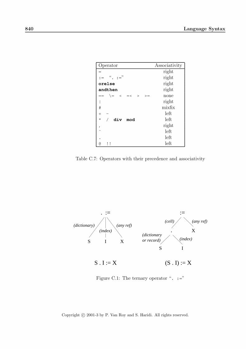
840 Language Syntax
Operator Associativity= right:= “. := ” rightorelse rightandthen right== \= < =< > >= none| right# mixfix+ - left* / div mod left, right˜ left. left@ !! left
Table C.7: Operators with their precedence and associativity
.
S I X
(any ref)(index)
(dictionary)
S . I := X
X
(any ref)
(S . I) := X
(cell)
. := :=
S I
(index)or record)(dictionary
Figure C.1: The ternary operator “. := ”
Copyright c© 2001-3 by P. Van Roy and S. Haridi. All rights reserved.

C.5 Keywords 841
andthen default false lock return
at define feat (*) meth self
attr dis (*) finally mod skip
break div for not (*) then
case do from of thread
catch else fun or (*) true
choice elsecase (*) functor orelse try
class elseif if prepare (*) unit
collect elseof (*) import proc
cond (*) end in prop
continue export lazy raise
declare fail local require (*)
Table C.8: Keywords
C.4.1 Ternary operator
There is one ternary (three-argument) operator, “. := ”, which is designed fordictionary and array updates. It has the same precedence and associativity as:= . It can be used in an expression position like := , where it has the effect of anexchange. The statement S.I:=X consists of a ternary operator with argumentsS, I , and X. This statement is used for updating dictionaries and arrays. Thisshould not be confused with (S.I):=X , which consists of the two nested binaryoperators . and := . The latter statement is used for updating a cell that isinside a dictionary. The parentheses are highly significant! Figure C.1 showsthe difference in abstract syntax between S.I:=X and (S.I):=X . In the figure,(cell) means any cell or object attribute, and (dictionary) means any dictionaryor array.
The distinction is important because dictionaries can contain cells. To updatea dictionary D, we write D.I:=X . To update a cell in a dictionary containing cells,we write (D.I):=X . This has the same effect as local C=D.I in C:=X end butis more concise. The first argument of the binary operator := must be a cell orobject attribute.
C.5 Keywords
Table C.8 lists the keywords of the language in alphabetic order. Keywordsmarked with (*) exist in Oz but are not used in this book. Keywords in boldfacecan be used as atoms by enclosing them in quotes. For example, ´ then ´ is anatom whereas then is a keyword. Keywords not in boldface can be used as atomsdirectly, without quotes.
Copyright c© 2001-3 by P. Van Roy and S. Haridi. All rights reserved.
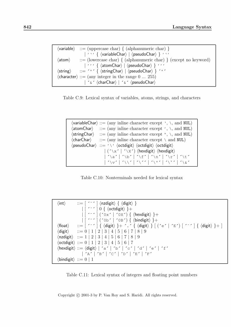
842 Language Syntax
〈variable〉 ::= (uppercase char) { (alphanumeric char) }| ’‘’ { 〈variableChar〉 | 〈pseudoChar〉 } ’‘’
〈atom〉 ::= (lowercase char) { (alphanumeric char) } (except no keyword)| ’’’ { 〈atomChar〉 | 〈pseudoChar〉 } ’’’
〈string〉 ::= ´ " ´ { 〈stringChar〉 | 〈pseudoChar〉 } ´ " ´
〈character〉 ::= (any integer in the range 0 ... 255)| ´ &´ 〈charChar〉 | ´ &´ 〈pseudoChar〉
Table C.9: Lexical syntax of variables, atoms, strings, and characters
〈variableChar〉 ::= (any inline character except ‘ , \ , and NUL)〈atomChar〉 ::= (any inline character except ’ , \ , and NUL)〈stringChar〉 ::= (any inline character except " , \ , and NUL)〈charChar〉 ::= (any inline character except \ and NUL)〈pseudoChar〉 ::= ’\’ 〈octdigit〉 〈octdigit〉 〈octdigit〉
| (´ \x ´ | ´ \X ´ ) 〈hexdigit〉 〈hexdigit〉| ´ \a ´ | ´ \b ´ | ´ \f ´ | ´ \n ´ | ´ \r ´ | ´ \t ´
| ´ \v ´ | ´ \\ ´ | ´ \ ´´ | ´ \" ´ | ´ \ `´ | ´ \& ´
Table C.10: Nonterminals needed for lexical syntax
〈int〉 ::= [ ´ ˜ ´ ] 〈nzdigit〉 { 〈digit〉 }| [ ´ ˜ ´ ] 0 { 〈octdigit〉 }+| [ ´ ˜ ´ ] (´ 0x ´ | ´ 0X´ ) { 〈hexdigit〉 }+| [ ´ ˜ ´ ] (´ 0b´ | ´ 0B´ ) { 〈bindigit〉 }+
〈float〉 ::= [ ´ ˜ ´ ] { 〈digit〉 }+ ´ . ´ { 〈digit〉 } [ (´ e´ | ´ E´ ) [ ´ ˜ ´ ] { 〈digit〉 }+ ]〈digit〉 ::= 0 | 1 | 2 | 3 | 4 | 5 | 6 | 7 | 8 | 9〈nzdigit〉 ::= 1 | 2 | 3 | 4 | 5 | 6 | 7 | 8 | 9〈octdigit〉 ::= 0 | 1 | 2 | 3 | 4 | 5 | 6 | 7〈hexdigit〉 ::= 〈digit〉 | ´ a´ | ´ b´ | ´ c ´ | ´ d´ | ´ e´ | ´ f ´
| ´ A´ | ´ B´ | ´ C | ´ D | ´ E´ | ´ F´
〈bindigit〉 ::= 0 | 1
Table C.11: Lexical syntax of integers and floating point numbers
Copyright c© 2001-3 by P. Van Roy and S. Haridi. All rights reserved.

C.6 Lexical syntax 843
C.6 Lexical syntax
This section defines the lexical syntax of Oz, i.e., how a character sequence istransformed into a sequence of tokens.
C.6.1 Tokens
Variables, atoms, strings, and characters
Table C.9 defines the lexical syntax for variable identifiers, atoms, strings, andcharacters in strings. An alphanumeric character is a letter (uppercase or low-ercase), a digit, or an underscore character. Unlike the previous sections whichdefine token sequences, this section defines character sequences. It follows fromthis syntax that an atom cannot have the same character sequence as a key-word unless the atom is quoted. Table C.10 defines the nonterminals neededfor Table C.9. “Any inline character” includes control characters and accentedcharacters. The NUL character has character code 0 (zero).
Integers and floating point numbers
Table C.11 defines the lexical syntax of integers and floating point numbers. Notethe use of the ´ ˜ ´ (tilde) for the unary minus symbol.
C.6.2 Blank space and comments
Tokens may be separated by any amount of blank space and comments. Blankspace is one of the characters tab (character code 9), newline (code 10), verticaltab (code 11), form feed (code 12), carriage return (code 13), and space (code32). A comment is one of three possibilities:
• A sequence of characters starting from the character % (percent) until theend of the line or the end of the file (whichever comes first).
• A sequence of characters starting from /* and ending with */, inclusive.This kind of comment may be nested.
• The single character ? (question mark). This is intended to mark theoutput arguments of procedures, as in:
proc {Max A B ?C} ... end
where C is an output. An output argument is an argument that gets boundinside the procedure.
Copyright c© 2001-3 by P. Van Roy and S. Haridi. All rights reserved.

844 Language Syntax
Copyright c© 2001-3 by P. Van Roy and S. Haridi. All rights reserved.

Appendix D
General Computation Model
“The removal of much of the accidental complexity of programmingmeans that the intrinsic complexity of the application is what’s left.”– Security Engineering, Ross J. Anderson (2001)
“If you want people to do something the right way, you must makethe right way the easy way.”– Traditional saying.
This appendix brings together all the general concepts introduced in the book.1
The resulting computation model is the shared-state concurrent model of Chap-ter 8. For convenience we call it the general computation model. While this modelis quite general, it is certainly not the final word in computation models. It isjust a snapshot that captures our current understanding of programming. Futureresearch will certainly change or extend it. The book mentions dynamic scopingand transaction support as two areas which require more support from the model.
The general computation model was designed in a layered fashion, by startingfrom a simple base model and successively adding new concepts. Each time wenoted a limitation in the expressiveness of a computation model, we had theopportunity to add a new concept. There was always a choice: either to keepthe model as is and make programs more complicated, or to add a concept andkeep programs simple. The decision to add the concept or not was based onour judgement of how complicated the model and its programs would be, whenconsidered together. “Complexity” in this sense covers both the expressivenessand ease of reasoning of the combination.
There is a strong element of creativity in this approach. Each concept bringssomething novel that was not there before. We therefore call it the creativeextension principle. Not all useful concepts end up in the general model. Someconcepts were added only to be superseded by later concepts. For example,this is the case for nondeterministic choice (Section 5.7.1), which is superseded
1Except for computation spaces, which underlie the relational computation model and theconstraint-based computation model.
Copyright c© 2001-3 by P. Van Roy and S. Haridi. All rights reserved.

846 General Computation Model
by explicit state. The general model is just one among many possible models ofsimilar expressiveness. Your judgement in this process may be different from ours.We would be interested to hear from any reader who has reached significantlydifferent conclusions.
Because earlier computation models are subsets of later ones, the later onescan be considered as frameworks inside of which many computation models cancoexist. In this sense, the general computation model is the most complete frame-work of the book.
D.1 Creative extension principle
We give an example to explain and motivate the creative extension principle.Let us start with the simple declarative language of Chapter 2. In that chapter,we added two concepts to the declarative language: functions and exceptions.But there was something fundamentally different in how we added each concept.Functions were added as a linguistic abstraction by defining a new syntax andshowing how to translate it into the kernel language (see Section 2.5.2). Excep-tions were added to the kernel language itself by adding new primitive operationsand defining their semantics (see Section 2.6). Why did we choose to do it thisway? We could have added functions to the kernel language and defined excep-tions by translation, but we did not. There is a simple but profound reason forthis: functions can be defined by a local translation but exceptions cannot. Atranslation of a concept is local if it requires changes only to the parts of theprogram that use the concept.
Starting with the declarative kernel language of Chapter 2, this book addedconcepts one by one. For each concept we had to decide whether to add it as alinguistic abstraction (without changing the kernel language) or to add it to thekernel language. A linguistic abstraction is a good idea if the translation is local.Extending the kernel language is a good idea if there is no local translation.
This choice is always a trade-off. One criterium is that the overall scheme,including both the kernel language and the translation scheme into the kernellanguage, should be as simple as possible. This is what we call the creativeextension principle. To some degree, simplicity is a subjective judgement. Thisbook makes one particular choice of what should be in the kernel languages andwhat should be outside. Other reasonable choices are certainly possible.
An additional constraint on the kernel languages of this book is that theyare all carefully chosen to be subsets of the full Oz language. This means thatthey are all implemented by the Mozart system. Users can verify that the kernellanguage translation of a program behaves in exactly the same way as the pro-gram. The only difference between the two is efficiency. This is useful both forlearning the kernel languages and for debugging programs. The Mozart systemimplements certain constructs more efficiently than their representation in thekernel language. For example, classes and objects in Oz are implemented more
Copyright c© 2001-3 by P. Van Roy and S. Haridi. All rights reserved.

D.2 Kernel language 847
〈s〉 ::=skip Empty statement| 〈s〉1 〈s〉2 Statement sequence| local 〈x〉 in 〈s〉 end Variable creation| 〈x〉1=〈x〉2 Variable-variable binding| 〈x〉=〈v〉 Value creation| { 〈x〉 〈y〉1 ... 〈y〉n} Procedure application| if 〈x〉 then 〈s〉1 else 〈s〉2 end Conditional| case 〈x〉 of 〈pattern〉 then 〈s〉1 else 〈s〉2 end Pattern matching| thread 〈s〉 end Thread creation| {ByNeed 〈x〉 〈y〉} Trigger creation| {NewName〈x〉} Name creation| 〈y〉=!! 〈x〉 Read-only view| try 〈s〉1 catch 〈x〉 then 〈s〉2 end Exception context| raise 〈x〉 end Raise exception| {FailedValue 〈x〉 〈y〉} Failed value| {NewCell 〈x〉 〈y〉} Cell creation| {Exchange 〈x〉 〈y〉 〈z〉} Cell exchange| {IsDet 〈x〉 〈y〉} Boundness test
Table D.1: The general kernel language
efficiently than their kernel definitions.
D.2 Kernel language
Table D.1 gives the kernel language of the general computation model. For clarity,we divide the table into five parts:
• The first part is the descriptive declarative model. This model allows tobuild complex data structures (rooted graphs whose nodes are records andprocedure values) but does not allow to calculate with them.
• The first and second parts taken together form the declarative concurrentmodel. This is the most general purely declarative model of the book. Allprograms written in this model are declarative.
• The third part adds security: the ability to build secure ADTs and programwith capabilities.
• The fourth part adds exceptions: the ability to handle exceptional situationsby doing non-local exits.
• The fifth part adds explicit state, which is important for building modularprograms and programs that can change over time.
Copyright c© 2001-3 by P. Van Roy and S. Haridi. All rights reserved.
848 General Computation Model
Taking all parts gives the shared-state concurrent model. This is the most generalmodel of the book. Chapter 13 gives the semantics of this model and all itssubsets.
D.3 Concepts
Let us now recapitulate the design methodology of the general model by startingwith a simple base model and briefly explaining what new expressiveness eachconcept brings. All models are Turing complete, that is, they are equivalent incomputing power to a Turing machine. However, Turing completeness is only asmall part of the story. The ease in which programs can be written or reasonedabout differs greatly in these models. Increased expressiveness typically goeshand in hand with increased difficulty to reason about programs.
D.3.1 Declarative models
Strict functional model The simplest practical model is strict functional pro-gramming with values. This model is defined in Section 2.7.1. In this model thereare no unbound variables; each new variable is immediately bound to a value.This model is close to the λ calculus, which contains just procedure definitionand application and leaves out the conditional and pattern matching. The λ cal-culus is Turing complete but is much too cumbersome for practical programming.
Sequential declarative model The sequential declarative model is defined inChapter 2. It contains all concepts in Table D.1 up to and including procedureapplication, conditionals, and pattern matching. It extends the strict functionalmodel by introducing dataflow variables. Doing this is a critical step becauseit prepares the way for declarative concurrency. For binding dataflow variables,we use a general operation called unification. This means that the sequentialdeclarative model does both deterministic logic programming and functional pro-gramming.
Threads The thread concept is defined in Section 4.1. Adding threads allowsthe model to express activities that execute independently. This model is stilldeclarative: adding threads leaves the result of a calculation unchanged. Only theorder in which the calculations are done is more flexible. Programs become moreincremental: incrementally building an input results in an incrementally-builtoutput. This is one form of declarative concurrency.
Triggers The trigger concept is defined in Section 4.5.1. Adding triggers allowsthe model to express demand-driven computations (laziness). This model is stilldeclarative since the result of a calculation is unchanged. Only the amount ofcalculation done to achieve the result changes (it can become smaller). Sometimes
Copyright c© 2001-3 by P. Van Roy and S. Haridi. All rights reserved.

D.3 Concepts 849
the demand-driven model can give results in cases where the data-driven modelwould go into an infinite loop. This is a second form of declarative concurrency.
D.3.2 Security
Names The name concept is defined in Section 3.7.5. A name is an unforgeableconstant that does not exist outside of a program. A name has no data oroperations attached to it; it is a first-class “key” or “right”. Names are the basisof programming techniques such as unbundled secure ADTs (see Section 6.4) andencapsulation control (see Section 7.3.3).
In the declarative model, secure ADTs can be built without names by usingprocedure values to hide values. The hidden value is an external reference ofthe procedure. But names add a crucial additional expressiveness. They make itpossible to program with rights. For example, separating data from operationsin a secure ADT or passing keys to programs to enable secure operations.
Strictly speaking, names are not declarative since successive calls to NewName
give different results. That is, the same program can return two different resultsif names are used to identify the result uniquely. But if names are used only toenforce security properties, then the model is still declarative.
Read-only views The read-only view concept is defined in Section 3.7.5. Aread-only view is a dataflow variable that can be read but not bound. It isalways paired with another dataflow variable that is equal to it but that canbe bound. Read-only views are needed to construct secure ADTs that exportunbound variables. The ADT exports the read-only view. Since it cannot bebound outside the ADT, this allows the ADT to maintain its invariant property.
D.3.3 Exceptions
Exception handling The exception concept is defined in Section 2.6.2. Addingexceptions allows to exit in one step from an arbitrarily large number of nestedprocedure calls. This allows to write programs that treat rare cases correctly,without complicating the program in the common case.
Failed values The failed value concept is defined in Section 4.9.1. A failedvalue is a special kind of value that encapsulates an exception. Any attempt touse the value or to bind it to a determined value will raise the exception. Whileexception handling happens within a single thread, failed values allow to passexceptions from the thread that detected the problem to other threads.
Failed values are useful in models that have both exceptions and triggers.Assume that a program calculates a value by a demand-driven computation, butthe computation raises an exception instead. What should the value be? It canbe a failed value. This will cause any thread that needs the value to raise anexception.
Copyright c© 2001-3 by P. Van Roy and S. Haridi. All rights reserved.

850 General Computation Model
D.3.4 Explicit state
Cells (explicit state) Explicit state is defined in Section 6.3. Adding stategives a program a memory: a procedure can change its behavior over successivecalls. In the declarative model this is not possible since all knowledge is in theprocedure’s arguments.
The stateful model greatly improves program modularity when compared tomodels without state. It increases the possibilities for changing a module’s im-plementation without changing its interface (see Section 4.7).
Ports (explicit state) Another way to add explicit state is by means of ports,which are a kind of asynchronous communication channel. As explained in Sec-tion 7.8, ports and cells are equivalent: each can implement the other in a simpleway. Ports are useful for programming message passing with active objects. Cellsare useful for programming atomic actions with shared state.
Boundness test (weak state) The boundness test IsDet lets us use dataflowvariables as a weak form of explicit state. The test checks whether a variable isbound or still unbound, without waiting when the variable is unbound. For manyprogramming techniques, knowing the binding status of a dataflow variable isunimportant. However, it can be important when programming a time-dependentexecution, i.e., to know what the instantaneous state is of an execution (seeSection 4.7.3).
Object-oriented programming Object-oriented programming is introducedin Chapter 7. It has the same kernel language as the stateful models. It is a richset of programming techniques that uses ideas from knowledge representation toimprove program structure. The two main ideas are to consider programs ascollections of interacting ADTs (which can be grouped together in associations)and to allow building ADTs incrementally (using inheritance, delegation, andforwarding).
D.4 Different forms of state
Adding explicit state is such a strong change to the model that it is important tohave weaker forms of state. In the above models we have introduced four formsof state. Let us summarize these forms in terms of how many times we can assigna variable, i.e., change its state. In order of increasing strength, they are:
• No assignment, i.e., programming with values only (monotonic execution).This is functional programming as it is usually understood. Programs arecompletely deterministic, i.e., the same program always gives the same re-sult.
Copyright c© 2001-3 by P. Van Roy and S. Haridi. All rights reserved.

D.5 Other concepts 851
• Single assignment, i.e., programming with dataflow variables (monotonicexecution). This is also functional programming, but more flexible since itallows declarative concurrency (with both lazy and eager execution). Pro-grams are completely deterministic, but the result can be given incremen-tally.
• Single assignment with boundness test, i.e., programming with dataflowvariables and IsDet (nonmonotonic execution). Programs are no longerdeterministic.
• Multiple assignment, i.e., programming with cells or ports (nonmonotonicexecution). Programs are no longer deterministic. This is the most expres-sive model.
We can understand these different forms of state in terms of an important prop-erty called monotonicity. At any time, a variable can be assigned to an element ofsome set S of values. Assignment is monotonic if as execution progresses, valuescan be removed from S but not added. For example, binding a dataflow variableX to a value reduces S from all possible values to just one value. A function fis monotonic if S1 ⊂ S2 =⇒ f(S1) ⊂ f(S2). For example, IsDet is nonmono-tonic since {IsDet X} returns false when X is unbound and true when X isbound, and {true } is not a subset of {false }. A program’s execution is mono-tonic if all its operations are monotonic. Monotonicity is what makes declarativeconcurrency possible.
D.5 Other concepts
D.5.1 What’s next?
The general computation model of this book is just a snapshot of an ongoingprocess. New concepts will continue to be discovered in the future using thecreative extension principle. What will these new concepts be? We cannot tellfor sure, since anticipating a discovery is the same as making that discovery! Butthere are hints about a few of the concepts. Two concepts that we are fairly sureabout, even though we do not know their final form, are dynamic scoping andtransaction support. With dynamic scoping the behavior of a component dependson its context. With transaction support the execution of a component can becanceled if it cannot complete successfully. According to the creative extensionprinciple, both of these concepts should be added to the computation model.
D.5.2 Domain-specific concepts
This book gives many general concepts that are useful for all kinds of programs.In addition to this, each application domain has its own set of concepts thatare useful only in that domain. These extra concepts complement the general
Copyright c© 2001-3 by P. Van Roy and S. Haridi. All rights reserved.
852 General Computation Model
concepts. For example, we can cite artificial intelligence [160, 136], algorithmdesign [41], object-oriented design patterns [58], multi-agent programming [205],databases [42], and numerical analysis [153].
D.6 Layered language design
The general computation model has a layered design. Each layer offers its ownspecial trade-off of expressiveness and ease of reasoning. The programmer canchoose the layer that is best-adapted to each part of the program. From the evi-dence presented in the book, it is clear that this layered structure is beneficial fora general-purpose programming language. It makes it easier for the programmerto say directly what he or she wants to say, without cumbersome encodings.
The layered design of the general computation model can be found to somedegree in many languages. Object-oriented languages such as Smalltalk, Eiffel,and Java have two layers: an object-oriented core and a second layer providingshared-state concurrency [60, 122, 10]. The functional language Erlang has twolayers: an eager functional core and a second layer providing message-passingconcurrency between active objects [9] (see also Section 5.6). Active objects aredefined within the functional core. The logic language Prolog has three layers:a logical core that is a simple theorem prover, a second layer modifying thetheorem prover’s operation, and a third layer providing explicit state [182] (seealso Section 9.7). The functional language Concurrent ML has three layers: aneager functional core, a second layer providing explicit state, and a third layerproviding concurrency [158]. The multiparadigm language Oz has many layers,which is why it was used as the basis for this book [180].
Copyright c© 2001-3 by P. Van Roy and S. Haridi. All rights reserved.

Bibliography
[1] Harold Abelson, Gerald Jay Sussman, and Julie Sussman. Structure andInterpretation of Computer Programs. The MIT Press, Cambridge, Mass,1985.
[2] Harold Abelson, Gerald Jay Sussman, and Julie Sussman. Structure andInterpretation of Computer Programs, Second Edition. The MIT Press,Cambridge, Mass, 1996.
[3] Ilies Alouini and Peter Van Roy. Le protocole reparti du langage DistributedOz (The distributed protocol of the Distributed Oz language). In ColloqueFrancophone d’Ingenierie de Protocoles (CFIP 99), pages 283–298, April1999.
[4] Edward G. Amoroso. Fundamentals of Computer Security Technology.Prentice Hall, 1994.
[5] Ross J. Anderson. Security Engineering: A Guide to Building DependableDistributed Systems. John Wiley & Sons, 2001.
[6] Gregory R. Andrews. Concurrent Programming: Principles and Practice.Addison-Wesley, 1991.
[7] Joe Armstrong. Higher-order processes in Erlang, January 1997. Unpub-lished talk.
[8] Joe Armstrong. Concurrency oriented programming in Erlang, November2002. Invited talk, Lightweight Languages Workshop 2002.
[9] Joe Armstrong, Mike Williams, Claes Wikstrom, and Robert Virding. Con-current Programming in Erlang. Prentice-Hall, Englewood Cliffs, N.J.,1996.
[10] Ken Arnold and James Gosling. The Java Programming Language, SecondEdition. Addison-Wesley, 1998.
[11] Arvind and R. E. Thomas. I-Structures: An efficient data type for func-tional languages. Technical Report 210, MIT, Laboratory for ComputerScience, 1980.
Copyright c© 2001-3 by P. Van Roy and S. Haridi. All rights reserved.

854 BIBLIOGRAPHY
[12] John Backus. Can programming be liberated from the von Neumann style?A functional style and its algebra of programs. Communications of theACM, 21(8):613–641, August 1978.
[13] John Backus. The history of FORTRAN I, II and III. ACM SIGPLANNotices, 13(8), August 1978.
[14] Henri E. Bal, Jennifer G. Steiner, and Andrew S. Tanenbaum. Programminglanguages for distributed computing systems. ACM Computing Surveys,21(3):261–322, September 1989.
[15] Holger Bar, Markus Bauer, Oliver Ciupke, Serge Demeyer, StephaneDucasse, Michele Lanza, Radu Marinescu, Robb Nebbe, Oscar Nierstrasz,Michael Przybilski, Tamar Richner, Matthias Rieger, Claudio Riva, Anne-Marie Sassen, Benedikt Schulz, Patrick Steyaert, Sander Tichelaar, andJoachim Weisbrod. The FAMOOS Object-Oriented Reengineering Hand-book. October 1999. Result of ESPRIT project FAMOOS.
[16] Philip A. Bernstein, Vassos Hadzilacos, and Nathan Goodman. Concurren-cy Control and Recovery In Database Systems. Addison-Wesley, 1987.
[17] Richard Bird. Introduction to Functional Programming using Haskell, Sec-ond Edition. Prentice Hall, 1998.
[18] Andrew D. Birrell and Bruce Jay Nelson. Implementing remote procedurecalls. ACM Transactions on Computer Systems, 2(1):39–59, February 1984.
[19] Darius Blasband. Language engineering: from a hobby, to a research activ-ity, to a trade, March 2002. Unpublished talk.
[20] Per Brand, Peter Van Roy, Raphael Collet, and Erik Klintskog. Pathredundancy in a mobile-state protocol as a primitive for language-basedfault tolerance. Technical Report RR2000-01, Departement d’IngenierieInformatique, Universite catholique de Louvain, 2000. Available athttp://www.info.ucl.ac.be.
[21] Ivan Bratko. PROLOG Programming for Articial Intelligence, Third Edi-tion. Addison-Wesley, 2000.
[22] Per Brinch Hansen. Structured multiprogramming. Communications of theACM, 15(7):574–578, July 1972.
[23] Per Brinch Hansen. Operating System Principles. Prentice Hall, 1973.
[24] Per Brinch Hansen. Java’s insecure parallelism. ACM SIGPLAN Notices,34(4):38–45, April 1999.
[25] Frederick P. Brooks, Jr. The Mythical Man-Month: Essays on SoftwareEngineering. Addison-Wesley, 1975.
Copyright c© 2001-3 by P. Van Roy and S. Haridi. All rights reserved.

BIBLIOGRAPHY 855
[26] Frederick P. Brooks, Jr. The Mythical Man-Month: Essays on SoftwareEngineering, Anniversary Edition. Addison-Wesley, 1995.
[27] Timothy A. Budd. Multiparadigm Programming in Leda. Addison-Wesley,1995.
[28] Luca Cardelli. A language with distributed scope. In Principles of Pro-gramming Languages (POPL), pages 286–297, 1995.
[29] Mats Carlsson et al. SICStus Prolog 3.8.1, December 1999. Available athttp://www.sics.se.
[30] Nicholas Carriero and David Gelernter. Linda in context. Communicationsof the ACM, 32(4):444–458, 1989.
[31] Nicholas Carriero and David Gelernter. Coordination languages and theirsignificance. Communications of the ACM, 35(2):96–107, February 1992.
[32] Emmanuel Chailloux, Pascal Manoury, and Bruno Pagano. Developpementd’applications avec Objective Caml. O’Reilly, Paris, France, 2000.
[33] Randy Chow and Theodore Johnson. Distributed Operating Systems andAlgorithms. Addison-Wesley, San Francisco, Calif., 1997.
[34] Keith L. Clark. PARLOG: the language and its applications. In A. J. Nij-man J. W. de Bakker and P. C. Treleaven, editors, Proceedings of the Con-ference on Parallel Architectures and Languages Europe (PARLE). VolumeII: Parallel Languages, volume 259 of Lecture Notes in Computer Science,pages 30–53, Eindhoven, The Netherlands, June 1987. Springer.
[35] Keith L. Clark and Frank McCabe. The control facilities of IC-Prolog.In D. Michie, editor, Expert Systems in the Micro-Electronic Age, pages122–149. Edinburgh University Press, Edinburgh, Scotland, 1979.
[36] Keith L. Clark, Frank G. McCabe, and Steve Gregory. IC-PROLOG —language features. In Keith L. Clark and Sten-Ake Tarnlund, editors, LogicProgramming, pages 253–266. Academic Press, London, 1982.
[37] Arthur C. Clarke. Profiles of the Future. Pan Books, 1973. Revised edition.
[38] William Clinger and Jonathan Rees. The revised4 report on the algorithmiclanguage Scheme. LISP Pointers, IV(3):1–55, July-September 1991.
[39] Helder Coelho and Jose C. Cotta. Prolog by Example: How to Learn, Teach,and Use It. Springer-Verlag, 1988.
[40] Alain Colmerauer. The birth of Prolog. In The Second ACM-SIGPLANHistory of Programming Languages Conference, pages 37–52, March 1993.ACM SIGPLAN Notices.
Copyright c© 2001-3 by P. Van Roy and S. Haridi. All rights reserved.

856 BIBLIOGRAPHY
[41] Thomas H. Cormen, Charles E. Leiserson, and Ronald L. Rivest. Introduc-tion to Algorithms. The MIT Press, McGraw-Hill, 1990.
[42] C. J. Date. An Introduction to Database Systems. Addison-Wesley, 1994.
[43] Harvey M. Deitel. An Introduction to Operating Systems. Addison-Wesley,1984.
[44] Serge Demeyer, Stephane Ducasse, Oscar Nierstrasz, and Ralph E. Johnson.Object Oriented Reengineering Patterns. Morgan Kaufmann, 2002.
[45] Edsger W. Dijkstra. A Primer of Algol 60 Programming. Academic Press,1962.
[46] Edsger W. Dijkstra. Go To statement considered harmful. Communicationsof the ACM, 11(3):147–148, March 1968.
[47] Denys Duchier. Loop support. Technical report, DFKI and Saarland Uni-versity, December 2001. Available at http://www.mozart-oz.org/.
[48] Denys Duchier, Claire Gardent, and Joachim Niehren. Concurrent con-straint programming in Oz for natural language processing. Technicalreport, Saarland University, Saarbrucken, Germany, 1999. Available athttp://www.ps.uni-sb.de/Papers/abstracts/oznlp.html.
[49] Denys Duchier, Leif Kornstaedt, and Christian Schulte. The Oz base envi-ronment. Technical report, Mozart Consortium, December 2001. Availableat http://www.mozart-oz.org/.
[50] Denys Duchier, Leif Kornstaedt, Christian Schulte, and Gert Smol-ka. A Higher-order Module Discipline with Separate Compilation, Dy-namic Linking, and Pickling. Technical report, Programming Sys-tems Lab, DFKI and Saarland University, 1998. DRAFT. Available athttp://www.mozart-oz.org/papers/.
[51] R. Kent Dybvig, Carl Bruggeman, and David Eby. Guardians in ageneration-based garbage collector, June 1993.
[52] E. W. Elcock. Absys: The first logic programming language–a retrospectiveand a commentary. Journal of Logic Programming, 9(1):1–17, 1990.
[53] Robert W. Floyd. Nondeterministic algorithms. Journal of the ACM,14(4):636–644, October 1967.
[54] Martin Fowler and Kendall Scott. UML Distilled: A Brief Guide to theStandard Object Modeling Language. Addison-Wesley Longman, Inc., 2000.
[55] Michael J. French. Invention and evolution: design in nature and engineer-ing. Cambridge University Press, 1988.
Copyright c© 2001-3 by P. Van Roy and S. Haridi. All rights reserved.

BIBLIOGRAPHY 857
[56] Daniel P. Friedman, Mitchell Wand, and Christopher T. Haynes. Essentialsof Programming Languages. The MIT Press, 1992.
[57] Tetsuro Fujise, Takashi Chikayama, Kazuaki Rokusawa, and AkihikoNakase. KLIC: A portable implementation of KL1. In Fifth GenerationComputing Systems (FGCS ’94), pages 66–79, December 1994.
[58] Erich Gamma, Richard Helm, Ralph Johnson, and John Vlissides. DesignPatterns: Elements of Reusable Object-Oriented Software. Addison-Wesley,1994.
[59] David Gelernter. Generative communication in Linda. ACM Transactionson Programming Languages and Systems, 7(1):80–112, January 1985.
[60] Adele Goldberg and David Robson. Smalltalk-80: The language and itsimplementation. Addison-Wesley, 1983.
[61] Danny Goodman. Dynamic HTML: The Definitive Reference, Second Edi-tion. O’Reilly & Associates, 2002.
[62] James Edward Gordon. The Science of Structures and Materials. ScientificAmerican Library, 1988.
[63] James Gosling, Bill Joy, and Guy Steele. The Java Language Specification.Addison-Wesley, 1996. Available at http://www.javasoft.com.
[64] Jim Gray and Andreas Reuter. Transaction Processing – Concepts andTechniques. Morgan Kaufmann, 1993.
[65] Donatien Grolaux. QTk module, 2000. Available athttp://www.mozart-oz.org/mozart-stdlib/index.html.
[66] Donatien Grolaux, Peter Van Roy, and Jean Vanderdonckt. QTk – a mixeddeclarative/procedural approach for designing executable user interfaces. In8th IFIP Working Conference on Engineering for Human-Computer Inter-action (EHCI’01), Lecture Notes in Computer Science, Toronto, Canada,May 2001. Springer-Verlag. Short paper.
[67] Donatien Grolaux, Peter Van Roy, and Jean Vanderdonckt. QTk – an inte-grated model-based approach to designing executable user interfaces. In 8thWorkshop on Design, Specification, and Verification of Interactive Systems(DSVIS 2001), Lecture Notes in Computer Science, Glasgow, Scotland,June 2001. Springer-Verlag.
[68] Robert H. Halstead, Jr. MultiLisp: A language for concurrent symboliccomputation. ACM Transactions on Programming Languages and Systems,7(4):501–538, October 1985.
Copyright c© 2001-3 by P. Van Roy and S. Haridi. All rights reserved.

858 BIBLIOGRAPHY
[69] Richard Hamming. The Art of Doing SCIENCE and Engineering: Learningto Learn. Gordon and Breach Science Publishers, 1997.
[70] Seif Haridi and Sverker Janson. Kernel Andorra Prolog and its computationmodel. In 7th International Conference on Logic Programming, pages 31–48. The MIT Press, June 1990.
[71] Seif Haridi, Peter Van Roy, Per Brand, Michael Mehl, Ralf Scheidhauer,and Gert Smolka. Efficient logic variables for distributed computing. ACMTransactions on Programming Languages and Systems, May 1999.
[72] Seif Haridi, Peter Van Roy, Per Brand, and Christian Schulte. Program-ming languages for distributed applications. New Generation Computing,16(3):223–261, May 1998.
[73] Seif Haridi, Peter Van Roy, and Gert Smolka. An overview of the design ofDistributed Oz. In the 2nd International Symposium on Parallel SymbolicComputation (PASCO 97). ACM, July 1997.
[74] Martin Henz. Objects for Concurrent Constraint Programming. Interna-tionale Series in Engineering and Computer Science. Kluwer Academic Pub-lishers, Boston, MA, USA, 1997.
[75] Martin Henz. Objects for Concurrent Constraint Programming, volume 426of The Kluwer International Series in Engineering and Computer Science.Kluwer Academic Publishers, Boston, November 1997.
[76] Martin Henz. Objects in Oz. Doctoral dissertation, Saarland University,Saarbrucken, Germany, May 1997.
[77] Martin Henz and Leif Kornstaedt. The Oz notation. Technical re-port, DFKI and Saarland University, December 1999. Available athttp://www.mozart-oz.org/.
[78] Martin Henz, Tobias Muller, and Ka Boon Ng. Figaro: Yet another con-straint programming library. In Workshop on Parallelism and Implementa-tion Technology for Constraint Logic Programming, International Confer-ence on Logic Programming (ICLP 99), 1999.
[79] Martin Henz, Gert Smolka, and Jorg Wurtz. Oz – a programming languagefor multi-agent systems. In 13th International Joint Conference on ArtificialIntelligence, pages 404–409. Morgan Kaufmann, August 1993.
[80] Martin Henz, Gert Smolka, and Jorg Wurtz. Oz—a programming languagefor multi-agent systems. In Ruzena Bajcsy, editor, 13th International JointConference on Artificial Intelligence, volume 1, pages 404–409, Chambery,France, 30 August–3 September 1993. Morgan Kaufmann Publishers.
Copyright c© 2001-3 by P. Van Roy and S. Haridi. All rights reserved.

BIBLIOGRAPHY 859
[81] Martin Henz, Gert Smolka, and Jorg Wurtz. Object-oriented concur-rent constraint programming in Oz. In Pascal Van Hentenryck and Vi-jay Saraswat, editors, Principles and Practice of Constraint Programming,pages 29–48, Cambridge, Mass., 1995. The MIT Press.
[82] Charles Antony Richard Hoare. Monitors: An operating system structuringconcept. Communications of the ACM, 17(10):549–557, October 1974.
[83] Charles Antony Richard Hoare. Communicating sequential processes. Com-munications of the ACM, 21(8):666–677, August 1978.
[84] Bruce K. Holmer, Barton Sano, Michael Carlton, Peter Van Roy, andAlvin M. Despain. Design and analysis of hardware for high performanceProlog. J. Log. Prog., 29:107–139, November 1996.
[85] Paul Hudak. Conception, evolution, and application of functional program-ming languages. Computing Surveys, 21(3):359–411, September 1989.
[86] Paul Hudak, John Peterson, and Joseph Fasel. A gentle introduction toHaskell version 98. Available at http://www.haskell.org/tutorial/.
[87] John Hughes. Why Functional Programming Matters. Computer Journal,32(2):98–107, 1989.
[88] Robert A. Iannucci. Parallel Machines: Parallel Machine Languages. TheEmergence of Hybrid Dataflow Computer Architectures. Kluwer, Dordrecht,the Netherlands, 1990.
[89] Daniel H. H. Ingalls. Design principles behind Smalltalk. Byte, 6(8):286–298, 1981.
[90] Joxan Jaffar and Michael Maher. Constraint logic programming: A survey.J. Log. Prog., 19/20:503–581, May/July 1994.
[91] Raj Jain. The Art of Computer Systems Performance Analysis. WileyProfessional Computing, 1991.
[92] Sverker Janson. AKL–A Multiparadigm Programming Language. PhD the-sis, Uppsala University and SICS, 1994.
[93] Sverker Janson and Seif Haridi. Programming paradigms of the Andor-ra Kernel Language. In International Symposium on Logic Programming,pages 167–183, October 1991.
[94] K. Jensen and N. Wirth. Pascal: User Manual and Report (Second Edition).Springer-Verlag, 1978.
[95] Richard Jones and Rafael Lins. Garbage Collection: Algorithms for Auto-matic Dynamic Memory Management. John Wiley & Sons, 1996.
Copyright c© 2001-3 by P. Van Roy and S. Haridi. All rights reserved.

860 BIBLIOGRAPHY
[96] Andreas Kagedal, Peter Van Roy, and Bruno Dumant.Logical State Threads 0.1, January 1997. Available athttp://www.info.ucl.ac.be/people/PVR/implementation.html.
[97] Gilles Kahn. The semantics of a simple language for parallel programming.In IFIP Congress, pages 471–475, 1974.
[98] Gilles Kahn and David B. MacQueen. Coroutines and networks of parallelprocesses. In IFIP Congress, pages 993–998, 1977.
[99] B. W. Kernighan and D. M. Ritchie. The C Programming Language (ANSIC), Second Edition. Prentice Hall, 1988.
[100] Gregor Kiczales, Jim des Rivieres, and Daniel G. Bobrow. The Art of theMetaobject Protocol. The MIT Press, 1991.
[101] Donald E. Knuth. The Art of Computer Programming: SeminumericalAlgorithms, volume 2. Addison-Wesley.
[102] Donald E. Knuth. The Art of Computer Programming: Fundamental Algo-rithms, volume 1. Addison-Wesley, 1973.
[103] Donald E. Knuth. Structured programming with go to statements. Com-puting Surveys, 6(4), December 1974.
[104] Leif Kornstaedt. Gump – a front-end generator for Oz. Tech-nical report, Mozart Consortium, December 2001. Available athttp://www.mozart-oz.org/.
[105] S. Rao Kosaraju. Analysis of structured programs. J. Computer and SystemSciences, 9(3), December 1974.
[106] Robert Kowalski. Logic for Problem Solving. North-Holland, 1979.
[107] James F. Kurose and Keith W. Ross. Computer networking: a top-downapproach featuring the Internet. Addison-Wesley, 2001.
[108] Leslie Lamport. LaTeX: A Document Preparation System, Second Edition.Addison-Wesley, 1994.
[109] Hugh C. Lauer and Roger M. Needham. On the duality of operating sys-tem structures. In Second International Symposium on Operating Systems,IRIA, October 1978. Reprinted in Operating Systems Review, 13(2), April1979, pp. 3–19.
[110] Doug Lea. Concurrent Programming in Java. Addison-Wesley, 1997.
[111] Doug Lea. Concurrent Programming in Java, Second Edition. Addison-Wesley, 2000.
Copyright c© 2001-3 by P. Van Roy and S. Haridi. All rights reserved.

BIBLIOGRAPHY 861
[112] Nancy Leveson and Clark S. Turner. An investigation of the Therac-25accidents. IEEE Computer, 26(7):18–41, July 1993.
[113] Henry Lieberman. Using prototypical objects to implement shared behav-ior in object-oriented systems. In 1st Conference on Object-Oriented Pro-gramming Languages, Systems, and Applications (OOPSLA 86), Septem-ber 1986. Also in Object-Oriented Computing, Gerald Peterson, ed., IEEEComputer Society Press, 1987.
[114] John Lloyd. Foundations of Logic Programming, Second Edition. Springer-Verlag, 1987.
[115] Nancy Lynch. Distributed Algorithms. Morgan Kaufmann, San Francisco,Calif., 1996.
[116] Bruce J. MacLennan. Principles of Programming Languages, Second Edi-tion. Saunders, Harcourt Brace Jovanovich, 1987.
[117] Michael Maher. Logic semantics for a class of committed-choice programs.In International Conference on Logic Programming (ICLP 87), pages 858–876, May 1987.
[118] Zohar Manna. The Mathematical Theory of Computation. McGraw-Hill,1974.
[119] Sun Microsystems. The Remote Method Invocation Specification, 1997.Available at http://www.javasoft.com.
[120] John McCarthy. LISP 1.5 Programmer’s Manual. The MIT Press, 1962.
[121] Michael Mehl, Christian Schulte, and Gert Smolka. Futuresand by-need synchronization for Oz. DRAFT. Available athttp://www.mozart-oz.org/papers/, May 1998.
[122] Bertrand Meyer. Object-Oriented Software Construction, Second Edition.Prentice Hall, 2000.
[123] Mark Miller, Marc Stiegler, Tyler Close, Bill Frantz, Ka-Ping Yee, ChipMorningstar, Jonathan Shapiro, and Norm Hardy. E: Open source dis-tributed capabilities, 2001. Available at http://www.erights.org.
[124] Mark Miller, Ka-Ping Yee, and Jonathan Shapiro. Capability myths de-molished. Draft available at http://zesty.ca/capmyths, 2003.
[125] Mark S. Miller, Chip Morningstar, and Bill Frantz. Capability-based finan-cial instruments. In Financial Cryptography 2000, Anguilla, British WestIndies, February 2000.
Copyright c© 2001-3 by P. Van Roy and S. Haridi. All rights reserved.

862 BIBLIOGRAPHY
[126] Robin Milner, Mads Tofte, and Robert Harper. Definition of Standard ML.MIT Press, Cambridge, MA, USA, 1990.
[127] J. Paul Morrison. Flow-Based Programming: A New Approach to Applica-tion Development. Van Nostrand Reinhold, 1994.
[128] Almetwally Mostafa, Ilies Alouini, and Peter Van Roy.Fault tolerant global store module, 2001. Available athttp://www.mozart-oz.org/mogul/info/mostafa/globalstore.html.
[129] Mozart Consortium. The Mozart Programming System version 1.2.3, De-cember 2001. Available at http://www.mozart-oz.org/.
[130] Peter Naur. Revised report on the algorithmic language ALGOL 60. Com-munications of the ACM, 1963.
[131] Rishiyur S. Nikhil. ID language reference manual version 90.1. TechnicalReport Memo 284-2, MIT, Computation Structures Group, July 1994.
[132] Rishiyur S. Nikhil. An overview of the parallel language Id – a foundationfor pH, a parallel dialect of Haskell. Technical report, Digital EquipmentCorporation, Cambridge Research Laboratory, 1994.
[133] Rishiyur S. Nikhil and Arvind. Implicit Parallel Programming in pH. Mor-gan Kaufmann, 2001.
[134] Donald A. Norman. The Design of Everyday Things. Basic Books, Inc.,1988.
[135] Theodore Norvell. Monads for the working Haskell programmer – a shorttutorial. Available at http://www.haskell.org/.
[136] Peter Norvig. Paradigms of Artificial Intelligence Programming: Case Stud-ies in Common Lisp. Morgan Kaufmann, 1992.
[137] K. Nygaard and O. J. Dahl. The Development of the SIMULA Languages,pages 439–493. Academic Press, 1981.
[138] Chris Okasaki. Purely Functional Data Structures. Cambridge UniversityPress, 1998.
[139] Richard A. O’Keefe. The Craft of Prolog. The MIT Press, 1990.
[140] Andreas Paepcke, editor. Object-Oriented Programming: The CLOS Per-spective. The MIT Press, 1993.
[141] Seymour Papert. Mindstorms: Children, Computers, and Powerful Ideas.The Harvester Press, 1980.
Copyright c© 2001-3 by P. Van Roy and S. Haridi. All rights reserved.

BIBLIOGRAPHY 863
[142] David Lorge Parnas. On the criteria to be used in decomposing systemsinto modules. Communications of the ACM, 15(12):1053–1058, December1972.
[143] David Lorge Parnas. Teaching programming as engineering. In 9th In-ternational Conference of Z Users, volume 967 of Lecture Notes in Com-puter Science. Springer-Verlag, 1995. Reprinted in Software Fundamentals,Addison-Wesley, 2001.
[144] David Lorge Parnas. Software Fundamentals. Addison-Wesley, 2001.
[145] F. Paterno. Model-based Design and Evaluation of Interactive Applications.Springer-Verlag, Berlin, 1999.
[146] David A. Patterson and John L. Hennessy. Computer Architecture: AQuantitative Approach, Second Edition. Morgan Kaufmann, 1996.
[147] Simon Peyton Jones. Tackling the awkward squad: monadic input/output,concurrency, exceptions, and foreign-language calls in Haskell. In TonyHoare, Manfred Broy, and Ralf Steinbruggen, editors, Engineering theoriesof software construction, pages 47–96. IOS Press, 2001. Presented at the2000 Marktoberdorf Summer School.
[148] Simon Peyton Jones, editor. Haskell 98 language and libraries: The revisedreport. Cambridge University Press, 2003. Also published as the January2003 Special Issue of the Journal of Functional Programming.
[149] Simon Peyton Jones, Andrew Gordon, and Sigbjorn Finne. ConcurrentHaskell. In Principles of Programming Languages (POPL), 1996.
[150] Shari Lawrence Pfleeger. Software Engineering: The Production of QualitySoftware, Second Edition. Macmillan, 1991.
[151] David Plainfosse and Marc Shapiro. A survey of distributed garbage collec-tion techniques. In the International Workshop on Memory Management,volume 986 of Lecture Notes in Computer Science, pages 211–249, Berlin,September 1995. Springer-Verlag.
[152] R. J. Pooley. An Introduction to Programming in SIMULA. BlackwellScientific Publishers, 1987.
[153] William H. Press, Brian P. Flannery, Saul A. Teukolsky, and William T.Vetterling. Numerical Recipes: The Art of Scientific Computing. CambridgeUniversity Press, 1986.
[154] Roger S. Pressman. Software Engineering, Sixth Edition. Addison-Wesley,2000.
Copyright c© 2001-3 by P. Van Roy and S. Haridi. All rights reserved.

864 BIBLIOGRAPHY
[155] Mahmoud Rafea, Fredrik Holmgren, Konstantin Popov, Seif Haridi, SteliosLelis, Petros Kavassalis, and Jakka Sairamesh. Application architecture ofthe Internet simulation model: Web Word of Mouth (WoM). In IASTEDInternational Conference on Modelling and Simulation MS2002, May 2002.
[156] Eric Raymond. The cathedral and the bazaar, May 1997.
[157] Juris Reinfelds. Teaching of programming with a programmer’s theoryof programming. In Informatics Curricula, Teaching Methods, and BestPractice (ICTEM 2002, IFIP Working Group 3.2 Working Conference).Kluwer Academic Publishers, 2002.
[158] John H. Reppy. Concurrent Programming in ML. Cambridge UniversityPress, 1999.
[159] James Rumbaugh, Ivar Jacobson, and Grady Booch. The Unified ModelingLanguage reference manual. Addison-Wesley, 1999.
[160] Stuart Russell and Peter Norvig. Artificial Intelligence: A modern ap-proach. Prentice Hall, 1995.
[161] Oliver Sacks. The Man Who Mistook His Wife for a Hat: And OtherClinical Tales. Touchstone Books, 1998.
[162] Jakka Sairamesh, Petros Kavassalis, Manolis Marazakis, Christos Nikolaos,and Seif Haridi. Information cities over the Internet: Taxonomy, principlesand architecture. In Digital Communities 2002, November 2001.
[163] Vijay A. Saraswat. Concurrent Constraint Programming. The MIT Press,1993.
[164] Vijay A. Saraswat, Martin C. Rinard, and Prakash Panangaden. Semanticfoundations of concurrent constraint programming. In Principles of Pro-gramming Languages (POPL), pages 333–352, 1991.
[165] Steve Schneider. Concurrent and Real-time Systems: The CSP Approach.John Wiley & Sons, 2000.
[166] Bruce Schneier. Applied Cryptography. John Wiley & Sons, 1996.
[167] Christian Schulte. Programming constraint inference engines. In Gert Smol-ka, editor, Proceedings of the Third International Conference on Principlesand Practice of Constraint Programming, volume 1330 of Lecture Notesin Computer Science, pages 519–533, Schloß Hagenberg, Austria, October1997. Springer-Verlag.
[168] Christian Schulte. Comparing trailing and copying for constraint program-ming. In International Conference on Logic Programming (ICLP 99), pages275–289. The MIT Press, November 1999.
Copyright c© 2001-3 by P. Van Roy and S. Haridi. All rights reserved.

BIBLIOGRAPHY 865
[169] Christian Schulte. Programming Constraint Inference Services. PhD thesis,Saarland University, Fachbereich Informatik, Saarbrucken, Germany, 2000.
[170] Christian Schulte. Programming deep concurrent constraint combinators.In Enrico Pontelli and Vıtor Santos Costa, editors, Practical Aspects ofDeclarative Languages, Second International Workshop, PADL 2000, vol-ume 1753 of Lecture Notes in Computer Science, pages 215–229, Boston,MA, USA, January 2000. Springer-Verlag.
[171] Christian Schulte. Oz Explorer – visual constraint programming sup-port. Technical report, Mozart Consortium, December 2001. Availableat http://www.mozart-oz.org/.
[172] Christian Schulte. Programming Constraint Services: High-Level Program-ming of Standard and New Constraint Services, volume 2302 of LectureNotes in Computer Science. Springer-Verlag, 2002.
[173] Christian Schulte and Gert Smolka. Encapsulated search for higher-orderconcurrent constraint programming. In 1994 International Symposium onLogic Programming, pages 505–520. The MIT Press, November 1994.
[174] Christian Schulte and Gert Smolka. Finite domain constraint program-ming in Oz. A tutorial. Technical report, DFKI and Saarland University,December 1999. Available at http://www.mozart-oz.org/.
[175] Ehud Shapiro. A subset of Concurrent Prolog and its interpreter. Tech-nical Report TR-003, Institute for New Generation Computer Technology(ICOT), Cambridge, Mass., January 1983.
[176] Ehud Shapiro, editor. Concurrent Prolog: Collected Papers, volume 1-2.The MIT Press, Cambridge, Mass., 1987.
[177] Ehud Shapiro. The family of concurrent logic programming languages.ACM Computing Surveys, 21(3):413–510, September 1989.
[178] Daniel P. Siewiorek, C. Gordon Bell, and Allen Newell. Computer Struc-tures: Principles and Examples. McGraw-Hill Book Company, 1982.
[179] Gert Smolka. The definition of Kernel Oz. In Andreas Podelski, editor,Constraints: Basics and Trends, volume 910 of Lecture Notes in ComputerScience, pages 251–292. Springer-Verlag, Berlin, 1995.
[180] Gert Smolka. The Oz programming model. In Computer Science Today, vol-ume 1000 of Lecture Notes in Computer Science, pages 324–343. Springer-Verlag, Berlin, 1995.
[181] Guy L. Steele, Jr. Common LISP: The Language. Digital Press, 1984.
Copyright c© 2001-3 by P. Van Roy and S. Haridi. All rights reserved.

866 BIBLIOGRAPHY
[182] Leon Sterling and Ehud Shapiro. The Art of Prolog–Advanced ProgrammingTechniques. Series in Logic Programming. The MIT Press, 1986.
[183] Marc Stiegler. The E Language in a Walnut. 2000. Draft, available athttp://www.erights.org.
[184] Bjarne Stroustrup. The C++ Programming Language, Third Edition.Addison-Wesley, 1997.
[185] Giancarlo Succi and Michele Marchesi. Extreme Programming Examined.Addison-Wesley, 2001.
[186] Sun Microsystems. The Java Series. Sun Microsystems, Mountain View,Calif., 1996. Available at http://www.javasoft.com.
[187] Clemens Szyperski. Component Software: Beyond Object-Oriented Pro-gramming. Addison-Wesley and ACM Press, 1999.
[188] Andrew Taylor. High-Performance Prolog Implementation. PhD thesis,Basser Department of Computer Science, University of Sydney, June 1991.
[189] Gerard Tel. An Introduction to Distributed Algorithms. Cambridge Univer-sity Press, Cambridge, United Kingdom, 1994.
[190] Evan Tick. The deevolution of concurrent logic programming. J. Log. Prog.,23(2):89–123, May 1995.
[191] Kasunori Ueda. Guarded Horn Clauses. In Eiti Wada, editor, Proceedingsof the 4th Conference on Logic Programming, volume 221 of Lecture Notesin Computer Science, pages 168–179, Tokyo, Japan, July 1985. Springer.
[192] Jeffrey D. Ullman. Elements of ML Programming. Prentice Hall, 1998.
[193] Peter Van Roy. VLSI-BAM Diagnostic Generator, 1989. Prolog programto generate assembly language diagnostics. Aquarius Project, University ofCalifornia, Berkeley.
[194] Peter Van Roy. Can Logic Programming Execute as Fast as ImperativeProgramming? PhD thesis, Computer Science Division, University of Cal-ifornia at Berkeley, December 1990. Technical Report UCB/CSD 90/600.
[195] Peter Van Roy. 1983–1993: The wonder years of sequential Prolog imple-mentation. J. Log. Prog., 19/20:385–441, May/July 1994.
[196] Peter Van Roy, Per Brand, Denys Duchier, Seif Haridi, Martin Henz, andChristian Schulte. Logic programming in the context of multiparadigm pro-gramming: the Oz experience. Theory and Practice of Logic Programming,2003. To appear.
Copyright c© 2001-3 by P. Van Roy and S. Haridi. All rights reserved.

BIBLIOGRAPHY 867
[197] Peter Van Roy, Per Brand, Seif Haridi, and Raphael Collet. Alightweight reliable object migration protocol. In Henri E. Bal, BoumedieneBelkhouche, and Luca Cardelli, editors, Internet Programming Languages,volume 1686 of Lecture Notes in Computer Science. Springer Verlag, Octo-ber 1999.
[198] Peter Van Roy and Alvin Despain. High-performance logic programmingwith the Aquarius Prolog compiler. IEEE Computer, pages 54–68, January1992.
[199] Peter Van Roy and Seif Haridi. Teaching programming broadly and deeply:the kernel language approach. In Informatics Curricula, Teaching Meth-ods, and Best Practice (ICTEM 2002, IFIP Working Group 3.2 WorkingConference). Kluwer Academic Publishers, 2002.
[200] Peter Van Roy and Seif Haridi. Teaching programming with the kernellanguage approach. In Workshop on Functional and Declarative Program-ming in Education (FDPE02), at Principles, Logics, and Implementationsof High-Level Programming Languages (PLI2002). University of Kiel, Ger-many, October 2002.
[201] Peter Van Roy, Seif Haridi, Per Brand, Gert Smolka, Michael Mehl, andRalf Scheidhauer. Mobile objects in Distributed Oz. ACM Transactions onProgramming Languages and Systems, 19(5):804–851, September 1997.
[202] Arthur H. Veen. Dataflow machine architecture. ACM Computing Surveys,18(4):365–396, December 1986.
[203] Duncan J. Watts. Small Worlds: The Dynamics of Networks between Orderand Randomness. Princeton University Press, 1999.
[204] Gerhard Weikum and Gottfried Vossen. Transactional Information Sys-tems: Theory, Algorithms, and the Practice of Concurrency Control andRecovery. Morgan Kaufmann, 2002.
[205] Gerhard Weiss, editor. Multiagent Systems: A Modern Approach to Dis-tributed Artificial Intelligence. The MIT Press, 1999.
[206] Claes Wikstrom. Distributed programming in Erlang. In the 1st Interna-tional Symposium on Parallel Symbolic Computation (PASCO 94 ), pages412–421, Singapore, September 1994. World Scientific.
[207] Herbert S. Wilf. generatingfunctionology. Academic Press, 1994.
[208] Glynn Winskel. The Formal Semantics of Programming Languages. Foun-dations of Computing Series. The MIT Press, Cambridge, Massachusetts,1993.
Copyright c© 2001-3 by P. Van Roy and S. Haridi. All rights reserved.

868 BIBLIOGRAPHY
[209] Noel Winstanley. What the hell are Monads?, 1999. Available athttp://www.haskell.org.
[210] David Wood. Use of objects and agents at Symbian, September 2000. Talkgiven at the Newcastle Seminar on the Teaching of Computing Science.
[211] Matthias Zenger and Martin Odersky. Implementing extensible compil-ers. In 1st International Workshop on Multiparadigm Programming withObject-Oriented Languages, pages 61–80. John von Neumann Institute forComputing (NIC), June 2001. Workshop held as part of ECOOP 2001.
Copyright c© 2001-3 by P. Van Roy and S. Haridi. All rights reserved.

Index
! (escaped variable marker), 506, 515! (cut) operation (in Prolog), 675, 679,
682$ (nesting marker), 54, 85, 363, 373* (multiplication) operation, 56, 823+ (addition) operation, 56, 823- (subtraction) operation, 56, 823. (field selector) operation, 56, 828. := (dictionary/array assignment) state-
ment, 439, 440, 841. := (dictionary/array exchange) ex-
pression, 841/ (floating division) operation, 56, 824:= (state assignment) statement, 499,
502:= (state exchange) expression, 502= (binding) operation, 45, 47, 48, 101== (equality) comparison, 57=< (less or equal) comparison, 57? (output argument), 59, 843@(state access) operation, 499, 502# (tupling) constructor, 143, 827, 833& (inline character) operator, 822< (strictly less) comparison, 57, 832<= (optional method argument) opera-
tor, 505> (strictly greater) comparison, 57>= (greater or equal) comparison, 57\ (backslash), 823\= (inequality) comparison, 57˜ (minus sign), 822| (list pairing) constructor, 54
Abelson, Harold, xxxiii, 43absolute error, 122abstract machine, 43
relation to semantic rules, 789substitution-based, 128–129
abstract syntax tree, 164, 165
abstraction, xxxiiactive object, 563class, 498collection, 438collector, 192, 326, 434, 488connector, 326control, 125database, 667encapsulated search, 637hierarchy in object-oriented program-
ming, 552lifecycle, 42Linda (tuple space), 594linguistic, 40–41, 126
case (pattern matching), 793class , 554conc (concurrent composition), 283delegation, 520for loop, 190, 451fun (function), 85functor (software component),
227gate (logic gate), 276local vs. global translation, 846monitor, 601parameter passing, 438protected scope (Java), 574while loop, 451
list comprehension, 307lock, 590, 606loop, 184mailbox, 398monitor, 600pipe of stream objects, 567procedural, 180protector, 326queue, 149, 303replicator, 326software component, 223
Copyright c© 2001-3 by P. Van Roy and S. Haridi. All rights reserved.

870 INDEX
specialization hierarchy, xxxiitermination detection, 390transaction, 608tuple space, 594
access (cell operation), 18, 422ACCLAIM project, xlaccumulator, 142–144
breadth-first traversal, 159declarative state, 416depth-first traversal, 158for loop, 192limit of declarative model, 315loop abstraction, 262loops, 187parser, 163Prolog, 143relation to difference lists, 144relation to fold operation, 187tree traversal, 195
ACID properties, 609action (in GUI), 693active memory, 75
size, 175, 314ActiveX, 466adder
n-bit, 347full, 273
addressIP, 209URL, 214
adjacency list, 468Adjoin operation, 440, 828AdjoinAt operation, 440, 828adjunction (environment), 63ADT (abstract data type), see typeadversary, 211agent, 357
concurrent component, 370message-passing approach, 584
Alarm operation, 309, 401alarm clock, xxixalgebra, xxxvii, 115algorithm
breadth-first traversal, 159cached state, 739compression, 180
copying dual-space garbage collec-tion, 79
Dekker’s algorithm for mutual ex-clusion, 578
depth-first traversal, 158distributed garbage collection, 740distributed locking, 727distributed unification, 739elevator, 384Flavius Josephus problem, 565Floyd-Warshall, 473garbage collection, 77Hamming problem, 298linear congruential generator, 478mergesort, 140, 169
generic version, 184mobile state, 739Newton’s method for square roots,
122nonalgorithmic programming, 634parallel transitive closure, 473Pascal’s triangle, 12quicksort, 235, 531random number generation, 476termination detection, 390thread scheduling, 245transitive closure, 467tree, 154tree drawing, 161, 278unification, 102word frequency, 201
aliasing, 426, 452allocation, 76always true (in temporal logic), 611Anderson, Ross J., 750, 845Andrews, Gregory, 590andthen operator, 84Append operation, 831apple, 493Apple Corporation, xlapplet, 724application
FlexClock example, 707ping-pong example, 310standalone, 225
Java, 561video display, 321
Copyright c© 2001-3 by P. Van Roy and S. Haridi. All rights reserved.

INDEX 871
applicative order reduction, 336Aquarius Prolog, 143arbitrary precision integer arithmetic, 6,
823arch, xxxiiarithmetic, 56Arity operation, 56, 828arity, 442, 828Armstrong, Joe, 590Arnold, Ken, 543array, 439
extensible, 443usage trade-offs, 442
ASCII (American Standard Code for In-formation Interchange), 462, 721
ask operation, 786, 793assert/1 operation (in Prolog), 669, 675assertion, 448assignment
axiomatic semantics, 449cell operation, 18, 422in-place, 314Java, 559monotonic, 851multiple, 851single, 44, 851to iteration variable, 191
association, 537, 850association list, 491asynchronous failure detection, 745ATM (Asynchronous Transfer Mode), 395atom, 53, 825
defining scope, 514predicate calculus, 645propositional logic, 644
atomic action, 588–625approaches to concurrency, 581reasoning, 588when to use, 584
atomicity, 23, 609AtomToString operation, 826attribute
final (in Java), 550, 558initialization, 503object, 502
availability, 717AXD301 ATM switch, 395
axiom, 646axiomatic semantics, 40, 444–453, 644
Backus, John, 34bagof/3 operation (in Prolog), 638, 683Bal, Henri, 340batching
distributed stream, 725, 730object invocations, 546, 572
Baum, L. Frank, 3Bernstein, Philip A., 609billion dollar budget, 527binary integer, 822binding
basic and nonbasic, 792dynamic, 511static, 512variable-variable, 48
bistable circuit (digital logic), 274blank space (in Oz), 843Blasband, Darius, 654block
file, 297imperative language, 491memory, 76, 77Smalltalk, 549
blocking operation, 243blue cut (in Prolog), 679, 681book
Component Software: Beyond Object-Oriented Programming, 466
Concurrent Programming in Erlang,590
Concurrent Programming in Java,589
Concurrent Programming: Princi-ples and Practice, 590
Object-Oriented Software Construc-tion, 495
Software Fundamentals, 466Structure and Interpretation of Com-
puter Programs, xxxiiiThe Art of Prolog, 679The Mythical Man-Month, 466Transaction Processing: Concepts and
Techniques, 590boolean, 53
Copyright c© 2001-3 by P. Van Roy and S. Haridi. All rights reserved.

872 INDEX
Borges, Jorge Luis, 633bottom-up software development, 455bound identifier occurrence, 65bounded buffer, 268
data-driven concurrent version, 268lazy version, 295monitor version, 602
brand, 504Brand, Per, xlbreadth-first traversal, 159break statement, 491break operation, 491bridge building, xxx, xxxiBrinch Hansen, Per, 600Brooks, Jr., Frederick P., 466Browser tool, see Mozart Programming
Systemby-need execution, 286–289, 798
WaitQuiet operation, 800Multilisp, 342Oz 3, 811
ByNeed operation, 287byte (in Java), 560bytestring, 833
calculator, 3calculus
analysis, 173first-order predicate, 645foundational, xxxiλ, xxxi, 43, 98, 336, 351, 795, 807,
813, 848π, xxxi, 43, 55, 807
call/1 operation (in Prolog), 675call by ..., see parameter passingcall graph, 318capability, 211
declarative, 213method label, 516revocable, 433, 488
Cardelli, Luca, 728cascading abort, 613case statement, 68, 793catch clause (in try ), 95causality, 241, 361Ceil operation, 824
cell (explicit state), 417, 422–425, 797,850
cellular phone, xxix, xxxiichannel
asynchronous, 355, 393component interface, 459dataflow variable, 337many-shot, 371one-shot, 371, 376port, 354synchronous, 629
character, 822alphanumeric, 51, 843Java, 560
choice statement, 636, 778chunk, 829
reflection, 524Church-Rosser Theorem, 336Churchill, Winston, 453Clarke, Arthur C., 106, 314class, 421, 493, 495, 497, 501, 552
abstract, 528, 552active object, 564common limitations, 545complete ADT definition, 498concrete, 529, 532, 552delegation, 517diagram, 534, 539encapsulation control, 512event manager example, 570forwarding, 517generic, 531higher-order programming, 532implementation, 554incremental ADT definition, 507inheritance, 508inner, 546inner (in Java), 558introduction, 20member, 502metaclass, 553mixin, 572parameterized, 531patching, 527programming techniques, 524reflection of object state, 523structure view, 525
Copyright c© 2001-3 by P. Van Roy and S. Haridi. All rights reserved.

INDEX 873
substitution property, 525, 527type view, 525
clausecase statement, 84definite, 662Erlang, 396Horn, xxxv, 647, 652, 662, 675
clockcontext-sensitive, 707digital circuit, 275digital logic, 271synchronization, 313
clonearray, 440computation space, 774dictionary, 441object, 523
closed distribution, 737closure, see procedure valuecluster, 717code duplication, 496code generator, 164coherence
between graphical views, 704cache, 463, 739network transparency, 726
collector, 192, 326, 434, 488COM (Component Object Model), 466combinations, 6combinator, 282comment (in Oz), 843common self, 517compaction, 77comparison, 57compilation
separate, 107standalone, 232
ping-pong example, 310unit, 225, 420, 457, 818
compiler, 163, 674extensible, 548Prolog, 676smart-aleck, 314
Compiler Panel tool, see Mozart Pro-gramming System
complete value, 47completeness
Turing, 848complexity
amortized, 149, 177, 440asymptotic, 169banker’s method, 178big-oh notation, 170introduction, 12–13physicist’s method, 178space, 175time, 13, 169worst-case, 169, 175
component, 114, 185, 223abstraction, 462avoiding dependencies, 463diagram, 360encapsulates a design decision, 462functor, 420further reading, 466future role, 464graph, 465implementation, 224interface, 224module, 420software, 224
compositionality, 419, 631class, 507encapsulated search, 638exception handling, 92Solve operation, 638
computation, 63iterative, 120recursive, 126secure, 210
computation model, xxvii, 31active object, 563constraint-based, 639, 653, 764data-driven concurrent, 240declarative concurrent with exceptions,
332declarative concurrent, 239declarative with exceptions, 93declarative, 50demand-driven concurrent with ex-
ceptions, 333demand-driven concurrent, 240, 286descriptive declarative, 117distributed, 718
Copyright c© 2001-3 by P. Van Roy and S. Haridi. All rights reserved.

874 INDEX
graph notation, 741extended relational, 673general, 845job-based concurrent, 628lazy concurrent, 240, 286maximally concurrent, 585, 628, 772message-passing concurrent, 354nondeterministic concurrent, 402, 653object-based, 543object-oriented, 496order-determining concurrent, 277relational, 635secure declarative, 205shared-state concurrent, 581stateful concurrent, 584, 786stateful, 421strict functional, 99atomic action, 588closed, 326concurrent constraint, 810concurrent logic programming, 292,
402, 813design principles, xxxiii, 845determinate concurrent constraint pro-
gramming, 343determinate parallel programming,
343deterministic logic programming, 648Erlang, 394Haskell, 328insecure, 326Java, 557, 625nondeterministic logic programming,
650open, 326partial failure, 326, 744Prolog, 674secure, 326semantics, 783using models together, xxxiv, 325
computation space, 666, 759computer engineering, xxxvicomputer science, xxxvicomputing, see informaticsconc statement, 283concurrency, 322
competitive, 259
cooperative, 259dataflow, 17declarative, 237, 247, 806Erlang, 394further reading, 589importance for programming, xxxinteractive interface, 90interleaving, 22introduction, 16Java, 625monitor safety, 601nondeterminism, 21order-determining, 277practical approaches, 581queue, 592rules of thumb, 584teaching, xxxvitransaction, 610
concurrency control, 573, 611, 751concurrent composition, 281, 393condition variable, 607conditional critical section, 605configuration, 787confinement
failure in declarative model, 250partial failure, 715transaction, 610
confluence, 336, 807connector, 326cons cell (list pair), 7, 54, 830consistency (in transaction), 609consistency protocol, 718constraint, 248
tree drawing, 161constructor, 560consumer, 262context, 92context-sensitive
grammar, 36GUI design, 707
continuation, 385procedure, 367record, 366
contract, 418contrapositive law, 644control abstraction
try – finally , 349
Copyright c© 2001-3 by P. Van Roy and S. Haridi. All rights reserved.

INDEX 875
break, 491concurrent composition, 282CSP communication, 629Erlang mailbox, 410iteration, 125loops, 186need for higher-order, 182Smalltalk block, 549
coordination model, 460, 594CORBA (Common Object Request Bro-
ker Architecture), 364, 466coroutine, 279, 459
relation to laziness, 290, 293, 582correctness, 644
introduction, 11–12Cray-1 computer, 178critical region, 590cryptography
unique name generation, 210curriculum (informatics), xxxvicurrying, xxxv, 196–197, 236
Haskell, 329cyclic structures, 104
dangling reference, 76, 183, 463Danvy, Olivier, 236data structure
active, 78class, 501cyclic, 102dictionary, 199difference list, 144difference structure, 144ephemeral, 150external, 79graph, 468higher order, 185infinite, 14list, 54, 132long-lived, 80partial, 47persistent, 303protected, 206, 429queue, 149record, 53recursive, 133size, 176
stack, 198store, 76tree, 153tuple, 53
data type, see typedata-driven execution, see eager execu-
tiondatabase, 667
deductive, 668distributed, 625in-memory, 176Mnesia (in Erlang), 395persistence, 667query, 668relational, 667shared-state concurrency, 584transaction, 608update, 668
dataflow, 61channel, 337declarative model, 18error, 91examples, 252I-structure, 342introduction, 17lazy execution, 290parallel transitive closure, 473rubber band, 255variable, 44, 49, 50
Date, C.J., 668Dawkins, Richard, 418DBMS (Database Management System),
668DCOM (Distributed Component Object
Model), 466deadlock, 613
callback, 365concurrency control, 613detection, 614digital logic simulation, 274lazy execution, 293prevention, 614
deallocation, 76debugging, 522
dangling reference, 77, 183declarative component, 314distributed application, 751
Copyright c© 2001-3 by P. Van Roy and S. Haridi. All rights reserved.

876 INDEX
erroneous suspension, 50, 91inspecting object attributes, 507
declarative, 113, 415declarative concurrency, see concurren-
cy, declarativedeclarative program, 248declare statement, 4, 88
syntax convention of book, xliii, 88define clause (in functor), 224Definite Clause Grammar (DCG), 143,
662Delay operation, 309delay gate (digital logic), 274delay operation (in Multilisp), 342delay point, 588delegation, 518–522
otherwise method, 506Dell Corporation, xl, 204, 475demand-driven execution, see lazy exe-
cutionDe Morgan’s law, 644denotational semantics, 40dependency
component, 227dataflow, 341declarative component, 314, 324grammar context, 36inheritance, 421order-determining concurrency, 277removal of sequential, 393sequential model, 419word frequency application, 231
depth-first traversal, 158dereferencing, 47design methodology
concurrent program, 372language, 42, 335, 549, 813, 852large program, 454small program, 221
design patterns, xxxv, 421, 493, 540–543
Composite pattern, 540destructive assignment
interaction with call by name, 490determinism (declarative programming),
113diagnostics, 633
dialog model, 704dictionary, 199, 440
declarative, 199efficiency, 203internal structure, 203list-based implementation, 200relation implementation, 671relation to record, 441relation to stream, 442secure declarative, 210standalone, 228stateful, 201tree-based implementation, 200tuple space implementation, 596usage trade-offs, 442word frequency implementation, 475Word of Mouth simulation, 482
difference list, 144difference structure, 144digital logic, 271
satisfiability problem, 179Dijkstra, Edsger Wybe, 444directed graph, 467disconnected operation, 747discriminant, 181disentailment, 105–106, 785distributed lexical scoping, 728distributed system, 326, 358, 363, 392,
713closed, 737open, 514, 715, 717, 720
Distribution Panel tool, see Mozart Pro-gramming System
div (integer division) operation, 56, 823divide-and-conquer, 140domain model, 703domain of discourse, 645dotted pair, 7, 830Duchier, Denys, xl, 389durability, 609dynamic
binding, 511linking, 225, 289scope, see scope, dynamictyping, 106–108
Dynamic HTML, 692
Copyright c© 2001-3 by P. Van Roy and S. Haridi. All rights reserved.

INDEX 877
eager executiondeclarative model, 99distributed producer/consumer, 725introduction, 13producer/consumer stream, 261relation to synchronization, 339strictness, 336
eager failure detection, 745EBNF (Extended Backus-Naur Form),
34, 662, 663, 685Einstein, Albert, 283Elcock, E. W., 634elephant, xxviielevator, see liftEmacs text editor, 817embedding, 185encapsulated
search, 637state, introduction, 18
encapsulation, 419Encyclopaedia Britannica (11th edition),
493Ende, Michael, 353entailment, 100, 105–106, 785Enterprise Java Beans, 465environment, 46, 62
adjunction, 63calculating with, 63contextual, 67interactive interface, 88restriction, 64
ephemeral data structure, 150, 303equality
structure, 426, 729token, 426, 720, 729
Ericsson (Telefonaktiebolaget LM Eric-sson), 327, 394
Erlang, 394–402error
absolute, 122domain, 97relative, 122type incorrect, 97variable not introduced, 836variable used before binding, 49
error logging, 570Escher, Maurits Cornelis, 689
Euclid, 3event (in GUI), 693event handler, 569event manager
active objects, 569adding functionality with inheritance,
571eventually true (in temporal logic), 611evolutionary software development, 455example programs (how to run), xliiiexception, 91–97, 549, 849
distribution fault, 749error , 97, 803failure , 97, 803system , 97uncaught, 95, 803
Exchange operation, 424exchange operation
on cells, 424on object attributes, 502
exclusive-or operation, 16execution state, 62exercise
(advanced exercise), xxxviii(research project), xxxviii
explicit state, see stateExplorer tool, see Mozart Programming
SystemExplorer tool (in Mozart), 763export clause (in functor), 224expression, 82
andthen operator, 84basic operation, 56basic value, 51ill-formed, 93λ notation, 98, 330nesting marker ($), 85normal order reduction, 336orelse operator, 84procedure value, 66receive (Erlang), 399
external resource, 79extreme programming, 456
factorial function, 4–25, 127–130, 234,626
fail statement, 636
Copyright c© 2001-3 by P. Van Roy and S. Haridi. All rights reserved.

878 INDEX
FailedValue operation, 334failure
declarative concurrency, 249detection, 745exception, 97failed value, 334inheritance, 496negation as failure, 675partial, 326software project, 527, 655transaction, 609unification, 103
fairnessstream merger, 406thread scheduling, 243, 245, 256, 339
false , 826fault model, 745fault tolerance
Erlang, 395FCFS (First-Come-First-Served), 375feature (record field name), 826FGCS (Fifth Generation Computer Sys-
tem), Japanese project, 405FIFO (First-In-First-Out), 149, 235, 343,
355, 375, 387, 459, 725, 730Erlang, 394message sending, 364port, 355
file, 213Filter operation, 194, 831finalization, 79, 486
lazy execution, 486finally clause (in try ), 95finite failure, 675finite state machine
event manager, 570firewall, 326first-argument indexing, 669fixpoint, 772Flatten operation, 145, 235, 301Flavius Josephus problem, 565–567floating point
arithmetic, 823number, 822
FloatToInt operation, 824Floor operation, 824flow control, 100, 266
lazy execution, 266thread priority, 269
Floyd, Robert W., 444, 634fold operation, 187
FoldL , 188, 469, 831FoldR , 188stream objects, 263
for statement, 190for loop, 451ForAll operation, 831formal language, 35forwarding, 518foundational calculus, xxxiframework
computation model as, 846France, 419free identifier occurrence, 59, 65, 645free memory, 76freeze/2 operation (in Prolog), 675fresh
name, 206variable, 790
full adder, 273fun statement, 85function, 85
incremental, 302introduction, 4lazy, 800monolithic, 302monotonic, 851partially-applied, 197state transition, 359
functional decomposition, 138, 547functional look, 198functor, 224, 457, 715
interactive use, 818main, 225Oz 3, 811
functor statement, 227future, 342future operation (in Multilisp), 342
Gamma, Erich, 540garbage collection, 75, 77
copying dual-space, 79distributed, 740external references, 485
Copyright c© 2001-3 by P. Van Roy and S. Haridi. All rights reserved.

INDEX 879
generational, 80lease-based, 740, 744real-time, 78root set, 77weighted reference counting, 740
gate statement, 277gate (digital logic), 271Gelernter, David, 594generalization, 575generate-and-test, 641generating function, 173genericity, 183–185
object-oriented programming, 531static and dynamic, 532
global condition, 158glue (in GUI), 698Glynn, Kevin, 327Godel’s Incompleteness Theorem, 646Gosling, James, 543grammar, 34–38
ambiguous, 36, 169context-free, 35context-sensitive, 36definite clause (DCG), 143, 662disambiguation, 36EBNF (Extended Backus-Naur Form),
34, 685left-recursive, 656natural language, 655nonterminal symbol, 34, 165terminal symbol, 34, 165unification, 662
graphbushy, 465component, 465distribution model, 741Haskell expression, 328hierarchical, 465implementation, 468nonlocal, 465Small World, 465
Gray, Jim, 590, 609green cut (in Prolog), 682grue cut (in Prolog), 682guarded method, 605guardian, 486GUI (Graphical User Interface)
AWT (Abstract Window Toolkit) pack-age, 689
component-based programming, 464design, 689Haskell fudgets, 689model-based, 703QTk module, 690read-only view, 704Swing components, xxxv, 689text input/output, 216Visual Studio, 689
Halting Problem, 212, 691Hamming problem, 298, 349Hamming, Richard, 298handler
event, 569exception, 91, 92finalization, 486GUI design, 216, 693, 692–698
HasFeature operation, 828hash table, 442Haskell, 327–331Helm, Richard, 540Herbert, Frank, 755hexadecimal integer, 822Hoare, Charles Antony Richard, 235, 444,
600Horn clause, xxxv, 647, 652, 662, 675HTML (HyperText Markup Language),
117, 689Hudak, Paul, 98, 314Hughes, John, 284
IBM Corporation, 43IDE (Interactive Development Environ-
ment), xliii, 817identifier, 4, 46
bound occurrence, 65escaped, 515free occurrence, 59, 65, 645
IEEE floating point standard, 550, 822if statement, 68, 793ILOG Solver, 676impedance matching, 325
concurrency, 585event manager example, 574
Copyright c© 2001-3 by P. Van Roy and S. Haridi. All rights reserved.

880 INDEX
imperative, 415implementation, 418import clause (in functor), 224inactive memory, 76incompleteness, 646inconsistency, 791incremental function, 300independence (declarative programming),
113infinite precision arithmetic, 6infinity
floating point, 824informatics, xxxvi
curriculum, xxxvisuccess of object-oriented program-
ming, 493usefulness of computation models,
xxviiiInformation Cities project, 421information hiding, 493information systems, xxxviinheritance, 21, 421, 493, 495, 508–543
avoiding method conflicts, 516cautionary tale, 526design patterns, 540directed and acyclic, 509event manager, 571factoring, 496generalization, 575implementation, 556implementation-sharing problem, 539Java, 558multiple, 508, 533
rules of thumb, 539simple, 508single, 508, 537software reuse, 496static and dynamic binding, 511structure view, 525syntactic aspect, 496thread priority, 258type view, 525upwards, 575
inherited argument, 163instantiation, 185, 419integer
tilde ˜ as minus sign, 822
interactive systemimportance of worst-case complexi-
ty, 177interface
general concept, 224Java, 558Runnable (in Java), 625
interface builder, 689interleaving semantics, 241, 784Internet, 209, 361, 713, 717, 723
simulation of Web use, 481interoperability, 108interpreter, 43
approach to define semantics, 43generic parser, 662GUI description, 712meta, 667metacircular, 43original Erlang, 396
IntToFloat operation, 824invariant, 137, 390, 420, 444IsAtom operation, 826IsChar operation, 824IsDet operation, 320, 321, 338, 402,
673, 850IsLock operation, 591ISO 8859-1 character code, 822, 825isolation, 609IsProcedure function, 57IsRecord operation, 828I-structure, 342, 473, 814IsTuple operation, 829
Janson, Sverker, xl, 675Java, 556–563, 625–626JavaBeans, 466Jefferson, Thomas, 11Johnson, Ralph, 540journaling, 538
Kahn, Gilles, 343kernel language, see computation modelkernel language approach, xxx, 38–43
choice of formalism, xxxiiikeywords (table of), 841knowledge representation, 850Knuth, Donald Erwin, 173, 477
Copyright c© 2001-3 by P. Van Roy and S. Haridi. All rights reserved.

INDEX 881
Kowalski, Robert, 415KWIC (keyword in context) index, 679
Label operation, 56, 828label (record identification), 20, 53λ calculus, xxxi, 43, 98, 336, 351, 795,
807, 813, 848LAN (local-area network), 361, 723, 745language
AKL, xl, 674, 810Absys, 415, 634Ada, 436, 629Algol, 415, 493
declarative concurrent, 343nondeterministic, 634
Alice, 108C++, 45, 49, 76, 183, 340, 449, 491,
493, 497, 510, 514, 516, 541,546, 551, 557
C-Linda, 594CLOS (Common Lisp Object Sys-
tem), 522CSP (Communicating Sequential Pro-
cesses), 629Clean, 331Cobol, 551, 654
parsing problem, 654Common Lisp, 60, 193Concurrent Haskell, xxxivConcurrent ML, xxxiv, 852Concurrent Prolog, 405C, 76, 182Eiffel, 525, 852Erlang, 77, 99, 327, 394–402, 460,
551, 570, 590, 809, 852E, 211FCP (Flat Concurrent Prolog), 405,
809FP, 335Flat GHC, 405Fortran, 415, 654
parsing problem, 654GHC (Guarded Horn Clauses), 405Haskell, xxviii, xxx, 45, 77, 99, 118,
140, 197, 277, 284, 291, 327–331, 335, 336, 340, 343, 349,461, 551, 689, 809
IC-Prolog, 405Id, 343, 814Java, xxviii, xxx, 43, 45, 49, 77,
183, 340, 434, 449, 466, 491,493, 497, 510, 514, 516, 541,546, 549–551, 556–563, 574, 589,600, 625–626, 689, 809, 852
monitor, 601Leda, xxxiLinda extension, 594, 629, 810Lisp, xxviii, 7, 60, 77, 132, 415, 663,
830ML, see Standard ML, Concurrent
ML, Objective CamlMercury, xxviii, 118, 331, 675, 809Miranda, 284, 349Multilisp, 342, 814Objective Caml, 549Obliq, 728Oz 1, Oz 2, Oz 3, 810–811Oz, xxxiii, xl, 513, 551, 676, 809,
846, 852Parlog, 405Pascal, 163, 182, 434, 809Prolog, xxviii, xxx, xxxv, 7, 32, 49,
77, 118, 143, 145, 277, 292, 335,340, 396, 405, 415, 551, 634,647, 652, 654, 662, 667, 669–673, 673–684, 809, 852
pure, 652SICStus, 193, 676
Scheme, xxviii, xxx, xxxi, xxxiv, 32,45, 60, 99, 291, 551, 809
Simula, 415, 493Smalltalk, xxviii, 45, 77, 340, 493,
497, 513, 514, 516, 522, 546,549, 550, 852
Standard ML, xxviii, xxxiv, 32, 45,99, 118, 140, 197, 291, 331, 335,809
Visual Basic, 465pH (parallel Haskell), 343, 814tcl/tk, 689, 690, 712assembly, 212, 314, 415, 557, 634coordination, 594formal, 35multiparadigm, xxxi
Copyright c© 2001-3 by P. Van Roy and S. Haridi. All rights reserved.

882 INDEX
non-strict, 336popular computation models, 809practical, 33secure, 211specification, 119symbolic, 55, 551
language designabstraction lifecycle, 42declarative, 335golden age, 415layered, 852lazy execution, 335object properties, 549trade-offs, 813
Lao-tzu, 283last call optimization, 74latch (digital logic), 275late error detection (at run-time), 509latency, 268
tolerance, 341LaTeX document, 463Latin-1, 462layered language design, 852lazy evaluation, 99
coroutining, 582example, 13explicit, 185Haskell, 328relation to call by need, 438, 490relation to non-strict evaluation, 336schedule, 350strictness analysis, 295, 329, 349
lazy execution, 283bounded buffer, 267flow control, 266Hamming problem, 298higher-order programming, 196incremental, 300introduction, 13monolithic, 302, 348needs finalization, 486relation to synchronization, 340
lazy failure detection, 745Lea, Doug, 589legal program, 33Length operation, 831lex/yacc parsing, 654
lexical analyzer, 34lexical scope, see scope, lexicallexical syntax (of Oz), 843lexically-scoped closure, see procedure
valuelexicographic order (of atoms), 57, 825Ley, Willy, 633library, 232lifecycle
abstraction, 42memory block, 76
lift control system, 374lifting
booleans to streams, 277serializability, 609synchronization, 366
lightweight transaction, 609Linda (tuple space), 594linguistic abstraction, see abstraction,
linguisticlinking, 214, 225, 227, 232, 458, 819
component, 226, 462dynamic, 289failure detection in Erlang, 395
Linux operating system, xl, 204, 475,504
list, 54, 131, 830difference, 144
advantage, 149flattening, 145introduction, 6nested, 138usage trade-offs, 442
list pair, 54, 830literal, 825liveness, 611Llull, Ramon, 633local statement, 58, 64, 790lock, 588, 590–591
get-release, 606implementation, 599introduction, 23Java, 626read, 630simple, 599thread-reentrant, 600transaction, 611
Copyright c© 2001-3 by P. Van Roy and S. Haridi. All rights reserved.

INDEX 883
write, 630lock statement, 23, 591locus of control, 279logic
gate, 271predicate calculus, 645propositional, 644temporal, 611
logic programming, 644, 646process model, 403, 809
logical equivalence, 247, 788configuration, 806
logical formula, 645logical semantics, 40, 644–653logical sentence, 645
assertion, 445invariant, 444
Louis XIV, 413, 418Lynch, Nancy, 361
Mac OS X operating system, xxxviii, xl,258
Macintosh computer, xlMacQueen, David, 343Maher, Michael, 675, 810mailbox, 460
Erlang, 394, 397implementation, 398
maintenance, 461MakeRecord operation, 828MakeTuple operation, 381, 829Manchester Mark I, 38Manna, Zohar, 444many-to-one communication, 358Map operation, 193, 470, 831mathematical induction, 11matrix
graph representation, 468list of lists implementation, 235
Max operation, 196measurement accuracy
constraint programming, 757Member operation, 831memoization, 425, 460
call by need, 438declarative programming, 315explicit state, 27, 703
GUI example, 703unification, 104
memoryaddress in abstract machine, 57consumption, 175content-addressable, 595leak, 76, 77
Prolog, 681lifecycle, 76
memory management, see garbage col-lection
message, 504message-passing concurrency, see object,
active, see object, portmeta-interpreter, 667, 685meta-object protocol, see protocol, meta-
objectmethod
object, 21, 502wrapping, 522
methodology, see software developmentMeyer, Bertrand, 453, 495, 533Microsoft Corporation, 466, 689middle-out software development, 455mind of programmer
capabilities (atoms vs. names), 516difference list, 149language design trade-offs, 813order-determining concurrency, 277state (implicit vs. explicit), 416use of constraints, 279
minus sign (use of tilde ˜ ), 822Mnesia (Erlang database), 395mod(integer modulo) operation, 56, 823model
logic, 645model-based GUI design, 703modularity, xxxv, 315, 417, 462
encapsulated search, 638reengineering, 527relation to concurrency, 243, 319relational model, 673system decomposition, 460
module, 185, 224, 457Array , 439Atom, 826Browser , 228
Copyright c© 2001-3 by P. Van Roy and S. Haridi. All rights reserved.

884 INDEX
Char , 823, 824Compiler , 817Connection , 721, 737Dictionary , 440Distribution (supplement), 724Fault , 745, 749File (supplement), 214, 298, 571Finalize , 485Float , 823Int , 823List , 263, 393, 831Module , 227, 421, 459, 736, 818MyList (example), 225Number, 16, 56, 185, 823OS, 377, 618, 701, 708, 736ObjectSupport , 523Open, 571, 735Pickle , 219Property , 95, 258, 260QTk, 216, 690, 735Record , 828Remote , 260, 737Space , 666String , 826Thread , 260, 280Time , 309Tk , 712Tuple , 829Value , 334, 832Base, 226, 233compilation unit, 457dynamic linking, 290
failure, 334dynamic typing, 107importing, 227interface, 459library, 232resource, 735, 752specification, 224System, 226, 233
MOGUL (Mozart Global User Library),225
monad, xxxv, 327, 337monitor, 588, 600–608
condition variable, 607guarded method, 605implementation, 605
Java language, 625Java semantics, 601
monolithic function, 302monotonicity, 851
constraint programming, 772dataflow variable, 341, 578need predicate, 799need property, 288store, 785thread reduction, 243, 785, 786
Moore’s Law, 178Morrison, J. Paul, 261Mozart Consortium, xxxviii, xl, 108Mozart Programming System, 259
Browser tool, 4, 89displaying cyclic structures, 104lists, 830WaitQuiet operation, 800
cheap concurrency, 256Compiler Panel tool, 817Distribution Panel tool, 817Explorer tool, 817garbage collection, 79interactive interface, 3, 88, 817kernel languages, 846library modules, 233limited role of the compiler, 510Open Source license, xxxviiioverview, xxxviiiPanel tool, 817performance, 204, 387separate compilation, 461thread scheduler, 257uncaught exception, 95, 803
multi-agent systems (MAS), xxxvii, 370,584
multimedia, 179multiprocessor
cluster, 717shared-memory, 716
mutable store (for cells), 797Myriorama, 277
name, 206, 720, 795, 825, 849defining scope, 514distributed computing, 717fresh, 206
Copyright c© 2001-3 by P. Van Roy and S. Haridi. All rights reserved.

INDEX 885
generation, 209name server, 411, 718Naur, Peter, 34needed variable, 288, 799negation as failure, 675nesting marker, 54, 85, 363, 373network awareness, 395, 729network transparency, 260, 395, 714neutral element, 188Newoperation, 501, 555NewActive operation, 564NewActiveExc operation, 569, 734NewArray operation, 439NewCell operation, 424NewDictionary operation, 440NewLock operation, 23, 591NewNameoperation, 206, 795, 825NewPort operation, 356NewStat operation, 731
resilient, 748Newton’s method for square roots, 122Newton, Isaac, 283nil , 830noise (electronic), 477non-strict evaluation, 336
Haskell, 328nonblocking operation, 338
receive (in Erlang), 402receive, 338send, 338stack, 585
noncompositional design, 465nondeterminism
choice statement, 633, 635, 778declarative concurrent model, 583don’t know, 325, 634introduction, 21limitation of declarative model, 319logic programming, 650observable, 22, 238, 319, 578, 581,
583, 584bounded buffer, 603Filter operation, 394lack of in Flavius Josephus prob-
lem, 567relation to exceptions, 332
relation to coroutines, 280
thread scheduler, 257nonvar operation (in Prolog), 673, 675normal order reduction, 336notify operation (in monitor), 600notifyAll operation (in monitor), 601NP-complete problems, 179number, 53, 821
O’Keefe, Richard, 113, 416, 681object, 421, 497, 549, 552
declarative, 431, 488, 575introduction, 19strong, 549
object code, 225object graph, 560object, active, 357, 563
defining behavior with a class, 564example, 564
object, port, 358, 421approaches to concurrency, 581Erlang, 570further reading, 590many-to-one communication, 358reactive, 359reasoning, 360sharing one thread, 385when to use, 584
object, stream, 261, 270–271, 419, 421,582
comparison with port object, 358Flavius Josephus problem, 567higher-order iteration, 262producer/consumer, 262transducer, 263
Ockham, William of, 31octal integer, 822Okasaki, Chris, 150, 178, 284, 335OLE (Object Linking and Embedding),
466OMG (Object Management Group), 466open distribution, 715, 717, 720open program, 205Open Source software, xxxviiioperating system, 211operational semantics, 40, 61, 647, 783–
814operator
Copyright c© 2001-3 by P. Van Roy and S. Haridi. All rights reserved.

886 INDEX
associativity, 36, 839infix, 54, 84, 187, 796, 828, 830, 832,
838mixfix, 827, 838postfix, 839precedence, 36, 838prefix, 838ternary, 841
OPI (Oz Programming Interface), 817optimistic scheduling, 612optimization, 179
avoid during development, 455combinatoric, 674compiler, 164eager execution, 308early error detection, 510first-argument indexing, 671memoization, 703monitor performance, 606object system, 552relational programming, 634short-circuit protocol, 567standard computer, 314thread priorities, 270
orelse operator, 84otherwise method, 506OTP (Ericsson Open Telecom Platform),
394overloading, 331Oz, Wizard of, 3ozc command, 232, 819
Panel tool, see Mozart Programming Sys-tem
Papert, Seymour, xxvii, 237paradigm, xxvii, xxxi, see computation
modeldeclarative, 32school of thought, xxx
parallelism, 241, 322importance of non-strictness, 337importance of worst-case complexi-
ty, 177parameter passing, 434–438
call by name, 437exercise, 489
call by need, 437
exercise, 490lazy evaluation, 438
call by reference, 59, 434Java, 561
call by value, 435Java, 561
call by value-result, 436call by variable, 435
parity, 16Parnas, David Lorge, xxxvi, 466parser, 34, 163–169
generic, 662gump tool, 41natural language, 654
partial termination, 247, 344, 806partial value, 47Pascal’s triangle, 6Pascal, Blaise, 7pass by ..., see parameter passingpattern matching
case statement, 8, 68function (in Erlang), 396Haskell, 327receive expression (in Erlang), 399reduction rule semantics, 787
pencil, xxxiiPentium III processor, 204, 475performance
cluster computing, 717competitive concurrency, 259constraint programming, 764Cray-1 supercomputer, 178declarative programming, 314dictionary, 204distributed stream, 730how to measure, 170lazy language, 295, 349low-cost PC, 178memoization, 27, 315mobile object, 730monitor, 606Mozart Programming System, 204,
387price of concurrency, 345role of optimization, 179, 270, 308role of parallelism, 241, 322transitive closure, 474
Copyright c© 2001-3 by P. Van Roy and S. Haridi. All rights reserved.

INDEX 887
“Word of Mouth” simulation, 491permanent failure, 745permutations, 4persistence
data structure, 152, 303database, 667Erlang, 395transaction, 609
personal computer, 6, 178, 256, 259, 294,309
pessimistic scheduling, 612Phidani Software, 654π calculus, xxxi, 43, 55, 807pipeline, 263pixel, 562placeholder
dataflow variable, 88future (in Multilisp), 342GUI design, 696, 712
planning, 633Plotkin, Gordon, 783point, 560POLA (Principle of Least Authority),
212polymorphism, 108, 466, 498
Haskell, 330Ponsard, Christophe, 551port (explicit state), 356–357, 725, 850portal, 481potential function, 178predicate calculus, 645preemption, 257preprocessor, 319
DCG (in Prolog), 662design patterns, 542extended DCG (in Prolog), 143fallacy of, 319
presentation model, 703principle
abstraction, 418avoid changing interfaces, 462avoid premature optimization, 179,
455balance planning and refactoring, 455centralized first, distributed later,
751compartmentalize responsibility, 454
creative extension, xxviii, 846decisions at right level, 464declarative concurrency, 247, 286document component interfaces, 454documented violations, 464eager default, lazy declared, 335either simple or wrong, xlencapsulate design decisions, 462enriching control (in logic program-
ming), 653error confinement, 91“everything should be an object”,
548exploit ADT uniformity, 549form mirrors content, 551freely exchange knowledge, 454layered language design, 852least authority, 212least privilege, 212minimize dependencies, 463minimize indirections, 463model independence, 460more is not better or worse, just dif-
ferent, xxxivneed to know, 212pay only on use, 631predictable dependencies, 463run time is all there is, 510separation of concerns, 574stateful component with declarative
behavior, 425syntax stability, 655system decomposition, 213use ADTs everywhere, 549working software keeps working, 60,
463, 728private scope, 513, 514
C++ and Java sense, 514Smalltalk and Oz sense, 513
probabilityExponential distribution, 480Gaussian distribution, 480Normal distribution, 480Uniform distribution, 478unique name generation, 210
proc statement, 66, 795procedure
Copyright c© 2001-3 by P. Van Roy and S. Haridi. All rights reserved.

888 INDEX
as component, 420basic operations, 57importance, 55order, 180tail-recursive, 74
procedure value (closure), 54, 66–67, 795anonymous, 54common limitation, 182, 558distributed lexical scoping, 728encoding as an object, 547higher-order programming, 180relation to inner class, 558
processconcurrent program design, 372CSP, 629distributed system, 713Erlang, 357, 397large program design, 454operating system, 259producer and consumer, 730runtime error, 97small program design, 221
processor, 241cluster computing, 717dataflow machine, 343, 473parallel functional programming, 337shared-memory multiprocessor, 716
producer, 262profiling, 180, 455program design, see software develop-
mentprogram point, 448programming, xxix, 3
component-based, 420concurrent, 581constraint, 45data-centered, 584declarative, 31, 415
descriptive, 117need for algorithms, 119programmable, 117
Erlang, 395flow-based, 261functional, 415future developments, 464good style, xxxvHaskell, 327
higher-order, 116, 126, 180–197introduction, 15relation to object-oriented, 544
imperative, 31, 415Java, 558, 625kernel language approach, xxxlogic, 45, 102, 145, 415, 644multi-agent, 420, 584multiparadigm, xxviii, xl
event manager, 573object-based, 21, 543object-oriented, 21, 421open, 107, 205paradigm, xxvii, xxx, xxxi, 32, see
computation modelProlog, 676real-time, 309relational, 633stateful, 31stateless, 31synchronous, 271techniques not covered in this book,
xliprogramming model, xxvii, 31Prolog, 673–684proof engineering, 119proof rule, 447propagate-and-search, 641property
liveness, 611object, 502safety, 611
propositional logic, 644protected scope, 514
C++ sense, 515Java sense, 574
protection boundary, 205protector, 326protocol, 361
by-need, 287communication, 721consistency, 718DHCP, 209distributed binding, 739distributed unification, 739eager copy, 739eager immediate copy, 740
Copyright c© 2001-3 by P. Van Roy and S. Haridi. All rights reserved.

INDEX 889
interaction (in GUI), 693invalidation, 739IP, 209lazy copy, 739meta-object, 522mobile state, 739negotiation, 384short-circuit, 567stationary state, 738TCP, 718, 745, 746timer, 376
pseudorandom numbers, 477Psion Series 3 palmtop computer, 385public scope, 513pure object-oriented language, 549
quadratic equation, 181quantifier, 445, 448, 645, 657
existential (in Prolog), 684quantum (in thread scheduling), 257query
database, 668logic programming, 646
queue, 149amortized ephemeral, 150amortized persistent, 303breadth-first traversal, 159concurrent, 387, 592priority, 614, 623worst-case ephemeral, 151worst-case persistent, 304
race condition, 22, 238raise statement, 94, 803random number generation, 476Raymond, Eric, 466reachable memory, 75real-time computing
garbage collection, 78hard, 177, 257, 259, 309soft, 309
reasoningalgebraic, 114, 118, 324atomic action, 588causal, 361, 583lift control system, 381logical, xxxiii, 114, 644
message-passing concurrent model,360
shared-shate concurrent model, 324stateful model, 324, 444
receiveasynchronous, 338nonblocking, 338synchronous, 338
receive expression (in Erlang), 399record, 20, 53, 826
adjoin, 828basic operations, 56, 828importance, 54usage trade-offs, 442
recurrence equation, 171recursion, 5, 116, 126
direct, 116indirect, 116mutual, 112polymorphic, 327programming with, 130tail recursion optimization, 74
red cut (in Prolog), 683Red Hat Corporation, xl, 204, 475reduction order, 336–337
applicative, 336normal, 336
reengineering, 527refactoring, 455reference, 720referential transparency, 116reflection, 522register
abstract machine, 57distributed binding, 743forwarding, 633in finalization, 486
relation, 667relative error, 122rendezvous, 629replicator, 326resolution
deadlock, 614logic programming, 647, 652, 675video display, 321
resource, 735, 752external, 79, 485
Copyright c© 2001-3 by P. Van Roy and S. Haridi. All rights reserved.

890 INDEX
file descriptor, 298localized, 715producer/consumer pipeline, 265use of laziness, 294
resting point, 344restriction (environment), 64retract/1 operation (in Prolog), 675Reuter, Andreas, 590, 609right, see nameRISC (Reduced Instruction Set Com-
puter) microprocessor, 633RMI (Remote Method Invocation), 361,
715, 730, 732Round operation, 824RPC (Remote Procedure Call), 361, 715rubber band, 255runic inscription, 783Runnable interface, 625
s-expression, 663Sacks, Oliver, 413safety, 611Saint-Exupery, Antoine de, 113Santayana, George, 703Saraswat, Vijay, 343, 675, 810scalability
compilation, 461multiprocessor, 717program development, 107weighted reference counting, 743
schedulerDelay operation, 310deterministic, 257lift control system, 375nondeterministic, 257randomness, 477round-robin, 257, 261thread, 243, 256transaction, 612
Schulte, Christian, xxxvii, xlscience, xxix, xxxiiscientific method, xxxiscope, 58
attribute, 516dynamic, 60lexical, 58, 65, 514, 546
absence in Prolog, 674
distributed, 728hiding, 224, 419, 431, 445, 488,
501, 555substitution, 805
private, 513, 514protected, 514public, 513static, see lexicaluser-defined, 514
searchaggregate, 683all-solutions, 638binary, 155breadth-first, 656constraint programming, 279contribution of AKL, 811danger, 652database query, 670depth-first, 634, 656deterministic, 634encapsulated, 637generate-and-test, 641iterative deepening, 656linear, 200logic programming, 674n-queens problem, 641one-solution, 638overuse, xxxvpropagate-and-search, 641pruning, 675relational computation model, 635relational programming, 634
search space, 634search tree, 637security
abstract data type, 204–213, 427application, 750atom vs. name, 514capability, 211distributed resources, 736distributed system, 749engineering, 750hardware, 750human society, 211implementation, 750kernel language concepts, 849language, 211, 750
Copyright c© 2001-3 by P. Van Roy and S. Haridi. All rights reserved.
INDEX 891
linguistic abstraction, 41mechanism, 211open distribution, 717policy, 211right, 795, 849static typing, 107threat model, 750
selfclone, 523delegation, 517dynamic binding, 511forwarding, 517Java, 559this notation, 558
self (in Erlang), 398semantic stack, 63semantics, 33
abstract machine, 57–80, 93–95, 243–246, 286–288, 355–357, 424–425
axiomatic, 40, 444–453, 644by-need trigger, 286cell, 424common abstractions, 809denotational, 40exceptions, 93interleaving, 784kernel language, see abstract ma-
chinekernel language approach, 39logical, 40, 644–653operational, 40, 61, 647, 783–814port, 355, 391secure types, 205semantic statement, 62SOS (Structural Operational Seman-
tics), 783thread, 243
Send operation, 356send
asynchronous, 338latency, 268nonblocking, 338synchronous, 338
separation of concerns, 574serializability, 609serialization, 715serializer, 325
setof/3 operation (in Prolog), 638, 679,683
Shakespeare, William, 817shared-state concurrency, see atomic ac-
tion, see lock, see monitor, seetransaction
sharing, 426Browser tool, 104, 830distributed state, 726distributed value, 722thread, 385
short-circuitconcurrent composition, 282Flavius Josephus problem, 567
side effect, 420declarative, 293
signal operation (in monitor), 600signature (for procedure), 131simulation
components, 421digital logic, 271–277inadequacy of declarative model, 176Internet, 421multi-agent, 420Small World, 491Word of Mouth, 481
single-assignment store, 44–50, 62, 785importance, 45
sink (consumer), 263skip statement, 64, 789SLDNF resolution, 675Small World
graph, 465simulation, 491
Smolka, Gert, xlsnapshot, 441, 724software development, 221, 453
bottom-up, 455compositional, 456distributed programming, 751evolutionary, 455extreme programming, 456importance of names, 514in the large, 453in the small, 221interactive interface, 88middle-out, 455
Copyright c© 2001-3 by P. Van Roy and S. Haridi. All rights reserved.
892 INDEX
stepwise refinement, 469, 613thin-to-thick, 455top-down, 10, 455
software engineering, 454component as unit of deployment,
224concurrency, 237distributed lexical scoping, 728further reading, 466informatics curriculum, xxxvilexical scoping, 60
software rot, 463Solve operation, 638, 778Sort operation, 831SOS (Structural Operational Semantics),
783source (producer), 263source code, 225
inexistent, 496interactive, 818million line, xxx, 38, 395, 461preprocessor input, 319reengineering, 527set of functors, 290textual scope, 65variable name, 46
specification, 418component, 465
specification language, 119speculative execution
non-strict language, 337stack
declarative object, 431depth-first traversal, 159open declarative, 198, 429proving it correct, 445secure declarative bundled, 431secure declarative unbundled, 208,
430secure stateful bundled, 431secure stateful unbundled, 433semantic, 62stateful concurrent, 585
standalone application, 225declare not allowed, 88Java, 561uncaught exception, 95
starvation, 280wait set implementation, 605
statecell (mutable variable), 422declarative, 416explicit, 18, 417implicit, 416lazy execution, 486lazy language, 337memory management, 79non-strict language, 337port (communication channel), 354reasoning with, 40, 444revocable capability, 433threading, 142transformation, 136
state transition diagram, 361, 376component design, 373floor component, 377lift component, 379lift controller component, 377transaction, 616
stateless (declarative programming), 113statement
case , 68, 793catch (clause in try ), 95choice , 636, 778conc , 283declare , 4, 88fail , 636finally (clause in try ), 95for , 190fun , 85functor , 227gate , 277if , 68, 793local , 58, 64, 790lock , 23, 591proc , 66, 795raise , 94, 803skip , 64, 789thread , 245, 789try , 94, 802break, 491declarative kernel language, 51interactive, 88procedure application, 68
Copyright c© 2001-3 by P. Van Roy and S. Haridi. All rights reserved.

INDEX 893
sequential composition, 64, 789suspendable, 67value creation, 65variable-variable binding, 65
staticbinding, 512linking, 225scope, see scope, lexicaltyping, xl, 52, 106–108
stdin (standard input), 232, 560stdout (standard output), 560Stirling’s formula for factorial, 626storage manager, 325store, 785
equivalence, 788mutable (for cells), 424mutable (for ports), 356predicate, 785read-only, 209, 800single-assignment, 44–50, 62, 101,
239, 785trigger, 287, 798value, 44
stream, 798deterministic, 261Java, 560merger, 403producer/consumer, 261usage trade-offs, 442
strict ..., see eager ...strict two-phase locking, 613strictness analysis, 295, 329, 349string, 54, 832StringToAtom operation, 826structure
compiler, 164compositional, 465difference, 144distribution, 260effect of concurrency, 256grammar, 34hierarchical, 456interpreter, 665noncompositional, 465program, 222, 223
structure equality, 105, 426, 729substitution, 129, 805
substitution property, 525, 527subtype
basic types, 52class hierarchy, 525
Sun Microsystems, 466superclass, 508, 520, 563supercomputer, 178supply-driven execution, see eager exe-
cutionsuspension
Delay operation, 310due to program error, 50, 91thread, 243, 280
Sussman, Gerald Jay, xxxiii, 43Sussman, Julie, xxxiii, 43Symbian Ltd., 385symbolic link, 463synchronization, 339–343
dataflow, 793synchronized keyword, 601, 625synchronized clocks, 313synchronous failure detection, 745syntactic sugar, 41, 80–85
local statement, 41state transition diagram, 377
syntax, 33convention for examples, xliiilanguage, 33Oz language, 835Oz lexical, 843
synthesized argument, 163system exception, 97Szyperski, Clemens, 466
tail recursion optimization, 74task, 784tautology, 645TCP (Transmission Control Protocol),
718, 745technology, xxix
dangers of concurrency, 23magic, 314software component, 466synchronous digital, 271transition to 64-bit, 80
Tel, Gerard, 361tell operation, 786, 791
Copyright c© 2001-3 by P. Van Roy and S. Haridi. All rights reserved.

894 INDEX
temporal logic, 611temporary failure, 745term (in Prolog), 676termination
detection, 281, 390ping-pong example, 311
failure in declarative program, 249partial, 247, 344, 806proof, 452total, 806
testing, 113, 222, 416text file, 213Thalys high-speed train, 390theorem prover, 119, 646, 675Therac-25 scandal, 23thin-to-thick software development, 455thinking machine, 633third-party independence, 341this, see selfThompson, D’Arcy Wentworth, 413thread, 848
declarative model, 237interactive interface, 90introduction, 17Java, 625monotonicity property, 243, 785, 786priority, 257ready, 243runnable, 243suspended, 243synchronization, 339
thread statement, 245, 789Thread class, 625throughput, 268thunk, 437ticket, 485, 721ticking, 311time complexity, 13time out, 745
Erlang, 399–402system design, 464
time slice, 257–259duration, 258
time-lease mechanism, 485, 740, 744timer protocol, 376timestamp, 209, 611token equality, 426, 720, 729
token passing, 587, 596, 599token syntax (of Oz), 835tokenizer, 34, 164top-down software development, 10, 455total termination, 806trade-off
asynchronous communication vs. faultconfinement, 751
compilation time vs. execution speed,461
composition vs. inheritance, 466compositional vs. noncompositional
design, 465dynamic vs. static scoping, 60functional vs. type decomposition,
547helper procedure placement, 123indexed collections, 439kernel language design, 846lazy vs. eager execution, 335manipulability vs. expressiveness, 691names vs. atoms, 516non-strictness vs. state, 337, 351optimistic vs. pessimistic schedul-
ing, 612planning vs. refactoring, 456semantics vs. implementation, 791single vs. multiple inheritance, 537specification language, 119type view vs. structure view, 526
transaction, 588, 608–625bank example, 205database, 668distributed, 625incarnation, 616logging example, 511nested, 625restart, 614tell operation, 792, 813
transaction manager, 619transaction processing monitor, 619transducer, 263transition, 376transitive closure, 467–475
declarative algorithm, 469, 473Floyd-Warshall algorithm, 473stateful algorithm, 471
Copyright c© 2001-3 by P. Van Roy and S. Haridi. All rights reserved.

INDEX 895
translator, see compilertree, 153
balanced, 154depth, 155drawing, 161Haskell expression, 328node depth, 159ordered binary, 154parse, 34, 164, 655search, 637stream merge, 406syntax, 164ternary, 154traversal, 158
trigger, 196, 286–290, 848by-need, 583internal, 286programmed, 286
true , 826try statement, 94, 802tuple, 53, 827
usage trade-offs, 441tuple space, 460, 594–598Turing machine, 43, 117, 691, 848two-phase locking, 612type, 51, 197
abstract, 197ADT, 197basic, 53bundled, 429class, 331concurrent ADT, 585declarative, 428descriptive, 132dynamic, 52, 106–108, 715hierarchy, 52inference, 99, 140, 327open, 427polymorphic, 330secure, 204–213, 427signature, 131, 327stateful, 428stateless, 428static, xl, 52, 106–108strong, 106, 327unbundled, 428weak, 106
type decomposition, 528, 547
UML (Unified Modeling Language), 493,534
undecidable problem, 212Unicode, 462, 822
Java, 560unification, 100–106, 848
algorithm, 102distributed, 739equivalence set of variables, 103examples, 101
unification grammar, 662unit , 826Unix operating system, xxxviii, 258, 311,
463, 560, 654pipe, xxx, 261
URL (Uniform Resource Locator), 214,721
limited lifetime, 463
value, 45complete, 47failed, 334, 804, 849partial, 47
value store, 44var operation (in Prolog), 675variable, 4
binding, 45, 47, 791dataflow, 44, 50, 848declarative, 44determined, 67, 103, 209, 288, 338,
673, 794equivalence set, 103escaped, 506, 515final (in Java), 558free, 59, 645fresh, 663, 790global, 89identifier, 4, 46instance, 502interactive, 89local, 182logic, 102mutable, see cellneeded, 288, 799read-only, 209, 212, 355, 388, 800,
849
Copyright c© 2001-3 by P. Van Roy and S. Haridi. All rights reserved.

896 INDEX
single-assignment, 342unification, 100
Virding, Robert, 590virtual machine, xxxi, 43, 685virtual string, 214, 833Visual Basic, 465Vlissides, John, 540VLSI-BAM microprocessor, 633VM (Virtual Machine) operating system,
43Vossen, Gottfried, 609
Wait operation (in dataflow), 794wait operation (in monitor), 600wait point, 588wait-for graph, 614WaitQuiet operation, 800WaitTwo operation, 320, 321, 401, 404,
407, 653WAN (wide-area network), 717, 745Warren, David H.D., 633watcher, 745, 747Weikum, Gerhard, 609wheel, xxxiiwhile loop, 451widget (in GUI), 216, 692, 693Width operation, 828Wikstrom, Claes, 590Wilf, Herbert S., 173Williams, Mike, 590window (in GUI), 693Windows operating system, xxxviii, 258wire, 371
many-shot, 371one-shot, 371, 376
Wood, David, 385word
frequency, 201memory, 76specification, 222
wrapping and unwrapping, 207WWW (World-Wide Web), 214
XML (Extensible Markup Language), 117
Copyright c© 2001-3 by P. Van Roy and S. Haridi. All rights reserved.