The Exchange Rate – A Shock-Absorber or Source of Shocks

RSC 2000/38 © 2000 Michael Artis & Michael Ehrmann

Robert Schuman Centre for Advanced Studies

The Exchange Rate.A Shock-Absorber or Source of Shocks?

A Study of Four Open Economies

Michael Artis & Michael Ehrmann

RSC No. 2000/38

EUI WORKING PAPERS

EUROPEAN UNIVERSITY INSTITUTE


All rights reserved.No part of this paper may be reproduced in any form

without permission of the authors.

© 2000 Michael Artis & Michael EhrmannPrinted in Italy in September 2000

European University InstituteBadia Fiesolana

I – 50016 San Domenico (FI)Italy


Robert Schuman Centre for Advanced Studies

Programme in Economic Policy

The Working Papers series

The Robert Schuman Centre for Advanced Studies’ Programme in EconomicPolicy provides a framework for the presentation and development of ideas andresearch that can constitute the basis for informed policy-making in any area towhich economic reasoning can make a contribution. No particular areas havebeen prioritized against others, nor is there any preference for “near-policy”treatments. Accordingly, the scope and style of papers in the series is varied.

Visitors invited to the Institute under the auspices of the Centre’s Programme, aswell as researchers at the Institute, are eligible to contribute.


Abstract*

The paper provides SVAR estimates for four open economies, those of the UK,Canada, Sweden and Denmark, making explicit a monetary policy reactionfunction and taking account of exchange rate targeting practices. The object ofthe analysis is to examine the idea that an independent money and exchange rateallow for effective shock-absorption. A polar extreme would be that exchangemarkets breed their own, and destabilizing, shocks. The paper’s findings varyfrom one economy to another: monetary union appears easy to recommend forSweden and Denmark, much less so for Canada and the UK.

Keywords: Optimal Currency Area, Structural Vector Autoregression, UK,Canada, Denmark, Sweden, EMU.

JEL: C32, E42, F31, F33

* We would like to thank Frank Smets for sharing his computer code. We should also like toacknowledge Andreas Beyer, Martin Ellison, Michael Funke and Katarina Juselius for helpfulcomments. We are grateful to the Research Council of the European University Institute forfinancial support.


1. Introduction

A key assumption of Optimal Currency Area (OCA) theory is that thepossession of an independent currency and an exchange rate provides thecountry concerned with a potential means to stabilise against idiosyncraticshocks. The assessment of whether that country should relinquish its monetaryindependence and join a currency union with one or more partners then proceedsas a cost benefit analysis (Krugman, 1990). Since there are benefits from havinga common currency the analysis turns on whether those benefits would outweighthe costs of foregoing the potential stabilisation effects of monetaryindependence. A different situation clearly arises if the foreign exchange marketfails to offer any stabilisation benefit and, still more, if that market happens toprovide an important independent source of shocks.

Given recent events in South East Asia it might come as no surprise tofind that foreign exchange markets, so far from providing a stabilisationfunction, actually contribute towards destabilisation. In a recent comment on theposition of the UK vis-à-vis the EMU, Buiter (1999a) has indeed suggested thata principal benefit of EMU membership for the UK might well be to escapefrom the destabilising effects of the sterling foreign exchange market: “I viewexchange rate flexibility as a source of shocks and instability as well as (or evenrather than) a mechanism for responding effectively to fundamental shocksoriginating elsewhere “ (ibid., p. 16).

An article IV consultation document of the International Monetary Fund(1999) has also drawn attention to the fact that output fluctuations in the UKhave in recent decades been relatively large; and that “important roles for theinterest rate and the exchange rate” in generating those fluctuations can beidentified. These are important points, which potentially indicate a key weaknessin the OCA approach.

The paper proceeds to examine the issue raised by Buiter empirically,using an SVAR approach. In order to provide perspective the scope of theanalysis is deliberately not restricted to the UK, however. Rather, we havechosen to examine the position of four countries which, like the UK, have largeneighbours with whom they trade a great deal, and with whom monetary unionis an important policy option. The four economies concerned are those of: theUK, Canada, Sweden and Denmark.

The UK is presently exercising its ‘opt-out’ from the European MonetaryUnion, and the policy debate there concerns the issue of whether and in whatcircumstances, the UK should relinquish its opt-out. It is generally recognizedthat a positive decision is unlikely to come at all soon. Denmark, too, has an

RSC 2000/38 © 2000 Michael Artis & Michael Ehrmann2

‘opt-out’ from the European Monetary Union and awaits a referendum toreverse its exercise of this provision. This referendum will take place relativelysoon. Sweden has no formal opt-out from the European Monetary Union but sofar has chosen not to pass the qualifying criteria laid down in the Treaty ofMaastricht. It is generally believed that a positive decision to qualify may betaken relatively soon. Canada has long exercised monetary independence fromthe United States and indeed does not presently have an option of ‘joining’ theUnited States as a full partner in a monetary union. But Canada could decide toadhere, say via a Currency Board arrangement, to the United States dollar. Therehas been a flurry of recent discussion of this type of option (see, e.g. Buiter(1999b), Courchene and Harris (1999), Laidler and Poschmann (1998)). Asillustrated below (Table 1), of these four countries the UK is the largest inrelation to its ‘neighbour’ (i.e., both Germany and the Euro-Area). Canada andSweden are of similar size relative to their neighbour (Sweden’s neighbourbeing Germany), and Denmark is the smallest. When the relative size ofDenmark and Sweden is measured against the Euro-Area, both countries areconsiderably smaller than Canada.

Using an SVAR approach to examine the topic in question seems themost obvious way to proceed. The methodology directly concerns itself with thestochastic behaviour of economies, which is the central issue here. Moreover, asdetailed below, there are some antecedent studies with which our results can becompared. There is also a small but growing literature on SVAR estimation ofopen economies which provides some useful pointers for the current study.

Table 1: Country comparison: size and openness

Size relativeto

neighbour*

Export sharein GDP

Import sharein GDP

Share ofexports to

neighbour*

Share ofimports fromneighbour*

Canada 0.09 40.7 39.0 0.83 0.67Denmark 0.07 / 0.02 36.0 32.0 0.22 / 0.44 0.22 / 0.51Sweden 0.10 / 0.03 43.8 36.8 0.11 / 0.38 0.19 / 0.49UK 0.66 / 0.20 28.7 29.2 0.11 / 0.46 0.12 / 0.44

Sources: OECD Main Economic Indicators, IMF Direction of Trade Statistics, OwnCalculations. *) Neighbour is US for Canada, Germany/Eurozone for the other countries.Relative size is measured on the basis of PPP-adjusted GDP. All data for 1997.


2. Existing Studies

Existing studies which use SVAR techniques to focus on the question addressedhere include those by Canzoneri et al. (1996), Funke (2000) and Thomas (1997).The IMF (1999) provides a provocative companion study. Whilst we addressbelow in detail the issue of the type of SVAR we favour in this study a briefreview of the existing studies is useful as a means of highlighting some common– and some different – features; and also with a view to establishing the‘conventional wisdom’ in the field.

The study by Canzoneri et al. (1996) offers 2 and 3-variable SVARs as avehicle for studying the stabilising role of the exchange rate in a number ofEuropean countries. The study embraces six countries – Austria, theNetherlands, France, Italy, Spain and the UK with quarterly data running from1970 to 1985. The 2-variable VARs incorporate a nominal exchange rate and arelative output variable. The ‘anchor’ country, against which the exchange rateis defined and relative output measured is, initially, Germany and then insubsequent exercises, various definitions of the ‘Core’ (starting with a smallcore of Germany, Austria and the Netherlands, progressively adding first Franceand then Spain). To assist in identifying shocks with theory concepts the 2-variable VARs are supplemented by relative government expenditure or relativemonetary velocity variables. The key restrictions which permit structuralinterpretations to be made of the estimates are similar to those suggested inClarida and Gali (1994). The 3-variable systems allow identification of threeshocks – a supply shock, a non-monetary demand shock and a nominal shock:the latter two are assumed to have no long run effect on output and the nominalshock not to influence the real exchange rate. In selecting the ‘preferred’ systemthe authors make substantial use, in the usual way, of over-identifyingrestrictions suggested by the relevant (Mundell-Fleming) theory. The key test towhich the estimates are subjected is whether the shocks identified via thevariance decompositions as most important for output are also those mostimportant for exchange rate fluctuations. With the principal exception of Italy,the answer to this question turns out to be (an only mildly qualified) ‘No’. At theone- to two-year horizon which seems most policy-relevant, the predominantfinding is that the shocks explaining most of the output variation are supplyshocks whereas those that explain the movement in the exchange rate arenominal shocks. A representative result is that, with respect to Germany, and ona horizon of two years, between 81 and 92 per cent of the variance of output isexplained by supply shocks; whilst (excluding the case of Italy), the variation inexchange rates at a 2-year horizon is due as to only 16-20 per cent to supplyshocks. The nominal shock is much more important in explaining exchange ratevariations – between 59 and 69 per cent (again, excluding Italy). The authorscautiously conclude that “The exchange rate seems to be acting more like an


asset price than the ‘shock absorber’ described by the literature on optimalcurrency areas”. This is not to say, however, that exchange rate shocks spill overto affect output. The nominal shock accounts for only 2-6 per cent of outputvariation. It is just that the exchange rate is moving in response to shocks otherthan those that drive output responses.

Funke’s (2000) study reaches a not-dissimilar conclusion. Funke analysesthe UK in relation to Euroland, using quarterly data for the period 1980:1 to1997:4 (for data reasons Luxembourg is excluded from the aggregation). TheSVARs are defined for relative output, the real ECU/£ exchange rate andrelative inflation. Using an identification scheme based on Clarida and Gali(1994) Funke distinguishes between supply shocks, real non-monetary demandshocks and nominal shocks. The variance decompositions show that relativeoutput is driven overwhelmingly by supply shocks (at all horizons) whereas thereal exchange rate is driven only as to some 18 per cent by those shocks andpredominantly by demand shocks (over 64 per cent). The author concludes that“the real ECU exchange rate has not played the shock absorber role that theoptimal currency literature suggests” (ibid., p. 18).

Thomas’s study of Sweden (Thomas, 1997) also employs the Clarida-Galiidentification scheme. Data on relative GDP, relative prices and the realexchange rate over the period 1979:1 to 1995:4 are used in a first system, withrelative government consumption replacing relative prices in a second system.Long run zero restrictions are identified in the response of output to demand andto nominal shocks and in the response of the exchange rate to nominal shocks, inthe same way as in the other studies. The exchange rate in this study is definedas a real effective (trade-weighted) exchange rate against Sweden’s 15 principaltrading partners, with relative output, prices and government consumption beingdefined against weighted aggregates of the same fifteen countries. Forecast errorvariance decompositions then show that at horizons of up to 8 quarters supplyshocks account for most of relative output, with demand and nominal shocksalso supplying a non-negligible proportion of the variance. By contrast, the realexchange rate responds little to supply shocks but predominantly to demandshocks, with nominal shocks also playing a non-negligible role. So far as theseresults go, then, the outcome in the Swedish case is somewhat more nuancedthan those established by Canzoneri et al. and by Funke for their cases.Nevertheless, Thomas concludes that Sweden would have little to lose fromjoining EMU provided that the demand shocks can be interpreted as“controllable policy shocks”. A tentative demonstration that these shocks areindeed associated with fiscal policy completes the paper.


The IMF study of the UK (IMF, 1999) reports estimates of a VAR modelfor the UK which yields provocative results in pointing to an important role forexchange rates and interest rates in accounting for the rather exceptionalfluctuations in output in that country, especially in the 1980s. Whilst the systemestimated is inspired by the modified Dornbusch-Mundell-Flemming modelunderlying the previous studies considered here, the analysis does not yield acomplete structural account and does not provide material for an analysis ofvariance decompositions.

This brief account of some studies which have attempted explicitly toevaluate the shock-absorbing role of the exchange rate allows for someconcluding general comments.

All of the structural VAR analyses reviewed have followed the exampleof Clarida and Gali (1994) in specifying the variables under consideration inrelative terms. The logic for doing so is obvious: the exchange rate itself is a‘relative’ variable and a drastic parsimony in the specification is permitted.Nevertheless, a strong restriction – that the transmission mechanism of shocks inthe economies compared is similar – is also implied. Whilst views differ on howlarge these differences are, we are quite impressed by their apparent size in thecase of a monetary policy transmission (e.g. Ehrmann 2000). Moreover, the“relative” formulation identifies only asymmetric shocks and thus yields noinformation on the comparative frequency of symmetric and asymmetric shocks.These observations will provide us with a point of departure subsequently forsuggesting an alternative SVAR specification. Second, it is worth recalling awell-known, but easily overlooked, caution in the interpretation of stabilisationeffects. If variable x (a policy instrument or stabilising variable) perfectlystabilises shocks which could impinge on variable y, then the ex post data willreveal variations in x and none in y: but it would be a mistake to conclude that xwas ineffective as a shock absorber! Third, in each of the SVAR studiesreviewed here, the countries concerned are ones in which some degree ofexchange rate targeting has been practised for part, at least, of the sample period.Unless special account is taken of this the results may well be uninformative.The central banks’ role in exchange rate management for the countries studied inthis paper is illustrated in table 2, where we present an intervention index for allfour countries. The index follows Weymark (1995) and takes the value 0 for afreely floating exchange rate, the value 1 for a fixed exchange rate, andintermediate values for intermediate cases where the central bank intervenes toreduce some exchange market pressure. A value above 1 indicates that thecentral bank’s reaction “overcompensates” the exchange market pressure. Ascan be seen the index confirms a high degree of exchange rate intervention forDenmark and Sweden, with Canada and the UK as intermediate cases.


Table 2: Intervention index, measured against the US$ for Canada, the DM/ECUotherwise (for details see appendix)

Canada Denmark Sweden UK0.50 1.04 / 0.74 0.92 / 0.77 0.36 / 0.38

Finally, whilst the SVAR studies reviewed above concentrated on the role of theexchange rate, it is worth recalling that OCA theory privileges the exchange rateas a key to an independent monetary policy. Thus a full evaluation of this issueshould attempt to make explicit a role for monetary policy. In the succeedingsections we set up an alternative SVAR identification and proceed to use it todescribe the economies of the UK, Canada, Sweden and Denmark. In doing sowe endeavour to take account of the concluding comments above.

3. Econometric Methodology

We now turn to an alternative SVAR specification. Following the seminalcontribution by Sims (1980), SVARs have become a frequently used tool ingauging the effects of monetary policy, and as such are useful in our framework,too. Most of the applications have been concerned with the US economy, andhave been fairly successful in identifying monetary policy effects. Afterencountering various empirical puzzles like the price or liquidity puzzle initially,later contributions have managed to avoid such counterintuitive results.

The countries we focus on in this paper are open economies, however,and in this area the SVAR methodology has not yet reached a consensus as howto overcome all the puzzles that have been encountered (e.g., the exchange ratepuzzle, first found by Grilli and Roubini (1995) which shows an exchange ratedepreciation following a contractionary monetary policy shock in the openeconomy). Several recent contributions devise strategies to find an appropriaterepresentation of SVAR models for open economies. Whereas Bagliano et al.(1999) develop a new indicator for monetary policy surprises, Kim and Roubini(1997), Faust and Rogers (1999), Cushman and Zha (1997) and Smets (1997)employ various identification schemes to properly account for the specificitiesof open economies. These contributions seem to converge in that the main issuefor modelling an open economy is to identify the role of the exchange rate in thecreation and propagation of disturbances.

For our purposes, we set up a VAR model consisting of]'[ *

tttttt eprryx ∆∆∆= , where, all variables except the interest rates being inlogs ty∆ denotes output growth, *

tr the foreign short-term nominal interest rate(i.e. of the currency block the countries might consider joining), tr the homeshort-term nominal interest rate, tp∆ inflation and te∆ the rate of appreciation of


the nominal exchange rate of the home currency against the currency block (i.e.,against the US$ or the ECU). The model is formulated as

ttt xLAxA ε+= −10 )( , (1)with ),0(~ εε ΣiidNt .

This model implies that the set of variables is subject to a vector ofstructural shocks, tε . These are comprised of ]'[

* et

mt

mt

dt

stt εεεεεε = , where

stε indicates a supply shock, d

tε a demand shock, *mtε and m

tε foreign and homemonetary policy shocks and e

tε the exchange rate shock. We refer to the lastthree as “nominal” shocks.

Equation (1) cannot be estimated – for estimation, the model has to beconverted into its reduced form

ttt AxLAAx ε101

10 )( −

−− += , (2)

which is not identified; to reconstruct (1) from the estimated parameters of (2),25 identification assumptions need to be imposed (equal to the number ofparameters in the matrix 0A ). Fifteen of these arise from the standard assumptionthat the structural errors have unit variance and are uncorrelated, i.e. I=Σε . Theother ten restrictions are derived as follows:

Firstly, we identify the supply shock as the only one in the system whichhas a permanent effect on output.1 This follows Blanchard and Quah (1989) andis equivalent to four restrictions, namely four zero-restrictions on the long-termeffects of the demand and nominal shocks on output. The matrix where therestrictions are imposed is derived from the moving average representation ofthe system

tt LBx ε)(= (3)The long-run effect of tε on tx is thus given by )1(B , a 55x -matrix. Therestrictions are imposed by setting the second to the fifth element in the first rowto zero.

Secondly, we assume that none of the nominal shocks has immediateeffects on output (or, in other words, that only the demand and supply shockscan influence output instantaneously); this imposes three more restrictions,namely zeros on the third to fifth element in the first row of )0(B . Wefurthermore assume that the foreign interest rate does not react

1 This means that we rule out the possibility of exchange rate shocks having a long run effecton output. Here we adopt Macdonald’s (1999) interpretation of the evidence as being that realexchange rates are (albeit slowly) mean-reverting. “Beachhead” and “pricing to market”models (Krugman (1989) and Dixit (1989)) help explain the slow pace of mean-reversionrather than underpinning hysterisis.


contemporaneously to a monetary policy shock in the home country, nor to anexchange rate shock. This assumption is justified by the special cases we arelooking at in this paper: the large country’s central bank is probably not verymuch concerned about the small country changing interest rates, and willtherefore not react to a monetary policy shock there. The same should hold forthe large country’s exchange rate against the small country. This way, two moreidentification restrictions have been found, again by imposing zeros on )0(B .The last restriction follows Smets (1997) and will be explained in more detail inthe next paragraph.

With both an interest rate and the exchange rate in the VAR, it is nolonger straightforward to distinguish whether shocks to these variables aremonetary policy shocks or whether they “are due to the monetary authorities’response to shocks to the exchange rate that could arise from speculative capitalmovements, changes in the risk premium or foreign interest rate changes”(Smets 1997: 598). We have accounted for the latter by explicitly modelling theforeign interest rate, but still have to find a credible identification scheme todisentangle monetary policy from exchange rate shocks. All the countries understudy here have experienced periods of exchange rate targeting, as indicated inBox 1. Hence identifying this appears crucial. To do so, we follow the approachadvised by Smets. He assumes that, once the effects of supply and demandshocks have been accounted for, the residuals in the reduced form consist of twoparts, namely a contribution from the monetary policy shock and one from theexchange rate shock:

et

mt

rtu εαεα 21 += (4)

et

mt

etu εβεβ 21 += (5)

Equation (4) shows that the interest rate is determined by the autonomousmonetary policy setting, m

tε , as well as in response to exchange market shocks,etε . Equivalently, the exchange rate depends on domestic monetary policy

shocks as well as exchange market disturbances.

The model (4) to (5) can be solved for the structural monetary policyshock, m

tε :et

rt

mt uu

1221

2

1221

2

βαβαα

βαβαβε

−+

−= (6)

Equation (6) denotes how the central bank sets its monetary policy, given thecurrent interest rate and the exchange rate. Normalising the sum of the weightson the two residuals to one, we arrive at

,)1( et

rt

mt uu ωωε +−= (7)


where 22

2

αβαω−

−= . 2α as defined in (4) is expected to be negative, since an

appreciation of the exchange rate should lead to a fall in the interest rate. 2β , onthe other hand, should be positive, as is obvious from (5). It follows that

]1,0[∈ω . By estimating the parameter ω , the identification problem can besolved, because then it is possible to identify the structural monetary policy andexchange rate shocks from the reduced form residuals. Transforming (7) into aregression model yields

,1

11

mt

et

rt uu ε

ωωω

−+

−−= (8)

a non-linear regression where the regressor and the disturbance are obviouslycorrelated. Hansen (1982) has suggested a GMM estimator for these cases,which contains the 2SLS-IV-estimator as a special case. The choice ofinstruments and the exact specification of the estimation follows Smets (1997).With the estimate for ω , it is then possible to calculate the response functionsand variance decompositions for the various shocks to the system.

4. Empirical Results4.1. Model set-up

We estimate the model in turn for each of the four countries. The variables usedare industrial production, a domestic and a foreign short-term interest rate (USrates as foreign rates for Canada, German rates as a proxy for Eurozone rates forDenmark, Sweden and the United Kingdom),2 consumer prices (RPIX for theUnited Kingdom), and the nominal exchange rate against the US dollar forCanada, against the ECU for Denmark, Sweden and the United Kingdom. Ashas become common practice in SVAR models of monetary policy, we alsoallow for commodity price inflation shocks. However, we assume that they ariseexogenously for the small countries under study here, so that we do not have toimpose any more identification restrictions.3 All data but the interest rates are inlogarithms; they are all monthly and seasonally adjusted. Unit root tests aresupplied in the appendix. Each model allows for a linear trend and is estimatedwith 6 lags.4 For Canada, the sample period is post-Bretton Woods 1974:1 to1998:12; for all the other countries it starts shortly after the creation of the ERM,

2 Canada: 3 month treasury bill rate; Denmark: call money rate; Germany: 3 month moneymarket rate; Sweden: 3 month treasury discount notes rate; UK: overnight interbank rate; US:federal funds rate.3 Commodity prices are denoted in U.S. dollars; the results are fairly robust to the exclusionof commodity price inflation.4 The linear trend removes non-stationarities in some variables; e.g. inflation is oftendownwards trending for our sample. The lag length was commonly chosen for all countries,ensuring that the residuals are well specified.


spanning 1980:1 to 1998:12. The models are stable over time, as is shown infigures 7 to 10 in the appendix.

In Denmark and Sweden, we correct the VARs for outliers during the1992/93 exchange rate crisis; in both countries, interest rates reachedunprecedented levels of around 20% p.a., roughly doubling the otherwiseprevailing levels of interest rates. These extraordinary occasions might beinteresting per se, but including them in the VAR would distort the estimates.

It might be questioned whether the set-up of our models allows for theidentification of foreign monetary policy shocks. The foreign central bank, whensetting its monetary policy, is mainly guided by the developments in its owncountry, much less so by those in the small neighbour (which is precisely theeffect feeding into the identification restrictions for the impulse responses).Identification of foreign monetary policy shocks would then mean, however,that the foreign economy has to be modelled explicitly, too; foreign inflation andoutput growth are natural candidates that should be considered. Tests on thereduced form surprisingly show that such an explicit modelling is not neededafter all: the exclusion restrictions on the foreign variables cannot be rejected fornearly any of the cases, as shown in table 7 in the appendix. Consequently, wecontinue the analysis with the smaller models.

4.2. Estimates for ω

As a first step, we estimate ω , the weight the central banks attach to theexchange rate. The results for various sample periods are reported in table 3(with t-statistics in brackets). The value of 0.34 (with a standard deviation of.11) for Canada is fairly encouraging: the current exchange rate enters directlyinto the Bank of Canada’s MCI (weighted by a factor of 1/3), which should bereflected in a significantly positive estimate for ω .5 For Denmark, the weight is,not unexpectedly, higher. Splitting the sample to check for robustness beforeand after the ERM exchange rate crisis of 1992/93 yields a fairly stable weight.This is not the case for Sweden, though. Sweden abandoned its exchange ratetarget in 1992 after the exchange rate crisis and switched to an inflationtargeting regime; this is reflected in the estimate of ω falling and furthermorebecoming insignificant. Nonetheless, the overall estimate is surprisingly low,given that the Swedish Riksbank was targeting a trade-weighted exchange rateup to 1992:11 (see Box 1). For the UK, the estimates turn out to be in a similarrange. During British ERM membership (1990:10- 1992:8), however, ω isaround twice as big as before and after. For the post-ERM period, when the

5 See also http://www.bank-banque-canada.ca/english/mci2.htm.


monetary policy regime abandoned the exchange rate target in exchange for aninflation target, ω turns out to be insignificant.

Table 3: Estimates for ω in equation (8)

Canada Denmark Sweden United Kingdom74:1-98:12

0.34(3.20)

80:1-98:1280:1-92:1293:1-98:12

0.53(1.98)0.53(2.54)0.64(4.05)

80:1-98:1280:1-92:1192:12-98:12

0.14(2.71)0.16(2.65)0.06(0.69)

80:1-98:1280:1-90:990:10-92:892:9-98:12

0.14(3.90)0.13(2.33)0.22(2.73)0.10(1.43)

Admittedly, the estimates of ω for all countries but Canada are somewhat lowerthan one would expect a priori, especially when compared with the estimates inSmets (1997), who finds 0.75 for France and 0.38 for Italy. It should be noted,however, that the models in this paper explicitly account for a foreign interestrate shock, which is not the case in Smets (1997). In his model, ω must behigher, since it includes also the effects of foreign monetary policy. As a matterof fact, Smets’ smaller four-variable model for Denmark yields an estimate of

85.0=ω , much larger than 53.0=ω as we find it here. In our approach, a centralbank which follows the monetary policy strategy of the large neighbour closely(like, e.g., Denmark), can nonetheless exhibit a relatively low ω .

To interpret the credibility of our estimates for ω , we consider it moreuseful to investigate its behaviour over time, to check whether the estimatesreplicate changes in monetary policy regimes, rather than putting too muchemphasis on the estimated level of ω . As shown in table 3, the estimates trackthe developments in monetary policy regimes (as detailed in Box 1) rather well.Additionally, we will perform robustness tests for the impulse responseanalyses, to ensure that the results do not depend critically on the estimatesobtained for ω .


Canada

Since June 1970, Canada has been operating a floating exchange rate regime, with the exchange rate

subject to considerable swings. The Bank of Canada did at times, however, manage the exchange rate,

like in February 1986, where downward pressure on the Canadian dollar was fought off.

Monetary policy was initially set around a target for a narrow monetary aggregate, M1. After

abandoning M1 as target in 1982, no other explicit target was announced until the introduction of an

inflation target in February 1991. In order to achieve this target, the Bank of Canada formulates a

monetary conditions index (MCI) as operational target, considering both short-term interest rates and

the exchange rate.

Denmark

Denmark participated in the EMS from its start in March 1979. Initially subject to several

devaluations, the exchange rate stabilised from September 1982. The depreciation against the DM

slowed down considerably, and the depreciation against the ECU turned into a steady appreciation.

The ERM exchange rate crisis of 1992/93, however, hit also the Danish krona: up to December 1992,

several interest rate increases and foreign exchange interventions were necessary to defend the

exchange rate. In August 1993, the ERM fluctuation bands were widened from ±2.25% to ±15%. At

present, Denmark participates in ERM2. Although the fluctuation bands are ±2.25%, the

Nationalbank is at present targeting a fixed exchange rate and regards the bands as a safety net.

Sweden

The Swedish Riksbank started targeting a trade-weighted exchange rate in 1977. On several

occasions, this exchange rate was subject to considerable market pressure. Whereas in many cases,

this pressure could be relieved by central bank actions, sometimes it led to sizeable devaluations like

in September 1981 and in October 1982. In 1989, all exchange controls were abolished, and in May

1991 the krona was pegged to the ECU, with a fluctuation band of ±1.5%. In November 1992,

however, the krona was forced out of the currency peg despite attempts to support it during the ERM

crisis. Two months later, an inflation target was announced. It is presently set to a CPI-inflation rate

of 1-3%.

United Kingdom

From 1980, the Bank of England had emphasised monetary aggregates (initially £m3) as intermediate

targets, but already in the mid-1980s a broader set of indicators was referred to. The exchange rate

gained importance in the range of indicators after 1986; for approximately one year, although never

officially declared, monetary policy shadowed the DM: Sterling moved within a narrow band just

below 3 DM. In October 1990, when Sterling entered the ERM, the exchange rate became the official

monetary policy target. Sterling’s ERM membership was suspended in September 1992, after which

an inflation targeting regime was introduced. In 1997 the Bank of England acquired full instrument

independence and was asked to pursue an inflation target (for RPIX) of 2½ per cent.

Box 1: Monetary policy and exchange rate policy history during the sample periodsSources: OECD Country Surveys, Central Banks, Artis and Lewis (1991)


4.3. Impulse Responses and Variance Decomposition

The results of the impulse response analysis are reported in figures 1 to 4 in theappendix, and those for the forecast error variance decomposition are providedin table 5. The calculations are performed with the estimate of ω obtained fromthe full sample period, i.e. .35 for Canada, .5 for Denmark, .15 for Sweden andthe United Kingdom (for a sensitivity analysis see figures 5 and 6 in theappendix). Note that the differenced variables in the VARs are now representedin levels, i.e. output, prices and exchange rates rather than their growth rates.

The impulse responses are shown with bootstrapped 10% confidencebounds. We have not managed to completely eliminate puzzling responses, yetthe vast majority of the impulse responses are as expected. In response to asupply shock, we would expect to see output increasing, home interest ratesdecreasing, prices falling and the exchange rate depreciating. The demandshock, whilst also leading to an increase in output should, on the other hand, beaccompanied by an increase in domestic interest rates, a rise in prices, and anappreciation of the exchange rate. Responses to a foreign monetary policy shockcan go either way, depending on the domestic central bank’s reaction. After acontractionary monetary policy shock, modelled by increasing domestic interestrates, reasonable responses would imply that output falls, as well as prices, andthat the exchange rate appreciates. The foreign interest rate should not react, orat least not very strongly, if our belief holds true that the large country is notvery much concerned about monetary policy shocks in the smaller country.Finally, an exchange rate depreciation should ideally lead to rising output, homeinterest rates and prices.

The most notable case where the impulse responses appear puzzlingoccurs for the British price response to nominal shocks. For all three nominalshocks, a price puzzle is evident. The puzzle is very robust to changes in themodel set-up. It seems to be mainly originating in the early 1980’s, since we caneliminate most of it by shortening the sample period to start in 1983:7;additionally, however, we have to convert the commodity prices into Sterling.On the other hand, the models are very successful in avoiding the exchange ratepuzzle.

4.3.1. Supply and Demand Shocks

To interpret the nature of supply and demand shocks, it is interesting to have alook at the response of both the foreign and domestic interest rates. Shocks thatare predominantly asymmetric require opposed responses of foreign anddomestic monetary policy (if the foreign central bank responds at all);symmetric shocks, on the other hand, should be accompanied by symmetric


monetary policy (and thus interest rate) responses. For Canada, Denmark andSweden we find significant responses of foreign interest rates that arefurthermore symmetric to the domestic response, which suggests that both thedomestic and the foreign economy are hit mainly by symmetric shocks,necessitating a parallel response of the respective interest rates. The case isdifferent for the UK, however. Here, the foreign interest rate does not reactsignificantly to either the supply or the demand shock. The directions ofresponse, furthermore, are opposed to those of the domestic interest rate,consistent with a conclusion that demand and supply shocks for the UK vs. theEurozone are predominantly asymmetric.

These results confirm our motivation to deviate from the earlier SVARstudies on the topic. Measuring all variables relative to the neighbour reducesthe analysis to one of asymmetric shocks, making it is impossible to gaugewhether such shocks are important. For the case of the UK, such a model seemsjustified, whereas for the other countries the role of the exchange rate as a shockabsorber would be implicitly overestimated. If asymmetric shocks occur onlyinfrequently, then the loss of the exchange rate as stabiliser is less severe than itis for a country which needs a stabilising tool more often, because it is hit byasymmetric shocks frequently.

4.3.2. Nominal Shocks

The three nominal shocks have very different effects on output in the fourcountries studied. Denmark and Sweden’s output responses to these shocks arequantitatively negligible (each shock explains less than one percent of thevariance in output at nearly all time horizons), and furthermore insignificant.This would suggest that the two countries can be relatively indifferent as towhether they pursue their own, independent, monetary policy, or join amonetary union. Matters are different for Canada and the UK, on the other hand.Here, nominal shocks can affect output to some extent (their sum explains morethan five percent of output variations for some horizons), and the responses areestimated to be significant. With nominal shocks as a tool to influence output, anindependent monetary policy looks more attractive (with the prerequisite thatmonetary policy can effectively influence inflation, which is the case for allcountries in our study). Note also that the persistence of the interest rateresponses is important: the more persistent, the larger the effects of nominalshocks on the real economy. Not surprisingly so; if a small country finds itdifficult to sustain an interest rate differential towards the large neighbour(which implies low persistence of the interest rate response in the SVARs), thenthe effects of such an interest rate deviation are obviously bound to be smaller.


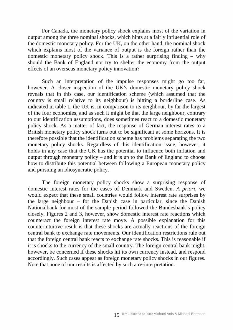
For Canada, the monetary policy shock explains most of the variation inoutput among the three nominal shocks, which hints at a fairly influential role ofthe domestic monetary policy. For the UK, on the other hand, the nominal shockwhich explains most of the variance of output is the foreign rather than thedomestic monetary policy shock. This is a rather surprising finding – whyshould the Bank of England not try to shelter the economy from the outputeffects of an overseas monetary policy innovation?

Such an interpretation of the impulse responses might go too far,however. A closer inspection of the UK’s domestic monetary policy shockreveals that in this case, our identification scheme (which assumed that thecountry is small relative to its neighbour) is hitting a borderline case. Asindicated in table 1, the UK is, in comparison to its neighbour, by far the largestof the four economies, and as such it might be that the large neighbour, contraryto our identification assumptions, does sometimes react to a domestic monetarypolicy shock. As a matter of fact, the response of German interest rates to aBritish monetary policy shock turns out to be significant at some horizons. It istherefore possible that the identification scheme has problems separating the twomonetary policy shocks. Regardless of this identification issue, however, itholds in any case that the UK has the potential to influence both inflation andoutput through monetary policy – and it is up to the Bank of England to choosehow to distribute this potential between following a European monetary policyand pursuing an idiosyncratic policy.

The foreign monetary policy shocks show a surprising response ofdomestic interest rates for the cases of Denmark and Sweden. A priori, wewould expect that these small countries would follow interest rate surprises bythe large neighbour – for the Danish case in particular, since the DanishNationalbank for most of the sample period followed the Bundesbank’s policyclosely. Figures 2 and 3, however, show domestic interest rate reactions whichcounteract the foreign interest rate move. A possible explanation for thiscounterintuitive result is that these shocks are actually reactions of the foreigncentral bank to exchange rate movements. Our identification restrictions rule outthat the foreign central bank reacts to exchange rate shocks. This is reasonable ifit is shocks to the currency of the small country. The foreign central bank might,however, be concerned if these shocks hit its own currency instead, and respondaccordingly. Such cases appear as foreign monetary policy shocks in our figures.Note that none of our results is affected by such a re-interpretation.


4.3.3. The Role of the Exchange Rate

To judge the role of the exchange rate as shock-absorber, it is necessary toanalyse its behaviour subsequent to supply and demand shocks. For none of thecountries are the responses of the exchange rate significant. Furthermore, thereactions are relatively weak: the variance decompositions show that only asmall proportion of the exchange rate variability can be attributed to demand andsupply shocks. This is logical for Canada, Sweden and Denmark anyway – if theshocks are symmetric in nature, then no exchange rate adjustment is needed torestore equilibrium. For the UK, on the other hand, where we have classified theshocks to be predominantly idiosyncratic, our results could support a minor rolefor the exchange rate as shock-absorber.

The major source of variability in exchange rates according to our resultsare nominal shocks: a depreciation following a foreign monetary policy shock,an appreciation caused by a domestic monetary policy shock, and shocks arisingin the foreign exchange market itself. For Canada, the exchange rate reactsstrongly to monetary policy shocks. It seems to play an important role in thetransmission of monetary policy. The shocks created by the exchange rate, onthe other hand, are of less importance for inflation and the real economy.Denmark suffers comparatively more from exchange rate shocks: a depreciationleads to considerable inflationary pressure, whereas it does not noticeably affectthe real economy. Sweden’s exchange market looks more like a source ofshocks than a shock absorber or shock transmitter: around ninety percent andmore of the variance of the exchange rate is explained by the exchange rateshock itself at all horizons! Nonetheless, an exchange rate shock does nottransmit major disturbances to the price level or the real economy. In the UK,the exchange rate plays, similarly to Canada, an important role in thetransmission mechanism of monetary policy. It reacts strongly to a monetarypolicy shock, but is also a prominent source of disturbances itself: but onceagain, as in the case of Sweden, the effects of an exchange rate shock on the realeconomy appear to be of minor magnitude.

5. Conclusions

The aim of this paper has been to cast light on the central issue in OCA theory –the stabilizing properties of an independent monetary policy and exchange rate.We have examined this question in the context provided by four open economies– the UK, Sweden, Denmark and Canada – each of which faces an importantpolicy option of monetary union (or a similar arrangement) with a bigneighbour.


We chose to tackle this question with an SVAR specification which drawson the SVAR literature on monetary policy in an open economy. Thespecification can be viewed as allowing for an identification of the symmetry ofshocks between the smaller country and its large neighbour: this is indicated bythe similarity in the shock-response of the large country’s monetary policy tothat of the smaller one.

Then, the specification also allows us to examine directly what shocks theexchange rate predominantly responds to. In similar fashion, we can alsodiscover what shocks predominantly drive output and monetary policy. Finally,we can discuss whether, in fact, monetary policy has significant effects on realoutput and prices and at what horizons.

Table 4 sums up our results through five criteria that are relevant for theevaluation of the monetary union options. All criteria are formulated such that apositive answer favours monetary union. Symmetry in shocks constitutes apositive indicator for monetary union as it suggests that stabilisation is littlecalled for. Evidence that monetary policy has little effect on output is also apositive indicator, as is evidence that the exchange rate is largely driven byshocks arising in the exchange market itself. The latter suggests that theexchange market so far from absorbing shocks, is creating its own. If theexchange rate tends to behave as a source of shocks, then monetary union iseven more favourable if these shocks affect output and/or prices strongly.

Table 4: Criteria to evaluate monetary union option

Criterion Canada Denmark Sweden UKSupply and demand shockspredominantly symmetric

+ + + -Monetary policy has little effect onoutput

- + + -Exchange rate not very responsiveto supply and demand shocks

+ + + +Exchange rate largely driven byshocks in the exchange market

- (+) + +Exchange rate shocks distort outputand/or prices

NA(+)

+ - +

What do these results suggest about the monetary union option for thesecountries? On this basis, in the case of Sweden, where shocks appearpredominantly symmetric, the exchange rate appears to “dance to its own tune”and monetary policy has little effect on output, there seems little doubt thatmonetary union would involve no loss. For Denmark, a similar verdict isavailable. The reasoning is slightly different. Shocks appear mainly symmetric,


again, but the exchange rate is quite strongly driven by monetary policyinnovations, and monetary policy itself responds to demand and supply shocks.However, the evidence is that monetary policy in Denmark has no effect onoutput. Once again, then, monetary union would occasion no loss. In the case ofCanada, whilst shocks are mainly symmetric, monetary policy has real effects,and the exchange rate is driven by relative monetary policy effects and even tosome extent by demand and supply shocks themselves (since the exchange rateis not mainly a source of shocks, the question whether exchange market shocksdistort output and/or prices is not relevant). A stabilizing role is feasible formonetary policy and the exchange rate. Monetary union, or in this case“dollarization” could involve loss. For the UK, there are inconsistentindications: shocks are asymmetric and monetary policy is (weakly) effective foroutput. On the other hand, a large component of variation in the exchange rate isdue to exchange market disturbances themselves: demand and supply shocks arenegligibly involved. Monetary policy itself is strongly influenced by innovationsin foreign monetary policy. The outcome for the monetary union option is notclear cut.

The results obtained in any SVAR exercise are only as good as theidentification scheme that is employed to ‘make sense’ of the residuals. Therestrictions involved here are, largely, conventional in that they have beenadopted in earlier studies of monetary policy effectiveness; and the over-identifying restrictions suggested by theoretical priors are all largely satisfied inour results. Nevertheless it cannot be ruled out that comparatively ‘minor’changes in specification could produce a different picture. The appendix carriesa sensitivity analysis in respect of variations in our assumptions about the‘degree’ of exchange rate targeting; in this case, although a number of detailedresults are changed none of our main conclusions is perceptibly affected. Thisevidence of the robustness of our conclusions is of course welcome, though atthis stage we still prefer to view the current paper as a preliminary exploration ofthe important issues under review.

Michael Artis,EUI and CEPRe-mail: [email protected];

Michael Ehrmann,EUIe-mail: [email protected]


References

Artis M. and M. Lewis (1991), “Money in Britain. Monetary Policy, Innovationand Europe”, New York: Philip Allan.

Bagliano F.C., Favero C.A. and F. Franco (1999), “Measuring Monetary Policyin Open Economies”, CEPR Discussion Papers, 2079, London.

Blanchard O.J. and D. Quah (1989), “The Dynamic Effects of AggregateDemand and Supply Disturbances”, American Economic Review, 79, 655-673.

Buiter W. (1999a), “Optimal Currency Areas: Why Does the Exchange RateRegime Matter? (with an Application to UK Membership of EMU)”, SixthRoyal Bank of Scotland, Scottish Economic Society Annual Lecture.

Buiter W. (1999b), “The EMU and the NAMU. What is the case for NorthAmerican Monetary Union?”, CEPR Discussion Papers, N° 2181.

Canzoneri M., Valles J. and J. Vinals (1996), “Do Exchange Rates Move toAddress International Macroeconomic Imbalances?”, CEPR Discussion Papers,1498, London.

Clarida R. and J. Gali (1994), “Sources of Real Exchange Rate Fluctuations:How Important Are Nominal Shocks?”, Carnegie-Rochester Conference Serieson Public Policy, 41, 1-56.

Courchene T. and R.G. Harris (1999), From Fixing to Monetary Union: Optionsfor North American Currency Integration, (D. Howe Institute, Toronto, June).

Cushman D.O. and T. Zha (1997), “Identifying Monetary Policy in a SmallOpen Economy under Flexible Exchange Rates”, Journal of MonetaryEconomics, 39, 433-448.

Dixit, A,K. (1989) “Hysterisis, import penetration and exchange rate pass-through”, Quarterly Journal of Economics, 104, 205-208.

Ehrmann M. (2000), “Comparing Monetary Policy Transmission AcrossEuropean Countries”, Weltwirtschaftliches Archiv, 136, 58-83.

Faust J. and J.H. Rogers (1999), “Monetary Policy’s Role in Exchange RateBehavior”, Board of Governors of the Federal Reserve System InternationalFinance Discussion Papers, 652, Washington.


Funke M. (2000), “Macroeconomic Shocks in Euroland vs the UK: Supply,Demand, or Nominal?”, mimeo, University of Hamburg, February.

Grilli V. and N. Roubini (1995), “Liquidity and Exchange Rates: PuzzlingEvidence From the G-7 Countries”, New York University Salomon BrothersWorking Paper, S/95/31, New York.

Hansen L.P. (1982), “Large Sample Properties of Generalized Method ofMoment Estimators”, Econometrica, 50, 1029-1054.

International Monetary Fund (1999), “United Kingdom: Selected Issues”,Washington, May.

Kim S. and N. Roubini (1997), “Liquidity and Exchange Rates in the G-7Countries: Evidence from Identified VARs”, mimeo, NYU, New York, April.

Krugman P. (1990), “Policy Problems of a Monetary Union,” in P. De Grauweand L. Papademos (eds.), The European Monetary System in the 1990s, Harlow:Longmans.

Krugman, P. (1989) “Exchange Rate Instability”, Cambridge, MA: MIT Press

Laidler D. and F. Poschmann (1998), Birth of a New Currency: The PolicyOutlook after Monetary Union in Europe,(D. Howe Institute, Toronto, June).

Macdonald R. (1999), “Exchange Rate Behaviour: Are FundamentalsImportant?”, Economic Journal, 109, November, F673-F691.

Sims C.A. (1980), “Macroeconomics and Reality”, Econometrica, 48, 1-48.

Smets F. (1997), “Measuring Monetary Policy Shocks in France, Germany andItaly: The Role of the Exchange Rate”, Swiss Journal of Economics andStatistics, 133, 597-616.

Thomas A. (1997), “Is the Exchange Rate a Shock Absorber? The Case ofSweden”, IMF Working Papers, 97/176, Washington, December.

Weymark D. (1995), “Estimating Exchange Market Pressure and the Degree ofExchange Market Intervention for Canada”, Journal of International Economics,39, 273-295.


AppendixFigure 1: Impulse Response Functions for Canada

CanadaSupply Shock

Out

put

0 10 20 30 40 50-0.008

0.000

0.008

0.016

0.024

Supply Shock

Fore

ign

Inte

rest

0 10 20 30 40 50-0.012

-0.006

0.000

0.006

Supply Shock

Inte

rest

0 10 20 30 40 50-0.010

-0.005

0.000

0.005

0.010

Supply Shock

Pric

es

0 10 20 30 40 50-0.014

-0.007

0.000

0.007

Supply Shock

Exch

ange

Rat

e

0 10 20 30 40 50-0.016

-0.008

0.000

0.008

0.016

Demand Shock

Out

put

0 10 20 30 40 50-0.008

0.000

0.008

0.016

0.024

Demand Shock

Fore

ign

Inte

rest

0 10 20 30 40 50-0.012

-0.006

0.000

0.006

Demand Shock

Inte

rest

0 10 20 30 40 50-0.010

-0.005

0.000

0.005

0.010

Demand Shock

Pric

es

0 10 20 30 40 50-0.014

-0.007

0.000

0.007

Demand Shock

Exch

ange

Rat

e

0 10 20 30 40 50-0.016

-0.008

0.000

0.008

0.016

Foreign MP Shock

Out

put

0 10 20 30 40 50-0.008

0.000

0.008

0.016

0.024

Foreign MP Shock

Fore

ign

Inte

rest

0 10 20 30 40 50-0.012

-0.006

0.000

0.006

Foreign MP Shock

Inte

rest

0 10 20 30 40 50-0.010

-0.005

0.000

0.005

0.010

Foreign MP Shock

Pric

es

0 10 20 30 40 50-0.014

-0.007

0.000

0.007

Foreign MP Shock

Exch

ange

Rat

e

0 10 20 30 40 50-0.016

-0.008

0.000

0.008

0.016

MP Shock

Out

put

0 10 20 30 40 50-0.008

0.000

0.008

0.016

0.024

MP Shock

Fore

ign

Inte

rest

0 10 20 30 40 50-0.012

-0.006

0.000

0.006

MP Shock

Inte

rest

0 10 20 30 40 50-0.010

-0.005

0.000

0.005

0.010

MP Shock

Pric

es

0 10 20 30 40 50-0.014

-0.007

0.000

0.007

MP Shock

Exch

ange

Rat

e

0 10 20 30 40 50-0.016

-0.008

0.000

0.008

0.016

Exch. Rate Shock

Out

put

0 10 20 30 40 50-0.008

0.000

0.008

0.016

0.024

Exch. Rate Shock

Fore

ign

Inte

rest

0 10 20 30 40 50-0.012

-0.006

0.000

0.006

Exch. Rate Shock

Inte

rest

0 10 20 30 40 50-0.010

-0.005

0.000

0.005

0.010

Exch. Rate Shock

Pric

es

0 10 20 30 40 50-0.014

-0.007

0.000

0.007

Exch. Rate Shock

Exch

ange

Rat

e

0 10 20 30 40 50-0.016

-0.008

0.000

0.008

0.016


Figure 2: Impulse Response Functions for Denmark

DenmarkSupply Shock

Out

put

0 10 20 30 40 50-0.009

0.000

0.009

0.018

0.027

Supply Shock

Fore

ign

Inte

rest

0 10 20 30 40 50-0.0040

0.0000

0.0040

0.0080

Supply Shock

Inte

rest

0 10 20 30 40 50-0.02

-0.01

0.00

0.01

Supply Shock

Pric

es

0 10 20 30 40 50-0.0035

0.0000

0.0035

0.0070

Supply Shock

Exch

ange

Rat

e

0 10 20 30 40 50-0.0090

-0.0045

0.0000

0.0045

0.0090

Demand Shock

Out

put

0 10 20 30 40 50-0.009

0.000

0.009

0.018

0.027

Demand Shock

Fore

ign

Inte

rest

0 10 20 30 40 50-0.0040

0.0000

0.0040

0.0080

Demand Shock

Inte

rest

0 10 20 30 40 50-0.02

-0.01

0.00

0.01

Demand Shock

Pric

es

0 10 20 30 40 50-0.0035

0.0000

0.0035

0.0070

Demand Shock

Exch

ange

Rat

e

0 10 20 30 40 50-0.0090

-0.0045

0.0000

0.0045

0.0090

Foreign MP Shock

Out

put

0 10 20 30 40 50-0.009

0.000

0.009

0.018

0.027

Foreign MP Shock

Fore

ign

Inte

rest

0 10 20 30 40 50-0.0040

0.0000

0.0040

0.0080

Foreign MP Shock

Inte

rest

0 10 20 30 40 50-0.02

-0.01

0.00

0.01

Foreign MP Shock

Pric

es

0 10 20 30 40 50-0.0035

0.0000

0.0035

0.0070

Foreign MP Shock

Exch

ange

Rat

e

0 10 20 30 40 50-0.0090

-0.0045

0.0000

0.0045

0.0090

MP Shock

Out

put

0 10 20 30 40 50-0.009

0.000

0.009

0.018

0.027

MP Shock

Fore

ign

Inte

rest

0 10 20 30 40 50-0.0040

0.0000

0.0040

0.0080

MP Shock

Inte

rest

0 10 20 30 40 50-0.02

-0.01

0.00

0.01

MP Shock

Pric

es

0 10 20 30 40 50-0.0035

0.0000

0.0035

0.0070

MP Shock

Exch

ange

Rat

e

0 10 20 30 40 50-0.0090

-0.0045

0.0000

0.0045

0.0090

Exch. Rate Shock

Out

put

0 10 20 30 40 50-0.009

0.000

0.009

0.018

0.027

Exch. Rate Shock

Fore

ign

Inte

rest

0 10 20 30 40 50-0.0040

0.0000

0.0040

0.0080

Exch. Rate Shock

Inte

rest

0 10 20 30 40 50-0.02

-0.01

0.00

0.01

Exch. Rate Shock

Pric

es

0 10 20 30 40 50-0.0035

0.0000

0.0035

0.0070

Exch. Rate Shock

Exch

ange

Rat

e

0 10 20 30 40 50-0.0090

-0.0045

0.0000

0.0045

0.0090


Figure 3: Impulse Response Functions for Sweden

SwedenSupply Shock

Out

put

0 10 20 30 40 50-0.01

0.00

0.01

0.02

0.03

Supply Shock

Fore

ign

Inte

rest

0 10 20 30 40 50-0.0060

-0.0030

0.0000

0.0030

0.0060

Supply Shock

Inte

rest

0 10 20 30 40 50-0.0090

-0.0045

0.0000

0.0045

0.0090

Supply Shock

Pric

es

0 10 20 30 40 50-0.012

-0.006

0.000

0.006

Supply Shock

Exch

ange

Rat

e

0 10 20 30 40 50-0.028

-0.014

0.000

0.014

Demand ShockO

utpu

t

0 10 20 30 40 50-0.01

0.00

0.01

0.02

0.03

Demand Shock

Fore

ign

Inte

rest

0 10 20 30 40 50-0.0060

-0.0030

0.0000

0.0030

0.0060

Demand Shock

Inte

rest

0 10 20 30 40 50-0.0090

-0.0045

0.0000

0.0045

0.0090

Demand Shock

Pric

es

0 10 20 30 40 50-0.012

-0.006

0.000

0.006

Demand Shock

Exch

ange

Rat

e

0 10 20 30 40 50-0.028

-0.014

0.000

0.014

Foreign MP Shock

Out

put

0 10 20 30 40 50-0.01

0.00

0.01

0.02

0.03

Foreign MP Shock

Fore

ign

Inte

rest

0 10 20 30 40 50-0.0060

-0.0030

0.0000

0.0030

0.0060

Foreign MP Shock

Inte

rest

0 10 20 30 40 50-0.0090

-0.0045

0.0000

0.0045

0.0090

Foreign MP Shock

Pric

es

0 10 20 30 40 50-0.012

-0.006

0.000

0.006

Foreign MP Shock

Exch

ange

Rat

e

0 10 20 30 40 50-0.028

-0.014

0.000

0.014

MP Shock

Out

put

0 10 20 30 40 50-0.01

0.00

0.01

0.02

0.03

MP Shock

Fore

ign

Inte

rest

0 10 20 30 40 50-0.0060

-0.0030

0.0000

0.0030

0.0060

MP Shock

Inte

rest

0 10 20 30 40 50-0.0090

-0.0045

0.0000

0.0045

0.0090

MP Shock

Pric

es

0 10 20 30 40 50-0.012

-0.006

0.000

0.006

MP Shock

Exch

ange

Rat

e

0 10 20 30 40 50-0.028

-0.014

0.000

0.014

Exch. Rate Shock

Out

put

0 10 20 30 40 50-0.01

0.00

0.01

0.02

0.03

Exch. Rate Shock

Fore

ign

Inte

rest

0 10 20 30 40 50-0.0060

-0.0030

0.0000

0.0030

0.0060

Exch. Rate Shock

Inte

rest

0 10 20 30 40 50-0.0090

-0.0045

0.0000

0.0045

0.0090

Exch. Rate Shock

Pric

es

0 10 20 30 40 50-0.012

-0.006

0.000

0.006

Exch. Rate Shock

Exch

ange

Rat

e

0 10 20 30 40 50-0.028

-0.014

0.000

0.014


Figure 4: Impulse Response Functions for the United Kingdom

United KingdomSupply Shock

Out

put

0 10 20 30 40 50-0.008

0.000

0.008

0.016

Supply Shock

Fore

ign

Inte

rest

0 10 20 30 40 50-0.0030

0.0000

0.0030

0.0060

Supply Shock

Inte

rest

0 10 20 30 40 50-0.0045

0.0000

0.0045

0.0090

Supply Shock

Pric

es

0 10 20 30 40 50-0.0090

-0.0045

0.0000

0.0045

0.0090

Supply Shock

Exch

ange

Rat

e

0 10 20 30 40 50-0.028

-0.014

0.000

0.014

0.028

Demand ShockO

utpu

t

0 10 20 30 40 50-0.008

0.000

0.008

0.016

Demand Shock

Fore

ign

Inte

rest

0 10 20 30 40 50-0.0030

0.0000

0.0030

0.0060

Demand Shock

Inte

rest

0 10 20 30 40 50-0.0045

0.0000

0.0045

0.0090

Demand Shock

Pric

es

0 10 20 30 40 50-0.0090

-0.0045

0.0000

0.0045

0.0090

Demand Shock

Exch

ange

Rat

e

0 10 20 30 40 50-0.028

-0.014

0.000

0.014

0.028

Foreign MP Shock

Out

put

0 10 20 30 40 50-0.008

0.000

0.008

0.016

Foreign MP Shock

Fore

ign

Inte

rest

0 10 20 30 40 50-0.0030

0.0000

0.0030

0.0060

Foreign MP Shock

Inte

rest

0 10 20 30 40 50-0.0045

0.0000

0.0045

0.0090

Foreign MP Shock

Pric

es

0 10 20 30 40 50-0.0090

-0.0045

0.0000

0.0045

0.0090

Foreign MP Shock

Exch

ange

Rat

e

0 10 20 30 40 50-0.028

-0.014

0.000

0.014

0.028

MP Shock

Out

put

0 10 20 30 40 50-0.008

0.000

0.008

0.016

MP Shock

Fore

ign

Inte

rest

0 10 20 30 40 50-0.0030

0.0000

0.0030

0.0060

MP Shock

Inte

rest

0 10 20 30 40 50-0.0045

0.0000

0.0045

0.0090

MP Shock

Pric

es

0 10 20 30 40 50-0.0090

-0.0045

0.0000

0.0045

0.0090

MP Shock

Exch

ange

Rat

e

0 10 20 30 40 50-0.028

-0.014

0.000

0.014

0.028

Exch. Rate Shock

Out

put

0 10 20 30 40 50-0.008

0.000

0.008

0.016

Exch. Rate Shock

Fore

ign

Inte

rest

0 10 20 30 40 50-0.0030

0.0000

0.0030

0.0060

Exch. Rate Shock

Inte

rest

0 10 20 30 40 50-0.0045

0.0000

0.0045

0.0090

Exch. Rate Shock

Pric

es

0 10 20 30 40 50-0.0090

-0.0045

0.0000

0.0045

0.0090

Exch. Rate Shock

Exch

ange

Rat

e

0 10 20 30 40 50-0.028

-0.014

0.000

0.014

0.028


Table 5: Variance Decompositions

CanadaVariance decomposition for outputStep Supply Shock Demand Shock Foreign Mon.

Pol. ShockMonetary

Policy ShockExchange Rate

Shock1 0.05 99.95 0 0 012 15.54 83.38 0.28 0.72 0.0824 32.17 63.88 0.15 3.27 0.5336 46.58 47.54 0.09 4.79 0.9948 57.68 35.96 0.06 5.12 1.1860 66.02 27.93 0.05 4.83 1.17

Variance decomposition for US interest rates1 76.37 3.64 19.99 0 012 62.39 31.42 5.23 0.12 0.8424 61.59 33.94 3.45 0.42 0.636 61.41 33.87 2.88 1.19 0.6548 61.11 33.43 2.61 2.03 0.8260 60.8 33.03 2.46 2.72 1

Variance decomposition for interest rates1 12.69 2.86 23.66 28.44 32.3612 30.14 27.86 8.2 14.52 19.2824 32.7 31.65 5.44 14.05 16.1536 34.86 32.73 4.83 12.89 14.6948 36.14 33.06 4.59 12.25 13.9660 36.83 33.11 4.46 12.01 13.59

Variance decomposition for CPI1 14.68 0.16 35.69 14.45 35.0112 53.82 1.84 12.98 11.66 19.724 72.13 0.93 7.46 7.61 11.8736 78.68 2.21 5.15 5.99 7.9748 80.82 4.05 3.92 5.59 5.6260 81.35 5.68 3.16 5.69 4.13

Variance decomposition for exchange rate1 3.49 0 54.26 17.34 24.9112 4.07 0.69 47.55 40.39 7.324 8.03 1.76 43.04 43.61 3.5536 11.23 2.8 40.62 42.9 2.4548 13.9 3.76 39.03 41.32 1.9960 16.2 4.62 37.85 39.57 1.77


DenmarkVariance decomposition for outputStep Supply Shock Demand Shock Foreign Mon.

Pol. ShockMonetary


Shock1 82 18 0 0 012 90.66 5.85 1.54 1.48 0.4624 94.6 3.36 0.86 0.86 0.3136 96.22 2.36 0.6 0.6 0.2348 97.09 1.81 0.46 0.46 0.1860 97.64 1.47 0.37 0.37 0.14

Variance decomposition for German interest rates1 18.77 66.16 15.07 0 012 9.9 61.1 14.06 9.51 5.4224 8.27 62.78 8.9 10.13 9.9236 7.86 63.05 7.58 10.23 11.2748 7.72 63.14 7.11 10.27 11.7660 7.66 63.18 6.92 10.29 11.96

Variance decomposition for interest rates1 4.66 8.01 46.99 32.59 7.7512 15.48 14.89 35.81 25.51 8.3124 13.49 25.97 29.02 22.32 9.1936 12.77 29.58 26.37 21.25 10.0448 12.48 31 25.32 20.82 10.3860 12.36 31.61 24.87 20.64 10.52


Variance decomposition for exchange rate1 0 0.37 0.15 50.77 48.712 3.05 1.25 4.42 47.33 43.9424 3.17 2.42 4.51 42.05 47.8636 2.94 3.72 4.36 38.75 50.2348 2.69 4.95 4.2 36.28 51.8860 2.49 6.02 4.06 34.37 53.07

SwedenVariance decomposition for outputStep Supply Shock Demand Shock Foreign Mon.

Pol. ShockMonetary


Shock1 33.03 66.97 0 0 0


12 55.29 41.79 1.51 0.77 0.6524 73.33 24.71 1.01 0.41 0.5436 82.19 16.41 0.72 0.26 0.4148 87.1 11.86 0.54 0.18 0.3260 90.09 9.1 0.42 0.14 0.25

Variance decomposition for German interest rates1 45.83 12.87 41.3 0 012 57.64 26.1 11.69 0.21 4.3524 60.04 26.95 8.61 0.23 4.1736 60.72 27.2 7.8 0.22 4.0648 60.98 27.3 7.49 0.22 460 61.09 27.35 7.37 0.21 3.98



Variance decomposition for exchange rate1 0.84 0.58 0.02 4.89 93.6712 1.2 0.57 0.11 2.24 95.8824 2.46 0.95 0.31 1.31 94.9736 3.87 1.49 0.57 0.91 93.1648 5.22 2.04 0.78 0.7 91.2760 6.41 2.52 0.94 0.57 89.57

United KingdomVariance decomposition for outputStep Supply Shock Demand Shock Foreign Mon.

Pol. ShockMonetary


Shock1 69.79 30.21 0 0 012 83.95 11.59 2.54 0.55 1.3624 85.99 5.3 6.39 1.57 0.7436 87.42 3.23 6.97 1.94 0.4448 89.31 2.63 5.94 1.75 0.3660 91.09 2.34 4.8 1.44 0.32


Variance decomposition for German interest rates1 0.62 3.38 96 0 012 0.96 4.72 78.95 14.17 1.1924 3.31 4.06 73.65 18.28 0.7136 5.62 7.36 67.64 18.28 1.148 6.79 10.28 63.77 17.57 1.5860 6.96 11.35 62.65 17.22 1.81


Variance decomposition for RPIX1 7.27 26.76 1.79 16.43 47.7512 7 17.06 40.99 2.08 32.8524 11.95 20.49 47.63 2.29 17.6436 14.94 26.09 45.18 2.55 11.2448 16.96 31.43 40.83 2.28 8.4960 18.28 35.76 36.79 1.89 7.29

Variance decomposition for exchange rate1 3.13 6.03 0.91 29.02 60.912 1.53 1.45 0.35 35.88 60.824 2.07 1.13 0.2 33.58 63.0236 2.44 1.31 0.4 32.02 63.8448 2.47 1.34 1.1 30.24 64.8660 2.32 1.23 2.04 28.46 65.94

Sensitivity Analysis

Figures 5 and 6 present estimates of the monetary policy and exchange rate shocks forvarying estimates of ω . Only the impulse responses to these two shocks depend on ω ,whereas for all others the identification remains unchanged. The solid lines represent theresults for 0=ω (i.e. a situation where the central bank does not take into account theexchange rate for its monetary policy at all), the dashed lines those for ω as estimated for thefull sample and used in the body of the paper, and the short-long-dashed lines denote theresults for ω twice as big as estimated for the full sample. In some cases, the results changeconsiderably. For Sweden, ignoring the role of the exchange rate in the monetary policysetting would lead to an exchange rate puzzle. For Canada, a price puzzle would result. Onthe other hand, setting ω to zero for the United Kingdom and to one for Denmark would helpto avoid the price puzzles. For the exchange rate shock, it is interesting to see that 0=ωleads to a basically non-existent interest rate response to exchange rate shocks for allhorizons. Doubling ω for Canada produces implausible results where the interest rate


reaction is so strong that the initial exchange rate depreciation is reversed into a highlypersistent appreciation, a result which supports our estimate for ω .

In any case, the results of this paper do not depend crucially on the choice of ω .Firstly, it affects only two out of the five shocks, and secondly, the overall picture of whichshock drives the exchange rate, whether monetary policy is effective and whether exchangerate shocks have a big effect on output is not changed.

Figure 5: Sensitivity of responses to a monetary policy shock

Monetary Policy Shocks - SensitivityCanada

Out

put

0 10 20 30 40 50-0.0042

-0.0028

-0.0014

-0.0000

0.0014

Fore

ign

Inte

rest

0 10 20 30 40 50-0.0010

-0.0005

0.0000

0.0005

0.0010

Inte

rest

0 10 20 30 40 50-0.0016

0.0000

0.0016

0.0032

0.0048

Pric

es

0 10 20 30 40 50-0.0027

-0.0018

-0.0009

0.0000

0.0009

Exch

ange

Rat

e

0 10 20 30 40 50-0.0030

0.0000

0.0030

0.0060

0.0090

Denmark

0 10 20 30 40 50-0.004

-0.002

0.000

0.002

0 10 20 30 40 50-0.002

-0.001

0.000

0.001

0 10 20 30 40 50-0.0025

0.0000

0.0025

0.0050

0.0075

0 10 20 30 40 50-0.0018

0.0000

0.0018

0.0036

0 10 20 30 40 500.0000

0.0018

0.0036

0.0054

Sweden

0 10 20 30 40 50-0.0016

0.0000

0.0016

0.0032

0 10 20 30 40 50-0.00060

-0.00030

0.00000

0.00030

0 10 20 30 40 50-0.0035

0.0000

0.0035

0.0070

0 10 20 30 40 50-0.0045

-0.0036

-0.0027

-0.0018

0 10 20 30 40 50-0.0040

0.0000

0.0040

0.0080

United Kingdom

0 10 20 30 40 50-0.002

-0.001

0.000

0.001

0 10 20 30 40 50-0.001

0.000

0.001

0.002

0 10 20 30 40 50-0.0018

0.0000

0.0018

0.0036

0.0054

0 10 20 30 40 50-0.004

-0.002

0.000

0.002

0 10 20 30 40 500.000

0.007

0.014

0.021


Figure 6: Sensitivity of responses to an exchange rate shock

Exchange Rate Shocks - SensitivityCanada

Out

put

0 10 20 30 40 50-0.004

-0.002

0.000

0.002

Fore

ign

Inte

rest

0 10 20 30 40 50-0.0012

-0.0006

0.0000

0.0006

0.0012

Inte

rest

0 10 20 30 40 50-0.0016

0.0000

0.0016

0.0032

0.0048

Pric

es

0 10 20 30 40 50-0.0009

0.0000

0.0009

0.0018

0.0027

Exch

ange

Rat

e

0 10 20 30 40 50-0.0090

-0.0045

0.0000

0.0045

Denmark

0 10 20 30 40 50-0.0032

-0.0016

0.0000

0.0016

0.0032

0 10 20 30 40 50-0.0021

-0.0014

-0.0007

-0.0000

0.0007

0 10 20 30 40 50-0.002

0.000

0.002

0.004

0.006

0 10 20 30 40 500.0008

0.0016

0.0024

0.0032

0 10 20 30 40 50-0.0054

-0.0036

-0.0018

0.0000

0.0018

Sweden

0 10 20 30 40 50-0.0018

-0.0009

0.0000

0.0009

0.0018

0 10 20 30 40 50-0.00120

-0.00080

-0.00040

-0.00000

0.00040

0 10 20 30 40 50-0.002

0.000

0.002

0.004

0 10 20 30 40 50-0.0032

-0.0016

0.0000

0.0016

0 10 20 30 40 50-0.0144

-0.0128

-0.0112

-0.0096

-0.0080

United Kingdom

0 10 20 30 40 50-0.001

0.000

0.001

0.002

0 10 20 30 40 50-0.0012

-0.0006

0.0000

0.0006

0.0012

0 10 20 30 40 50-0.0016

0.0000

0.0016

0.0032

0.0048

0 10 20 30 40 50-0.0035

-0.0028

-0.0021

-0.0014

-0.0007

0 10 20 30 40 50-0.0250

-0.0200

-0.0150

-0.0100

-0.0050

Unit root tests

Univariate unit root tests like the augmented Dickey-Fuller test revealed possiblenonstationarities for the interest rate series of the US, Germany and the UK. All the othervariables turned out to be stationary (in their first differences as they enter the VARs). Tojudge the degree of integration of series, it is, however, advisable to perform unit root testswithin the VAR system. Johansen’s tests for the cointegration rank in our six-variable VARsfavour a rank of six, indicating that all series can indeed be considered stationary whenestimated in the VAR system (see table 6). For Sweden, the cointegration rank is estimated tobe lower. Nonetheless, for comparability, we treat the Swedish variables as stationary.Another indicator that the assumption of stationary interest rates is admissible can be found inthe impulse responses. They return to baseline quickly, with converging error bounds. This isgenerally not the case if the variables are integrated.


Table 6: Results of Johansen’s trace test for cointegration rank

r = 0 r = 1 r = 2 R = 3 r = 4 r = 5Criticalvalues(90%)

89.37 64.74 43.84 26.70 13.31 2.71

Canada 235.12 130.19 78.03 36.27 13.96 4.08Denmark 271.45 170.47 102.77 52.85 14.76 2.74Sweden 286.64 175.04 108.60 50.08 8.90* 1.16*

UK 258.91 160.46 98.90 53.66 16.37 5.66

Calculation of the intervention index in table 2

The index follows Weymark (1995), with slight modifications. It is supposed to measure theextent to which central banks used foreign exchange reserves for interventions in the foreignexchange market in order to influence the exchange rate. According to Weymark, exchangemarket pressure can either lead to exchange rate changes or be absorbed by an appropriatecentral bank intervention. Exchange market pressure is thus defined as

ttt reEMP ∆+∆= η , (A1)where te∆ denotes the change in the nominal exchange rate (with te measured as thelogarithm of the exchange rate of the domestic versus the foreign currency), tr∆ the change in

foreign exchange reserves6 and t

t

re

∆∂∆∂

−=η the elasticity which converts the reserve changes

into equivalent exchange rate units.

Dividing (A1) by tEMP yields

t

t

t

t

EMPr

EMPe ∆

+∆

=η

1 , (A2)

the first term of which denotes the proportion of the exchange market pressure that is relievedby an exchange rate change, the second term of which indicates the proportion that is relievedby intervention activities of the central banks. The intervention index is then defined as

tt

t

t

tt

re

rEMP

r

∆+∆��

��

∆=

∆=

η

ητ1

(A3)

Whereas te∆ and tr∆ are readily observable, η needs to be estimated from astructural model. We re-estimate Weymark (1995) here, and refer to the original for furtherdetails.

From equation (A2) the properties of the index can be easily derived: for the case of afreely floating exchange rate, the index takes the value 0 because all exchange marketpressure is relieved by an according exchange rate change. A fixed exchange rate leads to a

6 We deviate from Weymark’s original definition here. We do not express the change in theforeign exchange reserves as a proportion of the inherited monetary base. Furthermore, we donot correct it with the money multiplier. The reserves are denominated in US$ for allcountries.


value of 1 for the index, because the first term in (A2) is zero. Intermediate cases lead to avalue of 10 << tτ .

Table 2 reports the average of the index over the estimated sample, which spans1974:1 to 1998:12 for Canada, 1980:1 to 1998:12 for Denmark and Sweden and (due to dataavailability) 1982:6 to 1998:11 for the UK.

Exclusion test for the extended modelsIn extended models, which include also foreign inflation ( *π ) and output growth ( *y∆ ), wetest whether the coefficients on *π and *y∆ in the equation on foreign interest rates are zero(joint test). Additionally, we provide equivalent tests in models where only one foreignvariable ( *π or *y∆ ) had been included.

Table 7: Tests for exclusion of foreign variables; significance levels in brackets;joint test is )12(2χ , single tests are )6(2χ

Canada Denmark Sweden UKJoint test 21.18 [0.05] 14.32 [0.28] 16.01 [0.19] 12.76 [0.39]

*π 6.23 [0.40] 12.09 [0.06] 14.19 [0.03]* 12.83 [0.05]*y∆ 19.17 [0.00]** 2.20 [0.90] 1.78 [0.94] 3.09 [0.80]

Stability tests

Figures 7 to 10 report breakpoint Chow-tests for the VARs of each country. Despite the fairlylong sample, which covers various monetary policy and exchange rate regimes for somecountries, the results support stability of our VARs. Merely for the Danish industrialproduction equation, there seem to be problems, which are not reflected in the systemestimates, however.


Figure 7: 5% Breakpoint Chow tests for Canada

1985 1990 1995

.5

1Interest Rate

1985 1990 1995

.5

1Foreign Interest Rate

1985 1990 1995

.5

1Inflation

1985 1990 1995

.5

1Commodity Price Inflation

1985 1990 1995

.5

1Industrial Production

1985 1990 1995

.5

1

1.5Exchange Rate

1985 1990 1995

.5

.75

1System

Figure 8: 5% Breakpoint Chow tests for Denmark

1985 1990 1995

.5

1Interest Rate

1985 1990 1995

.5


1985 1990 1995

1

2

3 Industrial Production

1985 1990 1995

.5

1Exchange Rate

1985 1990 1995

.5


1985 1990 1995

.5

1Inflation

1985 1990 1995

.5

1System


Figure 9: 5% Breakpoint Chow tests for Sweden

1985 1990 1995

.5

1Interest Rate

1985 1990 1995

.5


1985 1990 1995

.5

1Exchange Rate

1985 1990 1995

.5


1985 1990 1995

.5

1Inflation

1985 1990 1995

.5


1985 1990 1995

.5

1System

Figure 10: 5% Breakpoint Chow tests for the United Kingdom

1985 1990 1995

.5

1Interest Rate

1985 1990 1995

.5


1985 1990 1995

.5

1Exchange Rate

1985 1990 1995

.5


1985 1990 1995

.5

1Inflation

1985 1990 1995

.5


1985 1990 1995

.5

1System

The Exchange Rate – A Shock-Absorber or Source of Shocks

Documents

Transcript of The Exchange Rate – A Shock-Absorber or Source of Shocks