
The evolutionary learning rule for system identification
339
Advanced Information and Knowledge Processing
Transcript of The evolutionary learning rule for system identification

Advanced Information and Knowledge Processing

Also in this series
Gregoris Mentzas, Dimitris Apostolou, Andreas Abecker and Ron YoungKnowledge Asset Management1-85233-583-1
Michalis Vazirgiannis, Maria Halkidi and Dimitrios GunopulosUncertainty Handling and Quality Assessment in Data Mining1-85233-655-2
Asuncion Gomez-Perez, Mariano Fernandez-Lopez, Oscar CorchoOntological Engineering1-85233-551-3
Arno ScharlEnvironmental Online Communication1-85233-783-4
Shichao Zhang, Chengqi Zhang and Xindong WuKnowledge Discovery in Multiple Databases1-85233-703-6
Jason T.L. Wang, Mohammed J. Zaki, Hannu T.T. Toivonen and DennisShasha (Eds)Data Mining in Bioinformatics1-85233-671-4
C.C. Ko, Ben M. Chen and Jianping ChenCreating Web-based Laboratories1-85233-837-7

Manuel Grana, Richard Duro, Alicia d’Anjouand Paul P. Wang (Eds)
Information Processingwith EvolutionaryAlgorithms
From Industrial Applications to Academic Speculations
With 137 Figures

Manuel Grana, BSc, MSc, PhDUniversidad del Pais Vasco, San Sebastian, SpainRichard J. Duro, BSc, MSc, PhDUniversidad da Coruna, La Coruna, SpainAlicia d’Anjou, BSc, MSc, PhDUniversidad del Pais Vasco, San Sebastian, SpainPaul P. Wang, PhDDuke University, Durham, North Carolina, USA
Series EditorsXindong WuLakhmi Jain
British Library Cataloguing in Publication DataInformation processing with evolutionary algorithms : from
industrial applications to academic speculations. —(Advanced information and knowledge processing)1. Evolutionary computation 2. Computer algorithmsI. Grana, Manuel005.1ISBN 1852338660
Library of Congress Cataloging-in-Publication DataInformation processing with evolutionary algorithms : from industrial applications to
academic speculations / Manuel Grana ... [et al.].p. cm. — (Advanced information and knowledge processing)
ISBN 1-85233-866-0 (alk. paper)1. Evolutionary programming (Computer science) 2. Genetic algorithms. 3. Electronic
data processing. I. Grana, Manuel, 1958– II. Series.QA76.618.I56 2004006.3′36—dc22 2004059333
Apart from any fair dealing for the purposes of research or private study, or criticism or review, as permitted underthe Copyright, Designs and Patents Act 1988, this publication may only be reproduced, stored or transmitted, inany form or by any means, with the prior permission in writing of the publishers, or in the case of reprographicreproduction in accordance with the terms of licences issued by the Copyright Licensing Agency. Enquiries con-cerning reproduction outside those terms should be sent to the publishers.
AI&KP ISSN 1610-3947
ISBN 1-85233-866-0 Springer London Berlin HeidelbergSpringer Science+Business Mediaspringeronline.com
© Springer-Verlag London Limited 2005
The use of registered names, trademarks, etc. in this publication does not imply, even in the absence of a specificstatement, that such names are exempt from the relevant laws and regulations and therefore free for general use.
The publisher makes no representation, express or implied, with regard to the accuracy of the information con-tained in this book and cannot accept any legal responsibility or liability for any errors or omissions that may bemade.
Typesetting: Electronic text files prepared by authorsPrinted and bound in the United States of America34/3830-543210 Printed on acid-free paper SPIN 10984611
Preface
The last decade of the 20th century has witnessed a surge of interest in numer-ical, computation-intensive approaches to information processing. The linesthat draw the boundaries among statistics, optimization, arti�cial intelligenceand information processing are disappearing, and it is not uncommon to �ndwell-founded and sophisticated mathematical approaches in application do-mains traditionally associated with ad-hoc programming. Heuristics has be-come a branch of optimization and statistics. Clustering is applied to analyzesoft data and to provide fast indexing in the World Wide Web. Non-trivialmatrix algebra is at the heart of the last advances in computer vision.The breakthrough impulse was, apparently, due to the rise of the interest
in arti�cial neural networks, after its rediscovery in the late 1980s. Disguisedas ANN, numerical and statistical methods made an appearance in the in-formation processing scene, and others followed. A key component in manyintelligent computational processing is the search for an optimal value of somefunction. Sometimes, this function is not evident and it must be made explicitin order to formulate the problem as an optimization problem. The search of-ten takes place in high-dimensional spaces that can be either discrete, or con-tinuous or mixed. The shape of the high-dimensional surface that correspondsto the optimized function is usually very complex. Evolutionary algorithms areincreasingly being applied to information processing applications that requireany kind of optimization. They provide a systematic and intuitive frameworkto state the optimization problems, and an already well-established body oftheory that endorses their good mathematical properties. Evolutionary algo-rithms have reached the status of problem-solving tools in the backpack ofthe engineer. However, there are still exciting new developments taking placein the academic community. The driving idea in the organization of this com-pilation is the emphasis in the contrast between already accepted engineeringpractice and ongoing explorations in the academic community.After the seminal works of Holland, Goldberg and Schwefel, the �eld of
evolutionary algorithms has experienced an explosion of both researchers andpublications in both the application-oriented and the fundamental issues. It is

�
�
�
vi Preface
obviously difficult to present in a single book a complete and detailed pictureof the �eld. Therefore, the point of view of this compilation is more mod-est. Its aim has been to provide a glimpse of the large variety of problemstackled with evolutionary approximations and of the diversity of evolutionaryalgorithms themselves based on some of the papers presented at the Frontierson Evolutionary Algorithms Conference within JCIS 2002 and complementedwith some papers by well-known authors in the �eld on topics that were notfully covered in the sessions. Following the general trend in the �eld, mostof the papers are application-oriented. However, we have made an effort toinclude some that refer to fundamental issues as well as some that provide areview of the state of the art in some sub�eld.As the subtitle �From industrial applications to academic speculation-
s� suggests, the organization of the compilation follows an axis of nearnessto practical applications. We travel from industrial day-to-day problems andpractice to the more speculative works. The starting collection of papers isdevoted to immediate applications of clear economical value at present.
The chapter by T. Bäck is an example of successful consulting with atoolbox of computational methods that include evolutionary algorithmsaddressing nontrivial industrial problems. Although the emphasis of thechapter is on Evolutionary Strategies, Bäck�s work is a bright example ofa host of evolutionary solutions to everyday problems being developed atboth universities and the industry RD labs.The general approach of Deschaine and Francone is to reverse engineer asystem with Linear Genetic Programming at the machine code level. Thisapproach provides very fast and accurate models of the process that willbe subject to optimization. The optimization process itself is performedusing an Evolutionary Strategy with completely deterministic parameterself-adaptation. The authors have tested this approach in a variety of aca-demic problems. They target industrial problems, characterized by lowformalization and high complexity. As a �nal illustration they deal withthe design of an incinerator and the problem of subsurface unexplodedordnance detection.Nowadays there is a big industry of 3D computer modeling based on several3D scanning methods. The rendering of these 3D structures from a cloudof scanned points requires a triangulation de�ned on them which may bevery costly, depending on the number of scanned points, and subject tonoise. Smooth and efficient approximations are therefore desired. In thechapter by Weinert et al. we �nd the application of Evolution Strategiesto the problem of �nding optimal triangulation coverings of a 3D objectdescribed by a cloud of points. The authors introduce a special encodingof the triangulation on a real-valued vector, a prerequisite for the applica-tion of Evolution Strategies. This encoding consists of the modeling of thetriangulation as grid of springs and masses of varying coefficients. Thesecoefficients and the Z coordinate of the mass points result in a problem
�
�
�
�
Preface vii
encoding that is closed under conventional Evolution Strategy genetic op-erators.Another practical application domain of current interest is the exploita-tion of hyperspectral images, especially those that arise in remote sensing.The recent advances in hyperspectral sensors and the space programs thatinclude them in modern and future satellites imply that a large amountof data will be available in the near future. Fast, unsupervised analysismethods will be needed to provide adequate preprocessing of these data.Graña, Hernandez and d�Anjou propose an evolutionary algorithm to ob-tain an optimal unsupervised analysis of hyperspectral images given by aset of endmembers identi�ed in the image. The identi�cation is based onthe notion of morphological independence, and Morphological AssociativeMemories serve as detectors of this condition.The processing of digital images is already an exploding application do-main of computational methods. One of the issues of current interest,especially in the medical image domain and Magnetic Resonance Imaging(MRI), is the correction of illumination inhomogeneity (bias). Algorithmsfor illumination correction may be parametric or nonparametric. The latterare more computationally demanding. The formers require an appropriatemodeling framework. Fernandez et al. present a gradient-driven evolutionstrategy for the estimation of the parameters of an illumination modelgiven by a linear combination of Legendre polynomials. The gradient in-formation is used in the mutation operator and seems to improve theconvergence of the search, when compared with similar approaches.Job shop scheduling is a classical operations research problem and a recur-rent problem in many industrial settings, ranging from the planning of asmall workshop to the allocation of computing resources. Varela et al. pro-pose an encoding that allows the modular decomposition of the problem.This modular decomposition is of use for the de�nition of new genetic op-erators that always produce feasible solutions. In addition, the new geneticoperators bene�t from the local/global structural tradeoffs of the problem,producing an implicit search of local solutions, akin to the local search inmemetic approaches, but carried out in a parallel fashion.
The next batch of chapters includes works that present interesting andinnovative applications of evolutionary approaches. The emphasis is on thedeparture of the application from the conventional optimization problems.Topics range from archeology to mobile robotics control design.
The starting work is a fascinating application of evolution to the creationof a computational model that explains the emergence of an archaic state,the Zapotec state. The model is composed of the ontogenies evolved byspeci�c agents dealing with the data about the sites in the Oaxaca valley,embodied in a GIS developed in the project. One of the basic results isthe search for sites that may have been subject to warfare. A GA-driven

�
�
�
viii Preface
Rough Set data mining procedure was realized and its results comparedwith a decision tree approach.Phylogenetic is the search of evolutionary pathways between species basedon biological data. The phylogenic relations take the form of trees. Speciesare characterized by several attributes, and the construction of phyloge-netic trees is somehow reminiscent of decision tree construction. Attributesusually consist of phenotypic data, although recent approaches also use ge-netic data. Measures of the quality of phylogenetic trees are based on theparsimony evolutive relation representation. These parsimonious objectivefunctions have been used to guide heuristic search algorithms applied tophylogenetic tree construction. C.B. Congdon proposes an evolutionaryapproach to their construction. A GA is applied because only binary val-ued attributes are considered. A canonical tree is introduced to comparephylogenies, and the genetic mutation and crossover operators are de�nedaccordingly. Besides the comparison of the evolutionary approach withstandard algorithms, the effect of the genetic operators is studied.An active area in evolutionary robotics is the �eld of evolutionary devel-opment of robotic controllers. The need to test these controllers on thereal robot to evaluate the �tness function imposes stringent constraintson the number of �tness evaluations allowable. Therefore, the convergenceproblems of conventional evolutionary approaches are worsened becauseof the poor sampling of the �tness landscape. Becerra et al. introduceMacroevolutionary Algorithms for the design of robot controllers in thedomain of mobile robotics. Robot controllers take the form of arti�cialneural networks and the intended task is robust wall following in food orpoison rewarding environment. The Macroevolutionary Algorithms parti-tion the population into races that may evolve independently and, some-times, become extinct. The chapter studies the setting of the colonizationparameters that produce different exploitation/exploration balances.Parsing based on grammars is a common tool for natural language under-standing. The case of sublanguages associated with a speci�c activity, likepatent claiming, is that many features of the general language do not ap-pear, so that simpli�ed grammars could be designed for them. Learning ofgrammars from a corpus of the sublanguage is possible. Statistical learningtechniques tend to produce rather complex grammars. Cyre applies evolu-tion algorithms to the task of �nding optimal natural language context-freestatistical grammars. Because of the obvious difficulties in coding entiregrammars as individuals, Cyre�s approach is a GA whose individuals aregrammar rules, endowed with bucket-brigade rewarding mechanisms as inthe classical Holland classi�er systems. The evolutionary algorithm usesonly mutation in the form of random insertion of wildcards in selectedrules. The discovery of new rules is performed by instantiating the wild-card and evaluating the resulting rules. The �tness of a rule is the numberof parsed sentences it has contributed to parse. Rules with small �tness

�
�
�
�
Preface ix
are deleted in a culling step. Positive results are reported in this chapterwith some large corpora.Discovering the spatial structure of proteins from their spectral images isa result that may be in�uential to pharmacological and biological stud-ies. Gamalielsson and Olsson present the evaluation of protein structuremodels with off-lattice evolutionary algorithms. The type of evolutionaryalgorithms applied are evolution strategies with and without �tness sharingfor premature convergence avoidance. The encoding of the protein struc-ture is carried out by means of the angles between the residues. The mainexperimental argument of the paper is to study the effect of the �tnessfunction de�nition. The best results are obtained with a �tness functionthat assumes knowledge of the actual spatial structure. This is equivalentto a supervised training problem. Unsupervised structure discovery is real-ized by �tness functions de�ned on characteristics of the composing aminoacids.Classi�cation is the most basic intelligent process. Among the diversityof approaches, the decision trees and related rule-based systems have en-joyed a great deal of attention, with some big success. Riquelme presentsthe generation of hierarchical decision rules by evolutionary approaches,comparing it to classical C4.5 decision trees over a well-known benchmarkcollection of problems. The hierarchical decision rules possess some niceintrinsic features, such as the parsimonious number of tests performedto classify a data pattern. They are in fact a decision list, which is con-structed incrementally with the evolutionary algorithm serving as the ruleselector for each addition to the list. Individuals correspond to candidaterules. Continuous-valued attributes are dealt with by the de�nition of in-tervals that quantize the attribute value range. Crossover and mutationare accordingly de�ned to deal with interval speci�cations. The �tnessfunction computation involves the correctly classi�ed examples, the erro-neously classi�ed examples and the coverage of the problem space by therule.Evolvable hardware is an active �eld of research that aims at the unsu-pervised generation of hardware ful�lling some speci�cations. A fruitfularea in this �eld is that of evolving designs of gate circuits implement-ing Boolean functions speci�ed by truth tables, with great potential forapplication to circuit design. Hernandez Aguirre reviews the evolutionaryapproaches developed to handle this problem, which include classical bi-nary GA and modi�cations, Ant Colony Systems and variations of theGP. Future lines of research include the design of appropriate platforms,because most present work is performed in an extrinsic mode, while thedesired goal would be to perform the evolutionary search embedded in thehardware being optimized, that is, in an intrinsic way.System identi�cation is the estimation of the parameters and structureof a system processing an input signal, on the basis of the observed in-put/output pairs. It is used in the context of designing control for processes

�
�
�
x Preface
whose models are unknown or highly uncertain. Montiel et al. present anapproach to system identi�cation using breeder genetic algorithms, an evo-lutionary algorithm with features of Genetic Algorithms and EvolutionaryStrategies. They present a learning strategy and experimental results onthe identi�cation of an IIR �lter as the unknown system that show greatpromise.
We have clustered under the label of Issues in Evolution Algorithm Foun-dations a collection of papers that deal with some fundamental aspects ofevolutionary algorithms. Fundamental properties are usually related with con-vergence properties and domain of application.
The starting work is the state of the art review on multiobjective optimiza-tion by C.A. Coello et al. This tutorial paper provides a comprehensiveintroduction to the history and present state of the �eld, giving a clearpicture of the avenues for future research. A special emphasis is made onthe approaches followed in the literature to introduce elitism in multiob-jective evolutionary algorithms (MOEA). Elitism poses speci�c problemsin MOEA, because of the need to preserve nondominated solutions, andthe subtleties that appear when trying to combine them with the new gen-erations of solutions. In addition, a case is made for the use of constrainedsingle objective optimization problems as benchmarks for MOEAs, and,conversely, of the power of MOEAs as constraint satisfaction optimizationalgorithms.Premature convergence is one of the key problems in GAs, trapping themin local optima. Kubalik et al. lead us through a good review of approachesto avoid premature convergence. They propose and test a GA with LimitedConvergence (GALCO) to solve this convergence problem. The GALCOimposes a restriction of the difference between the frequencies of onesand zeros of each gene across the population. The replacement strategy isdesigned so as to ensure the preservation of the convergence restriction.No mutation is performed. Only one crossover operator is applied to eachgeneration. Empirical evaluations over deceptive functions are provided.When dealing with dynamic environments, the �tness function drivingthe evolutionary algorithm involves probing this environment, a processthat may not result in a steady response. A time-varying �tness functionappears in control-related applications, namely in mobile robotics. Twoquestions arise: (1) how much information do we need about the timeevolution of the �tness response to ensure appropriate knowledge of it todrive the evolutionary algorithm? and (2) how to synchronize the evolu-tionary algorithm and the environment? That is, how frequent must thesampling of the environment be to ensure its tracking by the evolutionaryalgorithm. Bellas et al. deal with these questions in the setting of evolutionbased learning of time-dependent functions by arti�cial neural networks.Their results provide insights to more complex and realistic situations.

�
�
�
Preface xi
The closing collection of chapters includes the more speculative approachesthat induce glimpses of the open roads for future developments. Some of theapproaches are loosely related to evolutionary algorithms except for the factthat they are population-based random global optimization algorithms.
Molecular Computing deals with the realization through molecular inter-action of complex computational processes. The work of Liu and Shimo-hara presents a molecular computing method based on the Rho family ofGTPases, that can be realized in situ (on living cells). They apply it atthe simulation level to a 3SAT problem, obtaining linear dependencies ofthe execution time and space requirements on the number of clauses andpropositions. The justi�cation lies in the fact that the computational unitsare the molecular pathways that grow exponentially with the number ofmolecules.Evolutionary games play a central role in the Arti�cial Life paradigm.Cases and Anchorena present several developments of the theory of evo-lutionary games that that try to bridge the conceptual chasm betweenDynamical Systems and Arti�cial Life, two rich research areas that in-volve divergent modeling of dynamical systems. Among the propositionsin the paper is the formalization as a grammatical model of two-personevolutionary games.Al-kazemi and Mohan present a discrete version of the Particle SwarmOptimization (PSO) that involves the partition of the population of par-ticles into coherent subpopulations, the de�nition of repulsive and attrac-tive phases and a greedy local search. PSO is a random, population-basedsearch algorithm, where particle motion can be assimilated to mutations inevolutionary algorithms. The results to benchmarck difficult discrete andcontinuous functions improve over other enhancements of PSO and GA.
As indicated above, the present compilation started with the FEA�2002workshop, embedded in the JCIS�2002 celebrated in Research Triangle Park,NC. Most of the chapters correspond to extended versions of selected paperspresented at the workshop. Some chapters have been requested of the authorswith the aim of obtaining a view of some speci�c issue not present at theworkshop. We want to express our gratitude to the members of the scienti�ccommittee that volunteered their time and insights to evaluate the paperssubmitted to the workshop:Jarmo Alander, Enrique Alba, Thomas Bäck, Helio J.C. Barbosa, Hi-
lan Bensusan, Peter Bentley, Maumita Bhattacharya, Stefano Cagnoni, ErickCantu-Paz, Yuehui Chen, Carlos A. Coello Coello, Marie Cottrell, Kelly Craw-ford, Alicia d�Anjou, Dipankar Dasgupta, Kalyanmoy Deb, Marco Dorigo,Gerry V. Dozier, Richard Duro, Candida Ferreira, Alex Freitas, Max Garzon,Andreas Geyer-Schulz, Christophe Giraud-Carrier, Robert Ghanea-Hercock,David Goldberg, Manuel Graña, Darko Grundler, Francisco Herrera, Vas-ant Honavar, Frank Hoffmann, Spyros A. Kazarlis, Tatiana Kalganova, SamiKhuri, Hod Lipson, Evelyne Lutton, John A.W. McCall, J.J. Merelo, Jae

xii Preface
Manuel GrañaRichard DuroAlicia d�AnjouPaul P. Wang
C. Oh, Bjorn Olsson, Ian C. Parmee, Frank Paseman, Andres Perez-Uribe,Jennifer L. Pittman, Alberto Prieto, Robert G. Reynolds, Leon Rothkrantz,Marco Ruso, Francisco Sandoval, Jose Santos, Marc Schoenauer, ShigeyoshiTsutsui, J. Luis Verdegay, Thomas Villmann, Klaus Weinert, Man LeungWong, Xin Yao, and Yun Seog Yeun.Finally, we acknowledge the �nancial support of the Ministerio de Ciencia
y Tecnología of Spain through grants TIC2000-0739-C04-02, TIC2000-0376-P4-04, MAT1999-1049-C03-03, DPI2003-06972 and VEMS2003-2088-c04. TheUniversidad del Pais Vasco has supported us through grant UPV/EHU00140.226-TA-6872/1999. Manuel is grateful to Caravan, Juan Perro, Amaral,Terry Pratcher and Stanislaw Lem for adding spice to our lives.
San Sebastian, SpainJanuary 2004

Contents
1
11
31
45
61
73
83
99
T. Bäck
L.M. Deschaine, F.D. Francone
K. Weinert, J. Mehnen, M. Schneider
M. Graña, C. Hernandez, A. d�Anjou
E. Fernandez, M. Graña, J. Ruiz-Cabello
R. Varela, C.R. Vela, J. Puente, D. Serrano, A. Suarez
A. Lazar, R.G. Reynolds
C. B. Congdon
. . . . . . . . . . . . . . . . . . . . . . . . . . . . . . . . . . . . . . . . . . . . . . . . . . . . . . . .
. . . . . . . . . . . . . . . . . . . . . . . . . . . . . . . . . . .
. . . . . . . . . . . . . . . . . . . . . . . . . . . . . .
. . . . . . . . . . . . . . . . . . . . . . . . . . . . . . .
. . . . . . . . . . . . . . . . . . . . . . . . . . .
. . . . . . . . . . . . . .
. . . . . . . . . . . . . . . . . . . . . . . . . . . . . . . . . . . . . . . . .
. . . . . . . . . . . . . . . . . . . . . . . . . . . . . . . . . . . . . . . . . . . . . . . . . .
1 Adaptive Business Intelligence Based on EvolutionStrategies: Some Application Examples of Self-AdaptiveSoftware
2 Extending the Boundaries of Design Optimization byIntegrating Fast Optimization Techniques with Machine CodeBased, Linear Genetic Programming
3 Evolutionary Optimization of Approximating Triangulationsfor Surface Reconstruction from Unstructured 3D Data
4 An Evolutionary Algorithm Based on MorphologicalAssociative Memories for Endmember Selection inHyperspectral Images
5 On a Gradient-based Evolution Strategy for ParametricIllumination Correction
6 A New Chromosome Codi�cation for Scheduling Problems
7 Evolution-based Learning of Ontological Knowledge for aLarge-Scale Multi-Agent Simulation
8 An Evolutionary Algorithms Approach to PhylogeneticTree Construction
xiv Contents
117
129
143
159
177
195
213
233
255
269
285
305
329
J.A. Becerra, J. Santos and R.J. Duro
W. Cyre
J. Gamalielsson, B. Olsson
J.C. Riquelme, J.S. Aguilar-Ruiz
A. Hernández-Aguirre
O. Montiel, O. Castillo, P. Melin, R. Sepulveda
C.A. Coello Coello, G. Toscano Pulido, E. Mezura Montes
J. Kubalík, L. Rothkrantz, J. Lazansk�
F. Bellas, J.A. Becerra, R.J. Duro
J.-Q. Liu, K. Shimohara
B. Cases, S.O. Anchorena
B. Al-kazemi, C.K. Mohan
. . . . . . . . . . . . . . . . . . . . . . . . . . . . .
. . . . . . . . . . . . . . . . . . . . . . . . . . . . . . . . . . . . . . . . . . . . . . . . . . . . . . .
. . . . . . . . . . . . . . . . . . . . . . . . . . . . . . . . . . . . . . . .
. . . . . . . . . . . . . . . . . . . . . . . . . . . . . . . . . . .
. . . . . . . . . . . . . . . . . . . . . . . . . . . . . . . . . . . . . . . . . . . .
. . . . . . . . . . . . . . . . . . . . .
. . . . . . . . . . . .
. . . . . . . . . . . . . . . . . . . . . . . . . . . . . .
. . . . . . . . . . . . . . . . . . . . . . . . . . . . . . . .
. . . . . . . . . . . . . . . . . . . . . . . . . . . . . . . . . . . . . . . .
. . . . . . . . . . . . . . . . . . . . . . . . . . . . . . . . . . . . . . . .
. . . . . . . . . . . . . . . . . . . . . . . . . . . . . . . . . . . . . . . .
. . . . . . . . . . . . . . . . . . . . . . . . . . . . . . . . . . . . . . . . . . . . . . . . . . . . . . . . . .
9 Robot Controller Evolution with MacroevolutionaryAlgorithms
10 Evolving Natural Language Grammars
11 Evaluating Protein Structure Prediction Models withEvolutionary Algorithms
12 Learning Decision Rules by Means of Hybrid-EncodedEvolutionary Algorithms
13 Evolvable Hardware Techniques for Gate-Level Synthesisof Combinational Circuits
14 The Evolutionary Learning Rule in System Identi�cation
15 Current and Future Research Trends in EvolutionaryMultiobjective Optimization
16 Genetic Algorithms with Limited Convergence
17 Evolution with Sampled Fitness Functions
18 Molecular Computing by Signaling Pathways
19 Strategy-Oriented Evolutionary Games: Toward aGrammatical Model of Games
20 Discrete Multiphase Particle Swarm Optimization
Index

List of Contributors
J. Aguilar-Ruiz
B. Al-kazemi
S.O. Anchorena
T. Bäck
J.A. Becerra
F. Bellas
B. Cases
O. Castillo
C.A. Coello Coello
C.B. Congdon
Dept. of Computer ScienceUniversity of SevillaAvda. Reina Mercedes Mercedes41012 Sevilla, Spain
Dept. of EECSSyracuse UniversitySyracuse, NY 13244-4100, USA
Dept. of LSIUniversidad Pais VascoApdo. 649, 20080,San Sebastián, Spain
NuTech SolutionsMartin-Schmeisser-Weg 15 8401D-44227 Dortmund, Germany
Grupo de Sistemas AutónomosUniversidade da CoruñaSpain
Grupo de Sistemas AutónomosUniversidade da CoruñaSpain
Dept. of LSIUniversidad Pais VascoApdo. 649, 20080,San Sebastián, Spain
Dept. of Computer ScienceTijuana Institute of TechnologyTijuana, Mexico
CINVESTAV-IPNAv. Instituto PolitécnicoNacional No. 2508México, D.F. 07300, Mexico
Dept. of Computer ScienceColby College5846 May�ower Hill DriveWaterville, ME 04901, USA

xvi List of Contributors
W. Cyre
A. d�Anjou
L.M. Deschaine
R.J. Duro
E. Fernandez
F.D. Francone
J. Gamalielsson
M. Graña
A. Hernández-Aguirre
C. Hernandez
J. Kubalík
J. Lazansk�
A. Lazar
J.-Q. Liu
J.Mehnen
P. Melin
Department of Electrical andComputer EngineeringVirginia TechBlacksburg, VA 24061, USA
Dept. CCIAUniversidad Pais VascoSpain
Science Applications Int. Co.360 Bay Street, Suite 200Augusta, GA 30901, USA
Grupo de Sistemas AutónomosUniversidade da CoruñaSpain
Dept. CCIAUniversidad Pais VascoSpain
RML Technologies, Inc.11757 Ken Caryl Ave., F-512Littleton, CO 80127, USA
Department Comp. ScienceUniversity of SkövdeBox 408541 28 Skövde, Sweden
Dept. CCIAUniversidad Pais VascoSpain
Center Math. ResearchComputer Science SectionCallejón Jalisco S/N,Guanajuato, Gto. 36240 México
Dept. CCIAUniversidad Pais VascoSpain
Department of CyberneticsCTU PragueTechnicka 2, 166 27 Prague 6Czech Republic
Department of CyberneticsCTU PragueTechnicka 2, 166 27 Prague 6Czech Republic
Arti�cial Intelligence LaboratoryWayne State UniversityDetroit, MI 48202, USA
ATR Human InformationScience LaboratoriesHikaridai, Seika-cho, Soraku-gunKyoto, 619-0288, Japan
Inst. Machining TechnologyUniversity of DortmundBaroper Str. 301D-44227 Dortmund, Germany
Dept. of Computer ScienceTijuana Institute of TechnologyTijuana, Mexico

List of Contributors xvii
E. Mezura Montes
C.K. Mohan
O. Montiel
B. Olsson
J. Puente
R.G. Reynolds
J. Riquelme
L. Rothkrantz
J. Ruiz-Cabello
J. Santos
M. Schneider
R. Sepulveda
D. Serrano
K. Shimohara
A. Suarez
G. Toscano Pulido
CINVESTAV-IPNAv. Instituto PolitécnicoNacional No. 2508México, D.F. 07300, Mexico
Dept. of EECSSyracuse UniversitySyracuse, NY 13244-4100, USA
CITEDINational Polytechnic InstituteTijuana, Mexico
Dept. Computer ScienceUniversity of SkövdeBox 408541 28 Skövde, Sweden
Centro de Inteligencia Arti�cialUniversidad de OviedoCampus de ViesquesE-33271 Gijon, Spain
Arti�cial Intelligence LaboratoryWayne State UniversityDetroit, MI 48202, USA
Dept. of Computer ScienceUniversity of SevillaAvda. Reina Mercedes Mercedes41012 Sevilla, Spain
Knowledge Based Systems G.Dept. Mediamatics, TU DelftP.O. Box 356, 2600 AJ DelftThe Netherlands
U. Resonancia MagneticaUniversidad ComplutensePaseo Juan XXIII, 1, MadridSpain
Grupo de Sistemas AutónomosUniversidade da CoruñaSpain
Inst. of Machining TechnologyUniversity of DortmundBaroper Str. 301D-44227 Dortmund, Germany
CITEDINational Polytechnic InstituteTijuana, Mexico
Centro de Inteligencia Arti�cialUniversidad de OviedoCampus de ViesquesE-33271 Gijon, Spain
ATR Human InformationScience LaboratoriesHikaridai, Seika-cho, Soraku-gunKyoto, 619-0288, Japan
Centro de Inteligencia Arti�cialUniversidad de OviedoCampus de ViesquesE-33271 Gijon, Spain
CINVESTAV-IPNAv. Instituto PolitécnicoNacional No. 2508México, D.F. 07300, Mexico

xviii List of Contributors
R. Varela
C.R. Vela
K.WeinertCentro de Inteligencia Arti�cialUniversidad de OviedoCampus de ViesquesE-33271 Gijon, Spain
Centro de Inteligencia Arti�cialUniversidad de OviedoCampus de ViesquesE-33271 Gijon, Spain
Inst. of Machining TechnologyUniversity of DortmundBaroper Str. 301D-44227 Dortmund, Germany

1___ ______ ______ ______ ______ ______ ______ ______ ______ ______ ______ ______ ______ ______ ______
Adaptive Business Intelligence Based onEvolution Strategies: Some ApplicationExamples of Self-Adaptive Software
T. Bäck
Summary. Self-adaptive software is one of the key discoveries in the field of evolutionarycomputation, originally invented in the framework of so-called Evolution Strategies in Ger-many. Self-adaptability enables the algorithm to dynamically adapt to the problem charac-teristics and even to cope with changing environmental conditions as they occur in unfore-seeable ways in many real-world business applications. In evolution strategies, self-adaptability is generated by means of an evolutionary search process that operates on thesolutions generated by the method as well as on the evolution strategy’s parameters, i.e., thealgorithm itself. By focusing on a basic algorithmic variant of evolution strategies, the fun-damental idea of self-adaptation is outlined in this paper. Applications of evolution strate-gies for NuTech’s clients include the whole range of business tasks, including R & D, tech-nical design, control, production, quality control, logistics, and management decisionsupport. While such examples can, of course, not be disclosed, we illustrate the capabilitiesof evolution strategies by giving some simpler application examples to problems occurringin traffic control and engineering.
1.1 Introduction
Over the past 50 years, computer science has seen quite a number of fundamentalinventions and, coming along with them, revolutions concerning the way howsoftware systems are able to deal with data. Although the special focus is debat-able, we claim that some of the major revolutions, roughly associated with decadesof the past century, can be summarized as follows:
• 1950s: Von Neumann architecture, simple operating systems, most basic pro-gramming languages.
• 1960s: Improved operating systems (especially UNIX), structured program-ming, object-oriented programming, functional and logic programming.
• 1970s: Relational model of Codd, relational database management systems(RDBMS).
• 1980s: Enterprise resource planning (ERP) systems, production planning(PPS) systems, reflecting an integrated toolbox on top of the RDBMS-level.

Thomas Bäck2
• 1990s: World Wide Web and Internet programming, facilitating a world-wideintegrating access to ERP- and PPS-systems.
• Now: Semantic exploitation of data by means of computational intelligencetechnologies, facilitating adaptive business intelligence applications.
The hierarchy outlined above is meant to be data-oriented, as data are usually thedriving force in business applications. Growing with the pure amount of data, theuniversal accessibility of data over the Internet, and the interconnetion of hetero-genous databases, a pressing need emerged to deal with data not only in a syntacticway, but also to treat it semantically by new technologies, i.e., to deal with incom-plete, imprecise, redundant, dynamic, and erroneous data. To mention just a fewexamples, consider the problem of identifying relevant information in the set of re-sults returned by an Internet search engine (INFERNOsearch, developed byNuTech Solutions, Inc., solves this problem in a fundamentally new way by ap-plying, among others, rough set technologies), or the problem of eliminating dupli-cates from enterprise databases, i.e., identifying semantically identical but syntacti-cally different entries.
Assigning meaning to data, deriving knowledge from data, building the appro-priate models from and about the data, and deriving optimal management decisionsupport are the key activitities to support companies in business processes from allfields of the process chain, including R & D, technical design, control, production,quality control, logistics, and strategic management. This set of key activities issummarized under the term adaptive business intelligence and implemented bymeans of technologies summarized under the term computational intelligence.Evolutionary algorithms and, in particular, evolution strategies are one of thekey technologies in the field of computational intelligence. In Section 1.2, we willexplain the concept of adaptive business intelligence. In Section 1.3, we concen-trate on evolution strategies and explain the basic idea of self-adaptive software.Section 1.4 then presents some application examples of the concept of adaptivebusiness intelligence and evolution strategies in particular, and a brief outlook isgiven in Section 1.5.
1.2. Adaptive Business Intelligence
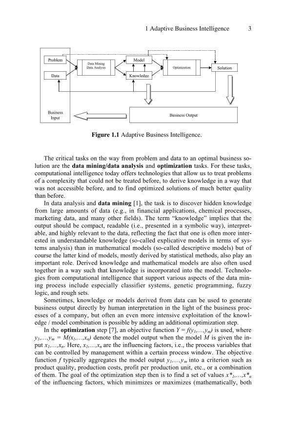
The general concept of the adaptive business intelligence approach is outlined inFigure 1.1. The methodology focuses completely on the business relevant aspects,i.e., on the business input and the business output. Business input means the prob-lem to be treated and solved, together with the corresponding data, while businessoutput is the problem knowledge or problem solution generated by the approach,which can be turned into business operations to improve desired aspects of thebusiness.
1 Adaptive Business Intelligence 3
The critical tasks on the way from problem and data to an optimal business so-lution are the data mining/data analysis and optimization tasks. For these tasks,computational intelligence today offers technologies that allow us to treat problemsof a complexity that could not be treated before, to derive knowledge in a way thatwas not accessible before, and to find optimized solutions of much better qualitythan before.
In data analysis and data mining [1], the task is to discover hidden knowledgefrom large amounts of data (e.g., in financial applications, chemical processes,marketing data, and many other fields). The term “knowledge” implies that theoutput should be compact, readable (i.e., presented in a symbolic way), interpret-able, and highly relevant to the data, reflecting the fact that one is often more inter-ested in understandable knowledge (so-called explicative models in terms of sys-tems analysis) than in mathematical models (so-called descriptive models) but ofcourse the latter kind of models, mostly derived by statistical methods, also play animportant role. Derived knowledge and mathematical models are also often usedtogether in a way such that knowledge is incorporated into the model. Technolo-gies from computational intelligence that support various aspects of the data min-ing process include especially classifier systems, genetic programming, fuzzylogic, and rough sets.
Sometimes, knowledge or models derived from data can be used to generatebusiness output directly by human interpretation in the light of the business proc-esses of a company, but often an even more intensive exploitation of the knowl-edge / model combination is possible by adding an additional optimization step.
In the optimization step [7], an objective function Y = f(y1,…,ym) is used, wherey1,…,ym = M(x1,…,xn) denote the model output when the model M is given the in-put x1,…,xn. Here, x1,…,xn are the influencing factors, i.e., the process variables thatcan be controlled by management within a certain process window. The objectivefunction f typically aggregates the model output y1,…,ym into a criterion such asproduct quality, production costs, profit per production unit, etc., or a combinationof them. The goal of the optimization step then is to find a set of values x*1,…,x*n
of the influencing factors, which minimizes or maximizes (mathematically, both
Figure 1.1 Adaptive Business Intelligence.
Business Input
Problem Model
Solution Data Mining
Data Analysis Optimization
Data Knowledge
Business Output

Thomas Bäck4
problems are equivalent) the objective function value; written usually asY ( )min max .
The need for accurate models that reflect all relevant aspects of reality impliesthat the optimization task becomes extremely complex, characterized by high-dimensional, nonlinear dependencies between process variables x1,…,xn and objec-tive function values Y = f(M(x1,…,xn)). Moreover, the functional dependency isoften discontinuous, noisy, or even time-dependent in case of dynamical optimiza-tion problems, and it might be very time-consuming to evaluate Y for one set ofvalues x1,…,xn, such that only a small number of pairs ((x1i,…,xni), Yi) can be gener-ated. Figure 1.2 illustrates a very simplified 2-dimensional cut from a real-worldminimization problem, where the objective function value Y is plotted as a functionof two real-valued process variables only. As one can see directly, a greedy mini-mization procedure might easily “get stuck” in a suboptimal “hole” without findingthe sharp peak if the method is not allowed to accept temporarily a worsening of Yat the benefit of overcoming such a locally optimal hole.
While a large number of special-purpose optimization methods is available forsimplified subclasses of the optimization problem, empirical research of the pastdecade has demonstrated that technologies from the field of computational intelli-gence, so-called evolutionary algorithms, are especially powerful for solving real-world problems characterized by this one or even by more of the above-mentionedfeatures. In particular, this includes evolution strategies and genetic algorithms (seee.g., [3, 2, 7]).
In many business applications, dynamics of the real-world business processes isof paramount importance as it requires timely adaptation of the process to chang-ing conditions (consider, e.g., plane and crew scheduling problems of big airlines,which require adaptations of the schedule on daily, weekly, monthly, quarterly, etc.time frames). Self-adaptability of software as implemented, e.g., in evolutionstrategies, one of the key computational intelligence technologies, is a key technol-
Figure 1.2 A nonlinear objective function

1 Adaptive Business Intelligence 5
ogy to guarantee adaptation even under fast-changing environmental conditions[6].
1.3 Self-Adaptive Software: Evolution Strategies
One of the key features of evolution strategies is that they adapt themselves to thecharacteristics of the optimization problem to be solved, i.e., they use a featurecalled self-adaptation to achieve a new level of flexibility. Self-adaptation allows asoftware to adapt itself to any problem from a general class of problems, to recon-figure itself accordingly, and to do this without any user interaction. The conceptwas originally invented in the context of evolution strategies (see, e.g., [6]), butcan of course be applied on a more general level [5]. Looking at this from the op-timization point of view, most optimization methods can be summarized by thefollowing iterative procedure, which shows how to generate the next vector(x1(t+1),…,xn(t+1)) from the current one:
(x1(t+1),…,xn(t+1)) = (x1(t),…,xn(t)) + st. (v1(t),…,vn(t)).
Here, (v1(t),…,vn(t)) denotes the direction of the next search step at iteration t+1,and st denotes the step size (a scalar value) for the search step length along this di-rection. Of course, the key to the success of an optimization method consists offinding effective ways to determine, at each time step t, an appropriate directionand step size (and there are hundreds of proposals how to do this). An evolutionstrategy does this in a self-adaptive way.
The basic idea of an evolution strategy, like other evolutionary algorithms aswell, consists of using the model of organic evolution as a process for adaptationand optimization. Consequently, the algorithms use a “population of individuals”representing candidate solutions to the optimization problem, and evolutionary op-erators such as variation (e.g., recombination and mutation) and selection in an it-erative way such as it is outlined in Figure 1.3. In evolution strategies, populationscan be rather small, like, e.g., in the example of a (1,10)-strategy. The notation in-dicates that 10 offspring solutions are generated by means of mutation from oneparent solution, and the best (according to the objective function value) of the off-spring individuals is chosen as the parent for the next iteration. It should be notedthat discarding the parent is done intentionally, because it allows the algorithm toaccept temporary worsenings in quality to overcome locally optimal solutions (cf.Figure 1.2). For the mutation operator, the basic variants of evolution strategies usenormally distributed variations z Ni i( )0, where N i 0,( ) denotes a normally
distributed random sample with expectation zero and standard deviation , i.e.,the mutation operator modifies a solution candidate (x1(t),…,xn(t)) by setting xi(t+1) =xi(t) + zi, where i = {1,…,n}. The mutation is normally distributed with expectedvalue zero and variance 2, i.e., step size and direction are implicitly defined bymeans of the normal distribution (here, the direction is random while the step size
is approximately n( )1 2/). The fundamental approach for self-adaptation is to
adapt itself online while optimizing by extending the representation of solutionsby the step size , i.e., ((x1(t),…,xn(t)), ), where now is a component of the in-

Thomas Bäck6
dividual (and different for each individual of a population), and the mutation op-erator proceeds according to the rule
= ( )( )= + ( )+( ) ( )
exp , ,
,
N
x x Ni t i t i
0 1
01
forming the new individual ((x1(t),…,xn(t)), ). In other words, is mutated first,and the mutated step size is then used to generate the offspring. There is no exter-nal control of step sizes at all. Instead, they are completely controlled by the algo-rithm itself, based on an autonomous adaptation process using the implicit feed-back of the quality criterion. A theoretical analysis for an analyzable objectivefunction has proven that, for this special case, self-adaptation generates an optimal
at any stage of the search process (see, e.g., [4] for a complete introduction toevolution strategy theory). In the above formulation, the special parameter de-notes a “learning rate”, which defines the speed of adaptation on the level of stan-dard deviations . According to the theoretical knowledge about the process, a
value of = ( )1 21 2
n/
is a robust and generally useful setting.
The method outlined above is only the most basic version of self-adaptation.Much more elaborate variants are in use, which allow for the self-adaptation ofgeneral, n-dimensional normal distributions, including correlations between thevariables, and also self-adaptive population sizes are currently under investigation.The resulting algorithms have no external parameters that need to be tuned for aparticular application.
Figure 1.3. The evolutionary loop.

1 Adaptive Business Intelligence 7
1.4 Examples
All adaptive business intelligence solutions provided by NuTech Solutions for itsclients are characterized by applying the most suitable combination of traditionaland computational intelligence technologies to achieve the best possible improve-ment of business processes. In all cases, the technical aspects of the implementa-tion and client’s problem are subject to nondisclosure agreements. Concerning theapplications of self-adaptive evolution strategies, the following three examples (seeFigure 1.3) illustrate the capabilities of these algorithms: the optimization of trafficlight schedules at street intersections to dynamically adapt the traffic light control
Figure 1.4. Examples of applications of evolution strategies: traffic light con-trol (top), elevator control optimization (middle), metal stamping process op-timization in automobile industry (bottom).

Thomas Bäck8
to the actual traffic situation (executed for the Dutch Ministry of Traffic, Rotter-dam, The Netherlands). The optimization of control policies for elevator control-lers to dynamically adapt elevator control to the actual traffic situation (executedfor Fujitec Ltd., Osaka, Japan), and the optimization of the metal stamping processto improve quality of the resulting car components while minimizing metal losses(executed for AutoForm Engineering, Zürich, Switzerland). In these examples, themodel is implemented by a simulation software already at the client’s disposal, i.e.,the optimization part (right part) of Figure 1.1 is executed by NuTech Solutions onthe basis of existing models. The dimensionality n of the model input is in thesmall to middle range, i.e., around 20–40, all of them real-valued. The two trafficcontrol problems are dynamic and noisy, and the evolution strategy locates andcontinuously maintains very high-quality solutions in an effective and flexible waythat cannot be achieved by other methods. In the metal stamping simulation, theevolution strategy is the first algorithm at all that makes the process manageable bymeans of optimization, and the method yields strong improvements when com-pared to hand-optimized processes.
1.5 Outlook
In this chapter, only very little information about the actual industrial impact ofadaptive business intelligence solutions based on computational intelligence tech-nologies can be disclosed. Much more complex applications, implementing thewhole scenario outlined in Figure 1.1, are presently in use by clients of NuTechSolutions, with an enormous economic benefit for these companies. In particular,those applications where data mining, model building, knowledge discovery, opti-mization, and management decision support are combined yield a new quality inbusiness process optimization. Adaptation and self-adaptation capabilities of thecorresponding software products play an extremely important role in this context,as many applications require a dynamic response capability of the applicable solu-tion software. The modern business environment clearly demonstrates the growingneed for adaptive business intelligence solutions, and computational intelligencehas proven to be the ideal technology to fulfill the needs of companies in the newcentury. Adaptive business intelligence is the realization of structured managementtechnologies (e.g., 6 Sigma, TQM) using technologies of the 21st century.
References
1. Adriaans P., D. Zantinge, Data Mining, Addison-Wesley, 1996.2. Bäck T., D.B. Fogel, Z. Michaewicz, Handbook of Evolutionary Computation,
Institute of Physics, Bristol, UK, 2000.3. Bäck T., Evolutionary Algorithms in Theory and Practice, Oxford University
Press, New York, 1996.

1 Adaptive Business Intelligence 9
4. Beyer H.-G., The Theory of Evolution Strategies, Series on Natural Computa-tion, Springer, Berlin, 2001.
5. Robertson P., H. Shrobe, R. Laddaga (eds.), Self-Adaptive Software. LectureNotes in Computer Science, Vol. 1936, Springer, Berlin, 2000.
6. Schwefel H.-P., Collective Phenomena in Evolutionary Systems. In Preprints ofthe 31st Annual Meeting of the International Society for General System Re-search, Budapest, Vol. 2, 1025-1033.
7. Schwefel H.-P., Evolution and Optimum Seeking, Wiley, New York, 1995.

2___ ______ ______ ______ ______ ______ ______ ______ ______ ______ ______ ______ ______ ______ ______
Extending the Boundaries of Design Opti-mization by Integrating Fast OptimizationTechniques with Machine Code Based,Linear Genetic Programming
L. M. Deschaine, F.D. Francone
2.1 Introduction
Engineers frequently encounter problems that require them to estimate control orresponse settings for industrial or business processes that optimize one or moregoals. Most optimization problems include two distinct parts: (1) a model of theprocess to be optimized; and (2) an optimizer that varies the control parameters ofthe model to derive optimal settings for those parameters.
For example, one of the research and development (R&D) case studies includedhere involves the control of an incinerator plant to achieve a high probability ofenvironmental compliance and minimal cost. This required predictive models ofthe incinerator process, environmental regulations, and operating costs. It also re-quired an optimizer that could combine the underlying models to calculate a real-time optimal response that satisfied the underlying constraints. Figure 2.1 showsthe relationship of the optimizer and the underlying models for this problem.
The incinerator example discussed above and the other case studies below didnot yield to a simple constrained optimization approach or a well-designed neuralnetwork approach. The underlying physics of the problem were not well under-stood; so this problem was best solved by decomposing it into its constituentparts—the three underlying models (Figure 2.1) and the optimizer.
This work is, therefore, concerned with complex optimization problems charac-terized by either of the following situations.
First: Engineers often understand the underlying processes quite well, but thesoftware simulator they create for the process is slow. Deriving optimal settings fora slow simulator requires many calls to the simulator. This makes optimization in-convenient or completely impractical. Our solution in this situation was to reverseengineer the existing software simulator using Linear Genetic Programming(LGP)—in effect, we simulated the simulator. Such “second-order” LGP simula-tions are frequently very accurate and almost always orders of magnitude fasterthan the hand-coded simulator. For example, for the Kodak Simulator, describedbelow, LGP reverse engineered that simulator, reducing the time per simulationfrom hours to less than a second. As a result, an optimizer may be applied to theLGP-derived simulation quickly and conveniently.

L.M. Deschaine, F.D. Francone12
Figure 2.1 How the optimizer and the various models operate together for the in-cinerator solution.
Second: In the incinerator example given above, the cost and regulatory modelswere well understood, but the physics of the incinerator plant were not. However,good-quality plant operating data existed. This example highlights the secondsituation in which our approach consistently yields excellent results. LGP built amodel of plant operation directly from the plant operation data. Combined with thecost and regulatory models to form a meta-model, the LGP model permits real-time optimization to achieve regulatory and cost goals.
For both of the above types of problems, the optimization and modeling toolsshould possess certain clearly definable characteristics:
• The optimizer should make as few calls to the process model as possible, con-sistent with producing high-quality solutions,
• The modeling tool should consistently produce high-precision models that exe-cute quickly when called by the optimizer,
• Both the modeling and optimizing tools should be general-purpose tools. Thatis, they should be applicable to most problem domains with minimal customi-zation and capable of producing good to excellent results across the wholerange of problems that might be encountered; and
• By integrating tools with the above characteristics, we have been able to im-prove problem-solving capabilities very significantly for both problem typesabove.
This work is organized as follows. We begin by introducing the Evolution Strate-gies with Completely Derandomized Self-Adaptation (ES-CDSA) algorithm as ouroptimization algorithm of choice. Next, we describe machine-code-based, LGP indetail and describe a three-year study from which we have concluded that machine-code-based, LGP is our modeling tool of choice for these types of applications. Fi-nally, we suggest ways in which the integrated optimization and modeling strategymay be applied to design optimization problems.

2 Extending the Boundaries of Design Optimization 13
2.2 Evolution Strategies Optimization
ES was first developed in Germany in the 1960s. It is a very powerful, general-purpose, parameter optimization technique [25,26,27]. Although we refer in thiswork to ES, it is closely related to Fogel’s Evolutionary Programming (EP) [7, 1].Our discussion here applies equally to ES and EP. For ease of reference, we willuse the term “ES” to refer to both approaches.
ES uses a population-based learning algorithm. Each generation of possible so-lutions is formed by mutating and recombining the best members of the previousgeneration. ES pioneered the use of evolvable “strategy parameters.” Strategy pa-rameters control the learning process. Thus, ES evolves both the parameters to beoptimized and the parameters that control the optimization [2].
ES has the following desirable characteristics for the uses in our methodology:
• ES can optimize the parameters of arbitrary functions. It does not need to beable to calculate derivatives of the function to be optimized, nor does the re-searcher need to assume differentiability and numerical accuracy. Instead, ESgathers gradient information about the function by sampling. [12]
• Substantial literature over many years demonstrates that ES can solve a verywide range of optimization problems with minimal customization. [25, 26, 27,12]
Although very powerful and not prone to getting stuck in local optima, typical ESsystems can be very time-consuming for significant optimization problems. Thus,canonical ES often fails the requirement of efficient optimization.
But in the past five years, ES has been extended using the ES-CDSA technique[12]. ES-CDSA allows a much more efficient evolution of the strategy parametersand cumulates gradient information over many generations, rather than single gen-eration as used in traditional ES.
As a rule of thumb, where n is the number of parameters to be optimized, usersshould allow between 100 and 200(n+3)2 function evaluations to get optimal usefrom this algorithm [12]. While this is a large improvement over previous ES ap-proaches, it can still require many calls by the optimizer to the model to be opti-mized to produce results. As a result, it is still very important to couple ES-CDSAwith fast-executing models. And that is where LGP becomes important.
2.3 Linear Genetic Programming
Genetic Programming (GP) is the automatic creation of computer programs to per-form a selected task using Darwinian natural selection. GP developers give theircomputers examples of how they want the computer to perform a task. GP softwarethen writes a computer program that performs the task described by the examples.GP is a robust, dynamic, and quickly growing discipline. It has been applied to di-verse problems with great success—equaling or exceeding the best human-createdsolutions to many difficult problems [14, 3, 4, 2].
This chapter presents three years of analysis of machine-code-based, LGP. Toperform the analyses, we used Versions 1 through 3 of an off-the-shelf commercial

L.M. Deschaine, F.D. Francone14
software package called Discipulus™ [22]. Discipulus is an LGP system that oper-ates directly on machine code.
2.3.1 The Genetic Programming Algorithm
Good, detailed treatments of GP may be found in [2, 14]. In brief summary, theLGP algorithm in Discipulus is surprisingly simple. It starts with a population ofrandomly generated computer programs. These programs are the “primordial soup”on which computerized evolution operates. Then, GP conducts a “tournament” byselecting four programs from the population—also at random—and measures howwell each of the four programs performs the task designated by the GP developer.The two programs that perform the task best “win” the tournament.
The GP algorithm then copies the two winner programs and transforms thesecopies into two new programs via crossover and mutation transformation opera-tors—in short, the winners have “children.” These two new child programs arethen inserted into the population of programs, replacing the two loser programsfrom the tournament. GP repeats these simple steps over and over until it has writ-ten a program that performs the selected task.
GP creates its “child” programs by transforming the tournament winning pro-grams. The transformations used are inspired by biology. For example, the GPmutation operator transforms a tournament winner by changing it randomly—themutation operator might change an addition instruction in a tournament winner to amultiplication instruction. Likewise, the GP crossover operator causes instructionsfrom the two tournament winning programs to be swapped—in essence, an ex-change of genetic material between the winners. GP crossover is inspired by theexchange of genetic material that occurs in sexual reproduction in biology.
2.3.2 Linear Genetic Programming Using Direct Manipulation of BinaryMachine Code
Machine-code-based, LGP is the direct evolution of binary machine code throughGP techniques [15, 16, 17, 18, 20]. Thus, an evolved LGP program is a sequenceof binary machine instructions. For example, an evolved LGP program might becomprised of a sequence of four, 32-bit machine instructions. When executed,those four instructions would cause the central processing unit (CPU) to performoperations on the CPU’s hardware registers. Here is an example of a simple, four-instruction LGP program that uses three hardware registers:
register 2 = register 1 + register 2register 3 = register 1 - 64register 3 = register 2 * register 3register 3 = register 2 / register 3
While LGP programs are apparently very simple, it is actually possible toevolve functions of great complexity using only simple arithmetic functions on aregister machine [18, 20].

2 Extending the Boundaries of Design Optimization 15
After completing a machine-code LGP project, the LGP software decompilesthe best evolved models from machine code into Java, ANSI C, or Intel Assemblerprograms [22]. The resulting decompiled code may be linked to the optimizer andcompiled or it may be compiled into a DLL or COM object and called from theoptimization routines.
The linear machine code approach to GP has been documented to be between 60to 200 times faster than comparable interpreting systems [10, 15, 20]. As will bedeveloped in more detail in the next section, this enhanced speed may be used toconduct a more intensive search of the solution space by performing more andlonger runs.
2.4 Why Machine-Code-based, Linear Genetic Programming?
At first glance, it is not at all obvious that machine-code, LGP is a strong candidatefor the modeling algorithm of choice for the types of complex, high-dimensionalproblems at issue here. But over the past three years, a series of tests was per-formed on both synthetic and industrial data sets—many of them data sets onwhich other modeling tools had failed. The purpose of these tests was to assessmachine-code, LGP’s performance as a general-purpose modeling tool.
In brief summary, the machine-code-based LGP software [22] has become ourmodeling tool of choice for complex problems like the ones described in this workfor several reasons:
• Its speed permits the engineer to conduct many runs in realistic timeframes on adesktop computer. This results in consistent, high-precision models with littlecustomization;
• It is well-designed to prevent overfitting and to produce robust solutions; and• The models produced by the LGP software execute very quickly when called by
an optimizer.
We will first discuss the use of multiple LGP runs as a key ingredient of this tech-nique. Then we will discuss our investigation of machine-code, LGP over the pastthree years.
2.5 Multiple Linear Genetic Programming Runs
GP is a stochastic algorithm. Accordingly, running it over and over with the sameinputs usually produces a wide range of results, ranging from very bad to verygood. For example, Figure 2.2 shows the distribution of the results from 30 runs ofLGP on the incinerator plant modeling problem mentioned in the introduction—theR2 value is used to measure the quality of the solution. The solutions ranged from avery poor R2 of 0.05 to an excellent R2 of 0.95. Our investigation to date stronglysuggests the typical LGP distribution of results from multiple LGP runs includes adistributional tail of excellent solutions that is not always duplicated by otherlearning algorithms.

L.M. Deschaine, F.D. Francone16
Figure 2.2 . Incinerator control data. Histogram of results for 30 LGP runs.
Figure 2.3 Typical comparative histograms of the quality of solutions producedby LGP runs (bars) and Neural Network runs (lines). Discussed in detail in [8].
For example, for three separate problem domains, an LGP system produced along tail of outstanding solutions, even though the average LGP solution was notnecessarily very good. By way of contrast, and in that same study, the distributionof many neural networks runs on the same problems often produced a good aver-age solution, but did not produce a tail of outstanding solutions like LGP [4,8].
Figure 2.3 shows a comparative histogram of LGP results versus neural networkresults derived from 720 runs of each algorithm on the same problem. Better solu-tions appear to the right of the chart. Note the tail of good LGP solutions (the bars)that is not duplicated by a comparable tail of good neural network solutions. Thissame pattern may be found in other problem domains [4,8].
To locate the tail of best solutions on the right of Figure 2.3, it is essential toperform many runs, regardless whether the researcher is using neural networks orLGP. This is one of the most important reasons why a machine-code approach toGP is preferable to other approaches. It is so much faster than other approaches,that it is possible to complete many runs in realistic timeframes on a desktop com-puter. That makes it more capable of finding the programs in the good tail of thedistribution.
Better Solutions

2 Extending the Boundaries of Design Optimization 17
2.6 Configuration Issues in Performing Multiple LGP Runs
Our investigation into exploiting the multiple run capability of machine-code-based LGP had two phases—largely defined by software versioning. Early ver-sions of the Discipulus LGP software permitted multiple runs, but only with user-predefined parameter settings.
As a result, our early multiple run efforts (described below as our Phase I inves-tigation) just chose a range of reasonable values for key parameters, estimated anappropriate termination criterion for the runs, and conducted a series of runs atthose selected parameter settings. For example, the chart of the LGP results on theincinerator CO2 data sets (Figure. 2.2) was the result of doing 30 runs using differ-ent settings for the mutation parameter.
By way of contrast, the second phase of our investigation was enabled by fourkey new capabilities introduced into later versions of the LGP software. Those ca-pabilities were
• The ability to perform multiple runs with randomized parameter settings fromrun to run;
• The ability to conduct hillclimbing through LGP parameter space based on theresults of previous runs;
• The ability to automatically assemble teams of models during a project that, ingeneral, perform better than individual models; and
• The ability to determine an appropriate termination criterion for runs, for a par-ticular problem domain, by starting a project with short runs and automaticallyincreasing the length of the runs until longer runs stop yielding better results.
Accordingly, the results reported below as part of our Phase II investigation arebased on utilizing these additional four capabilities.
2.7 Investigation of Machine-Code-Based, Linear GeneticProgramming—Phase I
We tested Versions 1.0 and 2.0 of the Discipulus LGP software on a number ofproblem domains during this first phase of our investigation. This Phase I investi-gation covered about two years and is reported in the next three sections.
2.7.1 Deriving Physical Laws
Science Applications International Corporation’s (SAIC’s) interest in LGP wasinitially based on its potential ability to model physical relationships. So the firsttest for LGP to see if it could model the well-known (to environmental engineers,at least) Darcy’s law. Darcy’s law describes the flow of water through porous me-dia. The equation is
Q=K*I*A, (2.1)

L.M. Deschaine, F.D. Francone18
where Q = flow [L3/T], K = hydraulic conductivity [L/T], I = gradient [L/L], and A= area [L2].
To test LGP, we generated a realistic input set and then used Darcy’s law toproduce outputs. We then added 10% random variation to the inputs and outputsand ran the LGP software on these data. After completing our runs, we examinedthe best program it produced.
The best solution derived by the LGP software from these data was a four-instruction program that is precisely Darcy’s law, represented in ANSI C as
Q = 0.0Q += IQ *= KQ *= A
In this LGP evolved program, Q is an accumulator variable that is also the finaloutput of the evolved program.
This program model of Darcy's law was derived as follows. First, it was evolvedby LGP. The “raw” LGP solution was accurate though somewhat unintelligible. Byusing intron removal [19] with heuristics and evolutionary strategies the specificform of Darcy’s law was evolved. This process is coded in the LGP software; weused the “Interactive Evaluator” module, which links to the “Intron Removal” andautomatic “Simplification” and “Optimization” functions. These functions combineheuristics and ES optimization to derive simpler versions of the programs that LGPevolves [22].
2.7.2 Incinerator Process Simulation
The second LGP test SAIC performed was the prediction of CO2 concentrations inthe secondary combustion chamber of an incinerator plant from process measure-ments from plant operation. The inputs were various process parameters (e.g., fueloil flow, liquid waste flow, etc.) and the plant control settings. The ability to makethis prediction is important because the CO2 concentration strongly affects regu-latory compliance.
This problem was chosen because it had been investigated using neural net-works. Great difficulty was encountered in deriving any useful neural networkmodels for this problem during a well-conducted study [5].
The incinerator to be modeled processed a variety of solid and aqueous waste,using a combination of a rotary kiln, a secondary combustion chamber, and an off-gas scrubber. The process is complex and consists of variable fuel and waste in-puts, high temperatures of combustion, and high-velocity off-gas emissions.
To set up the data, a zero- and one-hour offset for the data was used to constructthe training and validation instance sets. This resulted in a total of 44 input vari-ables. We conducted 30 LGP runs for a period of 20 hours each, using 10 differentrandom seeds for each of three mutation rates (0.10, 0.50, 0.95) [3]. The stoppingcriterion for all simulations was 20 hours. All 30 runs together took 600 hours torun.
2 Extending the Boundaries of Design Optimization 19
Two of the LGP runs produced excellent results. The best run showed a valida-tion data set R2 fitness of 0.961 and an R2 fitness of 0.979 across the entire dataset.
The two important results here were (1) LGP produced a solution that could notbe obtained using neural networks; and (2) only two of the 30 runs produced goodsolutions (see Figure 2.2), so we would expect to have to conduct all 30 runs tosolve the problem again.
2.7.3 Data Memorization Test
The third test SAIC performed was to see whether the LGP algorithm was memo-rizing data, or actually learning relationships.
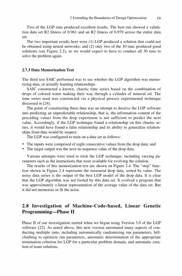
SAIC constructed a known, chaotic time series based on the combination ofdrops of colored water making their way through a cylinder of mineral oil. Thetime series used was constructed via a physical process experimental techniquediscussed in [24].
The point of constructing these data was an attempt to deceive the LGP softwareinto predicting an unpredictable relationship, that is, the information content of thepreceding values from the drop experiment is not sufficient to predict the nextvalue. Accordingly, if the LGP technique found a relationship on this chaotic se-ries, it would have found a false relationship and its ability to generalize relation-ships from data would be suspect.
The LGP was configured to train on a data set as follows:
• The inputs were comprised of eight consecutive values from the drop data; and• The target output was the next-in-sequence value of the drop data.
Various attempts were tried to trick the LGP technique, including varying pa-rameters such as the instructions that were available for evolving the solution.
The results of this memorization test are shown on Figure 2.4. The “step” func-tion shown in Figure 2.4 represents the measured drop data, sorted by value. Thenoisy data series is the output of the best LGP model of the drop data. It is clearthat the LGP algorithm was not fooled by this data set. It evolved a program thatwas approximately a linear representation of the average value of the data set. Butit did not memorize or fit the noise.
2.8 Investigation of Machine-Code-based, Linear GeneticProgramming—Phase II
Phase II of our investigation started when we began using Version 3.0 of the LGPsoftware [22]. As noted above, this new version automated many aspects of con-ducting multiple runs, including automatically randomizing run parameters, hill-climbing to optimize run parameters, automatic determination of the appropriatetermination criterion for LGP for a particular problem domain, and automatic crea-tion of team solutions.
L.M. Deschaine, F.D. Francone20
Figure 2.4 Attempt to model a chaotic time series with LGP.
0
5
10
15
20
25
0.05 0.15 0.25 0.35 0.45 0.55 0.65 0.75 0.85 0.95
R2 Values - Top 30 Runs
Nu
mb
er o
f S
olu
tio
ns
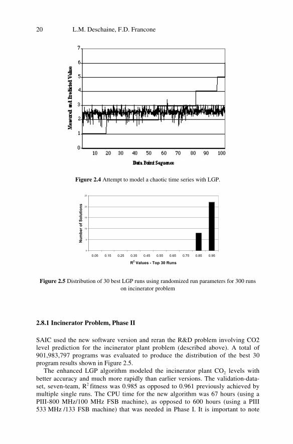
Figure 2.5 Distribution of 30 best LGP runs using randomized run parameters for 300 runson incinerator problem
2.8.1 Incinerator Problem, Phase II
SAIC used the new software version and reran the R&D problem involving CO2level prediction for the incinerator plant problem (described above). A total of901,983,797 programs was evaluated to produce the distribution of the best 30program results shown in Figure 2.5.
The enhanced LGP algorithm modeled the incinerator plant CO2 levels withbetter accuracy and much more rapidly than earlier versions. The validation-data-set, seven-team, R2 fitness was 0.985 as opposed to 0.961 previously achieved bymultiple single runs. The CPU time for the new algorithm was 67 hours (using aPIII-800 MHz/100 MHz FSB machine), as opposed to 600 hours (using a PIII533 MHz /133 FSB machine) that was needed in Phase I. It is important to note

2 Extending the Boundaries of Design Optimization 21
that the team solution approach was important in developing a better solution inless time.
2.8.2 UXO Discrimination
The preceding examples are regression problems. The enhanced LGP algorithmwas also tested during Phase II on a difficult classification challenge the determi-nation of the presence of subsurface unexploded ordnance (UXO).
The Department of Defense has been responsible for conducting UXO investi-gations at many locations around the world. These investigations have resulted inthe collection of extraordinary amounts of geophysical data with the goal of identi-fying buried UXO.
Evaluation of UXO/non-UXO data is time-consuming and costly. The standardoutcome of these types of evaluations is maps showing the location of geophysicalanomalies. In general, what these anomalies may be (i.e., UXO, non-UXO, boul-ders, etc.) cannot be determined without excavation at the location of the anomaly.
Figure 2.6 shows the performance of 10 published industrial-strength, discrimi-nation algorithms on the Jefferson Proving Grounds UXO data—which consistedof 160 targets [13]. The horizontal axis shows the performance of each algorithmin correctly identifying points that did not contain buried UXO. The vertical axisshows the performance of each algorithm in correctly identifying points that didcontain buried UXO. The angled line in Figure 2.6 represents what would be ex-pected from random guessing.
Figure 2.6 points out the difficulty of modeling these data. Most algorithms didlittle better than random guessing; however, the LGP algorithm derived a best-known model for correctly identifying UXO’s and for correctly rejecting non-UXO’s using various data set configurations [5, 13]. The triangle in the upperright-hand corner of Figure 2.6 shows the range of LGP solutions in these differentconfigurations.
0
10
20
30
40
50
60
70
80
90
100
0 10 20 30 40 50 60 70 80 90 100
Percent of Correct Non-UXO Discriminated [Better---->]
Per
cen
t o
f C
orr
ect
UX
O D
iscr
imin
ated
[B
ette
r---
->]
Geo-CentersNAEVA
Naval Rsch
Geophex
Battelle
AppliedPhysics
SC&A
ENSCOADI/Alpha
GTL
Line of no better discrimination than guessing
LGP Solution
Figure 2.6 LGP and 10 other algorithms applied to the UXO discrimination data [13].
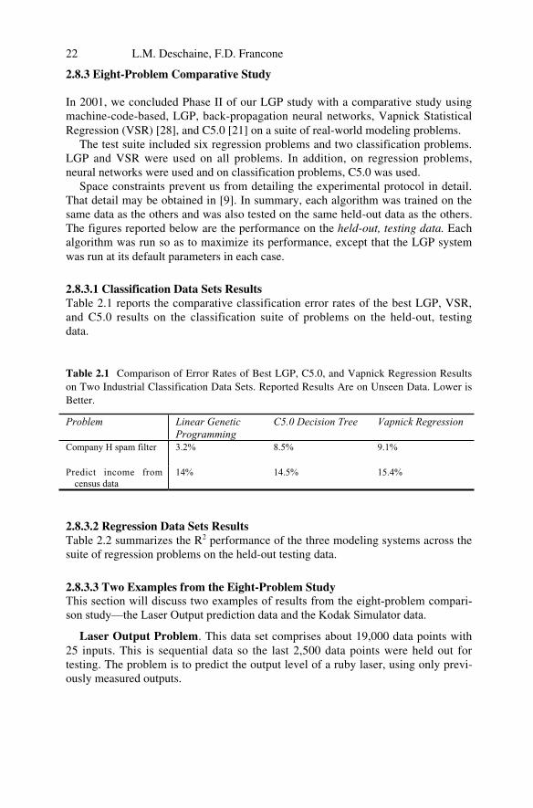
L.M. Deschaine, F.D. Francone22
2.8.3 Eight-Problem Comparative Study
In 2001, we concluded Phase II of our LGP study with a comparative study usingmachine-code-based, LGP, back-propagation neural networks, Vapnick StatisticalRegression (VSR) [28], and C5.0 [21] on a suite of real-world modeling problems.
The test suite included six regression problems and two classification problems.LGP and VSR were used on all problems. In addition, on regression problems,neural networks were used and on classification problems, C5.0 was used.
Space constraints prevent us from detailing the experimental protocol in detail.That detail may be obtained in [9]. In summary, each algorithm was trained on thesame data as the others and was also tested on the same held-out data as the others.The figures reported below are the performance on the held-out, testing data. Eachalgorithm was run so as to maximize its performance, except that the LGP systemwas run at its default parameters in each case.
2.8.3.1 Classification Data Sets ResultsTable 2.1 reports the comparative classification error rates of the best LGP, VSR,and C5.0 results on the classification suite of problems on the held-out, testingdata.
Table 2.1 Comparison of Error Rates of Best LGP, C5.0, and Vapnick Regression Resultson Two Industrial Classification Data Sets. Reported Results Are on Unseen Data. Lower isBetter.
Problem Linear GeneticProgramming
C5.0 Decision Tree Vapnick Regression
Company H spam filter 3.2% 8.5% 9.1%
Predict income fromcensus data
14% 14.5% 15.4%
2.8.3.2 Regression Data Sets ResultsTable 2.2 summarizes the R2 performance of the three modeling systems across thesuite of regression problems on the held-out testing data.
2.8.3.3 Two Examples from the Eight-Problem StudyThis section will discuss two examples of results from the eight-problem compari-son study—the Laser Output prediction data and the Kodak Simulator data.
Laser Output Problem. This data set comprises about 19,000 data points with25 inputs. This is sequential data so the last 2,500 data points were held out fortesting. The problem is to predict the output level of a ruby laser, using only previ-ously measured outputs.
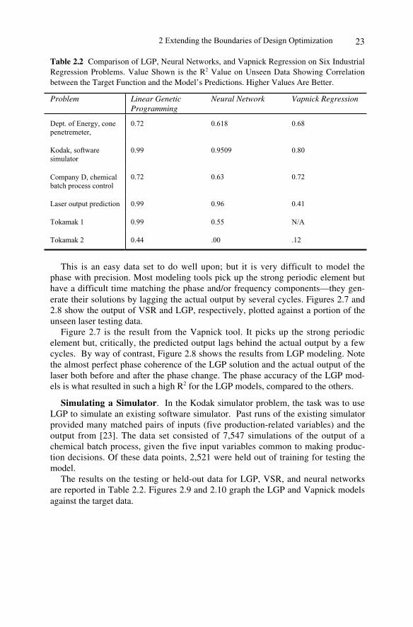
2 Extending the Boundaries of Design Optimization 23
Table 2.2 Comparison of LGP, Neural Networks, and Vapnick Regression on Six IndustrialRegression Problems. Value Shown is the R2 Value on Unseen Data Showing Correlationbetween the Target Function and the Model’s Predictions. Higher Values Are Better.
Problem Linear GeneticProgramming
Neural Network Vapnick Regression
Dept. of Energy, conepenetremeter,
0.72 0.618 0.68
Kodak, softwaresimulator
0.99 0.9509 0.80
Company D, chemicalbatch process control
0.72 0.63 0.72
Laser output prediction 0.99 0.96 0.41
Tokamak 1 0.99 0.55 N/A
Tokamak 2 0.44 .00 .12
This is an easy data set to do well upon; but it is very difficult to model thephase with precision. Most modeling tools pick up the strong periodic element buthave a difficult time matching the phase and/or frequency components—they gen-erate their solutions by lagging the actual output by several cycles. Figures 2.7 and2.8 show the output of VSR and LGP, respectively, plotted against a portion of theunseen laser testing data.
Figure 2.7 is the result from the Vapnick tool. It picks up the strong periodicelement but, critically, the predicted output lags behind the actual output by a fewcycles. By way of contrast, Figure 2.8 shows the results from LGP modeling. Notethe almost perfect phase coherence of the LGP solution and the actual output of thelaser both before and after the phase change. The phase accuracy of the LGP mod-els is what resulted in such a high R2 for the LGP models, compared to the others.
Simulating a Simulator. In the Kodak simulator problem, the task was to useLGP to simulate an existing software simulator. Past runs of the existing simulatorprovided many matched pairs of inputs (five production-related variables) and theoutput from [23]. The data set consisted of 7,547 simulations of the output of achemical batch process, given the five input variables common to making produc-tion decisions. Of these data points, 2,521 were held out of training for testing themodel.
The results on the testing or held-out data for LGP, VSR, and neural networksare reported in Table 2.2. Figures 2.9 and 2.10 graph the LGP and Vapnick modelsagainst the target data.
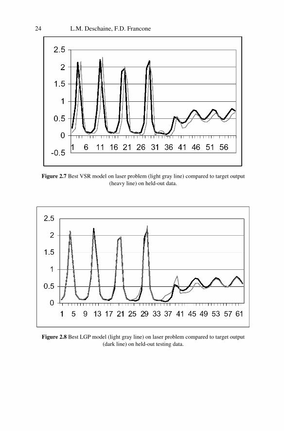
L.M. Deschaine, F.D. Francone24
Figure 2.7 Best VSR model on laser problem (light gray line) compared to target output(heavy line) on held-out data.
Figure 2.8 Best LGP model (light gray line) on laser problem compared to target output(dark line) on held-out testing data.

2 Extending the Boundaries of Design Optimization 25
Figure 2.9 Best Vapnick predictions of Kodak simulator data (light-gray series) vs. the tar-get data (dark line) on held-out data.
Figure 2.10 Best LGP model of company K simulator problem (light gray series) vs. targetdata (dark series) on the held-out data.
The LGP solution (Figure 2.10) so closely models the target output that the pre-dictions completely obscure the target output line. In fact, for all but six of the2,521 data points, the agreement between the LGP prediction and the actual valueis very good. The R2 fitness on the applied data set for the best team solution was0.9889. (A second batch of 232 LGP runs achieved a similar R2 fitness on the ap-

L.M. Deschaine, F.D. Francone26
plied data set of 0.9814, using a team of seven programs. The range of R2 for thetop 30 programs of this second batch was 0.9707 to 0.9585. This demonstratesanalysis repeatability using LGP.)
The Vapnick (Figure 2.9) and neural network solutions were not nearly soclose—the R2 for the Vapnick model was only 0.80, for example.
2.9 Conclusion Regarding Empirical Studies
The key results of the two phases of our empirical studies of the LGP algorithm areas follows.
First: The LGP software we used consistently produces excellent results on dif-ficult, industrial modeling problems with little customization of the learning algo-rithm. Note: LGP did not always produce better results than all other algorithmsstudied. However, on every problem studied, LGP produced a model that was asgood as, or better than, any other algorithm.
The performance of other learning algorithms was decidedly up-and-down. Forexample, Vapnick regression did quite well on the cone penetrometer and Com-pany D data but quite poorly on the laser and Company K problems. Neural net-works did quite well on the laser and Company K problems but not so well on theTokamak and incinerator CO2 data sets. C5.0 did well on the census problem butnot well on the spam filter problem.
We speculate that one important reason behind the consistently good perform-ance of LGP is that it performs, by default, many runs. Accordingly, it locates thetail of good performing solutions discussed above. Our comfort level that LGP willarrive at a good solution to most problems without customization or “tweaking” isone of the principal reasons we have settled on LGP as our modeling algorithm ofchoice for complex and difficult modeling problems.
Second: LGP produces robust models compared to other learning algorithms.Much less attention had to be paid to overfitting problems with the LGP softwarethan with other algorithms. This is not to say that LGP will never overfit data.Given the right data set, it will. But it does so less frequently than the neural net-work, Vapnick regression, and C5.0 alternatives we studied
The LGP system identifies the important inputs, and which are not. For exam-ple, we screened a wastewater treatment plant with 54 inputs and identified 7 im-portant ones. This reduces the number of inputs to monitor, allows assessment ofwhat will happen if an input goes off-line (for security and contingency planning),and enhances accelerated optimization by reducing the number of decision vari-ables, as discussed below.
2.10 Integrated System Analysis
This work is concerned with the building of a system comprised of integratedmodeling and optimization tools. The integrated tool suite, comprised of (1) ma-chine-code-based LGP for creating predictive models, and (2) ES-CDSA, is ex-
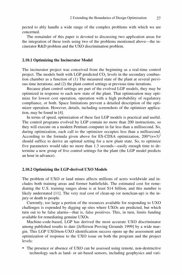
2 Extending the Boundaries of Design Optimization 27
pected to ably handle a wide range of the complex problems with which we areconcerned.
The remainder of this paper is devoted to discussing two application areas forthe integration of these tools using two of the problems mentioned above—the in-cinerator R&D problem and the UXO discrimination problem.
2.10.1 Optimizing the Incinerator Model
The incinerator project was conceived from the beginning as a real-time controlproject. The models built with LGP predicted CO2 levels in the secondary combus-tion chamber as a function of (1) The measured state of the plant at several previ-ous time iterations; and (2) the plant control settings at previous time iterations.
Because plant control settings are part of the evolved LGP models, they may beoptimized in response to each new state of the plant. That optimization may opti-mize for lowest cost operation, operation with a high probability of regulatorycompliance, or both. Space limitations prevent a detailed description of the opti-mizer operation. However, details, including screenshots of the optimizer applica-tion, may be found in [4].
In terms of speed, optimization of these fast LGP models is practical and useful.The control programs evolved by LGP contain no more than 200 instructions, sothey will execute on a modern Pentium computer in far less than a millisecond. So,during optimization, each call to the optimizer occupies less than a millisecond.According to the formula given above for ES-CDSA optimization, 200*(n+3)2
should suffice to derive an optimal setting for a new plant state. So, to optimizefive parameters would take no more than 1.3 seconds—easily enough time to de-termine a new group of five control settings for the plant (the LGP model predictsan hour in advance).
2.10.2 Optimizing the LGP-derived UXO Models
The problem of UXO or land mines affects millions of acres worldwide and in-cludes both training areas and former battlefields. The estimated cost for reme-diating the U.S. training ranges alone is at least $14 billion, and this number islikely understated [11]. The very real cost of clean-up (or nonclean-up) is the in-jury or death to people.
Currently, too large a portion of the resources available for responding to UXOchallenges is expended by digging up sites where UXOs are predicted, but whichturn out to be false alarms—that is, false positives. This, in turn, limits fundingavailable for remediating genuine UXOs.
Machine-code-based, LGP has derived the most accurate UXO discriminatoramong published results to date [Jefferson Proving Grounds 1999] by a wide mar-gin. This LGP UXO/non-UXO identification success opens up the assessment andoptimization of response to the UXO issue on both the program and the projectlevels:
• The presence or absence of UXO can be assessed using remote, non-destructivetechnology such as land- or air-based sensors, including geophysics and vari-
L.M. Deschaine, F.D. Francone28
ous wave length sensors. Developed to a high degree of accuracy, wide areascan be screened and analyzed to reduce the footprint of areas needing furtherinvestigation. This will help manage the sheer size of this challenge.
• Areas of interest identified as requiring further investigation can be prioritizedand ranked using good information on the probability or absence of UXO.This ranking would integrate the LGP UXO solution with multi-criteria/multi-objective decision support models; and
• Site-specific remedial action plans, known as “dig sheets,” can be optimally de-signed to focus efforts on high probability, UXO-containing areas. When thedecreased predicted likelihood of UXO presence and the field verified absenceof UXO are demonstrated, a stopping point for remedial activities, based onscientific principals and field validation, is provided.
2.11 Summary and Conclusions
We are in the early stages of building a comprehensive, integrated optimizationand modeling system to handle complex industrial problems. We believe a combi-nation of machine-code-based, LGP (for modeling) and ES CDSA (for optimiza-tion) together provides the best combination of available tools and algorithms forthis task.
By conceiving of design optimization projects as integrated modeling and opti-mization problems from the outset, we anticipate that engineers and researcherswill be able to extend the range of problems that are solvable, given today’s tech-nology.
Acknowledgments
The results presented in this work are part of a three-plus-year collaborative effortbetween SAIC and Register Machine Learning Technologies to advance the stateof the art of evolutionary computation as applied to complex systems. Specificallythanked for funding and latitude from SAIC are Joseph W. Craver, John Aucella,and Janardan J. Patel. Dr. Gregory Flach, Dr. Frank Syms, and Robert Walton aregratefully acknowledged for providing the input data sets used in some of the work– as are the researchers who need to keep their identity confidential for businessreasons. Christopher R. Wellington, Ad Fontes Academy, Centreville, Virginia,conducted the chaotic drop experiment. All computations were performed by, andresponsibility for their accuracy lies with, the authors.
References
1. Bäck, T., Schwefel, H.P. (1993) An Overview of Evolutionary Algorithms for Pa-rameter Optimization, Evolutionary Computation, 1(1):1-23.

2 Extending the Boundaries of Design Optimization 29
2. Banzhaf, W., Nordin, P., Keller, R., Francone, F. (1998) Genetic Programming, AnIntroduction, Morgan Kauffman Publishers, Inc., San Francisco, CA.
3. Deschaine, L.M. (2000) Tackling real-world environmental challenges with linear ge-netic programming. PCAI Magazine,15(5):35-37.
4. Deschaine, L.M., Patel, J.J., Guthrie, R.G., Grumski, J.T., Ades, M.J. (2001) “UsingLinear Genetic Programming to Develop a C/C++ Simulation Model of a Waste In-cinerator,” The Society for Modeling and Simulation International: Advanced Simula-tion Technology Conference, Seattle, WA, USA, ISBN: 1-56555-238-5, pp. 41-48.
5. Deschaine, L.M., Hoover, R.A. Skibinski, J. (2002) Using Machine Learning to Com-plement and Extend the Accuracy of UXO Discrimination Beyond the Best ReportedResults at the Jefferson Proving Grounds, (in press), Proceedings of Society for Mod-eling and Simulation International.
6. Fausett, L.V. (2000). A Neural Network Approach to Modeling a Waste IncineratorFacility, Society for Computer Simulation’s Advanced Simulation Technology Con-ference, Washington, DC, USA.
7. Fogel, D.B. (1992) Evolving Artificial Intelligence. Ph.D. thesis, University of Cali-fornia, San Diego, CA.
8. Francone, F., Nordin, P., and Banzhaf. W. (1996) Benchmarking the GeneralizationCapabilities of a Compiling Genetic Programming System Using Sparse Data Sets. InKoza et al. Proceedings of the First Annual Conference on Genetic Programming,Stanford, CA.
9. Francone F. (2002) Comparison of Discipulus™ Genetic Programming Software withAlternative Modeling Tools. Available at www.aimlearning.com.
10. Fukunaga, A., Stechert, A., Mutz, D. (1998) A Genome Compiler for High Perform-ance Genetic Programming. In Proceedings of the Third Annual Genetic ProgrammingConference, pp. 86-94, Morgan Kaufman Publishers, Jet Propulsion Laboratories,California Institute of Technology, Pasadena, CA.
11. Government Accounting Office (2001) DOD Training Range Clean-up Cost Estimatesare Likely Understated, Report to House of Representatives on Environmental Liabili-ties, USA General Accounting Office, April, Report no. GAO 01 479.
12. Hansen, N., Ostermeier, A. (2001) Completely derandomized self-adaptation in evo-lution strategies. Evolutionary Computation 9(2):159-195.
13. Jefferson Proving Grounds (1999) Jefferson Proving Grounds Phase IV Report: GraphES-1, May, Report No: SFIM-AEC-ET-CR-99051.
14. Koza, J., Bennet, F., Andre, D., and Keane, M. (1999) Genetic Programming III.Morgan Kaufman, San Francisco, CA.
15. Nordin, J.P. (1994) A Compiling Genetic Programming System that Directly Ma-nipulates the Machine Code. In Advances in Genetic Programming, K. Kinnear, Jr.(ed.), MIT Press: Cambridge MA.
16. Nordin, J.P. (1999). Evolutionary Program Induction of Binary Machine Code and itsApplications, Krehl Verlag.
17. Nordin, J.P., Banzhaf , W. (1995). Complexity Compression and Evolution. In Pro-ceedings of Sixth International Conference of Genetic Algorithms, Morgan KaufmannPublishers, Inc.
18. Nordin, J.P., Banzhaf, W. (1995). Evolving Turing Complete Programs for a RegisterMachine with Self Modifying Code. In Proceedings of Sixth International Conferenceof Genetic Algorithms, Morgan Kaufmann Publishers, Inc.
19. Nordin, J.P., Francone, F., and Banzhaf, W. (1996) Explicitly Defined Introns andDestructive Crossover in Genetic Programming. Advances in Genetic Programming 2,K. Kinnear, Jr. (ed.), MIT Press: Cambridge, MA.

L.M. Deschaine, F.D. Francone30
20. Nordin, J.P., Francone, F., and Banzhaf, W. (1998) Efficient Evolution of MachineCode for CISC Architectures Using Blocks and Homologous Crossover. In Advancesin Genetic Programming 3, MIT Press, Cambridge, MA.
21. Quinlan, R. (1998) Data Mining Tools See5 and C5.0. Technical report, RuleQuestResearch.
22. Register Machine Learning Technologies, Inc. (2002) Discipulus Users Manual, Ver-sion 3.0. Available at www.aimlearning.com.
23. Brian S. Rice and Robert L. Walton of Eastman Kodak. Company, Industrial Produc-tion Data Set.
24. Scientific American (Nov. 1999). Drop Experiment to Demonstrate a Chaotic TimeSeries.
25. Rechenberg, I. (1994). Evolutionsstrategie ’93, Fromann Verlag, Stuttgart, Germany.26. Schwefel, H.P. (1995). Evolution and Optimum Seeking. Sixth-Generation Computer
Technology Series, John Wiley & Sons, New York.27. Schwefel, H.P. and Rudolph, G. (1995). Contemporary Evolution Strategies. In Ad-
vances in Artificial Life, pp. 893-907, Springer-Verlag, Berlin.28. Vapnick V. (1998) The Nature of Statistical Learning Theory, Wiley-Interscience
Publishing.

3P
P
Summary.
IR
75% 90%
3.1 Introduction
3
Evolutionary Optimization of ApproximatingTriangulations for Surface Reconstructionfrom Unstructured 3D Data
The aim of surface reconstruction is to transfer the shape of physicalobjects, which have been sampled by tactile or optical scanning techniques, intocomputer-processable descriptions. Triangulation is the most common surface modelused in CAD/CAM systems. The processing time of a triangulation is decisively in�u-enced by the number of sampling points. Hence, either the sampling points have to bereduced or efficient triangulations have to be found. Due to the fact that for interpolat-ing triangulations the optimal distribution of the sampling points is generally difficultto �nd, here, self-organizing dynamic meshes are applied. The complex problem to�nd the best discrete approximation of a surface using a dynamic triangulation anda simple distance measure is solved by an evolution strategy. A special node-springdescription always encodes valid triangulations.
K. Weinert, J. Mehnen, and M. Schneider
The problem of triangulation can be classi�ed into two possible categories.The �rst class � and the most commonly known � is piecewise linear interpo-lation. This class of triangulations interpolates a set of unstructured pointsin with a surface consisting of triangular facets. The number of possiblevalid triangulations increases drastically with the number of points in . Thetask of optimal triangulation is to �nd a representation that renders the truesurface structure as realistic as possible. This problem is algorithmically verycomplex [5, 8]. In practical surface reconstruction the number of digitizingpoints can reach several million samples. In CAD/CAM systems the respec-tive triangulations become very large and difficult to handle. In fact, a lotof digitizing points are redundant (e.g., plane areas) and can be eliminatedfrom the original point set. In practical applications, to of the orig-inal points can be eliminated while high-tolerance demands are still met. Theproblem of automatic point reduction is to �nd �ltering criteria that efficientlyselect relevant sampling points [10].
3
3
3i i i i
j � � � j
� � � j
j
j k
S
S
S
32 Klaus Weinert et al.
3.2 Problem De�nition
| | | |
∈ { ∈ | �� } { | ∈ { } �� }
� �
�
IR
IR :=
IN = = ( ) IR 1= = ( ) 1 1
( ) 1
=
Approximating Triangulation ( )AT
P
AT
PP n S
r S Sn S z
T r S s x , y , zi r T T s , s , s �, �, � , . . . , r ,j m m
s , s , s j mT
ST T T j k
S
AT T PT S
T
The second triangulation class, called(also known under the term �mesh optimization�[4 ]), will be the subject mat-ter of this article. AT avoids the need to preselect sampling points. In fact,the more sampling points are used for AT, the better. In contrast to interpo-lating triangulations, the 3D surface of an approximating triangulation �ts a��exible� triangular surface into a set of sampling points as close as possible.The number of vertices of the AT is �xed and usually a lot smaller than thenumber of sampling points of . In contrast to interpolating triangulations,where only the graph structure of the edges is changed via edge �ipping, inthe case of the positions of the vertices are varied in 3D space while theconnections in the graph structure remain unchanged. Here, the approxima-tion problem is solved by an evolutionary optimization algorithm. This classof probabilistic algorithms is known to be robust and able to �nd good so-lutions also in cases where deterministic strategies fail. A special encodingwill be introduced which allows us to interpret a triangulation as a vector ofreal values. The EA in combination with a simple distance function is ableto �nd triangulations that are automatically adapted to the shape of a sur-face. This evolutionary approach reduces the in�uence of perhaps misleadinghuman assumptions about the search problem structure to a minimum and,hence, allows us to �nd �unbiased� solutions.
Typically, tactile as well as optical digitizing systems generate discrete pointsets that do not have undercuts. Due to technical reasons, in die and moldmaking undercuts are not allowed. This restriction is often used in surfacereconstruction and also applied in the following applications.Let be a set of discrete unstructured points in that describe a func-
tional surface. The number of points in is . Let be a set of points inwith elements ( is arbitrary but �xed and usually a lot smaller
than ). No two points in have the same value.A triangulation of a set of verticesin the 3D space is a setof triangles, where
1. , , are the vertices of a not degenerated (e.g., thepoints are not collinear) triangle .
2. Each triangle is de�ned by exactly three vertices of .3. Each two triangles and of , , do not intersect.4. The union of all triangles forms the convex hull of .
The problem of is to �nd a triangulation that approximatesbest. The vertices of (i.e., the points of ) can be changed arbitrarily in3D space with the only restriction that has to be a valid triangulationwithout undercuts.

∑| |
S
S
S
∈
�→∈
1 2 3
=1
2
1 5
1 8
= ( )
( ) =
( ) min
unrestricted
3.3 Encoding the AT
i
i i i S
S
P
i
i
S
S
S
S
T
T
S S
S
T
S
3 Evolutionary Optimization of Approximating Triangulations 33
d zP P T s , s , s T
SSE P, T d .
TP
T
T P
SSE P, TS D
D ST S T
T PD
T
A B Cs , . . . , s
c , . . . , c
Generally, the de�nition of an adequate quality criterion for triangulationsthat yields the best, i.e., highly realistic and efficient, descriptions of the origi-nal shape, is not easy to �nd [9, 5]. Smoothness criteria like the total absolutecurvature [11] have been optimal for interpolating triangulations. For AT thesimple sum of squared errors (SSE) was successful and yielded structurallysimilar results. Of course, only in special cases an AT represents a surface asexact as an interpolating triangulation. The idea to use an AT is that it giveshints about selection criteria where to select points for interpolating triangu-lations rather than to represent a surface with an AT directly. The SSE isde�ned by the sum of each distance (measured in parallel to the -axis) ofa point to a triangle of :
(3.1)
The SSE is calculated point by point. Because the triangulation alwayscovers the complete point set , it is always possible to �nd a triangle thatlies above or below a speci�c point. Due to the dynamic structure of thetriangulation , the reverse case must not be true. These triangles with nocorresponding point will not in�uence the SSE. In practice, this case does notappear very often but can cause problems. These triangles may arrange freelyin the 3D space, because their position does not undergo the selection process.Due to the fact that the triangles are always interconnected with each other,the total structure of the AT is only affected locally.
Approximating a triangulation into a point set is an optimization prob-lem of the type
(3.2)
denotes the space of possible (restricted) positions of the vertices of ofthe triangulation . The positions of the vertices of have to be chosenin a way that the SSE-distance of and is minimized.In order to map into an real valued space, the trian-
gulation is interpreted as a net of masses and springs (see Figure 3.1).In order to avoid solving time-consuming dynamic differential equations, thestatic equilibrium case is considered. The masses in the system are all zero.The positions of the inner points (here, , , ) depend uniquely on the
position of the supports (here, ) and the spring coefficients (here,). A change in one of the spring coefficients implies a change in the
position of all other mass points. Thus, a variation of one of the coefficienthas always a global effect, although the in�uence weakens linearly with thedistance.
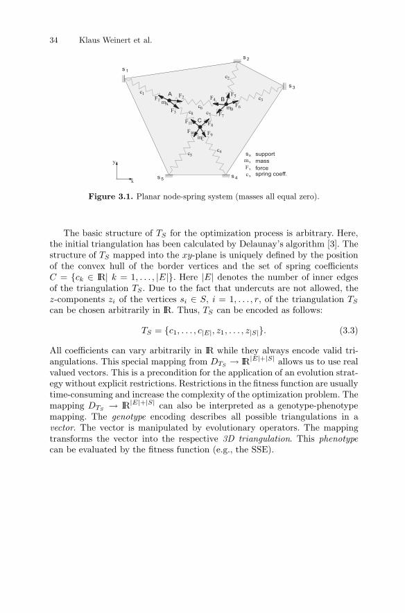
AB
C
c1
c2
c3
c4c5
c6
c7c8
cx
Fx
mx
sx
y
x
F2F1
F3
F4
F5
F6
F7
F9F10
F11 F8
AB
C
s 3
s 2
s 1
s 5s 4
mAmB
mC
support
mass
forcespring coeff.
S
S
1 1
+
+
Figure 3.1.
| | | |
| | | |
| | | |
{ ∈ | | |} | |
∈
{ }
→
→
= IR = 1
= 1IR
=
IRIR
IR
S
S
k
S
i i S
S
S E S
TE S
TE S
genotypevector
3D triangulation phenotype
T
T xy
C c k , . . . , E ET
z z s S i , . . . , r TT
T c , . . . , c , z , . . . , z .
D
D
34 Klaus Weinert et al.
Planar node-spring system (masses all equal zero).
The basic structure of for the optimization process is arbitrary. Here,the initial triangulation has been calculated by Delaunay�s algorithm [3]. Thestructure of mapped into the -plane is uniquely de�ned by the positionof the convex hull of the border vertices and the set of spring coefficients
. Here denotes the number of inner edgesof the triangulation . Due to the fact that undercuts are not allowed, the-components of the vertices , , of the triangulationcan be chosen arbitrarily in . Thus, can be encoded as follows:
(3.3)
All coefficients can vary arbitrarily in while they always encode valid tri-angulations. This special mapping from allows us to use realvalued vectors. This is a precondition for the application of an evolution strat-egy without explicit restrictions. Restrictions in the �tness function are usuallytime-consuming and increase the complexity of the optimization problem. Themapping can also be interpreted as a genotype-phenotypemapping. The encoding describes all possible triangulations in a
. The vector is manipulated by evolutionary operators. The mappingtransforms the vector into the respective . Thiscan be evaluated by the �tness function (e.g., the SSE).

PS
�| | �
128 128= 30 30
3 Evolutionary Optimization of Approximating Triangulations 35
3.4 Deterministic AT Optimization
3.5 Evolutionary AT Optimization
Terzpoulos and Vasilescu [8] use dynamic graphs for triangulations. The au-thors use a mass-spring system with spring coefficients that are adjusted ac-cording to the estimated curvature of the point set to be approximated. Theequilibrium state is calculated by solving a differential equation system. Intheir experiments a point set of sampling points is approximatedby a triangulation with . Typical for this approach is that it uses(manmade) assumptions about the correlation between the optimal positionof the vertices and the curvature estimated from the point cloud.Hoppe [4] uses a deterministic approximation scheme that utilizes least-
square distances as well as varying numbers of edges for a dynamic mass-spring-based triangulation model. An additional regularization term in the�tness function generates regular distribution of the vertices. This additionalterm supports the search for the minimum of an energy function. The strengthof the spring coefficients is decreased continuously in order to allow triangleswith tapered-off edges. The approach of Hoppe does not make expicit use of apriori assumptions about curvature properties, etc. It just needs the evaluationof an unbiased distance function.Algorri and Schmitt [1] introduce a different mass-spring model. The rela-
tion between the vertices and the sampling points is realized by a connectionbetween the vertex and its next-nearest sampling point. A nonlinear equationsystem models a dynamically oscillating net structure. The spring values ofthe system are calculated deterministically after each oscillation step. The de-�nition of the damping factor is not easy to adjust because on the one handthe system should remain long enough in oscillation to �nd a good globalsolution and on the other hand it should �anneal� fast enough to �nd a goodsolution.
All algorithms described in the last paragraph follow deterministic schemes.These approaches assume that the implemented algorithmic solution leadsdirectly and without any deterioration to the optimum solution. This impliesthat the general criteria to �nd a solution are already known and can beimplemented algorithmically. An evolutionary algorithm does not make anyassumptions about the path to the solution and, thus, is able to �nd thedesired optimum with only very little a priori knowledge.The evolution strategy (ES) is a special form of the superset called evo-
lutionary algorithms (EA). EA also comprise methods like genetic algorithms(GA), evolutionary programming (EP), and genetic programming (GP). EA,fuzzy logic, and neural networks belong to the general set called CI (computa-tional intelligence) techniques [12]. Evolutionary algorithms are probabilisticoptimization strategies that adopt the paradigms of evolution as introduced

′
′
�
x �
x �
′
′
{ }{ }
++ +
+
+
+
( + ) ( )
36 Klaus Weinert et al.
Evolutionary Algorithm
n
i � �
n n�
r r� �
�,�� �
�,� r r
� � �,�
∈ ∈∈
�
→∈ { }
⇔
� ∈ { }→
{ → } ∪ { → }∪
∅
∈ { }
∪
( ) IN ININ
( + )( )
( )1
: IR IR 1= 1 1
= ( )
( )
(1) = IR IR 1(2) = : IR(3)
= : :(4) ( ) = ( ( ( )))
= ( )= ( + )
(5)
(6)
�/� , � � ��
� ��, �
�, �� < � I n
nf n
� , i , . . . , n n , . . . , n� �
� �
EA I, , , �, s, �, �, �
� , � ES
I , n , . . . , n f, I
r I I m I I� P s Q m r P ,
Q �, �Q P � �
s s , s
� P Q�
by Darwin. The surprisingly robust and beautiful solutions of nature are themotivation to use this sophisticated approach.The evolution strategy is described in its basic form by the nomenclature
-ES [2]. Here, denotes the number of parents,the number of offspring, and a coefficient that de�nes the number ofparents involved in recombination. In the special case where two parents mateto form an offspring, the two commonly known short forms -ES and
-ES are used. The �+� sign denotes that offspring as well as parents areused by selection. The sign �,� denotes that only the offspring will be used toform the next parent population. In the case of a -selection the relation
is necessary. An individual consists of a set of real-valuedparameters (so called objective variables), which can be evaluated by an -dimensional �tness function (generally, ), and to strategyparameters , of the ES. Two additional globalparameters and characterize the strength of the normal distributed ran-dom mutation, which is applied to the objective variables of each individual.If only one step size is used, equals zero. A rotation matrix of correlationcoefficients as elements of the strategic parameters is introduced by Schwefel[11] but is not used in this context. Each complete individual consisting ofboth parameter sets is adapted by the evolutionary process. Hence, an ex-ternal deterministic adaptation of the step sizes is not necessary, because thestrategy parameters also undergo the selection process. Recombination inter-changes the genetic data of two or more parent individuals by intermediateor discrete exchange schemes.
An
(3.4)
is called an - :
individual:�tness function:probabilistic genetic operators:
selection:where in case of selection and
in case of selection.truncation selection:The individuals are ordered by their �tness evaluated by .The best survive.termination criterion: (e.g., a maximum number of generations)

′
+
11
�√ √ �
1 2
1 2
1 2 1
x �
i i
i i i i
′′′ { } ′
′′
′ ′
′
�′ �
→→→
→
� � �
�
∝ ∝ √
�
�
��
�
�
Encoding the AT
Problem De�nition
�
r r
�,��
�
i i i
i i i i
ni
i
O
P P
P P
O P P P
�
s
S
�
3 Evolutionary Optimization of Approximating Triangulations 37
== ( )= ( )
: IR: IR
( ) ( )
= ( (0 1) + (0 1))
= + (0 1)
IR = 1 0
2 ( ) ( 2 ) (0 1)
0 1
= + ( ) 2
= ( )
= 30 = 100 =
P IP r PP m P
P P
� , � s Q, P P
n
� � exp � N , � N , .
x x � N , .
� � .� �
� n � n N ,
II I
I I
I I I I /
I �S I
TS
Pf SSE P, T
�
� � n n
The algorithm iterates the following steps:(A) initialization:(B) recombination:(C) mutation:(D) evaluation:
(E) selection:(F) test termination criterion: either (B) or end.
Mutation is realized by �rst varying the step size parameters:
(3.5)
In a second step the objective variables are changed:
(3.6)
The vector can be initialized arbitrarily in (e.g., ). The fac-tors and depend on the dimension of the problem. A classic choice is
and , respectively [13]. denotes the
normal distribution with expectation and variance .Typically, either discrete or intermediate recombination is used. This op-
erator is applied separately to the objective and the strategic parameters.Bisexual discrete recombination generates one new offspring individual bymating two randomly selected parent individuals and . The compo-nents or of the parents are chosen by chance. Bisexual intermediaterecombination generates a new offspring individual by application of the for-mula: . From empirical results it is known thatintermediate recombination of the objective parameters and discrete recom-bination of the step sizes are a good choice.
The ES for optimizing an AT was implemented as follows:
The initial population is formed by triangulations (e.g., by Delaunaytriangulation [3]) of the point set . The individuals are encoded ac-cording to the description of (see paragraph ). In thebeginning, an equidistant point set in the plane is used to build .A set of sampling points of arti�cially designed objects is used.The �tness function (see paragraph )is applied.The termination criterion holds if a limiting maximum number of gener-ations is exceeded.
and . The complete set of step sizes is used, i.e., .Intermediate recombination of the objective parameters and discrete re-combination of the step sizes was the best choice during initial experiments
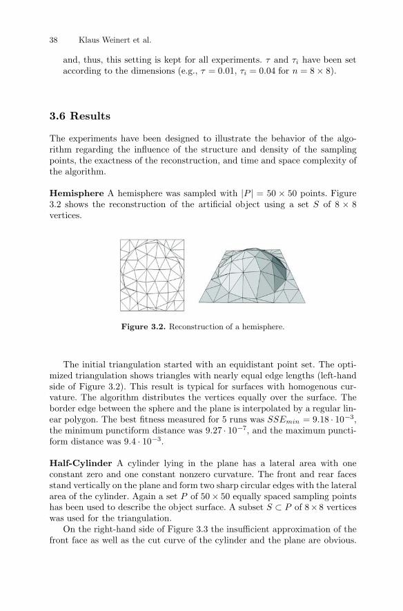
��
�
3
7
3
i
i
min
Figure 3.2.
3.6 Results
�
| | ��
��
�
�� �
� �� . � . n
PS
SSE ..
.
PS P
Hemisphere
Half-Cylinder
= 0 01 = 0 04 = 8 8
= 50 508 8
= 9 18 109 27 10
9 4 10
50 508 8
38 Klaus Weinert et al.
Reconstruction of a hemisphere.
and, thus, this setting is kept for all experiments. and have been setaccording to the dimensions (e.g., , for ).
The experiments have been designed to illustrate the behavior of the algo-rithm regarding the in�uence of the structure and density of the samplingpoints, the exactness of the reconstruction, and time and space complexity ofthe algorithm.
A hemisphere was sampled with points. Figure3.2 shows the reconstruction of the arti�cial object using a set ofvertices.
The initial triangulation started with an equidistant point set. The opti-mized triangulation shows triangles with nearly equal edge lengths (left-handside of Figure 3.2). This result is typical for surfaces with homogenous cur-vature. The algorithm distributes the vertices equally over the surface. Theborder edge between the sphere and the plane is interpolated by a regular lin-ear polygon. The best �tness measured for 5 runs was ,the minimum punctiform distance was , and the maximum puncti-form distance was .
A cylinder lying in the plane has a lateral area with oneconstant zero and one constant nonzero curvature. The front and rear facesstand vertically on the plane and form two sharp circular edges with the lateralarea of the cylinder. Again a set of equally spaced sampling pointshas been used to describe the object surface. A subset of verticeswas used for the triangulation.On the right-hand side of Figure 3.3 the insufficient approximation of the
front face as well as the cut curve of the cylinder and the plane are obvious.

Skew Steps
Figure 3.3.
Figure 3.4.
3 Evolutionary Optimization of Approximating Triangulations 39
Delaunay triangulation of a half-cylinder using the initial regular grid.
Optimized reconstruction of a half cylinder.
The triangulation algorithm of Delaunay used for the initial individual triesto generate triangles with equal edge lengths. On a regular point grid thisyields the typical structures that can be seen in the left-hand side of Figure3.3.
The optimized approximating triangulation is shown in Figure 3.4. Thevertices are distributed in a more efficient way than during the initialization.Long triangles are generated automatically only by application of the sim-ple SSE �tness function. This is especially noteworthy, because interpolatingtriangulations often generate small triangles. Even optimized interpolatingtriangulations need special �tness functions to be able to evolve long triangles[9]. The ability of the algorithm to generate nearly vertical triangles shouldalso be noticed.The special property of the EA is that it forms optimal structures just by
evaluating the �tness function and selecting the best solutions. It does notfollow �xed deterministic rules.
Sharp edges that do not exactly follow the orientation of thescanning lines may become problematic for 3D interpolating triangulations.Due to aliasing effects and the �xed vertex structure, these algorithms some-times tend to generate harmonica-shaped vertical structures. Leaving the re-
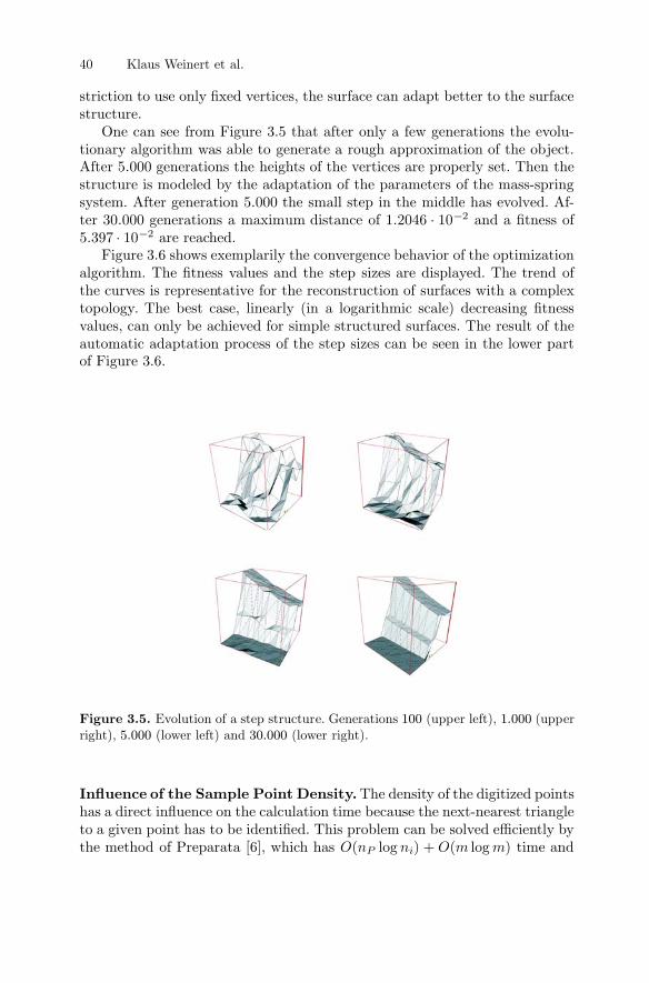
��
2
2
P i
��
.. .
Figure 3.5.
.
.. .
.
O n n O m m
100 1 0005 000 30 000
In�uence of the Sample Point Density.
5 000
5 00030 000 1 2046 10
5 397 10
( log ) + ( log )
40 Klaus Weinert et al.
Evolution of a step structure. Generations (upper left), (upperright), (lower left) and (lower right).
striction to use only �xed vertices, the surface can adapt better to the surfacestructure.One can see from Figure 3.5 that after only a few generations the evolu-
tionary algorithm was able to generate a rough approximation of the object.After generations the heights of the vertices are properly set. Then thestructure is modeled by the adaptation of the parameters of the mass-springsystem. After generation the small step in the middle has evolved. Af-ter generations a maximum distance of and a �tness of
are reached.Figure 3.6 shows exemplarily the convergence behavior of the optimization
algorithm. The �tness values and the step sizes are displayed. The trend ofthe curves is representative for the reconstruction of surfaces with a complextopology. The best case, linearly (in a logarithmic scale) decreasing �tnessvalues, can only be achieved for simple structured surfaces. The result of theautomatic adaptation process of the step sizes can be seen in the lower partof Figure 3.6.
The density of the digitized pointshas a direct in�uence on the calculation time because the next-nearest triangleto a given point has to be identi�ed. This problem can be solved efficiently bythe method of Preparata [6], which has time and

0.01
0.1
1
10
100
1000
0 5000 10000 15000 20000 g 30000
log
(f)
generations
fitness
300000
0.05
0.1
0.15
0.2
0.25
0 5000 10000 15000 20000 g
step
size
generations
0
0.05
0.1
0.15
0.2
0.25
0 5000 10000 15000 20000 g 30000st
ep
size
generations
min. step size (spring) min. step size (z.comp.)aver. step size (spring) aver. step size (z-comp.)max. step size (spring) max. step size (z-comp.)
10-3
10-2
10-1
1
8 10 20 30 40 50 60 70 80 90
10000
20000
40000
60000
t100000
runti
me
(log.)
[s]
dimension of the sampling points
dis
tance
(log.)
runtimefitness
aver.distance~~
i P
� ��
�
O n n m n
.
/
Figure 3.6.
Figure 3.7.
( )
10 10 90 908 8
100 10030 000
1 14
3 Evolutionary Optimization of Approximating Triangulations 41
Fitness function and step sizes.
In�uence of the number of sampling points on the �tness and the runtime.
space complexity ( number inner edges, number of triangles,number of sampling points).In the experiments the sample points of the half-cylinder have been used.
The number of the equidistant points is varied from to . Theinitial triangulation of the AT has vertices. In order to allow a comparisonof the triangulations, the distance of the resulting surfaces to asample point set was calculated. All runs stopped after generations.
Figure 3.7 shows the average distances of 5 runs and the amount of time(logarithmic scaling). The �gure supports the experience that a non-linearrelation between the amount of time and the number of points exists. It shouldbe noted that an increasing number of points does not have a relevant in�uenceon the �tness, if the proportion of the number of triangles to the number ofsampling points exceeds a certain limit (here about ). This oversamplingphenomenon is also typical for reconstructions with Non-Uniform RationalB-Splines (NURBS) [10] and gives a hint about the necessary resolution of an

10-3
10-2
10-1
1
4 6 8 10 12 14
10000
20000
40000
60000
t100000
run
tim
e(l
og
.)[s
]
dimension of the vertices
dis
tan
ce
(lo
g.)
fitnessaver.distance
runtime
z
�
�
Figure 3.8.
50 504
14
30 30
3.7 Conclusions and Outlook
In�uence of the Vertex Density.
42 Klaus Weinert et al.
In�uence of the vertex density on the �tness and the run time.
AT. For more complex geometries this effect is not so well pronounced butstill exists.
Generally, the higher the number of ver-tices of an AT, the better the approximations. Therefore, vertex high densitiesare desired. Of course, an oversampling effect appears here too if the numberof vertices reaches the number of sample points. The space complexity of thedata structure itself is not affected, because the number of triangles increasesonly linearly with the number of vertices.
In the experiment the geometry of the half-cylinder with samplingpoints has been used. The number of vertices has been increased from to. Figure 3.8 shows the �tness and the run time in relation to the number
of vertices. The experiments show that the number of vertices has a cubicin�uence on the run time. Therefore, the parameter settings for the AT shouldbe adequately chosen in order to �nd a compromise between run time andsurface quality. Vertex numbers over lead to unreasonable run times.Furthermore, instability problems may appear. Small vertical triangles evolvethat �t between the scan lines. These triangles do not contribute directlyto the �tness and therefore cannot be adapted. A different encoding of the-parameters of an individual may help to handle this problem.Experiments with large objects show that, due to the fact that long trian-
gles should be evolvable, generally it is not possible to split the surface intosmaller patches without losses in the reconstruction quality.
The technique of approximating triangulations is an important tool to �ndthe optimal distribution and density of sampling points. This data can be esti-mated by the positions of the vertices organized by an evolutionary algorithm.
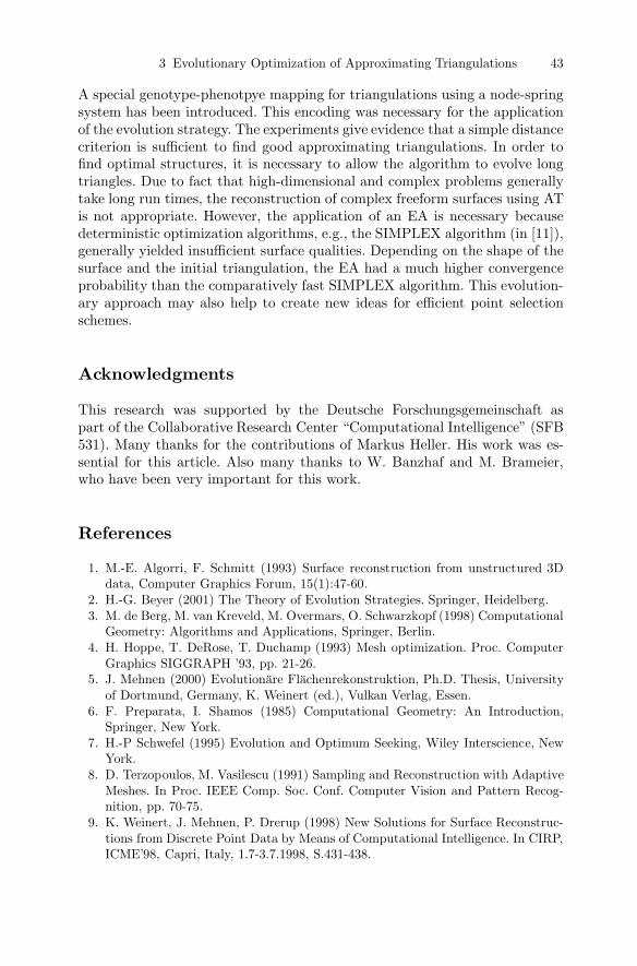
Acknowledgments
References
3 Evolutionary Optimization of Approximating Triangulations 43
1. M.-E. Algorri, F. Schmitt (1993) Surface reconstruction from unstructured 3Ddata, Computer Graphics Forum, 15(1):47-60.
2. H.-G. Beyer (2001) The Theory of Evolution Strategies. Springer, Heidelberg.3. M. de Berg, M. van Kreveld, M. Overmars, O. Schwarzkopf (1998) ComputationalGeometry: Algorithms and Applications, Springer, Berlin.
4. H. Hoppe, T. DeRose, T. Duchamp (1993) Mesh optimization. Proc. ComputerGraphics SIGGRAPH �93, pp. 21-26.
5. J. Mehnen (2000) Evolutionäre Flächenrekonstruktion, Ph.D. Thesis, Universityof Dortmund, Germany, K. Weinert (ed.), Vulkan Verlag, Essen.
6. F. Preparata, I. Shamos (1985) Computational Geometry: An Introduction,Springer, New York.
7. H.-P Schwefel (1995) Evolution and Optimum Seeking, Wiley Interscience, NewYork.
8. D. Terzopoulos, M. Vasilescu (1991) Sampling and Reconstruction with AdaptiveMeshes. In Proc. IEEE Comp. Soc. Conf. Computer Vision and Pattern Recog-nition, pp. 70-75.
9. K. Weinert, J. Mehnen, P. Drerup (1998) New Solutions for Surface Reconstruc-tions from Discrete Point Data by Means of Computational Intelligence. In CIRP,ICME�98, Capri, Italy, 1.7-3.7.1998, S.431-438.
A special genotype-phenotpye mapping for triangulations using a node-springsystem has been introduced. This encoding was necessary for the applicationof the evolution strategy. The experiments give evidence that a simple distancecriterion is sufficient to �nd good approximating triangulations. In order to�nd optimal structures, it is necessary to allow the algorithm to evolve longtriangles. Due to fact that high-dimensional and complex problems generallytake long run times, the reconstruction of complex freeform surfaces using ATis not appropriate. However, the application of an EA is necessary becausedeterministic optimization algorithms, e.g., the SIMPLEX algorithm (in [11]),generally yielded insufficient surface qualities. Depending on the shape of thesurface and the initial triangulation, the EA had a much higher convergenceprobability than the comparatively fast SIMPLEX algorithm. This evolution-ary approach may also help to create new ideas for efficient point selectionschemes.
This research was supported by the Deutsche Forschungsgemeinschaft aspart of the Collaborative Research Center �Computational Intelligence� (SFB531). Many thanks for the contributions of Markus Heller. His work was es-sential for this article. Also many thanks to W. Banzhaf and M. Brameier,who have been very important for this work.

44 Klaus Weinert et al.
10. K. Weinert, J. Mehnen (2000) Comparison of Selection Schemes for Discrete PointData for Evolutionary Optimized Triangulations and NURBS Surface Reconstruc-tions, ISA 2000, Wollongong, Australia, F. Nagdy and F. Kurfess (eds.), pp. 104-110, Dec. 11-15.
11. R. van Damme and L. Alboul (1994) Polyhedral metrics in surface reconstruction.Tight Triangulations, Technical report. University of Twente, Dep. of AppliedMathematics, Twente, The Netherlands.
12. J. C. Bezdek (1994) Computational Intelligence: Imitating Life. Chapter: Whatis Computational Intelligence. pp. 1-12, IEEE Press, New York.
13. T. Bäck (1996) Evolutionary Algorithms in Theory and Practice, Oxford Univer-sity Press, New York.

Summary.
4.1 Introduction
4
An Evolutionary Algorithm Based onMorphological Associative Memories forEndmember Selection in HyperspectralImages
M. Graña, C. Hernandez, A. d�Anjou
In this chapter we are concerned with the de�nition of spectral endmembersfor spectral unmixing of hyperspectral images. We study the application ofevolutionary algorithms combined with a morphological approach that usesMorphological Associative Memories (MAMs) to detect the endmember spec-tra in the image.Passive remote sensing evolution has produced measurement instruments
with ever-growing spectral breadth and resolution. Multispectral sensing al-lows the classi�cation of pixels. However, the recognition that pixels of interestare frequently a combination of materials has introduced the need to quanti-tatively decompose the pixel spectrum into their constituent material spectra.Hyperspectral sensor measurements in hundreds of spectral bands allow us toperform such �spectral unmixing� [13]. The reasons for the mixture of severalspectra in a single pixel are (1) the spatial resolution of the sensor implies that
In previous works we have introduced Morphological AutoassociativeMemories (MAM) as detectors of morphologically independent patterns and theirapplication to the task of endmember determination in hyperspectral images. Aftershifting the hyperspectral image data to the mean and taking the signs of the re-sulting hyperspectral patterns, we obtain a binary representation of the image pixels.Morphologically independent binary patterns can be seen as representations of the ver-tices of a convex region that covers most of the data. The MAMs are used as detectorsof morphologically independent binary patterns and the selected binary patterns aretaken as the guides for the selection of endmembers for spectral unmixing betweenthe image pixels. This process was de�ned in a greedy suboptimal fashion, whose re-sults depend largely on the initial conditions. We de�ne an Evolutionary Algorithmfor the search of the set of endmembers based on the morphological independencecondition and we compare it with a conventional Evolutionary Strategy tailored to theendmember detection task over a multispectral image.
46 M. Graña, C. Hernandez, A. d�Anjou
different land covers are included in the area whose radiance measurement re-sults in an image pixel, and (2) distinct materials are intimately mixed (e.g.,a beach). The second situation is independent of the sensor spatial resolutionand produces nonlinear mixtures, which are difficult to analyze. The �rst sit-uation produces mixtures that, often can be adequately modeled by a linearmixing model. In a previous chapter [10] we assume that the linear modelis correct, and we present an approach to the detection of endmembers forspectral unmixing in hyperspectral image processing through the applicationof MAMs.Brie�y introduced, Morphological Neural Networks are those that involve
somehow the maximum and/or minimum operators. Some fuzzy approachesare included in this de�nition. The kind of Morphological Neural Networksrange from pattern classi�ers [5], [15], [23], [28], target detection [7], [9], [17],[27], to associative memories for image restoration [19], [20], [21]. The MAMs[19], [20], [21] are the morphological counterpart of the Linear AssociativeMemories (LAM) [14] and the well known Hop�eld Autoassociative Memo-ries [11]. Like the LAMs, MAMs are constructed as correlation matrices butwith the substitution of the conventional matrix product by a min or maxmatrix product from Image Algebra [22]. Dual constructions can be madeusing the dual min and max operators. In [10] we propose the MAMs as de-tectors of morphological independent binary patterns and, therefore, as theendmember selection tool. The described algorithm is a local search process,highly sensitive to the initial conditions of the process. In this chapter weexplore the de�nition of an Evolutionary Algorithm devoted to the task ofendmember selection from a given image that uses the MAMs as detectorsof morphological independences. This new algorithm is a Genetic Algorithm[8] that searches the space of binary patterns that correspond to representa-tions of the endmembers looked for, which must be sets of morphologicallyindependent patterns. Through the chapter we call this algorithm GA withMorphological Independence restriction (GA-MI). Mutation is the genetic op-erator used. We use the MAM to test the morphological independence of thechildren. Because mutation does not preserve the morphological independenceand there is not any established procedure for its correction, the children thatdo not conform to the morphological independence requisite are discarded. Forcomparison we propose an Evolution Strategy [2], [3], [4] for the same task ofendmember design. In both evolutionary approaches, the objective functionto be minimized is the combination of the reconstruction error of the imagepixels and the satisfaction of the properties of a true abundance image: thefull additivity and nonnegativity of all the abundance image pixels.The structure of the chapter is as follows: In Section 4.2 we review the de�-
nition of the linear mixing model. Section 4.3 provides a review of basic resultsof MAMs. Section 4.4 describes our evolutionary algorithm of endmember se-lection for remote sensing hyperspectral images, and a competing conventionalevolution strategy approach. Section 4.5 presents some experimental results

�
�
�
∑
∑
�
=1
=1
1
M
i
i i
i
iMi i
T T
= + = +
= 1
0 = 1= 1
=
x s w Sa w
x Ss a
w
a S S S x
4.2 The Linear Mixing Model
a ,
d d Md , i , ..,M,
M d
a , i , ..., M.a .
.
4 Endmember Selection in Hyperspectral Images 47
of the proposed algorithm and the competing evolution strategy. Section 4.6gives our conclusions and directions of future work.
The linear mixing model can be expressed as follows:
(4.1)
where is the -dimensional received pixel spectrum vector, is thematrix whose columns are the -dimensional endmembers isthe -dimensional fractional abundance vector, and is the -dimensionaladditive observation noise vector. The linear mixing model is subjected totwo constraints on the abundances. First, to be physically meaningful, allabundances must be nonnegative Second, to account forthe entire composition the abundances must be fully additiveOften the process of spectral unmixing is performed on transformations
of the data intended to reduce the computational burden [13] or to enhancesome properties of the data [12]. We do not apply any dimension reductiontransformation here. The task of endmember determination is the focus of thischapter. In an already classical chapter [6], Craig starts with the observationthat the scatter plots of remotely sensed data are tear-shaped or pyramidalif two or three spectral bands are considered. The apex lies in the so-calleddark point. The endmember detection becomes the search for nonorthogonalplanes that enclose the data, forming a minimum volume simplex, hence thename of the method. Besides its computational cost the method requires theprespeci�cation of the number of endmenbers. Another step to the automaticendmember detection is the Conical Analysis method proposed in [12] andapplied to target detection. The extreme points in the data after a princi-pal component transformation are the searched for endmember spectra. Themethod is geometrically similar to Craig´s one but does not require costly lin-ear programming. It also requires the prespeci�cation of the desired numberof endmembers. Another approach is the modeling by Markov Random Fieldsand the detection of spatially consistent regions whose spectra will be assumedas endmembers [18]. A quite standard approach to endmember determinationis the use of standard libraries of spectra [13]. This approach requires greatexpertise and a prori knowledge of the data. Finally, there are interactiveexploration algorithms that are supported by speci�c software packages.Once the endmembers have been determined, the last task is the compu-
tation of the inversion that gives the fractional abundance and, therefore, thespectral unmixing. The simplest approach is the unconstrained least-squarederror estimation given by
(4.2)
R R
′
′ ′
′
2 2
=1 =1
=1
=1
x Sa
x y
y x
y x y x
y xx
y x
� � � �
�
�
�� � �� � � �
� �� �
� �
� � ∑ �
∧ [ � ] ∨ [ � ]
∨∧
�
48 M. Graña, C. Hernandez, A. d�Anjou
4.3 Morphological Associative Memories
‖ � ‖
∨ ∧ �∨ ∧
∨ ∧
�
� � � �
�
⇔ { }
⇔ { }
∀ � � � �∀ �
� � �
� � �
=
( +) ( + )
max min sup inf
( ) = ; = 1
=
= =
maxmin
= = [ ] = +
= = [ ] = +
;;
( ) = =
( )= =
� �
�� �
XY
k
�
� �XY
k
�
� �
ij ij
k ..n
ik kj
ij ij
k ..n
ik kj
XY XY
XY� �
XY
XY�
�XY
�XY XY
XY XY
XY XY XY XY
ε .
, , , , ,
X, Y , � , ..., k
W .
W , M ,
C A B c c a b ,
C A B c c a b .
W M� W M
� WM , W X Y M X.A X, Y A X Y A X
Y A BX, Y , W M
A W M B W X Y M X.
The abundances that result from this computation do not ful�ll the non-negative and full additivity conditions. It is possible to enforce each conditionseparately, but rather difficult to enforce both simultaneously [13]. As ouraim is to test an endmember determination procedure, therfore we will useunconstrained estimation (4.2) to compute the abundance images. We willshow intensity scaled and shifted images of the abundances to evaluate ourresults. As a measure of the quality of the decomposition obtained it is usefulto introduce the reconstruction error:
(4.3)
The work on MAMs stems from the consideration of an algebraic lattice struc-ture as the alternative to the algebraic framework for thede�nition of Neural Networks computation [19] [20]. The operators anddenote, respectively, the discrete and operators (resp., andin a continuous setting). The approach is termed morphological neural net-works because and correspond to the morphological dilation and ero-sion operators, respectively. Given a set of input/output pairs of pattern
, a heteroassociative neural network based
on the pattern�s cross correlation [14], [11] is built up asMimicking this construction procedure the works in [19], [20] propose thefollowing constructions of heteroassociative morphological memories
(4.4)
where is any of the or operators. Here and denote the andmatrix product, respectively, de�ned as follows:
(4.5)
(4.6)
It follows that the weight matrices and are lower and upper boundsof the max and min matrix products andtherefore the following bounds on the output patterns hold:
that can be rewritten as Amatrix is a -perfect ( -perfect) memory for if (). It can be proven that if and are -perfect and -perfect memories,resp., for then and are also -perfect and -perfect, resp.:
. Therefore, Conditions

i i i
i i i
′
′
�
�
�
�
�
�
� �
�
�
�
=1
=1
=
=
=
=
; = + ; =
+
= =
( )=
; +
; = +
=
; +
; = +
=
y x
y x
xx x x x xx x x x
x x
yx
x y
x x x y
x xx x
∀ � � �∀ � � �
∀ ∀ ∃ � ∀ ∀ ∃�
��
∀ � ∨ �∀ ∃ ∨ �
∀ � ∧ �∀ ∃ ∧ �
�
Theorem 1.
Theorem 2.
Theorem 3.
Corollary 1.
4 Endmember Selection in Hyperspectral Images 49
[ � ] [ � ]∨ � �
∧ � �
˜˜ ˜˜ ˜ ˜˜˜
˜˜ ∧ �∨ � ��˜ �∨ � ��
˜ ˜˜ ∨ �∧ � ��˜ �∧ � ��
˜˜
W
� W
M �
M
W � i j x x y y , M � i j x
x y y .
W X X M X X
. .
W
X, YW
j x x y y x ,
i j x x y y x .
MM
j x x y y x ,
i j x x y y x .
WM
X W
XY
� �XY
XY� �
XY
XY�j
k�
�j
�i
�i XY
�j
k�
�j
�i
�i
XX XX
�
� � � � �
� � � �
� �
XY�
�
XY� �
�j
�j i � �
�i
�i
�j
i�j
�j � �
�i
�i
�j
XY� �
XY� �
�j
�j i � �
�i
�i
�j
i�j
�j � �
�i
�i
�j
XY
XY
XX� �
� �
Perfect recall of HMM. The matrix is -perfect if and only
if the matrix contains a zero at each row. Similarly,
the matrix is -perfect if and only if the matrix
contains a zero at each row. These conditions are formulated for
as and for as
Perfect recall of AMM. Both erosive and dilative AMMs havethe perfect recall property: , for any .
robust
Robust perfect recall of HMM. Given input/output pairs ,the equality holds when the following relation holds:
Similarly for the conditions of robust perfect recall for given a noisycopy of , that is, the equality holds when
Given patterns , the equality holds when thenoise affecting the pattern is erosive and the following relation holds
of perfect recall of the stored patterns are given by the following theorem[19],[20]:
These results hold when we try to recover the output patterns from thenoise free input pattern. To take into account the noise, a special de�nitionof the kinds of noise affecting the input patterns is needed. Let be a noisyversion of If , then is an eroded version of Alternatively,we say that is subjected to erosive noise. If , then is a dilatedversion of . Alternatively, we say that is subjected to dilative noise. Mor-phological memories are very sensitive to these kinds of noise. The conditionsof perfect recall for , i.e., the retrieval of given a noisy copy, are given by the following theorem [19], [20].
(4.7)
(4.8)
The associative memory matrix is robust against controlled erosionsof the input patterns while the associative memory matrix is robustagainst controlled dilations of the input patterns. In the case of autoassociativememories the conditions for perfect recall of noisy patterns are a corollary forTheorem 3:
��
�
�
=
=
1
1
i i i
i i i
�
��
� �
��
De�nition 1.
∀ ∃ ∨ ��
∀ ∃ ∧ �
�
�
{ }{ }
∈∈
∈
˜ �∨ � �� ˜˜˜ �∧ � ��
˜˜ ˜
�
�
; = + =
; = +
( )= =
=
( ) =
=; = 1
; = 1
=
x
x x x
x zx y x z
x x yy x
y x
x x
y yy y
y
50 M. Graña, C. Hernandez, A. d�Anjou
i�j
�j � �
�i
�i
�j XY
�
� � �
i�j
�j � �
�i
�i
�j
ZZ
ZY
� �
ZY ZZ� � � �
k
�
�
k
XX XX
XX
XX
i j x x x x x . M
i j x x x x x
X, Y ZZ X, M X Z,
W Z Y.M
ZW
W M . >
X , ...,X � , ..., k ,
X � , ..., k .X
X , ...,W M/ X, X
W / X. XM / X.
Similarly, the equality
holds when the noise affecting the pattern is dilative and the
following relation holds: .
Morphological independence. Given a set of pattern vectors, a pattern vector is said to be morphologically indepen-
dent of in the erosive sense if and morphologicallyindependent of in the dilative sense if The set of pat-tern vectors is said to be morphologically independent in either sense whenall the patterns are morphologically indenpendent of the remaining patterns inthe set.
Remark 1.
The AMM will fail in the case of noise being a mixture of erosive anddilative noise. To obtain general robustness, the kernel method has been pro-posed [19], [21], [25]. A kernel for is de�ned as a set of patternsthat satisfy the following conditions: (1) (2) and (3)
Kernels are, therefore, selective erosions of the input patternsdesigned to ensure that the robustness against dilation of the memorieswill allow the recovering of patterns from either eroded and dilated ver-sions of the input patterns, and the memory will produce the desiredoutput response. That is, for corrupted inputs we are guaranteedthat Note that does not guarantee correctrecall.In order to characterize kernels and to obtain a constructive de�nition, the
notion of morphological independence and strong morphological independenceis introduced in [21]. Here we distinguish erosive and dilative versions of thisde�nition:
The strong morphological independence is introduced in [21] to give aconstruction for minimal kernels with maximal noise robustness. For binary-valued vectors, morphological independence and strong morphological inde-pendence are equivalent. For the current application we want to use AMMsas detectors of the set extreme points, to obtain a rough approximation ofthe minimal simplex that covers the data points. We need to establish �rst asimple fact in the following remark:
Given a set of pattern vectors and the erosiveand dilative memories constructed from it. Given a test patternif is morphologically independent of in the erosive sense, then
Also, if is morphologically independent of in the dilativesense, then
The endmembers that we are searching for are the corners of a high-dimensional box centered at the origin of the space. They are morphologicallyindependent vectors both in the erosive and dilative senses, and they enclosethe remaining vectors. The endmember detection process would apply the

k
� �
��
R
RR
x xy x
y y xy
x 0
f
a
f a
1
2
=1 =1
2
=1 =1
2
=1 =1
�
� �
∑∑ ∑∑ ∑∑∑
∈ { } ∈∈ { } �∈
{ � }
∈
∈} ∈
� ‖ ‖
kXX
XX�
XX�
XX
i i i i
d
M
M
n
i
m
j
n
i
m
j
n
i
m
j
k
4.4 The Detection of Spectral Endmembers
4 Endmember Selection in Hyperspectral Images 51
=
11
( = 1 0; = 0 0 ; = 1 )
( ) ; = 1 ; = 1
( ) ; = 1 ;
= 1 ( ) ; = 1 ; = 1
( ) = ( ) + (1 ( ) )
+ ( ( ))
X , ..., WM <
� , .., k W / X. >� , .., k M / X.
>b x > b x i , .., n .
i, j i , .., n j , .., m
� E Mi, j i , .., n
j , .., m ε i, j i , .., n j , .., m
E
F ,E ε i, j i, j
abs a i, j .
erosive and dilative AMMs constructed from the already detected endmem-bers to detect the new ones as suggested by the previous remark. Workingwith integer-valued vectors, a desirable property is that vectors already in-side the box de�ned by the endmembers would be detected as such. However,given a set of pattern vectors and the erosive anddilative memories constructed from it. A test pattern for some
would give Also, if the test pattern for some, then Therefore, working with integer-valued
patterns the detection of the morphologically independent patterns would beimpossible. However, if we consider the binary vectors obtained as the sign ofthe vector components, then morphological independence would be detected assuggested by the above remark. Let us denote by the expression the con-struction of the binary vector if if
In this section we describe both the approach based on the GA with morpho-logical independence restriction (GA-MI) and the standard Evolution Strategyde�ned for the problem at hand. The endmembers of a given hyperspectralimage under the linear mixture assumption correspond to the vertices of theminimal simplex that encloses the data points [6]. The region of the space en-closed by a set of vectors, simultaneously morphologically independent in botherosive and dilative senses resulting from the GA-MI, is a high-dimensionallinear convex region (i.e., bounded by hyperplanes). The result of the Evolu-tion Strategy is also a set of vertices that may de�ne a convex region. It isdifficult to give a quantitative measure of the goodness of a given set of end-members, which is needed for the de�nition of evolutionary approaches. Thepositive and full addition properties are the basic restriction to ful�ll, so thatthey are the basis for the de�nition of the �tness function. We have chosenthe reconstruction error in (4.3) as the regularization term. Let us formalize�rst the �tness function.Let us denote the hyperspectral im-
age, and the vectors of the mean and standard deviations of each bandcomputed over the image, the noise correction factor, and the set ofendmembers whose �tness is to be quanti�ed. Let
and be the abundanceestimations and reconstrucion error computed applying (4.2) and (4.3) ateach pixel with as the endmember collection. The �tness function to beminimized is de�ned as follows:
(4.9)

1
1
X .
�
��
� �
�
� �� �
1 1
+
+
+
{ | }
{ }{ }
∈ { }
{ } { }
�
∈ ∈
{ � }
{ }
k
B
B b
bB
x b
b
f f 0 f f 0bbb
b
B
f f
Bf
k
t i
i ij
ijd
i
i,
XX XX
XY
i,k
c c
XY XX i,k
XY XX i,k
i,k
i,k
i i
c
i
i
t i i
= ( ) 0
= ; = 1
= ; = 1
0 1
= =
( ) = ( ( ) + ) ( ) = ( ( ) )= ( )= ( )
( ) = ( ) ; = 1 ; = 1
( )
= ( ) ; = 1
( + )
k a i, j < .P N
K
P i , ..., N .
j , ..., M
,
X .
M W . YM .
i, j i, j � > i, j i, j � > .y M M .y M W .
y / Y y / YX
k
E
i, j i, j i , ..., n j , ..., m .
.i, j E .
P E , � i , ..., N .
� �
52 M. Graña, C. Hernandez, A. d�Anjou
Although we have no formal proof of the perfect recall of the HMM when the inputpatterns are morphologically independent, it is very likely and �ts nicely to use theHMM as the endmember identi�er. In practice, we search the set directly
In this equation Both evolutionary approaches havea population of individuals, each consisting of a set of endmembers ofsize . In the GA-MI we have a population of binary individuals
Each one of the individuals corresponds to a set ofendmembers, where each encodes the directions of the convexregion vertices. Each collection is morphologically independent in botherosive and dilative senses. The GA-MI evolves the population using a con-ventional mutation operator and a roulette wheel selection. However, eachtime a new individual is generated, it is tested for morphological indepen-dence, and if it fails to pass the test it is rejected and a new individual isgenerated. The test for morphological independence proceeds as follows:
1. Consider initially2. Construct the AMMs based on the morphologically independent binarysignatures: and De�ne orthogonal binary codes for theendmembers and construct the identi�cation HMM :
3. Consider the next endmember code:a) Compute the vector of the signs of the Gaussian noise corrections
andb) Computec) Computed) If and , then is morphologically independentin both senses. Go to step 2 adding to and resume the test,increasing . If not, the test fails and the individual is rejected.
To compute the set of endmembers corresponding to each we need�rst to consider the zero mean image
(4.10)
Then the endmember pixels are determined as the extreme points in thedirections speci�ed by the The �nal set of endmembers is the set of originalspectral signatures of the pixels selected as members ofThe Evolution Strategy follows the conventional de�nition and dynamics
[4]. Population individuals are given by a set of endmember hypothesis andtheir mutation variances Initial endmembers aregenerated by a random perturbation about the mean spectrum of the image,and the following generations are produced by the conventional schema ofperturbation and self-adaptation of the mutation variances. A strategyis used for selection, where the next generation is obtained as the best onesfrom the joint set of parents and children.

�
�
�
Figure 4.1.
Figure 4.2.
710 4558
448 2048
448 2048
4.5 Experimental results
4 Endmember Selection in Hyperspectral Images 53
Ground truth of the experimental image.
Evolution of the �tness function of the best individual of the GA withmorphological independence restriction and the evolution strategy.
The data used for the experimental work correspond to a multispectral imageof size of pixels which covers a large area including vegetation,cultivated land areas, and urban areas. This image has been acquired througha CASI (Compact Airborne Spectrographic Imager) sensor using a generalcon�guration of 14 bands, that is, each pixel is represented by a vector of 148-bpp gray scale values. From all the 14 bands of the original image, a smallerregion of pixels has been selected (cropped). For the operation ofboth the Evolutionary Algorithm and the Evolution Strategy a 8:1 subsampledversion of this region has been used to compute the �tness function value.However, �nal abundance results were computed over the pixelsregion.

Figure 4.3.
Figure 4.4.
54 M. Graña, C. Hernandez, A. d�Anjou
Endmembers found by the EA with the morphological independencerestriction.
Endmembers found by the Evolution Strategy tailored to the endmemberdetermination task.

A B C DE
Figure 4.5.
4 Endmember Selection in Hyperspectral Images 55
Abundance images corresponding to the endmembers discovered by theGA with the morphological independence restriction: GA-MI.
The ground truth of the image is composed of the following categories ofland cover: evergreen trees, deciduous trees, brushwoods, meadowsand crops, urban areas. The ground truth is visualized in Figure 4.1 as-signing an increasing intensity to the land cover categories: black correspondsto evergreen trees and white to urban areas. Figure 4.2 shows the plot of anevolution of the �tness value of the best individual for the GA-MI and theEvolution Strategy. In both algorithms the population size was 10, the numberof endmembers per individual was 5, and the number of mutations allowedwas 30. It can be appreciated that the GA-MI �nally obtains better quantita-tive results than the ES approach. However, the qualitative assessment of theresults must be done on the abundance images computed from the obtainedendmember spectra.The monitoring of the evolution of GA-MI shows that, although all the
individuals are collections of morphologically independent binary vectors, thecodi�cations seldom have a corresponding extreme point in the image. There-fore, GA-MI initially has collections of only one or two endmembers. The

M N� .
5
= 5 = 10= 10
Figure 4.6.
56 M. Graña, C. Hernandez, A. d�Anjou
Abundance images corresponding to the endmembers discovered by theEvolutionary Strategy.
evolution adds new meaningful endmembers to the best individuals. In the�nal best individual we have found 4 endmembers, whose spectra are plottedin Figure 4.3. The Evolution Strategy performs better most of the time ac-cording to Figure 4.2. However, it stagnates at the end. It gives endmembersplotted in Figure 4.4. The endmember spectra found are like noisy versions ofthe ones found in the image. It is worth noting that the GA-MI is performingspontaneously a process of selection of the appropriate number of endmem-bers, always below the upper bound �xed in the simulation. The number ofendmembers was �xed at , like the population size and thenumber of children generated
#2
#3
4.6 Conclusions and Further Work
4 Endmember Selection in Hyperspectral Images 57
The qualitative results are given by the abundance images computed us-ing the endmember spectra found by both approaches. The abundance imagesobtained from the spectral unmixing with the GA-MI endmembers are shownin Figure 4.5. Figure 4.6 presents the abundance images obtained from the ESendmembers. We �nd that the results are quite parallel: the abundance imageof endmember #1 found by the GA-MI is similar to the one of endmemberfound by the Evolutionary Strategy, and the corresponding endmembers
seem to be good detectors of vegetal cover including crops. Abundance image#2 of GA-MI is similar to the abundance image #5 of the Evolution Strategy.However, these images seem of little value. There are no interesting spatialstructures discovered in these images. It seems that the corresponding end-member spectra are noise detectors. The abundance images and #4 of theGA-MI correspond to the abundance images #3 and #4 of the EvolutionaryStrategy, respectively. The endmembers seem to correspond to detectors ofarti�cial constructs like buildings and roads.An interesting result is that the GA-MI has obtained the same qualitative
results with fewer endmembers than the ES. From a dimensionality reductionviewpoint, the GA-MI has been able to obtain a transformation of the im-age data from the original 14-dimensional space into a 4-dimensional space,preserving much of the qualitative information of the image and obtaining anoptimized reconstruction of the original image. We assert that the qualitativeinformation has been preserved because the main spatial features of the im-aged scene are detectable in the transformed images, and correspond to coverclasses de�ned in the ground truth. We may say that GA-MI outperforms theES in the sense of obtaining a more parsimonious representation of the imagedata.
We have proposed an Evolutionary Algorithm that uses the notion of morpho-logical independence and the Morphological Autoassociative Memory for test-ing it, for the task of hyperspectral image linear unmixing. Linear unmixing isboth a detection process and a dimension reduction process. It is very efficientfor the detection of small features, which can be blurred by other methods,like clustering-based unsupervised analysis of the images. The EvolutionaryAlgorithm ensures some degree of optimality of the endmembers extractedfrom the image, in the sense of minimum unmxing (and reconstruction) error.We have found that our algorithm improves over an Evolutionary Strategytailored to the problem, in the sense of the minimization of the proposed �t-ness function. We have also found that the GA-MI algorithm spontaneouslyperforms a selection of the appropriate number of endmembers. An added ap-peal of the approach proposed is that it uses the spectra found in the image.Using the actually measured spectra may reduce the interpretation problemswhen trying to decide the actual physical materials present in the scene.

Acknowledgments
References
Further work must be addressed to the experimentation with other hyper-spectral images, and the extensive testing of the parameter sensitivities of theapproach, keeping in mind that hyperspectral images are very large and needspeedy analysis methods.
The authors received partial support from projects of the Ministerio de Cien-cia y Tecnologia MAT1999-1049-C03-03, TIC2000-0739-C04-02, and TIC2000-0376-P4-04, and UPV/EHU 00140.226-TA-6872/1999 of the University ofThe Basque Country (UPV/EHU). The Center for Ecological Research andForestry Applications (CREAF) of the UAB kindly provided the experimentalmultispectral image and corresponding ground truth.
58 M. Graña, C. Hernandez, A. d�Anjou
1. Asano A., K. Matsumura, K. Itoh, Y. Ichioka, S. Yokozeki (1995) Optimizationof morphological �lters by learning, Optics Comm. 112 : 265-270
2. Bäck T., H.P. Schwefel (1993) An overview of Evolution Algorithms for parameteroptimization. Evolutionary Computation, 1:1-24.
3. Bäck T., H.P. Schwefel (1996) Evolutionary computation: An overview. IEEEICEC�96, pp.20-29.
4. Th. Bäck (1996) Evolutionary Algorithms in Theory and Practice, Oxford Uni-versity Press, New York.
5. Carpenter G.A., S. Grossberg, D.B. Rosen (1991) Fuzzy ART: Fast stable learningof analog patterns by an adaptive resonance system, Neural Networks, 4:759-771,
6. Craig M., Minimum volume transformations for remotely sensed data, IEEETrans. Geos. Rem. Sensing, 32(3):542-552.
7. Gader P.D., M.A. Khabou, A. Kodobobsky (2000) Morphological regularizationneural networks, Pattern Recognition, 33:935-944.
8. Goldberg D.F. (1989) Genetic Algorithms in Search, Optimization & MachineLearning, Addison-Wesley, Reading, MA.
9. Graña M., B. Raducanu (2001) On the application of morphological heteroasso-ciative neural networks. Proc. Intl. Conf. on Image Processing (ICIP), I. Pitas(ed.), pp. 501-504, Thessaloniki, Greece, October, IEEE Press.
10. Graña M., B. Raducanu, P. Sussner, G. Ritter (2002) On endmember detection inhyperspectral images with Morphological Associative Memories, Iberamia 2002,LNCS Springer-Verlag, in press.
11. Hop�eld J.J. (1982) Neural networks and physical systems with emergent collec-tive computational abilities, Proc. Nat. Acad. Sciences, 79:2554-2558,
12. Ifarraguerri A., C.-I Chang (1999) Multispectral and hyperspectral image analysiswith convex cones, IEEE Trans. Geos. Rem. Sensing, 37(2):756-770.
13. Keshava N., J.F. Mustard (2002) Spectral unimixing, IEEE Signal Proc. Mag.19(1):44-57
14. Kohonen T., (1972) Correlation Matrix Memory, IEEE Trans. Computers, 21:353-359.

4 Endmember Selection in Hyperspectral Images 59
15. Pessoa L.F.C , P. Maragos, (1998) MRL-�lters: a general class of nonlinear systemsand their optimal design for image processing, IEEE Trans. on Image Processing,7(7):966 -978,
16. Pessoa L.F.C , P. Maragos (2000) Neural networks with hybrid morphologi-cal/rank/linear nodes: A unifying framework with applications to handwrittencharacter recognition, Patt. Rec. 33:945-960
17. Raducanu B., M. Graña, P. Sussner (2001) Morphological neural networks forvision based self-localization. Proc. of ICRA2001, Intl. Conf. on Robotics andAutomation, pp. 2059-2064, Seoul, Korea, May, IEEE Press.
18. Rand R.S., D.M. Keenan (2001) A Spectral Mixture Process conditioned byGibbs-based partitioning, IEEE Trans. Geos. Rem. Sensing, 39(7):1421-1434.
19. Ritter G.X., J.L. Diaz-de-Leon, P. Sussner. (1999) Morphological bidirectionalassociative memories. Neural Networks, 12:851-867.
20. Ritter G.X., P. Sussner, J.L. Diaz-de-Leon. (1998) Morphological associativememories. IEEE Trans. on Neural Networks, 9(2):281-292.
21. Ritter G.X., G. Urcid, L. Iancu (2002) Reconstruction of patterns from noisy in-puts using morphological associative memories, J. Math. Imag. Vision, submitted.
22. Ritter G.X., J.N. Wilson, Handbook of Computer Vision Algorithms in ImageAlgebra, CRC Press:Boca Raton, Fla.
23. Rizzi A.,M. ,F.M. Frattale Mascioli (2002) Adaptive resolution Min-Max classi-�ers, IEEE Trans. Neural Networks 13(2):402-414.
24. Salembier P. (1992) Structuring element adaptation for morphological �lters, J.Visual Comm. Image Repres., 3:115-136.
25. Sussner P. (2001) Observations on Morphological Associative Memories and theKernel Method, Proc. IJCNN�2001, Washington, DC, July
26. Sussner P. (2002) , Generalizing operations of binary autoassociative morpholog-ical memories using fuzzy set theory, J. Math. Imag. Vision, submitted.
27. Won Y., P.D. Gader, P.C. Coffield (1997) Morphological shared-weight neuralnetwork with applications to automatic target detection, IEEE Trans. NeuralNetworks, 8(5):1195-1203.
28. Yang P.F., P. Maragos, (1995) Min-max classi�ers: Learnability, design and ap-plication, Patt. Rec., 28(6):879-899.
29. Zhang X.; C. Hang; S. Tan; PZ. Wang (1996) The min-max function differentiationand training of fuzzy neural networks, IEEE tTrans. Neural Networks 7(5):1139-1150.

5___ ______ ______ __________________ ______ ______ ______ ______ ______ ______ ______ ____________
On a Gradient-based Evolution Strategyfor Parametric Illumination Correction
Elsa Fernández, Manuel Graña, Jesús Ruiz-Cabello
Abstract. This chapter deals with the issue of illumination inhomogeneity correction inimages. The approach followed is that of estimating the illumination bias as a parametricmodel. The model is a linear combination of Legendre polynomials in the 2D or 3D space.The estimated bias is, therefore, a smooth function characterized by a small set ofparameters that define a search space of lower dimension than the images. Our work is anenhancement of the PABIC algorithm, using gradient information in the mutation operatorhence we name it GradPABIC. We apply our algorithm, the PABIC, and a conventionalEvolution Strategy (ES) over a set of synthetic images to evaluate them, through thecomparison of the correlation between the recovered images and the original one. ThePABIC and the EE are allowed the same number of fitness computations, while the GradPABIC number of fitness evaluations is two orders of magnitude lower, because of thegradient computation added complexity. Finally, we present some results on slices of asynthetic MRI volume.
5.1 Introduction
Illumination bias correction is a key problem in several domains, above all inmedical imaging and Magnetic Resonance Imaging (MRI). The bias correction iscritical in some cases to obtain meaningful image segmentations, because thesesegmentations are usually done on the basis of a known catalog of MR responsesof specific tissues. Pixels are classified according to their intensities and a set ofknown values. Besides the partial volume effect, the intensity inhomogeneities arethe main difficulty to obtain precise automatic segmentations. The contribution ofthe illumination to the image formation is multiplicative; therefore, its effectcannot be removed easily through traditional linear filtering algorithms. In thischapter we will not consider other noise contributions [6]. The classic approach tosolve this problem is the homomorphic filtering [3] that filters out the low-frequency components of the logarithm image Fourier transform. Illuminationgradients are usually smooth functions. Therefore, it is expected that the lowestcomponents of the logarithm image will correspond to the illumination bias.Working over the logarithm image trying to isolate the illumination components ofthe image is common to many other illumination correction algorithms. Fewalgorithms perform the correction, computing the division of the corrupted imageby the estimated bias. Among them, the straightforward approaches consist oftaking an image of the background and dividing the new images by it.

62 E. Fernandez, M. Graña, J. Ruiz-Cabello
There has been broad interest in this problem, which has produced a number ofalgorithms. A coarse taxonomy distinguishes between parametric andnonparametric methods. On the nonparametric class of algorithms, a well-foundedapproach is the one applying Bayesian image modeling to the image logarithm andusing some minimization method to estimate the most likely bias field logarithm.The estimation task [10] applies an EM algorithm, while [4] applies a minimizationof an entropy criterion. These works try to isolate the bias field. On the other hand,[1] introduces the effect of the bias field inside the classification adding a bias terminto the fuzzy c-means that they apply to the image pixels classification in order toobtain image segmentations. On the whole, nonparametric methods are computer-intensive and require huge amounts of memory in some cases. An approach thatgives good results based on the iterative deconvolution with Gaussian kernels isdescribed in [8].
Parametric methods assume some mathematical model of the illumination bias,whose estimation becomes fitting the model surface to the image intensityfunction. The model surfaces are always very smooth and the fitness criterioninvolves the approximation error. In [5] the bias model consists of multiplicativeand additive components that are modeled by a combination of smoothly varyingbasis functions. The parameters of this model are optimized such that theinformation of the corrected image is minimized while the global intensitystatistics are preserved. In [9] the illumination bias is modeled by a linearcombination of 2D or 3D Legendre polynomials. The coefficients of thiscombination are estimated by a random search, called PABIC, that looks like anoversimplified Evolution Strategy (ES) [2]. The ES are, as all the evolutionaryalgorithms, rather sensitive to the population size and the number of mutations.Small populations lead to premature convergence, and the PABIC is an extremecase. Therefore, premature convergence may be an issue for PABIC. In fact, thisphenomenon shows itself in the computational experiments by the high variance ofthe results of replicating the PABIC search. The application of an ES of equivalentcomputational complexity (allowing the same overall number of fitnessevaluations) leads to some improvement and a lower variance of the results.However, the “single solution per population” approach of PABIC remainsappealing for its simplicity. We have devised a modification of the PABIC thatuses the gradient information in the mutation operator, directing the algorithm tothe search in the directions of greater promise of improvement. We call thisapproach GradPABIC. It is a kind of instantaneous memetic algorithm [11]. Thecomputational experiments show the improvements of GradPABIC both in themean accuracy of the recovered image and in the reduction of the result’s variance.
The chapter structure is as follows: Section 5.2 recalls the formal statement ofthe illumination correction problem, and the basic homomorphic algorithm.Section 5.3 presents ES, and the PABIC as a specific instance, as well as theGradPABIC. Section 5.4 presents experimental results that confirm our discussion.Finally, Section 5.5 presents some conclusions and lines of further work.

5 On a Gradient Parametric Illumination Correction 63
5.2 Homomorphic Filtering
A classical image model is given by the equation:
f x y i x y r x y n x y( , ) ( , ) ( , ) ( , ).= + (5.1)
The observed (sensed) image f(x,y) is the product of the “real” image r(x,y) and theillumination field i(x,y). Besides it is perturbed by a random additive noise n(x,y),which is assumed usually as having zero-mean Gaussian distribution. This modelimplies that the effects of the illumination in the frequency space are spread overall the range of frequencies, because of the duality of product and convolution onthe Fourier transform. Linear filtering is able to remove sections of the frequencyspace but not to deconvolve the illumination effect. Early approaches tried toconvert the nonlinear problem into a linear one working on the logarithm of theimage. This is the homomorphic filtering approach [3].
If we discard the Gaussian additive noise, Eq. (5.1) becomes:),(),(),( yxryxiyxf = . The logarithm of the image is computed to obtain a linear
expression: ),(ln),(ln),( yxryxiyxg += . The Fourier transform of this
expression is ),(),(Iv)G(u, vuRvu += . The linear filtering of the image with a
filter H(u,v) is given by
S u v H u v G u v H u v I u v H u v R u v( , ) ( , ) ( , ) ( , ) ( , ) ( , ) ( , ).= = + (5.2)
From this expression it becomes clear that we can remove the illuminationcomponent by linear filtering of the logarithm image, assuming that theillumination logarithm is band-limited. A high-pass filter would allow to recoverthe real image after exponentiation of the filtered image in Eq. (5.2). If the filterapplied is a low-pass filter, we would obtain the estimation of the illuminationfield. A weakness of the method is the assumption that low-frequency componentsare only due to illumination effects. This is especially bad in MRI images wherethe tissues are assumed to correspond to constant-intensity regions.
5.3 Evolution Strategies and the Illumination CorrectionProblem
The initial discussion for any application of evolutionary algorithms is the functionto be minimized. In the case of parametric approaches to illuminationinhomogeneity correction, the objective function will be related to theapproximation error. In [9] the model of the illumination bias is a linearcombination of Legendre polynomials, denoted Pi (.) , where i is the order of thepolynomial. The reason for this choice is that they are orthogonal, thus theyconstitute a basis of smooth functions, ideal to model the smooth variations of theillumination gradient. The 2D bias field is modeled as follows:

64 E. Fernandez, M. Graña, J. Ruiz-Cabello
ˆ( , ) ( ) ( ) ( ).b x p p f x p P x P yi i ij i j
j
l i
i
l
i
m
= ==== 000
1
(5.3)
Therefore, the 2D fields P x P yi j( ) ( ) remain smooth and it can be proved that they
are orthogonal. In the case of the 3D volumes, needed for medical imaging, thegeneralization is straightforward. The true illumination bias is unknown, so it isimpossible to define the error of approximation related to it. The approach is thento assume (1) that we know the classes of objects present in the image, (2) thateach region in the image corresponding to an object has the same and constantintensity, and (3) that we know this intensity value. This is generally true formedical images where the tissues have a known response to a given imagingmethod. A noise term could be needed for model completeness but it is of no use inthe following, so it is neglected. The error is then defined as the approximation toan image whose pixels have exactly the class-defined intensities.
e valley r x y k
kx y
= ( )(ˆ , ),,
µ (5.4)
where valley() is an smooth convex function and ˆ ,r x y( ) is the estimatedreflectance obtained after correction. Many of the expressions in the original paper[9] refer to the modeling of the illumination as an additive term, which can beexplained in the framework of the homomorphic filtering. In this case thealgorithm would be estimating the filter to be applied to the logarithm image. Wehave preferred to assume that the Legendre polynomials are multiplicativemodulations of the image. Therefore, they must be normalized in the [0,1] range.The image correction is performed by dividing the observed image by theestimated bias: ˆ , , ˆ ,r x y f x y b x y( ) = ( ) ( ) . It must be noted that the corrected image
will have a greater signal-to-noise-ratio (SNR) in the regions of low estimated bias.The global minima of Eq. (5.4) will be configurations of pixel intensities such thateach one belongs to one of the predefined intensity classes µk . The expression ofthe error that we use in the derivation of the gradient is a special case of Eq. (5.4),when valley is a quadratic function:
e r x yf x y
b x yk
kx y
k
kx y
= ( ) = ( )( )
(ˆ , ),
ˆ ,.
, ,
µ µ2
2
(5.5)
It is easy to deduce an expression of the gradient of the error relative to eachparameter of the linear combination of Legendre polynomials.
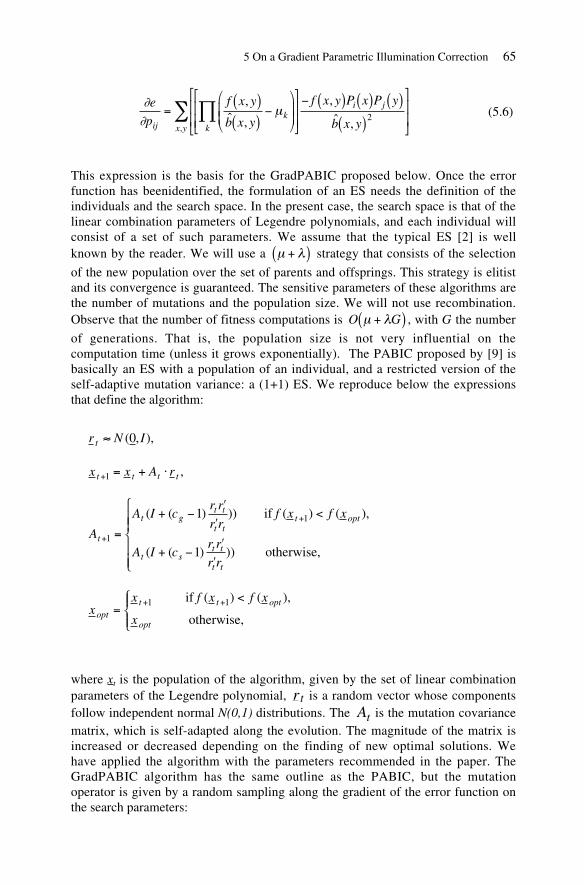
5 On a Gradient Parametric Illumination Correction 65
µe
p
f x y
b x y
f x y P x P y
b x yijk
k
i j
x y
= ( )( )
( ) ( ) ( )( )
,ˆ ,
,
ˆ ,,2 (5.6)
This expression is the basis for the GradPABIC proposed below. Once the errorfunction has beenidentified, the formulation of an ES needs the definition of theindividuals and the search space. In the present case, the search space is that of thelinear combination parameters of Legendre polynomials, and each individual willconsist of a set of such parameters. We assume that the typical ES [2] is wellknown by the reader. We will use a µ +( ) strategy that consists of the selection
of the new population over the set of parents and offsprings. This strategy is elitistand its convergence is guaranteed. The sensitive parameters of these algorithms arethe number of mutations and the population size. We will not use recombination.Observe that the number of fitness computations is O Gµ +( ) , with G the number
of generations. That is, the population size is not very influential on thecomputation time (unless it grows exponentially). The PABIC proposed by [9] isbasically an ES with a population of an individual, and a restricted version of theself-adaptive mutation variance: a (1+1) ES. We reproduce below the expressionsthat define the algorithm:
r N It ( , ),0
x x A rt t t t+ = +1 ,
A
A I cr r
r rf x f x
A I cr r
r r
t
t gt t
t tt opt
t st t
t t
+
+
=+ <
+1
11
1
( ( ) )) ( ) ( ),
( ( ) ))
if
otherwise,
xx f x f x
xoptt t opt
opt
=<+ +1 1 if
otherwise,
( ) ( ),
where xt is the population of the algorithm, given by the set of linear combinationparameters of the Legendre polynomial, rt is a random vector whose componentsfollow independent normal N(0,1) distributions. The At is the mutation covariancematrix, which is self-adapted along the evolution. The magnitude of the matrix isincreased or decreased depending on the finding of new optimal solutions. Wehave applied the algorithm with the parameters recommended in the paper. TheGradPABIC algorithm has the same outline as the PABIC, but the mutationoperator is given by a random sampling along the gradient of the error function onthe search parameters:

66 E. Fernandez, M. Graña, J. Ruiz-Cabello
r N It ( , ),0
x xf x
xrt t
t
it+ = + ( )
1 ,
xx f x f x
xoptt t opt
opt
=<+ +1 1 if
otherwise.
( ) ( ),
5.4 Experimental Results
To test the algorithms we have generated several instances of corrupted imagesfrom a chessboard image. We know the original uncorrupted image and theillumination bias field, and therefore we can compute the correlation between themand the estimated ones. The goal of the algorithms is to estimate the bias fields andto recover a clean chessboard image. PABIC parameters were set according to thenominal values recommended in [9]: c g r o w in the interval [1.01,1.1]and c cshrink grow= 1 4/ . The number of PABIC iterations is 9000. The maximum order
of the Legendre polynomials was 3. The ES was tested with µ = =100 300, andthe number of generations is 30, which gives the same number of fitnessevaluations of PABIC. The GradPABIC was allowed only 300 fitness evaluationsbecause of the cost of computing the gradient. We computed 30 replications of thealgorithm on each image. We computed the correlation between the recoveredchessboard images and the original ones, as well as the correlation between theoriginal illumination bias and the ones estimated by the correction algorithms. Theresults are summarized in Figures 5.1, 5.2, 5.3, and 5.4. Figure 5.1 plots theaverage correlation between the original image and the recovered one for eachimage and algorithm. The results of GradPABIC are better than the PABIC and ESin all cases. Figure 5.2 plots the standard deviation of the correlation between therecovered image and the ground truth for each image and algorithm. High standarddeviation implies low confidence in the algorithm results.
Again GradPABIC provides the best results in the sense of lower variance ofthe results for each image, but for some images where the ES improves it. Theworst results in terms of variance are the ones provided by the PABIC. The ES isless variable than PABIC, which is natural because of the improved convergenceproperties implied by the larger population. The PABIC, being a single individualor single-solution algorithm, has a poorer ability to escape bad local optima thanES. The good results of GradPABIC are more surprising, because it is also asingle-solution algorithm. It seems that the gradient information improves theconvergence of the algorithm.
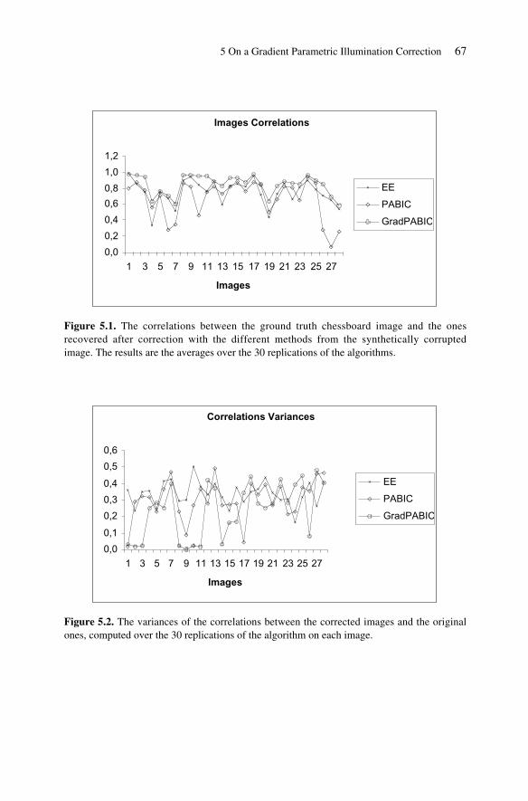
5 On a Gradient Parametric Illumination Correction 67
Images Correlations
0,0
0,2
0,4
0,6
0,8
1,0
1,2
1 3 5 7 9 11 13 15 17 19 21 23 25 27
Images
EE
PABIC
GradPABIC
Figure 5.1. The correlations between the ground truth chessboard image and the onesrecovered after correction with the different methods from the synthetically corruptedimage. The results are the averages over the 30 replications of the algorithms.
Correlations Variances
0,0
0,1
0,2
0,3
0,4
0,5
0,6
1 3 5 7 9 11 13 15 17 19 21 23 25 27
Images
EE
PABIC
GradPABIC
Figure 5.2. The variances of the correlations between the corrected images and the originalones, computed over the 30 replications of the algorithm on each image.

68 E. Fernandez, M. Graña, J. Ruiz-Cabello
Bias Correlations
0,75
0,80
0,85
0,90
0,95
1,00
1,05
1 3 5 7 9 11 13 15 17 19 21 23 25 27
Images
EE
PABIC
GradPABIC
Figure 5.3. The correlations between the ground truth illumination bias images and the onesestimated by the correction methods. The results are the averages over the 30 replications ofthe algorithm.
Correlations Variances
0,00
0,10
0,20
0,30
0,40
0,50
1 3 5 7 9 11 13 15 17 19 21 23 25 27
Images
EE
PABIC
GradPABIC
Figure 5.4. The standard deviations of the different correlations between the obtained biasimages and the original ones over the 30 replications of the algorithms.
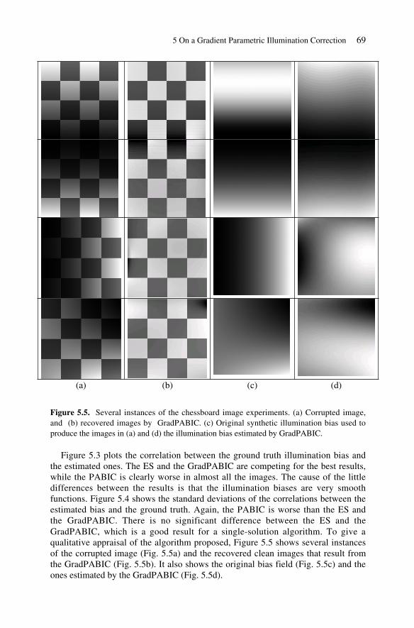
5 On a Gradient Parametric Illumination Correction 69
(a) (b) (c) (d)
Figure 5.5. Several instances of the chessboard image experiments. (a) Corrupted image,and (b) recovered images by GradPABIC. (c) Original synthetic illumination bias used toproduce the images in (a) and (d) the illumination bias estimated by GradPABIC.
Figure 5.3 plots the correlation between the ground truth illumination bias andthe estimated ones. The ES and the GradPABIC are competing for the best results,while the PABIC is clearly worse in almost all the images. The cause of the littledifferences between the results is that the illumination biases are very smoothfunctions. Figure 5.4 shows the standard deviations of the correlations between theestimated bias and the ground truth. Again, the PABIC is worse than the ES andthe GradPABIC. There is no significant difference between the ES and theGradPABIC, which is a good result for a single-solution algorithm. To give aqualitative appraisal of the algorithm proposed, Figure 5.5 shows several instancesof the corrupted image (Fig. 5.5a) and the recovered clean images that result fromthe GradPABIC (Fig. 5.5b). It also shows the original bias field (Fig. 5.5c) and theones estimated by the GradPABIC (Fig. 5.5d).

70 E. Fernandez, M. Graña, J. Ruiz-Cabello
(a) (b)
Figure 5.6. (a) Slices from a corrupted MRI voume, (b) corresponding slices of thecorrected volume given by the GradPABIC algorithm.

5 On a Gradient Parametric Illumination Correction 71
Figure 5.6 shows the results of the GradPABIC on an MRI synthetic volume ofthe brain corrupted with a known illumination bias. The slices correspond toselected axial, sagital, and coronal cuts of the corrupted and the restored volumes.
5.5 Conclusions
The PABIC algorithm for parametric illumination inhomogeneity correction inimages is a special case of ES. We have proposed GradPABIC as an improvementthat consists in using the gradient information of the error in the mutation operator.This is similar to an instantaneous memetic algorithm. GradPABIC gives betterresults and a smaller variance on a collection of synthetic images tested. Besidesthe improvement in accuracy of the image restoration, the reduction in variance ofthe results of the algorithm is very significant. As GradPABIC is a single-solutionevolutionary strategy, equivalent to reducing the population to a single individual,big variances are to expected. The reduction in variance points to GradPABIC asan especially good combination of the local search power of the gradient-basedalgorithms and the random search of evolutive algorithms.
Acknowledgments
We would like to acknowledge the Ministerio de Ciencia y Tecnología of Spainthrough grants TIC2000-0739-C04-02 and TIC2000-0376-P4-04. The Universidaddel Pais Vasco has supported us through a special grant as a consolidated researchgroup in the years 2004 to 2006.
References
1. Ahmed M.N., S.N. Yamany, N. Mohamed, A.A. Farag, T. Moriarty, (2002) A modifiedfuzzy C-means algorithm for bias field estimation and segmentation of MRI data, IEEETrans. Med. Imag. 21(3): 193-199.
2. Back T., H.-P. Schwefel, (1993) An overview of evolutionary algorithms for parameteroptimization, Evolutionary Computation, 1(1):1-23.
3. Gonzalez R.C., R.E Woods, (1990) Digital Image Processing, Academic Press, NewYork.
4.. Guillemaud, R.; Brady, M. (1997) Estimating the bias field of MR images, IEEE Trans.Med. Imag., 16(3); 238-251.
5. Likar B., M.A. Viergever, F. Pernus, (2001) Retrospective correction of MR intensityinhomogeneity by information minimization. IEEE Trans Med. Imag., 20(12):1398-1410.
6. Macovski A., (1996) Noise in MRI, Magn.Reson.Med. 36,(3):494-497.

72 E. Fernandez, M. Graña, J. Ruiz-Cabello
7. Sled J.G., G.B. Pike, (1998) Standing-wave and RF penetration artifacts caused by ellipticgeometry: An electrodynamic analysis of MRI, IEEE Trans Med Imag, 17(4):653-662.
8. Sled J.G., A.P. Zijdenbos, A.C. Evans, (1998) A nonparametric method for automaticcorrection of intensity nonuniformity in MRI data, IEEE Trans Med Imag, 17(1):87-97.
9. Styner M., G. Gerig, C. Brechbühler, G. Szekely, (2000) Parametric estimate of intensityinhomogeneities applied to MRI. IEEE Trans. Med. Imag. 19(3):153-165.
10. Wells, W.M., III; Grimson, W.E.L.; Kikinis, R.; Jolesz, F.A. (1996) Adaptivesegmentation of MRI data, IEEE Trans. Med. Imag., 15(4): 429-442.
11. http://www.densis.fee.unicamp.br/~moscato/memetic_home.html.
6___ ______ ______ ______ ______ ______ ______ ______ ______ ______ ______ ______ ______ ______ ______
A New Chromosome Codification forScheduling Problems
Ramiro Varela, Camino R. Vela, Jorge Puente, David Serrano, Ana Suárez
Summary. In this chapter we confront the Job Shop Scheduling problem by meansof Genetic Algorithms. Our aim is twofold: first to envisage a codification schemathat makes it clear what we consider the basic building blocks of a chromosome,that is the partial schedules of the set of tasks requiring the same resource; and thento design a scheduling policy that maintains as long as possible these partial sched-ules. The expected utility of this new codification is that it allows us to designknowledge-based operators and initialization strategies. We report results from anexperimental study on a small set of selected problems showing that our proposedcodification and scheduling algorithm layouts produce similar results to other con-ventional schemas. And at the same time this codification facilitates the design ofgenetic operators focused to produce promising building blocks.
6.1 Introduction
The application of GAs to scheduling problems has interested many researchers [1-4, 8, 11, 13] due to the fact that they seem to offer the ability to cope with the hugesearch spaces involved in optimization of constraint satisfaction problems [6]. Be-cause conventional GAs provide rather poor results for medium- and large-sizeproblems, a number of enhancements like elitism, local search, and structuredpopulation techniques have been proposed that improve their performance.
In this work we propose a new codification schema and a scheduling strategy forsolving Job Shop Scheduling (JSS) problems. The intuition behind this codificationis that partial schedules, i.e., schedules of the set of tasks requiring the same ma-chine, are the basic building blocks that contribute to a problem solution. Therefore,we first codify a chromosome as a set of partial schedules from which a problemsolution is built by the scheduling strategy. Whenever two or more partial schedulesare not compatible, a number of them should be modified in order to restore com-patibility. To do that we enhance the codification by means of a resource orderingvector that expresses a priority among resources, so that partial schedules of low-priority resources are broken first.

Ramiro Varela et al.74
We report experimental results from two implementations of conventional orgenuine GAs to compare our proposed codification against a well-known andwidely used schema: the permutations with repetition proposed by C. Bierwirth in[1]. What we expect of this new codification schema is that it will allow us to intro-duce new genetic operators that better cope with issues as epistasis and that facili-tate the exploitation of heuristic knowledge from the problem domain.
The remainder of this chapter is organised as follows: in Section 6.2 we intro-duce the JSS problem. Section 6.3 summarizes a conventional approach to JSSproblems based on the permutation with repetition schema proposed in [1]. In Sec-tion 6.4 we describe our proposed codification schema: the Task and Resource Or-dering (TRO), and the scheduling algorithm. Section 6.5 reports the results from anexperimental study on a set of well-known problems. Finally, in Section 6.6 wesummarize the main conclusions and propose some ideas for further work.
6.2 The JSS Problem
The JSS requires scheduling a set of jobs {J0,...,Jn-1} on a set of physical resources
t01 R0 t02 R1 t03 R2
4 3
t11 R0 t12 R2 t13 R1
2
3
t11 R2 t22 R0 t23 R23
3
end
1
3
2
start
0
0
0
4
2
43
23
33
33
21
23
13
33
Figure 6.1. A directed graph representation of a JSS problem instance with three jobs. Theresource requirement of every task is indicated within the boxes. Arcs are weighted with theprocessing time of the task at the outcoming node.
t01 R0 t02 R1 t03 R2
4 3
t11 R0 t12 R2 t13 R1
2
3
t21 R1 t22 R0 t23 R23
3
end
1
3
2
start
0
0
0
32
3
2
33
Figure 6.2. A solution to the problem of Figure 6.1. The makespan is 14

6 Codification for Scheduling Problems 75
or machines {R0,...,Rm-1}. Each job Ji consists of a set of tasks {ti0,...,ti(m-1)} or opera-tions to be sequentially scheduled. Each task has a fixed duration or processing timeduil and requires the exclusive use of a single resource. The objective is to come upwith a feasible schedule such that the completion time of the whole set of tasks, i.e.,the makespan, is minimized. Figure 6.1 shows a problem instance in a usual graphicrepresentation. From this representation a solution to the problem is an acyclic sub-graph that includes every node as well as every arc from sequential constraints, butonly a Hamiltonian selection from each resource, that is a subgraph that expresses alinear ordering among the set of tasks requiring the resource. The cost of the solu-tion is the cost of the longest path from the start node to the end node in the solutiongraph. Figure 6.2 shows a solution subgraph to the problem of Figure 6.1.
This representation of the JSS problem suggests that partial schedules of the sub-set of tasks requiring the same resource are the actual basic building blocks. Hencewe have tried to envisage a codification schema that allows us to design genetic op-erators to explicitly manipulate partial schedules. The long-term objective is thatthese operators can exploit knowledge from the problem domain.
6.3 Conventional Codification Schemas and SchedulingAlgorithms
Here we consider the codification schema proposed by C. Bierwirth [1]: the per-mutation with repetition schema. According to this representation, a chromosome iscodified by a permutation of the whole set of tasks of the problem at hand. Con-sider, for example, the problem depicted in Figure 6.1 and the permutation of itstasks (t31 t11 t12 t32 t01 t33 t13 t02 t03). From this permutation an individual is obtained byreplacing every task identifier by the corresponding job number; therefore we ob-tain (3 1 1 3 0 3 1 0 0). Consequently, this codification should be understood tomean the following: the first 2 represents the first task of the second job, the first 3is the first task of the third job, the second 2 is the second task of the second job,and so on. One of the main reasons to introduce this codification is that the geneticoperators always produce feasible chromosomes, as we will see in the followingparagraphs. The mutation operator we use in this work is the order-based mutation(OX) proposed by Syswerda [8]: two tasks are selected at random and their posi-tions are interchanged. At the same time, we use the generalized position crossover(GPX) proposed by Bierwirth [1]. In order to clarify how GPX works, consider thefollowing two parents:
Parent1 (3 1 1 3 0 3 1 0 0) Parent2 (0 3 3 0 1 1 0 1 3).
A substring is selected at random from parent1, for example the underlined sub-string that includes the second 1, the second and third 3, and the first 0. The off-spring is constructed by inserting that substring at the position it has in parent1 andfilling the remaining positions with the remaining tasks, in this case maintaining theordering they have in parent2. Hence, in this case we obtain the offspring
(3 0 1 3 0 3 1 0 1).

Ramiro Varela et al.76
The intuition behind the GPX operator is that the offspring inherits characteris-tics from both of the two parents by maintaining the relative ordering and positionof a number of tasks from parent1, and only the relative order of the remaining onesfrom parent2. However, the meaning of an allele might change during crossover;for example, the 0 of the former substring selected from parent1 represents the taskt01, while after being inserted into the offspring it represents t02. This effect is knownas implicit mutation of the crossover operator and in practice makes it difficult tocharacterize the effect of the genetic operators on the basic building blocks that inthis codification are considered as the partial ordering of subsequences.
In order to evaluate chromosomes a scheduling strategy must be defined thattranslates the chromosome codification into a schedule. The fitness value is, inprinciple, the inverse of the makespan of this schedule given that we have a mini-mization problem. In this work we used the following scheduling algorithm.
for each task in the chromosome from left to right do
set its start time to lowest value compatible withthe assignments made to the previous tasks in thechromosome;
This algorithm has a complexity that in the worst case is O(N2), N being the totalnumber of the problem tasks. The start time of a task is calculated as the maximumvalue of the completion time of the previous task in the job and the completiontimes of the scheduled tasks requiring the same resource. Figure 6.3 shows theGantt chart of the schedule produced for this algorithm when it is applied to thechromosome (3 1 1 3 0 3 1 0 0).
The above fitness function can be adjusted in order to better discriminate be-tween good and bad chromosomes. Here we consider the scaling. This is a commontechnique, as pointed out in [9]. The objective is either to accentuate or to soften thedifference between good and bad chromosomes in order to obtain a more accuratediscrimination. The underlying idea is that small relative differences among the fit-ness of good and bad chromosomes do not facilitate the selection of the best chro-mosomes and the elimination of the worse ones, whereas large relative differences
R0 t11 t22 t01
R1 t21 t13 t02
R2 t12 t23 t03
0 1 2 3 4 5 6 7 8 9 10 11 12 13 14 15
Figure 6.3. Solution produced to the problem of Figure. 6.1 by the former scheduling algo-rithm from the chromosome (3 1 1 3 0 3 1 0 0). The makespan is 14. It is the same solutionrepresented in the graph of Figure 6.2

6 Codification for Scheduling Problems 77
might produce the dominance of semi-optima chromosomes and hence the prema-ture convergence of the GA. Here, we consider a linear scaling that consists of re-placing the original fitness f by
f f b' ,= + (6.1)
b being a parameter that may be provided by the user or automatically determinedfrom the problem. Here we use the following strategy to compute the value of theparameter b. The objective is to establish a constant relation C among the best andmean fitness values at each generation. Hence we calculate the parameter b for agiven generation so that
C mean b best b= +( ) +( ) . (6.2)
Consequently, for each generation we will have
b mean best C C= ( ) ( )* 1 . (6.3)
C is the scaling parameter: its value must be greater than 1 and, in principle, isgiven by the user as the reminder parameters of the GA.
6.4 The TRO Codification Schema
In principle, a chromosome is represented by a Resource Matrix (RM). This is anm n× matrix where the jth row represents a partial schedule for the tasks requiringthe resource Rj. From a RM a schedule can be built by merging all of the partialschedules so that every precedence constraint is also satisfied. Unfortunately,sometimes this is not possible because of the lack of compatibility among partialschedules and hence a number of them should be modified. In order to do that, wetake up a priority schema for resources so that partial schedules of low-priority re-sources are modified first. To represent priorities we include into the chromosomerepresentation a Resource Priority vector (RP) that codifies a resource ordering,from high to low rescheduling priority. Figure 6.4a shows an RM representing par-tial schedules for the problem of Figure 6.1, and Figure 6.4 b shows an RP of pri-orities among resources.
The genetic operators we have used in this work are a natural extension of theformer GPX and OX. Given two chromosomes we first apply the GPX operator tothe pair composed by the ith row of each RM component, and then to the pair of RPcomponents. At the same time, the OX operator is applied to the RP component andto every row of the RM component of the offspring. Nevertheless, the design of ge-netic operators allows other possibilities, for example we could exploit any heuristicinformation about either promising partial schedules or criticality measures of theresources as an alternative choice of making random crossovers and mutations.
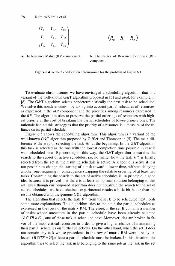
Ramiro Varela et al.78
To evaluate chromosomes we have envisaged a scheduling algorithm that is avariant of the well-known G&T algorithm proposed in [5] and used, for example, in[8]. The G&T algorithm selects nondeterministically the next task to be scheduled.We solve this nondeterminism by taking into account partial schedules of resources,as expressed in the MR component and the priorities among resources expressed inthe RP. The algorithm tries to preserve the partial orderings of resources with high-est priority at the cost of breaking the partial schedules of lower-priority ones. Therationale behind this strategy is that the priority of a resource is a measure of the re-liance on its partial schedule.
Figure 6.5 shows the scheduling algorithm. This algorithm is a variant of thewell-known G&T algorithm proposed by Giffler and Thomson in [5]. The main dif-ference is the way of selecting the task t at the beginning. In the G&T algorithmthis task is selected as the one with the lowest completion time possible in case itwas scheduled next. By working in this way, the G&T algorithm constrains thesearch to the subset of active schedules, i.e. no matter how the task * is finallyselected from the set B, the resulting schedule is active. A schedule is active if it isnot possible to change the starting of a task toward a lower time, without delayinganother one, requiring in consequence swapping the relative ordering of at least twotasks. Constraining the search to the set of active schedules is, in principle, a goodidea because it is proved that there is at least an optimal solution belonging to thisset. Even though our proposed algorithm does not constrain the search to the set ofactive schedules, we have obtained experimental results a little bit better than theresults obtained with the genuine G&T algorithm.
The algorithm that selects the task * from the set B to be scheduled next needssome more explanations. This algorithm tries to maintain the partial schedules asexpressed in the rows of the matrix RM. Therefore, if the set B contains a numberof tasks whose ancestors in the partial schedule have been already selected
B TR( ) , one of these task is scheduled next. Moreover, ties are broken in fa-
vor of the most critical resources in order to give a higher chance of maintainingtheir partial schedules on further selections. On the other hand, when the set B doesnot contain any task whose precedents in the row of matrix RM were already se-lected B TR =( )at least a partial schedule must be broken. In this situation, the
algorithm tries to select the task in B belonging to the same job as the task in the set
031312
021321
012211
ttt
ttt
ttt
( )210 RRR
a. The Resource Matrix (RM) component b. The vector of Resource Priorities (RP)component
Figure 6.4. A TRO codification chromosome for the problem of Figure 6.1.

6 Codification for Scheduling Problems 79
TB that requires the most critical resource, hence giving a chance to maintain thepartial schedule of this resource. Finally if there is not any task in the set B TBwith the same resource requirement, the task of B requiring the lowest-priority re-source is selected, therefore breaking its partial schedule.
S c h e d u lin g a lg o r it h m
A = { t 0 1 ,. .. ,t 0 ( m- 1 ) } ; / * fir st ta sk o f e ac h o f th e j o b s, at e ach s tep A i s t h e se t o f u n sch ed u l ed ta sk s w h o se p r ec ede n t s i n th e j o b ar e sc h ed u l ed * /
w h il e A d o {
D e te rmin e A s u c h th a t t t A, , w h er e t i s th e l o w est s ta rt ti m e if ta sk w as s ch e d u led n ex t;
L e t M ’ b e t h e m a ch in e r eq u ir ed b y , an d B t h e su b s et o f t ask s in A req u ir in g M ’;
D e le te fr o m B th o s e t as k s th at ca n n o t st ar t a t a t im e lo w er th an t du+ ;
S e le ct * f ro m B to b e sch ed u le d n e x t;
D e le te * f ro m A a n d in se rt th e n ex t ta sk o f th e sa m e jo b a s * i f * i s n o t t h e la st o n e o f it s jo b ;
}
en d .
Algorithm to Select * from B
T R = s et o f u n sc h e d u l ed ta sk s su c h th a t al l t h e ir p r ec ed e n t s i n th e c o r res p o n d in g r o w o f R M ar e alrea d y sc h e d u le d ;
if B TR( )th en *= ta sk o f B TR re q u ir in g t h e m o st cr it ica l re so u rc e, i. e, t h e o n e w it h h ig h e st
p ri o r ity i n R P ; el se JB = s et o f jo b s t o w h i ch th e tas k s o f B b elo n g s; T R B = su b se t o f ta sk s o f T R b e lo n g i n g to a jo b o f JB ;
if TRB( ) th en R * = se t o f re so u rc es re q u ir ed b y th e ta sk s o f T R B ; = ta sk o f T R B re q u iri n g to t h e m o st cr it ic al reso u r ce o f R * ( se e R P ) ; J * = j o b c o n t ai n in g th e t as k ; * = t as k o f B b el o n g in g to J* ; el se * = t as k o f B r eq u i rin g th e l ea st cr iti ca l res o u rce ( se e R P ) ;
en d .
Figure 6.5. Scheduling algorithm. t refers to the start time of task and du to its proc-essing time.
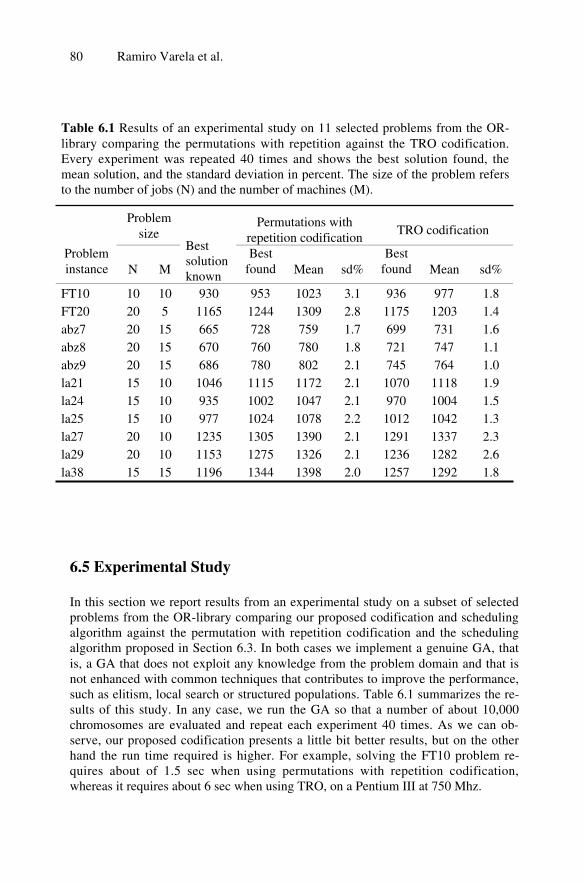
Ramiro Varela et al.80
6.5 Experimental Study
In this section we report results from an experimental study on a subset of selectedproblems from the OR-library comparing our proposed codification and schedulingalgorithm against the permutation with repetition codification and the schedulingalgorithm proposed in Section 6.3. In both cases we implement a genuine GA, thatis, a GA that does not exploit any knowledge from the problem domain and that isnot enhanced with common techniques that contributes to improve the performance,such as elitism, local search or structured populations. Table 6.1 summarizes the re-sults of this study. In any case, we run the GA so that a number of about 10,000chromosomes are evaluated and repeat each experiment 40 times. As we can ob-serve, our proposed codification presents a little bit better results, but on the otherhand the run time required is higher. For example, solving the FT10 problem re-quires about of 1.5 sec when using permutations with repetition codification,whereas it requires about 6 sec when using TRO, on a Pentium III at 750 Mhz.
Table 6.1 Results of an experimental study on 11 selected problems from the OR-library comparing the permutations with repetition against the TRO codification.Every experiment was repeated 40 times and shows the best solution found, themean solution, and the standard deviation in percent. The size of the problem refersto the number of jobs (N) and the number of machines (M).
Problemsize
Permutations withrepetition codification
TRO codification
Probleminstance N M
Bestsolutionknown
Bestfound Mean sd%
Bestfound Mean sd%
FT10 10 10 930 953 1023 3.1 936 977 1.8FT20 20 5 1165 1244 1309 2.8 1175 1203 1.4abz7 20 15 665 728 759 1.7 699 731 1.6abz8 20 15 670 760 780 1.8 721 747 1.1abz9 20 15 686 780 802 2.1 745 764 1.0la21 15 10 1046 1115 1172 2.1 1070 1118 1.9la24 15 10 935 1002 1047 2.1 970 1004 1.5la25 15 10 977 1024 1078 2.2 1012 1042 1.3la27 20 10 1235 1305 1390 2.1 1291 1337 2.3la29 20 10 1153 1275 1326 2.1 1236 1282 2.6la38 15 15 1196 1344 1398 2.0 1257 1292 1.8

6 Codification for Scheduling Problems 81
6.6 Final Remarks
In this chapter we proposed both a new chromosome codification and a schedulingalgorithm for JSS problems: the TRO schema, and a variant of the G&T algorithm.From the experimental results we can assume that the performance of this schema issimilar to the codification of permutations with repetition in conjunction with theconventional scheduling algorithm proposed in Section 6.2, when both of them areused with a genuine GA. Even though the reported experimental results are a littlebit better when using our proposed approach, this improvement might be a conse-quence of the scheduling algorithm. Of course, this algorithm could be used inconjunction with the permutation schema. On the other hand, the TRO codificationmakes the partial schedules of the resources clear and therefore it is expected that itwill allow us to envisage genetic operators and initialization strategies focused toobtain promising partial schedules. In order to do that we plan to exploit the heuris-tic proposed in [10] that we have already used to design the initialization strategyproposed in [12]. Therefore, we expect that the proposed TRO schema and thescheduling algorithm provide a useful way to hybridize a genetic algorithm bymeans of knowledge from any heuristic strategy.
References
1. Bierwirth, C... (1995) A generalized perutation approach to job shop scheduling withgenetic algorithms. OR Spektrum, 17:87-92.
2. Bierwirth, C., D. C. Mattfeld (1999) Production scheduling and rescheduling with Ge-netic algoritms, Evolutionary Computation, 7(1):1-17.
3. Dorndorf, U., E. Pesch, (1995) Evolution based learning in a job shop scheduling envi-ronment, Computers & Operations Research, 22:25-40.
4. Fang, H.L., P. Ross, D. Corne, (1993) A promising genetic algorithm approach to job-shop scheduling, rescheduling, and open-shop scheduling problems, Proc. Fifth Intel.Conf. Genetic Algorithms, 375-382.
5. Giffler, B., G.L Thomson,. (1960) Algorithms for solving production scheduling prob-lems, Operations Reseach, 8:487-503.
6. Goldberg, D. (1985) Genetic Algorithms in Search, Optimization & Machine Learning,Addison-Wesley, Reading, MA.
7. Grefenstette, J. J. (1987) Incorporating problem specific knowledge in genetic algo-rithms, in: Genetic Algorithms and Simulated Annealing, Morgan Kaufmann, pp. 42-60.
8. Matfeld, D. C. (1995) Evolutionary search and the job shop. Investigations on GeneticAlgorithms for Production Scheduling. Springer-Verlag.
9. Michalewicz, Z. (1994) Genetic Algorithms + Data Structures = Evolution Program.Second, Extended Edition, Springer-Verlag.
10. Sadeh, N., M.S. Fox, (1996) Variable and value ordering heuristics for the Job ShopScheduling Constraint Satisfaction Problem, Artificial Intelligence, 86:1-41.
11. Syswerda, G. (1991) Schedule Optimization Using Genetic Algorithms, in Handbookof Genetic Algorithms, (ed.) L. Davis, Van Nostrand Reinhold, New York, pp.1332-13490.

Ramiro Varela et al.82
12. Varela, R., C. R. Vela, J. Puente, A. Gómez (2003) A Knowledge-Based EvolutionaryStrategy for Scheduling Problems with Bottlenecks. European Journal of OperationalResearch. 145(1): 57-71.
13. Yamada, T. and Nakano, R. (1996) Scheduling by Genetic Local Search with multi-step crossover. In: Fourth Int. Conf. On Parallel Problem Solving from Nature (PPSNIV), Berlin, Germany, pp. 960-969.

7___ ______ ______ ______ ______ ______ ______ ______ ______ ______ ______ ______ ______ ______ ______
Evolution-based Learning of OntologicalKnowledge for a Large-scale Multi-agentSimulation
A. Lazar, R.G. Reynolds
7.1 Introduction
The results of the data mining [1] process can be used in many different ways.Therefore, the form of the knowledge collected will have a major impact on the ef-ficiency and effectiveness of its use in a given application. In this paper we exam-ine the problem of extracting knowledge for use by agents in a large-scale multi-agent system [2]. Here, the knowledge is ontological knowledge that representsconstraints that the physical and social environments placed upon the agents andtheir interactions. The ontological knowledge represents the semantic buildingblocks around which the world models are formed. For an agent in a particularmodel, only the things in his ontology can exist and it cannot perceive things thatare not represented in the ontology. An ontology [3] is a basic level of knowledgerepresentation scheme, a formal definition of entities and their properties, interac-tions, behaviors, and constraints. Each agent’s decisions need to be checked againstthese constraints prior to their execution. In a complex multi-agent system, hun-dreds of thousands of agents may need to check these constraints regularly, whichmeans that a successful data mining activity will need to produce a relatively smallset of syntactically simple rules for the process to be efficient. Fox et al. [3] haveused data mining techniques to produce corporate ontogenies.
Several factors can influence the nature of the ontological constraints that areproduced: first, the nature of the data collection and measurement process and theuncertainty induced into the data set by the presence of noise, second, the nature ofthe representation used to express the extracted patterns; e.g.,. whether it allows foruncertainty or not, third, the data mining technique employed and the assumptionsthat it makes about the collected data, fourth, how these constraints will be stored,accessed, and used by the agents involved.
For a given data set one can compare the different data mining techniques interms of the syntactic and semantics of the induced constraints. In this applicationwe are interested in simulating the emergence of the archaic state in the Valley ofOaxaca, Mexico. A state is among the most sophisticated and powerful structuresthat has emerged from the social evolution process. In the modern world these aretermed “nation states” with a government composed of a hierarchical decision-making structure where the decision-makers are either elected or appointed. States
Alina Lazar, Robert G. Reynolds84
are supported by various economies and are able to interact with each other viawarfare, trade, etc. Most states in the ancient world-often called archaic states-wereruled by hereditary royal families. These archaic states exhibited much internal di-versity with populations numbering from tens of thousands to millions. They had abureaucracy, organized religion, a military presence, large urban centers, publicbuildings, public works, and services provided by various professional specialists.The state itself could enter into warfare and trade-based relationships with otherstates and less complex neighbors.
The process by which complex social entities such as the state emerged fromlower level structures and other supporting economies has long been of prime in-terest to anthropologists and other disciplines as well. This is because the emer-gence of such a social structure can have a profound impact on the society’s physi-cal and social environment. However, the task of developing realisticcomputational models that aid in the understanding and explanation of state emer-gence has been a difficult one. This is the result of two basic factors:
1. The process of state formation inherently takes place on a variety of temporaland spatial scales. The emergence of hierarchical decision-making [4, 5] can beviewed as an adaptation that allows decision-makers to specialize their decisionsto particular spatial and temporal scales.
2. The formation of the state is a complex process that is fundamentally directedby the social variables but requiring dynamic interaction between the emergentsystem and its environment. Identifying the nature of these interactions is one ofthe reasons why the process of state formation is of such interest.
The goal of this project is to produce a large-scale knowledge-based computa-tional model of the origins of the Zapotec State [6], centered at Monte Alban, inthe Valley of Oaxaca, Mexico. State formation took place between 1400 B.C. and300 B.C. While archaic states have emerged in various parts of the world, the rela-tive isolation of the valley allowed the processes of social evolution to be morevisible there. Extensive surveys [7, 8, 9] of the 2,100-square-kilometer valley wereundertaken by the Oaxaca Settlement Pattern Project in the 1970s and 1980s. Thelocation and features of over 2,700 sites dating from the archaic period (8000 B.C.)to Late Monte Alban V (just prior to the arrival of the Spaniards) were docu-mented. Several hundred variables were recorded for each site. In addition, theysurveyed the 6.5-square-kilometer urban center of Monte Alban, a site that con-tained over 2,000 residential terraces. This site was the focus for early state forma-tion in the valley.
Both surveys provided the knowledge needed to create our multi-agent simula-tion model. We then produced a spatial temporal database that contained the resultsof both surveys and used data mining techniques from Artificial Intelligence [2] toproduce knowledge about site location, warfare, trade, and economic decisions tobe used for the construction of the multi-agent model. However, in order to do thiswe needed to add more data about the spatial and temporal context to both the re-gional and urban center surveys. Specifically, we had to add variables that allowedus to locate each site spatially and temporally to a level of precision consistent withthe scale of our simulation. For example, temporal periods are characterized by thepresence of pottery of different styles. That data was available only in text form.
7 Evolution-based Learning of Ontological Knowledge 85
All of this pottery data, over 130 variables for each residential terrace, was scannedinto the computer, corrected for errors, and added to the Monte Alban data set.This data allowed us to identify the periods that each terrace was occupied. Potterydata was also integrated into the regional data set.
In addition, the survey had produced hundreds of pages of hand-drawn mapsfor both the Monte Alban and regional surveys that contained the spatial contextfor the location of each site. Since our goal was to ask specific questions about thespatial and temporal context, we needed to tie each site into its mapped location.We then proceeded to digitize each of the maps and to associate each site objectwith its corresponding data record. This allowed us to produce a geographical in-formation system (GIS) that serves as our “virtual valley of Oaxaca”. This acts as avehicle for our data mining activities and as a knowledge base for the multi-agentsimulation and allows the results of the simulation to be displayed and comparedwith the actual data in a spatial context. It is envisioned that the resultant GIS sys-tem will be a useful tool for researchers and students from various fields to studythe emergence of complexity in the future.
In order to perform the data mining activities, we extended traditional datamining techniques and developed new ones in order to deal with the complexitiesinherent in the Oaxaca database. At the regional level we used Utgoff’s incre-mental decision tree algorithm (IDTI) [10] to generate the decision trees for eachregion and phase of the valley. The approach was used to generate decision treesthat discriminated between sites that were targets for warfare and those that werenot for a given period [11, 12].
However, given the many disparate steps under which the data was collectedand organized, it was felt that perhaps some improvements might be made by usinga technique that took into account the presence of uncertainty in the data, espe-cially in regions and periods when the social and settlement patterns were complexand prone to data collection error. To test this hypothesis we selected a period oftime just before the emergence of the state, Rosario, where there was evidence ofincreased social strife brought about in part by increased population growth. Thepart of the valley that exhibited the greatest population at the time, Etla, was alsoselected. Since the majority of the data was discrete rather than continuous in na-ture, we selected rough sets as a vehicle for representing uncertainty here.
We employed an evolutionary technique, Genetic Algorithms [13, 14], to con-trol the search in this case because Genetic Algorithms had been successfully usedwith Rough Sets previously. The decision systems or rule sets produced by bothapproaches were then compared in terms of their ability to decide about the loca-tion of sites that are targets for warfare in this period. We then compared the twoapproaches over all relevant phases of social evolution in the valley.
In Section 7.2 we begin with an overview of decision trees and their generation.Next Section 7.3 discusses the ways in which noise was introduced into the datahere. In Section 7.4 a general framework for the generation and description of de-cision systems is briefly presented. In Section 7.5 rough sets are introduced andembedded within an evolutionary search engine based upon Genetic Algorithms.Section 7.6 provides a comparison of a specific decision system for the Etla regionin the Rosario phase as produced by decision trees and rough sets, respectively.

Alina Lazar, Robert G. Reynolds86
slope<1.5
water<2.5 water<2.5
land<3
env_zone<3.5
irrigtype<2
land<1.5
water<1.5
0
0 1 0
0
0
0
0
0,1 0,1
env_zone<2.5
Figure 7.1 The decision tree for the locations of sites with evidence of raiding in Ro-sario phase in the Etla region of the valley.

7 Evolution-based Learning of Ontological Knowledge 87
Section 7.7 compares the two approaches together over all phases in the Etla re-gion. The rough set approach appears most useful in those phases with the mostevidence for change in social complexity. Section 7.8 gives our conclusions.
7.2 Decision Tree
Decision tree induction is a very good method for high-dimensional applications. Itis a fast, nonlinear prediction method and employs dynamic feature selection. Thesolution complexity is expressed in terms of the number of terminal nodes. Themost complex tree covers all cases in the training data. Pruning the tree and meas-uring the errors in progressively smaller trees find less complex solutions.
Any decision tree can be rewritten in a form of decision rule set. An implieddecision rule in a tree is a complete path to a terminal node. Because these rules arenot mutually exclusive, the size of the decision rule set can be much larger than thelogic needed for overlapping rules. One rule can combine a large number of termsor true-false conditions, which takes a lot of time for evaluation, when the rule setis used in an agent-based simulation.
One of the advantages of logic-based solutions as decision trees and corre-sponding decision rules is their powerful explanatory capabilities. Table 7.1 givesall of the relevant periods of social evolution in the valley. Tierras Largas marksthe beginning of early village settlement there. The state emerged at Monte Albanin period Monte Alban Ia. The valley came under control of the state by Monte Al-ban II, and Monte Alban IIIa signaled the decline of the state and its succession bya collection of city-states localized in different parts of the valley.
Table 7.1 Number of Terminal Nodes for Each Phase
Period Approximate date
Tierras Largas 1400 - 1150 BC
San Jose 1150 - 850 BCGuadalupe 850 - 700 BCRosario 700 - 500 BCMonte Alban Ia 500 - 300 BCMonte Alban Ic 300 - 150/100 BCMonte Alban II 150/100 BC - AD 200Monte Alban IIIa AD 200 - 500Monte Alban IIIb AD 500 - 700/750Monte Alban IV AD 700/750Monte Alban V AD 1000 - 1521

Alina Lazar, Robert G. Reynolds88
For some periods there were several hundred rules produced just for the war-fare constraint alone. Adding in the other constraints would produce a knowledgebase of several thousand rules at a minimum. However, since the data were col-lected over a ten-year period over varying landscapes using different surveyors andrecording equipment, it was felt that a significant amount of noise might be presentin the data. The original technique did not account explicitly for uncertainty in themeasurement data. Thus, it was possible that certain rules or rule conditions werepresent only to deal with the specific noise introduced into the process by the sur-vey methods and data transformation activities.
Table 7.2 Decision Rule Set Induced from the Decision Tree
Rules
1 env_zone<2.5 => decision(0)2 env_zone>=2.5 and slope<1.5 and water<2.5 => decision(0)3 env_zone>=2.5 and slope<1.5 and water>=2.5 => decision(1)4 env_zone>=2.5 and slope>=1.5 and water<2.5 and land<3 and env_zone<3.5
and irrigtype<2 and land<1.5 => decision(0)5 env_zone>=2.5 and slope>=1.5 and water<2.5 and land<3 and env_zone<3.5
and irrigtype<2 and land>=1.5 and water<1.5 => decision(0) or decision(1)6 env_zone>=2.5 and slope>=1.5 and water<2.5 and land<3 and env_zone<3.5
and irrigtype<2 and land>=1.5 and water>=1.5 => decision(0) or decision(1)7 env_zone>=2.5 and slope>=1.5 and water<2.5 and land<3 and env_zone<3.5
and irrigtype>=2 => decision(0)
8 env_zone>=2.5 and slope>=1.5 and water<2.5 and land<3 and env_zone>=3.5 =>decision(0)
9 env_zone>=2.5 and slope>=1.5 and water<2.5 and land>3 => decision(0)10 env_zone>=2.5 and slope>=1.5 and water>=2.5 => decision(0)
If this was the case, then by using a representation and associated learning tech-nique that dealt explicitly with uncertainty it might be that fewer rules would beneeded in periods where the noise is most pronounced.
7.3 Uncertainty in Data
Uncertainty in a data set, which can occur during data collection or data entry, isreferred to as noise in the data. One type of noise is the presence of missing attrib-ute values. In this case, the objects containing missing attributes values can be dis-carded or the missing values can be replaced with the most common values. An-other type of noise occurs because the available knowledge in many situations isincomplete and imprecise. This means that sometimes the attribute values for a setof objects are not sufficient and precise enough to differentiate between the desiredclasses of objects. In the Oaxaca data set, this may have occurred for many rea-

7 Evolution-based Learning of Ontological Knowledge 89
sons. The ancient sites may be damaged because of plowing, erosion, pot hunting,and grazing. Also, human perception is subjective, and many people worked on thecollection of the data. Some errors are also possible due to the scanning processsince much of the data was available only from printed text and hand-drawn mapsas described earlier.
Many different ways of representing and reasoning about uncertainty have beendeveloped in Artificial Intelligence. These theories include belief networks, non-monotonic logic, fuzzy sets along with fuzzy logic and rough sets. One approachbased on the rough set theory [15] provides a lower and upper approximation interms of a set describing a target concept depending on how the relationship be-tween two partitions of a finite universe is defined.
Given the discrete nature of the data set we selected the rough sets method forrepresenting uncertainty here. Since the rough set algorithm is inherently intracta-ble for large data sets like ours, an evolutionary based approach, here Genetic Al-gorithms, was employed to guide the search for the appropriate rough set rules.
7.4 Building Decision Systems
A decision rule is an assertion, of the form “if p then s”, denoted by p=>s, where pand s are logical formulas in the first-order logic. For each object, certain values ofthe condition attributes determine the value of the decision attribute. We define adecision system as a finite collection or set of decision rules. In order to obtain adecision system with a minimum number of rules, superfluous decision rules asso-ciated with the same decision class can be eliminated without disturbing the deci-sion-making process.
The problem of decision system construction is to induce a set of rule descrip-tors for decision classes from the input set of objects in a decision table. These setsof descriptors, named decision systems, consist of a set of decision rules. We canclassify the decision system as follows:
1. Decision systems with a minimum set of rules. They are focused on describinginput objects using a minimum number of necessary rules.
2. Decision systems with an exhaustive set of rules. These decision systems con-tain all possible decision rules.
3. Decision systems with a satisfactory set of rules. This category represents sets ofdecision rules, which satisfy given a priori user's requirement for an acceptabledecision system.
One strategy to find a simple decision system with good classificatory capabili-ties is to first induce an exhaustive set of rules, and then to prune away those rulesthat do not lower the decision system's performance significantly. An exhaustivedecision system can be generated from the reducts [16, 17].
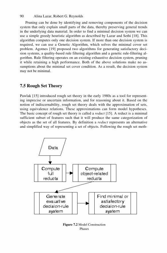
Alina Lazar, Robert G. Reynolds90
Pruning can be done by identifying and removing components of the decisionsystem that only explain small parts of the data, thereby preserving general trendsin the underlying data material. In order to find a minimal decision system we canuse a simple greedy heuristic algorithm as described by Lazar and Sethi [18]. Thisalgorithm computes only one decision system. If more than one decision system isrequired, we can use a Genetic Algorithm, which solves the minimal cover setproblem. Agotnes [19] proposed two algorithms for generating satisfactory deci-sion systems, a quality-based rule filtering algorithm and a genetic rule-filtering al-gorithm. Rule filtering operates on an existing exhaustive decision system, pruningit while retaining a high performance. Both of the above solutions make no as-sumptions about the minimal set cover condition. As a result, the decision systemmay not be minimal.
7.5 Rough Set Theory
Pawlak [15] introduced rough set theory in the early 1980s as a tool for represent-ing imprecise or uncertain information, and for reasoning about it. Based on thenotion of indiscernability, rough set theory deals with the approximation of sets,using equivalence relations. These approximations can form model hypotheses.The basic concept of rough set theory is called a reduct [15]. A reduct is a minimalsufficient subset of features such that it will produce the same categorization ofobjects as the set of all features. By definition a reduct represents an alternativeand simplified way of representing a set of objects. Following the rough set meth-
Figure 7.2 Model ConstructionPhases

7 Evolution-based Learning of Ontological Knowledge 91
odology, the full set of reducts is computed, a minimal reduct is chosen, and thedata table is vertically pruned. Then the object-related reducts are computed andthe exhaustive decision rule system is generated.
At the end, a pruning method for the decision rule set is applied in order to ob-tain a performant decision system that possesses a good balance between the num-ber of rules and the accuracy of the classifications. The process is shown in Figure7.2.
7.5.1 Genetic Algorithm for the Reduct Problem
Multisets are unordered collections of elements where an element can occur as amember more than once. A hitting set [20, 21] for a given multiset, MS, of ele-ments from P(C) is a set B, B C B C, such that the intersection between B andevery set in MS is nonempty.
HS MS B C B MS MS MSi i( ) = { } for all . (7.1)
The set B HS(MS) is a minimal hitting set of MS, iff B is no longer a hitting setwhenever any of its elements are removed. The set of minimal hitting sets is de-noted by minHS(MS).
For the reduct problem using a minimal hitting set, the population for the Ge-netic Algorithm is a set P of N individuals, each from the space P(C), where C isthe condition attributes set. Each individual is encoded as a binary vector, whereeach bit indicates the presence of an attribute in the set.
For this population, the fitness function rewards individuals hitting more sets inthe collection of sets corresponding to the discernibility function.
A possible fitness function proposed by Vinterbo [21] is the following:
f BC B
C
MSi MS MSi B
MS( )
{ }= + . (7.2)
The first term rewards smaller-sized individuals, and the second is used to ensurethat we reward sets that are hitting sets.
The fitness function is a discrete, multimodal function. The algorithm used byVinterbo and Ohrn [20] is the traditional Genetic Algorithm implementation. Thegenetic operators crossover, mutation, and inversion are used and selection is doneby the “roulette wheel” process. The same selection of individuals is used in orderto replace the individuals in the fixed-size population in the recombination step.Elitism and Boltzaman scaling are included. Initialization of the population is donerandomly, and the process stops when no more improvement in the average fitnessof the population is produced over a predefined number of generations.
Alina Lazar, Robert G. Reynolds92
7.6 Decision Trees and Rough Set Rules
Previously [12] computed decision trees from Tierras Largas phase through MonteAlban IIIa for all regions in the valley using Utgoff’s decision tree algorithm. Thegoal was to diferentiate between the sites that are targets for attack and the thosethat are not. Three variables were used in order to compute the decision: the pres-ence of burnt daubt at the site, other evidence of burning, and the presence of de-fensive walls. The variables used to predict these decisions from positive andnegative examples in the training set were: Environmental zone, Slope, Hiltop orRidge top, Soil Character, On the boundary between the loam and the swampyreagion, Water source, Depth of Water Table, Type of irrigation, and Land usetype among others.
In section 7.2 we presented a decision tree (Figure 7.1) and a corresponding de-cision system (Table 7.2) for the Rosario phase (700-500 B.C.) generated by thedecision tree approach. It is the fourth phase of occupation in the study, and at thattime population size and warfare increased substantially [6]. For example, it wasobserved that chunks of burnt daub appear on the surface of the villages seventimes more frequently than in the previous phases. There are 36 sites in the Rosariophase. The archaic state emerged in the period following this phase of increasedwarfare.
First, we performed a feature selection using the rough set guided by GeneticAlgorithm with the variables above. The rough set approach extracted the samefive variables as did the decision tree approach. They are: Environmental Zone,Slope, Hiltop or Ridge Top, Water Source, Type of Irrigation, and Land Use. Wethen computed the reducts, and the corresponding decision system is given in Ta-ble 7.3. This table represents the exhaustive set of rules produced. While it is clearthat several of the rules are so simple that they can be easily combined to produce asmaller set of rules overall, it is sufficient for comparative purposes here.
Our focus here is on the impact of the use of a technique, such as rough sets,that explicitly is able to deal with uncertainty in the recognition decision. From thisstandpoint there are two basic points of comparison. First, how many of the rulesidentify a site for attack unambiguously and, what percentage of the rules that se-lect sites for attack do they comprise? Second, in those cases in which the rule pro-duces a split decision we will need to resolve the tie using other means. The ques-tion is, how much effort do we need to spend in order to find out that we mustcontact another source to resolve the question?
In answer to the first question, explicitly dealing with uncertainty using therough set representation produced four rules that identify sites for attack as op-posed to just three rules in the decision tree approach. Of these four rules, two ofthe four (11 and 16) result in unambiguous decisions. That is, 50% of the rules thatcan conclude that a site can be attacked are unambiguous whereas the other twoneed further clarification. The decision trees approach produces 3 rules that canconclude that a site can be attacked, with only one of them (rule 3) being conclu-sive. Thus, only 33% of the rules that identify a site for attack are conclusive asopposed to 50% for the rough set approach. By taking data uncertainty into ac-count, the rough set approach not only produced more rules for the identification ofthe target concept, but also a higher percentage of unambiguous ones.

7 Evolution-based Learning of Ontological Knowledge 93
Table 7.3 Exaustive Decision System for the Rosario Phase in Etla Region
Rules1 env_zone(2) => decision(0)2 water(1) AND land(2) => decision(0) OR decision(1)3 env_zone(3) AND slope(2) AND water(2) AND
irrig_type(0) AND land(2) => decision(0) OR decision(1)4 slope(1) and water(2) => decision(0)5 water(4) => decision(0)6 land(1) => decision(0)7 land(4) => decision(0)8 env_zone(4) => decision(0)9 irrig_type(3) => decision(0)
10 irrig_type(4) => decision(0)11 slope(1) and water(3) => decision(1)12 slope(2) and water(3) => decision(0)13 water(0) => decision(0)14 irrig_type(2) => decision(0)15 irrig_type(1) => decision(0)16 water(3) and irrig_type(0) => decision(1)
The other question concerns the relative amount of effort expended to producean uncertain conclusion. In the decision system produced using Rough Sets, the in-conclusive rules have fewer conditions to be checked than for those from the deci-sion trees approach. Specifically, the inclusive rough set rules have 2 and 5 condi-tions respectively for a total of 7 conditions, one of which is shared between them(land type =2). In the decision tree system 8 conditions must be checked in the 2inconclusive rules for a total of 16. However, each shares the same 8 so that thetotal number of unique conditions to be tested is 8 as opposed to 6 for the RoughSet approach. More effort must then be expended in order to check the inconclu-sive rules in the decision tree approach as opposed to that for Rough Sets.
Since both approaches extracted the same set of condition variables, the differ-ences are likely to reflect the impact that noise in the data had on the relative per-formance of the approaches. By allowing for the presence of noise in the systemthe number and percentage of conclusive rules have been increased and the amountof effort spent on evaluating inconclusive rules decreased. This region and phasecombination reflects an increased complexity in the warfare patterning when com-pared to previous periods. While the complexity isn’t nearly as great in the subse-quent periods when the state emerges, even in this case specific efficiencies accrueto the use of approaches that take uncertainty explicitly into account. In the nextsection we will investigate this hypothesis by comparing the performance of thetwo approaches over all periods of interest in the valley.

Alina Lazar, Robert G. Reynolds94
7.7 Results
The two representational approaches were compared over the seven periods thatchronicle the emergence of social complexity in the valley. The decision treesresults are based on the average of the best solution for each of 20 runs withUtgoff’s Decision Tree algorithm. The Rough Set approach describes the bestsolution produced by the Genetic Algorithm-guided Rough Set algorithm using theperformance function described earlier.
DT-#c and RS-#c refer to the number of conditions in an average rule for thebest decision trees and rough sets rule set, respectively. For each of the 7 periods,the number of conditions in the rough set approach is never greater than that fordecision tree approach. In fact, aside from period II the number of terms in therough set representation is less than that for decision trees. Rosario through MonteAlban Ic correspond to periods of escalating warfare associated with theemergence of a state centered at the site of Monte Alban in the valley. Period IIcorresponds to a period in which the entire valley is under control of the state andthe focus of warfare moves outside of the valley as the Oaxacan state attempted tosubdue neighboring areas. Thus, the amount of warfare present in the valley at thattime is markedly reduced, and the simplicity of its patterns is equally characterizedby both approaches.
During the periods in which warfare patterns were the most complex (Rosario,Monte Alban Ia, Monte Alban Ic), the rough set representation produced rules witha total of 143 conditions as opposed to a total of 223 conditions for decision trees,a significant reduction in complexity. In terms of the simulation, if these rules needto be checked every time step for each of several thousand sites and severalthousand agents per site, the computational time saved can be significant.
DT-depth and RS-depth correspond to the maximum number of conditions in arule in the best rule set. In this case the rough set representation always has fewerconditions on average than the decision tree representation. The increased numberof conditions in the decision tree representation corresponds to that fact thatexplicit sources of noise are included as terms in the rules as opposed to beingremoved in the rough set representation. Variation can be produced by differentsurveyors and different landscapes and if their charcaterization is not part of ourgoal, an approach such as Rough Sets that works to exclude these terms will bemore successful.
Dt-#var and RS-#var correspond to the number of unique variables used asterms found in the best rule set of each. What is interesting here is that although therough set approach produces a rule set with fewer rules and fewer conditions perrule, the number of variables never differs by more than one between the twoapproaches. They are both using the same information to a different effect in each.This is, in fact, what we observed in the previous section where both approachesused the same subset of variables for their rule conditions. But, we observed thatthe actual behavior of the rules that were produced was different in terms ofidentifying the target concept.
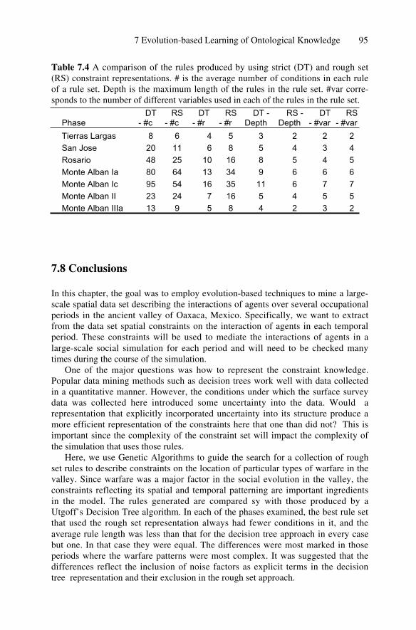
7 Evolution-based Learning of Ontological Knowledge 95
Table 7.4 A comparison of the rules produced by using strict (DT) and rough set(RS) constraint representations. # is the average number of conditions in each ruleof a rule set. Depth is the maximum length of the rules in the rule set. #var corre-sponds to the number of different variables used in each of the rules in the rule set.
7.8 Conclusions
In this chapter, the goal was to employ evolution-based techniques to mine a large-scale spatial data set describing the interactions of agents over several occupationalperiods in the ancient valley of Oaxaca, Mexico. Specifically, we want to extractfrom the data set spatial constraints on the interaction of agents in each temporalperiod. These constraints will be used to mediate the interactions of agents in alarge-scale social simulation for each period and will need to be checked manytimes during the course of the simulation.
One of the major questions was how to represent the constraint knowledge.Popular data mining methods such as decision trees work well with data collectedin a quantitative manner. However, the conditions under which the surface surveydata was collected here introduced some uncertainty into the data. Would arepresentation that explicitly incorporated uncertainty into its structure produce amore efficient representation of the constraints here that one than did not? This isimportant since the complexity of the constraint set will impact the complexity ofthe simulation that uses those rules.
Here, we use Genetic Algorithms to guide the search for a collection of roughset rules to describe constraints on the location of particular types of warfare in thevalley. Since warfare was a major factor in the social evolution in the valley, theconstraints reflecting its spatial and temporal patterning are important ingredientsin the model. The rules generated are compared sy with those produced by aUtgoff’s Decision Tree algorithm. In each of the phases examined, the best rule setthat used the rough set representation always had fewer conditions in it, and theaverage rule length was less than that for the decision tree approach in every casebut one. In that case they were equal. The differences were most marked in thoseperiods where the warfare patterns were most complex. It was suggested that thedifferences reflect the inclusion of noise factors as explicit terms in the decisiontree representation and their exclusion in the rough set approach.
PhaseDT
- #cRS
- #cDT
- #rRS
- #rDT -
DepthRS -
DepthDT
- #varRS
- #var
Tierras Largas 8 6 4 5 3 2 2 2San Jose 20 11 6 8 5 4 3 4Rosario 48 25 10 16 8 5 4 5Monte Alban Ia 80 64 13 34 9 6 6 6Monte Alban Ic 95 54 16 35 11 6 7 7Monte Alban II 23 24 7 16 5 4 5 5Monte Alban IIIa 13 9 5 8 4 2 3 2
Alina Lazar, Robert G. Reynolds96
A comparison of two decision systems from the first period where the twoapproaches begin to show larger differences in rule and condition number, Rosario,demonstrates that the rough set approach has a fewer percentage of inconclusiverules and a larger percentage of conclusive ones than for the decision treeapproach. In addtion, the rough set approach needs to evaluate fewer conditionsrelative to the inconclusive ones than the decision tree approach. These differences,it is argued, result from the explicit consideration of uncertainty into a period thatis more complex and more prone to the introduction of such uncertainty thanprevious periods.
The focus of the comparisons here was on the syntactic or structural differencesin the decision systems produced. In future work a comparison of the semanticdifferences will be accomplished by using the approaches to produce alternativeontologies in the agent-based simulation and assess the differences that areproduced. In other words, do the syntactic differences reflect semantic differencesin simulation model performance? And, what impact does the use of uncertainty torepresent ontological knowledge of the agents have on the basic simulation results?
References
1. Weiss SM, Indurkhya N (1998). Predictive Data Mining A Practical Guide. MorganKaufmann Publishers, Inc., San Francisco, Ca.
2. Russell SJ & Norvig P (1995). Artificial Intelligence a Modern Approach. PrenticeHall, Upper Saddle River, NJ.
3. Fox M, Barbuceanu M, Gruninger M & Lin J (1998). An Organizational Ontology forEnterprise Modeling. Simulation Organizations Computational – Models of Institu-tions and Groups. Prietula, MJ, Carley KM, Grasser, L eds. AAAI Press/ MIT PressMenlo Park, Ca., Cambridge, Ma.
4. Reynolds RG (1984). A computational model of hierarchical decision systems,'' Jour-nal of Anthropological Archaeology, No. 3, pp. 159-189.
5. Sandoe K (1998) Organizational Mnemonics Exploring the Role of Information Tech-nology in Collective Remembering and Forgetting. Simulation Organizations Com-putational – Models of Institutions and Groups. Prietula, MJ, Carley KM, Grasser, Leds. AAAI Press/ MIT Press, Menlo Park, Ca, Cambridge, Ma.
6. Marcus J, Flannery KV, (1996) Zapotec Civilization – How Urban Societies Evolvedin Mexico’s Oaxaca Valley, Thames and Hudson Ltd, London.
7. Blanton RE (1989). Monte Albán Settlement Patterns at the Ancient Zapotec Capital.Academic Press.
8. Blanton R.E, Kowalewski S, Feinman G, Appel J (1982) Monte Albán's Hinterland,Part I, the Prehispanic Settlement Patterns of the Central and Southern Parts of theValley of Oaxaca, Mexico. The Regents of the Univerity of Michigan, The Museum ofAnthropology.
9. Kowalewski SA, Feinman, GM, Finsten L, Blanton RE & Nicholas LM (1989) MonteAlbán's Hinterland, Part II, Prehispanic Settlement Patterns in Tlacolula, Etla, andOcotlan, the Valley of Oaxaca, Mexico. Vol. 1. The Regents of the University ofMichigan, The Museum of Anthropology.
10. Utgoff P E. (1989) Incremental Induction of Decision Trees, in Machine Learning, P.Langley, (ed.) pp. 161-186 Boston Kluwer.
7 Evolution-based Learning of Ontological Knowledge 97
11. Reynolds RG, Al-Shehri H (1998) Data Mining of Large-Scale Spatio-Temporal Da-tabases Using Cultural Algorithms and Decision Trees, in Proceedings of 1998 IEEEWorld Congress on Computational Intelligence, Anchorage, Ak.
12. Reynolds RG (1999). The Impact of Raiding on Settlement Patterns in the NorthernValley of Oaxaca: An Approach Using Decision Trees. In Dynamics in Human andPrimate Societies (T. Kohler and G. Gumerman, (eds.), Oxford University Press.
13. Goldberg DE (1989). Genetic Algorithms in Search, Optimization, and MachineLearning. Addison-Wesley Publishing Company, Inc.
14. Holland JH (1975). Adaptation in Natural and Artificial Systems. University of Michi-gan Press. Ann Arbor, MI
15. Pawlak Z (1991). Rough Sets - Theoretical Aspects of Reasoning about Data. KluwerAcademinc Publishers.
16. Øhrn A, Komorowski, J., Skowron, A., Synak, P. (1998). The Design and Implemen-tation of a Knowledge Discovery Toolkit Based on Rough Sets: The Rosetta System.Rough Sets in Knowledge Discovery L. Polkovski & A. Skowron, (eds.), PhysicaVerlag, Heidelberg, Germany:.
17. Øhrn A (2000). Rosetta Technical Reference Manual. Tech. Rep., Department ofComputer and Information Science, Norwegian University of Science and Technology(NTNU), Trondheim, Norway.
18. Lazar A, Sethi IK (1999). Decision Rule Extraction from Trained Neural NetworksUsing Rough Sets. Intelligent Engineering Systems Through Artificial Neural Net-works CH Dagli, AL Buczak, & J Ghosh, (eds.), Vol. 9 pp. 493-498, ASME Press,New York, NY.
19. Ågotnes T (1999, February). Filtering Large Propositional Rule Sets While RetainingClassifier Performance, Master's thesis, Norwegian University of Science and Tech-nology.
20. Vinterbo S & Øhrn A (1999). Approximate Minimal Hitting Sets and Rule Templates.21. Vinterbo S (1999, December). Predictive Models in Medicine: Some Methods for
Construction and Adaptation. Ph.D. Thesis, Norwegian University of Science andTechnology, Department of Computer and Information Science.
22. Øhrn A & Komorowski J (1997, March). Rosetta - a Rough Set Toolkit for Analysisof Data. Proceedings of Third International Joint Conference on Information Sci-ences, Durham, NC, Vol. 3, pp. 403-407.
23. Komorowski J & Øhrn A (1999) Modelling prognostic power of cardiac tests usingRough Sets. Artificial Intelligence in Medicine, Vol. 15, No. 2, pp. 167-191.
24. Fogel DB (1995). Evolutionary Computation - Toward a New Philosophy of MachineLearning. IEEE Press.
25. Ågotnes T, Komorowski J and Øhrn A (1999). Finding High Performance Subsets ofInduced Rule Sets: Extended Summary. Proceedings Seventh European Congress onInteligent Techniques and Soft Computing (EUFIT'99), Aachen, Germany H. J. Zim-mermann and K. Lieven, (eds.).
26. Crowston K (1994) Evolving Novel Organizational Forms. Computational Organiza-tion Theory. Carley KM, Prietula MJ, eds. Lawrence Erlbaum Associates Publisher,Hillsdale, NJ.

Summary.
8.1 Introduction
8
An Evolutionary Algorithms Approach toPhylogenetic Tree Construction
Phylogenetics is an approach used by biologists to investigate the evolu-tionary relationships among organisms. Typical software packages use heuristic searchmethods to navigate through the space of possible hypotheses (phylogenies) in an at-tempt to �nd one or more �best� hypotheses, as exhaustive search is not practical inthis domain. We have developed a system called Gaphyl, which uses an evolutionaryalgorithms approach to search for phylogenies, and an evaluation metric from a com-mon phylogenetics software package (Phylip). The evolutionary algorithms approachto search yields improvements over Phylip on the tasks investigated here.
C. B. Congdon
The human genome project and similar projects in biology have led to awealth of data and the rapid growth of the emerging �eld of bioinformatics, ahybrid discipline between biology and computer science that uses the tools andtechniques of computer science to help manage, visualize, and �nd patterns inthis wealth of data. The work reported here is an application to evolutionarybiology, and indicates gains from using evolutionary algorithms (EAs) as thesearch mechanism for the task.Phylogenetics [7] is a method widely used by biologists to investigate hy-
pothesized evolutionary pathways followed by organisms currently or previ-ously inhabiting the Earth. Given a data set that contains a number of dif-ferent species, each with a number of attribute values, phylogenetics softwareconstructs phylogenies, which are representations of the possible evolutionaryrelationships between the given species. A typical phylogeny is a tree struc-ture: the root of a tree can be viewed as the common ancestor, the leaves arethe species, and subtrees are subsets of species that share a common ancestor.Each branching of a parent node into offspring represents a divergence in oneor more attribute values of the species within the two subtrees. In an alter-nate approach, sometimes called �unrooted trees� or �networks�, the root of
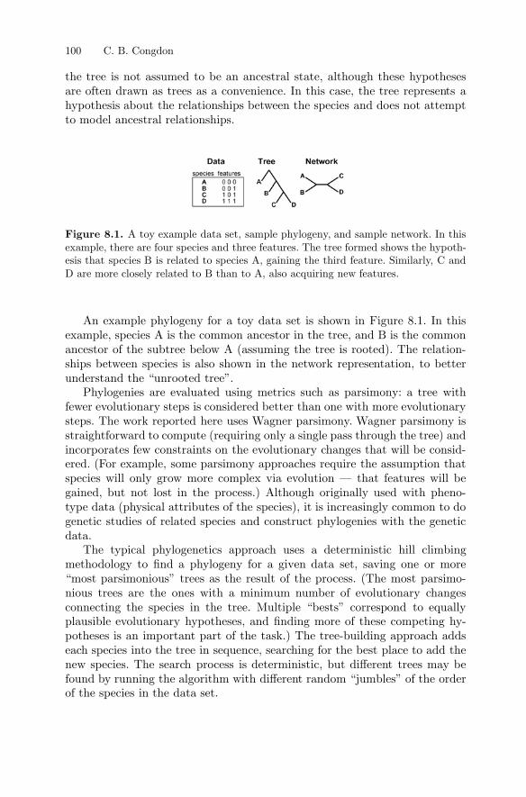
Figure 8.1.
100 C. B. Congdon
A toy example data set, sample phylogeny, and sample network. In thisexample, there are four species and three features. The tree formed shows the hypoth-esis that species B is related to species A, gaining the third feature. Similarly, C andD are more closely related to B than to A, also acquiring new features.
the tree is not assumed to be an ancestral state, although these hypothesesare often drawn as trees as a convenience. In this case, the tree represents ahypothesis about the relationships between the species and does not attemptto model ancestral relationships.
An example phylogeny for a toy data set is shown in Figure 8.1. In thisexample, species A is the common ancestor in the tree, and B is the commonancestor of the subtree below A (assuming the tree is rooted). The relation-ships between species is also shown in the network representation, to betterunderstand the �unrooted tree�.Phylogenies are evaluated using metrics such as parsimony: a tree with
fewer evolutionary steps is considered better than one with more evolutionarysteps. The work reported here uses Wagner parsimony. Wagner parsimony isstraightforward to compute (requiring only a single pass through the tree) andincorporates few constraints on the evolutionary changes that will be consid-ered. (For example, some parsimony approaches require the assumption thatspecies will only grow more complex via evolution that features will begained, but not lost in the process.) Although originally used with pheno-type data (physical attributes of the species), it is increasingly common to dogenetic studies of related species and construct phylogenies with the geneticdata.The typical phylogenetics approach uses a deterministic hill climbing
methodology to �nd a phylogeny for a given data set, saving one or more�most parsimonious� trees as the result of the process. (The most parsimo-nious trees are the ones with a minimum number of evolutionary changesconnecting the species in the tree. Multiple �bests� correspond to equallyplausible evolutionary hypotheses, and �nding more of these competing hy-potheses is an important part of the task.) The tree-building approach addseach species into the tree in sequence, searching for the best place to add thenew species. The search process is deterministic, but different trees may befound by running the algorithm with different random �jumbles� of the orderof the species in the data set.

8.2 Design Decisions
8 Phylogenetic Tree Construction 101
The evolutionary algorithms (EA) approach to problem solving has shownimprovements to hill climbing approaches on a wide variety of problems [25][4] [12]. In this approach, a population of possible solutions to the problem�breed�, producing new solutions; over a number of �generations�, the pop-ulation tends to include better solutions to the problem. The process usesrandom numbers in several different places, as will be discussed later.This research is an investigation into the utility of using evolutionary al-
gorithms as on the problem of �nding parsimonious phylogenies.
To hasten the development of our system, we used parts of two existing soft-ware packages. Phylip [6] is a phylogenetics system widely used by biologists.In particular, this system contains code for evaluating the parsimony of thephylogenies (as well as some helpful utilities for working with the trees). Usingthe Phylip source code rather than writing our own tree-evaluation modulesalso helps to ensure that our trees are properly comparable to the Phyliptrees. Genesis [9] is a genetic algorithms (GA) package intended to aid thedevelopment and experimentation with variations on the GA. In particular,the basic mechanisms for managing populations of solutions and the modulardesign of the code facilitate implementing a GA for a speci�c problem. Wenamed our new system Gaphyl, a re�ection of the combination of GA andPhylip source code.The research described here was conducted using published data sets avail-
able over the Internet [5] and was done primarily with the families of the su-perorder of Lamii�orae data set [1], consisting of 23 species and 29 attributes.This data set was chosen as being large enough to be interesting, but smallenough to be manageable. A second data set, the major clades of the an-giosperms [3], consisting of 49 species and 61 attributes, was used for furtherexperimentation.These data sets were selected because the attributes are binary, which sim-
pli�ed the tree-building process. As a preliminary step in evaluating the GAas a search mechanism for phylogenetics, �unknown� values for the attributeswere replaced with 1�s to make the data fully binary. This minor alterationto the data does impact the meaningfulness of the resulting phylogenies asevolutionary hypotheses, but does not affect the comparison of Gaphyl andPhylip as search mechanisms.

1
1
8.3 The Genetic Algorithm Approach
102 C. B. Congdon
As is the custom in the evolutionary computation community, the author dis-tinguishes different forms of evolutionary computation and is working speci�callywithin the �genetic algorithms� framework.
There are many variations on the GA approach , but a standard methodologyproceeds as follows:1. Generate a population of random solutions to the problem. (These are notassumed to be particularly good solutions to the problem, but serve as astarting point.)
2. The GA proceeds through a number of �generations�. In each generation:a) Assign a ��tness� to each solution, so that we know which solutionsare better than others.
b) Select a �parent� population through a biased random (with replace-ment) process, so that higher �tness solutions are more likely to beparents.
c) Use operators such as crossover, which combines parts of two par-ent solutions to form new solutions, and mutation, which randomlychanges part of a solution, to create a new population of solutions.
The algorithm terminates after a predetermined number of generations orwhen the solutions in the population have converged within a preset criterion(that is, until they are so similar that little is gained from combining parentsto form new solutions).Several factors should be evaluated when considering the utility of GAs
for a particular problem:
1. Is there a more straightforward means of �nding a �best� solution to theproblem? (If so, there is no point in using the GA approach.)
2. Can potential solutions to the problem be represented using simple datastructures such as bit strings or trees? (If not, it may be difficult to workwith the mechanics of the GA.)
3. Can a meaningful evaluation metric be identi�ed that will enable one torate the quality of each potential solution to your problem? (Withoutsuch a measure, the GA is unable to determine which solutions are morepromising to work with.)
4. Can operators be devised to combine parts of two �parent� solutions andproduce (viable) offspring solutions? (If the offspring do not potentiallyretain some of what made the parents �good�, the GA will not be markedlybetter than random trial and error.)
In the phylogenetics task, there is a standard approach to forming thephylogenies, but that process also has a stochastic element, so the standardapproach is not guaranteed to �nd �the best� phylogenies for a given data set.In the phylogenetics task, solutions to the problem are naturally representedas trees. In addition, a standard metric for evaluating a given tree is provided

Figure 8.2.
8.4.1 Crossover Operator
8.4 The GA for Phylogenetics
8 Phylogenetic Tree Construction 103
An example parent tree for a phylogeny problem with seven species. Asubtree for crossover has been identi�ed.
with the task (parsimony). However, there is a challenge for implementing thephylogenetics task using the GA approach: devising operators that produceoffspring from two parent solutions while retaining meaningful informationfrom the parents.
The typical GA approach to doing �crossover� with two parent solutions witha tree representation is to pick a subtree (an interior or root node) in bothparents at random and then swap the subtrees to form the offspring solution.The typical mutation operator would select a point in the tree and mutate itto any one of the possible legal values (here, any one of the species). However,these approaches do not work with the phylogenies because each species mustbe represented in the tree exactly once.Operators designed speci�cally for this task are described in the following
sections and in more detail in [2].
The needs for our crossover operator bear some similarity to traveling sales-person problems (TSPs), where each city is to be visited exactly once on atour. There are several approaches in the literature for working on this typeof problem with a GA. However, the TSP naturally calls for a string represen-tation, not a tree. In designing our own operator, we studied TSP approachesfor inspiration, but ultimately devised our own. We wanted our operator toattempt to preserve some of the species relationships from the parents. Inother words, a given tree contains species in a particular relationship to eachother, and we would like to retain a large degree of this structure via thecrossover process.

Figure 8.3.
Figure 8.4.
Figure 8.5.
104 C. B. Congdon
A second example parent tree for a phylogeny problem with seven species.A subtree for crossover has been identi�ed.
The offspring initially formed by replacing the subtree from parent1 withthe subtree from parent2.
The offspring tree has been pruned to remove the duplicate species F.
8.4.2 Canonical Form
8 Phylogenetic Tree Construction 105
Our crossover operator proceeds as follows:
1. Choose a species at random from one of the parent trees. Select a subtreeat random that includes this node, excluding the subtree that is onlythe leaf node and the subtree that is the entire tree. (The exclusionsprevent meaningless crossovers, where no information is gained from theoperation.)
2. In the second parent tree, �nd the smallest subtree containing all thespecies from the �rst parent�s subtree.
3. To form an offspring tree, replace the subtree from the �rst parent withthe subtree from the second parent. The offspring must then be pruned(from the �older� branches) to remove any duplicate species.
4. Repeat the process using the other parent as the starting point, so thatthis process results in two offspring trees from two parent trees.
This process results in offspring trees that retain some of the species rela-tionships from the two parents, and combine them in new ways.An example crossover is illustrated in Figures 8.2 through 8.5. The parents
are shown in Figures 8.2 and 8.3; Figure 8.4 shows the offspring formed viathe crossover operation and identi�es the subtree that must now be pruned,and Figure 8.5 shows the resulting offspring (after pruning species F). (Notethat in the phylogenies, swapping the left and right children does not affectthe meaning of the phylogeny.)
The Wagner parsimony metric uses �unrooted� trees, leading to many dif-ferent possible representations of �the same� phylogeny that are anchored atdifferent points. Furthermore, �ipping a tree (or subtree) left to right (switch-ing the left and right subtrees) does not alter the parsimony of a phylogeny(nor represent an alternative evolutionary hypothesis). Therefore, it soon be-came clear that Gaphyl would bene�t from a canonical form that could beapplied to trees to ascertain whether trees in the population represented thesame or distinct phylogenies.The canonical form we instituted picks the �rst species in the data set
to be an offspring of the root and �rotates� the tree (and �ips, if necessary)to keep the species relationships intact, but to reroot the tree at a givenspecies. (To simplify comparisons, we followed the default Phylip assumptionof making the �rst species in the data set the direct offspring of the rootof the tree.) Secondly, the subtrees are (recursively) rearranged so that leftsubtrees are smaller (fewer nodes) than right subtrees and that when left andright subtrees have the same number of nodes, a preorder traversal of the leftsubtree is alphabetically before a preorder traversal of the right subtree. Thisprocess is carried out when saving the �best� trees found in each generation,to ensure that no equivalent trees are saved among the best ones. Canonicalform is illustrated in Figure 8.6.

Figure 8.6.
8.4.3 Mutation Operators
8.4.4 Immigration
106 C. B. Congdon
An illustration of putting a tree into canonical form. The tree starts asin the top left; an alternate representation of the tree as a �network� is shown at thebottom left. First, the tree is rotated, so that the �rst species is an offspring of the root.Second, subtrees are rearranged so that smaller trees are on the left and alphabeticallylower species are on the left.
Trees are put into a canonical form when saving the best trees found ineach generation, to ensure that no equivalent trees are saved among the bestones.
The typical GA �mutation� operator takes a location in the solution at ran-dom and mutates it to some other value. Again, the standard operator wasnot suited to our representation, where each species must appear exactly oncein the tree. Instead, for our mutation operator, we selected two leaf nodes(species) at random, and swapped their positions in the tree.A second mutation operator picks a random subtree and a random species
within the subtree. The subtree is rotated to have the species as the left childof the root and reconnected to the parent. This second operator is based onthe mechanisms of the canonical form and was found empirically to help thesearch process.
Early runs with Gaphyl on the larger data set yielded trees with a parsimonyof 280, but not 279 (lower parsimony is better). Re�ection on the processand inspection of the population determined that the process seemed to beconverging too rapidly losing the diversity across individuals that enablesthe crossover operator to �nd stronger solutions. �Premature convergence�is a known problem in the GA community, and there are a number of goodapproaches for combating it. In Gaphyl, we opted to implement parallel pop-ulations with immigration. Adding immigration to the system allowed Gaphylto �nd the trees of �tness 279.

8.5 Experimental Results
8 Phylogenetic Tree Construction 107
8.5.1 Comparison of Gaphyl and Phylip
The immigration approach implemented here is fairly standard. The popu-lation is subdivided into a speci�ed number of subpopulations, which, in mostgenerations, are distinct from each other (crossovers happen only within agiven subpopulation). After a number of generations have passed, each popu-lation migrates a number of its individuals into other populations; each emi-grant determines at random which population it will move to and which treewithin that population it will uproot. The uprooted tree replaces the emigrantin the emigrant�s original population. The number of populations, the num-ber of generations to pass between migrations, and the number of individualsfrom each population to migrate at each migration event are determined byparameters to the system.
Recall that both Gaphyl and Phylip have a stochastic component, whichmeans that evaluating each system requires doing a number of runs. In Phylip,each distinct run �rst �jumbles� the species list into a different random order.In Gaphyl, there are many different effects of random number generation: theconstruction of the initial population, parent selection, and the selection ofcrossover and mutation points. For both systems, a number of different runsmust be done to evaluate the approach.
1. With the Lamii�orae data set, the performance of Gaphyl and Phylip iscomparable. Phylip is more expedient in �nding a single tree with the bestparsimony (72), but both Gaphyl and Phylip �nd 45 most parsimoniousphylogenies in about 20 minutes of run time.
2. With the angiosperm data set, a similar pattern emerges: Phylip is ableto �nd one tree with the best �tness (279) quite quickly, while Gaphylneeds more run time to �rst discover a tree of �tness 279. However, in acomparable amount of run time, Gaphyl is able to �nd 250 different mostparsimonious trees of length 279 (approximately 24 hours of run time).Phylip runs for comparable periods of time have not found more than 75distinct trees with a parsimony of 279. Furthermore, the trees found byPhylip are a proper subset of the trees found by Gaphyl.
In other words, Gaphyl is more successful than Phylip in �nding more trees(more equally plausible evolutionary hypotheses) in the same time period.The �rst task is considerably easier to solve, and Gaphyl does not require
immigration to do so. Example parameter settings are a population size of 500,500 generations, 50% elitism (the 250 best trees are preserved into the nextgeneration), 100% crossover, 10% �rst mutation, and 100% second mutation.
108 C. B. Congdon
8.5.2 Contribution of Operators
Empirically, it appears that 72 is the best possible parsimony for this dataset, and that there are not more than 45 different trees of length 72.The second task, as stated above, seems to bene�t from immigration in
order for Gaphyl to �nd the best-known trees (�tness 279). Successful parame-ter settings are 5 populations, population size of 500 (in each subpopulation),2000 generations, immigration of 5% (25 trees) after every 500 generations,50% elitism (the 250 best trees are preserved into the next generation), 100%crossover, 10% �rst mutation, and 100% second mutation. (Immigration doesnot happen following the �nal generation.) We have not yet done enough runswith either Phylip or Gaphyl to estimate the maximum number of trees atthis �tness, nor a more concise estimate of how long Phylip would have to runto �nd 250 distinct trees, nor whether 279 is even the best possible parsimonyfor this data set. In two days of run time, Phylip runs have not found morethat 100 distinct trees of �tness 279.The pattern that emerges is that as the problems get more complex,
Gaphyl is able to �nd a more complete set of trees with less work than whatPhylip is able to �nd. The work done to date illustrates that Gaphyl is apromising approach for phylogenetics work, as Gaphyl �nds a wider varietyof trees on this problem than Phylip does. This further suggests that Gaphylmay be able to �nd solutions better than those Phylip is able to �nd on datasets with a larger number of species and attributes, because it appears to besearching more successful regions of the search space.
To evaluate the contributions of the GA operators to the search, additionalruns were done with the �rst data set (and no immigration). Empirically,crossover and the second mutation operator had been found to be the largestcontributors to successful search, so attention was focused on the contributionsof these operators.In the �rst set of experiments, the �rst mutation rate was set to be 0%.
First, the crossover rate was varied from 0% to 100% at increments of 10%while the second mutation rate was held constant at 100%. Second, the sec-ond mutation rate was varied from 0% to 100% at increments of 10% whilethe crossover rate was held constant at 100%. at each parameter setting 20experiments were run; each experiment of 500 generations.Figure 8.7 illustrates the effects of varying the crossover rate (solid line)
and second mutation rate (dashed line) on the average number of generationstaken to �nd at least one tree of the known best �tness (72). Experiments thatdid not discover a tree of �tness 72 are averaged in as taking 500 generations.For example, 0% crossover was unable to �nd any trees of the best �tness inall 20 experiments, and so its average is 500 generations.This �rst experiment illustrates that, in general, higher crossover rates are
better. There is not a clear preference, however, for high rates of the secondform of mutation. To look at this operator more closely, the �nal populations

Figure 8.7.
8 Phylogenetic Tree Construction 109
The effect of varying crossover rate while holding second mutation con-stant and of varying the second mutation rate while holding the crossover rate constant.The average generation at which the best �tness (72) was found is illustrated.
of the 20 experiments were looked at to determine how many of the best treeswere found in each run.Figure 8.8 illustrates the effects of varying the crossover rate (solid line)
and second mutation rate (dashed line) on the average number of best treesfound. Experiments that did not discover a tree of �tness 72 are averaged inas �nding 0 trees. For example, 0% crossover was unable to �nd any trees ofthe best �tness in all 20 experiments, and so its average is 0 of the best trees.As Figure 8.9 illustrates, runs with a higher second mutation rate tend to
�nd more of the best trees than runs with a lower second mutation rate.The impact of the �rst mutation operator had seemed to be low based
on empirical evidence. So another set of experiments was done to assess thecontribution of this operator. In both, the crossover rate was set at 100%;in one, the second mutation rate was set at 0% and in the other, the secondmutation rate was set at 100%.The results of this experiment clearly indicate that higher rates of this
form of mutation are not bene�cial. Furthermore, this operator is not clearlycontributing to the search.In the �nal set of experiments, the �rst experiments of varying crossover
rate while holding second mutation rate constant and vice versa were repeated,but this time with a �rst mutation rate of 10%. The results are illustrated inFigure 8.10.

Figure 8.8.
Figure 8.9.
110 C. B. Congdon
The effects of varying crossover rate while holding second mutation con-stant and of varying the second mutation rate while holding the crossover rate con-stant. The average number of best trees (45 max) found by each parameter setting isillustrated.
The effect of varying the �rst mutation rate while holding crossover andsecond mutation constant. The crossover rate is 100% for both graphs; second mutationrates of 100% and 0% are shown. The average generation at which the best �tness (72)was found is illustrated.

Figure 8.10.
Table 8.1.
8.5.3 Contribution of Other Parameters
8 Phylogenetic Tree Construction 111
The effect of varying crossover rate while holding second mutationconstant and of varying the second mutation rate while holding the crossover rateconstant, this time with a �rst mutation rate of 10%. The average generation at whichthe best �tness (72) was found is illustrated.
The population size for each experiment described in Section 8.5.3. Whenthere are multiple populations, the number shown refers to the number of trees in eachdistinct population.
Gens Number of populations1 2 4 8 16
1600 1024 512 256 128 64800 2048 1024 512 256 128400 4096 2048 1024 512 256
An additional set of experiments were designed to assess tradeoffs in terms ofputting a �xed number of trees in one population or distributing them acrossa number of populations and tradeoffs between having larger population sizesor doing more generations, for a �xed number of evaluations in all cases. Theseexperiments were done using the angiosperms data set.
The base case may be thought of as 1 population of 1024 individuals, and1600 generations. Then, along one dimension, the population is divided across2, 4, 8, and 16 populations, a total of �ve variations. Along the other dimensionthe number of generations is halved as the population size is doubled, for

Table 8.2.
Table 8.3.
8.5.4 Exploration of Hybrid Possibilities
112 C. B. Congdon
The number of runs that found the best solution found across 20 runs,varying the number of populations and number of generations, with a constant 1024trees (split across the speci�ed number of populations).
Gens Number of populations1 2 4 8 16 sum
1600 1 2 1 2 1 7800 5 7 2 5 2 21400 3 3 4 0 0 10
sum 9 12 7 7 3
Average �tness of �nal populations found across 20 runs, varying thenumber of populations and number of generations, with a constant 1024 trees (splitacross the speci�ed number of populations).
Gens Number of populations1 2 4 8 16
1600 281.70 281.55 281.10 280.85 280.95800 280.60 279.95 280.25 279.95 280.15400 280.45 280.15 280.45 281.15 281.95
a total of three variations. This creates an array of 15 parameter settings,illustrated in Table 8.1. The horizontal axis shows the number of populations,the vertical axis shows the number of generations, and each interior cell showsthe population size.Twenty experiments, with different seeds to the random number genera-
tor, were done for each setting. When multiple populations are used, 5% ofthe population immigrates after 25%, 50%, and 75% of the generations havecompleted.The results of these experiments, illustrated in Tables 8.2 and 8.3, show
the best results with 2 populations of 1024 trees run for 800 generations, witha total of 7 out of the 20 runs �nding trees of the best-known �tness of 279. Ingeneral, it appears that two populations are better than one, but that theremight not be great gains from more than two populations. Further, it appearsthat the system bene�ts from a balance between a large population size anda large number of generations.
We have noted that Phylip is relatively quick to �nd at least one of the bestsolutions, but that over a span of time it does not �nd as many of the bests
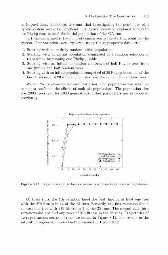
Figure 8.11.
8 Phylogenetic Tree Construction 113
Trajectories for the four experiments with seeding the initial population.
as Gaphyl does. Therefore, it seems that investigating the possibility of ahybrid system would be bene�cial. The hybrid variation explored here is touse Phylip runs to seed the initial population of the GA run.In these experiments, the point of comparison is the starting point for the
system. Four variations were explored, using the angiosperms data set:
1. Starting with an entirely random initial population.2. Starting with an initial population comprised of a random selection oftrees found by running one Phylip jumble.
3. Starting with an initial population comprised of half Phylip trees fromone jumble and half random trees.
4. Starting with an initial population comprised of 20 Phylip trees, one of thebest from each of 20 different jumbles, and the remainder random trees.
We ran 25 experiments for each variation. One population was used, soas not to confound the effects of multiple populations. The population sizewas 2000 trees, run for 1000 generations. Other parameters are as reportedpreviously.
Of these runs, the 4th variation fared the best, �nding at least one treewith the 279 �tness in 14 of the 25 runs. Secondly, the �rst variation foundat least one tree with 279 �tness in 5 of the 25 runs. The second and thirdvariations did not �nd any trees of 279 �tness in the 25 runs. Trajectories ofaverage �tnesses across all runs are shown in Figure 8.11. The results in thesaturation region are more closely presented in Figure 8.12.

Figure 8.12.
8.6 Conclusions and Future Work
114 C. B. Congdon
More detail on the trajectories for the four experiments with seedingthe initial population.
These experiments suggest that while seeding from Phylip runs may helpthe progress of the GA, the initial seeds must be sufficiently diverse for this�jump start� to be helpful. It appears that choosing the seed trees from asingle Phylip jumble is comparable to starting the GA with a population thathas already converged. (Note: This experiment was repeated with �ve distinctPhylip jumbles, always with similar results.)
The GA search process as implemented in Gaphyl represents an improvementover Phylip�s search process in its ability to �nd more trees than Phylip in thesame run time. One possible facet of this success is that the Gaphyl searchprocess is independent of the number of attributes (and attribute values); thecomplexity of the search varies with the number of species (which determinesthe number of leaf nodes in the tree). Phylip uses attribute information in itssearch process.The �rst mutation operator is perhaps the �obvious� form of mutation to
implement for this problem, and yet its use (at high levels) appears to detractfrom the success of the search. This points to the importance of evaluatingthe contributions of operators to the search process.There is obviously a wealth of possible extensions to the work reported
here. First, more extensive evaluations of the capabilities of the two systemsmust be done on the angiosperms data set, including an estimate of the max-imum number of trees of �tness 279 (and, indeed, whether 279 is the most

Acknowledgments
References
http://phylogeny.harvard.edu/treebase
http://evolution.genetics.washington.edu/phylip.html
Biol. J. Linn. Soc.
Principles of Data Mining and KnowledgeDicovery (PKDD 2001)
Cladistics
Handbook of Genetic Algorithms
Cladistics: A Practical Course in Systematics
8 Phylogenetic Tree Construction 115
1. L. An-Ming. (1990) A preliminary cladistic study of the families of the superorderlamii�orae. , 103:39�57 .
2. C. B. Congdon. (2001) Gaphyl: A genetic algorithms approach to cladistics. InL. De. Raedt and A. Siebes, editors,
, Lecture notes in arti�cial intelligence 2168, pages 67�78,New York. Springer.
3. R. Dahlgren and K. Bremer (1985) Major clades of the angiosperms. ,1:349�368.
4. L. Davis (1991) . Van Nostrand Reinhold, NewYork, NY.
5. M. J. Donaghue (2000) Treebase: A database of phylogenetic knowledge. web-based data repository. Available at .
6. J. Felsenstein. (1995) Phylip source code and documentation. Available via theweb at .
7. P. L. Forey, C. J. Humphries, I. L. Kitching, R. W. Scotland, D. J. Siebert, andD. M. Williams (1993) . Number 10in The Systematics Association. Clarendon Press, Oxford.
parsimonious tree possible). This would entail more extensive runs with bothapproaches. Furthermore, as evidenced by the unexpected result with themutation operator, the effect of the immigration operator in Gaphyl must beexplored further.Second, more work must be done with a wider range of data sets to evaluate
whether Gaphyl is consistently able to �nd a broader variety of trees thanPhylip, and perhaps able to �nd trees better than Phylip is able to �nd.Third, Gaphyl should be extended to work with nonbinary attributes. This
is particularly important in that phylogenetic trees are increasingly used bybiologists primarily with the A, C, G, T markers of genetic data.Finally, we need to compare the work reported here to other projects
that use GA approaches with different forms of phylogenetics, including [10]and [11]. Both of these projects use maximum likelihood for constructingand evaluating the phylogenies. The maximum likelihood approach (whichis known as a �distance-based method�) is not directly comparable to theWagner parsimony approach (which is known as a �maximum parsimony�approach).
I would like to thank Emily F. Greenfest, who worked with me in the initialdesign and implementation of this project. Thanks also to Judy L. Stone andRandall Downer for sharing their knowledge of phylogenetic theory and soft-ware. Thanks to Randolph M. Jones, Joshua R. Ladieu, and the anonymousreviewers for comments on previous versions of this paper.

http://www.cs.cmu.edu/afs/cs/project/ai-repository/ai/areas/genetic/ga/systems/genesis/
Genetic Algorithms in Search, Optimization and MachineLearning
Mol. Biol. Evol.
Paci�c Symposium onBiocomputing �96
An Introduction to Genetic Algorithms
116 C. B. Congdon
8. D. E. Goldberg (1989). Addison-Wesley, Reading, MA.
9. J. J. Grefenstette (1987) A user�s guide to GENESIS. Tech-nical report, Navy Center for Applied Research in AI, Washington,DC. Source code updated 1990; available at
.10. P. O. Lewis (1998) A genetic algorithm for maximum-likelihood phylogeny infer-ence using nucleotide sequence data. , 15(3):277�283.
11. H. Matsuda (1996) Protein phylogenetic inference using maximum likelihood witha genetic algorithm. In L. Hunter and T. E. Klein, editors,
, pages 512�523. World Scienti�c, London.12. M. Mitchell (1996) . MIT Press, Cam-bridge, MA.

9_______________________________________________________________________________________
Robot Controller Evolution withMacroevolutionary Algorithms
J. A. Becerra, J. Santos, R.J. Duro
Summary There are certain problems that require using small populations to explore fitnesslandscapes that are mostly flat, thus offering very little information, where the solutionsappear as sparsely distributed narrow peaks. This is the case of the evolution of controllersfor many problems in evolutionary robotics. Consequently, for these types of problems itshould be useful to consider the use of evolutionary algorithms that cluster the fewindividuals in the surroundings of the local good solutions permitting an adequate trade-offbetween exploration and exploitation. Macroevolutionary algorithms cover this need, andthrough the appropriate selection of the values for its parameters they perform in generalbetter than genetic algorithms for the case of very low population values. In this work westudy the influence of the two main parameters governing the search performed bymacroevolutionary algorithms as well as the influence of dividing populations into races.
9.1 Introduction
Due to the large computational requirements for calculating the fitness of eachsolution (possible robot controller), and in order to make computing timesbearable, most processes in evolutionary robotics imply very small populations.This is because every individual must live its life out in a real or simulatedenvironment and this life implies complex interactions incurring largecomputational costs per individual. It becomes especially critical when theevolution is carried out in the real robot.
In traditional methods of simulated evolution such as GAs, selective pressuredetermines how fast the population converges to a solution. The more pressure, thefaster the convergence, at the cost of increasing the probability of the solutionfound being suboptimal. Consequently, in this type of methodologies anexploration/exploitation dilemma is present whereby a designer can choose toconsider the evaluation of a large number of candidates throughout the searchspace or concentrate the search in the direction of a good, possibly suboptimal,solution. The choice of a good equilibrium between exploration and exploitation iseven more important when the computational requirements of the evaluation of theindividuals are very high as in the case of evolutionary robotics. Obviously, if anevolutionary roboticist requires reasonable solutions in bearable amounts of time,populations with a restricted number of individuals must be considered. As aconsequence of the small size of the populations, the evolutionary dynamics forthese systems stray from those established for so-called infinite population

Becerra et al.118
evolutionary systems, and the convergence properties become more brittle. Thisproblem becomes even more noticeable when the fitness functions lead tolandscapes that are mostly flat except for a very sparse distribution of peaks wherefit individuals are located. Much research is needed on the interplay of the differentparameters that control the evolutionary process and on the best possible solutionsfor this extreme low population, low information fitness function case. What wewill need is to use evolutionary algorithms that cluster the few individuals in thesurroundings of the local good solutions and allow a control of an adequate trade-off between exploration and exploitation.
One promising avenue out of the exploration/exploitation dilemma is anintermediate alternative in which the search is concentrated on or covers anadequate number of candidate solutions, not only one. A first possibleapproximation to this objective is the use of parallel evolutionary algorithms,imposing geographic constraints on the evolutionary search of differentsubpopulations. Although it is not the same as concentrating on several candidatesolutions, it can be an approximation, especially if the subpopulations coverdifferent areas of the search space, at least at the beginning of the evolutionprocess, as studied in [6]. Obviously, after a few generations, some subpopulationsmay contain individuals outside their assigned space due to mutations ormigrations of best individuals from other subpopulations, but, in general, theprocedure implies a more exhaustive search of the solution space and, thus, there isa tendency to prevent the premature convergence problem.
Another possibility to avoid the problem of ill-convergence is to obtainselection procedures that produce the desired clustering or concentration of thesearch efforts on the different candidate solutions of the fitness landscape. This iscalled “niching” in biology. In this biological sense, Goldberg [2] defines a nicheas an organism’s job or role in an environment, and a species as a type oforganisms with similar characteristics. At the computational level it means thatthese groups can be formed around each of the local fitness peaks of the solutionspace. In most evolutionary methods this effect does not appear due to the way inwhich evolutionary pressure is applied in traditional selection schemes such as theroulette wheel or tournament selection. The most classical solution in this line is toconsider the use of the so-called crowding operator 1: when a new individual isgenerated, it replaces the most similar individual of the population, which preventsthe possibility of having many similar individuals (“crowds”) at the same time inthe population. Thus, the key point in this approach seems to take into accountsome measure of similarity among the individuals. For example, Menczer et al. [5]use a local selection scheme for evolving neural networks in problems that requiremulticriteria fitness functions. For each individual in the population the authorsconsider a solution similar to itself. This individual is evaluated in an environmentwith shared resources that are consumed and replenished in time. If the energy ofthe new agent, considering the cost of creating it, is higher than a threshold, thenew individual remains in the population with half the energy. In any other case,the parent and the new individual die. The population is kept constant on averagethanks to an adequate conservation of the total energy in the environment.
Another more formal solution in the same line, which is the one we havefollowed in this work, is the one proposed by Marín and Solé [4]. The authorsconsider a new temporal scale, the “macroevolutionary” scale, in which the

9 Robot Controller Evolution 119
extinctions and diversification of species are modeled. The population isinterpreted as a set of species that model an ecological system with connectionsbetween them, instead of a number of independent entities as in classical GAs. Thespecies can become extinct if their survival ratio with respect to the others is nothigher than a survival coefficient. This ratio measures the fitness of a species withrespect to the fitness of the other species. When species become extinct, adiversification operator colonizes the holes with species derived from those thatsurvived or with completely new ones.
This paper deals with the study of several parameters and techniques that are ofinterest in order to make the evolutionary processes used to obtain robot controllersmore efficient. This problem must be handled using small populations, and itsfitness landscapes present huge areas with very low values and sparse hyper-dimensional peaks. This involves delimiting when a Macroevolutionary Algorithm(MA) performs better on average than a Genetic Algorithm. That is, defining thebest parameters in MAs so as to adequately balance exploration and exploitation,and how a population should be divided into races in order to optimize the searchfor an optimal solution.
9.2 Description of Macroevolutionary Algorithms
Here, we summarize the model proposed by Marín and Solé [4], which explainsthe dynamics of an ecosystem based only on the relation between species. Thus,the individuals in the population are referred to as species. They can survive orbecome extinct in each generation of the evolutionary process. The number ofspecies is a constant. The relation between them is established by a matrix inwhich the term Wi,j(t) represents the influence of species j on species i at time t,which is a continuous value in a given range. This influence is a measure of thedifference of the relative fitness of the two species, considering the distancebetween both in genotypic space:
Wf p f p
p pi j
i j
i j, =
( ) ( ), (9.1)
where pi=(pi1,…,pi
d) is the genotype of species i, with its parameters in a d-dimensional space. f represents the fitness of each species. Thus, the influence isthe difference in fitness with a normalization factor that weighs the distancebetween the two.
Two operators are applied to each generation:
1 . Selection operator: defines which species survive and which speciesbecome extinct. To determine this, the “state” of each individual iscalculated as

Becerra et al.120
S tW t
ii jj
p
+( ) = ( )11 0
01
if
otherwise,
,=,
(9.2)
that is, if the sum of the influences of a species relative to all the other species inthe population is positive, the species survives. Otherwise, it becomes extinct.
2. Colonization operator: it defines how the extinct species are replaced. Theauthors define a probability to determine if a new solution pn is generated.Otherwise exploitation of surviving solutions takes place through colonization.One of the surviving solutions, pb, is chosen as a base to replace the extinctsolution pi, and the new species that replaces the extinct one is attracted toward pb,in the following manner:
p tp t p t p t
pib b i
n
( )( ) ( ) ( )
+ =+ ( ) >
1if
if(9.3)
Figure 9.1 Different views of the fitness landscape with the variation of fourgenes (connection weights in the neural controller) while the others are fixed.Top-Left: different peaks in a well-defined area. Top right: flat landscape with asmall change in the surface level. Bottom left: another similar area ofconcentrated peaks. Bottom right: Another area, viewed from a differentreference point, that denotes a periodic distribution of peaks in a small area.

9 Robot Controller Evolution 121
where is a random number in [0,1], a random number in [-1,1], both withuniform distribution, describes a maximum radius around the surviving solutionand controls the percentage of random individuals. This parameter may act as atemperature, because it can decrease in evolutionary time so as to perform a type ofsimulated annealing process. That is, when the temperature is low, the randomnessis low, and, consequently, there is a tendency toward increased exploitation aroundthe surviving individuals and reduced exploration of new species. Thus, whenusing a macroevolutionary algorithm one can tweak with basically two parameters.On one hand, determines what proportion of the species are randomly generated,that is, how much exploitation or exploration we perform in a given generation. Onthe other, one can modify and thus juggle with the size of the attractor basinaround pb, that is, it permits deciding how the exploitation is carried out.
9.3 Experimental Setup for Testing the MA-based Evolution
As commented before, the comparison between GAs and MAs will be carried outin a problem where robot controllers, made up of artificial neural networks, are theend product. This is a very typical problem that implies a sparse fitness functionand a large amount of processing per individual. In particular, all the examplespresented here correspond to the evolution of a wall following controller for aPioneer II robot. The fitness is defined with hints in the environment that representfood or poison. This procedure allows more freedom than many handcrafted fitnessfunctions for the robot controller evolution to discover good behaviors, at the costof a more difficult fitness landscape. The controller is a neural network with a 6-node hidden layer, 8 inputs, and 2 outputs, which implies a total of 76 genesrepresenting the connection weights, slope of the sigmoid functions and bias in thedifferent nodes. Figure 9.1 displays partial views of the fitness landscape where 4out of the 76 genes that make up the chromosome are modified while the rest aremaintained constant at values corresponding to the best solution obtained. Thechosen genes are two connection weights between the inputs and a node in thehidden layer, and the two weights between this hidden node and the two outputnodes. It is well known that with genetic encodings of the parameters of distributedstructures such as neural networks, there can be a lot of different parameter setsthat obtain similar input-output mappings. As a consequence, several fitness peakscan appear in the search space. This is what is shown in Figure 9.1, where thefitness was obtained testing each individual in 20 different life situations. The axesx and y correspond to the variation of two of the genes, while the four viewscorrespond to four different selected combination values on the other two genes(weights connecting the hidden node with the output nodes), while the rest of thegenes remain fixed. This analysis is similar to the one carried out by Janson andFrenzel [3], who show slices of the error surface in a neural network with thevariation of only one gene, to demonstrate the difficulty for discovering the globaloptimum. Their neural network must predict the optimal transistor width for aCMOS switch. What the figure demonstrates is that the search space has a lot ofdifferent peaks in a lot of different areas, surrounded by flat surfaces with differentlevels.

Becerra et al.122
With that in mind in the experiments we describe evolution was carried outusing two types of algorithms. One of them was a pure genetic algorithm, with a0.8 crossover probability and a 0.1 mutation probability. Crossover was a standardone point crossover and mutation was random. The selection strategy employedwas tournament. The GA used a diagonal distribution for the initial population, asit has been shown to provide the best usage of resources [6]. This algorithm wastaken as a standard in order to compare different aspects. The other one was amacroevolutionary algorithm as commented before.
9.4 GA Versus MA
The first consideration one should make is how well GAs and MAs compare whenevolving solutions to a problem such as the one we are tackling, a problem thatmust be solved using small populations. In Figure 9.2 we display the resultscomparing the performance of a GA and a MA for different population sizes. Twomain characteristics stand out at first sight. On one hand, GAs display the classicalevolution curve for the best individual, that is, very fast fitness increase at thebeginning, when the GA is making use of the genetic material present in the initialpopulation and recombining it to obtain the best possible individuals from thismaterial, that is, very fast exploitation of the initial population, and a very slow,almost flat second part, where evolution is driven by mutation, as new geneticmaterial is required in order to find new combinations that provide better fitness, ina sense we have a second stage of exploration. This behavior, as pointed out in [6]makes GAs very dependent on the distribution of the initial population. This wouldnot be a big problem when large populations are used, as an initial randomdistribution would probably introduce enough genetic elements in the population toallow the algorithm paths for reaching the optimum, or close to it. When usingsmall populations, the best possible distribution of the initial population would be a
Figure 9.2. Evolution of the fittest for a GA and aMA with different population sizes (8 races).
0
50000
100000
150000
200000
250000
300000
350000
400000
450000
1 1000 1999
Generation
Fit
nes
s (a
rbit
rary
un
its)
GA population 1600GA population 800GA population 480MA population 1600MA population 800MA population 480

9 Robot Controller Evolution 123
diagonal, as it maximizes the spread of the gene variety, but it still constrainsevolution and makes it dependent on mutation (basically random search) after ashort period.
In the case of MAs, as mentioned before, exploration takes place first, andexploitation comes into play slowly throughout the process (when annealing isused). In fact, due to the way in which exploitation is carried out in this type ofalgorithms, new genetic material arises throughout the exploitation phase. Thisleads to a slower evolution in the beginning, but it is much more constant as shownin the figure. In fact, it usually leads to better results than GAs, especially in thelow population cases, such as those with 480 and 800 individuals.
In Figure 9.3 we see the very different behavior in terms of average fitness inboth types of evolutionary algorithms. In the GA, average fitness is far belowmaximum fitness and it never converges to it. The search space in this problemcould be described as a flat surface with sporadic high peaks. This particular searchspace leads to most of the individuals in the population, resulting from crossover orrandom mutation, being quite poor when performing the desired task. In the MAcase, this is very different. Because of the way exploitation is carried out in thisalgorithm, individuals tend to concentrate in the high peaks as time progresses.
9.5 Effect of Distribution into Races
Distributing the individuals into subpopulations that evolve independently and onlycommunicate through a periodic migration of best individuals between them can beshown to improve the evolution process. From the point of view of implementationit also permits distributing subpopulations among processors adding a concurrencylevel that leads to an acceleration of the process. We have tried this strategy bothfor GAs and MAs applied to the current problem. The case of GAs was presentedin [6]. In both cases, the subdivision of the population into races led to
Figure 9.3. Evolution of the average fitness for aGA and an MA with different population sizes (8races).
0
50000
100000
150000
200000
250000
300000
350000
400000
1 1000 1999
Generation
Fitn
ess
(arb
itrar
y un
its)
GA population 1600GA population 800GA population 480MA population 1600MA population 800MA population 480

Becerra et al.124
improvements in the final fitness of the best individuals. The evolution of fitnessfor the best individuals and for the average of the whole population in MAs areshown in Figures 9.4 and 9.5 as we change the number of races for a givenpopulation size.
Obviously, as the number of races increases, the number of individuals in a racedecreases. In fact, when too many races are considered, that is, when each racereaches a number of individuals below a critical point (related to the selectivepressure in that population), evolution in the case of GAs has very little initialgenetic variety and is mostly driven by mutation, that is, a random walk, andbasically tends to get stuck in a suboptimal individual. In the case of MAs thebehavior is quite similar: too few individuals cannot provide enough geneticvariety for exploitation to work well, as shown in the 16 races case of the figure.
0
50000
100000
150000
200000
250000
300000
350000
1 1000 1999
Generation
Fitn
ess
(arb
itrar
y un
its)
16 races16 races, double population 8 races 2 races
Figure 9.4. Evolution of the fittest in an MA with 800individuals for different numbers of races.
0
50000
100000
150000
200000
250000
300000
350000
1 1000 1999
Generation
Fit
nes
s (a
rbit
rary
un
its)
16 races16 races, double population 8 races 2 races
Figure 9.5. Evolution of the average fitness for anMA with 800 individuals distributed into differentnumbers of races.
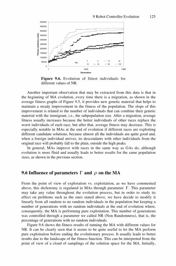
9 Robot Controller Evolution 125
Another important observation that may be extracted from this data is that inthe beginning of MA evolution, every time there is a migration, as shown in theaverage fitness graphs of Figure 9.5, it provides new genetic material that helps tomaintain a steady improvement in the fitness of the population. The slope of thisimprovement is related to the number of individuals that can combine their geneticmaterial with the immigrant, i.e., the subpopulation size. After a migration, averagefitness usually increases because the better individuals of other races replace theworst individuals of each race, but after that, average fitness may decrease. This isespecially notable in MAs at the end of evolution if different races are exploitingdifferent candidate solutions, because almost all the individuals are quite good and,when a foreign individual arrives, its descendants with other individuals from theoriginal race will probably fall to the plain, outside the high peaks.
In general, MAs improve with races in the same way as GAs do, althoughevolution is more fluid and usually leads to better results for the same populationsizes, as shown in the previous section.
9.6 Influence of parameters and on the MA
From the point of view of exploration vs. exploitation, as we have commentedabove, this dichotomy is regulated in MAs through parameter . This parametermay take any value throughout the evolution process, but in order to study itseffect on problems such as the ones stated above, we have decide to modify itlinearly from all random to no random individuals in the population but keeping anumber of generations with no random individuals at the end of evolution where,consequently, the MA is performing pure exploitation. This number of generationswas controlled through a parameter we called NR (Non Randomness), that is, thepercentage of generations with no random individuals.
Figure 9.6 shows the fitness results of running the MA with different values forNR. It can be clearly seen that it seems to be quite useful to let the MA performpure exploitation before ending the evolutionary process. It usually leads to betterresults due to the landscape of the fitness function. This can be interpreted from thepoint of view of a cloud of samplings of the solution space for the MA. Initially,
Figure 9.6. Evolution of fittest individuals fordifferent values of NR.
0
50000
100000
150000
200000
250000
300000
350000
400000
450000
500000
1 1000 1999
Generation
Fit
nes
s (a
rbit
rary
un
its)
0 5 10 20
30 40 80 100Tau

Becerra et al.126
we want the algorithm to explore as much of the solution space as possible so thatit does not miss any possible promising region. Once the main promising regionshave been found, the directional properties of MAs, which lead them to cluster testpoints around better solutions, will end up leading to clusters that will tend toconverge to a good solution. Thus, in this second part it is interesting to reducerandomness and perform more exploitation, that is, better coverage of promisingregions. In particular, for very flat fitness landscapes the initial exploration forpromising regions becomes more a problem of delimiting the important areas(which is much less costly than covering the whole region). Then, through theparticular exploitation phase of the MA by creating offspring located in betweenthe parents in the solution hyperspace, a fine-grained search is performed, leadingto the individuals clustering around the peaks.
Finally, we have experimented with parameter , which defines theneighborhood considered in the exploitation or colonization phase of the MA. Thetests carried out for different values of this parameter do not display a cleartendency in the MA behavior, which agrees with the same results of Marín andSolé [4] for the search in two landscapes, one with some local maxima of closeheights, and another one with infinite maxima around the global maximum. Theauthors conclude that “in most cases simulated annealing seems to be the bestchoice, being the specific -value less important. Because of that, the authorschoose in their comparison with GAs a value of 0.5 for the parameter, the sameone we have used in the NR tests.
9.7 Conclusions
In this article we have provided some results on evolving complex controllers withsmall populations for fitness functions with flat landscapes where sparse narrowpeaks are distributed. The basic idea is that macroevolutionary algorithms permitobtaining better results due to the way in which they handle theexploration/exploitation equilibrium, which, in effect, implies a lower selectivepressure at the beginning than traditional GAs, preventing, in most cases, thepremature convergence effects displayed by GAs. When these algorithms arecombined with the use of races and their NR parameter adjusted to appropriatevalues, the results obtained are quite comparable to GAs with much largerpopulations. Thus, using macroevolutionary algorithms and a race scheme,evolutions of systems whose individual fitness is very costly to calculate can beachieved in reasonable computation times through the use of small populations andthe inherent parallelization level provided by the race scheme.
Acknowledgments
This work was supported by the MCYT of Spain through project TIC2000-0739C0404 and Xunta de Galicia through project PGIDIT02PXIB10501PR.

9 Robot Controller Evolution 127
References
1. De Jong, K.A. (1975) An Analysis of the Behavior of a Class of a GeneticAdaptive Systems, Ph. Thesis, University of Michigan, Ann Arbor.
2. Goldberg, D.E. (1989) Genetic Algorithms in Search, Optimization and MachineLearning, New York, Addison-Wesley.
3. Janson, D.J., Frenzel, J.F. (1993) Training product unit neural networks withgenetic algorithms”, IEEE Expert 26-32.
4. Marín, J., Solé, R.V. (1999) Macroevolutionary algorithms: A new optimizationmethod on fitness landscapes, IEEE Transactions on Evolutionary Computation3(4):272-286.
5. Menczer, F., Street, W.N., Degeratu, M. (2001) Evolving heterogeneous neuralagents by local selection, Advances in the Evolutionary Synthesis of IntelligentAgents, M.J. Patel, V. Honavar and K. Balakrishnan (eds.), MIT Press, 337-365.
6. Santos, J., Duro, R.J., Becerra, J.A., Crespo, J.L., and Bellas F. (2001)Considerations in the application of evolution to the generation of robotcontrollers, Information Sciences ,133:127-148.

10___ ______ ______ __________________ ______ ______ ______ ______ ______ ______ ______ ____________
Evolving Natural Language Grammars
W. Cyre
10.1 Introduction
Most approaches to natural language understanding depend on a grammar to per-form the syntactic analysis of sentences. Manually developing a consistent, con-text-free grammar that accurately parses a good portion of a natural language re-quires considerable expertise and diligence and is a tedious task. Presently,statistical and machine learning methods are popular. Statistical grammars mayhave over tens of thousands of rules, which results in a high computational cost forparsing.
The problem of developing a grammar is simplified somewhat when the naturallanguage documents are limited to a particular domain. Examples of such re-stricted domains are medical records, weather reports, patents, and legal reports. Alanguage used in a restricted domain is called a sublanguage and tends to have alimited vocabulary, syntax, and semantics. For example, the sublanguage of inter-est to the present author is that used in manufacturer’s data sheets and U.S. patentsthat describe microprocessor system components. These documents have vocabu-laries limited to a narrow technical domain, and many sentence constructions ofgeneral English (such as questions and imperatives) do not occur. On the otherhand, sentences tend to be quite complex. Four examples of sentences from pat-ents that could not be parsed by an initial grammar, but that were parsed by anevolved grammar, are reproduced below.
“Once the subsystem controller has been set up, the central processing unit is then freeto carry out other operations in the system while the subsystem device controller itselfcontrols the transfers between memory and the peripheral device.” (1)“Another object of the invention is to provide an improved data processing system asdescribed above and further including a counter in the shared direct memory accesscontroller; selection means responsive to the address recognition means and an outputinstruction from the microprocessor for loading a value on the common data bus intothe counter; and, gating means connecting the counter to the common address bus sothat the contents of the counter may directly address the memory.” (2)“On the other hand, if the signal RADR-0 is at the low level, then a low level signal onlead 326 enables counters 322 and 323 so that they are loaded with data from the out-puts of QUAD MUX's 302 and 303. (3)“The probe signal is applied to Figure 3A where it enables the decoder 318 controllingthe loading of the address pointer counter, and further controls MUX's 302 and 303 soas to gate the data on the system data bus 200 through the MUX's to the address pointercounter.” (4)
130 W. Cyre
The conventions of a sublanguage may also depart from standard English. Forexample, computer engineers generally nominalize verbs to the infinitive form (“amemory write”, “generates an interrupt”) rather than a gerund (“a writing to mem-ory”, “generates an interruption”) as is done in general English. What is neededfor automated analysis of a sublanguage is a context-free grammar tailored to thespecific sublanguage. The problem of parsing the sublanguage may be exacerbatedby the need for results that are amenable to later semantic analysis. The semanticanalysis approach in the present example employs verb-centered templates calledcase frames [1]. A case frame for a particular verb, such as transfer, has slots forsemantic roles such as the agent, operand, source, and destination. These slots arefilled by noun phrases, which may include other frames that represent nominaliza-tions of other verbs. Semantic analysis is performed by tracing a parse tree fromtop to bottom, instantiating a case frame whenever a verb structure is encountered,and filling the frame’s slots with syntactically related noun phrases. Thus it is im-portant in this application to develop a context-free, phrase-structured grammarthat focuses on verb structures and noun phrases, as well as their syntactic connec-tives (subject/object position, prepositions, and subordinating conjunctions). Un-fortunately, the manual development of sublanguage grammars is a difficult andexpensive task. Statistical techniques are not attractive because large, manuallyparsed training sets in sublanguages are generally not available and are expensiveto produce.
The approach investigated here is to evolve sublanguage grammars. The initialgrammar has a small number of manually developed rules with the desired, con-text-free, phrase-structured style. But, this grammar parses only a small fraction ofthe sublanguage corpus. These initial rules represent the general rules of thesublanguage, and the genetic algorithm discovers the more specialized or exceptionrules. In experiments described later, the parsing ability of the evolved grammarwas much greater than that of the initial grammar after a relatively short number ofgenerations. In some cases, parsing capability grew from 17% to 90%, and yet, thenumber of rules remained relatively small. In addition, the evolution tends to pre-serve the style of the initial grammar.
10.2 Related Research
Recently, statistical methods and machine learning for generating grammars havebecome popular in natural language understanding [2]. Supervised learning meth-ods require a large database of manually analyzed sentences (tree bank), fromwhich the grammar is derived. A large general database is available from the Lin-guistic Data Consortium, and one grammar derived from the data is a 14,000-ruleprobabilistic grammar [3]. The style of the statistically derived grammars is con-strained to the manual parsing style used when creating the training corpus, whichin the above case has very shallow trees. Unsupervised methods [4] have also beenused. In these cases, the set of all possible grammar rules is constructed (incre-mentally) and the training algorithm discovers the rule probabilities. The grammargrowth is made incremental by ordering the training corpus on sentence length.Without additional constraints, these methods do not produce consistent results,even with quite small languages.
10 Evolving Natural Language Grammars 131
Earlier experiments in grammar evolution focused on very small context-freegrammars. Wyard [5] evolved a population of context-free grammars for two-symbol palindromes, and another population for a language with even numbers oftwo symbols. Each grammar of the population was evaluated based on its abilityto distinguish positive and negative strings. (Negative strings are examples that arenot in the target language.) The initial grammars were generated randomly. Elitistselection from the most fit 10% of grammars was used. Grammar rules were sub-ject to mutation with low probability, and the crossover point could occur any-where in a grammar, except inside the list of constituents of a right-hand side of arule. With populations of 1000 grammars and limited computational resources, thealgorithm found the palindrome grammar 40% of the time but never discovered anacceptable grammar for the second language. Some early experiments by the pre-sent author on natural language sentences with a similar approach were not encour-aging.
Lucas [6] followed a similar path, but developed a binary encoding of his nor-mal-form grammars. He evolved grammars that proved 80% to 100% competentfor two- and three-symbol palindromes. His population was much smaller (40grammars), and fitness was also evaluated on positive and negative strings. Hisinitial grammars were random.
Smith and Witten [7] used a binary and/or tree representation of the grammars.Their language consisted of several five-word English sentences on a vocabularyof about eight words. In their approach, the lexicon (parts of speech of the words)was evolved at the same time as the grammar rules. They also used bootstrapping(actually co-evolution of the evaluation test set) with a population of grammars butdid not require a constant size population. Their hybrid algorithm used an initialpopulation of 10 random grammars, each of which could parse one initial sentence.During each generation, another sentence was added to the test set. Selection forreproduction was based on grammar size, since each grammar could parse all cur-rent sentences. The selected grammars were either mutated or crossed over usingstandard tree operations of genetic programming, and the offspring were immedi-ately added to the population. Reproduction proceeded until at least one grammarcould parse all sentences, including the new one. Then all grammars that couldnot parse all sentences were culled from the population. For the next generation, anew sentence was added and the cycle repeated. This approach attempts to solve avery large problem in discovering the grammar and lexicon simultaneously. Eachword in the grammar must be represented as a leaf in a tree chromosome for eachof its parts of speech. In the automatic design problem, this means each tree wouldhave over 300,000 nodes! The approach reported here uses a single grammar (thepopulation consists of rules) and also performs part-of-speech tagging as well assyntactic analysis.
10.3 The Evolutionary Algorithm
This section describes a genetic algorithm developed for evolution of sublanguagegrammars of English. The population to be evolved by the Genetic Algorithm(GA) consists of a set of grammar rules (productions) of a context-free, phrase-structured grammar. Each grammar rule is a chromosome, so the GA actually op-

132 W. Cyre
erates on the phenotypes. This GA has some of the features of a classifier system[8] in that the grammar rules are rewarded by a bucket-brigade, and the GA hasseparate rule discovery and grammar evaluation phases. First, it is helpful to de-fine context-free grammars.
A Context-Free, Phrase Structured Grammar (CFPSG) consists of
• a finite set of terminals, T, also called the alphabet,• a finite set of nonterminals, V,• a special nonterminal, s, called the start symbol, and• a finite set of rules or productions, P, of the form R w , where R V
and w V T( ) * . [9]
For convenience, we will call the nonterminal, R, on the left-hand side of a rulethe result of the rule, and each terminal and nonterminal, wi, of the sequence, w =(w1, w2, ... ,wn), on the right-hand side of the rule will be called a constituent ofthe rule. In this study, a CFPSG that will parse a sublanguage of English is beingsought. The language for which a grammar is desired is defined by a corpus ofsentences, and the percentage of sentences in the language that the grammar parseswill be called the competence of the grammar. The corpus in this study was acollection of descriptive text from patents issued on direct memory access control-lers for digital computers. It is well known that a deterministic grammar cannot begenerated from only positive examples (sentences) of a language [10], but statisti-cal grammars can be. The present approach evolves grammar rules and with asmall extension can generate the probabilities.
During evolution, rule discovery and fitness evaluation employ a form of bot-tom-up, parallel chart parser that can find all parses of a sentence simultaneously.This parsing method also performs part-of-speech tagging, so the initial grammarformally includes a very large set of rules that map nonterminals onto Englishwords, such as processor noun . Parts of speech in this study include noun,verb, preposition, conjunction, determiner, adjectives, adverbs, and identifiers.These “rules” are in the form of a dictionary. In the domain of interest, an identi-fier is a proper name, an acronym, or any other unknown character string. To sim-plify the discussion here, however, we will consider the parts of speech to be ter-minals of the grammar to be evolved. Since English words often have more thanone part of speech, the input to the parser is actually graph, called an (initial) chart,rather than a string. In an initial chart, each node corresponds to position betweenwords, and the arcs are labeled by the parts of speech of the words. Since Englishis syntactically ambiguous, grammars to approximate English are also ambiguousand produce multiple parses for most sentences. Another goal of grammar evolu-tion is to minimize the ambiguity of the grammar to the extent it is possible.

10 Evolving Natural Language Grammars 133
Each rule of the grammar may be considered a variable-length chromosomeconsisting of the rule’s result, followed by its list of constituents. However, therules are not evaluated individually, but as a cooperating set, and the fitnesses ofthe rules are called their strengths, after the tradition of classifier systems. Evalua-tion is performed by parsing a collection of sentences (the corpus) using the gram-mar, and rewarding the rules based on how often they participate in successfullyparsing sentences. The individual grammar rules are rewarded by tracing eachparse tree from the top down for a successfully parsed sentence. The leaf nodes areparts of speech, and each nonleaf node of a parse tree represents a phrase con-structed by a rule. The top node of the tree receives a fixed reward. Each rule thatformed a successor node in the tree is awarded a fraction of that node’s reward. Iffor example, if the rule sentence noun phrase predicate was used in a parseof a sentence, it is given a reward, r, inversely proportional to the number of parsetrees that sentence has. (This is done to reduce the ambiguity of the grammar.)Next, the two rules that formed the noun-phase and the predicate constituents arethen each rewarded by k*r, for some constant k. This constant was determinedempirically.
The genetic algorithm is outlined in Figure 10.1. Each iteration of Step 1 is ageneration of the algorithm. It differs from general GAs in the discovery andculling steps. The genetic operations are performed during the discovery step.
As mentioned earlier, the initial population is derived manually. In the presentproject, this grammar was derived from several hundred sentences describing mi-croprocessor products [11]. To facilitate a later step of semantic analysis [12], acase grammar style was used, so that the major nonterminals included verb se-quence, nominal (high-level noun phrases), and adverbial. Other nonterminalsused during analysis include noun phrase, clause, predicate, and prepositionalphrase, as well as the parts of speech. It is very desirable during evolution of thegrammar to maintain this style of analysis, and therefore, no new nonterminalswere added during evolution. The initial grammar used in the present experimenthas 131 rules and is evaluated by the parallel chart parser to determine rule
Figure 10.1. The algorithm.
Genetic Algorithm for Grammar Evolution
0. Initialize population.
1. Repeat until stopping criterion.
a) Add rule schemata.
b) Discover new rules.
c) Replace rule schemata by new rules.
d) Evaluate grammar.
e) Cull unfit rules.
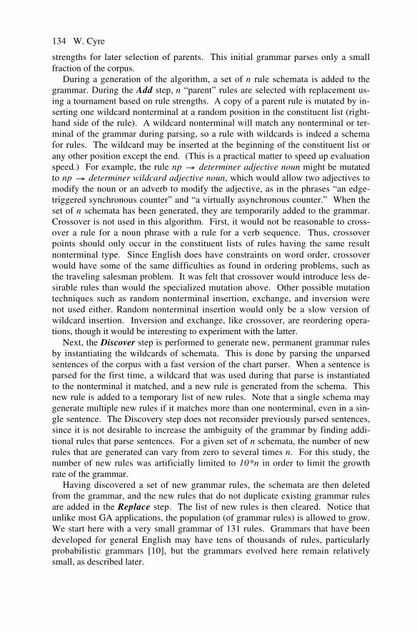
134 W. Cyre
strengths for later selection of parents. This initial grammar parses only a smallfraction of the corpus.
During a generation of the algorithm, a set of n rule schemata is added to thegrammar. During the Add step, n “parent” rules are selected with replacement us-ing a tournament based on rule strengths. A copy of a parent rule is mutated by in-serting one wildcard nonterminal at a random position in the constituent list (right-hand side of the rule). A wildcard nonterminal will match any nonterminal or ter-minal of the grammar during parsing, so a rule with wildcards is indeed a schemafor rules. The wildcard may be inserted at the beginning of the constituent list orany other position except the end. (This is a practical matter to speed up evaluationspeed.) For example, the rule np determiner adjective noun might be mutatedto np determiner wildcard adjective noun, which would allow two adjectives tomodify the noun or an adverb to modify the adjective, as in the phrases “an edge-triggered synchronous counter” and “a virtually asynchronous counter.” When theset of n schemata has been generated, they are temporarily added to the grammar.Crossover is not used in this algorithm. First, it would not be reasonable to cross-over a rule for a noun phrase with a rule for a verb sequence. Thus, crossoverpoints should only occur in the constituent lists of rules having the same resultnonterminal type. Since English does have constraints on word order, crossoverwould have some of the same difficulties as found in ordering problems, such asthe traveling salesman problem. It was felt that crossover would introduce less de-sirable rules than would the specialized mutation above. Other possible mutationtechniques such as random nonterminal insertion, exchange, and inversion werenot used either. Random nonterminal insertion would only be a slow version ofwildcard insertion. Inversion and exchange, like crossover, are reordering opera-tions, though it would be interesting to experiment with the latter.
Next, the Discover step is performed to generate new, permanent grammar rulesby instantiating the wildcards of schemata. This is done by parsing the unparsedsentences of the corpus with a fast version of the chart parser. When a sentence isparsed for the first time, a wildcard that was used during that parse is instantiatedto the nonterminal it matched, and a new rule is generated from the schema. Thisnew rule is added to a temporary list of new rules. Note that a single schema maygenerate multiple new rules if it matches more than one nonterminal, even in a sin-gle sentence. The Discovery step does not reconsider previously parsed sentences,since it is not desirable to increase the ambiguity of the grammar by finding addi-tional rules that parse sentences. For a given set of n schemata, the number of newrules that are generated can vary from zero to several times n. For this study, thenumber of new rules was artificially limited to 10*n in order to limit the growthrate of the grammar.
Having discovered a set of new grammar rules, the schemata are then deletedfrom the grammar, and the new rules that do not duplicate existing grammar rulesare added in the Replace step. The list of new rules is then cleared. Notice thatunlike most GA applications, the population (of grammar rules) is allowed to grow.We start here with a very small grammar of 131 rules. Grammars that have beendeveloped for general English may have tens of thousands of rules, particularlyprobabilistic grammars [10], but the grammars evolved here remain relativelysmall, as described later.

10 Evolving Natural Language Grammars 135
Next, the grammar is evaluated by the parallel parser to determine the strengthsof the rules for selection in the next generation. As mentioned earlier, each sen-tence-level rule that participates in a successful parse is given a reward that is in-versely proportionally to the ambiguity of the sentence (number of parse trees). Inaddition, a percentage of the reward is then added to each rule that formed a con-stituent necessary to satisfy the rule, in a chained bucket-brigade fashion. Hencewhen a sentence is parsed, every rule that participated in forming any parse tree forit is rewarded. There is an exception: if the number of parse trees exceeds a presetthreshold, then none of the participating rules is rewarded for that sentence. This isdone to minimize the growth of ambiguity in the grammar. Finally, any rules, ex-cept those in the initial grammar, that have very low strength are deleted from thegrammar in the Cull step. This prevents the grammar from accumulating rules thatare used very infrequently or that add significant ambiguity. It is assumed that dis-covered rules that are essential for parsing some sentence will be rediscovered in amore general or less ambiguous manner later.
10.4 Experiments
The experiments with a C++ implementation of the algorithm were run on text se-lected from U.S. patents on a type of digital device called a direct memory accesscontroller. The text was selected from the summary and detailed description sec-tions of the patents. This avoided many of the nonsentential structures in patentssuch as numbers, references, names, and legal claims. The corpora still containeda small amount of nonsentential structures from tables and headings. The diction-ary used to tag tokens with parts of speech included about 5000 words and was de-veloped manually. Not all words in the patents were in the dictionary. The un-known words plus acronyms and identifiers were classified as identifiers duringpreprocessing. A corpus may have several thousand instances of identifiers. Threesets of experiments were run, one on some large corpora of several thousand sen-tences, and two sets of experiments on a small corpus of about 400 sentences. Inmost cases, the experimenter limited the algorithm runs to a relatively small num-ber of generations to focus on the more interesting period of most rapid growth. Ina few cases the algorithm was run for many generations to demonstrate that a rea-sonably competent grammar could be evolved from a seriously inadequate gram-mar.
A limited number of experiments were run on three large corpora having 3557,3745, and 6943 sentences, respectively. The initial manual grammar parsed only6% to 9% of the sentences in these corpora, requiring 5 to 7 hours each on a500MHz Pentium PC for 30 generations of the algorithm. In each generation, 5schemata were generated, so that up to 50 new rules could be produced per gen-eration.
The other sets of experiments were performed on a small corpus of 385 sen-tences selected from the larger corpus. This corpus was cleaner than the large onesand intentionally contained more sentences that could be parsed with the initialgrammar, i.e., 17%, or 69 sentences. One set of experiments used a constant num-ber of schemata per generation (n = 5) to determine how repeatably the algorithmperformed. A different random number generator seed was used in each run to

136 W. Cyre
provide a different set of schemata. Another set was run on with a varying numberof schemata per generation to determine the effects of the number of schemata pergeneration on grammar growth. The results of the experiments are described in thenext section.
10.5 Results
10.5.1 Large Corpora Experiments
The evolution of the grammar for one of the large corpora is shown in Figure 10.2.This corpus has 3745 sentences, of which the initial grammar parses 266, or 7%.Growth of the grammar and its competence in parsing the sentences is rapid at firstand slows later, with the competence up to at 65% by the 20th generation and lev-eling to 71% by the 30th generation.
The size of the grammar grew to about 340% of its original size. Initially, morenew rules were generated than the limit (50 for 5 schemata). As can be seen, thenumber of new rules produced in a generation is rather erratic. The algorithm per-formed similarly on one of the other large corpora, but did only half as well on thethird corpus having 6943 sentences. In that run, the limit on the number of newrules was reached in nearly every generation.
Figure 10.2 Grammar evolution.
050
100150200250300350400450500
1 4 7 10 13 16 19 22 25 28 31
Generation
competencerulesnew rules

10 Evolving Natural Language Grammars 137
10.5.2 Performance Variability
Seven experiments run with the same small corpus of 385 sentences and parametervalues were performed to observe how consistently the algorithm performed.
Figure 10.3 Growth of grammar competence.
0
10
20
30
40
50
60
70
80
90
1 3 5 7 9 11 13 15 17 19 21 23
Generation
Com
pete
nce
average
minimum
maximum
Figure 10.4. Competence versus number of rules.
0
10
20
30
40
50
60
70
80
90
0 50 100 150 200 250 300
Number of Rules
Com
pete
nce
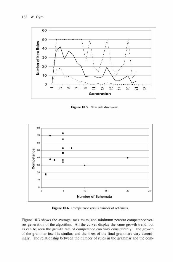
138 W. Cyre
Figure 10.5. New rule discovery.
0
10
20
30
40
50
60
1 3 5 7 9 11 13 15 17 19 21 23
Generation
Num
ber o
f New
Rul
es
Figure 10.3 shows the average, maximum, and minimum percent competence ver-sus generation of the algorithm. All the curves display the same growth trend, butas can be seen the growth rate of competence can vary considerably. The growthof the grammar itself is similar, and the sizes of the final grammars vary accord-ingly. The relationship between the number of rules in the grammar and the com-
Figure 10.6. Competence versus number of schemata.
0
10
20
30
40
50
60
70
80
0 5 10 15 20 25
Number of Schemata
Co
mp
eten
ce

10 Evolving Natural Language Grammars 139
petence of the grammar is shown in Figure 10.4 for the six runs with five sche-mata. The runs seem to have a nearly linear relationship between the number ofrules and competence, but with slightly different slopes. So, it appears that eachrun should eventually reach a desired competence, regardless of the order in whichschemata are introduced, but the final grammars may be different sizes.
Figure 10.5 shows the rate at which new rules are discovered. Discovery is veryrapid at first and was even truncated to the 10n limit. Discovery then tapers off. Inother runs, only an occasional new rule may be discovered in the later generations.This may result from there being no mechanism for preventing the same schematafrom being introduced in generation after generation. The discovery peaks may bedue to the occasional introduction of a new and fruitful schema. The number ofnew rules culled from the evolving grammars shows a similar pattern. While thenumber of rules culled was not a fixed percentage of the number of new rules, itwas generally less than 25% but did reach 67% in one case.
10.5.3 Varying the Number of Schemata
The effects of varying the number of schemata was studied with the same corpus of385 sentences by adding another 9 runs with the number of schemata varying be-tween 1 and 20. In each case, the algorithm was run for 20 generations. The com-petence of the evolved grammars after twenty generations versus the number ofschemata per generation is shown in Figure 10.6. A plot of the number of gram-mar rules versus the number of schemata has a similar shape. From this sparsedata, it does not appear that the number of schemata per generation has much effecton evolution. The runs in which only one schema was used, or where a large num-ber of schema were used, did not do as well as the intermediate cases. In someearlier experiments where only one schema could be introduced per generation, thegrammars generally leveled off at only twice their initial competence values.
10.5.4 Examples of Discovered Rules
A selection of the 568 new rules discovered by the genetic algorithm in the seriesof seven runs with 5 schemata appears in Table 10.1. Rows 1 through 5 show asingle rule that was discovered in five of the seven runs. Note that the rule has dif-ferent strengths in the runs. This useful rule allows an identifier to be appended tothe head of a noun phrase. This accepts constructions such as “Register X” and“Pin AG4/2”, which often occur in this domain. Rule 6 occurred in two runs andallows a modal (can, may, should) to prefix an active verb. It is surprising that thisrule was not discovered in all runs. That may be due to other rules that prefixedpredicate structures with modals, such as Rule 7, which was discovered in tworuns. The discovered rule with greatest strength is shown in row 8 of the table.This rule forms a sentence from a simple sentence followed by a nominal and a pe-riod. Its strength is twice the next-strongest rule and tenfold most other strong newrules, and yet it was found in only one run. The rule in row 9 was found in tworuns and forms a predicate with an active verb structure and two nominals. Thisaccommodates sentences with both an indirect and direct object (a construct not
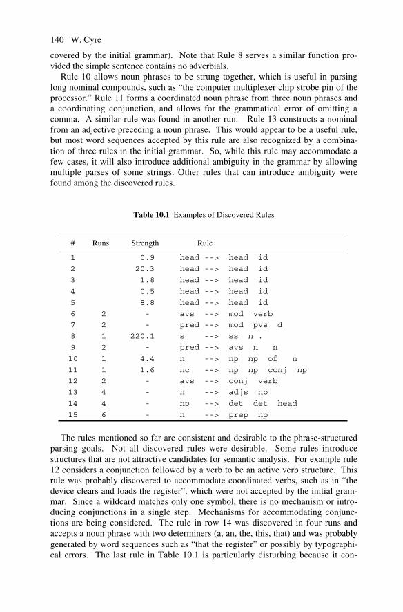
140 W. Cyre
covered by the initial grammar). Note that Rule 8 serves a similar function pro-vided the simple sentence contains no adverbials.
Rule 10 allows noun phrases to be strung together, which is useful in parsinglong nominal compounds, such as “the computer multiplexer chip strobe pin of theprocessor.” Rule 11 forms a coordinated noun phrase from three noun phrases anda coordinating conjunction, and allows for the grammatical error of omitting acomma. A similar rule was found in another run. Rule 13 constructs a nominalfrom an adjective preceding a noun phrase. This would appear to be a useful rule,but most word sequences accepted by this rule are also recognized by a combina-tion of three rules in the initial grammar. So, while this rule may accommodate afew cases, it will also introduce additional ambiguity in the grammar by allowingmultiple parses of some strings. Other rules that can introduce ambiguity werefound among the discovered rules.
Table 10.1 Examples of Discovered Rules
# Runs Strength Rule
1 0.9 head --> head id
2 20.3 head --> head id
3 1.8 head --> head id
4 0.5 head --> head id
5 8.8 head --> head id
6 2 - avs --> mod verb
7 2 - pred --> mod pvs d
8 1 220.1 s --> ss n .
9 2 - pred --> avs n n
10 1 4.4 n --> np np of n
11 1 1.6 nc --> np np conj np
12 2 - avs --> conj verb
13 4 - n --> adjs np
14 4 - np --> det det head
15 6 - n --> prep np
The rules mentioned so far are consistent and desirable to the phrase-structuredparsing goals. Not all discovered rules were desirable. Some rules introducestructures that are not attractive candidates for semantic analysis. For example rule12 considers a conjunction followed by a verb to be an active verb structure. Thisrule was probably discovered to accommodate coordinated verbs, such as in “thedevice clears and loads the register”, which were not accepted by the initial gram-mar. Since a wildcard matches only one symbol, there is no mechanism or intro-ducing conjunctions in a single step. Mechanisms for accommodating conjunc-tions are being considered. The rule in row 14 was discovered in four runs andaccepts a noun phrase with two determiners (a, an, the, this, that) and was probablygenerated by word sequences such as “that the register” or possibly by typographi-cal errors. The last rule in Table 10.1 is particularly disturbing because it con-

10 Evolving Natural Language Grammars 141
structs a nominal from a preposition followed by a noun phrase. Such constructsare indeed phrases but should be classified as prepositional phrases (that modifynouns) or adverbials (phrases that directly modify verbs). Similar rules were dis-covered that form noun phrases from prepositions and nouns. This rule may havebeen discovered to work with higher-order rules such as Rule 8 above. Presently, asimple sentence may have only up to three nominals and adverbials after the verb.Rule 8 with Rule15 allows one additional adverbial.
Although the competence of the grammar evolves vigorously, and most newrules appear reasonable, some of the discovered rules do not appear desirable fromthe standpoint of conventional English grammar, or because they introduce ambi-guity in the grammar. The “ungrammatical” or undesirable rules may be useful,however, in that they will enable semantic analysis of ungrammatical sentences.Ambiguity in the grammar is inconvenient because it increases the computationtime for both grammatical and semantic analysis. Ambiguity is introduced in thegrammar when the result nonterminal they construct can be synthesized by one ormore existing rules. In any case, the manner in which these undesirable rules areintroduced needs to be investigated so that they might be avoided.
10.6 Conclusions
A genetic algorithm has been presented for evolving context-free phrase-structuredgrammars from an initial, small, handcrafted grammar. The algorithm uses distinctdiscovery and evaluation steps, as well as a culling step to reduce the ambiguity ofthe grammar being evolved. The algorithm performs surprisingly well on devel-oping grammars for very complex sentences in a restricted domain of English. Thealgorithm was generally run for a small number of generations to observe the ini-tial growth of the grammar, but even then, it reached 90% competence in somecases.
Much remains to be investigated in this area. First, a method is needed to cullor avoid rules that form undesirable phrase structures from the semantic analysisperspective. This might be done by interaction with a user who affirms desirableparsings from time to time, as with the occasional environmental rewards in classi-fier systems. This interactive feedback could have the effects of negative trainingstrings. Alternatively, a semantic analyzer can be run on some of the parse treesand have the rules that participated in parse supporting a successful semanticanalysis rewarded enthusiastically. A mechanism needs to be added that will allowconjunction to be introduced in the form X conj X, rather than in two separate rules.
The competence of the evolving grammars seems to encounter ceilings below100% competence. This barrier must be overcome. It would also be interesting toincrease the number of schemata introduced in a generation as the grammarevolves. While this would tend to sustain rapid growth during the later genera-tions, it would also increase the evaluation time substantially, since that time de-pends heavily on the size of the grammar.
142 W. Cyre
Acknowledgments
The research reported here was supported in part by the National Science Founda-tion, Grant MIP-9707317.
References
1. W. A. Cook, (1989) Case Grammar Theory, Georgetown University Press, Washing-ton, DC.
2. C. Manning and H. Schütze, (1999) Foundations of Statistical Natural Language Proc-essing, MIT Press, Cambridge, MA.
3. E. Charniak, (1996) Tree-bank Grammars, Proceedings of the Thirteenth NationalConference on Artificial Intelligence, AAAI Press/MIT Press, Menlo Park, pp.1031-1036.
4. G. Carroll and E. Charniak, (1992) Two Experiments on Learning Probabilistic De-pendency Grammars from Corpora, Workshop Notes, Statistically-Based NLP Tech-niques, 1-13, AAAI Press, Menlo Park, CA,.
5. P. Wyard, (1991) Context free grammar induction using genetic algorithms, Proceed-ings of the 4th International Conference on Genetic Algorithms, 514–518.
6. S. Lucas, (1994) Structuring Chromosomes for Context-Free Grammar Evolution,First IEEE Int’l Conf. on Evolutionary Computation, 130-135.
7. T. Smith and I. Witten, (1995) A Genetic Algorithm for the Induction of Natural Lan-guage Grammars Proc. IJCAI-95 Workshop on New Approaches to Learning forNatural Language Processing,17-24, Montreal, Canada.
8. L. Booker, D. Goldberg, J. Holland, (1989) Classifier Systems and Genetic Algo-rithms,” Artificial Intelligence, 40, 235-282.
9. K-S. Fu, T. Booth, (1986) Grammatical Inference: Introduction and Survey, IEEETrans. Pattern Analysis and Machine Intelligence, 343-375, May
10. M. Gold, (1967) Language Identification in the Limit, Information and Control, 10,447-474.
11. W. R. Cyre (1995) A Requirements Sublanguage for Automated Analysis, Interna-tional Journal of Intelligent Systems, 10 (7), 665-689.
12. W. R. Cyre, (1997) Capture, Integration, and Analysis of Digital System Require-ments with Conceptual Graphs, IEEE Trans. Knowledge and Data Engineering, 9(1),8-23.
12 3
Summary.
11.1 Introduction
11
Evaluating Protein Structure PredictionModels with Evolutionary Algorithms
J. Gamalielsson and B. Olsson
Protein structure prediction is the task of predicting the three-dimensionalfolded structure of a protein, given information only about its amino acid se-quence. Computational methods for protein structure prediction have achievedlimited success, due to the immense complexity of the task, and it is well-known that �nding the lowest free-energy conformation of a protein is anNP-hard problem [14].When designing a computational method for protein structure prediction,
there are three main issues to address: ) how to represent candidate solutions,) what algorithm to use, ) what evaluation function to use. Representationof candidate solutions includes issues such as what structure elements to modeland whether to use a discrete or a continuous environment.
EAs are competent at solving complex, multimodal optimization prob-lems in applications with large and badly understood search spaces. EAs are thereforeamong the most promising algorithms for solving the protein structure predictionproblem. In this chapter, we use this insight to evaluate, and show the limitationsof, simpli�ed models for protein structure prediction. These simpli�ed models, e.g.,lattice-based models, have been proposed for their computational efficiency, and ithas been proposed that simpli�ed models will work if only a sufficiently competentoptimization algorithm is developed. However, in this chapter we show that simpli-�ed models do not contain the biological information necessary to solve the proteinstructure prediction problem. This is demonstrated in two steps: �rst, we show thatthe EA �nds the correct structure given a �tness function based on information ofthe known structure. This shows that the EA is sufficiently competent for accurateprotein structure prediction. Second, we show that the same algorithm fails to �ndcorrect structures when any of the simpli�ed models is used. Our main contribution isto have strengthened the hypothesis that solving the problem of protein structure pre-diction will require detailed models encoding information at the atomic level. We havealso demonstrated that EAs indeed are promising algorithms for eventually solvingthe protein structure prediction problem.
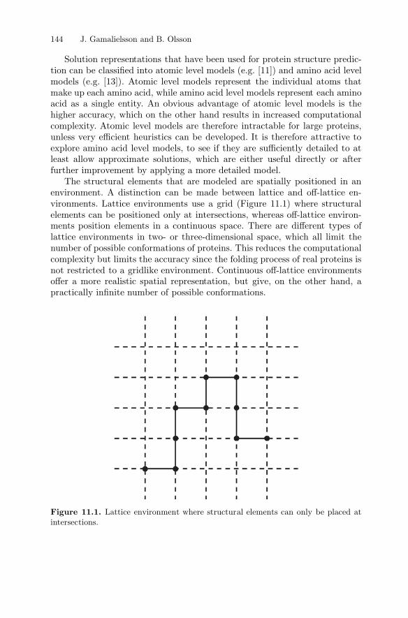
Figure 11.1.
144 J. Gamalielsson and B. Olsson
Lattice environment where structural elements can only be placed atintersections.
Solution representations that have been used for protein structure predic-tion can be classi�ed into atomic level models (e.g. [11]) and amino acid levelmodels (e.g. [13]). Atomic level models represent the individual atoms thatmake up each amino acid, while amino acid level models represent each aminoacid as a single entity. An obvious advantage of atomic level models is thehigher accuracy, which on the other hand results in increased computationalcomplexity. Atomic level models are therefore intractable for large proteins,unless very efficient heuristics can be developed. It is therefore attractive toexplore amino acid level models, to see if they are sufficiently detailed to atleast allow approximate solutions, which are either useful directly or afterfurther improvement by applying a more detailed model.The structural elements that are modeled are spatially positioned in an
environment. A distinction can be made between lattice and off-lattice en-vironments. Lattice environments use a grid (Figure 11.1) where structuralelements can be positioned only at intersections, whereas off-lattice environ-ments position elements in a continuous space. There are different types oflattice environments in two- or three-dimensional space, which all limit thenumber of possible conformations of proteins. This reduces the computationalcomplexity but limits the accuracy since the folding process of real proteins isnot restricted to a gridlike environment. Continuous off-lattice environmentsoffer a more realistic spatial representation, but give, on the other hand, apractically in�nite number of possible conformations.

�
� �R
= + + +
9
Figure 11.2.
� �� �
� �E E E E E E
E EE
tor vdW el pe tor
vdW el
pe
11 Evaluating Protein Structure Prediction Models 145
Generic amino acid structure with dihedral angles and . The struc-ture of the side chain is unique for each of the 20 amino acids.
Algorithms that have been applied to protein structure prediction includeseveral versions of EAs. In [12] and [13] a hybrid GA containing Monte Carlocomponents is compared with a pure Monte Carlo method on 2D and 3D HPmodels, where amino acids are classi�ed as hydrophobic (H) or polar (P) [4].On test sequences of 27 and 64 residues the hybrid GA was able to reachthe global energy minimum in fewer time steps than the pure Monte Carlomethod. A GA is used also in [8], which is based on [13] but avoid the use ofnonstandard properties (which are used in [13]) and introduces an improvedrepresentation resulting in faster convergence.
In [11] a GA is applied to protein structure prediction using a force �eldas �tness function and having structures being represented at the atomic levelby dihedral angles (Figure 11.2). The angles and are the main degrees offreedom when proteins fold, being located between the -carbon atom andthe NH group and between the -carbon and the CO group. In [11], totalenergy is calculated as , where is torsionangle potential, is van der Waals pair interactions, is electrostaticpotential, and is a pseudo-entropic term driving the protein to a globularstate. Simulations using the 46-residue protein 1CRN gave structures withroot mean square deviation RMSD Å from the native fold. Extensions tothe approach reduced RMSD to 4.4Å.In [2] an EA is applied in an off-lattice environment. Input to the algo-
rithm are the residue sequence and the preferred secondary structural states

� �
��
�
{ }
�
� �� �
�
1
1 1 1 1
1
1
1
1 1 1
11.2 Methods Tested
hyd
hyd
t tN
ti M M
i i i i
i i i i
i i i
11.2.1 Solution Representation
146 J. Gamalielsson and B. Olsson
( ) =
1 = ( )
= + sin cos ( = 2 )
= + sin sin ( = 2 )
= + cos ( = 2 )
= = = 0
E
E
P t N P t s , . . . , sM
M s � , � , . . . , � , �
x x R � � i , . . . ,M ,
y y R � � i , . . . ,M ,
z z R � i , . . . ,M ,
x y z R�
for different residues. The backbone structure of the �ttest solution in the lastgeneration is compared with the native fold of the protein. Nineteen targetproteins with fewer than 100 residues and mixed secondary structure compo-sitions are used to test the prediction performance, giving average RMSD =5.3Å.An off-lattice environment and amino acid level model is used also in
[9], which introduces a distance matrix representation of residue positionsinstead of the commonly used internal coordinate representation (dihedralangles). A distance matrix contains a distance for every residue pair. The�tness function has terms for punishment of residue clashes, for enforcementof correct distance between consecutive residues, and a term ( ) reward-ing closeness between hydrophobic residues. Residues are only classi�ed aseither hydrophobic or polar. gives optimal interaction potential whenthe distance between the interacting residues is 3.80Å. The EA is tested onthree 27-residue sequences, producing conformations with compact hydropho-bic cores. No comparison with real proteins is made.
We tested the application of EAs (with and without sharing) to simpli�ed,i.e., amino acid level, off-lattice models for protein structure prediction, withthe purpose of investigating if lattice-based models (e.g., the HP model [4])can be usefully transferred to off-lattice environments. We also propose andtest extensions to the HP model, using additional information about aminoacid properties.
The EA population at iteration contains solutions .A solution for a protein containing residues is represented by an array of
angles . To obtain the coordinates ofthe residues in 3D space, a transformation to rectangular coordinates is doneusing
(11.1)
(11.2)
(11.3)
where . is the distance between consecutive residues.Residue positions are approximated by their -carbon atom positions, whichare used to represent the shape of the backbone. This is a very simpli�edrepresentation where the con�gurations of the sidechains are not taken intoconsideration.

2c m
� ��
T n s p p �
c
m
i
i
m
m
2
max max
Table 11.1.
= 1
( )
= 10( )
= 0 7( )
= 4( = 0 = 1)
( )( )
1 ( ( )) ( ( 1))= 100
11.2.2 EA1. A Standard Evolutionary Algorithm
��
�R
P t
sP t
p .�, �
p /n nr r , �
s P tF s
t t F P t < F P tT n
p Tp
T n
11 Evaluating Protein Structure Prediction Models 147
Parameter Values Used in the EA1 Experiments.
Protein Residues
1CRN 46 9000 100 10 0.7 0.0444 12ETI 28 5400 100 10 0.7 0.0741 11CTI 29 5600 100 10 0.7 0.0714 13ZNF 30 5800 100 10 0.7 0.0690 11PPT 36 7000 100 10 0.7 0.0571 1
We found empirically that the mean distance between consecutive -carbon atoms for the proteins used in this work is 3.82Å with = 0.04Å.The distance between consecutive -carbon atoms was therefore set to unitdistance in the algorithm, corresponding to an actual distance of 3.80Å.The distance of 3.80Å has also been used, e.g., by [2]. The angular represen-tation is easy to implement and facilitates the application of genetic variationoperators.
The EA uses a population of 100 solutions, which are initialized asstraight structures, with all angles set to 0 (cf. [13]). Fitness is assigned ac-cording to one of the evaluation functions in Section 11.2.4. We use standardtournament selection without replacement and tournament size . Afterselection, the new population is divided into pairs of parent solutions,and standard single-point crossover is applied with . The crossoverpoint may not split an angle pair for a residue pair. Gaussian muta-tion is applied to all parameters (angles) of each individual with a probability
, where is the number of parameters. The mutation operator addsa random number from a normal distribution to a parametervalue.
After reproduction, all solutions in are evaluated and receive a�tness value , and elitism is applied by replacing the worst solution fromtime with the best solution from time if .The evolutionary cycle is repeated for iterations. The expressionsfor calculation of and were determined empirically. It is desirable to ad-just so that the same number of parameters are likely to be mutatedirrespective of the number of parameters. is proportional to becausea larger number of parameters usually gives a slower convergence rate. Ta-ble 11.1 shows the parameter settings used in simulations for the �ve differentproteins studied.

�
�
′
′
′
shar e
∑�
√√√√∑
=1
=1
2
360
2
148 J. Gamalielsson and B. Olsson
ii
nj i j
d�
�share
i j
m
k
i,k j,k
i i i
i
i j i j
i j i
i share
i
i,k
i
share
share
c m
11.2.3 EA2. An Evolutionary Algorithm with Sharing
11.2.4 Evaluation Functions
( ) =( )
( ( ))
( ) =1 ( )
0
( ) = ( ( 360) ( 360))
( ) ( )
= 100 ( ( )) ( )( )
( )
( 360)
= 16
= 100= 10 = 0 7 = 0 0741 = 1
F sF s
sh d s , s,
sh dd < �
,
d s , s rem s , rem s , .
F s s F ss n
n sh d s , s d s , ss s F s
F s �s �
rem s , ks
�
�� �
T
ns p . p . �
The standard EA uses no method to ensure that solutions in a populationare diverse, which may cause the algorithm to converge to a point where allsolutions are very similar [6]. Hence, there is a risk for premature convergenceand suboptimal solutions. EA2 is a modi�ed version of EA1 that uses a �tnesssharing strategy. Fitness sharing enforces diversity within a population bydemanding that each solution share its �tness with other solutions that arewithin the same region of the search space. The principle of �tness sharing,as described in [6], is de�ned in Eqs. (11.4) and (11.5). The problem-speci�cdistance measure used in this work is de�ned in equation 11.6.
(11.4)
ifotherwise
(11.5)
(11.6)
In Eq. (11.4), is the shared �tness for solution , is the raw �tnessreturned by the evaluation function for solution , is the population size( ), is the sharing function value for the distance ,which is the distance between solutions and . Hence, is used duringthe selection procedure instead of . In Eq. (11.5) de�nes the sizeof the neighborhood around solution and is a scaling parameter. In Eq.(11.6), is the remainder after dividing parameter of solutionwith 360. Hence, Eq. (11.6) is a modi�ed expression for Euclidean distance,
taking into consideration that the remainder from a division encodes thesame position as an angle . The consequence of the sharing function in Eq.(11.5) is that the closer two solutions are to each other, the more each solutionis penalized. Different parameter values for were tested during initialsimulations and was found appropriate. The parameter was setto 1.EA2 was applied to all evaluation functions, but only one target protein
(2ETI) was used. The number of iterations was extended from 5400 to9000, since the broader exploration done with a more diversi�ed populationmay require more time until convergence. The other EA parameters were setto the same values as described in Table 11.1 for the EA1 algorithm: ,
, , , and .
This section describes the evaluation functions that we de�ned and tested.

�
HP
�ij
�ij
� �� � � �
∑ ∑⎧⎪⎨⎪⎩
2
=1 = +2
1
1
Table 11.2.
=
=
+ 1 1 = 0
exp(1 ) 1 = 0
= 0
pr r
E e ,
e
p d < p ,
p d d p ,
p .
ij
i j
M
i
M
j i
ij
ij
d ij ij ij
ijij ij ij
d ij
11 Evaluating Protein Structure Prediction Models 149
Amino Acid Properties
Amino acid Hydrophobicity Charge Woese Miller
Alanine H H 7.0 -0.20Arginine P P 9.1 1.34Asparagine P X 10.0 0.69Aspartate P N 13.0 0.72Cysteine P X 4.8 -0.67Glutamine P X 8.6 0.74Glutamate P N 12.5 1.09Glycine P X 7.9 -0.06Histidine P P 8.4 -0.04Isoleucine H H 4.9 -0.74Leucine H H 4.9 -0.75Lysine P P 10.1 2.00Methionine H H 5.3 -0.71Phenylalanine H H 5.0 -0.67Proline H H 6.6 -0.44Serine P X 7.5 0.34Threonine P X 6.6 0.26Tryptophan H H 5.2 -0.45Tyrosine P X 5.4 0.22Valine H H 5.6 -0.61
is an adaptation of the lattice HP model [4] to off-lattice envi-ronments, using a similar approach as in [15] and [9]. We used the Ras-mol (http://www.umass.edu/microbio/rasmol/) prede�ned sets �Hydropho-bic� and �Polar�to classify amino acids, as shown in Table 11.2, in the columnmarked �Hydrophobicity�. Table 11.3 shows the potential for the HP en-ergy function for types of interactions between neighboring residues andin a lattice environment [10]. The off-lattice version uses a potential functiontaking the distance between interacting residues into account. An optimalinteraction potential equivalent to the lattice interaction potential for neigh-boring hydrophobic residues occurs at unit distance (3.8Å). Smaller distancesare penalized to enforce steric constraints, i.e., to avoid residue clashes. Thisapproach has been used in both lattice [13] and off-lattice models [9, 15]. Totalenergy is calculated using
(11.7)
,
, (11.8)

�
ij
i
j
p
r
r H P
H
P
= 1 = 6
1= 0 5
Solid lineDashed
ij
ij
ij
ij ij
ij
ij
ij
Table 11.3.
Figure 11.3.
E ei j d i j �
� p
e d� � �
ed �
�d �
�� .
150 J. Gamalielsson and B. Olsson
Interaction Potential for the HP Evaluation Function.
-1 00 0
Off-lattice HP model interaction potential. : pairwise hydropho-bic interactions (H-H). : all other types of interactions.
where is the total energy of a conformation, is energy potential betweenresidues and , is the Euclidean distance between residues and , andare constants, and is the interaction potential according to Table 11.3.
Eq. (11.8) is visualised in Figure 11.3, plotting against . We testeddifferent values for and before �xing them. Higher makes the penaltycurve steeper. Mutation of a single angle may change dramatically around
because of the steep penalty curve below this point. We founduseful for achieving a high penalty effect to avoid residue clashes while alsoavoiding too high sensitivity to mutation. Higher yields a reward curve thatapproaches 0 quicker as a function of . We found that must not be toohigh ( ) as this results in weak guidance toward globular structures forlong-distance interactions. was found adequate.

{1
eij�ij
ij
i
j
� �� � � �
�
�
�
Table 11.4. p
r
r H P N X
H
P
N
X
HPNX
WOESE
MILLER
EMP
w
w
d ij ij
ijij ij
ijwi
wj
m
m
m
ijmi
mj
ij
[4 8 13 0]
=+ 1 1
exp(1 ) 1
= 1 + 1= 1
[ 0 74 2 00]
= 1 = +
6 5
h. , .
h
c p d < ,
c p d d ,
p /h /hc
hh . , .
h
c p h h
d . emp
emp
11 Evaluating Protein Structure Prediction Models 151
Interaction Potential for the HPNX Evaluation Function.
-4 1 1 01 0 -1 01 -1 0 00 0 0 0
The �tness value returned by the evaluation function is negated total en-ergy, since EAs strives to maximize �tness and the total free energy of thenative fold is assumed to be at a minimum [1].
is an extension to HP to consider the charge of amino acids [10].Amino acids are classi�ed as hydrophobic (H), positively (P) or negatively (N)charged, or neutral (X), using the Rasmol prede�ned sets �Basic�, �Acidic�,and �Neutral� to subdivide the polar residues. The resulting classi�cation isshown in the column marked �Charge� in Table 11.2. The interaction po-tentials in the HPNX function are illustrated in Table 11.4. The energy isotherwise calculated as in HP (see Eqs. (11.7) and (11.8)).
uses polar requirement values , i.e., different degrees of polar-ity for different amino acids [16], which vary in the interval . A highcorresponds to a polar residue. The polar requirement values are shown
in the column marked �Woese� in Table 11.2. As this evaluation function ismore detailed than HP it should yield conformations structurally closer totarget conformations. The energy calculation uses Eq. (11.7) and
if
if(11.9)
where (so that hydrophobic interactions are rewarded),and .
uses degrees of hydrophobicity , according to the empiri-cal hydrophobicity scale of [5], where varies in the rangekcal/mol, and where negative values correspond to hydrophobicity. Thevalues are shown in the column marked �Miller� in Table 11.2. The energycalculation is de�ned by Eq. (11.9) with and .
uses empirically derived contact potentials for amino acid interac-tions. A contact potential describes the energy between two residues in prox-imity (typically, Å). In [7] a contact potential was determinedfor all pairs of amino acid types using 1168 known structures. The interactionbetween two Leucine residues gives the lowest of -7.37. Leucine is oneof the most hydrophobic amino acids and this supports the assumption that
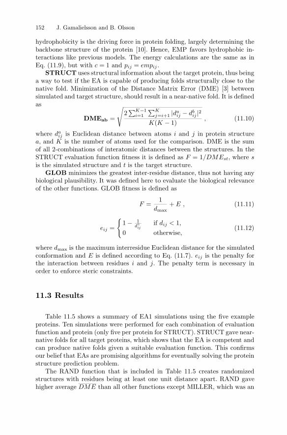
�ab
�ij
DME
√ ∑ ∑
{
| � |�
�
STRUCT
GLOB
11.3 Results
1=1 = +1
2
max
1
max
= 1 =
=2
( 1)
= 1
=1+
=1 1
0
ij ij
Ki
Kj i
aij
bij
aij
st
ijd ij
ij
152 J. Gamalielsson and B. Olsson
c p emp
d d
K K,
d i ja K
F /DME st
Fd
E ,
ed < ,
,
dE e
i j
DME
hydrophobicity is the driving force in protein folding, largely determining thebackbone structure of the protein [10]. Hence, EMP favors hydrophobic in-teractions like previous models. The energy calculations are the same as inEq. (11.9), but with and .
uses structural information about the target protein, thus beinga way to test if the EA is capable of producing folds structurally close to thenative fold. Minimization of the Distance Matrix Error (DME) [3] betweensimulated and target structure, should result in a near-native fold. It is de�nedas
(11.10)
where is Euclidean distance between atoms and in protein structure, and is the number of atoms used for the comparison. DME is the sumof all 2-combinations of interatomic distances between the structures. In theSTRUCT evaluation function �tness it is de�ned as , whereis the simulated structure and is the target structure.
minimizes the greatest inter-residue distance, thus not having anybiological plausibility. It was de�ned here to evaluate the biological relevanceof the other functions. GLOB �tness is de�ned as
(11.11)
if
otherwise(11.12)
where is the maximum interresidue Euclidean distance for the simulatedconformation and is de�ned according to Eq. (11.7). is the penalty forthe interaction between residues and . The penalty term is necessary inorder to enforce steric constraints.
Table 11.5 shows a summary of EA1 simulations using the �ve exampleproteins. Ten simulations were performed for each combination of evaluationfunction and protein (only �ve per protein for STRUCT). STRUCT gave near-native folds for all target proteins, which shows that the EA is competent andcan produce native folds given a suitable evaluation function. This con�rmsour belief that EAs are promising algorithms for eventually solving the proteinstructure prediction problem.The RAND function that is included in Table 11.5 creates randomized
structures with residues being at least one unit distance apart. RAND gavehigher average than all other functions except MILLER, which was an

DME max min
Table 11.5.
DME � DME DME
< . < . < . < .< . < . < . < .< . < . < . < .
< .
< . < . < . < .
0 05 0 05 0 05 0 050 05 0 05 0 05 0 050 05 0 05 0 05 0 05
0 05
0 19 0 09 0 23 0 14
11 Evaluating Protein Structure Prediction Models 153
DME Results (in Ångstroms) for EA1.
Protein
STRUCT 1CRNSTRUCT 2ETISTRUCT 1CTISTRUCT 3ZNF 0.3 0.2 0.4STRUCT 1PPT 0.5 0.1 0.6 0.5Avg.RAND 1CRN 12.6 5.3 25.1 6.1RAND 2ETI 9.0 2.2 12.9 6.6RAND 1CTI 9.1 3.5 15.3 5.5RAND 3ZNF 8.7 3.4 15.8 5.3RAND 1PPT 9.4 3.0 14.2 4.9Avg. 9.8 3.5 16.7 5.7HP 1CRN 7.3 0.4 7.9 6.8HP 2ETI 4.6 0.2 4.9 4.3HP 1CTI 7.8 0.5 8.8 7.0HP 3ZNF 5.0 0.2 5.2 4.6HP 1PPT 7.2 0.3 7.7 6.9Avg. 6.4 0.3 6.9 5.9HPNX 1CRN 7.1 0.3 7.7 6.8HPNX 2ETI 4.5 0.3 5.2 4.1HPNX 1CTI 7.9 0.7 9.1 7.2HPNX 3ZNF 4.8 0.3 5.3 4.4HPNX 1PPT 7.4 0.1 7.6 7.3Avg. 6.3 0.3 7.0 6.0WOESE 1CRN 6.6 0.2 7.0 6.4WOESE 2ETI 4.5 0.4 5.4 4.0WOESE 1CTI 5.2 0.5 6.3 4.7WOESE 3ZNF 4.6 0.2 5.0 4.3WOESE 1PPT 7.5 0.4 8.1 6.9Avg. 5.7 0.3 6.4 5.3MILLER 1CRN 7.6 0.4 8.3 7.0MILLER 2ETI 5.0 0.3 5.6 4.7MILLER 1CTI 12.3 7.8 20.3 4.8MILLER 3ZNF 36.8 0.0 36.8 36.8MILLER 1PPT 41.3 0.0 41.3 41.3Avg. 20.6 1.7 22.5 18.9EMP 1CRN 7.4 0.1 7.6 7.3EMP 2ETI 4.5 0.2 4.6 4.1EMP 1CTI 5.1 0.1 5.2 4.9EMP 3ZNF 5.6 0.2 5.9 5.2EMP 1PPT 9.1 0.1 9.3 8.9Avg. 6.3 0.1 6.5 6.1GLOB 1CRN 6.1 0.3 6.6 5.5GLOB 2ETI 4.0 0.3 4.5 3.5GLOB 1CTI 4.4 0.3 4.8 3.7GLOB 3ZNF 5.2 0.3 5.4 4.4GLOB 1PPT 8.2 0.2 8.5 7.9Avg. 5.6 0.3 6.0 5.0

= 5 6
max
min
DME .
DMEDME
<<<<<<
<<<<
Table 11.6.
100 100 100 99 100100 100 100100 99 100100 98 100100 100 100100 100
100100
154 J. Gamalielsson and B. Olsson
Hypothesis Con�dence Levels
ProteinHypothesis 1CRN 2ETI 1CTI 3ZNF 1PPTGLOB EMPGLOB HP 0 0GLOB HPNX 0 0GLOB WOESE 0 0WOESE HP 40 0WOESE HPNX 0 79 0EMP HP 0 57 0 0EMP HPNX 0 0 0 0EMP WOESE 0 0 40 0 0HPNX HP 63 47 0 79 0
unsuccessful application of the hydrophobicity scale of [5] and did not producecompact globular structures for all proteins.The most striking result seen in Table 11.5 is that GLOB, which simply
crumples the protein by minimizing the greatest interresidue distance, is themost successful function, having Å. Statistical data analysis (seeTable 11.6) shows that the difference between GLOB and both EMP andMILLER is signi�cant at the 99% level or higher for all �ve proteins. Inaddition, GLOB was better at the 98% signi�cance level than HP, HPNX, andWOESE for three out of �ve proteins. In addition, the average and
are lower for GLOB than for any other function except STRUCT.In these results, therefore, an evaluation function only rewarding compactconformations gives better DME values than several functions with presumedbiological relevance.
It is also notable that the average DME for every tested function (exceptSTRUCT) is too high for useful structure prediction, since a DME aboveapproximately 5Å can only correspond to weak structural similarities. Thisindiates that none of the functions tested is informative enough to guide thesearch to correct structure predictions. These functions can therefore at bestbe used to �nd approximate solutions to be further re�ned by more exactmethods.In order to evaluate the accuracy of the evaluation functions, we compared
for each evaluation function the �tness of the best evolved solution with the�tness assigned by the same �tness function to the native fold. As can beseen in Table 11.7, evolved structures always have higher or much higher�tness than the native fold, despite having large DME when compared withthe native fold, and thus being incorrect solutions. This result indicates thatthe evaluation functions are misleading, either in the sense that they leadthe EA to incorrect minima in search space regions far away from the native

� .
( )
0 91
corr F,D max min
2
1
2
1
3
1
( ) ( ) ( )
12131
Table 11.7.
Table 11.8.
ETI
CRN
ETI
CTI
ZNF
PPT
F D
corr F,D � corr F,D corr F,D
CRNETICTIZNFPPT
fold, or that they lead the EA to "overshoot" the target by overoptimizingthe structure past the correct solution. To further investigate the behaviorof these functions, we measured the correlation between the �tness valuesfound during the simulations and the DME deviation from the native fold.Table 11.8 shows this correlation for the HP function. As can be seen, thecorrelation is rather strong ( ) for every protein. This indicates that thefunction does lead the EA towards the correct region of the search space, buteither misses or overshoots the target. The correlation levels were similar forall other evaluation functions tested (data not shown).
Table 11.9 shows the results of using �tness sharing in EA2. There isno clear case of improvement in DME values, and on the contrary �tnesssharing gave worse DME results on the 2ETI protein for the two evaluation
11 Evaluating Protein Structure Prediction Models 155
Fitness results. For each protein, the �rst row shows average �tness of thebest individual in the �nal EA1 population, and the second row shows �tness of thenative fold. The additional row for shows average �tness of the best individualin the �nal EA2 population.
HP HPNX WOESE MILLER EMP GLOB107.9 453.6 184.0 168.9 2071.5 0.2358.4 251.7 145.7 84.0 1446.3 0.1324.8 95.2 69.4 56.2 815.2 0.299.9 51.5 62.0 29.2 643.1 0.2023.4 92.2 68.3 44.1 792.3 0.2825.3 77.7 71.0 4.1 896.1 0.309.6 38.9 62.3 -28.3 656.6 0.2010.1 20.0 70.8 -68.8 715.4 0.291.7 2.0 59.0 -163.4 536.8 0.1652.0 183.0 100.3 -30.1 1219.2 0.2727.5 96.4 76.9 -83.6 805.6 0.12
Correlation Between Fitness ( ) and DME ( ) for EA1 Using the HPEvaluation Function.
Protein
0.94 0.01 0.96 0.920.94 0.01 0.96 0.920.95 0.01 0.96 0.940.94 0.02 0.95 0.910.91 0.01 0.93 0.90

� �
DME
∑∑∑=1 =1 =1
max min
0 05 0 05 0 05
Table 11.9.
= 16
=1 1
( )
( )
11.4 Conclusions
DME � DME DME
< . < . < .
��
�T n
d s , s ,
d s , s s si
�
share
share
T
i
n
j
n
k
i j k
i j k j k
156 J. Gamalielsson and B. Olsson
EA2 versus EA1 on the protein 2ETI. Values within parantheses arefrom EA1 simulations and are repeated from Table 11.5 and 11.7 to make comparisoneasier.
Function
STRUCT 0.4 ( ) 0.1 (0.2) 0.6 ( ) 0.3 ( )HP 4.6 (4.6) 0.3 (0.2) 5.2 (4.9) 4.2 (4.3)HPNX 4.6 (4.5) 0.4 (0.3) 5.4 (5.2) 4.1 (4.1)WOESE 4.9 (4.5) 0.8 (0.4) 7.0 (5.4) 4.3 (4.0)MILLER 9.4 (5.0) 5.4 (0.3) 17.7 (5.6) 4.8 (4.7)EMP 4.4 (4.5) 0.2 (0.2) 4.8 (4.6) 4.2 (4.1)GLOB 3.9 (4.0) 0.2 (0.3) 4.1 (4.5) 3.5 (3.5)
functions STRUCT and MILLER. One reason for the worse results on thesetwo functions is the choice of sharing parameter value , which wasnonoptimal for these two functions. This value was suitable for otherfunctions, but further experimentation to �nd values suitable for STRUCTand MILLER was not conducted.
Given the lack of improvement when using �tness sharing, it is of interestto study the structural diversity of the populations. We therefore de�ned thefollowing measure of structural diversity:
(11.13)
where is the distance between solutions and at iteration stepaccording to Eq. (11.6). Table 11.10 shows the structural diversity whendifferent evaluation functions with (EA2) and without (EA1) �tness sharingare used. The mean diversity is considerably higher for the �tness sharingsimulations for all evaluation functions. This shows that the �tness sharingstrategy works, in the sense that it gives a higher structural diversity in thepopulation. The fact that this does not result in better DME results (seeTable 11.9) can only be attributed to the �tness functions being misleading.
Our results show that evolutionary algorithms can �nd correct protein struc-tures given the right �tness function, i.e., the STRUCT function. The problem,of course, is that this function requires that we already know the native struc-ture, and is therefore not of any use for structure prediction. It does indicate,

�� � � �max min
Table 11.10.
181
236
Acknowledgment
References
11 Evaluating Protein Structure Prediction Models 157
Structural diversity (protein 2ETI). For each evaluation function, the�rst row shows average diversity for EA1 simulations, and the second row shows averagediversity for EA2 simulations.
Evaluation function
HP1 505 11 528 4904509 382 5051 3798
HPNX1 477 6 486 4695103 672 6167 3961
WOESE1 442 12 462 4165109 898 7049 3957
MILLER1 446 5 453 4394204 322 4605 3738
EMP1 952 1084 3183 4204437 552 5625 3727
DME1 1443 1464 4019 48810705 5281 17893 5191
GLOB1 612 142 915 5244034 741 6046 3548
1. An�nsen, C.B. (1973) Principles that govern the folding of proteins chains. Sci-ence. , 223-230.
2. Dandekar, T., Argos, P. (1996) Folding the main-chain of small proteins with thegenetic algorithm. Journal of Molecular Biology. , 844-861.
however, that EAs are sufficiently powerful search algorithms for eventuallysolving the protein structure prediction problem.Our results also show that the simpli�ed models used in much research on
protein structure prediction do not give �tness functions informative enoughto guide the EA to accurate structure predictions. It is clear from our resultsthat these models are not fruitful abstractions of the folding process. It wassuggested in [12] that simpli�ed models (e.g., lattice-based HP) �exhibit manyof the features of real folding�. However, according to our results, they arefar from informative enough for useful structure prediction, since no functiongave an average DME below 5Å.
This work was supported in part by a grant to the second author from TheFoundation for Knowledge and Competence Development (grant 1507/97).

�
87
196
256
2
231
55
31
158 J. Gamalielsson and B. Olsson
3. Doucet, J.P., Weber, J. (1996) Computer-Aided Molecular Design. AcademicPress.
4. Lau, K., Dill, K. (1990) Theory for protein mutability and biogenesis. Proceedingsof the National Academy of Sciences of the USA. , 638�642
5. Miller, S., Janin, J., Lesk, A.M., Chothia, C. (1987) Interior and surface ofmonomeric proteins. Journal of Molecular Biology. , 641-656.
6. Michalewicz, Z.,Fogel, D.B. (2000) How to Solve It: Modern Heuristics. Springer-Verlag.
7. Miyazawa, S., Jernigan, R.L. (1996) Journal of Molecular Biology. , 623-644.8. Patton, A.L., Punch, W.F., Goodman, E.D. (1995) A Standard GA Approach toNative Protein Conformation Prediction. Proc. of the 6th Annual Intern. Conf.on Genetic Algorithms. 574-581.
9. Piccolboni, A., Mauri, G. (1997) Application of evolutionary algorithms to proteinfolding prediction. Proceedings of ICONIP. Springer.
10. Renner, A., Bornberg-Bauer, E. (1997) Exploring the �tness landscapes of latticeproteins. Paci�c Symposium on Biocomputing. , 361-372.
11. Schulze-Kremer, S. (1995) Molecular Bioinformatics: Algorithms and Applica-tions. Walter de Gruyter.
12. Unger, R., Moult, J. (1993) Genetic algorithms for protein folding simulations.Journal of Mol. Biology. , 75-81.
13. Unger, R., Moult, J. A (1993) Genetic Algorithm for 3D Protein Folding Simula-tions. Proc. of the 5th Annual Intern. Conf. on Genetic Algorithms, 581-588.
14. Unger, R., Moult, J. (1993) Finding the lowest free energy conformation of aprotein is a NP-hard problem. Bulletin of Mathematical Biology. (6), 1183�1198
15. Vail, D. (2001) Genetic algorithms as a search strategy and a novelmeans of potential punction discovery in the protein folding problem.Bowdoin College, Department of Computer Science, report available atwww.bowdoin.edu/ dvail2/protein.html
16. Woese, C.R., Dugre, D.H., Dugre, S.A., Kondo, M., Saxinger, W.C. (1966) Onthe fundamental nature and evolution of the genetic code. Cold Spring HarborSymp. Quant. Biol. , 723�736
Summary.HI DE R
12.1 Introduction
12
Learning Decision Rules by Means ofHybrid-Encoded Evolutionary Algorithms
This paper describes an approach based on evolutionary algorithms,HIDER ( erarchical cision ules), for learning rules in continuous and discretedomains. The algorithm produces a hierarchical set of rules, that is, the rules aresequentially obtained and must be therefore tried in order until one is found whoseconditions are satis�ed. In addition, the algorithm tries to obtain more understandablerules by minimizing the number of attributes involved. The evolutionary algorithm usesbinary coding for discrete attributes and integer coding for continuous attributes. Theinteger coding consists in de�ning indexes to the values that have greater probabilityof being used as boundaries in the conditions of the rules. Thus, the individuals han-dles these indexes instead of the real values. We have tested our system on real datafrom the UCI Repository, and the results of a 10-fold cross-validation are comparedto C4.5s and C4.5Rules. The experiments show that HIDER works well in practice.
J.C. Riquelme and J.S. Aguilar-Ruiz
Evolutionary Algorithms (EA) are a family of computational models inspiredby the concept of evolution. These algorithms employ a randomized searchmethod to �nd solutions to a particular problem [25]. This search is quitedifferent from the other learning methods mentioned above. An EA is anypopulation-based model that uses selection and recombination operators togenerate new sample examples in a search space [22]. EAs have been usedin a wide variety of optimization tasks [13] including numerical optimizationand combinatorial optimization problems, although the range of problems towhich EAs have been applied is quite broad. The main task in applying EAsto any problem consists of selecting an appropriate representation (coding)and an adequate evaluation function (�tness).Genetic-based searching algorithms for supervised learning, as GABIL [7]
or GIL [11], do not handle easily numeric attributes because the methodof encoding all possible values would lead to very long rules in the case or

12.2 Motivation
generalization
pure
Figure 12.1. Figure 12.2.
160 J.C. Riquelme, J.S. Aguilar-Ruiz
C4.5. HIDER.
real-valued attributes. Concretely, GABIL and GIL are so-called �conceptlearners� because they are designed for discrete domains. Other approaches,as SIA [19], have been motivated by a real-world data analysis task in acomplex domain (continuous and discrete attributes).The aim of our research was to obtain a set of rules by means of an
evolutionary algorithm to classify new examples in the context of supervisedlearning. With our approach, HIDER, we try to handle efficiently continuousand discrete attributes.The justi�cation of this method will be discussed in Section 12.2. The
characteristics of our approach are presented in section 12.3, where the coding,the algorithm, the selected �tness function, and a particular aspect named
, are detailed. Section 12.4 shows the experiments, the resultsand the analysis of them. In Section 12.5 the conclusions are summarized,some of which motivates the future works presented in Section 15.7.
Two arti�cial two�dimensional databases will be used to clarify the motivationof our approach. The way in which C4.5 splits the space is depicted in Figure12.1. The �gures within the circles describe the level on the tree where thetests (nodes) over these attributes are placed. See the region labeled as B onthe bottom left corner of Figure 12.1. C4.5 divides the region into two parts,however, we thought that the region should be completely covered by onlyone rule. This fact motivates us to design an algorithm able to discover suchrule.
HIDER is quite different because it does not divide the space by an at-tribute, but it extracts sequentially regions from the space. This permits usto obtain regions, i.e., all examples belong to the same category. As il-lustrated in Figure 12.2, the region labeled as B on the bottom left corner isdiscovered by HIDER.

�( 1)
i
i i i
ii
al u R
i
12.3 HIDER
decision list
Figure 12.3. Figure 12.4.
12 Learning Decision Rules with Hybrid-Encoded EAs 161
C4.5 HIDER
For another arti�cial two�dimensional database, Figure 12.3 shows theclassi�cation that C4.5 gives. Nevertheless, the quality of the rule set wouldbe improved if the algorithm �nds rules within others. The most evidentfeature, graphically observed in Figure 12.4, is the reduction of the number ofrules because of the rules overlapping. This characteristic motivates us to usehierarchical decision rules instead of independent (unordered) decision rules.
In short, the obtaining of larger regions (without damaging the predictionaccuracy) and the discovery of regions within others are the two main goalsthat have motivated the development of HIDER.
HIDER (HIerarchical DEcision Rules) uses an EA to search for the best solu-tions and produces a hierarchical set of rules. According to the hierarchy, anexample will be classi�ed by the th rule if it does not match the conditionsof the th preceding rules. The rules are obtained sequentially until thespace is totally covered. The behavior is similar to a [17]. Asmentioned in [6], the meaning of any single rule is dependent on all the otherrules that precede it in the rule list, so that it might be a problem for theexpert in understanding the rules (if there are many).When we want to learn rules in the context of continuous attributes, we
need to extend the concept of decision list in two ways: �rst, for adapting theBoolean functions to interval functions; and second, for representing manyclasses instead of the true and false values (positives and negatives examples).For each continuous (real) attribute we obtain the boundaries values, calledand (lower and upper bounds, respectively), which de�ne the space(range of the attribute ). These intervals allow us to include continuous at-tributes in a decision list. Our decision list does not have the last constantfunction true. However, we could interpret the last function as an unknown

12.3.1 Coding
if thenelse if thenelse if then
else
Figure 12.5.
coding�tness function
selectedrecombined offspring
162 J.C. Riquelme, J.S. Aguilar-Ruiz
conditions classconditions classconditions class
...............................................�unknown class�
Hierarchical set of rules.
function, that is, we do not know which class the example belongs to. There-fore, it may be advisable to say �unknown class� instead of making an erro-neous decision. From the viewpoint of the experiments, when no induced rulesare satis�ed, �unknown class� will be considered as an error.The structure of the set of rules will be as shown in Figure 12.5.
As mentioned in [8] one of the primary motivation for using real-codedEAs is the precision with which attribute values can be represented and an-other is the ability to exploit the continuous nature of functions of continuousattributes. We implemented our �rst versions with binary-coded GAs, but werealized that real-coded EAs were more efficient (time and quality of results).Before an EA can be run, a suitable for the problem must be de-
vised. We also require a , which assigns a �gure of merit toeach coded solution. During the run, parents are for reproduction and
to generate . These aspects are described below.
In order to apply EAs to a learning problem, we need to select an internalrepresentation of the space to be searched. These components are critical forthe successful application of the EAs to the problem of interest.Information on the environment comes from a data �le, where each exam-
ple has a class and a number of attributes. We have to codify that informationto de�ne the search space, which normally will be dimensionally greater. Eachattribute will be formed by several components in the search space, dependingon the speci�c representation. To �nd out an appropriate coding for the prob-lem is very difficult, but it is almost impossible to get the perfect one. Thereexist two basic principles for choosing the coding: the principle of meaningfulbuilding blocks and the principle of minimal alphabets [25].In our �rst approaches, we studied other EA-based classi�ers [7, 11] with
binary coding. These are generally used as concept learners, where codingassigns a bit to each value of the attribute, i.e., every attribute is symbolic(GABIL and GIL are two well-known systems). For example, an attributewith three possible values would be represented by three bits. A value of onein a bit indicates that the value of the attribute is present so that several bitscould be active for the same attribute. This coding is appropriate for symbolic

i i
i
i
i i
k
l u�i error �
error
l ub
Figure 12.6.
Figure 12.7.
12 Learning Decision Rules with Hybrid-Encoded EAs 163
Continuous (left) and discrete (right) attributes.
Example of coding.
domains. However, it is very difficult to use it in continuous domains, becausethe number of elements in the alphabet is very large, prohibiting a completesearch.Using binary encoding in continuous domains requires transformations
from binary to real for every attribute in order to apply the evaluation func-tion. Moreover, when we convert binary into real, the precision is being lost,so that we have to �nd the exact number of bits to eliminate the differencebetween any two values of an attribute. This ensures that a mutation of theless signi�cant bit of an attribute should include or exclude at least one ex-ample from the training set. Let and be the lower and upper bounds ofan attribute. Let be the least absolute difference between any two valuesof the attribute . The allowed for this attribute must be less than .Thus, the length of an attribute will depend on that .Nevertheless, the real coding is more appropriate with real domains, sim-
ply because it is more natural to the domain. A number of authors haveinvestigated nonbinary evolutionary algorithms theoretically [3, 4, 12, 20, 21].The representation for continuous and discrete attributes is best explained
by referring to Figure 12.6, where and are values representing an intervalfor the continuous attribute; are binary values indicating that the value ofthe discrete attribute is active or not. A last value (omitted in the �gure) isfor the class.
For example, for a database with two attributes, one continuous and onediscrete, an individual of the population could be as that depicted in Figure12.7.
� �1
1 2i i i i
� � �
{ }
��
� �
� �
�| |�
�
�
12.3.2 Algorithm
i i
i i i
r
i i
i i
i m
iu lN i
u lN
examples pruning factor
0 1 2 3 4= min( )
= max( )[ ]
[ ][ ]
([ ])
( )+
164 J.C. Riquelme, J.S. Aguilar-Ruiz
, , , ,l a
u a a, v
v, v,
,
RR E n
EE
r �epf
epf epf
l ui u l
a , . . . , a , . . . , a , class. . . , a � , a � , . . . , class
The number of classes determines the set of values to which it belongs,i.e., if there are �ve classes, the value will belong to the set .Each rule will be obtained from this representation, but whenor , where is an attribute, the rule will not have that value.For example, in the �rst case the rule would be and in the second case
, being any value within the range of the attribute (see Figure 12.7).If both values are equal to the boundaries, then the rule arises for thatattribute, which means that it is not relevant because either of the attribute�svalues will be covered by the whole range of that attribute . Underthese assumptions, some attributes might not appear in the set of rules. In thesame way, when every discrete value is active, that attribute does not appearin the rule.
The algorithm is a typical sequential covering EA [14]. It chooses the bestindividual of the evolutionary process, transforming it into a rule used toeliminate data from the training �le [19]. In this way, the training �le isreduced for the following iteration. HIDER searches for only one rule amongthe possible solutions, that compared to the algorithms based on the Michiganand Pittsburgh approaches, reduces the search space, even if several searchesmust be performed if several rules are to be learned.An overview of HIDER is shown in Figure 12.8. The algorithm is divided
in two parts: the procedure HIDER, which constructs the hierarchical set ofrules, and the function EvoAlg, which obtains one rule every time is called.Initially, the set of rules is empty, but in each iteration a rule is included(operator ) in ; is the training �le, and is the number of remainderexamples that have not been covered yet (exactly at the begining). Ineach iteration the training �le is reduced (operator ), eliminating thoseexamples that have been covered by the description of the rule ( ), i.e., theleft-hand side of the rule, independently of its class. A parameter , called
, controls the number of examples that will not becovered during the process (ranging from 0% to 5%). This factor ensures thatrules covering few examples are not generated. Some authors have pointed outthat these rules are undesirable, especially with noise in the domain [6, 10].The termination criterion is reached when more examples to cover do notexist, depending on . For the trials, we have set to 0.The evolutionary algorithm is run each time to discover one rule. The
method of generating the initial population (Initialize) consists of randomlyselecting an example from the training �le for each individual of the pop-ulation. Afterwards, an interval to which the example belongs is obtained.For example, in one dimension, let and be the lower and upper boundsof the attribute ; then, the range of the attribute is ; next, we ran-domly choose an example from the training �le;
could be an individual of the

NC1 2
��
�
0
0
1
1
1
r
i
i
i i i
i
i
∅| || | �
� { }� { ∈ | � }
∈ { | |}
:=:=
:=:=:=
:= 0:=
:= + 11
� :=:= + �
[0 ]
= (7 6 0) = (5 8 8 2 1 0 0 1 0 0)[5 8 8 2] (1 0 0 1 0)
= 1
� � , NC class
e . , blue, ind . , . , , , , , ,. , . , , , ,
bluewhite
j
E RRn E
E > n epfr ER R rE E e E e �
EiP
P , ii < num generations
i ij , . . . , Px P , i, jP P x, P , i, j
P , i
P
Procedure
while
end whileend
Function
while
for
end for
end whilereturnend
Figure 12.8.
12 Learning Decision Rules with Hybrid-Encoded EAs 165
HIDER( , )
EvoAlg( )
HIDER
EvoAlg( )
Initialize()Evaluation( )
Selection( )Recombination( )
Evaluation( )
best_of( )EvoAlg
Pseudocode of HIDER.
population where and are random values belonging to ( is thesize of the training data; is the number of different classes; and is thesame of the example). For discrete attributes, we ensure that the individualhas the same active value as the example. The remainder binary values arerandomly set to 0 or 1.For example, let the database be the one used in the Figure 12.7. A possible
individual for the initial population is obtained from a randomly selected ex-ample . The individual could be .The interval is for the continuous attribute and the valuesis for the discrete one. Notice that the value is active and other value( ) has been randomly set to 1. The individual keeps the same class thatof the example.Sometimes, the examples very near to the boundaries are hard to cover
during the evolutionary process. To solve this problem, the search space isincreased (currently, the lower bound is decreased by 5%, and the upper boundis increased by 5%), for continuous attributes.The evolutionary module incorporates elitism: the best individual of every
generation is replicated to the next one ( , see in Figure 12.8 the loop

i
i
1
1
�
�
| |
| |�| |
� �
∈∈
Crossover
2
2 1
1 232 1
12 2
12 1
32 2
Figure 12.9. Figure 12.10.
P
Pi
ji
ji
ki
ki
jiki
jiki
ji
ki
ji
ki
= 2 =
= + 1 =
+
0 10 1
0 0
[ ] [ ][ ]
[ ( ) ( )]
[ ( ) ( )]
[ ]
166 J.C. Riquelme, J.S. Aguilar-Ruiz
Crossover situation 1. Crossover situation 2.
j j j
j j P
p pp p p p
BLX �
� BLX .. I
BLX .
l , u l , u j ki l, u
l min l , l , max l , l
u min u , u ,max u , u
l, ul u
controlled by the variable ). A set of children (from to ) isobtained from copies of randomly selected parents, generated by their �tnessvalues and using the roulette wheel selection method. The remainder individ-uals (from to ) are formed by means of crossovers(recombination). As half of the new population is created by applying thecrossover operator, the probability of selecting an individual for crossing de-pends on its �tness value. These individuals could be mutated (recombination)later (only the individual from the elite will not be mutated). The evaluationfunction (evaluation) assigns a value of merit to each individual, which willbe further used in the next generation.
Wright�s linear crossover operator [24] creates three offspring: treating twoparents as two points and , one child is the midpoint of both, and theother two lie on a line determined by and . Radcliffe�s�at crossover [16] chooses values for an offspring by uniformly picking valuesbetween (inclusively) the two parents values. Eshelman and Schaffer [8] usea crossover operator that is a generalization of Radcliffe�s which is calledthe blend crossover ( - ). It uniformly picks values that lie between twopoints that contain the two parents, but it may extend equally on either sidedetermined by a user speci�ed EA-parameter . For example, - picksvalues from points that lie on an interval that extends on either side ofthe interval I between the parents. Logically, - is the Radcliffe�s �atcrossover.Our crossover operator is an extension of Radcliffes�s to parents coded as
intervals. Let and be the intervals of two parents and forthe same attribute . From these parents one children is generated byselecting values that satisfy the expression: and
. This type of crossover could produce two situ-ations, which are illustrated in Figures 12.9 and 12.10. When the intersectionof two intervals is not empty, as it is shown in Figure 12.9, the new inter-val is clearly obtained. However, a different situation is produced whenthe intersection is empty, because could be greater than . In this case, theoffspring is rejected.

1
1
i i
na
ndv
l u
nandv
RCRC
RC
RC
RC RC
Mutation
12.3.3 Generalization
12 Learning Decision Rules with Hybrid-Encoded EAs 167
When the attribute is discrete, the crossover operator is like uniformcrossover [18].
Mutation is applied to continuous attributes as follows: if the randomly se-lected location (gen) is or , then a quantity is subtracted or added, depend-ing on whether it is the lower or the upper bound, respectively (the quantity iscurrently the smaller Heterogeneous Overlap-Euclidean Metric (HOEM, [23])between any two examples). In case of discrete attributes, mutation changesthe value from 0 to 1, or viceversa, and it is applied with low probability. Weintroduce a speci�c mutation operator to generalize the attribute when nearlyall values are 1. In this case, the attribute does not appear in the rule.Mutation is always applied with probabilities 0.1 (individual) and (at-
tribute), where is the number of attributes. If the attribute is discrete, theprobability of mutating a value is , where is the number of discretevalues of that attribute.
Databases used as training �les do not have clearly differentiated areas, sothat to obtain a totally coherent rule system (without error from the training�le) involves a high number of rules. In [1] a system capable of producing arule set exempt from error (with respect to the training �le)is shown; however,sometimes it is interesting to reduce the number of rules in order to get a ruleset that may be used like a comprehensible linguistic model. In this way, itcould be better to have a system with fewer rules despite some errors than toomany rules and no errors. When databases present a distribution of examplesvery hard to classify, it may be interesting to introduce the relaxing coefficient( ) for understanding the behavior of databases by decreasing the numberof rules [2]. indicates what percentage of examples within a rule can havea different class than the rule has. behaves like the upper bound of theerror with respect to the training �le, that is, as an allowed error rate. To dealefficiently with noise and �nd a good value for , the expert should havean estimate of the noise percentage in its data. For example, if a databaseproduces too many rules when is 0, we could set to 5 to decrease thenumber of rules and, possibly, the error rate might be very similar.When an individual tries to expand and it always reaches examples of a
different Class, its �tness value cannot be higher, unless a few errors wereallowed. In this case, depending on the �tness function, such a value mightincrease. In Figure 12.11 (right) the individual cannot get bigger, unless oneerror is allowed, in which case the individual will have four new examples(left), increasing its �tness value.

�
RC
12.3.4 Fitness Function
Figure 12.11.
Figure 12.12.
= 36
= 16= 0
( ) = 2( ( )) + ( ) + ( )
( )
RC
RCRC
f
f i N CE i G i coverage i
N CE ii
168 J.C. Riquelme, J.S. Aguilar-Ruiz
Relaxing coefficient.
Number or rules varying for Pima database.
We have tested that the concept of the coefficient relaxation turns out tobe useful when the number of rules is greater than expected to understandthe information stored in the database.We used Pima Indians Diabetes database to analyze the in�uence of the
relaxing coefficient on both the error rate and the number of rules. This ex-ample showed that the error rate ranges from 18% to 34% depending on therelaxing coefficient (from 0 to 40) and therefore depending on the number ofrules (from 26 to 2; see Figure 12.12). When , HIDER produced onlytwo rules for the Pima database and the error rate mean was about 30%. Thelower error rate was achieved when . All the experiments reported inthe next tables were obtained using .
The �tness function must be able to discriminate between correct and in-correct classi�cations of examples. Finding an appropriate function is not atrivial task, due to the noisy nature of most databases.The evolutionary algorithm maximizes the �tness function for each in-
dividual. It is given by Eq. (12.1):
(12.1)
where is the number of examples being processed; is the class error,which is produced when the example belongs to the region de�ned by the

∏
��
�
| |
�
�| |
97
1715
=1
coverage
12.4 Results
i i
i
i i
i
m
i
i i
i
i i
i
12 Learning Decision Rules with Hybrid-Encoded EAs 169
( )
( ) ( ) + ( ) + ( )( ) = 7 ( ) = 9
( ) = 15 ( ) = 17
[ ]
[ ]
( ) =( )
( )
( ) =
( ) =
10
100 300
818
G i
f i N CE i G i coverage iCE i G i
CE i G i
l , ui k
i L , Ui A i
coverage xcoverage x, i
range x, i,
coverage x, iu l i ,k ,
range x, iU L i ,A .
rule but it does not have the same class; is the number of examplescorrectly classi�ed by the rule; and the of a rule is the proportion ofthe search space covered by such rule. Each rule can be quickly expanded to�nd more examples thanks to the coverage in the �tness function. The reasonwhy is not is as follows: for example,when and , we will have the same �tness value as when
and (the difference is 2; assuming the same coveragefor both). Therefore, we decided to penalty the second case ( is greater than) since fewer errors are preferred.The coverage of a rule is calculated by dividing the volume of the region
de�ned by the rule by the whole volume of the search space. Let bethe interval associated with an attribute of the rule; the number of activediscrete values of an attribute ; the range of a continuous attribute, and the number of different values of a discrete attribute . Then, thecoverage of a rule is given by
where
if the attribute is continuousif it is discrete
andif the attribute is continuousif it is discrete
The experiments described in this section are from the UCI Repository [5].The results obtained by HIDER have been compared to that of C4.5 Re-lease 8 and C4.5Rules. To measure the performance of each method, a -foldcross-validation was achieved with each dataset (18 databases that involvecontinuous and/or discrete attributes). The algorithms were all run on thesame training data and their induced knowledge structures tested using thesame test data, so that the 10 resulting performance numbers for C4.5Rules,C4.5, and HIDER are comparable. It is very important to note that the ex-periments were run with the same default settings for all parameters of theEA: a population size of as little as individuals and generations. Incases of small data sets, like Iris, the results would have been the same using asmaller number of generations (it had been enough around 50). There are verysmall numbers considering the number of examples and the dimensionality ofsome databases. HIDER needed about hours to complete the 10-fold cross-validation for the databases in a Pentium 400Mhz with 64 Mb of RAM.
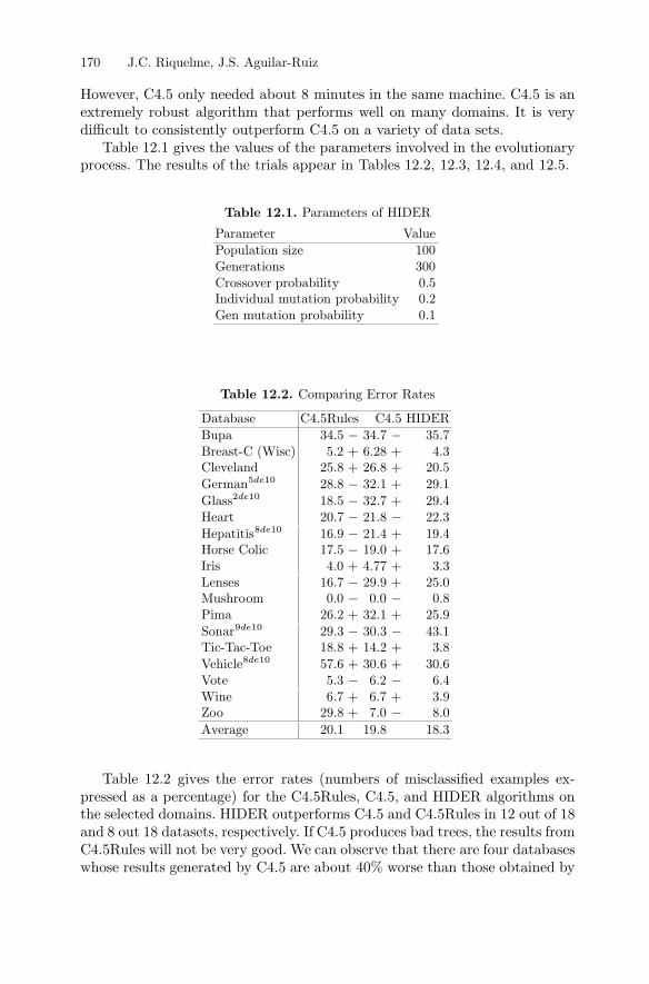
8
de
de
de
de
de
5 10
2 10
8 10
9 10
8 10
� �
��� ���
�� �
� �
� �
�
Table 12.1.
Table 12.2.
+ ++ +
+
+
++
+ ++
+ +
+ +
+ +
+ ++
170 J.C. Riquelme, J.S. Aguilar-Ruiz
Parameters of HIDER
Parameter ValuePopulation size 100Generations 300Crossover probability 0.5Individual mutation probability 0.2Gen mutation probability 0.1
Comparing Error Rates
Database C4.5Rules C4.5 HIDERBupa 34.5 34.7 35.7Breast-C (Wisc) 5.2 6.28 4.3Cleveland 25.8 26.8 20.5German 28.8 32.1 29.1Glass 18.5 32.7 29.4Heart 20.7 21.8 22.3Hepatitis 16.9 21.4 19.4Horse Colic 17.5 19.0 17.6Iris 4.0 4.77 3.3Lenses 16.7 29.9 25.0Mushroom 0.0 0.0 0.8Pima 26.2 32.1 25.9Sonar 29.3 30.3 43.1Tic-Tac-Toe 18.8 14.2 3.8Vehicle 57.6 30.6 30.6Vote 5.3 6.2 6.4Wine 6.7 6.7 3.9Zoo 29.8 7.0 8.0Average 20.1 19.8 18.3
However, C4.5 only needed about minutes in the same machine. C4.5 is anextremely robust algorithm that performs well on many domains. It is verydifficult to consistently outperform C4.5 on a variety of data sets.Table 12.1 gives the values of the parameters involved in the evolutionary
process. The results of the trials appear in Tables 12.2, 12.3, 12.4, and 12.5.
Table 12.2 gives the error rates (numbers of misclassi�ed examples ex-pressed as a percentage) for the C4.5Rules, C4.5, and HIDER algorithms onthe selected domains. HIDER outperforms C4.5 and C4.5Rules in 12 out of 18and 8 out 18 datasets, respectively. If C4.5 produces bad trees, the results fromC4.5Rules will not be very good. We can observe that there are four databaseswhose results generated by C4.5 are about 40% worse than those obtained by

� �er nr
��
��� �
�
��
�
Table 12.3.
Table 12.4.
+ ++ ++ +
++
+ ++ +
++
+ ++
+ +++
+ ++ +
+
12 Learning Decision Rules with Hybrid-Encoded EAs 171
Comparing Number of Rules
Database C4.5Rules C4.5 HIDERBupa 14.0 28.6 11.3Breast-C (Wisc) 8.1 21.9 2.6Cleveland 11.3 35.2 7.9German 5.2 181.5 13.3Glass 14.0 29.0 19.0Heart 10.5 29.2 9.2Hepatitis 5.4 13.8 4.5Horse Colic 4.1 39.3 6.0Iris 4.0 5.5 4.8Lenses 3.1 4.1 6.5Mushroom 17.2 15.7 3.1Pima 9.8 93.6 16.6Sonar 5.1 16.8 2.8Tic-Tac-Toe 10.7 93.9 11.9Vehicle 3.3 102.3 36.2Vote 6.6 14.7 4.0Wine 4.6 5.4 3.3Zoo 5.3 9.9 7.2Average 7.9 41.1 9.5
Comparing Global Results (C4.5/HIDER)
DatabaseBupa .97 2.53Breast-C (Wisc) 1.46 8.42Cleveland 1.31 4.46German 1.10 13.65Glass 1.11 1.53Heart .98 3.17Hepatitis 1.10 3.07Horse Colic 1.08 6.55Iris 1.40 1.15Lenses 1.20 .63Mushroom .01 5.00Pima 1.24 5.64Sonar .70 6.00Tic-Tac-Toe 3.69 7.89Vehicle 1.00 2.83Vote .96 3.68Wine 1.70 1.64Zoo .88 1.38Average 1.22 4.40
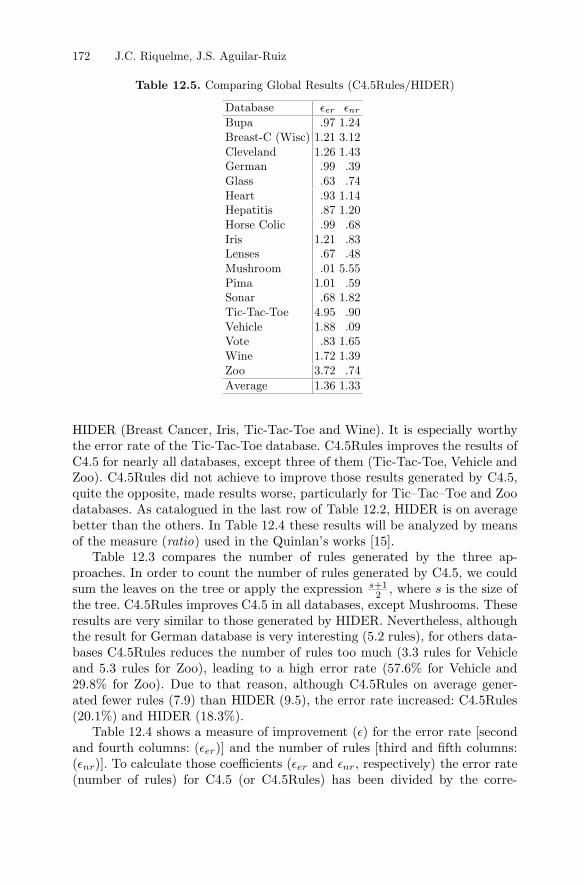
� �
+12
er nr
ratio
s
��
� � �
s
er
nr er nr
Table 12.5.
172 J.C. Riquelme, J.S. Aguilar-Ruiz
Comparing Global Results (C4.5Rules/HIDER)
DatabaseBupa .97 1.24Breast-C (Wisc) 1.21 3.12Cleveland 1.26 1.43German .99 .39Glass .63 .74Heart .93 1.14Hepatitis .87 1.20Horse Colic .99 .68Iris 1.21 .83Lenses .67 .48Mushroom .01 5.55Pima 1.01 .59Sonar .68 1.82Tic-Tac-Toe 4.95 .90Vehicle 1.88 .09Vote .83 1.65Wine 1.72 1.39Zoo 3.72 .74Average 1.36 1.33
HIDER (Breast Cancer, Iris, Tic-Tac-Toe and Wine). It is especially worthythe error rate of the Tic-Tac-Toe database. C4.5Rules improves the results ofC4.5 for nearly all databases, except three of them (Tic-Tac-Toe, Vehicle andZoo). C4.5Rules did not achieve to improve those results generated by C4.5,quite the opposite, made results worse, particularly for Tic�Tac�Toe and Zoodatabases. As catalogued in the last row of Table 12.2, HIDER is on averagebetter than the others. In Table 12.4 these results will be analyzed by meansof the measure ( ) used in the Quinlan�s works [15].Table 12.3 compares the number of rules generated by the three ap-
proaches. In order to count the number of rules generated by C4.5, we couldsum the leaves on the tree or apply the expression , where is the size ofthe tree. C4.5Rules improves C4.5 in all databases, except Mushrooms. Theseresults are very similar to those generated by HIDER. Nevertheless, althoughthe result for German database is very interesting (5.2 rules), for others data-bases C4.5Rules reduces the number of rules too much (3.3 rules for Vehicleand 5.3 rules for Zoo), leading to a high error rate (57.6% for Vehicle and29.8% for Zoo). Due to that reason, although C4.5Rules on average gener-ated fewer rules (7.9) than HIDER (9.5), the error rate increased: C4.5Rules(20.1%) and HIDER (18.3%).Table 12.4 shows a measure of improvement ( ) for the error rate [second
and fourth columns: ( )] and the number of rules [third and �fth columns:( )]. To calculate those coefficients ( and , respectively) the error rate(number of rules) for C4.5 (or C4.5Rules) has been divided by the corre-

12.5 Conclusions
12.6 Future Works
12 Learning Decision Rules with Hybrid-Encoded EAs 173
sponding error rate (number of rules) for HIDER. On average, HIDER foundsolutions that had less than one fourth of the rules output by C4.5. Surpris-ingly, C4.5 generated a number of rules �ve times greater than HIDER forone third of the databases. It is worth noting that applying HIDER, morethan two thirds of the databases produce less than half the rules. C4.5 onlywas better with the Lenses database. C4.5 made the error rate better for sixdatabases, although only three of them improved signi�cantly (Mushrooms,Sonar and Zoo). In summary, the averaged error rate generated by C4.5 is22% greater and the averaged number of rules 340%. This reason leads tous to make a comparison with C4.5Rules, mainly in regard to the number ofrules. The average ratio of the error rate of C4.5 to that of HIDER is 1.22,while the ratio of the number of rules is 4.40. Although the results in Table12.3 indicated that C4.5Rules improved on average (7.9 rules) to HIDER (9.5rules), analyzing the relative increase of the number of rules, we can observethat those numbers can be deceptive. C4.5Rules generates an averaged num-ber of rules 33% greater (fourth column), as well as an averaged error rate36% higher (�fth column), as it is shown in the last row of Table 12.5.As the overall averages at the bottom of the tables indicate, HIDER is
more accurate than C4.5, and C4.5 is more accurate than C4.5Rules. HIDERproduces fewer rules than C4.5Rules, which also generates fewer than C4.5.
An EA-based supervised learning tool to classify databases is presented in thispaper. HIDER produces a hierarchical set of rules, where each rule is tried inorder until one is found whose conditions are satis�ed by the example beingclassi�ed. The use of hierarchical decision rules led to an overall improvementof the performance on the 18 databases investigated here. In addition, HIDERimproves the �exibility to construct a classi�er varying the relaxing coefficient.In other words, one can trade off accuracy against understanding. HIDER wascompared to C4.5 and C4.5Rules and the number of rules as well as the errorrate were decreased. To summarize shortly, the experiments show that HIDERworks well in practice.
Evolutionary algorithms are very time-consuming. This aspect is being ana-lyzed from the viewpoint of the coding. We are designing a new type of codingthat uses natural numbers for both continuous and discrete attributes, so asthe speci�c genetic operators. This encoding method allows us to reduce thedimensionality of the search space so that the algorithm might converge morequickly.
v2
12.7 Acknowledgment
References
Another aspect being studied is the way in which the evaluation functionanalyzes each example from the database. Normally, the information is loadedin a vector, and for each individual of the population the whole vector isprocessed. Research on improvements to the data structure as input of EAsin order to reduce the time complexity is currently being conducted.
The research was supported by the Spanish Research Agency CICYT undergrant TIC2001�1143�C03�02.
Progress in Arti�cial IntelligenceIBERAMIA�98. Lecture Notes in Arti�cial Intelligence 1484. Springer-Verlag
Lecture Notes in Arti�cialIntelligence 1415. Springer-Verlag
Third International Conference on GeneticAlgorithms
Complex Systems
Machine Learning: Proceedings of the Fifth European Conference(EWSL-91)
Machine Learning
Foundations of Genetic Algorithms-2Genetic Algorithms in Search, Optimization and Machine
Learning
Machine learning
Machine Learning
Evolutionary ComputationGenetic Algorithms + Data Structures = Evolution Pro-
gramsMachine Learning
174 J.C. Riquelme, J.S. Aguilar-Ruiz
1. J. S. Aguilar, J. C. Riquelme, and M. Toro (1998) Decision queue classi�er forsupervised learning using rotated hyperboxes. In
,pages 326�336.
2. J. S. Aguilar, J. C. Riquelme, and M. Toro (1998) A tool to obtain a hierarchicalqualitative set of rules from quantitative data. In
, pages 336�346.3. J. Antonisse (1989) A new interpretation of schema notation that overturnsthe binary encoding constraint. In
, pages 86�97. Morgan Kaufmann.4. S. Bhattacharyya and G.J. Koehler (1994) An analysis of non-binary geneticalgorithms with cardinality . , 8:227�256.
5. C. Blake and E. K. Merz (1998) UCI repository of machine learning databases,1998.
6. P. Clark and R. Boswell (1991) Rule induction with cn2: Some recents im-provements. In
, pages 151�163.7. K. A. DeJong, W. M. Spears, and D. F. Gordon (1993) Using genetic algorithmsfor concept learning. , 1(13):161�188.
8. L. J. Eshelman and J. D. Schaffer (1993) Real-coded genetic algorithms andinterval-schemata. , pages 187�202.
9. D. E. Goldberg (1989). Addison-Wesley.
10. R. C. Holte (1993) Very simple classi�cation rules perform well on most commonlyused datasets. , 11:63�91.
11. C. Z. Janikow (1993) A knowledge-intensive genetic algorithm for supervisedlearning. , 1(13):169�228.
12. G.J. Koehler, S. Bhattacharyya, and M.D. Vose (1998) General cardinality geneticalgorithms. , 5(4):439�459.
13. Z. Michalewicz (1996). Springer-Verlag, 3 ed..
14. T. Mitchell (1997) . McGraw Hill.

Journal ofArti�cial Intelligence Research
Genetic Neural Networks on MIMD Computers
Machine LearningProceedings of
the Third International Conference on Genetic Algorithms
Proceedings of European Conference onMachine Learning
Evolutionary Computation
Evolutionary Computation
Journal of Arti�cial Intelligence ResearchFoun-
dations of Genetic Algorithms-1
12 Learning Decision Rules with Hybrid-Encoded EAs 175
15. J. R. Quinlan (1996) Improved use of continuous attributes in c4.5., 4:77�90.
16. N. J. Radcliffe (1990) . Ph. d.,University of Edinburgh.
17. R. L. Rivest (1987) Learning decision lists. , 1(2):229�246.18. G. Syswerda (1989) Uniform crossover in genetic algorithms. In
, pages 2�9.19. G. Venturini (1993) Sia: a supervised inductive algorithm with genetic search forlearning attributes based concepts. In
, pages 281�296.20. M.D. Vose and A.H. Wright (1998) The simple genetic algorithm and the walshtransform: Part i, theory. , 6(3):253�273.
21. M.D. Vose and A.H. Wright (1998) The simple genetic algorithm and the walshtransform: Part ii, the inverse. , 6(3):275�289.
22. D. Whitley (1993) A genetic algorithm tutorial. Technical Report CS-93-103,Colorado State University, Fort Collins, CO 80523.
23. D. R. Wilson and T. R. Martinez (1997) Improved heterogeneous distance func-tions. , 6(1):1�34.
24. A. H. Wright (1991) Genetic algorithms for real parameter optimization., pages 205�218.

Summary.
13.1 Introduction
13
Evolvable Hardware Techniques forGate-Level Synthesis of CombinationalCircuits
This chapter is about the synthesis of combinational logic circuits usingevolvable hardware. The chapter introduces several approaches recently followed bya number of researchers to tackle this problem. Research trends, immediate and foryears to come, are presented.
A. Hernández-Aguirre
A combinational circuit is the implementation of some Boolean function. Inreal- world applications, the usual goal is to derive that circuit that implementsthe function using the smallest number of components. There are several in-terpretations to this problem because in Boolean algebra there are differentsets of primitives with the �universal generator� property. Sets of primitiveoperators with this property are, for instance: {and, or, not },{and, xor, not},and {nand}. Although any of these sets is sound and complete in Booleanlogic, the circuits they generate differ in size. What they share, though, is thetop-down strategy used to create the circuit. Human designers derive suchminimum circuits by working in a top-down fashion. By a proof process andlots of human ingenuity, all knowledge about principles and valid operationsin the Boolean domain have been forged into a few axioms and laws. Humandesigners repeatedly apply the set of axioms of Boolean logic to a Booleanformula in order to transform it into an equivalent but shorter expression.Therefore, the resulting expression is derived or inferred through this deduc-tive process.Evolutionary computation techniques are popular design and optimiza-
tion tools that challenge human designers. Inspired in the Darwinian theoryof the evolution of the species, evolutionary techniques mimic the dynam-ics of a population where the �ttest individuals survive and reproduce, andtheir genes prevail in their children that populate the next generation. Anyindividual encodes a solution, a Boolean formula in our discussion, which is

{ }and, or, not
178 A. Hernández-Aguirre
13.2 Basic Concepts in Evolvable Hardware
intrinsic evolvable hardware extrinsic evolv-able hardware
only a partial solution of the problem. No knowledge other than how welleach individual solves the problem is used during the evolution. Evolutionarytechniques build upon partial solutions to synthesize the solution. As noted,no knowledge about Boolean domain is precomputed, or axioms used to �ndequivalent formulas; with no recipes at hand other than surviving, evolution-ary computation techniques construct or synthesize circuits. The solutions arequite uncommon since bottom-up mechanisms explore different areas of thesearch space [29].Evolvable Hardware (EHW for short) exploits this unique capacity for the
synthesis of circuits (which is not easily found on the human side). EHWis, in essence, a combination of evolutionary computation and recon�gurablehardware. In this nascent �eld there are several approaches that, combinedwith new technologies and platforms, have spawn a number of modalities.This chapter presents the most important current and future research
trends in evolvable hardware for the synthesis of combinational circuits. Thechapter is organized as follows. Section 13.2 deals with different approaches toevolvable hardware and makes a brief introduction to Boolean circuit synthe-sis. Section 13.3 introduces seven approaches to extrinsic evolvable hardware.Finally, Section 13.4 discusses some of the research trends.
The utter goals of any full evolvable hardware system are self-recon�gurationand self-adaptation. Self-recon�guration refers to the ability of a system tomodify its structure in order to tackle different tasks (in some closed domain)using the best resources available. Self-adaptation means the use of evolu-tionary techniques to generate the solution using such resources. Most EHWsystems are off-line learning system; therefore, they work in two steps. In stepone a new task is presented to the system; thus, a solution is generated byrecon�guration and adaptation. In step two the system responds to new inputdata in the way it has learned to do so. The adaptation algorithm can be ranin hardware or software. When it runs on hardware the technique is called
, whereas the other case is called. We could say the difference depends on the place where the
evolutionary algorithm is run. Figure 13.1 shows the modules of any intrin-sic evolvable hardware platform for combinational circuit design [15, 14, 13].The adaptation module is a GA embedded in hardware, the �tness evaluatormodule also runs in hardware, and the recon�gurable module is a PLA (anFPGA is frequently used instead of the PLA).Another issue is the �granularity� level used during the evolutionary
process. Granularity refers to how basic the primitive elements used for thesynthesis of solutions are. For example, �ne granularity evolution could onlyuse gates, but coarse granularity could combine these primitives

EVALUATOR
FITNESS
PLA SECTIONF
BOOLEAN VARIABLES
EVOLUTIONARYALGORITHM
X Y Z F
0 0 0 0
0 0 1 0
0 1 0 0
1 0 0 0
1 0 1 1
1 1 0 1
1 1 1 0
0 1 1 1
X Y Z F
0 0 0 0
0 0 1 0
0 1 0 0
1 0 0 0
1 0 1 1
1 1 0 1
1 1 1 0
0 1 1 1
EVALUATOR
FITNESS
F
BOOLEAN VARIABLES
EVOLUTIONARYALGORITHM
SIMULATOR
HDL, VERILOGSPICE
mixtrinsicevolution
Figure 13.1.
Figure 13.2.
13 Synthesis of Combinational Circuits 179
Intrinsic evolvable hardware system.
Extrinsic evolvable hardware system.
with other components built upon the primitives, say multiplexers and de-coders. The �ne granularity approach is called �gate-level�, whereas the othercase is called �functional-level�. Granularity must be considered at the timethe representation of the individuals is being de�ned because it has a directimpact on scalability (or capacity to design bigger circuits without chang-ing the algorithm). A clear advantage of extrinsic EHW is the better controlof granularity since adjustments are possible at any time. Figure 13.2 showsthe modules of an extrinsic evolvable hardware platform. The evolutionaryalgorithm is implemented in software, the �tness evaluator is also a programtightly coupled with a simulator (HDL, Verilog, or Spice). The simulator �ex-ecutes� every circuit in the population and the result is used to compute a�tness value. Notice that in this case everything is modeled in software, butcombinations of intrinsic and extrinsic are also possible and called
[28].
The evolutionary techniques used in EHW are: Genetic Algorithms (GA),Genetic Programming (GP), and Evolutionary Strategies (ES). Although GA
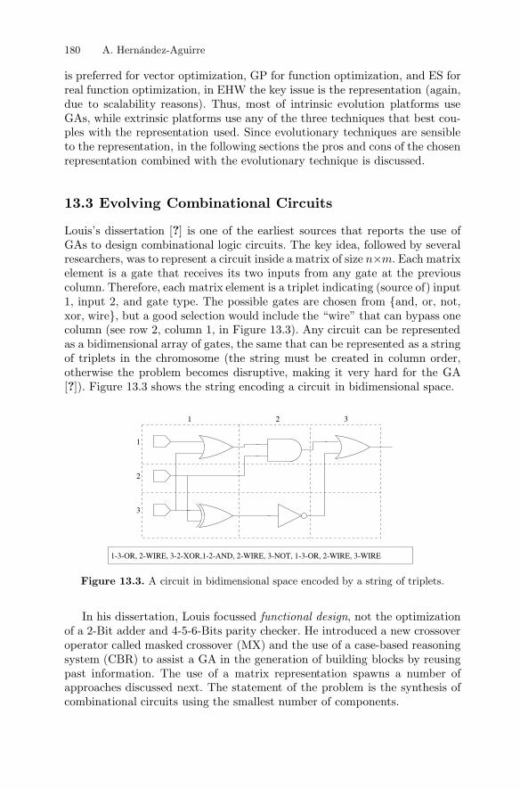
21
1-3-OR, 2-WIRE, 3-2-XOR,1-2-AND, 2-WIRE, 3-NOT, 1-3-OR, 2-WIRE, 3-WIRE
2
3
1
3
�n m
?
?
Figure 13.3.
functional design
13.3 Evolving Combinational Circuits
180 A. Hernández-Aguirre
A circuit in bidimensional space encoded by a string of triplets.
is preferred for vector optimization, GP for function optimization, and ES forreal function optimization, in EHW the key issue is the representation (again,due to scalability reasons). Thus, most of intrinsic evolution platforms useGAs, while extrinsic platforms use any of the three techniques that best cou-ples with the representation used. Since evolutionary techniques are sensibleto the representation, in the following sections the pros and cons of the chosenrepresentation combined with the evolutionary technique is discussed.
Louis�s dissertation [ ] is one of the earliest sources that reports the use ofGAs to design combinational logic circuits. The key idea, followed by severalresearchers, was to represent a circuit inside a matrix of size . Each matrixelement is a gate that receives its two inputs from any gate at the previouscolumn. Therefore, each matrix element is a triplet indicating (source of) input1, input 2, and gate type. The possible gates are chosen from {and, or, not,xor, wire}, but a good selection would include the �wire� that can bypass onecolumn (see row 2, column 1, in Figure 13.3). Any circuit can be representedas a bidimensional array of gates, the same that can be represented as a stringof triplets in the chromosome (the string must be created in column order,otherwise the problem becomes disruptive, making it very hard for the GA[ ]). Figure 13.3 shows the string encoding a circuit in bidimensional space.
In his dissertation, Louis focussed , not the optimizationof a 2-Bit adder and 4-5-6-Bits parity checker. He introduced a new crossoveroperator called masked crossover (MX) and the use of a case-based reasoningsystem (CBR) to assist a GA in the generation of building blocks by reusingpast information. The use of a matrix representation spawns a number ofapproaches discussed next. The statement of the problem is the synthesis ofcombinational circuits using the smallest number of components.

∑
��
dynamic
1 =
1
2 = 1 +
1 2
13 Synthesis of Combinational Circuits 181
fcorrect outputs
total number of outputs.
f
f f WireGates.
f f
13.3.1 Gate-Level Synthesis Using Binary GA
Fitness function.
Louis proposed the use of a matrix to represent a circuit, but several issuesstill had to be solved in order to use an evolutionary technique as a designtool. Coello et al. proposed the Binary Genetic Algorithm (BGA), a standardGA with binary representation, and a set of strategies to tackle the problem[1]. Problem statement. Use a GA with binary representation to synthesizea combinational circuit with the smallest number of components. The set ofprimitive gates is: {and, or, not, xor, wire}. The circuit is evolved inside amatrix, as explained in Section 13.3. The pending issues (not discussed so far)are
design of a �tness function suitable for both circuit design and optimizationmatrix size
The synthesis of circuits optimized in size is a task con-trolled by the �tness function. The �tness of a circuit is measured by com-paring the expected values de�ned in the truth table against the real outputvalues. Therefore, the function counts the number of correct matches andreturns the proportion of matches as the �tness value. The �tness functionworks in two stages, therefore called , which are applied at differenttimes of the evolution.
1. Stage one. The �tness function guides the search until the �rst 100%functional circuit (that fully complies with the truth table) appears in thepopulation.
2. Stage two. Once the �rst 100% functional circuit is generated, the �tnessfunction is switched to one that counts the number of �wire gates� in thecircuit, plus (above). This indirect strategy proved very efficient sincemore wires means fewer �real gates�.
Either �tness function is used to measure all the population, that is, it neverhappens that some circuits are measured with function and others withat some generation. Some circuits are harder to design when the truth tableis unbalanced, that is, the number of outputs in 1 (or 0) is much more thanthose in 0 (or 1). That kind of circuits presents the �genetic cliff� problem,which is the case of two individuals that are quite close in phenotypic spacehave an uncomparable distance in genotypic space; for example, a truth tablewith 15 ones and only 1 zero. The solution is a weighted �tness function thatgives to that zero a reasonable or similar importance of any 1. A good strategyis the following:
1. Count the number of 1s and 0s in the truth table.

1 = +
5 5
= 3
� �
��
�
�
�
representation bias
182 A. Hernández-Aguirre
wz wof wz No.ofzeros wo No.ofones
�
�
Matrix size.
Results and discussion.
13.3.2 Mending the Representation Bias: Gate-Level Synthesiswith NGA
2. All 1s found represent 50% of the total.3. All 0s found represent 50% of the total.4. Compute the weight of each zero, , and of each one, .5. .
The matrix serves as a reference for circuit connectivity andworks as an environment for the evolution. Therefore, it is important to usethe proper size for a circuit, but this is not a simple task. The size of thematrix is determined using the following procedure:
Start with a square matrix of size 5.If no feasible solution is found using this matrix, then increase the numberof columns by 1.If no feasible solution is found using this matrix, then increase the numberof rows by 1.Repeat steps 2 and 3 until a suitable matrix is found.
The BGA design tool has been successfully testedwith several circuit design problems, some of them reported in [1, 5, 6]. BGA�nds in most cases smaller circuits than those generated by human design-ers using Karnaugh maps. It also �nds smaller circuits than those generatedby special methods like the one proposed by Sasao that only uses ANDs &XORs gates [25]. BGA seems to favor the use of XOR gates, generating correctcircuits but hard for the humans to understand. Also, the �evolutionary trans-formations�that make a functional circuit smaller are hard to understand andfollow no apparent logic. The weakness of the method is the poor scalability.Bigger problems are almost impossible to solve since evolution is containedby the matrix, and search space limited to the bidimensional space. Anotherissue is the due to the binary representation. There aretwo sources of bias, one comes from the triplet representation, and the otherfrom the matrix size. For instance, when BGA uses 5 primitive gates it needs3 bits to represent all combinations, thus 3 out of 8 are not used. Similarly, ifthe matrix size is , 3 bits are needed to indicate where the input comesfrom, but again, 3 combinations are not used.
NGA is a GA with N-cardinality encoding. The purpose of using more thanone alphabet (of any cardinality) in the genotypic string is to encode thetriplets (see Fig. 13.3) in such a way that there are no combinations left withno use. Coello et al. [2] propose such a strategy in an approach called NGA. InFigure 13.4 a triplet using two alphabets is shown. Inputs 1 and 2 are any rowout of {1,2,3}. Therefore, by choosing the cardinality of alphabet thereis a one-to-one mapping between the alphabet symbol and the row number.Same for the speci�cation of the gate type. There are 5 gates, so the alphabethas cardinality 5.

=5=3
GateIn2In1
321
2
3
1
=3
Figure 13.4.
Results and discussion.
13.3.3 Functional-Level Synthesis
Results and discussion.
13 Synthesis of Combinational Circuits 183
A triplet representing a gate and its inputs with two alphabets.
Genetic operators selection, crossover, and muta-tion are not affected. NGA proved superior than BGA in most circuits, bothin terms of speed of convergence and in terms of total evaluations performed.The reason seems to be less disruption of the building blocks and better reuseof the circuit components. Also, because strings are shorter, the evolutionaryalgorithm exhibits better behavior.
Miller introduced an extrinsic EHW technique for functional-level design [22,23, 24]. As noted before, functional techniques are the combination of primitivegates with other components built over the primitive gates. Miller combinesANDs, ORs, XORs, and NOTs, with multiplexers and some more Booleanfunctions like NANDs, NORs, and the like. His set of 12 Boolean functionspretends to characterize the activity of any subset of a circuit. The adaptationmechanism is implemented by a GA. But the most important aspect is therepresentation. Using alphabets of cardinality greater than 2, a single geneencodes one of the 12 Boolean functions. This approach, although similar tothe NGA, has a drawback: the cardinality of the alphabet grows exponentiallywith the number of input variables. Miller also models circuit connectivity bya matrix; thus, evolution is contained by some matrix geometry.
Functional-level synthesis shows good scalabilitybecause the granularity is not restricted to only primitive gates. At the sametime, for the same reason, the circuit size is harder to optimize (some solutionscontrasted with NGA are clearly bigger).Miller also proposed a special form of Genetic Programming called Carte-
sian Genetic Programming (CPG), to tackle learning Boolean function prob-lems. Strictly speaking, it must be called GP because it evolves functions,although individuals are not trees as it is common in GP. CPG uses linear in-teger chromosomes; the advantage of this representation is the easiness of the
32 = 8
practical
states
184 A. Hernández-Aguirre
13.3.4 Bidirectional Incremental Evolution
13.3.5 Multiobjective EHW Optimization: MGA
evaluation of the strings. CPG does not evolve circuits but functional Booleanfunction expressions, and its goal is not the optimization of functions.
A re�ection on functional-level and gate-level makes one to think that what weneed is the best of both approaches. When primitive gates are used, scalabilityis poor but size optimization is possible. When gates are more complex, thenoptimization is poor. Thus, we can ask: could it not be possible to combinescalability and size optimization in just one method? Kalganova proposesBidirectional Incremental Evolution (BIE) to tackle this problem [17, 16].According to her, extrinsic EHW design of digital circuits (she meansreal-world applications) involves the following three major problems:
1. limitation in the chromosome length2. �stalling� effect in the evolution process3. restriction of the computation time
BIE solves the three of them by combining two main approaches: Divide-and-Conquer and Incremental Evolution. The key notion is to break downa complex task into simpler subtasks, evolve each of the subtasks, and thenmerge incrementally the evolved subsystems. In essence, BIE is the soundcombination of top-down and bottom-up methods. The former stage is con-ducted by a process called �evolution toward a modularized system�, the latterstage by a second process called �evolution toward an optimized system�. Analternative way to understand the work of Kalganova is through the workof Gero [9]. Gero�s Genetic Engineering system also combines top-down andbottom-up strategies. In the top-down stage, elementary building blocks aretargeted and those more likely to produce designs with the required charac-teristics are evolved. In the second stage, the proper design goals are focussedand the solution is generated by using the evolved primitive building blocks.Several researchers work in this problem, notably Seok, who also proposes adecomposition strategy for EHW [26].Kalgnova results are encouraging and promising. Further work needs to be
done to fully develop a BIE platform for circuit evolution.
The �tness function used by BGA and NGA has been called dynamic sinceit does change during evolution. The goal is to capture two possibleof the circuit (functional or not functional). Looking at the problem in thisway, a circuit can have many more states. For instance, if the truth table hasthree inputs and one output, then there are output values. A circuit iscalled in �state 3� if only 3 out of the 8 expected outputs are correct. Thus,the circuit design can be reformulated as the problem of ��lling all the stateswith the correct value�. Since there are many states, then the problem is to
j j
j j
�� �
⇒
X
X X
X
X X
X X
X X X X X X
X
13 Synthesis of Combinational Circuits 185
= 8+1 +1
( ) = ( ) = 0
= 0 =
= ( )
( )
( )
( ) = ( ) ( ) = ( ) + ( )
( )
to handle each of the outputs of a circuit as an objective
X XX
Results and discussion.
13.3.6 EHW Using the Ant System (AS)
mm m
if o t then fitness ,
else if v then fitness v,
else fitness f ,
o j tj v
f
if unfeasible f h else f h w .
w
design the �tness function able to �ll all the states. A dynamic �tness functionthat checks all circuit states is only possible for small circuits. Therefore, thesolution is to use a technique that considers each state as an objective, orindependent goal.Coello et al. [7] introduced the Multiobjective Genetic Algorithm (MGA)
whose evolutionary algorithm is based on the Vector Evaluated Genetic Al-gorithm (VEGA) to tackle this problem. The main idea behind the approachis to use a population-based multiobjective optimization technique, such asVEGA, . Thus, a cir-cuit with outputs becomes a problem with 8 restrictions plus a singleobjective function, that is, goals. VEGA splits the population intosubpopulations, assigning each subpopulation to a circuit output and givingto it the mission of matching the correct value speci�ed in the truth table.The issue is how to handle the different situations (or states) that could arise.The �tness of a circuit is evaluated as follows:
where refers to the value of output for the encoded circuit ; istarget value for output ; and is the number of outputs that are not matchedby the circuit . The �tness function is calculated as follows:
In this equation, h( ) refers to the number of matches between circuit andthe truth table, and is the number of wires in circuit . Kalganovaalso proposed the use of multiobjective optimization techniques based on theconcept of Pareto fronts for the optimization of logic circuits [17].
MGA was tested with similar complexity circuitsused to test BGA and NGA. MGA improves the behavior of NGA, that is,it requires less number of �tness function evaluations. In several cases thecircuits are even smaller than NGA (recall the NGA also improved BGAcircuits). Another interesting issue is the cooperative effort observed betweensubpopulations. The �tness function improves as more restrictions are met,and at the same time, the �tness function helps the subpopulations to evolvetoward the correct value.
The MGA system considers each circuit output as a restriction and splits thepopulation into subpopulations, assigning one output to one subpopulation.As noted, a cooperative effort is observed between subpopulations. MGA dis-tributes the overall effort among subpopulations, but the cooperation is not
pheromone
Results and discussion.
186 A. Hernández-Aguirre
under control of the algorithm, neither is knowledge of one subpopulationcommunicated to either one subpopulation.Coello et al. used the Ant System (AS) for the �rst time ever for the
design of combinational circuits [3, 4]. The Ant System is a meta-heuristicinspired by colonies of real ants. Ants deposit a chemical substance on theground ( ) that in�uences the behavior of the entire colony: ants willtend to walk over those paths where there is a larger amount of pheromone.Pheromone trails can be seen as a communication mechanism among ants.From the computer science perspective, the AS is a multiagent system whereinteractions among low-level agents (ants) results in the complex behaviorof the colony. The AS can be seen as a distributed knowledge system. Localknowledge collected by the agents (ants) is centralized, analyzed, and redis-tributed (passed back) to the local agents as an information of the collectivebehavior. If the colony gets closer to the goal, then the agents will know theyare �doing well� and their trails will be reinforced. Otherwise, the trails areabandoned (the pheromone evaporates) and new routes will be inspected. Thisis called reinforcement learning, a weaker form of supervised learning.There are three main ideas from real ant colonies that have been adopted
by the AS:
1. Indirect communication through pheromone trails.2. Shortest paths tend to have a higher growth rate of pheromone values.3. Ants have a higher preference (with certain probability) for paths thathave higher amount of pheromones.
The AS was proposed for the traveling salesman problem (TSP), and ac-cording to Dorigo [8], to apply efficiently the AS, it is necessary to reformulatethe problem as one in which we want to �nd the optimal path of a graph andto identify a way to measure the distance between nodes. Therefore, in theTSP, the ants traverse a path and try to �nd the shortest way to the goal.In the circuit design problem, the goal is to produce a fully functional circuitby minimizing a certain payoff function, and �shortest� means �fewer numberof gates�. Thus, the colony �nds a trail from the input to the output of thecircuit by assembling local information of low cost paths.
An important aspect of this application is that itshows the factibility of AS to work in other domains. As noted, the problemis how to translate or reformulate the problem at hand into a graph searchingprocedure. The advantage of the AS is its robustness; it consistently �ndsthe smallest known circuit for some truth table, having in this respect betterbehavior than the evolutionary techniques NGA and BGA. Its disadvantageis the performance, which tends to degrade rapidly as the size of the circuitincreases.

0 1
0 1
0 1 0 10 1
10 0 1 1 0
0
C2
C0 C1 C1
0 1C1 C0
FC2 C1 C00 0 00 0 10 1 00 1 11111
0011
0101
F000
0110
1
( A2, ( B1, ( A0, 0, 1 ), 0 ), ( B0, ( B1, 0, 1 ), ( B1, 1, 0 ) ) )
Figure 13.5.
13.3.7 EWH Using GP and Muxes
13 Synthesis of Combinational Circuits 187
Truth table for logic function speci�cation, circuit generated, and itscoding.
All discussed approaches use a matrix to represent circuit connectivity. Al-though all approaches have tried to improve all sorts of convergence and ro-bustness problems, the matrix itself is the source of the problem. This is sobecause the search space is restricted to the subset imposed by the matrixrepresentation. In other words, the matrix representation restraints the scal-ability of the algorithm (it has been told everywhere that the evolutionarytechnique used is not as important as the representation).Hernández-Aguirre [12, 11, 10] proposed gate-level EHW using GP and
multiplexers to improve the scalability problem by giving more freedom forexploration and exploitation through a representation that could grow andshrink as needed. Thus, the search space is not restricted by the geometryof the representation. The approach is a common GP application since indi-viduals are represented by trees and what is evolved is a function (Boolean).It is not clear though whether this approach is gate-level or functional-levelbecause the multiplexer works as a primitive (but it is built by the primitives{and,or,not}). The problem statement has not changed here: synthesize a cir-cuit using the smallest number of binary multiplexers using GP. An exampleof a synthesized circuit and its representation is shown in Figure 13.5. Notethat entering a multiplexer there are only 1s, 0s, and data from immediateprevious multiplexers.
Many GP applications have been illustrated by Koza [18], but he gen-erates Boolean functions and multiplexers in symbolic form, not gate-level(Koza has many proposals similar to gate-level but for electronic circuits [19])Multiplexers are sound components for the synthesis of circuits because theyare universal logic function generators, thus, an equivalent power shared withthe set of primitives {and,or,not} for the synthesis of circuits. A procedure

0
1
0
1
0
1
0
1
0
1
0
1
0
1
0 1
X Y
Z
Ao
CLASS "A"
Functional equivalence between Muxes class A and class B
CLASS "B"
Bo0 1
Z
Y X
CLASS "A"
Ao0 1
X Y
CLASS "B"
Bo0 1
X Y
Y Xf(000)
f(100)
f(010)
f(110)
f(001)
f(101)
f(011)
f(111)
X2 X1 X0
f(X2X1X0)
Implementation Muxes class A and class B
31
| |
1 2
�
�
j j
j j
( )
= 1 = 0
= � +
( )
n
j j
x j x j
j x j x
Figure 13.6.
class A class Bactive
f x , x , . . . , xx x
f x f x
f x f x f
mux, left child, right child
188 A. Hernández-Aguirre
Implementation of a multiplexer of -control lines by means of seven-control line. Muxes class �A� and class �B�. Functional equivalence between bothclasses.
to implement Boolean functions based on multiplexers uses Boolean residuesand Shannon�s expansion [27], de�ned next.The residue of a Boolean function with respect to a vari-
able is the value of the function for a speci�c value of . It is denoted by, for and by for .A Boolean function can then be expressed in terms of these residues in the
form of Shannon�s expansion:
Multiplexers can be �active low� or �active high� devices, a quality simplycalled here and . The control line is located on the side of theinput to be propagated when the control is . The active state will be �1�for all the examples presented in this paper. Circuits can be synthesized usingonly one or both mux classes. Figure 13.6 depicts both classes of multiplexersand the construction of larger multiplexers on simpler elements.
A circuit is represented by binary trees, which are encoded as lists. Es-sentially, each element of the list is the tripletthat encodes subtrees as nested lists. The tree captures the essence of thecircuit topology, allowing only children to feed their parent node (or 1s and0s as speci�ed in the problem statement). Crossover operator is implementedbetween node-node, node-leaf (node other than root node), and leaf-leaf. Mu-tation assigns a random value (in the range) to either node or leaf. The �tnessfunction is also dynamic and works in the same two stages as described in Sec-tion 13.3.1.The following Boolean functions, speci�ed by true terms, are samples of
some experiments.
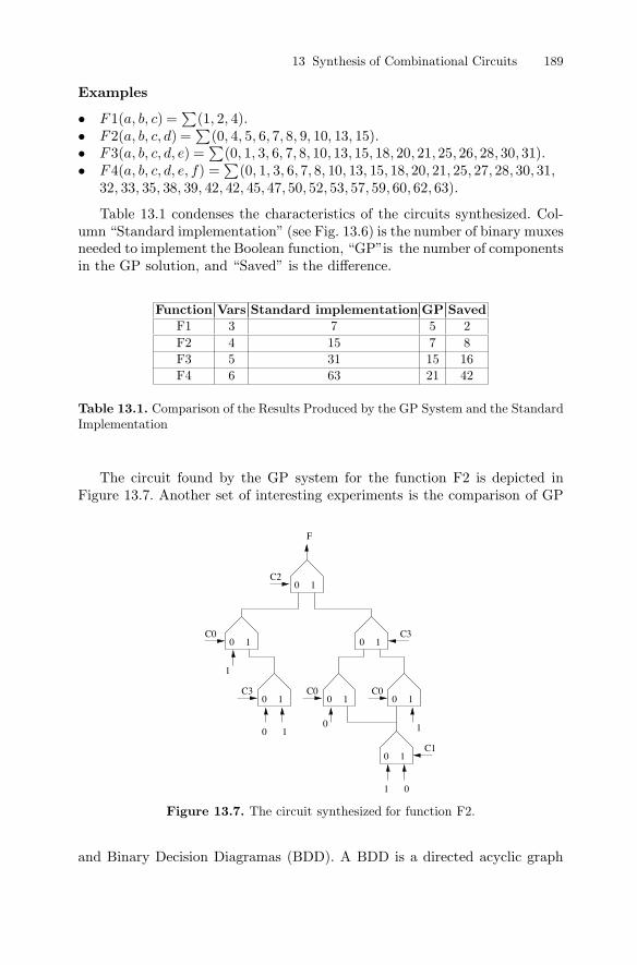
0 1
0 1 0 1
0 1 0 1
0 1
0 1
F
1
0 10
1
1
C2
C0 C3
C3 C0 C0
C1
0
∑∑∑∑����
Examples
Function Vars Standard implementation GP Saved
Table 13.1.
Figure 13.7.
F a, b, c , ,F a, b, c, d , , , , , , , , ,F a, b, c, d, e , , , , , , , , , , , , , , , ,F a, b, c, d, e, f , , , , , , , , , , , , , , , , ,, , , , , , , , , , , , , , , ,
1( ) = (1 2 4)2( ) = (0 4 5 6 7 8 9 10 13 15)3( ) = (0 1 3 6 7 8 10 13 15 18 20 21 25 26 28 30 31)4( ) = (0 1 3 6 7 8 10 13 15 18 20 21 25 27 28 30 3132 33 35 38 39 42 42 45 47 50 52 53 57 59 60 62 63)
13 Synthesis of Combinational Circuits 189
F1 3 7 5 2F2 4 15 7 8F3 5 31 15 16F4 6 63 21 42
Comparison of the Results Produced by the GP System and the StandardImplementation
The circuit synthesized for function F2.
..
.
.
Table 13.1 condenses the characteristics of the circuits synthesized. Col-umn �Standard implementation� (see Fig. 13.6) is the number of binary muxesneeded to implement the Boolean function, �GP�is the number of componentsin the GP solution, and �Saved� is the difference.
The circuit found by the GP system for the function F2 is depicted inFigure 13.7. Another set of interesting experiments is the comparison of GP
and Binary Decision Diagramas (BDD). A BDD is a directed acyclic graph

10
1
2
3
4
5
6
1
0 1
0 1
0 1
0 1
0 1
0
1
1
1
0
0
X3
X4
X6
X5
X1
X2
F
ROBDD
EVOLUTIONARYDESIGN
= + +1 2 3 4 5 6F X X X X X XFigure 13.8.
Results and discussion.
190 A. Hernández-Aguirre
ROBDD and GP circuit for .
where Shannon�s decomposition is carried out at each node. There are severalclasses of BDDs, for instance, Ordered BBDs (OBDD) and Reduced BDDs(RBDD). In OBDD a variable appears at most once on each path from theroot to a terminal node. An RBDD does not contain isomorphic subgraphsnor vertices with both edges pointing to the same node.
Extrinsic EHW using GP and multiplexers scalesup nicely for Boolean functions of up to 12 variables. The problem that pre-dates GP is �bloat�, thus, circuits grow up to contain several hundred nodesbefore the functional circuit is found. From there, the circuits begin to shrinkbecause the �tness function is changed to its second stage which favors smallercircuits. It is surprising that GP is rather more efficient in shrinking circuitsthan in growing them. Nonetheless, �introns� appear in the circuit, makingit hard for GP to eliminate the redundancy. Introns are part of the ADNchain, and why they are present is not clear, but apparently this redundancyis necessary for life. Contrasting GP and BDDs circuits is interesting. Circuitsin Figure 13.8 are similar in size, but what is important to note is their re-semblance in topology and difference in node ordering. The circuit generatedby GP in Figure 13.9 is smaller because the restriction imposed to the orderis not required. Nevertheless, it is not easy for BDD to generate of the GPcircuit. Finally, the �odd-parity� circuit shown in Figure 13.10 has minimumsize when it is implemented with XOR gates. The GP circuit captures thesame topology and matches the smallest possible size.
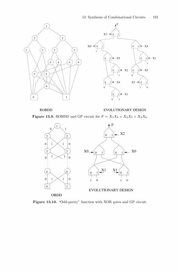
0 1
1
2 2
3 3 3 3
4 4 4 4
5 5
6
0 1
0 1
0 1
0 1
0 1
0 1
0 1
0 10 1
0 1
1
1 0
0
0 1
0
1
1
F
X3
X6 X4
X1
X5
X2
X1
X4
X2
X5
ROBDD EVOLUTIONARY DESIGN
0 1
0 10 1
0 1 0 1
1
2 2
3 3
n
0 1
0
0
0
0
1
0
0
011
1 1
1 1
n
001
X2
X0X0
X1X1
F
EVOLUTIONARY DESIGNOBDD
1
= + +1 4 2 5 3 6F X X X X X XFigure 13.9.
Figure 13.10.
13 Synthesis of Combinational Circuits 191
ROBDD and GP circuit for .
�Odd-parity� function with XOR gates and GP circuit.

�
�
�
poor scalability
13.4 Future Work
Acknowledgment
References
Intl. Journal ofSmart Engineering System Design
Computers and Electrical Engineering
Evolvable Systems: From Biology toHardware. Third Intl. Conf., ICES 2000
192 A. Hernández-Aguirre
1. C. Coello, A. Christiansen, and A. Hernández (2000) Use of evolutionary tech-niques to automate the design of combinational logic circuits.
, 2:299�314.2. C. Coello, A. Christiansen, and A. Hernández (2001) Towards automated evolu-tionary design of combinational circuits. ,27:1�28.
3. C. Coello, R. Zavala, B. Mendoza, and A. Hernández-Aguirre (2000) Ant ColonySystem for the Design of Combinational Logic Circuits. In Miller J., ThompsonA., Thomson P., and Forgarty T.C., (eds.),
, pages 21�30, Edinburgh, UK, October,Springer-Verlag.
The �eld of EHW promises many possibilities, not only in the gate-level syn-thesis arena, but in all kinds of adaptive hardware, either digital or electronic.The main issue in EHW applications is inherited from evolutionary techniques,being this . In order to solve it, the following topics deserve at-tention and research:
The genotype string length. Evolutionary techniques have to keep a repre-sentation of the search space within the organism. A larger or �ner granu-larity search space has a direct impact on the string length, causing �stal-lation� of the evolution. Shorter strings are desirable; thus, suitable targetplatforms for EHW are required, specially for intrinsic evolution.Suitable platforms. The genotype encodes information about the circuitbeing evolved for some target platform. The genotype is decoded and �in-terpreted� in order to �nd its meaning (or circuit). This is a slow processfor extrinsic evolvable hardware and painful for intrinsic evolution sinceevery con�guration has to be uploaded on the recon�gurable device inorder to have its �tness measured.Decomposition and assembling. A combination of top-down and bottom-up procedures has to be assembled and triggered at speci�c times of theevolution. This is a �natural way� for humans to proceed in the analysis ofcomplex systems; perhaps nature has evolved this trait in human beingsfor that purpose. If we could evolve this trait, our simulated organismswould be more capable at complex tasks.
The author acknowledges partial support for this work from CONCyTEGproject No. 01-02-202-111 and CONACyT No. I-39324-A.

Engineering Opti-mization
IntelligentEngineering Systems Through Arti�cial Neural Networks. Volume 6. Fuzzy Logicand Evolutionary Programming
Proceedings of the Intl. Conf. on Arti�cialNeural Nets and Genetic Algorithms
The SecondNASA/DoD Workshop on Evolvable Hardware
New Ideas in Optimization
Advances in Formal Design Methods for CAD
Arti�cial Neural Networksin Engineering Applications, ANNIE2000
Conf. on Evolutionary Computation 2000
The First NASA/DoD Workshopon Evolvable Hardware
Evolvable Systems: From Biology to Hardware. First Intl. Conf. (ICES�96)
Evolutionary Algorithms in Engineering Applications
Evolvable Systems: From Biology to Hardware. Fourth Intl. Conf.,ICES 2001
13 Synthesis of Combinational Circuits 193
4. C. Coello, R. Zavala, B. Mendoza, and A. Hernández-Aguirre (2002) Automateddesign of combinational logic circuits using the ant system.
, 34(2):109�127.5. C. A. Coello, A. D. Christiansen, and A. Hernández Aguirre (1996) Using ge-netic algorithms to design combinational logic circuits. In Cihan H. Dagli, MetinAkay, C. L. Philip Chen, B. R. Farnández, and Joydeep Ghosh, (eds.),
, pages 391�396. ASME Press, St. Louis, Missouri,USA.
6. C. A. Coello, A. D. Christiansen, and A. Hernández Aguirre (1997) AutomatedDesign of Combinational Logic Circuits using Genetic Algorithms. In D. G. Smith,N. C. Steele, and R. F. Albrecht, (eds.),
, pages 335�338. Springer-Verlag, Universityof East Anglia, England.
7. C. Coello Coello, A. Hernández Aguirre, and B. P. Buckles (2000) Evolution-ary Multiobjective Design of Combinational Logic Circuits. In Jason Lohn,Adrian Stoica, Didier Keymeulen, and Silvano Colombano, (eds.),
, pages 161�170. IEEE ComputerSociety.
8. M. Dorigo and G. Di Caro (1999) The Ant Colony Optimization Meta-heuristic. InD. Corne, M. Dorigo, and F. Glover, (eds.) . McGraw-Hill, USA.
9. J. S. Gero and V. A. Kazakov (1995) Evolving Building Blocks for Design usingGenetic Engineering: A Formal Approach. In J. S. Gero and F. Sudweeks, (eds.),
, pages 29�48. University of Sidney,Sidney, Australia.
10. A. Hernández Aguirre, B. P. Buckles, and C. A. Coello Coello (2000) EvolutionarySynthesis of Loolean Functions using Multiplexers. In
, pages 311�316. ASME Press, .11. A. Hernández Aguirre, B. P. Buckles, and C. A. Coello Coello (2000) Gate-levelSynthesis of Boolean Functions using Binary Multiplexers and Genetic Program-ming. In , pages 675�682. IEEE Com-puter Society, .
12. A. Hernández Aguirre, C. A. Coello Coello, and B. P. Buckles (1999) A GeneticProgramming Approach to Logic Function Synthesis by means of Multiplexers.In D. Keymeulen A. Stoica and J. Lohn, (eds.),
, pages 46�53. IEEE Computer Society.13. H. Iba, M. Iwata, and T. Higuchi (1996) Machine Learning Approach to Gate-Level Evolvable Hardware. In T. Higuchi, M. Iwata, and Weixin Liu, (eds.),
, pages327�343, Tsukuba, Japan, October 1996. Springer-Verlag.
14. H. Iba, M. Iwata, and T. Higuchi (1997) Gate-Level Evolvable Hardware: Empir-ical Study and Applications. In Dipankar Dasgupta and Zbigniew Michalewicz,(eds.), , pages 259�276.Springer-Verlag, Berlin.
15. M. Iwata, I. Kajitani, Y. Liu, N. Kajihara, and T. Higuchi (2001) Implementationof a Gate Level Evolvable Hardware Chip. In Yong Liu, Kiyoshi Tanaka, and M.Iwata, (eds.),
, pages 38�49, Tokio, Japan, Springer-Verlag.

The Second NASA/DoD Workshop on Evolvable Hardware
Evolvable Hardware Design of Combinational Logic Cir-cuits
Genetic Programming. On the Programming of Computers bymeans of Natural Selection
Proceedings of the First Annual Conf. on Genetic Pro-gramming
Genetic Algorithms as a Computational Tool for Design
Proceedings ofthe Fourth Intl. Conf. on Genetic Algorithms
Genetic Algorithmsand Evolution Strategy in Engineering and Computer Science
Genetic Programming and Evolvable Machines
Genetic Programming and Evolvable Machines
Logic Synthesis and Optimization
The Seconf NASA/DoD Workshopon Evolvable Hardware
BellSystem Technical Journal
Evolvable Systems: FromBiology to Hardware. Third Intl. Conf., ICES 2000
IEEE Trans. onEvolutionary Computation
194 A. Hernández-Aguirre
16. T. Kalganova (2000) Bidirectional incremental evolution in extrinsic evolvablehardware. In Jason Lohn, Adrian Stoica, Didier Keymeulen, and Silvano Colom-bano, (eds.), , pages65�74. IEEE Computer Society.
17. T. G. Kalganova (2000). PhD thesis, Napier University, Edinburgh, Scotland.
18. J. R. Koza (1992). MIT Press, Massachusetts, USA.
19. J. R. Koza, III F. H. Bennett, D. Andre, and M. A. Keane (1996) AutomatedWYWIWYG design of both the topology and component values of electrical cir-cuits using genetic programming. In J. R. Koza, D. E. Goldberg, D. B. Fogel,and Rick L. Riolo, (eds.),
, pages 123�131, Cambridge, Masachussetts, Stanford University, TheMIT Press.
20. Sushil J. L. (1993) . PhDthesis, Indiana University, Indiana, USA,.
21. Sushil J. L. and Rawlins G. (1989) Designer Genetic Algorithms: Genetic Algo-rithms in Structure Design. In Belew R.K. and Booker L.B., (eds.),
, pages 53�60, San Mateo, California.Morgan Kaufmann Publishers.
22. J. F. Miller, P. Thomson, and T. Fogarty (1998) Designing Electronic Cir-cuits Using Evolutionary Algorithms. Arithmetic Circuits: A Case Study. InD. Quagliarella, J. Périaux, C. Poloni, and G. Winter, (eds.),
, pages 105�131.Morgan Kaufmann, Chichester, England.
23. J. F. Miller, D. Job, and V. K. Vassilev (2000) Principles in the EvolutionaryDesign of Digital CircuitsPart I. ,1(1/2):7�35.
24. J. F. Miller, D. Job, and V. K. Vassilev (2000) Principles in the Evolutionary De-sign of Digital CircuitsPart II. ,1(3):259�288.
25. T. Sasao. (1993) . Kluwer Academic Press,Dordrecht, The Netherlands.
26. H.-S. Seok, K.-J. Lee, and B.-T. Zhang (2000) Genetic Programming of ProcessDecomposition Strategies for Evolvable Hardware. In Jason Lohn, A. Stoica, D.Keymeulen, and Silvano Colombano, (eds.),
, pages 25�34. IEEE Computer Society, .27. C. E. Shannon (1949) The synthesis of two-terminal switching circuits.
, 28(1).28. A. Stoica, R. Zebulum, and D. Keymeulen (2000) Mixtrinsic Evolution. In MillerJ., Thompson A., Thomson P., and ForgartyT.C., (eds.),
, pages 208�217, Edinburgh,UK. Springer-Verlag.
29. A. Thompson, P. Layzell, and R. Salem Zebulum (1999) Explorations in DesignSpace: Unconventional Design Through Arti�cial Evolution.
, 3(3):167�196.

14_______________________________________________________________________________________
The Evolutionary Learning Rule in SystemIdentification
Oscar Montiel, Oscar Castillo, Patricia Melin, Roberto Sepulveda
Summary. In this chapter, we are proposing an approach for integrating evolutionary com-putation applied to the problem of system identification in the well-known statistical signalprocessing theory. Here, some mathematical expressions are developed in order to justifythe learning rule in the adaptive process when a Breeder Genetic Algorithm is used as theoptimization technique. In this work, we are including an analysis of errors, energy meas-ures, and stability.
14.1 Introduction
The problem of determining a mathematical model for an unknown system by ob-serving its input-output data pairs is known as system identification, and it is animportant step when we wish to design a control law for a specific system. Realsystems are non-linear and have time variations; hence the best control laws thatwe can obtain are those based using real-time data from continuous-time stochasticprocesses [1].
Traditionally, system identification has been performed in two ways:
1. Using analytic models, i.e., obtaining mathematically the transfer function.2. Using experimental input-output data. In this way, the identification can be
achieved in two forms: nonparametric and parametric.
In this chapter we are interested in parametric models. As we mentioned, thereare several well-known techniques to perform the system identification process.Most of the parametric techniques are gradient-guided and are limited in highlymultidimensional search spaces. The system identification process generally in-volves two top-down steps, and these are structure identification and parameteridentification. In the first step, we need to apply a priori knowledge about the targetsystem for determining a class of model within the search for the most suitablemodel is going to be conducted [2] [3].
Here, we are using an evolutionary algorithm known as Breeder GeneticAlgorithm (BGA) that lays somehow in between Genetic Algorithms (GAs) andEvolutionary Strategies (ESs). Both methods usually start with a randomly gener-ated population of individuals, which evolves over the time in a quest to get bettersolutions for a specific problem. GAs are coded in binary forming strings calledchromosomes; they produce offsprings by sexual reproduction. Sexual reproduc-

O. Montiel et al.196
tion is achieved when two strings (i.e., parents) are recombined (i.e., crossover).Generally, the parents are selected stochastically, the search process is mainlydriven by the recombination operation, and the mutation is used as secondarysearch operator with low probability, to explore new regions of the search space.An ES is a random search, which models natural evolution by asexual reproduction[4]. It uses direct representation, that is, a gene is a decision variable and its alleleis the value of the variable [5] in ES the mutation is used as the search operator,and it uses the µ,( ) -strategy as a selection method. Thus, the BGA can be seen as
a combination of ESs and GAs, because it handles direct real variables, and trun-cation selection, which is very similar to µ,( ) -strategy, and the search process is
mainly driven by recombination making BGAs similar to GAs [6] [7] [8] [9] [10].
14.2 The Generic Identification Problem
Figure 14.1 shows the generic problem of system identification. Here, we have adigital signal input x(n) that is fed to the unknown system and to the adaptive filterat the same time. In this figure there is a "black box" enclosed by dashed lines; itsoutput is called the desired response signal and it is represented by d(n). The adap-tive system will compute a corresponding output signal sample y(n) at time n. Bothsignals, d(n) and y(n), are compared subtracting the two samples at time n, to ob-tain a desired response signal. This concept is expressed in equation form as
e n d n y n( ) = ( ) ( ) (14.1)
This block might have a pole-zero transfer function, an all-pole or auto-regressivetransfer function fixed or time-varying, a nonlinear mapping, or some other com-plex system. In the dashed “black-box”, we have an additive noisy signal known asthe observation noise signal because it corrupts the observation of the signal at theoutput of the unknown system [17]. Thus, the real desired signal d n( ) is contami-nated with noise; hence the signal d(n) is given by Eq. (14.2):
d n d n n( ) = ( ) + ( )ˆ . (14.2)
In the adaptive system block we could have any system with a finite number of pa-rameters that affect how y(n) is computed from x(n). In this work, we are using anadaptive filter with a Finite Impulse Response (FIR filter), and it is represented bythe equation
y n w n x n iii
L
( ) = ( ) ( )=0
1
(14.3)
or in vectorial form as
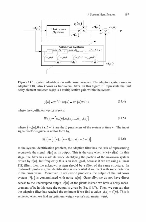
14 System Identification 197
UnknownSystem
( )n( )nx ( )nd
( )nd
( )ny
)(ne
Z-1 Z-1 Z-1...
...
w0(n) w1(n) w2(n) wL-1(n)
Adaptive systemx(n-1) x(n-2) x(n-L+1)
Figure 14.1. System identification with noise presence. The adaptive system uses anadaptive FIR, also known as transversal filter. In this figure z-1 represents the unitdelay element and each wi(n) is a multiplicative gain within the system.
y n W n X n X n W nT T( ) = ( ) ( ) = ( ) ( ), (14.4)
where the coefficient vector W(n) is
W n w n w n w nL( ) = ( ) ( ) ( )[ ]0 1 1, ,..., , (14.5)
where w n i Li( ){ }; 0 1 are the L parameters of the system at time n. The inputsignal vector is given in vector form by,
X n x n x n x n L( ) = ( ) ( ) +( )[ ], ,...,1 1 . (14.6)
In the system identification problem, the adaptive filter has the task of representingaccurately the signal ( )nd at its output. This is the case when y n d n( ) = ( )ˆ . In this
stage, the filter has made its work identifying the portion of the unknown systemdriven by x n( ) , but frequently this is an ideal goal, because if we are using a linearFIR filter, then the unknown system should be a filter of the same structure. Inreal-world problems, the identification is successful if we meet with some criterionin the error value. Moreover, in real-world problems, the output of the unknownsystem ( )nd is contaminated with noise n( ) . Generally, we do not have direct
access to the uncorrupted output d n( ) of the plant; instead we have a noisy meas-
urement of it; in this case the output is given by Eq. (14.7). Then, we can say thatthe adaptive filter has reached the optimum if we find a value y n d n( ) = ( ). This is
achieved when we find an optimum weight vector’s parameter W(n),

O. Montiel et al.198
W n W nOPT( ) = ( ). (14.7)
There are several methods to obtain the optimums values, each having its own ad-vantages and limitations, but they share the same limitation when the search spaceis big and multi-modal because they are gradient-guided local search techniques.
The correction term of the learning rule usually is function of the signal inputx(n), the desired output d(n), and the old weight estimate values wi(n-1). Thus, wecan write the compact expression as follows [11, 12]:
W n W n f X n d n W n( ) = ( ) + ( ) ( ) ( )[ ]1 1, , . (14.8)
Following these concepts, the least-mean-square algorithm (LMS) can be writtenas shown in Eq. (14.9).
W n W n X n e n( ) = ( ) + ( ) ( )[ ]1 µ , (14.9)
or, expanding the expression for the error, as
W n W n X n d i X W niT( ) = ( ) + ( ) ( ) ( )[ ]1 1µ , (14.10)
where µ is the step-size parameter.In order to analyze the learning rule for the BGA in a formal way, we are going
to introduce the next notation. We will use W nr ( ) to indicate the actual populationof r individuals of coefficient vectors W nr ( ) . By example, one individual is repre-sented as
W n w n w n w nL0 0 0 01 0 1( ) = ( ) ( ) ( )[ ], , ,, ,.., , (14.11)
where w0,1(n) belongs to the coefficient 1 of the individual number 0. W nr' ( ) be-longs to the next generation of coefficient after the evolutionary process. Then wehave
˜
, , ,
, , ,
, , ,
W n
W n
W n
W n
w n w n w n
w n w n w n
w n w n w n
r
r
L
L
r r r L
( ) =
( )( )
( )
=
( ) ( ) ( )( ) ( ) ( )
( ) ( ) ( )
0
1
0 0 01 0 1
1 0 11 1 1
0 1 1
M
K
K
M M O M
L
(14.12)
In the evolutionary process, the learning rule is a several step process. The evolu-tionary learning process begins with the evaluation of every coefficient vector ofthe population represented in Eq. (14.12) by W nr ( ) . This process is done using aspecific evaluation function “fi” known as the fitness function. After the wholepopulation has been evaluated, we need to perform a selection of the best of thispopulation. Generally, truncation selection is a good choice; with this process weobtain a pool W nT ( ) . The whole process, from expression (14.13) to (14.16), is re-
14 System Identification 199
peated until we reached the optimum value.
W T feval W nT r= ( )( )( )% ˜ , (14.13)
W n W n f W n W nr a a b' , ,( ) = ( ) + ( ) ( )[ ] (14.14)
W n Wr r' ' ,( ) = ( ) (14.15)
˜ ˜ ' .W n W nr r( ) = ( ) (14.16)
The fitness function (fi) will guide the search to find the optimum.
14.3 The Breeder Genetic Algorithm
In order to adjust the parameter vector, we used a BGA, which was designed ac-cording to the methods and theories used in the science of livestock breeding [11]and is based on advanced statistical methods [12, 13, 14, 15, 16, 17].
The BGA is defined as an eight-tuple
BGA P N T HC F termg= ( )0, , , , , , , , (14.17)
where Pg0 is the initial population of size N, T is the truncation threshold com-
monly referred as T%, represents the recombination operator, is the mutationoperator, HC is a hill-climbing method (by example: the gradient-guided LMS al-gorithm), F is the fitness function, and term is the termination criterion. In theBGA, T% 100
P best individuals at each generation are selected and mated randomly,
until the number of offsprings is equal the size of the population. A basic schemeof a BGA as shown is described in [5, 14].
Referring the BGA procedure to our problem, we need to generate randomly apopulation with P individuals, where each individual consists of n variables, eachof them related with a parameter, i.e., filter’s coefficient. By example, an individ-ual might consist of 50 floating-point variables; in this case, the adaptive FIR thatwe need to use will have 50 coefficients. The whole population is evaluated using afitness function, specifically designed to measure the aptitude of each individual.This evaluation is done applying a specific signal x(n) (Figure 14.1) to both sys-tems (unknown and adaptive systems) in order to calculate an error signal obtainedfrom the output of the unknown and adaptive systems. This error signal is the coreof the fitness function. After each individual of the parent population was evalu-ated, the best individual should be inserted in the population of the next generation,P’(t). In order to obtain this new population, which will replace the parent popula-tion, the BGA uses truncation selection. In truncation selection a percentage of thebest individuals are selected to mate, obtaining offsprings; self-mating is prohibited[15].
O. Montiel et al.200
The mutation operator is applied to each offspring, and the resulting individualsare inserted in the new population P’(t). The process is repeated until a termina-tion criterion is met. There are several recombination operators, but in this work,we used Extended Intermediate Recombination (EIR). In order to use this operator,we have if x =(xi,...xn) and y=(y1,...,yn) are the parents, then the successorz=(z1,...,zn) is calculated by
z x y x i ni i i i i= + ( ) =, 1,..., , (14.18)
where i d d+[ ],1 is chosen with uniform probability for each i and d 0, a
good choice is d = 0.25, which is the one that we used. The goal of the mutationoperator is to modify one or more parameters of zi, the modified objects (i.e., theoffsprings) appear in the landscape within a certain distance of the unmodified ob-jects (i.e., the parents). In this way, an offspring z', where z'=(z1,…,zn), is given by
z z rangei i i' = ± (14.19)
where rangei defines the mutation range and is calculated as ( )searchintervali .
In the Discrete Mutation operator (DM) is normally set to 0.1 or 0.2 and is veryefficient in some functions [4], but also we can set to 1. This is the case of theBroad Mutation Operator (BMO) proposed in [16] to solve problems where thedistance between the optimums and the actual position is larger than the DM op-erator could reach. This is the case of Scwefel’s function [16]. We will have inone step, that the mutation operator can reach points from zi only within the dis-tance given by ±rangei The sign + or – is chosen with probability of 0.5. Thevariable is computed by
= [ ]=
ii
i
K
i2 0 10
1
, , . (14.20)
Before mutation we set each i equals to 0, then each i is mutated to 1 withprobability p_=1/k, and only i = 1 contributes to the sum. On the average therewill be just one i with value 1, say i . Then is given by
= 2 i. (14.21)
In Eq. (14.20), K is a parameter originally related to the machine precision, i.e., thenumber of bits used to represent a real variable in the machine we are workingwith; traditionally K used values of 8 and 16. In practice, however, the value of Kis related to the expected value of mutation steps; in other words, the higher K is,the more fine-grained the resultant mutation operator is [5].

14 System Identification 201
14.4 Energy and Error Analysis
The objective of an adaptive scheme is to provide a better model for the unknownsystem. This is done using the output error sequence given in Eq. (14.1). This errorsequence measures how far d(i) is from y(i), in order to update the coefficient vec-tor W(n), providing a better model at each iteration. When the adaptive system istrying to match the unknown system, there exist different sources of errors. Thefirst source is due to the mathematical model that we are using to identify the un-known system. By example, if the unknown plant has the model of the InfiniteImpulse Response Filter (IIR) of Eq. (14.22), it is evident that we would need aninfinitely long tapped-delay line, whose realization is practically impossible.Therefore, when we are using a finite tapped delay line, the modeling errors are in-evitable.
y n v n x n ii
i
( ) = ( ) ( )= 0
. (14.22)
In this work, we used as an unknown system an IIR filter specified by the second-order difference equation given by (14.23). This problem was taken from [20].
d(n)-d(n-1)+0.9d(n-2)=x(n) n . (14.23)
The adaptive system is an FIR filter with 50 coefficients. As the filter has a higherdegree of freedom, the input-output response characteristic of the adaptive modelwill converge to match closely those of the unknown system.
If we have solved the system identification problem, and the model that we areusing is a good one, then we should have a way to measure the parameter errors inthe identification process [21]. If we considered that V(n) represents the coeffi-cient vector of the unknown system represented by Eq. (14.22), then we have tomeasure how far W(n) is from V(n). This quantity, We(n), will be referred to as theweight error at time n. The weight vector W(n)OPT is the optimal vector that betterwill represent V(n).
W n W n W ne OPT( ) = ( ) ( ). (14.24)
Using Eq. (14.25), we can obtain the value known as a priori estimation error (ea),
which measure how far )1(nWX Ti is from the uncorrupted output term
OPTTi WX ; hence we have
e i X W naT
e( ) = ( )1 . (14.25)
If we use the most recent weight vector, we can define the a posteriori estimationerror (ep),
e i X W naT
e( ) = ( )1 . (14.26)

O. Montiel et al.202
A good way to quantify the effect of these errors is the energy and power meas-ures. Then the energy E of a signal x(n) is [17].
E x nN
n
= ( )=
2.
(14.27)
The energy of a signal can be finite or infinite. The signal x(n) is called an energysignal if E is finite, thus is 0 < <E .
We can define the signal energy of the sequence x(n) over the finite interval -0 n N as [16]
E x nN
n
N
= ( )=
2
0
1
.(14.28)
Then we can express the signal energy as [16]
E EN
Nlim (14.29)
The average power of the signal x(n) is defined as [16]
PN
EN
Nlim1 (14.30)
We will use the definition of power provided in (16) to calculate a short-term aver-age ASE (Average of Squared Error), which will serve us in two ways; one is toestimate the convergence rate of the evolutionary algorithm, and the second way isfor using the inverse of this function (1/ASE) as the aptitude function, which willguide the evolutionary algorithm to get the optimums coefficients. The ASE func-tion is defined as
ASE mK
e kk n
n K
( ) = ( )= +
+1 2
1
.(14.31)
Here, m=n/K=1,2,…. The recommended averaging interval K may be selected tobe (approximately) K=10L [16].
14.5 Stability Analysis
In any practical application, an analysis of system's stability is important, since anunstable system usually exhibits erratic and extreme behavior and causes overflow[21]. To prove stability in this work, we used the next theorem, as well as conceptsabout causal systems:

14 System Identification 203
Theorem. An arbitrary relaxed system is said to be bounded input-bounded output(BIBO) stable if and only if every bounded input produces a bounded output.
Considering the previous theorem, if x(n) is the bounded input, there must be aconstant Mx such that
x n M x( ) < , (14.32)
and, if the output is bounded, there must be a constant My such that
y n M y( ) < . (14.33)
Although we are working with a time-varying system, for analysis purposes we areconsidering a window time where the system can be treated as a Linear Time in-variant system (LTI), and via mathematical induction generalize this result. Then,if we take the absolute value of both sides of Eq. (14.3), we obtain
y n w n x n ii
i
L
( ) = ( ) ( )= 0
1
. (14.34)
Then, we have
y n w n x n ii
i
L
( ) ( ) ( )= 0
1
. (14.35)
If the input is bounded, there exists a finite number Mx that satisfies Eq. (14.32),i.e., x n M x( ) , then we can rewrite Eq. (14.35) as
y n M w nx i
i
L
( ) ( )= 0
1
. (14.36)
From Eq. (14.36), we observe that the output is bounded if the impulse response ofthe system is absolutely summable, i.e.,
w ni
i
L
( ) <= 0
1
. (14.37)
In this work, Eq. (14.36) is easily satisfied since we have a finite number of coeffi-cients wi(k), and their values also are finite. This result implies that any excitationof a finite duration, applied to the input of the system, must produce an output ofnature "transient", this is when the system is stable. The input amplitude will decayeventually with time. This condition implies that W(z) must contain the unit circlewithin its Region of Convergence (ROC). Then,
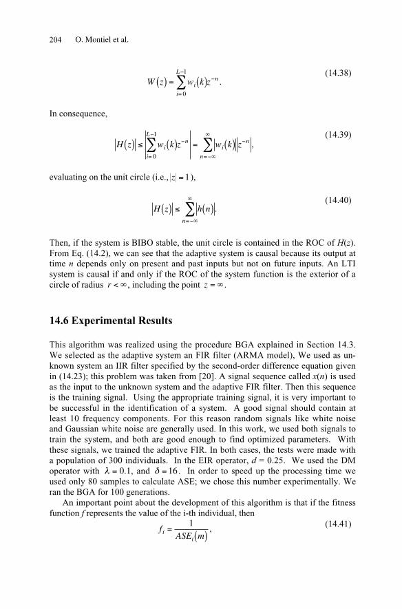
O. Montiel et al.204
W z w k zi
i
Ln( ) = ( )
= 0
1
.(14.38)
In consequence,
H z w k z w k zi
i
Ln
i
n
n( ) ( ) = ( )= =0
1
,(14.39)
evaluating on the unit circle (i.e., z = 1),
H z h nn
( ) ( )=
.(14.40)
Then, if the system is BIBO stable, the unit circle is contained in the ROC of H(z).From Eq. (14.2), we can see that the adaptive system is causal because its output attime n depends only on present and past inputs but not on future inputs. An LTIsystem is causal if and only if the ROC of the system function is the exterior of acircle of radius r < , including the point z = .
14.6 Experimental Results
This algorithm was realized using the procedure BGA explained in Section 14.3.We selected as the adaptive system an FIR filter (ARMA model), We used as un-known system an IIR filter specified by the second-order difference equation givenin (14.23); this problem was taken from [20]. A signal sequence called x(n) is usedas the input to the unknown system and the adaptive FIR filter. Then this sequenceis the training signal. Using the appropriate training signal, it is very important tobe successful in the identification of a system. A good signal should contain atleast 10 frequency components. For this reason random signals like white noiseand Gaussian white noise are generally used. In this work, we used both signals totrain the system, and both are good enough to find optimized parameters. Withthese signals, we trained the adaptive FIR. In both cases, the tests were made witha population of 300 individuals. In the EIR operator, d = 0.25. We used the DMoperator with = 0 1. , and = 16 . In order to speed up the processing time weused only 80 samples to calculate ASE; we chose this number experimentally. Weran the BGA for 100 generations.
An important point about the development of this algorithm is that if the fitnessfunction f represents the value of the i-th individual, then
fASE mi
i
=( )
1, (14.41)
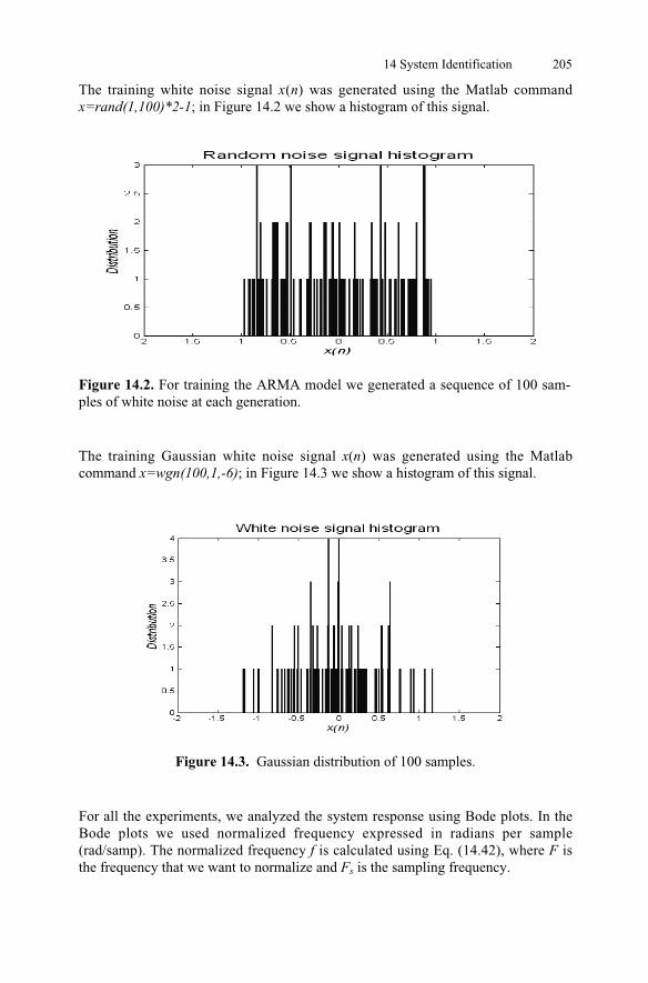
14 System Identification 205
The training white noise signal x(n) was generated using the Matlab commandx=rand(1,100)*2-1; in Figure 14.2 we show a histogram of this signal.
Figure 14.2. For training the ARMA model we generated a sequence of 100 sam-ples of white noise at each generation.
The training Gaussian white noise signal x(n) was generated using the Matlabcommand x=wgn(100,1,-6); in Figure 14.3 we show a histogram of this signal.
Figure 14.3. Gaussian distribution of 100 samples.
For all the experiments, we analyzed the system response using Bode plots. In theBode plots we used normalized frequency expressed in radians per sample(rad/samp). The normalized frequency f is calculated using Eq. (14.42), where F isthe frequency that we want to normalize and Fs is the sampling frequency.
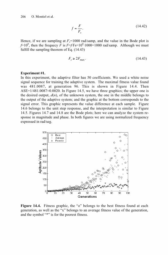
O. Montiel et al.206
fF
Fs
= .(14.42)
Hence, if we are sampling at Fs=1000 rad/samp, and the value in the Bode plot isf=100, then the frequecy F is F=f·Fs=100·1000=1000 rad/samp. Although we mustfulfill the sampling theorem of Eq. (14.43)
F Fs 2 max . (14.43)
Experiment #1.In this experiment, the adaptive filter has 50 coefficients. We used a white noisesignal sequence for training the adaptive system. The maximal fitness value foundwas 481.0087, at generation 96. This is shown in Figure 14.4. ThenASE=1/481.0087 0.0020. In Figure 14.5, we have three graphics; the upper one isthe desired output, d(n), of the unknown system, the one in the middle belongs tothe output of the adaptive system; and the graphic at the bottom corresponds to thesignal error. This graphic represents the value difference at each sample. Figure14.6 belongs to the unit step response, and the interpretation is similar to Figure14.5. Figures 14.7 and 14.8 are the Bode plots; here we can analyze the system re-sponse in magnitude and phase. In both figures we are using normalized frequencyexpressed in rad/seg.
Figure 14.4. Fitness graphic, the “o” belongs to the best fitness found at eachgeneration, as well as the “x” belongs to an average fitness value of the generation,and the symbol “*” is for the poorest fitness.

14 System Identification 207
Figure 14.5. Unit impulse response. Experiment 1.
Figure 14.6. Unit step response. Experiment 1.

O. Montiel et al.208
Figure 14.7. Behavior of the adaptive system.
Figure 14.8. Fitness function’s values. Experiment 2.

14 System Identification 209
Figure 14.9. Unit impulse response. Experiment 2.
Figure 14.10. Unit step response. Experiment 2.

O. Montiel et al.210
Figure 14.11. Magnitude response. Experiment 2.
Experiment #2.In this experiment, the adaptive filter has 50 coefficients. The maximal fitnessvalue found was 695.8930, at generation 95. Then ASE=1/695.8930 0.00144.
14.7 Conclusions
In this chapter we developed a set of equations in order to explain the learningprocess of the adaptive system when we are using a BGA in the system identifica-tion problem. We realized several experiments; here we showed the result of fourof them. In all cases, a full optimization was performed, obtaining low rates of av-erage error and good magnitude and phase response. Obviously, when we usedmore coefficients in the ARMA model we got a lower average error. This is natu-ral, because the more degrees of freedom the ARMA model has (FIR filter), the in-put-output response characteristic of the adaptive model will converge to matchclosely the unknown system.
References
1. C. W. Helstrom (1991) Probability and stochastic processes for engineers.Helstrom U.S.A.
2. J.-S. R. Jang, C.-T. Sun, E. Mizutani (1997) Neuro-Fuzzy and Soft Com-puting, A Computational Approach to Learning and Machine Intelligence.Matlab Curriculum Series. Prentice Hall.
14 System Identification 211
3. S.P. Harris, E.C. Ifeachor, (1996) Nonlinear FIR Filter Design by GeneticAlgorithm, in “1st Online Conference on Soft Computing”.http://www.lania.mx/~ccoello/EM00/harrisabs.txt
4. H. Mühlenbein . “6 Genet ic Algor i thms” . Borneohttp://citeseer.nj.nec.com/181734.html
5. L.A. Belanche. (1999) A Study in Function Optimization with the BreederGenetic Algorithm. Research Report LSI-99-36-R. Universitat Politécnicade Catalunya. http://citeseer.nj.nec.com/belanche99study.html
6. De Falco, A. Della Cioppa, P. Natale and E. Tarantino. (1997) ArtificialNeural Networks Optimization by means of Evolutionary Algorithms, 1997.http://citeseer.nj.nec.com/3503.html.
7. M.S. White, J.S. Flockton “Adaptive recursive filtering using evolutionaryalgorithms”, http://citeseer.nj.nec.com/392797.html
8. D. M. Etter, M. J. Hicks, and K. H. Cho. (1982) “Recursive filter designusing an adaptive genetic algorithm”. In Proceedings of the IEEE Interna-tional Conference on Acoustics, Speech and Signal Processing (ICASSP82), volume 2, pp. 635-638, IEEE.
9. O. Montiel, R. Sepúlveda, O. Castillo, P. Melin. (2001) “Application of aBreeder Genetic Algorithm for Filter Optimization”, In Proceedings of theInternational Conference on Artificial Intelligence IC-AI’2001, volume III,pp. 1199-1205, Las Vegas, Nevada, USA.
10. O. Montiel, R. Sepúlveda, O. Castillo, P. Melin (2001) A Breeder GeneticAlgorithm for Filter Optimization. In World Multiconference on Systemics,Cybernetics an Infomatics (ISAS/SCI 2001), volume IX Industrial Systems:Part I, pp. 556-562, Orlando, Florida, USA.
11. V. K. Madisetti, D. B. Williams (1997) “The Digital Signal ProcessingHandbook”, A CRC Handbook Published in Cooperation with IEEE Press,pp. 18-1, 18-7, 20-1, 20-4.
12. O. Montiel, O. Castillo, P. Melin, R. Sepúlveda (2002) "The EvolutionaryLearning Rule in System Identification". The 6th. World Multiconferenceon Systemics, Cybergenics and Informatics (SCI 2002), volume XVII In-dustrial Systems and Engineering III. pp. 205-210.
13. H. Mühlenbein. The equation for the response to selection and its use forprediction. http://citeseer.nj.nec.com/181734.html.
14. H. Mühlenbein, D. Schlierkamp-Voosen (1994) “The science of breedingand its application to the breeder genetic algorithm BGA”. EvolutionaryComputation, 1(4):335-360.
15. H. Mühlenbein, J. Bendisch, H.-M. Voigt. (1996) From recombination ofgenes to the estimation of distribution II. Continuous parameters. ParallelProblem Solving from Nature, Springer: Berlin, pp: 188-197.
16. I. De Falco. (1997) Sample Contributed Book, John Wiley & Sons. EditorJenny Smith. http://citeseer.nj.nec.com/cs.
17. H. Mühlenbein, S.-Voosen (1993) Predictive Model for Breeder GeneticAlgorithm. Evolutionary Computation. 1(1): 25-49.
18. Ralf Salomon. Genetic Algorithms and the O(n ln n) Complexity on Se-lected Test Functions. http://citesser.nj.nec.com/109962.html.
19. V. K. Madisetti, D. B. Williams. (1997) The Digital Signal ProcessingHandbook, A CRC Handbook Published in Cooperation with IEEE Press,pp. 18-1, 18-7, 20-1, 20-4.
20. V. K. Ingle, J. G. Proakis. (2000) Digital Signal Processing using Matlab.Ed. Brooks/Cole, , pp. 371-377.

O. Montiel et al.212
21. O. Montiel, O. Castillo, R. Sepúlveda. (2002) “Error and Energy Measuresin System Identification Using an Evolutionary Algorithm”, Proceedings ofthe International Conference on Artificial Intelligence IC-AI’2002. LasVegas, Nevada, USA.

1
1
Summary.
15.1 Introduction
15
Current and Future Research Trends inEvolutionary Multiobjective Optimization
http://delta.cs.cinvestav.mx/�ccoello/EMOOhttp://www.lania.mx/�ccoello/EMOO/ http://www.jeo.org/emo/
In this chapter we present a brief analysis of the current research per-formed on evolutionary multiobjective optimization. After analyzing �rst- and second-generation multiobjective evolutionary algorithms, we address two important issues:the role of elitism in evolutionary multiobjective optimization and the way in whichconcepts from multiobjective optimization can be applied to constraint-handling tech-niques. We conclude with a discussion of some of the most promising research trendsin the years to come.
The �rst author maintains an EMO repository with over 900 bibliographi-cal entries at: , with mirrors at
and .
C.A. Coello Coello, G. Toscano Pulido, E. Mezura Montes
Evolutionary algorithms have become an increasingly popular design and op-timization tool in the last few years, with a constantly growing development ofnew algorithms and applications [1]. Despite this considerably large volumeof research, new areas remain to be explored with sufficient depth. One ofthem is the use of evolutionary algorithms to solve multiobjective optimiza-tion problems.The �rst reported implementation of a multiobjective evolutionary algo-
rithm (MOEA) dates back to the mid-1980s [45, 46]. Since then, a considerableamount of research has been done in this area, now known as evolutionarymultiobjective optimization (EMO for short). The growing importance of this�eld is re�ected by a signi�cant increment (mainly during the last eight years)of technical papers in Intl. Conf.s and peer-reviewed journals, books, specialsessions in Intl. Conf.s and interest groups on the Internet [13].Evolutionary algorithms seem also particularly desirable for solving multi-
objective optimization problems because they deal simultaneously with a set

R R
�
→
F� � �
1 2
1 2
1 2
x x x
x
x
x
k
i
i
in
nT
n
15.2 Basic Concepts
214 C.A. Coello et al.
15.2.1 Pareto Optimality
[ ( ) ( ) ( )]
( ) 0 = 1 2
( ) = 0 = 1 2
: =[ ]
f , f , . . . , f ,
m
g i , , . . . , m,
p
h i , , . . . , p,
k fx , x , . . . , x
x , x , . . . , x
of possible solutions (the so-called population), which allows us to �nd severalmembers of the Pareto optimal set in a single run of the algorithm, insteadof having to perform a series of separate runs as in the case of the traditionalmathematical programming techniques. Additionally, evolutionary algorithmsare less susceptible to the shape or continuity of the Pareto front (e.g., theycan easily deal with discontinuous and concave Pareto fronts), whereas thesetwo issues are a real concern for mathematical programming techniques [8].This chapter deals with some of the current and future research trends in
evolutionary multiobjective optimization. The perspective adopted is derivedfrom our own research experience in the area and therefore the bias towardcertain particular topics of interest. The chapter is organized as follows. Sec-tion 15.2 presents some basic concepts used in multiobjective optimization.Section 15.3 brie�y describes the origins of evolutionary multiobjective opti-mization. Section 15.4 introduces the so-called �rst-generation multiobjectiveevolutionary algorithms. Second-generation multiobjective evolutionary algo-rithms are discussed in Section 15.5, emphasizing the role of elitism in evo-lutionary multiobjective optimization. Section 15.6 discusses ways in whichmultiobjective optimization concepts have been and could be incorporatedinto constraint-handling techniques (both for single and for multiobjectiveoptimization). Finally, Section 15.7 discusses some of the research trends thatare likely to be predominant in the next few years.
The emphasis of this chapter is the solution of multiobjective optimizationproblems (MOPs) of the form
minimize (15.1)
subject to the inequality constraints:
(15.2)
and the equality constraints:
(15.3)
where is the number of objective functions . We callthe vector of decision variables. We wish to determine from
among the set of all vectors that satisfy (15.2) and (15.3) the particularset of values that yield the optimum values of all the objectivefunctions.
It is rarely the case that there is a single point that simultaneously optimizesall the objective functions. Therefore, we normally look for �tradeoffs�, rather
i i
j j
��
��
�
∈ F∈ F �
∈ F
xx x x
x xx
x
x
( ) ( ) = 1( ) ( )
15.3 How It All Started
f f i , . . . , kf < f j
k kN/k N
N
15 Evolutionary Multiobjective Optimization 215
Edgeworth�Pareto optimalityPareto optimality
Pareto optimal
Pareto optimal setnondominated
Pareto front
properties
Vector EvaluationGenetic Algorithm
than single solutions when dealing with multiobjective optimization problems.The notion of �optimality� is, therefore, different in this case. The most com-monly adopted notion of optimality is that originally proposed by FrancisYsidro Edgeworth [21] and later generalized by V. Pareto [39]. Although someauthors call this notion (see, for example, [49]),we will use the most commonly accepted term: .We say that a vector of decision variables is if there
does not exist another such that for all andfor at least one .
In words, this de�nition says that is Pareto optimal if there exists nofeasible vector of decision variables which would decrease some criterionwithout causing a simultaneous increase in at least one other criterion. Un-fortunately, this concept almost always gives not a single solution, but rathera set of solutions called the . The vectors correspondingto the solutions included in the Pareto optimal set are called .The image of the Pareto optimal set under the objective functions is called
.
The potential of evolutionary algorithms for solving multiobjective optimiza-tion problems was hinted as early as the late 1960s by Rosenberg in his Ph.D.thesis [42]. Rosenberg�s study contained a suggestion that would have led tomultiobjective optimization if he had carried it out as presented. His sug-gestion was to use multiple (nearness to some speci�ed chemicalcomposition) in his simulation of the genetics and chemistry of a populationof single-celled organisms. Since his actual implementation contained only onesingle property, the multiobjective approach could not be shown in his work.The �rst actual implementation of what it is now called a multiobjective
evolutionary algorithm (or MOEA, for short) was Schaffer�s(VEGA), which was introduced in the mid-1980s, mainly
aimed for solving problems in machine learning [45, 46, 47].VEGA basically consisted of a simple genetic algorithm (GA) with a mod-
i�ed selection mechanism. At each generation, a number of subpopulationswere generated by performing proportional selection according to each objec-tive function in turn. Thus, for a problem with objectives, subpopulationsof size each would be generated (assuming a total population size of ).These subpopulations would then be shuffled together to obtain a new pop-ulation of size , on which the GA would apply the crossover and mutationoperators in the usual way. Schaffer realized that the solutions generated byhis system were nondominated in a local sense, because their nondominancewas limited to the current population, which was obviously not appropriate.Also, he noted a problem that in genetics is known as �speciation� (i.e., wecould have the evolution of �species� within the population which excel on

2
2
15.4 MOEAs: First Generation
216 C.A. Coello et al.
By �middling�, Schaffer meant an individual with acceptable performance, perhapsabove average, but not outstanding for any of the objective functions.
different aspects of performance). This problem arises because this techniqueselects individuals who excel in one dimension of performance, without look-ing at the other dimensions. The potential danger doing that is that we couldhave individuals with what Schaffer called �middling� performance in all di-mensions, which could be very useful for compromise solutions, but which willnot survive under this selection scheme, since they are not in the extreme forany dimension of performance (i.e., they do not produce the best value for anyobjective function, but only moderately good values for all of them). Specia-tion is undesirable because it is opposed to our goal of �nding Pareto optimalsolutions. Although VEGA�s speciation can be dealt with using heuristics orother additional mechanisms, it remained as the main drawback of VEGA.From the second half of the 1980s up to the �rst half of the 1990s, few
other researchers developed MOEAs. Most of the work reported back then in-volves rather simple evolutionary algorithms that use an aggregating function(linear in most cases) [33, 54], lexicographic ordering [24], and target-vectorapproaches [28]. All of these approaches were strongly in�uenced by the workdone in the operations research community and in most cases did not requireany major modi�cations to the evolutionary algorithm adopted.The algorithms proposed in this initial period are rarely referenced in the
current literature except for VEGA (which is still used by some researchers).However, the period is of great importance because it provided the �rst in-sights into the possibility of using evolutionary algorithms for multiobjectiveoptimization. The fact that only relatively naive approaches were developedduring this stage is natural considering that these were the initial attemptsto develop multiobjective extensions of an evolutionary algorithm. Such ap-proaches kept most of the original evolutionary algorithm structure intact(only the �tness function was modi�ed in most cases) to avoid any complexadditional coding. The emphasis in incorporating the concept of Pareto dom-inance into the search mechanism of an evolutionary algorithm would comelater.
The major step toward the �rst generation of MOEAs was given by D. Gold-berg on pages 199 to 201 of his famous book on genetic algorithms pub-lished in 1989 [25]. In his book, Goldberg analyzes VEGA and proposes aselection scheme based on the concept of Pareto optimality. Goldberg notonly suggested what would become the standard �rst generation MOEA, butalso indicated that stochastic noise would make such algorithm useless unlesssome special mechanism was adopted to block convergence. First-generationMOEAs typically adopt niching or �tness sharing for that sake. The mostrepresentative algorithms from the �rst generation are the following:

�
( )
( )
iti
iti( ) = 1 +
1
1
x t
p
x , t p .
n M
15 Evolutionary Multiobjective Optimization 217
Nondominated Sorting Genetic Algorithm
Niched-Pareto Genetic Algorithm
Multiobjective Genetic Algorithm
1. (NSGA): This algorithmwas proposed by Srinivas and Deb [48]. The approach is based on severallayers of classi�cations of the individuals as suggested by Goldberg [25].Before selection is performed, the population is ranked on the basis of non-domination: all nondominated individuals are classi�ed into one category(with a dummy �tness value, which is proportional to the population size,to provide an equal reproductive potential for these individuals). To main-tain the diversity of the population, these classi�ed individuals are sharedwith their dummy �tness values. Then this group of classi�ed individualsis ignored and another layer of nondominated individuals is considered.The process continues until all individuals in the population are classi�ed.Stochastic remainder proportionate selection is adopted for this technique.Since individuals in the �rst front have the M.imum �tness value, they al-ways get more copies than the rest of the population. This allows us tosearch for nondominated regions and results in convergence of the pop-ulation toward such regions. Sharing, by its part, helps to distribute thepopulation over this region (i.e., the Pareto front of the problem).
2. (NPGA): Proposed by Horn et al.[32]. The NPGA uses the tournament selection scheme based on Paretodominance. The basic idea of the algorithm is the following: two individ-uals are randomly chosen and compared against a subset from the entirepopulation (typically, around 10% of the population). If one of them isdominated (by the individuals randomly chosen from the population) andthe other is not, then the nondominated individual wins. When both com-petitors are either dominated or nondominated (i.e., there is a tie), theresult of the tournament is decided through �tness sharing [27].
3. (MOGA): Proposed by Fonsecaand Fleming [23]. In MOGA, the rank of a certain individual correspondsto the number of chromosomes in the current population by which it isdominated. Consider, for example, an individual at generation , whichis dominated by individuals in the current generation.The rank of an individual is given by [23]
rank (15.4)
All nondominated individuals are assigned rank , while dominated onesare penalized according to the population density of the correspondingregion of the tradeoff surface.Fitness assignment is performed in the following way [23]:a) Sort population according to rank.b) Assign �tness to individuals by interpolating from the best (rank )to the worst (rank ) in the way proposed by Goldberg (1989),according to some function, usually linear, but not necessarily.

2
2
( )
( )
O M M
O kMk M
�
�
�
�
�
���
218 C.A. Coello et al.
15.5 MOEAs: Second Generation
c) Average the �tnesses of individuals with the same rank, so that all ofthem are sampled at the same rate. This procedure keeps the globalpopulation �tness constant while maintaining appropriate selectivepressure, as de�ned by the function used.
The main questions raised during the �rst generation were
Are aggregating functions (so common before and even during the goldenyears of Pareto ranking) really doomed to fail when the Pareto front isnonconvex [16]? Are there ways to deal with this problem? Is it worthtrying? Some recent work seems to indicate that aggregating functions arenot death yet [35].Can we �nd ways to maintain diversity in the population without usingniches (or �tness sharing), which requires a process , where refersto the population size?If we assume that there is no way of reducing the process requiredto perform Pareto ranking ( is the number of objectives and is thepopulation size), how can we design a more efficient MOEA?Do we have appropriate test functions and metrics to evaluate quantita-tively an MOEA? Not many people worried about this issue until nearthe end of the �rst generation. During this �rst generation, practically allcomparisons were done visually (plotting the Pareto fronts produced bydifferent algorithms) or were not provided at all (only the results of theproposed method were reported).When will somebody develop theoretical foundations for MOEAs?
Summarizing, the �rst generation was characterized by the use of selectionmechanisms based on Pareto ranking and �tness sharing was the most com-mon approach adopted to maintain diversity. Much work remained to be done,but the �rst important steps toward a solid research area had been alreadytaken.
The second generation of MOEAs was born with the introduction of the no-tion of elitism. In the context of multiobjective optimization, elitism usually(although not necessarily) refers to the use of an external population (alsocalled secondary population) to retain the nondominated individuals. The useof this external �le raises several questions:
How does the external �le interact with the main population?What do we do when the external �le is full?Do we impose additional criteria to enter the �le instead of just usingPareto dominance?
+� �
strength
15 Evolutionary Multiobjective Optimization 219
Strength Pareto Evolutionary Algorithm
Strength Pareto Evolutionary Algorithm 2
Pareto Archived Evolution Strategy
Elitism can also be introduced through the use of a ( )-selection inwhich parents compete with their children and those which are nondominated(and possibly comply with some additional criterion such as providing a betterdistribution of solutions) are selected for the following generation.The previous points bring us to analyze in more detail the true role of
elitism in evolutionary multiobjective optimization. For that sake, we will re-view next the way in which some of the second-generation MOEAs implementelitism:
1. (SPEA): This algorithmwas introduced by Zitzler and Thiele [57]. This approach was conceived asa way of integrating different MOEAs. SPEA uses an archive containingnondominated solutions previously found (the so-called external nondom-inated set). At each generation, nondominated individuals are copied tothe external nondominated set. For each individual in this external set, a
value is computed. This strength is similar to the ranking valueof MOGA, since it is proportional to the number of solutions to which acertain individual dominates. It should be obvious that the external non-dominated set is in this case the elitist mechanism adopted. In SPEA, the�tness of each member of the current population is computed accordingto the strengths of all external nondominated solutions that dominate it.Additionally, a clustering technique called �average linkage method� [37]is used to keep diversity.
2. (SPEA2): SPEA2 hasthree main differences with respect to its predecessor [56]: (1) it incorpo-rates a �ne-grained �tness assignment strategy that takes into account foreach individual the number of individuals that dominate it and the num-ber of individuals by which it is dominated; (2) it uses a nearest-neighbordensity estimation technique that guides the search more efficiently; and(3) it has an enhanced archive truncation method that guarantees thepreservation of boundary solutions.Thefore, in this case the elitist mechanism is just an improved version ofthe previous.
3. (PAES): This algorithm was in-troduced by Knowles and Corne [36]. PAES consists of a (1+1) evolutionstrategy (i.e., a single parent that generates a single offspring) in combi-nation with a historical archive that records some of the nondominatedsolutions previously found. This archive is used as a reference set againstwhich each mutated individual is being compared. Such a historical archiveis the elitist mechanism adopted in PAES. However, an interesting aspectof this algorithm is the procedure used to maintain diversity, which con-sists of a crowding procedure that divides objective space in a recursivemanner. Each solution is placed in a certain grid location based on the

+� �
220 C.A. Coello et al.
Nondominated Sorting Genetic Algorithm II
Niched Pareto Genetic Algorithm 2
Pareto Envelope-based Selection Algorithm
values of its objectives (which are used as its �coordinates� or �geograph-ical location�). A map of such grid is maintained, indicating the numberof solutions that reside in each grid location. Since the procedure is adap-tive, no extra parameters are required (except for the number of divisionsof the objective space).
4. (NSGA-II): Deb etal. [18, 19, 20] proposed a revised version of the NSGA [48], called NSGA-II, which is more efficient (computationally speaking), that uses elitismand a crowded comparison operator that keeps diversity without speci-fying any additional parameters. The NSGA-II does not use an externalmemory as the previous algorithms. Instead, the elitist mechanism con-sists of combining the best parents with the best offspring obtained (i.e.,a ( )-selection).
5. (NPGA 2): E.son et al. [22]proposed a revised version of the NPGA [32] called the NPGA 2. This al-gorithm uses Pareto ranking but keeps tournament selection (solving tiesthrough �tness sharing as in the original NPGA). In this case, no externalmemory is used and the elitist mechanism is similar to the one adopted bythe NSGA-II. Niche counts in the NPGA 2 are calculated using individ-uals in the partially �lled next generation, rather than using the currentgeneration. This is called continuously updated �tness sharing and wasproposed by Oei et al. [38].
6. (PESA): This algo-rithm was proposed by Corne et al. [15]. This approach uses a small inter-nal population and a larger external (or secondary) population. PESA usesthe same hypergrid division of phenotype (i.e., objective funcion) spaceadopted by PAES to maintain diversity. However, its selection mechanismis based on the crowding measure used by the hypergrid previously men-tioned. This same crowding measure is used to decide what solutions tointroduce into the external population (i.e., the archive of nondominatedvectors found along the evolutionary process). Therefore, in PESA, theexternal memory plays a crucial role in the algorithm since it determinesnot only the diversity scheme, but also the selection performed by themethod. There is also a revised version of this algorithm, called PESA-II[14]. This algorithm is identical to PESA, except for the fact that region-based selection is used in this case. In region-based selection, the unit ofselection is a hyperbox rather than an individual. The procedure consistsof selecting (using any of the traditional selection techniques [26]) a hy-perbox and then randomly select an individual within such a hyperbox.The main motivation of this approach is to reduce the computational costsassociated with traditional MOEAs (i.e., those based on Pareto ranking).Again, the role of the external memory in this case is crucial to the per-
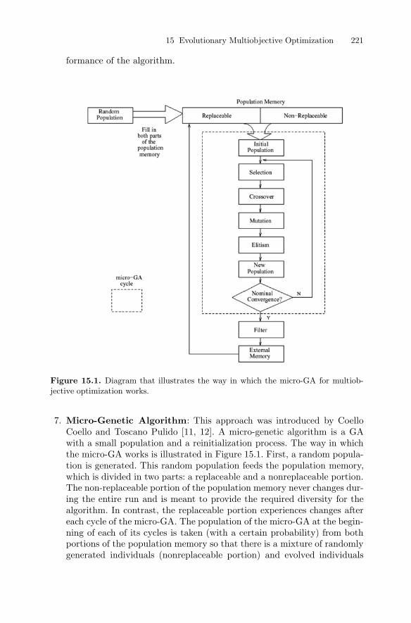
Figure 15.1.
Micro-Genetic Algorithm
15 Evolutionary Multiobjective Optimization 221
Diagram that illustrates the way in which the micro-GA for multiob-jective optimization works.
formance of the algorithm.
7. : This approach was introduced by CoelloCoello and Toscano Pulido [11, 12]. A micro-genetic algorithm is a GAwith a small population and a reinitialization process. The way in whichthe micro-GA works is illustrated in Figure 15.1. First, a random popula-tion is generated. This random population feeds the population memory,which is divided in two parts: a replaceable and a nonreplaceable portion.The non-replaceable portion of the population memory never changes dur-ing the entire run and is meant to provide the required diversity for thealgorithm. In contrast, the replaceable portion experiences changes aftereach cycle of the micro-GA. The population of the micro-GA at the begin-ning of each of its cycles is taken (with a certain probability) from bothportions of the population memory so that there is a mixture of randomlygenerated individuals (nonreplaceable portion) and evolved individuals

3
3
�
�
�
15.6 Relating Constraint Handling and MultiobjectiveOptimization
222 C.A. Coello et al.
This is assuming that there are two or more nondominated vectors. If there is onlyone, then this vector is the only one selected.
(replaceable portion). During each cycle, the micro-GA undergoes con-ventional genetic operators. After the micro-GA �nishes one cycle, twonondominated vectors are chosen from the �nal population and they arecompared with the contents of the external memory (this memory is ini-tially empty). If either of them (or both) remains as nondominated aftercomparing it against the vectors in this external memory, then they areincluded there (i.e., in the external memory). This is the historical archiveof nondominated vectors. All dominated vectors contained in the externalmemory are eliminated.The micro-GA uses then three forms of elitism: (1) it retains nondomi-nated solutions found within the internal cycle of the micro-GA; (2) ituses a replaceable memory whose contents is partially �refreshed� at cer-tain intervals; and (3) it replaces the population of the micro-GA by thenominal solutions produced (i.e., the best solutions found after a full inter-nal cycle of the micro-GA). Therefore, the micro-GA is another exampleof how elitism can play a vital role to improve the performance of anevolutionary algorithm used for multiobjective optimization.
Second-generation MOEAs can be characterized by an emphasis on effi-ciency and by the use of elitism (in the two main forms previously described).During the second generation, some important theoretical work also tookplace, mainly related to convergence [43, 44, 29, 30, 53]. Also, metrics andstandard test functions were developed to validate new MOEAs [55, 52].The main concerns during the second generation (which we are still living
nowadays) are the following:
Are our metrics reliable? What about our test functions? We have foundout that developing good metrics is in itself a multiobjective optimizationproblem, too. In fact, it is ironic that nowadays we are going back to trust-ing more visual comparisons than metrics as during the �rst generation.Are we ready to tackle problems with more than two objective functionsefficiently? Is Pareto ranking doomed to fail when dealing with too manyobjectives? If so, then what is the limit up to which Pareto ranking canbe used to select individuals reliably?What are the most relevant theoretical aspects of evolutionary multiob-jective optimization that are worth exploring in the shortterm?
Another research area within evolutionary multiobjective optimization thathas not been explored in enough detail in the current literature is constraint

m4
4
1 1m m
i
� � �
COMOGA
VEGA
x
x x x x xx x
x y y
fm m
v f , f , . . . , f f , . . . , ff
i m f f
( )+ 1
� = ( ( ) ( ) ( )) ( ) ( )( )
1 ( ) ( )
15 Evolutionary Multiobjective Optimization 223
The assumption that we have constraints will hold throughout this section.
handling (particularly for single-objective optimization). We believe that it isimportant to study the relationship between constraint handling and multi-objective optimization because of two main reasons: (1) constrained single-objective optimization problems can be restated as multiobjective optimiza-tion problems in a natural way; and (2) this sort of constrained single-objectiveoptimization problems can be used to measure performance of MOEAs ona more quantitative basis than when using conventional multiobjective testfunctions.The most straightforward approach to use multiobjective optimization
techniques to solve a single-objective optimization problems is to rede�nethe single-objective optimization of as a multiobjective optimizationproblem in which we will have objectives, where is the num-ber of constraints . Then, we can apply any MOEA to the new vector
, where are the original con-straints of the problem. An ideal solution would thus have =0 for
and for all feasible (assuming minimization).However, it should be clear that in single-objective optimization problems
we do not want just good tradeoffs; we want to �nd the best possible solutionsthat do not violate any constraints. Therefore, a mechanism such as Paretoranking may be useful to approach the feasible region, but once we arrive toit, we will need to guide the search with a different mechanism so that we canreach the global optimum. In order to achieve this goal, we should also be ableto maintain diversity in the population. Some of the most representative at-tempts to use multiobjective optimization techniques (or concepts) to handleconstraints in single-objective optimization problems are the following:
1. : Surry et al. [50] proposed the use of Pareto ranking andVEGA to handle constraints. In their approach, called COMOGA, thepopulation is ranked based on constraint violations (counting the num-ber of individuals dominated by each solution). Then, one portion of thepopulation is selected based on constraint ranking, and the rest based onreal cost (�tness) of the individuals. COMOGA compared fairly with apenalty-based approach in a pipe-sizing problem, and was less sensitive tochanges in the parameters, but the results achieved were not better thanthose found with a penalty function [50]. It should be added that CO-MOGA requires several extra parameters, although its authors argue thatthe technique is not particularly sensitive to the values of such parameters.
2. : Parmee and Purchase [40] implemented a version of VEGA thathandled the constraints of a gas turbine problem as objectives to allow aGA to locate a feasible region within the highly constrained search space ofthis application. However, VEGA was not used to further explore the fea-sible region, and instead the authors used specialized operators that wouldcreate a variable-sized hypercube around each feasible point to help the
∑x x
=1
� | � | ∈∈
+1
( ) = [0 ( )]
= ( )
m
i
i�
i j i i i
j j i j
i j
224 C.A. Coello et al.
m m
, g ,
�
d x x / x xj x Sx S S S d
x xx x x
dj
Line Search and Pareto Dominance
GA to remain within the feasible region at all times. It is important tonotice that no real attempt to reach the global optimum was made in thiscase. Coello [6] also proposed the use of a population-based multiobjectiveoptimization technique such as VEGA to handle each of the constraintsof a single-objective optimization problem as an objective. In this case,however, the goal was to approximate the global optimum. At each gener-ation, the population is split into subpopulations ( is the numberof constraints), so that a fraction of the population is selected using the(unconstrained) objective function as its �tness and another fraction usesthe �rst constraint as its �tness and so on. This approach provided goodresults in several optimization problems [6]. Its main disadvantage wasrelated to scalability issues. However, in a recent application in combi-national circuit design we were able to successfully deal with up to 49objective functions [7]. Furthermore, the approach showed an importantimprovement (in terms of efficiency) with respect to a previous GA-basedapproach developed by us for the same task [4].
3. : Camponogara and Talukdar [2]proposed to restate a single-objective optimization problem in such a waythat two objectives would be considered: the �rst would be to optimizethe original objective function and the second would be to minimize:
M. (15.5)
where is normally 1 or 2. Once the problem is rede�ned, nondominatedsolutions with respect to the two new objectives are generated. The solu-tions found de�ne a search direction , where ,
, and and are Pareto sets. The direction search is intendedto simultaneously minimize all the objectives. Line search is performed inthis direction so that a solution can be found such that dominatesand (i.e., is a better compromise than the two previous solutions
found). Line search takes the place of crossover in this approach, andmutation is essentially the same, where the direction is projected ontothe axis of one variable in the solution space. Additionally, a processof eliminating half of the population is applied at regular intervals (onlythe less �tted solutions are replaced by randomly generated points). Thisapproach has obvious problems to keep diversity, as it is re�ected by theneed to discard the worst individuals at each generation. Also, the use ofline search increases the computational cost of the approach and what isthe impact of the segment chosen to search in the overall performance ofthe algorithm is not clear.
xj
s
( ) = 1g , j , . . . , m
R
Min-Max
MOGA
NPGA
Domain Knowledge and Ranking
15 Evolutionary Multiobjective Optimization 225
4. : Jiménez et al. [34] proposed the use of a Min-Max approach[3] to handle constraints. The main idea of this technique is to apply a setof simple rules to decide the (binary tournament) selection process:a) If the two individuals being compared are both feasible, then selectbased on the minimum value of the objective function.
b) If one of the two individuals being compared is feasible and the otherone is infeasible, then select the feasible individual.
c) If both individuals are infeasible, then select based on the M.imumconstraint violation (M. for ). The individualwith the lowest M.imum violation wins.
A subtle problem with this approach is that the evolutionary process �rstconcentrates only on the constraint satisfaction problem and therefore itsamples points in the feasible region essentially at random [51]. This meansthat in some cases (e.g., when the feasible region is disjoint) we might landin an inappropriate part of the feasible region from which we will not beable to escape. However, this approach may be a good alternative to �nda feasible point in a heavily constrained search space. Deb [17] proposeda similar approach but using tournament selection based on feasibility.However, niching was required to maintain diversity in the population.
5. : Coello [5] explored the use of selection based on dominance (de-�ned in terms of feasibility) to handle constraints. In this case, ranking isperformed at three different levels: from two feasible individuals the onewith the highest �tness is preferred; if one is feasible and the other infeasi-ble, then the �rst is chosen; if both are infeasible, then the individual withthe lowest amount of constraint violation is chosen. This approach usesstochastic universal sampling so that the selection pressure is not too highand no extra procedures are required to maintain diversity. Also, adaptivecrossover and mutation rates were adopted as part of the approach.
6. : Coello and Mezura [10] proposed the use of tournaments basedon nondominance (as in the NPGA [32]) to handle constraints. An ad-ditional parameter, called selection rank ( ), is added to control theselection pressure of the approach. This parameter makes it unnecessaryto use equivalent class sharing (as in the NPGA) to maintain diversityand also decreases the (normally high) selection pressure originated fromusing tournament selection.
7. : Ray et al. [41] proposed a tech-nique to handle constraints in which the population is ranked both inobjective function space and in constraint space. The selection strategyadopted eliminates weaknesses from both spaces and ensures a better con-straint satisfaction in the offspring produced. The approach uses niches tomaintain diversity with Euclidean distances being the similary measureadopted. It also incorporates mating restrictions based on the information
�
�
�
�
�
�
�
226 C.A. Coello et al.
15.7 Where Are We Heading?
that each individual has of its own feasibility (this idea was inspired on anearlier approach by Hinterding and Michalewicz [31]), so that the globaloptimum can be reached through cooperative learning.
Some of the possible trends in this area are the following:
Use of other MOEAs to handle constraints. Some of these techniques maybe rather simple and still remain highly competitive. See, for example, [9].Use of online and self-adaptation in constraint-handling techniques bothfor single- and for multiobjective optimization.Extraction and reuse of knowledge obtained from the evolutionary processin order to guide more efficiently the search.Design (single-objective optimization) test functions that are particularlydifficult for MOEAs to tackle and devise appropriate metrics to measuretheir performance in this context.
Once we have been able to distinguish between the �rst and second generationsin evolutionary multiobjective optimization, a reasonable question is: whereare we heading now?In the last few years, there has been a considerable growth in the number
of publications related to evolutionary multiobjective optimization. However,the variety of topics covered is not as rich as the number of publicationsreleased each year. The current trend is to either develop new algorithms(validating them with some of the metrics and test functions available) or todevelop interesting applications of existing algorithms.We will �nish this section with a list of some of the research topics that
we believe that will keep researchers busy during the next few years:
New metrics with some insightful analysis of their behavior and limitations.Also, metrics that measure not only offline performance, but also onlineperformance are expected to arise.More test functions with more than two objectives and with high dimen-sionality. Concerns about epistasis, deception, dynamic functions, uncer-tainty, and noise should also be re�ected in the upcoming work in thistopic.Development of a theoretical framework that allows us to analyze thebehavior of MOEAs. Topics such as the run-time analysis and boundedconvergence times of an MOEA are expected to be tackled in the next fewyears. We should also expect more work on convergence and on modelingMOEAs using statistical tools.

15.8 Conclusions
Acknowledgments
References
Handbook of EvolutionaryComputation
3rd NordicWorkshop on Genetic Algorithms and Their Applications (3NWGA)
Multiobjective Decision Making: Theoryand Methodology
Intl. Journalof Smart Engineering System Design
Civil Engineering Systems
Engineering Optimization
Proc. of the SecondNASA/DoD Workshop on Evolvable Hardware
15 Evolutionary Multiobjective Optimization 227
1. T. Bäck, D.B. Fogel, and Z. Michalewicz, (1997) (eds.). Inst. of Physics Publishing and Oxford University Press, .
2. E. Camponogara and Sarosh N. Talukdar (1997) A genetic algorithm for con-strained and multiobjective optimization. In Jarmo T. Alander, (ed.),
, pages 49�62,Vaasa, Finland, August 1997. University of Vaasa.
3. V. Chankong and Y.Y. Haimes (1983). Systems Science and Engineering. North-Holland.
4. C.A. Coello, A.D. Christiansen, and A. Hernández Aguirre (2000) Use of evolu-tionary techniques to automate the design of combinational circuits.
, 2(4):299�314.5. C.A. Coello Coello (2000) Constraint-handling using an evolutionary multiobjec-tive optimization technique. , 17:319�346.
6. C.A. Coello Coello (2000) Treating Constraints as Objectives for Single-ObjectiveEvolutionary Optimization. , 32(3):275�308.
7. C.A. Coello Coello, A. Hernández Aguirre, and Bill P. Buckles (2000) Evolution-ary multiobjective design of combinational logic circuits. In Jason Lohn, AdrianStoica, Didier Keymeulen, and Silvano Colombano, (eds.),
, pages 161�170, Los Alamitos, CA,July 2000. IEEE Computer Society.
This chapter has provided a rather brief and general picture of the past,current, and future research in evolutionary multiobjective optimization. Abrief analysis of some of the most popular algorithms reported in the literaturehas also been provided together with a summary of the main contributionsmade in this area in the last few years. Finally, some promising areas of futureresearch were also provided.Our main goal was to provide a motivation for researchers and students to
get into this exciting research discipline to tackle the problems that are ourmain concern right now. Being a young research area, evolutionary multiob-jective optimization still has a lot of opportunities to offer to newcomers, andwe expect many of them to join us in the next few years.
This chapter is representative of the research performed by the Evolution-ary Computation Group at CINVESTAV-IPN (EVOCINV). The �rst authoracknowledges support from the mexican Consejo Nacional de Ciencia y Tec-nología (CONACyT) through project number 34201-A. The second and thirdauthors acknowledge support from CONACyT through a scholarship to pursuegraduate studies at CINVESTAV-IPN�s Electrical Engineering Department.
Knowledge and Information Systems. AnIntl. Journal
Computer Methods in Applied Mechanics and Engineering
Proc.of the Fifth Intl. Conf. on Adaptive Computing Design and Manufacture (ACDM2002)
First Intl. Conf. on Evolutionary Multi-CriterionOptimization
Proc. of the Genetic and Evolutionary Computation Conf.(GECCO�2001)
EvolutionaryAlgorithms for Solving Multi-Objective Problems
Proc. of the Genetic andEvolutionary Computation Conf. (GECCO�2001)
Proc. of the Parallel Problem Solving from Nature VI Conf.
Structural Optimization
Computer Methods in Applied Mechanics and Engineering
Proc. of the Parallel Problem Solving from
228 C.A. Coello et al.
8. C.A. Coello Coello (1999) A Comprehensive Survey of Evolutionary-Based Mul-tiobjective Optimization Techniques.
, 1(3):269�308.9. C.A. Coello Coello (2002) Theoretical and Numerical Constraint Handling Tech-niques used with Evolutionary Algorithms: A Survey of the State of the Art.
, 191(11-12):1245�1287.10. C.A. Coello Coello and E. Mezura Montes (2002) Handling Constraints in GeneticAlgorithms Using Dominance-Based Tournaments. In I.C. Parmee, (ed.),
, volume 5, pages 273�284, University of Exeter, Devon, UK, April 2002.Springer-Verlag.
11. C.A. Coello Coello and G. Toscano Pulido (2001) A Micro-Genetic Algorithmfor Multiobjective Optimization. In E. Zitzler, K. Deb, L. Thiele, C.A. CoelloCoello, and D. Corne, (eds.),
, pages 126�140. Springer-Verlag. Lecture Notes in Computer ScienceNo. 1993, 2001.
12. C.A. Coello Coello and G. Toscano Pulido (2001) Multiobjective Optimizationusing a Micro-Genetic Algorithm. In L. Spector, E. D. Goodman, A. Wu, W.B.Langdon, H.M. Voigt, M. Gen, S. Sen, M. Dorigo, S. Pezeshk, M. H. Garzon,and E. Burke, (eds.),
, pages 274�282, San Francisco, California, 2001. Morgan Kauf-mann Pub.
13. C.A. Coello Coello, D.A. Van Veldhuizen, and G. B. Lamont (2002). Kluwer Academic Pub., New
York. ISBN 0-3064-6762-3.14. D.W. Corne, N. R. Jerram, J. D. Knowles, and M. J. Oates (2001) PESA-II:Region-based Selection in Evolutionary Multiobjective Optimization. In Lee Spec-tor, E. D. Goodman, A. Wu, W.B. Langdon, H.M. Voigt, M. Gen, S. Sen, M.Dorigo, S. Pezeshk, M. H. Garzon, and E. Burke, (eds.),
, pages 283�290, San Francisco,California, 2001. Morgan Kaufmann Pub.
15. D.W. Corne, J. D. Knowles, and M. J. Oates (2000) The Pareto Envelope-basedSelection Algorithm for Multiobjective Optimization. In Marc Schoenauer, K.Deb, Günter Rudolph, Xin Yao, Evelyne Lutton, J. J. Merelo, and H.-P. Schwefel,(eds.), , pages 839�848,Paris, France, 2000. Springer. Lecture Notes in Computer Science No. 1917.
16. I. Das and J. Dennis (1997) A closer look at drawbacks of minimizing weightedsums of objectives for pareto set generation in multicriteria optimization prob-lems. , 14(1):63�69, 1997.
17. K. Deb (2000) An Efficient Constraint Handling Method for Genetic Algorithms., 186(2/4):311�338,
2000.18. K. Deb, S. Agrawal, A. Pratab, and T. Meyarivan (2000) A fast elitist non-dominated sorting genetic algorithm for multi-objective optimization: NSGA-II.KanGAL report 200001, Indian Inst. of Technology, Kanpur, India, 2000.
19. K. Deb, S. Agrawal, A. Pratab, and T. Meyarivan (2000) A fast elitist non-dominated sorting genetic algorithm for multi-objective optimization: NSGA-II.In Marc Schoenauer, K. Deb, Günter Rudolph, Xin Yao, Evelyne Lutton, J. J.Merelo, and H.-P. Schwefel, (eds.),

Nature VI Conf.
IEEE Trans. on Evolutionary Com-putation
Mathematical Physics
First Intl. Conf.on Evolutionary Multi-Criterion Optimization
Proc. of the Fifth Intl. Conf. on Genetic Algorithms
Genetic Algorithms and their Applications: Proc. of the First Intl. Conf. onGenetic Algorithms
Genetic Algorithms in Search, Optimization and MachineLearning
Foundations of Genetic Algorithms
Genetic Algorithmsand Their Applications: Proc. of the Second Intl. Conf. on Genetic Algorithms
Structural Optimization
European Journal of Operational Research
Journal of Heuristics
Proc. of the 5th Intl. Conf. on Evolu-tionary Computation
Proc. of the First IEEE Conf. onEvolutionary Computation, IEEE World Cong. on Computational Intelligence
Parallel Problem Solving from Nature, 2nd Workshop
Proc. of the 1999 Genetic and Evolutionary Computation Conf. Workshop Pro-gram
15 Evolutionary Multiobjective Optimization 229
, pages 849�858, Paris, France, 2000. Springer. Lecture Notes inComputer Science No. 1917.
20. K. Deb, A. Pratap, Sameer Agarwal, and T. Meyarivan (2002) A Fast and ElitistMultiobjective Genetic Algorithm: NSGA�II.
, 6(2):182�197.21. F. Y. Edgeworth (1981) . P. Keagan, London, England,1881.
22. M. E.son, A. Mayer, and J. Horn (2001) The Niched Pareto Genetic Algorithm2 Applied to the Design of Groundwater Remediation Systems. In E. Zitzler,K. Deb, L. Thiele, C.A. Coello Coello, and D. Corne, (eds.),
, pages 681�695. Springer-Verlag.Lecture Notes in Computer Science No. 1993, 2001.
23. C.M. Fonseca and P. J. Fleming (1993) Genetic algorithms for multiobjectiveoptimization: Formulation, discussion and generalization. In S. Forrest, (ed.),
, pages 416�423, San Mateo,CA, 1993. Morgan Kaufmann Pub.
24. M.P. Fourman (1985) Compaction of symbolic layout using genetic algorithms.In
, pages 141�153, Hillsdale, NJ, 1985. Lawrence Erlbaum.25. D.E. Goldberg (1989)
. Addison-Wesley Publishing Company, Reading, MA.26. D.E. Goldberg and K. Deb (1991) A comparison of selection schemes used ingenetic algorithms. In G.J. E. Rawlins, (ed.), ,pages 69�93. Morgan Kaufmann, San Mateo, CA, 1991.
27. D.E. Goldberg and J. Richardson (1987) Genetic algorithm with sharing formultimodal function optimization. In J. J. Grefenstette, (ed.),
,pages 41�49, Hillsdale, NJ, 1987. Lawrence Erlbaum.
28. P. Hajela and C. Y. Lin (1992) Genetic search strategies in multicriterion optimaldesign. , 4:99�107.
29. T. Hanne (2000) On the convergence of multiobjective evolutionary algorithms., 117(3):553�564.
30. T.Hanne (2000) Global multiobjective optimization using evolutionary algo-rithms. , 6(3):347�360.
31. R. Hinterding and Z. Michalewicz (1998) Your brains and my beauty: Parentmatching for constrained optimisation. In
, pages 810�815, Anchorage, Alaska, May 1998.32. J. Horn, N. Nafpliotis, and D.E. Goldberg (1994) A niched pareto genetic al-gorithm for multiobjective optimization. In
,volume 1, pages 82�87, Piscataway, NJ, June 1994. IEEE Service Center.
33. W. Jakob, M. Gorges-Schleuter, and C. Blume (1992) Application of geneticalgorithms to task planning and learning. In R. Männer and B. MandE., (eds.),
, Lecture Notes in ComputerScience, pages 291�300, Amsterdam, 1992. North-Holland Publishing Company.
34. F. Jiménez, J.L. Verdegay, and A.F. Gómez-Skarmeta (1999) Evolutionary tech-niques for constrained multiobjective optimization problems. In A. S. Wu, (ed.),
, pages 115�116, Orlando, Florida, July 1999.

Proc. of theGenetic and Evolutionary Computation Conf. (GECCO�2001)
Evolutionary Computation
Computers and Operations Research
Cours D�Economie Politique
AdaptiveComputing in Engineering Design and Control-�94
Proc. of the Genetic and Evolutionary Com-putation Conf. (GECCO�2000)
Simulation of genetic populations with biochemical prop-erties
Proc. of the 5th IEEE Conf. on EvolutionaryComputation
Proc. of the 2000 Conf. on EvolutionaryComputation
Multiple Objective Optimization with Vector Evaluated Ge-netic Algorithms
Genetic Algorithms and their Applications: Proc. of the FirstIntl. Conf. on Genetic Algorithms
Proc. of the 9th Intl. Joint Conf. on Arti�cial Intelligence (IJCAI-85)
Evolutionary Computation
Multicriteria Optimization in Engineering and the Sciences
230 C.A. Coello et al.
35. Y. Jin, T. Okabe, and B. Sendhoff (2001) Dynamic Weighted Aggregation forEvolutionary Multi-Objective Optimization: Why Does It Work and How? InLee Spector, E. D. Goodman, A. Wu, W.B. Langdon, H.M. Voigt, M. Gen, S.Sen, M. Dorigo, S. Pezeshk, M. H. Garzon, and E. Burke, (eds.),
, pages 1042�1049,San Francisco, California, 2001. Morgan Kaufmann Pub.
36. J. D. Knowles and D.W. Corne (2000) Approximating the nondominated frontusing the pareto archived evolution strategy. , 8(2):149�172.
37. J.N. Morse (1980) Reducing the size of the nondominated set: Pruning by clus-tering. , 7(1�2):55�66.
38. C.K. Oei, D.E. Goldberg, and S.J. Chang (1991) Tournament Selection, Niching,and the Preservation of Diversity. Technical Report 91011, Illinois Genetic Algo-rithms Laboratory, University of Illinois at Urbana-Champaign, Urbana, Illinois,December 1991.
39. V. Pareto (1896) , volume I and II. F. Rouge, Lau-sanne.
40. I. C. Parmee and G. Purchase (1994) The development of a directed genetic searchtechnique for heavily constrained design spaces. In I. C. Parmee, (ed.),
, pages 97�102, Plymouth, UK,1994. University of Plymouth, University of Plymouth.
41. T. Ray, T. Kang, and S.K. Chye (2000) An evolutionary algorithm for con-strained optimization. In D. Whitley, D. Goldberg, E. Cantú-Paz, L. Spector,I. Parmee, and H.-G. Beyer, (eds.),
, pages 771�777, San Francisco, California, 2000.Morgan Kaufmann.
42. R. S. Rosenberg (1967). PhD thesis, University of Michigan, Ann Arbor, MI.
43. G. Rudolph (1998) On a Multi-Objective Evolutionary Algorithm and Its Con-vergence to the Pareto Set. In
, pages 511�516, Piscataway, NJ, 1998. IEEE Press.44. G. Rudolph and A. Agapie (2000) Convergence Properties of Some Multi-Objective Evolutionary Algorithms. In
, volume 2, pages 1010�1016, Piscataway, NJ, July 2000. IEEE Press.45. J.D. Schaffer (1984)
. PhD thesis, Vanderbilt University, Nashville, TN.46. J.D. Schaffer (1985) Multiple objective optimization with vector evaluated geneticalgorithms. In
, pages 93�100, Hillsdale, NJ, 1985. LawrenceErlbaum.
47. J.D. Schaffer and J.J. Grefenstette (1985) Multiobjective learning via geneticalgorithms. In, pages 593�595, Los Angeles, CA, 1985. AAAI.
48. N. Srinivas and K. Deb (1994) Multiobjective optimization using nondominatedsorting in genetic algorithms. , 2(3):221�248.
49. W. Stadler (1988) Fundamentals of multicriteria optimization. In W. Stadler,(ed.), , pages 1�25.Plenum Press, New York, NY.

Control and Cybernetics
Evolutionary Computing. AISB Workshop. SelectedPapers
Multiobjective Evolutionary Algorithms: Classi�-cations, Analyses, and New Innovations
Late Breaking Papers atthe Genetic Programming 1998 Conf.
IEE/IEEE Workshop on Natural Algorithmsin Signal Processing
Evolutionary Computation
IEEE Trans. on EvolutionaryComputation
15 Evolutionary Multiobjective Optimization 231
50. P.D. Surry and N.J. Radcliffe (1997) The COMOGAmethod: Constrained optimi-sation by multiobjective genetic algorithms. , 26(3):391�412.
51. P.D. Surry, N.J. Radcliffe, and I.D. Boyd (1995) A multi-objective approach toconstrained optimisation of gas supply networks : The COMOGA method. InTerence C. Fogarty, (ed.),
, pages 166�180, Sheffield, U.K., 1995. Springer-Verlag. Lecture Notes inComputer Science No. 993.
52. D.A. Van Veldhuizen (1999). PhD thesis, Department of Electrical
and Computer Engineering. Graduate School of Engineering. Air Force Inst. ofTechnology, Wright-Patterson AFB, OH, May 1999.
53. D.A. Van Veldhuizen and G.B. Lamont (1998) Evolutionary computation andconvergence to a pareto front. In J.R. Koza, (ed.),
, pages 221�228, Stanford, CA, July 1998.Stanford University Bookstore.
54. P.B. Wilson and M.D. Macleod (1993) Low implementation cost IIR digital �lterdesign using genetic algorithms. In
, pages 4/1�4/8, Chelmsford, U.K., 1993.55. E. Zitzler, K. Deb, and L. Thiele (2000) Comparison of Multiobjective Evolu-tionary Algorithms: Empirical Results. , 8(2):173�195.
56. E. Zitzler, M. Laumanns, and L. Thiele (2001) SPEA2: Improving the StrengthPareto Evolutionary Algorithm. Technical Report 103, Computer Engineeringand Networks Laboratory (TIK), Swiss Fed. Inst. of Technology (ETH) Zurich,Gloriastrasse 35, CH-8092 Zurich, Switzerland, May 2001.
57. E. Zitzler and L. Thiele (1999) Multiobjective evolutionary algorithms: A compar-ative case study and the strength pareto approach.
, 3(4):257-271.
schema
16.1 Introduction
16
Genetic Algorithms with LimitedConvergence
J. Kubalík and L. Rothkrantz, J. Lazansk�
Genetic algorithms (GAs) are probabilistic search and optimization tech-niques, which operate on a population of chromosomes, representing potentialsolutions of the given problem [10]. In a standard GA, binary strings of onesand zeros represent the chromosomes. Each chromosome is assigned a �tnessvalue that expresses its quality considering the given objective function. Sucha population is evolved by means of reproduction and recombination opera-tors in order to breed the optimal solution�s chromosome. The evolution isrunning until some termination condition is ful�lled. The best chromosomeencountered so far is then considered as the found solution.The basic analysis of GA�s behavior is based on a notion of a
[15] as a template, which matches a certain class of chromosomes. As thepopulation evolves, some good schemata are represented by increasing numberof chromosomes while bad schemata disappear. The �xed positions of thosegood schemata constitute so-called building blocks (BBs), which representimportant components of the �nal solution. The optimum solution emergeswhen these building blocks are mixed together in an optimal way in somechromosome.GAs simultaneously carry out exploitation of the promising regions found
so far and exploration of other areas for potentially better solution. The weakpoint of a GA is that it often suffers from so-called premature convergence,which is caused by an early homogenization of genetic material in the pop-ulation. This means that no more exploration can be performed. There aremany factors affecting the convergence of a GA: the used population size,type and rate of application of crossover and mutation operators, encodingused and many others. Inadequate population size cannot provide the GAwith sufficient amount of genetic material to evolve the optimal chromosome.Improperly designed and set genetic operators cannot maintain an optimalbalance between exploitation and exploration of the GA.

16.2 Related Work
234 J. Kubalík et al.
This paper introduces a novel approach to protect GAs from getting stuckin local optima and so extending the search power of GAs. To achieve thiswe have proposed a GA where only limited convergence of the populationgenotype can take place.The paper starts with an overview of some recent approaches to the prob-
lems related somehow to prevent premature convergence, preserving the pop-ulation diversity (or better the multimodal diversity), and improving the per-formance of GAs in general. The next section introduces the proposed geneticalgorithm with limited convergence and discusses its aspects. Section 16.4brie�y describes the test problems used for experimental evaluation of theproposed algorithm. Empirical results presented in Section 16.5 show that thealgorithm performs very well across the representative set of search problems.Especially its explorative power and the ability to keep useful diversity of thepopulation are demonstrated there. Section 16.6 summarizes and concludesthe paper and mentions interesting topics to be studied in future in this area.
There are many factors that affect the convergence of a GA. The most in�u-encing and the most frequently studied are the used reproduction strategy,the size of the evolved population, the representation, i.e., the mapping of theproblem parameters on a binary string in conventional GAs, and last but notleast the used recombination operators and the frequency with which they areapplied and other problem-dependent parameters. Let us brie�y list some ofthe approaches that have been recently proposed to tackle the aspects men-tioned above.Dual GAs [3], [4] represent one possible way to introduce some kind of
redundancy into the evolved genetic material. The dual GAs use a standardbinary representation extended with just one bit, called the head bit or metabit, which is added to every individual in the population. This bit does notcode any information of the represented solution. Instead this extra bit isused to determine the way the informative part of the chromosome will beinterpreted. If the value of the head bit is 0, then the rest of the chromosomeis taken as it is. Otherwise if the head bit is 1 the string is interpreted asits binary complement. This means that two binary complementary stringsrepresent the same solution. In other words, the population may contain indi-viduals with completely different genotype but with the same phenotype andso the same �tness values.It has been obvious from the very beginning of the GA�s use that the pop-
ulation size plays a crucial role in determining the convergence quality of GAs.The population should be large enough to provide an adequate initial supplyof BBs. Another aspect of population sizing involves the decision making be-tween competing BBs. De Jong [5] recognized that the decision making for aparticular BB is strongly affected by contributions of other BBs. There are

16 Genetic Algorithms with Limited Convergence 235
several studies that try to estimate an adequate population size [8], [12], [14].However, a user should know much information about the problem at handlike the size of the considered BBs, the number of BBs in the problem, theaverage �tness variance of the considered BB, and some other conservativeassumptions in order to be able to use the theoretical estimates.Another factor that affects the convergence of GA is the selection scheme.
Generally, the selection should work so that the chromosomes representingbetter solutions are given a bigger chance to take part in the process of gener-ating a new and hopefully better population. The extent to which the betterchromosomes are favored is measured by so-called selection pressure. How-ever, if the selection pressure is too low, then the convergence to the optimalsolution is too slow. In the opposite case, i.e., if the selection pressure is toohigh, the population is prone to converge very fast toward some suboptimalsolution. So commensurate efforts have been spent to analyze various selectionschemes and to develop the convergence models of GAs under those selectionschemes [1], [11], [13], [23]. In order to keep the desired distribution of �tnessvalues in the population during the whole run, a proper scaling technique [22]might be engaged in GA as well.GAs are very often engaged in solving multimodal optimization problems.
This implies that the ability of the GA to keep just the "raw" diversity isnot good enough. Instead the multimodal diversity covering many niches ofthe search space is required. One early approach to maintain many niches inthe GA was based on utilization of so-called shared �tness values that werecalculated using a sharing function [9]. The general concept of �tness sharingis based on the idea that each individual�s �tness is divided by the numberof neighbors within the niche to which the given individual belongs. Thus thegoal desired state is such that the population is distributed over a numberof different peaks in the search space, with each peak receiving a fractionof the population in proportion to the height of that peak. It results in asituation that the convergence occurs within a niche, but convergence of thefull population is avoided.Other works dealing with maintenance of the population diversity date
back to the 1970s. Cavicchio [2] and De Jong [5] came up with techniquescalled preselection and crowding, respectively. Both are inspired by an ecolog-ical phenomenon that similar individuals in the natural population competeagainst each other for limited resources. Dissimilar individuals tend to occupydifferent niches, so they typically do not compete. As a result, the numberof members of a particular niche does not change during the evolution of thewhole population of �xed size. In preselection and crowding this is achievedso that the newly created individuals, which are to be inserted into the pop-ulation replace the most similar individuals in the current population. Thetwo methods differ in that how the individuals to be replaced are found. Incrowding the replacement is found among randomly chosen CF individuals.Preselection assumes that a parent is one of the closest individuals to thegenerated offspring so the parent is replaced if the competing child is bet-

236 J. Kubalík et al.
ter. Mahfoud studied several strategies of crowding and preselection in [20]and proposed a variation of preselection called deterministic crowding thatprocesses two parents and two offspring at a time and uses phenotypic simi-larity measure to determine which offspring competes against which parent.He shows that his method is better in clustering solutions about all peaks ofthe tested problems.Mengshoel and Goldberg [21] proposed a niching algorithm called prob-
abilistic crowding, which is a successor of the deterministic crowding. Thetwo core ideas in probabilistic crowding are (1) to hold tournaments betweensimilar individuals and (2) to let tournaments be probabilistic. Theoreticalanalysis and empirical results showed that probabilistic crowding is a simple,stable, predictable, and fast niching algorithm.A search performance of the GA can be also measured in terms of the
size of the search space explored during the run. To efficiently sample thewhole search space is the task for recombination operators, i.e., crossover andmutation operators. In standard genetic algorithms the crossover is consideredto be of the primary role in an exploration process while the mutation isused to preserve the diversity in the population and to preserve a loss ofinformation [10], [22]. However, the utility of crossover and mutation changeswith a population size. A mutation can be more useful than crossover when thepopulation size is small while a crossover is more useful when the populationis large.A proper use of recombination operators is even harder since there are
many different variants of crossover. The implementations differ between eachother in many aspects. The disruption effect of crossover, �rst analyzed for1-point crossover in [15], is the probability that the crossover will disrupt longschemata. This is important to predict how the promising schemata will bepropagated to subsequent populations. De Jong and Spears [6] characterizedrecombination in terms of productivity and exploration power. Those char-acteristics describe the ability of crossover to generate new sample points inthe search space. De Jong and Spears also derived a heuristics that the moredisruptive crossovers (which are also more productive and explorative) arebetter when the population is small and less disruptive operators are betterwhen the population is large relative to the problem size. For more recentwork on the role of recombination operators, see [26].Another approach is to dynamically adapt the rates of the utilization of
multiple operators during the run. Spears [25] used an extra tag-bit attachedto every individual to store the information about which crossover (1 is 2-pointand 0 is uniform crossover) should be preferred when crossing two parentalchromosomes. So if the parents both have 1 at the tag-bit position, thenthe 2-point crossover is used. Similarly, if both have 0, then uniform is used.Otherwise one of the two operators is chosen with a probability 0.5. Spearsfound that this adaptive approach always had a performance intermediatebetween the best and worst of the two single recombination operators.

M
N
16 Genetic Algorithms with Limited Convergence 237
Srinivas and Patnaik [27] used adaptive probabilities of crossover and mu-tation to achieve the twin goals of maintaining diversity in the population andsustaining convergence capacity of the GA. They increased the probability ofcrossover and mutation when the population was stuck at local optima anddecreased the probabilities when the population was scattered in the solutionspace. They also considered the need to preserve "good" solutions. This wasattempted by having low probabilities for highly �t individuals while poorsolutions will encounter high probability of crossover and mutation rate.Kubalík and Lazansk� proposed so-called partially randomized crossover
operators (PRX) as an enhancement of the traditional crossover opera-tors used for binary representation [16], [17], [18]. The enhancement of thecrossover functionality is in a modi�ed treatment of a common schema of theparents, which are the bits common to both parental chromosomes. Standardoperators work so that both offspring inherit unchanged all the bits of thecommon schema. As the population converges, the common schema occupiesa growing portion of the parent chromosomes and so the crossover can pro-duce only little new. The PRX operators do not strictly preserve the commonschema of the parents, since in one of the two generated offspring, a portionof the common schema is changed with the probability that evolves duringthe run. Thus, the population is not saturated with superior building blocksbut also with their randomly chosen binary complements. The diversity of thepopulation is permanently maintained, which helps to preserve the SGA fromgetting stuck in a local optimum and enhance the exploration of the searchspace beyond the limits imposed by the pure evolution.The PRX operators were engaged in genetic algorithms with permanent
re-initialization of parental common schemata proposed in [19]. The algorithmforks the search into two directions when creating a new population from theold one. To do so the main generation cycle consists of two steps. First, theprimary population is evolved for generations with the use of the PRXcrossover in order to produce both the direct and randomized offspring. Therandomized offspring are stored in the secondary population. Since it is derivedfrom the primary population, it still has much in common with the "mainstream" evolution so it does not represent quite random samples of the searchspace. As such the secondary population represents a source of hopefully usefuldiverse genetic material. Then the secondary population is re�ned through ashort evolution running for generations. Finally, these two populations aremerged together into one new primary population and the new main iterationcan be launched. The empirical results show that in such a way a diversity ofthe population can easily be maintained while converging faster and to bettersolutions than with the standard GA.
�
�
22 +
2 2
1 : 1 = 00 : = 2
2
238 J. Kubalík et al.
16.3 Genetic Algorithms with Limited Convergence
PopSize/C PopSize/ C
PopSize/ C
CPopSize C PopSize/
PopSize/
genetic algorithm withlimited convergence
ii
PopSize Cconvergence rate
This section describes a novel approach to improve the performance of GAs.The main goal of the proposed algorithm, called the
(GALCO), is to maintain the fruitful diversity of theevolved population during the whole run and so to preserve a GA from get-ting stuck in local optima. To achieve this a concept of imposing limits on theconvergence of the population is adopted.The algorithm inherits most of the features from the standard GA working
on a binary representation. In fact it is a type of the incremental GA whereonly one crossover operation is performed in each generation cycle (the stepfrom the old to the new population). As such it uses a standard selection strat-egy to choose the parents, a classical crossover operator (2-point crossover isused here, as commented further) for generating new chromosomes, and spe-cial rule for inserting of the offspring chromosomes into the population. Whatmakes the GALCO unique is just the way the convergence of the populationis maintained within speci�ed boundaries.There is a limit imposed on the maximum convergence of every position of
the representation. Let us denote the vector of genes at the th position of thechromosome over the whole population as the th column of the population.Then the limit is expressed as a symmetric integer interval [, ], where is the population size. The parameterdenotes the . Its value is the input parameter to the algorithmand can be chosen from the range 0 to . Strictly speaking,de�nes the maximal allowed difference of the frequency of ones and zerosin every column of the population. So the ratio of ones and zeros must be
during the whole run in the case of or the ratio can changeup to in favor of either ones or zeros for . Thisis a principal condition of the algorithm. To keep the condition valid duringthe whole run a special insertion rule for incorporating offspring into thepopulation has been used.The functional scheme of the GALCO is shown in Figure 16.3. First an
initial population of chromosomes is generated. It is made sure that the dis-tribution of ones and zeros does not violates the convergence constraint atany position of the chromosome. In our case the evolution starts from maxi-mally diverse population, i.e., every column of the population consists of anequal number of ones and zeros regardless of the chosen conver-gence range. The body of the algorithm is through steps 2�5, which realizesthe generation cycle of the incremental GA. In step 2 a pair of parental chro-mosomes is chosen according to the used selection strategy (a tournamentselection is used here). Then the parents are crossed over using the 2-pointcrossover to yield two new chromosomes. Note that there is no parameterspecifying the rate of application of the crossover needed since the parentsalways undergo this operation. The 2-point crossover was chosen intentionallysince it is the least disruptive recombination operator among the standard

2
Figure 16.1.
C << PopSize/
replace_with_mask
16 Genetic Algorithms with Limited Convergence 239
A functional schema of the GALCO algorithm.
Step 1 Generate initial population of size PopSizeStep 2 Choose parentsStep 3 Create offspring using the 2-point crossoverStep 4 Insert the offspring into the population according
to the following ruleif (max(child1,child2) > max(parent1,parent2))then replace both parents with the childrenelse{find(current_worst)replace_with_mask(child1, current_worst)find(current_worst)replace_with_mask(child2, current_worst)
}Step 5 if (not finished) then go to Step 2
operators. So it is best suited for preserving the promising building blockswhen mixing genes of two parental chromosomes. It is supposed to be a goodcounterpart to the arti�cially maintained rather high diversity in the popula-tion (as will be shown in Section 16.5, the best performance of the algorithmis achieved with the convergence rate ). There is no explicitmutation operator used in the algorithm.The most important action of the algorithm comes in step 4. Here the
offspring is inserted to the population according to the insertion rule, whichfollows two main objectives: (1) to use as much of the genetic material of thenewly generated individuals as possible and (2) not to violate the maximalallowed convergence rate. In practice this is implemented so that both childrenreplace their parents iff at least one of the children has better �tness than bothparents. Otherwise the children replace the worst individuals of the currentpopulation using the operator described below.The effect of replacing the parents with both offspring in the�then part
of the rule� is such that the distributions of ones and zeros do not changein any column of the population. This is obvious since the genetic mater-ial of parents and their children is invariant through the application of thecrossover operation. Thus it is ensured that if the old population does complywith the desired convergence range the new population must comply with theconvergence range as well.A slightly more complicated situation arises when the children are both of
rather poor quality. Replacing the parents with their offspring irrespectivelyof the offspring quality would cause problems with a slow convergence to theoptimal solution. Note that the case the parents produce �tter offspring ismuch less frequent than the opposite case, i.e., that both offspring are worsethan the better parent. So the breeding phase (crossover plus replacementof parents) would be in most cases counterproductive. Moreover the elitism,
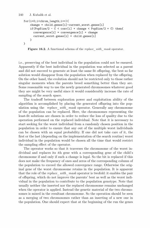
Figure 16.2. replace_with_mask
replace_with_mask
i
replace_with_mask
240 J. Kubalík et al.
A functional schema of the operator.
for(i=0;i<chrom_length;i++){change = child.genes[i]-current_worst.genes[i]if(PopSize/2 - C < conv[i] + change < PopSize/2 + C) then{convergence[i] = convergence[i] + changecurrent_worst.genes[i] = child.genes[i]
}}
i.e., preserving of the best individual in the population could not be ensured.Apparently if the best individual in the population was selected as a parentand did not succeed to generate at least the same �t offspring, the best so farsolution would disappear from the population when replaced by the offspring.On the other hand, the evolution should not be restricted only to those rathersingular moments when the parents breed something better than they are.Some reasonable way to use the newly generated chromosomes whatever goodthey are might be very useful since it would considerably increase the rate ofsampling of the search space.The tradeoff between exploration power and exploitation ability of the
algorithm is accomplished by placing the generated offspring into the pop-ulation using the operator. Generally any chromosomeof the population can be replaced. Here, the chromosomes representing theleast-�t solutions are chosen in order to reduce the loss of quality due to theoperation performed on the replaced individual. Note that it is necessary tostart seeking for the worst individual from a randomly chosen position in thepopulation in order to ensure that any out of the multiple worst individualscan be chosen with an equal probability. If one did not take care of it, the�rst or the last (depending on the implementation of the search routine) worstindividual in the population would be chosen all the time that would restrictthe sampling effect of the operator.The operator works so that it traverses the chromosome of the worst in-
dividual and replaces its th gene with a corresponding gene of the child�schromosome if and only if such a change is legal. So the bit is replaced if thisdoes not make the frequency of ones and zeros of the corresponding column ofthe population to exceed the allowed convergence range. Otherwise the orig-inal gene of the worst chromosome retains in the population. It is apparentthat the role of the operator is twofold: it enables the pairof offspring, which do not improve the parents� best as well as the worst indi-vidual in the population to contribute to the population genotype. Note thatusually neither the inserted nor the replaced chromosome remains unchangedwhen the operator is applied. Instead the genetic material of the two chromo-somes is mixed in the resultant chromosome. So the operation should be seenas a merging of two chromosomes rather than an inserting of a new one inthe population. One should expect that at the beginning of the run the genes
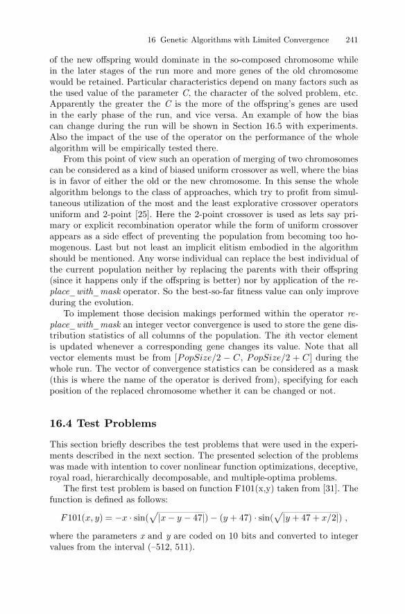
√ √
�
� � | � � | � � | |
16.4 Test Problems
PopSize/ C PopSize/ C
F x, y x x y y y x/ ,
2 2 +
101( ) = sin( 47 ) ( + 47) sin( + 47 + 2 )
CC
re-place_with_mask
re-place_with_mask
i
x y
16 Genetic Algorithms with Limited Convergence 241
of the new offspring would dominate in the so-composed chromosome whilein the later stages of the run more and more genes of the old chromosomewould be retained. Particular characteristics depend on many factors such asthe used value of the parameter , the character of the solved problem, etc.Apparently the greater the is the more of the offspring�s genes are usedin the early phase of the run, and vice versa. An example of how the biascan change during the run will be shown in Section 16.5 with experiments.Also the impact of the use of the operator on the performance of the wholealgorithm will be empirically tested there.From this point of view such an operation of merging of two chromosomes
can be considered as a kind of biased uniform crossover as well, where the biasis in favor of either the old or the new chromosome. In this sense the wholealgorithm belongs to the class of approaches, which try to pro�t from simul-taneous utilization of the most and the least explorative crossover operatorsuniform and 2-point [25]. Here the 2-point crossover is used as lets say pri-mary or explicit recombination operator while the form of uniform crossoverappears as a side effect of preventing the population from becoming too ho-mogenous. Last but not least an implicit elitism embodied in the algorithmshould be mentioned. Any worse individual can replace the best individual ofthe current population neither by replacing the parents with their offspring(since it happens only if the offspring is better) nor by application of the
operator. So the best-so-far �tness value can only improveduring the evolution.To implement those decision makings performed within the operator
an integer vector convergence is used to store the gene dis-tribution statistics of all columns of the population. The th vector elementis updated whenever a corresponding gene changes its value. Note that allvector elements must be from [ , ] during thewhole run. The vector of convergence statistics can be considered as a mask(this is where the name of the operator is derived from), specifying for eachposition of the replaced chromosome whether it can be changed or not.
This section brie�y describes the test problems that were used in the experi-ments described in the next section. The presented selection of the problemswas made with intention to cover nonlinear function optimizations, deceptive,royal road, hierarchically decomposable, and multiple-optima problems.The �rst test problem is based on function F101(x,y) taken from [31]. The
function is de�ned as follows:
where the parameters and are coded on 10 bits and converted to integervalues from the interval (�512, 511).

-512-256
0256
512x -512
-2560
256512
y
-1000
-500
0
500
1000
x y
i
i
� �y y
y
x y
1 2
1 2
1 2
x y xx x
x x
sc
Figure 16.3.
242 J. Kubalík et al.
Nonlinear and highly multimodal function F101( , ).
The function is used as basic building block of the problem. It is nonlinearnonseparable, and highly multimodal function of two variables. This meansthat the optimal value of one variable cannot be determined independentlyof the other parameter. Here the whole problem is constructed in such a waythat it consists of 7 triples , where each one contributes to theoverall �tness with the value F101( , ) + F101( , ). So the parameteris nonlinearly bound with two other parameters and , which makesthe problem even more difficult. The total length of the chromosome is 210bits. The �tness of the whole chromosome is calculated as the average valueof those 7 function contributions. The global minimum value of the problemcomposed of F101( , ) is �955.96.The next test problem is a representative of the deceptive problems, i.e.,
problems that are intentionally designed to make GAs converge toward somelocal deceptive optimum. Here, the problem is composed of the deceptivefunction DF3 taken from [30], which is 4-bit fully deceptive function withone global optimum in the string 1110 of the �tness 30. The function has adeceptive attractor 0000 of �tness 10, which is surrounded, in the search space,by four strings containing just one 1 with quite high �tness values 28, 27, 26,and 25. The problem is formed as concatenation of 50 DF3 functions resultingin a 200-bit-long chromosome. Thus the global optimum of the problem is1500. The de�nition of the search space of the DF3 function is shown inFigure 16.4.The used Royal Road problem (RR) is a 16-bit version of the RR1 single-
level royal road problem described in [7]. The problem is de�ned by enu-merating the schemata, where each schema has assigned its contributioncoefficient . The evaluation of an arbitrary chromosome is given as a sumof all contributions of those schemata that are covered by the chromosome.The used RR problem is de�ned as a concatenation of 10 16-bit schemata ofall ones. All building blocks have the equal contribution 16. Only the com-bination of all ones on the bits pertinent to a given schema contributes to

0
5
10
15
20
25
30
0000
1000
0100
0010
0001
0011
0101
0110
1001
1010
1100
1110
1101
1011
0111
1111
fitne
ss
string
0
0.2
0.4
0.6
0.8
1
0 0.2 0.4 0.6 0.8 1
f(x)
x
x
( )
6
height x
height x
F x �x ,
2( )
1( ) = sin (5 )
16.5 Experiments
meaningx
xnull
x
C
Figure 16.4. Figure 16.5.
16 Genetic Algorithms with Limited Convergence 243
Deceptive function DF3. Deb�s periodic functionF1( ).
the �tness with the nonzero value, any other combination has value 0. So theoptimal solution is the string of all ones with its �tness 160.Another test problem used in our experiments is a representative of hierar-
chically decomposable problems, namely the hierarchical-if-and-only-if func-tion (H-IFF) proposed in [29]. The hierarchical block structure of the functionis a balanced binary tree. Each block, consisting of two subblocks (a pair ofits children), contributes to the overall �tness by the value, which depends onits interpretation ( ) and its level in the tree. Each leaf node, corre-sponding to a single gene, contributes to the �tness by 1. Each inner nodeis interpreted as 1 if and only if its children are both 1s, as 0 iff they are both0s. In such a case the node contributes to the �tness by value , where
is the distance from the node to its antecedent leaves. Otherwisethe node is interpreted as and its contribution is 0. It follows from itsde�nition that the function has two global optima, one consists of all 1s andone of all 0s. For our purposes the 256-bit H-IFF function with the globaloptima of value 2304 was used.The last test function is the function F1 taken from [20] that was used
to analyze the ability of the GALCO algorithm to maintain multiple optimalsolutions in the population. The function is de�ned in the interval (0.0, 1.0)as follows:
where the parameter is coded on 30 bits so that the string of all zerosrepresents 0.0 and the string of all ones represent 1.0. The function is periodicwith 5 equally spaced maxima of equal height; see Figure 16.5.
This section presents an empirical analysis of the GALCO algorithm andshows some interesting aspects of this approach. The series of experimentswere carried out to reveal how the factors such as the convergence rate , the

�
C
C
CC
C
= 0
= 1= 20
= 1
Table 16.1.
-943 1500 2304
160
PopSize replace_with_mask
C CC
CC C
C CC
244 J. Kubalík et al.
An Effect of Varying ConvergenceRange on a Performance of the GALCO
F101 DF3 H-IFF RR225 -918 1480 1344 26200 -920 1490 1675 37100 -930 1496 2304 5650 -941 1500 2304 14020 15010 -942 1500 2304 1525 -942 1500 2304 1541 -941 1500 23040 -927 1498.5 1453 86
The population size 500 was used.
population size , and the utilization of the oper-ator affect the performance of the algorithm. GALCO is also compared tothe standard form of the incremental genetic algorithm (SIGA). Here, SIGAalways replaces the worst individuals of the population by the generated off-spring. Contrary to the GALCO, SIGA employs a simple mutation operator.The comparisons are based upon the quality of the achieved solutions as wellas the convergence characteristics of the algorithms. Both algorithms run forthe same number of �tness function evaluations, which is a commonly usedcondition when different evolutionary algorithms are compared. Each experi-ment were replicated 20 times and the average best-of-run values and averageconvergence courses are presented in tables and graphs.Let us �rst focus on how the performance of the algorithm depends on
the chosen convergence rate . Results achieved with various values ofare in Table 16.1. We can observe that small values of (means that ratherlow convergence is allowed) give better results than the bigger ones in general.This con�rms our assumption that the less the population can get homogenousthe higher the chance that better results will be generated is. However, thisassertion holds just when rather extreme values of are considered. The trendacross the whole interval of is such that starting from big the performanceimproves as the decreases until some optimum value of is reached (resultswritten in bold). Further when the decreases, the quality of the obtainedsolutions does not improve any more while the time needed to �nd the optimalsolution increases.
Apparently this is caused by the fact that the more diverse the populationis kept (an extreme case is discussed further) the more the convergencetoward the optimal solution slows down. Thus we can see that the averagebest-of-run value achieved with is worse than that achieved with theoptimal in the case of F101. In the case of DF3 and H-IFF problemsthe optimal average best-of-run values were achieved even with but it

0 100 200 300 400 500950
900
850
800
750
fitness evaluations (x1000)
fitne
ss
optimal CC=1C=0
0 100 200 300 400 5001300
1350
1400
1450
1500
fitness evaluations (x1000)
fitne
ss
optimal CC=1C=0
0 100 200 300 400 500500
1000
1500
2000
2304
fitness evaluations (x1000)
fitne
ss
optimal CC=1C=0
0 200 400 600 800 10000
16
32
48
64
80
96
112
128
144
160
fitness evaluations (x1000)
fitne
ss
optimal C=1C=0
C
C
C C C
= 1
= 0
C
replace_with_mask
Figure 16.6a�d.a b c
d
16 Genetic Algorithms with Limited Convergence 245
Mean convergence curves obtained with the optimal convergence rate, convergence rate =1 and =0 on the problem F101 ( ), DF3 ( ), H-IFF ( ), andRR ( ). The population size 500 was used.
took considerably longer time to �nd them. See Figure 16.6, where the averageconvergence curves with the optimal and are shown.Let us have a look at the results on the RR problem now. This is the
problem that requires the least convergence rate to get the best results. Thisresults from the nature of the benchmark. There are no smaller building blocksavailable besides those prede�ned 16-bits ones, which would guide the algo-rithm toward the complete optimal solution. So the algorithm can only relyon maximal diversity of individuals that would maximize a chance that allbuilding blocks will be generated and combined in one optimal chromosome.It is also interesting to see the effect of the opera-
tor. The results of experiments carried out with disabled replacement op-erator are in the last row of Table 16.1, where . It is evident thatthe operator greatly improves the performance of GALCO if used with areasonable frequency. There are considerable differences in average best-of-run values obtained on problems F101, H-IFF, and especially on RR. In the

0 50 100 150 2000.25
0.5
0.75
1
iterations (x1000)
utili
satio
n of
the
offs
prin
g ge
nes
C=1C=100
�
,200 000
= 1= 100
+
Figure 16.7.
CC
PopSize C PopSize C
replace_with_mask
replace_with_mask
re-place_with_mask
replace_with_mask
C
246 J. Kubalík et al.
Demonstration of a utilization of the genetic material of the offspringundergoing the operation. Graphs show an evolution of the ratio ofgenes taken from the offspring to the total number of genes, in which the chromosomesthat are merged by the operator (the offspring and the worstindividual in the population), mutually differ. The used population size was 250. Theview of the �rst iterations of the algorithm is provided.
case of the deceptive problem the best-of-run solutions achieved withoutoperator are quite close to the optimum. However, the two
variants of GALCO algorithm, the one that employs theoperator and the other one that does not, differs in the number of functionevaluations needed to come to the optimum solution. This is shown in Fig-ure 16.6.These results con�rm our intuition that not only a crossover operator ap-
plied explicitely to promising parents enables the good building blocks tocombine. Also a mixing of the genetic information of two rather poor chro-mosomes by the replacement operator is very fruitful. One should see that inthis way the worst individual in the population is given a high chance that itsgenes or complete building blocks will be combined with other genetic mater-ial. Note that without the replacement operator such a chance would be verysmall since the worst individual is almost unlikely to be chosen as a parent.Figure 16.7 shows an evolution of a utilization of genes taken from the
offspring chromosome. We can see that the characteristics differ from eachother in a way one would expect. When a small convergence rate is used (i.e.,
) the proportion of genes taken from the offspring is stable (around thevalue 2/3) during the whole run. The bigger is used (situation foris shown here) the more of the offspring genes can be used in the early stagesof the run. At the beginning of the run the offspring chromosome completelyreplaces the worst chromosome of the population. As the population convergesi.e., the distribution of ones and zeros in the population columns reaches theboundary values (either or ) the utilization of theoffspring genes drops down and then stabilizes around the value 2/3 as inthe former case. Note that the proportion of the worst individual genes is the

�
�
C
P . P .cross mut
= 1
= 1 0 = 0 01
PopSize
PopSize
Table 16.2.
2304-949 1500
160
Table 16.3.
-912 1476 1501
16 Genetic Algorithms with Limited Convergence 247
An Effect of Varying Population Size on a Performance of the GALCO
F101 DF3 H-IFF RR20 -928 1500 2304 6850 -937 1500 2304 147100 -943 1500 154150 2304 159200 -946 1500 2304 160250 -945 1500 2304 160500 -941 1500 2304 1601000 -928 1500 2304
The convergence range was used in these experiments.
Results of the SIGA Algorithm with Varying Population Sizes
F101 DF3 H-IFF RR500 -877 1449 1234 1491000 -907 1464 1348 1501500 -909 1473 1382 1442000 147
Other parameters of the SIGA were , , and the number of�tness function evaluations was 500,000.
complement to 1.0. So a considerable number of genes of the worst individualare used as well.Another factor, which strongly affects a performance of GAs, is the size
of the population. General trend in standard GAs is that the bigger the usedpopulation is, the better results can be achieved. This is because the bigpopulation provides better supply of necessary fundamental building blockswhen it is initialized and is less subject to premature convergence. On the otherhand, the evolution of large population toward high-quality solutions may betoo slow and at the expense of more computations performed (measured forinstance by a number of performed �tness function evaluations or crossoveroperations).
The results of experiments carried out in order to investigate a sensitivityof the GALCO to population size are presented in Table 16.2.
There are two important observations. First, the performance of the algo-rithm depends on the population size in a similar way as other GAs. As thepopulation size increases, the quality of the obtained results improves untilan optimal population size is reached (the results written in bold). Furtherincreasing of the size slows down the convergence to the optimal solution.In the case of F101 much worse solutions were found with population size1000 than with the population size 150. Similarly, much slower convergence

200
= 1
PopSize >
C
248 J. Kubalík et al.
16.6 Summary and Conclusions
to optimal solutions were observed when large populations ( )were used on DF3 and H-IFF problems. Again when solving the RR prob-lem the best results were achieved with the biggest tested population size. Astrange phenomenon can be observed on the DF3 problem. There, the optimalsolution was found even with a small population of 20 individuals. Such anunusual success of the algorithm on this benchmark could be easily explained.Recall that the DF3 function is a fully deceptive function with the deceptiveattractor in the string, which is a binary complement of the global desiredoptimum. This means that the deceptive building blocks (those with all 0s orat most one 1) tend to gradually proliferate in the population. However thesaturation of the population with those building blocks is limited due to the
. So in reaction to the increased number of deceptive building blocksthe number of building blocks composed of all 1s grows as well in order tokeep the balance of 1s and 0s in the population. Obviously such a mechanismshould work whenever a string representing a local optimum is close to thebinary complement of the global optimum string.The second observation is that the algorithm does not require very large
populations to be able to solve the problems. In fact, rather small populations(100�200 for our test problems, except the RR problem) can be used withGALCO to effectively search a complex solution space. This becomes evidentwhen compared to the results obtained with the standard incremental GA(SIGA), see Table 16.3. While the SIGA needs a large population to comeup with good solutions, the GALCO pro�ts from its inherent explorativepower described above. A comparison of the GALCO and SIGA in terms ofthe average convergence characteristics is shown in Figure 16.8. We can seethat the GALCO outperforms the SIGA on all test problems. An especiallyremarkable difference between the two algorithms can be observed on F101,DF3, and H-IFF problems, where SIGA did not give any comparably goodresult even with population size 2000.As we mentioned in the previous section some experiments were performed
to test the GALCO algorithm on its ability to discover many different globaloptima. The plots in Figure 16.9 show how the population samples the solutionspace of the F1 function after 50,000 and 500,000 performed �tness functionevaluations. It turned out that the algorithm is able to maintain a number ofsamples for each peak of the function. As the evolution goes on the individualsin the population become better and better. An important observation is thatthe proportions of the population are almost stable during this process.
We have introduced a novel approach for preserving population diversity. Itis based on an idea that the population is explicitly prevented from becomingtoo homogenous by simply imposing limits on its convergence. This is doneby specifying the maximum difference between frequency of ones and zeros

0 100 200 300 400 500950
900
850
800
750
fitness evaluations (x1000)
fitne
ss
GALCOSIGA
0 100 200 300 400 5001300
1350
1400
1450
1500
fitness evaluations (x1000)
fitne
ss
GALCOSIGA
0 100 200 300 400 500500
1000
1500
2000
2304
fitness evaluations (x1000)
fitne
ss
GALCOSIGA
0 200 400 600 800 10000
16
32
48
64
80
96
112
128
144
160
fitness evaluations (x1000)
fitne
ss
GALCOSIGA
0
0.2
0.4
0.6
0.8
1
0 0.2 0.4 0.6 0.8 1
f(x)
x
0
0.2
0.4
0.6
0.8
1
0 0.2 0.4 0.6 0.8 1
f(x)
x
Figure 16.8a�d.a b c d
Figure 16.9a�b. ab
16 Genetic Algorithms with Limited Convergence 249
Comparison of the convergence characteristics of GALCO and SIGAon the problem F101 ( ), DF3 ( ), H-IFF ( ), and RR ( ). It shows the convergencecharacteristics corresponding to the experiments marked bold in Table 16.2 and Table16.3, respectively.
The �nal distribution of 100 solutions after 50,000 ( ) and 500,000( ) �tness function evaluations. Proportions of the population after 50,000 and 500,000evaluations are 24-18-19-19-20 and 26-16-22-17-19, respectively.

2C << PopSize/
replace_with_mask
250 J. Kubalík et al.
at any position of the chromosome calculated over the whole population. Thealgorithm is of a type of the incremental GA where only one crossover opera-tion is performed in each generation cycle and the newly created individualsreplace some individuals of the current population.A speci�c replacement strategy is used to keep the desired distribution of
ones and zeros during the whole run. The pair of newly generated chromo-somes replace the parents if the best-�t chromosome out of those four ones isthe child. Under such an replacement operation the population genotype staysinvariant. Apparently the evolution of the population would be too limited ifwe relied on accepting only those new chromosomes, which improve the �tnessof their parents. To further boost up the exploration power of the algorithm aspecial replacement operator was introduced, which is used to insert as muchof the offspring genetic material as possible into the population. Actually thecurrently worst-�t chromosome of the population is merged with the new one.In fact this is just another recombination operation providing a means forbetter exploiting of genetic material of the poorly �t individuals.The proposed algorithm was experimentally tested on a representative set
of test problems. The results revealed several interesting aspects of the algo-rithm�s behavior. First, the best performance of the algorithm was achievedwith rather low convergence rate ( ). This means that thedistribution of ones and zeros is almost half-to-half in every column of thepopulation. This is in agreement with the intuition that the more equal thedistribution of ones and zeros is used, the less the algorithm is prone to prema-turely converge so the better results can be achieved. Due to its replacement�recombinative component the algorithm is able to go on to generate new sam-ple points of the search space even after the global optimum has been found.It was also shown that the algorithm is capable of maintaining multimodaldiversity of the population. So representatives of various optima can co-existin the population during the whole evolution.An interesting aspect of the proposed algorithm is that it does not re-
quire any tuning of the mutation or crossover probabilities. Apparently anyprobability of crossover less than 1.0 does not make any sense because oncea pair of parents is chosen they should be crossed over, otherwise the wholeaction does not have any effect. There is no explicit mutation operator usedin the algorithm. The variability of the population genotype is maintainedby preservation of the gene distribution combined with the high generativeability of the recombination crossover and operators. Forthe same reason the algorithm works efficiently with rather small populationsin comparison with standard GA. It was shown that from some value of thepopulation size its further increasing is counterproductive and the process of�nding the optimum solution slows down.Concluding this chapter we can say that the GALCO algorithm exhibits
many nice features. However, they were presented and con�rmed only in anempirical way. Future research in this area should focus on theoretical analysisof the algorithm. That would help us to better understand its behavior and to

Acknowledgments
References
Proceedings of the Fourth International Conference on Genetic Algorithms
Adaptive search using simulated evolution
ECAI 96: 12th European Conference on Arti�cialIntelligence
ECAI 96: 12th European Conference on Arti�cialIntelligence
An Analysis of the Behavior of a Class of Genetic AdaptiveSystems
Annals of Mathematics and Arti�cial Intelligence
Foundations of Genetic Algorithms2
Genetic Algorithms and Their Applications: Pro-ceedings of the Second ICGA
Genetic Algorithms in Search, Optimization and MachineLearning
estimate its convergence characteristics. Note that for our evaluation purposeswe have used test problems composed of tightly linked building blocks. Theapplicability of the algorithm to the problems with low linkage, i.e., the prob-lems with building blocks spread across the chromosome, should be studiedas well.
The authors would like to thank Petr Posik for many valuable comments andStepan Janda for his help with carrying out the experiments.The �rst author acknowledges the support provided by the TU Delft within
a frame of the Research Fellowship Program. The research was funded by theproject No. 102/02/0132 of the Grant Agency of the Czech Republic.
16 Genetic Algorithms with Limited Convergence 251
1. Baker, J.E. (1987) Reducing Bias and Inefficiency in the Selection Algorithm.In ,Lawrence Erlbaum Associates, Hillsdale, pp. 14�21
2. Cavicchio, D.J. (1970) , Ph.D. Thesis,Univ. of Michigan, Ann Arbor.
3. Collard, P., Gaspar, A. (1996) Royal-road landscapes for a dual genetic algo-rithm, in W. Wahlster, editor,
, Wiley & Son, pp 214�2174. Collard, P., Escazut, C. (1996) Fitness Distance Correlation in a Dual GeneticAlgorithm, in W. Wahlster, ed.,
, Wiley & Son, pp. 218�2225. De Jong, K.A. (1975)
, Doctoral Thesis, Dept. of Computer and Communication Sciences, Univ.of Michigan, Ann Arbor,
6. De Jong, K.A., Spears, W. (1992) A formal analysis of the role of multi-pointcrossover in genetic algorithms,(Switzerland: J C Baltzer A G Scienti�c Publishing Company), pp. 1-26.
7. Forrest, S., and M. Mitchell. (1993) Relative building-block �tness and the Build-ing Block Hypothesis, in Whitley, L.D. (Ed.),, pp. 109-126. San Mateo, CA: Morgan Kaufmann.
8. Goldberg, D.E. (1985) Optimal Initial Population Size for Binary-Coded GeneticAlgorithms,. TCGA Report No. 85001, University of Alabama, Department ofEngineering Mechanics.
9. Goldberg, D.E., Richardson, J.J. (1987) Genetic algorithms with sharing for mul-timodal function optimization,
, Lawrence Erlbaum Associates, Hillsdale, NJ, pp41-49
10. Goldberg D.E. (1989), Addison-Wesley, Reading, MA.
Foundations of Genetic Algo-rithms
Complex Systems
EvolutionaryComputation
Adaptation in Natural and Arti�cial Systems
Advances in Soft Computing
AIP Conference Proceedings of CASYS �2000
Quo Vadis Computational Intelligence?
Proceeding of Mendel 2001
Parallel ProblemSolving From Nature
Proceedings of the Genetic and Evo-lutionary Computation Conference
Genetic Algorithms + Data Structures = Evolution Pro-grams
Pro-ceedings of the Fourth Annual Conference on Evolutionary Programming
Handbook of EvolutionaryComputation
252 J. Kubalík et al.
11. Goldberg, D.E., Deb, K. (1991) A comparative analysis of selection schemes usedin genetic algorithms, in Rawlins, G. J. E. (Ed.),
, San Mateo, CA: Morgan Kaufmann, pp. 69-9312. Goldberg, D.E., Deb, K., Clark, J.H. (1992) Genetic algorithms, noise, and thesizing of populations. , 6:333-362,
13. Goldberg, D.E., Sastry, K. (2001) A Practical Schema Theorem for Genetic Al-gorithms Design and Tuning, IlliGAL Report No. 2001017, Illinois Genetic Algo-rithms Laboratory, University of Illinois at Urbana-Champaign,
14. Harik, G., Cantu-Paz, E., Goldberg, D.E., and Miller, B. L: (1999) The gambler�sruin problem, genetic algorithms, and the sizing of populations,
, 7(3):231-25315. Holland J.H. (1975) . University ofMichigan Press, Ann Arbor.
16. Kubalík, J., Lazansk�, J. (2000) Partially randomised Crossover Operators, In:, R. John & R. Birkenhead (Eds.), Heidelberg:
Physica-Verlag, pp 93-98.17. Kubalík, J., Lazansk�, J. (2001) A New Genetic Operator Maintaining PopulationDiversity, in , Dubois, D. (Ed.),American Institute of Physics, pp. 338-348.
18. Kubalík, J., Lazansk�, J. (2000) A New Genetic Operator with Enhanced Capabil-ities. In: Sincák, P. (ed.), Physica-Verlag,Heidelberg, Germany, pp. 305-310.
19. Kubalík, J., Lazansk�, J., Rothkrantz, L.J.M. (2001) On Extending of SearchPower of Genetic Algorithms by Means of Permanent Re-initialisation of ParentalCommon Schema, in , Brno University of Technology,pp. 1-6.
20. Mahfoud, S.W. (1992) Crowding and Preselection Revisited,, 2, R. Manner and B. Manderick (Eds), Elsevier Science
Publishers (North Holland), Amsterdam, pp. 27-36.21. Mengshoel, O.J., Goldberg, D.E. (1999) Probabilistic Crowding: DeterministicCrowding with Probabilistic Replacement, in
, W. Banzhaf, J. Daida, A. E. Eiben, M. H.Garzon, V. Honavar, M. Jakiela, R. E. Smith (Eds), Morgan Kaufmann Publish-ers, California,
22. Michalewicz Z. (1994), Springer-Verlag, Berlin Heidelberg, Second edition.
23. Miller, B., Goldberg, D.E. (1995) Genetic Algorithms, Tournament Selection, andthe Effects of Noise. IlliGAL Report No. 95006, Urbana: University of Illinois,Illinois Genetic Algorithms Laboratory.
24. Oei, C.K., Goldberg, D.E., Chang, S. J. (1991) Tournament selection, niching,and the preservation of diversity, IlliGAL Report No. 91011, Illinois Genetic Al-gorithms Laboratory, University of Illinois at Urbana-Champaign.
25. Spears, W.M. (1995) Adapting Crossover in Evolutionary Algorithms, in, J.R.
McDonnel, R. G. Reynolds and D.B. Fogel, eds., MIT press, Cambridge, 1995, pp367-384
26. Spears, W.M. (1997)Recombination Parameters, in, T. Back, D.B. Fogel, and Z. Michalewicz, eds., New York: Oxford
Univ. Press and Institute of Physics, pp E1:3:1-11

IEEE Transaction of Systems, Man and Cy-bernetics
Proceedings of The First IEEE Conference on Evolu-tionary Computation
Parallel Problem Solving from Nature
Foundations of Genetic Algorithms
Arti�cial Intelligence
16 Genetic Algorithms with Limited Convergence 253
27. Srinivas,M., and Patnaik, L. M. (1994) Adaptive Probabilities of Crossover andMutation in Genetic Algorithms, in
, 24:656-66728. Thierens, D., Goldberg, D.E.: (1994) Elitist Recombination: an integrated selec-tion recombination GA. In
, Vol 1, pp 508-512.29. Watson, R.A., Hornby, G.S. and Pollack, J.B. (1998) Modeling Building-BlockInterdependency. , proceedings of Fifth In-ternational Conference PPSN V, Springer, pp.97-106.
30. Whitley D. (1991) Fundamental Principles of Deception in Genetic Search. In:, G. Rawlins ed., Morgan Kaufmann, pp. 221-
241.31. Whitley D., Mathias, K., Rana, S., Dzubera, J. (1996) Evaluating EvolutionaryAlgorithms, , 85:245-276.
17___ ______ ______ __________________ ______ ______ ______ ______ ______ ______ ______ ____________
Evolution with Sampled Fitness Functions
F. Bellas, J. A. Becerra and R. J. Duro
Summary: In this chapter we study the effect of different parameters and algorithmicstrategies on the problem of working with sampled fitness functions in evolutionary proc-esses. Some results are presented on the effect of the size of the short-term memory and thenumber of generations of evolution in between updates. From these results it can be ob-served that there are some critical points that may be considered in order to define the limitsto which one can simplify the computations when working with sampled fitness functionswhile maintaining the same representative power.
We provide a study of different proposals for the construction of short-term memoriesand their replacement strategies in order to obtain the maximum information with the mini-mum use of resources when operating evolutionary algorithms in problems where the fitnessfunctions cannot be fully known and thus need to be sampled. We provide results for differ-ent functions and study the effect of the level of randomness of the replacement of a maxi-mum-minimum replacement strategy.
17.1 Introduction
In the realm of evolutionary computation many applications involve obtaining fit-ness data from partial samplings of the fitness function [2-8]. This fitness determi-nation may be carried out through an explicit mathematical function that is par-tially sampled or some type of environment that provides performance informationfor different actions carried out by the entity resulting from the phenotypic repre-sentation of the genotype. In any case, for every individual and determination offitness, the data employed is different, although part of the same function. Conse-quently, if the required optimal individual must achieve optimality for the wholefitness function, obtaining it implies the integration of series of partial snapshots ofthe fitness function. These snapshots depend on how the evolutionary process ispresented with the information on fitness.
If we translate this into a more formal computational environment, we have aproblem of obtaining a general representation of some type of function through thepresentation of sequences of partial data samples or frames. The traditional ap-proach to the problem has been to wait until enough frames had been compiled anduse the whole of the information to obtain the representation [3]. This is what wewould call a full (or very close to full) information fitness function. In the case ofthe agent-environment interaction, each agent would be made to interact with theenvironment for a very long period of time. This is all so well when we have asimple and static process that does not change, independently of how long it takesus to gather the information, and where the relevant data that must be considered toadequately model the process can be gathered and stored in reasonable time and

F. Bellas et al.256
space. It does not perform so well when we are working with complex dynamicprocesses. In this case, performing evolution with anything close to full informa-tion fitness functions becomes computationally very expensive, in fact, it becomesunapproachable.
In this paper we will try to provide some insight into the problem and presentsome results that will help to decide how to apply sampled fitness functions in or-der to obtain results that are often as good as with the complete fitness function.
17.2 Our Problem
The problem we have considered is to obtain world and internal models forautonomous robots through their online interaction with the world, whether real orsimulated. The information the agent receives from the environment in any giveninstant of time and which it must use to evaluate its models is partial and, in manycases, noisy or irrelevant. Any model it extracts from this instantaneous informa-tion will, in most cases, be useless for other instants of time. To generalize appro-priate models the agent will have to consider and relate information obtained inmany different instants of time in an efficient manner.
In more mathematical terms and considering a set of data that define a function,the fitness of the model is given by how well it fits the whole function and not byhow well it fits the individual point or the subset of points it is considering in agiven instant of time. This is what we have called a Sparse Fitness Function (SFF),the fitness of the individual is given by its response to several different instantane-ous local fitness functions, which together conform the desired global one.
In order to illustrate the problems encountered, we have performed tests onthree benchmark functions of increasing difficulty in order to obtain generalizableindications.
• Sin function: y = sin(x)• Logistic series: x(t) = 4x(t-1)/1-x(t-1)• 3D function: z = xsin(x) + ysin(y)
The idea was to obtain a neural network that would model these functionsthrough evolution. Each network consisted of one input neuron, two hidden layerswith four nodes, and one output neuron both for the sin and the logistic functions.In the case of the 3D function we have used a neural network with two input neu-rons, two hidden layers of six neurons each, and one output neuron. The evolutionwas carried out using 350 individuals (700 for the 3D function). The fitness of eachindividual was obtained by determining the mean squared error (MSE) between theoutput of the network and each one of the points of the signals contained in aShortTerm Memory (STM). This STM contains a window of data of the signal thatis fed to the STM replacement mechanism one item per instant of time.

17 Sampled Fitness Functions 257
How big the STM is and how many generations of the evolutionary algorithm weperform per data input are the main two parameters in terms of computing resourceusage. Each item in the STM must be run through the current model once per indi-vidual per generation so as to obtain an error term. Obviously, the smaller thenumber of individuals in a population, the smaller the STM and the less genera-tions per data input cycle we run the evolutionary algorithm the better in terms ofresources. The problem regarding population size is that, as commented in [1],there is a lower limit to the size of the populations we can use before running intopremature convergence problems. Consequently, we will have to concentrate onthe other two terms.
Figure 17.1. MSE of the output of the network after evolution with respect to the realfunction for different number of generations of evolution per interaction and STM sizes.
0,00
0,05
0,10
0,15
0,20
0,25
0,30
0,35
0,40
0,45
0,50
Mea
n S
quar
ed E
rror 1
24820100
Number of Generationsper interaction
Sin()
0,00
0,05
0,10
0,15
0,20
0,25
Mea
n S
quar
ed E
rror 1
24820100
Number of Generationsper interaction
Logistic
2,00
2,50
3,00
3,50
4,00
4,50
5,00
5,50
6,00
6,50
7,00
0 10 20 30 40 50 60 70 80
STM size (in items)
Mea
n S
quar
ed E
rror
124820
3D
Number of Generationsper interaction

F. Bellas et al.258
17.3 Short-Term Memory Size and Number of Generations perInteraction with the World
Figure 17.1 displays the evolution of the MSE of the output of the network with re-spect to the real function for different STM sizes and number of generations ofevolution per interaction. The three graphs that make up the picture correspond to
0,00
0,05
0,10
0,15
0,20
0,25
0,30
0,35
0,40
0,45
0,500 20 40 60 80 100
Number of generations per interaction
Mea
n S
qu
ared
Err
or
2 4 8 14 20 40 80STM sizeSin()
0,00
0,05
0,10
0,15
0,20
0,25
Mea
n S
qu
ared
Err
or
2 4 6 8 10 14 20 40 80STM size
Logistic
2,00
2,50
3,00
3,50
4,00
4,50
5,00
5,50
6,00
6,50
7,00
0 5 10 15 20
Number of generations per interaction
Mea
n S
qu
ared
Err
or
4 8 14 20 40 80STM size3D
Figure 17.2. MSE of the output of the network after evolution with respect to the realfunction for different STM sizes and number of generations of evolution per interaction.

17 Sampled Fitness Functions 259
the three functions. The MSE is calculated by running the resulting networks overthe whole signal and comparing the result to the original one. It is clear that forSTMs larger than 8 the MSE becomes almost a constant, independently of thenumber of generations per update. This implies that for a randomly filled STM onaverage, eight points of the signal provide enough information to model the wholesignal. Obviously, if we take, for example, a STM of 10, we will be on the safeside, no matter how many generations of the evolutionary process we run. This isnot necessarily the optimal solution, just the safest one. If we look at this graphmore closely, we see that for a STM of 4 and running 2 generations per iterationwe obtain almost the same error, but now, the computing required is much less. Letus take a look at this graph in another way (Figure 17.2). Now we can see thatthere are two types of behaviors with the number of generations per interactionwith the world. In the first case, for STMs, smaller than the critical size, if we carryout few generations per interaction, that is, if we evolve very little with a givenframe of the STM, the results improve with the number of generations up to apoint, in this case about 4 or 6 generations per interaction. More evolution withoutchanging data items in the STM leads to a problem of overfitting the current STMframe and not generalizing to the whole fitness function. In short, for these valuesof the STM, we have a concave function with a minimum for a given number ofgenerations per iteration. After the critical STM value is surpassed, there is nominimum, the function is monotonously decreasing with the number of genera-tions, implying that it is very difficult to overfit to the current STM as it provides agood enough representation of the signal to model it correctly without having touse many frames.
Figure 17.3 displays the variation of the MSE during evolution for six cases.We have first considered an STM of 2 and have evolved the networks for 2 gen-erations per interaction. There is a certain improvement, but, as two points is a verypoor representation of the signal, evolution on two points just leads to oscillationsin MSE, with very poor values. The networks never really learn the fitness func-tion; they tend to evolve toward the contents of the STM in a given instant of time.This is more marked if we take 100 generations per interaction for a short-termmemory of 2, now the MSE is basically pure noise. The network evolves to predictthe STM contents very well (two points) but not the signal. Consequently, the MSEwith respect to the signal becomes really deficient. As STM increases in size, as inthe case of the second set of graphs for STM 8 (middle graphs), we see that nowthe information in the STM starts to be relevant. There is an evolution toward areasonable representation of the signal (low MSE). With new interactions with theworld the STM changes, and some oscillations in the behavior of the MSE can beobserved, but, especially in the case where not many generations of the evolution-ary algorithm are run between interactions, the networks are not overfitted to theinstantaneous contents of the STM but tend to obtain a more general solution. Ob-viously, the more generations per interaction we run the evolution, the moremarked the overfitting of the instantaneous STM becomes. Finally, in the thirdcase, we present an STM of 20 (top graphs), well above the critical point for thisfunction. Now the networks evolve to a good prediction of the whole signal (lowMSE) with very little difference between running many or few generations of theevolutionary process between interactions with the world. The only appreciabledifference is that with more generations, the process is evidently faster.

F. Bellas et al.260
This is all very well for the logistic function, but what happens with other typesof functions? We have considered a simpler and a more difficult function (sin and3D). If we produce the same representations for these functions as we did for thelogistic one (Figures 17.1 and 17.2, top and bottom), it can be clearly seen that thebehavior is basically the same. On one hand, the sin() function provides represen-tations that are almost indistinguishable from those of the logistic function except,maybe, for the fact that they are smoother. This is a surprising result, indicatingthat for the network we are using, a sin() function is about as hard, or easy tomodel, as a logistic function. Well, if one looks at the state space this is probablytrue. Thus, it is good to see that for similar modeling difficulty, we obtain basicallythe same results.
On the other hand, if we go to a much harder function to model, such as the 3Done we indicated above, we see that, although the general behavior is similar, now
Fig ure17.3. Evolution of the MSE for STMs of sizes 2, 8, and 20 using the logistic func-tion. The top figure shows 2 generation per update of the STM, and the bottom figureshows 100 generations per update.
0
0,5
1
1,5
1 101 201 301 401 501 601 701 801 901
Interaction
MS
E
STM2
STM8
STM20
2 generations per interaction
0,00,5
0,00,5
0,5
0
0,6
1,2
1,8
1 101 201 301 401 501 601 701 801 901
Interaction
MS
E
STM2
STM8
STM20
100 generations per interaction
0,6
0,00,6
0,00,6
17 Sampled Fitness Functions 261
the critical point has changed; it has gone up to an STM of about 20. What is reallyinteresting about this is that by looking at the slope of the MSE function as a func-tion of the number of generations per interaction, one knows what side of the criti-cal STM point one is for a given function. As commented above for the logisticfunction, if one is below the critical point, a small number of generations per inter-action will provide better results in the global error. If one is above the criticalpoint, two considerations may be made. On one hand, a smaller STM could proba-bly be used, thus reducing computational load, on the other, the number of genera-tions per interaction will not really affect the outcome. Consequently, by delimitingwhere the critical point is located, one could think of tweaking with parameterssuch as the size of the STM, the evolutionary pressure of the process as well as thenumber of generations per interaction with the world in order to optimize the com-putational load and the probability of obtaining a successful evolution. Take intoaccount that if these parameters are not properly set, two consequences may arise.If the STM is too small or the evolutionary pressure per interaction too high(through many generations per interaction or an evolutionary algorithm with a highpressure), the network will never learn the global function and will overfit the cur-rent STM frame, thus producing a global oscillating MSE. On the other hand, largeSTMs will lead to very long processing times.
17.4 Critical Points
In the previous sections we have seen that when one studies the evolution of themean squared error of the model of a signal provided by an evolved ANN when thefitness function during evolution was sampled, a critical point arises for STM sizewhereby the behavior over this critical point is quite different from that below it.Below, the MSE is very dependent on STM size and evolutionary pressure. Aboveit, this dependence disappears. In fact, above it, it seems that no matter how manygenerations we evolve on a given frame of the STM, the results remain the same;there is no overfitting. Consequently, if the STM is above the critical point, whynot just evolve for a very large number of generations on a static STM without in-troducing any new data?. Well, there are two answers to this. First, this strategywould provide no capability of dealing with changing environments. Second, thecritical point we are considering is what we would call a dynamic sampling criticalpoint, this is, the contents of the STM are enough to model the signal if theychange at a reasonable rate.
In fact, one could define three different types of critical STM sizes. On onehand, we could define what we would call static consecutive sampling criticalpoint (SCS-CP). This critical size indicates what the minimum size of the STMmust be in order to provide a good enough representation of the signal if the STMdoes not input any new data and the data it contains are consecutive samples of thesignal. This point obviously depends on how good a representation of the signalone desires and on the sampling frequency. For a 63 sample per cycle representa-tion of the sin() function, in our case it results that an STM of 63 is required asSCS-CP.

F. Bellas et al.262
The second type of critical point is given by the average STM required to relia-bly represent the signal when this STM is static (no updating) and the points in itare random samples of the signal. This is what we call the static random samplingcritical point (SRS-CP), For the sin() function, the SRS-CP would be around 20.
Finally, we have the critical point we have derived in Part I, that is, the DynamicSampling Critical Point (DS-CP). In this case, the STM will be updated with somecriterion. As in the case of static critical points, it will also depend on how wesample the signals or environments. Obviously a DCS-CP (dynamic consecutivesampling critical point) will in general present a higher value than a DRS-CP (dy-namic random sampling critical point) given the better probability of a randomsampling of providing a good representation of the signal. In fact, for the sin()function, the DRS-CP turns out to be about 10 for the same sampling frequency asabove.
From a practical point of view, all of the above comments lead to the considera-tion that the minimum size necessary for the STM to be able to provide a goodenough representation of the signal to permit obtaining a model within a given er-ror margin depends on two factors: sampling frequency and dynamicity. Samplingfrequency, if above the frequency established by Shannon’s theorem, is only rele-vant if the data are taken in a consecutive manner. Any other STM updating strat-egy will reduce the influence of this factor.
Regarding dynamicity, any evolutionary strategy acting on a dynamic STM, thatis a STM that is updated with new information as new interactions with the func-tion or environment occur, will see a virtual STM that is larger than the real onejust as long as the evolutionary pressure on a single frame of the STM is not toolarge. Thus, for practical use one would think that the optimal usage of an STMwould occur when the maximum information on the signal is introduced in itthrough an appropriate update or replacement strategy and when this informationchanges with time at a rate compatible with the number of generations and evolu-tionary pressure of the algorithm in between interactions with the function or envi-ronment. When evolving between interactions or updates of a dynamically chang-ing STM, one does not want the population to converge to the current frame of theSTM; otherwise, when the next frame comes in, unless the STM is well above thestatic critical point, the performance of the solution evolved will be very poor. Theresult of something like this would be to have an algorithm that is constantly con-verging to the contents of the STMs but never really modeling the underlyingfunction or environment.
17.5 Replacement Mechanism
One of the most relevant aspects in managing dynamic STMs, as mentioned above,is the replacement mechanism. The better the replacement strategy, the better therepresentative power of each frame. Thus, a good replacement strategy maximizesthe information content of the memory.
To achieve this objective we have studied the effect of introducing a strategythat maximizes the minimum distance from every item in the STM to every otheritem. This approach implies defining a distance between items. In our case we havejust used a standard Euclidean distance taking each item in the STM as an n-

17 Sampled Fitness Functions 263
dimensional vector.This approach usually results in a very good distribution of the items in the n-
dimensional space conformed by the representations of the items in the short-termmemory. Evidently, this strategy does not imply any relation to the importance ofthe items towards the task in hand; it is just a maximization of the coverage of then-dimensional space by a limited number of vectors. It is just a geometric property.Notwithstanding this fact, this type of approach has provided a good selection ofthe points to be used for the evolution of representations as shown in Figure 17.7.
The problem with this approach is that after a maximum/minimum distanceconfiguration of the STM has been achieved, no changes occur in the STM, thus
-1
-0,8
-0,6
-0,4
-0,2
0
0,2
0,4
0,6
0,8
1
1 4 7 10 13 16 19 22 25 28 31 34 37 40 43 46 49 52 55 58 61 64
Real
Red
-1
-0,8
-0,6
-0,4
-0,2
0
0,2
0,4
0,6
0,8
1
1 4 7 10 13 16 19 22 25 28 31 34 37 40 43 46 49 52 55 58 61 64
Real
Red
-1
-0,8
-0,6
-0,4
-0,2
0
0,2
0,4
0,6
0,8
1
1 4 7 10 13 16 19 22 25 28 31 34 37 40 43 46 49 52 55 58 61 64
Real
Red
Figure 17.4. Model of the sin() function provided by the best network evolved usingdifferent replacement strategies for the STM. It is a size 4 STM with 8 generations ofevolution per update. The strategies considered are static (top), FIFO (middle), andmaximum-minimum replacement (bottom). The functions were sampled randomly.
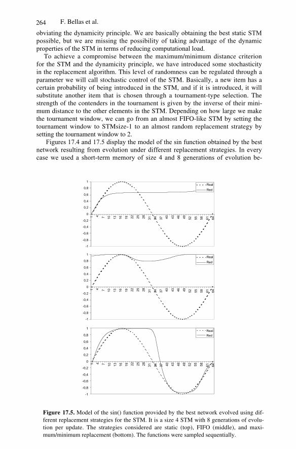
F. Bellas et al.264
obviating the dynamicity principle. We are basically obtaining the best static STMpossible, but we are missing the possibility of taking advantage of the dynamicproperties of the STM in terms of reducing computational load.
To achieve a compromise between the maximum/minimum distance criterionfor the STM and the dynamicity principle, we have introduced some stochasticityin the replacement algorithm. This level of randomness can be regulated through aparameter we will call stochastic control of the STM. Basically, a new item has acertain probability of being introduced in the STM, and if it is introduced, it willsubstitute another item that is chosen through a tournament-type selection. Thestrength of the contenders in the tournament is given by the inverse of their mini-mum distance to the other elements in the STM. Depending on how large we makethe tournament window, we can go from an almost FIFO-like STM by setting thetournament window to STMsize-1 to an almost random replacement strategy bysetting the tournament window to 2.
Figures 17.4 and 17.5 display the model of the sin function obtained by the bestnetwork resulting from evolution under different replacement strategies. In everycase we used a short-term memory of size 4 and 8 generations of evolution be-
-1
-0,8
-0,6
-0,4
-0,2
0
0,2
0,4
0,6
0,8
1
1 4 7 10 13 16 19 22 25 28 31 34 37 40 43 46 49 52 55 58 61 64
Real
Red
-1
-0,8
-0,6
-0,4
-0,2
0
0,2
0,4
0,6
0,8
1
1 4 7 10 13 16 19 22 25 28 31 34 37 40 43 46 49 52 55 58 61 64
Real
Red
-1
-0,8
-0,6
-0,4
-0,2
0
0,2
0,4
0,6
0,8
1
1 4 7 10 13 16 19 22 25 28 31 34 37 40 43 46 49 52 55 58 61 64
Real
Red
Figure 17.5. Model of the sin() function provided by the best network evolved using dif-ferent replacement strategies for the STM. It is a size 4 STM with 8 generations of evolu-tion per update. The strategies considered are static (top), FIFO (middle), and maxi-mum/minimum replacement (bottom). The functions were sampled sequentially.

17 Sampled Fitness Functions 265
tween updates . For the three models on Figure 17.4, the samples of the functionwere taken randomly. For the three of Figure 17.5, the samples were taken con-secutively. If one is working with real problems, both cases may arise. When anagent is exploring an environment, what it will perceive will be relatively randomdepending on its actions. On the other hand, when a signal is being analyzed, it isusually received in a consecutive fashion.
The top two graphs in both figures correspond to a static STM, that is, once it isfilled there is no replacement. As we see, in the case of the sequential samplingstrategy, the network learns to model the first points of the sin() function perfectly,as they are the only ones in the STM. Obviously, the model with respect to thewhole signal is very poor. When a randomly filled static STM is used, the modelimproves, but, as it only considers four points of the signal, it is quite sensitive tothe randomness of the points and usually overfits them without really modeling thesignal. This is shown in the top graph of Figure 17.4. In the middle graphs of bothfigures, the STM works as a FIFO. The oldest element is substituted by the newinput, without considering if the information provided by the new element is use-ful. It could be thought that this would be an appropriate strategy in autonomousrobotics, where older information is usually considered less relevant. The resultsare not much better than in the previous case. The network tends to overfit the localcontents of the STMs and, as these change continuously, it does not obtain a gen-eral representation of the signal.
Finally, in the bottom two graphs we display the case of the replacement strat-egy we introduced above. Now the models obtained are much better, even in thecase of the sequential sampling of the signal. This is mainly due to the fact thatnow a new data item has a low probability of being input to the STM if it provideslittle information (if it is not different from those present in the STM), but thisprobability is not zero, so the STM does not become static after a while.
The same results can be obtained for other functions. In figure 17.6 we displaythe evolution of fitness of the best network for a xsin(x)+ysin(y) function. We haveused an STM size of 40. The top figure displays the case of using a FIFO-like re-placement strategy. For this case the overfit of the current contents of the STMleads to very large oscillations in the fitness with respect to the global function.
If we consider a maximum-minimum replacement strategy, as shown in thebottom part of the figure, the fitness of the model in terms of the MSE improvesuntil it reaches a relatively constant value. If the network is tested, the model itprovides is quite good. As an illustration of the effects of this strategy, in Figure17.7 we present the final contents of the short-term memory for this last function.The homogeneity of the distribution of the data points within the [-10,10] interval,both on the x- and on the y-axes (inputs) is clear. We have also represented the z-value (output) as bars and it can be seen that when points are close in the x-y-plane,their z values are quite different. The replacement strategy obviously maximizesthe descriptive power of the STM, and, as it never stops being updated, the processcontemplates a larger virtual STM than the actual real one.

F. Bellas et al.266
Figure 17.7. Contents of the STM for the case of Figure 17.6. The points on the x-y-planecorrespond to the two inputs to the network in the interval [-10,10]. The bars provide the z-values (outputs).
Figure 17.6 Evolution of the fitness of the best individual for the sin(x)+ysin(y) functionusing a FIFO (top) and a maximum minimum replacement (bottom) over an STM size of40.
0
2
4
6
8
10
12
14
16
0 500 1000 1500 2000
0
2
4
6
8
10
12
14
16
0 500 1000 1500 2000
17 Sampled Fitness Functions 267
17.6 Conclusions
In this chapter we have provided a general view of some aspects to take into ac-count when designing evolutionary processes that require the use of sampled fit-ness functions. The study has concentrated on the size and replacement strategy ofthe contents of the short-term memory. From these results it can be inferred that byappropriately choosing STM size, evolutionary pressure of the algorithm and STMreplacement strategies in dynamic STMs, the quality of the results improve drasti-cally, leading to processes that require much less computational resources for thesame result quality.
Acknowledgments
This work was supported by the FEDER through project PROTECAS N.1FD1997-1262 MAR. and by the MCYT of Spain through project TIC2000-0739C0404.
References
1. Santos, J., Duro, R.J., Becerra, J.A., Crespo, J.L., and Bellas F. (2001) Considerations inthe Application of Evolution to the Generation of Robot Controllers, Information Sci-ences 133:127-148.
2. Beer, R.D. and Gallagher, J.C. (1992) Evolving Dynamical Neural Networks for AdaptiveBehavior, Adaptive Behavior, 1(1):91-122.
3. Cheng, M.Y. and Lin, C.S. (1997) Genetic Algorithm for Control Design of Biped Lo-comotion, Journal of Robotic Systems, 14(5):365-373.
4. Dain, R. A. (1998) Developing Mobile Robot Wall-Following Algorithms Using GeneticProgramming, Applied Intelligence, 8:33-41.
5. Floreano, D. and Mondada, F. (1998) Evolutionary Neurocontrollers for AutonomousMobile Robots, Neural Networks, 11:1461-1478.
6. Gomez, F. and Miikkulainen, R. (1997), Incremental Evolution of Complex General Be-havior, Adaptive Behavior, 5(3/4):317-342.
7. Jakobi, N. (1997) Evolutionary Robotics and the Radical Envelope of Noise Hypothesis,Adaptive Behavior, 6(2):325-368.
8. Nolfi, S. and Parisi, D. (1997) Learning to Adapt to Changing Environments in EvolvingNeural Networks, Adaptive Behavior, 5(1):75-98.
18___ ______ ______ __________________ ______ ______ ______ ______ ______ ______ ______ ____________
Molecular Computing by SignalingPathways
J.-Q. Liu and K. Shimohara
Summary. To reduce the computing cost (i.e., the molecular number and time) of molecularcomputers by using DNA, RNA, and other biomolecules is an important task for enhancingtheir computing performance with parallelism obtained by biological implementation. Forthis purpose, we propose a new molecular computing method, namely, computing with Rhofamily GTPases, which differs from the Adleman-Lipton paradigm of DNA computing [1,9]and surfaced-based techniques [2]. This method employs the signaling pathways (the path-ways of Rho family GTPases) of in situ cells that are formalized as a special kind of hyper-graph rewriting, thus forming “conceptualized pathway objects” that systematically guaran-tee the rigorousness of massive parallel computing processes. The 3-SAT problem is used as a benchmark for testing the algorithm of our method. Theinitial values, the given clauses of the 3-SAT problem, are encoded as signaling moleculesand treated as cell input by means of inter-cell communication. Then, after being transmittedby the sender molecules of the cells' skeleton, these molecules are accepted by the receptormolecules within the cells. Consequently, the pathways of the cells are activated to generatecandidate solutions in the reactant molecules' form in parallel. The process of making thesemolecules interact in a stepwise manner is carried out recursively based on the implicit con-straints within the problem solving itself. Depending on the complexity of the biologicalmechanism of the molecules for biochemical reactions in the cells, a high degree of auton-omy, both in computation theory and in biological faithfulness, is obtained by the entirecomputing process. By applying our method to solve 3-SAT problems, we have obtained aspace complexity of O m n×( ) and a time complexity of O(m), where m is the number of
clauses and n is the number of variables. The experimental results obtained from a corresponding software simulator (impleme n-tation) of our method show that the algorithm that we have obtained is efficient from theviewpoint of computing costs and that it also has reasonable biological faithfulness with astrong potential for further biological implementation by cells in situ.
18.1 Introduction
Biomolecular computing by DNA, RNA, or other biomolecules offers a new andunconventional computational paradigm and promises strong advantages in appli-cations for NP problem solving [1-9]. One of the most important challenges inmolecular computing is how to obtain an efficient degree of spatial complexity,e.g., how to obtain a linear order in space (the number of molecules), while keepingthe merits of the DNA computing in the linear time. For a 3-SAT problem [10],which is one of the most important benchmarks for testing DNA computing algo-rithms, two recent advances directly relate to this subject:

270 J.-Q. Liu and K. Shimohara
(1) The concurrent version of Schöning's algorithm [7] implemented by a DNAcomputation algorithm: Sergio Díaz, Juan Luis Esteban, and Mitsunori Ogi-hara [8] have realized a space complexity of O((2-2/k)n) and a time com-plexity of O (kmn+n3), where k is the literal number.
(2) Qinghua Liu et al. [2] have devised surfaced-based DNA computing for a 3-SAT (4,4) problem. Its time complexity would be O(m) and its space com-plexity would be O(2n) if their method were scaled. It is well known thatlinear time complexity is feasible in most forms of DNA computing [6]. Butwith respect to space complexity, M. Ogihara and A. Ray pointed out that insurface-based DNA computing, the DNA number used for solving a 3-SATproblem is at least 1015 [3]. In the important work of “DNA computing onsurface” in [2], DNA computing was successful in handling an intractableproblem (3-SAT). However, open problems still remain, such as, from atheoretical aspect, those described in the comments on surface-based DNAcomputing in [3]: “From a computer-science perspective these results areremarkable, but . . . The most serious remaining issue is the exponentiallyincreasing number of DNA molecules needed to compute even small 3-SATproblems…". The motivation for our work is to achieve molecular comput-ing with biological signaling pathways in cells where the complexity in-creases by the mechanism itself, so that we can obtain results at a linear costboth in space and time. Here, parallelism and auto-growing of the molecularcomputing mechanisms are the kernels that support this efficiency. Ourconcrete target is to explore the internal pathway mechanism in cells and toconstruct an efficient algorithm using them. In this paper, we propose a newmodel for molecular computing, in which computing is carried out by path-way objects and related signaling molecules in cells.
The original contributions of our work are
(1) The use of the pathways in cells (functional proteins and kinases) as com-puting units, focusing our efforts on the Rho family GTPases for potentialimplementation.
(2) We obtain an efficient algorithm with linear cost both in space and in time.(3) Systematic parallelism guaranteed by hypergraph rewriting and a high
degree of autonomy within the computing mechanism, which is used forthe formal reasoning about the ability to guarantee the validity of the theory.
This chapter is organized as follows: Section 18.2 gives an explanation of biologi-cal faithfulness and potential implementation, Section 18.3 describes a computingprocess that includes the representation and formal definition, Section 18.4 presentsexperimental results of software simulator implementation, and Section 18.5 out-lines the main points of our work.
18 Molecular Computing by Signaling Pathways 271
18.2 Biological Faithfulness
For use as further benchmarks, we have verified the following materials by meansof software simulation for potential implementation by Rho family GTPases of insitu cells (here, a 23-variable, 8-clause 3-SAT is taken as an example):
(1) The clause of the 3-SAT problem with three variables in the 3-SAT is con-structed by MLC (Myosin Light Chain) regulated by Rho, Rho-kinase, andmyosin phosphatase. The three literals for variables (e.g., X,Y,Z) are ex-pressed by MLC-p, MBS-cat-Rho-GTP, and Rho-kinase+Rho+GTP, andthe negative forms of the three variables, e.g., ¬ ¬ ¬( )X Y Z, , , are expressedby MLC, MBS-cat, and Rho-kinase. The molecular complexes that satisfythose clauses will be “output” by signaling senders and receptors throughdifferent channels in cells and will transit between different cells by inter-cell communication.
(2) The pathways of Rho family GTPases are regulated by the targets of theRho family GTPases = {Rho, Rac, Cdc42} corresponding to the three liter-als. The signaling molecules that encode the combined form of the candi-date solutions for the 3-SAT are {PIP 5-kinase, Rhophilin, Rhotekin, PKN,PRK2, citron, citron-kinase, Rho-kinase, MBS, MLC, p140mDia, p140 Sra-1, Por1, PI 3-kinase, S 6-kinase, IQGAP, PAKs, MLK3, MEKK4, MRCKs,WASP, N-WASP, and Ack}.
(3) Biologically faithful verification of our software simulator that comes fromthe experimental samples for cells in situ is based on the objects of rats. Be-cause the detection of the signaling molecules is feasible by the fluorescentstrength of hippocampal neurons regulated at the CRMP-2/TOAD-64/Ulip2/DRP-2 level by the Rho effector, Rho-kinase/ROK/ROCK [22].This is the most appropriate I/O approach for molecular computing bykinase-regulated pathways.
The I/O interface is different for input and output. The input clauses are regulatedby the target of the Rho family GTPases. The candidates are activated within thecells in uniform concentrations. We expect that the outputs will be verified by two-dimensional gel electrophoresis for the proteom (protein sequences/kinases) ex-pressions.
The main points of the computing processes are(1) Input: signaling molecules.(2) Output: signaling molecules.(3) Information encoded: the alphabetic symbols from (the name of the) mole-
cule complex (e.g., the combined forms of the encoded molecules for thecandidates shown in Figure 18.4). The combined forms of these moleculesfor special representations in a specific problem, in a more general sense,are the program codes for computing where they are carried out as com-puting programs whose abstract forms are coupled hypergraphs with thebiological faithfulness of signaling pathways.
(4) The computing units: in physical form, they are multicells in a living state,i.e., in situ cells. The computing principles:
“input -> pathway 0 -> … -> pathway m -> output”.

272 J.-Q. Liu and K. Shimohara
In the underlying computing processes, a “computing unit” is a “pathway,” whichis defined as a special kind of hypergraph with a topological constraint in space;the computing is the rewriting on the hypergraphs with coupled relations amongthe objects and interactions. The core mechanisms of computing on structures arebiochemical reactions for structural rewriting. From this, consequently, we can seethat the complexity within the underlying system itself is increased due to the in-teractions of pathways in the computing processes. Therefore, the computing costhas been cut into the linear order. In the 3-SAT, the pathway objects are selectedas candidates of combined forms of variables with assigned truth values (i.e., theforms in Section 18.3 by formal representation).
Figure 18.1. Autonomous interactions of pathways by kinases.
Figure 18.2. Rho family GTPases pathway in cells.

18 Molecular Computing by Signaling Pathways 273
The information flow in Rho family GTPases can be expressed in terms of com-puter science as illustrated in Figure 18.2. The green parts show the reactions, andthe brown parts show the equivalent rewriting relationship in theoretical computerscience. The material that we selected to make our kinase-based pathway mecha-nism for computing is the Rho-family GTPases of in situ cells, which consist of aseries of biochemical reactions whose output is determined by the input based onchains of coupled reactions with interactions. Here, the pathways are con-trolled/regulated by kinases, i.e., Rho family GTPases in our case. The relatedcomputing is carried out by the pathways and signaling molecules in cells, whichhere refers to molecular computing by kinases and their related molecules in livingcells (Figure 18.2). Kinase here refers to a phosphorylation enzyme that can acti-vate the pathway in cells: substrate + ATP --> substrate-O-P + ADP. The kinasespeeds up biochemical reaction by more than 100 times. Also, under the regulationof kinases, a huge number of pathways can efficiently operate in parallel. Moreimportantly, the kinases' phosphorylation is closely related to ATP, which is thecore of energy cycling in living cells. This key factor enables the “pathway” archi-tecture to be autonomous “computing” that consists of kinase-regulated reactions.
18.3 The Computing Process
The basic terms of graph rewriting [18] include:• A- an alphabet set;• (a) - the rank associated to a symbol, a A;• H - a hypergraph, which consists of vetex set VH and hyperedge set EH, i.e.,
H = < VH, EH > where V EH H = ;• labH(e) - the label assigned to a hyperedge e in A;• (labH(e)) - the length of the sequence of vertices with labH(e).
Now we define the formal system of hypergraph rewriting with topologicalconstraints [19] based on the relation of a structure and algebraic operators devel-oped especially for the “pathway” objects. For the object set of pathways, we de-fine a relation Rp(A) = {paha | a A}, where paha is ( (a)+2)-ary.
The hypergraph H definition is given by the structure
H V E K pah STR R AH H H aH a A p3 : ,= ( ) ( )( ) (18.1)
where we select the index 3 for |H|3 in order to distinguish it from the |H|1 and |H|2in [18] defined by Bruno Courcelle. The related predicate becomes
pah (x, y1, …, ym, z1, …, zn) , (18.2)
where x EH, y1, …, ym VH, labH(x) = a, n = (a), z1, …, zn are the controls in KH.Controls z1, …, zn are contained in the category CagH, and the related functor isgiven as F z z i j Nh i j: ; , . Notice that all of the operations are carried out on a
set of pathways that are a special kind of hypergraph under certain topologicalconditions that will be defined later in this section. The formal system we propose

274 J.-Q. Liu and K. Shimohara
here is a kind of molecular computing operation reflecting the idea of modelingfrom pathway to pathway, where pathway rewriting is conceptualized by operatorsdefined by rules.
Let L be a category, and we define a construct < Ob(L), Mor(X,Y), M >, whereOb(L) denotes the set of pathway objects, Mor(X,Y) is the morphism of X into Y (X,Y Ob(L)), and M is the law of composition designed by rule Q here. This is thecore of the formal system. The model can be formalized by the following con-struct:
Wcells = < V, T, D, U, E, Y, Z, PTs, Q > (18.3)
where V is the alphabet set; T is the terminal set T V( ) ; D is the set of {0, 1}; Uis the set of vertexes U V( ) ; E is the set of edges; Y is the set of hypergraphs<HE, U> in which HE is the set of hyperedges in Y, and the corresponding HR(hyperedge replacement) and VR (vertex replacement) are defined based on HE; Zis the set of local concentrations (discrete values); Z V( ) ; PTs is the set ofpathways, i.e., the directed graphs that have inputs and outputs in U and containhyperedges in HE with interactions that fall into HE. The pathway is designated asa class of special directed hypergraphs. Each one is defined as
[pathway] ::= [pathway] [single-hyperedge-with-two-vertexes] (18.4)
under the operation of Q; Q is the set of operators for operations on hypergraphs inHE from V and E, i.e., we have the set of Q = { Q1, Q2, Q3, Q4 } for the objectsin PTs. For the interactions in the set of all pathways, the operational processes car-ried out by the operator set of Q are formalized as the following four rules in termsof rewriting on hypergraphs that include (1) Rule Q1 (the rule of interaction) forthe interactions of pathways as defined in PTs; (2) Rule Q2 (the rule of feedback-making) for the addition of feedback in the pathways; (3) Rule Q3 for the additionof new pathways; and (4) Rule Q4 for pathway deletion. From the above model,we can derive the following forms of rewriting on “pathways”: (i) PTs(Gh)PTs(Gh') s.t. the objects of rewriting are limited to pathways obtained by Q, and(ii) Gh'' Gh''' s.t. the objects of rewriting are limited to hypergraphs by Q, whereGh, Gh', Gh'' and Gh''' refer to hypergraphs in Y and rewriting is carried outthrough executing the Q operators (more details on the operations of Q rules can befound in [17]).
Our method can conduct the following three forms of computing:
(1) The unified form of abstract computation: In the definition of theoreticalcomputers [11], the formal model obtained from our method equals the hy-pergraph rewriting: H H' s.t. Q rules, where H and H' refer to the hyper-graph before and after rewriting, respectively. We have proven it to beequivalent to a Turing machine in [12].
(2) Molecular computing as ALU (Algorithmic and Logic Unit): let the inputand output of the model be encoded by alphabetical symbols as binarynumbers. We have proposed and proven that the model can perform arith-

18 Molecular Computing by Signaling Pathways 275
metic operations such as addition, subtraction, multiplication, and division,and logic operations such as AND, OR, NOT, and XOR in [13].
(3) Molecular computation for NP problem solving: the application of ourmethod to the 3-SAT problem is the main topic in this paper as a new para-digm for NP problem solving.
According to the convention of model description for DNA computing [8], themodel is presented in the following form (a formal definition has been given in thissection):
Let i i i iC C C= 1 2 3 be a clause in a 3-SAT problem (i=1, …, m). The union ofall clauses i{ } takes the form 1 2 ... m . Cij (j=1,2,3) the variables takingdifferent truth assignments. Here, we define the positive form of the variable as thesignaling molecule Xij with the phosphorylation attached components O-Xij, and thenegative form is with de-phosphorylation N-Xij:
Cij as
Cij as
Figure 18.3. Representation of truth assignments to variables.
From the related channel Ch (X,Y,_Z)
Figure 18.4. Representation of candidates.
By the structure of |H|3, the rewriting on hypergraphs can be transferred into therewriting on the combined RPO (relative pushout)s, i.e., RPOsH w.r.t. CagH .
Equivalently, the rewriting on hypergraphs is denoted as GRiT, i.e., G G', whereG, G' refer to the hypergraphs, and transferred into the transductions among the bi-
Xij O-Xij
Xij N-Xij
X
O-X
Y
O-Y
Z
N-Z

276 J.-Q. Liu and K. Shimohara
graphs in terms of the following operator QH set on relation structure |H|i (here,i=3): {QH
Scope, QH
Binding, QH
Elision} w.r.t. , where refers to topological constraintssuch as homotopy and homology.
Let TogH, MogH, and BigH be the categories of topographs, monographs, and bi-graphs, wherein the bigraph [20] for hypergraphs is given as
GH = G (UH, ctrlH, GTH, GM
H): I J, (18.5)
where UH VH EH, ctrlH KH, GT
H in TogH, GMH in MogH, GH in BigH.
Within the equivalent class PATH of pathways, the transductions are exerted on thetopographs:
GTH = (V, ctrlH, prt ): m n, (18.6)
where prt is the parent of the vertexes in rewriting, m, n N.Among the different equivalent classes PATsH of pathways, the transductions
are exerted on the monographs:
GMH = (V, ctrlH, H), (18.7)
where H is the equivalent relationship of PATsH.Then GRiT becomes the transduction on BigH (KH, reactH), where the interac-
tion reactH in the category of bigraphical reactive systems BRSH is made by the in-teractions of bigraphs based on the QH
Scope.We have the following propositions and theorem according to [21]:
Proposition 18.1: GRiT(|H|3, BigH (KH, reactH)) is congruent iff the transductionson BigH (KH, reactH) are definable by the homotopy group for H.
Proposition 18.2: GRiT(|H|3, BigH (KH, reactH)) is congruent iff the transductionson BigH (KH, reactH) are definable by the homologous group for H.
Proposition 18.3: GRiT(|H|3, BigH (KH, reactH)) with redex of completeness on(pahaH)a A is capable of being represented by extended RPL. Here, RPL refersto Rescher Probabilistic Logic.
Theorem 18.1: Homological GRiT(|H|3, BigH (KH, reactH)) is capable of generatinga recursive enumerable set iff the input and output of the pathways PATsH
satisfies the constraint caused by H.
Here, “homological GRiT(|H|3, BigH (KH, reactH)” is also denoted as hGRiT(|H|3,BigH (KH, reactH)). Therefore, we obtain that signaling molecules with variant con-centrations under the robustness constraints are mapped into the set characterizedby the homotopy group and transductions on the pathways GH = G (UH, ctrlH, GT
H,GM
H): I -> J for hGRiT(|H|3, BigH (KH, reactH)) given in Theorem 18.1.The input of the model is { i}. Let Ch1, Ch2 ,… , Chm be the signaling mole-
cule channel in the membranes of cells, and Cij = 1 and Cij = 0 are represented asthe phosphorylation and de-phosphorylation forms, respectively. The computationis carried out by a set of corresponding pathways consisting of biochemical reac-tants in the cells. The pathways are interacted and sustained in cells. The output ofthe model is the solution of the 3-SAT problem.
18 Molecular Computing by Signaling Pathways 277
Here, the channel refers to the RECEPTOR molecules in the cells' membranethat recognize the molecules encoded as clauses in 3-SAT and activate the corre-sponding pathways in the cells. Pathways refer to the mechanism for cell commu-nication [14-16] that consists of a series of biochemical reactions and whose outputis determined by the input reactants and kinases used in the related computingprocesses. The relationship of molecular names between input and output is deter-mined by the corresponding concentrations that guarantee the sustaining of thepathway.
The four basic operations in the computing model are arranged as the following
steps:
Step 0: Initial pathway for clause input:
The clauses { i} in 3-SAT are encoded as the input of the pathways. Then, basedon the basic set of pathways we made in advance, the channels Ch1, Ch2, …, Chm
work as RECEPTORs RPj(Chi) for SENDERs defined as variables {Xj(Chi)}, wherei = 1, 2, …, m, j = 1, 2, …, m, and where Xj(Chi) denotes the channel Chi for Xj.Therefore, it is necessary to initialize the population of the candidates { i}, {Chij}and {Wcell}v (i, j, v = 0,1…).
Step 1: Interaction of pathways:
Pathways are generated (to grow in the biological sense) and encoded for candidatesolutions by interactions of the existing pathways under the hypergraph rewritingrules. Here, the neighboring pathways are selected as the objects for interactions(the measurement for neighborhood is defined as the minimum Hamming dis-tance of the variables of candidates).
Let k (k = 0, 1…) and l (l = 0,1, …) be two different RECEPTOR moleculesin cells represented for clauses { i}. They activate the input reactants in pathways
k and l.Let Wkl be the neighborhood of pathways k and l. The interaction of k and l
in Wkl is made by connecting their pathways to couple the common reactants forbiochemical reactions. This means that k and l activate k and l, respectively, inWkl for k = 0,1…, and l = 0,1, … .
Then we apply Q rules (i.e., the four rules that are discussed in this section forthe formalization) on the pathway { k} (k = 0,1,…) in the neighborhood and ac-tivate the related signaling mechanism of the pathways.
For the quantitative representation, the three main predicates that we define forGRiT are:
(1) VALPATH() --- To test for valid pathway, i.e.,VALPATH(pah (x, y1, …, ym, z1, …, zn,))
= True if pah in hGRiT(|H|3, BigH (KH, reactH)), = False if pah NOT in hGRiT(|H|3, BigH (KH, reactH)).
(2) ELELSN(pah (x, y1, …, ym, z1, …, zn,)) --- This shows the situation of eliminatingelision in pathways in hGRiT(|H|3, BigH (KH, reactH)), i.e.,
ELELSN(pah (x, y1, …, ym, z1, …, zn,))
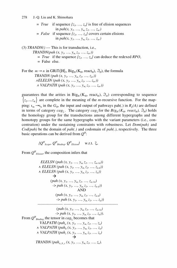
278 J.-Q. Liu and K. Shimohara
= True if sequence {z1, …, zn} is free of elision sequences in pah(x, y1, …, ym, z1, …, zn,) = False if sequence {z1, …, zn} covers certain elisions in pah(x, y1, …, ym, z1, …, zn,)
(3) TRANDN() --- This is for transduction, i.e.,TRANDN(pah (x, y1, …, ym, z1, …, zn,))
= True if the sequence {z1, …, zn} can deduce the redexed RPO, = False else.
For the m n in GRiT(|H|3, BigH (KH, reactH), H), the formulaTRANDN (pah (x, y1, …, ym, z1, …, zn,))
ELELSN (pah (x, y1, …, ym, z1, …, zn,))VALPATH (pah (x, y1, …, ym, z1, …, zn,))
guarantees that the arities in BigH (KH, reactH), H) corresponding to sequencez zn1, ..,{ } are complete in the meaning of the m-recursive function. For the map-
ping: m n in the GH, the input and output of pathways pah(.) in Rp(A) are definedin terms of category cag . The category cag for the BigH (KH, reactH), H) holdsthe homology group for the transductions among different hypergraphs and thehomotopy groups for the same hypergraphs with the variant parameters (i.e., con-centration) under the sustaining constraints with robustness. Let Dom(pah) andCod(pah) be the domain of pah(.) and codomain of pah(.), respectively. The threebasic operations can be derived from QH:
{QHScope, Q
HBinding, Q
HElision} w.r.t. ,
From QHElision, the composition infers that
ELELSN (pah (x, y1, …, ym, z1, …, zn-l-k))ELELSN (pah (x, y1, …, ym, z1, …, zn-k))ELELSN (pah (x, y1, …, ym, z1, …, zn))
(pah (x, y1, …, ym, z1, …, zn-l-k) -> pah (x, y1, …, ym, z1, …, zn-k)) AND
(pah (x, y1, …, ym, z1, …, zn-k) -> pah (x, y1, …, ym, z1, …, zn)) ------------------- -----------------------------------------
(pah (x, y1, …, ym, z1, …, zn-l-k) -> pah (x, y1, …, ym, z1, …, zn)).From QH
Binding, the tensor in cag , becomes thatVALPATH (paha (x, y1, …, ym, z1, …, zn)VALPATH (pahb (x, y1, …, ym, z1, …, zn)VALPATH (pahc (x, y1, …, ym, z1, …, zn)
TRANDN (paha_b_c (x, y1, …, ym, z1, …, zn).

18 Molecular Computing by Signaling Pathways 279
From QHScope, we can get that
TRANDN (pah (x, y1, …, ym, z1, …, zp …zq, …, zm))ELELSN (pah (x, y1, …, ym, z1, …, zp …zq … ,zn))
VALPATH (pah (x, y1, …, ym, z1, …, zp …zq, …, zk)). where p,q,m,n,k N.
For GRiT(|H|3, BigH (KH, reactH), H), GRiT(|H|3, BigH (KH, reactH), H) where H isthe equivalence given by the homological group, and the interactions of pathwaysare carried out for exploring the potential solutions of the 3-SAT problem.
Step 2: Pathway generation:
Let input node( k) be the input reactant of pathway k, let output node( k) be theoutput reactant of pathway k, and let internal node( k) be the internal reactants ofpathway k, where k is in the set of all pathways, e.g., X Y Z¬ implies thatpathway k covers the reactant molecules that correspond to the candidates as thesets of subpathways. The same parts are kept only once, and these are sustained bypathway k. Therefore, after the signaling feedback is executed on the pathways,the remaining parts are the candidates represented by the signaling molecules,where the reactants are designed to produce the additional chemicals { 's}(s=0,1,…) to feed the energy (e.g., ATP). The same is also true for another path-way k'. When k and ’k' interact by the operations of Q rules, different compo-nents are deleted due to the fact that they cannot be sustained. Then we get the fi-nal result. The advantage of this scheme is that the number of candidates has norelation to the molecules we set in advance. The recursive generation of pathwaysis executed to sift out the less suitable candidates. In the meantime, according tothe rules defined in this section for formalization, the common reactants in path-way k (k = 0,1, … ) with feedback ensure that the related pathways are sustained.This continues to loop until rewriting stops at the final stage, i.e., biochemical re-actions do not produce any more new reactants.
At this point, we need to check whether the solution has been obtained accord-ing to the terminal criterion: If yes, the computing process goes to the next step. If no, we must update the population and let the computing process go to Step 1.
Step 3: Judging by terminal criterion:
The criterion to judge the halting of the entire process is that the final variableform of the candidate is confirmed as the solution to the 3-SAT problem when nomore new pathways emerge. At this point, the existing pathways are identical in allof the cells. Finally, after the result is confirmed, the final solution will be decidedas the output.
We have proven that the algorithm can solve the 3-SAT problem with a linearcomplexity cost both in time and in space. The full proof can be found in [17].
Theorem 18.2 [17]: Its space complexity is O(m×n) and time complexity isO(m) when it is applied to solve a 3-SAT problem.

280 J.-Q. Liu and K. Shimohara
18.4 Experimental Result
In the sense of biological plausibility supported by real objects, our simulator isbased on feasible biological signaling pathways in cells that are constructed by Rhofamily GTPases [15,16,22]. We have verified that our method based on pathwayswith interactions is biologically faithful by simulation using biological supportingsoftware in [16]. Confirmed by the benchworks in biolabs, the kinase-based bio-chemical systems in living cells are an excellent biomachine for molecular com-
Number of variables
Figure 18.5. Relationship among the number of molecules to the number of variablesin 3-SAT.
Figure 18.6. A brief flow chart of the main part of our simulator.
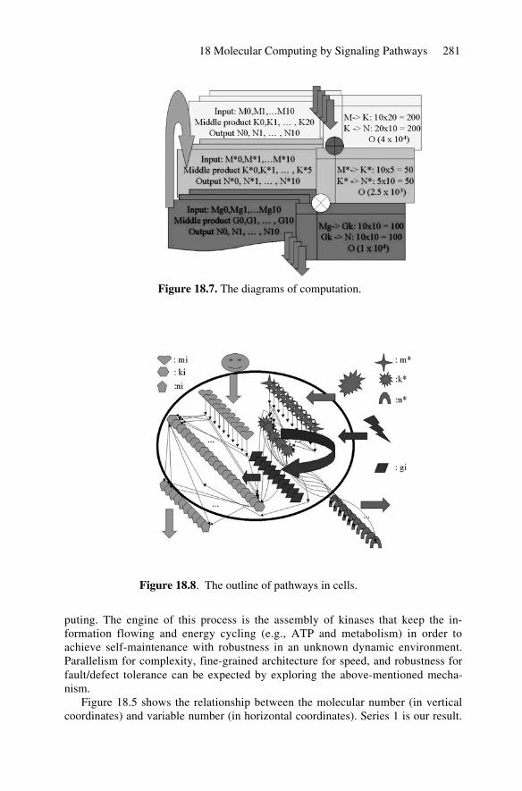
18 Molecular Computing by Signaling Pathways 281
puting. The engine of this process is the assembly of kinases that keep the in-formation flowing and energy cycling (e.g., ATP and metabolism) in order toachieve self-maintenance with robustness in an unknown dynamic environment.Parallelism for complexity, fine-grained architecture for speed, and robustness forfault/defect tolerance can be expected by exploring the above-mentioned mecha-nism.
Figure 18.5 shows the relationship between the molecular number (in verticalcoordinates) and variable number (in horizontal coordinates). Series 1 is our result.
Figure 18.7. The diagrams of computation.
Figure 18.8. The outline of pathways in cells.

282 J.-Q. Liu and K. Shimohara
Series 2 is the number of variables in the 3-SAT. Series 3 is the exponential num-ber of DNA molecules in surface-based DNA computing (e.g. [2]).
In the pathways and diagrams of the simulator shown in Figure 18.6 , Figure18.7 and Figure 18.8, respectively, the quantities such as Si = {mi, ki, ni}, S* ={m*, k*, n*}, and Sg = {g*}, in which ki and g* denote the kinases and k* denotesthe other enzyme, are set as follows:
(i) for the normal pathways in Si:the number of input reactants is 10;the number of middle products is 20;
the number of outputs is 10. the connection between M->K is 10 * 20 =200;
the connection between K ->N: 20 * 10 = 200;(ii) for the pathways with disturbance in S*:
the number of input reactants is 10;the number of middle products is 5;the number of outputs is 10;the connection between M*->K* is 10 * 5 = 50;the connection between K* ->N*: 5 * 10 = 50;
(iii) for the graph rewriting in Sg:the number of input reactants is 10;the number of middle products is 10;the number of outputs is 10;the connection between M->K is 10 * 10 = 100;the connection between K ->N: 10 * 10 = 100;
But the kinase number given by our simulator is only 6.The software simulator for our method has been implemented in C++. In the
current stage, our software simulator reaches a size of 10 quadrillion (1016) mole-cules. Using pathway-based modeling, we have solved the 50-variable, 30-clause3-SAT problem, (denoted as the 3-SAT (50,30), according to the convention oftheoretical computer science). For example, among the examples in our experi-ment, a typical situation for clauses is
X X X X X X X X X0 1 2 3 11 12 13 12 13( ) ( ) ( ) ¬ ¬( )... ,where 28 clauses use all 7 combined forms in
(X0, X1, X2), (X3, X4, X5), …, (X9, X10, X11)except ¬ ¬ ¬( ) ¬ ¬ ¬( )X X X X X X0 1 2 9 10 11,..., and the other two clauses= X X X X12 13 12 13( ) ¬ ¬( ) and . The solution is X0 = X1 = … = X11 = 1 and{(X12 = 0 and X13 = 1) or (X12 = 1 and X13 = 0)}, and X14, …, X49 takes valuesin the set of {1,0}. The number of signaling enzyme molecules is 14. This smallcost is affordable for molecular computing and the corresponding algorithm is thusefficient. Furthermore, the robustness of the scalable schemes is achieved in orderto maintain the identity of the pathways when the concentrations vary in the do-main of thresholds. The cost will fluctuate slightly around the theoretical curve.Figure 18.9 shows the relationship between the molecular number (vertical coordi-nates) and the variable number (horizontal coordinates). It illustrates a perform-ance comparison, with the best, average, and worst cases given in series 1, series 2and series 3, respectively.

18 Molecular Computing by Signaling Pathways 283
Figure 18.9. The relationship between the molecular number and the variable number.
18.5 Conclusion
In this chapter, we have proposed a new method of molecular computing con-structed by “Rho family GTPases”-based pathways and formalized as hypergraphrewriting. With regard to biological faithfulness, performance as a formal system,and the application of its algorithm to the 3-SAT problem, we have discussed ourmethod by explaining its functional factors. Furthermore, we have confirmed thatthe method is actually feasible for reducing the computing costs needed to solvethe 3-SAT problem and for potential biochemical implementation. Future workwill mainly focus on biologically realizing the method by using in situ cells with“Rho family GTPases”-regulated signaling pathways.
Acknowledgments
The authors sincerely thank Prof. Kozo Kaibuchi and his lab for their invaluableacademic help; Prof. Masami Ito, Prof. Manuel Graña Romay, Prof. Naoyuki Ina-gaki, Dr. Shinya Kuroda, and Dr. Mutsuki Amano for their advice and suggestions.This research was conducted as part of “Research on Human Communication”with funding from the Telecommunications Advancement Organization of Japan.The work is also partly supported by the Foh Ying Tung Education Foundation(Project No. 71063).
References
1. Adleman, L.M. (1994) Molecular computation of solutions to combinatorial problems.Science, 266:1021-1024.
2. Liu, Q., Wang, L., Frutos, A.Q., Condon, A.E., Corn, R.M., and Smith, L.M. (2000)DNA computing on surfaces. Nature, 403:175-179.
Molecular num
ber
Variable number

284 J.-Q. Liu and K. Shimohara
3. Ogihara, M. and Ray, A. (2000) DNA computing on a chip. Nature, 403:143-144.4. Sakamoto, K., Gouzu, H., Komiya, K., Kiga, D., Yokoyama, S., Yokomori, T., and
Hagiya, M. (2000) Molecular computation by DNA hairpin formation. Science,288:1223-1226.
5. Braich, R.S., Johnson, C., Rothemund, P.W.K., Hwang, D., Chelyapov, N. and Adleman,L.M. (2000) Solution of a satisfiability problem on a gel-based DNA computer. In Pre-proc. of DNA 6:31-42.
6. Condon, A., and Rozenberg, G., editors, (2000) Proc. of DNA6.7. Schöning, U. (1999) A probabilistic algorithm for k-SAT and constraint satisfaction
problems. In Proceedings of the 40th Symposium on Foundations of Computer Science,IEEE Computer Society, Los Alamitos, CA 410-414.
8. Díaz, S., Esteban, J.L., and Ogihara, M. (2000) A DNA-based random walk method forsolving k-SAT. In Pre-proc. of DNA 6:181-191.
9. Lipton, R. (1995) DNA solutions of hard computational problems. Science, 268:542-545.
10. Garey, M.R., Johnson, D.S. (1979) Computers and intractability - a guide to the theoryof NP-completeness. Freeman.
11. Rozenberg, G., Salomaa, A., eds. (1997) Handbook of formal languages. Springer-Verlag, Heidelberg.
12. Liu, J.-Q., and Shimohara, K. (2001) Pathway graph models for molecular computing insitu. RIMS Kokyuroku 1222, RIMS, Kyoto University 128-137.
13. Liu, J.-Q., and Shimohara, K. (2001) On arithmetic units and logic operators of kinase-based molecular computers. IPSJ SIG Notes, Vol. 2001, No. 93 25-32.
14. Scott, J.D., and Pawson, T. (2000) Cell communication: the inside story. ScientificAmerican 54-61.
15. Kaibuchi, K., Kuroda, S., and Amano, M. (1999) Regulation of the cytoskeleton and celladhesion by the Rho family GTPases in mammalian cells. Annu. Rev. Biochem. 68:459-486.
16. Liu, J.-Q., and Shimohara, K. (2001) Kinase computing in GTPases: analysis andsimulation. IPSJ SIG Notes, Vol. 2001, No. 91:29-32.
17. Liu, J.-Q., and Shimohara, K. (2003) On the computational complexity of molecularcomputing by pathways. ATR-HIS Technical Report.
18. Courcelle, B. (1997) The expression of graph properties and graph transformations inmonadic second-order logic. Chapter 5 of the "Handbook of graph grammars and com-puting by graph transformations, Vol. 1: Foundations", Rozenberg, R., (ed.), World Sci-entific (New-Jersey, London), 313-400.
19. Liu, J.-Q., and Shimohara, K. (2001) Graph rewriting in topology I: operators and thegrammar. SIG-FAI-A101-4 (9/21):21-26.
20. Milner, R. (2001) Bigraphical reactive systems: basic theory. (http://www.cl.cam.ac.uk/users/rm135/bigraphs.ps.gz).21. Liu, J.-Q., and Shimohara, K. (2001) Graph rewriting in topology II: computability.
Proc. of the 5th Symposium on Algebra, Language and Computation, Edited by Imaoka,T., and Shoji, K., (Shimane, Japan), 63-68.
22. Inagaki, N., Chihara, K., Arimura, N., et al., (2001) CRMP-2 induces axons in culturedhippocampal neurons. Nature Neuroscience, 4(8):781-782.

h
G
G
G
∈
SR
S
( ) IR( )
Summary.h � i, j h
i, jG
19.1 Theory of Games: a Background
19
Strategy-Oriented Evolutionary Games:Toward a Grammatical Model of Games
We generalize evolutionary games to have strategy oriented payoff: foreach strategy , is the number of survival offspring of the specie pro-duced by a contest . This minor change allows the natural extension of strategy-oriented games to a strategy-oriented replicator that extends the classical repli-cator of evolutionary games. We prove that the extension is strict by modelingthe logistic equation as an replicator. After that, we sketch the de�nition of agrammatical model of games implementing the logistic replicator.
B. Cases and S.O. Anchorena
In 1944 Von Neumman and Morgenstern [7] elaborated the principles of aTheory of Games that was conceived as a mathematical theory of human eco-nomic behavior. They developed a contrast between the �Robinson Crusoe�model of economy, of an isolated single person, and a social exchange econ-omy, with a moderate number of participants. Their aim was to establish thefoundation of economy in the rational behavior of agents that play strategygames performing the optimization of some self-interest criterion.Since that time [11], the Theory of Games has suffered wide development.
A �rst step was the introduction in 1950 of the concept of Nash equilibrium:the mathematical characterization of the sets of strategies that drive to themaximization of pro�ts and the minimization of losses in games. A secondqualitative step was the application of the Theory of Games to study andsimulate the biological evolution of species in 1973 by John M. Smith and Price[5, 6, 4]. In economy, the players are rational agents in a market competition.The payoff of games is measured in terms of goods or money. In biology, thegames model pairwise contests between animals in a large population, andthe payoff is measured in terms of Darwinian �tness (the expected number ofsurviving offspring).
R
∑∑
R
S∈
�� �
=1
=1
1 1 1
2 1 1
286 B. Cases, S.O. Anchorena
G
h
h
h
h
h
h
G
h
h
r c
kh h
h
hki h
hh h
h h
( ) = 0 1 2
( + 1) =( ( ))
( ( ) ( ))( ) =
( )
( ) ( )( )
( )( )
( ) 1 2( ) = 1 2 ( ) =
2
=
=
( + 1) =( ( ) ( ))
( ( ) ( ))=( ) ( )
( ) ( )
( + 1) = ( )(1 ( ))
( + 1) = 1 ( )(1 ( ))
Gx t , t , , , . . .
k
x tu e , x t
u x t , x tx t
e Ax t
x t Ax tx t ,
u e hA
Gh � i, j
h i, jA r
c r, c .� r, c . � r, c
G � �
A G hA A A A
x tv x t , x t
u x t , x t
x t A x t
x t Ax t,
v G
x t �x t x t ,
x t �x t x t .
In this section, we set the background of Theory of Games following theprecise notation of Weibull [11]. In Subsection 19.1.1 games in normal formand their pure strategies are introduced. In Subsection 19.1.2 we introducemixed strategies and the concepts of best reply and Nash equilibrium. Sec-tion 19.2 explains the principles of evolutionary games and the approachesto their study. In subsection 19.2.1 the approach based on mutations bringsto the de�nition of �evolutionarily stable strategy�. In Subsection 19.2.2 thedynamical approach based on replication and selection is described.The classical replicator of an evolutionary game determines the
dynamic of concentrations , of a population of individualsthat contest pairwise, following common strategies. The replicator is de�nedby the equations:
where is the payoff for mixed strategies, represents the pure strategyvector, and is the matrix of the game.Our contributions begin in Section 19.3.We generalize the evolutionary
games of M. Smith and Price to have strategy, oriented replicators .The modi�cation is minor: for each strategy , is the number ofsurviving offspring of the specie produced by a contest , represented bya matrix . For example: modeling the encounter of rabbits and carrots, the contest produces rabbits and indirectly 2 carrots if the rabbittransports the seeds to a good substrate. Hence, and.This is a re�nement of evolutionary games because the global payoff of
a game , , is identical to the payoff of classical evolutionarygames. Instead of playing a two-person symmetric game de�ned by the matrix, there is a different payoff, in fact a different game , for each strategy ,represented by the matrix . The matrix is the global payoff .The equations of a strategy-oriented replicator become to:
where is the payoff extended to mixed strategies of subgame .In Sections 19.4 and 19.5 we make a double contribution. First, we prove
that the class of evolutionary games with classical replicators is strictly con-tained in the class of evolutionary games with strategy-oriented replicators.Second, we base our proof on the representation of the logistic equation as astrategy-oriented replicator:
(19.1)
(19.2)

R RR
Example 1.
1
1
1
1 1
1 2
1 2
G
G
n
i i
i
n i i
n
i in
n
T
ij
19 Evolutionary Games 287
S
R
� { } �� { }
�� ∈
∈� � �
� ∈ ∈→ ∈
� →
�
�
{ }
{ }{ }
∈
19.1.1 Games in Normal Form: Pure Strategies
= 1= 1 2
1= ( )
=
: ( ):
( ) = ( ( ) ( )) ( )=
( )
1 2
= 1 2
= = =( ) ( ) ( ) ( )
1( ) ( )
=
= ( ) = ( ) = ( )
I i , . . . , i n .i S , , . . . , m
m .s s , . . . , s s S
i IS S . . . S
s S i Ii � S . i � s
� S� s � s , . . . , � s � s i
GI, S, �
v c
vc /
I ,
S S H,D SH,H , H,D , D,H , D,D
A� s s S B � s
B A
C ij C � s � i, j s i, j
We represent the logistic equation by an replicator in Section 19.4,and we prove in Section 19.5 the impossibility of representing it as a classicalreplicator .Finally, in Section 19.6 we describe a grammatical model that �ts exactly
to the notion of strategy-oriented replicator. We implement the logistic repli-cator of Section of section 19.5 using strategy-oriented grammars.
Following [11] the elements of the Theory of Games are
A set of players, ,For each player , a set of pure strategies for someintegerA vector , where is the pure strategy selected byplayer , called the pure strategy pro�le.The pure strategy space is the Cartesian product of purestrategies sets.For any pure strategy pro�le and player the payoff function ofth player is The associated payoff to player is .The combined pure strategy payoff function is such that
gives a payoff to each player .A game in normal form is, in terms of pure strategies, a triplet
.
The "hawk�dove" game designed by M. Smith and Price [5, 6, 4]is a model of animals contesting a resource, for example, a territory, of value, or victory, with a cost . The value is measured in terms of Darwinian�tness: it means that winning the contest will increase the number of survivaloffspring of the winner by . The cost of the �ght (the player gets hurt ortired) has a value of . Both players have probability of winning thecontest.Let the set of individuals be . Individuals are birds of the
same specie. The behaviors of the animals in the contest, the pure strate-gies, are �ght like a hawk, escalating and continuing until injured or un-til opponent retreats; or �ght like a dove, who displays without injuringthe opponent unless the other escalates and in this case retreats. The setsof strategies are . The space of pure strategies is
.When the number of players is two, the game is called a two-person game.
In this cases, the payoff of the game for player is given in a matrixrepresenting with . Matrix represents the payoff . Thegame is symmetric since . Note that symmetry is referred to players1 and 2.Matrix represents the combined payoff since the value in row and
column , when . Rows correspond to strategies
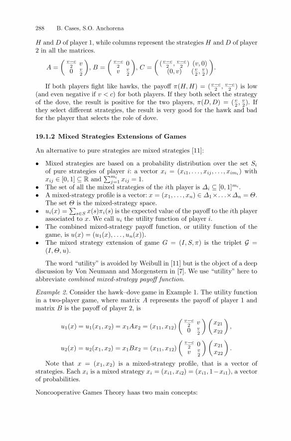
Ri
i
i
� � � �
� �
∈
�
�
�
∈ �� �� ∈ � �
�
�
� G
�
� � � � � �
∑
∑
� �� �� �� �
288 B. Cases, S.O. Anchorena
19.1.2 Mixed Strategies Extensions of Games
combined mixed-strategy payoff function
Example 2.
v c
v
v c
v
v c v c
v v
v c v c
v v
i
i i ij im
ijmj ij
im
n n
i s S i
i
n
v c
v
v c
v
i i i i i i
2
2
2
2
2 2
2 2
2 2
2 2
1
=1
1 1
1
1 1 1 2 1 2 11 122
2
21
22
2 2 1 2 1 2 11 122
2
21
22
1 2
1 2 1 1
12
=0
=0
=( ) ( 0)(0 ) ( )
( ) = ( )
( ) = ( )
= ( )[0 1] = 1
[0 1]= ( ) =
( ) = ( ) ( )
( ) = ( ( ) ( ))= ( ) =
( )
( ) = ( ) = = ( )0
( ) = ( ) = = ( )0
= ( )= ( ) = ( 1 )
H D H D
Av
Bv
C, v,, v ,
� H,H ,v < c
� D,D ,
Si x x , . . . , x , . . . , x
x , xi � ,
x x , . . . , x � . . . � ��
u x x s � s ix u i
u x u x , . . . , u xG I, S, �
I, �, u
AB
u x u x , x x Ax x , xv x
x,
u x u x , x x Bx x , xv
xx
.
x x , xx x x , x x , x
and of player , while columns represent the strategies and of playerin all the matrices.
, , .
If both players �ght like hawks, the payoff is low(and even negative if ) for both players. If they both select the strategyof the dove, the result is positive for the two players, . Ifthey select different strategies, the result is very good for the hawk and badfor the player that selects the role of dove.
An alternative to pure strategies are mixed strategies [11]:
Mixed strategies are based on a probability distribution over the setof pure strategies of player : a vector with
and .The set of all the mixed strategies of the th player is .A mixed-strategy pro�le is a vector: .The set is the mixed-strategy space.
is the expected value of the payoff to the th playerassociated to . We call the utility function of player .The combined mixed-strategy payoff function, or utility function of thegame, is .The mixed strategy extension of game is the triplet
.
The word �utility� is avoided by Weibull in [11] but is the object of a deepdiscussion by Von Neumann and Morgenstern in [7]. We use �utility� here toabbreviate .
Consider the hawk�dove game in Example 1. The utility functionin a two-player game, where matrix represents the payoff of player 1 andmatrix is the payoff of player 2, is
Note that is a mixed-strategy pro�le, that is a vector ofstrategies. Each is a mixed strategy , a vectorof probabilities.
Noncooperative Games Theory haas two main concepts:
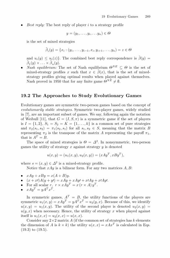
�
19 Evolutionary Games 289
1
1 1 +1
1
1 2
2 1 2 1 2 1 1 2
2 1
2
1 2
2
1 2
1 2
1 2
i n
i i i i i n
i i
nNE
NE
T
T T
T T
T T T
T
T T T
T
�∈
{ ∈� }
� �� �
∈
� ∅
{ } { }∈
∈
�� ′ ′ ′ ′ ′ ′� � ��
��
19.2 The Approaches to Study Evolutionary Games
Best reply:
Nash equilibrium:
evolutionarily stable strategies
= ( )
˜ ( ) = : ( ) =
( ) ( ) ˜( ) =˜ ( ) ˜ ( )
˜( )
=
= ( )= 1 2 = = = 1( ) = ( )
==
( ) = ( ( ) ( )) = ( )
= ( )
+ = ( + )( + ) ( + ) = + + +
= ( )=
=( ) = = = ( )
( ) = ( ) ( ) =( )
( ) = ( ) = ( )2 2
( ) =
i
y y , . . . , y , . . . y �
� y x y , . . . , y , x , y , . . . , y z �
u y u z � y� y . . . � y .
� �x x � x
�
G I, S, �I , S S K , . . . , k� s , s � s , s s , s S B
� A �A B
� �x y
u x, y u x, y , u x, y xAy , xBy ,
s x, y �xAy A,B
xAy xBy x A B yx x A y y xAy xAy x Ay x Ay .
r r xAy x r A yxAy yA x
A Bu x, y xAy yA x u y, x
u x, y u x, y u x, yu y, x x
u x, x u x, x u x, xA k
A k k u x, x xAx
The best reply of player to a strategy pro�le
is the set of mixed strategies
and . The combined best reply correspondence is
The set of Nash equilibrium is the set ofmixed-strategy pro�les such that , that is the set of mixed-strategy pro�les giving optimal results when played against themselves.Nash proved in 1950 that for any �nite game .
Evolutionary games are symmetric two-person games based on the concept of. Symmetric two-player games, widely studied
in [7], are an important subset of games. We say, following again the notationof Weibull [11], that is a symmetric game if the set of playersis , is a common set of pure strategiesand for all , meaning that the matrixrepresenting is the transpose of the matrix representing the payoff ,that is .The space of mixed strategies is . In nonsymmetric, two-person
games the utility of strategy against strategy is denoted
where is a mixed-strategy pro�le.Notice that is a bilinear form. For any two matrices :
.
For all scalar , ..
In symmetric games, , the utility functions of the players aresymmetric . Because of this, we identify
. The utility of the second player is denotedwhen necessary. Hence, the utility of strategy when played against
itself is .Consider any matrix (if the common set of strategies has elements
the dimension of is ) the utility is calculated in Eqs.(19.3) to (19.5).
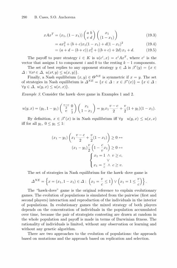
�
�
�
�
Example 3.
T
i i T i
NE
NE
v c
v
vc
NE
� �� �
� �� �
� �� �⎧⎨⎩
{ � � � �}
290 B. Cases, S.O. Anchorena
1 11
1
21 1 1 1
2
21 1
1 12
2
1
11 1 1 1
1 1
1 1 1 1
1 1 1
1
1
1 1 1 1
� �� �
�∈
�∈ { ∈
∀ ′ ∈ ′ � }∈
{ ∈ ∈ } { ∈∀ ∈ � }
� �� �
∈ ∀ �� �
� � � � ↔
� � � ↔∧ �∨∧ �
� ∈ � ∨ �
= ( (1 ))(1 )
= + ( + ) (1 ) + (1 )
= ( + ( + )) + (( + ) + 2 ) +
( ) =1( ) =
: ( ) ( )( ) =
= : ( ) = :( ) ( )
( ) = ( 1 )0
1=
2+2(1 + )(1 )
( ) ( ) ( )0 1
( )2+2(1 ) 0
( )21 0
= 1
=
= = ( 1 ) : = 1 = 1
xAx x , xa bc d
xx
ax b c x x d x
a d b c x b c d x d.
i K u e , x e Ax ei k
y � � y x� x �, u x , y u x, y
x, y � x y� x � x � x x �
y �, u y, x u x, x
u y, x y , yv
xx
y xv c v
y x .
x � x y u y, x u x, xy , y
x y xv c v
x
x yv c
vx
x v c,
x c v.
� x x , x � xv
cx
v
c.
(19.3)
(19.4)
(19.5)
The payoff to pure strategy is , where is thevector that assigns 1 to component and 0 to the resting components.The set of best replies to any opponent strategy is
.Finally, a Nash equilibrium is symmetric if . The set
of strategies in Nash equilibrium is.
Consider the hawk�dove game in Examples 1 and 2.
By de�nition, is in Nash equilibrium iffiff for all :
The set of strategies in Nash equilibrium for the hawk�dove game is
The �hawk-dove� game is the original reference to explain evolutionarygames. The evolution of populations is simulated from the pairwise (�rst andsecond players) interaction and reproduction of the individuals in the interiorof populations. In evolutionary games the mixed strategy of both playersdepends on the concentration of individuals in the population accumulatedover time, because the pair of strategists contesting are drawn at random inthe whole population and payoff is made in terms of Darwinian �tness. Therationality of individuals is limited, without any observation or learning andwithout any genetic algorithm.There are two approaches to the evolution of populations: the approach
based on mutations and the approach based on replication and selection.

∈1
=1
=1
1
∑
∑� " #
∑� " #
" #
∈
∈� ∈ ∈
� �
� ∀ ∈ �� ∀ ∈ � ⇒
∈
∈∈
RR
19 Evolutionary Games 291
y y
h
h K h
k
h h
h h T
kh h
h
hh
h
k
h
hh
G
n G
h
h
h
19.2.1 The Approach Based on Mutations
19.2.2 The Approach Based on Selection: The Replicator
(0 1)
= � (0 1) (0 � )
[ + (1 ) ] [ + (1 ) ]
( ) ( )= ( ( ) = ( ) ( ) ( ))
( )( ) = ( ) 0
( ) = ( ( ) ( ))( ) = ( ) ( )
( )
( ) =
( ) = ( )= 0 1 2
( + 1) = + ( ) ( )
( + 1) = + ( ) ( ) = ( + [ ( ) ( )]) ( )
( (0))(0) = ( (0) (0)) ( (0))
= ( )
( + 1) =+ ( )
+ [ ( ) ( )]( )
� ,
x �y x � , � , �
u x, �y � x > u y, �y � x .
y �, u y, x u x, x ,y �, y x u y, x u x, x u y, y < u x, y .
p th K t p t p t >
x t x t , . . . , x tx t p t /p t h K
t x t �
hx u e , x e Ax
u x, x x u e , xt , , , . . .
p t � u e , x t p t ,
p t � u e , x t p t � u x t , x t p t .
G t, xx x , . . . , x . t, x
x t t
x t� u e , x t
� u x t , x tx t .
There exists a population of individuals �programmed� to play some pure ormixed strategy. A small population share of �mutant� individualsthat play a different strategy is injected. The incumbent strategy is evolution-arily stable if it gets a higher payoff whenever the mutant strategy falls belowa certain limit.The strategy is an evolutionarily stable strategy (ESS) if for every
strategy , there exists some such that for all :
.The condition above is equivalent to the following two conditions:
Let be the population of individuals programmed to pure strategyat time step . The total population is .
The associated population state is the vector whereis the population share programmed to strategy
at time . A population state is formally equal to a mixed strat-egy: a vector that assigns a probability to each strategy, but in this case theprobability is identi�ed to the frequency of the strategists in the population.The expected payoff to any pure strategy if the state of the popu-
lation is is denoted . The associated population av-erage payoff, that is the average of any individual drawn at random, is
.The dynamic of a population is determined by the iterations :
(19.6)
(19.7)
de�nes the replicator , which determines, starting at any ini-tial condition the state of the population
at time step by the equations
(19.8)

1
2 2
����
Example 4.
" #" #
︷︸︸︷ ︷ ︸︸ ︷
292 B. Cases, S.O. Anchorena
v
v
v
G
u e ,x
u x ,xv� �v �
u e ,x
u x ,xv �v �
r
c
19.3 Strategy-Oriented Replicators
� ��
�
� � �� � � �� � � �
R
�� �
�
�
�
′
{ → → }
⇒′ { → → }
′→ ∈
1
2
2
11
1 2
22
0 22
2
1(0)
[ (0) (0)] 110 (1 )10 (1 ) 1
2(0)
[ (0) (0)] 110 (1 )10 (1 ) 2
1 1 2 1 2
pp �
p � � v/cx �, � � x
y u y, x � u x , xt
p u e , x p � � v� �
p u e , x p t � � v �p v� � v � v �
t
x x � x
x x � x
x � v/cx x
v/c x ,
x x , x x x
GG
rrcccr rc
P r rrccc, c ccc
r r cccr r rrccc cccrP r rrr, c cc
P PP, r r rrccc P
� P, rP, r � P, r
(0) =20 (0) = 20
(0) = 20(1 ) = 1(0) = ( 1 ) = 0 (0)
( (0)) = (1 ) = ( (0) (0))= 1
(1) = (0) (0) = (1 )20 = 10 (1 )
(1) = (0) ( ) = (1 )20(1 ) = 10 (1 )(1) = 10 (1 ) + 10 (1 ) = 10 (1 )
= 1
(1) =[ ]
(0) = = = (0)
(1) =[ ]
(0) = = 1 = (0)
(0) = = 1(1) = (0)
1 (0) = (1 0)
(1) = 1 = (0) (1) = 0 = 1 (0) = (0)
=
=
( )
( ) = 2( ) ( ) = 3
This example extends Example 3. Consider a population ofstrategists. The initial number of hawks is and the initial doves
are , where . We will iterate the replicator fromwith parameter . As shown in Example 3, is a Nash
equilibrium and for every strategy , .Hence, the population at step is
,,
.
The replicator gives the state of the population at step :
,
.
Then, every Nash equilibrium is a �xed point of thereplicator replicator since .If , the only Nash equilibrium is , a �xed point to the
replicator:.
It can be easily proved that every game can be reduced to an equivalentgame with nonnegative payoffs. In the following, we assume nonnegativevalues for the matrix of the game.
In this section we deal with a generalization of the replicator model of evolu-tionary games that we call the replicator oriented to strategy. This general-ization comes from a re�nement of the payoff function inspired in grammars:consider a population of rabbits, determined by symbol , and car-rots, symbol . A grammar is basically a set of rewriting rules, for example,
. In a step of derivation one rule is applied toany symbol in the string matching the left-hand side of the rule, replacing
the symbol by the right-hand side. For example: .Consider a different grammar de�ned by the rules .Interpreting a rewriting step as a game, assume that player 1 selects a
grammar, or while player 2 selects a symbol in the string. If the contestis , the payoff is determined by the rule . Note that eachsymbol is like a coin: the payoff is composed of two rabbits and three carrots.Hence, we need a function that de�nes the payoff of the contest
in �rabbit coins� and means �carrot coins�. In [1] wepresent a formalization of the hawk�dove game using Eco-grammar systems[2].

1
R
Rij
k
∑
∑∑ ∑
∑
" #
�{ } �
� ∈ ∈
�
R
∈∈
∈
∈
SS S
S
1
1
2
=1
1
=1
=1 =1
1
=1
+ +
1
De�nition 1.
De�nition 2.
19 Evolutionary Games 293
k
ki i
h
h h
h
k
G
ij
h
h h hkh h
h hT
h
kh h
kh h
T T
k
h h h
k
h
h h
G ... G
G G
n G
hh h h
T
T
h
hT h
h
= ( )
( ) = == 1 2 =
=
( ) ( )( )
= ( )
= ( )= ( )
( ) ( ) =
( )( ) =
=( ) =
( ) =
( ) = =
= ( )
( + 1) = ( + ( ( ) ( ))) ( )
( + 1) = ( + 1) = ( + ( ( ) ( ))) ( )
( (0))(0) = ( (0) (0)) ( (0)) =
( )
( + 1) =( + 1)
( + 1)=
+ ( ( ) ( ))
+ ( ( ) ( ))=
+ ( ) ( )
+ ( ) ( )
( ) ( ) ( )( )
G I, S, �,� , . . . , �
I, S, � K SS , , . . . , k S K K
� � �G
i, j h K � i, ji, j h
G I, S,�v h
G I, S, �,� , . . . , �G I, S, �
GA
i, j � i, j A ij A
A h K i, j� i, j A i j A
A Av x, y xA y G
x, y � G u x, y
v x, y xA y xAy
G I, S, �,� , . . . , �G
h K
p t � v x t , x t p t ,
p t p t � u x t , x t p t .
Gt, x
x x , . . . , x t, xx t t
x tp t
p t
� v x t , x t
� u x t , x t
� x t A x t
� x t Ax t.
A hx t A x t u e , x t
x t
is an evolutionary game oriented tostrategy if
The triplet is a symmetric two-person game whereis a common set of strategies, is the pure
strategy space, and the payoff is . We call the global payoffof .For each contest and each strategy , is the payoffof to strategy .Each triplet is a symmetric two-person game with utilityfunction called the subgame for strategy .
Let be an evolutionary game orientedto strategy. The dynamic of populations of is de�ned as the iteration with
:
We say that de�nes the strategy-oriented replicator denotedor simply . The expression determines, starting at any initialcondition , the state of the population
at time step by the equations:
An evolutionary game oriented to strategy is are�nement of the global game that we denote with the samename without loss of generality. With we denote the classical replicatorde�ned by the global game .The payoff of the global game is determined by the matrix , which gives
for contest the payoff , the component of row and columnof the matrix of the game .Matrix represents the payoff to strategy of contest being
the component of row and column of . The matrix
of the game is .Let be the utility function of subgame , where
are mixed strategies. The utility function of game is.
(19.9)
(19.10)
(19.11)
Compare Eq. (19.11) to the classical replicator in Section 19.2 Eq. (19.8).Now, there is a different matrix for each strategy and hence, the polyno-mial is quadratic. In the classical replicator, is linearand becomes quadratic when multiplied by .

k
1 2
1
�
�
�
′
′
Proposition 1.
� �� �
" # � �" #
�
⎛⎝ ⎞⎠
�
�
�
�
S SR
�
�
X X X ′
X X ′R
S RR
S ′
294 B. Cases, S.O. Anchorena
v c
V
T T
T
T
G G G
G
v c
c v
v
c v
G G
G G
G
k k
G ... G G
G
G
h hT h
h
h h hm
1 2 12
1
22
2 1 2
1 2 2 1
21 1
11 1 1
1 1
22 2
2 12
+
1
+2 1 1
221 1 2
22 1
2
221 1 2
+ +
1
Example 5.
Let be an evolutionary game and its classi-cal replicator. There exists a strategy-oriented gamesuch that .
Proof.
= (
) =0 0
=0 00
= +
( ) = ( ( ) ( )) ( ) = 1 ( )
[ ( ) ( )] =2( ) + 2 ( ) +
2
( ) ( ) = (1 0) ( ) ( ) = ( ) ( )
=+
2( ) + ( )
( ) ( ) = (0 1) ( ) ( )
= ( ) ( ) =2(1 ( ))
== ( )
( + 1) =( ) + ( )
( ) + 2 ( ) +
( + 1) =(1 ( ))
( ) + 2 ( ) +
(0)( (0)) = ( (0)) = ( )
= ( )= ( )
=
( )( )
( ) = = ( )
=0 0
0 0
G I, S, �,
� ,� Av
�
A � A A A
x t x t , x t x t x tt
u x t , x tcx t vx t
v
u e , x t x t , Ax t x t x t A x t
v cx t v x t
u e , x t x t , Ax t x t
x t A x tv
x t
G I, S, �
x tx t v x t
x t vx t,
x tx t
x t vx t.
xt t, x t, x x t
G I, S, �G I, S, �,� , . . . , �
x tx t
v x, x xA x u e , x x
A. . .
A . . . A. . .
Consider the hawk�dove game oriented to strategy:
where represents the payoff to hawks, while
represents the payoff to doves. is the matrix
of the game.Let where is a mixed strategy
representing the state of population at time step .By Eq. (19.5):
and
The strategy-oriented replicator is just the �hawk-dove�game replicator of the global game, considering :
The following proposition proves that the class of strategy-oriented repli-cators is a generalization of the class of classical replicators. We say that tworeplicators of any type ( means classical or strategy oriented) andare equivalent if for all initial state of the population and for all timestep , .
If is a replicator determining the state dynamic , to buildan equivalent strategy-oriented replicator determining , we identify
, where

′
� " #
⎛⎜⎝⎞⎟⎠
Proposition 2.
′
S
S
′ ′′
′ ′ ′′
′
′
� � �
19 Evolutionary Games 295
h
hh h
h
G
hh
G
h hh
hhT
T
h
�
�T
� h h �
h h �T
�T
hT
T T T
h h
19.4 Modeling the Logistic Equation as a StrategyOriented Replicator
0
( + 1) =+
( ( ) ( ))=( + ( ( ) ( ))
( ( ) ( ))= ( + 1)
( ) =+ ( ( ) ( ))
+ ( ( ) ( ))
( ) = ( ) =( ( ) ( ))
( ( ) ( ))
= 0
( ) =+ ( ) ( )
+ ( ) ( )
=
( ) ( ) == + = +
( ( ) ( )) = ( )( + ) ( ) =( ) ( ) + ( ) ( )
( ( ) ( )) = ( )( + ) ( ) = ( ) ( ) + ( ) ( )
( ) = ( )
( + 1) = ( )(1 ( )) 0 4
h A
x t� u e , x x
u x t , x t
� v x t , x t
u x t , x tx t .
x t� v x t , x t
� u x t , x t
h tt
x t x tv x t , x t
u x t , x t,
�
G
x t� x t A x t
� x t Ax t
A A h
Z
� . . . �
� . . . �
x t Z x t � tA A Z G A A Z
h v x t , x t x t A Z x tx t Z x t x t A x t
u x t , x t x t A Z x t x t Zx t x t Ax t .
t x t x t
z t �z t z t � ,
Let be a strategy oriented replicator where
is the state of the population of strategists at time . There exists an equiv-alent strategy-oriented replicator that for all time step ,
i.e., produces the same dynamics with .
Proof.
is a matrix of components , except the th row is copied from matrix . Byonly this identi�cation the population state dynamics become identical:
The state population dynamics of are determined by
, where is the matrix of the game and is the payoff to strategy .
Consider the matrix .... . .... .
Then for all time step . .Let be the matrix of the game , and let
be the payoff to strategy . Then,and
Consequently, for all time step , .
The logistic equation developed by May in 1976 [10, 3] has the form
with (19.12)

2
′
� �
� � � �
296 B. Cases, S.O. Anchorena
R C
R C
RR R
T
T
R R
CC C
T
T
R R
R R R
R R
R C
��
∈�
∈
∈ � �{ }
{ }{ }
�
� ��
� � � �→∧ �→∧
� ′′ ∨ ′
� ′
′� �
( ) [0 1]1
( ) [0 1]
( ) [0 1] 0 4= ( ) = 1 2
= = 1 = 2= ( ) ( ) ( ) ( )
= + =
= 0
( + 1) =( ( ) ( ))
( ( ) ( ))=( ) ( )
( ) ( )
= ( )(1 ( ))
( + 1) =( ( ) ( ))
( ( ) ( ))=( ) ( )
( ) ( )
= 1 ( )(1 ( ))
( +1) = ( )(1 ( ))
( ( ) ( )) =
( ( ) ( )) = ( + ) + ( + 2 ) + =
+ = + = 2 =
= = + = 2
= +
=+
=+
( ( ) ( )) =
0 = 4
z t ,�
z t ,
z t , t �G I, S, � I ,
K R, C R CS R, R , R, C , C, R , C,C
AR C A A
A A Aa bc d
.
�
x tv x t , x t
u x t , x t
x t A x t
x t Ax t
�x t x t ,
x tv x t , x t
u x t , x t
x t A x t
x t Ax t
�x t x t .
x t �x t x t
u x t , x t �
u x t , x t a d b c x b c d x d �
a d b c d d �
a d � b c �.
A A A
A� � �
� � �A
� � �� � �
u x t , x t �k, k
�
where means the relative frequency of an organism, for example,a population of rabbits, is the rate of reproduction of rabbits and
is the probability of resources, for example, carrots. This equationhas been widely studied because of its ecological interest and because it isparadigm of chaotic behavior. In this section we present a strategy-orientedreplicator that models the logistic equation. The logistic equation has values
for all if .Consider the game in normal form where are the
players, , where and , is the set of pure strategiescommon to both players, and is the spaceof pure strategy pro�les. The matrix of the game is , and the matricesrepresenting the payoff to strategies and are and , with
(19.13)
.By Proposition 2 the equations that govern the state of the population in
the strategy-oriented replicator have , and they are
(19.14)
(19.15)
Notice that is the quotient of two quadraticpolynomials. The only possibility of obtaining Eqs. (19.14) and (19.15) is when
is constant. From Eq. (19.5):
(19.16)
(19.17)
(19.18)
From Eq. (19.18) we conclude that is a matrix:
(19.19)
If the matrix of the game looks like matrices in Eq. (19.19) we ensurethat the whole population evolves in a constant rate . Fromthe de�nition of the logistic equation Eq. (19.12), the parameters arebounded by .

R C+
1
2
1
′� ′
′
�
� �L S S
�
� �
′ ��
� � � �
. " # ). " # )
" #� �
19 Evolutionary Games 297
R C
R CTR
TC
T
RR R
T
R R
CC C
T
R R
G G G G
R R R R
C R R
RR
R R R
R R
19.5 The Impossibility of Modeling the LogisticEquation as a Classical Replicator
A�
A� �
� � �
A A A A A A
� � /�
x tv x t , x t
�
x t A x t
�
�x t x t ,
x tv x t , x t
�
x t A x t
�
�x t x t .
h
x t �u e , x t
� u x t , x tx t �x t x t ,
x t �u e , x t
� u x t , x t�x t x t .
� u x t , x t r �
A
A
x tu e , x t x t
�
x t�
�x t x t
� x t x t ,
=00 0
=
+ = + =
=
( + 1) =( ( ) ( ))
=( ) ( )
= ( )(1 ( ))
( + 1) =( ( ) ( ))
=( ) ( )
= 1 ( )(1 ( ))
=
( ) = +( )
+ ( ( ) ( ))( ) = ( )(1 ( ))
( ) = +( )
+ ( ( ) ( ))= 1 ( ) (1 ( ))
+ ( ( ) ( )) = = 0
( ) =( ) ( )
= ( ) + (1 ( )) ( )
= (1 ( )) ( )
Consider and .
Notice that and have the form deduced inEq. (19.19). From the matrices we get the logistic equation represented as thepopulation state of a strategy-oriented replicator, when :
(19.20)
(19.21)
We call to the logistic replicator oriented to strategybuilt in this section.
We attempt in this section to model the logistic equation by means of theclassical replicator. The equation that de�nes the concentration of strategyin a population is
(19.22)
(19.23)
Reasoning like in Section 19.4, the only possibility to obtain that result ismaking constant. The parameter has null valueby proposition 2, since Proposition 1 ensures that classical replicators are asubclass of strategy-oriented replicators.Hence the matrix of the game is the same of the logistic replicator
oriented to strategy given in section 19.4, Eq. (19.19).Applying matrix to the Eqs. (19.22) and (19.23) that model concentra-
tions:
(19.24)

2" #
�� � �� ′ � �
� �
′
CC
R R R
R R
R
298 B. Cases, S.O. Anchorena
x tu e , x t x t
�
�
�x t x t x t
� x t x t .
�, �, �x t
( ) =( ) ( )
= 1 ( ) + (1 ( )) (1 ( ))
= 1 (1 ( )) ( )
( )
19.6 Towards a Grammatical Model of Games
(19.25)
Equations (19.24) and (19.25) are unsolvable if we look for valuesthat make the expression true for any population state . Thus, the logisticequation cannot be obtained as the dynamic of concentrations of a classicalreplicator.
The work above has been though related to grammars. Formal language theory[9] is a branch of theoretical computer sciences that develops abstract modelsof computation based on rewriting symbols in strings according to a �nite setof rules.In [1] we de�ned a grammatical model of the hawk�dove game using Eco-
grammars systems, but this work attempts to make a more general approachto a grammatical model of games. Eco-Grammar systems [8, 2] are an abstractmodel of computation with universal computation capability proposed as aformal frame to study systems composed of interdependent agents acting on acommon environment. This model was developed by Csuhaj-Varjú, Kelemen,Kelemenova and Paun [2] as a formal model of ecosystems. The six basicpostulates intended by the authors for the development of EG systems are
1. An ecosystem consists of an environment and a set of agents. The internalstates of the agents and the state of the environment are described bystrings of symbols, called words, over certain alphabets.
2. In an ecosystems there exists a universal clock that sets units of time,common to the agents and to the environment, and according to them thedevelopment of the agents and of the environment is considered.
3. The agent and the environment have developmental rules that correspondto context-free Lindenmayer systems, which are applied in parallel to allthe symbols that describe the state of the agents and of the environment.All the agents and the environment perform a parallel step of derivationat each unit of time.
4. The environmental rules are independent or the agents and independentof the state of the environment. Agents� developmental rules depend onthe state of the environment, which determines a subset of developmentalrules that is applicable to the internal state of the agent.

1 1
+
+
�
�
�
n i n
i i
Example 6.
h h � h h
i h h
a
a a
w
19 Evolutionary Games 299
→ ∈∈
∈
→ ∈∈
⇒ ∈ ∈→
⇒→
{ }∈
{ → → → }
⇒⇒ → →
⇒ ⇒⇒
→ → → → →
∈� �
⇒⇒ ⇒
= ( )
= ( )
= ( ) 00
=
= = ( )
=0
= ( )= ( )
1 1
0= ( )
= ( ) = (0)(0)
(1) ( )
� V, PV P
a � a V� V
εa V
Pa � a V
a V a� V, P P
xay x�y xay V x�y Va � P
� V, P L Pa . . . a � . . .� L
h a � P
V r, c r ccrcrc V
P c crc, r ε, r cc � V, P
crcrc crcrcrccrcrc crcrcrc c crc P r ε
crcrc ccrc cεcrc crcrc crccc r c r c crc ε crc cc crc L
c crc, r ε, c crc, r cc c crc
� V, P Pa V r � V, P
r � r a�
DCF D LG V, P
G V, P, w w wk w
w . . . w k
5. Agents act in the environment (and possible in the internal words of otheragents) according to action rules, which are rewriting rules used in chom-skyan (sequential) mode. At each instant of time, each agent uses a ruleselected from a set that depends on the internal state of the agent.
6. The action of the agents in the environment has greater priority than thedevelopment of the environment. Only the symbols of the environmen-tal string that are not affected by the agents will be rewritten by theenvironmental rules.
A rewriting grammar scheme is basically a pair formed of analphabet (a nonempty and �nite set of symbols) and a set of rewritingrules with the form , where (the set of nonempty words overV) and (the set of all the words over the alphabet including the emptyword denoted by ). The set of rules is context-free if all the left-hand sidesof the rules are symbols .We work in this paper only with context-free rules. A set of rules is
deterministic if there exists at most one rule with left-hand side .The set is complete if for each there is a rule with left-hand side .A grammar scheme is CF chomskyan if is a set of context-
free sequential rules. A step of derivation in CF sequential mode is denotedby the expression , where and iff the rule
is in .A grammar scheme is if is a set of context-free parallel
rules. The expression is a step of derivation inmode iff for each the rule is in .
Consider the alphabet , where means a rabbit anda carrot. A word represents a population of two rabbits and threecarrots. Let be the set of rules anda grammar scheme.The expression is a step of derivation in CF chomskyan
mode since and the rule is in . The ruleproduces derivation steps and .The expression is a step of derivation in
mode. Notice that rules , and areapplied each one to one symbol in the word.
Let be a grammar scheme. The number of rules in withthe same left-hand side is denoted . A grammar schemeis deterministic if , and is complete if for all symbols . Inthe following assume that every grammar is deterministic and complete(denoted or ).While a grammar scheme is a pair , a grammar is a triplet
where is a word called the axiom representingan initial population of symbols. A -step derivation is a sequence
of derivation steps starting at the axiom.

N1
1
1
m
i
h
i n i
n
1 1 2
1
1 1 11 1
1 1
1
300 B. Cases, S.O. Anchorena
= ( ) = 1 2= =
� = ( ) =( )
== = ( )
0 =
0
= 3 = 2
= ( ) = 1 2
{ }{ }
→ →
→ →
| | | || | ∈ | |
′| | | | | |
′ ⇒ ′ ⇒
→ | | | |
→
{ }
k
m
m m
k k m km
a a i
am
i
h h h
h a
i
h � ih h h �
ih ih
i
i
r c
i i
k
19.7 Strategy-Oriented Game Grammars:Implementing the Logistic Replicator
G I, S, � I ,S � , . . . , � S V
a . . . a
� a � . . . a �
� a � . . . a �
w � ww , . . . , w a
w w w w� i
a w xa x ax w / w x � w / w
�xa x x� x D L w a . . . a
� . . .�
D L�
z
r rrccr rrccr rrccr
aa a � q
a
G I, S, �,� , . . . , � I ,
An interpretation of grammars as games comes immediately. Consider agame , where , the strategies of the �rst player aregrammars , and the strategies of the second are thesymbols of the alphabet. The rules determine the payoff matrix representedbelow. Notice that each entry is occupied by exactly one rule because thegrammars are deterministic and complete.
global
...
The mixed strategies are determined by the state of the derived string.Each derivation step represents a move in the game. Let
be the vector that counts the occurrences of symbol inthe word , denoted . Let be the length of .If player 1 selects a grammar (a pure strategy ) and player 2 a symbolat random in the population, , the probability of is determined
by . The state of the population is , just the mixedstrategy of player two due to the mechanism of selection.If the selected grammar is DCF, the population at the following step
becomes . If grammars are , then. Thus, the mixed strategy of the second player varies in the next
step. Notice that a game with only one strategy for the �rst player is simplya DCF or a grammar. If the number of grammars is greater than one,the �rst player could elaborate mixed strategies selecting grammar withprobability .The coefficients of the matrix of payoffs are words composed of different
symbols and consequently the payoff is a natural number. For example, ruleproduces rabbits and carrots. This is a
minor problem since we can obtain any real nonnegative payoff using nonde-terministic and probabilistic sets of -rules (rules with the same left-hand side), that allow the selection of a rule with probability when thereis more than one rule with left-hand side . The discrete case is enough toillustrate an approach toward game grammars.
In this section we will specify more our model of a game grammar. For thispurpose, we will represent the logistic game developed in Section 19.4 in gram-matical terms.We call a strategy oriented game grammar to a strategy-oriented game
, where , the strategies of the �rst player

k1
� ′ ′ � ′ ′
1
2 10
3
1
′� ′
′
� ′
� ′ ′ � ′ ′
�→↓ ↓ ↓ ↓ ↓
⇓ ⇓ ⇓ ⇓ ⇓
c r c c r
� � � � � � � � �
r c c r c
� � � � �
r c c r c
c r c c c r c
19 Evolutionary Games 301
{ }{ }
→ →→ →
′� ′
→ →→ →
′
→ →→ → � ′
⇒
== =
=
( ) ( )
( )
( )
+
( ) ( )
( )( )
( ) ( )
( ) 0( ) 0 0
= =0
( )( ) + ( ) = ( )
a a
ki
r c
r r� � �
c c� � �
r
c
h
r c
r
r r,r�
c c,r
r c
r
r r,r
c c,r
c
r,c� �
c,c� � �
c
r,c
c,c
h
r c
� � � � � � �
k
r c
S � , . . . , �S V a , . . . , a x
i x x ε
x t x t� r c
x t � r c c c r
x t � r c r c
A r c� � � �
� � � �
� h
x t x t� r c
x t � r ε c rx t � r ε c ε
x t x tA r c
x t � �x t �
� r c� r c c c
� r c r c
A r c� � �
� � � �
h�
rw � c �
rccrc c r c r c .
� . . . �D L
i, j� i, j � i, j � i, j
are sequential grammars , and the strategies of the secondplayer are the symbols of the alphabet. Notationmeans the concatenation times of and . The rules determine thepayoff matrix for the logistic game:
(19.26)
The payoff is separated for each strategy :
In strategy-oriented game grammars, each strategy is identi�ed to aDCF grammar . This makes natural the use of the state of the populationas a mixed strategy: to simulate a move, we interpret every symbol in thestring as an agent while a carrot is the agent . Each agent selects atrandom a symbol to combat in the population and applies the correspondingrule.
This is the step of derivation:
The mechanism of derivation corresponds to the class of reproductive sim-ple Eco-grammar systems, as will be proved in a different paper. If all thegrammars are equal, , the grammar is formally identical to a
grammar.The derivation step can be subdivided to see the effect of separating the
payoff of each strategy in a different grammar: each encounter producesnew individuals.
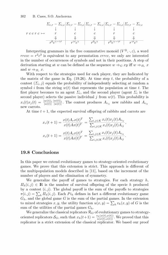
∑∑∑∑
∑∑
r
c
i j
ij ij
ij
ij
h
19.8 Conclusions
� ′ ′ � ′ ′
ý
| || |
| || |
∈∈
∈∈
�→
� � � � �↓ ↓ ↓ ↓ ↓
⇓ ⇓ ⇓ ⇓ ⇓
�
⇒ ⇒⇒
∈
RS
302 B. Cases, S.O. Anchorena
0 0 0
2 3
( )( )
( )( )
( ( ) ( ))( ( ) ( ))
( )=
( )( )
( )
( ) ( ) =
+ 1
( + 1) =( ) ( )
( ) ( )=
( ) ( )
( ) ( )
( + 1) =( ) ( )
( ) ( )=
( ) ( )
( ) ( )
( ) IR( )
( ) = ( )
( ) = ( )
( +1) =
c,r c,c r,r r,c c,r c,c c,r c,c r,r r,c
� � � � � � � � �
G �
�
i
i i
i jw tw t
w tw t r c
rr
T
T
i,j K i j r
i,j K i j ij
cc
T
T
i,j K i j c
i,j K i j ij
h
h h h
h
h h
h
G
G hv x t ,x tu x t ,x t
r c c r c
� � � � � � � � � �
r c c r c
r c r c r c r c r c
V , , εrrccc r c crrcc
w w xy w xw x
t� , ji w t t
� �j w t
x t x t A A
t
x tx t A x t
x t Ax t
x t x t A
x t x t A,
x tx t A x t
x t Ax t
x t x t A
x t x t A.
h� i, j h
i, j� i, j � i, j P iG G
x, y u x, y v x, y GG
x t
Interpreting grammars in the free commutative monoid , a wordis equivalent to any permutation , we only are interested
in the number of occurrences of symbols and not in their positions. A step ofderivation starting at can be de�ned as the sequence iffand .With respect to the strategies used for each player, they are Indicated by
the matrix of the game in Eq. (19.26). At time step , the probability of acontest equals the probability of independently selecting at random asymbol from the string that represents the population at time . The�rst player becomes to an agent , and the second player (agent is thesecond player) selects the passive individual from . This probability is
. The contest produces new rabbits andnew carrots.At time , the expected survival offspring of rabbits and carrots are
In this paper we extend evolutionary games to strategy-oriented evolutionarygames. We prove that this extension is strict. This approach is different ofthe multipopulation models described in [11], based on the increment of thenumber of players and the elimination of symmetry.We generalize the payoff of games to strategies. For each strategy ,
is the number of survival offspring of the specie producedby a contest . The global payoff is the sum of the payoffs to strategies
. Each de�nes in fact a different evolutionary game, and the global game is the sum of the partial games. In the extension
to mixed strategies , the utility function of is thesum of the utilities of the partial games .We generalize the classical replicators of evolutionary games to strategy-
oriented replicators , such that . We proved that thisreplicator is a strict extension of the classical replicator. We based our proof

GL
ESS
ESS
Acknowledgments
References
19 Evolutionary Games 303
1. S. Anchorena and B. Cases. �Eco-grammars to model biological systems: addingprobabilities to agents�. Proceedings of the European Conference on Arti�cialLife, ECAL 2002. Springer. Berlin (2001)
2. E. Csuhaj-Varju, J. Kelemen; A. Kelemenova and G. Paun (1997) Eco-GrammarSystems: A Grammatical Framework for Life-Like Interactions". Arti�cial Life,3(1):1-38
3. R.L. Devaney (1992) A �rst course in chaotic dynamical systems. Theory andexperiment. Studies in Nonlinearity. Addison-Wesley. U.S.A.
on the representation as a strategy-oriented replicator of the logistic equationcalled the logistic replicator .Finally, we sketch a grammatical model of two-person games that �ts ex-
actly to the notion of strategy-oriented replicator. We implement the logisticreplicator using strategy-oriented grammars.This work requires two extensions: the �rst direction, exploring the prop-
erties of the Nash equilibrium, and Lyapunov stable strategies. It seemsclear that the strategies in Nash equilibrium for two-person symmetric gamesand for strategy-oriented games are identical. In fact, they depend on theglobal payoff and not on the replicators. Respecting to , and Lyapunovstable strategies, they both depend on the dynamical properties of the repli-cators; this suggests that the results that are valid for classical replicators willextend to strategy-oriented replicators.The second direction to extend this work is relating formally Strategy-
oriented games to the hierarchy of Eco-grammar systems, a work initiatedin [1] representing the �hawk-dove� game as an eco-grammar system with aconstant number of agents. Strategy-oriented game grammars are qualitativelydifferent, since each symbol in the population has a dual interpretation: it isan agent and it is a passive individual.Finally, the main contribution of this work is opening a way to study
the sequences of moves in two-person games from the point of view of theircomplexity as formal languages, and relate it to the expected payoff. This isa step toward a hierarchy of dynamical systems in relation to a hierarchy ofgrammars that we consider necessary to unify concepts in complex systemsand arti�cial life.
Acknowledgment: This paper has been sponsored by the Spanish Interde-partmental Commission of Science and Technology (CICYT), project numberTEL1999-0181. And the University of the Basque Country project number9/upv 00003.230-13707/2001.

304 B. Cases, S.O. Anchorena
4. M. Smith, J. (1982) Evolution and Theory of Games. Cambridge University Press.Cambridge MA.
5. M. Smith, J. and Price, G.R. (1973) The logic of animal con�ict. Nature 246:15-186. M. Smith, J. (1978) La evolución del comportamiento in Evolución, Libros deInvestigación y Ciencia, Ed. Prensa Cientí�ca,Barcelona pp. 116-126
7. J. Von Neumann; O. Morgenstern. (1944) Theory of Games and economic behav-ior.Princeton University Press. U.S.A
8. Paun, G. (Ed.) (1995) Arti�cial Life: Grammatical Models. Black Sea University.Bucharest, Romania
9. Rozenberg, G. y A. Salomaa (Eds).(1997) Handbook of Formal Languages. Vol.1,2 3. Springer, Berlin
10. Sole, R., Manrubia, S. (1996)Orden y caos en sistemas complejos. Edicions UPC,Barcelona
11. Weibull, J. W. (1996) Evolutionary Game Theory. The MIT Press. Cambridge,MA.

20______________________________________________________________________________________
Discrete Multi-Phase Particle SwarmOptimization
B. Al-kazemi, C.K. Mohan
Summary. This chapter proposes the Discrete Multi-Phase Particle SwarmOptimization (DiMuPSO) algorithm, extending the PSO approach to problemscoded with discrete binary representations. The main features of DiMuPSO are inutilizing multiple groups of particles with different goals that are allowed to changewith time, alternately moving toward or away from the best solutions foundrecently. DiMuPSO also enforces steady improvement in solution quality,accepting only moves that improve fitness. Experimental simulations show thatDiMuPSO outperforms a genetic algorithm and a previous discrete version of PSOon several benchmark problems.
20.1 Introduction
The Particle Swarm Optimization (PSO) algorithm is a stochastic population-basedalgorithm, derived from bird flocking simulations [8, 17, 19]. This chapterproposes the Discrete Multi-Phase Particle Swarm Optimization (DiMuPSO)algorithm, successful in applying the PSO approach to problems coded withdiscrete binary representations. The main features of DiMuPSO are in utilizingmultiple groups of particles with different goals that are allowed to change withtime, alternately moving toward or away from the best solutions found recently.DiMuPSO also enforces steady improvement in solution quality, accepting onlymoves that improve fitness.
The rest of this section describes the PSO algorithm. Section 20.2 presentsthe DiMuPSO algorithm. Section 20.3 presents experimental results comparingDiMuPSO with a genetic algorithm and with a previous discrete version of PSO[15], on several deceptive optimization problems. Section 20.4 describes similarcomparisons for continuous optimization problems whose parameters are encodedusing discrete (binary vector) representations. Section 20.5 presents concludingremarks.
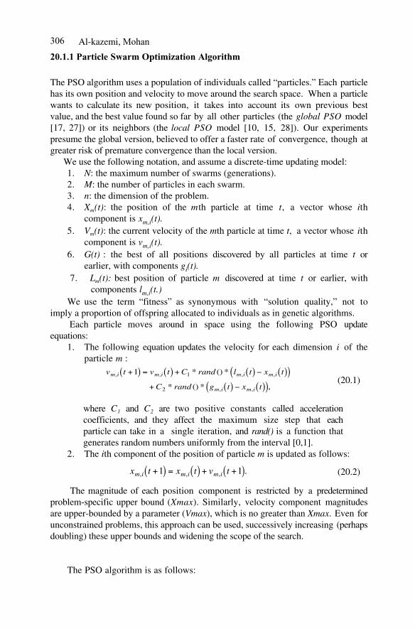
Al-kazemi, Mohan306
20.1.1 Particle Swarm Optimization Algorithm
The PSO algorithm uses a population of individuals called “particles.” Each particlehas its own position and velocity to move around the search space. When a particlewants to calculate its new position, it takes into account its own previous bestvalue, and the best value found so far by all other particles (the global PSO model[17, 27]) or its neighbors (the local PSO model [10, 15, 28]). Our experimentspresume the global version, believed to offer a faster rate of convergence, though atgreater risk of premature convergence than the local version.
We use the following notation, and assume a discrete-time updating model:1. N: the maximum number of swarms (generations).2. M: the number of particles in each swarm.3. n: the dimension of the problem.4. Xm(t): the position of the mth particle at time t, a vector whose ith
component is xm,i(t).5. Vm(t): the current velocity of the mth particle at time t, a vector whose ith
component is vm,i(t).6. G(t) : the best of all positions discovered by all particles at time t or
earlier, with components gi(t).7. Lm(t): best position of particle m discovered at time t or earlier, with
components lm,i(t.)We use the term “fitness” as synonymous with “solution quality,” not to
imply a proportion of offspring allocated to individuals as in genetic algorithms. Each particle moves around in space using the following PSO update
equations:1. The following equation updates the velocity for each dimension i of the
particle m :v t v t C rand l t x t
C rand g t x t
m i m i m i m i
m i m i
, , , ,
, ,
* () *
* () * ,
+( ) = ( ) + ( ) ( )( )+ ( ) ( )( )
1 1
2
(20.1)
where C1 and C2 are two positive constants called accelerationcoefficients, and they affect the maximum size step that eachparticle can take in a single iteration, and rand() is a function thatgenerates random numbers uniformly from the interval [0,1].
2. The ith component of the position of particle m is updated as follows:
x t x t v tm i m i m i, , , .+( ) = ( ) + +( )1 1 (20.2)
The magnitude of each position component is restricted by a predeterminedproblem-specific upper bound (Xmax). Similarly, velocity component magnitudesare upper-bounded by a parameter (Vmax), which is no greater than Xmax. Even forunconstrained problems, this approach can be used, successively increasing (perhapsdoubling) these upper bounds and widening the scope of the search.
The PSO algorithm is as follows:
20 Swarm Optimization 307
1. Initialize the population, randomly assigning each particle’s position andvelocity, which also provide initial values for lm,i components; the bestinitial particle’s position provides the initial G.
2. Repeatedly calculate the new velocity and then the new position for allparticles, using equations (20.1) and (20.2), and updating G and lm
components until a satisfactory solution G is found or computation limitsare exceeded.
20.2 Discrete Multiphase Particle Swarm Optimization
In several problems, PSO finds the optimum value more quickly than when usingtraditional evolutionary algorithms. This is explained by the fact that PSO uses acombination of local and global searches. The DiMuPSO algorithm is obtained bymodifying the PSO algorithm in three ways:
1. Dividing particles into multiple groups, increasing the diversity andexploration of the space.
2. Introducing different phases, between which the direction of particlemovement changes.
3. Moving only to positions that will increase fitness.
To begin with, our research attempts to increase population diversity andproblem space exploration capabilities of PSO, beginning by addressing thefollowing question: instead of the particles working in one group that flies towardthe best position found so far, what if the particles are divided into groups and eachgroup searches differently? That is, one group is directed toward the globally bestposition found so far, and the other flies in the opposite direction. This was thefirst step to developing the DiMuPSO algorithm, dividing the particles intoworking groups with different temporary goals.
In addition, we also observed that a considerable amount of computationaleffort is wasted by PSO in visiting states of poor fitness values. Although this isoften necessary for a stochastic algorithm to avoid being trapped in local minima,enlarging the notion of “neighborhood” in the search space is a possible approachthat allows pursuit of global optima using hill-climbing algorithms. We henceinvestigated a variation of the PSO that restricts each particle to move only to aposition with better fitness (than that particle’s current position). Hill-climbing hasbeen found to be helpful in other evolutionary algorithms such as memeticalgorithms [21].
Another observation was that each particle in PSO often continues to moveroughly in the same direction (toward G) especially when there is no change in G[3, 9, 14]. This leads to convergence of all particles toward local optima whosefitness may be low. Changing direction could lead to a better solution, and this isdone by allowing particles to vary their current goals or directions of search,depending on the current phase of each particle. If a particle finds no improvementin fitness for a prespecified period of time, it changes phase and continues search ina different direction.

Al-kazemi, Mohan308
Directions for particle movement are provided by the global and local best, asin PSO, except that the hill-climbing strategy implies that the local best is thesame as the current position. These two positions act as opposite poles for thevelocity vector, with one acting as attractor and the other as repellor, depending onthe phase. A related, but different, diversity improvement scheme is adopted by theShepherd and Sheepdog algorithm [24].
20.2.1 Update Equations
In DiMuPSO, the mth particle updates its jth velocity as follows:
vm,j(t+1) = min(Vmax, max(-Vmax, vm,j(t) + Cm(t) xm,j(t) - Cm(t) gj(t))), (20.3)
where Cm(t) equals either 1 or -1 depending on the current phase of the particle.Comparing with Eq. (20.1), we observe the disappearance of lm,i, not needed
since the hill-climbing strategy ensures that the current position of each particle isalso its best local position found so far. Separate memory for storing the best localposition is not needed.
The position update equation is a simple discretized version of Eq. (20.2),except that it is considered only a tentative position update, not to be accepted ifsuch an update diminishes a particle’s fitness:
Tentative x tv t x t
m jm j m j_
. ,,
, ,+( ) = +( ) + +( )( ) >11 1 1 0 5
0
if
otherwise.
20.2.2 Which Components to Update?
For multidimensional problems, the new position update equation poses a newissue:
1. Should we iteratively compare the previous fitness with the result ofupdating a single component (dimension) of the particle’s position at atime?
2. Or should we compare the previous fitness with the result of updating allthe components?
These two choices may be considered the extremes in answering the question ofwhat constitutes the neighborhood of a position in the search process—note that aneighborhood in this sense depends on the definition of the moves or operatorsused, not just on a predetermined problem space topology. The first choice isplagued by the problem that the particle can be trapped in local minima of theproblem space topology; this also requires one additional fitness evaluation perproblem dimension, increasing the computational expense significantly. The secondchoice leads to the possibility that very large moves are made that lead very far

20 Swarm Optimization 309
away from the previous position, since the problem space is discrete, violating theparadigm of particles moving to nearby points at each successive instant.
We address this issue by using a new sublength (sl) parameter in theDiMuPSO algorithm. The sl parameter will determine how many dimensions areconsidered for update at a time before evaluating the fitness of the tentativelychanged particle position. For example, if sl = 3, then the tentative updates to theparticle velocity and the position will be calculated for dimensions i to i+3. Iffitness is improved by updating the tentative new positions for the calculateddimensions, the particle will move to its new position, updating sl components ata time. If no improvement is found, there will be no change of the particles’position along those dimensions. Similar calculations are performed for othertuples of sl components of the position vector. In our experiments, sl was chosenrandomly from the interval [1, min(10, n)], where n is the dimensionality of thesearch space..
20.2.3 Phase Changes
In Eq. (20.3), xm,j(t) and gj(t) have opposite signs, so that the particle movestoward or away from the current global best position, depending on its currentphase. Phase change may be enforced after a fixed number of generations (phasechange frequency, pcf). Alternatively, in the adaptive version of this algorithm,phase is changed when there is no improvement within the current phase for aprespecified number of generations, referred to as the pcf.
20.2.4 Velocity Change
Many evolutionary algorithms rely on a restart mechanism to reduce the probabilityof being stuck in local optima of the objective function. This was done for particlepositions in the random particle approach [6]. A similar idea is applied in theDiMuPSO algorithm, periodically reinitializing all particle velocities (rather thanpositions) after a predetermined number (VC) of generations.
Figure 20.1 presents details of the DiMuPSO algorithm. The next twosections describe experimental results obtained using this algorithm.
20.3 Benchmark Problems and Results
This section describes the application of DiMuPSO algorithm to several discretebinary benchmark optimization problems. Section 20.3.1 describes each of thefunctions, Section 20.3.2 gives details of the experiments, and Section 20.3.3shows the results. Results are discussed in Section 20.3.4.

Al-kazemi, Mohan310
Figure 20.1. Details of the DiMuPSO algorithm.
20.3.1 Test Functions
Three different deceptive problems, each characterized by a large number of localoptima, were used for evaluation of the DiMuPSO algorithm: Goldberg’s order-3,Bipolar order-6, and Mühlenbein’s order-5 concatenation problems, described indetail below.
20.3.1.1 Order-3 Deceptive Problem
Goldberg’s deceptive order-3 problem [12] is presented here. The fitness of eachparticle is calculated as follows:
Initialize algorithm parameters such as pcf and N;Create and initialize positions and velocities of M particles;Initialize coefficients Cm to 1 for half the particles, and –1 for the rest;Initialize g to be the position of the particle with highest fitness;
for each swarm t [ 1…N]If (t is a multiple of VC) Reinitialize particle velocities;
For each particle m [1…M]Reverse the sign of Cm if Xm (t)= Xm ( t -pc f ) ;
Copy Xm (t) into Temp, the tentative new position vector;Let sl be a randomly drawn integer from [1, min(10,N)];for each j in 0...(n/sl –1),
for each i in [j*sl ... min(n, j*sl+sl-1 )],Update
v m,i(t+1) = min(Vmax, max(-Vmax, vm, i(t) + Cm (t) xm, i(t) - Cm (t) gi(t))) ;
andT e m p i = 1 if (vm, i(t+1) + xm, i(t)) > 0.5,
and 0 otherwise;
If (fitness(Temp) > fitness(Xm ) )for each i in [j*sl ... min(n, j*sl+sl-1)]
x m,i(t+1) = Tempi;else for each i in [j*sl ... min(n, j*sl+sl-1)]
Temp i = xm,i(t);
If fitness(Xm ) > f i t n e s s ( g )Update g=Xm;
Exit if fitness(g) meets prespecified solution qualityc r i t e r i a ;
20 Swarm Optimization 311
f X f xii
n
( ) = ( )=
31
3/
, where each xi is a disjoint 3-bit substring of X and
f x
if x
if x
if x
if x
i
i
i
i
i
3
0 9 0
0 6 1
0 3 2
1 0 3
( ) =
====
. ,
. ,
. ,
. ,
(20.4)
where xi denotes the sum of the bits in the 3-bit substring.
20.3.1.2 Bipolar Deceptive Problem
The Bipolar order-6 function [11] computes the fitness of a particle as the sum ofthe partial fitness functions obtained by applying a function f6 to disjoint six-bitsubstrings of the particle position. Function f6 has two optima with f6(X)=1 ifX=000000 or X=111111. Local optima occur with f6(X)=0.8 if |X|=3. Finally,these local optima are rendered deceptive by setting f6(X)=0.4 if |X|=2 or 4, andf6(X)=0.0 if |X|=1 or 5.
20.3.1.3 Mühlenbein’s Order-5 Problem
The last deceptive problem to be tested is Mühlenbein’s order-5 problem [22]. Asin the above two problems, the fitness of a particle is computed as the sum of afunction f5 applied to disjoint five-bit substrings of the particle position. But theoptimization task is rendered much more difficult by setting f5(X)=0 everywhereexcept at five positions: f5(00000) = 4, f5(00001) = 3, f5(00011) = 2, f5(00111) =1, and f5(11111) = 3.5.
20.3.2 Details of Experiments
DiMuPSO was compared to two other algorithms: traditional GA using one-pointcrossover and a discrete variation of the standard PSO developed by Kennedy andEberhart [2], referred to as KE-PSO here (elsewhere referred to as Q-DiPSO [1,20]). Each of the algorithms has special settings for its parameters that arepresented in the following subsections.
20.3.2.1 GA Settings
Table 20.1 shows a summary of parameter settings for GA algorithms used in ourexperiments. The one-point crossover operator was used, along with a bitwisemutation operator. The mutation probability was set to be the reciprocal of thebitstring length n (problem dimensionality). The crossover probability (px) was setto 0.9.

Al-kazemi, Mohan312
The population size was increased proportionally to the problemdimensionality, and the maximum number of generations was limited to 1000.
Binary tournament selection mechanism [7] was used; two individuals areselected at random and the fittest is selected [25].
20.3.2.2 KE-PSO Settings
Table 20.2 summarizes the parameter settings. The velocity equation was the sameas Eq. (20.1), with the only difference being in the position calculations (Eq. 20.2):KE-PSO uses velocity components to compute the probability with which eachposition component is determined to be 1. The new equation is as follows:
if , then = 1; else rand e x xvm i m i
m i( ) < ( )( ) =1 0,, , , (20.5)
where rand () is a random number generator using the interval [0, 1].Vmax was set to 5 and both coefficients were set to 2, as in [10, 27, 28].As with the GA algorithm, the swarm size varies according to the length of the
problem, and the maximum swarm number that can be reached is limited to 1000.
20.3.2.3 DiMuPSO Settings
Table 20.3 is a summary of the following DiMuPSO parameters used in theexperiments.
1. Phase changes were determined adaptively: a particle changes phase if noimprovement in fitness is observed in pcf=50 successive swarms(generations).
2. Sl was randomly generated for each individual in each swarm, in the range[1, min (10, n)].
3. VC = 5.The swarm size is set to 30. The maximum number of swarms is set to 1000,
as in the other algorithms. Vmax is set to 1, since discrete-binary functions arebeing tested. Also, Xmax is set to 1.
20.3.3 Results
The results for each of the defined test problems are given in the followingsubsections.
20.3.3.1 Goldberg’s Order-3 Problem
The results obtained were averaged over 20 runs. As shown in Table 20.5, the GAand the DiMuPSO algorithm reached optimum fitness for the problem’s size equalto 30, with the DiMuPSO algorithm requiring fewer fitness evaluations. TheDiMuPSO algorithm used fewer fitness evaluations than the GA.

20 Swarm Optimization 313
Table 20.1 GA Parameters
Parameter G AP m 1/nP x 0.9 N 1000
Table 20.2 KE-PSO Parameters
Parameter KE-PSOVmax 5M 100N 1,000C1 2C2 2
Table 20.3 DiMuPSO Parameters
Parameter DiMuPSO
M 30N 1000Cm 1 or –1Vmax 1S l Randomly generated for each particle in each swarm,
From the interval [1, min(10, M)]pcf 50 (adaptive)V C 5
Table 20.4 Population Sizes Used by GA and PSO for the Three Testing Problems.
G o l d b e r g B i p o l a r M ü h l e n b e i n
n G A P S O G A P S O G A P S O3 0 50 50 50 50 30 306 0 50 50 100 50 60 609 0 100 100 100 100 90 901 2 0 120 120 120 120 120 1201 5 0 120 120 150 150 150 150

Al-kazemi, Mohan314
As the dimensionality of the problem increased, the DiMuPSO algorithm was stillable to reach better fitness than the GA. On the other hand, KE-PSO was unable toreach optimum fitness for all different problem sizes.
Figure 20.2 shows the performance of each algorithm for a problem size of150 bits. The DiMuPSO algorithm reached optimum fitness. The GA and the KE-PSO algorithm were unable to reach optimum fitness.
20.3.3.2 Bipolar Order-6 Problem
The results were averaged over 20 runs. As observed from Table 20.6, theDiMuPSO algorithm reached optimum fitness for all the dimensions. The GA wasable to reach the best fitness for 30- and 60-bit problems. For a problem size of 30bits, the GA used fewer fitness evaluations than the DiMuPSO, but for 60 bits theDiMuPSO algorithm used fewer fitness evaluations than the GA. The KE-PSO wasunable to reach the best fitness for all the different instances of the problem.
Figure 20.3 shows the performance of the three algorithms for the 150-bitproblem. From the figure, and as mentioned earlier, the DiMuPSO algorithm wasthe only one that reached optimum fitness. In addition, the population size used bythe DiMuPSO algorithm was much smaller than that used by the GA and the KE-PSO algorithm. The DiMuPSO algorithm used 30 particles, whereas GA and KE-PSO used 150 individuals. Even though they used a larger number of individuals,both were unable to reach optimum fitness.
20.3.3.3 Mühlenbein’s order-5 Problem
What was observed earlier is true here as well. The DiMuPSO algorithm reachedoptimum fitness for all the dimensions. None of the other algorithms was able toreach the best fitness. Table 20.7 shows the results for all the algorithms fordifferent dimensions. As before, the DiMuPSO used fewer fitness evaluations toreach optimum fitness.
Figure 20.4 shows the results obtained for 150 bits. As mentioned earlier, theDiMuPSO was the only one that reached optimum fitness.
Table 20.5 Best Fitness Found Using GA, KE-PSO and DiMuPSO for Goldberg’sOrder-3 Deceptive Problem Instances of Different Dimensionality, Averaged over 20Trials
G A KE-PSO DiMuPSO
nB e s tF i t n e ss
F i t n e s sE v a l s
B e s tF i t n e s s
F i t n e s sE v a l s
B e s tF i t n e s s
F i t n e s sE v a l s
3 0 10 8,800 9.375 49,200 10 5,6246 0 19.845 43,175 16.725 48,300 20 17,0469 0 29.515 99,500 23.895 99,100 30 32,9881 2 0 39.025 120,000 30.78 117,840 40 39,5091 5 0 47.995 116,640 37.495 111,840 50 60,616

20 Swarm Optimization 315
Table 20.6 Best Fitness Found Using GA, KE-PSO and DiMuPSO for Bipolar order-6Deceptive Problem Instances of Different Dimensionality, Averaged over 20 Trials.
G A KE-PSO DiMuPSO
nBestFitness
FitnessEvals
BestFitness
FitnessEvals Best Fitness Fitness
Evals
3 0 5 8,070 4.67 48,450 5 9,3106 0 10 44,925 8.24 48,800 10 35,1189 0 14.82 94,745 11.71 99,300 15 68,811
1 2 0 18.97 119,520 14.92 117,840 20 98,4061 5 0 23.17 149,700 18 145,950 25 136,547
Table 20.7: Best Fitness Found Using GA, KE-PSO, and DiMuPSO for Mühlenbein’sOrder-5 Deceptive Problem Instances of Different Dimensionality, Averaged over 20Trials.
G A KE-PSO DiMuPSO
n BestFitness
FitnessEvals
BestFitness
FitnessEvals
BestFitness
FitnessEvals
3 0 23.75 12,602 20.875 29,880 24 9,3236 0 46.675 48,705 33.575 58,200 48 13,2489 0 70.2 81,990 44.425 89,460 96 39,3611 2 0 93.5 120,000 55 119,640 120 52,5901 5 0 116.575 140,000 63.175 144,750 148 55,069
Figure 20.2: Comparison of GA, KE-PSO, and DiMuPSO for Goldberg’s 150-bitproblem over 20 runs.

Al-kazemi, Mohan316
Figure 20.4 Comparison of GA, KE-PSO, and DiMuPSO for Mühlenbein’s150-bit problem using the same maximum generation: 1,000 over 20 runs.
Figure 20.3 Comparison of GA, KE-PSO, and DiMuPSO for Bipolar 150-bit problem over 20runs.

20 Swarm Optimization 317
20.3.4 Discussion
Experimental results show that DiMuPSO is a very efficient algorithm. It reachedoptimum fitness each time it was run, and it used fewer fitness evaluations to reachoptimum fitness each time. As problem dimensionality increased, the algorithmstill used fewer fitness evaluations and managed to reach optimum fitness eachtime.
Another observable factor is the time required by DiMuPSO to reach the bestfitness over the 20 runs. Table 20.8 shows the time needed for each algorithm tofinish the execution for the 20 runs for a 30-bit dimension. To be able to compareresults, all these numbers were obtained using a population size equal to 30 and amaximum generation of 1,000. As observed from the table, the DiMuPSOalgorithm required less time than the other two algorithms.
Table 20.8 Time Needed for Each Algorithm to Be Executed 20 Times in Seconds for30-bit Problems; Population Size Was Set to 30 and the Maximum Number ofGenerations to 1000.
Algor i thm Goldberg Bipolar MühlenbeinG A 26.718 22.692 32.056KE-PSO 82.839 180.930 90.209DiMuPSO 2.213 9.633 5.374
Table 20.9 Time Needed for Each Algorithm to Be Executed 20 Times in Seconds for120-bit Problems; Population Size Was Set to 120 and the Maximum Number ofGenerations to 1000.
Algor i thm Goldberg Bipolar MühlenbeinG A 425.351 452.660 444.579KE-PSO 748.438 727.225 711.402DiMuPSO 27.669 88.887 23.924
In order to observe the difference, the experiments were also conducted forhigher-dimensional problems. In Table 20.9, when the problem dimensionality isincreased to 120, the time needed by the other two algorithms is much more thanthe time needed by the DiMuPSO. It is important to note that only DiMuPSOreached the best fitness for this problem. The population size here was set to 120,and the maximum number of generations was limited to 1000. Experiments wereperformed on a Pentium III machine with 800MHz and 640Mb RAM.
20.4. Discrete Encoding, Continuous Space
The previous section addressed the application of DiMuPSO to discrete binaryfunctions. In this section, we describe how continuous optimization problems may

Al-kazemi, Mohan318
also be solved using DiMuPSO, using a discrete encoding for problem parameters.The overall methodology is similar to that of Kennedy and Eberhart [16], whoencoded particle position components using binary numbers. The calculations werecarried out using these binary numbers, and results were converted back to realnumbers. The same experimental settings were used as in Section 20.3, except thatthe population sizes for GA and PSO were set to 100, and DiMuPSO’s populationsize was set to 100 for one of the test functions (Rosenbrock) and 20 for the rest ofthe test functions; VC was set to 10 while pcf was set to 5. Section 20.4.1describes the test functions, and Section 20.4.2 shows the results for the variousfunctions, discussed further in Section 20.4.3.
20.4.1 Test Functions
Four benchmark problems were used to test the algorithms: DeJong F1 (Spherefunction), DeJong F2 (Rosenbrock), DeJong F5 (Foxholes), and Rastrigin. Thesefunctions were chosen because they represent the common difficulties inoptimization problems. These problems are described in the rest of this subsection.
20.4.1.1 Sphere Function (DeJong F1)
Sphere function [13] is a continuous, unimodal function generally used to measurethe efficiency of an algorithm. The graph of this function is shown in Figure 20.5[29]. The function is defined as follows:
f x x xi
i
n
i( ) = < <=
2
1
100 100, , where
where x is an n-dimensional, real-valued vector and xi is the ith element of that
vector. It has a global minimum of 0 at xi( ) = 0.
20.4.1.2 Rosenbrock Function (DeJong F2)
The Rosenbrock function [26] is a smooth function with a sharp ridge that distractsordinary optimization algorithms. This function can be quite difficult foralgorithms that are unable to identify promising search directions with littleinformation. Algorithms that take good direction for the search will perform well inthis function. The function is depicted in Figure 20.6, and the description is asfollows:
f x x x x xi( ) = ( ) + ( )100 1 2 048 2 04812
22
12, . . where .
The function has a minimum value of 0 at x x1 2 1 1, ,( ) = ( ) .
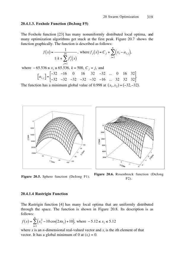
20 Swarm Optimization 319
20.4.1.3. Foxhole Function (DeJong F5)
The Foxhole function [23] has many nonuniformly distributed local optima, andmany optimization algorithms get stuck at the first peak. Figure 20.7 shows thefunction graphically. The function is described as follows:
f x
k f x
f x C x a
j
j
j j i i j
i
n
( ) =+ ( )
( ) = + ( )=
=
1
1 1
1
251
, ,, where
where and= =65 536 65 536 500. . , , ,x k C ji j
ai j,
...
....[ ] = 32 16 0 16 32 32 0 16 32
32 32 32 32 32 16 32 32 32
The function has a minimum global value of 0.998 at x x1 2 32 32, ,( ) = ( ) .
20.4.1.4 Rastrigin Function
The Rastrigin function [4] has many local optima that are uniformly distributedthrough the space. The function is shown in Figure 20.8. Its description is asfollows:
f x x x xi i ii
n
( ) = ( ) +( )=
2
1
10 2 10 5 12 5 12cos , . . where
where x is an n-dimensional real-valued vector and xi is the ith element of thatvector. It has a global minimum of 0 at (xi) = 0.
Figure 20.5. Sphere function (DeJong F1).Figure 20.6. Rosenbrock function (DeJong
F2).

Al-kazemi, Mohan320
Table 20.10 Results for Sphere Function, Averaged over 20 Runs.
G A KE-PSO DiMuPSO
Number ofbits for
encoding
Fitnessevals
Bestfitness
Fitnessevals
Bestfitness
Fitnessevals
Bestfitness
5 99,200 129.0 98,000 2281.0 7,641 104.1
1 0 99,100 47.6 86,600 1983.0 12,947 0.096
1 5 97,600 14.3 93,000 2170.2 19,673 0.000093
2 0 98,460 11.1 97,600 2169.3 22,515 0.000014
2 5 99,530 48.4 91,700 2249.2 30,618 0.000017
Table 20.11 Results for Rosenbrock (DeJong F2) Function, Averaged over 20 Runs.
GA KE-PSO DiMuPSO
Numberof
bits forencoding
Fitnessevals
Bestfitness
Fitnessevals
Bestfitness
Fitnessevals
Bestfitness
5 1,100 0.029 5,700 0.0081 83,100 0.0086
10 4,4400 0.027 94,500 0.00050 87,118 0.00019
15 84,260 0.031 70,030 0.00025 69,160 0.00015
20 91,430 0.046 78,975 0.00034 64,769 0.00012
25 95,180 0.043 64,935 0.00031 63,945 0.00029
Figure 20.7. Foxhole Function (DeJongF5).
Figure 20.8. Rastrigin Function.
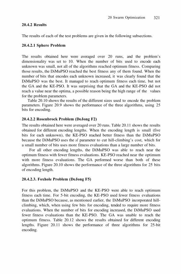
20 Swarm Optimization 321
20.4.2 Results
The results of each of the test problems are given in the following subsections.
20.4.2.1 Sphere Problem
The results obtained here were averaged over 20 runs, and the problem’sdimensionality was set to 10. When the number of bits used to encode eachunknown was small, not all of the algorithms reached optimum fitness. Comparingthose results, the DiMuPSO reached the best fitness any of them found. When thenumber of bits that encodes each unknown increased, it was clearly found that theDiMuPSO was the best. It managed to reach optimum fitness each time, but notthe GA and the KE-PSO. It was surprising that the GA and the KE-PSO did notreach a value near the optima, a possible reason being the high range of the valuesfor the problem parameters.
Table 20.10 shows the results of the different sizes used to encode the problemparameters. Figure 20.9 shows the performance of the three algorithms, using 25bits for encoding.
20.4.2.2 Rosenbrock Problem (DeJong F2)
The results obtained here were averaged over 20 runs. Table 20.11 shows the resultsobtained for different encoding lengths. When the encoding length is small (fivebits for each unknown), the KE-PSO reached better fitness than the DiMuPSObecause the DiMuPSO uses the sl parameter to cut hill-climbing’s cost, which fora small number of bits uses more fitness evaluations than a large number of bits.
For all other encoding lengths, the DiMuPSO was able to reach near theoptimum fitness with fewer fitness evaluations. KE-PSO reached near the optimumwith more fitness evaluations. The GA performed worse than both of thesealgorithms. Figure 20.10 shows the performance of the three algorithms for 25 bitsof encoding length.
20.4.2.3. Foxhole Problem (DeJong F5)
For this problem, the DiMuPSO and the KE-PSO were able to reach optimumfitness each time. For 5-bit encoding, the KE-PSO used fewer fitness evaluationsthan the DiMuPSO because, as mentioned earlier, the DiMuPSO incorporated hill-climbing, which, when using few bits for encoding, tended to require more fitnessevaluations. When the number of bits for encoding increased, the DiMuPSO usedfewer fitness evaluations than the KE-PSO. The GA was unable to reach theoptimum fitness. Table 20.12 shows the results obtained for different encodinglengths. Figure 20.11 shows the performance of three algorithms for 25-bitencoding.
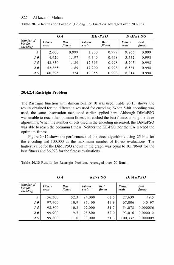
Al-kazemi, Mohan322
Table 20.12 Results for Foxhole (DeJong F5) Function Averaged over 20 Runs.
G A KE-PSO DiMuPSONumber ofbits forencoding
Fitnessevals
Bestfitness
Fitnessevals
Bestfitness
Fitnessevals
Bestfitness
5 2,600 0.999 1,800 0.999 9,866 0.999
1 0 4,920 1.197 9,340 0.998 3,532 0.998
1 5 43,830 1.189 12,595 0.998 5,703 0.998
2 0 52,865 1.189 17,200 0.998 6,561 0.998
2 5 60,395 1.324 12,355 0.998 8,814 0.998
20.4.2.4 Rastrigin Problem
The Rastrigin function with dimensionality 10 was used. Table 20.13 shows theresults obtained for the different sizes used for encoding. When 5-bit encoding wasused, the same observation mentioned earlier applied here. Although DiMuPSOwas unable to reach the optimum fitness, it reached the best fitness among the threealgorithms. When the number of bits used in the encoding increased, the DiMuPSOwas able to reach the optimum fitness. Neither the KE-PSO nor the GA reached theoptimum fitness.
Figure 20.12 shows the performance of the three algorithms using 25 bits forthe encoding and 100,000 as the maximum number of fitness evaluations. Thehighest value for the DiMuPSO shown in the graph was equal to 0.178649 for thebest fitness and 86,973 for the fitness evaluations.
Table 20.13 Results for Rastrigin Problem, Averaged over 20 Runs.
G A KE-PSO DiMuPSO
Number ofbits forencoding
Fitnessevals
Bestfitness
Fitnessevals
Bestfitness
Fitnessevals
Bestfitness
5 56,300 52.3 94,000 62.5 27,639 49.5
1 0 97,900 10.9 86,400 49.9 67,006 0.0497
1 5 98,800 10.8 92,000 51.7 54,078 0.000056
2 0 99,900 9.7 98,800 52.0 93,016 0.000012
2 5 99,800 11.0 99,000 51.3 100,332 0.000009

20 Swarm Optimization 323
20.4.3 Discussion
Experimental results show that the DiMuPSO algorithm is much more efficientthan the other two algorithms. The KE-PSO algorithm performed well in two setsof problems; namely, the Rosenbrock and the Foxhole problems. But even forthese two problems, the DiMuPSO algorithm required fewer fitness evaluations.
Figure 20.9 Comparison of evolution of best fitness values for minimizing spherefunction with parameter values represented using 25 bits over 20 runs.
Figure 20.10 Comparison of evolution of best fitness values for minimizingRosenbrock (DeJong F2) function with parameter values represented using 25 bits over20 runs.
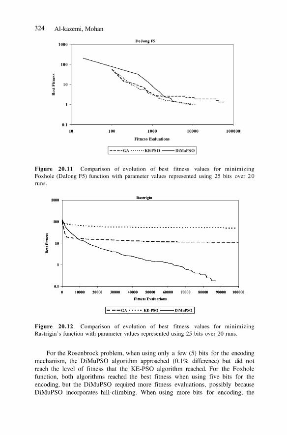
Al-kazemi, Mohan324
Figure 20.11 Comparison of evolution of best fitness values for minimizingFoxhole (DeJong F5) function with parameter values represented using 25 bits over 20runs.
Figure 20.12 Comparison of evolution of best fitness values for minimizingRastrigin’s function with parameter values represented using 25 bits over 20 runs.
For the Rosenbrock problem, when using only a few (5) bits for the encodingmechanism, the DiMuPSO algorithm approached (0.1% difference) but did notreach the level of fitness that the KE-PSO algorithm reached. For the Foxholefunction, both algorithms reached the best fitness when using five bits for theencoding, but the DiMuPSO required more fitness evaluations, possibly becauseDiMuPSO incorporates hill-climbing. When using more bits for encoding, the
20 Swarm Optimization 325
problem is harder, and use of the sl parameter helps reduce the number of fitnessevaluations required instead of degrading the performance.
As described in the previous section, the time used to execute 20 runs wasrecorded. DiMuPSO used less time than the two other algorithms. Table 20.14shows the time needed for each of the algorithms to be executed 20 times using apopulation size of 100 and maximum generation of 1,000.
Table 20.14 The Time Needed for Each Algorithm to Be Executed 20 Times in Secondsfor 25-bit Encoding; Population Size Was Set to 100 and Maximum Generation to 1,000
A l g o r i t h m S p h e r e(DeJong F1)
R o s e n b r o c k(DeJong F2)
F o x h o l e(DeJong F5)
R a s t r i g i n
G A 858,574 174,851 162,183 771,249KE-PSO 1149,332 178,606 39,777 1128,212DiMuPSO 35,691 132,390 6,789 110,548
20.5 Concluding Remarks
We have presented DiMuPSO, a variation of the particle swarm optimizationalgorithm for discrete optimization tasks. The main features of the new algorithmare the incorporation of hill climbing, the use of multiple groups of particles withdifferent search parameters, and the adaptive modification of particle goals as theycycle through different phases. Extensive experimental results show that the newalgorithm outperforms traditional GA and PSO algorithms for difficult benchmarkdiscrete and continuous optimization problems.
The modifications to PSO proposed in this paper are largely orthogonal toother improvements to PSO suggested in the literature [5, 18], and we expect thatseveral of those improvements can also be incorporated into the DiMuPSOapproach.
In related recent work [2], we have shown the applicability of this approachdirectly to continuous optimization tasks without discrete encoding, e.g.,successfully training the weights of feedforward neural networks for classificationproblems using a continuous version of DiMuPSO.
References
1. B. Al-kazemi and C. K. Mohan, (2002) Multi-Phase Discrete ParticleSwarm Optimization, Proc. The Fourth International Workshop onFrontiers in Evolutionary Algorithms (FEA 2002).
2. B. Al-kazemi and C. K. Mohan, (2002) Multi-Phase Generalization of theParticle Swarm Optimization Algorithm," Proc. Congress onEvolutionary Computation, Honolulu, Hawaii.

Al-kazemi, Mohan326
3. P. J. Angeline, (1998) Evolutionary Optimization Versus Particle SwarmOptimization: Philosophical and Performance Differences," Proc.Evolutionary Programming VII (EP98) LNCS 1447.
4. T. Bäck, G. Rudolph, and H. P. Schwefel, (1993) EvolutionaryProgramming and Evolution Strategies: Similarities and Differences,"Proc. 2nd Annual Conference on Evolutionary Programming, San Diego,CA.
5. F. van den Bergh and A.P Engelbrecht, (2001) Effects of Swarm Size onCooperative Particle Swarm Optimizers," Proc. GECCO 2001, SanFrancisco, USA.
6. Frans van den Bergh, (2001) An Analysis of Particle Swarm Optimizers,"(Ph.D. Dissertation, University of Pretoria, Pretoria).
7. Tobias Blickle and Lothar Thiele, (1995) A Comparison of SelectionSchemes used in Genetic Algorithms, Computer Engineering andCommunication Networks Lab (TIK), Zurich.
8. Roy W. Dobbins, Russell C. Eberhart, and Patrick K. Simpson, (1996) inComputational Intelligence PC Tools: Academic Press Professional, pp.212-226.
9. R. C. Eberhart and Y Shi, (1998) Comparison between GeneticAlgorithms and Particle Swarm Optimization, Proc. 7th internationalConference on Evolutionary Programming, San diego, California, USA.
10. R. C. Eberhart and J. Kennedy, (1995) A New Optimizer using ParticleSwarm Theory," Proc. the Sixth International Symposium on MicroMachine and Human Science, Nagoya, Japan.
11. D. E. Goldberg, K. Deb, and J. Horn, (1992) Massive Multimodality,Deception, and Genetic Algorithms, Parallel Problem Solving fromNature, vol. 2, pp. 37-46.
12. D. E. Goldberg, K. Deb, and B. Korb, (1990) Messy Genetic AlgorithmsRevisited: Studies in mixed size and scale, Complex Systems, vol. 4, pp.415-444.
13. K. De Jong, (1975) An Analysis of the Behaviour of a Class of GeneticAdaptive Systems, (Ph.D. Dissertation, University of Michigan).
14. J. Kennedy, (1998) The Behavior of Particles, Proc. EvolutionaryProgramming VII: 7th International Conference on EvolutionaryProgramming, San Diego, California, USA.
15. J. Kennedy, (1999) Small Worlds and Mega-Minds: Effects ofNeighborhood Topology on Particle Swarm Performance, Proc. Congresson Evolutionary Computation, Washington, DC, USA.
16. J. Kennedy and R. C. Eberhart, (1997) A Discrete Binary Version of theParticle Swarm Algorithm, Proc. Conf. on Systems, Man, andCybernetics, Piscataway, NJ.
17. J. Kennedy and R. C. Eberhart, (1995) Particle Swarm Optimization,Proc. IEEE International Conference on Neural Networks.
18. M. Løvbjerg, T. K. Rasmussen, and T. Krink, (2001) "Hybrid ParticleSwarm Optimizer with breeding and subpopulations," Proc. Third Geneticand Evolutionary Computation Conference.
20 Swarm Optimization 327
19. M.M. Millonas, (1994) "Swarms, Phase Transitions, and CollectiveIntelligence," in Artificial Life III, S. S. i. t. S. o. Complexity, Ed.:Addison Wesley Longman, pp. 417-445.
20. C. K. Mohan and B. Al-kazemi, (2001) Discrete Particle SwarmOptimization, Proc. Workshop on Particle Swarm Optimization,Indianapolis, IN: Purdue School of Engineering and Technology, IUPUI,2001.
21. Pablo Moscato, (1989) On Evolution, Search, Optimization, GeneticAlgorithms and Martial Arts: Towards Memetic Algorithms, CaliforniaInstitute of Technology, Pasadena, California, USA 826, 1989.
22. H. Mühlenbein, T. Mahnig, and A. O. Rodrigues, (1999) Schemata,Distributions and Graphical Modes in Evolutionary Optimization, Journalof Heuristics, vol. 5.
23. R. Patil, (1995) Intervals in Evolutionary Algorithms for GlobalOptimization," Los Alamos National Laboratory Unclassified 1196.
24. Denis Robilliard and Cyril Fonlupt, (1999) A Shepherd and a Sheepdog toGuide Evolutionary Computation, Proc. Evolutionary Computation,France.
25. A. Rogers and A. Prügel-Bennett, (1999) Genetic Drift in GeneticAlgorithm Selection Schemes, IEEE Transactions on EvolutionaryComputation, vol. 3, pp. 298-303, 1999.
26. F. Seredynski, P. Bouvry, and F. Arbab, (1997) Distributed EvolutionaryOptimization in Manifold: the Rosenbrock's Function Case Study, Proc.First International Workshop on Frontiers in Evolutionary Algorithms,Duke University , USA.
27. Y. Shi and R. C. Eberhart, (1999) Empirical study of Particle SwarmOptimization, Proc. Congress on Evolutionary Computation, Piscataway,NJ.
28. P. N. Suganthan, (1999) Particle Swarm Optimizer with NeighborhoodOperator," Proc. Congress on Evolutionary Computation, Piscataway, NJ:IEEE Service Center.
29. Deniz Yuret, (1994) From Genetic Algorithms to Efficient Optimization,(Master of Science Thesis, Massachusetts Institute Of Technology).

Index
3-SAT, 269
Abundance coefficients, 47Adaptive Business Intelligence, 2Amino Acids, 151Atractor, 248
Benchmark problems, 256Biology, 271Breeder Algorithm, 199
C4.5, 170Chromosome Codi�cation, 75Chromosome Encoding, 146, 162, 316Combinatorial Circuits, 178Constraint Handling, 222Convergence Models, 235Critical Points, 261
Data Mining, 3, 85Deceptive function, 243Deceptive Problems, 312Decision Rules, 159, 161Decision Systems, 88Decision Tree, 85DNA computing, 269
Ecosystem, 298Elitism, 165, 213Encoding, 33Endmembers, 47, 51Epistasis, 226Evolution Strategy, 5, 13, 35, 52, 55, 64Evolutionary Games, 285, 289
Evolvable Hardware, 177, 184
Gate-Level, 181Genetic Algorithm, 51, 55, 75, 88, 102,
122, 132, 147, 181, 199, 216, 233Genetic Programming, 13Grammar, 129, 292Graph Rewriting, 272
Homomorphic �ltering, 63Hybrid Encoding, 159Hypergraph, 273Hyperspectral images, 45, 53
Identi�cation Problem, 196Illumination correction, 61Industrial Applications, 6, 18Inmigration, 106Integrated System Analysis, 26
Job Shop Scheduling, 74
Learning Ruel, 195Limited Convergence, 233Linear Genetic Programming, 13Logistic Equation, 285, 295Long-term memory, 258
Macroevolutionary Algorithms, 119Magnetic Resonance Imaging, 70Mass-spring system, 35Micro Genetic Algorithm, 221Middling, 216Min-Max, 224Mixed Strategies, 288

330 Index
Molecular Computing, 270Morphological Associative Memories, 45,
48Morphological Independence, 50, 51Morphological Neural Networks, 46Multimodal Diversity, 234Multiobjective Optimization, 184, 213Multiphase optimization, 307Multiphase Particle Optimization, 306
Nash Equilibrium, 285Natural Language, 129Niching, 225, 236Non Cooperative Games, 288
Onthological knowledge, 83Optimization, 3, 11
Pareto Front, 214Particle Swarm, 306Pathways, 273Payoff, 285Phylogenetics, 99Premature Convergence, 106, 148, 234Protein Structure, 143
Races, 124Remote Sensing, 45Replicator, 291
Rewriting, 292Robot Controller, 117Rough Sets, 91
Sampled Fitness Functions, 255SAT, 269Scheduling Algorithm, 79Self-adaptation, 226Self-Adaptivity, 5Sequential Covering, 164Sharing Evolutionary Algorithm, 148Short-term memory, 258Signal Processing, 195Signaling Molecules, 272Sparse Fitness Function, 256Spectral unmixing, 47Stability Analysis, 202State Formation, 84Strategy Oriented Replicators, 286Structural Information, 152System Identi�cation, 195
Theory of Games, 285Triangulation, 32, 33, 38Truth Table, 181
Uncertainty, 87Utility, 288