The effects of unsymmetric matrix permutations and scalings in semiconductor device and circuit...

The Effects of Nonsymmetric Matrix

Permutations and Scalings in Semiconductor

Device and Circuit Simulation

by O.Schenk1, Stefan Rollin2 and Anshul Gupta3

IEEE Transactions on Computer-Aided Design of Integrated Circuits andSystems

23(3), pp 400-411, March 2004

1Department of Computer Science, University of Basel, Klingelbergstrasse 50,CH-4056 Basel, Switzerland email: [email protected]

2Integrated Systems Laboratory, Swiss Federal Institute of Technology Zurich,ETH Zurich

8092 Zurich, Switzerland. email: [email protected]

3IBM Research Devision, T.J.Watson Research Center, P.O.Box 218, YorktownHeights, NY, 10598

Publication available athttp://informatik.unibas.ch/personen/schenk_o.html

IEEE TRANSACTIONS ON COMPUTER-AIDED DESIGN OF INTEGRATED CIRCUITS AND SYSTEMS 2

The Effects of Unsymmetric Matrix Permutationsand Scalings in Semiconductor Device and Circuit

SimulationOlaf Schenk, Member, IEEE, Stefan Rollin, and Anshul Gupta, Member, IEEE

Abstract— The solution of large sparse unsymmetric linearsystems is a critical and challenging component of semiconductordevice and circuit simulations. The time for a simulation isoften dominated by this part. The sparse solver is expected tobalance different, and often conflicting requirements. Reliability,a low memory-footprint, and a short solution time are a few ofthese demands. Currently, no black-box solver exists that cansatisfy all criteria. The linear systems from both simulationscan be highly ill-conditioned and therefore quite challengingfor direct and iterative methods. In this paper, it is shownthat algorithms to place large entries on the diagonal usingunsymmetric permutations and scalings greatly enhance thereliability of both direct and preconditioned iterative solvers forunsymmetric linear systems arising in semiconductor device andcircuit simulations. The numerical experiments indicate that theoverall solution strategy is both reliable and cost effective.

Index Terms— Semiconductor device simulation, circuit sim-ulation, sparse linear solvers, numerical linear algebra, sparseunsymmetric matrices, preconditioning

I. INTRODUCTION

IN 1950, Van Roosbroeck [1] introduced the drift-diffusionequations, which are the commonly used model in semi-

conductor device simulation. The drift-diffusion equationsare a system of three coupled, nonlinear partial differentialequations (PDEs), which describe the relation between theelectrostatic potential and the densities of the charge car-riers in a semiconductor device. The coupling between thedifferent equations is highly nonlinear and implies numericaldifficulties. More sophisticated models have evolved since thebeginnings of semiconductor device simulation to describe theincreasingly complex devices.

The equations of the drift-diffusion model are:

−∇ · (ε∇ψ) , = q (p− n+ C)

q∂n

∂t−∇ · jn = −q R,

q∂p

∂t+ ∇ · jp = −q R,

Manuscript submitted to IEEE TCAD. This work was supported by theSwiss Commission of Technology and Innovation under contract number5648.1, the IBM T. J. Watson Research Center, and the Strategic ExcellencePositions on Computational Science of the Swiss Federal Institute of Tech-nology, Zurich

O. Schenk is with the Computer Science Department of the University ofBasel, Basel, Switzerland. S. Rollin is with Integrated Systems Laboratoryof the Swiss Federal Institute of Technology and Innovation (ETH), Zurich,Switzerland. Anshul Gupta is affiliated with the Mathematical SciencesDepartment of the IBM T. J. Watson Research Center, Yorktown Heights,USA.

where ψ is the electrostatic potential, n and p the electron andhole densities. These are the unknown variables. The otherquantities are given: ε is the dielectrical permittivity, C thedoping concentration, R the total recombination rate and q theelementary charge. The carrier current densities jc in equations(I) - (I) are substituted with the equations

jn = q (Dn∇n− µnn∇ψ) ,

jp = −q (Dp∇p+ µpp∇ψ) .

Here, µc are the carrier mobilities and Dc are the carrierdiffusivities. Typical challenges in solving the drift-diffusionequations include a large range of n and p, the steep gradientsof the solution variables, and the necessity to ensure thatn, p > 0 in the numerical computations.

Different discretizations are used to solve the drift-diffusionequations numerically. The Scharfetter-Gummel box methodand finite element discretizations are both used in modernsemiconductor device simulators [2], [3]. Regardless of thediscretization, a set of nonlinear equations must be solved.Two different approaches are used to solve these nonlinearequations [4]. The Gummel iteration can be seen as a block-Gauss-Seidel iteration on the nonlinear level. The three sets ofvariables electrostatic potential, electron and hole density aresolved in turn, by using the Poisson and continuity equations.A major drawback of this method is the deterioration of theconvergence, if the couplings between the variables becometoo strong. Often, the only possible way is to solve the non-linear equations simultaneously with the Newton method. Theresulting linear systems Ax = b, where A is an unsymmetricsparse n × n matrix, are three times larger than with theGummel method, highly ill-conditioned and significantly moredemanding.

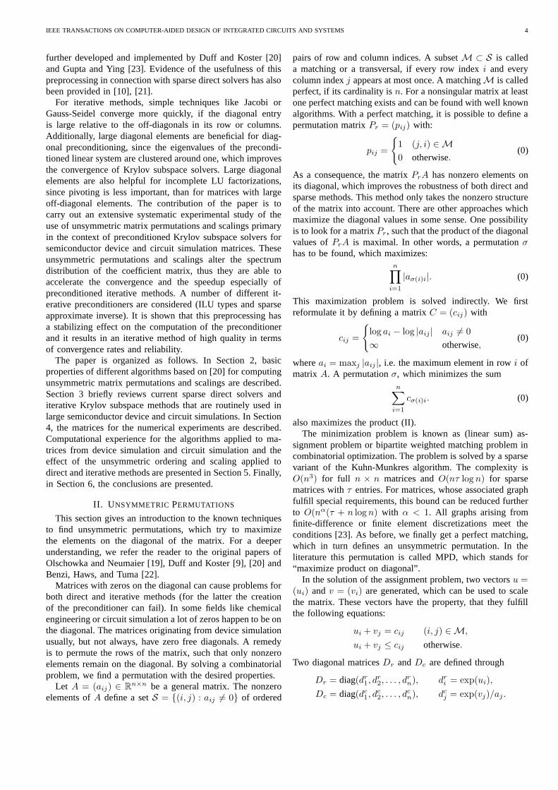
Figure 1 shows the distribution of the magnitude of elementsin a matrix from semiconductor device simulation. The firstpicture shows the 3 × 3 sparse block structure of a matrixresulting from the Newton linearization and discretizationof the drift-diffusion equations. The diagonal blocks of Aare related to the electrostatic potential ψ and the chargecarrier densities n, p in a semiconductor device, respectively.The values in the off-diagonal blocks of A represent thecoupling of the variables ψ, n and p. The first matrix showsall the elements, the second one shows only the largest 50%elements in absolute value, and the last one shows the largest10% elements. Due to the numerical properties of the carrierdensities, the largest 10% elements, which are in the off-diagonal blocks, can be several orders of magnitude larger


Fig. 1. Pictorial depiction of the magnitude of the elements in a matrix from semiconductor device simulation. The first picture shows the original coefficientmatrix. The second picture shows only 50% of the largest absolute values, the last picture the largest 10%.

than the elements in the diagonal blocks. These extremelylarge entries in the off-diagonal blocks are one main reason forthe difficulties in applying preconditioned iterative methods insemiconductor device simulation.

In circuit simulation often a series of linear systems issolved. For example, in transient analysis, a differential al-gebraic equation (DAE) leads in each time-step to a systemof nonlinear equations, usually to be solved with the Newtonmethod resulting in very sparse unsymmetric linear systemswith a lot of zeros on the diagonal in each matrix.

There are two main approaches to solving the unsymmetricsparse linear systems from both the Gummel and Newtonmethod and the matrices from circuit simulation. The first ap-proach is more conservative and uses sparse direct solver tech-nology. In the last few years algorithmic improvements [5], [6],[7], [8], [9], [10] alone have reduced the time for the directsolution of unsymmetric sparse systems of linear equations byalmost one or two order of magnitude. Remarkable progresshas been made in the increase of reliability, parallelizationand consistent high performance is now achieved for a widerange of computing architectures. As a result, a number ofsparse direct solver packages for solving such systems areavailable [7], [11], [12] and it is now common to solve theseunsymmetric sparse linear systems of equations with a directmethod that might have been considered impractically largeuntil recently.

Nevertheless, in large three-dimensional simulations withmore than 100K grid nodes, the memory requirements of directmethods as well as the time for the factorization may be toohigh. Therefore, a second approach, namely, preconditionedKrylov subspace methods, is often employed to solve thesesystems. This iterative approach has smaller memory require-ments and often smaller CPU time requirements than a directmethod. However, an iterative method may not converge tothe solution in some cases where a direct method is capableof finding the solution.

Various iterative methods are known and have been usedin semiconductor device and circuit simulations: CGS [13],GMRES(m) [14], BICGSTAB [15] and others. A good precon-ditioner is mandatory to achieve satisfactory convergence rateswith these methods. There have been several attempts [16],

[17], [18] to use preconditioned Krylov subspace methods withdifferent incomplete LU-factorizations (ILU) in this context,but in general the results have been far from satisfactoryfor non-trivial semiconductor device simulations. The primaryconcern of the device and circuit engineers is the lack ofrobustness of the iterative solver.

ILU preconditioners may work well and exist when thecoefficient matrix is an M-matrix and well conditioned. Ma-trices with these properties arise e.g. from the discretizationof second-order, elliptic partial differential equations and sim-ple preconditioning techniques such as incomplete Choleskytechniques are usually reliable under these circumstances anddeliver good convergence rates. Furthermore, a large numberof small diagonal values causes problems in the constructionof the ILU factors if no pivoting is applied during the ILUfactorization process. Moreover, the preconditioners are oftenunstable and the convergence deteriorates when the coeffi-cient matrix has zeros on the diagonal, and or is highlyunsymmetric. Furthermore, preconditioned Krylov subspacemethods rarely converge well when the off-diagonal valuesof the coefficient matrix are several orders of magnitudelarger than the diagonal entries as this is often the case insemiconductor device simulation simulations. These systemsstill pose a challenge for most preconditioned Krylov subspacesolvers.

Partial pivoting typically improves the robustness and theaccuracy of both direct and iterative solution process. Thedisadvantage is that partial pivoting in sparse matrix factor-ization causes the computational task-dependency graph tochange during execution, which can result in a significantcomputational overhead.

In [19], Olschowka and Neumaier introduce new permu-tations and scaling strategies for Gaussian elimination toavoid extensive pivoting strategies. The goal is to transformthe coefficient matrix A with diagonal scaling matrices Dr

and Dc and a permutation matrix Pr so as to obtain anequivalent system with a matrix PrDrADc that is betterscaled and more diagonally dominant. This preprocessing hasa beneficial impact on the accuracy of the solver and it alsoreduces the need for partial pivoting, thereby speeding up thefactorization process. These and other heuristics have been


further developed and implemented by Duff and Koster [20]and Gupta and Ying [23]. Evidence of the usefulness of thispreprocessing in connection with sparse direct solvers has alsobeen provided in [10], [21].

For iterative methods, simple techniques like Jacobi orGauss-Seidel converge more quickly, if the diagonal entryis large relative to the off-diagonals in its row or columns.Additionally, large diagonal elements are beneficial for diag-onal preconditioning, since the eigenvalues of the precondi-tioned linear system are clustered around one, which improvesthe convergence of Krylov subspace solvers. Large diagonalelements are also helpful for incomplete LU factorizations,since pivoting is less important, than for matrices with largeoff-diagonal elements. The contribution of the paper is tocarry out an extensive systematic experimental study of theuse of unsymmetric matrix permutations and scalings primaryin the context of preconditioned Krylov subspace solvers forsemiconductor device and circuit simulation matrices. Theseunsymmetric permutations and scalings alter the spectrumdistribution of the coefficient matrix, thus they are able toaccelerate the convergence and the speedup especially ofpreconditioned iterative methods. A number of different it-erative preconditioners are considered (ILU types and sparseapproximate inverse). It is shown that this preprocessing hasa stabilizing effect on the computation of the preconditionerand it results in an iterative method of high quality in termsof convergence rates and reliability.

The paper is organized as follows. In Section 2, basicproperties of different algorithms based on [20] for computingunsymmetric matrix permutations and scalings are described.Section 3 briefly reviews current sparse direct solvers anditerative Krylov subspace methods that are routinely used inlarge semiconductor device and circuit simulations. In Section4, the matrices for the numerical experiments are described.Computational experience for the algorithms applied to ma-trices from device simulation and circuit simulation and theeffect of the unsymmetric ordering and scaling applied todirect and iterative methods are presented in Section 5. Finally,in Section 6, the conclusions are presented.

II. UNSYMMETRIC PERMUTATIONS

This section gives an introduction to the known techniquesto find unsymmetric permutations, which try to maximizethe elements on the diagonal of the matrix. For a deeperunderstanding, we refer the reader to the original papers ofOlschowka and Neumaier [19], Duff and Koster [9], [20] andBenzi, Haws, and Tuma [22].

Matrices with zeros on the diagonal can cause problems forboth direct and iterative methods (for the latter the creationof the preconditioner can fail). In some fields like chemicalengineering or circuit simulation a lot of zeros happen to be onthe diagonal. The matrices originating from device simulationusually, but not always, have zero free diagonals. A remedyis to permute the rows of the matrix, such that only nonzeroelements remain on the diagonal. By solving a combinatorialproblem, we find a permutation with the desired properties.

Let A = (aij) ∈ Rn×n be a general matrix. The nonzero

elements of A define a set S = {(i, j) : aij 6= 0} of ordered

pairs of row and column indices. A subset M ⊂ S is calleda matching or a transversal, if every row index i and everycolumn index j appears at most once. A matching M is calledperfect, if its cardinality is n. For a nonsingular matrix at leastone perfect matching exists and can be found with well knownalgorithms. With a perfect matching, it is possible to define apermutation matrix Pr = (pij) with:

pij =

{

1 (j, i) ∈ M

0 otherwise.(0)

As a consequence, the matrix PrA has nonzero elements onits diagonal, which improves the robustness of both direct andsparse methods. This method only takes the nonzero structureof the matrix into account. There are other approaches whichmaximize the diagonal values in some sense. One possibilityis to look for a matrix Pr, such that the product of the diagonalvalues of PrA is maximal. In other words, a permutation σhas to be found, which maximizes:

n∏

i=1

|aσ(i)i|. (0)

This maximization problem is solved indirectly. We firstreformulate it by defining a matrix C = (cij) with

cij =

{

log ai − log |aij | aij 6= 0

∞ otherwise,(0)

where ai = maxj |aij |, i.e. the maximum element in row i ofmatrix A. A permutation σ, which minimizes the sum

n∑

i=1

cσ(i)i. (0)

also maximizes the product (II).The minimization problem is known as (linear sum) as-

signment problem or bipartite weighted matching problem incombinatorial optimization. The problem is solved by a sparsevariant of the Kuhn-Munkres algorithm. The complexity isO(n3) for full n × n matrices and O(nτ log n) for sparsematrices with τ entries. For matrices, whose associated graphfulfill special requirements, this bound can be reduced furtherto O(nα(τ + n logn) with α < 1. All graphs arising fromfinite-difference or finite element discretizations meet theconditions [23]. As before, we finally get a perfect matching,which in turn defines an unsymmetric permutation. In theliterature this permutation is called MPD, which stands for“maximize product on diagonal”.

In the solution of the assignment problem, two vectors u =(ui) and v = (vi) are generated, which can be used to scalethe matrix. These vectors have the property, that they fulfillthe following equations:

ui + vj = cij (i, j) ∈ M,

ui + vj ≤ cij otherwise.

Two diagonal matrices Dr and Dc are defined through

Dr = diag(dr1, d

r2, . . . , d

rn), dr

i = exp(ui),

Dc = diag(dc1, d

c2, . . . , d

cn), dc

j = exp(vj)/aj .


Fig. 2. Influence of unsymmetric permutations on the matrix from semiconductor device simulation shown in Figure 1. The first picture shows the originalcoefficient matrix. The second picture shows only 50% of the largest absolute values, the last picture the largest 10%. Note that a majority of the largestvalues have migrated to the block diagonal.

With the equations (II) and (II), it can be shown, that thescaled and permuted matrix A1 = PrDrADc is an I-matrix,for which holds:

|a1ii| = 1,

|a1ij | ≤ 1.

Olschowka and Neumaier [19] introduced these scalings andpermutation for reducing pivoting in Gaussian elimination offull matrices. We use the abbreviation MPS for these scalingsand the permutation, which stands for “maximize product ondiagonal with scalings.”

Figure 2 shows the effect of applying MPS on the dis-tribution of the magnitude of elements in the matrix fromsemiconductor device simulation shown in Figure 1. Thematrices in Figure 2 correspond to those in Figure 1, but scaledand permuted with MPS. Compared with the original matrix,the largest elements of the matrix now lie on the diagonal.

The linear assignment problem can also be used to maxi-mize the sum of the modulus of the diagonal elements. Insteadof (II) the matrix C is defined in the following way:

cij =

{

ai − |aij | aij 6= 0

0 otherwise.(0)

In contrary to the maximization of the product (II), it is notpossible to derive scalings with the same properties from thelinear assignment algorithm in this case. The acronym for“maximize sum of diagonals” is MSD.

Finding a bottleneck transversal is a further possibility tomaximize the diagonal elements to some extent. Instead oflooking at all diagonal values, a permutation σ is searched,which maximizes the smallest element on the diagonal, i.e.we maximize the expression

mini

|aσ(i)i|. (0)

Two different approaches are known to achieve this goal. Oneof them uses a slightly modified variant of the assignmentproblem. The other defines matrices Aε, where entries with|aij | ≤ ε from the original matrix are dropped. A matchingfor Aε is then searched. Interval nesting is used to find the

optimal ε and thus the desired permutation. These methodsdo not generate unique permutations and are sensitive to aprior scaling of the matrix. A major drawback is that only thesmallest values on the diagonal is regarded, which was alreadyreported in [9]. In the section with the numerical results, weuse the letters BT for the bottleneck transversal.

III. SOLVERS FOR SPARSE LINEAR SYSTEMS OF

EQUATIONS

In this section the algorithms and strategies that are usedin the direct and preconditioned iterative linear solvers in thenumerical experiments are discussed.

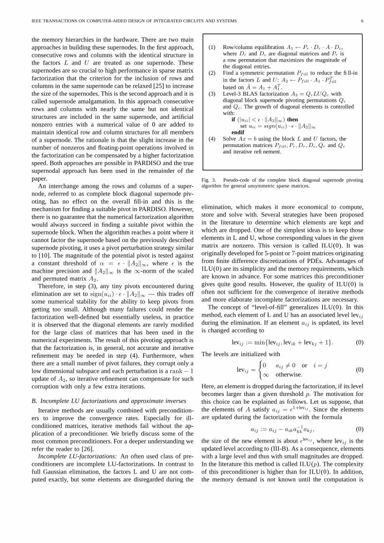
A. Sparse direct solver technology

Figure 3 outlines the PARDISO1 approach [12] to solvean unsymmetric sparse linear system of equations. Accordingto [10], it is very beneficial to precede the ordering byperforming an unsymmetric permutation to place large entrieson the diagonal and then to scale the matrix so that thediagonal entries are equal to one. Therefore, in step (1) therow permutation matrix, Pr, is chosen so as to maximizethe absolute value of the product of the diagonal entries inPrA. The code used to perform the permutations is takenfrom MC64, a set of Fortran routines that are included inHSL (formerly known as Harwell Subroutine Library). Furtherdetails on the algorithms and implementations are providedin [9]. The diagonal scaling matrices, Dr and Dc, are selectedso that the diagonal entries of A1 = PrDrADc are 1 inabsolute value and its off-diagonal entries are less than orequal to 1 in absolute value as in (II) - (II).

In step (2) any symmetric fill-reducing ordering can be com-puted based on the structure of PrA+ATP T

r , e.g. minimumdegree or nested dissection. All experiments reported in thispaper with PARDISO were conducted with a nested dissectionalgorithm [24].

Like other modern sparse factorization codes [7], [11],PARDISO relies heavily on supernodes to efficiently utilize

1More information on PARDISO can be obtained at http://www.computational.unibas.ch/cs/scicomp


the memory hierarchies in the hardware. There are two mainapproaches in building these supernodes. In the first approach,consecutive rows and columns with the identical structure inthe factors L and U are treated as one supernode. Thesesupernodes are so crucial to high performance in sparse matrixfactorization that the criterion for the inclusion of rows andcolumns in the same supernode can be relaxed [25] to increasethe size of the supernodes. This is the second approach and it iscalled supernode amalgamation. In this approach consecutiverows and columns with nearly the same but not identicalstructures are included in the same supernode, and artificialnonzero entries with a numerical value of 0 are added tomaintain identical row and column structures for all membersof a supernode. The rationale is that the slight increase in thenumber of nonzeros and floating-point operations involved inthe factorization can be compensated by a higher factorizationspeed. Both approaches are possible in PARDISO and the truesupernodal approach has been used in the remainder of thepaper.

An interchange among the rows and columns of a super-node, referred to as complete block diagonal supernode piv-oting, has no effect on the overall fill-in and this is themechanism for finding a suitable pivot in PARDISO. However,there is no guarantee that the numerical factorization algorithmwould always succeed in finding a suitable pivot within thesupernode block. When the algorithm reaches a point where itcannot factor the supernode based on the previously describedsupernode pivoting, it uses a pivot perturbation strategy similarto [10]. The magnitude of the potential pivot is tested againsta constant threshold of α = ε · ‖A2‖∞, where ε is themachine precision and ‖A2‖∞ is the ∞-norm of the scaledand permuted matrix A2.

Therefore, in step (3), any tiny pivots encountered duringelimination are set to sign(uii) · ε · ‖A2‖∞ — this trades offsome numerical stability for the ability to keep pivots fromgetting too small. Although many failures could render thefactorization well-defined but essentially useless, in practiceit is observed that the diagonal elements are rarely modifiedfor the large class of matrices that has been used in thenumerical experiments. The result of this pivoting approach isthat the factorization is, in general, not accurate and iterativerefinement may be needed in step (4). Furthermore, whenthere are a small number of pivot failures, they corrupt only alow dimensional subspace and each perturbation is a rank − 1update of A2, so iterative refinement can compensate for suchcorruption with only a few extra iterations.

B. Incomplete LU factorizations and approximate inverses

Iterative methods are usually combined with precondition-ers to improve the convergence rates. Especially for ill-conditioned matrices, iterative methods fail without the ap-plication of a preconditioner. We briefly discuss some of themost common preconditioners. For a deeper understanding werefer the reader to [26].

Incomplete LU-factorizations: An often used class of pre-conditioners are incomplete LU-factorizations. In contrast tofull Gaussian elimination, the factors L and U are not com-puted exactly, but some elements are disregarded during the

(1) Row/column equilibration A1 ← Pr ·Dr · A ·Dc,where Dr and Dc are diagonal matrices and Pr isa row permutation that maximizes the magnitude ofthe diagonal entries.

(2) Find a symmetric permutation Pfill to reduce the fill-inin the factors L and U : A2 ← Pfill ·A1 · P

Tfill

based on A = A1 + AT1 .

(3) Level-3 BLAS factorization A2 = QrLUQc withdiagonal block supernode pivoting permutations Qr

and Qc. The growth of diagonal elements is controlledwith:

if (|uii| < ε · ‖A2‖∞) thenset uii = sign(uii) · ε · ‖A2‖∞

endif(4) Solve Ax = b using the block L and U factors, the

permutation matrices Pfill, Pr, Dr, Dc, Qr and Qc

and iterative refinement.

Fig. 3. Pseudo-code of the complete block diagonal supernode pivotingalgorithm for general unsymmetric sparse matrices.

elimination, which makes it more economical to compute,store and solve with. Several strategies have been proposedin the literature to determine which elements are kept andwhich are dropped. One of the simplest ideas is to keep thoseelements in L and U, whose corresponding values in the givenmatrix are nonzero. This version is called ILU(0). It wasoriginally developed for 5-point or 7-point matrices originatingfrom finite difference discretizations of PDEs. Advantages ofILU(0) are its simplicity and the memory requirements, whichare known in advance. For some matrices this preconditionergives quite good results. However, the quality of ILU(0) isoften not sufficient for the convergence of iterative methodsand more elaborate incomplete factorizations are necessary.

The concept of “level-of-fill” generalizes ILU(0). In thismethod, each element of L and U has an associated level levij

during the elimination. If an element aij is updated, its levelis changed according to

levij := min{levij , levik + levkj + 1}. (0)

The levels are initialized with

levij =

{

0 aij 6= 0 or i = j

∞ otherwise.(0)

Here, an element is dropped during the factorization, if its levelbecomes larger than a given threshold p. The motivation forthis choice can be explained as follows. Let us suppose, thatthe elements of A satisfy aij = ε1+levij . Since the elementsare updated during the factorization with the formula

aij := aij − aika−1kk akj , (0)

the size of the new element is about εlevij , where levij is theupdated level according to (III-B). As a consequence, elementswith a large level and thus with small magnitudes are dropped.In the literature this method is called ILU(p). The complexityof this preconditioner is higher than for ILU(0). In addition,the memory demand is not known until the computation is


completed. Since it is solely based on the structure of thematrix and the numerical values of the matrix are not takeninto account, the resulting preconditioning can be poor.

In the ILUT(ε, q) factorization, the dropping is based on thenumerical values rather than the positions. Most incompletefactorizations are either row or column oriented. After a rowhas been computed in the ILUT(ε, q) factorization, all ele-ments in this row of L and U smaller than the given toleranceε are disregarded. In order to limit the size of the factors, onlythe q largest elements in each row are kept. For non-diagonallydominant and indefinite matrices, this preconditioner usuallygives better results than ILU(p).

The combination of ILU(p) and ILUT(ε, q) leads to afactorization, which is not often mentioned in the literature.We call this method ILUPT(p, ε) in the remainder of thisdocument. An element is always kept in this factorization, ifits level is zero. If the level is positive, the element is droppedif either the value is smaller than the given tolerance ε or itslevel exceeds p.

Incomplete LU-factorizations are often quite successfulin accelerating iterative methods. Nevertheless, some severeproblems may happen during the factorization. As in fullGaussian elimination, zero pivots can occur. A remedy is to usepivoting. Because of the underlying data structures, columnpivoting is the best choice, if the incomplete factorization iscomputed row-wise. Not only zero pivots but also small pivotsare a problem, since they lead to unstable and inaccuratefactorizations. Another cause of inaccuracy is due to thedropping of elements. Each element that is dropped, makesthe “error” of the factorization larger. Adapting the parametersmay improve this situation.

A successful computation of an incomplete factorizationdoes not guarantee the convergence of an iterative method.For indefinite matrices the factors are often far from beingdiagonal dominant. Even if the elements of L and U are withinreasonable bounds, ‖L−1‖ and ‖U−1‖ can be arbitrarily large,which is a sign for unstable triangular solves, which in turncan deteriorate the convergence.

Approximate inverses: The product of the factors in in-complete Gaussian eliminations, directly approximates a givenmatrix A. Other preconditioners approximate the inverse of A.A major advantage of this approach is that the application ofthe preconditioner requires one or more matrix-vector productsinstead of triangular solves. Therefore, these preconditionersare well suited to parallel environments.

The sparse approximate inverse preconditioner SPAI [27]computes a matrix M , which minimizes the Frobenius normof I − AM , where I is the identity matrix. M is equal toA−1, when the norm becomes zero. The inverse is usually afull matrix and thus M is only computed approximately. Sincethe relation

‖I −AM‖2F =

n∑

i=1

‖ei −Ami‖22 (0)

holds, each column can be determined independent of theothers (ei and mi are the i-th columns of I and M ). Atolerance ε is given to limit the fill-in and to control the

accuracy of the approximation of each column and thus thequality of the preconditioner.

The AINV algorithm [28] is based on an incompletebiconjugation process. Two triangular factors Z and W arecomputed, which approximate the inverse of A:

ZW T ≈ A−1. (0)

The triangular matrices are sparse approximations to theinverses of the factors L and U of a full Gaussian elimination.The biconjugation algorithm computes them without the priorcomputation of L and U . A dropping tolerance is used topreserve the sparsity of the factors. Again, the application ofthe preconditioner can be performed fully in parallel.

Like in direct methods, the linear systems are ordered beforethe preconditioner is computed. All mentioned preconditionersexcept for SPAI are sensitive to orderings. The purposeof the orderings is twofold. On one hand, the quality ofthe preconditioner depends on the ordering. In ILU(p) asan example, we have seen, that the dropping is based onthe positions only. A different ordering leads therefore to adifferent preconditioner. On the other hand, the ordering alsoinfluences the amount of fill-in in the preconditioners (exceptfor ILU(0)). The Reverse Cuthill-McKee (RCM) [29] orderingis usually used for incomplete LU-factorizations. RCM is notsuited for both direct methods and the preconditioner AINV,since it would result in high fill-ins in the factors. Multipleminimum degree and nested dissection are normally used forthem.

IV. DESCRIPTION OF THE TEST PROBLEMS

TABLE I

GENERAL INFORMATIONS AND STATISTICS OF THE MATRICES USED IN

THE NUMERICAL EXPERIMENTS.

name unknowns elements dim sim

27628 bjtcai 27’628 442’898 2D f54019 highK 54’019 996’414 2D f28984 Tetra 28’984 599’170 3D f51448 3D 51’448 1’056’610 3D fbarrier2-9 115’625 3’897’557 3D dibm matrix 2 51’448 1’056’610 3D figbt3 10’938 234’006 2D dmatrix-new 3 125’329 2’678’750 3D fmatrix 9 103’430 2’121’550 3D fnmos3 18’588 386’594 2D dohne2 181’343 11’063’545 3D dpara-4 153’226 5’326’228 3D dcircuit 1 2’624 35’823 2D mcircuit 2 4’510 21’199 2D mecl32 51’993 380’415 2D mpre2 659’033 5’959’282 2D mwang3 26’064 177’168 3D mwang4 26’068 177’196 3D m

This section gives an overview of the matrices that are usedfor the numerical experiments. Some general informationsabout the matrices are given in Table I. They are extractedfrom different semiconductor device simulations with differentsimulators. A part stems from simulations with FIELDAY[3] from the IBM T. J. Watson Research Center. Those are


TABLE II

CONDITIONING AND DIAGONAL DOMINANCE STATISTICS.

original scaled and permuted with MPSname condest d.d.rows d.d.cols condest d.d.rows d.d.cols27628 bjtcai 6.46e+19 11’774 13’571 1.16e+07 11’725 13’37254019 highK 5.85e+31 16’761 23’041 3.99e+07 16’749 21’83528984 Tetra 1.36e+41 12’869 13’365 1.97e+08 12’869 18’02451448 3D 1.29e+24 16’097 22’948 5.03e+07 16’110 22’196barrier2-9 5.49e+22 29’553 5’739 1.07e+19 26’280 53’226ibm matrix 2 1.29e+24 16’097 22’950 4.99e+07 16’740 22’337igbt3 4.74e+19 2’795 121 1.09e+09 2’770 5’237matrix-new 3 3.48e+22 68’450 78’339 6.59e+08 68’357 72’185matrix 9 3.08e+23 36’258 38’926 2.71e+07 37’052 40’808nmos3 1.09e+21 3’068 36 6.28e+06 3’048 6’671ohne2 3.30e+21 43’283 3’804 2.03e+20 42’509 90’323para-4 3.70e+23 41’321 6’271 4.22e+20 39’530 76’797circuit 1 1.89e+05 1’217 1’144 2.38e+06 1’261 2’504circuit 2 2.69e+04 3’466 560 2.19e+04 3’283 487ecl32 9.41e+15 31’446 35’574 1.94e+08 31’837 31’745pre2 3.11e+23 6’729 33 2.99e+14 178’421 152’798wang3 1.07e+04 16’097 22’950 4.96e+03 21’926 21’676wang4 4.91e+04 16’097 22’950 5.48e+03 24’762 21’526

marked with an “f” in the column “sim”. Others, labeledwith “d”, originate from the semiconductor device simulatorDESSISISE [2], which is a product of ISE Integrated SystemsEngineering Inc. The last matrices wang3 and wang4 comefrom semiconductor device simulation from a public sparsematrix collection [30] and all other matrices are circuit systemsfrom the same public collection. These matrices are markedwith an ’m’ in the Table I.

In Table II we have also listed the condition numbers and thenumber of diagonal dominant rows (d.d. rows) and columnsfor the original matrices and for the matrices permuted andscaled with MPS. We have used the algorithm MC71 fromHSL together with the direct solver PARDISO to estimate thecondition numbers.

As stated earlier and shown in Table II, most of thematrices are very ill-conditioned. The influence of MPS onthese condition number is significant for most of the matrices.The spectrum benefits from unsymmetric matrix scalings andpermutations and the ill-conditioning is greatly reduced formost of the matrices. The number of diagonal dominant rowsand columns is also affected by the permutation and scalingand increases by the preprocessing with MPS.

V. NUMERICAL RESULTS

The numerical experiments were performed on one proces-sor on a Regatta pSeries 690 Model 681 SMP nodes with aPower4 running at 1.3 GHz. The processor contains 32 KBL1 data cache, two fixed-point, two floating point and twoload/store execution units, associated with a large L2 cache,1440 KB, and an additional L3 cache directory and controls.All algorithms were implemented in Fortran 77 and C in 64-bitmode. The codes were compiled by xlf and xlc with the -O3optimization option and are linked with the IBM’s Engineeringand Scientific Subroutine Library (ESSL) for the basic linear

algebra subprograms (BLAS) that are optimized for RS6000processors.

A key design principle for producing high-performancescalable parallel, direct solver software is to perform partialpivoting as little as possible, whereas the key design principlefor robustness is to allow as much pivoting as possible. Acompromise is complete block supernode diagonal pivoting,where rows and columns of a supernode can be interchangedwithout affecting the computational task-dependency graph.This allows the a priori computation of the nonzero structureof the factors and allows at the same time a limited completepivoting within the diagonal supernodes blocks. Placing largeentries on the diagonal suggests the stability and accuracyof the direct factorization process with reduced pivoting inPARDISO can be improved. This is especially true for circuitsimulations, where it is very common for a lot of zeros toappear on the diagonals.

The numerical behavior of the complete block diagonalsupernode pivoting method in PARDISO with the originalmatrix and the unsymmetric scaled and permuted matrix isillustrated in Table III. A failure in the computation of thefactorization (zero pivot) is marked with “•”.

Two comments on the results in Table III are in order.First, we notice that for most of the semiconductor devicesimulation matrices, the number of nonzeros in the factorsand the operation count is not affected by an unsymmetricpermutation and scaling. However, we have observed forthese matrices that the numerical accuracy still benefits fromthe permutation. Secondly, it can be seen that MPS greatlyimproves the robustness of PARDISO and all four circuitsimulation matrices can now be solved with a backward errorthat is close to machine precision.

In this section, we also present the numerical results to seehow unsymmetric permutations influence the iterative solutionof the linear systems in semiconductor device and circuit


TABLE III

NUMBER OF FACTOR ENTRIES (×106 ) AND OPERATION COUNT (×10

9) IN

THE FACTORS COMPUTED BY PARDISO.

Matrix None MPS

entries ops entries ops

27628 bjtcai 3.12 0.45 3.12 0.4554019 highK 7.99 1.44 7.99 1.4428984 Tetra 13.2 8.42 13.2 8.4251448 3D 28.3 25.5 28.3 25.5barrier2-9 127. 217. 125. 212.ibm matrix 2 28.3 25.5 28.3 25.5igbt3 1.15 .100 1.15 .100matrix-new 3 93.4 177. 93.4 177.matrix 9 93.4 177. 93.4 177.nmos3 2.47 0.30 2.47 0.30ohne2 233. 334. 233. 334.para-4 178. 341. 178. 341.circuit1 • • 0.51 0.01circuit2 • • 0.47 0.01ecl32 25.1 22.4 25.1 22.4pre2 • • 97.9 166.wang3 16.1 12.3 7.63 4.58wang4 6.26 3.02 6.26 3.02

simulation. Usually, incomplete LU-factorizations are used inthese fields and therefore we have tested different versionsof them. Results with the approximate inverse preconditionerSPAI were also conducted.

For the preconditioning, there are always several choices:either left or right preconditioning can be used. For incompletefactorizations a combination of both is also possible. Weapplied left preconditioning in all cases. This implies, thatthe preconditioned residuals do not correspond to the un-preconditioned ones. However, the error of the preconditionedand the original system remains the same. In a majority of thetested matrices, the preconditioned residual and the residualsof the original systems are reduced by the same order ofmagnitude.

For the FIELDAY and DESSISISE matrices we had a righthand side b at our disposal, which directly came from thesemiconductor device application. For the circuit simulationmatrices no right hand side was given and therefore an artificialsolution of xi = 1, 1 ≤ i ≤ n was used. Additionalexperiments with other options such as bi = 1, 1 ≤ i ≤ nshowed similar results. The initial guess x0 was always zerofor the preconditioned iterative methods.

Two of the most famous iterative methods have beentested: BICGSTAB [15] and GMRES(m) [14]. To avoid toohigh memory consumption, we restarted GMRES after 20iterations. In both methods, we have implemented two dif-ferent stopping criteria: the iteration is stopped, if either thepreconditioned residual is reduced by a factor of 10−8 or amaximum of 200 iterations are reached. The latter criterion isa common and important choice in industrial semiconductordevice simulation applications since it makes no sense inthese industrial engineering environments to allow an infinitenumber of iterations for the preconditioned iterative solver.In order to be competitive with direct solvers, the options forthe iterative solver were determined during an extensive series

of pre-experiments in an attempt to fix the parameters for theiterative solver such that these options are the best on average.The performance of both iterative methods BICGSTAB andGMRES(m) is comparable. Our numerical results show, thatGMRES is faster, if only a few iterations are enough for theconvergence. This is especially the case, if we change thetolerance from 10−8 to 10−4. However, for the tolerance weused in the numerical experiments, more iteration steps arerequired and BICGSTAB becomes slightly faster in a majorityof cases. Our experience from complete semiconductor devicesimulations also indicates to prefer BICGSTAB over GMRES.For these reasons, we present the results for the former only.

As mentioned in Section III-B, a symmetric permutation isusually applied to the linear system before the preconditioneris computed. Thus the iterative solution consists of four steps:

1) Determination of an unsymmetric matrix permutationand scaling

2) A symmetric permutation is computed3) Creation of a preconditioner.4) Call of an iterative method (BICGSTAB)

The first two steps are optional. For the second step, we didvarious experiments with RCM, multiple minimum degree andnested dissection. However, we only list the results with RCM,since this ordering is usually the best choice for incompletefactorizations, as stated in [31], [32]. Our numerical experi-ments gave similar results.

The benefits of unsymmetric permutations and scalings for amatrix from semiconductor device simulation can be observedin Figure 2. It was already mentioned that these scalingsand permutations result in an I-matrix such that all diagonalelements are equal to one and all absolute values of the off-diagonal elements are less or equal to one. It can be clearlyseen that all heavy values are on the diagonal.

In Table IV we have listed the numerical results with andwithout an unsymmetric permutation for ILU(0). A failurein the computation of the factorization (zero pivot) is markedwith “•”. A number in parenthesis indicates, that the iterativemethod did not converge, i.e. 200 iterations were not enoughto reduce the norm of the preconditioned residual by a factorof 10−8. In this case, the number shows, by which amountthe preconditioned residual was reduced. On the one hand,this allows to see, whether the method would reach thegiven tolerance in a few additional steps or not. On theother hand, those combinations of parameters, for which 200iterations are reached, can be compared and determined whichcombination performs better. The influence of MPS on thenumber of iterations is not as high as one would expect. Forsome matrices the number of iterations is even worse withMPS than without. However, in our experience ILU(0) withthe unsymmetric permutation and scalings is slightly morestable. If the iterative method failed with MPS, then it didnot succeed without MPS either. But in some situations, thelinear systems could only be solved with MPS. Our resultscoincide with observations from others [22], that is, if a systemcan be solved by ILU(0) without MPS, then its influence isnot significant or even disadvantageous. We have also testedother unsymmetric permutations. With BT the incompletefactorization ILU(0) is often similar to the results without


an unsymmetric permutation. However, we have seen in otherresults not listed here, that ILU(0) with BT is often unstableand the iterative method does not reduce the un-preconditionedresiduals at all. The MSD ordering is the worst one: thecreation of the preconditioner often fails due to zero pivot.The results from MPD are comparable to those of MPS.As already mentioned, we also did some experiments withdifferent symmetric permutations, namely with RCM, multipleminimum degree and nested dissection. The results show, thatthe fewest number of iterations of BICGSTAB are reachedin combination with RCM. In addition, more systems can besolved with this ordering than with the others.

TABLE IV

NUMBER OF ITERATIONS OF BICGSTAB PRECONDITIONED WITH ILU(0)

FOR A RESIDUAL REDUCTION OF 10−8 . IF 200 ITERATIONS ARE

REACHED, THE NUMBER IN PARENTHESIS SHOWS THE REDUCTION OF THE

PRECONDITIONED RESIDUAL.

Matrix None BT MSD MPD MPS

27628 bjtcai (2.0e-5) (2.0e-5) (1.6e-6) 160 17754019 highK 156 156 • 155 16928984 Tetra (4.2e-6) (4.2e-6) • (1.0e-5) (5.3e-6)51448 3D 66 66 • 81 64barrier2-9 (8.6e-8) (6.7e-8) • 104 128ibm matrix 2 88 88 (8.1) 104 93igbt3 106 106 128 95 107matrix-new 3 125 125 (5.1e-2) 166 143matrix 9 68 68 • 71 66nmos3 (1.2e-4) (1.2e-4) (2.8e-4) (3.3e-4) (1.2e-6)ohne2 128 (2.0e-8) 165 (3.6e-8) 167para-4 (4.7e-7) (2.56) (1.7e-8) (1.1e-8) 168circuit 1 • 2 2 2 2circuit 2 • 17 16 16 14ecl32 139 139 (5.5e-7) 139 131pre2 • • • • •

wang3 • • 41 41 41wang4 57 54 57 57 43

In our ILUT(ε, q) implementation we do not limit thenumber of entries in each row, i.e. we set q = ∞. The impactof unsymmetric permutations on ILUT(0.01,∞) is quite high.The number of iterations for the convergence can be foundin Table V. A lot of systems can only be solved with MPS.However, not every unsymmetric permutation gives goodresults. The quality of BT and MSD with ILUT is comparableto the findings with ILU(0). A better choice is MPD, whichis better than omitting an unsymmetric permutation. The MPSordering requires the fewest iterations for convergence inalmost all cases. In addition, there are often fewer nonzeros inthe incomplete factors for this ordering than for the others. Asa result, the computation of the factorization is faster and oneiteration step is cheaper with MPS. For this preconditioner,the symmetric ordering does not have a large influence on thenumber of iterations. However, the nonzero elements in theincomplete factors is lower for RCM on the average comparedto the other tested symmetric orderings, which reduces thetime for one iteration of BICGSTAB.

The results of the ILUPT(5,0.01) factorization are given inTable VI. Here, the behavior is again different than for theprevious two factorizations. A lot of systems can be solved

TABLE V

NUMBER OF ITERATIONS OF BICGSTAB PRECONDITIONED WITH

ILUT(0.01,∞) FOR A RESIDUAL REDUCTION OF 10−8 . IF 200

ITERATIONS ARE REACHED, THE NUMBER IN PARENTHESIS SHOWS THE

REDUCTION OF THE PRECONDITIONED RESIDUAL.


27628 bjtcai (1.1e-3) (1.1e-3) (1.1) (3.3e-5) 12554019 highK (2.8e-3) (2.8e-3) • (2.7e-5) 8928984 Tetra (2.5e-5) (2.5e-5) • (6.7e-5) 7951448 3D 135 135 • 66 32barrier2-9 (4.5e-1) (4.7e-1) • (1.9e-8) 171ibm matrix 2 136 136 • 68 34igbt3 (8.8e-4) (8.8e-4) (2.8e-1) (3.4e-3) 54matrix-new 3 88 88 (5.1e-1) 74 47matrix 9 77 77 • 57 30nmos3 (1.1) (1.1) (3.6e-4) (1.0e-4) 22ohne2 (1.7e-5) (5.2e-6) (2.8e-3) (1.9e-4) 85para-4 77 (2.8e-4) (3.0e-4) (7.8e-6) 53circuit 1 • 3 3 3 4circuit 2 • 33 15 15 5ecl32 44 44 (2.2e-8) 44 55pre2 • • • • •

wang3 • • 24 24 29wang4 31 27 31 31 23

in combination with or without an unsymmetric permutation.What remains the same is the quality of the MSD ordering,where the computation of the preconditioner sometimes fails.The results of BT are better than before, but still not optimal inthe sense, that the un-preconditioned residuals are not reduced.Again, MPD is a better alternative. On the average, the bestchoice is MPS, but the difference with MPD and without anunsymmetric permutation is not as high as for ILUT.

TABLE VI

NUMBER OF ITERATIONS OF BICGSTAB PRECONDITIONED WITH

ILUPT(5,0.01) FOR A RESIDUAL REDUCTION OF 10−8 . IF 200

ITERATIONS ARE REACHED, THE NUMBER IN PARENTHESIS SHOWS THE

REDUCTION OF THE PRECONDITIONED RESIDUAL.


27628 bjtcai 155 155 70 89 7654019 highK 96 96 • 100 8328984 Tetra 194 194 • 100 8651448 3D 59 59 • 59 37barrier2-9 72 81 • 47 (1.1e-8)ibm matrix 2 64 64 (1.9e-3) 60 39igbt3 36 36 57 37 44matrix-new 3 89 89 (1.2e-3) 87 48matrix 9 50 50 • 52 31nmos3 51 51 112 48 30ohne2 59 • 59 90 72para-4 51 • 45 51 53circuit 1 • 2 2 2 2circuit 2 • 11 11 11 5ecl32 89 89 (5.0e-4) 89 54pre2 • • • • •

wang3 • • 46 46 27wang4 43 46 43 43 21

The number of iterations gives a good indication of thereliability of a preconditioner. However, the total time to per-form the four steps for the iterative solution is more important


TABLE VII

TOTAL TIME IN SECONDS FOR COMPLETE ITERATIVE SOLUTION. THE BEST TIME IS SHOWN IN BOLDFACE.

ILU(0) ILUT(0.01,∞) ILUPT(5,0.01) SPAI(0.1) SPAI(0.4)Matrix None MPS None MPS None MPS None MPS None MPS27628 bjtcai ‡ 2.53 ‡ 1.26 2.13 1.19 ‡ ‡ ‡ ‡54019 highK 4.45 5.11 ‡ 2.08 3.15 2.95 ‡ ‡ ‡ ‡28984 Tetra ‡ ‡ ‡ 1.02 3.26 1.81 ‡ 19.9 ‡ 5.2051448 3D 2.56 2.53 8.54 1.18 2.51 2.29 ‡ 38.5 ‡ 9.08barrier2-9 ‡ 22.2 ‡ 10.9 15.0 ‡ ‡ 401 ‡ 89.9ibm matrix 2 2.96 3.34 8.54 1.25 2.70 2.36 ‡ 38.3 ‡ 9.33igbt3 0.68 0.75 ‡ 0.31 0.36 0.40 ‡ ‡ ‡ ‡matrix-new 3 10.4 11.2 23.3 3.35 7.93 6.39 ‡ 145 ‡ ‡matrix 9 4.86 4.80 18.4 3.08 4.73 5.05 ‡ 82.8 ‡ 14.7nmos3 ‡ ‡ ‡ 0.33 0.77 0.54 ‡ 9.11 ‡ 2.55ohne2 66.0 86.6 ‡ 18.1 50.8 46.9 • • • •para-4 ‡ 35.8 6.63 6.31 16.9 13.2 ‡ 382 ‡ ‡circuit 1 • 0.02 • 0.01 • 1.17 3.01 3.10 1.45 1.45circuit 2 • 0.02 • 0.01 • 0.03 ‡ 1.23 ‡ 0.943ecl32 2.81 2.76 2.72 1.70 2.08 1.90 ‡ ‡ ‡ ‡pre2 • • • • • • ‡ ‡ ‡ ‡wang3 • 0.46 • 0.54 • 0.51 6.16 8.24 1.50 1.10wang4 0.53 0.46 0.62 0.40 0.46 0.38 ‡ 7.61 ‡ 1.48

because it directly influences the time for a semiconductordevice simulation. In Table VII, the total time for differentunsymmetric orderings and preconditioners are given. Thesituations in which the iterative method did not converge arelabeled with “‡”. ILU(0) without an unsymmetric permutationis often faster than with MPS. However, the latter succeedsfor more systems. ILUT(0.01,∞) together with MPS is forall but one examples the fastest combination. It is betweentwo and three times faster and significantly more stablethan ILU(0). The performance of ILUPT(5,0.01) is slightlybetter than ILU(0) but does not reach the one for ILUT. Acomparison of the times to perform the factorization shows,that ILUT is much cheaper to compute than ILUPT. For thelargest matrices, the former is about ten times faster. Thelarge difference comes from the fact, that ILUPT containsat least the nonzero structure of the original matrix. Thishas a significant influence on the number of elements in thefactors. As an example, for matrix “ohne2” about six timesmore elements appear in the factors of ILUPT. As a result,this makes both the factorization and one iteration step moreexpensive. Interestingly to note is the observation, that MPSreduces the factorization time of ILUPT in about half of thesystems, but the number of nonzeros remains the same.

The preconditioner SPAI can be a good choice in parallelenvironments, since the computation as well as the applicationof it is entirely parallel. The goal of our numerical experimentswith this preconditioner was to answer the questions, whetherunsymmetric permutations and scalings are beneficial forSPAI or not and if it is a viable alternative to incompleteLU-factorizations. The computation of SPAI does not dependon symmetric orderings and therefore we omitted them for thenumerical experiments.

Our numerical results with SPAI are summarized in Ta-ble VIII. The quality of the preconditioner SPAI is influ-enced by a tolerance. Two different tolerances have been

TABLE VIII

NUMBER OF ITERATIONS OF BICGSTAB PRECONDITIONED WITH SPAI

FOR A RESIDUAL REDUCTION OF 10−8 . IF 200 ITERATIONS ARE

REACHED, THE NUMBER IN PARENTHESIS SHOWS THE REDUCTION OF THE

PRECONDITIONED RESIDUAL.

SPAI(0.1) SPAI(0.4)Matrix None MPS None MPS

27628 bjtcai (8.8e-5) (1.2e-6) (5.4e-3) (6.2e-4)54019 highK (2.7e-4) (8.4e-5) (2.4e-4) (2.8e-4)28984 Tetra (4.7e-4) 103 (7.2e-4) 17851448 3D (1.9e-6) 84 (1.4e-3) 143barrier2-9 (4.8e-3) 131 (1.6e-2) 181ibm matrix 2 (1.1e-7) 77 (1.4e-6) 151igbt3 (1.8e-4) (5.0e-8) (2.3e-4) (1.8e-5)matrix-new 3 (2.2e-8) 145 (2.5e-7) (1.2e-8)matrix 9 (3.4e-2) 102 (1.7e-2) 154nmos3 (6.6e-1) 54 (4.9e-1) 97ohne2 • • • •

para-4 (1.6e-2) 101 (2.2e-1) (4.7e-8)circuit 1 4 4 6 6circuit 2 (4.9e-7) 60 (1.1e-6) 69ecl32 (2.2e-3) (1.4e-4) (6.5e-4) (1.0e-4)pre2 (1.3) (1.0e-2) (1.3) (2.0e-3)wang3 63 63 128 123wang4 (1.3e-5) 79 (5.0e-5) 92

used in the experiments. For the original matrices, BICG-STAB preconditioned with SPAI failed to converge for nearlyall matrices, i.e. the maximum number of iterations werereached. For those matrices, where 200 iterations are reached,the preconditioned residuals were nevertheless reduced bysome amount. However, the corresponding un-preconditionedresiduals were not reduced at all, but increased by someorders. The preprocessing with MPS helped in both regards:the iterative method succeeded for much more matrices thanbefore. In addition, the gap between the preconditioned andun-preconditioned residuals was smaller than before.


The reduction of the tolerance from 0.4 to 0.1 in SPAI ledto a significant improvement in the number of iterations andmore systems were successfully solved. On the other hand,the time to compute the approximate inverse preconditionerincreases about the same factor, in which the tolerance isreduced. Since for SPAI the overall solution time is dominatedby the computation of the preconditioner, the larger toleranceusually results in a smaller solution time, despite the numberof iterations is larger.

The numerical experiments revealed some disadvantagesof the sparse approximate inverse. First of all, SPAI couldsolve fewer systems than the incomplete factorizations. Com-paring the number of iterations to reduce the preconditionedresiduals by 10−8, the incomplete LU-factorizations requirefewer iterations. The major drawback of SPAI is the expensivecomputation. The creation of SPAI(0.4), which is faster thanSPAI(0.1), takes between 10 up to 500 times longer thanan ILUT(0.01,∞) factorization, despite the use of a highlyoptimized implementation. The total times are also given inTable VII. On the average, SPAI(0.4) is between 2 and 8 timesslower compared with the best incomplete factorization. Inaddition, complete semiconductor device simulations revealed,that SPAI is not robust enough and does not give satisfactoryresults.

VI. CONCLUSION

We have presented numerical experiments with linear sys-tems originating from semiconductor device simulation andfrom circuit simulations to study the influence of unsymmetricpermutations on direct and iterative solvers. The results show,that the use of unsymmetric permutations can improve theperformance for both classes of linear solvers.

The numerical experiments for the direct method for unsym-metric general matrices indicate that the use of row permuta-tions with complete block diagonal supernode pivoting enablesthe static computation of the task-dependency graph, resultingin an overall factorization strategy that is both reliable andcost-effective on shared memory multiprocessing architectures(SMPs). Further evidence of the usefulness of unsymmetricmatrix scalings on SMPs has been provided by Schenk andGartner in [12].

From our experiments, we see that, for the preconditionediterative Krylov subspace solvers, unsymmetric permutationscombined with scalings give the best results in terms of thenumber of required iterations and the time to compute thesolution. Especially for the preconditioner ILUT, where thedropping is based on the numerical values, the unsymmetricpermutation has a significant impact. The influence is smallerfor the incomplete factorizations ILU(0) and ILUPT, wherethe positions of the values determine the dropping. Therobustness of those preconditioners is nevertheless improvedwith the use of the unsymmetric permutations. On an average,the most efficient preconditioner for our matrices was theILUT factorization with unsymmetric scalings and permuta-tion (ILUT+MPS), which outperformed the others in a numberof cases. The method ILUT+MPS is both robust and costeffective and it is the only algorithm that could solve all but

one of our test matrices from semiconductor device and circuitsimulations.

The results conducted with SPAI showed, that this pre-conditioner is not competitive with the incomplete LU-factorizations for the matrices occurring in device and circuitsimulation. The time to compute the preconditioner dominatesthe solution process and is several times larger than for theincomplete LU-factorizations. In addition, the robustness ofSPAI is worse for matrices from semiconductor device andcircuit simulations.

ACKNOWLEDGMENT

Parts of this work were performed while the first authorwas an academic visiting scientist at the IBM T. J. WatsonResearch Center. The hospitality and support of IBM aregreatly appreciated. We are also grateful to the referees whomade many valuable suggestions and helped us to improve themanuscript.

REFERENCES

[1] W. V. Roosbroeck, “Theory of flow of electrons and holes in germaniumand other semiconductors,” Bell Syst. Tech. J., vol. 29, pp. 560–607,1950.

[2] Integrated Systems Engineering AG, DESSIS−ISE Reference Manual,ISE Integrated Systems Engineering AG (http://www.ise.com), 2003.

[3] IBM Thomas Watson Research Center, Fielday Reference Manual, IBMThomas Watson Research Center (http://www.research.ibm.com), 2003.

[4] R. Bank, D. Rose, and W. Fichtner, “Numerical methods for semi-conductor device simulation,” SIAM J. Scientific and Statistical Com-puting, vol. 4, no. 3, pp. 416–435, 1983.

[5] A. Gupta, “Improved symbolic and numerical factorization algorithmsfor unsymmetric sparse matrices,” SIAM J. Matrix Analysis and Appli-cations, vol. 24, no. 2, pp. 529–552, 2002.

[6] ——, “Recent advances in direct methods for solving unsymmetricsparse systems of linear equations,” ACM Trans. Math. Softw., vol. 28,no. 3, pp. 301–324, September 2002.

[7] P. R. Amestoy, I. S. Duff, J.-Y. L’Excellent, and J. Koster, “A fullyasynchronous multifrontal solver using distributed dynamic scheduling,”SIAM J. Matrix Analysis and Applications, vol. 23, no. 1, pp. 15–41,2001.

[8] O. Schenk, K. Gartner, and W. Fichtner, “Efficient sparse LU factoriza-tion with left-right looking strategy on shared memory multiprocessors,”BIT, vol. 40, no. 1, pp. 158–176, 2000.

[9] I. S. Duff and J. Koster, “The design and use of algorithms for permutinglarge entries to the diagonal of sparse matrices,” SIAM J. Matrix Analysisand Applications, vol. 20, no. 4, pp. 889–901, 1999.

[10] X. Li and J. Demmel, “A scalable sparse direct solver using static pivot-ing,” in Proceeding of the 9th SIAM conference on Parallel Processingfor Scientic Computing, San Antonio, Texas, March 22-34,1999.

[11] A. Gupta, “WSMP: Watson sparse matrix package (Part-II: directsolution of general sparse systems,” IBM T. J. Watson Research Center,Yorktown Heights, NY, Tech. Rep. RC 21888 (98472), November 20,2000.

[12] O. Schenk and K. Gartner, “Solving unsymmetric sparse systems oflinear equations with PARDISO,” to appear in Future GenerationComputer Systems, 2003.

[13] P. Sonneveld, “CGS, a fast Lanczos-type solver for nonsymmetric linearsystems,” SIAM J. Scientific and Statistical Computing, vol. 10, pp. 36–52, 1989.

[14] Y. Saad and M. H. Schultz, “GMRES: a generalized minimal residualalgorithm for solving nonsymmetric linear systems,” SIAM J. Scientificand Statistical Computing, vol. 7, pp. 856–869, 1986.

[15] H. van der Vorst, “Bi-CGSTAB: A fast and smoothly converging variantof Bi-CG for the solution of non-symmetric linear systems,” SIAM J.Scientific and Statistical Computing, vol. 13, no. 2, pp. 631–644, 1992.

[16] G. Heiser, C. Pommerell, J. Weis, and W. Fichtner, “Three-dimensionalnumerical semiconductor device simulation: Algorithms, architectures,results,” IEEE Transactions on Computer-Aided Design, vol. 10, no. 10,pp. 1218–1230, 1991.


[17] C. Pommerell and W. Fichtner, “PILS: An iterative linear solver packagefor ill-conditioned systems,” in Supercomputing ’91. Albuquerque, NM:ACM-IEEE, November 1991.

[18] H. van der Vorst, D. Fokkema, and G. Sleijpen, “Further improve-ments in nonsymmetric hybrid iterative methods,” in Simulation ofSemiconductor Devices and Processese, S. Selberherr, H. Stippel, andE. Strasser, Eds., vol. 5. Springer-Verlag, 1993, pp. 77–80.

[19] M. Olschowka and A. Neumaier, “A new pivoting strategy for gaussianelimination,” Linear Algebra and its Applications, vol. 240, pp. 131–151,1996.

[20] I. S. Duff and J. Koster, “On algorithms for permuting large entries to thediagonal of a sparse matrix,” SIAM J. Matrix Analysis and Applications,vol. 22, no. 4, pp. 973–996, 2001.

[21] P. R. Amestoy, I. S. Duff, J.-Y. L’Excellent, and X. S. Li, “Analysisand comparison of two general sparse solvers for distributed memorycomputers,” ACM Trans. Math. Softw., vol. 27, no. 4, pp. 338–421, 2002.

[22] M. Benzi, J. C. Haws, and M. Tuma, “Preconditioning highly indefiniteand nonsymmetric matrices,” SIAM J. Scientific Computing, vol. 22,no. 4, pp. 1333–1353, 2000.

[23] A. Gupta and L. Ying, “A fast maximum-weight-bipartite-matchingalgorithm for reducing pivoting in sparse gaussian elimination,” IBMT. J. Watson Research Center, Yorktown Heights, NY, Tech. Rep. RC21576 (97320), October 1999.

[24] G. Karypis and V. Kumar, “A fast and high quality multilevel schemefor partitioning irregular graphs,” SIAM J. Scientific Computing, vol. 20,no. 1, pp. 359–392, 1998.

[25] C. Ashcraft and R. Grimes, “The influence of relaxed supernodepartitions on the multifrontal method,” ACM Trans. Math. Softw., vol. 15,no. 4, pp. 291–309, 1989.

[26] Y. Saad, Iterative Methods for Sparse Linear Systems. PWS PublishingCompany, 1996.

[27] M. Grote and T. Huckle, “Parallel Preconditioning with Sparse Approx-imate Inverses,” SIAM J. Scientific Computing, vol. 18, pp. 838–853,1997.

[28] M. Benzi and M. Tuma, “A sparse approximate inverse preconditionerfor nonsymmetric linear systems,” SIAM J. Scientific Computing, vol. 19,no. 3, pp. 968 – 994, 1998.

[29] E. Cuthill and J. McKee, “Reducing the bandwidth of sparse symmetricmatrices,” in Proceedings of the 24th national conference of the ACM.ACM, 1969.

[30] T. Davis, University of Florida Sparse Matrix Collection, University ofFlorida, Gainesville, http://www.cise.ufl.edu/davis/sparse/.

[31] M. Benzi, D. B. Szyld, and A. van Duin, “Orderings for incompletefactorization preconditioning of nonsymmetric problems,” SIAM J. Sci-entific Computing, vol. 20, no. 5, pp. 1652–1670, 1999.

[32] M. Benzi, W. Joubert, and G. Mateescu, “Numerical experimentswith parallel orderings for ILU preconditioners,” Elect. Trans.Numer. Anal., vol. 8, pp. 88–114, 1999. [Online]. Available:http://etna.mcs.kent.edu/vol.8.1999/pp88-114.dir/pp88-114.html

Olaf Schenk was born in Wilhelmshaven, Germany,in 1967. He received the M.S. degree in appliedmathematics and computer science from the Univer-sity of Karlsruhe, Germany in 1996 and the Ph.D.degree in technical sciences from the Swiss FederalInstitute of Technology (ETH), Zurich, Switzerlandin 2000. His thesis research concerned the scalableparallel direct solution of large sparse unsymmetricsystems of linear equations.

Since 2001 he is a Research Associate at theComputer Science Department of the University in

Basel, Switzerland. In the second half of 2002 he has been an academicvisiting scientist at the Mathematical Science Department, IBM T. J. WatsonResearch Center, Yorktown Heights, NY. His current areas of researchinterests include scientific computing, numerical linear algebra, multilevelmethods, optimization, computational grids and its applications to engineeringproblems.

Stefan Rollin was born in 1974 in Baar, Switzer-land. He studied mathematics at the Swiss FederalInstitute of Technology (ETH), Zurich, Switzerland.After his studies, in April 2000, he joined theIntegrated Systems Laboratory at ETH, where he isworking for a doctoral degree. His main researchinterests are iterative solvers for linear systems fromsemiconductor device simulation and their paral-lelization on shared memory multiprocessor ma-chines.

Anshul Gupta was born in 1966 in New Delhi,India. He received a B.Tech. degree from the In-dian Institute of Technology, New Delhi, in 1988and a Ph.D. from the University of Minnesota in1995, both in Computer Science. He is currentlya research staff member at IBM T. J. Watson Re-search Center, Yorktown Heights, NY. His researchinterests include parallel algorithms, sparse matrixcomputations, and applications of parallel processingin scientific computing and optimization.

The effects of unsymmetric matrix permutations and scalings in semiconductor device and circuit...

Documents

Transcript of The effects of unsymmetric matrix permutations and scalings in semiconductor device and circuit...