THE EFFECTS OF TAX RATES ON ITS REVENUE AND GROWTH: A CASE STUDY OF MALAYSIA

18 JOURNAL OF GLOBAL BUSINESS AND ECONOMICS JANUARY 2013. VOLUME 6. NUMBER 1

THE EFFECTS OF TAX RATES ON ITS REVENUE AND GROWTH: A CASE STUDY OF

MALAYSIA

Sherly George

Faculty of Management Multimedia University

[email protected]

Supervisor

Professor Dr Syed Omar Syed Agil

University Tun Abdul Razak

ABSTRACT

. Tax is an important fiscal tool to ensure government expenditure is funded. The Malaysian

government generally imposes tax for both individuals and corporate sectors with the main objective to

raise revenue to sustain government expenditures.

This research focuses on two aspects, to evaluate the optimum tax rate that is appropriate for

the Malaysian government to impose on both individuals and corporate sectors. The second aspect is to

investigate the determinants that will affect the tax rates for both individual and corporate tax in

Malaysia.

Empirical analysis from the secondary data collected from various sources is conducted using the

software Econ Views 6. In order to find the appropriate optimum tax rate for Malaysia, a comparison study is being conducted on United States, India and Canada. Using the secondary data collected, a

Laffer graph is being plotted to show a rough estimation of the optimum tax rate. The approximate

optimum tax rate for Malaysia ranges from 35 – 42 percent for individual tax and 35 percent for

company tax. As for the determinants that affect tax rates, the author was able to identify and detect

the vital determinants that will affect the tax rates in Malaysia. There could be a high possibility that the

optimum tax rates will be affected by the determinants, however, this study was not conducted in this

research.

The significance of this research is to find the optimum tax rates for Malaysia and with this

optimum tax rates for both individual and company tax, Malaysia is able to generate higher tax returns.

It is also vital for Malaysian government to keep a tab on the vital determinants that can affect the optimum tax rates for both individual and company tax in Malaysia.

Field of Research: Tax Rates, Tax returns, Optimum tax rates, Macroeconomic determinants,

Developing economies.

--------------------------------------------------------------------------------------------------------------------------


1. Introduction

One of the crucial discussions on economics is how one perceives tax rates in relation to tax revenue and indirectly contributing to the economic growth of a country. Economic critics claim that with the reduction of tax rates, it generates lower revenue for the government thus contributing to lower economic growth and prosperity. Other economic writers claim that with reduced taxes would in turn benefit the higher income group as they are the ones who pay most taxes. This induces the task of this research to investigate further on how tax rates are related to tax returns and to detect vital macroeconomic variables that are affected by tax rates. This research is centred within the context on Malaysian case study. We can debate the significance of tax in various different case scenarios. The first scenario, we can state the possibility of not being charged any taxes by the government. In this case, we will worry about how the government would need to finance projects to develop the country. On the other hand, what if the income tax is charged at one hundred percent? Then we will rather not work and find a way to live life with maximum leisure. This would indirectly encourage evasion of taxes through other source of earnings, thus contributing to lower tax revenue and growth rate as many will be reluctant to go to work. With these extreme cases, it is obvious that tax rates do affect the generation of tax revenues and the contribution of the economic growth of a country. In the case where government can finance spending outside of taxation, we see the following:

(a) As the tax rate increases, as people choose to work less thus contributing to the lower productivity level. The higher the tax rate, the more time people spend evading taxes and the less time they spend on more productive activities. So the lower the tax rate, the higher the value of all the goods and services produced.

(b) Government tax revenue does not necessarily increase as the tax rate increases. The government will earn more tax income at 1% rate than at 0%, but they will not earn more at 100% than they will at 10%, due to the disincentives high tax rates caused. Thus, there is a peak tax rate where government revenue is the highest. The relationship between income tax rates and government revenue can be graphed on something called a LafferCurve.

With the above scenario, this research focuses on the appropriate tax rates for both individual and corporate to be imposed by the Malaysian government and whether at this rate, maximum tax revenue is being generated. This research will also investigate on the effect of tax rates on macroeconomic variables in Malaysia in order for the government to be cautious of the appropriate steps and policies to be implemented without jeopardizing the wealth of the country.


1.1 Terminology of “Tax”

The term “tax” originated centuries ago bearing a significant meaning and identity to both government and public. In Arabic as implicated in the Qu’ran, tax is referred to as “jizya”. However, the Qu’ran does not specify jizya to as tax per head. Taxed was a decree passed out by Caesar Augustus during the New testament where he stated that “the world should be taxed.”1

In Latin, the word “tax” is expressed as “taxo” which means “I estimate”. Many historians believe that the word “tax’ originated from Latin. Generally, tax is defined as a fee charged or “levied” by the government on income earned either through income earned by individuals known as Income Tax or on the production of goods and services by producers known as Corporate Tax. Normal interpretation in dictionary2, defines tax as sum of money to be paid by people or businesses to a government for public purposes. Taxes are also imposed by many sub- national entities. A tax is not a voluntary payment or donation but a mandatory contribution requiring the pursuant to a legislative authority and contribution imposed by government whether under the name of toll, tribute, impost, duty, custom, excise, subsidy, aid, supply, or etc. From the economic perspective, the definition of taxes differ where a tax is a non-penal yet a mandatory transfer of resources from the private to the public sector levied on a basis of predetermined criteria and without reference to specific benefits received. The main purpose of taxation is to finance government expenditure contributing significantly to the Gross Domestic Product of a country. The contribution of tax from both individual and corporate is known as Tax Revenue. From the Tax Revenue collected from both individual and corporate sector, the government will then fund expenditures for health, education and social services which contribute directly to the economic growth of a country. Furthermore, the purpose of tax is to ensure equality in the redistribution of wealth which means, transfer of income, wealth or property from some individuals or richer people in order to help the poor. 1.2 Overview of World Tax

Taxes are levied in money in modern taxation systems. Usually, tax collection is performed by a government agency chosen by the government itself. The tax rate is imposed at a certain percentage to various income levels earned by individual or companies governed by the respective country’s tax laws determining who should bear the tax burden or who should pay the tax. Besides that, taxation policies play an important role in the financial and economic development of a country and nation. A global overview comparison study is done to roughly approximate the individual and company taxes charged by each respective country such as China, India, USA and UK.

1 The Bible, New Testament, Luke 2: 1, King James Version

2Oxford Fajar Advance Learner’s English Dictionary, 2

nd Edition, 1999, (pg. 1961)


From Table 1 below, it shows that Malaysia’s tax revenue is 12.2 percent when government imposed tax rates zero until 26 percent for individuals and 25 percent for companies. Meanwhile, Singapore imposed 3.5 percent until 20 percent to individuals and 17 percent to companies. Although Singapore’s tax rate is lower than Malaysia, their GDP growth is higher than Malaysia which is 15.27 percent while Malaysia’s GDP growth is 7.156 percent. Besides that, Australia charged zero until 45 percent tax to individuals and 30 percent to companies which are relatively higher than Malaysia. Australia was able to obtain higher revenues than Malaysia due to higher tax rates to individuals and companies than Malaysia.

Table 1: Summary of Tax Rates and Tax Revenue for Several Countries.

Countries TAX REVENUE

(% OF GDP)

INDIVIDUAL TAX

RATES

COMPANY TAX

RATES

GDP GROWTH

United States (U.S)

26.9% 0-35% (federal) 0-10.55% (states)

0-38% (federal) 0-12% (states)

2.834%

United Kingdom (U.K)

39.0% 20% for annual incomes under £35000, 40% for annual incomes between £35000-150000£ and 50% for annual incomes over £150000

20% for annual profits under £300000 and 25% for annual profits over £300000

1.251%

India 17.7% 0–30% (+3% cess) 33.2175% 11.1%

China 17.0% 5–45% 25% 10.3%

Singapore 14.2% 3.5%–20% 17% 15.27%

Australia 30.8% 0–45% 1.5% (Medicare levy)

30% 2.747%

*Sources by Economy Watch, 2011 2. Literature Review

Tax is an important instrument used by government to gain Malaysia’s national income. The income gained by the government through taxation is recognized as Tax Revenue. Chapter two reviews the macroeconomic variables identified which will affect tax rates and tax returns.

Several authors have conducted researches on tax rates and tax returns in various aspects. Different authors have different opinions on the macroeconomic indicators provided on significant impact on tax rates and tax returns.


A study conducted by Arthur B. Laffer (2004) on tax rates and tax revenues led to the creation of a new model which illustrates as Laffer Curve. Laffer Curve shows that tax rates have two effects on tax revenues. The first effect is arithmetic effect where the relationship between tax rates and tax revenues are positive. It can be said that when tax rates are lower, tax revenue will be lowered by the amount of the decrease in the constant rate. Secondly, economic effect recognizes positive impact that lower tax rates have on work, output, employment and tax base by providing incentives to increase these activities. Therefore, arithmetic effects always work on the opposite direction of the economic effect. Change in tax rates on the tax revenues has no longer effect when arithmetic effect and economic effect combines together. By looking at Graph 1, it explains that the government would not collect any tax revenue when the tax rates are at zero percent. Government would collect no tax revenue when tax rates are at hundred percent because there would be no one who would be willing to work to earn an income. The Laffer curve neatly illustrates that there is an optimum point of tax rate beyond which total tax revenues decline. There is one point between zero percent and hundred percent lies a tax rate that will maximize tax revenue. This optimal rate would lie between any percentage greater than zero percent and less than hundred percent. By lowering tax rates through tax cut will increase revenues and at the same time it stimulates the economic. Through this action, it leads to the increase of output, employment and production which is a positive economy indicator. Arthur B. Laffer stated that lower unemployment and higher income is the sign where the economy growth is rapid.

Graph1 : The Laffer Curve.

Most researchers agree that a high marginal tax rate provides negative impacts to the economic growth. Milagros Palacios and KumiHarischandra expressed that high taxes would lead to negative impact on the economic growth in long-term. Taxes are important in determining the labour supply. Higher taxes will lead to a lower labour supply. Besides that, both of them agreed that the increase in


marginal tax rates will also affect the investment. High marginal of tax rates will lower willingness of investors to invest which brings lower returns to the investor. A reduce amount investor show negative consequences including the decrease in productivity of worker and reduce output. They concluded that increasing marginal tax rates would reduce the economic growth by creating strong disincentives to hard work, savings, investment and entrepreneurship. However, this research emphasises on the unemployment aspect. With more demands on labour supply, it shows that there are more job offers in the country and this indirectly indicate that the unemployment in that country is low. Loganathan, Nanthakumar, Taha and Roshaiza (2007) have conducted a research on the role of direct and indirect tax revenues on government expenditure in Malaysia. Data taken from year 2001 until 2006 were used to carry out their research on the role of direct and indirect tax revenues in Malaysia. They believe with the increase of tax revenue will lower the budget deficit in gross domestic product. The increase of government revenue shows that the economy is prospering. From the macroeconomic view, when the economy of a country is in a stable condition, it indicates that there is lower unemployment, higher gross domestic product (GDP) and there will be more investors who want to invest in that country and indirectly increase the government’s revenue. Government revenue has a positive relationship with government spending where the increase of government revenue, will also increase the government’s spending in a long run. Malaysian government strongly depends on the direct tax revenues such as the income tax form individuals, companies’ petroleum, stamp duty, estate duty and real property gain tax collected by Inland Revenue Board. Meanwhile, Malaysian government depend less on the indirect tax such as import duties, export duties, excise duties, sales tax and services tax where Malaysian government strongly depends on direct tax revenues. Royal Customs and Excise Department entrusted by the Malaysian government to collect this indirect tax. In order to determine empirical result in their research, they use Vector Autoregressive model (VAR) test and Co integration test to analysis their variables. On the other hand, they should have used Augmented Dickey-Fuller test before proceeding to the Co integration test in order to make variables stationary to prevent spurious regression which lead estimators and test statistics are misleading. Young Lee and Roger H. Gordon (2004) did research on tax structure and economic growth used data from 70 countries from year 1970 until 1997. The main objective of their research is to identify effects of tax structure on the economic growth rate by using cross-sectional and time-series data about country’s growth rates. As a result, they found out that corporate tax rate significantly negatively correlates with economic growth. The increase in corporate tax rates will lead to a lower future growth rates within countries. Lower corporate tax rates lead to lower personal tax revenue and encouraging more entrepreneurial activities. Lowering corporate tax rates can be a positive sign that investment growth is faster in short-run growth due to the lower tax rates. Besides that, they also found other tax variables including the average tax rate on labour income and effective overall

3. Theoretical Framework

The theoretical framework is divided into two main cases. Case 1 and Case 2 includes Part I that shows the types on individual and company taxes included in generating tax revenues. Case 1 and Case 2 of Part II depicts the macroeconomic variables used in this research.


Case 1: INDIVIDUAL TAX RATES

Part I

INDIVIDUAL TAX RATES

• Indirect Tax,

• Non-Resident Employees

• Non-Resident Partners TAX REVENUES

Un

em

plo

ym

ent

Balance

of

Payment

INDIVIDUAL TAX RATES

• Indirect Tax,

• Non-Resident Employees

• Non-Resident Partners

Sa

vin

g

De

po

sit

Ra

te

CP

I

Ex

cha

ng

e

Ra

te

GD

P

CORPORATE TAX RATES

• Resident Companies (RC)

• Non-Resident Companies (NRC)

• Private Companies (PC)

• Public Companies (PLC)

• Foreign Fund Management

TAX REVENUES


Part II

Case 2: CORPORATE TAX RATES.

Part I

Part II

4. Methodology

The data used for this research is based on secondary data obtained from various sources which is discussed in detail later. The methodology used to calculate the optimum tax rates are based on the Optimum Tax model. From the time series data obtained, a graph is plotted and from the graph, the Optimum tax rate for Malaysia is determined. As for the significant relationship of variables as mentioned in Chapter 3, EconsViews, a statistical tool is used to churn out statistical reports to further discuss the findings as stated in Chapter 5. 4.1 Sample and data collection method Data collection in this research is obtained by using secondary data. Most of the data were collected online and few data were obtained from books. The data collection is shown below:

Central

Bank

Policy

Rate

CP

I

Ex

cha

ng

e

Ra

te

Un

em

plo

ym

en

t

Balance

of

Payme

nt

CORPORATE TAX RATES

• Resident Companies (RC)

• Non-Resident Companies (NRC)

• Private Companies (PC)

• Public Companies (PLC) G

DP


Table 2: Data Collection

DATA SOURCE DATA COLLECTION

INTERNATIONAL MONETORY

FUND

(IMF)

� GDP growth � Unemployment � Consumer Price Index (CPI) � Tax Revenue

WORLD BANK � Balance of Payment (BOP) � Exchange Rate � Interest Rate in term of Central Bank

Policy Rate (EOP) and Saving Deposit Rate.

INLAND REVENUE BOARD

(LHDN)

� Corporate Tax Rates � Individual Tax Rates

4.2 Instrumentation

The data collected is based on the variables indicated in section 3. The data collected is based on the research problem and objectives produced thereat.

4.1 Problem Statement.

Every year, governments would impose different charges of tax rates to individuals and companies. As a result from these actions, tax return collected by the government would be different from year to year. In Malaysia, the tax rate charged for both individuals and companies’ tax had been consistent over a span of few years. However, the trend obviously is a downward trend in terms of tax rates and the tax returns generated were inconsistent throughout the year, thus failing to show a definite highest level of tax revenue collection by the Malaysian government. With the volatile state of business cycles, there were no clear indications of the significance of tax rates affecting the macroeconomic variables in Malaysia thus creating a questionable gap between the optimum tax rate to be charged to individuals and companies and also the relationship between the tax rates and macroeconomic variables in Malaysia.

4.2 Research Questions

Based on Section 4.1 Problem Statement, this research encompasses two broad sections:

4.2.1 PART A: OPTIMUM TAX RATE

• What is the optimum tax rate for both individual and company that the government should

impose in order to obtain maximum tax returns?


To investigate the relationship between tax rates and tax returns using Laffer’s Curve in Malaysia provinces using data over the period 1990 to 2010. Section A also includes a detailed research on the possibility of obtaining the optimum point tax rate in Malaysia in order to generate the maximum revenue.

4.2.2 PART B: MACROECONOMIC VARIABLES

What are other macroeconomic variables that affect tax rates in Malaysia from individual and

company’s aspect?

The focus of this research question will be on examining the key macroeconomic variables that will affect tax rates in Malaysia. By identifying the variables unconsciously it will boost the performance and productivity of the nation’s economy.

4.3 Research Objective.

There are two vital objectives that can be identified through this research. 4.3.1. PART A: OPTIMUM RATE

To obtain the approximate optimum tax rates for both individual and

company tax imposed by the government to generate maximum tax returns.

By identifying the optimum tax rates imposed by government to both individuals and companies in order to maximize government tax returns. A comparison study was conducted in three countries; India, Canada and Malaysia with regards to the Laffer Curve concept. 4.3.2 PART B : MACROECONOMIC VARIABLES

To identify and investigate the key macroeconomic variables that affect tax

rates in Malaysia from individual and company’s aspect.

By identifying the macroeconomic variables that will have an impact on tax rates, the government will be cautious in implementing the appropriate measures to not jeopardise the revenues generated from tax collection.

4.4 HYPOTHESIS STUDY

A statistical hypothesis test is a method of making decisions using data using Null- hypothesis tests. Null and alternate hypothesise can be constructed as below. Significant level of α set as 0.05, 0.10 and 0.15.


Case 1: INDIVIDUAL TAX RATES.

Null and Alternate Hypotheses Case 1.

Part I H0: There is no existence of an optimum tax rate for individual tax in an economy and the Laffer Curve analysis for a country can prove this.

H1: There is existence of an optimum tax rate for individual tax rate in an economy and the Laffer Curve analysis for a country failed to prove this.

Part II H0: There is no relationship between individual tax rates and exogenous macroeconomic variables. H1: There is a relationship between individual tax rates and exogenous macroeconomic variables. Case 2: COMPANY TAX RATES.

Null and Alternate Hypotheses Case 2.

Part I H0: There is no existence of an optimum tax rate for company tax in an economy and the Laffer Curve analysis for a country can prove this.

H1:There is existence of an optimum tax rate for company tax rate in an economy and the Laffer Curve analysis for a country fail to prove this.

Part II H0: There is no relationship between individual tax rates and exogenous macroeconomic variables. H1: There is a relationship between individual tax rates and exogenous macroeconomic variables.

The above are the Hypothesis that was set for the research and based on the requirements the following research questions were answered.

4.4 Empirical Models.


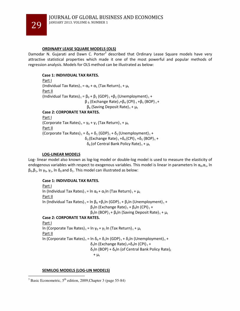
ORDINARY LEASE SQUARE MODELS (OLS)

Damodar N. Gujarati and Dawn C. Porter3 described that Ordinary Lease Square models have very attractive statistical properties which made it one of the most powerful and popular methods of regression analysis. Models for OLS method can be illustrated as below:


Part I (Individual Tax Rates) t = α0 + α1 (Tax Return) t + μt

Part II (Individual Tax Rates) t = β0 + β1 (GDP) t +β2 (Unemployment) t +

β 3 (Exchange Rate) t+β4 (CPI) t +β5 (BOP) t + β6 (Saving Deposit Rate) t + μt


Part I (Corporate Tax Rates) t = γ0 + γ1 (Tax Return) t + μt Part II (Corporate Tax Rates) t = δ0 + δ1 (GDP) t + δ2 (Unemployment) t +

δ3 (Exchange Rate) t +δ4 (CPI) t +δ5 (BOP) t + δ6 (of Central Bank Policy Rate) t + μt

LOG-LINEAR MODELS

Log- linear model also known as log-log model or double-log model is used to measure the elasticity of endogenous variables with respect to exogenous variables. This model is linear in parameters ln α0,α1, ln β0,β1, ln γ0, γ1, ln δ0 and δ1. This model can illustrated as below:


Part I ln (Individual Tax Rates) t = ln α0 + α1ln (Tax Return) t + μt

Part II ln (Individual Tax Rates) t = ln β0 +β1ln (GDP) t + β2ln (Unemployment) t +

β3ln (Exchange Rate) t + β4ln (CPI) t +

β5ln (BOP) t + β6ln (Saving Deposit Rate) t + μt Case 2: CORPORATE TAX RATES.

Part I ln (Corporate Tax Rates) t = ln γ0 + γ1 ln (Tax Return) t + μt Part II ln (Corporate Tax Rates) t = ln δ0 + δ1ln (GDP) t + δ2ln (Unemployment) t +

δ3ln (Exchange Rate) t+δ4ln (CPI) t + δ5ln (BOP) + δ6ln (of Central Bank Policy Rate)t + μt

SEMILOG MODELS (LOG-LIN MODELS)

3 Basic Econometric, 5

th edition, 2009,Chapter 3 (page 55-84)


These models are called as log-lin model because only the endogenous variable appears in the logarithmic form. Basically, parameters in log-lin models are linear. Log-lin models are shown as below:


Part I ln (Individual Tax Rates) t = α0 + α1 (Tax Return) + μt

Part II ln (Individual Tax Rates) t = β0 + β1 (GDP) +β2 (Unemployment) +

β 3 (Exchange Rate) +β4 (CPI) +β5 (BOP)+ β6 (Saving Deposit Rate) + μt

Case 2: CORPPORATE TAX RATES.

Part I ln (Corporate Tax Rates) t = γ0 + γ1 (Tax Return) + μt Part II ln (Corporate Tax Rates) t = δ0 + δ1 (GDP) + δ2 (Unemployment) +

δ3 (Exchange Rate) +δ4 (CPI) +δ5 (BOP) + δ6 (of Central Bank Policy Rate) + μt

SEMILOG MODELS (LIN-LOG MODELS)

Basically, it uses the same concept with log-lin model. The only different thing is that it logs all the exogenous variables. Lin-log models can be expressed as below:


Part I (Individual Tax Rates) t = ln α0 + α1ln (Tax Return) t + μt

Part II (Individual Tax Rates) t = ln β0 +β1ln (GDP) t + β2ln (Unemployment) t +

β3ln (Exchange Rate) t + β4ln (CPI) t +β5ln (BOP) t + β6ln (Saving Deposit Rate) t + μt


Part I (Corporate Tax Rates) t = ln γ0 + γ1 ln (Tax Return) t + μt Part II (Corporate Tax Rates) t = ln δ0 + δ1ln (GDP) t + δ2ln (Unemployment) t +

δ3ln (Exchange Rate) t+δ4ln (CPI) t + δ5ln (BOP) t + δ6ln (of Central Bank Policy Rate) t + μt

5. Finding & Discussion

5.0 Data Analysis

From the word empirical4 it means knowledge or information based on observation or experience which is not from the theory. This chapter argues about a method that researcher stated earlier in chapter

4Oxford Fajar Advance Learner’s English Dictionary, 2

nd Edition, 1999 (Pg 581)


three which analyzes and interprets the result. Basically, the researcher uses E-View 5 software in order to obtain or to get the results for this research.

5.1 INDIVIDUAL TAX RATES

5.1.1 TO OBTAIN OBJECTIVE ONE.

In this section, the researcher wants to identify the relationship between individual tax rates which Non-Resident Employees (NRE) and Non-Resident Partner (NRP) with tax revenue. Rates that are imposed by the government to Non-Resident Company (NRE) and Non-Resident Partner (NRP) show the same value. This study is to investigate the suitable tax rates the Malaysian government should impose to the Non-Resident Company (NRE) and Non-Resident Partner (NRP) in order to get higher tax returns or tax revenues. Below is the OLS model for this part: (ITR)t= 0.217651 + 0.004211 (Tax Revenue)t + μt

*Where INDIVIDUAL TAX RATES (ITR) = Non-Resident Company (NRE), Non-Resident Partner (NRP)

From the equation above, coefficient for α0 (0.217651) is the value of individual tax rates when tax revenue and the error term is equal to zero. With one unit increased in tax revenue, indirect tax rates for individual will increase with 0.004211 units. The expected relation between individual tax rates and tax revenue is positive. The value for R2 is 0.842046 indicates that there are 84.2 percent of tax revenue is able to explain individual tax rates. Meanwhile, R2 for other models also show the same result with OLS model where basically their R2 are bigger than 80 percent.

Table 3 : Correlation between ITR and TR in Equation 1.

ITR

ITR 1.000000

TR 0.917630

*Sources E-View

. Based on Table 3 above, correlation between Individual tax rates and tax revenue is quite high where almost 92 percent of tax revenue can explained as Individual Tax Rates. In order to investigate the relationship between endogenous variables and exogenous variable, t-test is conducted. Degree of freedom for t-test would be n-k where n is the number of observations used in the model and k is the number of parameter. There are 21 observations used in equation one. Reject H0 if the t-test is more than critical value or probability value is less than 0.05. As the researcher wants to find out the relationship between independent variables with dependent variables, α value would be 0.025 (0.05/2) because a two-tailed test is used.

H0: There is no relationship between Individual Tax Rates for individual and tax returns. H1: There is a relationship between Individual Tax Rates for individual and tax returns.

The number of parameter for this part would be 2 including intercept. Thus, the degree of freedom will be 21-2= 19. T-test value is 10.06419 at 5 percent of α level (two tails) and critical value is ±2.093.


Because t-test is more than critical value (10.06419>±2.093), reject H0. In addition, the probability of t-test for tax revenue in other models is lower than 0.05 which indicates that tax revenue is significant with Individual Tax Rate. It is obvious that from this t-test, there is a significant relationship between Individual Tax Rate and tax returns in Malaysia.

The f-test and multicollinerity test is quite unnecessary since there’s only one independent variable. However, multicollinerity test is still able to perform since it uses value R2. To perform this test, one can use Variance Inflation Factor (VIF) method which [1/ (1- R2)]. If the result shown is above 10, it indicates that there are serious multicollinerity and if the result shown is below 10, it indicates that there are nimulticollinerity. Below is the hypothesis for multicollinerity test:

Table 4 : Multicollinerity Test Summary in Equation 1

Model DV No

of

Obs

IV R2 VIF MULTICOLLINERITY

Linear ITR 21 TR 0.842046 6.3310 NO

Log-Linear

LIN (ITR)

21 Lin TR

0.811449 5.3036 NO

Log-Lin LIN (ITR)

21 TR 0.822900 5.6465 NO

Lin-Log ITR 21 Lin TR

0.827029 5.7813 NO

*Sources E-View

Based on Table 4, it shows that normal OLS model indicates there is no muticollinerity given that VIF value 8.4005 is below 10. This result is also supported by other three models since the VIF value is below that 10 which indicates that there is no multicollinerity in each models. Meanwhile, to identify whether there is autocorrelation or not, autocorrelation test is conducted. Autocorrelation in this test is to find out whether there is a miss-specification variable in the model. Basically there are several tests to detect autocorrelation in the models such as Serial Correlation LM test and Durbin Watson test. However, one needs to use Serial Correlation LM test instead of Durbin Watson test if there is autocorrelation in the series. If one uses Durbin Watson test, the result will indicate that there are autocorrelation in the model. In addition, models will show superior results when using significant points of dL and dU at 0.05 level of significant test while conducting autocorrelation test. To solve this problem, the researcher uses Breusch-Godfrey serial correlation LM test at points of dL and dU at 0.01 level of significant test.


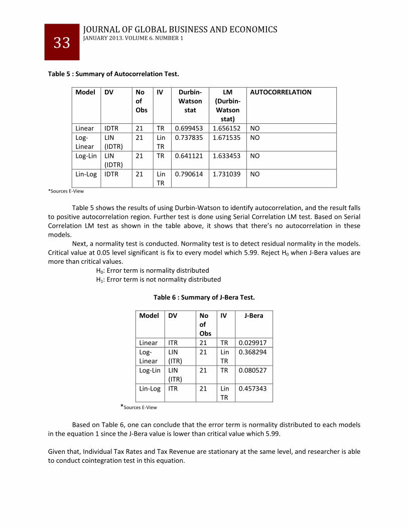
Table 5 : Summary of Autocorrelation Test.

Model DV No

of

Obs

IV Durbin-

Watson

stat

LM

(Durbin-

Watson

stat)

AUTOCORRELATION

Linear IDTR 21 TR 0.699453 1.656152 NO

Log-Linear

LIN (IDTR)

21 Lin TR

0.737835 1.671535 NO

Log-Lin LIN (IDTR)

21 TR 0.641121 1.633453 NO

Lin-Log IDTR 21 Lin TR

0.790614 1.731039 NO

*Sources E-View

Table 5 shows the results of using Durbin-Watson to identify autocorrelation, and the result falls to positive autocorrelation region. Further test is done using Serial Correlation LM test. Based on Serial Correlation LM test as shown in the table above, it shows that there’s no autocorrelation in these models. Next, a normality test is conducted. Normality test is to detect residual normality in the models. Critical value at 0.05 level significant is fix to every model which 5.99. Reject H0 when J-Bera values are more than critical values. H0: Error term is normality distributed H1: Error term is not normality distributed

Table 6 : Summary of J-Bera Test.

Model DV No

of

Obs

IV J-Bera

Linear ITR 21 TR 0.029917

Log-Linear

LIN (ITR)

21 Lin TR

0.368294

Log-Lin LIN (ITR)

21 TR 0.080527

Lin-Log ITR 21 Lin TR

0.457343

*Sources E-View Based on Table 6, one can conclude that the error term is normality distributed to each models in the equation 1 since the J-Bera value is lower than critical value which 5.99. Given that, Individual Tax Rates and Tax Revenue are stationary at the same level, and researcher is able to conduct cointegration test in this equation.


Table 7 Cointegration Rank Test

Hypothesized No. of CE (s)

Eigenvalue Trace Statitic 0.05 Critical Value

Probability

None* 0.424788 18.49571 15.49471 0.0171

At most 1* 0.343244 7.988409 3.841466 0.0047 Trace test indicates 2 cointegrationeqn(s) at the 0.05 level *denotes rejection of the hypothesis at the 0.05 level *MacKinnon-Haug-Michelis (1999) p-value *Sources E-View

. Based on Table 7,one can make a conclusion that tax revenue has a short term and long term relationship with Individual Tax Rates due to the probability is lower than 0.05.

5.1.2 TO OBTAIN OBJECTIVE TWO. In order to obtain the Optimum Tax value, the Laffer Curve concept for Individual Tax Rates vs Tax revenues in Malaysia are used to plot the graph below:

Graph 2: Laffer Curve concept for Individual Tax Rates vs Tax Revenue.

Based on Graph 2 plotted above, one can identify three Laffer Curve concept where the values are evident in year 1985, 1996-1998 and year 2000-2003. By following the current economic situation in Malaysia, the government should impose 29 percent of Individual Tax Rates to citizen. With this 29 percent, the government is able to generate higher returns of revenues where this can improve Malaysia’s economic system. On the other hand, if governments implement 40 percent of tax to citizen like in year 1985, Malaysian government is able to receive higher revenues than current revenues that Malaysia obtains.


5.1.3 TO OBTAIN OBJECTIVE THREE.

In this section, researcher intends to identify the relationship between Individual tax rates with other macroeconomic indicators to find out whether macroeconomic gives a positive or negative impact on individual tax rates. In this part, researcher should use stationary data. However, the stationary data is not used in this research. It is really wasted to delete this equation since it takes the same amount of time to generate result. For this part, the researcher applies original data to regress the equation below to obtain several results. Below is the OLS model for this part taken by the original data: (ITR)t= 0.175396 + 0.001316(GDP)t + 0.022121(UN) - 0.004222(ER)

+ 0.004214 (CPI) - 8.71E-06 (BOP) + 0.015549 (SDR) +μt

From the equation above, coefficient for δ0 (0.198248) is the value of individual tax rates when GDP, UN, ER, CPI, BOP, SDR and the error term is equal to zero. With one unit increased in GDP, individual tax rates will increase with 0.001316 units. When unemployment rate is increased by one unit, individual tax rates will also increase by 0.022121 units. Meanwhile, as the exchange rate is increased by one unit, individual tax rates will decrease by 0.004222 units. Besides that, when CPI is increased by one unit, individual tax rates increase by 0.004214 units. On other hand, when BOP and SDR is increased by one unit, individual tax rates will decrease by 8.71E-06 units and increased by 0.015549 unit. The expected relation between individual tax rates with GDP, UN, CPI and SDR is positive while ER and BOP is negative. Based on Table C, value in normal OLS for R2 is 0.877548 indicates that there is 87.8 percent of dependent variables able to explain individual tax. In the meantime, R2 for other models also show the same result like OLS model where basically their R2 is bigger than 80 percent which indicates that independent indicator can explain dependent variables.

Table 8 : Correlation between ITR and Other Macroeconomic Variables

ITR

ITR 1.000000

GDP 0.399273

UN 0.330430

ER -0.630566

CPI 0.531643

BOP -0.740174

SDR 0.718360 *Sources E-View

Table 8 indicates the correlation magnitude which is consistent with OLS model in this equation. Correlation between Individual Tax Rates with GDP and UN is quite low while ER, CPI, BOP and SDR are quite high. There are 39.9 percent of GDP, 33 percent of UN, 63.1 percent of ER, 53.2 percent of CPI, 74 percent of BOP and 71.8 percent of SDR can explain Individual Tax Rates.


Since the researcher wants to investigate the relationship between endogenous variables and exogenous variable, researcher needs to conduct a t-test. The degree of freedom for t-test would be n-k where n is the number of observations used in the model and k is the number of parameter. There are 21 observation used in equation one. Reject H0 if the t-test is more than critical value or probability value is less than 0.05. Since the researcher wants to find out the relationship between independent variables with dependent variables, α value would be 0.025 (0.05/2) because it uses a two-tailed test.

H0: There is no relationship between Individual Tax Rates and other macroeconomic indicators. H1: There is a relationship between Individual Tax Rates and other macroeconomic indicators.

Number of parameter for this part would be six together with intercept. So, degree of freedom will be 21-6= 15. Based on Table C, t-test value for GDP is 1.563446, UN is 4.618694, ER is -0.504690, CPI is 1.858448, BOP is 1.858448 and last variables which is SDR which t-test value is 3.182714. Critical Value is ±2.131 at 5 percent of significant α level (two tails). If the value for t-test is bigger than critical value, researcher needs to reject H0. Since the t-test for UN and SDR is more than critical value (4.618694, 3.182714 > ±2.093), reject H0. From this t-test, it indicates that variables such as unemployment rates and Saving Deposit Rate have relationships with individual tax rates in Malaysia. The researcher then proceeds to do f-test. Critical value for f-test is 2.60 where k value is 6 without including intercept. Below is the hypothesis for f-test: H0: All independent variables would not affect Individual Tax Rates. H1: Some of dependent variables are able to explain Individual Tax Rates.

Table 9: F-statistic summary between ITR and Other Macroeconomic Variables

Model DV No of

Obs

IV F-statistic Prob(F-

statistic)

Linear ITR 21 GDP, UN, ER, CPI, BOP, SDR

16.72175 0.000000

Log-Linear

LIN (ITR)

21 Lin (GDP, UN, ER, CPI, BOP, SDR)

75.14288 0.000459

Log-Lin LIN (ITR)

21 GDP, UN, ER, CPI, BOP, SDR

17.22450 0.000010

Lin-Log ITR 21 Lin (GDP, UN, ER, CPI, BOP, SDR)

61.42631 0.000682

*Sources E-View

Since, f-statistic for normal model is higher than critical value, reject H0. Other models for f-statistic show the same result as linear model where their f-statistic value is more than critical value. In conclusion, researcher found out there are some of macroeconomic variables that are able to explain Individual Tax Rates. Multicollinerity test is very important in this equation since it involves several macroeconomic variables. Based on the table below, there is no multicollinerity in all models especially in linear model since the VIF value is lower than 10.


Table 10 : MulticollinerityTest for Macroecnomic Variables

Model DV R2 VIF MULTICOLLINERITY

Linear/ Log-Lin

GDP 0.498597 1.9944 NO

UN 0.193668 1.2402 NO

ER 0.672082 0.3279 NO

CPI 0.400403 1.6678 NO

BOP 0.860066 7.1462 NO

SDR 0.786273 4.6788 NO

Log-Linear/ Lin-Log

GDP 0.380483 1.6142 NO

U 0.592280 2.4527 NO

ER 0.708831 3.4344 NO

CPI 0.733529 3.7528 NO

BOP 0.708533 3.4309 NO

SDR 0.746477 3.9444 NO *Sources E-View

Table 11 : Summary of Autocorrelation test for Macroeconomic Variables

Model DV IV Durbin-

Watson

stat

LM

(Durbin-

Watson

stat)

AUTOCORRELATION

Linear ITR GDP, UN, ER, CPI, BOP, SDR

1.631163 1.767125 INDECISION

Log-Linear

LIN (ITR)

Lin (GDP, UN, ER, CPI, BOP, SDR)

2.168514 1.956342 NO

Log-Lin LIN (ITR)

GDP, UN, ER, CPI, BOP, SDR

1.655683 1.747286 INDECISION

Lin-Log ITR Lin (GDP, UN, ER, CPI, BOP, SDR)

1.983075 2.029178 NO

*Sources E-View

Based on Table 11, the researcher used Durbin-Watson statistic to identify autocorrelation, result falls to indecision region. So researcher needs to carry on to Serial Correlation LM test. Based on


Serial Correlation LM test as shown in the table above, it shows that there are no autocorrelation in these log-linear and lin-log models while indecision for linear and log-linear equations. Next, the researcher proceeds to normality test. Normality test is to detect residual normality in the models. Critical value at 0.05 levels significant is fixed to every model which 5.99. Reject H0 when J-Bera values are more than critical value. H0: Error term is normality distributed H1: Error term is not normality distributed

Table 12 : Summary of J-Bera Test

Model DV IV J-Bera

Linear ITR GDP, UN, ER, CPI, BOP, SDR

0.067771

Log-Linear

LIN (ITR)

Lin (GDP, UN, ER, CPI, BOP, SDR)

1.494380

Log-Lin LIN (ITR)

GDP, UN, ER, CPI, BOP, SDR

0.003828

Lin-Log ITR Lin (GDP, UN, ER, CPI, BOP, SDR)

1.437661

*Sources E-View

The researcher can conclude that the error term is normality distributed to each models in the equations given since the J-Bera value is lower than critical value which 5.99. 5.2 COMPANY TAX RATES

5.2.1 TO OBTAIN OBJECTIVE ONE. In this section, researcher wants to identify the relationship between company tax rates which Resident Company (RC), Non-Resident Company (NRC), Private Company (PC) and Public Company ( PLC) with tax revenue. Rates that are required by the government to Resident Company (RC), Non-Resident Company (NRC), Private Company (PC) and Public Company (PLC) show the same value. Researcher wants to find out what is the suitable tax rates should the Malaysian government impose to the Resident Company (RC), Non-Resident Company (NRC), Private Company (PC) and Public Company ( PLC) in order to get higher tax returns or tax revenues. Below is the OLS model for this part: (CTR)t= 0.204055 + 0.004692 (Tax Revenue)t + μt

*Where COMPANY TAX RATES (CTR) = Resident Company (RC), Non-Resident Company (NRC), Private

Company (PC) and Public Company (PLC). From the equation above, coefficient for β0 (0.204055) is the value of company tax rates when tax revenue and the error term equals to zero. With one unit increased in tax revenue, Foreign Fund Management tax rates for company will increase with 0.004692 units. The expected relation between company tax rates and tax revenue is positive. The value for R2 is 0.874000 indicates that there are 87.4 percent of tax revenue which is able to explain company tax rates. Meanwhile, R2 for other models also show the same result like OLS model where basically their R2 is bigger than 85 percent.


Table 13 : Correlation between CTR and TR

CTR

CTR 1.000000

TR 0.934880 *Sources E-View

Based on Table 13, correlation between Company Tax Rates and tax revenue is quite high where almost 93.5 percent of tax revenues can explain the Company Tax Rates. Since the researcher wants to investigate the relationship between endogenous variables and exogenous variable, researcher needs to conduct t-test. The degree of freedom for t-test would be n-k where n is the number of observations used in the model and k is the number of parameter. There are 21 observations used in equation one. Reject H0 if the t-test is more than critical value or probability value less than 0.05. As the researcher wants to find out the relationship between independent variables with dependent variables, α value would be 0.025 (0.05/2) because it uses a two-tailed test.

H0: There is no relationship between Company Tax Rates and tax returns. H1: There is a relationship between Company Tax Rates and tax returns.

The number of parameter for this part would be 2 including intercept. Therefore, the degree of freedom will be 21-2= 19. T-test value is 11.48015 at 5 percent of α level (two tails) and critical value is ±2.093. Because t-test is more than critical value (11.48015>±2.093), reject H0. In addition, based on Table G, probability of t-test for tax revenue in other models is lower than 0.05 which indicates that tax revenue is significant with Company Tax Rate. As conclusion from this t-test, there’s a relationship between Company Tax Rate and tax returns in Malaysia. To do f-test and multicollinerity is quite unnecessary since there only one independent variable. However, multicollinerity test is still able to perform since it uses value R2. To perform this test, the researcher can use Variance Inflation Factor (VIF) method which [1/ (1- R2)]. If the result shown is above 10, it indicates that there are serious multicollinerity and if the result shown is below 10, it indicates that there are nimulticollinerity. Below is the hypothesis for multicollinerity test as shown in Table 14:

Table 14 : Multicollinerity Test Summary

Model DV No

of

Obs

IV R2 VIF MULTICOLLINERITY

Linear CTR 21 TR 0.874000 7.9365 NO

Log-Linear

LIN (CTR)

21 Lin TR

0.852094 6.7611 NO

Log-Lin LIN (CTR)

21 TR 0.852095 6.7611 NO

Lin-Log CTR 21 Lin TR

0.869926 7.6879 NO

*Sources E-View


Based on the table above, it shows that normal OLS model indicates that there is no muticollinerity given that VIF value 7.9365 which is below 10. This result is also supported by three other models since the VIF value is below that 10 which indicates that there is no multicollinerity in each models. Meanwhile, to identify whether there is autocorrelation or not, the researcher needs to do an autocorrelation test. Autocorrelation in this test is to find out whether there is a miss-specification variable in the model. Basically there are several tests which can detect autocorrelation in the models such as Serial Correlation LM test and Durbin Watson test. However, the researcher needs to use Serial Correlation LM test instead of Durbin Watson test if there is autocorrelation in the series. If researcher uses Durbin Watson test, the result will indicate that there’s autocorrelation in the model. In addition, models which show superior results when the researcher uses significant points of dL and dU at 0.05 level of significant test when conduct autocorrelation test. To solve this problem, the researcher uses Breusch-Godfrey serial correlation LM test at points of dL and dU at 0.01 level of significant test.

Table 15 : Summary of Autocorrelation Test.

Model DV No

of

Obs

IV Durbin-

Watson

stat

LM

(Durbin-

Watson

stat)

AUTOCORRELATION

Linear FF 21 TR 0.758242 1.524288 NO

Log-Linear

LIN (FF) 21 Lin TR

0.831868 1.586747 NO

Log-Lin LIN (FF) 21 TR 0.673478 1.539162 NO

Lin-Log FF 21 Lin TR

0.921053 1.619427 NO

*Sources E-View

Durbin-watson statistic is done to identify autocorrelation as shown in Table 15,the result falls to positive autocorrelation region. Hence, the researcher needs to carry on to Serial Correlation LM test. Based on Serial Correlation LM test as shown in table, it shows that there’s no autocorrelation in equation 5 for all models. Next, we proceed to normality test. Normality test is to detect residual normality in the models. Critical value at 0.05 level significant is fixed to every model which 5.99. Reject H0 when J-Bera values are more than critical value. H0: Error term is normality distributed H1: Error term is not normality distributed Table 16 : Summary of J-Bera Test.

Model DV No of

Obs

IV J-Bera

Linear CTR 21 TR 3.346583

Log-Linear LIN (CTR) 21 Lin 4.244915


TR

Log-Lin LIN (CTR) 21 TR 6.071893

Lin-Log CTR 21 Lin TR

1.696053

*Sources E-View

Based on Table 16, one can conclude that the error term is normality distributed to linear, log-linear and log-lin models in the Equation 5 since the J-Bera value is lower than critical value which 5.99. Meanwhile, error term is not normality distributed for log-lin model as J-Bera value is bigger than 5.99. Given that, Company Tax Rates and Tax Revenue are stationary at the same level, the researcher is able to conduct cointegration test in this equation.

Table 17 Cointegration Rank Test

Hypothesized No. of CE (s)

Eigenvalue Trace Statitic 0.05 Critical Value

Probability

None* 0.428590 16.88688 15.49471 0.0307

At most 1* 0.280455 6.253577 3.841466 0.0124 Trace test indicates 2 cointegrationeqn(s) at the 0.05 level *denotes rejection of the hypothesis at the 0.05 level *MacKinnon-Haug-Michelis (1999) p-value *Sources E-View

. From the above table, the researcher can conclude that tax revenue has a short-term and long-term relationship with Company Tax Rates due to the probability which is lower than 0.05.

5.2.2 TO OBTAIN OBJECTIVE TWO.

Besides that, the researcher needs to find out what is the optimum point that the government should impose to citizen in order to meet objective two. Below is Laffer Curve concept for Company Tax Rates vs Tax revenue in Malaysia.


Graph 3 : Laffer Curve concept for Company Tax Rates vs Tax Revenue.

Based on Graph 3, three optimum points were identified using Laffer Curve concept in year 1985, 1996-1998 and year 2000-2003. By following the current economic situation in Malaysia, government should impose 28 percent of Company Tax Rates to citizen. With this 29 percent, government is able to generate higher returns of revenue where this can improve Malaysia’s economic system. On the other hand, if governments implement 35 percent of tax to citizen like in year 1985, Malaysian government is able to receive higher revenues than current revenue that Malaysia obtains.

5.2.3 TO OBTAIN OBJECTIVE THREE.

In this section, the researcher intends to identify the relationship between Company tax rates with other macroeconomic indicators to find out whether macroeconomic gives a positive or negative impact on company tax rates. In this part, the researcher applies original data to regress the equation below to obtain several results. Below is the OLS model for this part taken from the original data: (CTR)t= 0.164421 + 0.001418 (GDP)t + 0.021083 (UN) + 0.002663 (ER)

+ 0.004718 (CPI) - 0.001333 (BOP) + 0.008975 (EOP) +μt

From equation above, coefficient for γ0 (0.198248) is the value of company tax rates when GDP, UN, ER, CPI, BOP, EOP and the error term is equal to zero. With one unit increased in GDP, company tax rates will increase with 0.001418 units. When unemployment rate is increased by one unit, company tax


rates also will increase by 0.021083 units. Meanwhile, as the exchange rate is increased by one unit, company tax rates will decrease by 0.002663 units. Besides that, when CPI is increased by one unit, company tax rates will increase by 0.004718 units. On other hand, when BOP and EOP is increased by one unit, company tax rates will decrease by 0.001333 units and increase by 00.008975 unit. The expected relation between company tax rates with GDP, UN, CPI, ER and EOP is positive while only BOP indicator shows a negative relationship. The value in normal OLS for R2 is 0.837428 indicates that there is 83.7 percent of dependent variables which is able to explain company tax. In the meantime, R2 for other models also show the same result like OLS model where basically their R2 is bigger than 83 percent which indicates that tax revenue indicator can explain Company Tax Rates.

Table 18 Correlation between CTR and Other Macroeconomic Variables

CTR

CTR 1.000000

GDP 0.511351

UN 0.309954

ER -0.670466

CPI 0.483430

BOP -0.789439

EOP 0.636831 *Sources E-View

Based on Table 18, the correlation between Company Tax Rates with UN and CPI is quite low while ER, CPI, BOP and EOP are quite high. In addition, only two variables show negative direction which ER and BOP variables as others show positive direction. There are 51.1 percent of GDP, 30.9 percent of UN, 67 percent of ER, 48.3 percent of CPI, 78.9 percent of BOP and 63.7 percent of EOP can explain Company Tax Rates. There are 21 observations used in equation six. Reject H0 if the t-test is more than critical value or probability value less than 0.05 and α value would be 0.025 (0.05/2) because it uses a two-tailed test.

H0: There is no relationship between Company Tax Rates and other macroeconomic indicators. H1: There is a relationship between Company Tax Rates and other macroeconomic indicators.

The number of parameters for this part would be six together with intercept. Thus, the degree of freedom will be 21-6= 15. The t-test value for GDP is 1.405200, UN is 3.381013, ER is 0.264283, CPI is 1.487118, BOP is -1.869576 and last variables which is EOP which t-test value is 1.268557. Critical Value is ±2.131 at 5 percent of significant α level (two tails). If the value for t-test is bigger than critical value, the researcher needs to reject H0. Since the t-test for UN is more than critical value (3.381013> ±2.093), reject H0. In conclusion from this t-test, it indicates that variables such as unemployment rate are considered when Malaysian government decides company’s tax rates. Next, we proceed to do f-test. Critical value for f-test when using 20 observations is 2.60, where k value is 6 without including intercept and critical value is 3.22 for 10 observations. Below is the hypothesis for f-test: H0: All independent variables do not affect Company Tax Rates.


H1: Some of dependent variables are able to explain Company Tax Rates.

Table 19 F-statistic summary between CTR and Other Macroeconomic Variables

Model DV No of

Obs

IV F-statistic Prob(F-

statistic)

Critical

Value

Linear CTR 21 GDP, UN, ER, CPI, BOP, EOP

12.01927 0.000080 2.60

Log-Linear

LIN (CTR)

11 Lin (GDP, UN, ER, CPI, BOP, EOP)

3.661752 0.114793 3.22

Log-Lin LIN (CTR)

21 GDP, UN, ER, CPI, BOP, EOP

11.74380 0.000090 2.60

Lin-Log CTR 11 Lin (GDP, UN, ER, CPI, BOP, EOP)

3.561257 0.119672 3.22

*Sources E-View

Since, f-statistic for normal model is higher than critical value, reject H0. Other models for f-statistic show the same result as linear model where their f-statistic value is more than critical value. In conclusion, the researcher found out that there are some of macroeconomic variables which are able to explain Company Tax Rates. Multicollinerity test is very important in this equation since it involves several macroeconomic variables. Based on the table below, there is no multicollinerity in all models in equation 7 especially in linear model when using the original data since the VIF value is lower than 10.

Table 20 Multicollinerity Test for Macroeoconomic Variables

Model DV R2 VIF MULTICOLLINERITY

Linear/ Log-Lin

GDP 0.445849 1.8046 NO

UN 0.244407 1.3235 NO

ER 0.641125 2.7865 NO

CPI 0.513438 2.0552 NO

BOP 0.789744 4.7561 NO

EOP 0.759332 4.1551 NO

Log-Linear/ Lin-Log

GDP 0.412916 1.7033 NO

U 0.637567 2.7591 NO

ER 0.420224 1.7248 NO

CPI 0.724746 3.6330 NO

BOP 0.706920 3.4120 NO

EOP 0.483811 1.9373 NO *Sources E-View


Table 21 Autocorrelation Test for Macroeconomic Variables

Model DV IV Durbin-

Watson stat

LM

(Durbin-

Watson

stat)

AUTOCORRELATION

Linear CTR GDP, UN, ER, CPI, BOP, EOP

1.706233 1.694893 INDECISION

Log-Linear

LIN (CTR)

Lin (GDP, UN, ER, CPI, BOP, EOP)

1.930886 2.264331 NO

Log-Lin LIN (CTR)

GDP, UN, ER, CPI, BOP, EOP

1.709125 1.747286 INDECISION

Lin-Log CTR Lin (GDP, UN, ER, CPI, BOP, EOP)

1.983075 2.029178 NO

*Sources E-View

Based on above table, autocorrelation test falls into indecision region when using Durbin-Watson and Serial Correlation LM test for linear and log-lin models when using the originals. Based on Serial Correlation LM test as shown in the above table, it shows that there’s no autocorrelation to find result for log-linear and lin-log models since value for Serial Correlation LM falls into no autocorrelation region. The next stage, the researcher proceeds to normality test. Normality test is to detect residual normality in the models. Critical value at 0.05 level significant is fixed to every model which 5.99. Reject H0 when J-Bera values are more than critical value. H0: Error term is normality distributed H1: Error term is not normality distributed Table 22 Summary of J-BeraTest .

Model DV IV J-Bera

Linear CTR GDP, UN, ER, CPI, BOP, EOP

1.019488

Log-Linear

LIN (CTR)

Lin (GDP, UN, ER, CPI, BOP, EOP)

0.337068

Log-Lin LIN (CTR)

GDP, UN, ER, CPI, BOP, EOP

2.121392

Lin-Log CTR Lin (GDP, UN, ER, CPI, BOP, EOP)

0.327432

*Sources E-View

Based on Table 22, one can conclude that the error term is normality distributed to each models in the Equation 6 since the J-Bera value’s lower than critical value which 5.99.


6. Conclusion In this part, the researcher will conclude all the findings obtained in chapter 5. Based on

objective one and two, the researcher found out that Malaysian government was able to obtain higher revenue when they imposed 29 percent of ITR and IDTR. In addition, Malaysian government’s able to gain more revenue when they imposed 28 percent for CTR while remains constant for FF which is 10 percent. Besides that, there is positive relationship between tax rates and tax revenue for both cases. Furthermore, when using the original data, the researcher found out that Malaysian government considers indicators such as UN and SDR to decide rate for ITR and IDTR. However, when researcher apply stationary data, there’s only one indicator significant to ITR and IDTR which CPI. Indicators such as BOP and ER give negative impacts when using the original data. 6.1 Limitation

There are many limitations or problems when the researcher conducted this study. The limitations are as shown below:

• Unable to get literature review on LafferCurve concept in Malaysia. Researcher unable to find out others study on LafferCurve concept in Malaysia. Most of the literature review that researcher search out is come from foreign country.

• Difficulty to collect data.

Researcher need to go to LembagaHasilDalamNegeri in Jalan Duta to get data for tax rates for individual and company. Researchers also need to change several times for variables since it not in the same value such as in percentage, real value or nominal value.

• Missing data collection.

There are missing value in data that researcher collect. To solve this problem, researcher conducts some calculations to find out missing value.

• Transform Data.

There are some modal that cannot be regress due to negative sign in linear modal, log-lin model and lin-log modal. Researcher removing negative value to zero value since E-view software unable to obtain result.

• Unable to conduct some test.

There are several test that researcher cannot do to several equation. Researcher able to perform cointegration test for a few equations. This happen maybe due to factor of smaller number of observation.

6.2 Recommendation.

Many people often view that paying a tax is a burden. However, tax is important since it is one of government’s resources to obtain the revenues. With money collected from the tax, government is able to boost up the economy, develop or improve infrastructure and public transport and other things for the citizens. From this research, the researcher found out that individuals or citizens need to pay 29 percent of their accumulated income per year to the government in this current economic. Also there are several taxes that individuals need to pay such as service tax which is 5 percent and many more to the government. It will be better if the government accumulates all the tax rates to lump sum rates which will be easier for citizens to pay their taxes and indirectly it will save cost and time. By looking at the


Australian tax, Australian government includes 1.5 percent for medical levy to their citizen where their total individual tax is zero until 45 percent.

Malaysian government can also implement tax like the Australian government. Maybe Malaysian government could include medical levy (1percent) and education levy (1.5 percent) in this lump sum tax. With this action, parents do not need to worry about their children’s school fees or university fees since they have already paid tax to the government. Based on Malaysian tax rates data for individuals, Malaysian government imposed 40 percent of tax rates to individuals in year 1985 and was able to gain higher revenue. This amount of tax rates can be applied to current years where this 40 percent tax must include medical levy, service tax, education levy and other taxes. In Malaysia, a person or an individual that has accumulated salary in one year below RM 2500 does not need to pay tax. This people are recognized as people with lower income. Nowadays, individuals that have been recognized as middle income and higher income are sharing the same burden where there are paying the same rates for their taxes. It is not fair since people with higher income earn more than the middle income. Therefore, people with higher income should pay more than the middle income. REFFERENCE

BOOKS

A S Hornby, (2nd Edition, 1999) “Oxford Fajar Advance Learner’s English Dictionary”. Page 1961 A S Hornby, (2nd Edition, 1999) “Oxford Fajar Advance Learner’s English Dictionary”. Page 1464 A S Hornby, (2nd Edition, 1999) “Oxford Fajar Advance Learner’s English Dictionary”. Page 1492 Joseph P. Daniels, David D. VanHoose, (3rdEdition , 2004) “ International Monetary and Financial Economics”. Page 12 Joseph P. Daniels, David D. VanHoose, (3rdEdition , 2004) “ International Monetary and Financial Economics”. Page 71 Joseph P. Daniels, David D. VanHoose, (3rdEdition , 2004) “ International Monetary and Financial Economics”. Page 12 Damodar N. Gujarati, Dawn C. Porter, (5th edition, 2009)“Basic Econometric”. Page 55-84

Damodar N. Gujarati, Dawn C. Porter, (5th edition, 2009)“Basic Econometric”. Chapter 10 Page 320-332 Damodar N. Gujarati, Dawn C. Porter, (5th edition, 2009)“Basic Econometric”. Chapter 12 Page 412-452

Damodar N. Gujarati, Dawn C. Porter, (5th edition, 2009)“Basic Econometric”. Chapter 21 Page 737-768

WEB ARTICLES

Milagros Palacios, KumiHarischandra (2008), “The Impact of Taxes on Economic Behavior”. 17-19. Retrieved from website: http://pirate.shu.edu/~rotthoku/Prague/ImpactofTaxesonEconomicbehavior.pdf


Arthur B. Laffer (June 1, 2004), “The LafferCurve: Past, Present and Future”. Retrieved from website: http://gates-home.com/files/Laffer%20Curve%20-%20Past%20Presetn%20and%20Future.pdf Loganathan, Nanthakumar, Taha, Roshaiza (August, 2007), “Have Taxes Led Government Expenditure In Malaysia”. Retrieved from website: http://www.jimsjournal.org/11%20Loganathan.pdf Young Lee,Roger H. Gordon (July 15, 2004), “Tax Structure and Economic Growth”.Retrieved from website: http://www.aiecon.org/advanced/suggestedreadings/PDF/sug334.pdf Bev Dahlby,ErgeteFerede (July, 2008), “Tax Cuts, Economic Growth and the Marginal Cost of Public Funds for Canadian Provincial Governments”.Retrieved from website: http://www.uofaweb.ualberta.ca/economics2/pdf/WP-Dahlby-Ferede-Tax-Cuts-Economic-Growth-July08.pdf WEBSITE

Inland Revenue Board of Malaysia.Retrieved from website: http://www.hasil.gov.my/index.php Taxation in United States (US). Retrieved from website:http://en.wikipedia.org/wiki/Taxation_in_the_United_States Taxation in United Kingdom (UK). Retrieved from website:http://en.wikipedia.org/wiki/Taxation_in_the_United_Kingdom Taxation in China. Retrieved from website:http://en.wikipedia.org/wiki/Taxation_in_the_People's_Republic_of_China Taxation in India. Retrieved from website:http://business.mapsofindia.com/india-tax/system.html Chartered Tax Institute of Malaysia.Retrieved from website: http://www.ctim.org.my/institute.asp Royal Malaysian Customs.Retrieved from website: http://www.customs.gov.my/

Copyright of Journal of Global Business & Economics is the property of Global ResearchAgency and its content may not be copied or emailed to multiple sites or posted to a listservwithout the copyright holder's express written permission. However, users may print,download, or email articles for individual use.

THE EFFECTS OF TAX RATES ON ITS REVENUE AND GROWTH: A CASE STUDY OF MALAYSIA

Documents

Transcript of THE EFFECTS OF TAX RATES ON ITS REVENUE AND GROWTH: A CASE STUDY OF MALAYSIA