The Effects of Exchange Rate Risk on Economic Performance : The Turkish Experience

THE EFFECTS OF EXCHANGE RATE RISK ON

ECONOMIC PERFORMANCE:

THE TURKISH EXPERIENCE

Hakan Berument* Bilkent University

and

N. Nergiz Dincer** Atilim University

and State Planning Organization

* The corresponding author: Department of Economics, Bilkent University, 06800 Ankara, Turkey; Phone:+90 312 266 2529; Fax: +90 312 266 5140; Email: [email protected]. ** The views presented here are those of the authors; they do not necessarily reflect the official position of the State Planning Organization or its staff.

1

THE EFFECTS OF REAL EXCHANGE RATE RISK ON

ECONOMIC PERFORMANCE:

THE TURKISH EXPERIENCE

Abstract

This study examines the effects of real exchange rate risk on the economic performance for an

emerging, small open economy: Turkey. When the ratios of the total foreign exchange

liabilities of the Central Bank of the Republic of Turkey (CBRT) to (1) total reserves, (2) the

CBRT’s reserves and (3) the CBRT’s total Turkish lira liabilities are taken proxy of exchange

rate risk, the empirical evidence suggests that the increase in exchange rate risk causes a

depreciation in the real exchange rate, an increase in prices and a decrease in output.

JEL Codes: E10, F31 and F41.

Keywords: Exchange Rate Risk, Turkey and VAR.

2

1. Introduction

The objective of policymakers is to lead their economies to a stable growth path. In

order to avoid fluctuations in the overall economy, it is important to align various policy

variables to stabilize the economy. In this paper, we examine the effects of the exchange rate

risk on macroeconomic variables using VAR models. The results of our models suggest that

the exchange rate risk decreases output, increases inflation and causes a depreciation for

Turkey during the 1987:02- 2002:09 period.

This study is focused on Turkey, which is a developing-small-open economy and is

not under heavy government regulations. Therefore, it is possible to observe the effects of the

financial markets on the real sector. Turkey has also suffered from high and persistent

inflation without running hyperinflation, along with volatile growth pattern for almost three

decades. This provides a unique environment for observing the interrelationships among

certain macroeconomic variables. This high inflation plays a magnifying role and allows us to

avoid the type 2 error – not rejecting the null hypothesis even if the null is false.

The Central Bank of the Republic of Turkey (CBRT) considers the real exchange

variability a threat to the stability of financial markets due to high dolarization and the

vulnerability of the Turkish economy to current account crises (see, Berument, 2003).

However, even if the CBRT fully intends to stabilize the real exchange rate, the CBRT does

not have complete control over the foreign exchange market. The CBRT can only stabilize

the market with the tools that it has. Stabilizing the foreign exchange market is costly; thus,

the CBRT may stabilize the market with the strength of its balance sheet. The stronger its

balance sheet is, the stronger the policy implementation will be. Even if the CBRT does not

take any action to stabilize the real exchange rate when it has a strong balance sheet,

speculation or volatility will be lower since the speculators know that the CBRT has explicitly

announced its concerns regarding the real exchange rate. Thus, we used the CBRT’s Total

Foreign Exchange (FX) liabilities as the indicator of the exchange rate risk. The higher the

CBRT’s FX liabilities, the less power the CBRT will have to stabilize the exchange rate and

the higher the exchange rate risk will be. Even if the speculators are not active, the public

will observe the CBRT’s balance sheet and realize that if there is a shock to FX markets

CBRT will be less willing to intervene in FX markets and currency will be more volatile.

To assess the effect of exchange rate risk on the economic performance, most of the

literature concentrates on the commitment of fixed exchange rate regime as a proxy for

3

exchange rate risk (see, for example, Agénor and Montiel, 1999; Chapter 7). However, under

the influence of the CBRT, the value of the Turkish lira against major currencies is aligned

daily, thus the real exchange rate is aligned continuously. In this study, we analyze the effects

of exchange rate risk on exchange rate, output and prices. A simple theoretical model that

incorporates the effect of exchange rate risk on economic performance is also provided in

Appendix A. To the best of our knowledge, there is no study that looks at the effect of

exchange rate risk on output, prices and exchange rate simultaneously. In the literature,

exchange rate volatility mostly assesses the effect of volatility on trade (See Cote, 1994 for a

discussion of this literature). However, studies looking at other macroeconomic effects of

exchange rate volatility are limited. Some of these studies explain the effects of exchange rate

volatility on bank stock returns (Tai, 2000), on interest rates (Berument and Gunay, 2003),

and on investment and output (Bleaney and Greenaway, 2000). Felmingham and Mansfield

(1997), on the other hand, examine the relationship between depreciation and exchange rate

volatility. Their results suggest that depreciation creates uncertainty and the premium varies

continuously until the market settles.

The contribution of this paper is two-fold. First of all, this is the only study that

addresses the effect of exchange rate risk within a dynamic framework for output, prices and

real exchange rate. Secondly, this paper assesses the effects of this relationship for a

developing country. The remainder of the paper is organized as follows: The next section

explains the developments in the Turkish exchange rate. Section 3 discusses exchange rate

risk measures. Section 4 introduces the data used in the analyses. Section 5 discusses the

analyses and the estimates and Section 6 concludes.

2. Developments in the Turkish Exchange Rate

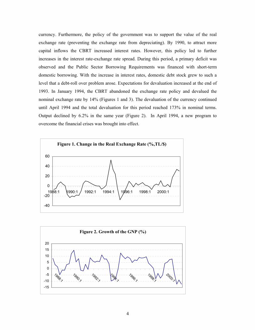
In the 1980’s, the government followed an exchange rate policy that aimed at

preventing the real exchange rate from appreciating (Figure 1), thereby supporting the export-

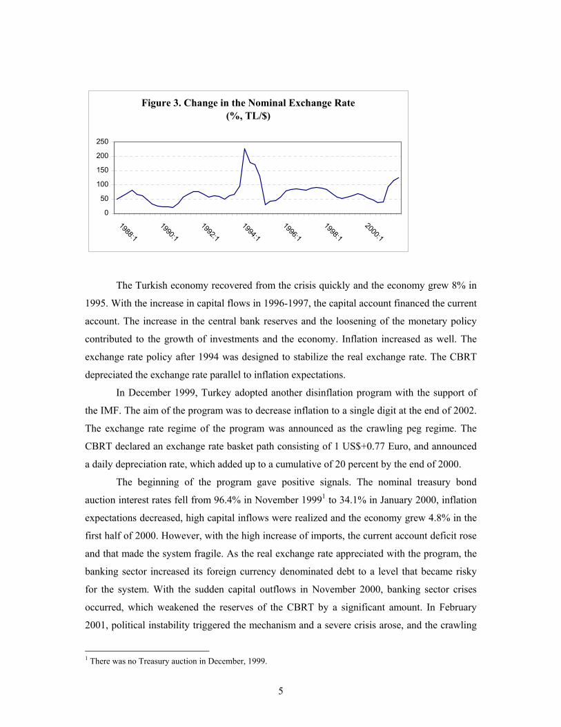
led growth strategy. As a result, the 1980’s were the years of integration with the world

economy for Turkey. Exports grew impressively and high growth rates were observed (Figure

2).

The Central Bank of the Republic of Turkey (CBRT), announced daily quotations

following the managed floating regime, and domestic currency was depreciated continuously

parallel to inflation expectations considering the real exchange rate. In 1989, the capital

account liberalized and in 1990 Turkey adopted a convertibility policy for the Turkish lira.

High capital inflows that were realized in the 1988-1990 period caused the appreciation of the

4

currency. Furthermore, the policy of the government was to support the value of the real

exchange rate (preventing the exchange rate from depreciating). By 1990, to attract more

capital inflows the CBRT increased interest rates. However, this policy led to further

increases in the interest rate-exchange rate spread. During this period, a primary deficit was

observed and the Public Sector Borrowing Requirements was financed with short-term

domestic borrowing. With the increase in interest rates, domestic debt stock grew to such a

level that a debt-roll over problem arose. Expectations for devaluation increased at the end of

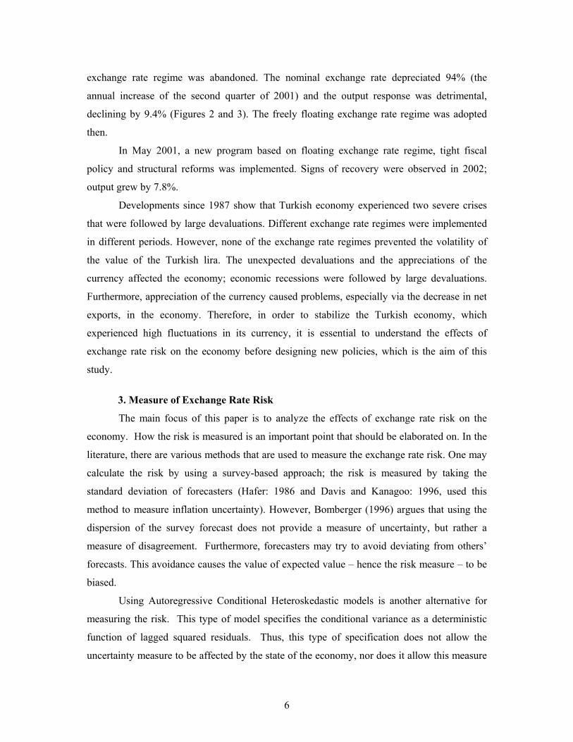
1993. In January 1994, the CBRT abandoned the exchange rate policy and devalued the

nominal exchange rate by 14% (Figures 1 and 3). The devaluation of the currency continued

until April 1994 and the total devaluation for this period reached 173% in nominal terms.

Output declined by 6.2% in the same year (Figure 2). In April 1994, a new program to

overcome the financial crises was brought into effect.

Figure 1. Change in the Real Exchange Rate (%,TL/$)

-40

-20

0

20

40

60

1988:1 1990:1 1992:1 1994:1 1996:1 1998:1 2000:1

Figure 2. Growth of the GNP (%)

-15

-10

-5

0

5

10

15

20

1988:1

1990:1

1992:1

1994:1

1996:1

1998:1

2000:1

5

Figure 3. Change in the Nominal Exchange Rate(%, TL/$)

0

50

100

150

200

250

1988:1

1990:1

1992:1

1994:1

1996:1

1998:1

2000:1

The Turkish economy recovered from the crisis quickly and the economy grew 8% in

1995. With the increase in capital flows in 1996-1997, the capital account financed the current

account. The increase in the central bank reserves and the loosening of the monetary policy

contributed to the growth of investments and the economy. Inflation increased as well. The

exchange rate policy after 1994 was designed to stabilize the real exchange rate. The CBRT

depreciated the exchange rate parallel to inflation expectations.

In December 1999, Turkey adopted another disinflation program with the support of

the IMF. The aim of the program was to decrease inflation to a single digit at the end of 2002.

The exchange rate regime of the program was announced as the crawling peg regime. The

CBRT declared an exchange rate basket path consisting of 1 US$+0.77 Euro, and announced

a daily depreciation rate, which added up to a cumulative of 20 percent by the end of 2000.

The beginning of the program gave positive signals. The nominal treasury bond

auction interest rates fell from 96.4% in November 19991 to 34.1% in January 2000, inflation

expectations decreased, high capital inflows were realized and the economy grew 4.8% in the

first half of 2000. However, with the high increase of imports, the current account deficit rose

and that made the system fragile. As the real exchange rate appreciated with the program, the

banking sector increased its foreign currency denominated debt to a level that became risky

for the system. With the sudden capital outflows in November 2000, banking sector crises

occurred, which weakened the reserves of the CBRT by a significant amount. In February

2001, political instability triggered the mechanism and a severe crisis arose, and the crawling

1 There was no Treasury auction in December, 1999.

6

exchange rate regime was abandoned. The nominal exchange rate depreciated 94% (the

annual increase of the second quarter of 2001) and the output response was detrimental,

declining by 9.4% (Figures 2 and 3). The freely floating exchange rate regime was adopted

then.

In May 2001, a new program based on floating exchange rate regime, tight fiscal

policy and structural reforms was implemented. Signs of recovery were observed in 2002;

output grew by 7.8%.

Developments since 1987 show that Turkish economy experienced two severe crises

that were followed by large devaluations. Different exchange rate regimes were implemented

in different periods. However, none of the exchange rate regimes prevented the volatility of

the value of the Turkish lira. The unexpected devaluations and the appreciations of the

currency affected the economy; economic recessions were followed by large devaluations.

Furthermore, appreciation of the currency caused problems, especially via the decrease in net

exports, in the economy. Therefore, in order to stabilize the Turkish economy, which

experienced high fluctuations in its currency, it is essential to understand the effects of

exchange rate risk on the economy before designing new policies, which is the aim of this

study.

3. Measure of Exchange Rate Risk

The main focus of this paper is to analyze the effects of exchange rate risk on the

economy. How the risk is measured is an important point that should be elaborated on. In the

literature, there are various methods that are used to measure the exchange rate risk. One may

calculate the risk by using a survey-based approach; the risk is measured by taking the

standard deviation of forecasters (Hafer: 1986 and Davis and Kanagoo: 1996, used this

method to measure inflation uncertainty). However, Bomberger (1996) argues that using the

dispersion of the survey forecast does not provide a measure of uncertainty, but rather a

measure of disagreement. Furthermore, forecasters may try to avoid deviating from others’

forecasts. This avoidance causes the value of expected value – hence the risk measure – to be

biased.

Using Autoregressive Conditional Heteroskedastic models is another alternative for

measuring the risk. This type of model specifies the conditional variance as a deterministic

function of lagged squared residuals. Thus, this type of specification does not allow the

uncertainty measure to be affected by the state of the economy, nor does it allow this measure

7

to be entered in to a VAR specification directly to assess the dynamic relationship between

the risk and economic performance.2

Kalman filtering could be used as another method to assess the risk. Basically, this

method also allows the parameters in the exchange rate rules to be variable. Even if the

exchange rate rule is not known by the public for the time period considered, Kalman filtering

generated variables are mostly exogenous to the public as set by the CBRT. Thus, it may not

represent the public’s perception of the exchange rate risk. Moreover, the perception is likely

to be affected by the state of the economy or the power of the central bank to influence the

exchange rate, but the Kalman filtering method does not allow for that.

However, in this paper we do not use these measures to assess the exchange rate risk;

instead, we use central bank balance sheet indicators, which reflect the CBRT’s strength to

affect the exchange rate volatility. These measures (1) can be observed by the public easily

and (2) show that the CBRT has the power to align the exchange rate.

In this respect, the variables we used as representative of the exchange rate risk in this

study are ratios of the total foreign exchange liabilities of the CBRT, FXL, to central bank

reserves; the ratio of FXL to total reserves, and the ratio of FXL to Turkish lira liabilities as

measured by the variable Central Bank money. Our reason for using these variables is that

whenever these ratios increase, it becomes more difficult for the central bank to keep the

domestic currency stable. This would be a negative signal for the market and exchange rate

volatility would be likely to occur. Lastly, following Strongin (1995), in order to avoid

double counting the Total Foreign Exchange Liabilities in both the nominator and

denominator, we used the lag value of variables in the denominator.3

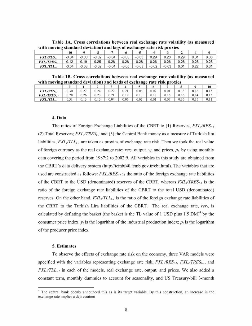
Table 1 presents the correlations between the variables that are gathered from the

CBRT’s balance sheet and the 3-monthly moving standard errors of the real exchange rate.

The results show that these variables are highly correlated with exchange rate volatility;

therefore, we would take these variables as a proxy for the exchange rate volatility.

2 Autoregressive Conditional Heteroskedastic specifications define the variability as a function of the lagged squared residuals but VAR specifications define the variability as a function of lagged dependent variables in the VAR system. Since both of them cannot be true at the same time, there is a specification problem if one uses an Autoregressive Conditional Heteroskedastic specification generated risk measure in a VAR setting. 3 The basic results of the paper remains robust when the current value of the variables in the denominator are used.

8

Table 1A. Cross correlations between real exchange rate volatility (as measured with moving standard deviation) and lags of exchange rate risk proxies

-10 -9 -8 -7 -6 -5 -4 -3 -2 -1 0 FXLt/RESt-1 -0.04 -0.03 -0.02 -0.04 -0.05 -0.03 0.29 0.28 0.29 0.31 0.30

FXLt/TRESt-1 0.12 0.19 0.25 0.28 0.28 0.28 0.26 0.26 0.28 0.28 0.28 FXLt/TLLt-1 -0.04 -0.03 -0.02 -0.04 -0.05 -0.03 -0.02 -0.03 0.01 0.22 0.31

Table 1B. Cross correlations between real exchange rate volatility (as measured

with moving standard deviation) and leads of exchange rate risk proxies 0 1 2 3 4 5 6 7 8 9 10

FXLt/RESt-1 0.30 0.27 0.24 0.22 0.21 0.06 0.02 0.01 0.33 0.16 0.15 FXLt/TRESt-1 0.28 0.26 0.23 0.21 0.19 0.18 0.17 0.16 0.16 0.14 0.13 FXLt/TLLt-1 0.31 0.13 0.13 0.04 0.06 0.02 0.01 0.07 0.16 0.15 0.11

4. Data

The ratios of Foreign Exchange Liabilities of the CBRT to (1) Reserves; FXLt/RESt-1

(2) Total Reserves; FXLt/TRESt-1 and (3) the Central Bank money as a measure of Turkish lira

liabilities, FXLt/TLLt-1 are taken as proxies of exchange rate risk. Then we took the real value

of foreign currency as the real exchange rate; rert; output, yt; and prices, pt, by using monthly

data covering the period from 1987:2 to 2002:9. All variables in this study are obtained from

the CBRT’s data delivery system (http://tcmbf40.tcmb.gov.tr/cbt.html). The variables that are

used are constructed as follows: FXLt/RESt-1 is the ratio of the foreign exchange rate liabilities

of the CBRT to the USD (denominated) reserves of the CBRT, whereas FXLt/TRESt-1 is the

ratio of the foreign exchange rate liabilities of the CBRT to the total USD (denominated)

reserves. On the other hand, FXLt/TLLt-1 is the ratio of the foreign exchange rate liabilities of

the CBRT to the Turkish Lira liabilities of the CBRT. The real exchange rate, rert, is

calculated by deflating the basket (the basket is the TL value of 1 USD plus 1.5 DM)4 by the

consumer price index. yt is the logarithm of the industrial production index; pt is the logarithm

of the producer price index.

5. Estimates

To observe the effects of exchange rate risk on the economy, three VAR models were

specified with the variables representing exchange rate risk, FXLt/RESt-1, FXLt/TRESt-1, and

FXLt/TLLt-1 in each of the models, real exchange rate, output, and prices. We also added a

constant term, monthly dummies to account for seasonality, and US Treasury-bill 3-month

4 The central bank openly announced this as is its target variable. By this construction, an increase in the exchange rate implies a depreciation

9

interest rates to account for the effects of the rest of the world. Based on the Bayesian

information criterion the lag order of VAR was set as 2. To assess the effect of the exchange

rate risk on the economic performance, a theoretically plausible model is presented in

Appendix A.

In order to observe the effects, the variables representing exchange rate risk are put

first in the ordering of each model. The exchange rate is expected to first respond to the risk.

Output would then react to the change in the exchange rate and the exchange rate risk,

therefore it is put in the third place in the ordering. Finally, because they would react to

changes in real exchange rates and output, prices are included at the end of the ordering.

5.1. Impulse Response Functions

The effects of shocks to the exchange rate risk are assessed by using impulse response

functions. Figures 4 to 6 report the impulse response functions of different variables, which

are highly correlated with exchange rate risk to the real exchange rate, output and prices when

one standard deviation shock is given to the exchange rate risk measures. The 80% confidence

bands are calculated using the bootstrap method with 500 draws and the middle line is for the

median of the draws.

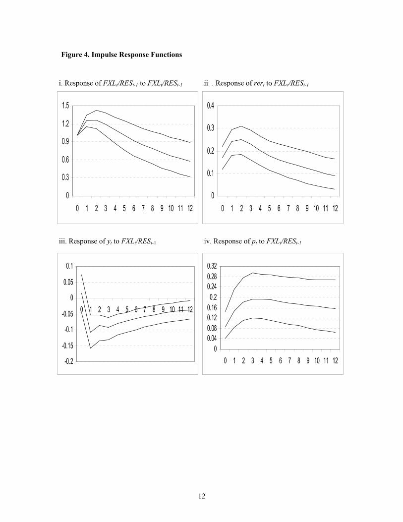
Figure 4 reports the impulse response functions of foreign exchange rate liabilities to

Central Bank reserves, real exchange rate, output and prices. The second diagram shows that a

positive shock to exchange rate risk causes a real exchange rate depreciation for the whole

period. For the first two months, the effect is higher; in other words, the initial effect is

overshooting. Then in the long run, the real exchange rate stabilizes at a level that is higher

than the initial one. The third diagram indicates that real output decreases as a response to a

shock to exchange rate risk after the first month. After the second month, the effect on output

of a shock to the exchange rate risk starts to recover but remains lower than the initial level

for the 12 months. As the last diagram presents, prices increase due to a positive shock to the

exchange rate risk for the whole period. To sum up, the results show that a shock to the

exchange rate risk causes real depreciation, decreases output and increases prices.

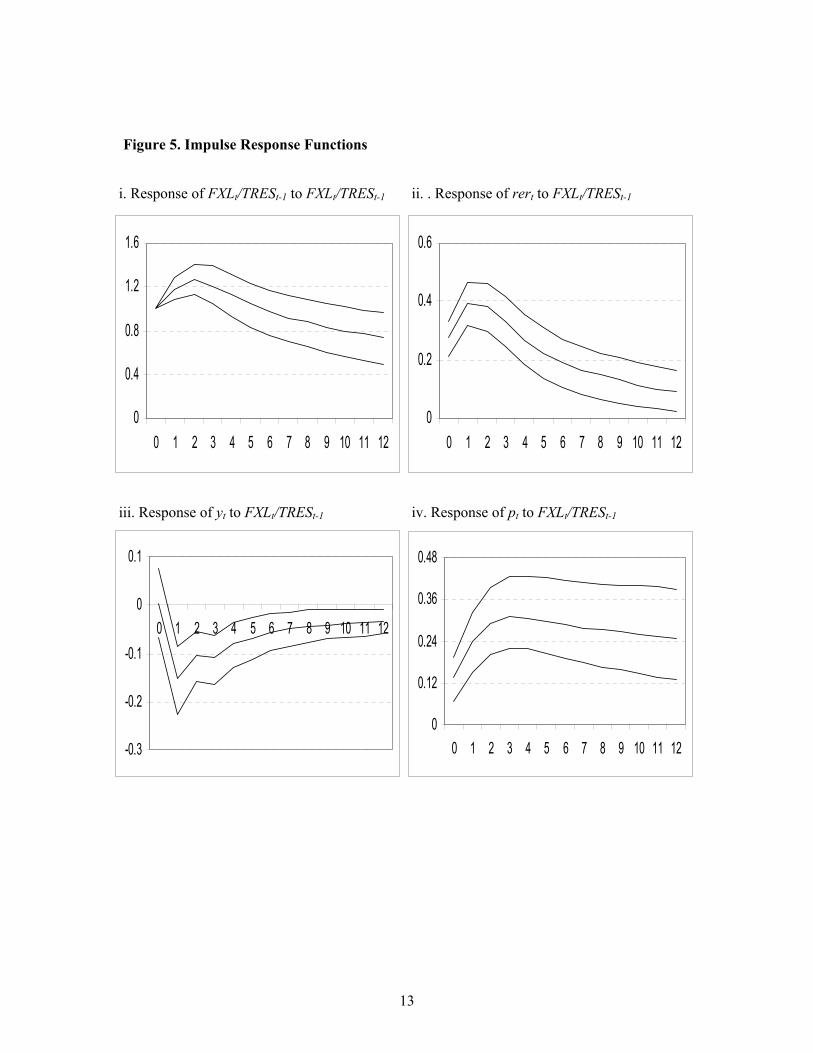
Figure 5 reports the impulse response functions of the foreign exchange rate liabilities

to total reserves, the real exchange rate, output and prices. The estimates indicate that a

positive shock to exchange rate risk causes a real depreciation for the whole period. For the

first months, overshooting is observed but then the real exchange rate converges to its new

long run level. The third diagram indicates that output decreases as a response to a positive

10

shock to exchange rate risk and remains lower than the initial level for 12 months. On the

other hand, prices increase after a positive shock to exchange rate risk is observed, and this

effect persists.

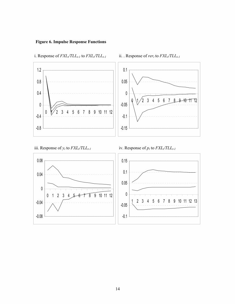
Figure 6 reports the impulse response functions of foreign exchange liabilities to

Central Bank money, the real exchange rate, output and prices. The figure indicates that the

responses of the real exchange rate, output and prices to a shock to exchange rate risk are

statistically insignificant.

5.2. Forecast Error Variance Decompositions

In addition to the assessment of the dynamic effects of exchange rate risk shocks by

using the impulse response functions, the forecast error variance decomposition analysis is

also performed to examine how exchange rate risk shocks contribute to the variability of key

economic aggregates.

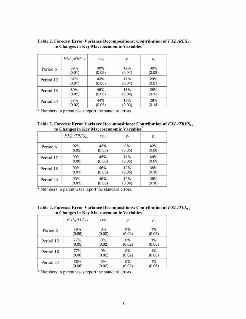
Table 2 reports the forecast error variance decomposition of the macroeconomic

variables due to FXLt/RESt-1. On the left, the time horizons at which forecast errors are

calculated are shown. The numbers in parentheses are standard errors. The results suggest that

the shocks do contribute significantly to macroeconomic fluctuations. 30-40% of the variation

in the real exchange rate, 12-19% of the variation in output and around 30% of the variation

in prices are explained by the exchange rate risk variable.

In Table 3, FXLt/TRESt-1 is used as a proxy for exchange rate risk and the forecast

error variance decomposition of the macroeconomic variables due to this variable is reported.

This set of estimates also suggests that the shocks contribute significantly to macroeconomic

fluctuations. Although the contribution of exchange rate risk shocks to output is smaller, the

basic results are robust.

Table 4 reports the forecast error variance decomposition of the macroeconomic

variables due to exchange rate risk, which is taken as FXLt/TLLt-1. However, these results

indicate that exchange rate risk shocks do not influence the fluctuations of real exchange rate,

output and prices, even if the last set of the results on the effect of the exchange rate risk on

economic performance is not robust. In all these specifications, the exchange rate risk

measure is usually explained by itself, suggesting that this variable is mostly exogenous.

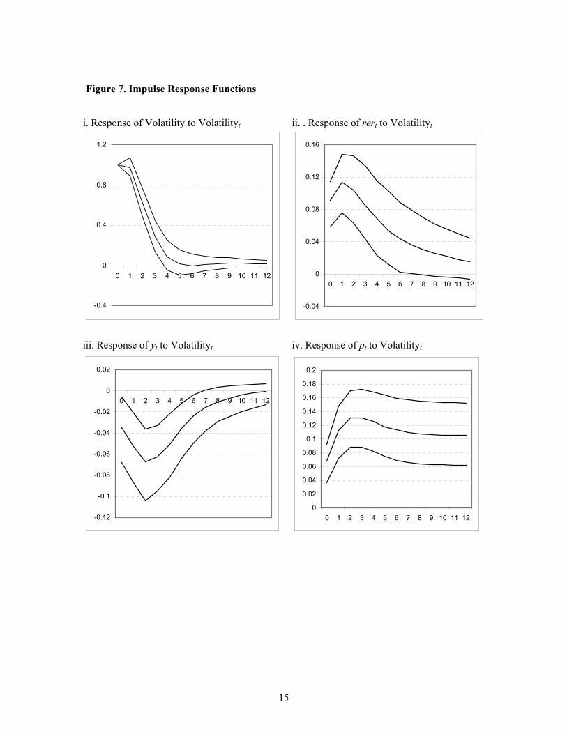
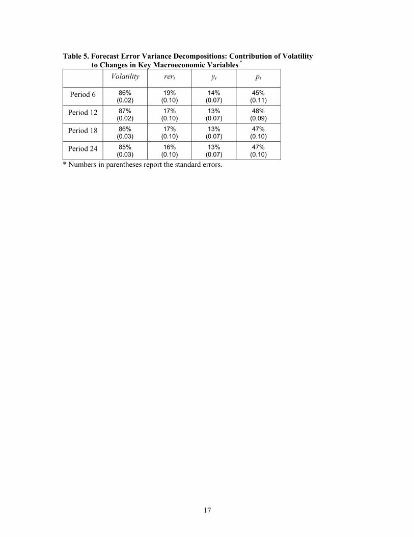
One could argue that the variables used to assess the exchange rate risk might be

misleading. Thus, we measured the exchange rate risk with the moving standard deviation

with 3-monthly window as in Table 1. Figure 7 and Table 5 report the impulse response

11

functions and forecast error variance decompositions with this measure. The results remain

robust.

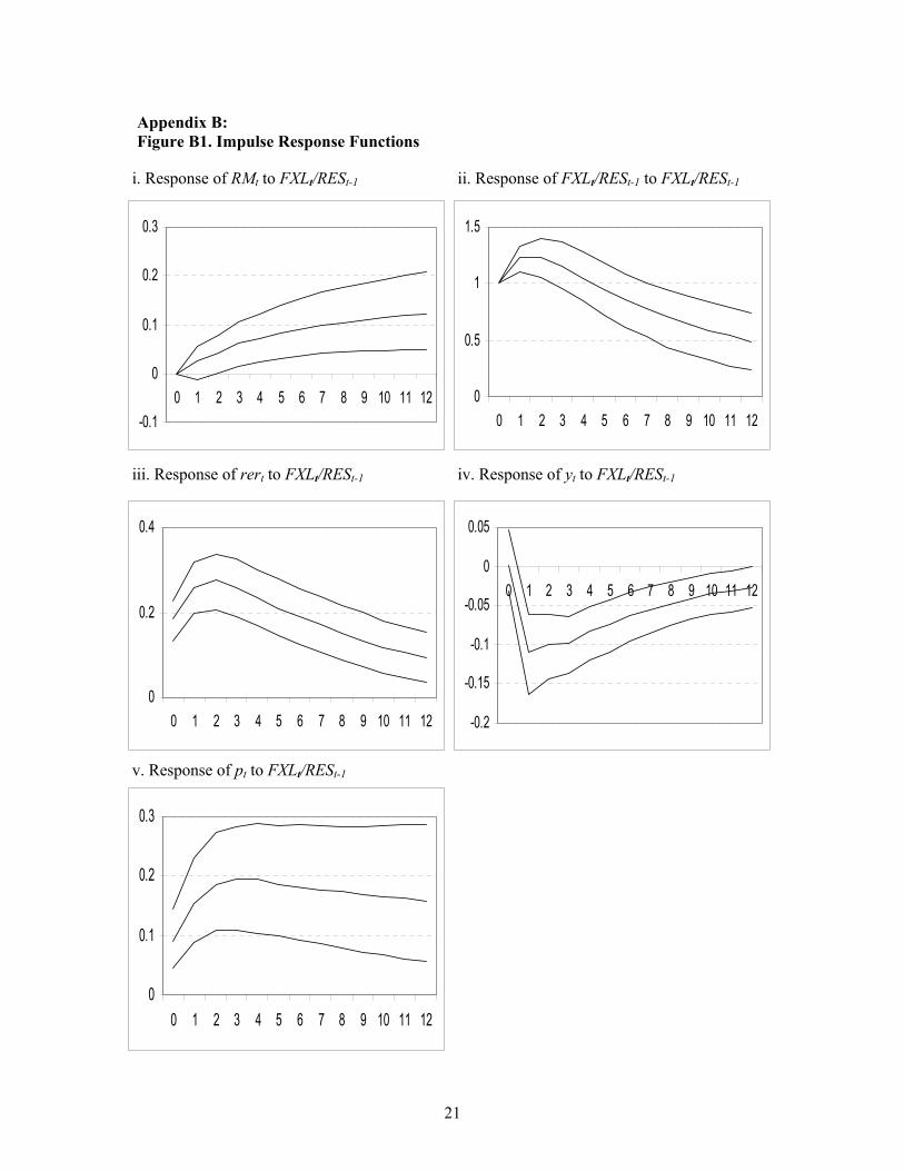
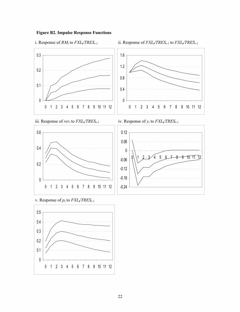
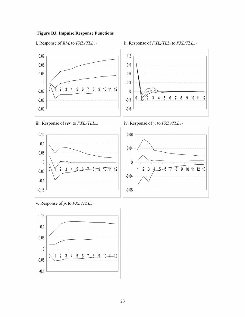
A decrease in the CBRT’s foreign exchange liabilities might be mimicking the

decrease in money supply in the market. Therefore, our estimates report the effect of the tight

monetary policy but not the exchange rate risk. In order to account for that, we included

reserve money as the first variable in the VAR specification. These results are not elaborated

on here but are reported in Appendix B. Overall, the basic conclusion was robust.

6. Conclusion

This paper assesses the effect of exchange rate risk for a small open developing

economy: Turkey. To measure the exchange rate risk, three measures were used from the

CBRT’s balance sheet: the ratio of the total foreign exchange liabilities to (1) the total

reserves, (2) the CBRT’s reserves and (3) the Turkish lira liabilities. This way of measuring

has some advantages to other econometrically heavy measures. First, these variables directly

measure the strength of the CBRT to stabilize the real exchange rate. Second these variables

are directly observable by the public; and third, they are not subject to specification tests like

the one in econometric models. The empirical evidence provided in this paper is parallel to

the economic priors as outlined in Appendix A. The higher exchange rate risk is associated

with a depreciation of the local currency, an increase in prices and a decrease in output.

12

Figure 4. Impulse Response Functions

i. Response of FXLt/RESt-1 to FXLt/RESt-1

ii. . Response of rert to FXLt/RESt-1

iii. Response of yt to FXLt/RESt-1

iv. Response of pt to FXLt/RESt-1

0

0.3

0.6

0.9

1.2

1.5

0 1 2 3 4 5 6 7 8 9 10 11 120

0.1

0.2

0.3

0.4

0 1 2 3 4 5 6 7 8 9 10 11 12

-0.2

-0.15

-0.1

-0.05

0

0.05

0.1

0 1 2 3 4 5 6 7 8 9 10 11 12

00.040.080.120.160.2

0.240.280.32

0 1 2 3 4 5 6 7 8 9 10 11 12

13


i. Response of FXLt/TRESt-1 to FXLt/TRESt-1

ii. . Response of rert to FXLt/TRESt-1

iii. Response of yt to FXLt/TRESt-1

iv. Response of pt to FXLt/TRESt-1

0

0.4

0.8

1.2

1.6

0 1 2 3 4 5 6 7 8 9 10 11 120

0.2

0.4

0.6

0 1 2 3 4 5 6 7 8 9 10 11 12

-0.3

-0.2

-0.1

0

0.1

0 1 2 3 4 5 6 7 8 9 10 11 12

0

0.12

0.24

0.36

0.48

0 1 2 3 4 5 6 7 8 9 10 11 12

14


i. Response of FXLt/TLLt-1 to FXLt/TLLt-1

ii. . Response of rert to FXLt/TLLt-1

iii. Response of yt to FXLt/TLLt-1

iv. Response of pt to FXLt/TLLt-1

-0.8

-0.4

0

0.4

0.8

1.2

0 1 2 3 4 5 6 7 8 9 10 11 12

-0.15

-0.1

-0.05

0

0.05

0.1

0 1 2 3 4 5 6 7 8 9 10 11 12

-0.08

-0.04

0

0.04

0.08

0 1 2 3 4 5 6 7 8 9 10 11 12

-0.1

-0.05

0

0.05

0.1

0.15

1 2 3 4 5 6 7 8 9 10 11 12 13

15


i. Response of Volatility to Volatilityt

-0.4

0

0.4

0.8

1.2

0 1 2 3 4 5 6 7 8 9 10 11 12

ii. . Response of rert to Volatilityt

-0.04

0

0.04

0.08

0.12

0.16

0 1 2 3 4 5 6 7 8 9 10 11 12

iii. Response of yt to Volatilityt

iv. Response of pt to Volatilityt

-0.12

-0.1

-0.08

-0.06

-0.04

-0.02

0

0.02

0 1 2 3 4 5 6 7 8 9 10 11 12

0

0.02

0.04

0.06

0.08

0.1

0.12

0.14

0.16

0.18

0.2

0 1 2 3 4 5 6 7 8 9 10 11 12

16

Table 2. Forecast Error Variance Decompositions: Contribution of FXLt/RESt-1 to Changes in Key Macroeconomic Variables *

FXLt/RESt-1 rert yt pt

Period 6 89% (0.01)

38% (0.09)

12% (0.04)

30% (0.08)

Period 12 92% (0.01)

43% (0.08)

17% (0.04)

29% (0.01)

Period 18 89% (0.01)

45% (0.06)

18% (0.04)

28% (0.13)

Period 24 87% (0.02)

44% (0.06)

19% (0.03)

26% (0.14)

* Numbers in parentheses report the standard errors.

Table 3. Forecast Error Variance Decompositions: Contribution of FXLt/TRESt-1

to Changes in Key Macroeconomic Variables* FXLt/TRESt-1 rert yt pt

Period 6 92% (0.02)

43% (0.08)

9% (0.05)

42% (0.08)

Period 12 93% (0.00)

45% (0.06)

11% (0.05)

40% (0.09)

Period 18 93% (0.01)

46% (0.05)

12% (0.05)

38% (0.10)

Period 24 93% (0.01)

45% (0.05)

12% (0.04)

36% (0.10)


Table 4. Forecast Error Variance Decompositions: Contribution of FXLt/TLLt-1

to Changes in Key Macroeconomic Variables *

FXLt/TLLt-1 rert yt pt

Period 6 78% (0.06)

0% (0.02)

0% (0.02)

1% (0.05)

Period 12 77% (0.05)

0% (0.02)

0% (0.02)

1% (0.06)

Period 18 77% (0.06)

0% (0.02)

0% (0.02)

1% (0.06)

Period 24 76% (0.06)

0% (0.02)

0% (0.02)

1% (0.06)


17

Table 5. Forecast Error Variance Decompositions: Contribution of Volatility to Changes in Key Macroeconomic Variables *

Volatility rert yt pt

Period 6 86% (0.02)

19% (0.10)

14% (0.07)

45% (0.11)

Period 12 87% (0.02)

17% (0.10)

13% (0.07)

48% (0.09)

Period 18 86% (0.03)

17% (0.10)

13% (0.07)

47% (0.10)

Period 24 85% (0.03)

16% (0.10)

13% (0.07)

47% (0.10)


18

References: Agénor, Pierre-Richard and Peter J. Montiel (1999). Development Macroeconomics, 2nd Edition, Princeton University Press, Princeton, NJ. Berument, H. (2003). “Measuring monetary policy for a small open economy: Turkey”, Journal of Macroeconomics, forthcoming. Berument, H., and A. Gunay. (2003). “Exchange rate risk and interest rate: a case study of Turkey”, Open Economies Review 14: 19-27. Berument, H. and M. Pasaogullari (2003). “Effects of the real exchange rate on output and infation: evidence from Turkey”, Developing Economies, (forthcoming). Bleaney, M., and D. Greenaway (2001). “The impact of trade and real exchange rate volatility on investment and growth in Sub-Saharan Africa”, Journal of Development Economics 65: 491-500. Bomberger, W. (1996). “Disagreement as a measure of uncertainty”, Journal of Money, Credit and Banking 28, 381-392. Cote, A. (1994). “Exchange rate volatility and trade: a survey,” Bank of Canada Working Paper, no. 5. Davis, G and B. Kanogo (1996). “On measuring the effect of inflation uncertainty on real GNP growth”, Oxford Economic Papers, 48: 163-175. Felmingham, B. and P. Mansfield (1997). “rationality and the risk premium on the Australian dollar”, International Economic Journal 11: 47-57. Hafer, R.W. (1986). “Inflation uncertainty and a test of the Friedman hypothesis”, Journal of Macroeconomics: 365-372. Kamin, S.B. (1996). “Exchange rates and inflation in exchange-rate based stabilizations: an empirical examination”, International Finance Discussion Paper, 554, Board of Governors of the Federal Reserve System, Washington, DC. Kamin, S.B. and J.H. Rogers (2000). “Output and the real exchange rate in developing countries: an application to Mexico”, Journal of Development Economics, 61: 85-109. Strongin, S. (1995). “The identification of monetary policy disturbances explaining the liquidity puzzle”, Journal of Monetary Economics, 35(3): 463-497. Tai, C. (2000). “Time-varying market, interest rate, and exchange rate risk premia in the us commercial bank stock returns”, Journal of Multinational Financial Management 10: 397-420.

19

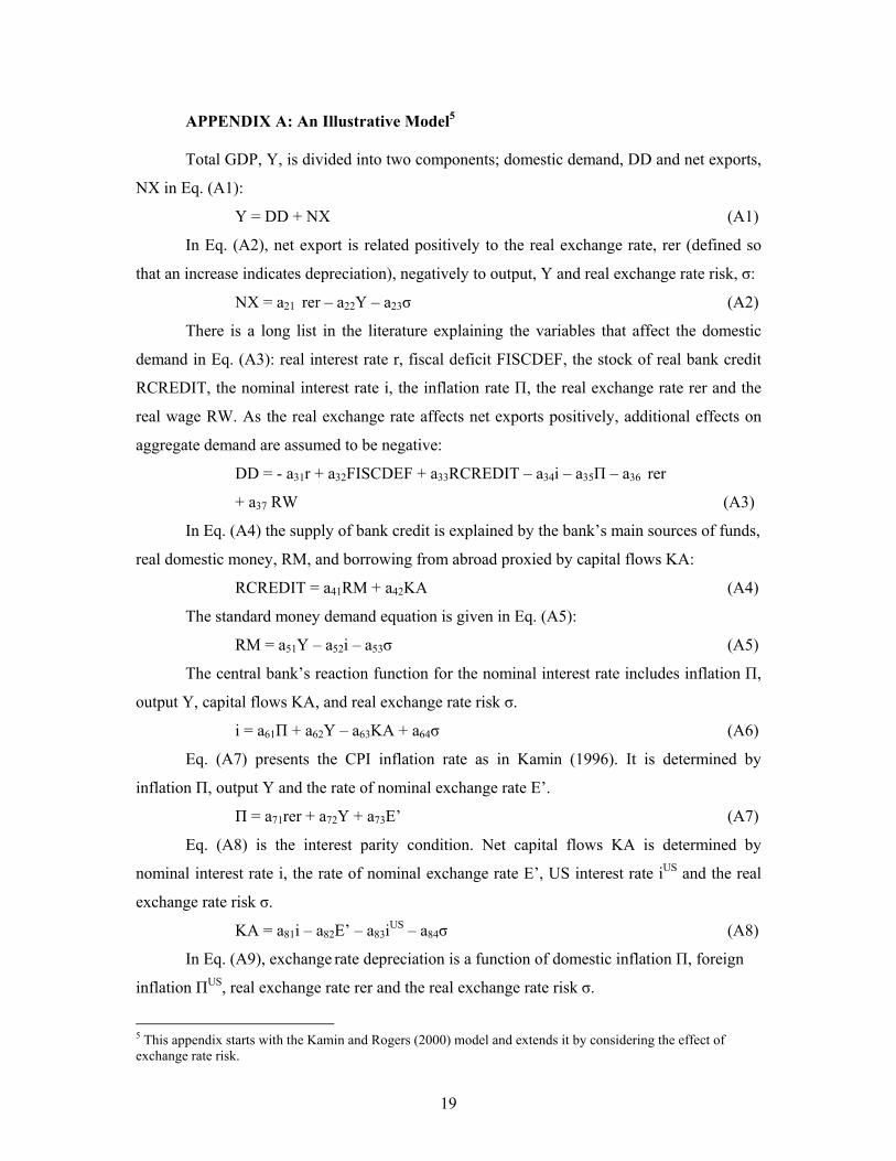
APPENDIX A: An Illustrative Model5

Total GDP, Y, is divided into two components; domestic demand, DD and net exports,

NX in Eq. (A1):

Y = DD + NX (A1)

In Eq. (A2), net export is related positively to the real exchange rate, rer (defined so

that an increase indicates depreciation), negatively to output, Y and real exchange rate risk, σ:

NX = a21 rer – a22Y – a23σ (A2)

There is a long list in the literature explaining the variables that affect the domestic

demand in Eq. (A3): real interest rate r, fiscal deficit FISCDEF, the stock of real bank credit

RCREDIT, the nominal interest rate i, the inflation rate Π, the real exchange rate rer and the

real wage RW. As the real exchange rate affects net exports positively, additional effects on

aggregate demand are assumed to be negative:

DD = - a31r + a32FISCDEF + a33RCREDIT – a34i – a35Π – a36 rer

+ a37 RW (A3)

In Eq. (A4) the supply of bank credit is explained by the bank’s main sources of funds,

real domestic money, RM, and borrowing from abroad proxied by capital flows KA:

RCREDIT = a41RM + a42KA (A4)

The standard money demand equation is given in Eq. (A5):

RM = a51Y – a52i – a53σ (A5)

The central bank’s reaction function for the nominal interest rate includes inflation Π,

output Y, capital flows KA, and real exchange rate risk σ.

i = a61Π + a62Y – a63KA + a64σ (A6)

Eq. (A7) presents the CPI inflation rate as in Kamin (1996). It is determined by

inflation Π, output Y and the rate of nominal exchange rate E’.

Π = a71rer + a72Y + a73E’ (A7)

Eq. (A8) is the interest parity condition. Net capital flows KA is determined by

nominal interest rate i, the rate of nominal exchange rate E’, US interest rate iUS and the real

exchange rate risk σ.

KA = a81i – a82E’ – a83iUS – a84σ (A8)

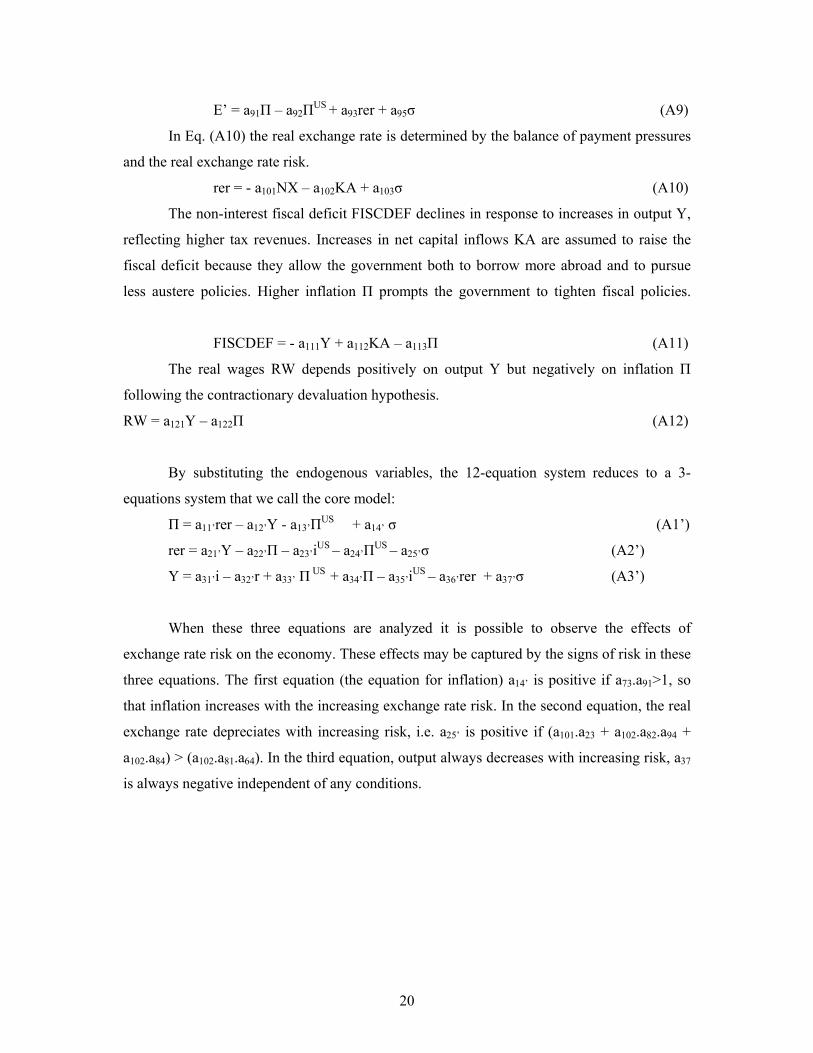
In Eq. (A9), exchange rate depreciation is a function of domestic inflation Π, foreign

inflation ΠUS, real exchange rate rer and the real exchange rate risk σ.

5 This appendix starts with the Kamin and Rogers (2000) model and extends it by considering the effect of exchange rate risk.

20

E’ = a91Π – a92ΠUS + a93rer + a95σ (A9)

In Eq. (A10) the real exchange rate is determined by the balance of payment pressures

and the real exchange rate risk.

rer = - a101NX – a102KA + a103σ (A10)

The non-interest fiscal deficit FISCDEF declines in response to increases in output Y,

reflecting higher tax revenues. Increases in net capital inflows KA are assumed to raise the

fiscal deficit because they allow the government both to borrow more abroad and to pursue

less austere policies. Higher inflation Π prompts the government to tighten fiscal policies.

FISCDEF = - a111Y + a112KA – a113Π (A11)

The real wages RW depends positively on output Y but negatively on inflation Π

following the contractionary devaluation hypothesis.

RW = a121Y – a122Π (A12)

By substituting the endogenous variables, the 12-equation system reduces to a 3-

equations system that we call the core model:

Π = a11’rer – a12’Y - a13’ΠUS + a14’ σ (A1’)

rer = a21’Y – a22’Π – a23’iUS – a24’ΠUS – a25’σ (A2’)

Y = a31’i – a32’r + a33’ Π US + a34’Π – a35’iUS – a36’rer + a37’σ (A3’)

When these three equations are analyzed it is possible to observe the effects of

exchange rate risk on the economy. These effects may be captured by the signs of risk in these

three equations. The first equation (the equation for inflation) a14’ is positive if a73.a91>1, so

that inflation increases with the increasing exchange rate risk. In the second equation, the real

exchange rate depreciates with increasing risk, i.e. a25’ is positive if (a101.a23 + a102.a82.a94 +

a102.a84) > (a102.a81.a64). In the third equation, output always decreases with increasing risk, a37

is always negative independent of any conditions.

21

Appendix B: Figure B1. Impulse Response Functions

i. Response of RMt to FXLt/RESt-1

ii. Response of FXLt/RESt-1 to FXLt/RESt-1

iii. Response of rert to FXLt/RESt-1

iv. Response of yt to FXLt/RESt-1

v. Response of pt to FXLt/RESt-1

-0.1

0

0.1

0.2

0.3

0 1 2 3 4 5 6 7 8 9 10 11 12 0

0.5

1

1.5

0 1 2 3 4 5 6 7 8 9 10 11 12

0

0.2

0.4

0 1 2 3 4 5 6 7 8 9 10 11 12 -0.2

-0.15

-0.1

-0.05

0

0.05

0 1 2 3 4 5 6 7 8 9 10 11 12

0

0.1

0.2

0.3

0 1 2 3 4 5 6 7 8 9 10 11 12

22

Figure B2. Impulse Response Functions

i. Response of RMt to FXLt/TRESt-1

ii. Response of FXLt/TRESt-1 to FXLt/TRESt-1

iii. Response of rert to FXLt/TRESt-1

iv. Response of yt to FXLt/TRESt-1

v. Response of pt to FXLt/TRESt-1

0

0.1

0.2

0.3

0 1 2 3 4 5 6 7 8 9 10 11 120

0.4

0.8

1.2

1.6

0 1 2 3 4 5 6 7 8 9 10 11 12

0

0.2

0.4

0.6

0 1 2 3 4 5 6 7 8 9 10 11 12 -0.24

-0.18

-0.12

-0.06

0

0.06

0.12

0 1 2 3 4 5 6 7 8 9 10 11 12

0

0.1

0.2

0.3

0.4

0.5

0 1 2 3 4 5 6 7 8 9 10 11 12

23

Figure B3. Impulse Response Functions

i. Response of RMt to FXLt/TLLt-1

ii. Response of FXLt/TLLt to FXL/TLLt-1

iii. Response of rert to FXLt/TLLt-1

iv. Response of yt to FXLt/TLLt-1

v. Response of pt to FXLt/TLLt-1

-0.09

-0.06

-0.03

0

0.03

0.06

0.09

0 1 2 3 4 5 6 7 8 9 10 11 12

-0.6

-0.3

0

0.3

0.6

0.9

1.2

0 1 2 3 4 5 6 7 8 9 10 11 12

-0.15

-0.1

-0.05

0

0.05

0.1

0.15

0 1 2 3 4 5 6 7 8 9 10 11 12

-0.08

-0.04

0

0.04

0.08

1 2 3 4 5 6 7 8 9 10 11 12 13

-0.1

-0.05

0

0.05

0.1

0.15

0 1 2 3 4 5 6 7 8 9 10 11 12

24

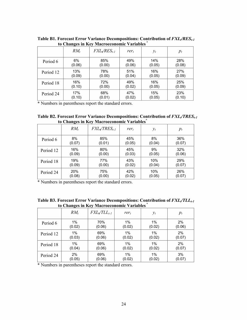
Table B1. Forecast Error Variance Decompositions: Contribution of FXLt/RESt-1

to Changes in Key Macroeconomic Variables * RMt FXLt/RESt-1 rert yt pt

Period 6 6% (0.06)

85% (0.00)

49% (0.06)

14% (0.05)

28% (0.08)

Period 12 13% (0.09)

78% (0.00)

51% (0.04)

16% (0.05)

27% (0.09)

Period 18 16% (0.10)

72% (0.00)

49% (0.02)

16% (0.05)

25% (0.09)

Period 24 17% (0.10)

68% (0.01)

47% (0.02)

15% (0.05)

23% (0.10)


Table B2. Forecast Error Variance Decompositions: Contribution of FXLt/TRESt-1

to Changes in Key Macroeconomic Variables* RMt FXLt/TRESt-1 rert yt pt

Period 6 8% (0.07)

85% (0.01)

45% (0.05)

8% (0.04)

36% (0.07)

Period 12 16% (0.09)

80% (0.00)

45% (0.03)

9% (0.05)

32% (0.06)

Period 18 19% (0.09)

77% (0.00)

43% (0.02)

10% (0.04)

29% (0.07)

Period 24 20% (0.08)

75% (0.00)

42% (0.02)

10% (0.05)

26% (0.07)


Table B3. Forecast Error Variance Decompositions: Contribution of FXLt/TLLt-1

to Changes in Key Macroeconomic Variables * RMt FXLt/TLLt-1 rert yt pt

Period 6 1% (0.02)

70% (0.06)

1% (0.02)

1% (0.02)

2% (0.06)

Period 12 1% (0.03)

69% (0.06)

1% (0.02)

1% (0.02)

2% (0.07)

Period 18 1% (0.04)

69% (0.06)

1% (0.02)

1% (0.02)

2% (0.07)

Period 24 2% (0.05)

69% (0.06)

1% (0.02)

1% (0.02)

3% (0.07)


The Effects of Exchange Rate Risk on Economic Performance : The Turkish Experience

Documents

Transcript of The Effects of Exchange Rate Risk on Economic Performance : The Turkish Experience