Estuarine, Coastal and Shelf Science 58 (2003) 137–145

The effect of water density variationson the tidal flushing of animal burrows

S.F. Heron*, P.V. Ridd

Marine Geophysical Laboratory, School of Mathematical and Physical Sciences, James Cook University, Townsville,

Queensland 4811, Australia

Received 2 February 2001; accepted 24 February 2003

Abstract

Animal burrows in mangrove swamps play an important role in the transport of various soluble materials, including salt.Flushing of burrows by inundating tides provides an efficient mechanism for the exchange of these materials. The density increase inthe burrow, due to salt diffusion from pore water into the burrow, causes a greater resistance to the flushing. As the salinity

difference between surface and burrow waters increases, the burrows no longer flush, and hydrostatic equilibrium exists between thedifferent density waters. A flume experiment was conducted to compare burrow flushing characteristics with theoretical predictions.The results were consistent with a simple analytical theory in predicting whether burrows would flush. When equilibrium wasattained, the difference between the interface depths was 10% greater than the theoretical prediction, which was within the

experimental error. In addition, a comparison between a two-opening and a three-opening burrow showed that there was no benefitto the flushing capability due to additional openings. Computational fluid dynamic models were undertaken to compare with theexperimental and theoretical flushing characteristics. These were also consistent with the flushing prediction theory. When

equilibrium was attained, the difference between the interface depths in the model was 33% greater than the theoretical prediction.The computational study with an additional opening supported the experimental evidence that there is no advantage to the flushing.Insight into small-scale processes unable to be accurately observed could be obtained from the models, e.g. oscillations of density

interfaces and turbulent scales at the burrow openings. The consistency in prediction of flushing between the theoretical,experimental and computational methods, now allows modelling of more complex burrow structures with great confidence.� 2003 Elsevier Ltd. All rights reserved.

Keywords: burrows; computer simulation; flushing time

1. Introduction

Computational fluid dynamics (CFD) gives an insightinto processes that are often otherwise unable to beobserved. Many industrial processes can increase theirefficiency by interpretation of CFD models. CFDpackages are commonly used for these purposes, oneexample of such packages being the Fluid DynamicsAnalysis Package (FIDAP). Similarly it is possible touse these techniques and packages to examine in detail

* Corresponding author. Department of physics, Georgetown

University, Washington, DC 20057, USA.

E-mail address: sfh5@georgetown.edu (S.F. Heron).

0272-7714/03/$ - see front matter � 2003 Elsevier Ltd. All rights reserved.

doi:10.1016/S0272-7714(03)00068-4

the flows in environmental situations which are difficultor unable to be physically observed.

CFD models of large scale processes have givengreater insight into processes in oceans, bays andestuaries (Bode, Mason, & Middleton, 1997; Furukawa,Wolanski, & Mueller, 1997; Wolanski & Ridd, 1986),however, modelling of small-scale environmental pro-cesses is much less common. Flow in animal burrowshas, in recent years, received an increased focus(Allanson, Skinner, & Imberger, 1992; Webster, 1992).Burrows perform a significant role in the exchangebetween surface and ground waters in a variety ofmarine and freshwater environments. Irrigation andflushing of animal burrows located in the beds andbanks of lakes, rivers, estuaries and ocean coasts, pro-vide a mechanism which can enhance water exchange,

138 S.F. Heron, P.V. Ridd / Estuarine, Coastal and Shelf Science 58 (2003) 137–145

and thus the transport of materials such as salt, nutrients,oxygen and pollutants.

In mangrove areas, the transport of salt is of greatimportance. As groundwater is absorbed from thesediment by the mangrove roots, salt is excluded at theroots. There is thus an increase in salt concentration inthe soil surrounding the mangrove roots. This sedimentis highly impermeable and greatly impedes the diffusivetransport of the salt away from the roots; the coefficientof salt diffusion for mangrove swamp sediment wascalculated by Hollins, Ridd, and Read (1999) to be4.6� 10�5m�2 day�1. In swamps without animal bur-rows the salt must diffuse from the root to the surfacewater, however, with burrows present the distance overwhich diffusion occurs is much shorter, and thus thediffusion time is significantly decreased. The removal ofthe burrow water then completes the salt-removalprocess. As a high tide inundates the swamp, the watersurface has a small, but significant, slope. The pressuredifference across the burrow openings due to this slopecauses flow in the burrow; flushing the burrow water,and thus removing the salt. Hollins and Ridd (in press),Ridd (1996), and Stieglitz, Ridd, and Muller (2000)showed that burrow water, and hence the salt, issignificantly flushed by any tide that inundates theground surface at the burrow openings. The burrowflushing process can provide a much faster mechanismfor salt-removal from root to surface, as compared withdiffusion from root to surface.

Stieglitz et al. (2000) suggested that the flushing ofanimal burrowsmight be completed in approximately 1 h,within the time span of a single-tidal event. Thesemeasurements were undertaken by replacing burrowwater with a same-density sugar solution, and measuringthe conductivity change as the sugar water was flushedand replaced with (higher conductivity) surface water. Incontrast, Hollins and Ridd (in press) used two methods,which suggest that the volume of water flushed duringa single-tidal event is approximately one-third of theburrow volume. The first of these methods used rhoda-mine dye to trace the burrow water during the tidalinundation, and measured the relative fluorescence overthe tidal period to determine the mixing characteristics.The second involved oxygenmeasurements of the burrowwater. Oxygen diffusion from mangrove roots andmicrobial oxygen consumption were accounted for, andthe results showed a significant increase in oxygenconcentration as oxygen-rich surface water inundatedthe burrow water. The two methods of Hollins and Ridd(in press) were consistent in the observation that one-thirdof the burrow volume was flushed during the tidal event.

Heron and Ridd (2001) described a method by whichCFD can be used to predict the tidal flushing of animalburrows. The method defined a pressure gradient acrossthe flow domain, according to the water slope, whichcaused flow across the surface and through the burrow.

Obstructions to the surface flow (including surface andbuttress roots) were modelled and their effects on thesurface water velocities and burrow flushing rates weredetermined. Flushing times were measured for burrowsof varying complexity of geometry. Burrows in somemangrove forests have been observed to reach totaldepths of 1.2m (Stieglitz et al., 2000), and models werecreated for single loop and several multiply-connectedloops to this depth. The study showed that burrowflushing times predicted by CFD models were of thesame order as those observed in mangrove swamps, i.e.that there is significant flushing of burrows withina single-tidal event.

This work furthers the work of Heron and Ridd(2001) by investigating the effect on flow rates of densityvariations in the flow domain. As discussed, mangroveroots exclude salt into the highly impermeable sediment,which then diffuses into the animal burrows. This causesthe density of burrow water to increase and so itbecomes greater than that of the surface �flushing� water.A typical value for the density of the surface water (seawater) is 1028 kgm�3, and burrow water density mayreach 1053 kgm�3 at the landward boundary of theswamp, however, values around 1033 kgm�3 (approxi-mately 0.5% variation) are more common. This increasein density is expected to increase the time required toflush the burrow. Flume experiments using a simpleburrow geometry are compared with the CFD modeloutput. This work also incorporates the observationthat burrows often have more than the simple twoopenings, and investigates this effect upon the flushingrate of the burrow.

2. Methods

2.1. Experiment

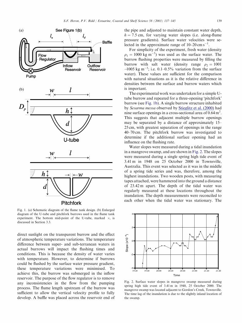
A flume tank was constructed of the design shown inFig. 1a. The flume was constructed from PVC pipe, andclear plastic tubing was used for the burrow. Thediameter of the flume was Dp ¼ 15 cm, and the lengthsupstream and downstream of the burrow werelu ¼ 4:0 m and ld ¼ 1:7 m, respectively. The character-istic lengths of the burrow were the internal diameter,w ¼ 3 cm, the distance between the openings, l ¼ 40 cm,and the depth to the inside of the burrow, d ¼ 23 cm.These values were selected to be consistent withobservations of the burrows of the crab, Sesarma messa,in mangrove swamps, and with burrows from literature(Allanson et al., 1992; Stieglitz et al., 2000).

Surface water from the inflow reservoir was pumpedinto a flow regulator and then through the flume to theoutflow reservoir, returning to the inflow reservoir.Large variations in burrow and flume temperatures wereobserved over short time periods. These were caused by

139S.F. Heron, P.V. Ridd / Estuarine, Coastal and Shelf Science 58 (2003) 137–145

direct sunlight on the transparent burrow and the effectof atmospheric temperature variations. The temperaturedifference between super- and sub-terranean waters inactual burrows will impact the flushing times andconditions. This is because the density of water varieswith temperature. However, to determine if burrowscould be flushed by the surface water pressure gradient,these temperature variations were minimised. Toachieve this, the burrow was submerged in the inflowreservoir. The purpose of the flow regulator is to removeany inconsistencies in the flow from the pumpingprocess. The flume length upstream of the burrow wassufficient to allow the vertical velocity profile to fullydevelop. A baffle was placed across the reservoir end of

Fig. 1. (a) Schematic diagram of the flume tank design. (b) Enlarged

diagram of the U-tube and pitchfork burrows used in the flume tank

experiment. The bottom mid-point of the U-tube, marked �, is

discussed in Section 3.3.

the pipe and adjusted to maintain constant water depth,h ¼ 7:5 cm, for varying water slopes (i.e. along-flumepressure gradients). Surface water velocities were se-lected in the approximate range of 10–20 cm s�1.

For simplicity of the experiment, fresh water (densityq1 ¼ 1000 kg m�3) was used as the surface water. Theburrow flushing properties were measured by filling theburrow with salt water (density range q2 ¼ 1001�1005 kg m�3; i.e. 0.1–0.5% variation from the surfacewater). These values are sufficient for the comparisonwith natural situations as it is the relative difference indensities between the surface and burrow waters whichis important.

The experimentalworkwas undertaken for a simpleU-tube burrow and repeated for a three-opening �pitchfork�burrow (see Fig. 1b). A single burrow structure inhabitedby Sesarma messa observed by Stieglitz et al. (2000) hadnine surface openings in a cross-sectional area of 0.64m2.This suggests that adjacent multiple burrow openingsmay be separated by a distance of approximately 15–25 cm, with greatest separation of openings in the range40–70 cm. The pitchfork burrow was investigated todetermine if the additional surface opening had aninfluence on the flushing rate.

Water slopes were measured during a tidal inundationin amangrove swamp, and are shown in Fig. 2. The slopeswere measured during a single spring high tide event of3.41m in 1948 on 25 October 2000 in Townsville,Australia. This event was selected as it was in the middleof a spring tide series and was, therefore, among thehighest inundations. Two wooden posts, with measuringtapes attached,were hammered into the ground adistanceof 23.42m apart. The depth of the tidal water wasregularly measured at these locations throughout theinundation. The depth measurements were reconciled toeach other when the tidal water was stationary. The

Fig. 2. Surface water slopes in mangrove swamp measured during

spring high tide event of 3.41m in 1948, 25 October 2000. The

mangrove swamp was located adjacent to Gordon’s Creek, Townsville.

The time lag of the inundation is due to the slightly inland location of

the swamp.

140 S.F. Heron, P.V. Ridd / Estuarine, Coastal and Shelf Science 58 (2003) 137–145

measured slopes were predominantly 1� 10�4 on bothflood and ebb tides with slopes as high as 1� 10�3 and4� 10�4 observed in the initial and final stages, re-spectively, of the tide. This range of values is consistentwith reported values (Aucan & Ridd, 1999; Wolanski,Mazda, & Ridd, 1992).

The water slope in the flume tank could be de-termined whenever the burrow was filled with a dyedsalt solution with density sufficiently high that theburrow would not flush. The different density watersðq1 < q2Þ will reach hydrostatic equilibrium as shown inFig. 3. The positions of the interfaces between thesurface and burrow waters can be measured. Thepressure in each side of the U-tube will be equal, i.e.:

q1gh1 þ q1gd1 ¼ q1gh2 þ q1gd2 þ q2gðd1 � d2Þ

and thus,

ðh1 � h2Þ ¼q2 � q1

q1

� �ðd1 � d2Þ

The surface water slope is given by S0 ¼ ðh1 � h2Þ=l, sothe difference in the interface depths is:

Dd¼ ðd1 � d2Þ ¼q1S0l

Dqð1Þ

where q1 is the surface water density, l the distancebetween the burrow openings and Dq is the difference insurface and burrow densities.

The maximum slope obtained with the smooth PVCpipe was 3� 10�4. The Manning coefficient for smoothPVC pipe is reported as n ¼ 0:009 (Street, Watters, &Vennard, 1996), and is related to the flow velocity, V, by:

V¼ 1

nR2=3S

1=20 ð2Þ

Fig. 3. Hydrostatic pressure equilibrium in a U-tube burrow due to

surface water slope and different density burrow and surface waters.

where R is the hydraulic radius (ratio of water cross-sectional area to wetted perimeter). If we keep the flowvelocity and the hydraulic radius constant in theexperimental setup, the roughness (corresponding to n)must be increased to produce the desired slope range.Sand and gravel were applied to the PVC surface toincrease the roughness characteristic, and thereby themaximum slope.

2.2. Numerical model

The model geometry matched the along flow cross-section of the flume tank (see Fig. 1b) and the modeldomain length was defined as 2.0m, with the burrowlocated centrally. The tidal flushing was modelled in twodimensions using FIDAP. This package uses the finiteelement method to solve the isothermal Navier–Stokesequations (Fluid Dynamics International, 1993):

Continuity:qqqt

þr � qu¼ 0

Momentum: qquqt

þ u � ru

� �

¼�rpþr � s� qgþ qf ð3Þ

TransientþConvective¼ PressureþViscous

�BuoyancyþBody Force

where the symbolism is as follows—q is the density; u thevelocity; r the gradient, divergence operator; p thepressure; s the stress tensor; g the gravity; t the time andf is the body force.

All parameters and equations were non-dimensional-ised to provide greater ease and flexibility in theimplementation of the models.

The boundary condition driving the surface waterflow was determined from the surface slope of theincoming tidal water. The pressure difference across thedomain due to this slope was simulated and producedthe appropriate vertical velocity profile. Heron and Ridd(2001) outlines this method further.

The effects of turbulence were modelled using themixing length model. This model is automated withinthe framework of FIDAP version 7.62 and defines theappropriate mixing length for each individual meshelement. This boundary layer model allows for thetransition from the viscous sub-layer to the outer flowregion. This simplifies the solution process as there is norequirement for additional turbulence parameters, andtherefore there are less equations to solve.

The steady-state velocity and pressure profiles weredetermined by solving the time-independent continuityand momentum equations, with constant density as-sumed throughout the domain. These profiles were used

141S.F. Heron, P.V. Ridd / Estuarine, Coastal and Shelf Science 58 (2003) 137–145

as initial conditions for the transient density-dependentmodels.

The variation in density between surface and burrowwater is small compared with the overall magnitude ofdensity, and so it is appropriate to use the Boussinesqapproximation. This approximation assumes that thedensity is constant in all terms of the momentumequation except the Buoyancy term. The effect of densityvariation for this term was modelled by use of a tracer todefine the more saline water. Density is defined for theBuoyancy term by:

q¼ q1ð1� bccÞ ð4Þ

where c is the concentration of tracer and bc is the tracervolume expansion coefficient.

The time-dependent tracer equation is defined fortracer n, and must be solved in conjunction with thecontinuity and momentum equations:

Tracer; n: qqcnqt

þ u � rcn

� �¼ qr � ðanrcnÞ þ qcn þRn

ð5Þ

TransientþConvective¼Diffusiveþ SourceþReaction

where cn is the tracer concentration, an the moleculardiffusivity, qcn the source term and Rn is the chemicalreaction rate.

The molecular diffusivity of the tracer was defined asthe value of salt in water at 25 �C, an ¼ 1:6� 10�9 m2 s�1

(Nye & Tinker, 1977). For this analysis the source andreaction terms are removed, however, these could beretained for further analyses, e.g. investigating oxygentransport.

The initial condition for the tracer is defined as beingunity for the burrow water, and zero for the surfacewater. The tracer volume expansion coefficient, bc, is

defined by the densities of surface (q1) and burrow (q2)waters, as:

bc ¼q1 � q2

q1

� �ð6Þ

For example, taking the values of q1 ¼ 1000 kg m�3

and q2 ¼ 1005 kg m�3, the value for the volume expan-sion coefficient is bc ¼ �0:005.

Models with the U-tube and pitchfork geometrieswere solved to compare with the experimental work.

3. Results

3.1. Flume experiment

The experiment was conducted for burrow water saltconcentrations of 1, 3 and 5 g l�1, and with four differentvelocities at the top of the surface water. The flushingcharacteristics were determined for each of the U-tubeandpitchfork burrows. The results are illustrated inTable1a and b, respectively. The Dd values for the pitchforkburrow are determined from the right- and left-handtines, i.e. the �U� sections of the burrow. The interface inthe middle (vertical) tine of the pitchfork was alwaysbetween the depths of the outer sections at equilibrium.The experimental error in the Dd values is 0.5 cm.

There are three distinct regions of each table: (1)those for which flushing occurs quickly (dark grey), (2)those for which equilibrium was reached (light grey) and(3) those which lie on the boundary between theseconditions (white), i.e. partial or very slow flushing. Inthis third region, the interface positions were initiallyvery close to equilibrium and diffusion of salt across theinterfaces eventually started the flushing of the burrow.The asterisk (*) indicates when complete flushing haseventually occurred under these conditions.

Table 1

Experimental flushing characteristics for U-tube and pitchfork burrows

Surface water velocity (cm s�1) [slope]

Burrow water salt concentration ( g l�1)

1 3 5

(a) Experimental flushing characteristics for U-tube burrow

10.4 [1.64] Equilibrium Dd=9.0 cm Equilibrium Dd=2.2 cm Equilibrium Dd=1.6 cm

13.4 [2.72] Equilibrium Dd=14.5 cm Equilibrium Dd=4.0 cm Equilibrium Dd=2.5 cm

16.8 [4.27] *Flushed in 15min 30 s Equilibrium Dd=4.5 cm Equilibrium Dd=3.5 cm

20.9 [6.61] Flushed in 2min 20 s Equilibrium Dd=9.5 cm Equilibrium Dd=5.5 cm

(b) Experimental flushing characteristics for pitchfork burrow

10.4 [1.64] Equilibrium Dd=6.0 cm Equilibrium Dd=2.25 cm Equilibrium Dd=1.25 cm

13.4 [2.72] Equilibrium Dd=14.25 cm Equilibrium Dd=2.75 cm Equilibrium Dd=2.5 cm

16.8 [4.27] *Flushed in 20min 08 s Equilibrium Dd=7.5 cm Equilibrium Dd=3.0 cm

20.9 [6.61] Flushed in 3min 15 s Equilibrium Dd=11.0 cm Equilibrium Dd=4.75 cm

Direct flushing—dark grey, equilibrium—light grey, boundary condition—white. The asterisk (*) indicates when complete flushing has eventually

occurred under these conditions.

142 S.F. Heron, P.V. Ridd / Estuarine, Coastal and Shelf Science 58 (2003) 137–145

To determine the slopes corresponding to eachvelocity one can eliminate S0 from Eqs. (1) and (2),which leads to the expression:

ffiffiffiffiffiffiffiffiffiffiffiffiDqDd

p¼n ffiffiffiffiffiffiffiffi

q1Lp n

R2=3

om ð7Þ

Fig. 4 shows the linear relation betweenffiffiffiffiffiffiffiffiffiffiffiffiDqDd

pand m

for the flume data. The linear regression through theorigin has a slope of 2.55 (with standard deviation of0.18). As the surface water density and the openingseparation are known, one can determine the propor-tionality term ð1=nÞR2=3 in Eq. (2) from this slope. Therelation between the surface slope, S0, and surfacevelocity, m, for the flume is thus known. The slopescorresponding to the velocities are bracketed next to thevelocities in Table 1. The error in the calculation of theslopes is 13%.

We are now able to compare the measured Dd withthose calculated using Eq. (1), as shown in Fig. 5. Thereis a variation of 10% between the experimental valuesand the predicted values, which is within the experi-mental error.

3.2. CFD: simple U-tube burrow withdensity variation

The initial density-dependent CFD study was con-ducted using the simple U-tube burrow with the samecharacteristic dimensions as for the flume experiment.Values for the tracer volume expansion coefficient weredefined to correspond with density differences betweensurface and burrow water in the range 1–5 kgm�3. Slopevalues were input to the model in the range 1� 10�4–1� 10�3. Results of the models are shown in Table 2a.

Comparison of the flume tank results with those fromthe model shows that the distinction between the threeregions (direct flushing, boundary region and equilibri-um) is consistent with the S0 and Dq values.

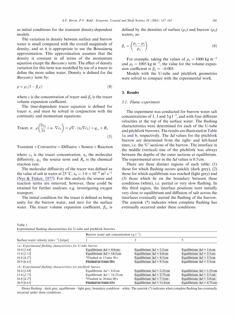
Plotting the interface depth difference, Dd, at equilib-rium for the model against theoretical prediction (Fig. 6)

Fig. 4. Scatter plot offfiffiffiffiffiffiffiffiffiffiffiffiDqDd

pvs m from experimental data. The

straight line slope is 2.55.

shows that the model over-predicts the theory by 33%,compared with 10% for the flume tank. This difference ismost likely due to the different turbulent roughnessparameters in the flume and model (automated defini-tion). However, this is a secondary effect compared withthe pressure difference due to the slope, which is theprimary influence upon the flushing properties of theburrows. While this difference is significant, the consis-tency between the model and experiment in predictingwhether a burrow will flush remains. Future work willattempt to overcome this variation using a differentmethod for turbulence definition.

The CFD models were also run for the pitchforkburrow geometry, and the results are summarised inTable 2b. Density differences of 1, 2 and 3 kgm�3 weremodelled to compare flushing rates with those of theU-tube geometry. The higher density differences werenot re-modelled as they were expected to reach equili-brium for all slope values, as for the U-tube burrow.

If these results are compared with those of the U-tube(Table 2a), the consistency in the distinction between thethree regions can again be seen. The pitchfork flushingtimes are slightly greater in general, in comparison withthe U-tube, which is probably reflective simply of theincrease in volume of the burrow. The interface depthdifference, Dd, is also slightly greater for the pitchforkthan for the U-tube. This may be attributed to theincrease in friction in the burrow region, due to theadditional opening; hence an increase in the localisedslope, and thus the Dd value. From comparison of theresults for the different geometries of experimental andcomputational approaches, it is clear that there is no

Fig. 5. Interface depth difference, Dd, at equilibrium. Experimental

values plotted against theoretical values. The straight line slope is 1.10.

143S.F. Heron, P.V. Ridd / Estuarine, Coastal and Shelf Science 58 (2003) 137–145

advantage to the flushing in having the additionalsurface opening.

3.3. CFD: small-scale processes

From the models insight can be gained into small-scale processes that cannot be accurately observed. For

Fig. 6. Interface depth difference, Dd, at equilibrium. CFD model

values plotted against theoretical values. The straight line slope is 1.33.

situations where equilibrium is reached, the modelshows the surface water plume moving down theupstream opening of the burrow towards the equilib-rium point. The inertia of the flushing motion causesthe pressure equilibrium to be passed. This causes theburrow flow to reverse until the equilibrium is againovershot, but to a lesser extent, and the burrow waterflow is again in the forward direction. This oscillatorymotion continues until the equilibrium is attained.

This damped oscillation effect in animal burrows wasdescribed in Ridd (1996) and used to determine thefriction to the flow of the burrow walls. Ridd (1996)perturbed a filled burrow and then considered theposition of the interface between water and air whichfollowed the damped oscillation equation:

x¼ e�t=sðA cos xtþB sin xtÞ ð8Þ

where x is the interface position about the equilibriumposition, t the time, s the characteristic decay time of theoscillation and x is the angular frequency of the oscilla-tion. A and B are arbitrary constants.

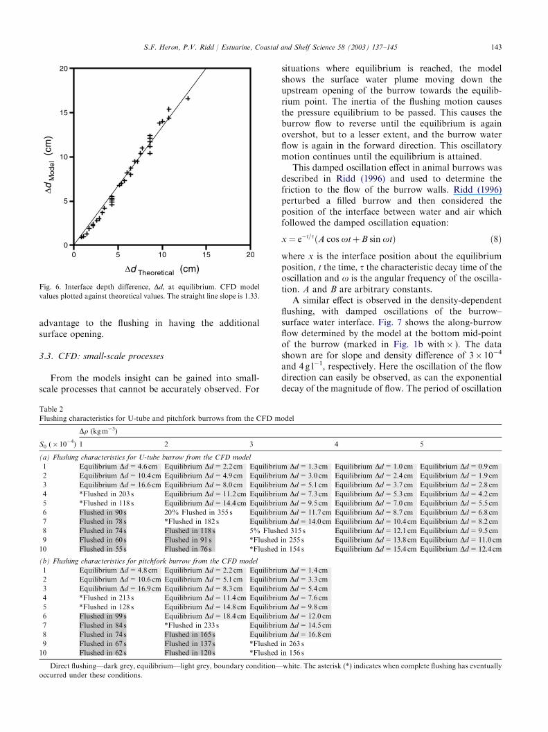
A similar effect is observed in the density-dependentflushing, with damped oscillations of the burrow–surface water interface. Fig. 7 shows the along-burrowflow determined by the model at the bottom mid-pointof the burrow (marked in Fig. 1b with� ). The datashown are for slope and density difference of 3� 10�4

and 4 g l�1, respectively. Here the oscillation of the flowdirection can easily be observed, as can the exponentialdecay of the magnitude of flow. The period of oscillation

Table 2

Flushing characteristics for U-tube and pitchfork burrows from the CFD model

S0 (� 10�4)

Dq (kgm�3)

1 2 3 4 5

(a) Flushing characteristics for U-tube burrow from the CFD model

1 Equilibrium Dd=4.6 cm Equilibrium Dd=2.2 cm Equilibrium Dd=1.3 cm Equilibrium Dd=1.0 cm Equilibrium Dd=0.9 cm

2 Equilibrium Dd=10.4 cm Equilibrium Dd=4.9 cm Equilibrium Dd=3.0 cm Equilibrium Dd=2.4 cm Equilibrium Dd=1.9 cm

3 Equilibrium Dd=16.6 cm Equilibrium Dd=8.0 cm Equilibrium Dd=5.1 cm Equilibrium Dd=3.7 cm Equilibrium Dd=2.8 cm

4 *Flushed in 203 s Equilibrium Dd=11.2 cm Equilibrium Dd=7.3 cm Equilibrium Dd=5.3 cm Equilibrium Dd=4.2 cm

5 *Flushed in 118 s Equilibrium Dd=14.4 cm Equilibrium Dd=9.5 cm Equilibrium Dd=7.0 cm Equilibrium Dd=5.5 cm

6 Flushed in 90 s 20% Flushed in 355 s Equilibrium Dd=11.7 cm Equilibrium Dd=8.7 cm Equilibrium Dd=6.8 cm

7 Flushed in 78 s *Flushed in 182 s Equilibrium Dd=14.0 cm Equilibrium Dd=10.4 cm Equilibrium Dd=8.2 cm

8 Flushed in 74 s Flushed in 118 s 5% Flushed 315 s Equilibrium Dd=12.1 cm Equilibrium Dd=9.5 cm

9 Flushed in 60 s Flushed in 91 s *Flushed in 255 s Equilibrium Dd=13.8 cm Equilibrium Dd=11.0 cm

10 Flushed in 55 s Flushed in 76 s *Flushed in 154 s Equilibrium Dd=15.4 cm Equilibrium Dd=12.4 cm

(b) Flushing characteristics for pitchfork burrow from the CFD model

1 Equilibrium Dd=4.8 cm Equilibrium Dd=2.2 cm Equilibrium Dd=1.4 cm

2 Equilibrium Dd=10.6 cm Equilibrium Dd=5.1 cm Equilibrium Dd=3.3 cm

3 Equilibrium Dd=16.9 cm Equilibrium Dd=8.3 cm Equilibrium Dd=5.4 cm

4 *Flushed in 213 s Equilibrium Dd=11.4 cm Equilibrium Dd=7.6 cm

5 *Flushed in 128 s Equilibrium Dd=14.8 cm Equilibrium Dd=9.8 cm

6 Flushed in 99 s Equilibrium Dd=18.4 cm Equilibrium Dd=12.0 cm

7 Flushed in 84 s *Flushed in 233 s Equilibrium Dd=14.5 cm

8 Flushed in 74 s Flushed in 165 s Equilibrium Dd=16.8 cm

9 Flushed in 67 s Flushed in 137 s *Flushed in 263 s

10 Flushed in 62 s Flushed in 120 s *Flushed in 156 s

Direct flushing—dark grey, equilibrium—light grey, boundary condition—white. The asterisk (*) indicates when complete flushing has eventually

occurred under these conditions.

144 S.F. Heron, P.V. Ridd / Estuarine, Coastal and Shelf Science 58 (2003) 137–145

is observed to be 21 s, which corresponds to an angularfrequency of x ¼ 0:29 s�1. The decay time of thedamped oscillation, i.e. the time to decay the oscillationamplitude by a factor of 1/e (0.37), is seen to be 23 s. Astime proceeds the model shows that the system movestowards a state of equilibrium. The period and decaytime observed by Ridd (1996) were of the order of 2 and3 s, respectively. The variation from these values is dueto the large differences in the burrow length anddiameter.

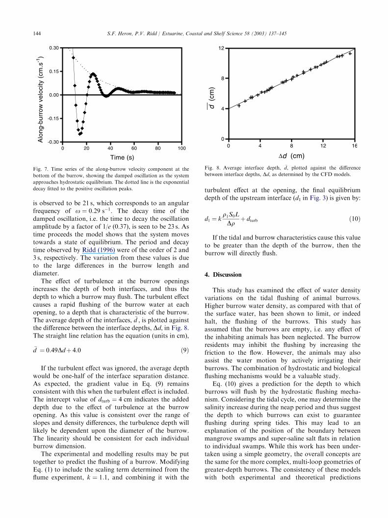
The effect of turbulence at the burrow openingsincreases the depth of both interfaces, and thus thedepth to which a burrow may flush. The turbulent effectcauses a rapid flushing of the burrow water at eachopening, to a depth that is characteristic of the burrow.The average depth of the interfaces, d�, is plotted againstthe difference between the interface depths, Dd, in Fig. 8.The straight line relation has the equation (units in cm),

d� ¼ 0:49Ddþ 4:0 ð9Þ

If the turbulent effect was ignored, the average depthwould be one-half of the interface separation distance.As expected, the gradient value in Eq. (9) remainsconsistent with this when the turbulent effect is included.The intercept value of dturb ¼ 4 cm indicates the addeddepth due to the effect of turbulence at the burrowopening. As this value is consistent over the range ofslopes and density differences, the turbulence depth willlikely be dependent upon the diameter of the burrow.The linearity should be consistent for each individualburrow dimension.

The experimental and modelling results may be puttogether to predict the flushing of a burrow. ModifyingEq. (1) to include the scaling term determined from theflume experiment, k ¼ 1:1, and combining it with the

Fig. 7. Time series of the along-burrow velocity component at the

bottom of the burrow, showing the damped oscillation as the system

approaches hydrostatic equilibrium. The dotted line is the exponential

decay fitted to the positive oscillation peaks.

turbulent effect at the opening, the final equilibriumdepth of the upstream interface (d1 in Fig. 3) is given by:

d1 ¼ kq1S0L

Dqþ dturb ð10Þ

If the tidal and burrow characteristics cause this valueto be greater than the depth of the burrow, then theburrow will directly flush.

4. Discussion

This study has examined the effect of water densityvariations on the tidal flushing of animal burrows.Higher burrow water density, as compared with that ofthe surface water, has been shown to limit, or indeedhalt, the flushing of the burrows. This study hasassumed that the burrows are empty, i.e. any effect ofthe inhabiting animals has been neglected. The burrowresidents may inhibit the flushing by increasing thefriction to the flow. However, the animals may alsoassist the water motion by actively irrigating theirburrows. The combination of hydrostatic and biologicalflushing mechanisms would be a valuable study.

Eq. (10) gives a prediction for the depth to whichburrows will flush by the hydrostatic flushing mecha-nism. Considering the tidal cycle, one may determine thesalinity increase during the neap period and thus suggestthe depth to which burrows can exist to guaranteeflushing during spring tides. This may lead to anexplanation of the position of the boundary betweenmangrove swamps and super-saline salt flats in relationto individual swamps. While this work has been under-taken using a simple geometry, the overall concepts arethe same for the more complex, multi-loop geometries ofgreater-depth burrows. The consistency of these modelswith both experimental and theoretical predictions

Fig. 8. Average interface depth, d�, plotted against the difference

between interface depths, Dd, as determined by the CFD models.

145S.F. Heron, P.V. Ridd / Estuarine, Coastal and Shelf Science 58 (2003) 137–145

provides confidence in the results of future models withmore complex burrow structures. Using these tech-niques, computer simulations assist our understandingof the flushing process.

Acknowledgements

Thanks to Suzanne Hollins, Mal Heron and IanWebster for their assistance in the preparation of themanuscript. The manuscript was revised while S.F.H.was visiting Penn State Altoona.

References

Allanson, B. R., Skinner, D., & Imberger, J. (1992). Flow in prawn

burrows. Estuarine, Coastal and Shelf Science 35, 253–266.

Aucan, J., & Ridd, P. V. (1999). Tidal asymmetry in creeks surrounded

by salt flats and mangroves with small swamp slopes. Mangroves

and Salt Marshes 69, 1–10.

Bode, L., Mason, L. B., & Middleton, J. H. (1997). Reef parameter-

isation schemes with applications to tidal modelling. Progress in

Oceanography 40, 285–324.

Fluid Dynamics International. (1993). Fluid dynamics analysis package

v7.0 theory manual. Evanston, IL: FDI.

Furukawa, K., Wolanski, E., & Mueller, H. (1997). Currents and

sediment transport in mangrove forests. Estuarine, Coastal and

Shelf Science 44, 301–310.

Heron, S., & Ridd, P. V. (2001). The use of computational fluid

dynamics in predicting the flushing of animal burrows. Estuarine,

Coastal and Shelf Science 52, 411–421.

Hollins, S., & Ridd, P. The concentration and consumption of oxygen

in large animal burrows in tropical mangrove swamps. Estuarine,

Coastal and Shelf Science, in press.

Hollins, S., Ridd, P. V., & Read, W. W. (1999). Measurement of the

diffusion coefficient for salt in salt flat and mangrove soils.

Mangroves and Salt Marshes 73, 1–6.

Nye, P. H., & Tinker, B. (1977). Solute movement in the soil–root system

(pp. 69–91). Oxford: Blackwell.

Ridd, P. V. (1996). Flow through animal burrows in mangrove creeks.

Estuarine, Coastal and Shelf Science 43, 617–625.

Stieglitz, T., Ridd, P., & Muller, P. (2000). Passive irrigation and

functional morphology of crustacean burrows in a tropical man-

grove swamp. Hydrobiologia 421, 69–76.

Street, R. L., Watters, G. Z., & Vennard, J. K. (1996). Elementary fluid

mechanics (7th ed., 757 pp.). New York, NY: Wiley.

Webster, I. T. (1992). Wave enhancement of solute exchange within

empty burrows. Limnology and Oceanography 37, 630–643.

Wolanski, E., Mazda, Y., & Ridd, P. (1992). Mangrove hydrodynam-

ics. In A. Robertson, & D. Alongi (Eds.), Tropical mangrove

ecosystems (pp. 43–61). Washington, DC: AGU.

Wolanski, E., & Ridd, P. (1986). Tidal mixing and trapping in man-

grove swamps. Estuarine, Coastal and Shelf Science 23, 759–771.