The effect of temperature and fish size on growth of juvenile ...

NORWEGIAN COLLEGE OF FISHERIES SCIENCE

The effect of temperature and fish size on growth of juvenile lumpfish (Cyclopterus lumpus L.)

Ane Vigdisdatter Nytrø

Master's Degree Thesis in Fisheries Science

Field of Study - Aquaculture Biology - (60 credits) August 2013

1

Preface

This thesis was written in the period August 2012 – August 2013, aided by supervisors,

friends and colleagues who each and all deserve my greatest gratitude. First of all, to my

supervisor, professor Albert Kjartansson Imsland who spent dark hours guiding me through

the jungle of articles, temperature optimums and statistical obstacles, a great thank you for all

your help and motivation. To my other supervisor, professor Inger-Britt Falk-Petersen, thank

you for your patience, your feedback and your helpful guidance, and to Dr. Atle Foss for

shipping in from Bergen to teach me how to pit-tag and sample my 348 new found pets. To

the ladies in the office and to the boys at Troms Marin Yngel; I could not have done without

you!

Kjørsvikbugen, 10. Augsut 2013.

Ane Vigdisdatter Nytrø.

3

Contents

ABSTRACT ......................................................................................................................... 5

1. INTRODUCTION ........................................................................................................... 6

1.1 THE ROLE OF CLEANER-FISH IN AQUACULTURE ............................................................... 6

1.2 THE LUMPFISH............................................................................................................... 7

1.3 LUMPFISH, A SPECIES SUITED FOR AQUACULTURE? ......................................................... 8

1.4 GROWTH AND FEEDING IN JUVENILE MARINE SPECIES ..................................................... 8

1.5 THE PHYSIOLOGY OF TEMPERATURE RELATED GROWTH IN JUVENILE FISH ..................... 10

1.6 OBJECTIVES ................................................................................................................ 10

2. MATERIALS AND METHODS ................................................................................... 11

2.1 FISH STOCK AND REARING CONDITIONS ........................................................................ 11

2.2 EXPERIMENTAL DESIGN ............................................................................................... 13

2.3 GROWTH AND FEED CALCULATIONS ............................................................................. 16

2.4 STATISTICAL METHODS ............................................................................................... 17

3. RESULTS ...................................................................................................................... 19

3.1 EXPERIMENT 1 ............................................................................................................ 19

3.1.1 Mortality .............................................................................................................. 19

3.1.2 Effects of temperature on growth ......................................................................... 19

3.1.3 Effect of fish size on growth ................................................................................. 24

3.1.4 Size and growth ranking ...................................................................................... 25

3.2 EXPERIMENT 2 ............................................................................................................ 27

3.2.1 Mortality .............................................................................................................. 27

3.2.2 Effect of temperature on feed utilization ............................................................... 27

4. DISCUSSION ................................................................................................................ 28

4.1 THE EFFECT OF TEMPERATURE ON GROWTH .................................................................. 28

4.2 SIZE-RELATED GROWTH AND OPTIMUM TEMPERATURES FOR GROWTH ........................... 29

4.3 GROWTH EFFECTS IN TERMS OF Q10 .............................................................................. 33

4.4 SIZE RANK – CORRELATION.......................................................................................... 33

4.5 EFFECT OF TEMPERATURE ON FEED RELATED PARAMETERS ........................................... 34

5. CONCLUSIONS ............................................................................................................ 38

4

REFERENCES .................................................................................................................. 39

APPENDIX I - DISCUSSION OF MATERIAL AND METHODS................................. 45

FISH STOCK....................................................................................................................... 45

Rearing conditions ....................................................................................................... 45

Size hierarchies ............................................................................................................ 46

Mortality ...................................................................................................................... 47

Possible secondary effects of photoperiod .................................................................... 47

Feed-related parameters .............................................................................................. 48

APPENDIX II - TABLES .................................................................................................. 50

1. DESCRIPTIVE STATISTICS ............................................................................................... 50

1.1 Experimental conditions ......................................................................................... 50

2. RESPONSE VARIABLES ................................................................................................... 53

3. ANOVA ....................................................................................................................... 55

3.1 Two-way nested ANOVA ......................................................................................... 55

3.2 One-way ANOVA .................................................................................................... 60

4. STUDENT-NEWMAN-KEULS TEST .................................................................................. 60

5. ANCOVA .................................................................................................................... 66

6. LEVENE’S TEST FOR HOMOGENEITY OF VARIANCE .......................................................... 68

7. SPEARMAN RANK CORRELATION .................................................................................... 69

8. Q10 TEMPERATURE EFFECT ON SPECIFIC GROWTH RATE .................................................. 70

9. KOLOMGOROV-SMIRNOV TESTS FOR NORMALITY ........................................................... 71

APPENDIX III - THE LUMPFISH .................................................................................. 73

GENERAL LUMPFISH BIOLOGY ........................................................................................... 73

DISTRIBUTION .................................................................................................................. 74

SPAWNING BEHAVIOR ....................................................................................................... 74

FEEDING, HABITAT PREFERENCES AND MIGRATIONS OF LARVAL- AND JUVENILE LUMPFISH .. 76

FEEDING, HABITAT PREFERENCES AND MIGRATIONS OF ADULT LUMPFISH ........................... 77

STOCK SIZE AND FISHERIES................................................................................................ 78

APPENDIX IV – MEAN WEIGHTS – EXPERIMENT 2 ............................................... 80

5

Abstract

The aim of this study was to investigate the effect of temperature and fish size on growth

response and feeding parameters of juvenile Atlantic lumpfish Cyclopterus Lumpus L. Two

experiments were carried out, experiment 1 with emphasis on temperature related growth and

experiment 2 as a satellite group to examine the effect of temperature on feeding parameters.

On 11 April 2013 a number of 348 juvenile lumpfish (mean initial weight 26.5 g, S.E. ± 0.6)

were individually tagged and randomly distributed alongside a sub-group of 337 untagged

specimens (mean initial weight 21.9 g, S.E. 0.04) between 10 experimental units. This

produced the outline for experiment 1 and further growth analysis. Fish were adapted to

temperatures of 4, 7, 10, 13 °C and ambient (average temperature 5.8 °C, S.E. ± 0.04) before

rearing at constant temperature throughout the experimental period. Experiment 2 consisted of

241 unmarked fish (mean initial weight 46.7 g, S.E. ± 1.0) reared at ambient temperature

(average temperature 5.8 °C, S.E. ± 0.04) and 13 °C in two replicate groups for each

temperature (n = 60 per replicate group). Feed was collected to estimate feeding parameters

for each temperature group.

Higher temperatures increased final weight and length, overall specific growth factor and feed

intake, but minor effects were observed for feed conversion efficiency between the two

treatment groups of experiment 2. The optimal temperature for growth decreased with

increasing size. The negative effect of suboptimal temperatures was most significant for the

highest temperatures 10 and 13 °C with increasing weight.

This study demonstrated that temperatures 7, 10 and 13 °C for weight classes 25 – 200 g

induces an overall increase in growth for juvenile lumpfish relative to that of temperatures of

ambient and 4 °C. An ontogenetic shift in temperature preference for growth with increasing

size was observed. The results indicate that an increase in temperature does not have any

significant effect on feed utilization and that temperatures below ambient (5.8 °C, S.E. ± 0.4)

restricts growth.

6

1. Introduction

The production of Atlantic salmon Salmo salar (L.) in Norway reached 1.5 million tons in

2009, making Norway the greatest producer of captive Atlantic salmon in the world

(Torrissen et al. 2011). The parasitic sea louse Lepeophteirus salmonis (Krøyer) has been

reported to cause increased cortisol levels, alterations in physiological homeostasis, osmotic

imbalance and mortality in salmonids (Grimnes & Jakobsen 1996; Bjorn et al. 2001; Heuch et

al. 2005; Sivertsgard et al. 2007) and salmon farms are assumed to be among the main causes

of mortality in juvenile wild salmonids, constituting a contributing factor to decreasing stocks

of wild fish (Bjorn et al. 2001; Krkosek et al. 2007; Costello 2009). The high concentration of

potential hosts for lice in sea pens has been a problem since the onset of the salmon farming

industry in the 1970s. Attempts to reduce the concentration of lice in sea pens has been a main

goal ever since, not only as an economic concern, but also in terms of animal welfare and

potential costs for the eco-system (Brandal et al. 1976; McVicar 1997; Asche et al. 2005;

Krkosek et al. 2006). Due to the persistence of re-infections of sea louse, efficient control

management strategies are hard to find (McVicar 2004). Today the density of lice is mainly

regulated by the aid of chemoterapeutants, but increasing resistance to delousing agents such

as avermectins (SLICE ®) (Burridge et al. 2010), organophosphates (Salmosan ®) (Fallang et

al. 2004) and pyrethroids (Excis ®, Betamax ® and AlphaMax ®) (Sevatdal & Horsberg

2003; Burridge et al. 2010) is an emerging problem in aquaculture (Jimenez et al. 2012).

Furthermore, such medical treatments are often expensive (Costello 2009), stressful to fish

(Burka et al. 1997) and hazardous to the environment (Burridge et al. 2010).

1.1 The role of cleaner-fish in aquaculture

The biological control of sea lice through the use of “cleaner fish” has recently become a

feasible option due to the increased occurrence of resistant lice, the reduced public acceptance

of the use of chemotherapeutants in food production and the urgent need for an effective and

sustainable method of parasite control in Atlantic salmon aquaculture (Denholm et al., 2002;

Treasurer, 2002). Today cleaner-fish present the only environmentally friendly alternative to

chemical de-lousing of salmonids (Cowx et al. 1998; Treasurer 2002). Their use has a lower

impact on the environment, reduces cortisol levels of farmed fish, and is often found to be a

cheaper alternative to chemical treatments (Treasurer 2002). Cleaner fish have been utilized

7

as a predator of sea louse in salmon net pens for several years, efficiently grazing on ecto-

parasites; mobile pre-adult and adult lice (Groner et al. 2013). In northern parts of Norway

low temperatures are a challenge for cleaner fish species such as ballan wrasse (Labrus

bergylta, Asxanius) and goldsinny wrasse (Ctenolabrus rupestris, L.), limiting their

distribution in northern waters (Cowx et al. 1998; Lein et al. 2013). Furthermore, Lein et al.

(2013) showed a decrease in the appetite of ballan wrasse for lice with decreasing

temperatures. This calls for an alternative cleaner-fish species with a natural northern

distribution and a better adaptation to cold temperatures. Observations from pilot experiments

have indicated that juvenile lumpfish, Cyclopterus lumpus (L.) potentially will graze on pre-

adult and adult stages of sea lice attached to salmon (Willumsen 2001; Andersen & Vestvik

2012; GIFAS 2012).

1.2 The lumpfish

The lumpfish is a scale-less, short and thick fish, easily distinguishable by their high dorsal

crest, which covers the first dorsal fin entirely. The pelvic fins are modified to constitute a

ventral suction disc, allowing specimens to rest on vegetation, rocky substrate and algae

(Bigelow & Schroeder 1953; Davenport 1985).

The species is commonly found in the arctic margins of the North Atlantic; in the east from

80° north off Spitsbergen and Nova Zemlya in the north to Portugal in the south. In the west

the species has been frequently found along the coasts of America from Cape Cod to Canada

and the coasts of Greenland 70° north in the north-west (Cox & Anderson 1922; Andrijasev

1964; Blacker 1983). The migratory behavior of lumpfish is similar to that of coastal benthic

teleosts, but adults are also frequently found mid-water in open oceans outside the spawning

season (Cox & Anderson 1922; Andrijasev 1964; Myrseth 1971; Davenport & Kjorsvik

1986). As a semi-pelagic species, it spends most of its life at offshore feeding grounds at deep

water before conducting an active migration over great distances towards shallow coastal

waters to spawn between winter and early spring (Myrseth 1971; Blacker 1983; Davenport

1985; Goulet et al. 1986; Holst 1993; Mitamura et al. 2012).

The first one to two years post hatch juveniles spend summer and autumn in the upper surface

waters of tide pools in the intertidal zone (Moring 1990) but some juveniles have also been

8

observed at deep sea (Daborn & Gregory 1983; Davenport 1985). Tide pools offer the young

shelter and food in the form of seaweed, other algae and a fluctuating availability of prey

between tidal cycles (Moring 1990). Juveniles are typically observed in association to algae,

either attached or nearby. Algae are shelter to harpacticoids, a preferred prey species of

juvenile lumpfish among planktonic animals and phytal species (Ingolfsson & Kristjansson

2002). As they outgrow the protective shelters of tide pools at 4-5 cm they are forced to

migrate to deeper water to avoid predations (Moring 1990; Albert 2000), decreasing water

temperatures and hence declining availability of algae (Moring 1990). The Norwegian sea is

believed to be an important nursery area for lumpfish originating from spawning grounds off

the North Atlantic coast (Holst 1993).

1.3 Lumpfish, a species suited for aquaculture?

Attempts to breed lumpfish to produce spawning fish for roe were attempted by Klokseth and

Øiestad (1999) and Haaland (1996). Early pilot scale experiments confirmed that adult

lumpfish could with ease be reared and would spawn in captivity (Klokseth & Øiestad 1999;

Andersen & Vestvik 2012), but that further research was needed to obtain better results in

terms of growth (Benfey & Methven 1986; Havforskningsinstituttet 2003). Despite these

results, most research on lumpfish has mainly been focused on wild populations for

documenting the spawning migrations, its peculiar spawning behavior and larval- and juvenile

trade-offs in foraging behavior, as these factors have been of concern to lumpfish roe fisheries

(Holst 1993; Torstensen 1998; Sunnanå 2007a). An early attempt to create a production

protocol for the domestication of lumpfish has been piloted by Schaer and Vestvik (2012) for

Arctic Cleanerfish AS.

1.4 Growth and feeding in juvenile marine species

Foraging-predator tradeoffs and feeding behavior have been discussed for juvenile lumpfish

in the wild (Moring 1989; Ingolfsson & Kristjansson 2002), but little effort has been spent on

estimating the growth efficiency of the juvenile lumpfish in captivity. The metabolic cost of

foraging and trade-off strategies in juvenile and larval lumpfish has been discussed (Brown et

9

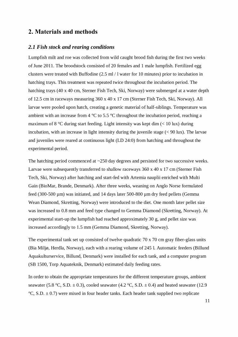
al. 1997; Killen et al. 2007; Jobling et al. 2012), but with an emphasis on live feeds rather

than formulated.

According to Jobling (1997) the preferred temperature of a species is often closer to the

temperature optimum for growth rather than the optimal temperature for food consumption

and – conversion. The temperature-related growth rates of juvenile fish have been studied for

several marine species including spotted wolfish Anarhichas minor (Òlafson) (Imsland et al.

2006), cod Gadus morhua (L.) (Bjornsson et al. 2001; Imsland et al. 2005), turbot

Scophthalmus maximus (L.) (Imsland et al. 2007a), halibut Hippoglossus hippoglossus (L.)

(Hallaraker et al. 1995; Jonassen et al. 1999), plaice Pleuronectes platessa (L.) and flounder

Platichthys flesus (L.) (Fonds et al. 1992).

Temperatures above that of the temperature optimum for growth rapidly decreases the

specific growth rate in several species. Growth rates for juveniles have commonly been found

to follow a bell shaped curve for several species, with increasing growth (SGR % day-1

) until

reaching a maximum at the temperature optimum and decreases rapidly with further increase

in temperature (Otterlei et al. 1999; Bjornsson et al. 2001). Furthermore, an ontogenetic shift

in optimum temperatures for growth can be observed in several species. Investigating specific

growth rates and feed conversion ratios enables us to examine the optimal temperature for

ingested food used for growth. The close relationship between ingestion rate and growth rate

should also be stressed, as growth is also determined by food supply (Jobling 1997).

Land based aquaculture utilizes the possibility of maximizing the effect of temperature

manipulation on growth and feed efficiency. Optimal temperatures for growth rates have been

shown to be higher than the temperature optimum for ingestion rate (Jobling 1997). Finding

the temperature optimums for the two factors is hence crucial to increase production

efficiency, as temperature is interpreted as the most important external factor for growth

(Brett & Groves 1979; Jobling 1997).

10

1.5 The physiology of temperature related growth in juvenile fish

Increasing temperature causes two main counteracting effects on growth:

1. Increase in the energy cost for maintenance metabolism, hence decreasing the scope

for growth.

2. Increase in the efficiency of food energy transformation to net energy (Brett &

Groves 1979; Elliott 1982; Pörtner et al. 2001; Van Ham et al. 2003), thus increasing

the scope for growth.

Temperatures have a secondary effect in terms of increasing oxygen consumption at high

temperatures (Hallaraker et al. 1995; Jonassen et al. 2000b), and causes energy costs to

decrease at continuous light and at lower temperatures (Imsland & Jonassen 2001). In terms

of feed costs a maximum- and maintenance ration (Rmax and Rmaint, respectively) can be

established, defining the available energy for somatic growth and metabolic functions. Rmax

and Rmaint both decrease with increasing fish size, but Rmaint at a slower rate than Rmax,

reducing the available energy for somatic growth (Brett & Groves 1979). This causes more

developed specimens to allocate energy mainly for maintenance purposes (Rmaint), while

younger have a larger capacity for distributing energy towards growth. At higher temperatures

the increased metabolic rates will eventually exceed that of possible gain by the means of

increased food intake (Hallaraker et al. 1995; Jonassen et al. 2000b) which in the end will

reduce the final possible growth rate (Jonassen et al. 1999). These factors yield the dome

shaped curve for Topt FCE and Topt SGR observed for juvenile fish of several marine species

(Fonds et al. 1992; Bjornsson & Tryggvadottir 1996; Jonassen et al. 1999; Otterlei et al. 1999;

Bjornsson et al. 2001; Imsland et al. 2005; Imsland et al. 2006).

1.6 Objectives

In the following described experiments the effects of temperature on growth and feed

conversion efficiency of juvenile lumpfish were studied. The main objective of the current

study was to compare growth- related parameters between juvenile fish at temperatures of 4,

7, 10 , 13 °C and ambient temperature (5.8 °C ± S.D. 0.3). Furthermore, a satellite study was

carried out with an subordinate objective of comparing feed utilization at ambient temperature

(5.8 °C ± S.D. 0.1) and 13 °C.

11

2. Materials and methods

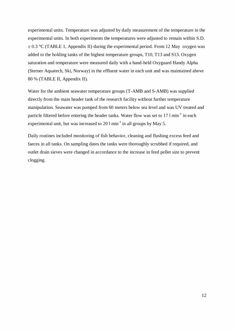
2.1 Fish stock and rearing conditions

Lumpfish milt and roe was collected from wild caught brood fish during the first two weeks

of June 2011. The broodstock consisted of 20 females and 1 male lumpfish. Fertilized egg

clusters were treated with Buffodine (2.5 ml / l water for 10 minutes) prior to incubation in

hatching trays. This treatment was repeated twice throughout the incubation period. The

hatching trays (40 x 40 cm, Sterner Fish Tech, Ski, Norway) were submerged at a water depth

of 12.5 cm in raceways measuring 360 x 40 x 17 cm (Sterner Fish Tech, Ski, Norway). All

larvae were pooled upon hatch, creating a genetic material of half-siblings. Temperature was

ambient with an increase from 4 °C to 5.5 °C throughout the incubation period, reaching a

maximum of 8 °C during start feeding. Light intensity was kept dim (< 10 lux) during

incubation, with an increase in light intensity during the juvenile stage (< 90 lux). The larvae

and juveniles were reared at continuous light (LD 24:0) from hatching and throughout the

experimental period.

The hatching period commenced at ~250 day degrees and persisted for two successive weeks.

Larvae were subsequently transferred to shallow raceways 360 x 40 x 17 cm (Sterner Fish

Tech, Ski, Norway) after hatching and start-fed with Artemia nauplii enriched with Multi

Gain (BioMar, Brande, Denmark). After three weeks, weaning on Anglo Norse formulated

feed (300-500 µm) was initiated, and 14 days later 500-800 µm dry feed pellets (Gemma

Wean Diamond, Skretting, Norway) were introduced to the diet. One month later pellet size

was increased to 0.8 mm and feed type changed to Gemma Diamond (Skretting, Norway). At

experimental start-up the lumpfish had reached approximately 30 g, and pellet size was

increased accordingly to 1.5 mm (Gemma Diamond, Skretting, Norway).

The experimental tank set up consisted of twelve quadratic 70 x 70 cm gray fiber-glass units

(Bia Miljø, Herdla, Norway), each with a rearing volume of 245 l. Automatic feeders (Billund

Aquakulturservice, Billund, Denmark) were installed for each tank, and a computer program

(SB 1500, Torp Aquateknik, Denmark) estimated daily feeding rates.

In order to obtain the appropriate temperatures for the different temperature groups, ambient

seawater (5.8 °C, S.D. ± 0.3), cooled seawater (4.2 °C, S.D. ± 0.4) and heated seawater (12.9

°C, S.D. ± 0.7) were mixed in four header tanks. Each header tank supplied two replicate

12

experimental units. Temperature was adjusted by daily measurement of the temperature in the

experimental units. In both experiments the temperatures were adjusted to remain within S.D.

± 0.3 °C (TABLE 1, Appendix II) during the experimental period. From 12 May oxygen was

added to the holding tanks of the highest temperature groups, T10, T13 and S13. Oxygen

saturation and temperature were measured daily with a hand-held Oxyguard Handy Alpha

(Sterner Aquatech, Ski, Norway) in the effluent water in each unit and was maintained above

80 % (TABLE II, Appendix II).

Water for the ambient seawater temperature groups (T-AMB and S-AMB) was supplied

directly from the main header tank of the research facility without further temperature

manipulation. Seawater was pumped from 60 meters below sea level and was UV treated and

particle filtered before entering the header tanks. Water flow was set to 17 l min-1

in each

experimental unit, but was increased to 20 l min-1

in all groups by May 5.

Daily routines included monitoring of fish behavior, cleaning and flushing excess feed and

faeces in all tanks. On sampling dates the tanks were thoroughly scrubbed if required, and

outlet drain sieves were changed in accordance to the increase in feed pellet size to prevent

clogging.

13

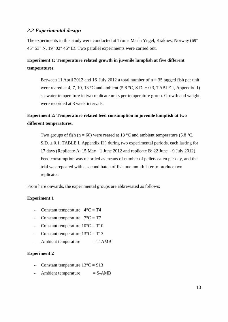
2.2 Experimental design

The experiments in this study were conducted at Troms Marin Yngel, Kraknes, Norway (69°

45" 53" N, 19° 02" 46" E). Two parallel experiments were carried out.

Experiment 1: Temperature related growth in juvenile lumpfish at five different

temperatures.

Between 11 April 2012 and 16

July 2012 a total number of n = 35 tagged fish per unit

were reared at 4, 7, 10, 13 °C and ambient (5.8 °C, S.D. ± 0.3, TABLE I, Appendix II)

seawater temperature in two replicate units per temperature group. Growth and weight

were recorded at 3 week intervals.

Experiment 2: Temperature related feed consumption in juvenile lumpfish at two

different temperatures.

Two groups of fish (n = 60) were reared at 13 °C and ambient temperature (5.8 °C,

S.D. ± 0.1, TABLE I, Appendix II ) during two experimental periods, each lasting for

17 days (Replicate A: 15 May - 1 June 2012 and replicate B: 22 June – 9 July 2012).

Feed consumption was recorded as means of number of pellets eaten per day, and the

trial was repeated with a second batch of fish one month later to produce two

replicates.

From here onwards, the experimental groups are abbreviated as follows:

Experiment 1

- Constant temperature 4°C = T4




- Ambient temperature = T-AMB

Experiment 2

- Constant temperature 13°C = S13

- Ambient temperature = S-AMB

14

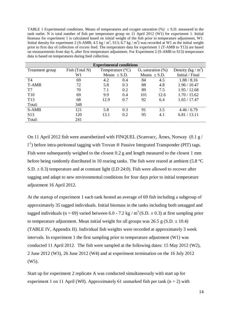
TABLE 1 Experimental conditions. Means of temperatures and oxygen saturation (%) ± S.D. measured in the

tank outlet. N is total number of fish per temperature group on 11 April 2012 (W1) for experiment 1. Initial

biomass for experiment 1 is calculated based on initial weight of the fish prior to temperature adjustment, W1.

Initial density for experiment 2 (S-AMB; 4.5 kg / m3, S13; 6.7 kg / m3) was recorded at W1 as the initial weight

prior to first day of collection of excess feed. The temperature data for experiment 1 (T-AMB to T13) are based

on measurements from day 6, after first temperature adjustment. For Experiment 2 (S-AMB to S13) temperature

data is based on temperatures during feed collection.

Experimental conditions

Treatment group Fish (Total N)

W1

Temperature (°C)

Means ± S.D.

O2 saturation (%)

Means ± S.D.

Density (kg / m3)

Initial / Final

T4 69 4.2 0.4 84 4.5 1.88 / 8.16 T-AMB 72 5.8 0.3 88 4.8 1.96 / 10.47

T7 70 7.1 0.2 89 7.5 1.95 / 12.68

T10 69 9.9 0.4 101 12.6 1.70 / 15.62 T13 68 12.9 0.7 92 6.4 1.65 / 17.47

Total: 348

S-AMB 121 5.8 0.3 91 3.5 4.46 / 6.79

S13 120 13.1 0.2 95 4.1 6.81 / 13.11 Total: 241

On 11 April 2012 fish were anaesthetized with FINQUEL (Scanvacc, Årnes, Norway (0.1 g /

l-1

) before intra-peritoneal tagging with Trovan ® Passive Integrated Transponder (PIT) tags.

Fish were subsequently weighed to the closest 0.2 g and length measured to the closest 1 mm

before being randomly distributed in 10 rearing tanks. The fish were reared at ambient (5.8 °C

S.D. ± 0.3) temperature and at constant light (LD 24:0). Fish were allowed to recover after

tagging and adapt to new environmental conditions for four days prior to initial temperature

adjustment 16 April 2012.

At the startup of experiment 1 each tank hosted an average of 69 fish including a subgroup of

approximately 35 tagged individuals. Initial biomass in the tanks including both untagged and

tagged individuals (n = 69) varied between 6.0 - 7.2 kg / m3 (S.D. ± 0.3) at first sampling prior

to temperature adjustment. Mean initial weight for all groups was 26.5 g (S.D. ± 10.4)

(TABLE IV, Appendix II). Individual fish weights were recorded at approximately 3 week

intervals. In experiment 1 the first sampling prior to temperature adjustment (W1) was

conducted 11 April 2012. The fish were sampled at the following dates: 15 May 2012 (W2),

2 June 2012 (W3), 26 June 2012 (W4) and at experiment termination on the 16 July 2012

(W5).

Start up for experiment 2 replicate A was conducted simultaneously with start up for

experiment 1 on 11 April (W0). Approximately 61 unmarked fish per tank (n = 2) with

15

average initial weights of 25 g (25.3 g, S.D. ± 5.6 g, TABLE III, Appendix II) were selected

at random and anesthetized according to the same methods as stated above, before initial

weighing to the closest 0.2 g. Only one replicate (A) of each temperature group (S-AMB and

S13) was produced at this point. Fish were allowed to adapt to new environments and

temperatures prior to initial weighing on 15 May (W1) and startup of feed collection. During

the adaption period fish were fed to satiation and were offered a continuous feed supply and

reared at continuous light. No excess feed was collected during this period. This procedure

was repeated on the 22 June (W1) when experiment 2 replicate B was initiated. Average

initial weight for the fish in the two replicate units was 25 g (25.1 g, S.D. ± 4.6, TABLE III,

Appendix II) and n = 60 fish per tank.

In experiment 1 fish were fed to satiation and feed was available 24 h daily using automatic

feeders. In experiment 2 fish were fed to satiation between 07:00 and 15:00, and excess feed

pellets collected in a sieve and counted daily at 15:00. Excess feed in the tank was gently

brushed into the outlet, flushed, collected in the sieve and counted. Meal size for the

following day was then adjusted according to the amount of excess feed, and weighed out in

grams.

During the experiments, fish were fed a commercial formulated feed, Amber Neptun ST

(Skretting, Norway). Pellet size was adjusted from 1.5 mm to 3 mm during the trial period

dependent on fish size with the first introduction of 2 mm pellets to all tanks on 7 May in

experiment 1. Pellet size 3 mm was introduced to temperature groups T10 and T13 on 5 July.

At all sampling dates, fish were anaesthetized (FINQUEL, Scanvacc, Årnes, Norway (0.1 g /

l1). All fish were starved 24 hours prior to all samplings.

For tagged fish, individual tag

number was recorded prior to weight-measurements to the nearest 0.2 g and length measured

to the nearest 0.1 cm. All untagged fish were individually weighed to the nearest 0.2 g. After

measurements, fish were allowed to recover before being returned to their respective tank.

For experiment 2 the feed collection period lasted from 15 May (W1) to 1 June (W2) for

replicate A. Feed collection for replicate B lasted from 22 June (W1) to 9 July (W2).

Experiment 2 was terminated on 1 June (Replicate A) and 9 July 2012 (Replicate B) in

relation to the final sampling (W2).

16

2.3 Growth and feed calculations

Specific growth rate (SGR) was calculated according to the following formula (Houde &

Schekter 1981)

SGR = (eg-1) x 100

Where g is the instantaneous growth coefficient defined as:

g = ( ) ( )

where W2 and W1 are mean wet weights for individually tagged fish in

grams at days t2 and t1, respectively.

Geometric mean (GM) weight were calculated using

GM= ( , where W1 and W2 W2 and W1 are mean wet weights for individually

tagged fish in grams at days t2 and t1, respectively.

Total feed consumption (CT) was calculated as:

CT = Fs –Fc

Where Fs is total feed supplied in grams (g) and Fc is total collected excess feed.

Daily feeding rate (F%) was calculated as:

F % = [

] ( )

Where C is total feed consumption per tank in the period, and B1 and B2 are fish biomass (g)

in the tank at days t2 and t1, respectively.

Feed conversion rate (FCE) was calculated as:

17

FCE = ( )

Where C is total feed consumption in the tank for the period, and B1 and B2 are fish biomass

(g) in the tank at days t2 and t1.

Temperature effect on growth (Q10) was calculated according to Houde and Schekter (1981)

and Schmidt-Nielsen (1990):

Q10 = (SGR2 / SGR1)10/(

T2-T1)

Where SGR2 and SGR1 are specific growth rates for two temperature groups where T2 and

T1 are temperatures for the two groups, respectively.

2.4 Statistical Methods

All statistical analyses in this study were done in STATISTICA 10.0 (Statsoft, Inc., 2012).

Normality of distributions was assessed using a Kolmogorov-Smirnov test (Zar 1984) and

homogeneity of variances was tested using Levene’s F-test. The effect of temperature on

weight and SGR was tested using a two-way nested Analysis of Variance (ANOVA) (Zar

1984), where the replicates were nested in temperature treatment groups.

For FCE, F % and CT where only group data existed, a one-way ANOVA was applied.

Significant ANOVA’s were followed by a Student-Newman-Keuls multiple comparison test

(Zar 1984) in order to identify differences among treatments.

Size ranking (initial size rank versus final size rank) was tested using Spearman’s rank

correlation (Zar 1984), where a parabolic regression was used to analyze the relationship

between SGR and temperature. The regression was made using the average growth rates of

tagged fish in three size groups; 25 - 30, 100 - 110 and 160 - 200 g. An equal number of fish

from the same size class at each temperature was selected in terms of individual wet weight in

grams. The optimal temperature for growth (Topt SGR) was calculated as the zero solution to

the first derivate of the parabolic regression. Geometric mean weight versus daily specific

18

growth rate (SGR % day-1

) were analyzed using a two way Analysis of Covariance

(ANCOVA).

A significance level of α = 0.05 was used unless stated otherwise.

19

3. Results

3.1 Experiment 1

3.1.1 Mortality

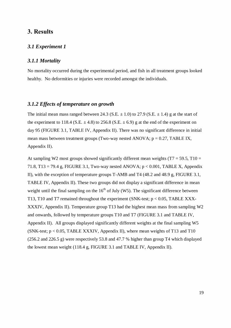
No mortality occurred during the experimental period, and fish in all treatment groups looked

healthy. No deformities or injuries were recorded amongst the individuals.

3.1.2 Effects of temperature on growth

The initial mean mass ranged between 24.3 (S.E. ± 1.0) to 27.9 (S.E. ± 1.4) g at the start of

the experiment to 118.4 (S.E. ± 4.8) to 256.8 (S.E. ± 6.9) g at the end of the experiment on

day 95 (FIGURE 3.1, TABLE ΙV, Appendix II). There was no significant difference in initial

mean mass between treatment groups (Two-way nested ANOVA; p = 0.27, TABLE ΙX,

Appendix ΙΙ).

At sampling W2 most groups showed significantly different mean weights (T7 = 59.5, T10 =

71.8, T13 = 79.4 g, FIGURE 3.1, Two-way nested ANOVA; p < 0.001, TABLE X, Appendix

II), with the exception of temperature groups T-AMB and T4 (48.2 and 48.9 g, FIGURE 3.1,

TABLE IV, Appendix II). These two groups did not display a significant difference in mean

weight until the final sampling on the 16th of July (W5). The significant difference between

T13, T10 and T7 remained throughout the experiment (SNK-test; p < 0.05, TABLE XXX-

XXXIV, Appendix II). Temperature group T13 had the highest mean mass from sampling W2

and onwards, followed by temperature groups T10 and T7 (FIGURE 3.1 and TABLE IV,

Appendix II). All groups displayed significantly different weights at the final sampling W5

(SNK-test; p < 0.05, TABLE XXXIV, Appendix II), where mean weights of T13 and T10

(256.2 and 226.5 g) were respectively 53.8 and 47.7 % higher than group T4 which displayed

the lowest mean weight (118.4 g, FIGURE 3.1 and TABLE IV, Appendix II).

20

Date

Mas

s (g

)

11 April 15 May 2 June 26 June 16 July

0

20

40

60

80

100

120

140

160

180

200

220

240

260

280

ns

a

b

c

d

da

b

c

d

e

a

b

c

d

da

b

c

d

d

T4

T-AMB

T7

T10

T13

FIGURE 3.1. Weight development for juvenile lumpfish reared at five different temperatures (n = 68-72 in each

experimental group).Vertical whiskers indicate standard error of mean ( S.E.) of individually tagged fish.

Results for two replicates are combined. Different letters indicate statistical differences between groups, with “a”

as the highest value. Vertical lines indicating S.E.. may be obscured by symbols.

The same temperature effect was visible for length measurements. Mean lengths ranged from

8.4 (S.E. ± 0.1) to 8.8 cm (S.E. ± 0.2) at the start of the experiment W1 on 11 April to 14.4

(S.E. 0.2) to 18.2 cm (S.E. ± 0.2) at the final sampling W5 at 16 July (FIGURE 3.2 and

TABLE V, Appendix II). No significant difference was found in initial lengths between

treatments (Two-way nested ANOVA; p = 0.47, TABLE XIV, Appendix II).

On 15 May (W2) no significant differences in length were found between temperature groups

T4 and T-AMB (Both groups 10.6 cm (S.E. ± 0.2 / 0.2), FIGURE 3.2 and TABLE V,

Appendix II, SNK-test; p = 0.92, TABLE XXXVI, Appendix II). Lengths for temperature

groups T10 (11.9, S.E. ± 0.2) and T13 ((12.1 cm, S.E. ± 0.1), FIGURE 3.2, TABLE V,

Appendix II) were also insignificantly different to each other (SNK-test; p = 0.27, TABLE

XXXVI, Appendix II).

21

At W3 (2 June) no significant difference was found between mean lengths of temperature

groups T4 and T-AMB (11.7 cm (S.E. ± 0.2) and 11.8 cm (S.E. ± 0.2), FIGURE 3.2, TABLE

V, Appendix II). The two groups had a significantly lower mean length than all other

temperature groups throughout the experimental period (SNK-test; TABLE XXXVI-XXXIX,

Appendix II). After 2 June all groups showed significantly different mean lengths (T4 = 12.9

cm (S.E. ± 0.2), T-AMB = 13.5 cm (S.E. ± 0.2), T7 = 14.9 cm (S.E. ± 0.2), T10 = 15.9 cm

(S.E. ± 0.2), T13 = 16.5 cm (S.E. ± 0.2), FIGURE 3.2, TABLE VI, SNK-test; TABLE

XXXVII-XXXIX, Appendix II).

Date

Len

gth

(cm

)

11 April 15 May 2 June 26 June 16 July

6

8

10

12

14

16

18

20

ns

a

b

c

d

e

a

b

c

d

d

a

a

b

c

c

a

b

c

d

e

T4

T-AMB

T7

T10

T13

FIGURE 3.2. Length development for juvenile lumpfish reared at five different temperatures (n = 348).Vertical

whiskers indicate standard error of mean ( S.E.) of individually tagged fish. Results for two replicates are

combined. Different letters indicate statistical differences between groups, with “a” as the highest value. Vertical

lines indicating S.E may be obscured by symbols.

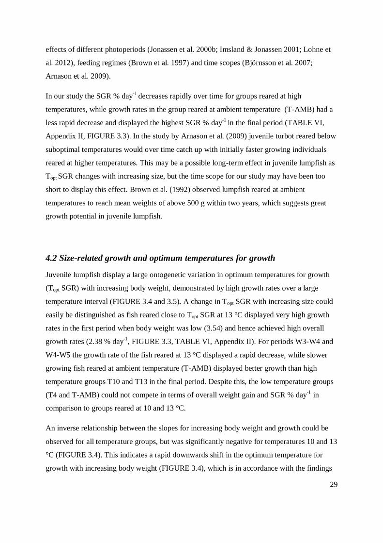
Mean specific growth rates ranged from 1.30 to 3.54 % day-1

(FIGURE 3.3, TABLE VI,

Appendix II). The temperature effect on SGR % day-1

was clearly observable in the first

period 11 April – 15 May (W1 – W2), as most temperature groups were significantly different

to each other with the exception of temperature groups T4 and T-AMB (1.71 and 1.78 % day-

1, FIGURE 3.3, TABLE VI, Appendix II, SNK-test; p = 0.19, TABLE XLI, Appendix II).

Similarly, between 15 May and 2 June all groups displayed significantly different growth

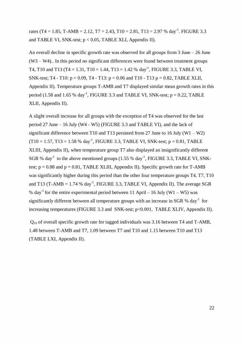
22

rates (T4 = 1.85, T-AMB = 2.12, T7 = 2.43, T10 = 2.81, T13 = 2.97 % day-1

. FIGURE 3.3

and TABLE VI, SNK-test; p < 0.05, TABLE XLI, Appendix II).

An overall decline in specific growth rate was observed for all groups from 3 June – 26 June

(W3 – W4).. In this period no significant differences were found between treatment groups

T4, T10 and T13 (T4 = 1.31, T10 = 1.44, T13 = 1.42 % day-1

, FIGURE 3.3, TABLE VI,

SNK-test; T4 - T10: p = 0.09, T4 - T13: p = 0.06 and T10 - T13 p = 0.82, TABLE XLII,

Appendix II). Temperature groups T-AMB and T7 displayed similar mean growth rates in this

period (1.58 and 1.65 % day-1

, FIGURE 3.3 and TABLE VI, SNK-test; p = 0.22, TABLE

XLII, Appendix II).

A slight overall increase for all groups with the exception of T4 was observed for the last

period 27 June – 16 July (W4 - W5) (FIGURE 3.3 and TABLE VI), and the lack of

significant difference between T10 and T13 persisted from 27 June to 16 July (W1 – W2)

(T10 = 1.57, T13 = 1.58 % day-1

, FIGURE 3.3, TABLE VI, SNK-test; p = 0.81, TABLE

XLIII, Appendix II), when temperature group T7 also displayed an insignificantly different

SGR % day-1

to the above mentioned groups (1.55 % day-1

, FIGURE 3.3, TABLE VI, SNK-

test; p = 0.88 and p = 0.81, TABLE XLIII, Appendix II). Specific growth rate for T-AMB

was significantly higher during this period than the other four temperature groups T4, T7, T10

and T13 (T-AMB = 1.74 % day-1

, FIGURE 3.3, TABLE VI, Appendix II). The average SGR

% day-1

for the entire experimental period between 11 April – 16 July (W1 – W5) was

significantly different between all temperature groups with an increase in SGR % day-1

for

increasing temperatures (FIGURE 3.3 and SNK-test; p<0.001, TABLE XLIV, Appendix II).

Q10 of overall specific growth rate for tagged individuals was 3.16 between T4 and T-AMB,

1.48 between T-AMB and T7, 1.09 between T7 and T10 and 1.15 between T10 and T13

(TABLE LXI, Appendix II).

23

FIGURE 3.3. Specific growth rates (SGR % day-1 ± S.E., n = 68-72, see TABLE VI, Appendix VI) for

individually tagged juvenile lumpfish during the experimental period. The five temperature regimes are

separated by colors as presented. Different letters indicate significant differences between treatments (SNK-test;

p<0.05, TABLE XL – XLIV, Appendix II).

24

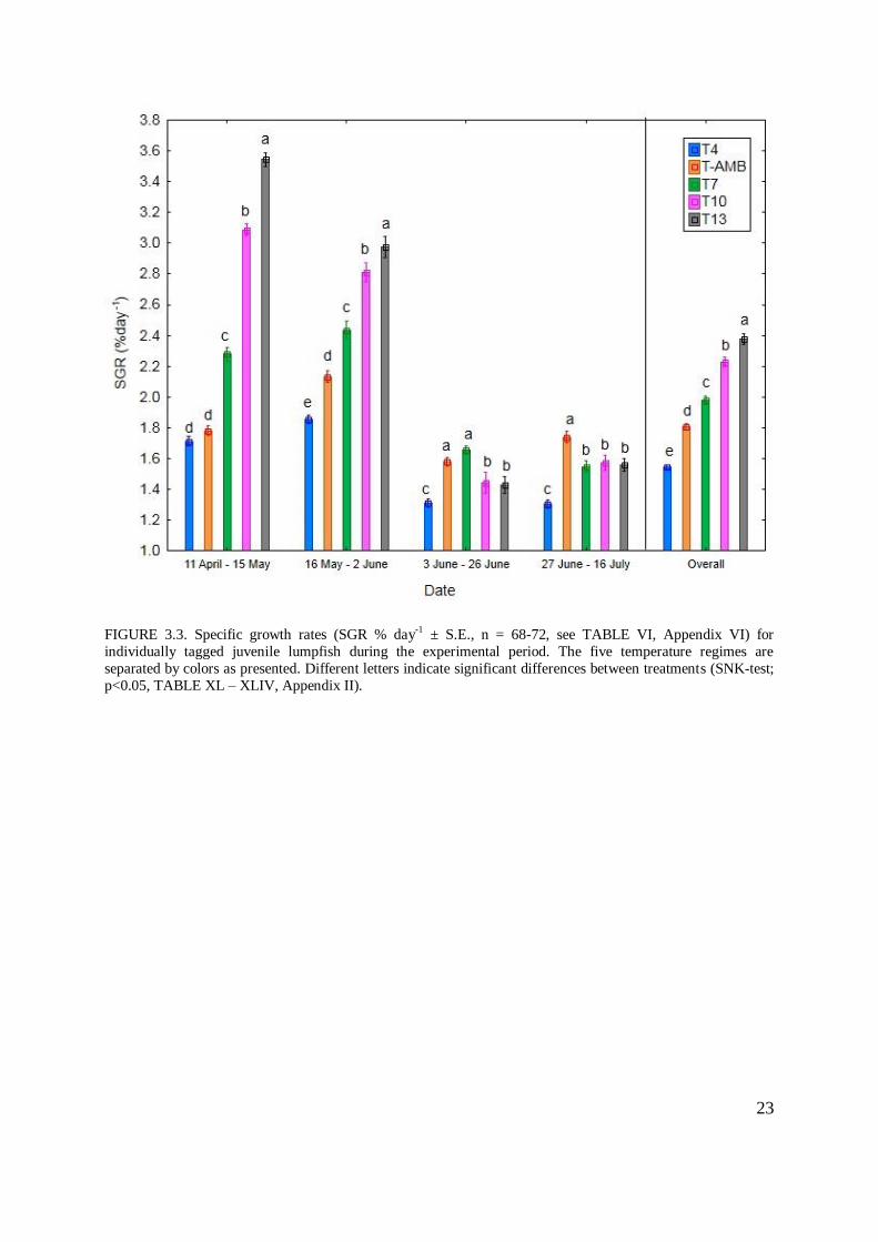
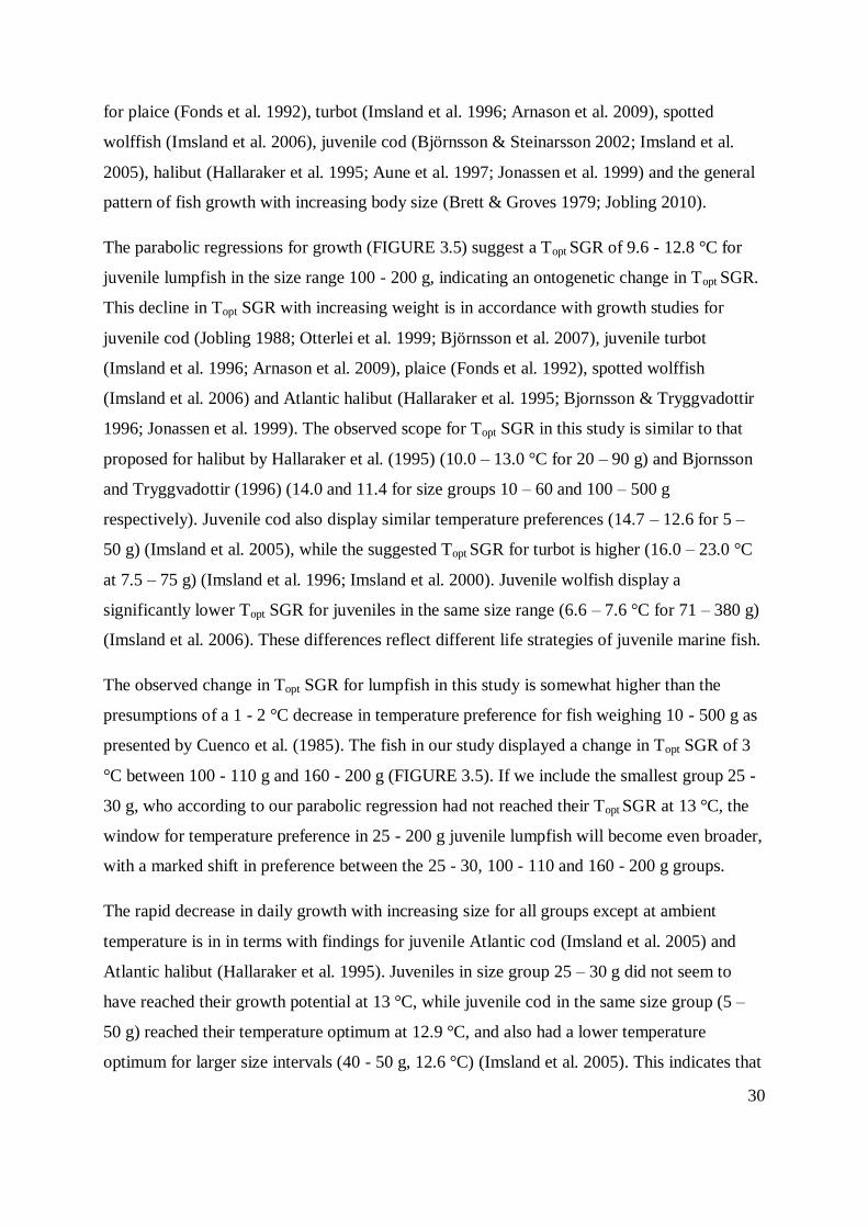
3.1.3 Effect of fish size on growth

Regression lines for SGR was highly correlated to mass (two-way ANCOVA, p<0.001;

TABLE LIII Appendix II) and growth rates declined with body weight for temperature groups

T4, T7, T10 and T13 (linear regression; p = 0.019, p = 0.006, p = 0.004 and p = 0.002,

FIGURE 3.4 (a), (c) and (d)), but was not significant for temperature group T-AMB (linear

regression; p = 0.346, FIGURE 3.4 (b)). The negative effect of increasing weight on SGR %

day-1

was especially pronounced for temperature groups T10 and T13 (FIGURE 3.4 (d) and

(e)). ANCOVA comparisons of linear regressions for T10 and T13 displayed parallel lines for

the two groups (two-way ANCOVA; p = 0.132, TABLE LVII, Appendix II), while regression

lines for temperature groups T4, T-AMB and T7 were non-parallel (two-way ANCOVA,

TABLE LIV – LVI, Appendix II).

Geometric mean mass (g)

SG

R (

% d

ay-1

)

20 40 60 80 100 120 140 160 180 200 220 2401.0

1.4

1.8

2.2

2.6

3.0

3.4

3.8

20 40 60 80 100 120 140 160 180 200 220 2401.0

1.4

1.8

2.2

2.6

3.0

3.4

3.8

20 40 60 80 100 120 140 160 180 200 220 2401.0

1.4

1.8

2.2

2.6

3.0

3.4

3.8

20 40 60 80 100 120 140 160 180 200 220 2401.0

1.4

1.8

2.2

2.6

3.0

3.4

3.8

20 40 60 80 100 120 140 160 180 200 220 2401.0

1.4

1.8

2.2

2.6

3.0

3.4

3.8

(a) (d)

(b) (e)

(c)

FIGURE 3.4. Specific growth rate (SGR % day-1) plotted against geometric mean weight of juvenile lumpfish.

Each data point consists of 32-37 individually tagged fish from each replicate. (a) T4: SGR = 2.089 - 0.0078X, p

= 0.019, (b) T-AMB: SGR = 1.9943 – 0.0024X, p = 0.346, (c) T7: SGR = 2.7313 - 0.0078X, p = 0.006, (d) T10:

SGR = 3.6491 - 0.0118X, p = 0.004, (e) T13: SGR = 4.1425 - 0.0131X, p = 0.002. Number of data points (n) =

8 for all groups.

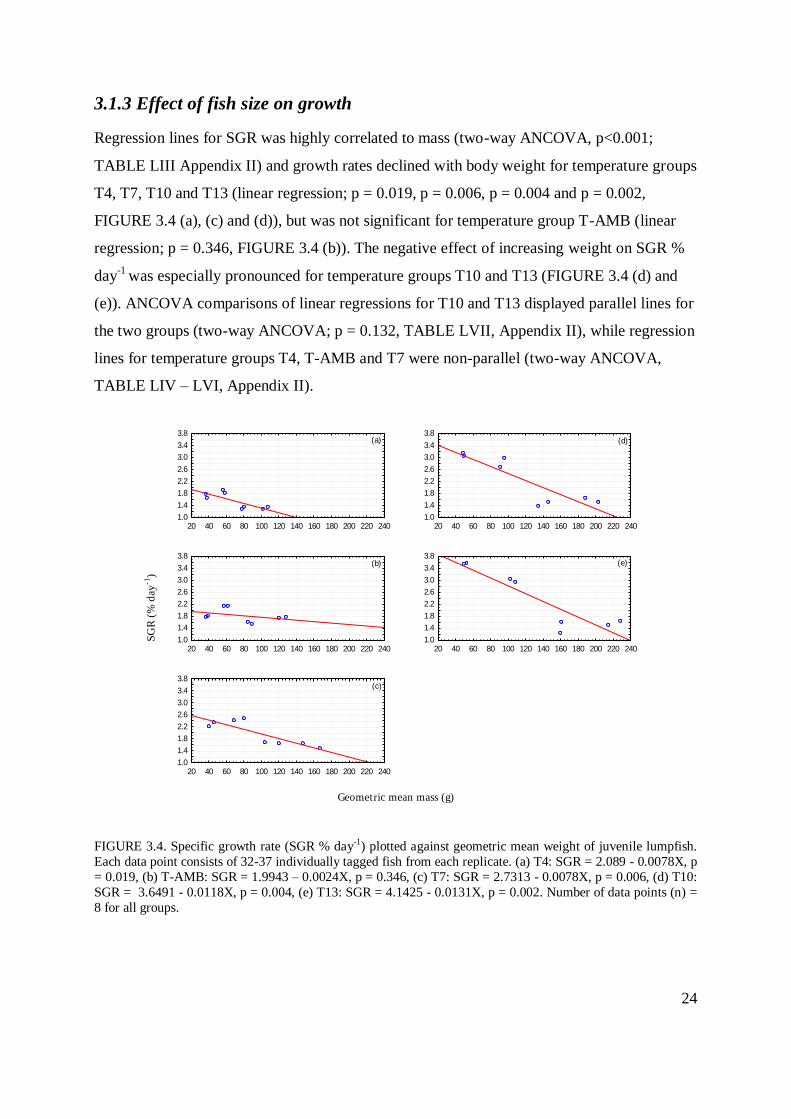
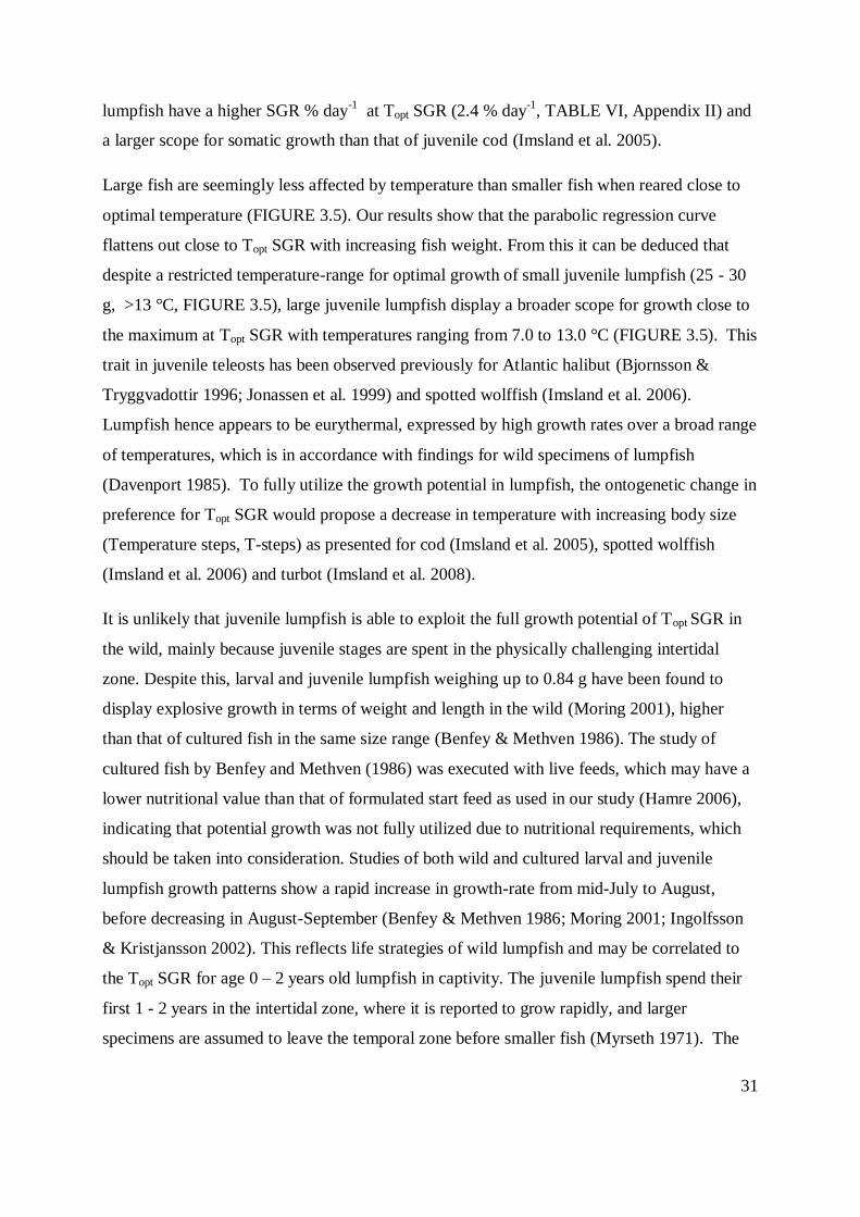
25

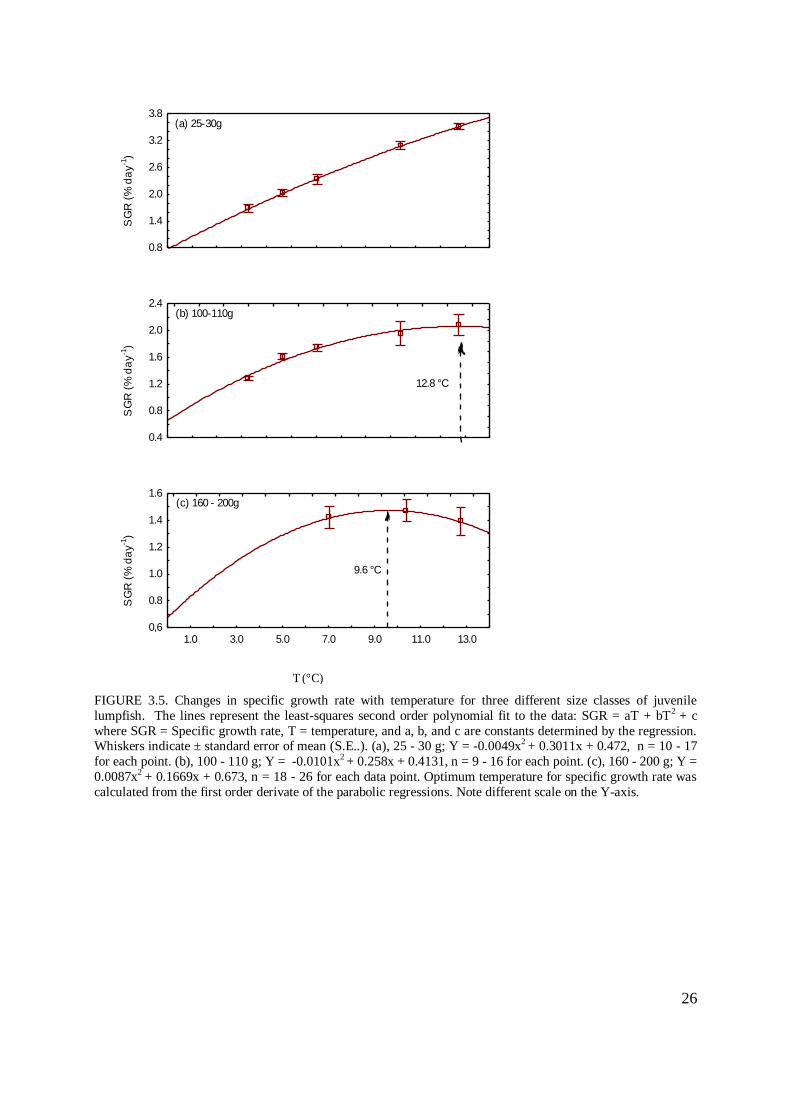
Growth rates were plotted against temperature for three size classes of fish (25 - 30, 100 - 110

and 160 - 200 g: FIGURE 3.5 (a) – (c)) to produce the parabolic regressions: 25-30 g Y =

0.472 + 0.3011x – 0.0049 x2, 100 - 110 g Y = 0.4131 + 0.258x – 0.0101x

2, 160 - 200 g Y =

0.673 + 0.1669x – 0.0087 x2

(FIGURE 3.5 (a) – (c)). A trend in decreasing growth rate (SGR

% day-1

) indicated that temperature optimums for maximum specific growth rate declined

markedly with increasing body mass for all temperature groups.

Temperature optimums were calculated from the first order derivate of the parabolic

regressions (dSGR / dT = 0). The Topt SGR was estimated to be 9.6 °C for the 160 - 200 g

group, while fish in size rank 100 - 120 g did not reach their temperature optimum during the

study but the first order derivate of the parabolic regression demonstrates a calculated Topt

SGR at 12.8 °C. The smallest group (25 - 30 g) did not seem to have reached their

temperature optimum for maximal growth at 13 °C (FIGURE 3.5 (a)).

3.1.4 Size and growth ranking

A significant size rank correlation (initial weight v. final weight) was maintained at all

temperature regimes (rSp > 0.50, p<0.05, TABLE LX, Appendix II). Size rank correlation was

highest for the coldest temperature groups T4 and T-AMB (rSp = 0.95, rSp = 0.93), and lowest

for the warmest temperature group T13 (rSp = 0.67, TABLE LX, Appendix II). Initial vs. final

growth rates were only correlated for T-AMB (rSp = 0.25)) and was negative for T4 and T13

(rSp = -0.05 and rSp = -0.002, TABLE LX, Appendix II).

26

T (°C)

SG

R (

% d

ay

-1)

1 3 5 7 9 11 130.8

1.4

2.0

2.6

3.2

3.8S

GR

(%

da

y-1

)

1 3 5 7 9 11 130.4

0.8

1.2

1.6

2.0

2.4

SG

R (

% d

ay

-1)

1.0 3.0 5.0 7.0 9.0 11.0 13.00,6

0.8

1.0

1.2

1.4

1.6

(a) 25-30g

(b) 100-110g

12.8 °C

(c) 160 - 200g

9.6 °C

FIGURE 3.5. Changes in specific growth rate with temperature for three different size classes of juvenile

lumpfish. The lines represent the least-squares second order polynomial fit to the data: SGR = aT + bT2 + c

where SGR = Specific growth rate, T = temperature, and a, b, and c are constants determined by the regression. Whiskers indicate ± standard error of mean (S.E..). (a), 25 - 30 g; Y = -0.0049x2 + 0.3011x + 0.472, n = 10 - 17

for each point. (b), 100 - 110 g; Y = -0.0101x2 + 0.258x + 0.4131, n = 9 - 16 for each point. (c), 160 - 200 g; Y =

0.0087x2 + 0.1669x + 0.673, n = 18 - 26 for each data point. Optimum temperature for specific growth rate was

calculated from the first order derivate of the parabolic regressions. Note different scale on the Y-axis.

27

3.2 Experiment 2

3.2.1 Mortality

No mortality was recorded for experiment 2. All fish appeared healthy and without injuries

throughout the experimental period.

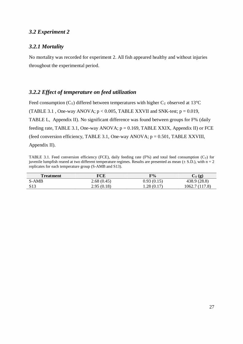
3.2.2 Effect of temperature on feed utilization

Feed consumption (CT) differed between temperatures with higher CT observed at 13°C

(TABLE 3.1 , One-way ANOVA; p < 0.005, TABLE XXVII and SNK-test; p = 0.019,

TABLE L, Appendix II). No significant difference was found between groups for F% (daily

feeding rate, TABLE 3.1, One-way ANOVA; p = 0.169, TABLE XXIX, Appendix II) or FCE

(feed conversion efficiency, TABLE 3.1, One-way ANOVA; p = 0.501, TABLE XXVIII,

Appendix II).

TABLE 3.1. Feed conversion efficiency (FCE), daily feeding rate (F%) and total feed consumption (CT) for juvenile lumpfish reared at two different temperature regimes. Results are presented as mean (± S.D.), with n = 2

replicates for each temperature group (S-AMB and S13).

Treatment FCE F% CT (g)

S-AMB 2.68 (0.45) 0.93 (0.15) 438.9 (28.8)

S13 2.95 (0.18) 1.28 (0.17) 1062.7 (117.8)

28

4. Discussion

4.1 The effect of temperature on growth

The results of the present study show that mean weights, lengths and growth rates of juvenile

lumpfish were significantly influenced by temperature and fish size. Mean weights and

lengths showed a significant, stepwise increase with increasing temperature for most

samplings. Mean weights and lengths were significantly lower for groups T4 and T-AMB

compared to all other temperature groups, during and at the end of experiment 1. No other

published studies of temperature related growth studies in the presented size range for

juvenile is known at the time of writing.

Overall SGR % day-1

was found to have a significant increase with increasing temperature.

Fish reared at 13 °C (T13) had the highest growth-rates for the two first periods of the

experiment, 11 April – 15 May and 16 May – 2 June (3.09 and 2.91 % day-1

respectively)

while juvenile lumpfish reared at ambient temperature (5.1 – 6.5 °C , T-AMB) and 7 °C (T7)

had the highest growth rates for the third period 3 June – 26 June (1.65 % day-1

). Lumpfish

reared at ambient temperature (T-AMB) displayed the highest growth rate during the final

period 27 June – 16 July (1.74 % day-1

, FIGURE 3.3 and TABLE VI, Appendix II). The low

overall SGR % day-1

for groups reared at the lowest temperatures (T4 and T-AMB) produced

a fish with an overall mean weight which is 54 and 43 % lower compared to that of fish

reared at 13 °C (T13). Fish reared at 4 °C (T4) displayed the overall lowest growth rate

(TABLE VI, Appendix II). This is in accordance with findings from wild juveniles caught

outside southwestern Iceland, as wild fish displayed little or no growth during the cold

months of the first winter (Ingolfsson & Kristjansson 2002).

The decline in growth is consistent with findings for juvenile halibut in the same size range,

displaying a 8 – 35 % increase in final body weight when increasing temperature from 10.0 to

13.0 °C (Hallaraker et al. 1995; Bjornsson & Tryggvadottir 1996), and a increase in final

body weight by 46 and 49 % when increasing temperature from 6.0 and 7.0, respectively to

13.0 °C (Hallaraker et al. 1995; Jonassen et al. 1999). A further increase in temperature from

that of Topt SGR is found to decrease maximum weight (Björnsson & Steinarsson 2002).

Despite consistency in the findings of increased final weight with increasing temperature,

these comparisons of final weight between studies do not take into consideration possible

29

effects of different photoperiods (Jonassen et al. 2000b; Imsland & Jonassen 2001; Lohne et

al. 2012), feeding regimes (Brown et al. 1997) and time scopes (Björnsson et al. 2007;

Arnason et al. 2009).

In our study the SGR % day-1

decreases rapidly over time for groups reared at high

temperatures, while growth rates in the group reared at ambient temperature (T-AMB) had a

less rapid decrease and displayed the highest SGR % day-1

in the final period (TABLE VI,

Appendix II, FIGURE 3.3). In the study by Arnason et al. (2009) juvenile turbot reared below

suboptimal temperatures would over time catch up with initially faster growing individuals

reared at higher temperatures. This may be a possible long-term effect in juvenile lumpfish as

Topt SGR changes with increasing size, but the time scope for our study may have been too

short to display this effect. Brown et al. (1992) observed lumpfish reared at ambient

temperatures to reach mean weights of above 500 g within two years, which suggests great

growth potential in juvenile lumpfish.

4.2 Size-related growth and optimum temperatures for growth

Juvenile lumpfish display a large ontogenetic variation in optimum temperatures for growth

(Topt SGR) with increasing body weight, demonstrated by high growth rates over a large

temperature interval (FIGURE 3.4 and 3.5). A change in Topt SGR with increasing size could

easily be distinguished as fish reared close to Topt SGR at 13 °C displayed very high growth

rates in the first period when body weight was low (3.54) and hence achieved high overall

growth rates (2.38 % day-1

, FIGURE 3.3, TABLE VI, Appendix II). For periods W3-W4 and

W4-W5 the growth rate of the fish reared at 13 °C displayed a rapid decrease, while slower

growing fish reared at ambient temperature (T-AMB) displayed better growth than high

temperature groups T10 and T13 in the final period. Despite this, the low temperature groups

(T4 and T-AMB) could not compete in terms of overall weight gain and SGR % day-1

in

comparison to groups reared at 10 and 13 °C.

An inverse relationship between the slopes for increasing body weight and growth could be

observed for all temperature groups, but was significantly negative for temperatures 10 and 13

°C (FIGURE 3.4). This indicates a rapid downwards shift in the optimum temperature for

growth with increasing body weight (FIGURE 3.4), which is in accordance with the findings

30

for plaice (Fonds et al. 1992), turbot (Imsland et al. 1996; Arnason et al. 2009), spotted

wolffish (Imsland et al. 2006), juvenile cod (Björnsson & Steinarsson 2002; Imsland et al.

2005), halibut (Hallaraker et al. 1995; Aune et al. 1997; Jonassen et al. 1999) and the general

pattern of fish growth with increasing body size (Brett & Groves 1979; Jobling 2010).

The parabolic regressions for growth (FIGURE 3.5) suggest a Topt SGR of 9.6 - 12.8 °C for

juvenile lumpfish in the size range 100 - 200 g, indicating an ontogenetic change in Topt SGR.

This decline in Topt SGR with increasing weight is in accordance with growth studies for

juvenile cod (Jobling 1988; Otterlei et al. 1999; Björnsson et al. 2007), juvenile turbot

(Imsland et al. 1996; Arnason et al. 2009), plaice (Fonds et al. 1992), spotted wolffish

(Imsland et al. 2006) and Atlantic halibut (Hallaraker et al. 1995; Bjornsson & Tryggvadottir

1996; Jonassen et al. 1999). The observed scope for Topt SGR in this study is similar to that

proposed for halibut by Hallaraker et al. (1995) (10.0 – 13.0 °C for 20 – 90 g) and Bjornsson

and Tryggvadottir (1996) (14.0 and 11.4 for size groups 10 – 60 and 100 – 500 g

respectively). Juvenile cod also display similar temperature preferences (14.7 – 12.6 for 5 –

50 g) (Imsland et al. 2005), while the suggested Topt SGR for turbot is higher (16.0 – 23.0 °C

at 7.5 – 75 g) (Imsland et al. 1996; Imsland et al. 2000). Juvenile wolfish display a

significantly lower Topt SGR for juveniles in the same size range (6.6 – 7.6 °C for 71 – 380 g)

(Imsland et al. 2006). These differences reflect different life strategies of juvenile marine fish.

The observed change in Topt SGR for lumpfish in this study is somewhat higher than the

presumptions of a 1 - 2 °C decrease in temperature preference for fish weighing 10 - 500 g as

presented by Cuenco et al. (1985). The fish in our study displayed a change in Topt SGR of 3

°C between 100 - 110 g and 160 - 200 g (FIGURE 3.5). If we include the smallest group 25 -

30 g, who according to our parabolic regression had not reached their Topt SGR at 13 °C, the

window for temperature preference in 25 - 200 g juvenile lumpfish will become even broader,

with a marked shift in preference between the 25 - 30, 100 - 110 and 160 - 200 g groups.

The rapid decrease in daily growth with increasing size for all groups except at ambient

temperature is in in terms with findings for juvenile Atlantic cod (Imsland et al. 2005) and

Atlantic halibut (Hallaraker et al. 1995). Juveniles in size group 25 – 30 g did not seem to

have reached their growth potential at 13 °C, while juvenile cod in the same size group (5 –

50 g) reached their temperature optimum at 12.9 °C, and also had a lower temperature

optimum for larger size intervals (40 - 50 g, 12.6 °C) (Imsland et al. 2005). This indicates that

31

lumpfish have a higher SGR % day-1

at Topt SGR (2.4 % day-1

, TABLE VI, Appendix II) and

a larger scope for somatic growth than that of juvenile cod (Imsland et al. 2005).

Large fish are seemingly less affected by temperature than smaller fish when reared close to

optimal temperature (FIGURE 3.5). Our results show that the parabolic regression curve

flattens out close to Topt SGR with increasing fish weight. From this it can be deduced that

despite a restricted temperature-range for optimal growth of small juvenile lumpfish (25 - 30

g, >13 °C, FIGURE 3.5), large juvenile lumpfish display a broader scope for growth close to

the maximum at Topt SGR with temperatures ranging from 7.0 to 13.0 °C (FIGURE 3.5). This

trait in juvenile teleosts has been observed previously for Atlantic halibut (Bjornsson &

Tryggvadottir 1996; Jonassen et al. 1999) and spotted wolffish (Imsland et al. 2006).

Lumpfish hence appears to be eurythermal, expressed by high growth rates over a broad range

of temperatures, which is in accordance with findings for wild specimens of lumpfish

(Davenport 1985). To fully utilize the growth potential in lumpfish, the ontogenetic change in

preference for Topt SGR would propose a decrease in temperature with increasing body size

(Temperature steps, T-steps) as presented for cod (Imsland et al. 2005), spotted wolffish

(Imsland et al. 2006) and turbot (Imsland et al. 2008).

It is unlikely that juvenile lumpfish is able to exploit the full growth potential of Topt SGR in

the wild, mainly because juvenile stages are spent in the physically challenging intertidal

zone. Despite this, larval and juvenile lumpfish weighing up to 0.84 g have been found to

display explosive growth in terms of weight and length in the wild (Moring 2001), higher

than that of cultured fish in the same size range (Benfey & Methven 1986). The study of

cultured fish by Benfey and Methven (1986) was executed with live feeds, which may have a

lower nutritional value than that of formulated start feed as used in our study (Hamre 2006),

indicating that potential growth was not fully utilized due to nutritional requirements, which

should be taken into consideration. Studies of both wild and cultured larval and juvenile

lumpfish growth patterns show a rapid increase in growth-rate from mid-July to August,

before decreasing in August-September (Benfey & Methven 1986; Moring 2001; Ingolfsson

& Kristjansson 2002). This reflects life strategies of wild lumpfish and may be correlated to

the Topt SGR for age 0 – 2 years old lumpfish in captivity. The juvenile lumpfish spend their

first 1 - 2 years in the intertidal zone, where it is reported to grow rapidly, and larger

specimens are assumed to leave the temporal zone before smaller fish (Myrseth 1971). The

32

decreasing change in temperature preference with increasing body size may reflect the

secondary effect of migration, as sea migrating juvenile lumpfish may better exploit the

differences in temperature between the inter-tidal zone, which is in accordance with the

findings of juvenile plaice, (Fonds 1979; Fonds et al. 1992), and juvenile turbot (Imsland et

al. 1996; Imsland & Jonassen 2001).

It has been suggested that lumpfish return to spawn in the same area year after year

(Thorsteinsson 1981; Mitamura et al. 2012). Species with large north-south distributions such

as juvenile turbot and Atlantic cod have been shown to display differences in terms of Topt

SGR between latitudinal groups, indicating a genetic difference between populations which

cannot be overcome during an acclimatization process (Imsland et al. 2000; Pörtner et al.

2001). This may very well be a pronounced effect in lumpfish culture as well, as this is a

specie with a large geographic distribution and large size differences between populations

(Davenport 1985), and large observed polymorphism in loci between populations

(Skirnisdottir et al. 2013). It is however uncertain to what extent genes affect fitness. The

differences in terms of life strategies of marine fish are found to produce little differentiation

in genetic markers within a specie (Imsland et al. 2000), but temperature has been observed to

have a greater effect on growth rate in cod than genetic influences (Björnsson & Steinarsson

2002). Genotype vs. environment interactions are difficult to predict as they depend on

family (population), life stage of the fish, environmental factors and specie. Environmental

factors such as temperature, salinity and available food sources have been observed to have

great importance on family-effects in juvenile cod, accounting for up to 90 % of a trait such as

growth (Imsland et al. 2011).

Increasing mortality with increasing weight at high temperatures as observed for Atlantic cod

(Bjornsson et al. 2001) may also be a problem in lumpfish culture. Hence, more experiments

to investigate the optimal temperatures with increasing growth should be undertaken to

investigate possible long-term effects of this rapid growth at high temperatures, together with

possible effects of the thermal history of the fish during juvenile stages, which may also have

consequences for further growth potential (Aune et al. 1997).

33

4.3 Growth effects in terms of Q10

Increasing the temperature from 4 (T4) to 5.8 °C (T-AMB) gave the highest overall increase

in growth rate calculated as Q10 ratio (Q10 = 3.16, TABLE LXI, Appendix II), while

increasing the temperature from 5.8 °C (T-AMB) to 7 °C (T7) increased the Q10 ratio by 1.48,

indicating that an increase of temperature from ambient has a positive effect on specific

growth rate. The effect on Q10 for increasing the temperature from 7 °C and 10 °C to 13°C

was 1.12 and 1.15 respectively, suggesting little positive effect of further increasing the

temperature for culture of juvenile lumpfish. These values for Q10 in juvenile lumpfish

indicate a lower temperature optimum compared to that of juvenile halibut (Hallaraker et al.

1995; Jonassen et al. 1999). This indicates that the temperature was in overall not above

optimum of the size groups investigated, though parabolic regression concluded otherwise in

terms of the largest size groups from 7, 10 and 13 °C. The smallest effect in terms of Q10 was

observed between 7 °C and 10 °C at Q10 =1.09. The effect on Q10 is reduced as temperature

draws near to Topt SGR, and is more pronounced when suboptimal and lower temperatures are

compared. This observed effect is a common finding when using Q10 as a thermal coefficient

in terms of growth (Hallaraker et al. 1995; Imsland et al. 1996; Jonassen et al. 1999; Imsland

et al. 2005). Heating water from 4 °C to 5.8 °C in lumpfish aquaculture can therefore produce

high growth at low costs for the size-group studied.

4.4 Size rank – correlation

An evident size rank correlation was found for all temperature groups, which is consistent

with findings for juveniles of several marine species (Hallaraker et al. 1995; Imsland et al.

1996; Aune et al. 1997; Jonassen et al. 1999; Imsland et al. 2005; Imsland et al. 2006).The

stabile size rank, especially for low-temperature groups (TABLE LX, Appendix II) indicates

that individual fish remain their relative size position throughout the experimental period.

Correlation for weight was lower for high temperature groups (T13 rs = 0.65, T10 rs = 0.71,

TABLE LX, Appendix II) than for low temperature groups (T7 rs = 0.87, T-AMB rs = 0.93,

T4 = 0.95). This is in accordance with findings for juvenile fish (Hallaraker et al. 1995;

Jonassen et al. 1999), and may indicate that some individuals have a larger window for

growth related temperature preference, which may be underlined by genetic effects. Our

results indicate that individuals maintain their relative size position throughout the

34

experimental period, indicating what may be the early establishment of a stable size ranking,

which is consistent with other findings for juvenile lumpfish (Haaland 1996) and other marine

species (Imsland et al. 1998; Imsland et al. 2006).

Juvenile lumpfish are found to be highly territorial and group together within the same size

groups (Haaland 1996). Haaland (1996) found that the impact of hierarchies in captive

juvenile lumpfish had an increasing impact on growth rates with time. Larger, dominant

individuals would spend more time swimming and hunting for prey, hence increasing their

energy requirements. Smaller, subordinate individuals would on the other hand spend more

time stationary at the bottom of the tank, limiting their access to feed. This prevented neither

the dominant nor the subordinate fish to maximize their potential growth, which also may

have been an effect in our study as individual growth rates varied greatly within all

temperatures, displaying significant size correlations throughout the experimental periods.

4.5 Effect of temperature on feed related parameters

The morphology, physiology and behavior of a species is closely related to each other (Huey

1991) and the energy available for anabolic processes in ectotherms is restricted by reduced

energy intake at low temperatures (Jobling 1994). Optimum temperatures for growth are often

slightly higher than that of optimum temperatures for maximum feed conversion efficiency

(Jobling 1994; Bjornsson & Tryggvadottir 1996; Jobling 1997). Our results indicated that

there was no significant difference in feed conversion ratio between ambient temperature

groups (S-AMB, 5.1 – 6.3 °C, TABLE I, Appendix II) and the groups reared at 13 °C (S13).

The minimum feed conversion efficiency (FCE) was very high in all experiments (S-AMB =

2.68 and S13 = 2.96 , TABLE VIII, Appendix II ), far superior to that of juvenile cod (1.18 –

1.35 %) (Imsland et al. 2005), turbot (0.82 – 1.21 %) (Imsland et al. 2000; Imsland et al.

2007a), spotted wolffish (1.11 – 1.37 %) (Imsland et al. 2006; Magnussen et al. 2008),

Atlantic salmon (0.77 – 1.35 %) (Handeland et al. 2008; Björnsson & Jönsson 2012) when

reared close to Topt FCE in the same size range. This represents a very significant cost benefit

for lumpfish farming, as feed costs are the greatest single cost factor in aquaculture.

The high FCE in juvenile lumpfish can be explained by several factors. Ingolfsson and

Kristjansson (2002) found that only 28 % of 1482 juvenile lumpfish collected in June-

35

September had food in their stomachs, whereas 27 % of the juveniles in the same study had

remains of food in their stomach. This may indicate a rapid degradation of prey in juvenile

lumpfish, as a study by Vandendriessche et al. (2007) observed food in all stomachs, also in

winter.

Juvenile lumpfish have a limited aerobic scope, which limits the possibility of active

searching. The effect of temperature on metabolism may therefore be assumed to have a great

impact on lumpfish. Lumpfish’s foraging profile indicates minimizing its prey encounter rate

on the behalf of not maximizing their net energy gain (Jobling 1997), and display a sit-and-

wait foraging strategy, clinging to substrate before ambushing their prey (Brown 1986;

Haaland 1996; Ingolfsson & Kristjansson 2002; Jobling et al. 2012). In comparison to most

other fish larvae, lumpfish do not form the s-shaped posture before ambush (Brown 1986).

This strategy is 6 - 12 % more efficient in terms of metabolic costs, compared to that of active

searching, but only if the prey density supplies a sufficient net energy gain (Jobling et al.

2012). When prey density is low, actively searching for food is a more efficient foraging

strategy than clinging, allowing lumpfish to yield energy at a faster rate, despite the increase

in energy expenditure (Jobling et al. 2012) but also increases risk of predation (Killen et al.

2007).

Brown (1986) observed that juvenile lumpfish above 40 mm would utilize the suction disc to

cling while feeding. This size range overlaps with the size group observed in our study, hence

indicating that the juvenile lumpfish in our experiment may have utilized this foraging

strategy. This underlines the possible importance of the adhesive disc for feeding strategies

throughout juvenile stages. Despite this, there has been some doubt with regard to feeding

strategies in captive lumpfish with increasing size, as Haaland (1996) and Killen et al. (2007)

found that only smaller submissive fish would feed while clinging, and larger specimens

would readily feed in the water column. Due to the significant size rank in our study one

would assume that stable hierarchies as observed by Haaland (1996) do exist (TABLE LX,

Appendix II), which may have caused differences in foraging strategy between size-rankings

of fish.

Juvenile lumpfish feed throughout the year (Vandendriessche et al. 2007). Small juvenile

lumpfish with yolk sacks are found to feed on small crustaceans (harpacticoid copepods)

before shifting to amphipods (Callopius laeciusculus and Parathemisto gaudichaudi) with

36

increasing size (Daborn & Gregory 1983; Ingolfsson & Kristjansson 2002). This further

indicates an ontogenetic change in terms of prey size in juvenile lumpfish, which further may

reflect their change in habitat and hence temperature preference with increasing size (Daborn

& Gregory 1983; Brown 1986; Moring 1989).

In our study, no difference in FCE between temperature groups was observed, which is

similar to effects earlier observed for Atlantic cod (Imsland et al. 2005). FCE for juvenile

turbot has been found to accelerate until maximum FCE at Topt FCE, before decelerating

again at suboptimal temperatures (Van Ham et al. 2003). Topt FCE is generally somewhat

lower than that of Topt SGR (Jobling 1997). The two temperatures presented in experiment 2

may hence have been on each side of this scale, but results for Topt SGR presented for the

same size interval in experiment 1 (>13 °C for 25 – 30 g and 12.8 °C for 100 – 100 g,

FIGURE 3.5) would indicate a Topt FCE higher than the temperature in the highest

temperature group (S13), as Topt SGR was not reached for the group reared at 13 °C (T13) in

experiment 1. This may have been a contributing factor to the lack of significant difference in

FCE between the high and low temperature groups, as both temperatures may have been

suboptimal for FCE. Temperature therefore had an effect on metabolism and total feed

consumption, but did not have an effect on overall feed utilization. In terms of commercial

lumpfish farming this indicates that lumpfish can reach optimal sizes in shorter time at

optimal temperatures, but at the same feed cost as for fish reared at ambient temperatures.

Another possible explanation for the insignificant difference in FCE between temperature

groups S-AMB and S13 at satiation level in our study may be explained by the approximately

same stomach size and same ability to digest. Despite these findings, feed consumption is to a

large extent influenced by feed composition in terms of energy content, along with the

feeding frequency (Brett & Groves 1979).

Imsland et al. (2000) suggested an inter-population difference in energy utilization, with

increasing FCE at higher latitudes due to shorter growth periods in the north. The same study

furthermore suggested that the energy allocation and utilization of a specie can vary according

to differences in the environment. Lumpfish have been found to display high polymorphism

in genetic loci between Icelandic and Canadian populations (Skirnisdottir et al. 2013). Due to

the large geographic distribution one may hence be able to exploit differences in feed

37

utilization in culture of juvenile lumpfish for commercial production as well, if such genetic

effects of growth exists in lumpfish.

Lumpfish juveniles are known to feed selectively, ignoring plentiful species of prey,

especially slow moving or small particles (Haaland 1996; Ingolfsson & Kristjansson 2002)

showing little interest for pellets in the bottom of the tank (Haaland 1996). In our study there

was very often excess pellets at the bottom of the tank, which may indicate that despite

having unlimited access to feeds in the time span offered, fish may not have fed to satiation,

and may very well have exposed an effect of compensatory growth similar effect to that of

juvenile turbot (Van Ham et al. 2003).

38

5. Conclusions

Increased temperatures had a positive effect on growth in terms of weight, length and growth

rate, but had no significant effects on feed conversion efficiency. Temperatures of 10 - 13 °C

led to 31- 35 % higher overall growth rates and 48-53 % higher final weights compared to

that of juvenile lumpfish reared at 4 °C.

Overall growth rate, weight and length was significantly higher for T13 (13 °C) compared to

that of all other temperature groups, and mean lengths and weights displayed a significant,

stepwise increase with increasing temperature for most samplings. Temperature optimums for

growth decreased with increasing body weight, suggesting an ontogenetic shift in temperature

preferences for growth. For size groups 100 – 110 g and 160 – 200 g parabolic regressions

suggested optimum temperatures for growth of 12.8 and 9.6 °C respectively. The temperature

optimum for growth in the size group 25 – 30 g was not reached in the investigated

temperature interval (4 – 13 °C), but an optimum temperature for growth above 13 °C is

suggested. Growth rate declined with increasing size for all temperature groups, but

temperature tolerance increased with increasing body size. In order to fully utilize the

decrease in optimum temperature with increasing fish size, the utilization of “temperature

steps”, a reduction in temperature with increasing body size is suggested.

Increased temperature caused an increase in total consumption of feed (CT), but had no effect

on feed conversion efficiency (FCE) or daily feeding rate (F%). The limited effect of

temperature seen on temperature on FCE and F% may be due to the limited duration of the

experiment, and too coarse temperature ranges to be able to pinpoint a temperature optimum

for feed conversion efficiency. This lacking sensitivity of FCE close to optimal temperature of

growth may have important consequences for lumpfish farming, as this indicates that

lumpfish can reach a large size in a short time, but at the same cost as slower growing

individuals at low temperatures.

39

References

Able, K. W. & Irion, W. (1985). Distribution and reproductive seasonality of snailfishes and lumpfishes in the St. Lawrence River estuary and the Gulf of St. Lawrence. Canadian journal

of zoology, 63 (7): 1622-1628.

Albert, O. T. (2000). Lumpsucker (Cyclopterus lumpus) otoliths : dissection, mounting and age-

reading. Rapport / Fiskeriforskning. Tromsø: Fiskeriforskning. 22 s. pp. Andersen, P. & Vestvik, N. (2012). Rognkjeks - En dans på roser? Flatanger: Aqua Kompetanse A/S.

Andrijasev, A. P. (1964). Fishes of the northern seas of the U.S.S.R. Jerusalem: Israel Program for

Scientific Translations. 617 s. pp. Arnason, T., Bjornsson, B., Steinarsson, A. & Oddgeirsson, M. (2009). Effects of temperature and

body weight on growth rate and feed conversion ratio in turbot (Scophthalmus maximus).

Aquaculture, 295 (3-4): 218-225. Asche, F., Guttormsen, A. G., Sebulonsen, T. & Sissener, E. H. (2005). Competition between farmed

and wild salmon: the Japanese salmon market. Agricultural Economics, 33 (3): 333-340.

Aune, A., Imsland, A. K. & Pittman, K. (1997). Growth of juvenile halibut, Hippoglossus

hippoglossus (L.), under a constant and switched temperature regime. Aquaculture Research, 28 (12): 931-939.

Bañón, R., Garazo, A. & Fernández, A. (2008). Note about the presence of the lumpsucker

Cyclopterus lumpus (Teleostei, Cyclopteridae) in Galician waters (NW Spain). Journal of Applied Ichthyology, 24 (1): 108-109.

Benfey, T. J. & Methven, D. A. (1986). Pilot-scale rearing of larval and juvenile lumpfish

(Cyclopterus lumpus L.), with some notes on early development. Aquaculture, 56 (3): 301-306.

Bigelow, H. B. & Schroeder, W. C. (1953). Fishes of the Gulf of Maine; the lumpfishes, Family

Cyclopteridae. U.S. Fish and Wildlife Service Fish Bulletin, 74: 459-463.

Bjorn, P. A., Finstad, B. & Kristoffersen, R. (2001). Salmon lice infection of wild sea trout and Arctic char in marine and freshwaters: the effects of salmon farms. Aquaculture Research, 32 (12):

947-962.

Bjornsson, B. & Tryggvadottir, S. V. (1996). Effects of size on optimal temperature for growth and growth efficiency of immature Atlantic halibut (Hippoglossus hippoglossus L.). Aquaculture,

142 (1-2): 33-42.

Bjornsson, B., Steinarsson, A. & Oddgeirsson, M. (2001). Optimal temperature for growth and feed

conversion of immature cod (Gadus morhua L.). Ices Journal of Marine Science, 58 (1): 29-38.

Björnsson, B. & Steinarsson, A. (2002). The food-unlimited growth rate of Atlantic cod (Gadus

morhua). Canadian Journal of Fisheries and Aquatic Sciences, 59 (3): 494-502. Björnsson, B., Steinarsson, A. & Árnason, T. (2007). Growth model for Atlantic cod (Gadus morhua):

Effects of temperature and body weight on growth rate. Aquaculture, 271 (1): 216-226.

Björnsson, B. T. & Jönsson, E. (2012). The impact of temperature on the metabolome and endocrine metabolic signals in Atlantic salmon (Salmo salar).

Blacker, R. W. (1983). Pelagic records of the lumpsucker, Cyclopterus lumpus L. Journal of Fish

Biology, 23 (4): 405-417.

Boeuf, G. & Le Bail, P. (1999). Does light have an influence on fish growth? Aquaculture, 177 (1): 129-152.

Brandal, P. O., Egidius, E. & Romslo, I. (1976). Host Blood - Major Food Component for Parasitic

Copepod Lepeophtheirus-Salmonis Kroyeri, 1838 (Crustacea-Caligidae). Norwegian Journal of Zoology, 24 (4): 341-343.

Brett, J. R. & Groves, T. D. D. (1979). Physiological energetics. Fish physiology, 8: 274.

Brown, J. A. (1986). The development of feeding behaviour in the lumpfish, Cyclopterus lumpus L. Journal of fish biology, 29 (sA): 171-178.

40

Brown, J. A., Somerton, D. C., Methven, D. A. & Watkins, J. R. (1992). Recent advances in lumpfish

Cyclopterus lumpus and ocean pout Macrozoarces americanus larviculture. Journal of the

World Aquaculture Society, 23 (4): 271-276. Brown, J. A., Wiseman, D. & Kean, P. (1997). The use of behavioural observations in the larviculture

of cold-water marine fish. Aquaculture, 155 (1-4): 297-306.

Burka, J. F., Hammell, K. L., Horsberg, T. E., Johnson, G. R., Rainnie, D. J. & Speare, D. J. (1997). Drugs in salmonid aquaculture - A review. Journal of Veterinary Pharmacology and

Therapeutics, 20 (5): 333-349.

Burridge, L., Weis, J., Cabello, F., Pizarro, J. & Bostick, K. (2010). Chemical use in salmon

aquaculture: a review of current practices and possible environmental effects. Aquaculture, 306 (1): 7-23.

Campbell, A. & Stasko, A. (1986). Movements of lobsters (Homarus americanus) tagged in the Bay

of Fundy, Canada. Marine Biology, 92 (3): 393-404. Collins, M. A. (1976). The lumpfish (Cyclopterus lumpus L.) in Newfoundland waters. Can. Field-

Nat., 90 (1): 64-67.

Costello, M. J. (2009). How sea lice from salmon farms may cause wild salmonid declines in Europe and North America and be a threat to fishes elsewhere. Proceedings of the Royal Society B:

Biological Sciences, 276 (1672): 3385-3394.

Cowx, I. G., O'Grady, K. T., Sundt, R. C. & Jørstad, K. E. (1998). Genetic population structure of

goldsinny wrasse, Ctenolabrus rupestris (L.), in Norway: implications for future management of parasite cleaners in the salmon farming industry. Fisheries Management and Ecology, 5

(4): 291-302.

Cox, P. & Anderson, M. (1922). No. 1: A study of the lumpfish(Cyclopterus lumpus L.). Contributions to Canadian Biology and Fisheries, 1 (1): 1-20.

Cuenco, M. L., Stickney, R. R. & Grant, W. E. (1985). Fish Bioenergetics and Growth in Aquaculture

Ponds .2. Effects of Interactions among Size, Temperature, Dissolved-Oxygen, Unionized

Ammonia and Food on Growth of Individual Fish. Ecological Modelling, 27 (3-4): 191-206. Daborn, G. R. & Gregory, R. S. (1983). Occurrence, Distribution, and Feeding-Habits of Juvenile

Lumpfish, Cyclopterus-Lumpus L in the Bay of Fundy. Canadian Journal of Zoology-Revue

Canadienne De Zoologie, 61 (4): 797-801. Davenport, J., Lønning, S. & Kjørsvik, E. (1983). Ammonia output by eggs and larvae of the

lumpsucker, Cyclopterus lumpus, the cod, Gadus morhua and the plaice, Pleuronectes

platessa. Journal of the Marine Biological Association of the United Kingdom, 63 (03): 713-723.

Davenport, J. (1985). Synopsis of biological data on the lumpsucker, Cyclopterus lumpus (Linnaeus,

1758). FAO fisheries synopsis. Rome: FAO. VI, 31 s. pp.

Davenport, J. & Kjorsvik, E. (1986). Buoyancy in the Lumpsucker Cyclopterus-Lumpus. Journal of the Marine Biological Association of the United Kingdom, 66 (1): 159-174.

Elliott, J. M. (1982). The Effects of Temperature and Ration Size on the Growth and Energetics of

Salmonids in Captivity. Comparative Biochemistry and Physiology B-Biochemistry & Molecular Biology, 73 (1): 81-91.

Fallang, A., Ramsay, J. M., Sevatdal, S., Burka, J. F., Jewess, P., Hammell, K. L. & Horsberg, T. E.

(2004). Evidence for occurrence of an organophosphate-resistant type of acetylcholinesterase in strains of sea lice (Lepeophtheirus salmonis Kroyer). Pest Management Science, 60 (12):

1163-1170.

Fonds, M. (1979). Laboratory Observations on the Influence of Temperature and Salinity on

Development of the Eggs and Growth of the Larvae of Solea-Solea (Pisces). Marine Ecology Progress Series, 1 (2): 91-99.

Fonds, M., Cronie, R., Vethaak, A. D. & Vanderpuyl, P. (1992). Metabolism, Food-Consumption and

Growth of Plaice (Pleuronectes-Platessa) and Flounder (Platichthys-Flesus) in Relation to Fish Size and Temperature. Netherlands Journal of Sea Research, 29 (1-3): 127-143.

41

GIFAS. (2012). Study II: Assesment of efficiancy of grazing of sea lice (Leophteirus salmonis) by

lumpfish (Cyclopterus lumpus L.) from farmed atlantic salmon (Salmo salar L.) using

different stocking densities. Small lumpfish (60g): Phase I: Gildeskål Forskningsstasjon A/S. Goulet, D., Green, J. M. & Shears, T. H. (1986). Courtship, Spawning, and Parental Care Behavior of

the Lumpfish, Cyclopterus-Lumpus L, in Newfoundland. Canadian Journal of Zoology-Revue

Canadienne De Zoologie, 64 (6): 1320-1325. Goulet, D. & Green, J. M. (1988). Reproductive success of the male lumpfish (Cyclopterus lumpus

L.)(Pisces: Cyclopteridae): evidence against female mate choice. Canadian journal of

zoology, 66 (11): 2513-2519.

Grimnes, A. & Jakobsen, P. J. (1996). The physiological effects of salmon lice infection on post-smolt of Atlantic salmon. Journal of Fish Biology, 48 (6): 1179-1194.

Groner, M. L., Cox, R., Gettinby, G. & Revie, C. W. (2013). Use of agent-based modelling to predict

benefits of cleaner fish in controlling sea lice, Lepeophtheirus salmonis, infestations on farmed Atlantic salmon, Salmo salar L. Journal of Fish Diseases, 36 (3): 195-208.

Haaland, T. (1996). Oppforing av rognkjeks. Bodø: [T. Haaland]. III, 29 bl. pp.

Hallaraker, H., Folkvord, A. & Stefansson, S. O. (1995). Growth of juvenile halibut (Hippoglossus hippoglossus) related to temperature, day length and feeding regime. Netherlands Journal of

Sea Research, 34 (1-3): 139-147.

Hamre, K. (2006). Nutrition in cod (Gadus morhua) larvae and juveniles. ICES Journal of Marine

Science: Journal du Conseil, 63 (2): 267-274. Handeland, S. O., Imsland, A. K. & Stefansson, S. O. (2008). The effect of temperature and fish size

on growth, feed intake, food conversion efficiency and stomach evacuation rate of Atlantic

salmon post-smolts. Aquaculture, 283 (1): 36-42. Havforskningsinstituttet. (2003). Vitenskapelig grunnlag for nye arter i oppdrett. Fisken og havet, 6-

2003: 54-55.

Heuch, P. A., Bjorn, P. A., Finstad, B., Holst, J. C., Asplin, L. & Nilsen, F. (2005). A review of the

Norwegian 'National Action Plan Against Salmon Lice on Salmonids': The effect on wild salmonids (vol 246, pg 79, 2005). Aquaculture, 250 (1-2): 535-535.

Holst, J. C. (1993). Observations on the distribution of lumpsucker (Cyclopterus lumpus, L.) in the

Norwegian Sea. Fisheries Research, 17 (3–4): 369-372. Houde, E. D. & Schekter, R. D. (1981). Growth rates, rations and coholrt consumption of marine fish

larvae in relation to prey concentrations. Rapports et Proces-Verbaux des Reunions Conseil

International pour l'Exploration de la Mer, 178: 441-453. Huey, R. B. (1991). Physiological Consequences of Habitat Selection. American Naturalist, 137: S91-

S115.

Imsland, A. K., Sunde, L. M., Folkvord, A. & Stefansson, S. O. (1996). The interaction of temperature

and fish size on growth of juvenile turbot. Journal of Fish Biology, 49 (5): 926-940. Imsland, A. K., Nilsen, T. & Folkvord, A. (1998). Stochastic simulation of size variation in turbot:

possible causes analysed with an individual‐based model. Journal of Fish Biology, 53 (2):

237-258. Imsland, A. K., Foss, A., Névdal, G., Cross, T., Bonga, S. W., Ham, E. A. & Stefansson, S. O. (2000).

Countergradient variation in growth and food conversion efficiency of juvenile turbot. Journal

of Fish Biology, 57 (5): 1213-1226.

Imsland, A. K. & Jonassen, T. M. (2001). Regulation of growth in turbot (Scophthalmus maximus Rafinesque) and Atlantic halibut (Hippoglossus hippoglossus L.): aspects of environment ×

genotype interactions. Reviews in Fish Biology and Fisheries, 11 (1): 71-90.

Imsland, A. K., Foss, A., Folkvord, A., Stefansson, S. O. & Jonassen, T. M. (2005). The interrelation between temperature regimes and fish size in juvenile Atlantic cod (Gadus morhua): effects

on growth and feed conversion efficiency. Fish Physiology and Biochemistry, 31 (4): 347-361.

Imsland, A. K., Foss, A., Sparboe, L. O. & Sigurdsson, S. (2006). The effect of temperature and fish size on growth and feed efficiency ratio of juvenile spotted wolffish Anarhichas minor.

Journal of Fish Biology, 68 (4): 1107-1122.

42

Imsland, A. K., Bjornsson, B. T., Gunnarsson, S., Foss, A. & Stefansson, S. O. (2007a). Temperature

and salinity effects on plasma insulin-like growth factor-I concentrations and growth in

juvenile turbot (Scophthalmus maximus). Aquaculture, 271 (1): 546-552. Imsland, A. K., Foss, A., Alvseike, T., Folkvord, A., Stefansson, S. O. & Jonassen, T. M. (2007b).

Interaction between temperature and photoperiod on growth and feeding of Atlantic cod

(Gadus morhua): possible secondary effects. Canadian Journal of Fisheries and Aquatic Sciences, 64 (2): 239-248.

Imsland, A. K., Gunnarsson, S., Asgeirsson, A., Roth, B., Schram, E. & Foss, A. (2008). Commercial‐scale Validation of Temperature‐step Rearing on Growth Physiology in Turbot, Scophthalmus

maximus. Journal of the World Aquaculture Society, 39 (5): 684-691. Imsland, A. K., Koedijk, R., Stefansson, S. O., Foss, A., Hjörleifsdóttir, S., Hreggvidsson, G. Ó.,

Otterlei, E. & Folkvord, A. (2011). A retrospective approach to fractionize variation in body

mass of Atlantic cod Gadus morhua. Journal of Fish Biology, 78 (1): 251-264. Ingolfsson, A. & Kristjansson, B. K. (2002). Diet of juvenile lumpsucker Cyclopterus lumpus

(Cyclopteridae) in floating seaweed: Effects of ontogeny and prey availability. Copeia (2):

472-476.

Jimenez, D. F., Heuch, P. A., Revie, C. W. & Gettinby, G. (2012). Confidence in assessing the effectiveness of bath treatments for the control of sea lice on Norwegian salmon farms.

Aquaculture, 344: 58-65.

Jobling, M. (1988). A review of the physiological and nutritional energetics of cod, Gadus morhua L., with particular reference to growth under farmed conditions. Aquaculture, 70 (1): 1-19.

Jobling, M. (1994). Fish bioenergetics: Chapman & Hall.

Jobling, M. (1997). Temperature and growth: Modulation of growth rate via temperature change. Global warming: implications for freshwater and marine fish. . Cambridge (UK): Cambridge

university press, . 225-253 pp.

Jobling, M. (2010). Are compensatory growth and catch-up growth two sides of the same coin?

Aquaculture International, 18 (4): 501-510. Jobling, M., Alanärä, A., Kadri, S. & Huntingford, F. (2012). Feeding Biology and Foraging.

Aquaculture and Behavior: Wiley-Blackwell. 121-149 pp.

Johannesson, J. (2006). Lumpfish caviar: from vessel to consumer: FAO. Jonassen, T. M., Imsland, A. K. & Stefansson, S. O. (1999). The interaction of temperature and fish

size on growth of juvenile halibut. Journal of Fish Biology, 54 (3): 556-572.

Jonassen, T. M., Imsland, A. K., Fitzgerald, R., Bonga, S. W., Ham, E. V., Naevdal, G., Stefansson, M. O. & Stefansson, S. O. (2000a). Geographic variation in growth and food conversion

efficiency of juvenile Atlantic halibut related to latitude. Journal of Fish Biology, 56 (2): 279-

294.

Jonassen, T. M., Imsland, A. K., Kadowaki, S. & Stefansson, S. O. (2000b). Interaction of temperature and photoperiod on growth of Atlantic halibut Hippoglossus hippoglossus L. Aquaculture

Research, 31 (2): 219-227.

Killen, S. S., Brown, J. A. & Gamperl, A. K. (2007). The effect of prey density on foraging mode selection in juvenile lumpfish: balancing food intake with the metabolic cost of foraging.

Journal of Animal Ecology, 76 (4): 814-825.

Klokseth, V. & Øiestad, V. (1999). Sluttrapport - Rognkjeks klargjøres for oppdrett.

Krkosek, M., Lewis, M. A., Volpe, J. P. & Morton, A. (2006). Fish farms and sea lice infestations of wild juvenile salmon in the Broughton Archipelago - A rebuttal to Brooks (2005). Reviews in

Fisheries Science, 14 (1-2): 1-11.

Krkosek, M., Ford, J. S., Morton, A., Lele, S., Myers, R. A. & Lewis, M. A. (2007). Declining wild salmon populations in relation to parasites from farm salmon. Science, 318 (5857): 1772-

1775.

Lein, I., Noble, C., Nergaard, S. & Helland, S. (2013). Evaluering av beiteeffektivitet hos berggylt i merd med stor laks. 2013: 12.

43

Lohne, P., Imsland, A. K., Larsen, S., Foss, A. & Pittman, K. (2012). Interactive effect of photoperiod

and temperature on the growth rates, muscle growth and feed intake in juvenile Atlantic

halibut. Aquaculture Research, 43 (2): 187-197. Magnussen, A. B., Imsland, A. K. & Foss, A. (2008). Interactive effects of different temperatures and

salinities on growth, feed conversion efficiency, and blood physiology in juvenile spotted

wolffish, Anarhichas minor Olafsen. Journal of the World Aquaculture Society, 39 (6): 804-811.

McVicar, A. H. (1997). Disease and parasite implications of the coexistence of wild and cultured

Atlantic salmon populations. Ices Journal of Marine Science, 54 (6): 1093-1103.

McVicar, A. H. (2004). Management actions in relation to the controversy about salmon lice infections in fish farms as a hazard to wild salmonid populations. Aquaculture Research, 35

(8): 751-758.

Michelsen, H. K. (2011). Prey selection of the Red King Crab (Paralithodes camtschaticus) preying on lumpfish eggs (Cyclopterus lumpus), sea urchins (Strongylocentrotus droebachiensis) and

scallops (Chlamys islandica): University of Tromsø.

Mikkelsen, N. & Pedersen, T. (2012). Invasive red king crab affects lumpsucker recruitment by egg consumption. Mar Ecol Prog Ser, 469: 87-99.

Mitamura, H., Thorstad, E. B., Uglem, I., Bjorn, P. A., Okland, F., Naesje, T. F., Dempster, T. & Arai,

N. (2012). Movements of lumpsucker females in a northern Norwegian fjord during the

spawning season. Environmental Biology of Fishes, 93 (4): 475-481. Moring, J. R. (1989). Food-Habits and Algal Associations of Juvenile Lumpfish, Cyclopterus-Lumpus

L, in Intertidal Waters. Fishery Bulletin, 87 (1): 233-237.

Moring, J. R. (1990). Seasonal Absence of Fishes in Tidepools of a Boreal Environment (Maine, USA). Hydrobiologia, 194 (2): 163-168.

Moring, J. R. & Moring, S. W. (1991). Short‐term movements of larval and juvenile lumpfish,

Cyclopterus lumpus L., in tidepools. Journal of fish biology, 38 (6): 845-850.

Moring, J. R. (2001). Intertidal growth of larval and juvenile lumpfish in Maine: A 20-year assessment. Northeastern Naturalist, 8 (3): 347-354.

Myrseth, B. (1971). Fekunditet, vekst, levevis og ernæring hos Cyclopterus lumpus L. : hovedoppgave

i fiskeribiologi. Bergen ,: Universitetet. 113 bl. pp. Otterlei, E., Nyhammer, G., Folkvord, A. & Stefansson, S. O. (1999). Temperature- and size-

dependent growth of larval and early juvenile Atlantic cod (Gadus morhua): a comparative

study of Norwegian coastal cod and northeast Arctic cod. Canadian Journal of Fisheries and Aquatic Sciences, 56 (11): 2099-2111.

Pörtner, H. O., Berdal, B., Blust, R., Brix, O., Colosimo, A., De Wachter, B., Giuliani, A., Johansen,

T., Fischer, T., Knust, R., et al. (2001). Climate induced temperature effects on growth

performance, fecundity and recruitment in marine fish: developing a hypothesis for cause and effect relationships in Atlantic cod (Gadus morhua) and common eelpout (Zoarces viviparus).

Continental Shelf Research, 21 (18–19): 1975-1997.

Rusyaev, S. M. (2013). On the spatial relationship between the spawning and feeding parts of the range of lumpfish Cyclopterus lumpus (Cyclopteridae) in the Barents Sea and adjacent waters

(according to results of analysis of the size composition similarity). Journal of Ichthyology, 53

(6): 397-403.

Schaer, M. & Vestvik, N. (2012). Rognkjeks ABC - forbredelese og bruk av en lusespiser i laksemerd. Steine: Arctic Cleanerfish AS.

Schmidt-Nielsen, K. (1990). Animal physiology: Adadption and Environment. Cambridge:

Cambridge University Press, 4th edition. Sevatdal, S. & Horsberg, T. E. (2003). Determination of reduced sensitivity in sea lice

(Lepeophtheirus salmonis Kroyer) against the pyrethroid deltamethrin using bioassays and

probit modelling. Aquaculture, 218 (1-4): 21-31. Sivertsgard, R., Thorstad, E. B., Okland, F., Finstad, B., Bjorn, P. A., Jepsen, N., Nordal, T. &

McKinley, R. S. (2007). Effects of salmon lice infection and salmon lice protection on fjord

migrating Atlantic salmon and brown trout post-smolts. Hydrobiologia, 582: 35-42.

44

Skirnisdottir, S., Olafsdottir, G., Olafsson, K., Jendrossek, T., ap Dafydd Lloyd, H., Helyar, S.,

Pampoulie, C., Danielsdottir, A. K. & Kasper, J. M. (2013). Twenty-two novel microsatellite

loci for lumpfish (Cyclopterus lumpus). Conservation Genetics Resources, 5 (1): 177-179. Sunnanå, K. (2007a). Notat om rådgiving for fisket etter rognkjeks i 2008.: Havforskningsinstituttet.

1-5 pp.

Sunnanå, K. (2007b). Rognkjeks. Kyst og havbruk: 88-87. Sunnanå, K. (2009). Rognkjeks og rognkall. In vol. 2009 Kyst og havbruk, pp. 95-96:

Havforskningsinstiuttet.

Thorsteinsson, V. (1981). The ageing validation of the lumpsucker (Cyclopterus lumpus) and the age

composition of the lumpsucker in Icelandic lumpsucker fisheries. ICES CM, 1981: G58. Torrissen, O., Olsen, R. E., Toresen, R., Hemre, G. I., Tacon, A. G. J., Asche, F., Hardy, R. W. & Lall,

S. (2011). Atlantic Salmon (Salmo salar): The "Super-Chicken" of the Sea? Reviews in

Fisheries Science, 19 (3): 257-278. Torstensen, E. (1998). Rognkjeks, en kommersiell ressurs på Skagerrakkysten? Fisken og havet.

Bergen: Havforskningsinstituttet. 6 bl. pp.

Treasurer, J. W. (2002). A review of potential pathogens of sea lice and the application of cleaner fish in biological control. Pest Management Science, 58 (6): 546-558.

Van Ham, E. H., Berntssen, M. H. G., Imsland, A. K., Parpoura, A. C., S., W., E., S. & Stefansson, S.

O. (2003). The influence of temperature and ration on growth, feed conversion, body

composition and nutrient retention of juvenile turbot (Scophthalmus maximus). Aquaculture, 217 (1–4): 547-558.

Vandendriessche, S., Messiaen, M., O'Flynn, S., Vincx, M. & Degraer, S. (2007). Hiding and feeding

in floating seaweed: floating seaweed clumps as possible refuges or feeding grounds for fishes. Estuarine, Coastal and Shelf Science, 71 (3): 691-703.

Williams, P. J. & Brown, J. A. (1991). Developmental changes in foraging-predator avoidance trade-

offs in larval lumpfish Cyclopterus lumpus. Marine Ecology Progress Series, 76: 53-60.

Willumsen, L. (2001). Fangst av rognkjeks (Cyclopterus Lumpus L.) og rognkjeks som lusespiser på laks: Gildeskål Forskningsstasjon as.

Zar, J. (1984). Biostatistical analysis. New Jersey, Prentiice-Hall International.

.

45

Appendix I - Discussion of material and methods

Fish stock

The juvenile lumpfish in this study were collected from wild caught brood stock, and all egg

batches were pooled. All batches of roe were fertilized with milt from the same male, hence

all juveniles in experiment 1 and 2 were half siblings. Due to the mixed set-up of spawning

groups, the maternal effects cannot be separated from other possible genetic stock effects. A

genetic differences in terms of scope of growth between populations of lumpfish is also

possible, as size differences between latitudinal populations have been observed (Davenport

1985). Observations by Imsland et al. (2000) indicate that juvenile turbot from high latitudes

display greater growth capacity and a higher Topt FCE & SGR than that of populations of a

southern bound distribution. This rapid growth is assumed to be an effect of short growing

season, which may also be an explanatory factor for the small size of lumpfish in the Bay of

Fundy (Daborn & Gregory 1983; Davenport 1985) relative to other observations of counter

specimens further north, though temperatures in shallow areas of the Bay of Fundy are

observed to reach 0 – 4 °C in winter (Campbell & Stasko 1986). It is also possible that the

individual differences in growth were due to sex-related differences, as lumpfish females

generally are larger than male specimens of the same age (Davenport 1985; Moring 2001).

No visual differences between males and females were observed throughout the experimental

period, therefore it is not possible to relate the effects of sex to size or growth rate in this

study.

Rearing conditions

Flow rates were increased from 16 l min-1

to 20 l min-1

during the adaption period of the

experiment 1 in order to adjust the circulation and oxygen level in the rearing tanks. For

experiment 2 the flow rate was set to 20 l min-1

for the entire experimental period. The

measured oxygen saturation fell below 80% saturation in the high temperature groups on

some occasions (TABLE II, Appendix II), but this was corrected by the addition of oxygen in

the holding tanks for the groups reared at 7, 10 and 13 °C. The addition of oxygen to the high

46

– temperature groups caused slight differences in oxygen saturation between groups, but this

is assumed to have little or no effects on growth, as all groups were reared at mean values

above 80 % saturation (TABLE II, Appendix II), and drops in saturation were short term and

corrected for by the means of manual adjustment on a daily basis.

The time span of experiment 1 was approximately 3 months, which is thought to be sufficient

to evaluate the temperature effects on growth in juvenile marine fish (Imsland et al. 2005;

Björnsson et al. 2007; Imsland et al. 2007b) and subsequently to provide evidence of

differences in size due to temperature manipulation and hence the establishment of Topt SGR

for different size groups. In our study the indications of an ontogenetic shift were prominent

from period 3 (3 June – 26 June, FIGURE 3.3 and TABLE VI, Appendix II). In order to

evaluate whether the observed size differences between temperature groups were maintained

over a longer period or if fish reared at ambient temperatures would catch up with high

temperature groups over time as suggested by (Van Ham et al. 2003) our experimental period

should ideally consist of additionally 1 – 2 growth periods. Our results do in fact indicate an

incipient increase in SGR at ambient temperature over time (FIGURE 3.3, TABLE VI,

Appendix II). In contrast, the time span proposed for experiment 2 is suggested to be too short

to observe any effects of temperature on feeding regime (Björnsson et al. 2007), as no effects

on FCE or F were observed in this study.

Size hierarchies

The fish used in both experiments were graded according to weight prior to the experiment

(TABLE III, Appendix II) to reduce the effects of size hierarchies on feeding and growth, as

observed in previous studies of juvenile lumpfish (Hallaraker et al. 1995; Killen et al. 2007)

and other juvenile marine fish (Hallaraker et al. 1995; Imsland et al. 1996; Aune et al. 1997;

Jonassen et al. 2000b; Imsland et al. 2005). Results from size ranking (initial versus final

weight) indicate that size hierarchies in fact did form in all groups of experiment 1 (TABLE

LX, Appendix II), but it is unknown to which extent this may have had an effect on growth

and feeding behavior. Growth capacity in the fish may be a result of inherent growth capacity

(Imsland et al. 2006), but this effect is questionable in the present study as all fish were half-

siblings. No evident signs of physical damage on pectoral fins, tails or eyes were observed

47

throughout the experimental period, but this proposed effect of dominance has been observed

in larger groups of lumpfish at higher densities (own observations).

Mortality

No mortality was observed during the experiment, but juvenile lumpfish reared at 16 °C have

been observed to show negative effects of long term rearing at such high temperatures (own

observations). Cataract leading to blindness, and in the long term decreased ability to forage

and increased mortality as a consequence has been observed for lumpfish at approximately

150 g (own observations). Hence, the long-term effects of increased temperatures should be

questioned, as rearing fish at 13 °C over long periods of time may cause undesirable effects.

The utilization of T-steps to adapt Topt SGR to increasing body size may be an efficient

solution (Imsland et al. 2006; Imsland et al. 2008).

Possible secondary effects of photoperiod

Lumpfish in this study were reared under constant light. Photoperiod affects melatonin

synthesizing pineal and retinal cells, hence producing an endocrine and neuroendocrine signal

of darkness and light through the pituitary-thyroid-axis (Boeuf & Le Bail 1999). Possible

secondary effects on photoperiod should not be out ruled, as temperature – growth studies for

juvenile halibut have shown enhancing effects on continuous light periods for growth at low

or sub-optimal temperatures and negative effects close to Topt SGR (Jonassen et al. 2000b;

Lohne et al. 2012), but this growth effect may be species specific (Boeuf & Le Bail 1999) and

dependent on the changing optimum temperature for growth with increasing size (Imsland et

al. 2007b). Despite this, Lohne et al. (2012) found no indications that photoperiod modulates

Topt for SGR and feeding in juvenile halibut, while (Jonassen et al. 2000a) found that growth

in juvenile halibut would gradually increase with increasing natural day length, though not

exceeding the growth of fish reared at constant photoperiod. Imsland and Jonassen (2001)

suggested an increase in overall metabolism due to increased metabolic capacity at constant

photoperiod at low temperatures, but the nocturnal activity of lumpfish is yet unknown. It has

been suggested that the effect of photoperiod increases for species with a low standard

metabolic rate (Boeuf & Le Bail 1999) which according to the findings of our study in terms

48

of growth and FCE may lead us to believe that photoperiod modulation most likely would

have a great effect on juvenile lumpfish growth. It has also been questioned whether the

positive effect of increased temperature on growth has been related to elevated FCE or CT

(Boeuf & Le Bail 1999). Further studies must be undertaken to undermine the possible effects

of photoperiod on growth in juvenile lumpfish at different temperatures. Experiment 2 was

carried out in two time periods, one in May – June (5.1 – 5.7 °C, TABLE I, Appendix II), the

other in June – July (5.9 – 6.3 °C, TABLE I, Appendix II). For the group reared at ambient

temperature, this may have affected the results of increasing water temperature between the

two experiments, but no attempts at correcting for such effects were undertaken.

Feed-related parameters

The feed conversion efficiency (FCE) observed in experiment 2 was very high. Probable

errors includes the underestimation of feed intake CT, or the overestimation of growth in the

time-scope studied. The underestimation of feed intake is highly unlikely, as pellets were

counted manually every day. On the contrary, crushed pellet were not observed in the sieve

used for collecting feed in experiment 2, but the long time-span between initial feeding pulse

(07:00) and collecting and counting of pellets at the end of the day (15:00) may have caused

some food particles to run through the sieve, though this is not likely. Upon feed collection all

pellets present in the sieve appeared compact and firm, therefore it unlikely that this may have

led to an overestimation of CT causing the high FCE observed in experiment 2. The SGR %

day-1

for both experiment 1 and 2 were calculated according to the formula presented in

“materials and methods”, and were conducted using the same personnel and equipment at

each sampling. In the results for experiment 2 a significant difference in SGR was found, but

no difference in FCE between temperature groups S-AMB and S13. Temperature therefore

had an effect on metabolism and total feed consumption, but did not have an effect on overall

feed utilization. There is a trend for higher FCE for fish reared at high temperatures, but the

observed difference is insignificant (SNK-test; p = 0.0506, TABLE LI, Appendix II). The

lack of difference in observed FCE and F % between S-AMB and S13 may be explained by

only two replicates per group and a short sampling period (17 days) to observe an effect of

increased temperature. The lack of difference in temperature effect has also been shown in

experiments for juvenile Atlantic cod (Björnsson et al. 2007). Björnsson et al. (2007) stated

49

that adaption time for fish reared at high temperatures is longer than that of fish reared at low

temperatures. Furthermore, fish were offered an unlimited amount of feed prior to start-up of

the experiment, before being offered a feed during a restricted time interval per day during the

experimental period. Positive effects of high feeding frequencies at high temperatures have

been observed in juvenile cod (Imsland et al. 2007a). Pulse feeding of larval lumpfish has

been observed to increased growth and feeding behavior, presumably due to mimicking the

pattern of food abundance in tide pools (Brown et al. 1997). Van Ham et al. (2003) found that

juvenile turbot exposed to restricted feeding would optimize their feeding regime in order to

utilize the feed stuffs in a more efficient manner, hence increasing feed conversion efficiency.

In experiment 2 of the present study, juveniles were subjected to unlimited feeding 24 hours

per day in short pulses prior to experimental start up. During the experimental period feed was

offered between 07:00 – 15:00, hence restricting the time scope in which feed was offered.

This may have had an effect on the compensatory growth as displayed in turbot (Van Ham et

al. 2003), but the time scope (here 17 days) is probably too short to establish the existence of

such effect (Björnsson et al. 2007). Despite offering the same amount of feed as prior to the

experimental period, one may argue that fish may have had an increased CT if feed was

offered in a longer time span per day. As lumpfish prefer foraging in the water column in

contrast to at the bottom of the tank, it may be argued that the feeding pulses provided

between 0700 – 1500 were too short to allow the fish to fully utilize the daily scope of CT, as

the feed would reach the bottom of the tank quite rapidly, allowing feed to accumulate at the

tank bottom. Standard deviations for measurements of CT were high due two only two

replicate groups for each sample and as a result of increasing feed consumption per day with

increasing body size, due to the rapid growth. Only one experimental period was used for

observing temperature related feeding behavior in lumpfish, and the experimental period was

probably too short to observe an effect on temperature on feeding parameters (Björnsson et al.

2007).

Maturing lumpfish do not appear to feed during the winter before or during the breeding

season in spring – summer (Davenport et al. 1983; Davenport 1985). Females from present

experiment did in fact begin to spawn batches of eggs in the following spring, aged 2 years

(Personal observation). As present experiments were conducted in spring to summer one year

in advance to mating behavior was observed, one would assume that the effect of maturation

would not have any impact on the results of present study.

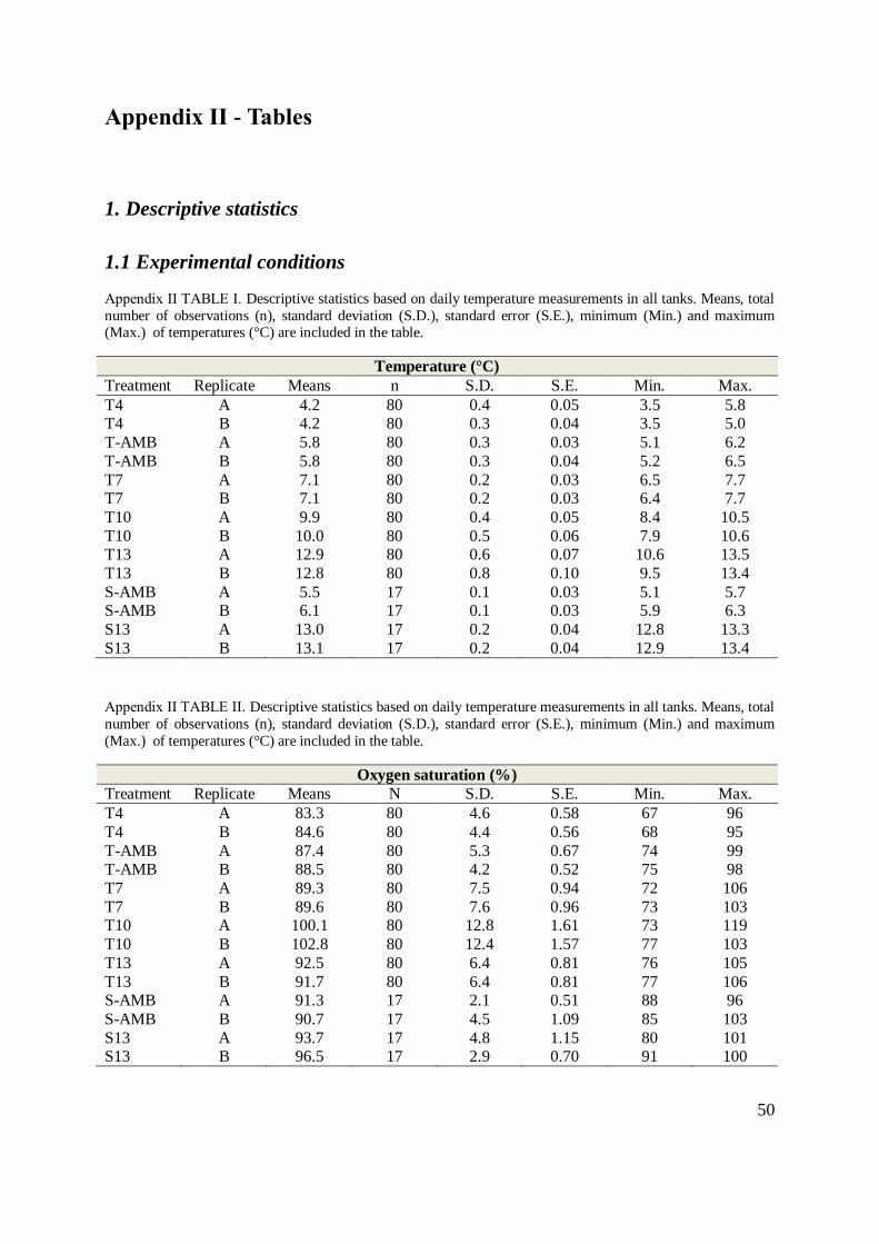
50

Appendix II - Tables

1. Descriptive statistics

1.1 Experimental conditions

Appendix ΙΙ TABLE Ι. Descriptive statistics based on daily temperature measurements in all tanks. Means, total

number of observations (n), standard deviation (S.D.), standard error (S.E.), minimum (Min.) and maximum (Max.) of temperatures (°C) are included in the table.

Temperature (°C)

Treatment Replicate Means n S.D. S.E. Min. Max.

T4 A 4.2 80 0.4 0.05 3.5 5.8 T4 B 4.2 80 0.3 0.04 3.5 5.0

T-AMB A 5.8 80 0.3 0.03 5.1 6.2

T-AMB B 5.8 80 0.3 0.04 5.2 6.5

T7 A 7.1 80 0.2 0.03 6.5 7.7 T7 B 7.1 80 0.2 0.03 6.4 7.7

T10 A 9.9 80 0.4 0.05 8.4 10.5

T10 B 10.0 80 0.5 0.06 7.9 10.6 T13 A 12.9 80 0.6 0.07 10.6 13.5

T13 B 12.8 80 0.8 0.10 9.5 13.4

S-AMB A 5.5 17 0.1 0.03 5.1 5.7 S-AMB B 6.1 17 0.1 0.03 5.9 6.3

S13 A 13.0 17 0.2 0.04 12.8 13.3

S13 B 13.1 17 0.2 0.04 12.9 13.4

Appendix ΙΙ TABLE ΙΙ. Descriptive statistics based on daily temperature measurements in all tanks. Means, total

number of observations (n), standard deviation (S.D.), standard error (S.E.), minimum (Min.) and maximum

(Max.) of temperatures (°C) are included in the table.

Oxygen saturation (%)

Treatment Replicate Means N S.D. S.E. Min. Max.

T4 A 83.3 80 4.6 0.58 67 96

T4 B 84.6 80 4.4 0.56 68 95

T-AMB A 87.4 80 5.3 0.67 74 99 T-AMB B 88.5 80 4.2 0.52 75 98

T7 A 89.3 80 7.5 0.94 72 106

T7 B 89.6 80 7.6 0.96 73 103 T10 A 100.1 80 12.8 1.61 73 119

T10 B 102.8 80 12.4 1.57 77 103

T13 A 92.5 80 6.4 0.81 76 105

T13 B 91.7 80 6.4 0.81 77 106 S-AMB A 91.3 17 2.1 0.51 88 96

S-AMB B 90.7 17 4.5 1.09 85 103

S13 A 93.7 17 4.8 1.15 80 101 S13 B 96.5 17 2.9 0.70 91 100

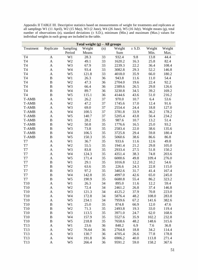
51

Appendix ΙΙ TABLE ΙΙΙ. Descriptive statistics based on measurements of weight for treatments and replicates at

all samplings W1 (11 April), W2 (15 May), W3 (2 June), W4 (26 June), W5 (16 July). Weight means (g), total

number of observations (n), standard deviations (± S.D.), minimum (Min.) and maximum (Max.) values for

individual weights in each group are included in the table.

Total weight (g) – All groups

Treatment Replicate Sampling

Period

Weight

Means

(n) Weight

Sum

± S.D. Weight

Min.

Weight

Max.

T4 A W1 28.3 33 932.4 9.8 13.8 44.4

T4 A W2 49.1 33 1620.2 16.3 25.8 82.4 T4 A W3 67.9 33 2239.3 22.2 36.4 108.4

T4 A W4 93.4 33 3082.8 29.3 52.2 146.8

T4 A W5 121.8 33 4018.0 35.9 66.0 180.2 T4 B W1 26.3 36 943.8 11.6 11.0 54.4

T4 B W2 47.3 36 2704.0 19.6 22.4 92.2

T4 B W3 66.4 36 2389.6 26.5 29.8 126.6

T4 B W4 89.7 36 3230.8 34.5 39.2 169.2 T4 B W5 115.1 36 4144.6 43.6 51.0 216.2

T-AMB A W1 26.2 37 970.0 10.7 6.4 53.6

T-AMB A W2 47.2 37 1745.6 17.0 12.4 91.6 T-AMB A W3 69.0 37 2554.4 24.4 18.8 127.0

T-AMB A W4 100.5 37 3781.8 33.9 36.2 178.2

T-AMB A W5 140.7 37 5205.4 43.8 56.4 234.2 T-AMB B W1 28.2 35 987.6 10.7 13.2 51.4

T-AMB B W2 50.8 35 1776.6 16.5 25.0 93.2

T-AMB B W3 73.8 35 2583.4 22.0 38.6 135.6

T-AMB B W4 106.5 35 3725.8 29.4 59.8 180.4 T-AMB B W5 150.3 35 5060.6 38.6 86.6 86.8

T7 A W1 36.7 35 933.6 11.6 12.6 49.8

T7 A W2 55.5 35 1941.4 21.2 29.8 105.0 T7 A W3 83.8 35 2933.4 27.5 51.8 150.2

T7 A W4 124.3 35 4351.4 38.3 74.8 203.6

T7 A W5 171.4 35 6000.6 49.8 109.4 276.0 T7 B W1 29.1 35 1016.8 12.2 10.2 54.6

T7 B W2 63.6 35 226.6 24.3 22.8 115.0

T7 B W3 97.2 35 3402.6 31.7 41.4 167.4

T7 B W4 142.8 35 4997.0 42.6 65.0 245.0 T7 B W5 190.9 35 6680.8 55.4 86.2 323.2

T10 A W1 26.3 34 895.0 11.6 12.2 59.4

T10 A W2 72.4 34 2461.2 26.8 37.4 146.8 T10 A W3 121.3 34 4125.2 37.9 70.8 223.0

T10 A W4 172.8 34 5876.4 48.2 108.0 283.8

T10 A W5 234.1 34 7959.6 67.2 141.6 382.6

T10 B W1 25.0 35 874.8 66.9 12.0 47.6 T10 B W2 71.3 35 2493.8 19.3 33.0 119.4

T10 B W3 113.5 35 3971.0 24.7 62.0 168.6

T10 B W4 157.9 35 5527.6 35.9 102.2 232.8 T10 B W5 218.8 35 7658.6 48.2 148.6 315.6

T13 A W1 23.6 36 848.2 6.9 7.6 36.8

T13 A W2 76.64 36 2764.8 18.8 34.2 114.4 T13 A W3 130.7 36 4705.4 26.6 77.8 178.8

T13 A W4 191.8 36 6906.2 40.0 113.8 271.4

T13 A W5 266.4 36 9591.2 59.0 158.2 367.6

52

T13 B W1 25.1 32 804.4 10.3 10.0 56.6

T13 B W2 82.0 32 2624.0 24.3 34.0 145.4

T13 B W3 136.5 32 4368.2 32.4 73.8 228.4 T13 B W4 183.5 32 5871.2 44.1 108.6 324.0

T13 B W5 246.1 32 7873.8 54.9 167.4 430.4

S-AMB A W1 39.1 61 2385.0 8.9 23.6 62.6 S-AMB A W2 59.7 61 3649.9 13.2 35.2 97.8

S-AMB B W1 34.5 60 2070.6 6.9 21.2 50.2

S-AMB B W2 52.6 60 3158.8 10.2 34.4 79.4

S13 A W1 68.2 60 4093.5 12.6 40.2 97.8 S13 A W2 127.1 60 7623.8 23.3 84.0 176.0

S13 B W1 45.2 60 2714.8 7.6 32.8 64.8

S13 B W2 91.5 60 5488.0 14.5 57.6 131.8

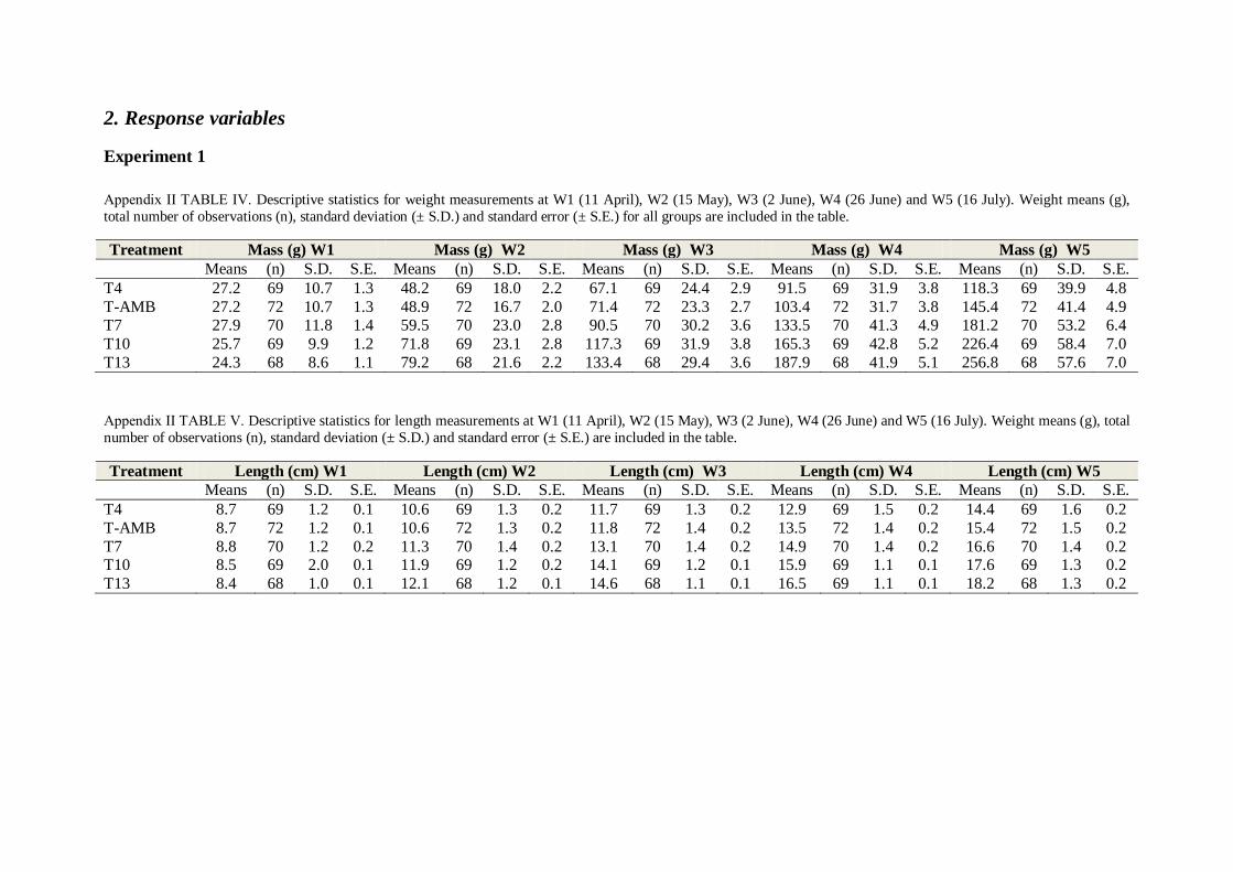
2. Response variables

Experiment 1

Appendix ΙΙ TABLE ΙV. Descriptive statistics for weight measurements at W1 (11 April), W2 (15 May), W3 (2 June), W4 (26 June) and W5 (16 July). Weight means (g),

total number of observations (n), standard deviation (± S.D.) and standard error (± S.E.) for all groups are included in the table.

Treatment Mass (g) W1 Mass (g) W2 Mass (g) W3 Mass (g) W4 Mass (g) W5

Means (n) S.D. S.E. Means (n) S.D. S.E. Means (n) S.D. S.E. Means (n) S.D. S.E. Means (n) S.D. S.E.

T4 27.2 69 10.7 1.3 48.2 69 18.0 2.2 67.1 69 24.4 2.9 91.5 69 31.9 3.8 118.3 69 39.9 4.8

T-AMB 27.2 72 10.7 1.3 48.9 72 16.7 2.0 71.4 72 23.3 2.7 103.4 72 31.7 3.8 145.4 72 41.4 4.9 T7 27.9 70 11.8 1.4 59.5 70 23.0 2.8 90.5 70 30.2 3.6 133.5 70 41.3 4.9 181.2 70 53.2 6.4

T10 25.7 69 9.9 1.2 71.8 69 23.1 2.8 117.3 69 31.9 3.8 165.3 69 42.8 5.2 226.4 69 58.4 7.0

T13 24.3 68 8.6 1.1 79.2 68 21.6 2.2 133.4 68 29.4 3.6 187.9 68 41.9 5.1 256.8 68 57.6 7.0

Appendix ΙΙ TABLE V. Descriptive statistics for length measurements at W1 (11 April), W2 (15 May), W3 (2 June), W4 (26 June) and W5 (16 July). Weight means (g), total

number of observations (n), standard deviation (± S.D.) and standard error (± S.E.) are included in the table.

Treatment Length (cm) W1 Length (cm) W2 Length (cm) W3 Length (cm) W4 Length (cm) W5


T4 8.7 69 1.2 0.1 10.6 69 1.3 0.2 11.7 69 1.3 0.2 12.9 69 1.5 0.2 14.4 69 1.6 0.2

T-AMB 8.7 72 1.2 0.1 10.6 72 1.3 0.2 11.8 72 1.4 0.2 13.5 72 1.4 0.2 15.4 72 1.5 0.2

T7 8.8 70 1.2 0.2 11.3 70 1.4 0.2 13.1 70 1.4 0.2 14.9 70 1.4 0.2 16.6 70 1.4 0.2 T10 8.5 69 2.0 0.1 11.9 69 1.2 0.2 14.1 69 1.2 0.1 15.9 69 1.1 0.1 17.6 69 1.3 0.2

T13 8.4 68 1.0 0.1 12.1 68 1.2 0.1 14.6 68 1.1 0.1 16.5 69 1.1 0.1 18.2 68 1.3 0.2

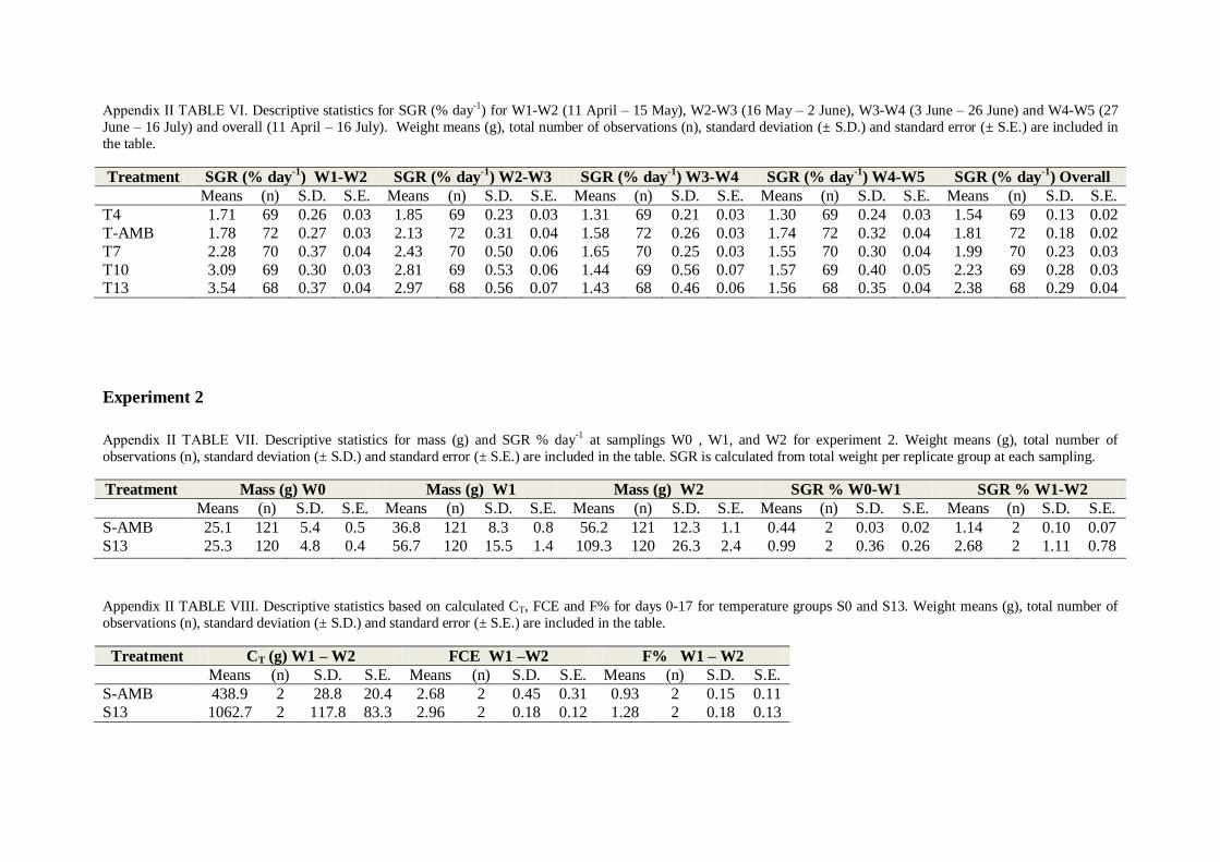
Appendix ΙΙ TABLE VI. Descriptive statistics for SGR (% day-1) for W1-W2 (11 April – 15 May), W2-W3 (16 May – 2 June), W3-W4 (3 June – 26 June) and W4-W5 (27

June – 16 July) and overall (11 April – 16 July). Weight means (g), total number of observations (n), standard deviation (± S.D.) and standard error (± S.E.) are included in

the table.

Treatment SGR (% day-1

) W1-W2 SGR (% day-1




) Overall


T4 1.71 69 0.26 0.03 1.85 69 0.23 0.03 1.31 69 0.21 0.03 1.30 69 0.24 0.03 1.54 69 0.13 0.02

T-AMB 1.78 72 0.27 0.03 2.13 72 0.31 0.04 1.58 72 0.26 0.03 1.74 72 0.32 0.04 1.81 72 0.18 0.02

T7 2.28 70 0.37 0.04 2.43 70 0.50 0.06 1.65 70 0.25 0.03 1.55 70 0.30 0.04 1.99 70 0.23 0.03

T10 3.09 69 0.30 0.03 2.81 69 0.53 0.06 1.44 69 0.56 0.07 1.57 69 0.40 0.05 2.23 69 0.28 0.03 T13 3.54 68 0.37 0.04 2.97 68 0.56 0.07 1.43 68 0.46 0.06 1.56 68 0.35 0.04 2.38 68 0.29 0.04

Experiment 2

Appendix ΙΙ TABLE VII. Descriptive statistics for mass (g) and SGR % day-1 at samplings W0 , W1, and W2 for experiment 2. Weight means (g), total number of

observations (n), standard deviation (± S.D.) and standard error (± S.E.) are included in the table. SGR is calculated from total weight per replicate group at each sampling.

Treatment Mass (g) W0 Mass (g) W1 Mass (g) W2 SGR % W0-W1 SGR % W1-W2


S-AMB 25.1 121 5.4 0.5 36.8 121 8.3 0.8 56.2 121 12.3 1.1 0.44 2 0.03 0.02 1.14 2 0.10 0.07

S13 25.3 120 4.8 0.4 56.7 120 15.5 1.4 109.3 120 26.3 2.4 0.99 2 0.36 0.26 2.68 2 1.11 0.78

Appendix II TABLE VIII. Descriptive statistics based on calculated CT, FCE and F% for days 0-17 for temperature groups S0 and S13. Weight means (g), total number of

observations (n), standard deviation (± S.D.) and standard error (± S.E.) are included in the table.

Treatment CT (g) W1 – W2 FCE W1 –W2 F% W1 – W2

Means (n) S.D. S.E. Means (n) S.D. S.E. Means (n) S.D. S.E.

S-AMB 438.9 2 28.8 20.4 2.68 2 0.45 0.31 0.93 2 0.15 0.11

S13 1062.7 2 117.8 83.3 2.96 2 0.18 0.12 1.28 2 0.18 0.13

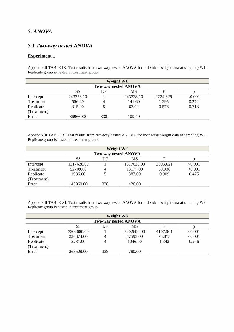
3. ANOVA

3.1 Two-way nested ANOVA

Experiment 1

Appendix II TABLE IX. Test results from two-way nested ANOVA for individual weight data at sampling W1.

Replicate group is nested in treatment group.

Weight W1

Two-way nested ANOVA

SS DF MS F p

Intercept 243328.10 1 243328.10 2224.829 <0.001

Treatment 556.40 4 141.60 1.295 0.272

Replicate (Treatment)

315.00 5 63.00 0.576 0.718

Error 36966.80 338 109.40

Appendix II TABLE X. Test results from two-way nested ANOVA for individual weight data at sampling W2.


Weight W2


SS DF MS F p

Intercept 1317628.00 1 1317628.00 3093.621 <0.001

Treatment 52709.00 4 13177.00 30.938 <0.001 Replicate

(Treatment)

1936.00 5 387.00 0.909 0.475

Error 143960.00 338 426.00

Appendix II TABLE XI. Test results from two-way nested ANOVA for individual weight data at sampling W3.


Weight W3


SS DF MS F p

Intercept 3202600.00 1 3202600.00 4107.961 <0.001 Treatment 230374.00 4 57593.00 73.875 <0.001

Replicate

(Treatment)

5231.00 4 1046.00 1.342 0.246

Error 263508.00 338 780.00

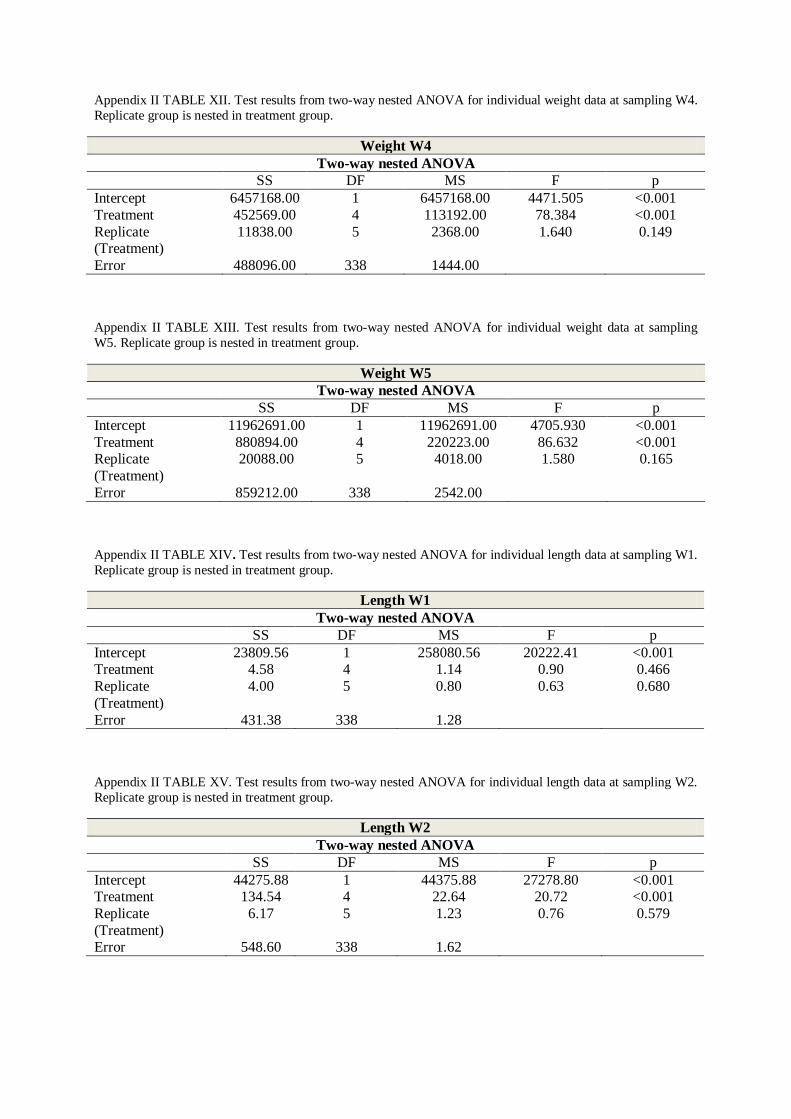
Appendix II TABLE XII. Test results from two-way nested ANOVA for individual weight data at sampling W4.


Weight W4


SS DF MS F p

Intercept 6457168.00 1 6457168.00 4471.505 <0.001

Treatment 452569.00 4 113192.00 78.384 <0.001


11838.00 5 2368.00 1.640 0.149

Error 488096.00 338 1444.00

Appendix II TABLE XIII. Test results from two-way nested ANOVA for individual weight data at sampling

W5. Replicate group is nested in treatment group.

Weight W5


SS DF MS F p

Intercept 11962691.00 1 11962691.00 4705.930 <0.001


(Treatment)

20088.00 5 4018.00 1.580 0.165

Error 859212.00 338 2542.00

Appendix II TABLE XIV. Test results from two-way nested ANOVA for individual length data at sampling W1.


Length W1


SS DF MS F p

Intercept 23809.56 1 258080.56 20222.41 <0.001 Treatment 4.58 4 1.14 0.90 0.466

Replicate

(Treatment)

4.00 5 0.80 0.63 0.680

Error 431.38 338 1.28

Appendix II TABLE XV. Test results from two-way nested ANOVA for individual length data at sampling W2.


Length W2


SS DF MS F p


Replicate

(Treatment)

6.17 5 1.23 0.76 0.579

Error 548.60 338 1.62

Appendix II TABLE XVI. Test results from two-way nested ANOVA for individual length data at sampling W3.


Length W3


SS DF MS F p

Intercept 59700.01 1 59700.01 36473.11 <0.001

Treatment 446.73 4 111.68 68.23 <0.001


6.12 5 1.22 0.75 0.588

Error 553.25 338 1.64

Appendix II TABLE XVII. Test results from two-way nested ANOVA for individual length data at sampling


Length W4


SS DF MS F p

Intercept 75612.68 1 75612.68 43563.16 <0.001


(Treatment)

9.66 5 1.93 1.11 0.353

Error 586.67 338 1.74

Appendix II TABLE XVIII. Test results from two-way nested ANOVA for individual length data at sampling


Length W5


SS DF MS F p

Intercept 93962.31 1 93962.31 46126.95 <0.001


(Treatment)

5.77 338 1.15 0.57 0.726

Error 688.52 338 2.04

Appendix II TABLE XIX. Test results from two-way nested ANOVA for individual SGR data for W1-W2 (11

April – 15 May). Replicate group is nested in treatment group.

SGR % day-1

W1 – W2


SS DF MS F p

Intercept 2136.421 1 2136.421 21438.68 <0.001


(Treatment)

0.766 5 0.153 1.54 0.177

Error 33.683 338 0.100

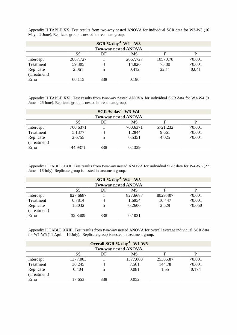
Appendix II TABLE XX. Test results from two-way nested ANOVA for individual SGR data for W2-W3 (16

May – 2 June). Replicate group is nested in treatment group.

SGR % day-1

W2 – W3


SS DF MS F P

Intercept 2067.727 1 2067.727 10570.78 <0.001

Treatment 59.305 4 14.826 75.80 <0.001


2.061 5 0.412 22.11 0.041

Error 66.115 338 0.196

Appendix II TABLE XXI. Test results from two-way nested ANOVA for individual SGR data for W3-W4 (3

June – 26 June). Replicate group is nested in treatment group.

SGR % day-1

W3-W4


SS DF MS F P

Intercept 760.6371 1 760.6371 5721.232 <0.001


(Treatment)

2.6755 5 0.5351 4.025 <0.001

Error 44.9371 338 0.1329

Appendix II TABLE XXII. Test results from two-way nested ANOVA for individual SGR data for W4-W5 (27

June – 16 July). Replicate group is nested in treatment group.

SGR % day-1

W4 – W5


SS DF MS F P


Replicate

(Treatment)

1.3032 5 0.2606 2.529 <0.050

Error 32.8409 338 0.1031

Appendix II TABLE XXIII. Test results from two-way nested ANOVA for overall average individual SGR data for W1-W5 (11 April – 16 July). Replicate group is nested in treatment group.

Overall SGR % day-1

W1-W5


SS DF MS F P

Intercept 1377.003 1 1377.003 25365.87 <0.001

Treatment 30.245 4 7.561 144.78 <0.001

Replicate

(Treatment)

0.404 5 0.081 1.55 0.174

Error 17.653 338 0.052

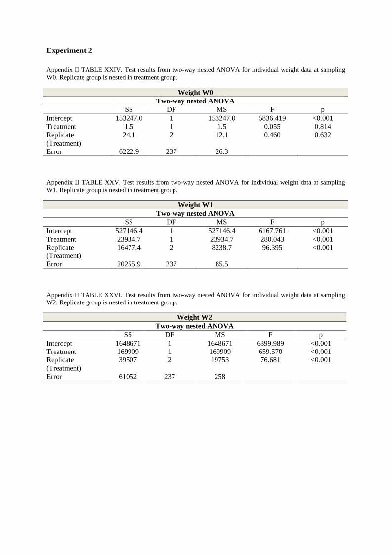
Experiment 2

Appendix II TABLE XXIV. Test results from two-way nested ANOVA for individual weight data at sampling


Weight W0


SS DF MS F p

Intercept 153247.0 1 153247.0 5836.419 <0.001

Treatment 1.5 1 1.5 0.055 0.814 Replicate

(Treatment)

24.1 2 12.1 0.460 0.632

Error 6222.9 237 26.3

Appendix II TABLE XXV. Test results from two-way nested ANOVA for individual weight data at sampling


Weight W1


SS DF MS F p

Intercept 527146.4 1 527146.4 6167.761 <0.001


(Treatment)

16477.4 2 8238.7 96.395 <0.001

Error 20255.9 237 85.5

Appendix II TABLE XXVI. Test results from two-way nested ANOVA for individual weight data at sampling


Weight W2


SS DF MS F p

Intercept 1648671 1 1648671 6399.989 <0.001 Treatment 169909 1 169909 659.570 <0.001

Replicate

(Treatment)

39507 2 19753 76.681 <0.001

Error 61052 237 258

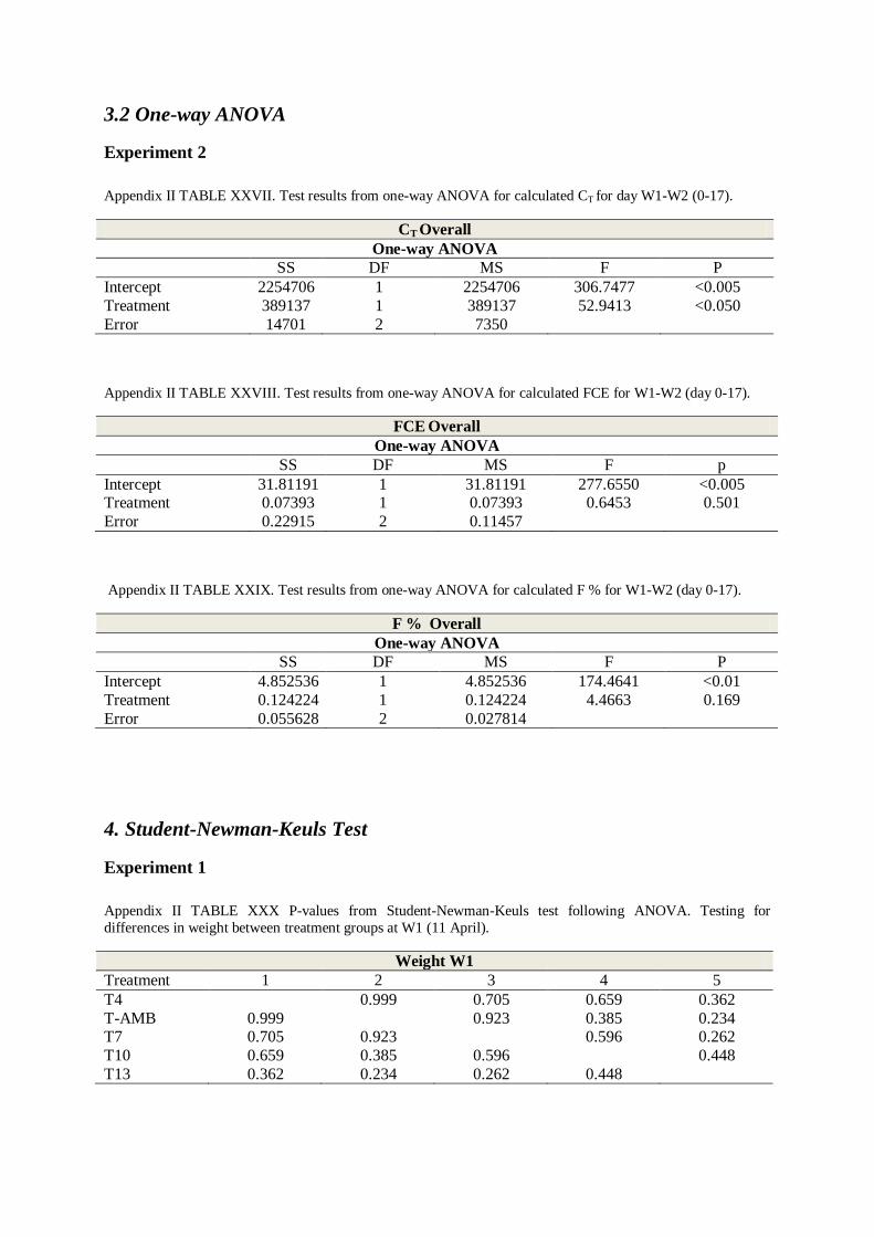
3.2 One-way ANOVA

Experiment 2

Appendix II TABLE XXVII. Test results from one-way ANOVA for calculated CT for day W1-W2 (0-17).

CT Overall

One-way ANOVA

SS DF MS F P

Intercept 2254706 1 2254706 306.7477 <0.005

Treatment 389137 1 389137 52.9413 <0.050

Error 14701 2 7350

Appendix II TABLE XXVIII. Test results from one-way ANOVA for calculated FCE for W1-W2 (day 0-17).

FCE Overall

One-way ANOVA

SS DF MS F p

Intercept 31.81191 1 31.81191 277.6550 <0.005 Treatment 0.07393 1 0.07393 0.6453 0.501

Error 0.22915 2 0.11457

Appendix II TABLE XXIX. Test results from one-way ANOVA for calculated F % for W1-W2 (day 0-17).

F % Overall

One-way ANOVA

SS DF MS F P

Intercept 4.852536 1 4.852536 174.4641 <0.01

Treatment 0.124224 1 0.124224 4.4663 0.169

Error 0.055628 2 0.027814

4. Student-Newman-Keuls Test

Experiment 1

Appendix II TABLE XXX P-values from Student-Newman-Keuls test following ANOVA. Testing for

differences in weight between treatment groups at W1 (11 April).

Weight W1

Treatment 1 2 3 4 5

T4 0.999 0.705 0.659 0.362

T-AMB 0.999 0.923 0.385 0.234 T7 0.705 0.923 0.596 0.262

T10 0.659 0.385 0.596 0.448

T13 0.362 0.234 0.262 0.448

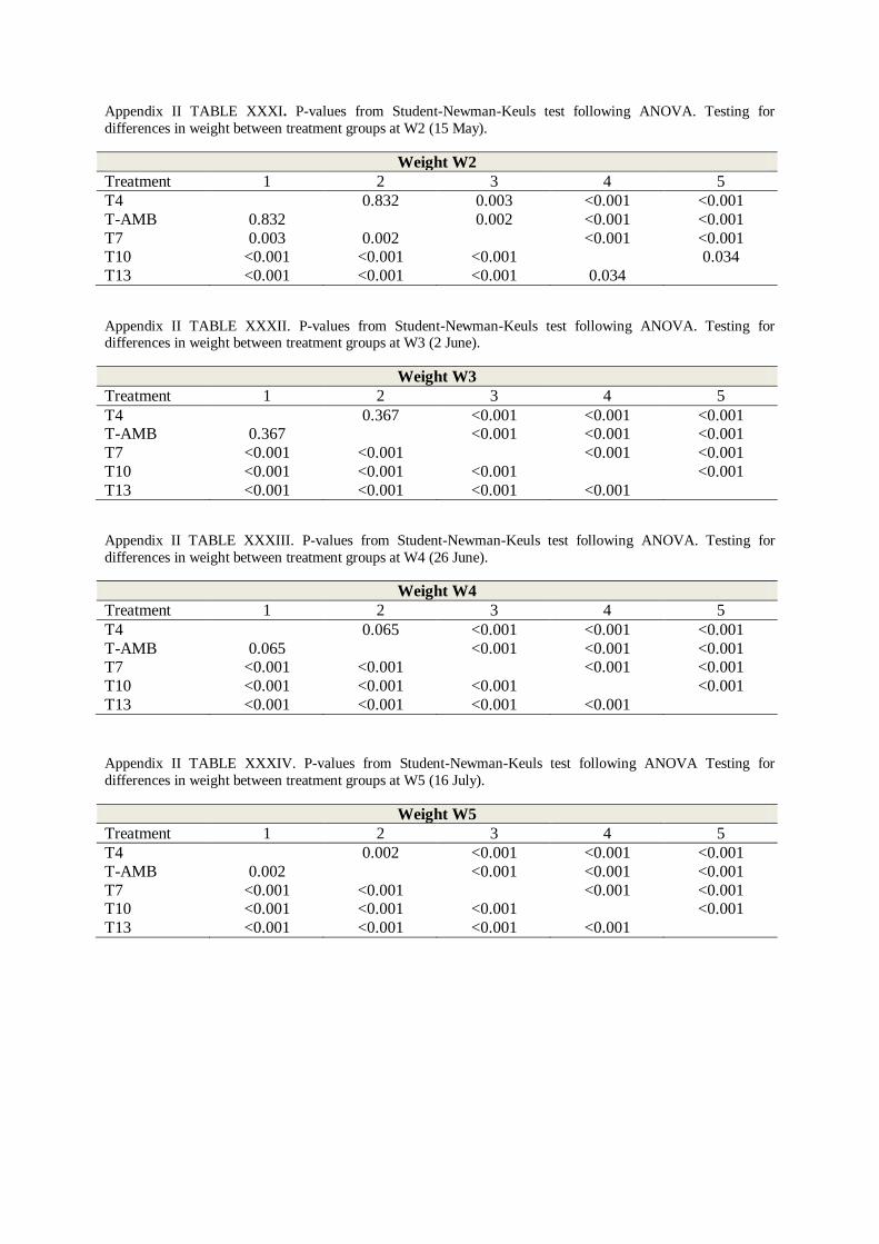
Appendix II TABLE XXXI. P-values from Student-Newman-Keuls test following ANOVA. Testing for

differences in weight between treatment groups at W2 (15 May).

Weight W2

Treatment 1 2 3 4 5

T4 0.832 0.003 <0.001 <0.001

T-AMB 0.832 0.002 <0.001 <0.001

T7 0.003 0.002 <0.001 <0.001 T10 <0.001 <0.001 <0.001 0.034

T13 <0.001 <0.001 <0.001 0.034

Appendix II TABLE XXXII. P-values from Student-Newman-Keuls test following ANOVA. Testing for differences in weight between treatment groups at W3 (2 June).

Weight W3

Treatment 1 2 3 4 5

T4 0.367 <0.001 <0.001 <0.001 T-AMB 0.367 <0.001 <0.001 <0.001

T7 <0.001 <0.001 <0.001 <0.001

T10 <0.001 <0.001 <0.001 <0.001

T13 <0.001 <0.001 <0.001 <0.001

Appendix II TABLE XXXIII. P-values from Student-Newman-Keuls test following ANOVA. Testing for

differences in weight between treatment groups at W4 (26 June).

Weight W4

Treatment 1 2 3 4 5

T4 0.065 <0.001 <0.001 <0.001

T-AMB 0.065 <0.001 <0.001 <0.001 T7 <0.001 <0.001 <0.001 <0.001

T10 <0.001 <0.001 <0.001 <0.001

T13 <0.001 <0.001 <0.001 <0.001

Appendix II TABLE XXXIV. P-values from Student-Newman-Keuls test following ANOVA Testing for

differences in weight between treatment groups at W5 (16 July).

Weight W5

Treatment 1 2 3 4 5

T4 0.002 <0.001 <0.001 <0.001

T-AMB 0.002 <0.001 <0.001 <0.001

T7 <0.001 <0.001 <0.001 <0.001 T10 <0.001 <0.001 <0.001 <0.001

T13 <0.001 <0.001 <0.001 <0.001

Appendix II TABLE XXXV. P-values from Student-Newman-Keuls test following ANOVA. Testing for

differences in length between treatment groups at W1 (11 April).

Length W1

Treatment 1 2 3 4 5

T4 0.754 0.789 0.635 0.511

T-AMB 0.754 0.830 0.552 0.534

T7 0.789 0.830 0.642 0.466 T10 0.635 0.552 0.642 0.636

T13 0.511 0.534 0.466 0.636

Appendix II TABLE XXXVI. P-values from Student-Newman-Keuls test following ANOVA Testing for differences in length between treatment groups at W2 (15 May).

Length W2

Treatment 1 2 3 4 5

T4 0.915 0.003 <0.001 <0.001 T-AMB 0.915 0.002 <0.001 <0.001

T7 0.003 0.002 0.008 <0.001

T10 <0.001 <0.001 0.008 0.265

T13 <0.001 <0.001 <0.001 0.265

Appendix II TABLE XXXVII. P-values from Student-Newman-Keuls test following ANOVA Testing for

differences in length between treatment groups at W3 (2 June).

Length W3

Treatment 1 2 3 4 5

T4 0.230 <0.001 <0.001 <0.001

T-AMB 0.230 <0.001 <0.001 T7 <0.001 <0.001 <0.001

T10 <0.001 <0.001 <0.001 0.028

T13 <0.001 <0.001 <0.001 0.028

Appendix II TABLE XXXVIII. P-values from Student-Newman-Keuls test following ANOVA. Testing for

differences in length between treatment groups at W4 (26 June).

Length W4

Treatment 1 2 3 4 5

T4 0.008 <0.001 <0.001 <0.001

T-AMB 0.008 <0.001 <0.001 <0.001

T7 <0.001 <0.001 <0.001 <0.001 T10 <0.001 <0.001 <0.001 0.007

T13 <0.001 <0.001 <0.001 0.007

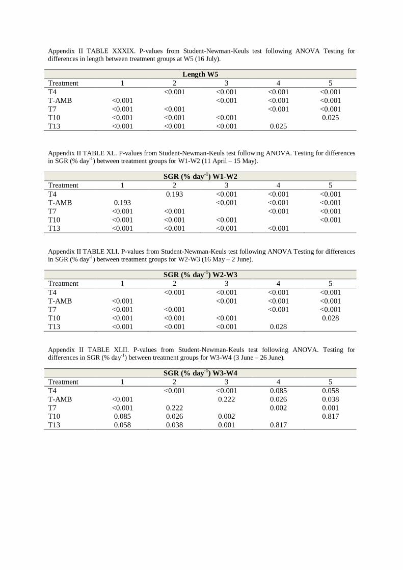
Appendix II TABLE XXXIX. P-values from Student-Newman-Keuls test following ANOVA Testing for

differences in length between treatment groups at W5 (16 July).

Length W5

Treatment 1 2 3 4 5

T4 <0.001 <0.001 <0.001 <0.001

T-AMB <0.001 <0.001 <0.001 <0.001

T7 <0.001 <0.001 <0.001 <0.001 T10 <0.001 <0.001 <0.001 0.025

T13 <0.001 <0.001 <0.001 0.025

Appendix II TABLE XL. P-values from Student-Newman-Keuls test following ANOVA. Testing for differences

in SGR (% day-1) between treatment groups for W1-W2 (11 April – 15 May).

SGR (% day-1

) W1-W2

Treatment 1 2 3 4 5

T4 0.193 <0.001 <0.001 <0.001 T-AMB 0.193 <0.001 <0.001 <0.001

T7 <0.001 <0.001 <0.001 <0.001

T10 <0.001 <0.001 <0.001 <0.001 T13 <0.001 <0.001 <0.001 <0.001

Appendix II TABLE XLI. P-values from Student-Newman-Keuls test following ANOVA Testing for differences

in SGR (% day-1) between treatment groups for W2-W3 (16 May – 2 June).

SGR (% day-1

) W2-W3

Treatment 1 2 3 4 5

T4 <0.001 <0.001 <0.001 <0.001

T-AMB <0.001 <0.001 <0.001 <0.001 T7 <0.001 <0.001 <0.001 <0.001

T10 <0.001 <0.001 <0.001 0.028

T13 <0.001 <0.001 <0.001 0.028

Appendix II TABLE XLII. P-values from Student-Newman-Keuls test following ANOVA. Testing for

differences in SGR (% day-1) between treatment groups for W3-W4 (3 June – 26 June).

SGR (% day-1

) W3-W4

Treatment 1 2 3 4 5

T4 <0.001 <0.001 0.085 0.058

T-AMB <0.001 0.222 0.026 0.038

T7 <0.001 0.222 0.002 0.001 T10 0.085 0.026 0.002 0.817

T13 0.058 0.038 0.001 0.817

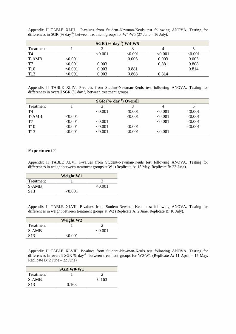
Appendix II TABLE XLIII. P-values from Student-Newman-Keuls test following ANOVA. Testing for

differences in SGR (% day-1) between treatment groups for W4-W5 (27 June – 16 July).

SGR (% day-1

) W4-W5

Treatment 1 2 3 4 5

T4 <0.001 <0.001 <0.001 <0.001

T-AMB <0.001 0.003 0.003 0.003

T7 <0.001 0.003 0.881 0.808 T10 <0.001 0.003 0.881 0.814

T13 <0.001 0.003 0.808 0.814

Appendix II TABLE XLIV. P-values from Student-Newman-Keuls test following ANOVA. Testing for differences in overall SGR (% day-1) between treatment groups.

SGR (% day-1

) Overall

Treatment 1 2 3 4 5

T4 <0.001 <0.001 <0.001 <0.001 T-AMB <0.001 <0.001 <0.001 <0.001

T7 <0.001 <0.001 <0.001 <0.001

T10 <0.001 <0.001 <0.001 <0.001

T13 <0.001 <0.001 <0.001 <0.001

Experiment 2

Appendix II TABLE XLVI. P-values from Student-Newman-Keuls test following ANOVA. Testing for

differences in weight between treatment groups at W1 (Replicate A: 15 May, Replicate B: 22 June).

Weight W1

Treatment 1 2

S-AMB <0.001 S13 <0.001

Appendix II TABLE XLVII. P-values from Student-Newman-Keuls test following ANOVA. Testing for

differences in weight between treatment groups at W2 (Replicate A: 2 June, Replicate B: 10 July).

Weight W2

Treatment 1 2

S-AMB <0.001

S13 <0.001

Appendix II TABLE XLVIII. P-values from Student-Newman-Keuls test following ANOVA. Testing for

differences in overall SGR % day-1 between treatment groups for W0-W1 (Replicate A: 11 April – 15 May,

Replicate B: 2 June – 22 June).

SGR W0-W1

Treatment 1 2

S-AMB 0.163

S13 0.163

Appendix II TABLE XLIX. P-values from Student-Newman-Keuls test following ANOVA.. Testing for

differences in overall SGR % day-1 between treatment groups at W1-W2 (Replicate A: 15 May – 2 June,

Replicate B; 22 June – 10 July).

SGR % day-1

W1-W2

Treatment 1 2

S-AMB 0.190

S13 0.190

Appendix II TABLE L. P-values from Student-Newman-Keuls test following ANOVA. Testing for differences in CT between treatment groups for W1-W2 (Replicate A: 15 May – 2 June, Replicate B; 22 June – 10 July).

CT W1-W2

Treatment 1 2

S-AMB 0.019 S13 0.019

Appendix II TABLE LI. P-values from Student-Newman-Keuls test following ANOVA. Testing for differences

in FCE between treatment groups for W1-W2 (Replicate A: 15 May – 2 June, Replicate B; 22 June – 10 July).

FCE W1-W2

Treatment 1 2

S-AMB 0.0506

S13 0.0506

Appendix II TABLE LII. P-values from Student-Newman-Keuls test following ANOVA. Testing for differences

in F% between treatment groups for W1-W2 (Replicate A: 15 May – 2 June, Replicate B; 22 June – 10 July).

F% W1-W2

Treatment 1 2

S-AMB 0.169

S13 0.169

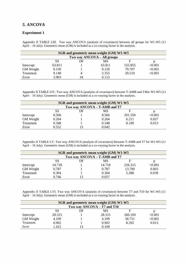
5. ANCOVA

Experiment 1

Appendix II TABLE LIII. Two way ANCOVA (analysis of covariance) between all groups for W1-W5 (11

April – 16 July). Geometric mean (GM) is included as a co-varying factor in the analysis.

SGR and geometric mean weight (GM) W1-W5

Two way ANCOVA – All groups

SS DF MS F p

Intercept 63.811 1 63.811 555.855 <0.001

GM Weight 9.150 1 9.150 79.707 <0.001 Treatment 9.148 4 2.355 20.510 <0.001

Error 3.903 34 0.115

Appendix II TABLE LIV. Two way ANCOVA (analysis of covariance) between T-AMB and T4for W1-W5 (11



Two way ANCOVA – T-AMB and T7

SS DF MS F p

Intercept 8.566 1 8.566 201.550 <0.001

GM Weight 0.264 1 0.264 6.211 0.027

Treatment 0.348 1 0.348 8.190 0.013 Error 0.552 13 0.042

Appendix II TABLE LV. Two way ANCOVA (analysis of covariance) between T-AMB and T7 for W1-W5 (11



Two way ANCOVA – T-AMB and T7

SS DF MS F p

Intercept 14.718 1 14.718 256.315 <0.001

GM Weight 0.787 1 0.787 13.700 0.003

Treatment 0.304 1 0.304 5.288 0.039 Error 0.746 13 0.057

Appendix II TABLE LVI. Two way ANCOVA (analysis of covariance) between T7 and T10 for W1-W5 (11



Two way ANCOVA – T7 and T10

SS DF MS F p

Intercept 28.315 1 28.315 260.169 <0.001

GM Weight 4.109 1 4.109 38.751 <0.001 Treatment 0.902 1 0.902 8.292 0.013 Error 1.415 13 0.109

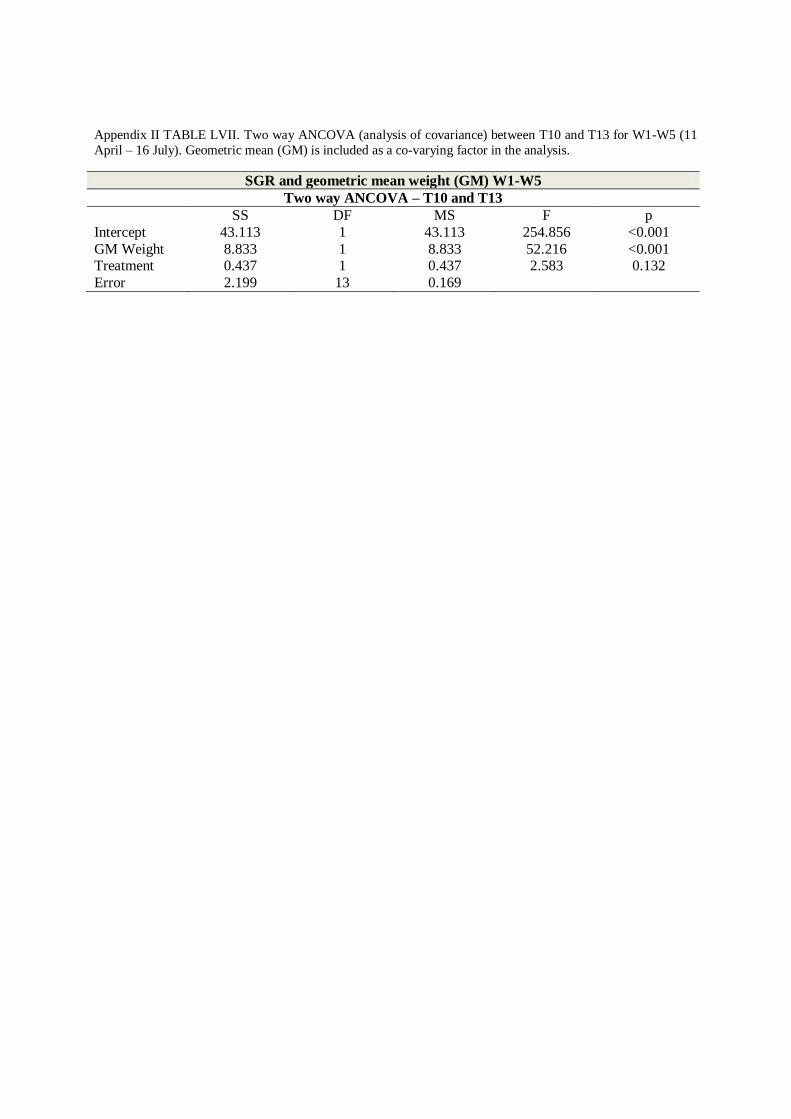
Appendix II TABLE LVII. Two way ANCOVA (analysis of covariance) between T10 and T13 for W1-W5 (11



Two way ANCOVA – T10 and T13

SS DF MS F p

Intercept 43.113 1 43.113 254.856 <0.001

GM Weight 8.833 1 8.833 52.216 <0.001 Treatment 0.437 1 0.437 2.583 0.132

Error 2.199 13 0.169

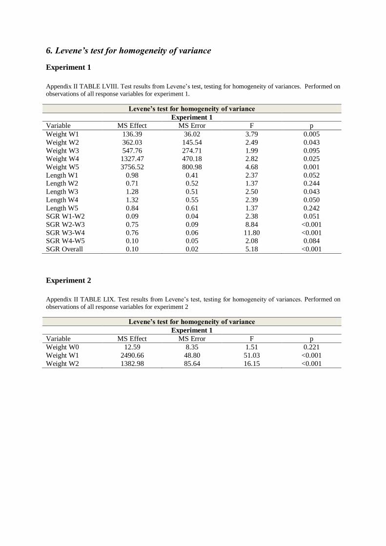
6. Levene’s test for homogeneity of variance

Experiment 1

Appendix II TABLE LVIII. Test results from Levene’s test, testing for homogeneity of variances. Performed on

observations of all response variables for experiment 1.

Levene’s test for homogeneity of variance

Experiment 1

Variable MS Effect MS Error F p

Weight W1 136.39 36.02 3.79 0.005

Weight W2 362.03 145.54 2.49 0.043

Weight W3 547.76 274.71 1.99 0.095 Weight W4 1327.47 470.18 2.82 0.025

Weight W5 3756.52 800.98 4.68 0.001

Length W1 0.98 0.41 2.37 0.052 Length W2 0.71 0.52 1.37 0.244

Length W3 1.28 0.51 2.50 0.043

Length W4 1.32 0.55 2.39 0.050

Length W5 0.84 0.61 1.37 0.242 SGR W1-W2 0.09 0.04 2.38 0.051

SGR W2-W3 0.75 0.09 8.84 <0.001

SGR W3-W4 0.76 0.06 11.80 <0.001 SGR W4-W5 0.10 0.05 2.08 0.084

SGR Overall 0.10 0.02 5.18 <0.001

Experiment 2

Appendix II TABLE LIX. Test results from Levene’s test, testing for homogeneity of variances. Performed on

observations of all response variables for experiment 2

Levene’s test for homogeneity of variance

Experiment 1

Variable MS Effect MS Error F p

Weight W0 12.59 8.35 1.51 0.221

Weight W1 2490.66 48.80 51.03 <0.001

Weight W2 1382.98 85.64 16.15 <0.001

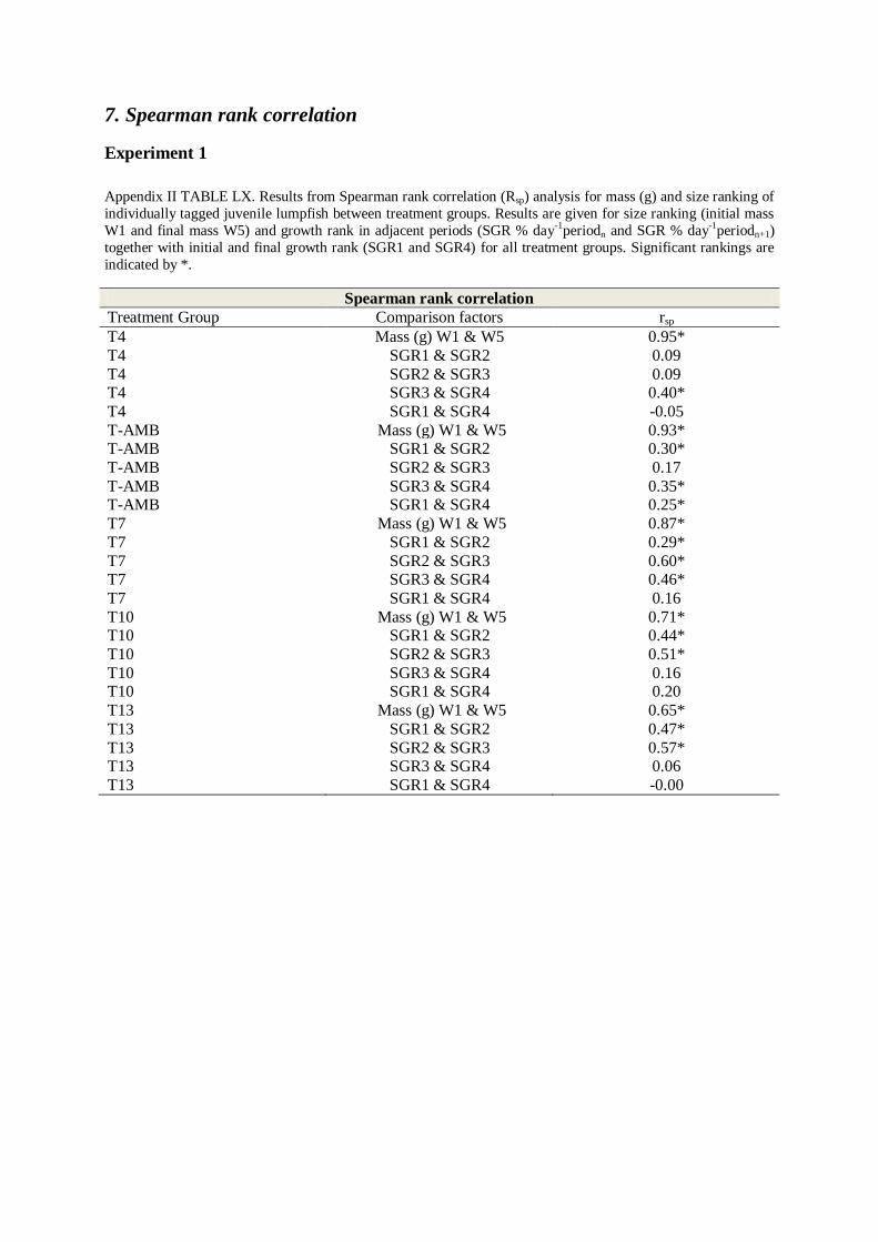
7. Spearman rank correlation

Experiment 1

Appendix II TABLE LX. Results from Spearman rank correlation (Rsp) analysis for mass (g) and size ranking of

individually tagged juvenile lumpfish between treatment groups. Results are given for size ranking (initial mass

W1 and final mass W5) and growth rank in adjacent periods (SGR % day-1periodn and SGR % day-1periodn+1)

together with initial and final growth rank (SGR1 and SGR4) for all treatment groups. Significant rankings are

indicated by *.

Spearman rank correlation

Treatment Group Comparison factors rsp

T4 Mass (g) W1 & W5 0.95*

T4 SGR1 & SGR2 0.09

T4 SGR2 & SGR3 0.09 T4 SGR3 & SGR4 0.40*

T4 SGR1 & SGR4 -0.05

T-AMB Mass (g) W1 & W5 0.93* T-AMB SGR1 & SGR2 0.30*

T-AMB SGR2 & SGR3 0.17

T-AMB SGR3 & SGR4 0.35* T-AMB SGR1 & SGR4 0.25*

T7 Mass (g) W1 & W5 0.87*

T7 SGR1 & SGR2 0.29*

T7 SGR2 & SGR3 0.60* T7 SGR3 & SGR4 0.46*

T7 SGR1 & SGR4 0.16

T10 Mass (g) W1 & W5 0.71* T10 SGR1 & SGR2 0.44*

T10 SGR2 & SGR3 0.51*

T10 SGR3 & SGR4 0.16 T10 SGR1 & SGR4 0.20

T13 Mass (g) W1 & W5 0.65*

T13 SGR1 & SGR2 0.47*

T13 SGR2 & SGR3 0.57* T13 SGR3 & SGR4 0.06

T13 SGR1 & SGR4 -0.00

8. Q10 Temperature effect on specific growth rate

Experiment 1

Appendix II, TABLE LXI. Table of calculated values of temperature effect on growth rate, Q10. Values for SGR

% day-1 are calculated as overall group means for the period W1-W5 (11 April – 16 July).

Q10 of specific growth rate

Comparison factor Q10

SGR T4 & SGR T-AMB 3.16

SGR T4 & SGR T7 2.25

SGR T4 & SGR T10 1.58 SGR T4 & SGR T13 1.41

SGR T-AMB & SGR T7 1.48

SGR T-AMB & SGR T10 1.20 SGR T-AMB & SGR T13 1.18

SGR T7 & SGR T10 1.09

SGR T7 & SGR T13 1.12

SGR T10 & SGR T13 1.15

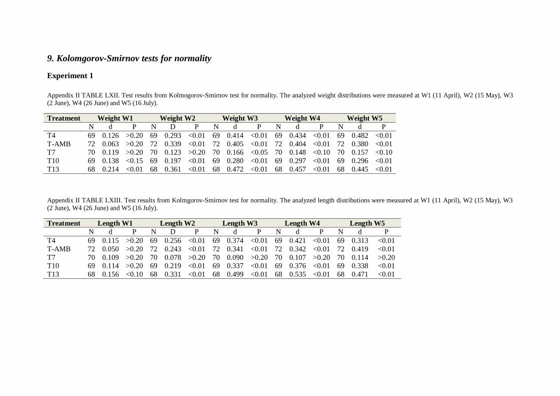
9. Kolomgorov-Smirnov tests for normality

Experiment 1

Appendix II TABLE LXII. Test results from Kolmogorov-Smirnov test for normality. The analyzed weight distributions were measured at W1 (11 April), W2 (15 May), W3

(2 June), W4 (26 June) and W5 (16 July).

Treatment Weight W1 Weight W2 Weight W3 Weight W4 Weight W5

N d P N D P N d P N d P N d P

T4 69 0.126 >0.20 69 0.293 <0.01 69 0.414 <0.01 69 0.434 <0.01 69 0.482 <0.01

T-AMB 72 0.063 >0.20 72 0.339 <0.01 72 0.405 <0.01 72 0.404 <0.01 72 0.380 <0.01 T7 70 0.119 >0.20 70 0.123 >0.20 70 0.166 <0.05 70 0.148 <0.10 70 0.157 <0.10

T10 69 0.138 <0.15 69 0.197 <0.01 69 0.280 <0.01 69 0.297 <0.01 69 0.296 <0.01

T13 68 0.214 <0.01 68 0.361 <0.01 68 0.472 <0.01 68 0.457 <0.01 68 0.445 <0.01

Appendix II TABLE LXIII. Test results from Kolmgorov-Smirnov test for normality. The analyzed length distributions were measured at W1 (11 April), W2 (15 May), W3

(2 June), W4 (26 June) and W5 (16 July).

Treatment Length W1 Length W2 Length W3 Length W4 Length W5

N d P N D P N d P N d P N d P

T4 69 0.115 >0.20 69 0.256 <0.01 69 0.374 <0.01 69 0.421 <0.01 69 0.313 <0.01

T-AMB 72 0.050 >0.20 72 0.243 <0.01 72 0.341 <0.01 72 0.342 <0.01 72 0.419 <0.01

T7 70 0.109 >0.20 70 0.078 >0.20 70 0.090 >0.20 70 0.107 >0.20 70 0.114 >0.20 T10 69 0.114 >0.20 69 0.219 <0.01 69 0.337 <0.01 69 0.376 <0.01 69 0.338 <0.01

T13 68 0.156 <0.10 68 0.331 <0.01 68 0.499 <0.01 68 0.535 <0.01 68 0.471 <0.01

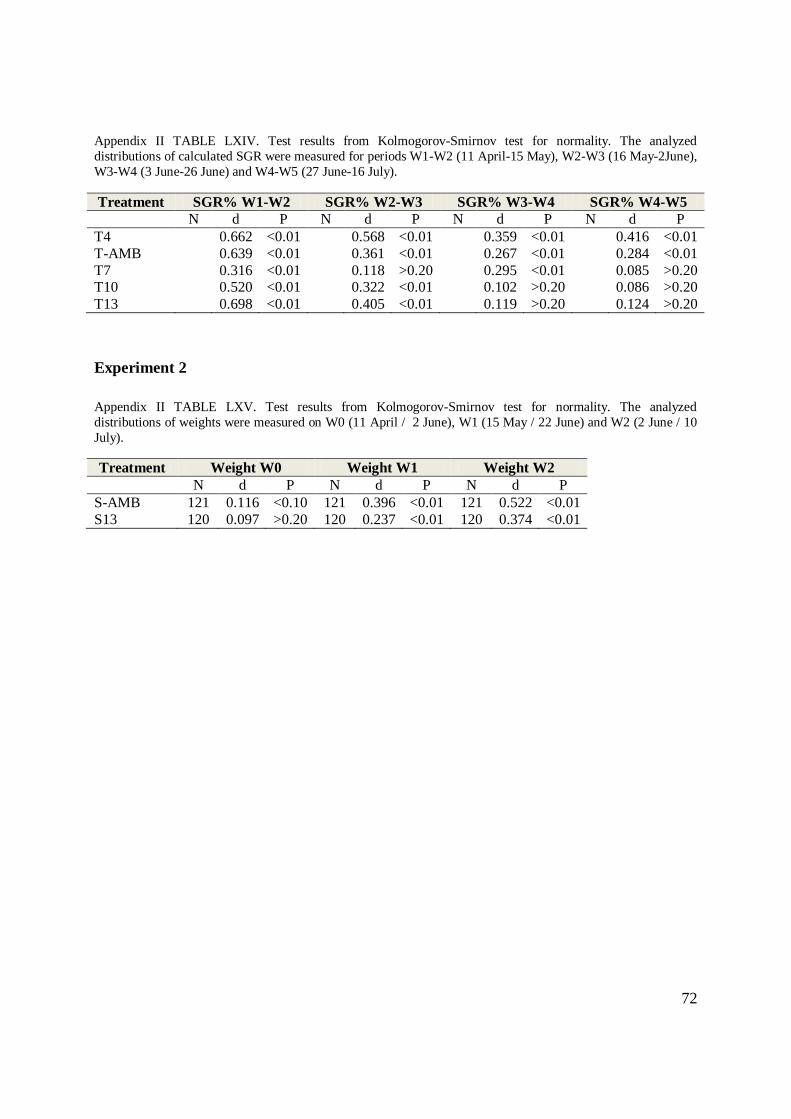
72

Appendix II TABLE LXIV. Test results from Kolmogorov-Smirnov test for normality. The analyzed

distributions of calculated SGR were measured for periods W1-W2 (11 April-15 May), W2-W3 (16 May-2June),

W3-W4 (3 June-26 June) and W4-W5 (27 June-16 July).

Treatment SGR% W1-W2 SGR% W2-W3 SGR% W3-W4 SGR% W4-W5

N d P N d P N d P N d P

T4 0.662 <0.01 0.568 <0.01 0.359 <0.01 0.416 <0.01

T-AMB 0.639 <0.01 0.361 <0.01 0.267 <0.01 0.284 <0.01

T7 0.316 <0.01 0.118 >0.20 0.295 <0.01 0.085 >0.20 T10 0.520 <0.01 0.322 <0.01 0.102 >0.20 0.086 >0.20

T13 0.698 <0.01 0.405 <0.01 0.119 >0.20 0.124 >0.20

Experiment 2

Appendix II TABLE LXV. Test results from Kolmogorov-Smirnov test for normality. The analyzed

distributions of weights were measured on W0 (11 April / 2 June), W1 (15 May / 22 June) and W2 (2 June / 10

July).

Treatment Weight W0 Weight W1 Weight W2

N d P N d P N d P

S-AMB 121 0.116 <0.10 121 0.396 <0.01 121 0.522 <0.01

S13 120 0.097 >0.20 120 0.237 <0.01 120 0.374 <0.01

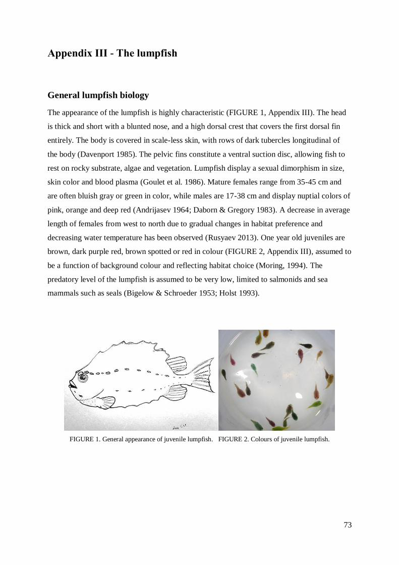
73

Appendix III - The lumpfish

General lumpfish biology

The appearance of the lumpfish is highly characteristic (FIGURE 1, Appendix III). The head

is thick and short with a blunted nose, and a high dorsal crest that covers the first dorsal fin

entirely. The body is covered in scale-less skin, with rows of dark tubercles longitudinal of

the body (Davenport 1985). The pelvic fins constitute a ventral suction disc, allowing fish to

rest on rocky substrate, algae and vegetation. Lumpfish display a sexual dimorphism in size,

skin color and blood plasma (Goulet et al. 1986). Mature females range from 35-45 cm and

are often bluish gray or green in color, while males are 17-38 cm and display nuptial colors of

pink, orange and deep red (Andrijasev 1964; Daborn & Gregory 1983). A decrease in average

length of females from west to north due to gradual changes in habitat preference and

decreasing water temperature has been observed (Rusyaev 2013). One year old juveniles are

brown, dark purple red, brown spotted or red in colour (FIGURE 2, Appendix III), assumed to

be a function of background colour and reflecting habitat choice (Moring, 1994). The

predatory level of the lumpfish is assumed to be very low, limited to salmonids and sea

mammals such as seals (Bigelow & Schroeder 1953; Holst 1993).

FIGURE 1. General appearance of juvenile lumpfish. FIGURE 2. Colours of juvenile lumpfish.

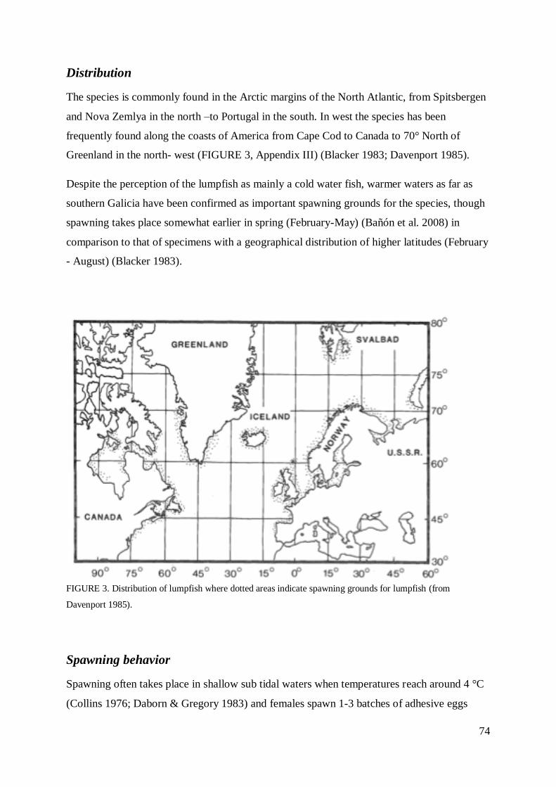
74

Distribution

The species is commonly found in the Arctic margins of the North Atlantic, from Spitsbergen

and Nova Zemlya in the north –to Portugal in the south. In west the species has been

frequently found along the coasts of America from Cape Cod to Canada to 70° North of

Greenland in the north- west (FIGURE 3, Appendix III) (Blacker 1983; Davenport 1985).

Despite the perception of the lumpfish as mainly a cold water fish, warmer waters as far as

southern Galicia have been confirmed as important spawning grounds for the species, though

spawning takes place somewhat earlier in spring (February-May) (Bañón et al. 2008) in

comparison to that of specimens with a geographical distribution of higher latitudes (February

- August) (Blacker 1983).

FIGURE 3. Distribution of lumpfish where dotted areas indicate spawning grounds for lumpfish (from

Davenport 1985).

Spawning behavior

Spawning often takes place in shallow sub tidal waters when temperatures reach around 4 °C

(Collins 1976; Daborn & Gregory 1983) and females spawn 1-3 batches of adhesive eggs

75

(Andrijasev 1964; Collins 1976; Daborn & Gregory 1983). Males enter fjords prior to females

to establish nesting sites, usually depressions in the substrate in the near-shore tidal zone

(Goulet et al. 1986). Each female produces approximately 80 000 – 159 000 eggs per

spawning season (Andrijasev 1964; Collins 1976; Daborn & Gregory 1983). The sex-ratio of

lumpfish catches is imbalanced, Bañón et al. (2008) found a 7 : 1 proportional balance

favorable to female lumpfish, which is probably favorable to the spawning season as males

are observed to take care of several batches at once (Mitamura et al. 2012). Eggs in nests can

be the results of one or several female spawnings, as males can mate with several females,

and females likewise with several males. Many batches of eggs can hence be deposited in the

nest over time, allowing the male to guard from 10 000 to 200 000 eggs at once (Goulet et al.

1986). The male lumpfish guards the eggs until hatch at 190 – 220 day degrees, blowing and

fanning fresh water over the eggs and chases away possible predators (Goulet & Green 1988),

such as conger eel (Conger vulgaris) and common wolffish (Anarhichas lupus) and sea

urchins (Echinus esculentus) (Davenport 1985; Goulet et al. 1986). The cunner

(Tautigikabrus adspersus) often attacks nests in groups which causes the males to give up the

fight (Goulet et al. 1986). Other potential predators include the red king crab (Paralithides

camtchaticus), a new generalist predator in the Barents Sea (Michelsen 2011; Mikkelsen &

Pedersen 2012). Temperatures below 5 C are also observed to cause mortality in eggs

(Goulet & Green 1988).

Eggs are approximately 2 mm in diameter and eggs of the same batch are uniform in color.

Unripe eggs found in ovaries are rosy-pink, while spawned eggs vary from red, pink, green,

purple, blue and yellow (FIGURE 4, Appendix III), gradually losing their color-intensity

throughout egg development (Collins 1976; Davenport 1985). Larvae are 4 - 7.4 mm in length

at hatch (Andrijasev 1964; Collins 1976; Daborn & Gregory 1983) and are well developed,

already possessing the characteristic ventral adhesive disc (Benfey & Methven 1986).

FIGURE 4 .Colours of lumpfish roe

Courtship behavior in terms of nuptial coloration and body movements together with

"parental care" such as fanning of eggs and nest cleaning is shown to increase the

76

reproductive success of males, on behalf of morphological traits such as body size (Goulet et

al. 1986), but females are observed to have little or no preference in male body size or nest

characteristics (Goulet & Green 1988).

Feeding, habitat preferences and migrations of larval- and juvenile lumpfish

Yolk sacks of larval lumpfish are spent within 10-15 days at 9.5 - 14 °C (Benfey & Methven

1986; Brown 1986) and larvae start feeding within one week of hatch (Benfey & Methven

1986). Both juvenile and larval lumpfish display the ventral suction disc, allowing them to

cling to substrate from an early age. Larvae and small juveniles are frequently found in

association to or clinging to algae (Daborn & Gregory 1983; Davenport 1985; Moring 1990),

especially Laminaria (Moring & Moring 1991) or eelgrass (Moring 1989) providing shelter

from predators, camouflage and allowing them to forage plankton in the pelagic zone (Moring

& Moring 1991; Williams & Brown 1991). Juveniles mostly feed on phytal species with a

preference for harpaticoids (genus Harpacticus) (Moring 1989).

Juveniles are selective feeders, eluding sessile and slow moving particles and prey (Ingolfsson

& Kristjansson 2002). An ontogenetic change in prey size preference with increasing fish size

has been observed (Ingolfsson & Kristjansson 2002) and small juveniles are mainly observed

feeding while clinging to substrate, increasing swimming behavior with escalating body size

(Brown 1986; Jobling et al. 2012).The density of prey organisms is also crucial for lumpfish

behavior as juveniles at low prey densities are more active swimming and hunting for prey

than that of fellow specimens at high prey densities. At high prey densities juveniles will to a

great extent feed while clinging (Jobling et al. 2012).

Juvenile and larval lumpfish reside in the intertidal pool throughout their first summer and

autumn, occasionally observed in the upper waters at open sea (Moring 1990), or at deep sea

(Daborn & Gregory 1983; Davenport 1985). Tide pools and the inter-tidal zone provide

important nurseries area for larval and juvenile lumpfish. Larval and juvenile lumpfish will

selectively migrate between tide pools and sub tidal areas between tidal cycles, probably

dependent of prey abundances and predators present (Moring & Moring 1991). In Maine,

juveniles are found in tide pools between June and December (Moring 1990). With decreasing

temperature the abundance of algal refugees decline and tide pools become less attractive

habitats for juveniles (Moring & Moring 1991), and at 1-2 years of age the juveniles outgrow

77

the refugees of the tide pools, and are forced out to sea (Moring 2001).

Feeding, habitat preferences and migrations of adult lumpfish

Lumpfish do not school, but aggregate in spawning periods and occasionally when feeding

(Andrijasev 1964; Bañón et al. 2008). They display similarities in migratory behavior to that

of coastal benthic teleosts, but are also frequently found in mid-water in open oceans outside

the spawning season (Davenport & Kjorsvik 1986). Lumpfish are semi-pelagic and will travel

great distances to offshore feeding grounds, before returning to coastal spawning grounds

between winter and early spring (Blacker 1983; Davenport 1985; Goulet et al. 1986; Holst

1993; Mitamura et al. 2012). They are often found mid-water as a frequent by-catch at 0-80

meters and occasionally feeding over abyssal waters up to 380 meters (Able & Irion 1985).

Mitamura et al. (2012) observed females migrating between neighboring fjords in search of

spawning males, before residing for approximately 1-3 weeks to spawn. Lumpfish are active

swimmers, often observed swimming against the current when performing migratory

movements away from shore (Mitamura et al. 2012), but can also exploit water currents

facilitate rapid migrations to feeding grounds for lumpfish (Rusyaev 2013). Minimum speeds

of female lumpfish leaving spawning grounds exceed 0.72 km per hour, making lumpfish

females vulnerable to passive gears exploited in fisheries (Mitamura et al. 2012).

Temperature factors are crucial to lumpfish, as feeding grounds for the lumpfish spawning on

the northern coasts of Norway and Russia are limited by the polar front (Rusyaev 2013).

Adult fish mostly feed on macrozooplankton, euphasids, amphipods and isopods (Myrseth

1971; Blacker 1983; Daborn & Gregory 1983) and it is a common belief that lumpfish do not

eat during the spawning period and in summer while performing spawning migrations

(Andrijasev 1964; Myrseth 1971; Collins 1976; Daborn & Gregory 1983), though this has

been a matter of discussion (Moring 1989A) as stomachs containing ctenophores or jellyfish

during spawning season has occurred (Able & Irion 1985).

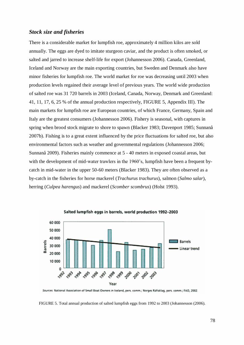
78

Stock size and fisheries

There is a considerable market for lumpfish roe, approximately 4 million kilos are sold

annually. The eggs are dyed to imitate sturgeon caviar, and the product is often smoked, or

salted and jarred to increase shelf-life for export (Johannesson 2006). Canada, Greenland,

Iceland and Norway are the main exporting countries, but Sweden and Denmark also have

minor fisheries for lumpfish roe. The world market for roe was decreasing until 2003 when

production levels regained their average level of previous years. The world wide production

of salted roe was 31 720 barrels in 2003 (Iceland, Canada, Norway, Denmark and Greenland:

41, 11, 17, 6, 25 % of the annual production respectively, FIGURE 5, Appendix III). The

main markets for lumpfish roe are European countries, of which France, Germany, Spain and

Italy are the greatest consumers (Johannesson 2006). Fishery is seasonal, with captures in

spring when brood stock migrate to shore to spawn (Blacker 1983; Davenport 1985; Sunnanå

2007b). Fishing is to a great extent influenced by the price fluctuations for salted roe, but also

environmental factors such as weather and governmental regulations (Johannesson 2006;

Sunnanå 2009). Fisheries mainly commence at 5 - 40 meters in exposed coastal areas, but

with the development of mid-water trawlers in the 1960’s, lumpfish have been a frequent by-

catch in mid-water in the upper 50-60 meters (Blacker 1983). They are often observed as a

by-catch in the fisheries for horse mackerel (Trachurus trachurus), salmon (Salmo salar),

herring (Culpea harengus) and mackerel (Scomber scombrus) (Holst 1993).

FIGURE 5. Total annual production of salted lumpfish eggs from 1992 to 2003 (Johannesson (2006).

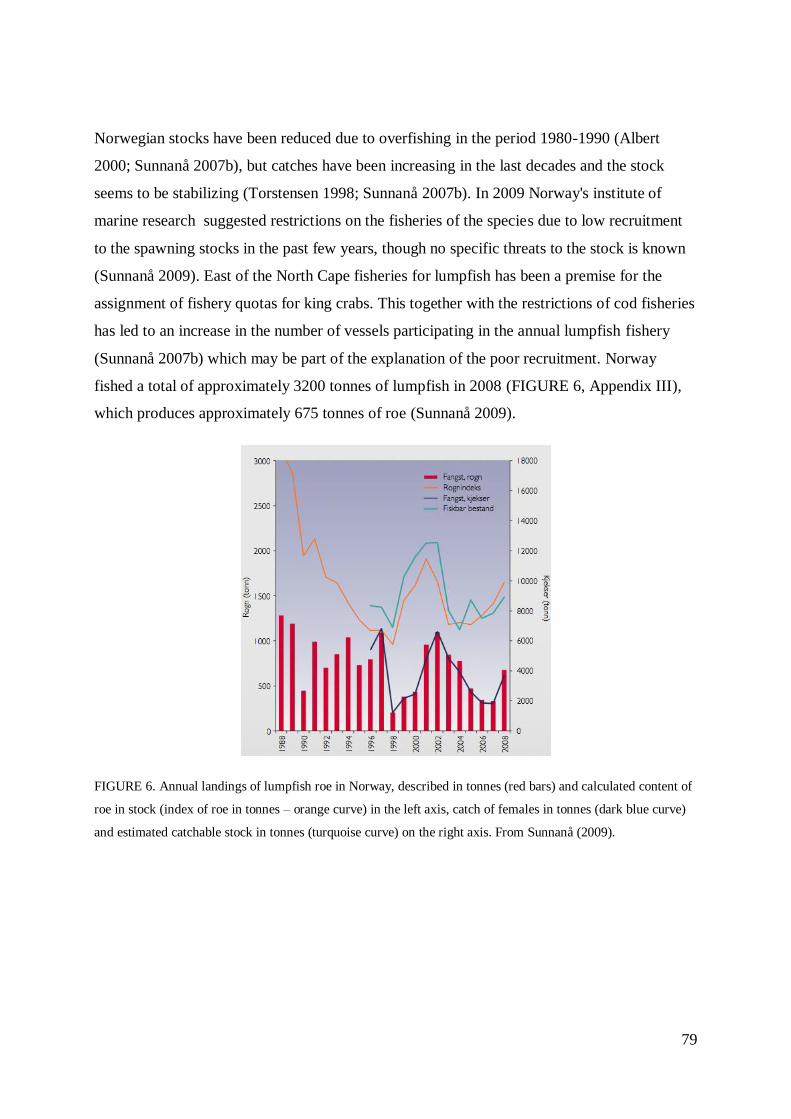
79

Norwegian stocks have been reduced due to overfishing in the period 1980-1990 (Albert

2000; Sunnanå 2007b), but catches have been increasing in the last decades and the stock

seems to be stabilizing (Torstensen 1998; Sunnanå 2007b). In 2009 Norway's institute of

marine research suggested restrictions on the fisheries of the species due to low recruitment

to the spawning stocks in the past few years, though no specific threats to the stock is known

(Sunnanå 2009). East of the North Cape fisheries for lumpfish has been a premise for the

assignment of fishery quotas for king crabs. This together with the restrictions of cod fisheries

has led to an increase in the number of vessels participating in the annual lumpfish fishery

(Sunnanå 2007b) which may be part of the explanation of the poor recruitment. Norway

fished a total of approximately 3200 tonnes of lumpfish in 2008 (FIGURE 6, Appendix III),

which produces approximately 675 tonnes of roe (Sunnanå 2009).

FIGURE 6. Annual landings of lumpfish roe in Norway, described in tonnes (red bars) and calculated content of

roe in stock (index of roe in tonnes – orange curve) in the left axis, catch of females in tonnes (dark blue curve)

and estimated catchable stock in tonnes (turquoise curve) on the right axis. From Sunnanå (2009).

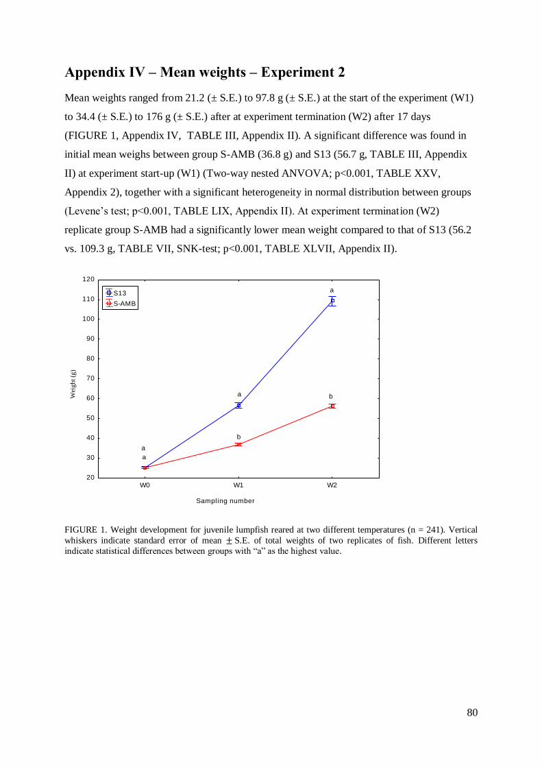
80

Appendix IV – Mean weights – Experiment 2

Mean weights ranged from 21.2 (± S.E.) to 97.8 g (± S.E.) at the start of the experiment (W1)

to 34.4 (± S.E.) to 176 g (± S.E.) after at experiment termination (W2) after 17 days

(FIGURE 1, Appendix IV, TABLE III, Appendix II). A significant difference was found in

initial mean weighs between group S-AMB (36.8 g) and S13 (56.7 g, TABLE III, Appendix

II) at experiment start-up (W1) (Two-way nested ANVOVA; p<0.001, TABLE XXV,

Appendix 2), together with a significant heterogeneity in normal distribution between groups

(Levene’s test; p<0.001, TABLE LIX, Appendix II). At experiment termination (W2)

replicate group S-AMB had a significantly lower mean weight compared to that of S13 (56.2

vs. 109.3 g, TABLE VII, SNK-test; p<0.001, TABLE XLVII, Appendix II).

Sampling number

Wei

gh

t (g

)

W0 W1 W220

30

40

50

60

70

80

90

100

110

120

S13

S-AMB

a

a

a

a

b

b

FIGURE 1. Weight development for juvenile lumpfish reared at two different temperatures (n = 241). Vertical

whiskers indicate standard error of mean S.E. of total weights of two replicates of fish. Different letters

indicate statistical differences between groups with “a” as the highest value.

The effect of temperature and fish size on growth of juvenile ...

Documents

Transcript of The effect of temperature and fish size on growth of juvenile ...