The Effect of Cram Schooling for Math:

A Counterfactual Analysis

Ping-Yin Kuan

Associate Professor Department of Sociology

National Chengchi University E-mail: soci1005@nccu.edu.tw

A paper prepared for the Summer Meeting on Work, Poverty, and Inequality in the 21st Century, the Research Committee on Social Stratification and Mobility (RC28), International Sociological Association, August 6-9, 2008, Stanford University, Palo Alto, California, USA. This paper is a part of the session of “The Varieties of Training: From Cram Schools to Vocational Training.”

Abstract

Private cram schooling is prevalent in Taiwan. Students go to cram schools or

seek private tutoring after regular school hours in order to receive extra learning or

gain a competitive edge. Since cram schooling is believed to have positive effects on

learning achievement, which in turn will affect stratification process, the present paper

attempts to answer the following questions: (1) What factors influence students’

participation in math cramming? (2) Does cram schooling for math work? (3) If it

works, how big is the average effect? (4) What kinds of student benefit most and least

from math cramming?

Using data gathered by Taiwan Education Panel Study (TEPS) in 2001 and 2003,

the present research employs the method of propensity score matching to estimate the

average treatment effect of the 9th graders who participated in math cramming

programs. The present research finds that family backgrounds and the previous math

performance would influence the chances of students’ participation in cram schooling

for math. The results of the counterfactual analysis reveal that the average treatment

effect of math cramming is fairly small. Moreover, the benefit of math cramming in

general is negatively related to the tendency of participating in math cramming and

the prior math ability.

Keywords: cram schooling, educational achievement, educational stratification,

counterfactual, propensity score matching

2

The Effect of Cram Schooling for Math: A Counterfactual Analysis

Ping-Yin Kuan

In the last decade, the educational system in Taiwan has undergone significant

changes. One important reform policy, as recommended by the officially sanctioned

Commission on Education Reform (CER), was to improve the system of admission to

senior high schools and universities (The Commission on Education Reform, 1996;

see also Government Information Office, 2001). The reform involves a new system of

multiple channels for admission and a reformed scheme of basic competency tests.

One primary goal of these changes intended to stem the alarming and growing

phenomenon of high school students attending Buxiban (cram schools) or seeking

private supplementary tutoring after already long regular school hours. The main

purpose of attending cram schools or tutoring programs is to do well in the

competitive entrance examinations and be admitted to good schools or colleges. The

CER, echoing the dissatisfaction of the public, concerned very much the negative

psychological, educational, social, and economic impacts of the inordinate attention,

both students and parents alike, on entrance examinations and the consequent

emphasis on rote memorization of materials taught at both regular and cram schools.

After a decade of educational reform, the number of four-year colleges and

universities has risen from 67 in 1996 to 147 in 2006 and net percentages of junior

and senior high schools graduates entering a higher level of schooling were 99.77%

and 83.91% respectively in 2006 (The Ministry of Education 2007). To the dismay of

well-intentioned educational reformers, the prevalence of cram schooling among high

school students has increased considerably. According to the online official statistics,

3

the number of so called Wen-Li1 Buxiban, cramming schools served mainly to

students preparing for major academic subjects covered by the entrance examination

of all levels, has risen from 1,844 in 1999 to 9,344 in 2008 (Education Bureau,

Kaohsiung City Government 2008). The phenomenal growth of registered Buxibans

reflects the rising demand of aspired students and their parents.

The popularity of cramming programs has both cultural and institutional bases.

Culturally, Taiwan, a predominantly ethnic Chinese society, has deep roots in

Confucianism which emphasizes the value of meritocracy and the use of competitive

examinations to choose talents (Zeng 1999). While the educational reform in Taiwan

for the last decade has tried to make institutional changes that may lessen the

influence of the examination culture on education, the core institutional arrangement

so far still maintains nationally administered entrance examinations and the stake of

examinations remains high. Students would need very high scores to be admitted to

top ranked senior high schools and universities. Their allocated positions in the

hierarchy of secondary schools and institutions of higher education are linked fairly

tightly to the future opportunities in labor market and general status system. In short,

the current educational system in Taiwan still has institutional characteristics that

contribute to the development of shadow education (Stevenson and Baker 1992). On

the individual level, the prevalence of attending cramming school may also reflect the

belief of many students or their parents that cram schooling for examinations works.

Whether cram schooling or private tutoring2 has a positive effect on academic

performance concerns not only the welfare of participating students, but also their

fellow students who may not have opportunity or resource to undertake such activities.

1 The literal meaning of Wen-Li in Chinese is “literature and science.” 2 Since private tutoring and cram schooling are private supplementary learning activity, the present research will use “cram schooling,” which is more common, to cover both private tutoring and cram schooling in the following discussion.

4

If cram schooling is found to have a significant positive effect, it will have important

consequences on the stratification process. Hence, the main research question of this

paper is to investigate how big the effect, if any, of cramming for mathematics, a

subject that many high school students in Taiwan, as everywhere else, find torturing

and have difficulty in getting good scores in examinations.

It is not easy, however, to properly assess the effect of cram schooling on math

performance. The researcher needs to account for all the important individual and

social factors influencing students’ participation in math cramming and math

performance. As long as students are free to choose whether or not to participate in

cramming programs and if there is any important unobservable variable such as

intelligence, the researcher will have difficulty in getting unbiased estimate of the

causal effect of cram schooling on math achievement. With these difficulties in mind,

the following sections will first discuss in more details about the nature of cram

schooling and its implications for the proper assessment of the effect of cram

schooling. The attempt to properly estimate the effect of math cramming is framed by

the section describing the counterfactual approach and the related method of

propensity score matching. I then describe the data used for the analysis and present

the findings.

The Nature of Cram Schooling and its Implications for Proper

Assessment of Causal Effects

Specifically, the type of cramming activity examined in the present research has

the following characteristics: (1) it is a type of organized and structured learning

outside of schools, (2) the goal of participating in this type of supplementary learning

is to prepare for the competitive process of entrance examinations and the preparation

includes improvement and enhancement of students’ knowledge about academic

5

subjects as well as test-taking skills, (3) the cramming activities may take place in

large-sized classes or in the form of one-on-one tutoring, (4) the participation needs

private resources provided mostly by students’ families, (5) participating students may

see the activities either as remedial intending to catch up with their fellow students or

as enhancement aiming to gain a competitive edge (see also Baker, Akiba, LeTendre,

and Wiseman 2001, Bray 2003).

Cram schooling as defined by the above characteristics gives clues to why cram

schooling per se may have a positive effect on academic performance as well as the

possibility that cram schooling may work differently for different kinds of students.

These characteristics also point out that the assessment of effect of cram schooling is

easily confounded with the effects of other factors influencing the opportunity of

undertaking cram schooling and the possibility of omitted variables in previous

studies.

The first three characteristics mentioned above are directly relevant to the

expectation that cram schooling can have a positive effect on academic achievement.

These three characteristics are related to extra learning time and instructional

resources. There are at least three kinds of literature addressing the relationship

between extra learning time and resources and academic performance. The first kind

is about the effect of school learning time. John Carroll’s (1963) “Model of Schooling

Learning” is the first major theoretical framework stipulating the role of time played

in learning a given task at school (see also Carroll 1989). Carroll maintains that

success of learning a given task is dependent on the time a student spends in relation

to the amount of time he or she needs to learn. Within his framework, three factors

influencing “the time required to learn” are identified. They are: (1) student aptitude,

(2) ability to understand instruction, and (3) quality of instruction. Two factors

influencing “the time spent in learning” are: (1) time allowed for learning, and (2) the

6

time the learner is willing to learn.

Carroll’s model shows that the relationship between learning time and learning

achievement is dependent on student’s ability, effort, given opportunity, and teaching

environment. This model of school learning is supported by later empirical studies

conducted in either experimental or actual school settings (e.g., Gettinger 1985,

Berliner 1990). Further evaluation of empirical studies in industrial societies also

shows that allocated time at school, such as the daily instructional time or number of

school days, has little or no relationship to student achievement. In contrast, the

amount of time that students are participating in learning activities (engaged time) and

time when learning actually occurs (academic learning time) has impacts on student’s

achievement (Aronson, Zimmerman, and Carlos 1999).

Although Carroll’s model is about school learning, it can be applied to the

evaluation of the effect of cram schooling, which after all is considered as a shadow

of formal schooling (Stevenson and Baker 1992). Clearly, extra learning time outside

of schools by itself may or may not help students. According to Carroll’s model, given

extra learning time, the effect of cram schooling will be different among participating

students depending on student’s own initiative, ability and effort.

The second kind of literature that may lead us to expect cram schooling having a

positive effect pertains to the work about the relationship between seasonal learning

and student’s achievement. Entwisle and her colleagues have used the “faucet theory”

to explain poor children’s increasing drawback in academic achievement after

summer breaks (e.g., Entwisle, Alexander, and Olson 1997; Alexander, Entwisle, and

Olson 2007). They find that poor and middle-class children make similar achievement

gains when schools are in session. At times, poor or disadvantaged children may even

gain a little bit more than middle-class children during the school year. When school

is closed in summer, middle-class children still make progress in reading and math

7

because of better home learning environment and structured activities offered during

the break. Lack of such kind of resources and activities, low-SES children lose

grounds in learning during the summer. Hence, when school is in session, the faucet

of learning resource is turned on, which benefits all children equally. Entwisle and her

colleagues further point out that the disappointing result of the summer school in

reducing achievement gap can be attributed to the fact that add-on services across the

board benefits advantaged or brighter students more than disadvantaged or not so

bright students (Entwisle, Alexander, and Olson 2001).

The findings of seasonal learning suggest that cram schooling as an extra

learning resource provided by the family should benefit participating students

positively in academic achievement. Moreover, the findings also suggest that extra

structured learning provided by summer schools or cram schools may benefit students

of different ability level or different backgrounds differently.

The third kind of literature reviewed here, in comparison with the previous

discussed literature, is more directly relevant to the present research. This is the

research literature about the effect of coaching or test preparation. The activities of

coaching or improvement of test-taking skills mentioned in this literature, however,

may take place in school or outside of school and in a relatively short period of time.

The kind of coaching closest to cram schooling in Taiwan is coaching for the

Scholastic Aptitude Test (SAT), a high-stakes test (see Becker 1990). Coaching for

standardized tests like SAT involves acquiring familiarity with the test, reviewing

material relevant to the test content, and learning testwiseness (Allalouf and

Ben-Shakhar1998: 32).. These elements of coaching for the SAT are in common with

cram schooling defined earlier. Does coaching for the SAT help students to gain in the

test? In her meta-analysis of 23 reports on coaching for the SAT, Becker (1990)

concludes that coaching helps to increase SAT scores but the effects are fairly small.

8

In the case of SAT verbal test, the published studies show that the coached groups in

general exceed control groups by 0.09 standard deviations. The effect of coaching is a

bit stronger on SAT math test. The consistent result found is about 0.16 standard

deviations. Becker’s review also points out most of previous studies of coaching in

general are poorly designed. A central design issue identified in the coaching literature

is about the role of self-selection into coaching. In an attempt to address this issue,

Briggs (2001) uses the method of propensity score matching to assess the effect of

coaching on the SAT. He also concludes that coaching has very small positive effects.

The review of the possible effect of cram schooling so far has pointed out the

issue of self-selection and possible heterogeneous causal effects even among those

who participate in cram schooling. These issues have important implications for the

proper evaluation of the causal effect of cram schooling. The last two characteristics

of the nature of cram schooling mentioned earlier further demonstrate the possible

complication involved in the accurate assessment of the causal effect of cram

schooling.

The fourth characteristics mentioned above clearly show that students’

participation in cram schooling not only involves family’s economic capital but also

social capital entailed by parental expectation and interest in children’s learning. If

cultural capital is considered as a resource monopolized by dominant social class

signified by enforcing educational evaluative criteria favorable to their children

(Lareau and Weininger 2003), then participation in cram schooling can also be viewed

as a form of cultural capital invested by families to increase or ensure their children’s

opportunities in accessing scarce rewards. Hence, one possible baseline difference is

in family’s socioeconomic backgrounds and parental involvement in learning.

The fifth characteristics also indicate that the participation would need student’s

own initiative or at least their conformity to parental wish. Both students and parents

9

should also have some expectation that cram schooling would work. The individual

difference in the willingness to participate and expectation of the outcome of the

participation are also baseline differences.3 These family and individual differences

may also have impacts on the actual effect of cram schooling. It is conceivable that

students who have strong motivation to compete or high expectation of the cram

schooling would have different gain in undertaking such an activity from those who

are unwilling to go to cram schools but are coerced by their parents. It is also

conceivable that students of better prior academic ability, which is very much

influenced by better socioeconomic backgrounds and better schools (Shavit and

Blossfeld 1993; Marks, Cresswell, and Ainley 2006), would benefit differently from

those who are poorly prepared. In short, even among those who undertake cram

schooling, there may be differential causal effects. The evaluation of the effect of

cram schooling can be further complicated if we would like to know whether the

results of participants is the same as those who did not participate. Since these two

groups may be fairly different, their causal effects of cram schooling may also be

different.

Previous empirical studies on cram schooling in Taiwan, which mainly used the

method of multiple regression analysis, have confirmed both social and individual

factors systematically influencing the participation of cram schooling. The studies

using national representative survey data have shown that parental levels of education

and occupational level are positively related to the degree of participation in cram

schooling of high school students (Sun and Hwang 1996; Lin and Chen 2006; Liu

2006; Hwang and Cheng 2008). Parental educational expectation is also found to have

3 In 2003, Taiwan Education Panel Survey, the data of which is a part of the data used for the present research and described in more details later, asked 9th graders if they could choose freely, whether they would attend cram schools. For those who said yes, about 76% undertook cram schooling. For those who say no, about 38% attended cram schools. These findings show that those who undertook cram schooling were either more motivated or had high expectation that cram schooling would work.

10

independent effect on the participation in cram schooling (Liu 2006).

Other significant individual and social factors found to affect the participation in

cram schooling are gender, ethnicity, family income, family type, sib size, and level of

urbanization of either birthplaces or school locations (Sun and Hwang 1996; Lin and

Chen 2006; Liu 2006). Lin and Chen (2006), however, also conclude that the

explanatory power of family and individual factors on the participation in cram

schooling is quite small. The small effect of these factors is explained by over 80% of

senior high school students having the experience of attending cram schools.

Moreover, both Lin and Chen (2006) and Liu (2006) find that the amount of cram

schooling and the educational achievement is curvilinear. Liu’s research also show

that after taking into account of family backgrounds and individual characteristics, the

direct effect of cram schooling on academic achievement is reduced about one half.

While these previous studies of cram schooling in Taiwan are helpful in our

understanding of the effect of cram schooling, their estimates of the causal effect of

cram schooling may still be biased. First of all, these studies have omitted important

variables such as the willingness to participate and intelligence. These omitted

variables may contribute both the explanation of the participation in cram schooling

and academic achievement. Variables related to the school or class learning climate,

such as the competitiveness of classmates, are also neglected in the previous research.

Furthermore, these studies have not fully explored the possibility of heterogeneous

causal effects. As mentioned earlier, it is possible that students of different degree of

motivation, prior academic ability, and family socioeconomic backgrounds may

benefit differently from cram schooling.

In order to take into account properly these baseline differences and possible

heterogeneous causal effects, it would be ideal if an experiment on cram schooling

could be carried out. This experiment would randomly assign students to attend

11

cramming programs or not to attend. Since this kind of experiment is not possible in

real life, it would then be necessary to use observational data and proper statistical

analysis to control for baseline differences and account for heterogeneous effects. As

it will be shown in later discussion, conventional OLS regression method may not be

the best statistical tool for this task. Instead, methods such as propensity score

matching, which is developed under the counterfactual framework and explicitly

taking into account baseline differences and heterogeneity of causal effects, should be

considered in estimating the effect of cram schooling.

The Counterfactual Framework and Propensity Score Matching

As long as we do not have experimental design and have only observational

studies available to examine the effect of cram schooling, what then can be done to

handle selection bias caused by omitted variables and explore possible heterogeneous

causal effects? The method used in this research is the propensity score matching,

which uses observed family, school, and individual characteristics of students to

match students who undertake cram schooling and those who do not and then

calculates the average difference in outcomes between these two groups. With proper

assumptions, this matching method is able to estimate separately the average causal

effect of those who participate in cram schooling and those who do not as well as an

overall average estimate of the effect for these two groups combined. The matching

method is developed under the framework of the counterfactual causal inference. To

explain how this matching method works, it is useful to understand the counterfactual

framework of causality with a binary cause which presupposes two potential

outcomes for all members of the population.4

4 The discussion of the counterfactual model and propensity score matching in this paper follows the discussion presented in Morgan and Winship (2007). See also Winship and Morgan (1999), Winship and Sobel (2004), and Morgan and Harding (2006).

12

If the participation in the cramming school is a random variable, D, that is equal

to 1 if the student participates in cram schooling and equal to 0 if not. Using the

language of the experimental design, those who undertake cram schooling can be

described as experiencing the treatment and those who do not is in the control group.

Since every student may or may not undertake cram schooling, for every student there

are two potential outcomes student which are denoted as Y1 and Y0. Y1 is the potential

outcome for the individual student participating in cram schooling (D = 1) and Y0 is

the potential outcome for the individual student with no cram schooling (D = 0). The

causal effect of the treatment for every student is defined as: δ = Y1 – Y0, that is, the

difference between the outcome if the student undertakes cram schooling and the

outcome if the same student does not undertake cram schooling. This causal effect on

the individual level is not observable since in reality we can only observe one of the

outcomes for each student. If we are willing to make certain assumptions about the

joint law of Y1, Y0, and D, then we can identify the average treatment effect on the

whole population (ATE):

δATE = E[Y1 – Y0] = E[Y1] – E[Y0]. (1)

ATE is a commonly investigated causal effect and estimated in the observational

study by a random sample of the population of interest. In an observation study, the

researcher faces the situation that a proportion of the population of interest taking the

treatment would have fairly different characteristics than those who did not take the

treatment. If the proportion of the population taking the treatment is π, then Equation

(1) becomes

δATE = {πE[Y1| D = 1] + (1–π) E[Y1| D = 0]} (2)

– {πE[Y0| D = 1] + (1–π)E[Y0| D = 0]}.

Equation (2) can be rearranged and expressed as

δnaive = E[Y1 | D = 1] – E[Y0| D = 0] = δATE (3)

13

+ {E[Y0| D = 1] + E[Y0| D = 0]}

+ (1–π){E[δ|D = 1] – E[δ|D = 0]}.

Equation (3) shows that the naïve estimator, δnaive, an estimator often used in the

observational study, is a combination of the true average treatment effect, δATE, plus

two potential sources of biases. The first potential source of bias, E[Y0| D = 1] + E[Y0|

D = 0], is a baseline bias. This bias exists because in the absence of treatment, the

average situation of those in the treatment group would not be the same as those in the

no-treatment group. The second source of bias, (1–π){E[δ|D = 1] – E[δ|D = 0]}, is a

differential treatment effect bias. This bias exists because the expected treatment

effect for those in treatment group and those in the no-treatment group are different.

Equation (2) also shows that δATE is a weighted combination of two conditional

average treatment effects: the average treatment effect on the treated (ATT) and the

average treatment effect on the untreated (ATU). In the present case, ATT is the

average treatment effect for those who typically undertake cram schooling for math

and ATU is the average treatment effect for those who typically do not participate in

cram schooling. ATT and ATU are defined respectively as

δATT = E[Y1 – Y0| D = 1] = E[Y1| D = 1] – E[Y0| D = 1], (5)

δATU = E[Y1 – Y0| D = 0] = E[Y1| D = 0] – E[Y0| D = 0]. (6)

In order to obtain an unbiased and consistent estimation of ATU, one needs to

assume that E[Y1| D = 1] = E[Y1| D = 0], i.e., the expected treatment effect for those

in treatment group and those in the no-treatment group are the same. To obtain an

unbiased and consistent estimate of ATT, one needs to assert that E[Y0| D = 1] equals

to E[Y0| D = 0], i.e., no baseline difference between the treated group and the

untreated group. In general, the necessary assumption for the unbiased and consistent

estimation of ATT is less demanding than for ATU. In the case of the present research,

the needed condition for estimating ATT is to assume that those participate in cram

14

schooling would, on average, do no better or no worse without cram schooling than

those who actually have no cram schooling. ATT is an commonly examined subject of

interest since if there is no treatment effect on the treated, it is reasonable to assume

that the same treatment would not benefit the untreated. In the present research, only

if cram schooling has a significant impact on those undertaking such an activity

would it be necessary for us to consider the possible effect of extra learning outside of

schools on those who do not undertake cram schooling.

In an observational study, the assumption of no baseline difference or the same

treatment effect for both the treated and untreated group is very unlikely. However, if

one is willing to assume the independence between Y0, Y1 and D conditionally on a

set of observable covariates X, then E[Y0| D = 1, X= x] = E[Y0| D = 0, X= x] and

E[Y1| D = 1, X= x] = E[Y1| D = 0, X= x]. If these conditional independence

assumptions are satisfied, then one is able to stratify the sample into subgroups

conditioning on these covariates to estimate E[Y0| D = 1] and E[Y1| D = 0]. Within

each subgroup, the researcher selects a case from the no-treatment group to match a

case from the treated group based on observed characteristics of X and calculates the

differences in the observed outcomes.

In practice, realization of assumptions of the conditional independence requires a

considerable number of observable covariates and the limited sample size makes the

conventional method of stratification and matching conditioning on all these variables

impossible to implement. Paul R. Rosenbaum and Donald B. Rubin, in a set of papers,

developed the method of propensity score matching and solved a variety of practical

problems (see Morgan and Harding 2006). The method stipulates that the systematic

differences between those who take the treatment and those who do not can be

captured completely by a set of observed selection variables S and this conditional

independence implies independence conditionally on a specific function of S, called

15

the propensity score. The propensity score is a one-dimensional summary measure of

the probability of being treated and can be noted as Pr (D = 1|S). This probability is

between 0 and 1. The method solves the problem of matching individuals on the

whole set of conditioning variables. It is enough to match the treated and the untreated

on their propensity scores. One potential drawback of the method is the possibility of

no suitable matches for all treatment cases. In fact, if the probability of being treated

equal to 1, it is not possible to find a counterfactual in the no-treatment group. In short,

one can only estimate the treatment effect for matched cases.

The actual procedure of propensity score matching is fairly straightforward (see

Caliendo and Kopeinig 2008). First of all, the propensity score for each case in the

sample is estimated with all covariates by a logit or probit regression model. The

matching of propensity scores between the treated and untreated cases can be

performed by one of the many matching algorithms available for several statistical

packages. In general, these matching algorithms can be grouped into four types: exact

matching, nearest-neighbor matching, interval matching, and kernel matching.

Morgan and Harding (2006: 34) suggested that nearest-neighbor caliper matching

with replacement, interval matching, and kernel matching should be preferred to

nearest-neighbor matching without replacement. They also recommended matching

on both the propensity score and the Mahalanobis metric for achieving balance. After

matching is performed, it is important to assess the matching quality. One simple way

to assess the matching quality is to perform a two sample t-test to check if there is a

significant difference in sample means of each covariate for the treatment and the

matched control groups. After the matching quality is verified, one can estimate the

specific average treatment effect.

For the present research, the propensity score matching is performed by

“psmatch2,” a Stata 10 routine developed by Edwin Leuven and Barbara Sianesi

16

(2003). The matching algorithm chosen is kernel matching with Epanechnikov kernel

and the matching is on both the propensity score and the Mahalanobis metric to

achieve balance.

Data and Measures

The present research uses the public released data sets collected by Taiwan

Education Panel Survey (TEPS) in 2001 and 2003 (Chang 2003). In 2001, with the

support and authorization of the Ministry of Education, National Council of Science,

and Academia Sinica in Taiwan, TEPS using multistage stratified sampling method

surveyed 20,004 7th graders in 333 junior high schools. These sampled students were

surveyed again in their 9th grade. The follow-up sample size is 18, 903. The sample

size of the public released data is 70% of the surveyed students.5 TEPS data were

collected by administering the ability test and student’s questionnaire in the classroom

under a standardized condition. Each surveyed students was also asked to take home a

copy of parent’s questionnaire for one of his or her parents or guardians to answer,

and the answered questionnaire was taken back for field staff to collect. Surveys were

also administered to surveyed students’ homeroom teachers, Chinese language

teachers, English teachers, and Math teachers.

For the present research, I used 2001 and 2003 student data, 2001 parent data,

and 2001 data of math teacher’s evaluation of surveyed students. The sample size of

each data is slightly different. The sample size of the 2001 public released student

data is 13,978. After merging this data with the follow-up student data and deleting

cases that have no information about math ability test scores, cram schooling for math

in 2003, gender, and ability grouping, the sample size reduces to 12,025. For all other

5 Please refer to http://www.teps.sinica.edu.tw/introduction.htm for basic information about TEPS (in Chinese).

17

variables used in the analysis, I use either mode or median to replace their missing

values to reduce the loss of the sample size.6 The sample size for the present research

is further reduced to 11,373, which is the analytical sample with common support

after the matching.

The present research focuses on estimating the effect of math cramming

undertaken in the first semester of the 9th grade. The choice of estimating the effect of

math cramming in the 9th grade is due to the fact that 9th graders would face their first

senior high school entrance examination held in the second semester. Hence, the main

purpose of cram schooling for math should be for this examination. The math ability

of these students was also measured by TEPS in the later half of the first semester in

2003. Another reason to study the effect of math cramming is because math learning

is largely taken place at school or cram schools rather than at home. Moreover,

coaching for math standardized tests is also shown to be more effective (Becker 1990).

The original math ability scores given by TEPS are IRT scores (Yang, Tam, and

Huang 2004). For the ease of presentation and understanding, I transform the IRT

scores into normal curve equivalent (NCE) scores for the sample before matching (N

= 12,025), which range from 1 to 99 with a mean of 50 and a standard deviation of

21.06. Table 1 shows that the mean of the math ability NCE scores for the matched

sample (N=11,373) is 64.564 and the standard deviation is 29.858. The variable of

math cramming in the 9th grade is coded as a dummy variable with 1 indicating the

student undertaking math cramming during the first semester of the 9th grade and 0 for

no math cramming. Table 1 shows that about 47% of student included for the present

research undertook cram schooling in the 9th grade and a similar percentage of

students have the experience of attending cram schools or seeking private tutoring

6 I also use listwise deletion to deal with missing values and the final result of analysis is very similar to the findings presented in this paper.

18

ever since they were 5th graders.

Other than variables of the math ability scores in the 9th grade, the experience of

math cramming in the first semester of the 9th grade, and student’s own initiative in

undertaking math cramming, and if students attends a high ability class in the 9th

grade, all other variables used for matching are obtained from the TEPS 2001 data. In

total, I used 27 variables for propensity score matching. Most of these other variables

are variables often considered in previous empirical studies of cram schooling in

Taiwan or studies of coaching in other countries (Stevenson and Baker 1992; Sun and

Hwang 1996; Powers and Rock 1999; Baker, Akiba, and Wiseman 2001; Briggs 2001;

Lin and Chen 2006; Liu 2006). These matching variables can be grouped into three

types: (1) student’s individual characteristics which include gender, learning habits,

and math achievement in the 7th grade, (2) family backgrounds, and (3) school and

class characteristics, which include school types and class environment regarding

academic competition and ability grouping. Variables such as student’s learning habits,

prior math achievement, and school or class characteristics are rarely available for

previous studies of cram schooling in Taiwan. The following are more detailed

description of the measurement and coding the variables used in propensity score

matching. Summary statistics of variables are presented in Table 1 for both sample

cases included in and excluded from the present study.

[Table 1 is about here]

1. Student’s individual characteristics

(1) Gender: 1 is male and 0 is female.

(2) The homework subject that spends most time in doing: 1 is math and 0 is

other subjects.

19

(3) Never let anything distract doing homework since elementary school: This is

an ordinal variable treated as a continuous variable in the analysis. The

variable ranges from 1 to 4 with 1 indicating and 4 indicating strongly

disagree.

(4) Always review course lessons after school since elementary school: Same as

(3).

(5) Always try to solve difficult problems in learning since very young: Same as

(3).

(6) Math is always a headache: Same as (3).

(7) Can keep up with math teaching: This ordinal variable and the next two are

math teacher’s evaluation of surveyed students. The variable is treated as a

continuous variable in the analysis and ranges from 1 to 4. 1 means that the

student’s learning pace is way ahead of teaching, 2 means that the student can

keep up with teaching, 3 means that the student cannot keep up with teaching,

and 4 means that the student is way behind.

(8) Math homework performance: This ordinal variable is math teachers to

evaluate if students always, sometimes, rarely, or never late in turning in

math homework. 1 means always and 4 means never.

(9) Attend special class for gifted students in the 7th grade: Students are asked if

they attend special classes for students who are evaluated to be gifted in

certain academic subjects such as math, science, and Chinese or English

languages. The variable is dummy coded with 1 meaning yes or 0 meaning

no.

(10) Make own decision about undertaking cram schooling: A dummy coded

variable with 1 indicating yes and 0 indicating no.

(11) Cram schooling experiences: This variable is coded into four categories

20

including before 4th grade or never, from 5th grade to 7th grade, 7th grade only,

and from 5th to 6th grade. The category of “from 5th grade to 7th grade” is the

reference group in the regression analysis.

(12) Math ability IRT scores in the 7th grade: This variable is a continuous

variable.

2. Family backgrounds

(1) Ethnicity: Four ethnic groups are constructed according to parents’ answer

about their ethnicity. They are Minnan, Hakka, Mainlander, and Aborigine.

Minnan is the reference group in the regression analysis.

(2) Parental education level: Three parental education levels are constructed

according to the highest level of education attained by either parent. Three

levels are high school, college, and graduate school. The level of high school

is the reference group in the regression analysis.

(3) Parent occupation: The three types of parental occupation constructed are

professional or clerical workers, sales and service workers, and other. The

classification is based on the differentiation of white collar and blue collar

jobs as well as the consideration of the sample size of each category.

(4) Monthly family income: The monthly family income is divided into less than

NT$20,000, NT$20,000 to less than NT$50,000, NT$50,000 to less than

NT$100,000, and NT$100,000 or above.7

(5) Living with both biological parents: This variable is dummy coded with 1

indicating yes and 0 indicating no.

(6) Sib size: This variable is constructed from student’s answers to four questions

regarding the number of younger and older sisters and brothers. This number

7 The annual average exchange rate between NT dollars and US dollars is about34.999 to 1 in 2001 (Directorate-General of Budget, Account, and Statistics, Executive Yuan 2007).

21

of siblings is double checked and corrected with five questions about whether

living with siblings, the number of siblings under 18 years old, if parents are

partial towards a particular sibling, and the relationship between siblings.

(7) Parental educational expectation: This variable is coded into three levels of

educational expectation. They are expectation of getting a high school

diploma, getting a college degree, and getting a graduate degree. The

reference group in the regression analysis is getting a high school diploma.

3. School and class characteristics

(1) Attend private school: 1 means yes and 0 means no.

(2) The 9th grade class is a high ability class: 1 means yes and 0 means no.

(3) Poor class climate for learning: This is an ordinal variable ranges from 1 to 4

with 1 indicating strongly agree and 4 indicating strongly disagree.

(4) Class average grade is good: Same as (3).

(5) Classmates often discuss homework or study together: Same as (3).

(6) Intense academic competition among classmates: Same as (3).

(7) Classmates often discuss about the entrance examination: Same as (3).

(8) School location: This variable is about the level of urbanization of the school

location. The three levels are rural, small city, and major city. Rural is the

reference group in the regression analysis.

Results

Factors influence the participation in cram schooling for math in the 9th grade

Table 2 shows the result of logistic regression of participation in cram schooling

for math in the 9th grade on student’s individual characteristics, family backgrounds,

and school and class characteristics. The first regression model includes often

considered variables in Taiwan’s previous studies. These variables are student’s

22

gender, cram schooling experiences, family backgrounds variables, and school

location. The result of this model is similar to these earlier studies (e.g., Liu 2006).

Model 2 to Model 5 are hierarchically nested. Model 2 includes only variables related

to student individual characteristics. Model 3 adds family backgrounds variables to

the analysis and Model 4 further adds variables related to school and class

characteristics. The last model, Model 5, further includes the indicator of prior math

ability as measured by the math ability IRT scores in the 7th grade. Since the prior

math ability is an outcome of both measured and unmeasured variables in the 7th

grade, the addition of this variable can help us to examine if the analysis without this

variable is seriously biased in any way.

[Table 2 is about here]

The comparison of regression coefficients of Model 1, Model 2, and Model 3

shows that patterns of effects of variables related to student’s individual

characteristics and of variables related to family backgrounds do not change much

with additional variables included in the analysis and, hence, are fairly independent in

their impacts on the chance of participation in math cramming in the 9th grade. This

finding also suggests that previous studies, as exemplified by Model 1, may have

overestimated the effect of cram schooling without taking into account of student’s

learning habits or personal traits. The result of Model 4 further shows that some

school and class characteristics also have relatively independent effects on the chance

of attending cram schools. Model 5 shows that the prior math ability has a significant

positive impact on undertaking math cramming in the 9th grade as well. While the

addition of this variable reduces the impact of other variables somewhat, the effect

seems to be quite independent. Again, this result points to the possibility of

23

unobserved variables, which may bias the estimation of the causal effect of cram

schooling. If such variables exist, however, the possible bias seems rather small.

Specifically, the result of Model 5 indicates that those who undertake cram

schooling for math in the 9th grade tend to be female, non-aborigine, living with both

biological parents, with fewer siblings, with parents who are more educated and have

higher educational expectation. Students who have good learning habits such as

spending much time in doing math homework, always review course lessons after

school, and always turn in math homework in time are also tend to take on cram

schooling for math. Apparently, the previous experience in cram schooling is not

favorable for some students, since those who attended cram schools earlier and did

not attend persistently tend not to continue cram schooling for math in the 9th grade.

Students who can make their own decision about attending cram schools also avoid

undertaking cramming activity. These findings reveal that students who undertake

cram schooling for math in the 9th grade are either those who have good learning

habits and good math ability. Students who attend public schools in more urbanized

areas, have more competitive and studious classmates, and have poor class climate in

learning also have a better chance of attending cram schools for math. All these

factors that have positive effect on the chance of participating in cram schooling for

math are baseline differences that need to be taken into account in the estimation of

the causal effect and some of which are usually absent in the analysis of previous

studies.

Average treatment effects of cram schooling for math in the 9th grade

Built on the models presented in Table 2, Table 3 contrasts the results of OLS

regression and propensity score matching (PSM) under different models. Table 3

shows that when the OLS estimation of the gross positive effect of the math

24

cramming in the 9th grade is about 11 points, which is near one half of the standard

deviation of the NCE scores. This obvious increase in the math performance without

taking account of baseline differences among those who undertake cram schooling

and those do not are probably the phenomenon perceived by parents and students who

believe in the positive effect of cram schooling and publicly advertised by cram

schools about their success in Taiwan. After the inclusion of variables usually

included in the analysis of previous studies (Model 1), the OLS estimation of the

effect of cram schooling for math in the 9th grade is reduced about one half to 5.795.

The amount of reduction is also similar to earlier empirical studies in Taiwan (e.g.,

Liu 2006). With only student’s individual characteristics in the model (Model 2), the

OLS estimation of the cram schooling is 6.571. Further inclusion of variables related

to family backgrounds and school and class characteristics (Model 5), the OLS

estimate again reduces nearly by one half to 3.757. Model 6 shows that the addition of

the math ability in the 7th grade makes the effect of cram schooling even smaller and

the OLS estimate becomes 2.784, which is about one half of the effect of math

cramming shown in Model 2 and is only one tenth of the standard deviation of the

NCE scores. This finding indicates that without the proper account of baseline

differences of students at both individual and contextual level, the conventional OLS

estimation of the effect of cram schooling is, as expected, upwardly biased.

[Table 3 is about here]

The results of Table 3 reveal that assuming the estimation of PSM method is

closer to the true value,8 the OLS estimate of the average treatment effect for the

8 Morgan and Harding (2006) conducted simulations and showed that in general PSM estimates were closer to the parameter.

25

whole population (ATE) is downwardly biased. Consistently across models, PSM

estimates for the ATE are slightly larger than OLS estimates. The reason for bigger

PSM estimation of the ATE is apparently due to the average treatment effect of cram

schooling for math in the 9th grade is bigger slightly for those who did not undertake

such an activity (i.e., ATU) than for those who did undertake such an activity (i.e.,

ATT) and for the whole population the proportion of students who did not take on

cram schooling for math in the 9th grade is also a bit larger. Table 3 further shows that

average treatment effects on the treated (ATT) are also consistently a little bit smaller

than OLS estimates across models. Moreover, with the addition of the prior math

ability into the analytical model, differences between the OLS estimate and all PSM

estimates are narrowed. As expected, the addition of the prior math ability reduces the

effect of cram schooling for math by about 1 NCE score with the largest reduction in

the case of the ATU (about 1.3 points) and the smallest reduction in the case of the

ATT (0.4 point). Once again, the difference between estimates of Model 5 and Model

6 suggests the possible existence of omitted variables. The bias caused by omitted

variables on the estimation is not too big after a rich set of variables has been included

in the analytical model.

I further explore the possibility of heterogeneous causal effects of math

cramming on those who actually undertake math cramming in the 9th grade (ATT). I

use three variables in turn to stratify the analytical sample and then perform the

matching within each stratum and calculate the difference in outcomes within each

stratum. These three variables for sample stratification are propensity scores for math

cramming in the 9th grade, math ability scores in the 7th grade, and parental

educational levels. For each of the first two variables, I stratify them into 5 separate

strata in terms of quintiles and then recombine these strata into 2 strata as shown in

Table 4 and Table 5. For parental educational levels, I use three levels of parental

26

education as strata and then combine college level and graduate school level as one

stratum (see Table 6).

Table 4 shows that with or without the prior math ability score included for

matching, the effect of math cramming in the 9th grade is nonlinearly related to the

tendency of undertaking math cramming when propensity scores are stratified into

five strata. The estimated causal effect is largest for those who have the lowest

propensity to undertake such an activity. In the fourth stratum, the estimated causal

effect becomes smaller as the tendency for math cramming is increasing and reduces

to about one half the size of the ATT for the total sample. Then, the size of the causal

effect bounces back in the fifth stratum to about the size of the ATT for the total

sample. This changing pattern of causal effects may not come as a surprise since those

who have higher tendency of math cramming are those who are more studious and

motivated, have better prior ability, and have better family backgrounds. In short,

those who stand on a higher baseline in the first place may have already learned what

needs to be learned and will not gain as much as those whose baseline is lower.

However, the pattern also indicates that for those who are highly competitive and with

highest math ability, math cramming may help them to reach higher than those who

are just a rank below them. When the propensity scores are stratified into two strata

with the first to the third stratum combined as one stratum and the fourth and the fifth

as another stratum, the result essentially confirms the case that math cramming is

more useful for those who are less likely to undertake such an activity in the 9th grade.

However, since the absolute size of the causal effect for the students of the 1st to 3rd

stratum is still fairly small, math cramming in the 9th grade may not be much of the

help for them to surpass the performance of those who are more motivated and more

prepared in the competitive entrance examination.

27

[Table 4 is about here]

In the case of the stratification of prior math ability, a similar pattern can be

observed as sizes of the causal effect of math cramming are related to strata of prior

math ability scores in a U shape. The smallest effect is observed in the 3rd stratum (see

Table 5). In general, math cramming would benefit slightly more for those whose

prior math ability is lower than for those whose ability is higher. The result for

recombined strata also confirms this observation. Finally, in the case of the

stratification of parental educational levels, the pattern of changing causal effects

clearly shows that math cramming is more effective for students whose parents have

only high school education. The ATT for students whose parents are high school

graduates is almost twice larger than the effect size of those whose parents are college

graduates. The causal effect for students’ parents who have graduate school degrees is

negative. However, for this stratum, the matched sample size of the treated (N = 171)

is slightly smaller than the matched sample size of the untreated (N = 179). This may

cause the estimation of the ATT somewhat unreliable. It should be said once again

that the estimated causal effect is fairly small. Cram schooling per se will not likely to

change the fate of students with disadvantaged family backgrounds. After all, those

who have better educated parents will also be more likely to attend cram schools and

they will also benefit from cram schooling even if the effect is smaller.

[Table 5 and Table 6 are about here]

Conclusion and Discussion

Cram schooling is prevalent among students in Taiwan. The competitive entrance

examination system tied with the hierarchically ranked system of secondary schools

28

and institutions of higher education drive students and their parents to seek

supplementary learning opportunities with private family resources. The belief that

cram schooling is helpful for gaining a competitive edge is also a factor that

contributes to the growth of Buxiban. This growth continues in Taiwan despite the

fact that possible negative impacts of cram schooling are well acknowledged by the

public and that the educational reform in the last decade has made the college

education much more accessible. Students in Taiwan are always under considerable

pressure to achieve academically ever since they enter elementary schools. With this

societal background in mind, the purpose of the present research is to assess the

causal effect of cram schooling for math in the 9th grade, which is the time when

junior high students face their first major entrance examination for senior high schools

and make decision about whether to choose academic or vocational track.

An accurate assessment of the causal effect of cram schooling for math, however,

needs to take into account seriously all possible baseline differences between the

group of students who undertake cramming activities and the group who do not. It is

also possible that cram schooling have differential effects for different kinds of

students. The understanding of how cram schooling may have a positive effect on

academic performance also alerts us to take seriously baseline differences and

possible heterogeneous causal effects at both the level of individual student and the

level of student’s learning environments. These are questions related to issues of

self-selection bias and omitted variables. Conventional regression methods like the

OLS regression in general are not the most suitable statistical tools to deal with these

issues. The present research uses the method of propensity score matching, which is

developed under the framework of counterfactual causal inference, to tackle these

issues and attempts to get a more accurate estimation of cram schooling on math

performance. What propensity score matching attempts to achieve is to make those

29

who actually experienced the treatment of interest, which in this case is cram

schooling for math in the 9th grade, with those who have no such an experience

comparable under the assumption that after the matching all differences between

treated and untreated are eliminated except their treatment status. If this assumption is

valid, then the result obtained by the method of propensity score matching should be

close to that obtained by an experimental design with randomization. With proper

assumptions, the method can also give us separate estimations of causal effect for the

whole population, those who are actually exposed to the treatment, and those who do

not.

The present research uses the data set provided by Taiwan Education Panel

Survey. TEPS data sets collected in 2001and 2003 give the present research an

advantage over previous studies in cram schooling by offering a rich set of variables

related to student’s individual characteristics, family backgrounds, and school and

class characteristics. By being a panel survey, the research can also explore the

advantage of using outcome variables of interest obtained from the previous survey.

In this case of the present research, this outcome variable of interest is the math ability

score in the 7th grade. With this outcome variable, the research may be able to control

for the impact of omitted variables on the estimation of the causal effect of a

particular cause on the later math performance.

The major findings of the present research are revealing in several ways. First of

all, the findings show that after taking into account of baseline differences in the

participation in math cramming, the average causal effect of math cramming in the 9th

grade is positive but fairly small. Moreover, the effect of math cram differs depending

on the tendency of undertaking such an activity, on prior math ability, and on parental

education levels. In general, students who are more likely to attend cram schools, who

have better prior math ability, and whose parents are highly educated would benefit

30

less from math cramming than their fellow students who do not have these tendencies

or advantages. While the present research have not explored further the possible

effects of math cramming for those who actually did not attend cram schools, the

result of PSM estimation of the effect of math cramming on these students suggests

that math cramming would probably even more beneficial to them. Since these

students include those who are likely to have disadvantaged backgrounds, this

counterfactual finding has the policy implication for government to implement

after-school programs for the disadvantaged students. Studies in the U. S. have found

positive effects of after-school programs focusing on academic instruction (e.g., Black,

Doolittle, Zhu, Unterman, and Grossman 2008; see also Bodilly and Beckett 2005). It

should be cautioned, however, that the effect of cram schooling is fairly small. An

academically focused after-school program that aims to reduce the inequality between

disadvantaged and advantaged students in academic achievement may not be able to

change the learning gap. Furthermore, the advantaged students may seek cram

schooling or private tutoring with family resources.

Even though the positive effect of cram schooling for math in the 9th grade is

found to be fairly small in the present research, I doubt, however, if this result will be

able to persuade students or parents who believe in such an effect not to undertake

cram schooling. After all, for students who are at the top of the competitive pyramid,

one or two points still matter a lot if a small change of scores means the chance of

being admitted to a desired top-ranked school, university, or academic program. For

those who are not so competitive, cram schooling may have a positive psychological

effect not accounted for in the present research. In a society that emphasizes effort not

innate ability as the basis of academic achievement, undertaking cram schooling

matters a lot since it has its cultural significance (Stevenson and Stigler 1992).

On the methodological front, the difference between the estimated effects of the

31

OLS regression method and the method of PSM is very small. This finding supports

the view that if the OLS regression model meets all of the assumptions of regression

analysis, the OLS regression method will get estimates close to the method of PSM.

However, if the assumptions are not met, then propensity score matching has the

advantages, among others, of being a nonparametric method, more efficient, and able

to provide the information about the comparability of treated and untreated cases

(Harding 2003). Of course, a researcher normally will not be able to know in advance

or fully if regression assumptions are violated. For the present research, I have the

advantage of using TEPS data sets, which not only provided a rich set of variables but

also an outcome variable of interest of an earlier panel, to examine possible biases

caused by omitted variables or inappropriate functional forms.

The method of PSM has its limitations. The results of Table 3 also show that

when important variables are not available for matching, then the method of PSM by

itself cannot overcome the problem of omitted variables. Furthermore, at present,

available PSM matching routines for common statistical packages cannot be

employed easily to handle treatment variables other than binary variables. For

many-valued treatment, researchers will need to recode each value into a binary

variable and perform matching for each pair of binary treatment variables (see

Morgan and Winship 2007: 53-57). The present research has only examined the causal

effect of math cramming in the 9th grade which is taken as a binary variable.

Obviously, many important issues about the effects of cram schooling will need to

consider cram schooling as many-valued treatments. For instance, the effect of cram

schooling may be cumulative, which involves the number of hours, semesters, or

academic subjects of cramming activities. These are all important issues about cram

schooling that need to deal with many-valued treatments.

Future studies of the effect of cram schooling should also consider international

32

comparisons. Neighboring societies of Taiwan like China, Japan, and South Korea,

which have similar institutional arrangements in education and share Confucian belief

in meritocracy, also experienced the seemly non-stoppable expansion of cramming

industry (Zeng 1999; Bray 2003). Whether or not cram schooling has similarly small

effect in these countries should be examined with appropriate methods and data in the

future.

33

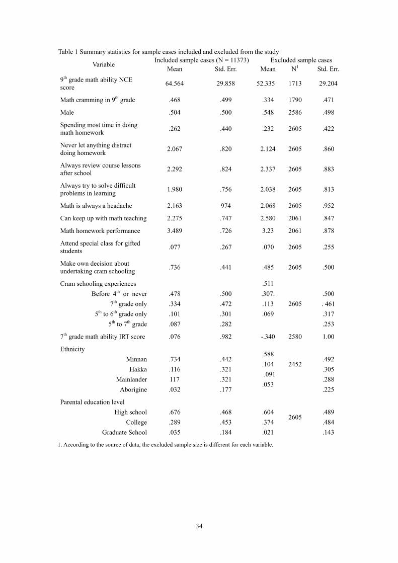
Table 1 Summary statistics for sample cases included and excluded from the study Included sample cases (N = 11373) Excluded sample cases

Variable Mean Std. Err. Mean N1 Std. Err.

9th grade math ability NCE score 64.564 29.858 52.335 1713 29.204

Math cramming in 9th grade .468 .499 .334 1790 .471

Male .504 .500 .548 2586 .498

Spending most time in doing math homework .262 .440 .232 2605 .422

Never let anything distract doing homework 2.067 .820 2.124 2605 .860

Always review course lessons after school 2.292 .824 2.337 2605 .883

Always try to solve difficult problems in learning 1.980 .756 2.038 2605 .813

Math is always a headache 2.163 974 2.068 2605 .952

Can keep up with math teaching 2.275 .747 2.580 2061 .847

Math homework performance 3.489 .726 3.23 2061 .878

Attend special class for gifted students .077 .267 .070 2605 .255

Make own decision about undertaking cram schooling .736 .441 .485 2605 .500

Cram schooling experiences Before 4th or never 7th grade only

5th to 6th grade only 5th to 7th grade

.478 .334 .101 .087

.500 .472 .301 .282

.511 .307. .113 .069

2605

.500 . 461 .317 .253

7th grade math ability IRT score .076 .982 -.340 2580 1.00

Ethnicity Minnan Hakka

Mainlander Aborigine

.734 .116 117 .032

.442 .321 .321 .177

.588

.104 .091 .053

2452

.492 .305 .288 .225

Parental education level High school

College Graduate School

.676 .289 .035

.468 .453 .184

.604 .374 .021

2605

.489 .484 .143

1. According to the source of data, the excluded sample size is different for each variable.

34

Table 1 (continued)

Included sample cases (N = 11373) Excluded sample cases

Variable Mean Std. Err. Mean N1 Mean

Parental occupation Professional or clerical

Sales or serviceOther

.338 .238 .425

.473 .426 .494

.244 .190 .566

2605

.429 .392 .496

Monthly family income Under NT$20,000

NT$20,000 – Less than NT$50,000NT$50,000 – Less than NT$100,000

NT$100,000 or above

.092 .412 .356 .140

.289 .492 .478 .347

.169 .422 .292 .118

2452

.375 .494 .455 .323

Living with both biological parents .816 .388 .636 2605 .481

Sib size 1.773 1.285 1.738 2516 1.390

Parental educational expectation High school diploma

College degreeGraduate degree

.096 .654 .250

.294 .476 .433

.148 .658 .194

2452

.356 .475 .395

Attend private school .119 .323 .109 2605 .311

The 9th grade class is a high ability class .187 .390 .149 2605 .356

Poor class climate for learning 2.828 .834 2.767 2605 .882

Class average grade is good 2.379 .860 2.341 2605 .898

Classmates often discuss homework or study together

2.128 .780 2.170 2605 .831

Intense academic competition among classmates

2.160 .843 2.188 2605 . 882

Classmates often discuss entrance examination

2.680 .829 2.613 2605 .866

School location Rural

Small cityMajor city

.050 .371 .579

.219 .483 .494

.136 .377 .486

2605

.343 .485 .500

1. According to the source of data, the excluded sample size is different for each variable.

35

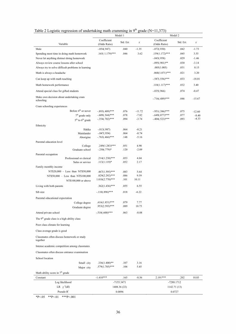
Table 2 Logistic regression of undertaking math cramming in 9th grade (N=11,373) Model 1 Model 2

Variable Coefficient

(Odds Ratio) Std. Err. z

Coefficient (Odds Ratio)

Std. Err. z

Male -.054(.947) .040 -1.35 -.072(.930) .042 -1.73

Spending most time in doing math homework .165( 1.179)*** .046 3.62 .159(1.172)*** .045 3.55

Never let anything distract doing homework -.043(.958) .029 -1.46

Always review course lessons after school -.095(.901)** .030 -3.14

Always try to solve difficult problems in learning .005(1.005) .031 0.15

Math is always a headache .068(1.071)*** .021 3.20

Can keep up with math teaching -.587(.556)*** .033 -18.01

Math homework performance .110(1.117)*** .032 3.40

Attend special class for gifted students -.035(.966) .074 -0.47

Make own decision about undertaking cram schooling -.716(.489)*** .046 -15.67

Cram schooling experiences

Before 4th or never

7th grade only

5th to 6th grade

-.893(.409)*** -.609(.544)*** -.354(.702)***

.076 .078 .094

-11.72 -7.82 -3.74

-.951(.386)*** -.649(.077)*** -.404(.523)***

.075 .077 .093

-12.60

-8.40 -4.33

Ethnicity Hakka

Mainlander Aborigine

-.013(.987) -.047(.954)

-.763(.466)***

.064 .064 .148

-0.21 -0.74 -5.16

Parental education level College

Graduate school

.249(1.283)***

-.250(.779)*

.051 .120

4.90 -2.09

Parental occupation Professional or clerical

Sales or service

.214(1.238)***

.113(1.119)*

.053 .052

4.04 2.17

Family monthly income

NT$20,000 – Less than NT$50,000

NT$50,000 – Less than NT$100,000

NT$100,000 or above

.467(1.595)*** .829(2.292)***

1.018(2.770)***

.083 .086 .101

5.64 9.59

10.11

Living with both parents .362(1.436)*** .055 6.55

Sib size -.110(.896)*** .018 -6.22

Parental educational expectation

College degree

Graduate degree

.616(1.851)*** .953(2.593)***

.079 .089

7.77

10.75

Attend private school -.510(.600)*** .063 -8.08

The 9th grade class is a high ability class

Poor class climate for learning

Class average grade is good

Classmates often discuss homework or study together

Intense academic competition among classmates

Classmates often discuss entrance examination

School location

Small city

Major city

.336(1.400)**

.579(1.785)***

.107 .106

3.16 5.45

Math ability score in 7th grade

Constant -1.410*** .165 -8.56 2.191*** .202 10.85

Log likelihood -7155.3471 -7288.1712

LR χ2(df) 1408.36 (22) 1142.71 (13)

Pseudo R2 0.0896 0.0727

*P<.05 **P<.01 ***P<.001

36

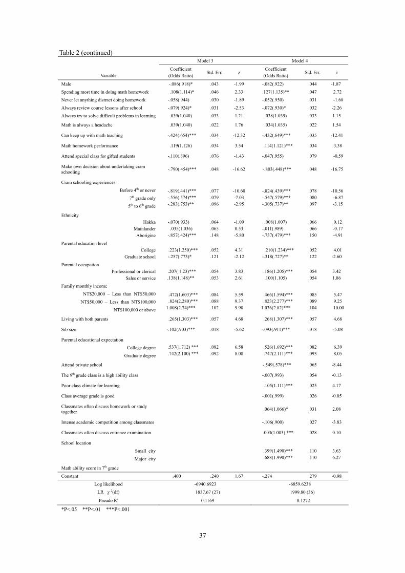
Table 2 (continued) Model 3 Model 4

Variable Coefficient

(Odds Ratio) Std. Err. z

Coefficient (Odds Ratio)

Std. Err. z

Male -.086(.918)* .043 -1.99 -.082(.922) .044 -1.87

Spending most time in doing math homework .108(1.114)* .046 2.33 .127(1.135)** .047 2.72

Never let anything distract doing homework -.058(.944) .030 -1.89 -.052(.950) .031 -1.68

Always review course lessons after school -.079(.924)* .031 -2.53 -.072(.930)* .032 -2.26

Always try to solve difficult problems in learning .039(1.040) .033 1.21 .038(1.039) .033 1.15

Math is always a headache .039(1.040) .022 1.76 .034(1.035) .022 1.54

Can keep up with math teaching -.424(.654)*** .034 -12.32 -.432(.649)*** .035 -12.41

Math homework performance .119(1.126) .034 3.54 .114(1.121)*** .034 3.38

Attend special class for gifted students -.110(.896) .076 -1.43 -.047(.955) .079 -0.59

Make own decision about undertaking cram schooling -.790(.454)*** .048 -16.62 -.803(.448)*** .048 -16.75

Cram schooling experiences

Before 4th or never

7th grade only

5th to 6th grade

-.819(.441)*** -.556(.574)*** -.283(.753)**

.077 .079 .096

-10.60 -7.03 -2.95

-.824(.439)*** -.547(.579)*** -.305(.737)**

.078 .080 .097

-10.56

-6.87 -3.15

Ethnicity Hakka

Mainlander Aborigine

-.070(.933) .035(1.036)

-.857(.424)***

.064 .065 .148

-1.09 0.53 -5.80

.008(1.007)

-.011(.989) -.737(.479)***

.066 .066 .150

0.12 -0.17 -4.91

Parental education level College

Graduate school

.223(1.250)***

-.257(.773)*

.052 .121

4.31 -2.12

.210(1.234)***

-.318(.727)**

.052 .122

4.01 -2.60

Parental occupation Professional or clerical

Sales or service

.207( 1.23)*** .138(1.148)**

.054 .053

3.83 2.61

.186(1.205)***

.100(1.105)

.054 .054

3.42 1.86

Family monthly income

NT$20,000 – Less than NT$50,000

NT$50,000 – Less than NT$100,000

NT$100,000 or above

.472(1.603)*** .824(2.280)***

1.008(2.74)***

.084 .088 .102

5.59 9.37 9.90

.466(1.594)*** .823(2.277)***

1.036(2.82)***

.085 .089 .104

5.47 9.25 10.00

Living with both parents .265(1.303)*** .057 4.68 .268(1.307)*** .057 4.68

Sib size -.102(.903)*** .018 -5.62 -.093(.911)*** .018 -5.08

Parental educational expectation

College degree

Graduate degree

.537(1.712) *** .742(2.100) ***

.082 .092

6.58 8.08

.526(1.692)*** .747(2.111)***

.082 .093

6.39 8.05

Attend private school -.549(.578)*** .065 -8.44

The 9th grade class is a high ability class -.007(.993) .054 -0.13

Poor class climate for learning .105(1.111)*** .025 4.17

Class average grade is good -.001(.999) .026 -0.05

Classmates often discuss homework or study together .064(1.066)* .031 2.08

Intense academic competition among classmates -.106(.900) .027 -3.83

Classmates often discuss entrance examination .003(1.003) *** .028 0.10

School location

Small city

Major city

.399(1.490)*** .688(1.990)***

.110 .110

3.63 6.27

Math ability score in 7th grade

Constant .400 .240 1.67 -.274 .279 -0.98

Log likelihood -6940.6923 -6859.6238

LR χ2(df) 1837.67 (27) 1999.80 (36)

Pseudo R2 0.1169 0.1272

*P<.05 **P<.01 ***P<.001

37

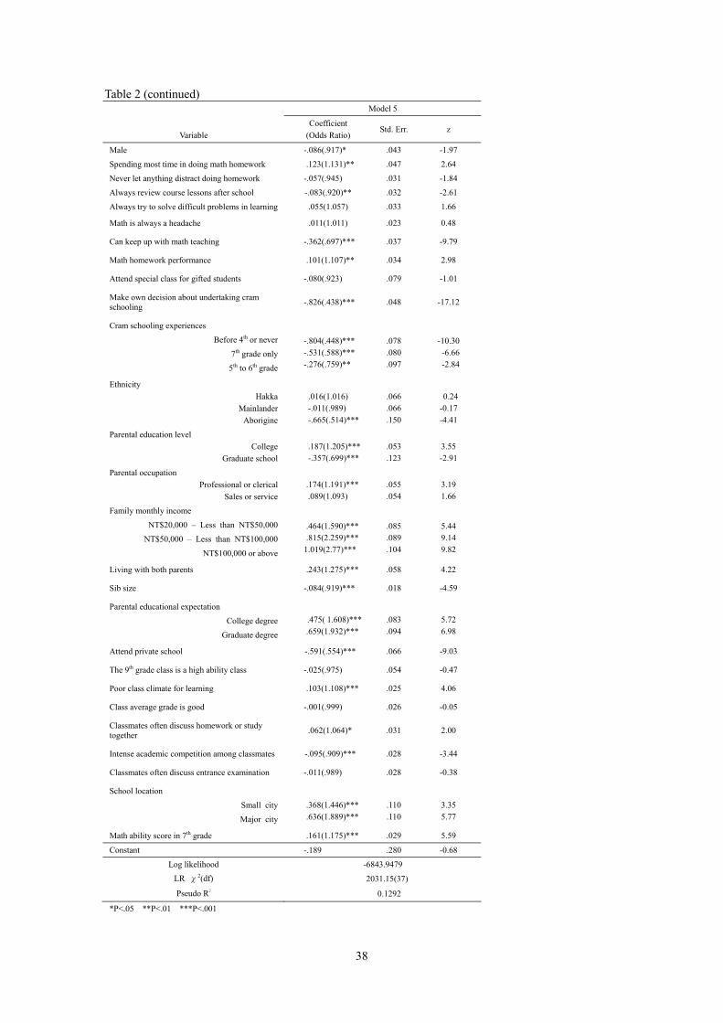
Table 2 (continued) Model 5

Variable Coefficient

(Odds Ratio) Std. Err. z

Male -.086(.917)* .043 -1.97

Spending most time in doing math homework .123(1.131)** .047 2.64

Never let anything distract doing homework -.057(.945) .031 -1.84

Always review course lessons after school -.083(.920)** .032 -2.61

Always try to solve difficult problems in learning .055(1.057) .033 1.66

Math is always a headache .011(1.011) .023 0.48

Can keep up with math teaching -.362(.697)*** .037 -9.79

Math homework performance .101(1.107)** .034 2.98

Attend special class for gifted students -.080(.923) .079 -1.01

Make own decision about undertaking cram schooling -.826(.438)*** .048 -17.12

Cram schooling experiences

Before 4th or never

7th grade only

5th to 6th grade

-.804(.448)*** -.531(.588)*** -.276(.759)**

.078 .080 .097

-10.30 -6.66 -2.84

Ethnicity Hakka

Mainlander Aborigine

.016(1.016) -.011(.989) -.665(.514)***

.066 .066 .150

0.24 -0.17 -4.41

Parental education level College

Graduate school

.187(1.205)*** -.357(.699)***

.053 .123

3.55 -2.91

Parental occupation Professional or clerical

Sales or service

.174(1.191)***

.089(1.093)

.055 .054

3.19 1.66

Family monthly income

NT$20,000 – Less than NT$50,000

NT$50,000 – Less than NT$100,000

NT$100,000 or above

.464(1.590)*** .815(2.259)***

1.019(2.77)***

.085 .089 .104

5.44 9.14 9.82

Living with both parents .243(1.275)*** .058 4.22

Sib size -.084(.919)*** .018 -4.59

Parental educational expectation

College degree

Graduate degree

.475( 1.608)*** .659(1.932)***

.083 .094

5.72 6.98

Attend private school -.591(.554)*** .066 -9.03

The 9th grade class is a high ability class -.025(.975) .054 -0.47

Poor class climate for learning .103(1.108)*** .025 4.06

Class average grade is good -.001(.999) .026 -0.05

Classmates often discuss homework or study together .062(1.064)* .031 2.00

Intense academic competition among classmates -.095(.909)*** .028 -3.44

Classmates often discuss entrance examination -.011(.989) .028 -0.38

School location

Small city

Major city

.368(1.446)*** .636(1.889)***

.110 .110

3.35 5.77

Math ability score in 7th grade .161(1.175)*** .029 5.59

Constant -.189 .280 -0.68

Log likelihood -6843.9479

LR χ2(df) 2031.15(37)

Pseudo R2 0.1292

*P<.05 **P<.01 ***P<.001

38

Table 3 Average treatment effect of math cramming: Comparisons between OLS and PSM Model (N=113731)

Variable OLS Model PSM Model

ATE ATT ATU

Difference between OLS and

PSM (ATE)

Model 1：Math cramming in 9th grade 11.328*** (.380) 2 ---3 --- --- ---

Model 2：Math cramming in 9th grade + Variables of Model 1 in Table 2

5.795*** (.355) 5.903 5.360 6.379 - 0.108

Model 3：Math cramming in 9th grade + Variables of Model 2 in Table 2

6.571*** (.329) 6.751 5.889 7.509 - 0.180

Model 4：Math cramming in 9th grade + Variables of Model 3 in Table 2

3.720*** (.316) 3.828 2.910 4.645 - 0.108

Model 5：Math cramming in 9th grade + Variables of Model 4 in Table 2

3.757*** (.313) 3.817 3.044 4.504 - 0.060

Model 6：Math cramming in 9th grade + Variables of Model 5 in Table 2

2.784*** (.264) 2.922 2.639 3.176 - 0.138

1. The sample used for comparing OLS and PSM estimates is the matched sample with common support. 2. Numbers within the parenthesis are standard errors. 3. Model 1 has no matching variable and hence no estimation of ATE、ATT, or ATU.

Table 4 Average treatment effects for those undertaking math cramming (ATT) stratified by propensity scores

PSM Model 1 (includes all matching variables)

PSM Model 2 (matching without math ability score in 7th grade)

Propensity scores ATT Matched sample size

Unmatched sample size ATT Matched

sample size Unmatched sample size

Total sample 2.636 11,373 15 3.001 11,385 3 1st stratum (lowest propensity) 3.370 2,260 15 4.945 2,276 1

2nd stratum 4.307 2,248 27 5.436 2,277 0 3rd stratum 2.791 2,244 30 3.982 2,274 3 4th stratum 1.344 2,239 36 1.732 2,277 0 5th stratum (highest propensity) 2.621 2,178 96 3.133 2,263 14

1st – 3rd stratum 3.343 6,821 3 4.486 6,831 0 4th – 5th stratum 1.813 4,496 53 2.503 4,550 4

Table 5 Average treatment effects for those undertaking math cramming (ATT) stratified by math ability

scores in the 7th grade PSM Model 3 Math ability scores in the 7th

grade ATT Matched sample size Unmatched sample sizeTotal sample 2.636 11,373 15 1st stratum (Lowest ability) 3.022 2,253 22 2nd stratum 3.424 2,250 25 3rd stratum 2.205 2,254 20 4th stratum 2.326 2,259 16 5th stratum (highest ability) 2.927 2,238 36 1st – 3rd stratum 2.677 6,815 9 4th – 5th stratum 1.957 4,540 9

39

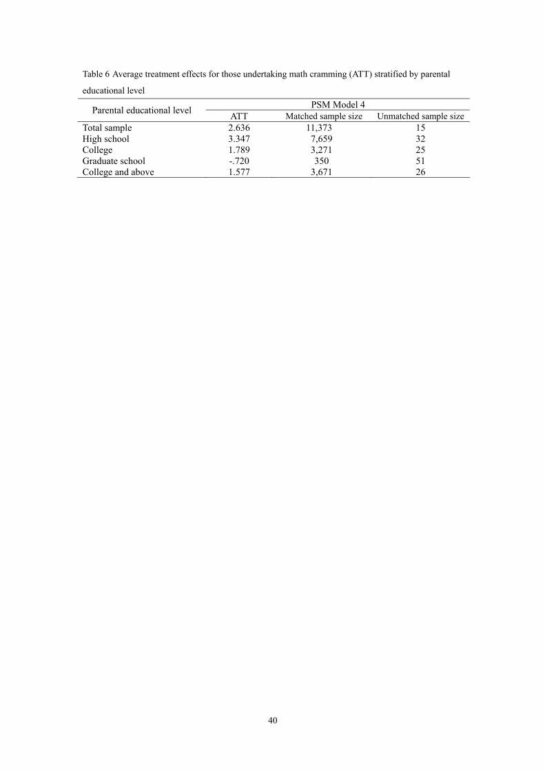
Table 6 Average treatment effects for those undertaking math cramming (ATT) stratified by parental

educational level PSM Model 4 Parental educational level ATT Matched sample size Unmatched sample size

Total sample 2.636 11,373 15 High school 3.347 7,659 32 College 1.789 3,271 25 Graduate school -.720 350 51 College and above 1.577 3,671 26

40

References

Alexander, Karl L., Dorris R. Entwisle, and Linda Steffel Olson. 2007. “Lasting

Consequences of Summer Learning Gap.” American Sociological Review 72:

167-180.

Aronson, Julie, Joy Zimmerman and Lisa Carlos. 1999. “Improving Student

Achievement by Extending School: Is It Just a Matter of Time?” San

Francisco: WestEd. Retrieved June 15, 2008

(http://eric.ed.gov/ERICDocs/data/ericdocs2sql/content_storage_01/0000019b

/80/15/ea/c4.pdf).

Baker, David P., Motoko Akiba, Gerald K. LeTendre, and Alexander W. Wiseman.

2001. “Worldwide Shadow Education: Outside-School Learning, Institutional

Quality of Schooling, and Cross-National Mathematics Achievement.”

Educational Evaluation and Policy Analysis 1: 1-17.

Becker, Betsy Jane. 1990. “Coaching for the Scholastic Aptitude Test: Further

Synthesis and Appraisal.” Review of Educational Research 60: 373-417.

Berliner, David C. 1990. What’s All the Fuss About Instructional Time? The Nature of

Time in Schools: Theoretical Concepts, Practitioner Perceptions. New York:

Teacher College Press.

Black, Alison Rebeck, Fred Doolittle, Pei Zhu, Rebecca Unterman, and Jean Baldwin

Grossman. 2008. The Evaluation of Enhanced Academic Instruction in

After-School Programs : Findings After the First Year of Implementation

(NCEE 2008-4021). Washington, D. C.: National Center for Education

Evaluation and Regional Assistance, Institute of Education Sciences, U.S.

Department of Education. Retrieved July 22, 2008

(http://www.mdrc.org/staff_publications_1.html).

41

Bodilly, Susan J. and Megan K. Beckett. 2005. Making Out-of-School-Time Matter:

Evidence for an Action Agenda. Santa Monica, CA: RAND Corporation.

Retrieved July 22, 2008

(http://www.rand.org/pubs/monographs/2005/RAND_MG242.pdf).

Bray, Mark. 2003. Adverse Effects of Private Supplementary Tutoring: Dimensions,

Implications and Governmental Responses. Paris: International Institute for

Educational Planning. Retrieved November 10, 2007

(http://unesdoc.unesco.org/images/0013/001330/133039e.pdf).

Caliendo, Marco and Sabine Kopeinig. 2008. “Some Practical Guidance for the

Implementation of Propensity Score Matching” Journal of Economic Surveys

22: 31-72.

Carroll, John B. 1963. “A Model of School Learning.” Teachers College Record 64:

723-733.

Carroll, John B. 1989. “The Carroll Model: A 25-Year Retrospective and Prospective

View.” Educational Research 31: 26-31.

Chang, Ly-Yun. 2003. Taiwan Education Panel Survey: Base Year (2001) Student

Data and Parent Data [public release computer file]. Center for Survey

Research, Academia Sinica [producer, distributor].

Department of Statistics, Ministry of Education. 2007. “Summary of Education at All

Levels.” Educational Statistics of the Republic of China. Taipei, Taiwan:

Ministry of Education, Executive Yuan. Retrieved February 12, 2008

(http://www.edu.tw/EDU_WEB/EDU_MGT/STATISTICS/EDU7220001/ebooks

/edu96/10.pdf?open).

Directorate-General of Budget, Accounting, and Statistics, Executive Yuan. 2007.

Statistical Yearbook of the Republic of China 2006. Taipei, Taiwan:

42

Directorate-General of Budget, Accounting, and Statistics, Executive Yuan.

Retrieved July 20, 2008

(http://eng.dgbas.gov.tw/public/data/dgbas03/bs2/yearbook_eng/y139.pdf).

Education Bureau, Kaohsiung City Government. 2008. All Cities and Counties

Short-Term Buxiban Information Management System. Kaohsiung, Taiwan:

Kaohsiung City Government. Retrieved July 8, 2008

(http://bsb.edu.tw/afterschool/english/index-e.jsp).

Entwisle, Dorris R., Karl L. Alexander and Linda Steffel Olson. 1997. Children,

Schools and Inequality. Boulder, Colorado:Westview Press.

Entwisle, Dorris R., Karl L. Alexander and Linda Steffel Olson, 2001. “Keep the

Faucet Flowing: Summer Learning and Home Environment.” American

Educator 25 (3): 10-15, 47.

Gettinger, Maribeth. 1985. “Time Allocated and Time Spent Relative to Time Needed

for Learning as Determinants of Achievement.” Journal of Educational

Psychology 77: 3-11.

Government Information Office. 2001. “ROC Educational Reform.” The Republic of

China Yearbook-Taiwan 2001. Taipei, Taiwan: Government Information Office,

Executive Yuan. Retrieved February 12, 2008

(http://www.gio.gov.tw/taiwan-website/5-gp/yearbook/2001/chpt17-3.htm#26).

Harding, David J. 2003. “Counterfactual Models of Neighborhood Effects: The Effect

of Neighborhood Poverty on Dropping Out and Teenage Pregnancy.” American

Journal of Sociology 109: 676-719.

Leuven, Edwin and Barbara Sianesi. 2003. “Psmatch2: Stata Module to perform full

Mahalanobis and Propensity Score Matching, Common Support Graphing, and

Covariate Imbalance Testing.” Retrieved October 17, 2007

(http://ideas.repec.org/c/boc/bocode/s432001.html, version 3.0.0.).

43

Lin, Da-Sen and Yi-Fen Chen. 2006. “Cram School Attendance and College Entrance

Exam Scores of Senior High School Students in Taiwan.” Bulletin of

Educational Research 52 (4): 35-70. (in Chinese)

Liu, Jeng. 2006. “The Transition, Efficacy, and Stratification of Cram Schooling in

Taiwan.” Bulletin of Educational Research 52 (4): 1-33. (in Chinese)

Marks, Gary N., John Cresswell, and John Ainley. 2006. “Explaining Socioeconomic

Inequalities in Student Achievement: The Role of Home and School Factors.”

Educational Research and Evaluation 12: 105-128.

Morgan, Stephen L. and David J. Harding. 2006. “Matching Estimators of Causal

Effects Prospects and Pitfalls in Theory and Practice.” Sociological Methods

and Research 35(1): 3-60.

Morgan, Stephen L. and Christopher Winship. 2007. Counterfactuals and Causal

Analysis: Methods and Principles for Social Research. Cambridge: Harvard

University Press.

Powers, Donald E. and Donald A. Rock, 1999, “Effects of Coaching on SAT I:

Reasoning Test Scores.” Journal of Educational Measurement 36 (2): 93-118.

Shavit, Yossi and Hans-Peters Blossfeld, eds. 1993. Persistent Inequality: Changing Educational Attainment in Thirteen Countries. Boulder, CO: Westview.

Stevenson, David L. and David P. Baker. 1992. “Shadow Education and Allocation in

Formal Schooling: Transition to University in Japan.” American Journal of

Sociology 97: 1639-1657.

Stevenson, David L. and James Stigler. 2002. The Learning Gap: Why Our Schools

are Failing, and What We Can Learn from Japanese and Chinese Education.

New York: Summit Books.

Sun, Ching-Shan and Yih-Jyh Hwang. 1996. “Shadow Education, Cultural Capital

44

and Educational Attainment.” Taiwanese Journal of Sociology 19: 95-139. (in

Chinese).

The Commission on Education Reform. 1996. The General Consultation Report for

Education Reform. Taipei, Taiwan: The Commission on Education Reform,

Executive Yuan. Retrieved February 12, 2008

(http://www.sinica.edu.tw/info/edu-reform/farea2/). (in Chinese)

Winship, Christopher and Stephen L. Morgan. 1999. “The Estimation of Causal

Effects from Observational Data.” Annual Review of Sociology 25: 659-707.

Winship, Christopher and Michael Sobel. 2004. “Causal Inference in Sociological

Studies.” Pp. 481-503 in M. Hardy, ed., The Handbook of Data Analysis.

Thousand Oaks, CA: Sage.

Yang, Meng-Li, Tony Tam, and Min-Hsiung Huang. 2004. Psychometric Report for

the Abilities Test of TEPS 2001. Taipei: Academia Sinica. Retrieved November 19,

2007 (http://www.teps.sinica.edu.tw/description/TestingReport2004-2-10.pdf).

(in Chinese)

Zeng, Kanming. 1999. Dragon Gate: Competitive Examinations and Their

Consequences. London: Cassell.

45