The e¤ects of the introduction of tax incentiveson retirement savings

Juan Ayuso� Juan F. Jimenoy Ernesto Villanuevaz

February 2007

Abstract

This paper examines the e¤ects of tax incentives on retirement sav-ings in Spain, which were �rst introduced in 1988. We use a panel of taxreturns and another on household expenditure during the period 1984-1992 to examine the incidence of the introduction of these incentives oncontributions to pension funds and on saving. We �rst identify the popu-lation cohorts who most used these incentives. Then we use data on theevolution of consumption of these cohorts to �nd that there is substan-tial heterogeneity in the response of household saving to tax incentives.Most contributions to pension funds are by older/high income individuals.While the overall amount of new saving we estimate is limited (around10 cents per euro contributed on average), saving responses di¤er sub-stantially across age groups. In particular, we document very small con-sumption drops among the group of households between 56 and 65 yearsof age, the group that most actively contributed to the plan, while we�nd instead a larger decrease in consumption expenditures of the groupof households between 46 and 55 years of age.

Keywords : Pension funds, tax incentives, savingsJEL Codes : D14, H24, H55.

1 Introduction

Tax incentives of retirement savings are present in many countries. However,whether they do indeed raise savings, rather than simply producing a change inthe composition of households�wealth portfolios, is a controversial issue.In the empirical literature on the e¤ectiveness of tax incentives at raising

savings, there are dissenting sets of results.1 For instance, while Poterba, Ventiand Wise (1995 and 1996) �nd that in the US funds accumulated in Individ-ual Retirement Accounts (IRAs) and 401(k) plans are mostly net additions to

�Banco de EspañayBanco de España, CEPR and IZAzBanco de España1For a recent survey of this literature, see Hawksworth (2006).

1

saving, Gale and Scholz (1994) and Engen, Gale and Scholz (1996) concludethat tax incentives of retirement savings have a strong e¤ect on the allocationof saving and wealth, but little or not e¤ect on the level, and that virtuallyall of the reported increase in �nancial assets in IRAs can be attributed tostock market booms, higher real interest rates, and shifts in non �nancial as-sets, debt, pensions and Social Security�s wealth.2 Hubbard and Skinner (1996)argue that probably "the truth lies somewhere between the two extremes", asthe results seem to rely on the assumed degree of substitution between taxablesaving and saving eligible for tax incentives.3 Attanasio, Banks and Wake�eld(2004) notice that new contributors to IRAs,who face higher marginal interestrates, should experiment a lower consumption growth than old contributors ifthe tax-favoured scheme is e¤ectively rising saving. However, they �nd that thestock of non-IRAs assets grows less for new contributors than for continuingcontributors, being the most likely cause that new contributors are reshu­ ingexisting portfolios into the IRAs, and not changing their consumption-savingdecision.4

Outside the US, there is not much evidence for other countries on this issue.5

This unsatisfying state of a¤airs is, to a large extent, due to three substantiveproblems that make it very di¢ cult to identify the e¤ects of tax incentives onsaving:i) The wide heterogeneity in the individual responses to tax incentives. The

e¤ects of tax incentives on saving, as on the value of pension wealth, depend onmany factors, such as age, the existence of liquidity constraints, the relevanceof bequest motives, the di¤erence between the time discount factor and ratesof return, and plausible distortionary e¤ects on labour supply. Additionally,individual preferences for saving may change through time (beyond the changesimplied by the life-cycle model), as it may change the degree of substitutabilitybetween retirement savings and other forms of savings, including housing wealth.All these factors a¤ect, not only to the rate of return of di¤erent assets, butalso to degree of substitutability among them.

2 In the US, there are two schemes favouring retirement savings, IRAs and 401(k) plans.Contributions to IRAs are tax-deductible up to certain limits. Deposits in 401(k) accountsare also tax-deductible. In both cases, the return to the contributions accrues tax free andtaxes are paid upon withdrawal. Participation in IRAs is voluntary, but only employees of�rms that o¤er them are elligible to participate in 401(k) plans. Employees� contributionsto 401(k) plans can be "matched" by employer�s contributions and, under certain conditions,employees may borrow funds from their 401(k) accounts.

3While Poterba, Venti and Wise (1996) interpret the fact that many households do notparticipate in IRAs as indication of the imperfect substitution between IRAs-saving and tax-able saving, Engen, Gale and Scholz (1996) believe that participation arises mostly from tastefor saving.

4This is consistent with the large elasticities of substitution between pension wealth andpersonal savings typically found in other empirical studies (see Attanasio and Rohwedder,2003 and the references therein).

5See Milligan (2002) and Veall (2001) on Canada, Blundell, Emerson and Wake�eld (2006)and Chung, Disney, Emmerson and Wake�led (2006) on the UK, and Japelli and Pistaferri(2002) on Italy. There is also some aggregate evidence based on cross-country regressions(e.g. Lopez-Murphy and Musalem, 2004), pointing out that the accumulation of pensionfunds increases national savings only when they are compulsory.

2

ii) The lack of microeconomic data on consumption, saving, and wealth. Notonly the e¤ects of tax incentives may be di¤erent across individuals, also changesin tax incentives of retirement savings typically go in hand with other changes intaxes and/or in pension wealth that also a¤ect individuals in a di¤erent mannerdepending upon their position in the life cycle and their accumulated wealth.Hence, the identi�cation of the e¤ects of tax incentives on saving requires theobservation of a wide range of �nancial and personal characteristics determin-ing marginal tax rates, earnings volatility, pension wealth, discount and inter-est rates, etc, together with individual/household-level information on income,consumption, and wealth and its composition. Moreover, since households arelikely to have di¤erent underlying preferences for savings (substitution and in-come e¤ects vary across individuals), the estimation of the impact of changesin tax incentives requires using panel data to control for unobserved individualcharacteristics.iii) The di¤erential impact that tax incentives may have at the moment when

they are introduced with respect a situation in which they have been operativefor a long period. Tax incentives for retirement saving may a¤ect both tothe level of saving and to the composition of wealth. Typically, contributionsto pension funds exempted from income taxation (the usual instrument thatimplements these tax incentives) are subject to certain limits, which are morelikely to be binding at the moment when tax incentives are introduced. Thus,there is likely to be some gradual adjustment to the desired level of savings andto the optimal wealth composition after the introduction of tax incentives forretirement savings. This implies that the e¤ects of tax incentives at the momentof its introduction are likely to be di¤erent to their e¤ects in a situation in whichthey have been operative for some time so that individuals�wealth compositionis closer to the desired one and the limits to exempted contributions from incometaxation could be less binding.In this paper we aim at providing further empirical evidence on the impact

of tax incentives on saving by examining the e¤ects of the introduction of taxincentives of retirement in Spain in 1988.6 Pension funds in Spain, the �nancialinstruments where retirement savings are deposited under some �scal favourabletreatment, have similar features to post-86 IRAs in the US. Contributions tothose funds were tax-exempted for all individuals up to a generous amount(4,500 euro in 1988), allowed tax-free accrual of savings but limited disposalof accumulated funds before retirement. Finally, upon lump-sum withdrawalafter retirement, taxation depends on the form of withdrawal: if redemptiontakes place in a lump-sum payment 40% is exempted from income taxation, ifredemption is in form of annuity, then it is taxed at marginal tax rate on income.We analyze the impact of the introduction of these tax incentives in two steps.First, we use a panel of tax returns to identifyin the population cohorts who

6 In a companion paper (Ayuso, Jimeno and Villanueva, 2007) we use more recent datafrom the Spanish Survey of Household Finances, which contains information on householdwealth and its composition, and on consumption, to investigate further to what extent taxincentives promote retirement savings, after these tax incentives have been operative for someperiod.

3

most used these incentives. Secondly, we use a pnale of household consumptionto estimating the impact of tax incentives on consumption/saving of di¤erentpopulation groups.We think that this paper contributes to the literature on tax incentives

to save in three di¤erent ways. First, we are able to use data spanning theperiods before and after the introduction of tax-favoured retirement plans. Inthe absence of a controlled experiment, such as in Du�o et al. (2006), examiningthe evolution of savings around the introduction of the tax exemption mitigatessome of the problems in the analysis of IRAs in the US, that typically study theimpact using post-introduction trends among di¤erent groups in the population.Secondly, we focus on the impact of the introduction of the pension funds

program on household consumption, rather than on household wealth. In doingthis, we follow Attanasio and DeLeire (2002) and depart from the work sum-marized in Poterba, Venti and Wise (1996) or Engen and Gale (1996), whofocus on the impact of tax incentives to retirement saving on household wealth.While household wealth is a very important outcome, household consumptionalso conveys complementary useful information. In the presence of employercontributions, household consumption is more likely to re�ect how the �ow ofactive household saving is a¤ected by tax incentives than household wealth (seeChernouzhukov and Hansen, 2001). Moreover, according to the permanent in-come hypotheses, household wealth is much more a¤ected by transitory incomechanges than household consumption (Blundell and Preston, 1998). Any analy-sis that focuses on group-speci�c changes in household wealth over time faces theproblem of disentangling between the impact of tax incentives and the impactof between-group income changes.7

Thirdly, we extend the techniques in Attanasio and de Leire (2002), whoinfer the impact of tax incentives on new saving by comparing the consumptionchanges of new contributors (who experience an e¤ective increase in the interestrate) to those of old contributors (who only experienced the increase of interestrate at the time of the �rst contribution). Bernheim (2002) and Poterba, Ventiand Wise (1996) object that the variation associated to actual contributionsmay re�ect other variables (preference for present consumption, income risk,borrowing constraints, preference for liquid portfolios) rather than the incentiveto save.8To get around the omitted variables problem, we build a variable thatsummarizes the incentives to contribute. Our instrumental variable is the inter-action between the income tax marginal rate and the age of the individual atthe time of introduction of the exemption. Individuals with higher income tax

7Also, using consumption allows comparisons of tax incentives across countries. Whilevirtually every European country has an expenditure survey, very few countries have detailedSCF or SIPP -type of household wealth surveys.

8A �rst objection by Bernheim (2002) is that the timing of contributions is correlatedwith saving preferences of the households, and that such di¤erences are hard to detect usingconsumption growth - a poor indicator of intrinsic thrift according to Bernheim, Skinner andWeingberg (1997). In addition, Bernheim (2002) and Poterba, Venti and Wise (1996) alsoargue that Attanasio and De Leire�s (2002) results can be also be re-interpreted as contribu-tions of old contributors representing new saving and those of new contributors representingportfolio reshu­ ing.

4

marginal rates experiment a higher increase in post-tax returns (Milligan 2001,who cites many others) and age proxies income risk and preference for liquidassets. We check that our variable is indeed a strong predictor of contributions:it was mainly �lers in the top quartile of labor earnings who exempted contri-butions and, within that group, average contributions increased monotonicallywith age. Using a separate expenditure survey, we then examine if the con-sumption growth of broad age groups in the top income quartile, relative to ourcontrol group of young households, experienced a drop around the introductionof the exemption.Our results suggest that there is indeed substantial heterogeneity in the con-

tributions to pension funds and in the response of household saving to tax in-centives. While the overall amount of new saving we estimate is limited (around10 cents per euro contributed on average), saving responses di¤er substantiallyacross age groups - a �nding also reported in the literature on 401(k)s.9 In par-ticular, we document very small consumption drops among the group of house-holds between 56 and 65 years of age, the group that most actively contributedto the plan. We document a larger decrease in consumption expenditures of thegroup of households between 46 and 55 years of age. A way of interpreting suchpattern of responses is that households in the verge of retirement �nd pensionfunds and other saving forms as strong substitutes, and tend to exhaust tax-exempted contribution limits by reshu­ ing their wealth portfolios. Conversely,groups further away from retirement, with plausibly less accumulated wealthand for whom contribution limits are plausibly not binding, need to save moreto take advantage of the tax incentives of retirement savings.The structure of this paper is as follows. Section 2 provides a description

of the main regulation of pension funds in Spain when tax incentives were in-troduced in 1988. Section 3 contains some theoretical discussion of the factorsdetermining the impact of the introduction of tax incentives on retirement sav-ing. Section 4 discusses the characteristics of the panel data of tax returns andthe expenditure survey used for the empirical exercise. Section 5 examines theincidence of contributions over time, while Section 6 compares contributionsand the evolution of consumption across population cohorts in order to infertheir e¤ects on the level of saving. Finally, Section 7 contains some concludingremarks.

2 The introduction of tax incentives of retire-ment savings in Spain

In Spain the �rst piece of legislation regulating private pension funds was notpassed until 1987, when the Ley de Planes y Fondos de Pensiones (formally,

9Chernouzhoukov and Hansen (2004) document small wealth responses to 401(k)s in thetop of the wealth distribution and some evidence of new saving at the bottom. Engen andGale (2000) compare trends in household wealth across individuals that are not eligible forthe 401(k)s and those that are not, and document substantial heterogeneity across incomeand age groups.

5

Ley 8/87 ) established three types of private pension plans: employment plans(planes de empleo), under which the sponsor is a non-�nancial �rm while its em-ployees are the plan members, associate plans (planes asociados), under whichthe sponsor is some legal association and the association members are entitledto contribute to the plan, and individual plans (planes individuales), created by�nancial entities �that act as sponsors �and open to any individual who wantsto contribute.Contributions to these funds were exempted from income taxation, up to

certain limits. More concretely, contributions below the minimum of 15% oflabour income and half a million pesetas (3,005.06 euros) where directly de-ducted from the income tax base. An additional 15% of contributions beyondthis limit but below 750,000 pesetas (4,507.59 euros) was deductible from theincome tax quota. It is worth noting that up to 1987, the income tax leviedhousehold individual partners jointly. Since 1988, however, couples may decidewhether to be taxed jointly or individually. In the former case (joint incometax return) limits apply to each spouse individually, and therefore could evendouble for households opting for joint income taxation.10

Upon redemption, funds were subject to income taxation at di¤erent ratesdepending upon how redemption took place. They were considered non-regularincome if received as a single payment and as a regular income when receivedin the form of annuities. In the �rst case, 40% of the payment was exemptedfrom taxation, while in the second case it was taxed at the marginal tax rateon income. As the income tax on non-regular income is lower than that onregular income � in order to correct the distortion created by tax rates thatincrease whit income level when multi-period income accumulates in a singleyear �redemption in the form of a single payment was, in general, much moreprevalent.11

As in this paper we focus on the e¤ects on household consumption of the in-troduction of tax incentives of retirement saving, it is important to bear in mindthat two other important changes in household income taxation were introducedin 1988. On the one hand, income tax marginal rates were substantially mod-i�ed. The rate was set to zero for income below 600,000 pst (3,606.07 euros)and raised to from 8% to 25%, at that income level. The number of rates wasreduced from 34 to 16, and the maximum one was set at 56%, 10 percentagepoints less than one year before. The e¤ects of these changes on household netincome and therefore on household consumption will heavily depend on theirpre-tax income level. Also, as commented above, in 1988 household individualpartners were allowed to decide whether to pay income taxes individually orjointly. As the income tax is highly progressive, households were both spouses

10Subsequent changes in the related regulation have modi�ed these limits several times.Currently, after the changes e¤ective as from the beginning of 2007, there is no deductibilityin the income tax quota and the limits for deductibility from the tax basis have been set atthe minimum between 30% of labour income and 10,000 euros for tax payers below 50 years,and the minimum between 50% of labour income and 12,500 euros for tax payers aged morethan 50.11Since 2007, however, redemption funds are considered regular income irrespectively of the

form they are received.

6

had labour income massively opted for individual taxation.12

3 Some theoretical considerations

Typically the analysis of tax incentives of retirement saving is conducted in anequivalent manner to the rise in the marginal rate of return to saving. Under thisanalysis, tax incentives increase this marginal rate of return so that the impacton saving would depend on substitution and income e¤ects. The realtive size ofthese two e¤ects crucially depends on the prevalence of borrowing constraintsand preferences for liquid assets.To grasp some intuition about the determinants of these e¤ects, let us con-

sider an individual with initial wealth W0: When tax incentives for retirementsavings are introduced, contributions to pension funds, f; yield a tax deductionwhich is given by f� , for f � f and f� for f > f , where f is the limit appliedto contributions for tax-exemption, and � is the marginal tax rate on income.When the pension fund is redeemed, only a fraction � of the receipts are subjectto the marginal tax rate on income, � 0: Thus, assuming that the time discountrate is equal to the accrual rate of the pension fund, contributions to pensionfunds increase individual wealth by f�(1��� 0=�), for f � f and f�(1��� 0=�)for f > f : Hence, the smaller � and the smaller the ratio between future andcurrent marginal tax rates on income are, the larger this wealth increase is.Insofar as marginal tax rates rise with income, individuals who expect a higherfall in income after retirement would experience a larger wealth increase fromcontributing to pension funds. This also suggests that individuals will concen-trate their contributions to pension funds in those periods when their incomesand, hence the marginal tax rates they face, are highest.13 Thus, the incentivesto contribute in pension funds result from the interaction between tax incentivesfor retirement saving and the income tax and bene�t systems.Notice that, if there are not borrowing constraints, initial wealth, W0, does

not determine the optimal contribution to the pension fund. In this case, con-tributions to pension funds could arise, not only through higher saving, but alsoby (unconstrained) reshu­ ing the wealth portfolio. However, when there areborrowing constraints, individuals without initial wealth can only contribute topension funds by saving more, while individuals with positive wealth could alsoreshu­ e their asset holdings to bene�t from the tax incentives of retirementsaving.Finally, if there are borrowing constraints, the decision on retirement saving

is also a¤ected by the di¤erent liquidity characteristics of retirement savings andother savings. Individuals facing higher income risks would regard retirementsavings as an imperfect substitute of normal savings, as the former can only be

12Female labour market participation rates in Spain have traditionally been relatively low,more so for the older population cohorts. Thus, the e¤ects of voluntary joint income tax �lingare likely to depend on the age of the household�s head..13Blundell, Emmerson and Wake�eld (2006) also highlight that some individuals face a very

strong incentive to contribute to pension funds at particular times during their working lives.

7

used to smooth consumption after retirement.These considerations lead us to conclude that, upon introduction of tax

incentives of retirement savings, the e¤ects on saving would be di¤erent de-pending on several individual characteristics, such as, initial wealth, incomepro�le and other factors (household composition, etc.) determining current andfuture marginal tax rates on income, and borrowing constraints, income risks,and preference for liquidity. For some individuals, with invariant marginal rateof returns to savings, there would be only a wealth e¤ect and no substitutione¤ect, so that their consumption pro�les would shift upwards. For others, themarginal rate of return to savings would change, there would be a substitutione¤ect, and, as a result, there would be a change in the slope of their incomepro�les.Since in the data we cannot identify all of the factors determining income and

subtitution e¤ects, we characterize the impact of tax incentives of retirementsavings on total saving using demographic and income groups. First, we condi-tion the analysis of the contribution to pension funds by focusing on individualsat the top of the income distribution, that at the time of the reform faced thehighest income tax marginal rates. We regard individuals between 18-35 yearswhen tax incentives were introduced as the most likely to have accumulated lesswealth and to �nd pension funds less attractive for liquidity reasons. Hence,we expect contributions to pension funds from these individuals to be low. Wealso expect contributions to pension funds to increase with age and marginaltax rates on income. As for impact on consumption, we expect to �nd a largerconsumption drop among medium-age individuals with high income. For theseindividuals incentives for contributing to pension funds are largest, as incomeand marginal tax rates on income are at their peaks, and uncertainty and liquid-ity considerations are less important than for younger individuals. Also, for thispopulation group, accumulated wealth is not at its highest, so that reshu­ ingunder borrowing constraints cannot be too large, and contributions to pensionfunds need to arise from lower consumption. Finally for older individuals, closeto retirement, wealth is higher and liquidity considerations are even less relevant,so that contributions to pension funds are more likely to arise from reshu­ ingof the wealth portfolio than from higher saving.

4 Data sets and empirical strategy

We use two data sets. The �rst is a micro panel of tax returns �led by individualsbetween 1982 and 1998 and collected by the Spanish Tax Agency (the so-calledPanel of Income Tax Returns). The second is a household expenditure survey.

4.1 The Panel of Income Tax Returns: 1988-1998

In 1987 the Spanish tax authority sampled 1 in 25 tax returns in 48 out of the 52Spanish provinces, and then tracked back the returns of those �lers from 1982

8

and forward until 1998.14 To maintain the representativeness of the sample, thetax authority also added in each year after 1988 a refreshment sample with newtax returns. The introduction of the pension fund program in 1988 coincidedwith a major tax change. Before 1988, married couples had to �le jointly. Afterthe tax reform in 1988 the two members of a married couple were allowed to�le separate tax returns. The 1988 reform had direct consequences both for thedesign of the sample and for the validity of our analysis. We start by discussingthe consequences for the sample, and di¤er the discussion on the implicationsfor our analysis to Section 6.3. Due to compulsory joint �ling in the year inwhich the sample was made, the Statistical Agency was able to identify pre-1988"�scal households" and then keep track of the tax returns �led by each memberof the original 1987 couple - even if married �lers opted for �ling separately ina particular year.We mainly use this sample to identify who contributed to pension funds

at the onset of the program and to quantify the mean contribution by groups.The unit of our analysis is the 1987 tax �ling unit. The Panel of Income TaxReturns contains all the information contained in a tax return (excluding allinformation that can threat anonymity). We collect the amount contributed topension funds by each tax return in the �ling unit. We include both individualand employer contributions, but nothing substantially changes when we excludeemployer contributions, which represents a very small fraction of the total inthe immediate years after the introduction of the tax incentives. We also usethe yearly income of the tax �ling unit and some information on householdcomposition (marital status and the number of children below 18 years of age).For 70% of the original 1987 sample, the Tax Agency also collected the age ofthe main �ler. We only use the subsample that contains age.15

Panel A of Table 1 shows the evolution of the fraction of tax units with atleast one contributor. While initially low, the fraction of contributors rapidlyexpanded during the 80s, and at the end of the decade some 24% of tax �lershad made a contribution. Possibly because contributors in 1988 reported higherincomes than contributors who did their initial contribution after that year,the mean and median contribution declined in real terms during the decade:from 221,873 pts. (1,333.5 euros, about 6% of the gross labor income reportedby �lers who contributed) in 1988 to 197,659.6 pts. (1,188 euros) in 1998.As we discuss below, the vast majority of contributions (70%) were made by�ling units that reported gross labor income in the top quartile of the incomedistribution. Contributions in the high end of the income distribution wererelatively persistent: 81% of contributors who were in the top income quintilein 1988 and started contributing would contribute on the following year, andthe average number of contributions over a six- year period was 5.04 (see TableA.1)We focus the analysis on the years following the introduction of the tax

14Due to a special tax regime, the Basque Country and Navarra, which represent about 5%of the Spanish population, were not covered.15We have dropped the contributions to pension funds by tax �lers who report self-employed

income, since in this case income reported could be subject to serious measurement bias.

9

exemption: 1988-1991. Panel B of Table 1 shows the summary statistics of thissubsample. The mean gross labor income reported by the tax unit was 2,319,635pts. (13,941 euros). The (unconditional) average contribution is 10,927 pts.(65,7 euros) with 5% of tax units actually making a contribution. The meanage of the main �ler is 41 years.

4.2 The Household Expenditure Survey (ECPF)

The second sample uses the 1985-1991 waves of a quarterly expenditure surveycalled Encuesta Continua de Presupuestos Familiares (henceforth, ECPF).16

The ECPF interviews some 3,000 households in each wave. Households arehanded a notebook to record their expenses on food, transportation, textiles,health and schooling during some weeks of the quarter (see references above).Also, households report retrospective information about more bulky purchases,like furniture, cars, electronic goods (TV, and others) and white goods (wash-ing machines, dishwashers, fridges). Respondent households are tracked duringeight quarters (at most), and report information about household compositionand the income received by each household member, with some disaggregationon income sources. Due to problems with calculating pre-tax earnings, we focuson households headed by an employed individual.The reason to focus only on a few waves is that one should only observe a

consumption drop when households start contributing and presumably adjusttheir savings plan in response to the introduction of tax incentives. After thatinitial period, the life-cycle hypothesis predicts that, holding other variablesconstant, individuals who face higher interest rates tend to delay consumptionto the future.17 Thus, we use the periods when we observe more new �lersstarting to contribute (see Table 1, Panel A, �rst column).The key variables in our analysis are total household expenditures and a

measure of marginal tax rate on income. Rather than working with incometax marginal rates, which are not directly observed in this survey, we choseto work with pre-tax income, and concentrate on the top quartile of the la-bor income distribution. We obtained yearly pre-tax income by applying thewithholding tax rates and adding contributions to the post-tax income reportedin the ECPF. Regarding household expenditure, we have little priors on howspeci�c household consumption components react to changes in tax incentives.Thus, and following Attanasio and Brugiavini (2003), we include basically allconsumption components (including the expenditure in all durable goods, buthousing). The main characteristics of this sample are shown in Tables 2A and2B.16See Browning and Collado (2001, forthcoming), Carrasco, López-Salido and Labeaga

(2005) and Albarrán (2004) for recent uses of the ECPF to test theories of consumptionbehavior.17See Attanasio and DeLeire (2002) who discuss this point in detail.

10

4.3 Empirical strategy

The empirical analysis proceeds in three steps. The �rst veri�es that laborearnings at the time of the introduction of the tax incentives of retirementsaving are strong predictors of both the probability of contributing and of theamount contributed to pension funds. To that end, we use the panel of taxreturns.The second step builds on the previous results and examines the evolution

of mean consumption growth of the groups that, according to the panel of taxreturns, used the contributions most heavily. The data set used in this step is theExpenditure Survey. While this strategy allows us to detect consumption dropsaround the time of the introduction of the tax incentives, we cannot quantifyhow much new saving is created.Thus, in the third step we use Two-Sample Two Stage Least Squares to

relate mean contributions to pension funds and mean drops in expenditure.In what follows, we discuss each of these steps in detail.

4.3.1 Distribution of contributions when tax incentives were intro-duced

Following the theoretical considerations sketched in Section 3, we examine bothcontributions to pension funds around the date of the introduction of tax incen-tives of retirement savings. As already mentioned, we expect households withhigher income tax marginal rates to experience a larger wealth e¤ect from taxincentives and, thus, to have a higher incentive to contribute. Secondly, withinhouseholds with similar income tax marginal rates, those in the latter part oftheir working lives are most likely to contribute, as wealth is plausibly higher,and income risk and liquidity considerations are less relevant. We check thesehypothesis using the panel of tax returns to compute the average probabilityof contributing and the average contribution by age group (holding the quartileof labor earnings constant). We divide the sample along two dimensions: i) agegroups (in four 10-years brackets), and ii) pre-tax labor earnings of the 1987 tax�ling unit. This easily identi�es individuals who contributed to pension fundsby most after the introduction of tax incentives of retirement savings.

4.3.2 Changes in expenditure when tax incentives were introduced

In the second step we compare contributions and consumption growth for in-dividuals with high income tax marginal rates in the later part of their work-ing lives (the �treatment group�) to that of individuals with high income taxmarginal rates and headed by a person below 35 years of age (the "controlgroup").This test based on consumption growth has the advantage of control-ling for unobserved di¤erences between the control and treatment group, as longas they remain constant over time. It is also una¤ected by trends in saving thata¤ected similarly to individuals within the same income quartile or within the

11

same age group.18

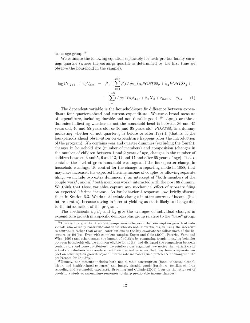
We estimate the following equation separately for each pre-tax family earn-ings quartile (where the earnings quartile is determined by the �rst time weobserve the household in the sample):

logCh;q+4 � logCh;q = �0 +i=3Xi=1

�i(Age_i)hPOST88q + �4POST88q +

+i=3Xi=1

(Age_i)h�4+i + �8Xit + "h;q+4 � "h;q (1)

The dependent variable is the household-speci�c di¤erence between expen-diture four quarters-ahead and current expenditure. We use a broad measureof expenditure, including durable and non durable goods.19 Age_i are threedummies indicating whether or not the household head is between 36 and 45years old, 46 and 55 years old, or 56 and 65 years old. POST88q is a dummyindicating whether or not quarter q is before or after 1987.1 (that is, if thefour-periods ahead observation on expenditure happens after the introductionof the program). Xit contains year and quarter dummies (excluding the fourth),changes in household size (number of members) and composition (changes inthe number of children between 1 and 2 years of age, changes in the number ofchildren between 3 and 5, 6 and 13, 14 and 17 and after 65 years of age). It alsocontains the level of gross household earnings and the four-quarter change inhousehold earnings. To control for the change in reporting mode in 1988, thatmay have increased the expected lifetime income of couples by allowing separate�ling, we include two extra dummies: i) an intercept of "both members of thecouple work", and ii) "both members work" interacted with the post 88 dummy.We think that those variables capture any mechanical e¤ect of separate �lingon expected lifetime income. As for behavioral responses, we brie�y discussthem in Section 6.3. We do not include changes in other sources of income (likeinterest rates), because saving in interest-yielding assets is likely to change dueto the introduction of the program.The coe¢ cients �1; �2 and �3 give the averages of individual changes in

expenditure growth in a speci�c demographic group relative to the "base" group.18One could argue that the right comparison is between the consumption growth of indi-

viduals who actually contribute and those who do not. Nevertheless, in using the incentiveto contribute rather than actual contributions as the key covariate we follow most of the lit-erature on 401(k)s. Even with complete samples, Engen and Gale (2000), Poterba, Venti andWise (1996) and others assess the impact of 401(k)s by comparing trends in saving behaviorbetween households eligible and non-eligible for 401(k) and disregard the comparison betweencontributors and non-contributors. To reinforce our argument, we notice that variations inactual contributions are correlated with unobserved variables that may have a separate im-pact on consumption growth beyond interest rate increases (time preference or changes in thepreferences for liquidity).19Namely, our measure includes both non-durable consumption (food, tobacco, alcohol,

leisure and health-related expenses) and lumply durable goods (furniture, textiles, childrenschooling and automobile expenses). Browning and Collado (2001) focus on the latter set ofgoods in a study of expenditure responses to sharp predictable income changes.

12

Those averages mix households that contribute to pension funds and those thatdo not. Note that only contributors faced a positive wealth e¤ect at the time ofthe introduction of the program. If contributions were �nanced from changes inconsumption we would expect �1; �2 and �3 to be negative. On the contrary, ifcontributions were �nanced from reshu­ ing assets, and not from higher saving,we would expect �1; �2 and �3 to non-negative.Mean impacts on consumption changes may not be the only relevant mo-

ment. The propotion of �lers who contributed to pension funds between 1988and 1991 was low (see Table 1). Thus, the introduction of tax incentives isunlikely to have generated a constant impact throughout the consumption dis-tribution; on the contrary, it is likely to be located in speci�c centiles of the dis-tribution of expenditure changes. Secondly, our expenditure measure includesdurable goods. If households delayed the purchase of a car or of new furni-ture to �nance their contributions, we would expect again a nonlinear impactover the distribution of expenditure changes. Thus, as a further speci�cationcheck, we report estimates of the impact of the interaction of age dummiesand income group on the 25th, 50th, 75th and 90th centiles of the distributionof consumption drops. Finally, and given that consumption growth is clearlyheteroskedastic, we tighten our estimates presenting Weighted Least Squares(WLS) estimates, weighting observations by the inverse of the absolute value ofthe residual of a consumption change equation estimated by OLS.

Robustness check A potential problem with model (1) is that it attributesany di¤erential trend in expenditure growth that happened between 1985 and1990 in the age groups we consider to the introduction of tax incentives of retire-ment saving. To control for age-speci�c trends, in some speci�cations we use asa benchmark the evolution of consumption of the group with incomes betweenthe 50th and the 75th centile of the distribution of earnings. Namely, using thesubsample of households whose income is above the median, we estimate thefollowing model:

logCh;q+4 � logCh;q = �0 +i=3Xi=1

i(Age_i)hPOST88q � 1(Y > Y:75)

+i=3Xi=1

4+i(Age_i)hPOST88q + 8POST88q � 1(Y > Y:75)

+i=3Xi=1

8+i(Age_i)h � 1(Y > Y:75) +i=3Xi=1

12+i(Age_i)h

+ 16POST88q + 171(Y > Y:75) + 18Xit + uh;q+4 � uh;q (2)

Model (2) attributes to tax incentives any trend in the expenditure growth ofhouseholds in the later part of their working life and in the upper quartile ofthe distribution of earnings that is di¤erent from the corresponding trend in thesecond quartile of the distribution of earnings. Model (2) makes the implicitassumption that, if tax incentives of retirement saving had not been introduced,

13

the di¤erence in consumption growth between households in the top quartilewith ages above 45 and households below 35 would have evolved as the samedi¤erence among households in the second-to-top income quartile.

4.3.3 The impact of contributions to pension funds on new house-hold saving

A parameter commonly used in the literature that evaluates the impact of taxincentives on retirement saving is "How much new saving does an extra euroof contributions generate"? The strategy described above cannot address thatquestion. To assess the amount of new saving generated by the tax incentives,and following Angrist and Krueger (1992), we combine moments from the twosamples using 2SLS estimates.Namely, we are interested in the parameter �1 of the following relationship:

Cit = �0 + �1Contrit + "it (3)

where Cit measures yearly consumption and Contrit is the amount contributedto pension funds. Most likely, Contrit is correlated with "it because householdsthat contribute have di¤erent preferences for present consumption and for liquidportfolios. Assuming that the interaction of age and income quartile at the timeof the introduction of the exemption (Zit) only a¤ects consumption growththrough its impact on contributions to pension funds, then Zit is correlatedwith contributions but not with consumption, so that it identi�es �1; which canbe obtained as follows:

�1 =Cov(Zit; Cit)

Cov(Zit; Contrit)(4)

In a data set containing information on both contributions to pension fundsand changes in consumption, �1 could be estimated using two-stage least squares.We do not have such a sumple. However, nothing in the previous expressionrequires to compute both terms of the ratio using the same sample. Thus, weuse the panel of tax returns to compute the denominator and the expendituresurvey to compute the numerator. Nevertheless, this procedure needs some carewith the compatibility of the two samples.

5 By how much did tax incentives promote con-tributions to pension funds?

Table 3 presents the size of contributions to pension funds of di¤erent popula-tion groups obtained using the 1988-1991 waves of the Panel of Tax Returns.Population groups are de�ned by age groups (in four 10-year brackets) and thepre-tax labor earnings of the 1987 tax �ling unit. The centiles are computedusing the Expenditure Survey, to keep consistency across samples.

14

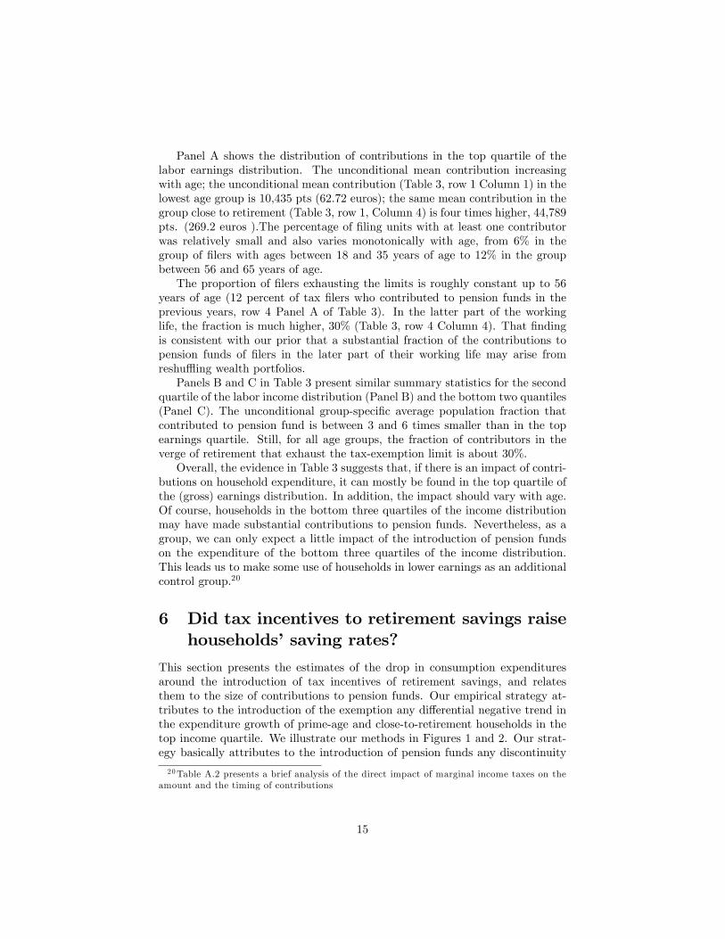
Panel A shows the distribution of contributions in the top quartile of thelabor earnings distribution. The unconditional mean contribution increasingwith age; the unconditional mean contribution (Table 3, row 1 Column 1) in thelowest age group is 10,435 pts (62.72 euros); the same mean contribution in thegroup close to retirement (Table 3, row 1, Column 4) is four times higher, 44,789pts. (269.2 euros ).The percentage of �ling units with at least one contributorwas relatively small and also varies monotonically with age, from 6% in thegroup of �lers with ages between 18 and 35 years of age to 12% in the groupbetween 56 and 65 years of age.The proportion of �lers exhausting the limits is roughly constant up to 56

years of age (12 percent of tax �lers who contributed to pension funds in theprevious years, row 4 Panel A of Table 3). In the latter part of the workinglife, the fraction is much higher, 30% (Table 3, row 4 Column 4). That �ndingis consistent with our prior that a substantial fraction of the contributions topension funds of �lers in the later part of their working life may arise fromreshu­ ing wealth portfolios.Panels B and C in Table 3 present similar summary statistics for the second

quartile of the labor income distribution (Panel B) and the bottom two quantiles(Panel C). The unconditional group-speci�c average population fraction thatcontributed to pension fund is between 3 and 6 times smaller than in the topearnings quartile. Still, for all age groups, the fraction of contributors in theverge of retirement that exhaust the tax-exemption limit is about 30%.Overall, the evidence in Table 3 suggests that, if there is an impact of contri-

butions on household expenditure, it can mostly be found in the top quartile ofthe (gross) earnings distribution. In addition, the impact should vary with age.Of course, households in the bottom three quartiles of the income distributionmay have made substantial contributions to pension funds. Nevertheless, as agroup, we can only expect a little impact of the introduction of pension fundson the expenditure of the bottom three quartiles of the income distribution.This leads us to make some use of households in lower earnings as an additionalcontrol group.20

6 Did tax incentives to retirement savings raisehouseholds�saving rates?

This section presents the estimates of the drop in consumption expendituresaround the introduction of tax incentives of retirement savings, and relatesthem to the size of contributions to pension funds. Our empirical strategy at-tributes to the introduction of the exemption any di¤erential negative trend inthe expenditure growth of prime-age and close-to-retirement households in thetop income quartile. We illustrate our methods in Figures 1 and 2. Our strat-egy basically attributes to the introduction of pension funds any discontinuity

20Table A.2 presents a brief analysis of the direct impact of marginal income taxes on theamount and the timing of contributions

15

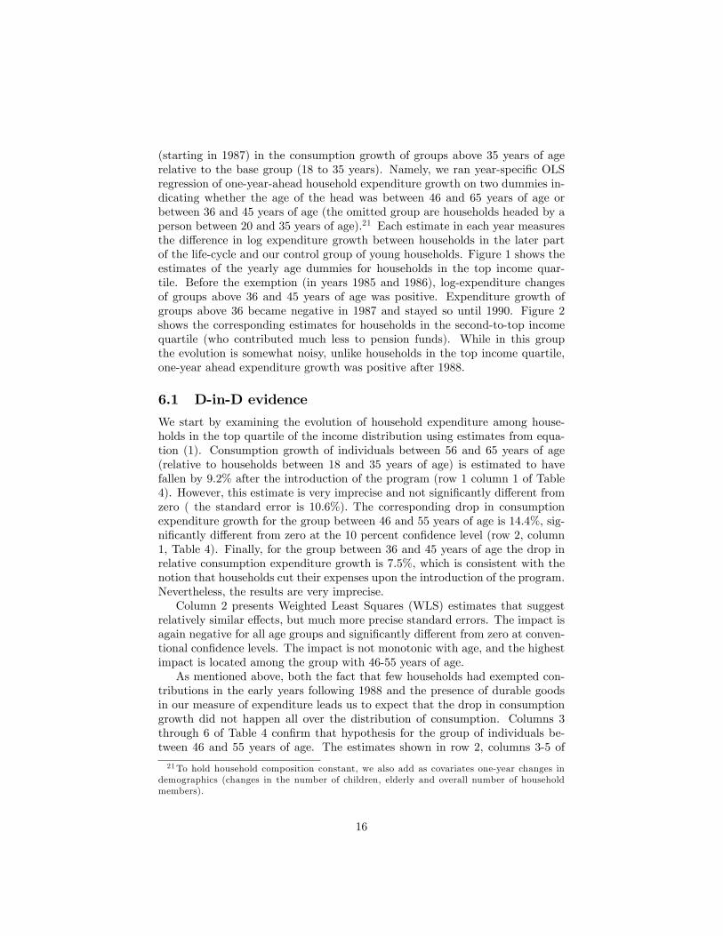
(starting in 1987) in the consumption growth of groups above 35 years of agerelative to the base group (18 to 35 years). Namely, we ran year-speci�c OLSregression of one-year-ahead household expenditure growth on two dummies in-dicating whether the age of the head was between 46 and 65 years of age orbetween 36 and 45 years of age (the omitted group are households headed by aperson between 20 and 35 years of age).21 Each estimate in each year measuresthe di¤erence in log expenditure growth between households in the later partof the life-cycle and our control group of young households. Figure 1 shows theestimates of the yearly age dummies for households in the top income quar-tile. Before the exemption (in years 1985 and 1986), log-expenditure changesof groups above 36 and 45 years of age was positive. Expenditure growth ofgroups above 36 became negative in 1987 and stayed so until 1990. Figure 2shows the corresponding estimates for households in the second-to-top incomequartile (who contributed much less to pension funds). While in this groupthe evolution is somewhat noisy, unlike households in the top income quartile,one-year ahead expenditure growth was positive after 1988.

6.1 D-in-D evidence

We start by examining the evolution of household expenditure among house-holds in the top quartile of the income distribution using estimates from equa-tion (1). Consumption growth of individuals between 56 and 65 years of age(relative to households between 18 and 35 years of age) is estimated to havefallen by 9.2% after the introduction of the program (row 1 column 1 of Table4). However, this estimate is very imprecise and not signi�cantly di¤erent fromzero ( the standard error is 10.6%). The corresponding drop in consumptionexpenditure growth for the group between 46 and 55 years of age is 14.4%, sig-ni�cantly di¤erent from zero at the 10 percent con�dence level (row 2, column1, Table 4). Finally, for the group between 36 and 45 years of age the drop inrelative consumption expenditure growth is 7.5%, which is consistent with thenotion that households cut their expenses upon the introduction of the program.Nevertheless, the results are very imprecise.Column 2 presents Weighted Least Squares (WLS) estimates that suggest

relatively similar e¤ects, but much more precise standard errors. The impact isagain negative for all age groups and signi�cantly di¤erent from zero at conven-tional con�dence levels. The impact is not monotonic with age, and the highestimpact is located among the group with 46-55 years of age.As mentioned above, both the fact that few households had exempted con-

tributions in the early years following 1988 and the presence of durable goodsin our measure of expenditure leads us to expect that the drop in consumptiongrowth did not happen all over the distribution of consumption. Columns 3through 6 of Table 4 con�rm that hypothesis for the group of individuals be-tween 46 and 55 years of age. The estimates shown in row 2, columns 3-5 of

21To hold household composition constant, we also add as covariates one-year changes indemographics (changes in the number of children, elderly and overall number of householdmembers).

16

Table 4 suggest that the drops in consumption growth were driven by a few largechanges: the 75th-centile of the consumption drop was 26 log points (standarderror: .12) and the 90th centile (a drop of .33 log-points, with an standard errorof .17 log-points). Conversely median consumption growth did not change asmuch (19.7 log points, but the standard error is 10.2). In other words, the av-erage drop in expenditure is due to the behavior of a limited set of households.For households close to retirement (56-65), we �nd a constant drop at di¤erentcentiles, a �nding that leads us to suspect that the estimates in row 1, Column1 of Table 4 may re�ect other trends. Finally, for our youngest treatment group(individuals between 36-45 years of age), while the estimates are not signi�-cantly di¤erent from zero, the magnitude of the coe¢ cients also suggests thatthe fall in consumption expenditure growth was concentrated in the very highcentiles (-22 log-points at the 90th centile).Rows 4 through 6 of Table 4 present estimates from a similar speci�cation

to that in Panel A, but for households with incomes between the 50th and the75th centiles. Those households faced lower marginal tax rates on income andcontributed less on average, as documented in Table 3. Thus, if the decreasesin consumption expenditure growth documented in rows 1-3 of Table 4 areindeed due to the introduction of tax incentives of retirement savings, we should�nd lower impact of the introduction of the program on their consumptiongrowth. The point estimates in row 5 (the group between 46 and 55 years ofage) con�rms that prior: the drop in consumption growth oscillates between .033(OLS speci�cation) and .046 (WLS speci�cation) and they are signi�cantly lowerthan in the top quartile of the distribution of earnings. Further, the distributionof the drop in expenditure among the 46-55 age group is very di¤erent from thatin the top income quartile: the drop in consumption growth is not located atthe largest centiles of the distribution of consumption growth, but is basicallyuniform over the distribution.Rows 7 through 9 in Table 4 repeat the analysis now using the change in the

level (rather than logs) of consumption expenditures. The advantage of thatspeci�cation is that one can readily interpret the magnitude of the consumptiondrop and informally compare it to the estimates in Table 3, to see how likely itis that the drop in consumption was indeed due to increases in contributions topension funds. The results in row 8 of Column 2 suggest that average expen-diture among the group with ages between 46 and 55 fell by about 77,000 pts(463 euros) and that the average drop was far from constant, but driven by arelatively small set of households. Note that this average is much higher thanthe excess contribution of the 46-55 group with respect to the base group withages between 20 and 35: (17,000 pts or 102 euros, as it results from substractingColumn 1, row 1 from Column 4, row 1 in Table 3).In rows 10 to 12 of Table 4, we examine the concepts of expenditure that

fall, and run a regression similar to equation (1), but in which the dependentvariable only contains the following set of durable goods: "white" durable goods(purchases of fridges, dishwashers, washing machines... etc), electronic goods(TVs, radios, CD players), cars and furniture. The results in row 11 suggestthat, among the group that most diminished expenditure (46-55 years of age),

17

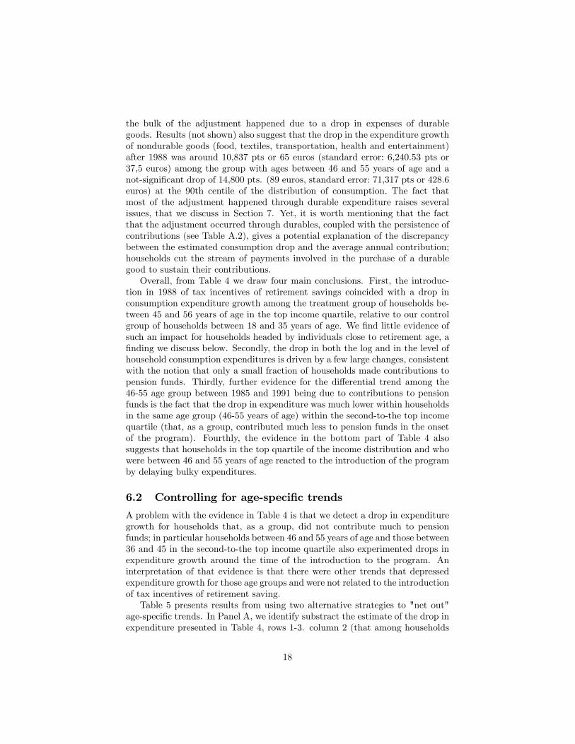
the bulk of the adjustment happened due to a drop in expenses of durablegoods. Results (not shown) also suggest that the drop in the expenditure growthof nondurable goods (food, textiles, transportation, health and entertainment)after 1988 was around 10,837 pts or 65 euros (standard error: 6,240.53 pts or37,5 euros) among the group with ages between 46 and 55 years of age and anot-signi�cant drop of 14,800 pts. (89 euros, standard error: 71,317 pts or 428.6euros) at the 90th centile of the distribution of consumption. The fact thatmost of the adjustment happened through durable expenditure raises severalissues, that we discuss in Section 7. Yet, it is worth mentioning that the factthat the adjustment occurred through durables, coupled with the persistence ofcontributions (see Table A.2), gives a potential explanation of the discrepancybetween the estimated consumption drop and the average annual contribution;households cut the stream of payments involved in the purchase of a durablegood to sustain their contributions.Overall, from Table 4 we draw four main conclusions. First, the introduc-

tion in 1988 of tax incentives of retirement savings coincided with a drop inconsumption expenditure growth among the treatment group of households be-tween 45 and 56 years of age in the top income quartile, relative to our controlgroup of households between 18 and 35 years of age. We �nd little evidence ofsuch an impact for households headed by individuals close to retirement age, a�nding we discuss below. Secondly, the drop in both the log and in the level ofhousehold consumption expenditures is driven by a few large changes, consistentwith the notion that only a small fraction of households made contributions topension funds. Thirdly, further evidence for the di¤erential trend among the46-55 age group between 1985 and 1991 being due to contributions to pensionfunds is the fact that the drop in expenditure was much lower within householdsin the same age group (46-55 years of age) within the second-to-the top incomequartile (that, as a group, contributed much less to pension funds in the onsetof the program). Fourthly, the evidence in the bottom part of Table 4 alsosuggests that households in the top quartile of the income distribution and whowere between 46 and 55 years of age reacted to the introduction of the programby delaying bulky expenditures.

6.2 Controlling for age-speci�c trends

A problem with the evidence in Table 4 is that we detect a drop in expendituregrowth for households that, as a group, did not contribute much to pensionfunds; in particular households between 46 and 55 years of age and those between36 and 45 in the second-to-the top income quartile also experimented drops inexpenditure growth around the time of the introduction to the program. Aninterpretation of that evidence is that there were other trends that depressedexpenditure growth for those age groups and were not related to the introductionof tax incentives of retirement saving.Table 5 presents results from using two alternative strategies to "net out"

age-speci�c trends. In Panel A, we identify substract the estimate of the drop inexpenditure presented in Table 4, rows 1-3. column 2 (that among households

18

in the top quartile of the income distribution) to the corresponding drop inexpenditure reported in Table 4, rows 4-6 column (2). We do this by usingthe triple-di¤erences estimator in (2). We report WLS, and estimates of theexpenditure drop at di¤erent centiles. The estimates are very similar to thosereported in Table 4, rows 1-3, and we do not comment them in detail.Panel B of Table 5 introduces an additional source of identi�cation. Accord-

ing to the theoretical discussion, tax incentives of retirement saving operatethrough the income tax marginal rate. The reason is that households withhigher income tax marginal rates experience a larger increase in the returnto retirement saving and consequently a stronger substitution e¤ect. Hence,we explore if the expenditure drop after the introduction of tax incentives isstronger among households that faced higher income marginal tax rates22 Weestimate the following model again for the top two quartiles of the distributionof earnings.

logCh;q+4 � logCh;q = �0 + �1(Age_i)hPOST88q1(Y:75)mtaxh+�2(Age_i)hPOST88qmtaxh + �3(Age_i)h1(Y:75)

+�4(Age_i)h �mtaxh + �5POST88qmtaxh+�6POST88q1(Y:75) + �7(Age_i)h1(Y:75) + �8(Age_i)h

+ 9POST88q + �101(Y > Y:75) + �11mtaxh

+�18Xit + �h;q+4 � �h;q (5)

where Age_i stands for three age group dummies: 36-45, 46-55 and 56-65.The parameter of interest is �1 that measures the impact of income tax mar-ginal rates on average expenditure drop after the introduction of the exemptionamong households in the top quartile of the income distribution. Model (3)holds constant age-speci�c trends by introducing as a co-variate a triple inter-action between income tax marginal rates, age group and a post 88 dummy andlower level interactions between age, income marginal tax rates and the post 88dummy. If higher income tax marginal rates are associated to larger drops inconsumption growth, we should expect �1 to be negative. The results shown inTable 5, Panel B con�rm that for the group between ages 46 and 55, higher con-sumption drops happened among households with higher income tax marginalrates.

6.3 Other changes correlated with the reform

Table A.3 examines if our key variable that identi�es the incentive to contribute(a di¤erential trend between 1985 and 1990 among di¤erent age groups in thetop quartile of the income distribution) is correlated with other outcomes.

22For each household in the sample, we computed the marginal income tax using the rulesbetween 1985 and 1988, ignoring all capital income (that is, we compute the marginal incometax on the �rst euro of capital income). After 1988, for each household we estimated whetherit was more tax-advantageous to �le separately or jointly and, for those for whom separate�ling was optimal, we imputed to the household the highest marginal income tax of the couple.

19

1) Purchase of a house: Table A.3 shows the evolution of the probabilityof purchasing a house in the ECPF before and after the 1988 reform, by agegroup. We �nd a sizable drop (-1.7 percent, relative to a overall statistic of 2.3percent) in the probability of doing so in our base group, perhaps indicatingthat the drop in expenditure in the 46-55 age group was not con�ned to "small"durables.2) Joint �ling: The introduction of tax incentives of retirement savings in

1988 coincided with a major tax reform that changed compulsory joint �lingto voluntary individual or joint �ling. Such reform is likely to have changedthe income tax marginal rate and the taxable income of households. In otherwords, the 1988 introduction of separate �ling may have a¤ected the expectedpermanent income and consumption of di¤erent age groups. For example, ifjoint �ling was specially prevalent among households headed by our controlgroup (persons between 18 and 36 years of age), the estimates in Model (1)would attribute to tax incentives what really is an income e¤ect associated toa positive shock to labor supply. In principle, we focus on the top incomequartile, that experienced similar tax changes, but there could be a problem ifthe option of separate tax �ling a¤ected di¤erently di¤erent age groups. Wecheck that possibility in Table A.3. Table A.3 Column 2 shows the impact ofour instrument ( a post-1988 dummy) on the probability that a tax �ling unit�les jointly. The group of tax �lers headed by a person between 46 and 55years of age was 3.7% more likely to �le jointly than the base group. Thus, as aconsequence of the tax reform, the 46-55 age group did not experience such anincome increase as the base group. Still, it is not clear to what extent this is aproblem. First, while the estimate is very precise, it is relatively small: less than4% with respect to 64% of �lers who �led jointly in that income group. Secondly,we control for changes in family income in our consumption regressions shownin Table 4, for an indicator of whether both members of the couple work andan interaction of that variable with the post 88 dummy.3) Spouse participation: While the e¤ect estimated is large (8 percent points),

as shown in Column 3 of Table 5, it is also very imprecisely estimated and notsigni�cantly di¤erent from zero. In addition such drop in participation is hardto reconcile with such a tiny impact of our instrument on joint �ling.While we need to work more on the confounding impact of the 1988 separate

tax �ling, it is not that clear that all the impact in Table 4 is driven by suchreform.

7 How much new saving are pension funds gen-erating?

This section combines expenditure data and data from contributions to estimatehow much new saving was generated by the introduction of pension funds.The evidence in Table 4 suggest that the adjustment among the group with

ages between 46 and 55 and in the top income quartile happened through drops

20

in durable consumption expenditures (i.e., households delayed the purchase ofa new car or furniture to contribute to pension funds). By de�nition, the peri-odicity of those expenses exceeds the year, so unadjusted comparisons of annualcontributions to drops in observed expenditure with periodicity over the yearare not informative. The problem would be solved with either a su¢ cientlylong panel of household expenses or with detailed information about the stockof durables. Nevertheless, despite of the fact that the ECPF is one of the longestcomprehensive consumption data sets in Europe, it only follows households forup to 2 years. Furthermore, the ECPF contains little information about wealthstocks.Our strategy is then to use the depreciation rates in Fraumeni (1997) to

distribute among several periods the bulky expenditure in durable goods whenwe observe one such purchase in the data. Namely, whenever we observe thepurchase of a durable good, we attribute to the year of the purchase (and subse-quent periods if the household stays in the sample) the fraction of the purchasethat is depreciated.23 Unfortunately, we can estimate neither the �ow of ser-vices from durables obtained by households who own durables but do not makea transaction during the sample period nor, for households that engage in atransaction, the consumption of the durable goods owned prior to the purchaseof a new good. We suspect that our measure overestimates consumption drops(basically, because we assign a zero to pre-purchase consumption of durablegoods). Summary statistics of those variables are shown in Table 2.Table 6 reruns the results in Table 4, now using our corrected measure of

expenditure. The WLS results in rows 1 through 3 of Table 6 are qualitativelyconsistent with those in Table 4 but the magnitude is of course much lower (forthe 46-55 group, we estimate a drop in our consumption measure of 2.8 percent).For the rest of the groups, we document small and not signi�cantly di¤erent fromzero drops in expenditure, once we distribute expenditures in durables amongperiods. The estimates at di¤erent centiles are now not signi�cantly di¤erentfrom zero at conventional signi�cance levels, but the pattern of the magnitudeof the coe¢ cients is qualitatively similar to that documented in Table 4.The second Panel in Table 6 documents the evolution of the level of peri-

odi�ed expenditure around the introduction of the tax incentives. The averageexpenditure drop in the 46-55 year-old group is about 11,972 pts (78 euros, stan-dard error: 6,717 pts or 40 euros). We �nd positive e¤ects for the age groups of56-65 and 36-45.Columns 2-4 of Table 6 provide an informal assessment of the extent of new

saving by age group within the top quartile of the family earnings distribution.Column 2 presents the drop in consumption estimated in Table 6, Column 1relative to the control group, as estimated in Panel A of Table 6. In Column3, we document the unconditional average contribution by each group minus

23Our procedure amounts to multiplying .165 to the observed total payment for a car, .1179to the cost of furniture, .165 to expenditures in white goods and .1833 for electronic goodslike a TV or a radio. We obtain those estimates from Fraumeni (1997), who in turn obtainsthe estimates from Hulten and Wyko¤ (1995). See Bover (2005) for an application to Spanishdata.

21

the contribution of the control group. The estimates in Column 1 are obtainedsubstracting magnitudes in row 1 of Table 3. For example, the estimated drop inconsumption in the log speci�cation for the 36 to 45 age group, presented in row1 of column 3, and is 7,970 pts (48 euros). On average, that group contributed10,327 pts. (62 euros) to pension funds, yielding an estimate of increased savingof 77 cents per euro contributed. As for the group between 46 and 55 yearsof age, they contributed 19,727 pts (119 euros), and their consumption fell by10,530 pts. (63 euros). In the 46-55 year-old group, 53 cents of new saving werecreated per euro contributed. Possibly the most surprising result is that in row1. The contributions of the group that most actively contributed (top incomequartile, ages between 56 and 65) represented no new saving at all and mostlikely came from portfolio reshu­ ing. In Panel B of Table 7 we present resultsusing consumption drop in levels as the dependent variable.A more formal, but perhaps less informative way of summarizing the degree

of new saving created by the pension funds program is to look at two-sampleTwo Stage Least Squares. Those estimates are presented in Table 7. The �rstcolumn is the �rst-stage equation, that predicts contributions to pension fundsusing the age group of the main �ler at the time of the introduction of taxincentives, and restricting taxpayers to those who were in the top of the incomedistribution that year. The age dummies are signi�cantly di¤erent from zeroat any conventional signi�cance level. The TSLS estimate is presented in thesecond column of Table 7. While extremely imprecise, results suggests thateach additional euro of contributions reduced consumption by 10 cents (also inColumn (3) that gives a weighted least squared version of the TSLS estimation).As we discuss above, those average estimates conceal substantial heterogeneityacross age groups.

8 Concluding Remarks

The identi�cation of the e¤ects of tax incentives of retirement saving is blurredby several dii�culties, such as the wide heterogeneity in the individual responses,the lack of microeconomic data on consumption, saving, and wealth, and thedi¤erential impact that tax incentives may have at the moment when they areintroduced with respect a situation in which they have been operative for along period. In this paper we have examined the e¤ects tax incentives of re-tirement savings in Spain at the period in which they were �rst introduced.Thus, by using data spanning the periods before and after the introduction oftax-favoured retirement plans, we can observe changes in consumption trendsamong di¤erent groups in the population which could be related to contribu-tions to pension funds. For establishing this relationship, we mostly rely onthe fact that individuals with higher income tax marginal rates experiment ahigher wealth e¤ect from the introduction of tax incentives, while we use ageas proxy for income risk and preference for liquid assets, another dimension inwhich retirement savings di¤ers from normal savings.While the overall amount of new saving we estimate is limited (around 10

22

per euro contributed on average), saving responses di¤er substantially across agegroups. In particular, we document very small consumption drops among thegroup of households between 56 and 65 years of age, the group that most activelycontributed to the plan, while we �nd instead a larger decrease in consumptionexpenditures of the group of households between 46 and 55 years of age. In ourview, these results cast doubts about the e¤ectiveness of these tax incentivesto promote retirement savings, specially when compared to the �scal costs thatthey have in terms of lost government revenues.

23

References

[1] Albarrán, P (2004) "The Econometrics of Income Dynamics and RotatingPanels, with an Application to Precautionary Saving�mimeograph, Uni-versidad Carlos III

[2] Angrist, J.D., and A.B. Krueger (1992) "The E¤ect of Age at School En-try on Educational Attainment: An Application of Instrumental Variableswith Moments from Two Samples" Journal of the American Statistical As-sociation Vol. 87, No. 418: 328-336

[3] Attanasio O.P. and A. Brugiavini (2003), Social security and households�saving, Quarterly Journal of Economics,. vol.118, n.3, pag.1075-1120

[4] Attanasio, O. P., J. Banks, and M. Wake�eld (2004): "E¤ectiveness ofTax incentives to Boost (Retirement) Saving: Theoretical Motivation andEmpirical Evidence", OECD Economic Studies, 39, 2. pp. 145-172.

[5] Attanasio, O.P. and T. De Leire (2002): "The E¤ect of Individual Retire-ment Accounts on Household Consumption and National Saving", Eco-nomic Journal, volume 112(6), pages 504-538

[6] Attanasio, O.P. and S. Rohwedder (2003): "Pension Wealth and HouseholdSaving: Evidence from Pension Reforms in the United Kingdom", AmericanEconomic Review, 93:5, pp.1499-1521

[7] Ayuso, J., J.F. Jimeno y E. Villanueva (2007): "Who bene�ts from taxincentives of retirement saving? Cross-sectional evidence from the SpanishSurvey of Household Finances" work in progress

[8] Bernheim, D. (2002) "Taxation and Saving" in Handbook of Public Eco-nomics

[9] Bernheim, D., J. Skinner and S. Weinberg (2001) "What Accounts for theVariation in Retirement Saving Across US Households?" American Eco-nomic Review 91(4): 832-857

[10] Blundell, R., C. Emmerson, and M. Wake�eld (2006): "The Importance ofIncentives in In�uencing Private Retirement Saving: Known Knowns andKnown Unknowns", The Institute for Fiscal Studies, Working Paper 06/09.

[11] Blundell, R. and I. Preston (1998) "Consumption inequality and incomeuncertainty" Quarterly Journal of Economics, 113 603-640

[12] Bover, O. (2005) "Wealth E¤ects on Consumption: Microeconometric Es-timates from the Spanish Survey of Household Finances" Bank of SpainWorking Paper number 0522

[13] Collado, M.D., and M. Browning (forthcoming) "Habits and heterogeneityin demands: a panel data analysis" Journal of Applied Econometrics.

24

[14] Collado, M.D., and M. Browning (2001) "The Response of Expenditures toAnticipated Income Changes: Panel data Estimates", American EconomicReview Vol. 91(3), 681-692

[15] Carrasco, R., J.D. López-Salido, and J.M. Labeaga (2005): "Consumptionand Habits: Evidence from Panel Data", Economic Journal, 115, 144-165,2005

[16] Chernozhukov, V. and C. Hansen (2004) "The impact of 401(k) participa-tion on the wealth distribution: an instrumental quantile regression analy-sis" Review of Economics and Statistics 86(3), pp. 735-51.

[17] Chung, W., R. Disney, C. Emmerson and M. Wake�eld (2006) �PublicPolicy and retirement saving incentives in the UK �mimeo, NottinghamUniversity.

[18] Du�o, E., W. G. Gale, J. Liebman, P. Orszag, and E. Saez (2006) "Savingincentives for low- and medium- income families: Evidence from a �eld ex-periment with H&R Block" Quarterly Journal of Economics 121(4): 1311-1346.

[19] Engen E., and W. Gale (2000) �The E¤ects of 401(k) Plans on HouseholdWealth: Di¤erences Across Earnings Groups�NBER Working Paper no.8032 Cambridge, Mass.

[20] Engen, E. M., W. G. Gale, and J. K. Scholz (1996): "The Illusory E¤ects ofSaving Incentives on Saving", The Journal of Economic Perspectives, Vol.10. No. 4 (Autumn, 1996), pp. 113-138.

[21] Fraumeni, B. (1997) "The Measurement of Depreciation in teh US NationalIncome and Product Accounts" Survey of Current Business July. 7-23

[22] Gale, W.G., and J.K. Scholz (1994): "IRAs and Household Saving", Amer-ican Economic Review, 84:5, pp. 1233-1260.

[23] Hawksworth, J. (2006): "Review of research relevant to assessing the impactof the proposed National Pension Savings Scheme on household savings",Department for Work and Pensions, Research Report No 373.

[24] Hubbard, R. G. and J. S. Skinner (1996): "Assessing the E¤ectiveness ofSaving Incentives", The Journal of Economic Perspectives, Vol. 10. No. 4(Autumn, 1996), pp. 73-90.

[25] Hulten, C.R. and F.C. Wyko¤ (1995) "Introductory Remarks: Issues inthe Measurement of Economic Depreciation " Economic Inquiry January10-23.

[26] Jappelli, T. and L. Pistaferri (2002) �Tax Incentives and the Demand forLife Insurance: Evidence from Italy� Journal of Public Economics, July2003, vol. 87, 1779-99.

25

[27] López Murphy, P. and A. R. Musalem (2004): "Pension Funds and NationalSaving", mimeo.

[28] Milligan, K. (2002) "Tax-preferred Savings Accounts and Marginal TaxRates: Evidence on RRSP Participation," Canadian Journal of EconomicsVol. 35 (August, 2002), pp. 436-456

[29] Poterba J. M., S. F. Venti, and D. A. Wise (1995): "Do 401(k) contributionscrowd out other personal saving?", Journal of Public Economics, 58, pp.1-32.

[30] Poterba J. M., S. F. Venti, and D. A. Wise (1996): "How Retirement SavingPrograms Increase Saving", The Journal of Economic Perspectives, Vol. 10.No. 4 (Autumn, 1996), pp. 91-112.

[31] Veall, M. (2001) �Did tax �attening a¤ect RRSP contributions?�, CanadianJournal of Economics, 2001, vol. 34, issue 1, pages 120-131.

26

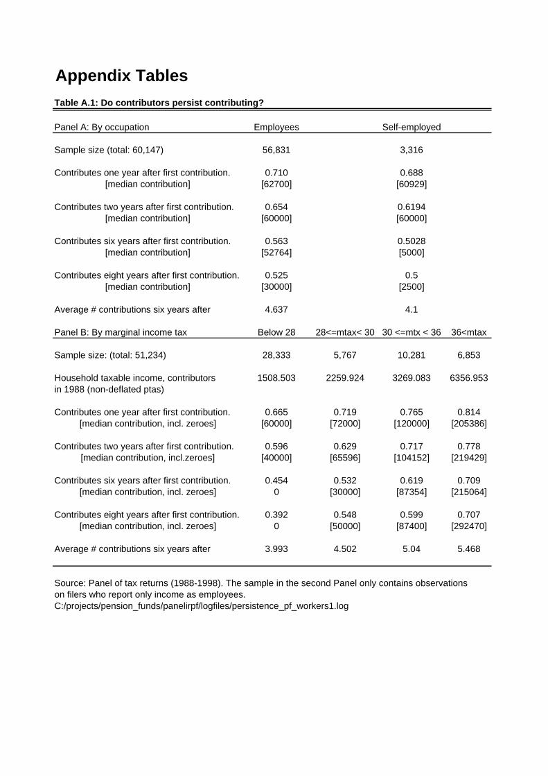
Appendix TablesTable A.1: Do contributors persist contributing?

Panel A: By occupation Employees Self-employed

Sample size (total: 60,147) 56,831 3,316

Contributes one year after first contribution. 0.710 0.688 [median contribution] [62700] [60929]

Contributes two years after first contribution. 0.654 0.6194 [median contribution] [60000] [60000]

Contributes six years after first contribution. 0.563 0.5028 [median contribution] [52764] [5000]

Contributes eight years after first contribution. 0.525 0.5 [median contribution] [30000] [2500]

Average # contributions six years after 4.637 4.1

Panel B: By marginal income tax Below 28 28<=mtax< 30 30 <=mtx < 36 36<mtax

Sample size: (total: 51,234) 28,333 5,767 10,281 6,853

Household taxable income, contributors 1508.503 2259.924 3269.083 6356.953in 1988 (non-deflated ptas)

Contributes one year after first contribution. 0.665 0.719 0.765 0.814 [median contribution, incl. zeroes] [60000] [72000] [120000] [205386]

Contributes two years after first contribution. 0.596 0.629 0.717 0.778 [median contribution, incl.zeroes] [40000] [65596] [104152] [219429]

Contributes six years after first contribution. 0.454 0.532 0.619 0.709 [median contribution, incl. zeroes] 0 [30000] [87354] [215064]

Contributes eight years after first contribution. 0.392 0.548 0.599 0.707 [median contribution, incl. zeroes] 0 [50000] [87400] [292470]

Average # contributions six years after 3.993 4.502 5.04 5.468

Source: Panel of tax returns (1988-1998). The sample in the second Panel only contains observations on filers who report only income as employees.C:/projects/pension_funds/panelirpf/logfiles/persistence_pf_workers1.log

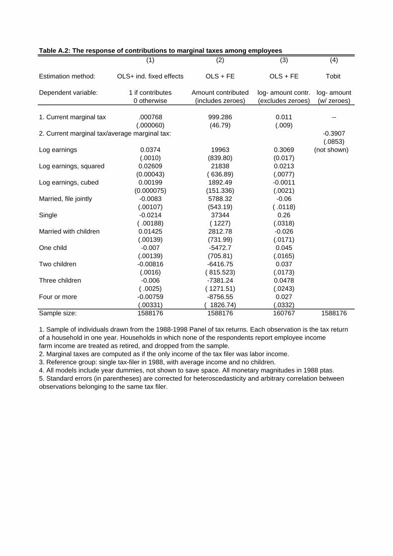
Table A.2: The response of contributions to marginal taxes among employees(1) (2) (3) (4)

Estimation method: OLS+ ind. fixed effects OLS + FE OLS + FE Tobit

Dependent variable: 1 if contributes Amount contributed log- amount contr. log- amount0 otherwise (includes zeroes) (excludes zeroes) (w/ zeroes)

1. Current marginal tax .000768 999.286 0.011 --(.000060) (46.79) (.009)

2. Current marginal tax/average marginal tax: -0.3907(.0853)

Log earnings 0.0374 19963 0.3069 (not shown)(.0010) (839.80) (0.017)

Log earnings, squared 0.02609 21838 0.0213(0.00043) ( 636.89) (.0077)

Log earnings, cubed 0.00199 1892.49 -0.0011(0.000075) (151.336) (.0021)

Married, file jointly -0.0083 5788.32 -0.06(.00107) (543.19) ( .0118)

Single -0.0214 37344 0.26( .00188) ( 1227) (.0318)

Married with children 0.01425 2812.78 -0.026(.00139) (731.99) (.0171)

One child -0.007 -5472.7 0.045(.00139) (705.81) (.0165)

Two children -0.00816 -6416.75 0.037(.0016) ( 815.523) (.0173)

Three children -0.006 -7381.24 0.0478( .0025) ( 1271.51) (.0243)

Four or more -0.00759 -8756.55 0.027(.00331) ( 1826.74) (.0332)

Sample size: 1588176 1588176 160767 1588176

1. Sample of individuals drawn from the 1988-1998 Panel of tax returns. Each observation is the tax return of a household in one year. Households in which none of the respondents report employee incomefarm income are treated as retired, and dropped from the sample.2. Marginal taxes are computed as if the only income of the tax filer was labor income.3. Reference group: single tax-filer in 1988, with average income and no children.4. All models include year dummies, not shown to save space. All monetary magnitudes in 1988 ptas.5. Standard errors (in parentheses) are corrected for heteroscedasticity and arbitrary correlation betweenobservations belonging to the same tax filer.

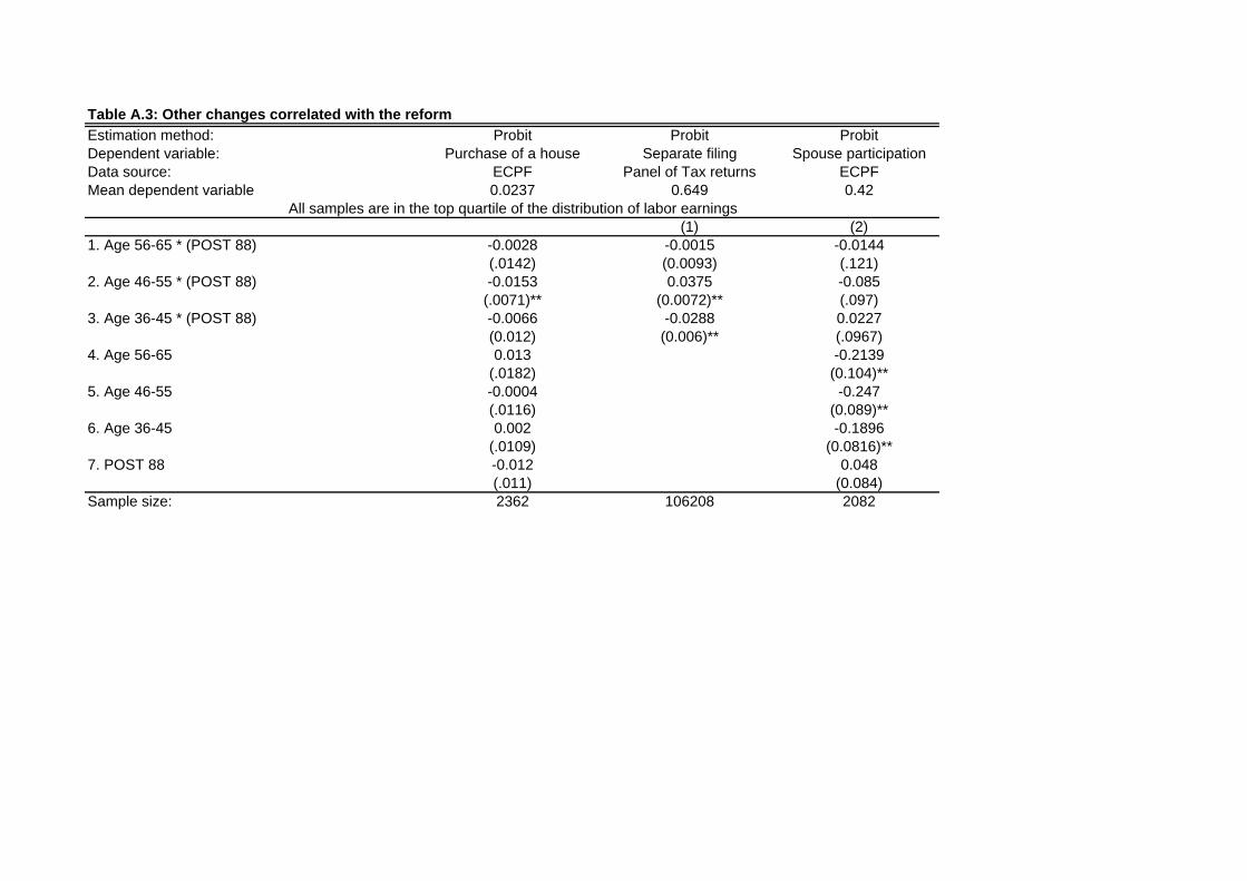
Table A.3: Other changes correlated with the reformEstimation method: Probit Probit ProbitDependent variable: Purchase of a house Separate filing Spouse participationData source: ECPF Panel of Tax returns ECPFMean dependent variable 0.0237 0.649 0.42

(1) (2)1. Age 56-65 * (POST 88) -0.0028 -0.0015 -0.0144

(.0142) (0.0093) (.121)2. Age 46-55 * (POST 88) -0.0153 0.0375 -0.085

(.0071)** (0.0072)** (.097)3. Age 36-45 * (POST 88) -0.0066 -0.0288 0.0227

(0.012) (0.006)** (.0967)4. Age 56-65 0.013 -0.2139

(.0182) (0.104)**5. Age 46-55 -0.0004 -0.247

(.0116) (0.089)**6. Age 36-45 0.002 -0.1896

(.0109) (0.0816)**7. POST 88 -0.012 0.048

(.011) (0.084)Sample size: 2362 106208 2082

All samples are in the top quartile of the distribution of labor earnings

Tables and FiguresTable 1: Summary statistics of Panel of Tax Returns.

Panel A: The incidence of contributions to "pension funds" and amounts.

Year 1 if contributes Mean (if nonzero) Median (if nonzero) 10th perc. 90th perc.1988 0.024 221.874 126.203 22.707 5001989 0.036 198.689 112.704 21.132 469.6021990 0.053 186.099 105.642 23.376 445.4361991 0.073 194.961 101.102 24.756 507.4871992 0.107 173.765 93.376 14.242 440.2161993 0.128 179.449 94.874 15.069 464.8891994 0.138 175.005 85.303 14.128 472.0991995 0.162 187.642 93.579 13.562 508.581996 0.172 185.718 91.05 14.69 489.6581997 0.210 185.344 93.074 15.751 479.5551998 0.246 197.66 94.628 16.41 524.027

Panel B: Characteristics of 1988-1991 sample

Mean Std. Dev. Min. Max.

Contribution to pension funds 10.927 66.799 0 750

Fraction who contribute 0.0535 0.225 0 1

Contribution/gross earnings 0.063 0.072 0.001 0.4(if positive)

Household taxable income 2319.635 1.691 614.875 168.000

4-quarter change, yearly income 147.765 615.618 -43.8 77500

Family size 3.374 1.13 2 12(excluding adults above 18 years)Age 41.25 11.06 20 65

Sample size: 1225311. All monetary magnitudes in 1000s of 1987 pta.2. Sample used in Panel A: 1988-1998 Panel of Tax returns. We only include contributions made by tax units with a filer between 18 and 65 years of age that do not report self-employed incomeContributions include both employer and individual contributions, and are aggregated at the level of 1987fiscal unit (In 1987 couples had to file income taxes jointly) 3. Sample used in Panel B: All filers between 18 and 65 years who do not report self-employment orprofessional income, between 1988 and 1991. Contributions include those made by the employer, and are aggregated at the level of the 1987 fiscal unit.

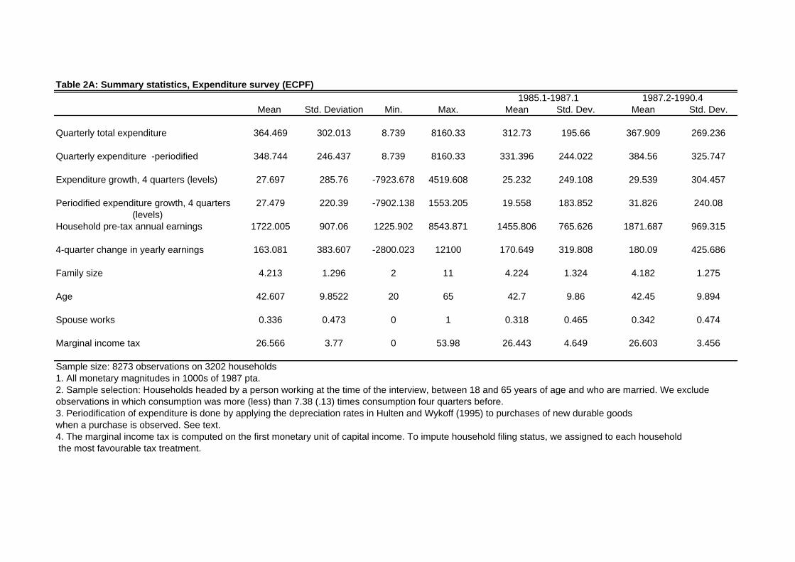
Table 2A: Summary statistics, Expenditure survey (ECPF)

Mean Std. Deviation Min. Max. Mean Std. Dev. Mean Std. Dev.

Quarterly total expenditure 364.469 302.013 8.739 8160.33 312.73 195.66 367.909 269.236

Quarterly expenditure -periodified 348.744 246.437 8.739 8160.33 331.396 244.022 384.56 325.747

Expenditure growth, 4 quarters (levels) 27.697 285.76 -7923.678 4519.608 25.232 249.108 29.539 304.457

Periodified expenditure growth, 4 quarters 27.479 220.39 -7902.138 1553.205 19.558 183.852 31.826 240.08(levels)

Household pre-tax annual earnings 1722.005 907.06 1225.902 8543.871 1455.806 765.626 1871.687 969.315

4-quarter change in yearly earnings 163.081 383.607 -2800.023 12100 170.649 319.808 180.09 425.686

Family size 4.213 1.296 2 11 4.224 1.324 4.182 1.275

Age 42.607 9.8522 20 65 42.7 9.86 42.45 9.894

Spouse works 0.336 0.473 0 1 0.318 0.465 0.342 0.474

Marginal income tax 26.566 3.77 0 53.98 26.443 4.649 26.603 3.456

Sample size: 8273 observations on 3202 households1. All monetary magnitudes in 1000s of 1987 pta.2. Sample selection: Households headed by a person working at the time of the interview, between 18 and 65 years of age and who are married. We excludeobservations in which consumption was more (less) than 7.38 (.13) times consumption four quarters before.3. Periodification of expenditure is done by applying the depreciation rates in Hulten and Wykoff (1995) to purchases of new durable goodswhen a purchase is observed. See text.4. The marginal income tax is computed on the first monetary unit of capital income. To impute household filing status, we assigned to each household the most favourable tax treatment.

1985.1-1987.1 1987.2-1990.4

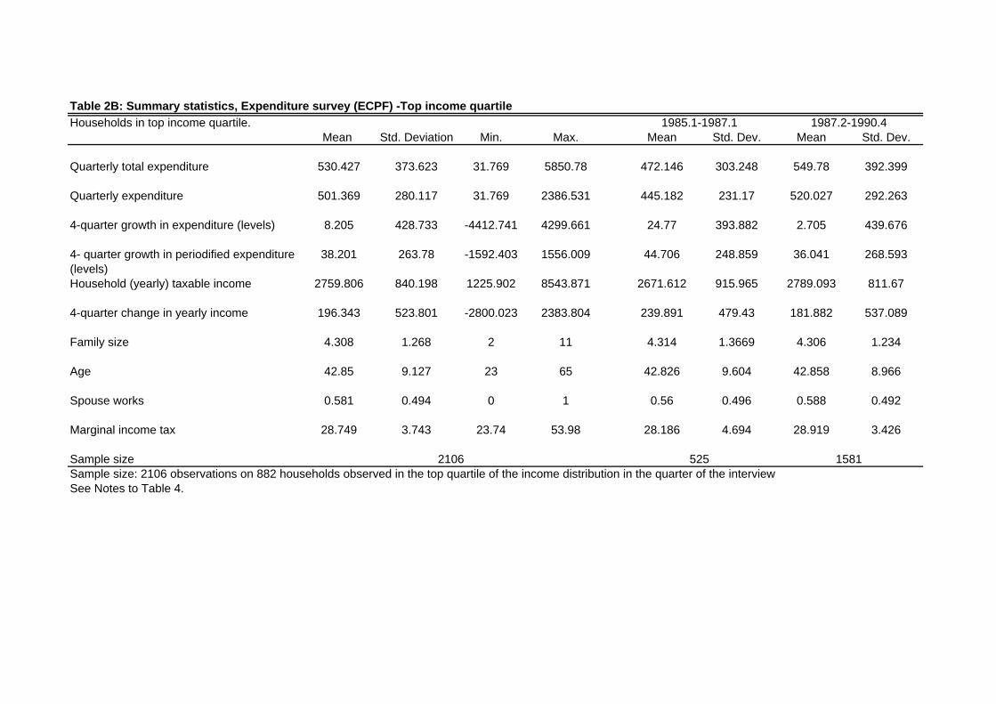
Table 2B: Summary statistics, Expenditure survey (ECPF) -Top income quartileHouseholds in top income quartile.

Mean Std. Deviation Min. Max. Mean Std. Dev. Mean Std. Dev.

Quarterly total expenditure 530.427 373.623 31.769 5850.78 472.146 303.248 549.78 392.399

Quarterly expenditure 501.369 280.117 31.769 2386.531 445.182 231.17 520.027 292.263

4-quarter growth in expenditure (levels) 8.205 428.733 -4412.741 4299.661 24.77 393.882 2.705 439.676

4- quarter growth in periodified expenditure 38.201 263.78 -1592.403 1556.009 44.706 248.859 36.041 268.593(levels)Household (yearly) taxable income 2759.806 840.198 1225.902 8543.871 2671.612 915.965 2789.093 811.67

4-quarter change in yearly income 196.343 523.801 -2800.023 2383.804 239.891 479.43 181.882 537.089

Family size 4.308 1.268 2 11 4.314 1.3669 4.306 1.234

Age 42.85 9.127 23 65 42.826 9.604 42.858 8.966

Spouse works 0.581 0.494 0 1 0.56 0.496 0.588 0.492

Marginal income tax 28.749 3.743 23.74 53.98 28.186 4.694 28.919 3.426

Sample size Sample size: 2106 observations on 882 households observed in the top quartile of the income distribution in the quarter of the interviewSee Notes to Table 4.

2106

1985.1-1987.1 1987.2-1990.4

525 1581

Table 3: Contribution to pension funds by age and income group, 1988-1991Panel A: Gross annual labor earnings in the top quantile of the ECPF.

(1) (2) (3) (4)Age 18-35 Age 36-45 Age 46-55 Age 56-65

1. Amount contributed (includes 0s) 10.435 20.762 30.162 44.7892. Percentage households that contribute 0.061 0.0919 0.1153 0.1213. Contribution/taxable income (if positive) 0.068 0.0647 0.071 0.1064. Exhausts limit? 0.122 0.122 0.142 0.305

Sample size [48027] [40325] [22241] [11938]Marginal income tax

Panel B: Gross annual labor earnings in the second quartile in the ECPF.

Age 18-35 Age 36-45 Age 46-55 Age 56-655. Amount contributed 2.964 4.770 6.734 9.8586. Percent contrib. 0.0314 0.041 0.047 0.0477. Contribution/income (if positive) 0.054 0.0971 0.079 0.1158. Exhausts limit? 0.084 0.105 0.1356 0.268

Sample size [34540] [17291] [12190] [9471]Marginal income tax

Panel C: Gross annual labor earnings in the bottom half of the ECPF.

Age 18-35 Age 36-45 Age 46-55 Age 56-659. Amount contributed 1.106 4.770 3.375 4.19810. Percent contrib. 0.014 0.0246 0.027 0.02211. Contribution/income (if positive) 0.076 0.0971 0.198 0.13412. Exhausts limit? 0.12 0.105 0.197 0.317

Sample size [86799] [26861] [12190] [9471]Source: 1988-1991 Panel of Income Tax Returns, sample of households where main filer is an employee. All magnitudes in 1000s ptas of 19871. Each tax filing unit in 1987 (a period of compulsory joint tax filing by couples) contributes an observation per year, regardless of filing mode.2. Sample partitions were done according to the pre-tax family earnings centiles in the ECPF.3. Labor earnings are the sum of gross earnings (including tax withholdings and social security contributions) declared by the filing unit if the original tax unit in 1988 continues to file jointly and of the tax reports of the spouses in the case of separate filings.

33.4

26.56

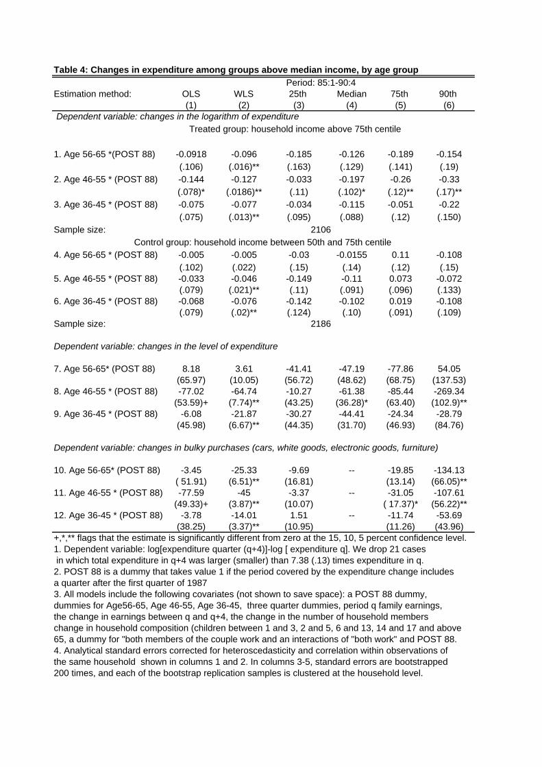
Table 4: Changes in expenditure among groups above median income, by age group

Estimation method: OLS WLS 25th Median 75th 90th (1) (2) (3) (4) (5) (6)

1. Age 56-65 *(POST 88) -0.0918 -0.096 -0.185 -0.126 -0.189 -0.154(.106) (.016)** (.163) (.129) (.141) (.19)

2. Age 46-55 * (POST 88) -0.144 -0.127 -0.033 -0.197 -0.26 -0.33(.078)* (.0186)** (.11) (.102)* (.12)** (.17)**

3. Age 36-45 * (POST 88) -0.075 -0.077 -0.034 -0.115 -0.051 -0.22(.075) (.013)** (.095) (.088) (.12) (.150)

Sample size:

4. Age 56-65 * (POST 88) -0.005 -0.005 -0.03 -0.0155 0.11 -0.108(.102) (.022) (.15) (.14) (.12) (.15)

5. Age 46-55 * (POST 88) -0.033 -0.046 -0.149 -0.11 0.073 -0.072(.079) (.021)** (.11) (.091) (.096) (.133)

6. Age 36-45 * (POST 88) -0.068 -0.076 -0.142 -0.102 0.019 -0.108(.079) (.02)** (.124) (.10) (.091) (.109)

Sample size:

Dependent variable: changes in the level of expenditure

7. Age 56-65* (POST 88) 8.18 3.61 -41.41 -47.19 -77.86 54.05(65.97) (10.05) (56.72) (48.62) (68.75) (137.53)

8. Age 46-55 * (POST 88) -77.02 -64.74 -10.27 -61.38 -85.44 -269.34(53.59)+ (7.74)** (43.25) (36.28)* (63.40) (102.9)**

9. Age 36-45 * (POST 88) -6.08 -21.87 -30.27 -44.41 -24.34 -28.79(45.98) (6.67)** (44.35) (31.70) (46.93) (84.76)

Dependent variable: changes in bulky purchases (cars, white goods, electronic goods, furniture)

10. Age 56-65* (POST 88) -3.45 -25.33 -9.69 -- -19.85 -134.13( 51.91) (6.51)** (16.81) (13.14) (66.05)**

11. Age 46-55 * (POST 88) -77.59 -45 -3.37 -- -31.05 -107.61(49.33)+ (3.87)** (10.07) ( 17.37)* (56.22)**

12. Age 36-45 * (POST 88) -3.78 -14.01 1.51 -- -11.74 -53.69(38.25) (3.37)** (10.95) (11.26) (43.96)

+,*,** flags that the estimate is significantly different from zero at the 15, 10, 5 percent confidence level.1. Dependent variable: log[expenditure quarter (q+4)]-log [ expenditure q]. We drop 21 cases in which total expenditure in q+4 was larger (smaller) than 7.38 (.13) times expenditure in q. 2. POST 88 is a dummy that takes value 1 if the period covered by the expenditure change includesa quarter after the first quarter of 19873. All models include the following covariates (not shown to save space): a POST 88 dummy,dummies for Age56-65, Age 46-55, Age 36-45, three quarter dummies, period q family earnings,the change in earnings between q and q+4, the change in the number of household memberschange in household composition (children between 1 and 3, 2 and 5, 6 and 13, 14 and 17 and above65, a dummy for "both members of the couple work and an interactions of "both work" and POST 88.4. Analytical standard errors corrected for heteroscedasticity and correlation within observations ofthe same household shown in columns 1 and 2. In columns 3-5, standard errors are bootstrapped200 times, and each of the bootstrap replication samples is clustered at the household level.

2186

Control group: household income between 50th and 75th centile

Treated group: household income above 75th centile

Period: 85:1-90:4

Dependent variable: changes in the logarithm of expenditure

2106

Table 5: The impact of exemption on expenditure growth, accounting for age-specific trends

Panel A: Using dummies WLS 25th Median 75th 90th

1. Age 56-65 * (POST 88) * (Y>y.75) -.081 -.011 -.112 -.195 -.055(.029)** (.206) (.178) (.185) (.23)

2. Age 46-55 * (POST 88) * (Y>y.75) -.108 .144 -.099 -.232 -.347(.024)** (.148) (.139) (.150)+ (.204)*

3. Age 36-45 * (POST 88) * (Y>y.75) 0.0199 .214 .053 .0315 -.11(.024) (.153) (.133) (.147) (.186)

4. Age 56-65 * (POST 88) -.003(.023) (not shown)

5. Age 46-55 * (POST 88) -0.033(.0184)*

6. Age 36-45 * (POST 88) -0.091(.020)

(Additional regressors listed in footnotes, but not shown)

Panel B: Using marginal income taxes

4. Age 56-65 * (POST 88) * (Y>y.75) * MTAX -0.05 .328 -.17 -.38(.071) (.73) (.71) (.77)

5. Age 46-55 * (POST 88) * (Y>y.75) * MTAX -.314 .524 -.20 -.81(.065)** (.54) (.52) (.53)

6. Age 36-45 * (POST 88) * (Y>y.75) * MTAX .115 .678 .41 -.005(.075) (.57) (.49) (.53)

7. Age 56-65 * (POST 88) * MTAX -.23(.055) (not shown)

8. Age 46-55 * (POST 88) * MTAX -.14(.04)**

9. Age 36-45 * (POST 88) * MTAX -.37(.06)**

(Additional regressors listed in footnotes, but not shown)

1. y.75 denotes the 75th centile of the distribution of family earnings, computed each ECPF survey year2. Additional regressors in Panel A: Dummies for each age grgoup, a post 88 dummy, a dummy of earnings above the the 75th centile", interactions between "income over the over 75th centile" and each age group, interaction between post 88 and the "income above 75th" dummy. In addition,we include the same set of covariates listed at the bottom of Table 43. Additional set of regressors in Panel B: the marginal income tax, a dummy for post 88, dummies for each age group, interactions between MTAX and post 88, interactions between MTAX and age groupdummies and the same set of covariates listed at the bottom of Table 4.

Impact at different centiles

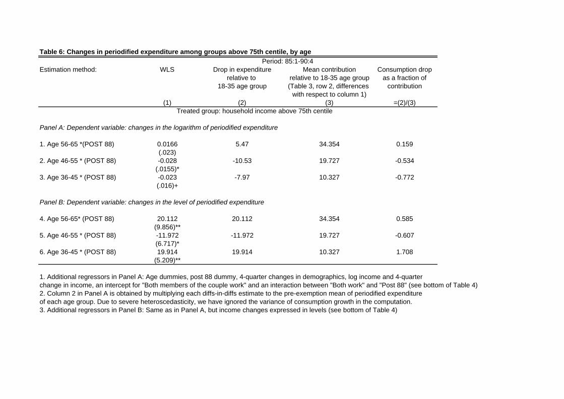
Table 6: Changes in periodified expenditure among groups above 75th centile, by age

Estimation method: WLS Drop in expenditure Mean contribution Consumption droprelative to relative to 18-35 age group as a fraction of

18-35 age group (Table 3, row 2, differences contributionwith respect to column 1)

(1) (2) (3) =(2)/(3)

1. Age 56-65 *(POST 88) 0.0166 5.47 34.354 0.159(.023)

2. Age 46-55 * (POST 88) -0.028 -10.53 19.727 -0.534(.0155)*

3. Age 36-45 * (POST 88) -0.023 -7.97 10.327 -0.772(.016)+

Panel B: Dependent variable: changes in the level of periodified expenditure

4. Age 56-65* (POST 88) 20.112 20.112 34.354 0.585(9.856)**

5. Age 46-55 * (POST 88) -11.972 -11.972 19.727 -0.607(6.717)*

6. Age 36-45 * (POST 88) 19.914 19.914 10.327 1.708(5.209)**

1. Additional regressors in Panel A: Age dummies, post 88 dummy, 4-quarter changes in demographics, log income and 4-quarter change in income, an intercept for "Both members of the couple work" and an interaction between "Both work" and "Post 88" (see bottom of Table 4)2. Column 2 in Panel A is obtained by multiplying each diffs-in-diffs estimate to the pre-exemption mean of periodified expenditureof each age group. Due to severe heteroscedasticity, we have ignored the variance of consumption growth in the computation.3. Additional regressors in Panel B: Same as in Panel A, but income changes expressed in levels (see bottom of Table 4)

Period: 85:1-90:4

Treated group: household income above 75th centile

Panel A: Dependent variable: changes in the logarithm of periodified expenditure

Table 7: TSLS estimates of new savingFirst-stage equation Weighted TSLS First-stage equation Weighted TSLS

Dependent variable: Contributions Consumption drop Contributions Consumption drop(1) (3) (4) (5)

1. Contributed amount -- 0.108 -- -0.098(.276) (.168)

1. Age 56-65*POST 88 30.749 28.249(2.279)** (2.27)**

2. Age 46-55*POST 88 20.173 14.998(1.370)** (1.259)**

3. Age 36-45*POST 88 11.518 4.491(.979)** (1.084)**

4. Earnings 0.01(.001)

Notes to Table 7: other covariates (not shown) listed at the bottom of Table 4

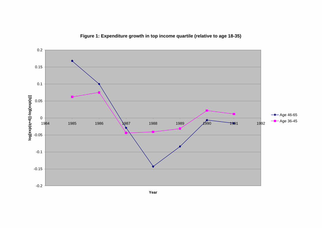
Figure 1: Expenditure growth in top income quartile (relative to age 18-35)

-0.2

-0.15

-0.1

-0.05

0

0.05

0.1

0.15

0.2

1984 1985 1986 1987 1988 1989 1990 1991 1992

Year

log[

exp(

q+4)

]-log

[exp

(q)]

Age 46-65Age 36-45

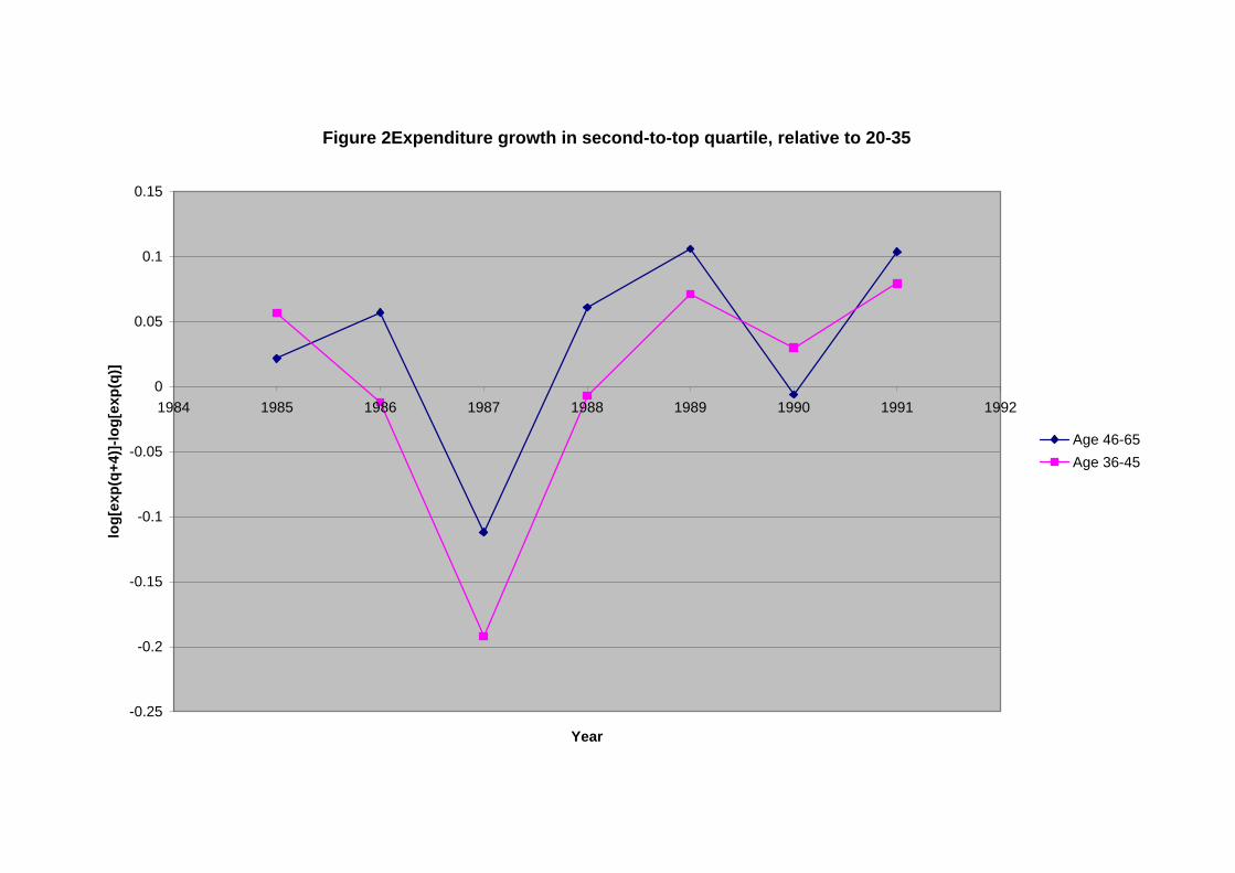
Figure 2Expenditure growth in second-to-top quartile, relative to 20-35

-0.25

-0.2

-0.15

-0.1

-0.05

0

0.05

0.1

0.15

1984 1985 1986 1987 1988 1989 1990 1991 1992

Year

log[

exp(

q+4)

]-log

[exp

(q)]

Age 46-65Age 36-45