The eagle simulations of galaxy formation

Astronomy and Computing 15 (2016) 72–89

Contents lists available at ScienceDirect

Astronomy and Computing

journal homepage: www.elsevier.com/locate/ascom

Full length article

The eagle simulations of galaxy formation: Public release of halo andgalaxy cataloguesI

S. McAlpine a,⇤, J.C. Helly a, M. Schaller a, J.W. Trayford a, Y. Qua, M. Furlonga, R.G. Bower a,R.A. Crainb, J. Schaye c, T. Theuns a, C. Dalla Vecchia d,e, C.S. Frenka, I.G. McCarthyb,A. Jenkins a, Y. Rosas-Guevara f, S.D.M. White g, M. Baesh, P. Campsh, G. Lemson i

a Institute for Computational Cosmology, Department of Physics, University of Durham, South Road, Durham, DH1 3LE, UKb Astrophysics Research Institute, Liverpool John Moores University, 146 Brownlow Hill, Liverpool L3 5RF, UKc Leiden Observatory, Leiden University, P.O. Box 9513, 2300 RA Leiden, The Netherlandsd Instituto de Astrofísica de Canarias, C/ Vía Láctea s/n, 38205 La Laguna, Tenerife, Spaine Departamento de Astrofísica, Universidad de La Laguna, Av. del Astrofísico Francisco Sánchez s/n, 38206 La Laguna, Tenerife, Spainf Departamento de Astronomía, Universidad de Chile, Casilla 36-D, Las Condes, Santiago, Chileg Max-Planck-Institut fur Astrophysik, Karl-Schwarzschild-Str. 1, D-85748 Garching, Germanyh Sterrenkundig Observatorium, Universiteit Gent, Krijgslaan 281, B-9000 Gent, Belgiumi Department of Physics & Astronomy, Johns Hopkins University, Baltimore, MD, 21218, USA

a r t i c l e i n f o

Article history:Received 5 October 2015Accepted 25 February 2016Available online 17 March 2016

Keywords:Cosmology: theoryGalaxies: formationGalaxies: evolutionMethod: numerical

a b s t r a c t

We present the public data release of halo and galaxy catalogues extracted from the eagle suite ofcosmological hydrodynamical simulations of galaxy formation. These simulations were performed withan enhanced version of the gadget code that includes amodified hydrodynamics solver, time-step limiterand subgrid treatments of baryonic physics, such as stellar mass loss, element-by-element radiativecooling, star formation and feedback from star formation and black hole accretion. The simulationsuite includes runs performed in volumes ranging from 25 to 100 comoving megaparsecs per side,with numerical resolution chosen to marginally resolve the Jeans mass of the gas at the star formationthreshold. The free parameters of the subgrid models for feedback are calibrated to the redshift z = 0galaxy stellar mass function, galaxy sizes and black hole mass–stellar mass relation. The simulations havebeen shown to match a wide range of observations for present-day and higher-redshift galaxies. The rawparticle data have been used to link galaxies across redshifts by creatingmerger trees. The indexing of thetree produces a simple way to connect a galaxy at one redshift to its progenitors at higher redshift andto identify its descendants at lower redshift. In this paper we present a relational database which we aremaking available for general use. A large number of properties of haloes and galaxies and their mergertrees are stored in the database, including stellar masses, star formation rates, metallicities, photometricmeasurements andmock gri images. Complex queries can be created to explore the evolution ofmore than105 galaxies, examples of which are provided in the Appendix. The relatively good and broad agreementof the simulations with a wide range of observational datasets makes the database an ideal resource forthe analysis of model galaxies through time, and for connecting and interpreting observational datasets.

© 2016 Elsevier B.V. All rights reserved.

1. Introduction

Galaxy formation is a complex, non-linear process that involvesa wide range of physical and astrophysical phenomena, from the

I http://www.eaglesim.org/database.php.⇤ Corresponding author.E-mail addresses: [email protected] (S. McAlpine),

[email protected] (J.C. Helly), [email protected] (M. Schaller).

evolution of dark matter clustering to intricate feedback effectscoupling gas cooling and outflows to star and black hole formation.Theoretical studies of galaxy formation thus require rigorousdetailed modelling to link together these phenomena over a verywide range of scales. Two techniques have been developed forthis purpose: semianalytic modelling (White and Frenk, 1991)and hydrodynamical simulations (Carlberg et al., 1990; Katz et al.,1992). Both techniques have been extensively developed over thepast 25 years (e.g. Porter et al., 2014; Henriques et al., 2015; Lacey

http://dx.doi.org/10.1016/j.ascom.2016.02.0042213-1337/© 2016 Elsevier B.V. All rights reserved.

http://dx.doi.org/10.1016/j.ascom.2016.02.004

http://www.elsevier.com/locate/ascom

http://www.elsevier.com/locate/ascom

http://crossmark.crossref.org/dialog/?doi=10.1016/j.ascom.2016.02.004&domain=pdf

http://www.eaglesim.org/database.php

mailto:[email protected]




S. McAlpine et al. / Astronomy and Computing 15 (2016) 72–89 73

et al., 2015, for semi-analytic models) and (e.g. Oppenheimer et al.,2010; Puchwein and Springel, 2013; Dubois et al., 2014; Okamotoet al., 2014; Vogelsberger et al., 2014; Khandai et al., 2015, forhydrodynamical simulations).

Recently, the Virgo1 Consortium’s ‘‘Evolution and Assemblyof GaLaxies and their Environments’’ simulation suite (eagle,Schaye et al., 2015; Crain et al., 2015) has been able to reproducekey observational datasets, such as the present-day stellar massfunction of galaxies, the correlation of black hole mass andstellar mass and the dependence of galaxy sizes on stellarmass, with unprecedented fidelity. As well as reproducing theseobservations, which were used during the calibration of thesimulation parameters, the simulation outputs match many otherproperties of the observed galaxy population and the intergalacticmedium both at the present day and at earlier epochs, as we brieflydiscuss below. These simulations therefore provide a powerfulresource for understanding the formation of galaxies and forlinking and interpreting observational datasets.

The aim of this paper is to introduce and make availablea relational database that can be queried using the StructuredQuery Language (sql) to explore and exploit the halo and galaxycatalogues of the main eagle simulations. Columns containingintegrated quantities describing the galaxies, such as stellar mass,star formation rates, metallicities and luminosities, are providedfor more than 105 simulated galaxies and these can be individuallyfollowed through their evolution across cosmic time. This databaseis available at the address http://www.eaglesim.org/database.php.

The simulations follow the gravitational hydrodynamical equa-tions, tracking the evolution of baryons and dark matter. The ini-tial conditions reflect the small density fluctuations observed inthe cosmic microwave background (CMB). By tracking the move-ment of baryon and darkmatter particles, the simulations calculatehow these fluctuations are amplified by gravity, and how pressureand radiative cooling of baryons separate these two matter com-ponents of the universe. The simulations include subgrid formu-lations to account for processes that cannot be directly resolvedin the calculation and that describe how stars and black holesform and impact the matter distribution around them. eagle im-proves on previous hydrodynamical simulations of representativevolumes, through the use of physically motivated subgrid sourceand sink terms as well as through the adoption of a clear strat-egy for the calibration of uncertain subgrid parameters (Crain et al.,2015) and by producing a galaxy population that reproducesmanyof the characteristics of the observed population over a wide rangeof redshifts.

The usability of the simulation data products is greatlyenhanced when presented in a relational database, making itsimple and quick to select galaxy samples based on multiplegalaxy properties, to connect them to their halos and to followtheir evolution over cosmic time (Lemson and Springel, 2006).Such databases were originally designed to host results from largesurveys (e.g. the SDSS SkyServer Szalay et al., 2000) and laterthe halo catalogues from dark matter simulations and galaxycatalogues from semi-analytic models (applied to the MillenniumSimulation, see Lemson and Virgo Consortium, 2006). They havesince been expanded to include the wider range of data availablefrom hydrodynamical simulations (e.g. Dolag et al., 2009; Khandaiet al., 2015; Nelson et al., 2015). The database allows multipleindexing of the data that significantly enhances access speed andallows the selection of smaller data subsets that can be quicklyanalysed using simple scripting languages. This approach avoids

1 http://virgo.dur.ac.uk/.

the need for the user to copy the raw simulation data or evenjust the full galaxy catalogues, reducing data transfer volumes to amanageable level. The galaxy properties stored in the database canbe compared to observations or to othermodels, whilst the physicsof galaxy formation can be explored by tracking an individualgalaxy’s behaviour and environment through cosmic time.

This paper is intended as a reference guide for accessing thepublicly available eagle database, and is laid out as follows.Section 2 presents a brief overview of the eagle simulation suite,including the list of simulations available in the database and thevalues of the subgrid parameters that vary, as well as an overviewof the construction of the merger trees and database tables. Ashort tutorial describing how to access the data is presented inSection 3.We give somewords of caution and some remarks on thesimulations in Section 4 and conclude in Section 5. Some additionalexamples combining the python and sql languages to access thedata are given in Appendix A whilst the full list of galaxy and haloproperties available in this data release is given in Appendix Btogether with a list of output redshifts in Appendix C and detailedequations given in Appendix D. Throughout this paper we quotemagnitudes in the AB system and use ‘h-free’ units unless statedotherwise.

2. The EAGLE simulation suite

The eagle simulation suite is a set of cosmological hydrody-namical simulations in cubic, periodic volumes ranging from 25to 100 comoving megaparsecs (cMpc) per side that track the evo-lution of both baryonic (gas, stars and massive black holes) andnon-baryonic (dark matter) elements from a starting redshift ofz = 127 to the present day. All simulations adopt a flat ⇤CDMcosmology with parameters taken from the Planckmission (PlanckCollaboration et al., 2014) results: ⌦⇤ = 0.693, ⌦m = 0.307,⌦b = 0.04825, �8 = 0.8288, ns = 0.9611, Y = 0.248 andH0 = 67.77 km s�1 Mpc�1 (i.e. h = 0.6777). The initial condi-tions were generated using second-order Lagrangian perturbationtheory (Jenkins, 2010) and the phase information is taken from thepublic panphaisa Gaussian white noise field (Jenkins, 2013). Fulldetails of how the ICsweremade are given in Appendix B of Schayeet al. (2015). The simulation suite was run with a modified versionof thegadget-3 SmoothedParticleHydrodynamics (SPH) code (lastdescribed by Springel, 2005), and includes a full treatment of grav-ity and hydrodynamics. The modifications to the SPH method arecollectively referred to as anarchy (Dalla Vecchia, (in prep.), seealso Appendix A of Schaye et al., 2015; Schaller et al., 2015a), anduse the C2 kernel of Wendland (1995), the pressure–entropy for-mulation of SPH of Hopkins (2013), the time-step limiters intro-duced by Durier and Dalla Vecchia (2012), the artificial viscosityswitch of Cullen and Dehnen (2010) and a weak thermal conduc-tion term of the form proposed by Price (2008). The effects of thisstate-of-the-art formulation of SPHon the galaxyproperties are ex-plored in detail by Schaller et al. (2015a).

2.1. Subgrid model

Processes not resolved by the numerical scheme are imple-mented as subgrid source and sink terms in the differentialequations. For each process, schemes were adopted that are assimple as possible and that only depend on the local hydrody-namic properties. This last requirement differentiates eagle frommost other cosmological, hydrodynamical simulation projects


http://virgo.dur.ac.uk/

74 S. McAlpine et al. / Astronomy and Computing 15 (2016) 72–89

Table 1Parameters describing the available simulations. From left-to-right the columns show: simulation name suffix; comoving box size; total number of particles; initialbaryonic particlemass; darkmatter particlemass; comoving Plummer-equivalent gravitational softening length;maximumphysical softening length and the subgridmodelparameters that vary: nH,0, nn, Cvisc and 1TAGN (see Section 4 of Schaye et al., 2015, for an explanation of their meaning).

Identifier L (cMpc) N mg (M�) mdm (M�) ✏com (ckpc) ✏phys (pkpc) nH,0 (cm�3) nn Cvisc 1TAGN (K)

Ref-L0025N0376 25 2 ⇥ 3763 1.81⇥106 9.70⇥ 106 2.66 0.70 0.67 2/ln10 2⇡ 108.5

Ref-L0025N0752 25 2 ⇥ 7523 2.26⇥105 1.21⇥ 106 1.33 0.35 0.67 2/ln10 2⇡ 108.5

Recal-L0025N0752 25 2 ⇥ 7523 2.26⇥105 1.21⇥ 106 1.33 0.35 0.25 1/ln10 2⇡ ⇥103 109.0

Ref-L0050N0752 50 2 ⇥ 7523 1.81⇥106 9.70⇥ 106 2.66 0.70 0.67 2/ln10 2⇡ 108.5

AGNdT9-L0050N0752 50 2 ⇥ 7523 1.81⇥106 9.70⇥ 106 2.66 0.70 0.67 2/ln10 2⇡ ⇥102 109.0

Ref-L0100N1504 100 2⇥15043 1.81⇥106 9.70⇥ 106 2.66 0.70 0.67 2/ln10 2⇡ 108.5

(e.g. Oppenheimer et al., 2010; Puchwein and Springel, 2013; Vo-gelsberger et al., 2014; Khandai et al., 2015) and ensures that galac-tic winds develop without pre-determined mass loading factorsanddirections,without anydirect dependence onhalo or darkmat-ter properties.

The simulation tracks the time-dependent stellar mass lossdue to winds from massive stars and AGB stars, core collapse su-pernovae and type Ia supernovae (Wiersma et al., 2009b). Ra-diative cooling and heating is implemented element-by-elementfollowing Wiersma et al. (2009a). Cold dense gas is preventedfrom artificial fragmentation by implementing an effective tem-perature pressure floor as described by Schaye and Dalla Vec-chia (2008). Star formation is implemented stochastically follow-ing the pressure-dependent Kennicutt–Schmidt relation (Schayeand Dalla Vecchia, 2008), with the inclusion of a metal-dependentstar formation threshold designed to track the transition from awarm, atomic to an unresolved, cold, molecular gas phase, as pro-posed by Schaye (2004). The initial stellar mass function is thatgiven by Chabrier (2003). Feedback from star formation is imple-mented thermally and stochastically following themethod of DallaVecchia and Schaye (2012). Seed black holes are placed in haloesgreater than a threshold mass of 1010 M�/h and tracked followingthe methodology of Springel et al. (2005a) and Booth and Schaye(2009). Gas accretion onto black holes follows amodified version ofthe Bondi–Hoyle accretion rate, described by (Rosas-Guevara et al.,2015, but modified as described by Schaye et al., 2015), and feed-back is implemented following the stochastic AGN heating schemedescribed by Schaye et al. (2015) and making use of the energythreshold of Booth and Schaye (2009). The details of the implemen-tation and parametrisation of these schemes aremotivated and de-scribed in detail by Schaye et al. (2015).

Because of our limited understanding of these processes andbecause of the limited resolution of the simulations, the subgridsource and sink terms involve free parameters whose valuesmust be determined by comparison of the simulation results to asubset of the observational data. In the case of eagle, the subgridparameters were calibrated for feedback from star formation andAGN by using three properties of galaxies at redshift z = 0,specifically the galaxy stellar mass function, the galaxy size–stellarmass relation, and the black hole mass–stellar mass relation. Thecalibration strategy is described in detail by Crain et al. (2015) whoalso presented additional simulations to demonstrate the effect ofparameter variations.

Once the simulations have been calibrated using a subset ofthe observational data, they can be validated by comparison toadditional datasets. Studies have so far shown that the simulationsbroadly reproduce a variety of other observables such as the z = 0Tully–Fisher relation, specific star formation rates and the columndensity distribution of intergalactic C IV and O VI (Schaye et al.,2015), the H I and H2 properties of galaxies (Bahé et al., submitted,

Lagos et al., 2015), the column density distribution of intergalacticmetals (Schaye et al., 2015), galaxy rotation curves (Schaller et al.,2015b), the z = 0 luminosity function and colour–magnitudediagram (Trayford et al., 2015), the evolution of the galaxy stellarmass function (Furlong et al., 2015) and the high-redshift H Icolumn density distribution (Rahmati et al., 2015).

2.2. The simulations in the database

Table 1 summarises the simulations that have been incorpo-rated into the database, including the comoving cubic box length,baryonic and non-baryonic particle masses and gravitational soft-ening lengths. Together these parameters determine the dynamicrange and resolution that can be achieved by the simulation. Thesimulation name includes a suffix to indicate the simulation boxlength in comoving megaparsecs (e.g. L0100) and the cube root ofthe initial number of particles per species (e.g. N1504). Simulationswith the same subgridmodel as the primary run (L0100N1504) aredenotedwith the prefix ‘‘Ref-’’. As discussed in Schaye et al. (2015),the ‘‘Recal-’’ higher-resolution simulation uses values of the sub-grid parameters that have been recalibrated following the sameprocedure used for the reference simulation to improve the fit tothe z = 0 galaxy stellar mass function, allowing the user to testthe weak convergence of the code.2 See Schaye et al. (2015) fordefinitions and discussion of the concepts of weak and strong con-vergence. Note that Recal-L0025N0752 should be compared to theRef-L0025N0376 calculation to ensure that the same range of halomass is sampled in both cases, eliminating differences due to thesimulation volume. To a similar end, the Ref-L0025N0752 modelis provided to allow the user to test the strong convergence of theresults. This simulation uses all the subgrid parameters of the ref-erence model but at a higher mass resolution. All the 25 cMpc vol-umes share the same large-scale initial fluctuations, so that objectsappear in (approximately) the same spatial locations in all threeruns.

Finally, the database also includes the additional simulationAGNdT9-L0050N0752 that uses a higher AGN heating temperatureand increased black hole accretion viscosity parameter, Cvisc. Asdiscussed by Schaye et al. (2015), this results in a better match tothe properties of diffuse gas in galaxy group haloes, but has only asmall effect on the properties of galaxies. This simulation uses thesame initial phases as the Ref-L0050N0752model, allowing objectsto be matched.

2.3. Halo, subhalo and galaxy identification

The raw particle data themselves are not required for manycomparisons with observations. In order to reduce the volume

2 As discussed in Section 4, performing convergence tests is strongly encouraged.


of data to be downloaded and simplify analysis, we process thesimulation outputs individually to locate bound structures whichwe identify with galaxies and their associated dark matter haloes.The processing steps are described in detail by Schaye et al. (2015).In brief, overdensities of dark matter are identified using the‘‘Friends-of-Friends’’ (FoF) method (Davis et al., 1985) adoptinga linking length of 0.2 times the average inter-particle spacing.Baryonic particles are then assigned to the same FoF-halo as theirclosest dark matter neighbour. Self-bound ‘‘subhaloes’’, which cancontain both baryonic and dark matter, are later identified usingthe subfind algorithm (Springel et al., 2001; Dolag et al., 2009)using all particle species.

It is important to note that particles are not shared betweensubhaloes so that the correspondence between particles andsubhaloes is unique. We identify the baryonic component of eachsubhalo with a galaxy and will refer to them as such from nowon. Resolved subhaloes always have a clear central concentrationand there is a clear identification between the galaxies in thesimulations and galaxies that would be identified in observationalstudies. Note that small subhaloes, especially at high redshift, maynot contain any stars or even gas but will still be present in thecatalogues. A FoF halo may contain several subhaloes (or sub-groups in the subfind terminology); we define the subhalo thatcontains the particle with the lowest value of the gravitationalpotential to be the central galaxy while any remaining subhaloesare classified as satellite galaxies (denoted SubGroupNumber =0 and SubGroupNumber > 0 respectively in the databasenomenclature, see below).

The stellar mass assigned to a galaxy may include diffuseparticles at a large distance. Such particles make up the intra-cluster/intra-group light and would not normally be included ina galaxy’s photometry. We therefore also include aperture-basedmeasurements in the database.

Exceptionally, subfind may identify an internal high-densitycomponent of a galaxy as a distinct subhalo. Such spuriousidentifications are discussed in Section 4 and are labelled in themain database table with the field Spurious.

For each simulation we release 29 snapshot outputs betweenredshift 20 and 0 (the full list of released output redshifts is givenin the Appendix Table C.1). We later analyse the properties of eachsubhalo in post-processing in order to calculate galaxy and subhaloproperties, such as stellarmasses, galaxy sizes, star formation ratesand luminosities. Each subhalo and hence each galaxy is assignedan index, its GalaxyID, that allows one to identify an objectuniquely both in space and time. Note that since the GalaxyIDis unique to a particular output redshift, a galaxy will change itsGalaxyID over time. The 29 catalogues of galaxies are then linkedthrough time via a galaxy merger tree, allowing one to track theevolution of a galaxy (through the evolution of its GalaxyID) withtime. The construction and structure of these trees is presented inSection 2.6.

2.4. Integrated quantities

At each redshift the galaxies are processed one-by-one toproduce integrated quantities from the raw particle information.These are the quantities stored in the different tables of thedatabase.

For the simplest quantities, such as galaxy mass, metallicityor star formation rate, the post-processing only involves a sim-ple summation over the particles but other quantities, such as lu-minosities in various filters, require much more involved calcula-tions. The full list of quantities present in the database, together

with a description of the post-processing operations performed, isgiven in Appendix B. To allow for an easier comparisonwith obser-vational measurements, masses, star formation rates and velocitydispersions are also computed within fixed spherical apertures.

2.5. Mock gri images

For visualisation purposes, images are provided for galaxieswith 30 physical kpc (pkpc) aperture stellar masses > 1010M�.Images are generated from mock observations made using theskirt code (Baes et al., 2003; Camps and Baes, 2015), with galaxev(Bruzual and Charlot, 2003) and mappings iii (Groves et al.,2008) spectra to represent star particles and young Hii regionsrespectively, as described by Trayford et al. (in prep.). A square fieldof view of 60 pkpc on a side is used for observations in the SDSS gribands (Doi et al., 2010), with the galaxy spectra red-shifted to z =0.1 to approximate SDSS colours. No artificial seeing is added to theimages. Each galaxy above the stellar mass threshold is observedface- and edge-on to the galactic plane, defined using the stellarangularmomentumvectorwithin 30 pkpc. A ‘box’ projection is alsoprovided,with galaxies viewed down the simulation z-axis and thehorizontal and vertical image axes corresponding to the simulationx and y axes respectively. The three-colour gri images are preparedfrom the virtual skirt observations adopting themethod of Luptonet al. (2004). Fig. 1 shows these three images for the same examplegalaxy.

2.6. Merger trees

As galaxies rarely evolve in isolation, they are subject tomergers with neighbouring galaxies. This adds serious complexityto tracing the history of an individual galaxy from the present-day to its formation and as such we must construct a merger treeto connect galaxies across simulation output times. Descendantsubhaloes and hence galaxies are identified using the D-Treesalgorithm (Jiang et al., 2014), with a complete description ofits adaptation to the eagle simulations provided in Qu et al.(in prep.). In essence, the algorithm traces subhaloes usingthe Nlink most bound particles of any species, identifying thesubhalo that contains the majority of these particles as asubhalo’s descendant at the next output time. We define Nlink =min(100,max(0.1Ngalaxy, 10)), where Ngalaxy is the total numberof particles in the parent subhalo. This allows the identificationof descendants, even in the case where most particles have beenstripped and it minimises the misprediction of mergers during fly-bys (Fakhouri and Ma, 2008; Genel et al., 2009).

The galaxy with the most Nlink particles at the next output isidentified as the single descendant of a galaxy, while a descendantgalaxy can have multiple progenitors. The trees are stored inmemory following themethod introduced by Lemson and Springel(2006) for the Millennium Simulation (see also the supplementarymaterial of Springel et al., 2005b, where the details of thetree ordering are summarised). However, the main progenitor,corresponding to the main branch of the tree, is defined as theprogenitor with the largest ‘branch mass’, i.e., the mass summedacross all earlier outputs as proposed by De Lucia and Blaizot(2007). This definition of the main progenitor, as opposed to thesimple definition of the progenitor with the largestmass, is used toavoid main branch swapping in the case of similar-mass mergers,as explained byQu et al. (in prep.). Note that because the progenitorwith the largest branch mass determines the main branch of the


Fig. 1. Mock gri images of a galaxy at z = 0.1 as available in the database. The left, central and right panels correspond to the Image_face, Image_edge and Image_boxviews (in the database nomenclature) of the same simulated galaxy (GalaxyID = 16116800 in the Ref-L0100N1504 simulation). The images are 60 pkpc on a side. Notethe clear presence of a bulge, of dust absorption and of spiral arms.

tree, main branch galaxies do not necessarily correspond to thecentral galaxy (or SubGroupNumber = 0 galaxy) of a givenhalo.

There are two further aspects of the merger trees that must bekept in mind when analysing the simulation:

• A galaxy can disappear from a snapshot but reappear at a latertime (e.g. if one galaxy passes through another one). To accountfor this, descendants are identified using up to 5 snapshots atlater times.

• Care must be taken when determining mass ratios, for examplein the case of mergers, as galaxies can lose or gain mass due tothe definition of the subhaloes.

Both of these relatively rare cases are considered further by Quet al. (in prep.), who discuss their impact on the assembly of galaxymass.

2.7. Technical aspects and infrastructure

Multiple layouts and frameworks are available for storinglarge datasets (such as MongoDB,3 SciDB,4 Hadoop,5. . . ) eachcoming with advantages and shortcomings. In the case ofgalaxy catalogues extracted from cosmological simulations, theMillennium simulation used an sql database for its public releaseand the wider astronomy community has since developed afamiliarity with its structure and way to query the data. To allowusers the simplest transition between databases, we have adoptedthe same framework and a similar table design as the Millenniumsimulation sql database (Lemson and Virgo Consortium, 2006).More efficient ways of querying the data could exist, with differingdatabase formats or table structures, however we decided thatmaintaining the familiar aspects of previous databases outweighsthe potential performance gains.

The server hosting the front end web interface operates onCentos linux, running Apache Tomcat 6.0.24. This server interfaceswith the database host, submitting queries and having their resultsstreamed via a Java web application (originally written for the

3 https://www.mongodb.org/.4 http://www.paradigm4.com/.5 http://hadoop.apache.org/.

Millennium simulation). The database itself is stored on a singlephysical Windows Server 2008 system with 128 GB of ram, 80 TBof disk storage and two Xeon E5-2670 CPUs which runs MicrosoftSQL Server 2012. Themain table for the largest simulation contains65,996,151 rows, which corresponds to ⇡300 GB of disk space.

Columns are indexed on disk as follows (see below for thedescription of the content of each table):

1. The SubHalo and Sizes tables have a clustered index on theGalaxyID. This allows joins between the tables and queriesfor progenitors and descendants to run efficiently. GalaxyIDrows are assigned such that progenitors of each galaxy have acontinuous range of GalaxyID.

2. The SubHalo tables have an additional index on (Snapnum,GalaxyID) due to the common nature of queries that requesta particular time in the simulation.

3. The Aperture tables have a clustered index on the combi-nation of (GalaxyID, ApertureSize) and (ApertureSize,GalaxyID) to aid queries searching for all information abouta single galaxy or one aperture size for many galaxies respec-tively.

4. The FOF tables are clustered on the combination (SnapNum,GroupID), which uniquely identifies the FoF group and can beused to join to the SubHalo table.

Typical queries (such as the ones given as examples in Section 3)take a few milliseconds to complete on the server. More complexqueries (i.e. joining multiple tables or navigating the merger treesformultiple galaxies at the same time) can take up to a few seconds.As the usage goes up, additional indexing of the columns couldbe added to improve the performance of common, more complex,queries.

The mock gri images have been processed once for the entiresimulation and are stored on a separate server. When queryingimages, the sql server generates valid HTML tags containing thelinks to the images. No caching has been put in place but suchfacility could easily be added in case of large demand.

3. Use of the database

This section provides an overview of the database inter-face and of the different tables available for each simulation.

https://www.mongodb.org/

http://www.paradigm4.com/

http://hadoop.apache.org/


Simple examples of how to query and combine the tables arepresented.

3.1. Database interface

The main interface to the eagle database is shown in Fig. 3.Users familiar with the Millennium database (Lemson and VirgoConsortium, 2006) and its clones will recognise the main featuresof the interface and should be able to adapt their scripts easily tothe eagle database.

sql queries can be typed in the main text box (number 1 in theFigure) and are submitted to the database by pressing either of thebuttons to the right (number 2). Some help with sql queries can beobtained by clicking on the corresponding button. The results ofqueries submitted to the browser are returned at the bottom of thepage in the form of an HTML table6 (number 7). This allows usersto submit small queries and quickly verify the syntax. If imagesare being queried, they will appear directly in the results table.Larger, more complex queries should be submitted to the streamand will be returned in Comma-Separated-Value (CSV) format in anewwindow. The number of rows returned by the browser queriescan be specified via the drop-down menu (number 3). The streamqueries always return all rows. Previous queries can be recoveredusing the drop-down menu (number 4).

The queries from this paper are available as examples (number5). These can later be adapted to match the user’s need. All theavailable simulations and their tables are listed in the left-handpanel (number 6) with links to the documentation describing eachentry in the table. All registered users receive a private database(MyDB) inwhich they can store query results for further processingat a later date. A link to MyDB is provided (number 11). Examplesof how to create and manage such private tables can be obtainedby clicking on the buttons at the bottom of the screen (number 8).Finally, some documentation, a list of credits are given at the topof the page (numbers 9 & 10).

3.2. Galaxy merger-tree traversal

In order to simplify the navigation of the trees, the database isstored with depth-first ordering (see, Lemson and Springel, 2006,Qu et al., in prep.). The progenitors of a galaxy can then easily beidentified. To allow simple traversing of the merger tree of a givengalaxy (with its unique GalaxyID), three additional columns areassigned to each galaxy:

1. TopLeafID: This is theGalaxyID of the highest-redshiftmainbranch progenitor.All the galaxies on the main progenitor branch of a galaxy withGalaxyID i and TopLeafID j have a GalaxyID in the range[i, j] in ascending redshift order.

2. LastProgID: This is the maximum GalaxyID of all progeni-tors irrespective of their branch.All the galaxies on any progenitor branch of a galaxy withGalaxyID i and LastProgID k have a GalaxyID in the range[i, k].

3. DescendantID: This is the GalaxyID of the unique descen-dant galaxy of i.If no descendant galaxy is identified then the DescendantIDof a galaxy is set to its own GalaxyID.

6 Note that the browser queries time out after 90 s. More substantial queriesshould be submitted via the stream queries option. These only time out after 30min.

Fig. 2. Merger history of a galaxy with a z = 0.18 stellar mass M⇤ ⇠ 1010 M�indicated by the circled dot. Symbol colours and sizes are scaled with the logarithmof the stellar mass. The GalaxyID of this galaxy points towards it, as indicatedby the arrow. The main progenitor branch is indicated with a thick black line, allother brancheswith a thin line. The TopLeafID gives the GalaxyID of the highestredshift galaxy on themain progenitor branchwhilst the LastProgID (not shown)gives the maximum GalaxyID of all the progenitors of the galaxy considered.Querying all galaxies with an ID between GalaxyID and LastProgIDwill returnall the progenitor galaxies in the tree. (For interpretation of the references to colourin this figure legend, the reader is referred to the web version of this article.)

Table 2sql tables available for each simulation. The tables are prefixed with the name ofthe simulation to which they correspond. For example, the table of magnitudes forthe 50 Mpc Ref-model is labelled RefL0050N0752_Magnitudes as can be seen onFig. 3.

sql table name Contents

SubHalo Main galaxy propertiesFOF Halo propertiesSizes Galaxy sizesAperture Galaxy properties in 3D aperturesMagnitudes Galaxy photometry in the GAMA bands

In Fig. 2 we show a merger tree for a typical galaxy, indicatedby its GalaxyID. The main branch is shown using a thicker blueline and the IDs required to navigate the tree are shown witharrows pointing towards the galaxy to which they correspond inthe tree.7

Examples using the sql language showing how to traverse thetree forwards and backwards in time are provided in Appendix A.

3.3. Content of the database

The eagle database for each simulation has informationdistributed across five sql ‘tables’ listed in Table 2, whose contentsare detailed in Appendix B.

SubHalo: This is the main table containing properties ofgalaxies, for example masses (of dark matter, gas, stars, and blackholes), star formation rates, metallicities and angular momentum.The GalaxyID of a galaxy can be used to navigate through

7 Users familiarwith theMillenniumdatabase canmodify the queries by replacingHaloID with GalaxyID, mainLeafID or endMainBranchID with TopLeafIDand lastProgenitorId with LastProgID. Note also that in the Millenniumdatabase, a galaxy with no descendant has its DescendantID set to �1 and notto GalaxyID as in the eagle database.


Fig. 3. The interface of the eagle database. sql queries should be entered into the query area (1) and can be executed either via the ‘browser’ or ‘stream’ buttons (2). Thebrowser query returns a limited number of results (3) at the bottom of the page (7), pressing the Reformat button will then return the full results in the selected format(default CSV) and Plot(VOPlot) is a simple way to visualise the data. This is the easiest method to test sql scripts. The stream query returns all the results in a CSV format ina separate window to ease their download to a local device. Previous queries can be restored from the drop-down menu (4). The example query buttons (5) insert examplesql queries into the query area to help new users with the syntax and structure of the database. Similarly, examples creating andmanaging a private database are generatedby clicking on the buttons (8). The list of available simulations and tables is given on the left hand side (6) with links to further documentation describing their contents.Users’ own database tables are listed below (11). Further step-by-step documentation on how to use the web interface is provided (9) as well as links pointing to credits andacknowledgements (10).

its descendants and progenitors as well as to join the galaxyproperty table to other tables containing additional properties. Theexamples below demonstrate how to do this.

A full description of the contents of the SubHalo table is givenin Table B.1.

Aperture: This table contains masses, star formation rates andvelocity dispersions measured in a range of spherical apertures.Table B.4 gives a full list of the fields present in that sql table. Thistable can be joined to the SubHalo table via the GalaxyID of theobjects.

Magnitudes: This table contains non-dust-attenuated rest-frame broad-band magnitudes in the SDSS ugriz filters (Doi et al.,2010) and in the UKIRT YJHK filters (Hewett et al., 2006), computedin 30 pkpc spherical apertures for all galaxies with stellar massgreater than 108.5 M� as described in Trayford et al. (2015). SeeTable B.5 in the appendix for more details. This table can be joinedto the SubHalo table via the GalaxyID of the objects.

Sizes: This table contains half-mass sizes of galaxies computedstarting from apertures, as presented in Furlong et al., (in prep.).


See Table B.3 in the appendix for a full list of available quantities.This table can be joined to the SubHalo table via the GalaxyID ofthe objects.

FOF: This table contains properties of haloes, for example massand spherical overdensity radii. A full description of the contentsof the FOF group table, including the units and dimensions ofeach variable, is given in Table B.2. This table can be joined tothe SubHalo table via the GroupID of the galaxies, given in theSubHalo table.

The FOF and SubHalo tables also contain a field with randomnumber uniformly distributed in the range [0, 1) allowing theusers to generate unbiased sub-samples of galaxies or haloes.

3.4. Querying the database tables

In this section we will illustrate the use of the database bypresenting simple example queries showing the basic usage of thedifferent sql tables.

The queries can be typed directly into the web interface orused in a Python script, as described in Appendix A, or using theUNIX wget command as described in the online documentation.The first example illustrates how to query the main galaxy table(SubHalo) in order to plot the relation between rmax and vmax atz = 0 (Snapnum = 28) for the Ref-L0100N1504 simulation. Inthe database nomenclature, these quantities are VmaxRadius andVmax (see Table B.1).The sql command to be typed in the input window is

Listing 1: Generate rmax-vmax table at z = 0SELECT

VmaxRadius as r_max, -- The two variables weVmax as v_max -- want to extract

FROMRefL0100N1504_SubHalo -- The simulation

WHERESnapNum = 28 -- The snapshot

Clicking on the ‘‘Query (stream)’’ will open a new windowcontaining the resulting two-column table with headers ‘‘r_max’’and ‘‘v_max’’ in CSV format.

For many applications, multiple sql tables have to be queriedat the same time. The properties of a galaxy can be retrievedacross the tables by joining their GalaxyID. A rest-framecolour–magnitude diagram using the SDSS g and r bands at z =0.1 (SnapNum = 27) for central galaxies (SubGroupNumber = 0)with a stellar mass larger than 109 M� (Mass_Star > 1.0e9) ina 30 pkpc aperture (ApertureSize = 30) can be constructedby joining the SubHalo table to the Magnitudes and Apertureones.

This query reads

Listing 2: Generate table of g � r vs. r colour-magnitude table forcentral galaxies withM⇤ > 109 at z = 0.1-- Select the quantities we wantSELECT

(MAG.g_nodust - MAG.r_nodust) as g_minus_r ,MAG.r_nodust as r

-- Define aliases for the three tablesFROM

RefL0100N1504_SubHalo as SH,RefL0100N1504_Magnitudes as MAG,RefL0100N1504_Aperture as AP

-- Apply the conditionsWHERE

SH.SnapNum = 27 and -- z=0.1SH.SubGroupNumber = 0 and -- Centrals onlyAP.Mass_Star > 1.0e9 and -- Mass limit

AP.ApertureSize = 30 and -- Aperture size-- Join the objects in the 3 tables

SH.GalaxyID = MAG.GalaxyID andSH.GalaxyID = AP.GalaxyID

and will return a two-column table with ‘‘g_minus_r’’ and ‘‘r’’as headers containing the colours and r-band magnitudes of theselected galaxies.

Note that, as discussed in Section 4, we recommend to alwaysuse quantities measured in apertures to avoid incorporating intra-cluster light into mass or star formation rate estimates.

Another common use of the database is to track one galaxyacross time. To this end, one can navigate through the mainprogenitor branch. This final example tracks an interesting object(GalaxyID = 1848116) discovered at redshift z = 1 throughtime and constructs the stellar metallicity evolution accompaniedby the mock gri face-on images of the object at all redshifts. Onehence has to construct a query that returns all of the descendants(on the main branch) of the object by finding all galaxies that havethe interesting object’s GalaxyID between their own GalaxyIDand their TopLeafID. To get the progenitors one additionallyrequests all galaxies with GalaxyID between the interestingobject’s GalaxyID and its TopLeafID. This demonstrates themerger tree navigation introduced in Section 2.6. Note that addingconditions on the snapshot number (SnapNum) helps speed up thequeries dramatically. This query reads

Listing 3: Returns the evolution along the main branch of stellarmetallicity with redshift of a given galaxy with its images. Toreturn the evolution along all branches replace TopLeafID withLastProjID in line 20.-- Select the quantities we wantSELECT

SH.Redshift as z,SH.Stars_Metallicity as Z,SH.Image_Face as face

-- Define two aliases for the main tableFROM

-- Properties we want to extractRefL0025N0752_Subhalo as SH,-- Acts as a reference pointRefL0025N0752_Subhalo as REF


REF.GalaxyID=1848116 and -- GalaxyID at z=1-- To find descendants((SH.SnapNum > REF.SnapNum and REF.GalaxyIDbetween SH.GalaxyID and SH.TopLeafID) or-- To find progenitors(SH.SnapNum <= REF.SnapNum and SH.GalaxyIDbetween REF.GalaxyID and REF.TopLeafID))

-- Order the output by redshiftORDER BY

SH.Redshift

and will return a sorted table with a redshift and a metallicitycolumn as well as a column containing the postage-stamp imagesof the galaxy at each redshift when using the ‘‘Query (browser)’’button. These examples along with the more complex queriesgiven in Appendix A are listed on the webpage documentation.

4. Recommendations, caveats and credits

4.1. Caveats regarding the usage of the data

In this section we list a series of recommendations and knownlimitations that the authors have uncovered while working on theanalysis of the simulation and the preparation of the database.These points should be taken into consideration to exploit the


simulation outputs fully and to avoidmistakes in the interpretationof the results.

Finite resolution. When using the galaxy catalogues, it should beremembered that the properties of low-mass galaxies should betreated with caution. Large numbers of particles are required toadequately sample the formation history of a galaxy. In general,we find that many galaxy properties are unreliable below astellar mass of 109 M� for the intermediate resolution simulations(Schaye et al., 2015). For any given quantity, these effects canbe assessed by comparing the Ref-L0025N0376 simulation withthe higher-resolution Recal-L0025N0752 and Ref-L0025N0752simulations.

Finite volume. Although the main simulation is one of the largestof its kind, its volume is still only 10�3 cGpc3, a volume muchsmaller than the volumes typically probed by surveys of theextragalactic Universe. This implies that rare objects are unlikelyto be found in the simulation volume. Moreover, due to missinglarge-scalemodes, the number density of rare objectswill typicallybe underestimated. Only a handful of haloes with mass M200(Group_M_Crit200 in the FOF table) above 1014 M� are presentin themain simulation, limiting the analysis of cluster-like objects.The convergence with box size can be assessed by comparingthe main simulation to the smaller volumes that use the sameresolution.

Aperture masses and SFRs. The stripping of satellite galaxies asthey orbit within a halo generates a significant mass loss at largeradii. The resulting diffuse light (and any diffuse star formation)is extremely difficult to observe and is not commonly includedin observational galaxy catalogues. Furthermore, the total galaxystellar masses and star formation rates can depend strongly onthe precise assignment of particles to the main subhalo withineach FOF group by the subfind algorithm, which can lead tospurious total mass evolution. For these reasons, studies publishedby the EAGLE team use aperture masses and star formation rates,typically in an aperture of 30 pkpc. As discussed by Schaye et al.(2015), this corresponds roughly to an R80 Petrosian aperture andis hence particularly well-suited to comparison with observations.We recommend the use of aperture values when available.

Self-bound star clusters and black holes. As discussed by Schayeet al. (2015), small dense stellar regions within galaxies mayoccasionally be identified by subfind as distinct subhaloes andhence ‘galaxies’. These appear in the catalogue as rather unusualobjects with little stellar mass but anomalously high metallicityor black hole mass. These ‘‘spurious’’ galaxies are flagged in thedatabase in the column Spurious (see the table in Appendix B).Such objects should not be considered as genuine galaxies andshould be discarded from samples of simulated galaxies.

Black hole masses and accretion rates. The black hole massesgiven in the main table (table SubHalo, column BlackHoleMass)do not directly correspond to themass of the central supermassiveblack hole of a galaxy, but to a summed value of all black holesassigned to that subhalo. For cases where BlackHoleMass >106 M� this closely approximates the mass of the most massiveblack hole. MassType_BH refers to the sum of the black holeparticle masses (see Appendix D for details of particle and subgridmasses) and therefore should not be used for a galaxy’s black holemass. Similarly, due to the coarse time sampling of the outputs, thehigh temporal variability of the black hole accretion rates cannotbe captured in the database outputs and as such the quantityBlackHoleMassAccretionRate should be treated with greatcare.

Stellar velocity dispersion and morphology. The fieldStellarVelocityDispersion stored in the SubHalo table isa measure of the kinetic energy of the stars, � = p

3EK/2M , andnot a measure of the amount of stellar kinetic energy in disper-sion as opposed to rotation. In particular, it cannot be used to dis-tinguish rotationally supported galaxies (spirals) from dispersionsupported galaxies (ellipticals).

Galaxy images andmagnitude tables. The images provided in thedatabase are generated using only the particles within a particularsubhalo, in order to correspond with an entry in the databasetables. As a result satellites or merging partners may not be visiblein the images. While the images are observed as if redshifted toz = 0.1 to approximate typical SDSS colours, the magnitudetables are measured in the rest-frame. The inclusion of differentpopulation synthesis models, dust absorption and the relativescaling of images also implies that images are not reducible tomagnitude table entries.

This simulation is not the real Universe. The papers presentingeagle have shown that the simulation broadly reproduces a wideset of observational properties of galaxies and the intergalacticmedium. When using the database it should nevertheless beremembered that there are known discrepancies between thesimulation results and observational data. In particular, wehighlight the following points:

• Although the z = 0.1 stellar mass function was used inthe calibration of the simulation, the stellar mass densityis approximately 20% lower than inferred from observations(Schaye et al., 2015; Furlong et al., 2015). This missing masscan be related to the slight undershoot of the ‘‘knee’’ of thesimulated galaxy stellar mass function.

• The evolution of specific star formation rates broadly followsthe trends seen in observational data, but with a normalisationlower by, depending on redshift, 0.3–0.5 dex (Schaye et al.,2015; Furlong et al., 2015). Note, however, that the eaglegalaxies are in good agreement with the recent recalibrationof star formation indicators by Chang et al. (2015) (see Fig. 5of Schaller et al., 2015a).

• The present-day stellar mass–metallicity relation in the inter-mediate-resolution Ref-model is flatter than the one inferredfrom observational data (Schaye et al., 2015). Note, however,that the relation becomes steeper in the higher-resolutionRecal-L0025N0752 simulation, in agreement with the observa-tions.

• The transition from active to passive galaxies occurs at too higha stellarmass at z = 0 (Schaye et al., 2015; Trayford et al., 2015).

This list of flaws is certainly not exhaustive. Future papers willundoubtedly uncover further deficiencies.

4.2. Acknowledgement of usage

To recognise the effort of the individuals involved in the designand execution of these simulations, in their post-processing and inthe construction of the database, we kindly request the following:

• Publications making use of the eagle data extracted from thepublic database are kindly requested to cite the original papersintroducing the project (Schaye et al., 2015; Crain et al., 2015)as well as this paper.

• Publications making use of the database should add the follow-ing line in their acknowledgement section: ‘‘We acknowledgethe Virgo Consortium for making their simulation data available.


The eagle simulations were performed using the DiRAC-2 facilityat Durham,managed by the ICC, and the PRACE facility Curie basedin France at TGCC, CEA, Bruyères-le-Châtel’’.

• Furthermore, publications referring to specific aspects of thesubgrid models, hydrodynamics solver, or post-processingsteps (such as the construction of images or photometricquantities, and the construction of merger trees), are kindlyrequested to not only cite the above papers, but also the originalpapers describing these aspects. The appropriate references canbe found in section 2 of this paper and in Schaye et al. (2015).

5. Conclusions

This paper introduces a public sql relational database8containing the integrated quantities and merger histories formore than 105 galaxies from the eagle suite of hydrodynamicsimulations. The database contains all the galaxies from the largesteagle simulation as well as galaxies from smaller volumes wherethe resolution and AGN model were varied. The details of thesesimulations are presented by Schaye et al. (2015) and a listof published results using the simulation can be found on ourwebsites.9

For each galaxy in the database and at each redshift, weprovide a wide range of basic halo and galaxy properties suchas stellar masses, gas masses, unextincted magnitudes, angularmomenta, star formation rates and gri images, as well as extensiveinformation on metal abundances. Three additional tables givethe properties of galaxies measured in a series of apertures, morephysically motivated galaxy sizes and galaxy photometry. Usingtheir merger trees, galaxies can be tracked through time and theirassembly history explored by analysing their progenitors.

By making the halo and galaxy data public we hope that oursimulationswill be helpful both for comparisonwith observationaldata, and as a tool for gaining physical insight into the physics ofgalaxy formation.

In Section 4 we presented some limitations of the simulationsthat should be borne in mind when using the database. In particu-lar, caution should be exercised because of the finite resolution ofthe simulations. Over timewe intend tomake additional data prod-ucts available as the relevant papers are accepted for publication.These will include, among other quantities, photometry includingdust extinction and information on the morphology of the galax-ies. At later stages, we may also release merger trees with highertime resolution, more simulations models from Crain et al. (2015)as well as the raw particle data.

The eagle database will hopefully be a powerful resource forthe community to explore the physics of galaxy formation, and tohelp interpret observational data.

Acknowledgements

This work would have not be possible without Lydia Heck andPeter Draper’s technical support and expertise. We are grateful toall members of the Virgo Consortium and the eagle collaborationwho have contributed to the development of the codes andsimulations used here, as well as to the people who helpedwith the analysis. We thank Jaime Salcido for his help producing

8 Available at the address http://www.eaglesim.org/database.php.9 http://eagle.strw.leidenuniv.nl/ and http://www.eaglesim.org.

Fig. A.1. Figure created by the python script.

Fig. 3, Violeta Gonzalez-Perez, Qi Guo and Claudia Lagos for usefulcomments on early drafts as well as Chris Barber, Bart Clauwensand Sean McGee for testing earlier versions of the eagle database.

This work was supported by the Science and TechnologyFacilities Council (grant number ST/F001166/1); European Re-search Council (grant numbers GA 267291 ‘‘Cosmiway’’ and GA278594 ‘‘GasAroundGalaxies’’) and by the Interuniversity Attrac-tion Poles Programme initiated by the Belgian Science Policy Of-fice (AP P7/08 CHARM). RAC is a Royal Society University ResearchFellow.

This work used the DiRAC Data Centric system at DurhamUniversity, operated by the Institute for Computational Cosmologyon behalf of the STFC DiRAC HPC Facility (www.dirac.ac.uk). Thisequipment was funded by BIS National E-infrastructure capitalgrant ST/K00042X/1, STFC capital grant ST/H008519/1, and STFCDiRAC Operations grant ST/K003267/1 and Durham University.DiRAC is part of the National E-Infrastructure. We acknowledgePRACE for awarding us access to the Curiemachine based in Franceat TGCC, CEA, Bruyères-le-Châtel.

The web site described in this paper was based on the one buildfor theMillennium Simulation as part of the activities of the GermanAstrophysical Virtual Observatory (GAVO).

Appendix A. Examples of more complex queries

Python—Galaxy stellar mass function. This example10 repli-cates Fig. 4 from Schaye et al. (2015) comparing the galaxy stel-lar mass function at z = 0.1 (SnapNum = 27) in 30 pkpc aper-tures for three of the eagle simulations. The link to the databaseis created with the module eagleSqlTools available from the re-lease website11 (this module serves as an interface to access theeagle database). After the connection is established (on line 9), themodule can submit queries to the database. Each of the chosen ta-ble properties (in this case we have only chosen the galaxy stellarmasses) is returned in a dictionary that can be then manipulatedlike any other python dictionary. We use the GROUP BY sql key-word to bin the data directly on the server and reduce the amountof data being downloaded. The output created by this script isshown in Fig. A.1.

10 Which can also bedownloadedhere: http://icc.dur.ac.uk/Eagle/Database/GSMF.py.11 Or directly here: http://icc.dur.ac.uk/Eagle/Database/eagleSqlTools.py.


http://eagle.strw.leidenuniv.nl/

http://www.eaglesim.org

http://www.dirac.ac.uk

http://icc.dur.ac.uk/Eagle/Database/GSMF.py

http://icc.dur.ac.uk/Eagle/Database/eagleSqlTools.py


import eagleSqlTools as sqlimport numpy as npimport matplotlib.pyplot as plt

# A r r a y o f c h o s e n s i m u l a t i o n s . E n t r i e s r e f e r t o t h e s i m u l a t i o n name and c o m o v i n g b o x l e n g t h .mySims = np.array([(’RefL0100N1504’, 100.), (’AGNdT9L0050N0752’, 50.), (’RecalL0025N0752’, 25.)])

# T h i s u s e s t h e e a g l e S q l T o o l s m o d u l e t o c o n n e c t t o t h e d a t a b a s e w i t h y o u r u s e r n am e and p a s s w o r d .# I f t h e p a s s w o r d i s n o t g i v e n , t h e m o d u l e w i l l p r om p t f o r i t .con = sql.connect("<username >", password="<password >")

for sim_name , sim_size in mySims:

print sim_name

# C o n s t r u c t a nd e x e c u t e q u e r y f o r e a c h s i m u l a t i o n . T h i s q u e r y r e t u r n s t h e n umb e r o f g a l a x i e s# f o r a g i v e n 30 p k p c a p e r t u r e s t e l l a r ma s s b i n ( c e n t e r e d w i t h 0 . 2 d e x w i d t h ) .myQuery = "SELECT \

0.1+floor(log10(AP.Mass_Star)/0.2)⇤0.2 as mass, \count(⇤) as num \

FROM \%s_SubHalo as SH, \%s_Aperture as AP \

WHERE \SH.GalaxyID = AP.GalaxyID and \AP.ApertureSize = 30 and \AP.Mass_Star > 1e8 and \SH.SnapNum = 27 \

GROUP BY \0.1+floor(log10(AP.Mass_Star)/0.2)⇤0.2 \

ORDER BY \mass"%(sim_name , sim_name)

# E x e c u t e q u e r y .myData = sql.execute_query(con, myQuery)

# N o r m a l i z e b y v o l um e and b i n w i d t h .hist = myData[’num’][:] / float(sim_size)⇤⇤3.hist = hist / 0.2

plt.plot(myData[’mass’], np.log10(hist), label=sim_name , linewidth=2)

# L a b e l p l o t .plt.xlabel(r’log$_{10}$ M$_{⇤}$ [M$_{\odot}$]’, fontsize=20)plt.ylabel(r’log$_{10}$ dn/dlog$_{10}$(M$_{⇤}$) [cMpc$^{�3}$]’, fontsize=20)plt.tight_layout()plt.legend()

plt.savefig(’GSMF.png’)plt.close()

SQL—Black holemass vs. stellarmass. This example replicates Fig. 10 from Schaye et al. (2015) showing the black hole mass as a functionof stellar mass at redshift z = 0.1 (SnapNum = 27) for the reference (L0100N1504) run. As mentioned in Section 4 we use the black holesubgrid mass, BlackHoleMass, and treat the stellar mass of a galaxy as the mass contained within a 30 pkpc aperture. SubHalo tableproperties are connected to the Aperture table via each galaxy’s unique GalaxyID.

-- Select the quantities we wantSELECT

AP_Star.Mass_Star as sm,SH.BlackHoleMass as bhm

-- Define aliases for the two tablesFROM

RefL0100N1504_Subhalo as SH,RefL0100N1504_Aperture as AP_Star


SH.SnapNum = 27 -- z=0.1and SH.GalaxyID = AP_Star.GalaxyID -- Match galaxies to Aperture tableand AP_Star.ApertureSize = 30 -- Select aperture size to be 30 pkpcand AP_Star.Mass_Star > 0 -- Only return stellar masses > 0and SH.BlackHoleMass > 0 -- Only return black hole masses > 0

SQL—Galaxy size vs. stellar mass. This example is similar to Fig. 9 from Schaye et al. (2015) comparing galaxy size as a function of stellarmass at redshift z = 0.1 (SnapNum = 27) for each galaxy in the reference (L0100N1504) run. For galaxy sizes, we use the half mass radiusof the galaxies from the Sizes table.We connect them to the galaxy’s stellar mass via the unique GalaxyID identifier. As with the previousexample, we must connect to the SubHalo table to retrieve the SnapNum value.


AP.Mass_Star as sm,SIZES.R_halfmass100 as size



RefL0100N1504_Subhalo as SH,RefL0100N1504_Aperture as AP,RefL0100N1504_Sizes as SIZES


SH.SnapNum = 27 -- z=0.1and SH.GalaxyID = AP.GalaxyID -- Match galaxies to Aperture tableand SH.GalaxyID = SIZES.GalaxyID -- Match galaxies to Sizes tableand AP.ApertureSize = 30 -- Select aperture size to be 30 pkpcand AP.Mass_Star > 0 -- Only return stellar masses > 0

SQL—Joining FOF and SubHalo tables. This example shows how to join the properties of galaxies to their parent FoF halo. In this case, wecompute the offset between the centre of the potential of the galaxy and the FoF halo. When dealing with positions within these volumes,remember to account for box periodicity. In principle, it is not necessary to match the SnapNum of the tables as well as the GroupID, butthis speeds up the query.


SH.CentreOfPotential_x as sh_x,SH.CentreOfPotential_y as sh_y,SH.CentreOfPotential_z as sh_z,FOF.GroupCentreOfPotential_x as fof_x,FOF.GroupCentreOfPotential_y as fof_y,FOF.GroupCentreOfPotential_z as fof_z,SH.MassType_Star as mstar,FOF.GroupMass as fof_mass,square(SH.CentreOfPotential_x -FOF.GroupCentreOfPotential_x)

+ square(SH.CentreOfPotential_y -FOF.GroupCentreOfPotential_y)+ square(SH.CentreOfPotential_z -FOF.GroupCentreOfPotential_z) as dist

-- Define aliases for the two tablesFROM

RefL0050N0752_Subhalo as SH,RefL0050N0752_FOF as FOF


SH.MassType_Star > 1.0e11 -- Only return stellar masses > 1.0e11and SH.SnapNum = 27 -- z=0.1and FOF.SnapNum = SH.SnapNum -- Join SnapNum to speed up queryand FOF.GroupID = SH.GroupID -- Join GroupID to speed up query

SQL—Linking a progenitor to its descendants. This example shows how to select a random subset of MilkyWay like galaxies, and extractinformation about the location and specific star formation rates (within a 30 pkpc aperture) of all their progenitors above a stellar massof 109 M�.


DES.GalaxyID,PROG.Redshift ,PROG.MassType_DM ,PROG.MassType_Star ,AP.SFR / (AP.Mass_Star+0.0001) as ssfr,PROG.CentreOfPotential_x ,PROG.CentreOfPotential_y ,PROG.CentreOfPotential_z


RefL0100N1504_Subhalo as PROG,RefL0100N1504_Subhalo as DES,RefL0100N1504_Aperture as AP


DES.MassType_Star between 1.0e10 and 6e10 -- Select Milky Way like stellar massand DES.MassType_DM between 5.0e11 and 2.0e12 -- Select Milky Way like halo massand DES.RandomNumber < 0.1 -- Take a random subset of theseand DES.SnapNum = 28 -- At redshift z=0and PROG.GalaxyID between DES.GalaxyID and DES.LastProgID -- Then find galaxy progenitorsand AP.ApertureSize = 30 -- Select aperture size to be 30 pkpcand AP.GalaxyID = DES.GalaxyID -- Match galaxies to Aperture tableand AP.Mass_Star > 1.0e9 -- Only return galaxies with stellar mass > 1e9

-- Order the outputORDER BY

DES.MassType_Star desc,PROG.Redshift asc,PROG.MassType_Star desc


Appendix B. Description of all fields contained in the database

See Table B.1.

Appendix C. List of snapshot output times

See Table C.1.

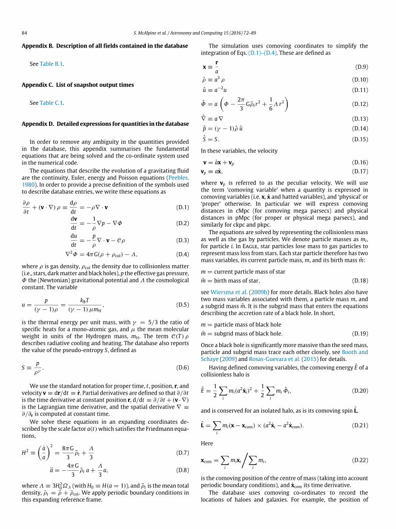
Appendix D. Detailed expressions for quantities in the database

In order to remove any ambiguity in the quantities providedin the database, this appendix summarises the fundamentalequations that are being solved and the co-ordinate system usedin the numerical code.

The equations that describe the evolution of a gravitating fluidare the continuity, Euler, energy and Poisson equations (Peebles,1980). In order to provide a precise definition of the symbols usedto describe database entries, we write these equations as

@⇢

@t+ (v · r) ⇢ ⌘ d⇢

dt= �⇢r · v (D.1)

dvdt

= � 1⇢

rp � r� (D.2)

dudt

= � p⇢

r · v � C⇢ (D.3)

r2� = 4⇡G(⇢ + ⇢col) � ⇤, (D.4)

where ⇢ is gas density, ⇢col the density due to collisionless matter(i.e., stars, darkmatter andblack holes), p the effective gas pressure,� the (Newtonian) gravitational potential and ⇤ the cosmologicalconstant. The variable

u = p(� � 1)⇢

= kBT(� � 1) µmH

, (D.5)

is the thermal energy per unit mass, with � = 5/3 the ratio ofspecific heats for a mono-atomic gas, and µ the mean molecularweight in units of the Hydrogen mass, mH. The term C(T ) ⇢describes radiative cooling and heating. The database also reportsthe value of the pseudo-entropy S, defined as

S ⌘ p⇢�

. (D.6)

We use the standard notation for proper time, t , position, r, andvelocity v ⌘ dr/dt ⌘ r. Partial derivatives are defined so that @/@tis the time derivative at constant position r, d/dt ⌘ @/@t + (v ·r)is the Lagrangian time derivative, and the spatial derivative r ⌘@/@r is computed at constant time.

We solve these equations in an expanding coordinates de-scribed by the scale factor a(t)which satisfies the Friedmann equa-tions,

H2 ⌘✓aa

◆2

= 8⇡G3

⇢t + ⇤

3(D.7)

a = �4⇡G3

⇢t a + ⇤

3a, (D.8)

where⇤ ⌘ 3H20⌦⇤ (withH0 ⌘ H(a = 1)), and ⇢t is themean total

density, ⇢t = ⇢ + ⇢col. We apply periodic boundary conditions inthis expanding reference frame.

The simulation uses comoving coordinates to simplify theintegration of Eqs. (D.1)–(D.4). These are defined as

x ⌘ ra

(D.9)

⇢ ⌘ a3 ⇢ (D.10)

u ⌘ a�2u (D.11)

� = a✓

� � 2⇡3

G⇢t r2 + 16⇤ r2

◆(D.12)

r ⌘ ar (D.13)p = (� � 1)⇢ u (D.14)

S = S. (D.15)

In these variables, the velocity

v = ax + vp (D.16)vp ⌘ ax, (D.17)

where vp is referred to as the peculiar velocity. We will usethe term ‘comoving variable’ when a quantity is expressed incomoving variables (i.e. x, x and hatted variables), and ‘physical’ or‘proper’ otherwise. In particular we will express comovingdistances in cMpc (for comoving mega parsecs) and physicaldistances in pMpc (for proper or physical mega parsecs), andsimilarly for ckpc and pkpc.

The equations are solved by representing the collisionless massas well as the gas by particles. We denote particle masses as mi,for particle i. In Eagle, star particles lose mass to gas particles torepresentmass loss from stars. Each star particle therefore has twomass variables, its current particle mass,m, and its birth mass m:

m = current particle mass of starm = birth mass of star, (D.18)

see Wiersma et al. (2009b) for more details. Black holes also havetwo mass variables associated with them, a particle mass m, anda subgrid mass m. It is the subgrid mass that enters the equationsdescribing the accretion rate of a black hole. In short,

m = particle mass of black holem = subgrid mass of black hole. (D.19)

Once a black hole is significantlymoremassive than the seedmass,particle and subgrid mass trace each other closely, see Booth andSchaye (2009) and Rosas-Guevara et al. (2015) for details.

Having defined comoving variables, the comoving energy E of acollisionless halo is

E = 12

X

i

mi(a2xi)2 + 12

X

i

mi �i, (D.20)

and is conserved for an isolated halo, as is its comoving spin L,

L =X

i

mi(x � xcom) ⇥ (a2xi � a2xcom). (D.21)

Here

xcom =X

i

mixi�X

i

mi, (D.22)

is the comoving position of the centre of mass (taking into accountperiodic boundary conditions), and xcom its time derivative.

The database uses comoving co-ordinates to record thelocations of haloes and galaxies. For example, the position of


Table B.1Full listing of the content of the main galaxy properties table and description of the columns. These properties are contained in tables denoted [modelname]_SubHalo.The first five lines of the table give the indices used to navigate between the side tables and through the merger trees. Particle types are dark matter, gas, stars and blackholes and collective properties such as Mass sum over all of these particles unless otherwise stated. Columns in this table exist for each of three different components:star-forming gas (SF), non-star-forming gas (NSF) and stars (Stars). As these properties are repeated for each of these components, we only describe them once. In thedatabase each property will be preceded with either [SF/NSF/Stars]_ before its name. For instance, the metallicity field will exist in three variants: SF_Metallicity,NSF_Metallicity and Stars_Metallicity for the metallicity of the star-forming gas, of the non star-forming gas and of the stars, respectively. Any sum used todescribe a property is the sum of all particles for that component only.

SubHalo

Field Units Description

GalaxyID – Unique identifier of a galaxy. This identifier enables linking the SubHalo table to the Aperture,Magnitudes and Sizes tables.

LastProgID – Used for merger tree traversal, Section 2.6.TopLeafID – Used for merger tree traversal, Section 2.6.DescendantID – GalaxyID of the descendant of this galaxy, Section 2.6.GroupID – Unique identifier of the FoF halo hosting this galaxy. This identifier enables linking the SubHalo table

to the FOF table.Redshift – Redshift at which these properties are computed.Snapnum – Snapshot number at which these properties are computed.GroupNumber – Integer identifier of the FoF halo hosting this galaxy. GroupNumber is only unique to a given snapshot

and hence cannot be used to identify the same halo across multiple snapshots.SubGroupNumber – Integer identifier of this galaxy within its FoF halo. SubGroupNumber is only unique to a given FoF

halo in a given snapshot and hence cannot be used to identify the same galaxy across multipleoutputs. The condition ‘‘SubGroupNumber = 0’’ selects central galaxies.

Spurious – Value is 1 if the galaxy is an artefact of the subfind algorithm and 0 if the galaxy is a genuine object,see Section 4.

Image_face–

Weblink to the mock gri image of the galaxy in the three different orientations (face-on, edge-on andalong the simulation z-axis). When querying the database via the browser, the image appears in thecolumn of the results table.

Image_edgeImage_boxBlackHoleMass M� Sum of all the black hole subgrid masses in this galaxy. See Eq. (D.19) for a description of the subgrid

mass m of a black hole, and Section 4 for cautions using black hole masses.BlackHoleMassAccretionRate M� yr�1 Total instantaneous accretion rate of all black holes, see Section 4 for cautions.CentreOfMass_x

cMpc Co-moving position of the centre of mass, Eq. (D.23).CentreOfMass_yCentreOfMass_zCentreOfPotential_x

cMpc Co-moving position of the minimum of the gravitational potential defined by the position of the mostbound particle.CentreOfPotential_y

CentreOfPotential_zGasSpin_x

pkpc km s�1 Spin per unit mass of all gas particles, L/M , with L given by Eq. (D.21).GasSpin_yGasSpin_zHalfMassRad_DM pkpc Physical radius enclosing half of the dark matter mass.HalfMassRad_Gas pkpc Physical radius enclosing half of the gas mass.HalfMassRad_Star pkpc Physical radius enclosing half of the stellar mass.HalfMassRad_BH pkpc Physical radius enclosing half of the black hole particle mass,m, as defined in Eq. (D.19).HalfMassProjRad_DM pkpc Projected physical radius enclosing half of the dark matter mass, averaged over three orthogonal

projections.HalfMassProjRad_Gas pkpc Projected physical radius enclosing half of the gas mass, averaged over three orthogonal projections.HalfMassProjRad_Star pkpc Projected physical radius enclosing half of the stellar mass, averaged over three orthogonal

projections.HalfMassProjRad_BH pkpc Projected physical radius enclosing half of the black hole particle mass,m (Eq. (D.19)), averaged over

three orthogonal projections.InitialMassWeightedBirthZ z Mean redshift of formation of stars, weighted by birth mass m (Eq. (D.18)). Calculated viaP

i mi zi/P

i mi where zi is the redshift the star particle iwas formed and mi its birth mass.InitialMassWeightedStellarAge Gyr Mean age of stars, weighted by birth mass. Calculated via

Pi mi(t � ti)/

Pi mi where t is cosmic

time, and ti and mi formation time and birth mass of the star particle i, respectively.KineticEnergy M� (km/s)2 Total kinetic energy EK , Eq. (D.26).Mass M� Total current mass of all particles (i.e.

Pi mi where mi is the mass of the particle).

MassType_DM M� Total dark matter mass.MassType_Gas M� Total gas mass.MassType_Star M� Total stellar mass,

Pi mi , wheremi is the stellar particle mass from Eq. (D.18).

MassType_BH M� Total black hole mass,P

i mi , wheremi is the black hole particle mass from Eq. (D.19).RandomNumber – Random number uniform in the range [0, 1).StarFormationRate M� yr�1 Total star formation rate,

Pi m?,i , where m?,i is the star formation rate of gas particle i.

StellarInitialMass M� Sum of birth masses of all stars,P

i mi , where mi is the birth mass of star particle i from Eq. (D.18).StellarVelDisp km s�1 One dimensional velocity dispersion of stars, ((2 Star_KineticEnergy)/(3 MassType_Star))1/2,

where Star_KineticEnergy is the kinetic energy of stars.ThermalEnergy M� (km/s)2 Total thermal energy Eu , Eq. (D.28).TotalEnergy M� (km/s)2 Total energy Etot, Eq. (D.29).Velocity_x

km s�1 Peculiar velocity, Eq. (D.24).Velocity_y(continued on next page)


Table B.1 (continued)

SubHalo


Velocity_zVmax km s�1 Maximum value of the circular velocity, (G(M(<r)/r))1/2, whereM(<r) is the total mass enclosed in

a sphere of physical radius r .VmaxRadius pkpc Physical radius where the circular velocity equals Vmax.Hydrogen –

Total mass in this element divided by the total mass (both for a given component). These aretherefore absolute abundances which do not depend on the solar abundance.

Helium –Carbon –Nitrogen –Oxygen –Neon –Magnesium –Silicon –Sulphur –Calcium –Iron –IronFromSNIa – Total mass in Iron contributed by ejecta from Type Ia supernovae, divided by the total mass.KineticEnergy M� (km/s)2 Total kinetic energy EK , Eq. (D.26).Mass M� Total mass,

Pi mi , wheremi is the particle mass.

MassFromAGB M� Total mass contributed by ejecta of AGB stars.MassFromSNII M� Total mass contributed by ejecta from massive stars and type II supernovae.MassFromSNIa M� Total mass contributed by ejecta from type Ia SN supernovae.MassWeightedEntropy kms2 ( 1010 M�

Mpc )23 Mass-weighted pseudo entropy of all particles,

Pi miSi/

Pi mi , where Si is the pseudo-entropy (Eq.

(D.6)) andmi is the mass of the particle i. (Entry present for gas components only.)MassWeightedTemperature K Mass-weighted temperature,

Pi miTi/

Pi mi , where Ti is the temperature andmi is the mass of the

particle i. (Entry present for gas components only.)Metallicity – Metal mass fraction,

Pi miZi/

Pi mi , where Zi is the metallicity andmi is the mass of the particle i.

MetalsFromAGB M� Total metal mass contributed by ejecta from AGB stars.MetalsFromSNII M� Total metal mass contributed by ejecta from massive stars and SN Type II supernovae.MetalsFromSNIa M� Total metal mass contributed by ejecta from Type Ia supernovae.Spin_x

pkpc km s�1 Spin per unit mass, L/M , from Eq. (D.21).Spin_ySpin_zThermalEnergy M� (km/s)2 Total thermal energy Eu , Eq. (D.28). (Entry present for gas components only.)TotalEnergy M� (km/s)2 Total energy Etot, Eq. (D.29). The potential energy contribution does include the other components as

well, E� = 12

Pi mi

�ia .

Table B.2Full listing of the content of the halo table and description of the columns. These properties are contained in tables denoted [modelname]_FOF. This table can be linked tothe [modelname]_SubHalo table using the unique GroupID identifier.

FOF


GroupID – Unique identifier of a halo (i.e. a FoF group). This identifier enables linking a halo to all its galaxies and theirproperties in the SubHalo table.

Redshift – Redshift at which these properties are computed.SnapNum – Snapshot number containing that halo.GroupCentreOfPotential_x

cMpc Co-moving position of the minimum of the gravitational potential of the halo.GroupCentreOfPotential_yGroupCentreOfPotential_zGroupMass M� Total Friends-of-Friends mass of this halo.Group_M_Crit200

M� Total mass within the corresponding Group_R_Critxxx radius, where xxx = 200, 500 or 2500, respectivelyGroup_M_Crit500Group_M_Crit2500Group_M_Mean200

M� Total mass within the corresponding Group_R_Meanxxx radius, where xxx = 200, 500 or 2500, respectivelyGroup_M_Mean500Group_M_Mean2500Group_M_TopHat200 M� Total mass within radius Group_R_Tophat200.Group_R_Crit200

pkpc Physical radius within which the mean density is xxx times the critical density of the Universe, where xxx = 200,500 or 2500, respectively.Group_R_Crit500

Group_R_Crit2500Group_R_Mean200

pkpc Physical radius within which the mean density is xxx times themean density of the Universe, where xxx = 200,500 or 2500, respectively.Group_R_Mean500

Group_R_Mean2500Group_R_TopHat200 pkpc Physical radius within which the mean density is 18⇡2 + 82(⌦m(z) � 1) � 39(⌦m(z) � 1)2 times the critical

density of the Universe. This is based on the spherical top-hat collapse model of Bryan and Norman (1998).NumOfSubhalos – Number of subhaloes (galaxies) identified as belonging to this halo.RandomNumber – Random number uniform in the range [0, 1).


Table B.3Full listing of the content of the galaxy sizes table and description of the columns. These properties are contained in tables denoted [modelname]_Sizes. This table containshalf-mass sizes of the stellar component of galaxies using spherical apertures (Furlong et al. in prep.). TheGalaxyID column can be used to join this table to the corresponding[modelname]_SubHalo table. Only galaxies with total stellar massM⇤ > 108 M� have entries in this table.

Sizes


GalaxyID – Unique identifier of a galaxy as per SubHalo table.R_halfmass30 pkpc Half mass radius of stellar component within a spherical (3D) 30 pkpc aperture.R_halfmass100 pkpc Half mass radius of stellar component within a spherical (3D) 100 pkpc aperture.R_halfmass30_projected pkpc Projected half mass radius of stellar component within a circular (2D) 30 pkpc aperture (averaged over three orthogonal

projections).R_halfmass100_projected pkpc Projected half mass radius of stellar component within a circular (2D) 100 pkpc aperture (averaged over three orthogonal

projections).

Table B.4Full listing of the content of the aperture table and description of the columns. These properties are contained in tables denoted [modelname]_Aperture. This table containsmeasurements within spherical apertures centred on the minimum of the gravitational potential of a given galaxy. Each row represents a set of measurements for a singlegalaxy using a single aperture size in physical kpc. The GalaxyID column can be used to join this table to the corresponding [modelname]_SubHalo table.

Aperture


GalaxyID – Unique identifier of a galaxy as per SubHalo table.ApertureSize pkpc Spherical (3D) aperture radius used for this measurement. Quantities are measured in a sphere centred at the centre of the potential,

i.e. at the location of the most bound particle. Available aperture sizes are: 1, 3, 5, 10, 20, 30, 40, 50, 70 and 100 pkpc.VelDisp km s�1 One dimensional velocity dispersion of stars, ((2 KineticEnergy_Star)/(3Mass_Star))1/2, where KineticEnergy_Star is the kinetic

energy of stars, and the sum is over stars within the aperture.SFR M� yr�1 Star formation rate within the aperture.Mass_BH M� Total particle mass,

Pi mi (Eq. (D.19)), of all black holes within the aperture.

Mass_DM M� Total dark matter mass within the aperture.Mass_Gas M� Total gas mass within the aperture.Mass_Star M� Total stellar mass,

Pi mi (Eq. (D.18)), within the aperture.

Table B.5Full listing of the content of the magnitudes table and description of the columns. These properties are contained in tables denoted [modelname]_Magnitudes. This tablecontains absolute rest-frame magnitudes without dust attenuation for all galaxies with M⇤ > 108.5 M� contained in the SubHalo table. This table can be joined to theSubHalo table using the GalaxyID field. The magnitudes in the different SDSS (Doi et al., 2010) and UKIRT (Hewett et al., 2006) filters have been computed in 30 pkpcspherical apertures following the procedure described by Trayford et al. (2015).

Magnitudes


GalaxyID – Unique identifier of a galaxy as per SubHalo table.u_nodust mag Rest-frame absolute magnitude (AB) in the u band without dust attenuation.g_nodust mag Rest-frame absolute magnitude (AB) in the g band without dust attenuation.r_nodust mag Rest-frame absolute magnitude (AB) in the r band without dust attenuation.i_nodust mag Rest-frame absolute magnitude (AB) in the i band without dust attenuation.z_nodust mag Rest-frame absolute magnitude (AB) in the z band without dust attenuation.Y_nodust mag Rest-frame absolute magnitude (AB) in the Y band without dust attenuation.J_nodust mag Rest-frame absolute magnitude (AB) in the J band without dust attenuation.H_nodust mag Rest-frame absolute magnitude (AB) in the H band without dust attenuation.K_nodust mag Rest-frame absolute magnitude (AB) in the K band without dust attenuation.

the centre of a galaxy or halo (stored as CentreOfMass in thedatabase) is

CentreOfMass = xcom =Pimi xi

Pimi

, (D.23)

where the sum runs over all particles that belong to the ob-ject taking into account periodic boundary conditions. Simi-larly, the centre of potential of an object (database variableCentreOfPotential) is given in comoving coordinates.

The velocity of a halo or galaxy (database variable Velocity)refers to its peculiar velocity,

Velocity = a xcom = a

Pimi xi

Pimi

. (D.24)

All other variables are expressed in physical coordinates, forexample the spin vector of a galaxy is computed as

Spin =Pimi (ri � rcom) ⇥ (vi � vcom)

Pimi

, (D.25)

where rcom and vcom are the physical position and velocity of thecentre of mass. The expressions for physical kinetic, potential,thermal, and total energy are, respectively

EK = 12

X

i

mi (v � vcom)2 (D.26)

E� = 12

X

i

mi�i

a(D.27)


Table C.1List of all output redshifts for all the simulations present in the database. Note thatsql queries are made easier by the use of the snapshot number rather than theredshift. Lookback times are given in Gigayears.

SnapNum Redshift Lookback time Expansion factor

28 0.00 0.00 1.00027 0.10 1.34 0.90926 0.18 2.29 0.84625 0.27 3.23 0.78724 0.37 4.16 0.73223 0.50 5.19 0.66522 0.62 6.01 0.61921 0.74 6.71 0.57620 0.87 7.37 0.53619 1.00 7.93 0.49918 1.26 8.86 0.44317 1.49 9.49 0.40216 1.74 10.05 0.36515 2.01 10.53 0.33214 2.24 10.86 0.30913 2.48 11.16 0.28712 3.02 11.66 0.24911 3.53 12.01 0.22110 3.98 12.25 0.2019 4.49 12.46 0.1828 5.04 12.63 0.1667 5.49 12.75 0.1546 5.97 12.86 0.1435 7.05 13.04 0.1244 8.07 13.16 0.1103 8.99 13.25 0.1002 9.99 13.32 0.0911 15.13 13.53 0.0620 20.00 13.62 0.047

Eu =X

i

mi (a2ui) (D.28)

Etot = EK + E� + Eu. (D.29)

References

Baes, M., et al., 2003. Radiative transfer in disc galaxies—III. The observedkinematics of dusty disc galaxies. Mon. Not. R. Astron. Soc. 343, 1081–1094.doi:10.1046/j.1365-8711.2003.06770.x. arXiv:astro-ph/0304501.

Booth, C.M., Schaye, J., 2009. Cosmological simulations of the growth of supermas-sive black holes and feedback from active galactic nuclei: method and tests.Mon. Not. R. Astron. Soc. 398, 53–74. doi:10.1111/j.1365-2966.2009.15043.x.arXiv:0904.2572.

Bruzual, G., Charlot, S., 2003. Stellar population synthesis at the resolution of 2003.Mon. Not. R. Astron. Soc. 344, 1000–1028.

Bryan, G.L., Norman, M.L., 1998. Statistical properties of x-ray clusters: Analyticand numerical comparisons. Astrophys. J. 495, 80–99. doi:10.1086/305262.arXiv:astro-ph/9710107.

Camps, P., Baes, M., 2015. SKIRT: An advanced dust radiative transfercode with a user-friendly architecture. Astron. Comput. 9, 20–33.doi:10.1016/j.ascom.2014.10.004. arXiv:1410.1629.

Carlberg, R.G., Couchman, H.M.P., Thomas, P.A., 1990. Cosmological velocity bias.Astrophys. J. 352, L29–L32. doi:10.1086/185686.

Chabrier, G., 2003. Galactic stellar and substellar initial mass function. Publ. Astron.Soc. Pac. 115, 763–795. doi:10.1086/376392. arXiv:astro-ph/0304382.

Chang, Y.Y., van der Wel, A., da Cunha, E., Rix, H.W., 2015. Stellar masses and starformation rates for 1M galaxies from SDSS+WISE. Astrophys. J. Suppl. 219, 8.doi:10.1088/0067-0049/219/1/8. arXiv:1506.00648.

Crain, R.A., et al., 2015. The EAGLE simulations of galaxy formation: calibration ofsubgrid physics andmodel variations.Mon. Not. R. Astron. Soc. 450, 1937–1961.doi:10.1093/mnras/stv725. arXiv:1501.01311.

Cullen, L., Dehnen, W., 2010. Inviscid smoothed particle hydrodynamics. Mon.Not. R. Astron. Soc. 408, 669–683. doi:10.1111/j.1365-2966.2010.17158.x.arXiv:1006.1524.

Dalla Vecchia, C., Schaye, J., 2012. Simulating galactic outflows with thermal su-pernova feedback. Mon. Not. R. Astron. Soc. 426, 140–158. doi:10.1111/j.1365-2966.2012.21704.x. arXiv:1203.5667.

Davis, M., Efstathiou, G., Frenk, C.S., White, S.D.M., 1985. The evolution of large-scale structure in a universe dominated by cold dark matter. Astrophys. J. 292,371–394. doi:10.1086/163168.

De Lucia, G., Blaizot, J., 2007. The hierarchical formation of the brightestcluster galaxies. Mon. Not. R. Astron. Soc. 375, 2–14. doi:10.1111/j.1365-2966.2006.11287.x. arXiv:astro-ph/0606519.

Doi, M., et al., 2010. Photometric response functions of the sloan digital skysurvey imager. Astron. J. 139, 1628–1648. doi:10.1088/0004-6256/139/4/1628.arXiv:1002.3701.

Dolag, K., Borgani, S., Murante, G., Springel, V., 2009. Substructures in hy-drodynamical cluster simulations. Mon. Not. R. Astron. Soc. 399, 497–514.doi:10.1111/j.1365-2966.2009.15034.x. arXiv:0808.3401.

Dubois, Y., et al., 2014. Dancing in the dark: galactic properties trace spinswings along the cosmic web. Mon. Not. R. Astron. Soc. 444, 1453–1468.doi:10.1093/mnras/stu1227. arXiv:1402.1165.

Durier, F., Dalla Vecchia, C., 2012. Implementation of feedback in smoothed particlehydrodynamics: towards concordance of methods. Mon. Not. R. Astron. Soc.419, 465–478. doi:10.1111/j.1365-2966.2011.19712.x. arXiv:1105.3729.

Fakhouri, O., Ma, C.P., 2008. The nearly universal merger rate of dark matterhaloes in ⇤CDM cosmology. Mon. Not. R. Astron. Soc. 386, 577–592.doi:10.1111/j.1365-2966.2008.13075.x. arXiv:0710.4567.

Furlong, M., et al., 2015. Evolution of galaxy stellar masses and star formationrates in the EAGLE simulations. Mon. Not. R. Astron. Soc. 450, 4486–4504.doi:10.1093/mnras/stv852. arXiv:1410.3485.

Genel, S., Genzel, R., Bouché, N., Naab, T., Sternberg, A., 2009. The halo mergerrate in the millennium simulation and implications for observed galaxy mergerfractions. Astrophys. J. 701, 2002–2018. doi:10.1088/0004-637X/701/2/2002.arXiv:0812.3154.

Groves, B., Dopita, M.A., Sutherland, R.S., Kewley, L.J., Fischera, J., Leitherer, C.,Brandl, B., van Breugel,W., 2008.Modeling the pan-spectral energy distributionof starburst galaxies. IV. The controlling parameters of the starburst SED.Astrophys. J. Suppl. 176, 438–456. doi:10.1086/528711. arXiv:0712.1824.

Henriques, B.M.B., White, S.D.M., Thomas, P.A., Angulo, R., Guo, Q., Lemson, G.,Springel, V., Overzier, R., 2015. Galaxy formation in the Planck cosmology—I.Matching the observed evolution of star formation rates, colours and stellarmasses. Mon. Not. R. Astron. Soc. 451, 2663–2680. doi:10.1093/mnras/stv705.arXiv:1410.0365.

Hewett, P.C., Warren, S.J., Leggett, S.K., Hodgkin, S.T., 2006. The UKIRT infrareddeep sky survey ZY JHK photometric system: passbands and synthetic colours.Mon. Not. R. Astron. Soc. 367, 454–468. doi:10.1111/j.1365-2966.2005.09969.x.arXiv:astro-ph/0601592.

Hopkins, P.F., 2013. A general class of Lagrangian smoothed particle hydrodynamicsmethods and implications for fluid mixing problems. Mon. Not. R. Astron. Soc.428, 2840–2856. doi:10.1093/mnras/sts210. arXiv:1206.5006.

Jenkins, A., 2010. Second-order Lagrangian perturbation theory initial conditions forresimulations. Mon. Not. R. Astron. Soc. 403, 1859–1872. doi:10.1111/j.1365-2966.2010.16259.x. arXiv:0910.0258.

Jenkins, A., 2013. A new way of setting the phases for cosmological multiscaleGaussian initial conditions. Mon. Not. R. Astron. Soc. 434, 2094–2120.doi:10.1093/mnras/stt1154. arXiv:1306.5968.

Jiang, L., Helly, J.C., Cole, S., Frenk, C.S., 2014. N-body dark matter haloes withsimple hierarchical histories. Mon. Not. R. Astron. Soc. 440, 2115–2135.doi:10.1093/mnras/stu390. arXiv:1311.6649.

Katz, N., Hernquist, L., Weinberg, D.H., 1992. Galaxies and gas in a cold dark matteruniverse. Astrophys. J. 399, L109–L112. doi:10.1086/186619.

Khandai, N., Di Matteo, T., Croft, R., Wilkins, S., Feng, Y., Tucker, E., DeGraf, C., Liu,M.S., 2015. TheMassiveBlack-II simulation: the evolution of haloes and galaxiesto z = 0. Mon. Not. R. Astron. Soc. 450, 1349–1374. doi:10.1093/mnras/stv627.arXiv:1402.0888.

Lacey, C.G., et al. 2015. A unifiedmulti-wavelengthmodel of galaxy formation. ArXive-prints arXiv:1509.08473.

Lagos, C.d.P., et al., 2015. Molecular hydrogen abundances of galaxies inthe EAGLE simulations. Mon. Not. R. Astron. Soc. 452, 3815–3837.doi:10.1093/mnras/stv1488. arXiv:1503.04807.

Lemson, G., Springel, V., 2006. Cosmological simulations in a relational database:Modelling and storing merger trees. In: Gabriel, C., Arviset, C., Ponz, D.,Enrique, S. (Eds.), Astronomical Data Analysis Software and Systems XV.In: Astronomical Society of the Pacific Conference Series, vol. 351. p. 212.

Lemson, G., Virgo Consortium, T., 2006. Halo and galaxy formation histories fromthe millennium simulation: Public release of a VO-oriented and SQL-queryabledatabase for studying the evolution of galaxies in the LambdaCDM cosmogony.ArXiv Astrophysics e-prints arXiv:astro-ph/0608019.

Lupton, R., Blanton, M.R., Fekete, G., Hogg, D.W., O’Mullane, W., Szalay, A., Wherry,N., 2004. Preparing red–green–blue images from CCD data. Publ. Astron. Soc.Pac. 116, 133–137. doi:10.1086/382245. arXiv:astro-ph/0312483.

Nelson, D., et al. 2015. The illustris simulation: Public data release. ArXiv e-prints.doi: 10.1016/j.ascom.2015.09.003. arXiv:1504.00362.

Okamoto, T., Shimizu, I., Yoshida, N., 2014. Reproducing cosmic evolution ofgalaxy population from z = 4 to 0. Publ. Astron. Soc. Japan 66, 70.doi:10.1093/pasj/psu046. arXiv:1404.7579.

Oppenheimer, B.D., Davé, R., Kere≤, D., Fardal, M., Katz, N., Kollmeier, J.A., Weinberg,D.H., 2010. Feedback and recycled wind accretion: assembling the z = 0 galaxymass function. Mon. Not. R. Astron. Soc. 406, 2325–2338. doi:10.1111/j.1365-2966.2010.16872.x. arXiv:0912.0519.

Peebles, P.J.E., 1980. The large-scale structure of the universe.Planck Collaboration, et al., 2014. Planck 2013 results. I. Overview of prod-

ucts and scientific results. Astron. Astrophys. 571, A1. doi:10.1051/0004-6361/201321529. arXiv:1303.5062.

Porter, L.A., Somerville, R.S., Primack, J.R., Johansson, P.H., 2014. Understanding thestructural scaling relations of early-type galaxies. Mon. Not. R. Astron. Soc. 444,942–960. doi:10.1093/mnras/stu1434. arXiv:1407.0594.

http://dx.doi.org/10.1046/j.1365-8711.2003.06770.x

http://arxiv.org/astro-ph/0304501

http://dx.doi.org/10.1111/j.1365-2966.2009.15043.x

http://arxiv.org/abs/0904.2572

http://refhub.elsevier.com/S2213-1337(16)30013-0/sbref3

http://dx.doi.org/10.1086/305262




http://dx.doi.org/10.1086/185686

http://dx.doi.org/10.1086/376392


http://dx.doi.org/10.1088/0067-0049/219/1/8


http://dx.doi.org/10.1093/mnras/stv725


http://dx.doi.org/10.1111/j.1365-2966.2010.17158.x


http://dx.doi.org/10.1111/j.1365-2966.2012.21704.x

http://dx.doi.org/10.1111/j.1365-2966.2012.21704.x

http://dx.doi.org/10.1111/j.1365-2966.2012.21704.x


http://dx.doi.org/10.1086/163168

http://dx.doi.org/10.1111/j.1365-2966.2006.11287.x

http://dx.doi.org/10.1111/j.1365-2966.2006.11287.x

http://dx.doi.org/10.1111/j.1365-2966.2006.11287.x


http://dx.doi.org/10.1088/0004-6256/139/4/1628


http://dx.doi.org/10.1111/j.1365-2966.2009.15034.x


http://dx.doi.org/10.1093/mnras/stu1227


http://dx.doi.org/10.1111/j.1365-2966.2011.19712.x


http://dx.doi.org/10.1111/j.1365-2966.2008.13075.x




http://dx.doi.org/10.1088/0004-637X/701/2/2002


http://dx.doi.org/10.1086/528711




http://dx.doi.org/10.1111/j.1365-2966.2005.09969.x


http://dx.doi.org/10.1093/mnras/sts210


http://dx.doi.org/10.1111/j.1365-2966.2010.16259.x

http://dx.doi.org/10.1111/j.1365-2966.2010.16259.x

http://dx.doi.org/10.1111/j.1365-2966.2010.16259.x


http://dx.doi.org/10.1093/mnras/stt1154




http://dx.doi.org/10.1086/186619






http://refhub.elsevier.com/S2213-1337(16)30013-0/sbref32


http://dx.doi.org/10.1086/382245




http://dx.doi.org/10.1093/pasj/psu046


http://dx.doi.org/10.1111/j.1365-2966.2010.16872.x

http://dx.doi.org/10.1111/j.1365-2966.2010.16872.x

http://dx.doi.org/10.1111/j.1365-2966.2010.16872.x


http://dx.doi.org/10.1051/0004-6361/201321529

http://dx.doi.org/10.1051/0004-6361/201321529

http://dx.doi.org/10.1051/0004-6361/201321529





Price, D.J., 2008. Modelling discontinuities and Kelvin Helmholtz instabilitiesin SPH. J. Comput. Phys. 227, 10040–10057. doi:10.1016/j.jcp.2008.08.011.arXiv:0709.2772.

Puchwein, E., Springel, V., 2013. Shaping the galaxy stellar mass function withsupernova- and AGN-driven winds. Mon. Not. R. Astron. Soc. 428, 2966–2979.doi:10.1093/mnras/sts243. arXiv:1205.2694.

Rahmati, A., Schaye, J., Bower, R.G., Crain, R.A., Furlong, M., Schaller, M., Theuns, T.,2015. The distribution of neutral hydrogen around high-redshift galaxies andquasars in the EAGLE simulation. Mon. Not. R. Astron. Soc. 452, 2034–2056.doi:10.1093/mnras/stv1414. arXiv:1503.05553.

Rosas-Guevara, Y.M., et al., 2015. The impact of angular momentum on black holeaccretion rates in simulations of galaxy formation.Mon. Not. R. Astron. Soc. 454,1038–1057. doi:10.1093/mnras/stv2056. arXiv:1312.0598.

Schaller, M., Dalla Vecchia, C., Schaye, J., Bower, R.G., Theuns, T., Crain, R.A., Furlong,M., McCarthy, I.G., 2015a. The EAGLE simulations of galaxy formation: theimportance of the hydrodynamics scheme. Mon. Not. R. Astron. Soc. 454,2277–2291. doi:10.1093/mnras/stv2169. arXiv:1509.05056.

Schaller, M., et al., 2015b. Baryon effects on the internal structure of ⇤CDMhaloes in the EAGLE simulations. Mon. Not. R. Astron. Soc. 451, 1247–1267.doi:10.1093/mnras/stv1067. arXiv:1409.8617.

Schaye, J., 2004. Star formation thresholds and galaxy edges: Why and where.Astrophys. J. 609, 667–682. doi:10.1086/421232. arXiv:astro-ph/0205125.

Schaye, J., et al., 2015. The EAGLE project: simulating the evolution and assemblyof galaxies and their environments. Mon. Not. R. Astron. Soc. 446, 521–554.doi:10.1093/mnras/stu2058. arXiv:1407.7040.

Schaye, J., Dalla Vecchia, C., 2008. On the relation between the Schmidt andKennicutt–Schmidt star formation laws and its implications for numericalsimulations. Mon. Not. R. Astron. Soc. 383, 1210–1222. doi:10.1111/j.1365-2966.2007.12639.x. arXiv:0709.0292.

Springel, V., 2005. The cosmological simulation code GADGET-2. Mon. Not.R. Astron. Soc. 364, 1105–1134. doi:10.1111/j.1365-2966.2005.09655.x.arXiv:astro-ph/0505010.

Springel, V., Di Matteo, T., Hernquist, L., 2005a. Modelling feedback from starsand black holes in galaxy mergers. Mon. Not. R. Astron. Soc. 361, 776–794.doi:10.1111/j.1365-2966.2005.09238.x. arXiv:astro-ph/0411108.

Springel, V., et al., 2005b. Simulations of the formation, evolution and clusteringof galaxies and quasars. Nature 435, 629–636. doi:10.1038/nature03597.arXiv:astro-ph/0504097.

Springel, V., White, S.D.M., Tormen, G., Kauffmann, G., 2001. Populating a cluster ofgalaxies—I. Results at [formmu2]z = 0. Mon. Not. R. Astron. Soc. 328, 726–750.doi:10.1046/j.1365-8711.2001.04912.x. arXiv:astro-ph/0012055.

Szalay, A.S., Kunszt, P.Z., Thakar, A.R., Gray, J., Slutz, D., 2000. The sloan digital skysurvey and its archive. In:Manset, N., Veillet, C., Crabtree, D. (Eds.), AstronomicalData Analysis Software and Systems IX. In: Astronomical Society of the PacificConference Series, vol. 216. p. 405. arXiv:astro-ph/9912382.

Trayford, J.W., et al., 2015. Colours and luminosities of z = 0.1 galaxiesin the EAGLE simulation. Mon. Not. R. Astron. Soc. 452, 2879–2896.doi:10.1093/mnras/stv1461. arXiv:1504.04374.

Vogelsberger, M., et al., 2014. Introducing the Illustris Project: simulating thecoevolution of dark and visible matter in the Universe. Mon. Not. R. Astron. Soc.444, 1518–1547. doi:10.1093/mnras/stu1536. arXiv:1405.2921.

Wendland, H., 1995. Piecewise polynomial, positive definite and compactlysupported radial functions of minimal degree. Adv. Comput. Math. 4, 389–396.doi:10.1007/BF02123482.URL http://www.springerlink.com/index/10.1007/BF02123482.

White, S.D.M., Frenk, C.S., 1991. Galaxy formation through hierarchical clustering.Astrophys. J. 379, 52–79. doi:10.1086/170483.

Wiersma, R.P.C., Schaye, J., Smith, B.D., 2009a. The effect of photoionization on thecooling rates of enriched, astrophysical plasmas. Mon. Not. R. Astron. Soc. 393,99–107. doi:10.1111/j.1365-2966.2008.14191.x. arXiv:0807.3748.

Wiersma, R.P.C., Schaye, J., Theuns, T., Dalla Vecchia, C., Tornatore, L., 2009b.Chemical enrichment in cosmological, smoothed particle hydrodynamicssimulations. Mon. Not. R. Astron. Soc. 399, 574–600. doi:10.1111/j.1365-2966.2009.15331.x. arXiv:0902.1535.

http://dx.doi.org/10.1016/j.jcp.2008.08.011


http://dx.doi.org/10.1093/mnras/sts243










http://dx.doi.org/10.1086/421232




http://dx.doi.org/10.1111/j.1365-2966.2007.12639.x

http://dx.doi.org/10.1111/j.1365-2966.2007.12639.x

http://dx.doi.org/10.1111/j.1365-2966.2007.12639.x


http://dx.doi.org/10.1111/j.1365-2966.2005.09655.x


http://dx.doi.org/10.1111/j.1365-2966.2005.09238.x


http://dx.doi.org/10.1038/nature03597


http://dx.doi.org/10.1046/j.1365-8711.2001.04912.x







http://dx.doi.org/10.1007/BF02123482

http://www.springerlink.com/index/10.1007/BF02123482

http://dx.doi.org/10.1086/170483

http://dx.doi.org/10.1111/j.1365-2966.2008.14191.x


http://dx.doi.org/10.1111/j.1365-2966.2009.15331.x

http://dx.doi.org/10.1111/j.1365-2966.2009.15331.x

http://dx.doi.org/10.1111/j.1365-2966.2009.15331.x


The eagle simulations of galaxy formation

Documents

Transcript of The eagle simulations of galaxy formation