The dynamics underlying pseudo-plateau bursting in a pituitary cell model

Journal of Mathematical Neuroscience (2011) 1:12DOI 10.1186/2190-8567-1-12

R E S E A R C H Open Access

The dynamics underlying pseudo-plateau bursting in apituitary cell model

Wondimu Teka · Joël Tabak · Theodore Vo ·Martin Wechselberger · Richard Bertram

Received: 27 June 2011 / Accepted: 8 November 2011 / Published online: 8 November 2011© 2011 Teka et al.; licensee Springer. This is an Open Access article distributed under the terms of theCreative Commons Attribution License

Abstract Pituitary cells of the anterior pituitary gland secrete hormones in responseto patterns of electrical activity. Several types of pituitary cells produce short burstsof electrical activity which are more effective than single spikes in evoking hormonerelease. These bursts, called pseudo-plateau bursts, are unlike bursts studied mathe-matically in neurons (plateau bursting) and the standard fast-slow analysis used forplateau bursting is of limited use. Using an alternative fast-slow analysis, with onefast and two slow variables, we show that pseudo-plateau bursting is a canard-inducedmixed mode oscillation. Using this technique, it is possible to determine the region ofparameter space where bursting occurs as well as salient properties of the burst suchas the number of spikes in the burst. The information gained from this one-fast/two-slow decomposition complements the information obtained from a two-fast/one-slowdecomposition.

W TekaDepartment of Mathematics, Florida State University, Tallahassee, FL 32306, USAe-mail: [email protected]

J TabakDepartment of Biological Science, Florida State University, Tallahassee, FL 32306, USAe-mail: [email protected]

T Vo · M WechselbergerSchool of Mathematics and Statistics, University of Sydney, Sydney, NSW 2006, Australia

T Voe-mail: [email protected]

M Wechselbergere-mail: [email protected]

R Bertram (�)Department of Mathematics, and Programs in Neuroscience and Molecular Biophysics, Florida StateUniversity, Tallahassee, FL 32306, USAe-mail: [email protected]

http://dx.doi.org/10.1186/2190-8567-1-12

mailto:[email protected]





of 23 Teka et al.

Keywords Bursting · mixed mode oscillations · folded node singularity · canards ·mathematical model

1 Introduction

Bursting is a common pattern of electrical activity in excitable cells such as neuronsand many endocrine cells. Bursting oscillations are characterized by the alternationbetween periods of fast spiking (the active phase) and quiescent periods (the silentphase), and accompanied by slow variations in one or more slowly changing vari-ables, such as the intracellular calcium concentration. Bursts are often more efficientthan periodic spiking in evoking the release of neurotransmitter or hormone [1–3].

The endocrine cells of the anterior pituitary gland display bursting patterns withsmall spikes arising from a depolarized voltage [2–5]. Similar patterns have beenobserved in single pancreatic β-cells isolated from islets [6–8]. Figure 1(a) showsa representative example from a GH4 pituitary cell. Several mathematical modelshave been developed for this bursting type [5, 8–10]. Prior analysis showed that thedynamic mechanism for this type of bursting, called pseudo-plateau bursting, is sig-nificantly different from that of square-wave bursting (also called plateau bursting)which is common in neurons [11–13]. Yet this analysis did not determine the possi-ble number of spikes that occur during the active phase of the burst. The goal of thispaper is to understand the dynamics underlying pseudo-plateau bursting, with a focuson the origin of the spikes that occur during the active phase of the oscillation.

Minimal models for pseudo-plateau bursting can be written as

ε1V = f (V,n, c) (1.1)

n = g(V,n) (1.2)

c = ε2h(V, c) (1.3)

where V is the membrane potential, n is the fraction of activated delayed rectifier K+channels, and c is the cytosolic free Ca2+ concentration. The velocity functions arenonlinear, and ε1 and ε2 are parameters that may be small.

The variables V , n and c vary on different time scales (for details, see Section 2).By taking advantage of time-scale separation, the system can be divided into fast andslow subsystems. In the standard fast/slow analysis one considers ε2 ≈ 0, so that V

and n form the fast subsystem and c represents the slow subsystem. One then studiesthe dynamics of the fast subsystem with the slow variable treated as a slowly vary-ing parameter [12, 15–18]. This approach has been very successful for understand-ing plateau bursting, such as occurs in pancreatic islets [19], pre-Bötzinger neuronsof the brain stem [20], trigeminal motoneurons [21] or neonatal CA3 hippocampalprincipal neurons [14], Fig. 1(b). It has also been useful in understanding aspects ofpseudo-plateau bursting such as resetting properties [11], how fast subsystem man-ifolds affect burst termination [17], and how parameter changes convert the systemfrom plateau to pseudo-plateau bursting [12].

An alternate approach, which we use here, is to consider ε1 ≈ 0, so that V isthe sole fast variable and n and c form the slow subsystem. With this approach, we

Journal of Mathematical Neuroscience (2011) 1:12 of 23

Fig. 1 (a) Pseudo-plateau bursting in a GH4 pituitary cell line. (b) Plateau bursting in a neonatal CA3hippocampal principal neuron. Reprinted with permission from [14].

show that the active phase of spiking arises naturally through a canard mechanism,due to the existence of a folded node singularity [22–25]. Also, the transition fromcontinuous spiking to bursting is easily explained, as is the change in the number ofspikes per burst with variation of conductance parameters. Thus, the one-fast/two-slow variable analysis provides information that is not available from the standardtwo-fast/one-slow variable analysis in the case of pseudo-plateau bursting.

2 The mathematical model

We use a model of the pituitary lactotroph, which produces pseudo-plateau burstingover a range of parameter values [10]. To achieve a minimal form, we use the modelwithout A-type K+ current (IA). It includes three variables: V (membrane potential),n (fraction of activated delayed rectifier K+ channels), and c (cytosolic free Ca2+concentration). The equations are:

Cm

dV

dt= −(ICa + IK + IK(Ca) + IBK) (2.1)

dn

dt= (n∞(V ) − n)

τn

(2.2)

dc

dt= −fc(αICa + kcc) (2.3)

where ICa is an inward Ca2+ current, IK is an outward delayed rectifying K+ cur-rent, IK(Ca) is a small-conductance Ca2+-activated K+ current, and IBK is a fast-activating large-conductance BK-type K+ current. The currents in the equationsabove are:

ICa = gCam∞(V )(V − VCa) (2.4)

IK = gKn(V − VK) (2.5)

IK(Ca) = gK(Ca)s∞(c)(V − VK) (2.6)

IBK = gBKb∞(V )(V − VK). (2.7)

of 23 Teka et al.

Table 1 Parameter values for the lactotroph model.

Parameter Value Description

Cm 5 pF Membrane capacitance of the cell

gCa 2 nS Maximum conductance of Ca2+ channels

VCa 50 mV Reversal potential for Ca2+vm −20 mV Voltage value at midpoint of m∞sm 12 mV Slope parameter of m∞gK 4 nS Maximum conductance of K+ channels

VK −75 mV Reversal potential for K+vn −5 mV Voltage value at midpoint of n∞sn 10 mV Slope parameter of n∞τn 43 ms Time constant of n

gK(Ca) 1.7 nS Maximum conductance of K(Ca) channels

Kd 0.5 μM c at midpoint of s∞gBK 0.4 nS Maximum conductance of BK-type K+ channels

vb −20 mV Voltage value at midpoint of f∞sb 5.6 mV Slope parameter of f∞fc 0.01 Fraction of free Ca2+ ions in cytoplasm

α 0.0015 μM fC−1 Conversion from charge to concentration

kc 0.16 ms−1 Rate of Ca2+ extrusion

The steady state activation functions are given by:

m∞(V ) =(

1 + exp

(vm − V

sm

))−1

(2.8)

n∞(V ) =(

1 + exp

(vn − V

sn

))−1

(2.9)

s∞(c) = c2

c2 + K2d

(2.10)

b∞(V ) =(

1 + exp

(vb − V

sb

))−1

. (2.11)

Default parameter values are given in Table 1.The variables V , n and c vary on different time scales. The time constant of V

is given by τV = Cm/gT otal , where gT otal = gKn + gBKb∞(V ) + gCam∞(V ) +gK(Ca)s∞(c). During a bursting oscillation, the minimum of gT otal is 0.483 pS andthe maximum is 3 pS. Hence, Cm

maxgT otal≤ τV ≤ Cm

mingT otal, or 1.7 ms ≤ τV ≤ 10.4 ms,

for Cm = 5 pF, a typical capacitance value for lactotrophs. The time constant for n isτn = 43 ms. For the variable c, the time constant is 1

fckc= 1

(0.01)(0.16)ms = 625 ms.

Thus, n and c change more slowly than V . This time scale separation between V and(c, n) can be accentuated when Cm is made smaller than the default 5 pF, i.e., whenCm → 0, τV gets smaller and V varies much faster. Thus, we can view the capacitance


Cm as a representative of the dimensionless singular perturbation parameter ε1 in thismodel (Eq. 1.1).

All numerical simulations and bifurcation diagrams (both one- and two-parameter)are constructed using the XPPAUT software package [26], using the Runge-Kutta in-tegration method, and computer codes can be downloaded from the following web-site: http://www.math.fsu.edu/~bertram/software/pituitary. The surface in Fig. 9 wasconstructed using the AUTO software package [27]. All graphics were produced withthe software package MATLAB.

3 Geometric singular perturbation theory

3.1 The reduced system

We consider the full system (Eqs. (2.1)-(2.3)) as having one fast variable V and twoslower variables n and c. The time-scale separation can be accentuated by decreasingthe singular perturbation parameter Cm. This facilitates analysis of the system dy-namics [28]. In the limit Cm → 0, the trajectories of the system lie on a 2-D surfacecalled the critical manifold. If we define the right hand side of Eq. (2.1) by

f (V, c,n) = −(ICa + IK + IK(Ca) + IBK) (3.1)

then the critical manifold is the surface S satisfying

S ≡ {(V , c, n) ∈ R3 : f (V, c,n) = 0}. (3.2)

The equation f (V, c,n) = 0 can be solved in explicit form for n as

n = n(c,V ) = − 1

gK

[gCam∞(V )

(V − VCa)

(V − VK)+ gK(Ca)s∞(c) + gBKb∞(V )

]. (3.3)

The critical manifold (3.3) is a folded surface (Fig. 2) that consists of three sheetsseparated by two fold curves (L− and L+). The lower and upper sheets are attracting( ∂f∂V

< 0) and the middle sheet is repelling ( ∂f∂V

> 0). The lower (L−) and upper (L+)fold curves are given by

L± ≡{(V , c, n) ∈ R

3 : f (V, c,n) = 0 and∂f

∂V(V, c,n) = 0

}. (3.4)

This yields two constant V values and two equations for n in the form of n = n(c).Thus, the fold curves (L±) are (V ±, c, n±(c)) where V − and V + are constant V

values. The curve L+ is projected vertically (along the fast variable V ) onto the lowersheet to obtain the projection curve P(L+), and similarly for the (L−) projectiononto the upper sheet. Figure 2 shows the critical manifold, the fold curves and theprojections of the fold curves.

The reduced flow (when Cm → 0) is described by (3.3), the differential equationfor c (Eq. (2.3)), and a differential equation for V which can be obtained by differen-tiating f (V, c,n) = 0 with respect to time. That is,

− ∂f

∂V

dV

dt= ∂f

∂c

dc

dt+ ∂f

∂n

dn

dt(3.5)

http://www.math.fsu.edu/~bertram/software/pituitary

of 23 Teka et al.

Fig. 2 The critical manifoldand fold curves with theirprojections for gK = 4 nS andgBK = 0.4 nS. The curves L−and L+ are the lower and upperfold curves, respectively. P(L−)

and P(L+) are the projections ofL− and L+ onto the upper andlower sheets of the criticalmanifold, respectively. FN is afolded node singularity, and SC(green curve) is the strongcanard. The singular periodicorbit (black curve) issuperimposed on the criticalmanifold.

where n satisfies Eq. (3.3), and n, c satisfy Eqs. (2.2), (2.3). The two differentialequations for the reduced system are thus

− ∂f

∂V

dV

dt= (−fc(αICa + kcc)

)∂f

∂c+

((n∞(V ) − n)

τn

)∂f

∂n(3.6)

dc

dt= −fc(αICa + kcc). (3.7)

Since ∂f∂V

= 0 on L±, the reduced system is singular along the fold curves. The sys-

tem can be desingularized by rescaling time with τ = −(∂f∂V

)−1t . The desingularizedsystem is then

dV

dτ= (−fc(αICa + kcc)

)∂f

∂c+

((n∞(V ) − n)

τn

)∂f

∂n(3.8)

dc

dτ= fc(αICa + kcc)

∂f

∂V. (3.9)

Defining

F(V, c,n) = (−fc(αICa + kcc))∂f

∂c+

((n∞(V ) − n)

τn

)∂f

∂n, (3.10)

we have the desingularized system

dV

dτ= F(V, c,n) (3.11)

dc

dτ= fc(αICa + kcc)

∂f

∂V. (3.12)

The desingularized system describes the flow on the critical manifold. Because ofthe time rescaling, the flow on the middle sheet, where ∂f

∂V> 0, must be reversed to

obtain the equivalent reduced flow.


3.2 Folded singularities and canards

Equilibria of the desingularized system are classified as ordinary singularities andfolded singularities. An ordinary singularity is an equilibrium of Eqs. (2.1)-(2.3) andsatisfies

f (V, c,n) = 0 (3.13)

n = n∞(V ) (3.14)

c = −αICa

kc

. (3.15)

A folded singularity lies on a fold curve (L+ or L−), and satisfies:

f (V, c,n) = 0 (3.16)

F(V, c,n) = 0 (3.17)

∂f

∂V= 0. (3.18)

A folded singularity is classified as a folded node if the eigenvalues are real and havethe same sign, a folded saddle if the eigenvalues are real and have opposite signs, ora folded focus if the eigenvalues are complex [22, 23, 25, 29]. For parameter valuesused in Fig. 2, the system has a folded node (with negative eigenvalues) on L+ (FN,blue point, in Fig. 2), and a folded focus on L− (not shown).

There are an infinite number of singular trajectories on the top sheet that passthrough the folded node (FN). These are called singular canards [22]. The singularcanard that enters the FN in the direction of the strong eigenvector is called the strongcanard (SC, green curve, in Fig. 2). This curve and the fold curve L+ delimit thesingular funnel that consists of all initial conditions whose trajectories for the reducedsystem pass through the folded node. The singular funnel and key curves are projectedonto the (c,V )-plane in Fig. 3. The different panels are obtained with different valuesof the parameter gK .

3.3 Singular periodic orbits, relaxation oscillations, and mixed mode oscillations

A singular periodic orbit (Fig. 2, black curve with arrows) can be constructed bysolving the desingularized system for the flow on the top and bottom sheets of thecritical manifold, and then projecting the trajectory from one sheet to the other alongfast fibers when the trajectory reaches a fold curve. The singular periodic orbit isthe closed curve constructed in this way. This process was discussed in detail in [22,28, 30]. Briefly, the trajectory moves along the bottom sheet until L− is reached. Atthis point the reduced flow is singular ( ∂f

∂V= 0). The quasi-steady state assumption

f (V, c,n) = 0 is no longer valid and there is a rapid motion away from the fold curveL−. This rapid motion is seen as vertical movement to the top sheet (the dynamicsare governed by the layer problem, see [22, 28]). The trajectory moves to a point onP(L−) and from there is once again governed by the desingularized equations, mov-ing along the top sheet until L+ is reached. The fast vertical downward motion along

of 23 Teka et al.

Fig. 3 The critical manifold is projected onto the (c,V )-plane for (a) gK = 5.1 nS, gBK = 0.4 nS and(b) gK = 4 nS, gBK = 0.4 nS. L− and L+ are the lower and upper fold curves, respectively. P(L−) andP(L+) are the projections of L− and L+. The shaded regions are singular funnels which are delimited bythe curves L+ and the strong canards (SC, green curves). The singular periodic orbits (black curves witharrows) are superimposed. FN is a folded node singularity. δ < 0 in panel (a) and δ > 0 in panel (b).

fast fibers returns the trajectory to a point on P(L+) on the bottom sheet, completingthe cycle.

When the singular periodic orbit reaches L− it jumps up to a point on P(L−). Ifthis point on P(L−) is in the singular funnel, then the orbit will move through theFN. Otherwise it will not. Let δ denote the distance measured along P(L−) from thephase point on P(L−) of the singular periodic orbit to the strong canard (SC in Fig. 3).When the phase point is on the strong canard, δ = 0. Let δ > 0 when the phase pointis in the singular funnel and δ < 0 when the phase point is outside the singular funnel.Singular canards are produced when δ > 0.

In Fig. 3(a) the singular periodic orbit jumps to a point on P(L−) outside of thesingular funnel (δ < 0), so it does not enter the FN. This orbit is a relaxation oscilla-tion [31]. In Fig. 3(b) δ > 0, so the orbit is a singular canard. Away from the singularlimit, this singular canard perturbs to an actual canard that is characterized by smalloscillations about L+ [22]. The combination of these small oscillations with the largeoscillations that occur due to jumps between upper and lower sheets yields mixedmode oscillations [24, 32]. The small oscillations have zero amplitude in the singularcase, which grows as

√Cm for Cm sufficiently small [23]. A discriminating condition

between relaxation and mixed mode oscillations is δ = 0, where the singular periodicorbit jumps to P(L−) on the SC curve.

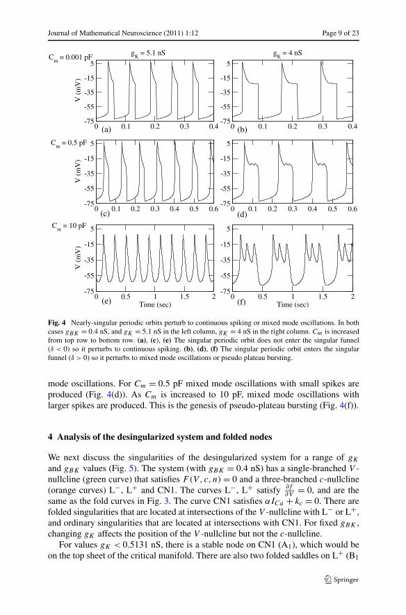
When Cm > 0 the full system (Eqs. (2.1)-(2.3)) produces spiking for δ < 0 andmixed mode oscillations for δ > 0. Figure 4 shows these two different cases forgBK = 0.4 nS. For gK = 5.1 nS (δ < 0 in Fig. 3(a)), the nearly-singular periodicorbit produced when Cm = 0.001 pF (Fig. 4(a)) perturbs to continuous spiking whenCm = 10 pF (Fig. 4(e)). When gK = 4 nS the singular periodic orbit enters the singu-lar funnel (Fig. 3(b)), so when Cm is increased the singular orbit transforms to mixed


Fig. 4 Nearly-singular periodic orbits perturb to continuous spiking or mixed mode oscillations. In bothcases gBK = 0.4 nS, and gK = 5.1 nS in the left column, gK = 4 nS in the right column. Cm is increasedfrom top row to bottom row. (a), (c), (e) The singular periodic orbit does not enter the singular funnel(δ < 0) so it perturbs to continuous spiking. (b), (d), (f) The singular periodic orbit enters the singularfunnel (δ > 0) so it perturbs to mixed mode oscillations or pseudo plateau bursting.

mode oscillations. For Cm = 0.5 pF mixed mode oscillations with small spikes areproduced (Fig. 4(d)). As Cm is increased to 10 pF, mixed mode oscillations withlarger spikes are produced. This is the genesis of pseudo-plateau bursting (Fig. 4(f)).

4 Analysis of the desingularized system and folded nodes

We next discuss the singularities of the desingularized system for a range of gK

and gBK values (Fig. 5). The system (with gBK = 0.4 nS) has a single-branched V -nullcline (green curve) that satisfies F(V, c,n) = 0 and a three-branched c-nullcline(orange curves) L−, L+ and CN1. The curves L−, L+ satisfy ∂f

∂V= 0, and are the

same as the fold curves in Fig. 3. The curve CN1 satisfies αICa + kc = 0. There arefolded singularities that are located at intersections of the V -nullcline with L− or L+,and ordinary singularities that are located at intersections with CN1. For fixed gBK ,changing gK affects the position of the V -nullcline but not the c-nullcline.

For values gK < 0.5131 nS, there is a stable node on CN1 (A1), which would beon the top sheet of the critical manifold. There are also two folded saddles on L+ (B1

of 23 Teka et al.

Fig. 5 V -nullclines (green), the three-branched c-nullcline (orange), and singularities for gBK = 0.4 nSand different values of gK (units in nS). Filled circles represent stable singularities and unfilled circlesrepresent unstable singularities. Red circles (filled or unfilled) are ordinary singularities. Filled and unfilledcircles in blue are folded nodes and folded saddles, respectively. Filled circles in cyan are folded foci. Thepoints TR1 and TR2 are transcritical bifurcations (type II folded saddle-node bifurcations) and SN1 andSN2 are standard saddle-node bifurcations (type I folded saddle-node bifurcations).

and C1) and two folded foci on L− (D1 and E1). When gK is increased to 0.5131 nSthe stable node A1 moves down and to the left and the folded saddle B1 moves to theleft. These two equilibria coalesce at a transcritical bifurcation (TR1). This transcrit-ical bifurcation corresponds to a bifurcation of folded singularities called a type IIfolded saddle-node [22, 30, 33]. Following this bifurcation, the folded singularity isa folded node. For gK = 4 nS, the equilibria on L+ are the folded node (B3) and thefolded saddle (C3). The equilibrium on CN1 (A3) is now a saddle point. There is noqualitative change of equilibria on L−.

When gK is increased to 7.588 nS the equilibria B3 and C3 coalesce at a saddle-node bifurcation point (SN1). This is a standard saddle-node bifurcation of foldedsingularities and is called a type I folded saddle-node [22, 30, 33]. As gK is increasedto 43.1 nS, the folded focus D5 moves to the left and changes to a folded node at D6.The saddle points on CN1 move downward and to the left as gK is increased. ForgK = 129.2 nS, the saddle point A6 coalesces with the fold node D6 at a secondtranscritical bifurcation (TR2); again a type II folded saddle-node. Beyond this, theordinary singularity (A8,A9) is stable and the folded singularity becomes a foldedsaddle. Moreover the folded focus E6 has become a folded node (E7). As gK is in-


creased further to 137.2 nS, there is a second type I saddle-node bifurcation (SN2) atwhich the folded node and the folded saddle coalesce and disappear. For the valuesgK > 137.2 nS, the only equilibrium is on CN1 and is an ordinary stable node (A9).This is on the bottom sheet of the critical manifold.

Varying gBK slightly affects the V -nullcline and strongly affects the c-nullclinein the (c,V )-phase plane. Increasing gBK moves the fold curves together, eventuallytaking the fold out of the critical manifold. Figure 6 shows qualitative changes in theequilibria when gBK is varied, with gK = 7.588 nS. When gBK = 0.2 nS there isa saddle point on CN1 (A) and two folded foci (D and E) on L− (Fig. 6(a)). WhengBK is increased to 0.4 nS, the curve L+ moves down and a type I folded saddle-nodebifurcation occurs (SN1 in Fig. 6(b)). When gBK is increased further, the saddle-nodesplits into a folded node (B) and a folded saddle (C) on L+, as shown for gBK = 1nS in Fig. 6(c).

The folded node (B) and the saddle point (A) coalesce at a transcritical bifurcation(type II folded saddle-node) when gBK = 3.96 nS (TR1 in Fig. 6(d)). Beyond this,the ordinary singularity (A) is a stable node that lies on the top sheet of the criti-cal manifold. When gBK = 20 nS the folded singularities are either saddles or foci,Fig. 6(e). For gBK ≈ 32.12 nS the two folded foci on L− change to folded nodes.Finally, when gBK is increased to 32.1224 nS, the fold curves L+ and L− merge. Asa result, the folded saddles coalesce with the folded nodes at type I folded saddle-node bifurcations (SN3 and SN4 in Fig. 6(f)). Beyond this, there is only a stablenode (A in Fig. 6(g)). The disappearance of the L+ and L− curves correspond to thedisappearance of the fold in the critical manifold.

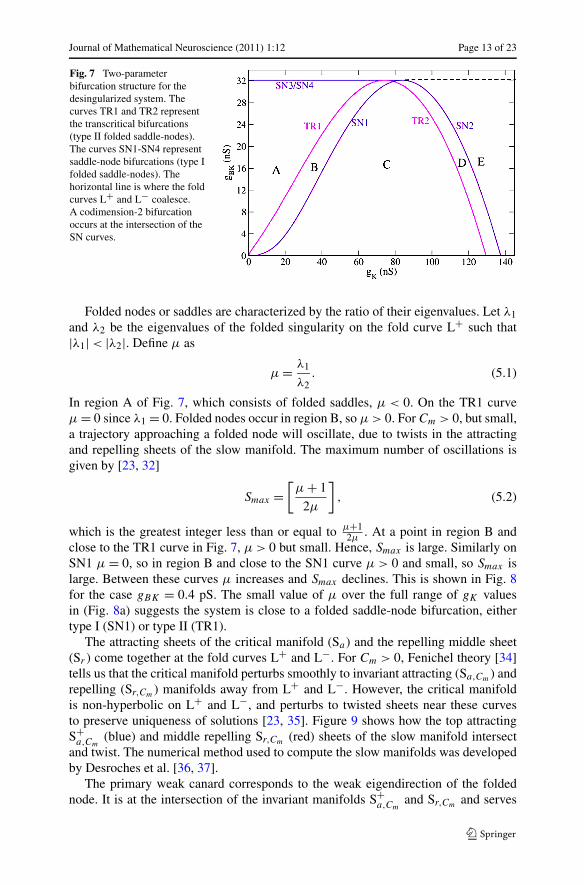
The two-parameter bifurcation diagram in Fig. 7 summarizes the variations of thebifurcations in Fig. 5 and Fig. 6 over a range of gK and gBK values. The curvesTR1 and TR2 correspond to the transcritical bifurcations (type II folded saddle-nodebifurcations), and SN1-SN4 correspond to the saddle-node bifurcations (type I foldedsaddle-node bifurcations). At gBK = 32.1224 nS the L+ and L− lines coalesce intoa single line. This contains the SN3 and SN4 bifurcations, up until SN3 and SN4coalesce at a codimension-2 bifurcation (for gK = 83.7122 nS). For large gK , theL+/L− line contains no folded singularities (dashed line).

For gK and gBK values in regions A, D and E there is only a stable node and thefull system is in a depolarized (A) or hyperpolarized (D or E) steady state. In the leftportion of region C there is a folded focus which becomes a folded node in the rightportion of C. This family of folded singularities is on L−. In region D there is a foldednode on L− for negative values of c. Region B consists of the folded nodes on L+,and it is the key region for the existence of mixed mode oscillations, since δ > 0 formuch of this region (shown below).

5 Twisted slow manifolds and secondary canards

The folded nodes discussed above are important since they yield small oscillations(for Cm > 0) in all trajectories entering the singular funnel. In this section we explainthe genesis of those oscillations (for more details, see [22, 23, 28, 32]).

of 23 Teka et al.

Fig. 6 V -nullclines (green), c-nullclines (orange) and ordinary and folded singularities for a range of gBK

values with gK = 7.588 nS. (a) gBK = 0.2 nS, (b) gBK = 0.4 nS, (c) gBK = 1 nS, (d) gBK = 3.96 nS,(e) gBK = 20 nS, (f) gBK = 32.1224 nS, and (g) gBK = 32.2 nS. The color convention for equilibria isas in Fig. 5.


Fig. 7 Two-parameterbifurcation structure for thedesingularized system. Thecurves TR1 and TR2 representthe transcritical bifurcations(type II folded saddle-nodes).The curves SN1-SN4 representsaddle-node bifurcations (type Ifolded saddle-nodes). Thehorizontal line is where the foldcurves L+ and L− coalesce.A codimension-2 bifurcationoccurs at the intersection of theSN curves.

Folded nodes or saddles are characterized by the ratio of their eigenvalues. Let λ1and λ2 be the eigenvalues of the folded singularity on the fold curve L+ such that|λ1| < |λ2|. Define μ as

μ = λ1

λ2. (5.1)

In region A of Fig. 7, which consists of folded saddles, μ < 0. On the TR1 curveμ = 0 since λ1 = 0. Folded nodes occur in region B, so μ > 0. For Cm > 0, but small,a trajectory approaching a folded node will oscillate, due to twists in the attractingand repelling sheets of the slow manifold. The maximum number of oscillations isgiven by [23, 32]

Smax =[μ + 1

2μ

], (5.2)

which is the greatest integer less than or equal to μ+12μ

. At a point in region B andclose to the TR1 curve in Fig. 7, μ > 0 but small. Hence, Smax is large. Similarly onSN1 μ = 0, so in region B and close to the SN1 curve μ > 0 and small, so Smax islarge. Between these curves μ increases and Smax declines. This is shown in Fig. 8for the case gBK = 0.4 pS. The small value of μ over the full range of gK valuesin (Fig. 8a) suggests the system is close to a folded saddle-node bifurcation, eithertype I (SN1) or type II (TR1).

The attracting sheets of the critical manifold (Sa) and the repelling middle sheet(Sr ) come together at the fold curves L+ and L−. For Cm > 0, Fenichel theory [34]tells us that the critical manifold perturbs smoothly to invariant attracting (Sa,Cm ) andrepelling (Sr,Cm ) manifolds away from L+ and L−. However, the critical manifoldis non-hyperbolic on L+ and L−, and perturbs to twisted sheets near these curvesto preserve uniqueness of solutions [23, 35]. Figure 9 shows how the top attractingS+

a,Cm(blue) and middle repelling Sr,Cm (red) sheets of the slow manifold intersect

and twist. The numerical method used to compute the slow manifolds was developedby Desroches et al. [36, 37].

The primary weak canard corresponds to the weak eigendirection of the foldednode. It is at the intersection of the invariant manifolds S+

a,Cmand Sr,Cm and serves

of 23 Teka et al.

Fig. 8 The effects of varying gK on the eigenvalue ratio (μ) and the maximum number of oscillations(Smax ) for gBK = 0.4 nS. (a) μ = 0 at TR1 and SN1. (b) Smax is largest near the bifurcation points.

Fig. 9 A portion of the twisted slow manifold for Cm = 2 pF, gK = 4 nS and gBK = 0.4 nS. The topattracting (S+

a,Cm, blue surface) and middle repelling (Sr,Cm , red surface) sheets of the slow manifold

are twisted around the blue dashed curve, which is the axis of rotation. The primary strong canard (SC,green) moves from the attracting to the repelling sheet without any rotations. The secondary canards ξ1(gray curve, one rotation), ξ2 (purple curve, two rotations) and ξ3 (gold curve, three rotations) flow fromthe attracting to repelling sheet with different numbers of rotations. A portion of the pseudo-plateau bursttrajectory (PPB, black curve) is superimposed and has two small oscillations. The full system has unstableequilibrium (cyan, filled curcle).

as their axis of rotation. All other canards twist about the primary weak canard; theyfollow S+

a,Cmas it twists and then follow Sr,Cm for a distance as it twists. The primary

strong canard, which corresponds to the strong eigendirection of the folded node,moves along S+

a,Cmto Sr,Cm without any rotation (SC, green curve in Fig. 9). Other,

secondary, canards rotate a number of times, depending on how close they are to


Fig. 10 (a) Pseudo-plateau burst trajectories are projected onto the (c,V )-plane for gK = 4 nS andgBK = 0.4 nS, and different values of Cm. Key structures from the desingularized system are also shown.WED (pink curve) is the line tangent to the weak eigendirection of the folded node. (b) Magnification ofpanel (a) in the vicinity of the weak eigendirection and fold curve L+.

the primary strong canard. A secondary canard that makes k small rotations in thevicinity of the folded node is called the kth secondary canard. Figure 9 shows thefirst (ξ1, gray), second (ξ2, purple) and third (ξ3, olive) secondary canards that makeone, two and three rotations, respectively. For Cm > 0, but small, there are Smax − 1secondary canards which divide the funnel region between the primary canards intoSmax subsectors [24]. The first subsector is bounded by the strong canard SC and thefirst secondary canard ξ1 and trajectories entering here have one rotation. The secondsubsector is bounded by ξ1 and ξ2 and trajectories entering here have two rotations.The last subsector is bounded by the last secondary canard and the primary weakcanard. The maximal rotation number is achieved in the last subsector; trajectoriesentering here have Smax rotations [23, 28, 32].

Figure 9 also shows a portion of the pseudo-plateau burst trajectory (PPB, blackcurve) for Cm = 2 pF. It enters the funnel region in the rotational subsector boundedby ξ1 and ξ2, and hence, makes two full rotations and then leaves the repelling sheetas it moves towards the lower attracting manifold S−

a,Cm. These rotations are the small

oscillations or “spikes” during the burst active phase.Figure 10(a) shows burst trajectories for three values of Cm projected onto the

(c,V )-plane. Also shown are L+, L−, the singular strong canard SC and the foldednode of the desingularized system. Finally, the line along the weak eigendirection ofthe folded node is included (WED, pink curve). With Cm = 0.001 pF the system isnearly singular and the “bursting” trajectory enters and leaves the folded node alongthe WED. The small oscillations near the folded node are too small to see. The regionnear the folded node is magnified in Fig. 10(b). With Cm = 0.1 pF the burst trajectoryagain passes through the folded node along the WED, but now the small oscillations

of 23 Teka et al.

Fig. 11 (a) Mixed mode oscillation borders for Cm → 0. The region of mixed mode oscillations (MMOs)is bounded by the two curves TR1 and δ = 0. Steady state and spiking solutions occur to the left of theTR1 curve and to the right of the δ = 0 curve, respectively. (b) Magnification of panel (a) for a smallerrange of values of gK and gBK .

are visible in Fig. 10(b). The small oscillations of this burst trajectory first decreaseand then increase in amplitude. This is often seen in mixed mode oscillations thatare associated with a folded node singularity, in contrast to those associated with asingular Hopf bifurcation, where the amplitude of successive small oscillations in-creases [38]. Finally, with Cm = 2 pF (the value used in Fig. 9) the small oscillationsare prominent even in the larger vertical scale used in Fig. 10(a).

6 The boundaries of mixed mode oscillations

For a periodic mixed mode oscillation (i.e., pseudo-plateau bursting) solution to exist,there must be a folded node singularity and the periodic orbit must enter the funnel.In this section we construct curves in the two-parameter gK -gBK plane that formboundaries for the existence of mixed mode oscillations.

From Fig. 7 we know that folded node singularities only occur in regions B and C(and in region D for negative values of the Ca2+ concentration). Those in region Coccur on L− and the periodic orbit never enters the corresponding singular funnel. Wetherefore focus on region B. This region is highlighted in Fig. 11(a). Above the TR1curve the system has a depolarized stable steady state. Below the SN1 curve the sys-tem spikes continuously. Between these curves a folded node singularity exists, andthe requirement for periodic mixed mode oscillations is that δ > 0. That is, the sin-gular orbit must enter the singular funnel. Thus, the final curve delimiting the MMOsregion is δ = 0 (the set of gK and gBK values at which the singular periodic orbitintersects both the strong canard and the curve P(L−)), shown in green in Fig. 11.For parameter values between the δ = 0 and TR1 curves periodic mixed mode os-cillations, i.e., pseudo-plateau bursting, exist and are stable. This critical region ismagnified in Fig. 11(b).

Figure 12 shows how the burst duration and the number of spikes in a burst varyover a range of gK and gBK values for Cm = 5 pF. A similar map of parameterspace was used previously in the analysis of a parabolic burster [39]. Two-parameter


Fig. 12 The active phase duration and the number of spikes per burst of the full system for Cm = 5 pF.The system displays steady state, spiking or bursting solutions. Steady state and spiking solutions arerepresented by black dots and small black circles, respectively. The bursting region is bounded by thesupercritical Hopf bifurcation (HB, black) and the right branch of the period doubling (PD, green) curves.The bursting patterns in this region are represented by colored circles. The size of a circle represents theactive phase duration, with larger circles corresponding to longer active phase durations. The color of acircle represents the number of spikes per burst. Cyan circles correspond to smaller number of spikes perburst (minimum of two spikes) and the largest dark red circle corresponds to the largest number of spikeper burst (36 spikes in a burst).

bifurcation curves of the full system (Eqs. (2.1)-(2.3)) are also shown. These includea curve of supercritical Hopf bifurcations (HB, black) and a curve of period doublings(PD, green). To the left of the HB curve the system is at a steady state (black dots), andto the right of and above the PD curve the system produces continues spiking (smallblack circles). For the values of gK and gBK inside the PD curve the system producespseudo-plateau bursting oscillations (MMOs), represented by colored circles.

In the bursting region the active phase duration and the number of spike per burstvary with respect to the values of gK and gBK . The size of each circle represents theactive phase duration, and the color of the circle (from cyan to dark red) representsthe number of spikes in a burst. A burst with larger number of spikes has longeractive phase duration, and in an actual cell this determines the amount of Ca2+ influxand hormone released. The bursts that have the shorter active phase duration and thesmaller number of spikes occur near the right branch of the PD curve. These burstsare represented by smaller cyan circles in Fig. 12. For example, when gBK = 1 nSand gK = 6 nS the system produces bursting oscillations with three spikes per burst(as in Fig. 4(f)). When one moves away from the right to the left branch of the PDcurve by increasing gBK or decreasing gK the burst duration becomes longer andthe number of spikes in a burst becomes larger. The longest active phase duration isabout 8.4 sec and the largest number of spikes per burst is about 36, represented bythe largest dark red circle. These values will change when Cm is changed.

The region between the HB and the left branch of the PD curves is bistable be-tween bursting and continuous spiking. Orange circles with small black circles at thecenters represent bistable solutions that are simulated by varying the initial condi-

of 23 Teka et al.

tions. This shows that the borders of the bursting region are the HB and the rightbranch of the PD curves. The dark blue circles represent bursting oscillations withoutsmall oscillations since the amplitudes of the spikes are almost zero, i.e., the smalloscillations are too small to see.

The results that are shown in Fig. 12 are very consistent with the analysis of themixed mode oscillations in Fig. 11. The HB and TR1 curves overlap, demonstratingthat for small Cm the HB of the full system corresponds to a type II saddle-nodebifurcation of the desingularized system. Also, the HB curve and the left branch ofthe PD curve are almost indistinguishable for small Cm. For these Cm values (Cm <

0.001 pF), the right branch of the PD curve converges to the δ = 0 curve of thedesingularized system. Hence, the left and right borders of the MMOs in the singularlimit Cm → 0 pF correspond to the left and right borders of the bursting region ofthe full system for Cm > 0, with the exception that the bursting region is smaller forlarger values of Cm. Also, the bistable region between the PD and HB curves onlyexists as the left PD moves away from the HB, which occurs as Cm is increased.

In Fig. 11 the MMOs region delimited by the TR1 and δ = 0 curves can be dividedinto subregions that have different numbers of small oscillations. For parameter val-ues in the subregion near the curve δ = 0 the periodic orbit enters the funnel regionnear the strong (primary) canard. This subregion corresponds to the first subsectorof the funnel region, and for Cm > 0 only one small oscillation occurs in a burst.This corresponds to the jump from the lower attracting sheet to the upper attractingsheet and is not due to the folded node. When one moves leftward by decreasing gK ,δ increases and the periodic orbit enters the funnel region through other subsectors.As a result, the number of small oscillations in a burst increases. When one movesto the subregion near or on the TR1 curve by decreasing gK further, the periodicorbit enters the funnel region through the last subsector. The number of small oscil-lations is closer to Smax , the maximum number of spikes in a burst as determinedby the eigenvalues of the folded node. Moreover, increasing gBK has the same effectas decreasing gK . These trends in the number of small oscillations obtained from ananalysis of the desingularized system [28] are expressed far from the singular limit asshown in Fig. 12 where Cm = 5 pF. Here the longest bursts occur near the HB curves,as predicted.

7 A comparison with a two-fast/one-slow variable analysis

Using a one-fast/two-slow variable analysis we have shown the genesis of the spikesin a burst and how the number of spikes in a burst varies in the gK -gBK parameterspace. The regions for steady states, pseudo-plateau bursting (mixed mode oscilla-tions) and spiking are clearly identified in this parameter space (Fig. 11). This hasbeen done by investigating the qualitative changes of the desingularized system whenparameters gK (Fig. 5) and gBK (Fig. 6) are varied, which are summarized in Fig. 7.

Here we investigate whether this information can be obtained from a standard two-fast/one-slow variable analysis. Figure 13(a) shows a bifurcation diagram of the V -nfast subsystem with c treated as a parameter (referred to as a “z-curve”). The subsys-tem is bistable over a large range of c values, with stable depolarized and hyperpolar-ized steady states, separated by saddle points. The c-nullcline is superimposed, now


Fig. 13 Two-fast/one-slow analysis for gBK = 0.4 nS, Cm = 10 pF and different values of gK . The black“z-curve” is the curve of equilibria of the V -n fast subsystem. This has stable (solid) and unstable (dashed)branches. (a) gK = 0.1 nS, the full system with stable equilibrium (A1) is in a depolarized steady state.(b) gK = 4 nS, the fast subsystem has an unstable limit cycle that emerges from the subcritical Hopf bifur-cation (subHB). Pseudo-plateau bursting (PPB, black trajectory) is produced. The equilibrium of the fullsystem (A3) is unstable. (c) gK = 5.1 nS, the full system produces periodic spiking that appears unrelatedto the fast subsystem bifurcation structure. The equilibrium point of the full system (A) is unstable. In allpanels the system is bistable over a range of c-values. The points A1 and A3 are the same equilibriumpoints as A1 and A3 in Fig. 5, respectively.

thinking of c as a slowly-changing variable rather than as a parameter. This is thestandard approach used in a two-fast/one-slow variable analysis. In all three panelsof Fig. 13 parameters are set at gBK = 0.4 nS, Cm = 10 pF, and gK is varied.

In Fig. 13(a), with gK = 0.1 nS, there is an intersection of the c-nullcline onthe upper stable branch at location A1. This is a stable equilibrium of the full 3-dimensional system, and corresponds to A1 in the analysis shown in Fig. 5. Thus,

of 23 Teka et al.

both types of analysis indicate that the system will come to rest at a depolarizedsteady state when gK = 0.1 nS.

When gK is increased there is a subcritical Hopf bifurcation on the upper branchwith emergent unstable periodic solutions of the fast-subsystem. This is shown inFig. 13(b) for the case gK = 4 nS. Pseudo-plateau bursting occurs for this and nearbyvalues of gK . The full system unstable equilibrium (A3) corresponds to A3 in Fig. 5.

The superimposed burst trajectory in Fig. 13(b) only weakly follows the fast-subsystem bifurcation diagram. Most notably, there are no stable periodic solutionsof the fast subsystem, only bistability between two steady states. Also, the trajec-tory never follows the lower branch of stationary solutions and greatly overshoots thelower knee.

The subcritical Hopf bifurcation migrates leftward when gK is increased to 5.1 nS.The unstable branch of periodics goes through a saddle-node bifurcation, yielding abranch of stable periodic solutions of the fast subsystem (Fig. 13(c)). There is bista-bility between upper and lower branches of the z-curve which is typically a necessarycondition for bursting with this type of analysis. However, bursting is not producedfor this value of gK . Instead, the system spikes continuously.

This example illustrates that features well described by the one-fast/two-slow vari-able analysis are not at all well described by a standard two-fast/one-slow variableanalysis. Most notably, the transition from bursting to spiking is well characterized inthe one-fast/two-slow variable analysis as the point at which δ = 0. Note that this isnot a bifurcation point of the desingularized system, but reflects the jump point fromthe lower sheet of the slow manifold to the upper sheet. In contrast, the bursting tospiking transition is not predicted from the two-fast/one-slow analysis, and indeed theperiodic spiking trajectory of the full system occurs over a range of the fast-subsystembifurcation diagram that contains only stable equilibria. The one-fast/two-slow ap-proximation is good even at higher values of Cm, for example, when Cm = 5 pF(Fig. 12). Similar remarks apply for smaller values of Cm, where the one-fast/two-slow approximation becomes more accurate while the two-fast/one-slow approxima-tion does not. The two-fast/one-slow approximation becomes more accurate when c

is much slower than both V and n, but in this case only a stable steady solution or arelaxation oscillation is produced.

8 Discussion

The canard mechanism has been used to understand mixed mode oscillations in sev-eral neuronal models [30, 37, 40–44]. In these examples, the small oscillations cor-respond to subthreshold oscillations that occur between the electrical impulses. Wehave previously analyzed pseudo-plateau bursting in a pituitary lactotroph model us-ing canard theory [28]. However, the model used was a simplification in which thecytosolic free Ca2+ concentration was treated as a fixed parameter and the secondslow variable (in addition to the variable n used here) was an inactivation variablefor an A-type K+ current. In the current paper, we again focused on pseudo-plateaubursting in a pituitary lactotroph model, but now with emphasis on a BK-type K+current. In this analysis, we have examined the effects of changing the parameters


Cm, gK and gBK . The parameter gBK is important for producing bursting oscilla-tions in actual pituitary cells in which bursting is converted to spiking when BK-typeK+ channels are blocked [45].

Here, using Cm to control the separation in time scales, we identified two slowvariables (n, c) and one fast variable (V ). Using the one-fast/two-slow variable anal-ysis we showed that pseudo-plateau bursting is a canard-induced mixed mode oscilla-tion. There are two main requirements for the existence of these bursting oscillations[22–24, 32]. One is that the desingularized system must have a folded node singular-ity, i.e., the eigenvalue ratio (μ) has to be positive. The second requirement is that thesingular periodic orbit should enter the singular funnel and pass through the foldednode, i.e., δ should be positive. In short, canard-induced mixed mode oscillationsexist if both μ and δ are positive.

Using this technique we can understand several features of the burst and severaltrends that occur as parameters are varied. When both μ and δ are positive, smalloscillations are produced during the active phase of a burst and their amplitude isproportional to

√Cm for Cm sufficiently small [23]. We obtained the bursting borders

in the (gK,gBK)-plane (Figs. 11 and 12), and predicted how the active phase durationand the number of spikes per burst vary with changes in parameters.

The singular perturbation analysis performed here is technically more effectiveand informative in the singular limit (i.e., for sufficiently small values of Cm) [22,23]. However, it provides useful information even far from this limit, as we showedin Figs. 11 and 12. Eventually, as the singular parameter (Cm) is increased suffi-ciently, new dynamics will be introduced, and the insights from the singular analysisare no longer valid.

The one-fast/two-slow decomposition used here contrasts with the two-fast/one-slow variable analysis used previously for pseudo-plateau bursting [10–13]. Our anal-ysis explains the origin of the small-amplitude spikes that occur during the activephase of pseudo-plateau bursting, the transition between spiking and bursting, andinformation about how the number of spikes per burst varies with parameters. Whilethe two-fast/one-slow variable analysis provides little information on these things,it does provide valuable information about how one can make a transition betweenplateau and pseudo-plateau bursting as one or more parameters are changed [12]. Italso provides information about complex phase resetting properties [11] and the ter-mination of spikes in a burst [17]. Both fast/slow decompositions are approximations,however, to a system that evolves on three time scales. Some studies [13, 17, 18] fo-cus on the dynamics of the full system, and illustrate the complexity of the seeminglysimple set of equations. The advantage of obtaining useful information of the full sys-tem by a two-fast/one-slow or one-fast/two-slow decomposition points to the fact thatsystem (2.1)-(2.3) actually evolves on three time scales: V fast, n intermediate and c

slow. This can also be seen by the magnitude of μ which is bounded from above byμmax ≈ 0.07 (Fig. 8(a)). Hence, we are close to folded saddle-node regimes (type Iand type II) [33, 38] and a more detailed bifurcation analysis may explain the relationbetween the two-fast/one-slow and one-fast/two-slow splitting. This is left for futurework.

of 23 Teka et al.

Competing interests

The authors declare that they have no competing interests.

Authors’ contributions

WT, JT, TV, MW, and RB performed the analysis. WT wrote the manuscript with assistance from JT, TV,MW, and RB. All authors read and approved the final manuscript.

Acknowledgements This work was supported by NSF grant DMS 0917664 to RB and NIH grant DK043200 to RB and JT.

References

1. Lisman, J.E.: Bursts as a unit of neural information: making unreliable synapses reliable. TrendsNeurosci. 20, 38–43 (1997)

2. Van Goor, F., Zivadinovic, D., Martinez-Fuentes, A.J., Stojilkovic, S.S.: Dependence of pituitary hor-mone secretion on the pattern of spontaneous voltage-gated calcium influx. Cell type-specific actionpotential secretion coupling. J. Biol. Chem. 276, 33840–33846 (2001)

3. Stojilkovic, S.S., Zemkova, H., Van Goor, F.: Biophysical basis of pituitary cell type-specific Ca2+signaling-secretion coupling. Trends Endocrinol. Metab. 16, 152–159 (2005)

4. Kuryshev, Y.A., Childs, G.V., Ritchie, A.K.: Corticotropin-releasing hormone stimulates Ca2+ entrythrough L- and P-type Ca2+ channels in rat corticotropes. Endocrinology 137, 2269–2277 (1996)

5. Tsaneva-Atanasova, K., Sherman, A., Van Goor, F., Stojilkovic, S.S.: Mechanism of spontaneous andreceptor-controlled electrical activity in pituitary somatotrophs: experiments and theory. J. Neuro-physiol. 98, 131–144 (2007)

6. Falke, L.C., Gillis, K.D., Pressel, D.M., Misler, S.: Perforated patch recording allows long-term mon-itoring of metabolite-induced electrical activity and voltage-dependent Ca2+ currents in pancreaticislet β cells. FEBS Lett. 251, 167–172 (1989)

7. Kinard, T., Vries, G.D., Sherman, A., Satin, L.S.: Modulation of the bursting properties of singlemouse pancreatic beta-cells by artificial conductances. Biophys. J. 76(3), 1423–1435 (1999)

8. Zhang, M., Goforth, P., Bertram, R., Sherman, A., Satin, L.: The Ca2+ dynamics of isolated mouseβ-cells and islets: implications for mathematical models. Biophys. J. 84, 2852–2870 (2003)

9. LeBeau, A.P., Robson, A.B., McKinnon, A.E., Sneyd, J.: Analysis of a reduced model of corticotrophaction potentials. J. Theor. Biol. 192, 319–339 (1998)

10. Tabak, J., Toporikova, N., Freeman, M.E., Bertram, R.: Low dose of dopamine may stimulate prolactinsecretion by increasing fast potassium currents. J. Comput. Neurosci. 22, 211–222 (2007)

11. Stern, J.V., Osinga, H.M., LeBeau, A., Sherman, A.: Resetting behavior in a model of bursting insecretory pituitary cells: distinguishing plateaus from pseudo-plateaus. Bull. Math. Biol. 70, 68–88(2008)

12. Teka, W., Tsaneva-Atanasova, K., Bertram, R., Tabak, J.: From plateau to pseudo-plateau bursting:making the transition. Bull. Math. Biol. 73(6), 1292–1311 (2011)

13. Tsaneva-Atanasova, K., Osinga, H.M., Riess, T., Sherman, A.: Full system bifurcation analysis ofendocrine bursting models. J. Theor. Biol. 264, 1133–1146 (2010)

14. Safiulina, V.F., Zacchi, P., Taglialatela, M., Yaari, Y., Cherubini, E.: Low expression of Kv7/M chan-nels facilitates intrinsic and network bursting in the developing rat hippocampus. J. Physiol. 586(22),5437–5453 (2008)

15. Rinzel, J.: A formal classification of bursting mechanisms in excitable systems. In: Teramoto, E.,Yamaguti, M. (eds.) Mathematical Topics in Population Biology, Morphogenesis, and Neurosciences.Lecture Notes in Biomathematics, pp. 267–281. Springer, Berlin (1987)

16. Rinzel, J., Ermentrout, G.B.: Analysis of neural excitability and oscillations. In: Koch, C., Segev, I.(eds.) Methods in Neuronal Modeling: From Synapses to Networks, 2nd edn, pp. 251–292. MIT Press,Cambridge, MA (1998)


17. Nowacki, J., Mazlan, S., Osinga, H.M., Tsaneva-Atanasova, K.: The role of large-conductancecalcium-activated K+ (BK) channels in shaping bursting oscillations of a somatotroph cell model.Physica D 239, 485–493 (2010)

18. Osinga, H.M., Tsaneva-Atanasova, K.: Dynamics of plateau bursting depending on the location of itsequilibrium. J. Neuroendocrinol. 22(12), 1301–1314 (2010)

19. Bertram, R., Sherman, A.: Negative calcium feedback: the road from Chay-Keizer. In: Coombes, S.,Bressloff, P. (eds.) The Genesis of Rhythm in the Nervous System, pp. 19–48. World Scientific, NewJersey (2005)

20. Butera, R.J., Rinzel, J., Smith, J.C.: Models of respiratory rhythm generation in the pre-Bötzingercomplex. I. Bursting pacemaker neurons. J. Neurophysiol. 82, 382–397 (1999)

21. Del Negro, C.A., Hsiao, C.F., Chandler, S.H.: Outward currents influencing bursting dynamics inguinea pig trigeminal motoneurons. J. Neurophysiol. 81(4), 1478–1485 (1999)

22. Szmolyan, P., Wechselberger, M.: Canards in R3. J. Differ. Equ. 177, 419–453 (2001)

23. Wechselberger, M.: Existence and bifurcation of canards in R3 in the case of a folded node. SIAM J.

Appl. Dyn. Syst. 4, 101–139 (2005)24. Brøns, M., Krupa, M., Wechselberger, M.: Mixed mode oscillations due to the generalized canard

phenomenon. Fields Inst. Commun. 49, 39–63 (2006)25. Desroches, M., Guckenheimer, J., Krauskopf, B., Kuehn, C., Osinga, H., Wechselberger, M.: Mixed-

mode oscillatons with multiple time-scales. SIAM Rev. (2011, in press)26. Ermentrout, B.: Simulating, Analyzing, and Animating Dynamical Systems: A Guide to XPPAUT for

Researchers and Students. SIAM, Philadelphia (2002)27. Doedel, E.J., Champneys, A.R., Fairgrieve, T.F., Kuznetsov, Y.A., Oldeman, K.E., Paffenroth, R.C.,

Sandstede, B., Wang, X.J., Zhang, C.: AUTO-07P:: Continuation and bifurcation software for ordinarydifferential equations. http://cmvl.cs.concordia.ca/ (2007)

28. Vo, T., Bertram, R., Tabak, J., Wechselberger, M.: Mixed mode oscillations as a mechanism forpseudo-plateau bursting. J. Comput. Neurosci. 28, 443–458 (2010)

29. Wechselberger, M.: A propos de canards (apropos canards). American Mathematical Society (2011,in press)

30. Rubin, J., Wechselberger, M.: Giant squid-hidden canard: the 3D geometry of the Hodgkin-Huxleymodel. Biol. Cybern. 97, 5–32 (2007)

31. Szmolyan, P., Wechselberger, M.: Relaxation oscillations in R3. J. Differ. Equ. 200, 69–104 (2004)

32. Rubin, J., Wechselberger, M.: The selection of mixed-mode oscillations in a Hodgkin-Huxley modelwith multiple timescales. Chaos 18, 015105 (2008)

33. Krupa, M., Wechselberger, M.: Local analysis near a folded saddle-node singularity. J. Differ. Equ.248(12), 2841–2888 (2010)

34. Fenichel, N.: Geometric singular perturbation theory. J. Differ. Equ. 31, 53–98 (1979)35. Guckenheimer, J., Haiduc, R.: Canards at folded nodes. Mosc. Math. J. 5, 91–103 (2005)36. Desroches, M., Krauskopf, B., Osinga, H.M.: The geometry of slow manifolds near a folded node.

SIAM J. Appl. Dyn. Syst. 7(4), 1131–1162 (2008)37. Desroches, M., Krauskopf, B., Osinga, H.M.: Mixed-mode oscillations and slow manifolds in the

self-coupled FitzHugh-Nagumo system. Chaos 18, 015107 (2008)38. Guckenheimer, J.: Singular Hopf bifurcation in systems with two slow variables. SIAM J. Appl. Dyn.

Syst. 7(4), 1355–1377 (2008)39. Guckenheimer, J., Gueron, S., Harriswarrick, R.M.: Mapping the dynamics of a bursting neuron.

Philos. Trans. R. Soc. Lond. B, Biol. Sci. 341(1298), 345–359 (1993)40. Guckenheimer, J., HarrisWarrick, R., Peck, J., Willms, A.: Bifurcation, bursting, and spike frequency

adaptation. J. Comput. Neurosci. 4(3), 257–277 (1997)41. Brøns, M., Kaper, T.J., Rotstein, H.G.: Introduction to focus issue: mixed mode oscillations: experi-

ment, computation, and analysis. Chaos 18, 015101 (2008)42. Erchova, I., McGonigle, D.J.: Rhythms of the brain: An examination of mixed mode oscillation ap-

proaches to the analysis of neurophysiological data. Chaos 18, 015115 (2008)43. Rotstein, H.G., Wechselberger, M., Kopell, N.: Canard Induced mixed-mode oscillations in a medial

entorhinal cortex Layer II Stellate Cell Model. SIAM J. Appl. Dyn. Syst. 7(4), 1582–1611 (2008)44. Ermentrout, B., Wechselberger, M.: Canards, clusters, and synchronization in a weakly coupled in-

terneuron model. SIAM J. Appl. Dyn. Syst. 8, 253–278 (2009)45. Van Goor, F., Li, Y.X., Stojilkovic, S.S.: Paradoxical role of large-conductance calcium-activated K+

(BK) channels in controlling action potential-driven Ca2+ entry in anterior pituitary cells. J. Neurosci.21, 5902–5915 (2001)

http://cmvl.cs.concordia.ca/

The dynamics underlying pseudo-plateau bursting in a pituitary cell model

Documents

Transcript of The dynamics underlying pseudo-plateau bursting in a pituitary cell model