Decision Making 1

The Dynamic Interactions between Situations and Decisions

Jerome R. Busemeyer, Ryan K. Jessup, & Eric Dimperio

Indiana University

May 19, 2006

To appear in

Robbins, P. & Aydede, M. (Eds) Cambridge Handbook of Situated Cognition. Cambridge University Press.

Send Correspondence to:

Jerome R. Busemeyer Indiana University 1101 E. 10th St. Bloomington IN 47405 jbusemey@indiana.edu

Decision Making 2

The majority of judgment and decision making research is based on laboratory

experiments using very simple and artificial stimulus conditions. Eliciting preferences

between simple gambles of the form ‘get $x with probability p, otherwise $y’ is the

primary basis on which rational principles of decision making are tested (Goldstein &

Weber, 1995). The foundation of modern decision theories (see Luce, 2000), are built on

findings from these simple gambling paradigms. These laboratory experiments are quite

far removed from real-life decisions, nevertheless, many of the findings do generalize to

real world applications (Levin, Louviere, Schepanski, 1983). However, new empirical

phenomena and unique theoretical issues have surfaced by studying decision making in

more natural environments. One of the goals of this chapter is to review these new

findings and theoretical issues. A second goal is to examine more closely whether or not

theories built from simple laboratory experiments are capable of addressing these new

challenges.

1. Situated Decision Making

The term ‘situated cognition’ may be unfamiliar to many decision researchers, but

the ideas are not. Many decision researchers have considered, very seriously, the

importance of using realistic environments for the study of decision making. Decision

researchers have used terms such as ‘social judgment theory’ or ‘decision analysis’ or

‘naturalistic decision making’, which may be less familiar to cognitive scientists, to

describe their explorations into work in the area of situated cognition.

Social judgment theory (see Hammond, Stewart, Brehmer, & Steinmann, 1975) is

generally interested in understanding how experts form judgments based on cues

provided by the environment. For example, in an experimental study of highway safety

Decision Making 3

policies (Hammond, Hamm, Grassia, & Pearson, 1987), expert highway engineers were

asked to predict accident rates for highways described by scenarios (e.g., videos). The

scenarios were designed to manipulate 10 cues that were identified as essential by the

experts (e.g., highway size, traffic speed, traffic volume, etc.). Each scenario was

constructed by sampling a combination of cue values for the 10 cues. To estimate each

expert’s policy (i.e. the rule mapping cues to predictions), judgments were obtained from

each expert using 40 different highway scenarios. Statistical models (e.g., regressing the

judgments on the cue values) were then used to estimate the expert’s policy. From these

analyses one can determine the importance weight of each cue for making a judgment.

Research in social judgment theory is based on Egon Brunswick’s (1952)

concepts of representative design and ecological validity. A representative design is

achieved by sampling judgment situations by a method that preserves ecological validity;

ecological validity holds when the sample correlations between cues and the criterion

match the corresponding true correlations in the population. For example, highway size,

traffic speed, and traffic volume are correlated with each other and correlated with

accident rates in the real world, and these correlations should be reflected in sample

scenarios presented to the experts. Students of Brunswick reject the use of experimental

designs that create artificial and unnatural situations which break these correlations. For

example, although the use of uncorrelated cues (e.g., factorial designs) would facilitate

the statistical analysis of experts’ policies, this artificial design violates the naturally

occurring correlations among cues. According to Brunswick (and social judgment

researchers, see Dhami, Hertwig, & Hoffrage, 2004 for a recent review), tampering with

the naturally occurring environmental relations could destroy the phenomena under

Decision Making 4

investigation. Instead, judgment situations should be sampled in a representative fashion

so that the ecological validities of cues are maintained. In the above example of highway

safety judgments, a representative sampling of situations was achieved by designing cue

combinations that reproduced the true or natural inter-correlations and ecological

validities of cues for the population of highways under study.

The discovery of general principles of human judgment is a primary objective of

social judgment research. For example, in the highway safety study, researchers may be

interested in how the presentation format of the cues (abstract bar graphs vs. concrete

videos) generally affects the expert’s policies. Experimental methods are still preferred

over natural observation or field research for this purpose. However, the experiments are

designed so that both the stimuli (situations to be judged) and participants (judges) are

sampled in a way that represents the real world population of situations and people.

Decision analysis is concerned with the development of prescriptive methods for

improving difficult real-life decisions (Keeney & Raiffa, 1976; Clemens, 1996). A real-

life example (see Von Winterfeldt & Edwards, 1986) is a case in which an oil company

had to select a site to drill for oil. The basic principle is to divide and conquer – a

complex decision is broken down into small manageable parts, judgments are made with

respect to each part, and then these small parts are re-combined to form an overall

evaluation. Experts consult with decision analysts who help them form a representation

of the problem in terms of decision trees (actions and events over time). Then probability

estimates are elicited from the experts concerning the uncertain events on the branches of

the decision tree. The consequences of the actions along the branches of the trees are

decomposed into attributes, and each action is evaluated with respect to each attribute.

Decision Making 5

For example, on the one hand an oil site may have a large oil reserve, but on the other

hand it may be located in an environmentally protected region. Finally, a rational or

optimal rule, called the multi-attribute expected utility rule, is used to combine the

probabilities and values into a summary measure of utility.

Research in decision analysis is primarily concerned with the development and

testing of methods for representing decision scenarios, tools for estimating probabilities,

and techniques for eliciting value judgments. Decision support systems serve as

important external resources for decision makers – statistical analyses and computer

simulations are used to help estimate event probabilities; computer analyses are used to

provide instant feedback about expected utilities; sophisticated human computer

interfaces are used to help elicit judgments, facilitate group discussion, and communicate

results.

The most difficult and controversial aspect of this research is assessing the quality

of decisions produced by these methods (see Yates, 1990 ). One cannot simply rely on

the outcome of a single decision because of its probabilistic nature. A rational decision

process may yield an unfortunate outcome by chance. For example, a carefully selected

drilling site may nevertheless turn out to be a disaster because of an unpredictable

environmental event (e.g., a hurricane). Many important decisions, such as selecting a

drilling site, are made only once, which provide little opportunity to learn from

experience. There are no absolute criterion for identifying a ‘correct decision’ because

the decisions depend on personal beliefs and subjective values. Assessing decision

quality has been a long standing problem in the evaluation of decision analysis tools.

Two minimal criteria for evaluating decision quality are consistency and robustness – the

Decision Making 6

decision should not be affected by irrelevant changes in representation or by small

adjustments caused by minor judgment errors (Kaplan, 1996).

Naturalistic decision making refers to a research methodology for understanding

how actions are selected in dynamic, complex, real-life situations that involve high

stakes, a high degree of uncertainty, and high time pressure (Zsambok, & Klein, 1997).

For example, in a study of emergency decisions, researchers followed 30 expert

firefighting units to 126 emergency scenes and observed and recorded their activities;

they also intensively interviewed the command and control decision makers immediately

after the incidents (Klein, 1999). The findings from this field research indicated that

traditional decision theory provided little help in these types of decisions -- they are much

too complex and uncertain, and time is much too short to evaluate all the feasible actions.

Consequently, research on naturalistic decisions has uncovered some new views

of decision making (Lipshitz, Klein, Orasanu, & Salas, 2001). First, situation assessment

seems to be the most crucial component of the process for these types of decisions. Given

a situational assessment, the next most important process is option generation. In many

cases, following a situation assessment, the appropriate action is clear and immediate. In

these cases, the decision seems fairly obvious, so that there is very little in the way of

actual evaluation of alternative actions. This led Klein (1998) to propose what he calls the

recognition-primed decision model. According to this model, after completing a situation

assessment and developing a mental model of the situation, the decision maker generates

or retrieves an action that matches the assessed situation. Then this action is mentally

simulated to determine its feasibility and the possibility of failure to achieve the goal. If

the initially generated action is evaluated as acceptable (likely to succeed in achieving the

Decision Making 7

goal), then the action is carried out without further deliberation or comparison with

competing options. If it is not acceptable, then a second option is generated and evaluated

for acceptability, etc. Thus the options are evaluated serially one at a time and never

directly compared. This contrasts sharply with traditional decision theory in which all

options are carefully compared simultaneously, and the best option in a choice set is

selected. In fact, the recognition-primed decision process is more closely related to Herb

Simon’s (1955) search and satisficing principles. It is also closely related to the ‘take the

best’ heuristic used by Gigerenzer and Todd (see Todd’s chapter in this volume).

Given the emphasis on real-life decisions, naturalistic decision making relies

heavily on field research and interview methods, and these methods have raised some

concerns (LeBoeuf & Shafir, 2001). One is that field research methods lack the control

and measurement precision needed to rigorously test for decision biases. For example,

much of naturalistic decision research is based on retrospective interviews, and basic

research has shown that these retrospective reports (as distinct from online protocols)

inaccurately reflect the basis of decisions (Nisbett & Wilson, 1977, Ericsson & Simon,

1984). This is because of possible hindsight biases (Fischoff & Slovic, 1978), and

memory recall failures and distortions (Loftus, 2003).

One of the distinct advantages of naturalistic decision making is also one of its

greatest disadvantages. On the one hand, an intense focus on a specific yet complex

situation generates a detailed description of that one real-life decision. On the other hand,

this understanding is limited to that particular situation, and very little generalization to

other decision situations is possible. In other words, the approach produces detailed

descriptions but fails to produce general principles (Yates, 1990).

Decision Making 8

Dynamic decision making tasks provide a good compromise between

experimental control needed for basic research and simulation of real-life decisions

(Edwards, 1962). For example, You (1989) studied a simulated health management task

in which subjects controlled their (simulated) patients’ health using a (hypothetical) drug

treatment. Participants chose a dosage level on each of 14 (simulated) days on the basis

of feedback from a patient's previous records (treatments and health states). Each

simulated patient was actually programmed to respond according to a delayed second

order linear feedback system. The initially novice decision makers were given extensive

training with a total of 20 simulated patients so that they develop some expertise for this

particular task.

These types of laboratory tasks have some trade-offs that should be recognized.

First, these tasks are artificially made to allow for experimental control and theoretical

tractability, and they often end up oversimplifying the real-life tasks they simulate. Still,

more complex tasks that provide greater realism have been designed without giving up

the benefits of the laboratory. (e.g., Brehmer & Allard's, 1991, fire-fighting simulation

task, or flight simulators for training pilots). Second, the experimenter is giving up a

certain degree of control so that stimulus events are influenced by the behavior of the

subject. Thus the design and analysis of such research would be better served if

experimenters adapted a more cybernetic paradigm rather than the traditional stimulus-

response paradigm. (cf. Brehmer, 1992; Rapoport, 1975).

An important question that arises from this research is how to characterize the

decision making process for these complex dynamic tasks. One approach (Jagacinski &

Miller, 1978; Jagacinski & Hah, 1988) is to estimate the decision maker’s control policy

Decision Making 9

by regressing the control decision (e.g., the drug treatment level) on the past decisions

and past states of the system (past treatments and health levels). This provides an

understanding of the importance of different kinds of information used to make control

decisions in dynamic tasks. For example, You (1989) found that subjects’ treatment

decisions on each trial could be represented by a linear control model in which subjects

made use of information about treatments and health states lagging back in time up to

two previous (simulated) days.

Although human performers with extensive task training remain sub-optimal in

dynamic decision tasks (Sterman, 1994), most of the past studies reveal regular learning

effects. Subjective policies may follow different paths but tend to evolve toward the

optimal control policy over multiple trial blocks (Jagacinski & Miller, 1978; Jagacinski &

Hah, 1988; You, 1989). Therefore, it is the particular learning processes that are more

significant for explaining much of the variance in human performance on dynamic

decision tasks (cf., Hogarth, 1981). At least three different approaches to learning to

control dynamic systems have been developed Anzai (1984) developed a production rule

model to describe how humans learn to navigate a simulated ship. An artificial neural

network model was developed to describe learning in a sugar production task (Gibson,

Fichman, & Plaut, 1997). An exemplar (instance base, or case base) learning approach

has been used in several dynamic control applications (Dienes & Fahey, 1995; Gonzalez,

Lerch, & Lebiere, 2003; Gilboa, & Schmeidler, 1995).

According to the exemplar learning approach, the decision maker matches the

current state of the dynamic task with similar states that occurred in the past, and recalls

the outcomes of those past decisions. The action producing the best outcome in the past is

Decision Making 10

then chosen for the current state. This is related to the idea of matching situations with

actions in the recognition-primed decision model proposed by naturalistic decision

researchers. So it seems that lessons learned from the laboratory using dynamic decision

tasks converge on the same answers as those learned from studying naturalistic decision

situations.

2. Alternate Approaches to Naturalistic Decisions: Sequential Sampling Processes

Does the decision process really change so dramatically for naturalistic decisions

as compared to laboratory decisions? Instead of looking for help from traditional

decision theory, perhaps it would be better to look for help from Cognitive Psychology.

Researchers from sensation (Smith, 1995), perception (Link & Heath, 1975), memory

(Ratcliff, 1978), categorization (Nosofsky & Palmeri, 1997; Ashby 2000) and decision

making under uncertainty (Busemeyer & Townsend, 1993) have converged on the

common idea that decisions are made by a sequential sampling process: information and

evaluations are sequentially sampled and accumulated over time in parallel for each

possible course of action, and the process stops as soon as the strength for one action

exceeds a threshold bound.

Sequential sampling models of decision making originated in research on signal

detection types of decisions. For example, a radar operator may need to decide whether a

blip moving on the screen is an enemy or a friendly agent; or a radiologist may need to

decide whether an image should be diagnosed as a harmless tumor or a cancerous node.

In laboratory studies of signal detection, highly practiced individuals make decisions

under uncertainty (e.g., low signal to noise ratio) within short deadlines (e.g., within a

second) and real payoffs (e.g., lose $1.00 for each error). Although this situation clearly

Decision Making 11

differs from real-life emergency decisions, the basic theoretical ideas may still be

applicable.

The early versions of signal detection theory (Green and Swets, 1966) were static

and assumed that a decision was based on a fixed sample of information. These early

models were effective for describing how hits (correctly responding signal) and false

alarms (incorrectly responding signal) varied as a function of signal strength, prior

probabilities, and payoffs. However, these early models failed to account for speed–

accuracy trade offs, as they provided no mechanism for predicting choice response time.

The subsequent development of sequential sampling models (Vickers, 1979; Luce 1986)

provided a dynamic extension of signal detection theory, which not only accounted for hit

and false alarm rates, but also choice response time, and the relation between speed and

accuracy.

The sequential sampling model of decision making is quite different from the

recognition-primed decision model in two important ways. First, several courses of action

are evaluated in a parallel competition over time for selection, rather than serially.

Second, situation assessment dynamically interacts with decision making. The

assessment process does not run independently until completion; but rather it can

terminate early or late during processing depending on the relative strengths of the

competing alternatives. Let us analyze a real-life example to see how a sequential

sampling model of decision making differs from the recognition-primed decision model.

An experienced motorcyclist is riding cross country on his motorcycle, cruising

around 80 km per hour down a two lane state highway when he came 25 meters behind a

truck traveling in the same direction, loaded down with old car tires. The highway is in

Decision Making 12

poor condition, filled with pot holes left by snow plows from the previous winter. The

truck bumps into of one of these pits, causing a tire to somersault out of the truck and

land flat on the road, directly in the motorcyclist’s path. Thus the motorcyclist faces an

emergency situation, upon which he very quickly generates three potential plans of

action: (A) drive straight over the tire, (B) swerve to the side, or (C) slam on the breaks. 1

Now the standard operating procedure for most motorists in this situation is to

slam on the breaks, but the motorcyclist notices that there was a line of cars following

closely, and he could get hit from behind. He could also swerve to the side, but he notices

that the road had no shoulder, and an abrupt turn could topple the bike. The only

remaining option under consideration is to drive straight over the tire, but his chain may

get caught, causing the bike to flip over. These and many other thoughts and feelings race

through his head during the brief second in which a decision must be made.

The basic ideas behind the sequential sampling model for this example can be

understood by considering Figure 1 below. The horizontal axis of the figure represents

time, and the vertical axis represents the strength of preference. Each trajectory shows the

preference strength for an action across time. The zero time point marks the onset of the

decision process (that is, the onset of the emergency situation). The top flat line

represents the threshold bound (located at .70 in the figure), i.e., the strength of

preference that an action needs to exceed in order to make a decision. Notice that Action

C (slam on breaks) begins with a positive bias because this is the standard operating

procedure for this type of emergency; Actions A and B start at lower initial values

because they are more unconventional.

1 This incident happened to the first author who decided to drive straight over the tire and survived to tell this story.

Decision Making 13

As the deliberation process unfolds, evaluations start pouring into the decision

maker’s mind. In this example, evaluations favoring Action A (drive straight over)

steadily overcome action C (slam on breaks), and action B (swerve) is driven

systematically downward in preference. Before 250 ms, action C dominates the race;

Actions A and C strongly compete at 350 ms; but after 600 ms, Action A overcomes

Action C. However, the threshold is set to low criterion, allowing it to be reached for the

first time by Action C at 250 ms, and so Action C is executed at this moment (for this

example).

<Insert Figure 1 about here>

Notice that this description of the decision process is quite different from that

given by the recognition-primed decision model. According to the latter, the rider would

spend most of his time making a situation assessment, and would not even consider

actions until the situation assessment process was complete. In contrast, the sequential

sampling model allows situation assessment to feed online into action evaluation. It can

stop early if there is a sufficiently strong preference to warrant action, or it can continue

longer if necessary to more clearly discriminate the competing options.

According to the recognition-primed model, once the situation was assessed, a

single action that matches the situation is activated. The action that best matches this

particular situation would be to slam on the breaks, which is the standard operating

procedure for this kind of situation for most drivers. Only if the evaluation of the first

action failed to exceed a threshold would another action be considered. Thus actions are

evaluated in a serial manner, and very likely only the first action is considered at all. This

contrasts sharply with the sequential sampling model in which all three actions are

Decision Making 14

retrieved simultaneously, and all three dynamically compete over time in a race for

threshold bound to be selected.

The threshold bound has a crucial function in the sequential sampling process. It

determines the strength of preference required before making a decision. If this is set to a

very low value, then very little strength is needed to make the decision. For example, if

the threshold was set to 1.0 instead of .70, then Action A would be selected a little after

750 ms. Setting the threshold to a high value requires more information to be processed

and longer average decision times. Thus the threshold is used to control speed – accuracy

trade-offs. Short deadlines would require low thresholds to make quick decisions, but

high stakes would push the threshold up higher to avoid making fast errors. Impulsive

decision makers tend to use a low threshold and act with little thought, while careful

decision makers tend to use a higher threshold and spend more time in thought before

acting. In short, the threshold is a parameter used to control the average amount of time to

spend on making a decision.

A threshold parameter is also used in the recognition-primed model, but it serves

a different purpose. Rather than controlling the length of time spent on situation

assessment, it determines the likelihood of choosing the first action that matches the

situation. If the threshold is very high, then the first action is likely to be passed up even

if it is the best. If the threshold is very low, then the first action is likely to be chosen

even if it is actually the worst. Thus, increasing the threshold does increase decision time,

but it does not necessarily increase accuracy in the recognition-primed decision model.

Despite the differences mentioned above between the two models, they can mimic

each other under certain circumstances. Suppose one used the sequential sampling

Decision Making 15

process to make decisions. If there is a strong bias for the standard operating procedure

for a given situation, and if the threshold bound is set very low under extreme time

pressure, then the sequential sampling model behaves very much like the recognition-

primed decision model. For in this case, it is very likely that the sequential sampling

model will select the initially favored action for a particular situation.

There is a simple empirical test that can be performed to distinguish these two

models. The sequential sampling model predicts that the average amount of time required

to make a decision depends not only on the action that is chosen, but also on the nature of

the action that was not chosen. If the discriminability is high, that is, the incoming

information strongly and consistently favors one action over another, then a decision will

tend to be made very quickly; but if the discriminability is low, that is, the incoming

information inconsistently or weakly favors one action over another, then a decision will

tend to be made more slowly. In short, average decision time is inversely related to

discriminability between the competing actions. In contrast, the recognition prime model

assumes that actions are evaluated serially, and the time required to evaluate a given

action only depends on the comparison of this action with a threshold, and it does not

depend on the strength of other possible competing actions. In laboratory experiments

using signal detection type of tasks, the evidence clearly indicates that decision time is

inversely related to discriminability between competing options (see Luce, 1986; Vickers,

1979). However, this finding may be restricted to choices between a small number of

competing options, and it may not be true for situations that provide a very large number

of choices (e.g., choosing a move in chess, see Klein, 1989).

Decision Making 16

This brings us to ask -- under what conditions might one expect the sequential

sampling process versus a recognition-primed decision process to be used in naturalistic

decisions? In the motorcyclist example, only a very small number of competing actions

are immediately available, and there is a great deal of conflict among the competing

actions. This is very likely to be a situation where a sequential sampling type of

deliberation process is needed to separate out one option from a few strong competitors.

However, consider for example searching through a very large set of possibilities, such as

an escape route in an emergency with many possible exits. Here a serial search through

options until one exceeds a threshold is a more likely description of the process. There is

a growing literature examining stopping rules that individuals use to serially search

through large option sets (e.g. see Beardon, 1997, for a review see Diederich, 2003).

3. Decision Field Theory

Figure 1 provides only a descriptive illustration of how a sequential sampling

decision process works. To get a clearer idea, we will provide a more formal specification

of a theory, called decision field theory2, which was specifically designed for decision

making under uncertainty with time stress (Busemeyer & Townsend, 1993; Roe,

Busemeyer, & Townsend, 2001). However, we should mention that there are also other

competing theories that provide alternate dynamic accounts of the decision making

process (see, e.g., Holyoak & Simon, 1999; Usher & McClelland, 2004).

Consider the motorcyclist’s decision once again, and for simplicity, suppose that

there are four possible outcomes that could result from each action: (c1) a safe maneuver

without damage or injury; (c2) laying the motorcycle down and damaging the motorcycle,

but escaping with minor cuts and bruises; (c3) crashing into another vehicle, damaging 2 The name decision field theory reflects the influence of Kurt Lewin’s (1936) Field theory of conflict.

Decision Making 17

the motorcycle and suffering serious injury, (c4) flipping the motorcycle over and getting

killed. In the motorcyclist’s opinion, driving straight over the tire (action A) is very risky,

with high possibilities for the extreme consequences, c1 and c4. Swerving (action B) is

more likely to produce consequence c2, and slamming on the brakes (action C) is more

likely to produce consequence c3. The affective evaluation of the j-th consequence is

symbolized as mj, which is a real number that represents the decision maker’s personal

feelings about each consequence, such that higher mj‘s are evaluated as better

consequences (clearly m1 > m2 > m3 > m4 in this example).

Figure 2 provides a connectionist interpretation of decision field theory for this

example. The affective evaluations shown on the far left are the inputs to this network.

At any moment in time, the decision maker anticipates the consequences of each action,

which produces a momentary evaluation, Ui(t), for action i, shown as the first layer of

nodes in Figure 2. This momentary evaluation is an attention weighted average of the

affective evaluation of each consequence: Ui(t) = ∑ Wij(t)⋅mj. The attention weight, Wij(t)

for consequence j produced by action i at time t, is assumed to fluctuate according to a

stationary stochastic process. This reflects the idea that attention is shifting from moment

to moment, causing changes in the anticipated consequences of each action across time.

For example, at one moment in time the decision maker may believe he can successfully

drive straight over the tire, but at the next moment he may change his mind and fear that

the tire will get entangled with the motorcycle chain.

The momentary evaluation of each action is compared with other actions to form

a valence for each action at each moment, vi(t) = Ui(t) – U.(t), where U.(t) equals the

average across all the momentary actions. The valence represents the momentary

Decision Making 18

advantage or disadvantage of each action, and this is shown as the second layer of nodes

in Figure 2. If the decision maker is being attracted to one action by a positive valence,

then he or she must be repelled from other actions by negative valences, so that the total

valence balances out to zero. All the actions cannot become attractive simultaneously.

Finally, the valences are the inputs to a dynamic system that integrates the

valences over time to generate the output preferences states. The output preference state

for action i at time t is symbolized as Pi(t), which is represented by the last layer of

nodes in Figure 2 (and plotted as the trajectories in Figure 1). The dynamic system is

described by the following linear stochastic difference equation:

Pi(t+h) = ∑ sij ⋅ Pj(t) + vi(t+h) (1)

where h is a small time step in the deliberation process. The positive self feedback

coefficient, sii = s > 0, controls the memory for past input valences for a preference state.

The negative lateral feedback coefficients, sij = sji < 0 for i ≠ j produce competition

among actions so that the strong inhibit the weak. The magnitudes of the lateral

inhibitory coefficients are assumed to be an increasing function of the similarity between

choice options. These lateral inhibitory coefficients are important for explaining context

effects on preference, which are described later.

The initial state of preference, Pi(0), represents the effect of past experience on

the current decision. In the above example shown in Figure 1, the option representing the

standard operating procedure for a decision may start with a positive bias. The initial

state can also reflect the status quo or default option. It is generally assumed that the

initial preference states sum to zero, so that positive initial biases must be offset by

negative initial biases.

Decision Making 19

Are dynamic models of decision making, such as decision field theory, radically

different from the traditional expected utility model? To answer this question, it is

informative to analyze the simple binary choice case in which the decision maker must

choose between actions A versus B (let us set h = 1 for simplification). In this simple

case, Equation 1 implies

[PA(t+1) – PB(t+1) ] = α⋅ [PA(t) – PB(t)] + [UA(t+1) – UB(t+1)] (2)

where α = (s11 – s21) and 0 < α < 1. The solution to this difference equation is

∑=

−+ −+−⋅=−t

BAt

BAt

BA UUPPtPtP1

1 )]()([)]0()0([)]()([τ

τ τταα (3)

The stochastic element Ui(t) can be broken down into two parts: its expectation plus its

stochastic residual. The expectation of Ui(t) is given by

ui = E[Ui(t)] = E[ ∑ Wij (t)⋅mj ] = ∑ E[Wij (t)]⋅mj = ∑ wij⋅mj , (4)

where wij = E[Wij(t)] is the mean attention weight or decision weight as it is called in

traditional decision theory. The last expression on the right hand side of Equation 2 is the

same formula that defines the weighted utility of an action according to modern decision

theories (see, e.g., Tversky & Kahneman, 1992). Therefore we can define the residual as

εi(t) = [Ui(t) – ui]. Inserting Ui(t) = [ui +εi(t)] into Equation 3 produces

∑∑=

−

=

−+ −+−+−⋅=−t

BAt

t

BAt

BAt

BA uuPPtPtP11

1 )]()([)()]0()0([)]()([τ

τ

τ

τ τετεααα ,

which can be simplified as follows

)()(1

1)]()([1

1 terroruubiastPtP BA

tt

BA +−⋅⎟⎟⎠

⎞⎜⎜⎝

⎛−−

+⋅=−+

+

ααα . (5)

The bottom line, according to Equation 5, is that the difference in preference

states evolves from an initial bias toward the difference in expected utilities over time

Decision Making 20

(plus sampling error). Thus there is a direct connection between the difference in

expected utility and the difference in preference states of decision field theory. Both

models share a common set of parameters: the decision weights, wij, representing the

belief that an action will produce a consequence; and the values, mj , of the consequences.

Decision field theory also includes three new parameters: the initial bias [PA(0) – PB(0)] ,

the growth rate parameter α , and the variance of the residual error. The variance of the

residual is important for explaining the probabilistic nature of choice behavior

(Busemeyer & Townsend, 1993), the growth rate parameter is important for explaining

changes in strength of preference strength as a function of deliberation time (see

Busemeyer, 1985), and the initial bias is important for producing reversals ( for examples

of bias under time pressure, see Diederich, 2003).

In summary, we examined a claim that naturalistic decisions required a

completely new type of decision theory. Next, we argued that sequential sampling theory,

which assumes a dynamic interaction between situation assessment and decision

processes, provides a viable explanation for many naturalistic decisions. Finally, we

showed that sequential sampling models, such as decision field theory, can be viewed as

dynamic extensions of the traditional decision theories. Therefore, sequential sampling

models provide a theoretical bridge between traditional decision theories and naturalistic

decisions.

4. Situated Cognition in the Laboratory: Context Dependent Preferences

Effects of choice context on preference are not limited to naturalist situations. On

the contrary, basic research with simple choice problems provides compelling evidence

that our preferences are constructed in a highly context-dependent manner (Payne

Decision Making 21

Bettman, 1992). Consider the following experiment by Tversky and Kahneman (1991)

which was designed to test a rational principle of choice called independence from

irrelevant alternatives. According to this principle, if option X is favored over Y in the

choice context that includes option Rx, then X should also be preferred over Y in the

choice context that includes option Ry.

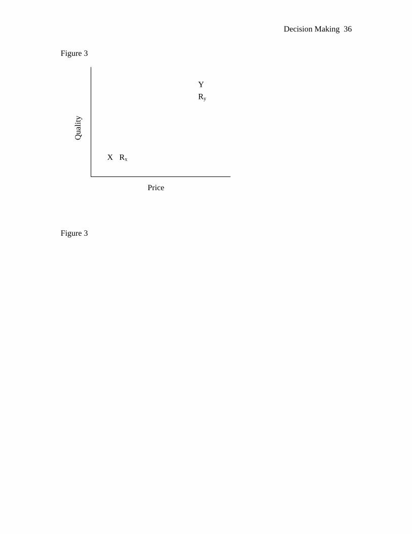
The basic ideas of the experiment are illustrated in Figure 3, where each letter

shown in the figure represents a choice option described by two attributes; for example,

consumer products that vary in price and quality. In this case, option X is low on price

and quality, whereas option Y is high on price and quality. When presented with a

straight binary choice between options X and Y, the options are (approximately) equally

favored. The main theoretical question concerns the addition of a third option to the set,

which is used to manipulate the choice context.

The critical context manipulation in this experiment was the introduction of a

third option, called the reference option, represented by either option Rx or option Ry.

Under one condition, participants were asked to imagine that they currently owned the

commodity Rx, and they were then given a choice of keeping Rx or trading it for either

commodity X or commodity Y. From the reference point of Rx, option X has a small

advantage on price and no disadvantage on quality, whereas Y has large advantages on

quality and large disadvantages on price. Under these conditions, Rx was rarely chosen,

and X was favored over Y. Under another condition, participants were asked to imagine

that they owned option Ry, and they were then given a choice of keeping Ry or trading it

for either X or Y. From the reference point of Ry, Y has a small advantage and no

Decision Making 22

disadvantages, whereas X now has both large advantages and disadvantages. Under this

condition, Ry was rarely chosen again, but now Y was favored over X.

In summary, even though the reference options, Rx and Ry, were rarely ever

chosen, nevertheless, they changed the choice context, causing the preference order for X

and Y to reverse across the two contexts. This preference reversal violates the rational

principle of choice called independence from irrelevant alternatives. This is just one

example violation of this principle, but there are many others (see Tversky & Simonson,

1993; Roe et al., 2001).

What causes these context effects on preferences? Tversky and Kahneman (1991)

interpreted this particular result in terms of a loss aversion effect: Option X was favored

when Y entailed large losses relative to the reference point Rx, but the opposite occurred

when X entailed large losses relative to the reference point Ry. But this explanation

leaves one to wonder about the mechanism that causes loss aversion.

Decision field theory provides a dynamic mechanism for explaining the reference

point effect as well as many other context dependent preference effects (see Roe et al.,

2001; Busemeyer & Johnson, 2004). According to decision field theory, these context

effects are generated by the recurrent network shown as the third layer in Figure 2. We

will skip the mathematical derivations here, and simply present the conceptual ideas.

According to decision field theory, these effects are contrast effects like edge

enhancement effects that occur in the retina (alternately, these effects can be

conceptualized in the context of the lateral inhibition occurring within the striatum, part

of the basal ganglia, during the process of action selection; see Frank, 2005; Wickens,

1997). The inferior reference option makes the closely related attractive option shine.

Decision Making 23

First consider the choice set that includes options X, Y, and Rx. Recall that according to

decision field theory, the lateral inhibitory links in the network depend on the similarity

between options. Note that the reference point Rx is very similar to X, and so the lateral

inhibitory link between these two is strong; whereas Rx is very dissimilar to Y, and so the

lateral inhibitory link between these two is weak. Also note that Rx always experiences a

disadvantage with respect to option X. This arrangement of options then produces the

following dynamics: as processing time passes, option Rx is slowly driven down toward a

negative preference state; this negative preference feeds back through a negative lateral

inhibitory link to produce an enhancement or bolstering of option X. In other words, the

relatively poor reference option, Rx, makes its close neighbor, option X, shine brighter.

The distant option Y does not experience this enhancement because the lateral inhibitory

link is too weak. Therefore the preference state for X gradually dominates Y. When the

choice context is changed to include X, Y, and Ry, the same reasoning holds, but now

option Y is bolstered by being close to a relatively poor reference Ry.

The above explanation for context dependent preferences depends on a dynamic

inhibitory mechanism that takes time to build up. Thus, decision field theory predicts that

these context effects should get stronger as deliberation time gets longer. In contrast, if

these effects were caused by the use of simple heuristics to save time and effort, then the

opposite is predicted – context effects should get larger with shorter deliberation times

that force individuals to fall back on simple heuristic rules to save time. In fact, past

research has found that the context effects get larger with longer deliberation times,

consistent with the predictions of a dynamic model and contrary to a heuristic choice

model (see Simonson, 1989; Dhar, Knowlis, & Sherman, 2000).

Decision Making 24

5. Concluding Comments

The majority of decision research is based on simple laboratory experiments, and

modern decision theories have been built on the basis of these findings. Recently, various

groups of researchers have questioned the usefulness of these theories when applied to

real-life situations. Three related programs of research have examined judgment or

decision making through from what could be called a situated cognition perspective.

Social judgment theory focuses on expert judgments using environmentally-provided cue

– criterion relations. Decision analysis endeavors to provide people with optimized

decision tools for real life decisions in order to improve the quality of these decisions.

Naturalistic decision making represents a paradigm in which descriptive models of

dynamic, complex, high uncertainty, high stakes, and real-life decision situations are

sought. Furthermore, they argue that in these complex, real-life situations, there is not

enough time or computational resources to systematically evaluate all the options.

Consequently, naturalistic decision researchers claim that new theories and methods of

research are needed.

In this chapter, we have attempted to address these concerns, specifically those of

naturalistic decision researchers, through the use of dynamic, as opposed to static, tools.

Rather than rejecting traditional decision theory and research when we enter naturalistic

situations, we have tried to argue that a dynamic perspective (see Port & Van Gelder,

1995, Van Gelder, 1998) provides a foundation for building bridges between traditional

decision theories and naturalistic decisions. Sequential sampling models were developed

Decision Making 25

from Cognitive Psychology to understand real-time cognitive processes observed in

simple laboratory experiments. According to these models, decision makers make an

online assessment of the situation which interacts with the evaluation of competing

options over time; likewise, information accumulates in real-time and decision times are

influenced by a threshold for accrued information. We have argued that dynamic theories

of decision making have the power to explain the basic findings from laboratory

experiments, such as context dependent preferences, as well as new phenomena that arise

in the study of naturalistic decisions.

Decision Making 26

References

Anzai, Y. (1984). Cognitive control of real -time event driven systems. Cognitive

Science, 8, 221-254.

Ashby, F. G. (2000). A stochastic version of general recognition theory. Journal of

Mathematical Psychology, 44, 310-329.

Beardon, A. F. (1991). Iteration of rational functions: complex analytic dynamical

systems.New York: Springer-Verlag.

Brehmer, B. & Allard, R. (1991). Real-time dynamic decision making: Effects of task

complexity and feedback delays. In J. Rasmussen, B. Brehmer, and J. Leplat

(Eds.) Distributed decision making; Cognitive models for cooperative work.

Chichester: Wiley.

Brehmer, B. (1992). Dynamic decision making: Human control of complex systems. Acta

Psychologica, 81, 211-241.

Brunswik, E. (1952) The conceptual framework of psychology. Chicago, IL: Chicago

University Press,

Busemeyer, J. R. (1985). Decision making under uncertainty: A comparison of simple

scalability, fixed sample, and sequential sampling models. Journal of

Experimental Psychology, 11, 538-564.

Busemeyer, J. R., & Johnson, J. G. (2004). Computational models of decision making. In

D. J. Koehler & N. Harvey (Eds.), Blackwell handbook of judgment and decision

making (1st ed., pp. xvi, 664 p.). Oxford: Blackwell Publishing.

Busemeyer, J. R., & Townsend, J. T. (1993). Decision field theory: A dynamic-cognitive

approach to decision making in an uncertain environment. Psychological Review,

Decision Making 27

100, 432-459.

Clemens, R. (1996). Making Hard Decisions: An Introduction to Decision Analysis (2

ed.). Boston, MA: PWS-Kent Publishing Co. (1991).

Dhami, M. K., Hertwig, R., & Hoffrage, U. (2004). The Role of Representative Design in

an Ecological Approach to Cognition. Psychological Bulletin, 130(6), 959-988.

Dhar, R., Nowlis, S. M., & Sherman, S. J. (2000). Trying hard or hardly trying: An

analysis of context effects in choice. Journal of Consumer Psychology, 9, 189-

200.

Diederich, A. (2003). MDFT account of decision making under time pressure.

Psychonomic Bulletin and Review, 10(1), 157-166.

Dienes, Z. & Fahey, R. (1995). Role of specific instances in controlling a dynamic

system. Journal of Experimental Psychology: Learning, Memory, & Cognition,

21, 848-862.

Edwards, W. (1962). Dynamic decision theory and probabilistic information processing.

Human Factors, 4, 59-73.

Einstein, G. O., & McDaniel, M. A. (Eds.). (2004). Memory fitness: a guide for

successful aging.New Haven, CT: Yale University Press.

Ericsson, K. A., & Simon, H. A. (1984). Protocol analysis: verbal reports as

data.Cambridge, Mass.: MIT Press.

Fischoff, B., & Slovic, P. (1978). A little learning. confidence in multicue judgment

tasks.Eugene, OR: Decision Research.

Decision Making 28

Frank, M. J. (2005). Dynamic Dopamine Modulation in the Basal Ganglia: A

Neurocomputational Account of Cognitive Deficits in Medicated and

Nonmedicated Parkinsonism. Journal of Cognitive Neuroscience, 17(1), 51-72.

Gibson, F., Fichman, M. & Plaut, D. C. (1997) Learning in dynamic decision tasks:

Computational model and empirical evidence. Organizational Behavior and

Human Performance, 71, 1-35.

Gilboa, I., & Schmeidler, D. (1995). Case-based theory. The Quarterly Journal of

Economics, 110, 607–639.

Goldstein, W. M., & Weber, E. U. (1997). Content and discontent: Indications and

implications of domain specificity in preferential decision making. In . J. R.

Busemeyer et al (Eds.) The Psychology of Learning and Motivation, Vol 32.

Decision Making from a Cognitive Perspective, San Diego: Academic Press,

1995, pp. 83-136.

Gonzalez, C., Lerch, J.F., & Lebiere, C. (2003). Instance-based learning in dynamic

decision making. Cognitive Science, 27, 591-635.

Green, D. M., & Swets, J. A. (1966). Signal Detection Theory and Psychophysics.

Oxford, England: Wiley.

Hammond, K. R., Hamm, R. M., Grassia, J., & Pearson, T. (1987). Direct comparison of

the efficacy of intuitive and analytical cognition in expert judgment. IEEE

Transactions on Systems, Man, & Cybernetics, 17(5), 753-770.

Hogarth, R. M. (1981) Beyond discrete biases: Functional and dysfunctional aspects of

judgmental heuristics. Psychological Bulletin, 90, 197-217.

Decision Making 29

Holyoak, K. J., & Simon, D. (1999). Bidirectional reasoning in decision making by

constraint satisfaction. Journal of Experimental Psychology: General, 128(1), 3-

31.

Jagacinski, R. J. & Hah, S. (1988). Progression-regression effects in tracking repeated

patterns. Journal of Experimental Psychology: Human Perception and

Performance, 14, 77-88.

Jagacinski, R. J. & Miller, R. A. (1978). Describing the human operator’s internal model

of a dynamic system. Human Factors, 20, 425-433.

Keeney, R. L., & Raiffa, H. (1976). Decisions with multiple objectives: preferences and

value tradeoffs. New York: Wiley.

Kaplan, M. (1996) Decision theory as philosophy. Cambridge: Cambridge University

Press.

Klein, G. A. (1989). Recognition primed decisions. Advances in man-machine systems

research, 5, 47-92 Greenwich, CT: JAI Press

LeBoeuf, R. A., & Shafir, E. (2001). Problems and methods in naturalistic decision-

making research. Journal of Behavioral Decision Making, 14(5), 373-375.

Levin, I. P., Louviere, J. J., Schepanski, A. A., & Norman, K. L. (1983). External validity

tests of laboratory studies of information integration. Organizational Behavior &

Human Performance, 31(2), 173-193.

Link, S. W., & Heath, R. A. (1975). A sequential theory of psychological discrimintation.

Psychometrika, 40, 77-111.

Loftus, E. F. (2003). Make-Believe Memories. American Psychologist, 58(11), 867-873.

Luce, R. D. (1986). Response times: their role in inferring elementary mental

Decision Making 30

organization.New York: Oxford University Press.

Luce, R. D. (2000). Utility of gains and losses: Measurement-theoretical and

experimental approaches.Mahwah, NJ: Lawrence Erlbaum Associates.

Nisbett, R. E., & Wilson, T. D. (1977). Telling more than we can know: Verbal reports

on mental processes. Psychological Review, 84(3), 231-259.

Nosofsky, R. M., & Palmeri, T. J. (1997). An exemplar-based random walk model of

speeded classification. Psychological Review, 104, 226-300.

Payne, J. W., Bettman, J. R., & Johnson, E. J. (1992). Behavioral decision research: A

constructive processing perspective. Annual Review of Psychology, 43, 87-131.

Port, R. F., & Van Gelder, T. (Eds.). (1995). Mind as motion: explorations in the

dynamics of cognition.Cambridge, MA: MIT Press.

Rapoport, A. (1975). Research paradigms for studying dynamic decision behavior. In D.

Wendt & C. Vlek (Eds.) Utility, Probability, and Human Decision Making,

Dordrecht-Holland: Reidel. (Pp. 347-369).

Ratcliff, R. (1978). A theory of memory retrieval. Psychological Review, 85, 59-108.

Roe, R. M., Busemeyer, J. R., & Townsend, J. T. (2001). Multi-alternative decision field

theory: A dynamic connectionist model of decision-making. Psychological

Review, 108, 370-392.

Simon, H. A. (1955). A behavioral model of rational choice. Quarterly Journal of

Economics, 69, 99-118.

Simonson, I. (1989). Choice based on reasons: The case of attraction and compromise

effects. Journal of Consumer Research, 16(158-174).

Decision Making 31

Smith, P. L. (1995). Psychophysically principled models of visual simple reaction time.

Psychological Review, 102(3), 567-593.

Sterman, J. D. (1994). Learning in and about complex systems. System Dynamics Review,

10, 291-330.

Tversky, A., & Kahneman, D. (1991). Loss aversion in riskless choice: A reference

dependent model. Quarterly Journal of Economics, 106, 1039-1061.

Tversky, A., & Kahneman, D. (1992). Advances in prospect theory: Cumulative

representations of uncertainty. Journal of Risk and Uncertainty, 5, 297-323.

Tversky, A., & Simonson, I. (1993). Context dependent preferences. Management

Science, 39, 1179-1189.

Usher, M., & McClelland, J. L. (2004). Loss Aversion and Inhibition in Dynamical

Models of Multialternative Choice. Psychological Review, 111(3), 757-769.

Van Gelder, T. (1998) The dynamical hypothesis in cognitive science. Behavioral and

Bran Sciences, 21, 615-

Vickers, D. (1979). Decision processes in visual perception.New York: Academic Press.

Von Winterfeldt, D., & Edwards, W. (1986). Decision analysis and behavioral

research.Cambridge: Cambridge University Press.

Yates, J. F. (1990). Judgment and Decision Making.New Jersey: Prentice Hall.

Decision Making 32

You (1989). Disclosing the decision - maker’s internal model and control policy in a

dynamic decision task using a system control paradigm. Unpublished MA thesis,

Purdue University.

Wickens, J. (1997). Basal ganglia: Structure and computations. Network: Computation in

Neural Systems, 8, R77-R109.

Decision Making 33

Figures

Figure 1. Example of the decision process for the motorcyclist’s decision.

Horizontal axis is time, and vertical axis is preference, and each trajectory represents an

action. The top flat line is the threshold bound.

Figure 2. Connectionist interpretation of decision field theory for the

motorcyclist’s example.

Figure 3. Illustration of stimuli used to produce reference point effects. The

horizontal axis represents price, the vertical axis represent quality, and each point

represents a consumer product.

Decision Making 34

Figure 1

0 0.2 0.4 0.6 0.8-2

-1.5

-1

-0.5

0

0.5

1

1.5

Tim e in ms

Pref

eren

ce S

tate

ABC

Figure 1

Decision Making 35

Figure 2

Figure 2

B

A

B

C

A

C C

B

A

m1

m2

m3

Weights Contrasts

Valences PreferencesMomentary Evaluations

m4

Decision Making 36

Figure 3

Y Ry

Qua

lity

X Rx

Price

Figure 3