The Detection of Broken Rotor Bars in Variable Speed ... - CORE
222
CONDITION MONITORING OF INDUCTION MOTORS: The Detection of Broken Rotor Bars in Variable Speed Induction Motor Drives by Andrew Gary Innes, B.E. (Hons.) Submitted in fulfilment of the requirements for the degree of Doctor of Philosophy. University of Tasmania June 1999
-
Upload
khangminh22 -
Category
Documents
-
view
6 -
download
0
Transcript of The Detection of Broken Rotor Bars in Variable Speed ... - CORE

CONDITION MONITORING OF INDUCTION MOTORS:
The Detection of Broken
Rotor Bars in Variable Speed
Induction Motor Drives
by Andrew Gary Innes, B.E. (Hons.)
Submitted in fulfilment of the requirements for the degree of
Doctor of Philosophy.
University of Tasmania
June 1999
Statement of Originality
This thesis contains no material which has been accepted for a degree or diploma
by the University or any other institution, except by way of background
information and duly acknowledged in the Thesis, and to the best of my
knowledge and belief no material previously published or written by another
person except where due acknowledgement is made in the text of the Thesis.
Andrew Innes.
Authority of Access
This thesis may be made available for loan and limited copying in accordance with
the Copyright Act 1968.
Andrew Innes.
ii
Abstract
The squirrel cage induction motor is the most common means of converting
electrical energy to mechanical energy. As such they form a very important part of
modem industrial plants. Adverse service conditions may cause faults to develop
within a motor that eventually result in the motor failing. If warning of an
impending failure can be obtained, the motor can be scheduled for repair or
replacement before catastrophic failure occurs, thus avoiding costly excess down
time of plant.
A fault which occurs in cage induction motors, is where a fracture occurs between
the end ring and a rotor bar, or in an end-ring segment. These faults may be
detected by examining the frequency spectrum of the stator current, while the
motor is operating under loaded conditions, for the presence of characteristic
frequency components. The basic theory is reasonably well known, however little
work has been done on detecting faults when the motor is controlled by a variable
frequency drive, which causes extra frequency components to appear in the stator
current spectrum.
A variable speed drive controls the speed of an induction motor by changing the
frequency of the supply voltage. Thus the problem of detecting faults becomes one
of analysing a non-stationary signal. One approach to solve this problem is to
synchronously sample the stator current waveform, such that the sampling process
tracks any change in frequency, producing a useful frequency spectrum. A
hardware system based on a phase locked loop circuit is developed in order to
implement such a process.
In order to determine which frequencies are produced by a pulse-width modulated
(PWM) drive, a theoretical analysis of various PWM methods is carried out, with
iii

iv
particular reference to fault frequency components. The change in frequency
component amplitudes between mains operation and VSD operation and also with
change in load is also examined experimentally. The uncertainty in amplitude due
to the signal processing techniques employed, is also determined by experiment.
The effects of changes in frequency component amplitudes on the detection of
faults is discussed.
A full-transient model for the induction motor is developed as an assembly of
inductively coupled coils using a model that can represent the effects of individual
rotor bars. The effect of a broken rotor bar on the frequencies that are introduced
into the supply current can then be predicted.
Finally, the possible application of time-frequency and continuous wavelet
transform analysis to the problem of a non-stationary signal is examined. Various
types of transform are compared to find the most suitable for tracking frequency
components as they change.

Acknowledgements
Firstly I would like to thank my supervisor Mr Richard Langman for his guidance
and support in conducting this research. I would also like to acknowledge my
associate supervisor Mr Peter Watt for initiating this project and for providing
some initial impetus in the practicalities of data acquisition and signal processing.
I would like to thank Mr Graeme Vertigan and Pasminco EZ Pty. Ltd., for their
permission to take measurements around their factory and for tolerating the
subsequent disruption to their production.
Also I would like to thank Dr Michael Robinson and Pope Electric Motors
Australia Pty. Ltd. for providing extra rotors and proprietary information on our
laboratory motor, and the illuminating technical discussions on induction motor
design.
This research was partially funded by a grant from the Electricity Supply
Association of Australia Limited.
My thanks must go to all the academic staff in the Department of Electrical and
Electronic Engineering at the University of Tasmania, in particular Dr Richard
Lane (now with the University of Canterbury), Dr David Lewis, Dr John Ameaud
(now with the Hydro Electric Commission Tasmania), Mr Gregory The, Dr Habib
Talhami, Mr John Brodie, and Professor Thong Nguyen, for the many and varied
discussions we have had. I would also like to acknowledge all the technical staff,
in particular Mr Glenn Mayhew for his help with electronic design work and
solving electromagnetic interference problems, Mr Steven A very for the design
and fabrication of various mechanical devices, and Mr Russell Twining and Mr
David Craig for their help with computing.
v

vi
Many thanks must go to my fellow students, John McCulloch, Quang Ha, Bonnie
Law, Alan Liew, and Mike O'Day for their help and friendship. In particular I
would like to thank Jason Pieloor, Marc Stoksik, David McLaren and Andrew
Bainbridge-Smith who have been there since the start. I would also like to thank
Sarah Booker for some proof reading.
I would like to thank Joanna Foulkes for her support and encouragement, and
proof reading of the manuscript.
Finally, I would like to thank my parents for the many years which they have
supported and encouraged me.

Contents
Abstract iii
Acknowledgements v
Contents vii
Figures xii
Symbols and Abbreviations xvii
Preface xxi
1 Introduction 1
1.1 Maintenance and Condition Monitoring ....................................................... 1
1.2 Types of Electric Motors ............................................................................... 3
1.3 Failure Modes of the Induction Motor ......................................................... .4
1.4 Condition Monitoring of Induction Motors ................................................... ?
1.5 Detection of Broken Rotor Bars .................................................................... 9
1.6 Condition Monitoring oflnduction Motors fed by Variable Speed Drives.lO
1.7 Contribution of this Thesis .......................................................................... 11
1.8 Organisation of the Thesis ........................................................................... 11
2 Theory of the Induction Motor 14
2.1 Introduction ................................................................................................. 14
2.2 Air Gap Flux Analysis ................................................................................. 15
2.2.1 Torque Production in the Induction Motor. ......................................... 15
2.2.2 Induction Motor Model.. ...................................................................... 16
2.2.3 Magnetomotive Force of an AC Winding ........................................... 17
vii

CONTENTS viii
2.2.3.1 Magnetomotive Force of a Single Tum ....................................... 17
2.2.3.2 Magnetomotive Force for the Whole Stator Winding .................. 18
2.2.3.3 Rotor Magnetomotive Force ........................................................ 20
2.2.4 Air gap Magnetic Permeance [46] ....................................................... 21
2.2.5 Air gap Flux Density Distribution ....................................................... 23
2.3 Effect of Broken Rotor Bars ........................................................................ 24
2.4 The Effect of Inter-Bar Currents .................................................................. 25
2.5 Summary ...................................................................................................... 27
3 Signal Processing 29
3.1 Introduction ................................................................................................. 29
3.2 The Fourier Transform ................................................................................ 30
3.2.1 The Discrete Fourier Transform .......................................................... 31
3 .2.2 The Fast Fourier Transform (FFT) ...................................................... 33
3.3 Windowing and Window Functions ............................................................ 34
3.3.1 Figures of Merit for Window Functions .............................................. 38
3.3.2 Window Functions ............................................................................... 39
3.3.2.1 Rectangle Window ....................................................................... 39
3.3.2.2 Hanning Window ........................................................................ .40
3.3.2.3 Hamming Window ....................................................................... 41
3.3.2.4 Blackman Window ....................................................................... 43
3.3.3 Effect of Window Functions on a Typical Stator Current Spectrum ... 44
3.3.4 Statistical Analysis of Variation in Sideband Amplitudes ................... 47
3.4 Parametric Models for Spectral Estimation ................................................. 48
3.4.1 Frequency Resolution of Spectrum Estimates .................................... .49
3.4.2 Prony's Method .................................................................................... 50
3.4.3 Results .................................................................................................. 54
3.5 Summary ...................................................................................................... 56
4 Phase Locked Loops and Synchronous Sampling 58
4.1 Introduction ................................................................................................. 58
4.2 The Phase Locked Loop .............................................................................. 59
4.2.1 The Basic PLL Circuit ......................................................................... 59

CONTENTS ix
4.2.2 Frequency Multiplying PLL Circuit.. .................................................. 61
4.3 Synchronous Sampling and the PLL. .......................................................... 63
4.4 PLL Circuit Implementation ........................................................................ 64
4.5 Circuit Performance with Mains Supplied Induction Motors ..................... 67
4.6 Application to Variable Speed Drives ......................................................... 69
4.6.1 Circuit Performance with Variable Speed Drives ................................ 70
4.7 Summary ...................................................................................................... 72
5 Variable Speed Drives 74
5.1 Introduction ................................................................................................. 74
5.2 Induction Motor Speed Control.. ................................................................. 75
5.3 Pulse-width Modulation .............................................................................. 77
5.3.1 Natural Sampled PWM ........................................................................ 79
5.3.2 Symmetric Regular Sampled PWM ..................................................... 80
5.3.3 Asymmetric Regular Sampled PWM ................................................... 82
5.3.4 Optimised PWM .................................................................................. 83
5.3.5 Random PWM ..................................................................................... 83
5.3.6 Space Vector PWM ............................................................................. 84
5.4 Effects of PWM Voltage Waveforms on Detection of Fault Frequencies .. 85
5.5 Effect of Supply Frequency on Rotor Fault Frequency Amplitudes in the
Stator Current Spectrum ........................................................................... 86
5.6 Summary ...................................................................................................... 96
6 Numerical Modelling of Induction Motors with Broken Rotor Bars 99
6.1 Introduction ................................................................................................. 99
6.2 The Theory of Coupled Coils .................................................................... 100
6.3 Simple Coupled Coil Models of the Induction Motor. .............................. 103
6.4 Coupled Coil Models of the Induction Motor with Individual Rotor Bars
Modelled ................................................................................................ 105
6.4.1 Rotor Model ....................................................................................... 105
6.4.2 Stator Model ...................................................................................... 107
6.5 Previous Work ........................................................................................... 110
6.6 Models Including the Stator Windings Explicitly ..................................... 111

CONTENTS X
6.6.1 Phase Model [121] ............................................................................. 112
6.6.2 Line-to-line Model [121] ................................................................... 113
6. 7 Modelling a Broken Rotor Bar .................................................................. 116
6.8 Solving the Model ..................................................................................... 118
6.8.1 Calculation of Inductances ................................................................. 118
6.8.2 Calculation of Flux Linkages ............................................................. 118
6.8 .3 Calculation of Currents ...................................................................... 118
6.8.4 Calculation of Speed and Angular Displacement.. ............................ 118
6.9 Numerical Solution of Ordinary Differential Equations ........................... 119
6.9.1 Euler's Method .................................................................................. 119
6.9.2 Runge-Kutta Methods ........................................................................ 120
6.9.3 Other Methods of Solving ODEs ....................................................... 121
6.10 Numerical Solution of the Induction Motor Model. ................................ 121
6.10.1 Stator-Rotor Mutual Inductance ...................................................... 122
6.10.2 Tuning Stator Inductance Value ...................................................... 123
6.10.3 Computer Implementation Issues .................................................... 124
6.10.4 Simulation of Broken Rotor Bars .................................................... 128
6.11 Summary .................................................................................................. 128
7 Experimental Studies 130
7.1 Introduction ............................................................................................... 130
7.2 Differences Between the Detection of Broken Rotor Bars in Mains-supplied
and VSD-supplied Induction Motors ..................................................... 131
7 .2.1 Experimental Arrangements .............................................................. 132
7 .2.2 Undamaged Rotor Measurements ...................................................... 134
7.2.3 Damaged Rotor Measurements .......................................................... 136
7 .2.4 Comparison of Reference Spectra ..................................................... 138
7.3 Detection of Rotor Damage in an Industrial Plant using the PLL ............. l38
7.4 Software Methods ..................................................................................... .141
7.5 Simulation Methods .................................................................................. 142
7.6 Conclusion ................................................................................................. 143

CONTENTS xi
8 Time-Frequency and Wavelet Analysis 145
8.1 Introduction ............................................................................................... 145
8.2 Time-Frequency Analysis .......................................................................... 147
8.2.1 Short Time Fourier Transform (STFT) ............................................. .l49
8.2.2 Wigner-Ville Distribution (WVD) ..................................................... 150
8.2.3 Choi-Williams Distribution (CWD) .................................................. 151
8.2.4 Zhao-Atlas-Marks Distribution (ZAM) ............................................. 151
8.3 Wavelet Analysis ....................................................................................... 152
8.3.1 The Continuous Wavelet Transform .................................................. 152
8.4 Analysis of Stator Current Waveforms ..................................................... 156
8.4.1 Time-Frequency Analysis of Current Waveforms ............................. 156
8.4.2 Wavelet Analysis of Current Waveforms .......................................... 158
8.5 Summary .................................................................................................... 159
9 Summary and Recommendations for Future Work 170
9.1 Introduction ............................................................................................... 170
9.2 Summary ofWork ..................................................................................... 171
9.3 Future Extensions ...................................................................................... 175
9.3.1 Implementation .................................................................................. 175
9.3.2 Modelling of the Induction Motor with Broken Rotor Bars .............. 176
9.3.3 Artificial Intelligence ......................................................................... 177
9.4 Concluding Remarks ................................................................................. 177
Appendix A Laboratory Equipment
Appendix B Analytical Expressions for PWM Waveforms
References
178
181
188

Figures
1.1 Incidence of fault types in induction motors ................................................. 5
1.2 Squirrel cage rotor ......................................................................................... 8
2.1 Induction motor cross-section ..................................................................... 16
2.2 Magnetomotive force distribution of a single full-pitched coil.. ................. 17
2.3 Stator winding and flux pattern ................................................................... 18
3.1 Aliasing of sampled waveforms .................................................................. 31
3.2(a) Original time signal ................................................................................. 34
3.2(b) Synchronously sampled signal. ............................................................... 34
3.2(c) Asynchronously sampled signal. ............................................................. 35
3.3(a) Frequency spectrum of 3.2(a) .................................................................. 35
3.3(b) Frequency spectrum of 3.2(b) ................................................................. 36
3.3(c) Frequency spectrum of 3.2(c) .................................................................. 36
3.4(a) Sampled data ........................................................................................... 37
3.4(b) Window function (Hanning window) ..................................................... 37
3.4(c) Windowed data ....................................................................................... 37
3.4(d) Frequency spectrum of windowed and non-wi~dowed data .................. .38
3.5(a) Rectangle window .................................................................................. .40
3.5(b) Normalised frequency respose of rectangle window ............................. .40
3.6(a) Hanning window ..................................................................................... 41
3.6(b) Normalised frequency respose of Hanning window .............................. .41
3.7(a) Hamming window ................................................................................... 42
3. 7 (b) Normalised frequency res pose of Hamming window ............................ .42
3.8(a) Blackman window ................................................................................... 44
3.8(b) Normalised frequency respose of Blackman window ............................. 44
3.9(a) Stator current frequency spectrum- rectangle window ......................... ..45
3.9(b) Stator current frequency spectrum- Hanning window .......................... .45
xii

FIGURES xiii
3.9(c) Stator current frequency spectrum- Hamming window ........................ .46
3.9(d) Stator current frequency spectrum- Blackman window ........................ .46
3.10 Variation in sideband amplitude with data record number ........................ 48
4.1 Basic PLL block diagram ............................................................................ 60
4.2 Frequency multiplying digital phase locked loop block diagram ................ 62
4.3 Block diagram of the synchronous sampling system ................................... 64
4.4 Circuit for implementation of phase locked loop ........................................ 66
4.5 Non-synchronously sampled spectrum ........................................................ 68
4.6 Synchronously sampled spectrum ............................................................... 68
4.7 Stator current spectrum for fixed frequency sampling with varying supply
voltage ...................................................................................................... 69
4.8 Spectrum of stator current with PLL controlled sampling and varying
supply voltage frequency .......................................................................... 70
4.9 Broadening of the supply frequency peak due to PLL losing lock. ............. 72
5.1 Circuit diagram of a variable speed drive .................................................... 76
5.2 Three-level PWM waveform, R=21, M=0.9, with 50Hz fundamental ....... 78
5.3 Natural sampled PWM ................................................................................ 79
5.4 Frequency spectrum of natural sampled PWM, R=20, M=0.9,Jm =50Hz ... 80
5.5 Regular sampling ......................................................................................... 81
5.6 Frequency spectrum of regular sampled PWM, R=20, M=0.9,Jm =50Hz ... 81
5.7 Frequency spectrum of asymmetric regular sampled PWM, R=20, M=0.9,
fm =50Hz ................................................................................................... 82
5.8 Frequency spectrum of space vector PWM waveform, R=20, M=0.9,
fm =50Hz ................................................................................................... 84
5.9 Typical stator current frequency spectrum .................................................. 87
5.10 Average sideband amplitude- constant slip (0.04 p.u.) ............................ 88
5.11 Standard deviation of sideband amplitude- constant slip (0.04 p.u.) ....... 88
5.12 Amplitude of third harmonic of drive frequency ....................................... 89
5.13 Standard deviation of amplitude of third harmonic of drive frequency .... 89
5.14 Amplitude of reflected frequency component relative to drive frequency
amplitude .................................................................................................. 91
5.15 Standard deviation of amplitude of reflected frequency component.. ....... 91
FIGURES xiv
5.16 Ripple on the DC link voltage ................................................................... 92
5.17 Measured drive voltage output waveform-!J =45Hz .............................. 92
5.18 Frequency spectrum of PWM voltage waveform 0-100Hz ....................... 93
5.19 Frequency spectrum of PWM voltage waveform 0-5000Hz ..................... 93
5.20 Variation of sideband amplitude with load (50Hz) ................................... 94
5.21 Standard deviation of sideband amplitude with load (50Hz) .................... 94
5.22 Variation of sideband amplitude with load (45Hz) ................................... 95
5.23 Standard deviation of sideband amplitude with load (45Hz) .................... 95
5.24 Variation of sideband amplitude with load (40Hz) ................................... 96
5.25 Standard deviation of sideband amplitude with load (40Hz) .................... 96
6.1 The total flux linking coil k is the sum of self and mutual fluxes ............. 101
6.2 The per-phase equivalent circuit of the induction motor ........................... 104
6.3 Equivalent circuit of rotor loops ................................................................ 106
6.4 Developed diagram of the connections of half the stator windings in a
concentrically wound stator with 36 slots and 3 coils per group ........... 114
6.5 Equivalent circuit with rotor bar Nb broken .............................................. 117
6.6 Inductance and derivative curves calculated for the Pope motor .............. 123
6.7 Modified stator-rotor mutual inductance curves ....................................... 125
6.8 Sinusoidal stator-rotor mutual inductance curves ..................................... 125
6.9 Speed and torque for simulated start up with sinusoidal stator voltage and
sinusoidal inductance curves .................................................................. 126
6.10 Speed and torque for simulated start up with sinusoidal stator voltage and
piecewise linear inductance curves ........................................................ 126
6.11 Spectrum of simulated stator current using a sinusoidal voltage supply and
sinusoidal inductance curves, with a broken rotor bar ........................... 127
6.12 Spectrum of simulated stator current using a 50Hz PWM voltage supply
and piecewise linear inductance curves, with a broken rotor bar ........... 127
7.1 Arrangement of motor and loading generator ........................................... 133
7.2 Arrangement of data acquisition system .................................................... l34
7.3 Stator current spectrum with undamaged rotor and mains supply ............ 135
7.4 Stator current spectrum with undamaged rotor and VSD supply .............. 135
7.5 Damage to rotor of test motor .................................................................... 136

FIGURES XV
7.6 Stator current spectrum with damaged rotor and mains supply ................ 137
7. 7 Stator current spectrum with damaged rotor and VSD supply .................. 137
7.8 Stator current spectrum of pump motor, 48.3Hz supply frequency ........... 139
7.9 Stator current spectrum of pump motor, 43.6Hz drive frequency ............. 141
8.1 Division of the frequency domain ............................................................. 153
8.2 The Morlet wavelet. ................................................................................... 155
8.3 Stator current waveform for the drive frequency ramping from 30Hz to
50Hz ....................................................................................................... l61
8.4 Spectrum of mains supply current waveform ............................................ 161
8.5 STFT of mains supply current waveform .................................................. 162
8.6 Wavelet transform of mains supply current waveform ............................. 162
8.7 STFT of mains supply current waveform after 400Hz high-pass filteringl63
8.8 Wavelet transform of mains supply current waveform after 400Hz high-
pass filtering ........................................................................................... 163
8.9 STFT of current waveform with drive frequency ramping from 30Hz to
50Hz ....................................................................................................... 164
8.10 STFT of current waveform with drive frequency ramping from 30Hz to
50Hz, after 400Hz high-pass filtering, 512 point window ..................... 164
8.11 STFT of current waveform with drive frequency ramping from 30Hz to
50Hz, after 400Hz high-pass filtering, 1024 point window ................... 165
8.12 STFT of current waveform with drive frequency ramping from 30Hz to
50Hz, after 400Hz high-pass filtering, 2048 point window ................... 165
8.13 Wigner-Ville distribution of current waveform with drive frequency
ramping from 30Hz to 50Hz .................................................................. 166
8.14 Wigner-Ville distribution of current waveform with drive frequency
ramping from 30Hz to 50Hz, after 400Hz high-pass filtering ............... 166
8.15 Choi-Williams distribution of current waveform with drive frequency
ramping from 30Hz to 50Hz .................................................................. 167
8.16 Choi-Williams distribution of current waveform with drive frequency
ramping from 30Hz to 50Hz, after 400Hz high-pass filtering ............... 167
8.17 Zhao-Atlas-Marks distribution of current waveform with drive frequency
ramping from 30Hz to 50Hz .................................................................. 168

FIGURES xvi
8.18 Zhao-Atlas-Marks distribution of current waveform with drive frequency
ramping from 30Hz to 50Hz, after 400Hz high-pass filtering ............... 168
8.19 Wavelet transform of current current waveform with drive frequency
ramping from 30Hz to 50Hz ................................................................. .169

Symbols and Abbreviations
The following symbols are used in this thesis:
ak. bk Fourier coefficients of order k.
a, Angular span of coil i.
F Fourier transform.
<P Magnetic flux.
<p Angular position around stator bore from some reference.
<i'in Phase of input signal.
<i'out Phase of output signal.
F Magnetomotive force.
f Frequency (Hz).
J,. Frequency of rotor current (Hz).
fc PWM carrier frequency.
fm PWM modulating frequency.
fi Supply frequency (Hz).
!bb Broken rotor bar fault frequencies (Hz).
Is Sampling frequency (Hz).
g Air gap length.
g-1 Inverse gap function.
I Current.
hb Broken bar current.
IN Normal bar current.
i Current.
J Moment of inertia.
ln(x) Bessel function of the first kind, order n.
K Viscous friction.
xvii

SYMBOLS AND ABBREVIATIONS xviii
K vco VCO gain.
Kpc Phase comparator gain.
Kp Pitch factor.
Kpi Pitch factor for ith harmonic.
Kd Distribution factor.
Kdi Distribution factor for ith harmonic.
'A Magnetic flux linkage.
A Permeance.
L Inductance.
Lzs Stator leakage inductance.
Lzr Rotor leakage inductance.
Lm Magnetising inductance.
l Length of rotor.
M Mutual inductance.
N Number of turns in a coil.
Nb Number of rotor bars.
Ns1 Number of turns in stator winding.
Nr Number of rotor slots.
N.1· Number of stator slots.
Ni Winding function of coil i.
p Number of pole pairs.
R Resistance and Reluctance.
Rc Inter-bar reistance per unit core length.
Rbb Rotor bar resistance.
r Average air gap radius.
s Per unit slip.
8 Angular displacement.
Sm Mechanical angular displacement of rotor with respect to a stator
reference.
T Period.
Te Eectromagnetic torque developed by the motor.
TL Load torque.

SYMBOLS AND ABBREVIATIONS xix
t Time.
v Voltage.
Vc Control voltage.
Vin Input voltage.
Vpc Phase comparator voltage.
ffis Synchronous angular frequency (raclls).
ffi] Fundamental supply angular frequency (rad/s).
ffiin Input signal angular frequency (rad/s).
ffir Angular frequency of rotor current (raclls).
ffiout Output signal angular frequency (rad/s).
ffio PLL free running angular frequency (rad/s).
xb Rotor bar leakage reactance.
zb Rotor bar leakage impedance.
Zi Number of turns in coil i.
The following subscripts may be applied to the symbols above:
de Dynamic eccentricity.
is Sator harmonic orders.
ir Rotor harmonic orders.
I~ Sator harmonic orders.
]r Rotor harmonic orders.
ls Stator harmonic orders.
lr Rotor harmonic orders.
ms Stator harmonic orders.
mr Rotor harmonic orders.
r Rotor.
rt Rotor.
s Stator.
st Stator.
sa Saturation.
se Static eccentricity.

SYMBOLS AND ABBREVIATIONS XX
The following abbreviations are used in the text:
ASD Adjustable speed drive.
AID Analogue to digital.
CSI Current source inverter.
hp Horsepower.
PLL Phase locked loop.
PWM Pulse width modulation.
TEFC Totally enclose, fan cooled.
VSD Variable speed drive.
VSI Voltage source inverter.

Preface
This project originated in 1989 with a local zinc company, Pasminco EZ Ltd., who
were having problems with some critical induction motors. These motors were
driving two large cooling tower fans via reduction gearboxes. If one of these fans
were to become inoperative during the summer months, it would shut down the
entire plant. The company estimates that this would cost around one million
dollars per day. The motors are in an awkward position high above the ground,
requiring a large crane to be brought onsite in order to effect replacement. Hence
the company were interested in any warning of impending failure that could be
obtained. Due to a lack of local commercial expertise, they called the University,
whereupon Peter Watt, Richard Langman and Dr David Lewis began an
investigation and took some initial measurements.
Two years later this project was continued as a PhD topic by the author. After
some initial work assembling a suitable data acquisition system, and examining
the literature in the field, it was noticed that the number of variable speed drives in
industry was increasing, yet no work had been done on fault detection in the
motors controiied by these drives. Hence it was decided to concentrate on fault
detection in induction motors controlled by variable speed drives.
As there are no drive manufacturers in Australia, it was not feasible to develop an
integrated condition monitoring system. Bearing in mind the existing large
installed base of variable speed drives and the necessity to make non-invasive,
non-destructive measurements in industrial situations, it was decided to
concentrate on condition monitoring methods which depend only on
measurements made external to the drive. Due to the lack of internal, often
proprietry information concerning the drive and the motor the methods developed
must also be independent of any such information.
xxi

PREFACE xxii
Supporting Publications
In the course of this work the following papers were published:
Innes A.G., Watt P.A., and Langman R.A., "Condition monitoring of large induction motors", Proceedings of the Australasian Instrumentation and Measurement Conference, pp265-271, Auckland, New Zealand, 24-27 November 1992.
Innes A.G., "The use of Prony's method for modelling induction motor current waveforms under fault conditions", Proceedings of the 2nd International Conference on Modelling and Simulation, Vol. 1, pp297-303, Melbourne, Australia, 12-14 July 1993.
Innes A.G., Langman R.A., and Mayhew G.R., "Condition monitoring of variable speed induction motor drives", Proceedings of the International Conference on Electrical Machines in Australia, Vol. 1, pp158-163, Adelaide, Australia, 14-16 September 1993.
Innes A.G. and Langman R.A., "The effects of variation in the supply frequency on the detection of broken rotor bars in variable speed induction motor drives", Proceedings of the 29th Universities Power Engineering Conference, Vol. 2, pp581-584, Galway, Ireland, 14-16 September 1994.
Innes A.G. and Langman R.A., "The detection of broken rotor bars in variablespeed induction motor drives", Proceedings of the International Conference on Electrical Machines, Vol. 2, pp294-298, Paris, France, 5-8 September 1994.
Ho S.Y.S., Innes A.G., and Langman R.A., "Stator current frequency analysis for condition monitoring of induction motors. Part II: Variable supply frequency", Journal of Electrical and Electronics Engineering Australia, Vol. 17, No.1, pp 57-69, March 1997.
The following reports were also produced:
Innes A.G., Langman R.A., Report on tests conducted at Pasminco EZ Pty. Ltd., December 1991.
Innes A.G., Langman, R.A., Watt P.A., Final Report to ESAA - Condition Monitoring of Induction Motors, November 1994.

CHAPTER 1
Introduction
Electrical machines are very important to the modem way of life, indeed we have
become very dependent upon them in our daily lives. Machines generate the
electricity that we use and they also convert that electrical energy into mechanical
energy to perform useful work. Hence it can be very important that these machines
do not fail unexpectedly.
1.1 Maintenance and Condition Monitoring
There are three means of maintaining a plant [1]:
(i) run to breakdown,
(ii) fixed-interval maintenance,
(iii) condition-based maintenance.
The first option, run to breakdown, simply operates the system until a part breaks.
The part is then replaced and the system operation resumed. This method has the

INTRODUCTION 2
advantage of being extremely simple to implement, and also uses the component
to the end of its useful life. Of course, the major disadvantage is that the time at
which system breakdown occurs tends to be random. This may result in
unexpected, and hence often costly, system outages.
The second, and probably most familiar, option is fixed-interval maintenance,
where parts of the system are replaced at pre-determined time intervals. The
choice of time interval is dictated by two requirements, maximum utilisation of
component lifetime to minimise waste, and minimisation of unexpected failures.
A compromise between these two factors is generally established by experience
and testing. However, system failures will still occur, and maximum lifetime of
components will not generally be used before they are replaced, leading to
wastage.
Condition-based maintenance is a method where component replacement is
scheduled according to an estimate of the remaining life of the part. Condition
monitoring of the system is required in order to provide knowledge of the system
condition and of the rate at which deterioration is occurring. A condition-based
maintenance program provides the best of both worlds; maximum lifetime of
equipment is ensured and unscheduled outages are minimised. However, all of
this comes at the cost of actually implementing such a program, in terms of both
labour and capital costs. Condition monitoring of a system relies on measuring
one or more parameters of that system in order to determine any deterioration that
is occurring. Such measurements may require expensive instrumentation, a
significant labour commitment to record the data, and expert knowledge to
interpret the results.
Condition monitoring is only financially feasible where either the replacement
cost of the equipment being monitored is high, or where unscheduled outages have
a high cost in terms of lost production time. Since induction motors are relatively
cheap items, it is plant outages caused by motor failure which incur the high costs
that can justify a condition monitoring programme.

INTRODUCTION 3
1.2 Types of Electric Motors
There are many different types of electric motor for converting electrical energy
into mechanical energy. The three main types used in industry are DC motors,
synchronous motors, and induction motors. A DC motor needs a source of DC
power to supply a stationary field winding, and, via a commutator and brushes, a
rotating armature winding. This complexity of construction means that the DC
motor is the most expensive to build and maintain of the three types. The
advantage that DC motors have is the ease of speed control, which until recently,
has seen them dominate variable speed drive applications.
The synchronous motor uses a source of DC power to excite a rotating field
winding and an AC source to excite the stator winding. The synchronous motor
rotates at a synchronous speed set by the frequency of the AC supply. This
machine is used where a constant speed is required, regardless of load. The cost of
a synchronous machine is more than for a similarly rated induction motor although
it is still less than a DC machine. The main applications of synchronous machines
is in very high power applications.
The polyphase induction motor is the cheapest to produce and run of the three
types. It only requires a source of polyphase AC voltage to be applied to the stator
winding in order to operate, no connection need be made to the rotor. The voltage
applied to the stator produces a magnetic flux wave which rotates around the
stator at synchronous speed. With the rotor rotating at a slower speed, currents are
induced in the rotor winding which produce a magnetic flux which couples with
the stator flux to produce torque. The rotor accelerates until the torque produced
balances the load torque. The difference between this speed and the synchronous
speed is known as the slip, usually expressed in per unit terms by dividing by
synchronous speed.
There are two different types of rotor windings which may be used to construct an
induction motor. Both have a laminated iron core with slots for the windings. One
is known as a wound rotor and has a full three-phase winding of copper wire,
similar to the stator. The ends of each phase winding are brought out via slip rings

INTRODUCTION 4
and brushes to allow external connection of resistors to improve starting torque
[2].
The second type of winding is called the squirrel cage, and consists of rotor bars
which run axially through the rotor laminations, and are joined at the ends by end
rings, to form a cylindrical cage. The cage may be constructed by fabricating
copper bars and end-rings, or by casting aluminium into the previously prepared
rotor iron. The latter technique is mainly used in the smaller sizes of induction
motor ( <50kW), as the probability of producing a good casting decreases with
increasing size. The squirrel cage winding is by far the most common of the two.
It also contributes to the simplicity and high reliability of the induction motor,
making the induction motor the most commonly used electric motor.
1.3 Failure Modes of the Induction Motor
In order to monitor the condition of an induction motor, or indeed any system, it is
necessary to know the manner in which failure can occur and the relevant
parameters to measure in order to detect impending failure. The failure modes of
induction motors may be divided into four main groups: bearing faults, stator
faults, rotor faults, and other faults. There have been a few surveys performed in
order to quantify the relative incidence of these failure modes.
The IEEE Industry Applications Society has carried out two industrial reliability
surveys, one in 1973 [3] and another in 1982 [4]. The EPRI performed its own
survey in 1982 [5]. Recently Thorsen and Dalva [6] also performed a survey. The
results obtained by these surveys are illustrated in Figure 1.1.
The four surveys are not directly comparable as they all survey different target
groups, nevertheless they do provide useful information on the relative incidence
of fault types in induction motors. The 1973 IEEE report [3] is a very broad
survey of many types of electrical equipment, such as transformers, generators,
transmission lines, etc., as well as motors.

Other 15%
Rotorrelated
6%
Statorrelated
50%
Bearingrelated
29%
(a) 1973 IEEE Survey [3].
Other 12%
Rotor-related Bearing-
10% related 41%
Stator-related
37%
(c) EPRI Survey [5].
INTRODUCTION
Other 16%
Rotorrelated
9%
related 25%
Bearingrelated 50%
(b) 1982 IEEE Survey [4].
Other 28%
Bearing-
Rotor- related
related 51%
5%
Stator-related
16%
(d) Thorsen and Dalva Survey [6].
Figure 1.1: Incidence of fault types in induction motors.
5
It is clear that the predominant fault type is bearing-related with stator related
faults second. Rotor-related faults account for around 5-10% of induction motor
failures, which is quite small, but still a significant number.
The 1973 IEEE report (3] surveyed 17 companies with motors, covering 10
different industries. It is not very clear on the exact split up of failure types nor
does it give any indication of the proportion of wound rotor induction motors
included in the survey. This is probably because it was a very broad survey of
many types of electrical equipment, such as transformers, generators, transmission
lines, etc., as well as motors. It is likely that the motors were, on average, quite old

INTRODUCTION 6
and this IS why the distribution of faults is somewhat different to the other
surveys.
The 1982 IEEE report [4] surveyed 75 plants from 33 companies across a number
of different industries. It concentrates on motors only, and specifically, motors no
older than 15 years, and greater than 200hp rated output. A total of 294 induction
motor failures were reported, all of which were presumably cage rotor machines,
as there is a separate category listed for wound rotor motors. Again bearing faults
predominate (50%) with stator faults second (24.7%) as the leading causes of
failure. Rotor related faults account for 9% of failure, however, on closer
inspection the rotor cage and core account for only 3% of failures.
The 1982 EPRI report [5] surveyed only electric utility companies. There were
4797 motors surveyed, of which 97% were cage rotor induction motors. 872 of
these motors were found to have failed. Bearing related faults accounted for 41%
of failures and stator faults 37%. Rotor faults caused 105 failures with cage faults
accounting for 5% of all failures.
The more recent (1994) survey of Thorsen and Dalva [6], surveyed only squirrel
cage induction motors in the offshore oil industry, petrochemical industry, gas
terminals, and oil refineries. Most of the 2596 motors surveyed were offshore.
There were a total of eight companies surveyed with eleven plants. The number of
failures reported was 1637.
From the details of the four reports, it would appear that the greatest number of
faults are due to bearings (50%). Stator faults account for around 20% of faults.
Actual cage faults, as a subset of rotor-related faults, account for around 5% of
failures. Although small, this is still a significantly large number to warrant
detailed study, as the major cost involved with induction motor failures is not the
motor itself, but the cost of downtime.

INTRODUCTION 7
1.4 Condition Monitoring of Induction Motors
The previous section described the various failure modes of the induction motor.
This section describes the techniques which have been developed to detect the
various types of fault. Bearing damage is probably the fault which is best
understood, and the easiest to detect [1]. The technology developed for the
detection of bearing faults in other industrial machines, principally by vibration
measurements, is directly applicable to induction motors. Damage to stator
windings can be detected by various means. Partial discharge tests can detect
actual damage that has occurred [7]. Negative-sequence components can give an
indication of stator damage [8]. Chow and Fei [9] used the bispectrum for
detecting asymmetrical faults, including supply unbalance and stator winding
faults. Chen et al. [10] described a novel system for measuring the temperature
inside an induction motor which used the power supply leads as a data
transmission link to a variable speed drive. Natarajan [11] detected failures by
sensing unbalanced stator currents.
Rotor faults are much more difficult to deal with, mainly because the rotor is
rotating quite quickly making it very difficult to attach transducers directly to the
rotor body. Hence, indirect measurement techniques are required to detect rotor
damage. There are a number of different faults which are classified as rotor
related. The rotor may not be supported such that it is centred in the stator bore,
which is termed static eccentricity, and the air gap length varies only with position
around the bore and is independent of movement. Dynamic eccentricity occurs
when the rotor shaft is bent, or the rotor and shaft are not concentric. This causes
the length of the air gap to vary with both bore position and rotor movement. Both
types of eccentricity cause an unbalanced magnetic pull on the rotor [12], which
may result in the rotor and stator rubbing which can quickly cause serious damage.
Other rotor-related faults which can occur include rotor balancing weights
becoming dislodged from the rotor and being jammed between rotor and stator.
Wound rotor machines may have winding insulation breakdown.

INTRODUCTION 8
The last type of rotor-related fault, which only occurs in cage rotor machines, is
broken rotor bars. A cage rotor is constructed either by fabricating copper bars, or
by casting aluminium, to create a structure similar to that shown in Figure 1.2. The
iron laminations are first prepared by punching holes for the shaft and bars, and
then stacking them together to form the core. For a fabricated rotor, copper bars
are then driven through each slot to give a tight fit. The end rings are formed by
welding on a copper ring, or sometimes in smaller machines, the bars are made
longer and bent over and brazed to form the end ring. A cast rotor is formed by
placing the iron stack in a sand casting mould and filling the mould with molten
aluminium. This forms the bars and the end rings in one operation. This method is
only used on the smaller sizes of motor ( <50kW) because it is difficult to keep the
core hot enough for the aluminium to flow through the core in larger machines.
The casting method can cause difficulties in that voids can form due to air bubbles
and also due to aluminium cooling prematurely in the slots. It has the advantage
that it is possible to construct rotors with more complex bar shapes than with
fabricated copper cages.
Figure 1.2: Squirrel cage rotor (iron core not shown).
With fabricated rotors, breaks can occur between where the rotor bars and end
rings are joined, due to movement of the bars in the slots. The centrifugal and

INTRODUCTION 9
magnetic forces on the rotor bars are high, especially during starting, and when
combined with forces due to thermal expansion, can cause rotor bars to move
slightly in the slots. This may cause fatigue cracking to occur between the rotor
bars and end rings, resulting in a high-resistance joint. The heating caused by this
can cause further damage to the bars and end rings, as well as the iron laminations.
Squirrel cage rotors can also suffer from fatigue cracking, although there is not the
welded joint there is in fabricated rotors. Small voids in the casting can also cause
stress concentrations and localised heating effects which may ultimately lead to
failure.
1.5 Detection of Broken Rotor Bars
There has been a large amount of work done on the detection of broken rotor bars
in induction motors. It has been noted that broken rotor bars cause a pulsation at
twice the slip frequency in the stator current [13] [14]. Others have used this as a
means of detecting broken bars in an induction motor [7] [15-27].
In addition to the current, axial flux may be monitored in order to detect faults
[28] [29]. Axial flux is difficult to measure as modem motors are designed to limit
this flux as much as possible. Therefore, it is hard to detect. Vibration can also be
used to detect rotor faults [28], although the amplitude of vibrations caused by a
damaged rotor is small relative to that caused by damaged bearings.
Another technique which has been applied to the detection of broken rotor bars,
and condition monitoring in general, is parameter estimation [30] [31]. A model is
assumed for the motor, and an algorithm is used to calculate the model parameters
based on measurements of current and voltage. When the parameter being
measured changes too much an alarm is raised. Du et al. [32] used such a method
to calculate the rotor resistance and rotor temperature on-line. These methods are
dependent on the correct model being chosen, and are also vulnerable to noise and
normal parameter variation, as they generally involve numerical integration.
Legowski and Trzynadlowski [33] have recently suggested that the instantaneous
stator power could be more useful than current analysis for the detection of faults.

INTRODUCTION 10
However, their method is more difficult to use than just current analysis as it
requires the voltage to be measured as well. The advantage that it has is that the
fundamental component of the spectrum of the instantaneous power is twice the
frequency of the voltage and the current. Hence fault frequency components are
further removed from the fundamental in the spectrum which makes them easier
to resolve.
1.6 Condition Monitoring of Induction Motors fed by Variable
Speed Drives
As noted in the previous section, a large amount of research work has been done
on detecting induction motor faults, but in the main, this has concerned only
mains supplied induction motors. Very little has been performed on motors
supplied by variable speed drives. As the use of variable speed drives is increasing
it would seem pertinent to further explore the subject. The first publication on
condition monitoring of variable speed drives was by Thomson [34] which gave a
general overview of the possibilities. Cardoso and Saraiva [35] were the first to
describe a practical application of condition monitoring to a variable speed drive
fed induction motor. They used a current-source inverter to control their induction
motor, and calculated the two-phase Park's vector for the supply current and
voltage. By displaying the locus of this vector on a CRO, they showed that faults
could be detected through changes in the patterns displayed.
Thian [36] published a PhD thesis on the topic of methods of condition
monitoring variable speed drive fed induction motors, although he does not appear
to have published any papers. In this work, he considers some of the fault
frequencies and the interactions of these with the extra supply harmonics caused
by the variable speed drive. He also considers monitoring of current, vibration and
axial flux for the detection of stator and rotor faults. Some experimental work was
done on the change in amplitude of various frequency components, but these
changes do not appear to have been calculated relative to the supply frequency
component magnitude.

INTRODUCTION 11
Sethuraman and Sarvanan [37] examined some of the harmonics produced by
pulse-width modulated voltage waveforms and the impact these had on their test
motor and drive.
1. 7 Contribution of this Thesis
To date no-one has examined the detection of rotor damage in an induction motor
controlled by a variable speed drive, when the drive output frequency varies. This
thesis examines the implications that variable speed drives have for the detection
of rotor damage and the impact of fault frequencies.
One way of coping with varying frequency signals is synchronous sampling of the
signal. A circuit based on a phase locked loop was constructed in order to achieve
synchronous sampling. The circuit was found to work very well with mains
supplied induction motors. However, it was affected by the frequency jitter of
some variable speed output waveforms, which resulted in it not working on some
drives.
A transient model of the induction motor was developed so that pulse width
modulated voltage waveforms could be simulated. The effects of simulating a
broken rotor bar in the model were also examined.
Time-frequency and wavelet analysis are very new techniques which are
particularly suited to the analysis of waveforms where the frequency components
vary with time. This thesis applies such methods to the problem of detecting fault
frequencies in stator current waveforms, as the supply frequency varies.
1.8 Organisation of the Thesis
The next chapter of this thesis examines the theoretical air gap flux distribution
for a symmetrical induction motor, and from this information predicts the
frequency components that should be present in the stator current waveform. The
effect of a broken bar in the rotor is then considered and the effect on the stator
current waveform predicted.

INTRODUCTION 12
Chapter 3 examines the Fourier Transform and the effects of synchronous and
non-synchronous sampling of signals. The use of window functions and their
effect on the calculation of frequency spectra is investigated. The theory of a
parametric spectrum estimation technique, Prony' s method, is developed, and the
results of applying the method to measured data is reported.
Chapter 4 develops the theory of phase locked loops and the design of a circuit
based on a phase locked loop which ensures that a signal is synchronously
sampled. The circuit is used to sample the stator current waveform of a mains
supplied induction motor and also with a variable speed drive. The benefits and
difficulties encountered with synchronous sampling for condition monitoring are
described.
Chapter 5 describes the theory of operation of variable speed drives for the speed
control of induction motors. The various types of pulse width modulated output
waveforms from these drives are analysed to obtain the frequency content. The
implications that the extra frequency components have for condition monitoring
are examined. The impact that operating induction motors at different supply
frequencies has on the detection of fault frequencies, and the variation due to
different load levels is experimentally assessed.
Chapter 6 develops and implements a mathematical model for the induction motor
with a broken rotor bar. Each rotor bar is modelled individually, as is each coil of
the stator winding. Transient loads are also accounted for. These factors make the
model suitable for simulating variable speed drive supplied induction motors.
Some results using the model are also presented.
Chapter 7 reflects upon the correspondence between the theoretical studies and the
practical applications. Some more industrial case studies are also presented.
Chapter 8 examines the application of time-frequency and wavelet analysis to the
stator current waveform of an induction motor with a broken rotor bar. It is shown
that such an analysis is helpful in detecting fault frequency components, especially

INTRODUCTION 13
in variable speed drives when the drive frequency varies during the time that the
data is recorded.
The last chapter of this thesis provides a summary of the work done and gives
some suggestions for future work on the topic.

CHAPTER 2
The Air Gap Flux Density
of the Induction Motor
2.1 Introduction
In order to monitor the condition of an induction motor, it is necessary to know
what to monitor in order to detect damage. For an operating induction motor it is
possible to measure the stator current, stator voltage, leakage flux, speed, torque,
temperature, and vibration. The stator temperature is commonly measured with a
thermistor inserted into the stator windings when the machine is manufactured.
The stator temperature can be very different to the rotor temperature because of
the insulating effects of the air gap. Hence temperature measurement by the
thermistor is not very useful for detecting high rotor temperatures. The external
frame temperature will reflect any internal rise, but at a much reduced magnitude
due to external cooling. Speed and torque sensors are not usually attached to
motors in industrial situations, so these cannot be directly measured. Vibration is
14

THE AIR GAP FLUX DENSITY OF THE INDUCTION MOTOR 15
routinely measured, especially in large motors, by attaching transducers at
strategic locations on the motor frame. These measurements can be very helpful in
detecting bearing faults [1] [38].
The axial leakage flux can be measured by using a search coil consisting of a
number of turns of wire, placed near either end of the motor. Any flux which
couples with the coil induces a voltage in it which may be measured [39].
However, modern induction motors are designed so that leakage flux is
minimised, which makes it rather difficult to measure.
Voltage and current are the easiest quantities to measure as there is generally a
control cabinet where connections to the motor are made. The voltage can be
measured here by connecting a sensor to the motor supply terminals. Current is
measured by clamping a current transformer or Hall effect transducer around the
motor supply cable.
Rotor faults may be detected by the presence of particular frequency components
in the spectrum of the stator current [13]. An analytical expression for the flux
pattern in the air gap of the induction motor, is required to predict the frequency
components in the spectrum of the stator current which result from stator and rotor
winding slots. This is then extended to deal with the asymmetry caused by a
broken rotor bar. This chapter develops such an analysis.
2.2 Air Gap Flux Analysis
2.2.1 Torque Production in the Induction Motor
Torque is produced by an induction motor as a result of the interaction of the air
gap flux produced by the stator windings and the flux produced by the rotor
windings. The stator windings are constructed in such a way so that a three phase
voltage applied to the windings sets up a rotating three-phase magnetic field. This
process has been described by many authors [40-45]. This magnetic field rotates
around the stator bore at synchronous speed, ms rad/s:

THE AIR GAP FLUX DENSITY OF THE INDUCTION MOTOR 16
(2.1)
wheref1 is the frequency of the supply voltage, andp is the number of pole pairs.
The magnetomotive force, F, produced by the field sets up a magnetic flux l/J = FIR, in the air gap and the rotor core (where R is the reluctance of the magnetic
path). This magnetic flux links with the rotor windings and induces a voltage in
them, which in tum causes a current to flow [ 45]. Since the rotor winding is in a
magnetic field there is a force exerted on it given by Ampere's law [45]. The
tangential force is converted to torque and the rotor will tum.
Since this thesis deals only with three phase induction motors, the mathematical
theory will only be derived for three phase stator windings. If required, all results
can be extended to an arbitrary number of phases.
0 0
stator
Figure 2.1: Induction motor cross-section.
2.2.2 Induction Motor Model
As a first approximation, an induction motor can be considered to consist of two
smooth, coaxial ferromagnetic cylinders separated by an air gap of radial length g.
Several conductors are distributed around the surface of each cylinder and

THE AIR GAP FLUX DENSITY OF THE INDUCTION MOTOR 17
connected in a certain pattern. A cross-section of such a motor, with six stator and
six rotor conductors, is shown in Figure 2.1. The following analysis assumes that
the stator windings are symmetrical, and that the stator voltage is balanced and
sinusoidal.
2.2.3 Magnetomotive Force of an A C Winding
A mathematical expression for the magnetomotive force of the stator winding can
be developed by recognising that the stator winding consists of a number of coils
connected together. In order to build up the complete magnetomotive force pattern
in the machine, it is best to start by examining a single turn of wire in the stator.
2.2.3.1 Magnetomotive Force of a Single Turn
First consider a single, full-pitched stator coil carrying a current i. A developed
diagram of this coil is shown in Figure 2.2.
Ni
0 • f-----------l\..X f-----------l • 8 n 2n
-Ni
Angular Displacement - Electrical Radians
Figure 2.2: Magnetomotive force distribution of a single full-pitched coil.

THE AIR GAP FLUX DENSITY OF THE INDUCTION MOTOR 18
For the current directions shown and a coil of N turns, the magnetomotive force,
F, has a value of Ni from zero to iC radians, and -Ni from iC to 2tc. That is, it is a
square wave and may be expressed as a Fourier series [41]:
4Ni ( . e sin28 sin38 ) F=-- sm +--+--+ ... 1C 2 3
(2.2)
If the current is then assumed to be sinusoidal, i =I cos Ol!f, then:
4NI = 1 . F = --cosm1t L, -sme
Ji V=l V (2.3)
2.2.3.2 Magnetomotive Force for the Whole Stator Winding
In order to construct the stator winding, a number of coils are connected in series
to form a group, which makes up one magnetic pole of the stator winding. Each
phase winding is formed by connecting an appropriate number of groups in a
series or parallel combination. The complete three-phase stator winding consists
of three of the phase windings. This situation is illustrated in Figure 2.3 for a four
pole machine.
s
One coil of phase A
Magnetic flux
Figure 2.3: Stator winding and flux pattern.
The flux pattern for phase A at the instant the current in phase A is at a maximum
is shown. The actual connection of coils to form a group is shown in Figure 6.4
for a 36 slot, concentric coil, stator winding, with three coils per group.

THE AIR GAP FLUX DENSITY OF THE INDUCTION MOTOR 19
The angle around the stator bore can either be measured in mechanical angle or
electrical angle. If, in Figure 2.3, the flux density is followed around the stator
bore, it proceeds from a maximum at a North pole to a minimum at a South pole,
maximum, and then a minimum again. That is, it goes through two complete
cycles or 4n electrical radians, but only 2n mechanical radians. Calculating
quantities in electrical angles makes them independent of the number of pole
pairs.
If the coils do not span the complete pole, that is, the span is less than n electrical
radians, then the voltage induced in the coil is slightly less than that for the
equivalent full-pitch coil. The proportion by which it is lower is known as the
pitch factor Kp [45], and each harmonic has a different value. The coils which
make up the group are usually distributed over an angle of 60°. Thus the voltages
in each coil are slightly out of phase. When the voltages are added vectorially, the
resultant is slightly less than if they were all in phase. The reduction in the voltage
is given by the distribution factor Kd [45], and again each harmonic has a different
value. This chapter is only concerned with the frequency components that are
present, not the amplitudes, thus both the pitch and distribution factors will be
ignored.
By adding together the magnetomotive forces of all the coils which comprise the
stator, and adjusting the currents appropriately for each phase, the complete
magnetomotive force for the stator winding can be found [45]:
F = 6Nsr -fiJI [ Kpi Kdi sin( B- wit)+ t K"5Kd5 sin( 58+ Wit) 7rp
+1;-KP7Kd7 sin(7B-wit)+-fiKPIIKdll sin(llB+wit) (2.4)
+ /3 K pi3Kd13 sin(l3B- Wit)+ I~ Kpi7Kd17 sin(17 e +Wit)+ ... ]
It should be noted that there are no harmonics in this equation that are even, or a
multiple of three (triplen). This is because the three phase winding causes these
harmonics to be cancelled when the magnetomotive forces are summed together.
This is only the case for a balanced three phase winding, and a balanced three

THE AIR GAP FLUX DENSITY OF THE INDUCTION MOTOR 20
phase supply voltage. If one or both of these conditions is false then all harmonics
will be contained in the magnetomotive force.
The above expression assumes an integral number of stator slots per pole. It is also
possible to calculate an expression for a fractional slot winding, where the number
of stator slots per pole is not an integer. In this case the expression contains all of
the harmonics, resulting in [46]:
= =
F, ( e, t) = L L Fz,rn, cos[lspe- miOrt] (2.5) ls=::l m.,=-oo
In practice, most useful induction motor designs can be considered to be
equivalent to a full-pitch winding [47].
2.2.3.3 Rotor Magnetomotive Force
The magnetomotive force for the rotor winding, referred to the stator, may be
found in a similar manner to the stator, resulting in:
Fr(e,t) = L LFz,rn, cos[l,.pB-(m,.sw1 +l,.pw,.)t] (2.6) l,=I m,=-=
The order of the harmonics, 18 , m8 , !,., mro and the corresponding magnitudes, Fzm,
in Equations (2.5) and (2.6) are dependent on the construction details of the
machine such as the number and shape of slots, number of phases, and the
winding connections.
The total magnetomotive force in the air gap is simply the sum of the stator and
rotor equations, giving:
= =
Fzotaz(B,t)= L LFz,rn, cos[l.,pe-m/»J]
= = (2.7)
[s::::;l ms=-=
+ L LFz,rn, cos[lrpB-(mrsW1 +lrpwr)t] l,=l m,=-oo

THE AIR GAP FLUX DENSITY OF THE INDUCTION MOTOR 21
2.2.4 Air gap Magnetic Permeance [ 46]
The magnetic flux distribution in the air gap may be calculated by multiplying the
magnetomotive force distribution of the windings by the permeance of the air gap.
The initial assumption that the air gap is smooth is not true, as both the rotor and
stator iron laminations contain slots in which the windings are contained. This will
have an effect on the air gap permeance, as the permeance of the winding material
is different to that of iron.
In practical machines, due to the presence of stator slotting, rotor slotting and
saturation effects, the air gap permeance varies continuously when the rotor is in
motion. The permeance of an air gap bounded by a slotted stator and a smooth
rotor is given by [46]:
=
As1(0) = L,An,, cosnstNs10 (2.8) nst=O
where Nst is the number of stator slots, n81 is the harmonic order.
The permeance of an air gap bounded by a slotted rotor and a smooth stator is
given by [46]:
Ar1(0) = LAn, cos[nnNrt(O-mrt)] (2.9) nr1 =0
where Nrt is the number of rotor slots, Wr is the angular speed of the rotor, nr1 is the
harmonic order.
The combination of these two permeance effects is given approximately as [46]:
(2.10)
where k is a constant. Hence the combination of the stator and rotor slotting
permeances is approximately:
= =
A,.t,rt(e,t)= L L,An,n,, cos[(nrtNr ±nstNJO-nrtNrmrt] (2.11) n.1.1 =0 n11 =0

THE AIR GAP FLUX DENSITY OF THE INDUCTION MOTOR 22
The air gap permeance wave due to static rotor eccentricity can be expressed as:
=
Ase(B) = LAn, cosnsee (2.12) n.w'=O
Similarly, the air gap permeance wave due to dynamic rotor eccentricity is given
by:
Ade(B,t) = L,An", cos[nde(B-wrt)] (2.13) ntle=O
Saturation of the iron core can be represented by an air gap which varies in both
space and time. The apparent air gap becomes larger in regions of maximum flux
density and has twice the number of pole pairs and twice the frequency of the
fundamental wave [47]. The permeance is thus:
Asa(B) = L,An'" cos[nsa(2pB-2w/)] (2.14) nsa=O
where n.sa is an integer, p is the number of pole pairs, and COt is the fundamental
angular frequency.
Assuming that the permeances from the gap centre to the stator is equal to that
from the gap centre to the rotor, then the total air gap permeance, Arata!, can be
obtained by combining Equations (2.11) to (2.14) [48]:
00 co co 00 00
Atotal(B,t) = L L L L L An,,n,,n,,nd,,n,,
xcos{[n,1Ns ±nr(Nr ±nse ±nde ±2nwp]B
-[ (nrtNr ± nde)(1- S) I p ± 2nsa ]w1t} (2.15)
where Anw,n,.,,n,e,nde·n'" is the coefficient resulting from the appropriate combinations of
the individual permeance amplitude coefficients.

THE AIR GAP FLUX DENSITY OF THE INDUCTION MOTOR 23
2.2.5 Air gap Flux Density Distribution
The flux density in the air gap of an induction motor is given by the product of the
magnetomotive force and the permeance as:
(2.16) (~ Js i, },
where
(2.17)
(2.18)
(2.19)
(2.20)
It can be seen that the flux density distribution varies in both space (i coefficients),
and time (j coefficients). It is the time components that affect the frequency
components of the flux, and, since these fluxes are moving relative to the stator
winding, the harmonics are induced in the stator current. Hence frequency analysis
of the stator current should reveal these frequencies.
Obviously there is a vast number of frequency components which result from the
above equation. In order to simplify matters somewhat, consider just the
frequencies caused by stator and rotor slotting, and neglect eccentricity and
saturation effects. That is, nse = 0, nde = 0, nsa = 0, while ns and nr vary from 0 to
oo, ls and lr vary from 1 to oo, and ms and mr vary from -00 to +oo. Some of the
lower frequency components caused by slotting effects are listed in Table 2.1. The
amplitude of the harmonic components decreases with increasing frequency,
hence the higher order frequencies are not usually significant, or even measurable
above the background noise level.
From Table 2.1 it can be seen that the rotor slotting will cause frequency
components to appear in the stator current spectrum at Nr{J)r and Nr{J)r±{J)1• These
components can be used to obtain an estimate for the speed of the motor if the
number of rotor slots is known.

THE AIR GAP FLUX DENSITY OF THE INDUCTION MOTOR 24
n,. ms m,. l,. ]s j,.
1 0 0 0 N,.m,. N,.OJ,.
1 1 0 0 N,.m,.±OJJ N,.m,.
1 0 1 0 N,.m,. N,.OJ,.±SOJj
1 0 0 1 N,.m,. (N,.±p)m,.
Table 2.1: Stator current frequency components caused by rotor slotting.
2.3 Effect of Broken Rotor Bars
The derivations above considered a perfectly symmetrical rotor cage. The
frequency spectrum of the stator current with a broken rotor bar can then be
considered as the sum of the effects of the symmetrical case, and a disturbance
caused by the broken bar. Deleroi [49] [50] modelled a broken rotor bar by
replacing it with a current source exactly opposite to the current that would
normally flow in the bar.
This current sets up a magnetic field which is superimposed on the symmetrical
rotor magnetic field. If the stator magnetic field is considered to consist of only a
single frequency component, f 1, then the currents induced in the rotor bars are also
sinusoidal and have a frequency of sf1 (slip frequency). This current creates two
magnetic fields which rotate with respect to the rotor, one which rotates in the
same direction as the rotor and another which rotates in the opposite direction.
When this is referred to the stator reference frame, the fields are rotating at
synchronous speed and synchronous speed minus twice slip frequency,
respectively.
The disturbance current introduced to model the broken bar, flows equally to the
adjacent bars via the end-rings. This is the cause of the two magnetic fields

THE AIR GAP FLUX DENSITY OF THE INDUCTION MOTOR 25
travelling in opposite directions. In fact, there are more than just two frequencies
because the magnetic field has a shape similar to Figure 2.2. Hence a Fourier
series contains many harmonics. When these harmonics are referred back to the
stator reference frame, and then to the stator current, the frequency components
found in the current are given by [49]:
(2.21)
where p is the number of pole pairs. Most common winding designs cancel the
triplen harmonics, hence k/2p = 1,5,7,11,13, ....
Thus the stator current frequency components caused by a broken rotor bar are as
stated in Table 2.2. The first component (k/2p = 1) has the largest magnitude,
because the magnitudes decrease with increasing order, and this is the frequency
component which is most often used for detecting broken rotor bars [13].
k/2p /bbl /bb2
1 f,(1-2s) j,
5 f,(5-6s) f 1(5-4s)
7 f 1(7-8s) f 1(7-6s)
11 f 1(11-12s) / 1(11-IOs)
13 fi(13-14s) fi(13-12s)
Table 2.2: Stator current frequency components due to a broken rotor bar.
2.4 The Effect of Inter-Bar Currents
The core of the rotor is constructed from a stack of pre-punched circular iron
laminations which are separated by an insulating layer. As described in Chapter 1,

THE AIR GAP FLUX DENSITY OF THE INDUCTION MOTOR 26
the squirrel cage is constructed by either driving copper bars through the
laminations, or casting molten aluminium into the slots. There is no insulating
material between the bars and the laminations in either case. This gives rise to a
low contact resistance between bar and core, which is a function of temperature
and current [51]. The low resistance will allow inter-bar currents to flow through
the laminations [47]. If there is a broken rotor bar, these currents can become quite
large, and the assumption that no current flows in a broken bar, is false.
Kerszenbaum and Landy [52] studied the existence of inter-bar currents in an
induction motor with a damaged rotor. They developed an approximation for the
current entering a bar from the opposite end to which it is broken. As a proportion
of the normal, unbroken bar, current, it is:
lbb ::::: 1- 1 IN cosh.Al
(2.22)
where:
(2.23)
and Zb is the bar impedance (Rb + }Xb), R, is the inter-bar resistance per unit core
length, and l is the core length.
Thus the current in the broken bar is dependent on the slip because the bar leakage
reactance, Xb, is dependent on the slip-frequency, sf1, of the rotor current.
In their experimental work, Kerszenbaum and Landy measured rotor bar currents
by placing Rogowski coils around the bars, close to the end rings. One of the bars
was broken by detaching it from the end ring at one end. They found that the
current entering the non-broken end of the bar was as large or larger than the
normal bar current for most frequencies. They also found that the current in the
adjacent bars at the broken end was up to twice the normal bar current, and that
the results from Equation (2.22) were found to fit the measured data reasonably
well, especially if the end-ring impedance was taken into account.

THE AIR GAP FLUX DENSITY OF THE INDUCTION MOTOR 27
The inter-bar currents can cause burning of the rotor core laminations due to the
heating caused by the contact resistance. This can provide a visual clue to the
location of rotor bar damage, when the machine is disassembled, as it is often
difficult to find cage faults due to the bars being located in closed slots.
Since inter-bar currents have the effect of increasing the current which flows in a
broken bar, it would appear that the unbalance in the magnetic field would be
lessened. Hence the amplitudes of fault frequencies in the stator current would
also decrease. Walliser and Landy [53] examined the effect that inter-bar currents
have on the detection of these fault frequencies.
Their experimental studies confirmed this theory. The amplitude of the lower
twice slip-frequency sideband in the frequency spectrum of the stator current of
their test motor, was found to be about 4dB less when the broken bar was not
insulated from the laminations. They also discovered that there was not a
significant change in the sideband amplitude between the non-broken bar cage and
the uninsulated broken bar case. The sideband appearance for the non-broken cage
was attributed to imbalances resulting from the construction of the test motor. The
test motor was an inverted motor, that is, the rotor cage is stationary while the
stator rotates inside it. These findings imply that inter-bar currents may make the
detection of broken rotor bars (by stator current analysis), more problematic.
The effect of inter-bar currents will generally be ignored, except where stated, in
this thesis.
2.5 Summary
This chapter has examined how the induction motor operates. Theoretical
expressions for the magnetic field harmonics in the air gap of the machine are
developed which account for the effects of slotting. The effect of a broken rotor
bar on the magnetic field in the air gap is determined qualitatively and an
expression for the fault frequency components, which appear in the stator current
spectrum, developed. The main fault frequencies for broken rotor bar detection are

THE AIR GAP FLUX DENSITY OF THE INDUCTION MOTOR 28
known as twice slip-frequency sidebands, as they result from the modulation of
the supply frequency, /bb = /1(1 ± 2s).
The result of considering a slotted stator is that frequency components could
appear in the stator current spectrum, with a principal frequency of NrOJ,·- m1•
Finally, the effect of inter-bar currents are discussed. It is shown that their
presence will tend to lessen the effect that a broken bar will have on the
production of distinct frequencies in the stator current.

CHAPTER 3
Signal Processing
3.1 Introduction
As described in Chapter 2, induction motor faults can cause various frequency
components to appear in the stator current spectrum. There are several useful
signal processing techniques that can be implemented in software to analyse
sampled data records of the stator current waveform. The first, and most common
method, is the Fourier transform, usually implemented as the Fast Fourier
Transform (FFT) for sampled data. Less well known are the parametric methods
of signal analysis [54] [55], such as Prony's method and Auto-Regressive Moving
Average (ARMA) techniques. These methods use a mathematical model to
approximate the signal, and the algorithm then finds values for the parameters of
the model which give the best fit to the data. From the parameters, the frequency
spectrum can be determined.
This chapter covers basic Fourier Transform theory and the use of window
functions to reduce the effects of leakage. The effect of the different window
29

SIGNAL PROCESSING 30
functions on a typical stator current spectrum are examined. The theoretical basis
of Prony's method is described and the application of the technique to the
detection of broken rotor bars in induction motors is explained.
3.2 The Fourier Transform
The Fourier Series represents a periodic signal as a sum of sinusoids. For a signal
x(t) which is a periodic time function, integrable over its period, then the Fourier
Series is defined as [56]:
a ~ [ 2JTnt . 2JTnt] x(t)=-0 + LJ ancos--+bnsm--2 n~! T T
(3.1)
where Tis the period of the signal and:
2 fT/2 2rckt ak =- x(t)cos--dt
T -T/2 T (3.2)
2 fT/2 2Tfkt bk =- x(t)sin--dt
T -T/2 T (3.3)
The series may be expressed in a complex exponential form as [57]:
= .21lkt
x(t) = L X(k )e'r (3.4) k~-=
where
1 T/2 - j 21lkt
X(k)=-J x(t)e T dt T -T/2
(3.5)
The Fourier Transform of x(t) is defined as
(3.6)
X(f) is known as the spectrum of x(t) and may be a real or complex valued
function. The signal x(t) may be recovered from its spectrum via the inverse
Fourier transform:

SIGNAL PROCESSING 31
(3.7)
The symbol F is used to denote the Fourier transform Equation (3.6), that is
X(j) =F {x(t)}.
3.2.1 The Discrete Fourier Transform
When working with sampled data, the signal is only known for a finite set of
discrete times. Thus a discrete version of Equation (3.6), known as the Discrete
Fourier Transform (DFT), is required:
1 N-1 .21lkn
X(k) = -L,x(n)e-1N
N n=O
k = 0,1,2, ... ,N -1 (3.8)
where N is the number of samples of x(t).
The sampled data x(n), which is the discrete-time version of x(t), is transformed to
give a discrete spectrum X(k). The integer values, k, are known as frequency bin
numbers.
0
-0.5
-1.0-
Figure 3.1: Aliasing of sampled waveforms.
If a signal is sampled at a frequency fs Hz, where fs = liT and T is the sampling
interval, then the signal has a spectrum that repeats at intervals of f 1• This is
because a sinusoid with frequency fo Hz, sampled at !s Hz has the same sampled
waveform as a sinusoid with frequency ifo+mfs) Hz, sampled at j 1 Hz where m is
an integer. This gives rise to the phenomenon known as aliasing, which is
illustrated in Figure 3.1. A 1Hz sine wave and a 9Hz sine wave are sampled at
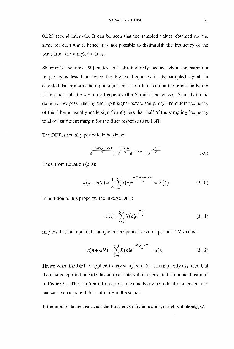
SIGNAL PROCESSING 32
0.125 second intervals. It can be seen that the sampled values obtained are the
same for each wave, hence it is not possible to distinguish the frequency of the
wave from the sampled values.
Shannon's theorem [58] states that aliasing only occurs when the sampling
frequency is less than twice the highest frequency in the sampled signal. In
sampled data systems the input signal must be filtered so that the input bandwidth
is less than half the sampling frequency (the Nyquist frequency). Typically this is
done by low-pass filtering the input signal before sampling. The cutoff frequency
of this filter is usually made significantly less than half of the sampling frequency
to allow sufficient margin for the filter response to roll off.
The DFT is actually periodic inN, since:
-}277n(k+mN) -j27lkn - j27lkn
e N = e-N-e-J2111nn = e-N- (3.9)
Thus, from Equation (3.9):
1 N-1 -j2n(k+mN)n
X ( k + mN) = - L x( n )e N = X ( k) N n~o
(3.10)
In addition to this property, the inverse DFT:
N-1 .27lkn
x(n)= LX(k)/N (3.11) k~O
implies that the input data sample is also periodic, with a period of N, that is:
N -I .27lk(n+mN)
x( n + mN) = L X ( k )/ N = x( n) (3.12) k~o
Hence when the DFT is applied to any sampled data, it is implicitly assumed that
the data is repeated outside the sampled interval in a periodic fashion as illustrated
in Figure 3.2. This is often referred to as the data being periodically extended, and
can cause an apparent discontinuity in the signal.
If the input data are real, then the Fourier coefficients are symmetrical aboutfs/2:

SIGNAL PROCESSING 33
X ( N - k) = - L x( n )e-1 N = - L x( n )e 1
/V = X* ( k) 1 N-1 2n(N-k)n [ 1 N-1 .21lkn]*
N n=O N n=O
(3.13)
where * indicates the complex conjugate.
For real data X(k) = x*(N-k), so to examine the frequency spectrum of a signal we
only need to look at the first N/2 Fourier coefficients. This gives the positive half
of the spectrum from zero frequency up to the Nyquist frequency.
3.2.2 The Fast Fourier Transform (FFT)
The DFT may be calculated directly using Equation (3.8), but this is a process that
takes a time proportional to the square of the number of points (N 2), hence the
time taken to compute the transform can rapidly become intractable for large
values of N. However an alternative exists, discovered by Cooley and Tukey [59],
which computes the DFT in a time proportional to the logarithm of the number of
points multiplied by the number of points (N logN). This algorithm is known as
the Fast Fourier Transform (FFT) and has become a commonly used engineering
tool with the advent of the digital computer. The general algorithm has been
described by many authors [59-64].
One limitation of the FFT algorithm is that it requires the number of input data
samples to be a power of two. In general it requires a special effort to ensure that
the number of data points sampled is a power of two. If it is not convenient to
sample a number of points which is a power of two, there are more complicated
algorithms, known as Prime Factor Algorithms (PFA) [65], which can still
calculate the Fourier transform quickly. These methods can compute the DFT
efficiently when the prime factors of the number of input samples are small in
magnitude. However, as the prime factors of N grow larger, these algorithms
reduce to the direct implementation of the DFT, Equation (3.8). Practically, these
algorithms are useful only when all prime factors of the number of samples are
less than about 30, although this depends on the speed of the computer which is
performing the computation, and upon the requirements of the application. In
general, it is easier to sample a number of points which is a power of two.

SIGNAL PROCESSING 34
3.3 Windowing and Window Functions
Since the Fourier Transform assumes that the input data ts periodic, Equation
(3.12), there can appear to be a jump discontinuity in the periodic extension of the
input signal if it is not sampled such that a whole number of cycles are captured,
that is, if it is not synchronously sampled. This is illustrated in Figure 3.2. Figure
3.2(a) shows the original time-domain signal (5Hz sine wave), 3.2(b) illustrates
synchronous sampling, while 3.2(c) shows the effects of asynchronous sampling
and the jump discontinuities which result.
1\
q.s
' II II I I I I I I I I I I
I I
-0.5 I
I I I I
I I
I I
I I
I I
I I I I II II
I 0 (\ 1\ (\ (\ (\ A
0.5
00 05 I 0 tim (s)
- .5
-J.B v v v v
Figure 3.2(a): Original time signal.
I I I I I I I IJ
1,'
II I 0 (\ (\ (\ 1\ II I I I I
I I 10.5
I 00 05 I I I I
-Q.5~ I I
I I
I I
II II
-1.0
tim (s)
v --- Sampled data-l ~ - - - - - Periodic ext~
1\ " II II
I I II
I I I I I
I I I I I
I 0
I I I
I I II
1,'
(\
I.
v
' II II I I I I I I I I I I
1.5
I I I I II II
Figure 3.2(b): Synchronously sampled signal.

SIGNAL PROCESSING
~ 1\ 1.0
: \ : ~ iII I I I I I I
I I I 1 10.5 1 ~ I I
I I ; II
J I I I
; I I I
f---r--'---t-1--&e--0.5 I
11
I I
~ : I : I
I I : : I I I I
~ ; : ; -Q.s \; \I
\ i ~ : \ 1
II \.' -1.0
1\ (\ A II II II I
II I I 1
II II I
I I I I I I I
I I I I I I I
I I I I I I I I I I I I I I I I I I I I I I I I I I I I I I I I I I
I I I I I
I I I I I
I I
I I I I I
f---'Lo; I 00 05 I I I
1).
I I I I I I I
I tim (s) I
I I I I I
I I I I I I I
I I I I
I I I I I
I I I I
I I I I
I I I I
I I I I I
I
I· I
I I I I I
I I I I I v II
II II v v 1/ II \I
Figure 3.2(c): Asynchronously sampled signal.
The frequency spectra of the signals in Figure 2 are shown below:
0.5
0.4
.1J 0.3 a ~ < 0.2
0.1
Frequency (Hz)
Figure 3.3(a): Frequency spectrum of Figure 3.2(a).
35
It can be seen that the discontinuity in the asynchronous sampling of Figure 3.2(c)
causes spreading of the peak in the frequency domain in Figure 3.3(c). This is
known as leakage. The DFT maps the continuous frequency spectrum onto a
discrete set of basis functions, which are the complex exponentials of Equation
(3.8). Only frequencies which map exactly onto one of the basis functions will be
represented by a single component in the frequency spectrum, as shown in Figure
3.3(b). Frequencies which do not map exactly will map onto all of the basis
functions, causing the leakage observed in Figure 3.3(c).
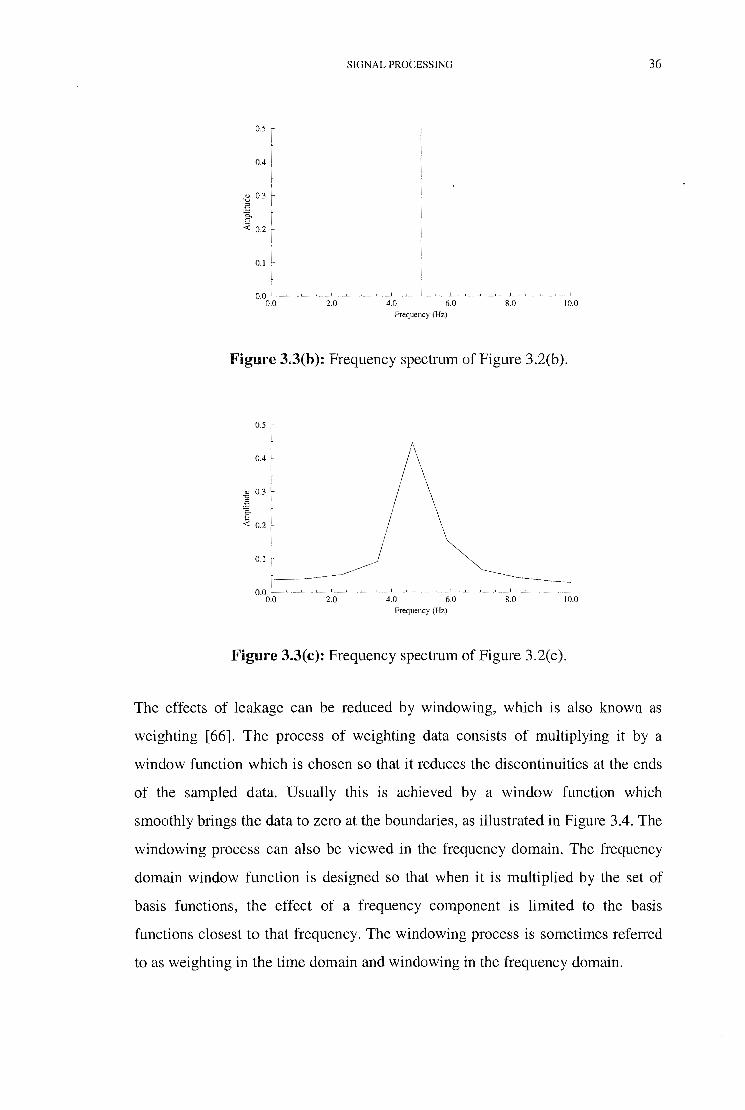
0.5
0.4
{j 0.3 8
~ < 0.2
0.1
SIGNAL PROCESSING
Frequency (Hz)
Figure 3.3(b): Frequency spectrum of Figure 3.2(b).
0.5
0.4
{j 0.3 .€ ]" < 0.2
0.1
2.0 4.0 6.0 8.0 10.0 Frequency (Hz)
Figure 3.3(c): Frequency spectrum of Figure 3.2(c).
36
The effects of leakage can be reduced by windowing, which is also known as
weighting [66]. The process of weighting data consists of multiplying it by a
window function which is chosen so that it reduces the discontinuities at the ends
of the sampled data. Usually this is achieved by a window function which
smoothly brings the data to zero at the boundaries, as illustrated in Figure 3.4. The
windowing process can also be viewed in the frequency domain. The frequency
domain window function is designed so that when it is multiplied by the set of
basis functions, the effect of a frequency component is limited to the basis
functions closest to that frequency. The windowing process is sometimes referred
to as weighting in the time domain and windowing in the frequency domain.

SIGNAL PROCESSING
1.0
0.5-
0.0 +-t--+++-+--t--t-+f-t--1--+-+--t+t--t-++t+t--i-+·+--t+1-+t--+ 00
-0.5
-1.0
1.0
0.5
05 I 0 I 5 I'm()
20
Figure 3.4(a): Sampled data.
25 3.0
0.0 -1-"''---+-----t--___,r-------t---+----· -t-----+----t-------<----t------1 0.0 0.5 1.0 1.5 2.0 2.5 3.0
time(s)
Figure 3.4(b): Window function (Hanning window).
1.0
0.5
0.0 0
-0.5
-1.0
0
A
A A
1:\ I\ A/\" vov 10 I 5 20 v2V im ()
v v
v
Figure 3.4(c): Windowed data.
--1 3.0
37

0.0
-20.0
~ -40.0
" '0
.€
"' -60.0 E <(
-80.0
-100.0 0.0 2.0
SIGNAL PROCESSING
' ' ' ' I
' I I
I I
Spectrum no window -~ ~ - - Spectrum- Hanning wil~
4.0 6.0 Frequency (Hz)
8.0 10.0
Figure 3.4(d): Frequency spectrum of windowed and non-windowed data.
3.3.1 Figures of Merit for Window Functions
38
Harris [66] describes several figures of merit by which the performance of
window functions may be judged. He calculates these figures for many different
windows. The minimum resolution bandwidth of a window is the minimum
spacing between two frequency components of equal amplitude, if they are to be
resolved. This is given as a number of bins, where a bin is the fundamental
frequency resolution fs/N. For one frequency component to have the minimum
effect on another due to leakage, it is best if the rate at which sidelobes decrease is
as large as possible. This is usually quoted in dB/octave. For detecting small
amplitude frequency components in the presence of those of larger amplitude, it is
important that the sidelobes adjacent to the mainlobe be as low as possible.
Since a window reduces the amplitude of the data at either end of the sampled data
record, it appears to the DFT that the signal changes in amplitude. The effect that
this has on the amplitudes of the components of the frequency spectrum is known
as processing loss [66]. If a frequency component lies half-way between two DFT
frequency bins, then the power will be spread equally between the two bins,
neither of which will have an amplitude as great as the single component alone
would have. This is known as scalloping loss [66]. Processing loss and scalloping
loss can be combined to give the worst case processing loss for a particular
window. Harris [66] noted that this was always between 3.0dB and 4.3dB for the

SIGNAL PROCESSING 39
windows which he examined. This means that a frequency component of a signal
may have its amplitude reduced by an amount up to the worst case processing
loss, when the DFT is calculated, depending on where it lies with respect to the
frequency bins. Hence, several different records of the same signal may exhibit
different spectra, due to slight changes in the frequency sampled, and the sampling
process itself. This is explored further in Section 3.3.4.
3.3.2 Window Functions
There are many useful window functions available. Harris [66] and Nuttall [67]
provide a good overview and evaluation of the performance of each window
according to certain metrics. There are a few of particular relevance to this thesis,
namely the rectangular, Hanning, Hamming, and Blackman windows. The
following sections detail the time and frequency responses of these windows, and
shows the results of applying the windows to a typical stator current spectrum.
3.3.2.1 Rectangle Window
The rectangle window has a value of one over the observation interval and zero
elsewhere. It is automatically applied by the process of sampling a signal. It is
defined as:
w(n) = 1 n = O,l,2, ... ,N -1 (3.14)
The normalised frequency spectrum for the rectangle window is:
. (NO) D( 0) = exp(- j N -1 e) sm l
2 . (e) sm 2
(3.15)
This function is known as the Dirichlet kernel [66]. This has a first sidelobe level
of about -13dB and the sidelobes fall off at a rate of 6dB per octave. The 6dB
bandwidth is 1.21 bins, which is the minimum possible for any window, and the
worst case processing loss is 3.92dB.

SIGNAL PROCESSING 40
The frequency response of the rectangle window IS shown in the following
diagrams where N = 40:
1.5
1.0 •••••••••••••••••••••••••••••••••••••••
0.5 .
0.0 ~-~-c.._.__L.~~~_,____j~~~~~-'--~~~__J 0.0 10.0 20.0 30.0 40.0
n
Figure 3.5(a): Rectangle window.
0.0
-20.0
iii' -40.0 :::\ " '0 2
t -60.0
-80.0
-100.0 0.0 1.0 2.0 3.0
Nonnalized Frequency (rad)
Figure 3.5(b): Normalised frequency response of rectangle window.
3.3.2.2 Hanning Window
The Hanning window belongs to a general class of window functions of the form
cos"'. The special case of the Hanning window has a= 2:
w( n) = cos2 nnj N = 0.5[ 1- cos( 2nnj N) J (3.16)
The normalised frequency spectrum of is:
w( e)= 0.5D( e) +0.25[ D(e- 2nj N)+ D(e- 2nj N)] (3.17)
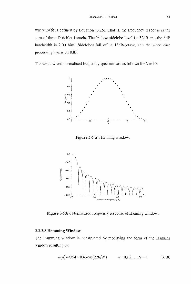
SIGNAL PROCESSING 41
where D(B) is defined by Equation (3.15). That is, the frequency response is the
sum of three Dirichlet kernels. The highest sidelobe level is -32dB and the 6dB
bandwidth is 2.00 bins. Sidelobes fall off at 18dB/octave, and the worst case
processing loss is 3 .18dB.
The window and normalised frequency spectrum are as follows for N = 40:
1.0 .... 0.8
~ 0.6 2 ~ E < 0.4
0.2
0.0 • --._J
0 10 20 30 40 n
Figure 3.6(a): Hanning window.
0.0
-20.0
"' -40.0 ~ ~ 2
I -60.0
-80.0
-100.0 0.0
Nonnalized Frequency (rad)
Figure 3.6(b ): Normalised frequency response of Hanning window.
3.3.2.3 Hamming Window
The Hamming window is constructed by modifying the form of the Hanning
window resulting in:
w( n) = 0.54- 0.46 cos( 2TCn/ N) n = 0,1,2, . .. ,N -1. (3.18)

SIGNAL PROCESSING 42
The normalised frequency spectrum of Equation (3.18) is:
w( e)= 0.54D( e)+ 0.23[ D( e- 2nj N) + D( B+ 2nj N)] (3.19)
where D(B) is defined by Equation (3.15).
l.O .... 0.8
-15 0.6 a ~ " .;: 0.4
0.2 . . ... 0.0
0 10 20 30 40 n
Figure 3.7(a): Hamming window.
0.0
-20.0
iii' -40.0 :s
<U '0 a ·a on -60.0 ~
-80.0
-100.0 0.0
Normalized Frequency (rad)
Figure 3.7(b): Normalised frequency response of the Hamming window.
This choice approximately cancels the first sidelobe of the Hanning response,
giving high attenuation around the main lobe, with a highest sidelobe level of
-43dB. However the discontinuity at the boundaries causes the remaining
sidelobes to fall of at only 6dB per octave, which is much slower than the Hanning
window. The 6dB bandwidth is 1.81 bins, and the worst case processing loss
3.10dB.

SIGNAL PROCESSING 43
3.3.2.4 Blackman Window
The Blackman window is similar to the Hamming window in that it is also a
constructed window. It is a member of the more general class of windows of the
form:
N/2
w(n) = L,(-1tamcos(2JZmn/N) n = 0,1,2, ... , N -1 (3.20) m=O
N/2
where L,am = 1. m=O
This general form also includes the Hanning and Hamming windows where only
a0 and a1 are non-zero in Equation (3.20). The Blackman window is generated
using ao = 0.42, a1 = 0.50, a2 = 0.08, giving:
w(n) = 0.42- 0.50cos(2Trnj N) + 0.08cos( 4Trn/ N) n = 0,1,2, ... ,N -1 (3.21)
The normalised frequency spectrum is then:
w(o)= o.42D(o)-o2s[v(o- 2; )+v(o+ ~)]
(3.22)
+004[v(e- :')+v(o+ :')] The window and spectrum are shown in Figure 3.8.
This construction cancels the third and the fourth sidelobes of the Dirichlet kernel,
whilst eliminating boundary discontinuities, giving sidelobes which fall off at a
rate of 18dB per octave. The first sidelobe level is -53dB and the 6dB bandwidth
is 2.13 bins, the worst case processing loss is 3.47dB. This makes it particularly
suitable for detecting low magnitude frequency components in the presence of
larger components.

05' ::<:!,
" "0 B ·a bO
~
1.0
0.8
.g 0.6 2 §. .;;: 0.4
0.2
0.0
0.0
-20.0
-40.0
-60.0
-80.0
-100.0
0
0.0
SIGNAL PROCESSING
--"--~----'- . 10 20
Figure 3.8(a): Blackman window.
1.0 2.0 3.0 Nonnalized Frequency (rad)
Figure 3.8(b): Normalised frequency spectrum of the Blackman window.
3.3.3 Effect of Window Functions on a Typical Stator Current Spectrum
44
In order to demonstrate the effect that each of the above window functions has on
a typical stator current spectrum, each of one of them is applied in tum to the same
data set. The motor used was the Pope motor (Appendix A) with a broken rotor
bar. It was supplied from the mains and the speed was measured with an optical
tachometer as 1464 rpm. Hence the twice slip-frequency sidebands should appear
at (50±2.4)Hz. Data was sampled at a rate of 10kHz, and 32768 data points were
collected, giving a basic frequency resolution (see Section 3.4.1) of 0.3052Hz. The
results are shown in Figure 3.9.

Amplitude (dB) 0
-10
-20
-30
-40
-50
-60
-70
-80
-90
-100 0 10 20 30
SIGNAL PROCESSING
40
O.OOOOOOdB 50.05Hz
50 60
Frequency (Hz)
70 80 90 100
Figure 3.9(a): Stator current frequency spectrum- rectangle window.
Amplitude (dB) 0
-10
-20
-30
-40
-50
-60
O.OOOOOOdB 50.05Hz
-38.30dB 47.00Hz
I
50
-40.7ldB 53. 10Hz
60
Frequency (Hz)
70 80 90 100
Figure 3.9(b): Stator current frequency spectrum- Hanning window.
45

Amplitude (dB)
0
-10
-20
-30
-80
-90
-100'--------0 10 20 30
SIGNAL PROCESSING
O.OOOOOOdB 50.05Hz
-39.64dB 46.69Hz -4l.28dB
53.10Hz
40 50 60
Frequency (Hz)
70 80 90 100
Figure 3.9(c): Stator current frequency spectrum- Hamming window.
Amplitude (dB)
0
-10
-20
-30
-40
-50
-60
O.OOOOOOUB 50.05Hz
-38.30rJB 47.00Hz
I
50
-40.7JdB 53. 10Hz
60
Frequency (Hz)
70 80 90 100
Figure 3.9(d): Stator current frequency spectrum- Blackman window.
46

SIGNAL PROCESSING 47
The difference in the rate at which the sidelobes fall off for different windows is
evident when Figures 3.9(a) and (c) are compared with 3.9(b) and (d). The former
have sidelobes which fall off at 6.0dB/octave, whilst the latter fall off at
18.0dB/octave. It is also interesting to note the difference in the amplitudes of the
twice slip-frequency sidebands caused by the window functions. The sidebands
cannot even be seen when the rectangle window is used, which shows how useful
the window functions are.
3.3.4 Statistical Analysis of Variation in Sideband Amplitudes
In order to determine the variation in amplitude which could be encountered in a
practical application of the sampling process, an experiment was performed. The
Pope motor (see Appendix A), with a broken rotor, was supplied from the mains
and loaded to rated load by a DC generator and resistor bank. After waiting a
while for the system to reach a steady state, one hundred records of the stator
current waveform were consecutively sampled. The signal was sampled at a rate
of 3.2kHz with an 800Hz low-pass filter for anti-aliasing. 32 768 data points were
sampled for each record and the FFT, with a Blackman window, used to compute
the spectrum. The amplitudes of the twice slip-frequency sidebands were then
extracted and the following statistics computed:
Statistic Lower Sideband Upper sideband
Mean Amplitude (dB) -36.05 -35.79
Standard Deviation 1.11 1.12
Range (dB) 5.13 5.65
Table 3.1: Statistics for sampling under constant conditions.
It can be seen that, even though the load and input voltages were not changed,
there was some variation in the amplitudes of the sidebands. The standard
deviation was about 1.1 for both sidebands whilst the range of values was about

SIGNAL PROCESSING 48
5dB. That is, there was a 5dB variation between the maximum and minimum
values of the sidebands. Figure 3.10 plots the variation in sideband amplitude with
the data record number. This is effectively a plot against time as the current was
sampled at approximately regular intervals. The total time taken to collect all of
the data records was about 30 minutes. From the graph it would appear that the
amplitude fluctuations are random over this time, with no trend being apparent.
This would indicate that the machine system had reached a steady-state before
sampling was begun.
-32
-34
~ Q)
] -36
1 -38
r-=-----Lower Sideband
~Upper Sideband
-40 '---~---L--~----'---~---'---"---------'-----L---__j 0 w ~ w w 100
Sample Number
Figure 3.10: Variation in sideband amplitude with data record number.
3.4 Parametric Models for Spectral Estimation
The Fourier transform uses a fixed set of basis functions as a model for the signal
being analysed. The functions are a discrete set of sinusoids as given in Equation
(3.8), the frequency of which are fixed by the sampling frequency, and the number
of data points. Parametric methods also assume that the time domain signal can be
described by a mathematical model, but not necessarily a sum of sinusoids. The
parameters of that model are then calculated using the sampled data, from which
the frequency spectrum of the signal may be obtained.
SIGNAL PROCESSING 49
Parametric models can produce better spectral estimates than Fourier transform
methods, particularly with regard to spectral resolution, because the basis
functions of the model are not restricted in the way that those of the Fourier
transform are. The Fourier methods assume that the signal outside the sampling
interval window is zero, that is, it is implicitly windowed by a rectangular window
function. This is not a realistic assumption. By constructing a time-domain model
we can make a more realistic estimate of the signal outside the window. Thus the
need for window functions, and the adverse effects they can have on the spectral
estimate, is eliminated. However, improvement in the estimation of the spectrum
is highly dependent upon how well the model approximates the signal in question.
The assumption that the signal is stationary is particularly troublesome when
dealing with variable speed drives, since the speed control is achieved by varying
the fundamental frequency. If this happens whilst sampling data, then a Fourier
transform of the data will not generally yield useful results. Since a parametric
model requires far less data to produce a spectral estimate, the data is sampled for
a much shorter time, reducing the likelihood of the frequency changing during
sampling.
The particular parametric technique examined here is Prony's method, as it offers
better results than other techniques.
3.4.1 Frequency Resolution of Spectrum Esthnates
The basic resolution of the DFT is fs/N, that is, it is governed by the sampling rate
and the number of points sampled. To increase the resolution, either the number of
points sampled must be increased, or the sampling frequency decreased. The
highest frequency in the resulting spectrum is Js/2, so the sampling frequency
cannot be reduced indefinitely, especially when it is considered that an anti
aliasing filter limits the highest frequency to be less than this. Increasing the
number of points sampled causes the sampling time to increase as well. This
implies that the signal sampled must remain stationary for longer, which can be a
problem with industrial drives. As a guide, if the sampling frequency is 5kHz, and
the anti-aliasing filter cutoff is 2kHz, 16 384 points sampled gives a basic

SIGNAL PROCESSING 50
frequency resolution, fiN, of only 0.3052Hz. If the twice slip-frequency
sidebands are at ±1Hz, then there are only three bins separating them from the
supply frequency peak. The total sampling time to collect the data, is 3.2768
seconds.
Parametric methods only require a few data samples in order to form a spectral
estimate. If the model has n parameters, then only n points are required in order to
solve for those parameters. Generally, parametric methods use a system of over
determined equations so that a least-squares fit may be performed to determine the
parameters, which lessens the effect of any noise. In this case a number of points
required is greater than n. For example, a model consisting of 20 sinusoids, would
have 60 parameters, amplitude, frequency and phase of each sinusoid, and the
number of samples required to solve for these parameters would be greater then
60, dependent on the algorithm used. Hence the signal is required to be stationary
for a much shorter time than a Fourier spectrum of equivalent resolution.
3.4.2 Prony's Method
Prony's method is not a spectral estimation technique in the usual sense, rather it is
a way of modelling data by fitting damped exponential functions. However it can
be extended to provide a spectral estimate.
In 1795 Gaspard Riche, Baron de Prony [54] [55], proposed that the laws
governing the expansion of gases could be modelled by the sum of damped
exponentials. His original model had two parameters for each exponential
function, An and an. Hence for a model of order p, 2p data points are required in
order to solve the set of simultaneous equations. If xi is the datum recorded at time
ti, then the set of equations that must be solved is given by:
p
X;= L~ exp(ant;) (3.23) n=l
for 1 ~ i ~ 2p.
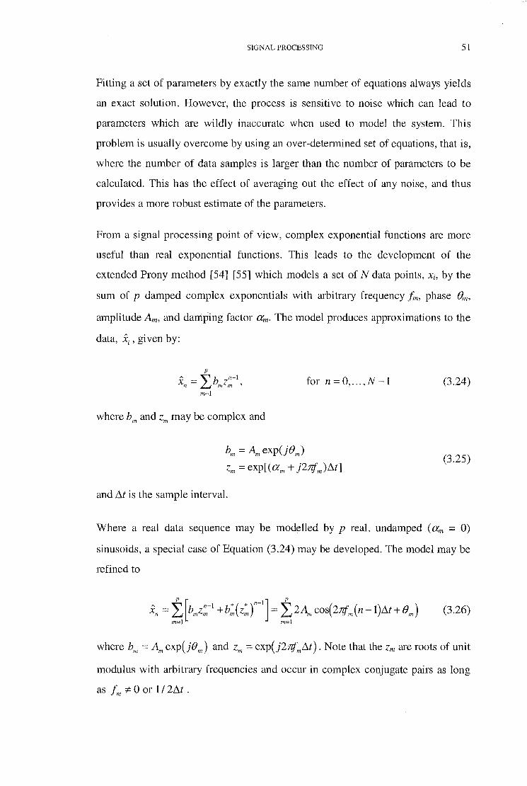
SIGNAL PROCESSING 51
Fitting a set of parameters by exactly the same number of equations always yields
an exact solution. However, the process is sensitive to noise which can lead to
parameters which are wildly inaccurate when used to model the system. This
problem is usually overcome by using an over-determined set of equations, that is,
where the number of data samples is larger than the number of parameters to be
calculated. This has the effect of averaging out the effect of any noise, and thus
provides a more robust estimate of the parameters.
From a signal processing point of view, complex exponential functions are more
useful than real exponential functions. This leads to the development of the
extended Prony method [54] [55] which models a set of N data points, Xi, by the
sum of p damped complex exponentials with arbitrary frequency fm, phase Bm,
amplitude Am, and damping factor fXm. The model produces approximations to the
data, xi' given by:
for n = 0, ... , N -1 (3.24)
where bm and zm may be complex and
bm =An exp(}Bm)
Zm = exp[(am + j21ifm)M] (3.25)
and 11t is the sample interval.
Where a real data sequence may be modelled by p real, undamped ( fXm = 0)
sinusoids, a special case of Equation (3.24) may be developed. The model may be
refined to
xn = f[bmz;-1 +b:(z:r-1]= f2Amcos(21ifm(n-1)11t+Bm) m=l m=l
(3.26)
where bm =An exp(jBm) and zm = exp(j21ifm11t). Note that the Zm are roots of unit
modulus with arbitrary frequencies and occur in complex conjugate pairs as long
as fm :7: 0 or 11 211t.

SIGNAL PROCESSING 52
Finding the set of Am, B m , fn,, and p that minimise:
N-1
E= Llxn -xJ (3.27) n=O
is a difficult non-linear problem, which may be solved iteratively. Another method
is Prony's technique, which solves two sets of linear equations leaving the non
linearity in a polynomial rooting procedure.
In order to do this one must solve for the roots, which are the zm above, of the
polynomial:
2p 2p
'f'(z)= IT(z-zJ= Laklp-k =0 (3.28) i=l k=O
with a0 = 1 and the a; being real coefficients. It is obvious that coefficient a2P is
given by:
2p
a2p = rr Z;. i=l
(3.29)
Due to each Z; having unit modulus, z~1 = z:, and )a2P) = 1, it can be shown that
the polynomial below has the same roots as (3.28)
(3.30)
Since the roots are of unit modulus and o~cur in complex conjugate pairs, then we
must have ak = a2 Pa;p-k for k = 0, ... ,2 p. A linear difference equation with (3.28)
as its solution may be written [54]:
p
apxn-p + L(ap_kxn-p+k +ap+kxn-p-k) = 0 k=l
for 2p+1~n~N. (3.31)
This equation may be divided through by aP to provide a more convenient form:
p
xn-p + L ( gkxn-p+k + g:xn-p-k) = o k=l
(3.32)

SIGNAL PROCESSING 53
where gk = ap-k/ap. From this equation the conjugate linear smoothing error can be
defined as:
(3.33)
which minimises the squared smoothing error:
(3.34)
Setting the partial derivatives of ps with respect to g1 through to gP to zero gives
the following equations expressed in matrix form.
where
(3.35)
N
and ri,k = L ( x~_ jxn-k + xn-p+jx~-p+k) . n=2p+l
Solving this set of equations gives the set of polynomial coefficients ak, which
satisfy the least squares criteria. Once these have been determined, the roots of the
polynomial (3.28) may be found using a polynomial rooting procedure. Once the
roots have been found, the problem becomes linear in the remaining parameters,
b1, ... ,bp. The set of linear equations which must be solved using a least squares
procedure is:
(3.36)
where
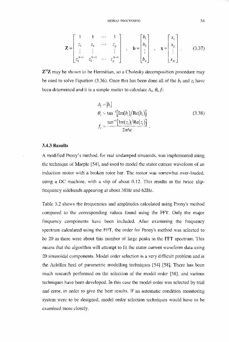
SIGNAL PROCESSING 54
1 1 1 bl XI
Z= zl z2 zp
b= b2 x2
(3.37) x=
N-1 N-1 N-1 bp zl z2 Zp XN
zHz may be shown to be Hermitian, so a Cholesky decomposition procedure may
be used to solve Equation (3.36). Once this has been done all of the bi and Zi have
been determined and it is a simple matter to calculate Ai, ~' fi:
A =/b;/ B; = tan-1[1m(b;)jRe(b;)] (3.38)
tan -I [ Im( Z;) / Re( Z;)] J; = 21ll'1t
3.4.3 Results
A modified Prony' s method, for real undamped sinusoids, was implemented using
the technique of Marple [54], and used to model the stator current waveform of an
induction motor with a broken rotor bar. The motor was somewhat over-loaded,
using a DC machine, with a slip of about 0.12. This results in the twice slip
frequency sidebands appearing at about 38Hz and 62Hz.
Table 3.2 shows the frequencies and amplitudes calculated using Prony's method
compared to the corresponding values found using the FFT. Only the major
frequency components have been included. After examining the frequency
spectrum calculated using the FFT, the order for Prony's method was selected to
be 20 as there were about this number of large peaks in the FFT spectrum. This
means that the algorithm will attempt to fit the stator current waveform data using
20 sinusoidal components. Model order selection is a very difficult problem and is
the Achilles heel of parametric modelling techniques [54] [58]. There has been
much research performed on the selection of the model order [58], and various
techniques have been developed. In this case the model order was selected by trial
and error, in order to give the best results. If an automatic condition monitoring
system were to be designed, model order selection techniques would have to be
examined more closely.

SIGNAL PROCESSING 55
The same set of sampled stator current data was used for both sets of results. The
stator current was sampled at 3200Hz, to gather 32 768 samples. The FFT used
all of these data points to obtain a reasonable frequency resolution, whilst the
Prony results were generated using only 200 sample points. It can be seen that the
Prony method generates comparable results to the FFT method while using two
orders of magnitude less data points.
Prony FFT Prony FFT
Frequency (Hz) Frequency (Hz) Amplitude (dB) Amplitude (dB)
49.98 50.03 0.00 0.00
38.36 38.01 -22.47 -20.20
13.22 13.88 -20.43 -35.21
63.31 62.05 -38.81 -40.29
76.15 74.07 -39.12 -48.30
85.42 86.19 -35.75 -49.57
97.60 98.21 -38.70 -51.36
149.81 150.09 -34.57 -34.73
250.84 250.16 -34.61 -31.93
211.93 214.00 -37.62 -39.01
314.55 314.06 -36.17 -37.79
351.12 350.22 -42.71 -40.31
Table 3.2: Comparison of Prony analysis and FFT results
Prony's method makes the problem of peak detection much easier than with the
FFT. Any leakage in the spectrum causes a single frequency component to be
spread over a number of frequency bins, making detection of the single frequency
component much more difficult. Since Prony' s method models the signal by single
frequency components, no such difficulties are encountered.

SIGNAL PROCESSING 56
Unfortunately Prony' s method is not all that useful, when applied in the manner
above, as it is not all that good at modelling signals where there are two frequency
components close together, but with a large difference in amplitude. In this case
the smaller signal tends to be overlooked. This is why such a large slip value was
used in the experimental work, as it was found that if the slip was much smaller
then the sidebands became undetectable. An attempt was made to remove the
mains frequency using a highly tuned notch filter, unfortunately it was not
possible to make the notch selective enough so that it did not affect the sidebands
of interest.
3.5 Summary
Chapter 2 showed that faults in induction motors could be detected by examining
the frequency spectrum of the stator current waveform. This chapter has examined
the theoretical basis of the signal processing techniques used in order to calculate
the frequency spectrum. The Fourier transform is the basic tool for calculating
frequency spectra, and it is often misunderstood and misused. The consequences
of aliasing and the implicit periodicity of the Discrete Fourier Transform were
examined. The use of window functions for reducing the effects of leakage due to
the periodic nature of the DFT was also examined. Various common window
functions and their properties were discussed and their effect on frequency spectra
calculated was illustrated using a typical stator current spectrum.
Since the twice slip-frequency sidebands are so important for the detection of rotor
damage, a statistical analysis of the variation in sideband amplitude due to slight
variations in sampling and motor operation, was performed. One hundred records
of the stator current were sampled with the motor and load operating in a steady
state. The sideband amplitudes were calculated and their variation analysed and
plotted. It was found that the standard deviation was about ldB for an average
value of about -36dB, whilst the amplitudes had a range of about 5dB. Thus for
any particular frequency spectrum there may be an uncertainty in the sideband
amplitudes of up to ±3dB. It is important to take this variation into account when
trying to detect broken rotor bars.

SIGNAL PROCESSING 57
Finally, a parametric spectrum estimation technique, Prony' s method was
examined. Parametric techniques model the signal using a limited number of
frequency components, and require only a small number of data points in order to
solve for the model parameters. The Prony method examined here uses a model
order of 20, which required 200 data points to be sampled. In contrast, the Fourier
transform required 32 768 data points in order to generate a spectrum with
reasonable frequency resolution. This illustrates the great advantage of parametric
techniques. However, the disadvantage is that they are not good at modelling
signals with components that are close together in frequency, but of greatly
different amplitude.

4.1 Introduction
CHAPTER 4
Phase Locked Loops and
Synchronous Sampling
In Chapter 2 it was shown that broken rotor bars in an induction machine cause
modulation sidebands of twice slip-frequency (±2sfi) to appear around the supply
frequency (ji Hz) component in the frequency spectrum of the stator current, when
the machine is running with a per-unit slip of s. These peaks may be quite close to
the supply frequency peak if the slip is small, especially for large induction motors
which often have a slip at rated load of around 0.01. If there is any leakage (as
described in Chapter 3) of the supply frequency peak, then these sidebands may be
obscured. One possible solution is windowing, as outlined previously; however if
the basic frequency resolution is low, this may still be insufficient to distinguish
the sidebands.
58

PHASE LOCKED LOOPS AND SYNCHRONOUS SAMPLING 59
A more elegant solution is to ensure that the current waveform is synchronously
sampled, which causes the supply frequency peak to occupy only a single
frequency bin in the resulting spectrum. Thus the sideband peaks will not be
obscured so long as the frequency bin width is narrow enough to resolve them
from the supply peak. A hardware solution, in the form of a phase locked loop,
can be utilised in order to ensure that synchronous sampling occurs. In variable
speed drive applications it also has the benefit of tracking any change in the
supply frequency, and thus produce a useful spectrum.
This chapter outlines the principles of operation of phase locked loops and the
development of a circuit to control the sampling process. Results are presented for
motors on both fixed (mains) and variable frequency supplies.
4.2 The Phase Locked Loop
The phase locked loop (PLL) is a circuit which produces an output signal which
has a frequency the same as, or a constant multiple of, the frequency of the input
signal. The output frequency of the circuit can track changes in the input
frequency over a limited range, called the tracking range. When the signal is first
applied to the circuit, the PLL will only lock if the input frequency is within the
capture range of the circuit. The tracking range is normally greater than the
capture range. To ensure that a signal is synchronously sampled, an integer
number of cycles of the fundamental must be sampled. The easiest way to do this
is to sample a fixed number of points per cycle. A frequency multiplying PLL
multiplies the frequency of the input signal by an integer. If the resulting
frequency is used to control the sampling device, then a fixed number, dependent
on the frequency multiplier, of samples per cycle will be sampled. Thus, a
frequency multiplying PLL can ensure that a signal is synchronously sampled.
4.2.1 The Basic PLL Circuit
The basic configuration of a PLL circuit consists of a phase comparator, a low
pass filter (loop filter), and a voltage controlled oscillator (VCO). The phase
comparator produces a voltage which is proportional to the phase difference

PHASE LOCKED LOOPS AND SYNCHRONOUS SAMPLING 60
between the input and output waveforms. This voltage is then low-pass filtered to
obtain the DC component, which is then applied to the VCO. The VCO produces
a periodic output waveform at a frequency which is controlled by the input DC
voltage. This configuration is illustrated in Figure 4.1.
vin(t) Phase
vpc (t) - Low-pass vc (t)
Voltage Controlled vm,1(t)
Input Comparator Loop Filter Oscillator (VCO) Output
Figure 4.1: Basic PLL block diagram.
The principle of operation of the circuit is quite simple. The frequency of the
output signal of the VCO, OJ0u1(t), is proportional to the input control voltage:
(4.1)
where ~is the free-running frequency (zero control voltage) of the VCO, Kvco is
the gain of the VCO, and vc(t) is the control voltage.
The phase comparator compares the phases of the input and output waveforms,
and produces a voltage, Vpc(t), proportional to the difference:
(4.2)
where Kpc is the gain of the phase comparator, r/Jin(t) is the phase of the input
signal, and </Jour(t) is the phase of the output signal. Vpc(t) will usually have an AC
component which is undesirable, hence a low-pass filter is used to obtain the DC
component which is used to control the VCO.
When the circuit is operating in the locked state, OJout = OJin· The VCO control
voltage is then:
(4.3)

PHASE LOCKED LOOPS AND SYNCHRONOUS SAMPLING 61
This must also be the average value of the phase comparator output voltage. In
general this means that there must be a constant phase difference between the
input and output waveforms, if Wtn is constant. If the input frequency changes,
then the phase comparator output voltage will also change, causing the VCO
output frequency to change. Eventually the output frequency becomes the same as
the input frequency and the PLL is locked. The time taken for this to occur is
known as the settling time of the PLL.
4.2.2 Frequency Multiplying PLL Circuit
There are several types of phase comparator circuit which may be used to
implement a PLL. Conceptually, the simplest is an analog multiplier. If the input
and output signals are sinusoids of frequency w, then the output of such a phase
comparator is:
where Vtn and Vaut are the amplitudes, and r/Jtn and r/Jout are the phases, of the input
and output signals respectively.
Equation (4.4) shows that the phase comparator output voltage has a DC
component proportional to the phase difference of the input and output
waveforms, and an AC component at twice the input frequency. The loop filter
removes the unwanted AC component.
Usually [69] PLL circuits are used to produce square wave output and need a
square wave input signal. In this case a digital logic circuit can be used to perform
the function of a phase detector. Such circuits are termed digital phase locked
loops (DPLLs), although most of the circuit is still analog. This is the type of PLL
which is designed here, as a logic level output signal is required to drive the AID
converters.

PHASE LOCKED LOOPS AND SYNCHRONOUS SAMPLING 62
It is also possible [69] to construct all-digital phase locked loops (sometimes
termed ADPLLs) which may be implemented in hardware or software. Since an
ADPLL is digital in nature, the output frequency can only change in discrete steps.
This causes the output frequency to suffer from frequency jitter because the
required output frequency is most likely not to be one of the possible discrete
output frequencies. The number of output frequency possibilities is dependent on
the clock frequency of the digital circuit, and hence the magnitude of the jitter is
also dependent on the clock frequency. A significant amount of jitter in the output
frequency will prevent synchronous sampling from being achieved, hence the jitter
must be minimised by using a high clock frequency. A preliminary design for a
hardware ADPLL required a clock frequency of several gigahertz, in order to keep
the predicted frequency jitter to an acceptable level. This frequency requirement
makes implementation of an ADPLL impractical as it would require a custom
fabricated chip in GaAs technology.
For the remainder of this thesis the term PLL is used to broadly refer to DPLLs as
well.
A frequency divider may be added into the feedback loop of a DPLL as shown in
Figure 4.2. The PLL then produces an output signal at a frequency N times the
input signal frequency, whereN is the frequency divisor.
V;n(t) Phase
Vpc (t) Low-pass
vc (t) Voltage Controlled
Vont(t)
Input Comparator Loop Filter Oscillator (VCO) Output
+N
Figure 4.2: Frequency multiplying digital phase locked loop block diagram.
The theory of operation of such a PLL is covered in great detail by Best [69], and
Encinas [70].

PHASE LOCKED LOOPS AND SYNCHRONOUS SAMPLING 63
4.3 Synchronous Sampling and the PLL
As shown in Chapter 3, synchronously sampling a sinusoidal signal causes the
resulting spectrum to consist of a single line. A multi -component signal composed
of one large sinusoid plus many smaller components can be sampled in
synchronism with the main component. This component and any multiples of it
will then appear as single lines in the frequency spectrum. Other, asynchronous
components will appear as peaks which are spread over several frequency bins, as
illustrated in Chapter 3. Since the largest component will appear as a single line, it
will not mask smaller components allowing them to be more easily detected.
In order to synchronously sample a signal it is necessary to capture an integral
number of cycles of the waveform. In order to perform an FFT on the resulting
data it is preferable to have a number of samples that is a power of two. Taking
into account the aforementioned constraints, and the fact that the frequency
multiplication factor for the PLL must be an integer, it is best to take a number of
samples per cycle that is a power of two. That is, the frequency multiplication
factor should be a power of two.
Thus synchronous sampling can be achieved by using a digital phase locked loop,
with a frequency multiplying factor that is a power of two, to drive the sampling
control of an AID converter. The complete system block diagram for acquiring
current waveforms in this manner is shown in Figure 4.3.
There are three signals which could be used as the input signal for the PLL in a
VSD system. One is the supply voltage, another is the modulating signal, and the
third is the drive carrier frequency. VSDs generally only have the first signal
available at externally accessible terminals, hence for an independent condition
monitoring system, this is the only useful signal. Hence the PLL circuit is
designed to lock only to this signal. Should the other two signals be available, then
it might be possible to use either of them, however detailed knowledge of the
drive is required. The modulating signal is essentially the same as the voltage
output signal as far as the PLL is concerned, but should provide a cleaner
frequency signal. The carrier frequency may not be useful since it is not

PHASE LOCKED LOOPS AND SYNCHRONOUS SAMPLING 64
necessarily related to the actual drive output frequency. This is completely
dependent on the drive system, however if the carrier frequency is, in fact, related
to the output frequency then it may prove to be quite useful in that it could
eliminate some of the frequency multiplication necessary in the PLL resulting in a
more stable system.
Input
Signal Anti-aliasing Amplifier
Filter
L----. Phase
Comparator
- Sample and Hold AID Converter
Circuit
r Sampling control
Schmitt Frequency r--Trigger Counter
Low-pass Voltage Controlled -Loop Filter Oscillator (VCO)
Divide by N
Counter
===> Sampled
Data Output
p~ amp ling
requency Count
Figure 4.3: Block diagram of the synchronous sampling system.
4.4 PLL Circuit Implementation
A circuit to implement the system of Figure 4.3 was designed and built and is
shown in Figure 4.4. The circuit is based around the CD4046B Micropower
Phase-Locked Loop chip [71] made by National Semiconductor Corporation. A
similar circuit was developed by Ferrero and Ottoboni [72], for power systems
applications. Another similar circuit for condition monitoring use was recently
granted a patent by Linehan et al. [73]. The circuit described in the patent is
essentially the same as that in Figure 4.4, and previously reported in [74].
The 4046 PLL chip has two phase comparators, a source follower, VCO, and a
zener diode. The zener diode is supplied for power supply regulation purposes and
was not used in the circuit. Phase comparator one is an exclusive OR gate which

PHASE LOCKED LOOPS AND SYNCHRONOUS SAMPLING 65
maintains 90° phase shift between input and output signals at the VCO free
running frequency, the phase shift varies from 0° to 180° over the tracking range
of the PLL. The second phase comparator is an edge-controlled digital memory
network that gives oo phase shift between the input and output signals whenever
the circuit is locked. The frequency range of the output signal of the wide-range
linear VCO is determined by external components. Equations for calculating the
value of these components may be found in [7 5]. Phase comparator one was
chosen to be used in this application as it has a much greater immunity to noise
[71] than the alternative.
The amplitude of the input wave is not critical, however it should be greater than
about 0.5 Vrms. The input enters the circuit at terminals PI and P2, and a
comparator based on a TL071 operational amplifier, detects the zero crossings to
produce a square wave at the same frequency. This is used as the input to the 4046
digital phase locked loop, the output of which is divided by a 4020 digital counter
and passed back to the phase detector input to form the feedback loop. The
fundamental frequency is multiplied by a factor of either 16, 32, 64, 128 or 256,
which is manually set by SWI, to generate the output clock signal. The resulting
clock waveform is passed through a 4049 inverter to provide buffering for
external sampling circuitry.
A 74LS393 binary counter chain is used to accurately count the frequency of the
clock signal output. The counter may either be gated externally, or internally by a
4538 monostable, which provides a gating pulse of 0.6 seconds. A 4011 provides
logic to control the source of the gating pulse.
The circuit is tuned for a 50Hz centre frequency and a tracking range of 32-68Hz,
which gives a capture range of 45-55Hz. This is because the mains frequency is
50Hz, so the circuit may also be used on mains supplied motors as well as VSDs
operating in the 45-55Hz range.

~ ..... I1Q
= """ t"')
.a;. :,;. .. n ~· c: ...... ,..... ()> >-;
~· ........ (D
~ .-~ -· 0 ::l 0 ......,
'"d ::r :::.:> r:FJ (D
0 0
8 0.. -0 0
'"d
A
I-
B
1--
c
f---
D
1 2 l 3 4
PI C\
A e. sv s\ne 4~7Bn ~::: PC\
P2 R\ PC2 e.sv s•ne Rl RJ R2 D-]_ < 11<11 41<7 R5 R6
] lN9\4 R4 -
~~5 ~ fD2 191!1< 1001< V~g~~ en -:- Rll 1--
101< ~ .-----! 101·
PO -ts ""'?" pdout
_ C7 ....L.
U4:A -:- \00n] B
""'?" 4949
CLK = 2""'n • F' (s\nel -=:=-Cior4<=n<=Gl
~ 1--
RIB tl<ll
+04 ~ IN914
CB \Bu
CTB mA +s B
CLR R\1 J91< 05 +
IN914.
-:;--:;-
49tl
~ R\2 J91<
1
-b-
U7: C 4911
, I
~ 12--5- -~- ~ 09 !Hll! SU\:A l!U! SUI:BI
vn o 1 o..A.Ij'-"-0 o..A.Ij'-"-0 1
tt~=~~~g~~~~~~N ~~--l,u • 1_ •t_o_r _c_N_I ____ 1,11 L 6_o_r_ c~ U6: B 74 J9J
!:>---++-' C L K 0 B t--*7"" 0\ f--"'-'-~: 02
11R OJ
c
1-
OT2 T 't le D
><;IH Ul~l
2
R\J 11<9 -b-
Ol.J 0v CT0 TRG RST
I '--
3
Mains-Phase-Locked Clock Source SA\4Ze rNUI'Iber
Oat e: .1\ 11AR 1996 Ft le:_C: \T.EJ1P\LI'INES_l/l
IRevtston t. B
Sheet I or t Draun 8Yi __ 6RI1
4
:g > r:FJ til r 0 n ;.; g) r 0 0 "t:l r:FJ
> z t:l
"' -< z n ::r: ;>;) 0 z 0 c r:FJ r:FJ > $; ;>1 z Cl
0\ 0\

PHASE LOCKED LOOPS AND SYNCHRONOUS SAMPLING 67
4.5 Circuit Performance with Mains Supplied Induction Motors
The mains supply voltage is a more or less smooth sinsusoid at a fixed frequency
(50Hz in Australia), which produces a sinusoidal stator current waveform at the
same frequency in the induction motor. The frequency may vary due to changes in
the total load on the whole power system, but in general any deviation from the
nominal frequency is quite small and occurs reasonably slowly. In Tasmania, the
deviation is usually less than ±O.lHz, although it may occasionally be more due to
extreme changes in system load [76]. These are the conditions for which the PLL
circuit (Figure 4.4) was designed.
The results obtained were very good as can be seen by comparing a windowed
non-synchronously sampled spectrum (Figure 4.5) with a PLL sampled spectrum
(Figure 4.6). The mains supply frequency peak reduces to a single line in the
spectrum, allowing the twice slip frequency sidebands, at 47.64Hz and 52.33Hz,
to stand out much more clearly. The two sets of data were sampled at slightly
different load levels, which is why the sidebands are at slightly different
frequencies in the two spectra. There were 16 384 points sampled for each data
record, at a rate of 3 .2kHz
Any change in the mains frequency, that occurs during sampling, tends to expand
the width of the peak at that frequency in Figure 4.5. The PLL synchronous
sampling circuit causes the sampling frequency to change in sympathy with any
change in the mains frequency, so no spreading occurs.
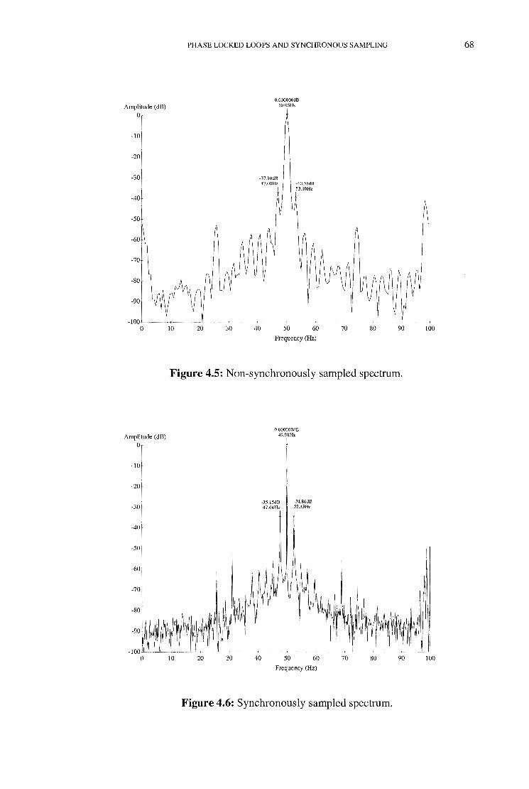
Amplitude (dB)
0
-10
-20
-30
-40
-50
Amplitude (dB) 0
-10
-20
-30
-40
-50
-60
-70
-80
-100 --0
PHASE LOCKED LOOPS AND SYNCHRONOUS SAMPLING
O.OOOOOOdB 50.05Hz
~37.80dB
47.00Hz
50
-40.35dB 53. 10Hz
I
60
Frequency (Hz)
70 80 90
Figure 4.5: Non-synchronously sampled spectrum.
10 20 30 40
O.OOOOOOdB 49.98Hz
-35.15dB 47.64Hz
50
-34.86dB 52.33Hz
60
Frequency (Hz)
70 80
Figure 4.6: Synchronously sampled spectrum.
90
68
100
100

PHASE LOCKED LOOPS AND SYNCHRONOUS SAMPLING 69
4.6 Application to Variable Speed Drives
A variable speed drive (VSD) changes the speed of an induction motor by
changing the frequency of the voltage supplied to the stator windings. This makes
the detection of sidebands caused by broken rotor bars much more difficult, as
these too will move as the supply frequency changes. If fixed-rate sampling is
used to acquire data, and the supply frequency changes during the acquisition
period, then the spectrum calculated is similar to that shown in Figure 4. 7.
Obviously there is no useful information visible in this spectrum.
Amplitude (dB)
-80
-90
-100 0 10 20 30 40 50 60 70 80 90 100
Frequency (Hz)
Figure 4.7: Stator current spectrum for fixed frequency sampling with varying
supply voltage frequency.
Using the PLL to control the sampling process causes the sampling frequency to
track any change that occurs in the supply frequency. This allows a clean spectrum
to be produced as shown in Figure 4.8. The sidebands and supply frequency can
be seen quite clearly in comparison to Figure 4.7. There is some spreading of the
sideband peaks which is due to the change in supply frequency and the change in
the slip, and hence of the sideband frequency relative to the supply frequency.

Amplitude (dB) 0
-10
-20
-30
-40
PHASE LOCKED LOOPS AND SYNCHRONOUS SAMPLING
O.OOOOOOdB 50.33Hz
-26.49dB 47.28Hz -28.lldB
53 .38Hz
I
Frequency (Hz)
70
Figure 4.8: Spectrum of stator current with PLL controlled sampling and varying
supply voltage frequency.
Since the sampling frequency changes over the time of data acquisition the
frequencies assigned to the bins of the FFT are rather arbitrary. The values
actually assigned in Figure 4.8 are based on the average sampling frequency over
the 0.65536 seconds immediately prior to the start of the sampled data record.
This value is obtained using the counter circuit described in Section 4.4, and
external gating controlled by software.
4.6.1 Circuit Performance with Variable Speed Drives
The PLL sampling circuit was tried on a number of VSD - induction motor
combinations, both in the field and the laboratory. It was found to perform
reasonably well in some circumstances and rather badly in others. One difficulty
was found to lie with the limited tracking range of the phase locked loop. It is
quite difficult to design a PLL with a wide tracking range and a good step
response at such low frequencies. Thus the operation of the device is constrained

PHASE LOCKED LOOPS AND SYNCHRONOUS SAMPLING 71
by the limited tracking range of approximately 36Hz, centred about 50Hz. It is
possible to increase the tracking range of the PLL at the expense of step response
time, which may be a viable solution in some circumstances.
Another solution which would be applicable if the frequency variation of the drive
system did not exceed the tracking range but was centred at a different frequency,
would be to have a bank of PLL circuits, each with a different centre frequency.
These circuits would have overlapping tracking ranges, so an initial fixed
frequency sampling of the signal could occur to determine the best PLL circuit to
use. In practice this would be somewhat cumbersome, and it would probably be
better to simply custom design a PLL to suit a particular drive system, if such a
design is possible.
A second, more serious, problem was discovered in the course of laboratory tests.
One VSD in the laboratory, an ABB SAMI GS (Appendix A), was found to have a
very high frequency jitter on the output waveform, even when operating at a
"constant" output frequency. This jitter was occasionally of large enough
magnitude to cause the PLL circuit to lose lock, causing non-synchronous
sampling to occur until it regained lock. This produced spectra of the form shown
in Figure 4.9, with broadening of the supply frequency peak apparent when
compared to Figure 4.8.
In order to quantify the magnitude of the frequency jitter, the stator current
waveform was observed on a digital CRO. The CRO was triggered on the rising
zero crossing of the waveform, and the timebase adjusted to display about one
cycle across the display at the nominal drive frequency. The next rising zero
crossing after the trigger was then observed to vary in position by up to 5% from
one cycle to the next. This is an extremely fast rate of change, and it would be
impossible to design a PLL circuit which could track frequency changes this rapid.
In order to combat the effects of the jitter and the noise spikes, an attempt was
made to filter the signal before applying it to the input of the PLL. To do this a
commercial Kron-Hite double-gang variable filter (see Appendix A) was used. A
low pass Butterworth response was chosen and the two filters cascaded with a

PHASE LOCKED LOOPS AND SYNCHRONOUS SAMPLING 72
cutoff frequency of 80Hz selected. However, this appeared to make no noticeable
difference to the results obtained. Varying the cutoff frequency of the filters also
made no discemable difference to the resulting frequency spectra, until the supply
frequency was filtered out of course.
Amplitude (dB) 0
-10
-20
-30
-40
-100-- ·--<·--· _,_
0 10 20 30
O.OOOOOOdB 50.33Hz
·27.55dB 47.28Hz -30.05dB
53 .38Hz
40 50 60
Frequency (Hz)
70 80 90 100
Figure 4.9: Broadening of supply frequency peak due to PLL losing lock.
It is thought that the jitter may be due to the variation in tum-on and tum-off time
of the semiconductor switches in the drive, as a result of varying amounts of
current being switched [77]. It is likely that all drives may suffer this to greater or
lesser degrees. Hence, the PLL method may not be that useful. However, if the
circuit could be integrated as part of the drive, then the PLL could be driven from
the power electronics control signals. This would solve the problem as these
signals should not suffer from frequency jitter.
4.7 Summary
A frequency multiplying phase locked loop can be used to ensure that the stator
current waveform is synchronously sampled. This has the benefit of reducing the

PHASE LOCKED LOOPS AND SYNCHRONOUS SAMPLING 73
supply frequency peak to a single line in the frequency spectrum, eliminating the
need for windowing, and allowing the broken rotor bar sidebands to be very well
defined and easy to identify. It also has the major advantage that any change in the
supply frequency is tracked and synchronous sampling maintained.
This chapter develops a design for a PLL circuit, based on the 4046B integrated
circuit, which generates a clock waveform at a constant multiple of the frequency
of the signal being sampled. When used to control the sampling hardware, this
circuit ensures that a signal is synchronously sampled. The circuit was designed
for a centre frequency of 50Hz, and tuned to have a capture range of 45-55Hz, and
a tracking range of 32-68Hz. This design makes it particularly suitable for mains
supply operation.
The frequency tracking behaviour of the PLL sampling method naturally leads to
application of the system to motors supplied by variable speed drives. In this case
the supply frequency can vary quite widely. It was found that the circuit
performance was unsatisfactory in some cases, depending on the drive used and
the frequency variation that occurred. The main problem was found to be rapid
jitter of the output frequency of the drive, which caused the PLL to lose lock.
However, this problem could be overcome if the PLL sampling technique was
integrated as part of the variable speed drive itself, as jitter-free control signals
would be accessible.

CHAPTER 5
Variable Speed Drives
5.1 Introduction
The great disadvantage of the induction motor in industrial applications, is that it
is very difficult to control the speed, because it is dependent on the supply
frequency and the load torque. Before the advent of semiconductor switching
devices, speed control of the induction motor could only be done by manipulating
the rotor currents on wound rotor machines, or by using a pole changing stator
winding. These methods have now become obsolete due to the invention of the
variable speed drive (VSD), which changes the frequency of the supply to the
motor, hence controlling the speed.
The VSD produces a variable frequency output waveform by rectifying the AC
mains supply to produce a DC source, which is then switched on and off by the
semiconductor switches in order to produce a pulsed output waveform. By
controlling the fundamental frequency of these pulses, the motor supply
frequency, and hence speed, is controlled. Since the output waveforms are
74

VARIABLE SPEED DRIVES 75
essentially a string of square pulses, the frequency spectrum contains many more
harmonics than does the mains frequency spectrum.
This chapter describes the various classifications of variable speed drives, and
examines the frequency spectra of the switching strategies that are used. The
implications that the extra harmonic frequency components have for the detection
of fault frequencies in the supply current for condition monitoring, are examined.
An experimental study of the impact of the motor supply frequency on the relative
amplitudes of fault frequency components of the stator current waveform is also
reported. As is the influence of different load power levels on the twice slip
frequency sideband amplitudes.
5.2 Induction Motor Speed Control
In the past, when only a fixed frequency mains supply was available, there were
three methods of speed control [42]. The first method works only if the motor is
loaded, and it is based on the observation that the slip is dependent on the rotor
resistance and the rotor current. By changing the rotor resistance, via variable
resistors connected to the rotor windings by slip rings, the speed can be controlled.
This method has the disadvantage that a significant amount of power is dissipated
in the rotor circuit, decreasing the efficiency, approximately in proportion to the
decrease in speed.
The second technique uses a special stator winding that allows the number of
poles of the motor to be varied. Motors wound in this way are known as pole
changing motors. Of course, this only allows step changes in speed and requires a
specially constructed motor. It may be combined with the aforementioned method,
to give a wider speed range.
The third method requires the use of one or more other machines to impress a
voltage on the rotor winding which controls the actual rotor currents. By
controlling the impressed voltage so that it adds or subtracts to the rotor voltage,
the slip and hence the speed may be controlled. Particular drives of this type are
the Scherbius drive and the Kramer system [41].

VARIABLE SPEED DRIVES 76
The first and third methods of speed control require a wound rotor induction
motor rather than the more robust cage rotor, and even so it is difficult to control
the speed accurately. A better alternative, which works for both cage and wound
rotor induction motors, is to control the frequency of the supply voltage. This may
be done by controlling the generation of the supply voltage. Prior to the invention
of power semiconductor switching devices, this had to be done by controlling the
generating machine itself. Power semiconductor switching devices have made it
possible to control the switching of large currents at high frequencies, by small
control signals. It is now possible to build rectifiers which produce a DC voltage
from the AC mains, and inverters which switch this voltage suitably to produce an
AC voltage at a different frequency. This voltage can then be used to control the
speed of an induction motor. The complete device, consisting of a rectifier, a DC
link, and an inverter (as shown in Figure 5.1), is known variously as a variable
speed drive (VSD), variable frequency drive (VFD), and an adjustable speed drive
(ASD). This thesis uses the term variable speed drive, or simply, drive.
DC Link
Mains -+------. Supply -t---t---;
Rectifier Inverter
Figure 5.1: Circuit diagram of a variable speed drive.
Induction
Motor
The object of a VSD is to produce a three phase voltage with a fundamental
component which is as large as possible because induction motors are usually
designed to suit a single frequency supply voltage. It is also desirable to reduce
harmonics in the audible range as these may be detrimental to people working in
the vicinity of the motor or drive. Harmonics also contribute to heating [78] [79]
[51], by increased core loss, and torques at non-synchronous speeds. The heating
is detrimental to motor longevity as it causes insulation degradation, and also
mechanical stresses due to thermal expansion and contraction.

VARIABLE SPEED DRIVES 77
There are three broad classifications of frequency converters used for AC motors
[80]. They are the voltage-source inverter (VSI), the current-source inverter (CSI),
and the cycloconverter. The VSI uses a DC voltage link from the mains supply
rectifier to the inverter. The CSI uses a DC current link as the input to the inverter,
which produces a switched current output waveform. Cycloconverters are direct
AC to AC frequency converters and are only used in very high power applications
where the output frequency is generally less than the input frequency. This thesis
examines only the VSI as it is by far the most common type of frequency
converter in all but the highest power applications [81].
The AC output voltage of the drive may take various forms, all of which have the
common property that they are switched waveforms. The output voltage is
switched to a number of discrete levels, with the object being to produce a
fundamental component that is as large as possible in comparison to any
harmonics that are produced. Obviously the simplest example of such a switching
strategy is simply a square wave, however this has many large amplitude
harmonics. A better approach is to have more than two output levels, for example,
a six-step method [82]. However, as the number of output levels increases, the
complexity of the switching circuits increases. Another way to reduce harmonics
is to change the duration of the output pulses rather than the amplitude. This
process is known as pulse-width modulation (PWM) and is currently the most
popular form of drive output.
5.3 Pulse-width Modulation
Pulse-width modulation (PWM) is a technique derived from communications
theory [83], where a pulse train has the width of each pulse varied by an
instantaneous sample of a modulating signal. In VSD applications the modulating
signal is usually a sinusoid, which produces an inverter output voltage that has a
fundamental component at the frequency of the modulating signal. A typical,
three-level, PWM waveform and the corresponding fundamental frequency
component is shown in Figure 5 .2.

VARIABLE SPEED DRIVES 78
There are several different modulation strategies that can be used to produce a
PWM output. The most widely used PWM techniques are carrier-based, that is,
there is a basic underlying switching signal, called the carrier, which is compared
to a modulating signal in order to determine the switching times of the inverter.
There are several different ways of making this comparison, resulting in PWM
methods known as natural sampled, symmetric and asymmetric regular sampled,
optimised, random, and space vector.
There are two definitions which are relevant to PWM waveforms. First there is the
frequency ratio, R, which is the ratio between the carrier frequency, fc., and the
modulating frequency, fm:
(5.1)
When R is an integer, the modulation process is called synchronous PWM.
Asynchronous PWM, where R is not an integer, causes subharmonics of the
fundamental frequency to appear in the output which is undesirable in most
applications [81].
1.5
1.0
0.5 I
0.0
-0.5
-1.0
-1.5 0.00
\
\
\
O.Ql
I
I
--" I
I
0.02 0.03 Time (s)
Figure 5.2: Three-level PWM waveform, R = 21, M = 0.9, with 50Hz
fundamental.

VARIABLE SPEED DRIVES 79
The other definition is the modulation depth, M, which is the ratio between the
amplitude of the modulating signal, Am, and the amplitude of the carrier signal, Ac:
(5.2)
When M is greater than one the process IS said to be overmodulated.
Overmodulation can cause the output to contain many more harmonics than when
M is less than one. As M is increased the inverter output waveform degenerates to
a square wave.
5.3.1 Natural Sampled PWM
In natural sampled PWM [83] [84] the switching times are defined by the
intersection points of the carrier and modulating signals, as illustrated in Figure
5.3. Generally, the carrier signal is a triangular waveform and the modulating
signal is a sinusoid. This method is the simplest to implement in analog
electronics and has been the favoured option for such drives.
r---- --T -- I M_odulating
signal ~ -----~ 1
~~ I ~
: :~c.a ·1cr : I Slg al I I I I
PWM tj ~ --- -- .. Ll L,- - ··-outpl~~=----1 _ _
~ -Lp -- -1
Figure 5.3: Natural sampled PWM.
It can be seen that the width of the output pulses is proportional to the amplitude
of the modulating wave at the switching instants. To find the pulse widths

VARIABLE SPEED DRIVES 80
analytically, it is necessary to solve for the intersections of the two waveforms.
This results [84] [85] in a transcendental equation for the pulse width:
(5.3)
A theoretical expression for the frequency spectrum (Appendix B) was derived by
Bowes [85], and is illustrated in Figure 5.4.
0
-20
~ -40 ~
<1) ., B ·s bJ) -60 C':l
~
-80
-100 I I 0 1000 2000 3000 4000 5000
Frequency (Hz)
Figure 5.4: Frequency spectrum of natural sampled PWM, R = 20, M = 0.9,
fm =50.
5.3.2 Symmetric Regular Sampled PWM
Symmetric regular sampled PWM uses a sample-and-hold circuit to sample the
modulating signal at the same frequency as the carrier, as shown in Figure 5.5.
This sampled version of the modulating signal is compared to the carrier signal to
generate the switching points from the intersections. This results in pulsewidths
given by [86]:
(5.4)

0
-20
~ -40 2.,
<1l '"C)
B ·~
-60 o:!
~
-80
-100 I 0
VARIABLE SPEED DRIVES
Carrier signal \/
Modulaling signal
>-· --~
Asymmetrical sampling
Symmelrical sampling
Symrne lrical regular sampled l'WM
AsymmeLrical regular sampled PWM
Figure 5.5: Regular Sampling.
I 1000 2000 3000
Frequency (Hz)
81
I 4000 5000
Figure 5.6: Frequency spectrum of regular sampled PWM, R = 20, M = 0.9,
fm =50Hz.
Thus, the pulse widths are proportional to the amplitude of the modulating signal
at the instants at which it is sampled. Both the width and positions of the pulses
are predictable due to the regular sampling of the modulating signal. An
expression for the frequency spectrum was derived by Franz6 et al [87] (Appendix

VARIABLE SPEED DRIVES 82
B) and is illustrated in Figure 5.6. The amount of second and third harmonic of the
modulating signal is rather large in Figure 5.6. A practical design would use
parameters which minimise these harmonics.
5.3.3 Asymmetric Regular Sampled PWM
Asymmetric regular sampled PWM also uses a sample-and-hold circuit to sample
the modulating signal, but at a frequency twice that of the carrier, as shown in
Figure 5.3. In this case the leading and trailing edges of the pulse are modulated
by different amounts, hence the modulation is asymmetric. The pulse widths are
given by [86]:
(5.5)
Franz6 et al [87] derived an expression for the frequency spectrum (Appendix B)
and results in the spectrum of Figure 5. 7.
0
-20
;:Q -40 ~
(!..)
'D B ·s bJ)
-60 ro ::8
-80
-100 I I 0 1000 2000 3000 4000 5000
Frequency (Hz)
Figure 5.7: Frequency spectrum of asymmetric regular sampled PWM,R = 20,
M = 0.9,Jm =50Hz.

VARIABLE SPEED DRIVES 83
5.3.4 Optimised PWM
It is possible to optimise the PWM waveform with respect to some performance
criteria, for example, elimination of particular harmonics, or limiting peak current.
From these criteria a set of equations in terms of the switching angles of the
inverter can be found. These equations may be solved numerically to find the
switching angles, which can then be programmed into the controller. Optimised
PWM methods are not strictly carrier based since the number of switching angles
during an output cycle is usually fixed and thus it is these values which are
optimised. Usually optimised PWM can only be implemented in digital
microprocessor based drives. Naturally there are many possible optimisation
schemes [86] [88-92] which all have different spectra, which will not be quoted
here. In general, these methods have frequency spectra which are similar to the
spectra of the natural or regular sampled methods described above, except that
some harmonics may be eliminated.
5.3.5 Random PWM
Random PWM (RPWM) is a technique which randomises the pulse positions of
the PWM output waveform [93]. It is usually implemented by randomly adjusting
the frequency of the carrier wave and using a regular sampling technique to
generate the switching angles. RPWM causes part of the harmonic power to be
transferred to the continuous spectrum as noise, which contrasts with the PWM
methods discussed previously (Sections 5.2.1-4), which all have a discrete
frequency spectrum. The harmonics in these spectra can cause harmful effects in
the induction motor [94], so by reducing the amplitudes of these harmonics and
spreading the power out as noise, RPWM can reduce these undesirable effects.
The frequency spectrum of RPWM depends on the exact algorithm used to
generate the waveform [95] [96]. However, most have in common that there is a
large fundamental component present, a low number and level of harmonics, and a
high background noise level in the spectrum [97]. This can only be good for
condition monitoring purposes as it means that the number and level of harmonics

VARIABLE SPEED DRIVES 84
resulting from the drive are quite small, hence frequency components relevant to
fault detection are not masked.
5.3.6 Space Vector PWM
Space vector PWM represents the required three-phase output voltage on a phasor
diagram by Park's transform [98]. This vector is then approximated by the closest
vector that the inverter is capable of producing [99]. This determines the
switching angles of the inverter. Depending on the algorithm used, the output can
be equivalent to regular sampled asymmetric PWM [98], or it can be optimised
[99]. Thus the frequency spectrum of space vector PWM is similar to the regular
and optimised spectra. Boys and Handley [100] have derived a theoretical
expression for the spectrum (Appendix B) and a typical example is shown in
Figure 5.8.
0
-20
~ -40 Q)
'"d 8 -~
-60 "' ~
-80
-100 0 500 1000 1500 2000 2500
Frequency (Hz)
Figure 5.8: Frequency spectrum of space vector PWM waveform, R = 20,
M = 0.9,Jm =50Hz.

VARIABLE SPEED DRIVES 85
5.4 Effects of PWM Voltage Waveforms on Detection of Fault
Frequencies
The mains supply voltage should, theoretically, consist of a single frequency
sinusoid. The analysis of Chapter 2 was based on such an assumption. In practice
the mains will also contain odd harmonics of the fundamental frequency. These
components will cause currents at these frequencies in the stator windings, which
will cause currents to flow in the rotor at frequencies suitably modified by the slip.
This implies that if there is a rotor bar fault, fault frequency components will also
be generated at frequencies other than those in Table 2.2.
Since PWM voltage waveforms are essentially sinusoids with severe harmonic
distortion, this same argument also holds for stator current frequencies generated
by rotor faults. From the analysis of the preceding section it can be seen that the
spectrum of PWM waveforms generally have components at mwc ± nwm, and the
main output frequency Wm. There may also be multiples of Wm and We present,
depending on the type of modulation used. In addition to these components, there
may be subharmonics of the modulating frequency present if the frequency ratio,
R, is not an integer.
These frequency components must be taken into account for condition monitoring
purposes. Most of the components are quite high in the frequency range, so would
not pose a problem for fault frequency detection, however, this is dependent on
the exact parameters used to implement the PWM. If the frequency ratio is low,
then it is quite possible that products of the modulation process may interfere with
the detection of fault frequency components. The components listed above appear
in the voltage waveform. When these enter the motor, extra currents are induced
in the stator and rotor. Hence the stator current spectrum will contain all of the
above frequency components, plus any modulation products that result from the
interaction of the various frequency components within the machine.
The frequency components may mask the rotor slotting frequencies, as these are
usually quite high, and could well be in the range of drive harmonics. This makes
the task of speed detection rather difficult. Ideally the drive and condition

VARIABLE SPEED DRIVES 86
monitoring system would be integrated, so that the drive would use an optimised
modulation strategy that eliminated harmonics that could mask fault frequency
components.
5.5 Effect of Supply Frequency on Rotor Fault Frequency
Amplitudes in the Stator Current Spectrum
Changing the supply frequency of an induction motor will also change the values
of reactances within the motor. Naturally, this will have an effect on the
amplitudes of the stator current frequency spectrum, which has implications for
the detection of faults, as faults are detected by relative amplitudes of frequency
components. This problem is too difficult to solve theoretically for all frequency
components, so an experimental approach was taken. In order to determine the
effects of change in drive output frequency on the relative amplitudes of frequency
components, the Pope motor (Appendix A) with a damaged rotor was run at
different frequencies by the ABB drive (Appendix A). The induction motor was
loaded by a DC generator and resistor bank combination.
In order to evaluate the change in twice-slip frequency sideband amplitudes,
twenty records of the current were measured at drive output frequencies between
20Hz and 62Hz. The motor was loaded by a DC machine such that the slip was
held constant at 0.04p.u. for each drive frequency tested. A FFT was then
performed on each record to obtain the frequency spectrum, a Blackman window
was used to weight the data to avoid end-effects. A typical spectrum is shown in
Figure 5.9. The average values, over the twenty records, for the lower sideband
and the upper sideband were then plotted against frequency (Figure 5.10). The
average of these sideband amplitudes was also plotted on the same axes.
It can be seen that the amplitude of the lower sideband increases with frequency,
whilst that of the upper sideband decreases with frequency. However the change in
the sideband frequencies is such that the average of the two amplitudes remains
relatively constant at about -40dB. The standard deviation of the sideband
amplitudes is acceptably small when compared to the magnitude of the average. It
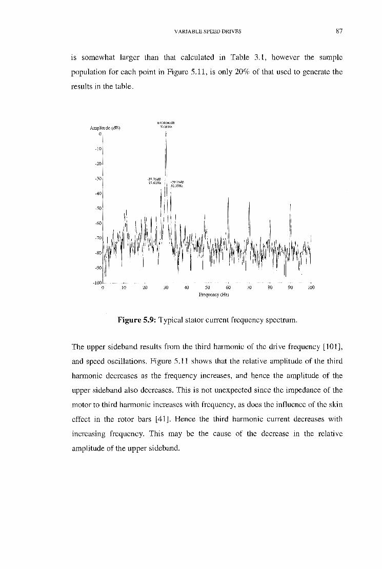
VARIABLE SPEED DRIVES 87
IS somewhat larger than that calculated in Table 3.1, however the sample
population for each point in Figure 5.11, is only 20% of that used to generate the
results in the table.
Amplitude (dB)
0
-10
-20
-30
-40
-50
-60
-100 0 10 20
O.OOOOOOdB 30.06Hz
~37.76dB 27.62Hz ~39.76dB
32.35Hz
30 40 50 60 70 80 90
Frequency (Hz)
Figure 5.9: Typical stator current frequency spectrum.
100
The upper sideband results from the third harmonic of the drive frequency [101],
and speed oscillations. Figure 5.11 shows that the relative amplitude of the third
harmonic decreases as the frequency increases, and hence the amplitude of the
upper sideband also decreases. This is not unexpected since the impedance of the
motor to third harmonic increases with frequency, as does the influence of the skin
effect in the rotor bars [41]. Hence the third harmonic current decreases with
increasing frequency. This may be the cause of the decrease in the relative
amplitude of the upper sideband.

-20
-30
/"',
p:)
~ <l.)
] -40
S" ~
-50 -
VARIABLE SPEED DRIVES
.----.Lower sideband
8-----B Upper sideband
+----+Average
Drive Frequency (Hz)
Figure 5.10: Average sideband amplitude -constant slip (0.04 p.u.).
5
...__.Lower sideband
4 G----0 Upper sideband
0 L---~----~~~~--~_L ____ J_ ____ L_ _____ L_ __ ~--~~----~
20 30 40 50 60 70 Drive Frequency (Hz)
Figure 5.11: Standard deviation of average sideband amplitude -constant slip
(0.04 p.u.).
88

VARIABLE SPEED DRIVES
-30
-40
~
~ <!)
'"d -50 .B ]' ~
-60
-70 L_ ________ L---------~--------~--------~------~
75 100 125 150 175 200 Dlive Frequency (Hz)
Figure 5.12: Amplitude of third harmonic of drive frequency.
2.0
1.5 ~ 0 ·.g
·;;;; <!)
Q 1.0 '"d 8
'"d § ci'l
0.5
0.0 '-----------L-----------'------------'----------~------~ 75 100 125 150 175 200
Third Harmonic of Dlive Frequency (Hz)
Figure 5.13: Standard deviation of amplitude of third harmonic of drive
frequency.
89
Upon close examination of the spectra of the recorded data, it was noticed that
each spectrum had a frequency component at (100- /d)Hz, where/dis the drive
output frequency. This component is henceforth termed the reflected frequency.
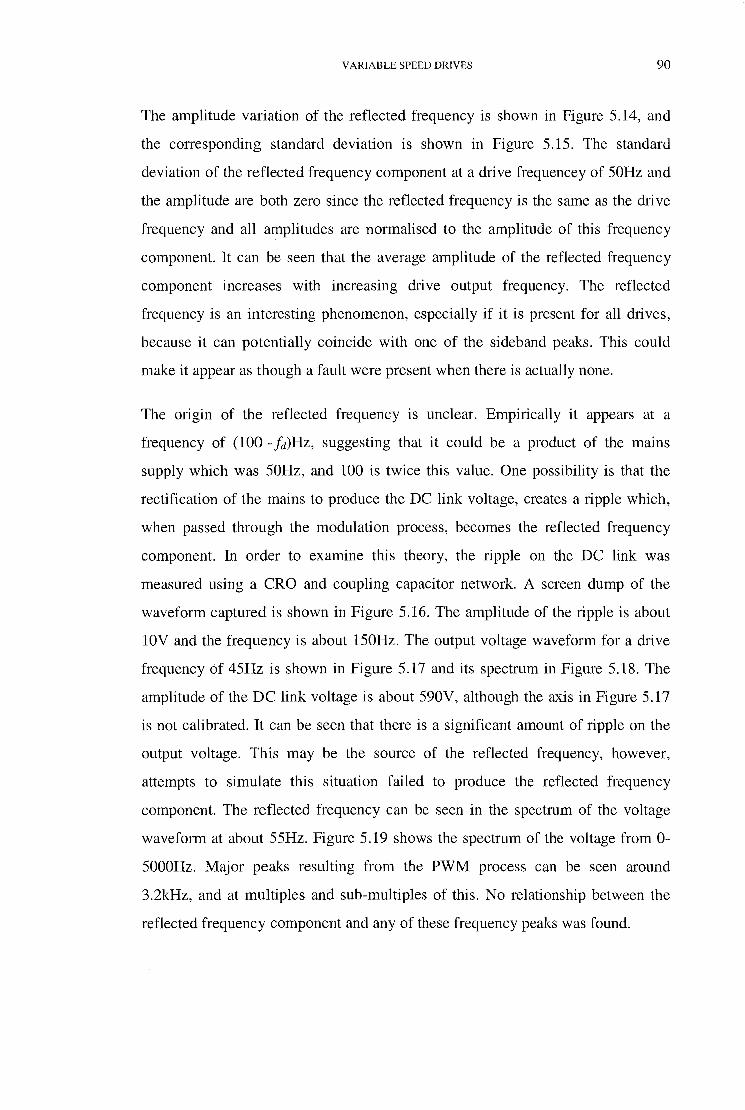
VARIABLE SPEED DRIVES 90
The amplitude variation of the reflected frequency is shown in Figure 5.14, and
the corresponding standard deviation is shown in Figure 5.15. The standard
deviation of the reflected frequency component at a drive frequencey of 50Hz and
the amplitude are both zero since the reflected frequency is the same as the drive
frequency and all amplitudes are normalised to the amplitude of this frequency
component. It can be seen that the average amplitude of the reflected frequency
component increases with increasing drive output frequency. The reflected
frequency is an interesting phenomenon, especially if it is present for all drives,
because it can potentially coincide with one of the sideband peaks. This could
make it appear as though a fault were present when there is actually none.
The origin of the reflected frequency is unclear. Empirically it appears at a
frequency of (100- /J)Hz, suggesting that it could be a product of the mains
supply which was 50Hz, and 100 is twice this value. One possibility is that the
rectification of the mains to produce the DC link voltage, creates a ripple which,
when passed through the modulation process, becomes the reflected frequency
component. In order to examine this theory, the ripple on the DC link was
measured using a CRO and coupling capacitor network. A screen dump of the
waveform captured is shown in Figure 5.16. The amplitude of the ripple is about
lOV and the frequency is about 150Hz. The output voltage waveform for a drive
frequency of 45Hz is shown in Figure 5.17 and its spectrum in Figure 5.18. The
amplitude of the DC link voltage is about 590V, although the axis in Figure 5.17
is not calibrated. It can be seen that there is a significant amount of ripple on the
output voltage. This may be the source of the reflected frequency, however,
attempts to simulate this situation failed to produce the reflected frequency
component. The reflected frequency can be seen in the spectrum of the voltage
waveform at about 55Hz. Figure 5.19 shows the spectrum of the voltage from 0-
5000Hz. Major peaks resulting from the PWM process can be seen around
3.2kHz, and at multiples and sub-multiples of this. No relationship between the
reflected frequency component and any of these frequency peaks was found.

0
-10
~ -20
] ~ s -30 <r::
-40
VARIABLE SPEED DRIVES
-50 ~~--~----~------~----~----~----~------~--~ 25 30 35 40 45 50 55 60 65
Drive Frequency (Hz)
Figure 5.14: Amplitude of reflected frequency component relative to drive
frequency amplitude.
1.5 j:l 0 ·g
·;;: <1)
Q 1.0 "0 ~
"0
~ (/]
0.5
Drive Frequency (Hz)
91
Figure 5.15: Standard deviation of amplitude of reflected frequency component.

VARIABLE SPEED DRIVES
Tek mil 20kS/s 3 Acqs !.. ·{ ·····T ·l··
. . . . . i . . .
•••• ; •••• ; ' ' •• t.
lOOmV M 2.5ms c J 56mV
Figure 5.16: Ripple on the DC link voltage.
Amplitude 4000
3500
3000
2500
2000 -G..r ,. r+-
1500
1000
500
0 0.020
H_IOO_O
'
'
0.022 0.024 0.026 0.028 0.030
Time (seconds)
Cl11 Freq 154.8Hz
J I
0.032
92
Figure 5.17: Measured drive voltage output waveform- fd =45Hz. Vertical axis
is not calibrated.

Amplitude (dB) 0
-10
-20
-30
-40
-50
-90
-100 ____ ,_ 0 10 20
VARIABLE SPEED DRIVES
O.OOOOOOdB 45.0lHz
30 40 50
-48.76dB 54.93Hz
60
Frequency (Hz)
70 80
-4I.72dB 90.03Hz
90 100
Figure 5.18: Frequency spectrum of PWM voltage waveform 0-lOOHz.
Amplitude (dB)
-20
-30
0 500 1000 1500 2000
Frequency (Hz)
Figure 5.19: Frequency spectrum of PWM voltage waveform 0-SOOOHz.
93

VARIABLE SPEED DRIVES 94
The variation of sideband amplitude with load was also examined. The results are
plotted in Figures 5.20-5.25 together with the standard deviation. It can be seen
that the amplitude of the upper sideband decreased with increasing load and the
amplitude of the lower sideband increases with load. Thus, it is necessary to take
into account the load level when examining the amplitude of sidebands for
condition monitoring.
-34.0
-36.0
~ -38.0
~ B 1 -40.0
-42.0
-44.0 2.0
•--e Lower sideband
0----E)Upper sideband_
Output Power (kW)
Figure 5.20: Variation of sideband amplitude with load (50Hz).
1.5
§ 1.0 ·p
"' -~ Q
I f/J 0.5
_____.Lower sideband
0----E) Upper sideband
Output Power (kW)
Figure 5.21: Standard deviation of sideband amplitude with load (50Hz).
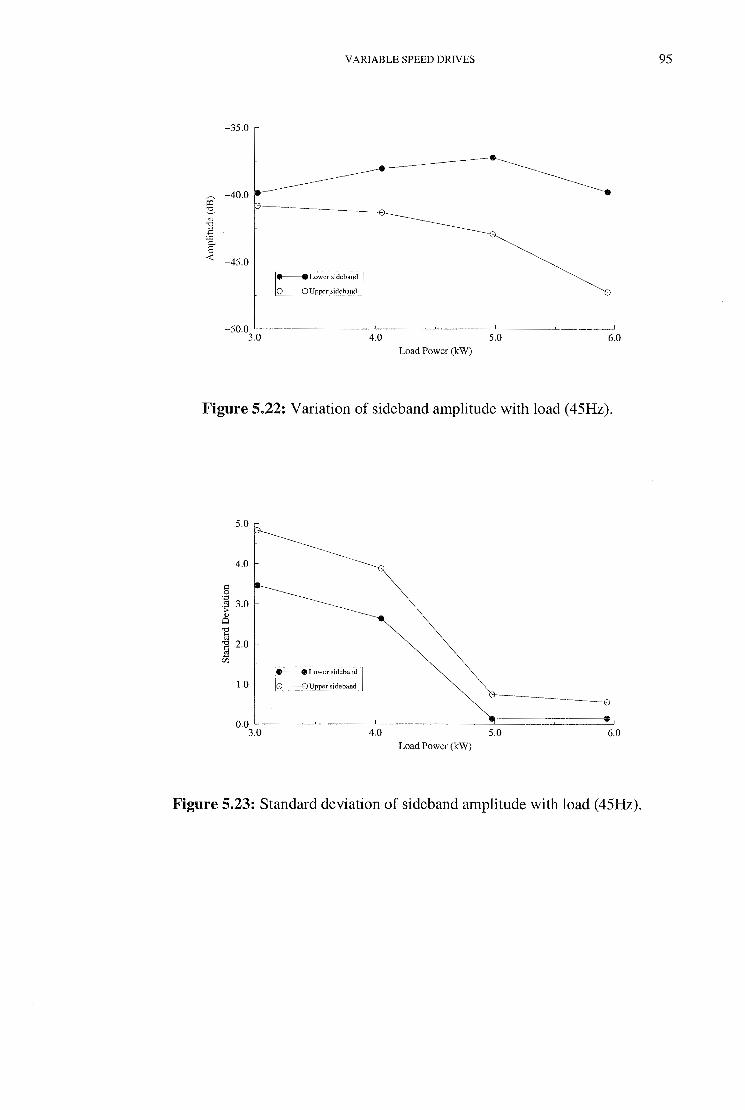
~ "' '0 . .§
j
-35.0
-40.0
-45.0
VARIABLE SPEED DRIVES
----
___________.Lower sideband
G-------------8 Upper sideband
-50.0 '------~----'-----~---_j_---~--____J 3.0 4.0 5.0 6.0
Load Power (kW)
Figure 5.22: Variation of sideband amplitude with load (45Hz).
5.0
4.0
§ ';:l
·~ 3.0
8 ] ] 2.0
ill
1.0
----------B
o.o L---~---_[__---~---~======~-=-==-=-=--~ 3.0 4.0 5.0 6.0
Load Power (kW)
Figure 5.23: Standard deviation of sideband amplitude with load (45Hz).
95

-36.0
-38.0
~ -40.0
~ ~ -42.0 ~
VARIABLE SPEED DRIVES
~Lower sideband
-44.0 G----ElUppersidebHnd
-46.0 '----~----'---~--~--~--'----~-----' 2.0 3.0 4.0 5.0 6.0
Load Power (kW)
Figure 5.24: Variation of sideband amplitude with load (40Hz).
0.8
~Lower sideband
G----El Upper sideband
0.6
0.2
0.0 '----~--_j_--~--__j__--~-___j--~--__j 2.0 3.0 4.0 5.0 6.0
Load Power (kW)
Figure 5.25: Variance of sideband amplitude with load (40Hz).
5.6 Summary
96
The advent of the semiconductor switch has led to the development of inverters
which can produce an output waveform of controllable frequency. This chapter
has examined various pulse-width modulation strategies which are used by
inverters in order to produce the desired output voltage waveform. The strategies
examined include natural-sampled, symmetric and asymmetric sampled,

VARIABLE SPEED DRIVES 97
optimised, random, and space vector. The frequency spectra of these strategies
have been examined, as has the implications that they have for condition
monitoring.
It was found that PWM strategies generally produce output harmonics at a number
of discrete frequencies including the modulating frequency and harmonics, the
carrier frequency and harmonics, and modulation products which combine the
carrier and modulating frequencies. These frequency components are only a
problem if they mask any fault frequency components. Most of the components
are quite high in the frequency range, but this is dependent on the parameters used
to implement the PWM waveform. They may mask the rotor slotting frequencies,
which could be a problem for condition monitoring systems which depend on
these to find the speed of the motor. The effect of drive harmonics could be
completely disregarded if the drive and condition monitoring systems were
integrated. The drive could then use an optimised PWM technique to eliminate
any frequency components that may mask fault frequency components.
This chapter also considered the effect of the drive frequency on the amplitudes of
the twice slip-frequency sidebands. The amplitude of the upper sideband was
found to decrease with increasing drive frequency, whilst that of the lower
sideband increased. The average of the two appeared to remain about constant.
Hence it may be better to consider using the average of the upper and lower
sideband amplitudes as an indicator of rotor damage rather than either in isolation.
The effect of load level on the amplitude of the sidebands was also examined by
varying the load at constant supply frequencies. It was found that the amplitude of
the lower sideband increased with increasing load, whilst that of the upper
sideband decreased. Again it is necessary to consider both sidebands to gain a
better indication of damage.
Finally an interesting phenomenon, which was termed the reflected frequency, was
noted when examining the spectra collected at different drive frequencies. The
reflected frequency appeared at (100 -.fd)Hz, where.fd is the drive frequency, in the
spectrum of the stator current. This component can mask the sideband frequencies,

VARIABLE SPEED DRIVES 98
so it must be taken into account when examining the sideband amplitudes. The
origin of the reflected frequency is unknown, though it is thought it could be a
product of the rectification of the mains to produce the DC link voltage. A drive
output waveform was observed to contain a large ripple component and its
spectrum contained the reflected frequency. However attempts to simulate this
were unsuccessful.

6.1 Introduction
CHAPTER 6
Numerical Modelling of
Induction Motors with
Broken Rotor Bars
A mathematical model of a system can be used to simulate the behaviour of a real
system and aid in its study. If a set of mathematical equations can be obtained
which describe the behaviour of the system, then numerical methods can be used
to solve those equations to simulate the behaviour of the system.
In general, there are two distinct methods of simulating induction motors, finite
element analysis and coupled circuit analysis. Finite element analysis effectively
breaks the machine up into very small regions and then solves magnetic field
equations subject to constraints at the boundaries of each of these regions [102]. A
99
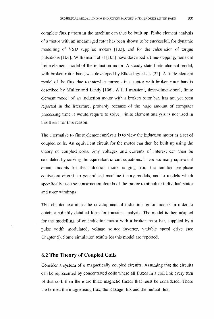
NUMERICAL MODELLING OF INDUCTION MOTORS WITH BROKEN ROTOR BARS 100
complete flux pattern in the machine can thus be built up. Finite element analysis
of a motor with an undamaged rotor has been shown to be successful, for dynamic
modelling of VSD supplied motors [103], and for the calculation of torque
pulsations [104]. Williamson et al [105] have described a time-stepping, transient
finite element model of the induction motor. A steady-state finite element model,
with broken rotor bars, was developed by Elkasabgy et al. [22]. A finite element
model of the flux due to inter-bar currents in a motor with broken rotor bars is
described by Muller and Landy [106]. A full transient, three-dimensional, finite
element model of an induction motor with a broken rotor bar, has not yet been
reported in the literature, probably because of the huge amount of computer
processing time it would require to solve. Finite element analysis is not used in
this thesis for this reason.
The alternative to finite element analysis is to view the induction motor as a set of
coupled coils. An equivalent circuit for the motor can then be built up using the
theory of coupled coils. Any voltages and currents of interest can then be
calculated by solving the equivalent circuit equations. There are many equivalent
circuit models for the induction motor ranging from the familiar per-phase
equivalent circuit, to generalised machine theory models, and to models which
specifically use the construction details of the motor to simulate individual stator
and rotor windings.
This chapter examines the development of induction motor models in order to
obtain a suitably detailed form for transient analysis. The model is then adapted
for the modelling of an induction motor with a broken rotor bar, supplied by a
pulse width modulated, voltage source inverter, variable speed drive (see
Chapter 5). Some simulation results for this model are reported.
6.2 The Theory of Coupled Coils '
Consider a system of n magnetically coupled circuits. Assuming that the circuits
can be represented by concentrated coils where all fluxes in a coil link every turn
of that coil, then there are three magnetic fluxes that must be considered. These
are termed the magnetising flux, the leakage flux and the mutual flux.

NUMERICAL MODELLING OF INDUCTION MOTORS WITH BROKEN ROTOR BARS 101
The total flux linking any one of the coils is the superposition of the self flux and
(n-1) components of mutual flux, as shown in Figure 6.1. For a coil, k, the self
flux consists of two components, the magnetising flux, ci>mk, which links all the
other coils, and the leakage flux, cf>1k, which links only the one coil. Thus the total
flux is:
cplk
n
(f>k = (f>lk +cf>mk + L(f>kj j=l }*k
~~·~···-=~ ~-i:~S ···· cDk2 v2
(6.1)
Figure 6.1: The total flux linking coil k is the sum of self and mutual fluxes.
The flux linkages are:
n
ILk= Nkcf>k =ILtk +ILmk + L,ILkJ j=l j#
where Nk is the number of turns of coil k.
(6.2)
Since cf> = ANi, these components may be written m terms of the magnetic
permeance, A, of one tum as:

NUMERICAL MODELLING OF INDUCTION MOTORS WITH BROKEN ROTOR BARS 102
Azk = Nkit>zk = AzkN;ik
Amk = Nkit>mk =AnkN;ik
Ak = Nkit>k = Ak.NkN i. J J .I .I 1
where ik is the current flowing in coil k.
Hence the following inductances may be defined:
Leakage inductance:
Magnetising inductance:
Self inductance:
Mutual inductance between coil k and coil j:
The permeances AkJ = A1k, hence MkJ = MJk·
(6.3)
(6.4)
(6.5)
(6.6)
(6.7)
The total flux linkage for each of the n coils can be expressed in matrix form using
Equations (6.3)-(6.7)as:
AI ~ Miz MI3 Min i,
Az Mzi Lz Mz3 M2n i,
A3 = M3, M3z L3 M3n ii (6.8)
An Mni Mn2 Mn3 Ln l,
Which may be written:

NUMERICAL MODELLING OF INDUCTION MOTORS WITH BROKEN ROTOR BARS 103
A.= Li (6.9)
The instantaneous voltage applied to coil k is:
(6.10)
Which is written in matrix form for all coils as:
R. dA.
V= I+-dt
(6.11)
If the inductance matrix, L, is constant then (6.11) may be written:
R. Ldi v= 1+ -dt
(6.12)
otherwise:
R . . dL L di V= I+I-+ -
dt dt (6.13)
The induction motor can be modelled using this theory since the stator and rotor
windings can be considered to consist of concentrated coils, linked by magnetic
flux. Models can either use Equation (6.13) directly, or Equations (6.9) and (6.11)
can be used simultaneously.
6.3 Simple Coupled Coil Models of the Induction Motor
Coupled circuit models view the induction motor as a set of concentrated
windings, which move relative to each other, coupled by mutual magnetic fluxes.
The simplest such model is the familiar per-phase equivalent circuit [41] as shown
in Figure 6.2.
This model is only suited to the analysis of an induction motor under balanced,
steady-state conditions. Using Kron's generalised machine theory [107]. and
reference-frame theory [40], a two-phase equivalent circuit model can be derived
[108], which can be used for a rotor with unbalanced impedances [40].

NUMERICAL MODELLING OF INDUCTION MOTORS WITH BROKEN ROTOR BARS 104
The models which are most useful for modelling broken rotor bars explicitly
model each rotor bar. It is also useful if the model can account for transient effects
in order to account for the effects of PWM voltage waveforms. A truly general
model also includes the separate effects of each coil of the stator winding.
Figure 6.2: The per-phase equivalent circuit of the induction motor.
The simplest models for damaged rotors are based on the assumption that the rotor
can be represented by an unbalanced three-phase winding. This is obviously more
realistic in the case of wound-rotor induction machines that for squirrel-cage rotor
machines.
One of the first models proposed was by Barton [109] which modelled the
machine as a combination of positive and negative-sequence equivalent circuits.
The basis of the model is that a balanced, positive-sequence, three-phase voltage
system applied to the symmetrical stator winding of an induction motor, produces
a magnetic field in the air gap, which rotates forward at synchronous speed Ws.
This field also rotates forward with respect to the rotor windings at a speed sWs
(where s is the slip) and induces in these windings a voltage at this frequency (s.fs)
which causes positive-sequence currents to flow in these windings.
If the rotor windings are asymmetrical, then the positive-sequence currents
generate negative-sequence voltages. These cause a negative-sequence magnetic
field to be produced in the air gap, which rotates backward relative to the rotor at a
speed of sws and backward relative to the stator at a speed of (2s - 1 )Ws. The
negative-sequence current induced in the stator windings thus has a frequency of
(2s- 1) .fs·
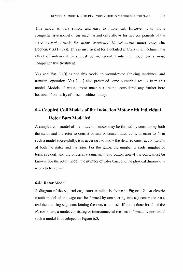
NUMERICAL MODELLING OF INDUCTION MOTORS WITH BROKEN ROTOR BARS 105
This model is very simple and easy to implement. However it is not a
comprehensive model of the machine and only allows for two components of the
stator current, namely the mains frequency ifs) and mains minus twice slip
frequency (f1(1 - 2s)). This is insufficient for a detailed analysis of a machine. The
effect of individual bars must be incorporated into the model for a more
comprehensive treatment.
Vas and Vas [110] extend this model to wound-rotor slip-ring machines, and
transient operation. Vas [111] also presented some numerical results from this
model. Models of wound rotor machines are not considered any further here
because of the rarity of these machines today.
6.4 Coupled Coil Models of the Induction Motor with Individual
Rotor Bars Modelled
A coupled coil model of the induction motor may be formed by considering both
the stator and the rotor to consist of sets of concentrated coils. In order to form
such a model successfully, it is necessary to know the detailed construction details
of both the stator and the rotor. For the stator, the number of coils, number of
turns per coil, and the physical arrangement and connection of the coils, must be
known. For the rotor model, the number of rotor bars, and the physical dimensions
needs to be known.
6.4.1 Rotor Model
A diagram of the squirrel cage rotor winding is shown in Figure 1.2. An electric
circuit model of the cage can be formed by considering two adjacent rotor bars,
and the end ring segments joining the two, as a mesh. If this is done for all of the
Nb rotor bars, a model consisting of interconnected meshes is formed. A portion of
such a model is developed in Figure 6.3.

NUMERICAL MODELLING OF INDUCTION MOTORS WITH BROKEN ROTOR BARS 106
Figure 6.3: Equivalent circuit of rotor loops.
The rotor is modelled as Nb individual loops each with a loop current of i,.k as
shown above. Rb is the resistance of each rotor bar, Re is the resistance of the
section of end ring between adjacent bars, Lb is the rotor bar leakage inductance,
and Le is the end ring leakage inductance. The actual bar currents, ibk' may be
found as the difference of adjacent mesh currents:
(6.14)
Thus writing Equations (6.9) and (6.1) for the rotor we have the following
equations:
(6.15)
(6.16)
where
vr =[vrl vr2 ... v~~ ver =[OJ
Ir = [ir1 ir2 i ier r,,
(6.17) I, =[i,
1 i is, r s2
Ar=[Ar1
Ar ... ). Aer 2 r,,

NUMERICAL MODELLING OF INDUCTION MOTORS WITH BROKEN ROTOR BARS 107
2(Rb + Re) -Rb 0 0 Re
-Rb 2(Rb + Re) -Rb 0 Re
0 -Rb 2(Rb + Re) 0 Re R = (6.18) r
Re
-Rb 0 0 2(Rb + Re)
Re Re Re Re NbRe
Lr, + 2( Lb + Le) Lr,r2 - Lb Lrr - Lb In
Le
L -L r2r1 b Lr2 + 2( Lb + Le) L rzrn Le
L L -4 L Le Lrr =
r3rl r3r2 ~1r,1 (6.19)
L -L r,,r1 b L r,,r2 Lr, + 2( Lb + Le) Le
Le Le Le NbLe
There is no coupling between the magnetic field created by the end ring current
and the stator magnetic field, hence the mutual inductance terms are zero:
L St't
L s1r2 L
Strn 0
Lszrt L L 0 Lsr = szrz szr,, (6.20)
L smrl L smrz Ls
m'n 0
The end ring current, ie, is zero except when one end nng IS broken. For
simplicity, the remaining analysis will ignore ie.
6.4.2 Stator l\1odel
For a stator which consists of m coils, the following equations can be formed in a
similar manner to the rotor, from Equations (6.9) and (6.11 ):
(6.21)
(6.22)
where

NUMERICAL MODELLING OF INDUCTION MOTORS WITH BROKEN ROTOR BARS 108
Vs = [v,1 Vsz v,mr
As= [ As1 Asz A-s,r
(6.23)
L Ls s L SJ I 2 StSm
L = ss
Ls s 2 I Lsz L, s '2 111 (6.24)
LSmSI Lsms2 L Sm
R SJ
0 0
0 Rs 0 R = 2
s (6.25)
0 0 Rsm
Equations (6.15), (6.16), (6.21), and (6.22) form the general coupled circuit model
for an induction motor with m stator coils and n rotor bars. In order to determine
the parameters of this model and solve it, several different approaches have been
taken. These differ in the assumptions made about the machine.
Williamson and Smith [105] developed a steady-state model which assumes that
the speed is constant, and that the stator winding is a symmetrical three-phase
winding supplied by a balanced three-phase voltage source. Since the stator is
symmetrical and the speed is constant, the stator can be represented by a single
phase with all quantities being phasors as all frequencies are fixed. Only two
frequency components, mains frequency and a twice slip frequency component,
are modelled in the stator current. The rotor loops have only slip-frequency loop
currents flowing. This model is good for modelling mains supplied induction
motors, however it is not a transient model as the speed is assumed constant.
Equations (6.15), (6.16), (6.21), and (6.22) may be combined to eliminate the flux
linkage terms to obtain:
dLT I dL I V=RI+ srs+ rrr
r r r dt dt (6.26)
(6.27)

NUMERICAL MODELLING OF INDUCTION MOTORS WITH BROKEN ROTOR BARS 109
Now L,.,. and Lss are constant, hence:
V - R I dL~,. I LT diS L dl,. r - r r + -- s + sr-+ rr-dt dt dt
(6.28)
dL dl dl V = R I + __ sr I + L _,. + L _s s s s dt r sr dt ss dt (6.29)
Now dLs,. dLsr dOm dLsr --=----=--(1) dt dOm dt dOm m
(6.30)
where em is the angular displacement, and ffim is the angular velocity.
Hence,
(6.31)
(6.32)
The quantities ffim dLs/ld8m l~, and ffim dLs,.ld8m I,., are commonly referred to as
rotational voltages as they arise due to the relative motion of the rotor coils with
respect to stator coils.
In order to form a transient model, the mechanical equations governing the system
must be considered. They are usually framed as:
dOm (J) =-
m dt
dmm = _!_(T- T - Km ) dt J e L m
T =IT dLsr I e s dO r
m
(6.33)
(6.34)
(6.35)
where J = moment of inertia of rotor and load, Te = electromagnetic torque
developed by the motor, h =load torque on motor, and K =viscous friction.

NUMERICAL MODELLING OF INDUCTION MOTORS WITH BROKEN ROTOR BARS 110
6.5 Previous Work
Vas [112] combined Equations (6.31) and (6.32) into one matrix equation, and
transformed the equations into the rotor reference frame in order to simplify
solution of the equations. His model represented the stator windings as a
symmetrical two-phase d-q model, with sinusoidal air gap magnetic flux density.
He also considered the mechanical equations creating a full transient model.
Lipowski and Duggal [113] used a similar formulations to Vas, but failed to notice
that a transformation in to the rotor reference frame greatly simplifies the solution.
They examined only harmonics of the supply frequency in the stator current and
defined a "distortion factor" which is a measurement of the harmonic distortion.
The behaviour of the distortion factor with change in relative position of broken
rotor bars was examined. It would appear that the distortion factor is not very
useful as there was only a very small change in the value as the number of broken
bars increased.
Ritchie et al. [114] also used Equations (6.31) and (6.32) combined into one set of
equations, though in this case, they considered the stator and rotor variables in
their respective reference frames. The stator winding was modelled as an ideal,
sinusoidally distributed winding, excited from a balanced, three phase voltage
source. The air gap length was regarded as constant and the rotor and stator
surfaces smooth. They calculated a stator current waveform and compared it to a
measured waveform. To simulate a broken bar, they assumed that the current in it
was zero. This gave them a result which did not match the measured results very
closely. Instead of modelling the broken bar by an open circuit, they adjusted the
bar resistance until the simulated results matched those measured. This was found
to occur when the broken bar resistance was about eleven times the normal bar
resistance. They did not calculate the frequency spectrum of the stator current, nor
did they use a metric to compare their simulated and measured waveforms,
presumably making the comparison by eye.
Deng and Ritchie [101] also modelled the motor using flux linkages, that is
Equations (6.15), (6.16), (6.21), and (6.22), again combined into one system of

NUMERICAL MODELLING OF INDUCTION MOTORS WITH BROKEN ROTOR BARS 111
equations, They discuss the stator magnetomotive force harmonics, but do not
model them. Again, they use an ideal stator winding, but no mechanical equations.
As a result, the stator current spectrum that is calculated, contains only the supply
frequency and (1-2s)f1 components.
6.6 Models Including the Stator Windings Explicitly
The first attempt at modelling the induction motor to explicitly include the effects
of all magnetomotive force harmonics was that of Fudeh and Ong [115] [116].
They considered a general m coil stator winding, and n coil rotor winding,
machine. However the stator windings were restricted to be identical, symmetrical
and uniformly distributed, while the rotor had n uniformly distributed windings.
They developed equations which transformed all the variables into the two phase
a-~-0 form. They then used the equations developed to numerically model the
torque-speed characteristics of induction motors [117].
Toliyat et al. [118] [119] took a different approach and modelled arbitrary stator
windings by considering them to be concentrated coils. The magnetomotive force
generated by each coil was assumed to be rectangular, as in Figure 2.2. The
inductances were calculated using winding function analysis [119]. The model
was then used to analyse a five phase induction machine for variable speed drive
applications.
Toliyat and Lipo [120] and Luo et al. [121] considered the effect of broken rotor
bars and end rings on this model. However, Luo only considered mains supply and
current source inverter operation, while Toliyat considered mains supply and a
six-step voltage source inverter. Toliyat and Lipo gave a stator current spectrum
for a broken bar case, however it is difficult to interpret their results as their
graphs are inadequately labelled. It would appear that their simulation produced
only the (1-2s)f1 sideband and did not produce the upper sideband. This is odd as
their model includes the mechanical equations, and the upper sideband is a result
of speed variation caused by the broken rotor bar. Luo et al. neglected the end ring
current in their model, which calls into question the technique they use to model a

NUMERICAL MODELLING OF INDUCTION MOTORS WITH BROKEN ROTOR BARS 112
broken end ring. They model the broken end ring by forcing the relevant loop
current to zero, however there should be a voltage across the intact end ring
segment of the loop, which would cause a current to flow [105]. This should then
affect the other loop currents; however this does not appear to have been taken
into account.
The remainder of this chapter develops the equations to model an induction motor
driven by a PWM-VSI variable speed drive. The effect of broken rotor bars on the
frequency spectrum of the stator current is examined.
6.6.1 Phase Model [121]
Luo et al [121] use the model as defined by Equations (6.15), (6.16), (6.21), (6.22)
, (6.33), and (6.34), although they neglect any friction coefficient K. Restating
these equations, but neglecting the end ring current as broken end rings are not
modelled:
V" =RJs + d)..s ,, ,, dt
dBm --=OJ
dt m
(6.36)
(6.37)
(6.38)
(6.39)
(6.40)
(6.41)
(6.42)
The machine inductances are calculated by the use of winding functions [119],
which can model any arrangement of concentrated coils within the machine.
Assuming that the permeance of iron is infinite, the mutual inductance between
any two windings, i andj, in a machine is given by [119]:

NUMERICAL MODELLING OF INDUCTION MOTORS WITH BROKEN ROTOR BARS 113
where em is the angular position of the rotor with respect to a stator reference, <p is
an angular position around the stator surface, g-1(8m, <p) is the inverse gap function
and is 1/g if the air gap is assumed to be uniform, lis the length of the rotor, and r
is the average air gap radius. N/8m, <p) is the winding function of coil i, and
represents the magnetomotive force distribution along the air gap for a unit current
in coil i. The self-inductance for a coil can be calculated by setting i = j.
The winding function Ni(8m, <p) for a coil is similar to the magnetomotive force
diagram in Figure 2.2, except that the span of the loop is not Jr, resulting in:
(6.44) otherwise.
where C4 is the angular span of the coil, which extends from eil to 812, Zi is the
number of turns in the coil. For a squirrel cage rotor, each coil is considered to
consist of just one turn, that is Zi = 1.
6.6.2 Line-to-line Model [121]
The model described by Equations (6.15), (6.16), (6.21), (6.22), (6.33), and (6.34)
is unsuitable for simulating most motors, which have delta connected windings or
a star point which is not readily accessible, as Equation (6.21) uses the stator
phase voltages. These are not readily measured, but the line-to-line voltages are. If
the voltages are balanced and the motor is symmetrical, then it is easy to calculate
the phase voltages, however this is not useful for a general simulation which
allows unbalanced conditions. A model can be developed from the equations
which uses the line-to-line voltage rather than the phase voltage [121].

NUMERICAL MODELLING OF INDUCTION MOTORS WITH BROKEN ROTOR BARS 114
I I
I
I
I
I
I
I I
I I
I I
I I
I I
I I I
I I
I I
I I / I -' I
~-·\ \ 1/ \ \ A I
\ / \1 I
\ I\ I \ I
I I I
I\ 1\ I \ I / 'AI
I I
I \ I \
1\ I I I
~ - -·- ·---~ \ \ \
~ \ \
\ \
\
\
\
\
I I
00 ..... \
\ - - -
I r-..... \ I
\0 I ..... \ I
r------------, I ~ \
r-------------, I 7 \
I ,...;
,--------------, I
I
('() .....
\
\
0 ,...;
00
r-
I
I - - -
\ I \._ ____________ _J
\0
'--------------' tr)
\
\ I \._ ____________ J
7
\
\ \ \
\ \ \
\ \ \ \ \ \
\ \ \
\ \ \ \ \ \ \
\ \ \ \
\ \ \ \ \ ' \ \ I \ \ ' I I
\ \ /, I I
' 'i. '/ I ' I ' I '
I
I
I
I
I I
I I
I
I
\ '> \1 I ' I' '
'A '( \ I ' I '
I I
\ I
I I I
I
Figure 6.4: Developed diagram of the connections of half the stator windings in a
concentrically wound stator with 36 slots and 3 coils per group.
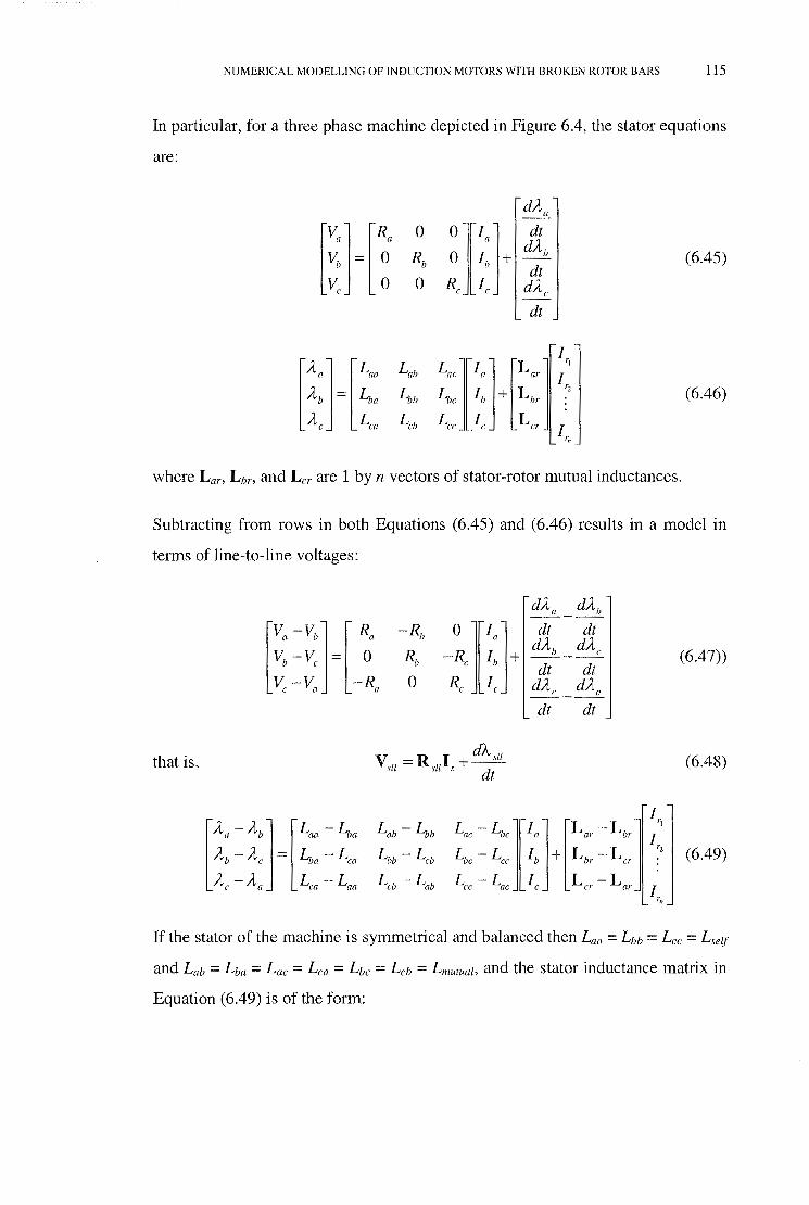
NUMERICAL MODELLING OF INDUCTION MOTORS WITH BROKEN ROTOR BARS 115
In particular, for a three phase machine depicted in Figure 6.4, the stator equations
are:
dAa n lR, 0
~r+ dt
~ = ~ Rb dAb (6.45) dt
0 Rc Ic dAc
dt
I
l A,] l Loo Lab L"'Jn lL,,]
Tt
I Ab = Lba Lbb 4c Ib + Lbr
r2 (6.46)
Ac Lea Lcb Lee Ie Lcr I r,,
where Lm·, Lbr, and Lcr are 1 by n vectors of stator-rotor mutual inductances.
Subtracting from rows in both Equations (6.45) and (6.46) results in a model in
terms of line-to-line voltages:
that is,
-Rb
vb-vc = 0 Rb lv,-v,ll R,
Vc -Va -Ra 0 -}1~} V R I d'Asu
sll = sll s + dt
Lab- Lbb
Lbb- Lcb
L,'b- Lab
dAa _dAb
dt dt dAb_ dAc dt dt
(6.47))
dAc _ dAa dt dt
(6.48)
(6.49)
If the stator of the machine is symmetrical and balanced then Laa = Lbb = Lee = Lse(f
and Lab = Lba = Lac = Lea = Lbc = Lcb = Lmutuaz, and the stator inductance matrix in
Equation (6.49) is of the form:

NUMERICAL MODELLING OF INDUCTION MOTORS WITH BROKEN ROTOR BARS 116
l ~ -: -0LJ (6.50)
-L 0 L
where L = Lseif - Lmutual . This matrix is singular and hence does not have an
inverse, which makes numerical solution of the model, as described later,
impossible. However, if there is no neutral connection to the machine the stator
currents must sum to zero, hence the last equation of (6.49) may be replaced by an
equation involving only the stator currents to obtain:
or:
Lab- Lbb
Lbb- Lcb
1
(6.51)
(6.52)
Equations (6.48) and (6.52) together with the rotor equations (6.37) and(6.39) and
the mechanical equations (6.41) and (6.42) form a complete line-to-line model of
the induction machine.
6. 7 Modelling a Broken Rotor Bar
A broken rotor bar can be modelled by simply removing one bar from the above
model, and adjusting the matrices accordingly. For example, if the last rotor bar is
broken (bar number Nb), then the rotor equivalent circuit has this bar removed and
a double-width loop instead, as shown in Figure 6.5.

NUMERICAL MODELLING OF INDUCTION MOTORS WITH BROKEN ROTOR BARS 117
Re Re Re Le Re Le
(,,c)b (,lb i i r
ibl bNb-1 Nb-1
Lb Lb
Re Re Le Re Re Le
Figure 6.5: Equivalent circuit with rotor bar Nb broken.
This reduces the number of loop currents by one. The parameters for the new,
double-width, loop are changed slightly from the non-broken case. The mutual
inductance, Lmrb, between rotor loops increases, the self inductance, L,.,.b, also
changes, and the leakage for the new loop has two extra Le components. That is,
only the last row and column are different. The new rotor self-inductance matrix is
then:
L,.,. + 2( Lb + L_) Lrnr - Lb
Lrnr - Lb L,.,. + 2( 4 + Le)
L,.,. = (6.53)
Only the last element of the rotor resistance matrix changes, as no change occurs
to the mutual resistances between rotor loops, hence:
2(Rb + Re) -Rb 0 0
-Rb 2(Rb + Re) -Rb 0
R = r 0 -Rb 2(Rb + Re) 0 (6.54)
-Rb 0 0 2Rb +4Re
The stator-rotor inductance matrix also changes because one of the rotor loops is
now a double-width loop, hence the winding function for the loop Nt(Bm,¢)
changes since it is dependent on the span of the loop. Therefore any mutual
inductances involving this loop must also change.

NUMERICAL MODELLING OF INDUCTION MOTORS WITH BROKEN ROTOR BARS 118
6.8 Solving the Model
The set of differential equations which form the model can be solved numerically
to produce a time domain simulation of the behaviour of the motor. A model was
constructed based on the 4 pole Pope motor (see Appendix A). This motor has 36
stator slots, with three coils per group, and a 32 slot rotor.
6.8.1 Calculation of Inductances
In order to calculate the inductances, the construction details of the machine must
be known. The matrices Lss, Lsu, Ls,., dLs,/d8m, and Lm can then be calculated
using Equation (6.43). Since the stator is symmetrical, it is sufficient to calculate
inductances for 0 ~ Bm ~ rc as the patterns repeat for the other half of the bore.
6.8.2 Calculation of Flux Linkages
The flux linkage vectors, Asu and A.,., can be found by integrating Equations (6.36)
and (6.37). Once the flux linkages and the inductance matrices are calculated, the
stator and rotor current vectors can be found.
6.8.3 Calculation of Currents
In order to solve the model it is necessary to find expressions for I,. and Is, which
may be found by solving Equations (6.38), (6.39), (6.48), and (6.52)
simultaneously to give:
(6.55)
(6.56)
6.8.4 Calculation of Speed and Angular Displacement
The torque generated by the motor can be calculated from Equation (6.40), then
this can be used in Equation (6.41) which is integrated to find (J)m· This is then
integrated (6.42) to obtain Sm.

NUMERICAL MODELLING OF INDUCTION MOTORS WITH BROKEN ROTOR BARS 119
6.9 Numerical Solution of Ordinary Differential Equations
An ordinary differential equation (ODE) can always be written as a set of first
order differential equations of the form:
dy =f(t,y(t)) dt
(6.57)
This is usually expressed as an initial value problem, that is, an initial value y( a) = y0 is given and it is required to find a function y(t) defined over an interval [a,b]
which satisfies Equation (6.57). Thus an initial value is required, as well as the
differential equation.
There are a number of techniques for numerically solving initial value problems.
The simplest, and easiest to understand, are one-step methods. Given the initial
value problem above, we seek an approximation to the solution y(t). The general
one-step method is an iteration of the form:
i = O,l, ... ,n-1. (6.58)
The function c{l(xi,yi;h) is called the increment function, and provides a means of
obtaining Yi+I from Yi· The step size, h, may be changed when proceeding from a
to b to estimate y(t) if an error analysis indicates a need to do so. The two one-step
methods which will be considered here are Euler's method and the Runge-Kutta
method.
6.9.1 Euler's Method
Euler's method is the simplest one-step method. Given that we know y(a) = y0 and
that we also know the gradient of the curve, y' = f(t,y ), at that point, then it seems
reasonable that the next point on the curve could be found by proceeding along a
line of this gradient. Soy( a+h) can be approximated by:
y(a +h)""' y(a)+hy'(a) =Yo +hf(a,y0 ) (6.59)
In general, the estimated value of y( a+h) will not be on the solution curve y(t), but
for well-behaved functions and sufficiently small step size a satisfactory
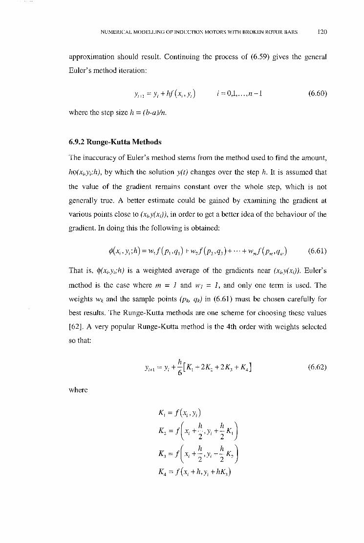
NUMERICAL MODELLING OF INDUCTION MOTORS WITH BROKEN ROTOR BARS 120
approximation should result. Continuing the process of (6.59) gives the general
Euler's method iteration:
i = 0,1, ... , n - 1 (6.60)
where the step size h = (b-a)/n.
6.9.2 Runge-Kutta Methods
The inaccuracy of Euler's method stems from the method used to find the amount,
h$(xi,yi;h), by which the solution y(t) changes over the step h. It is assumed that
the value of the gradient remains constant over the whole step, which is not
generally true. A better estimate could be gained by examining the gradient at
various points close to (xi,y(xi)), in order to get a better idea of the behaviour of the
gradient. In doing this the following is obtained:
(6.61)
That is, $(xi,yi;h) is a weighted average of the gradients near (xi,y(x1)). Euler's
method is the case where m = 1 and WJ = 1, and only one term is used. The
weights Wk and the sample points (pk, qk) in (6.61) must be chosen carefully for
best results. The Runge-Kutta methods are one scheme for choosing these values
[62]. A very popular Runge-Kutta method is the 4th order with weights selected
so that:
(6.62)
where
Kt = f ( x,' y;)
Kz = f(x; +~,y; +~K1 )
K 3 = f( X; +~,y; +~K2 ) K4 = f(x, +h,y, +hK3 )

NUMERICAL MODELLING OF INDUCTION MOTORS WITH BROKEN ROTOR BARS 121
It is popular because it is easy to implement, and virtually always succeeds in
giving a good approximation. The drawbacks are that it is computationally
inefficient and errors are harder to control than other methods. The Runge-Kutta
can also be modified so that the step size, h, is not constant, but changes in
response to an estimation of the error in the approximation. These are generally
referred to as variable-step Runge-Kutta methods or Runge-Kutta-Fehlberg
methods.
6.9.3 Other Methods of Solving ODEs
Other alternative methods of solving ODEs exist [60] such as Richardson
extrapolation, also known as Burlisch-Stoer methods, and predictor-corrector
methods. Both of these methods are more complex to implement than the Runge
Kutta and also less likely to converge. However they are potentially more accurate
and faster to compute.
6.10 Numerical Solution of the Induction Motor Model
Equations (6.36) and (6.37) can be written in the form of (6.57) by the substitution
of (6.53) and (6.54). Hence these equations can be solved using a Runge-Kutta
method to find the flux linkages, Asu and 'A,. This is not the case for the
mechanical equations (6.41) and (6.42), which cannot easily be written in the form
y' = f(t,y). Hence a Runge-Kutta method cannot be used to find the solution.
Instead a Euler method was chosen to perform the integration.
In order to solve the system of equations it is necessary to calculate the various
coefficient matrices. Some of the matrices are constant, whereas others are
dependent on the angular displacement of the rotor and must be calculated for
every iteration. Those which are constant involve either the stator or the rotor
only, and these need only be calculated once. These matrices are Rs, Lss, Rn Lrr,
Rszz, and Lsll· The stator-rotor inductance matrices, L~'~"' Lsru, and dLsrld~n, are
dependent on the exact position of the rotor at each iteration, hence these matrices
must be re-calculated at every step. This is not difficult as the mutual inductance

NUMERICAL MODELLING OF INDUCTION MOTORS WITH BROKEN ROTOR BARS 122
curves are piecewise linear functions, which may be implemented using a fast,
table-lookup function.
6.10.1 Stator-Rotor Mutual Inductance
The stator-rotor mutual inductance curves were calculated using Equation (6.44),
and the stator winding layout shown in Figure 6.4. The resulting curves for both a
normal rotor loop, and a broken bar (double width) loop are shown, as are the
derivatives of these two curves.
Unfortunately it was found that the model was numerically unstable with the
derivative of inductance curves as shown in Figure 6.6. The step changes in the
derivative curves caused the torque calculation to become unstable. In order to
circumvent this problem, it was noted that a real winding coil in an induction
motor is not infinitely narrow. In fact, the winding occupies the width of one
whole slot, hence instead of there being a step change in the derivative of
inductance curve, as in Figure 6.6, there should be a gradual change over the slot
width. For simplicity the winding function was modelled as a linear change over
the slot width, for both the stator and the rotor windings. When this type of change
is taken into account the resulting derivative of the mutual inductance curves is
modelled as shown in Figure 6.7. Using these curves stabilised the model.
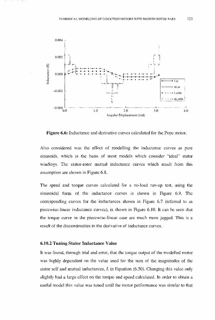
NUMERICAL MODELLING OF INDUCTION MOTORS WITH BROKEN ROTOR BARS 123
0.004
I
J:iJ 0.002
g J
I
<l) I 0 I
.@ 0.000 <>--<>--<>---<>--<>
0 .g - _..-• -·- .. --+---+- ....
E~u, ~ ...., <>-------<> dLsr
-0.002 -• Lsrbb
-o dLsrbb
-0.004 0.0 1.0 2.0 3.0 4.0
Angular Displacement (rad)
Figure 6.6: Inductance and derivative curves calculated for the Pope motor.
Also considered was the effect of modelling the inductance curves as pure
sinusoids, which is the basis of most models which consider "ideal" stator
windings. The stator-rotor mutual inductance curves which result from this
assumption are shown in Figure 6.8.
The speed and torque curves calculated for a no-load run-up test, using the
sinusoidal form of the inductance curves is shown in Figure 6.9. The
corresponding curves for the inductances shown in Figure 6.7 (referred to as
piecewise-linear inductance curves), is shown in Figure 6.10. It can be seen that
the torque curve in the piecewise-linear case are much more jagged. This is a
result of the discontinuities in the derivative of inductance curves.
6.10.2 Tuning Stator Inductance Value
It was found, through trial and error, that the torque output of the modelled motor
was highly dependent on the value used for the sum of the magnitudes of the
stator self and mutual inductances, Lin Equation (6.50). Changing this value only
slightly had a large effect on the torque and speed calculated. In order to obtain a
useful model this value was tuned until the motor performance was similar to that
NUMERICAL MODELLING OF INDUCTION MOTORS WITH BROKEN ROTOR BARS 124
measured from the test motor. In order to do this the value of L was adjusted to
give best results in terms of torque, speed and current, and also to match the run
up time of the test motor. The other model parameters were adjusted slightly to
examine the effects on the simulation, however none exhibited such strong
influence as the stator inductances.
6.10.3 Computer Implementation Issues
The model was implemented using a program written in the 'C' language, using
the Meschach [122] matrix library to implement the matrix functions. Matrix
inverses were calculated using a singular value decomposition (SVD) routine. The
program was run on a variety of computers, but the principal platform was a Sun
Microsystems SPARC 10, Model 402, with dual 40MHz processors. The amount
of RAM required was minimal (less than 1 megabyte).
For simulating 50Hz sinusoidal mains voltages, a step size of 78.125 micro
seconds was used, as this effectively synchronously sampled the current
waveforms. The maximum step size for satisfactory simulation of PWM voltage
waveforms was found to be about 10 micro-seconds. Simulating the Pope machine
with PWM voltage waveforms required about 34 hours of CPU time in order to
produce one second of simulated time data! It is quite possible that the program
could be optimised somewhat in various areas, as no serious effort was expended,
however it would still be a very CPU intensive task. It may also be possible to
make some performance gains by using an alternative to the fourth order Runge
Kutta algorithm for integration, but the problem remains that both the PWM
voltage and the derivative of the stator-rotor mutual inductance contain step
changes. This can be troublesome for most integration algorithms, which is why
the Runge-Kutta was chosen as it converges under most circumstances.
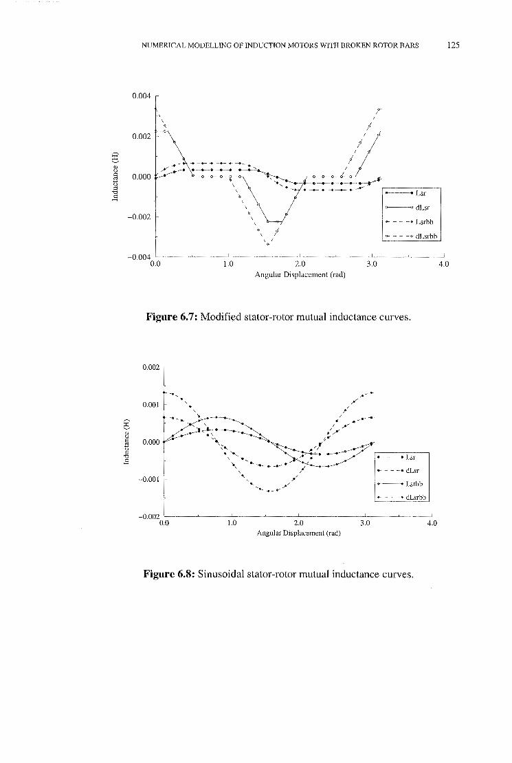
g (]) 0
§
~ ~ -
NUMERICAL MODELLING OF INDUCTION MOTORS WITH BROKEN ROTOR BARS 125
0.004
\
\
"' 0.002
0.000
j
l<r
I
i,/j r-<>--<>--<>--<>I_J .. .... ~
• ~•- +- ......,............__. __ .. ..-•-- '..____.----L-s-r --,
-0.002
-0.004 0.0 1.0
\ ~ j
I \ I
<r
2.0
Angular Displacement (rad)
<>------<> dLsr
+- - - -• Lsrbb
<>- --- -o dLsrbb
3.0
Figure 6.7: Modified stator-rotor mutual inductance curves.
0.002
... , . 0.001 ' .
@ (I) u ~ 0.000 ~ ::J
1l ,.________. Lsr H
.. -- -• dLsr
-0.001 ____, Lsrbb
+- - - -• dLsrbb
-0.002 '-----~--____j__ 0.0 1.0 2.0 3.0 4.0
Angular Displacement (rad)
Figure 6.8: Sinusoidal stator-rotor mutual inductance curves.
4.0
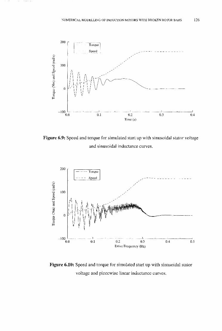
NUMERICAL MODELLING OF INDUCTION MOTORS WITH BROKEN ROTOR BARS 126
Figure 6.9: Speed and torque for simulated start up with sinusoidal stator voltage
and sinusoidal inductance curves.
200
100
0
/ /
/ /
/ /
-100 L---~-----L----~----~--~----~----~----L----~----~ 0.0 0.1 0.2 0.3 0.4 0.5
Drive Frequency (Hz)
Figure 6.10: Speed and torque for simulated start up with sinusoidal stator
voltage and piecewise linear inductance curves.
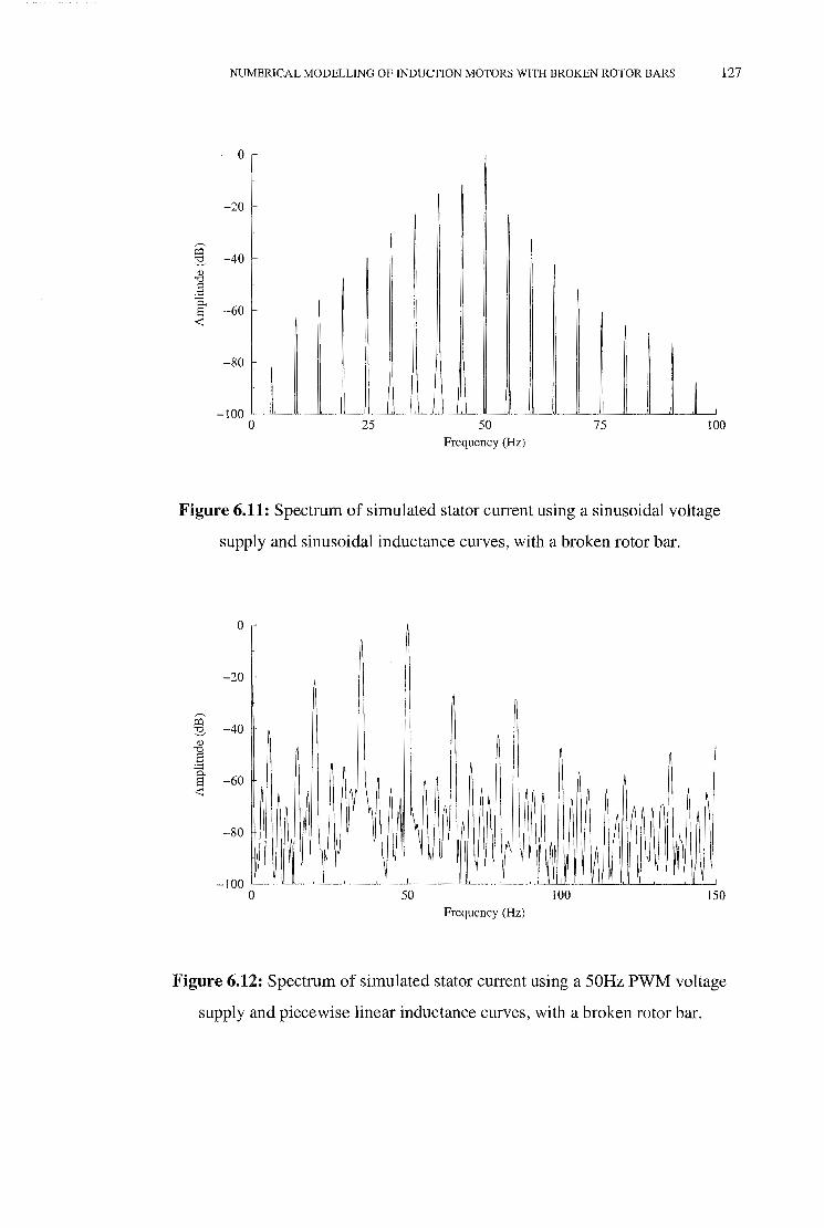
NUMERICAL MODELLING OF INDUCTION MOTORS WITH BROKEN ROTOR BARS 127
0
-20
,--,
~ -40 Q)
'"d
~ 8 -60 -<
-80
-100 _L
0 25 50 75 100 Frequency (Hz)
Figure 6.11: Spectrum of simulated stator current using a sinusoidal voltage
supply and sinusoidal inductance curves, with a broken rotor bar.
0
-20
~ -40 Q)
'"d B @: -60 -<
I~ ~ ~
l( -80 ~
~ ~ ~ ~ -100 0 50 100 150
Frequency (Hz)
Figure 6.12: Spectrum of simulated stator current using a 50Hz PWM voltage
supply and piecewise linear inductance curves, with a broken rotor bar.
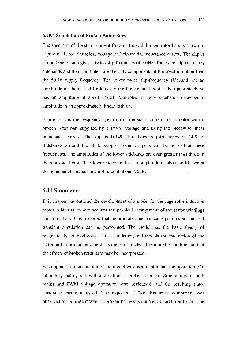
NUMERICAL MODELLING OF INDUCTION MOTORS WITH BROKEN ROTOR BARS 128
6.10.4 Simulation of Broken Rotor Bars
The spectrum of the stator current for a motor with broken rotor bars is shown in
Figure 6.11, for sinusoidal voltage and sinusoidal inductance curves. The slip is
about 0.060 which gives a twice slip-frequency of 6.0Hz. The twice slip-frequency
sidebands and their multiples, are the only components of the spectrum other then
the 50Hz supply frequency. The lower twice slip-frequency sideband has an
amplitude of about -12dB relative to the fundamental, whilst the upper sideband
has an amplitude of about -22dB. Multiples of these sidebands decrease in
amplitude in an approximately linear fashion.
Figure 6.12 is the frequency spectrum of the stator current for a motor with a
broken rotor bar, supplied by a PWM voltage and using the piecewise-linear
inductance curves. The slip is 0.149, thus twice slip-frequency is 14.9Hz.
Sidebands around the 50Hz supply frequency peak can be noticed at these
frequencies. The amplitudes of the lower sidebands are even greater than those in
the sinusoidal case. The lower sideband has an amplitude of about -6dB, whilst
the upper sideband has an amplitude of about -26dB.
6.11 Summary
This chapter has outlined the development of a model for the cage rotor induction
motor, which takes into account the physical arrangement of the stator windings
and rotor bars. It is a model that incorporates mechanical equations so that full
transient simulation can be performed. The model has the basic theory of
magnetically coupled coils as its foundation, and models the interaction of the
stator and rotor magnetic fields as the rotor rotates. The model is modified so that
the effects of broken rotor bars may be incorporated.
A computer implementation of the model was used to simulate the operation of a
laboratory motor, both with and without a broken rotor bar. Simulations for both
mains and PWM voltage operation were performed, and the resulting stator
current spectrum analysed. The expected (l-2s)f1 frequency component was
observed to be present when a broken bar was simulated. In addition to this, the

NUMERICAL MODELLING OF INDUCTION MOTORS WITH BROKEN ROTOR BARS 129
upper sideband (1+2s)f1 was also observed due to the full transient nature of the
model, which allowed the speed and torque to oscillate.
The amplitude of the sidebands was rather higher than those measured from the
test motor. This was probably due to inter-bar currents in the test motor, which
would tend to reduce the amplitude of the magnetic disturbance, and hence, the
amplitude of the sidebands that were measured. Inter-bar currents were not
accounted for in the model, which assumed that the bars were insulated from the
iron core, whereas in practice they are not. It would be possible to account for the
effects of inter-bar currents using the model of Walliser and Landy [53], or that of
Heller [47]. However, these models would add extra components to the matrices
used in the differential equations. Given that the model already required 34 hours
per second of simulated time to run, this would make the model intractable at the
present time.

CHAPTER 7
Experimental Studies
7.1 Introduction
This thesis has examined methods of detecting rotor faults in induction motors
driven by variable speed drives and developed a numerical model to simulate such
a motor. Some work has been done previously on detecting rotor damage in
induction motors operating from the mains supply, however very little interest has
been shown in induction motors supplied by variable speed drives. Given the large
installed base of variable speed drives, and that a large number of new drive
installations in industrial situations tend to be variable speed drives, this topic is of
growing importance.
Several methods of detecting rotor damage have been examined in this thesis. The
basic theory of detecting damage in a motor with a variable speed drive is the
same as that with the motor driven from the mains supply. However, there are a
number of complicating factors which make the detection of broken rotor bars
with a variable speed drive difficult; the major problem is, of course, that the
130

EXPERIMENTAL STUDIES 131
output frequency of the variable speed drive can vary, whereas the frequency of
the mains is constant for all practical purposes. This makes the detection of fault
frequency components quite difficult, as the components must be detected relative
to a changing fundamental supply frequency.
In addition to this, the drive itself introduces various frequency components due to
the modulation techniques used to control the drive output frequency. These
frequencies may mask or interfere with fault frequency components, and must be
taken into account.
A numerical model of the induction motor was developed in order to simulate the
effects of a broken rotor bar.
This chapter starts by examining the differences in the current spectra between the
motor with an undamaged rotor and one with a damaged rotor when that motor is
supplied by the mains or a VSD. This shows the effect of rotor damage on the
spectra and also the difference when a VSD supply is used instead of the mains
supply.
An example of using the PLL circuit developed in Chapter 4 to confirm the
diagnosis of rotor damage in a motor supplied by a VSD driving a pump in an
industrial plant is also described. This motor was initially diagnosed by a
commercial vibration condition monitoring company as having rotor damage, the
plant operating company wanted confirmation of this diagnosis by electrical
monitoring methods before proceeding with any remedial action. Fortunately the
electrical testing performed confirmed the results of the vibration testing.
7.2 Differences Between the Detection of Broken Rotor Bars in
Mains-supplied and VSD-supplied Induction Motors
It has already been established that broken rotor bars in mains-supplied induction
motors can be detected by examining the frequency spectrum of the stator current
for the presence and amplitude of sidebands around the supply frequency at twice
the slip frequency. It stands to reason that such sidebands should be present when

EXPERIMENTAL STUDIES 132
the motor is supplied by a variable speed drive. The differences in the frequency
spectra between the two situations needs to be examined.
It would be very difficult, if not impossible, to fully describe the difference
between frequency spectra theoretically, hence an experimental approach is taken.
In order to make a valid comparison, one motor is used with two rotors, one of
which is deliberately damaged. This motor is then operated from either the mains
supply or a VSD, with either rotor in order that the resulting spectra may be
compared.
7.2.1 Experimental Arrangements
A motor was bought specifically for conducting laboratory tests. It is the
previously mentioned 7 .5kW Pope induction motor, the specifications of which
are given in Appendix A. Two rotors were purchased for this machine in order to
have one which could be intentionally damaged and one which could remain
undamaged for comparison purposes. The alternative to this would be to construct
a machine which would allow a rotor bar to be "broken" as has been described by
several authors [7, 29]. The former approach was taken in preference to building a
laboratory motor for two reasons; one was that it was a commercially designed
and manufactured motor exactly as would be used in industry hence could be
expected to perform as such, whereas a constructed laboratory machine may have
different performance characteristics. The other reason was that budgetary
constraints would not allow a major project to construct a machine to be
undertaken.
A commercially produced VSD (a SAMI GS drive manufactured by ABB) was
also purchased in order to drive the motor. The drive selected was rated at 20kVA
in order to allow the motor to be moderately overloaded without tripping the drive
overload protection, should the need arise.
This motor was coupled to a DC generator and resistor load board in order to
provide a variable load on the motor. The DC generator specifications are
included in Appendix A. A photograph of this arrangement is included as Figure

EXPERIMENTAL STUDIES 133
7 .1. The load resistor bank can be seen to the right, next to the loading DC
generator, the test motor is under the table, and the data acquisition computer and
VSD are on top of the table. Figure 7.2 gives another view of the data acquisiton
equipment setup. The FCC current clamp can be seen resting on top of the sample
and-hold hardware, which is next to the acquisition computer. The VSD unit can
be seen at the top-left comer of the picture.
Figure 7.1: Arrangement of motor and loading generator.

EXPERIMENTAL STUDIES 134
Figure 7.2: Arrangement of data acquisition system.
7 .2.2 Undamaged Rotor Measurements
In order to make a comparison between damaged and undamaged rotors some
baseline measurements were made with the undamaged rotor in the machine. The
motor was loaded by a DC generator connected to a resistor load bank. The load
was adjusted by changing the field voltage of the DC machine until the power
measured going into the resistor load bank was approximately 7.5kW as this is the
rated output power of the motor. The mains frequency is 50Hz, hence the VSD
output frequency was also adjusted to 50Hz so that a valid comparison between
the spectra could be made.

EXPERIMENTAL STUDIES
O.OOOOdB
Amplitude (dB) 49.97Hz
0 I
-10
-20
-30
-40 -50.8876
46.92H·
-50 .6377dB 3.10Hz
-60
-70
-80
-90
10 20 30 40 50 60 70 80 90 100
Frequency (Hz)
Figure 7.3: Stator current spectrum with undamaged rotor and mains supply.
Amplitude (dB)
0 10 20 30 40
O.OOOOdB 49.97Hz
50 60
Frequency (Hz)
70 80 90 100
Figure 7.4: Stator current spectrum with undamaged rotor and VSD supply.
135

EXPERIMENTAL STUDIES 136
7 .2.3 Damaged Rotor Measurements
The same measurements as were made in the previous section were repeated after
the rotor had been deliberately damaged in order to simulate a real fault. This was
achieved by milling through the end-ring to separate one end-ring and a rotor bar.
A photograph of the rotor after this operation this is shown in Figure 7.5. This
rotor was then replaced in the machine and the measurements performed again,
resulting in the current spectra shown in Figures 7.6 and 7.7.
Figure 7.5: Damage to rotor of test motor.
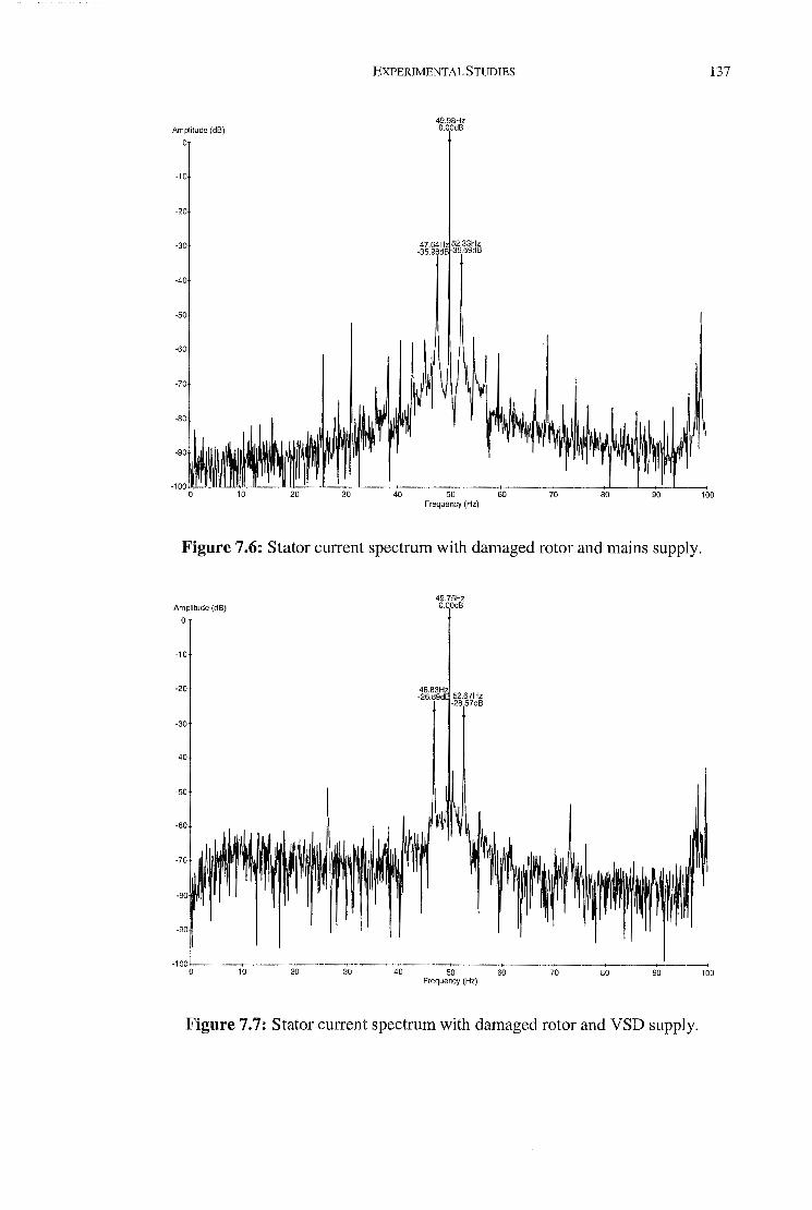
Amplitude (dB)
0
-10
-20
-30
-40
-50
-60
·70
EXPERIMENTAL STUDIES
40
49.98Hz O.OOdB
47 64H 52.33Hz -35:96d 35.59dB
50 60 Frequency (Hz)
137
70 80 100
Figure 7.6: Stator current spectrum with damaged rotor and mains supply.
Amplitude (dB)
0
·10
·20
-30
-40
·50
50 60 Frequency (Hz)
70 80 90
Figure 7.7: Stator current spectrum with damaged rotor and VSD supply.
100

EXPERIMENTAL STUDIES 138
7 .2.4 Comparison of Reference Spectra
It can be seen that by comparing Figure 7.3 and Figure 7.6 the spectrum with the
motor supplied by the mains develops large sidebands at twice the slip frequency
around the supply frequency peak.
When comparing Figure 7.4 and Figure 7.7 it can be seen that there is a similar
difference between the two spectra as was seen in the prior case. Again there are
significant sidebands at twice the slip frequency around the supply frequency
peak.
Figure 7.6 and Figure 7.7 are the stator current spectra for the same motor under
approximately the same loading conditions, with practically the same supply
frequency, yet the amplitudes of the sideband peaks are markedly different. The
sideband amplitudes are about 8dB higher with a VSD supply than with the mains
supply. This is quite a significant difference and is a factor which must be taken
into account when examining the current spectra of induction motors for condition
monitoring purposes. The difference in the amplitudes is probably due to larger
amplitudes of the supply frequency harmonics contributing to the larger sideband
amplitudes.
7.3 Detection of Rotor Damage in an Industrial Plant using the
PLL
In addition to the tests performed with the PLL described in Chapter 4 several
tests were made on the circuit at an industrial plant. Some of these tests are
detailed in the following passages.
A pump motor at an industrial plant had been diagnosed by a vibration condition
monitoring company as having rotor damage. The plant operator requested that
this diagnosis be checked by electrical methods. The motor was supplied by a
VSD hence this was a prime opportunity to test the PLL circuit.
Very little was known about the drive, motor and pump combination, however the
following details were noted. The motor was a Pope TEFC induction motor rated

EXPERIMENTAL STUDIES 139
at 90kW, 1480 rpm, 415V, 50Hz. The drive was manufactured by PDL, model
ASD330, and the motor was directly coupled to a centrifugal pump.
The data acquisition set up was the same as usual. A portable computer with a
PCL-818 AID card, anti-aliasing filters, sample and hold circuitry. An isolation
transformer was used to supply the computer from the mains in order to avoid any
earth loops which could potentially trigger any drive protection systems. The
Fluke current probe was clamped around one of the motor supply cables in order
to sense the stator current.
Data was sampled at a rate of 32 times the fundamental supply frequency which is
approximately 1600Hz in this case. During sampling the supply voltage frequency
varied between 48Hz and 50Hz. The resulting frequency spectrum of the stator
current is shown in Figure 7.8.
Magnltud• (d8l
-10
-20
-30
-40
-90
42 .32Hz -32 .OS dB
48.31H• 0 .OOdB
54.30Hz -35 .0Bd8
-100 J.---. _____ _,_ _____ _,_ __ _____., __ __, _________ _,__ __ __,
10 20 30 40 50 GO 70 80 90 Frequency (Hz)
Figure 7.8: Stator current spectrum of pump motor, 48.3Hz supply frequency.
It is quite obvious that there are significant sidebands at about ±5.5Hz around the
supply frequency peak. It was not possible to measure the speed of the motor due
100

EXPERIMENTAL STUDIES 140
to the inaccessible location. The sidebands are at a rather high frequency offset
from the supply frequency, which means that either the motor was heavily
overloaded and running at a much slower speed than the rated speed, or that the
sidebands are not twice slip-frequency sidebands. A third alternative is that the
peaks are not due to rotor damage at all, but are instead due to varying load torque.
The last scenario is fairly unlikely as the mechanical setup was a direct coupled
centrifugal pump. Since the pump was direct coupled, there was no gearing to
influence the torque, so this cannot cause any variation in load torque. A
centrifugal pump should be balanced, so the pump itself should also not cause any
variation in load torque. Thus the conclusion is that the sidebands are most likely
due to rotor damage and that they are either twice slip-frequncy or a multiple.
The conclusion of rotor damage is also consistent with the findings of the
vibration analysis which was performed. Unfortunately the vibration analysis
results cannot be presented here as permission was not granted for the proprietry
information to be published.
The motor was later taken out of service, dismantled and examined by the
technical staff of the company. Some evidence of rotor damage was found,
confirming the prognosis determined from processing the data obtained using the
PLL sampling circuit.
An interesting side-effect of using the PLL circuit for data acquisition when a
VSD is involved is illustrated in Figure 7.9. Here the PLL has locked on to the
upper sideband frequency since the supply frequency was outside the capture
range of the PLL. This causes the sideband to appear as a single line, whilst the
supply freqeuncy appears as a spread peak. This redistribution of the spectral
energy affects the relative amplitude of the peaks, leading to values which are not
comparable with those shown in Figure 7.8. This situation must be detected so
that misleading results are not reported when using the PLL sampling method.

Amplitude (dB) 0
0 10 20 30
EXPERIMENTAL STUDIES
O.OOOOdB 43.64Hz
40 50 60
Frequency (Hz)
70 80 90 100
Figure 7.9: Stator current spectrum of pump motor, 43.6Hz drive frequency.
7.4 Software Methods
141
The PLL sampling method works reasonably well, but it does have a number of
problems. There is an extra circuit board which must be included somewhere, it
was contained in an external box attached to the sampling system for the protable
equipment setup used in the previous section. However the most important
constraint is the lock range of the PLL circuit design itself. The lock range is quite
limited for acceptable response time for the low frequencies encountered in power
systems, this in turn limits the range over which the frequency of a VSD can vary
yet good data still be obtained.
In order to overcome these limitations, a software approach was sought that could
use a standard data acquisition system and obtain useful spectral estimates.
Prony' s method was selected after reviewing the literature as offerring the most
promise of the parametric spectral estimate methods [55]. This is because Prony's
method models the spectrum as a set of individual frequency components, which
EXPERIMENTAL STUDIES 142
is the expected behaviour of the motor system, rather than as a continuous spectral
envelope.
The result of applying Prony' s method to an induction motor system was reported
in Table 3.2. Whilst these results seem reasonable, it was found by
experimentation that Prony's method had difficulty resolving two components of
similar frequency, but differing magnitude. This behaviour is due to the number of
frequency components which exist in the current spectrum of an induction motor
which result from harmonics of the supply frequency and are of comparable
amplitude to the slip-frequency sidebands. When the least-squares algorithm
solves for the minimum error, the desired frequencies are often lost amongst all of
the others. Note that all of the spectra shown in this thesis display the amplitude
on a logarithmic scale, whereas Prony' s method solves for the amplitudes linearly,
hence the apparent difference in amplitude is not so pronounced. An attempt was
made to use a notch filter to remove the fundamental frequency component in
order to reduce this effect. However the notch filter also had the effect of
removing the adjacent sidebands, resulting in no net improvement.
7.5 Simulation Methods
Since the simulation methods rely on calculation of machine parameters which
require intimate design details of the motor, it is generally only possible to
simulate laboratory machines. The construction details of commercially available
motors are not generally made available by the motor design companies because
this represents their investment in intellectual property. Hence it is quite difficult
to obtain the required data in order to calculate the values of the circuit elements
in the simulation model. However, simulation can be a useful tool when trying to
understand the behaviour of an induction machine, thus it is worth the effort of
trying to develop a usable model.
Chapter 6 describes the development of a simulation model based upon a circuit
model of the induction motor which allows for the effects of individual rotor bars
to be modelled. Due to the generosity of Pope Electric Motors Australia Pty. Ltd.,
it was possible to obtain some of the design blueprints of the laboratory motor.

EXPERIMENTAL STUDIES 143
This allowed the calculation of the values of circuit components, and thus actually
solve the model to produce the results shown in Chapter 6.
The difficulty with the circuit model of the induction motor is that calculation of
the circuit parameters is a very approximate task at best. In order to tune these
parameters, small deviations were made in the parameters on a trial and error
basis, and the effect that this had on the speed and torque curves for a simulated
run up was observed. The curves were compared to those obtained from the real
motor start up and the set of parameters which gave the best match were selected
to form the model.
When a VSD supplied motor was simulated, it was found that the model
parameters needed to be re-tuned. This is to be expected as the VSD ouput
contains a much richer variety of harmonic frequency than does the mains supply.
Due to saturation effects, the circuit parameters do not behave in a linear fashion
with change in frequency, hence the net effect of the circuit components can be
expected to vary with harmonic content. This is one of the major draw backs of
the circuit modelling technique.
The simulation results of Figures 6.11 and 6.12 were the best that could be
obtained after tuning the model parameters for mains and VSD operation of the
motor. As can be seen, these exhibit similar behaviour to the physical system in
that the relevant frequency components are present. However, the amplitude and
frequency of these components do not match the experimental system very well.
In order to obtain a better match, the circuit model may need to be modified to
include frequency dependent component values but this would require more
computing power than was available.
7.6 Conclusion
This chapter has expanded upon some of the experimental work described in the
previous chapters. Results were presented for the laboratory motor with both a
damaged and undamaged rotor running from either a mains or a VSD supply. This
shows the emergence of the twice-slip frequency sidebands and how the amplitude

EXPERIMENTAL STUDIES 144
An industrial case study describing the successful application of the PLL sampling
was elaborated upon, showing the usefulness of the device in a VSD application.
Parametric spectral modelling using Prony's method was also expanded upon and
compared to the Fourier transform current spectrum on the laboratory motor.
Unfortunately it was found that the fundamental supply frequency masked the
sideband frequency components too much to be detected by Prony's method.
Simulation of the laboratory motor using a circuit based model was also discussed
in reference to the measured spectra. Although the model exhibited the same
general behaviour as the physical system, the resulting absolute values were not in
good agreement with reality. This is probably due to the non-linear nature of the
physical system being modelled by a linear circuit. The model could possibly be
improved by introducing frequency-dependent parameters, however this would
exponentially increase the computation time.

8.1 Introduction
CHAPTER 8
Time-Frequency and
Wavelet Analysis
The problem of detecting broken rotor bars in an induction motor controlled by a
variable speed drive is really one of determining the frequency spectrum of a non
stationary signal. The basic problem with Fourier analysis is that the Fourier
transform assumes that the signal is stationary over the period of the analysis, as
explained in Chapter 3. The purpose of a variable speed drive is to vary the supply
frequency in order to control the speed of the motor. If a change in the supply
frequency occurs during the time that the current waveform is sampled, then the
signal is not stationary. This may also occur with a mains supplied induction
motor, because if the load torque varies during the sampling period, then the slip
changes, and hence any frequency components dependent on the slip also change.
This is not as serious a problem as the VSD case since the supply frequency is
145

TIME-FREQUENCY AND WAVELET ANALYSIS 146
always the dominant component in the frequency spectrum of the stator current,
which doesn't change significantly with a mains supplied motor.
Given that the signal that is sampled is non-stationary, what techniques can be
used to overcome the problem? One technique is to discover how the frequency
components change with time, that is, analyse the signal in a two-dimensional
time-frequency space. Such methods try to determine the instantaneous frequency
components of the signal at an instant of time. Of course it is impossible to
achieve such an aim, due to the uncertainty principle, so the time-frequency plane
is broken up into regions, and the time and frequency components of these regions
is estimated.
There are two distinct types of analysis in current use. The first is time-frequency
analysis, and the second wavelet analysis. The basic difference between the two
methods is that time-frequency methods have constant resolution in both the time
and frequency axes, whereas in wavelet analysis the time and frequency
resolutions are inter-dependent.
Time-frequency and wavelet methods have only recently been applied to condition
monitoring and fault detection problems. Newland [123] [124] applied wavelets to
the analysis of vibration signals in buildings in order to learn more about ground
transmitted vibration. Tansel et al. [125] used wavelet based encoding and neural
networks to detect tool damage in microdrilling operations. Forrester [126] used
the STFT and Wigner-Ville distribution to find faults in the gears of helicopter
transmission systems. Loughlin et al. [127] used time-frequency analysis to
examine drilling and grinding operations in order to detect tool wear. Williams et
al. [128] also apply time-frequency analysis to the detection of bearing failure
from vibration measurements. McFadden [129] use the wavelet transform to
analyse vibration signals from a helicopter gearbox in order to detect damage to a
gear caused by fatigue cracking.
There has been very little application of time-frequency and wavelet methods to
VSDs and condition monitoring of induction motors. Salvatore and Stasi [130]
used the Wigner-Ville distribution and their own time-frequency representation to

TIME-FREQUENCY AND WAVELET ANALYSIS 147
examine the voltage and current signals of a VSD in order to monitor the
instantaneous complex power, but only with a constant drive output frequency.
The most interesting work to date has been that of Burnett et al. [131] [132], who
use a time-frequency method to examine the stator current during the run up of a
mains supplied induction motor with broken rotor bars. The 50Hz mains
frequency and the twice slip-frequency sidebands are removed using a notch filter,
and the resulting waveform digitised. By tracking the variation over time of what
they term "Deleroi" frequency components, they claim to be able to predict the
location of broken rotor bars. The change in slip over time is found from the time
frequency representation of the lower twice slip-frequency sideband. From this
information, the change in speed over time can be found and, by integration, the
angular displacement. By working backwards from the time-frequency plot, the
location of the rotor damage with respect to the reference point, can be found.
This chapter develops the theory of time-frequency analysis and wavelet analysis
techniques, and applies them to some sampled stator current waveforms.
8.2 Time-Frequency Analysis
The application of time-frequency analysis is a recent development in the signal
processing field, partially due to the amount of computing power required to
calculate time-frequency distributions in a reasonable time. One of the first to
examine signals in the time-frequency domain was Gabor [133], who developed
the technique now known as the Short-Time Fourier Transform (STFT), and also
known as the spectrogram or Gabor transform.
The STFT is perhaps the easiest time-frequency distribution to comprehend, as the
STFT calculates the Fourier Transform of the input signal by applying a short
window function centred at a particular time, and then taking the Fourier
transform of the result. The window is then moved along to a new time and the
process repeated. Effectively the STFT assumes that the signal remains stationary
over the length of the window.

TIME-FREQUENCY AND WAVELET ANALYSIS 148
If the time at which the window is centred is t, the input signal is s( r), and the
window is h( i), then the windowed signal is:
sw ( 1:- t) = s( 1: )h( 1:- t) (8.1)
Now, if the time variable is considered to be 1:, the Fourier transform of the
windowed signal is:
=
S(t,J)= J e-JZ1ifrs(r)h(r-t)dr (8.2)
and the power spectrum is:
(8.3)
Performing this at a multiplicity of times, t, forms the complete STFT distribution
Most popular time-frequency representations can be expressed in terms of the
general bilinear time-frequency distribution proposed by Cohen [138]:
pz(t ,J) = fJJ e12nv(u-t) g( v, r)z(u + r/2 )z* ( u -r/2 )e-JZ7if1: dvdudr (8.4)
Here z is an analytic signal, that is, it contains no negative frequencies. The
function g(v, 't") determines the characteristics of the time-frequency distribution,
and is known as the kernel. If the integration with respect to v is performed, we
have:
Pz (t ,J) = Jf G(t, r)z(u + r/2 )z* ( u- r/2 )e-JZ1ifr dudr (8.5)
The discrete time implementation of this is:
M M
Pz(n,k) = L LG(p,m)z(n+ p+m)z*(n+ p-m)e-J4mnkJN (8.6)
m=-M p=-M
This is equivalent to the following:
(8.7)

TIME-FREQUENCY AND WAVELET ANALYSIS 149
where F is the discrete Fourier transform operator, * is discrete time convolution,
and Kz(n,m) = z(n+m)z *cn-m) is the bilinear kernel function. The time-frequency
distribution may be calculated from this form, given any determining function
G(n,m).
8.2.1 Short Time Fourier Transform (STFT)
As explained previously, the STFT may simply be viewed as the process of sliding
a window along the data and calculating the Fourier transform of each windowed
data segment. This gives the frequency components at times corresponding to the
centres of the windows. The kernel function for the STFT is:
and the determining function for a rectangular window is:
G(n,m)={~' 0,
(P-1) lm+nl~ 2 ;
otherwise.
(8.8)
(8.9)
The results obtained from the STFT are highly dependent on the function which is
used to window the data. The window used may be any suitable function as
discussed in Chapter 3.
The STFT does have some disadvantages. If a signal has two distinctly different
components which are combined together, then two different window functions
may be needed to give the best results for each component. In this case a
compromise window may have to be chosen, which may not give satisfactory
results for either component. The STFT also has difficulties when analysing
rapidly varying signals, because if the window is made short enough to resolve the
rapid changes, then the frequency resolution is very low and may not resolve the
frequency components of the signal. However, this is true for most time-frequency
distributions, although it is possible to design distributions which are optimal for
particular types of signals.

TIME-FREQUENCY AND WAVELET ANALYSIS 150
8.2.2 Wigner-Ville Distribution (WVD)
The Wigner-Ville distribution was developed as an alternative to the STFT to
overcome its shortcomings with respect to time and frequency resolution of
rapidly varying signals. It is particularly optimal for a chirp [134], which is a
signal that has a frequency which increases quadratically with time.
The kernel function of the WVD is:
g(v,r)= 1 (8.10)
or expressed as the determining function:
G(n,m) = {o(n), 0,
-(M-1) < < (M-1). 2 _m_ 2 '
otherwise. (8.11)
Unfortunately, the WVD suffers from a phenomenon known as cross terms. If a
signal, x(t), consists of two sinusoids of frequencies f 1 and /2, and amplitudes A1
and A2 respectively:
then the Wigner-Ville distribution is:
p(t,J) = A;o(f- !1)+ ~8(!- fz)
+2A1Az8(f- ft; fz )cos{2n(f2 - / 1)t}
(8.12)
(8.13)
The first two terms are the two sinusoids, whilst the third term is a component at a
frequency of (/1+/2)/2 which has an amplitude that varies sinusoidally in time. This
is the cross term and results from the interaction of the two sinusoids. If there are
more than two sinusoidal components, in the signal, then there will be cross terms
present which result from all combinations of the frequencies. The cross terms can
make interpretation of the distribution difficult, hence other distributions have
been introduced which suppress these terms.

TIME-FREQUENCY AND WAVELET ANALYSIS 151
8.2.3 Choi-Williams Distribution (CWD)
The Choi-Williams distribution (CWD) [135], also known as the exponential
distribution (ED), has a kernel which is an exponential function. This distribution
overcomes some of the disadvantages of both the STFf and the WVD, providing
good resolution with reduced interference effects [136]. The kernel of the CWD
IS:
(8.14)
and the corresponding determining function is:
( ) ~CJjn -on2/4m2
G n,m = e 2m
(8.15)
where cr is a smoothing parameter. As cr becomes very large, Equation (8.14)
approaches one and the distribution becomes equivalent to the WVD. Varying cr
trades off cross term suppression and resolution; the larger cr is the better the
frequency resolution becomes, but the cross terms become larger. Choi and
Williams [135] experimented with the value of cr, and decided that a value of one
was optimal for their purposes. In applying the method to stator current
waveforms, it was decided that better frequency resolution was called for than
Choi and Williams required. After examining their results, a value of 10 was
chosen for cr.
8.2.4 Zhao-Atlas-Marks Distribution (ZAM)
The Zhao-Atlas-Marks (ZAM) distribution has a kernel [137]:
( ) ( ) sin(2nvlrl/ a)
g v, r = g 1 r --'------'-'-~ 1CV
(8.16)
where g1(1:) is a window function, and parameter a is greater than or equal to 2 in
order to satisfy theoretical requirements [138].
The determining function is:

TIME-FREQUENCY AND WAVELET ANALYSIS
\n\ ~ mja otherwise
152
(8.17)
where a= ln(100)/(2M2) and M is the window length. This kernel enhances the
time and frequency resolutions while suppressing cross terms [138]. Most work
has taken g1 to be one and a to have a value of 2. The distribution has been
applied to speech [139], with good results, especially for signals that are rich in
harmonics. For this reason it was chosen to be applied to the stator current
waveform.
8.3 Wavelet Analysis
Any time-frequency analysis of signals would be incomplete without an
investigation of the use of the continuous wavelet transform (CWT). This section
therefore uses the CWT to analyse current waveforms of induction motors (both
fixed and variable speed drives) with undamaged and broken rotor bars. We begin
with an introduction to the CWT before presenting the results of this analysis.
8.3.1 The Continuous Wavelet Transform
The CWT provides an alternative time-frequency representation by trading time
and frequency resolution. This is particularly appropriate for signals composed of
high frequency components of short duration plus low frequency components of
long duration [140] which are often characteristic of the type of current
waveforms produced by an induction motor with a damaged rotor bar.
One way of interpreting the CWT is to compare it to the Short Time Fourier
Transform (STFT) (see Section 8.2.1). Figure 8.1 shows the division of the
frequency domain for (a) the STFT with uniform coverage and (b) for the wavelet
transform with logarithmic coverage.

TIME-FREQUENCY AND WAVELET ANALYSIS
a)
Commnt Ba.nd'Nidth (S TF T Case-)
FIJ?qllE'n::y f
b) Commnt Relative- Ba:ndv'lidth (WT CasE')
FI'E'qllE'nc:yf
Figure 8.1: Division of the frequency domain (a) for the STFT (uniform
coverage) and (b) for the wavelet transform (logarithmic coverage) [140].
153
When the wavelet analysis is viewed from a filter bank point of view we can see,
from Figure 8.1 that the analysis filter is no longer spread evenly over the
frequency axis (as for the STFT case), but regularly spread in a logarithmic scale.
In other words the time resolution increases with the central frequency of the
analysis filters, and the change in frequency, iJf, must be proportional to f.
Accordingly, iJf and therefore Lit, change with the centre frequency of the analysis
filter, with the only limitation imposed by the uncertainty principle (otherwise
known as Heisenberg's inequality),
1 llf llt ~-.
4n (8.18)
As a result the time resolution becomes arbitrarily good at high frequencies, while
the frequency resolution becomes arbitrarily good at low frequencies. For
example, two closely located impulsive events can be distinguished in the analysis
by going up to higher frequencies in order to increase time resolution, or two very
TIME-FREQUENCY AND WAVELET ANALYSIS 154
close peaks in the frequency spectrum can be eventually separated by going down
to lower analysis frequencies in order to increase the frequency resolution [140].
The CWT implements the above ideas by using filter banks with impulse
responses defined as scaled (that is dilated or compressed) versions of the same
mother wavelet, or analysing wavelet [141]:
(8.19)
where a is a scale factor and 1/ -vfaj is used for energy normalisation. The CWT
of a function x(t) is then defined as,
CWTx(a,r) = Ft J x(t)lf/(t~r)dt (8.20)
where * denotes the complex conjugate and r is a shift parameter [140]. From
Equation (8.20) we see that the transform domain consists of a time-scale plane
(or time frequency-plane as scale and frequency are inversely related) similar to
those resulting from the STFT.
There are many known wavelets. Strictly speaking, only functions that are
bandpass in nature, have some degree of regularity and satisfy an admissibility
function can be classed as wavelets. The admissibilty condition is given by [142]:
(8.21)
where !jr( w) is the Fourier transform of lf/(x) .
Finding functions that satisfy this condition is not always easy. In many cases this
condition is relaxed slightly so that all that is required is that the wavelet have a
DC value of zero, that is.,
(8.22)
In this section the current waveforms are analysed using the mother wavelet

TIME-FREQUENCY AND WAVELET ANALYSIS 155
lfl(t) = eict e -~ (8.23)
which is called the Morlet wavelet [143] [144]. The Morlet wavelet is not, strictly
speaking, an admissible wavelet basis since lj/(0) * 0. For certain values of c,
however, (c ~ 5.0) this wavelet becomes very close to admissible and, due to its
mathematically tractable closed form expression, its implementation is relatively
straightforward. The shape of the Morlet wavelet is illustrated in Figure 8.2.
Following Heneghan et al. [145] we approximate a sampled version of the CWT
by:
+=
CWI:[a,b] = L,x[m]lfl:[b-m] m=-oo
(8.24) +=
= L,x[b- m]lfl:[m] m=-oo
where 1f1: [ m] represents a sampled version of the continuous function.
(\) "0
0.5 :::!
1 0
~ -0.5 p:::
-1 -6 -4 -2 2 4 6
(\) 1 "0 8
J 0.5
0 ;>-. 8 ·~!)-0.5
s -1 ...... -6 -4 -2 2 4 6
0~------~----==--~------~--------~~=-----L-------~
-6 -4 -2 0 Time (s)
2
Figure 8.2: The Morlet wavelet.
4 6
TIME-FREQUENCY AND WAVELET ANALYSIS 156
8.4 Analysis of Stator Current Waveforms
In order to compare the time-frequency and wavelet analysis techniques, the
methods were applied to two measured stator current waveforms. Both waveforms
were taken from the Pope motor (Appendix A), with a damaged rotor and loaded
by a DC machine. The first is the current waveform for mains supply, and the
second is the current waveform for a VSD ramping the drive frequency from 30Hz
to 50Hz, and is shown in Figure 8.3.
The STFT and wavelet transforms were applied to a mains frequency current
waveform, in which the signal is stationary, and the results are shown in Figure
8.5 and Figure 8.6, respectively.
8.4.1 Time-Frequency Analysis of Current Waveforms
Time-frequency distributions were calculated using the TFSA 4.0 package [146]
and MATLAB® [147]. They are displayed as greyscale images where white
indicates the highest amplitude and black the lowest. The amplitudes are plotted
on a logarithmic scale. Unless otherwise stated the window length used is 1024
points. Filtering of the current waveform was achieved using the signal processing
toolbox of MATLAB®.
The results of applying the STFT to the mains frequency current waveform is
shown in Figure 8.5, and the spectrum calculated using the whole data record is in
Figure 8.4. It can be seen that, in this case, the STFT does not have sufficient
frequency resolution to resolve the twice slip-frequency sidebands. The frequency
resolution can be increased by lengthening the window used to include more data
points. Naturally this decreases the time resolution, and in the limit, the time
frequency distribution collapses to the spectrum of Figure 8.4. It can still be
displayed as a time-frequency distribution because when the window function falls
outside the data length it is simply zero-padded. The zero padding is the cause of
the fringing patterns that can be seen at times less than 0.1 seconds, and greater
than 0.9 seconds in Figure 8.5. However, some useful information can still be
gained from the time-frequency distribution. If the data is high-pass filtered by a

TIME-FREQUENCY AND WAVELET ANALYSIS 157
filter with a cutoff frequency of 400Hz, the result is the STFf shown in Figure
8.7. The rotor slotting frequency at about 800Hz can be seen quite clearly. This
frequency component provides valuable information about the speed of the motor.
There is still a residual mains frequency component as the filter employed only
attenuated frequencies in the stop band by 70dB.
Figure 8.9 shows the STFf of the current waveform when the drive frequency
ramps up from 30Hz to 50Hz. The fundamental drive frequency is visible at the
bottom of the image and can be seen to increase slightly over time, as would be
expected. The twice slip-frequency sidebands are not at all visible. The effect of
different window lengths on the STFT, is illustrated in Figures 8.10-8.12. These
figures are the STFT of the stator current waveform as the drive frequency ramped
up from 30Hz to 50Hz, with a 400Hz high-pass filter. Figure 8.10 has a window
length of 512 samples giving a frequency resolution of 4.88Hz. Figure 8.11 has a
window length of 1024 samples giving a frequency resolution of 2.44Hz, and
Figure 8.12 has a window length of 2048 samples, giving a frequency resolution
of 1.22Hz. It can be seen that the long window length gave the narrowest lines
when the frequency was constant, yet had the largest amount of blur as the
frequency ramped up. Conversely, the shortest window had the widest frequency
lines, but tracked the change in frequency the best.
The other frequency components in the time-frequency plane are the result of the
modulation process. The two components below 1000Hz decrease in frequency,
while the two above increase. This behaviour is consistent with that described in
Chapter 5, where the drive output frequency components include multiples of the
carrier plus and minus multiples of the carrier frequency. Hence as the modulating
(drive) frequency increases, the sidebands will move away from the multiples of
the carrier frequency. This is what occurs in Figures 8.10-8.12 up until about 0.8
seconds. At this point in time it would appear that the drive modulation process
changes, causing the jump in frequencies. The new frequencies are present until
about 1 second, at which point the spectrum returns to a similar situation to the
start, except that it would appear that the carrier frequency has increased, and thus
all components have increased in frequency.

TIME-FREQUENCY AND WAVELET ANALYSIS 158
Figures 8.13-8.18 show the time-frequency distributions which result from
application of the various distributions described above to the stator current
waveform as the drive ramped up in frequency from 30Hz to 50Hz. Time
frequency distributions for both 400Hz high-pass filtered and unfiltered data are
calculated.
The Wigner-Ville distribution of the stator current is shown in Figure 8.13. The
drive frequency can be seen at the lower edge of the image. It then shows what can
only be cross terms around 500Hz. The Wigner-Ville distribution of the filtered
waveform, Figure 8.14, looks much more like the STFT result, except that there
are many more lines present, most of which are also cross terms. This serves to
illustrate the problems that cross terms are for the Wigner-Ville distribution. It
would appear that the Wigner-Ville distribution is not particularly useful for
condition monitoring purposes.
Figure 8.15 shows the Choi-Williams distribution for the unfiltered current
waveform. Not many frequency components are evident in this image, due to the
large amplitude fundamental. The Choi-Williams distribution of the filtered
current waveform, Figure 8.16, shows the same frequency components as the
STFT in Figure 8.11, except that the regions of changing frequency are more
clearly defined than with the STFT.
The Zhao-Atlas Marks distribution is shown in Figures 8.17 and 8.18 for the
unfiltered and filtered stator current waveforms, respectively. The first image is
again dominated by the drive frequency, and little else is apparent. The second
figure is similar to that obtained from the Choi-Williams distribution. The rotor
slotting frequency can be seen, as can the drive harmonics. However, there are a
lot more cross terms in between these components.
8.4.2 Wavelet Analysis of Current Waveforms
The wavelet transforms were all calculated using the Uvi_ Wave toolbox for
MATLAB® from the Universidad de Vigo in Spain.

TIME-FREQUENCY AND WAVELET ANALYSIS 159
The wavelet transform of the mains supply current waveform is shown in Figure
8.6 for scale values form 1 to 40. The mains frequency component causes the
broad band centred at a scale of about 17. Frequency and scale have an inverse
relationship, thus low frequencies have high scales, and high frequencies, low
scales. The wavelet transform of the filtered current waveform is shown in Figure
8.8. There is a component at a scale of about 10 which is probably the rotor
slotting frequency, but little else is evident.
The wavelet transform of the ramped frequency current waveform is shown in
Figure 8.19. The broad sweep of the frequency as it ramps up dominates the image
to the exclusion of all else. Little useful information is provided.
8.5 Summary
Time-frequency and wavelet transform analysis can provide a picture of how the
frequency components of a multiple component signal change in time. The
resolution is limited by the uncertainty theorem, as the frequency resolution is
increased, the time resolution decreases.
The application of these methods to the analysis of stator current waveforms was
not very successful. It would appear that the frequency resolution would never be
good enough to distinguish the twice slip-frequency sidebands from the supply
frequency. It would appear that this is a general problem of detecting low-level
signals in the presence of larger signals.
More success was obtained when the current waveform was high-pass filtered to
eliminate the supply frequency component. The short-time Fourier transform
displayed the rotor slotting harmonics and drive modulation products. The Choi
Williams distribution did an even better job of this for sections of the signal where
the frequency components were changing. The Wigner-Ville suffered severely
from cross terms which cluttered up the image and obscured the real signal
components. The Zhao-Atlas-Marks distribution provided no information at all,
and is clearly the wrong distribution to be using for these purposes.

TIME-FREQUENCY AND WAVELET ANALYSIS 160
Thus it can be concluded that time-frequency and wavelet methods are not useful
for detecting twice slip-frequency sidebands. However, they do serve a purpose in
that the rotor slotting frequency and drive modulation frequency components can
be observed after high-pass filtering the signal. This could be useful for condition
monitoring because it allows the speed variation to be calculated if the number of
rotor slots are known. Also it can identify sections of the sampled data where the
supply frequency is constant, which may allow other techniques to concentrate
their analysis on this section. There is a huge disadvantage to these methods in
that they require a lot of computer processing time to calculate and also require a
large amount of computer memory due to the three-dimensional nature of the
result.

TIME-FREQUENCY AND WAVELET ANALYSIS 161
25
20
15
10
$ 5
~ 0 s -5 u
-10
-15
-20
-25 0.0 0.1 0.2 0.3 0.4 0.5 0.6 0.7 0.8 0.9
Time (s)
Figure 8.3: Stator current waveform for drive frequency ramping from 30Hz to
50Hz.
0
-20
6!1 -40 :3 <!.)
"d
.g 0..
-60 s -<e
-80
-100 0 250 500 750 1000 1250
Frequency (Hz)
Figure 8.4: Spectrum of mains supply current waveform.

g ;;.-. u
1200
1000
800
~ 600
! 400
200
15
~ 20 u
(I)
TIME-FREQUENCY AND WAVELET ANALYSIS
0.1 0.2 0.3 0.4 0.5 0.6 0.7 0.8 0.9 Time (s)
Figure 8.5: STFT of mains supply current waveform.
100 200 300 400 500 Time (ms)
600 700 800 900 1000
Figure 8.6: Wavelet transform of mains supply current waveform.
162

g ;..., (.)
1200
1000
800
J 600
400
200
0.1
TIME-FREQUENCY AND WAVELET ANALYSIS
0.2 0.3 0.4 0.5 0.6 0.7 0.8 0.9 Time (s)
Figure 8.7: STFT of mains supply current waveform after 400Hz high-pass
filtering.
100 200 300 400 500 Time (ms)
600 700 800 900 1000
163
Figure 8.8: Wavelet transform of mains supply current waveform after 400Hz
high-pass filtering.

2500
2000
'N' 1500 r:s » u e ~
p:.. 1000
500
0.2
TIME-FREQUENCY AND WAVELET ANALYSIS
0.4 0.6 0.8 Time (s)
1.2
164
1.4 1.6
Figure 8.9: STFT of current waveform with drive frequency ramping from 30Hz
to 50Hz.
2500
2000
'N' 1500 r:s G' e g. ~
p:.. 1000
500
0.2 0.4 0.6 0.8 Time (s)
1.2 1.4 1.6
Figure 8.10: STFT of current waveform with drive frequency ramping from 30Hz
to 50Hz, after 400Hz high-pass filtering, 512 point window.

2500
2000
'N 1500 tS
L~ 500
0.2
TIME-FREQUENCY AND WAVELET ANALYSIS
0.4 0.6 0.8 Time (s)
1.2
165
1.4 1.6
Figure 8.11: STFT of current waveform with drive frequency ramping from 30Hz
to 50Hz, after 400Hz high-pass filtering, 1024 point window.
2500
2000
'N 1500 tS "" l 1: ~ 1000
500
100 200 300 400 500 600 700 800 900 Time (s)
Figure 8.12: STFT of current waveform with drive frequency ramping from 30Hz
to 50Hz, after 400Hz high-pass filtering, 2048 point window.

2500
2000
N'l500 e; :>..
Lo 500
0.2
TIME-FREQUENCY AND WAVELET ANALYSIS
0.4 0.6 0.8 Time (s)
1.2
166
1.4 1.6
Figure 8.13: Wigner-Ville distribution of current waveform with drive frequency
ramping from 30Hz to 50Hz.
2500
2000
N' 1500 e; G' g & :!:!
u... 1000
500
0.2 0.4 0.6 0.8 Time (s)
1.2 1.4 1.6
Figure 8.14: Wigner-Ville distribution of current waveform with drive frequency
ramping from 30Hz to 50Hz, after 400Hz high-pass filtering.

2500
2000
N'l500 6
L~ 500
0.2
TIME-FREQUENCY AND WAVELET ANALYSIS
0.4 0.6 0.8 Time (s)
1.2 1.4 1.6
Figure 8.15: Choi-Williams distribution of current waveform with drive
frequency ramping from 30Hz to 50Hz.
2500
2000
N' 1500 6 ;..,
I fJ.; 1000
500
0.2 0.4 0.6 0.8 Time (s)
1.2 1.4 1.6
Figure 8.16: Choi-Williams distribution of current waveform with drive
frequency ramping from 30Hz to 50Hz, after 400Hz high-pass filtering.
167

2500
2000
N'l500 ¢ [)'
~ ~
u.. 1000
500
0.2
TIME-FREQUENCY AND WAVELET ANALYSIS
0.4 0.6 0.8 Time (s)
1.2 1.4 1.6
Figure·8.17: Zhao-Atlas-Marks distribution of current waveform with drive
frequency ramping from 30Hz to 50Hz.
2500
2000
N'l500 ¢ [)' 5 & &: 1000
500
0.2 0.4 0.6 0.8 Time (s)
1.2 1.4 1.6
Figure 8.18: Zhao-Atlas-Marks distribution of current waveform with drive
frequency ramping from 30Hz to 50Hz, after 400Hz high-pass filtering.
168

2
4
6
8
~ 10 (.)
[/)
12
14
16
18
20
TIME-FREQUENCY AND WAVELET ANALYSIS 169
200 400 600 800 1000 1200 1400 1600 Time (ms)
Figure 8.19: Wavelet transform of current waveform with drive frequency
ramping from 30Hz to 50Hz.

CHAPTER 9
Summary and Recommendations
for Future Work
9.1 Introduction
This thesis has examined a variety of topics related to the detection of broken
rotor bars in squirrel cage induction motors, with particular reference to those
motors controlled by variable speed drives. There has been significant research
world-wide on the detection of broken rotor bars in mains supplied induction
motors, but very little on motors controlled by variable speed drives. As the use of
such drives becomes more widespread, this subject will gain in importance. This
study examined some of the implications that variable speed drives have for the
detection of rotor damage. In addition, a model was developed to allow the
numerical simulation of induction motors with broken rotor bars, supplied by
voltage source inverter drives.
170

SUMMARY AND RECOMMENDATIONS FOR FUTURE WORK 171
This chapter summarises the important points encountered during the course of
this study. A number of possible extensions and areas of improvement which
could be further investigated are also outlined.
9.2 Summary of Work
Chapter 2 showed that broken rotor bars may be detected by the presence of twice
slip-frequency sidebands in the stator current frequency spectrum, that is there are
frequency components atfbb = f1(l ± 2s), wherej1 is the supply frequency, and sis
the per unit slip. The effects of window functions on the detection of these
frequency components was examined in Chapter 3. Since the twice slip-frequency
sidebands are so important for the detection of rotor damage, a statistical analysis
of the variation in sideband amplitude due to slight variations in sampling and
motor operation, was performed. One hundred records of the stator current were
sampled with the motor operating in a steady state. The sideband amplitudes were
calculated and their variation analysed and plotted. It was found that the standard
deviation was about ldB for an average value of about -36dB, whilst the
amplitudes had a range of about 5dB. Thus for any particular frequency spectrum
there may be an uncertainty in the sideband amplitudes of up to ±3dB. It is
important to take this variation into account.
A parametric spectrum estimation technique, Prony' s method, was also examined
as a possible alternative to the Fourier transform. Parametric techniques model the
signal using a limited number of frequency components, and require only a small
number of data points in order to solve for the model parameters. The Prony
method examined here uses a model order of 20, which required 200 data points
to be sampled. In contrast, the Fourier transform required 32 768 data points in
order to generate a spectrum with reasonable frequency resolution. Thus
parametric techniques have the advantage that the signal being sampled need only
be stationary for a very short time. However, the disadvantage is that they are not
good at modelling signals with components that are close together in frequency,
but of greatly different amplitude.

SUMMARY AND RECOMMENDATIONS FOR FUTURE WORK 172
A frequency multiplying phase locked loop (PLL) can be used to ensure that the
stator current waveform is synchronously sampled. This has the benefit of
reducing the supply frequency peak to a single line in the frequency spectrum,
eliminating the need for windowing, and allowing the broken rotor bar sidebands
to be very well defined and easy to identify. It also has the major advantage that
any change in the supply frequency is tracked and synchronous sampling
maintained.
Chapter 4 developed a design for a PLL circuit, based on the 4046B integrated
circuit, which generates a clock waveform at a constant multiple of the frequency
of the signal being sampled. When used to control the sampling hardware, this
circuit ensures that a signal is synchronously sampled. The circuit was designed
for a centre frequency of 50Hz, and tuned to have a capture range of 45-55Hz, and
a tracking range of 32-68Hz. This design makes it particularly suitable for mains
supply operation.
The frequency tracking behaviour of the PLL sampling method naturally leads to
application of the system to motors supplied by variable speed drives, in which the
supply frequency can vary quite widely. It was found that the PLL circuit
performance was sometimes unsatisfactory, depending on the drive used and the
frequency variation that occurred. The main problem was found to be rapid jitter
of the output frequency of the drive, which caused the PLL to lose lock. However,
this problem could be overcome if the PLL sampling technique was integrated as
part of the variable speed drive itself, as jitter-free control signals would be
accessible.
The advent of the semiconductor switch has led to the development of the variable
speed drive. Chapter 5 examined various pulse-width modulation strategies which
are used by drives in order to produce the desired output voltage waveform. The
strategies examined include natural-sampled, symmetric and asymmetric sampled,
optimised, random, and space vector. The frequency spectra of these strategies
have been examined, as has the implications that they have for condition
monitoring.

SUMMARY AND RECOMMENDATIONS FOR FUTURE WORK 173
It was found that pulse-width modulation strategies generally produce output
harmonics at a number of discrete frequencies including the modulating frequency
and harmonics, the carrier frequency and harmonics, and modulation products
which combine the carrier and modulating frequencies. These frequency
components are only a problem for condition monitoring if they mask any fault
frequency components. Most of the components are quite high in the frequency
range, but this is dependent on the parameters used to implement the pulse-width
modulated waveform. They may mask the rotor slotting frequencies, which could
be a problem for condition monitoring systems which depend on these to find the
speed of the motor. The effect of drive harmonics could be completely disregarded
if the drive and condition monitoring systems were integrated. The drive could
then use an optimised pulse-width modulated technique to eliminate any
frequency components that may mask fault frequency components.
This chapter also considered the effect of the drive frequency on the amplitudes of
the twice slip-frequency sidebands. The amplitude of the upper sideband was
found to decrease with increasing drive frequency, whilst that of the lower
sideband increased. The average of the two appeared to remain about constant.
Hence it may be better to consider using the average of the upper and lower
sideband amplitudes as an indicator of rotor damage rather than either in isolation.
The effect of load level on the amplitude of the sidebands was also examined by
varying the load at constant supply frequencies. It was found that the amplitude of
the lower sideband increased with increasing load, whilst that of the upper
sideband decreased. Again it is necessary to consider both sidebands to gain a
better indication of damage.
Finally an interesting phenomenon, which was termed the reflected frequency, was
noted when examining the spectra collected at different drive frequencies. The
reflected frequency appeared at (100- fd)Hz, where fd is the drive frequency, in the
spectrum of the stator current. This component can mask the sideband frequencies,
so it must be taken into account when examining the sideband amplitudes. The
origin of the reflected frequency is unknown, though it is thought it could be a

SUMMARY AND RECOMMENDATIONS FOR FUTURE WORK 174
product of the rectification of the mains to produce the DC link voltage. A drive
output waveform was observed to contain a large ripple component and its
spectrum contained the reflected frequency. However attempts to simulate this
were unsuccessful.
The next chapter described the development of a mathematical model for the cage
rotor induction motor, which takes into account the physical arrangement of the
stator windings and rotor bars. The model incorporates torque and inertia into
mechanical equations in order to allow full transient simulation. The motor model
is based on magnetically coupled coils, and models the interaction of the stator
and rotor magnetic fields as the rotor rotates by means of detailed descriptions of
both stator and rotor coil geometry. It was modified in order to incorporate the
effects of broken rotor bars.
A computer implementation of the model was used to simulate the operation of a
laboratory motor, both with and without a broken rotor bar. Simulations for both
mains and pulse-width modulated voltage operation were performed, and the
resulting stator current spectrum analysed. The expected (1-2s)f1 frequency
component was observed to be present when a broken bar was simulated. In
addition to this, the upper sideband (1+2s)f1 was also observed due to the full
transient nature of the model, which allowed the speed and torque to oscillate.
The amplitude of the sidebands was rather higher than those measured from the
test motor. This was probably due to inter-bar currents in the test motor, which
would tend to reduce the amplitude of the magnetic disturbance, and hence, the
amplitude of the sidebands that were measured. Inter-bar currents were not
accounted for in the model, which assumed that the bars were insulated from the
iron core, whereas in practice they are not.
The next chapter examined some experimental results, both from a laboratory
motor and an industrial case study. This demonstrated the utility of the PLL
sampling circuit in an industrial situation, proving its use as a diagnostic tool.

SUMMARY AND RECOMMENDATIONS FOR FUTURE WORK 175
The final chapter examined time-frequency and wavelet analysis of the stator
current waveforms. It was found that these methods gave an overall picture of how
the main frequency components of the waveform varied over time. However, the
necessary resolution to distinguish the sidebands was lacking. The main use of
these techniques would be to obtain the speed of the motor by tracking the rotor
slotting frequency. Alternatively, they could be used to determine the times when
the motor was operating at a constant speed, allowing other techniques to focus on
this time.
9.3 Future Extensions
9.3.1 Implementation
This thesis has provided some background work on the detection of broken rotor
bars in an induction motor supplied by a variable speed drive. This information
could be used as the basis for implementing a condition monitoring system.
Modem variable speed drives are completely controlled by a digital computer, and
all functions can be programmed. Since the system is already digital, it would be
relatively simple to integrate another processing unit which would be dedicated to
condition monitoring. Data could be obtained from the primary control computer
to get the drive output frequency or even the actual switching times of the
modulation control. In general, variable speed drives have current sensing
transducers already installed to detect over-current faults. These could be utilised
by a condition monitoring system to obtain the current waveform required to
detect faults.
Since variable speed drives are increasingly part of an overall computerised plant
control system, it seems obvious to use them for condition monitoring. Indeed,
most drives already monitor internal quantities in order to detect some drive faults.
It is a simple extension to provide full motor monitoring facilities. There are two
options for implementing a condition monitoring system. One scenario would
have the drive simply collecting raw data and sending it back through the
communications link to a centralised processing facility for analysis. The other

SUMMARY AND RECOMMENDATIONS FOR FUTURE WORK 176
would have a drive intelligent enough to analyse the data internally and advise the
central control of any imminent faults. Both strategies are equally valid, though
the first would certainly be cheaper to implement, and probably involve little more
than reprogramming of the drive computer.
This type of condition monitoring system has several advantages over one which
requires manual data collection. The first is that the motor can be continuously
monitored in order to detect faults as they occur. The major advantage is that it
does not require the data to be manually sampled, this increases the quality of the
data, and decreases the costs. In fact, a fully automated system could be set up for
remote condition monitoring.
It would seem to be relatively simple for a drive manufacturer to offer an
integrated condition monitoring option for existing and new drive products.
9.3.2 Modelling of the Induction Motor with Broken Rotor Bars
The major improvement which could be made to the numerical modelling would
be to include the effect of inter-bar currents. Heller and Hamata [47] modelled the
core as a lattice of impedances between each bar. This is quite realistic to the
extent that each lamination is insulated from the next and so could be modelled as
a lumped impedance. However, there are too many laminations to model each
individually so a number of them must be grouped as one equivalent lamination.
Even so, including inter-bar currents in this way would increase the size of the
matrices by a factor equal to the number of lumped impedances used to model the
core laminations. As the time taken to run the simulations is proportional to the
square of the size of the matrices, the computing time required rapidly becomes
astronomical.
Another way to incorporate the effects of inter-bar currents may be to include the
equation developed by Kerszenbaum and Landy [52], Equation (2.22). This would
adjust them magnitude of the currents flowing in each bar, and should result in a
more realistic simulation. It would not increase the computational complexity by
much as it would only modify each bar current by a correction factor.

SUMMARY AND RECOMMENDATIONS FOR FUTURE WORK 177
Another improvement to the model may be to include the effects of variation of
inductance parameters with frequency. This would require the parameters, which
are constants at the moment, to be modelled as varying with frequency.
9.3.3 Artificial Intelligence
The frequency spectrum of the stator current of an induction motor with a broken
rotor bar contains a very large number of frequency components, especially when
it is supplied by a variable speed drive. The process of determining which
components are caused by what factors is a very difficult problem for most human
experts. If a truly automatic condition monitoring system is to be built, then it is
necessary for a computer to be able to successfully analyse the data collected. This
is made easier if the condition monitoring system is integrated with a variable
speed drive, as then more information is available to the algorithm.
Recently there has been some research reported which examines the feasibility of
using neural networks [148-151], and expert systems [152] [153]. The future of
condition monitoring systems certainly lies in this direction, as systems must
become more automated. These methods will still need to be able to identify the
origins of the various components of the frequency spectrum, hence there is still a
need for basic research into the mechanisms causing each component to appear.
9.4 Concluding Remarks
This thesis has examined factors affecting the detection of broken rotor bars in
induction motors supplied by variable speed drives. This area will become more
important in time as the popularity of variable speed drives increases. The interest
in the practical implementation of condition monitoring systems will also increase
as companies try to further improve productivity by decreasing unscheduled
outages. As the squirrel cage induction motor will continue to be the workhorse of
industry for the foreseeable future, its continued operation will be vital to this
process.

APPENDIX A
Laboratory Equipment
A.l Induction Motors
The main motor used for laboratory experiments was manufactured by Pope
Electric Motors Australia Pty. Ltd. This motor had two different rotors available
for it, one was the original, whilst the other was damaged by milling through the
junction between one rotor bar and an end-ring. The motor has the following
specifications:
Rated output: 7.5kW.
Rated current: 14.1A.
Rated speed: 1420 rpm.
Moment of inertia: 0.040 kgm2
415V, 50Hz, 3 phase, delta connected, 0.86 power factor, 4 pole.
178

APPENDIX A- LABORATORY EQUIPMENT
Design details:
36 slot stator, concentric winding, three coils/group, 75 turns per coil.
32 rotor slots, cast aluminium cage.
Calculated values:
Stator resistance: 1.6Q
Stator inductance: 0.346H
Rotor bar resistance: 52.43 J.!Q
Rotor bar leakage reactance: 0. 77 46 J.!H
End ring segment resistance: 0.06972 J.!Q
End ring segment leakage reactance: 0.003622J.!H
A.2 Current Clamps
179
Two types of current clamp were used to sample the stator current waveform of
induction motors.
A.2.1 Fluke Current Clamp
This is a Hall-effect, multimeter style clamp, made by Fluke Inc. It has an
amplifier located in the handles, and it is all enclosed in a plastic case.
Model: 80i-1010
Current Range: 1-lOOOA DC, 1-700A AC
Frequency range: DC to 440Hz
Output: lm V per amp
Uncertainty: 2-5% depending on current.
A.2.2 FCC Current Clamp
This is an RF type, fully shielded, wound transformer, manufactured by Fischer
Custom Communications Inc.

Model: F-14-1
Serial No: 22
APPENDIX A - LABORATORY EQUIPMENT
Frequency response: Flat from 10Hz- 400kHz. (with terminator)
A.3 Variable Speed Drives
180
The main variable speed drive that was used in the laboratory was a SAMI GS
manufactured by ABB Stromberg Drives Oy, Finland.
Model: ACS501-020-3
Rated output 20kVA.
A.4 DC Loading Generator
The machine used in the laboratory as a DC generator to load the induction motor
was manufactured by MacFarlane and was rated at:
Rated Output lOhp
Rated Speed 1500 rpm
Armature 240V 29A
Field 200V lA
Serial number 13206
A.S Data Acquisition System
The data acquisition system consisted of a 486 based PC, with a PCL-818 data
acquisition card. A Keithley MetraByte SSH-4 simultaneous sample-and-hold
board was used to hold up to four channels of data. Custom designed anti-aliasing
filters were used.

APPENDIX B
Analytical Expressions for
PWM Waveforms
B.l Introduction
It is possible to analyse PWM waveforms to derive analytical expressions using a
two-dimensional Fourier transform approach [83]. This results in analytical
expressions for the time waveform as follows, for natural and regular sampled
PWM. Space vector PWM can be analysed by considering a general switched
waveform and decomposing it into patterns which have a symmetry property. The
Fourier transforms of these can then be summed to get a spectrum of the original
waveform [100]. In the following sections ln(x) is an nth order Bessel function of
the first kind [154]. The waveform is assumed to be a line-to-line waveform of a
three-phase system produced by the difference of two line-to-neutral waveforms.
There are three possible output levels : -E, 0, and E. The carrier wave has an
angular frequency of me rad/s, and the modulating wave has an angular frequency
181

APPENDIX B- ANALYTICAL EXPRESSIONS FOR PWM WAVEFORMS 182
of mm, and an initial phase of q). The frequency ratio is R = mj OJ,m and M is the
modulation depth, which is the ratio of the amplitudes of the carrier and
modulating waves.
B.2 Natural Sampled PWM
A natural sampled PWM waveform, PWMna1(t), can be expressed as [85]:
PWMnat(t)= EMsin(mmt+q))+
2E = ±= J (mn-M) -L,. L,. n sin[(mmc +nmm)t+n¢] IT m=I n=±I m
nodd
B.3 Symmetrical Regular Sampled PWM
(B.l)
An analytical expression for a symmetrical regular sampled PWM waveform,
PWM~rs(t), is [87]:
J (!!___MIT) ( ) 4E ~ R . (nn) ~ h R 2 . {( ) *}
PWM srs t = 7 ~--;;-Sill 3 ~= h + n sm h + n y hi'-n
J (m* MIT) 4E = ±= 1 IT = h 2 +--;;z ~n~ m* sin(~) h~= h+n sin{(h+n)y*}
ni'-mp hi'-n
{{-!)""'' -l}sin{(m' +h)~}]
+ln( m*M ~}n-2y*)sin{(m* +n) ~}+±sin(m*n)sin(ny*)] (B.2)
X cos (mmc +nmm)t +nq)--n-n-+-{ n IT IT} R 3 2

APPENDIX B- ANALYTICAL EXPRESSIONS FOR PWM WAVEFORMS 183
where:
* n m =m+-R
• {arccos-1-;
y= M O· '
M>1,
M :::;1.
B.4 Asymmetrical Regular Sampled PWM
(B.3)
(B.4)
(B.5)
An analytical expression for a symmetrical regular sampled PWM waveform,
PWMars(t), is [87]:
J (!!___ M tr) ( ) 4£ ~ 1 . (ntr) ~ h R 2 . {( ) *}
PWM ars t = 7 ~-;;- sm 3 h~= h + n sm h + n y h*-n
xcos nw t+n<l>---n-+-( ntr :r :r)
m 2R 3 2
x{HJ""'' -l}sin{(m+h) ~}]
+ J n ( m * M ; ) 7r- 2 y *)sin{ ( m + n) ; }
+±sin(ny') sin(~; )cos(mn-)- cos(nn-)}]
xcos (mw +nw )t+w"---n-+-{ ntr :r :r}
c m 'f' 2R 3 2
where the symbols are defined in the previous section.
(B.6)
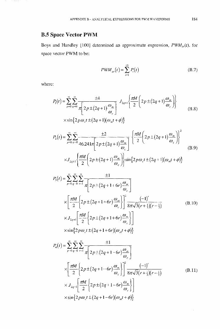
APPENDIX B-ANAL YTJCAL EXPRESSIONS FOR PWM WAVEFORMS 184
B.S Space Vector PWM
Boys and Handley [100] determined an approximate expression, PWMsv(t), for
space vector PWM to be:
15
PWM,.v(t)= L~(t) (B.7) i~I
where:
~(t)= 'LL ±4
p~O q~O n[2p ±(2q + 1) mm] me
1,, .. { m:; (zr±(2q+l):: )} (B.8)
X sin{ 2pmct ± (2q + 1)( mmt + r/J)}
(B.9)
~(t)='LL'L [ J p~O q=O r~I 7r 2 p ± ( 2q + 1 + 6r) {0 m
me
±1
X [nM {2p ± (2q + 1 + 6r) mm }]' j:lt !)',)( ') (B.IO) 2 m c 8n 3 r + 3 r- 3
x J,,.,[ m:; { 2p±(2q + 1 +6r) ::} ]
X sin{ 2pmct ±(2q + 1 + 6r)(mmt + ¢)}
P4(t)= LLL [ ] p=Oq=Or=l 7r 2p±(2q+1-6r)::
±1
x[nM {2 +(2 + 1-6r) mm }]z ( -1)' 2 P- q me 8n.J3(r+t)(r-t) (B.ll)
xI,,,[ m:; {zr±(2q+l-6r):: }]
xsin{ 2pmJ ±(2q + 1- 6r)(mmt + ¢)}

APPENDIX B- ANALYTICAL EXPRESSIONS FOR PWM WAVEFORMS 185
.fs(t)= it ±(-1~ M 4 Jo{nM(2p±3(2r+1)mm)} p=Or=on.J3(2r+3)(2r+3) 2 me (B.12)
x sin{2pmJ ± 3(2r + 1)(mmt + f/J)}
~ ( t) = :t t t ±( -1 ): M 4
p=Oq=O r=O n.J3(2r+3)(2r+3)
x J,, { m:: ( 2p±(3(2r+ 1)+ 2q) ::) } (B.13)
X sin{2pm ,t ± ( 3(2r + 1) + 2q )( mmt + f/J)}
J;(t)= :tt:t ±(-1):·M 4
p=O q=O r=O n.J3( 2r + 3 )( 2r + 3)
x J,, { m:: ( 2p±(3(2r+ 1)-2q) :: )} (B.14)
X sin{ 2pm J ± ( 3(2r + 1)- 2q)( mmt + f/J)}
= = 4 {nM ( m J} Ps(t)= LL [ - .J 12q- (2p+1)±2q___!!!_ p=Oq=O 7r (2p+ 1)±2q (J)m 2 (J)c
(J)c (B.15)
X sin{ ( 2p + 1)m J ± 2q( mmt + f/J)}
R (t)- ~ 2 {nM (2 + 1)}z 9
- ~ 46.241n( 2 p + 1) 2 P
x J 0 { n~ ( 2 p + 1)} sin { ( 2 p + 1 )w J} (B.16)
(B.17)

APPENDIX B- ANALYTICAL EXPRESSIONS FOR PWM WAVEFORMS 186
1 ( 1)r ~~(t)= LL - I I
'"" '"' {tzp + 1) ± 6<~:] snv'3(r + 3)(r- ,)
X [ 'rt:; {(2p+ 1)±6r :: }J J0 [ 'rt:; {(2p+ 1) ±6r ::} ] (B.18)
X sin { ( 2 p + 1 )cv ct ± 6r( OJ mt + qJ)}
~z(t)= iii 1 (-1)1r I '"" ,., ,., {tzp + 1) ± (2q + 6r) ::] 8nv'3(r + s)(r- s)
x[ 'rt:; {(2p+l)±(2q+6r)::}J (B.19)
x 12,[ 'rt:; {(2p+ 1)±(2q +6r) ::} ]
x sin{(2p + 1)wJ ± (2q + 6r )(wmt + ¢)}
~3(t)= tit 1 (-l)lr I '"0 '"
0 ,., {tzp + 1) ± (2q- 6r) ::] Snv'3(r + ,)(r- ,)
x [ 'rt:; {(zp + 1)±(2q -6r) :: }J (B.20)
xJ,,[ 'rt:; {(2p+ 1)±(2q- 6r) ::} ]
xsin{(2p + 1)wct ±(2q -6r)(wn/ + ¢)}
= = = ( 1)r M ~4(t)= LLL - 2 4
p=O q=O r=O n-J3(2r + 3)(2r + 3)
x [ m:: { ( 2 p + I) ± ( ( 2q + I) - 3( 2r + I)) :: }J x 12,,,{ 'rt:; ((2p + !) ± ((2q + !) - 3(2r + 1)) ::) }
X sin{ (2p + 1)wct ± ((2q + 1)-3(2r + 1))(wmt + ¢)}
(B.21)

APPENDIX B- ANALYTICAL EXPRESSIONS FOR PWM WAVEFORMS
( l)r M ~s(t)=LL.L -
2 4
p~Oq=O r~O nJ3(2r+3)(2r+3)
x [ rm; {(2p+ 1)±((2q + 1)+ 3(2r+ !)) :: }J x 12,,, { m: ( (2p +I)±( (2q + !) + 3{2r+ !)) ::) }
X sin{ (2p +!)met± ((2q + 1) + 3(2r + l))(mmt + ¢)}
187
(B.22)

REFERENCES 189
[11] Natarajan R., "Failure identification of induction motors by sensing unbalanced stator currents", IEEE Transactions on Energy Conversion, Vol. 4, No.4, pp585-590, December 1989.
[12] Binns K.J. and Dye M., "Identification of principal factors causing unbalanced magnetic pull in cage induction motors", Proceedings of the lEE, Vol. 120, No.3, pp349-354, March 1973.
[13] Hargis C., Gaydon B.G., and Kamash K., "The detection of rotor defects in induction motors", International Conference on Electrical Machines -Design and Applications, lEE Conference Publication No. 213, pp213-220, London, 13-15 July 1982.
[14] Kliman G.B., "Spectral analysis of induction motor current to detect rotor faults with reduced false alarms", US Patent Number 5,049,815, 17 September 1991.
[15] ElderS., Watson J.F. and Thomson W.T., "Fault detection in induction motors as a result of transient analysis", lEE Publication No. 310, pp182-186, 1989.
[16] Tavner P.J., Armin K.K. and Hargis C., "An electrical technique for monitoring induction motor cages", Proceedings of the Third International Conference on Electrical Machines and Drives, lEE Publication No. 282, pp43-46, 16-18 November 1987.
[17] Keuck J.D., Criscoe J.C. and Burstein N.M., "Assesment of valve actuator motor rotor degradation by fourier analysis of current waveform", IEEE Transactions on Energy Conversion, Vol. 7, No. 3, pp460-469, September 1992.
[18] Thomson W.T. and Chalmers S.J., "On-line condition monitoring of electrical machines - research to applications", Proceedings of the Vibration Analysis for Condition Monitoring - Techniques and User Experience Seminar, British Institute of Non-Destructive Testing, pp73-87, 1984
[19] Hirvonen R., "On-line condition monitoring of defects in squirel cage motors", Proceedings of the International Conference on Electrical Machines, Vol. 2, pp267-272, Paris, France, 5-8 September 1994.
[20] Gaydon B.G. and Hopgood D.J., "Faltering pulse can reveal an ailing motor", Electrical Review Vol, 205, No. 14, pp37-38, 12 October 1979.
[21] Kliman G.B. and Koegl R.A., "Noninvasive detection of broken rotor bars in operating induction motors", IEEE Transactions on Energy Conversion, Vol. 3, No 4, pp873-879, December 1988.
[22] Elkasabgy N.M., Eastham A.R., and Dawson G.E., "The detection of broken bars in the cage rotor of an induction machine", Conference

REFERENCES 190
Record of the IEEE Industry Applications Society Annual Meeting, Vol. 1, pp181-187, 1988.
[23] Steele M.E., Ashen R.A., and Knight L.G., "An electrical method for condition monitoring of motors", International Conference on Electrical Machines - Design and Applications, lEE Conference Publication No. 213, pp231-235, London, 13-15 July 1982.
[24] Kliman G.B. and Stein J., "Methods of motor current signature analysis", Electric Machines and Power Systems, Vol. 20, pp463-474, 1992.
[25] Watt P.A. and Langman R.A., "Condition monitoring of large induction motors", IE Aust. Conference on Industrial Drives, pp213-219, Rockhampton, Australia, 18-20 September1991
[26] Innes A.G., Watt P.A., and Langman R.A., "Condition monitoring of large induction motors", Proceedings of the Australasian Instrumentation and Measurement Conference, pp265-271, Auckland, New Zealand, 24-27 November 1992.
[27] Kryter R.C. and Haynes H.D., "Condition monitoring of machinery using motor current signature analysis", Sound and Vibration, pp 14-21, September 1989.
[28] Thomson W.T., Leonard R.A., Milne A.J., and Penman J., "Failure identification of offshore induction motor systems using on-condition monitoring", Proceedings of the Fourth National Reliability Conference, 1983.
[29] Leonard R.A. and Thomson W .T., "Vibration and stray flux monitoring for unbalanced supply and inter-tum winding fault diagnosis in induction motors", British Journal of NDT, Vol. 28, pp211-215, July 1986.
[30] Cho K.R., Lang J.H. and Umans S.D., "Detection of broken rotor bars in induction motors using state and parameter estimation", IEEE Transactions on Industry Applications, Vol. 28 No. 3, pp702-709, May/June 1992.
[31] Firoozian R. and Lee C.C., "Condition monitoring of automatic control systems using parameter and systems identification: a numerical investigation", Transactions of the Institute of Measurement and Control, Vol. 16, No.2, pp86-98, 1994.
[32] Du B., Capolino G.A. and Dessoude M., "A fast algorithm for a PCbased motor surveillant system", Proceedings of the International Conference on Electrical Machines, Vol. 2, pp273-277, Paris, France, 5-8 September 1994.
[33] Legowski S.F. and Trzynadlowski A.M., "Instantaneous stator power as a medium for the signature analysis of induction motors", Conference

REFERENCES 191
Record of the 30th Industry Applications Society Annual Meeting, Vol.1, pp619-624, 8-12 October 1995.
[34] Thomson W.T. and Stewart I.D., "On-line current monitoring for fault diagnosis in inverter fed induction motors", Proceedings of the Third International Conference on Power Electronics and Variable-Speed Drives, lEE Conference Publication 291, pp432-435, 1988.
[35] Marques Cardoso A.J. and Sousa Saraiva E.S., "Condition monitoring of current source inverter-fed induction machines", Proceedings of the 6th Conference on Power Electronics and Motion Control, Vol. 3, pp744-748, Budapest, Hungary, 1990.
[36] Thian B.M., Methods for Monitoring the Condition of Electrical Machines Fed from Variable Speed Drives, PhD Thesis, University of Aberdeen, UK, 1991.
[37] Sethuraman S.K. and Saravanan M.G., "Pulse width modulated embedded control and on-line condition monitoring of induction motors", Proceedings of the 29th Universities Power Engineering Conference, Vol. 2, pp645-647, Galway, Ireland, 14-16 September 1994.
[38] Healy J.A., Condition Monitoring at Associated Pulp and Paper Mills Wesley Vale, Tasmania, M. Eng. Sc. Thesis, University of Tasmania, Australia, 1991.
[39] Penman J., Dey M.N., Tait A.J., and Bryan W.E., "Condition monitoring of electrical drives", lEE Proceedings Part B, Vol. 133, No. 3, pp142-148, May 1986.
[40] Krause P.C., Wasynczuk 0. and Sudhoff S.D., Analysis of Electrical Machinery, IEEE Press, New York, 1995.
[41] Alger P.L., Induction Machines: Their Behaviour and Uses 2nd ed., Gordon and Breach, Switzerland, 1995.
[42] Liwschitz-Garik M. and Whipple C.C., Electric Machinery: Volume 2 AC Machines, D. Van Nostrand Company Inc., New York, 1946.
[43] Chapman F.T., A Study of the Induction Motor, Chapman and Hall Ltd., London, 1930.
[44] Kostenko M. and Piotrovsky L., Electrical Machines: Part Two, Foreign Languages Publishing House, Moscow, 1962.
[45] Chochran P.L., Polyphase Induction Motors: Analysis, Design, and Application, Marcel Dekker Inc., New York, 1989.
[46] Yang S.J., Low-noise Electrical Motors, Clarendon Press, Oxford, 1981.

REFERENCES 192
[47] Heller B. and Hamata V., Harmonic Field Effects in Induction Machines, Elsevier Scientific Publishing Company, Amsterdam, 1977.
[48] Cameron J.R., Thomson W.T., and Dow A.B., "Vibration and current monitoring for detecting airgap eccentricity in large induction motors", lEE Proceedings Part B, Vol. 133, No.3, pp155-163, May 1986.
[49] Deleroi W., "Der stabbruch im KafigHiufer eines asynchronmotors, Teil 1: beschreibung mittels tiberlagerung eines stOrfeldes", Archiv for Elektrotechnik, Vol. 67, pp91-99, 1984.
[50] Deleroi W., "Squirrel cage motor with broken bar in the rotor- physical phenomena and their experimental assessment", Proceedings of the International Conference on Electrical Machines, Vol. 3, pp767-770, Budapest, Hungary, 1982.
[51] Christofides N., "Origins of load losses in induction motors with cast aluminium rotors", Proceedings of the lEE, Vol. 112, No. 12, pp2317-2332, December 1965.
[52] Kerszenbaum I. and Landy C.F., "The existence of large inter-bar currents in three phase squirrel cage motors with rotor-bar and/or endring faults", IEEE Transactions on Power Apparatus and Systems, Vol. 103, No.7, pp1854-1862, July 1984.
[53] Walliser R.F. and Landy C.F., "Determination of interbar current effects in the detection of broken rotor bars in squirrel cage induction motors", IEEE Transactions on Energy Conversion, Vol. 9, No. 1, ppl52-158, March 1994.
[54] Marple S.L., Digital Spectral Analysis, Prentice-Hall Inc., Englewood Cliffs New Jersey, 1987.
[55] Kay, S.}.1., Marple, S.L., "Spectrum analysis - A modem perspective", Proceedings of the IEEE, Vol. 69, No. 11, pp 1380-1419, November 1981.
[56] Gabel R.A. and Roberts R.A., Signals and Linear Systems 3rd ed., John Wiley and Sons, New York, 1987.
[57] Stuart R.D., An Introduction to Fourier Analysis, Chapman and Hall, London, 1982.
[58] Shannon C.E. and Weaver W., The Mathematical Theory of Communication, University of Illinois Press, Urbana USA, 1971.
[59] Burrus C.S. and Parks T.W., DFTIFFT and Convolution Algorithms, John Wiley and Sons, New York, 1985.

REFERENCES 193
[60] Press W.H., Teukolsky S.A., Vetterling W.T. and Flannery B.P., Numerical Recipes in C: The Art of Scientific Computing 2nd ed., Cambridge University Press, Cambridge UK, 1992.
[61] Elliott D.F. and Rao K.R., Fast Transforms: Algorithms, Analyses, Applications, Academic Press, New York, 1982.
[62] Johnson L.W. and Riess R.D., Numerical Analysis 2nd ed, Addison Wesley, Reading Massachusetts, 1982.
[63] Oppenheim A.V. and Shafer R.W., Digital Signal Processing, PrenticeHall Inc., Englewood Cliffs New Jersey, 1975.
[64] Rabiner L.R. and Gold B., Theory and Application of Digital Signal Processing, Prentice-Hall Inc., Englewood Cliffs New Jersey, 1975.
[65] Burrus C.S. and Eschenbacher P.W., "An in-place, in-order prime factor FFT algorithm", IEEE Transactions on Acoustics, Speech and Signal Processing, Vol. 29, No.4, pp806-817, August 1981.
[66] Harris F.J., "On the use of windows for harmonic analysis with the discrete fourier transform", Proceedings of the IEEE, Vol. 66, No. 1, pp51-83, January 1978.
[67] Nuttall A.H., "Some windows with very good sidelobe behaviour", IEEE Transactions on Acoustics, Speech and Signal Processing, Vol. 29, No. 1, pp84-91, February 1981.
[68] Mitra S.K. and Kaiser J.F., Handbook for Digital Signal Processing, John Wiley and Sons, New York, 1993.
[69] Best R.E., Phase-Locked Loops, McGraw-Hill Inc., New York, 1984.
[70] Encinas J.B., Phase Locked Loops, Chapman and Hall, London, 1993.
[71] National Semiconductor Corporation, CMOS Databook, National Semiconductor Corporation, California, USA, 1981.
[72] Ferrero A. and Ottoboni R., "A low-cost frequency multiplier for synchronous sampling of periodic signals", IEEE Transactions on Instrumentation and Measurement, Vol. 41, No.2, pp203-207, April 1992.
[73] Linehan D.J., Bunch S.L., and Lyster C.T., "Method and apparatus for generating motor current spectra to enhance motor system fault detection", US Patent Number 5,461,329, 24 October, 1995.
[74] Innes A.G., Langman R.A., and Mayhew G.R., "Condition monitoring of variable speed induction motor drives", Proceedings of the International

REFERENCES 194
Conference on Electrical Machines in Australia, Vol. 1, pp158-163, Adelaide, Australia, 14-16 September 1993.
[75] Layos M. and Haritantis 1., "Modelling of commercially available phase locked loop ICs", International Journal of Electronics, Vol. 75, No.2, pp315-326, 1993.
[76] Private communication with control room staff of the Hydro Electric Commission of Tasmania, March 1996.
[77] Holtz J., "Pulsewidth modulation for electronic power conversion", Proceedings ofthe IEEE, Vol. 82, No.8, ppl194-1214, August 1994.
[78] Klingshim E.A. and Jordan H.E., "Polyphase induction motor performance and losses on nonsinusoidal voltage sources", IEEE Transactions on Power Apparatus and Systems, Vol. 87, No. 3, pp624-631, March 1968.
[79] Boys J.T. and Miles M.J., "Empirical thermal model for inverter-driven cage induction machines", lEE Proceedings Part B: Electric Power Applications, Vol. 141, No.6, pp360-372, November 1994.
[80] Boldea I. and Nasar S.A., Vector Control of AC Drives, CRC Press, Boca Raton, USA, 1992.
[81] Mohan N., Undeland T.M. and Robbins W.P., Power Electronics: Converters, Applications and Design, John Wiley and Sons, New York, 1989.
[82] Shepherd W. and Hulley L.N., Power Electronics and Motor Control, Cambridge University Press, Cambridge, UK, 1987.
[83] Black H.S., Modulation Theory, Van Nostrand, New York, 1953.
[84] Bowes S.R., "New sinusoidal pulsewidth-modulated invertor", Proceedings of the lEE, Vol. 122, No. 11, pp1279-1285, November 1975.
[85] Bowes S.R. and Bird B.M., "Novel approach to the analysis and synthesis of modulation processes in power convertors", Proceedings of the lEE, Vol. 122, No.5, pp507-513, May 1975.
[86] Bowes S.R. and Clements R.R., "Computer-aided design of PWM inverter systems", lEE Proceedings Part B: Electric Power Applications, Vol. 129, No. 1, pp1-17, January 1982.
[87] Franz6 G., Mazzucchelli M., Puglisi L., and Sciutto G., "Analysis of PWM techniques using uniform sampling in variable-speed electrical drives with large speed range", IEEE Transactions on Industry Applications, Vol. 21, No.4, pp966-974, July/August 1985.

REFERENCES 195
[88] Zach F.C., Martinez R., Keplinger S., and Seiser A., "Dynamically optimal switching patterns for PWM inverter drives (for minimization of the torque and speed ripples)", IEEE Transactions on Industry Applications, Vol. 21, No.4, pp975-986, July/August 1985.
[89] Zach F.C. and Ertl H., "Efficiency optimal control for AC drives with PWM inverters", IEEE Transactions on Industry Applications, Vol. 21, No.4, pp987-1000, July/August 1985.
[90] Dewan S.B. and Straughen A., Power Semiconductor Circuits, John Wiley and Sons, New York, 1975.
[91] Bowes S.R. and Midoun A., "Suboptimal switching strategies for microprocessor-controlled PWM inverter drives", lEE Proceedings Part B: Electric Power Applications, Vol. 132, No.3, pp133-148, May 1985.
[92] Houldsworth J.A. and Grant D.A., "The use of harmonic distortion to increase the output voltage of a three-phase PWM inverter", IEEE Transactions on Industry Applications, Vol. 20, No. 5, pp1224-1228, September/October 1984.
[93] Trzynadlowski A.M., Legowski S., and Kirlin R.L., "Random pulsewidth modulation technique for voltage-controlled power inverters", International Journal of Electronics, Vol. 68, No.6, pp 1027-1037, 1990.
[94] Chalmers B.J. ed, Electric Motor Handbook, Butterworths, London, 1988.
[95] Kirlin R.L., Kwok S., Legowski S., and Trzynadlowski A.M., "Power spectra of a PWM inverter with randomized pulse position", IEEE Transactions on Power Electronics, Vol. 9, No.5, pp463-472, September 1994.
[96] Boys J.T., "Theoretical spectra for narrow-band random PWM waveforms", lEE Proceedings Part B: Electric Power Applications, Vol. 140, No.6, pp393-400, November 1993.
[97] Habetler T.G. and Divan D.M., "Acoustic noise reduction in sinusoidal PWM drives using a randomly modulated carrier", IEEE Transactions on Power Electronics, Vol. 6, No.3, pp356-363, July 1991.
[98] van der Broeck H.W., Skudley H., and Stanke G.V., "Analysis and realization of a pulsewidth modulator based on voltage space vectors", IEEE Transactions on Industry Applications, Vol. 24, No. 1, pp142-150, January/February 1988.
[99] Handley P.G. and Boys J.T., "Practical real-time PWM modulators: an assessment", lEE Proceedings Part B: Electric Power Applications, Vol. 139, No.2, pp96-102, March 1992.

REFERENCES 196
[100] Boys J.T. and Handley P.O., "Harmonic analysis of space vector modulated waveforms", lEE Proceedings Part B: Electric Power Applications, Vol. 137, No.4, pp197-204, July 1990.
[101] Deng X. and Ritchie E., "Detection of broken rotor bars in induction motor rotors by investigating the flux linkages of the stator winding", Proceedings of the International Conference on Electrical Machines in Australia, Vol. 1, pp164-169, Adelaide, Australia, 14-16 September 1993.
[102] Chari M.V.K., and Silvester P.P., Finite Element Problems in Electrical and Magnetic Field Problems, John Wiley and Sons, New York, 1980.
[103] Salon S., Palma R., and Hwang C.C., "Dynamic modeling of an induction motor connected to an adjustable speed drive", IEEE Transactions on Magnetics, Vol. 25, No.4, pp3061-3063, July 1989.
[104] Salon S., Burow D., Slavik C., Bushman R., and DeBortoli M., "Comparison of pulsating torques in induction motors by analytic and finite element methods", Proceedings of the International Conference on Electrical Machines, Vol 3 pp732-737, Paris, France, 5-8 September 1994.
[105] Williamson S. and Smith A.C., "Steady-state analysis of 3-phase cage motors with rotor-bar and end-ring faults", lEE Proceedings Part B, Electrical Power Applications, Vol. 129, No.3, pp 93-100, May 1982.
[106] Muller G.H. and Landy C.F., "Finite element analysis of field distribution of squirrel cage induction motors having broken rotor bars and interbar currents", Proceedings of the International Conference on Electrical Machines, Vol. 2, pp577-581, Paris, France, 5-8 September 1994.
[107] O'Kelly D. and Simmons S., Introduction to Generalized Electrical Machine Theory, McGraw-Hill, London, 1968.
[108] Krause P.C., "Method of multiple reference frames applied to the analysis of symmetrical induction machinery", IEEE Transactions on Power Apparatus and Systems, Vol. 87, No. 1, pp218-227, January 1968.
[109] Barton T.H. and Doxey B.C., "The operation of three-phase induction motors with unsymmetrical impedance in the stator circuit", Proceedings of the lEE Part A: Power Engineering, Vol. 102, No. 1, pp71-79, February 1955.
[110] Vas P. and Vas J., "Transient and steady-state operation of induction motors with rotor asymmetries", Archiv fur Elektrotechnik, Vol. 59, pp55-60, 1977.

REFERENCES 197
[111] Vas P., "Steady state and transient performance of induction motors with rotor asymmetry", IEEE Transactions on Power Apparatus and Systems, Vol. 101, No.9, pp3246-3251, September 1982.
[112] Vas P., Filippetti F., Franceschini G. and Tassoni C., "Transient modelling oriented to diagnostics of induction machines with rotor asymmetries", Proceedings of the International Conference on Electrical Machines, Vol. 2, pp62-67, Paris, France, 5-8 September 1994.
[113] Lipowski J.S. and Duggal B.R., "Monitoring faults in the rotor of a squirrel-cage induction motor throught the analysis of harmonic content of stator currents", Proceedings of the International Power Engineering Conference, pp484-490, Singapore, 18-19 March 1993.
[114] Ritchie E., Deng X. and Jokinen T., "Dynamic model of three-phase squirrel cage induction motors with rotor faults", Proceedings of the International Conference on Electrical Machines, Vol. 2, pp348-352, Paris, France, 5-8 September 1994.
[115] Fudeh H.R. and Ong C.M., "Modeling and analysis of induction machines contammg space harmonics part I: modeling and transformation", IEEE Transactions on Power Apparatus and Systems, Vol. 102, No.8, pp2608-2615, August 1983.
[116] Fudeh H.R. and Ong C.M., "Modeling and analysis of induction machines containing space harmonics part ll: analysis of asynchronous and synchronous actions", IEEE Transactions on Power Apparatus and Systems, Vol. 102, No.8, pp2616-2620, August 1983.
[117] Fudeh H.R. and Ong C.M., "Modeling and analysis of induction machines containing space harmonics part lll: three-phase cage rotor induction machines", IEEE Transactions on Power Apparatus and Systems, Vol. 102, No.8, pp2621-2628, August 1983.
[118] Toliyat H.A., Lipo T.A., and White J.C., "Analysis of a concentrated winding induction motor for adjustable speed drive applications part 1 (motor analysis)", IEEE Transactions on Energy Conversion, Vol. 6, No. 4, pp679-683, December 1991.
[119] Toliyat H.A., Analysis of Concentrated Winding Induction and Reluctance Machines for Adjustable Speed Drive Applications, PhD Thesis, University of Wisconsin-Madison, USA, 1991.
[120] Toliyat H.A. and Lipo T.A., "Transient analysis of cage induction machines under stator, rotor bar and end ring faults", IEEE Transactions on Energy Conversion, Vol. 10, No.2, pp241-247, June 1995.

REFERENCES 198
[121] Luo X., Liao Y., Toliyat H.A., El-Antably A. and Lipo T.A., "Multiple coupled circuit modeling of induction machines", IEEE Transactions on Industry Applications, Vol. 31, No.2, pp311-317, March/April1995.
[122] Stewart D.E. and Leyk Z., Meschach: Matrix Computations in C, Proceedings of the Centre for Mathematics and its Applications, Volume 32, The Australian National University, Canberra, Australia, 1994.
[123] Newland D.E., "Wavelet analysis of vibration, part 1: Theory", Transactions of the ASME: Journal of Vibration and Acoustics, Vol. 116, pp409-416, October 1994.
[124] Newland D.E., "Wavelet analysis of vibration, part 1: Wavelet maps", Transactions ofthe ASME: Journal ofVibration and Acoustics, Vol. 116, pp417-425, October 1994.
[125] Tansel I. N., Mekdeci C., Rodriguez 0., and Uragun B., "Monitoring drill conditions with wavelet based encoding and neural networks", International Journal of Machine Tools and Manufacture, Vol. 33, No.4, pp559-575, 1993.
[126] Forrester D., "Time-frequency analysis in machine fault detection", in Time-frequency Signal Analysis - Methods and Applications (Boashash B. ed.), Longman Cheshire, Melbourne, Australia, 1992.
[127] Loughlin P., Atlas L., Bernard G., and Pitton J., "Application of timefrequency analysis to the monitoring of machining processes", Life Extension of Aging Machinery and Structures, Proceedings of the 49th Society of Machinery Failure Prevention Technology Conference (Pusey H.C. ed.), Vibration Institute, Illinois, USA, April 1995.
[128] Williams W.J., "Bearing monitoring using reduced interference distributions", Life Extension of Aging Machinery and Structures, Proceedings of the 49th Society of Machinery Failure Prevention Technology Conference (Pusey H.C. ed.), Vibration Institute, Illinois, USA, April1995.
[129] McFadden P.D., "Application of the wavelet transform to early detection of gear failure by vibration analysis", Proceedings of the Condition Monitoring '94 Conference (Jones M.H. ed.), pp172-183, Swansea, UK, 1994.
[130] Salvatore L. and Stasi S., "Monitoring of inverter drives in timefrequency domain", Proceedings of the International Conference on Electrical Machines, Vol. 2, pp73-78, Paris, France, 5-8 September 1994.
[131] Burnett R., Watson J.F., and Elder S., "The detection and location of rotor faults within three phase induction motors", Proceedings of the

REFERENCES 199
International Conference on Electrical Machines, Vol. 2, pp288-293, Paris, France, 5-8 September 1994.
[132] Burnett R. and Watson J.F., "The current analysis program - a software tool for rotor fault detection in three phase induction motors", Electrical Machines and Drives, lEE Conference Publication No. 412, pp156-160, 11-13 September 1995.
[133] Gabor D., "Theory of communication", The Journal of the lEE Part III: Radio and Communication Engineering, Vol. 93, No. 26, November 1946.
[134] Speiser J.M., Whitehouse H.J. and Allen J.C., "Wideband time-frequency distributions", in Time frequency Signal Analysis - Methods and Applications (Boashash B. ed.), Longman Cheshire, Melbourne, Australia, 1992.
[135] Choi H. and Williams W.J., "Improved time-frequency representation of multi component signals using exponential kernels", IEEE Transactions on Acoustics, Speech, and Signal Processing, Vol. 37, No.6, pp862-871, June 1989.
[136] Williams W.J. and Jeong J., "Reduced interference time-frequency distributions", in Time-frequency Signal Analysis - Methods and Applications (Boashash B. ed. ), Longman Cheshire, Melbourne, Australia, 1992.
[137] Zhao Y., Atlas L.E., and Marks II R.J., "The use of cone-shaped kernels for generalized time-frequency representations of nonstationary signals", IEEE Transactions on Acoustics, Speech, and Signal Processing, Vol. 38, No.7, pp1084-1091, July 1990.
[138] Cohen L., "Introduction: A primer on time-frequency analysis", in Timefrequency Signal Analysis- Methods and Applications (Boashash B. ed.), Longman Cheshire, Melbourne, Australia, 1992.
[139] Atlas L.E., Loughlin P.J., and Pitton J.W., "Signal analysis with cone kernel time-frequency distributions and their application to speech", in Time-frequency Signal Analysis - Methods and Applications (Boashash B. ed.), Longman Cheshire, Melbourne, Australia, 1992.
[140] Rioul 0. and Vetterli M., "Wavelets and signal processing", IEEE Signal Processing Magazine, Vol. 8, No.4, pp14-38, October 1991.
[141] Graps A., "An introduction to wavelets", IEEE Computational Science and Engineering, Summer, pp50-61, 1995.
[142] Daubechies I., Ten Lectures on Wavelets, CBMS-NSF Series in Applied Mathematics, SIAM, Philadelphia, Pennsylvania, 1992.

REFERENCES 200
[143] Grossman A., Kronland-Martinet R., Morlet J., "Reading and understanding continuous wavelet transforms," in Wavelets: Frequency Methods and Phase Space, 2nd ed. (Combes J.M., Grossman A., Tchamitchian Ph., Eds.), pp. 2-20, New York: Springer-Verlag, 1989/1990.
[144] Morlet J., Arens G., Fourgeau E., and Giard D., "Wave propagation and sampling theory", Geophysics, Vol. 47, No. 2, pp203-236, February 1982.
[145] Heneghan C., Khanna S.M., Flock A, Ulfendahl M., Brundin L., and Teich M.C., "Investigating the nonlinear dynamics of cellular motion in the inner ear using the short-time fourier and continuous wavelet transforms", IEEE Transactions on Signal Processing, Vol. 42, No. 12, pp3335-3352, December 1994.
[146] Boashash B., Boles P., Reilly A., Frazer G., and Hatton B., TFSA TimeFrequency Analysis Toolbox, Signal Processing Research Centre, Queensland Univeristy of Technology, Brisbane, Australia, 1994.
[147] The Mathworks Inc., MATLAB Reference Guide, The Mathworks Inc., Natick Ma., USA, 1992.
[148] Filippetti F., Franceschini G., and Tassoni C., "Neural networks aided on-line diagnostics of induction motor rotor faults", IEEE Transactions on Industry Applications, Vol. 31, No.4, pp892-899, July/August 1995.
[149] Penman J. and Yin C.M., "Feasability of using unsupervised learning, artificial neural networks for the condition monitoring of electrical machines", lEE Proceedings - Electric Power Applications, Vol. 141, No.6, pp317-322, November 1994.
[150] Filippetti F., FranceschiniG., Tassoni C., Meo S., and Ometto A., "Neural network aided on-line diagnostics of induction machine stator faults", Proceedings of the 30th Universities Power Engineering Conference, Vol. 1, pp148-151, London, UK, 5-7 September 1995.
[151] Penman J., Stavrou A., Yin C.M., Jiang H., and Hatzipantelis E., "Machine diagnostics with ANNs: possibilities and problems", Proceedings of the International Conference on Electrical Machines, Vol. 2, pp363-368, Paris, France, 5-8 September 1994.
[152] Protopapas C.A., Kaminaris S.D., Machias A.V., and Papadias B.C., "An expert system for fault repairing and maintenance of electric machines", IEEE Transactions on Energy Conversion, Vol. 5, No. 1, pp79-83. March 1990.
[153] Gentile G., Rotondale N., Tursini M., Franceschini G., and Tassoni C., "An approach to knowledge-base representation in electric drive fault

REFERENCES 201
diagnosis", Proceedings of the International Conference on Electrical Machines, Vol. 2, pp358-362, Paris, France, 5-8 September 1994.
[154] Watson G.N., Theory of Bessel Functions, Cambridge University Press, Cambridge, UK, 1922.