The Design And Testing Of An Axial Condenser Fan

THE DESIGN AND TESTING OF AN

AXIAL CONDENSER FAN

by

David Michael Kirk

A thesis submitted in partial fulfillment of the requirements for the degree

of

Master of Science

in

Mechanical Engineering

MONTANA STATE UNIVERSITY Bozeman, Montana

April 2021

©COPYRIGHT

by

David Michael Kirk

2021

All Rights Reserved

ii

TABLE OF CONTENTS

1. INTRODUCTION .....................................................................................................................1

Fan Application ........................................................................................................................ 1 Heat Pump Form Factors .......................................................................................................... 3 Research Intent ......................................................................................................................... 5

2. BACKGROUND .......................................................................................................................6

Refrigeration Cycle .................................................................................................................. 6 Fan Concepts ............................................................................................................................ 8

General Fan Designs ........................................................................................................... 8 Fan Performance Equations .............................................................................................. 11 Fan Pressure Relationships ............................................................................................... 12 Performance curves. .......................................................................................................... 13 Fan Affinity Laws ............................................................................................................. 14

Efficient Design Practices ...................................................................................................... 15 Blade Twist ....................................................................................................................... 15 Tip Clearance .................................................................................................................... 16 Solidity .............................................................................................................................. 16 Leveraging Airfoil Characteristics .................................................................................... 17 Blade Sweep...................................................................................................................... 19

CFD ........................................................................................................................................ 20 Turbulence Model ............................................................................................................. 21 Meshing and Y+ ................................................................................................................ 23 Periodic Boundaries .......................................................................................................... 25 Porous-Pressure Jump Inlet............................................................................................... 27

3. COMPUTER AIDED ENGINEERING METHOD ................................................................28

Fan Blade Generator ............................................................................................................... 28 Simulation Methodology ........................................................................................................ 30 Redesign Process .................................................................................................................... 37

Redesign Results ............................................................................................................... 39

4. EXPERIMENTAL METHOD .................................................................................................44

3D Printed Prototype .............................................................................................................. 44 Test Method 1 ......................................................................................................................... 46

Results: Method 1 ............................................................................................................. 50 Test Method 2 ......................................................................................................................... 51

Results: Method 2 ............................................................................................................. 54

iii

TABLE OF CONTENTS CONTINUED

5. IMPROVEMENTS AND FUTURE WORK...........................................................................57

Simulation Improvements ...................................................................................................... 57 Design Improvements ............................................................................................................. 59 Measurement Improvements .................................................................................................. 60

6. CONCLUSION ........................................................................................................................62

7. REFERENCES CITED ............................................................................................................64

iv

LIST OF TABLES

Table Page

1. CFD model physics specifications. ............................................................................... 33

2. Simulation results of the baseline sheet metal fan within the condenser unit. .............................................................................................................. 33

3. Comparison of simulated performance values between 2 prism layer mesh specifications and subsequent wall y+ values. ..................................................... 35

4. Simulation results of the baseline sheet metal fan with periodic boundaries. ...................................................................................................... 37

5. Simulation results of the optimized fan within the condenser unit. .............................. 40

6. Condenser unit test stand experimental results of the baseline fan at 1105 RPM ........................................................................................................... 50

7. Condenser unit test stand experimental results of the proposed fan at 1105 RPM ........................................................................................................... 50

8. AMCA 210 experimental data scaled to 1105 RPM. ................................................... 54

9. Interpolated performance parameters of the proposed fan design flow rate from the scaled AMCA 210 experimental results at 1105 RPM...................................................................................................... 56

10. Unsteady CFD model physics specifications. ............................................................. 58

11. Implicit unsteady performance results of the proposed fan ........................................ 58

v

LIST OF FIGURES

Figure Page

1. Air-cooled heat exchangers in the Forced draft (L) and induced draft (R) configurations. ................................................................................................................ 2

2. Diagram of a split system heat pump. ............................................................................. 4

3. AAON RQ series rooftop air cooled heat pump unit. ..................................................... 4

4. Theoretical vapor compression refrigeration cycle diagram. ......................................... 6

5. Flow of cool (blue) and hot (red) air through a Microchannel heat exchanger. ............................................................................................................... 8

6. Design of a centrifugal impeller (Left) and its housing (Right). .................................... 9

7. Design of an axial impeller (Left) and its housing (Right). ............................................ 9

8. Diagram of static and total pressure through a non-ducted inlet and outlet axial fan. ...................................................................................................... 12

9. A sample diagram of fan performance curves. ............................................................. 14

10. Diagram of blade angle (BA) and chord length (c). ................................................... 15

11. Visualization of blade twist through a side view of a generic fan. ............................. 16

12. Velocity comparisons around an airfoil. ..................................................................... 18

13. Fan blade airfoil cross sections (gold). ....................................................................... 18

14. Diagram of an airfoil with feature labels. ................................................................... 19

15. Forward and Backward swept blades. ........................................................................ 20

16. Velocity profile of a turbulent boundary layer. .......................................................... 23

17. Wall u+ as a function of wall y+ through the boundary sublayer. ............................... 24

18. Systematic structuring of prism layer cells to situate the cell centers within appropriate sublayers. .......................................................................... 25

19. Computational domain for a 3-bladed fan with various fluid boundary labels: Rotating region (Rot), Inlet: mass flow rate inlet, Periodic boundary (Per_3), and Outlet: Zero total pressure outlet. ............................ 26

vi

LIST OF FIGURES CONTINUED

Figure Page

20. Condenser unit test stand used for collecting coil pressure differentials, velocities, and motor power data. .......................................................... 27

21. NACA Series 4 Airfoil fan blade generator interface. ................................................ 29

22. Undeformed traditional airfoil fan blade geometry. ................................................... 29

23. Leading and trailing edge control points. ................................................................... 30

24. Baseline fan physical (Left) and digitized (right) representations. ............................. 31

25. Orifice plate physical (Left) and digitized (right) representations. ............................. 31

26. Geometry scene of the recreated condenser unit. ....................................................... 32

27. Condenser coil, casing, motor, mounting mechanism, fan and orifice plate geometry representation with a pressure jump inlet for the coil indicated in purple. ......................................................................................... 32

28. Velocity vector scene of the baseline fan within the condenser unit. ......................... 34

29. Scaled view of the mesh density and 1 mm thick prism layer containing 14 inflation layers applied to the fan blade surfaces ................................. 35

30. Velocity vector scene of the baseline fan being simulated at 4060.3 CFM showcasing the highlighted rotating region with periodic boundaries. .................................................................................................... 36

31. The changes in static pressure (left) and static efficiency (right) are compared with the change in power as the blade camber is increased from 0-7%. .................................................................................................. 37

32. The changes in static pressure (left) and static efficiency (right) are compared with the change in power as the blade camber high point position is increased from 50-70%. ................................................................... 38

33. Redesign methodology through parametric modification of blade shape ............................................................................................................. 39

vii


Figure Page

34. Geometry scene portraying the redesigned proposed fan with included hub mounting features. ................................................................................. 40

35. Comparison of the proposed and base fan performance parameters. ......................... 42

36. Comparison of the proposed and base fan static efficiencies with respect to flow rate. ..................................................................................................... 42

37. Velocity vector scene visualization of air recirculation within the fan blade tip-housing clearance zone. ......................................................................... 43

38. Visualization from the Markforged Eiger cloud interface of the 3D printed structure with concentric fiberglass layers represented in yellow. ................................................................................................. 45

39. 3D printed fan (top) and assembly (bottom). .............................................................. 45

40. Cross section side view of Method 1 testing configuration. ....................................... 46

41. Fan traverse measurement locations were indicated by 1-inch incremental tick marks. ............................................................................................... 47

42. Alnor Telescoping Pitot Tube (Left); Fluke 922 Airflow Meter (Right). ................... 47

43. Fluke 922 Airflow Meter Specifications. .................................................................... 48

44. 1/3 horsepower motor efficiency and power output curves along with a plotted interpolation point for 250 Watts of motor power demand. ............................................................................................................ 49

45. Top view diagram of Method 2 testing configuration. The variable supply was used to regulate control the tested fan volumetric flow rate, and flow measurement nozzles were used to measure this flow rate and system static pressure within the recirculation corridor. ................................................................................................. 52

46. The proposed fan mounted in horizontal configuration within the orifice plate. .......................................................................................................... 53

47. Fan speed control and power measurement instrumentation. ..................................... 53

viii


Figure Page

48. Comparison of the proposed fan pressure and power curves that were generated by the CFD simulation (black) and experimental testing using Method 2 (red). The test point from Method 1 (blue) is also compared. ......................................................................................................... 55

49. Comparison of the proposed fan efficiency curves that were generated by the CFD simulation (black) and experimental testing using Method 2 (red). The test point from Method 1 (blue) is also compared. ......................................................................................................... 55

ix

ABSTRACT

Axial or propeller fans are a subset of turbomachinery whose application is prevalent in everyday life. In the case of heating, ventilation, air conditioning, and refrigeration (HVAC&R), fans can be a large source of inefficient energy consumption due to their physical operating nature. With the global push for more efficient systems, components of HVAC&R equipment such as fans have become a focal point for researchers in academia and industry alike. Technological improvements in research equipment such as computational fluid dynamics (CFD) and additive manufacturing play a large role in achieving these improved efficiencies. The goal of this research is to improve the efficiency of an axial fan intended for cooling a micro-channel heat exchanger that is used in rooftop condenser units. A higher efficiency retrofit fan was iteratively designed using a commercial CFD software package, Star CCM+, which constitutes much of the research conducted in this project. The iterative models show that significant efficiency gains can be achieved through incremental alterations of classical fan blade geometry elements such as pitch, camber, skew, cross section loft path, chord length, thickness, etc. A physical model of the fan design thought to be the optimal choice for experimental analysis was 3D printed and tested using an AMCA Standard 210 setup. Upon analysis of the physical test results, several discrepancies between simulated and actual results were discovered, highlighting the importance of CFD model validation in the design process. Despite the efficiency gains and advancements in user-friendly packaged software, the simulation underpredicted the power demand and incorrectly depicted the fan’s performance at critical operating points showing that improper usage of these experts’ tools can inadvertently lead to developed solutions with significant error. While the designed fan achieves an improved peak static efficiency and volumetric flow rate of 53.9% and 4334 CFM respectively, it ultimately did not meet the operating parameters of the specific unit it was designed for and further improvements to the CFD model are needed.

1

CHAPTER ONE

INTRODUCTION

Fan Application

Efficient fan performance is essential for numerous operations in industry ranging from

urban high rises providing offices with high productivity and comfortable work environments to

agriculture where air quality is controlled in spaces that contain livestock or plants. Throughout

these commercial environments, the electricity required to operate fan motors composes a

significant portion of the energy costs for space conditioning [1]. In today’s push towards more

sustainable practices, more focus is being placed on these heating ventilation air conditioning

and (HVAC&R) subsystems of the built environment which account for nearly 44% of a

commercial building’s energy usage [2]. In continuing these endeavors, it is important to identify

key aspects of subsystems that are causing inefficiencies to exist.

In addition to the traditional aspects of fan performance, fan noise also becomes of

interest. The building application, location of HVAC&R equipment, and code regulations

required by the presiding government entity often dictate the noise restrictions of the building’s

systems. For example, the noise requirements for a performing arts theater located in an urban

setting will differ from that of a rural manufacturing facility. Nevertheless, the noise generated

by fans can negatively impact the acoustic environment of a conditioned space. Therefore, the

noise produced by the fan is a function of its physical design, volumetric flow rate, total

pressure, and efficiency [3]. According to the American Society of Heating, Refrigerating, and

Air-Conditioning Engineers (ASHRAE), the noise for turbomachinery is associated with blade-

2 flow occurrences such as turbulence interaction with walls. Blade passage frequency can result in

narrow-band frequency that stands out from background noise conditions. Noise reduction

techniques exist such as unequally spacing the fan blades around its circumference and increased

distance between the fan and its housing [4]. However, these noise reduction actions can

negatively impact the fan’s efficiency.

Although the operational efficiency of the fan is the primary focus of this study, other

system design factors can lead to overall efficiency improvements. It has been shown through

previous experimentation that the configuration of the fan with respect to the heat transfer

element has an effect on the overall performance due to plume recirculation or ambient

conditions [5]. Two common configurations are shown in Figure 1.

Figure 1. Air-cooled heat exchangers in the Forced draft (L) and induced draft (R) configurations [5].

The fan’s proximity to the to the heat exchanger is also an important consideration. This

distance between the heat exchanger and fan can be optimized to maximize the air flow

distribution across the heat exchanger which improves the performance of the system as a whole

[6].

3

It has become customary to perform analysis and optimize turbomachinery designs using

commercial computational fluid dynamics (CFD) packages [7]. The usage of CFD in HVAC&R

equipment design can circumvent the costly process of manufacturing prototype design

iterations. Prototyping can at times be so costly in certain situations that it is forgone entirely [8].

Despite the implementation of CFD, the build and test approach remains as a necessary design

methodology not only to validate the fan’s performance, but also to highlight physical loss

mechanisms [9]. In addition to CFD modeling, it is important to validate the results yielded from

the simulation. Oftentimes, marginal increases in efficiency purported by CFD models can be

confused with system noise and error. Because of the cost of prototyping, new technologies have

emerged to combat product development barriers. Of these advancements in rapid prototyping

methods, additive manufacturing (AM), also referred to as 3D printing, have become

increasingly popular in the attempt to lower the costs of product development. As is common

with prototyping, 3D printing facilitates customized one-off production [10]. AM processes

require no tooling or special skills and impose relatively no limits on the complexity of part

geometries, further reducing prototyping costs [11].

Heat Pump Form Factors

Heating and cooling a space within building systems typically involves the application of

the vapor compression cycle (which is also referred to as the refrigeration cycle) in heat pumps.

Each component in the refrigeration cycle works to optimize the heat transfer between

conditioned and unconditioned environments. Each system will consist of combinations of a

refrigerant compressor, condenser, expansion valve, and evaporator. Because not all air

conditioning applications are the same, these heat pumps come in various form factors and are

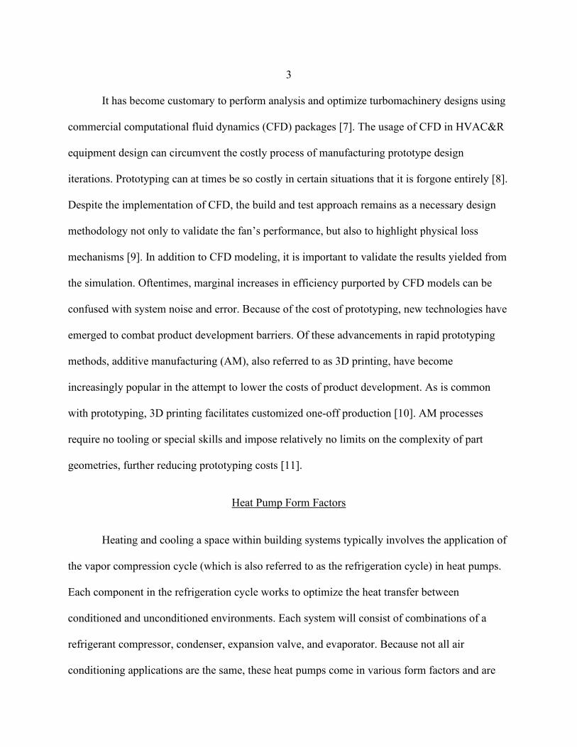
4 designed for specific building use cases. Figure 2 depicts a setup commonly found in residential

applications known as a split system where the condenser is physically separated from the

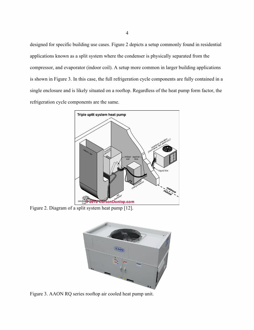
compressor, and evaporator (indoor coil). A setup more common in larger building applications

is shown in Figure 3. In this case, the full refrigeration cycle components are fully contained in a

single enclosure and is likely situated on a rooftop. Regardless of the heat pump form factor, the

refrigeration cycle components are the same.

Figure 2. Diagram of a split system heat pump [12].

Figure 3. AAON RQ series rooftop air cooled heat pump unit.

5

Research Intent

This research documents the process of designing and testing new fan blades using both

CFD and various physical experimental methodologies. Optimization efforts were geared

towards a rooftop condenser unit outfitted with a 30-inch diameter sheet metal orifice plate and a

motor that has a peak efficiency rating at 1/3 horsepower (~248 Watts) power output. The design

parameters for the airflow were a target volumetric flow rate of 4500 ft3/min, CFM, (7645.5

m3/hr) at 0.2 inches of water, in-H2O, (49.768 Pa) static pressure. These design parameters result

in a peak static efficiency of 42.5%.

6

CHAPTER TWO

BACKGROUND

Refrigeration Cycle

HVAC&R relies heavily on the refrigeration cycle. This process consists of four primary

thermodynamic operations. Figure 4 details each stage of the cycle as well as corresponding

thermodynamic property changes.

Figure 4. Theoretical vapor compression refrigeration cycle diagram [13].

From the perspective of a cooling operation, the evaporator (between states 4 and 1)

absorbs the heat from the building environment. This value is described by Equation 1where �̇�𝑚

is the mass flow rate of the refrigerant. The condenser rejects that heat into the outdoor

environment, which is governed by Equation 2.

7

4�̇�𝑞1 = �̇�𝑚(ℎ1 − ℎ4) 1

2�̇�𝑞3 = �̇�𝑚(ℎ2 − ℎ3) 2

j�̇�𝑞i is the heat transfer rate between states 𝑖𝑖 and 𝑗𝑗, �̇�𝑚 is the fluid mass flow rate, and ℎ𝑖𝑖

and ℎ𝑗𝑗 is the fluid enthalpy at state 𝑖𝑖 and 𝑗𝑗 respectively.

It is during the stage of working fluid condensation that axial fans are employed to

facilitate the heat exchange from the refrigerant to the outdoor air. It can be seen through the

correlation of Equation 2 and the thermodynamic diagrams in Figure 4 that the cooling capacity

of a heat pump can be manipulated by the temperature gradient of the refrigerant between States

2 and 3.

Fans are prolific turbomachines that commonly fulfill roles within cooling and ventilating

applications such as drawing large volumes of air through heat exchanger media to cool a

working fluid. This media can take the form of electric resistive elements or various tube-fin or

microchannel radiator-style configurations depending on system constraints. A common heat

transfer application is found in condensers and evaporators utilized in building HVAC&R

systems. A cross section of a microchannel heat exchanger is shown in Figure 5. Cooler air is

depicted entering from the left, absorbing heat from the refrigerant within the copper tubing

embedded in the mesh and exhausting at a higher temperature on the right.

8

Figure 5. Flow of cool (blue) and hot (red) air through a Microchannel heat exchanger.

Fan Concepts

General Fan Designs

Fans can broadly be categorized into two groups: centrifugal (Figure 6) and axial (Figure

7) fans. Centrifugal fans utilize centrifugal force created by rotating the air column between the

blades and kinetic energy from the velocity leaving the impeller to create a pressure difference.

9

Figure 6. Design of a centrifugal impeller (Left) and its housing (Right) [14].

Axial fans, also known as propeller fans, produce their pressure solely via the change in

air velocity as it travels along the blades’ axis of rotation [14]. Axial fans were the focus during

this study.

Figure 7. Design of an axial impeller (Left) and its housing (Right) [14].

Axial fans are susceptible to many external factors that can decrease their performance.

One of these factors is crossflow caused by wind. Specifically, an axial fan subjected to cross

flow wind will have a lower than optimal flow rate which both decreases its efficiency and

effectiveness at transferring heat [15].

10

Traditionally, axial fans are situated near the heat transfer device such that the air being

drawn through the heat exchanger is supplied from ambient conditions and is exhausted at

ambient conditions. These boundaries indicate that there should theoretically be little to no

differential pressure for the fan to overcome. This is convenient for a propeller fan since it is

designed to operate near free delivery scenarios [16]. Therefore, axial propeller fans are

commonly utilized for externally placed heat transfer applications due to their high volumetric

flow rate capabilities with respect to their ability to overcome back pressure in the system.

Heat transfer is an indicator of a fan’s effectiveness in a system. For a convective mode of heat

transfer, Kröger [5] describes the heat transfer ability in Equation 3 which has been modified to

match the nomenclature of Equation 2. In this version, 2�̇�𝑞3 is the heat transfer of the condenser

unit, �̇�𝑚𝑎𝑎 is the mass flow rate of the fan, 𝑇𝑇𝑎𝑎𝑖𝑖and 𝑇𝑇𝑎𝑎𝑜𝑜 are the temperature of the air at the heat

exchanger inlet and outlet respectively, and 𝑐𝑐𝑝𝑝𝑎𝑎 is the specific heat of the air.

2�̇�𝑞3 = �̇�𝑚𝑎𝑎𝑐𝑐𝑝𝑝𝑎𝑎�𝑇𝑇𝑎𝑎𝑜𝑜 − 𝑇𝑇𝑎𝑎𝑖𝑖� 3

Equation 3 indicates that the volumetric flow rate produced by the fan is directly tied to

the overall performance of a condenser unit. If the fan’s air flow rate can be increased, the

condenser unit’s capacity will be improved. However, the increased flow rate of a fan is often

coupled with higher fan motor demand. Therefore, it is a challenge to the designer to balance

flow rate with power demand where the mechanical efficiency of the fan becomes an important

parameter.

11 Fan Performance Equations

The performance of the fan can be approached from several perspectives depending on

the application. In general, fan efficiency is a function of the induced mass flow rate, air density,

the power required to drive the fan, and the pressure drop across the fan interfaces. For pressure,

three primary categories exist: Static, Dynamic (or velocity), and Total. The total pressure is

defined as the sum of the static and dynamic pressures. AMCA 210 defines two types of

efficiency, the fan static efficiency (Equation 4), and the fan total efficiency (Equation 5) [17].

𝜂𝜂𝑠𝑠 =𝑄𝑄 ∙ 𝑃𝑃𝑓𝑓𝑠𝑠𝐻𝐻

4

𝜂𝜂𝑡𝑡 =Q ∙ 𝑃𝑃𝑓𝑓𝑡𝑡𝐻𝐻

5

In the equations above, 𝑄𝑄 (Equation 6) is the volumetric flow rate, 𝑃𝑃𝑓𝑓𝑠𝑠 and 𝑃𝑃𝑓𝑓𝑡𝑡 are the fan static

and fan total pressures respectively, and 𝐻𝐻 (Equation 7) is the shaft power input to the fan.

Details for fan pressures are provided in the next section.

𝑄𝑄 =𝑚𝑚𝜌𝜌̇ 6

�̇�𝑚 and 𝜌𝜌 are the mass flow rate and density of air, respectively.

𝐻𝐻 = 𝜔𝜔 ∙ 𝜏𝜏 7

𝜔𝜔, is the rotational speed of the fan, and 𝜏𝜏 is the torque imposed on the shaft of the fan.

12 Fan Pressure Relationships

The approximate total and static pressure trends within a fan test chamber can be

visualized in Figure 8. Upstream of the fan region, negative static and total pressures are being

measured. Both static and total pressures are theoretically equivalent in the far-field region

upstream of the fan, and the air velocity is approximately zero.

Figure 8. Diagram of static and total pressure through a non-ducted inlet and outlet axial fan.

The theoretical fan static and total pressures are defined in Equation 8 and Equation 9

respectively.

𝑃𝑃𝑓𝑓𝑠𝑠 = 𝑃𝑃𝑠𝑠2 − 𝑃𝑃𝑡𝑡1 8

𝑃𝑃𝑓𝑓𝑡𝑡 = 𝑃𝑃𝑡𝑡2 − 𝑃𝑃𝑡𝑡1 9

13

Planes 1 and 2 in Figure 8 are highly turbulent in physical test setups. Therefore,

experimental measurements for total and static pressures are taken far upstream of the fan and

then correlated through Bernoulli’s principle to the Plane 1 and 2 positions. As air is drawn

through a heat exchanger coil, resistance to the flow is manifested in the form of static pressure.

It is less crucial for a condenser fan to produce higher velocity pressures since the air only needs

enough momentum to avoid recirculation back through the condenser unit. For cases of rooftop

units, recirculation is less likely. Therefore, for rooftop condenser fan applications, static

pressure is the most important pressure to generate. Higher fan static efficiencies indicate how

effective the fan is resisting the coil resistance with a high mass flow rate at suitable power

consumption. In cases such as building ventilation systems that have long lengths of ducts and

series of air filters, a higher total efficiency is desirable with the requirement of maintained air

movement.

Performance curves.

The efficiencies (static and total) of a single fan geometry are not constant values but

rather are dependent on the operating conditions of the fan. Therefore, it is standard to plot

efficiency, power, and pressure with respect to the operating volumetric flow rate (Figure 9).

These performance curves are used to determine the fan’s suitability for a proposed application.

14

Figure 9. A sample diagram of fan performance curves.

For optimization, it is advised that a fan is selected such that its peak efficiency operating point

coincides with the peak efficiency point of its specified motor.

Fan Affinity Laws

A useful set of equations known as fan laws exist for predicting fan performance values

at equal efficiency operating points [3]. These equations behave as non-dimensional scaling

operators and can be rearranged to solve for dependent variables. Adaptations of these equations

that predict the operating parameters of a fan (subscript 2) with respect to an identical fan

operating at known conditions (subscript 1) and constant air density are shown in Equation 10.

𝑄𝑄1𝑄𝑄2

=𝜔𝜔1

𝜔𝜔2 10 (a)

𝑃𝑃1𝑃𝑃2

= �𝜔𝜔1

𝜔𝜔2�2 10 (b)

𝐻𝐻1𝐻𝐻2

= �𝜔𝜔1

𝜔𝜔2�3 10 (c)

15

Efficient Design Practices

Blade Twist

A handbook by Bleier outlines fan airflow properties that improve efficiency [16]. The

airflow of an axial fan should be evenly distributed over the fan blade. In other words, the axial

air velocity should be the same from the fan hub to the blade tip [16]. A twist is applied by

uniformly altering the blade angle over its lofted length. The blade angle (BA) is defined by the

angle of incidence between the blade’s chord line which is colinear with the blade chord length

dimension (𝑐𝑐) and the fan rotation plane as shown in Figure 10.

Figure 10. Diagram of blade angle (BA) and chord length (c).

Larger blade angles near the center and smaller blade angles toward the tip can be used to

compensate for the gradient of air velocity along the blade face due to the linear relationship

between tangential velocity and radial position on a rotating body [16]. This blade twist effect is

displayed in Figure 11.

16

Figure 11. Visualization of blade twist through a side view of a generic fan.

Tip Clearance

The clearance between the fan blade tip and its housing is known to have large effects on

efficiency. Manufacturing processes and tolerances have historically dictated tip clearance

requirements. Therefore, tip clearance has often remained large enough to account for system

assembly inconsistencies such as eccentric placement of a motor within the fan housing. Higher

tip clearance in turbomachinery results in lower efficiency and higher broadband sound levels

[18]. Kameier and Neise also found that simply placing a strip of Velcro within the clearance gap

showed significant improvements in efficiency and aeroacoustic performance. The specific

reason for the performance improvement was not identified, but it was speculated that the strip

acted as a turbulence generator.

Solidity

Solidity is used to track the effect of the number of blades has on fan performance.

Physically, the solidity describes how much of a fan’s swept circumference is occupied by the

fan blades. For a fan with hub radius 𝑟𝑟ℎ, the fan solidity, 𝜎𝜎, is related to the number of blades,

𝑁𝑁𝑏𝑏, constant chord length, 𝑐𝑐, and the outer fan radius, 𝑅𝑅 through Equation 11.

17

𝜎𝜎 =𝑁𝑁𝑏𝑏𝑐𝑐

𝜋𝜋𝑅𝑅 �1 + 𝑟𝑟ℎ𝑅𝑅�

11

In the 1940’s fan curve experiments were conducted by the National Advisory

Committee for Aeronautics (NACA) on an axial flow fan where the number of evenly spaced fan

blades was decreased after each fan curve was generated [19]. The performance curves were

compared between using 24, 18, 12, 9, and 6 blades corresponding to solidity values of 0.86,

0.64, 0.43, 0.32, and 0.21 respectively. For configurations without the use of guide vanes, the

higher efficiencies tended to occur at the lower solidity values. However, higher pressures were

recorded at higher solidity values. Within the region of efficient operating flow rates, the rise in

pressure across the fan as well as the power demand had direct ties to the solidity. From Equation

11 and the previous studies, fan pressure is directly related to the number of blades and the chord

length [19]. In other words, an increase in the number of blades can increase the fan pressure.

Additionally, increasing the chord length can also increase the fan pressure. Depending on the

application, the target pressure would need to be balanced with the power demand to achieve an

optimal efficiency.

Leveraging Airfoil Characteristics

An airfoil can greatly improve the pressure performance of an axial fan [20]. The two

sides of an axial fan are distinguished by their pressures. The upstream surface of the fan is

referred to as the suction side, while the downstream surface is referred to as the pressure side. It

is well established that airfoil geometries are useful in increasing the differential pressure across

wing surfaces to create desirable effects such as lift. Through Bernoulli’s principle, pressure is

18 inversely related to the velocity of a fluid. In an idealized case, the flow field can be visualized in

Figure 12.

Figure 12. Velocity comparisons around an airfoil [21].

Since the velocity above the portrayed wing is higher than below the wing, the lower

pressure below the wing will generate vertical lift. This principle can then be applied to

turbomachinery by including an airfoil in each blade cross section as depicted in Figure 13.

Figure 13. Fan blade airfoil cross sections (gold).

19

One of the best documented airfoils is the NACA Series 4. The airfoil is primarily

defined by its chord, which is the line connecting the leading and trailing edges. Other features

and their nomenclature are shown in Figure 14.

Figure 14. Diagram of an airfoil with feature labels [22].

As its name suggests, this airfoil construction consists of four parametric values: chord,

maximum camber, 𝑀𝑀, (which is defined by a percentage of the blade chord), the position of the

maximum camber, 𝑃𝑃, (defined in 10ths of the chord length from the leading edge), and the

thickness, 𝑋𝑋𝑋𝑋, (also defined in a percentage of the chord length). The labelling scheme is as

follows:

𝑁𝑁𝑁𝑁𝑁𝑁𝑁𝑁 𝑀𝑀𝑃𝑃𝑋𝑋𝑋𝑋

𝑒𝑒.𝑔𝑔.

𝑁𝑁𝑁𝑁𝑁𝑁𝑁𝑁 4509

The above numerical example has a maximum camber of 4% of the chord, a high point (or

maximum camber position) of 5 “tenths” of the chord, and a thickness of 9% of the chord.

Blade Sweep

It has also been shown that properly incorporating a forward sweep to an axial fan blade

can result in improved aerodynamic performance [23] as well as improved aeroacoustics [24].

20 However, this improvement does not occur with backward swept blades. The two forms of skew

are depicted in Figure 15.

Figure 15. Forward and Backward swept blades.

CFD

CFD software packages have been developed to model fluid flow of varying complexity.

Although each package’s approach to the problem may differ slightly, they all use the governing

Navier-Stokes equations. These equations are partial differential equations (PDEs) and do not

have globally applicable analytical solutions. Therefore, they are often iteratively solved through

different numerical methods. Commercial CFD packages usually will leverage the finite volume

method. This method requires the computational domain to be divided into structured or

unstructured elements or “cells,” each containing discretized forms of the equations that govern

fluid flow and dependent fundamental fluid properties such as density and temperature. For

three-dimensional fluid problems, Star CCM+ uses the finite volume method where the fluid

domain is divided into smaller 3D cells. Discretized conservation equations are applied to each

subdivided volume to solve for each dependent variable that is stored at the finite volumes cell

center. The governing equations (continuity, momentum, and energy) can be written such that

21 they account for time dependent (transient or unsteady) effects of fluid flow. They can also be

written as a steady state form where the time rate of change of the finite volume’s fluid property

term is considered to be negligible. The governing equations do not inherently account for

effects such as turbulence, therefore, additional terms for various turbulence models are

introduced.

Turbulence Model

The SST (or Shear Stress Transport) k-omega turbulence model has widespread use in

the aerospace industry as it is applied to CFD problems using Reynolds-Averaged Navier-Stokes

(RANS) turbulence simulations. The k-omega turbulence model shows superior accuracy with

low-Reynolds numbers and transitional flows [25]. The Reynolds number is a non-dimensional

value dependent on the fluid velocity (𝑢𝑢), density (𝜌𝜌), viscosity (𝜇𝜇), and effective length (𝐿𝐿) of

the contact surface. The Reynolds number (𝑅𝑅𝑒𝑒) is calculated by Equation 12.

𝑅𝑅𝑒𝑒 =𝜌𝜌𝑢𝑢𝐿𝐿𝜇𝜇

12

Menter [26] introduced an adaptation to the k-omega turbulence model to better predict flow

separations in aerospace applications. This adaptation is applied to the Shear-Stress Transport

model and is shown in Equation 13 and Equation 14.

𝐷𝐷𝜌𝜌𝐷𝐷𝐷𝐷𝐷𝐷

= 𝜏𝜏𝑖𝑖𝑗𝑗𝜕𝜕𝑢𝑢𝑖𝑖𝜕𝜕𝑥𝑥𝑗𝑗

− 𝛽𝛽∗𝜌𝜌𝜔𝜔𝐷𝐷 +𝜕𝜕𝜕𝜕𝑥𝑥𝑗𝑗

�(𝜇𝜇 + 𝜎𝜎𝑘𝑘𝜇𝜇𝑡𝑡)𝜕𝜕𝐷𝐷𝜕𝜕𝑥𝑥𝑗𝑗

� 13

𝐷𝐷𝜌𝜌𝜔𝜔𝐷𝐷𝐷𝐷

=𝛾𝛾𝜈𝜈𝑡𝑡𝜏𝜏𝑖𝑖𝑗𝑗

𝜕𝜕𝑢𝑢𝑖𝑖𝜕𝜕𝑥𝑥𝑗𝑗

− 𝛽𝛽𝜌𝜌𝜔𝜔2 +𝜕𝜕𝜕𝜕𝑥𝑥𝑗𝑗

�(𝜇𝜇 + 𝜎𝜎𝜔𝜔𝜇𝜇𝑡𝑡)𝜕𝜕𝜔𝜔𝜕𝜕𝑥𝑥𝑗𝑗

� + 2(1 − 𝐹𝐹1)𝜌𝜌𝜎𝜎𝜔𝜔21𝜔𝜔𝜕𝜕𝐷𝐷𝜕𝜕𝑥𝑥𝑗𝑗

𝜕𝜕𝜔𝜔𝜕𝜕𝑥𝑥𝑗𝑗

14

22 His adaptation incorporates a blending function, 𝐹𝐹1 (Equation 15), that is dependent on a fluid

finite volume’s proximity, 𝑦𝑦, to a wall boundary.

𝐹𝐹1 = tanh(𝑎𝑎𝑟𝑟𝑔𝑔14) 15

Where 𝑎𝑎𝑟𝑟𝑔𝑔14 is:

𝑎𝑎𝑟𝑟𝑔𝑔14 = min �𝑚𝑚𝑎𝑎𝑥𝑥 �𝐷𝐷12

0.09𝜔𝜔𝑦𝑦;500𝜈𝜈𝑦𝑦2𝜔𝜔

� ;4𝜌𝜌𝜎𝜎𝜔𝜔2𝐷𝐷𝑁𝑁𝐷𝐷𝑘𝑘𝜔𝜔𝑦𝑦2

� 16

This blending function then transitions between the full k-omega and the k-epsilon forms of the

transport equation. In general:

𝑖𝑖𝑖𝑖 𝐹𝐹1 = 1 → 𝐷𝐷 𝑜𝑜𝑚𝑚𝑒𝑒𝑔𝑔𝑎𝑎

𝑖𝑖𝑖𝑖 𝐹𝐹1 = 0 → 𝐷𝐷 𝑒𝑒𝑒𝑒𝑒𝑒𝑖𝑖𝑒𝑒𝑜𝑜𝑒𝑒

Menter noted that the shear stresses at the wall boundary still were being overpredicted,

so a second blending function, 𝐹𝐹2 (Equation 17), was introduced as an eddy viscosity (Equation

19) limiter that is dependent on the cell distance to the closest wall.

𝐹𝐹2 = tanh(𝑎𝑎𝑟𝑟𝑔𝑔22) 17

Where

𝑎𝑎𝑟𝑟𝑔𝑔22 = max�2𝐷𝐷12

0.09𝜔𝜔𝑦𝑦;500𝜈𝜈𝑦𝑦2𝜔𝜔

� 18

𝜈𝜈𝑡𝑡 =𝑎𝑎1𝐷𝐷

max(𝑎𝑎1𝜔𝜔;𝛺𝛺𝐹𝐹2) 19

23

In summary, the SST k-omega turbulence model was selected to accurately model the

near-wall fluid-surface interactions while also maintaining accurate treatment of free-stream and

far field flow behavior.

Meshing and Y+

For aerodynamic simulations, it is important to allow for the accounting of near wall flow

behaviors such as flow separation. These flow behaviors are important due to the method of

solving wall shear stress. For turbulent flow, wall shear stress is computed through Equation 20

where 𝒖𝒖𝝉𝝉 is dependent on the turbulence modeling approach.

𝜏𝜏𝑤𝑤 = �𝜌𝜌𝒖𝒖𝝉𝝉2𝒗𝒗�𝑡𝑡𝑎𝑎𝑡𝑡𝑡𝑡𝑡𝑡𝑡𝑡𝑡𝑡𝑖𝑖𝑎𝑎𝑡𝑡�𝒗𝒗�𝑡𝑡𝑎𝑎𝑡𝑡𝑡𝑡𝑡𝑡𝑡𝑡𝑡𝑡𝑖𝑖𝑎𝑎𝑡𝑡�

� 20

𝒖𝒖𝝉𝝉 is the wall friction velocity, 𝜌𝜌 is the fluid density, and 𝒗𝒗�𝑡𝑡𝑎𝑎𝑡𝑡𝑡𝑡𝑡𝑡𝑡𝑡𝑡𝑡𝑖𝑖𝑎𝑎𝑡𝑡 is the RANS averaged

tangential velocity vector. As fluid flows across a surface with a non-slip condition, meaning that

the fluid velocity at the surface is zero, a series of sublayers is created which is known as the

boundary layer. Figure 16 depicts the various regions within the boundary layer.

Figure 16. Velocity profile of a turbulent boundary layer [25].

Within this boundary layer, the fluid viscosity has varying degrees of influence. As

mentioned before, a pure k-omega turbulence model is most accurate with low Reynolds number

24 flows. The best application of the model would be within the viscous sublayer. As the flow

begins to transition towards the free stream region, the effects of turbulence overtake those of the

fluid viscosity. The relationship between the sublayer treatment methods (black curves) and

empirical data (blue curve) is shown in Figure 17.

Figure 17. Wall u+ as a function of wall y+ through the boundary sublayer [25].

Figure 17 shows that the low y+ treatment, y+ < 5, is accurate for the viscous sublayer,

while the high y+ treatment, 30 < y+ < 300, is more appropriate for the log layer. Wall y+, a mesh

density-sensitive parameter, is used to define the limits of the sublayers as well as the

applicability of the turbulence models. It is formally defined in Equation 21 where 𝑦𝑦 is the

distance from the finite volume cell center to the wall, 𝜌𝜌 is the fluid density, 𝑢𝑢∗ is the velocity

scale that is a representative of the fluid velocity in the near-wall region, and 𝜇𝜇 is the fluid

dynamic viscosity.

𝑦𝑦+ =𝑦𝑦𝜌𝜌𝑢𝑢∗𝜇𝜇

21

25

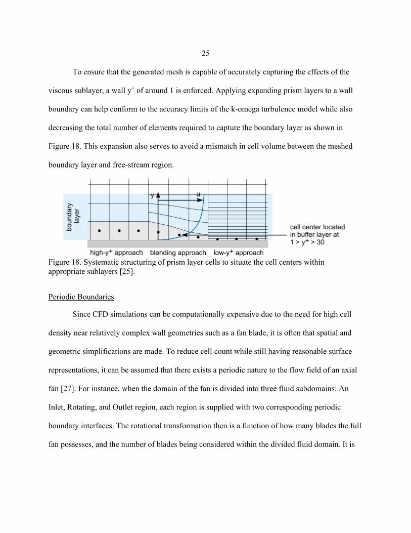
To ensure that the generated mesh is capable of accurately capturing the effects of the

viscous sublayer, a wall y+ of around 1 is enforced. Applying expanding prism layers to a wall

boundary can help conform to the accuracy limits of the k-omega turbulence model while also

decreasing the total number of elements required to capture the boundary layer as shown in

Figure 18. This expansion also serves to avoid a mismatch in cell volume between the meshed

boundary layer and free-stream region.

Figure 18. Systematic structuring of prism layer cells to situate the cell centers within appropriate sublayers [25].

Periodic Boundaries

Since CFD simulations can be computationally expensive due to the need for high cell

density near relatively complex wall geometries such as a fan blade, it is often that spatial and

geometric simplifications are made. To reduce cell count while still having reasonable surface

representations, it can be assumed that there exists a periodic nature to the flow field of an axial

fan [27]. For instance, when the domain of the fan is divided into three fluid subdomains: An

Inlet, Rotating, and Outlet region, each region is supplied with two corresponding periodic

boundary interfaces. The rotational transformation then is a function of how many blades the full

fan possesses, and the number of blades being considered within the divided fluid domain. It is

26 common to only model one blade at a time. Therefore, the overall rotational transformation in

degrees can be computed through Equation 22.

𝑇𝑇𝜃𝜃 =360°𝑁𝑁𝑏𝑏𝑡𝑡𝑎𝑎𝑏𝑏𝑡𝑡𝑠𝑠

22

The periodic boundary cell faces are then mapped to each other through this

transformation, flow data is transferred between each periodic interface. An example of this

periodic boundary setup is shown in Figure 19 for a three-bladed propeller fan where 𝑇𝑇𝜃𝜃 = 120°.

Figure 19. Computational domain for a 3-bladed fan with various fluid boundary labels: Rotating region (Rot), Inlet: mass flow rate inlet, Periodic boundary (Per_3), and Outlet: Zero total pressure outlet.

27 Porous-Pressure Jump Inlet

Simulation of a microchannel condenser coil can be computationally expensive due to the

scale of the fin gaps relative to other system geometries. To approximate the coil’s resistive

effects, a porous inlet with a pressure jump may be specified. This boundary condition involves

measurement and plotting of velocities and pressure differentials (𝑉𝑉 and Δ𝑃𝑃 respectively) across

the condenser coil shown in Figure 20.

Figure 20. Condenser unit test stand used for collecting coil pressure differentials, velocities, and motor power data.

The plotted data points are then fit with a second order curve. The equation of the curve fit

provides the viscous and inertial coefficients (𝑃𝑃𝑣𝑣 and 𝑃𝑃𝑖𝑖 respectively) in the form of Equation 23.

Δ𝑃𝑃 = 𝑃𝑃𝑖𝑖𝑉𝑉2 + 𝑃𝑃𝑣𝑣𝑉𝑉 23

For this research, a previous study on the same condenser unit in consideration had obtained

pressure and velocity measurements and determined the above coefficients to be: 𝑃𝑃𝑣𝑣 = 17.246

and 𝑃𝑃𝑖𝑖 = 1.9252 [28].

28

CHAPTER THREE

COMPUTER AIDED ENGINEERING METHOD

Fan Blade Generator

Fan blade designs can be geometrically complex and are typically modelled using

Computer Aided Design (CAD) software. A CAD package, Rhinoceros (Rhino3D) was chosen

for this research. Each blade geometry was generated using Grasshopper, a plugin for Rhino3D

that allows for parametric alterations to curvatures by which the blade is constructed. This

software also facilitated a relatively streamlined process of performing surface and Boolean solid

operations to create single surface body representations that are compatible with CFD programs.

For the blade root cross section, a NACA Series 4 airfoil was selected due to its simple

construction, claimed suitability in low-speed applications, tolerance of manufacturing

inaccuracies, and light debris accumulation such as dust and insects [29]. The airfoil generator

developed by Paterson [29] was adapted such that the cross section would be swept through two

rails, each rail consisting of its own parametric curve values. Some of the generator controls are

shown in Figure 21. The output of the generator thus far is a traditional axial propeller fan,

Figure 22.

29

Figure 21. NACA Series 4 Airfoil fan blade generator interface.

Figure 22. Undeformed traditional airfoil fan blade geometry.

As previously mentioned, introducing a forward sweep to the fan’s design can be

advantageous for static efficiency improvements. To allow for this prospect, control points

(shown in Figure 23) were added to the rails to allow for systematic blade sweep deformation

with respect to the leading and trailing edges.

30

Figure 23. Leading and trailing edge control points.

Unlike the undeformed blade in Figure 22, the alteration of the cross section’s swept path

results in a different airfoil at the blade tip with respect to the blade root in terms of the relations

to the chord length. This effect was allowed for structural purposes when prototyping the design.

A potentially thicker blade would increase the mass at the blade tip causing unwanted deflection

and mechanical vibration issues during operation and testing.

Simulation Methodology

The bulk of the iterative design testing was conducted using the RANS steady state solver

within Star CCM+. Initially, a baseline simulation was run with a fan blade that is currently used

in the condenser unit. Simulation results are geometrically dependent, so the baseline stamped

sheet metal fan, Figure 24, and orifice plate, Figure 25, were digitized and applied to the fluid

model of the condenser unit from Figure 27. Additionally, approximations for the motor and

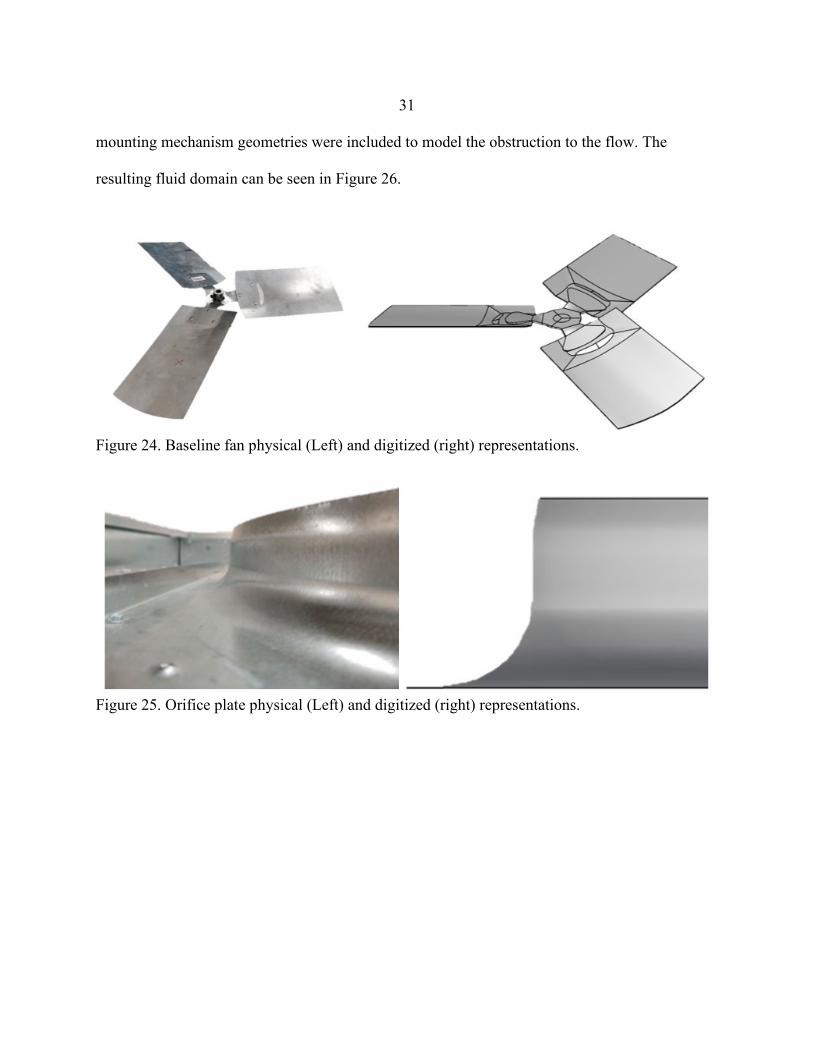
31 mounting mechanism geometries were included to model the obstruction to the flow. The

resulting fluid domain can be seen in Figure 26.

Figure 24. Baseline fan physical (Left) and digitized (right) representations.

Figure 25. Orifice plate physical (Left) and digitized (right) representations.

32

Figure 26. Geometry scene of the recreated condenser unit.

The viscous and inertial coefficients for surface porosity are applied to the condenser inlet

geometry as shown in Figure 27. This allows for modelling the resistive effects of the condenser

coil.

Figure 27. Condenser coil, casing, motor, mounting mechanism, fan and orifice plate geometry representation with a pressure jump inlet for the coil indicated in purple.

Condenser Coil

33

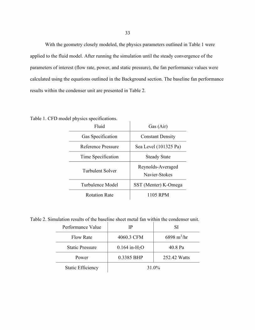
With the geometry closely modeled, the physics parameters outlined in Table 1 were

applied to the fluid model. After running the simulation until the steady convergence of the

parameters of interest (flow rate, power, and static pressure), the fan performance values were

calculated using the equations outlined in the Background section. The baseline fan performance

results within the condenser unit are presented in Table 2.

Table 1. CFD model physics specifications. Fluid Gas (Air)

Gas Specification Constant Density

Reference Pressure Sea Level (101325 Pa)

Time Specification Steady State

Turbulent Solver Reynolds-Averaged

Navier-Stokes

Turbulence Model SST (Menter) K-Omega

Rotation Rate 1105 RPM

Table 2. Simulation results of the baseline sheet metal fan within the condenser unit. Performance Value IP SI

Flow Rate 4060.3 CFM 6898 m3/hr

Static Pressure 0.164 in-H2O 40.8 Pa

Power 0.3385 BHP 252.42 Watts

Static Efficiency 31.0%

34

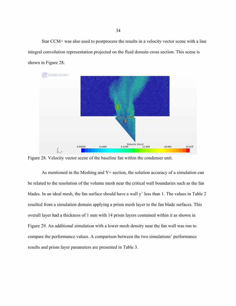
Star CCM+ was also used to postprocess the results in a velocity vector scene with a line

integral convolution representation projected on the fluid domain cross section. This scene is

shown in Figure 28.

Figure 28. Velocity vector scene of the baseline fan within the condenser unit.

As mentioned in the Meshing and Y+ section, the solution accuracy of a simulation can

be related to the resolution of the volume mesh near the critical wall boundaries such as the fan

blades. In an ideal mesh, the fan surface should have a wall y+ less than 1. The values in Table 2

resulted from a simulation domain applying a prism mesh layer to the fan blade surfaces. This

overall layer had a thickness of 1 mm with 14 prism layers contained within it as shown in

Figure 29. An additional simulation with a lower mesh density near the fan wall was run to

compare the performance values. A comparison between the two simulations’ performance

results and prism layer parameters are presented in Table 3.

35

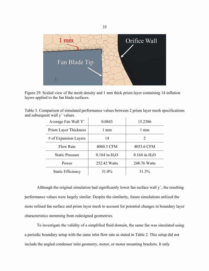
Figure 29. Scaled view of the mesh density and 1 mm thick prism layer containing 14 inflation layers applied to the fan blade surfaces.

Table 3. Comparison of simulated performance values between 2 prism layer mesh specifications and subsequent wall y+ values.

Average Fan Wall Y+ 0.0843 15.2386

Prism Layer Thickness 1 mm 1 mm

# of Expansion Layers 14 2

Flow Rate 4060.3 CFM 4053.6 CFM

Static Pressure 0.164 in-H2O 0.164 in-H2O

Power 252.42 Watts 248.76 Watts

Static Efficiency 31.0% 31.3%

Although the original simulation had significantly lower fan surface wall y+, the resulting

performance values were largely similar. Despite the similarity, future simulations utilized the

more refined fan surface and prism layer mesh to account for potential changes in boundary layer

characteristics stemming from redesigned geometries.

To investigate the validity of a simplified fluid domain, the same fan was simulated using

a periodic boundary setup with the same inlet flow rate as stated in Table 2. This setup did not

include the angled condenser inlet geometry, motor, or motor mounting brackets. It only

36 included the curvature of the orifice/fan housing along with cylindrical inlet and outlet regions.

A velocity vector scene was also produced for this simplified domain. This scene is shown in

Figure 30.

Figure 30. Velocity vector scene of the baseline fan being simulated at 4060.3 CFM showcasing the highlighted rotating region with periodic boundaries.

Table 4 presents the results from the simulation with periodic boundaries. The static

pressures and power demand differing by 12.8% and 0.9% respectively. Similar results in power

demand between the simplified domain and full-scale setup allowed for quickly iterating through

designs and generating fan performance curves. The discrepancy in static pressure caused the

efficiency purported by the periodic boundary simulation to be inflated by 3.6%. Therefore, it

was conjectured that the full-scale model that included the full condenser unit, the motor, and

motor mounting brackets would have better agreement with experimental performance

measurements.

37 Table 4. Simulation results of the baseline sheet metal fan with periodic boundaries.

Performance Value IP SI





Redesign Process

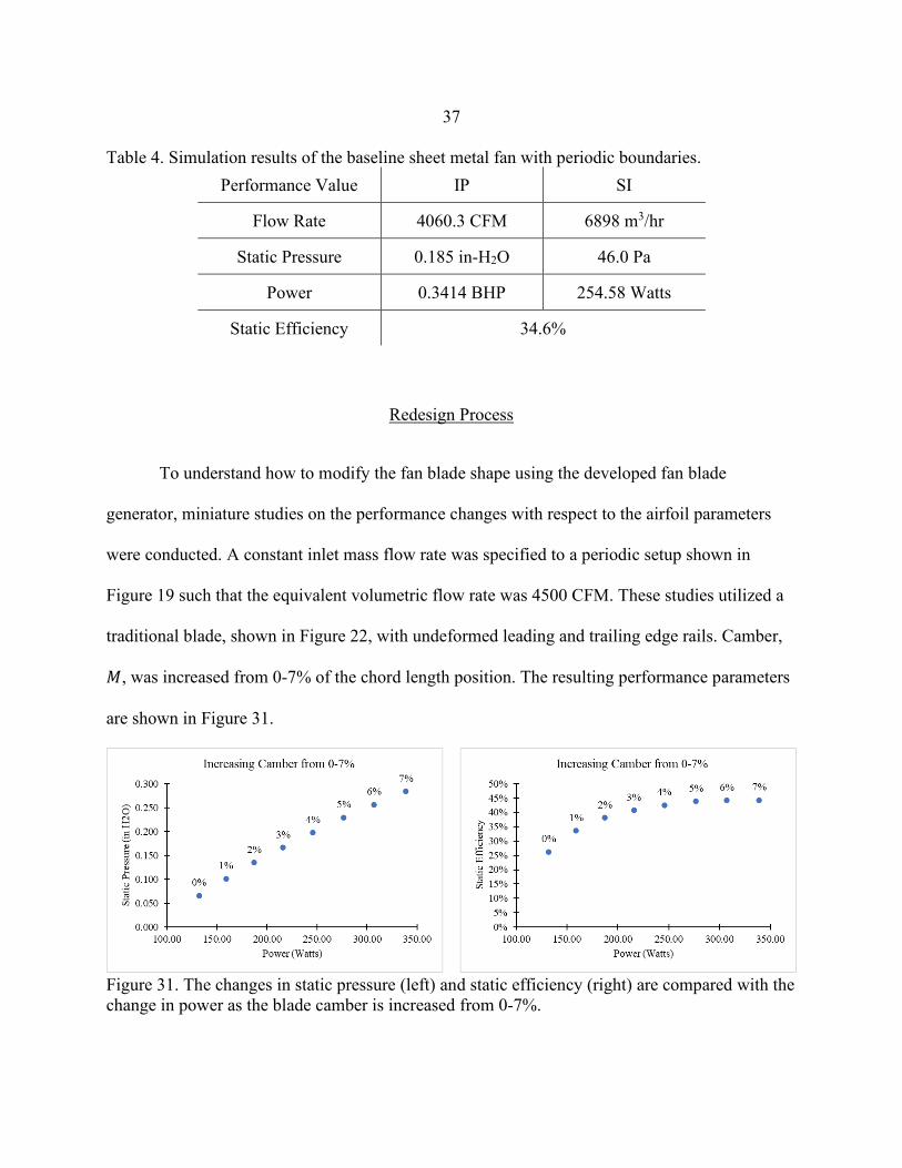
To understand how to modify the fan blade shape using the developed fan blade

generator, miniature studies on the performance changes with respect to the airfoil parameters

were conducted. A constant inlet mass flow rate was specified to a periodic setup shown in

Figure 19 such that the equivalent volumetric flow rate was 4500 CFM. These studies utilized a

traditional blade, shown in Figure 22, with undeformed leading and trailing edge rails. Camber,

𝑀𝑀, was increased from 0-7% of the chord length position. The resulting performance parameters

are shown in Figure 31.

Figure 31. The changes in static pressure (left) and static efficiency (right) are compared with the change in power as the blade camber is increased from 0-7%.

38

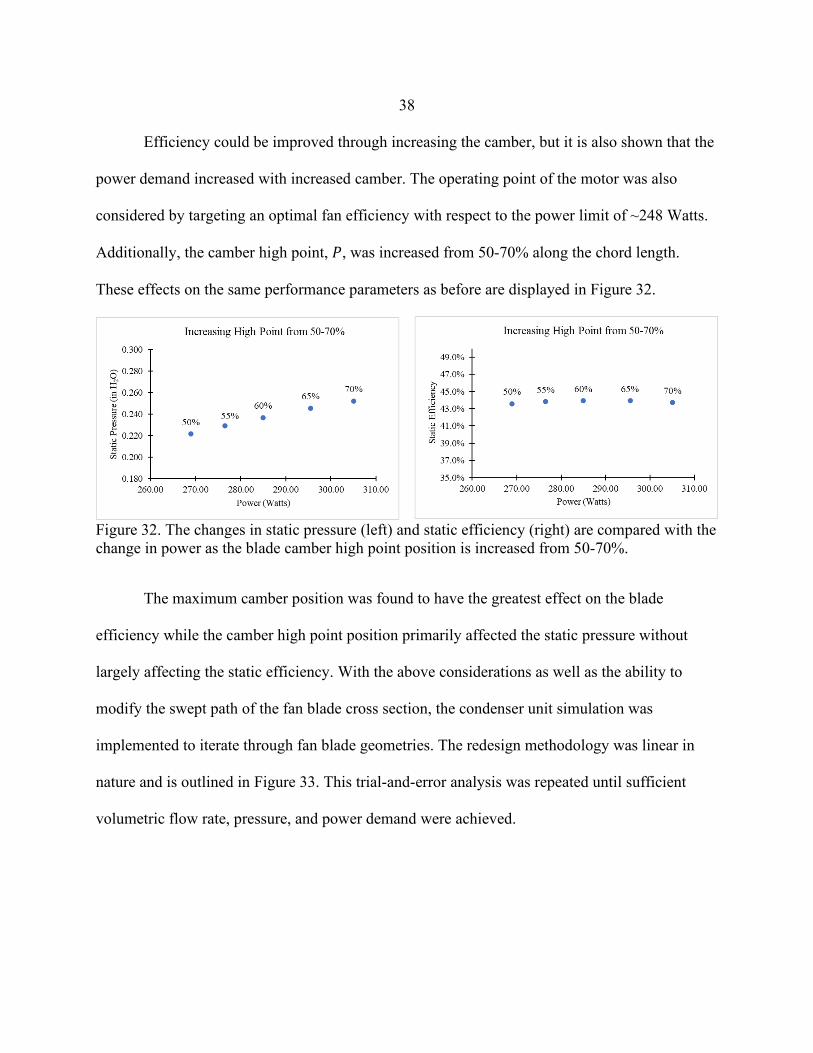
Efficiency could be improved through increasing the camber, but it is also shown that the

power demand increased with increased camber. The operating point of the motor was also

considered by targeting an optimal fan efficiency with respect to the power limit of ~248 Watts.

Additionally, the camber high point, 𝑃𝑃, was increased from 50-70% along the chord length.

These effects on the same performance parameters as before are displayed in Figure 32.

Figure 32. The changes in static pressure (left) and static efficiency (right) are compared with the change in power as the blade camber high point position is increased from 50-70%.

The maximum camber position was found to have the greatest effect on the blade

efficiency while the camber high point position primarily affected the static pressure without

largely affecting the static efficiency. With the above considerations as well as the ability to

modify the swept path of the fan blade cross section, the condenser unit simulation was

implemented to iterate through fan blade geometries. The redesign methodology was linear in

nature and is outlined in Figure 33. This trial-and-error analysis was repeated until sufficient

volumetric flow rate, pressure, and power demand were achieved.

39

Figure 33. Redesign methodology through parametric modification of blade shape

Redesign Results

The final fan CAD geometry is portrayed in Figure 34, and its performance parameters

yielded from the full-scale simulation are presented in Table 5. The root airfoil cross section was

a NACA 5506 with a chord length of 4 inches. The blade tip angle was 8° and was twisted by

18° at its root. The hub height and diameter were defined by the blade twist and motor diameter

respectively. Displacement of the blade lofting rails had given it a forward skew appearance. The

appearance of the pentagonal shape at the fan’s hub was to account for the workspace within the

selected 3D printer. More information on the prototyping procedure is discussed in the

Experimental Method section of this thesis.

40

Figure 34. Geometry scene portraying the redesigned proposed fan with included hub mounting features.

Table 5. Simulation results of the optimized fan within the condenser unit. Performance Value IP SI





According to the condenser unit simulation, the optimized fan design had resulted in a

9.3% increase in volumetric flow rate, 11.6% increase in static pressure, 12.8% decrease in

power, and 12.3% absolute increase in static efficiency.

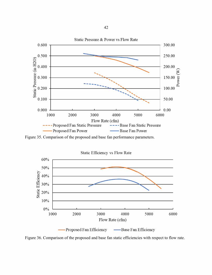
Fan performance curves of the proposed fan were generated by running the periodic

boundary simulation setup and iterating through inlet flow rate specifications. As explained in

the Background section, the resulting performance values of static pressure, power, and

efficiency were plotted with respect to the tested flow rate. The simulated performance curves

are presented in Figure 35 and Figure 36. From these performance curves, the proposed fan is

41 predicted to perform at higher efficiencies over the base fan with a lower power requirement and

higher generated static pressure. Additionally, the performance predicted by the full-scale

condenser unit simulation aligned well with the simulated performance curves.

42

Figure 35. Comparison of the proposed and base fan performance parameters.

Figure 36. Comparison of the proposed and base fan static efficiencies with respect to flow rate.

43

Despite the overall performance improvements, it was observed that without mitigation

of leakage effects, any clearance between the blade tip and its housing will result in some

amount of air recirculation. As previously noted, fan blade tip clearance has a large effect on

efficiency. This effect of blade tip recirculation can be visualized in Figure 37 within a Star

CCM+ velocity vector scene.

Figure 37. Velocity vector scene visualization of air recirculation within the fan blade tip-housing clearance zone.

44

CHAPTER FOUR

EXPERIMENTAL METHOD

The following section details the process of prototyping, testing, and comparing the

simulated performance of the proposed fan to experimentally collected data.

3D Printed Prototype

A working prototype of the fan was produced to test the results of the simulated data.

Given the moderately complex curvatures and high geometric accuracy required to validate the

computer model, the fan was manufactured using a Markforged X7 3D printer. Markforged

printers use a proprietary filament, Onyx, which is a composite of nylon and embedded carbon

fiber particles and yields high-strength end-use prints. Due to the limited workspace within most

3D printers, larger geometries are often printed in sections. Since this fan design is rotationally

symmetric, single blades were designed to be 3D printed and affixed to a center hub. With the

fan rotating at 1105 RPM, high blade loading from pressure and shear forces coupled with

mechanical vibration could cause high tip deflection and in turn damage the fused filament layer

bonds of the prototype material. Reinforcement layers of concentric fiberglass filament were

applied to the fan blades to achieve a higher rigidity and strength than with the extruded filament

alone. Visualization of this internal structure is provided in Figure 38, and the resulting 3D

printed part and fan assembly are presented in Figure 39.

45

Figure 38. Visualization from the Markforged Eiger cloud interface of the 3D printed structure with concentric fiberglass layers represented in yellow.

Figure 39. 3D printed fan (top) and assembly (bottom).

46

Test Method 1

Since the condenser test stand is non-ducted, the following method was used to estimate

the differences in performance between the current and redesigned fans. The testing setup is

depicted in Figure 40 where measurement traverses were outlined immediately upstream and

downstream of the fan.

Figure 40. Cross section side view of Method 1 testing configuration.

A fishing line with 1-inch increments marked along its length was stretched across the

diameter of the orifice outlet to indicate the location of velocity and pressure measurements

(Figure 41). Pressure measurements were taken by fitting an Alnor Telescoping Pitot Tube to a

Fluke 922 Airflow Meter (Figure 42). The specifications for the Fluke 922 Airflow Meter are

given in Figure 43. Total and Static Pressures were recorded directly above and below the fan at

47 each tick mark along the fan diameter traverse.

Figure 41. Fan traverse measurement locations were indicated by 1-inch incremental tick marks.

Figure 42. Alnor Telescoping Pitot Tube (Left); Fluke 922 Airflow Meter (Right).

48

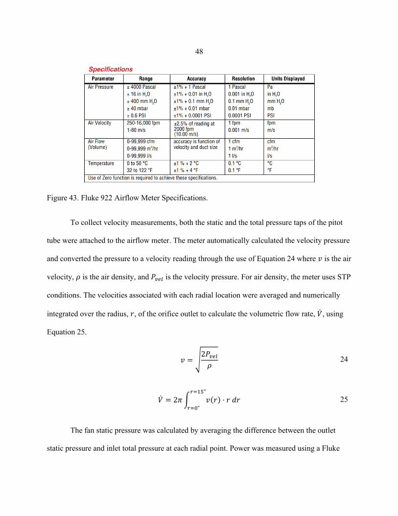
Figure 43. Fluke 922 Airflow Meter Specifications.

To collect velocity measurements, both the static and the total pressure taps of the pitot

tube were attached to the airflow meter. The meter automatically calculated the velocity pressure

and converted the pressure to a velocity reading through the use of Equation 24 where 𝑣𝑣 is the air

velocity, 𝜌𝜌 is the air density, and 𝑃𝑃𝑣𝑣𝑡𝑡𝑡𝑡 is the velocity pressure. For air density, the meter uses STP

conditions. The velocities associated with each radial location were averaged and numerically

integrated over the radius, 𝑟𝑟, of the orifice outlet to calculate the volumetric flow rate, �̇�𝑉, using

Equation 25.

𝑣𝑣 = �2𝑃𝑃𝑣𝑣𝑡𝑡𝑡𝑡𝜌𝜌

24

�̇�𝑉 = 2𝜋𝜋� 𝑣𝑣(𝑟𝑟) ⋅ 𝑟𝑟 𝑑𝑑𝑟𝑟𝑟𝑟=15"

𝑟𝑟=0" 25

The fan static pressure was calculated by averaging the difference between the outlet

static pressure and inlet total pressure at each radial point. Power was measured using a Fluke

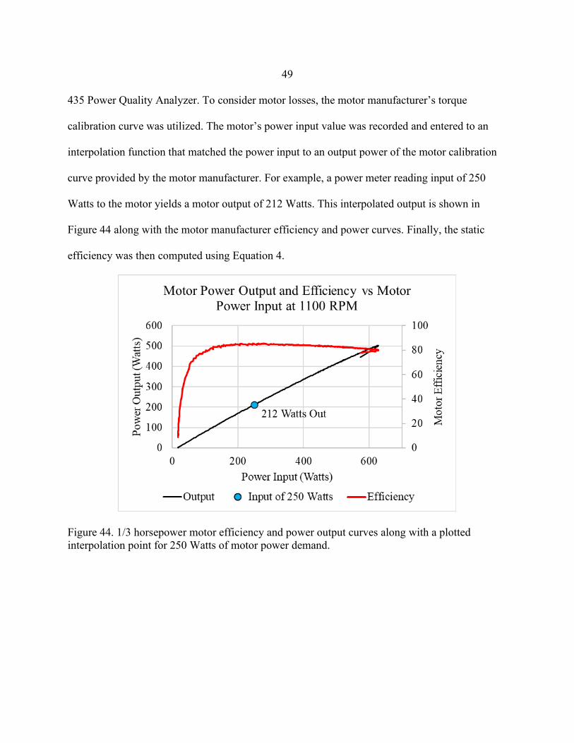
49 435 Power Quality Analyzer. To consider motor losses, the motor manufacturer’s torque

calibration curve was utilized. The motor’s power input value was recorded and entered to an

interpolation function that matched the power input to an output power of the motor calibration

curve provided by the motor manufacturer. For example, a power meter reading input of 250

Watts to the motor yields a motor output of 212 Watts. This interpolated output is shown in

Figure 44 along with the motor manufacturer efficiency and power curves. Finally, the static

efficiency was then computed using Equation 4.

Figure 44. 1/3 horsepower motor efficiency and power output curves along with a plotted interpolation point for 250 Watts of motor power demand.

50 Results: Method 1

The experiment was run for each fan type rotating at 1105 RPM. The results for the

proposed and base fan test runs are shown in Table 6 and Table 7 respectively.

Table 6. Condenser unit test stand experimental results of the baseline fan at 1105 RPM Baseline Fan – Test Method 1




Power 0.2843 BHP 212 Watts


Table 7. Condenser unit test stand experimental results of the proposed fan at 1105 RPM Proposed Fan – Test Method 1






For the baseline fan, the median and average air velocities in feet per minute (fpm) were

846 fpm and 542 fpm respectively. The proposed fan had median and average air velocities of

1142 fpm and 755 fpm respectively. These air velocities and pressures are within the operating

range of the measurement device. However, they are nearing the lower limit of the device’s

accurate range of 250-16,000 fpm.

51

If the error effects are assumed to be similar in the measurement procedures for the

baseline and proposed fan, a significant increase in static efficiency of 21% with respect to the

current design was observed. Despite the increased efficiency, it is evident that the simulation

had underpredicted the power demand of the proposed fan by nearly 27%. In contrast, the

baseline fan power had been overpredicted by 19%. A potential cause for the opposing errors

may be due to the difference in fan material. The baseline fan, being made of sheet metal, is

significantly more rigid than the 3D printed plastic prototype fan.

Test Method 2

Further testing using a setup likened to AMCA 210 Standard Figure 15 [17] was required

to accurately measure the performance of the proposed fan. The key differences between the

testing procedures of Methods 1 and 2 are the measurement locations for static pressure and flow

rate. Method 2 used flow measurement nozzles and pressure sensors that were situated far

upstream from the turbulent fan region. Flow straighteners were also incorporated to ensure

steady airflow and pressure measurements. The setup of Method 2 is depicted in Figure 45.

52

Figure 45. Top view diagram of Method 2 testing configuration. The variable supply was used to regulate control the tested fan volumetric flow rate, and flow measurement nozzles were used to measure this flow rate and system static pressure within the recirculation corridor.

The fan was mounted in a horizonal orientation within the modelled orifice plate (Figure

46). The wall containing the fan separated two large airtight chambers where the recirculation in

between was regulated by a variable speed booster fan. The power was again monitored using a

Fluke power quality analyzer, while the fan speed was controlled by a voltage generating a 0-10

Volt signal directly inputted to an electronically commutated (EC) motor. The speed control and

power measurement instrumentation are displayed in Figure 47.

53

Figure 46. The proposed fan mounted in horizontal configuration within the orifice plate.

Figure 47. Fan speed control and power measurement instrumentation.

Through the process of increasing the system resistance with the booster fan, it was found

that the motor began to “torque limit,” meaning that the motor internal controls were lowering

the rotational speed to maintain an operationally efficient power level. The motor is designed to

operate within the region of 1/3 horsepower output at 85% efficiency. Outside of this operation

range, the motor efficiency drastically decreases. To account for the torque limiting, the lower

speeds were recorded at each test point. Fan affinity laws from Equation 10 were then used to

54 scale the performance data points to a common speed of 1105 RPM. To calculate the static

efficiency, the power output was assumed to be 85% of the scaled motor input.

Results: Method 2

The fan law scaled experimental results are plotted and compared to those predicted by

the CFD simulation in Figure 48 and Figure 49. Additionally, the single testing point obtained

from Method 1 is included in both performance plots. The full record of the scaled Method 2

experimental data is provided in Table 8.

Table 8. AMCA 210 experimental data scaled to 1105 RPM. Flow Rate

(CFM) Static Pressure

(in H2O) Motor Power

(Watts) Fan Power

(Watts) Fan Power

(BHP) Static

Efficiency

5801.00 0.120 340.00 289.00 0.39 28.32%

5500.00 0.190 380.00 323.00 0.43 38.03%

5109.35 0.302 436.71 371.20 0.50 48.94%

4762.60 0.369 472.93 401.99 0.54 51.39%

4334.42 0.446 495.85 421.47 0.57 53.92%

3863.64 0.512 524.63 445.93 0.60 52.13%

3363.19 0.565 534.86 454.63 0.61 49.15%

2776.38 0.641 534.17 454.05 0.61 46.10%

2283.06 0.717 490.88 417.25 0.56 46.10%

55

Figure 48. Comparison of the proposed fan pressure and power curves that were generated by the CFD simulation (black) and experimental testing using Method 2 (red). The test point from Method 1 (blue) is also compared.

Figure 49. Comparison of the proposed fan efficiency curves that were generated by the CFD simulation (black) and experimental testing using Method 2 (red). The test point from Method 1 (blue) is also compared.

56

Figure 48 and Figure 49 show a large discrepancy between simulated and standard

experimental values. The CFD model underpredicted the power requirement by as much as 45%.

Despite the significantly higher power demand, the experimental static pressure was similarly

higher with respect to the simulation. This higher static pressure translated to a higher static

efficiency. Although a higher static efficiency had been achieved, it was determined that the

proposed fan was not suited for a 1/3 horsepower motor application due to its greater power

demand. A linear interpolation of the scaled data points for the designed flow rate of 4500 CFM

is shown in Table 9. The motor would not be capable of operating at its rated efficiency of 85%.

Table 9. Interpolated performance parameters of the proposed fan design flow rate from the scaled AMCA 210 experimental results at 1105 RPM

Proposed Fan – Test Method 2


Flow Rate 4500 CFM 7646 m3/hr



Static Efficiency 53%

Figure 48 and Figure 49 also display a strong correlation between the volumetric flow

rate and fan power demand measured in Method 1 and Method 2 with only a 4% difference.

However, the corresponding static pressure between the two methods had a difference of 62%

difference. This static pressure discrepancy may be due to an unsuitable measurement location

for the static pressure caused by largely turbulent airflow in the regions near the fan blades.

57

CHAPTER FIVE

IMPROVEMENTS AND FUTURE WORK

Simulation Improvements

Given the large discrepancy between the experimental and simulated fan blade

performance results, the fluid model requires alteration. Some of these changes may involve

altering the fluid domain geometry to better match the experimental setup in that the inlet and

outlet regions may require enlargement. The assumed periodic flow may also not be accurate.

Transitioning to transient/unsteady simulations without periodic boundaries began to show

improved experimental agreement. However, this did not fully account for the discrepancy. Also,

the effects of the environmental conditions such as air pressure showed minor effects on the

model’s agreement to experimental data. To demonstrate the impact of the considerations

mentioned above, an unsteady simulation was run with the model specifications outlined in

Table 10 and initial conditions from the first 300 iterations of a steady state model. The results

from the unsteady simulation are presented in Table 11.

58 Table 10. Unsteady CFD model physics specifications.

Fluid Multi-Component Gas (Air, H2O)

Mass Fraction [99.1% Air, 0.9% H2O]

Gas Specification Ideal Gas

Reference Pressure (99751 Pa)

Time Specification Implicit Unsteady

Time Step 8.64 x 10-4 s

Turbulent Solver Detached Eddy Simulation (DES)

Turbulence Model SST (Menter) K-Omega

Simulated Physical Time 0.55 seconds

Rotation Rate 1105 RPM

Table 11. Implicit unsteady performance results of the proposed fan Proposed Fan – Implicit Unsteady


Flow Rate 4334 CFM 7364 m3/hr



Static Efficiency 61%

The fluid model outlined in Table 10 incorporated the air properties that were present

during experimental testing in Method 2. A parametric study of air properties such as humidity,

temperature, pressure, and air density should be conducted to investigate their effects on fan

performance. If the variation of performance results is less than the overall tolerance of

59 experimental measurement equipment, the effects of these air properties may be deemed

negligible for condenser fan applications.

Another potential source of error may be caused by the prototype’s material behavior.

The fan was treated as a perfectly rigid body that did not deflect under the forces exerted by the

air on each blade. A fluid structure interaction model can be invoked within Star CCM+ to

simulate the effects of blade deflection on the fan performance parameters. Additionally, the

produced fan prototype may differ dimensionally than what was modelled. Although the utilized

3D printer has a Z layer resolution of 50 to 250 microns, there is potential for dimensional

defects during the heat-intensive printing process. A profilometer should be used to verify the

dimensional accuracy of the prototype.

Design Improvements

The assumption of global performance improvement offerings of airfoils is not entirely

accurate. Although a fan may experience overall efficiency gains by using an airfoil, not every

radial position along the blade length exists within the effective Reynolds number regime for

airfoils. At low Reynolds numbers (below 105), the lift-to-drag ratio is considerably reduced

[30]. Careful consideration should be made to ensure that the application of an airfoil is suitable

for the design conditions. In the case of the axial fan considered in this study, most of the

Reynolds numbers fall below the threshold of 105. Additional control over the blade cross-

section shape and its morphing progression as it is swept from its root to the blade tip could give

rise to improved optimization parameters for specific operating conditions. Furthermore, the

AMCA 210 tested fan static pressure at the desired flow rate is high enough that a decrease in

pressure can be afforded by the system. As mentioned in the background section, lowering the

60 fan solidity through decreasing the blade count would result in a pressure reduction.

Additionally, the power requirements would be reduced. Given the trends mentioned in the

background, a three-bladed fan of the same fan shape could also experience a similar peak

efficiency to the five-blade configuration.

Redesign Process Improvements

Future work could investigate incorporating blade element theory into the fan blade

generator program that was developed in Grasshopper. Within the workspace of Grasshopper,

custom coding panels can be added to the geometry design space. These panels utilize scripting

languages such as C#, Python, and VBA. A custom script could be written such that a user could

specify performance requirements, and the subsequent blade shape would be generated. Blade

element theory also has its limitations in its prediction accuracy. Therefore, simulation and

experimental validation would be required to confirm the utility of the optimization program.

Alterations could then be made to the script to account for discrepancies that arise during

experimentation.

Measurement Improvements

When comparing the data from Test Methods 1 and 2, the parameter to match with the

highest certainty is the power output from the motor. For the operating conditions within the

condenser unit test stand in Method 1, the fan had a power demand of 301 Watts at an estimated

flow rate of 5581.3 CFM. The most similar power demand demonstrated in Method 2 was

recorded at 289 Watts with a measured flow rate of 5801 CFM. With the expected behavior of

the fan to demand more power at lower flow rates, the two observed flow rate values were

61 relatively similar. The flow rate and power measurement had decent alignment with the

corresponding trends in Table 8.

Conversely, the static pressure measurement did not align with the trends which can be

attributed to its measurement technique in Method 1. A more accurate measurement practice for

static pressure could be to create a rectangular array nearest the downstream face of the

condenser coil. The static pressure could then be estimated by computing the area average of

each static pressure with respect to their locations. Future testing to determine the validity of this

measurement technique could involve targeting the flow rate observed in Method 1 using the test

setup in Method 2 and comparing the resulting power demand and static pressure.

The power measurement method can also be improved. Methods 1 and 2 relied on the

motor manufacturer data for the motor performance. In cases where the motor was torque

limiting, the output power was calculated with the nominal motor efficiency of 85%. A rotary

torque sensor should be integrated with the motor shaft and the fan coupler. The true fan power

demand could then be calculated through the product of the torque and motor speed

measurements.

62

CHAPTER SIX

CONCLUSION

In this study, an axial condenser fan was redesigned and prototyped using modern

analysis and manufacturing techniques. The full-scale 3D printed prototype was successfully

tested at full speed such that experimental data could be gathered and compared to the CFD

simulation. Simulated and experimental data showed that an adherence to fan blade design

practices such as blade twist, forward sweep, and low tip clearance could lead to improved

efficiencies.

In comparing the simulation techniques, simplifying the full fan geometry to a single

blade with periodic boundaries could reduce the computation time and yield similar performance

results to the full-scale computer model. However, strictly making comparisons between two fan

designs within CFD environments without early experimental validation, albeit with identical

fluid domains, physics parameters, and recommended meshing practices, can be a flawed

approach and may add unnecessary cost and time in the redesign process.

Although the redesigned fan had desirable performance with respect to the base fan in the

simulated setup, experimental data differed greatly to the detriment of the redesigned fan’s

suitability for the intended application. It is therefore recommended to initially compare the base

fan simulated performance curves to experimental values prior to beginning the redesign process.

It was demonstrated that measuring fan performance parameters within a condenser unit

test stand has the promise of providing accurate values for volumetric flow rate at a given power

demand. Future experimentation would be required to determine the proper measurement

practices for fan static pressure within the condenser unit test stand. With the current

63 measurement setup in Method 1, analyzing a fan within the condenser unit test stand only serves

the purpose of determining a single operating point’s volumetric flow rate and the motor power

demand. For accurate characterization of the complete fan performance, testing setups like

Method 2 are required. However, when considering the refrigeration cycle’s function, the fan is

responsible for providing a sufficient mass flow rate to achieve the required heat transfer across

the condenser coil. The governing condenser coil heat transfer equation does not include a

pressure term. If the fan can provide the necessary flow rate, the efficiency of the refrigeration

cycle will be benefited by a lower fan power demand. According to the flow rate determined in

Method 1, at the full motor speed of 1105 RPM, the fan was producing roughly 1000 CFM more

than the desired 4500 CFM. By using fan laws and the known full speed flow rate of 5581 CFM

a power demand of 301.18 watts, the rotation speed and power can be calculated such that the

desired flow rate of 4500 CFM is achieved. With these condition inputs, the fan speed could be

reduced to 891 RPM and would only require 158 Watts of shaft power. This lower speed would

allow the redesigned fan to consume 25% less power than the baseline fan.

64

REFERENCES CITED

[1] Improving Fan System Performance: A Sourcebook for Industry. United States(in English), 2003.

[2] CBECS 2012: Energy Usage Summary.

[3] R. American Society of Heating and I. Air-Conditioning Engineers, "21.2 Principles of Operation," in 2016 ASHRAE Handbook - Heating, Ventilating, and Air-Conditioning Systems and Equipment (I-P Edition): American Society of Heating, Refrigerating and Air-Conditioning Engineers, Inc. (ASHRAE).

[4] R. American Society of Heating and I. Air-Conditioning Engineers, "References," in 2017 ASHRAE® Handbook - Fundamentals (SI Edition): American Society of Heating, Refrigerating and Air-Conditioning Engineers, Inc. (ASHRAE).

[5] D. G. Kröger, "1.1 Cooling Towers," in Air-Cooled Heat Exchangers and Cooling Towers - Thermal-Flow Performance Evaluation and Design, Volume 1: PennWell.

[6] J. Moore, R. Grimes, and E. Walsh, "Influence of the Flow From an Axial Fan on the Performance of a Heat Exchanger," Volume 10: Heat and Mass Transport Processes, Parts A and B, pp. 129-138, 2011, doi: 10.1115/IMECE2011-62696 info:doi/10.1115/IMECE2011-62696.

[7] S. Castegnaro, "Aerodynamic Design of Low-Speed Axial-Flow Fans: A Historical Overview," Designs, vol. 2, no. 3, p. 20, 2018, doi: 10.3390/designs2030020.

[8] A. Gebhardt, "6.4 Make or Buy?," in Rapid Prototyping: Hanser Publishers.

[9] A. Senlis (France) 6-8 April 2022 - International Conference on Fan Noise, Applications and Systems. "Fan 2022 conference." https://www.fan2022.org/gb/fan-aerodynamics.html (accessed March 5, 2021.

[10] P. Barnes, "5.6 3D Printing," in BIM in Principle and in Practice (3rd Edition): ICE Publishing.

https://www.fan2022.org/gb/fan-aerodynamics.html

https://www.fan2022.org/gb/fan-aerodynamics.html

65 [11] M. Somireddy, "Mechanical behaviour of 3D printed composite parts with short carbon

fiber reinforcements," Engineering Failure Analysis, vol. 107, 2019, doi: https://doi.org/10.1016/j.engfailanal.2019.104232.

[12] C. D. a. Associates, "Split System Diagram," ed.

[13] R. American Society of Heating and I. Air-Conditioning Engineers, "2.2.2 Theoretical Single-Stage Cycle Using a Pure Refrigerant or Azeotropic Mixture," in 2017 ASHRAE® Handbook - Fundamentals (SI Edition): American Society of Heating, Refrigerating and Air-Conditioning Engineers, Inc. (ASHRAE).

[14] R. American Society of Heating and I. Air-Conditioning Engineers, "21.2 Principles of Operation," in 2016 ASHRAE Handbook - Heating, Ventilating, and Air-Conditioning Systems and Equipment (I-P Edition): American Society of Heating, Refrigerating and Air-Conditioning Engineers, Inc. (ASHRAE), 2016.

[15] M. B. Wilkinson, "The Design of an Axial Flow Fan for Air-Cooled Heat Exchanger Applications," Master of Engineering (Mechanical), Faculty of Engineering, Stellenbosch University, 2017.

[16] F. P. Bleier, Fan Handbook Selection, Application, and Design, 1 ed. The McGraw-Hill Companies, Inc.: McGraw-Hill Education (in English), 1997.

[17] ANSI/AMCA Standard 210–07/ANSI/ASHRAE Standard 51–16, Laboratory Methods of Testing Fans for Certified Aerodynamic Performance Rating, 2016.

[18] F. Kameier and W. Neise, Experimental Study of Tip Clearance Losses and Noise in Axial Turbomachines. 1995, pp. 229-243.

[19] E. B. Bell and L. J. DeKoster, "The Effect of Solidity, Blade Section, and Contravane Angle on the Characteristics of an Axial-Flow Fan," NATIONAL AERONAUTICS AND SPACE ADMIN LANGLEY RESEARCH CENTER HAMPTON VA, 1942.

[20] B. L. Zhou, J. P. Yuan, Z. X. He, and F. Hong, "Effect of Different Airfoils on Performance of Axial Fan," Advanced Materials Research, vol. 945-949, pp. 928-934, 2014, doi: 10.4028/www.scientific.net/AMR.945-949.928.

https://doi.org/10.1016/j.engfailanal.2019.104232

66 [21] C. E. Dole, J. E. Lewis, J. R. Badick, and B. A. Johnson, "Flight Theory and

Aerodynamics - A Practical Guide for Operational Safety (3rd Edition)," ed: John Wiley & Sons.

[22] L. M. Nicolai and G. E. Carichner, "F.2 NACA Airfoil Nomenclature and Characteristics," in Fundamentals of Aircraft and Airship Design, Volume I - Aircraft Design: American Institute of Aeronautics and Astronautics (AIAA).

[23] J. Vad, "Aerodynamic effects of blade sweep and skew in low-speed axial flow rotors at the design flow rate: An overview," Proceedings of the Institution of Mechanical Engineers, Part A: Journal of Power and Energy, vol. 222, no. 1, pp. 69-85, 2008/02/01 2008, doi: 10.1243/09576509JPE471.

[24] M. G. Beiler and T. H. Carolus, "Computation and Measurement of the Flow in Axial Flow Fans With Skewed Blades," Journal of Turbomachinery, vol. 121, no. 1, pp. 59-66, 1999, doi: 10.1115/1.2841234.

[25] CD-adapco (2019). STAR-CCM+ 14.04.011 User Guide. Melville, NY, USA: CD-adapco Inc.

[26] F. R. Menter, "Two-equation eddy-viscosity turbulence models for engineering applications," AIAA journal, vol. 32, no. 8, pp. 1598-1605, 1994.

[27] L. Yang, O. Hua, and D. Zhao-Hui, "Optimization Design and Experimental Study of Low-Pressure Axial Fan with Forward-Skewed Blades," International Journal of Rotating Machinery, vol. 2007, p. 085275, 2007/08/22 2007, doi: 10.1155/2007/85275.

[28] S. P. Kuluris, "Influence of orifice plate shape on condenser unit effectiveness," Montana State University-Bozeman, College of Engineering, 2018.

[29] G. Paterson, "NACA series 4 aerofoil generator," in Grasshopper3D vol. 2020, ed, 2018.

[30] J. Winslow, H. Otsuka, B. Govindarajan, and I. Chopra, "Basic Understanding of Airfoil Characteristics at Low Reynolds Numbers (104–105)," Journal of Aircraft, vol. 55, no. 3, pp. 1050-1061, 2018/05/01 2017, doi: 10.2514/1.C034415.

The Design And Testing Of An Axial Condenser Fan

Documents

Transcript of The Design And Testing Of An Axial Condenser Fan