Mathematical model of the industrial kitchen steam condenser

Mathematical model of the industrial kitchen steam

condenser

Rafał Robert Wieczorek

Thesis to obtain the Master of Science Degree in

Energy Engineering and Management

Supervisors: Prof. Pedro Jorge Martins Coelho

Dr. Arkadiusz Ryfa

Examination Committee

Chairperson: Prof. Francisco Manuel da Silva Lemos

Supervisor: Prof. Pedro Jorge Martins Coelho

Member of the Committee: Prof. Viriato Sérgio de Almeida Semião

June 2018

iii

Acknowledgments

After an intensive period of seven months, today is the day: writing this note of thanks is the

finishing touch on my dissertation. It has been a period of intense learning for me, not only in the scientific

arena but also on a personal level. I would like to reflect on the people who have supported and helped

me so much throughout this period.

I would first like to thank my supervisors Prof. Pedro Jorge Martins Coelho at Instituto Superior

Tecnico in Lisbon and Dr Arkadiusz Ryfa at Silesian University of Technology in Gliwice. I want to thank

you both for your cooperation and guidance which let me successfully complete my dissertation. I would

like to particularly thank Prof. Pedro Jorge Martins Coelho for great reliance on me at the beginning and

Dr Arkadiusz Ryfa for providing me with the tools that I needed to choose the right direction and

accomplish the goal.

I would also like to thank two much bigger teams. First of all, the Retech company for their

collaboration and references I was given to conduct my research. Last but not least words of thanks I

would like to target at the KIC Innoenergy. This dissertation has been developed as well as many more

activities thanks to Clean Fossil and Alternative Fuels Energy MSc program which I have a great

pleasure to be part of.

Thank you very much, everyone.

v

Abstract

The numerical simulation of a top hood steam condenser (THSC) is reported in the present

thesis. A THSC supports the daily work of a large-scale mass cooking oven, and its main goal is to

prevent the accumulation of water vapour in the air released to the kitchen. A secondary goal of the

THSC is to reduce the unpleasant smells and to avoid increased humidity that may lead to mist

appearance. The operation of a THSC depends on its geometry and working conditions: temperature

and humidity of the air in the kitchen, flow rate of steam flowing from the oven to the THSC. The main

goal of the present study is to develop a mathematical model to simulate the behaviour of the steam

condenser implemented in Visual Basic for Application. It is based on the combination of a single pipe

CFD model and on global mass and energy balances for the THSC. The predictions are validated

against available experimental data. The developed THSC model requires much less computing time

and human effort to produce satisfactory solutions in comparison with a fully developed CFD model, and

allows the user to investigate the behaviour of the THSC under various operating conditions, and to

perform an analysis of the effect of possible configuration changes. Among the studied modifications,

the reduction of the number of pipes, which has no impact on the condensation efficiency, is

recommended. This improvement minimizes the cost of the THSC and can be carried out with presently

used ovens.

Keywords: top hood steam condenser, Fluent, Visual Basic for Application, CFD simulation, working

conditions

vii

Resumo

Este trabalho descreve a simulação numérica de um condensador de vapor (top hood steam

condenser - THSC). O condensador apoia o trabalho diário de um forno e tem como principal objetivo

impedir a acumulação de vapor água na cozinha. Os objetivos secundários são a redução de odores

desagradáveis e o impedimento do aumento da humidade que pode levar ao aparecimento de névoa.

A operação do condensador depende da sua geometria e condições de funcionamento: temperatura e

humidade do ar na cozinha, caudal de vapor escoado do forno/fogão para o condensador. O objetivo

principal deste estudo é o desenvolvimento de um modelo matemático para simular o comportamento

do condensador, implementado em Visual Basic. Este modelo baseia-se na combinação de um modelo

de CFD para um único tubo e em balanços globais de massa e energia para o condensador. As

previsões são validadas por comparação com dados experimentais disponíveis. O modelo

desenvolvido requer muito menos tempo de cálculo para obter soluções satisfatórias comparativamente

a um modelo completo de CFD, permite ao utilizador investigar o comportamento do condensador para

diferentes condições de funcionamento e analisar o efeito de possíveis alterações geométricas. Entre

as modificações estudadas, recomenda-se a diminuição do número de tubos, o que não afeta a

eficiência da condensação. Este melhoramento irá minimizar os custos do condensador e pode ser

efetuado com os fogões atualmente utilizados.

Palavras chave: top hood steam condenser, Fluent, Visual Basic for Application, simulação

computacional de dinâmica de fluidos, condições de funcionamento

ix

Contents

ABSTRACT ......................................................................................................................................... V

RESUMO ........................................................................................................................................... VII

LIST OF FIGURES............................................................................................................................. XI

LIST OF TABLES ............................................................................................................................ XIII

LIST OF ACRONYMS ...................................................................................................................... XV

NOMENCLATURE ........................................................................................................................... XVI

1. INTRODUCTION ...................................................................................................................... 1

1.1. RELATED WORK .......................................................................................................................... 2

1.2. OBJECTIVES................................................................................................................................ 3

1.3. THESIS STRUCTURE .................................................................................................................... 5

2. TOP HOOD STEAM CONDENSER ....................................................................................... 6

3. MODEL...................................................................................................................................... 7

3.1. Geometry ............................................................................................................................ 8

3.2. Mesh .................................................................................................................................... 8

3.3. Fluent model setup .......................................................................................................... 9

3.4. Turbulence model selection ........................................................................................ 12

3.5. Analytical model of the pipe heat transfer ............................................................... 16

3.6. Fin efficiency analysis .................................................................................................. 24

3.7. Pipe equation ................................................................................................................... 25

3.8. THSC model development ........................................................................................... 27

3.8.1. Heat losses ....................................................................................................................... 27

3.8.2. Distribution of air and steam ....................................................................................... 30

3.8.3. Correction factors .......................................................................................................... 30

3.8.4. Description of THSC model operations .................................................................... 32

3.8.5. Validation .......................................................................................................................... 35

3.8.6. Technological modifications ....................................................................................... 37

4. ANALYSIS OF THSC WORK ............................................................................................... 41

5. CONCLUSIONS ..................................................................................................................... 51

APPENDIX A ..................................................................................................................................... 57

APPENDIX B ..................................................................................................................................... 63

xi

List of Figures

FIGURE 1 TOP-SIDE, TOP AND SIDE VIEW OF THSC ............................................................................................................. 6

FIGURE 2 GEOMETRY OF THE PIPE IN DM WITH DIMENSIONS (LEFT) AND EDGE SIZING LOCATION (RIGHT) ...................................... 8

FIGURE 3 INITIAL (LEFT) AND BENCHMARK (RIGHT) MESHES GENERATED FOR THE PIPE ............................................................... 9

FIGURE 4 LOCATION OF BOUNDARY CONDITIONS IN ANSYS FLUENT FOR SINGLE PIPE MODEL .................................................... 11

FIGURE 5 AIR (LEFT), FIN&AIR (MIDDLE), OUTLET (RIGHT) CROSS-SECTION SURFACES ............................................................. 12

FIGURE 6 NON-PHYSICAL RESULTS FOR MESH VII.............................................................................................................. 14

FIGURE 7 TEMPERATURE AT OUTFLOW (TOP LINE) AND CROSS-SECTION (BOTTOM LINE) IN: BENCHMARK, MESH XII, MESH III, MESH IV

...................................................................................................................................................................... 15

FIGURE 8 VELOCITY AT OUTFLOW (TOP LINE) AND CROSS-SECTION (BOTTOM LINE) IN: BENCHMARK, MESH XII, MESH III, MESH IV .. 16

FIGURE 9 FLOWCHART OF ITERATION FOR STEAM HEAT TRANSFER COEFFICIENT ...................................................................... 17

FIGURE 10 TEMPERATURE AT CROSS-SECTIONS T3H3A5M3S4 ......................................................................................... 20

FIGURE 11 VELOCITY AT CROSS-SECTION (MIDDLE RIGHT) AND OUTFLOW (RIGHT) T3H3A5M3S4 ............................................ 20

FIGURE 12 CORRELATION BETWEEN POWER AND MASS FLOW RATE OF AIR ............................................................................ 21

FIGURE 13 CORRELATION BETWEEN POWER AND ANGLE OF AIR FLOW RATE ........................................................................... 22

FIGURE 14 CORRELATION BETWEEN POWER AND AIR HUMIDITY .......................................................................................... 22

FIGURE 15 CORRELATION BETWEEN POWER AND STEAM TEMPERATURE ............................................................................... 23

FIGURE 16 CORRELATION BETWEEN POWER AND AIR TEMPERATURE .................................................................................... 23

FIGURE 17 SURFACES OF HEAT LOSS IN THSC .................................................................................................................. 28

FIGURE 18 SURFACES OF WALL CONDENSATION IN CONDENSATION CHAMBERS OF THSC ......................................................... 29

FIGURE 19 INPUT DATA FOR EPS CALIBRATION ................................................................................................................. 30

FIGURE 20 COMPARISON OF POWER OUTPUT FOR THSC MODEL AND FLUENT WITHOUT CORRECTION FACTORS (TOP) AND WITH THEM

(BOTTOM)........................................................................................................................................................ 31

FIGURE 21 FLOWCHART OF THSC MODEL ...................................................................................................................... 32

FIGURE 22 TEMPERATURE RESULTS FROM THSC MODEL VS MEASUREMENTS ........................................................................ 36

FIGURE 23 RH RESULTS FROM THSC MODEL VS MEASUREMENTS ....................................................................................... 36

FIGURE 24 CONDENSATE RESULTS FROM THSC MODEL VS MEASUREMENTS .......................................................................... 37

FIGURE 25 THSC MODEL - ENLARGED STEAM PASSAGE ..................................................................................................... 37

FIGURE 26 TEMPERATURE RESULTS FROM THSC MODEL VS MEASUREMENTS – 1ST AND 8TH TIER SWITCHED OFF ........................... 38

FIGURE 27 TEMPERATURE RESULTS FROM THSC MODEL VS MEASUREMENT - 1ST AND 2ND TIER SWITCHED OFF ............................. 39

FIGURE 28 RH RESULTS FROM THSC MODEL VS MEASUREMENT - 1ST AND 8TH TIER SWITCHED OFF ............................................ 39

FIGURE 29 RH RESULTS FROM THSC MODEL VS MEASUREMENTS - 1ST AND 2ND TIER SWITCHED OFF ........................................... 40

FIGURE 30 CONDENSATE RESULTS FROM THSC MODEL VS MEASUREMENTS – 1ST AND 8TH TIER SWITCHED OFF .......................... 40

FIGURE 31 CONDENSATE RESULTS FROM THSC MODEL VS MEASUREMENTS – 1ST AND 2ND TIER SWITCHED OFF .......................... 41

FIGURE 32 THSC WORK ANALYSIS - GRAPH OF INFLUENCE OF RH ........................................................................................ 43

FIGURE 33 THSC WORK ANALYSIS - GRAPH OF INFLUENCE OF TEMPERATURE ......................................................................... 44

FIGURE 34 THSC WORK ANALYSIS - GRAPH OF INFLUENCE OF STEAM FLOW RATE (ROWS 1-9) .................................................. 46

FIGURE 35 THSC WORK ANALYSIS - GRAPH OF INFLUENCE OF STEAM FLOW RATE (ROWS 10-18) .............................................. 47

xii

FIGURE 36 WORKSHEET "INPUT_OUTPUT" IN THE THSC MODEL - INPUTS ........................................................................... 57

FIGURE 37 WORKSHEET "INPUT_OUTPUT" IN THE THSC MODEL - OUTPUTS ........................................................................ 57

FIGURE 38 WORKSHEET "COMPLEMENTARY_DATA" IN THE THSC MODEL - SAMPLE DETAILED DATA FOR RIGHT SECTION OF THSC . 58

FIGURE 39 WORKSHEET "SAVES" IN THE THSC MODEL - PARAMETERS FOR CALCULATION........................................................ 58

FIGURE 40 GUI1 - INITIAL DATA FOR TOP HOOD STEAM CONDENSER ................................................................................. 59

FIGURE 41 GUI1 - HELP ............................................................................................................................................. 59

FIGURE 42 GUI2 - USER-DEFINED OPTIONS..................................................................................................................... 60

FIGURE 43 WARNING COMMUNICATES - CHOICE WINDOW (LEFT) AND ERROR WINDOW (RIGHT) ............................................... 60

FIGURE 44 GUI2 - HELP ............................................................................................................................................. 61

FIGURE 45 GUI4 - RESULTS ......................................................................................................................................... 62

xiii

List of Tables

TABLE 1 VELOCITIES, TEMPERATURES, FLUX VALUES AND EDGE SIZING FOR MESH I-IV .............................................................. 13

TABLE 2 Y* VALUES FOR MESH I-IV ............................................................................................................................... 13

TABLE 3 VELOCITIES, TEMPERATURES, FLUX VALUES AND EDGE SIZING FOR I-IV, XII, XIII MESHES AND BENCHMARK ..................... 15

TABLE 4 CONVECTIONAL HEAT TRANSFER COEFFICIENT ITERATION ........................................................................................ 17

TABLE 5 MODEL CASES................................................................................................................................................ 19

TABLE 6 POWER OUTPUT FROM FLUENT SIMULATION FOR ALL CASES .................................................................................... 24

TABLE 7 HEAT TRANSFER COEFFICIENT FOR PLANE TUBE ..................................................................................................... 25

TABLE 8 COMPARISON OF EMPIRICAL PIPE EQUATION VARIANTS .......................................................................................... 26

TABLE 9 HEAT LOSS TO THE SURROUNDING THROUGH EXTERNAL WALLS ................................................................................ 28

TABLE 10 HEAT PROVIDED THROUGH THE WALLS IN CONDENSATION CHAMBERS OF THSC ....................................................... 29

TABLE 11 CORRECTION FACTORS FOR THSC MODEL ......................................................................................................... 31

TABLE 12 VALIDATION DATA OF THSC MODEL UNDER DEFAULT WORKING CONDITION ............................................................ 35

TABLE 13 THSC WORK ANALYSIS – INCREASE OF RH OF AIR ............................................................................................... 42

TABLE 14 THSC WORK ANALYSIS - OUTFLOW RESULTS FOR CHANGE OF RH ........................................................................... 42

TABLE 15 THSC WORK ANALYSIS - INCREASE OF AIR TEMPERATURE ..................................................................................... 43

TABLE 16 THSC WORK ANALYSIS - OUTFLOW RESULTS FOR CHANGE OF TEMPERATURE ............................................................ 44

TABLE 17 THSC WORK ANALYSIS - INCREASE OF STEAM FLOW RATE ..................................................................................... 45

TABLE 18 THSC WORK ANALYSIS - OUTFLOW RESULTS FOR CHANGE OF STEAM FLOW RATE....................................................... 46

TABLE 19 THSC WORK ANALYSIS - INCREASE OF STEAM FLOW RATE (MIXTURE OF AIR/WATER MIST APPEARANCE) ........................ 47

TABLE 20 THSC WORK ANALYSIS - OUTFLOW RESULTS FOR CHANGE OF STEAM FLOW RATE (MIXTURE OF AIR/WATER MIST

APPEARANCE) ................................................................................................................................................... 47

TABLE 21 THSC WORK ANALYSIS - INPUT DATA FOR PIPES MODIFICATION ............................................................................. 48

TABLE 22 THSC WORK ANALYSIS - OUTFLOW RESULTS FOR CHANGE OF PIPES WITH EQUAL DISTRIBUTION OF STEAM...................... 48

TABLE 23 THSC WORK ANALYSIS - OUTFLOW RESULTS FOR CHANGE OF PIPES WITH INTERNAL FORMULA FOR DISTRIBUTION OF STEAM

...................................................................................................................................................................... 49

TABLE 24 THSC WORK ANALYSIS - OUTFLOW RESULTS FOR CHANGE OF PIPES IN RIGHT SECTION WITH INTERNAL FORMULA FOR

DISTRIBUTION OF STEAM ..................................................................................................................................... 49

TABLE 25 SET OF ALL MESHES AND BENCHMARK .............................................................................................................. 63

xv

List of Acronyms

BSL Baseline (turbulence k-ω model)

CFD Computational Fluid Dynamics

DM Design Modeler

EES Engineering Equation Solver

Eps Correction factors in THSC

EWT Enhanced Wall Treatment

FOU First Order Upwind

GGNB Green-Gauss Node Based

GUI Guideline Userform Interface

LSCB Least Squares Cell Based

RH Relative Humidity

SWT Standard Wall Treatment

THSC Top Hood Steam Condenser

VBA Visual Basic for Application

xvi

Nomenclature

latin

𝐴 the angle (α) at which the air inflow the pipe, °

𝐴𝑓𝑖𝑛 area of a single fin, m2

𝐴𝑠 area of the pipe, m2

𝐶1𝜀 , 𝐶2𝜀, 𝐶3𝜀 Constants, -

𝑐𝑝𝑙 specific heat of liquid, J/kg-K

𝐷𝑒 external diameter of the pipe, m

𝐷𝑓 the share of steam mass flow rate directed to the right section of THSC, -

𝐷𝑖 internal diameter of the pipe, m

𝐸 total energy, J

𝑓 friction coefficient, -

𝑔 gravitational acceleration, m/s2

𝐺𝑏 generation of turbulence kinetic energy due to buoyancy, -

𝐺𝑘 generation of turbulence kinetic energy due to mean velocity gradients, -

𝐺ω generation of ω, -

𝐻 (𝑅𝐻) relative humidity of air, -

ℎ𝑎𝑖𝑟_𝑖𝑛 heat transfer coefficient of air inside collecting chamber, W/m2-K

ℎ𝑎𝑖𝑟_𝑜𝑢𝑡 heat transfer coefficient of air outside THSC, W/m2-K

ℎ𝑓𝑖𝑛𝑛𝑒𝑑 heat transfer coefficient inside finned tube, W/m2-K

ℎ𝑝𝑙𝑎𝑛𝑒 heat transfer coefficient inside plane tube, W/m2-K

ℎ𝑆 enthalpy of steam for 𝑇𝑠𝑡𝑒𝑎𝑚 , (𝑆), kJ/kg

ℎ𝑠𝑡𝑒𝑎𝑚 heat transfer coefficient of steam, W/m2-K

ℎ𝑓𝑔 enthalpy of vaporization, J/kg

ℎ𝑓𝑔∗ modified latent heat of vaporization, J/kg

ℎ𝑗 sensible enthalpy of species j, J/kg

𝐽𝑖⃗⃗ diffusion flux of species i, kg/m2-s

𝐽𝑗 diffusion flux of species j, kg/m2-s

𝑘 kinetic energy per unit mass, J/kg

𝑘 thermal conductivity of the wall, W/m-K

𝑘𝑒𝑓𝑓 effective conductivity, W/m-K

𝑘𝑙 thermal conductivity of the liquid, W/m-K

𝐿 length of the pipe, m

�̇�𝑎𝑖𝑟,𝑖, (𝑀) mass flow rate of the air flowing through the i pipe in THSC, kg/s,

�̇�𝑐𝑜𝑛𝑑 mass flow rate of steam condensed on the walls of condensation chambers in THSC, kg/s

�̇�𝑐𝑜𝑛𝑑,𝑖 mass flow rate of steam condensed on the i pipe in THSC, kg/s

𝑀𝐻2𝑂, 𝑀𝑑𝑎 molar mass of water and dry air, kgH2O/kmolH2O , kgda/kmolda

�̇�𝑠𝑡𝑒𝑎𝑚 total steam mass flow rate, kg/s

�̇�𝑠𝑡𝑒𝑎𝑚_𝑙𝑒𝑓𝑡,𝑖 mass flow rate of steam left to be condensed on the i pipe in THSC, kg/s

𝑁 number of tubes, -

𝑛𝑓𝑖𝑛 number of fins, -

𝑁𝑢 Nusselt number, -

𝑝 static pressure, Pa

𝑝𝑜 air pressure, hPa

𝑝𝑠𝑎𝑡 , 𝑝𝑠𝑎𝑡,𝑜𝑢𝑡,𝐿 saturation pressure for 𝑇, 𝑇𝑜𝑢𝑡,𝐿, hPa

𝑃𝑟 Prandtl number, -

𝑄𝐶𝐹𝐷 power output of pipe from CFD model, W

xvii

𝑄𝑔𝑎𝑖𝑛 heat gain from walls of condensation chambers, W

𝑄𝑙𝑜𝑠𝑡 heat loss through the THSC walls, W

𝑄𝑝𝑖𝑝𝑒 power output of pipe from formula in THSC, W

𝑅𝑒 Reynolds number, -

𝑡 Time, s

𝑇 temperature of the air, K

𝑇𝑎𝑖𝑟_𝑖𝑛 temperature of air inside collecting chamber, K

𝑇𝑎𝑖𝑟_𝑜𝑢𝑡 temperature of air outside THSC, K

𝑡𝑏𝑓𝑖𝑛𝑛𝑒𝑑 area-weighted temperature just for the pipe interface base, K

𝑡𝑓 average temperature of the fluid in tube, K

𝑡𝑓𝑖𝑛 fin thickness, m

𝑡𝑓𝑖𝑛𝑛𝑒𝑑 area-weighted average-wall temperature at pipe interface for whole area with fins, K

𝑡𝑓𝑙𝑢𝑖𝑑 mass-weighted average-static temperature at interior of the pipe for fluid, K

𝑇𝑜𝑢𝑡,𝐿 temperature of mixed air flow rates at the outflow of collecting chamber, K

𝑇𝑠𝑎𝑡 saturation temperature, K

𝑇𝑠 surface temperature, K

𝑇𝑠𝑡𝑒𝑎𝑚, (𝑆) temperature of the steam, K

𝑡𝑤 temperature of the wall in tube, K

𝑇𝑤𝑎𝑙𝑙_𝑎𝑖𝑟 temperature of side and top external wall, K

𝑇𝑤𝑎𝑙𝑙_𝑠𝑡𝑒𝑎𝑚 temperature of backside external wall, K

𝑢𝑖 velocity magnitude on 𝑥𝑖 coordinate, m/s

𝑌𝑘 dissipation of k due to turbulence, -

𝑌𝑀 contribution of fluctuating dilatation in compressible turbulence to overall dissipation rate, -

𝑌i local mass fraction of ith species, -

𝑌ω dissipation of ω due to turbulence, -

greek

Γ effective diffusivity, -

𝛿 thickness of the wall, m

휀 turbulent dissipation rate, m2/s3

휀 emissivity of the wall surface, -

휀 coefficient for gases, -

휀𝑇 , 휀𝐴, 휀𝑆, 휀𝐻 correction factors with respect to: 𝑇, 𝐴, 𝑆, 𝐻, -

𝜂𝑓𝑖𝑛 efficiency of the fin, -

𝜇 dynamic viscosity, Pa-s

𝜇𝑙 viscosity of the liquid, kg/m-s

𝜌 Density, kg/m3

𝜌𝑙 density of the liquid, kg/m3

𝜌𝑣 density of the vapour, kg/m3

𝜎 turbulent Prandtl number for k and 휀, -

𝜎 Stefan-Boltzmann constant, W/m2-K4

𝜈 velocity, m/s

𝜏̿ stress tensor, Pa

𝜏�̿�𝑓𝑓 effective stress tensor, Pa

𝜔 specific dissipation rate, s-1

1

1. Introduction

A condenser is a device designed to change the phase of a working fluid from vapour to liquid

during the condensation process [1]. It is rather used among other subparts of the technological cycle

than separately. The condenser is a heat exchanger putting media of different phases and temperatures

into indirect contact so that the energy can easily flow. It can be divided according to size, construction

and working medium. Nevertheless, society may associate it mainly with power engineering sector and

air conditioning. In reality, condensers are developed and exist in a great amount of non-power

producing appliances. One of them, named top hood steam condenser (THSC), is connected with large-

scale mass cooking ovens used in gastronomy.

Invention and technological progress of THSC, as well as other heat exchangers, would not be

possible without the continuous creation of prototypes and their verification by measurements. However,

at the time of economical reasoning such an approach is not sufficient from the investment point of view

[2]. To assure the cost limiting, before the production of the first prototype a model of the particular

device is created. Similarly, for existing solutions, a model constitutes the grounds for improvements

and cost decrease. For both situations, feedback prevents over-scaling and insufficient work of the heat

exchanger. That is why nowadays the program-based designing and physical constructing are equally

needed for final results. In general, when creating the model two approaches may be chosen. The first

way is to make a highly complex model with full numerical computational fluid dynamics (CFD)

analysis [3]. Deciding on this, there would be a price to pay for the very detailed solution. Namely, such

a model needs a relatively big amount of time and computational effort. Alternatively, there is another

way that consists of developing a simple mathematical model that relies only on balance equations (e.g.

of mass and energy like in the case of THSC) generating a much faster response.

A top hood steam condenser is the crucial element of ovens, both in a kitchen and at industrial

level, where various types of food are prepared [4]. Thanks to it the air outside the oven is free of high

humidity and fog, which are unhealthy. This increased humidity without condenser may appear outside

as a result of the food preparation process during which hot air accumulates water. Furthermore, food

preparation results in smells production that may be unpleasant. The same THSC helps in absorbing

them guaranteeing a neutral scent of the nearby air. Since the operating conditions of the THSC depend

on varying conditions inside the oven as well as in the kitchen, the essential step is to analyze its work.

The condensers can be cooled down with either water or air [5]. As the connection of water to THSC is

not desired by the manufacturer (since it is treated as an operating disadvantage) [4] only air cooling is

taken into consideration. When looking at air-cooled condenser the obvious configuration is that steam

condensates inside the tubes while air flows at the outside. Then, the outside surface is finned to

facilitate the heat flow [6]. Such designs are deeply studied and described. The analyzed condenser is,

however, a unique construction. Namely, in THSC the air flows inside the internally finned tubes which

are surrounded by the steam. This kind of pipe has not been analyzed in the literature yet. Moreover,

the pipe of such a construction is rarely met on the market, which makes the company strongly

dependent on one of the subcontractors. Having in mind the condenser is already on sale and the pipe

is an underbelly of a whole device, the Retech company is highly interested in the improvement of THSC

2

production process. According to the relatively big number of pipes mounted in THSC, the suspicion

appears that it is over-scaled and that the number of pipes may be reduced. If so, then minimizing the

number of pipes in each condenser would lead to a decreased pipes stock and improved accounting

liquidity of the Retech company.

The Retech company declares an interest in the model that can present the performance of

THSC under various working conditions with respect to the actual geometry of their device. In addition,

the model is aimed to foresee trends of THSC behaviour for structural changes. It is pointed out that the

crucial issue is the calculation time and availability of the software for the company employees. Even

though CFD model of whole THSC can fully foresee its performance, the computational power and price

of the software are not attractive to the company. The ease of use and fast response of the model are

agreed to characterize its work at the price of a simplified way of calculated results [4]. Therefore, to

address all requirements a mathematical model implemented in Excel is proposed.

1.1. Related work

Searching for heat exchangers in the literature allows one find that those devices are commonly

used in a wide range of applications, from power production in power units to chemical processing or

air-conditioning and heating systems in households. The device facilitates the exchange of heat between

two fluids differing in temperature but, in comparison to mixing chambers, it does not allow them to mix.

Heat transfer in heat exchangers usually consists of two phenomena like convection in each fluid and

conduction through the wall separating the two fluids [1]. A vast range of applications requires different

types of hardware that operate with different configurations of heat transfer equipment. The devices are

matched with requirements within the specified constraints that, in consequence, result in numerous

types of heat exchanger designs.

Heat exchangers may be classified by their degree of compactness, by flow arrangement, or by

construction. According to the first category, compactness of heat exchangers is expressed by the ratio

of heat transfer surface area to unit volume (called area density). Within this classification compact

device is the one that comprises large heat transfer keeping small volume (area density greater or equal

than 700 m2/m3). Furthermore, both flows can either run side by side (e.g. in double-pipe), be in

counterflow (with cold and hot streams flowing in opposite directions) or in crossflow (having two flow

streams normal to each other) with respect to flow arrangement. Finally, in classification by construction

one can distinguish heat exchangers in the form of double-pipe (fluids flow inside the internal pipe and

through the annular space between the two pipes) or shell-and-tube (from one U-tube bundle up to a

several hundred tubes packed in the shell) [5]. Apart from this, an innovative type of plate and frame (or

just plate) heat exchanger with the widespread use or regenerative type with the alternate passage of

the cold and hot fluids through a porous mass with high storage capacity can be found. To reflect specific

applications, heat exchangers are often given specific names like condenser – most important type of

heat exchanger with respect to the area of interest of this thesis.

Most condensers used for both home and industrial appliances are air-cooled exchangers or

shell-and-tube exchangers [6]. In the former, usually the ambient air as coolant is blown across the tubes

3

by fans and condensing vapor flows inside a bank of finned tubes. Other types of equipment are less

frequently used (double-pipe, plate-and-frame, direct contact condensers). Mentioned fins are mounted

optionally but, assuming good condensate drainage (right fin spacing), condensing coefficients for

finned tubes tend to be substantially higher than for plain ones [7]. That is why usually in air-cooled

steam condensers the fins appear to increase heat transfer surface area compensating far less specific

heat value for air as the cooling medium. Moreover, it can be said that generally finned heat exchangers

are used when liquid flows inside the tubes while the second fluid is a gas. When plate-type exchangers

are concerned they are described as un-finned, finned on one side only or finned on both the process-

air side and the cooling air-side (provided always that in close-circuit appliances the process-air side is

never finned because of the obstruction risk with respect to deposition of impurities) [8]. When reading

articles about the phenomenon of heat transfer it is easy to come to a conclusion that neither tried

theoretical sources nor modern experimental study [9] considers the situation in which air-cooled

condenser consists of internally finned tubes.

Even though, analyzed THSC can be classified as compact, air-cooled heat exchanger with

mixed cross-flow configuration, there is no such a construction mentioned in the literature. In other

words, steam condenser with fins mounted inside the tubes where air flows is a unique conception for

this device. Usually, according to literature, air-cooled steam condenser works with hot process fluid

flowing through a bank of finned tubes while ambient air is blown across the tubes impelled by one or

more fans. Therefore, it is clear the air that exhibits a heat transfer coefficient lower by two-three orders

of magnitude than that of water needs enlarged contact area to intensify the heat transfer on the internal

side of the tubes. The lack of corresponding examples in literature results in two main conclusions.

Unfortunately, the work of this thesis cannot be based on already developed references, which makes

it more complicated; results and conclusions cannot be easily compared to work of other authors. On

the other hand, such a situation makes this work a real research work which is a more challenging task.

What is more, afterthoughts from this work are unique at the moment of the document creation, which

makes them even more attractive.

1.2. Objectives

Since the following thesis is made in cooperation with the industry – Retech company, the goals

standing behind it are correlated mainly with the needs of this company. As it is mentioned in an

introduction above, production of THSC carries nowadays relatively high level of reliance on

subcontractors because of the internally finned pipes. The rareness of this type of pipes influences the

cost of the condenser and finally the cost of the THSC itself. Unfortunately, THSC on its own is only a

subpart of another Retech product on sale. That is why the company cannot fully resign from this product

but looks for improvements of their THSC design. Here, one can find the first general aim of this work –

to find the way or tool helping in the process of improvement.

Nevertheless, it is necessary to understand the way how the THSC works. Since the most

important thing is the quality of the released air, it has to be defined which input parameters influence

the performance of the condenser and, more important, what kind of values should be identified for

4

verification of the right operation of THSC. The answer for the latter is the humidity, temperature and

carried smells (or to be strict the lack of last in the outlet air). To keep a comfortable atmosphere in the

kitchen, the THSC has to firstly filter the air from food fragrances. Secondly, it must limit the temperature

and humidity increase preventing the accumulation of humidity in the room where the oven is located

and, in consequence, the creation of mould. That is why output parameters like temperature and relative

humidity of the released air have to be anticipated with respect to given inputs. Moreover, the user has

to be informed about the appearance of a mixture of air/water mist at the outlet of THSC, which

disqualifies its work as a condenser [4].

According to the fact the THSC is on sale in only one variant at the moment, it is crucial to verify

what is the exact range of feasible working conditions under which its performance is right. This

information answers the question about possible applications and limits which cannot be exceeded. On

the other hand, there is a suspicion that considered the design of THSC is highly over-scaled in many

appliances and generates unreasonable investment cost. That is why it should be allowed to check what

is the margin for optimization for various set of working conditions. In the framework of the thesis, it is

verified whether the THSC model can predict the behaviour of the device also when implementing the

structural changes – testing another prototype. In other words, the model aims to reflect the THSC

performance with actual design and when reducing the surface area of heat exchange. Thanks to that,

not only extreme working conditions can be tested but also customized versions of THSC. Knowing

what to do to help in improvements, namely which aspects have to be analyzed, permits to have time

to consider how this should be done.

In this part, the main goal is to create the model that allows Retech employees to analyze

independently the work of THSC. As mentioned previously, theoretically the most straightforward

solution would be to create the numerical model of the whole THSC. Nevertheless, fully developed CFD

model of THSC involves an enormous number of elements and complicated mesh. It requires a huge

amount of time not only to calculate the results but also to be prepared after any change of geometry.

To make any adjustments in the model one has to know exactly what to change in the setup. Since

Retech company is not interested in either buying the license for CFD software, which is costly, or

ordering consecutive researches from outsourcing companies, a mathematical model seems to be a

better solution. However, since mass and energy balances made to the entire device is not enough to

reflect the performance of THSC it is decided that those two approaches meet halfway. Namely, a

numerical model of the single pipe is performed to describe the behaviour of the condenser itself for

various air/steam values. Then, feedback from this analysis is integrated into the mathematical model

that consists of mass and energy balances of several subsections of THSC. This simplified THSC model

is designed to generate a quick response for a wide range of inputs. The other reason standing behind

the project is the availability of the Microsoft Office.

Thanks to CFD model of the single pipe the representative number of case differing by working

condition is performed. Having the results, it is possible to answer the question whether this model is

necessary at all or tabular efficiencies for externally finned pipes can be used. Since a possible number

of cases is infinite the analyzed ones are chosen to cover the widest feasible area of change. Results

5

of the CFD simulations for the single pipe are used as a base for a development of the single pipe

thermal response model. In the form of the empirical equation, the model of the single pipe is combined

with global mass and energy balances to create one final air-cooled steam condenser model. After this

integration, and since the goal is to have reliable feedback, a major step is to validate the predictions of

the THSC model against data from measurements [10].

While fulfilling this goal further activities may focus on refining the THSC model from the point

of view of its future service by Retech company employees. The THSC model is created in the form of

black box keeping in mind there should be no need of interfering with the code or demand for advanced

knowledge. The aim is to make the programme as user-friendly as possible. Therefore, its operation is

controlled by conditions which not only eliminate mistakes but also activate reports informing the user

in the event of an exceptional situation. In order to provide easy access and service, THSC model is

implemented with the use of Graphical User Interface (GUI) in Excel file with an intuitive interface based

on Visual Basic language.

It should be emphasized that the CFD model for THSC would give more accurate results than

the present mathematical model. Nevertheless, building consecutive prototypes, as well as advanced

numerical models, is not fast enough and what is more important generates costs that can be avoided

by the manufacturer. That is why for the preliminary analyzes Retech company is willing to receive the

mathematical model providing quick and rough analysis of the THSC work without demand for high

computational power and huge investment. According to that, the main goal of the thesis is to answer

the question whether a relatively simple model which can be used independently by Retech company is

able to reflect the performance of THSC.

1.3. Thesis structure

The whole thesis consists of a few stages of work in different softwares and connected with

separate duties. To achieve the goals, the study is organized in the following chapters. Apart from the

introduction, thesis consists of four more chapters. In chapter 2, the top hood steam condenser

construction is described and its way of work is illustrated. Chapter 3 presents the whole preparation

process and description of the THSC model. Sections 3.1 and 3.2 describe the process of building the

geometry and mesh necessary to create a single pipe model. Sections 3.3 and 3.4 introduce the model

settings in Fluent as well as the selection of activated models. Section 3.5 describes the choice of

parameters as well as their influence on the power of the pipe described in numerical model. Section

3.6 verifies the legitimacy of using above model to describe the operation of a single pipe in relation to

the usage of available tabular values, illustrating the efficiency of externally finned pipes. Section 3.7

focuses on creating an empirical equation describing the work of a single pipe. The entire section 3.8

describes the creation of the final THSC model taking into account heat losses, flow rates distribution

and necessary correction factors calibrating its performance. Finally, in the same subchapter, a flowchart

is presented depicting the work of the model itself. The prepared THSC model is validated and used for

verification of a new prototype. In chapter 4, the THSC work under different operating conditions and

6

settings is analyzed using THSC model. The last chapter 5 gathers conclusions and afterthoughts from

work.

2. Top Hood Steam Condenser

When analyzing the construction of THSC, two parts should be distinguished: cold (blue) and

hot (red) in Figure 1. The former includes the air inlet (1) with filters (2) and a fan (3). The hot part

consists of distribution chamber (4) and two condensation sections: the left (5) and right (6) where each

consists of 24 pipes. Below the left condensation chamber there are two steam channels (7). In addition,

there can be also distinguished two heated air collecting chambers on the sides of condensation

sections respectively (8-9) and the mixing chamber (10) located above the distribution chamber and

condensation sections. Last two locations are air outflow (11) and condensate runoff (12).

1. Air inflow (blue arrow) 6. Right condensation section 11. Air outflow (orange arrow)

2. Air filters 7. Steam inflow (red arrow) 12. Condensate (navy arrow)

3. Fan 8. Left air collecting chamber 13. Steam passage

4. Distribution chamber 9. Right air collecting chamber 14. Vents

5. Left condensation section

10. Mixing chamber

Figure 1 Top-side, top and side view of THSC

To describe the principle of operation of the THSC it is reasonable to start from the cold part of

the condenser. The atmospheric air is sucked in (1) and flows through the filters (2) and a fan (3) to the

distribution chamber (4) where it spreads between 48 pipes divided equally on the right (6) and left (5)

sections of THSC. The air absorbs there the heat from the condensing steam flowing between the pipes,

perpendicularly to them. The already warmed air leaving the tubes comes to the collecting chambers

behind the appropriate sections and passes over them to the mixing chamber (10) from where it is

12.

14. 14.

7.

4.

top-side view

2. 3.

1.

2.

6.

5.

11.

8.

9.

13.

1. 2.

7.

4. 5. 8.

10.

side view 11.

12.

13.

14.

7

directly released through the air outflow (12) to the surroundings of the device. The steam enters the

THSC via steam channels (7) and is divided between two condensation sections. To the left section (5)

steam comes directly while to the right one (6) it goes through the narrow steam passage (13). After the

condensation process, the appearing condensate flows down to the oven through the condensate runoff

(12). If some of the steam does not condensate passing through all 8 columns of the pipes then it is

sucked by the fan through the small vents (14) installed on the wall that separates cold and hot part of

THSC. That amount of steam then is mixed with air from the inflow.

3. Model

The THSC model consists of two parts. First of all, a CFD model of a single pipe is prepared to

estimate the dependence of the condensation on various working condition. The second part is the mass

and energy balances for different parts of THSC i.e. left section of the THSC, the right one, collecting

chambers and finally the mixing chamber of the condenser. Therefore, the creation of the final model

consists of a few stages working with mainly Fluent, Engineering Equation Solver (EES) and VBA in

Excel. In the following subchapters, the whole process is described starting from CFD model for a single

pipe from THSC through building the matrix of solutions and verifying the parameters up to their

implementation and final THSC model creation.

Having all the necessary dimensions available on complex CFD assembly drawing the model

of a single pipe in the whole condenser does not have to be created from the scratch [4]. Although, the

geometry of the single pipe can be copied directly from the mentioned drawing, it is decided to build up

a new one. Assembly drawings consist of many detailed dimensions and parts separated in the way

which let the constructor know how to manufacture and assemble the final products. That information is

good to have in mind but unessential for numerical purposes. In consequence, that drawing is organized

with respect to a different approach.

To ensure good quality of the results it is decided to build a fully structural hexahedral mesh

through the pipe [3]. This decision has to be made before the creation of the geometry as it influences

all the initial steps starting from a sketch in DM and ending on edge sizing of the elements in Mesher. It

means single solid part of the pipe, as well as the single volume of air inside it, is divided into much

smaller hexahedral subparts to prevent the creation of non-structural or mixed mesh which is easier to

be built but worse from the quality of solution point of view.

The second reason is having much smaller parts it is possible to specify more precisely where

the model has denser mesh and where not necessary. This is crucial when the amount of mesh elements

has to be limited like in this project. To solve the mass and energy balances mentioned mesh is

condensed both inside and nearby the fins where intense heat exchange took place (a temperature

gradient is higher between neighouring points) while in the core of the pipe the same mesh can stay

thinner (the same gradient is lower).

8

3.1. Geometry

Before drawing the geometry of the single pipe in Design Modeler all the necessary dimensions

and features related to this pipe have to be found in documentation [4], see Figure 2. First of all, it is

checked that the 0.95 mm thick pipe (1) is made of steel and has 285.6 mm of length (2). Along the pipe

of 28 mm internal diameter (3), there are 12 fins mounted evenly around the circumference. Each of the

1mm thick fin (4) has 6.25 mm of length (5). Additionally, fins end at the top with a curvature of 0.5 mm

diameter and at the base the filletings on both sides are 0.6 mm diameter. According to last two

dimensions at this stage of mesh building, an important simplification is assumed. All the top and bottom

curvatures of the fins are neglected and fins are assumed to be square. It can be done since from the

heat transfer point of view the change is negligible. On the other hand, numerically, for the mesh creation

and Fluent calculation, such an assumption drastically improves the feasibility of the solution. It is related

to the fact that when some small curvatures were left the software would have problems with meshing

close to them influencing the quality of the final mesh [3]. The final effect of the geometry can be seen

in Figure 2 below.

Although the geometry of the pipe is symmetrical, the pipes are installed in the THSC

perpendicularly to the outlet of the fan. In consequence, the air flows through the pipes of THSC in

a non-symmetrical way under different angles. Since there is no certain information how the air flow rate

will deflect inside the pipe, at this stage of model preparation the only way is to take the geometry of the

whole pipe instead of a repeatable pipe fragment.

3.2. Mesh

Before the analysis, another assumption related to the mesh is set. This time it is the academic

campus version of Ansys that should be used. This results in the mesh that should consist of not more

than half of a million elements (512,000 elements). The goal is to have the reliable and fast model. Such

3.

1.

2.

4.

5.

Figure 2 Geometry of the pipe in DM with dimensions (left) and edge sizing location (right)

9

a demanding condition results in validation of mesh in each subpart of the geometry. In consequence,

the number of the elements is decreased, for example in the middle of the pipe where heat transfer

between neighboring layers of the air is not that important. On the other hand, next to the fins the same

number is increased. Since a number of the elements along the pipe is to be decreased, edge sizing is

additionally used with the bias factor. It provides denser mesh at the inlet where the flow rate is more

irregular in comparison to the outflow.

To eliminate doubts whether the solution depends on the number of elements and keep the

limitation, it is decided to generate one much bigger mesh. This mesh consisting of 2 million elements

is validated and assumed as a benchmark for coarser ones. To implement the benchmark mesh in

Fluent without any limitation one of the university clusters is used. Initially, meshes I-IV with various

meshes are created (presented in next chapter in Tables 1-2). Based on the results two models, namely

I and II are rejected as they produced unfeasible results in terms of velocity and temperature. On the

basis of models III and IV, the new models with changed edge sizing and using bias factor are prepared.

The aim of this is to find the mesh which is the combination of III and IV models with results close enough

to benchmark (right view in Figure 3) to accept the model as the final one.

3.3. Fluent model setup

To generate solutions for a single pipe model ANSYS Fluent software is used. Going through

the Setup it is decided to use a Steady Flow Solver with turned off gravity as for the gas it has no

significant influence. Since the flow of air involves heat transfer ANSYS Fluent solves not only

conservation equations for mass and momentum but also for the energy.

According to the fact that in this case there is not source of mass taken into account the equation

for mass conservation applied in Fluent is as follows (1).

Figure 3 Initial (left) and benchmark (right) meshes generated for the pipe

10

∇ ∙ (𝜌𝜈 ) = 0 (1)

𝜌 – density kg/m3, 𝜈 – velocity m/s

Similarly, in case of momentum conservation equation, there is not either source of the

momentum or gravitational body force. That is why formula of the equation is given as (2).

∇ ∙ (𝜌𝜈 𝜈 ) = −∇p + ∇ ∙ (𝜏̿) (2)

𝑝 – static pressure Pa, 𝜏̿ – stress tensor Pa

For the energy in ANSYS Fluent, keeping in mind that there is no volumetric heat source

included, the equation used for calculation is given in the following form of equation (3). In this equation

𝑘𝑒𝑓𝑓 – depends on turbulent thermal conductivity related to the used turbulence model. Since the model

is pressure-based the reference temperature for enthalpy is 298.15 K.

∇ ∙ (𝜈 (𝜌𝐸 + 𝑝)) = ∇ ∙ (𝑘𝑒𝑓𝑓∇T − ∑ℎ𝑗

𝑗

𝐽𝑗⃗⃗ + (𝜏�̿�𝑓𝑓 ∙ 𝜈 )) (3)

𝜏�̿�𝑓𝑓 – effective stress tensor Pa, E – total energy J, 𝑘𝑒𝑓𝑓 – effective conductivity W/m-K, T –

temperature K, ℎ𝑗 – sensible enthalpy of species j J/kg, 𝐽𝑗 – diffusion flux of species j kg/m2-s

When describing the viscosity model it is worth to mention that two turbulence models are

tested, namely k-ε and k-ω. For the former one Standard, k-ε model with Standard Wall Functions is

activated without taking into account any user-defined source terms. To obtain the turbulence kinetic

energy and rate of dissipation following transport equations (4-5) are used.

𝜕

𝜕𝑥𝑖

(𝜌𝑘𝑢𝑖) =𝜕

𝜕𝑥𝑗

[(𝜇 +𝜇𝑡

𝜎𝑘

)𝜕𝑘

𝜕𝑥𝑗

] + 𝐺𝑘 + 𝐺𝑏 − 𝜌휀 − 𝑌𝑀 (4)

𝜕

𝜕𝑥𝑖

(𝜌휀𝑢𝑖) =𝜕

𝜕𝑥𝑗

[(𝜇 +𝜇𝑡

𝜎𝜀

)𝜕휀

𝜕𝑥𝑗

] + 𝐶1𝜀

휀

𝑘(𝐺𝑘 + 𝐶3𝜀𝐺𝑏) − 𝐶2𝜀𝜌

휀2

𝑘 (5)

k – kinetic energy per unit mass J/kg, 휀 – turbulent dissipation rate m2/s3, 𝑢𝑖 – velocity

magnitude on 𝑥𝑖 coordinate m/s, 𝜇 – dynamic viscosity Pa-s, 𝜎 – turbulent Prandtl number for k and 휀, 𝐺𝑘 – generation of turbulence kinetic energy due to mean velocity gradients, 𝐺𝑏 –

generation of turbulence kinetic energy due to buoyancy, 𝑌𝑀 – contribution of fluctuating

dilatation in compressible turbulence to overall dissipation rate, 𝐶1𝜀 , 𝐶2𝜀, 𝐶3𝜀 – constants

Since not this but the k-ω model is used, the transport equations for Standard k- ω Model with

Standard Wall Functions is used to obtain turbulence kinetic energy and its rate of dissipation as shown

(6-7).

𝜕

𝜕𝑥𝑖

(𝜌𝑘𝑢𝑖) =𝜕

𝜕𝑥𝑗

(Γ𝑘

𝜕𝑘

𝜕𝑥𝑗

) + 𝐺𝑘 − 𝑌𝑘 (6)

𝜕

𝜕𝑥𝑖

(𝜌𝜔𝑢𝑖) =𝜕

𝜕𝑥𝑗

Γ𝜔

𝜕𝜔

𝜕𝑥𝑗

+ 𝐺𝜔 − 𝑌𝜔 (7)

𝜔 – specific dissipation rate s-1, Γ – effective diffusivity, 𝐺ω – generation of ω, 𝑌𝑘 – dissipation

of k due to turbulence, 𝑌ω – dissipation of ω due to turbulence

11

Because in the air there is also a water-vapor included, species model is activated with species

conservation equation without any user-defined sources. That is why the formula for species transport

is given as (8).

Having the models chosen next step is to specify properties of the materials. Constant values

are used since within the analyzed range changes there are not significant variations to be taken into

account. Thus, for pipe made of steel, density, specific heat and thermal conductivity are taken

respectively equal to: 8030 kg/m3, 502.48 J/kg-K, 16.27 W/m-K.

To set the boundary conditions for the pipe, first the wall condition is set for external, inlet and

outlet walls as well as the pipe interface. The external wall is the one and only having the convection

boundary condition (dark red color – (1) in Figure 4). Initially hsteam – heat transfer coefficient is set at

the level of 9000 W/m2-K with respect to preliminary analytical calculation in EES and free stream

temperature equals to the steam one which is 373 K. Analytical calculations prove that assumption of

temperature boundary condition instead of convective one influences the heat flux transferred through

the pipe. For the inlet and outlet wall, the insulation has to be set by choosing the zero heat flux (red

color – (2) in Figure 4). For a plane of air at the inlet (green color – (3) in Figure 4) with 25 mm hydraulic

diameter given [1] initially the velocity condition is set. This calculated hydraulic value is necessary since

it differs from the dimension of the pipe because of the fins which influence the results. In addition, the

velocity of the air and the turbulent intensity are specified as 10 m/s and 10% respectively. There is no

data allowing for verification of the velocity profile thus, it is assumed uniform. The flow rate of the air

initially is normal to the boundary (α=0° in Figure 4). For the same boundary condition, the temperature

is specified as 300 K while at the outlet only the outflow is set with no other specification. Outflow

condition is enough in single pipe model since, differently from CFD model, for the whole THSC [10] in

the single pipe model the pressure drop at the outlet of the pipe does not influence the air flow rate

distribution and final results. Values such as the temperature of air and steam as well as the direction

of the flow rate are changed further when calculating various cases of single pipe model to know the

correlation between them and the power of the single pipe.

∇ ∙ (𝜌𝜈 𝑌𝑖) = −∇ ∙ 𝐽𝑖⃗⃗ (8)

𝑌i – local mass fraction of ith species, 𝐽𝑖⃗⃗ – diffusion flux of species i kg/m2-s

1. 2.

3. α

Figure 4 Location of boundary conditions in ANSYS Fluent for single pipe model

12

When the boundary conditions are set the methods are specified in the Solution. At the

beginning, the First Order Upwind (FOU) option is chosen with the Green-Gauss Node Based (GGNB)

Gradient. Though they are not the proper ones they let the solution to initially converge. It happens like

that since the values for succeeding cells are calculated based on the relation of precedent cell.

Afterwards, the GGNB Gradient with Second Order Upwind (SOU) option is set. At that time, for each

cell calculation, all the neighboring elements are taken into account.

3.4. Turbulence model selection

As it is mentioned before two turbulence models are tested: k-ε and k-ω. First one is dedicated

for flows with high Reynolds number like in this case (about 17,000 for 10 m/s). Depending on the

parameter Y* dissimilar approaches for the subdivisions of the near-wall region can be applied. Either

Standard Wall Treatment (SWT), for which the correctness of the results can be assumed when the

mentioned parameter is not lower than 11.225 or the Enhanced Wall Treatment (EWT) where Y* must

not be higher than 1.

Four meshes (labelled I-IV) with various element density are generated. Below, in Table 1, a

comparison of edge sizings between all four meshes can be observed (numbers in the brackets

correspond to right view in Figure 2). Meshes from I to III are built similarly using face meshing for all 53

elements on the base of the pipe. That guarantees the square elements have the regular and repeatable

shape. The only difference between them is the number of elements generated in particular bodies.

Enough number of elements between the fins (right view (1) in Figure 2) in those models results in too

dense mesh inside the pipe. Such a huge density in the core of the flow is unnecessary since there is

no big change happening there. Differently from these three meshes, the face meshing in the IV mesh

covers all the same elements except 4 arcs inside. Thanks to that the edge sizing for two opposite edges

of those quadrants can differ. Then some triangular elements might appear there but it is an acceptable

sacrifice. In consequence, the number of inner elements can be significantly reduced separately from

air-between-fins-spaces where this amount matters a lot.

Verification of the results is conducted comparing the temperature and velocity in two ways:

values for surface integrals at the outlet and in macroscopic way contours at cross-section planes. Even

though the net values for total heat transfer and mass flow rate in fluxes confirm convergence of the

Figure 5 Air (left), Fin&air (middle), Outlet (right) cross-section surfaces

13

models, the results for surface integrals are not identical. The received temperatures and velocities are

compared in Table 1 below. The potential reason of those discrepancies is noticed further in

macroscopic comparison of temperature and velocity profiles. Surfaces are presented in the Figures 5.

Table 1 Velocities, temperatures, flux values and edge sizing for mesh I-IV

K- ε models

mesh name IV III II I

surface integrals report type surface* velocity values [m/s]

mass-weighted average

air cross-section 10.93 10.62 10.56 10.57

fin&air cross-section 12.02 11.45 11.26 10.55

outlet air 10.78 10.74 10.71 10.65

report type surface* temperature values [K]


air cross-section 309.00 309.08 310.21 309.87

fin&air cross-section 305.31 306.88 309.58 312.69

outlet air 333.93 329.91 332.22 331.66

fluxes

mass flow rate net results [kg/s] -8.67E-19 -1.82E-17 -7.81E-18 6.94E-18

total heat transfer rate net results [W] -8.40E-11 -2.27E-12 9.71E-11 -2.31E-11

edge sizing** number of elements

air top/bottom between fins (1) 16 6 8 8

air between fins side (2) 23 10 12 13

fin top/bottom side (3) 4 2 3 3

inside square side (4) 40 24 33 33

between arcs side (5) 8 4 6 6

pipe side (along the pipe) 200 100 110 120 *cross-sections showed in Figure 5, ** numbers corresponds to the right view in Figure 2

For all cases, there is a problem: the generated mesh would be either too dense or too sparse.

As it can be seen in values from the Table 2 neither SWT nor EWT are proper. Though the k-ε model is

mostly the first choice for Fluent in this case according to a limited number of elements the results do

not fit a specified range of values what is an obstacle.

Table 2 Y* values for mesh I-IV

K- ε models

mesh name IV III II I

report type surface Y* values

facet minimum pipe interface

shadow

7.62 8.24 8.83 10.43

facet maximum 16.53 20.57 20.08 26.41

facet average 10.39 12.34 12.43 16.16

Therefore, it is decided to switch from k-ε model to k-ω one in which results do not depend on

the Y* parameter and which avoids numerical instability. Having the viscous model changed the rest of

the settings and steps are repeated for a new simulation like before. In total, 13 meshes are analyzed:

I-IV corresponds to the previous ones with the k-ε model. Comparing them to the benchmark meshes I

14

and II are rejected according to relatively incorrect results. Meshes III and IV are better but not

satisfactory enough. That is why meshes V-XIII are newly generated taking the feedback from III and IV

as a starting point. Meshes V-X are denser along the pipe at the price of a smaller number of elements

in cross-section. Meshes XI-XII are modified with opposite approach giving up a high number of

elements along the pipe to make the mesh denser in cross-section.

All the meshes are correct according to the results from fluxes and both mass and energy

balances. However, simulations V-XI generated non-physical results in some number of cells. Namely,

just behind the inlet where the boundary condition is set to 300 K the temperature in some elements is

below this value. The sample situation from one of the models can be observed below in

Figure 6.

Not being sure about the source of such a numerical discrepancy and having in mind it might

undermine the model validity all models with such results are rejected. Since such a behaviour is not

observed for the last two meshes, where the number of elements is coarser in cross-section, the final

choice is between the two of them. Comparing models XII and XIII with III and IV it turns out that

decreasing the number of elements alongside and having denser mesh between fins indicate a better

quality of the results. The reduced number of elements along the pipe comparing XII and XIII does not

improve the quality of the results with respect to the benchmark. Therefore, it is decided mesh XII

(orange in Table 3) is satisfactory enough comparing to benchmark to be the final one. The results of

the analysis for all meshes and benchmark are shown in Appendix B while error-free ones are gathered

in Table 3. Moreover, in Figures 7-8, three meshes are compared macroscopically with the benchmark.

Figure 6 Non-physical results for mesh VII

15

Table 3 Velocities, temperatures, flux values and edge sizing for I-IV, XII, XIII meshes and benchmark

K- ω models mesh name benchmark I II III IV XII XIII

surface integrals

report type

surface* velocity values [m/s]


air cross-section 11.03 10.68 10.72 10.73 11.02 11.22 11,27

fin&air cross-section 11.09 10.38 11.28 11.55 12.15 11.97 12,17

outlet air 11.28 10.91 10.99 11.02 11.07 11.14 11.17

report type

surface* temperature values [K]


air cross-section 309.27 311.23 311.31 310.15 309.67 308.36 308,30

fin&air cross-section 311.32 316.11 311.64 307.86 305.97 306.12 305,23

outlet air 331.11 333.54 334.09 331.05 334.06 331.27 331.28

fluxes

mass flow rate net results [kg/s]

3.7E-17 -1.7E-17 0.0E+00 0.0E+00 6.9E-18 -2.6E-18 -1.4E-17

total heat transfer rate net results [W]

-4.8E-13 6.2E-12 -1.2E-11 -1.6E-12 -2.6E-11 4.7E-12 6.2E-12

edge sizing** number of elements

air top/bottom between fins (1) 16 6 8 8 10 14 16

air between fins side (2) 23 10 12 13 14 16 16

fin top/bottom side (3) 4 2 3 3 3 3 3

inside square side (4) 40 24 33 33 20 20 20

between arcs side (5) 8 4 6 6 6 6 6

pipe side (along the pipe) 200 100 110 120 100 95 88

*cross-sections showed in Figure 5, ** numbers corresponds to the right view in Figure 2

Figure 7 Temperature at outflow (top line) and cross-section (bottom line) in: benchmark, mesh XII, mesh III, mesh IV

16

3.5. Analytical model of the pipe heat transfer

The model XII described in the previous chapter is the final one and thus it is used further when

generating an input data for the analytical model. Having the model ready, to simulate next the various

states under which the pipe can be during THSC work, it has to be decided which parameters may

change. The first factor, which may matter is hsteam – the convection heat transfer coefficient outside the

pipe for steam condensation [11]. The final value is calculated iteratively using the written code in

Engineering Equation Solver and Fluent final model. Mentioned EES software is used since it is a

dedicated engineering tool for complicated calculations, making it course the iterative process, that

eliminates the problem of equations transformation [12]. What is even more important in this case is that

it has built-in thermodynamic tables from which necessary parameters can be read-in. The procedure

of computing hsteam consists of a few steps starting from assumption for hsteam in Fluent. For given hsteam

the power and wall temperature are obtained. The latter is used in EES to calculate the new hsteam for

horizontal tubes in vertical tier [13] and power from equations (9-11). The new hsteam is applied in Fluent

as a new assumption.

ℎℎ𝑜𝑟𝑖𝑧,𝑁 𝑡𝑢𝑏𝑒𝑠 = 0.729 ∙ [𝑔 ∙ 𝜌𝑙 ∙ (𝜌𝑙 − 𝜌𝑣) ∙ ℎ𝑓𝑔

∗ ∙ 𝑘𝑙3

𝜇𝑙 ∙ (𝑇𝑠𝑎𝑡 − 𝑇𝑠) ∙ 𝑁 ∙ 𝐷𝑒

]

1/4

(9)

ℎ𝑓𝑔∗ = ℎ𝑓𝑔 + 0.68 ∙ 𝑐𝑝𝑙 ∙ (𝑇𝑠𝑎𝑡 − 𝑇𝑠) (10)

𝑄 = ℎℎ𝑜𝑟𝑖𝑧 ∙ 𝐴𝑠 ∙ (𝑇𝑠𝑎𝑡 − 𝑇𝑠) (11)

𝑔 – gravitational acceleration m/s2, 𝜌𝑙 – density of the liquid kg/m3, 𝜌𝑣 – density of the vapour kg/m3, ℎ𝑓𝑔

∗ - modified latent heat of vaporization J/kg, 𝑘𝑙 – thermal conductivity for the liquid

W/m-K, 𝜇𝑙 – viscosity of the liquid kg/m-s, 𝑇𝑠𝑎𝑡 – saturation temperature K, 𝑇𝑠 – surface

temperature K, 𝑁 – number of tubes, 𝐷𝑒 – external diameter of the pipe m, ℎ𝑓𝑔 – enthalpy of

vaporization J/kg, 𝑐𝑝𝑙 – specific heat of liquid J/kg-K, 𝐴𝑠 – area of the pipe m2

Figure 8 Velocity at outflow (top line) and cross-section (bottom line) in: benchmark, mesh XII, mesh III, mesh IV

17

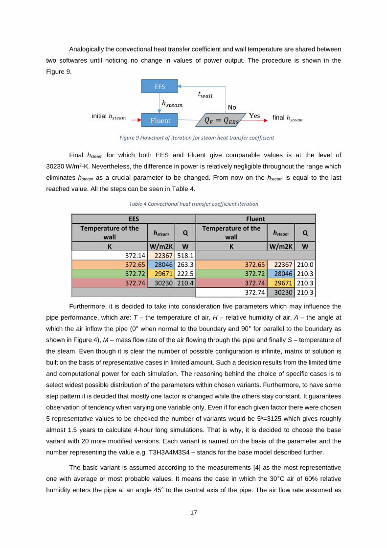
Analogically the convectional heat transfer coefficient and wall temperature are shared between

two softwares until noticing no change in values of power output. The procedure is shown in the

Figure 9.

Final hsteam for which both EES and Fluent give comparable values is at the level of

30230 W/m2-K. Nevertheless, the difference in power is relatively negligible throughout the range which

eliminates hsteam as a crucial parameter to be changed. From now on the hsteam is equal to the last

reached value. All the steps can be seen in Table 4.

Table 4 Convectional heat transfer coefficient iteration

EES Fluent

Temperature of the wall

hsteam Q Temperature of the

wall hsteam Q

K W/m2K W K W/m2K W

372.14 22367 518.1

372.65 28046 263.3 372.65 22367 210.0

372.72 29671 222.5 372.72 28046 210.3

372.74 30230 210.4 372.74 29671 210.3

372.74 30230 210.3

Furthermore, it is decided to take into consideration five parameters which may influence the

pipe performance, which are: T – the temperature of air, H – relative humidity of air, A – the angle at

which the air inflow the pipe (0° when normal to the boundary and 90° for parallel to the boundary as

shown in Figure 4), M – mass flow rate of the air flowing through the pipe and finally S – temperature of

the steam. Even though it is clear the number of possible configuration is infinite, matrix of solution is

built on the basis of representative cases in limited amount. Such a decision results from the limited time

and computational power for each simulation. The reasoning behind the choice of specific cases is to

select widest possible distribution of the parameters within chosen variants. Furthermore, to have some

step pattern it is decided that mostly one factor is changed while the others stay constant. It guarantees

observation of tendency when varying one variable only. Even if for each given factor there were chosen

5 representative values to be checked the number of variants would be 55=3125 which gives roughly

almost 1.5 years to calculate 4-hour long simulations. That is why, it is decided to choose the base

variant with 20 more modified versions. Each variant is named on the basis of the parameter and the

number representing the value e.g. T3H3A4M3S4 – stands for the base model described further.

The basic variant is assumed according to the measurements [4] as the most representative

one with average or most probable values. It means the case in which the 30°C air of 60% relative

humidity enters the pipe at an angle 45° to the central axis of the pipe. The air flow rate assumed as

EES

Fluent initial ℎ𝑠𝑡𝑒𝑎𝑚

𝑡𝑤𝑎𝑙𝑙

ℎ𝑠𝑡𝑒𝑎𝑚

𝑄𝐹 = 𝑄𝐸𝐸𝑆

No

final ℎ𝑠𝑡𝑒𝑎𝑚 Yes

Figure 9 Flowchart of iteration for steam heat transfer coefficient

18

average is equal to 1/48 of the measured mass flow rate flowing through THSC which is 0.003958 kg/s

(corresponds to the velocity of 10 m/s and Re=17006) while the steam temperature is 100°C [10]. When

setting these parameters in Fluent except air mass flow rate and its temperature the other ones have to

be given indirectly. For the air humidity, one more time the EES software with its tables is used to

calculate the mass fraction of water for given temperature. The angle value is put in the form of Cartesian

coordinates while the steam temperature is set as a temperature of the wall. All those values are

specified in the form of boundary conditions.

Then, choosing the modification it is assumed that when changing one parameter the others

remain the same as in base variant. In the end, three more specific sets of values are specified. Two of

them assume two opposite extreme conditions for heat exchange in the pipe while the last one is

randomly chosen with all values not set previously. When it comes to air temperature it is assumed the

values may vary from T1 – 20°C to T6 – 40°C. Other temperatures of the air should not appear in the

kitchen where people work. In case of air humidity, the range H1 – 40 to H6 – 100 percent as well as

the angle of air flow rate A1 – 10° to A6 – 80° is much wider. Both factors can strongly vary what prevent

from limiting the range. Nevertheless, it should be highlighted that specific perpendicular arrangement

of the pipes towards the main air inflow [4] eliminate the possibility of small angle values and flow parallel

to pipe axis. More probable are the high values which still taking turbulence and swirl into account cannot

be taken for granted. In the case of air flow rate values are specified intuitively starting from M1 – half

of default mass flow rate (equal to 0.003958 kg/s and related to 10 m/s velocity and Re=17006) up to

M5 – double basic value (equal to 0.007917 kg/s and related to 20 m/s and Re=34014). At the end the

temperature of the steam is decreased from S4 – 100°C up to S1 – 90°C since the air may appear

together with the steam which causes lower saturation temperature.

Statistically, the values of all parameters should appear the same amount of times except the

basic ones which can be seen in major part. All the cases are gathered together in Table 5 where orange

background highlights unchanged factors with respect to the basic case while the white color points out

the varying one.

19

Table 5 Model cases

Variant name

parameter

air temperature

air humidity

air inlet angle

air mass flow rate

steam temperature

C % kg/s C

T3H3A4M3S4 30 60 45 0.003958 100

T1H3A4M3S4 20 60 45 0.003958 100

T2H3A4M3S4 25 60 45 0.003958 100

T5H3A4M3S4 35 60 45 0.003958 100

T6H3A4M3S4 40 60 45 0.003958 100

T3H1A4M3S4 30 40 45 0.003958 100

T3H2A4M3S4 30 50 45 0.003958 100

T3H5A4M3S4 30 80 45 0.003958 100

T3H6A4M3S4 30 100 45 0.003958 100

T3H3A1M3S4 30 60 10 0.003958 100

T3H3A3M3S4 30 60 30 0.003958 100

T3H3A5M3S4 30 60 60 0.003958 100

T3H3A6M3S4 30 60 80 0.003958 100

T3H3A4M1S4 30 60 45 0.001979 100

T3H3A4M4S4 30 60 45 0.005937 100

T3H3A4M5S4 30 60 45 0.007916 100

T3H3A4M3S1 30 60 45 0.003958 90

T3H3A4M3S2 30 60 45 0.003958 94

T6H6A5M1S1 40 100 60 0.001979 90

T1H1A2M5S4 20 40 20 0.007916 100

T4H4A6M2S3 32 70 80 0.002968 98

The procedure of generating solutions for each of the cases is similar to the previously described

for the k-ω model. The only exception takes place in the T3H3A6M3S4 and T4H4A6M2S3 variant where

convergence problems appear. Therefore, to prevent such problems those calculations are initialized

from the beginning with applied Baseline k-ω (BSL) turbulence model with curvature correction

activated. Though chosen BSL model is similar to standard k-ω, it consists of blending function. It

activates standard k-ω model in the near-wall region and transformed k-ε one far away from the surface.

In addition, the curvature correction sensitizes model to the effects of streamline curvature.

Since all cases differed from each other it is hard to present each of them in this work. Therefore,

it is decided to show a sample result T3H3A5M3S4 in which the angle is 60°. First of all, one can see

the temperature and velocity distribution on the same planes which are used to present both

k-ε and k-ω models (Figures 7-8). Views in Figures 10-11 show the flow inside a pipe is no longer

symmetrical with respect to the pipe axis, which in consequence gives unequal heat transfer along the

pipe. That is why the velocity and temperature profiles are somehow moved in comparison to those from

previous Figures.

20

It can be said the inflowing air in this case enters the pipe towards the left side from the shown

perspective and bounces to the opposite one. In time, until the outflow both velocity and temperature

values spread out more and more evenly. Nevertheless, the trend of velocity decrease from the core of

the flow to the walls corresponds to the opposite change in a temperature increase from external walls

to the core. It happens like this since the lower the speed of medium the more heat is absorbed and

accumulated in one place increasing the temperature and impairing the heat transfer rate. Even though,

unequally loaded walls may mean the pipe does not work evenly on the whole perimeter, it can be seen

further in Table 6 that unsymmetrical flow and appearing swirling terms give the higher power output.

Having all the models finished it is possible to analyze the influence of each factor on the power

of the pipe. It is decided to develop an empirical equation as such approach allows for encompassing

all analyzed parameters on the power of the pipe. Since the empirical equation has to define the

Figure 10 Temperature at cross-sections T3H3A5M3S4

Figure 11 Velocity at cross-section (middle right) and outflow (right) T3H3A5M3S4

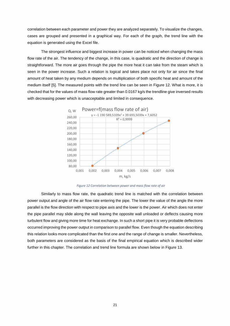
21

correlation between each parameter and power they are analyzed separately. To visualize the changes,

cases are grouped and presented in a graphical way. For each of the graph, the trend line with the

equation is generated using the Excel file.

The strongest influence and biggest increase in power can be noticed when changing the mass

flow rate of the air. The tendency of the change, in this case, is quadratic and the direction of change is

straightforward. The more air goes through the pipe the more heat it can take from the steam which is

seen in the power increase. Such a relation is logical and takes place not only for air since the final

amount of heat taken by any medium depends on multiplication of both specific heat and amount of the

medium itself [5]. The measured points with the trend line can be seen in Figure 12. What is more, it is

checked that for the values of mass flow rate greater than 0.0167 kg/s the trendline give inversed results

with decreasing power which is unacceptable and limited in consequence.

Similarly to mass flow rate, the quadratic trend line is matched with the correlation between

power output and angle of the air flow rate entering the pipe. The lower the value of the angle the more

parallel is the flow direction with respect to pipe axis and the lower is the power. Air which does not enter

the pipe parallel may slide along the wall leaving the opposite wall unloaded or deflects causing more

turbulent flow and giving more time for heat exchange. In such a short pipe it is very probable deflections

occurred improving the power output in comparison to parallel flow. Even though the equation describing

this relation looks more complicated than the first one and the range of change is smaller. Nevertheless,

both parameters are considered as the basis of the final empirical equation which is described wider

further in this chapter. The correlation and trend line formula are shown below in Figure 13.

y = -1 190 589,5109x2 + 39 693,5039x + 7,6052R² = 0,9999

80,00

100,00

120,00

140,00

160,00

180,00

200,00

220,00

240,00

260,00

0,001 0,002 0,003 0,004 0,005 0,006 0,007 0,008

Q, W

m, kg/s

Power=f(mass flow rate of air)

Figure 12 Correlation between power and mass flow rate of air

22

The rest of the parameters show linear behaviour. The increase of relative humidity (RH) of the

air and steam temperature in analyzed range result in an increase of the power. In the case of the RH,

the reason of such a trend is the greater specific heat value for water vapour comparing to two times

smaller value of the same parameter for air. In consequence, the higher humidity in air the more heat it

can take. On the other hand, mentioned increase is relatively small, almost negligible. The reason for

that is that the humidity represents only a tiny part of the air. The trend line with the predicted values is

shown in Figure 14.

The increase of power with respect to steam temperature growth is related to the temperature

gradient which drives the heat exchange process. The higher the temperature difference between hot

and cold media would be the greater power output became. The correlation can be observed in

Figure 15.

y = 0,0077559123x2 - 0,1938093674x + 138,5566319398R² = 0,9905550786

135,00

140,00

145,00

150,00

155,00

160,00

165,00

170,00

175,00

10 20 30 40 50 60 70 80

Q, W

angle, °

Power=f(angle of air flow rate)

y = 0,02390924x + 145,40501207 R² = 0,99999653

146,00

146,20

146,40

146,60

146,80

147,00

147,20

147,40

147,60

147,80

148,00

40 50 60 70 80 90 100

Q, W

RH, %

Power=f(air humidity)

Figure 13 Correlation between power and angle of air flow rate

Figure 14 Correlation between power and air humidity

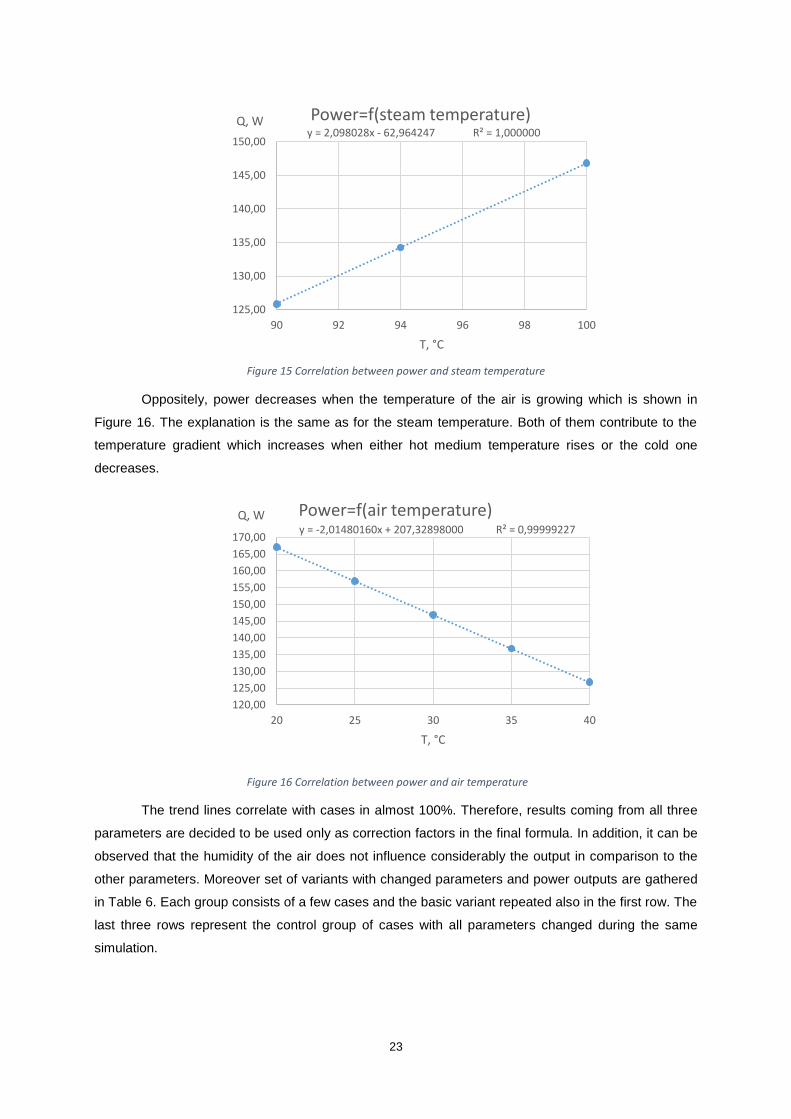
23

Oppositely, power decreases when the temperature of the air is growing which is shown in

Figure 16. The explanation is the same as for the steam temperature. Both of them contribute to the

temperature gradient which increases when either hot medium temperature rises or the cold one

decreases.

The trend lines correlate with cases in almost 100%. Therefore, results coming from all three

parameters are decided to be used only as correction factors in the final formula. In addition, it can be

observed that the humidity of the air does not influence considerably the output in comparison to the

other parameters. Moreover set of variants with changed parameters and power outputs are gathered

in Table 6. Each group consists of a few cases and the basic variant repeated also in the first row. The

last three rows represent the control group of cases with all parameters changed during the same

simulation.

y = -2,01480160x + 207,32898000 R² = 0,99999227

120,00

125,00

130,00

135,00

140,00

145,00

150,00

155,00

160,00

165,00

170,00

20 25 30 35 40

Q, W

T, °C

Power=f(air temperature)

y = 2,098028x - 62,964247 R² = 1,000000

125,00

130,00

135,00

140,00

145,00

150,00

90 92 94 96 98 100

Q, W

T, °C

Power=f(steam temperature)

Figure 16 Correlation between power and air temperature

Figure 15 Correlation between power and steam temperature

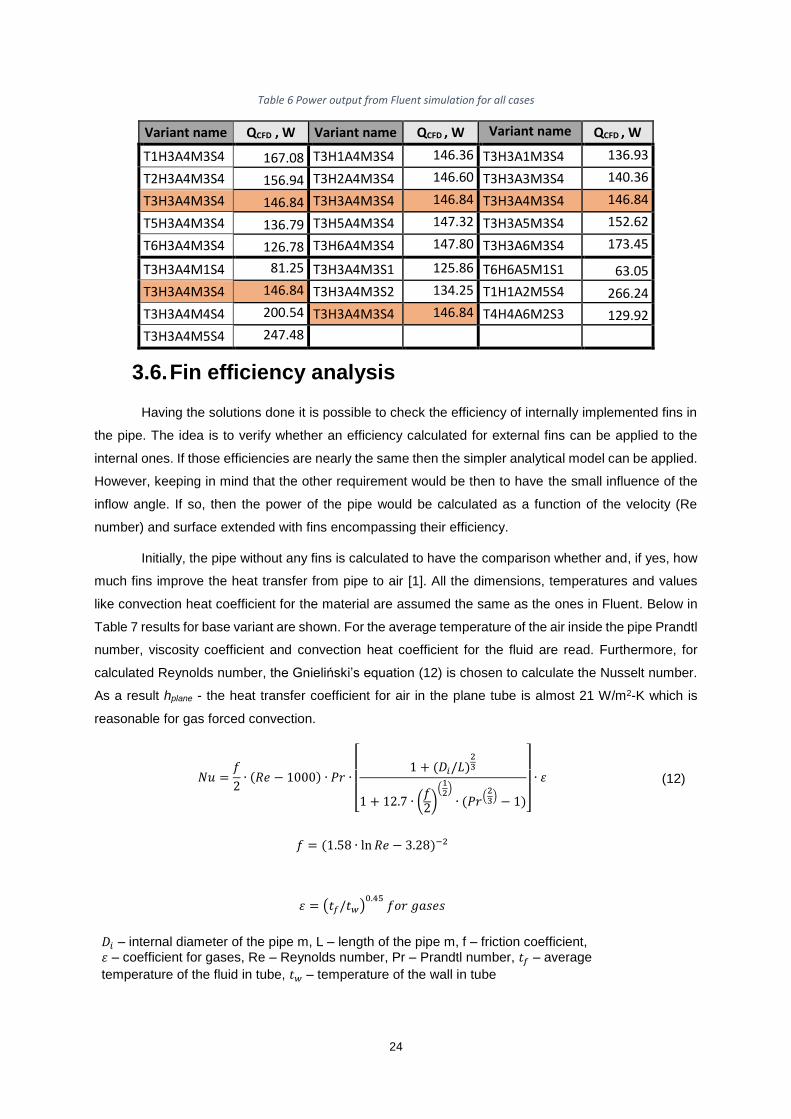
24

Table 6 Power output from Fluent simulation for all cases

Variant name QCFD , W Variant name QCFD , W Variant name QCFD , W

T1H3A4M3S4 167.08 T3H1A4M3S4 146.36 T3H3A1M3S4 136.93








T3H3A4M5S4 247.48

3.6. Fin efficiency analysis

Having the solutions done it is possible to check the efficiency of internally implemented fins in

the pipe. The idea is to verify whether an efficiency calculated for external fins can be applied to the

internal ones. If those efficiencies are nearly the same then the simpler analytical model can be applied.

However, keeping in mind that the other requirement would be then to have the small influence of the

inflow angle. If so, then the power of the pipe would be calculated as a function of the velocity (Re

number) and surface extended with fins encompassing their efficiency.

Initially, the pipe without any fins is calculated to have the comparison whether and, if yes, how

much fins improve the heat transfer from pipe to air [1]. All the dimensions, temperatures and values

like convection heat coefficient for the material are assumed the same as the ones in Fluent. Below in

Table 7 results for base variant are shown. For the average temperature of the air inside the pipe Prandtl

number, viscosity coefficient and convection heat coefficient for the fluid are read. Furthermore, for

calculated Reynolds number, the Gnieliński’s equation (12) is chosen to calculate the Nusselt number.

As a result hplane - the heat transfer coefficient for air in the plane tube is almost 21 W/m2-K which is

reasonable for gas forced convection.

𝑁𝑢 =𝑓

2∙ (𝑅𝑒 − 1000) ∙ 𝑃𝑟 ∙

[

1 + (𝐷𝑖/𝐿)23

1 + 12.7 ∙ (𝑓2)

(12)

∙ (𝑃𝑟(23) − 1)]

∙ 휀 (12)

𝑓 = (1.58 ∙ ln 𝑅𝑒 − 3.28)−2

휀 = (𝑡𝑓/𝑡𝑤)0.45

𝑓𝑜𝑟 𝑔𝑎𝑠𝑒𝑠

𝐷𝑖 – internal diameter of the pipe m, L – length of the pipe m, f – friction coefficient, 휀 – coefficient for gases, Re – Reynolds number, Pr – Prandtl number, 𝑡𝑓 – average

temperature of the fluid in tube, 𝑡𝑤 – temperature of the wall in tube

25

Table 7 Heat transfer coefficient for plane tube

𝑓= 0.007965 -

휀= 0.6124 -

𝑁𝑢= 21.4 -

ℎ𝑝𝑙𝑎𝑛𝑒= 20.6 W/m2-K

To receive the same heat transfer coefficient but for finned pipe there is a need to read power

output (QCFD in Table 6) and temperatures: of the wall and free stream from Fluent. Besides, the area of

heat exchange grows up (13) because of the fins. Using, the area-weighted average-wall temperature

at pipe interface for the whole area with fins (368.65 K) and mass-weighted average-static temperature

at the interior of the pipe for fluid (321.25 K) the new hfinned for finned pipe equal to almost 46 W/m2-K is

found using formula (14).

Knowing that the temperature distribution alongside the fin differ two lines are made in Fluent to

read the area-weighted temperature just for the pipe interface base without fins taken into account. For

this temperature, which is higher, the efficiency of the fin can be conducted to compensate that

difference (15). Since the temperatures at the base and top of the fins are not the same the efficiency

has to be lower than 100%.

𝑄𝐶𝐹𝐷 = [𝐿 ∙ (𝜋 ∙ 𝐷𝑖 − 𝑛𝑓𝑖𝑛 ∙ 𝑡𝑓𝑖𝑛) + 𝑛𝑓𝑖𝑛 ∙ 𝐴𝑓𝑖𝑛 ∙ 𝜂𝑓𝑖𝑛] ∙ (𝑡𝑏𝑓𝑖𝑛𝑛𝑒𝑑 − 𝑡𝑓𝑙𝑢𝑖𝑑) ∙ ℎ𝑓𝑖𝑛𝑛𝑒𝑑 (15)

𝜂𝑓𝑖𝑛 – efficiency of the fin, 𝑡𝑏𝑓𝑖𝑛𝑛𝑒𝑑 – area-weighted temperature just for the pipe interface

base K

Having the hfinned for the finned pipe the tabular efficiency for the external fin is checked. In the

case of base variant, the calculated efficiency is 88% while the tabular one is 93%. Such a procedure is

repeated for a couple of cases. Comparison of all proves the tables cannot be used in the case of

internally installed fins and that usage of Fluent simulation is the right choice. It is so, the efficiencies

differ and what is more for the internally installed fins values (82-88%) are always 5-6% lower than for

externally installed ones (88-94% respectively). Combining this fact with the strong dependency of the

pipe power on inflow angle indicates that the model relying solely on fin efficiency and velocity of the air

is unreliable. The already existing formulas are not suitable for tubes internally finned.

3.7. Pipe equation

To compute the empirical equation for model all the cases are divided into two groups. The first

one gathers most of the cases with a representative range of change within parameters. In Table 6 and

𝐴𝑡𝑜𝑡𝑎𝑙 = 𝑛𝑓𝑖𝑛 ∙ 𝐴𝑓𝑖𝑛 + 𝐿 ∙ (𝜋 ∙ 𝐷𝑖 − 𝑛𝑓𝑖𝑛 ∙ 𝑡𝑓𝑖𝑛) (13)

𝐴𝑓𝑖𝑛 – area of a single fin m2, 𝑛𝑓𝑖𝑛 – number of fins, 𝑡𝑓𝑖𝑛 – fin thickness m

𝑄𝐶𝐹𝐷 = 𝐴𝑡𝑜𝑡𝑎𝑙 ∙ (𝑡𝑓𝑖𝑛𝑛𝑒𝑑 − 𝑡𝑓𝑙𝑢𝑖𝑑) ∙ ℎ𝑓𝑖𝑛𝑛𝑒𝑑 (14)

𝑄𝐶𝐹𝐷 – power output W, 𝑡𝑓𝑖𝑛𝑛𝑒𝑑 – area-weighted average-wall temperature at pipe interface

for whole area with fins K, 𝑡𝑓𝑙𝑢𝑖𝑑 – mass-weighted average-static temperature at interior of the

pipe for fluid K, ℎ𝑓𝑖𝑛𝑛𝑒𝑑 – heat transfer coefficient inside finned tube W/m2-K

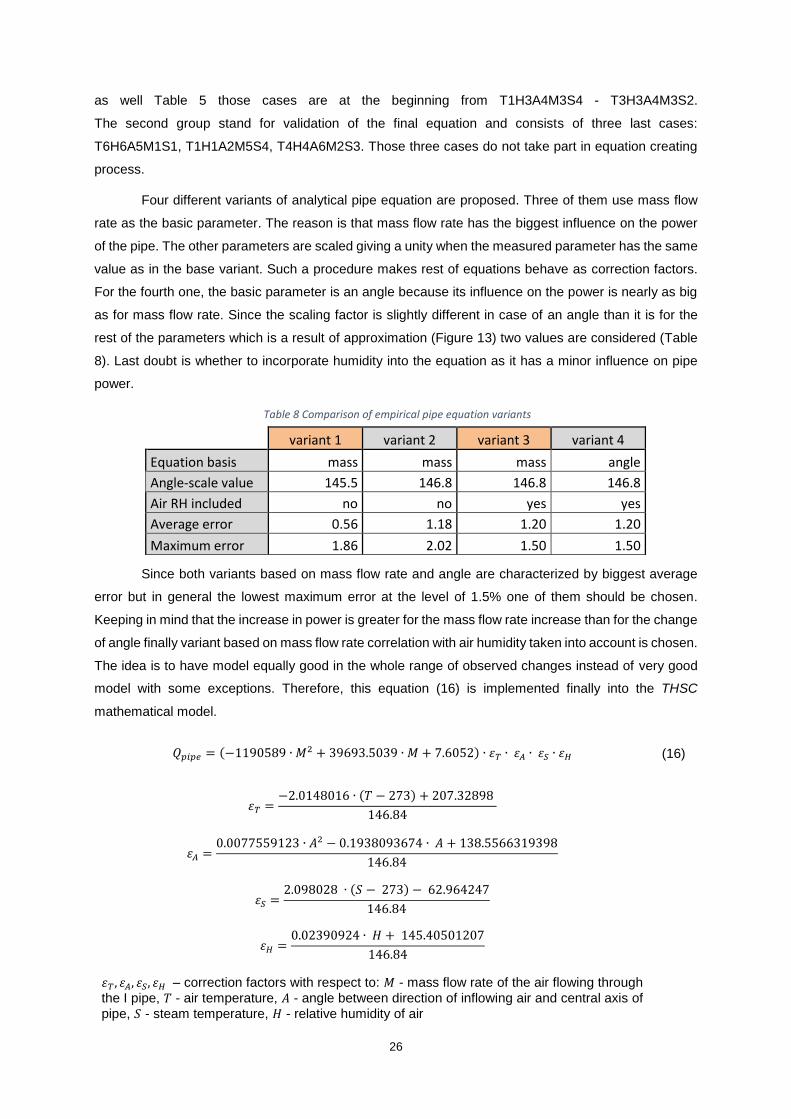
26

as well Table 5 those cases are at the beginning from T1H3A4M3S4 - T3H3A4M3S2.

The second group stand for validation of the final equation and consists of three last cases:

T6H6A5M1S1, T1H1A2M5S4, T4H4A6M2S3. Those three cases do not take part in equation creating

process.

Four different variants of analytical pipe equation are proposed. Three of them use mass flow

rate as the basic parameter. The reason is that mass flow rate has the biggest influence on the power

of the pipe. The other parameters are scaled giving a unity when the measured parameter has the same

value as in the base variant. Such a procedure makes rest of equations behave as correction factors.

For the fourth one, the basic parameter is an angle because its influence on the power is nearly as big

as for mass flow rate. Since the scaling factor is slightly different in case of an angle than it is for the

rest of the parameters which is a result of approximation (Figure 13) two values are considered (Table

8). Last doubt is whether to incorporate humidity into the equation as it has a minor influence on pipe

power.

Table 8 Comparison of empirical pipe equation variants

Since both variants based on mass flow rate and angle are characterized by biggest average

error but in general the lowest maximum error at the level of 1.5% one of them should be chosen.

Keeping in mind that the increase in power is greater for the mass flow rate increase than for the change

of angle finally variant based on mass flow rate correlation with air humidity taken into account is chosen.

The idea is to have model equally good in the whole range of observed changes instead of very good

model with some exceptions. Therefore, this equation (16) is implemented finally into the THSC

mathematical model.

𝑄𝑝𝑖𝑝𝑒 = (−1190589 ∙ 𝑀2 + 39693.5039 ∙ 𝑀 + 7.6052) ∙ 휀𝑇 ∙ 휀𝐴 ∙ 휀𝑆 ∙ 휀𝐻 (16)

휀𝑇 =−2.0148016 ∙ (𝑇 − 273) + 207.32898

146.84

휀𝐴 =0.0077559123 ∙ 𝐴2 − 0.1938093674 ∙ 𝐴 + 138.5566319398

146.84

휀𝑆 =2.098028 ∙ (𝑆 − 273) − 62.964247

146.84

휀𝐻 =0.02390924 ∙ 𝐻 + 145.40501207

146.84

휀𝑇 , 휀𝐴, 휀𝑆, 휀𝐻 – correction factors with respect to: 𝑀 - mass flow rate of the air flowing through

the I pipe, 𝑇 - air temperature, 𝐴 - angle between direction of inflowing air and central axis of

pipe, 𝑆 - steam temperature, 𝐻 - relative humidity of air

variant 1 variant 2 variant 3 variant 4

Equation basis mass mass mass angle

Angle-scale value 145.5 146.8 146.8 146.8

Air RH included no no yes yes

Average error 0.56 1.18 1.20 1.20

Maximum error 1.86 2.02 1.50 1.50

27

3.8. THSC model development

The choice of Visual Basic for Application as the base for final model of THSC comes from the

wide availability of this software. Although, Excel is widely met in industrial companies it is not a first

thought engineering tool. Differently from EES, this program has no built-in tables and iterative way of

computing results which causes some difficulties. The first obstacle is overcome by steam_IAPWS

module implementation. This module allows reading directly input steam parameters. The non-iterative

character of VBA work results in the longer process of code planning. Nevertheless, having in mind the

user will not interfere inside it, there is no risk of the program to be more problematic in use.

Previously described activities in Fluent and work on the equation of pipe behaviour let the

program to model the THSC under different conditions. To let the user change input data and show how

particular modifications in parameters and construction may end up an interface with hidden condition

statements and warnings has to be set. All of them make the program user-friendly without any need

for deep thermodynamics knowledge.

The assumption is to create the tool which can guide its user without essential knowledge

through the whole process. Therefore, at the beginning all input data values are checked whether they

are from the range analyzed in Fluent. If not, there is a possibility of extrapolation of the results. After

computation reaches the finish line the user is informed via activated reports of this fact. If some value

drastically exceeded that range it would terminate the work of the program and point out the problem.

In some situations, the model can precise the source of an error and give the hint of next step. Besides,

the information is stored in help menu where one can find answers for questions about the program

before initializing the calculation.

Excel, being most handful program in storing and presenting data, allows the user to reprocess

given results to analyze it later. That is why in separate Worksheets, both crucial and complementary

values are loaded after computation. They are sorted in the way those most valuable ones are

highlighted without too many details but with guaranteed access to more of them if needed. To make it

even easier VBA let create a convenient graphical interface. The procedure is very intuitive using the

potential of a few GUIs shown in set order with respect to user’s choices.

Mentioned GUI and reports not only minimize the number of discrepancies but in critical

moments suggest where to find the source of the problem. In the GUIs, the clear difference between

input and output boxes is kept. In the end, the work comes to almost mechanical activities supported by

the graphical representation of THSC. Organization of the GUIs is described in Appendix A.

3.8.1. Heat losses

Since, the heat exchange takes place not only through described pipes, between air and steam,

but also with the walls the influence of that has to be taken into account. To calculate the amount of heat

lost to the environment outside EES software is used. Parameters vary depending on working

conditions, and calculation of a single case may be insufficient as the effect is relatively small comparing

to the amount of heat exchanged internally. That is why average values are used to check that

28

phenomenon with and without radiation. Namely, the final amount of lost heat between the air inside

and outside through side areas Aside=0.072556 m2 each, top one Atop=0.107040 m2 as well as steam

and air outside through backside Aback=0.119037 m2 is calculated for k=16.27 W/m-K for 1.5 mm thick

steel and three values of heat transfer coefficient. Values differ between the air inside collecting chamber

(Tair_in=310.6 K), outside THSC (Tair_out=297.1 K), and for steam at the backside of THSC (Tsteam=373.15

K) being equal to 46, 6 and 30230 W/m2-K respectively. The surfaces taken into account are shown in

Figure 17. To calculate that heat without radiation, below equations are used [11] and corresponding

results are shown in Table 9.

𝑄𝑙𝑜𝑠𝑡 = 𝑞𝑎𝑖𝑟 ∙ (2 ∙ 𝐴𝑠𝑖𝑑𝑒 + 𝐴𝑡𝑜𝑝) + 𝑞𝑠𝑡𝑒𝑎𝑚 ∙ 𝐴𝑏𝑎𝑐𝑘 (17)

𝑞𝑎𝑖𝑟 =𝑇𝑎𝑖𝑟_𝑖𝑛 − 𝑇𝑎𝑖𝑟_𝑜𝑢𝑡

𝑅𝑎𝑖𝑟

(18)

𝑞𝑠𝑡𝑒𝑎𝑚 =𝑆 − 𝑇𝑎𝑖𝑟_𝑜𝑢𝑡

𝑅𝑠𝑡𝑒𝑎𝑚

(19)

𝑅𝑎𝑖𝑟 =1

ℎ𝑎𝑖𝑟_𝑖𝑛

+𝛿

𝑘+

1

ℎ𝑎𝑖𝑟_𝑜𝑢𝑡

(20)

𝑅𝑠𝑡𝑒𝑎𝑚 =1

ℎ𝑠𝑡𝑒𝑎𝑚

+𝛿

𝑘+

1

ℎ𝑎𝑖𝑟_𝑜𝑢𝑡

(21)

𝛿 – thickness of the wall m, 𝑇𝑎𝑖𝑟_𝑖𝑛 – temperature of air inside collecting chamber K, 𝑇𝑎𝑖𝑟_𝑜𝑢𝑡 –

temperature of air outside THSC K, ℎ𝑎𝑖𝑟_𝑖𝑛 – heat transfer coefficient of air inside collecting

chamber W/m2-K, ℎ𝑎𝑖𝑟_𝑜𝑢𝑡 – heat transfer coefficient of air outside THSC W/m2-K, 𝑘 – thermal

conductivity of the wall W/m-K,

1 – side areas Aside, 2 – top area Atop, 3 – backside area Aback

Figure 17 Surfaces of heat loss in THSC

Table 9 Heat loss to the surrounding through external walls

𝑅𝑎𝑖𝑟= 0.189 K-m2/W

𝑅𝑠𝑡𝑒𝑎𝑚= 0.167 K-m2/W

𝑞𝑎𝑖𝑟= 71.44 W/m2

𝑞𝑠𝑡𝑒𝑎𝑚= 456 W/m2

𝑄𝑙𝑜𝑠𝑡= 72.3 W

When taking into account the radiation, formulas have to be modified since the temperature of

the external wall is not known. Therefore, iterative nature of work in EES occurs very helpful saving a

lot of time. The equation for heat loss stays the same (17) but formulas for heat rates are changed from

12. 13. top-side view

1.

1. 3.

2.

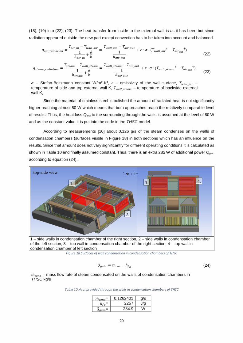
29

(18), (19) into (22), (23). The heat transfer from inside to the external wall is as it has been but since

radiation appeared outside the new part except convection has to be taken into account and balanced.

𝑞𝑎𝑖𝑟_𝑟𝑎𝑑𝑖𝑎𝑡𝑖𝑜𝑛 =𝑇𝑎𝑖𝑟_𝑖𝑛 − 𝑇𝑤𝑎𝑙𝑙_𝑎𝑖𝑟

1ℎ𝑎𝑖𝑟_𝑖𝑛

+𝛿𝑘

=𝑇𝑤𝑎𝑙𝑙_𝑎𝑖𝑟 − 𝑇𝑎𝑖𝑟_𝑜𝑢𝑡

1ℎ𝑎𝑖𝑟_𝑜𝑢𝑡

+ 휀 ∙ 𝜎 ∙ (𝑇𝑤𝑎𝑙𝑙_𝑎𝑖𝑟4 − 𝑇𝑎𝑖𝑟𝑜𝑢𝑡

4) (22)

𝑞𝑠𝑡𝑒𝑎𝑚_𝑟𝑎𝑑𝑖𝑎𝑡𝑖𝑜𝑛 =𝑇𝑠𝑡𝑒𝑎𝑚 − 𝑇𝑤𝑎𝑙𝑙_𝑠𝑡𝑒𝑎𝑚

1ℎ𝑠𝑡𝑒𝑎𝑚

+𝛿𝑘

=𝑇𝑤𝑎𝑙𝑙_𝑠𝑡𝑒𝑎𝑚 − 𝑇𝑎𝑖𝑟_𝑜𝑢𝑡

1ℎ𝑎𝑖𝑟_𝑜𝑢𝑡

+ 휀 ∙ 𝜎 ∙ (𝑇𝑤𝑎𝑙𝑙_𝑠𝑡𝑒𝑎𝑚4 − 𝑇𝑎𝑖𝑟𝑜𝑢𝑡

4) (23)

𝜎 – Stefan-Boltzmann constant W/m2-K4, 휀 – emissivity of the wall surface, 𝑇𝑤𝑎𝑙𝑙_𝑎𝑖𝑟 –

temperature of side and top external wall K, 𝑇𝑤𝑎𝑙𝑙_𝑠𝑡𝑒𝑎𝑚 – temperature of backside external

wall K,

Since the material of stainless steel is polished the amount of radiated heat is not significantly

higher reaching almost 80 W which means that both approaches reach the relatively comparable level

of results. Thus, the heat loss Qlost to the surrounding through the walls is assumed at the level of 80 W

and as the constant value it is put into the code in the THSC model.

According to measurements [10] about 0.126 g/s of the steam condenses on the walls of

condensation chambers (surfaces visible in Figure 18) in both sections which has an influence on the

results. Since that amount does not vary significantly for different operating conditions it is calculated as

shown in Table 10 and finally assumed constant. Thus, there is an extra 285 W of additional power Qgain

according to equation (24).

1 – side walls in condensation chamber of the right section, 2 – side walls in condensation chamber of the left section, 3 – top wall in condensation chamber of the right section, 4 – top wall in condensation chamber of left section

Figure 18 Surfaces of wall condensation in condensation chambers of THSC

𝑄𝑔𝑎𝑖𝑛 = �̇�𝑐𝑜𝑛𝑑 ∙ ℎ𝑓𝑔 (24)

�̇�𝑐𝑜𝑛𝑑 – mass flow rate of steam condensated on the walls of condensation chambers in THSC kg/s

Table 10 Heat provided through the walls in condensation chambers of THSC

�̇�𝑐𝑜𝑛𝑑= 0.1262401 g/s

ℎ𝑓𝑔= 2257 J/g

𝑄𝑔𝑎𝑖𝑛= 284.9 W

12. 13. top-side view

2.

1. 3. 4.

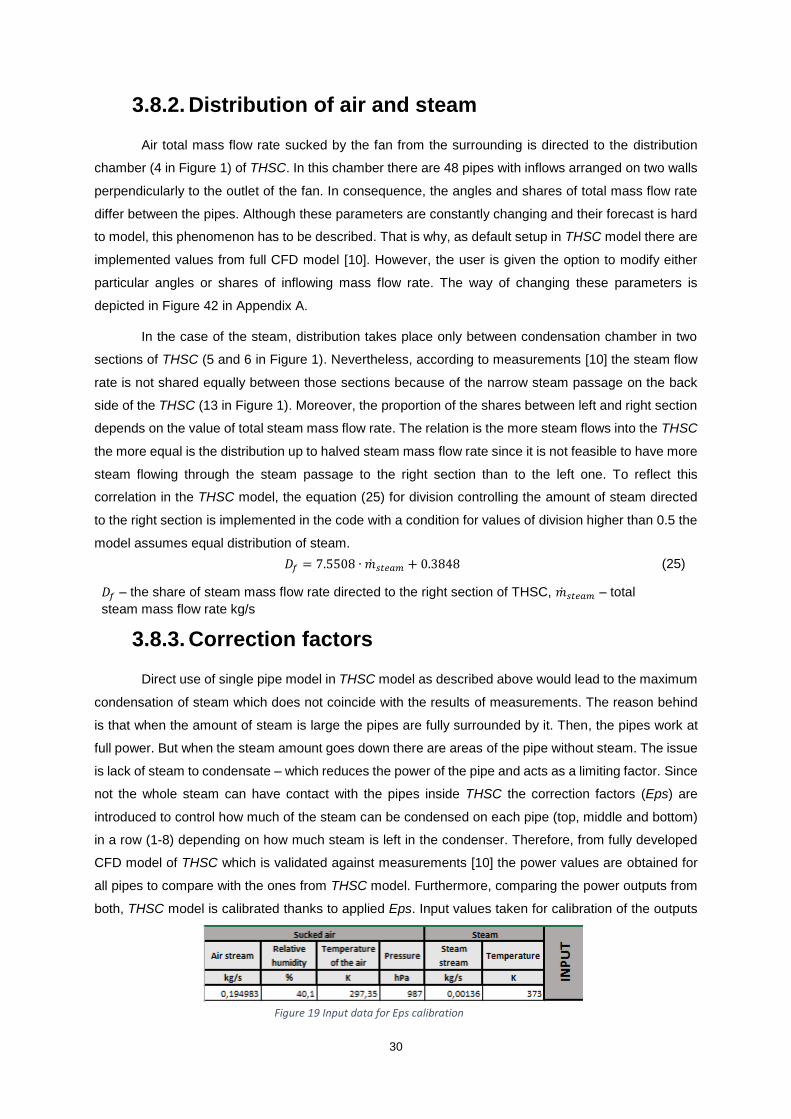
30

3.8.2. Distribution of air and steam

Air total mass flow rate sucked by the fan from the surrounding is directed to the distribution

chamber (4 in Figure 1) of THSC. In this chamber there are 48 pipes with inflows arranged on two walls

perpendicularly to the outlet of the fan. In consequence, the angles and shares of total mass flow rate

differ between the pipes. Although these parameters are constantly changing and their forecast is hard

to model, this phenomenon has to be described. That is why, as default setup in THSC model there are

implemented values from full CFD model [10]. However, the user is given the option to modify either

particular angles or shares of inflowing mass flow rate. The way of changing these parameters is

depicted in Figure 42 in Appendix A.

In the case of the steam, distribution takes place only between condensation chamber in two

sections of THSC (5 and 6 in Figure 1). Nevertheless, according to measurements [10] the steam flow

rate is not shared equally between those sections because of the narrow steam passage on the back

side of the THSC (13 in Figure 1). Moreover, the proportion of the shares between left and right section

depends on the value of total steam mass flow rate. The relation is the more steam flows into the THSC

the more equal is the distribution up to halved steam mass flow rate since it is not feasible to have more

steam flowing through the steam passage to the right section than to the left one. To reflect this

correlation in the THSC model, the equation (25) for division controlling the amount of steam directed

to the right section is implemented in the code with a condition for values of division higher than 0.5 the

model assumes equal distribution of steam.

3.8.3. Correction factors

Direct use of single pipe model in THSC model as described above would lead to the maximum

condensation of steam which does not coincide with the results of measurements. The reason behind

is that when the amount of steam is large the pipes are fully surrounded by it. Then, the pipes work at

full power. But when the steam amount goes down there are areas of the pipe without steam. The issue

is lack of steam to condensate – which reduces the power of the pipe and acts as a limiting factor. Since

not the whole steam can have contact with the pipes inside THSC the correction factors (Eps) are

introduced to control how much of the steam can be condensed on each pipe (top, middle and bottom)

in a row (1-8) depending on how much steam is left in the condenser. Therefore, from fully developed

CFD model of THSC which is validated against measurements [10] the power values are obtained for

all pipes to compare with the ones from THSC model. Furthermore, comparing the power outputs from

both, THSC model is calibrated thanks to applied Eps. Input values taken for calibration of the outputs

𝐷𝑓 = 7.5508 ∙ �̇�𝑠𝑡𝑒𝑎𝑚 + 0.3848 (25)

𝐷𝑓 – the share of steam mass flow rate directed to the right section of THSC, �̇�𝑠𝑡𝑒𝑎𝑚 – total

steam mass flow rate kg/s

Figure 19 Input data for Eps calibration

31

and verification of THSC model with the Fluent [4] are as given in Figure 19. Calibrated THSC model

further on is validated against measurements [10].

In consequence, the limitation works only when the amount of steam is relatively small, close to

or below the maximum available amount of steam condensed on the pipe. When the flow rate is much

bigger, calculated limits for Eps are above physical limits for a single pipe and do not activate. Therefore,

for a given Eps values gathered in Table 11 it can be observed in Figure 20 the correlation between

results from Fluent (fully developed CFD model of THSC) [4] and mathematical THSC model.

Table 11 Correction factors for THSC model

In Figure 20 (top view) power outputs without correction are presented. It can be observed at

the beginning the THSC model is condensing more than according to Fluent. At some point, there is no

more steam left and the power drops to zero. In addition, in the line from Fluent it is worth to notice that

1 2 3 4 5 6 7 8

top

Eps

0.085 0.095 0.15 0.235 0.175 0.24 0.435 0.6

LEFT

middle 0.08 0.085 0.115 0.175 0.12 0.14 0.25 0.56

bottom 0.06 0.06 0.075 0.1 0.085 0.085 0.14 0.2

top 0.11 0.125 0.185 0.335 0.15 0.2 0.34 0.65

RIG

HT

middle 0.085 0.105 0.145 0.23 0.1 0.115 0.19 0.5

bottom 0.045 0.05 0.065 0.1 0.08 0.075 0.105 0.28

Figure 20 Comparison of power output for THSC model and Fluent without correction factors (top) and with them (bottom)

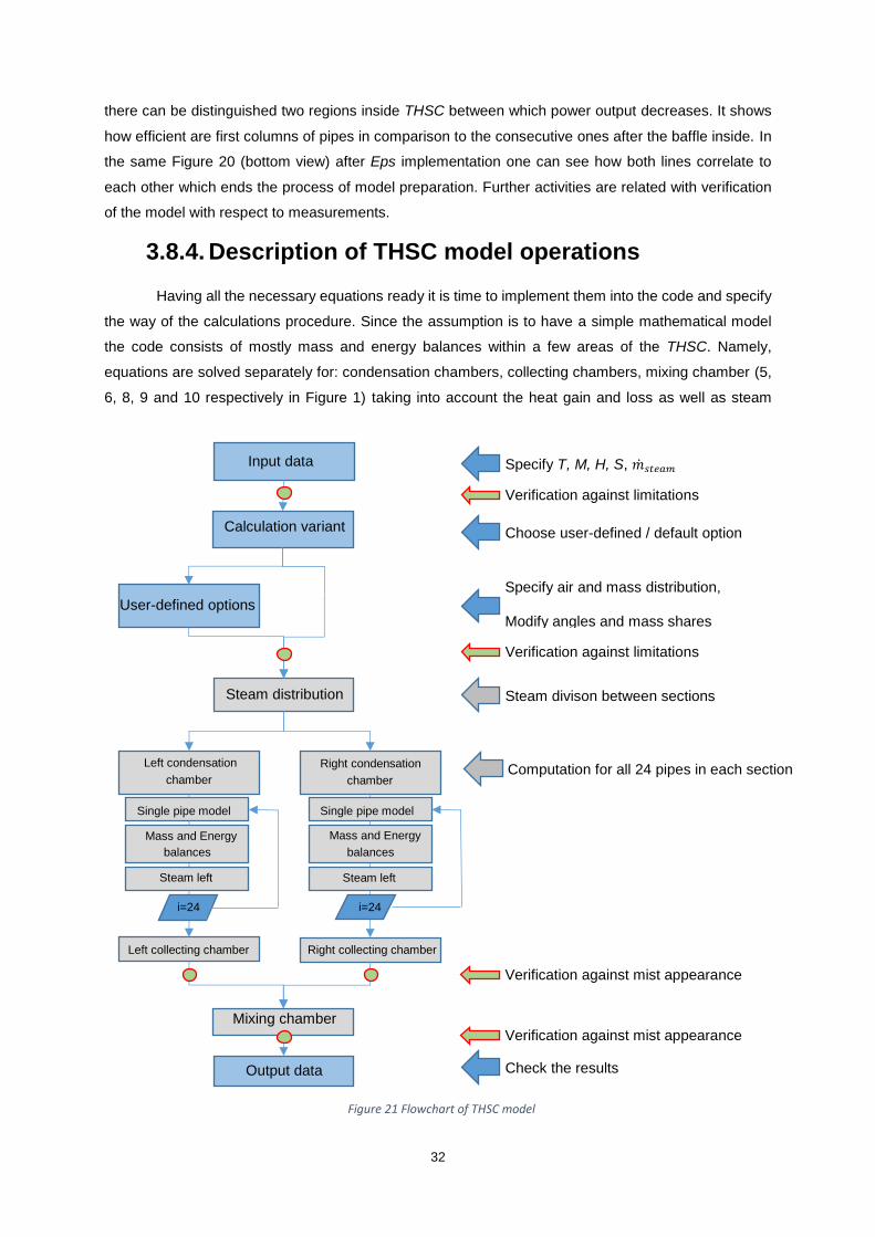
32

there can be distinguished two regions inside THSC between which power output decreases. It shows

how efficient are first columns of pipes in comparison to the consecutive ones after the baffle inside. In

the same Figure 20 (bottom view) after Eps implementation one can see how both lines correlate to

each other which ends the process of model preparation. Further activities are related with verification

of the model with respect to measurements.

3.8.4. Description of THSC model operations

Having all the necessary equations ready it is time to implement them into the code and specify

the way of the calculations procedure. Since the assumption is to have a simple mathematical model

the code consists of mostly mass and energy balances within a few areas of the THSC. Namely,

equations are solved separately for: condensation chambers, collecting chambers, mixing chamber (5,

6, 8, 9 and 10 respectively in Figure 1) taking into account the heat gain and loss as well as steam

Input data Specify T, M, H, S, �̇�𝑠𝑡𝑒𝑎𝑚

Verification against limitations

Choose user-defined / default option Calculation variant

User-defined options

Verification against limitations

Specify air and mass distribution,

Modify angles and mass shares

Steam divison between sections Steam distribution

Left condensation Right condensation chamber chamber

Single pipe model

balances

Steam left

Mass and Energy

Output data

Single pipe model

balances

Steam left

Mass and Energy

Mixing chamber Verification against mist appearance

Right collecting chamber Left collecting chamber

Check the results

i=24 i=24

Verification against mist appearance

Computation for all 24 pipes in each section

Figure 21 Flowchart of THSC model

33

distribution variant. The general procedure of calculation in THSC model is presented in the flowchart

in Figure 21.

At the beginning one can specify the input values: temperature of the air (T), relative humidity

of air (H), air mass flow rate (M) and finally steam mass flow rate (�̇�𝑠𝑡𝑒𝑎𝑚) with its temperature

(𝑇𝑠𝑡𝑒𝑎𝑚 , (𝑆)) (Block 1 in Figure 21). After verification of input data against limitations, user can choose

the calculation variant (Block 2 in Figure 21): default or user-defined which influences further steps. In

the case of user-defined option one can additionally specifies air inflow angle (A) and shares of air mass

flow rate between the pipes as well as the way of steam and air mass flow rate distribution (Block 3 in

Figure 21). If given values satisfy the limiting conditions all the values are inserted into the code and

used for calculation.

First of all steam mass flow rate is divided between the left and right condensation chamber

according to internal formula (25) or equally and decreased by the amount of steam condensed on the

walls

(Table 10). For the air mass flow rate entering the distribution chamber (4 in Figure 1) of THSC the

saturation pressure is read. Then the degree of humidity (26) and specific enthalpy (27) are calculated.

Furthermore, the calculation for left (and then right) section of condensation chamber can be

done. Since in one section there are 8 columns of 3 pipes each, the calculation is repeated 24 times.

Assuming none of the values exceeds the analyzed range and no unfeasible result occurs the following

equations are solved. First of all for given input parameters the power of the pipe is calculated from

single pipe model equation (16) and the corresponding amount of condensed steam from equation (28)

shown below. The same value is validated against Eps (Table 11) and modified if needed.

𝑋𝑖𝑛 =

𝐻𝑖

100∙ 𝑝𝑠𝑎𝑡,𝑖𝑛,𝑖

𝑝𝑜 −𝐻𝑖

100∙ 𝑝𝑠𝑎𝑡,𝑖𝑛,𝑖

∙𝑀𝐻2𝑂

𝑀𝑑𝑎

(26)

ℎ𝑤𝑎,𝑖𝑛,𝑖 = 1.005 ∙ (T − 273.15) + 𝑋𝑖𝑛 ∙ (1.88 ∙ (T − 273.15) + 2501) (27)

𝑝𝑠𝑎𝑡,𝑖𝑛,𝑖 – saturation pressure for 𝑇 hPa, 𝑀𝐻2𝑂, 𝑀𝑑𝑎 – molar mass of water and dry air

kgH2O/kmolH2O , kgda/kmolda, 𝑝𝑜 – air pressure hPa

�̇�𝑐𝑜𝑛𝑑,𝑖 =𝑄𝑝𝑖𝑝𝑒,𝑖

ℎ𝑓𝑔 (28)

�̇�𝑐𝑜𝑛𝑑,𝑖 – mass flow rate of steam condensed on the i pipe in THSC kg/s, 𝑖 – number of

calculated pipe 1-24

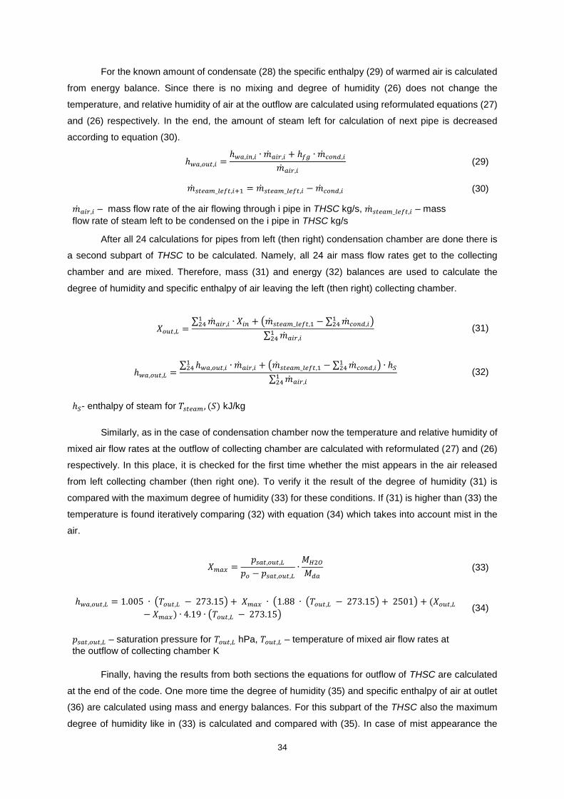
34

For the known amount of condensate (28) the specific enthalpy (29) of warmed air is calculated

from energy balance. Since there is no mixing and degree of humidity (26) does not change the

temperature, and relative humidity of air at the outflow are calculated using reformulated equations (27)

and (26) respectively. In the end, the amount of steam left for calculation of next pipe is decreased

according to equation (30).

After all 24 calculations for pipes from left (then right) condensation chamber are done there is

a second subpart of THSC to be calculated. Namely, all 24 air mass flow rates get to the collecting

chamber and are mixed. Therefore, mass (31) and energy (32) balances are used to calculate the

degree of humidity and specific enthalpy of air leaving the left (then right) collecting chamber.

Similarly, as in the case of condensation chamber now the temperature and relative humidity of

mixed air flow rates at the outflow of collecting chamber are calculated with reformulated (27) and (26)

respectively. In this place, it is checked for the first time whether the mist appears in the air released

from left collecting chamber (then right one). To verify it the result of the degree of humidity (31) is

compared with the maximum degree of humidity (33) for these conditions. If (31) is higher than (33) the

temperature is found iteratively comparing (32) with equation (34) which takes into account mist in the

air.

Finally, having the results from both sections the equations for outflow of THSC are calculated

at the end of the code. One more time the degree of humidity (35) and specific enthalpy of air at outlet

(36) are calculated using mass and energy balances. For this subpart of the THSC also the maximum

degree of humidity like in (33) is calculated and compared with (35). In case of mist appearance the

ℎ𝑤𝑎,𝑜𝑢𝑡,𝑖 =ℎ𝑤𝑎,𝑖𝑛,𝑖 ∙ �̇�𝑎𝑖𝑟,𝑖 + ℎ𝑓𝑔 ∙ �̇�𝑐𝑜𝑛𝑑,𝑖

�̇�𝑎𝑖𝑟,𝑖

(29)

�̇�𝑠𝑡𝑒𝑎𝑚_𝑙𝑒𝑓𝑡,𝑖+1 = �̇�𝑠𝑡𝑒𝑎𝑚_𝑙𝑒𝑓𝑡,𝑖 − �̇�𝑐𝑜𝑛𝑑,𝑖 (30)

�̇�𝑎𝑖𝑟,𝑖 – mass flow rate of the air flowing through i pipe in THSC kg/s, �̇�𝑠𝑡𝑒𝑎𝑚_𝑙𝑒𝑓𝑡,𝑖 – mass

flow rate of steam left to be condensed on the i pipe in THSC kg/s

𝑋𝑜𝑢𝑡,𝐿 =∑ �̇�𝑎𝑖𝑟,𝑖 ∙ 𝑋𝑖𝑛

124 + (�̇�𝑠𝑡𝑒𝑎𝑚_𝑙𝑒𝑓𝑡,1 − ∑ �̇�𝑐𝑜𝑛𝑑,𝑖

124 )

∑ �̇�𝑎𝑖𝑟,𝑖124

(31)

ℎ𝑤𝑎,𝑜𝑢𝑡,𝐿 =∑ ℎ𝑤𝑎,𝑜𝑢𝑡,𝑖 ∙ �̇�𝑎𝑖𝑟,𝑖

124 + (�̇�𝑠𝑡𝑒𝑎𝑚_𝑙𝑒𝑓𝑡,1 − ∑ �̇�𝑐𝑜𝑛𝑑,𝑖

124 ) ∙ ℎ𝑆

∑ �̇�𝑎𝑖𝑟,𝑖124

(32)

ℎ𝑆- enthalpy of steam for 𝑇𝑠𝑡𝑒𝑎𝑚 , (𝑆) kJ/kg

𝑋𝑚𝑎𝑥 =𝑝𝑠𝑎𝑡,𝑜𝑢𝑡,𝐿

𝑝𝑜 − 𝑝𝑠𝑎𝑡,𝑜𝑢𝑡,𝐿

∙𝑀𝐻2𝑂

𝑀𝑑𝑎

(33)

ℎ𝑤𝑎,𝑜𝑢𝑡,𝐿 = 1.005 ∙ (𝑇𝑜𝑢𝑡,𝐿 − 273.15) + 𝑋𝑚𝑎𝑥 ∙ (1.88 ∙ (𝑇𝑜𝑢𝑡,𝐿 − 273.15) + 2501) + (𝑋𝑜𝑢𝑡,𝐿

− 𝑋𝑚𝑎𝑥) ∙ 4.19 ∙ (𝑇𝑜𝑢𝑡,𝐿 − 273.15) (34)

𝑝𝑠𝑎𝑡,𝑜𝑢𝑡,𝐿 – saturation pressure for 𝑇𝑜𝑢𝑡,𝐿 hPa, 𝑇𝑜𝑢𝑡,𝐿 – temperature of mixed air flow rates at

the outflow of collecting chamber K

35

value of specific enthalpy (36) is recalculated and which is more important the user is informed about

critical failure of THSC performance.

3.8.5. Validation

Validation of the model is provided for two THSC working conditions. Firstly the default work is

examined which means all of the pipes are active and the steam distribution is controlled internally by

equation (25) dependent on its flow rate [10]. The amount of compared cases, i.e. measurements for

various oven and kitchen operating conditions, is equal to 19. All the input data are gathered below in

Table 12.

Table 12 Validation data of THSC model under default working condition

Sucked air Steam

Air flow rate

Relative humidity

Temperature of the air

Pressure Steam flow

rate Temperature

kg/s % K hPa kg/s K

1 0.220000 31.50 300.4 987.00 0.00131 373.15

2 0.189000 29.10 298.4 987.00 0.00065 373.15

3 0.222000 31.00 299.5 987.00 0.00075 373.15

4 0.188000 27.70 299.5 987.00 0.00094 373.15

5 0.188000 33.00 299.5 987.00 0.00134 373.15

6 0.221000 33.50 299.9 987.00 0.00147 373.15

7 0.187000 29.30 299.1 987.00 0.00162 373.15

8 0.220000 29.90 300.2 987.00 0.00170 373.15

9 0.188000 32.00 299.2 987.00 0.00144 373.15

10 0.189000 27.50 299.4 987.00 0.00161 373.15

11 0.222000 25.70 298.5 987.00 0.00202 373.15

12 0.188000 31.50 299.4 987.00 0.00255 373.15

13 0.221000 29.00 300.0 987.00 0.00252 373.15

14 0.187000 29.00 300.0 987.00 0.00202 373.15

15 0.222000 21.30 298.5 987.00 0.00244 373.15

16 0.190000 33.80 298.7 987.00 0.00095 373.15

17 0.208019 40.30 297.1 987.20 0.00136 373.15

18 0.209162 41.80 297.9 987.10 0.00136 373.15

19 0.209661 43.10 297.2 987.00 0.00136 373.15

𝑋𝑜𝑢𝑡 =∑ �̇�𝑎𝑖𝑟,𝑖 ∙ 𝑋𝑖𝑛

148 + (�̇�𝑠𝑡𝑒𝑎𝑚 − �̇�𝑐𝑜𝑛𝑑 − ∑ �̇�𝑐𝑜𝑛𝑑,𝑖

148 )

∑ �̇�𝑎𝑖𝑟,𝑖148

(35)

ℎ𝑤𝑎,𝑜𝑢𝑡 =∑ ℎ𝑤𝑎,𝑜𝑢𝑡,𝑖 ∙ �̇�𝑎𝑖𝑟,𝑖

148 + (�̇�𝑠𝑡𝑒𝑎𝑚 − �̇�𝑐𝑜𝑛𝑑 − ∑ �̇�𝑐𝑜𝑛𝑑,𝑖

148 ) ∙ ℎ𝑆 − 𝑄𝑙𝑜𝑠𝑡 + 𝑄𝑔𝑎𝑖𝑛

∑ �̇�𝑎𝑖𝑟,𝑖124

(36)

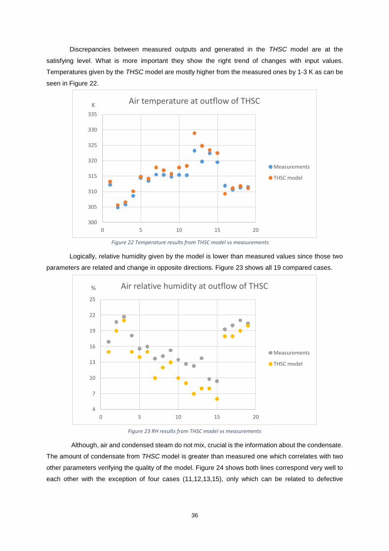
36

Discrepancies between measured outputs and generated in the THSC model are at the

satisfying level. What is more important they show the right trend of changes with input values.

Temperatures given by the THSC model are mostly higher from the measured ones by 1-3 K as can be

seen in Figure 22.

Logically, relative humidity given by the model is lower than measured values since those two

parameters are related and change in opposite directions. Figure 23 shows all 19 compared cases.

Although, air and condensed steam do not mix, crucial is the information about the condensate.

The amount of condensate from THSC model is greater than measured one which correlates with two

other parameters verifying the quality of the model. Figure 24 shows both lines correspond very well to

each other with the exception of four cases (11,12,13,15), only which can be related to defective

Figure 23 RH results from THSC model vs measurements

Figure 22 Temperature results from THSC model vs measurements

300

305

310

315

320

325

330

335

0 5 10 15 20

KAir temperature at outflow of THSC

Measurements

THSC model

4

7

10

13

16

19

22

25

0 5 10 15 20

% Air relative humidity at outflow of THSC

Measurements

THSC model

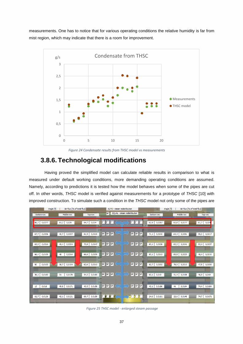
37

measurements. One has to notice that for various operating conditions the relative humidity is far from

mist region, which may indicate that there is a room for improvement.

3.8.6. Technological modifications

Having proved the simplified model can calculate reliable results in comparison to what is

measured under default working conditions, more demanding operating conditions are assumed.

Namely, according to predictions it is tested how the model behaves when some of the pipes are cut

off. In other words, THSC model is verified against measurements for a prototype of THSC [10] with

improved construction. To simulate such a condition in the THSC model not only some of the pipes are

Figure 25 THSC model - enlarged steam passage

Figure 24 Condensate results from THSC model vs measurements

0

0,5

1

1,5

2

2,5

3

0 5 10 15 20

g/s Condensate from THSC

Measurements

THSC model

38

assumed with zero air flow rate going through them but also the steam distribution is changed. The latter

is based on assumption when cutting first rows of pipes and enlarging the open space instead (red box

in Figure 25), the steam divides no longer with formula (25) but equally (EQUAL option switched on)

between both sections.

Until now, because of the very narrow passage, the right section is not enough used in

comparison to the left one limiting the amount of steam for right section [10]. It may happen the left one

works fully loaded along all its rows of pipes while the other one has steam only for the first few tiers.

Two approaches are tested to see whether the model is sensitive for a specific choice of row number.

Switching off the 1st and 8th tier in both sections as the first one and doing the same with 1st and 2nd

(counting from the steam inlets side). Both of them test whether the THSC model can visualize the

behaviour of THSC with changed geometry by cutting the pipes and influencing the steam distribution.

For a new prototype of THSC when 1st and 8th pipe are turned off the temperatures differ by

maximum 2.5 K between THSC model and what is measured: namely the worst results are observed in

cases (3, 4, 7, 9). Mostly those from THSC model are lower but still reach very satisfactory level of

correlation differing not more than 1 K which is presented in Figure 26.

For the same temperature comparison but with 1st and 2nd tier switched off THSC model give

higher values of these parameters which results in even better solution with respect to measurement.

Worse results with a difference over 1 K are for two cases (4 and 9). This increase of temperature means

more condensate appears from THSC which is correlated with Eps coefficients – higher in value for

consecutive rows of pipes. That is why for this case when 2nd row of pipes with worse Eps is turned off

instead of 8th one in the model more steam is condensed. Such a trend takes place only for steam flow

rate close to default one which is limited by correction coefficients. The graph is shown in Figure 27.

Figure 26 Temperature results from THSC model vs measurements – 1st and 8th tier switched off

309,00

310,00

311,00

312,00

313,00

314,00

315,00

316,00

0 2 4 6 8 10 12 14

K Air temperature at outflow of THSC

Measurements

THSC model

39

Comparing relative humidity the difference has not exceeded 4 percentage point between THSC

model and measurements. In case of switching off 1st and 8th tier the results can be checked in

Figure 28. Although having almost all temperatures from VBA lower than measured the corresponding

RH values are not always higher than measured ones, namely only half of them.

When changing the 8th tier into 2nd one the RH decreases and since previously half of them are

higher and the other half lower than measured values now most of them occurred below the measured

Figure 28 RH results from THSC model vs measurement - 1st and 8th tier switched off

Figure 27 Temperature results from THSC model vs measurement - 1st and 2nd tier switched off

15,00

17,00

19,00

21,00

23,00

25,00

27,00

29,00

31,00

0 2 4 6 8 10 12 14


Measurements

THSC model

309,00

310,00

311,00

312,00

313,00

314,00

315,00

316,00

0 2 4 6 8 10 12 14

K Air temperature at outflow of THSC

Measurements

THSC model

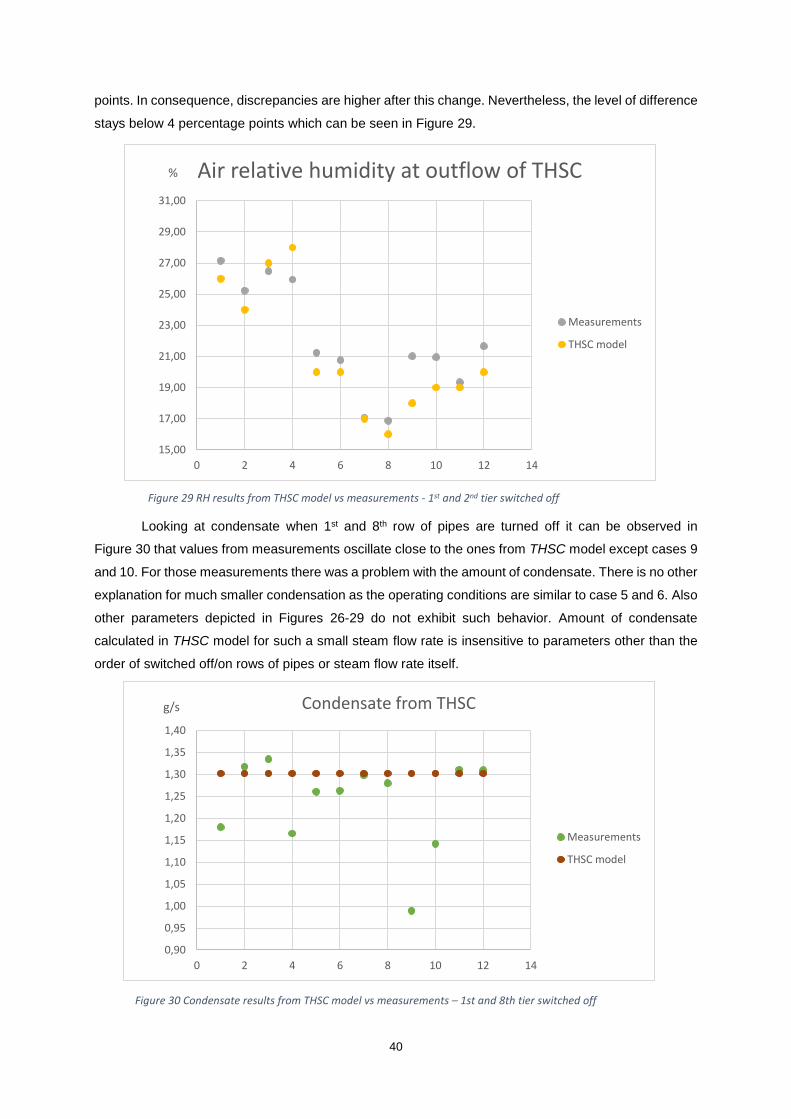
40

points. In consequence, discrepancies are higher after this change. Nevertheless, the level of difference

stays below 4 percentage points which can be seen in Figure 29.

Looking at condensate when 1st and 8th row of pipes are turned off it can be observed in

Figure 30 that values from measurements oscillate close to the ones from THSC model except cases 9

and 10. For those measurements there was a problem with the amount of condensate. There is no other

explanation for much smaller condensation as the operating conditions are similar to case 5 and 6. Also

other parameters depicted in Figures 26-29 do not exhibit such behavior. Amount of condensate

calculated in THSC model for such a small steam flow rate is insensitive to parameters other than the

order of switched off/on rows of pipes or steam flow rate itself.

Figure 29 RH results from THSC model vs measurements - 1st and 2nd tier switched off

Figure 30 Condensate results from THSC model vs measurements – 1st and 8th tier switched off

15,00

17,00

19,00

21,00

23,00

25,00

27,00

29,00

31,00

0 2 4 6 8 10 12 14


Measurements

THSC model

0,90

0,95

1,00

1,05

1,10

1,15

1,20

1,25

1,30

1,35

1,40

0 2 4 6 8 10 12 14


Measurements

THSC model

41

When switching 1st and 2nd rows of pipes the amount of condensate from THSC model is each

time greater than measured one which increased the average discrepancy of the results. The reason of

that is Eps value for 8th row is allowing to condense more than on 2nd pipe. The results are shown in

Figure 31.

Although, temperatures and relative humidity reach the satisfactory level the comparison of

condensate from THSC model with measured values shows it is insensitive to parameters change. Such

a behavior is an influence of Eps correction factors. When more front rows of pipes are turned off more

steam is led further and condensed there in a greater amount. Still, the difference in condensate values

relates to relatively low level (low RH) far from the region at which mixture of air/water mist can appear.

It has to be highlighted that above the level of limitation when the steam flow rate is high enough not

only each switched off row results in decreased condensate value but also other parameters influence

the results.

According to all analyses it is observed that the model is not perfectly corresponding to every

measurement [10]. Nevertheless, THSC model according to tested cases can be assumed as an

adequate tool to observe trends of change. Imperfections depending on simplification are small enough

to be accepted and worth time saved in comparison to the full model. But of course, it has to be

highlighted that such a model cannot be used as one and only tool for making final decisions. Any

change based on THSC model analysis before carrying it out has to be verified in real scale prototype

or at least fully developed CFD model.

4. Analysis of THSC work

The THSC is aimed to condensate steam and eliminate the risk of a mixture of air/water mist

appearance at the outlet. Therefore, the analysis which is presented further take into account worsening

conditions favourable water droplets creation at the outlet. The analysis is started for the input data from

base construction for which the THSC model is positively validated. The values taken for calculation can

Figure 31 Condensate results from THSC model vs measurements – 1st and 2nd tier switched off

0,90

0,95

1,00

1,05

1,10

1,15

1,20

1,25

1,30

1,35

1,40

0 5 10 15


Measurements

THSC model

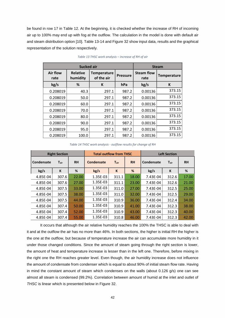
42

be found in row 17 in Table 12. At the beginning, it is checked whether the increase of RH of incoming

air up to 100% may end up with fog at the outflow. The calculation in the model is done with default air

and steam distribution option [10]. Table 13-14 and Figure 32 show input data, results and the graphical

representation of the solution respectively.

Table 13 THSC work analysis – increase of RH of air

Sucked air Steam

Air flow rate

Relative humidity


Pressure Steam flow

rate Temperature

kg/s % K hPa kg/s K

0.208019 40.3 297.1 987.2 0.00136 373.15

0.208019 50.0 297.1 987.2 0.00136 373.15

0.208019 60.0 297.1 987.2 0.00136 373.15

0.208019 70.0 297.1 987.2 0.00136 373.15

0.208019 80.0 297.1 987.2 0.00136 373.15

0.208019 90.0 297.1 987.2 0.00136 373.15

0.208019 95.0 297.1 987.2 0.00136 373.15

0.208019 100.0 297.1 987.2 0.00136 373.15

Table 14 THSC work analysis - outflow results for change of RH

Right Section Total outflow from THSC Left Section

Condensate Tair RH Condensate Tair RH Condensate Tair RH

kg/s K % kg/s K % kg/s K %

4.85E-04 307.6 22.00 1.35E-03 311.1 18.00 7.43E-04 312.6 17.00

4.85E-04 307.6 27.00 1.35E-03 311.1 23.00 7.43E-04 312.6 21.00

4.85E-04 307.5 33.00 1.35E-03 311.0 27.00 7.43E-04 312.5 25.00

4.85E-04 307.5 38.00 1.35E-03 311.0 32.00 7.43E-04 312.5 29.00

4.85E-04 307.5 44.00 1.35E-03 310.9 36.00 7.43E-04 312.4 34.00

4.85E-04 307.4 50.00 1.35E-03 310.9 41.00 7.43E-04 312.3 38.00

4.85E-04 307.4 52.00 1.35E-03 310.9 43.00 7.43E-04 312.3 40.00

4.85E-04 307.4 55.00 1.35E-03 310.8 46.00 7.43E-04 312.3 42.00

It occurs that although the air relative humidity reaches the 100% the THSC is able to deal with

it and at the outflow the air has no more than 46%. In both sections, the higher is initial RH the higher is

the one at the outflow, but because of temperature increase the air can accumulate more humidity in it

under those changed conditions. Since the amount of steam going through the right section is lower,

the amount of heat and temperature increase is lesser than in the left one. Therefore, before mixing in

the right one the RH reaches greater level. Even though, the air humidity increase does not influence

the amount of condensate from condenser which is equal to about 90% of initial steam flow rate. Having

in mind the constant amount of steam which condenses on the walls (about 0.126 g/s) one can see

almost all steam is condensed (99.2%). Correlation between amount of humid at the inlet and outlet of

THSC is linear which is presented below in Figure 32.

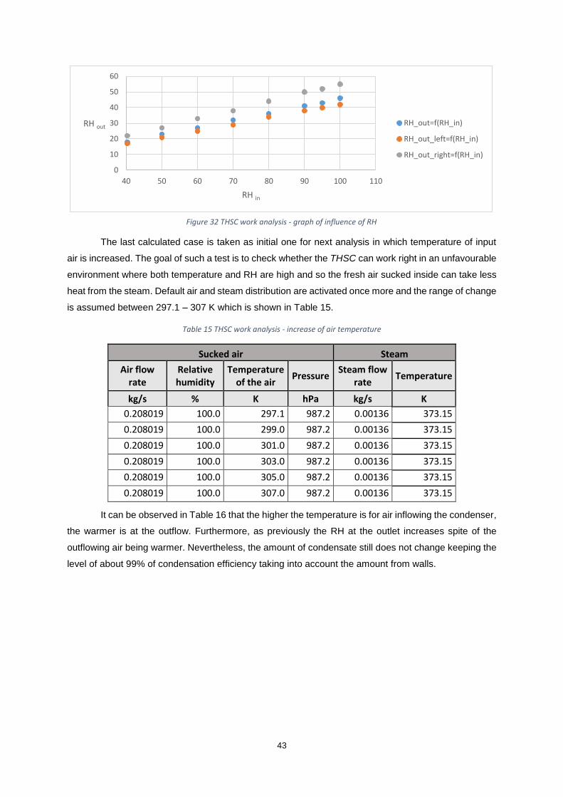
43

The last calculated case is taken as initial one for next analysis in which temperature of input

air is increased. The goal of such a test is to check whether the THSC can work right in an unfavourable

environment where both temperature and RH are high and so the fresh air sucked inside can take less

heat from the steam. Default air and steam distribution are activated once more and the range of change

is assumed between 297.1 – 307 K which is shown in Table 15.

Table 15 THSC work analysis - increase of air temperature

Sucked air Steam

Air flow rate

Relative humidity


Pressure Steam flow

rate Temperature

kg/s % K hPa kg/s K

0.208019 100.0 297.1 987.2 0.00136 373.15

0.208019 100.0 299.0 987.2 0.00136 373.15

0.208019 100.0 301.0 987.2 0.00136 373.15

0.208019 100.0 303.0 987.2 0.00136 373.15

0.208019 100.0 305.0 987.2 0.00136 373.15

0.208019 100.0 307.0 987.2 0.00136 373.15

It can be observed in Table 16 that the higher the temperature is for air inflowing the condenser,

the warmer is at the outflow. Furthermore, as previously the RH at the outlet increases spite of the

outflowing air being warmer. Nevertheless, the amount of condensate still does not change keeping the

level of about 99% of condensation efficiency taking into account the amount from walls.

0

10

20

30

40

50

60

40 50 60 70 80 90 100 110

RH out

RH in

RH_out=f(RH_in)

RH_out_left=f(RH_in)

RH_out_right=f(RH_in)

Figure 32 THSC work analysis - graph of influence of RH

44

Table 16 THSC work analysis - outflow results for change of temperature

Nevertheless, the initial conditions of the air do not result in fog appearance (a mixture of

air/water mist) neither at the outflow nor at any of the sections. One more time, because of the same

reason as previously, the temperature of the air in right section is lower. In consequence the relative

humidity reaches more percentage points comparing two the left one as in Figure 33.

Figure 33 THSC work analysis - graph of influence of temperature

The last analysis under default option is connected with steam flow rate increase. In this case,

amount of steam is the multiple of initial flow rate 0.00136 kg/s (like in first 9 rows in Table 17) until mass

flow rate reaches the value 0.01224 kg/s. Next cases are calculated with the same step but starting from

a doubled value equal to 0.02448 kg/s (given in 10th row which is double flow rate from 9th row).

40

45

50

55

60

296 298 300 302 304 306 308

RH

ou

t

T in

RH_out=f(T_in,RH_in_max)

RH_out_left=f(T_in,RH_in_max)

RH_out_right=f(T_in,RH_in_max)




4.85E-04 307.4 55.00 1.35E-03 310.8 46.00 7.43E-04 312.3 42.00

4.85E-04 309.3 56.00 1.35E-03 312.7 46.00 7.43E-04 314.1 43.00

4.85E-04 311.2 56.00 1.35E-03 314.6 47.00 7.43E-04 316.1 44.00

4.85E-04 313.1 57.00 1.35E-03 316.5 48.00 7.43E-04 318.0 44.00

4.85E-04 315.1 58.00 1.35E-03 318.5 48.00 7.43E-04 319.9 45.00

4.85E-04 317.0 58.00 1.35E-03 320.4 49.00 7.43E-04 321.8 46.00

45

Table 17 THSC work analysis - increase of steam flow rate

Sucked air Steam

Air flow rate

Relative humidity


Pressure Steam flow

rate Temperature

kg/s % K hPa kg/s K

0.208019 100.0 307.0 987.2 0.00136 373.15

0.208019 100.0 307.0 987.2 0.00272 373.15

0.208019 100.0 307.0 987.2 0.00408 373.15

0.208019 100.0 307.0 987.2 0.00544 373.15

0.208019 100.0 307.0 987.2 0.0068 373.15

0.208019 100.0 307.0 987.2 0.00816 373.15

0.208019 100.0 307.0 987.2 0.00952 373.15

0.208019 100.0 307.0 987.2 0.01088 373.15

0.208019 100.0 307.0 987.2 0.01224 373.15

0.208019 100.0 307.0 987.2 0.02448 373.15

0.208019 100.0 307.0 987.2 0.02584 373.15

0.208019 100.0 307.0 987.2 0.0272 373.15

0.208019 100.0 307.0 987.2 0.02856 373.15

0.208019 100.0 307.0 987.2 0.02992 373.15

0.208019 100.0 307.0 987.2 0.03128 373.15

0.208019 100.0 307.0 987.2 0.03264 373.15

0.208019 100.0 307.0 987.2 0.034 373.15

0.208019 100.0 307.0 987.2 0.03536 373.15

Increasing the amount of steam from first three cases is low enough to be limited by Eps

coefficients. That is the reason why temperature is getting higher while the relative humidity value drops.

Amount of condensate increases while increasing the steam flow rate depending on Eps limitation.

When the same amount of steam is higher like in next rows the THSC works with maximum possible

power since there is enough steam inside it to be sure pipes are all the time surrounded by steam.

Thenceforth, the amount of condensate does not change and each additional portion of steam

results in increased humidity at the end. Although the pipes work with maximum power, condensation

efficiency decreases while steam flow rate is increasing since the amount of condensate compared to

enlarging amount of steam give lower percentage results. One more thing is worth underlining in this

place. Since the model at the end takes into account both heat losses through the walls and the water

condensed on the walls which give bigger value, the temperature at the outflow is higher than the ones

from both left and right section. Particular values can be checked both in Table 18 and Figure 34-35.

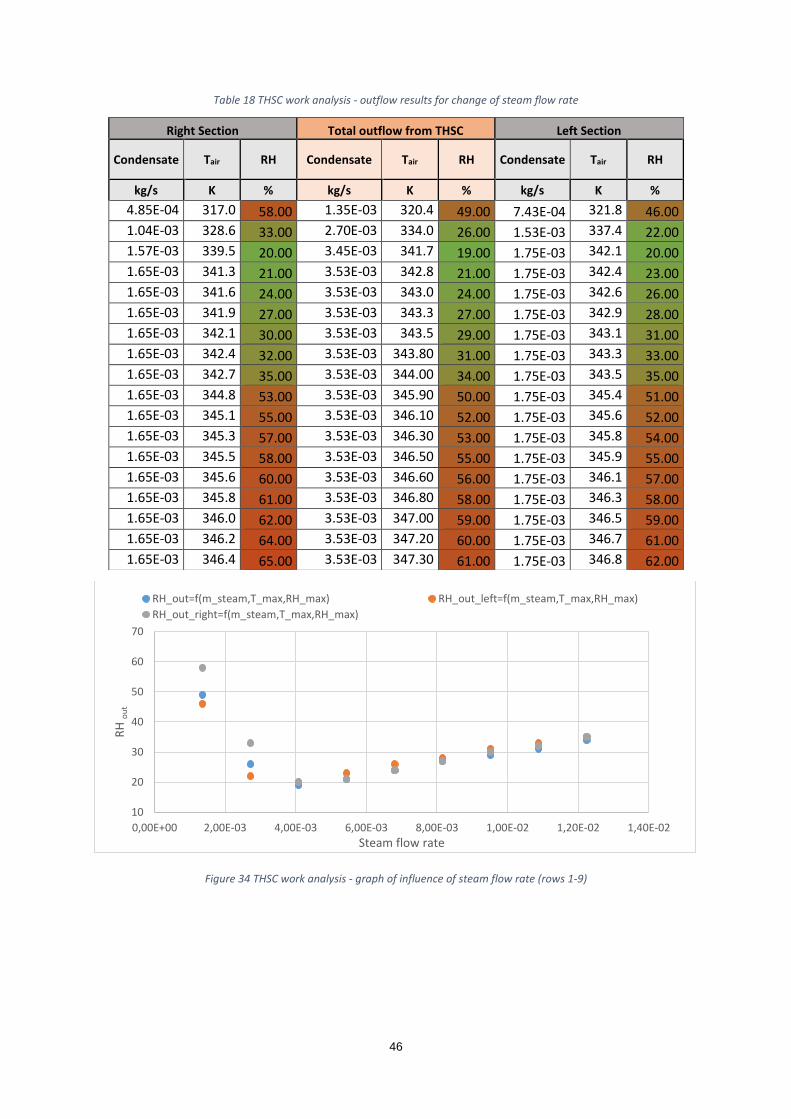
46

Table 18 THSC work analysis - outflow results for change of steam flow rate

Figure 34 THSC work analysis - graph of influence of steam flow rate (rows 1-9)

10

20

30

40

50

60

70

0,00E+00 2,00E-03 4,00E-03 6,00E-03 8,00E-03 1,00E-02 1,20E-02 1,40E-02

RH

ou

t

Steam flow rate

RH_out=f(m_steam,T_max,RH_max) RH_out_left=f(m_steam,T_max,RH_max)

RH_out_right=f(m_steam,T_max,RH_max)




4.85E-04 317.0 58.00 1.35E-03 320.4 49.00 7.43E-04 321.8 46.00

1.04E-03 328.6 33.00 2.70E-03 334.0 26.00 1.53E-03 337.4 22.00

1.57E-03 339.5 20.00 3.45E-03 341.7 19.00 1.75E-03 342.1 20.00

1.65E-03 341.3 21.00 3.53E-03 342.8 21.00 1.75E-03 342.4 23.00

1.65E-03 341.6 24.00 3.53E-03 343.0 24.00 1.75E-03 342.6 26.00

1.65E-03 341.9 27.00 3.53E-03 343.3 27.00 1.75E-03 342.9 28.00

1.65E-03 342.1 30.00 3.53E-03 343.5 29.00 1.75E-03 343.1 31.00

1.65E-03 342.4 32.00 3.53E-03 343.80 31.00 1.75E-03 343.3 33.00

1.65E-03 342.7 35.00 3.53E-03 344.00 34.00 1.75E-03 343.5 35.00

1.65E-03 344.8 53.00 3.53E-03 345.90 50.00 1.75E-03 345.4 51.00

1.65E-03 345.1 55.00 3.53E-03 346.10 52.00 1.75E-03 345.6 52.00

1.65E-03 345.3 57.00 3.53E-03 346.30 53.00 1.75E-03 345.8 54.00

1.65E-03 345.5 58.00 3.53E-03 346.50 55.00 1.75E-03 345.9 55.00

1.65E-03 345.6 60.00 3.53E-03 346.60 56.00 1.75E-03 346.1 57.00

1.65E-03 345.8 61.00 3.53E-03 346.80 58.00 1.75E-03 346.3 58.00

1.65E-03 346.0 62.00 3.53E-03 347.00 59.00 1.75E-03 346.5 59.00

1.65E-03 346.2 64.00 3.53E-03 347.20 60.00 1.75E-03 346.7 61.00

1.65E-03 346.4 65.00 3.53E-03 347.30 61.00 1.75E-03 346.8 62.00

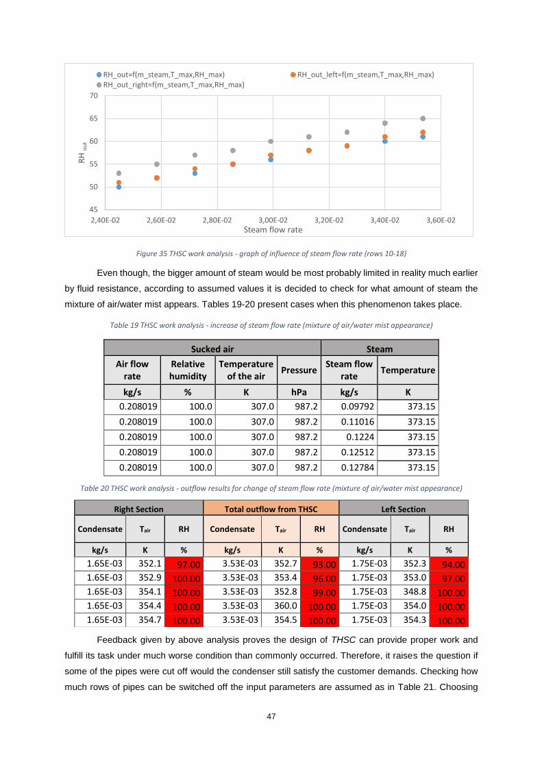
47

Figure 35 THSC work analysis - graph of influence of steam flow rate (rows 10-18)

Even though, the bigger amount of steam would be most probably limited in reality much earlier

by fluid resistance, according to assumed values it is decided to check for what amount of steam the

mixture of air/water mist appears. Tables 19-20 present cases when this phenomenon takes place.

Table 19 THSC work analysis - increase of steam flow rate (mixture of air/water mist appearance)

Sucked air Steam

Air flow rate

Relative humidity


Pressure Steam flow

rate Temperature

kg/s % K hPa kg/s K

0.208019 100.0 307.0 987.2 0.09792 373.15

0.208019 100.0 307.0 987.2 0.11016 373.15

0.208019 100.0 307.0 987.2 0.1224 373.15

0.208019 100.0 307.0 987.2 0.12512 373.15

0.208019 100.0 307.0 987.2 0.12784 373.15

Table 20 THSC work analysis - outflow results for change of steam flow rate (mixture of air/water mist appearance)

Feedback given by above analysis proves the design of THSC can provide proper work and

fulfill its task under much worse condition than commonly occurred. Therefore, it raises the question if

some of the pipes were cut off would the condenser still satisfy the customer demands. Checking how

much rows of pipes can be switched off the input parameters are assumed as in Table 21. Choosing

45

50

55

60

65

70

2,40E-02 2,60E-02 2,80E-02 3,00E-02 3,20E-02 3,40E-02 3,60E-02

RH

ou

t

Steam flow rate

RH_out=f(m_steam,T_max,RH_max) RH_out_left=f(m_steam,T_max,RH_max)RH_out_right=f(m_steam,T_max,RH_max)




1.65E-03 352.1 97.00 3.53E-03 352.7 93.00 1.75E-03 352.3 94.00

1.65E-03 352.9 100.00 3.53E-03 353.4 96.00 1.75E-03 353.0 97.00

1.65E-03 354.1 100.00 3.53E-03 352.8 99.00 1.75E-03 348.8 100.00

1.65E-03 354.4 100.00 3.53E-03 360.0 100.00 1.75E-03 354.0 100.00

1.65E-03 354.7 100.00 3.53E-03 354.5 100.00 1.75E-03 354.3 100.00

48

the user-defined option instead of default one the number of working pipes and fluid distribution can be

controlled. Rows of pipes are counted from steam inlets to air fan (1 for top one and 8 for bottom one in

Figure 42 in Appendix A). Two approaches are examined with the same, unchanged amount of inlet air

which is equally redistributed between the rest off working pipes (chosen option - Assume initial air flow

rate in Figure 42).

Table 21 THSC work analysis - input data for pipes modification

Sucked air Steam

Air flow rate

Relative humidity


Pressure Steam flow

rate Temperature

kg/s % K hPa kg/s K

0.208019 100.0 307.0 987.2 0.00136 373.15

Firstly, it is assumed the rows of pipes are switched off symmetrically. It means when turning

off the first row of pipes in both left and right section three pipes are chosen as not working in each,

which gives six pipes in total. In addition to this, the steam flow rate is distributed equally between

sections starting from the case when first rows of pipes are switched off (chosen option – EQUAL in

Figure 42). Such an assumption checks whether enlarging of steam passage in lieu of first rows of pipes

can give satisfactory effect. From the moment when 3 or more tiers are turned off, the model informs

that calculation based on air mass flow rate enters extrapolation region. Nevertheless, THSC works right

even with only 2 last rows of pipes. When trying to switch off the 7th one model is too far from the

analyzed region where power starts to be negative which is not feasible. It might be said that with no

consequence the first rows of pipes can be switched off since there is no change at the outflow.

Nevertheless, condensation efficiency is kept around 99% until the 4th row is switched off when

condensate decreases up to 1.33 g/s. The results can be observed in Table 22.

Table 22 THSC work analysis - outflow results for change of pipes with equal distribution of steam

To be sure, the steam distribution is not influencing significantly the results in the same approach

the calculations are repeated with the steam flow rate distributed according to internal formula

dependent on the amount of steam inflowing the THSC (EQUAL option is not activated). In this case,

steam passage stays the same although the pipes are switched off while all the other assumptions are

as those described above. The same communications about extrapolation and negative power appear


Switched off rows of pipes Condensate Tair RH Condensate Tair RH Condensate Tair RH

number kg/s K % kg/s K % kg/s K %

- 4.85E-04 317.0 58.00 1.35E-03 320.4 49.00 7.43E-04 321.8 46.00

1 6.13E-04 319.7 51.00 1.35E-03 320.3 49.00 6.13E-04 319.2 52.00

1,2 6.12E-04 319.6 51.00 1.35E-03 320.3 49.00 6.12E-04 319.2 52.00

1,2,3 6.07E-04 319.5 51.00 1.34E-03 320.3 50.00 6.10E-04 319.2 52.00

1,2,3,4 6.00E-04 319.4 52.00 1.33E-03 320.1 50.00 6.04E-04 319.1 53.00

1,2,3,4,5 5.93E-04 319.2 52.00 1.32E-03 320.0 50.00 5.98E-04 319.0 53.00

1,2,3,4,5,6 5.78E-04 318.9 54.00 1.29E-03 319.7 51.00 5.84E-04 318.7 54.00

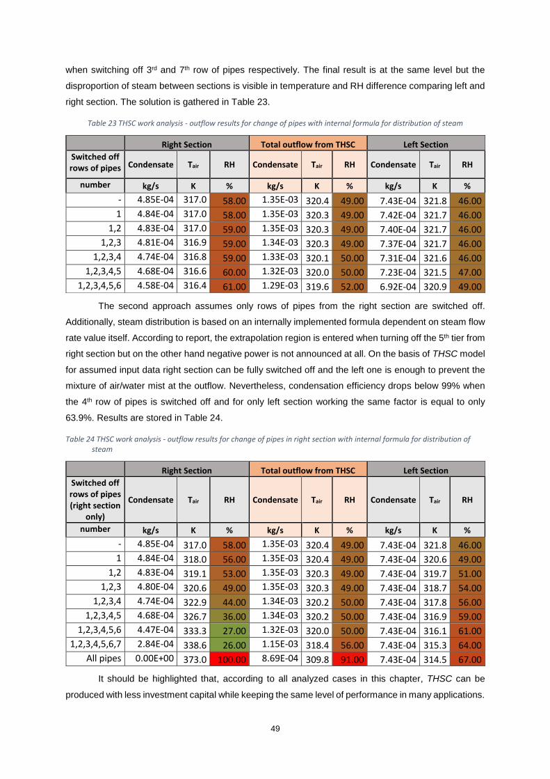
49

when switching off 3rd and 7th row of pipes respectively. The final result is at the same level but the

disproportion of steam between sections is visible in temperature and RH difference comparing left and

right section. The solution is gathered in Table 23.

Table 23 THSC work analysis - outflow results for change of pipes with internal formula for distribution of steam

The second approach assumes only rows of pipes from the right section are switched off.

Additionally, steam distribution is based on an internally implemented formula dependent on steam flow

rate value itself. According to report, the extrapolation region is entered when turning off the 5th tier from

right section but on the other hand negative power is not announced at all. On the basis of THSC model

for assumed input data right section can be fully switched off and the left one is enough to prevent the

mixture of air/water mist at the outflow. Nevertheless, condensation efficiency drops below 99% when

the 4th row of pipes is switched off and for only left section working the same factor is equal to only

63.9%. Results are stored in Table 24.

Table 24 THSC work analysis - outflow results for change of pipes in right section with internal formula for distribution of steam

It should be highlighted that, according to all analyzed cases in this chapter, THSC can be

produced with less investment capital while keeping the same level of performance in many applications.


Switched off rows of pipes Condensate Tair RH Condensate Tair RH Condensate Tair RH


- 4.85E-04 317.0 58.00 1.35E-03 320.4 49.00 7.43E-04 321.8 46.00

1 4.84E-04 317.0 58.00 1.35E-03 320.3 49.00 7.42E-04 321.7 46.00

1,2 4.83E-04 317.0 59.00 1.35E-03 320.3 49.00 7.40E-04 321.7 46.00

1,2,3 4.81E-04 316.9 59.00 1.34E-03 320.3 49.00 7.37E-04 321.7 46.00

1,2,3,4 4.74E-04 316.8 59.00 1.33E-03 320.1 50.00 7.31E-04 321.6 46.00

1,2,3,4,5 4.68E-04 316.6 60.00 1.32E-03 320.0 50.00 7.23E-04 321.5 47.00

1,2,3,4,5,6 4.58E-04 316.4 61.00 1.29E-03 319.6 52.00 6.92E-04 320.9 49.00


Switched off rows of pipes (right section

only)



- 4.85E-04 317.0 58.00 1.35E-03 320.4 49.00 7.43E-04 321.8 46.00

1 4.84E-04 318.0 56.00 1.35E-03 320.4 49.00 7.43E-04 320.6 49.00

1,2 4.83E-04 319.1 53.00 1.35E-03 320.3 49.00 7.43E-04 319.7 51.00

1,2,3 4.80E-04 320.6 49.00 1.35E-03 320.3 49.00 7.43E-04 318.7 54.00

1,2,3,4 4.74E-04 322.9 44.00 1.34E-03 320.2 50.00 7.43E-04 317.8 56.00

1,2,3,4,5 4.68E-04 326.7 36.00 1.34E-03 320.2 50.00 7.43E-04 316.9 59.00

1,2,3,4,5,6 4.47E-04 333.3 27.00 1.32E-03 320.0 50.00 7.43E-04 316.1 61.00

1,2,3,4,5,6,7 2.84E-04 338.6 26.00 1.15E-03 318.4 56.00 7.43E-04 315.3 64.00

All pipes 0.00E+00 373.0 100.00 8.69E-04 309.8 91.00 7.43E-04 314.5 67.00

50

In other words, it is recommended to consider the production of a few versions of the same THSC but

with a limited amount of rows of pipes inside it. Such an unsophisticated change would not influence

significantly the process of either production the THSC or its fitting together with already produced

ovens. At the same time, a removal of any number of internally finned pipes would decrease the

production cost of the whole device.

Apart from this, the THSC model is compared with measured results and as a simplified version

of fully developed CFD model it generates a solution with acceptable discrepancy taking into account

the availability of the software and relatively much shorter time needed for any kind of analysis done by

the user.

51

5. Conclusions

Within the framework of this thesis, a top hood steam condenser mathematical model is

developed. Its final version written in Visual Basic for Application in Excel satisfies the Retech company

needs to have software for private use free of paid license and straightforward for users without specific

technical background. Satisfying all the demands there are required not only global mass and energy

balances but also an empirical equation of a single pipe and other correlations.

Work on the full steam condenser model consists of several stages starting from CFD

simulation, through GUI creation and implementation of developed single pipe thermal response model

up to validation the THSC model against measurements and preliminary analysis of possible change.

The first conclusion is related to building a geometry and a mesh of the single pipe which has

to be fully structural hexahedral one. If non-structural or mixed mesh appeared the quality of solution

would be significantly decreased and influence final results [3]. Based on that, it is crucial to create the

mentioned geometry that consisted of only separate, replicated quadrilateral sketches.

Furthermore, the mesh aimed at solving the heat transfer phenomena can be simplified. Indeed,

all the chamfers and filletings are eliminated improving the feasibility of the numerical solution in Fluent

[3]. From the heat transfer point of view that change has negligible influence and that is why it is accepted

without any hazard for results.

Another limitation, which strongly influences the development of single pipe model, is to use a

student Ansys license which allows for usage of only half of a million elements mesh. Such model is

successfully validated against benchmark prepared with the full version of the Fluent. The goal is

achieved by refining the mesh inside and nearby the fins where the heat transfer is intense at the cost

of the elements in the core of the pipe. The right approach to mesh creation and specific settings with

chosen models in Fluent plays crucial role from the technical point of view.

Nevertheless, one of the most important conclusions of the thesis is that usage of tabular

efficiencies for fins would negatively affects the results. At first sight, values computed for externally

finned pipes can be applied for this rare situation of internally mounted fins. Such an approach would

be wrong if it were accepted. According to heat transfer coefficient from a few cases calculated in Fluent,

the efficiencies for internal and external fins on the same geometry are compared. Each time the

efficiency of the internally installed fins is 5 to 6 percentage points lower than for tabular ones, which

are very accurate. Lack of correspondence between efficiencies proves different behaviours depending

on the place of fins mounting. Thus, decision of single pipe modeling in Fluent in this particular case is

reasonable.

Since each simulation in Fluent lasts relatively long time and it is impossible to check all

configurations the representative amount of cases is chosen to cover the widest possible distribution of

the parameters within variants. Influence of five chosen factors on the power of the pipe is analyzed and

used as the basis for formula implemented to VBA code. From the simulation, it occurs that the power

in single pipe grows mostly along with mass flow rate of air. More important is the fact, for values greater

52

than 0.0167 kg/s the behaviour is inversed with decreasing power trendline. Since this is unacceptable

it is limited by internal conditions in THSC model. For the rest of the factors such a phenomenon does

not appear and so they can be limited within the just feasible range of input data.

An empirical equation is developed after testing four different approaches. The chosen one is

based on air mass flow rate as the most influential factor. For all of them, Excel coefficients are taken

from trendlines. Except air mass flow rate parameter other four are treated as correction factors in

equation (16). Such a decision is made with respect to the smallest maximum error (1.5%) comparing

all variants. The final empirical equation aim is assumed to model the single pipe work equally good

within the whole range of solutions. That is why other variants having smaller average errors with some

exceptions reaching 2% or even more are rejected.

As it is already mentioned the user should not be obliged to know either the fundamentals of

heat transfer phenomenon or use sophisticated CFD simulation software. Therefore, widely available

Excel with VBA is chosen to create the fully developed model. The interface connecting the user with

the software is designed with transparent GUIs which guide him through the whole procedure of data

implementation. Mistakes like wrong format or values entering the extrapolation region are verified by

conditions embedded in the model. Such an approach minimizes user errors since model helps to

localize the source of the problem or eliminates them fully. Such a user-friendly model let the process

of usage acceptable for any employee being its huge asset from the company point of view.

Assumed simplifications and built-in equations like the one for the power and Eps correction

factors result in some discrepancies comparing results from the model to the measured ones [10].

Nevertheless, the model allows the user to observe right trends of changes and results at satisfactory

level. On the other hand, computing power and time needed for calculation in THSC model is orders of

magnitude smaller than using the whole THSC Fluent model. It is worth mentioning that the single

change in the Fluent model of THSC may take from a few hours to weeks to converge the model while

work with the THSC model is limited to a couple of seconds. Taking into account all the aspects the

existence of such a tool facilitates preliminary analysis with a much lower cost both human power and

monetary.

The last but not least conclusion comes from the analysis carried out with the THSC model. The

analysis is aimed to verify whether the considered design of THSC, which is on sale in a single variant,

is over-scaled in many appliances and demonstrate the theory that there is the margin for optimization.

According to received results it occurs the THSC is most probably overscaled since even much worse

operating conditions do not result in a mixture of air/water mist appearance at the outflow which is a

disqualifying factor. Nevertheless, the amount of condensate decreases and so, related with it,

condensation efficiency of a device also decreases.

For a relative humidity of inlet air equal to 100%, the RH of the outflowing air reaches maximum

of 46%. Adding to this the inlet air temperature increase up to 307 K results in only 3 more percentage

point in RH at the outflow. The condensation efficiency in both cases does not drop below 99% (taking

into account that constant value of 0.126 g/s of steam which is condensed on the walls). Keeping those

two parameters and increasing the steam mass flow rate, the amount of humidity does not exceed the

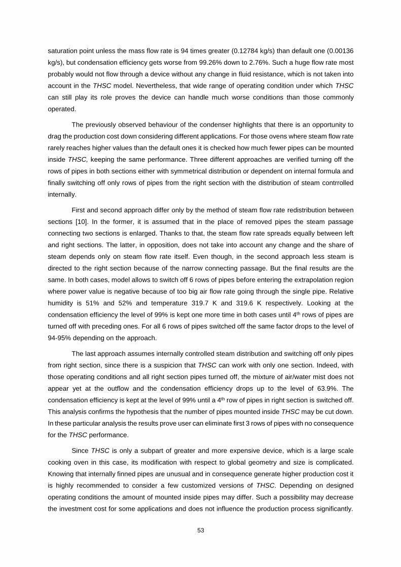
53

saturation point unless the mass flow rate is 94 times greater (0.12784 kg/s) than default one (0.00136

kg/s), but condensation efficiency gets worse from 99.26% down to 2.76%. Such a huge flow rate most

probably would not flow through a device without any change in fluid resistance, which is not taken into

account in the THSC model. Nevertheless, that wide range of operating condition under which THSC

can still play its role proves the device can handle much worse conditions than those commonly

operated.

The previously observed behaviour of the condenser highlights that there is an opportunity to

drag the production cost down considering different applications. For those ovens where steam flow rate

rarely reaches higher values than the default ones it is checked how much fewer pipes can be mounted

inside THSC, keeping the same performance. Three different approaches are verified turning off the

rows of pipes in both sections either with symmetrical distribution or dependent on internal formula and

finally switching off only rows of pipes from the right section with the distribution of steam contrrolled

internally.

First and second approach differ only by the method of steam flow rate redistribution between

sections [10]. In the former, it is assumed that in the place of removed pipes the steam passage

connecting two sections is enlarged. Thanks to that, the steam flow rate spreads equally between left

and right sections. The latter, in opposition, does not take into account any change and the share of

steam depends only on steam flow rate itself. Even though, in the second approach less steam is

directed to the right section because of the narrow connecting passage. But the final results are the

same. In both cases, model allows to switch off 6 rows of pipes before entering the extrapolation region

where power value is negative because of too big air flow rate going through the single pipe. Relative

humidity is 51% and 52% and temperature 319.7 K and 319.6 K respectively. Looking at the

condensation efficiency the level of 99% is kept one more time in both cases until 4th rows of pipes are

turned off with preceding ones. For all 6 rows of pipes switched off the same factor drops to the level of

94-95% depending on the approach.

The last approach assumes internally controlled steam distribution and switching off only pipes

from right section, since there is a suspicion that THSC can work with only one section. Indeed, with

those operating conditions and all right section pipes turned off, the mixture of air/water mist does not

appear yet at the outflow and the condensation efficiency drops up to the level of 63.9%. The

condensation efficiency is kept at the level of 99% until a 4th row of pipes in right section is switched off.

This analysis confirms the hypothesis that the number of pipes mounted inside THSC may be cut down.

In these particular analysis the results prove user can eliminate first 3 rows of pipes with no consequence

for the THSC performance.

Since THSC is only a subpart of greater and more expensive device, which is a large scale

cooking oven in this case, its modification with respect to global geometry and size is complicated.

Knowing that internally finned pipes are unusual and in consequence generate higher production cost it

is highly recommended to consider a few customized versions of THSC. Depending on designed

operating conditions the amount of mounted inside pipes may differ. Such a possibility may decrease

the investment cost for some applications and does not influence the production process significantly.

54

Moreover, this kind of change does not hamper the fitting of THSC as subpart with the more expensive

product - oven.

One of the main aims of the thesis is to find out whether the THSC model with implemented

CFD single pipe model may correlate with the actual THSC. Successfully accomplished goal saves time

and human power being used by Retech company for improvements of the device. For this particular

model, it can be checked how the changes in working conditions and geometry influence the

performance of THSC. Results comparing to measurements reach a satisfactory level of accuracy.

Nevertheless, future work in this field is required in order to extend the possible range of analyzed

operating conditions. In addition, other approaches to correction factors can be used to develop the

model and for improvement of the overall results quality. What is more, the same idea of the model can

be used for other equipments if needed since the Retech company produces a dozen of similar devices.

The process of their development, as well as the one considered in this work, would proceed more

efficiently when combined with user-friendly software. Easy to access, THSC models without huge

investment costs can lead to better device performance and reduced expenditures thanks to quickly

forecasted results of changes. The same model can allow a higher level of device customization which

makes both the product more desirable from the customer point of view and saves raw materials if not

needed for production which makes the process more eco-friendly.

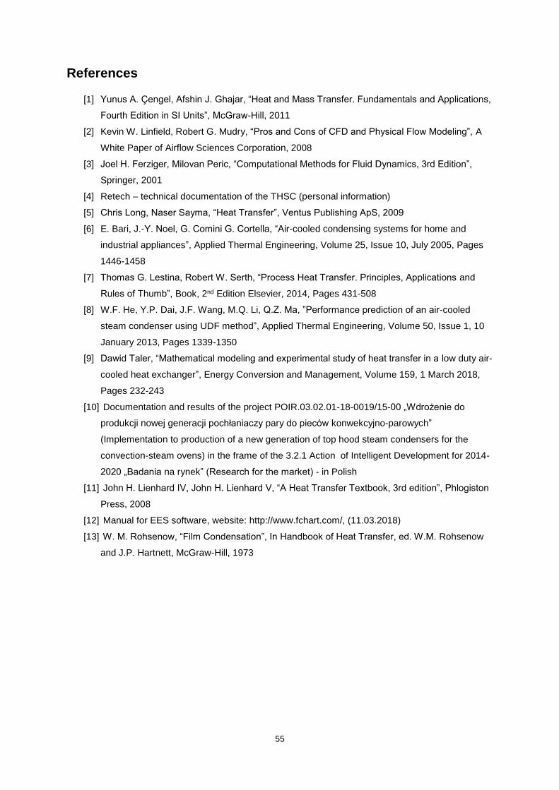
55

References

[1] Yunus A. Çengel, Afshin J. Ghajar, “Heat and Mass Transfer. Fundamentals and Applications,

Fourth Edition in SI Units”, McGraw-Hill, 2011

[2] Kevin W. Linfield, Robert G. Mudry, “Pros and Cons of CFD and Physical Flow Modeling”, A

White Paper of Airflow Sciences Corporation, 2008

[3] Joel H. Ferziger, Milovan Peric, “Computational Methods for Fluid Dynamics, 3rd Edition”,

Springer, 2001

[4] Retech – technical documentation of the THSC (personal information)

[5] Chris Long, Naser Sayma, “Heat Transfer”, Ventus Publishing ApS, 2009

[6] E. Bari, J.-Y. Noel, G. Comini G. Cortella, “Air-cooled condensing systems for home and

industrial appliances”, Applied Thermal Engineering, Volume 25, Issue 10, July 2005, Pages

1446-1458

[7] Thomas G. Lestina, Robert W. Serth, “Process Heat Transfer. Principles, Applications and

Rules of Thumb”, Book, 2nd Edition Elsevier, 2014, Pages 431-508

[8] W.F. He, Y.P. Dai, J.F. Wang, M.Q. Li, Q.Z. Ma, ”Performance prediction of an air-cooled

steam condenser using UDF method”, Applied Thermal Engineering, Volume 50, Issue 1, 10

January 2013, Pages 1339-1350

[9] Dawid Taler, “Mathematical modeling and experimental study of heat transfer in a low duty air-

cooled heat exchanger”, Energy Conversion and Management, Volume 159, 1 March 2018,

Pages 232-243

[10] Documentation and results of the project POIR.03.02.01-18-0019/15-00 „Wdrożenie do

produkcji nowej generacji pochłaniaczy pary do pieców konwekcyjno-parowych”

(Implementation to production of a new generation of top hood steam condensers for the

convection-steam ovens) in the frame of the 3.2.1 Action of Intelligent Development for 2014-

2020 „Badania na rynek” (Research for the market) - in Polish

[11] John H. Lienhard IV, John H. Lienhard V, “A Heat Transfer Textbook, 3rd edition”, Phlogiston

Press, 2008

[12] Manual for EES software, website: http://www.fchart.com/, (11.03.2018)

[13] W. M. Rohsenow, “Film Condensation”, In Handbook of Heat Transfer, ed. W.M. Rohsenow

and J.P. Hartnett, McGraw-Hill, 1973

56

Appendix

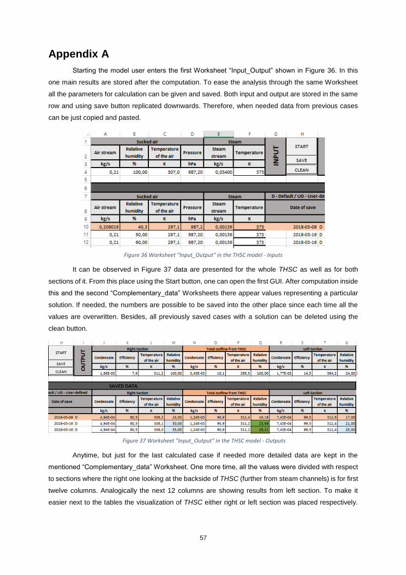
57

Appendix A

Starting the model user enters the first Worksheet “Input_Output” shown in Figure 36. In this

one main results are stored after the computation. To ease the analysis through the same Worksheet

all the parameters for calculation can be given and saved. Both input and output are stored in the same

row and using save button replicated downwards. Therefore, when needed data from previous cases

can be just copied and pasted.

It can be observed in Figure 37 data are presented for the whole THSC as well as for both

sections of it. From this place using the Start button, one can open the first GUI. After computation inside

this and the second “Complementary_data” Worksheets there appear values representing a particular

solution. If needed, the numbers are possible to be saved into the other place since each time all the

values are overwritten. Besides, all previously saved cases with a solution can be deleted using the

clean button.

Anytime, but just for the last calculated case if needed more detailed data are kept in the

mentioned “Complementary_data” Worksheet. One more time, all the values were divided with respect

to sections where the right one looking at the backside of THSC (further from steam channels) is for first

twelve columns. Analogically the next 12 columns are showing results from left section. To make it

easier next to the tables the visualization of THSC either right or left section was placed respectively.

Figure 37 Worksheet "Input_Output" in the THSC model - Outputs

Figure 36 Worksheet "Input_Output" in the THSC model - Inputs

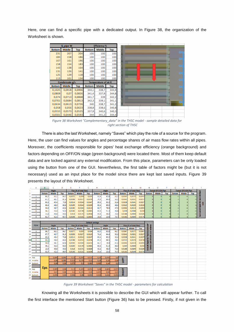
58

Here, one can find a specific pipe with a dedicated output. In Figure 38, the organization of the

Worksheet is shown.

There is also the last Worksheet, namely “Saves” which play the role of a source for the program.

Here, the user can find values for angles and percentage shares of air mass flow rates within all pipes.

Moreover, the coefficients responsible for pipes' heat exchange efficiency (orange background) and

factors depending on OFF/ON stage (green background) were located there. Most of them keep default

data and are locked against any external modification. From this place, parameters can be only loaded

using the button from one of the GUI. Nevertheless, the first table of factors might be (but it is not

necessary) used as an input place for the model since there are kept last saved inputs. Figure 39

presents the layout of this Worksheet.

Knowing all the Worksheets it is possible to describe the GUI which will appear further. To call

the first interface the mentioned Start button (Figure 36) has to be pressed. Firstly, if not given in the

Figure 39 Worksheet "Saves" in the THSC model - parameters for calculation

Figure 38 Worksheet "Complementary_data" in the THSC model - sample detailed data for right section of THSC

59

Worksheet then here the Inputs can be specified or modified. Moreover, before calculation necessary is

to decide whether the VBA should use the default values or the user is willing to specify more details.

In Figure 40, the first GUI is presented.

Units and last used values for both air and steam set an example of a possible input to be

entered. If not enough then user can find a wider explanation by clicking Help button (Figure 40). There

one can find also a description of two possible options of calculation, the feasible, recommended ranges

and crucial tips. How the Help GUI looks like can be observed in Figure 41.

Assuming the default option was to be used the next GUI would show the pre-defined angles

and air flow rate shares with visualization of internal distribution [10]. At this stage, the user can accept

the conditions as they are or go back and decide on user-defined working conditions. The same window

would appear for a user-defined option with additional options. Therefore, in Figure 42, the presented

interface is not the one for basic, default model but the second in which user can implement changes.

Figure 40 GUI1 - Initial Data for Top Hood Steam Condenser

Figure 41 GUI1 - Help

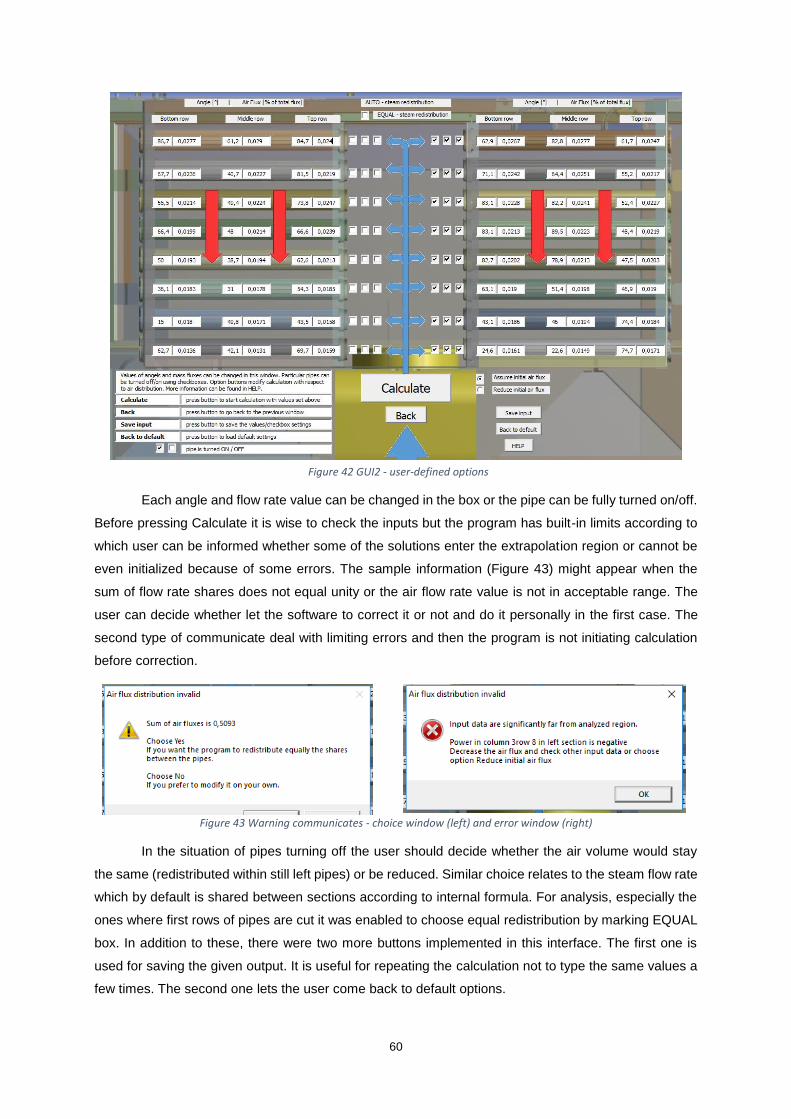
60

Each angle and flow rate value can be changed in the box or the pipe can be fully turned on/off.

Before pressing Calculate it is wise to check the inputs but the program has built-in limits according to

which user can be informed whether some of the solutions enter the extrapolation region or cannot be

even initialized because of some errors. The sample information (Figure 43) might appear when the

sum of flow rate shares does not equal unity or the air flow rate value is not in acceptable range. The

user can decide whether let the software to correct it or not and do it personally in the first case. The

second type of communicate deal with limiting errors and then the program is not initiating calculation

before correction.

Figure 43 Warning communicates - choice window (left) and error window (right)

In the situation of pipes turning off the user should decide whether the air volume would stay

the same (redistributed within still left pipes) or be reduced. Similar choice relates to the steam flow rate

which by default is shared between sections according to internal formula. For analysis, especially the

ones where first rows of pipes are cut it was enabled to choose equal redistribution by marking EQUAL

box. In addition to these, there were two more buttons implemented in this interface. The first one is

used for saving the given output. It is useful for repeating the calculation not to type the same values a

few times. The second one lets the user come back to default options.

Figure 42 GUI2 - user-defined options

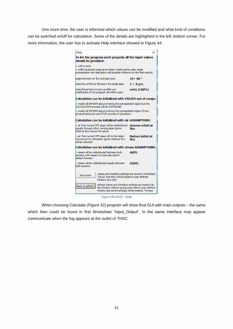
61

One more time, the user is informed which values can be modified and what kind of conditions

can be switched on/off for calculation. Some of the details are highlighted in the left, bottom corner. For

more information, the user has to activate Help interface showed in Figure 44.

When choosing Calculate (Figure 42) program will show final GUI with main outputs – the same

which then could be found in first Worksheet “Input_Output”. In the same interface may appear

communicate when the fog appears at the outlet of THSC.

Figure 44 GUI2 - Help

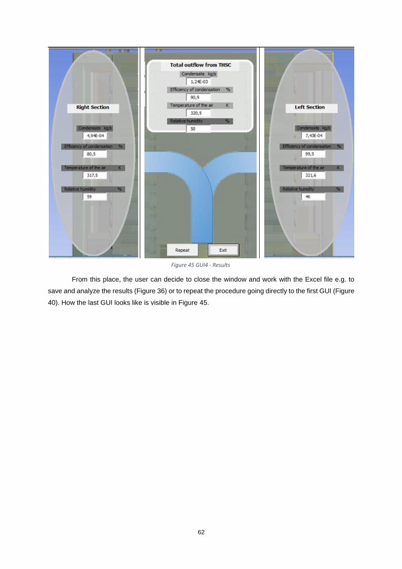
62

From this place, the user can decide to close the window and work with the Excel file e.g. to

save and analyze the results (Figure 36) or to repeat the procedure going directly to the first GUI (Figure

40). How the last GUI looks like is visible in Figure 45.

Figure 45 GUI4 - Results

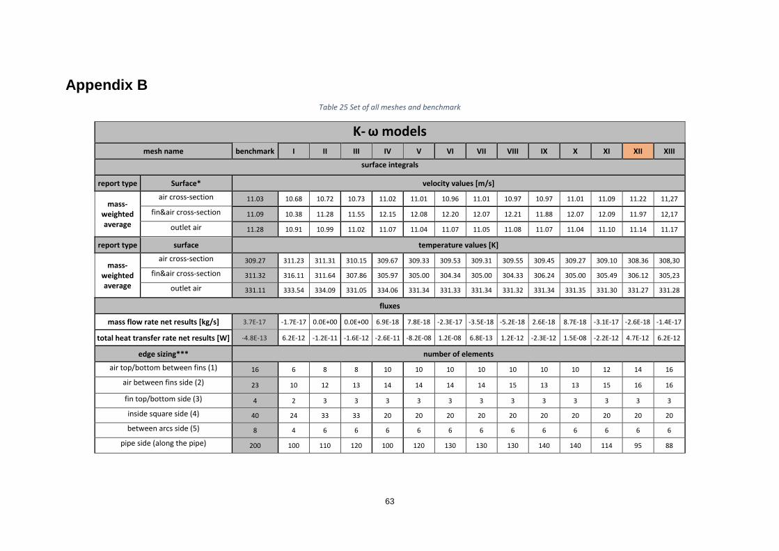
63

Appendix B

Table 25 Set of all meshes and benchmark

K- ω models mesh name benchmark I II III IV V VI VII VIII IX X XI XII XIII

surface integrals

report type Surface* velocity values [m/s]


air cross-section 11.03 10.68 10.72 10.73 11.02 11.01 10.96 11.01 10.97 10.97 11.01 11.09 11.22 11,27

fin&air cross-section 11.09 10.38 11.28 11.55 12.15 12.08 12.20 12.07 12.21 11.88 12.07 12.09 11.97 12,17

outlet air 11.28 10.91 10.99 11.02 11.07 11.04 11.07 11.05 11.08 11.07 11.04 11.10 11.14 11.17

report type surface temperature values [K]


air cross-section 309.27 311.23 311.31 310.15 309.67 309.33 309.53 309.31 309.55 309.45 309.27 309.10 308.36 308,30

fin&air cross-section 311.32 316.11 311.64 307.86 305.97 305.00 304.34 305.00 304.33 306.24 305.00 305.49 306.12 305,23

outlet air 331.11 333.54 334.09 331.05 334.06 331.34 331.33 331.34 331.32 331.34 331.35 331.30 331.27 331.28

fluxes

mass flow rate net results [kg/s] 3.7E-17 -1.7E-17 0.0E+00 0.0E+00 6.9E-18 7.8E-18 -2.3E-17 -3.5E-18 -5.2E-18 2.6E-18 8.7E-18 -3.1E-17 -2.6E-18 -1.4E-17

total heat transfer rate net results [W] -4.8E-13 6.2E-12 -1.2E-11 -1.6E-12 -2.6E-11 -8.2E-08 1.2E-08 6.8E-13 1.2E-12 -2.3E-12 1.5E-08 -2.2E-12 4.7E-12 6.2E-12

edge sizing*** number of elements

air top/bottom between fins (1) 16 6 8 8 10 10 10 10 10 10 10 12 14 16

air between fins side (2) 23 10 12 13 14 14 14 14 15 13 13 15 16 16

fin top/bottom side (3) 4 2 3 3 3 3 3 3 3 3 3 3 3 3

inside square side (4) 40 24 33 33 20 20 20 20 20 20 20 20 20 20

between arcs side (5) 8 4 6 6 6 6 6 6 6 6 6 6 6 6

pipe side (along the pipe) 200 100 110 120 100 120 130 130 130 140 140 114 95 88

Mathematical model of the industrial kitchen steam condenser

Documents

Transcript of Mathematical model of the industrial kitchen steam condenser