CCGGEEHH WWoorrkkiinngg PPaappeerr SSeerriieess

The contribution of migration to economic development

in Holland and the Netherlands 1510-1900

Peter Foldvari, Debrecen University

Bas van Leeuwen, Utrecht University, Warwick University

Jan Luiten van Zanden, Utrecht University

Januari 2012

Working paper no. 25

http://www.cgeh.nl/working-paper-series/

© 2011 by Authors. All rights reserved. Short sections of text, not to exceed two paragraphs, may be quoted without explicit permission provided that full credit, including © notice, is given to the source.

The contribution of migration to economic development

in Holland and the Netherlands 1510-1900

Peter Foldvari, Debrecen University

Bas van Leeuwen, Utrecht University, Warwick University

Jan Luiten van Zanden, Utrecht University

Abstract Migration always played an important role in Dutch society. However, little quantitative

evidence on its effect on economic development is known for the period before the 20th

century even though some stories exist about their effect on the Golden Age. Applying a new

dataset on migration and growth for the period 1510-1900 in a system of equations, we find

that in the Golden Age, the 18th century, and the 19th century there was a direct positive effect

of migration on productivity. However, when taking account of indirect effects via human-

and physical capital, only during the Golden Age the net effect of migration on per capita

GDP was positive. This seems to confirm those studies that claim that the Golden Age at least

partially benefitted from immigration.

Keywords: Economic growth, Immigration, Holland, endogenous development, Human capital

JEL Codes: J15, N13, N33

Corresponding author: Peter Foldvari: peter.foldvari@econ.unideb.hu

Acknowledgements:

1

1. Introduction Migration is a ‘hot’ topic. Historians, not entirely insensitive for those kinds of societal debates, have also turned to examples of large migration flows to study their long term impact on society and economy. The Dutch Republic is one of those cases that have been discussed a lot in this literature. There is consensus that a lot of migration occurred and that it may have been one of the keys factors behind the success of this economy during its ‘Golden Age’ (1580-1670). It has also been concluded it those large migration flows did not have negative effects on society and economy (for example Lucassen and Lucassen 2011). The debate we engage with in this paper is about the question how important immigration was for economic success. Here we can distinguish two views.

One view, argued most forcefully by Jonathan Israel (1989) and echoed until today (e.g. Esser 2007), is that the spectacular success of the Dutch republic after 1580 was to a very large extent due to the immigration of highly schooled and relatively wealthy entrepreneurs and skilled labourers from the south – Flanders and Brabant. They fled for the Spanish forces, relocated in the cities of Holland and Zeeland, and brought with them the high-valued added activities that created a big economic boost. In other words, the Golden Age mainly consisted of the relocation of the economic centre of the Low Countries from Antwerp and the surrounding areas to Amsterdam – a process resulting from the Spanish reconquest of the south. In this scenario, the migration flow of the period between the 1580s and the 1620s is the decisive link between Flemish and Dutch prosperity.

Other authors (Van Zanden 1993; De Vries and Van der Woude 1997) have, in contrast, argued that the growth of the Holland economy was first of all based on endogenous developments: the emergence of an efficient set of institutions there, set in motion a process of autonomous economic growth, which already started between 1350 and 1500 when, for example, the share of urbanisation rose from 23% to 40% making Holland one of the most urbanised (and non-agricultural) regions in the world. In this view, the growth spurt of the Golden Age was the continuation of a process of economic growth that began much earlier. It was also logical that the expelled merchants and craftsmen of Flanders after 1585 moved to Holland and Zeeland, because this region offered by far the most attractive opportunities for them – such as an efficient set of institutions. In the ‘endogenous-growth-model’ the immigration wave of 1580-1620 is a relevant and important development, but its contribution to long term economic growth is limited. What is perhaps more important in this approach (as formulated by De Vries and Van der Woude 1997 and by Van Zanden 1993), is that the Holland labour market was a very open one, which, when the economy accelerated after 1580, was able to attract increasingly large numbers of labourers from the rest of the Netherlands (Brabant, Overijssel, Friesland) and from parts of Germany and Scandinavia. The VOC, for example, became an employer of thousands of sailors and soldiers recruited from all parts of the North Sea area. It has been argued that this very flexible supply of unskilled and semi-skilled labour, which continued during the 17th and 18th centuries, was a key to the long-term economic success of the region.

The discussion on the links between economic development and migration so far has concentrated on these themes (there have, for example, no contributions which approached this subject from another perspective – looking at Heckscher-Ohlin forces, for example). The debate has mostly centred on measuring the numbers of migrants and on their impact – but only few have attempted to quantify that impact (but see Gelderblom 2000). We think that we can try to take the discussion to a new level because we have just finished a large research project constructing the national accounts of Holland on an annual basis between 1514 and 1807 (in fact, the series goes back to 1347, but the pre 1514 estimates are very tentative). As a result, we think we have a much more detailed picture of economic growth in Holland in this period, making it possible to test those ideas more rigorously. Moreover, we are now also

2

able to estimate the inflow of migrants into Holland somewhat better, thanks to new estimates of the demographic development of Holland between 1514 and 1807, a spinoff of the project on reconstructing the national accounts.

In order to check the results acquired, and as a kind of ‘control-group’, we have applied the method for estimating the effects on immigration on growth on the data for the 19th century as well.

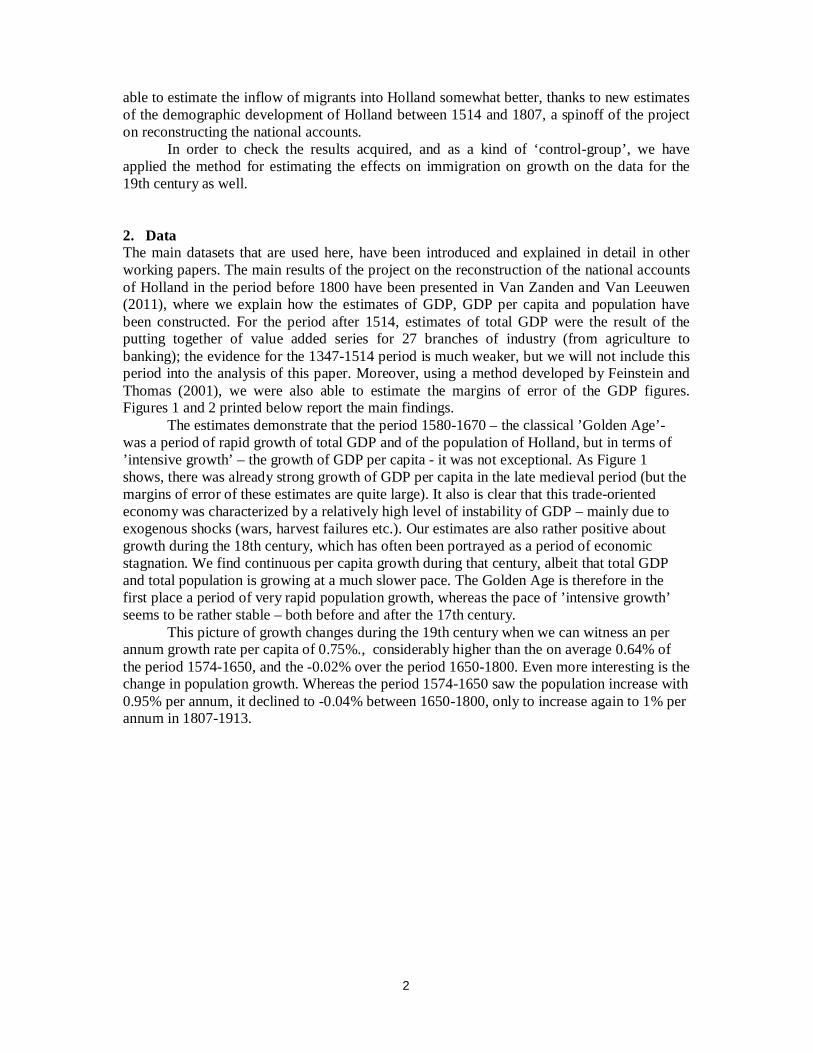
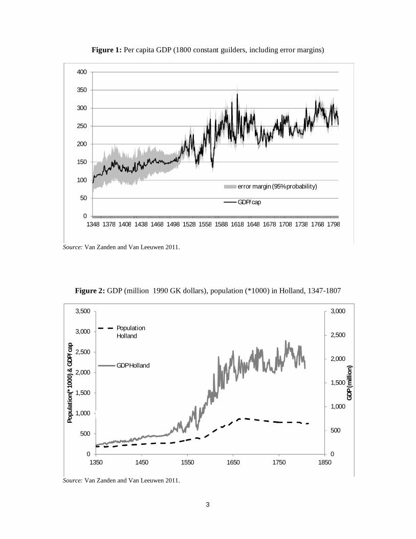
2. Data The main datasets that are used here, have been introduced and explained in detail in other working papers. The main results of the project on the reconstruction of the national accounts of Holland in the period before 1800 have been presented in Van Zanden and Van Leeuwen (2011), where we explain how the estimates of GDP, GDP per capita and population have been constructed. For the period after 1514, estimates of total GDP were the result of the putting together of value added series for 27 branches of industry (from agriculture to banking); the evidence for the 1347-1514 period is much weaker, but we will not include this period into the analysis of this paper. Moreover, using a method developed by Feinstein and Thomas (2001), we were also able to estimate the margins of error of the GDP figures. Figures 1 and 2 printed below report the main findings. The estimates demonstrate that the period 1580-1670 – the classical ’Golden Age’- was a period of rapid growth of total GDP and of the population of Holland, but in terms of ’intensive growth’ – the growth of GDP per capita - it was not exceptional. As Figure 1 shows, there was already strong growth of GDP per capita in the late medieval period (but the margins of error of these estimates are quite large). It also is clear that this trade-oriented economy was characterized by a relatively high level of instability of GDP – mainly due to exogenous shocks (wars, harvest failures etc.). Our estimates are also rather positive about growth during the 18th century, which has often been portrayed as a period of economic stagnation. We find continuous per capita growth during that century, albeit that total GDP and total population is growing at a much slower pace. The Golden Age is therefore in the first place a period of very rapid population growth, whereas the pace of ’intensive growth’ seems to be rather stable – both before and after the 17th century.

This picture of growth changes during the 19th century when we can witness an per annum growth rate per capita of 0.75%., considerably higher than the on average 0.64% of the period 1574-1650, and the -0.02% over the period 1650-1800. Even more interesting is the change in population growth. Whereas the period 1574-1650 saw the population increase with 0.95% per annum, it declined to -0.04% between 1650-1800, only to increase again to 1% per annum in 1807-1913.

3

Figure 1: Per capita GDP (1800 constant guilders, including error margins)

Source: Van Zanden and Van Leeuwen 2011.

Figure 2: GDP (million 1990 GK dollars), population (*1000) in Holland, 1347-1807

Source: Van Zanden and Van Leeuwen 2011.

0

50

100

150

200

250

300

350

400

1348 1378 1408 1438 1468 1498 1528 1558 1588 1618 1648 1678 1708 1738 1768 1798

error margin (95% probability)

GDP/cap

0

500

1,000

1,500

2,000

2,500

3,000

0

500

1,000

1,500

2,000

2,500

3,000

3,500

1350 1450 1550 1650 1750 1850

GDP

(mill

ion)

Popu

latio

n(*1

000)

& G

DP/c

ap

Population Holland

GDP Holland

4

Figure 3: GDP (million 1990 GK dollars), population (*1000), and GDP/cap in the

Netherlands, 1800-1913

Source: Van Zanden et al. (accessed 2011).

It is thus clear that, both the period 1574-1650 and 1800-1900 saw considerable growth in both per capita output and population. Yet, there were considerable differences in terms of migration. Immigration was a main factor behind the sharp increase in population growth during the post 1580 period. In another paper we have presented estimates of the main demographic features of the Holland, including estimates of the minimum level of immigration to the region. The total population of Holland increased from 275,000 in 1514 to 400,000 in 1572 – an increase that was almost entirely the result of its own natural increase. After 1572 there was first a small dip, followed by very rapid growth resulting in a peak level of about 880,000 in 1672. This was followed by a moderate decline to about 783,000 in 1750, after which the population stabilized at this level for about 50 years. This stabilization remained until the mid-19th century. Afterwards, we saw larger number of migrants entering the Netherlands, but never in those magnitudes as recorded in the 17th century.

Figure 4 presents the estimates of the population curve of Holland, including our estimates of net immigration. In the final decades of the 16th century net immigration (from outside of Holland) was about 3,800 per year, to increase to on average 5,200 during the 17th century; the peak of around 10,000 immigrants occurred about 1650. Total immigration in Holland between 1574 and 1650 is estimated at 480,000 - so larger, for example, than the original population of Holland in 1570. These are lower bound estimates; they are based on the difference between the natural increase of the population and its actual growth, and therefore do not include people who emigrated from Holland (for example, left on the ships of the East Indies Company); their total number is roughly estimated at about 200 to 250,000 (Lucassen 2002), bringing total immigration to about 700,000. We also ignore in our estimates temporary migratory flows, such as the seasonal workers analysed by Lucassen (1987). Clearly, immigration was huge in the late 16th and 17th century.

0

5000

10000

15000

20000

25000

30000

0

1000

2000

3000

4000

5000

6000

7000

1800 1820 1840 1860 1880 1900 1920

GDP

(mill

ion)

Popu

latio

n (*

1000

) & G

DP/

cap Population Netherlands

GDP/cap Netherlands

GDP Netherlands

5

In the late 17th and 18th century the number of migrants fell to on average 1,300 migrants per year while in 19th century the number of migrants increased from ca. 7,000 per annum in the 1860s to roughly 17,000 in the 1890s. Even though these latter migrants were bigger in number than in the Golden Age, we have to be aware that they made up a far smaller proportion of the total population. Lucassen and Penninx (and Oomens), for example, calculated that, whereas the share of migrants in the population in the 1890s was around 1.6%, in 1600 it was no less than 10%. And these numbers are for the Netherlands, while most migrants would have travelled to Holland.

Figure 4: Population (in 1000, right-hand scale); Annual number of immigrants (in 1000, Left-hand scale) for Holland and the Netherlands, 1510-1800

Source: This paper, Oomens (1989), and 200 jaar statistiek in tijdreeksen

Migration can have a direct on economic growth (for example via technological development) but it may also work via the factors of production such as physical-or human capital if the migrants brought these two assets along with them to Holland/the Netherlands. Therefore, in our following analysis we also include series of physical-and human capital. We will use non-residential physical capital for Holland (Van Zanden and Van Leeuwen 2011) and the Netherlands (Van Zanden, accessed 2011). Human capital for Holland is taken from Van Zanden and Van Leeuwen (2011) and for the Netherlands from Foldvari, Van Leeuwen, and Van Leeuwen-Li (2010).

3. Method In this paper we aim at calculating the effect of migration on economic growth. In the literature, it is argued that migration can have a direct effect on economic growth, or indirect via the factors of production (e.g. Dolado et al. 1994; Walz 1995). Likewise, Morley (2006) argues for a reverse causality between migration and growth. Hence, since this can work

0

1000

2000

3000

4000

5000

6000

7000

-5

0

5

10

15

20

25

30

35

40

45

1510 1550 1590 1630 1670 1710 1750 1790 1830 1870 1910

Popu

latio

n (*

1000

)

no. m

igra

nts p

er a

nnum

(*10

00)

Holland: annual migration

Netherlands: annual immigration

Holland: total population

Netherlands: total population

6

directly, or via physical and human capital and since it can have reverse causality, we estimate a system of equations with migration, physical-and human capital, and per capita GDP. We start with assuming that only a level effect exists. This is warranted both empirically and theoretically. Empirically, we found, using cross-correllograms, that there is no level-growth effect between variables. Theoretically, we can think like Jones (1995), who argues that if variables that are thought to lead to a permanent change in the rate of per capita income growth really had this effect, with their value increasing over time, economic growth should be accelerating. Since for the early modern period we find no significant economic growth at all, and for the 19th century we find a stable growth rate of roughly 0.6% annually, permanent growth effects are not likely. For this reason, the following system of equations suffices:

10 11 12 13 1,

20 21 22 23 2,

30 31 32 33 3,

40 41 42 43 4,

ln lnln ln

ln lnln ln

t t t t t

t t t t t

t t t t t

t t t t t

y k mig avyears uk y mig avyears u

mig y k avyears uavyears y k mig u

, where k is physical capital stock, mig is the number of migrants (in 1000s) per annum, avyears is average years of education in the population aged 15 years and older, and y is per capita GDP. The system we estimate allows for level effects between any set of variables, and is based on the assumption of no exogenous trend in any of the processes. This is especially important in case of the production function (the first equation within the system) which can be seen as an augmented version of the intensive form of a Cobb-Douglas production function, with constant returns to scale, which makes it possible to omit population. As we wrote above, the lack of a significant growth rate of the per capita GDP makes it very likely that no long-run TFP growth occurred in the period.

There are three problems with estimating equations within a system. The first is simultaneity: we assume here that all four variables are endogenous, that is, they are determined within the system. As such, estimating the parameters by OLS would result in a bias, since the error-terms in each equation are correlated with the explanatory variables. This can be solved by using instruments that are either predetermined or exogenous. Since we do not have exogenous variables that are time variant, we need to rely on predetermined instruments, namely the lagged values of the endogenous variables. We apply a Generalized Method of Moment estimator, which is based on the assumption that the instruments are all uncorrelated with the error-terms. Using the sample moments, we arrive at five moment conditions for each equations, and in each equation we estimate four parameters. This means that all four equations are overidentified, which allows us to use a Sargan-test to find out if our instruments are indeed uncorrelated with the error-terms. The null-hypothesis of the Sargan-test is that the instruments are proper.

The second problem is that with historical data we often have a relatively high degree of measurement error. If measurement error (even with zero mean) is present in the explanatory variables, this causes the error-term to be correlated with the right-hand side variables causing to a (downward) bias in parameter estimation. Instrumentation is however again a correct solution to this problem, once we assume that measurement errors are not autocorrelated: in this case the measurement error present in the lagged values of the variables should not be correlated with the error-terms.

The third problem is that the error-terms of the four equations are likely to be correlated. This does not cause a bias in the estimates but reduces efficiency (inflates standard errors). This is usually solved by means of a Seemingly Unrelated Regressions (SUR) methodology,

7

developed by Zellner (1962). The Three Stage Least Squares (3SLS) Method combines SUR with instrumentation (2SLS) and therefore is the correct method for our purposes. A relation among the four error-terms is very likely, since they are all key macroeconomic/demographic variables, affected by common sources of shocks, like plagues, wars, and cycles in economic performance.

We thus first estimate a GMM to test the validity of the instruments, followed by a 3SLS to get unbiased coefficients of above model. We use the results from the 3SLS procedure to interpret the coefficients.

4. Regression results

We report the regression results in Table 1. The coefficients and t-statistics are from the 3SLS method. The validity of the instruments is tested for by means of a Sargan-test of over-identifying restrictions from a GMM estimation. Table 2 has the outcomes of the test.

Table 1: Results from the 3SLS estimation 1574-1650 1650-1799 1574-1799 1866-1900 coeff t-stat coeff t-stat coeff t-stat coeff t-stat

log GDP per capita constant 6.57 27.2 5.11 62.6 5.45 49.4 6.52 11.3 log capital p.c. 1.58 11.2 0.273 3.45 0.32 3.25 0.643 5.03 migration 0.020 5.76 0.010 4.30 0.02 5.75 0.003 0.98 average years of educ -0.072 -0.38 0.310 11.8 0.14 4.16 -0.081 -0.86

log capital per capita constant -3.75 -12.9 -3.04 -6.17 -2.15 -6.90 -7.56 -9.96 log GDP p.c. 0.53 10.1 0.378 3.79 0.19 3.18 0.877 5.06 migration -0.009 -3.74 0.018 8.61 0.02 10.3 -0.006 -2.10 average years of educ 0.144 1.41 0.209 5.21 0.30 18.9 0.351 4.86

migration

constant -205.6 -4.01 -45.7 -2.11 -41.0 -2.75 -367.0 -1.96 log GDP p.c. 33.9 4.42 16.4 4.10 14.9 5.82 28.6 0.96 log capital p.c. -34.4 -2.46 25.7 9.09 27.4 11.0 -48.9 -2.38 average years of educ 0.80 0.12 -16.7 -15.5 -14.2 -27.5 32.5 9.61

average years of education constant 1.49 1.11 -7.50 -8.77 -1.55 -1.67 10.1 2.56 log GDP p.c. 0.02 0.08 1.76 12.3 0.84 5.19 -0.606 -0.93 log capital p.c. 0.69 2.26 0.729 4.18 2.19 17.7 1.719 4.56 migration 0.00 -0.49 -0.049 -13.8 -0.07 -28.0 0.018 5.74

8

Table 2: Sargan test for the validity of instruments period J-statistic p-value 1574-1799 0.123 0.998 1574-1650 0.187 0.996 1650-1799 0.134 0.998 1860-1900 0.196 0.996

Note: the null-hypothesis of the test is that the instruments are valid (uncorrelated with the error-terms) For all periods we find that the Sargan-test cannot reject the null-hypothesis at any conventional level of significance that the instruments are uncorrelated with the error-terms and are valid. Another possible problem is that the results in Table 1 might be the products of spurious regressions, since some of the variable may be non-stationary. Spurious regression arises if the residuals are non-stationary. In order to check the validity of the results, we carry our unit root test on each residual (Table 3).

Table 3: p-values of the ADF test of the residuals by equation equation 1574-1650 1650-1799 1574-1799 1866-1900 1 0.000 0.000 0.000 0.000 2 0.000 0.000 0.000 0.000 3 0.000 0.009 0.000 0.029 4 0.020 0.001 0.000 0.028

Note: the null-hypothesis is that the residuals are non-stationary. The p-values form the ADF tests on the residuals are reassuring: none of the residuals are non-stationary at 5% level of significance. Since the most serious problem of the ADF test is low power, that is, its tendency not to reject the null-hypothesis of non-stationarity even when it is not true (high probability of type II error), the rejection can be accepted without any concerns. Since it has become a practice in empirical literature to carry out statistical analysis on differenced variables irrespectively of the stationarity of the residuals from the regression on levels, we feel necessary to include a formal argument why this can be a mistake in case of data with measurement errors (see Appendix). 5. Interpretation of the results The general finding in Table 1 is that migration had a significant, positive, direct effect on the level of GDP per capita in the early modern period, while it cannot be found during the 19th century (as expected since migration is small as a percentage of the population). The existence of a direct positive effect in the early modern period indicates that migrants were on average more productive than the domestic population, which is not true for the 19th century. Once we take two subperiods of the early modern age: the Golden Age (1574-1650) and the era of modest development (1650-1799) we find that the effect of migrants on per capita income reduced over time: in the first period one thousand more immigrants caused per capita income to increase by 2% in the long-run, in the post 1650 period we find only half of this effect. We can also observe a fundamental change in the process of economic growth: education did not matter much for the income generation during the Golden Age, while it definitely did after 1650. Strangely we again find no evidence for an economy driven by education in the second half of the 19th century. The lack of a direct effect is however not an evidence for the lack of any effects.

9

We can identify indirect effects in the system of equations as well. Migration had a changing effect on physical capital accumulation: during the Golden Age migrants arrived with less physical capital than what the average local had. Later however, migrants contributed to a higher level of physical capital probably due to higher saving-rates. For the 19th century we again find a reversal: migrants again contribute to a reduction in the per capita physical capital stock.

As for human capital, migration had seemingly no effect on average schooling during the Golden Age, while it had a negative effect after 1650. The reason can again be found in the different educational composition of the migrants compared to the locals. In the second half of the 19th century however, migrant seem to have contributed to more education in the population, either by sending their children to school more often than the locals, but also possibly that they came from Germany and other European countries with relatively well-developed mass-education. The total effect on GDP (direct and indirect, i.e. via capital and education) can also be estimated for the different periods (see Table 4). We find that the direct effect of migration

Table 4: The direct and indirect effect of 1,000 new migrants on GDP per capita 1574-1650 1650-1799 1866-1900

direct effect on per capita GDP

2% 1% 0.30%

effect on capital -0.90% 1.80% -0.60%

effect on education (years) 0 -0.049 0.018

indirect effect via capital and education on GDP per capita

-1.42% -1.04% -1.84%

total effect on per capita GDP 0.55% -0.05% -1.54%

always increased productivity. However, when the effects via education and physical capital is taken onboard only in the Golden Age migrants had a positive net effect on GDP/cap. 6. Conclusion Migration always played an important role in Dutch society. The absolute number of migrants clearly increased strongly during the 80 years war and the Golden Age. However, as argued by Esser (2007, 268), this was not so much a break with the past but rather an acceleration of already existing migrant flows. We do find, however, that migrant flows dropped from the Golden Age to the 18th century, to increase again thereafter. Yet, even though the absolute number of migrants was highest in the late 19th century, relative to the population their numbers were much more significant during the Golden Age. Applying a system of equations, we find that in all three periods (the Golden Age, the 18th century, and the 19th century) there was a direct positive effect of migration on productivity. However, in the 18th century and the 19th century the indirect effects via capital and education were overwhelmingly negative. This means that only during the Golden Age the net effect of migration on per capita GDP was positive. This seems to confirm those

10

studies that claim that, for example, rich merchants went to Amsterdam and brought their capital and networks along (Van Dillen 1958; Brulez 1960). Yet, the negative effect of migration on capital seems to suggest that migration from Flanders was rarely from rich merchants but rather by younger men (Gelderblom 2000). Hence, this field needs further research. References Brulez, W. (1960). De diaspora der Antwerpse kooplui op het einde van de 16e eeuw.

Bijdragen voor Geschiedenis der Nederlanden, 15, 229-306. Dillen, J.A. van, (1958). Het oudste aandeelhoudersregister van de kamer Amsterdam der

Oost-Indische Compagnie. Martinus Nijhoff:The Hague. Dolado, J., Goria, A., and Ichino, A. (1994). Immigration, Human Capital and Growth in the

Host Country: Evidence from Pooled Country Data. Journal of Population Economics, 7(2), 193-215.

Gelderblom, O. (2000). Zuid-Nederlandse kooplieden en de opkomst van de Amsterdamse stapelmarkt (1578-1630), Verloren: Hilversum.

Esser, R. (2007). From province to nation: Immigration in the Dutch Republic in the late 16th and early 17th centuries. In S.G. Ellis and L. Klusakova (eds.), Imaging frontiers, contesting identities, Pisa University Press: Pisa, pp. 163-276.

Israel, J. (1989). Dutch Primacy in World Trade, 1585-1740. 1989, Oxford University Press: Oxford.

Jones, C. I. (1995). Time Series Tests of Endogenous Growth Models. Quarterly Journal of Economics, 110(2), 495-525.

Feinstein, Ch. H., and Thomas, M. (2001). A Plea for Errors,’ Discussion Papers in Economic and Social History, Number 41, University of Oxford.

Lucassen, J. (1987). Migrant Labour in Europe: the Drift to the North Sea. Croom Helm: Beckenham.

Lucassen, J. (2002). Immigranten in Holland, Een kwantitatieve benadering. IISH working paper series no. 3.

Lucassen, L., and Lucassen, J. (2011). Winnaars en Verliezers. Bert Bakker, Amsterdam. Morley, B. (2006). Causality between economic growth and immigration: An ARDL bounds

testing approach. Economics Letters, 90(1), 72-76. Oomens, C.A. (1989). De loop der bevolking van Nederland in de negentiende eeuw.

Statistische onderzoekingen nr. M35. SDU-uitgeverij/CBS-publicaties: Den Haag. Vries, J. de, and Van der Woude, A. (1997). The first modern economy. Success, failure and

perseverance of the Dutch economy, 1500-1815. Cambridge UP: Cambridge. Walz, U. (1995). Growth (Rate) Effects of Migration. Zeitschrift für Wirtschafts- und

Sozialwissenschaften, 115, 199-221. Zanden, J.L. van (1993). The Rise and Decline of Holland’s economy. Manchester U.P:

Manchester. Zanden, J.L. van (accessed 2011), National accounts of the Netherlands, 1807-1913.

(http://nationalaccounts.niwi.knaw.nl/start.htm) Zanden, J.L. van, and Van Leeuwen, B. (2011, forthcoming). Persistent but not consistent:

The growth of national income in Holland 1347-1807. Explorations in Economic History.

Zellner, A. (1962). An efficient method of estimating seemingly unrelated regression equations and tests for aggregation bias. Journal of the American Statistical Association, 57(298), 348–368.

11

Appendix Regression on first-differences versus levels with measurement errors in variables As reported in the paper, the residuals from the regression analysis were found stationary and, hence, we can safely argue that our results are not spurious. One might argue though, that nevertheless a first difference should be preferred. We argue in this appendix that this is not true once we have measurement errors in our variables, since first differencing increases the error to signal ratio, leading to (downward) biased results. We can show this as follows. Let us assume that variable y can be observed with a random measurement error.

*t t ty y , where y* denotes the observed variable, and ε is the measurement error.

2(0, )t IID � Let us define the error to signal ratio (ESR) as follows:

*

2

2

variance of measurement errorvariance of signal

y

ESR

In this case the ESR is: 2

2

1

1 y

ESR

.

What happens if we use instead the first difference of y* in a statistical analysis?

*

1 1t t t t ty y y *

2 2 212 ( , ) 2

t tty t ty

Cov y y , where we made use of our assumption that the measurement

error is not autocorrelated, and is uncorrelated with any y’s, and we assumed homoscedasticity for both variables.

The ESR in this case is: 21

2 2

1( , )12

y t t

ESRCov y y

, which is, if y is positively

autocorrelated, smaller than in the non-differenced version. In case y is a random walk process (as required so that we have chance to obtain spurious results):

1

2 21( , )

t tt t y yCov y y

2 2 2

2 2 2

1 1

1 12 2

y y y

ESR

12

Figure A.1: Simulation of the error to signal ratio using level of first-differenced variables

The above figure shows that the error to signal ratio is always higher if we take the

first difference of a random walk process. The conclusion is that if we find that our results are not spurious (the residuals are stationary), we should not prefer the results from a regression on first-differenced variables, and a regression on first-differences cannot be used to validate the results from a regression on the levels since it suffers from an even higher bias.

0

0.1

0.2

0.3

0.4

0.5

0.6

0.7

0.8

0.9

1

0 1 2 3 4 5 6 7 8 9 10

Erro

to si

gnal

ratio

signal variance / error variance

ESR (level) ESR(diff)