The continuous Bernoulli: fixing a pervasive error invariational autoencoders

Gabriel Loaiza-GanemDepartment of Statistics

Columbia Universitygl2480@columbia.edu

John P. CunninghamDepartment of Statistics

Columbia Universityjpc2181@columbia.edu

Abstract

Variational autoencoders (VAE) have quickly become a central tool in machinelearning, applicable to a broad range of data types and latent variable models. By farthe most common first step, taken by seminal papers and by core software librariesalike, is to model MNIST data using a deep network parameterizing a Bernoullilikelihood. This practice contains what appears to be and what is often set aside as aminor inconvenience: the pixel data is [0, 1] valued, not {0, 1} as supported by theBernoulli likelihood. Here we show that, far from being a triviality or nuisance thatis convenient to ignore, this error has profound importance to VAE, both qualitativeand quantitative. We introduce and fully characterize a new [0, 1]-supported, singleparameter distribution: the continuous Bernoulli, which patches this pervasive bugin VAE. This distribution is not nitpicking; it produces meaningful performanceimprovements across a range of metrics and datasets, including sharper imagesamples, and suggests a broader class of performant VAE.1

1 Introduction

Variational autoencoders (VAE) have become a central tool for probabilistic modeling of complex,high dimensional data, and have been applied across image generation [10], text generation [14],neuroscience [8], chemistry [9], and more. One critical choice in the design of any VAE is the choiceof likelihood (decoder) distribution, which stipulates the stochastic relationship between latents andobservables. Consider then using a VAE to model the MNIST dataset, by far the most common firststep for introducing and implementing VAE. An apparently innocuous practice is to use a Bernoullilikelihood to model this [0, 1]-valued data (grayscale pixel values), in disagreement with the {0, 1}support of the Bernoulli distribution. Though doing so will not throw an obvious type error, theimplied object is no longer a coherent probabilistic model, due to a neglected normalizing constant.This practice is extremely pervasive in the VAE literature, including the seminal work of Kingmaand Welling [20] (who, while aware of it, set it aside as an inconvenience), highly-cited follow upwork (for example [25, 37, 17, 6] to name but a few), VAE tutorials [7, 1], including those in hugelypopular deep learning frameworks such as PyTorch [32] and Keras [3], and more.

Here we introduce and fully characterize the continuous Bernoulli distribution (§3), both as a meansto study the impact of this widespread modeling error, and to provide a proper VAE for [0, 1]-valueddata. Before these details, let us ask the central question: who cares?

First, theoretically, ignoring normalizing constants is unthinkable throughout most of probabilisticmachine learning: these objects serve a central role in restricted Boltzmann machines [36, 13],graphical models [23, 33, 31, 38], maximum entropy modeling [16, 29, 26], the “Occam’s razor”nature of Bayesian models [27], and much more.

1Our code is available at https://github.com/cunningham-lab/cb.

33rd Conference on Neural Information Processing Systems (NeurIPS 2019), Vancouver, Canada.

Second, one might suppose this error can be interpreted or fixed via data augmentation, binarizingdata (which is also a common practice), stipulating a different lower bound, or as a nonprobabilisticmodel with a “negative binary cross-entropy” objective. §4 explores these possibilities and finds themwanting. Also, one might be tempted to call the Bernoulli VAE a toy model or a minor point. Let usavoid that trap: MNIST is likely the single most widely used dataset in machine learning, and VAE isquickly becoming one of our most popular probabilistic models.

Third, and most importantly, empiricism; §5 shows three key results: (i) as a result of this error,we show that the Bernoulli VAE significantly underperforms the continuous Bernoulli VAE acrossa range of evaluation metrics, models, and datasets; (ii) a further unexpected finding is that thisperformance loss is significant even when the data is close to binary, a result that becomes clear byconsideration of continuous Bernoulli limits; and (iii) we further compare the continuous Bernoullito beta likelihood and Gaussian likelihood VAE, again finding the continuous Bernoulli performant.

All together this work suggests that careful treatment of data type – neither ignoring normalizingconstants nor defaulting immediately to a Gaussian likelihood – can produce optimal results whenmodeling some of the most core datasets in machine learning.

2 Variational autoencoders

Autoencoding variational Bayes [20] is a technique to perform inference in the model:

Zn ∼ p0(z) and Xn|Zn ∼ pθ(x|zn) , for n = 1, . . . , N, (1)

where each Zn ∈ RM is a local hidden variable, and θ are parameters for the likelihood of observablesXn. The prior p0(z) is conventionally a Gaussian N (0, IM ). When the data is binary, i.e. xn ∈{0, 1}D, the conditional likelihood pθ(xn|zn) is chosen to be B(λθ(zn)), where λθ : RM → RD is aneural network with parameters θ. B(λ) denotes the product ofD independent Bernoulli distributions,with parameters λ ∈ [0, 1]D (in the standard way we overload B(·) to be the univariate Bernoulli or theproduct of independent Bernoullis). Since direct maximum likelihood estimation of θ is intractable,variational autoencoders use VBEM [18], first positing a now-standard variational posterior family:

qφ((z1, ..., zn)|(x1, ..., xn)

)=

N∏n=1

qφ(zn|xn),with qφ(zn|xn) = N(mφ(xn),diag

(s2φ(xn)

))(2)

where mφ : RD → RM , sφ : RD → RM+ are neural networks parameterized by φ. Then, usingstochastic gradient descent and the reparameterization trick, the evidence lower bound (ELBO)E(θ, φ) is maximized over both generative and posterior (decoder and encoder) parameters (θ, φ):

E(θ, φ) =N∑n=1

Eqφ(zn|xn)[log pθ(xn|zn)]−KL(qφ(zn|xn)||p0(zn)) ≤ log pθ((x1, . . . , xN )

). (3)

2.1 The pervasive error in Bernoulli VAE

In the Bernoulli case, the reconstruction term in the ELBO is:

Eqφ(zn|xn)[log pθ(xn|zn)] = Eqφ(zn|xn)

[ D∑d=1

xn,d log λθ,d(zn)+(1−xn,d) log(1−λθ,d(zn))]

(4)

where xn,d and λθ,d(zn) are the d-th coordinates of xn and λθ(zn), respectively. However, critically,Bernoulli likelihoods and the reconstruction term of equation 4 are commonly used for [0, 1]-valueddata, which loses the interpretation of probabilistic inference. To clarify, hereafter we denote theBernoulli distribution as p̃(x|λ) = λx(1 − λ)1−x to emphasize the fact that it is an unnormalizeddistribution (when evaluated over [0, 1]). We will also make this explicit in the ELBO, writingE(p̃, θ, φ) to denote that the reconstruction term of equation 4 is being used. When analyzing [0, 1]-valued data such as MNIST, the Bernoulli VAE has optimal parameter values θ∗(p̃) and φ∗(p̃); thatis:

(θ∗(p̃), φ∗(p̃)) = argmax(θ,φ)

E(p̃, θ, φ). (5)

2

3 CB: the continuous Bernoulli distribution

In order to analyze the implications of this modeling error, we introduce the continuous Bernoulli, anovel distribution on [0, 1], which is parameterized by λ ∈ (0, 1) and defined by:

X ∼ CB(λ) ⇐⇒ p(x|λ) ∝ p̃(x|λ) = λx(1− λ)1−x. (6)We fully characterize this distribution, deferring proofs and secondary properties to appendices.

Proposition 1 (CB density and mean): The continuous Bernoulli distribution is well defined, that is,0 <

∫ 1

0p̃(x|λ)dx <∞ for every λ ∈ (0, 1). Furthermore, if X ∼ CB(λ), then the density function

of X and its expected value are:

p(x|λ) = C(λ)λx(1− λ)1−x,where C(λ) =

2tanh−1(1− 2λ)

1− 2λif λ 6= 0.5

2 otherwise(7)

µ(λ) := E[X] =

λ

2λ− 1+

1

2tanh−1(1− 2λ)if λ 6= 0.5

0.5 otherwise(8)

Figure 1 shows logC(λ), p(x|λ), and µ(λ). Some notes warrant mention: (i) unlike the Bernoulli,the mean of the continuous Bernoulli is not λ; (ii) however, like for the Bernoulli, µ(λ) is increasingon λ and goes to 0 or 1 when λ goes to 0 or 1; (iii) the continuous Bernoulli is not a beta distribution(the main difference between these two distributions is how they concentrate mass around theextrema, see appendix 1 for details), nor any other [0, 1]-supported distribution we are aware of(including continuous relaxations such as the Gumbel-Softmax [28, 15], see appendix 1 for details);(iv) C(λ) and µ(λ) are continuous functions of λ; and (v) the log normalizing constant logC(λ) iswell characterized but numerically unstable close to λ = 0.5, so our implementation uses a Taylorapproximation near that critical point to calculate logC(λ) to high numerical precision. Proof: Seeappendix 3.

0.0 0.2 0.4 0.6 0.8 1.0parameter

0.75

1.00

1.25

1.50

1.75

2.00

2.25

2.50

log

C()

log normalizing constant

0.0 0.2 0.4 0.6 0.8 1.0x

0.5

1.0

1.5

2.0

2.5

p(x|

)

density

0.1

0.2

0.3

0.4

0.5

0.6

0.7

0.8

0.9

para

met

er

0.0 0.2 0.4 0.6 0.8 1.0parameter

0.0

0.2

0.4

0.6

0.8

1.0

()

meancontinuous BernoulliBernoulli

Figure 1: continuous Bernoulli log normalizing constant (left), pdf (middle) and mean (right).

Proposition 2 (CB additional properties): The continuous Bernoulli forms an exponential family,has closed form variance, CDF, inverse CDF (which importantly enables easy sampling and the useof the reparameterization trick), characteristic function (and thus moment generating function too)and entropy. Also, the KL between two continuous Bernoulli distributions also has closed form andC(λ) is convex. Finally, the continuous Bernoulli admits a conjugate prior which we call the C-Betadistribution. See appendix 2 for details. Proof: See appendix 3.

Proposition 3 (CB Bernoulli limit): CB(λ) λ→0−−−→ δ(0) and CB(λ) λ→1−−−→ δ(1) in distribution; thatis, the continuous Bernoulli becomes a Bernoulli in the limit. Proof: See appendix 3.

This proposition might at a first glance suggest that, as long as the estimated parameters are closeto 0 or 1 (which should happen when the data is close to binary), then the practice of erroneouslyapplying a Bernoulli VAE should be of little consequence. However, the above reasoning is wrong, asit ignores the shape of logC(λ): as λ→ 0 or λ→ 1, logC(λ)→∞ (Figure 1, left). Thus, if data isclose to binary, the term neglected by the Bernoulli VAE becomes even more important, the exactopposite conclusion than the naive one presented above.

Proposition 4 (CB normalizing constant bound): C(λ) ≥ 2, with equality if and only if λ = 0.5.And thus it follows that, for any x, λ, we have log p(x|λ) > log p̃(x|λ). Proof: See appendix 3.

3

This proposition allows us to interpret E(p̃, θ, φ) as a lower lower bound of the log likelihood (§4).

Proposition 5 (CB maximum likelihood): For an observed sample x1, . . . , xN ∼iid CB(λ), themaximum likelihood estimator λ̂ of λ is such that µ(λ̂) = 1

N

∑n xn. Proof: See appendix 3.

Beyond characterizing a novel and interesting distribution, these propositions now allow full analysisof the error in applying a Bernoulli VAE to the wrong data type.

4 The continuous Bernoulli VAE, and why the normalizing constant matters

We define the continuous Bernoulli VAE analogously to the Bernoulli VAE:

Zn ∼ N (0, IM ) and Xn|Zn ∼ CB (λθ(zn)) , for n = 1, . . . , N (9)

where again λθ : RM → RD is a neural network with parameters θ, and CB(λ) now denotes theproduct of D independent continuous Bernoulli distributions. Operationally, this modification resultsonly in a change to the optimized objective; for clarity we compare the ELBO of the continuousBernoulli VAE (top), E(p, θ, φ), to the Bernoulli VAE (bottom):

E(p, θ, φ) =

N∑n=1

−KL(qφ||p0) + Eqφ

[D∑d=1

xn,d log λθ,d(zn) + (1− xn,d) log(1− λθ,d(zn)) + logC(λθ,d(zn))

]

E(p̃, θ, φ) =

N∑n=1

−KL(qφ||p0) + Eqφ

[D∑d=1

xn,d log λθ,d(zn) + (1− xn,d) log(1− λθ,d(zn))],

Analogously, we denote θ∗(p) and φ∗(p) as the maximizers of the continuous Bernoulli ELBO:

(θ∗(p), φ∗(p)) = argmax(θ,φ)

E(p, θ, φ). (10)

Immediately, a number of potential interpretations for the Bernoulli VAE come to mind, some ofwhich have appeared in literature. We analyze each in turn.

4.1 Changing the data, model or training objective

One obvious workaround is to simply binarize any [0, 1]-valued data (MNIST pixel values or oth-erwise), so that it accords with the Bernoulli likelihood [24], a practice that is commonly followed(e.g. [34, 2, 28, 15, 12]). First, modifying data to fit a model, particularly an unsupervised model, isfundamentally problematic. Second, many [0, 1]-valued datasets are heavily degraded by binarization(see appendices for CIFAR-10 samples), indicating major practical limitations. Another workaroundis to change the likelihood of the model to a proper [0, 1]-supported distribution, such as a beta or atruncated Gaussian. In §5 we include comparisons against a VAE with a beta distribution likelihood(we also made comparisons against a truncated Gaussian but found this to severely underperform allthe alternatives). Gulrajani et al. [11] use a discrete distribution over the 256 possible pixel values.Knoblauch et al. [22] study changing the reconstruction and/or the KL term in the ELBO. Whiletheir main focus is to obtain more robust inference, they provide a framework in which the BernoulliVAE corresponds simply to a different (nonprobabilistic) loss. In this perspective, empirical resultsmust determine the adequacy of this objective; §5 shows the Bernoulli VAE to underperform itsproper probabilistic counterpart across a range of settings. Finally, note that none of these alternativesprovide a way to understand the effect of using Bernoulli likelihoods on [0, 1]-valued data.

4.2 Data augmentation

Since the expectation of a Bernoulli random variable is precisely its parameter, the Bernoulli VAEmight (erroneously) be assumed to be equivalent to a continuous Bernoulli VAE on an infinitelyaugmented dataset, obtained by sampling binary data whose mean is given by the observed data;indeed this idea is suggested by Kingma and Welling [20]2. This interpretation does not hold3; itwould result in a reconstruction term as in the first line in the equation below, while a correct Bernoulli

2see the comments in https://openreview.net/forum?id=33X9fd2-9FyZd3see http://ruishu.io/2018/03/19/bernoulli-vae/ for a looser lower bound interpretation

4

VAE on the augmented dataset would have a reconstruction term given by the second line (not equal,as the order of expectation can not be switched since qφ depends on Xr on the second line):

Ezn∼qφ(zn|xn)

[EXn∼B(xn)

[ D∑d=1

Xn,d log λθ,d(zn) + (1−Xn,d) log λθ,d(zn)]]

(11)

6= EXn∼B(xn)

[Ezn∼qφ(zn|Xn)

[ D∑d=1

Xn,d log λθ,d(zn) + (1−Xn,d) log λθ,d(zn)]].

4.3 Bernoulli VAE as a lower lower bound

Because the continuous Bernoulli ELBO and the Bernoulli ELBO are related by:

E(p̃, θ, φ) +N∑n=1

D∑d=1

Ezn∼qφ(zn|xn)[logC(λθ,d(zn))] = E(p, θ, φ) (12)

and recalling Proposition 4, since log 2 > 0, we get that E(p̃, θ, φ) < E(p, θ, φ). That is, usingthe Bernoulli VAE results in optimizing an even-lower bound of the log likelihood than using thecontinuous Bernoulli ELBO. Note however that unlike the ELBO, E(p̃, θ, φ) is not tight even if theapproximate posterior matches the true posterior.

4.4 Mean parameterization

The conventional maximum likelihood estimator for a Bernoulli, namely λ̂B = 1N

∑n xn, maximizes

p̃(x1, ..., xN |λ) regardless of whether data is {0, 1} and [0, 1]. As a thought experiment, considerx1, . . . , xN ∼iid CB(λ). Proposition 5 tells us that the correct maximum likelihood estimator, λ̂CBis such that µ(λ̂CB) = 1

N

∑n xn, where µ is the CB mean of equation 8. Thus, while using λ̂B is

incorrect, one can (surprisingly) still recover the correct maximum likelihood estimator via λ̂CB =

µ−1(λ̂B). One might then (wrongly) think that training a Bernoulli VAE, and then subsequentlytransforming the decoder parameters with µ−1, would be equivalent to training a continuous BernoulliVAE; that is, λθ∗(p) might be equal to µ−1(λθ∗(p̃)). This reasoning is incorrect: the KL term inthe ELBO implies that λθ∗(p)(zn) 6= µ−1(xn), and so too λθ∗(p̃)(zn) 6= xn, and as such λθ∗(p) 6=µ−1(λθ∗(p̃)). In fact, our experiments will show that despite this flawed reasoning, applying thistransformation can recover some, but not all, of the performance loss from using a Bernoulli VAE.

5 Experiments

We have introduced the continuous Bernoulli distribution to give a proper probabilistic VAE for[0, 1]-valued data. The essential question that we now address is how much, if any, improvement weachieve by making this choice.

5.1 MNIST

One frequently noted shortcoming of VAE (and Bernoulli VAE on MNIST in particular) is thatsamples from this model are blurry. As noted, the convexity of logC(λ) can be seen as regularizingsample values from the VAE to be more extremal; that is, sharper. As such we first compared samplesfrom a trained continuous Bernoulli VAE against samples from the MNIST dataset itself, from atrained Bernoulli VAE, and from a trained Gaussian VAE, that is, the usual VAE model with a decoderlikelihood pθ(x|z) = N (ηθ(z), σ

2θ(z)), where we use η to avoid confusion with µ of equation 8.

These samples are shown in Figure 2. In each case, as is standard, we show the parameter outputby the generative/decoder network for a given latent draw: λθ∗(p)(z) for the CB VAE, λθ∗(p̃)(z)for the B VAE, and ηθ∗(z) for the N VAE. Qualitatively, the continuous Bernoulli VAE achievesconsiderably superior samples vs the Bernoulli or Gaussian VAE, owing to the effect of logC(λ)pushing the decoder toward sharper images. Further samples are in the appendix. Dai and Wipf [4]consider why Gaussian VAE produce blurry images; we point out that our work (considering thelikelihood) is orthogonal to theirs (considering the data manifold).

5

data

CB VAE

B VAE

N VAE

Figure 2: Samples from MNIST, continuous Bernoulli VAE, Bernoulli VAE, and Gaussian VAE.

5.2 Warped MNIST datasets

The most common justification for the Bernoulli VAE is that MNIST pixel values are ‘close’ tobinary. An important study is thus to ask how the performance of continuous Bernoulli VAE vs theBernoulli VAE changes as a function of this ‘closeness.’ We formalize this concept by introducinga warping function fγ(x) that, depending on the warping parameter γ, transforms individual pixelvalues to produce a dataset that is anywhere from fully binarized (every pixel becomes {0, 1}) tofully degraded (every pixel becomes 0.5). Figure 3 shows fγ for different values of γ, and the (ratheruninformative) warping equation appears next to Figure 3.

Importantly, γ = 0 corresponds to an unwarped dataset, i.e., the original MNIST dataset. Further, notethat negative values of γ warp pixel values towards being more binarized, completely binarizing it inthe case where γ = −0.5, whereas positive values of γ push the pixel values towards 0.5, recoveringconstant data at γ = 0.5. We then train our competing VAE models on the datasets induced bydifferent values of γ and compare the difference in performance as γ changes. Note importantly that,because γ induces different datasets, performance values should primarily be compared betweenVAE models at each γ value; the trend as a function of γ is not of particular interest.

0.0 0.2 0.4 0.6 0.8 1.0x

0.0

0.2

0.4

0.6

0.8

1.0

f(x

)

warping functions

0.50.40.30.20.1

0.00.10.20.30.40.5

warp

ing

Figure 3: fγ for different γ values.

fγ(x) =

1(x ≥ 0.5), if γ = −0.5min

(1,max

(0,x+ γ

1 + 2γ

)), if γ ∈ (−0.5, 0)

γ + (1− 2γ)x, if γ ∈ [0, 0.5]

Figure 4 shows the results of various models applied to these different datasets (all values are anaverage of 10 separate training runs). The same neural network architectures are used across thisfigure, with architectural choices that are quite standard (detailed in appendix 4, along with traininghyperparameters). The left panel shows ELBO values. In dark blue is the continuous BernoulliVAE ELBO, namely E(p, θ∗(p), φ∗(p)). In light blue is the same ELBO when evaluated on atrained Bernoulli VAE: E(p, θ∗(p̃), φ∗(p̃)). Most importantly, note the γ = 0 values; the continuousBernoulli VAE achieves a 300 nat improvement over the Bernoulli VAE. This finding supports theprevious qualitative finding and the theoretical motivation for this work: significant quantitative gainsare achieved via the continuous Bernoulli model. This finding remains true across a range of γ (darkblue above light blue in Figure 4), indicating that regardless of how ‘close’ to binary a dataset is, thecontinuous Bernoulli is a superior VAE model.

One might then wonder if the continuous Bernoulli is outperforming simply because the Bernoullineeds a mean correction. We thus apply µ−1, namely the map from Bernoulli to continuous Bernoullimaximum likelihood estimators (equation 8 and §4.4), and evaluate the same ELBO on µ−1(λθ∗(p̃)) asthe decoder shown in light red (Figure 4, left). This result, which is only achieved via the introductionof the continuous Bernoulli, shows two important findings: first, that indeed some improvement over

6

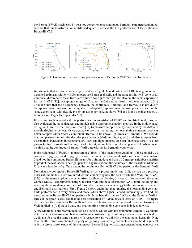
the Bernoulli VAE is achieved by post hoc correction to a continuous Bernoulli parameterization; butsecond, that this transformation is still inadequate to achieve the full performance of the continuousBernoulli VAE.

0.4 0.2 0.0 0.2 0.4warping

0

200

400

600

800

1000

1200

1400

1600

ELBO

1470

1139

1416

ELBO for VAE

(p, * (p), * (p))(p, * (p), * (p))(p, * (p), * (p)) with 1

0.4 0.2 0.0 0.2 0.4warping

2

4

6

8

10

ince

ptio

n sc

ore

inception scores of VAE

IS dataIS * (p)(z)IS * (p)(z)IS ( * (p)(z))IS ( * (p)(z))

0.4 0.2 0.0 0.2 0.4warping

0.2

0.4

0.6

0.8

1.0

accu

racy

knn accuracy of VAE latents(p)(p)

Figure 4: Continuous Bernoulli comparisons against Bernoulli VAE. See text for details.

We also note that we ran the same experiment with log likelihood instead of ELBO (using importanceweighted estimates with k = 100 samples; see Burda et al. [2]), and the same results held (up to smallnumerical differences; these traces are omitted for figure clarity). We also ran the same experimentfor the β-VAE [12], sweeping a range of β values, and the same results held (see appendix 5.1).To make sure that the discrepancy between the continuous Bernoulli and Bernoulli is not due tothe approximate posterior not being able to adequately approximate the true posterior, we ran thesame experiments with flexible posteriors using normalizing flows [34] and found the discrepancy tobecome even larger (see appendix 5.1).

It is natural to then wonder if this performance is an artifact of ELBO and log likelihood; thus, wealso evaluated the same datasets and models using different evaluation metrics. In the middle panelof Figure 4, we use the inception score [35] to measure sample quality produced by the differentmodels (higher is better). Once again, we see that including the normalizing constant producesbetter samples (dark traces / continuous Bernoulli lie above light traces / Bernoulli). We includethat comparison on both the decoder parameters λ (dark and light green) and also samples fromdistributions indexed by those parameters (dark and light orange). One can imagine a variety of otherparameter transformations that may be of interest; we include several in appendix 5.1, where againwe find that the continuous Bernoulli VAE outperforms its Bernoulli counterpart.

In the right panel of Figure 4, to measure usefulness of the latent representations of these models, wecompute mφ∗(p)(xn) and mφ∗(p̃)(xn) (note that m is the variational posterior mean from equation2 and not the continuous Bernoulli mean) for training data and use a 15-nearest neighbor classifierto predict the test labels. The right panel of Figure 4 shows the accuracy of the classifiers (denotedK(φ)) as a function of γ. Once again, the continuous Bernoulli VAE outperforms the Bernoulli VAE.

Now that the continuous Bernoulli VAE gives us a proper model on [0, 1], we can also proposeother natural models. Here we introduce and compare against the beta distribution VAE (not β-VAE[12]); as the name implies, the generative likelihood is Beta(αθ(z), βθ(z)). We repeated the samewarped MNIST experiments using Gaussian VAE and beta distribution VAE, both including andignoring the normalizing constants of those distributions, as an analogy to the continuous Bernoulliand Bernoulli distributions. First, Figure 5 shows again that that ignoring the normalizing constanthurts performance in every metric and model (dark above light). Second, interestingly, we find thatthe continuous Bernoulli VAE outperforms both the beta distribution VAE and the Gaussian VAE interms of inception scores, and that the beta distribution VAE dominates in terms of ELBO. This figureclarifies that the continuous Bernoulli and beta distribution are to be preferred over the Gaussian forVAE applied to [0, 1] valued data, and that ignoring normalizing constants is indeed unwise.

A few additional notes warrant mention on Figure 5. Unlike with the continuous Bernoulli, we shouldnot expect the Gaussian and beta normalizing constants to go to infinity as extrema are reached, sowe do not observe the same patterns with respect to γ as we did with the continuous Bernoulli. Notealso that the lower lower bound property of ignoring normalizing constants does not hold in general,as it is a direct consequence of the continuous Bernoulli log normalizing constant being nonnegative.

7

0.4 0.2 0.0 0.2 0.4warping

900

800

700

600

500

ELBO

ELBO for Gaussian VAE

(p, * (p), * (p))(p, * (p), * (p))

0.4 0.2 0.0 0.2 0.4warping

2

4

6

8

10

ince

ptio

n sc

ore

inception scores of Gaussian VAE

IS dataIS * (p)(z)IS * (p)(z)IS ( * (p)(z), 2

* (p)(z))IS ( * (p)(z), 2

* (p)(z))

0.4 0.2 0.0 0.2 0.4warping

0.2

0.4

0.6

0.8

1.0

accu

racy

knn accuracy of Gaussian VAE latents(p)(p)

0.4 0.2 0.0 0.2 0.4warping

0

500

1000

1500

2000

ELBO

ELBO for beta distribution VAE(p, * (p), * (p))(p, * (p), * (p))

0.4 0.2 0.0 0.2 0.4warping

2

4

6

8

10

ince

ptio

n sc

ore

inception scores of beta distribution VAE

IS dataIS mean( * (p)(z), * (p)(z))IS mean( * (p)(z), * (p)(z))IS Beta( * (p)(z), * (p)(z))IS Beta( * (p)(z), * (p)(z))

0.4 0.2 0.0 0.2 0.4warping

0.2

0.4

0.6

0.8

accu

racy

knn accuracy of beta distribution VAE latents(p)(p)

Figure 5: Gaussian (top panels) and beta (bottom panels) distributions comparisons between includingand excluding the normalizing constants. Left panels show ELBOs, middle panels inceptions scores,and right panels 15-nearest neighbors accuracy.

Table 1: Comparisons of training with and without normalizing constants for CIFAR-10. Forconnection to the panels in Figures 4 and 5, column headers are colored accordingly.

distribution objective map E(p, θ∗, φ∗) IS w/ samples IS w/ parameters K(φ∗)CB/B E(p, θ, φ) · 1007 1.15 2.31 0.43

E(p̃, θ, φ) µ−1 916 1.49 4.55 0.42E(p̃, θ, φ) · 475 1.41 1.39 0.42

Gaussian E(p, θ, φ) · 1891 1.86 3.04 0.42E(p̃, θ, φ) · -42411 1.24 1.00 0.1

beta E(p, θ, φ) · 3121 2.98 4.07 0.47E(p̃, θ, φ) · -38913 1.39 1.00 0.1

5.3 CIFAR-10

We repeat the same experiments as in the previous section on the CIFAR-10 dataset (without commonpreprocessing that takes the data outside [0, 1] support), a dataset often considered to be a bad fitfor Bernoulli VAE. For brevity we evaluated only the non-warped data γ = 0, leading to the resultsshown in Table 1 (note the colored column headers, to connect to the panels in Figures 4,5). The topsection shows results for the continuous Bernoulli VAE (first row, top), the Bernoulli VAE (third row,top), and the Bernoulli VAE with a continuous Bernoulli inverse map µ−1 (second row, top). Acrossall metrics – ELBO, inception score with parameters λ, inception score with continuous Bernoullisamples given λ, and k nearest neighbors – the Bernoulli VAE is suboptimal. Interestingly, unlikein MNIST, here we see that using the continuous Bernoulli parameter correction µ−1 (§4.4) to aBernoulli VAE is optimal under some metrics. Again we note that this is a result belonging to thecontinuous Bernoulli (the parameter correction is derived from equation 8), so even these resultsemphasize the importance of the continuous Bernoulli.

We then repeat the same set of experiments for Gaussian and beta distribution VAE (middle andbottom sections of Table 1). Again, ignoring normalizing constants produces significant performanceloss across all metrics. Comparing metrics across the continuous Bernoulli, Gaussian, and betasections, we see again that the Gaussian VAE is suboptimal across all metrics, with the optimaldistribution being the continuous Bernoulli or beta distribution VAE, depending on the metric.

8

5.4 Parameter estimation with EM

Finally, one might wonder if the performance improvements of the continuous Bernoulli VAE overthe Bernoulli VAE and its corrected version with µ−1 are merely an artifact of not having access tothe log likelihood and having to optimize the ELBO instead. In this section we show, empirically,that the answer is no. We consider estimating the parameters of a mixture of continuous Bernoullidistributions, of which the VAE can be thought of as a generalization with infinitely many components.We proceed as follows: We randomly set a mixture of continuous Bernoulli distributions, ptrue, withK components in 50 dimensions (independent of each other) and sample from this mixture 10000times in order to generate a simulated dataset. We then use the EM algorithm [5] to estimate themixture coefficients and the corresponding continuous Bernoulli parameters, first using a continuousBernoulli likelihood (correct), and second using a Bernoulli likelihood (incorrect). We then measurehow close the estimated parameters are from ground truth. To avoid a (hard) optimization problemover permutations, we measure closeness with KL divergence between the true distribution ptrue andthe estimated pest.

The results of performing the procedure described above 10 times and averaging the KL values(over these 10 repetitions), along with standard errors, are shown in Figure 6. First, we can see thatwhen using the correct continuous Bernoulli likelihood, the EM algorithm correctly recovers the truedistribution. We can also see that, as the number of mixture components K gets larger, ignoring thenormalizing constant results in worse performance, even after correcting with µ−1, which helps butdoes not fully remedy the situation (except at K = 1, as noted in §4.4).

0 5 10 15 20 25 30mixture components K

0

2

4

6

8

10

12

14

KL(p

true

||pes

t)

bias of likelihood for mixture

plus 1

Figure 6: Bias of the EM algorithm to estimate CB parameters when using a CB likelihood (darkblue), B likelihood (light blue) and a B likelihood plus a µ−1 correction (light red).

6 Conclusions

In this paper we introduce and characterize a novel probability distribution – the continuous Bernoulli– to study the effect of using a Bernoulli VAE on [0, 1]-valued intensity data, a pervasive error inhighly cited papers, publicly available implementations, and core software tutorials alike. We showthat this practice is equivalent to ignoring the normalizing constant of a continuous Bernoulli, andthat doing so results in significant performance decrease in the qualitative appearance of samplesfrom these models, the ELBO (approximately 300 nats), the inception score, and in terms of the latentrepresentation (via k nearest neighbors). Several surprising findings are shown, including: (i) thatsome plausible interpretations of ignoring a normalizing constant are in fact wrong; (ii) the (possiblycounterintuitive) fact that this normalizing constant is most critical when data is near binary; and (iii)that the Gaussian VAE often underperforms VAE models with the appropriate data type (continuousBernoulli or beta distributions).

Taken together, these findings suggest an important potential role for the continuous Bernoullidistribution going forward. On this point, we note that our characterization of the continuousBernoulli properties (such as its ease of reparameterization, likelihood evaluation, and sampling)make it compatible with the vast array of VAE improvements that have been proposed in the literature,including flexible posterior approximations [34, 21], disentangling [12], discrete codes [28, 15],variance control strategies [30], and more.

9

Acknowledgments

We thank Yixin Wang, Aaron Schein, Andy Miller, and Keyon Vafa for helpful conversations, and theSimons Foundation, Sloan Foundation, McKnight Endowment Fund, NIH NINDS 5R01NS100066,NSF 1707398, and the Gatsby Charitable Foundation for support.

References[1] Pytorch VAE turotial: https://github.com/pytorch/examples/tree/master/vae,

Keras VAE turotial: https://blog.keras.io/building-autoencoders-in-keras.html.

[2] Y. Burda, R. Grosse, and R. Salakhutdinov. Importance weighted autoencoders. arXiv preprintarXiv:1509.00519, 2015.

[3] F. Chollet et al. Keras. https://keras.io, 2015.

[4] B. Dai and D. Wipf. Diagnosing and enhancing vae models. In International Conference onLearning Representations, 2019.

[5] A. P. Dempster, N. M. Laird, and D. B. Rubin. Maximum likelihood from incomplete data viathe em algorithm. Journal of the Royal Statistical Society: Series B (Methodological), 39(1):1–22, 1977.

[6] N. Dilokthanakul, P. A. Mediano, M. Garnelo, M. C. Lee, H. Salimbeni, K. Arulkumaran, andM. Shanahan. Deep unsupervised clustering with gaussian mixture variational autoencoders.arXiv preprint arXiv:1611.02648, 2016.

[7] C. Doersch. Tutorial on variational autoencoders. arXiv preprint arXiv:1606.05908, 2016.

[8] Y. Gao, E. W. Archer, L. Paninski, and J. P. Cunningham. Linear dynamical neural populationmodels through nonlinear embeddings. In Advances in neural information processing systems,pages 163–171, 2016.

[9] R. Gómez-Bombarelli, J. N. Wei, D. Duvenaud, J. M. Hernández-Lobato, B. Sánchez-Lengeling,D. Sheberla, J. Aguilera-Iparraguirre, T. D. Hirzel, R. P. Adams, and A. Aspuru-Guzik. Auto-matic chemical design using a data-driven continuous representation of molecules. ACS centralscience, 4(2):268–276, 2018.

[10] K. Gregor, I. Danihelka, A. Graves, D. Rezende, and D. Wierstra. Draw: A recurrent neuralnetwork for image generation. In International Conference on Machine Learning, pages1462–1471, 2015.

[11] I. Gulrajani, K. Kumar, F. Ahmed, A. A. Taiga, F. Visin, D. Vazquez, and A. Courville.Pixelvae: A latent variable model for natural images. In International Conference on LearningRepresentations, 2017.

[12] I. Higgins, L. Matthey, A. Pal, C. Burgess, X. Glorot, M. Botvinick, S. Mohamed, and A. Ler-chner. beta-vae: Learning basic visual concepts with a constrained variational framework. InInternational Conference on Learning Representations, volume 3, 2017.

[13] G. E. Hinton. Training products of experts by minimizing contrastive divergence. Neuralcomputation, 14(8):1771–1800, 2002.

[14] Z. Hu, Z. Yang, X. Liang, R. Salakhutdinov, and E. P. Xing. Toward controlled generation oftext. In Proceedings of the 34th International Conference on Machine Learning-Volume 70,pages 1587–1596. JMLR. org, 2017.

[15] E. Jang, S. Gu, and B. Poole. Categorical reparameterization with gumbel-softmax. InInternational Conference on Learning Representations, 2017.

[16] E. T. Jaynes. Information theory and statistical mechanics. Physical review, 106(4):620, 1957.

[17] Z. Jiang, Y. Zheng, H. Tan, B. Tang, and H. Zhou. Variational deep embedding: an unsupervisedand generative approach to clustering. In Proceedings of the 26th International Joint Conferenceon Artificial Intelligence, pages 1965–1972. AAAI Press, 2017.

[18] M. I. Jordan, Z. Ghahramani, T. S. Jaakkola, and L. K. Saul. An introduction to variationalmethods for graphical models. Machine learning, 37(2):183–233, 1999.

10

[19] D. P. Kingma and J. Ba. Adam: A method for stochastic optimization. In InternationalConference on Learning Representations, 2015.

[20] D. P. Kingma and M. Welling. Auto-encoding variational bayes. In International Conferenceon Learning Representations, 2014.

[21] D. P. Kingma, T. Salimans, R. Jozefowicz, X. Chen, I. Sutskever, and M. Welling. Improvedvariational inference with inverse autoregressive flow. In Advances in neural informationprocessing systems, pages 4743–4751, 2016.

[22] J. Knoblauch, J. Jewson, and T. Damoulas. Generalized variational inference. arXiv preprintarXiv:1904.02063, 2019.

[23] D. Koller, N. Friedman, and F. Bach. Probabilistic graphical models: principles and techniques.MIT press, 2009.

[24] H. Larochelle and I. Murray. The neural autoregressive distribution estimator. In Proceedings ofthe Fourteenth International Conference on Artificial Intelligence and Statistics, pages 29–37,2011.

[25] A. B. L. Larsen, S. K. Sønderby, H. Larochelle, and O. Winther. Autoencoding beyond pixelsusing a learned similarity metric. In International Conference on Machine Learning, pages1558–1566, 2016.

[26] G. Loaiza-Ganem, Y. Gao, and J. P. Cunningham. Maximum entropy flow networks. InInternational Conference on Learning Representations, 2017.

[27] D. J. MacKay. Information theory, inference and learning algorithms. Cambridge universitypress, 2003.

[28] C. J. Maddison, A. Mnih, and Y. W. Teh. The concrete distribution: A continuous relaxation ofdiscrete random variables. In International Conference on Learning Representations, 2017.

[29] R. Malouf. A comparison of algorithms for maximum entropy parameter estimation. In pro-ceedings of the 6th conference on Natural language learning-Volume 20, pages 1–7. Associationfor Computational Linguistics, 2002.

[30] A. Miller, N. Foti, A. D’Amour, and R. P. Adams. Reducing reparameterization gradientvariance. In Advances in Neural Information Processing Systems, pages 3708–3718, 2017.

[31] K. P. Murphy, Y. Weiss, and M. I. Jordan. Loopy belief propagation for approximate inference:An empirical study. In Proceedings of the Fifteenth conference on Uncertainty in artificialintelligence, pages 467–475. Morgan Kaufmann Publishers Inc., 1999.

[32] A. Paszke, S. Gross, S. Chintala, G. Chanan, E. Yang, Z. DeVito, Z. Lin, A. Desmaison,L. Antiga, and A. Lerer. Automatic differentiation in pytorch. In NIPS-W, 2017.

[33] J. Pearl. Reverend Bayes on inference engines: A distributed hierarchical approach. CognitiveSystems Laboratory, School of Engineering and Applied Science, University of California, LosAngeles, 1982.

[34] D. Rezende and S. Mohamed. Variational inference with normalizing flows. In InternationalConference on Machine Learning, pages 1530–1538, 2015.

[35] T. Salimans, I. Goodfellow, W. Zaremba, V. Cheung, A. Radford, and X. Chen. Improvedtechniques for training gans. In Advances in neural information processing systems, pages2234–2242, 2016.

[36] P. Smolensky. Information processing in dynamical systems: Foundations of harmony theory.Colorado Univ at Boulder Dept of Computer Science, 1986.

[37] C. K. Sønderby, T. Raiko, L. Maaløe, S. K. Sønderby, and O. Winther. Ladder variationalautoencoders. In Advances in neural information processing systems, pages 3738–3746, 2016.

[38] M. J. Wainwright and M. I. Jordan. Graphical models, exponential families, and variationalinference. Foundations and Trends in Machine Learning, 1(1–2):1–305, 2008.

11