arX

iv:1

010.

4915

v2 [

astr

o-ph

.CO

] 16

Dec

201

0DRAFT VERSIONDECEMBER20, 2010Preprint typeset using LATEX style emulateapj v. 11/10/09

THE CLUSTERING OF MASSIVE GALAXIES ATz ∼ 0.5 FROM THE FIRST SEMESTER OF BOSS DATA

MARTIN WHITE1,2,3, M. BLANTON4, A. BOLTON5, D. SCHLEGEL3, J. TINKER4, A. BERLIND6, L. DA COSTA7, E. KAZIN 4, Y.-T. L IN8,M. M AIA 7, C.K. MCBRIDE6, N. PADMANABHAN 9, J. PAREJKO9, W. PERCIVAL10, F. PRADA11, B. RAMOS7, E. SHELDON12, F. DE

SIMONI 7, R. SKIBBA 13, D. THOMAS10, D. WAKE9, I. ZEHAVI 14, Z. ZHENG9, R. NICHOL10, DONALD P. SCHNEIDER15, M ICHAEL A.STRAUSS16, B.A. WEAVER4, DAVID H. WEINBERG17

1 Department of Physics, University of California Berkeley,CA2 Department of Astronomy, University of California Berkeley, CA

3 Lawrence Berkeley National Laboratory, 1 Cyclotron Road, Berkeley, CA4 Center for Cosmology and Particle Physics, New York University, NY

5 Dept. Physics and Astronomy, University of Utah, UT6 Dept. Physics, Vanderbilt University, Nashville, TN

7 Observatorio Nacional, Brazil8 IPMU, University of Tokyo, Japan

9 Yale Center for Astronomy and Astrophysics, Yale University, New Haven, CT10 Institute of Cosmology and Gravitation, University of Portsmouth, UK

11 Instituto de Astrofisica de Andalucia, Granada, Spain12 Brookhaven National Laboratory

13 Steward Observatory, University of Arizona, AZ14 Dept. Astronomy, Case Western Reserve University, OH

15 Dept. Astronomy and Astrophysics, Penn State University, PA16 Dept. Astrophysical Sciences, Princeton University, NJ and

17 Ohio State University, Dept. of Astronomy and CCAPP, Columbus, OH(Dated: December 20, 2010)

Draft version December 20, 2010

ABSTRACTWe calculate the real- and redshift-space clustering of massive galaxies atz ∼ 0.5 using the first semester of

data by the Baryon Oscillation Spectroscopic Survey (BOSS). We study the correlation functions of a sample of44,000 massive galaxies in the redshift range 0.4< z< 0.7. We present a halo-occupation distribution modelingof the clustering results and discuss the implications for the manner in which massive galaxies atz ∼ 0.5occupy dark matter halos. The majority of our galaxies are central galaxies living in halos of mass 1013h−1M⊙,but 10% are satellites living in halos 10 times more massive.These results are broadly in agreement withearlier investigations of massive galaxies atz ∼ 0.5. The inferred large-scale bias (b ≃ 2) and relatively highnumber density (n = 3×10−4h3Mpc−3) imply that BOSS galaxies are excellent tracers of large-scale structure,suggesting BOSS will enable a wide range of investigations on the distance scale, the growth of large-scalestructure, massive galaxy evolution and other topics.Subject headings: cosmology: large-scale structure of universe

1. INTRODUCTION

The distribution of objects in the Universe displays a highdegree of organization, which in current models is due toprimordial fluctuations in density which were laid down atvery early times and amplified by the process of gravitationalinstability. Characterizing the evolution of this large-scalestructure is a central theme of cosmology and astrophysics.In addition to allowing us to understand the structure itself,large-scale structure studies offer an incisive tool for prob-ing cosmology and particle physics and sets the context forour modern understanding of galaxy formation and evolu-tion. Since the pioneering studies of Humason et al. (1956);Gregory & Thompson (1978); Joeveer & Einasto (1978) andthe first CfA redshift survey (Huchra et al. 1983), galaxy red-shift surveys have played a key role in this enterprise, andever larger surveys have provided increasing insight and evertighter constraints on cosmological models.

This paper presents the first measurements of the cluster-ing of massive galaxies from the Baryon Oscillation Spectro-scopic Survey (BOSS; Schlegel et al. 2009) based on a sam-ple of galaxy redshifts observed during the period Januarythrough July 2010. We demonstrate that BOSS is efficiently

obtaining redshifts of some of the most luminous galaxies atz ≃ 0.5, and has already become the largest such redshift sur-vey ever undertaken. The high bias and number density ofthese objects (described below) make them ideal tracers oflarge-scale structure, and suggest that BOSS will make a sig-nificant impact on many science questions including a deter-mination of the cosmic distance scale, the growth of structureand the evolution of massive galaxies.

The outline of the paper is as follows. In §2 we brieflydescribe the BOSS survey and observations, and define thesample we focus on in this paper. Our clustering results aredescribed in §3 and interpreted in the framework of the halomodel in §4, where we also compare to previous work on theclustering of massive galaxies at intermediate redshift. Weconclude with a discussion of the implications of these resultsin §5, while some technical details on the construction of ourmock catalogs are relegated to an Appendix. Throughout thispaper when measuring distances we refer to comoving sep-arations, measured inh−1Mpc with H0 = 100hkms−1 Mpc−1.We convert redshifts to distances, assuming aΛCDM cos-mology withΩm = 0.274,ΩΛ = 0.726 andh = 0.70. This isthe same cosmology as assumed for the N-body simulations

2 White et al.

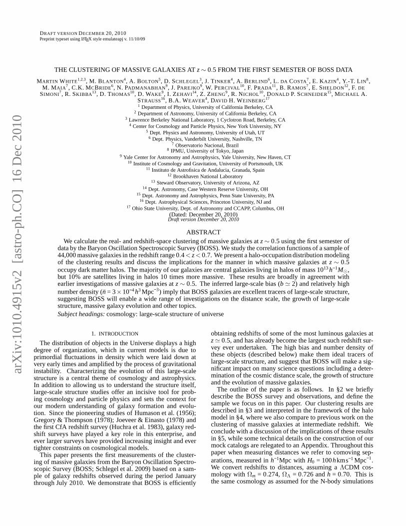
FIG. 1.— The (comoving) number density of galaxies,n(z) for the sampledescribed in the text (§2). The vertical dashed lines indicate the redshift limitswe use in our analysis: 0.4 < z < 0.7.

from which we make our mock catalogs (see Appendix A).

2. OBSERVATIONS

The Sloan Digital Sky Survey (SDSS; York et al. 2000)mapped nearly a quarter of the sky using the dedicated SloanFoundation 2.5 m telescope (Gunn et al. 2006) located atApache Point Observatory in New Mexico. A drift-scanningmosaic CCD camera (Gunn et al. 1998) imaged the sky in fivephotometric bandpasses (Fukugita et al. 1996; Smith et al.2002; Doi et al. 2010) to a limiting magnitude ofr ≃ 22.5.The imaging data were processed through a series of pipelinesthat perform astrometric calibration (Pier et al. 2003), photo-metric reduction (Lupton et al. 2001), and photometric cali-bration (Padmanabhan et al. 2008). The magnitudes were cor-rected for Galactic extinction using the maps of Schlegel etal.(1998). BOSS, a part of the SDSS-III survey (Eisenstein et al.,in prep.) has completed an additional 3,000 square degreesof imaging in the southern Galactic cap, taken in a manneridentical to the original SDSS imaging. All of the data havebeen processed through the latest versions of the pipelinesandBOSS is obtaining spectra of a selected subset (Padmanabhanet al., in preparation) of 1.5 million galaxies approximatelyvolume limited toz ≃ 0.6 (in addition to spectra of 150,000quasars and various ancillary observations). The targets areassigned to tiles of diameter 3 using an adaptive tiling algo-rithm (Blanton et al. 2003). Aluminum plates are drilled withholes corresponding to the positions of objects on each tile,and manually plugged with optical fibers that feed a pair ofdouble spectrographs. These spectrographs are significantlyupgraded from those used by SDSS-I/II (York et al. 2000;Stoughton et al. 2002), with improved chips with better redresponse, higher throughput gratings, 1,000 fibers (instead of640) and a 2′′ entrance aperture (was 3′′). The spectra coverthe range 3,600Å to 10,000Å, at a resolution of about 2,000.

BOSS makes use of luminous galaxies selected from themulti-color SDSS imaging to probe large-scale structure atintermediate redshift (z < 0.7). These galaxies are among themost luminous galaxies in the universe and trace a large cos-mological volume while having high enough number densityto ensure that shot-noise is not a dominant contributor to theclustering variance. The majority of the galaxies have old stel-lar systems whose prominent 4,000Å break in their spectral

FIG. 2.— The distribution of absolute magnitudes for the sampleanalyzedin this paper. We havek+e corrected ther-band magnitudes toz ≃ 0.55 usingtheg− i color assuming a passively evolving galaxy – since the redshift rangeis small this amounts to a small correction. This sample consists of intrinsi-cally very bright, and massive, galaxies with stellar masses several times thecharacteristic mass in a Schechter fit. The luminosity function of Faber et al.(2007) atz = 0.5, converted fromB to r band assuming a redshiftedz = 0 el-liptical galaxy template, has a characteristic luminosityof −19.8. Convertingthe Bell et al. (2004) luminosity function using a high-z single burst modelgives−20. So all of the CMASS galaxies are brighter than this characteristicluminosity.

energy distributions makes them relatively easy to select inmulti-color data.

The strategy behind, and details of, our target selection arecovered in detail in Padmanabhan et al. (in preparation). Cutsin color-magnitude space allow a roughly volume-limitedsample of luminous galaxies to be selected, and partitionedinto broad redshift bins. Briefly, we follow the SDSS-I/II pro-cedure described in Eisenstein et al. (2001) and define a “ro-tated” combination of colorsd⊥ = (r − i) − (g − r)/8. The sam-ple we analyze in this paper (the so-called “CMASS sample”since it is approximately stellar mass limited) is defined via

d⊥ > 0.55 and i < 19.9 and ifiber2< 21.5i < 19.86+ 1.6(d⊥− 0.8) and r − i < 2 (1)

where magnitude cuts use “cmodel magnitudes” and col-ors are defined with “model magnitudes”, except forifiber2which is the magnitude in the 2′′ spectroscopic fiber (seeStoughton et al. 2002; Abazajian et al. 2004, for definitionsofthe magnitudes and further discussion). There are two addi-tional cuts to reduce stellar contamination,zpsf − z ≥ 9.125−0.45z andrpsf− r > 0.3.

These cuts isolate thez ∼ 0.5, high mass galaxies. Thei − d⊥ constraint is approximately a cut in absolute magni-tude or stellar mass, withd⊥ closely tracking redshift forthese galaxies. As discussed in detail in Padmanabhan etal. (in preparation), the slope of thei − d⊥ cut is set to par-allel the track of a passively evolving, constant stellar massgalaxy as determined from the population synthesis modelsof Maraston et al. (2009). This approach leads to an approx-imately stellar mass limited sample. We restrict ourselvestogalaxies in the redshift range 0.4 < z < 0.7 (Fig. 1). Notethat our selection gives the majority of the galaxies within∆z = 0.1 of the median – this has the advantage of makingthe analysis relatively straightforward but means we need tocombine with other samples to obtain leverage in redshift. Acomparison of the cuts defining this sample with other, simi-

Massive galaxy clustering 3

FIG. 3.— (Top) The sky coverage of the galaxies used in this analysis,in orthographic projection centered onαJ2000 = 180 andδJ2000 = 0. Theregions A, B and C described in the text are marked. (Bottom) Azoom inof region A with the greyscale showing completeness. This region is themost contiguous of the three, and region B is the least contiguous owing tohardware problems in the early part of the year.

lar, samples in the literature will be presented in Padmanab-han et al. (in prep.). In general BOSS goes both fainter andbluer than the earlier samples, targeting “luminous galaxies”not “luminous red galaxies”.

The distribution of absolute (r-band) magnitude for thesample is shown in Fig. 2, where we see that all of the CMASSgalaxies are intrinsically very luminous. Using the modelingof Maraston et al. (in preparation) on the BOSS spectra wefind the median stellar mass of the sample is 1011.7 M⊙. Whilethe detailed numbers depend on assumptions about e.g. theinitial mass function, these galaxies are at the very high massend of the stellar mass function at this redshift for any reason-able assumptions.

The clustering measurements in this paper are based on thedata taken by BOSS up to end of July 2010, which includes120,000 galaxies over 1,600 deg2 of sky. However, the dataprior to January 2010 were taken in commissioning mode andlittle of those data are of survey quality. Once we trim the datato contiguous regions (Fig. 3) with high redshift completenessand select galaxies atz ∼ 0.5 we are left with 44,000 galax-ies, covering 580 square degrees, which we have used in ouranalysis.

The sky coverage of our sample can be seen in Figure 3.We view the data as comprising three regions of the sky, here-after referred to as A, B and C (see Figure). Galaxies in these

20 15 10 5 0 5 10 15 20R [Mpc/h]

20

15

10

5

0

5

10

15

20

Z

[M

pc/h

]

0.5

1.0

2.04.0

8.0

20 15 10 5 0 5 10 15 20R [Mpc/h]

20

15

10

5

0

5

10

15

20

Z [M

pc/h

]

0.5 0.5

1.0

2.0

4.0

8.0

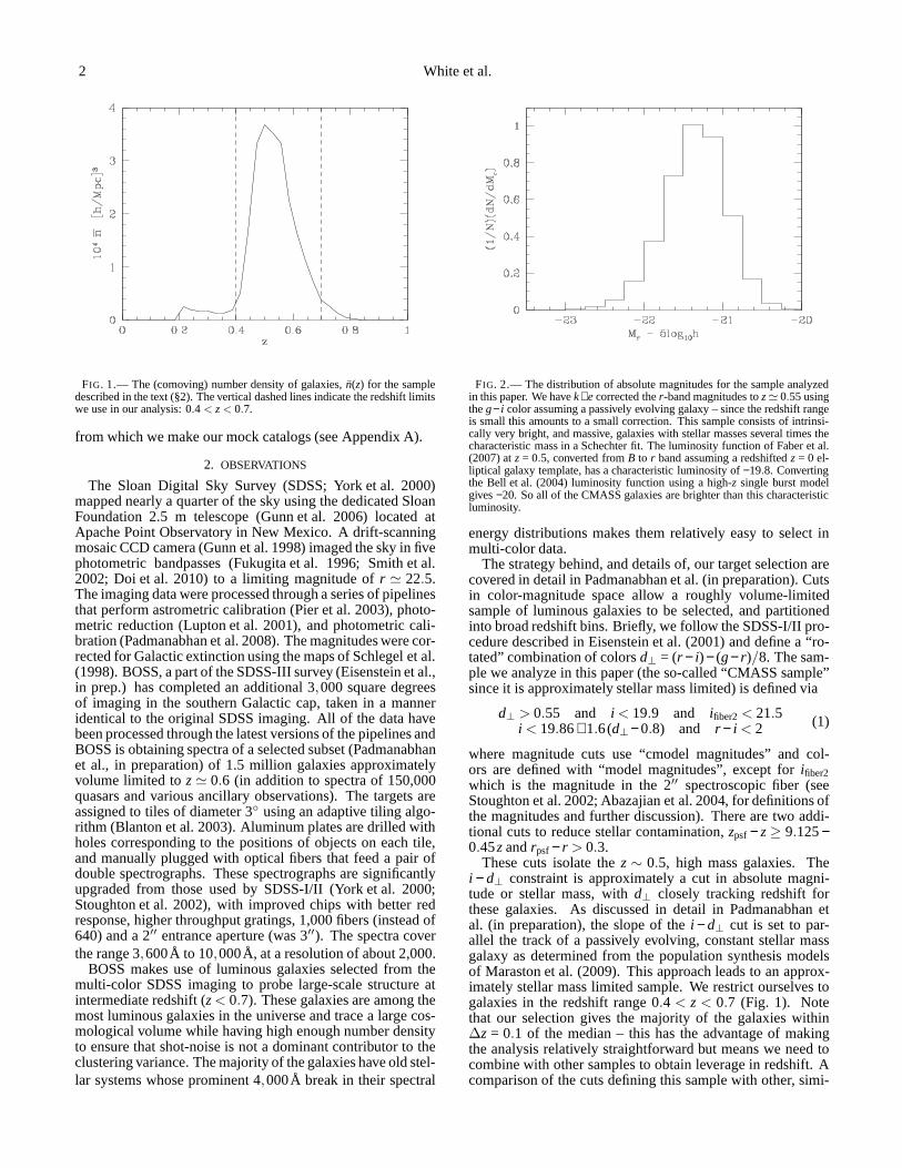
FIG. 4.— Contours of the redshift-space correlation function,ξ(R,Z), forour 0.4< z < 0.7 galaxy sample (see text). Note the characteristic elongationin theZ direction at smallR (fingers-of-god) and squashing at largeR (super-cluster infall). The upper panel shows the results from the BOSS data, whilethe lower panel is from our mock catalogs. The level of agreement is quitegood, as can be seen more quantitatively in later figures.

regions are separated from those in any other region by sev-eral hundred Mpc, and we shall consider them independent.Convenient “rectangular” boundaries to the regions are

A : 105 < αJ2000< 135 , 25 < δJ2000< 60 (2)B : 125 < αJ2000< 240 , −5 < δJ2000< 5 (3)C : 185 < αJ2000< 255 , 10 < δJ2000< 45 . (4)

These boundaries yield widths (heights) of 600 (700), 2600(270) and 1600 (800)h−1Mpc respectively atz ≃ 0.5. As weshall discuss below, the data are consistent with having thesame clustering and redshift distribution in all three regions.

3. CLUSTERING MEASURES

4 White et al.

We compute several two-point, configuration-space cluster-ing statistics in this paper. The basis for all of these calcula-tions is the two-point galaxy correlation function on a two-dimensional grid of pair separations parallel and perpendicu-lar to the line-of-sight:ξ(R,Z).

To estimate the counts expected for unclustered objectswhile accounting for the complex survey geometry, we gen-erate random catalogs with the detailed radial and angular se-lection functions of the sample but with 50× the number ofpoints. Numerous tests have confirmed that the survey selec-tion function factorizes into an angular and a redshift piece.The redshift selection function can be taken into account bydistributing the randoms according to the observed redshiftdistribution of the sample. The completeness on the sky isdetermined from the fraction of target galaxies in a sectorfor which we obtained a high-quality redshift, with the sec-tors being areas of the sky covered by a unique set of spec-troscopic tiles (see Blanton et al. 2003; Tegmark et al. 2004).We use the MANGLE software (Swanson et al. 2008) to trackthe angular completeness. In computing the redshift com-pleteness we omit galaxies for which a redshift was alreadyknown from an earlier survey from both the target and suc-cess lists, and then later randomly sample such galaxies withthe resulting completeness in constructing the input catalog.Since very few of our targets atz ∼ 0.5 have existing red-shifts this is a very small correction. Not all of the spectrataken resulted in a reliable redshift, and the failure probabilityhas angular structure due to hardware limitations. These re-sult in spatial signal-to-noise fluctuations in observations. Wefind no evidence that this failure is redshift dependent - lowand high redshift failure regions have the same redshift dis-tribution. We therefore apply a small angular correction forthis spatial structure by up-weighting galaxies based on thesignal-to-noise of each spectrum, and the probability of red-shift measurement. This is a small correction and only affectsour results at the percent level. To avoid issues arising fromsmall-number statistics we only keep sectors with area largerthan 10−4sr, or approximately 0.3 sq. deg. At the observedmean density (150deg−2) we expect several tens of galaxiesin any such region, enabling us to reliably determine the red-shift completeness1. We trim the final area to all sectors withcompleteness greater than 75%, producing our final sampleof 44,000 galaxies, distributed as 5,000 in region A, 14,000in region B and 24,000 in region C. After the cut the median,galaxy-weighted completeness is 88%, 84% and 88% in re-gions A, B and C respectively.

We estimateξ(R,Z) using the Landy & Szalay (1993) esti-mator

ξ(R,Z) =DD − 2DR + RR

RR(5)

whereDD, DR andRR are suitably normalized numbers of(weighted) data-data, data-random and random-random pairsin bins of (R,Z). We experimented with two sets of weights,one to correct for fiber collisions (described below) and one

1 Assuming binomial statistics, ifM of N galaxies have redshifts the mostlikely completeness isc = M/N, the mean is (M +1)/(N +2) and the varianceonc is [M(N −M)+N +1]/[(N +2)2(N +3)]. For example ifN = 12 andM = 9the error onc is approximately 10%. ForN ≥ 100 the error is under 5%. Un-less the scatter is somehow correlated with the signal theseuncertainties arenegligible. In fact, we find that ignoring the exact value of the completenessin constructing our random catalog only slightly alters ourfinal ξ.

to reduce the variance of the estimator. The latter was

wi =1

1+ n(zi)ξV (s)(6)

wheren(zi) is the mean density at redshiftzi andξV is a modelfor the volume-integrated redshift-space correlation functionwithin s. We approximatedξV = 4πs2

0s, corresponding toξ(s) = (s/s0)−2 and tooks0 = 8h−1Mpc. The details of theweighting scheme did not affect our final result on the scalesof interest to us here – in fact dropping this weight altogethergave comparable results and so we neglect this weight in whatfollows.

We are unable to obtain redshifts for approximately 7% ofthe galaxies due to fiber collisions – no two fibers on anygiven observation can be placed closer than 62′′. At z ≃ 0.5the 62′′ exclusion corresponds to 0.4h−1Mpc. Where possi-ble we obtain redshifts for the collided galaxies in regionswhere plates overlap, but the remaining exclusion must be ac-count for. We correct for the impact of this by (a) restrictingour analysis to relatively large scales and (b) up-weightinggalaxy-galaxy pairs in the analysis with angular separationssmaller than 62′′. The weight is derived by comparing theangular correlation function of the entire photometric sam-ple with that of the galaxies for which we obtained redshifts(Hawkins et al. 2003; Li et al. 2006; Ross et al. 2007). Thisratio is very close to unity above 62′′ but significantly de-pressed below this scale. Note that in our situation there isa close correspondence between angular separation and trans-verse separation since our survey volume is a relatively nar-row shell with reasonably large radius, so the number of pairsfor which this correction is appreciable is quite small.

Contours of the 2D correlation function for our 0.4 < z <0.7 galaxy sample are shown in Figure 4. Note the character-istic elongation in theZ direction at smallR (fingers-of-god)and squashing at largeR (super-cluster infall).

To mitigate the effects of redshift space distortions we fol-low standard practice and compute fromξ(R,Z) the projectedcorrelation function (e.g. Davis & Peebles 1983)

wp(R) = 2∫ ∞

0dZ ξ(R,Z) . (7)

In practice we integrate to 100h−1Mpc, which is sufficientlylarge to include almost all correlated pairs. We also computethe angularly averaged, redshift space correlation function,ξ(s), and the cross-correlation between the CMASS sampleselected from the imaging and the spectroscopic samples,w×.For all of these measures the full covariance matrix is com-puted from a set of mock catalogs based on a halo-occupationdistribution (HOD) modeling of the data (§4 and AppendixA).

We now discuss each of the clustering measurements inturn, beginning with the real-space clustering.

3.1. Real-space clustering

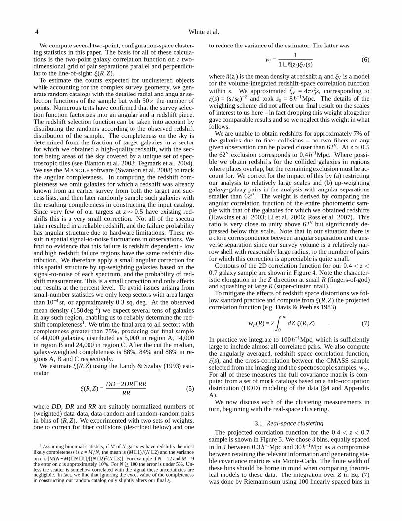
The projected correlation function for the 0.4 < z < 0.7sample is shown in Figure 5. We chose 8 bins, equally spacedin lnR between 0.3h−1Mpc and 30h−1Mpc as a compromisebetween retaining the relevant information and generatingsta-ble covariance matrices via Monte-Carlo. The finite width ofthese bins should be borne in mind when comparing theoret-ical models to these data. The integration overZ in Eq. (7)was done by Riemann sum using 100 linearly spaced bins in

Massive galaxy clustering 5

R 0.40 0.71 1.27 2.25 4.00 7.11 12.65 22.50Rwp 167.68 134.49 147.63 168.29 208.77 242.70 255.89 230.36σ 15.91 6.26 6.54 7.87 9.89 14.16 20.49 28.77

0.40 1.000 0.266 0.185 0.216 0.202 0.174 0.139 0.1680.71 – 1.000 0.346 0.329 0.312 0.299 0.238 0.2021.27 – – 1.000 0.580 0.533 0.561 0.487 0.3712.25 – – – 1.000 0.695 0.652 0.552 0.4174.00 – – – – 1.000 0.793 0.703 0.5227.11 – – – – – 1.000 0.826 0.64612.65 – – – – – – 1.000 0.80222.50 – – – – – – – 1.000

TABLE 1The projected correlation function data and covariance matrix, for 8 equally spaced bins in lnR. BothR andwp are measured in units ofh−1Mpc, with R quotedat the bin mid-point. To reduce the condition number of the covariance matrix we quote means, errors and covariances onRwp, which removes much of the runof wp with scale and makes the quoted data points more similar in magnitude. The error bars,σi, from the diagonal ofC, are broken out separately in the 3rd rowand the correlation matrix,Ci j/(σiσ j) is quoted in the lower part of the table. The full covariancematrix should be used in any fit, and the finite width of theR

bins should be included in theoretical predictions.

FIG. 5.— The projected correlation function for the 0.4< z < 0.7 sample inregions A, B and C (lines) and for the combined sample (pointswith errors).The errors on the individual samples have been suppressed for clarity. Thedata are combined using the full covariance matrix, but onlythe diagonalelements are plotted. Thewp implied by a power-law correlation functionof slope−1.8 and correlation length of 7.5h−1Mpc forms a reasonable fit tothe data with 1< Rp < 10h−1Mpc but we do not plot it here for clarity. The(thick) long-dashed-dotted line shows the prediction of the best-fitting HODmodel (§4), which provides a reasonable fit on all scales plotted (recall theerrors are correlated).

Z. The results were well converged at this spacing, becauseof the “smearing” of the correlation function along the line-of-sight due to redshift space effects. The data were analyzedseparately in each of regions A, B and C and then combinedin a minimum variance manner:

C−1w(tot)p =

∑

α=A,B,C

[

C(α)]−1

w(α)p (8)

withC−1 =

∑

α

[

C(α)]−1

(9)

wherew(α)p represents the vector ofwp measurements from

regionα =A, B or C. Not surprisingly, the combined result isdominated by the results from region C. To reduce the condi-tion number of the covariance matrix, and the dynamic rangein wp, we fit throughout toRwp and quote the results in thatform. Thewp points are quite covariant, in part because the

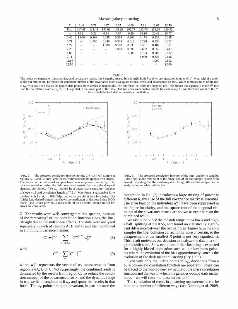
FIG. 6.— The projected correlation function of the high- and low-z samples(lines), split at the mid-point of the range, and of the full sample (points witherrors), indicating that the clustering is evolving littleand the sample can beanalyzed in one wide redshift bin.

integration in Eq. (7) introduces a large mixing of power atdifferentR, thus use of the full covariance matrix is essential.The error bars on the individualw(α)

p have been suppressed inthe figure for clarity, and the square-root of the diagonal ele-ments of the covariance matrix are shown as error bars on thecombined result.

We also subdivided the redshift range into a low-z and high-z half, splitting atz = 0.55, and found no statistically signifi-cant difference between the two samples (Figure 6; in the splitsamples the fiber collision correction is more uncertain, sothedisagreement at the smallestR point is not very significant).This result motivates our decision to analyze the data in a sin-gle redshift slice. Slow evolution of the clustering is expectedfor a highly biased population such as our luminous galax-ies where the evolution of the bias approximately cancels theevolution of the dark matter clustering (Fry 1996).

Even with only the 8 data points inwp, deviations from apure power-law correlation function are apparent. These canbe traced to the non-power-law nature of the mass correlationfunction and the way in which the galaxies occupy dark matterhalos – we will return to these issues in §4.

The calculation of errors in clustering measurements can bedone in a number of different ways (see Norberg et al. 2009,

6 White et al.

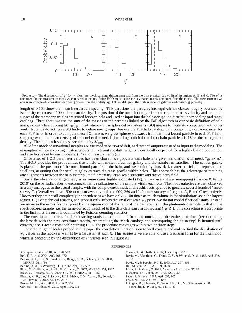
for discussion). We first tried a bootstrap estimate, dividingthe survey regions into 8-22, roughly equal area “pixels” andsampling from these regions with replacement (Efron & Gong1983). Unfortunately the irregular geometry and relativelysmall sky coverage meant we were not able to obtain a covari-ance matrix which was stable against changes in the pixeliza-tion. We anticipate that as the survey progresses this tech-nique will become more robust. In the meantime, we com-puted the covariance from a series of mock catalogs derivedfrom an iterative procedure using N-body simulations as de-scribed in Appendix A. We will show in Figure A1 that thedistribution ofχ2 from our mock catalogs encompasses thevalue obtained for the data in regions A, B and C if both arecomputed using the mock-based covariance matrix and thebest-fitting HOD model (§4). This indicates that the measure-ments we obtain are completely consistent with being drawnfrom the underlying HOD model, given the finite number ofgalaxies and observing geometry.

3.2. Redshift-space clustering

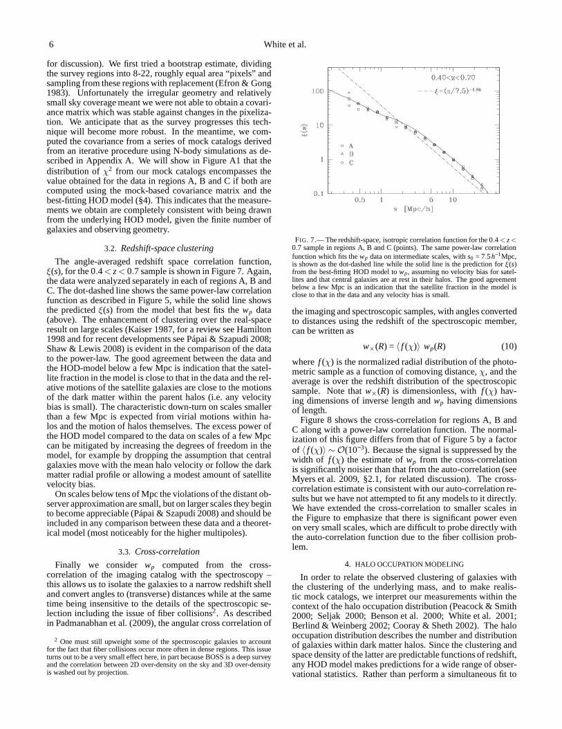
The angle-averaged redshift space correlation function,ξ(s), for the 0.4< z < 0.7 sample is shown in Figure 7. Again,the data were analyzed separately in each of regions A, B andC. The dot-dashed line shows the same power-law correlationfunction as described in Figure 5, while the solid line showsthe predictedξ(s) from the model that best fits thewp data(above). The enhancement of clustering over the real-spaceresult on large scales (Kaiser 1987, for a review see Hamilton1998 and for recent developments see Pápai & Szapudi 2008;Shaw & Lewis 2008) is evident in the comparison of the datato the power-law. The good agreement between the data andthe HOD-model below a few Mpc is indication that the satel-lite fraction in the model is close to that in the data and the rel-ative motions of the satellite galaxies are close to the motionsof the dark matter within the parent halos (i.e. any velocitybias is small). The characteristic down-turn on scales smallerthan a few Mpc is expected from virial motions within ha-los and the motion of halos themselves. The excess power ofthe HOD model compared to the data on scales of a few Mpccan be mitigated by increasing the degrees of freedom in themodel, for example by dropping the assumption that centralgalaxies move with the mean halo velocity or follow the darkmatter radial profile or allowing a modest amount of satellitevelocity bias.

On scales below tens of Mpc the violations of the distant ob-server approximation are small, but on larger scales they beginto become appreciable (Pápai & Szapudi 2008) and should beincluded in any comparison between these data and a theoret-ical model (most noticeably for the higher multipoles).

3.3. Cross-correlation

Finally we consider wp computed from the cross-correlation of the imaging catalog with the spectroscopy –this allows us to isolate the galaxies to a narrow redshift shelland convert angles to (transverse) distances while at the sametime being insensitive to the details of the spectroscopic se-lection including the issue of fiber collisions2. As describedin Padmanabhan et al. (2009), the angular cross correlationof

2 One must still upweight some of the spectroscopic galaxies to accountfor the fact that fiber collisions occur more often in dense regions. This issueturns out to be a very small effect here, in part because BOSS is a deep surveyand the correlation between 2D over-density on the sky and 3Dover-densityis washed out by projection.

FIG. 7.— The redshift-space, isotropic correlation function for the 0.4< z<0.7 sample in regions A, B and C (points). The same power-law correlationfunction which fits thewp data on intermediate scales, withs0 = 7.5h−1Mpc,is shown as the dot-dashed line while the solid line is the prediction for ξ(s)from the best-fitting HOD model towp, assuming no velocity bias for satel-lites and that central galaxies are at rest in their halos. The good agreementbelow a few Mpc is an indication that the satellite fraction in the model isclose to that in the data and any velocity bias is small.

the imaging and spectroscopic samples, with angles convertedto distances using the redshift of the spectroscopic member,can be written as

w×(R) = 〈 f (χ)〉 wp(R) (10)

where f (χ) is the normalized radial distribution of the photo-metric sample as a function of comoving distance,χ, and theaverage is over the redshift distribution of the spectroscopicsample. Note thatw×(R) is dimensionless, withf (χ) hav-ing dimensions of inverse length andwp having dimensionsof length.

Figure 8 shows the cross-correlation for regions A, B andC along with a power-law correlation function. The normal-ization of this figure differs from that of Figure 5 by a factorof 〈 f (χ)〉 ∼ O(10−3). Because the signal is suppressed by thewidth of f (χ) the estimate ofwp from the cross-correlationis significantly noisier than that from the auto-correlation (seeMyers et al. 2009, §2.1, for related discussion). The cross-correlation estimate is consistent with our auto-correlation re-sults but we have not attempted to fit any models to it directly.We have extended the cross-correlation to smaller scales inthe Figure to emphasize that there is significant power evenon very small scales, which are difficult to probe directly withthe auto-correlation function due to the fiber collision prob-lem.

4. HALO OCCUPATION MODELING

In order to relate the observed clustering of galaxies withthe clustering of the underlying mass, and to make realis-tic mock catalogs, we interpret our measurements within thecontext of the halo occupation distribution (Peacock & Smith2000; Seljak 2000; Benson et al. 2000; White et al. 2001;Berlind & Weinberg 2002; Cooray & Sheth 2002). The halooccupation distribution describes the number and distributionof galaxies within dark matter halos. Since the clustering andspace density of the latter are predictable functions of redshift,any HOD model makes predictions for a wide range of obser-vational statistics. Rather than perform a simultaneous fitto

Massive galaxy clustering 7

FIG. 8.— The cross-correlation function,w×(R), of the spectroscopic andphotometric samples which is proportional towp(R) (Eq. 10). The dot-dashed line represents a power-law correlation function. Error bars havebeen suppressed to avoid obscuring the figure. Due to the small value of〈 f (χ)〉 ∼ O(10−3) the error bars are significant, especially at large scales,and are roughly the difference between the plotted lines forregions A, B andC.

the real- and redshift-space correlation functions (includingtheir covariances) we choose to fit to the the real-space clus-tering only and show that the models which best fit these dataalso provide a reasonable description of the redshift-spaceclustering results. This avoids the need to make additionalassumptions for modeling the redshift space correlation func-tion. We also implicitly assume that we are measuring a uni-form sample of galaxies across the entire redshift range, sothat a single HOD makes sense. We tested this assumption bysplitting the sample into high- and low-redshift subsamples.

We use a halo model which distinguishes between centraland satellite galaxies with the mean occupancy of halos:

N(M) ≡ 〈Ngal(Mhalo)〉 = Ncen(M) + Nsat(M) . (11)

Each halo either hosts a central galaxy or does not, while thenumber of satellites is Poisson distributed with a meanNsat.The mean number of central galaxies per halo is modeledwith3

Ncen(M) =12

erfc

[

ln(Mcut/M)√2σ

]

(12)

and

Nsat(M) = Ncen

(

M −κMcut

M1

)

α

(13)

for M > κMcut and zero otherwise. This form implicitly as-sumes that halos do not host satellite galaxies without hostingcentrals, which is at best an approximation, but this is reason-able for the purposes of computing projected clustering. Dif-ferent functional forms have been proposed in the literature,but the current form is flexible enough for our purposes.

To explore the plausible range of HOD parameter spacewe applied the Markov Chain Monte Carlo method (MCMC;e.g., see Gilks et al. 1996) to thewp data using aχ2-basedlikelihood. This method generates a “chain” of HOD pa-rameters whose frequency of appearance traces the likelihood

3 Note that our definition ofσ can be interpreted as a fractional “scatter” inmass at threshold but is a factor ln(10)/

√2 different than that in Zheng et al.

(2005).

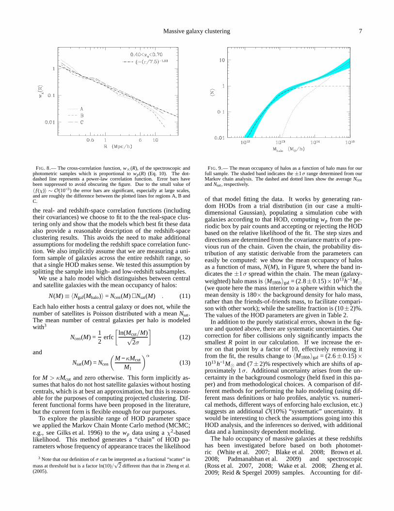
FIG. 9.— The mean occupancy of halos as a function of halo mass forourfull sample. The shaded band indicates the±1σ range determined from ourMarkov chain analysis. The dashed and dotted lines show the averageNcenandNsat, respectively.

of that model fitting the data. It works by generating ran-dom HODs from a trial distribution (in our case a multi-dimensional Gaussian), populating a simulation cube withgalaxies according to that HOD, computingwp from the pe-riodic box by pair counts and accepting or rejecting the HODbased on the relative likelihood of the fit. The step sizes anddirections are determined from the covariance matrix of a pre-vious run of the chain. Given the chain, the probability dis-tribution of any statistic derivable from the parameters caneasily be computed: we show the mean occupancy of halosas a function of mass,N(M), in Figure 9, where the band in-dicates the±1σ spread within the chain. The mean (galaxy-weighted) halo mass is〈M180b〉gal = (2.8±0.15)×1013h−1M⊙

(we quote here the mass interior to a sphere within which themean density is 180× the background density for halo mass,rather than the friends-of-friends mass, to facilitate compari-son with other work); while the satellite fraction is (10±2)%.The values of the HOD parameters are given in Table 2.

In addition to the purely statistical errors, shown in the fig-ure and quoted above, there are systematic uncertainties. Ourcorrection for fiber collisions only significantly impacts thesmallestR point in our calculation. If we increase the er-ror on that point by a factor of 10, effectively removing itfrom the fit, the results change to〈M180b〉gal = (2.6±0.15)×1013h−1M⊙ and (7±2)% respectively which are shifts of ap-proximately 1σ. Additional uncertainty arises from the un-certainty in the background cosmology (held fixed in this pa-per) and from methodological choices. A comparison of dif-ferent methods for performing the halo modeling (using dif-ferent mass definitions or halo profiles, analytic vs. numeri-cal methods, different ways of enforcing halo exclusion, etc.)suggests an additionalO(10%) “systematic” uncertainty. Itwould be interesting to check the assumptions going into thisHOD analysis, and the inferences so derived, with additionaldata and a luminosity dependent modeling.

The halo occupancy of massive galaxies at these redshiftshas been investigated before based on both photomet-ric (White et al. 2007; Blake et al. 2008; Brown et al.2008; Padmanabhan et al. 2009) and spectroscopic(Ross et al. 2007, 2008; Wake et al. 2008; Zheng et al.2009; Reid & Spergel 2009) samples. Accounting for dif-

8 White et al.

lgMcut 13.08±0.12 (13.04)lgM1 14.06±0.10 (14.05)σ 0.98±0.24 (0.94)κ 1.13±0.38 (0.93)α 0.90±0.19 (0.97)

TABLE 2The mean and standard deviation of the HOD parameters (see Eqs. 12 and13) from our Markov chain. The particular values for our best-fit model are

given in parentheses.

FIG. 10.— The HOD parameters,Mcut andM1−sat, as a function of num-ber density for a variety of intermediate redshift, massivegalaxy samplesfrom the literature (c.f. Fig. 12 of Brown et al. 2008). HereM1−sat is thehalo mass which hosts, on average, one satellite which is easier to com-pare when different functional forms forN(M) are in use. The data aretaken from Phleps et al. (2006), Mandelbaum et al. (2006), Kulkarni et al.(2007), Blake et al. (2008), Brown et al. (2008), Padmanabhan et al. (2009),Wake et al. (2008), Zheng et al. (2009) and this work, as notedin the legend.Error bars on the individual points have been suppressed forclarity, but aretypically 0.1 dex. The solid line in the lower panel shows thehalo mass func-tion atz = 0.55 for comparison. The value ofMcut for a sample of only centralgalaxies with no scatter between observable and halo mass would follow thisline.

ferences in sample selection and redshift range, our resultsappear quite consistent with the previous literature (seeFig. 10).

Our galaxies populate a broad range of halo masses, withan approximate power-law dependence of the mean numberof galaxies per halo with halo mass for massive halos and abroad roll-off at lower halo masses. The low mass behav-ior is driven by the amplitude of the large-scale clusteringincombination with the relatively high number density of oursample and encodes information about the scaling of the cen-tral galaxy luminosity with halo mass and its distribution.Wefind that the halos with masses (2− 3)× 1013h−1M⊙ containon average one of our massive galaxies. At these redshiftssuch halos are quite highly biased (see below), correspondingto galaxy groups, and we expectb(z) ∝ 1/D(z), whereD(z) isthe linear growth rate, leading to an approximately constantclustering amplitude with redshift.

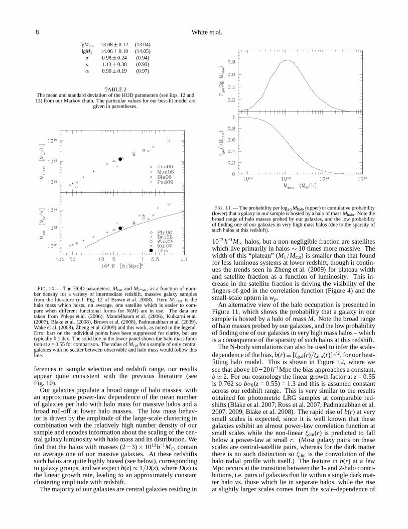
The majority of our galaxies are central galaxies residing in

FIG. 11.— The probability per log10Mhalo (upper) or cumulative probability(lower) that a galaxy in our sample is hosted by a halo of massMhalo. Note thebroad range of halo masses probed by our galaxies, and the lowprobabilityof finding one of our galaxies in very high mass halos (due to the sparsity ofsuch halos at this redshift).

1013h−1M⊙ halos, but a non-negligible fraction are satelliteswhich live primarily in halos∼ 10 times more massive. Thewidth of this “plateau” (M1/Mcut) is smaller than that foundfor less luminous systems at lower redshift, though it contin-ues the trends seen in Zheng et al. (2009) for plateau widthand satellite fraction as a function of luminosity. This in-crease in the satellite fraction is driving the visibility of thefingers-of-god in the correlation function (Figure 4) and thesmall-scale upturn inwp.

An alternative view of the halo occupation is presented inFigure 11, which shows the probability that a galaxy in oursample is hosted by a halo of massM. Note the broad rangeof halo masses probed by our galaxies, and the low probabilityof finding one of our galaxies in very high mass halos – whichis a consequence of the sparsity of such halos at this redshift.

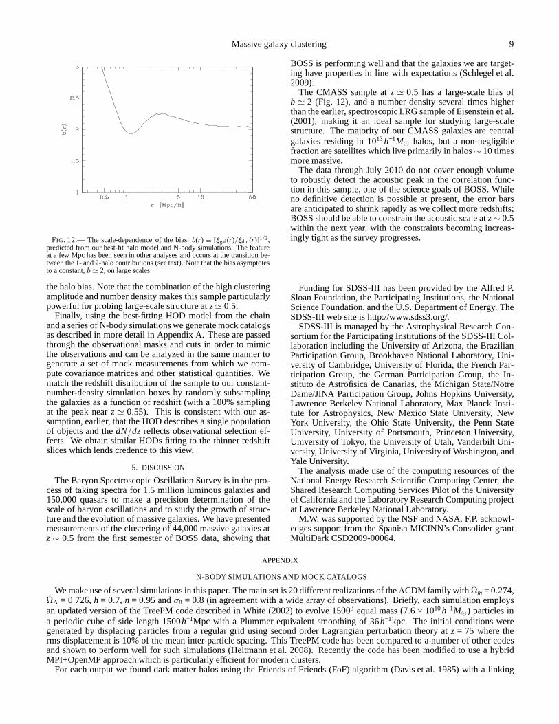
The N-body simulations can also be used to infer the scale-dependence of the bias,b(r)≡ [ξgal(r)/ξdm(r)]1/2, for our best-fitting halo model. This is shown in Figure 12, where wesee that above 10− 20h−1Mpc the bias approaches a constant,b ≃ 2. For our cosmology the linear growth factor atz = 0.55is 0.762 sobσ8(z = 0.55) = 1.3 and this is assumed constantacross our redshift range. This is very similar to the resultsobtained for photometric LRG samples at comparable red-shifts (Blake et al. 2007; Ross et al. 2007; Padmanabhan et al.2007, 2009; Blake et al. 2008). The rapid rise ofb(r) at verysmall scales is expected, since it is well known that thesegalaxies exhibit an almost power-law correlation functionatsmall scales while the non-linearξdm(r) is predicted to fallbelow a power-law at smallr. (Most galaxy pairs on thesescales are central-satellite pairs, whereas for the dark matterthere is no such distinction soξdm is the convolution of thehalo radial profile with itself.) The feature inb(r) at a fewMpc occurs at the transition between the 1- and 2-halo contri-butions, i.e. pairs of galaxies that lie within a single darkmat-ter halo vs. those which lie in separate halos, while the riseat slightly larger scales comes from the scale-dependence of

Massive galaxy clustering 9

FIG. 12.— The scale-dependence of the bias,b(r) ≡ [ξgal(r)/ξdm(r)]1/2,predicted from our best-fit halo model and N-body simulations. The featureat a few Mpc has been seen in other analyses and occurs at the transition be-tween the 1- and 2-halo contributions (see text). Note that the bias asymptotesto a constant,b ≃ 2, on large scales.

the halo bias. Note that the combination of the high clusteringamplitude and number density makes this sample particularlypowerful for probing large-scale structure atz ≃ 0.5.

Finally, using the best-fitting HOD model from the chainand a series of N-body simulations we generate mock catalogsas described in more detail in Appendix A. These are passedthrough the observational masks and cuts in order to mimicthe observations and can be analyzed in the same manner togenerate a set of mock measurements from which we com-pute covariance matrices and other statistical quantities. Wematch the redshift distribution of the sample to our constant-number-density simulation boxes by randomly subsamplingthe galaxies as a function of redshift (with a 100% samplingat the peak nearz ≃ 0.55). This is consistent with our as-sumption, earlier, that the HOD describes a single populationof objects and thedN/dz reflects observational selection ef-fects. We obtain similar HODs fitting to the thinner redshiftslices which lends credence to this view.

5. DISCUSSION

The Baryon Spectroscopic Oscillation Survey is in the pro-cess of taking spectra for 1.5 million luminous galaxies and150,000 quasars to make a precision determination of thescale of baryon oscillations and to study the growth of struc-ture and the evolution of massive galaxies. We have presentedmeasurements of the clustering of 44,000 massive galaxies atz ∼ 0.5 from the first semester of BOSS data, showing that

BOSS is performing well and that the galaxies we are target-ing have properties in line with expectations (Schlegel et al.2009).

The CMASS sample atz ≃ 0.5 has a large-scale bias ofb ≃ 2 (Fig. 12), and a number density several times higherthan the earlier, spectroscopic LRG sample of Eisenstein etal.(2001), making it an ideal sample for studying large-scalestructure. The majority of our CMASS galaxies are centralgalaxies residing in 1013h−1M⊙ halos, but a non-negligiblefraction are satellites which live primarily in halos∼ 10 timesmore massive.

The data through July 2010 do not cover enough volumeto robustly detect the acoustic peak in the correlation func-tion in this sample, one of the science goals of BOSS. Whileno definitive detection is possible at present, the error barsare anticipated to shrink rapidly as we collect more redshifts;BOSS should be able to constrain the acoustic scale atz ∼ 0.5within the next year, with the constraints becoming increas-ingly tight as the survey progresses.

Funding for SDSS-III has been provided by the Alfred P.Sloan Foundation, the Participating Institutions, the NationalScience Foundation, and the U.S. Department of Energy. TheSDSS-III web site is http://www.sdss3.org/.

SDSS-III is managed by the Astrophysical Research Con-sortium for the Participating Institutions of the SDSS-IIICol-laboration including the University of Arizona, the BrazilianParticipation Group, Brookhaven National Laboratory, Uni-versity of Cambridge, University of Florida, the French Par-ticipation Group, the German Participation Group, the In-stituto de Astrofisica de Canarias, the Michigan State/NotreDame/JINA Participation Group, Johns Hopkins University,Lawrence Berkeley National Laboratory, Max Planck Insti-tute for Astrophysics, New Mexico State University, NewYork University, the Ohio State University, the Penn StateUniversity, University of Portsmouth, Princeton University,University of Tokyo, the University of Utah, Vanderbilt Uni-versity, University of Virginia, University of Washington, andYale University.

The analysis made use of the computing resources of theNational Energy Research Scientific Computing Center, theShared Research Computing Services Pilot of the Universityof California and the Laboratory Research Computing projectat Lawrence Berkeley National Laboratory.

M.W. was supported by the NSF and NASA. F.P. acknowl-edges support from the Spanish MICINN’s Consolider grantMultiDark CSD2009-00064.

APPENDIX

N-BODY SIMULATIONS AND MOCK CATALOGS

We make use of several simulations in this paper. The main setis 20 different realizations of theΛCDM family with Ωm = 0.274,ΩΛ = 0.726,h = 0.7, n = 0.95 andσ8 = 0.8 (in agreement with a wide array of observations). Briefly, each simulation employsan updated version of the TreePM code described in White (2002) to evolve 15003 equal mass (7.6×1010h−1M⊙) particles ina periodic cube of side length 1500h−1Mpc with a Plummer equivalent smoothing of 36h−1kpc. The initial conditions weregenerated by displacing particles from a regular grid usingsecond order Lagrangian perturbation theory atz = 75 where therms displacement is 10% of the mean inter-particle spacing.This TreePM code has been compared to a number of other codesand shown to perform well for such simulations (Heitmann et al. 2008). Recently the code has been modified to use a hybridMPI+OpenMP approach which is particularly efficient for modern clusters.

For each output we found dark matter halos using the Friends of Friends (FoF) algorithm (Davis et al. 1985) with a linking

10 White et al.

FIG. A1.— The distribution ofχ2 for wp from our mock catalogs (histograms) and from the data (vertical dashed lines) in regions A, B and C. Theχ2 iscomputed for the measured or mockwp compared to the best-fitting HOD model using the covariance matrix computed from the mocks. The measurements weobtain are completely consistent with being drawn from the underlying HOD model, given the finite number of galaxies and observing geometry.

length of 0.168 times the mean interparticle spacing. This partitions the particles into equivalence classes roughly bounded byisodensity contours of 100× the mean density. The position of the most-bound particle, the center of mass velocity and a randomsubset of the member particles are stored for each halo and used as input into the halo occupation distribution modeling and mockcatalogs. Throughout we use the sum of the masses of the particles linked by the FoF algorithm as our basic definition of halomass, except when quoting〈M180b〉gal in §4 where we use spherical over-density (SO) masses to facilitate comparison with otherwork. Note we do not run a SO finder to define new groups. We use the FoF halo catalog, only computing a different mass foreach FoF halo. In order to compute these SO masses we grow spheres outwards from the most bound particle in each FoF halo,stopping when the mean density of the enclosed material (including both halo and non-halo particles) is 180× the backgrounddensity. The total enclosed mass we denote byM180b.

All of the mock observational samples are assumed to be iso-redshift, and “static” outputs are used as input to the modeling. Theassumption of non-evolving clustering over the relevant redshift range is theoretically expected for a highly biased population,and also borne out by our modeling (§4) and measurements (§3).

Once a set of HOD parameter values has been chosen, we populate each halo in a given simulation with mock “galaxies”.The HOD provides the probabilities that a halo will contain acentral galaxy and the number of satellites. The central galaxyis placed at the position of the most bound particle in the halo, and we randomly draw dark matter particles to represent thesatellites, assuming that the satellite galaxies trace themass profile within halos. This approach has the advantage ofretainingany alignments between the halo material, the filamentary large-scale structure and the velocity field.

Since the observational geometry is in some cases highly elongated (Fig. 3), we use volume remapping (Carlson & White2010) on the periodic cubes to encompass many realizations of the sample within each box. The mock galaxies are then observedin a way analogous to the actual sample, with the completeness mask and redshift cuts applied to generate several hundred“mocksurveys”. (Overall we have 1500 mock surveys, divided into 900, 360 and 240 mock surveys of regions A, B and C respectively.However they are not all completely independent as we have only ∼ 100 times as much volume in the simulations as in the largestregion, C.) For technical reasons, and since it only affectsthe smallest scalewp point, we do not model fiber collisions. Insteadwe increase the errors for that point by the square root of theratio of the pair counts in the photometric sample to that in thespectroscopic sample (i.e. the same correction applied to the data-data pairs in computingξ(R,Z)). This correction is appropriatein the limit that the error is dominated by Poisson counting statistics.

The covariance matrices for the clustering statistics are obtained from the mocks, and the entire procedure (reconstructingthe best-fit with the new covariance matrix, recomputing themock catalogs and recomputing the clustering) is iterated untilconvergence. Given a reasonable starting HOD, the procedure converges within two or three steps.

Over the range of scales probed in this paper the correlationfunction is quite well constrained and we find the distribution ofwp values in the mocks is well fit by a Gaussian at eachR. This suggests we are able to use a Gaussian form for the likelihood,which is backed up by the distribution ofχ2 values seen in Figure A1.

REFERENCES

Abazajian, K., et al. 2004, AJ, 128, 502Bell, E. F., et al. 2004, ApJ, 608, 752Benson, A. J., Cole, S., Frenk, C. S., Baugh, C. M., & Lacey, C.G. 2000,

MNRAS, 311, 793Berlind, A. A., & Weinberg, D. H. 2002, ApJ, 575, 587Blake, C., Collister, A., Bridle, S., & Lahav, O. 2007, MNRAS, 374, 1527Blake, C., Collister, A., & Lahav, O. 2008, MNRAS, 385, 1257Blanton, M. R., Lin, H., Lupton, R. H., Maley, F. M., Young, N., Zehavi, I.,

& Loveday, J. 2003, AJ, 125, 2276Brown, M. J. I., et al. 2008, ApJ, 682, 937Carlson, J., & White, M. 2010, ApJS, 190, 311

Cooray, A., & Sheth, R. 2002, Phys. Rep., 372, 1Davis, M., Efstathiou, G., Frenk, C. S., & White, S. D. M. 1985, ApJ, 292,

371Davis, M., & Peebles, P. J. E. 1983, ApJ, 267, 465Doi, M., et al. 2010, AJ, 139, 1628Efron, B., & Gong, G. 1983, American Statistician, 37, 36Eisenstein, D. J., et al. 2001, AJ, 122, 2267Faber, S. M., et al. 2007, ApJ, 665, 265Fry, J. N. 1996, ApJ, 461, L65+Fukugita, M., Ichikawa, T., Gunn, J. E., Doi, M., Shimasaku,K., &

Schneider, D. P. 1996, AJ, 111, 1748

Massive galaxy clustering 11

Gilks, W. R., Richardson, S., & Spiegelhalter, D. J. 1996, Markov ChainMonte Carlo in Practice (London: Chapman and Hall, 1966)

Gregory, S. A., & Thompson, L. A. 1978, ApJ, 222, 784Gunn, J. E., et al. 1998, AJ, 116, 3040—. 2006, AJ, 131, 2332Hamilton, A. J. S. 1998, in Astrophysics and Space Science Library, Vol.

231, The Evolving Universe, ed. D. Hamilton, 185–+Hawkins, E., et al. 2003, MNRAS, 346, 78Heitmann, K., et al. 2008, Computational Science and Discovery, 1, 015003Huchra, J., Davis, M., Latham, D., & Tonry, J. 1983, ApJS, 52,89Humason, M. L., Mayall, N. U., & Sandage, A. R. 1956, AJ, 61, 97Joeveer, M., & Einasto, J. 1978, in IAU Symposium, Vol. 79, Large Scale

Structures in the Universe, ed. M. S. Longair & J. Einasto, 241–250Kaiser, N. 1987, MNRAS, 227, 1Kulkarni, G. V., Nichol, R. C., Sheth, R. K., Seo, H., Eisenstein, D. J., &

Gray, A. 2007, MNRAS, 378, 1196Landy, S. D., & Szalay, A. S. 1993, ApJ, 412, 64Li, C., Kauffmann, G., Jing, Y. P., White, S. D. M., Börner, G., & Cheng,

F. Z. 2006, MNRAS, 368, 21Lupton, R., Gunn, J. E., Ivezic, Z., Knapp, G. R., & Kent, S. 2001, in

Astronomical Society of the Pacific Conference Series, Vol.238,Astronomical Data Analysis Software and Systems X, ed. F. R.HarndenJr., F. A. Primini, & H. E. Payne, 269–+

Mandelbaum, R., Seljak, U., Kauffmann, G., Hirata, C. M., & Brinkmann, J.2006, MNRAS, 368, 715

Maraston, C., Strömbäck, G., Thomas, D., Wake, D. A., & Nichol, R. C.2009, MNRAS, 394, L107

Myers, A. D., White, M., & Ball, N. M. 2009, MNRAS, 399, 2279Norberg, P., Baugh, C. M., Gaztañaga, E., & Croton, D. J. 2009, MNRAS,

396, 19Padmanabhan, N., White, M., Norberg, P., & Porciani, C. 2009, MNRAS,

397, 1862

Padmanabhan, N., et al. 2007, MNRAS, 378, 852—. 2008, ApJ, 674, 1217Pápai, P., & Szapudi, I. 2008, MNRAS, 389, 292Peacock, J. A., & Smith, R. E. 2000, MNRAS, 318, 1144Phleps, S., Peacock, J. A., Meisenheimer, K., & Wolf, C. 2006, A&A, 457,

145Pier, J. R., Munn, J. A., Hindsley, R. B., Hennessy, G. S., Kent, S. M.,

Lupton, R. H., & Ivezic, Ž. 2003, AJ, 125, 1559Reid, B. A., & Spergel, D. N. 2009, ApJ, 698, 143Ross, N. P., Shanks, T., Cannon, R. D., Wake, D. A., Sharp, R. G., Croom,

S. M., & Peacock, J. A. 2008, MNRAS, 387, 1323Ross, N. P., et al. 2007, MNRAS, 381, 573Schlegel, D., White, M., & Eisenstein, D. 2009, in ArXiv Astrophysics

e-prints, Vol. 2010, astro2010: The Astronomy and Astrophysics DecadalSurvey, 314–+

Schlegel, D. J., Finkbeiner, D. P., & Davis, M. 1998, ApJ, 500, 525Seljak, U. 2000, MNRAS, 318, 203Shaw, J. R., & Lewis, A. 2008, Phys. Rev. D, 78, 103512Smith, J. A., et al. 2002, AJ, 123, 2121Stoughton, C., et al. 2002, AJ, 123, 485Swanson, M. E. C., Tegmark, M., Hamilton, A. J. S., & Hill, J. C. 2008,

MNRAS, 387, 1391Tegmark, M., et al. 2004, ApJ, 606, 702Wake, D. A., et al. 2008, MNRAS, 387, 1045White, M. 2002, ApJS, 143, 241White, M., Hernquist, L., & Springel, V. 2001, ApJ, 550, L129White, M., Zheng, Z., Brown, M. J. I., Dey, A., & Jannuzi, B. T.2007, ApJ,

655, L69York, D. G., et al. 2000, AJ, 120, 1579Zheng, Z., Zehavi, I., Eisenstein, D. J., Weinberg, D. H., & Jing, Y. P. 2009,

ApJ, 707, 554Zheng, Z., et al. 2005, ApJ, 633, 791