Fizyoloji Ders Notları Version 0.5 (LTS) Powerpoint destekli

arX
iv:1
207.
6114
v1 [
astr
o-ph
.CO
] 25
Jul
201
2
Mon. Not. R. Astron. Soc.000, 1–21 (2012) Printed 27 July 2012 (MN LATEX style file v2.2)
Stellar masses of SDSS-III/BOSS galaxies atz ∼ 0.5 and constraintsto galaxy formation models
Claudia Maraston1,4⋆, Janine Pforr2, Bruno M. Henriques3, Daniel Thomas1,4,David Wake4, Joel R. Brownstein12, Diego Capozzi1,4, Kevin Bundy5,Ramin A. Skibba6, Alessandra Beifiori7, Robert C. Nichol1,4, Edd Edmondson1,Don P. Schneider8,9, Yanmei Chen10,11, Karen L. Masters1,4, Oliver Steele1,Adam S. Bolton12, Donald G. York13, Dmitry Bizyaev14, Howard Brewington14,Elena Malanushenko14, Viktor Malanushenko14, Stephanie Snedden14,Daniel Oravetz14, Kaike Pan14, Alaina Shelden14, Audrey Simmons141Institute of Cosmology and Gravitation, Dennis Sciama Building, Burnaby Road, Portsmouth PO1 3FX2National Optical Astronomy Observatories, 950 N. Cherry Ave., Tucson, AZ, 85719, USA3Max-Planck-Institut fur Astrophysik, Karl-Schwarzschild-Str. 1, 85741 Garching b. Munchen, Germany4South East Physics Network, www.sepnet.ac.uk4Department of Astronomy,Yale University,P.O. Box 208101,New Haven, CT 06520-8101, USA5Kavli Institute for the Physics and Mathematics of the Universe, Todai Institutes for Advanced Study, the University ofTokyo, Kashiwa, Japan 277-8583 (Kavli IPMU, WPI)6Steward Observatory, University of Arizona, 933 North Cherry Avenue, Tucson, AZ 85721, USA7Max-Planck-Institut fur Extraterrestrische Physik, Giessenbachstrae, D-85748 Garching, Germany8Department of Astronomy and Astrophysics, The Pennsylvania State University, University Park, PA 168029Institute for Gravitation and the Cosmos, The PennsylvaniaState University, University Park, PA 1680210 Department of Astronomy, Nanjing University, Nanjing 210093, China11 Key Laboratory of Modern Astronomy and Astrophysics (Nanjing University), Ministry of Education, Nanjing 210093, China12Department of Physics & Astronomy, University of Utah, 115 South 1400 East, Salt Lake City, UT 84112 USA13Department of Astronomy and Astrophysics and the Fermi Institute, The University of Chicago, 5640 South Ellis Avenue, Chicago, IL 6061514Apache Point Observatory, P.O. Box 59, Sunspot, NM 88349-0059, USA
Accepted. Received; in original form 25 July 2012
ABSTRACTWe calculate stellar masses for∼ 400, 000 massive luminous galaxies at redshift∼0.2 − 0.7 using the first two years of data from the Baryon Oscillation Spectroscopic Sur-vey (BOSS). Stellar masses are obtained by fitting model spectral energy distributions tou, g, r, i, z magnitudes. Accurate BOSS spectroscopic redshifts are used to constrain the fits.We find that the distribution of stellar masses in BOSS is narrow (∆ logM ∼ 0.5 dex) andpeaks at aboutlog M/M⊙ ∼ 11.3 (for a Kroupa initial stellar mass function), and that themass sampling is uniform over the redshift range 0.2 to 0.6, in agreement with the intendedBOSS target selection. The galaxy masses probed by BOSS extend over∼ 1012M⊙, provid-ing unprecedented measurements of the high-mass end of the galaxy mass function. We findthat the galaxy number density above∼ 2.5 · 1011M⊙ agrees with previous determinationswithin 2σ, but there is a slight offset towards lower number densitiesin BOSS. This alleviatesa tension between thez
∼< 0.1 and the high-redshift mass function. We perform a comparison
with semi-analytic galaxy formation models tailored to theBOSS target selection and vol-ume, in order to contain incompleteness. The abundance of massive galaxies in the modelscompare well with the BOSS data. However, no evolution is detected from redshift∼ 0.6 to0 in the data, whereas the abundance of massive galaxies in the models increases to redshiftzero. BOSS data display colour-magnitude (mass) relationssimilar to those found in the lo-cal Universe, where the most massive galaxies are the reddest. On the other hand, the modelcolours do not display a dependence on stellar mass, span a narrower range and are typicallybluer than the observations. We argue that the lack of a colour-mass relation in the models ismostly due to metallicity, which is too low in the models.
Key words: galaxies: stellar content; galaxies: evolution; galaxies: formation
c© 2012 RAS

2 C. Maraston et al.
1 INTRODUCTION
In the cold dark matter hierarchical Universe model (White &Rees1978), galaxies grow from primordial density fluctuations inthe power spectrum (Blumenthal et al. 1984; Davis et al. 1985)and assemble their mass over cosmic time through a variety ofprocesses, such as star formation, merging and accretion (e.g.Kauffmann et al. 1993; Somerville & Primack 1999; Cole et al.2000; Hatton et al. 2003; Menci et al. 2004; Monaco et al. 2007;Henriques & Thomas 2010; Guo et al. 2011; Henriques et al.2012). The observational tracing of the galaxy mass growth as afunction of redshift is a powerful diagnostic of the galaxy for-mation process, which has been investigated by many groups,through large galaxy surveys (e.g. the Sloan Digital Sky Survey,SDSS, York et al. 2000; COMBO-17, Wolf et al. 2001; MUNICS,Drory et al. 2001; DEEP2, Davis et al. 2003; GOODS, Dickin-son et al. 2003; VVDS, Le Fevre et al. 2005; 2SLAQ, Cannonet al. 2006; COSMOS, Scoville et al. 2007; GMASS, Kurk et al.2008; GAMA, Driver et al. 2011; CANDELS, Grogin et al. 2011;SERVS, Mauduit et al. 2012. See also the review by Renzini 2006).
The massive (M∼> 5 · 1010 M⊙) component of the galaxypopulation is particularly interesting in the context of galaxyformation and cosmology because the stellar population proper-ties, such as stellar ages and chemical abundances, of massivegalaxies are notoriously challenging to models, e.g. the high-fraction of α-elements over iron and the [α/Fe] versus galaxystellar mass relation (Worthey et al. 1992; Davies et al. 1993;Carollo & Danziger 1994; Rose et al. 1994; Bender & Paquet1995; Jorgensen et al. 1995; Greggio 1997; Trager et al. 2000;Kuntschner 2000; Proctor & Sansom 2002; Smith et al. 2009;Thomas et al. 2005, 2010), the uniformly old stellar ages with littleevidence of star formation (Bower et al. 1992, 1998; Thomas et al.2005; Bernardi et al. 2006), the independence of the stellarpopula-tion properties of the environment (Peng et al. 2010; Thomaset al.2010). There are still many unknowns in the process of galaxyfor-mation and evolution, both at the high and low mass end of thegalaxy distribution (see reviews by Silk 2011 and White 2011),which are thought to be mostly related to the baryonic componentof galaxies, especially to the poorly known processes involvinggas physics, such as star formation and feedback from stars andAGN (e.g. Governato et al. 1998; Kauffmann & Haehnelt 2000;Croton et al. 2006; Bower et al. 2006; Ciotti & Ostriker 2007;Oppenheimer & Dave 2008; Johansson et al. 2012), and their in-terplay with the mass assembly over cosmic time (e.g., Boweret al.2012).
An efficient way to probe the galaxy formation process isto study the galaxy luminosity and stellar mass functions andtheir evolution with redshift. In the local universe, recent resultson the stellar mass function of galaxies include Blanton et al.(2003), Bell et al. (2003), Baldry et al. (2004), Baldry et al. (2006),Baldry et al. (2008), Li & White (2009), Baldry et al. (2012).
At larger look-back times, several authors studied the stellarmass function as a function of redshift (Brinchmann & Ellis 2000;Drory et al. 2001, 2004, 2005; Cohen 2002; Dickinson et al. 2003;Fontana et al. 2003, 2006; Rudnick et al. 2003; Glazebrook etal.2004; Bundy et al. 2005; Conselice et al. 2005; Borch et al.2006; Cimatti et al. 2006; Bundy et al. 2006; Pozzetti et al. 2007;Perez-Gonzalez et al. 2008; Marchesini et al. 2009; Ilbert et al.2010; Pozzetti et al. 2010), reaching redshifts of about 4. At z < 1,which is the focus of this work, the galaxy stellar mass functionappears to evolve slowly, with about half of the total stellar massdensity atz ∼ 0 already in place atz ∼ 1. Moreover, little if no
evolution is detected at the high-mass end (M ∼> 1011 M⊙), which
is one of the manifestations of thedownsizingscenario for galaxyformation in both star formation and mass assembly (Cimattiet al.2006; Renzini 2006, 2009; Peng et al. 2010). Such limited evolu-tion for the most massive galaxies belowz ∼ 1 is also supportedby luminosity function studies (Wake et al. 2006; Cool et al.2008)as well as by the lack of evolution of galaxy clustering (Wakeet al.2008; Tojeiro & Percival 2010).
In this work we exploit the Baryon Oscillation Spectro-scopic survey (BOSS; Schlegel et al. 2009; Dawson et al. 2012,submitted), which is part of the Sloan Digital Sky Survey III(Eisenstein et al. 2011), for calculating galaxy stellar masses andthe galaxy stellar mass function atz ∼ 0.5. The advantage of-fered by BOSS is the unprecedented survey area - 10,000deg intotal, and roughly 1/3 complete at the time of writing - and a selec-tion cut favouring the most massive galaxies (M ∼
> 1011 M⊙). Thehuge area coverage, and the redshift range, which lies in themiddleof the theoretical late-time mass-assembly epoch (De Luciaet al.2006), renders BOSS an excellent survey for galaxy evolution stud-ies.
In this first study we do not apply completeness correctionsand focus on alight-conedmass function. The comparison withgalaxy formation models will be performed with simulationstai-lored to the BOSS target selection and volume. The global stel-lar mass and luminosity function for the BOSS survey, includ-ing completeness, will be published in subsequent papers. As wewill see from the comparison with other published mass func-tions, BOSS may be essentially complete at the high-mass end(M ∼
> 5 · 1011 M⊙).The aim of this publication is twofold. First, we describe the
stellar mass calculation and discuss the results. We also comparephotometric masses with spectroscopic ones that were obtained us-ing PCA algorithm applied to BOSS spectra (Chen et al. 2012).Wethen calculate the mass function over the redshift range 0.45 to0.7 and compare the resulting stellar mass density and the galaxycolours with semi-analytic models of galaxy formation and evolu-tion, to obtain clues to the late-time evolution of massive galax-ies. In particular, given the unprecedented statistics offered by theBOSS sample at the massive end, we can study whether the mainbody of passive galaxies in the models has the correct mass distri-bution and the right colours.
There have been several examples of such an approach in theliterature. Benson et al. (2003) extensively studied the constraintsto the theoretical galaxy luminosity function that are posed by datain the local Universe. Almeida et al. (2008) focus on luminous, redgalaxies atz∼< 0.5 and compare the observed luminosity func-tion with galaxy formation models - by Bower et al. (2006) andBaugh et al. (2005) - which adopt different feedback mechanismsfor quenching star formation. Fontanot et al. (2009) study the com-parison of the stellar mass function in various semi-analytic mod-els with data over a wide redshift range. Neistein & Weinmann(2010) discuss degeneracies of semi-analytic models including dif-ferent prescriptions for cooling and feedback, and their abilityto match several observational constraints, including thegalaxymass function. The task of comparing galaxy formation modelsto quantities derived from data, especially at high look-back time,is not an easy one, as modelled data rather than pure observablesneed to be used. Some works have concentrated on theobserved-frame which avoids the extra-assumptions involved in translat-ing the observed colours and luminosities into physical quantities(Tonini et al. 2009), while others support the use of thederived-propertyplane in any case (Conroy et al. 2010). Here we consider
c© 2012 RAS, MNRAS000, 1–21
BOSS stellar masses 3
the comparisons in both systems of reference, by comparing galaxycolours in the observed frame, and the galaxy mass function usingdata-modelled stellar masses.
Finally, we compare the light-coned BOSS mass function withmass functions from the literature.
The paper is organised as follows. In Section 2 we introducethe BOSS data, in Section 3 we detail the stellar mass calculationand in Section 4 we present and discuss the results relative to thestellar masses of BOSS galaxies. In Section 5 we perform the com-parison with semi-analytic models and in Section 6 we summarisethe work and draw conclusions.
Throughout the paper the cosmology from WMAP1, i.e.ΩM = 0.25, H0 = 0.73 km s−1Mpc−1, ΩT = 1, is assumedfor consistency with the galaxy evolution models (Guo et al.2011;Henriques et al. 2012)1.
2 BOSS GALAXY DATA
The BOSS survey (Schlegel et al. 2009) aims at constraining thelate time acceleration in the Universe via Baryon Acoustic Oscilla-tions (Eisenstein et al. 2005; see also Anderson et al. 2012 for thefirst results on BOSS), with an observational effort of galaxy spec-troscopy and photometry over five years, that started in Fall2009.An overview of BOSS is given in Dawson et al. (2012,submit-ted). Below we summarise the key aspects that are relevant to thispaper. BOSS is one of four surveys of the SDSS-III collaboration(Eisenstein et al. 2011) using an upgrade of the multi-object spec-trograph (Smee et al. 2012,submitted) on the 2.5m SDSS telescope(Gunn et al. 2006) located at Apache Point Observatory in NewMexico. BOSS obtains medium resolution (R = 2000) spectra forgalaxies, QSOs and stars in the wavelength range3750−10000 A.Standard SDSS imaging using a drift-scanning mosaic CCD cam-era (Gunn et al. 1998) is obtained for luminous galaxies overtheredshift range 0.3 to 0.7, selected to be the most massive andwith a uniform mass sampling with redshift (White et al. 2011;Eisenstein et al. 2011). The acquired photometry has been releasedwith the Data Release 8 (DR8, Aihara et al. 2011), and the firstsetof spectra will be made publicly available with the Data Release 9(DR9), in Summer 2012 (Ahn et al. 2012,submitted).
For the project, we calculated photometric stellar massesfor BOSS galaxies. We use the galaxy spectroscopic redshiftde-termined by the BOSS pipeline (Bolton et al. 2012,submitted;Schlegel et al. 2012,in prep.) and standardu, g, r, i, z SDSS pho-tometry (Fukugita et al. 1996) for performing spectral energy dis-tribution (SED) fitting at fixed spectroscopic redshift in order toobtain a best-fit model and from it an estimate of the stellar mass(see Section 3). The values of stellar mass and the routines to per-form the same calculations for the rest of the BOSS survey will bemade publicly available through DR9 in Summer 2012.2
Spectroscopic redshifts are determined from BOSS spectra us-ing the latest version of the SDSS Spec 1D pipeline and an ex-tensive set of templates, based on both stellar empirical spectra as
1 Note that for the DR9 release, see Section 2, a slightly different cosmol-ogy has been adopted, namelyΩ = 0.258, H0 = 71.9 km s−1Mpc−1,ΩT = 1,. We checked that this implies a negligible effect on stellar masses.2 For this work we selected objects with solid spectroscopic redshiftdetermination (corresponding to the flagzwarning=0) and we used theprimary spectroscopic observation available (using flagspecprimary=1).These flags select a total number of galaxies which is slightly lower thanwhat will be available with DR9.
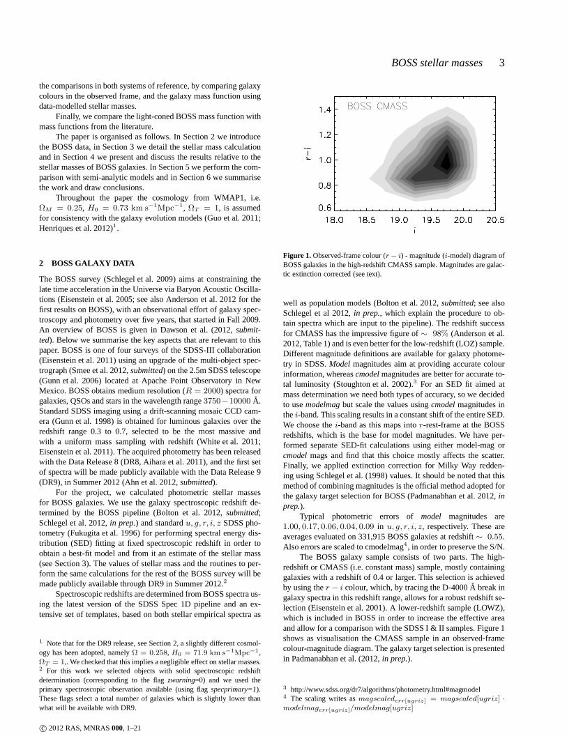
Figure 1. Observed-frame colour (r− i) - magnitude (i-model) diagram ofBOSS galaxies in the high-redshift CMASS sample. Magnitudes are galac-tic extinction corrected (see text).
well as population models (Bolton et al. 2012,submitted; see alsoSchlegel et al 2012,in prep., which explain the procedure to ob-tain spectra which are input to the pipeline). The redshift successfor CMASS has the impressive figure of∼ 98% (Anderson et al.2012, Table 1) and is even better for the low-redshift (LOZ) sample.Different magnitude definitions are available for galaxy photome-try in SDSS.Model magnitudes aim at providing accurate colourinformation, whereascmodelmagnitudes are better for accurate to-tal luminosity (Stoughton et al. 2002).3 For an SED fit aimed atmass determination we need both types of accuracy, so we decidedto usemodelmagbut scale the values usingcmodelmagnitudes inthei-band. This scaling results in a constant shift of the entireSED.We choose thei-band as this maps intor-rest-frame at the BOSSredshifts, which is the base for model magnitudes. We have per-formed separate SED-fit calculations using either model-mag orcmodelmags and find that this choice mostly affects the scatter.Finally, we applied extinction correction for Milky Way redden-ing using Schlegel et al. (1998) values. It should be noted that thismethod of combining magnitudes is the official method adopted forthe galaxy target selection for BOSS (Padmanabhan et al. 2012, inprep.).
Typical photometric errors ofmodel magnitudes are1.00, 0.17, 0.06, 0.04, 0.09 in u, g, r, i, z, respectively. These areaverages evaluated on 331,915 BOSS galaxies at redshift∼ 0.55.Also errors are scaled to cmodelmag4, in order to preserve the S/N.
The BOSS galaxy sample consists of two parts. The high-redshift or CMASS (i.e. constant mass) sample, mostly containinggalaxies with a redshift of 0.4 or larger. This selection is achievedby using ther − i colour, which, by tracing the D-4000A break ingalaxy spectra in this redshift range, allows for a robust redshift se-lection (Eisenstein et al. 2001). A lower-redshift sample (LOWZ),which is included in BOSS in order to increase the effective areaand allow for a comparison with the SDSS I & II samples. Figure1shows as visualisation the CMASS sample in an observed-framecolour-magnitude diagram. The galaxy target selection is presentedin Padmanabhan et al. (2012,in prep.).
3 http://www.sdss.org/dr7/algorithms/photometry.html#magmodel4 The scaling writes asmagscalederr[ugriz] = magscaled[ugriz] ·modelmagerr[ugriz]/modelmag[ugriz]
c© 2012 RAS, MNRAS000, 1–21

4 C. Maraston et al.
The BOSS data sample, including both CMASS and LOWZ,that was acquired through September 2011, contains over 400,000galaxies5. In this paper we focus on the CMASSz∼> 0.4 samplefor the comparison with galaxy formation models.
3 STELLAR MASS CALCULATION
Photometric stellar masses (M∗) are obtained with the standardmethod of SED fitting (e.g. Sawicki & Yee 1998), where observedmagnitudes are fitted to model templates to obtain a model stellarpopulation that best matches the data. The normalisation ofthismodel to the data provides an estimate of the galaxy stellar mass.
The fitting can be performed at fixed redshift or by leaving theredshift as a free parameter to be adjusted and determined with thefitting method itself. Here - by virtue of the BOSS spectroscopicredshift - we can use the fixed redshift option. The adopted fittingmethod and stellar templates are described below.
3.1 Galaxy model templates
We adopt two sets of templates in order to encompass plausiblevariations in the star formation histories of BOSS galaxies.
First is a passive template, which we found to best matchthe redshift evolution of luminous red galaxies (LRGs) fromthe2dF SDSS LRG and Quasar (2SLAQ) survey (Cannon et al.2006) up to a redshift of 0.6 (Cool et al. 2008; Maraston et al.2009). The reason for the better match, with respect to standardsolar metallicity passive models or models with star formation(e.g., Eisenstein et al. 2001; Wake et al. 2006) is twofold. First,we use empirical model atmospheres in place of the standardKurucz-type ones, which produce a slightly ”bluer”g − r anda slightly ”redder” r − i as the galaxy data suggested. The ef-fect of various model atmospheres/empirical stellar libraries onthe optical spectral shape of a stellar population model is dis-cussed in detail in Maraston & Stromback (2011) where the samespectral shape as in empirical libraries is found in the new-generation theoretical model atmospheres calculated withthe soft-ware MARCS (Gustafsson et al. 2008). The correct shape of themodel around theV -band has been confirmed using data of starclusters in M31 (Peacock et al. 2011) as well as in the Milky WayMaraston & Stromback (2011).
Second, we add a small fraction (3%) of old metal-poor starsinto the main metal-rich model. Old metal-poor stars add blue lightto the passive metal-rich model which, opposite to young stars,is slowly evolving with redshift, in better agreement with thosedata. This two-component model can be explained as to representa metal-poor halo in these massive galaxies.
In addition to the passive model, we consider a suite of tem-plates with star formation, namely exponentially-declining star for-matione−t/τ , with τ = 0.1, 0.3, 1 Gyr and ”truncated” models,where star formation is constant for a certain time and zero after-wards, with truncation times of 0.1, 0.3 and 1 Gyr. Each star for-mation history is composed of 221 ages, and is calculated forfourdifferent metallicities, namely0.2, 0.5, 1 and2 solar. This selectionof templates was used in Daddi et al. (2005) and Maraston et al.(2006) for the SED-fit of passive galaxies atz ∼ 2. We refer to thissecond template as SF. Both template models were calculatedfor a
5 We additionally calculated the stellar masses of DR7 galaxies with thesame method, which will be published separately
Salpeter (1955) and a Kroupa (2001) initial mass function (IMF),and in both cases the stellar mass lost due to stellar evolution is sub-tracted from the total mass budget. The stellar mass budget includ-ing white dwarf, neutron star and black-hole remnants follows ourprevious calculations (Maraston 1998, 2005) and is based ontheinitial mass versus final massrelations by Renzini & Ciotti (1993).For a single burst population following passive evolution,the frac-tion of mass lost is around30 to 40% depending on the assumedIMF (Maraston 2005, Figure 27).6
3.2 Fitting code and method
We employ the fitting codeHyperZ(Bolzonella et al. 2000), and inparticular an adapted version of it, namedHyperZspec, in whichthe SED fitting is performed at a fixed spectroscopic redshift. Thislatest version also uses a finer age grid of 221 ages for each star for-mation history, instead of the 51 adopted in earlier versions7. Theuse of a denser grid, though not changing any result appreciably,allows for a better recovery of galaxy properties (Pforr et al. 2012).The code can be used with various stellar population models (seeBolzonella et al. 2010; Maraston et al. 2006, 2010). For thisworkwe adopt the models described in Section 3.1.
The fitting procedure is based on maximum-likelihood algo-rithms and the goodness of the fit is quantified via reducedχ2 (χ2
r )statistics. The code computesχ2
r for a large number of templates,which differ in their SFHs, and identifies the best-fitting template.It should be noted that in the reducedχ2
r calculated via HyperZ,the degrees of freedom are only set by the number of photomet-ric filters (minus unity), and not by the actual intrinsic degree offreedom of the adopted template (e.g. age, metallicity, star forma-tion history, reddening). This implies that theχ2
r obtained with dif-ferent templates should not be compared quantitatively. The codedoes not interpolate on the template grids, hence the template setmust be densely populated. The internal reddeningE(B − V ) asparametrized by various laws can be used as an additional free pa-rameter.
An important feature of our analysis is that we do not includereddening in our fitting procedure. This is because our studyof theSED fit of simulated galaxies (Pforr et al. 2012) shows that the levelof degeneracy increases and solutions with unlikely low ages andsubstantial dust may have favourableχ2
r values when reddening isincluded as a free parameter. This problem is known as age/dustdegeneracy (e.g. Renzini 2006 for a review). These young, dustymodels provide a good representation of the photometric SED, butthe derived mass significantly underestimates the true total galaxymass (Pforr et al. 2012, Figure 11). Our work further shows that thiseffect is more severe in old galaxies that have experienced arecent,small burst of star formation. Such galaxies are, in the simulationsand likely in the real Universe,mostly found at redshift below 1,i.e. in the realm of BOSS observations. Higher-redshift galaxies -by having overall younger stellar populations and a smallerspreadin age - suffer less from these degeneracies.
In summary, to keep our SED-fit mass estimates as protectedas possible from the age-dust degeneracy, we do not include red-dening. Reddening for BOSS galaxies can be quantified throughemission-line studies (Thomas et al. 2012,submitted, Figure 8)
6 As stellar mass losses are not always subtracted from the total mass in theliterature, we provide values with and without the inclusion of this effect.7 The latest version of theHyperZspeccode was kindly made available tous by Micol Bolzonella.
c© 2012 RAS, MNRAS000, 1–21
BOSS stellar masses 5
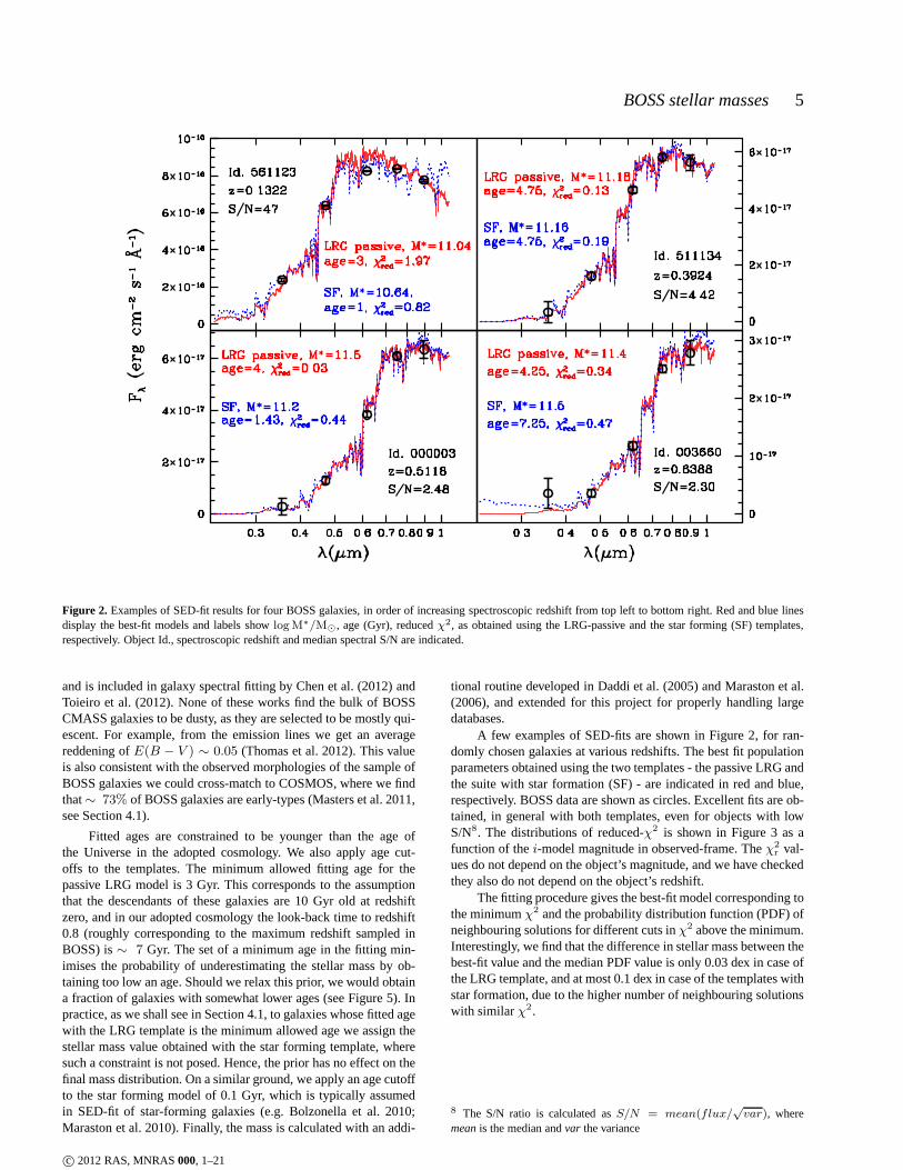
Figure 2. Examples of SED-fit results for four BOSS galaxies, in order of increasing spectroscopic redshift from top left to bottomright. Red and blue linesdisplay the best-fit models and labels showlogM∗/M⊙, age (Gyr), reducedχ2, as obtained using the LRG-passive and the star forming (SF)templates,respectively. Object Id., spectroscopic redshift and median spectral S/N are indicated.
and is included in galaxy spectral fitting by Chen et al. (2012) andToieiro et al. (2012). None of these works find the bulk of BOSSCMASS galaxies to be dusty, as they are selected to be mostly qui-escent. For example, from the emission lines we get an averagereddening ofE(B − V ) ∼ 0.05 (Thomas et al. 2012). This valueis also consistent with the observed morphologies of the sample ofBOSS galaxies we could cross-match to COSMOS, where we findthat∼ 73% of BOSS galaxies are early-types (Masters et al. 2011,see Section 4.1).
Fitted ages are constrained to be younger than the age ofthe Universe in the adopted cosmology. We also apply age cut-offs to the templates. The minimum allowed fitting age for thepassive LRG model is 3 Gyr. This corresponds to the assumptionthat the descendants of these galaxies are 10 Gyr old at redshiftzero, and in our adopted cosmology the look-back time to redshift0.8 (roughly corresponding to the maximum redshift sampledinBOSS) is∼ 7 Gyr. The set of a minimum age in the fitting min-imises the probability of underestimating the stellar massby ob-taining too low an age. Should we relax this prior, we would obtaina fraction of galaxies with somewhat lower ages (see Figure 5). Inpractice, as we shall see in Section 4.1, to galaxies whose fitted agewith the LRG template is the minimum allowed age we assign thestellar mass value obtained with the star forming template,wheresuch a constraint is not posed. Hence, the prior has no effecton thefinal mass distribution. On a similar ground, we apply an age cutoffto the star forming model of 0.1 Gyr, which is typically assumedin SED-fit of star-forming galaxies (e.g. Bolzonella et al. 2010;Maraston et al. 2010). Finally, the mass is calculated with an addi-
tional routine developed in Daddi et al. (2005) and Marastonet al.(2006), and extended for this project for properly handlinglargedatabases.
A few examples of SED-fits are shown in Figure 2, for ran-domly chosen galaxies at various redshifts. The best fit populationparameters obtained using the two templates - the passive LRG andthe suite with star formation (SF) - are indicated in red and blue,respectively. BOSS data are shown as circles. Excellent fitsare ob-tained, in general with both templates, even for objects with lowS/N8. The distributions of reduced-χ2 is shown in Figure 3 as afunction of thei-model magnitude in observed-frame. Theχ2
r val-ues do not depend on the object’s magnitude, and we have checkedthey also do not depend on the object’s redshift.
The fitting procedure gives the best-fit model correspondingtothe minimumχ2 and the probability distribution function (PDF) ofneighbouring solutions for different cuts inχ2 above the minimum.Interestingly, we find that the difference in stellar mass between thebest-fit value and the median PDF value is only 0.03 dex in caseofthe LRG template, and at most 0.1 dex in case of the templates withstar formation, due to the higher number of neighbouring solutionswith similarχ2.
8 The S/N ratio is calculated asS/N = mean(flux/√var), where
meanis the median andvar the variance
c© 2012 RAS, MNRAS000, 1–21

6 C. Maraston et al.
Figure 4. Photometric stellar masses of BOSS galaxies in the first two years of data. The two histograms showlogM∗/M⊙ as obtained with different galaxytemplates: the LRG passive model of Maraston et al. (2009) (red), in which a small fraction (3%) of old metal-poor stars is added to a dominant metal-rich(Z = Z⊙) population, both being coeval and in passive evolution, and a set of templates with star formation (blue), ranging fromτ -models to constant SF.Stellar masses obtained with the SF template are systematically lower due to the lower M/L of young populations. Calculations shown here refer to a KroupaIMF and included mass-losses from stellar evolution. Average errors onlogM∗/M⊙ are 0.1 dex (cfr. Figure 9).
Figure 3. Reducedχ2 (χ2r ) as a function of observed-framei-model mag-
nitude for the SED fits of BOSS galaxies.
4 RESULTS
We have calculated the photometric stellar massesM∗ for ∼
400, 000 massive luminous galaxies from the first two years of dataof the SDSS-III BOSS survey. The calculations of stellar mass willbe released with the Data Release 9 (DR9), as well as ages, starformation histories (SFH), star formation rate (SFR), and metal-licities, for each of the two template fittings and the two adoptedIMFs. Ages, SFRs and stellar masses are provided with their 68%
confidence levels. We also derive median stellar masses by takingthe median of the PDF and list them together with their 68% confi-dence levels. In each case, we provideM∗ with and without stellarmass-loss due to stellar evolution. We note here that, even if weprovide all quantities derived through the SED-fit, the procedure isstudied as to maximise the quality ofM∗ determination. The otherby-products of the fits should be considered less certain. Futurework will be invested in more detailed spectral analysis.
Figure 4 shows the distribution of stellar masses of BOSSgalaxies for the combined CMASS and LOWZ samples, for theLRG (red) and the SF template (blue). Plotted values refer totheKroupa IMF, and stellar mass loss has been accounted for in thecalculations. The mass histogram is thin and well defined, pointingto a uniform mass distribution as a function of redshift as was theaim of the BOSS target selection (White et al. 2011; Eisenstein etal. 2011), which we quantify later in this section.
The results for both templates agree reasonably well in indi-cating a peak stellar mass of∼ 11.3 logM (for a Kroupa IMF,1.6 higher for a Salpeter IMF). Stellar masses derived with the SFtemplate (blue) show an excess of lower mass values which is dueto the lower ages for some of the galaxies derived with this tem-plate, see Figure 5. Except for an excess of younger galaxieswiththe SF template, the age distributions agree remarkably well, in-dependently of the adopted template, which confirms the homoge-neous nature of the CMASS sample (see also Tojeiro et al. 2012).
In Appendix A we discuss in detail the comparison with otherstellar mass calculations performed in BOSS, while in Appendix
c© 2012 RAS, MNRAS000, 1–21

BOSS stellar masses 7
Figure 5. The distribution of stellar ages obtained for BOSS galaxiesusingdifferent templates for SED fitting, namely the LRG passive template (red)and the template with star formation (blue).
B we present rest-frame magnitudes that are a by-product of thefitting and will be available via DR9.
As previously mentioned, the target selection for the BOSSsurvey aimed for a uniform mass sampling as a function of redshift.We can now test whether this goal has been achieved. Figures 7and8 show the stellar mass distributions in various redshift bins, for thecalculations referred to the two different templates, LRG passiveand SF, for the combined CMASS plus LOWZ samples9.
A remarkably uniform mass sampling is achieved in a largeredshift range spanning between redshift 0.2 and 0.6, when stel-lar masses are determined with the LRG passive template.10. Atz∼> 0.6, the mass distribution is skewed towards higher values,which is probably due to the magnitude limit of the survey. Fromthese plots we infer that BOSS becomes incomplete atz∼> 0.6andlogM∗/M⊙ ∼
< 11.3. This suggestion will be qualitatively con-firmed when we will compare the BOSS mass function with litera-ture values (Section 5.2.1).
The assumed template impacts the uniformity of the masssampling, as should be expected. Figure 8 shows that, when inter-preted with templates including star formation, a fractionof BOSSgalaxies get lower stellar masses, which leads to secondarypeaksin the mass distributions. Note, however, that the redshiftbins be-tween 0.2 and 0.6 are not strongly affected by the assumed tem-plate, and the mass distribution remains fairly uniform over thisredshift range.
9 Note that for these plots we have not applied any cut inχ2r , but we have
checked that the consideration of only acceptable values would not changeif not minimally the histograms.10 The meanlogM∗/M⊙ (for a Kroupa IMF, including stellar masslosses) in the various redshift bins are: for the LRG template, 11.25at 0.2∼<z∼< 0.4, 11.27 at0.4∼<z∼< 0.5, 11.27 at0.5∼<z∼< 0.6, 11.42at 0.6∼<z∼< 0.7, and 11.62 atz∼> 0.7; for the SF template, 11.11 at0.2∼<z∼< 0.4, 11.11 at0.4∼<z∼< 0.5, 11.14 at0.5∼<z∼< 0.6, 11.26 at0.6∼<z∼< 0.7, and 11.31 atz∼> 0.7; for the merged template, 11.25 at0.2∼<z∼< 0.4, 11.22 at0.4∼<z∼< 0.5, 11.26 at0.5∼<z∼< 0.6, 11.36 at0.6∼<z∼< 0.7, and 11.48 atz∼> 0.7.
4.1 The final BOSS mass distribution: sorting templates bygalaxy morphology
As described in the previous section, we calculate stellar masseswith two templates in separate runs. Hence, each BOSS galaxyhastwo possible values ofM∗ according to the different templates weadopt. This will be useful when the stellar masses of BOSS galaxiesare used for comparison with results from other surveys in whichvarious templates are adopted. Nonetheless, for most science ap-plications it would also be useful to have one preferred choice ofM∗.
In this section we describe a colour criterion to assign stellarmass values from different templates to observed galaxies which isbased on the galaxy morphology.
In Masters et al. (2011), we cross-matched the BOSS sam-ple with the COSMOS survey (Capak et al. 2007) which provideshigh resolutionI-band imaging from the Hubble Space Telescope(HST) over 2 square degrees. The cross-match yields 240 BOSStarget galaxies for which detailed morphological information wasobtained
We found that∼ 73% of the galaxies in CMASS are early-types, and the rest∼ 27% is composed by late-types. Critical to theanalysis of the present paper, we defined a simple colour criterionof g − i, namelyg − i∼> 2.35, which allows us to separate early-types from later-types with better than 90% purity. Here we employthis colour criterion to assign mass values obtained with differenttemplates to the different morphological classes. We use the best fitLRG mass for objects withg − i∼> 2.35, and the best fit SF massfor galaxies withg−i∼< 2.35, which is the location of most spirals.
The final totalM∗ distribution of BOSS CMASS galaxies isshown in Figure 6. Similar to Figure 4, the total mass distributionstill peaks atlogM∗/M⊙ ∼ 11.3 (for a Kroupa IMF) and is dom-inated by the mass values obtained with the LRG template, as themajority of galaxies in CMASS is of early-type. The adoptionof thevalues obtained with the SF template implies an excess of galaxieswith logM∗/M⊙ ∼ 10.8 with respect to the distribution obtainedusing the LRG template.
The distribution of errors on stellar mass for the final mergedtemplate calculation is shown in Figure 9. The average uncertaintyon logM∗ is ∼ 0.1 dex. We have verified that the error is not de-pendent on galaxy mass, and is also not asymmetric.
We have also tested the goodness of our template choice withmock galaxies with known input mass. Figure 10 shows the com-parison between input stellar mass (x-axis) of mock galaxies froma semi-analytic model (as in Pforr et al. 2012) at redshift 0.5, andtheir photometric stellar masses (y-axis) we obtain by the SED-fit to their broadbandu, g, r, i, z photometry with the LRG pas-sive template. The red colour highlights those mocks that haveg− i∼> 2.35, which corresponds to the colour region where we usethe LRG template in the BOSS sample. The stellar masses of these”reddest” galaxies are well recovered with the LRG template, witha scatter of only 0.06 dex. The red points correspond to fits withχ2
∼< 20, which is well above our acceptable cut (χ2
∼< 2). Black
points represent the results for mock galaxies with bluer colours,g − i∼< 2.35. For these, the application of the LRG passive tem-plate would lead to an overestimate of the mass, so for these typesof objects in BOSS we use stellar masses obtained with the SF tem-plate.
In summary, our mass distribution may still not be the per-fect representation of the true stellar masses, but it is anchored toreal data through the colour cut and is supported by simulations.Moreover, in a companion paper (Beifiori et al 2012,in prep.) we
c© 2012 RAS, MNRAS000, 1–21

8 C. Maraston et al.
Figure 6. The finalM∗ distribution of BOSS/CMASS galaxies where values of stellar mass obtained with different templates are assigned according to thegalaxy morphology - early-type or star-forming - using the cut in apparent colourg − i ∼ 2.35. Galaxies on the red side of the colour cut getM∗ fromthe passive LRG template and those on the blue side from the SFtemplate. The total stellar mass distribution of BOSS galaxies peaks at∼ 11.3 M⊙, for aKroupa IMF, with a mean of∼ 11.28 M⊙ and a FWHM of∼ 0.5 dex.
Figure 7. The distribution of stellar mass in the combined CMASS andLOWZ sample, in various redshift bins (normalised to the peak mass valuein each bin), for results obtained with the LRG passive template. The massdistribution is fairly uniform in the redshift range0.2∼<z∼< 0.6 (cfr. green,black and blue histograms).
compareM∗ with dynamical massesMdyn. The two quantities cor-relate well andM∗ is never larger thanMdyn, thereby providingfurther support to the robustness ofM∗.
Finally, Figure 11 similarly to Figures 7 and 8 shows themerged template mass distribution for various redshift slices. Thesame conclusions hold.
Figure 8. As in Figure 7 for the SF template.
5 COMPARISON TO GALAXY EVOLUTION MODELS
5.1 The semi-analytic model
We compare our results with a theoretical light-cone based on thelatest version of the Munich semi-analytic galaxy formation andevolution model (Guo et al. 2011; Henriques et al. 2012). Theseare built on top of the Millennium dark matter simulation thattraces the evolution of dark matter haloes in a comoving cubic box500h−1Mpc on a side. Merger trees are complete for sub-halosabove a mass resolution limit of1.7 × 1010h−1M⊙. A Λ-CDM
c© 2012 RAS, MNRAS000, 1–21

BOSS stellar masses 9
-0.8 -0.6 -0.4 -0.2 0 0.2 0.4 0.6 0.80
Figure 9. Errors on stellar masses for the merged-template sample, for fitswith χ2 ∼< 2. Errors are around 0.1 dex on average.
Figure 10.Effect of fitting star-forming galaxies with the passive LRGtem-plate, using mock galaxies from semi-analytic models at redshift 0.5 withknown stellar mass. Red points highlight mock galaxies withg − i∼> 2.35.The stellar masses of these red galaxies are well recovered with a scatter ofonly 0.06 dex. For bluer galaxies (black points) the application of the LRGpassive template leads to overestimate the mass.
Figure 11. The merged template mass distribution for four redshift slices,normalised to the peak mass value in each bin.
WMAP1-based cosmology is adopted (Spergel et al. 2003) withpa-rametersH0 = 73 km · s−1Mpc−1,Ωm = 0.25,ΩΛ = 0.75, n =1 andσ8 = 0.9.
Baryonic matter forming galaxies is treated as follows. Ini-tial hot gas masses are derived from the mass of correspondingdark matter haloes after collapse, assuming a cosmic abundance ofbaryonsfb = 0.17. The fate of the gas is then followed throughdifferent phases using analytical prescriptions, in particular dur-ing cooling and star formation, which maybe empirically derived.Feedback from Supernovae II and/or AGNs act to inhibit coolingand - in case of Supernovae - may also reheat the gas, or eject itinto an external reservoir. The full evolution history of galaxies -including merging, satellite infall and star formation - isthen fol-lowed toz = 0. The version of the models used by Henriques et al.(2012) includes AGN feedback as in Croton et al. (2006), the dustmodel introduced by De Lucia & Blaizot (2007) and the redshift-evolving cold gas-to-dust ratio from Kitzbichler & White (2007).This simulation also includes more efficient supernova II feedbackand a more realistic treatment of satellite galaxy evolution and ofmergers as introduced by Guo et al. (2011).
The spectrophotometric properties of semi-analytic galaxiesare obtained using stellar population models. Single-burst or Sim-ple Stellar Population (SSPs) models are assigned to each stellargeneration, which is weighted by the mass contribution of the in-dividual star formation episode to the total galaxy mass. Henriqueset al. (2011; 2012) have updated the De Lucia et al. (2006) andthe latest Guo et al. (2011) semi-analytic models with the Maras-ton (2005) stellar population models, such that now each semi-analytic model is available with multiple choices of input stellarpopulation models. As it has been discussed in the recent litera-ture (Tonini et al. 2009; Fontanot & Monaco 2010; Henriques et al.2011), the specifics of the stellar population models adopted inthe galaxy formation model shape the spectra of model galaxies,which has an important effect on the comparison between modelsand data.
The method used to construct the mock catalog is described indetail in Henriques et al. (2012).11 In addition to the pencil-beamformat that was originally available, the model is now provided
11 Light cones and data products are publicly available athttp://www.mpa-garching.mpg.de/millennium.
c© 2012 RAS, MNRAS000, 1–21
10 C. Maraston et al.
with an all sky light-cone (4π) that we will use in this work. Themodel catalogue is limited to an observed-frame AB (Oke & Gunn1983) magnitude ofi∼< 21.0, significantly deeper than the BOSSlimit of i∼< 19.9. It was constructed by replicating the Millenniumsimulation box (500 Mpc ·h−1 on a side) with no additional trans-formations applied.
The original volume of the Millennium simulation is largeenough to sample the most massive galaxies in the Universe, whichmakes the comparison with BOSS data interesting. Note that themodels are normalised to the local mass function, which impactson the mass of the most massive galaxies that can be found in thesimulations.
To make a direct data model comparison we apply to the semi-analytic models the same magnitude colour selection cut that wasapplied to define the observed sample (the CMASS cut). Here thestellar population model has an effect. The adoption of the Maras-ton (2005) models instead of the Bruzual & Charlot (2003) modelsallow more semi-analytic galaxies to enter the BOSS cut. In thefollowing analysis we shall mostly use the semi-analytic modelsbased on the Maraston (2005) models.
Figure 12 shows, in the BOSS target selection plot of theobserver-framei-mag vs thedperp colour12, the portion of modelgalaxies entering the CMASS selection cut. Only a tiny fraction ofthe Millennium galaxies satisfies this selection criterion, becausethe CMASS cut is designed to select the most luminous and mas-sive galaxies in the Universe (Eisenstein et al. 2011, Padmanabhanet al. 2012,in prep.).
An illustrative approach is to compare the colour distributionsof models and data within the target selection cut. Figure 13ex-pands the BOSS selection region in Figure 12. Colours of modelsand data agree generally well, though one notes a deficit of redgalaxies in the models over the entire redshift range. In Section 7.3we shall discuss this issue in more detail.
5.2 Stellar mass densities
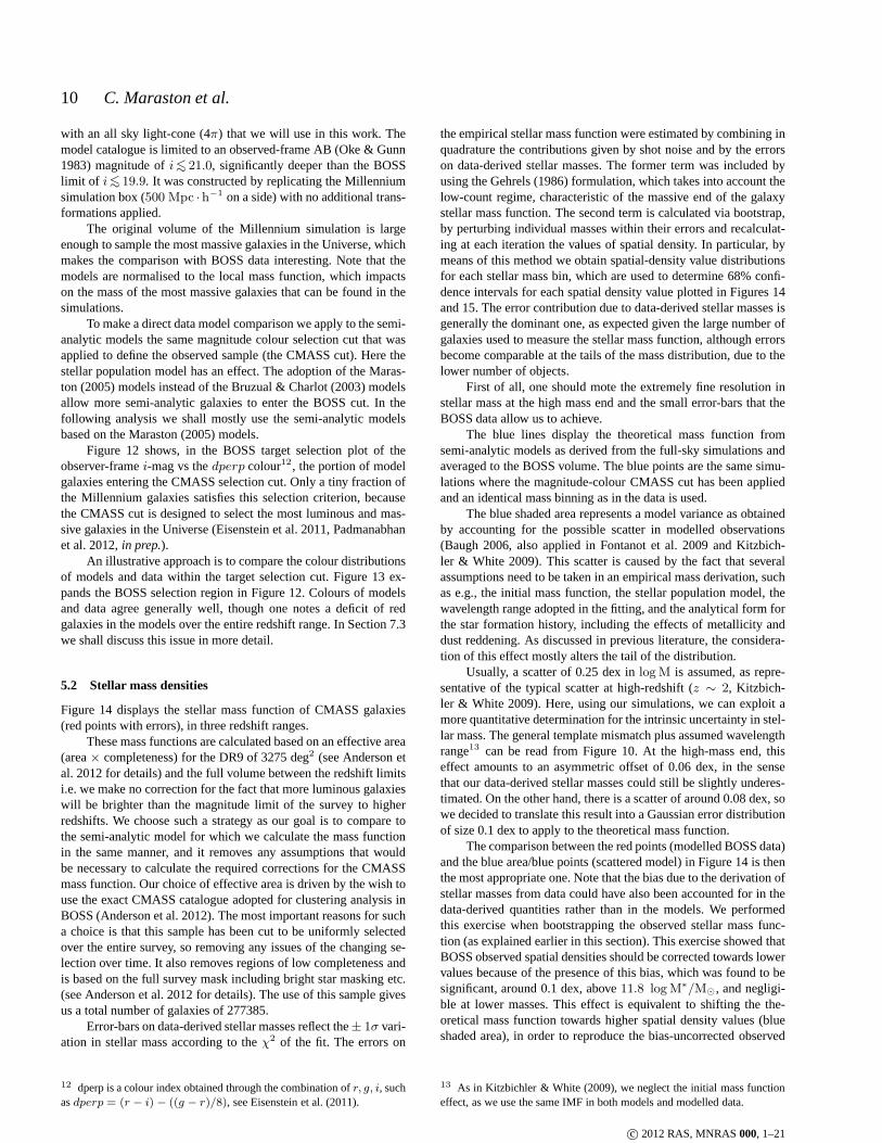
Figure 14 displays the stellar mass function of CMASS galaxies(red points with errors), in three redshift ranges.
These mass functions are calculated based on an effective area(area× completeness) for the DR9 of 3275 deg2 (see Anderson etal. 2012 for details) and the full volume between the redshift limitsi.e. we make no correction for the fact that more luminous galaxieswill be brighter than the magnitude limit of the survey to higherredshifts. We choose such a strategy as our goal is to comparetothe semi-analytic model for which we calculate the mass functionin the same manner, and it removes any assumptions that wouldbe necessary to calculate the required corrections for the CMASSmass function. Our choice of effective area is driven by the wish touse the exact CMASS catalogue adopted for clustering analysis inBOSS (Anderson et al. 2012). The most important reasons for sucha choice is that this sample has been cut to be uniformly selectedover the entire survey, so removing any issues of the changing se-lection over time. It also removes regions of low completeness andis based on the full survey mask including bright star masking etc.(see Anderson et al. 2012 for details). The use of this samplegivesus a total number of galaxies of 277385.
Error-bars on data-derived stellar masses reflect the± 1σ vari-ation in stellar mass according to theχ2 of the fit. The errors on
12 dperp is a colour index obtained through the combination ofr, g, i, suchasdperp = (r − i) − ((g − r)/8), see Eisenstein et al. (2011).
the empirical stellar mass function were estimated by combining inquadrature the contributions given by shot noise and by the errorson data-derived stellar masses. The former term was included byusing the Gehrels (1986) formulation, which takes into account thelow-count regime, characteristic of the massive end of the galaxystellar mass function. The second term is calculated via bootstrap,by perturbing individual masses within their errors and recalculat-ing at each iteration the values of spatial density. In particular, bymeans of this method we obtain spatial-density value distributionsfor each stellar mass bin, which are used to determine 68% confi-dence intervals for each spatial density value plotted in Figures 14and 15. The error contribution due to data-derived stellar masses isgenerally the dominant one, as expected given the large number ofgalaxies used to measure the stellar mass function, although errorsbecome comparable at the tails of the mass distribution, dueto thelower number of objects.
First of all, one should mote the extremely fine resolution instellar mass at the high mass end and the small error-bars that theBOSS data allow us to achieve.
The blue lines display the theoretical mass function fromsemi-analytic models as derived from the full-sky simulations andaveraged to the BOSS volume. The blue points are the same simu-lations where the magnitude-colour CMASS cut has been appliedand an identical mass binning as in the data is used.
The blue shaded area represents a model variance as obtainedby accounting for the possible scatter in modelled observations(Baugh 2006, also applied in Fontanot et al. 2009 and Kitzbich-ler & White 2009). This scatter is caused by the fact that severalassumptions need to be taken in an empirical mass derivation, suchas e.g., the initial mass function, the stellar population model, thewavelength range adopted in the fitting, and the analytical form forthe star formation history, including the effects of metallicity anddust reddening. As discussed in previous literature, the considera-tion of this effect mostly alters the tail of the distribution.
Usually, a scatter of 0.25 dex inlogM is assumed, as repre-sentative of the typical scatter at high-redshift (z ∼ 2, Kitzbich-ler & White 2009). Here, using our simulations, we can exploit amore quantitative determination for the intrinsic uncertainty in stel-lar mass. The general template mismatch plus assumed wavelengthrange13 can be read from Figure 10. At the high-mass end, thiseffect amounts to an asymmetric offset of 0.06 dex, in the sensethat our data-derived stellar masses could still be slightly underes-timated. On the other hand, there is a scatter of around 0.08 dex, sowe decided to translate this result into a Gaussian error distributionof size 0.1 dex to apply to the theoretical mass function.
The comparison between the red points (modelled BOSS data)and the blue area/blue points (scattered model) in Figure 14is thenthe most appropriate one. Note that the bias due to the derivation ofstellar masses from data could have also been accounted for in thedata-derived quantities rather than in the models. We performedthis exercise when bootstrapping the observed stellar massfunc-tion (as explained earlier in this section). This exercise showed thatBOSS observed spatial densities should be corrected towards lowervalues because of the presence of this bias, which was found to besignificant, around 0.1 dex, above11.8 logM∗/M⊙, and negligi-ble at lower masses. This effect is equivalent to shifting the the-oretical mass function towards higher spatial density values (blueshaded area), in order to reproduce the bias-uncorrected observed
13 As in Kitzbichler & White (2009), we neglect the initial massfunctioneffect, as we use the same IMF in both models and modelled data.
c© 2012 RAS, MNRAS000, 1–21

BOSS stellar masses 11
Figure 12.Semi-analytic model galaxies from the model of Henriques etal. (2012) using the Maraston (2005) stellar population models, in the observer-framedperp(= (r − i)− ((g − r)/8) colour vsi-mag in the redshift range∼ 0.5 to ∼ 0.7. The CMASS selection cut is shown as dashed lines.
mass function. We decided to account for the bias in the modelsbecause other data-derived mass functions we shall comparewithin Section 5.2.1 (see Fig. 19) do not take this bias into account.
First of all, it is interesting that the models coincide at the mas-sive end independently of whether or not the CMASS cut is applied(compare blue points to blue dashed lines). This result implies thata selection like the CMASS one is perfectly suited to select themost massive galaxies at least from the simulation point of view.In other words, there are no massive galaxies in the models that theCMASS selection would miss.
In Figure 14 one sees that neither the models nor the dataevolve significantly over the BOSS redshift range. This is perhapsnot surprising since the redshift spanned is narrow.
The models and data agree overall quite well. The turnover inthe mass function occurs at slightly different masses, which couldresult from the different colours of model galaxies and data(seenext Section), the photometric errors, or both. There is a mild deficitof massive galaxies in the models in the mass rangelogM∗/M⊙ ∼
11.3 − 11.6, which extends to higher masses (logM∗/M⊙ ∼ 12)in the highest redshift bin. There is also a lack of lower massgalax-ies in the models, between 10.5 and 11.0logM∗/M⊙. This lattereffect originates from the fact that model galaxies with this masshave blue colours which cause them to be excluded by the CMASScut. In Section 7.2 we shall compare the colours of models anddataas a function of mass.
The model comparison we present here reaches the highestpossible galaxy masses, and cosmic variance, thanks to hugeBOSSvolume/area, is negligible. We comment on other comparisons ofthis kind that were previously performed in the literature in the Dis-cussion. We should note that, for the comparison with semi-analyticmodels, the set of masses for BOSS galaxies we use, whether fromthis work or from Chen et al. (2012) does not alter the essenceofthe conclusions. However, the lowerM∗ values for BOSS galaxiesobtained in this paper (see Appendix A) make the comparison withthe models more favourable.
The BOSS data show little evolution within the explored red-shift and mass range, but this statement should be taken withcau-tion as we are not dealing with a complete sample; the incomplete-ness of BOSS is presently not known. For example, note the lower
mass density atlogM∗/M⊙ ∼ 11.5 at the highest redshift bin(right-hand panel) with respect toz = 0.55, which is the repre-sentative redshift for BOSS; this suggests that CMASS is notcom-plete abovez ∼ 0.6 around this mass value, as already arguedin Section 4. This results is in qualitative agreement with ongoingsimulations of the BOSS completeness (M. Swanson et al. 2012, inpreparation). As we shall see in the next section when comparingwith previous results from the literature, the BOSS sample may benot severely incomplete at the high-mass end (logM∼
> 11.5) overthe entire BOSS redshift range.
5.2.1 Comparison with published mass functions
The lack of evolution displayed by the field massive galaxy massfunction from the BOSS data is in qualitative agreement withear-lier results in the literature (e.g. Drory et al. 2004; Bundyet al.2006; Cimatti et al. 2006; Ilbert et al. 2010; Pozzetti et al.2010),including studies considering the luminosity function instead ofthe mass function in the same redshift range explored here(e.g. Blanton et al. 2003; Wake et al. 2006; Cool et al. 2008;Loveday et al. 2012).
Our approach, which considers identical volumes in the mod-els and data, should be free from issues related to the unknowncompleteness of the BOSS sample, and allows us to make a mean-ingful model-data comparison. Even if the completeness is as yetunknown, it is also instructive to compare our results with the liter-ature in order to estimate where the new BOSS data stand.
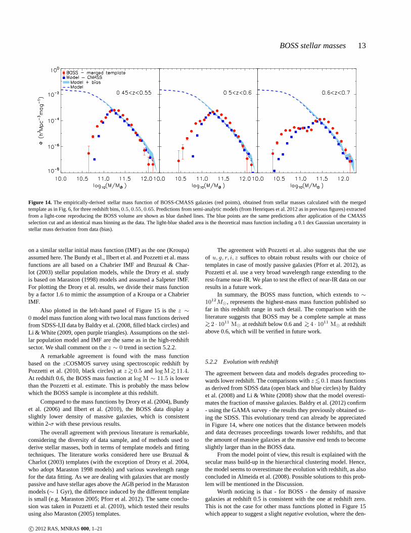
Figure 15 is identical to Figure 14, but with the addition ofempirical mass functions derived from other data samples, namely:Drory et al. (2004, open circles), derived from the MUNICSK-selected survey with photometric redshift; Bundy et al. (2006,green open symbols) derived from DEEP2 data; Ilbert et al. (2010,purple triangles) for the COSMOS sample using photometric red-shifts, and Pozzetti et al. (2010, black filled circles), forthe zCOS-MOS sample with spectroscopic redshifts. There are severalothermass functions in the literature, e.g. Borch et al. (2006), Fontanaet al. (2006), Bell et al. (2003), but we do not discuss these resultsas we focus on the high-mass end and explore a high-resolution inredshift binning. In this comparison we need to use works based
c© 2012 RAS, MNRAS000, 1–21

12 C. Maraston et al.
Figure 13.Observed-frame colours of semi-analytic models as in Figure 12 (left-hand columns) and BOSS data (right-hand columns), in the BOSS selectioncut plane ofdperpcolour andi-magnitude
c© 2012 RAS, MNRAS000, 1–21
BOSS stellar masses 13
Figure 14. The empirically-derived stellar mass function of BOSS-CMASS galaxies (red points), obtained from stellar masses calculated with the mergedtemplate as in Fig. 6, for three redshift bins,0.5, 0.55, 0.65. Predictions from semi-analytic models (from Henriques etal. 2012 as in previous figures) extractedfrom a light-cone reproducing the BOSS volume are shown as blue dashed lines. The blue points are the same predictions after application of the CMASSselection cut and an identical mass binning as the data. The light-blue shaded area is the theoretical mass function including a 0.1 dex Gaussian uncertainty instellar mass derivation from data (bias).
on a similar stellar initial mass function (IMF) as the one (Kroupa)assumed here. The Bundy et al., Ilbert et al. and Pozzetti et al. massfunctions are all based on a Chabrier IMF and Bruzual & Char-lot (2003) stellar population models, while the Drory et al.studyis based on Maraston (1998) models and assumed a Salpeter IMF.For plotting the Drory et al. results, we divide their mass functionby a factor 1.6 to mimic the assumption of a Kroupa or a ChabrierIMF.
Also plotted in the left-hand panel of Figure 15 is thez ∼
0 model mass function along with two local mass functions derivedfrom SDSS-I,II data by Baldry et al. (2008, filled black circles) andLi & White (2009, open purple triangles). Assumptions on thestel-lar population model and IMF are the same as in the high-redshiftsector. We shall comment on thez ∼ 0 trend in section 5.2.2.
A remarkable agreement is found with the mass functionbased on thezCOSMOS survey using spectroscopic redshift byPozzetti et al. (2010, black circles) atz∼> 0.5 and logM∼
> 11.4.At redshift 0.6, the BOSS mass function atlogM ∼ 11.5 is lowerthan the Pozzetti et al. estimate. This is probably the mass belowwhich the BOSS sample is incomplete at this redshift.
Compared to the mass functions by Drory et al. (2004), Bundyet al. (2006) and Ilbert et al. (2010), the BOSS data display aslightly lower density of massive galaxies, which is consistentwithin 2-σ with these previous results.
The overall agreement with previous literature is remarkable,considering the diversity of data sample, and of methods used toderive stellar masses, both in terms of template models and fittingtechniques. The literature works considered here use Bruzual &Charlot (2003) templates (with the exception of Drory et al.2004,who adopt Maraston 1998 models) and various wavelength rangefor the data fitting. As we are dealing with galaxies that are mostlypassive and have stellar ages above the AGB period in the Marastonmodels (∼ 1 Gyr), the difference induced by the different templateis small (e.g. Maraston 2005; Pforr et al. 2012). The same conclu-sion was taken in Pozzetti et al. (2010), which tested their resultsusing also Maraston (2005) templates.
The agreement with Pozzetti et al. also suggests that the useof u, g, r, i, z suffices to obtain robust results with our choice oftemplates in case of mostly passive galaxies (Pforr et al. 2012), asPozzetti et al. use a very broad wavelength range extending to therest-frame near-IR. We plan to test the effect of near-IR data on ourresults in a future work.
In summary, the BOSS mass function, which extends to∼
1012M⊙, represents the highest-mass mass function published sofar in this redshift range in such detail. The comparison with theliterature suggests that BOSS may be a complete sample at mass
∼> 2 · 1011 M⊙ at redshift below 0.6 and∼> 4 · 1011 M⊙ at redshiftabove 0.6, which will be verified in future work.
5.2.2 Evolution with redshift
The agreement between data and models degrades proceeding to-wards lower redshift. The comparisons withz∼< 0.1 mass functionsas derived from SDSS data (open black and blue circles) by Baldryet al. (2008) and Li & White (2008) show that the model overesti-mates the fraction of massive galaxies. Baldry et al. (2012)confirm- using the GAMA survey - the results they previously obtained us-ing the SDSS. This evolutionary trend can already be appreciatedin Figure 14, where one notices that the distance between modelsand data decreases proceedings towards lower redshifts, and thatthe amount of massive galaxies at the massive end tends to becomeslightly larger than in the BOSS data.
From the model point of view, this result is explained with thesecular mass build-up in the hierarchical clustering model. Hence,the model seems to overestimate the evolution with redshift, as alsoconcluded in Almeida et al. (2008). Possible solutions to this prob-lem will be mentioned in the Discussion.
Worth noticing is that - for BOSS - the density of massivegalaxies at redshift 0.5 is consistent with the one at redshift zero.This is not the case for other mass functions plotted in Figure 15which appear to suggest a slightnegativeevolution, where the den-
c© 2012 RAS, MNRAS000, 1–21
14 C. Maraston et al.
Figure 15. Similar to Figure 14, but showing four mass functions from the literature: Bundy et al. (2006, green squares) derived from DEEP2 data; Ilbertet al. (2010, purple triangles) for the COSMOS sample based on photometric redshifts; Pozzetti et al. (2010, black circles), for thezCOSMOS sample withspectroscopic redshifts; Drory et al. (2004, open circles)from theK-band selected MUNICS survey with photometric redshifts. The left panel shows two localz∼< 0.1 mass functions from Li & White (2009) and Baldry et al. (2008)as derived from SDSS data.
sity of massive galaxies at high-redshift is higher than at redshiftzero.14
Though this apparent negative evolution could be caused by aslight shift at high-zdue to the larger errors affecting mass determi-nations caused by the photometry of fainter objects, it is interestingto note that our mass function based on BOSS does not appear tobeaffected by this problem. Though we cannot exclude that thiseventhappens by chance and that we are actually incomplete at the high-mass end, if confirmed this good result is probably due the verywide area covered by BOSS, which is virtually free from cosmicvariance issues, and by the accuracy of spectroscopic redshifts.
The low-z empirical mass function is relevant to the modelsbecause it is used to normalise the models themselves (Li & White2009). Examining Figure 15 it appears that both thez ∼ 0 andz ∼
0.5 BOSS data can now be used simultaneously and consistently tocalibrate the models over a wider redshift range.
5.3 Colours vs mass and the metallicity of galaxies
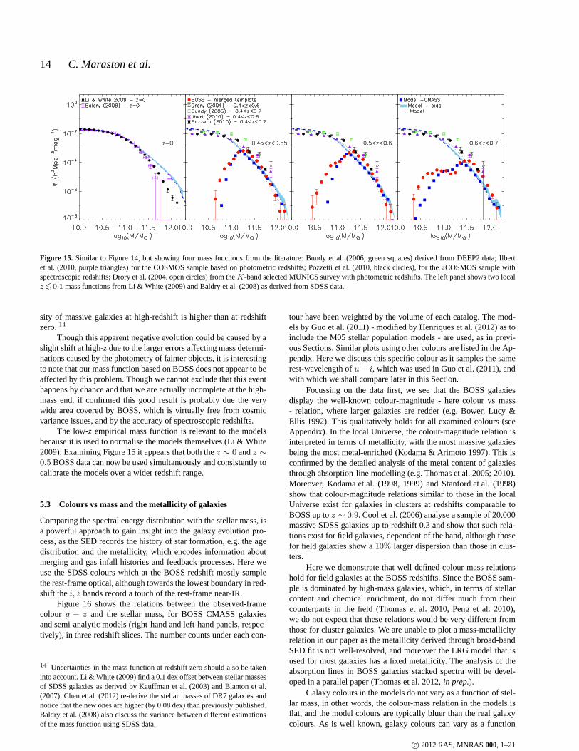
Comparing the spectral energy distribution with the stellar mass, isa powerful approach to gain insight into the galaxy evolution pro-cess, as the SED records the history of star formation, e.g. the agedistribution and the metallicity, which encodes information aboutmerging and gas infall histories and feedback processes. Here weuse the SDSS colours which at the BOSS redshift mostly samplethe rest-frame optical, although towards the lowest boundary in red-shift thei, z bands record a touch of the rest-frame near-IR.
Figure 16 shows the relations between the observed-framecolour g − z and the stellar mass, for BOSS CMASS galaxiesand semi-analytic models (right-hand and left-hand panels, respec-tively), in three redshift slices. The number counts under each con-
14 Uncertainties in the mass function at redshift zero should also be takeninto account. Li & White (2009) find a 0.1 dex offset between stellar massesof SDSS galaxies as derived by Kauffman et al. (2003) and Blanton et al.(2007). Chen et al. (2012) re-derive the stellar masses of DR7 galaxies andnotice that the new ones are higher (by 0.08 dex) than previously published.Baldry et al. (2008) also discuss the variance between different estimationsof the mass function using SDSS data.
tour have been weighted by the volume of each catalog. The mod-els by Guo et al. (2011) - modified by Henriques et al. (2012) astoinclude the M05 stellar population models - are used, as in previ-ous Sections. Similar plots using other colours are listed in the Ap-pendix. Here we discuss this specific colour as it samples thesamerest-wavelength ofu− i, which was used in Guo et al. (2011), andwith which we shall compare later in this Section.
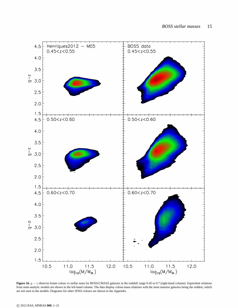
Focussing on the data first, we see that the BOSS galaxiesdisplay the well-known colour-magnitude - here colour vs mass- relation, where larger galaxies are redder (e.g. Bower, Lucy &Ellis 1992). This qualitatively holds for all examined colours (seeAppendix). In the local Universe, the colour-magnitude relation isinterpreted in terms of metallicity, with the most massive galaxiesbeing the most metal-enriched (Kodama & Arimoto 1997). Thisisconfirmed by the detailed analysis of the metal content of galaxiesthrough absorption-line modelling (e.g. Thomas et al. 2005; 2010).Moreover, Kodama et al. (1998, 1999) and Stanford et al. (1998)show that colour-magnitude relations similar to those in the localUniverse exist for galaxies in clusters at redshifts comparable toBOSS up toz ∼ 0.9. Cool et al. (2006) analyse a sample of 20,000massive SDSS galaxies up to redshift 0.3 and show that such rela-tions exist for field galaxies, dependent of the band, although thosefor field galaxies show a10% larger dispersion than those in clus-ters.
Here we demonstrate that well-defined colour-mass relationshold for field galaxies at the BOSS redshifts. Since the BOSS sam-ple is dominated by high-mass galaxies, which, in terms of stellarcontent and chemical enrichment, do not differ much from theircounterparts in the field (Thomas et al. 2010, Peng et al. 2010),we do not expect that these relations would be very differentfromthose for cluster galaxies. We are unable to plot a mass-metallicityrelation in our paper as the metallicity derived through broad-bandSED fit is not well-resolved, and moreover the LRG model that isused for most galaxies has a fixed metallicity. The analysis of theabsorption lines in BOSS galaxies stacked spectra will be devel-oped in a parallel paper (Thomas et al. 2012,in prep.).
Galaxy colours in the models do not vary as a function of stel-lar mass, in other words, the colour-mass relation in the models isflat, and the model colours are typically bluer than the real galaxycolours. As is well known, galaxy colours can vary as a function
c© 2012 RAS, MNRAS000, 1–21
BOSS stellar masses 15
Figure 16.g − z observer-frame colour vs stellar mass for BOSS/CMASS galaxies in the redshift range 0.45 to 0.7 (right-hand column). Equivalent relationsfrom semi-analytic models are shown in the left-hand column. The data display colour-mass relations with the most massive galaxies being the reddest, whichare not seen in the models. Diagrams for other SDSS colours are shown in the Appendix.
c© 2012 RAS, MNRAS000, 1–21
16 C. Maraston et al.
of age, metallicity or dust content. Dust effects should play a minorrole, as the bulk of the massive CMASS galaxies are not very dusty,as already discussed (see Section 3.2).
A substantially younger age component in the models - whichcauses colours to remain blue - is also not the main driving ofthismismatch as - at redshift 0.5 - the galaxy ages in the present semi-analytic models are strongly peaked at old ages, with a very lowpercentage scattering to low ages (Henriques et al. 2011, Figure5). This conclusion would not be the same for other semi-analyticmodels, as the same Figure shows.
We are left with metallicity effects as a possible explana-tion. It is known that galaxies in semi-analytic models are gener-ally quite metal-poor even at high-masses; their metallicity barelyreaches the solar value as discussed e.g. by Pipino et al. (2009),Henriques & Thomas (2010, , their Figure 10) and also brieflypointed out in Tonini et al. (2009) and Pforr et al. (2012). More-over, Sakstein et al. (2011) describe the difficulty in matching themass-metallicity relation at high-redshift even when implementinga sophisticated recipe for chemical enrichment. We shall return tothis point for the discussion.
We also should comment on the effect of population synthesismodels. We checked that the use of the BC03 population modelsmakes only a marginal difference in the semi-analytic modelpre-dictions in the SDSS bands, which sample a rest-frame spectralregion, between 3400A and 6400A, which is not vastly differentbetween the two models, especially because the model galaxies aremostly old and have roughly half-solar metallicity. The choice ofpopulation synthesis model appears to matter, however, at highermetallicity, as we discuss below.
Guo et al. (2011) perform a similar analysis as in Figure 16,by comparing the rest-frameu − i galaxy colours in bins of stel-lar mass at redshift zero, using SDSS data. Models and data arefound to compare remarkably well for galaxies with masses inthe rangelogM∗/M⊙ ∼ 9.5 − 10.515. At the high-mass end,logM∗/M⊙ ∼
> 10.5, model galaxies are found to be bluer and tospan a narrower colour range with respect to the data. The discrep-ancy discussed by Guo et al. is identical to the one we point outin Figure 16 for galaxies at redshift∼ 0.5. Galaxy metallicities atredshift zero are centred around 0.5Z⊙. This value is smaller thanwhat is inferred by observational data using stellar population mod-elling of absorption lines (Thomas et al. 2005, 2010; Gallazzi et al.2006; Smith et al. 2009), as discussed by Henriques & Thomas(2010).
Hence, our conclusion is that the main cause of the discrep-ancy between models and data for the colours of massive galaxieslies in the metallicity, which is too low in the models. Guo etal.(2011) conclude the opposite, namely that metallicity/ageeffectsare unlikely to be able to explain this discrepancy. This conclusionis based on the evidence that theu − i colour of the Bruzual &Charlot (2003) models for 12 Gyr and twice solar metallicity(anda Chabrier IMF) is at most 3.07, whereas the peak of the data isaround 3 and extends up to∼ 3.5. On the other hand, the equivalentmodel from Maraston 2005 (for a Kroupa IMF) hasu−i = 3.4716 .Hence, the semi-analytic models with a higher metallicity for the
15 At lower masses, the models are redder, which - as discussed by theauthors - is due to substantial fraction of dwarf satellites(roughly half) inthe models which finish their star formation early and becomepassive. Theobserved fraction of such passive dwarfs is substantially smaller. Our datado not encompass this low-mass range hence we cannot addressfurther thisproblem.16 See www.maraston.eu
galaxies and using the M05 stellar population models could matchthe colours, for metallicity values - between solar and twice solar -that are in accord with what is derived observationally. This findingfurther stresses the importance of evolutionary population synthe-sis for the theoretical modelling of galaxies (Tonini et al.2009;Henriques et al. 2011; Monaco & Fontanot 2010).
The conclusion from this section is that the most massivegalaxies in the models need to be more metal-rich to match theobservations.
6 SUMMARY AND DISCUSSION
We have calculated the photometric stellar masses for galaxies inthe BOSS survey from the commissioning stage through the firstrelease of data to the public (DR9). We have used the BOSS spec-troscopic redshift and standard SDSS photometryu, g, r, i, z, toperform broad-band spectral energy distribution (SED) fitting withHyperZ (Bolzonella et al. 2000) using various galaxy templates.In particular, we exploit our previously published Luminous RedGalaxy (LRG) best-fitting template (Maraston et al. 2009), whichis composed of a major metal-rich population containing traces(3% by mass) of metal-poor stars, both populations being coevaland in passive evolution. This template provides a good descriptionof the redshift evolution of theg, r, i colours of LRG galaxies inthe redshift range 0.3 to 0.6 from the 2SLAQ survey (Marastonetal. 2009; see also Cool et al. 2008 who used a preliminary versionof the same template). This template was also used to design thetarget selection for BOSS (Eisenstein et al. 2011; Padmanabhan etal. 2012,in prep.). Furthermore, as the BOSS target selection in-cludes galaxies that are bluer than the classical LRGs, we also usea template suite allowing star formation, ranging from standardτ -models to constant star formation and spanning a wide metallicityrange (from 0.2 solar to twice solar). For both templates we employa Salpeter (1955) as well as a Kroupa (2001) Initial Mass Function(IMF) and consider the mass lost via stellar evolution.
Independently of the adopted template, the result is that BOSSgalaxies are massive and display a narrow mass distribution, whichpeaks atlogM/M⊙ ∼ 11.3 for a Kroupa IMF. We also study theuniformity of the mass sampling as a function of redshift andfindthat BOSS is a mass-uniform sample over the redshift range 0.2to 0.6 (see also White et al. 2011). Qualitatively speaking,incom-pleteness emerges at redshift above 0.6 andlogM∗/M⊙ ∼
< 11.6.The galaxy stellar mass depends on the adopted template, and
generally it is not obvious which template is the best choiceasthe galaxy star formation history is not known. To make a robusttemplate choice is especially difficult for large galaxy databases,in which objects cannot be handled on an individual basis. For ob-taining a unique set of reference stellar masses, we adopt anem-pirical colour cut developed in a companion paper (Masters et al.2011) which is able to separate galaxies with early-type morpholo-gies from later-type ones at redshift above 0.4. We then use thestellar masses obtained with the LRG passive model for galaxieson the ’early-type side’ of the colour criterium, and the values ob-tained with the star-forming template for galaxies on the ’late-type’side. In this way we obtain a merged mass distribution in which theassignment of the stellar population template is motivatedby theobserved galaxy morphology.
The BOSS galaxy sample used here, comprising∼ 400, 000 massive galaxies at redshifts∼ 0.3 − 0.7, isideally suited to study at unprecedented detail the evolution ofthe most massive galaxies at late epochs. We compare the mass
c© 2012 RAS, MNRAS000, 1–21

BOSS stellar masses 17
distribution and the colours of BOSS galaxies with predictionsfrom semi-analytic models of galaxy evolution based on theMillennium simulations (Guo et al. 2011; Henriques et al. 2012).The simultaneous comparison of mass and colour is crucial. Thesequantities in the models are affected by the prescription for AGNfeedback (Guo et al. 2011; De Lucia & Blaizot 2007; Croton et al.2006; Cattaneo et al. 2005), which is likely far too simplified, andprobably incorrect in detail (Bower et al. 2012).
To perform a robust comparison free as much as possiblefrom possible completeness issues, we consider the models in light-cones using the BOSS effective area and the target selectioncuts.The large area of the BOSS survey and the selection cut at the high-mass end allow us to pose results on an unprecedentedly solidsta-tistical ground.
Overall the models perform well in comparison with the datain terms of stellar mass density distribution at redshift∼ 0.5. Thisis already visible in previous work (cfr. Figure 20 by Pozzetti etal. 2010). We extend this conclusion to the density of very massivegalaxies,logM∗/M⊙ ∼ 12, finding that the data match rather wellwith the models.
It is the evolution fromz ∼ 0.5 to z ∼ 0 where the largestdiscrepancy between models and data lies. The data do not appearto have evolved, considering the effect of photometric errors onthe high-redshift side, whereas the models evolve consistently withthe hierarchical mass build-up. This conclusion is qualitatively con-sistent with those taken in previous articles (Fontanot et al. 2009,Pozzetti et al. 2010, Ilbert et al. 2010), who noticed that the evolu-tion at the high-mass end of the empirical mass function is muchmilder than the one at the low-mass end, in agreement with thebaryonic mass downsizing. On the contrary, the models display anup-sizingwhere the massive end and especially the passive popula-tion (Cattaneo et al. 2008; Fontanot et al. 2009) evolves faster withrespect to the low-mass end. Due to the BOSS target selectionwecan only conclude about the high-mass end here, but we are ableto extend the analysis to the very massive end that was not probedpreviously.
The extension to high mass is crucial for understanding theevolution of the most massive galaxies with respect to galaxy for-mation models. For example, Bower et al. (2006) conclude that thepredicted mass function in their semi-analytic models reproducesreasonably well the observations all over the redshift range fromzero to five. Examining their Figure 6, however, one notices thattheir model at redshift 0.5 lacks the most massive galaxies com-pared to our BOSS results and to the semi-analytic models we usehere. Bower et al. could use only observed mass functions that ex-tended up to∼ 1011 M⊙.
Almeida et al. (2008) on the other hand noticed that the ob-served luminosity function of LRG atz ∼ 0.5 is not matched byeither the Bower et al. (2006) or the Baugh et al. (2005) semi-analytic model of galaxy formation and evolution. The Boweretal. model is successful at predicting such abundance at lower red-shift (z ∼ 0.24). This implies a different redshift evolution in themodels and the data similar to what we find here. The models weuse in this work appear to be more successful at redshift 0.5 than atlower redshift, as already discussed in the literature.
As star formation is quenched by AGN feedback in these mod-els, the secular evolution of massive galaxies is mostly determinedby mergers, particularly by minor mergers, since for the most mas-sive galaxies the mass ratio to other galaxies is always large. Therelative growth of the mass function betweenz=0.5 andz=0 istherefore strongly affected by the treatment of the physicsof satel-lite galaxies. In particular, tidal disruption of stellar material can
significantly decrease the amount of mass accreted onto massivegalaxies, and moving it into the intra-cluster light (Monaco et al.2007; Henriques & Thomas 2010). A more effective implementa-tion of this process could help reducing the excessive buildup ofmassive galaxies in the Guo et al. (2011) models and ease the ten-sion withz=0 data.
We find that our light-coned mass function compares well withthe mass function based on thezCOSMOS survey(Pozzetti et al.2010). Our determinations find slightly lower densities of massivegalaxies with respect to other published works (by Drory et al.2004, Bundy et al. 2006, Ilbert et al. 2010). The comparison withthese previous analysis suggests that BOSS is a complete sample atmass∼> 2·1011 M/M⊙ at redshift below 0.6 and∼> 4·1011 M/M⊙
at redshift above 0.6. These suggestions will be verified quantita-tively in future works.
Also noteworthy, the BOSS mass function atz ∼ 0.5 does notappear to be in tension with local mass functions in giving a highernumber of massive galaxies at high redshift with respect to redshiftzero, as seen in previous work. This positive result, if not due toincompleteness of the BOSS sample, should come from a combi-nation of the very large area and accurate spectroscopic redshift ofBOSS, which are the major strengths of the survey.
In summary, the BOSS mass function which extends up to∼ 1012M⊙ represents the highest-mass mass function publishedso far in this redshift range in such detail in redshift and mass.BOSS now offers an interesting data base of massive galaxiesforcalibrating models of galaxy formation and evolution at thehigh-est mass end at high-redshift which is protected by cosmic varianceand small-number statistics.
A comparison of the colours of BOSS galaxies and modelsdemonstrates that BOSS galaxies define colour-mass relations sim-ilar to those of local galaxies, with colours becoming redder withstellar mass. The models, however, span a narrower (bluer) colourrange, and in particular their colours do not vary with stellar mass,i.e. the models do not display a colour-mass relation. We argue thatthe main driver for this discrepancy is the metallicity, which in themodels is too low, a conclusion which is consistent with evidencefrom other work in the literature. Interestingly, Guo et al.(2011)discarded this possibility when comparing - in a similar fashion aswe do here - SDSS galaxies with models at redshift 0. Their conclu-sion is based on the evidence that Bruzual & Charlot (2003) pop-ulation synthesis model colours do not vary enough as a functionof metallicity as to encompass the observed colours. On the otherhand, the Maraston (2005) model colours show a stronger variationwith metallicity (between solar and twice solar) which would justbe appropriate to reconcile the models with the data. In summary,an improvement to the models should go in the direction of gaininga higher metallicity for the most massive galaxies.
The low metallicity of massive galaxies may be more a prob-lem of semi-analytic models than galaxy formation in general.In fact, chemical enrichment in hydro-dynamical simulations pro-ceeds more efficiently than in semi-analytic models and galaxiesreach higher metallicities (Dave’, Finlator and Oppenheimer 2006;Naab et al.,in preparation; Dave’ et al. 2012; Cattaneo et al. 2011).On the other hand, semi-analytic models are still the most efficientapproach for large galaxy simulations, hence the goal should be toimprove upon the star formation, chemical enrichment and feed-back in semi-analytic models of galaxies. Moreover, it may be thefull hierarchical growth, in terms of satellite accretion and gas in-fall, which is responsible for diluting the metallicity (Henriques &Thomas 2010), which is not yet included in full hydro-dynamicalsimulations. Much effort is currently invested in galaxy formation
c© 2012 RAS, MNRAS000, 1–21
18 C. Maraston et al.
science and the next few years will certainly see major step forwardtowards the solution of these problems.
ACKNOWLEDGMENTS
Funding for SDSS-III has been provided by the Alfred P. SloanFoundation, the Participating Institutions, the NationalScienceFoundation, and the U.S. Department of Energy Office of Science.The SDSS-III web site is http://www.sdss3.org/. SDSS-III is man-aged by the Astrophysical Research Consortium for the Participat-ing Institutions of the SDSS-III Collaboration including the Uni-versity of Arizona, the Brazilian Participation Group, BrookhavenNational Laboratory, University of Cambridge, Carnegie MellonUniversity, University of Florida, the French Participation Group,the German Participation Group, Harvard University, the Institutode Astrofisica de Canarias, the Michigan State/Notre Dame/JINAParticipation Group, Johns Hopkins University, Lawrence BerkeleyNational Laboratory, Max Planck Institute for Astrophysics, MaxPlanck Institute for Extraterrestrial Physics, New MexicoStateUniversity, New York University, Ohio State University, Pennsyl-vania State University, University of Portsmouth, Princeton Uni-versity, the Spanish Participation Group, University of Tokyo, Uni-versity of Utah, Vanderbilt University, University of Virginia, Uni-versity of Washington, and Yale University.Numerical computations were performed on the Sciama High Per-formance Compute (HPC) cluster which is supported by the ICG,SEPNet and the University of Portsmouth.CM acknowledges relevant discussions with Ivan Baldry, OlivierLe Fevre and Danilo Marchesini on the galaxy mass function,andwith Matt Auger and Michele Cirasuolo on stellar mass determina-tions. A special thank to Micol Bolzonella for her help with the useof the HyperZ software.
REFERENCES
Ahn C. P., et al., 2012, ApJS, submittedAihara H. et al., 2011, ApJS, 193, 29Almeida C., Baugh C. M., Wake D. A., Lacey C. G., Benson A. J.,Bower R. G., Pimbblet K., 2008, MNRAS, 386, 2145
Anderson L. et al., 2012, ArXiv e-printsBaldry I. K., Balogh M. L., Bower R. G., Glazebrook K., NicholR. C., Bamford S. P., Budavari T., 2006, MNRAS, 373, 469
Baldry I. K. et al., 2012, MNRAS, 421, 621Baldry I. K., Glazebrook K., Brinkmann J., IvezicZ., LuptonR. H., Nichol R. C., Szalay A. S., 2004, ApJ, 600, 681
Baldry I. K., Glazebrook K., Driver S. P., 2008, MNRAS, 388,945
Baugh C. M., 2006, Reports on Progress in Physics, 69, 3101Baugh C. M., Lacey C. G., Frenk C. S., GraNatureo G. L., SilvaL., Bressan A., Benson A. J., Cole S., 2005, MNRAS, 356, 1191
Bell E. F., McIntosh D. H., Katz N., Weinberg M. D., 2003, ApJS,149, 289
Bender R., Paquet A., 1995, in IAU Symposium, Vol. 164, StellarPopulations, van der Kruit P. C., Gilmore G., eds., p. 259
Benson A. J., Bower R. G., Frenk C. S., Lacey C. G., Baugh C. M.,Cole S., 2003, ApJ, 599, 38
Bernardi M., Nichol R. C., Sheth R. K., Miller C. J., BrinkmannJ., 2006, AJ, 131, 1288
Blanton M. R. et al., 2003, ApJ, 592, 819
Blumenthal G. R., Faber S. M., Primack J. R., Rees M. J., 1984,Nature, 311, 517
Bolton A., et al., 2012, AJ, submittedBolzonella M. et al., 2010, A&A, 524, A76Bolzonella M., Miralles J.-M., Pello R., 2000, A&A, 363, 476Borch A. et al., 2006, A&A, 453, 869Bower R. G., Benson A. J., Crain R. A., 2012, MNRAS, 422, 2816Bower R. G., Benson A. J., Malbon R., Helly J. C., Frenk C. S.,Baugh C. M., Cole S., Lacey C. G., 2006, MNRAS, 370, 645
Bower R. G., Kodama T., Terlevich A., 1998, MNRAS, 299, 1193Bower R. G., Lucey J. R., Ellis R. S., 1992, MNRAS, 254, 601Brinchmann J., Ellis R. S., 2000, ApJL, 536, L77Bruzual G., Charlot S., 2003, MNRAS, 344, 1000Bundy K., Ellis R. S., Conselice C. J., 2005, ApJ, 625, 621Bundy K. et al., 2006, ApJ, 651, 120Cannon R. et al., 2006, MNRAS, 372, 425Capak P. et al., 2007, ApJS, 172, 99Carollo C. M., Danziger I. J., 1994, MNRAS, 270, 523Cattaneo A., Blaizot J., Devriendt J., Guiderdoni B., 2005,MN-RAS, 364, 407
Cattaneo A., Dekel A., Faber S. M., Guiderdoni B., 2008, MN-RAS, 389, 567
Cattaneo A., Mamon G. A., Warnick K., Knebe A., 2011, A&A,533, A5
Chen Y.-M. et al., 2012, MNRAS, 421, 314Cimatti A., Daddi E., Renzini A., 2006, A&A, 453, L29Ciotti L., Ostriker J. P., 2007, ApJ, 665, 1038Cohen J. G., 2002, ApJ, 567, 672Cole S., Lacey C. G., Baugh C. M., Frenk C. S., 2000, MNRAS,319, 168
Conroy C., White M., Gunn J. E., 2010, ApJ, 708, 58Conselice C. J. et al., 2005, ApJ, 633, 29Cool R. J. et al., 2008, ApJ, 682, 919Cool R. J., Eisenstein D. J., Johnston D., Scranton R., BrinkmannJ., Schneider D. P., Zehavi I., 2006, AJ, 131, 736
Croton D. J. et al., 2006, MNRAS, 365, 11Daddi E. et al., 2005, ApJ, 626, 680Dave R., Finlator K., Oppenheimer B. D., 2006, MNRAS, 370,273
Dave R., Finlator K., Oppenheimer B. D., 2012, MNRAS, 421, 98Davies R. L., Sadler E. M., Peletier R. F., 1993, MNRAS, 262,650
Davis M., Efstathiou G., Frenk C. S., White S. D. M., 1985, ApJ,292, 371
Davis M. et al., 2003, in Society of Photo-Optical Instrumenta-tion Engineers (SPIE) Conference Series, Vol. 4834, Society ofPhoto-Optical Instrumentation Engineers (SPIE) Conference Se-ries, Guhathakurta P., ed., pp. 161–172
Dawson K. S., et al., 2012, AJ, submittedDe Lucia G., Blaizot J., 2007, MNRAS, 375, 2De Lucia G., Springel V., White S. D. M., Croton D., KauffmannG., 2006, MNRAS, 366, 499
Dickinson M. et al., 2003, Spitzer Proposal, 196Driver S. P., Hill D. T., Kelvin L. S., others, 2011, MNRAS, 265Drory N., Bender R., Feulner G., Hopp U., Maraston C., SnigulaJ., Hill G. J., 2004, ApJ, 608, 742
Drory N., Bender R., Snigula J., Feulner G., Hopp U., MarastonC., Hill G. J., Mendes de Oliveira C., 2001, ApJL, 562, L111
Drory N., Salvato M., Gabasch A., Bender R., Hopp U., FeulnerG., Pannella M., 2005, ApJL, 619, L131
Eisenstein D. J., Annis J., Gunn J. E., others, 2001, AJ, 122,2267Eisenstein D. J. et al., 2011, AJ, 142, 72
c© 2012 RAS, MNRAS000, 1–21

BOSS stellar masses 19
Eisenstein D. J. et al., 2005, ApJ, 633, 560Fontana A. et al., 2003, ApJL, 594, L9Fontana A. et al., 2006, A&A, 459, 745Fontanot F., De Lucia G., Monaco P., Somerville R. S., Santini P.,2009, MNRAS, 397, 1776
Fontanot F., Monaco P., 2010, MNRAS, 405, 705Fukugita M., Ichikawa T., Gunn J. E., Doi M., Shimasaku K.,Schneider D. P., 1996, AJ, 111, 1748
Gallazzi A., Charlot S., Brinchmann J., White S. D. M., 2006,MNRAS, 370, 1106
Gehrels N., 1986, ApJ, 303, 336Glazebrook K., Tober J., Thomson S., Bland-Hawthorn J., Abra-ham R., 2004, AJ, 128, 2652
Governato F., Baugh C. M., Frenk C. S., Cole S., Lacey C. G.,Quinn T., Stadel J., 1998, Nature, 392, 359
Greggio L., 1997, MNRAS, 285, 151Grogin N. A. et al., 2011, ApJS, 197, 35Gunn J. E. et al., 1998, AJ, 116, 3040Gunn J. E. et al., 2006, AJ, 131, 2332Guo Q. et al., 2011, MNRAS, 413, 101Gustafsson B., Edvardsson B., Eriksson K., Jørgensen U. G.,Nordlund A. A., Plez B., 2008, A&A, 486, 951
Hatton S., Devriendt J. E. G., Ninin S., Bouchet F. R., GuiderdoniB., Vibert D., 2003, MNRAS, 343, 75
Henriques B., Maraston C., Monaco P., Fontanot F., Menci N.,DeLucia G., Tonini C., 2011, MNRAS, 415, 3571
Henriques B. M. B., Thomas P. A., 2010, MNRAS, 403, 768Henriques B. M. B., White S. D. M., Lemson G., Thomas P. A.,Guo Q., Marleau G.-D., Overzier R. A., 2012, MNRAS, 421,2904
Ilbert O. et al., 2010, ApJ, 709, 644Johansson P. H., Naab T., Ostriker J. P., 2012, ArXiv e-printsJorgensen I., Franx M., KjaergA&Ard P., 1995, MNRAS, 276,1341
Kauffmann G., Haehnelt M., 2000, MNRAS, 311, 576Kauffmann G., White S. D. M., Guiderdoni B., 1993, MNRAS,264, 201
Kitzbichler M. G., White S. D. M., 2007, MNRAS, 376, 2Kodama T., Arimoto N., 1997, A&A, 320, 41Kodama T., Arimoto N., Barger A. J., Arag’on-Salamanca A.,1998, A&A, 334, 99
Kodama T., Bower R. G., Bell E. F., 1999, MNRAS, 306, 561Kroupa P., 2001, MNRAS, 322, 231Kuntschner H., 2000, The Observatory, 120, 165Kurk J. et al., 2008, in Astronomical Society of the Pacific Con-ference Series, Vol. 399, Panoramic Views of Galaxy Formationand Evolution, Kodama T., Yamada T., Aoki K., eds., p. 332
Le Fevre O. et al., 2005, in Bulletin of the American Astronom-ical Society, Vol. 37, American Astronomical Society MeetingAbstracts, p. 1252
Li C., White S. D. M., 2009, MNRAS, 398, 2177Loveday J. et al., 2012, MNRAS, 420, 1239Maraston C., 1998, MNRAS, 300, 872Maraston C., 2005, MNRAS, 362, 799Maraston C., Daddi E., Renzini A., et al., 2006, ApJ, 652, 85Maraston C., Pforr J., Renzini A., Daddi E., Dickinson M.,Cimatti A., Tonini C., 2010, MNRAS, 407, 830
Maraston C., Stromback G., 2011, MNRAS, 418, 2785Maraston C., Stromback G., Thomas D., Wake D. A., NicholR. C., 2009, MNRAS, 394, L107
Marchesini D., van Dokkum P. G., Forster Schreiber N. M., FranxM., Labbe I., Wuyts S., 2009, ApJ, 701, 1765
Masters K. L. et al., 2011, MNRAS, 418, 1055Mauduit J.-C. et al., 2012, ArXiv e-printsMenci N., Cavaliere A., Fontana A., Giallongo E., Poli F., Vit-torini V., 2004, ApJ, 604, 12
Monaco P., Fontanot F., Taffoni G., 2007, MNRAS, 375, 1189Neistein E., Weinmann S. M., 2010, MNRAS, 405, 2717Oke J. B., Gunn J. E., 1983, ApJ, 266, 713Oppenheimer B. D., Dave R., 2008, MNRAS, 387, 577Peacock M. B., Zepf S. E., Maccarone T. J., Kundu A., 2011, ApJ,737, 5
Peng Y.-j. et al., 2010, ApJ, 721, 193Perez-Gonzalez P. G. et al., 2008, ApJ, 675, 234Pforr J., Maraston C., Tonini C., 2012, MNRAS, 422, 3285Pipino A., Chiappini C., Graves G., Matteucci F., 2009, MNRAS,396, 1151
Pozzetti L. et al., 2007, A&A, 474, 443Pozzetti L. et al., 2010, A&A, 523, A13Proctor R. N., Sansom A. E., 2002, MNRAS, 333, 517Renzini A., 2006, ARA&A, 44, 141Renzini A., 2009, MNRAS, 398, L58Renzini A., Ciotti L., 1993, ApJL, 416, L49Rose J. A., Bower R. G., Caldwell N., Ellis R. S., Sharples R. M.,Teague P., 1994, AJ, 108, 2054
Rudnick G. H., Rix H.-W., Franx M., Labbe I., FIRES Collabo-ration, 2003, in Bulletin of the American Astronomical Society,Vol. 36, American Astronomical Society Meeting Abstracts,p.146.11
Sakstein J., Pipino A., Devriendt J. E. G., Maiolino R., 2011, MN-RAS, 410, 2203
Salpeter E. E., 1955, ApJ, 121, 161Sawicki M., Yee H.K.C., 1998, AJ, 115, 1329Schlegel D., White M., Eisenstein D., 2009, in Astronomy, Vol.2010, astro2010: The Astronomy and Astrophysics Decadal Sur-vey, p. 314
Schlegel D. J., Finkbeiner D. P., Davis M., 1998, ApJ, 500, 525Scoville N. et al., 2007, ApJS, 172, 1Silk J., 2011, in IAU Symposium, Vol. 277, IAU Symposium,Carignan C., Combes F., Freeman K. C., eds., pp. 273–281
Smee S. A., et al., 2012, AJ, submittedSmith R. J., Lucey J. R., Hudson M. J., 2009, MNRAS, 400, 1690Somerville R. S., Primack J. R., 1999, MNRAS, 310, 1087Stanford S. A., Eisenhardt P. R., Dickinson M., 1998, ApJ, 492,461
Stoughton C. et al., 2002, AJ, 123, 485Thomas D., Maraston C., Bender R., 2005, Highlights of Astron-omy, 13, 189
Thomas D., Maraston C., Schawinski K., Sarzi M., Silk J., 2010,MNRAS, 404, 1775
Tojeiro R., Percival W. J., 2010, MNRAS, 405, 2534Tojeiro R. et al., 2012, MNRAS, 424, 136Tonini C., Maraston C., Devriendt J., Thomas D., Silk J., 2009,MNRAS, 396, L36
Trager S. C., Faber S. M., Worthey G., Gonzalez J. J., 2000, AJ,120, 165
Wake D. A. et al., 2006, MNRAS, 372, 537Wake D. A. et al., 2008, MNRAS, 387, 1045White M. et al., 2011, ApJ, 728, 126White S., 2011, in Galaxy Formation: An International Confer-ence, Online at ”http://astro.dur.ac.uk/Gal2011”
White S. D. M., Rees M. J., 1978, MNRAS, 183, 341Wolf C., Dye S., Kleinheinrich M., Meisenheimer K., Rix H.-W.,Wisotzki L., 2001, A&A, 377, 442
c© 2012 RAS, MNRAS000, 1–21
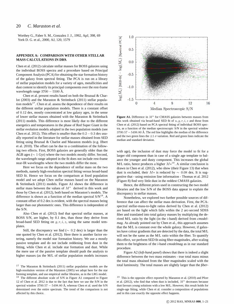
20 C. Maraston et al.
Worthey G., Faber S. M., Gonzalez J. J., 1992, ApJ, 398, 69York D. G. et al., 2000, AJ, 120, 1579
APPENDIX A: COMPARISON WITH OTHER STELLARMASS CALCULATIONS IN DR9.
Chen et al. (2012) calculate stellar masses for BOSS galaxies usingthe individual BOSS spectra and a procedure based on PrincipalComponent Analysis (PCA) for obtaining the star formation historyof the galaxy from spectral fitting. The PCA is run on a libraryof stellar population models for a variety of ages, metallicities anddust content to identify its principal components over the rest-framewavelength range3700 − 5500 A.
Chen et al. present results based on both the Bruzual & Char-lot (2003) and the Maraston & Stromback (2011) stellar popula-tion models17. Chen et al. assess the dependence of their results onthe different stellar population models. There is a constant offsetof 0.12 dex, mostly concentrated at low galaxy ages, in the senseof lower stellar masses obtained with the Maraston & Stromback(2011) models. This difference is most likely due to the differentenergetics and temperatures in the phase of Red Super Giant in thestellar evolution models adopted in the two population models (seeChen et al. 2012). This offset is smaller than the0.2− 0.3 dex usu-ally reported in the literature for stellar masses obtainedfrom SEDfitting using Bruzual & Charlot and Maraston models (e.g. Ilbertet al. 2010). The offset can be due to a combination of the follow-ing two effects. First, BOSS galaxies are generally older than theAGB ages (∼ 1 Gyr) where the two models mostly differ. Second,the wavelength range adopted in the fit does not include rest-framenear-IR wavelengths where the two models differ the most.
Here we focus on the dependence of stellar mass on the twomethods, namely high-resolution spectral fitting versus broad-bandSED fit. Hence we focus on the comparison at fixed populationmodel and we adopt Chen stellar masses based on the Maraston& Stromback (2011) models. Figure A1 shows the difference instellar mass between the values ofM∗ derived in this work andthose by Chen et al. (2012), both based on Maraston’s models.Thedifference is shown as a function of the median spectral S/N18. Aconstant offset of 0.2 dex is evident, with the spectral masses beinglarger than our photometric ones. This difference is independent ofthe S/N.
Also Chen et al. (2012) find that spectral stellar masses, atBOSS S/N, are higher, by 0.1 dex, than those they derive frombroad-band SED fitting ong, r, i, z, using the same model tem-plates.
Still, the discrepancy we find (∼ 0.2 dex) is larger than theone quoted by Chen et al. (2012). Here there is another factoren-tering, namely the model star formation history. We use a mostlypassive template and do not include reddening from dust in thefitting, while Chen et al. include star formation and dust. Whilethe mere use of the passive template should push the analysistohigher masses (as the M/L of stellar population models increases
17 The Maraston & Stromback (2011) stellar population modelsare thehigh-resolution version of the Maraston (2005) we adopt here for the starforming template, and use empirical stellar libraries, as in the LRG model.18 The different absolute scale of S/N in Figure A1 compared to Figure12 of Chen et al. 2012 is due to the fact that here we use the S/N in thespectral window3700.57 − 5498.80 A, whereas Chen et al. used the S/Ndetermined over the entire spectrum. The trend of the comparison is notaffected by this choice.
Figure A1. Difference inM∗ for CMASS galaxies between masses fromthis work obtained via broad-band SED fit ofu, g, r, i, z and those fromChen et al. (2012) based on PCA spectral fitting of individualBOSS spec-tra, as a function of the median spectroscopic S/N in the spectral window3700.57− 5498.80 A. The red line highlights the median of the differenceand the two green lines the±1 σ variation. Red and green lines indicate themedian and standard deviation.
with age), the inclusion of dust may force the model to fit for alarger old component than in case of a single age template to bal-ance the younger and dusty component. This increases the globalM/L ratio, hence produces a higherM∗
19. A similar conclusion isdrawn in Chen et al. (2012), who show (their Figure 13) that whendust is excluded, theirM∗ is reduced by∼ 0.08 dex. It is sug-gestive that - using emission line information - Thomas et al. 2012(Figure 8) find very little dust in the reddest CMASS galaxies.
Hence, the different priors used in constructing the two modellibraries and the low S/N of the BOSS data appear to explain thediscrepancy in stellar masses.
Nonetheless, we explored two further possible sources of dif-ference that can affect the stellar mass derivation. First,the PCA-spectral stellar-mass-to-light ratios derived by Chen et al. (2012)are based on the light which falls within the 2 arc-second SDSSfiber and translated into total galaxy masses by multiplyingthe de-rived M/L ratio by the light (in thei-band) derived fromcmodel-mag. As already pointed out by Chen et al., this approach assumesthat the M/L is constant over the whole galaxy. However, if galax-ies have colour gradients that are detected by the data, the total M/Lwill not be the same as the M/L ratio within the fiber. To quantifythis effect, we perform SED fit using fiber-magnitudes, afterscalingthem to the brightness of thei-bandcmodelmagas in our standardprocedure.
Figure A2 (left-hand panel) shows that there is indeed a slightdifference between the two mass estimates - true total mass minusthe total mass obtained from the fiber magnitudes scaled withthetotal luminosity. The total masses are slightly larger thanthefiber-
19 This is the opposite effect reported by Maraston et al. (2010) and Pforret al. (2012), who find that when dust is included,M∗ decreases becausedust favours young solutions with a low M/L. However, this result holds forsingle-age fitting, while Chen et al. consider a compositionof populationsand in this case exactly the opposite effect happens.
c© 2012 RAS, MNRAS000, 1–21
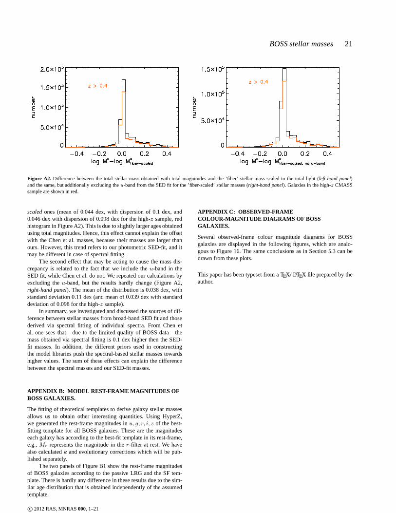
BOSS stellar masses 21
Figure A2. Difference between the total stellar mass obtained with total magnitudes and the ’fiber’ stellar mass scaled to the totallight (left-hand panel)and the same, but additionally excluding theu-band from the SED fit for the ’fiber-scaled’ stellar masses (right-hand panel). Galaxies in the high-z CMASSsample are shown in red.
scaledones (mean of 0.044 dex, with dispersion of 0.1 dex, and0.046 dex with dispersion of 0.098 dex for the high-z sample, redhistogram in Figure A2). This is due to slightly larger ages obtainedusing total magnitudes. Hence, this effect cannot explain the offsetwith the Chen et al. masses, because their masses are larger thanours. However, this trend refers to our photometric SED-fit,and itmay be different in case of spectral fitting.
The second effect that may be acting to cause the mass dis-crepancy is related to the fact that we include theu-band in theSED fit, while Chen et al. do not. We repeated our calculationsbyexcluding theu-band, but the results hardly change (Figure A2,right-hand panel). The mean of the distribution is 0.038 dex, withstandard deviation 0.11 dex (and mean of 0.039 dex with standarddeviation of 0.098 for the high-z sample).
In summary, we investigated and discussed the sources of dif-ference between stellar masses from broad-band SED fit and thosederived via spectral fitting of individual spectra. From Chen etal. one sees that - due to the limited quality of BOSS data - themass obtained via spectral fitting is 0.1 dex higher then the SED-fit masses. In addition, the different priors used in constructingthe model libraries push the spectral-based stellar massestowardshigher values. The sum of these effects can explain the differencebetween the spectral masses and our SED-fit masses.
APPENDIX B: MODEL REST-FRAME MAGNITUDES OFBOSS GALAXIES.
The fitting of theoretical templates to derive galaxy stellar massesallows us to obtain other interesting quantities. Using HyperZ,we generated the rest-frame magnitudes inu, g, r, i, z of the best-fitting template for all BOSS galaxies. These are the magnitudeseach galaxy has according to the best-fit template in its rest-frame,e.g.,Mr represents the magnitude in ther-filter at rest. We havealso calculatedk and evolutionary corrections which will be pub-lished separately.
The two panels of Figure B1 show the rest-frame magnitudesof BOSS galaxies according to the passive LRG and the SF tem-plate. There is hardly any difference in these results due tothe sim-ilar age distribution that is obtained independently of theassumedtemplate.
APPENDIX C: OBSERVED-FRAMECOLOUR-MAGNITUDE DIAGRAMS OF BOSSGALAXIES.
Several observed-frame colour magnitude diagrams for BOSSgalaxies are displayed in the following figures, which are analo-gous to Figure 16. The same conclusions as in Section 5.3 can bedrawn from these plots.
This paper has been typeset from a TEX/ LATEX file prepared by theauthor.
c© 2012 RAS, MNRAS000, 1–21
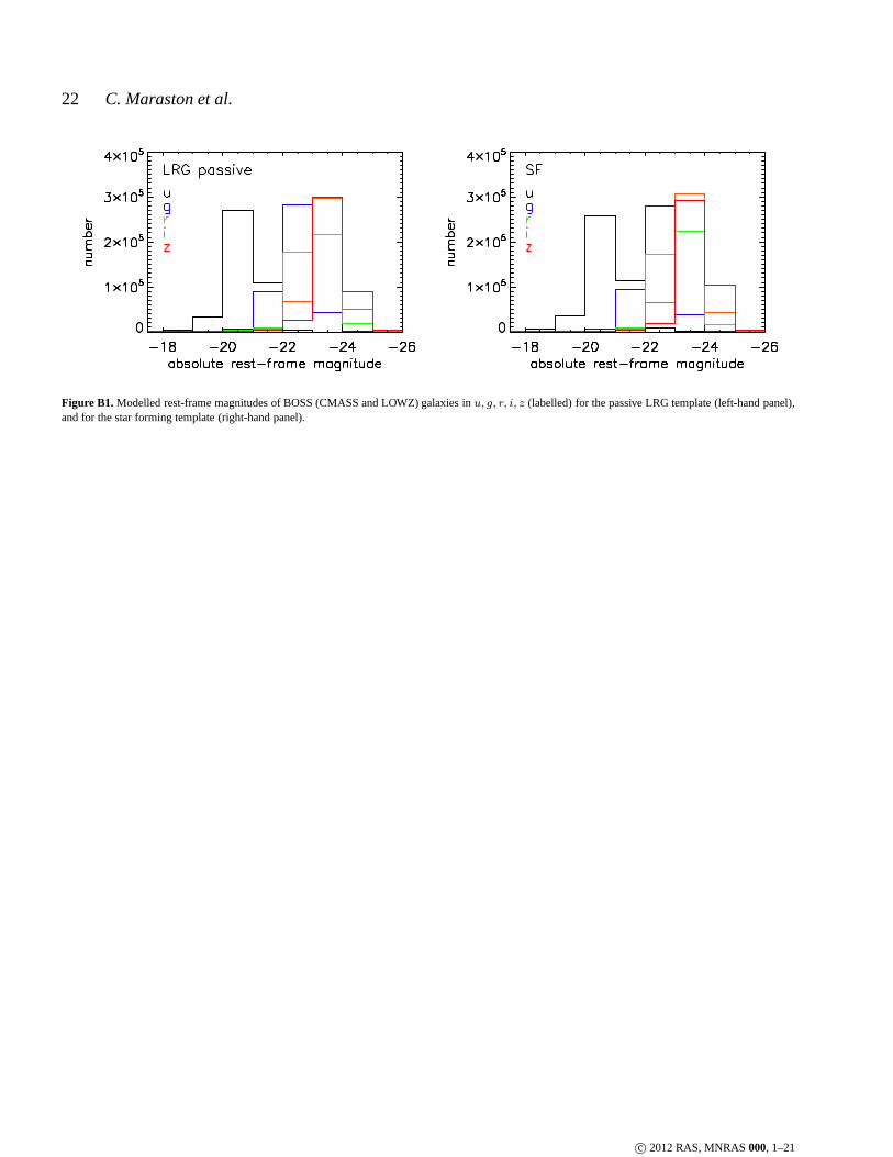
22 C. Maraston et al.
Figure B1. Modelled rest-frame magnitudes of BOSS (CMASS and LOWZ) galaxies inu, g, r, i, z (labelled) for the passive LRG template (left-hand panel),and for the star forming template (right-hand panel).
c© 2012 RAS, MNRAS000, 1–21
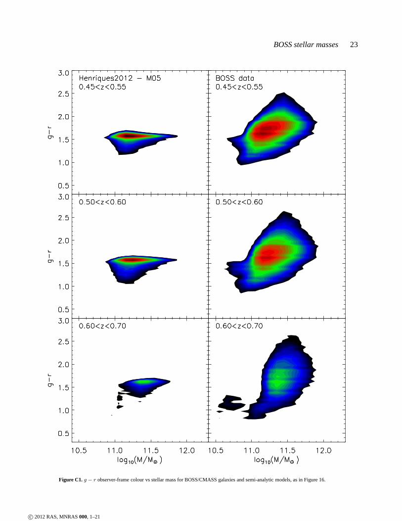
BOSS stellar masses 23
Figure C1. g − r observer-frame colour vs stellar mass for BOSS/CMASS galaxies and semi-analytic models, as in Figure 16.
c© 2012 RAS, MNRAS000, 1–21

24 C. Maraston et al.
Figure C2. r − i observer-frame colour vs stellar mass for BOSS/CMASS galaxies and semi-analytic models, as in Figure 16.
c© 2012 RAS, MNRAS000, 1–21
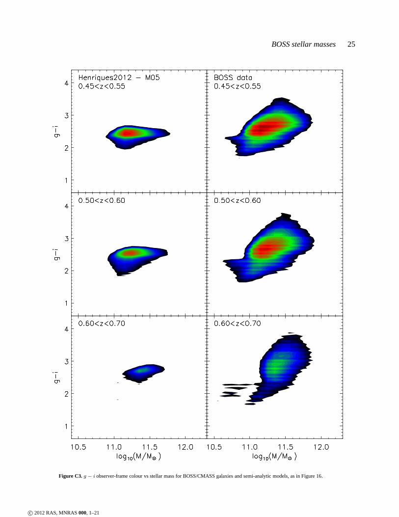
BOSS stellar masses 25
Figure C3. g − i observer-frame colour vs stellar mass for BOSS/CMASS galaxies and semi-analytic models, as in Figure 16.
c© 2012 RAS, MNRAS000, 1–21
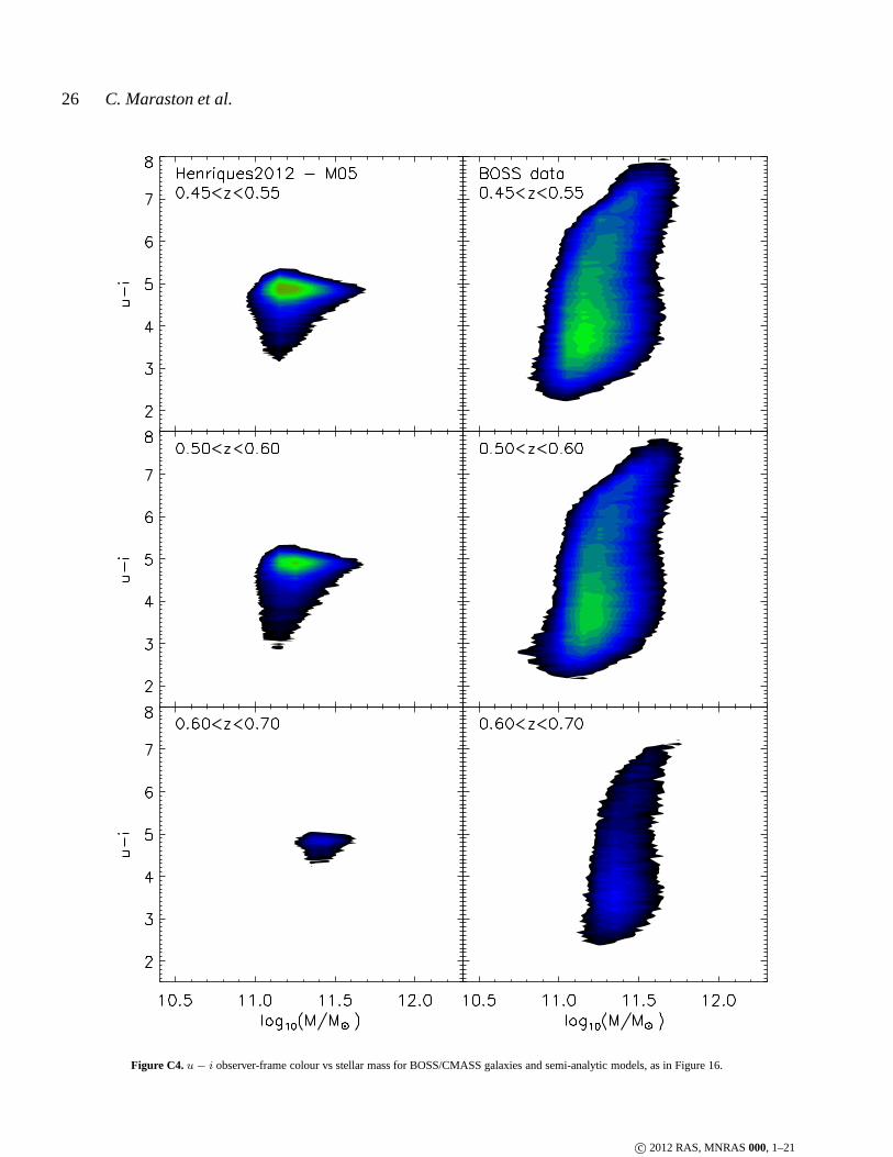
26 C. Maraston et al.
Figure C4.u− i observer-frame colour vs stellar mass for BOSS/CMASS galaxies and semi-analytic models, as in Figure 16.
c© 2012 RAS, MNRAS000, 1–21

Copyright © 2022 FDOKUMEN