The Characterization of Twenty Sequenced HumanGenomesKimberly Pelak1., Kevin V. Shianna1., Dongliang Ge1., Jessica M. Maia1, Mingfu Zhu1, Jason P. Smith1,

Elizabeth T. Cirulli1, Jacques Fellay1, Samuel P. Dickson1, Curtis E. Gumbs1, Erin L. Heinzen1, Anna C.

Need1, Elizabeth K. Ruzzo1, Abanish Singh1, C. Ryan Campbell1, Linda K. Hong1, Katharina A. Lornsen1,

Alexander M. McKenzie1, Nara L. M. Sobreira2, Julie E. Hoover-Fong2, Joshua D. Milner3, Ruth Ottman4,5,

Barton F. Haynes6, James J. Goedert7, David B. Goldstein1*

1 Center for Human Genome Variation, Duke University School of Medicine, Durham, North Carolina, United States of America, 2 McKusick-Nathans Institute of Genetic

Medicine, Johns Hopkins University School of Medicine, Baltimore, Maryland, United States of America, 3 Allergic Inflammation Unit, Laboratory of Allergic Diseases,

National Institute of Allergy and Infectious Diseases, Bethesda, Maryland, United States of America, 4 G. H. Sergievsky Center and Departments of Epidemiology and

Neurology, Columbia University, New York, New York, United States of America, 5 Division of Epidemiology, New York State Psychiatric Institute, New York, New York,

United States of America, 6 Duke Human Vaccine Institute, Duke University, Durham, North Carolina, United States of America, 7 Infections and Immunoepidemiology

Branch, Division of Cancer Epidemiology and Genetics, National Cancer Institute, Rockville, Maryland, United States of America

Abstract

We present the analysis of twenty human genomes to evaluate the prospects for identifying rare functional variants thatcontribute to a phenotype of interest. We sequenced at high coverage ten ‘‘case’’ genomes from individuals with severehemophilia A and ten ‘‘control’’ genomes. We summarize the number of genetic variants emerging from a study of thismagnitude, and provide a proof of concept for the identification of rare and highly-penetrant functional variants byconfirming that the cause of hemophilia A is easily recognizable in this data set. We also show that the number of novelsingle nucleotide variants (SNVs) discovered per genome seems to stabilize at about 144,000 new variants per genome,after the first 15 individuals have been sequenced. Finally, we find that, on average, each genome carries 165 homozygousprotein-truncating or stop loss variants in genes representing a diverse set of pathways.

Citation: Pelak K, Shianna KV, Ge D, Maia JM, Zhu M, et al. (2010) The Characterization of Twenty Sequenced Human Genomes. PLoS Genet 6(9): e1001111.doi:10.1371/journal.pgen.1001111

Editor: Greg Gibson, Georgia Institute of Technology, United States of America

Received January 27, 2010; Accepted August 3, 2010; Published September 9, 2010

This is an open-access article distributed under the terms of the Creative Commons Public Domain declaration which stipulates that, once placed in the publicdomain, this work may be freely reproduced, distributed, transmitted, modified, built upon, or otherwise used by anyone for any lawful purpose.

Funding: Funding was provided by the Bill and Melinda Gates Foundation grant 157412, with additional funding by the National Institute of Allergy andInfectious Diseases (NIAID) Center for HIV/AIDS Vaccine Immunology (CHAVI) grant AI067854. Funding for the collection of control samples was provided in partby RC2MH089915 from the National Institute of Mental Health, and Award Number RC2NS070344 from the National Institute Of Neurological Disorders AndStroke. This research was supported in part by funding from the Division of Intramural Research, NIAID, National Institutes of Health. The funders had no role instudy design, data collection and analysis, decision to publish, or preparation of the manuscript.

Competing Interests: The authors have declared that no competing interests exist.

* E-mail: d.goldstein@duke.edu

. These authors contributed equally to this work.

Introduction

The technology to sequence entire human genomes has evolved

rapidly in recent years. Massively-parallel sequencing techniques

have been developed, and it is now possible to sequence an entire

human genome in little more than a week. Programs to align these

short reads and call the resulting variants are being developed and

optimized [1,2], and the cost to sequence a genome has

plummeted. Single human genomes have been sequenced on a

number of different next-generation sequencing platforms [3–6].

Whole genome sequencing has also been used to identify rare,

disease-causing variants by sequencing the genome of one or a

small number of affected individuals and then performing

necessary follow-up work to confirm the variant [7-9], and it has

also been used to study the patterns of variation that develop in

cancerous cells [10,11].

It will be essential going forward to be able to characterize the

patterns of variation in larger sets of sequenced genomes. As a

first step in that direction, we have characterized the patterns of

variation observed in 20 human genomes that were sequenced

at high coverage using the Illumina Genome Analyzer IIx

platform.

Results

Study populationWe sequenced individuals with hemophilia A who were thought

to have been exposed to HIV-1, and who will contribute to a

larger future study to identify genetic determinants of resistance to

infection with HIV-1. We also considered ten genomes from

various other non-HIV- related projects (Table S1), hereafter

referred to collectively as ‘‘controls’’ for convenience. The ten

hemophilia patients are all of European ancestry, as are seven of

the controls. Two of the controls are Hispanic and one control is

African American. This was confirmed using a principal

component analysis [12].

PLoS Genetics | www.plosgenetics.org 1 September 2010 | Volume 6 | Issue 9 | e1001111

Whole Genome SequencingThe DNA for this study was extracted from blood samples or

peripheral blood mononuclear cells (PBMCs). For each sequenced

genome, we aimed to produce 70–80 billion bases that passed

Illumina’s quality filters. Some individuals were sequenced at

much higher coverage (about 150–200 billion bases) to assess how

coverage affects variant calling. To determine overall coverage, all

gaps (stretches of N’s) in the reference genome (NCBI human

genome assembly build 36; Ensembl core database release 50_36l

[13]) were excluded, resulting in the reference having

2,855,343,769 bases. After accounting for PCR duplicates and

reads that did not align to the reference genome, genomic

coverage of the autosomes ranged from 206 to 516 (Table 1). We

further defined a ‘‘covered’’ base as a base with at least five reads

where the Phred-like consensus score was greater than zero. On

average across the autosomes, 97.45% of the reference genome

was covered with at least five reads at each base, with a range of

92.49% to 99.65% coverage across the 20 genomes (Table 1).

Identifying single nucleotide variants (SNVs), smallinsertion/deletions (indels) and copy number variants(CNVs)

The short-reads were aligned with the Burrows-Wheeler

Alignment tool (BWA) [1], and the genetic differences between

our sequenced genomes and the reference were identified using

modified settings in the SAMtools variant calling program [2]. On

average, we identified approximately 3.5 million SNVs and

610,000 indels per genome (Table S2). Over 87% of the SNVs

identified in each of the 20 genomes were found in the dbSNP

database (Figure 1, Table S3), similar to what has been seen in

other reports (Table S4), and 43.45% are in the HapMap project

database (Table S3) [14]. The number of indels we observed is also

similar to other reports (Table S5), although there were only a

limited number of indels included in dbSNP (n = 13,727, version

Author Summary

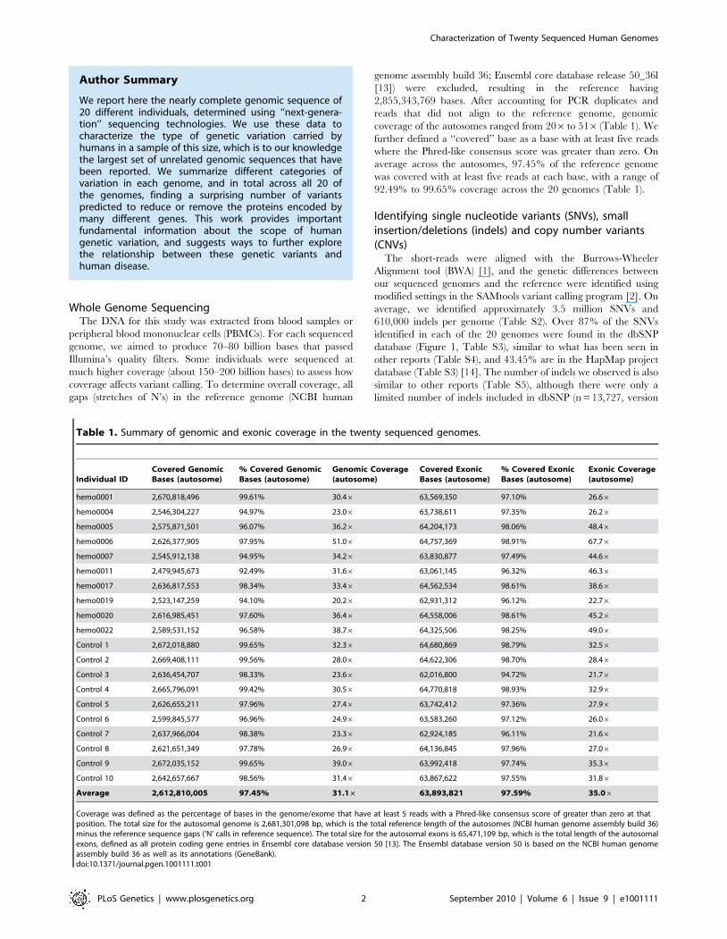
We report here the nearly complete genomic sequence of20 different individuals, determined using ‘‘next-genera-tion’’ sequencing technologies. We use these data tocharacterize the type of genetic variation carried byhumans in a sample of this size, which is to our knowledgethe largest set of unrelated genomic sequences that havebeen reported. We summarize different categories ofvariation in each genome, and in total across all 20 ofthe genomes, finding a surprising number of variantspredicted to reduce or remove the proteins encoded bymany different genes. This work provides importantfundamental information about the scope of humangenetic variation, and suggests ways to further explorethe relationship between these genetic variants andhuman disease.

Table 1. Summary of genomic and exonic coverage in the twenty sequenced genomes.

Individual IDCovered GenomicBases (autosome)

% Covered GenomicBases (autosome)

Genomic Coverage(autosome)

Covered ExonicBases (autosome)

% Covered ExonicBases (autosome)

Exonic Coverage(autosome)

hemo0001 2,670,818,496 99.61% 30.46 63,569,350 97.10% 26.66

hemo0004 2,546,304,227 94.97% 23.06 63,738,611 97.35% 26.26

hemo0005 2,575,871,501 96.07% 36.26 64,204,173 98.06% 48.46

hemo0006 2,626,377,905 97.95% 51.06 64,757,369 98.91% 67.76

hemo0007 2,545,912,138 94.95% 34.26 63,830,877 97.49% 44.66

hemo0011 2,479,945,673 92.49% 31.66 63,061,145 96.32% 46.36

hemo0017 2,636,817,553 98.34% 33.46 64,562,534 98.61% 38.66

hemo0019 2,523,147,259 94.10% 20.26 62,931,312 96.12% 22.76

hemo0020 2,616,985,451 97.60% 36.46 64,558,006 98.61% 45.26

hemo0022 2,589,531,152 96.58% 38.76 64,325,506 98.25% 49.06

Control 1 2,672,018,880 99.65% 32.36 64,680,869 98.79% 32.56

Control 2 2,669,408,111 99.56% 28.06 64,622,306 98.70% 28.46

Control 3 2,636,454,707 98.33% 23.66 62,016,800 94.72% 21.76

Control 4 2,665,796,091 99.42% 30.56 64,770,818 98.93% 32.96

Control 5 2,626,655,211 97.96% 27.46 63,742,412 97.36% 27.96

Control 6 2,599,845,577 96.96% 24.96 63,583,260 97.12% 26.06

Control 7 2,637,966,004 98.38% 23.36 62,924,185 96.11% 21.66

Control 8 2,621,651,349 97.78% 26.96 64,136,845 97.96% 27.06

Control 9 2,672,035,152 99.65% 39.06 63,992,418 97.74% 35.36

Control 10 2,642,657,667 98.56% 31.46 63,867,622 97.55% 31.86

Average 2,612,810,005 97.45% 31.16 63,893,821 97.59% 35.06

Coverage was defined as the percentage of bases in the genome/exome that have at least 5 reads with a Phred-like consensus score of greater than zero at thatposition. The total size for the autosomal genome is 2,681,301,098 bp, which is the total reference length of the autosomes (NCBI human genome assembly build 36)minus the reference sequence gaps (‘N’ calls in reference sequence). The total size for the autosomal exons is 65,471,109 bp, which is the total length of the autosomalexons, defined as all protein coding gene entries in Ensembl core database version 50 [13]. The Ensembl database version 50 is based on the NCBI human genomeassembly build 36 as well as its annotations (GeneBank).doi:10.1371/journal.pgen.1001111.t001

Characterization of Twenty Sequenced Human Genomes

PLoS Genetics | www.plosgenetics.org 2 September 2010 | Volume 6 | Issue 9 | e1001111

129, validated) so overlap comparisons in this case are not

informative. The average transition to transversion ratio is 2.08

and average homozygote to heterozygote ratio is 0.59 (Table S6),

both consistent with what has been reported previously [3,15,16]

(Table S7).

We used the genomic distribution of the number of aligned

reads (read depth) to infer copy number state in 2 kb windows

using a hidden Markov model approach, incorporating SNV

genotype status, implemented in a software package called

‘‘Estimation by Read Depth with SNVs’’ or ERDS [17]. We

predicted 5,821 distinct copy number variants (CNVs) on the

autosomes (6,204 across the whole genome) that were greater than

2 kb in length, and that had unique start and stop coordinates (we

note, however, that even the same CNV will often be inferred to

have slightly different start and stop points, meaning that it is in

general not possible to determine which CNVs are identical across

samples using only the location information). There was an

average of 338 deletions (covering 0.72% of the autosomes) and

411 duplications (covering 0.79% of the autosomes) per genome.

The median (mean) size of these CNVs was 34kb (58kb) [17]. We

further note that this method is designed to detect test genomes

that differ from the reference genome in genomic regions that are

present in normal or nearly normal copy number state in the

reference genome (corresponding to having a copy number count

of two in typical genomic regions). ERDS is not designed to

provide an absolute count for heavily amplified regions of the

genome and in its current implementation will be insensitive to

quantitative differences in highly amplified regions in comparison

with the approach embodied, for example, in MrFAST [18].

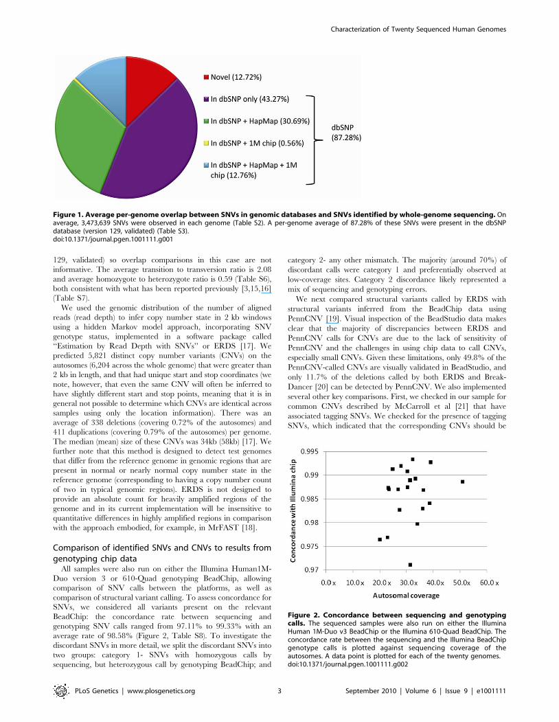
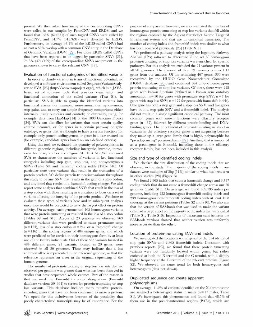
Comparison of identified SNVs and CNVs to results fromgenotyping chip data

All samples were also run on either the Illumina Human1M-

Duo version 3 or 610-Quad genotyping BeadChip, allowing

comparison of SNV calls between the platforms, as well as

comparison of structural variant calling. To assess concordance for

SNVs, we considered all variants present on the relevant

BeadChip: the concordance rate between sequencing and

genotyping SNV calls ranged from 97.11% to 99.33% with an

average rate of 98.58% (Figure 2, Table S8). To investigate the

discordant SNVs in more detail, we split the discordant SNVs into

two groups: category 1- SNVs with homozygous calls by

sequencing, but heterozygous call by genotyping BeadChip; and

category 2- any other mismatch. The majority (around 70%) of

discordant calls were category 1 and preferentially observed at

low-coverage sites. Category 2 discordance likely represented a

mix of sequencing and genotyping errors.

We next compared structural variants called by ERDS with

structural variants inferred from the BeadChip data using

PennCNV [19]. Visual inspection of the BeadStudio data makes

clear that the majority of discrepancies between ERDS and

PennCNV calls for CNVs are due to the lack of sensitivity of

PennCNV and the challenges in using chip data to call CNVs,

especially small CNVs. Given these limitations, only 49.8% of the

PennCNV-called CNVs are visually validated in BeadStudio, and

only 11.7% of the deletions called by both ERDS and Break-

Dancer [20] can be detected by PennCNV. We also implemented

several other key comparisons. First, we checked in our sample for

common CNVs described by McCarroll et al [21] that have

associated tagging SNVs. We checked for the presence of tagging

SNVs, which indicated that the corresponding CNVs should be

Figure 1. Average per-genome overlap between SNVs in genomic databases and SNVs identified by whole-genome sequencing. Onaverage, 3,473,639 SNVs were observed in each genome (Table S2). A per-genome average of 87.28% of these SNVs were present in the dbSNPdatabase (version 129, validated) (Table S3).doi:10.1371/journal.pgen.1001111.g001

Figure 2. Concordance between sequencing and genotypingcalls. The sequenced samples were also run on either the IlluminaHuman 1M-Duo v3 BeadChip or the Illumina 610-Quad BeadChip. Theconcordance rate between the sequencing and the Illumina BeadChipgenotype calls is plotted against sequencing coverage of theautosomes. A data point is plotted for each of the twenty genomes.doi:10.1371/journal.pgen.1001111.g002

Characterization of Twenty Sequenced Human Genomes

PLoS Genetics | www.plosgenetics.org 3 September 2010 | Volume 6 | Issue 9 | e1001111

present. We then asked how many of the corresponding CNVs

were called in our samples by PennCNV and ERDS, and we

found that 9.8% (62/631) of such tagged CNVs were called by

PennCNV, and 54.7% (345/631) were detected by ERDS.

Furthermore, on average 43.1% of the ERDS-called CNVs had

at least a 50% overlap with a common CNV entry in the Database

of Genomic Variants (DGV) [22]. For those ERDS called CNVs

that have been reported to be tagged by particular SNVs [21],

74.3% (371/499) of the corresponding SNVs are present in the

genomes shown to carry the relevant CNV [17].

Evaluation of functional categories of identified variantsIn order to classify variants in terms of functional potential, we

developed a software environment called SequenceVariantAnaly-

zer or SVA [23] (http://www.svaproject.org/), which is a JAVA-

based set of software tools that provides visualization and

functional annotation of the called variants (Text S1). In

particular, SVA is able to group the identified variants into

functional classes (for example, non-synonymous, synonymous,

stop gain), and to carry out simple frequency comparisons either

internally (using our cases and controls) or externally, using, for

example, data from HapMap [14] or the 1000 Genomes Project

[24]. SVA can also filter for variants that meet certain quality

control measures, or for genes in a certain pathway or gene

ontology, or genes that are thought to have a certain function (for

example, only protein-coding genes), or genes in a user-created list

(for example, candidate genes based on user-defined criteria).

Using this tool, we evaluated the quantity of polymorphisms in

different genomic regions, including intergenic, intronic, intron-

exon boundary and exonic (Figure S1, Text S1). We also used

SVA to characterize the numbers of variants in key functional

categories including stop gain, stop loss, and nonsynonymous

SNVs (Table S9) and frameshift coding indels (Table S10). Of

particular note were variants that result in the truncation of a

protein product. We define protein-truncating variants throughout

this study to be any SNV that results in the gain of a stop codon,

and any indel that results in a frameshift coding change. We also

report some analyses that combined SNVs that result in the loss of

a stop codon with those resulting in truncation to focus on a set of

variants affecting the integrity of the protein product. We chose to

evaluate these types of variants here and in subsequent analyses

since they would be predicted to have the largest effect on protein

activity. On average, each genome had 165 homozygous variants

that were protein truncating or resulted in the loss of a stop codon

(Tables S9 and S10). Across all 20 genomes we observed 563

different variants that were predicted to cause premature stops

(n = 123), loss of a stop codon (n = 24), or a frameshift change

(n = 416) in the coding regions of 484 unique genes, and which

were predicted to be carried in their homozygous form by at least

one of the twenty individuals. Out of these 563 variants located in

484 different genes, 21 variants, located in 20 genes, were

observed in all 20 genomes. These may indicate that a less

common allele is represented in the reference genome, or that the

reference represents an error in the original sequencing of the

human genome.

The number of protein-truncating or stop loss variants that we

observed per genome was greater than what has been observed in

studies that have sequenced whole exomes. Part of the reason is

that we used the Ensembl transcript designations (Ensembl

database versions 50_361) to screen for protein-truncating or stop

loss variants. This database includes many putative protein-

encoding genes that have not been confirmed to make a protein.

We opted for this inclusiveness because of the possibility that

poorly characterized transcripts may be of importance. For the

purpose of comparison, however, we also evaluated the number of

homozygous protein-truncating or stop loss variants that fell within

the regions captured by the Agilent SureSelect Exome Targeted

Enrichment system and that are in canonical transcripts. The

number of coding indels and frameshift indels was similar to what

has been observed previously [25] (Table S11).

We performed a pathway analysis using the Ingenuity Pathway

Analysis (IPA) software to determine if the set of homozygous

protein-truncating or stop loss variants were enriched for specific

pathways. For this analysis we excluded the 21 variants present in

all 20 genomes. The removal of these 21 variants removed 17

genes from our analysis. Of the remaining 467 genes, 330 were

recognized by the HUGO Gene Nomenclature Committee

(HGNC) database [26], and contained 364 unique homozygous

protein truncating or stop loss variants. Of these, there were 228

genes with known functions (defined as a known gene ontology

annotation; n = 50 for genes with premature stop SNV; n = 7 for

genes with stop loss SNV; n = 177 for genes with frameshift indels).

One gene has both a stop gain and a stop loss SNV, and five genes

have both a stop gain SNV and a frameshift indel. The analysis

did not result in a single significant canonical pathway. The most

common genes with known functions were olfactory receptor

genes (n = 32), followed by different protein-binding and DNA-

binding genes. The enrichment of protein-truncating or stop loss

variants in the olfactory receptor genes is not surprising because

they make up a large gene family that is highly polymorphic for

‘‘pseudogenizing’’ polymorphisms [27]. Anything that is annotated

as a pseudogene in Ensembl, including those in the olfactory

receptor family, has not been included in this analysis.

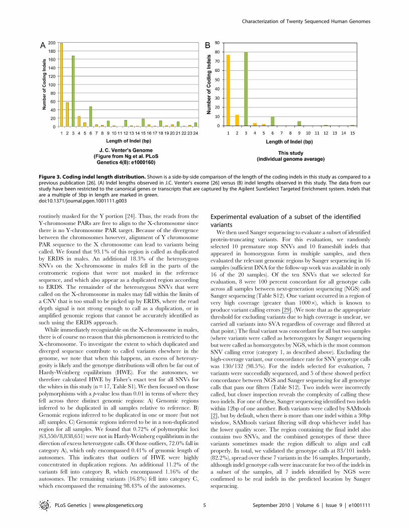
Size and type of identified coding indelsWe checked the size distribution of the coding indels that we

observed in the study. The majority of the coding indels in our

dataset were multiples of 3bp (51%), similar to what has been seen

in other studies [28] (Figure 3).

We found 2,865 indels that cause a frameshift change and 3,737

coding indels that do not cause a frameshift change across our 20

genomes (Table S10). On average, we found 609,795 indels per

genome, including 132 homozygous frameshift coding indels and

239 homozygous non-frameshift coding indels with at least 106coverage at the variant positions (Tables S2 and S10). We also saw

that the version of SAMtools that was used to make the variant

calls had a large effect on the zygosity of the indels that were called

(Table S1, Table S10). Inspection of discordant calls between the

SAMtools versions showed that neither version was uniformly

more accurate than the other.

Location of protein-truncating SNVs and indelsWe investigated the locations within genes of the 554 identified

stop gain SNVs and 2,865 frameshift indels. Consistent with

previous reports [28], we found that these protein-truncating

variants were not randomly located within genes, but rather

enriched at both the N-termini and the C-termini, with a slightly

higher frequency at the C-termini of the relevant proteins (Figure

S2). We observed the same trend for both homozygotes and

heterozygotes (data not shown).

Duplicated sequence can create apparentpolymorphisms

On average, 11.2% of variants identified on the X-chromosome

are assigned a heterozygote status in males (n = 17 males, Table

S1). We investigated this phenomenon and found that 48.5% of

them are in the pseudoautosomal regions (PARs), which are

Characterization of Twenty Sequenced Human Genomes

PLoS Genetics | www.plosgenetics.org 4 September 2010 | Volume 6 | Issue 9 | e1001111

routinely masked for the Y portion [24]. Thus, the reads from the

Y-chromosome PARs are free to align to the X-chromosome since

there is no Y-chromosome PAR target. Because of the divergence

between the chromosomes however, alignment of Y chromosome

PAR sequence to the X chromosome can lead to variants being

called. We found that 93.1% of this region is called as duplicated

by ERDS in males. An additional 18.3% of the heterozygous

SNVs on the X-chromosome in males fell in the parts of the

centromeric regions that were not masked in the reference

sequence, and which also appear as a duplicated region according

to ERDS. The remainder of the heterozygous SNVs that were

called on the X-chromosome in males may fall within the limits of

a CNV that is too small to be picked up by ERDS, where the read

depth signal is not strong enough to call as a duplication, or in

amplified genomic regions that cannot be accurately identified as

such using the ERDS approach.

While immediately recognizable on the X-chromosome in males,

there is of course no reason that this phenomenon is restricted to the

X-chromosome. To investigate the extent to which duplicated and

diverged sequence contribute to called variants elsewhere in the

genome, we note that when this happens, an excess of heterozy-

gosity is likely and the genotype distributions will often be far out of

Hardy-Weinberg equilibrium (HWE). For the autosomes, we

therefore calculated HWE by Fisher’s exact test for all SNVs for

the whites in this study (n = 17, Table S1). We then focused on those

polymorphisms with a p-value less than 0.01 in terms of where they

fell across three distinct genomic regions: A) Genomic regions

inferred to be duplicated in all samples relative to reference. B)

Genomic regions inferred to be duplicated in one or more (but not

all) samples. C) Genomic regions inferred to be in a non-duplicated

region for all samples. We found that 0.72% of polymorphic loci

(63,550/8,838,651) were not in Hardy-Weinberg equilibrium in the

direction of excess heterozygote calls. Of those outliers, 72.0% fall in

category A), which only encompassed 0.41% of genomic length of

autosomes. This indicates that outliers of HWE were highly

concentrated in duplication regions. An additional 11.2% of the

variants fell into category B, which encompassed 1.16% of the

autosomes. The remaining variants (16.8%) fell into category C,

which encompassed the remaining 98.43% of the autosomes.

Experimental evaluation of a subset of the identifiedvariants

We then used Sanger sequencing to evaluate a subset of identified

protein-truncating variants. For this evaluation, we randomly

selected 10 premature stop SNVs and 10 frameshift indels that

appeared in homozygous form in multiple samples, and then

evaluated the relevant genomic regions by Sanger sequencing in 16

samples (sufficient DNA for the follow-up work was available in only

16 of the 20 samples). Of the ten SNVs that we selected for

evaluation, 8 were 100 percent concordant for all genotype calls

across all samples between next-generation sequencing (NGS) and

Sanger sequencing (Table S12). One variant occurred in a region of

very high coverage (greater than 10006), which is known to

produce variant calling errors [29]. (We note that as the appropriate

threshold for excluding variants due to high coverage is unclear, we

carried all variants into SVA regardless of coverage and filtered at

that point.) The final variant was concordant for all but two samples

(where variants were called as heterozygotes by Sanger sequencing

but were called as homozygotes by NGS, which is the most common

SNV calling error (category 1, as described above). Excluding the

high-coverage variant, our concordance rate for SNV genotype calls

was 130/132 (98.5%). For the indels selected for evaluation, 7

variants were successfully sequenced, and 5 of these showed perfect

concordance between NGS and Sanger sequencing for all genotype

calls that pass our filters (Table S12). Two indels were incorrectly

called, but closer inspection reveals the complexity of calling these

two indels. For one of these, Sanger sequencing identified two indels

within 12bp of one another. Both variants were called by SAMtools

[2], but by default, when there is more than one indel within a 30bp

window, SAMtools variant filtering will drop whichever indel has

the lower quality score. The region containing the final indel also

contains two SNVs, and the combined genotypes of these three

variants sometimes made the region difficult to align and call

properly. In total, we validated the genotype calls at 83/101 indels

(82.2%), spread over these 7 variants in the 16 samples. Importantly,

although indel genotype calls were inaccurate for two of the indels in

a subset of the samples, all 7 indels identified by NGS were

confirmed to be real indels in the predicted location by Sanger

sequencing.

Figure 3. Coding indel length distribution. Shown is a side-by-side comparison of the length of the coding indels in this study as compared to aprevious publication [26]. (A) Indel lengths observed in J.C. Venter’s exome [26] versus (B) indel lengths observed in this study. The data from ourstudy have been restricted to the canonical genes or transcripts that are captured by the Agilent SureSelect Targeted Enrichment system. Indels thatare a multiple of 3bp in length are marked in green.doi:10.1371/journal.pgen.1001111.g003

Characterization of Twenty Sequenced Human Genomes

PLoS Genetics | www.plosgenetics.org 5 September 2010 | Volume 6 | Issue 9 | e1001111

Additionally, we obtained an estimate of how well SNVs were

called overall in this dataset using other experimental methods. To

do this we identified a class of ‘‘vulnerable’’ SNVs as those that

passed our variant calling criteria and were 1) observed in just one

sample and 2) and were not listed in dbSNP. Of these

‘‘vulnerable’’ SNVs, we chose 20 at random. Since these SNVs

were likely to have a higher than average false positive rate, this

analysis should have given us a conservative estimate of how well

SNVs are being called overall. We genotyped these 20

‘‘vulnerable’’ SNVs by TaqMan in a total of 16 samples, including

the sample putatively carrying each variant. We used Illumina

Custom TaqMan SNP Genotyping Assays for genotyping. We

then assessed whether the SNV showed evidence of variability in

any of the samples, and if so, an individual blinded to the NGS

data identified which sample contained the variant. We found that

the genotypes we observed by TaqMan showed perfect concor-

dance with the genotype observed by NGS sequencing for 18 of

the 20 variants investigated. No variant was observed for the

remaining two assays. Thus, at least 18 of these 20 variants are

real, giving us a conservative estimate of 90% accuracy for calling

‘‘vulnerable’’ SNVs.

Comparison of cases to controlsTo see whether we could easily identify the gene causing

hemophilia in the cases, we next tested for enrichment of specific

clearly functional variants in the set of 10 cases compared with the

10 controls. We identified first all protein-truncating or stop loss

variants in homozygous form on the autosomes or present on the

X chromosome, and we ranked all genes in the genome in terms of

the number of cases affected. A variant was included in these

counts as long as: 1) it was never observed in homozygous form in

the controls, 2) no other protein-truncating or stop loss variant in

the same gene was present in homozygous form in the controls, 3)

it had a minor allele frequency of less than 25% in the controls

(observed in heterozygous form in 5 or fewer of the 10 controls), 4)

it had a minimum of 106coverage on autosomes or 56coverage

on the sex chromosomes to be considered a homozygote, and 5)

the affected gene was present in the HGNC database [26].

Not surprisingly, the gene with the most affected cases was

Factor VIII (F8), mutations in which are known to cause

hemophilia A. In our study, six of the hemophilia patients had

identified protein truncating mutations (Table 2, Table S13,

Figure S3). Table S14 lists all genes that fit the criteria and have

protein-truncating or stop loss variants in at least 3 cases,

regardless of HGNC classification. We did not identify disease

causing mutations in the F8 gene for four of the hemophiliacs.

However, it is well documented that a particular large inversion

contributes to around 40% of all the severe type A hemophilia

patients [30,31]. Inversions are difficult to identify from short

sequencing reads using current analysis tools, and in the case of

F8, this is further complicated by regions of repetitive sequence

that flank the known F8 inversion.

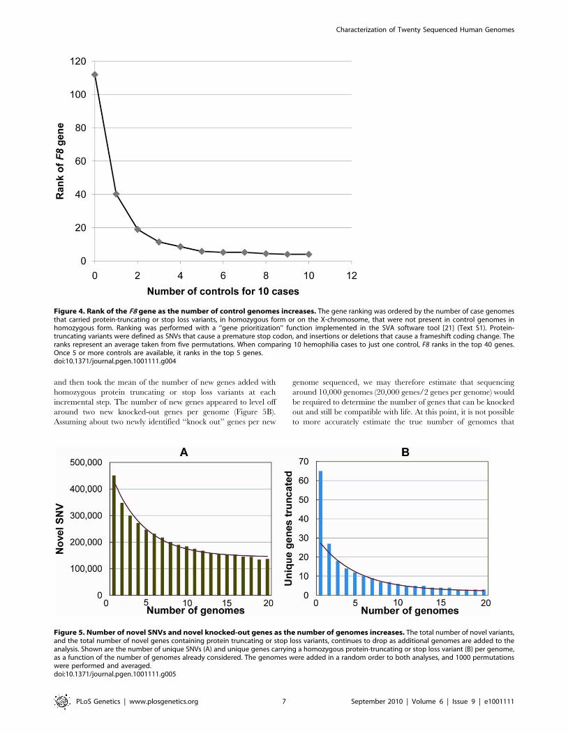
We also determined how many controls would be required to

identify F8 in our 10 cases, by evaluating the rank of the F8 gene

as defined above. We found that once we had five controls, F8

consistently ranked among the top five genes that showed an

enrichment of variants in cases and not in the controls (Figure 4).

Furthermore, the identification of the cluster of variants in F8

served as a proof-of-concept, by demonstrating that the technical

and bioinformatic approaches that we used in this paper are

sufficient to identify rare disease-causing variants.

We next evaluated the scope for identifying specific coding

variants that show a significant enrichment in our designated

‘‘cases.’’ In our dataset, there are 39,374 coding SNVs or indels

that are present in at least two cases. Since variants in this class

would be more likely to influence traits of interest than variants not

annotated as functional, it seems reasonable to treat such groups of

functional variants as a separate class in association studies [32].

The maximum imbalance that a variant could show in the current

data set was to be present in the 10 cases and absent in the 10

controls, which would generate a p-value of 161025. However, a

Bonferroni correction for 39,374 tests requires a p-value of

1.361026 to be significant at a = 0.05. Thus, it is not possible to

reach significance in this size dataset, even for maximally

imbalanced results.

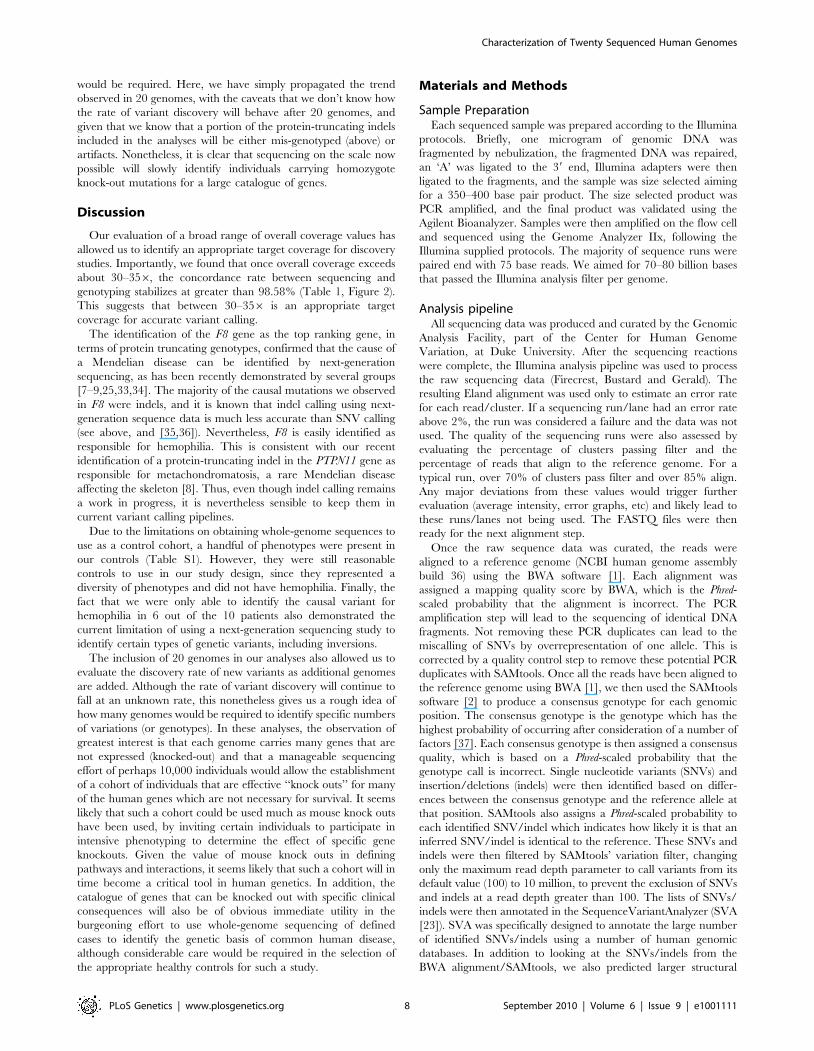
Number of novel SNVs as a function of genomesconsidered

Finally, we evaluated how many novel SNVs were identified as

the number of study subjects increased. Considering one of the

genomes at random, we found on average 443,000 SNVs not in

dbSNP. We then asked how many new SNVs were added per

genome, considering both variants in dbSNP and variants

‘‘discovered’’ in the previously considered genomes. We permuted

the order of genomes 1000 times and then took the mean of the

number of SNVs added at each incremental step. The number of

new SNVs per genome appeared to level off at around 144,000

novel SNVs by the 15th genome (Figure 5A, Text S1).

We also considered the related question of how many new genes

have been observed to be ‘‘knocked-out’’ by homozygous protein-

truncating or stop loss variants per new genome that has been

sequenced. Again, we permuted the order of genomes 1000 times

Table 2. Prioritization of protein-truncating or stop loss variants enriched in hemophilia samples.

Rank Gene# controls het (homo,but with low coverage) SNV Count Indel Count Total Count Comment

1 F8 0 1 4 5 Visual inspection of the alignment shows a sixthsample that also has a deletion in F8. It is called as aheterozygote by SAMtools.

2 C16orf84 2 0 5 5

3 C8orf80 4 0 4 4

4 PRB1 2 (+1) 4 0 4

5 EFCAB2 2 (+1) & 0 0 3 3 2 variants. Both occur in the same cases, with thesame zygosity

Only canonical genes (with a defined HUGO Gene Nomenclature Committee (HGNC) database entry [26]) were included.See Table S14 for a full list of genes.doi:10.1371/journal.pgen.1001111.t002

Characterization of Twenty Sequenced Human Genomes

PLoS Genetics | www.plosgenetics.org 6 September 2010 | Volume 6 | Issue 9 | e1001111

and then took the mean of the number of new genes added with

homozygous protein truncating or stop loss variants at each

incremental step. The number of new genes appeared to level off

around two new knocked-out genes per genome (Figure 5B).

Assuming about two newly identified ‘‘knock out’’ genes per new

genome sequenced, we may therefore estimate that sequencing

around 10,000 genomes (20,000 genes/2 genes per genome) would

be required to determine the number of genes that can be knocked

out and still be compatible with life. At this point, it is not possible

to more accurately estimate the true number of genomes that

Figure 4. Rank of the F8 gene as the number of control genomes increases. The gene ranking was ordered by the number of case genomesthat carried protein-truncating or stop loss variants, in homozygous form or on the X-chromosome, that were not present in control genomes inhomozygous form. Ranking was performed with a ‘‘gene prioritization’’ function implemented in the SVA software tool [21] (Text S1). Protein-truncating variants were defined as SNVs that cause a premature stop codon, and insertions or deletions that cause a frameshift coding change. Theranks represent an average taken from five permutations. When comparing 10 hemophilia cases to just one control, F8 ranks in the top 40 genes.Once 5 or more controls are available, it ranks in the top 5 genes.doi:10.1371/journal.pgen.1001111.g004

Figure 5. Number of novel SNVs and novel knocked-out genes as the number of genomes increases. The total number of novel variants,and the total number of novel genes containing protein truncating or stop loss variants, continues to drop as additional genomes are added to theanalysis. Shown are the number of unique SNVs (A) and unique genes carrying a homozygous protein-truncating or stop loss variant (B) per genome,as a function of the number of genomes already considered. The genomes were added in a random order to both analyses, and 1000 permutationswere performed and averaged.doi:10.1371/journal.pgen.1001111.g005

Characterization of Twenty Sequenced Human Genomes

PLoS Genetics | www.plosgenetics.org 7 September 2010 | Volume 6 | Issue 9 | e1001111

would be required. Here, we have simply propagated the trend

observed in 20 genomes, with the caveats that we don’t know how

the rate of variant discovery will behave after 20 genomes, and

given that we know that a portion of the protein-truncating indels

included in the analyses will be either mis-genotyped (above) or

artifacts. Nonetheless, it is clear that sequencing on the scale now

possible will slowly identify individuals carrying homozygote

knock-out mutations for a large catalogue of genes.

Discussion

Our evaluation of a broad range of overall coverage values has

allowed us to identify an appropriate target coverage for discovery

studies. Importantly, we found that once overall coverage exceeds

about 30–356, the concordance rate between sequencing and

genotyping stabilizes at greater than 98.58% (Table 1, Figure 2).

This suggests that between 30–356 is an appropriate target

coverage for accurate variant calling.

The identification of the F8 gene as the top ranking gene, in

terms of protein truncating genotypes, confirmed that the cause of

a Mendelian disease can be identified by next-generation

sequencing, as has been recently demonstrated by several groups

[7–9,25,33,34]. The majority of the causal mutations we observed

in F8 were indels, and it is known that indel calling using next-

generation sequence data is much less accurate than SNV calling

(see above, and [35,36]). Nevertheless, F8 is easily identified as

responsible for hemophilia. This is consistent with our recent

identification of a protein-truncating indel in the PTPN11 gene as

responsible for metachondromatosis, a rare Mendelian disease

affecting the skeleton [8]. Thus, even though indel calling remains

a work in progress, it is nevertheless sensible to keep them in

current variant calling pipelines.

Due to the limitations on obtaining whole-genome sequences to

use as a control cohort, a handful of phenotypes were present in

our controls (Table S1). However, they were still reasonable

controls to use in our study design, since they represented a

diversity of phenotypes and did not have hemophilia. Finally, the

fact that we were only able to identify the causal variant for

hemophilia in 6 out of the 10 patients also demonstrated the

current limitation of using a next-generation sequencing study to

identify certain types of genetic variants, including inversions.

The inclusion of 20 genomes in our analyses also allowed us to

evaluate the discovery rate of new variants as additional genomes

are added. Although the rate of variant discovery will continue to

fall at an unknown rate, this nonetheless gives us a rough idea of

how many genomes would be required to identify specific numbers

of variations (or genotypes). In these analyses, the observation of

greatest interest is that each genome carries many genes that are

not expressed (knocked-out) and that a manageable sequencing

effort of perhaps 10,000 individuals would allow the establishment

of a cohort of individuals that are effective ‘‘knock outs’’ for many

of the human genes which are not necessary for survival. It seems

likely that such a cohort could be used much as mouse knock outs

have been used, by inviting certain individuals to participate in

intensive phenotyping to determine the effect of specific gene

knockouts. Given the value of mouse knock outs in defining

pathways and interactions, it seems likely that such a cohort will in

time become a critical tool in human genetics. In addition, the

catalogue of genes that can be knocked out with specific clinical

consequences will also be of obvious immediate utility in the

burgeoning effort to use whole-genome sequencing of defined

cases to identify the genetic basis of common human disease,

although considerable care would be required in the selection of

the appropriate healthy controls for such a study.

Materials and Methods

Sample PreparationEach sequenced sample was prepared according to the Illumina

protocols. Briefly, one microgram of genomic DNA was

fragmented by nebulization, the fragmented DNA was repaired,

an ‘A’ was ligated to the 39 end, Illumina adapters were then

ligated to the fragments, and the sample was size selected aiming

for a 350–400 base pair product. The size selected product was

PCR amplified, and the final product was validated using the

Agilent Bioanalyzer. Samples were then amplified on the flow cell

and sequenced using the Genome Analyzer IIx, following the

Illumina supplied protocols. The majority of sequence runs were

paired end with 75 base reads. We aimed for 70–80 billion bases

that passed the Illumina analysis filter per genome.

Analysis pipelineAll sequencing data was produced and curated by the Genomic

Analysis Facility, part of the Center for Human Genome

Variation, at Duke University. After the sequencing reactions

were complete, the Illumina analysis pipeline was used to process

the raw sequencing data (Firecrest, Bustard and Gerald). The

resulting Eland alignment was used only to estimate an error rate

for each read/cluster. If a sequencing run/lane had an error rate

above 2%, the run was considered a failure and the data was not

used. The quality of the sequencing runs were also assessed by

evaluating the percentage of clusters passing filter and the

percentage of reads that align to the reference genome. For a

typical run, over 70% of clusters pass filter and over 85% align.

Any major deviations from these values would trigger further

evaluation (average intensity, error graphs, etc) and likely lead to

these runs/lanes not being used. The FASTQ files were then

ready for the next alignment step.

Once the raw sequence data was curated, the reads were

aligned to a reference genome (NCBI human genome assembly

build 36) using the BWA software [1]. Each alignment was

assigned a mapping quality score by BWA, which is the Phred-

scaled probability that the alignment is incorrect. The PCR

amplification step will lead to the sequencing of identical DNA

fragments. Not removing these PCR duplicates can lead to the

miscalling of SNVs by overrepresentation of one allele. This is

corrected by a quality control step to remove these potential PCR

duplicates with SAMtools. Once all the reads have been aligned to

the reference genome using BWA [1], we then used the SAMtools

software [2] to produce a consensus genotype for each genomic

position. The consensus genotype is the genotype which has the

highest probability of occurring after consideration of a number of

factors [37]. Each consensus genotype is then assigned a consensus

quality, which is based on a Phred-scaled probability that the

genotype call is incorrect. Single nucleotide variants (SNVs) and

insertion/deletions (indels) were then identified based on differ-

ences between the consensus genotype and the reference allele at

that position. SAMtools also assigns a Phred-scaled probability to

each identified SNV/indel which indicates how likely it is that an

inferred SNV/indel is identical to the reference. These SNVs and

indels were then filtered by SAMtools’ variation filter, changing

only the maximum read depth parameter to call variants from its

default value (100) to 10 million, to prevent the exclusion of SNVs

and indels at a read depth greater than 100. The lists of SNVs/

indels were then annotated in the SequenceVariantAnalyzer (SVA

[23]). SVA was specifically designed to annotate the large number

of identified SNVs/indels using a number of human genomic

databases. In addition to looking at the SNVs/indels from the

BWA alignment/SAMtools, we also predicted larger structural

Characterization of Twenty Sequenced Human Genomes

PLoS Genetics | www.plosgenetics.org 8 September 2010 | Volume 6 | Issue 9 | e1001111

variation by developing an ‘‘Estimation by Read Depth with

SNVs’’ or ERDS method, based on a Hidden Markov Model [17].

This was an extension to the methods described in Bentley et al.

[3] and draft codes from Scally, A. [38]. Further details describing

the analysis tools are presented in Text S1.

Data accessThe raw reads for a portion of the genomes used in this study

are available on the NCBI sequence read archive, under study ID

SRP001691 (http://www.ncbi.nlm.nih.gov/sra/SRP001691). We

do not have consent from the patients and/or permission from the

Duke IRB to release the raw reads for several of the genomes used

in this study.

Supporting Information

Figure S1 Location of identified variants observed across all 20

genomes. These graphs show the functional distribution of SNVs

(A) and indels (B) based on their location in relation to annotated

transcripts.

Found at: doi:10.1371/journal.pgen.1001111.s001 (1.65 MB TIF)

Figure S2 Position of protein truncating variants within coding

sequences. These graphs show the relative locations of stop-gain

SNVs (A) and frameshift indels (B) within protein-coding

sequences. A relative location near 0.1 (left side of x-axis) indicates

that the variant is near the N-terminus, while a location near 1.0

(right side of x-axis) indicates that the variant is near the C-

terminus. The y-axis is the absolute count of variants. Figures

include both homozygous and heterozygous variants from across

all 20 genomes.

Found at: doi:10.1371/journal.pgen.1001111.s002 (0.83 MB TIF)

Figure S3 F8 variants. This image shows the positions of the F8

variants that were observed in our dataset. Image modified from

Ge et al. and Hubbard et al.

Found at: doi:10.1371/journal.pgen.1001111.s003 (0.09 MB TIF)

Table S1 General characteristics for each genome.

Found at: doi:10.1371/journal.pgen.1001111.s004 (0.06 MB

DOC)

Table S2 Variants identified for each individual genome.

Found at: doi:10.1371/journal.pgen.1001111.s005 (0.04 MB

DOC)

Table S3 Overlap of SNVs identified by sequencing with those

that are included in the dbSNP database, HapMap, or are on the

Illumina 1M chip, version 1.

Found at: doi:10.1371/journal.pgen.1001111.s006 (0.06 MB

DOC)

Table S4 Overlap of dbSNP and SNVs identified by sequenc-

ing.

Found at: doi:10.1371/journal.pgen.1001111.s007 (0.05 MB

DOC)

Table S5 Number of indels identified in whole-genome

sequencing studies and in dbSNP.

Found at: doi:10.1371/journal.pgen.1001111.s008 (0.06 MB

DOC)

Table S6 Transition to transversion ratios and homozygote to

heterozygote ratios.

Found at: doi:10.1371/journal.pgen.1001111.s009 (0.04 MB

DOC)

Table S7 Comparison of transition to transversion ratios and

homozygote to heterozygote ratios.

Found at: doi:10.1371/journal.pgen.1001111.s010 (0.05 MB

DOC)

Table S8 Comparison of SNV calls made from whole-genome

sequence versus genotype data.

Found at: doi:10.1371/journal.pgen.1001111.s011 (0.05 MB

DOC)

Table S9 SNVs by their function and predicted number of

homozygotes.

Found at: doi:10.1371/journal.pgen.1001111.s012 (0.07 MB

DOC)

Table S10 Indels by their function and homozygosity.

Found at: doi:10.1371/journal.pgen.1001111.s013 (0.06 MB

DOC)

Table S11 Comparison of individual average number of coding

indels, restricted to exome captured regions and canonical genes

and transcripts.

Found at: doi:10.1371/journal.pgen.1001111.s014 (0.04 MB

DOC)

Table S12 Validating protein-truncating variants using Sanger

sequencing.

Found at: doi:10.1371/journal.pgen.1001111.s015 (0.05 MB

DOC)

Table S13 Causal variants of type A hemophilia observed in this

study.

Found at: doi:10.1371/journal.pgen.1001111.s016 (0.04 MB

DOC)

Table S14 Prioritization of all genes enriched for protein

truncating variants in hemophilia samples.

Found at: doi:10.1371/journal.pgen.1001111.s017 (0.04 MB

DOC)

Text S1 Supplementary methods.

Found at: doi:10.1371/journal.pgen.1001111.s018 (0.04 MB

DOC)

Acknowledgments

We would like to acknowledge David Valle and Joseph P. McEvoy for

access to samples, and David Valle and Thomas J. Urban for comments on

the manuscript.

Author Contributions

Conceived and designed the experiments: KVS DBG. Performed the

experiments: KVS JPS CEG CRC LKH KAL AMM. Analyzed the data:

KP DG JMM MZ JPS ETC JF SPD ELH ACN EKR AS. Contributed

reagents/materials/analysis tools: NLMS JEHF JDM RO BFH JJG.

Wrote the paper: KP KVS JF DBG.

References

1. Li H, Durbin R (2009) Fast and accurate short read alignment with Burrows-

Wheeler transform. Bioinformatics 25: 1754–1760.

2. Li H, Handsaker B, Wysoker A, Fennell T, Ruan J, et al. (2009) The

Sequence Alignment/Map format and SAMtools. Bioinformatics 25:

2078–2079.

3. Bentley DR, Balasubramanian S, Swerdlow HP, Smith GP, Milton J, et al.

(2008) Accurate whole human genome sequencing using reversible terminator

chemistry. Nature 456: 53–59.

4. Wang J, Wang W, Li R, Li Y, Tian G, et al. (2008) The diploid genome

sequence of an Asian individual. Nature 456: 60–65.

Characterization of Twenty Sequenced Human Genomes

PLoS Genetics | www.plosgenetics.org 9 September 2010 | Volume 6 | Issue 9 | e1001111

5. Wheeler DA, Srinivasan M, Egholm M, Shen Y, Chen L, et al. (2008) The

complete genome of an individual by massively parallel DNA sequencing.

Nature 452: 872–876.

6. Ahn SM, Kim TH, Lee S, Kim D, Ghang H, et al. (2009) The first Korean

genome sequence and analysis: full genome sequencing for a socio-ethnic group.

Genome Res 19: 1622–1629.

7. Lupski JR, Reid JG, Gonzaga-Jauregui C, Rio Deiros D, Chen DC, et al. (2010)

Whole-genome sequencing in a patient with Charcot-Marie-Tooth neuropathy.

N Engl J Med 362: 1181–1191.

8. Sobreira NLM, Cirulli ET, Avramopoulos D, Wohler E, Oswald GL, et al.

(2010) Whole genome sequencing of a single individual identifies a Mendelian

disease gene. PLoS Genet 6: e1000991.

9. Roach JC, Glusman G, Smit AF, Huff CD, Hubley R, et al. (2010) Analysis of

genetic inheritance in a family quartet by whole-genome sequencing. Science

328: 636–639.

10. Ley TJ, Mardis ER, Ding L, Fulton B, McLellan MD, et al. (2008) DNA

sequencing of a cytogenetically normal acute myeloid leukaemia genome.

Nature 456: 66–72.

11. Lee W, Jiang Z, Liu J, Haverty PM, Guan Y, et al. (2010) The mutation

spectrum revealed by paired genome sequences from a lung cancer patient.

Nature 465: 473–477.

12. Price AL, Patterson NJ, Plenge RM, Weinblatt ME, Shadick NA, et al. (2006)

Principal components analysis corrects for stratification in genome-wide

association studies. Nat Genet 38: 904–909.

13. Hubbard TJ, Aken BL, Ayling S, Ballester B, Beal K, et al. (2009) Ensembl 2009.

Nucleic Acids Res 37: D690–697.

14. Frazer KA, Ballinger DG, Cox DR, Hinds DA, Stuve LL, et al. (2007) A second

generation human haplotype map of over 3.1 million SNPs. Nature 449:

851–861.

15. Levy S, Sutton G, Ng PC, Feuk L, Halpern AL, et al. (2007) The diploid genome

sequence of an individual human. PLoS Biol 5: e254.

16. Hale MC, McCormick CR, Jackson JR, Dewoody JA (2009) Next-generation

pyrosequencing of gonad transcriptomes in the polyploid lake sturgeon

(Acipenser fulvescens): the relative merits of normalization and rarefaction in

gene discovery. BMC Genomics 10: 203.

17. Zhu M, Need AC, Ge D, Singh A, Feng S, et al. (2010) Detection of copy

number variation using whole genome sequence data from twenty human

genomes. Manuscript in preparation.

18. Alkan C, Kidd JM, Marques-Bonet T, Aksay G, Antonacci F, et al. (2009)

Personalized copy number and segmental duplication maps using next-

generation sequencing. Nat Genet 41: 1061–1067.

19. Wang K, Li M, Hadley D, Liu R, Glessner J, et al. (2007) PennCNV: an

integrated hidden Markov model designed for high-resolution copy number

variation detection in whole-genome SNP genotyping data. Genome Res 17:

1665–1674.

20. Chen K, Wallis JW, McLellan MD, Larson DE, Kalicki JM, et al. (2009)

BreakDancer: an algorithm for high-resolution mapping of genomic structuralvariation. Nat Methods 6: 677–681.

21. McCarroll SA, Kuruvilla FG, Korn JM, Cawley S, Nemesh J, et al. (2008)

Integrated detection and population-genetic analysis of SNPs and copy numbervariation. Nat Genet 40: 1166–1174.

22. Iafrate AJ, Feuk L, Rivera MN, Listewnik ML, Donahoe PK, et al. (2004)Detection of large-scale variation in the human genome. Nat Genet 36:

949–951.

23. Ge D, Ruzzo EK, Shianna KV, He M, Allen A, et al. (2010) Annotation,visualization, and analysis of variants emerging from whole-genome and whole-

exome sequencing using SVA. Manuscript in preparation.24. The 1000 Genomes Project (2009) http://www.1000genomes.org/page.php.

25. Ng SB, Turner EH, Robertson PD, Flygare SD, Bigham AW, et al. (2009)Targeted capture and massively parallel sequencing of 12 human exomes.

Nature 461: 272–276.

26. Eyre TA, Ducluzeau F, Sneddon TP, Povey S, Bruford EA, et al. (2006) TheHUGO Gene Nomenclature Database, 2006 updates. Nucleic Acids Res 34:

D319–321.27. Gilad Y, Man O, Paabo S, Lancet D (2003) Human specific loss of olfactory

receptor genes. Proc Natl Acad Sci U S A 100: 3324–3327.

28. Ng PC, Levy S, Huang J, Stockwell TB, Walenz BP, et al. (2008) Geneticvariation in an individual human exome. PLoS Genet 4: e1000160.

29. Malhis N, Jones SJM (2010) High quality SNP calling using Illumina data atshallow coverage. Bioinformatics 26: 1029–1035.

30. Naylor J, Brinke A, Hassock S, Green PM, Giannelli F (1993) CharacteristicmRNA abnormality found in half the patients with severe haemophilia A is due

to large DNA inversions. Hum Mol Genet 2: 1773–1778.

31. Antonarakis SE, Kazazian HH, Tuddenham EG (1995) Molecular etiology offactor VIII deficiency in hemophilia A. Hum Mutat 5: 1–22.

32. Cirulli ET, Goldstein DB (2010) Uncovering the roles of rare variants incommon disease through whole-genome sequencing. Nat Rev Genet 11:

415–425.

33. Choi M, Scholl UI, Ji W, Liu T, Tikhonova IR, et al. (2009) Genetic diagnosisby whole exome capture and massively parallel DNA sequencing. Proc Natl

Acad Sci U S A 106: 19096–19101.34. Ng SB, Buckingham KJ, Lee C, Bigham AW, Tabor HK, et al. (2010) Exome

sequencing identifies the cause of a mendelian disorder. Nat Genet 42: 30–35.35. Krawitz P, Rodelsperger C, Jager M, Jostins L, Bauer S, et al. (2010) Microindel

detection in short-read sequence data. Bioinformatics 26: 722–729.

36. Koboldt DC (2010) Challenges of sequencing human genomes. Brief Bioinform,Advance publication 2 June 2010.

37. Li H, Ruan J, Durbin R (2008) Mapping short DNA sequencing reads andcalling variants using mapping quality scores. Genome Res 18: 1851–1858.

38. Scally A, Bentley DR (2009) Personal Communication Hidden Markov Model

for Copy-number Variation.

Characterization of Twenty Sequenced Human Genomes

PLoS Genetics | www.plosgenetics.org 10 September 2010 | Volume 6 | Issue 9 | e1001111