The Challenge of Machine Learning in Space Weather:Nowcasting and Forecasting

E. Camporeale1,2

1CIRES, University of Colorado Boulder, Boulder, CO, USA, 2Centrum Wiskunde & Informatica, Amsterdam,The Netherlands

Abstract The numerous recent breakthroughs in machine learning make imperative to carefullyponder how the scientific community can benefit from a technology that, although not necessarily new, istoday living its golden age. This Grand Challenge review paper is focused on the present and future roleof machine learning in Space Weather. The purpose is twofold. On one hand, we will discuss previousworks that use machine learning for Space Weather forecasting, focusing in particular on the fewareas that have seen most activity: the forecasting of geomagnetic indices, of relativistic electrons atgeosynchronous orbits, of solar flares occurrence, of coronal mass ejection propagation time, and of solarwind speed. On the other hand, this paper serves as a gentle introduction to the field of machine learningtailored to the Space Weather community and as a pointer to a number of open challenges that we believethe community should undertake in the next decade. The recurring themes throughout the review arethe need to shift our forecasting paradigm to a probabilistic approach focused on the reliable assessment ofuncertainties, and the combination of physics-based and machine learning approaches, known as gray box.

Plain Language Summary In the last decade, machine learning has achieved unforeseenresults in industrial applications. In particular, the combination of massive data sets and computing withspecialized processors (graphics processing units, or GPUs) can perform as well or better than humans intasks like image classification and game playing. Space weather is a discipline that lives between academiaand industry, given the relevant physical effects on satellites and power grids in a variety of applications,and the field therefore stands to benefit from the advances made in industrial applications. Today, machinelearning poses both a challenge and an opportunity for the space weather community. The challenge isthat the current data science revolution has not been fully embraced, possibly because space physicistsremain skeptical of the gains achievable with machine learning. If the community can master the relevanttechnical skills, they should be able to appreciate what is possible within a few years time and what ispossible within a decade. The clearest opportunity lies in creating space weather forecasting models thatcan respond in real time and that are built on both physics predictions and on observed data.

1. Artificial Intelligence: Is This Time for Real?The history of artificial intelligence (AI) has been characterized by an almost cyclical repetition of springsand winters: periods of high, often unjustified, expectations, large investments, and hype in the media, fol-lowed by times of disillusionment, pessimism, and cutback in funding. Such a cyclical trend is not atypicalfor a potentially disruptive technology, and it is very instructive to try to learn lessons from (in)famous AIpredictions of the past (Armstrong et al., 2014), especially now that the debate about the danger of artificialgeneral intelligence (i.e., AI pushed to the level of human ability) is in full swing (Russell & Bohannon, 2015;Russell & Norvig, 2016). Indeed, it is unfortunate that most of the AI research of the past has been plaguedby overconfidence and that many hyperbolic statements about utility of AI had very little scientific basis.Even the initial Dartmouth workshop held in 1956, credited with the invention of AI, had underestimatedthe difficulty of understanding language processing.

At the time of writing some experts believe that we are experiencing a new AI spring (e.g., Bughin & Hazan,2017; Olhede & Wolfe, 2018), which possibly started as early as 2010. This might or might not be followed byyet another winter. Still, many reckon that this time is different, for the very simple reason that AI has finallyentered industrial production, with several of our everyday technologies being powered by AI algorithms.In fact, one might not realize that, for instance, most of the time we use an app on our smartphone, we are

FEATURE ARTICLE10.1029/2018SW002061

Key Points:• Machine learning (ML) has enabled

advances in industrial applications;space weather researchers areadopting and adapting MLtechniques

• This introduction to machinelearning concepts is tailored forthe Space Weather community, butapplicable to many othercommunities

• This introduction describesforecasting opportunities in agray-box paradigm that combinesphysics-based and machine learningapproaches

Correspondence to:E. Camporeale,enrico.camporeale@colorado.edu

Citation:Camporeale, E. (2019). The challengeof machine learning in Space Weather:Nowcasting and forecasting. SpaceWeather, 17, 1166–1207. https://doi.org/10.1029/2018SW002061

Received 16 AUG 2018Accepted 3 JUN 2019Accepted article online 4 JUL 2019Published online 9 AUG 2019

©2019. American Geophysical Union.All Rights Reserved.

CAMPOREALE 1166

Space Weather 10.1029/2018SW002061

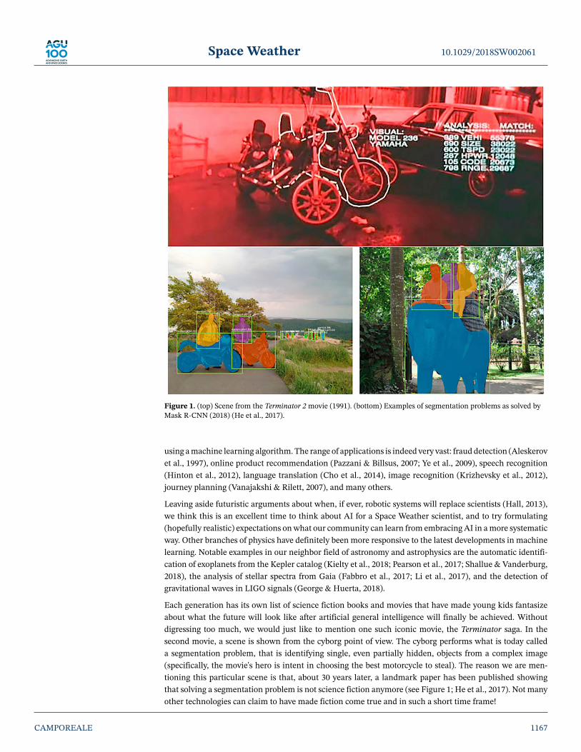
Figure 1. (top) Scene from the Terminator 2 movie (1991). (bottom) Examples of segmentation problems as solved byMask R-CNN (2018) (He et al., 2017).

using a machine learning algorithm. The range of applications is indeed very vast: fraud detection (Aleskerovet al., 1997), online product recommendation (Pazzani & Billsus, 2007; Ye et al., 2009), speech recognition(Hinton et al., 2012), language translation (Cho et al., 2014), image recognition (Krizhevsky et al., 2012),journey planning (Vanajakshi & Rilett, 2007), and many others.

Leaving aside futuristic arguments about when, if ever, robotic systems will replace scientists (Hall, 2013),we think this is an excellent time to think about AI for a Space Weather scientist, and to try formulating(hopefully realistic) expectations on what our community can learn from embracing AI in a more systematicway. Other branches of physics have definitely been more responsive to the latest developments in machinelearning. Notable examples in our neighbor field of astronomy and astrophysics are the automatic identifi-cation of exoplanets from the Kepler catalog (Kielty et al., 2018; Pearson et al., 2017; Shallue & Vanderburg,2018), the analysis of stellar spectra from Gaia (Fabbro et al., 2017; Li et al., 2017), and the detection ofgravitational waves in LIGO signals (George & Huerta, 2018).

Each generation has its own list of science fiction books and movies that have made young kids fantasizeabout what the future will look like after artificial general intelligence will finally be achieved. Withoutdigressing too much, we would just like to mention one such iconic movie, the Terminator saga. In thesecond movie, a scene is shown from the cyborg point of view. The cyborg performs what is today calleda segmentation problem, that is identifying single, even partially hidden, objects from a complex image(specifically, the movie's hero is intent in choosing the best motorcycle to steal). The reason we are men-tioning this particular scene is that, about 30 years later, a landmark paper has been published showingthat solving a segmentation problem is not science fiction anymore (see Figure 1; He et al., 2017). Not manyother technologies can claim to have made fiction come true and in such a short time frame!

CAMPOREALE 1167

Space Weather 10.1029/2018SW002061

2. The Machine Learning RenaissanceOne of the reasons why the current AI spring might be very different from all the previous ones, and in factnever revert to a winter, is the unique combination of three factors that have never been simultaneouslyexperienced in our history. First, as we all know, we live in the time of big data. The precise meaning of whatconstitutes big data depends on specific applications. In many fields the data is securely guarded as the goldmine on which a company's wealth is based (even more than proprietary, but imitable, algorithms). Luckily,in the field of Space Weather most of the data and associated software is released to the public (NationalAcademies of Sciences & Medicine, 2018).

The second factor is the recent advancement in GPUs computing. In the early 2000s GPU producers (notably,Nvidia) were trying to extend their market to the scientific community by depicting GPUs as acceleratorsfor high performance computing (HPC), hence advocating a shift in parallel computing where CPU clusterswould be replaced by heterogeneous, general-purpose, GPU-CPU architectures. Even though many suchmachines exist today, especially in large HPC labs worldwide, we would think that the typical HPC userhas not been persuaded to fully embrace GPU computing (at least in space physics), possibly because of thesteep learning curve required to proficiently write GPU codes. More recently, during the last decade, it hasbecome clear that a much larger number of users (with respect to the small niche of HPC experts) was readyto enter the GPU market: machine learning practitioners (along with bitcoin miners!). And this is why GPUcompanies are now branding themselves as enablers of the machine learning revolution.

It is certainly true that none of the pioneering advancements in machine learning would have been possiblewithout GPUs. As a figure of merit, the neural network (NN) NASnet, which delivers state-of-the-art resultson classification tasks of ImageNet and CIFAR-10 data sets, required using 500 GPUs for 4 days (includingsearch of optimal architecture; Zoph et al., 2017). Hence, a virtuous circle, based on a larger and largernumber of users and customers has fueled the faster than Moore's law increase in GPU speed witnessed inthe last several years. The largest difference between the two groups of GPU users targeted by the industry,that is, HPC experts and machine learning practitioners (not necessarily experts) is in their learning curve.While a careful design and a deep knowledge of the intricacies of GPU architectures is needed to successfullyaccelerate an HPC code on GPUs, it is often sufficient to switch a flag for a machine learning code to trainon GPUs.

This fundamental difference leads us to the third enabling factor of the machine learning renaissance: thehuge money investments from Information Technology (IT) companies, that have started yet another virtu-ous circle in software development. Indeed, companies like Google or Facebook own an unmatchable sizeof data to train their machine learning algorithms. By realizing the profitability of machine learning appli-cations, they have largely contributed to the advancement of machine learning, especially making their ownsoftware open-source and relatively easy to use (see, e.g., Abadi et al., 2016). Arguably, the most successfulapplications of machine learning are in the field of computer vision. Maybe because image recognition andautomatic captioning are tasks that are very easy to understand for the general public, this is the field wherelarge IT companies have advertised their successes to the nonexperts and attempted to capitalize them. Clas-sical examples are the Microsoft bot that guesses somebody's age (https://www.how-old.net), which got 50million users in 1 week, and the remarkably good captioning bot www.captionbot.ai (see Figure 2 takenfrom Donahue et al., 2015, for a state-of-the-art captioning example).

In a less structured way, the open-source scientific community has also largely contributed to the advance-ment of machine learning software. Some examples of community-developed python libraries that are nowwidely used are theano (Bergstra et al., 2010), scikit-learn (Pedregosa et al., 2011), astroML (VanderPlaset al., 2012), emcee (VanderPlas et al., 2012), and PyMC (Patil et al., 2010), among many others. This hassomehow led to an explosion of open-source software, which is very often overlapping in scope. Hence,ironically the large number of open-source machine learning packages available might actually constitutea barrier to somebody that entering the field is overwhelmed by the amount of possible choices. In the fieldof heliophysics alone, the recent review by Burrell et al. (2018) compiles a list of 28 python packages.

As a result of the unique combination of the three above discussed factors, for the first time in history alayperson can easily access terabytes of data (big data), afford to have a few thousand cores at their disposal(GPU computing), and easily train a machine learning algorithm with absolutely no required knowledge ofstatistics or computer science (large investments from IT companies in open-source software).

CAMPOREALE 1168

Space Weather 10.1029/2018SW002061

Figure 2. Automatically generating captions to images represents a state-of-the-art achievement in Machine Learning, that combines image recognition andnatural language processing. Figure taken from the arXiv version of Donahue et al., 2015 (2015; arXiv:1411.4389).

The purpose of this review is twofold. On one hand, we will discuss previous works that use machine learn-ing for Space Weather forecasting. The review will be necessarily incomplete and somewhat biased, and weapologize for any relevant work we might have overlooked. In particular, we will focus on a few areas whereit seems that several attempts of using machine learning have been proposed in the past: the forecasting ofgeomagnetic indices, of relativistic electrons at geosynchronous orbits, of solar flares occurrence, of coronalmass ejection (CME) propagation time, and of solar wind speed. On the other hand, this paper serves as agentle introduction to the field of machine learning tailored to the Space Weather community and, as thetitle suggests, as a pointer to a number of open challenges that we believe the community should undertakein the next decade. In this respect, the paper is recommended to bold and ambitious PhD students!

This review is organized as follows. Section 3 briefly explains why and how Space Weather could benefitfrom the above described machine learning renaissance, and it concisely introduces the several tasks thata machine learning algorithm can tackle. Section 4 introduces the typical machine learning workflow andthe appropriate performance metrics for each task. Section 5 constitutes the review part of the paper. Eachsubsection (geomagnetic indices, relativistic electrons at geosynchronous Earth orbit (GEO), solar images)is concluded with a recapitulation and an overview of future perspective in that particular field. Section 6discusses a few new trends in machine learning that we anticipate will soon have an application in the pro-cess of scientific discovery. Section 7 concludes the paper by discussing the future role of machine learningin Space Weather and space physics, in the upcoming decade, and by commenting our personal selection ofopen challenges that we encourage the community to consider.

3. Machine Learning in Space WeatherHow can Space Weather benefit from the ongoing machine learning revolution? First of all, we would liketo clarify that Space Weather is not new to machine learning. As many other subjects that are ultimatelyfocused on making predictions, several attempts to use (mainly, but not only) NNs have been made sincethe early 1990s. This will be particularly clear in section 5, which is devoted to a (selected) review of pastliterature. Especially in some areas such as geomagnetic index prediction, the list of early works is quiteoverwhelming. Before proceeding in commenting how machine learning can be embraced by the SpaceWeather community, it is therefore necessary to address the (unfortunately still typical) skeptical reaction of

CAMPOREALE 1169

Space Weather 10.1029/2018SW002061

Table 1Data Used for Space Weather

Mission WebsiteACE http://www.srl.caltech.edu/ACE/Wind https://wind.nasa.gov/DSCOVR https://www.nesdis.noaa.gov/content/dscovr-deep-space-climate-observatorySOHO https://sohowww.nascom.nasa.gov/STEREO https://stereo.gsfc.nasa.gov/SDO https://sdo.gsfc.nasa.gov/OMNI https://omniweb.gsfc.nasa.gov/index.htmlVAP http://vanallenprobes.jhuapl.edu/GOES https://www.goes.noaa.govPOES https://www.ospo.noaa.gov/Operations/POES/index.htmlGPS https://www.ngdc.noaa.gov/stp/space-weather/satellite-data/satellite-systems/gps/DMSP https://www.ngdc.noaa.govGround-based magnetometers http://www.intermagnet.orgGONG https://gong.nso.edu/

Note. ACE = Advanced Composition Explorer; DSCOVR = Deep Space Climate Observatory; SOHO = Solar andHeliospheric Observatory; STEREO = Solar Terrestrial Relations Observatory; SDO = Solar Dynamics Observatory;VAP = Van Allen Probes; GOES = Geostationary Operational Environmental Satellite system; POES = PolarOperational Environmental Satellites; DMSP = Defense Meteorological Satellite Program; GONG = Global OscillationNetwork Group.

many colleagues that wonder “if everything (i.e., any machine learning technique applied to Space Weather)has been tried already, why do we need to keep trying?” There are two simple answers, in my opinion. First,not everything has been tried; for example, deep learning based on convolutional NNs (CNN, see Appendix),which incidentally is one of the most successful trends in machine learning (LeCun et al., 2015), has beenbarely touched in this community. Second, machine learning has never been as successful as it is now: this isdue to the combination of the three factors discussed in section 2 thanks to which it is now possible to trainand compare a large number of models on a large size data set. In this respect, it is instructive to realize thatthe basic algorithm on which a CNN is based has not changed substantially over the last 30 years (LeCunet al., 1990). What has changed is the affordable size of a training set, the software (open-source pythonlibraries) and the hardware (GPUs). Hence, this is the right time when it is worth to retest ideas proposed10 or 20 years ago, because what did not seem to work then might prove very successful now.

Space Weather possesses all the ingredients often required for a successful machine learning application. Asalready mentioned, we have a large and freely available data set of in situ and remote observations collectedover several decades of space missions. Restricting our attention on data typically used for Space Weatherpredictions, the Advanced Composition Explorer (ACE), Wind, and the Deep Space Climate Observatory(DSCOVR) provide in situ plasma data in proximity of the first Lagrangian point (L1), with several temporalresolution, some of which date back 20 years. The Solar and Heliospheric Observatory (SOHO), the Solar Ter-restrial Relations Observatory (STEREO), and the Solar Dynamics Observatory (SDO) provide Sun images atdifferent wavelengths, magnetograms, and coronographs, also collectively covering a 20-year period. More-over, the OMNI database collects data at both hour and minutes frequency of plasma and solar quantities,as well as geomagnetic indices. Other sources of Space Weather data are the twin Van Allen Probes whosedatabase is now quite sizable, having entered their seventh year of operation; the Geostationary OperationalEnvironmental Satellite system (GOES) provides measurements of geomagnetic field, particle fluxes andX-rays irradiance at geostationary orbit. Recently, 16 years of GPS data have been released to the public, pro-viding a wealth of information on particle fluxes (Morley et al., 2017). Particle precipitation is measured bythe Polar Operational Environmental Satellites (POES) and the Defense Meteorological Satellite Program(DMSP).In addition to space-based measurements, an array of ground-based magnetometer monitors theEarth's magnetic field variation on time scales of seconds. A list of data sources for Space Weather can befound in Table 1.

CAMPOREALE 1170

Space Weather 10.1029/2018SW002061

Table 2Comparison Between White- and Black-Box Approaches

White (physics-based) Black (data-driven)Computational cost Generally expensive. Often not Training might be expensive

possible to run in real-time. (depending on the datasize) butexecution is typically very fast.

Robustness Robust to unseen data and rare Not able to extrapolate outsideevents. the range of the training set.

Assumptions Based on physics approximations. Minimal set of assumptions.

Consistency with observations Verified a posteriori. Enforced a priori.Steps toward a gray-box approach Data-driven parameterization of inputs. Enforcing physics-based conUncertainty quantification Usually not built-in. It requires It can be built-in.

Monte Carlo ensemble.

Furthermore, we have rather sophisticated physics-based models and a fair understanding of the physicsprocesses behind most Space Weather events. The fact that a first-principle approach will never be feasiblefor forecasting Space Weather events is essentially due to the large separation of scales in space and timeinvolved, to the short time lag between causes and effects, and the consequent enormous computational costof physics-based models. In this respect, we believe that it is fair to say that the Space Weather communityhas a good understanding of why some models have poor forecasting capabilities, for example, what is themissing physics in approximated models (see, e.g., Welling et al., 2017), and what links of the Space Weatherprediction chain will benefit more to a coupling with a data-driven approach. Therefore, Space Weatherseems to be an optimal candidate for a so-called gray-box approach.

As the name suggests, the gray-box paradigm sits in between two opposites approaches. For the purpose ofthis paper, black-box methods refer to ones that are completely data-driven, seeking empirical correlationsbetween variables of interests, and do not typically use a priori physical information on the system of inter-est (Ljung, 2001; Sjöberg et al., 1995). Machine learning falls in this category (but see section 6 for recenttrends in machine learning that do make use of physics law). On the other end of the spectrum of predictivemethods, white-box models are based on assumptions and equations that are presumed valid, irrespectiveof data (just in passing we note that physics is an experimental science, therefore physical laws are actuallyrooted in data validation. However, once a given theory stands the test of time, its connection to experimen-tal findings is not often questioned or checked). All physics-based models, either first principle or basedon approximations, are white box. Note that this distinction is different from what the reader can foundin other contexts. For instance, in Uncertainty Quantification or in Operations Research, a model is saidto be used as a black box whenever the internal specifics are not relevant. Other uses of the white- versusblack-box paradigm involve the concept of interpretability (Molnar, 2018). However, we find that concepttoo subjective to be applied rigorously and dangerously prone to philosophical debates. Table 2 succinctlydescribes the advantages and disadvantages of the two approaches, namely computational speed and abilityto generalize to out-of-sample (unseen or rare) data.

In the gray-box paradigm one tries to maximize the use of available information, be it data or priorphysics knowledge. Hence, a gray-box approach applies either when a physics-based model is enhanced bydata-derived information, or when a black-box model incorporates some form of physics constraints. In thefield of Space Weather there are at least three ways to implement a gray-box approach. First, by realizingthat even state-of-the-art models rely on ad hoc assumptions and parameterization of physical inputs, onecan use observations to estimate such parameters. This usually leads to an inverse problem (often ill-posed)that can be tackled by Bayesian parameter estimation and data assimilation (see, e.g., Reich & Cotter, 2015,for an introductory textbook on the topic). Bayes's theorem is the central pillar of this approach. It allows toestimate the probability of a given choice of parameters, conditioned on the observed data, as a function ofthe likelihood that these data are indeed observed when the model uses the chosen parameters. In mathe-matical terms, Bayes's formula expresses the likelihood of event A occurring when event B is true, p(A|B)as a function of the likelihood of event B occurring when event A is true, p(B|A). In short, the parameters

CAMPOREALE 1171

Space Weather 10.1029/2018SW002061

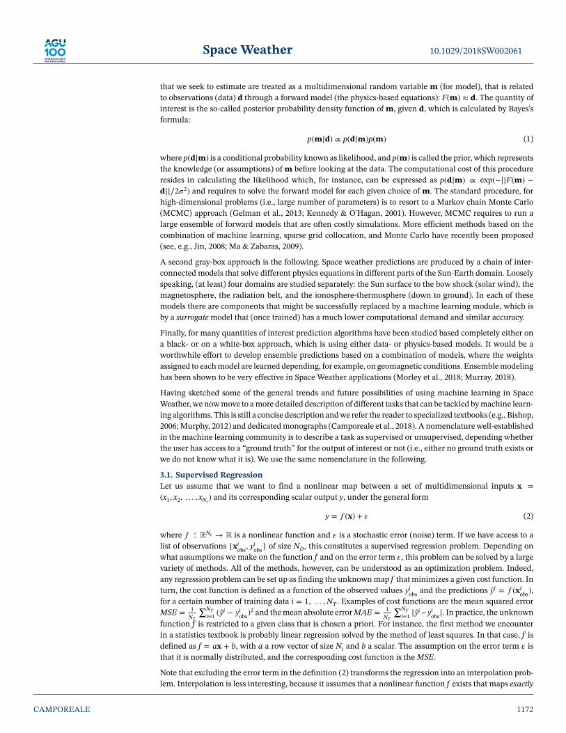
that we seek to estimate are treated as a multidimensional random variable m (for model), that is relatedto observations (data) d through a forward model (the physics-based equations): F(m) ≈ d. The quantity ofinterest is the so-called posterior probability density function of m, given d, which is calculated by Bayes'sformula:

p(m|d) ∝ p(d|m)p(m) (1)

where p(d|m) is a conditional probability known as likelihood, and p(m) is called the prior, which representsthe knowledge (or assumptions) of m before looking at the data. The computational cost of this procedureresides in calculating the likelihood which, for instance, can be expressed as p(d|m) ∝ exp(−||F(m) −d||∕2𝜎2) and requires to solve the forward model for each given choice of m. The standard procedure, forhigh-dimensional problems (i.e., large number of parameters) is to resort to a Markov chain Monte Carlo(MCMC) approach (Gelman et al., 2013; Kennedy & O'Hagan, 2001). However, MCMC requires to run alarge ensemble of forward models that are often costly simulations. More efficient methods based on thecombination of machine learning, sparse grid collocation, and Monte Carlo have recently been proposed(see, e.g., Jin, 2008; Ma & Zabaras, 2009).

A second gray-box approach is the following. Space weather predictions are produced by a chain of inter-connected models that solve different physics equations in different parts of the Sun-Earth domain. Looselyspeaking, (at least) four domains are studied separately: the Sun surface to the bow shock (solar wind), themagnetosphere, the radiation belt, and the ionosphere-thermosphere (down to ground). In each of thesemodels there are components that might be successfully replaced by a machine learning module, which isby a surrogate model that (once trained) has a much lower computational demand and similar accuracy.

Finally, for many quantities of interest prediction algorithms have been studied based completely either ona black- or on a white-box approach, which is using either data- or physics-based models. It would be aworthwhile effort to develop ensemble predictions based on a combination of models, where the weightsassigned to each model are learned depending, for example, on geomagnetic conditions. Ensemble modelinghas been shown to be very effective in Space Weather applications (Morley et al., 2018; Murray, 2018).

Having sketched some of the general trends and future possibilities of using machine learning in SpaceWeather, we now move to a more detailed description of different tasks that can be tackled by machine learn-ing algorithms. This is still a concise description and we refer the reader to specialized textbooks (e.g., Bishop,2006; Murphy, 2012) and dedicated monographs (Camporeale et al., 2018). A nomenclature well-establishedin the machine learning community is to describe a task as supervised or unsupervised, depending whetherthe user has access to a “ground truth” for the output of interest or not (i.e., either no ground truth exists orwe do not know what it is). We use the same nomenclature in the following.

3.1. Supervised RegressionLet us assume that we want to find a nonlinear map between a set of multidimensional inputs x =(x1, x2, … , xNi

) and its corresponding scalar output y, under the general form

𝑦 = 𝑓 (x) + 𝜀 (2)

where 𝑓 ∶ RNi → R is a nonlinear function and 𝜀 is a stochastic error (noise) term. If we have access to a

list of observations {xiobs, 𝑦

iobs} of size ND, this constitutes a supervised regression problem. Depending on

what assumptions we make on the function f and on the error term 𝜀, this problem can be solved by a largevariety of methods. All of the methods, however, can be understood as an optimization problem. Indeed,any regression problem can be set up as finding the unknown map f that minimizes a given cost function. Inturn, the cost function is defined as a function of the observed values 𝑦i

obs and the predictions ��i = 𝑓 (xiobs),

for a certain number of training data i = 1, … ,NT . Examples of cost functions are the mean squared errorMSE = 1

NT

∑NTi=1 (��

i − 𝑦iobs)

2 and the mean absolute error MAE = 1NT

∑NTi=1 |��i−𝑦i

obs|. In practice, the unknownfunction f is restricted to a given class that is chosen a priori. For instance, the first method we encounterin a statistics textbook is probably linear regression solved by the method of least squares. In that case, f isdefined as f = ax + b, with a a row vector of size Ni and b a scalar. The assumption on the error term 𝜀 isthat it is normally distributed, and the corresponding cost function is the MSE.

Note that excluding the error term in the definition (2) transforms the regression into an interpolation prob-lem. Interpolation is less interesting, because it assumes that a nonlinear function f exists that maps exactly

CAMPOREALE 1172

Space Weather 10.1029/2018SW002061

x into y. In other words, the term 𝜀 takes into account all possible reasons why such exact mapping mightnot exist, including observational errors and the existence of latent variables. In particular, different valuesof y might be associated to the same input x, because other relevant inputs have not been included in x(typically because not observed, hence the name latent).

The input x and the output y can be taken as quantities observed at the same time, in which case the problemis referred to as nowcasting, or with a given time lag, which is the more general forecasting. In principle asupervised regression task can be successfully set and achieve good performances for any problem for whichthere is a (physically motivated) reason to infer some time-lagged causality between a set of drivers and anoutput of interest. In general, the dimension of the input variable can be fairly large. For instance, one canemploy a time history of a given quantity, recorded with a certain time frequency. Examples of supervisedregression in Space Weather are the forecast of a geomagnetic index, as function of solar wind parametersobserved at L1 (Gleisner et al., 1996; Lundstedt & Wintoft, 1994; Macpherson et al., 1995; Uwamahoro &Habarulema, 2014; Valach et al., 2009; Weigel et al., 1999), the prediction of solar energetic particles (SEPs)(Fernandes, 2015; Gong et al., 2004; Li et al., 2008), of the F10.7 index for radio emissions (Ban et al., 2011;Huang et al., 2009), of ionospheric parameters (Chen et al., 2010), of sunspot numbers or, more in general,of the solar cycle (Ashmall & Moore, 1997; Calvo et al., 1995; Conway et al., 1998; Fessant et al., 1996;Lantos & Richard, 1998; Pesnell, 2012; Uwamahoro et al., 2009), of the arrival time of interplanetary shocks(Vandegriff et al., 2005), and of CMEs (Choi et al., 2012; Sudar et al., 2015).

Regression problems typically output a single-point estimates as a prediction, lacking any way of estimat-ing the uncertainty associated to the output. Methods exist that produce probabilistic outputs, either bydirectly using NNs (Gal & Ghahramani, 2016), or by using Gaussian Processes (GP; Rasmussen, 2004). Morerecently, a method has been developed to directly estimate the uncertainty of single-point forecast, produc-ing calibrated Gaussian probabilistic forecast (Camporeale et al., 2019). The archetype method of supervisedregression is the NN. See Box 1 for a short description of how a NN works.

3.2. Supervised ClassificationThe question that a supervised classification task answers is as follows: What class does an event belong to?This means that a list of plausible classes has been precompiled by the user, along with a list of examples ofevents belonging to each individual class (supervised learning). This problem is arguably the most popularin the machine learning community, with the ImageNet challenge being its prime example (Deng et al.,2009; Russakovsky et al., 2015). The challenge, that has been active for several years and it is now hostedon the platform kaggle.com, is to classify about hundred thousands images in 1,000 different categories. In2015 the winners of the challenge (using deep NNs) have claimed to have outperformed human accuracy inthe task.

In practice any regression problem for a continuous variable can be simplified into a classification task, byintroducing arbitrary thresholds and dividing the range of predictands into “classes.” One such example, inthe context of Space Weather predictions, is the forecast of solar flare classes. Indeed, the classification intoA, B, C, M, and X classes is based on the measured peak flux in (W/m2) arbitrarily divided in a logarithmicscale. In the case of a “coarse-grained” regression problem, the same algorithms used for regression can beused, with the only change occurring in the definition of cost functions and a discrete output. For instance,a real value output z (as in a standard regression problem) can be interpreted as the probability of the asso-ciated event being true or false (in a binary classification setting), by squashing the real value through aso-called logistic function:

�� = 𝜎(z) = 11 + e−z . (3)

Because 𝜎(z) is bounded between 0 and 1, its probabilistic interpretation is straightforward. Then, a simpleand effective cost function is the cross-entropy C, defined as

C(𝑦, z) = (𝑦 − 1) log(1 − 𝜎(z)) − 𝑦 log(𝜎(z)) (4)

where y is the ground true value of the event (0-false or 1-true) and z is the outcome of the model, squashedin the interval [0, 1] via 𝜎(z). One can verify that C(y, z) diverges to infinity when |𝑦− ��| = 1, that is, the eventis completely misspecified, and it tends to zero when |𝑦− ��| → 0. This approach is called logistic regression(even though it is a classification problem).

CAMPOREALE 1173

Space Weather 10.1029/2018SW002061

Other problems represent proper classification tasks (i.e., in a discrete space that is not the result of acoarse-grained discretization of a continuous space). Yet the underlying mathematical construct is thesame. Namely, one seeks a nonlinear function f that maps multidimensional inputs to a scalar output as inequation (2) and whose predicted values �� minimize a given cost function. In the case of image recognition,for instance, the input is constituted by images that are flattened into arrays of pixel values. A popular classi-fier is the Support Vector Machine (SVM; Vapnik, 2013), which finds the hyperplane that optimally dividesthe data to be classified (again according to a given cost function) in its high-dimensional space (equal tothe dimensionality of the inputs), effectively separating individual events into classes.

In the context of Space Weather, an example is the automatic classification of sunspot groups according to theMcIntosh classification (Colak & Qahwaji, 2008), or the classification of solar wind into types based on dif-ferent solar origins (Camporeale et al., 2017). It is useful to emphasize that, contrary to regression problems,interpreting the output of a classification task from a probabilistic perspective is much more straightforward,when using a sigmoid function to squash an unbounded real-value output to the interval [0, 1]. However,some extra steps are often needed to assure that such probabilistic output is well calibrated, that is, it is sta-tistically consistent with the observations (see, e.g., Niculescu-Mizil & Caruana, 2005; Zadrozny & Elkan,2001).

3.3. Unsupervised Classification, Also Known as ClusteringUnsupervised classification applies when we want to discover similarities in data, without deciding a priorithe division between classes or, in other words, without specifying classes and their labels. Yet again, this canbe achieved by an optimization problem, where the “similarity” between a group of events is encoded intoa cost function. This method is well suited in cases when a “ground truth” cannot be easily specified. Thistask is harder (and more costly) than supervised classification, since a criterion is often needed to specifythe optimal number of classes. A simple and often used algorithm is the so-called k-means, where the userspecifies the number of clusters Nk, and each observation xi = (xi

1, xi2, … , xi

Ni) is assigned to a given cluster.

The algorithm aims to minimize the within-cluster variance, defined as∑NK

k=1∑

i∈Sk||xi − k||2, where the first

sum is over the number of clusters, the second sum is over the points assigned to the cluster k, and 𝜇k is thecentroid of cluster k.

An unsupervised NN is the self-organizing map (SOM; Kohonen, 1997). The output of the network is atwo-dimensional topology of neurons, each of which maps to a specific characteristic of the inputs. In aself-organizing map, similar inputs activate close by neurons, hence, aggregating them into clusters. Eventhough some initial choice and constraint in the network architecture need to be done, this method dis-penses from choosing a priori the number of clusters and it indeed gives a good indication of what an optimalnumber might be.

In Space Weather, an unsupervised classification of the solar wind has been performed in Heidrich-Meisnerand Wimmer-Schweingruber (2018), and a self-organizing map has been applied to radiation belt particledistributions in Souza et al. (2018). It is fair to say, however, that the majority of past studies have focusedon supervised learning.

3.4. Dimensionality ReductionThe last family of methods that we concisely describe is dimensionality reduction. This is a family of tech-niques that aims at reducing the size of a data set, preserving its original information content, with respectto a specific prediction objective. It is very important in the context of multidimensional data sets, such aswhen working with images, since a data set can easily become very sizable and data handling becomes amajor bottleneck in the data science pipeline. A dimensionality reduction technique can be also used to rankthe input variables in terms of how important they are with respect to forecasting an output of interest, againwith the intent of using the smallest size of data that conveys the maximum information. Dimensionalityreduction is not often performed in the context of Space Weather. A recent example is the use of PrincipalComponent Analysis (PCA) for the nowcasting of SEPs (Papaioannou et al., 2018).

4. Machine Learning WorkflowIn this final section before the review part of the paper, we summarize the different phases that constitutethe workflow in applying machine learning to a Space Weather problem (and maybe more generally to anyphysics problem). This is not to be considered as a strict set of rules but rather as a guideline for good practice.

CAMPOREALE 1174

Space Weather 10.1029/2018SW002061

This workflow is inspired by the scikit-learn algorithm cheat sheet (https://scikit-learn.org/stable/tutorial/machine_learning_map/).

4.1. Problem FormulationThe importance of formulating the problem in a well-posed manner cannot be overstated. The relativeeasiness of using an off-the-shelf machine learning library poses the serious risk of trying to use machinelearning for problems that are not well formulated, and therefore whose chances of success are slim. It isnot straightforward to define what a well-posed problem is. First, one has to define what is the objective ofthe study and to address a number of questions related to the well-posedness of the problem:

• Predict a quantity: Regression (see section 3.1) Is there any physical motivation that guides us into choosingthe independent variables? Are time dependence and causality taken into account? Forecasting or Now-casting? Do we have enough data so that the trained algorithm will be generalizable? Is the uniqueness ofthe input-output mapping physically justified?

• Predict a category- Labels are known: Supervised Classification (see section 3.2) Are the labeled classes uniquely defined

and disjoint? Do we expect to be controlling variables that uniquely define the boundary between classes?Is the data balanced between classes?

- Labels are not known: Clustering (see section 3.3) Is there a physical reason for the data to aggregatein clusters? Do we have a physical understanding of what is the optimal variables space where cluster-ing becomes more evident? Do we expect to be able to physically interpret the results obtained by theclustering algorithm? Is the data representative of all the clusters we might be interested into?

• Discover patterns or anomalies in the data: Dimensionality reduction (see section 3.4) Is there a physi-cal motivation that can guide our expectation of the optimal dimensionality? Are there variables that aretrivially redundant or strongly correlated?

4.2. Data Selection and PreprocessingThe quality of the data will largely affect the goodness of a machine learning algorithm. After all, machinelearning constructs a nontrivial representation of the data, but it will not be able to find information thatis not contained in the data in the first place. This is the step where a specific domain expertise andcollaboration with the persons responsible for the data management (for instance, the PI of a satellite instru-ment) becomes very important. From an algorithmic point of view, data preprocessing involves so-calledexploratory data analysis, which consists in collecting descriptive statistics (probability distribution, per-centile, median, correlation coefficients, etc.) and low-dimensional visualization that is descriptive of thedata (heat maps, scatter plots, box plots, etc.). In this step human intuition can still play a role in steeringthe machine learning workflow toward the most effective algorithm.

A word of caution is needed in overtrusting statistical quantities such as the linear correlation coefficient: anintriguing example of obviously different data sets that share the same statistics can be found in Matejka andFitzmaurice (2017). Hence, it is worth mentioning a field of research devoted to understanding nonlinearcausal relationship between physical observables that uses tools adopted from Information Theory. A wholereview could be devoted to that topic, and here we will only uncover the tip of the iceberg. For a recent review,we refer the reader to Johnson and Wing (2018). In short, within the field of System Science, InformationTheory can be used to address the following question: What is the smallest possible (i.e., not redundant)set of variables that are required to understand a system? Using ideas based on the well-known Shannonentropy (Shannon, 1948), one can define Mutual Information as the amount of information shared betweentwo or more variables, one can look at cumulant-based cost as a measure of nonlinear dependence betweenvariables and finally infer their causal dependence by studying their transfer entropy. For instance, Winget al. (2016) have studied the relationship between solar wind drivers and the enhancement of radiationbelt electron flux, within a given time-lag. This approach not only is able to rank the proposed drivers interms of importance but also provides a maximum time horizon for predictions, above which the causalrelationship between inputs and outputs becomes insignificant. This is extremely valuable in designing aforecasting model, because it informs the modeler on what inputs are physically relevant (hence avoiding toingest rubbish in). Other studies of Space Weather relevance are Johnson and Wing (2005), Materassi et al.(2011), and Wing et al. (2018).

Preprocessing also involves data cleaning and taking care of any data gaps one might encounter. Unfortu-nately, the way data gaps are handled (for instance, gaps can be filled by interpolation, or data with gapscan be discarded) can affect the final outcome. Also, one has to think of how to deal with any outliers. Areoutliers physically relevant (and maybe the extreme events we are interested in predicting) or just noise?

CAMPOREALE 1175

Space Weather 10.1029/2018SW002061

Figure 3. Example of overfitting with polynomial regression. By increasingthe order of the polynomial l, the error with respect to the training datadecreases (until for l = 9 the data points are fitted exactly), but the modelbecomes less and less generalizable to unseen data. For reference, the datawere generated as a cubic function of x with small Gaussian noise.

And finally, one might consider if it makes sense to augment the data toreduce imbalance or improve the signal-to-noise ratio (see also section 6).

4.3. Algorithm SelectionThe choice of the most promising algorithm depends on a number of fac-tors. Unfortunately, this is the area where the science overlaps with theart. One interesting consideration is that, in theory, there is no reason forone algorithm to outperform other algorithms: when interpreted as opti-mization problems, a local minima of a chosen cost function should bedetected as a local minima by any algorithm. However, in practice, theinternal working of a given algorithm is related to a particular choice ofthe free parameters (hyperparameters), and one cannot fully explore thehyperparameter space. Hence, algorithm selection often boils down to atrade-off between accuracy, training time, and complexity of the model.

Other considerations involve whether the model needs to be regularlyretrained (for instance, with incoming new data like in the model of Linget al., 2010, discussed in section 5.3), how fast the model runs in predic-tion mode (after being trained), and whether it is scalable with respectto increasing the data set size. For a more detailed discussion aboutwhere each machine learning algorithm stands in terms of accuracy,computational cost, and scalability, we refer the reader to specializedtextbooks.

However, there is one simple concept that is useful to introduce, which divides the algorithms in two camps:parametric versus nonparametric. Models that have a fixed number of parameters are called parametric,while models where the number of parameters grows with the amount of training data are called non-parametric. The former have the advantage of being faster to train and to be able to handle large data set.The disadvantage is that they are less flexible and make strong assumptions about the data that might notbe appropriate. On the other hand, nonparametric models make milder assumptions but are often com-putationally intractable for large (either in size or in dimensions) data sets (Murphy, 2012). Examples ofparametric models include linear and polynomial regressions and NNs. Nonparametric models includek-means and kernel methods such as GP, SVM, and kernel density estimators.

4.4. Overfitting and Model SelectionAfter selecting a machine learning algorithm, the next step consists in training the model, that is, to optimizeits parameters. Yet there are a number of parameters, dubbed hyperparameters that are free to choose (i.e.,their value is not a result of an optimization problem). Appropriately tuning the hyperparameters can have anonnegligible impact on the accuracy and computational cost of training a model. Moreover, in parametricmodels the number of hyperparameters is itself a degree of freedom (for instance, the number of neurons ina NN). Model selection deals with the choice of hyperparameters.

It is also important to stress the concept of overfitting, which is frequently invoked as a weakness of machinelearning, but often inappropriately. The idea can be easily understood by analyzing polynomial regression inone dimension. Let us assume to have 10 data points that we want to approximate by means of a polynomialfunction. Recalling our nomenclature in definition (2), 𝑓 (x) =

∑lalxl (where l is now an exponent and the

index of the unknown vector of coefficients a). In principle, one can always find the ninth order polynomialthat fits exactly our 10 points, for which the model error 𝜀 = 0, no matter how it is defined. However, thiswould result in a highly oscillatory function that will unlikely pass close to any new data point that we willobserve in the future and rapidly diverging outside the range of the initial data points (see Figure 3).

This is a simple example of data overfitting, where the underlying function was made fit the noise ratherthan the signal, reducing the error 𝜀 to zero, when calculated on the training set. On the other end of thespectrum in polynomial regression, one might equally be unhappy with using a simple linear function, asthe one described in section 3.1, which might not be able to capture, for instance, a faster than linear increasein x. Eventually, the problem we face is a trade-off between the complexity of the model, that is, its ability tocapture higher-order nonlinear functions and its ability to generalize to unseen data. This problem is com-mon to any machine learning algorithm, where the complexity (number of hyperparameters) can be chosen

CAMPOREALE 1176

Space Weather 10.1029/2018SW002061

and fine-tuned by the user. For instance, in a NN, a larger number of neurons and hidden layers determineits ability to approximate more and more complex functional forms. The risk is to convince ourselves to havedevised a very accurate predictor that effectively is not able to predict anything else than what has been fedas training data.4.4.1. Training and ValidatingSeveral strategies exist to circumvent this misuse of machine learning algorithms. Unfortunately, they allcome at the cost of not using the entire wealth of data at our disposal and to sacrifice some of that. In practice,one divides the available data into three disjoint sets: training, validation, and test. The training set is usedto effectively fine-tune the many unknown parameters that constitute the model. Algorithms are commonlytrained iteratively by one of the many variants of a stochastic gradient descent method (Ruder, 2016), whichseeks to reduce the value of the cost function at each iteration by updating the unknown parameters thatenter in the definition of the chosen cost function. Especially for not very large data sets, one can push suchminimization to very low values of the cost function, which corresponds to an overfit on the training set. Inorder to avoid overfitting, the cost function is periodically evaluated (every few iterations) on the validationset. Because the algorithm does not use these data (validation) in the minimization of the cost function, thisshould not decrease unless the method has captured some generic features of the data that are not specific tothe training set. In practice what happens is that both cost functions evaluated on the training and validationsets decrease (on average) for a certain number of iterations, until at some point the cost calculated on thevalidation set stops decreasing and starts increasing. That is a sign that the algorithm is starting to pickfeatures that are distinctive of the training set and not generalizable to the validation set. In other words, itis starting to fit the noise, and the iterations should be stopped. At that point, further reducing the score onthe validation set (for the same amount of model complexity) would probably require more information interms of latent variables.4.4.2. Cross ValidationAnother procedure that is often used in machine learning is called cross validation (Schaffer, 1993; Shao,1993). In order to assure that a given model is not specific to an arbitrary choice of a training set and that itsgood performance is not just good luck, one can split the original training set into k disjoint partitions anduse k−1 of them as training set and the remaining one as validation set. By permuting the role of validationand training, one can train k different models, whose performance should approximately be equal and whoseaverage performance can be reported.4.4.3. Testing and MetricsFinally, the test set plays the role of “fresh”, unseen data on which the performance metrics should be cal-culated and reported once the model has been fine-tuned and no further modifications will be done. A fewsubtle pitfalls can be encountered using and defining the three sets. For instance, in the past it was commonto split a data set randomly, while it is now understood that if temporal correlations exist between events(which always exist in the common case of time series of observations), a random split would result in anartifactual increase of performance metrics for the simple reason that the unseen data in the validation setare not truly unseen, if they are very similar to events that belong to the training set because they are tem-porally close. Another pitfall concerns the fine-tuning or the choice of a model a posteriori, that is, after ithas been evaluated on the test set. Let us assume that we have two competing models that have been trainedand validated. Any further information that is gained by evaluating the models on the test set should not beused to further improve the models or to assess which model performs better.

Both the final performance and the cost function are represented in terms of metrics. It is a good practiceto use different metrics for the two purposes. In this way one can assure that the model performs well withrespect to a metric that it was not trained to minimize, hence, showing robustness. We report a list of perfor-mance metrics and cost functions routinely used for regression and classification, both in the deterministicand probabilistic cases in Table 3. A useful concept is that of skill score where the performance of a model iscompared with respect to a baseline model. Usually, the baseline is chosen as a zero-cost model, such as apersistence or a climatological model. For extensive discussions about metric selection, the reader is referredto Bloomfield et al. (2012), Bobra and Couvidat (2015), Liemohn et al. (2018), and Morley et al. (2018).4.4.4. Bias-Variance DecompositionThe mentioned trade-off between complexity and ability to generalize can be understood mathematically bydecomposing the error in what is known as bias-variance decomposition. The bias represents the extent towhich the average prediction over all data sets differs from the desired outcome. The variance measures the

CAMPOREALE 1177

Space Weather 10.1029/2018SW002061

Table 3Performance Metrics for Binary Classification and Regression, Both for Deterministic andProbabilistic Forecasts

Performance metric Definition CommentsBinary classification—Deterministic

Sensitivity, hit-rate, recall, true TPR = TPP The ability to find all positive

positive rate events. Vertical axis in theROC curve (perfect TPR = 1)

Specificity, selectivity, true TNR = TNN The ability to find all negative

negative rate events.False positive rate FPR = FP

N = 1 − TNR Probability of false alarm.

Horizontal axis in Receiver Op-erating Characteristic (ROC)

curve (perfect FPR = 0).Precision, positive predicted PPV = TP

TP+FP The ability not to label as pos-

value itive a negative event (perfectPPV = 1).

Accuracy ACC = TP+TNP+N Ratio of the number of correct

predictions. Not appropriate forlarge imbalanced data set (e.g.,

N ≫ P).F1 score F1 = 2PPV ·TPR

PPV+TPR Harmonic mean of positive

predicted value (precision) andtrue positive rate (sensitivity),

combining the ability of findingall positive events and to not

mis-classify negatives.Heidke Skill Score (1) HSS1 = TP+TN−N

P = It ranges between −∞ and 1.

TPR(

2 − 1PPV

)Perfect HSS1 = 1. A model

that always predicts false canbe used as a baseline, having

HSS1 = 0.Heidke Skill Score (2) HSS2 = It ranges between −1 and 1.

2(TP·TN)−(FN·FP)P(FN+TN)+N(TP+FP) Skill score compared to a ran-

dom forecast.True Skill Score TSS = TPR − FPR = Difference between true and

TPTP+FN − FP

FP+TN false positive rates. Maximum

distance of ROC curve fromdiagonal line. Ranges between−1 and 1. It is unbiased withrespect to class-imbalance.

extent to which the solutions for individual data vary around their average or, in other words, how sensitivea model is to a particular choice of data set (Bishop, 2006). Very flexible models (more complex, many hyper-parameters) have low bias and high variance and more rigid models (less complex, few hyperparameters)have high bias and low variance. Many criteria exist that help select a model, by somehow penalizing com-plexity (for instance, limiting the number of free parameters), such as the Bayesian Information Criterion(Schwarz, 1978), the Akaike Information Criterion (Akaike, 1998), and the Minimum Description Length(Grünwald, 2007). This is a wide topic, and we refer the reader to more specialized literature.

CAMPOREALE 1178

Space Weather 10.1029/2018SW002061

Table 3 Continued

Binary classification—ProbabilisticBrier score BS = 1

N∑N

i=1 (𝑓i − oi)2 N is the forecast sample size,

fi is the probability associatedto the event i to occur, oi is

the outcome of event i (1-trueor 0-false). Ranges between 0

and 1. Negatively oriented (i.e.,perfect for BS = 0).

Ignorance score IGN = 1N∑(oi- Definitions as above, except

1) log(1 − 𝑓i) − oi log(𝑓i) IGN ranges between 0 and ∞.Continuous variable (regression)—Deterministic

Mean square error MSE = 1N∑N

i=1 (��i − 𝑦i)2 N is the size of the sample, ��i

is the ith prediction (scalarreal value) and yi is the cor-

responding observation. MSEpenalizes larger errors (sensitive

to outliers).Root-mean-square error RMSE =

√MSE It has the same units as y

Normalized-mean-square error NRMSE = RMSE��

�� is either defined as the mean

of y or its range ymax − ymin

Mean absolute error MAE = 1N∑N

i=1 |��i − 𝑦i| MAE penalizes all errors

equally: it is less sensitive tooutliers than MSE.

Average relative error ARE = 1N∑N

i=1|��i−𝑦i||𝑦i|

Correlation coefficient cc or R = 𝜇�� and 𝜇y are, respectively, the∑Ni=1(��i−𝜇��)(𝑦i−𝜇𝑦)√∑N

i=1 (��i−𝜇��)2√∑N

i=1 (𝑦i−𝜇𝑦)2mean values of the predictions

�� and of the observations y.R ranges between −1 (perfectanticorrelation) to 1 (perfect

correlation)

Prediction efficiency PE = 1 −∑N

i=1 (��i−𝑦i)2∑Ni=1 (𝑦i−𝜇𝑦)2

Perfect prediction for PE = 1

Median symmetric accuracy 𝜁 = Qi = ��i∕𝑦i and M stands for100(exp(M(| log Qi|)) − 1) Median. See Morley et al. (2018)

5. Review of Machine Learning in Space WeatherIn this section we review some of the literature concerning the use of machine learning in Space Weather.We focus our attention on three applications that seem to have received most scrutiny: the forecast of geo-magnetic indices, relativistic electrons at geosynchronous orbits, and solar eruptions (flares and CMEs).This review has no pretension of completeness, and as all reviews, is not free from a personal bias. However,the intention is to give an idea of the wide breadth of techniques covered over the years, more than to offerdetailed comments on specific works. Also, even if we report performance metrics, it has to be kept in mindthat an apple to apple comparison is often not possible, because different techniques have been tested ondifferent data sets. Finally, Figure 4 emphasizes the timeliness of this review, by showing the distribution ofpublication years of the works cited in this paper (only the papers presenting a machine learning techniquefor Space Weather). The explosion of interest that has occurred in 2018 (the last bar to the right) is quiteremarkable. Time will tell if that was just noise in the data.

CAMPOREALE 1179

Space Weather 10.1029/2018SW002061

Table 3 Continued

Continuous variable (regression)—ProbabilisticContinuous rank probability CRPS = N is the size of the sample,Score 1

N∑

i ∫∞−∞ (Fi(z) − H(z − 𝑦i))2dz Fi(𝑦) is the i-th forecast prob-

ability cumulative distributionfunction (CDF), and H is the

Heaviside function. CRPS col-lapses to MAE for deterministicpredictions, and it has an ana-lytical expression for Gaussianforecast Gneiting et al. (2005).

Ignorance score I(p, y) = pi(yi) is the probability den1N∑

i − log(pi(𝑦i)) -sity function associated to the

ith forecast, calculated for theobserved value yi

Note. In binary classification (deterministic) P and N are the total number of positives and negatives, respectively, andTP, TN, FP, and FN denote true-positive/negative and false-positive/negative. For probabilistic binary classification, fis the forecasted probability and o is the real outcome (1-true or 0-false). For deterministic regression, y is the observedreal-valued outcome and �� is the corresponding prediction.

5.1. Geomagnetic IndicesA geomagnetic index is a simple measure of geomagnetic activity that attempts to condense a rich set ofinformation about the status of the magnetosphere in a single number. Many such indices exist: historicallyKp and Dst are probably the most widely used, but many more have been proposed (AE, AL, AU, ap, am,IHV, Ap, Cp, C9, SYMH, and ASYH; Menvielle et al., 2011; Rostoker, 1972). Each index is meant to capturea different aspect of geomagnetic activity, such as local geographical dependency. An interesting attemptto construct a single composite index that would uniquely define the geomagnetic state has been recentlyproposed in Borovsky and Denton (2018).

The prediction of a geomagnetic index has always been a very attractive area for machine learning appli-cations because of its straightforward implementation, the well-posed definition of indices, the availabilityof large historical data set, and the restricted range of possible outcomes. Dst and Kp are the ones that have

Figure 4. Number of publications between 1993 and 2018 in the area ofmachine learning applied to Space Weather cited in this review.

received most attention, with the first models proposed in Lundstedt andWintoft (1994), Gleisner et al. (1996), and Wu and Lundstedt (1997).5.1.1. Forecasting KpThe use of a NN to forecast Kp either one or multiple hours in advancehas been proposed in Bala et al. (2009), Boberg et al. (2000), Costello(1998), Gholipour et al. (2004), Tan et al. (2018), Uwamahoro andHabarulema (2014), Valach and Prigancová (2006), Wing et al. (2005),and Wintoft et al. (2017), among others. Real-time forecasts based onsome of these models are running at RWC, Sweden (http://www.lund.irf.se/forecast/kp/), Rice Space Institute, USA (http://mms.rice.edu/mms/forecast.php), INPE, Brazil (http://www2.inpe.br/climaespacial/portal/swd-forecast/), and the Space Environment Prediction Center, China(http://eng.sepc.ac.cn/Kp3HPred.php).

The U.S. Space Weather Prediction Center (SWPC/NOAA) has providedreal-time 1 and 4 hr ahead forecast based on the Wing et al. (2005) modelfrom 2010 to 2018, when the Wing Kp was replaced by the physics-basedGeospace model developed at the University of Michigan (Tóth et al.,2012). The Wing Kp model used solar wind parameters at L1 (|Vx|,density, IMF |B|, Bz) and the current value of Kp to predict the futureKp ≈1 hr ahead (a modified model predicted 4 hr ahead). By compar-ing with the competing models of the time (i.e., the models by Costello,

CAMPOREALE 1180

Space Weather 10.1029/2018SW002061

1998 and Boberg et al., 2000 and the NARMAX model, Ayala Solares et al., 2016; Boynton et al., 2018), Winget al. (2005) reported a higher performance attributed to a larger training set and the inclusion of nowcastKp, which is highly correlated with its future values and a correlation coefficient R = 0.92. However, theauthors noticed that this metric, by itself, does not indicate how well a model performs.

Because Kp is a discrete index, one can look at metrics designed for discrete events that take into accountthe number of true/false positive/negative. One such metric is the True Skill Score (see Table 3) that wasconsidered in Wing et al. (2005), where they reported a TSS ∼ 0.8 for the range 2 ≤ Kp ≤ 8. They con-sidered both feed forward and recurrent NNs, with one hidden layer and the number of hidden neuronsranging between 4 and 20. The data set covered the period 1975–2001, which was randomly split into train-ing and test sets of equal size. It is now realized that a random split is not the best procedure, since the testset (on which the final metrics are reported) gets contaminated by the training set. In other words, the twosets are not completely independent and the reported performance is higher than if it was calculated on outof samples (unseen) data.

A parallel, independent effort has been carried out by the Rice Space Institute, which provides real-time 1-hrand 3-hr forecasts (Bala & Reiff, 2012; Bala et al., 2009). These predictions are also based on NNs, with theinteresting characteristic of using coupling functions (and their history) as inputs. The original work usedonly the Boyle index (BI), which empirically approximates the polar cap potential as a function of solar windspeed, magnitude of interplanetary magnetic field, and clock angle (Boyle et al., 1997). Improved models alsoincluded dynamic pressure. Comparing the use of BI, Newell, and Borovsky coupling functions (Borovsky,2008; Newell et al., 2007) resulted in very similar forecasting performance, with Newell having slightly bettermetrics (correlation coefficient, root-mean-square error, and average relative error). This result seems to bein line with the general idea that NNs are universal approximators, and given enough expressive powers (interms of number of hidden layers and number of neurons), they should be able to transform the inputs intoany complex nonlinear function. Hence, the question arises of how beneficial it is to feed the network witha given coupling function, rather than the individual physical quantities that enter in such function andthat might just depend on how deep the network is or on the numbers of neurons for single hidden layernetworks.

Ji et al. (2013) proposed to improve past work based on NNs by also including all three components ofinterplanetary magnetic field and the y component of electric field. They reported higher performancewith respect to the models by Bala and Reiff (2012), Costello (1998), an Wing et al. (2005); however, thecomparison was not carried out with equal network architecture or same training and test data set.

The model of Boberg et al. (2000) was recently improved in Wintoft et al. (2017). The main innovationswith respect to the original work are the inclusion of local time and day of the year as inputs and the useof an ensemble of networks. Also, the model was designed not to forecast Kp with a prefixed lead time(i.e., 1 hr ahead), but by using a variable propagation lead time that depends on the solar wind velocity. Asa result, the lead times range between 20 and 90 min. Although this might seem more accurate, it bringsin the additional difficulty of accurately estimating the solar wind propagation time and to quantify theuncertainties associated with such estimate. The reported performance was RMSE ∼ 0.7 and correlationcoefficient cc ∼ 0.9.

Some very interesting elements of novelty in the use of NN to forecast Kp have been presented in Tan et al.(2018). Following the current trend of “going deep,” and leveraging of recent advances in NNs, they pro-posed to use a Long Short-Term Memory network (LSTM; Hochreiter & Schmidhuber, 1997; Gers et al.,1999). This is a special type of recurrent network, and its main characteristic is the ability of retaining infor-mation from the past, being able to automatically choose the optimal time lag, that is, how long back in timethe information is still relevant. LSTM has been successfully employed in many fields of time series forecast-ing (Goodfellow et al., 2016). They also discuss the well-known problem of data-imbalance, meaning thatthe distribution of Kp is highly skewed, with a typical ratio of storm to nonstorm close to 1:30. The mainfeature that differentiate this work from all the previous papers, is the idea of first casting the problem intoa classification task, namely, to predict whether the next 3 hr fall in the storm (Kp ≥ 5) or quiet (Kp < 5)condition. They then train two separate regression submodels for each case. Hence, the prediction pipelineis made of a classification step, which decides which submodel for regression is called. Obviously, each sub-model is trained only on the relevant data set. This can be seen as a special case of ensemble modeling (withonly two members), where the final outcome is not an average of all ensemble predictions but rather a win-

CAMPOREALE 1181

Space Weather 10.1029/2018SW002061

ner takes all model. The apparent downside is that any misclassification in the pipeline will likely result ina bad performance of the regression submodels. The authors studied the correlation between 11 candidateinput parameters and eventually (probably also due to the heavy load of the LSTM training) chose only threeinputs: proton density, Kp, and the Boyle index BI. The final metrics are not overwhelmingly superior toprevious works: RMSE = 0.64 and cc = 0.81.

A methodology based on Nonlinear Autoregressive with Exogenous inputs (NARX) was presented in AyalaSolares et al. (2016). This family of models is not very dissimilar from NN, in that the expected output ismodeled as a superposition of nonlinear functions of the inputs. In NARX, such nonlinear functions aretaken as a large combination of monomials or polynomials of inputs, including error terms. In principle,one could retain a large number of terms; however, in practice the vast majority of monomials will have noinfluence on the output. One of the objectives of a NARX model is to identify a parsimonious combinationof inputs. An algorithm to identify the most important terms is the so-called FROLS (Forward RegressionOrthogonal Least Square) algorithm (Billings, 2013; Billings et al., 1989), which is used in combinationwith the error reduction ratio index to measure the significance of each candidate model term. In AyalaSolares et al. (2016) six terms were eventually identified as input drivers: past Kp values, solar wind speed,southward interplanetary magnetic field, the product of the two, solar wind pressure, and its square root.Several models were proposed and tested, for a different range of prediction time lag, using 6 months ofdata from the year 2000 for training and 6 months for testing. However, only one model provided a true(3 hr ahead) forecast that is not using future values of some input. Those models resulted in the followingperformance: RMSE ∼ 0.8, cc ∼ 0.86, and PE ∼ 0.73. In particular, the authors noted a consistent bias inunderpredicting events with Kp ≥ 6.

Finally, the recent work by Wang et al. (2015) stands out in providing a probabilistic forecast (rather than asingle-point prediction), by constructing conditional probabilities over almost 40,000 3-hourly events in theperiod August 2001 to April 2015. The authors have tested more than 1,200 models by considering differentcombination of three conditional parameters, among a possible choice of 23 inputs. They cast the problemas a classification task that forecasts the category of Kp rather than its value (the 28 discrete values aregrouped into four categories: quiet, active, minor storm, and strong storm). The performance of the modelsis appropriately measured in terms of Rank Probability Score (RPS), Discrimination Distance (DISC), andrelative operating characteristic area (ROCA). The best performing model yields an RPS value equal to 0.05,which is about half of what results by using a classical climatological model. Hence, this model can providea simple and effective baseline to test future probabilistic predictions.5.1.2. Forecasting DstThe Dst index is based on four low-latitude stations, and it measures the deviation of the horizontal com-ponent of the Earth's magnetic field from its long-term average. It is a proxy for the axisymmetric magneticsignature of magnetospheric ring currents (Sugiura, 1963). It is an hourly based index, measured in nan-otesla, and it can be considered a continuous value index, even though it is expressed as an integer, withminimal increments of 1 nT.

As already mentioned, the forecasting of Dst has been the subject of intensive investigation using machinelearning techniques. Wu and Lundstedt (1996, 1997) presented one of the first applications of artificial NNsfor 1- to 8-hr-ahead forecasts. They have proposed the use of a two-layer network with feedback connection(Elman architecture, Elman, 1990) which was designed to capture time-dependent dynamics. They tested acombination of solar wind parameter inputs, including speed, density, total magnetic field and its southwardcomponent, and their products. They used a data set covering years 1963–1992. The best performing networkyielded a correlation coefficient cc ∼ 0.9, root-mean-square error RMSE ∼ 15, and prediction efficiencyPE ∼ 0.8, for 1 hr ahead. The general conclusion for predictions more than 1 hr ahead was that the initialphase of a storm was not accurately predicted, while the main phase could be predicted relatively well upto 2 hr in advance. This model was further improved and made operational (for 1 hr ahead) in Lundstedtet al. (2002). A remarkable feature is that the trained network is extremely compact (especially comparedto today's standards), with only four hidden layer neurons. The values of weights and bias were given in thepaper, and relative scripts are available on http://lund.irf.se/rwc/dst/models/.

Kugblenu et al. (1999) have improved the prediction performance of 1-hr-ahead forecast, by including the3-hr time history of Dst and achieving a performance efficiency PE as high as 0.9. However, they trained andtested their network exclusively on storm times (20 storms for testing and 3 storms only for testing).

CAMPOREALE 1182

Space Weather 10.1029/2018SW002061

Pallocchia et al. (2006) made the interesting argument that in situ solar wind plasma instruments tend tofail more often than magnetometers, because they can saturate for several hours due to large emission ofparticles and radiation. This can be problematic for operational forecasting based on solar wind densityand velocity. For this reason, they proposed an algorithm based exclusively on IMF data and the use of anElman network, dubbed EDDA (Empirical Dst Data Algorithm). Somewhat surprisingly, they reported aperformance comparable to the Lund network (with the caveat that training and test sets were different,58,000 hourly averages used for EDDA and 40,000 for Lund). An interesting test was shown on the 2003 Hal-loween storm, when the ACE/SWEPAM instrument malfunctioned for several hours, transmitting incorrectvalues of density and bulk flow speed, while the ACE/MAG magnetometer continued to produce reliabledata. In this situation the Lund operational forecast becomes unreliable, while EDDA still produces validpredictions.

Vörös and Jankovicová (2002) have made the interesting suggestion of using the information about the scal-ing characteristics of magnetic fluctuations as an additional input to a NN. They have implemented this bycomputing the so-called Hölder exponent of past geomagnetic time series and shown that it significantlyimproved the prediction accuracy. They also expanded the standard set of inputs by including time deriva-tives of magnetic field intensity, solar wind speed, and density and performed a dimensionality reductionof inputs by using PCA, effectively reducing the number of inputs to two. A related idea has been morerecently proposed in Alberti et al. (2017), where the time scales associated with solar wind-magnetosphericcoupling have been investigated through an Empirical Mode Decomposition, with the suggestion that infor-mation relevant at different time scales (i.e., above or below 200 min) can directly be used for geomagneticforecasting.

Lethy et al. (2018) have presented an extensive study on the geoeffectiveness of different combinations ofsolar wind parameters, on the effect of different training set periods and of different prediction horizonand time delays, using a single-layer NN. They have presented results covering 1- to 12-hr-ahead predic-tions, and reporting RMSE ∼ 12 and cc ∼ 0.9 for 12-hr-ahead forecast (tested on a few storms in theperiod 2016–2017). The authors remark that their method has slightly lower accuracy than other methodsfor short-time prediction but that it stands out in medium-term (12 hr) prediction.

The standard method of training a NN is by using a so-called back-propagation algorithm, where the iterativeupdate of weights and biases are calculated by using information on the gradient (i.e., calculated analyticallyin a NN) and the repeated application of the chain rule for derivatives (Carè & Camporeale, 2018). Othermethods exist, based on global optimization techniques including simulated annealing, genetic algorithms,and particle swarm. The latter method has been proposed in Lazzús et al. (2017), for training a feed-forwardNN with a single hidden layer containing 40 neurons. The particle-swarm technique has the advantage ofbeing less sensitive to the weights' initial conditions, and less prone to being “stuck” in local minima duringtraining. In this work, the authors used inputs composed of the time history of Dst only and a remarkablylarge data set for training, validation, and test sets (1990–2016). Six different models for forecasting Dst 1to 6 hr ahead were trained. Predictions up to 3 hr ahead yielded relatively high accuracy when specificallytested on 352 geomagnetic storms (the metrics, however, were calculated on the whole data set includingthe training set): they reported a RMSE ∼ 10.9 for 1 hr ahead and RMSE ∼ 25 for 3-hr-ahead predictions.

Yet a different method to train a NN, based on a Genetic Algorithm has been presented in Vega-Jorqueraet al. (2018), where 1- to 6-hr-ahead predictions were developed using a single hidden layer NN. The resultswere very good for 1 hr ahead, but degraded strongly for 6 hr ahead (RMSE ∼ 14). A Genetic Algorithmapproach was also proposed in Semeniv (2015).

The majority of the machine learning approaches to forecasting geomagnetic indices use NNs. However,other machine learning techniques have been proposed. Lu et al. (2016) have compared the use of SVM(Vapnik, 2013) with NNs. They have identified 13 solar wind input parameters, trained and tested theirmodels on 80 geomagnetic storms (1995–2014). K-fold cross validation was used, meaning that one fifth ofthe data set (i.e., 16 storms) was left out for testing, repeating the experiment 5 times with different trainingsets, and finally averaging the results. Their best model achieved a correlation coefficient cc ∼ 0.95.

Choi et al. (2012) used the value of Dst to distinguish between geoeffective (Dst < −50) and nongeoeffectiveCMEs and used a SVM to forecast that feature. The input parameters for the SVM classification were the

CAMPOREALE 1183

Space Weather 10.1029/2018SW002061

speed and angular width of CME obtained from SOHO/LASCO and the associated X-ray flare class. Onehundred six CMEs in the period 2003–2010 were used for prediction, yielding an accuracy of 66%.

Wei et al. (2007) used an expansion in radial basis function (RBF) to model Dst as function of the time historyof solar wind dynamic pressure and the product of velocity and magnetic field amplitude. The RBF kernelwas chosen as a multiscale squared exponential. A total of 10 inputs and 15 regressors were selected. Themodel presented a good performance, even though it was tested on a very limited portion of data (156 hronly).

A NARMAX approach has been proposed in Boaghe et al. (2001) and Boynton et al. (2011). By employingthe error reduction ratio technique, they have inferred that the best coupling function between solar windparameters and Dst is p1∕2V 4∕3BTsin6(𝜃∕2) and derived an expression to forecast 1-hr-ahead Dst as function ofthe past values of Dst and of the history of the coupling function. The analytical expression is explicitly givenin Boynton et al. (2011). Finally, the model was tested for 10 years of data (1998–2008) yielding a correlationcoefficient cc ∼ 0.97.

A NARX methodology has been compared to the use of Support Vector Regression (SVR) in Drezet et al.(2002), by using the 7-hr time history of Dst and VBz only. The SVR method differs from other black-boxapproaches in the way it enforces parsimony (model complexity), by selecting a low-dimensional basis.

Parnowski, (2008, 2009) has used a simple linear regression approach, that yielded a prediction efficiency ashigh as PE ∼ 0.975 for 1-hr-ahead forecast and PE ∼ 0.9 for 3 hr ahead. They used a statistical method basedon the Fisher statistical parameter to calculate the significance of candidate regressors (Fisher, 1992). Thefinal total number of regressors was in the range 150–200. Aside from parameters whose geoeffectiveness iswell understood (and used in previous model), one interesting result concerned the longitudinal flow angle,which was found to have a statistical significance larger than 99%.

Sharifie et al. (2006) have proposed a Locally Linear Neurofuzzy model based on a Gaussian RBF for 1- to4-hr-ahead predictions. The model was trained using 10 years of data (1990–1999) and tested for a 6-monthperiod, yielding cc ∼ 0.87 and RMSE ∼ 12 for 4 hr ahead.

Other methods include relevance vector machine (Andriyas & Andriyas, 2015) and Bayesian NNs(Andrejková & Levicky, 2003).

All the approaches discussed above fall in the category of supervised learning, where a nonlinear mappingis sought between a set of inputs and the predicted Dst output. An approach based on unsupervised learninghas instead been proposed by Tian et al. (2005), based on the methodology of SOMs networks (Kohonen,1997). A SOM is a NN where no “ground truth” output is provided and the objective of the network is tocluster similar events in a two-dimensional map, where the distance between neurons signifies a similaritybetween inputs. Tian et al. (2005) have classified Ey ∼ VBz into 400 categories, using a data set covering theperiod 1966–2000. A total of 21 categories (neurons) have then been identified as indicators of geomagneticstorms, out of which six were connected to large storms (defined as Dst ≤ −180 nT). Even though thisapproach does not provide a predicted value for Dst (i.e., it is a classification task, rather than a regression), itis still interesting to evaluate its performance in terms of predicting the occurrence of a storm. The authorsidentified 14 categories that provide a 90% probability of intense storm, and the six categories associatedwith strong storms have a missing prediction rate of about 10%. These are promising results, with the onlydrawback that the authors did not separately evaluate the performance on training and test sets (based onthe argument that the training is unsupervised). Hence, it would be interesting to compute the predictionrate of the trained network on unseen data.

We finally turn our attention to probabilistic forecast. The overwhelming majority of methods provide asingle-point estimate, with no indication of probabilities or uncertainties associated to the forecast. However,the quantification of uncertainties and the understanding of how they propagate from data to models andbetween interconnected models is becoming a predominant theme in Space Weather, recently highlightedin Knipp et al. (2018). In fact, the operational and decision-making aspect of Space Weather depends largelyon the uncertainty of a forecast and on the reliability of such uncertainty.

Chen et al. (1997) have introduced a Bayesian method to predict the geoeffectiveness of solar wind struc-tures (defined as geoeffective when they result in Dst < −80), that has been subsequently tested for real-timeWIND/IMF data covering the period 1996–2010 in Chen et al. (2012). Even though, strictly speaking, this is

CAMPOREALE 1184

Space Weather 10.1029/2018SW002061

not a machine learning approach, it is still worth commenting, being one of the few real-time probabilisticpredictions of Dst. In fact, although a large emphasis is given in the original paper on the physical featuresand recognition of magnetically organized structures, the method essentially employs a statistical analysis.The original method considers the components of the magnetic field and the clock angle as sufficient fea-tures to obtain a large accuracy rate for moderate to large storms, while the inclusion of solar wind speed anddensity slightly improves the classification of weak storms. The method is a straightforward implementationof Bayes theorem using probability distribution functions constructed from the OMNI database coveringthe period 1973–1981. The output of the prediction is the estimated duration of an event and its associatedprobability to be geoeffective. A contingency table presented in Chen et al. (2012) (where a probability istranslated into a binary classification using 50% as a threshold) shows an accuracy rate of 81% (on a total of37 storms).

A more sophisticated probabilistic method, based on GP has been proposed in Chandorkar et al. (2017)and Chandorkar and Camporeale (2018). GP regression is a Bayesian method that is very appealing forits straightforward implementation and nonparametric nature. One assumes a certain covariance structure(kernel) between data points (i.e., between all pairs of training and test points) and predictions are made bycalculating Gaussian probabilities conditioned on the training set. By working with Gaussian distributionsthe mathematical implementation is analytically tractable, and it boils down to simple linear algebra. Theoutput is a prediction in terms of a mean and standard deviation of a Gaussian distribution. Chandorkaret al. (2017) have tested a GP autoregressive model (using past history of Dst, solar wind speed, and Bz asregressors) on the set of 63 storms proposed in Ji et al. (2012) for the period 1995–2006. They reported aRMSE ∼ 12 and cc ∼ 0.97 for 1-hr-ahead prediction.

A clear advantage with respect to parametric models, such as NNs, is that the number of adjustable parame-ters (hyperparameters, see section 4) in a GP is typically very small. On the other hand, a major drawback isthe nonoptimal scalability with the size of the data set. To overcome the computational bottlenecks, sparse(approximate) GP has been proposed and it has become a standard procedure in the Machine Learningliterature (see, e.g., Rasmussen, 2004).

An interesting approach that combines the power and scalability of NNs with the probabilistic interpretationof GP has recently been presented in Gruet et al. (2018). In this work, an LSTM NN is trained to provide upto 6-hr-ahead prediction of Dst using solar wind parameters and the magnetic field amplitude recorded bya GPS satellite. The NN prediction is then used as a mean function for a GP regression problem, with thefinal outcome being a Gaussian probabilistic prediction. The model yields a RMSE ∼ 10 and cc ∼ 0.9 for6-hr-ahead predictions, with relevant information on the uncertainty of the predictions, even when testedfor storm events.

5.2. Recapitulation—Geomagnetic IndicesIt is evident that geomagnetic index prediction has served as a testbed for a plethora of machine learningtechniques for the last 20 years. This short review is necessarily incomplete (for more related or similarworks, see; Barkhatov et al., 2000; Dolenko et al., 2014; Gavrishchaka & Ganguli, 2001, 2001; Gleisner &Lundstedt, 1997; Hernandez et al., 1993; Mirmomeni et al., 2006; Pallocchia et al., 2008; Revallo et al., 2014;2015; Srivastava, 2005; Stepanova et al., 2008; Stepanova & Pérez, 2000; Takalo & Timonen, 1997; Watanabeet al., 2002, 2003). The reader might feel overwhelmed by the quantity and the diversity of published work.Yet it is not easy to formulate a clear answer to the question: how well are machine learning techniquesdoing in predicting geomagnetic indices? There are at least two main reasons: the first is that the body ofliterature has grown in an inorganic way, meaning that new works have not always built on previous resultsand experience and often new papers propose novel methods that are not straightforward to compare toearly works.

The second reason is that the degree of freedom for any machine learning technique is quite large, in termsof the regressors to use and how long of a time history is appropriate, time horizon (how many hoursahead to predict), how to deal with data gaps, the time periods used for training, validation, and test, thecross-validation strategy, the metrics chosen to assess accuracy and reliability, and the complexity of a model(e.g., number of layers and neurons in a NN, hyperparameters in kernel-based methods). The issue of themost appropriate choice of inputs is probably the topic that the most skeptics in the community use to crit-icize a machine learning approach. The argument is that by letting an algorithm choose what parametersare the most informative, with no regard for the physics behind it, one can risk to associate causal informa-

CAMPOREALE 1185

Space Weather 10.1029/2018SW002061

tion to parameters that are actually not physically relevant and to develop a model that cannot distinguishvery well the signal from the noise, or in other words that is not very able to generalize to unseen data (theproverbial “rubbish in-rubbish out”). In fact, the indisputable advantage of a physics-based model is that itwill return a sensible result for any set of (sensible) inputs, and not only for a subset of seen data, as long asthe assumptions and limitations of the model are valid.

Looking back at the evolution of machine learning models for geomagnetic indices, one can certainly noticethat the early models were very cautious on choosing inputs and many papers provide physical argument tojustify their choice. Also, there was a certain tendency (often not explicitly spelled out) to design parsimo-nious models, that is, to have a trade-off between the complexity of the model and its accuracy. One reasonis the notorious problem of overfitting, again related to the lack of generality, but something to keep in mindto properly put in perspective models as old as 5 or 10 years is that training a complex model was expen-sive. Nowadays, the advances in GPU computation and the availability of machine learning libraries thatexploit GPUs with no effort for the user, have clearly moved the field into trying more complex models, thearchetype of which are deep NNs. The easiness of using open-access software for training a large (not nec-essarily deep) NN is a double-edged sword. On one hand, it will allow us to explore increasingly complexmodels, in terms of number of inputs and nonlinear relationship among them, which were simply out ofreach a decade ago. On the other hand, the “rubbish in-rubbish out” paradigm will always lurk in the inde-cipherable complexity of a model, even though to be completely fair, we have not encountered, in preparingthis review, a single work that uses a given input without providing even a vague physical motivation, simplybecause it seems to work!5.2.1. What Has Not Been Done Yet?The importance of being able of accurately predict geomagnetic indices several hours in advance is twofold.First, by incorporating some information of the Earth-magnetosphere system, geomagnetic indices give awarning on upcoming geomagnetic storms; second, they are often used to parameterize physical quantitiesin computational models. For instance, diffusion coefficients in radiation belt quasi-linear models are oftenparameterized in terms of Kp (see, e.g., Tu et al., 2013). Hence, the alleged superiority of physics-basedmodels is severely weakened by their dependence on parameters empirical determined.

Most, if not all, previous works have focused on short- or medium-time prediction from solar wind drivers,often incorporating knowledge of the past state of the geomagnetic field, by using the same or other indicesas input, or by using low or medium Earth orbit satellites (Gruet et al., 2018). For physical reasons, these pre-dictions cannot be made for horizon times longer than about 12 hr. In the future, we will see more attemptsat forecasting indices directly from solar inputs that allow a prediction horizon of the order of days. Forinstance, Valach et al. (2014) have presented a NN for forecasting the C9 index based on geometrical proper-ties of CMEs, such as position angle, width and linear velocity, and of observed X-ray flares, but still withoutusing images.

The direct use of solar images and magnetograms will present a major challenge that will certainly be tack-led in the near future, both in terms of data handling (with several Gigabytes of data at our disposal fromSOHO and SDO) and in terms of the most optimal design of an accurate machine learning method. A deepconvolutional NN seems to be the most obvious choice (at least as a first attempt), given its well-documentedability of detecting features in images. However, there are many aspects that we do not currently know: Dosolar images contain enough information for predicting geomagnetic states? Would a one-step approach(from Sun to Earth) be feasible or should we envision a multistep (Sun to L1, to magnetosphere, to Earth)similarly to what is done in modular physics-based simulations? Is the events imbalance (meaning a largeabundance of quiet time compared to a very few instances of storms, especially large storms) an insurmount-able obstacle to the success of machine learning techniques, or will we be able to overcome it by augmentingdata either empirically or through simulations?

We believe that the answer to most of these question will be established within the next decade. And finally,how to incorporate physics knowledge into a machine learning algorithm (or vice versa), to create a propergray-box approach is, in my view, the ultimate holy grail quest for Space Weather forecasting.

5.3. Relativistic Electrons at Geosynchronous OrbitOne of the most challenging tasks in Space Weather forecasting is the prediction of relativistic electronsat GEO. In particular, it is known that megaelectronvolt electron fluxes in the Earth's radiation belt areaffected by a combination of physical processes that lead to loss and local acceleration (Baker et al., 2018;

CAMPOREALE 1186

Space Weather 10.1029/2018SW002061

Camporeale, 2015; Reeves et al., 2013; Ukhorskiy & Sitnov, 2012). One of the first attempts to use an artificialNN to predict the flux of energetic electrons at GEO was presented in Stringer et al. (1996), where GOES-7data was used to forecast the hourly averaged logarithm of electron flux at energies of 3–5 MeV, 1 hr ahead. Afeed-forward NN with a single hidden layer was used, varying the number of neurons between 7 and 11. Thetraining set was composed of 1,000 hr of data starting from 1 July 1989 and 1,000 hr starting from 1 January1990 were used for testing. The inputs of the NN were the following: 4 hr history of the electron flux, Kpand Dst indices, plus the magnetic local time MLT of the predicted electron flux (1 hr in the future). Despiteachieving very good results in terms of both prediction efficiency and root-mean-square error (PE ∼ 0.95and RMSE ∼ 0.1) the authors pointed out that due to the strong autocorrelation of Log(flux) at a lag of 1 hr“… the NN is not much better than linear extrapolation one hour into the future. Indeed [...] to first order,the output depends only on the previous history of the Log(flux).” Unfortunately, a comparison againsta persistence model (where the output 1-hr ahead is simply taken as the value at current time) was notquantitatively performed.

Building on this work, Fukata et al. (2002) have proposed a more involved NN, known as Elman architecture,which has still only one hidden layer (15 neurons), but it contains feedback connections from the hiddento the input layer. They did not use the past history of the Log(flux) as input, but instead, they proposedto use the AL magnetic index. History of AL and Dst were incorporated in

∑AE and

∑Dst, which are the

summation of the index values from the time of Dst minimum in the main phase. They explicitly focusedon forecasting 1-hr-ahead relativistic electron flux during a storm recovery phase. Nine storms in the period1978–1994 were used for training and 20 storms for testing. The average value of PE turned out to be 0.71,which is lower than the one reported by Stringer et al. (1996) (not calculated on the same test set). They alsoexperimented by dropping out inputs and noticed that

∑AE is more important than

∑Dst.

A completely different approach has been taken by O'Brien and McPherron (2003), by leveraging on theexpressive power of NNs as nonlinear regressors combined with a genetic algorithm to systematicallyexplore the large dimensional input space. In that paper, the authors explicitly state that their goal wasto build a simple empirical model for the energetic electron flux, rather than a forecasting tool. About700 different NNs were tested, with different combination of outputs and time lags that included Kp, Dst,AE, and ULF wave power, each with time lags ranging from 0 to 48 hr in the past. Interestingly, thebest performing (feed-forward) NN used only five hidden layer neurons and four magnetospheric inputs:Dst(t),Dst(t−1),Dst(t−4), and ULF(t). The root-mean-square error on out-of-sample data was 0.122 (the samemetric computed for the persistence model was equal to 0.138). The skill score with respect to the persistencemodel was 22%. The main goal of that work, however, was to derive an analytical dynamical equation forthe time change of the electron flux. Hence, the NN was merely used to identify the most important magne-tospheric drivers (solar wind drivers were purposefully excluded). As we will see, this is a recurring themein the (space) physics community where some sort of dissatisfaction often results by using the black-boxmachinery of NNs. In that respect, the work of O'Brien and McPherron (2003) was one of the first attempts toopen the black box, deriving an (hopefully easy to interpret) analytical formula, in the context of relativisticelectrons dynamics. The analytical formula was derived using a statistical phase-space analysis techniquecombined with least squares optimization to fit coefficients. When used for 1-hr-ahead prediction, the for-mula achieved a skill score of only 4%. However, the authors argued that the true value of the dynamicequation was to be appreciated when deriving multiple-hour predictions (with the skill score getting as highas 50% for 48-hr-ahead prediction). Still, it remains unclear how much of the reported skill scores is due tothe goodness of the empirical analytical model, or to the fact that persistence becomes completely uselessafter a few hours. Finally (as rightly pointed out by the authors), the derived empirical equation has no fore-casting value, because it will need future values of Dst and ULF wave power to perform multiple-hour-aheadpredictions.

More recent works have focused on developing models for the daily averaged electron flux (rather thanhourly averaged; Kitamura et al., 2011; Lyatsky & Khazanov, 2008; Ukhorskiy et al., 2004). From a SpaceWeather perspective a 1-day-ahead forecast is certainly more useful than only a few-hour-ahead prediction.However, a word of caution is needed, because what “one-day ahead” really means in most of the papersdiscussed hereafter is the daily averaged value of electron flux, which is averaged over a period of 24 hr. Byshifting the focus on predicting an averaged quantity, one clearly loses the ability of forecasting sudden largeevents, which, on the other hand, are the most interesting and challenging.

CAMPOREALE 1187

Space Weather 10.1029/2018SW002061

Ling et al. (2010) have systematically tested feed-forward NNs with a single hidden layer, by varying thenumber of hidden neurons and the number of inputs. They focused on >2-MeV electrons measured by theGOES-7 satellite. They used the time history of electron flux and Kp as inputs and tested the best perform-ing NN for a period of 6 months starting from 1 January 2009. A somewhat unsatisfactory result was thatthe performance metrics seemed to be very sensitive with respect to the size of the training data. The PE for1-day-ahead forecast jumped from 0.58 to 0.67 when the training set period was enlarged from 6 months to1 year. Also, to overcome a neuron saturation problem, the authors settled on a strategy where the modelis retrained daily (with incoming new data), using a training set size of 2 years. In this way, the mean PEfor 1-, 2-, and 3-day forecast is 0.71, 0.49, and 0.31, respectively. Finally, the authors reported a better per-formance (for the period 1998–2008) with respect to the linear filter model REFM (Relativistic ElectronForecast Model) developed by Baker et al. (1990), which is still currently implemented at the NOAA SWPC(https://www.swpc.noaa.gov/products/relativistic-electron-forecast-model).

The same group of authors have compared their NN model (dubbed FluxPred) against the SWPC-REFMmodel and the semiempirical model by Li et al. (2001), for 1-, 2-, and 3-day-ahead predictions in the period1996–2008 (Perry et al., 2010). The Li et al. (2001) model is a nice example of gray-box modeling, wherea physics-based radial diffusion equation is data-augmented, by parameterizing boundary conditions anddiffusion coefficients as functions of past solar wind observations. The result of Perry et al. (2010) was mostlyinconclusive, that is, each model did well at different phases of the solar cycle, and there was no clear winner.Quoting the paper: “Over all, the three models give slightly better +1 day and much better +2 day forecaststhan persistence [...]. All models are solar cycle-dependent, meaning predictions are better during solarminimum and worse during solar maximum.” Somewhat hidden in the conclusion of this comparison study,however, lie a suggestion that, almost 10 years later, is rapidly becoming a mainstream idea in forecasting,namely, the use of ensembles, for example, giving different weights to different models during differentphases of the solar cycle.

Other competing models that are based on more standard statistical analysis are Turner and Li (2008) andKellerman et al. (2013), which reported prediction efficiencies not dissimilar from the models based on NNs.For instance, Figure 8 in Kellerman et al. (2013) shows PE as function of time for the period 1992–2010,roughly ranging from 0.4 to 0.8 (1-day ahead) and 0.2 to 0.6 (2-days ahead).

Yet another methodology that is complementary to NNs is the use of an autoregressive model in one ofits many flavors. Specifically, a NARX model was presented in Wei et al. (2011), where the model perfor-mance was specifically compared to the model of Ukhorskiy et al. (2004). Higher average values of PE werereported for the years 1995 and 2000 on which the new algorithm was tested. The extension from NARX toNARMAX (NARX with Moving Average) was presented in Balikhin et al. (2011), and Boynton et al. (2013)studied separately several energy bands. With this approach, an explicit formula linking inputs to outputcan be derived, from which the long-standing idea of the NARMAX proponents is that some physics insightcan be learned (for instance, which terms contribute the most). For example, in Wei et al. (2011) 30 mono-mial terms involving solar wind speed v, dynamics pressure Pdyn, vBz term, AsyH, and Symh geomagneticindices were retained, even though the explicit formula for the forecasting of electron flux was not explicitlygiven. Balikhin et al. (2016) have compared the performance of the Sheffield SNB3 GEO online forecast tool(based on NARMAX) against the SWPC-REFM model for the period 2012–2014. The accuracy of the fore-cast in terms of PE was very similar for the two models with SNB3 GEO performing slightly (5–10%) better.Moreover, the authors pointed out that one main deficiency in relativistic electron forecast is the inability ofpredicting dropouts caused by mangetopause shadowing (Turner et al., 2012), which in turn is due to poorforecast of solar wind parameters at L1.

Sakaguchi et al. (2013) and Sakaguchi et al. (2015) have proposed multivariate autoregressive models basedon Kalman filters to forecast GEO and Medium Earth Orbit energetic electrons (see also Rigler et al., 2004).A cross-correlation analysis was carried out to identify physical drivers, for a range of time lags and differentL shells. The more highly correlated quantities are solar wind speed, magnetic field, dynamics pressure, andthe geomagnetic indices Kp and AE. Predictions from 1 to 10 days ahead were tested in a 8-month window(September 2012 to December 2013). Interestingly, predictions for GEO yielded smaller prediction efficiencythan for L = 3.6, 4.6, 5.6. Indeed, a clear trend was found where orbits closer to Earth (smaller values of L)were easier to predict.

CAMPOREALE 1188

Space Weather 10.1029/2018SW002061

Bortnik et al. (2018) have proposed a two hidden layers NN to model radiation belt electrons in the energyrange 1.8–7.7 MeV and L < 6, by using the SYM-H index (sampled at 5-min cadence). They used ∼188,000data points from the Relativistic Electron Proton Telescope instrument on-board the two Van Allen Probesand achieved a correlation coefficient in the range ∼0.73–0.84, generally becoming progressively lower withincreasing energy.

All the cited models focused on high-energy electrons (>2 MeV). One of the very few models that attemptedto predict also lower energies has been presented in Shin et al. (2016). They still used a rather simple NN,although the number of hidden neurons was now increased to 65. Also, it is interesting that their networkwas designed to forecast simultaneously 24-hourly values of the electron flux in a 1-day window. Regardingthe inputs, a slight novelty with respect to past work was the use of the Akasofu parameter (Akasofu, 1981).All input variables were considered with their 4-hr history. The main results were as follows: The predictionefficiency decreases with decreasing electron energy, and it depends on the magnetic local time (more so forlow energies than high energies). The reported PE for >2 MeV electrons was 0.96 (1 hr ahead) and ∼0.7 (24hr ahead), when tested with GOES 15 data. However, it has to be pointed out that these metrics have beencalculated on the validation test and not on an independent test set. Hence, the generality of such a goodperformance was not demonstrated.

Following the current trend in Machine Learning of “going deeper,” a deep learning model has finallyappeared in the arena of energetic electron flux forecasting, in 2018. The paper by Wei et al. (2018) uses aso-called LSTM (Hochreiter & Schmidhuber, 1997), which has been successfully employed in time seriesforecasting. In this paper, both daily and hourly forecasts are presented, testing several combinations ofinputs and number of hidden neurons (the largest being 512). Three years (2008–2010) were used for test-ing. Maybe because of the computational cost of training a LSTM network, only three inputs were used inall experiments (one of which is always the flux itself). As a result, the prediction efficiency reported is notsubstantially higher than what was obtained with more traditional networks. For instance, the highest PEfor the daily prediction (averaged over 1 year of forecast) was 0.911.

Finally, the paper by Miyoshi and Kataoka (2008) needs to be mentioned, for the simple reason that itappears to be the only model that produces a probabilistic forecast instead of single-point predictions. Theimportance of probabilistic predictions is a recurring theme in this review paper and they pose an importantchallenge for future Space Weather research. The model of Miyoshi and Kataoka (2008) is not very sophis-ticated, being based on the statistical analyses of superimposed epochs, taking seasonality and solar windspeed into account. The model is essentially a climatological model, and the forecast is based on long timeaverage (11 years) of observed stream interfaces. Unfortunately, no quantitative metrics were discussed.

5.4. Recapitulation—Relativistic Electrons at Geosynchronous OrbitSimilarly to the predictions of geomagnetic indices, it is hard to draw a straightforward conclusion fromthe review presented in the previous section for relativistic electrons at geosynchronous orbit. Many dif-ferent approaches have been tried, mostly using NNs, but lessons from past works have not always beentaken in consideration. Hence, newer models often did not outperform older ones. Moreover, a trait thatundermines most works in the field of Space Weather predictions is the lack of a standard and agreed-onset of “challenges” or benchmarks commonly used to assess and validate different models. As a result, themetrics reported in one paper cannot easily be transferred to another paper, which is trained and testedon different sets. In passing, we note that the Space Weather community has been involved in the past incommunity-wide validation efforts, especially to support model transition to operations. One such exampleconcerns the geospace model to predict ground magnetic field perturbations (Glocer et al., 2016; Pulkkinenet al., 2013; Welling et al., 2018).

It appears that the inaccuracies of current models are mostly due to the uncertainties in the forecast of solarwind parameters that are used as drivers to estimate future fluxes of relativistic electrons. Another sourceof uncertainty might be to the internal magnetospheric dynamics that is not easily captured by black-boxmodels (for instance, substorm cycles). As highlighted in Jaynes et al. (2015), a simple causal relationshipbetween a fast solar wind driver and the enhancement of radiation belt electron fluxes might miss the rareoccurrences when high-speed solar wind streams do not produce flux enhancements, if the two distinctpopulation of electrons (termed source and seed) are not properly accounted for.

CAMPOREALE 1189

Space Weather 10.1029/2018SW002061

We notice that even though most early works have focused on geomagnetic orbit, nowadays we might haveenough data to train models that cover a wider range of orbits (with increasing relevance to Space Weather).In this perspective, a gray-box approach can once again be very effective. For instance, the Fokker-Planck(quasi-linear) approach that describes the evolution of particle phase space density through a multidimen-sional diffusion equation (Drozdov et al., 2015; Tu et al., 2013) will benefit from a machine learning estimateof boundary conditions (Pakhotin et al., 2014) and from Bayesian parameterization of diffusion coefficientsand electron timeloss (Camporeale & Chandorkar, 2017). We emphasize that the model presented in Li et al.(2001) represents an early (non-Bayesian) attempt of gray-box modeling, with a large number of ad hocassumptions and empirical chosen parameterization, which could in the future be improved by means ofBayesian data assimilation and machine learning.

Finally, most of the considerations about geomagnetic indices predictions (section 5.2), hold true for theforecast of relativistic electrons as well. The main challenge in the future will be to extend the predictionsto longer time horizon. This will necessarily mean coupling particle forecasts to the forecasts of solar windconditions, eventually driven by solar images. It will also require to understand and being able to model thepropagation of uncertainties from one model to another.

5.5. Solar ImagesAs already mentioned, solar images offer a large amount of information that seems to be well versed formachine learning techniques. Because the overall amount of data that one would like to use for machinelearning can easily exceed hundreds of gigabytes (SDO produces about 1.5 Tb of data per day), it is importantto use some dimensionality reduction techniques. These are methods that, exploiting the linear or nonlin-ear relations between attributes in the data, seek to apply a transformation to the original data set, reducingtheir initial dimensionality, at the cost of a minimal loss of information. Banda et al. (2013) have investi-gated several dimensionality reduction techniques for large-scale solar images data (linear methods: PCA,Singular Value Decomposition, Factor Analysis, Locality Preserving Projections; and nonlinear methods:Isomap, Kernel PCA, Laplacian Eigenmaps, and Locally Linear Embedding). For details on each one of thesetechniques, the reader is referred to the original publications and references therein.

The two tasks where solar images can be effectively used and that we discuss in the following are theprediction of solar flares and of CMEs propagation time.5.5.1. Solar FlaresMost of the works that use solar images tackle the problem of solar flares prediction. Solar flares are a sud-den conversion of magnetic energy into particle kinetic energy associated with large fluxes of X-rays. Flaresare categorized as A-, B-, C-, M-, or X-classes, depending on their X-rays peak flux measured by the Geo-stationary Operational Environment Satellite (GOES). Flares forecast is certainly one of the major activearea of research in Space Weather, due to their technological consequences, such as radio communicationblack-outs, or increase in satellite drag. One of the first attempts to use a NN to predict flares is probablyFozzard et al. (1988). Seventeen binary inputs were used to feed a five-neuron hidden layer, that resultedin three output neurons (one for each flare class: C, M, and X). Another pioneering work was proposedin Borda et al. (2002), where a single hidden layer feed-forward NN was used to perform a binary classifi-cation on the occurrence of flares. They used images from the Argentinian HASTA telescope and selectedseven features extracted from the images. The data set was necessarily small (361 events in total), and theyreported an accuracy of 95%

More recently, Wang et al. (2008) have developed a single hidden layer NN that uses features based on threequantities extracted from SOHO/MDI images: the maximum horizontal gradient, the length of the neutralline, and the number of singular points of the photospheric magnetic field. Data from 1996-2001 was usedfor training and the whole year 2002 was used for testing. A full performance analysis was not conducted,but the overall ratio of correct forecast was indicated to be around 69%.

Yu et al. (2009) have realized the importance of analyzing time sequences of predictors. They used the samethree features as in Wang et al. (2008) and have employed an analysis based both on autocorrelation andon mutual information, to select the optimal sliding window of past events from which their method wouldbe trained. The chosen window contained 45 data points, with cadence 96 min (the sampling intervals ofSOHO/MDI magnetograms). They have tested two different machine learning techniques: a Decision Tree,and a Learning Vector Quantization NN which is a particular version of a NN for supervised classification

CAMPOREALE 1190

Space Weather 10.1029/2018SW002061

(Kohonen, 1990). The main result of the paper was in showing how the sliding window helped in boostingthe performance of both methods by about 10%.

Yu et al. (2010) have proposed a method based on a Bayesian network using again the same three featuresas in Wang et al. (2008). The Bayesian network is a probabilistic graphical model that connects variables bytheir respective conditional probabilities. The output of the network is a binary classifier (flare/no-flare),which in this case predicts whether a flare of at least class C1.0 is produced within a 48-hr window. The bestmodel presented in Yu et al. (2010) yielded a hit rate of ∼88% and Heidke Skill Score HSS ∼ 0.7.

Bian et al. (2013) have investigated a method based on the so-called Extreme Learning Machine (ELM;Huang et al., 2006). ELMs have a controversial history, but they can simply be understood as single hiddenlayer feed-forward NNs, with the interesting feature of having their hidden weights and biases randomlychosen. The training does not employ a standard iterative algorithm, such as back-propagation or an evo-lutionary algorithm. Instead, the optimal weights associated to the output layer are calculated via linearalgebra (least squares), by pseudo-inverting the matrix associated with the hidden layer. This translates in amuch faster training and performances often competing with standard and deep NNs (Huang et al., 2015).In Bian et al. (2013) the total unsigned magnetic flux, the length of the strong-gradient magnetic polarity,and the total magnetic energy dissipation associated to an active region are used as inputs. The predictionmethod is a combination of an Ordinal Logistic Regression (OLR) method with an ELM. The OLR outputconsists in four probabilities, respectively associated with classes A or B, class C, M, and X. The OLR out-put is then fed into the ELM to produce a binary classification. The method yielded positive and negativeaccuracies of about 30% and 90%, respectively, for M-class flares.

Boucheron et al. (2015) have developed a SVR model that predicts the type and the time of the occurrenceof a flare. They have extracted 38 spatial features from 594,000 images (time period 2000–2010) from theSOHO/MDI magnetogram. The output of their regression method is a continuous real value, which is thenmapped to a given class. They account for the imbalance of the data set across different classes, by subsam-pling the larger classes (weak flares), and they employ a 100-fold cross-validation strategy. They reported anaverage error of 0.75 of a GOES class.

Bobra and Couvidat (2015) used a SVM classifier to forecast whether a region will be flaring or not, byusing 13 features (selected among 25 by evaluating their Fisher ranking score; Fisher, 1992), obtained by theSDO/HMI vector magnetograms. They have identified 303 examples of active regions that have producedflare (either within a 24- or 48-hr window), in the time period May 2010 to May 2014, and 5,000 examplesof nonflaring active regions. They achieve remarkably good results, with the obvious caveat of a limited testset (which is selected as 30% of the whole data set, hence resulting in only about 90 positives). Interestingly,Bobra and Couvidat (2015) present an excellent overview of different performance metrics used for binaryclassification, and some of their fallacies when the data set is imbalanced, as in solar flare prediction. Seealso Bloomfield et al. (2012) for a discussion of skill scores, in this context. Previous similar works usedline-of-sight magnetic field data, sunspot numbers, McIntosh class, and solar radio flux as input attributes(Leka et al., 2018; Li et al., 2007; Qahwaji & Colak, 2007; Song et al., 2009; Yuan et al., 2010).

Nishizuka et al. (2017) have built on the work of Bobra and Couvidat (2015) and analyzed the importance of65 features obtained from 11,700 active regions tracked in the period 2010–2015. The features were obtainedfrom line-of-sight and vector magnetograms (SDO/HMI) and from GOES X-ray data. Moreover, a novelty ofthis work was to recognize the importance of the chromospheric brightening extracted from the SDO/AIA1600 Å images. Three machine learning techniques were compared: k-Nearest Neighbor (k-NN) classifier, aSVM classifier, and an extremely randomized tree. The k-NN yielded the best results, with a TSS greater than0.9. A caveat of this work, pointed out by the authors, is that they have used a random shuffle cross-validationstrategy, that would artificially enhance performance. They also note that the standardization of attributesstrongly affects the prediction accuracy, and that this was not yet widely acknowledged by the solar flareforecasting community. Finally, a somewhat unsettling finding is that the persistent nature of the flares,which is the indication of the maximum X-ray intensity in the last 24 hr, turned out the be the most importantfeature, once again highlighting the importance of persistent models in Space Weather forecasting.

The same authors have presented a model based on a deep NN in Nishizuka et al. (2018). Here, the fallacyof randomly splitting the training and test sets was openly addressed and rectified. The same features as inNishizuka et al. (2017) were used, with the addition of features extracted from the SDO/AIA 131 Å images,

CAMPOREALE 1191

Space Weather 10.1029/2018SW002061

totaling 79 features. The network was designed with seven hidden layers, each with either 79 or 200 nodes.The output layer produced a two-dimensional vector (p(M), p(C)) denoting the probability of a M or C classevent, respectively. The final results, tested on the whole 2015 year, were very promising, yielding a TSS ∼0.8, 0.6 for M and C class prediction, respectively.

An important milestone in the use of machine learning for solar flare predictions is represented by theEU-H2020 project FLARECAST, which was explicitly tasked with automatic forecasting based on both sta-tistical and machine learning techniques. A comprehensive report of the project can be found in Florioset al. (2018) (see also Massone & Piana, 2018). Being a fully dedicated 3-year project, there are several aspectsworth commenting. All the codes produced in the project have been released and are open-access, thuspromising a future legacy and the possibility of a long-standing community-based effort to improve andadopt their methods. Florios et al. (2018) presents a detailed comparison between three machine learningmethods (a single-layer feed-forward NN, a SVM, and a random forest), and some non–machine learning(statistical) methods. They tackle specifically the classification task for >M1 and >C1 classes, both as abinary and a probabilistic prediction. Overall, seven predictors were chosen (six of which were computedboth from line of sight and magnetograms and three respective radial component), and several performancemetrics were calculated. Interestingly, the paper also provides ROC curves and reliability diagrams for prob-abilistic forecasts. Although no single method was consistently superior over the whole range of tasks andperformance metrics, the random forest was slightly better than the other methods, with the best reportedTSS ∼ 0.6. Also, by using a composite index that weights accuracy, TSS and HSS, and ranking differentmethods (with different probability thresholds), the random forest scored in the top six positions for both Mand C classes forecast. Finally, the paper proves the superior ability of forecasting of the machine learningmethods versus the statistical ones. Unfortunately, the authors used a random split between training andtest sets, which is well known to artificially increase the performance metrics and leaves room for questionsabout the generalization of the results.

Several novelties with respect to previous approaches have been introduced by Jonas et al. (2018). Theyrecast the problem from a fixed-time forecast (e.g., 12- or 24-hr-ahead prediction) to the prediction of flareoccurrence within a certain time window; that is, will an active region produce an M or X class flare withinthe next T hours? They specifically investigated short-time (T = 2) and daily (T = 24) predictions. Similarto Bobra and Couvidat (2015), a strong emphasis was put on the imbalanced nature of data (with a posi-tive/negative ratio of 1/53 for the 24-hr prediction). They appropriately split the data into training and testsets, by segregating all the data associated with the same active region to either one of the sets. One of themost interesting novelties, from a machine learning perspective, is that, along with the classical featuresderived from vector magnetic field (same as in Bobra & Couvidat, 2015), and features that characterize thetime history of an active region, they also considered features automatically extracted from HMI and AIAimage data. They did that by applying a filtering (convolution) procedure, followed by a nonlinear activa-tion function and downsampling the filtered image to a single scalar. In principle, this procedure is not verydissimilar to what is done in a CNN, except the filters are not trained to minimize a specific cost function,but they are chosen a priori.

This is an interesting approach that allows to compare the predictive power of physics motivated and auto-matically extracted features. Despite having automatically generated features from 5.5 Tb of image data,taken between May 2010 and May 2014, and to have at their disposal a rich set of features, the authorshave then resorted to use linear classifiers. Two methods were compared (with different regularizationterm), both designed to minimize the TSS. They found that the (automatically generated) photosphericvector-magnetogram data combined with flaring history yields the best performance, even though bysubstituting the automatically generated features with the physical ones does not strongly degrade theperformance (within error bars, TSS ∼ 0.8). Somewhat surprisingly, when using all combined features(physics-based, flare history, and automatically generated from HMI and AIA), the performance was appre-ciably lower than in the previous two cases. In conclusion, as pointed out by the authors, the results of thispaper were only slightly better than the original results presented in Bobra and Couvidat (2015). Yet, it wouldbe interesting to asses if the automatically generated features would benefit more from a nonlinear classifier.

It is interesting to notice that all the works commented above do not use solar images directly as inputs forthe classifiers, but instead, they rely on features extracted from the solar images. The majority of the modelsuse features that have an interpretable physical meaning. In this sense it seems that the solar flare forecasting

CAMPOREALE 1192

Space Weather 10.1029/2018SW002061

community (even its machine learning enthusiast portion) has not yet embraced a full black-box approachwhere the feature extraction is fully automated.

The single exception is represented by the recent paper by Huang et al. (2018). Here, images of active regionpatches of size 100×100 pixels, extracted both from SOHO/MDI and SDO/HMI, are directly fed into a CNN,without a prior hand-crafted feature extraction. Two convolutional layers with sixty-four 11×11 filters eachare used. As it is customary, the features extracted from the convolutional layers are then fed into two fullyconnected layers, respectively, with 200 and 20 neurons, which finally produce a binary output. The modelforecasts C, M, and X class flares for 6-, 12-, 24-, and 48-hr periods. The performance metrics do not seemto yield superior results than early works with prechosen features. The TSS ranges between ∼0.5 for C classand ∼0.7 for X class.5.5.2. CMEs and Solar Wind SpeedCMEs are violent eruptions of magnetized plasma that leave the surface of the Sun with speed as large as1,000 km/s. Predicting the evolution of a CME as it expands away from the Sun and travels toward Earthis one of the major challenges of Space Weather forecasting (Kilpua et al., 2019). Indeed, it is well knownthat the speed and the magnetic field amplitude and orientation of the plasma that impinges on the Earth'smagnetosphere are causally related to the onset of geomagnetic storms (Gosling, 1993). The low-densitymagnetized plasma that constitutes the solar wind is well described by magnetohydrodynamics (MHD), andthe standard way of forecasting CME propagation adopted by all major Space Weather forecasting providers,is to resolve numerically the MHD equations, with boundary and initial conditions appropriate to mimic anincoming CME (see, e.g., Lee et al., 2013; Liu et al., 2013; Parsons et al., 2011; Scolini et al., 2018). We note inpassing that the problem of determining boundary and initial conditions (which are not completely observ-able) constitute a core challenge for quantifying the uncertainties associated with numerical simulations(Kay & Gopalswamy, 2018), and where machine learning techniques can also be successfully employed,especially within the gray-box paradigm commented in section 3.

Because many models and codes have been developed in years by different groups, an effort to collect andcompare results of different models is being coordinated by the NASA's Community Coordinated ModelingCenter (CCMC), with a public scoreboard available at https://kauai.ccmc.gsfc.nasa.gov/CMEscoreboard/.The web-based submission form allows any registered user to submit in real time their forecast. Riley et al.(2018) have recently presented a statistical analysis of the 32 distinct models that have been submitted inthe interval 2013–2017, for a total of 139 forecasts. Even though different teams have made different num-ber of submissions (ranging from 114 forecasts from the NASA Goddard Space Weather Research Centerto just 1 from the CAT-PUMA team), this paper provides a useful baseline against which any new modelshould compare its performance. We refer the reader to the original paper to appreciate the many caveats ofthe statistical analysis (for instance, the bias due to choosing which events to submit), but for the purposeof this review it is sufficient to capture the overall picture. The mean absolute error of the arrival time aver-aged over models ranges between MAE = 11.2 hr (2013) and MAE = 22.6 hr (2018), with typical standarddeviations of ±20 hr. Interestingly, the authors noted the somewhat discouraging result that forecasts havenot substantially improved in 6 years.

Liu et al. (2018) have presented a model to predict the arrival time of a CME, using SVM. A list of 182geo-effective CMEs was selected in the period 1996–2015, with average speeds ranging between 400 and1,500 km/s. Eighteen features were extracted both from coronagraph images (SOHO/LASCO) and fromnear-Earth measurement (OMNI2 database). By ranking the importance of the features, based on theirFisher score, they showed that the CME average and final speed estimated from the field of view of LASCOC2 are by far the most informative inputs, followed by the CME angular width and mass, and the ambientsolar wind Bz. The performance of the method was remarkable, with a root-mean-square error RMSE ∼7.3 hr.

The relationship between CMEs and flares is still not completely understood. Indeed, some active regionstrigger both a flare and a CME, while in other regions flares are not associated to a CME. In Bobra andIlonidis (2016), the authors have developed a classifier based on SVM to study features that can distinguishbetween the two cases and eventually to forecast whether an active region can produce an M or X classflare. The methodology is very similar to the one in Bobra and Couvidat (2015), with 19 physically motivatedfeatures extracted from the SDO/HMI vector magnetometer. The best performing method yields a TSS ∼ 0.7and uses no more than six features.

CAMPOREALE 1193

Space Weather 10.1029/2018SW002061

Inceoglu et al. (2018) have extended the methodology presented in Bobra and Couvidat (2015) devisinga three-category classifier: the new method predicts if an active region will produce only a flare, a flareassociated with CME and SEPs, or only a CME. The machine learning algorithms explored are a (multiclass)SVM, and a single hidden layer NN. The work builds on the previous findings of Bobra and Couvidat (2015)in choosing the features and selecting active regions from SDO/HMI images. Several models were built andcompared with prediction times ranging from 12 to 120 hr. The performance in terms of TSS was very high,with the best models achieving TSS ∼ 0.9.

The study of CME propagation is obviously only a part of the bigger challenge of being able to accuratelymodel and forecast the ambient solar wind properties, in particular speed and magnetic field. A comprehen-sive review about the state of the art in solar wind modeling resulting from a workshop on “Assessing SpaceWeather Understanding and Applications” can be found in MacNeice et al. (2018). One of the main con-clusions of the review is that currently empirical models outperform both semiempirical and physics-basedmodels in forecasting solar wind speed at L1, and all models perform poorly in forecasting Bz.

One of the main application of machine learning in forecasting solar wind speed 3 days ahead was presentedin Wintoft and Lundstedt (1997, 1999). A potential field model was employed to expand the photosphericmagnetic field obtained from magnetograms to 2.5 Rs. A time series of the source surface magnetic field wasthen fed to a radial basis NN to output the daily average solar wind speed. The best model gave a RMSE ∼90 km/s and cc ∼ 0.58.

The hourly averaged solar wind speed was predicted using SVR in Liu et al. (2011). Several case studies werepresented focusing either on CME arrival or coronal hole high-speed streams, but overall a certain degreeof one-step persistence seemed to dominate the results. Indeed, the fact that a persistence model yields anexcellent performance in short-term predictions has been known for long. This has to do with the fact thatsolar wind variations occur on average on long time scales and that sudden variations are relatively rare.Hence, when averaged over long time periods the performance calculated by means of simple metrics suchas RMSE is not sensitive to large errors in predicting sudden changes of speed.

A simple statistical model (not machine learning) based on the construction of conditional probability den-sity functions (PDF) has been presented in Bussy-Virat and Ridley (2014) and later refined in Bussy-Viratand Ridley (2016). The PDF model is based on past speed values and slope (i.e., if the speed is increasing ordecreasing) and it outputs a probabilistic prediction by linearly combining the prediction based on the PDFand the actual speed observed one solar rotation ago. The PDF model was shown to perform equal or betterthan the persistence model for all times up to 5-day prediction (the further out the prediction, the better themodel), with an error ranging from RMSE ∼ 66 to RMSE ∼ 90 km/s.

Inspired by the model of Wintoft and Lundstedt (1997), Yang et al. (2018) have developed a NN-based modelthat predicts solar wind speed 4 days in advance. The Potential Field Source Surface (PFSS) model wasused to derive seven attributes, to which they added the solar wind speed 27 days in the past. Once again, apersistence model provides a very strong baseline. Indeed, a prediction based solely on the past solar windspeed (approximately one solar rotation in the past), yields already a correlation coefficient cc ∼ 0.5 and aRMSE ∼ 95 km/s. The final model results in cc ∼ 0.74 and RMSE ∼ 68 km/s, which is probably the state ofthe art, as of today.

Other works that have tackled the problem of solar wind velocity predictions are Dolenko et al. (2007),Innocenti et al. (2011), and Liu et al. (2011).

5.6. Recapitulation—Solar ImagesThe first thing that appears evident by reviewing the literature of machine learning techniques applied toforecast of solar flares, CMEs, and solar wind prediction is that solar images are rarely used directly as inputs.Indeed, with the exception of Huang et al. (2018), all the presented works use solar images (magnetogramsand extreme ultra violet images) to extract features that are either hand-crafted (physics-based) or auto-matically extracted via predefined filters. One might wonder whether this choice is simply dictated by thecomputational cost of processing images and having a large dimensional input in machine learning algo-rithms. As highlighted by the FLARECAST project (Florios et al., 2018), machine learning techniques havebeen shown to give better performance than statistical methods. This motivates the quest for more advancedand accurate techniques. The three problems discussed in the last section, however, are profoundly differ-ent in nature. The imbalanced nature of solar flares data makes it hard to judge the generality of the results.

CAMPOREALE 1194

Space Weather 10.1029/2018SW002061

In this respect, it has to be noticed that almost exclusively SDO images have been used. Despite the wealthof information and the high resolution provided by SDO, an open question remains of whether 8 years ofdata (i.e., less than a solar cycle) are adequate to train, validate, and test a machine learning model. Theyare probably not, and it will be worth to try combining SDO and SOHO images to have a larger data set.This is not straightforward, since the instruments are different, and it would require some careful prepro-cessing. Regarding CMEs propagation and solar wind speed forecast, it seems that simple empirical modelsare still hard to beat and that adding complexity in terms of machine learning algorithms often does notpay off. However, it is also true that advanced (computationally demanding) machine learning techniques,such as deep learning, have not been tried yet. This certainly seems to be a field where the combinationof physics-based models, such as MHD propagation simulations, and machine learning models might besuccessfully integrated in a gray-box approach.

5.7. Other Space Weather-Related AreasThere are several other areas where machine learning has been applied in a less systematic way but that arenonetheless promising for a data-driven approach. Plasmaspheric electron density estimation has been pro-posed in Zhelavskaya et al., 2017 (2017, 2018). Concerning the ionosphere-thermosphere region, ionosphericscintillation has been modeled in Jiao et al. (2017), Lima et al. (2015), Linty et al. (2019), McGranaghanet al. (2018), and Rezende et al. (2010). The estimation of maps of total electron content (TEC) has beentackled in Acharya et al. (2011), Habarulema et al. (2007), Habarulema et al. (2009), Hernandez-Pajareset al. (1997), Leandro and Santos (2007), Watthanasangmechai et al. (2012), Wintoft and Cander (2000), andTulunay et al. (2006). The foF2 parameter (which is the highest frequency that reflects from the ionosphericF2-layer) has been studied in Oyeyemi et al. (2005), Poole and McKinnell (2000), and Wang et al. (2013),and thermosphere density in Choury et al. (2013) and Pérez et al. (2014).

6. New Trends in Machine LearningA somewhat different interpretation of machine learning with respect to what has been discussed untilnow divides its applications into two fields. On one side, machine learning can be used to accelerate andautomate a number of tasks that are very well understood and mastered by human intelligence. Supervisedclassification is a typical example, where the advantage of “teaching” a machine how to distinguish objectsstays in the ability of classifying them in an automatic, faster, and possibly more accurate way than it wouldhave been done by humans. On the other side, machine learning can be used for knowledge discovery, thatis, to truly deepen our understanding of a given system, by uncovering relationships and patterns not readilyidentifiable. A remarkable example is in algorithms learning how to play games without knowledge of anypreprogrammed rule, using techniques that belong to a subfield of machine learning called reinforcementlearning (RL), which is orthogonal with respect to what has been discussed in section 3. A reference textbookis Sutton and Barto (2018). The most famous example is now AlphaGO, which has defeated Lee Sedol, theworld champion in the game of Go. This might not sound so extraordinary (particularly to non-Go players,like myself). After all it was already clear in 1997, with the defeat of Chess master Kasparov from DeepBlue(IBM), that computers could beat human masters in complex games (although it has to be noted that Deep-Blue and AlphaGO are technically very different, with the latter not being specifically preprogrammed).However, what has happened in the AlphaGo-Seidol game was something that will stay in the annals of AI.The computer played (at least one time) a move that was simply not understood by the experts. It was atfirst believed to be a mistake, until it became clear that the software had actually discovered a new strategythat the collective intelligence accumulated in thousands of years of playing had not yet considered. This isknowledge discovery at its finest (see Holcomb et al., 2018; Metz, 2016, for an account of the now famousMove 37).

Obviously, many applications live in between the two fields of discovery and automation, and machinelearning is moving at such a fast pace that more and more applications and ideas will be unveiled in thecoming decade. In this section we describe three new ideas in machine learning that we believe will soonbecome tools for scientific discovery in physics.

Physics-informed NNs. We have described how a gray-box approach combines data-driven machine learn-ing with physics-based simulations (see section 3). The field of scientific computing, that is, the ability ofnumerically solving equations, is the backbone of numerical simulations. It has solid roots in half a cen-tury of discoveries in computer science and in the even longer history of numerical analysis. As such, it

CAMPOREALE 1195

Space Weather 10.1029/2018SW002061

is a discipline that, so far, seems to be immune to machine learning. However, recent works have investi-gated how to solve differential equations by using deep NNs (see, e.g., Raissi & Karniadakis, 2018; Rudyet al., 2017). The underlying idea is that a NN constructs a nonlinear map between inputs and outputsthat, as complex as it might be, is analytically differentiable. Hence, one can enforce a set of equationsto be very accurately satisfied on a given number of points in a computational domain. This idea doesnot differ very much from mesh-less grid methods, that expand the function of interest into a basis (forinstance, using RBFs; see, e.g., Fasshauer, 1996; Liu, 2002). The main difference resides in the fact thatNNs offer a much richer set of basis, in terms of functions that can be represented. Examples have beenshown where fluid equations, such as the Burgers equation, can be solved accurately, even reproduc-ing shocks (Raissi et al., 2017) and free parameters to be estimated from data (Raissi et al., 2017). Beingable to solve partial differential equations with machine learning probably does not exclude the needto solve the same equations with standard methods, and the two approaches need to be understood ascomplementary. However, it is worth investigating in which situations an expensive physics simulation(for instance, the MHD expansion of the solar wind) might be substituted by a quicker machine learningapproximation.

Automatic machine learning. There is a certain dichotomy in essentially all the NN works commented inthis review. While, on one hand, by resorting to NNs, one surrenders any hope to describe the problemat hand by means of a clear, intelligible input-output relationship (and the use of a black-box machineryis indeed an abundant criticism), on the other hand, it still seems that the typical work does not exploitin full the capability of NNs, by resorting to the most simple architecture, the multilayer feed-forwardnetwork. In a sense, a certain degree of understanding on how the network works and the ability to graspit graphically is still preserved. In passing, the reader might have noticed that we have (intentionally) notincluded here the typical graph of a NN. Such a visual explanation of NNs can be found in the majorityof papers in this review.Of course, the main reason to use simple networks might simply be the computational cost of trainingand comparing different architectures. Still, from the perspective of seeking the best nonlinear map thatdescribes data using a NN, there are no particular reasons to stick to a simple, human-intelligible network.Based on this premise, a recent trend called auto-ML goes in the direction of automatically searchingfor the most performing architecture, and to optimize a certain number of hyperparameters. From amathematical perspective, this is again an optimization problem, even though the search space is nowdiscrete (e.g., number of neurons). Hence, promising techniques use genetic algorithm to make differentnetworks compete, in search of the most performing one for a given task (Hutter et al., 2019).In the field of Space Weather, auto-ML might be particularly effective when dealing with different sub-systems, such as the radiation belts, the ring current, and the solar wind, which have both internaldynamics and external interactions between them. Being able to explore the most efficient graph connec-tions among neurons pertaining to different physical domains might result in a better ability of encodingthe complex Sun-Earth interactions.

Adversarial training. A major weakness of NNs is that they are vulnerable to adversarial examples. In thecontext of image classification, for example, an adversarial example is an image that has been producedby applying a small perturbation to an original image. That perturbation can be tailored in such a way thatcauses the algorithm to misclassify the image. A straightforward way of generating adversarial exampleshas been proposed in Goodfellow et al. (2015). If we denote with x, y, and L(x, y) the original input, thetarget output, and the loss function, respectively, then a new input

x′ = x + 𝜀sign(∇xL(x, 𝑦)

)(5)

(where 𝜀 is a small value) will result in a larger loss function than the one calculated on the original inputx. Simply put, the adversarial example perturbs the input in the “right” direction to increase the loss.Taking into account adversarial examples makes a machine learning model more robust and generaliz-able. An important application of the idea of adversarial examples are Generative Adversarial Networksthat can be used to artificially generate inputs hence augmenting data or filling gaps in the data. A recentexample of the use of Generative Adversarial Networks in space physics is the generation of TEC maps(Chen et al., 2019).

CAMPOREALE 1196

Space Weather 10.1029/2018SW002061

7. ConclusionsMore than a decade ago, in a review paper of that time, Lundstedt (2005) pointed out that physics-basedmodels were under development but that it could have taken as long as 10 years for those models to reallybe useful for forecasting. The prediction was spot on, as only recently forecasters have started to use moresystematically global simulations to forecast geomagnetic activity (see, e.g., Kitamura et al., 2008; Liemohnet al., 2018; Pulkkinen et al., 2013; Welling et al., 2017). On the other hand, early adopters of machine learn-ing (even before the term was widely used) have encouraged the physics community to look more closelyat machine learning techniques, also at least a decade ago. For instance, Karimabadi et al. (2007) haveprototyped a machine learning technique to automatically discover features such as flux transfer events(Karimabadi et al., 2009).

Figure 4 suggests that the field has now reached some degree of recognition within the space physics andSpace Weather community. Forecasting based on machine learning techniques is certainly not yet the main-stream approach, but there is no reason to doubt that it will become more and more predominant within thenext decade. My personal prediction is that, in particular, the gray-box approach that we have tried to high-light and comment several times in this review will slowly take the place of more conventional physics-basedmodels.

A certain skepticism surrounding the use of machine learning in physics is undeniable. The main argu-ment revolves around the fact that we (supposedly) do not still understand why certain machine learningtechniques work, and this is in stark contrast to our perfect understanding of physics laws (Newton's,Navier-Stokes, Maxwell's, etc.) and their assumptions and limitations. In reality, physics-based models failat least as often as empirical models in Space Weather forecasting, for the simple reasons that their assump-tions can usually be checked only a posteriori and that they still rely on several empirical (data-derived)parameterizations.

This review is definitely not the place to discuss in length one or the other thesis. However, we would liketo briefly mention that research on the mathematical foundations of machine learning and its connectionwith physics is a growing and intense area. The reader interested in the theme of why machine learningworks so well in physics and why deep learning often works better than shallow learning should consult,for example, Lin et al. (2017) and Poggio et al. (2017).

Going back to the field of Space Weather predictions, we would like to conclude with a list of challengesthat we envision will be tackled within the next decade and that we encourage the community to address.Whether or not this research will result in better forecasting capabilities is hard to say, but we are prettyconfident that it will at least result in a better understanding and acquired knowledge of the Sun-Earthsystem.

7.1. Future Challenges in Machine Learning and Space WeatherThe information problem. What is the minimal physical information required to make a forecast? This prob-

lem lies at the heart of the failure or success of any machine learning application. If the features chosenas input do not contain enough information to set up the forecasting problem as physically meaning-ful in terms of cause-effect, the machine learning task is hopeless. Even though our understanding ofthe underlying physics of most Space Weather problems can help in formulating a well-posed task, thisremains an open challenge in many applications. For instance, is it sufficient to use solar images frommagnetograms and extreme ultraviolet channels to be able to predict solar flares? The approach that usestools from information theory should help answer some of these questions, even if they provide ratherqualitative indications.

The gray-box problem. What is the best way to make an optimal use of both our physical understanding,and our large amount of data in the Sun-Earth system? The models that are routinely used in SpaceWeather forecasting are inevitably approximated and rely on the specification of several parameters thatare often not observable. An example is the diffusion coefficients in the quasi-linear approach for theEarth's radiation belts. An appropriate popular aphorism in statistics is that all models are wrong, someare useful (Box, 1979). The physics-based models employed in predicting solar wind propagation andCME arrival time are not competitive with respect to empirical models (Riley et al., 2018). How do weincorporate a gray-box approach in Space Weather modeling? Learning from other geophysical fields,promising approaches seem to be Bayesian data assimilation and parameter estimation. In turn, these

CAMPOREALE 1197

Space Weather 10.1029/2018SW002061

approaches open the problem of running ensemble simulations in a reasonable amount of time, whichresults in the surrogate problem (see below). On the other hand, non-Bayesian approaches to solve aninverse problem, based on deep learning, might be equally promising.

The surrogate problem. What components in the Space Weather chain can be replaced by an approx-imated black-box surrogate model? What is an acceptable trade-off between lost of accuracy andspeed-up? For instance, in scientific computing and uncertainty quantification, several methods havebeen devised to combine a few high-accuracy simulations with many low-accuracy ones to quickly scanthe space of nonobservable input parameters. These methods take the name of multifidelity models(Fernández-Godino et al., 2016; Forrester et al., 2007). On the other hand, is it possible to devise surrogatemodels that enforce physical constraints, such as conservation laws, hence reducing the search space ofallowed solutions?

The uncertainty problem. Most Space Weather services provide forecast in terms of single-point predictions.There is a clear need of understanding and assessing the uncertainty associated to these predictions.Propagating uncertainties through the Space Weather chain from solar images to L1 measurements tomagnetospheric and ground-based observations is a complex task that is computationally demanding.The Uncertainty Quantification community has devised methods to estimate uncertainties in ways thatare cheaper than brute force, and the Space Weather community should become well versed in thesetechniques. The mainstream approach is called nonintrusive, and it boils down to collecting an ensembleof runs using a deterministic model and estimating uncertainties from the statistics of the ensemble. Thetwo difficulties of this approach (that is essentially a Monte Carlo method) are in selecting how to scan theinput parameter space to produce the ensemble and how to estimate the probability associated with eachindividual input parameter. More details on these problems can be found in Camporeale et al. (2019).

The too often too quiet problem. Space weather data sets are typically imbalanced: many days of quiet con-ditions and a few hours of storms. This poses a serious problem in any machine learning algorithm thattries to find patterns in the data. It is also problematic for defining meaningful metrics that actually assessthe ability of a model to predict interesting events. On one hand, the problem will automatically allevi-ate with more and more data being used for machine learning. On the other hand, it raises the questionabout whether it is appropriate to augment the available data with synthetic data that hopefully do notdegrade the information content of the data set. Something that will be worth pursuing in the future isto use simulation data in the machine learning pipeline.

The knowledge discovery problem. Finally, the problem that many physicists care the most about when think-ing about using machine learning. How do we distill some knowledge from a machine learning modeland improve our understanding of a given system? How do we open the black-box and reverse-engineera machine learning algorithm? As already mentioned, this is now a very active area of research in thecomputer science and neuroscience departments. Ultimately, a machine learning user is faced with theproblem of focusing either on the make it work, or on the make it understandable. We believe that thisis a dilemma too well known to Space Weather scientists, being a discipline rooted in physics but with aclear operational goal. We also think that a systematic machine learning approach to Space Weather will,in the long term, benefit both the forecasting and the science behind it.

In conclusion, the argument behind the push of better understanding what is going on in the black boxis simple: How can we trust an algorithm that we do not have full control of? However, as pointed outfrom Pierre Baldi, we trust our brain all the time, yet we have very little understanding of how it works(Castelvecchi, 2016).

Appendix A: Neural Networks: A Short Tour With Some Math and No BiologyA NN is a powerful and elegant way of approximating a complex nonlinear function as a composition ofelementary nonlinear functions. In its simplest form, a NN takes a multidimensional input argument x ={x1, x2, … , xNi

} of dimension Ni and outputs a single scalar y, by applying the following mapping:

𝑦(x) =q∑

i=1wi𝜎

( Ni∑𝑗=1

ai𝑗x𝑗 + bi

), (A1)

where 𝜎(·) is a continuous nonlinear function (in jargon called activation function). Historically, activationfunctions were chosen as sigmoids, that is, with lims→∞𝜎(s) = 1 and lims→−∞𝜎(s) = 0. Modern NN use

CAMPOREALE 1198

Space Weather 10.1029/2018SW002061

a REctified Linear Unit (RELU) or some modifications of it as an activation function. A RELU 𝜎 holds𝜎(s) = max(0, s). In equation (A1), wi and aij represent weights, and b is a so-called bias vector. Effectively, w,a, and b represent free parameters that need to be optimized. A NN represented by equation (A1) is called asingle hidden-layer feed-forward network. In simple words, the input vector goes first through a linear trans-formation by the weights a and the bias vector b (this can be represented as a matrix-vector multiplication).The new vector resulting from such transformation is then fed into the activation function. This operation isrepeated q times (each time with different weights a and biases b), and in turn the q results of 𝜎(·) are againlinearly combined through the weight vector w. The number q is a free parameter, in jargon called numberof neurons. Equation (A1) might look as a cumbersome mathematical construct and not an intuitive way ofdefining an approximation for a given nonlinear function. However, the theory of NN has a strong mathe-matical foundation, in the proof that equation (A1) can approximate any continuous function with arbitraryprecision, for q large enough (Cybenko, 1989). A practical way of understanding NN, especially when com-pared to more traditional methods, is that the superposition of activation functions provide a much richerbasis function, being optimized (through the fine-tuning of the free parameters) to the nonlinear functionthat is approximated. An open question remains on how to judiciously choose the values for the weights andbiases. This is done through training using backpropagation. First, a cost function needs to be chosen (seesection 3.1) that measures the distance between the observed and predicted output values. The optimizationproblem that the NN seeks to solve is to minimize a given cost function. Because equation (A1) is analytical,one can compute the derivative of the cost function with respect to each weight, by a simple application ofthe chain rule of differentiation. Once these derivatives are computed, an iterative gradient descent methodcan be applied.

What is Deep Learning? The output of equation (A1) can be used as an input to another set of activationfunctions (not necessarily with the same functional form), which then can be fed to yet another layer andso on. In this way one can construct a multilayer NN by a simple concatenation of single layers. It is saidthat the network grows in depth, hence Deep Learning. Going back to the basis function interpretation, theadvantage of going deep is that the family of functional forms that can be represented becomes much larger,giving the network a larger expressive power. The downside, of course, is that the number of weights alsoincreases and the related training cost and overfitting problems.

What is a Convolutional Neural Network (CNN)? The structure described above constitutes what is called adense layer. When the input is highly dimensional, like in the case of an image where each pixel representsan input, dense layers can rapidly result in a too large number of weights. One solution is to replace thematrix-vector multiplication in equation (A1) to a convolution operation. In this case, a discrete filter (forinstance, a 3× 3 matrix) is introduced and the unknown weights to be optimized are the entries of the filter.The filtered input (i.e., the image convolved with the filter) is then fed to an activation function, similarlyto a standard NN. Also, a convolutional layer is often part of a deep network, where the output of a layer isfed as the input of the next layer. By using CNN, there are two advantages. First, the number of weights isreduced and input independent, with respect to a dense layer network. Second, the application of a filteringoperation is particularly well posed when dealing with images. In fact, filtering can extract spatial featuresat a given characteristic scale, while retaining spatial transformation invariance (such as translation or rota-tion invariance). Moreover, the repeated application of filters can process the input image on a number ofdifferent scales and different levels of feature abstraction.

References

Abadi, M., Barham, P., Chen, J., Chen, Z., Davis, A., Dean, J., et al. (2016). Tensorflow: A system for large-scale machine learning. In 12th{USENIX} Symposium on Operating Systems Design and Implementation ({OSDI} 16 (pp. 265–283). Savannah, GA, United States.

Acharya, R., Roy, B., Sivaraman, M., & Dasgupta, A. (2011). Prediction of ionospheric total electron content using adaptive neural networkwith in-situ learning algorithm. Advances in Space Research, 47(1), 115–123.

Akaike, H. (1998). Information theory and an extension of the maximum likelihood principle, Selected papers of Hirotugu Akaike(pp. 199–213). New York: Springer.

Akasofu, S.-I. (1981). Energy coupling between the solar wind and the magnetosphere. Space Science Reviews, 28(2), 121–190.Alberti, T., Consolini, G., Lepreti, F., Laurenza, M., Vecchio, A., & Carbone, V. (2017). Timescale separation in the solar

wind-magnetosphere coupling during St. Patrick's Day storms in 2013 and 2015. Journal of Geophysical Research: Space Physics, 122,4266–4283. https://doi.org/10.1002/2016JA023175

Aleskerov, E., Freisleben, B., & Rao, B. (1997). Cardwatch: A neural network based database mining system for credit card fraud detection.In Computational intelligence for financial engineering (cifer), 1997., proceedings of the ieee/iafe 1997 (pp. 220–226). IEEE.

Andrejková, G., & Levicky, M. (2003). Neural networks using Bayesian training. Kybernetika, 39(5), 511–520.

AcknowledgmentsThis work was partially supported byNWO Vidi Grant 639.072.716. Thisproject has received funding from theEuropean Union's Horizon 2020research and innovation programmeunder Grant Agreement 776262 (AIDAwww.aida-space.eu). We are grateful toRyan McGranaghan for many usefuldiscussions. No data was used.

CAMPOREALE 1199

Space Weather 10.1029/2018SW002061

Andriyas, T., & Andriyas, S. (2015). Relevance vector machines as a tool for forecasting geomagnetic storms during years 1996–2007. Journalof Atmospheric and Solar-Terrestrial Physics, 125, 10–20.

Armstrong, S., Sotala, K., & Ó hÉigeartaigh, S. S. (2014). The errors, insights and lessons of famous AI predictions—And what they meanfor the future. Journal of Experimental & Theoretical Artificial Intelligence, 26(3), 317–342.

Ashmall, J., & Moore, V. (1997). Long-term prediction of solar activity using neural networks. Proceedings of AI Applications inSolar-Terrestrial Physics, Lund, Sweden, 117–122.

Ayala Solares, J. R., Wei, H.-L., Boynton, R. J., Walker, S. N., & Billings, S. A. (2016). Modeling and prediction of global magnetic disturbancein near-Earth space: A case study for Kp index using NARX models. Space Weather, 14, 899–916. https://doi.org/10.1002/2016SW001463

Baker, D., Erickson, P., Fennell, J., Foster, J., Jaynes, A., & Verronen, P. (2018). Space weather effects in the Earth's radiation belts. SpaceScience Reviews, 214(1), 17.

Baker, D., McPherron, R., Cayton, T., & Klebesadel, R. (1990). Linear prediction filter analysis of relativistic electron properties at 6.6 RE .Journal of Geophysical Research, 95(A9), 15,133–15,140.

Bala, R., & Reiff, P. (2012). Improvements in short-term forecasting of geomagnetic activity. Space Weather, 10, S06001. https://doi.org/10.1029/2012SW000779

Bala, R., Reiff, P., & Landivar, J. (2009). Real-time prediction of magnetospheric activity using the Boyle index. Space Weather, 7, 04003.https://doi.org/10.1029/2008SW000407

Balikhin, M. A., Boynton, R. J., Walker, S. N., Borovsky, J. E., Billings, S. A., & Wei, H.-L. (2011). Using the NARMAX approach to modelthe evolution of energetic electrons fluxes at geostationary orbit. Geophysical Research Letters, 38, L18105. https://doi.org/10.1029/2011GL048980

Balikhin, M., Rodriguez, J., Boynton, R., Walker, S., Aryan, H., Sibeck, D., & Billings, S. (2016). Comparative analysis of NOAA REFMand SNB3GEO tools for the forecast of the fluxes of high-energy electrons at GEO. Space Weather, 14, 22–31. https://doi.org/10.1002/2015SW001303

Ban, P.-P., Sun, S.-J., Chen, C., & Zhao, Z.-W. (2011). Forecasting of low-latitude storm-time ionospheric foF2 using support vector machine.Radio Science, 46, RS6008. https://doi.org/10.1029/2010RS004633

Banda, J., Angryk, R., & Martens, P. (2013). On dimensionality reduction for indexing and retrieval of large-scale solar image data. SolarPhysics, 283(1), 113–141.

Barkhatov, N., Bellustin, N., Levitin, A., & Sakharov, SYu (2000). Comparison of efficiency of artificial neural networks for forecasting thegeomagnetic activity index Dst . Radiophysics and Quantum Electronics, 43(5), 347–355.

Bergstra, J., Breuleux, O., Bastien, F., Lamblin, P., Pascanu, R., Desjardins, G., et al. (2010). Theano: A CPU and GPU math expressioncompiler. In Proceedings of the python for scientific computing conference (scipy) (Vol. 4, 3–10). Austin, TX.

Bian, Y., Yang, J., Li, M., & Lan, R. (2013). Automated flare prediction using extreme learning machine. Mathematical Problems inEngineering, 2013, 917139.

Billings, S. A. (2013). Nonlinear system identification: NARMAX methods in the time, frequency, and spatio-temporal domains: John Wiley& Sons.

Billings, S., Chen, S., & Korenberg, M. (1989). Identification of MIMO non-linear systems using a forward-regression orthogonal estimator.International journal of control, 49(6), 2157–2189.

Bishop, C. M. (2006). Pattern recognition and machine learning: Springer-Verlag New York.Bloomfield, D. S., Higgins, P. A., McAteer, R. J., & Gallagher, P. T. (2012). Toward reliable benchmarking of solar flare forecasting methods.

The Astrophysical Journal Letters, 747(2), L41.Boaghe, O., Balikhin, M., Billings, S., & Alleyne, H. (2001). Identification of nonlinear processes in the magnetospheric dynamics and

forecasting of Dst index. Journal of Geophysical Research, 106(A12), 30,047–30,066.Boberg, F., Wintoft, P., & Lundstedt, H. (2000). Real time Kp predictions from solar wind data using neural networks. Physics and Chemistry

of the Earth, Part C: Solar, Terrestrial & Planetary Science, 25(4), 275–280.Bobra, M. G., & Couvidat, S. (2015). Solar flare prediction using SDO/HMI vector magnetic field data with a machine-learning algorithm.

The Astrophysical Journal, 798(2), 135.Bobra, M. G., & Ilonidis, S. (2016). Predicting coronal mass ejections using machine learning methods. The Astrophysical Journal,

821(2), 127.Borda, R. A. F., Mininni, P. D., Mandrini, C. H., Gómez, D. O., Bauer, O. H., & Rovira, M. G. (2002). Automatic solar flare detection using

neural network techniques. Solar Physics, 206(2), 347–357.Borovsky, J. E. (2008). The rudiments of a theory of solar wind/magnetosphere coupling derived from first principles. Journal of Geophysical

Research, 113, A08228. https://doi.org/10.1029/2007JA012646Borovsky, J. E., & Denton, M. H. (2018). Exploration of a composite index to describe magnetospheric activity: Reduction of the

magnetospheric state vector to a single scalar. Journal of Geophysical Research: Space Physics, 123, 7384–7412. https://doi.org/10.1029/2018JA025430

Bortnik, J., Chu, X., Ma, Q., Li, W., Zhang, X., Thorne, R. M., et al. (2018). Artificial neural networks for determining magnetosphericconditions. Machine learning techniques for space weather, 279–300.

Boucheron, L. E., Al-Ghraibah, A., & McAteer, R. J. (2015). Prediction of solar flare size and time-to-flare using support vector machineregression. The Astrophysical Journal, 812(1), 51.

Box, G. E. (1979). Robustness in the strategy of scientific model building. In R. L. Launer, & G. N. Wilkinson (Eds.), Robustness in statistics(pp. 201–236). Elsevier.

Boyle, C., Reiff, P., & Hairston, M. (1997). Empirical polar cap potentials. Journal of Geophysical Research, 102(A1), 111–125.Boynton, R., Balikhin, M., Billings, S., Reeves, G., Ganushkina, N., Gedalin, M., et al. (2013). The analysis of electron fluxes at

geosynchronous orbit employing a NARMAX approach. Journal of Geophysical Research: Space Physics, 118, 1500–1513. https://doi.org/10.1002/jgra.50192

Boynton, R., Balikhin, M., Billings, S., Sharma, A., & Amariutei, O. (2011). Data derived NARMAX Dst model. Annales geophysicae,29, 965–971.

Boynton, R., Balikhin, M., Wei, H.-L., & Lang, Z.-Q. (2018). Applications of NARMAX in space weather. In Machine learning techniquesfor space weather (pp. 203–236). Elsevier.

Bughin, J., & Hazan, E. (2017). The new spring of artificial intelligence: A few early economies. VoxEU.org.Burrell, A. G., Halford, A., Klenzing, J., Stoneback, R. A., Morley, S. K., Annex, A. M., et al. (2018). Snakes on a spaceship—An overview

of python in heliophysics. Journal of Geophysical Research: Space Physics, 123, 10,384–10,402. https://doi.org/10.1029/2018JA025877Bussy-Virat, C., & Ridley, A. (2014). Predictions of the solar wind speed by the probability distribution function model. Space Weather, 12,

337–353. https://doi.org/10.1002/2014SW001051

CAMPOREALE 1200

Space Weather 10.1029/2018SW002061

Bussy-Virat, C., & Ridley, A. (2016). Twenty-four hour predictions of the solar wind speed peaks by the probability distribution functionmodel. Space Weather, 14, 861–873. https://doi.org/10.1002/2016SW001437

Calvo, R., Ceccato, H., & Piacentini, R. (1995). Neural network prediction of solar activity. The Astrophysical Journal, 444, 916–921.Camporeale, E. (2015). Resonant and nonresonant whistlers-particle interaction in the radiation belts. Geophysical Research Letters, 42,

3114–3121. https://doi.org/10.1002/2015GL063874Camporeale, E., Carè, A., & Borovsky, J. E. (2017). Classification of solar wind with machine learning. Journal of Geophysical Research:

Space Physics, 122, 10,910–10,920. https://doi.org/10.1002/2017JA024383Camporeale, E., & Chandorkar, M. (2017). Bayesian inference of radiation belt loss timescales. AGU Fall Meeting Abstracts.Camporeale, E., Chu, X., Agapitov, O. V., & Bortnik, J. (2019). On the generation of probabilistic forecasts from deterministic models. Space

Weather, 17, 455–475. https://doi.org/10.1029/2018SW002026Camporeale, E., Wing, S., & Johnson, J. (2018). Machine learning techniques for space weather. Amsterdam: Elsevier.Carè, A., & Camporeale, E. (2018). Regression, Machine learning techniques for space weather (pp. 71–112). Elsevier.Castelvecchi, D. (2016). Can we open the black box of AI? Nature News, 538(7623), 20.Chandorkar, M., & Camporeale, E. (2018). Probabilistic forecasting of geomagnetic indices using Gaussian process models, Machine

learning techniques for space weather (pp. 237–258): Elsevier.Chandorkar, M., Camporeale, E., & Wing, S. (2017). Probabilistic forecasting of the disturbance storm time index: An autoregressive

Gaussian process approach. Space Weather, 15, 1004–1019. https://doi.org/10.1002/2017SW001627Chen, J., Cargill, P. J., & Palmadesso, P. J. (1997). Predicting solar wind structures and their geoeffectiveness. Journal of Geophysical

Research, 102(A7), 14,701–14,720.Chen, Z., Jin, M., Deng, Y., Wang, J.-S., Huang, H., Deng, X., & Huang, C.-M. (2019). Improvement of a deep learning algorithm for total

electron content (TEC) maps: Image completion. Journal of Geophysical Research: Space Physics, 124, 790–800. https://doi.org/10.1029/2018JA026167

Chen, J., Slinker, S. P., & Triandaf, I. (2012). Bayesian prediction of geomagnetic storms: Wind data, 1996–2010. Space Weather, 10, S04005.https://doi.org/10.1029/2011SW000740

Chen, C., Wu, Z., Xu, Z., Sun, S., Ding, Z., & Ban, P. (2010). Forecasting the local ionospheric foF2 parameter 1 hour ahead during disturbedgeomagnetic conditions. Journal of Geophysical Research, 115, A11315. https://doi.org/10.1029/2010JA015529

Cho, K., Van Merriënboer, B., Gulcehre, C., Bahdanau, D., Bougares, F., Schwenk, H., & Bengio, Y. (2014). Learning phrase representationsusing RNN encoder-decoder for statistical machine translation. arXiv preprint arXiv:1406.1078.

Choi, S., Moon, Y.-J., Vien, N. A., & Park, Y.-D. (2012). Application of support vector machine to the prediction of geo-effective halo CMES.Journal of the Korean Astronomical Society, 45, 31–38.

Choury, A., Bruinsma, S., & Schaeffer, P. (2013). Neural networks to predict exosphere temperature corrections. Space Weather, 11, 592–602.https://doi.org/10.1002/2013SW000969

Colak, T., & Qahwaji, R. (2008). Automated McIntosh-based classification of sunspot groups using MDI images. Solar Physics, 248(2),277–296.

Conway, A., Macpherson, K., Blacklaw, G., & Brown, J. (1998). A neural network prediction of solar cycle 23. Journal of GeophysicalResearch, 103(A12), 29,733–29,742.

Costello, K. A. (1998). Moving the rice MSFM into a real-time forecast mode using solar wind driven forecast modules (PhD Thesis), RiceUniversity.

Cybenko, G. (1989). Approximation by superpositions of a sigmoidal function. Mathematics of control, signals and systems, 2(4), 303–314.Deng, J., Dong, W., Socher, R., Li, L.-J., Li, K., & Fei-Fei, L. (2009). ImageNet: A large-scale hierarchical image database. In 2009 ieee

conference on computer vision and pattern recognition (pp. 248–255). IEEE.Dolenko, S., Myagkova, I., Shiroky, V., & Persiantsev, I. (2014). Objective discrimination of geomagnetic disturbances and prediction of Dst

index by artificial neural networks. In Proceedings of the 10th intl. conf. problems of geocosmos (pp. 270–275). St. Petersburg.Dolenko, S., Orlov, Y. V., Persiantsev, I., & Shugai, Y. S. (2007). Neural network algorithms for analyzing multidimensional time series for

predicting events and their application to study of Sun-Earth relations. Pattern Recognition and Image Analysis, 17(4), 584–591.Donahue, J., Anne Hendricks, L., Guadarrama, S., Rohrbach, M., Venugopalan, S., Saenko, K., & Darrell, T. (2015). Long-term recurrent

convolutional networks for visual recognition and description. In Proceedings of the IEEE conference on computer vision and patternrecognition (pp. 2625–2634). Boston, MA, USA.

Drezet, P., Harrison, R., & Balikhin, M. (2002). A kernel-based technique for forecasting geomagnetic activity and prediction of Dst.Advances in Space Research, 30(10), 2181–2188.

Drozdov, A., Shprits, Y., Orlova, K., Kellerman, A., Subbotin, D., Baker, D., et al. (2015). Energetic, relativistic, and ultrarelativistic electrons:Comparison of long-term verb code simulations with Van Allen probes measurements. Journal of Geophysical Research: Space Physics,120, 3574–3587. https://doi.org/10.1002/2014JA020637

Elman, J. L. (1990). Finding structure in time. Cognitive science, 14(2), 179–211.Fabbro, S., Venn, K., O'Briain, T., Bialek, S., Kielty, C., Jahandar, F., & Monty, S. (2017). An application of deep learning in the analysis of

stellar spectra. Monthly Notices of the Royal Astronomical Society, 475(3), 2978–2993.Fasshauer, G. E. (1996). Solving partial differential equations by collocation with radial basis functions. In Proceedings of Chamonix

(Vol. 1997, pp. 1–8). Vanderbilt University Press.Fernandes, J. M. C. C. (2015). Space weather prediction using soft computing techniques.Fernández-Godino, M. G., Park, C., Kim, N.-H., & Haftka, R. T. (2016). Review of multi-fidelity models. arXiv preprint arXiv:1609.07196.Fessant, F., Bengio, S., & Collobert, D. (1996). On the prediction of solar activity using different neural network models. Annales geophysicae,

14, 20–26.Fisher, R. A. (1992). Statistical methods for research workers, Breakthroughs in statistics (pp. 66–70). New York, NY: Springer.Florios, K., Kontogiannis, I., Park, S.-H., Guerra, J. A., Benvenuto, F., Bloomfield, D. S., & Georgoulis, M. K. (2018). Forecasting solar flares

using magnetogram-based predictors and machine learning. Solar Physics, 293(2), 28.Forrester, A. I., Sóbester, A., & Keane, A. J. (2007). Multi-fidelity optimization via surrogate modelling. In Proceedings of the royal society

of london a: mathematical, physical and engineering sciences (Vol. 463, pp. 3251–3269). The Royal Society.Fozzard, R., Bradshaw, G., & Ceci, L. (1988). A connectionist expert system that actually works. In Advances in neural information processing

systems (pp. 248–255). Denver, CO, USA.Fukata, M., Taguchi, S., Okuzawa, T., & Obara, T. (2002). Neural network prediction of relativistic electrons at geosynchronous orbit during

the storm recovery phase: Effects of recurring substorms. Annales geophysicae, 20, 947–951.Gal, Y., & Ghahramani, Z. (2016). Dropout as a Bayesian approximation: Representing model uncertainty in deep learning. In international

conference on machine learning (pp. 1050–1059).

CAMPOREALE 1201

Space Weather 10.1029/2018SW002061

Gavrishchaka, V. V., & Ganguli, S. B. (2001). Optimization of the neural-network geomagnetic model for forecasting large-amplitudesubstorm events. Journal of Geophysical Research, 106(A4), 6247–6257.

Gavrishchaka, V. V., & Ganguli, S. B. (2001). Support vector machine as an efficient tool for high-dimensional data processing: Applicationto substorm forecasting. Journal of Geophysical Research, 106(A12), 29,911–29,914.

Gelman, A., Stern, H. S., Carlin, J. B., Dunson, D. B., Vehtari, A., & Rubin, D. B. (2013). Bayesian data analysis. Boca Raton, Florida:Chapman and Hall/CRC.

George, D., & Huerta, E. (2018). Deep learning for real-time gravitational wave detection and parameter estimation: Results with advancedLIGO data. Physics Letters B, 778, 64–70.

Gers, F. A., Schmidhuber, J., & Cummins, F. (1999). Learning to forget: Continual prediction with LSTM.Gholipour, A., Lucas, C., & Araabi, B. N. (2004). Black box modeling of magnetospheric dynamics to forecast geomagnetic activity. Space

Weather, 2, S07001. https://doi.org/10.1029/2003SW000039Gleisner, H., & Lundstedt, H. (1997). Response of the auroral electrojets to the solar wind modeled with neural networks. Journal of

Geophysical Research, 102(A7), 14,269–14,278.Gleisner, H., Lundstedt, H., & Wintoft, P. (1996). Predicting geomagnetic storms from solar-wind data using time-delay neural networks.

Annales geophysicae, 14, 679–686.Glocer, A., Rastätter, L, Kuznetsova, M., Pulkkinen, A., Singer, H., Balch, C., et al. (2016). Community-wide validation of geospace model

local K-index predictions to support model transition to operations. Space Weather, 14, 469–480. https://doi.org/10.1002/2016SW001387Gneiting, T., Raftery, A. E., Westveld, A. H. III, & Goldman, T. (2005). Calibrated probabilistic forecasting using ensemble model output

statistics and minimum CRPS estimation. Monthly Weather Review, 133(5), 1098–1118.Gong, J.-c., Xue, B.-s., Liu, S.-q., Zou, Z.-m., Miao, J., & Wang, J.-l. (2004). Short-term prediction of solar proton events by neural network

method. Chinese Astronomy and Astrophysics, 28(2), 174–182.Goodfellow, I., Bengio, Y., Courville, A., & Bengio, Y. (2016). Deep learning (Vol. 1). Cambridge: MIT press.Goodfellow, I. J., Shlens, J., & Szegedy, C. (2015). Explaining and harnessing adversarial examples. arXiv preprint arXiv:1412.6572.Gosling, J. T. (1993). The solar flare myth. Journal of Geophysical Research, 98(A11), 18,937–18,949.Gruet, M., Chandorkar, M., Sicard, A., & Camporeale, E. (2018). Multiple hours ahead forecast of the Dst index using a combination of

long short-term memory neural network and Gaussian process. Space Weather, 16, 1882–1896. https://doi.org/10.1029/2018SW001898Grünwald, P. D. (2007). The minimum description length principle: MIT press.Habarulema, J. B., McKinnell, L.-A., & Cilliers, P. J. (2007). Prediction of global positioning system total electron content using neural

networks over South Africa. Journal of Atmospheric and Solar-Terrestrial Physics, 69(15), 1842–1850.Habarulema, J. B., McKinnell, L.-A., Cilliers, P. J., & Opperman, B. D. (2009). Application of neural networks to South African GPS TEC

modelling. Advances in Space Research, 43(11), 1711–1720.Hall, J. S. (2013). Further reflections on the timescale of AI. In D. L. Dowe (Ed.), Algorithmic probability and friends. Bayesian prediction

and artificial intelligence (pp. 174–183). Berlin, Heidelberg: Springer.He, K., Gkioxari, G., Dollár, P., & Girshick, R. (2017). Mask R-CNN. In 2017 IEEE International Conference on Computer Vision (iccv)

(pp. 2980–2988). IEEE.Heidrich-Meisner, V., & Wimmer-Schweingruber, R. F. (2018). Solar wind classification via k-means clustering algorithm, Machine learning

techniques for space weather (pp. 397–424). Elsevier.Hernandez, J., Tajima, T., & Horton, W. (1993). Neural net forecasting for geomagnetic activity. Geophysical research letters, 20(23),

2707–2710.Hernandez-Pajares, M., Juan, J., & Sanz, J. (1997). Neural network modeling of the ionospheric electron content at global scale using GPS

data. Radio Science, 32(3), 1081–1089.Hinton, G., Deng, L., Yu, D., Dahl, G. E., Mohamed, A.-r., Jaitly, N., et al. (2012). Deep neural networks for acoustic modeling in speech

recognition: The shared views of four research groups. IEEE Signal processing magazine, 29(6), 82–97.Hochreiter, S., & Schmidhuber, J. (1997). Long short-term memory. Neural computation, 9(8), 1735–1780.Holcomb, S. D., Porter, W. K., Ault, S. V., Mao, G., & Wang, J. (2018). Overview on DeepMind and its AlphaGo Zero AI, Proceedings of the

2018 international conference on big data and education (pp. 67–71). Honolulu, HI, USA: ACM.Huang, G., Huang, G.-B., Song, S., & You, K. (2015). Trends in extreme learning machines: A review. Neural Networks, 61, 32–48.Huang, C., Liu, D.-D., & Wang, J.-S. (2009). Forecast daily indices of solar activity, F10.7, using support vector regression method. Research

in Astronomy and Astrophysics, 9(6), 694.Huang, X., Wang, H., Xu, L., Liu, J., Li, R., & Dai, X. (2018). Deep learning based solar flare forecasting model. I. Results for line-of-sight

magnetograms. The Astrophysical Journal, 856(1), 7.Huang, G.-B., Zhu, Q.-Y., & Siew, C.-K. (2006). Extreme learning machine: Theory and applications. Neurocomputing, 70(1-3), 489–501.Hutter, F., Kotthoff, L., & Vanschoren, J. (2019). Automatic machine learning: methods, systems, challenges. Springer International

Publishing.Inceoglu, F., Jeppesen, J. H., Kongstad, P., Marcano, N. J. H., Jacobsen, R. H., & Karoff, C. (2018). Using machine learning methods to

forecast if solar flares will be associated with CMEs and SEPs. arXiv preprint arXiv:1806.07117.Innocenti, M. E., Lapenta, G., Vršnak, B., Crespon, F., Skandrani, C., Temmer, M., et al. (2011). Improved forecasts of solar wind parameters

using the Kalman filter. Space Weather, 9, S10005. https://doi.org/10.1029/2011SW000659Jaynes, A., Baker, D., Singer, H., Rodriguez, J., Loto'aniu, T., Ali, A., et al. (2015). Source and seed populations for relativistic electrons: Their

roles in radiation belt changes. Journal of Geophysical Research: Space Physics, 120, 7240–7254. https://doi.org/10.1002/2015JA021234Ji, E.-Y., Moon, Y.-J., Gopalswamy, N., & Lee, D.-H. (2012). Comparison of Dst forecast models for intense geomagnetic storms. Journal of

Geophysical Research, 117, A03209. https://doi.org/10.1029/2011JA016872Ji, E.-Y., Moon, Y.-J., Park, J., Lee, J.-Y., & Lee, D.-H. (2013). Comparison of neural network and support vector machine methods for Kp

forecasting. Journal of Geophysical Research: Space Physics, 118, 5109–5117. https://doi.org/10.1002/jgra.50500Jiao, Y., Hall, J. J., & Morton, Y. T. (2017). Automatic equatorial GPS amplitude scintillation detection using a machine learning algorithm.

IEEE Transactions on Aerospace and Electronic Systems, 53(1), 405–418.Jin, B. (2008). Fast Bayesian approach for parameter estimation. International Journal for Numerical Methods in Engineering, 76(2), 230–252.Johnson, J. R., & Wing, S. (2005). A solar cycle dependence of nonlinearity in magnetospheric activity. Journal of Geophysical Research,

110, A04211. https://doi.org/10.1029/2004JA010638Johnson, J. R., & Wing, S. (2018). An information-theoretical approach to space weather. In Machine learning techniques for space weather

(pp. 45–69): Elsevier.Jonas, E., Bobra, M., Shankar, V., Hoeksema, J. T., & Recht, B. (2018). Flare prediction using photospheric and coronal image data. Solar

Physics, 293(3), 48.

CAMPOREALE 1202

Space Weather 10.1029/2018SW002061

Karimabadi, H., Sipes, T., Wang, Y., Lavraud, B., & Roberts, A. (2009). A new multivariate time series data analysis technique: Automateddetection of flux transfer events using Cluster data. Journal of Geophysical Research, 114, A06216. https://doi.org/10.1029/2009JA014202

Karimabadi, H., Sipes, T., White, H., Marinucci, M., Dmitriev, A., Chao, J., et al. (2007). Data mining in space physics: Minetool algorithm.Journal of Geophysical Research, 112, A11215. https://doi.org/10.1029/2006JA012136

Kay, C., & Gopalswamy, N. (2018). The effects of uncertainty in initial CME input parameters on deflection, rotation, Bz , and arrival timepredictions. Journal of Geophysical Research: Space Physics, 123, 7220–7240. https://doi.org/10.1029/2018JA025780

Kellerman, A., Shprits, Y., & Turner, D. (2013). A geosynchronous radiation-belt electron empirical prediction (GREEP) model. SpaceWeather, 11, 463–475. https://doi.org/10.1002/swe.20074

Kennedy, M. C., & O'Hagan, A. (2001). Bayesian calibration of computer models. Journal of the Royal Statistical Society: Series B (StatisticalMethodology), 63(3), 425–464.

Kielty, C. L., Bialek, S., Fabbro, S., Venn, K., O'Briain, T., Jahandar, F., & Monty, S. (2018). Starnet: A deep learning analysis of infrared stellarspectra. In Proceedings Volume 10707, Software and Cyberinfrastructure for Astronomy V; SPIE Astronomical Telescopes, Instrumentation,2018, Austin, Texas, United States (Vol. 10707, pp. 107072W).

Kilpua, E., Lugaz, N., Mays, L., & Temmer, M. (2019). Forecasting the structure and orientation of earthbound coronal mass ejections.Space Weather, 17, 498–526. https://doi.org/10.1029/2018SW001944

Kitamura, K., Nakamura, Y., Tokumitsu, M., Ishida, Y., & Watari, S. (2011). Prediction of the electron flux environment in geosynchronousorbit using a neural network technique. Artificial Life and Robotics, 16(3), 389–392.

Kitamura, K., Shimazu, H., Fujita, S., Watari, S., Kunitake, M., Shinagawa, H., & Tanaka, T. (2008). Properties of AE indices derived fromreal-time global simulation and their implications for solar wind-magnetosphere coupling. Journal of Geophysical Research, 113, A03S10.https://doi.org/10.1029/2007JA012514

Knipp, D. J., Hapgood, M. A., & Welling, D. (2018). Communicating uncertainty and reliability in space weather data, models andapplications. Space Weather, 16, 1453–1454. https://doi.org/10.1029/2018SW002083

Kohonen, T. (1990). Improved versions of learning vector quantization. In 1990 ijcnn international joint conference on Neural networks,1990. (pp. 545–550). IEEE.

Kohonen, T. (1997). Exploration of very large databases by self-organizing maps. In Proceedings of international conference on neuralnetworks (icnn'97) (Vol. 1, pp. PL1–PL6). IEEE.

Krizhevsky, A., Sutskever, I., & Hinton, G. E. (2012). Imagenet classification with deep convolutional neural networks. In Advances inneural information processing systems (pp. 1097–1105).

Kugblenu, S., Taguchi, S., & Okuzawa, T. (1999). Prediction of the geomagnetic storm associated Dst index using an artificial neural networkalgorithm. Earth, planets and space, 51(4), 307–313.

Lantos, P., & Richard, O. (1998). On the prediction of maximum amplitude for solar cycles using geomagnetic precursors. Solar Physics,182(1), 231–246.

Lazzús, J., Vega, P., Rojas, P., & Salfate, I. (2017). Forecasting the Dst index using a swarm-optimized neural network. Space Weather,15, 1068–1089. https://doi.org/10.1002/2017SW001608

LeCun, Y., Bengio, Y., & Hinton, G. (2015). Deep learning. Nature, 521(7553), 436.LeCun, Y., Boser, B. E., Denker, J. S., Henderson, D., Howard, R. E., Hubbard, W. E., & Jackel, L. D. (1990). Handwritten digit recognition

with a back-propagation network. In Advances in neural information processing systems (pp. 396–404).Leandro, R., & Santos, M. (2007). A neural network approach for regional vertical total electron content modelling. Studia Geophysica et

Geodaetica, 51(2), 279–292.Lee, C., Arge, C., Odstrcil, D., Millward, G., Pizzo, V., Quinn, J., & Henney, C. (2013). Ensemble modeling of CME propagation. Solar

Physics, 285(1-2), 349–368.Leka, K., Barnes, G., & Wagner, E. (2018). The NWRA classification infrastructure: Description and extension to the discriminant analysis

flare forecasting system (daffs). EDP Sciences.Lethy, A., El-Eraki, M. A., Samy, A., & Deebes, H. A. (2018). Prediction of the Dst index and analysis of its dependence on solar wind

parameters using neural network. Space Weather, 16, 1277–1290. https://doi.org/10.1029/2018SW001863Li, R., Cui, Y., He, H., & Wang, H. (2008). Application of support vector machine combined with k-nearest neighbors in solar flare and

solar proton events forecasting. Advances in Space Research, 42(9), 1469–1474.Li, X.-R., Pan, R.-Y., & Duan, F.-Q. (2017). Parameterizing stellar spectra using deep neural networks. Research in Astronomy and

Astrophysics, 17(4), 36.Li, X., Temerin, M., Baker, D., Reeves, G., & Larson, D. (2001). Quantitative prediction of radiation belt electrons at geostationary orbit

based on solar wind measurements. Geophysical Research Letters, 28(9), 1887–1890.Li, R., Wang, H.-N., He, H., Cui, Y.-M., & Du, Z.-L. (2007). Support vector machine combined with k-nearest neighbors for solar flare

forecasting. Chinese Journal of Astronomy and Astrophysics, 7(3), 441.Liemohn, M., Ganushkina, N. Y., De Zeeuw, D. L., Rastaetter, L., Kuznetsova, M., Welling, D. T., et al. (2018). Real-time SWMF at

CCMC: Assessing the Dst output from continuous operational simulations. Space Weather, 16, 1583–1603. https://doi.org/10.1029/2018SW001953

Liemohn, M. W., McCollough, J. P., Jordanova, V. K., Ngwira, C. M., Morley, S. K., Cid, C., et al. (2018). Model evaluation guidelines forgeomagnetic index predictions. Space Weather, 16, 2079–2102. https://doi.org/10.1029/2018SW002067

Lima, G., Stephany, S., Paula, E., Batista, I., & Abdu, M. (2015). Prediction of the level of ionospheric scintillation at equatorial latitudes inBrazil using a neural network. Space Weather, 13, 446–457. https://doi.org/10.1002/2015SW001182

Lin, H. W., Tegmark, M., & Rolnick, D. (2017). Why does deep and cheap learning work so well? Journal of Statistical Physics, 168(6),1223–1247.

Ling, A., Ginet, G., Hilmer, R., & Perry, K. (2010). A neural network-based geosynchronous relativistic electron flux forecasting model.Space Weather, 8, S09003. https://doi.org/10.1029/2010SW000576

Linty, N., Farasin, A., Favenza, A., & Dovis, F. (2019). Detection of GNSS ionospheric scintillations based on machine learning decisiontree. IEEE Transactions on Aerospace and Electronic Systems, 55(1), 303–317.

Liu, G. R. (2002). Mesh free methods: Moving beyond the finite element method. CRC Press.Liu, D., Huang, C., Lu, J., & Wang, J. (2011). The hourly average solar wind velocity prediction based on support vector regression method.

Monthly Notices of the Royal Astronomical Society, 413(4), 2877–2882.Liu, Y. D., Luhmann, J. G., Lugaz, N., Möstl, C., Davies, J. A., Bale, S. D., & Lin, R. P. (2013). On Sun-to-Earth propagation of coronal mass

ejections. The astrophysical journal, 769(1), 45.Liu, J., Ye, Y., Shen, C., Wang, Y., & Erdélyi, R. (2018). A new tool for CME arrival time prediction using machine learning algorithms:

CAT-PUMA. The Astrophysical Journal, 855(2), 109.

CAMPOREALE 1203

Space Weather 10.1029/2018SW002061

Ljung, L. (2001). Black-box models from input-output measurements. In Imtc 2001. proceedings of the 18th ieee instrumentation andmeasurement technology conference. rediscovering measurement in the age of informatics (cat. no. 01ch 37188) (Vol. 1, pp. 138–146). IEEE.

Lu, J., Peng, Y., Wang, M., Gu, S., & Zhao, M. (2016). Support vector machine combined with distance correlation learning for Dst forecastingduring intense geomagnetic storms. Planetary and Space Science, 120, 48–55.

Lundstedt, H. (2005). Progress in space weather predictions and applications. Advances in Space Research, 36(12), 2516–2523.Lundstedt, H., Gleisner, H., & Wintoft, P. (2002). Operational forecasts of the geomagnetic Dst index. Geophysical Research Letters,

29(24), 2181. https://doi.org/10.1029/2002GL016151Lundstedt, H., & Wintoft, P. (1994). Prediction of geomagnetic storms from solar wind data with the use of a neural network. Annales

Geophysicae, 12, 19–24.Lyatsky, W., & Khazanov, G. V. (2008). A predictive model for relativistic electrons at geostationary orbit. Geophysical Research Letters, 35,

L15108. https://doi.org/10.1029/2008GL034688Ma, X., & Zabaras, N. (2009). An efficient Bayesian inference approach to inverse problems based on an adaptive sparse grid collocation

method. Inverse Problems, 25(3).MacNeice, P., Jian, L., Antiochos, S., Arge, C., Bussy-Virat, C., DeRosa, M., et al. (2018). Assessing the quality of models of the ambient

solar wind. Space Weather, 16, 1644–1667. https://doi.org/10.1029/2018SW002040Macpherson, K., Conway, A., & Brown, J. (1995). Prediction of solar and geomagnetic activity data using neural networks. Journal of

Geophysical Research, 100(A11), 21,735–21,744.Massone, A. M., & Piana, M. (2018). Machine learning for flare forecasting, Machine learning techniques for space weather (pp. 355–364):

Elsevier.Matejka, J., & Fitzmaurice, G. (2017). Same stats, different graphs: Generating datasets with varied appearance and identical statistics

through simulated annealing, Proceedings of the 2017 CHI Conference on Human Factors in Computing Systems (pp. 1290–1294). Denver,CO, USA: ACM.

Materassi, M., Ciraolo, L., Consolini, G., & Smith, N. (2011). Predictive space weather: An information theory approach. Advances in SpaceResearch, 47(5), 877–885.

McGranaghan, R. M., Mannucci, A. J., Wilson, B., Mattmann, C. A., & Chadwick, R. (2018). New capabilities for prediction ofhigh-latitude ionospheric scintillation: A novel approach with machine learning. Space Weather, 16, 1817–1846. https://doi.org/10.1029/2018SW002018

Menvielle, M., Iyemori, T., Marchaudon, A., & Nosé, M. (2011). Geomagnetic indices. Geomagnetic observations and models, Springer,183–228.

Metz, C. (2016). How Google's AI viewed the move no human could understand. WIRED. March, 14.Mirmomeni, M., Shafiee, M., Lucas, C., & Araabi, B. N. (2006). Introducing a new learning method for fuzzy descriptor systems with the

aid of spectral analysis to forecast solar activity. Journal of Atmospheric and Solar-Terrestrial Physics, 68(18), 2061–2074.Miyoshi, Y., & Kataoka, R. (2008). Probabilistic space weather forecast of the relativistic electron flux enhancement at geosynchronous

orbit. Journal of Atmospheric and Solar-Terrestrial Physics, 70(2-4), 475–481.Molnar, C. (2018). Interpretable machine learning. A Guide for Making Black Box Models Explainable.Morley, S. K., Brito, T. V., & Welling, D. T. (2018). Measures of model performance based on the log accuracy ratio. Space Weather, 16,

69–88. https://doi.org/10.1002/2017SW001669Morley, S., Sullivan, J., Carver, M., Kippen, R., Friedel, R., Reeves, G., & Henderson, M. (2017). Energetic particle data from the global

positioning system constellation. Space Weather, 15, 283–289. https://doi.org/10.1002/2017SW001604Morley, S., Welling, D., & Woodroffe, J. (2018). Perturbed input ensemble modeling with the space weather modeling framework. Space

Weather, 16, 1330–1347. https://doi.org/10.1029/2018SW002000Murphy, K. P. (2012). Machine learning: A probabilistic perspective: MIT press.Murray, S. A. (2018). The importance of ensemble techniques for operational space weather forecasting. Space Weather, 16, 777–783.

https://doi.org/10.1029/2018SW001861National Academies of Sciences, E., & Medicine (2018). Open source software policy options for NASA Earth and space sciences. National

Academies Press.Newell, P., Sotirelis, T., Liou, K., Meng, C.-I., & Rich, F. (2007). A nearly universal solar wind-magnetosphere coupling function inferred

from 10 magnetospheric state variables. Journal of Geophysical Research, 112, A01206. https://doi.org/10.1029/2006JA012015Niculescu-Mizil, A., & Caruana, R. (2005). Obtaining calibrated probabilities from boosting, UAI'05 Proceedings of the Twenty-First

Conference on Uncertainty in Artificial Intelligence (pp. 413). Edinburgh, Scotland.Nishizuka, N., Sugiura, K., Kubo, Y., Den, M., & Ishii, M. (2018). Deep flare net (DEFN) model for solar flare prediction. The Astrophysical

Journal, 858(2), 113.Nishizuka, N., Sugiura, K., Kubo, Y., Den, M., Watari, S., & Ishii, M. (2017). Solar flare prediction model with three machine-learning

algorithms using ultraviolet brightening and vector magnetograms. The Astrophysical Journal, 835(2), 156.O'Brien, T., & McPherron, R. (2003). An empirical dynamic equation for energetic electrons at geosynchronous orbit. Journal of Geophysical

Research, 108(A3), 1137. https://doi.org/10.1029/2002JA009324Olhede, S., & Wolfe, P. (2018). The AI spring of 2018. Significance, 15(3), 6–7.Oyeyemi, E., Poole, A., & McKinnell, L. (2005). On the global model for foF2 using neural networks. Radio Science, 40, RS6011. https://

doi.org/10.1029/2004RS003223Pakhotin, I., Drozdov, A., Shprits, Y., Boynton, R., Subbotin, D., & Balikhin, M. (2014). Simulation of high-energy radiation belt electron

fluxes using NARMAX-VERB coupled codes. Journal of Geophysical Research: Space Physics, 119, 8073–8086. https://doi.org/10.1002/2014JA020238

Pallocchia, G., Amata, E., Consolini, G., Marcucci, M., & Bertello, I. (2006). Geomagnetic Dst index forecast based on IMF data only.Annales Geophysicae, 24, 989–999.

Pallocchia, G., Amata, E., Consolini, G., Marcucci, M., & Bertello, I. (2008). AE index forecast at different time scales through an ANNalgorithm based on L1 IMF and plasma measurements. Journal of Atmospheric and Solar-Terrestrial Physics, 70(2-4), 663–668.

Papaioannou, A., Anastasiadis, A., Kouloumvakos, A., Paassilta, M., Vainio, R., Valtonen, E., et al. (2018). Nowcasting solar energeticparticle events using principal component analysis. Solar Physics, 293(7), 100.

Parnowski, A. (2008). Statistical approach to Dst prediction. Journal of Physical Studies, 12(4).Parnowski, A. (2009). Regression modeling method of space weather prediction. Astrophysics and Space Science, 323(2), 169–180.Parsons, A., Biesecker, D., Odstrcil, D., Millward, G., Hill, S., & Pizzo, V. (2011). Wang-Sheeley-Arge—Enlil cone model transitions to

operations. Space Weather, 9, 3004. https://doi.org/10.1029/2011SW000663Patil, A., Huard, D., & Fonnesbeck, C. J. (2010). PyMC: Bayesian stochastic modelling in Python. Journal of statistical software, 35(4), 1.

CAMPOREALE 1204

Space Weather 10.1029/2018SW002061

Pazzani, M. J., & Billsus, D. (2007). Content-based recommendation systems. The adaptive web, Springer pp. 325–341.Pearson, K. A., Palafox, L., & Griffith, C. A. (2017). Searching for exoplanets using artificial intelligence. Monthly Notices of the Royal

Astronomical Society, 474(1), 478–491.Pedregosa, F., Varoquaux, G., Gramfort, A., Michel, V., Thirion, B., Grisel, O., et al. (2011). Scikit-learn: Machine learning in Python. Journal

of machine learning research, 12(Oct), 2825–2830.Pérez, D., Wohlberg, B., Lovell, T. A., Shoemaker, M., & Bevilacqua, R. (2014). Orbit-centered atmospheric density prediction using artificial

neural networks. Acta Astronautica, 98, 9–23.Perry, K., Ginet, G., Ling, A., & Hilmer, R. (2010). Comparing geosynchronous relativistic electron prediction models. Space Weather, 8,

S12002. https://doi.org/10.1029/2010SW000581Pesnell, W. D. (2012). Solar cycle predictions (invited review). Solar Physics, 281(1), 507–532.Poggio, T., Mhaskar, H., Rosasco, L., Miranda, B., & Liao, Q. (2017). Why and when can deep-but not shallow-networks avoid the curse of

dimensionality: A review. International Journal of Automation and Computing, 14(5), 503–519.Poole, A. W., & McKinnell, L.-A. (2000). On the predictability of f0f2 using neural networks. Radio Science, 35(1), 225–234.Pulkkinen, A., Rastätter, L, Kuznetsova, M., Singer, H., Balch, C., Weimer, D., et al. (2013). Community-wide validation of geospace model

ground magnetic field perturbation predictions to support model transition to operations. Space Weather, 11, 369–385. https://doi.org/10.1002/swe.20056

Qahwaji, R., & Colak, T. (2007). Automatic short-term solar flare prediction using machine learning and sunspot associations. Solar Physics,241(1), 195–211.

Raissi, M., & Karniadakis, G. (2018). Hidden physics models: Machine learning of nonlinear partial differential equations. Journal ofComputational Physics, 357, 125–141.

Raissi, M., Perdikaris, P., & Karniadakis, G. E. (2017). Physics informed deep learning (part i): Data-driven solutions of nonlinear partialdifferential equations. arXiv preprint arXiv:1711.10561.

Raissi, M., Perdikaris, P., & Karniadakis, G. E. (2017). Physics informed deep learning (part ii): Data-driven discovery of nonlinear partialdifferential equations. arXiv preprint arXiv:1711.10566.

Rasmussen, C. E. (2004). Gaussian processes in machine learning. Advanced lectures on machine learning, Springer pp. 63–71.Reeves, G., Spence, H. E., Henderson, M., Morley, S., Friedel, R., Funsten, H., et al. (2013). Electron acceleration in the heart of the Van

Allen radiation belts. Science, 341(6149), 991–994.Reich, S., & Cotter, C. (2015). Probabilistic forecasting and Bayesian data assimilation. Cambridge: Cambridge University Press.Revallo, M., Valach, F., Hejda, P., & Bochnícek, J. (2014). A neural network dst index model driven by input time histories of the solar

wind–magnetosphere interaction. Journal of Atmospheric and Solar-Terrestrial Physics, 110, 9–14.Revallo, M., Valach, F., Hejda, P., & Bochnícek, J. (2015). Modeling of CME and CIR driven geomagnetic storms by means of artificial

neural networks. Contributions to Geophysics and Geodesy, 45(1), 53–65.Rezende, L. F. C., de Paula, E. R., Stephany, S., Kantor, I. J., Muella, M., de Siqueira, P., & Correa, K. (2010). Survey and prediction of the

ionospheric scintillation using data mining techniques. Space Weather, 8, S06D09. https://doi.org/10.1029/2009SW000532Rigler, E., Baker, D., Weigel, R., Vassiliadis, D., & Klimas, A. (2004). Adaptive linear prediction of radiation belt electrons using the Kalman

filter. Space Weather, 2, S03003. https://doi.org/10.1029/2003SW000036Riley, P., Mays, MLeila, Andries, J., Amerstorfer, T., Biesecker, D., Delouille, V., et al. (2018). Forecasting the arrival time of coronal mass

ejections: Analysis of the CCMC CME scoreboard. Space Weather, 16, 1245–1260. https://doi.org/10.1029/2018SW001962Rostoker, G. (1972). Geomagnetic indices. Reviews of Geophysics, 10(4), 935–950.Ruder, S. (2016). An overview of gradient descent optimization algorithms. arXiv preprint arXiv:1609.04747.Rudy, S. H., Brunton, S. L., Proctor, J. L., & Kutz, J. N. (2017). Data-driven discovery of partial differential equations. Science Advances,

3(4), e1602614.Russakovsky, O., Deng, J., Su, H., Krause, J., Satheesh, S., Ma, S., et al. (2015). ImageNet Large scale visual recognition challenge.

International Journal of Computer Vision (IJCV), 115(3), 211–252.Russell, S., & Bohannon, J. (2015). Artificial intelligence. Fears of an AI pioneer. Science (New York, NY), 349(6245), 252–252.Russell, S. J., & Norvig, P. (2016). Artificial intelligence: A modern approach. Malaysia: Pearson Education Limited,.Sakaguchi, K., Miyoshi, Y., Saito, S., Nagatsuma, T., Seki, K., & Murata, K. (2013). Relativistic electron flux forecast at geostationary orbit

using Kalman filter based on multivariate autoregressive model. Space Weather, 11, 79–89. https://doi.org/10.1002/swe.20020Sakaguchi, K., Nagatsuma, T., Reeves, G. D., & Spence, H. E. (2015). Prediction of MeV electron fluxes throughout the outer radiation belt

using multivariate autoregressive models. Space Weather, 13, 853–867. https://doi.org/10.1002/2015SW001254Schaffer, C. (1993). Selecting a classification method by cross-validation. Machine Learning, 13(1), 135–143.Schwarz, G. (1978). Estimating the dimension of a model. The Annals of Statistics, 6(2), 461–464.Scolini, C., Verbeke, C., Poedts, S., Chané, E., Pomoell, J., & Zuccarello, F. P. (2018). Effect of the initial shape of coronal mass ejections on

3-D MHD simulations and geoeffectiveness predictions. Space Weather, 16, 754–771. https://doi.org/10.1029/2018SW001806Semeniv, O. (2015). The combined approach for space weather prediction with a guaranteed method and evolutionary algorithm. Journal

of Physical Studies, 19(3), 3003.Shallue, C. J., & Vanderburg, A. (2018). Identifying exoplanets with deep learning: A five-planet resonant chain around Kepler-80 and an

eighth planet around Kepler-90. The Astronomical Journal, 155(2), 94.Shannon, C. E. (1948). A mathematical theory of communication. Bell system technical journal, 27(3), 379–423.Shao, J. (1993). Linear model selection by cross-validation. Journal of the American statistical Association, 88(422), 486–494.Sharifie, J., Lucas, C., & Araabi, B. N. (2006). Locally linear neurofuzzy modeling and prediction of geomagnetic disturbances based on

solar wind conditions. Space Weather, 4, S06003. https://doi.org/10.1029/2005SW000209Shin, D.-K., Lee, D.-Y., Kim, K.-C., Hwang, J., & Kim, J. (2016). Artificial neural network prediction model for geosynchronous electron

fluxes: Dependence on satellite position and particle energy. Space Weather, 14, 313–321. https://doi.org/10.1002/2015SW001359Sjöberg, J., Zhang, Q., Ljung, L., Benveniste, A., Delyon, B., Glorennec, P.-Y., et al. (1995). Nonlinear black-box modeling in system

identification: A unified overview. Automatica, 31(12), 1691–1724.Song, H., Tan, C., Jing, J., Wang, H., Yurchyshyn, V., & Abramenko, V. (2009). Statistical assessment of photospheric magnetic features in

imminent solar flare predictions. Solar Physics, 254(1), 101–125.Souza, V. M., Medeiros, C., Koga, D., Alves, L. R., Vieira, L. E. A., Dal Lago, A., et al. (2018). Classification of magnetospheric particle

distributions via neural networks, Machine Learning Techniques for Space Weather (pp. 329–353). Elsevier.Srivastava, N. (2005). A logistic regression model for predicting the occurrence of intense geomagnetic storms. Annales geophysicae, 23,

2969–2974.

CAMPOREALE 1205

Space Weather 10.1029/2018SW002061

Stepanova, M., Antonova, E., Munos-Uribe, F., Gordo, S. G., & Torres-Sanchez, M. (2008). Prediction of geomagnetic storm using neuralnetworks: Comparison of the efficiency of the satellite and ground-based input parameters. In Journal of physics: Conference series.(Vol. 134, p. 012041).

Stepanova, M., & Pérez, P (2000). Autoprediction of Dst index using neural network techniques and relationship to the auroral geomagneticindices. Geofisica Internacional-Mexico, 39(1), 143–146.

Stringer, G., Heuten, I., Salazar, C., & Stokes, B. (1996). Artificial neural network (ann) forecasting of energetic electrons at geosynchronousorbit. Radiation Belts: Models and Standards, 97, 291–295.

Sudar, D., Vršnak, B., & Dumbovic, M. (2015). Predicting coronal mass ejections transit times to Earth with neural network. Monthly Noticesof the Royal Astronomical Society, 456(2), 1542–1548.

Sugiura, M. (1963). Hourly values of equatorial Dst for the IGY. Annals of the International Geophysical Year.Sutton, R. S., & Barto, A. G. (2018). Reinforcement learning: An introduction: MIT press.Takalo, J., & Timonen, J. (1997). Neural network prediction of AE data. Geophysical Research Letters, 24(19), 2403–2406.Tan, Y., Hu, Q., Wang, Z., & Zhong, Q. (2018). Geomagnetic index Kp forecasting with LSTM. Space Weather, 16, 406–416. https://doi.org/

10.1002/2017SW001764Tian, J., Zhang, J., & Pu, Z. (2005). Classification of solar wind structures and intense geomagnetic storm alarms with self-organizing maps.

Advances in Space Research, 36(12), 2372–2377.Tóth, G., Van der Holst, B., Sokolov, I. V., De Zeeuw, D. L., Gombosi, T. I., Fang, F., et al. (2012). Adaptive numerical algorithms in space

weather modeling. Journal of Computational Physics, 231(3), 870–903.Tu, W., Cunningham, G., Chen, Y., Henderson, M., Camporeale, E., & Reeves, G. (2013). Modeling radiation belt electron dynamics during

GEM challenge intervals with the DREAM3D diffusion model. Journal of Geophysical Research: Space Physics, 118, 6197–6211. https://doi.org/10.1002/jgra.50560

Tulunay, E., Senalp, E. T., Radicella, S. M., & Tulunay, Y. (2006). Forecasting total electron content maps by neural network technique.Radio science, 41(4), RS4016.

Turner, D. L., & Li, X. (2008). Quantitative forecast of relativistic electron flux at geosynchronous orbit based on low-energy electron flux.Space Weather, 6, S05005. https://doi.org/10.1029/2007SW000354

Turner, D., Morley, S., Miyoshi, Y., Ni, B., & Huang, C.-L. (2012). Outer radiation belt flux dropouts: Current understanding and unresolvedquestions. Dynamics of the Earth's radiation belts and inner magnetosphere, 199, 195–212.

Ukhorskiy, A., & Sitnov, M. (2012). Dynamics of radiation belt particles. The Van Allen probes mission, Springer pp. 545–578.Ukhorskiy, A., Sitnov, M., Sharma, A., Anderson, B., Ohtani, S., & Lui, A. (2004). Data-derived forecasting model for relativistic electron

intensity at geosynchronous orbit. Geophysical Research Letters, 31, L09806. https://doi.org/10.1029/2004GL019616Uwamahoro, J., & Habarulema, J. B. (2014). Empirical modeling of the storm time geomagnetic indices: A comparison between the local

K and global Kp indices. Earth, Planets and Space, 66(1), 95.Uwamahoro, J., McKinnell, L.-A., & Cilliers, P. J. (2009). Forecasting solar cycle 24 using neural networks. Journal of Atmospheric and

Solar-Terrestrial Physics, 71(5), 569–574.Valach, F., Bochnícek, J., Hejda, P., & Revallo, Miloš (2014). Strong geomagnetic activity forecast by neural networks under dominant

southern orientation of the interplanetary magnetic field. Advances in Space Research, 53(4), 589–598.Valach, F., & Prigancová, A. (2006). Neural network model for Kp prediction based on one-hour averages of solar wind data. Contributions

to Geophysics and Geodesy, Special issue, 53, 61–71.Valach, F., Revallo, M., Bochnícek, J., & Hejda, P. (2009). Solar energetic particle flux enhancement as a predictor of geomagnetic activity

in a neural network-based model. Space Weather, 7, S04004. https://doi.org/10.1029/2008SW000421Vanajakshi, L., & Rilett, L. R. (2007). Support vector machine technique for the short term prediction of travel time. In 2007 ieee, Intelligent

vehicles symposium (pp. 600–605). IEEE.Vandegriff, J., Wagstaff, K., Ho, G., & Plauger, J. (2005). Forecasting space weather: Predicting interplanetary shocks using neural networks.

Advances in Space Research, 36(12), 2323–2327.VanderPlas, J., Connolly, A. J., Ivezic, Ž., & Gray, A. (2012). Introduction to astroML: Machine learning for astrophysics. In 2012 conference

on intelligent data understanding (pp. 47–54). IEEE.Vapnik, V. (2013). The nature of statistical learning theory: Springer science & business media.Vega-Jorquera, P., Lazzús, J. A., & Rojas, P. (2018). Ga-optimized neural network for forecasting the geomagnetic storm index. Geofísica

internacional, 57(4), 239–251.Vörös, Z, & Jankovicová, D. (2002). Neural network prediction of geomagnetic activity: A method using local hölder exponents. Nonlinear

Processes in Geophysics, 9(5/6), 425–433.Wang, H., Cui, Y., Li, R., Zhang, L., & Han, H. (2008). Solar flare forecasting model supported with artificial neural network techniques.

Advances in Space Research, 42(9), 1464–1468.Wang, J., Zhong, Q., Liu, S., Miao, J., Liu, F., Li, Z., & Tang, W. (2015). Statistical analysis and verification of 3-hourly geomagnetic activity

probability predictions. Space Weather, 13, 831–852. https://doi.org/10.1002/2015SW001251Wang, R., Zhou, C., Deng, Z., Ni, B., & Zhao, Z. (2013). Predicting foF2 in the China region using the neural networks improved by the

genetic algorithm. Journal of Atmospheric and Solar-Terrestrial Physics, 92, 7–17.Watanabe, S., Sagawa, E., Ohtaka, K., & Shimazu, H. (2002). Prediction of the Dst index from solar wind parameters by a neural network

method. Earth, planets and space, 54(12), e1263–e1275.Watanabe, S., Sagawa, E., Ohtaka, K., & Shimazu, H. (2003). Operational models for forecasting Dst. Advances in Space Research,

31(4), 829–834.Watthanasangmechai, K., Supnithi, P., Lerkvaranyu, S., Tsugawa, T., Nagatsuma, T., & Maruyama, T. (2012). TEC prediction with neural

network for equatorial latitude station in Thailand. Earth, Planets and Space, 64(6), 473.Wei, H.-L., Billings, S., Sharma, ASurjalal, Wing, S., Boynton, R., & Walker, S. (2011). Forecasting relativistic electron flux using dynamic

multiple regression models. In Annales geophysicae. (Vol. 29, p. 415).Wei, L., Zhong, Q., Lin, R., Wang, J., Liu, S., & Cao, Y. (2018). Quantitative prediction of high-energy electron integral flux at geostationary

orbit based on deep learning. Space Weather, 16, 903–916. https://doi.org/10.1029/2018SW001829Wei, H.-L., Zhu, D.-Q., Billings, S. A., & Balikhin, M. A. (2007). Forecasting the geomagnetic activity of the Dst index using multiscale

radial basis function networks. Advances in Space Research, 40(12), 1863–1870.Weigel, R., Horton, W., Tajima, T., & Detman, T. (1999). Forecasting auroral electrojet activity from solar wind input with neural networks.

Geophysical research letters, 26(10), 1353–1356.Welling, D. T., Anderson, B. J., Crowley, G., Pulkkinen, A. A., & Rastätter, L. (2017). Exploring predictive performance: A reanalysis of the

geospace model transition challenge. Space Weather, 15, 192–203. https://doi.org/10.1002/2016SW001505

CAMPOREALE 1206

Space Weather 10.1029/2018SW002061

Welling, D., Ngwira, C., Opgenoorth, H., Haiducek, J., Savani, N., Morley, S., et al. (2018). Recommendations for next-generation groundmagnetic perturbation validation. Space Weather, 16, 1912–1920. https://doi.org/10.1029/2018SW002064

Wing, S., Johnson, J. R., Camporeale, E., & Reeves, G. D. (2016). Information theoretical approach to discovering solar wind drivers of theouter radiation belt. Journal of Geophysical Research: Space Physics, 121, 9378–9399. https://doi.org/10.1002/2016JA022711

Wing, S., Johnson, J., Jen, J., Meng, C.-I., Sibeck, D., Bechtold, K., et al. (2005). Kp forecast models. Journal of Geophysical Research, 110,A04203. https://doi.org/10.1029/2004JA010500

Wing, S., Johnson, J. R., & Vourlidas, A. (2018). Information theoretic approach to discovering causalities in the solar cycle. TheAstrophysical Journal, 854(2), 85.

Wintoft, P., & Cander, L. R. (2000). Ionospheric foF2 storm forecasting using neural networks. Physics and Chemistry of the Earth, Part C:Solar, Terrestrial & Planetary Science, 25(4), 267–273.

Wintoft, P., & Lundstedt, H. (1997). Prediction of daily average solar wind velocity from solar magnetic field observations using hybridintelligent systems. Physics and Chemistry of the Earth, 22(7-8), 617–622.

Wintoft, P., & Lundstedt, H. (1999). A neural network study of the mapping from solar magnetic fields to the daily average solar windvelocity. Journal of Geophysical Research, 104(A4), 6729–6736.

Wintoft, P., Wik, M., Matzka, J., & Shprits, Y. (2017). Forecasting Kp from solar wind data: Input parameter study using 3-hour averagesand 3-hour range values. Journal of Space Weather and Space Climate, 7, A29.

Wu, J.-G., & Lundstedt, H. (1996). Prediction of geomagnetic storms from solar wind data using Elman recurrent neural networks.Geophysical research letters, 23(4), 319–322.

Wu, J.-G., & Lundstedt, H. (1997). Geomagnetic storm predictions from solar wind data with the use of dynamic neural networks. Journalof Geophysical Research, 102(A7), 14,255–14,268.

Yang, Y., Shen, F., Yang, Z., & Feng, X. (2018). Prediction of solar wind speed at 1 AU using an artificial neural network. Space Weather,16, 1227–1244. https://doi.org/10.1029/2018sw001955

Ye, Q., Zhang, Z., & Law, R. (2009). Sentiment classification of online reviews to travel destinations by supervised machine learningapproaches. Expert systems with applications, 36(3), 6527–6535.

Yu, D., Huang, X., Wang, H., & Cui, Y. (2009). Short-term solar flare prediction using a sequential supervised learning method. SolarPhysics, 255(1), 91–105.

Yu, D., Huang, X., Wang, H., Cui, Y., Hu, Q., & Zhou, R. (2010). Short-term solar flare level prediction using a Bayesian network approach.The Astrophysical Journal, 710(1), 869.

Yuan, Y., Shih, F. Y., Jing, J., & Wang, H.-M. (2010). Automated flare forecasting using a statistical learning technique. Research in Astronomyand Astrophysics, 10(8), 785.

Zadrozny, B., & Elkan, C. (2001). Obtaining calibrated probability estimates from decision trees and naive Bayesian classifiers. InProceedings of the Eighteenth International Conference (ICML 2001) (Vol. 1, pp. 609-616). Williams College.

Zhelavskaya, I. S., Shprits, Y. Y., & Spasojevic, M. (2017). Empirical modeling of the plasmasphere dynamics using neural networks. Journalof Geophysical Research: Space Physics, 122, 11,227–11,244. https://doi.org/10.1002/2017JA024406

Zhelavskaya, I. S., Shprits, Y. Y., & Spasojevic, M. (2018). Reconstruction of plasma electron density from satellite measurements viaartificial neural networks, Machine learning techniques for space weather (pp. 301–327). Elsevier.

Zoph, B., Vasudevan, V., Shlens, J., & Le, Q. V. (2017). Learning transferable architectures for scalable image recognition. arXiv preprintarXiv:1707.07012 vol. 2, 6.

CAMPOREALE 1207