THE CAPTURE AND RECREATION OF 3D AUDITORY ...

ABSTRACT

Title of dissertation: THE CAPTURE AND RECREATION OF3D AUDITORY SCENES

Zhiyun Li, Doctor of Philosophy, 2005

Dissertation directed by: Professor Ramani DuraiswamiDepartment of Computer ScienceInstitute of Advanced Computer Studies

The main goal of this research is to develop the theory and implement practical

tools (in both software and hardware) for the capture and recreation of 3D auditory

scenes. Our research is expected to have applications in virtual reality, telepresence,

film, music, video games, auditory user interfaces, and sound-based surveillance.

The first part of our research is concerned with sound capture via a spherical

microphone array. The advantage of this array is that it can be steered into any 3D

directions digitally with the same beampattern. We develop design methodologies

to achieve flexible microphone layouts, optimal beampattern approximation and

robustness constraint. We also design novel hemispherical and circular microphone

array layouts for more spatially constrained auditory scenes.

Using the captured audio, we then propose a unified and simple approach for

recreating them by exploring the reciprocity principle that is satisfied between the

two processes. Our approach makes the system easy to build, and practical. Using

this approach, we can capture the 3D sound field by a spherical microphone array

and recreate it using a spherical loudspeaker array, and ensure that the recreated

sound field matches the recorded field up to a high order of spherical harmonics. For

some regular or semi-regular microphone layouts, we design an efficient parallel im-

plementation of the multi-directional spherical beamformer by using the rotational

symmetries of the beampattern and of the spherical microphone array. This can

be implemented in either software or hardware and easily adapted for other regular

or semi-regular layouts of microphones. In addition, we extend this approach for

headphone-based system.

Design examples and simulation results are presented to verify our algorithms.

Prototypes are built and tested in real-world auditory scenes.

THE CAPTURE AND RECREATION OF 3D AUDITORYSCENES

by

Zhiyun Li

Dissertation submitted to the Faculty of the Graduate School of theUniversity of Maryland, College Park in partial fulfillment

of the requirements for the degree ofDoctor of Philosophy

2005

Advisory Commmittee:

Dr. Ramani Duraiswami, Chair/AdvisorDr. Dennis M. Healy, Dean’s RepresentativeDr. Larry S. DavisDr. Amitabh VarshneyDr. David MountDr. Nail A. Gumerov

c° Copyright by

Zhiyun Li

2005

PREFACE

路漫漫其修远兮，吾将上下而求索。

－－屈原《离骚》(B.C.313-312)

This famous ancient Chinese motto has been driving countless people to search

after truths for more than two thousand years. While there is no exact English

translation, different people have different understandings. For me, it is a perfect

summary of my PhD study: the road ahead is endless and unpredictable, yet up and

down I’ll unyieldingly explore with my ever increasing curiosity.

When I was still in primary school, I was taught that scientific research is like

mountain climbing. Well, I never climbed a mountain, so I just simply assumed that

is because the mountain is high. Many years later, I gradually understand more.

The height is actually not that important because in most research, we just don’t

know how high we can achieve or it is just an endless journey. Instead, what really

challenges me is that I often find myself in the middle of a dark and dangerous path.

I can’t see where the light is to allocate my limited resources. Yet I can’t look back

either since I can’t afford to give up. Even worse, I am not sure this is the right

path. At the beginning, I repeatedly asked myself: should I change a path or move

forward? Later I learned that it is more than a choice. In either case, I will install

some hooks and ropes there in the hope that some time in the future, I may come

ii

across this point again and make ends meet, and hopefully become wiser for the

next move.

In this sense, my whole research experience is a process of exploration and

installing hooks and ropes, and this dissertation is such a converging point in my

past long journey. In this dissertation, I am finally able to combine my knowledges,

ideas, skills and tools from physics, mathematics, signal processing, mechanical

engineering and computer science into one piece. Thank God!

The only pity in my PhD journey here is that I have just too many things to

try, but my time is relatively too limited.

iii

DEDICATION

谨以此文感谢我的父母及孪生兄弟

To my parents for their support and encouragement, also to my twin brother

for our unique learning experience since the first minute in our lives.

iv

ACKNOWLEDGMENTS

I owe my gratitude to all the people who have made this dissertation possible

and because of whom my PhD journey has converged to this starting point for the

rest of my life.

First and foremost I’d like to thank my advisor, Professor Ramani Duraiswami

for giving me an invaluable opportunity to work on the spherical microphone array

project. His clear foresight and deep insight have led this project on its right track.

It has been a great pleasure to work with and learn from such an extraordinary

individual.

I would also like to thank my previous advisor, Professor Amitabh Varshney.

He enlightened me on how to do research, otherwise, I may still walk aimlessly in

darkness. And I thank Dr. Nail A. Gumerov for his remarkable physics and math-

ematics skills. Thanks are due to Professor Larry S. Davis, Professor Dave Mount

and Professor Dennis Healy for agreeing to serve on my dissertation committee and

for sparing their invaluable time reviewing the manuscript.

My colleagues and friends deserve a special mention. They are Dmitry N.

Zotkin, Elena Grassi, Kexue Liu, Zhihui Tang, Vikas C. Raykar, Changjiang Yang

and Ryan Farell from Perceptual Interfaces and Reality Lab, and Xuejun Hao, Chang

Ha Lee, Aravind Kalaiah, Thomas Baby from Graphics Lab, and other friends in-

cluding Xiaoming Zhou, Xinhui Zhou, Zhenyu Zhang, Waiyian Chong and Xinhua

v

He from Computer Science Department or Electrical & Computer Engineering De-

partment. Without their help in my research and life, I may have stopped anywhere

in this long journey.

I owe my deepest thanks to my family - my parents and twin brother. They

gave me the unique life experience.

I would like to acknowledge financial support from NSF Award 0205271.

vi

TABLE OF CONTENTS

List of Figures xiii

1 Research Motivation and Overview 1

1.1 Auditory Interfaces . . . . . . . . . . . . . . . . . . . . . . . . . . . . 1

1.2 Capture of 3D Auditory Scenes . . . . . . . . . . . . . . . . . . . . . 4

1.3 Recreation of 3D Auditory Scenes . . . . . . . . . . . . . . . . . . . . 6

2 Introduction to 3D Audio 8

2.1 3D Audio Capture . . . . . . . . . . . . . . . . . . . . . . . . . . . . 8

2.1.1 Directivity of Microphone . . . . . . . . . . . . . . . . . . . . 8

2.1.2 Spatial Recording with Multiple Channels . . . . . . . . . . . 11

2.1.3 Spatial Filtering with Microphone Array . . . . . . . . . . . . 12

2.2 3D Audio Recreation . . . . . . . . . . . . . . . . . . . . . . . . . . . 12

2.2.1 Recreation of 3D Audio over Headphones . . . . . . . . . . . . 12

2.2.2 Recreation of 3D Audio over Loudspeakers . . . . . . . . . . . 15

2.3 3D Virtual Audio Modeling . . . . . . . . . . . . . . . . . . . . . . . 16

2.3.1 Room Reverberation and Distance Cues . . . . . . . . . . . . 16

2.3.2 Air Absorption . . . . . . . . . . . . . . . . . . . . . . . . . . 18

2.3.3 Object Occlusion and Diffraction . . . . . . . . . . . . . . . . 18

3 Brief Tutorial on Theoretical Acoustics 19

3.1 Acoustic Wave Equation . . . . . . . . . . . . . . . . . . . . . . . . . 19

3.2 Helmholtz Equation . . . . . . . . . . . . . . . . . . . . . . . . . . . . 20

vii

3.3 Solution Using Green’s Function . . . . . . . . . . . . . . . . . . . . . 21

3.4 Solution Using Separation of Variables . . . . . . . . . . . . . . . . . 23

3.4.1 Separation of Variables in Cylindrical Coordinate System . . . 23

3.4.2 Separation of Variables in Spherical Coordinate System . . . . 24

3.5 Special Functions . . . . . . . . . . . . . . . . . . . . . . . . . . . . . 25

3.5.1 Legendre Polynomials . . . . . . . . . . . . . . . . . . . . . . 25

3.5.2 Spherical Harmonics . . . . . . . . . . . . . . . . . . . . . . . 25

3.5.3 Bessel Functions . . . . . . . . . . . . . . . . . . . . . . . . . 26

3.6 Wave Scattering from Rigid Surface . . . . . . . . . . . . . . . . . . . 26

3.6.1 Scattering from a Rigid Cylinder . . . . . . . . . . . . . . . . 27

3.6.2 Scattering from a Rigid Sphere . . . . . . . . . . . . . . . . . 28

4 Flexible and Optimal Design of Spherical Microphone Arrays for Beamform-

ing1 30

4.1 Introduction . . . . . . . . . . . . . . . . . . . . . . . . . . . . . . . . 31

4.2 Principle of Spherical Beamformer . . . . . . . . . . . . . . . . . . . . 32

4.3 Discrete Spherical Array Analysis . . . . . . . . . . . . . . . . . . . . 34

4.3.1 Previous Work . . . . . . . . . . . . . . . . . . . . . . . . . . 36

4.3.2 Orthonormality Error Noise Analysis . . . . . . . . . . . . . . 37

4.3.3 Design Examples . . . . . . . . . . . . . . . . . . . . . . . . . 40

4.4 Simplified Optimization of Desired Beampattern for Discrete Array . 43

4.4.1 Discrete Spherical Beamformer as Finite Linear System . . . . 45

1This chapter is based on our original work in [63][61][60][64].

viii

4.4.2 Maximum Beampattern Order for Robust Beamformer . . . . 47

4.4.3 Design Examples . . . . . . . . . . . . . . . . . . . . . . . . . 49

4.5 Optimal Approximation Subject to the WNG Constraint . . . . . . . 51

4.5.1 Constrained Optimization . . . . . . . . . . . . . . . . . . . . 52

4.5.2 Adaptive Implementation . . . . . . . . . . . . . . . . . . . . 53

4.5.3 Convergence and Optimal Step Size . . . . . . . . . . . . . . . 57

4.5.4 Simulation Results . . . . . . . . . . . . . . . . . . . . . . . . 58

4.6 Conclusions . . . . . . . . . . . . . . . . . . . . . . . . . . . . . . . . 62

5 Hemispherical Microphone Arrays for Sound Capture and Beamforming2 63

5.1 Introduction . . . . . . . . . . . . . . . . . . . . . . . . . . . . . . . . 63

5.2 Design of A Hemispherical Microphone Array . . . . . . . . . . . . . 65

5.2.1 Acoustic Image Principle . . . . . . . . . . . . . . . . . . . . . 65

5.2.2 A Symmetric and Uniform Layout . . . . . . . . . . . . . . . . 66

5.2.3 Discrete Hemispherical Beamforming . . . . . . . . . . . . . . 67

5.3 Effective Calibration . . . . . . . . . . . . . . . . . . . . . . . . . . . 68

5.4 Simulation and Experimental Results . . . . . . . . . . . . . . . . . . 71

5.4.1 Verification of Hemispherical Beamformer . . . . . . . . . . . 71

5.4.2 Verification of Flexible and Optimal Spherical Array Design . 72

5.4.3 Test in Real-World Auditory Scenes . . . . . . . . . . . . . . . 74

5.5 Precomputed Fast Spherical Beamforming . . . . . . . . . . . . . . . 75

5.5.1 Time Domain Mixing via Orthonormal Decomposition . . . . 78

2This chapter is based on our original work in [59].

ix

5.5.2 Verification . . . . . . . . . . . . . . . . . . . . . . . . . . . . 79

5.6 Conclusions . . . . . . . . . . . . . . . . . . . . . . . . . . . . . . . . 80

6 Cylindrical Microphone Arrays for Sound Capture and Beamforming3 81

6.1 Scattering from a rigid cylinder . . . . . . . . . . . . . . . . . . . . . 82

6.2 Cylindrical Beamforming . . . . . . . . . . . . . . . . . . . . . . . . . 83

6.3 Practical Design and Analysis . . . . . . . . . . . . . . . . . . . . . . 87

6.3.1 Discreteness . . . . . . . . . . . . . . . . . . . . . . . . . . . . 87

6.3.2 Practical Beampattern . . . . . . . . . . . . . . . . . . . . . . 88

6.3.3 Robustness . . . . . . . . . . . . . . . . . . . . . . . . . . . . 89

6.3.4 Beampattern in 3D Sound Field . . . . . . . . . . . . . . . . . 91

7 Recreate 3D Auditory Scenes Via Reciprocity4 95

7.1 Loudspeaker Array-Based System . . . . . . . . . . . . . . . . . . . . 95

7.1.1 Recording as 3D Sound Field Projection . . . . . . . . . . . . 96

7.1.2 Recreation as 3D Sound Field Unprojection . . . . . . . . . . 98

7.1.3 Extension to Point-Source Form . . . . . . . . . . . . . . . . . 101

7.1.4 Design Example and Simulations . . . . . . . . . . . . . . . . 103

7.1.5 Efficient Multi-directional Beamformer . . . . . . . . . . . . . 106

7.2 Headphone-Based System . . . . . . . . . . . . . . . . . . . . . . . . 108

7.2.1 Ideal HRTF Selection . . . . . . . . . . . . . . . . . . . . . . . 108

7.2.2 HRTF Approximation In Orthogonal Beam-Space . . . . . . . 110

3This chapter is based on our original work in [62].4This chapter is based on our original work in [65].

x

7.2.3 Recreation Algorithm . . . . . . . . . . . . . . . . . . . . . . . 112

7.2.4 Design Examples . . . . . . . . . . . . . . . . . . . . . . . . . 112

7.2.5 Summary . . . . . . . . . . . . . . . . . . . . . . . . . . . . . 113

7.3 A Discrete Huygens Principle Interpretation . . . . . . . . . . . . . . 114

7.3.1 Solutions by Discrete Huygens Principle . . . . . . . . . . . . 115

7.3.2 Simulation Results . . . . . . . . . . . . . . . . . . . . . . . . 117

8 Recreate 2D Auditory Scenes5 120

8.1 Loudspeaker Array-Based System . . . . . . . . . . . . . . . . . . . . 120

8.1.1 Plane Wave Case . . . . . . . . . . . . . . . . . . . . . . . . . 120

8.1.2 Spherical Wave Case . . . . . . . . . . . . . . . . . . . . . . . 122

8.1.3 Simulation . . . . . . . . . . . . . . . . . . . . . . . . . . . . . 126

8.2 Headphone-Based System . . . . . . . . . . . . . . . . . . . . . . . . 129

8.2.1 Ideal HRTF Selection . . . . . . . . . . . . . . . . . . . . . . . 129

8.2.2 HRTF Approximation Via Orthonormal Decomposition . . . . 130

8.2.3 Reproduction from Recordings . . . . . . . . . . . . . . . . . . 132

8.2.4 Surround Audio Design Example . . . . . . . . . . . . . . . . 133

9 Experiment in Traffic Auditory Scenes6 135

10 Conclusions 142

11 On-going and Future Work 144

11.1 Multiple Array Data Fusion . . . . . . . . . . . . . . . . . . . . . . . 144

5This chapter is based on our original work in [62].6This chapter is based on our original work in [64].

xi

11.2 3D Sound Texture Resynthesis . . . . . . . . . . . . . . . . . . . . . . 145

11.3 Complex Environment Analysis . . . . . . . . . . . . . . . . . . . . . 145

11.4 3D Auditory Scene Editing . . . . . . . . . . . . . . . . . . . . . . . . 145

11.5 Real-Time Implementation . . . . . . . . . . . . . . . . . . . . . . . . 146

Bibliography 148

xii

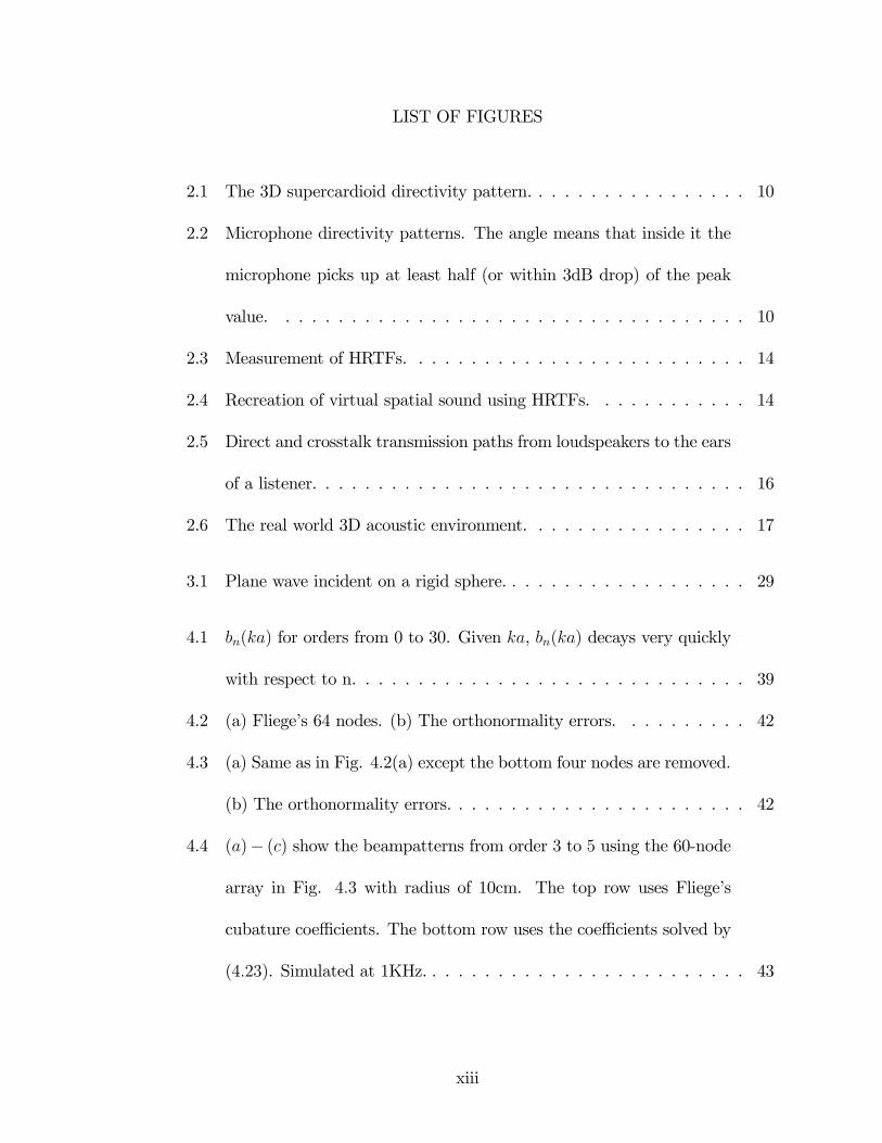
LIST OF FIGURES

2.1 The 3D supercardioid directivity pattern. . . . . . . . . . . . . . . . . 10

2.2 Microphone directivity patterns. The angle means that inside it the

microphone picks up at least half (or within 3dB drop) of the peak

value. . . . . . . . . . . . . . . . . . . . . . . . . . . . . . . . . . . . 10

2.3 Measurement of HRTFs. . . . . . . . . . . . . . . . . . . . . . . . . . 14

2.4 Recreation of virtual spatial sound using HRTFs. . . . . . . . . . . . 14

2.5 Direct and crosstalk transmission paths from loudspeakers to the ears

of a listener. . . . . . . . . . . . . . . . . . . . . . . . . . . . . . . . . 16

2.6 The real world 3D acoustic environment. . . . . . . . . . . . . . . . . 17

3.1 Plane wave incident on a rigid sphere. . . . . . . . . . . . . . . . . . . 29

4.1 bn(ka) for orders from 0 to 30. Given ka, bn(ka) decays very quickly

with respect to n. . . . . . . . . . . . . . . . . . . . . . . . . . . . . . 39

4.2 (a) Fliege’s 64 nodes. (b) The orthonormality errors. . . . . . . . . . 42

4.3 (a) Same as in Fig. 4.2(a) except the bottom four nodes are removed.

(b) The orthonormality errors. . . . . . . . . . . . . . . . . . . . . . . 42

4.4 (a)− (c) show the beampatterns from order 3 to 5 using the 60-node

array in Fig. 4.3 with radius of 10cm. The top row uses Fliege’s

cubature coefficients. The bottom row uses the coefficients solved by

(4.23). Simulated at 1KHz. . . . . . . . . . . . . . . . . . . . . . . . . 43

xiii

4.5 Using the 60-nodes array in Fig. 4.3, the horizontal lines show the

mode bounds for robust beamforming at given ka. . . . . . . . . . . . 50

4.6 The beampatterns of order 3 to 5 for the 60-nodes array in Fig. 4.3

using simplified optimization. . . . . . . . . . . . . . . . . . . . . . . 50

4.7 The random layout of 64 microphones on a sphere of radius 10cm. . . 51

4.8 Unconstrained beampatterns from order 3 to 5 for the array in Fig.

4.7. . . . . . . . . . . . . . . . . . . . . . . . . . . . . . . . . . . . . . 51

4.9 Mode bounds for the array in Fig. 4.7. . . . . . . . . . . . . . . . . . 52

4.10 The geometric interpretation. . . . . . . . . . . . . . . . . . . . . . . 56

4.11 Iteration process for beampattern of order 3. The red (thick) curves

use the left scale, blue (thin) curves right scale. . . . . . . . . . . . . 59

4.12 Constrained optimal beampattern of order 3. . . . . . . . . . . . . . . 59

4.13 Precision comparisions for order 4 beamforming: (a) Comparison of

unconstrained and constrained beampattern coefficients with regular

order 4 beampattern coefficients c4B4. (b) Residue comparison be-

tween unconstrained and constrained beampattern coefficients. Both

plots show the absolute values. . . . . . . . . . . . . . . . . . . . . . 60

4.14 Constrained optimal beampattern of order 4. . . . . . . . . . . . . . . 60

4.15 Constrained optimal beampattern of order 5. It is actually a superdi-

rective beampattern. . . . . . . . . . . . . . . . . . . . . . . . . . . . 61

4.16 The iteration process optimally approximates the DI of the regular

beampattern of order 5. The red (thick) curves use the left scale, blue

(thin) curves right scale. . . . . . . . . . . . . . . . . . . . . . . . . . 61

xiv

4.17 The beampattern of the regular implementation of superdirective

beamformer. . . . . . . . . . . . . . . . . . . . . . . . . . . . . . . . . 62

5.1 A hemispherical microphone array built on the surface of a half bowl-

ing ball. Its radius is 10.925cm. . . . . . . . . . . . . . . . . . . . . . 65

5.2 The hemispherical array with a rigid plane is equivalent to a spherical

array in free space with real and image sources. . . . . . . . . . . . . 66

5.3 The symmetric and uniform layout of 128 nodes on a spherical surface.

The blue (dark) nodes are for real microphones. The yellow (light)

nodes are images. . . . . . . . . . . . . . . . . . . . . . . . . . . . . . 68

5.4 Discrete orthonormality errors. Plot shows absolute values. . . . . . . 69

5.5 Simulation and Experimental results: (a) simulation of 3D scanning

result with two sound sources, the beamformer is of order 8; (b)

experimental result using the calibrated beamfomer of order 8; (c)

simulation result after sound sources are moved; (d) experimental

result using the same calibrated beamformer. . . . . . . . . . . . . . . 72

5.6 (a) The 88-node layout is generated by removing 40 symmetric nodes

in the 128-node layout in Fig. 5.3. (b) The order 7 beampattern

using equal quadrature weights at 2.5KHz. . . . . . . . . . . . . . . . 73

5.7 (a) The simulated source localization result using the array in Fig.

5.6. The beamformer at each direction is made with equal quadrature

weights. (b) The experimental result using equal quadrature weights.

Real sound source is from (π/4,−π/2), at 2.5kHz. . . . . . . . . . . . 74

xv

5.8 The simulated optimal localization result without WNG constraint. . 75

5.9 Localization results using optimal beamformers under different WNG

constraints. Top left: 0dB < WNG < 5dB. Top right: 5dB <

WNG < 10dB. Bottom left: 10dB < WNG < 15dB. Bottom right:

WNG > 20dB. . . . . . . . . . . . . . . . . . . . . . . . . . . . . . . 76

5.10 Moving sound source tracking. Plots show the azimuth and elevation

angles of the energy peak at each frame. The tracking is performed

in the frequency band from 3kHz to 6kHz, with beamformers of order

seven (3kHz~4kHz) and eight (4kHz~6kHz). . . . . . . . . . . . . . . 77

5.11 Sound separation using hemispherical beamformer. The signals in

the right column correspond to segments in the original signals in the

left column. . . . . . . . . . . . . . . . . . . . . . . . . . . . . . . . . 77

5.12 Gain comparision of direct beamforming and fast mixing in time do-

main. Plot shows the absolute value for each beamforming direction.

Simulated in order eight with θk = (π/4, π/4). . . . . . . . . . . . . . 79

6.1 A plane wave incident on a rigid cylinder. . . . . . . . . . . . . . . . 83

6.2 An(ka) for n from 0 to 20. . . . . . . . . . . . . . . . . . . . . . . . . 86

6.3 Bn(ka) for n from 0 to 20. . . . . . . . . . . . . . . . . . . . . . . . . 87

6.4 Beampatterns for M = 1, 5, 10, 16. . . . . . . . . . . . . . . . . . . . . 89

6.5 Spatial aliasing. . . . . . . . . . . . . . . . . . . . . . . . . . . . . . . 90

6.6 White noise gain. . . . . . . . . . . . . . . . . . . . . . . . . . . . . . 91

xvi

6.7 Polar Beampatterns for different elevation angles at 5 kHz. The beam-

pattern for θ = π/2 is of order 13 with WNG ≈ −5.96 dB. . . . . . . 92

6.8 3D beampattern of order 13 at 5 kHz, looking at ϕ = 0. (lighted to

show 3D effect.) . . . . . . . . . . . . . . . . . . . . . . . . . . . . . . 92

7.1 Left: the microphone array captures a 3D sound field remotely. Right:

the loudspeaker array recreates the captured sound field to achieve

the same sound field. . . . . . . . . . . . . . . . . . . . . . . . . . . 96

7.2 System workflow: for each chosen direction θi = (θi, ϕi), we first

beamform the 3D sound field into that direction using our N-order

beamformer, then simply playback the resulted signal from the loud-

speaker in that direction. . . . . . . . . . . . . . . . . . . . . . . . . 97

7.3 The layout of 32 microphones on a rigid sphere with radius of 5 cm.

(The sphere is lighted to show the 3D effect, NOT the sound scattering.)102

7.4 The layout of 32 loudspeakers in free space arranged as a sphere of

large radius. . . . . . . . . . . . . . . . . . . . . . . . . . . . . . . . . 103

7.5 The plane wave of 4 kHz incident from positive direction of X-axis

scattered by the microphone array. Plot shows the pressure on the

equator. . . . . . . . . . . . . . . . . . . . . . . . . . . . . . . . . . . 104

7.6 The recreated plane wave to order 4. Plot shows the 2×2m2 area on

the z = 0 plane. . . . . . . . . . . . . . . . . . . . . . . . . . . . . . . 105

7.7 The rotational symmetry of icosahedron. . . . . . . . . . . . . . . . . 107

7.8 The efficient structure of the multi-directional spherical beamformer. 108

xvii

7.9 HRTF approximations to orders 5 and 10. Plot shows the magnitude

in dB scale. . . . . . . . . . . . . . . . . . . . . . . . . . . . . . . . . 113

7.10 Phases of the approximations to orders 5 and 10. . . . . . . . . . . . 114

7.11 1KHz sound source at 2a, recorded using a=10cm spherical array with

64 Fliege nodes. Plot shows the recreated sound field using 64 virtual

plane waves. . . . . . . . . . . . . . . . . . . . . . . . . . . . . . . . . 117

7.12 Same setup, but using only 60 microphones and 60 virtual plane waves.118

7.13 recorded using spherical array with 324 Fliege’s nodes with a=8cm.

8KHz source from 2a. Plot shows the recreated sound field using 324

virtual plane waves. . . . . . . . . . . . . . . . . . . . . . . . . . . . . 118

7.14 Recreated plane wave of 1KHz, using 64 nodes mic array in free space

with a = 10cm. Recreated by 64 virtual plane waves. . . . . . . . . . 119

7.15 Free space, 8KHz plane wave, recorded using free space 32-nodes mic

array with radius a = 3cm. Recreated by 32 virtual plane waves. . . . 119

8.1 H5,H10 and H16 at frequency 2 kHz. . . . . . . . . . . . . . . . . . . . 124

8.2 H5,H10 and H16 at frequency 5 kHz. . . . . . . . . . . . . . . . . . . . 126

8.3 Reproduce the 5 kHz plane wave to order 5 using plane waves. . . . . 126

8.4 Reproduce the 5 kHz plane wave to order 10 using plane waves. . . . 127

8.5 Reproduce the 5 kHz plane wave to order 16 using plane waves. . . . 127

8.6 Reproduce the 5 kHz plane wave to order 5 using spherical waves. . . 127



xviii


8.10 HRTFs in spatial frequency domain. . . . . . . . . . . . . . . . . . . 134

9.1 The snapshot of our spherical microphone array system. . . . . . . . . 136

9.2 The scenario of the experiment. A car is moving from left to right.

The spherical microphone array is placed on the roadside. . . . . . . . 136

9.3 Tracking one vehicle using the spherical microphone array. . . . . . . 138

9.4 3D localization of the first chosen frame. The car is now on the left

side of the array. . . . . . . . . . . . . . . . . . . . . . . . . . . . . . 139

9.5 The car is now roughly in front of the array. . . . . . . . . . . . . . . 140

9.6 The car now moves to the right side of the array. . . . . . . . . . . . 140

9.7 Tracking two vehicles using the spherical microphone array. . . . . . . 141

xix

Chapter 1Research Motivation and Overview

Our research is originally motivated by the goal to create customizable au-

dio user interfaces (CAUI) for the visually impaired and the sighted although our

contributions will enrich the 3D audio technologies in general. There are approx-

imately 4 million blind or visually impaired people in the US. CAUI aims to help

these people interact with surrounding environment [37][68][96][76].

Our research motivation is best illustrated by a hypothetical application: cre-

ating a CAUI system to train a blind or visually impaired to cross a street or even

drive a vehicle safely. To implement this system, therefore, our research is focused

on the capture and recreation of 3D auditory scenes.

In this chapter, we first briefly review perceptual interfaces, especially auditory

interfaces, then we overview our capture and recreation technologies, respectively.

1.1 Auditory Interfaces

Since the human sight accounts for a large portion of all perceptual informa-

tion, most human-computer interfaces (HCI) and virtual reality (VR) systems are

based on graphics technologies. To extend that, perceptual interfaces aim to achieve

effective human-computer interactions using full human perceptions: visual, tactile

and auditory, etc. In [13], the concept of voice and gesture commanding was intro-

duced to accommodate more natural human-machine interaction. Some examples

include two-handed input [20], direct manipulation and natural language [22], image

1

manipulation using speech and gestures [49], facial expression [87], using ultrasonic

pointer and displaywall [67][66].

We are interested in auditory interfaces in our research. Auditory information

plays an important role in human’s interaction with the world, especially for the

visually impaired people. With the advance in 3D sound recording and playback

technologies, it is possible to build a sound-based VR system [97]. In this section,

we briefly review the advantages, techniques and challenges of auditory interfaces.

The advantages of auditory interfaces haven’t been fully exploited. In sum-

mary, there are three major occasions where auditory interfaces may be desirable:

1. when the information can be conveyed both auditorily and visually, or only

auditorily;

2. when the users want to perform more than one task at a time;

3. when visual displays are not easily available, for safety reasons or for visually

impaired individuals.

The auditory interfaces can be implemented by two general approaches: speech

based and non-speech based. The speech based techniques are relatively well studied

[15]. However, they also have serious limits. Because speech interfaces are basically

to translate information into text and then pronounce it, they are usually slow and

even impossible sometimes. The non-speech based techniques partially solved those

difficulties. They include three main techniques: auditory icons, earcons and sonifi-

cation. Each technique has been successfully applied to certain types of applications.

2

The first technique is auditory icons, which are analogous to graphical icons

[75][44]. The auditory icons use everyday sounds, such as water pouring and door

opening, to represent the operations that users would do with graphic icons. Audi-

tory icons are tightly limited in both the sound dimension and the mapping dimen-

sion. The sounds have to exist in everyday world and the mapping has to convey the

meaning of everyday events. The expected advantage of using auditory icons is a

intuitive mapping between the sounds and their meaning. This advantage, however,

is also its weakness because of the difficulty in more complicated interfaces.

In contrast with auditory icons, earcons take advantage of several dimensions

of sound, such as pitch, timbre, rhythm and spatial location [10]. Typically, earcons

are short musical sounds. More information such as computer object, operation, or

interaction can be efficiently communicated to the user. In addition, earcons can

be combined to represent composite meanings. The effectiveness of an earcon-based

auditory interface largely depends on how well the sounds are designed. However,

the mapping is implicit and much less directly connected with human perceptual

capabilities than that of auditory icons.

Since sound is multidimensional, it has the potential to convey multidimen-

sional data efficiently. Therefore, the task of sonification is the translation from

data dimensions to sound dimensions. Sonification has a wide range of applications

such as the visualization of DNA sequences [12], aid in economic forecasting [72]

and visualization of geographical data [96][95].

The auditory interface research is still in its early stages. One major challenge

is to fully understand and exploit the multidimensional properties of sound such as

3

pitch, timbre, loudness, duration and spatial cues. In our research, we are mostly

interested in spatial cues. Spatial cues have been attracting a great deal of research

effort in psychoacoustics to understand [92][79][5][19][18][17][57][80] and simulate

them [73][8][70][25]. To capture and recreate spatial sound, we develop the theory

and implement practical tools.

1.2 Capture of 3D Auditory Scenes

This is apparently the first step of the implementation if we desire the train-

ing to be as realistic as possible. We wish the captured auditory scene has high

resolutions to provide reliable training materials. That means we must use a mi-

crophone array since an individual microphone cannot capture the sound’s spatial

information.

There are various designs for microphone arrays to capture and analyze sound

fields. Geometrically, most such arrays fall into one of three designs: linear, circular

and spherical. Perhaps the most straightforward design is the linear microphone

array. In [85], general linear sensor arrays for beamforming are elaborated. A more

symmetric and compact configuration is the circular microphone array such as the

one for speech acquisition described in [58]. To capture the 3D sound field, we

prefer a 3D symmetric configuration: the spherical microphone array. Spherical

microphone arrays are recently becoming the subject of some study as they allow

omnidirectional sampling of the sound-field, and may have applications in soundfield

capture. In [3], the sound field was captured using a spherical microphone array in

free space. Microphones can also be positioned on the surface of a rigid sphere to

4

make use of the scattering effect. The paper [71] presented a preliminary analysis

of such arrays, and showed how sound can be analyzed using them. This paper

performed an elegant separation of the analysis and beamforming parts by using

a modal beamformer structure. The beamformer using such configuration has the

same shape of beampattern in all directions.

In practice, however, we have to consider the cable outlet and the mounting

base. In Chapter 4, we propose an extension of this approach that allows flexible

microphone placements with minimal performance compromise.

If the sound sources are bounded within 3D halfspace, we can design a hemi-

spherical microphone array using the acoustic image principle. This will be detailed

in Chapter 5. In this chapter, we also develop a precomputed fast beamforming

algorithm.

In our hypothetical application, the traffic auditory scene is largely two di-

mensional or “surround”, with all sound sources roughly moving on a plane. Other

such examples include cocktail party, roundtable conference, surround music, etc.

So to build a full spherical microphone array seems redundant. Our third problem is

to design and build a microphone array for capturing and spatial filtering of higher

order surround sound field.

The circular microphone arrays should be the obvious choice in this case. In

previous work, the circular microphone array is assumed to be placed in free space

[58]. Although that seems simpler to model, it has some drawbacks in practice,

especially the loss of spatial information with the presence of noise. To overcome

this drawback, we parallel the design of our spherical microphone array and propose

5

a circular microphone array mounted on the surface of a rigid cylinder. We use

this array to record the scattered surround sound field. The spatial filtering, or

beamforming, is based on the orthonormal decomposition of the recorded sound

field by this array. Detailed description is in Chapter 6.

1.3 Recreation of 3D Auditory Scenes

With the captured auditory scene, the next step is to recreate it as exactly

to the original scene as possible so that the trainee believes she is physically there.

There are two general ways: recreation over headphone or loudspeakers. Therefore,

our next problem to develop the theory of recreation from captured scenes.

People have proposed several schemes to build the microphone-loudspeaker

array system. In [9], based on the Kirchhoff-Helmholtz integral on a plane, the sound

field is captured by a directive microphone array, and recreated by a loudspeaker

array. That is called the Wave Field Synthesis (WFS) method. While this system

works well in an auditorium environment where the listening area can be separated

from the primary source area by a plane, it is hard to render an immersive perception

in a 3D sound field. Further, a quantification of the approximations made is not

presented. In [82], a general framework was proposed, which uses a microphone

array beamformer with a localization and tracking system to identify the sound

sources, then uses the loudspeaker array to recreate them with the correct spatial

cues. To work properly, however, it requires a robust and accurate localization and

tracking system and a highly directive beamformer which are usually expensive, if

available.

6

Loudspeaker arrays have similar configurations as microphone arrays to recre-

ate the sound field. In [27][9], a linear loudspeaker array is designed recreate the

sound field on a 2D plane. In [88], a theoretical analysis for using a spherical loud-

speaker array to recreate 3D sound field was provided.

In Chapter 7, we apply this approach to analyze and design our microphone-

loudspeaker integrated system. We explore the reciprocity between capturing and

recreating sound and used it to propose a simple and unified way to capture and

recreate a 3D sound field to higher orders of spherical harmonics. Besides using

loudspeaker arrays which are usually expensive, we also can build a personalized 3D

audio system over headphones with HRTFs. We present this approach in Chapter

7. In addition, we present an alternative interpretation using the discrete Huygens

principle.

In addition, we develop the theory for recreating the recorded 2D auditory

scenes, by both headphone and loudspeaker array. This will be in Chapter 8.

The effectiveness of our algorithms is verified by various design examples and

simulations throughout this dissertation. Our algorithms are further demonstrated

by experimental results using our prototypes as shown in Fig. 5.1 and Fig. 7.39.

7

Chapter 2Introduction to 3D Audio

The goal of 3D audio is to capture and recreate spatial sound field accurately

so that the listener feels she is actually there. It also includes creating virtual 3D

auditory scenes. This chapter gives a tutorial on related 3D audio technologies for

microphones, headphones and loudspeakers, and also discusses the modelling of 3D

virtual audio.

2.1 3D Audio Capture

The device to record sound signal is microphone. In this section, we first

present a brief introduction of microphones with emphasis on the 3D spatial record-

ing properties. Then we review some popular spatial recording technologies using

microphones as individual components. To achieve more flexible spatial recording

and filtering, we need the microphone array. Several geometric designs for different

applications will be introduced here.

2.1.1 Directivity of Microphone

The basic principle of microphone is to convert variations in air pressure into

equivalent electrical variations, in current or voltage. While there are many ways

to convert sound into electrical energy, the two most popular methods are dynamic

and condenser. For more details, please refer to [32]. In our research, we are more

concerned about the directivity (or polar) patterns (in dB scale) of a microphone,

that is, how well it picks up sound from various directions. Most microphones can

8

be placed in one of two main groups: omnidirectional and directional.

Omnidirectional Microphones

Omnidirectional microphones are supposed to pick up sound from every 3D

directions equally. The output should only depend on the relative distance between

the sound source and the microphone. However, even the best omnidirectional

microphones tend to have distorted directivity patterns, especially at higher fre-

quencies. This is caused by many factors. One of them is the physical geometry of

the omnidirectional microphone. When the wave length of sound is comparable or

smaller than the microphone size, the scattering and shadowing effects will distort

the directivity pattern.

Directional Microphones

Directional microphones are specially designed to selectively pick up the sound

from one direction (usually from the front) and suppress the sound incident from

all other directions. Again, the real-world directivity patterns depend on frequen-

cies. This directional ability is usually achieved with external openings and internal

passages in the microphone to allow sound to reach both sides of the diaphragm cor-

responding to the desired directivity pattern. The basic directivity patterns include

cardioid, supercardioid, hypercardioid and bidirectional. A 3D plot of supercardioid

pattern is shown in Fig. 2.1.

A comparison is shown in 2D in Fig. 2.2.

9

Figure 2.1: The 3D supercardioid directivity pattern.

Figure 2.2: Microphone directivity patterns. The angle means that inside it themicrophone picks up at least half (or within 3dB drop) of the peak value.

10

2.1.2 Spatial Recording with Multiple Channels

Probably the simplest recording is monaural recording. It uses a single micro-

phone so the spatial cues are missed. To record at least some spatial cues, however,

multiple recording channels are used.

In two-channel recording, or stereo, there are two widely used methods: co-

incident and spaced microphones. In coincident microphone recording, the spatial

sound is recorded by two directional microphones pointing in different directions

but as close to each other as possible. Therefore, the time difference is expected

to be eliminated while capturing the intensity differences. In spaced microphone

recording, two identical microphones are spaced some distance apart to capture the

time difference. These two stereo recording techniques can be combined together to

capture both the intensity and time differences.

To capture the same complete spatial cues as a pair of human ears do, a natural

method is to place two small microphones in each ear canal of a dummy head, or

even a person, to record an auditory scene. This is called the binaural recording.

To playback, it simply feeds each channel to each ear through headphones.

The surround sound systems extended this goal further using more than two

channels. In quadraphonic system, four microphones are placed at the four corners

of a room, with each channel feeding a loudspeaker. However, this technology only

lasted for a short time, technically because it was inaccurate and non-realistic in

presenting a 3D sound source. To overcome those difficulties, a more advanced sys-

tem, the Ambisonics, was developed to provide a relatively high resolution surround

11

sound. we show this is only a special case of our approach in later chapters.

2.1.3 Spatial Filtering with Microphone Array

In multiple channel recording, although various coding schemes are designed

to accommodate efficient data transmission, they are transparent to the input and

the corresponding output channels. In other words, every channel actually works

independently. To make multiple channels collaborate more efficiently, microphone

arrays arranged in different geometries are designed to perform specific spatial sam-

pling and filtering. For example, microphones arranged along a line samples one

dimensional space, circular microphone array samples two dimensional space, and

a spherical microphone array is for three dimensional space sampling which is ap-

propriate for our research. More details on spherical microphone arrays will be

presented in later chapters.

2.2 3D Audio Recreation

There are two general ways to recreate 3D audio: by headphone and by loud-

speakers.

2.2.1 Recreation of 3D Audio over Headphones

To recreate 3D audio over headphones, we need to understand how humans

can localize sounds using only two ears. Suppose there is a sound source in 3D space

generating a sound wave that propagates to the ears of the listener. When the sound

source is to the left of the listener, the sound reaches the left ear before the right ear

which causes an interaural time difference (ITD). In addition, because of the acoustic

12

scattering by the listener’s torso, head and pinna, the intensity received at the left

ear is different from that at the right ear, which is called the interaural intensity

difference (IID). Therefore, signal received by each ear is the result of a different and

complicated filtering process depending on the direction of the incident sound. The

human auditory system then compares these two channel signals, extracts the spatial

cues and derives the spatial location of the sound source. The exact mechanism is

still not completely known. More detailed information about sound localization by

human listeners can be obtained in [46][11].

A source-filter model is used to describe this process. Specifically, the trans-

formation from the sound signal generated by the source to the signal received by an

ear is a filter called the head-related transfer function (HRTF). HRTFs are usually

measured by inserting miniature microphones into the ear canals of a human subject

or a manikin. A measurement signal is played by a loudspeaker from many different

directions and recorded by the microphones. This process is shown in Fig. 2.3.

By reciprocity, the locations of microphone and speech can be exchanged without

effecting the results. Using a microphone array to record multiple HRTFs at a time,

this approach makes the tedious measurement process significantly faster [98].

Since the spatial cues have been captured by the measurement for the listener,

the recreation of 3D audio is to reproduce the same spatial cues at the ears of the

listener using a pair of measured HRTFs. When a sound is filtered by the HRTFs

and fed into the headphones, the listener will perceive the sound is from the location

specified by the HRTFs. This process is called binaural synthesis (binaural signals

are defined as the signals at the ears of a listener) as shown in Fig. 2.4.

13

HRTFR HRTFL

microphonesreal sound

HRTFR HRTFL

microphones

HRTFR HRTFLHRTFR HRTFLHRTFR HRTFL

microphonesreal sound

Figure 2.3: Measurement of HRTFs.

HRTFR HRTFL

sound

virtual sound headphones

HRTFR HRTFL

sound

virtual sound headphones

Figure 2.4: Recreation of virtual spatial sound using HRTFs.

14

Binaural synthesis works extremely well when the listener’s own HRTFs are

used to synthesize the spatial cues [92][93]. In practice, since HRTFs are not easily

available for every listeners, 3D audio systems typically use a single set of HRTFs

previously measured from a particular human or manikin subject. Some HRTF

databases are KEMAR [2][43] and CIPIC [6]. However, HRTFs depend on the

geometries of the subject’s torso, head and especially pinna, this makes HRTFs

highly individual. Therefore, spatial cues are not always correctly recreated for a

listener if using HRTFs measured from a different individual. Common errors are

front/back confusions and elevation errors [91]. This is the major limit of headphone-

based 3D audio systems.

2.2.2 Recreation of 3D Audio over Loudspeakers

The simplest loudspeaker-based spatial audio system is to use two loudspeak-

ers. In contrast with headphone-based systems, sound from the two loudspeakers

are not separately perceived by the listener’s ears. Instead, both ears receive the

signals from both loudspeakers in direct and crosstalk paths as shown in Fig. 2.5.

To correctly recreate spatial cues, the crosstalk must be eliminated by a care-

fully designed digital filter, often called a crosstalk canceller [41][40]. This filter

cancels the crosstalk at a pre-specified location for the listener, or called sweet spot,

thus separates the two channels. However, when listening, the listener must be

facing forward in the sweet spot to get the best spatial cues. An extension is the

surround sound system which uses more than two channels. As with binaural syn-

thesis, accurate crosstalk canceller is also very individual.

15

crosstalk

direct direct

Figure 2.5: Direct and crosstalk transmission paths from loudspeakers to the earsof a listener.

To solve this problem, one approach is to recreate the 3D sound field around

the listener using loudspeaker arrays as described in section 1.3.

2.3 3D Virtual Audio Modeling

In addition to recreate 3D audio from real recordings, it can also be simulated

virtually. 3D virtual audio aims to create complete 3D auditory scenes, by modelling

3D acoustic environments in real world such as room reverberation and distance cues,

air absorption, object occlusion and diffraction, etc. as shown in Fig. 2.6. One such

system is described in [97].

2.3.1 Room Reverberation and Distance Cues

Room reverberation is caused by the reflection of sound waves. The listener

will hear the sound wave from the source via a direct path if it exists, followed by

reflections off nearby surfaces, or called early reflections, then late reflections in all

directions, or called diffuse reverberation. The reverberation time is defined as the

16

Figure 2.6: The real world 3D acoustic environment.

duration between the initial level and 60 dB decay.

Apparently, the loudness of the sound provides the main distance cue if the

listener knows the normal loudness of that sound. Another important distance

cue is the relative loudness of reverberation since it provides the relative spatial

information about the source location and the environment. A simple example is

that a distant source sounds more reverberant than close ones.

In practice, the geometry of acoustic environment is modelled as a simple room

with reflective surfaces, then the early reflection can be easily computed, such as by

beam tracing [39]. The computation of late reverberation is expensive because of

the large number of reflections in all directions. Some alternative methods include

recursive filters [42], feedback delay networks [54], and fast multipole method (FMM)

[30], etc.

17

2.3.2 Air Absorption

Air absorption also provides spatial cues of the acoustic environment. When

sound wave propagates through air, part of its energy is absorbed along the path.

Air absorption depends on sound frequency and atmospheric conditions such as

temperature and humidity etc. In general the more distant the sound source is, the

more energy will be absorbed. In addition, low frequency sound propagates further

than high frequency sound. The resulting effect is actually a lowpass filter.

2.3.3 Object Occlusion and Diffraction

As shown in Fig. 2.6, the sound path may be bent around occluding objects.

This can be modelled by acoustic scattering theory. If the size of the occluding

object is comparable to the wavelength, scattering is strong; if much smaller, the

object is approximately transparent to the wave; if much bigger, then the wave

will be reflected. Again, the occluding effect can be modelled as a lowpass filter.

However, the computation is expensive and the cost increases dramatically with

more occluding objects. For simple geometric objects like spheres, the scattering

can be computed efficiently using FMM [47].

18

Chapter 3Brief Tutorial on Theoretical Acoustics

In this chapter, we give a brief tutorial on theoretical acoustics. We emphasize

on the basic concepts and results instead of strict derivations. This will provide a

self-contained background for the works in later chapters. More details can be easily

found in any acoustics textbooks, e.g. [74].

3.1 Acoustic Wave Equation

We introduce the wave motion in air, the most important type of wave motion

in acoustics. We first study the motion of plane waves of sound. Plane waves

have the same direction of propagation everywhere in space whose “crests” are in

planes perpendicular to the direction of propagation. The detailed properties of the

acoustic wave motion in a fluid depend on the ratios between the amplitude and

frequency of the acoustic motion and the molecular mean-free-path and the collision

frequency, on whether the fluid is in thermodynamic equilibrium or not, and on the

shape and thermal properties of the boundaries enclosing the fluid. In our work,

we use a simplified, yet practical model of acoustic wave motion in an ideal fluid

which is uniform and continuous, at rest in thermodynamic equilibrium and without

nonlinear effects.

The two basic observations of acoustic waves are:

1. a pressure gradient produces an acceleration of the fluid;

2. a velocity gradient produces a compression of the fluid.

19

In one-dimensional case, they are formulated as:

ρ∂u

∂t= −∂p

∂x, (3.1)

κ∂p

∂t= −∂u

∂x, (3.2)

where u is the velocity flow of fluid in the x-direction, p is the pressure in the fluid,

ρ is the mass per unit volume of the fluid, and κ is the compressibility of the fluid.

Eliminating u, we have:

∂2p

∂x2=1

c2∂2p

∂t2c2 =

1

κρ, (3.3)

which is the one-dimensional wave equation. It is easy to extend this to three-

dimensional case:

∇2p = 1

c2∂2p

∂t2, (3.4)

where ∇2 is the Laplacian operator defined as:

∇2 = ∂2

∂x2+

∂2

∂y2+

∂2

∂z2. (3.5)

It is usually to express p as the velocity potential φ, so the wave equation becomes:

∂2φ

∂t2= c2∇2φ, (3.6)

where c is the acoustic wave speed in air, it is approximately 343m/ s.

3.2 Helmholtz Equation

If we assume the solutions of wave equation are time harmonic standing waves

of frequency ω

φ(r, t) = e−iωtψ(r), (3.7)

20

substitute (3.7) into (3.6), we find ψ(r) satisfies the homogeneous Helmholtz equa-

tion:

(∇2 + k2)ψ(r) = 0, (3.8)

where k = ω/c is the wave number. The solutions of the Helmholtz equation are

the solutions of the wave equation in frequency domain.

If there is a harmonic wave source f(r)e−iωt then we have the inhomogeneous

Helmholtz equation:

(∇2 + k2)ψ(r) = f(r). (3.9)

3.3 Solution Using Green’s Function

Instead of solving ψ(r) in (3.9) directly, we first introduce the Green’s function

G(r1, r2) satisfying:

(∇2 + k2)G(r1, r2) = δ3(r1 − r2), (3.10)

then we can construct the solution for (3.9):

ψ(r) =

ZG(r1, r2)f(r2)dr2. (3.11)

So our problem becomes to solve G(r1, r2) in (3.10).

Because of the spherical symmetry of this problem, the solution is only depen-

dent on r = |r1 − r2|. Using:

∇2G = 1

r2∂

∂r

µr2∂G

∂r

¶=1

r

∂2

∂r2(rG), (3.12)

the problem is then:

1

r

µ∂2

∂r2(rG) + k2(rG)

¶=

δ(r)

4πr2. (3.13)

21

So for r > 0, we have

∂2

∂r2(rG) + k2(rG) = 0, (3.14)

which has a well-known general form solution:

G =A

4πreikr +

B

4πre−ikr. (3.15)

Under the radiation condition, the waves move away from the source. So we must

take B = 0.

G =A

4πreikr, r > 0. (3.16)

We extend this to all values of r by defining G to be the generalized function

G = lim→0

µAH(r − )

4πreikr¶, (3.17)

where

H(x) =

1 x > 0

12

x = 0

0 x < 0

(3.18)

is the Heaviside step function. Then we have:

∇2G = −Ak2eikr

4πr−Aδ(r). (3.19)

So

(∇2 + k2)G = −Aδ(r). (3.20)

Hence, we take A = −1. The solution for G is:

G(r) = − 1

4πreikr = − 1

4π|r1 − r2|eik|r1−r2|. (3.21)

22

Therefore, the solution of the inhomogeneous Helmholtz equation (3.9) satisfying

the outward radiation condition is:

ψ(r1) = − 14π

Zf(r2)

|r1 − r2|eik|r1−r2|dr2. (3.22)

3.4 Solution Using Separation of Variables

While the solution using Green’s function has a compact form of integral,

sometimes, we desire a series solution so that each component can be analyzed

individually.

3.4.1 Separation of Variables in Cylindrical Coordinate System

In cylindrical coordinate system, the Helmholtz equation (3.8) becomes:

1

r

∂

∂r

µr∂ψ

∂r

¶+1

r2∂2ψ

∂ϕ2+

∂2ψ

∂z2+ k2ψ = 0. (3.23)

Let

ψ(r) = R(r)Φ(ϕ)Z(z), (3.24)

(3.23) then becomes three ordinary differential equations:

Z 00 + µZ = 0, (3.25)

Φ00 + n2Φ = 0, (3.26)

r2R00 + rR0 + (k2r2 − n2)R = 0, (3.27)

where µ, n2, k2 are constants decided by boundary conditions. (3.25) and (3.26) can

be solved easily. To solve (3.27), let x = kr and y(x) = R(r), (3.27) then becomes:

x2y00 + xy0 + (x2 − n2)y = 0, (3.28)

which is the nth-order Bessel’s equation. The solution is a series of Bessel functions.

23

3.4.2 Separation of Variables in Spherical Coordinate System

Similarly, in spherical coordinate system, the Helmholtz equation (3.8) be-

comes:

1

r2∂

∂r

µr2∂u

∂r

¶+

1

r2 sin θ

∂

∂θ

µsin θ

∂u

∂θ

¶+

1

r2 sin2 θ

∂2u

∂ϕ2+ λu = 0. (3.29)

Let

u(r, θ, ϕ) = R(r)Θ(θ)Φ(ϕ), (3.30)

we have:

Φ00 +m2Φ = 0, m = 0, 1, 2, ... (3.31)

1

sin θ

d

dθ

µsin θ

dΘ

dθ

¶+

·l(l + 1)− m2

sin2 θ

¸Θ = 0, (3.32)

r2d2R

dr2+ 2r

dR

dr+ [k2r2 − l(l + 1)]R = 0. (3.33)

Let x = cos θ and y(x) = Θ(θ), then (3.32) becomes:

(1− x2)y00 − 2xy0 +·l(l + 1)− m2

1− x2

¸y = 0, (3.34)

which is the associated Legendre differential equation. The solutions are associated

Legendre polynomials. The combined solution ofΘ andΦ is the spherical harmonics.

For (3.33), let x = kr and 1√xy(x) = R(r), it becomes:

x2y00 + xy0 +

"x2 −

µl +

1

2

¶2#y = 0, (3.35)

which is the spherical Bessel equation. The solutions are the spherical Bessel func-

tions.

24

3.5 Special Functions

The following are the special functions we mentioned in the last section. These

functions will be used to generate the solutions to the problems of wave scattering,

from a rigid sphere and a rigid cylinder, which are the cases for our research.

3.5.1 Legendre Polynomials

The Legendre polynomial of order l is defined as:

Pl(x) =1

2ll!

dl

dxl(x2 − 1)l, (3.36)

or as an expansion:

Pl =1

2l

bl/2cXk=0

(−1)k(2l − 2k)!k!(l − k)!(l − 2k)!x

l−2k, (3.37)

where bl/2c is the floor of l/2.

The associated Legendre polynomials are the solutions to the associated Legen-

dre differential equation. They can be derived from Legendre polynomials:

Pml (x) = (−1)m(1− x2)m/2 d

m

dxmPl(x)

=(−1)m2ll!

(1− x2)m/2 dl+m

dxl+m(x2 − 1)l. (3.38)

3.5.2 Spherical Harmonics

The spherical harmonics are defined as:

Y ml (θ, ϕ) =

s2l + 1

4π

(l −m)!

(l +m)!Pml (cos θ)e

imϕ, (3.39)

and they are orthonormal to each other on the spherical surface Ω:ZΩ

Y m∗n (θ, ϕ)Y m0

n0 (θ, ϕ)dΩ = δnn0δmm0 . (3.40)

25

3.5.3 Bessel Functions

The Bessel function of the first kind Jv(x) can be expressed as a series of

gamma functions:

Jv(x) =∞Xk=0

(−1)k(x/2)v+2kk!Γ(v + k + 1)

. (3.41)

The Bessel function of the second kind Nv(x) (or sometimes called Yv(x)) is defined

as:

Nv(x) =Jv(x) cos vπ − J−v(x)

sin vπ, v /∈ Z (3.42)

Nn(x) = limv→n

Nv(x), n = 0, 1, 2, ... (3.43)

The Bessel functions of the third kind, or Hankel functions of the first and second

kinds, are defined as:

H(1)n (x) = Jn(x) + iNn(x), (3.44)

H(2)n (x) = Jn(x)− iNn(x), (3.45)

The spherical Bessel functions of all three kinds are:

jl(x) =

rπ

2xJl+ 1

2(x), (3.46)

nl(x) =

rπ

2xNl+ 1

2(x), (3.47)

h(1)l (x) =

rπ

2xH(1)

l+12

(x), (3.48)

h(2)l (x) =

rπ

2xH(2)

l+12

(x). (3.49)

3.6 Wave Scattering from Rigid Surface

The problem of plane wave scattering from a rigid surface is to find that

solution to the Helmholtz equation which satisfies

26

1. the Neumann boundary condition on the rigid surface,

2. the boundary condition at infinity as when r →∞, the wave is a plane wave,

and

3. the outward radiation condition.

By linearity, the solution has two parts: the incident plane wave and the

scattered wave:

ψ = ψin + ψscat (3.50)

3.6.1 Scattering from a Rigid Cylinder

Suppose the incident plane wave perpendicular to an infinite rigid cylinder of

radius a is:

ψin = eik·r = eikr cosϕ. (3.51)

This plane wave can be expressed in terms of cylindrical waves:

ψin =∞Xn=0

ninJn(kr) cos(nϕ) (3.52)

where Jn(x) is the nth-order Bessel function of x, and n are Neumann symbols

defined as:

n =

1, n = 0;

2, n ≥ 1;. (3.53)

The boundary condition that the solution represent a plane wave plus a scattered

wave, outgoing only, demands that the scattered wave have the form:

ψscat =X

AninHn(kr) cos(nϕ) (3.54)

27

where Hn(x) is the nth-order Hankel function of x which ensures that all the scat-

tered wave is outward. To satisfy the Neumann boundary condition, we must have:

∂ψ

∂r

¯r=a

= 0 (3.55)

which is:∞Xn=0

ninJ 0n(ka) cos(nϕ) +

∞Xn=0

AninH 0

n(ka) cos(nϕ) = 0 (3.56)

So the solution for An is:

An = − nJ 0n(ka)H 0

n(ka)(3.57)

and the scattered wave is:

ψscat = −∞Xn=0

nin J

0n(ka)

H 0n(ka)

Hn(kr) cos(nϕ) (3.58)

The complete solution for the Helmholtz equation under boundary conditions is:

ψ = ψin + ψscat

=∞Xn=0

nin

·Jn(kr)− J 0n(ka)Hn(kr)

H 0n(ka)

¸cos(nϕ) (3.59)

3.6.2 Scattering from a Rigid Sphere

Similarly, we can derive the solution in the rigid sphere case.

As shown in Fig. 3.1, for a unit magnitude plane wave with wavenumber

k incident from direction θk = (θk, ϕk), the incident field at an observation point

rs = (θs, rs) = (θs, ϕs, rs) can be expanded as

ψin (rs,k) = 4π∞Xn=0

injn(krs)nX

m=−nY mn (θk)Y

m∗n (θs), (3.60)

28

X

Y

ZObservation point

Plane wave

rsWavenumber k

a

),( ss ϕϑ),( kk ϕϑ

sϑ

sϕ

Wave direction

Figure 3.1: Plane wave incident on a rigid sphere.

where jn is the spherical Bessel function of order n, Y mn is the spherical harmonics

of order n and degree m. ∗ denotes the complex conjugation. At the same point,

the field scattered by the rigid sphere of radius a is [47]:

ψscat (rs,k) = −4π∞Xn=0

inj0n(ka)

h0n(ka)hn(krs)

nXm=−n

Y mn (θk)Y

m∗n (θs). (3.61)

The total field on the surface (rs = a) of the rigid sphere is:

ψ (θs,θk, ka) = [ψin (rs,k) + ψscat (rs,k)]|rs=a

= 4π∞Xn=0

inbn(ka)nX

m=−nY mn (θk)Y

m∗n (θs), (3.62)

bn(ka) = jn(ka)− j0n(ka)

h0n(ka)hn(ka), (3.63)

where hn are the spherical Hankel functions of the first kind.

29

Chapter 4Flexible and Optimal Design of Spherical Microphone Arrays forBeamforming1

This chapter describes a methodology for designing a flexible and optimal

spherical microphone array for beamforming. Using the approach, a spherical mi-

crophone array can have very flexible layouts of microphones on the spherical sur-

face, yet optimally approximate a desired beampattern of higher orders within a

specified robustness constraint. Depending on the specified beampattern order, our

approach automatically achieves optimal performances in two cases: when the spec-

ified beampattern order is reachable within the robustness constraint, we achieve a

beamformer with optimal approximation of the desired beampattern; otherwise we

achieve a superdirective beamformer, both robustly. For efficient implementation,

we also developed an adaptive algorithm. It converges to the optimal performance

quickly while exactly satisfying the specified frequency response and robustness con-

straint in each adaptive step without accumulated roundoff errors. One direct ad-

vantage is it makes much easier to build a real world system, such as those with cable

outlets and a mounting base, with minimal effects on the performance. Simulation

results are presented in this chapter. In the next chapter, we use a hemispherical

microphone array to verify our algorithms. Experimental results will be presented

in section 5.4.2.1This chapter is based on our original work in [63][61][60][64].

30

4.1 Introduction

Spherical arrays of microphones are recently becoming a subject of interest as

they allow omnidirectional sampling of the soundfield, and may have applications

in soundfield capture [65]. The paper [71] presented a first analysis of such arrays,

and showed how sound can be analyzed using them. This paper performed an ele-

gant separation of the analysis and beamforming parts by using a modal beamformer

structure. One implicit aspect of the analysis is that the distribution of microphones

on the surface of the sphere seems to be redundant considering the results achieved.

This is because the beamforming relies on numerical quadrature of spherical har-

monics. In [71] this is done using a specified regular distribution of points, which

has two issues:

1. For practical arrays, it may not be possible to place microphones precisely

at all the quadrature locations. Moving even one microphone destroys the

quadrature.

2. If higher order beamformers are necessary, quadrature points may be unavail-

able.

We discuss these issues further in the chapter. Here, we propose an extension

of this approach that allows flexible microphone placements. Then we show how the

array can achieve optimal performance.

This chapter is organized into four sections. In section 4.2, we present the

basic principle of beamforming using a spherical microphone array. In section 4.3,

31

we give a theoretical analysis of the discrete system. This part includes a summary

of previous work and an analysis of orthonormality error: how it is introduced into

the system, how it gets amplified and how it affects performance. To cancel the

error noise optimally, we propose an improved solution and compare several design

examples including a practical one. In section 4.4, we formulate our optimization

problem into a finite linear system. We simplify the optimization by using reduced

degrees of freedom (DOFs) for specified beamforming direction. The resulting beam-

former then is checked against the robustness constraint. The upper bound of the

beampattern order is derived theoretically. We again use the example from section

4.3 to demonstrate our simplified optimization. Nevertheless, we also point out its

unrobustness especially for ill-conditioned layouts. This limitation will be solved

in section 4.5 by a controlled trade-off between the accuracy of approximation and

robustness. We formulate it as a constrained optimization problem and develop an

adaptive implementation. We will show our algorithm automatically optimizes in

two different situations: the superdirective beampattern or the desired beampattern

of pre-specified order. Our adaptive implementation inherits the advantages of the

classical ones in [38] and [24].

4.2 Principle of Spherical Beamformer

The basic principle of spherical beamformer is to make use of the orthonor-

mality of spherical harmonics to decompose the soundfield arriving at a spherical

array. The orthogonal components of the soundfield are then linearly combined to

approximate a desired beampattern [71].

32

Using the notations in section 3.6.2 and Fig. 3.1, suppose we capture the

sound field using a spherical microphone array, each microphone at the spherical

surface point θs samples the complex pressure of the total field as:

ψ (θs,θk, ka) = [ψin (rs,k) + ψscat (rs,k)]|rs=a = 4π∞Xn=0

inbn(ka)nX

m=−nY mn (θk)Y

m∗n (θs),

(4.1)

bn(ka) = jn(ka)− j0n(ka)

h0n(ka)hn(ka). (4.2)

Following [71], if we assume that the pressure recorded at each point θs on the

surface of the sphere Ωs, is weighted by

Wm0n0 (θs, ka) =

Y m0n0 (θs)

4πin0bn0(ka), (4.3)

applying the orthonormality of spherical harmonics

ZΩs

Y m∗n (θs)Y

m0n0 (θs)dΩs = δnn0δmm0 , (4.4)

the total output from a pressure-sensitive spherical surface is

ZΩs

ψ (θs,θk, ka)Wm0n0 (θs, ka)dΩs = Y m0

n0 (θk). (4.5)

This shows the response of the plane wave incident from θk, for a continuous

pressure-sensitive spherical microphone, is Y m0n0 (θk). Since any square-integrable

function F (θ) can be expanded in terms of complex spherical harmonics, we can

implement arbitrary beampatterns. For example, an ideal beampattern looking at

the direction θ0 can be modeled as a delta function

F (θ,θ0) = δ(θ − θ0), (4.6)

33

which can be expanded into an infinite series of spherical harmonics [4]:

F (θ,θ0) = 2π∞Xn=0

nXm=−n

Y m∗n (θ0)Y

mn (θ). (4.7)

So the weight at each point θs to achieve this beampattern is

w(θ0,θs, ka) =∞Xn=0

1

2inbn(ka)

nXm=−n

Y m∗n (θ0)Y

mn (θs). (4.8)

The advantage of this system is that it can be steered into any 3D direction digitally

with the same beampattern. This is for an ideal continuous microphone array on a

spherical surface. Further, to achieve this we need infinite summations.

4.3 Discrete Spherical Array Analysis

This section also follows [71], but we make the band limit restrictions ex-

plicit. For a real-world system, however, we have a discretely sampled array with S

microphones mounted at (θs), s = 1, 2, ..., S. To adapt the spherical beamforming

principle to the discrete case, the continuous integrals are approximated by weighted

summations, or quadratures2 [84, p. 71]:

4π

S

SXs=1

Y m∗n (θs)Y

m0n0 (θs)C

m0n0 (θs) = δnn0δmm0 , (4.9)

(n = 0, ..., Neff ;m = −n, ..., n;

n0 = 0, ..., N ;m0 = −n0, ..., n0),

where Cm0n0 (θs) is the quadrature coefficient for Y

m0n0 at θs. Neff is the maximum

order with significant strength, i.e. the band limit of spatial frequency in terms of

2While cubature is sometimes used for representing nodes and weights in 2D, we prefer to usethe word quadrature, which is in any case used for still higher dimensions.

34

spherical harmonics orders. N is the order of beamformer. (4.9) can be solved in

the least squares sense to minimize the 2-norm of the residues for (4.9).

Therefore, to approximate a regular beampattern of order N , which is ban-

dlimited in the sense that it has no components of order greater than N ,

FN(θ,θ0) = 2πNXn=0

nXm=−n

Y m∗n (θ0)Y

mn (θ), (4.10)

the weights for the beamformer are:

wN(θ0,θs, ka) =NXn=0

1

2inbn(ka)

nXm=−n

Y m∗n (θ0)Y

mn (θs)C

mn (θs). (4.11)

To evaluate the robustness of a beamformer, we use the white noise gain

(WNG) [16], usually in dB scale:

WNG(θ0,θs, ka) = 10 log10

Ã|dW|2WHW

!, (4.12)

where d is the row vector of complex pressure at each microphone position produced

by the plane wave of unit magnitude from the desired beamforming direction θ0 and

W is the column vector of complex weights for each microphone. WNG defines the

sensitivity on the white noise including the environmental noise, the device noise

and implicitly, the microphone position mismatches among other perturbations.

Positive WNG means an attenuation of white noise, whereas negative means an

amplification.

To evaluate the directivity of a beampattern, we use the directivity index (DI)

[16], also in dB:

DI(θ0,θs, ka) = 10 log10

Ã4π |H(θ0)|2RΩs|H(θ)|2 dΩs

!, (4.13)

35

where H(θ) is the actual beampattern and H(θ0) is the component in the desired

look direction. For regular beampattern of order N , the DI is 20 log10(N + 1). DI

represents the ability of the array to suppress a diffuse noise field. It is the ratio of

the gain for the look direction θ0 to the average gain over all directions.

4.3.1 Previous Work

The previous work can be summarized according to the choices made for

Cmn (θs) and optimization.

In [71], Cmn (θs) are intuitively chosen to be unit to provide relative accuracy

for some “uniform” layouts such as the 32 nodes defined by a truncated icosahedron.

This straightforward choice simplifies the computation, however, it is not for “non-

uniform” layouts and it doesn’t leave any other DOF for optimization subject to

the WNG constraint except the beampattern order N . In addition, we will see that

even small errors can destroy the beampattern. In [3], several options are mentioned

including equiangular grid layout [50] and an intuitive equidistance layout [36]. The

common limitation of those schemes is that they are inflexible. If a patch of the

spherical surface is inappropriate for mounting microphones, the orthonormality

error may be large, thereby destroying the beampattern as the quadrature relation

will not hold.

The approach in [52, Chapter 3] is equivalent to choosing Cmn (θs) to be in-

dependent of θs. The remaining (N + 1)2 DOFs are not used to satisfy (4.9) but

maximize the directivity within WNG constraint. The optimization is performed

by using an undetermined Lagrangian multiplier. Since there is no simple relation

36

between the multiplier and the resulting WNG, the implementation uses a straight-

forward trial-and-error strategy.

4.3.2 Orthonormality Error Noise Analysis

Unfortunately, (4.9) can’t be satisfied exactly for over-determined or rank-

deficient system in general, which is usually the case. In addition, the number of

equations in (4.9) for each pair of n0 and m0 depends on Neff . Then for any choice

of Cm0n0 (θs), we always have:

4π

S

SXs=1

Y m∗n (θs)Y

m0n0 (θs)C

m0n0 (θs) = δnn0δmm0 + mm0

nn0 , (4.14)

where mm0nn0 is usually the non-zero error caused by discreteness.

Now, we see how this error could degrade the performance of soundfield decom-

position. To extract the component of order n0 and degree m0 from the soundfield

(3.62), we consider the quadratures of (4.5) for ψmn (θs,θk, ka), denoting one com-

ponent of ψ at order n and degree m:

Pmn (θk, ka) =

ZΩs

ψmn (θs,θk, ka)

Y m0n0 (θs)C

m0n0 (θs)

4πin0bn0(ka)dΩs (4.15)

where:

ψmn (θs,θk, ka) = 4πi

nbn(ka)Ymn (θk)Y

m∗n (θs). (4.16)

Using S discrete points, we have:

Pmn (θk, ka) = Y m

n (θk)

·inbn (ka)

in0bn0 (ka)

¸(δnn0δmm0 + mm0

nn0 ). (4.17)

We notice that: ·inbn (ka)

in0bn0 (ka)

¸δnn0δmm0 = δnn0δmm0 (4.18)

37

So, (4.17) can be rewritten as:

Pmn (θk, ka) = Y m

n (θk)δnn0δmm0 +

·inbn(ka)

in0bn0(ka)

¸mm0nn0 (4.19)

The second term is the noise caused by scaled orthonormality error mm0nn0 . We call

it the orthonormality error noise (OEN) which is possible with any discrete mi-

crophone array layout. To prevent it from damaging the orthonormality, we must

have: ¯inbn(ka)

in0bn0(ka)mm0nn0

¯¿ 1 (4.20)

So, we get:

| mm0nn0 | ¿

¯bn0(ka)

bn(ka)

¯, ∀n, n0,m,m0 (4.21)

Since bn decays very quickly with respect to n as shown in Fig.4.1, for a given

microphone number and layout, we cannot decompose the high order component of

soundfield if (4.21) fails. In addition, we can see (4.21) is independent of magnitude

of the incoming sound wave. That means: even if the microphones have recorded

the high order components, the system may be unable to decompose them.

To prevent errors from being amplified, we include the frequency-dependent

scale factor

Bnn0(ka) =

bn(ka)

bn0(ka)(4.22)

into (4.9). The linear system for quadrature coefficients then becomes a weighted

38

10-1 100 101-40

-35

-30

-25

-20

-15

-10

-5

0

ka

bn [dB]

b0

b1

b2

b3

b4

b5

b6

Figure 4.1: bn(ka) for orders from 0 to 30. Given ka, bn(ka) decays very quicklywith respect to n.

least squares problem:

minCm0n0 (θs,ka)

°°°°°4πSSXs=1

Y m∗n (θs)Y

m0n0 (θs)C

m0n0 (θs, ka)B

nn0(ka)− δnn0δmm0

°°°°°2

2

, (4.23)

(n = 0, ..., Neff ;m = −n, ..., n;

n0 = 0, ..., N ;m0 = −n0, ..., n0).

The discrete orthonormalities in (4.23) weighted with smaller |Bnn0(ka)| are less im-

portant than those with larger |Bnn0(ka)|. Since Bn

n0(ka) converges to zero when n

increases for given n0, compared with (4.9), (4.23) suppresses the orthonormalities

in higher orders and adds more accuracy to the lower orders. In addition, since

Bnn0(ka) converges to zero rapidly with respect to n, this weighting also significantly

lessens the sensitivity of the solutions on the choice of Neff only if¯bNeff

(ka)¯is

small enough compared with |bN(ka)|, e.g. for ka = 1.83, Neff = N + 3 will make

39

¯bNeff

(ka)¯at least 40dB below |bN(ka)| for N = 3, 4, 5.

4.3.3 Design Examples

A quadrature formula provides locations at which we evaluate the function

and weights to multiply and sum up to obtain the integral. It was proven that

any quadrature formula of order N over the sphere should have more than S =

(N +1)2 quadrature nodes [81][48]. If the quadrature functions have the bandwidth

upto order N , to achieve the exact quadrature using equiangular layout, we need

S = 4(N + 1)2 nodes [28]. This is too large and redundant for our application.

For special layouts, S can be made much smaller. For example, for a spherical grid

which is a Cartesian product of equispaced grid in ϕ and the grid in θ in which the

nodes distributed as zeros of the Legendre polynomial of degree N +1 with respect

to cos θ we need S = 2(N + 1)2 [77]. Another special design with equal quadrature

coefficients is called the spherical t-design [48]. While these designs achieve exact

quadratures, however, they are for strictly band-limited functions and S is still

large considering our quadrature function is the multiplication of two band-limited

functions. This means that to achieve a beampattern of order five we need at least

144 microphones.

If we use approximate quadrature formula, then it may be possible to reduce

S. Intuitively, we want the microphones distributed "uniformly" on the spherical

surface. Unfortunately, it has been proven that only five regular polyhedrons (or

called "Platonic solids") exist: tetrahedron, cube, dodecahedron, icosahedron and

octahedron [34]. Semi-regular polyhedrons can be used also such as the truncated

40

icosahedron used in [71] to layout 32 microphones. The general problem to distrib-

ute arbitrary number of points approximately “uniformly” on a spherical surface is

numerically solved by Fliege in [36] by minimizing the potential energy of a distrib-

ution of movable electrons on a perfect conducting sphere. Then, one set of optimal

quadrature coefficients are solved.

Fig. 4.2(a) shows Fliege’s 64-node layout in [36]. Fig. 4.2(b) shows the er-

rors of orthogonal conditions of spherical harmonics using those optimal quadrature

coefficient for each nodes. However, those optimal quadrature coefficients are not

generally available for other flexible layouts. More importantly, for a given layout,

especially for a “non-uniform” one, we will explain in the next section that there is

no such a single optimal set of coefficients to satisfy all orthogonal conditions.

For example, Fig. 4.3(a) is the layout of our array using the angular positions of

those 64 nodes with four nodes at the bottom removed because of the cable outlet.

Fig. 4.3(b) shows the orthonormality errors using the 60 nodes and quadrature

coefficients. It is less accurate compared with Fig. 4.2(b). The top row in Fig.

4.4 shows the beampatterns from order three to five using this configuration. At

order three, the beampattern is distorted. At order four, the orthonormality errors

significantly damage the beampattern. At order five, the beampattern is almost

completely destroyed. The bottom row in Fig. 4.4 shows the beampatterns using

the quadrature coefficients solved by (4.23), which optimally approximate the regular

beampatterns.

41

(a) (b)

Figure 4.2: (a) Fliege’s 64 nodes. (b) The orthonormality errors.

(a) (b)

Figure 4.3: (a) Same as in Fig. 4.2(a) except the bottom four nodes are removed.(b) The orthonormality errors.

42

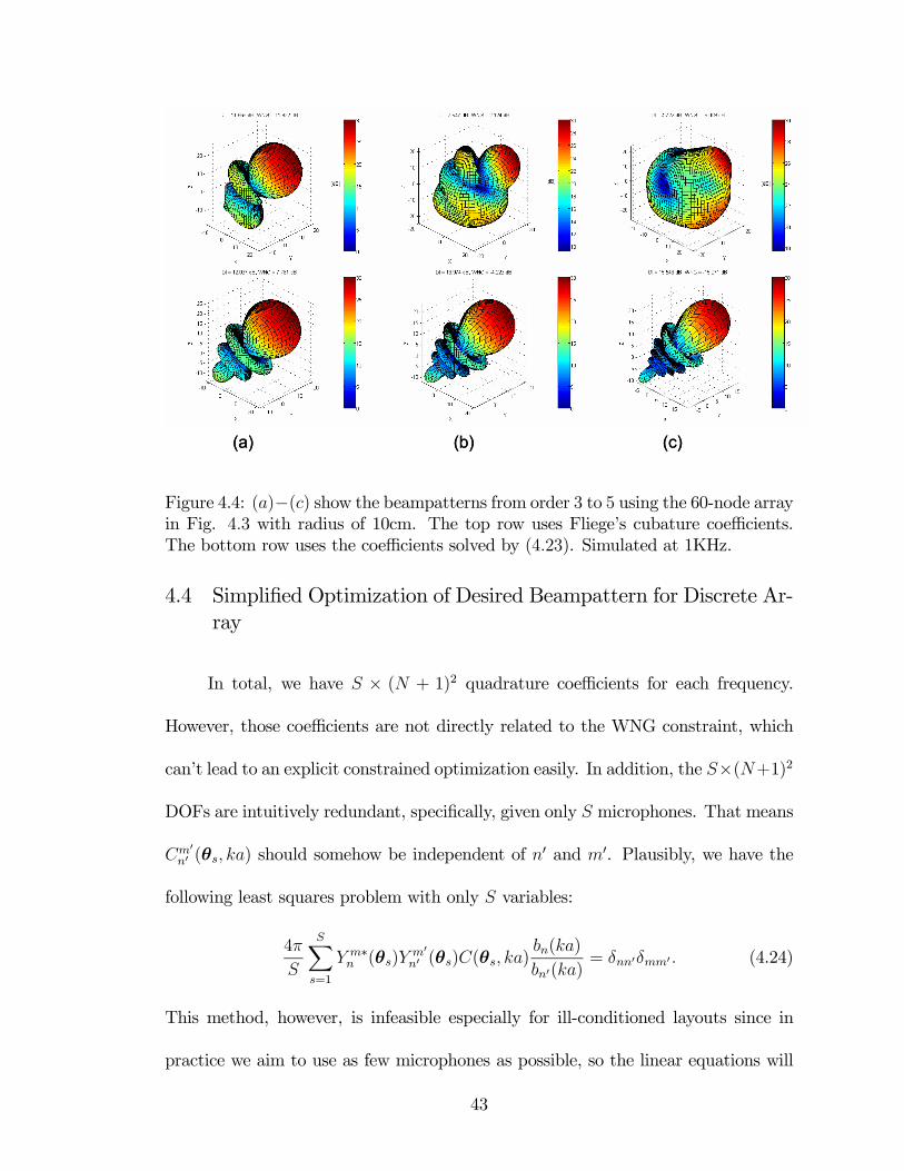
(a) (b) (c)(a) (b) (c)

Figure 4.4: (a)−(c) show the beampatterns from order 3 to 5 using the 60-node arrayin Fig. 4.3 with radius of 10cm. The top row uses Fliege’s cubature coefficients.The bottom row uses the coefficients solved by (4.23). Simulated at 1KHz.

4.4 Simplified Optimization of Desired Beampattern for Discrete Ar-ray

In total, we have S × (N + 1)2 quadrature coefficients for each frequency.

However, those coefficients are not directly related to the WNG constraint, which

can’t lead to an explicit constrained optimization easily. In addition, the S×(N+1)2

DOFs are intuitively redundant, specifically, given only S microphones. That means

Cm0n0 (θs, ka) should somehow be independent of n

0 and m0. Plausibly, we have the

following least squares problem with only S variables:

4π

S

SXs=1

Y m∗n (θs)Y

m0n0 (θs)C(θs, ka)

bn(ka)

bn0(ka)= δnn0δmm0 . (4.24)

This method, however, is infeasible especially for ill-conditioned layouts since in

practice we aim to use as few microphones as possible, so the linear equations will

43

largely outnumber the microphones which makes the optimization less meaningful.

Instead of satisfying (4.24), we can use C(θs, ka) to maximize the directivity sub-

ject to the WNG constraint, which simply returns to a classical solved problem of

designing a superdirective and robust beamformer [24]. This method doesn’t aim to

optimally approximate a desired beampattern of a specified order N . It invalidates

the main advantage of using a spherical microphone array, i.e. the same beampat-

tern in all steering directions. An example using this feature is the system described

in [65].

An alternative explanation is: because the optimization on (4.24) is indepen-

dent on the beamforming direction, it is too ambitious to find such a single set of

optimal weights for every beamforming directions. This, in turn, also implies that

the optimization using S DOFs should be performed for each beamforming direction.

In this section, we follow this approach and develop algorithms to find the optimal

weights for regular beampatterns. We will first formulate the discrete spherical

beamformer into a linear system. The optimal solution of this linear system subject

to the WNG constraint will be the optimal approximation of the desired beampat-

tern. Then we present straightforward solutions. Design examples are provided to

demonstrate our approach.

44

4.4.1 Discrete Spherical Beamformer as Finite Linear System

To achieve a regular beampattern of order N (4.10), a discrete spherical beam-

former with S microphones can be formulated as a finite linear system:

AW = cNBN , (4.25)

dW = 1, (4.26)

where (4.25) defines the beampattern, and (4.26) the frequency response to the sound

from the beamforming direction. Without loss of generality, here we consider an all-

pass filter. In (4.25), A are the coefficients of the spherical harmonics expansion of

the soundfield in (3.62):

A = [ A1 A2 · · · AS], (4.27)

As = 4π

i0b0(ka)Y0∗0 (θs)

i1b1(ka)Y−1∗1 (θs)

...

iNbN(ka)YN∗N (θs)

i(N+1)b(N+1)(ka)Y−(N+1)∗(N+1) (θs)

...

iNeff bNeff(ka)Y

Neff∗Neff

(θs)

, (4.28)

(s = 1, ..., S.)

45

W is the vector of complex weights to be assigned to each microphone at (θs, a):

W =

W (θ0,θ1, ka)

W (θ0,θ2, ka)

...

W (θ0,θS, ka)

. (4.29)

BN is the vector of coefficients of the beampattern of order N steered to (θ0) in

(4.10):

BN = 2π

Y 0∗0 (θ0)

Y −1∗1 (θ0)

...

Y N∗N (θ0)

0

...

0

. (4.30)

In (4.26), d is the row vector of the complex pressure at each microphone position

produced by a plane wave of unit magnitude from the desired beamforming direction

θ0:

d =

d1

d2

...

dS

T

=

ψ(θ1,θ0, ka)

ψ(θ2,θ0, ka)

...

ψ(θS,θ0, ka)

T

. (4.31)

46

In (4.25), cN is a normalizing coefficient to satisfy the all-pass frequency response

(4.26). The least squares solution of (4.25) is

W =£(AHA)−1AH

¤cNBN . (4.32)

Then cN can be determined using (4.26). If we assume (4.25) has small residues,

from (4.10), the a priori estimate of cN is

cN ≈ 1

2πPN

n=0

Pnm=−n Y m

n (θ0)Ym∗n (θ0)

. (4.33)

According to the spherical harmonic addition theorem, cN is independent of (θ0)

and (4.33) can be simplified easily

cN ≈ 1PNn=0

2n+12

Pn(cos 0)=

2

(N + 1)2. (4.34)

We will use it to predict the maximum order in the next subsection.

Note that because we have absorbed all frequency dependence (ka) into the

linear system, this must be solved for each frequency.

4.4.2 Maximum Beampattern Order for Robust Beamformer

A robust beamformer requires a minimumWNG of δ2 (such as −6 dB in [16]):

|dW|2WHW

≥ δ2. (4.35)

Substituting (4.26) into (4.35), we have a spherical constraint onW:

WHW ≤ δ−2. (4.36)

Assume the maximum order we can possibly decompose robustly is Nmax, then

the linear system (4.25) becomes:

AW = cNmaxBNmax , (4.37)

47

where

cNmax ≈2

(Nmax + 1)2. (4.38)

Suppose we have a least squares solution of W to (4.37), considering the

following equations of order Nmax:

4π

iNmaxbNmax(ka)YM∗Nmax

(θ1)

iNmaxbNmax(ka)YM∗Nmax(θ2)

...

iNmaxbNmax(ka)YM∗Nmax

(θS)

T

W (θ0,θ1, ka)

W (θ0,θ2, ka)

...

W (θ0,θS, ka)

≈ 2πcNmaxY M∗

Nmax(θ0), (4.39)

(M = −Nmax, ..., Nmax)

Using Cauchy’s Inequality, we have:¯¯

SXs=1

iNmaxbNmax(ka)YM∗Nmax(θs)W (θ0,θs, ka)

¯¯2

≤Ã

SXs=1

¯iNmaxbNmax(ka)Y

M∗Nmax(θs)

¯ |W (θ0,θs, ka)|!2

≤SXs=1

¯iNmaxbNmax(ka)Y

M∗Nmax(θs)

¯2 SXs=1

|W (θ0,θs, ka)|2

= |bNmax(ka)|2SXs=1

¯Y M∗Nmax(θs)

¯2 SXs=1

|W (θ0,θs, ka)|2

So:

WHW =SXs=1

|W (θ0,θs, ka)|2

&¯cNmaxY

M∗Nmax(θ0)

¯22 |bNmax(ka)|2

PSs=1

¯Y M∗Nmax

(θs)¯2 . (4.40)

48

From (4.36), we have:

δ−2 &¯cNmaxY

M∗Nmax

(θ0)¯2

2 |bNmax(ka)|2PS

s=1

¯Y M∗Nmax

(θs)¯2 , (4.41)

which is:

|bNmax(ka)| &√2¯Y MNmax(θ0)

¯δ

(Nmax + 1)2qPS

s=1

¯Y MNmax

(θs)¯2 , for all M = −Nmax, ..., Nmax.

(4.42)

Therefore, given a spherical microphone array and the beamforming direction, for

each frequency, we know the upper bound order Nmax of a robust beamformer.


We still use the 60-nodes layout at 1 kHz as an example. We set δ = 10−0.3, i.e.

the minimum WNG is −6dB. Fig. 4.5 shows the bounds for θ0 = (π/4, π/4), where

the red (dashed) lines show the bounds. For example, the black (dash-dot) line

shows 1kHz (ka = 1.8318) in our case. Since the intersection of the black line and

the n = 4 mode is above the n = 4 bound, while its intersection with n = 5 mode

is below the n = 5 bound, we predict the maximum order of a robust beamformer

is four. Fig. 4.6 shows resulted beampatterns of order from three to five using the

simplified optimization. The WNG of order 5 beamformer falls below the minimum

of −6dB as predicted. These results are almost identical to the bottom row in Fig.

4.4.

As a general example, Fig. 4.7 shows a random layout of 64 nodes. Fig. 4.8

shows the beampatterns from order three to five at 1kHz. Their WNGs are all

below -6dB. It seems to be contradictory to the bounds shown in Fig. 4.9, however,

49

10-1 100 101-60

-50

-40

-30

-20

-10

0n=0

n=0

n=1

n=1

n=2

n=2

n=3

n=3

n=4

n=4

n=5

n=5

n=6

n=6

ka=1.8318ka

bn [d

B]

Figure 4.5: Using the 60-nodes array in Fig. 4.3, the horizontal lines show the modebounds for robust beamforming at given ka.

Figure 4.6: The beampatterns of order 3 to 5 for the 60-nodes array in Fig. 4.3using simplified optimization.

50

Figure 4.7: The random layout of 64 microphones on a sphere of radius 10cm.

Figure 4.8: Unconstrained beampatterns from order 3 to 5 for the array in Fig. 4.7.

we will show in the next section that the robust beamformers up to order four are

still achievable, with constrained relaxation on the least squares solution (4.32).

4.5 Optimal Approximation Subject to the WNG Constraint

In the previous section, we minimize the residue of a finite linear system and

check the resulted beamformer against the WNG constraint. In this section, we

extend the algorithm further to address the following two aspects:

51

10-1 100 101-60

-50

-40

-30

-20

-10

0 n=0

n=0

n=1

n=1

n=2

n=2

n=3

n=3

n=4

n=4

n=5

n=5

n=6

n=6

ka=1.8318

ka

bn [d

B]

Figure 4.9: Mode bounds for the array in Fig. 4.7.

1. we need to relax the approximations to stay within the constraint such as in

Fig. 4.7.

2. we need a robust and superdirective beamformer with maximum directivity

index.

The two problems are closely related to each other and can be formulated as

a unified constrained optimization.

4.5.1 Constrained Optimization

To design a robust spherical beamformer with finite microphones, yet optimally

approximate the desired beampattern to certain order (e.g. the ideal beampattern

in our case), we need to optimize the following 2-norm function:

minWkAW− cNBNk22 (4.43)

52

subject to:

dW = 1, (4.44)

WHW ≤ δ−2. (4.45)

This optimization can be numerically solved by some blackbox software packages,

such as MATLAB function fmincon, etc. Another way is to use Tikhonov regular-

ization. Specifically, we place a 2-norm constraint onW by appending a damping

matrix with the regularization parameter λ: A

λI

W =

cNBN

0

, (4.46)

The solution is:

W =£(AHA+ λ2I)−1AH

¤cNBN .

This regularization parameter λ, however, is not directly related to the WNG con-

straint. A trial-and-error strategy can be used in implementation.

4.5.2 Adaptive Implementation

The most straightforward way to implement this system is to precompute all

the weights for each pre-defined 3D direction and store them in a lookup table. This

method, however, is not very efficient because of the obvious trade-off between the

spatial resolution and the cost of storage. In this subsection, we reformulate our

problem so that we can parallel the method in [24] to design an adaptive implemen-

tation which automatically and robustly converges to the desired beamformer of a

specified order in any steering directions.

53

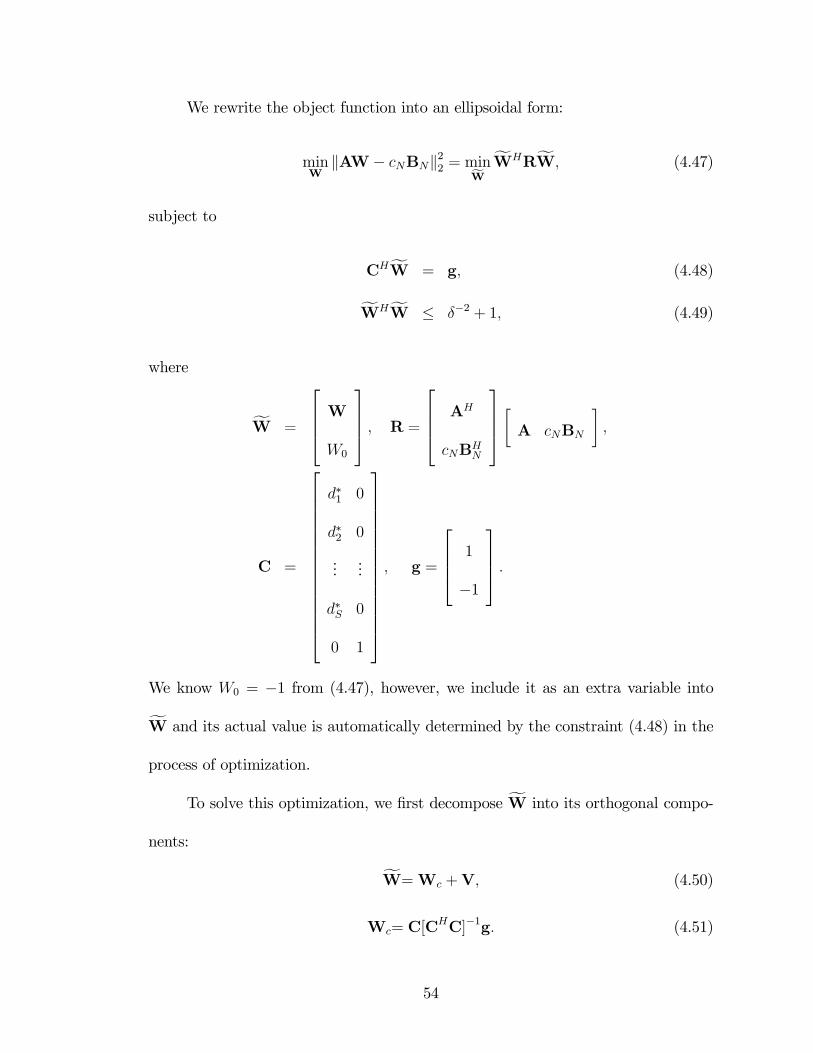
We rewrite the object function into an ellipsoidal form:

minWkAW− cNBNk22 = minfW fWHRfW, (4.47)

subject to

CHfW = g, (4.48)

fWHfW ≤ δ−2 + 1, (4.49)

where

fW =

W

W0

, R =

AH

cNBHN

· A cNBN

¸,

C =

d∗1 0

d∗2 0

......

d∗S 0

0 1

, g =

1

−1

.

We know W0 = −1 from (4.47), however, we include it as an extra variable into

fW and its actual value is automatically determined by the constraint (4.48) in the

process of optimization.

To solve this optimization, we first decompose fW into its orthogonal compo-

nents:

fW=Wc +V, (4.50)

Wc= C[CHC]−1g. (4.51)

54

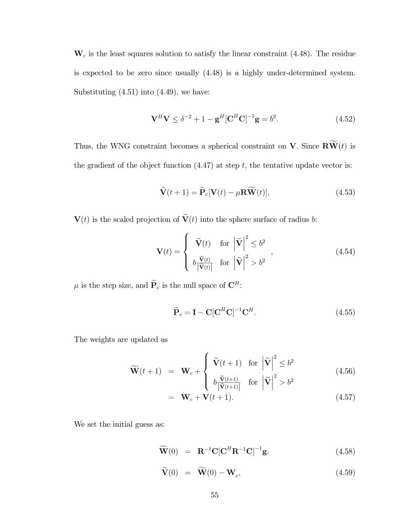
Wc is the least squares solution to satisfy the linear constraint (4.48). The residue

is expected to be zero since usually (4.48) is a highly under-determined system.

Substituting (4.51) into (4.49), we have:

VHV ≤ δ−2 + 1− gH [CHC]−1g = b2. (4.52)

Thus, the WNG constraint becomes a spherical constraint on V. Since RfW(t) is

the gradient of the object function (4.47) at step t, the tentative update vector is:

eV(t+ 1) = ePc[V(t)− µRfW(t)], (4.53)

V(t) is the scaled projection of eV(t) into the sphere surface of radius b:V(t) =

eV(t) for

¯ eV¯2 ≤ b2

beV(t)|eV(t)| for

¯ eV¯2 > b2, (4.54)

µ is the step size, and ePc is the null space of CH :

ePc = I−C[CHC]−1CH . (4.55)

The weights are updated as

fW(t+ 1) = Wc +

eV(t+ 1) for

¯ eV¯2 ≤ b2

beV(t+1)|eV(t+1)| for

¯ eV¯2 > b2(4.56)

= Wc +V(t+ 1). (4.57)

We set the initial guess as:

fW(0) = R−1C[CHR−1C]−1g, (4.58)

eV(0) = fW(0)−Wc, (4.59)

55

constraint

Object function

unconstrainedoptimal solution

constrainedoptimal solution

Initial guess

Iteration path

constraint

Object function

unconstrainedoptimal solution

constrainedoptimal solution

Initial guess

Iteration path

Figure 4.10: The geometric interpretation.

which is equivalent to the solution we get in section 4.4. If the resulting WNG is

within constraint, the iteration will stay with this solution, otherwise, it will start the

constrained optimization process, both automatically. At each step, the constraints

(4.48) and (4.49) are satisfied exactly. In addition, similar to the methods in [24]

and [38], round-off errors don’t accumulate. This iteration is independent of the

actual signal processing rate, so it may be implemented more efficiently as a parallel

unit with other processors.

The geometric interpretation of this constrained optimization is shown in Fig.

4.10.

56

4.5.3 Convergence and Optimal Step Size

From (4.53) and (4.56), we have

eV(t+ 1) = ePc [V(t)− µR [Wc +V(t)]]

= ePc [I−µR]V(t)− µePcRWc. (4.60)

Let

eV(t+ 1) = γ(t+ 1)V(t+ 1), (4.61)

γ(t+ 1) =

1 for

¯ eV¯2 ≤ b2

|eV(t+1)|b

for¯ eV¯2 > b2

≥ 1, (4.62)

we then have:

V(t+ 1) =1

γ(t+ 1)ePc [I−µR]V(t)− 1

γ(t+ 1)µePcRWc

=ePc [I−µR]t+1Qt

i=0 γ(i+ 1)V(0)−

"tX

k=0

ePkc [I−µR]kQki=0 γ(i+ 1)

#µePcRWc. (4.63)

To guarantee convergence, we need

0 < µ <2

σmax, (4.64)

where σmax is the maximum eigenvalue of R.

Although it is difficult to precisely model and control γ if possible, it won’t

cause divergence from (4.62) and will be very close to one in practice. Thus the

optimal step size µopt can be roughly estimated as the least squares solution of

µoptσ = 1, (4.65)

which is

µopt =£(σTσ)−1σT

¤1, (4.66)

57

where σ is the column vector of eigenvalues of R, and 1T , [1, ..., 1] is the vector of

ones with the length of σ.

4.5.4 Simulation Results

We use our algorithm to solve the two cases we mentioned at the beginning of

this section.

We go back to the example in Fig. 4.7 and Fig. 4.8. We first simulate the

beamformer of order three. Fig. 4.11 shows the iteration process using the optimal

step size. As can be seen from this figure, the optimization goal is not to maximize

the DI, instead it converges to the regular beampattern of order three. The resulted

beampattern is shown in Fig. 4.12. Fig. 4.14 shows the optimal approximations

of the regular beampattern of order four subject to the WNG constraint. There is

minimal difference between the beampatterns in Fig. 4.14 and Fig. 4.7(b). The

comparisons of residues are shown in Fig. 4.13.

If we desire optimal directivity, we can approximate the ideal beampattern as

(4.7). In practice, we just need to approximate an order above the theoretical upper

bound derived in (4.42), such as order 5 in this case. It is best to demonstrate this

via simulations. Fig. 4.16 clearly shows the actual DI is approaching the regular DI

of order five. Fig. 4.15 shows the resulted beampattern. Fig. 4.17 shows the regular

implementation of superdirective beamformer, which results in the nearly identical

beampattern as Fig. 4.15. These simulations also demonstrates our algorithm can

robustly reconfigure itself after microphone reorganization.

58

100 101 102 103-0.05

0

0.05

0.1

0.15

0.2

0.25

0.3

0.35

Obj

ect F

unci

ton

unconstrainedconstrained

100 101 102 103

10.8

11

11.2

11.4

11.6

11.8

12

12.2

12.4

Dire

ctiv

ity In

dex

[dB

]

Iteration Steps

regular beampattern DIactual DI

Figure 4.11: Iteration process for beampattern of order 3. The red (thick) curvesuse the left scale, blue (thin) curves right scale.

Figure 4.12: Constrained optimal beampattern of order 3.

59

0 20 40 60 800

0.05

0.1

0.15

0.2

0.25

# of beampattern coefficients

coef

f. va

lue

(abs

)

regularunconstrainedconstrained

0 20 40 60 8010 -18

10 -16

10 -14

10 -12

10 -10

10 -8

10 -6

10 -4

10 -2

10 0

# of beampattern coefficients

resi

dues

(abs

)


Figure 4.13: Precision comparisions for order 4 beamforming: (a) Comparison ofunconstrained and constrained beampattern coefficients with regular order 4 beam-pattern coefficients c4B4. (b) Residue comparison between unconstrained and con-strained beampattern coefficients. Both plots show the absolute values.

Figure 4.14: Constrained optimal beampattern of order 4.

60

-50

510

15-5

05

1015

-5

0

5

10

15

20

Y

DI = 15.00 dB, WNG = -6.00 dB

X

Z

0

5

10

15

20

25

30

[dB]

Figure 4.15: Constrained optimal beampattern of order 5. It is actually a superdi-rective beampattern.

100 101 102 103 104 105-0.2

0

0.2

0.4

0.6

0.8

1

1.2

1.4

Obj

ect F

unci

ton


100 101 102 103 104 1059

10

11

12

13

14

15

16

Dire

ctiv

ity In

dex

[dB]

Iteration Steps

ideal beampattern DIactual DI

Figure 4.16: The iteration process optimally approximates the DI of the regularbeampattern of order 5. The red (thick) curves use the left scale, blue (thin) curvesright scale.

61

-50

510

15-5

05

1015

-5

0

5

10

15

20

Y

DI = 15.00 dB, WNG = -6.00 dB

X

Z

0

5

10

15

20

25

30

[dB]

Figure 4.17: The beampattern of the regular implementation of superdirective beam-former.

4.6 Conclusions

This chapter describes a flexible and optimal design of spherical microphone

arrays for beamforming. We analyzed the effects of discrete orthonormality error

and proposed a constrained optimization approach to achieve optimal beamformer,

either with regular or superdirective beampattern. An adaptive implementation is

developed. Various design examples are presented. Experimental results will be

presented in the next chapter.

62

Chapter 5Hemispherical Microphone Arrays for Sound Capture andBeamforming1

In this chapter, we design and demonstrate a hemispherical microphone ar-

ray for spatial sound acquisition and beamforming. Our design makes use of the

acoustic image principle. It is especially appropriate for a half 3D acoustic environ-

ment where all sound sources are constrained on one side of a rigid plane. It avoids

the difficulties of building a full spherical microphone array yet keeps the advan-

tage of achieving a direction-invariant beampattern. A special microphone layout

is designed for simple implementation. We also propose an approach to effectively

calibrate data-independent coefficients of the system. Simulation and experimental

results are presented. We also use the hemispherical array to verify the optimal

design algorithms in Chapter 4. In addition, we present a pre-computed fast beam-

forming algorithm.

5.1 Introduction

Spherical microphone arrays are attracting increasing interest since they can

capture a 3D soundfield and provide direction-invariant beampatterns in all direc-

tions [71][3]. In practice, using only a finite number of microphones, various layouts

have been designed to optimally cancel the error caused by discreteness. The mi-

crophone positions can be either carefully selected to achieve optimal performances

[77] or quite flexible with minimal performance compromise [61].


63

However, to physically build a full spherical microphone array on a rigid sphere

is a challenging or impossible task. More importantly, in numerous real-world sce-

narios where sound sources are located in a constrained acoustic environment instead

of a full 3D space, a full spherical array is either uneconomic or redundant. For ex-

ample, in a conference room environment, all sound sources are usually above the

table surface which forms a half 3D space. In this case, a hemispherical array may

be a better choice because:

1. The table surface is usually rigid and inevitably creates acoustic images of the

real sound sources, which validates the design of a hemispherical array.

2. Given a specified number of microphones and a sphere of given radius, a hemi-

spherical array will have a denser microphone arrangement, thereby allowing

for analysis of a wider frequency range. Even in an acoustic environment with-

out image sources, using a hemispherical array mounted on a rigid plane to

create images may be appropriate since it provides higher order beampatterns.

3. A hemispherical array is easier to build and maintain, it can be mounted on

a rigid surface such as table surface or wall, and wires can be conveniently

placed to the microphones.

Fig. 5.1 shows our prototype of a hemispherical array with 64 microphones

installed on the surface of a half bowling ball. This chapter is organized into three

parts. We first briefly review the theories of spherical beamformer and propose

a methodology to design a hemispherical microphone array using the principle of

64

Table surface

Table surface

Hemispherical microphone array

Figure 5.1: A hemispherical microphone array built on the surface of a half bowlingball. Its radius is 10.925cm.

images. Next, an effective calibration algorithm is proposed. Finally, our algorithms

are demonstrated by simulation and experimental results using our prototype.

5.2 Design of A Hemispherical Microphone Array

In this section, we make use of the acoustic image principle to design a hemi-

spherical microphone array.

5.2.1 Acoustic Image Principle

Suppose a sound source is placed on one side of a perfectly rigid plane, then in

any point on the same side of the plane, the sound pressure is the combined result

of unbounded irradiations of this sound source and the image sound source which

lies on the other side of the plane symmetrically with respect to the plane. This is

the acoustic image principle [74]. If we attach a rigid plane to the bottom of the

65

image hemisphereimage source

real sourcereal hemisphere

rigid plane



=



rigid plane



=

Figure 5.2: The hemispherical array with a rigid plane is equivalent to a sphericalarray in free space with real and image sources.

hemispherical array (see Fig. 5.2), the pressure at each real microphone position

θs = (θs, ϕs) can be easily solved by removing the rigid plane and adding the image

source at θk = (θk = π − θk, ϕk) and the image hemispherical array. In addition,

the image microphone at θs = (θs = π − θs, ϕs) receives the same pressure as its

counterpart. In other words, the rigid plane acts as an acoustic mirror. The solution

on θs is:

ψh(θs) = 4π∞Xn=0

inbn(ka)nX

m=−nAmn (θk)Y

m∗n (θs), (5.1)

Amn (θk) = Y m

n (θk) + Y mn (θk). (5.2)

5.2.2 A Symmetric and Uniform Layout

For a discrete hemispherical microphone array, the rigid plane creates a sym-

metric spherical layout of microphones with respect to the plane. Intuitively, we

desire this symmetric layout also be “uniform" over the whole spherical surface,

especially in the neighborhood of the rigid plane. Although the spherical layout can

66

be made more flexible at the cost of extra computation [61], we want a layout with

minimal implementation overhead.

To find a "uniform" layout, we use the simulation described in [36]. It min-

imizes the potential energy of a distribution of movable electrons on a perfectly

conducting sphere. It is obvious that if the simulation starts with a symmetric ini-

tial layout, the resulting layout in each iteration step is guaranteed symmetric, so

is the final layout. We use this approach to obtain a 128-node layout that is both

symmetric and uniform. Specifically, to make it repeatable, we start with Fliege’s

64-node layout [36]. We flip it upside down and add it on the original nodes to create

128 nodes, then perform the simulation until all nodes are optimally separated. The

resulting layout is shown in Fig. 5.3. No nodes are too close to the z = 0 plane, or

the rigid plane, which also helps avoid technical construction difficulties.

5.2.3 Discrete Hemispherical Beamforming

For a hemispherical array with S microphones uniformly mounted at θs, s =

1, 2, ..., S, the image microphones are at θs. To adapt the spherical beamforming

principle as described in section 4.2 to the discrete case, the continuous integrals

(4.4) are approximated by:

2π

S

SPs=1

Y m∗n (θs)Y

m0n0 (θs) + Y m∗

n (θs)Ym0n0 (θs) ≈ δnn0δmm0 , (5.3)

where (n = 0, ..., Nmax;m = −n, ..., n; n0 = 0, ..., N ;m0 = −n0, ..., n0), Nmax is the

band limit of spatial frequency in terms of spherical harmonics orders, N is the

order of beamforming. In general, more precise approximation can be achieved by

using appropriate cubature weights [36]. For simplicity, we just use equal cubature

67

Figure 5.3: The symmetric and uniform layout of 128 nodes on a spherical surface.The blue (dark) nodes are for real microphones. The yellow (light) nodes are images.

weights without significantly affecting the results. To verify this, Fig. 5.4 shows the

absolute errors of (5.3) using the layout in Fig. 5.3.

Therefore, to approximate the regular beampattern of order N as in (4.10),

the weight for the s-th microphone is:

ws =NXn=0

Pnm=−n Y

m∗n (θ0)

hY mn (θs) + Y m

n (θs)i

2inbn(ka). (5.4)

5.3 Effective Calibration

In section 5.2, we derived the ideal beamformer from the ideal solution in (5.1).

In practice, many factors will affect the complex pressure captured by the real-world

hemispherical microphone array, such as table surface geometry and impedance,

68

Figure 5.4: Discrete orthonormality errors. Plot shows absolute values.

array placement, microphone positions and characteristics, etc. To achieve better

results, the array has to be calibrated to match the theoretical solution.

According to our system settings and the beamforming algorithm, a complete

calibration is unnecessary for our prototype. Instead, by examining (5.4), we propose

a simple yet effective calibration. We notice that bn(ka) describes the theoretical

strength of the order n expansion in (5.1). The actual bn(ka) captured by the real-

world microphone array has to match the theoretical value in (5.4) so that they can

cancel each other to synthesize the desired 3D beampatterns, such as (4.10). This

is especially important for high order beamforming since high order components of

captured soundfield are increasingly weak because of the convergence of (5.1). This

can be clearly observed in Fig. 4.1. Another advantage to calibrate bn(ka) lies in

69

its independence of the incident waves in calibration, if they are known in advance.

In this case, the calibration can be made in one measurement.

We describe the actual soundfield captured by our hemispherical array as:

ψh = 4πNmaxXn=0

inbn(ka)nX

m=−nCmn (ka)Y

m∗n (θs) + , (5.5)

where bn(ka) denotes the captured bn(ka). Cmn (ka) is the soundfield coefficient,

which is known during calibration. For a single plane wave of unit amplitude incident

from θk, in our hemispherical array setting, Cmn (ka) = Am

n (θk) as in (5.2). is the

residual error not included in bn(ka). To calibrate bn(ka) at order n0, we assign

one component from the hemispherical beamforming weight in (5.4) for the s-th

microphone:

wn0s =

n0Xm0=−n0

Y m0∗n0 (θ0)

hY m0n0 (θs) + Y m0

n0 (θs)i, (5.6)

and the total output is:

Ψn0 =2π

S

SXs=1

wn0s ψh. (5.7)

≈ 4πin0bn0(ka)

n0Xm0=−n0

Cm0n0 (ka)Y

m0∗n0 (θ0),

We then have:

bn0(ka) =Ψn0

4πin0Pn0

m0=−n0 Cm0n0 (ka)Y

m0∗n0 (θ0)

+ ε, (5.8)

where ε contains and the orthonormality errors from (5.3). If ε is zero-mean

Gaussian with respect to the beamforming direction θ0, then we can estimate bn0(ka)

by averaging over every θ0 with only one measurement if the calibration environment

defined by Cm0n0 (ka) can be precisely modeled.

70

5.4 Simulation and Experimental Results

This section has two parts. First, we verify our hemispherical beamformer

design. Second, we verify our flexible and optimal design described in Chapter 4.

5.4.1 Verification of Hemispherical Beamformer

We first show the simulation result. Suppose in free space, there are two plane

waves of 4 kHz incident from (π/4,−π/2) and (3π/4,−π/2), respectively. Using

the 128-node spherical microphone array, we scan every 3D direction using the

beamformer of order eight. For each direction, we plot the amplitude of the output

from this beamformer as a 3D point with the amplitude value as the distance to

the origin. The 3D scanning result is shown in Fig. 5.5(a). Please do not confuse

this with the beampattern of the 128-node array. In fact, this scanning result is the

sum of the two 3D beampatterns of order eight, steered respectively to (π/4,−π/2)

and its image (3π/4,−π/2). If the beamformer is steered to (π/4,−π/2), the sound

from (3π/4,−π/2) will be significantly suppressed. The plot is shown in linear scale

for clearer separation of two sources.

In calibration, we play the same sound from a real sound source from (π/4,−π/2).

The hemispherical array is set up on the table surface as shown in Fig. 5.1. We

then use the approach in section 5.3 to calibrate. The 3D scanning result using the

calibrated beamformer is shown in Fig. 5.5(b). Ideally, it should be the same as

Fig. 5.5(a), but it also detected some reflections from other surfaces of the room,

especially from the back direction (π/2, π/2).

To demonstrate this calibration is independent of the sound source locations,

71

(a) (b)

(c) (d)

(a) (b)

(c) (d)

Figure 5.5: Simulation and Experimental results: (a) simulation of 3D scanningresult with two sound sources, the beamformer is of order 8; (b) experimental resultusing the calibrated beamfomer of order 8; (c) simulation result after sound sourcesare moved; (d) experimental result using the same calibrated beamformer.

we move the real sound source to about (π/3,−π/2). Fig. 5.5(c) shows the simula-

tion result. In our experiment, we use the same calibrated beamformer to scan. The

scanning result is shown in Fig. 5.5(d). As expected, the back reflection is stronger

in this case.

5.4.2 Verification of Flexible and Optimal Spherical Array Design

We use the hemispherical array to verify our optimal design algorithm in Chap-

ter 4. Instead of building another spherical microphone array with a non-uniform

72

(a) (b)

Figure 5.6: (a) The 88-node layout is generated by removing 40 symmetric nodes inthe 128-node layout in Fig. 5.3. (b) The order 7 beampattern using equal quadratureweights at 2.5KHz.

layout, we simply block 20 channels in our 64-node hemispherical array. The re-

sulting 44-node (88-node if including images) layout is shown in Fig. 5.6(a). As

expected, the straightforward implementation of beamformer using equal quadra-

ture weights has distorted beampatterns such as the one shown in Fig. 5.6(b).

Please note that since the array layout is no longer uniform on the spherical surface,

the beampattern will have different shapes in different steering directions. There-

fore, the 3D localization result won’t have the same shape as the beampattern in

Fig. 5.6(b). Using the straightforward implementation, the simulated 3D localiza-

tion result is shown in Fig. 5.7(a), and the experimental result is shown in Fig.

5.7(b). Using the simplified optimization algorithm in Chapter 4, without WNG

constraint, the simulation result is shown in Fig. 5.8, which is the ideal result for

our 44-node hemispherical array. In practice, the implementation must be under

WNG constraint. Fig. 5.9 shows the experimental results of localization under dif-

73

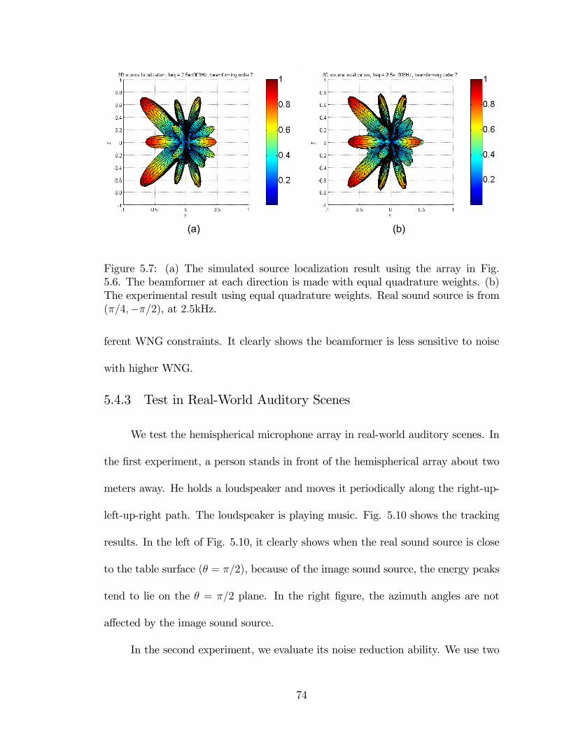
(a) (b)

Figure 5.7: (a) The simulated source localization result using the array in Fig.5.6. The beamformer at each direction is made with equal quadrature weights. (b)The experimental result using equal quadrature weights. Real sound source is from(π/4,−π/2), at 2.5kHz.

ferent WNG constraints. It clearly shows the beamformer is less sensitive to noise

with higher WNG.

5.4.3 Test in Real-World Auditory Scenes

We test the hemispherical microphone array in real-world auditory scenes. In

the first experiment, a person stands in front of the hemispherical array about two

meters away. He holds a loudspeaker and moves it periodically along the right-up-

left-up-right path. The loudspeaker is playing music. Fig. 5.10 shows the tracking

results. In the left of Fig. 5.10, it clearly shows when the real sound source is close

to the table surface (θ = π/2), because of the image sound source, the energy peaks

tend to lie on the θ = π/2 plane. In the right figure, the azimuth angles are not

affected by the image sound source.

In the second experiment, we evaluate its noise reduction ability. We use two

74

Figure 5.8: The simulated optimal localization result without WNG constraint.

loudspeakers facing the hemispherical array from (1.075, 2.7594) and (1.1456,−0.2408)

respectively. The two loudspeakers are playing different sounds, one is music, the

other speech. Using the hemispherical beamformer, the two sounds are separated.

Fig. 5.11 shows the results.

5.5 Precomputed Fast Spherical Beamforming

Suppose we perform N-order spherical beamforming to L uniform 3D direc-

tions (θi), i = 1, ..., L. Then, according to (4.10), for the ith beamformed result,

the incident wave from θk has the gain of

NXn=0

nXm=−n

Y m∗n (θk)Y

mn (θi). (5.9)

Here we omit the constant coefficient for clarity.

Now we want a new beamformed result at the direction θj, which is different

from any (θi), i = 1, ..., L. Apparently, the straightforward approach is to make a

75

Figure 5.9: Localization results using optimal beamformers under different WNGconstraints. Top left: 0dB < WNG < 5dB. Top right: 5dB < WNG < 10dB.Bottom left: 10dB < WNG < 15dB. Bottom right: WNG > 20dB.

76

Figure 5.10: Moving sound source tracking. Plots show the azimuth and elevationangles of the energy peak at each frame. The tracking is performed in the frequencyband from 3kHz to 6kHz, with beamformers of order seven (3kHz~4kHz) and eight(4kHz~6kHz).

Figure 5.11: Sound separation using hemispherical beamformer. The signals in theright column correspond to segments in the original signals in the left column.

77

regular spherical beamforming at the direction θj. However, since we already have

L beamformed results, we can design an efficient way to achieve this in time domain.

5.5.1 Time Domain Mixing via Orthonormal Decomposition

We notice that the following identityZΩ

("NXn=0

nXm=−n

Y m∗n (θk)Y

mn (θ)

#×"

NXn=0

nXm=−n

Y mn (θj)Y

m∗n (θ)

#)dΩ

=NXn=0

nXm=−n

Y m∗n (θk)Y

mn (θj) (5.10)

can be rewritten into a discrete approximation:

LXi=1

("NXn=0

nXm=−n

Y m∗n (θk)Y

mn (θi)

#×"

NXn=0

nXm=−n

Y mn (θj)Y

m∗n (θi)

#)

≈NXn=0

nXm=−n

Y m∗n (θk)Y

mn (θj). (5.11)

This clearly means if we apply the weight

Wi =NXn=0

nXm=−n

Y mn (θj)Y

m∗n (θi) (5.12)

to the ith beamformed result, and sum all L results up, we get the new beamformed

result as if we steer the beamformer to θj.

Now, the last confusion remains: if Wi is a complex number, that means for

each frequency, the phase shift is the same. In another word, Wi is an all-pass filter

but not in linear phase. That can’t lead an efficient implementation in time domain.

Fortunately, it is easy to prove thatWi is always a real number using addition

theorom of spherical harmonics:

NXn=0

nXm=−n

Y mn (θj)Y

m∗n (θi) =

NXn=0

2n+ 1

4πPn(cos γ), (5.13)

78

Figure 5.12: Gain comparision of direct beamforming and fast mixing in time do-main. Plot shows the absolute value for each beamforming direction. Simulated inorder eight with θk = (π/4, π/4).

where γ is the angle between θj and θi.

Therefore, the fast spherical beamforming algorithm is:

1. Precompute the beamformed results in L uniform directions.

2. To fast beamform at a new direction θj, we multiply Wi to each precom-

puted channel in time domain and then sum them up.

5.5.2 Verification

To verify this algorithm, we use the 128 nodes in Fig. 5.3 as both microphone

positions and beamforming directions. Using 120 equiangular θj in 3D space, we

compare the results of (5.10) and (5.11). Fig. 5.12 verifies its effectiveness.

79

5.6 Conclusions

We designed a hemispherical microphone array using the acoustic image prin-

ciple. It can be seen as a symmetric spherical microphone array across the edge of

real and image space, which is easy to build and install. It is especially appropriate

in numerous scenarios where sound sources are constrained in a half 3D space. We

built an array using 64 microphones positioned on a hemispherical surface. The

layout of real and image microphones is both symmetric and uniform, which leads

to a simple implementation of hemispherical beamformer. An effective calibration

method is proposed to extract the data-independent coefficients of the system from

the captured soundfield. The simulation and experimental results demonstrate the

effectiveness of our design. In addition, we use the hemispherical array to verify

the optimal algorithms described in Chapter 4 with real data. A precomputed fast

spherical beamforming algorithm is also presented and verified.

80

Chapter 6Cylindrical Microphone Arrays for Sound Capture and Beamforming1

The previous two chapters have established the theories for 3D audio system

using spherical microphone array. However, sometimes we only desire the spatial

filtering in one angular dimension, such as in surround sound field.

In this chapter, we propose a novel circular microphone array system for

recording and spatial filtering high order surround sound field. In our array, omni-

directional microphones are uniformly mounted along the cross-section circle on the

side surface of a sound-rigid cylinder. We will use this array to record the scattered

surround sound field, which can capture more spatial information than other de-

signs without scatterer [58]. The spatial filtering, or beamforming, is based on the

orthogonal decomposition of the recorded sound field by this array. Design example

and performance analysis are presented to demonstrate its effectiveness.

The main advantages of our system are:

1. It is easier to build and more practical to use for surround auditory scenes,

especially compared with the spherical array;

2. It is highly efficient and effective in recording and spatial filtering surround

auditory scenes;

3. It is highly scalable.

In the rest of this chapter, we first introduce the theory of acoustic scattering1This chapter is based on our original work in [62].

81

from a rigid cylinder. We then develop the theory of cylindrical beamforming in

section 6.2. In addition, we explain why we need a rigid cylinder instead of using

the microphone array in free space. To demonstrate our design, we analyze the

performance of a practical example in section 6.3. We address the practical design

issues such as discreteness, practical beampattern, robustness, and its performance

in 3D sound field. Both theoretical analyses and simulation results are presented.

6.1 Scattering from a rigid cylinder

Considering a general scenario as shown on the left side in Fig. 6.1, where

a unit magnitude plane sound wave of wave number k is incident from (θk, ϕk),

an infinite length rigid cylinder of radius a is positioned vertically at the origin

of the coordinate system, and the continuous circular microphone array is on the

cross-section circle at z = 0 plane. The complex pressure at the observation point

r = (r, π/2, ϕ) on the z = 0 plane is:

ψin = eik·r. (6.1)

If k is perpendicular to the axis of the cylinder (z-axis), i.e. θk = π/2, we then have:

ψin = eikr cos(ϕ−ϕk), (6.2)

where k = kkk. Now it is reduced to a 2D problem as shown on the right side in

Fig. 6.1. We will come back to the 3D issues in section 6.3.4.

From section 3.6.1, this plane wave can be expressed in terms of cylindrical

waves [74]:

ψin =∞Xn=0

ninJn(kr) cos [n(ϕ− ϕk)] , (6.3)

82

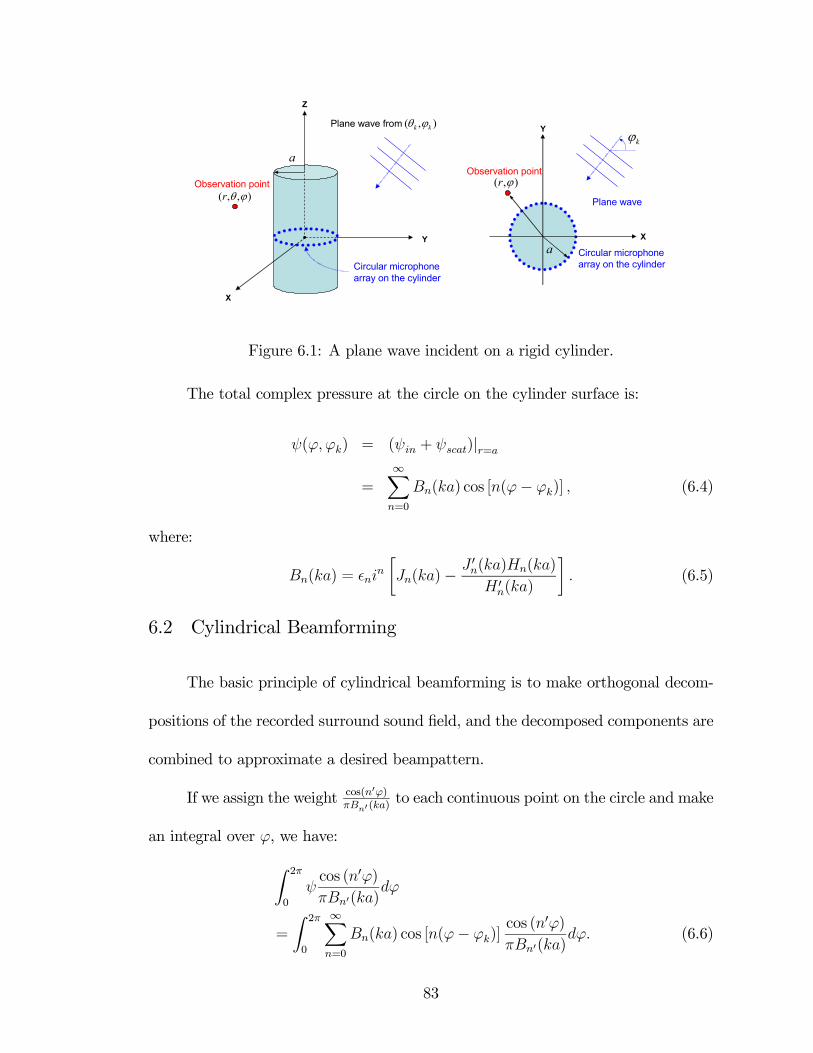
Observation point),,( ϕθr

Plane wave from ),( kk ϕθ

Circular microphone array on the cylinder

Y

X

Z

a

Y

X

kϕ

Plane wave

Observation point

Circular microphone array on the cylinder

),( ϕr

a

Figure 6.1: A plane wave incident on a rigid cylinder.

The total complex pressure at the circle on the cylinder surface is:

ψ(ϕ,ϕk) = (ψin + ψscat)|r=a

=∞Xn=0

Bn(ka) cos [n(ϕ− ϕk)] , (6.4)

where:

Bn(ka) = nin

·Jn(ka)− J 0n(ka)Hn(ka)

H 0n(ka)

¸. (6.5)

6.2 Cylindrical Beamforming

The basic principle of cylindrical beamforming is to make orthogonal decom-

positions of the recorded surround sound field, and the decomposed components are

combined to approximate a desired beampattern.

If we assign the weight cos(n0ϕ)πBn0(ka)

to each continuous point on the circle and make

an integral over ϕ, we have:Z 2π

0

ψcos (n0ϕ)πBn0(ka)

dϕ

=

Z 2π

0

∞Xn=0

Bn(ka) cos [n(ϕ− ϕk)]cos (n0ϕ)πBn0(ka)

dϕ. (6.6)

83

Since

cos [n(ϕ− ϕk)] = cos(nϕ) cos(nϕk) + sin(nϕ) sin(nϕk), (6.7)

and using the following integral identities:

Z 2π

0

cos(nϕ) cos(n0ϕ)dϕ = πδnn0 , (6.8)Z 2π

0

sin(nϕ) cos(n0ϕ)dϕ = 0, (6.9)Z 2π

0

cos(n0ϕ)dϕ = 0, (6.10)

for n, n0 6= 0, where δnn0 is the Kronecker delta function defined as:

δnn0 =

1, n = n0

0, n 6= n0. (6.11)

We then have: Z 2π

0


dϕ = cos(n0ϕk), (n0 > 0), (6.12)

That means the wave from ϕk direction has the gain of cos(n0ϕk).

Similarly, if the weight is sin(n0ϕ)πBn0(ka)

, we have:

Z 2π

0

ψsin (n0ϕ)πBn0(ka)

dϕ = sin(n0ϕk), (n0 > 0), (6.13)

In addition, when the weight is 12πB0(ka)

, we have:

Z 2π

0

ψ1

2πB0(ka)dϕ

=1

2πB0(ka)

(Z 2π

0

B0(ka)dϕ+

Z 2π

0

∞Xn=1

Bn cos [n(ϕ− ϕk)] dϕ

)= 1. (6.14)

If the ideal beampattern is a peak at ϕ0 and zero everywhere else, it can be

84

modeled as the delta function δ(ϕ− ϕ0)2. Its Fourier series expansion is:

δ(ϕ− ϕ0) =1

2π+1

π

∞Xn=1

[cos(nϕ0) cos(nϕ) + sin(nϕ0) sin(nϕ)]. (6.15)

Therefore, to achieve the ideal beampattern f(ϕ, ϕ0) = δ(ϕ − ϕ0), the weight for

the microphone at point ϕ is:

w(ϕ, ϕ0) =1

4π2B0(ka)+1

π

∞Xn=1

·cos(nϕ0)

cos(nϕ)

πBn(ka)+ sin(nϕ0)

sin(nϕ)

πBn(ka)

¸=

1

4π2B0(ka)+1

π2

∞Xn=1

cos[n(ϕ− ϕ0)]

Bn(ka). (6.16)

Some careful readers may have noticed the similarity between the fomulas (6.3)

and (6.4) in the sense that both are the infinite series of cosine functions except the

coefficients are different. We rewrite (6.3) as:

ψin =∞Xn=0

An cos [n(ϕ− ϕk)] , (6.17)

where

An = ninJn(kr). (6.18)

It is plausible that the cosine components recorded by a circular microphone array

in free space can also be extracted similarly as we did in section 6.2. So why bother

to scatter the plane wave by a rigid cylinder? The intuition is: the scattering makes

the pressure distribution along the circular microphone array more complicated,

especially for higher frequency wave, so more spatial information is captured. This

is illustrated more clearly in Fig. 6.2 and Fig. 6.3. When ka is relatively small,

the cylinder is approximately transparent to the sound wave, so An(ka) and Bn(ka)

2It is also called “Dirac’s delta function” or the “impulse symbol”. Refer [74, pp. 31] for theformal definition. Don’t be confused with the Kronecker delta function as (6.11).

85

10-1 100 101-40

-35

-30

-25

-20

-15

-10

-5

0

5

20lo

g10

|An(k

a)|

[d

B]

ka

n=0

n=1

n=2

n=3

n=4

2.4

Figure 6.2: An(ka) for n from 0 to 20.

have similar behaviors. When ka increases, the scattering effect is stronger, so

the irregular pressure distribution along the circular array contains richer spatial

frequency content. For example, in Fig. 6.2, when ka lies in the first notch of

A0(ka) which is about 2.4, apparently the spatial frequency component of n = 0

cannot be extracted robustly since it is too weak compared to the n = 1 component

and hidden by noise. While at the same ka in Fig. 6.3, the component of n = 0

is boosted to about −6 dB which is much easier to be extracted. There are more

notches for larger ka in Fig. 6.2 although An(ka) finally converges with respect to

n for given ka. On the contrary, in Fig. 6.3, for fixed ka, Bn(ka) exhibits smoother

convergence with the increase of n.

In summary, with the help of the scattering from the cylinder, it is much easier

to extract the desired spatial components.

86

10-1 100 101-40

-35

-30

-25

-20

-15

-10

-5

0

5

20lo

g10

|Bn(k

a)|

[d

B]

ka

n=0

n=1

n=2

n=3

n=4

2.4

Figure 6.3: Bn(ka) for n from 0 to 20.

6.3 Practical Design and Analysis

As an example, suppose we have a cylinder with radius of 10 cm, our array has

32 microphones positioned uniformly on the circle. We will analyze the performance

of this system. Since we only care about the pressure on the microphones which is

on the side surface of the cylinder, in practice, the cylinder can be of finite length

and the microphone array can be placed away from both endpoints. The scattered

sound field distortion is negligible at the microphone positions.

6.3.1 Discreteness

So far we have assumed a continuous circular microphone array. In practice,

however, we have to use finite number of microphones positioned discretely on a

circle. According to the well-known sampling theorem, to fully reconstruct a band-

limited signal, it must be sampled at a rate at least twice as fast as the highest

87

frequency. This sampling rate is called the Nyquist frequency. This theorem is for

both spatial and temporal sampling.

In our system, we assume the temporal sampling rate is already fast enough.

Our concern is the spatial sampling rate with respect to the number of microphones

on a circle. Using N microphones positioned uniformly on the circle, the sampling

rate is N . So we can fully capture the sound field with highest spatial frequency

of n = N/2. For example, in Fig. 6.3, when ka = 1, the amplitude of the spatial

frequency component of n = 4 is about −40 dB which is negligible in practice, so we

may just say the highest spatial frequency is n = 3 and we need N = 6 microphones.

For the array with N microphones, if the highest spatial frequency with sig-

nificant amplitude is M(M ≤ N/2), the weight is:

wM(ϕ, ϕ0) =1

4π2B0(ka)+1

π2

MXn=1

cos[n(ϕ− ϕ0)]

Bn(ka). (6.19)

With fixed a, the spatial frequency content depends on the temporal frequency.

This is also illustrated in Fig. 6.3 when ka increases, the sound field along the

circular array contains higher spatial frequencies. Spatial aliasing occurs when the

sound field contains spatial frequency greater than N/2.

6.3.2 Practical Beampattern

The ideal beampattern is defined as (6.15). In the real array with finite number

of microphones, using the practical weight as (6.19), the actual beampattern is an

M-truncated version of (6.15):

fM(ϕ,ϕ0) =1

2π+1

π

MXn=1

cos[n(ϕ− ϕ0)]. (6.20)

88

-3 -2 -1 0 1 2 3-50

-40

-30

-20

-10

0

10

azimuth angle φ

[dB]

M=1M=5M=10M=16

Figure 6.4: Beampatterns for M = 1, 5, 10, 16.

We say this beampattern is of order M . In Fig. 6.4, we plot a few beampatterns of

different orders. To show the spatial aliasing effects, we compare the beampatterns

at high frequencies against the theoretical beampattern of order 16, which is the

maximum order for our example. The plot is for θ = π/2 and ϕ = [−π, π] as shown

in Fig. 6.5.

6.3.3 Robustness

A robust beamformer requires the minimum white noise gain (WNG) is −6

dB, that is [16]:

WNG = 10 log10

Ã¯WHd

¯2WHW

!≥ −6 dB, (6.21)

whereW is the weight vector applied to the circular microphone array to beamform

at the direction (π/2, 0):

W = [wM(ϕ1, 0), wM(ϕ2, 0), ..., wM(ϕN , 0)], (6.22)

89

-3 -2 -1 0 1 2 3-70

-60

-50

-40

-30

-20

-10

0

azimuth angle φ

[dB]

10KHz15KHztheoretical

Figure 6.5: Spatial aliasing.

and d is the vector of the complex pressure produced at the array by a plane wave

of unit magnitude incident from the same direction:

d = [ψ(ϕ1, 0), ψ(ϕ2, 0), ..., ψ(ϕN , 0)]. (6.23)

Here ϕi specifies the individual microphone position:

ϕi = 2π(i− 1)/N, i = 1, ..., N. (6.24)

Fig. 6.6 shows the WNGs at different orders using our configuration. For

example, when ka is in the range of [0.13, 0.55], the beamformer can only work

robustly at order 1; when ka is in the range of [0.55, 1.14], the beamformer can work

robustly at order 2, etc.

90

10-1 100 101-10

-5

0

5

10

15

20

ka

Whi

te N

oise

Gai

n [d

B]

M=1

M=2

M=3 M=4 M=5 M=10 M=15

minimum WNG: -6 dB

Figure 6.6: White noise gain.

6.3.4 Beampattern in 3D Sound Field

Our system is designed to make spatial filtering of two dimensional auditory

scenes where sound sources are roughly on the same plane specified by the circular

microphone array. In the real world, however, undesired sound can come from all

3D directions other than on this plane, such as the room reverberations or other

noise.

In Fig. 6.7, we plot the polar beampatterns for different elevation angles.

It clearly shows when the wave direction is moving away from the plane specified

by the microphone array, the beampattern tends to be less directive. This can be

explained theoretically. Suppose the sound wave is from (θk, ϕk) and the component

of the wave number k perpendicular to the cylinder axis (z-axis) is k⊥, the incident

91

10

20

30

π/6

-5 π/6

π/3

-2 π/3

π/2

- π/2

2π/3

- π/3

5π/6

- π/6

±π 0

θ=π/8θ=π/4θ=3π/8θ=π/2

[dB]

[dB]

[dB]

Figure 6.7: Polar Beampatterns for different elevation angles at 5 kHz. The beam-pattern for θ = π/2 is of order 13 with WNG ≈ −5.96 dB.

Figure 6.8: 3D beampattern of order 13 at 5 kHz, looking at ϕ = 0. (lighted to show3D effect.)

92

wave is:

ψin = eik·r = eik⊥·r = eik⊥r cos(ϕ−ϕk), (6.25)

where:

k⊥ = k sin θk. (6.26)

Accordingly, (6.12), (6.13) and (6.14) become:Z 2π

0


dϕ =Bn0 (k⊥a)Bn0(ka)

cos(n0ϕk), (6.27)Z 2π

0

ψsin (n0ϕ)πBn0(ka)

dϕ =Bn0 (k⊥a)Bn0(ka)

sin(n0ϕk), (6.28)Z 2π

0

ψ1

2πB0(ka)dϕ =

B0 (k⊥a)B0(ka)

, (6.29)

(n0 > 0).

Therefore, the actual M-truncated beampattern for θk is:

fM(ϕ, ϕ0, θk) =1

2π

B0 (k⊥a)B0(ka)

+1

π

MXn=1

Bn (k⊥a)Bn(ka)

cos[n(ϕ− ϕ0)]. (6.30)

From Fig. 6.3, we notice that except B0(ka) is monotonically decreasing, each

Bn(ka) (n > 0) has only one peak. On the left side of its peak, it is monotonically

increasing and on the right side monotonically decreasing3. Since k⊥a < ka for

θk 6= π/2, there exists a threshold integer m (0 < m < M) such that:Bn (k⊥a)Bn(ka)

≥ 1, 0 ≤ n ≤ m

Bn (k⊥a)Bn(ka)

< 1, m < n ≤M

. (6.31)

That means the higher spatial frequency components are suppressed while the lower

spatial frequency components are amplified. Apparently, this low-pass filter makes

the resulted beampattern less directive.3Strict theoretical proof omitted here.

93

The full 3D beampattern is shown in Fig. 6.8. It has a strawberry-like shape.

Therefore, our array can also be used in 3D auditory scenes where spatial filtering

in the azimuthal dimension is desired.

94

Chapter 7Recreate 3D Auditory Scenes Via Reciprocity1

In this chapter, we develop the theories of building a high order 3D audio

capture and recreation system. As we have discussed in Section 1.3, the previ-

ous designs are either unsuitable for 3D immersive applications [9], or unstable in

complex auditory scenes [82]. Our contribution is to use the reciprocity between

capturing and recreating to design a simple, robust and unified 3D audio system

in high orders of spherical harmonics. We will apply this approach in loudspeaker

array-based and headphone-based systems.

7.1 Loudspeaker Array-Based System

We use a microphone array mounted on a rigid sphere for the capture and

a spherical loudspeaker array in free space for playback. A scenario is shown in

Fig. 7.1. A design example and simulation results are presented to demonstrate the

effectiveness of our system.

The main advantages of our system are:

1. the reciprocity between capturing and recreating processes makes the system

easy to build;

2. the performance is robust and optimal with the given number of microphones

and loudspeakers;


95

Figure 7.1: Left: the microphone array captures a 3D sound field remotely. Right:the loudspeaker array recreates the captured sound field to achieve the same soundfield.

3. the capturing part is compact and portable which is convenient to record the

immersive 3D sound field;

4. the system is highly scalable.

In addition, for some regular or semi-regular microphone layouts, there exists

efficient parallel implementations of the multi-directional spherical beamformer. We

will illustrate this in Section 7.1.5.

Our system can be seen as an extension to higher orders of the Ambisonics

system, which only captures and recreates the 3D sound field to the first order of

spherical harmonics [45][1].

7.1.1 Recording as 3D Sound Field Projection

We present a concept of viewing the spherical beamforming as a form of pro-

jection which leads to the design of the proposed system.

96

),( ii ϕθ

),( kk ϕθ

plane wave

),,,( iikkNF ϕθϕθ beamforming direction

loudspeaker position ),( ii ϕθ

loudspeaker in this directionplaybacks this beamformed signal

),( ii ϕθ

),( kk ϕθ

plane wave

),,,( iikkNF ϕθϕθ beamforming direction

loudspeaker position ),( ii ϕθ

loudspeaker in this directionplaybacks this beamformed signal

Figure 7.2: System workflow: for each chosen direction θi = (θi, ϕi), we first beam-form the 3D sound field into that direction using our N-order beamformer, thensimply playback the resulted signal from the loudspeaker in that direction.

In a real-world system, we only have a finite number of microphones distrib-

uted on the spherical surface discretely. With S microphones the following discrete

version of (4.4) can be approximately satisfied:

4π

S

SXs=1

Y m∗n (θs)Y

m0n0 (θs) = δnn0δmm0 , (7.1)

where the equation holds to order N. The achieved beampattern of order N is a

truncated version of (4.7):

FN(θ,θ0) = 2πNXn=0

nXm=−n

Y m∗n (θ0)Y

mn (θ). (7.2)

Each beamformed signal not only picks up the sound from the desired direction

(θ0), but also from other directions. We assume the 3D sound field is composed of

plane waves. The beamforming can be viewed as a projection process. This is

97

illustrated in Fig. 7.2, where it is shown in 2D for clarity. In this example, the

beamformer (N = 3) is pointing to (θi). We can think of the plane wave from (θk)

as weighted by

FN(θk,θi) = 2πNXn=0

nXm=−n

Y m∗n (θi)Y

mn (θk) (7.3)

before it is projected into the (θi) direction. We view this projected plane wave as

a subsource.

Suppose we beamform the recorded signals in D directions. This creates D

subsources for the 3D sound field.

7.1.2 Recreation as 3D Sound Field Unprojection

As shown in Fig. 7.2, if the D beamforming directions are well chosen, we

can simply playback the D subsources from their respective directions. We wish to

recreate the original 3D sound field to order N .

In this section, we first derive a theoretical condition for achieving the recre-

ation. We then find an approximate and optimal solution that provides us a simple

and unified way to recreate the 3D sound field from the subsources.

Theoretical Condition for Recreation

We assume all loudspeakers are positioned in free space and arranged as a

spherical array with a radius large enough to produce plane waves at the observation

points (this will be relaxed in the next section). Each loudspeaker plays back the

identical signal weighted by a complex coefficient al(k). The resulted sound field

98

inside this sphere is:

ψc = 4π∞Xn=0

injn(krs)nX

m=−n

LXl=1

al(k)Ymn (θl)Y

m∗n (θs), (7.4)

where (θl), l = 1, ..., L are the angular positions of L loudspeakers and (θs, rs) is the

observation point inside the sphere.

To recreate the 3D sound field exactly, we let (3.60) equal (7.4):

ψin = ψc (7.5)

Let Ωs be the spherical surface of radius rs. Here we only require rs to be less

than the radius of the loudspeaker array and satisfy the plane wave assumption, not

necessarily equal to the radius of the microphone array. We have:

ZΩs

ψinYm0n0 (θs)dΩs =

ZΩs

ψcYm0n0 (θs)dΩs. (7.6)

Using (4.4), we get:

Y m0n0 (θk) =

LXl=1

al(k)Ym0n0 (θl), (7.7)

(n0 = 0, ...,∞, m0 = −n0, ..., n0).

Please note (7.7) is independent of the observation point. To recreate the 3D

sound field to order N , we need (adapted from [88]):

Pa =cb (7.8)

where c is a constant, a is the vector of unknown weights to be assigned to each

99

loudspeaker;

P =

Y 00 (θ1) Y 0

0 (θ2) · · · Y 00 (θL)

Y −11 (θ1) Y −11 (θ2) · · · Y −11 (θL)

Y 01 (θ1) Y 0

1 (θ2) · · · Y 01 (θL)

Y 11 (θ1) Y 1

1 (θ2) · · · Y 11 (θL)

......

. . ....

Y −NN (θ1) Y −NN (θ2) · · · Y −NN (θL)

......

. . ....

Y NN (θ1) Y N

N (θ2) · · · Y NN (θL)

; (7.9)

and

b =

Y 00 (θk)

Y −11 (θk)

Y 01 (θk)

Y 11 (θk)

...

Y −NN (θk)

...

Y NN (θk)

. (7.10)

Here (θk) is the direction from which the original plane wave is incident.

Reproduction as the Reciprocal of Beamforming

If we choose the beamforming directions (θi) and loudspeaker angular posi-

tions (θl) to all be the same L angular positions, in such a way that the discrete

100

orthonormality of spherical harmonics can be satisfied to order N , we have:

4π

L

LXi=1

FN(θk,θi)Ym0n0 (θi) = Y m0

n0 (θk). (7.11)

So we have the solution of a as:

a =

FN(θk,θ1)

FN(θk,θ2)

...

FN(θk,θL)

. (7.12)

This clearly shows that each loudspeaker plays back exactly the beamformed

signal with the beampattern pointing to itself as shown in Fig. 7.2.

7.1.3 Extension to Point-Source Form

Thus far, we have assumed the loudspeakers are far enough to generate plane

waves. In this section, we extend the algorithms to the general point-source model.

If the loudspeakers can be modeled as point sources, the soundfield recreated

by the spherical loudspeaker array with radius r becomes [23]:

ψc = 4π∞Xn=0

injn(krs)Rn(kr)nX

m=−n

LXl=1

al(k)Ymn (θl)Y

m∗n (θs),

where

Rn(kr) = −ikreikri−nhn(kr). (7.13)

The condition for recreation, (7.7), then becomes:

Y m0n0 (θk) = Rn0(kr)

LXl=1

al(k)Ym0n0 (θl), (7.14)

(n0 = 0, ...,∞, m0 = −n0, ..., n0).

101

Figure 7.3: The layout of 32 microphones on a rigid sphere with radius of 5 cm. (Thesphere is lighted to show the 3D effect, NOT the sound scattering.)

To have an optimal solution to order N , we have to modify our spherical

beamformer. Specifically, we normalize the expansion of the beampattern (7.3) to:

FN(θk,θi) = 2πNXn=0

nXm=−n

Y m∗n (θi)

Y mn (θk)

Rn(kr). (7.15)

The solution of (7.14) is then:

a =

FN(θk,θ1)

FN(θk,θ2)

...

FN(θk,θL)

. (7.16)

102

Figure 7.4: The layout of 32 loudspeakers in free space arranged as a sphere of largeradius.

7.1.4 Design Example and Simulations

To start our design, we need a layout of discrete points on a spherical surface

which satisfy (7.1) to some order. The angular positions specified by the centers

of the faces of a truncated icosahedron can satisfy (7.1) to order 4 according to

[71]. Other layouts can be used also such as in [35][50][63]. We just use these 32

angular positions to design our system. Our microphone array is as shown in Fig.

7.3 where the 32 omnidirectional microphones are positioned on a rigid sphere of

radius 5 cm. Our loudspeaker array is as shown in Fig. 7.4 with the same 32 angular

positions. We capture the 3D sound field using the microphone array, and then use

the (normalized) spherical beamformer to steer the signals to these 32 directions.

Finally, we recreate the 3D sound field using the loudspeaker array.

103

Figure 7.5: The plane wave of 4 kHz incident from positive direction of X-axisscattered by the microphone array. Plot shows the pressure on the equator.

We simulate our system by a plane wave of 4kHz incident from the positive

direction of X-axis in Fig. 7.3. Fig. 7.5 shows the scattered sound field on the

equator of the spherical microphone array. Fig. 7.6 is the recreated plane wave to

order 4 on the z = 0 plane.

Please note that a spherical microphone array can also be rotated arbitrarily

without affecting the results. Because of the reciprocity between the beamformer

and the loudspeaker arrays, the beamforming directions and the loudspeaker arrays

must have the same angular positions. However, there may exist efficient parallel

implementation of the multi-directional beamformer if the microphone array loca-

tions can be made consistent with the beamforming directions in some way. We will

illustrate this in Section 7.1.5.

When we only decompose the 3D sound field to the first order of spherical

104

Figure 7.6: The recreated plane wave to order 4. Plot shows the 2 × 2m2 area onthe z = 0 plane.

harmonics, our system mimics the Ambisonics system by pointing the bidirectional

beampattern (the first order spherical harmonics) to the left-right, front-back, and

up-down along with the omnidirectional beampattern (the zeroth order spherical

harmonics) [45][1].

Like most microphone arrays that sample the 3D space discretely, the spherical

microphone array has a spatial aliasing problem [71]. Low frequency requires larger

sphere to decompose higher orders of spherical harmonics while high frequency re-

quires denser microphones to avoid spatial aliasing. To broaden the frequency band,

we may need a larger sphere with more microphones. Another solutions may be to

use nested spherical microphone arrays, or multiple arrays.

105

7.1.5 Efficient Multi-directional Beamformer

If the layout of microphones is regular or semi-regular, we can make use of

rotational symmetries of the microphone array and of the beampattern to design an

efficient parallel multi-directional spherical beamformer. For specificity, we consider

a regular icosahedron to illustrate the idea. It can be easily adapted to other regular

or semi-regular microphone layouts.

A regular icosahedron, as shown in Fig. 7.7, is rotationally symmetric around

any line connecting the origin and an arbitrary node. If the symmetric axis is as

shown in the figure, there are two groups of nodes 2, 3, 4, 5, 6 and 7, 8, 9, 10, 11

on two different cones along with the two endpoints 1 and 12 of the line.

The rotational symmetry of the beampattern is formulated as the spherical

harmonic addition theorem. Let γ be the angle between the two spherical coordi-

nates (θ0) and (θ). We have:

sin θ sin θ0 cos(ϕ− ϕ0) + cos θ cos θ0 = cos γ, (7.17)

which defines a cone with respect to (θ). According to the spherical harmonic addi-

tion theorem, we have:

nXm=−n

Y m∗n (θ0)Y

mn (θ) =

2n+ 1

4πPn(cos γ), (7.18)

where Pn(x) is the Legendre polynomial of degree n. So the value of the beampattern

on the cone is defined by (7.17) as a function of γ:

2πNXn=0

nXm=−n

Y m∗n (θ0)Y

mn (θ) =

NXn=0

2n+ 1

2Pn(cos γ). (7.19)

106

Figure 7.7: The rotational symmetry of icosahedron.

From (4.8), the weight for each microphone at (θs) is:

f(θs) = f(γj) =NXn=0

2n+ 1

8πinbn(ka)Pn(cos γj), (7.20)

(s = 1, ...12; j = 1, 2, 3, 4).

For each beamforming direction specified by the spherical coordinates of the

icosahedron’s nodes, there are only four γ values for the icosahedron layout: 0, 1.1071, π−

1.1071, π. For example, if the beampattern is pointing to node 1, node 1 has γ1 = 0

and nodes 2, 3, 4, 5 and 6 have γ2 = 1.1071, etc.; if the beampattern is pointing

to node 2, node 2 has γ1 = 0 and nodes 1, 3, 6, 7 and 8 have γ2 = 1.1071, etc..

Thus, to build a twelve-directional beamformer, for each microphone, we only need

to make four multiplications corresponding to four γ values instead of twelve. The

structure of the multi-directional spherical beamformer is shown in Fig. 7.8.

107

……

…

mic1

mic2

mic3

mic12

)( 1γf)( 2γf)( 3γf)( 4γf

)( 1γf)( 2γf)( 3γf)( 4γf

)( 1γf)( 2γf)( 3γf)( 4γf

)( 1γf)( 2γf)( 3γf)( 4γf

beamforming directions:

)( 11 ϕθ ,

)( 22 ϕθ ,

)( 33 ϕθ ,

)( 1212 ϕθ ,

)( 11 ϕθ ,

)( 22 ϕθ ,

)( 33 ϕθ ,

)( 1212 ϕθ ,

……

…

……

…

mic1

mic2

mic3

mic12

)( 1γf)( 2γf)( 3γf)( 4γf

)( 1γf)( 2γf)( 3γf)( 4γf

)( 1γf)( 2γf)( 3γf)( 4γf

)( 1γf)( 2γf)( 3γf)( 4γf

beamforming directions:

)( 11 ϕθ ,

)( 22 ϕθ ,

)( 33 ϕθ ,

)( 1212 ϕθ ,

)( 11 ϕθ ,

)( 22 ϕθ ,

)( 33 ϕθ ,

)( 1212 ϕθ ,

……

…

Figure 7.8: The efficient structure of the multi-directional spherical beamformer.

7.2 Headphone-Based System

In this section, we develop a coupled theory of reproducing real 3D auditory

scenes by headphone from 3D recordings by spherical microphone array through

HRTF approximation. The currently available HRTF databases are described in

[2][6]. For simple auditory scene with only a few sound sources, we can first use

the spherical beamformer to locate the sound sources, then filter the beamformed

signals with the HRTFs in those corresponding directions. For complex auditory

scenes, however, we need algorithm which is independent with the source locations.

7.2.1 Ideal HRTF Selection

In an ideal case, we assume the HRTF is already measured continuously on the

spherical surface of radius r. Our goal is to select the correct HRTF for a specified

direction. Although it seems trivial for an ideal case, we use this as a starting point

108

and extend it to more practical cases in the following sections.

We drop the arguments k and r for simplicity, the HRTF for the sound of wave

number k from the point (r,θ) is [31]:

ψ(θ) =∞Xn=0

nXm=−n

αnmhn(kr)Ymn (θ), (7.21)

where hn and Y mn have the same definitions as in the last section, and αnm are

the fitting coefficients which can be determined using real-world discrete HRTF

measurements [31].

Suppose we want to select the HRTF for the direction (θk), we apply the

following delta function (ideal beampattern) to each measured HRTF:

F (θ, ϕ) = δ(θ − θk), (7.22)

we have: ZΩs

ψ(θ)F (θ)dΩs = ψ(θk), (7.23)

where Ωs is the spherical surface. Obviously, the delta function simply selects the

value we need and discards everything else.

To present another viewpoint of HRTF selection, we rewrite (7.23) into a more

“complicated” form by using (7.21) and (4.7):

ZΩs

" ∞Xn=0

nXm=−n

αnmhn(kr)Ymn (θ)

#×"2π

∞Xn=0

nXm=−n

Y m∗n (θ)Y m

n (θk)

#dΩs

=∞Xn=0

nXm=−n

αnmhn(kr)Ymn (θk). (7.24)

Alternatively, this can be easily proven by using the orthonormalities of spherical

harmonics (4.4).

109

7.2.2 HRTF Approximation In Orthogonal Beam-Space

In practice, however, HRTFs are measured on discrete points. In this case,

(7.24) and (4.4) can only hold approximately and in finite orders. In addition, using

a practical spherical array with finite number of microphones, the beampattern is

(4.10).

The HRTF for the sound of wave number k from the measurement point (r,θi)

is:

ψ(θi) =∞Xn=0

nXm=−n

αnmhn(kr)Ymn (θi), (7.25)

( i = 1, ..., B )

where B is the number of HRTF measurements.

The weighted combination of HRTFs then becomes:

BXi=1

ψ(θi)FN(θk,θi). (7.26)

If the HRTF measurement points (θi), i = 1, ...B, are approximately uniformly

distributed on a spherical surface so that the orthonormality of spherical harmonics

holds up to order N 0, then the HRTF can be expanded into two groups:

ψ(θi) = ψN 00 (θi) + ψ∞N 0+1(θi), (7.27)

where

ψN 00 (θi) =

N 0Xn=0

nXm=−n

αnmhn(kr)Ymn (θi), (7.28)

ψ∞N 0+1(θi) =∞X

n=N 0+1

nXm=−n

αnmhn(kr)Ymn (θi). (7.29)

110

So (7.26) can be rewritten as:

BXi=1

hψN 00 (θi) + ψ∞N 0+1(θi)

iFN(θk,θi)

=BXi=1

ψN 00 (θi)FN(θk,θi) (7.30)

+BXi=1

ψ∞N 0+1(θi)FN(θk,θi) (7.31)

= ψmin(N 0,N)0 (θk) + (7.32)

which is the approximation of HRTF up to the order min(N 0, N). Here the error

consists of two parts: one is the orthonormality error from (7.30) which is supposed

to be small according to the discrete orthonormalities; the other is from (7.31) which

is also small with well-chosen N 0 because of the convergence of the series expansion

in (7.25).

If HRTF are not measured on uniformly distributed angular points, which

is the case for all currently available measurements, we can first obtain a uniform

version via interpolation [31]. In addition, we can interpolate as many points as

we want to satisfy the orthonormality to arbitrarily high orders. In this case, the

HRTF approximation at (θk) depends only on the order of beampattern N , which

is:BXi=1

ψ(θi)FN(θk,θi) = ψN0 (θk) + . (7.33)

Therefore, apparently if there is a plane wave incident from (θk) in the original

auditory scene, it will be automatically filtered with the corresponding HRTF, in

the approximation of order N.

111

7.2.3 Recreation Algorithm

Suppose we have built a spherical microphone array to record a 3D auditory

scene. The spherical beamformer for this array has the beampattern as in (4.10).

To reproduce the 3D auditory scene from the recordings, there are three steps:

1. beamform the recordings to (θi) for i = 1, ..., B (the “uniformly” interpolated

point);

2. filter the beamformed signal at (θi) with the personalized HRTF ψ(θi) for

i = 1, ..., B;

3. superimpose the resulted signals for i = 1, ..., B.

With the currently available HRTF measurements, the only factor that deter-

mines reproduction quality is the beampattern order N of the spherical microphone

array.


We use the KEMAR HRTF measurements [2] to demonstrate our design. In

Fig. 7.9, the red (solid) line shows the HRTF measurement at the position just in

front of the manikin. The green (dot) line shows the approximation to order five

supposing we have a spherical microphone array of order five. It is a good approxi-

mation for frequencies until about 2KHz. It is also a relatively close approximation

until 4KHz which may be used in spatial speech acquisition and reproduction. The

blue (dash) line shows the approximation to order 10, which closely matches the

measurement until about 6KHz. The phases are compared in Fig. 7.10.

112

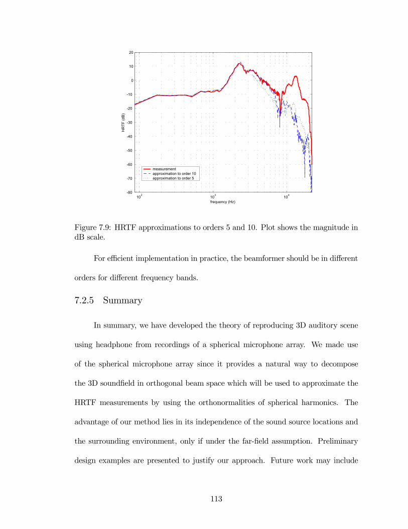
102 103 104-80

-70

-60

-50

-40

-30

-20

-10

0

10

20

frequency (Hz)

HR

TF (d

B)

measurementapproximation to order 10approximation to order 5

Figure 7.9: HRTF approximations to orders 5 and 10. Plot shows the magnitude indB scale.

For efficient implementation in practice, the beamformer should be in different

orders for different frequency bands.

7.2.5 Summary

In summary, we have developed the theory of reproducing 3D auditory scene

using headphone from recordings of a spherical microphone array. We made use

of the spherical microphone array since it provides a natural way to decompose

the 3D soundfield in orthogonal beam space which will be used to approximate the

HRTF measurements by using the orthonormalities of spherical harmonics. The

advantage of our method lies in its independence of the sound source locations and

the surrounding environment, only if under the far-field assumption. Preliminary

design examples are presented to justify our approach. Future work may include

113

500 1000 1500 2000 2500 3000 3500 4000 4500 5000 5500 6000-4

-3

-2

-1

0

1

2

3

4

frequency (Hz)

phas

e (r

adia

n)

measurementapproximation to order 10approximation to order 5

Figure 7.10: Phases of the approximations to orders 5 and 10.

reduced-dimensional description of HRTF measurements, calibration of spherical

microphone array, efficient data structure, extension to near-field case, etc.

7.3 A Discrete Huygens Principle Interpretation

This section describes a simple recreation algorithm by using discrete Huygens’

principle. It provides a clear and simple insight of the recreation algorithm. It

also completely removes the trouble caused by quadratures of spherical harmonics,

especially for unbalanced microphone and virtual plane wave layouts. In addition, it

provides extremely flexible microphone array and virtual plane waves designs. Since

the weights are directly contributed to the final recreated field, it is easy to include

the robustness constraints, such as the White Noise Gain.

It is obviously that this algorithm can be derived from wave equations directly

without using Huygens principle. In this sense, this section will try to provide an

114

integrated viewpoint of different recreation algorithms and more insights among

them.

7.3.1 Solutions by Discrete Huygens Principle

For band-limited 3D sound field, Huygens Principle can be approximated by

discrete sampling points, limited by Nyquist spatial frequency.

We first consider a unit magnitude plane wave k in free space, incident from

direction θk, at the observation point (a,θj), i = 1, ...,M, the complex pressure is:

ψin(θk,a,θj) = 4π

pXn=0

injn(ka)nX

m=−nY mn (θk)Y

m∗n (θj). (7.34)

M is the number of observation points or microphones. p is the band limit. a is

the radius of the observation point. It doesn’t have to be the same value for all

observation points. We will extend this later in this section.

This can be easily extended into arbitrarily complicated band-limited sound

field by linearity. We will see later our algorithm only depends on the recordings on

microphones, not on the complexity of sound field.

To recreate the original real sound field using L virtual plane waves in free

space from directions θi, i = 1, ..., L, we only need to recreate the sound field at the

finite sampling points for band-limited sound field:

ψin(θk,a,θj) =LXi=1

wiψin(θi, a,θj). (7.35)

(j = 1, ...,M.)

where wi is the complex weight assigned to each virtual plane wave incident from

115

θi. We then have:

pXn=0

injn(ka)nX

m=−nY mn (θk)Y

m∗n (θj)

=LXi=1

wi

"pX

n=0

injn(ka)nX

m=−nY mn (θi)Y

m∗n (θj)

#

=LXi=1

wiAp(θi,θj), (7.36)

To insert a rigid spherical array of radius a in both real and virtual cases, we then

have:

ψtotal(θk,a,θj) =LXi=1

wiψtotal(θi, a,θj). (7.37)

That is:

pXn=0

in·jn(ka)− j0n(ka)

h0n(ka)hn(ka)

¸ nXm=−n

Y mn (θk)Y

m∗n (θj)

=LXi=1

wi

"pX

n=0

in·jn(ka)− j0n(ka)

h0n(ka)hn(ka)

¸)

nXm=−n

Y mn (θi)Y

m∗n (θj)

#

=LXi=1

wiBp(θi,θj). (7.38)

(7.38) can be formed into a linear system:

Bp(θ1,θ1) Bp(θ2,θ1) · · · Bp(θL,θ1)

Bp(θ1,θ2) Bp(θ2,θ2) · · · Bp(θL,θ2)

· · · · · · . . . · · ·

Bp(θ1,θM) Bp(θ2,θM) · · · Bp(θL,θM)

w1

w2

...

wL

=

ψtotal(θk, a,θ1)

ψtotal(θk, a,θ2)

...

ψtotal(θk, a,θM)

.

(7.39)

It is obvious to me that the solution of wi, i = 1, ..., L also satisfies (7.36).

Please note the right side of (7.39) is just a sampling of the sound field, i.e. a

recording. It can be multiple sources in complicated acoustic environment.

116

Figure 7.11: 1KHz sound source at 2a, recorded using a=10cm spherical array with64 Fliege nodes. Plot shows the recreated sound field using 64 virtual plane waves.

7.3.2 Simulation Results

We first use microphone array on rigid sphere to record the sound field. Figure

7.11-7.13 show the recreation results. Please note Fig. 7.12 uses 60 mics and 60

virtual plane waves.

We can also use microphone array in free space as in Fig. 7.14. In this case,

we can use multiple arrays easily. For example, we can use two small microphone

arrays apart to sample the regions around each ear, each with radius 3cm and 32

nodes (face centers of truncated icosahedron). Then we can use two sets of 32 virtual

plane waves to recreate sound field at those two regions sampled by two mic arrays,

respectively. Therefore, we recreate the sound field around left and right ears, then

filtered by HRTF. A simulation result for the region around one ear is shown in Fig.

7.15.

117

Figure 7.12: Same setup, but using only 60 microphones and 60 virtual plane waves.

Figure 7.13: recorded using spherical array with 324 Fliege’s nodes with a=8cm.8KHz source from 2a. Plot shows the recreated sound field using 324 virtual planewaves.

118

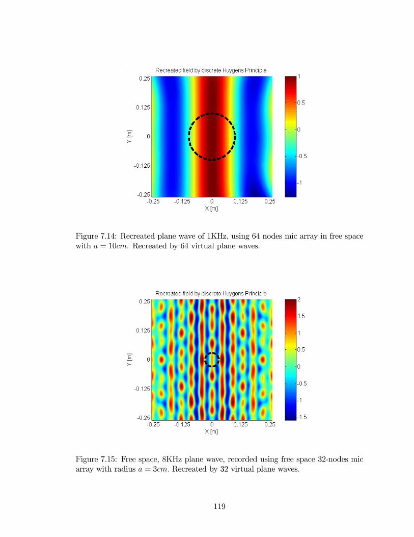
Figure 7.14: Recreated plane wave of 1KHz, using 64 nodes mic array in free spacewith a = 10cm. Recreated by 64 virtual plane waves.

Figure 7.15: Free space, 8KHz plane wave, recorded using free space 32-nodes micarray with radius a = 3cm. Recreated by 32 virtual plane waves.

119

Chapter 8Recreate 2D Auditory Scenes1

This chapter parallels Chapter 7 to develop the theories of reproducing the

recorded surround auditory scenes through loudspeaker array and headphone.

8.1 Loudspeaker Array-Based System

Suppose we have recorded the surround auditory scene using our circular mi-

crophone array, the next step is to reproduce it with a circular loudspeaker array.

In this array, L loudspeakers are positioned uniformly around a circle in free space.

To achieve the optimal performance given the number of microphones (N) used in

recording, we let L equal to N . For clarity, we still use the notation L for the

number of loudspeakers. In this section, we first consider the plane wave case where

the radius of the circular loudspeaker array is large enough to produce plane waves

at the observation points. We will derive the theoretical condition of reproduction,

and give a simple solution to ensure the optimal performance. Then we extend this

to the spherical wave case where the circle of the loudspeaker array is small so that

every loudspeaker can be modeled as a point sound source.

8.1.1 Plane Wave Case

We denote the L loudspeaker positions as ϕl, l = 1, ..., L, which are also the

plane wave incident directions. Suppose we feed every loudspeaker with the identical

signal of wave number k, and the output of the l-th loudspeaker is weighted by a


120

complex number al(k), the reproduced sound field at the observation point ϕ is a

weighted combination of plane waves:

pc =∞Xn=0

ninJn(kr)

LXl=1

al(k) cos [n(ϕ− ϕl)] . (8.1)

To perfectly reproduce the original sound field, it requires (6.3) equal (8.1). Thus

the condition for reproduction is:

cos [n(ϕ− ϕk)] =LXl=1

al(k) cos [n(ϕ− ϕl)] , (8.2)

(n = 0, ...,∞).

That is:

cos (nϕk) =LXl=1

al(k) cos (nϕl) , (8.3)

sin (nϕk) =LXl=1

al(k) sin (nϕl) , (8.4)

(n = 0, ...,∞).

However, since we only can record the sound field up to order M , the reproduction

can be achieved to order M at most. If we let:

al(k) = fM(ϕk, ϕl) =1

2π+1

π

MXn0=1

cos[n0(ϕk − ϕl)], (8.5)

then (8.3) and (8.4) can be satisfied to order M as following:

LXl=1

al(k) cos (nϕl)

=LXl=1

(1

2π+1

π

MXn0=1

cos[n0(ϕk − ϕl)]

)cos (nϕl)

= cos(nϕk) (n = 0, ...,M), (8.6)

121

and

LXl=1

al(k) sin (nϕl)

=LXl=1

(1

2π+1

π

MXn0=1


)sin (nϕl)

= sin(nϕk) (n = 0, ...,M). (8.7)

The physical meaning is clear: if each loudspeaker plays back the beamformed signal

in this direction, the loudspeaker array will recreate the original surround sound field

to order M .

8.1.2 Spherical Wave Case

Thus far, we have assumed the loudspeakers are far enough from the obser-

vation points to generate plane waves. In this section, we extend the algorithm

to the general point-source model where the reproduced sound field is a weighted

combination of spherical waves.

Suppose the radius of the circular loudspeaker array is r0. If the loudspeakers

can be modeled as point sources, the sound field at the observation point (r, θ, ϕ)

reproduced by the circular loudspeaker array becomes [23]:

pc = 4π∞Xn=0

injn(kr)Rn(kr0)nX

m=−n

LXl=1

al(k)Ymn (θl, ϕl)Y

m∗n (θ, ϕ), (8.8)

where

Rn(kr0) = −ikr0eikr0i−nhn(kr0). (8.9)

Normally, the listener is at the center of the circular ring of the loudspeakers, so

122

θl = π/2 and θ = π/2. Since

Y mn (

π

2, ϕ) ≡

s2n+ 1

4π

(n−m)!

(n+m)!Pmn (cos

π

2)eimϕ

=

s2n+ 1

4π

(n−m)!

(n+m)!Pmn (0)e

imϕ, (8.10)

the recreated sound field is:

pc = 4π∞Xn=0

injn(kr)Rn(kr0)LXl=1

al(k)nX

m=−n

·2n+ 1

4π

(n−m)!

(n+m)!

¸[Pm

n (0)]2 eim(ϕl−ϕ).

(8.11)

Using the identity relating associated Legendre polynomials with negative m to the

corresponding functions with positive m:

P−mn (x) = (−1)m (n−m)!

(n+m)!Pmn (x), (8.12)

we have:

nXm=−n

h2n+14π

(n−m)!(n+m)!

i[Pm

n (0)]2 eim(ϕl−ϕ)

=nX

m=0

m

h2n+14π

(n−m)!(n+m)!

i[Pm

n (0)]2 cos [m(ϕl − ϕ)] . (8.13)

let

En = 4πinjn(kr)Rn(kr0), (8.14)

Fmn = m

·2n+ 1

4π

(n−m)!

(n+m)!

¸[Pm

n (0)]2 . (8.15)

123

10-4 10-3 10-2 10-1 10010-5

100

105

|H5|

r

10-4 10-3 10-2 10-1 10010-5

100

105

|H10

|

r

10-4 10-3 10-2 10-1 10010-5

100

105

|H16

|

r

Figure 8.1: H5, H10 and H16 at frequency 2 kHz.

So we have:

pc =LXl=1

al(k)∞Xn=0

En

nXm=0

Fmn cos [m(ϕl − ϕ)]

=LXl=1

al(k)∞X

m=0

Ã ∞Xn=m

EnFmn

!cos [m(ϕl − ϕ)]

=LXl=1

al(k)∞Xn=0

Ã ∞Xm=n

EmFnm

!cos [n(ϕl − ϕ)]

=∞Xn=0

Ã ∞Xm=n

EmFnm

!LXl=1

al(k) cos [n(ϕl − ϕ)] . (8.16)

Comparing (8.16) against (6.3) or (6.17), the condition for reproduction is:Ã ∞Xm=n

EmFnm

!LXl=1

al(k) cos [n(ϕl − ϕ)] = An cos [n(ϕ− ϕk)] , (n = 0, ...,∞).

(8.17)

That is:

124

Ã ∞Xm=n

EmFnm

!LXl=1

al(k) cos (nϕl) = An cos (nϕk) , (8.18)Ã ∞Xm=n

EmFnm

!LXl=1

al(k) sin (nϕl) = An sin (nϕk) , (8.19)

(n = 0, ...,∞).

Similarly, (8.18) and (8.19) can be satisfied for n = 0 to M with the solution of

al(k) as:

al(k) =AnP∞

m=nEmFnm

fM(ϕk, ϕl)

= Hn(k, r, r0)

(1

2π+1

π

MXn0=1


), (8.20)

which is still the beampattern but multiplied by a variable coefficient:

Hn(k, r, r0) =AnP∞

m=nEmFnm

. (8.21)

To analyze its effects on the reproduced sound field, we plot Hn(k, r, r0) with r0 =

1m. Figure 8.1 plots H5,H10 and H16 at 2 kHz with respect to r. Figure 8.2 plots

the same functions at 5 kHz. Several interesting observations are:

1. If r is small compared with r0, i.e. the observation points are in the far field

area, Hn ≈ 1. This is roughly the same as the plane wave case;

2. At fixed frequency, with larger n, the far field area stretches. This is because

the first zero of Hn occurs at the same r as the first zero of Jn(kr), the n-th

order Bessel function of the first kind;

3. The far field area shrinks as the frequency increases, which is obvious since

the first zero of Jn(kr) for fixed n is a constant number, when k increases, r

has to decrease to stay in the far field area.

125

10-4 10-3 10-2 10-1 10010-5

100

105

|H5|

r

10-4 10-3 10-2 10-1 10010-5

100

105

|H10

|

r

10-4 10-3 10-2 10-1 10010-5

100

105

|H16

|

r

Figure 8.2: H5, H10 and H16 at frequency 5 kHz.

Figure 8.3: Reproduce the 5 kHz plane wave to order 5 using plane waves.

8.1.3 Simulation

We simulate the reproduction of a plane wave of 5 kHz incident from ϕ =

π/4. Figure 8.3-8.5 show the reproduction by plane waves to the order 5, 10, 16,

respectively. Figure 8.6-8.8 show the reproduction by spherical waves at the same

orders with r0 = 1m. Figure 8.9 shows the reproduction to order 5 at 2 kHz. As we

have predicted, the reproduction is effective in a larger area than in Figure 8.6.

126



Figure 8.6: Reproduce the 5 kHz plane wave to order 5 using spherical waves.

127




128

8.2 Headphone-Based System

In this section, we achieve optimal personalized reproduction from the record-

ing of our circular microphone array, with the cylindrical beamformer as the bridge.

8.2.1 Ideal HRTF Selection

In an ideal case, we assume the HRTF is already measured continuously on the

spherical surface of radius r. Our goal is to select the correct HRTF for a specified

direction. Although it seems trivial for an ideal case, we use this as a starting point

and extend it into more practical cases in the following sections.

We drop the arguments k and r for simplicity, the HRTF for the sound of wave

number k from the point (r, θ, ϕ) can be modeled as [31]:

ψ(θ, ϕ) =∞Xn=0

nXm=−n

αnmhn(kr)Ymn (θ, ϕ), (8.22)

where hn is the first kind spherical Hankel function of order n, Y mn is the spherical

harmonics of order n and degree m, and αnm is the fitting coefficients.

In surround audio case, θ = π/2, we have:

Y mn (

π

2, ϕ) ≡

s2n+ 1

4π

(n−m)!

(n+m)!Pmn (cos

π

2)eimϕ

=

s2n+ 1

4π

(n−m)!

(n+m)!Pmn (0)e

imϕ, (8.23)

So:

ψ(π

2, ϕ) =

∞Xn=0

nXm=−n

Anmhn(kr)eimϕ, (8.24)

129

where

Anm = αnm

s2n+ 1

4π

(n−m)!

(n+m)!Pmn (0). (8.25)

Suppose we want to select the HRTF for the spatial point (r, π/2, ϕk), we apply

the following weighting function (ideal beampattern) to each measured HRTF:

δ(ϕ− ϕk) =1

2π

∞Xn=−∞

ein(ϕ−ϕk). (8.26)

According to the property of delta function, we have:

Z 2π

0

ψ(π

2, ϕ)δ(ϕ− ϕk)dϕ = ψ(

π

2, ϕk), (8.27)

Obviously, the weighting function simply selects the value we need and discards

everything else.

To present another viewpoint of HRTF selection, we rewrite (8.27) into a more

“complicated” form:

Z 2π

0

" ∞Xn=0

nXm=−n

Anmhn(kr)eimϕ

#"1

2π

∞Xn=−∞

ein(ϕ−ϕk)#dϕ

=∞Xn=0

nXm=−n

Anmhn(kr)eimϕk . (8.28)

Alternatively, this can be easily proved using the orthonormality of exponential

functions:

1

2π

Z 2π

0

eimϕeinϕdϕ = δmn. (8.29)

8.2.2 HRTF Approximation Via Orthonormal Decomposition

In practice, however, HRTFs are measured on discrete points. In this case,

(8.28) and (8.29) can only hold approximately and in finite orders. In addition, using

130

a practical cylindrical array with finite number of microphones, the beampattern is

an M-truncated version of (6.15).

Suppose the HRTF for the sound of wave number k from the measurement

point (r, π/2, ϕi) is:

ψ(π

2, ϕi) =

∞Xn=0

nXm=−n

Anmhn(kr)eimϕi , (8.30)

( i = 1, ..., B )

where B is the number of HRTF measurements.

When the beamformer is looking at ϕi, the gain for sound wave from ϕk is the

truncated beampattern to order M :

fM(ϕk, ϕi) = fM(ϕi, ϕk)

=1

2π

MXn=−M

ein(ϕi−ϕk). (8.31)

The weighted combination of HRTFs then becomes:

BXi=1

fM(ϕi, ϕk)ψ(π

2, ϕi). (8.32)

If the HRTF measurement points (θi, ϕi), i = 1, ...B, are uniformly distributed

on a circle so that the orthonormality of Fourier exponential functions holds up to

order N 0, then the HRTF can be expanded into two groups:

ψ(π

2, ϕi) = ψN 0

0 (π

2, ϕi) + ψ∞N 0+1(

π

2, ϕi), (8.33)

where

ψN 00 (

π

2, ϕi) =

N 0Xn=0

nXm=−n

Anmhn(kr)eimϕi , (8.34)

ψ∞N 0+1(π

2, ϕi) =

∞Xn=N 0+1

nXm=−n

Anmhn(kr)eimϕi . (8.35)

131

So (8.32) can be rewritten as:

BXi=1

fM(ϕi, ϕk)hψN 00 (

π

2, ϕi) + ψ∞N 0+1(

π

2, ϕi)

i=

BXi=1

fM(ϕi, ϕk)ψN 00 (

π

2, ϕi) (8.36)

+BXi=1

fM(ϕi, ϕk)ψ∞N 0+1(

π

2, ϕi) (8.37)

= ψmin(N 0,M)0 (

π

2, ϕk) + , (8.38)

which is the approximation of HRTFs up to the order min(N 0, M). Here the error

consists of two parts: one is the orthonormality error from (8.36) which is supposed

to be small according to the discrete orthonormalities; the other is from (8.37) which

is also small with well-chosen N 0 because of the convergence of the series expansion

in (8.22) [31]. We will provide a design example in the next section.

If HRTFs are not measured on uniformly distributed angular points, we can

first obtain a uniform version via interpolation [31]. In addition, given the number

of microphones used in recording, we need to make at least the same number of

HRTF measurements so that the recorded spatial information can be recreated fully.

In this case, the HRTF approximation at (π/2, ϕk) depends only on the order of

beampattern M , which is:

ψM0 (

π

2, ϕk) + . (8.39)

8.2.3 Reproduction from Recordings

From the analysis of HRTF approximation, the algorithm to reproduce the

surround sound through headphone becomes quite obvious and intuitive: we first

132

beamform the recordings to (π/2, ϕi), and filter the beamformed signal with the

HRTF measured at the same direction, then sum them up for i = 1, ..., B. After

that, the resulted two-channel signals are fed into the headphone.

With the currently available HRTF measurements, the only factor that deter-

mines reproduction quality is the beampattern order M of the cylindrical micro-

phone array.

8.2.4 Surround Audio Design Example

To illustrate our design, we use the KEMAR HRTF data [2]. In our case, we

only consider the measurements on the equator where θ = π/2. Fig. 8.10 shows

the magnitudes of spatial frequency components at different temporal frequencies.

For example, the HRTF at 861.3Hz has significant spatial frequency components for

|n| ≤ 4 (negative n actually is 72 + n in Fig. 8.10.). From Fig. 6.3, ka should have

the value of 2.4 roughly to have the beampattern of order 4, which means the radius

of the cylinder is approximately 15 cm. Similarly, at 2584.0Hz, the significant spatial

frequency components are for |n| ≤ 9, so we desire ka ≈ 7 to achieve a beampattern

of order 9. Again we estimate the radius of the cylinder as a ≈ 15 cm. We can do

this at other temporal frequencies plotted in Fig. 8.10. As the temporal frequency

increases, the required radius a decreases. At 9474.6Hz, the required a is well less

than 10 cm. In practice, we can just set the radius a as 15 cm.

To determine the minimum number of microphones required in this array, we

first have to know the temporal frequency band according to specific applications.

For example, in surround speech acquisition, the frequency is from 500Hz to 4 kHz.

133

0 10 20 30 40 50 60 70 800

10

20

30

40

50

60

70

80

90

100

Spatial frequency n

Mag

nitu

de o

f spa

tial f

requ

ency

com

pone

nts

861.3Hz2584.0Hz4306.6Hz6029.3Hz7752.0Hz9474.6Hz

Figure 8.10: HRTFs in spatial frequency domain.

From Fig. 8.10, the significant spatial frequency components are |n| ≤ 16. There-

fore, 32 microphones are enough for this application.

134

Chapter 9Experiment in Traffic Auditory Scenes1

Traffic surveillance is usually based on computer vision and has been attracting

many researchers [21][78][86][55]. On the other hand, the sound from a running

vehicle also provides rich information about the vehicle. Researchers have used

analogous methods from computer vision for vehicle sound signature recognition

[94]. To extract spatial information from the auditory scene, however, we use our

spherical microphone array. This chapter presents our preliminary 3D auditory scene

analysis in simple traffic environment. The experiment also tests the performance

of our spherical microphone array.

Our system is as shown in Fig. 9.1. The main part is the spherical micro-

phone array, which consists of 60 omnidirectional microphones (Knowles FG-3629)

mounted on the rigid spherical surface of radius 10 cm. The positions of the 60

microphones are decided as the 64 nodes in [35] with four nodes removed because of

the cable outlet and the mounting base. The sound signals received by the array will

flow through a 64 channel pre-amplifier before acquired by two 32 channel NI-DAQ

cards on the computer.

We took the spherical microphone array system to roadside to record real-

world traffic auditory scenes. A simple scenario is as shown in Fig. 9.2 where a car

is moving from the left side of the array to the right side along the street.

To track the car in this scenario from the recordings, for each frame, we simply


135

Figure 9.1: The snapshot of our spherical microphone array system.

Microphone array

1 2 3

Y

X

Figure 9.2: The scenario of the experiment. A car is moving from left to right. Thespherical microphone array is placed on the roadside.

136

steer the spherical beamformer to every 3D direction to search for the peaks. We

assume the sound from the car is stronger than the sound from all other directions.

So the peaks indicate the car locations. Since the spectrum of the sound from the

car is not constant, the localization is performed at multiple frequencies. We will

extend this to multiple sound source localization later in this section. The tracking

path is shown in Fig. 9.3 where the left and right sides of the array correspond to

azimuth angle π and 0, respectively. The jitters on the tracking path may be caused

by several factors:

1. the sound spectrum from the vehicle is not constant across the recording time;

2. the sound source is not simply a point source since many parts of a running

vehicle can make sound;

3. the environment itself is very noisy with wind blowing, people walking and

talking, a building being constructed on the other side of the street, the re-

flections from walls and the ground surface in addition to self noise of the

system.

When the car is far away from the array, its sound fades into the environmental

noise. So the jitters tend to be more salient at the two endpoints of the path. We

will see this more clearly in the two-vehicle case later.

To show the actual 3D localization performance of the spherical beamformer,

we pick three typical frames of the recorded sound as numbered 1-3 in Fig. 9.2. The

localization result is a 3D surface, where each surface point represents a localization

137

0 50 100 150 200 250 300 350 400 450 5000

0.5

1

1.5

2

2.5

3

Frames

Azi

mut

h

main sourcenoise

Figure 9.3: Tracking one vehicle using the spherical microphone array.

angle and its distance from the origin represents the amplitude of the beamformed

signal. In an ideal free space environment under plane wave assumption, using a

standard beampattern, the localization surface will have the same shape of this

beampattern pointing to the plane wave direction. In a real-world environment,

however, those factors listed above will affect the final result which may in turn

provide some spatial cues about the sound source and the environment. For clarity,

we only show the localizations using a single frequency at about 2kHz, and plot in

normalized linear scale instead of dB scale. We provide two different viewpoints for

each figure, the left plot is from the same viewpoint as in Fig. 9.2 while the right one

is from an appropriate 3D viewpoint. The first 3D localization is shown in Fig. 9.4.

The localization for the second chosen frame is shown in Fig. 9.5, which indicates

the effect of a spreading sound source at this frequency. In addition, the irregular

sidelobes are likely caused by all kinds of noise. Fig. 9.6 shows the 3D localization

138

Figure 9.4: 3D localization of the first chosen frame. The car is now on the left sideof the array.

for the third chosen frame. It clearly shows a second sound source at this frequency,

real or image, but weak. We can also see this sound is from the lower part of the

car, possibly from the running wheels or brakes.

We also tested our system in a more challenging scenario. In another experi-

ment, we recorded two cars moving from right to left successively in different speed.

Fig. 9.7 shows the tracks of two cars.

139

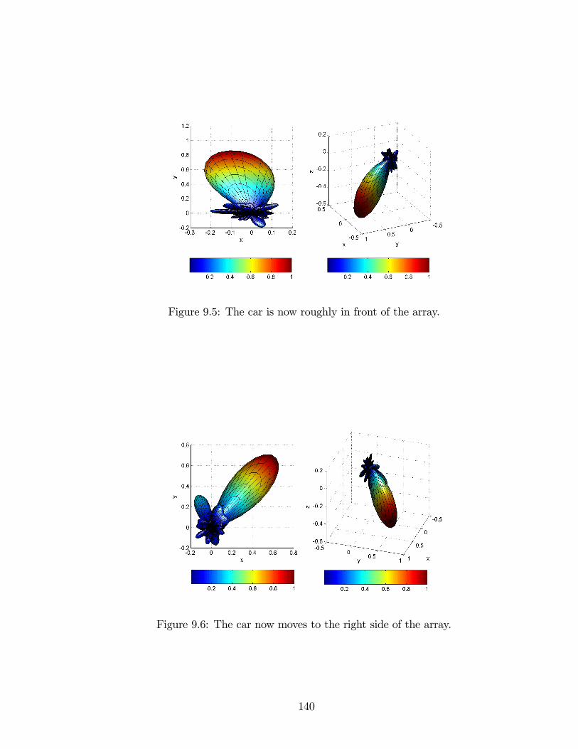
Figure 9.5: The car is now roughly in front of the array.

Figure 9.6: The car now moves to the right side of the array.

140

0 200 400 600 800 1000 1200 1400 16000

0.5

1

1.5

2

2.5

3

Frames

Azim

uth

1st sound source2nd sound source

Figure 9.7: Tracking two vehicles using the spherical microphone array.

141

Chapter 10Conclusions

We have developed the theories and tools for capture and recreation of 3D

auditory scenes. Our contributions are:

1. We propose a flexible and optimal design of spherical microphone arrays for

beamforming. We analyze the discrete orthonormality error of spherical har-

monics and cancel them by several methods. A simplified algorithm is designed

to easily control the robustness of the resulting beamformer. An adaptive im-

plementation is presented. It optimally converges to desired beampatterns

under pre-specified robustness constraint. Design examples and simulation

results are provided.

2. We design and build a hemispherical microphone array using the acoustical

image principle. Simulation and experimental results demonstrate that a hemi-

spherical microphone array with a hard plane is equivalent to a full spherical

array with image microphones and image sound sources. We also use the

hemispherical array to verify our methodology in 1.

3. We propose a pre-computed fast spherical beamforming algorithm. It achieves

fast mixing in time domain.

4. We design the cylindrical beamforming algorithm using a circular microphone

array mounted on a rigid cylinder. It is practical in 2D auditory scenes.

142

5. We design loudspeaker and headphone based algorithms for optimal recreation

of spatial auditory scenes. It exploits the reciprocity between the capture and

recreation processes. In addition, we present an alternative interpretation

using the discrete Huygens principle.

6. We test our spherical microphone array in real-world traffic scenes.

143

Chapter 11On-going and Future Work

The on-going and future work will focus on extending our established work.

Here we just give a short list of some possible researches.

11.1 Multiple Array Data Fusion

Up to now, we only use a single spherical microphone array to capture auditory

scenes. Just like people using multiple cameras in computer vision [26], we can use

more than one array to capture the auditory scene from different locations. The

recordings are expected to deliver more information about the sound source and the

surrounding acoustical environment.

For example, the performance of the spherical microphone array we have dis-

cussed is related to the microphone numbers and the sphere size. To work with

broader band sound signals, we may need a nested spherical microphone array with

each layer has different number of microphones and different radius. Another ex-

ample is that we can use multiple arrays to localize the sound source in 3D space,

not just an angular position.

Since our ultimate goal is to recreate a dynamic 3D auditory scene from record-

ings, we should allow the listener to move in the scene. In [31], HRTFs can be

interpolated and range extrapolated. We believe that we can implement a system

integrating multiple microphone arrays, recreation algorithms, head tracking and

HRTF interpolation and range extrapolation to achieve the dynamic workthrough

144

in 3D auditory scenes.

11.2 3D Sound Texture Resynthesis

Probably the best way to describe sound texture is by examples: crackling fire,

running water, raining, applause, moving vehicle, large group of people chatting, etc.

It is usually monotonic and contains a lot of self-similiar sound frames. The concept

of sound texture is from its counterpart in graphics: image texture.

The analysis and resynthesis of image texture have been extensively explored

in [33][14][51][89][90][83], etc. Recently, sound texture has started to attract some

attentions, such as in [7][69][29]. We plan to follow this direction further into 3D

sound texture using our 3D auditory scene capture and recreation technologies and

tools.

11.3 Complex Environment Analysis

In our experiments with our spherical microphone array, we found the results

are more or less affected by the surrounding environment such as undesired noise,

reflection, etc. While the difference between ideal free space and real-world environ-

ment adds some irregularities in the experimental results, this also provides some

clue about the environment.

11.4 3D Auditory Scene Editing

In a video game, there are only limited set of graphics components created

by laser scanner, camera, or/and modeling software. The editing and resynthesis of

those components give the object astonishing details and dynamics. In addition, to

145

achieve some special visual effects in a movie which is impossible to happen in real

scenes, the editing and resynthesis are the keys.

We want to implement the same functionalities in auditory scenes. In that way,

we only need to make limited set of recordings, then we can generate as many desired

auditory scenes as we need. In addition to beamforming, there are many algorithms

of blind signal separation (BSS) to separate one sound source from the other [16].

Those techniques may let us be able to edit the individual auditory objects in the

recorded scenes. Another application is to migrate the recorded auditory scenes into

a new acoustic environment.

11.5 Real-Time Implementation

For some applications, it is important to process the data in real time. There-

fore, we have to design a highly efficient signal processing unit. This will be ad-

dressed in two parts:

1. Efficient data structure and codec. The raw data recorded by the microphone

array has a large size even for a short time recording. This may be a bottleneck

in the band-limited remote applications such as teleconference. Fortunately,

the multichannel data are apparently redundant in the sense they are highly

correlated to each other. We need to implement an efficient data structure

and codec to store and transmit the recordings.

2. Efficient rendering pipeline on graphics hardware. In previous chapters, we

have made some efforts to design an efficient parallel implementation of multi-

146

directional spherical beamformer and pre-computed fast spherical beamform-

ing. However, the multichannel signal processing is still expensive. To solve

this problem, we will make use of the parallel architecture of the modern

graphics hardware, i.e. the graphics processing unit (GPU). Some examples of

using GPU for general purposes are [56][53].

147

BIBLIOGRAPHY

[1] Ambisonics website. http://www.ambisonic.net.

[2] KEMAR website. http://sound.media.mit.edu/KEMAR.html.

[3] Abhayapala, T. D., and Ward, D. B. Theory and design of high order

sound field microphones using spherical microphone array. In Proceedings of

IEEE International Conference on Acoustics, Speech, and Signal Processing

(ICASSP’02) (May 2002), vol. 2, pp. 1949—1952.

[4] Abramowitz, M., and Stegun, I. A., Eds. Handbook of Mathematical

Functions. U.S. Government Printing Office, 1964.

[5] Algazi, V. R., Avendano, C., and Duda, R. O. Low-frequency ILD

elevation cues. J. Acoust. Soc. Am. 106 (1999), 2237.

[6] Algazi, V. R., Duda, R. O., Thompson, D. M., and Avendano, C. The

CIPIC HRTF database. In Proceedings of IEEE Workshop on Applications of

Signal Processing to Audio and Acoustics (New Paltz, NY, Oct. 2001), pp. 99—

102.

[7] Athineos, M., and Ellis, D. Sound texture modelling with linear prediction

in both time and frequency domains. In Proceedings of IEEE International

Conference on Acoustics, Speech, and Signal Processing (ICASSP2003) (2003),

vol. 5, pp. 648—651.

148

[8] Begault, D. R., Wenzel, E. M., Lee, A. S., and Anderson, M. R.

Direct comparison of the impact of head-tracking, reverberation and individ-

ualized head-related transfer functions on the spatial perception of a virtual

speech source. J. Audio Eng. Soc. 49, 10 (2001), 904—916.

[9] Berkhout, A., Vries, D., and Vogel, P. Acoustic control by wave field

synthesis. Journal of the Acoustical Society of America 93, 5 (May 1993), 2764—

2778.

[10] Blattner, M., Greenberg, R., and Sumikawa, D. Earcons and icons:

Their structure and common design principles. Human Computer Interaction

4, 1 (1989), 11—44.

[11] Blauert, J. Spatial Hearing. MIT Press, Cambridge, MA., 1983.

[12] Bly, S., Frysinger, S. P., Lunney, D., Mansur, D. L., Mezrich, J. J.,

and Morrison, R. C. Readings in Human-Computer Interaction: A Multi-

Disciplinary Approach. Los Altos: Morgan-Kauffman, 1987, ch. Communicat-

ing with Sound, pp. 420—424.

[13] Bolt, R. A. "put-that-there": Voice and gesture at the graphics interface. In

ACM 7th Annual Conference on Computer Graphics and Interactive Techniques

(SIGGRAPH’80) (Seattle, WA, 1980), pp. 262—270.

[14] Bonet, J. D. Multiresolution sampling procedure for analysis and synthesis

of texture images. In Proceedings of SIGGRAPH 1997 (1997).

149

[15] Bradford, J. H. The human factors of speech-based interfaces: A research

agenda. In ACM SIGCHI Bulletin (Apr. 1995), vol. 27, pp. 61—67.

[16] Brandstein, M., and Ward, D., Eds. Microphone Arrays. Springer-Verlag,

New York, 2001.

[17] Brungart, D. S. Auditory localization of nearby sources III: Stimulus effects.

J. Acoust. Soc. Am. 106 (1999), 3589—3602.

[18] Brungart, D. S., and Durlach, N. I. Auditory localization of nearby

sources II: Localization of a broadband source in the near field. J. Acoust. Soc.

Am. 106 (1999), 1956—1968.

[19] Brungart, D. S., and Rabinowitz, W. M. Auditory localization of nearby

sources i: Head-related transfer functions. J. Acoust. Soc. Am. 106 (1999),

1465—1479.

[20] Buxton, W., and Myers, B. A study in two-handed input. In CHI ’86

Conference on Human Factors in Computing Systems (Apr. 1986), pp. 321—

326.

[21] Chen, Y. Highway overhead structure detection using video image sequences.

IEEE Transactions on Intelligent Transportation Systems 4, 2 (June 2003),

67—77.

[22] Cohen, P. R., and Sullivan, J. W. Synergistic use of direct manipulation

and natural language. In CHI’89 (1989), pp. 227—234.

150

[23] Colton, D., and Kress, R. Inverse Acoustic and Electromagnetic Scattering

Theory. Springer-Verlag, New York, 1997.

[24] Cox, H., Zeskind, R. M., and Owen, M. M. Robust adaptive beamforming.

IEEE Transactions on Acoustics, Speech, and Signal Processing ASSP-35, 10

(Oct. 1987), 1365—1376.

[25] Culling, J. F., Hodder, K. I., and Toh, C. Y. Effects of reverberation on

perceptual segregation of competing voices. J. Acoust. Soc. Am. 114 (2003),

2871—2876.

[26] Cutler, R., Duraiswami, R., Qian, J., and Davis, L. Design and im-

plementation of the university of maryland keck laboratory for the analysis of

visual movement. Tech. Rep. CS-TR-4329, Computer Science Dept., Univ. of

Maryland, College Park, MD 20742.

[27] de Vries, D., and Boone, M. Wave field synthesis and analysis using

array technology. In Proceedings of IEEE Workshop on Applications of Signal

Processing to Audio and Acoustics (Oct. 1999), pp. 15—18.

[28] Driscoll, J. R., and D. M. Healy, J. Computing Fourier transforms and

convolutions on the 2-sphere. Adv. Appl. Math. 15 (1994), 202—250.

[29] Dubnov, S., Bar-Joseph, Z., El-Yaniv, R., Lischinski, D., and Wer-

man, M. Synthesizing sound textures through wavelet tree learning. Computer

Graphics and Application (July/August 2002), 38—48.

151

[30] Duraiswami, R., Gumerov, N., Zotkin, D., and Davis, L. Efficient

evaluation of reverberant sound fields. In Proc. 2001 IEEE Workshop on Ap-

plications of Signal Processing to Audio and Acoustics (New Paltz, NY., 2001),

pp. 203—206.

[31] Duraiswami, R., Zotkin, D., and Gumerov, N. Interpolation and range

extrapolation of HRTFs. In Proceedings of IEEE International Conference on

Acoustics, Speech, and Signal Processing (ICASSP2004) (Montreal, Canada,

May 17-21 2004), pp. IV45—IV48.

[32] Eargle, J. Handbook of Recording Engineering. Van Nostrand Reinhold, New

York, NY, USA, 1996.

[33] Efros, A. A., and Leung, T. K. Texture synthesis by non-parametric

sampling. In Proceedings of IEEE International Conference on Computer Vi-

sion(ICCV99) (Corfu, Greece, Sept. 1999), pp. 1033—1038.

[34] Euclid. The Thirteen Books of the Elements: Books X-XIII., vol. 3. Dover,

New York, 1956.

[35] Fliege, J., and Maier, U. A two-stage approach for computing cubature

formulae for the sphere. Tech. Rep. Ergebnisberichte Angewandte Mathematik,

No. 139T, Fachbereich Mathematik, Universität Dortmund, 44221 Dortmund,

Germany, Sept. 1996.

152

[36] Fliege, J., and Maier, U. The distribution of points on the sphere and cor-

responding cubature formulae. IMA Journal on Numerical Analysis 19 (1999),

317—334.

[37] Frauenberger, C., and Noisternig, M. 3d audio interfaces for the blind.

In Proceedings of the 9th International Conference on Auditory Display (July

2003), pp. 280—283.

[38] Frost, O. L. An algorithm for linearly constrained adaptive array processing.

Proceedings of the IEEE 60, 8 (Aug. 1972), 926—935.

[39] Funkhouser, T., Tsingos, N., Carlbom, I., Elko, G., Sondhi, M.,

West, J. E., Pingali, G., Min, P., and Ngan, A. A beam tracing method

for interactive architectural acoustics. J. Acoust. Soc. Am. 115, 2 (Feb. 2004),

739—756.

[40] Gardner, W. G. 3-D Audio Using Loudspeakers. PhD thesis, Dept. of Media

Arts and Sciences, MIT, 1997.

[41] Gardner, W. G. Head tracked 3-d audio using loudspeakers. In Proc. IEEE

Workshop on Applications of Signal Processing to Audio and Acoustics (New

Paltz, NY., 1997).

[42] Gardner, W. G. Reverberation Algorithms. Kluwer Academic, Norwell, MA.,

1998.

[43] Gardner, W. G., and Martin, K. D. HRTF measurements of a KEMAR.

J. Acoust. Soc. Am. 97, 6 (1995), 3907—3908.

153

[44] Gaver, W. W. Synthesizing auditory icons. In SIGCHI Conference on Human

Factors in Computing Systems (Amsterdam, The Netherlands, 1993), pp. 228—

235.

[45] Gerzon, M. Periphony: With-height sound reproduction. J. Audio Eng. Soc.

21 (Jan. 1973), 2—10.

[46] Gilkey, R., and Anderson, T. R., Eds. Binaural and Spatial Hearing in

Real and Virtual Environments. Lawrence Erlbaum Associates, Mahwah, NJ.,

1997.

[47] Gumerov, N. A., and Duraiswami, R. Fast Multipole Methods for

the Helmholtz Equation in Three Dimensions. Elsevier Science, 2005.

ISBN:0080443710.

[48] Hardin, R. H., and Sloane, N. J. A. McLaren’s improved snub cube and

other new spherical designs in three dimensions. Discrete and Computational

Geometry 15 (1996), 429—441.

[49] Hauptmann, A. G. Speech and gestures for graphic image manipulation.

In ACM CHI 89 Human Factors in Computing Systems Conference (1989),

pp. 241—245.

[50] Healy, D., Rockmore, D., and Moor, S. An FFT for the 2-sphere and

applications. In Proceedings of IEEE International Conference on Acoustics,

Speech, and Signal Processing (ICASSP’96) (May 1996), vol. 3, pp. 1323—1326.

154

[51] Heeger, D., and Bergen, J. Pyramid based texture Analysis/Synthesis. In

Proceedings of SIGGRAPH 95 (1995).

[52] Huang, Y., and Benesty, J., Eds. Audio Signal Processing For Next-

Generation Multimedia Communication Systems. Kluwer Academic Publishers,

2004.

[53] J. Bolz, I. Farmer, E. G., and Schroeder, P. Sparse matrix solvers

on the GPU: Conjugate gradients and multigrid. In SIGGRAPH2003 (2003),

pp. 917—924.

[54] Jot, J., and Chaigne, A. Digital delay networks for designing artificial

reverberators. In Proc. Audio Eng. Soc. Conv. (1991).

[55] Jung, Y., Lee, K., and Ho, Y. Content-based event retrieval using sematic

scene interpretation for automated traffic surveillance. IEEE Transactions on

Intelligent Transportation Systems 2, 3 (Sept. 2001), 151—163.

[56] Krueger, J., and Westermann, R. Linear algebra operators for GPU

implementation of numerical algorithms. In SIGGRAPH2003 (2003), pp. 908

— 916.

[57] Kulkarni, A., and Colburn, H. S. Infinite-impulse-response models of the

head-related transfer function. J. Acoust. Soc. Am. 115 (2004), 1714—1728.

[58] Li, Y., Ho, K., and Kwan, C. Design of broad-band circular ring microphone

array for speech acquisition in 3-d. In Proceedings of IEEE International Con-

155

ference on Acoustics, Speech, and Signal Processing (ICASSP’03) (Apr. 2003),

vol. 5, pp. V221—V224.

[59] Li, Z., and Duraiswami, R. Hemispherical microphone arrays for sound cap-

ture and beamforming. In IEEE Workshop on Applications of Signal Processing

to Audio and Acoustics (WASPAA’05) (New Paltz, New York, Oct. 2005).

[60] Li, Z., and Duraiswami, R. Robust and flexible design of spherical micro-

phone arary. IEEE Trans. on Speech and Audio Processing (2005). (submitted).

[61] Li, Z., and Duraiswami, R. A robust and self-reconfigurable design of

spherical microphone array for multi-resolution beamforming. In Proceedings

of IEEE International Conference on Acoustics, Speech, and Signal Processing

(ICASSP’05) (Mar. 2005), vol. IV, pp. 1137—1140.

[62] Li, Z., Duraiswami, R., and Davis, L. S. Recording and reproducing high

order surround auditory scenes for mixed and augmented reality. In IEEE and

ACM International Symposium on Mixed and Augmented Reality (Arlington,

VA, Nov. 2004), pp. 240—249.

[63] Li, Z., Duraiswami, R., Grassi, E., and Davis, L. S. Flexible layout

and optimal cancellation of the orthonormality error for spherical microphone

arrays. In Proceedings of IEEE International Conference on Acoustics, Speech,

and Signal Processing (Montreal, Quebec, Canada, May 17-21 2004), pp. IV41—

44.

156

[64] Li, Z., Duraiswami, R., Grassi, E., and Davis, L. S. A spherical micro-

phone array system for traffic scene analysis. In Proceedings of the 7th IEEE

International Conference on Intelligent Transportation Systems (ITSC2004)

(Washington, DC, October 3-6 2004).

[65] Li, Z., Duraiswami, R., and Gumerov, N. A. Capture and recreation of

higher order 3d sound fields via reciprocity. In Proceedings of the 10th Interna-

tional Conference on Auditory Display (ICAD2004) (Sydney, Australia, July

6-9 2004).

[66] Li, Z., Lee, C. H., and Varshney, A. A real-time seamless tiled display

system for 3d graphics with user interaction. Tech. Rep. CS-TR-4696, CS Dept.,

University of Maryland, 2005.

[67] Li, Z., and Varshney, A. A real-time seamless tiled display for 3d graphics.

In Proceedings of 7th Annual Symposium on Immersive Projection Technology

(IPT 2002) (Orlando, FL, March 24 - 25 2002).

[68] Loomis, J. M. Basic and applied research relating to auditory displays for

visually impaired people. In Proceedings of the 9th International Conference on

Auditory Display (July 2003), pp. 300—302. invited talk.

[69] Lu, L., Li, S., Liu, W., Zhang, H., and Mao, Y. Audio textures. In

Proceedings of IEEE International Conference on Acoustics, Speech, and Signal

Processing (ICASSP2002) (May 2002), vol. 2, pp. 1761—1764.

157

[70] Macpherson, E. A., and Middlebrooks, J. C. Listener weighting of cues

for lateral angle: The duplex theory of sound localization revisited. J. Acoust.

Soc. Am. 111 (2002), 2219—2236.

[71] Meyer, J., and Elko, G. A highly scalable spherical microphone array

based on an orthonormal decomposition of the soundfield. In Proceedings of

IEEE International Conference on Acoustics, Speech, and Signal Processing

(ICASSP’02) (May 2002), vol. 2, pp. 1781—1784.

[72] Mezrich, J., Frysinger, S., and Slivjanovski, R. Dynamic represen-

tation of multivariate time series data. Journal of the Americal Statistical

Association 79 (1984), 34—40.

[73] Middlebrooks, J. C. Virtual localization improved by scaling non-

individualized external-ear transfer functions in frequency. J. Acoust. Soc. Am.

106 (1999), 1493—1510.

[74] Morse, P., and Ingaard, K. Theoretical Acoustics. McGraw Hill, New

York, 1968.

[75] Mynatt, E. D., and Edwards, W. K.Mapping GUIs to auditory interfaces.

In ACM Symposium on User Interface Software and Technology (UIST ’92).

(1992), pp. 61—88.

[76] Ohuchi, M., Iwaya, Y., Suzuki, Y., and Munekata, T. A game for

visually impaired children with a 3-d virtual auditory display. In Proceedings

158

of the 9th International Conference on Auditory Display (July 2003), p. 309.

abstract.

[77] Rafaely, B. Analysis and design of spherical microphone arrays. IEEE Trans-

actions on Speech and Audio Processing 13 (2005), 135—143.

[78] Schoepflin, T., and Dailey, D. Dynamic camera calibration of roadside

traffic management cameras for vehicle speed estimation. IEEE Transactions

on Intelligent Transportation Systems 4, 2 (June 2003), 90—98.

[79] Shaw, E. A. G. Acoustical features of the human external ear. In Binaural and

Spatial Hearing in Real and Virtual Environments, R. Gilkey and T. Anderson,

Eds. Erlbaum, New York, 1997, pp. 25—48.

[80] Shinn-Cunningham, B. G., Kopco, N., and Martin, T. J. Localizing

nearby sound sources in a classroom: Binaural room impulse responses. J.

Acoust. Soc. Am. 117, 5 (May 2005), 3100—3115.

[81] Taylor, M. Cubature for the sphere and the discrete spherical harmonic

transform. SIAM J. Numer. Anal. 32, 2 (1995), 667—670.

[82] Teutsch, H., Spors, S., Herbordt, W., Kellermann, W., and Raben-

stein, R. An integrated real-time system for immersive audio applications. In

Proceedings of IEEE Workshop on Applications of Signal Processing to Audio

and Acoustics (New Paltz, NY, USA, Oct. 2003).

[83] Turk, G. Texture synthesis on surfaces. In Proceedings of SIGGRAPH (2001).

159

[84] Ueberhuber, C. W. Numerical Computation 2: Methods, Software, and

Analysis. Springer-Verlag, Berlin, 1997.

[85] Veen, B., and Buckley, K. Beamforming: A versatile approach to spatial

filtering. IEEE ASSP Magazine (Apr. 1988), 4—24.

[86] Veeraraghavan, H., Masoud, O., and Papanikolopoulos, N. Com-

puter vision algorithms for intersection monitoring. IEEE Transactions on

Intelligent Transportation Systems 4, 2 (June 2003), 78—89.

[87] Walker, J., Sproull, L., and Subramani, R. Using a human face in

an interface. In CHI’94 Human Factors in Computing Systems (Boston, Apr.

1994), pp. 85—91.

[88] Ward, D. B., and Abhayapala, T. D. Reproduction of a plane-wave sound

field using an array of loudspeakers. IEEE Transactions on Speech and Audio

Processing 9, 6 (Sept. 2001), 697—707.

[89] Wei, L.-Y., and Levoy, M. Fast texture synthesis using tree-structured

vector quantization. In Proceedings of SIGGRAPH (2000), pp. 479—488.

[90] Wei, L.-Y., and Levoy, M. Texture synthesis over arbitrary manifold sur-

faces. In Proceedings of SIGGRAPH (2001), pp. 355—360.

[91] Wenzel, E. M., Arruda, M., Kistler, D. J., and Wightman, F. L.

Localization using nonindividualized head-related transfer functions. J. Acoust.

Soc. Am. 94, 1 (1993), 111— 123.

160

[92] Wightman, F. L., and Kistler, D. J. Headphone simulation of free-field

listening. i: Stimulus synthesis. J. Acoust. Soc. Am. 85, 2 (1989), 858—867.

[93] Wightman, F. L., and Kistler, D. J. Headphone simulation of free-field

listening. II: Psychophysical validation. J. Acoust. Soc. Am. 85, 2 (1989), 868—

878.

[94] Wu, H., Siegel, M., and Khosla, P. Vehicle sound signature recogni-

tion by frequency vector principal component analysis. IEEE Transactions on

Instrumentation and Measurement 48, 5 (Oct. 1999), 1005—1009.

[95] Zhao, H., Plaisant, C., Shneiderman, B., and Duraiswami, R. Sonifi-

cation of geo-referenced data for auditory information seeking: Design principle

and pilot study. In 10th International Conference on Auditory Display (Sydney,

Australia, July 2004).

[96] Zhao, H., Plaisant, C., Shneiderman, B., Zotkin, D., and Du-

raiswami, R. Sonification of dynamic choropleth maps: Geo-referenced data

exploration for the vision-impaired. In Proceedings of the 9th International

Conference on Auditory Display (July 2003), p. 307. abstract.

[97] Zotkin, D. N., Duraiswami, R., and Davis, L. S. Rendering localized

spatial audio in a virtual auditory space. IEEE Transactions on Multimedia 6,

4 (Aug. 2004), 553—564.

161

[98] Zotkin, D. N., Duraiswami, R., Grassi, E., and Gumerov, N. A. Fast

head related transfer function measurement via reciprocity. J. Acoust. Soc. Am.

(2005). submitted.

162

THE CAPTURE AND RECREATION OF 3D AUDITORY ...

Documents

Transcript of THE CAPTURE AND RECREATION OF 3D AUDITORY ...