The butterfly did it: The aberrant vote for Buchanan in Palm Beach County, Florida

The Butterfly Did It: The Aberrant Vote for Buchanan in Palm BeachCounty, FloridaJONATHAN N. WAND Cornell UniversityKENNETH W. SHOTTS Northwestern UniversityJASJEET S. SEKHON Harvard UniversityWALTER R. MEBANE, JR. Cornell UniversityMICHAEL C. HERRON Northwestern UniversityHENRY E. BRADY University of California, Berkeley

W e show that the butterfly ballot used in Palm Beach County, Florida, in the 2000 presidentialelection caused more than 2,000 Democratic voters to vote by mistake for Reform candidate PatBuchanan, a number larger than George W. Bush’s certified margin of victory in Florida. We use

multiple methods and several kinds of data to rule out alternative explanations for the votes Buchananreceived in Palm Beach County. Among 3,053 U.S. counties where Buchanan was on the ballot, PalmBeach County has the most anomalous excess of votes for him. In Palm Beach County, Buchanan’sproportion of the vote on election-day ballots is four times larger than his proportion on absentee(nonbutterfly) ballots, but Buchanan’s proportion does not differ significantly between election-day andabsentee ballots in any other Florida county. Unlike other Reform candidates in Palm Beach County,Buchanan tended to receive election-day votes in Democratic precincts and from individuals who voted forthe Democratic U.S. Senate candidate. Robust estimation of overdispersed binomial regression modelsunderpins much of the analysis.

Beginning on election day November 7, 2000,Palm Beach County (PBC), Florida, attractednational and eventually international attention

because thousands of voters in the county complainedthat they had difficulty understanding the now infa-mous butterfly ballot. As a result, they claimed thatthey had cast invalid or erroneous presidential votes.Lawyers working for the Democratic Party reportedlycollected 10,000 affidavits sworn by voters with com-

plaints about some aspect of their election-day experi-ences in the county (Associated Press 2000b; Firestone2000a, 2000b; Van Natta 2000; Van Natta and Moss2000). Shortly after election day, eleven groups of PBCvoters filed independent lawsuits seeking relief, claim-ing they and others had made mistakes in their votesfor president because of the confusing format of theballot.1 Many of them stated that they had intended tovote for Democratic candidate Al Gore but by mistakechose Reform candidate Pat Buchanan. The number ofvotes involved was more than enough to have tippedthe presidential vote in Florida from Republican can-didate George W. Bush to Gore, thus giving himFlorida’s 25 electoral votes and the presidency.2

PBC is a heavily Democratic, politically liberalcounty that conventional wisdom says should providefew Buchanan votes. Two days after the election, BayBuchanan, Pat Buchanan’s sister and campaign man-ager, said “she was startled to hear Bush strategist KarlRove argue Thursday that Buchanan has strong sup-port in a county where his campaign never bought anad and never paid a visit” (Garvey 2000).3 Yet, the

Jonathan N. Wand is a doctoral candidate, Department of Govern-ment, Cornell University; Lamarck Inc., 171 Newbury Street, 5th Floor,Boston, MA 02116 ([email protected]). Kenneth W. Shotts is AssistantProfessor of Political Science, Northwestern University, Evanston, IL60208-1006 ([email protected]). Jasjeet S. Sekhon is AssistantProfessor of Government, Harvard University, 34 Kirkland Street,Cambridge, MA 02138 ([email protected]). Walter R. Me-bane, Jr., is Associate Professor of Government, Cornell University,Ithaca, NY 14853-4601 ([email protected]). Michael C. Herron isAssistant Professor of Political Science, Northwestern University,Evanston, IL 60208-1006 ([email protected]). Henry E.Brady is Professor of Political Science, University of California,Berkeley, CA 94720-5100 ([email protected]).

Herron worked on this paper while a Postdoctoral ResearchFellow at the Center for Basic Research in the Social Sciences,Harvard University. Previous versions were presented at the 2001Joint Statistical Meetings, American Statistical Association, SocialStatistics Section, Atlanta, GA, August 5–9, and at the 2001 annualmeeting of the Public Choice Society, San Antonio, TX, March 9–11.The authors, who are listed in reverse alphabetical order, served asunpaid expert witnesses in Case CL 00-10992AF in the FifteenthJudicial Circuit of Florida, West Palm Beach: Beverly Rogers and RayKaplan v. The Palm Beach County Elections Canvassing Commission;et al. (see Brady et al. 2001). The authors thank Todd Rice andLamarck, Inc., for their generous support and provision of comput-ing resources, Kevin Matthews of the Department of Geography,George Mason University, for mapmaking services, Benjamin Bishinand Laurel Elms for research assistance, and seminar participants atColumbia University, Cornell University, Harvard University, andNorthwestern University for helpful comments.

1 The cases filed in the Fifteenth Judicial Circuit of Florida, WestPalm Beach, were CL 00-10965, CL 00-10970, CL 00-10988AE, CL00-109922AF, CL 00-11000AH, CL 00-11084AH, CL 00-11098AO,CL 00-1146AB, CL 00-1240AB, CL 00-129OAB, and CL 00-113O2AO. These were consolidated by Administrative Order No.2.061-11/00. Texts of the filings and of the Fifteenth Circuit Courtrulings in the cases are available from http://www.pbcountyclerk.com/.2 Bush received 271 electoral votes, one more than needed to win,and Gore received 266. One Elector pledged to Gore from Wash-ington, DC, left her ballot blank, reducing Gore’s count from 267(Mitchell 2001; Stout 2000).3 The story further observes that “longtime Reform members in thestate described a party in ‘disarray’ with little organization, much less

American Political Science Review Vol. 95, No. 4 December 2001

793

county supplied 19.6% of Buchanan’s votes in Florida.In contrast, only 5.4% of his Florida votes came fromPBC in the 1996 Republican presidential primary,which did not use a butterfly ballot.4

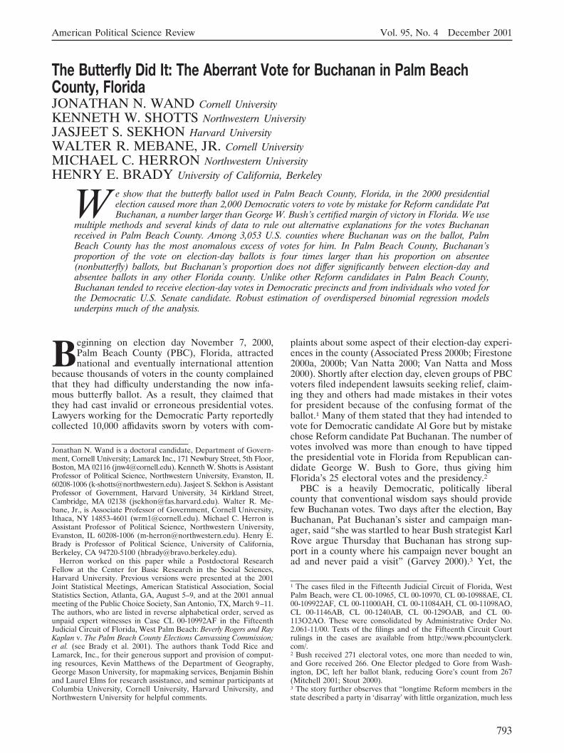
The butterfly ballot, shown in Figure 1, was aninnovation of Theresa LePore, Supervisor of Electionsfor PBC.5 The distinctive format was used only in PBCand only for election-day ballots for president. It is a“butterfly” because two columns of names of candi-dates (the wings of the butterfly), all for the sameoffice, sandwich a single column of punch holes be-tween the names. These punch holes are alternately forthe left-hand and right-hand side of the ballot. Thus,the first valid punch hole (identified on the ballot as#3) is for Bush, the first candidate on the left-handside. The second valid punch hole (identified on theballot as #4) is for Buchanan, the first candidate on theright-hand side. On the left, however, the second

candidate listed is Gore, and someone who scanneddown the left-hand column without looking to the rightcould mistakenly conclude that the first two punchholes corresponded, respectively, to Bush and Gore.Having made such an incorrect reading, a Bush voterwould still be likely to punch the first hole, but a Gorevoter might mistakenly punch the second and vote forBuchanan.

Sinclair et al. (2000) report experimental evidencethat a double-column ballot format like the one used inPBC can be more confusing and cause more votererrors than a single-column ballot. Other publishedresearch on the effects of ballot design is scarce anddoes not provide much guidance regarding the errorsthe PBC butterfly ballot may have induced (Campbelland Miller 1957; Darcy 1986; Hamilton and Ladd1996).

Did the butterfly ballot cost Gore the presidency?The lawsuits filed by citizens of PBC were thrown outbecause the Supreme Court of Florida ruled that theballot was not illegal,6 but the ruling neither dependedupon nor implied anything about the ballot’s effect on

a groundswell of support for Buchanan in a place even he concedesis not his base.”4 In 2000, Buchanan received 0.787% of the presidential vote in PBCwhile garnering only 0.3% of the overall Florida presidential vote. Incontrast, Ross Perot, the Reform candidate for president in 1996,received only 7.7% of the PBC vote and garnered 9.1% of the Floridavote. These data are from the Florida Department of State.5 Reportedly, LePore “split the names over two pages to make thetype larger.” Two days after the election she was quoted as saying:“Hindsight is 20-20, but I’ll never do it again” (Engelhardt 2000).Merzer and Miami Herald (2001) describe how LePore went aboutdesigning the ballot and many other defects in the administration ofthe election in Florida.

6 The court stated: “Even accepting appellants’ allegations, weconclude as a matter of law that the Palm Beach County ballot doesnot constitute substantial noncompliance with the statutory require-ments mandating the voiding of the election” (Supreme Court ofFlorida, Fladell, et al. v. Palm Beach County Canvassing Board, etc. etal. Case Nos. SC 00-2373 and SC 00-2376). The cases did notprogress to hearings regarding the facts.

FIGURE 1. The Palm Beach County Bufferfly Ballot

Source: AP Worldwide Photos, Gary I. Rothstein. Reprinted with permission.

The Butterfly Did It: The Aberrant Vote for Buchanan in Palm Beach County, Florida December 2001

794

voter behavior. The court did not rule on whether Gorelost the election because of the ballot. Our goal is toinvestigate that question by determining whether thebutterfly ballot caused several thousand Gore support-ers to vote mistakenly for Buchanan.

OVERVIEW

Among scholars who posted an analysis on the Internetshortly after the election, a consensus quickly formedthat the vote for Buchanan in PBC was anomalouslylarge. Of the 3,407 votes that Buchanan received in theinitial, uncertified count of PBC ballots, a typicalestimate was that he received about 2,800 more votesthan were to be expected based on voting patternselsewhere in Florida.7 The number of apparently acci-dental votes for Buchanan exceeded Bush’s officialmargin of victory in Florida, which was only 537 votesmore than Gore.8 But the early analysis did not showunambiguously that the butterfly ballot was the causeor that the erroneous Buchanan votes would otherwisehave gone to Gore.

To test whether Democratic voters mistakenly votedfor Buchanan because of the butterfly ballot, we usemultiple methods and diverse data sources to rule outalternative explanations for the Buchanan vote in PBC.First, we show that Buchanan’s vote was anomalouslyhigh on election day. Specifically, we prove three keyfacts. (1) Anomalies in the Buchanan vote as large asthe one in PBC did not occur in any other county in thecountry in 2000. (2) The vote for the Reform candidatein the previous presidential election, Ross Perot, wasnot anomalous in PBC in 1996. (3) PBC voters whoused election-day ballots (the butterfly format) re-corded unusually high support for Buchanan, whilethose who used absentee ballots (no butterfly format)evinced the expected level of support for him.

Second, we show that Buchanan’s excess of supportwas almost entirely from Democratic voters. Here wedemonstrate two key facts. (1) The unusually high levelof support for Buchanan was concentrated in precinctswith high levels of support for Democratic candidatesfor other offices and not in precincts with high levels ofsupport for Reform candidates for other offices. (2)Individual ballots confirm these patterns: Democraticvoters (as measured by votes in the U.S. Senateelection) who voted on election day were much morelikely to support Buchanan than were Democraticvoters who used absentee ballots. We conclude that thebutterfly ballot caused at least 2,000 Democratic votersto vote mistakenly for Buchanan.

Our conclusions depend upon repeated compari-sons: across counties, between election-day ballots andabsentee ballots, and across precincts. To determinewhether the Buchanan vote is anomalous, we comparethe actual number of votes received by Buchanan in acounty to the votes predicted by a well-specified statis-tical model that uses past votes and demographiccharacteristics of all the counties in the same state toform estimates. When actual votes deviate significantlyfrom what is expected, we have what statisticians callan outlier. Then, to isolate sharply the effect of thebutterfly format, we compare Buchanan’s share of thevotes on election day to his share on absentee ballotsacross all Florida counties. Next, to determine whetherBuchanan’s votes in PBC were concentrated in areaswith high levels of support for Democratic candidates,we compare how well Democratic strength in a pre-cinct predicts Buchanan votes versus votes for Reformcandidates for other offices. Finally, we use a compar-ison between Buchanan votes on individual election-day (butterfly) and absentee (nonbutterfly) ballots tocompute our minimum estimate for the number ofDemocratic voters the butterfly ballot caused to votemistakenly for Buchanan instead of Gore.

A simple way to estimate the expected votes forBuchanan is to take the percentage of Buchanan votersin each county and regress it, using ordinary leastsquares (OLS), on past votes and demographic char-acteristics. Then an examination of the differencebetween the actual and expected vote might tell uswhether the county was anomalous. This proceduremight be misleading, however, because of three majorstatistical problems. First, the counties differ in size—the smallest have only a few hundred voters, while thelargest have millions—leading to the problem of het-eroskedasticity. Second, heteroskedasticity is exacer-bated because the expected proportion of votes forBuchanan varies over counties. Third, because OLS isnotoriously subject to outliers, any OLS-based esti-mates designed to detect them are suspect. All threeproblems must be solved in order to get reliable results.

To understand why differing county size is a prob-lem, consider a hypothetical example. Suppose thereare two counties, in both of which Buchanan is ex-pected to receive 1% of the vote. One county has 100voters, so the expected Buchanan vote is one, and theother has 100,000 voters, so the expected vote forBuchanan is 1,000. In the small county a 2% excess ofvotes over the expected value corresponds to an ob-served total of three Buchanan votes: (3 � 1)/100 �100% � 2%. In the large county an observed vote of3,000 for Buchanan would be required to produce thesame 2% discrepancy. But two “extra” Buchanan votesby chance in the small county are much more likelythan an extra 2,000 in the large county. For instance,using a simple binomial model for the count of votesfor Buchanan, the z-score for the discrepancy is (3 �1)/�100 � .01 � .99 � 2 in the small county but(3000 � 1000)/�100000 � .01 � .99 � 64 in the largecounty.

To avoid the heteroskedasticity problem, we use ageneralization of the standard binomial model to esti-

7 In Brady et al. (2001) we list the early posters, including ourselves.Brady posted analysis on November 9, and Wand, Shotts, Sekhon,Mebane, and Herron posted on November 11. Lists of empiricalwork posted on the Internet through the end of November 2000,appear at http://www.bestbookmarks.com/election (created byJonathan O’Keeffe), http://www.sbgo.com/election.htm (created bySebago Associates), and http://madison.hss.cmu.edu (created byGreg Adams and Chris Fastnow).8 The final, certified results gave Bush 2,912,790 votes and Gore2,912,253 votes in Florida. A few days after the election, theAssociated Press reported a vote margin of 327 based on the initial,automatic recount across Florida (Wakin 2000).

American Political Science Review Vol. 95, No. 4

795

mate expected vote counts, and we use statistics thatadjust for the counts’ variances when making compar-isons across counties. In the model the probability of avote is a function of past votes and demographicfactors. The variance of the vote count can be greaterthan in a standard binomial model. The resultingmodel is called an overdispersed binomial model. Thestatistics we compare across counties are studentizedresiduals (Carroll and Ruppert 1988, 31–4), which aredefined as the simple difference between observed votecount and expected vote count, divided by the esti-mated standard deviation of the observed count.

The overdispersed binomial regression model treatsthe count of votes for Buchanan in a particular geo-graphic area as having the mean and variance of abinomial random variable, except that the variance ismultiplied by a constant scale factor. As described indetail by McCullagh and Nelder (1989, 125), the scalefactor may reflect a process in which each vote count isa sum of vote counts produced at lower levels ofaggregation, where each lower-level aggregate is abinomial random variable. According to such a moti-vation for the model the binomial distribution thatdescribes each lower-level count may have a distinctprobability parameter (p. 125). In this way the over-dispersed binomial model recognizes the heterogeneityamong the clusters of voters whose choices comprisethe vote counts we analyze. We describe the overdis-persed binomial model in greater detail in Appendix A.

The most important methodological innovation inour analysis is that we develop new methods for robustestimation of the overdispersed binomial regressionmodel. These guard against the possibility, which isvery real with OLS estimation, that an outlier maydestroy the estimation. Without robust methods, asingle large outlier may mask other outliers (Atkinson1986), which means that the distorted data appear tobe the norm rather than the exceptions. Masking alsomay occur when there are several outliers that aresimilar in magnitude. For instance, in the simplest caseof estimating the average for a set of numbers, it is easyto see that the sample mean can be greatly affected bya single exceptionally large value. Masking occurs whenthis one very large point so greatly alters the samplemean that other large but smaller points do not appearto be as discrepant as they truly are from the meanvalue that characterizes most of the sample data.Similarly, masking can occur when a few exceptionallylarge or small data points, all of about the same size,pull the sample mean toward themselves so that noneof them are far from the sample mean value, althoughin fact they do not represent the same statisticaldistribution as the rest of the data. Masking makes itdifficult to determine which data points really dodeviate from what we should expect.

The primary reason to use robust estimators in thePBC situation is that the voter complaints, legal cases,and media reports strongly suggest that the electoralresults there were produced by processes substantiallydifferent from the standard political factors (partisan-ship, liberalism-conservatism, policy positions) thatcause voters to act predictably from one election to

another and that produced the results elsewhere inFlorida. We want our models to predict what wouldhave happened without idiosyncratic factors such as aconfusing ballot form. Significant departures fromthose predictions will indicate that idiosyncratic factorsmust be at work.

Data weakness is another reason for robust estima-tion. Because our models are based on the results fromother elections, anomalies in those elections will give adistorted picture of the standard political factors thatpredict the vote in the current one. The robust estima-tors we use protect against the influence of suchdistortions. A county in which the previous electionresults are highly distorted will not affect the parameterestimates and, indeed, will itself appear to be anoutlier. We describe our robust estimation methods inmore detail in Appendix A.

BUCHANAN’S VOTE IN COUNTIES ACROSSTHE UNITED STATES

To assess how excessive Buchanan’s PBC vote appearsto be when compared to outcomes across the countryin 2000, we use the overdispersed binomial regressionmodel to estimate the expected number of votes castfor Buchanan out of all votes cast for Buchanan, Gore,Bush, Ralph Nader (Green Party), Harry Browne(Libertarian Party), Howard Phillips (Constitution Par-ty), John Hagelin (Natural Law Party), or any write-incandidates. We predict votes for Buchanan, given thetotal number of votes cast for all presidential candi-dates, in each U.S. county in 2000.9 Two kinds ofinformation, the results of previous elections and thedemographic characteristics of the county, are avail-able and highly relevant for making such predictions.The previous election outcome is a proxy not only forthe array of interests and party sentiments in eachcounty but also for the strength of local party mobili-zation. We use two variables to represent the precedingelection result: the proportion of votes officially re-ceived by the Republican candidate in the 1996 presi-dential election; and the proportion of votes officiallyreceived by the Reform Party candidate in the 1996presidential election. We supplement them with a setof nine demographic variables. Seven of the variablescome from the 2000 Census of Population and Hous-ing: the proportions of county population in each offour Census Bureau race categories (namely, white,black, Asian and Pacific Islander, and American Indianor Alaska Native); 2000 proportion Hispanic; 2000population density (computed as 2000 population/1990square miles); and 2000 population.10 The eighth andninth are the 1990 proportion of population with acollege degree and 1989 median household money

9 We ignore undervotes (no apparent vote recorded on the ballot),overvotes (votes for more than one presidential candidate on a singleballot), and other spoiled ballots. For discussions of undervotes andovervotes in PBC see Engelhardt and McCabe 2001a, 2001b.10 The 2000 Census data were built from Census 2000 RedistrictingData (Public Law 94–171) Summary File, Matrices PL1, PL2, PL3,and PL4 (U.S. Census Bureau, 2001, “FactFinder Tables,” accessedApril 7, 2001, at http://factfinder.census.gov).


796

income. We do not use the number of voters registeredas Reform Party members because voter registration isnonpartisan in many states.

We cannot use all eleven variables (plus a constant)in our models at once, because we estimate the modelseparately for each state (except for four states that wepool because each has only a few counties; see below),and with that many variables a state would need tohave about 40 to 60 counties to produce reliableestimates. But 21 states (including the District ofColumbia) have fewer than 50 counties. Therefore, weinclude the two vote proportion variables in all themodels and use principal components of the demo-graphic data. To maximize the efficiency of the infor-mation gained from the demographic variables, wecompute principal components of the set of residualsobtained by regressing each demographic variable onthe previous election proportion variables and theconstant.11 The regressions on the election variablesand the computation of principal components are doneseparately for each state.

For the results of the county-level analysis that wereport in detail here, we use only the first principalcomponent of the Census data. As we explain below,using more principal components does not substan-tively change the results that bear on PBC. Hence, theexpected vote for Buchanan in county i in the givenstate is based on a linear predictor defined by:

xi�� 0 � �1 x1i � �2 x2i � �3 x3i,

where x1i is the 1996 proportion of votes received bythe Republican candidate, x2 i is the 1996 proportion ofvotes received by the Reform candidate, x3i is theprincipal component, and �0, �1, �2, and �3 are con-stant coefficients.

We compare PBC to the 3,053 counties in theUnited States for which we can robustly estimate theoverdispersed binomial model and hence computestudentized residuals. Because they have too few coun-ties to analyze separately, we pool the data for Con-necticut, Delaware, Hawaii, and Rhode Island (whichhave, respectively, eight, three, four, and five counties),using dummy variables to give each state a differentintercept but requiring the other coefficients to be thesame for all four states.12 The dependent variable is thecount yi of votes for Buchanan in each county i in the2000 election. The studentized residuals are compara-ble across states.13

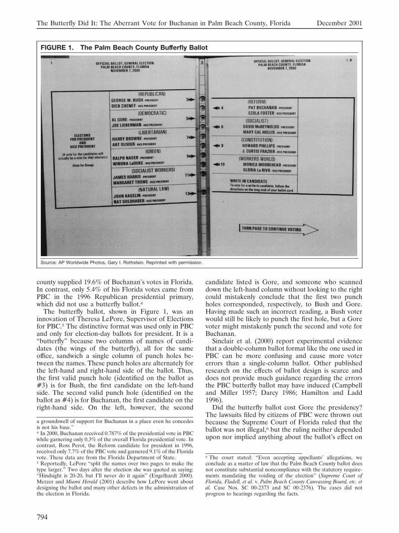
PBC has the largest residual14 among the 3,053counties in our analysis. This result can be seen in

Figure 2, which presents boxplots that display thedistribution of the residuals for each state.15 Theresidual for PBC not only has the largest positive valuebut also is the largest in absolute magnitude. Buchananreceived vastly more votes in PBC than predicted bythe county’s electoral history and demographic profile.

Appendix Table B-1 lists the residuals, expectedBuchanan vote proportion, actual Buchanan vote pro-portion, and number of valid presidential ballots for allcounties for which the residual is greater than 4.0 orless than �4.0, namely, all the outliers. There are 68positive outliers and eight negative outliers. The dif-ference between the number of positive and the num-ber of negative outliers reflects the overall positiveskew of the residuals that is visible for most states inFigure 2. Outliers occur in 31 of the 49 states coveredby the analysis.

The outlier status of some counties is readily ex-plained. Jasper County, South Carolina, which has thesecond largest residual in our analysis, did not receivemuch national media attention because the outcomewas immaterial to the 2000 presidential contest. Bushdefeated Gore in South Carolina by 220,376 votes, butonly 6,469 presidential ballots were cast in JasperCounty. Nonetheless, there were serious problems witha voting machine in the county’s Tillman precinct,where Gore and Bush each received one vote,Buchanan 239 votes, and Nader 111 votes. The prob-lems in the precinct affected vote totals for otheroffices. Indeed, “the State Board of Canvassers unani-mously said [. . .] that problems in the county councilelection were so numerous that a new election shouldbe held.”16

PBC is not geographically contiguous to any otheroutlier, but many of the counties listed in Table B-1 arecontiguous to another outlier. Table 1 displays the setsof counties from Table B-1 that are geographicallycontiguous. Sixteen of the twenty-five largest positiveoutliers belong to such a cluster. Two clusters includecounties from two states (West Virginia and Ohio,Kansas and Missouri), and another includes countiesfrom three states (South Dakota, Iowa, and Nebraska).Because these span state borders, it is highly unlikelythat the exceptional support for Buchanan reflectsproblems of ballot format or electoral administration.Most likely the reason is special success in mobilizingvoters for Buchanan in those areas.

Plausible explanations also can be produced forsome of the remaining outliers, but we do not empha-size these because the residuals for all of those countiesare much smaller than that for PBC, and some outliersare not stable over variations in the model specifica-tions. In contrast, the size and relative position of theresiduals are stable for counties such as PBC or Jasper,for which voting irregularities were reported, or Han-cock County in West Virginia and Pottawatomie

11 We standardize the residuals of the demographic variables to havevariance equal to 1.0 before computing the principal components.12 With only one county, the District of Columbia cannot be ana-lyzed. Our collection of counties (or equivalents) includes all statesexcept Michigan, where Buchanan was not on the ballot and couldreceive only write-in votes. For Alaska we use the 25 county-equivalents defined by the U.S. Census Bureau for reporting 1990Census data.13 We use the final, certified vote counts for each state. See AppendixB for data sources.14 Throughout the rest of this article the word residual always refersto the studentized residual, as defined in Appendix A, equation A-1,unless otherwise indicated.

15 Whiskers extend to the nearest value not beyond 1.5 times theinterquartile range. The residuals for the pooled states (CT, DE, HI,and RI) are omitted.16 See the December 28, 2000, issue of the Beaufort Gazette andAssociated Press 2000a for allegations regarding the Tillman pre-cinct.


797

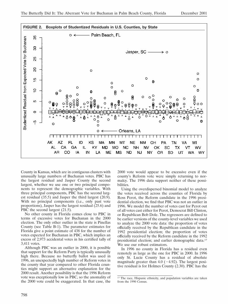
County in Kansas, which are in contiguous clusters withunusually large numbers of Buchanan votes. PBC hasthe largest residual and Jasper County the secondlargest, whether we use one or two principal compo-nents to represent the demographic variables. Withthree principal components, PBC has the second larg-est residual (35.5) and Jasper the third largest (20.9).With no principal components (i.e., only past voteproportions), Jasper has the largest residual (25.6) andPBC the second largest (21.5).

No other county in Florida comes close to PBC interms of excessive votes for Buchanan in the 2000election. The only other outlier in the state is PinellasCounty (see Table B-1). The parameter estimates forFlorida give a point estimate of 438 for the number ofvotes expected for Buchanan in PBC, which implies anexcess of 2,973 accidental votes in his certified tally of3,411 votes.

Although PBC was an outlier in 2000, it is possiblethat support for the Reform Party is typically unusuallyhigh there. Because no butterfly ballot was used in1996, an unexpectedly high number of Reform votes inthe county that year compared to other Florida coun-ties might support an alternative explanation for the2000 result. Another possibility is that the 1996 Reformvote was exceptionally low in PBC, so the anomality ofthe 2000 vote could be exaggerated. In that case, the

2000 vote would appear to be excessive even if thecounty’s Reform vote were simply returning to nor-malcy. The 1996 data support neither of these possi-bilities.

Using the overdispersed binomial model to analyzethe votes received across the counties of Florida byRoss Perot, the Reform candidate in the 1996 presi-dential election, we find that PBC was not an outlier in1996. We model the number of votes cast for Perot outof all votes cast either for Perot, Democrat Bill Clinton,or Republican Bob Dole. The regressors are defined tobe earlier versions of the county-level variables we usedto analyze the 2000 vote data: the proportion of votesofficially received by the Republican candidate in the1992 presidential election; the proportion of votesofficially received by the Reform candidate in the 1992presidential election; and earlier demographic data.17

We use our robust estimators.In 1996 no county in Florida has a residual even

remotely as large as the one for PBC in 2000. In 1996only St. Lucie County has a residual of absolutemagnitude greater than 4.0 (�4.92). The largest posi-tive residual is for Holmes County (2.30). PBC has the

17 The race, Hispanic ethnicity, and population variables are takenfrom the 1990 Census.

FIGURE 2. Boxplots of Studentized Residuals in U.S. Counties, by State


798

seventh most negative residual (�1.86). PBC was notan outlier in 1996.

The 2000 vote for Buchanan in PBC was extremelyunusual—clearly, among the most unusual in the en-tire country. The vast difference between the residualfor PBC and the residuals for the other countiesconfirms that a large anomaly occurred relative to thevote predicted for Buchanan based on PBC’s votinghistory and demographic profile.

A NATURAL EXPERIMENT: FLORIDA’SELECTION-DAY AND ABSENTEE VOTERSIN 2000

Buchanan’s vote total in PBC in the 2000 presidentialelection was anomalously large, but how can we be surethat the cause was the butterfly ballot? Because thatformat was not used for absentee ballots, the electiongives us a natural experiment: One group of PBCvoters (election day) used a butterfly ballot but asecond group (absentee) did not. If Buchanan’s votetotal in the county reflects true support among thevoters, then this support should be present in bothpools of ballots. But if the butterfly ballot is responsiblefor Buchanan’s vote then his support should comedisproportionately from votes on election day.

A limitation of this natural experiment is that themechanism that allocates voters to either the election-day pool or the absentee pool is not random assign-ment (Achen 1986). Voters self-select to be in theabsentee group.18 Some, such as military personnelstationed overseas, must cast absentee ballots. Absen-tee voters may not be representative of voters ingeneral, but there are good reasons to believe that theinfluences on their voting behavior are similar acrossthe counties. PBC’s absentee voters are probably sim-ilar to those in at least some of the other counties, andwe would expect their level of support for Buchanan tobe similar as well. Therefore, if we take the differencebetween the proportion of those voting for Buchananon election day and the proportion voting for him onabsentee ballots, PBC’s difference should cluster withthe differences for other counties, unless somethinglike the butterfly ballot has caused it to be distinctlydifferent.

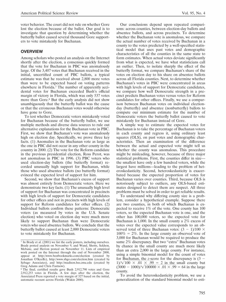
This difference analysis shows disproportionate sup-port for Buchanan among election-day voters in PBC.Figure 3 plots the difference—election-day proportionminus absentee proportion—for all 67 counties ofFlorida by the number of presidential ballots cast ineach county.19 One can see that PBC has one of thelargest differences in the state, although four countieshave larger differences, and a few others have differ-ences close in value to that of PBC.20 But in all thosecounties the voting population is much smaller than inPBC, where 433,186 ballots were cast for president. InCalhoun, the largest county with a difference greaterthan PBC’s, there were 5,174 ballots cast for president.

The significance of the population size disparity isthat even if voting processes are identical in all thecounties, there will be greater variability in the differ-

18 According to 2000 Florida Statutes, title IX, chapter 101.62, aregistered voter need not give any reason for requesting an absenteeballot.19 The data are based on certified numbers from the Florida Depart-ment of State and precinct-level returns provided by the 67 Floridacounties. We used the precinct data to calculate the absentee returns.20 The difference in PBC is 0.00634 (433,186 presidential ballots),exceeded by Liberty (0.0177, 2,410 ballots), Calhoun (0.00959, 5,174ballots), Hamilton (0.00731, 3,964 ballots), and Dixie (0.00706, 4,666ballots). Union and Baker counties have the next largest differencesafter PBC, in both cases 0.00620. The numbers of presidential ballotscast in those counties were, respectively, 3,826 and 8,154.

TABLE 1. Contiguous Counties amongThose with the Largest Studentized Residualsfor the Buchanan VoteState County NameOH HockingOH Athens

MD WicomicoMD Somerset

SD UnionIA SiouxNE DixonNE ThurstonNE DakotaIA PlymouthIA Woodbury

MT Deer LodgeMT Silver Bow

KS WabaunseeKS ShawneeKS Pottawatomie

CO ArapahoeCO JeffersonCO Adams

KY KentonKY Boone

WI WoodWI LincolnWI Marathon

KS WyandotteMO Jackson

OH BelmontWV OhioWV MarshallOH JeffersonWV BrookeWV Hancock

MO St. Louis CityMO St. Louis

MN RamseyMN Hennepin

Note: Results based on 3,053 counties. This table presents all contig-uous counties with studentized residuals of magnitude greater than orequal to 4.0.


799

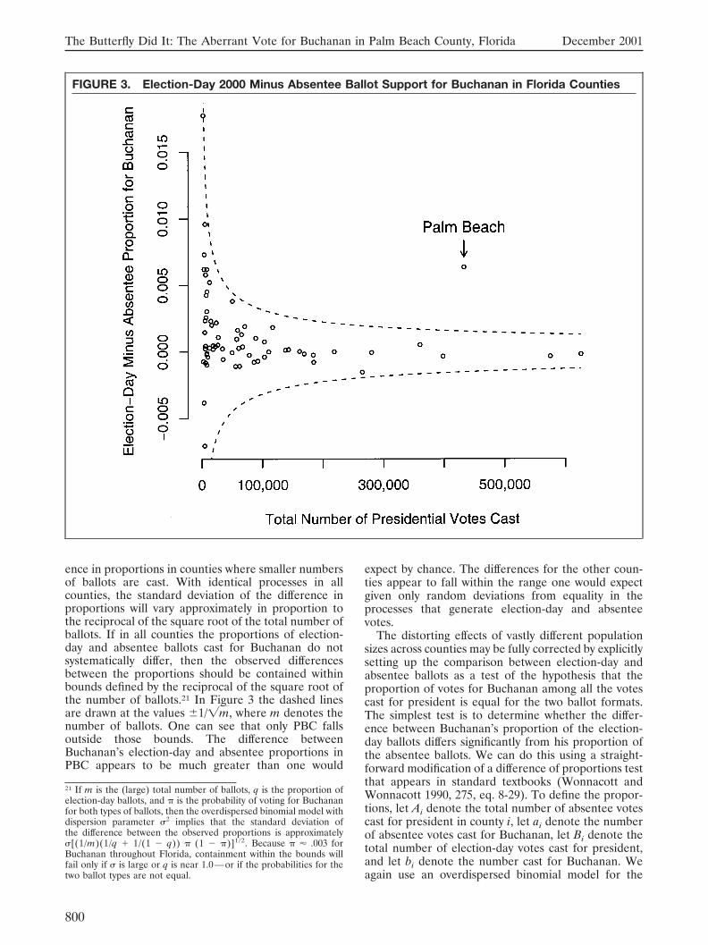
ence in proportions in counties where smaller numbersof ballots are cast. With identical processes in allcounties, the standard deviation of the difference inproportions will vary approximately in proportion tothe reciprocal of the square root of the total number ofballots. If in all counties the proportions of election-day and absentee ballots cast for Buchanan do notsystematically differ, then the observed differencesbetween the proportions should be contained withinbounds defined by the reciprocal of the square root ofthe number of ballots.21 In Figure 3 the dashed linesare drawn at the values �1/�m, where m denotes thenumber of ballots. One can see that only PBC fallsoutside those bounds. The difference betweenBuchanan’s election-day and absentee proportions inPBC appears to be much greater than one would

expect by chance. The differences for the other coun-ties appear to fall within the range one would expectgiven only random deviations from equality in theprocesses that generate election-day and absenteevotes.

The distorting effects of vastly different populationsizes across counties may be fully corrected by explicitlysetting up the comparison between election-day andabsentee ballots as a test of the hypothesis that theproportion of votes for Buchanan among all the votescast for president is equal for the two ballot formats.The simplest test is to determine whether the differ-ence between Buchanan’s proportion of the election-day ballots differs significantly from his proportion ofthe absentee ballots. We can do this using a straight-forward modification of a difference of proportions testthat appears in standard textbooks (Wonnacott andWonnacott 1990, 275, eq. 8-29). To define the propor-tions, let Ai denote the total number of absentee votescast for president in county i, let ai denote the numberof absentee votes cast for Buchanan, let Bi denote thetotal number of election-day votes cast for president,and let bi denote the number cast for Buchanan. Weagain use an overdispersed binomial model for the

21 If m is the (large) total number of ballots, q is the proportion ofelection-day ballots, and � is the probability of voting for Buchananfor both types of ballots, then the overdispersed binomial model withdispersion parameter 2 implies that the standard deviation ofthe difference between the observed proportions is approximately[(1/m)(1/q 1/(1 � q)) � (1 � �)]1/2. Because � � .003 forBuchanan throughout Florida, containment within the bounds willfail only if is large or q is near 1.0—or if the probabilities for thetwo ballot types are not equal.

FIGURE 3. Election-Day 2000 Minus Absentee Ballot Support for Buchanan in Florida Counties


800

totals ai and bi, with statewide dispersion parameter 2.Because Ai and Bi are large, the equality hypothesisimplies that the following z-score is normal with meanzero and unit variance:

zi � �1�bi/Bi � ai/Ai

� �bi/Bi �1 � bi/Bi

Bi�

�ai/Ai �1 � ai/Ai

Ai��1/2

If zi is significantly greater than zero, then in propor-tional terms election-day voters cast ballots forBuchanan much more often than did absentee voters.If zi is significantly less than zero, then support forBuchanan was disproportionately great among absen-tee voters. To compute zi we need an estimate of . Weuse the estimate of the scale parameter that we ob-tained for the 2000 Florida data when we estimated thecounty-level overdispersed binomial model. That esti-mate is � 3.81.

PBC has zi � 6.3, a value more than six standarddeviations away from the value of zero that is expectedunder the equality hypothesis. The next largest positivevalue among the remaining counties of Florida is 1.65,and 58 counties have a z-score of magnitude less than1.0. Only one negative value, a z-score of �1.1 forDuval County, is more than one standard deviationaway from zero.

In PBC, election-day votes went to Buchanan vastlymore often, in proportional terms, than did absenteevotes. The results of the election-day versus absenteeballot natural experiment strongly support the conclu-sion that Buchanan’s anomalous support was caused bythe butterfly ballot.

Underlying the dramatic test statistic value for PBCis the fact that county voters supported Buchanan onelection day at a rate (.0085) approximately four timesthat of absentee voters (.0022). If election-day votershad cast ballots for Buchanan at the rate that absenteevoters did, he would have received 387,356 � 0.0022 �854 election-day votes. In fact he received 3,310 elec-tion-day votes. By this method one might gauge thenumber of accidental votes for Buchanan because ofthe butterfly ballot as follows: 3,310 � 854 � 2,456votes.

PRECINCT-LEVEL ANALYSIS OF PALMBEACH COUNTY RETURNS

Who made the mistakes on the butterfly ballot? Was itvoters who favored Bush or those who wanted to votefor Gore? At an intuitive level, mistakes seem lesslikely for Bush voters, who had to match the firstcandidate with the first punch hole, than for Gorevoters, who had to match the second candidate with thethird punch hole. Furthermore, it was a large numberof Democratic voters who complained that the ballotcaused them to vote for Buchanan by mistake. None-theless, it is important to examine the possibility thatBuchanan received votes intended for both candidates.

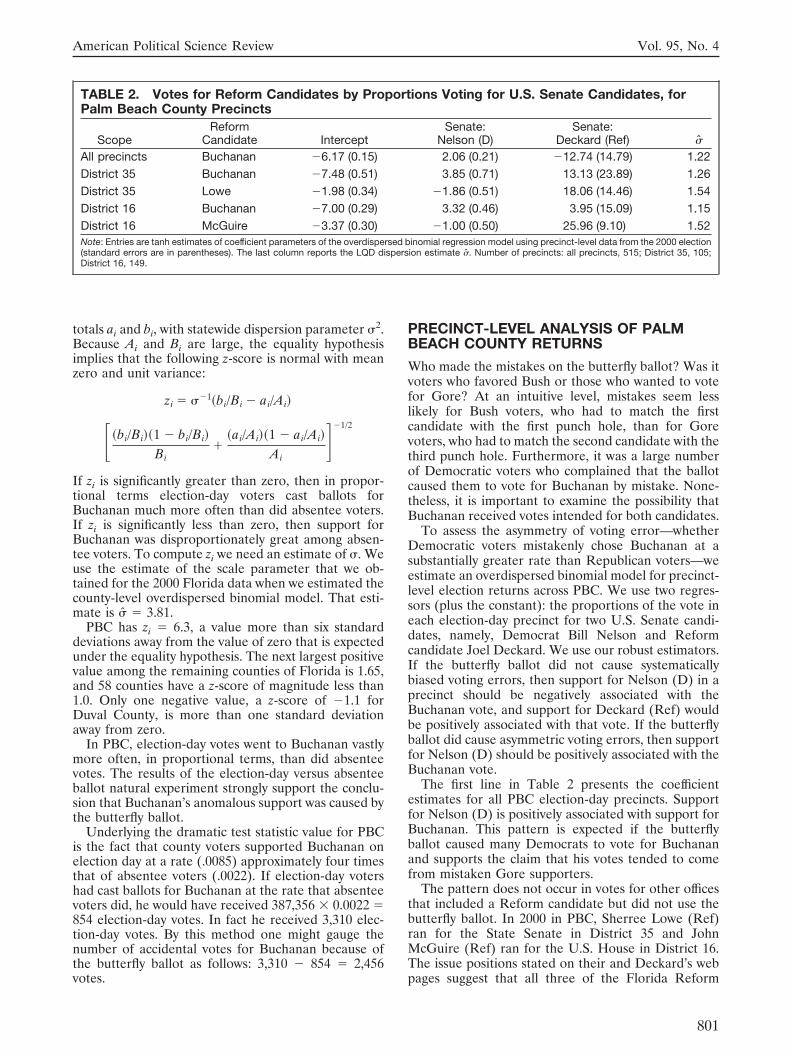
To assess the asymmetry of voting error—whetherDemocratic voters mistakenly chose Buchanan at asubstantially greater rate than Republican voters—weestimate an overdispersed binomial model for precinct-level election returns across PBC. We use two regres-sors (plus the constant): the proportions of the vote ineach election-day precinct for two U.S. Senate candi-dates, namely, Democrat Bill Nelson and Reformcandidate Joel Deckard. We use our robust estimators.If the butterfly ballot did not cause systematicallybiased voting errors, then support for Nelson (D) in aprecinct should be negatively associated with theBuchanan vote, and support for Deckard (Ref) wouldbe positively associated with that vote. If the butterflyballot did cause asymmetric voting errors, then supportfor Nelson (D) should be positively associated with theBuchanan vote.

The first line in Table 2 presents the coefficientestimates for all PBC election-day precincts. Supportfor Nelson (D) is positively associated with support forBuchanan. This pattern is expected if the butterflyballot caused many Democrats to vote for Buchananand supports the claim that his votes tended to comefrom mistaken Gore supporters.

The pattern does not occur in votes for other officesthat included a Reform candidate but did not use thebutterfly ballot. In 2000 in PBC, Sherree Lowe (Ref)ran for the State Senate in District 35 and JohnMcGuire (Ref) ran for the U.S. House in District 16.The issue positions stated on their and Deckard’s webpages suggest that all three of the Florida Reform

TABLE 2. Votes for Reform Candidates by Proportions Voting for U.S. Senate Candidates, forPalm Beach County Precincts

ScopeReform

Candidate InterceptSenate:

Nelson (D)Senate:

Deckard (Ref) �

All precincts Buchanan �6.17 (0.15) 2.06 (0.21) �12.74 (14.79) 1.22District 35 Buchanan �7.48 (0.51) 3.85 (0.71) 13.13 (23.89) 1.26District 35 Lowe �1.98 (0.34) �1.86 (0.51) 18.06 (14.46) 1.54District 16 Buchanan �7.00 (0.29) 3.32 (0.46) 3.95 (15.09) 1.15District 16 McGuire �3.37 (0.30) �1.00 (0.50) 25.96 (9.10) 1.52Note: Entries are tanh estimates of coefficient parameters of the overdispersed binomial regression model using precinct-level data from the 2000 election(standard errors are in parentheses). The last column reports the LQD dispersion estimate �. Number of precincts: all precincts, 515; District 35, 105;District 16, 149.


801

candidates were in sympathy with the Buchanan fac-tion. For instance, all were pro-life and looked askanceat free trade. Deckard went so far as to expressconcerns about legal immigration.22

We robustly estimate two models for election-dayprecincts in PBC in each district. In both districts weanalyze the votes received by Buchanan. For District 35we also analyze the votes received by Lowe (Ref), andfor District 16 we analyze the votes for McGuire (Ref).Because the butterfly ballot was used only for thepresidential vote, we expect support for Nelson (D) tobe negatively associated with support both for Lowe(Ref) and for McGuire (Ref).

The coefficient estimates in Table 2 match thoseexpectations, while in both districts support for Nelson(D) remains positively associated with the Buchananvote. These results support the claim that the butterflyballot caused systematic, biased voter errors that costGore more votes than Bush. Democratically inclinedprecincts (as measured by the Nelson [D] vote propor-tion) have fewer votes for Reform candidates in gen-eral (i.e., Lowe and McGuire) but have more votes forBuchanan. The difference is the butterfly ballot.

These findings refute one possible explanation forthe positive association between Nelson’s vote shareand Buchanan votes, which is that Reform Party mem-bers in PBC tend to live among Democrats. Such anexplanation is contradicted by the negative associationbetween the proportion of votes for Nelson (D) andthe votes for Lowe (Ref) and for McGuire (Ref).

We also can refute another class of alternativeexplanations for Buchanan’s vote total in PBC: It mayhave been caused by a group of anomalous precinctswithin the county. In other words, anomalous resultsconcentrated within a few precincts would suggest thatexcess votes were the result of localized phenomenarather than the butterfly ballot which was used uni-formly throughout the county. For example, malfunc-tioning vote machines—such as the one in Tillmanprecinct in Jasper County, South Carolina—could haverecorded extra votes for Buchanan in a few precincts.Merzer and the Miami Herald (2001, 78–80) documentthe existence of malfunctioning machines in numerousPBC precincts: 96 of 462 ballots from tests conductedimmediately before polls opened showed failures. Orthere may have been intentional fraud in a few pre-cincts. Finally, pockets of intense election-day Reformmobilization could have delivered the extra votes.

Such explanations, however, are quite difficult toreconcile with our precinct-level findings. Given ouruse of a robust estimator, the coefficient estimates inTable 2 would not be affected by a few precinct-levelanomalies produced by irregular voting processes.23

Moreover, a localized mobilization effort should affectoutcomes in multiple races, but the peculiar relation-

ship between Nelson (D) vote share and Reform voteis present only in the presidential race, which used thebutterfly ballot.24

COMPARISON USING INDIVIDUAL PALMBEACH COUNTY BALLOTS

We extend our analysis to ballot-level data from PBC,25

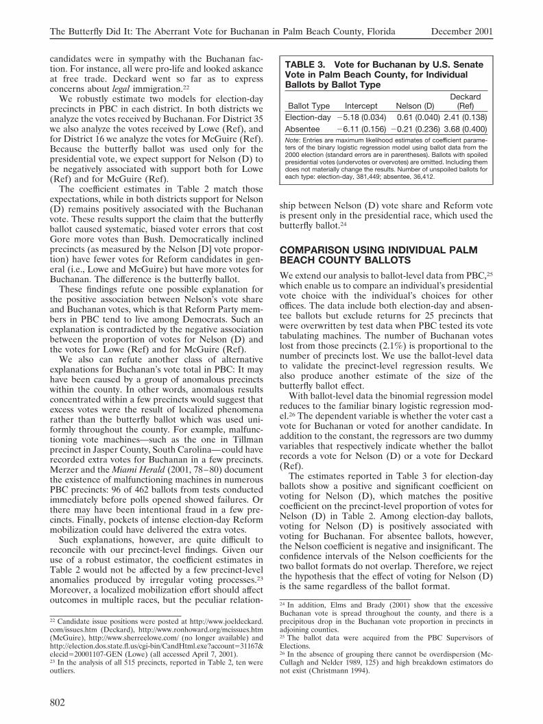
which enable us to compare an individual’s presidentialvote choice with the individual’s choices for otheroffices. The data include both election-day and absen-tee ballots but exclude returns for 25 precincts thatwere overwritten by test data when PBC tested its votetabulating machines. The number of Buchanan voteslost from those precincts (2.1%) is proportional to thenumber of precincts lost. We use the ballot-level datato validate the precinct-level regression results. Wealso produce another estimate of the size of thebutterfly ballot effect.

With ballot-level data the binomial regression modelreduces to the familiar binary logistic regression mod-el.26 The dependent variable is whether the voter cast avote for Buchanan or voted for another candidate. Inaddition to the constant, the regressors are two dummyvariables that respectively indicate whether the ballotrecords a vote for Nelson (D) or a vote for Deckard(Ref).

The estimates reported in Table 3 for election-dayballots show a positive and significant coefficient onvoting for Nelson (D), which matches the positivecoefficient on the precinct-level proportion of votes forNelson (D) in Table 2. Among election-day ballots,voting for Nelson (D) is positively associated withvoting for Buchanan. For absentee ballots, however,the Nelson coefficient is negative and insignificant. Theconfidence intervals of the Nelson coefficients for thetwo ballot formats do not overlap. Therefore, we rejectthe hypothesis that the effect of voting for Nelson (D)is the same regardless of the ballot format.

22 Candidate issue positions were posted at http://www.joeldeckard.com/issues.htm (Deckard), http://www.ronhoward.org/mcissues.htm(McGuire), http://www.sherreelowe.com/ (no longer available) andhttp://election.dos.state.fl.us/cgi-bin/CandHtml.exe?account�31167&elecid�20001107-GEN (Lowe) (all accessed April 7, 2001).23 In the analysis of all 515 precincts, reported in Table 2, ten wereoutliers.

24 In addition, Elms and Brady (2001) show that the excessiveBuchanan vote is spread throughout the county, and there is aprecipitous drop in the Buchanan vote proportion in precincts inadjoining counties.25 The ballot data were acquired from the PBC Supervisors ofElections.26 In the absence of grouping there cannot be overdispersion (Mc-Cullagh and Nelder 1989, 125) and high breakdown estimators donot exist (Christmann 1994).

TABLE 3. Vote for Buchanan by U.S. SenateVote in Palm Beach County, for IndividualBallots by Ballot Type

Ballot Type Intercept Nelson (D)Deckard

(Ref)Election-day �5.18 (0.034) 0.61 (0.040) 2.41 (0.138)Absentee �6.11 (0.156) �0.21 (0.236) 3.68 (0.400)Note: Entries are maximum likelihood estimates of coefficient parame-ters of the binary logistic regression model using ballot data from the2000 election (standard errors are in parentheses). Ballots with spoiledpresidential votes (undervotes or overvotes) are omitted. Including themdoes not materially change the results. Number of unspoiled ballots foreach type: election-day, 381,449; absentee, 36,412.


802

Table 4 shows the proportion of votes in PBC goingto Buchanan among all ballots that record U.S. Senatevotes for either Nelson (D) or Deckard (Ref). Theproportions show that PBC voters who support theDemocratic Senate candidate are significantly morelikely to vote for Buchanan on the butterfly ballot thanare their counterparts who use the absentee ballot—indeed, six times more likely. Fewer than two in onethousand absentee voters in PBC who vote for Nelson(D) also vote for Buchanan, but among election-dayNelson voters the figure is ten in one thousand. If wetreat the absentee proportion as the proportion ofvotes truly intended to go to Buchanan, then about 8.5of every 1,000 Nelson voters in PBC—about 2,300voters—appear to have voted mistakenly forBuchanan.27 Because most (89.6%) absentee Nelsonvoters voted for Gore, we can further conclude that atleast 2,000 of the 2,300 would have been Gore votes.

In contrast, Table 4 shows that individuals who votefor Deckard (Ref) are more likely to vote forBuchanan on the absentee ballot. Deckard voters whosupport Buchanan should not be affected by the but-terfly ballot, and the difference between election-dayand absentee Buchanan vote proportions is small.

The ballot data add to the evidence that the butterflyballot caused systematic voting errors in PBC that costGore votes. In particular, these data help rule out thepossibility that Buchanan’s exceptional support in thecounty was a result of populist appeals he made orpolicy positions he took that Democrats found attrac-tive. The ballot data show that the appeals wouldsomehow have to have been effective for Democratswho voted on election day but not Democrats who usedan absentee ballot.

We gain analytical precision with the ballot data, butthe ballot-level analysis complements rather than re-places the county and precinct analyses presentedabove. Ballot-level data are rarely retained or madeavailable after an election, so it is not generally possibleto compare these results across states or counties.Without such comparisons, the ballot-level results mustbe considered with some caution. Moreover, ballotdata from 2% of the precincts in PBC are not available,but no data are missing for our precinct-level analysis.

Also, unlike the county and precinct analysis, theanalysis of individual ballots cannot use robust estima-tion techniques. In the absence of robust—high break-down point—results, it would have been possible toclaim that the aberrations we found may be limited toa few idiosyncratic precincts and not characteristic ofPBC as a whole. But the aberrations prevail through-out the county.

CONCLUSION

We have examined the source of the anomalous sup-port for Buchanan in PBC by focusing on allegationsthat the county’s use of a butterfly ballot causedsystematic voting errors that boosted the number ofvotes for Buchanan.28 Robust estimation of overdis-persed binomial regression models showed that, withrespect to the Reform vote in 2000, PBC is the largestoutlier among all counties in the United States we wereable to examine. We also showed that PBC was not aReform vote outlier in 1996, a presidential year inwhich the county did not use a butterfly ballot. In somecounties around the country we found clear auxiliaryevidence of problems with ballots, voting machines, orelection administration. In still others there are strongindications that Buchanan received an exceptionalnumber of votes because he had exceptional politicalsupport in those places. There is no reason to believethat he had such mobilized support in PBC.

Having confirmed that in 2000 PBC was an outlier,we sought to verify whether the butterfly ballot was thecause. A comparison of election-day versus absenteeballot results across all Florida counties shows thatBuchanan’s success in PBC did not extend to absenteevoters, who did not use the butterfly ballot. We exam-ined the claim that Democratic presidential candidateAl Gore in particular was harmed by the butterflyballot. We found that Buchanan’s support in PBCtended to come from more Democratic precincts andfrom those who voted for the Democratic candidate forthe U.S. Senate, which supports the claim that mis-taken votes for Buchanan tended to come from Goresupporters.

Was the butterfly ballot pivotal in the 2000 presiden-tial race? The evidence is very strong that it was. HadPBC used a ballot format in the presidential race thatdid not lead to systematic biased voting errors, ourfindings suggest that, other things equal, Al Gorewould have won a majority of the officially certifiedvotes in Florida.

Our analysis complements the efforts of mediagroups to inspect ballots throughout Florida in order toassess what result would have been produced by com-pleting the recount that the U.S. Supreme Courtterminated, or by conducting a count using uniformstandards throughout the state. As of this writing onlythe results of a statewide inspection conducted by the

27 This number is calculated by 269,835 � 0.0085 � 2,294. Thenumber 269,835 is the total Nelson (D) received in the entire countyon election day, including the precincts missing from the ballot data.

28 A related allegation is that the PBC ballot led to excessiveovervoting in the presidential race (Merzer and Miami Herald 2001).The subject of overvoting is beyond the scope of this article (recallfootnote 9; also see Bridges 2001).

TABLE 4. Proportion Voting for Buchanan byU.S. Senate Vote Choice and Ballot Type inPalm Beach County

SenateCandidate

Election-Day Ballots Absentee Ballots

Proportion N Proportion NBill Nelson (D) 0.0102 228,455 0.0017 17,779Joel Deckard

(Ref) 0.0590 1,000 0.0808 99Note: Entries are the proportion of ballots with a vote for Buchanan outof the N ballots of each type voted for each Senate candidate, usingballot data from the 2000 election. Ballots with spoiled presidentialvotes (undervotes or overvotes) are omitted.


803

Miami Herald have been reported.29 Our analysis an-swers a counterfactual question about voter intentionsthat such investigations cannot resolve. The inspectionsmay clarify the number of voters who marked theirballot in support of the various candidates, but theinspections cannot tell us how many voters markedtheir ballot for a candidate they did not intend tochoose.

Citing the results from various scenarios in whichvotes were counted using one of several reasonableuniform standards, the Herald concludes “After studyand analysis of 111,261 overvotes and 64,826 under-votes, [. . .] the outcome still depends on the standardused to gauge undervotes. Gore wins narrowly undertwo undervote standards, by margins of 332 and 242votes; Bush wins narrowly under two other undervotestandards, by 407 and 152 votes (Merzer 2001a; seealso Merzer 2001b). Evidently, the number of votesthat were intended for Gore but that went to Buchananbecause of the butterfly ballot is large enough to havechanged the election outcome given any of severalreasonable standards that might have been used tocount the votes in Florida.

Although we focus here on the butterfly ballot inPBC, our methods could be used on a regular basis aspart of an ongoing effort to identify election anomaliesand improve the administration of elections by elimi-nating such anomalies. Our robust estimation andoutlier detection methods offer an accurate and pow-erful technology for detecting irregular vote outcomes.But determining why a particular irregularity occursrequires a strategy of triangulation, such as the one wepursue here. Different models and different types ofdata need to be marshaled to eliminate plausiblealternative explanations. In the case of PBC and the2000 presidential election, such a strategy leads to theconclusion that “the butterfly did it.”

APPENDIX A: STATISTICAL MODEL ANDESTIMATION METHODS

The Overdispersed Binomial RegressionModelThe overdispersed binomial regression model is defined asfollows. Let i indicate one of n geographic areas, i � 1, . . . ,n. Let yi denote the count of votes for Buchanan in area i, andlet mi denote the total number of ballots cast for all presi-dential candidates in area i. Given mi and a probability value�i, the expected value of yi is

E�yi P mi, � i � mi� i,

and the variance of yi is

E�� yi � mi�i 2 P mi, �i, 2� � 2 mi�i �1 � �i ,

with 2 � 0 (McCullagh and Nelder 1989, 125, eq. 4.20). If2 � 1, then the variance is the same as the variance of astandard binomial random variable. If 2 � 1, then there isoverdispersion relative to a purely binomial model. Theprobability value �i is a logistic function of a linear predictordenoted xi

��, where xi is a vector of k regressors, and � is an

unknown constant vector of coefficient parameters. Theprobability �i is defined by:

� i �1

1 � exp� � xi��

.

We do not treat the overdispersed binomial model as fullycharacterizing a likelihood function for the data. We treat themodel as what McCullagh and Nelder (1989) describe as a“quasi-likelihood.” As they explain (pp. 323–48), under fairlymild conditions estimates of parameters of the mean that arebased on a quasi-likelihood have desirable properties, such asasymptotic unbiasedness, asymptotic optimality, and asymp-totic normality. In the current analysis, the quasi-likelihoodapproach means that we assume only that the mean andvariance formulas we define are good descriptions of thedata. In fact, by using the robust estimation methods definedbelow, we assume somewhat less than that and still obtainestimates with good statistical properties. We require onlythat the mean and variance formulas are good descriptionsfor most of the observed vote counts in each collection ofdata for which we estimate parameters. In the analysis ofcounty-level data, this means that the model is good for mostof the counties in each state, and in the analysis of data forPBC precincts, for most of the precincts in PBC.

The idea that the model is good for most of the data doesnot mean that the model fully characterizes the process thatgenerated most of the vote counts. Obviously, the process isvastly more complicated than our spare model specificationscould possibly represent in full. Rather, the idea is that ourestimator of the model’s parameters converges asymptoti-cally to a unique value for each parameter. In the theory ofrobust estimation this idea is made precise by the assumptionthat a probability model exists relative to which the estimatoris Fisher consistent (Hampel et al. 1986, 82). If applied to allthe data, that property would be for all practical purposes thesame as the unique identifiability and convergence propertiesthat White (1994) demonstrates are necessary for what hecalls a “quasi maximum likelihood estimator” (QMLE) tohave good statistical properties.30 The robust estimationmethods we use have good statistical properties even whenthe property holds only for a majority of the observations.

Robust EstimationBreakdown Points. The key property of the robust estima-tors we use is that they have a high breakdown point. In afinite sample, the breakdown point of an estimator is thesmallest proportion of the observations that must be replacedby arbitrary values in order to force the estimator to producevalues arbitrarily far from the parameter values that gener-ated the original data (Donoho and Huber 1983). Thegeneral concept of breakdown point (e.g., the asymptoticbreakdown point) has the same connotation, although exten-sive technical apparatus is required to achieve full generality(Hampel 1971). To illustrate the breakdown point idea, weconsider again the case of estimating the average for a set ofnumbers. For concreteness, suppose that the numbers origi-nate from an unbiased sample of size n from a process thathas mean zero and finite variance. As an estimator of the truemean, the sample mean has a breakdown point of 1/n,because only one of the n data points needs to be replaced to

29 See Miami Herald 2001 and Merzer and Miami Herald 2001.

30 The McCullagh and Nelder (1989) concept of quasi-likelihood,which has to do with using a model that one believes is correct onlyfor the first two moments of the data (the mean and covariancematrix), is not the same as the QMLE of White (1994), which has todo with the asymptotic properties of a model that is misspecified.


804

force the sample mean to take a value arbitrarily far from thetrue mean. If one data point is replaced with another valuefar from zero but all the other data remain unchanged, thenthe value of the sample mean moves toward the distorteddata value; if the distorted data value is moved indefinitely farfrom zero, the sample mean moves indefinitely far from zero.Asymptotically, as the sample size n increases to infinity, thesample mean has a breakdown point of zero, because 1/n 20. The same is true for any least-squares estimator or, indeed,for any estimator that always puts positive weight on all theobserved data. In contrast, as an estimator of the true meanin our example, the sample median has a breakdown point of1/2. In order to move the sample median arbitrarily far fromthe true mean of zero, at least half the data points have to bereplaced with values arbitrarily far from zero.

The highest possible asymptotic breakdown point for anestimator of a regression model’s mean parameters is 1/2. Weuse estimators that achieve that maximum for all possibleways of distorting the data. We do not use the well-knownminimum absolute deviations estimator (also known as theL1 estimator) because it has a breakdown point of only 1/nrelative to distortions of the regressors (Rousseeuw andLeroy 1987, 10–2). A robust estimator called least median ofsquares (LMS) (Rousseeuw 1984) does achieve the maxi-mum breakdown point and is widely used. Western (1995)discusses high breakdown estimation of linear models usingLMS and suggests an approach to robust estimation ofgeneralized linear models. Christmann (1994) discusses ap-plication of LMS to a grouped binomial model (albeitwithout overdispersion). But LMS converges more slowlyand is less efficient than the estimators we use.

The high breakdown point of the estimators we use meansthat the estimates of model parameters remain stable evenwhen unusual voting processes occur in several of the ngeographic areas for which we are estimating the model.When we use the estimates to compute studentized residualsfor counties, a large anomaly in one county will not maskcomparable or perhaps somewhat smaller anomalies thatoccur in other counties. Hampel et al. (1986, 67) discuss therelationship between the breakdown point and masking.Without a high breakdown point estimator we would under-estimate the frequency of highly anomalous election results.When we directly interpret the parameters of precinct-levelmodels, large departures from the model in several precinctswill not make the interpretations untrustworthy.

The robust methods we use also perform well in theabsence of anomalies. If there are no anomalies, the robustestimator is consistent and is almost as efficient as anestimator, such as simple iteratively reweighted least squares,that ignores the possibility of anomalous observations.

Two Robust Estimators. To obtain robust estimates of theparameters of the overdispersed binomial model, we com-bine two different estimators. We use one to estimate thescale, � �2, and the vector of coefficients, �, and then weuse a second to obtain a much more efficient estimate of �.The second estimator depends on the first one’s estimate ofthe scale, . The first estimator is called the least quartiledifference (LQD) estimator (Croux, Rousseeuw, and Hossjer1994; Rousseeuw and Croux 1993), and the second is calledthe hyperbolic tangent (tanh) estimator (Hampel, Rous-seeuw, and Ronchetti 1981).

Both estimators minimize functions of particular forms ofresiduals. Given a vector of estimates �, let �i � [1 exp(�xi

�/�)]�1 denote the estimated probability of voting forBuchanan in geographic area i. The residual that we use inthe LQD estimator is:

r*i �yi � mi� i

�mi� i�1 � � i .

Ordinarily, with an overdispersed binomial model in theabsence of outliers, a good moment estimator for 2 may bedefined in terms of ri* (McCullagh and Nelder 1989, 126–7,eq. 4.23). The distributional assumption we make is that formost of the observations i, computing ri* with � � � wouldproduce a set of independent normal random variables eachhaving variance 2. If the distributional assumption held forall the observations, including in the asymptotic limit as n1�, then the LQD estimate, , would be consistent for thescale . If some observations (up to half the data) do notsatisfy the distributional assumption, then asymptotically thedifference between and remains bounded. The LQDestimator is defined by choosing � to minimize approximatelythe first quartile of the set of absolute differences{�ri

* � rj*�: i � j} Further details are given below.

Given a scale estimate , the tanh estimator for � is basedon the residual:

ri �yi � mi� i

�mi� i�1 � � i .

The tanh estimator uses a function �(ri) to downweightobservations that have large residuals. The weight applied toeach observation is defined by:

wi � ��ri /ri, for ri � 01, for ri � 0.

The definition of � has a complicated functional form that westate in equation A-2. Here we characterize the weight valuesthat � implies. The weights change qualitatively at thresholdsdefined by two constants, p � 1.8 and c � 4.0) (we furtherexplain the constants below). Observations that have residu-als in the range �p � ri � p have wi � 1: They are notdownweighted. Observations that have residuals in the rangep � �ri� � c have weights that gradually diminish to zero as �ri�approaches c. Observations that have residuals of magnitudegreater than c, meaning c � �ri�, have wi � 0. The tanhestimator completely rejects such observations so that theyhave no effect on the tanh estimate �.

We define an outlier to be any observation that has wi � 0.The usual method used to estimate an overdispersed

binomial regression model is an iteratively reweighted least-squares algorithm, which is equivalent to maximum likeli-hood estimation of the coefficients of a standard binomialregression model with the dispersion 2 estimated subse-quently (McCullagh and Nelder 1989, 114–28). To imple-ment the tanh estimator we modify that algorithm by weight-ing observation i by wi, with wi computed using the coefficientestimates from the previous iteration and the LQD estimate. The estimate of remains unchanged throughout theestimation. Numerical convergence is required for both the �values and the weights. To start the iterations we use theLQD estimates for the initial coefficients and use the LQDvalues (ri

* � mediri*)/ for an initial set of residuals ri (medi

ri* denotes the median of the ri

* values, i�1, . . . ,n).To estimate the asymptotic variance of the coefficient

estimates and hence standard errors, we use the sandwichestimator avar(�) � 2J�1IJ�1, where I is the outer productof the score, and J is the Hessian for a standard binomiallikelihood evaluated at �, weighting each observation by wi.Justification for this estimate, based on White (1994), ap-pears below.

Studentized Residuals Definition. To define the studentizedresiduals that we use to compare counties, we adjust the


805

residuals ri for variation associated with each county’s regres-sors. We use the usual adjustment for the influence (orleverage) each observation yi has on the estimated expectedvote counts mi�i, modified to take into account the weightingthat occurs with the tanh estimator via wi. The adjustment isa function of quantities hi, which are defined as follows.Using W to denote a diagonal matrix that has diagonal entriesWii � wi, V to denote a diagonal matrix with Vii � [mi�i (1 ��i)]�1/2, and X to denote the n � k matrix of the regressors(row i of X is xi

�), define the matrix H � VX(X�VWVX)�1X�V. If no observations are downweighted, sothat wi � 1 for all i � 1, . . . , n, then H is the matrix definedin equation 12.3 of McCullagh and Nelder (1989, 397). Inthat case, each diagonal element of H (i.e., Hii) measures theinfluence of yi on mi�i. When observation i is downweighted(wi � 1), the influence interpretation still applies when wi �0. If wi � 0, then yi has no effect on mi�i, and �Hii measureserror variation associated with forecasting observation i.Hence we define hi � Hii if wi � 0 and hi � �Hii if wi �0, and the studentized residual is:

r i � ri /�1 � hi. (A-1)

The adjustment by (1 � hi)�1/2 makes the variance of the

residuals ri constant for all observations that have wi � 0, i �1, . . . , n. For the outliers (wi � 0) we do not make anyclaim about what distribution the residuals may have, but theadjustment should at least reduce one source of variationamong them.

Because in the county-level analysis we estimate the pa-rameters of the model separately for each state (except forfour states that have few counties), the studentized residualsfor counties in a state that are not outliers all have the samevariance and so are directly comparable. Across states thevariances differ slightly because of the following technicalvariations in the sampling distributions. The variance foreach state is approximately the variance of a t-distributionwith degrees of freedom equal to the number of counties inthe state that are not outliers. We do not attempt to adjust forthat source of variation across states because it is negligiblecompared to the variation caused by the seriously anomalousprocesses that occurred in some counties, turning them intooutliers. In no case would one expect to observe a residual ofmagnitude greater than 4.0—which would make the countyan outlier—for a nonanomalous county.

Robust Estimation Method DetailsThe LQD Estimator and Its Properties. One may understandthe LQD estimator intuitively as an extension of the idea ofusing the interquartile range to estimate the dispersion of aset of data. The LQD estimator focuses on the (2

hk) orderstatistic of the set {� ri

* � rj*� : i � j} of absolute differences,

where hk � [(n k)/2] and {ri* � rj

*� : i � j} has (2n) elements.

Following Croux, Rousseeuw, and Hossjer (1994) we use thenotation

Q*n � ��r*i � r*j � : i � j��hk2�:�n

2�to denote that order statistic. For large n and k small relativeto n, (2

hk)/(2n) � 1/4, so that Qn

* is approximately the firstquartile of the absolute differences. To implement LQD wechoose estimates � to minimize Qn

*. Let �LQD* designate theestimated coefficient vector, and let Qn

* designate the corre-sponding minimized value of Qn

*. The LQD scale estimate is

�Q*n

�2��1 �5/8 ,

where ��1 is the quantile function for the standard normaldistribution. The normality assumption we make about ri* justi-fies the factor [�2��1 (5/8)]�1 (Rousseeuw and Croux 1993,1277).

The LQD objective function is difficult to optimize. Be-cause high breakdown point estimators are not smoothfunctions of the data, optimization typically does not rely onderivative information but instead depends on combinatorialalgorithms (Stromberg 1993). We use the global optimizerGENetic Optimization Using Derivatives (GENOUD)(Sekhon and Mebane 1998), which combines global evolu-tionary algorithm methods with a local, quasi-Newtonmethod to solve difficult unconstrained optimization prob-lems.31 Sekhon and Mebane discuss the theoretical basis forexpecting GENOUD to find the global optimum when theobjective function, as in the LQD case, is not a smoothfunction of the data. They also present Monte Carlo exper-iments and examples that demonstrate the algorithm’s effec-tiveness. The evolutionary algorithm component of GE-NOUD excels at finding the neighborhood of the optimumeven when the objective function is highly irregular. Localderivative information, when it exists, is useful for efficientlygoing from a neighborhood of the optimum to the optimum.Even when the derivatives provide no useful information, theevolutionary algorithm component of GENOUD is able tofind the global optimum. Optimization is more efficient,however, when the derivatives are informative. In the LQDcase, derivatives provide useful local information. Therefore,the quasi-Newton component of GENOUD significantlyimproves the efficiency of the overall optimization algorithm.But the global optimization properties of GENOUD comefrom its evolutionary algorithm component.

For a linear regression model, Croux, Rousseeuw, andHossjer (1994) show that the LQD estimator converges at arate of n�1/2 and has a Gaussian efficiency of 67.1% for all thecoefficients except the intercept, which in a linear regressionmodel LQD does not estimate.32 Gaussian efficiency refers tothe efficiency of the estimator when the disturbance is anidentically and independently distributed Gaussian randomvariable with conditional mean zero (which implies that themodel is correctly specified for all observations). LMS, incontrast to LQD, converges at the slower rate of n�1/3 andhas a Gaussian efficiency of 37.0% (Rousseeuw and Croux1993, 1279). LQD also provides a good estimate of thedispersion when the disturbance has an asymmetric distribu-tion, because LQD does not estimate the scale by measuringa symmetric spread of the residuals around a central locationvalue (Rousseeuw and Croux 1993).

To use LQD to estimate 2 we need to define residualsthat are reasonably well described by a reference model ofnormality with zero mean and variance 2. If the overdis-persed binomial model correctly describes the mean andvariance for all the data, then given any consistent estimatefor �, the residuals ri* are approximately normal with thedesired mean and variance.

The approximate normality of ri* depends on conditionssuch as independence across i and sufficiently large values formi�i(1 � �i). In view of the small proportion of the votes thatBuchanan received, it is important to consider for how small

31 See http://jsekhon.fas.harvard.edu/rgenoud/ for an R version of theGENOUD software and http://jsekhon.fas.harvard.edu/genoud/ formore information.32 In the linear model the constant cancels in the differences (ri*� rj*).In the overdispersed binomial regression model such cancellationdoes not occur because of the nonlinear factor [�i (1 � �i ]�1/2 inri*. Hence, the LQD estimator of the overdispersed binomial model

has information about the constant.


806

a value of mi�i the normality model is plausible. Notice thatX2 � ¥i�1

n (ri*)2 is the Pearson chi-squared statistic. Larntz

(1978, 255–6) enumerates the exact distribution of X2 forbinomial data and concludes that, even for sample size n assmall as 10 or 15, inferences reached by using the asymptoticchi-squared distribution are reasonable when all expectedvalues mi�i and mi(1 � �i) are greater than 1.0. We takesuch results as supporting our use of the reference normalmodel for the county data. No state has more than a fewcounties with mi so small that the expected vote for Buchananis less than 1.0.

The case is less clear for the precinct data. Because theexpected proportion of the vote for Buchanan in PBC isabout 0.001 (see Table B-1), a typical precinct would have tohave mi � 1,000 voters to have one expected vote forBuchanan. Among the 515 election-day precincts in PBC, 172have mi � 1,000, but 56 have mi � 100. Koehler and Larntz(1980, 337) show (for Poisson variables) that the Poissoninformation kernel declines rapidly to zero as the expectedvalue goes from one to zero. Koehler and Larntz (p. 338)observe that, consequently, the asymptotic (in n) mean of thelikelihood-ratio chi-squared statistic “can be much smallerthan the chi-squared mean when many expected frequenciesare smaller than one-half”; McCullagh (1986) demonstratesone important respect in which the chi-squared approxima-tion survives better for the Pearson statistic than for thelikelihood-ratio statistic as mi decreases to one. That maysuggest that our estimates of are biased somewhat down-ward for the precinct data.

The Tanh Estimator and Its Properties. To estimate �, a tanhestimator that uses the LQD scale estimate is more efficientthan the LQD estimator alone. In addition to achieving themaximum breakdown point, tanh estimators minimize theasymptotic variance of the estimates for a given upper boundd on how sensitive the variance is to a change in thedistribution of the data. Hampel et al. (1986, 125–36) explainthe concept of the change-of-variance function that makesthe foregoing concept of sensitivity precise. Given a goodestimate of the scale, tanh estimators are by definition themost efficient possible estimators of location that have a finiterejection point, which means that some observations mayreceive zero weight, and the key robustness property ofbounded response to arbitrary changes in parts of the data(Hampel et al. 1986, 166). Hampel, Rousseeuw, andRonchetti (1981) prove existence and optimality propertiesof tanh estimators (see also Hampel et al. 1986, 160–8).Hampel et al. (1986, 328) conjecture that the tanh estimatorof location extends directly to a tanh estimator for linearregression. We are applying the estimator to a nonlinearregression model.

The tanh estimator is a redescending M-estimator oflocation that is based on the function

��u � �u, for 0 � �u� � p

(A�d � 1))1/2 tanh �12��d � 1

� B2/A 1/2�c � �u� �sign�u , for p � �u� � c0, for c � �u�

(A-2)

where p, c, d, A, and B are constants satisfying 0 � p � c andother conditions (Hampel et al. 1981, 645). For c � �u�, thesign of �(u) equals the sign of u. For u increasing from p toc, �(u) descends from its maximum value �( p) � p to�(c) � 0, and for u increasing from �c to �p, �(u) descendsfrom �(�c) � 0 to its minimum value �(�p) � �p.Hampel, Rousseeuw, and Ronchetti (1981, 645) and Hampel

et al. (1986, 162) visually depict the shape of �. Optimalityrequires that along the curves between �( p) and �(c) andbetween �(�c) and �(�p), the value of � is such that thereis a constant ratio between the sensitivity of the variance to achange in the data and the asymptotic variance. Indeed, thevalue of the ratio is d. Given a choice of d and of thetruncation point c, minimizing the asymptotic variance of theestimator while satisfying such conditions implies uniquevalues for p, A and B of (2) (Hampel et al. 1986, 162–4). Weuse c � 4.0 and d � 5.0, which imply values p � 1.8, A �0.86 and B � 0.91 (Hampel, Rousseeuw, and Ronchetti1981, 645, Table 2).33

Given a scale estimate and a vector of trial estimates �,we compute the residuals ri and then weights wi. Observationi is weighted by wi in what is otherwise the usual iterativelyreweighted least-squares algorithm to estimate �. Full itera-tion makes this weighted estimator equivalent to the tanhM-estimator (Hampel et al. 1986, 116). Because redescendingM-estimators such as the tanh estimator have multiple solu-tions, starting values affect the results.

Asymptotic Covariance Matrix of Tanh Coefficient Estimates.The sandwich estimator avar(�) is valid for the robustestimator insofar as the conditions for Theorem 6.4 of White(1994, 92) hold. The necessary assumptions are 2.1 (completeprobability space), 2.3 (measurability, compact parameterspace, and continuity), 3.1 (uniform convergence), 3.2� (inte-rior identifiably unique maximizers), 3.6 (continuous differ-entiability), 3.7(a) (uniform convergence of score vector), 3.8(uniform convergence of Hessian), 3.9 (negative definiteHessian), and 6.1 (score obeys central limit theorem withpositive definite covariance matrix). Hampel et al. (1986, 82)directly assume 2.1 and 2.3. The assumption of Fisherconsistency (p. 83) implies 3.1. Given a suitable modelparameterization, their Theorem 5 (pp. 160–2) implies 3.6and 3.7(a) for all observations that are not outliers, andoptimization by Newton’s method from suitable startingvalues (compare p. 152) implies 3.2�, 3.8, 3.9, and 6.1.

APPENDIX B: COUNTY-LEVEL ELECTIONRETURNS DATA SOURCES AND TABLE OFOUTLIERSFor AL, AR, AZ, CO, CT, GA, IA, ID, IL, IN, KS, KY, LA,MA, MD, MN, MO, MS, MT, ND, NE, NH, NJ, NM, NV,NY, OH, OR, PA, RI, SC, SD, TN, TX, UT, VA, WA, andWI, the data are certified (or “official”) election results fromeach state’s Secretary of State (or comparable office), orresults reported on the Secretary of State’s website, originallycollected by David Leip (with updates as of December 16,2000) and posted at http://www.uselectionatlas.org (accessedJanuary 10 or 21, 2001). For NY we obtained data separatelyfor the City of New York.34 For ME (December 18, 2000)and WV (December 20, 2000) we accessed data from http://www.uselectionatlas.org on the indicated dates.

For the remaining states except AK we obtained data fromofficial websites, as follows: CA, California Secretary of State,

33 Hampel, Rousseeuw, and Ronchetti (1981) use k for the tuningparameter of � that we have denoted by d. The same informationabout the tuning parameters appears in Hampel et al. (1986, 163,Table 2) with notation r and k used for the parameters we havedenoted by c and d.34 http://www.vote.nyc.ny.us/BoePages/Results/2000General/allg2000.pdf (accessed February 21, 2001).


807

TABLE B-1. U.S. Counties with the Largest Positive and Negative Studentized Residuals from2000 Vote for Buchanan

State County NameStudentized

Residual

Vote Proportion Numberof Ballots OrderExpected Actual

FL Palm Beach 36.14 0.0010 0.0079 433,186 1SC Jasper 28.26 0.0013 0.0379 6,469 2KS Pottawatomie 19.53 0.0096 0.0528 7,731 3WV Hancock 18.16 0.0048 0.0289 13,472 4NV Clark 15.88 0.0037 0.0080 381,845 5WV Brooke 15.57 0.0046 0.0286 9,405 6OH Jefferson 14.56 0.0066 0.0303 34,636 7OH Athens 14.23 0.0049 0.0292 25,447 8MN Hennepin 13.67 0.0010 0.0040 573,846 9NE Douglas 12.52 0.0018 0.0038 183,156 10WI Milwaukee 12.25 0.0010 0.0037 433,537 11MN Ramsey 11.67 0.0009 0.0057 244,278 12IA Woodbury 11.49 0.0038 0.0107 37,896 13WV Marshall 10.35 0.0054 0.0196 13,498 14WV Ohio 10.25 0.0031 0.0126 17,964 15AZ Maricopa 9.99 0.0057 0.0080 899,808 16MT Silver Bow 9.89 0.0100 0.0265 16,703 17KS Shawnee 9.67 0.0048 0.0097 74,373 18MO St. Louis 9.66 0.0012 0.0024 486,884 19KS Sedgwick 9.41 0.0034 0.0062 163,417 20MO St. Louis City 9.30 0.0005 0.0025 124,752 21AR Union 8.95 0.0052 0.0186 15,609 22MO Jackson 8.55 0.0014 0.0030 272,062 23AR Faulkner 8.50 0.0052 0.0148 29,216 24IA Plymouth 8.20 0.0043 0.0143 10,118 25OH Belmont 7.79 0.0074 0.0218 30,141 26CO Adams 7.60 0.0049 0.0093 107,852 27CO Jefferson 7.48 0.0034 0.0058 235,491 28FL Pinellas 7.47 0.0010 0.0025 398,472 29NE Dakota 7.33 0.0046 0.0144 6,061 30WI Marathon 7.22 0.0041 0.0116 58,374 31NM Bernalillo 7.19 0.0011 0.0019 204,319 32SD Minnehaha 7.13 0.0034 0.0062 61,369 33NY Erie 6.95 0.0050 0.0079 424,654 34NE Thurston 6.95 0.0063 0.0245 2,082 35MD Somerset 6.59 0.0025 0.0064 7,604 36KS Wyandotte 6.42 0.0025 0.0057 48,272 37CO El Paso 6.39 0.0047 0.0073 200,757 38VA Warren 6.35 0.0026 0.0088 11,166 39NE Dixon 6.31 0.0080 0.0233 2,792 40WI Lincoln 5.99 0.0046 0.0178 14,239 41TX Harris 5.84 0.0014 0.0017 974,822 42OH Ashland 5.81 0.0061 0.0176 21,258 43IA Dubuque 5.79 0.0040 0.0074 40,323 44PA Allegheny 5.46 0.0024 0.0036 582,478 45KY Boone 5.41 0.0021 0.0043 31,984 46GA Whitfield 5.35 0.0045 0.0081 23,169 47WI Wood 5.34 0.0048 0.0123 35,761 48KY Kenton 5.10 0.0021 0.0036 55,987 49MS Leflore 5.09 0.0012 0.0039 11,276 50CO Arapahoe 4.96 0.0031 0.0048 189,942 51MS Washington 4.85 0.0012 0.0033 18,328 52IA Sioux 4.84 0.0018 0.0056 14,692 53KS Wabaunsee 4.76 0.0098 0.0260 3,420 54AK Matanuska-Susitna 4.60 0.0191 0.0311 21,254 55MT Deer Lodge 4.55 0.0101 0.0254 4,534 56MS Wilkinson 4.54 0.0022 0.0078 4,098 57IN Allen 4.48 0.0059 0.0083 114,320 58KY Graves 4.25 0.0032 0.0063 14,212 59WI Brown 4.22 0.0032 0.0060 107,769 60SC Abbeville 4.19 0.0022 0.0084 8,374 61SD Union 4.19 0.0100 0.0189 5,772 62


808

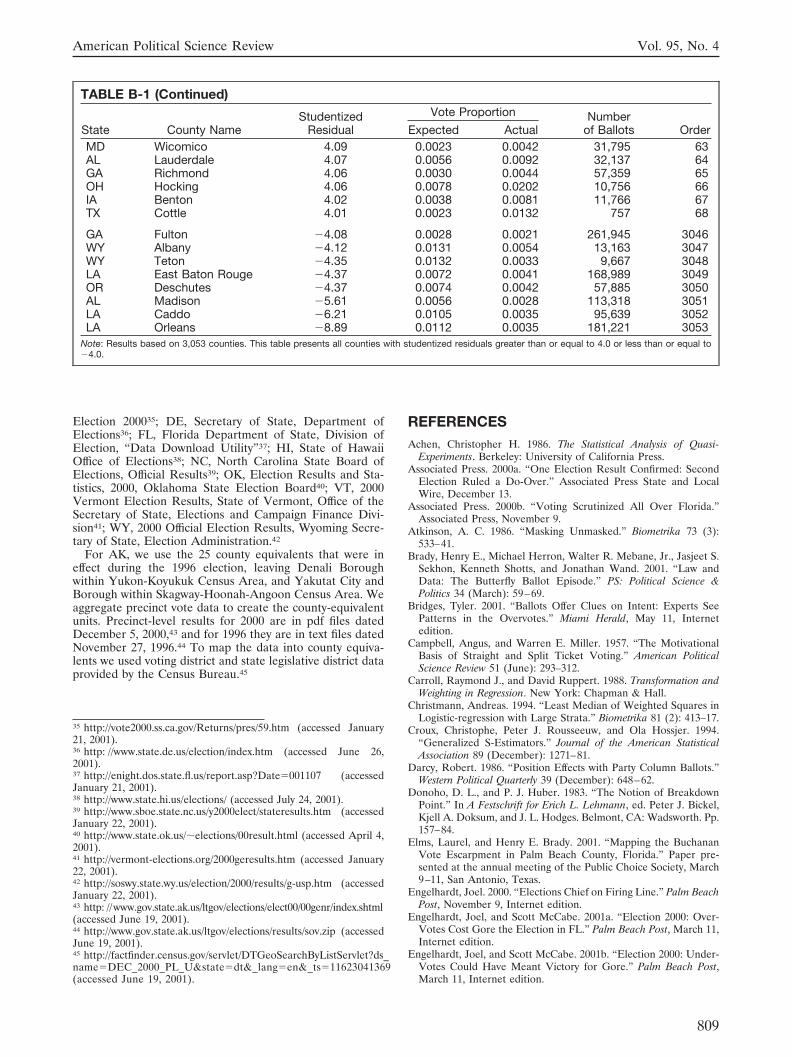
Election 200035; DE, Secretary of State, Department ofElections36; FL, Florida Department of State, Division ofElection, “Data Download Utility”37; HI, State of HawaiiOffice of Elections38; NC, North Carolina State Board ofElections, Official Results39; OK, Election Results and Sta-tistics, 2000, Oklahoma State Election Board40; VT, 2000Vermont Election Results, State of Vermont, Office of theSecretary of State, Elections and Campaign Finance Divi-sion41; WY, 2000 Official Election Results, Wyoming Secre-tary of State, Election Administration.42

For AK, we use the 25 county equivalents that were ineffect during the 1996 election, leaving Denali Boroughwithin Yukon-Koyukuk Census Area, and Yakutat City andBorough within Skagway-Hoonah-Angoon Census Area. Weaggregate precinct vote data to create the county-equivalentunits. Precinct-level results for 2000 are in pdf files datedDecember 5, 2000,43 and for 1996 they are in text files datedNovember 27, 1996.44 To map the data into county equiva-lents we used voting district and state legislative district dataprovided by the Census Bureau.45

REFERENCESAchen, Christopher H. 1986. The Statistical Analysis of Quasi-

Experiments. Berkeley: University of California Press.Associated Press. 2000a. “One Election Result Confirmed: Second

Election Ruled a Do-Over.” Associated Press State and LocalWire, December 13.

Associated Press. 2000b. “Voting Scrutinized All Over Florida.”Associated Press, November 9.

Atkinson, A. C. 1986. “Masking Unmasked.” Biometrika 73 (3):533–41.

Brady, Henry E., Michael Herron, Walter R. Mebane, Jr., Jasjeet S.Sekhon, Kenneth Shotts, and Jonathan Wand. 2001. “Law andData: The Butterfly Ballot Episode.” PS: Political Science &Politics 34 (March): 59–69.

Bridges, Tyler. 2001. “Ballots Offer Clues on Intent: Experts SeePatterns in the Overvotes.” Miami Herald, May 11, Internetedition.

Campbell, Angus, and Warren E. Miller. 1957. “The MotivationalBasis of Straight and Split Ticket Voting.” American PoliticalScience Review 51 (June): 293–312.

Carroll, Raymond J., and David Ruppert. 1988. Transformation andWeighting in Regression. New York: Chapman & Hall.

Christmann, Andreas. 1994. “Least Median of Weighted Squares inLogistic-regression with Large Strata.” Biometrika 81 (2): 413–17.

Croux, Christophe, Peter J. Rousseeuw, and Ola Hossjer. 1994.“Generalized S-Estimators.” Journal of the American StatisticalAssociation 89 (December): 1271–81.

Darcy, Robert. 1986. “Position Effects with Party Column Ballots.”Western Political Quarterly 39 (December): 648–62.

Donoho, D. L., and P. J. Huber. 1983. “The Notion of BreakdownPoint.” In A Festschrift for Erich L. Lehmann, ed. Peter J. Bickel,Kjell A. Doksum, and J. L. Hodges. Belmont, CA: Wadsworth. Pp.157–84.

Elms, Laurel, and Henry E. Brady. 2001. “Mapping the BuchananVote Escarpment in Palm Beach County, Florida.” Paper pre-sented at the annual meeting of the Public Choice Society, March9–11, San Antonio, Texas.

Engelhardt, Joel. 2000. “Elections Chief on Firing Line.” Palm BeachPost, November 9, Internet edition.

Engelhardt, Joel, and Scott McCabe. 2001a. “Election 2000: Over-Votes Cost Gore the Election in FL.” Palm Beach Post, March 11,Internet edition.

Engelhardt, Joel, and Scott McCabe. 2001b. “Election 2000: Under-Votes Could Have Meant Victory for Gore.” Palm Beach Post,March 11, Internet edition.

35 http://vote2000.ss.ca.gov/Returns/pres/59.htm (accessed January21, 2001).36 http: //www.state.de.us/election/index.htm (accessed June 26,2001).37 http://enight.dos.state.fl.us/report.asp?Date�001107 (accessedJanuary 21, 2001).38 http://www.state.hi.us/elections/ (accessed July 24, 2001).39 http://www.sboe.state.nc.us/y2000elect/stateresults.htm (accessedJanuary 22, 2001).40 http://www.state.ok.us/�elections/00result.html (accessed April 4,2001).41 http://vermont-elections.org/2000geresults.htm (accessed January22, 2001).42 http://soswy.state.wy.us/election/2000/results/g-usp.htm (accessedJanuary 22, 2001).43 http: //www.gov.state.ak.us/ltgov/elections/elect00/00genr/index.shtml(accessed June 19, 2001).44 http://www.gov.state.ak.us/ltgov/elections/results/sov.zip (accessedJune 19, 2001).45 http://factfinder.census.gov/servlet/DTGeoSearchByListServlet?ds_name�DEC_2000_PL_U&state�dt&_lang�en&_ts�11623041369(accessed June 19, 2001).

TABLE B-1 (Continued)

State County NameStudentized

Residual

Vote Proportion Numberof Ballots OrderExpected Actual

MD Wicomico 4.09 0.0023 0.0042 31,795 63AL Lauderdale 4.07 0.0056 0.0092 32,137 64GA Richmond 4.06 0.0030 0.0044 57,359 65OH Hocking 4.06 0.0078 0.0202 10,756 66IA Benton 4.02 0.0038 0.0081 11,766 67TX Cottle 4.01 0.0023 0.0132 757 68

GA Fulton �4.08 0.0028 0.0021 261,945 3046WY Albany �4.12 0.0131 0.0054 13,163 3047WY Teton �4.35 0.0132 0.0033 9,667 3048LA East Baton Rouge �4.37 0.0072 0.0041 168,989 3049OR Deschutes �4.37 0.0074 0.0042 57,885 3050AL Madison �5.61 0.0056 0.0028 113,318 3051LA Caddo �6.21 0.0105 0.0035 95,639 3052LA Orleans �8.89 0.0112 0.0035 181,221 3053

Note: Results based on 3,053 counties. This table presents all counties with studentized residuals greater than or equal to 4.0 or less than or equal to�4.0.


809

Firestone, David. 2000a. “Democrats Still Prefer to Keep Counting.”New York Times, November 11, Internet edition.

Firestone, David. 2000b. “Party Mobilized on Ballot Even as VotesWere Cast.” New York Times, November 11, Internet edition.

Garvey, Megan. 2000. “Bay Buchanan Sees Something Peculiar inPalm Beach Voting.” Los Angeles Times, November 10, Internetedition.

Hamilton, James T., and Helen F. Ladd. 1996. “Biased Ballots? TheImpact of Ballot Structure on North Carolina Elections in 1992.”Public Choice 87 (3/4): 259–80.

Hampel, F. R. 1971. “A General Qualitative Definition of Robust-ness.” Annals of Mathematical Statistics 42 (December): 1887–96.

Hampel, Frank R., Elvezio M. Ronchetti, Peter J. Rousseeuw, andWerner A. Stahel. 1986. Robust Statistics: The Approach Based onInfluence Functions. New York: Wiley.

Hampel, Frank R., Peter J. Rousseeuw, and Elvezio Ronchetti. 1981.“The Change-of-Variance Curve and Optimal Redescending M-Estimators.” Journal of the American Statistical Association 76(September): 643–8.

Koehler, Kenneth J., and Kinley Larntz. 1980. “An EmpiricalInvestigation of Goodness-of-Fit Statistics for Sparse Multinomi-als.” Journal of the American Statistical Association 75 (June):336–44.

Larntz, Kinley. 1978. “Small-Sample Comparisons of Exact Levelsfor Chi-Squared Goodness-of-Fit Statistics.” Journal of the Amer-ican Statistical Association 73 (January): 253–63.

McCullagh, Peter. 1986. “The Conditional Distribution of Goodness-of-Fit Statistics for Discrete Data.” Journal of the AmericanStatistical Association 81 (March): 104–7.

McCullagh, Peter, and John A. Nelder. 1989. Generalized LinearModels, 2d ed. New York: Chapman & Hall.

Merzer, Martin. 2001a. “‘Overvotes’ Leaned to Gore, But to Win, HeNeeded Help of Dimpled Ballots.” Miami Herald, May 11, Internetedition.

Merzer, Martin. 2001b. “Review Shows Ballots Say Bush, But GoreBackers Have Some Points to Argue.” Miami Herald, April 4,Internet edition.

Merzer, Martin, and the staff of the Miami Herald. 2001. The MiamiHerald Report: Democracy Held Hostage. New York: St. Martin’s.

Miami Herald. 2001. “About This Project.” Miami Herald. May 11,Internet edition.

Mitchell, Alison. 2001. “Results Official, at Last: Bush DefeatsGore.” New York Times, January 7, Internet edition.

Rousseeuw, P. J. 1984. “Least Median of Squares Regression.”Journal of the American Statistical Association 79 (December):871–80.

Rousseeuw, Peter J., and Christophe Croux. 1993. “Alternatives tothe Median Absolute Deviation.” Journal of the American Statisti-cal Association 88 (December): 1273–83.

Rousseeuw, Peter J., and Annick M. Leroy. 1987. Robust Regressionand Outlier Detection. New York: Wiley.

Sekhon, Jasjeet Singh, and Walter R. Mebane, Jr. 1998. “GeneticOptimization Using Derivatives: Theory and Application to Non-linear Models.” Political Analysis 7: 189–203.

Sinclair, Robert C., Melvin M. Mark, Sean E. Moore, Carrie A.Lavis, and Alexander S. Soldat. 2000. “An Electoral ButterflyEffect.” Nature 408 (December 7): 665–6.

Stout, David. 2000. “As Electors Cast Their Votes, Bush Confers inWashington.” New York Times, December 18, Internet edition.

Stromberg, Arnold J. 1993. “Computation of High BreakdownNonlinear Regression Parameters.” Journal of the American Sta-tistical Association 88 (March): 237–44.

Van Natta, Don, Jr. 2000. “Gore to Contest Recount Result in PalmBeach.” New York Times, November 25, Internet edition.

Van Natta, Don, Jr., and Michael Moss. 2000. “Democratic ‘WarRoom’ Tries to Oversee the Battle for Florida, to Mixed Results.”New York Times, November 11, Internet edition.

Wakin, Daniel J. 2000. “Bush Campaign Pushes for a Gore Conces-sion.” New York Times, November 10, Internet edition.

Western, Bruce. 1995. “Concepts and Suggestions for Robust Re-gression Analysis.” American Journal of Political Science 39 (Au-gust): 786–817.

White, Halbert. 1994. Estimation, Inference and Specification Analy-sis. New York: Cambridge University Press.

Wonnacott, Thomas H., and Ronald J. Wonnacott. 1990. Introduc-tory Statistics, 5th ed. New York: Wiley.


810

The butterfly did it: The aberrant vote for Buchanan in Palm Beach County, Florida

Documents

Transcript of The butterfly did it: The aberrant vote for Buchanan in Palm Beach County, Florida