1

The burden of monopolies on South African

households with different incomes: How

Competition Policy can contribute towards a more

equitable society

*PRELIMINARY DRAFT*

Yongama Njisane, Ricky Mann, Keabetswe Mojapelo, Pontsho

Mathebula and Matthew Clance‡

Abstract

The paper examines welfare loss due to monopolies on households with different

expenditure (incomes) shares. Furthermore, we present anecdotal evidence of the

importance of competition policy in protecting consumers and ensuring economic

participation by all. To do this, we follow Creedy & Dixon’s (1998) study of the relative

burden of monopoly on households measured as the loss (static) of consumer surplus for

households with different income and linking it with demand elasticities derived from

expenditure levels from Statistics South Africa’s Household Income and Expenditure Survey

2010/2011. The results show that the effects of the relative burden of monopoly power on

South African households by expenditure group, is, obviously felt more by lower income

group compared to the higher income groups. However, a direct comparison with the

Australian and Mexican studies shows that welfare loss to lower income households in

South Africa is far more detrimental even at the middle income level. More importantly, the

results induce the premise that monopoly power substantially affects the distribution of

welfare and deters progress on reducing inequality and poverty.

Economists at the Competition Commission South Africa, Policy and Research Division. Pretoria, South Africa. For any enquiries, email: Yongaman@Compcom.co.za ‡ Senior Lecture at the University of Pretoria, Department of Economics, Pretoria. South Africa. Email:

Matthew.Clance@up.ac.za The views expressed in this article are strictly ours and do not reflect those of the Competition

Commission of South Africa. -

2

1. Introduction

The South African economy is characterized by the effects of the historical legacy of the

economic concentration and ownership, collusive practices and the abuse of power by firms

in dominant positions throughout the apartheid era (Parsons, 2009 and Roberts & Makhaya,

2014). In addressing the imbalances arising from such, the South African Competition Act

No. 89 of 1998 (as amended) (the “Competition Act”) envisaged a role for the competitive

process in rectifying the distortions and inequalities created by the past racial segregation

regime. This allows Competition policy to be used as a complementary policy to other growth

strategies and a tool towards inclusive growth through the facilitation of greater equality of

opportunities which breaks down the barriers to fair competition in an economy.

Post-apartheid South Africa adopted an economy exhibited by high levels of concentration,

resulting in unfavourable prices charged to consumers; difficulties in the creation of

employment opportunities and feeble development of small and medium businesses

(Makhaya & Roberts, 2014). Major economic sectors such as electricity, transportation,

construction, mining, agriculture and telecommunication services were and are largely still

dominated by monopolies. In light of this, the South African Competition Commission (“the

Commission”) adopted a prioritisation Framework which identified these sectors and more

that accelerated growth to support employment creation, consumer welfare and business

development, with a reaching impact on low income households but also on industrial

development and employment. These sectors included financial services; food and agro-

processing; infrastructure and construction; and intermediate industrial products. There has

been instances of monopolistic and cartel behaviour, most notably in the, the bread, milk,

poultry and wheat and maize cartel cases, which impacted directly on the consumer welfare

and also effort to reduce poverty and inequality.

In light of the above, we examine the relationship between the level of household

expenditure (income) and the relative burden of monopoly. We adopt the approach by

Creedy & Dixon (1998), where they combine the static net consumer loss method of

assessing the cost on monopolies with a method of linking demand elasticities to income

levels. In section 2, we present literature conducted on welfare and monopoly conduct,

including studies conducted for Australia and Mexico. Section 3, we outline the data used in

this model, Statistics South Africa (“StatsSA”) household Income and Expenditure Survey

2010/2011 (“IES”). In section 4, we present the model outlined in Creedy & Dixon (1998) and

Frisch (1954), which shows how in the absence of direct evidence on the price elasticities of

3

demand, cross-sectional information contained in the composition of household expenditure

can be used to generate a set of estimates of the relative welfare loss for households with

different levels of income. The estimates of relative welfare loss extracted from the

information in the IES are presented in section 5, and then conclude.

2. Literature Review

There have been numerous studies conducted in South Africa on past monopolistic

behaviour and cartel conduct in various sectors and their harm on consumers. In the bread

and flour cartel active between 1999 and 2007, Mncube (2014) provides evidence of the

flour cartel in relation to overcharges to independent bakeries and found that the

overcharges were ranging from 9% to 31%. This indicates that consumers were harmed by

the cartel, by paying significant higher prices. In the poultry case where Rainbow, Astral,

Country Bird and Pioneer Foods on behalf of AGRI and Tydstroom Poultry were involved in

cartel conduct through information exchange and price fixing, Grimbeek (2012) shows that

savings to consumers due to intervention by the Commission amounted to R1.2 billion.

These cases highlight some of the impact that competition policy has had in South Africa.

The dismantling of the anti-competitive conduct in these key sectors, particularly food and

agro-processing, not only results in competitive pricing, innovation and increased product

choice, but contributes to the reduction of socio-economic disparities by making this

essential goods and services within the economic reach for lower income households.

More general studies on the distributional and welfare consequences of monopoly power on

consumers are exhibited in studies by Creedy & Dixon (1998, 1999) Urzúa (2013) and

Argent & Begazo (2015). All these studies posit the hypothesis that the welfare loss caused

by monopoly with significant market power would vary by consumers income groups. Creedy

and Dixon (1998) examine the relative burden of monopoly in Australia, measured as the

(static) loss of consumer surplus for different household income levels. The study combines

the static net consumers’ loss method of assessing the cost of monopoly with a method of

linking demand elasticities to expenditure (income) levels across 30 households groups. In

the absence of information about variations in elasticity with total expenditure, they calculate

own price elasticity using household budget data following the approach developed by Frisch

(1959). The results show that the relative welfare loss associated with monopoly power is

higher for low expenditure (income) households groups than for high income households

groups. In Creedy and Dixon (1999), the analysis was further extended by measuring the

4

relative burden of monopoly using equivalent variation and equivalent income, for different

household income levels. The results showed the same effects, propounding evidence of

greater welfare loss to lower income households relative to higher income households due to

monopolies.

Urzúa (2013) expands on the above studies using an alternate estimation of demand price

elasticities to show the regional distributive and welfare loss by firms with market power in

Mexico. The author estimates price elasticities following Deaton (1988, 1990) where

quantities and unit values are corrected for quality differences before estimating the

statistical relation between quantity and unit values. The results show that welfare losses

due to the exercise of monopoly power are not only significant but also larger, in relative

terms, for the poor. Furthermore, regions with the poorest inhabitants are most affected by

firms with market power. Argent and Begazo (2015) build on Urzúa (2013) to investigate the

link between competitive, well-functioning food markets and consumer welfare in Kenya.

Using the technique of spatial variation developed by Deaton (1988, 1990), the authors show

that welfare costs from monopoly power for sugar and maize are borne by the poor though

disproportionately.

The paper builds on these studies in literature, positing a similar hypothesis in order to

understand the detriment caused by monopoly power on South African lower income

consumers relative to other countries. To do this, we follow Creedy & Dixon’s (1998)

approach, which is outlined in the next section, beginning with the theoretical underpinnings

of the model and then explain the simulation method used to capture the necessary

parameters that will enable us to expound on the subject.

3. Theoretical outline: Measuring welfare loss

Following Creedy & Dixon’s (1998) static consumers’ surplus method of measuring welfare

loss resulting from a monopoly, we adopt their assumption the true social net cost of

monopoly is proportional to the loss of consumers’ surplus and the proportionality is the

same across households. The model further assumes that actual price is treated as the

monopoly price, 𝑝𝑚. Strictly speaking, this results in the measure of deadweight loss being a

reflection of all market distortions and not just the impact of the exercise of monopoly power.

Marginal cost, 𝑚𝑐, is assumed to be constant and independent of output or market

conditions. Finally it is assumed that marginal costs, 𝑚𝑐, is equal to the competitive price, 𝑝𝑐.

5

The net loss of consumers’ surplus, 𝐵, is measured using the standard textbook formula that

the area of the loss triangle is half the price difference multiplied by the reduction in the

quantity demanded. This is given by:

𝐵 =(𝑝𝑚 − 𝑝𝑐)(𝑞𝑐 − 𝑞𝑚)

2… … … … … … … … … … … . (1)

Following this, we define the Lerner index of monopoly power1, 𝑀, as:

𝑀 =𝑝𝑚 − 𝑚𝑐

𝑝𝑚… … … … … … … … … … … … … … … . … (2)

Using the assumption that 𝑝𝑐 = 𝑚𝑐 , we rearrange (2) as follows:

𝑀 ∗ 𝑝𝑚 = 𝑝𝑚 − 𝑚𝑐 … … … … … … … … … … … … … … … (3)

Substituting (3) into (1) gives

𝐵 =𝑀 ∗ 𝑝𝑚(𝑞𝑐 − 𝑞𝑚)

2… … … … … … … … … … … … … … (4)

The term (𝑞𝑐 − 𝑞𝑚) can be expressed in terms of the own-price elasticity of demand, 𝜂,

approximated by:

𝜂 =(𝑞𝑚 − 𝑞𝑐)

(𝑝𝑚 − 𝑝𝑐)

𝑝𝑚

𝑞𝑚… … … … … … … … … … … … … … … … . (5)

Substituting (3) into (5) and rearranging gives:

𝑞𝑚 − 𝑞𝑐 = 𝜂𝑀𝑞𝑚 … … … … … … … … … … … … … … … … . (6)

Then (6) into (4) results in:

𝐵 =𝑀2𝜂(𝑝𝑚𝑞𝑚)

2… … … … … … … … … … … … … … … . . . (7)

Following Cowling & Mueller (1978), we assume myopic profit maximization, such that

𝑀 = −𝜂−1 … … … … … … … … … … … … … … … … … … . . (8)

Following that, we substitute (8) into (7), which gives:

𝐵 = −𝑝𝑚𝑞𝑚

2𝜂… … … … … … … … … … … … … … … … … … … . (9)

Finally, let 𝑤𝑖 = 𝑝𝑚𝑞𝑚, then aggregate the welfare loss on each item of expenditure and

express it as a proportion of total expenditure on all item. This results in welfare loss 𝐿:

𝐿 = −1

2∑

𝑤𝑖

𝜂𝑖

𝑛

𝑖=1

… … … … … … … … … … … … … … … … … … … (10)

Where 𝑤𝑖 is the ratio of expenditure on the 𝑖th item to total expenditure.

Equation (10) can be calculated for an individual consumer or a group of consumers with

similar expenditure patterns, with the latter allowing for comparisons of the burden of

monopoly across income or expenditure groups. However, equation (10) is based on several

1 The Lerner index of monopoly power measures the “degree of monopoly. The wider the wedge between 𝑝

and 𝑚𝑐, the greater the monopoly power.

6

contentious assumptions. This includes profit maximization and the assumption that all

producers are pure monopolists or oligopolists selling homogenous goods and aiming to

maximize joint profits. Furthermore, the model does not incorporate issues such as X-

efficiency and general equilibrium effects amongst others. Additionally, the model does not

consider the benefits that might accrue from a monopoly through scales and innovation in

the absence of competition. Creedy & Dixon (1985) defend the validity of the model on the

grounds of Posner (1975) and Dixon (1995), who argue that to the extent that the missing

items are proportional to the loss of consumers’ surplus, equation (10) can still be used to

calculate relative loss for different income or expenditure groups.

Incorporating Posner (1975) and Dixon (1995), as well making the assumption that it is

possible to model the economy as if each income group operates in a different market for

each commodity; we define the relative burden of monopoly for a low income household 𝐿𝑙

relative to that of a high-income household, 𝐿𝐻 as:

𝑧 =𝐿𝑙

𝐿𝐻=

∑ (𝑊𝐿𝑖

𝑛𝑖=1 /𝜂𝑙𝑖

)

∑ (𝑊𝐻𝑖

𝑛𝑖=1 /𝜂𝐻𝑖

)… … … … … … … … … … … … … … … . . (11)

By making the assumption that it is possible to model the economy as if each income group

operates in a different market, we make the robust assumption there exist some

heterogeneity in quantity and quality of purchase within and between different income

groups.

4. Simulation specification: Estimating price elasticities

In order to compute equation (11), one requires a set of estimates of own-price elasticities

for each income group. There are several literature contributions on demand and price

elasticities in South Africa. A plethora of these studies use the Almost Ideal Demand System

model (“AIDS”) of Deaton & Muelbauer (1980) and its variation, the Quadratic Almost Ideal

System model (“QUAIDS”) of Banks et al (1997)2. Ground and Koch(2007) finds that

techniques (AIDS, QUAIDS etc.) suggested for developed economy data cannot be applied

to South African data with impunity owing to evidence that shows that South African survey

data does not comply with the necessary assumptions for analysing expenditure functions

using non-linear share ratios and compositional data techniques. Koch (2010) further

highlights another drawback to the models, showing that most AIDS and QUAIDS

specifications allow the estimates to fall outside the unit interval despite the Engel curve’s

2 These studies include, inter alia, the analysis of Agbola (2003), Taljaard et al (2003), Bopape &

Myers (2007) and Dunne & Edkins (2008).

7

restriction that expenditure shares must lie on or within the unit interval, while all expenditure

shares must sum to unity. In the same regard, Koch (2010) shows the problem can be

circumvented using the fractional multinomial logit model (FMNL) of Papke & Wooldridge

(1996) and Mullahy (2010) which uses the QUAIDS as an index function within an empirical

specification that forces the shares to be positive, so that they fall within the unit interval,

while also forcing the additivity restriction to hold.

However, according to Koch (2010), the FMNL requires good pricing data in order to perform

optimally. Due to the limitations of the IES and lack of pricing data, implementation of the

FMNL is unsurmountable. Alternatively, we could use the spatial variations approach due to

Deaton (1988, 1990,) à la Urzúa (2013) to estimate the price elasticities. However due to the

insoluble obstruction owing to the reliability and absence of quantity data in local surveys

(which is necessary for the calculation of unit values), we conclude using Creedy & Dixon’s

(1998) adoption of Frisch’s (1959) approximation of price elasticities.

The methodology follows the analysis pioneered by Frisch (1959) which assumes a model

that uses the assumption of additivity, whereby the marginal utility of good 𝑖 is independent

of the consumption of good 𝑗. Deaton (1974) criticizes the assumption of additivity, citing that

this assumption implies approximate linear relationships between own-price and income

elasticities, thus leading to a distortion of demand measurements. However, according to

Creedy & Dixon (1998), Frisch’s (1959) approach suitable for application to broad groups of

commodities than to individual commodities. For a directly additive utility function of the

form 𝑈 = ∑ 𝑢𝑖(𝑞𝑖)𝑛𝑖=1 , Frisch (1959) showed that:

𝜂𝑖 =𝑒𝑖

𝜉− 𝑒𝑖𝑤𝑖 (1 +

𝑒𝑖

𝜉) , … … … … … … … … … … … … … … … . . (12)

Where 𝑒𝑖 = 1 +Δ𝑤𝑖

𝑤𝑖⁄

Δ𝑦𝑦⁄

for 𝑤 is the share of total expenditure by each household group

whereas 𝑦 is the total expenditure by household group. This represents the income elasticity

of demand and 𝜉 is the elasticity of the marginal utility of income, normally referred to as the

Frisch parameter. The relative burden, 𝐿𝑙

𝐿𝐻, is obtained by substituting (12) into (11) to get:

𝐿𝐻

𝐿𝐿=

∑ {𝑒𝐿𝑖

𝑤𝐿𝑖𝜉𝐿− 𝑒𝐿𝑖 (1 +

𝑒𝐿𝑖𝜉𝐿

)}−1

𝑛𝑖=1

∑ {𝑒𝐻𝑖

𝑤𝐻𝑖𝜉𝐻− 𝑒𝐻𝑖 (1 +

𝑒𝐻𝑖𝜉𝐻

)}−1

𝑛𝑖=1

… … … … … … … … … … (13)

The relative burden of monopoly varies across households, as 𝑤𝑖, 𝑒𝑖 and 𝜉 vary. It is

expected that some or all of these vary with income (total expenditure). Since the estimates

of 𝜉 are not available, it is advisable to specify a pattern using a priori assumptions. It is not

8

possible to say exactly how the resultant level of welfare loss will vary with income (total

expenditure), as it depends upon offsetting variations in the three sets of variables. Frisch's

assumptions regarding the variation in 𝜉 , along with the available evidence from other

demand studies, were discussed in detail in Cornwell and Creedy (1997), where it was

suggested that a modified double-log form specification for the variation in 𝜉 with income

(total expenditure) should be used.

The linear expenditure system involves a minimum absolute value of unity, but the absolute

value is higher for lower total expenditure groups, for whom committed expenditure is

expected to form higher proportion of income. With the variation in the Frisch parameter, the

problem with it is that the parameters cannot be estimated using cross-sectional data;

however it can be solved by using extraneous information. Frisch (1959) suggested that the

parameter varies inversely with total expenditure, with low-income household having a

relatively high absolute value and high-income households having relatively low absolute

value. Frisch did not give any reasons for this hypothesis, however empirical research

support the hypotheses, such as Lluch, et al. (1977), William (1978) and Rimmer (1995).

Given the role of the variation in 𝜉, it is useful to produce alternative results for different

specifications for 𝜉. Therefore instead of assuming a constant elasticity relationship between

𝜉 and total expenditure (𝑚) as in Lluch, et al. (1977), and William (1978), the following

specification is used:

In(−𝜉) = 𝑎 − 𝛼𝐼𝑛(𝑚 + 𝜃) … … … … … … … … … … … … . . (14)

The values of 𝑎 , 𝛼 and 𝜃 are generated following a process of trial and error, to produce

values of 𝜉3 corresponding with ( 𝑚) total expenditure (income). Using these values, to

calibrate the variations in the Frisch parameters, own-price elasticity for each commodity and

total expenditure group are calculated.

5. Data description

To calculate the relative burden of monopoly using the model above, we use data from

StatsSA’s IES 2010/2011. The survey is used to provide relevant statistical information on

household consumption expenditure patterns conditional on household characteristics,

3 Theoretical Frisch parameters:

𝜉 = −10, this value represents extremely poor households groups 𝜉 = −2, this value represents the middle income household group 𝜉 =−0.1, this value represents the rich part of the household groups

9

income and expenditure per item captured using the Classification of Individual Consumption

According to Purpose (“COICOP”) method as well specific particulars on each person in the

household. The survey covered all nine provinces, as well four types of settlements: urban

formal, urban informal, traditional area and rural informal. The sample covered

approximately 27 665 households across South Africa over a period of one year between

September 2010 and August 2011, based on the 2001 Population Census.

The COICOP list contains 20 consumptions groups including non-expenditure consumption

groups, represented by in-kind consumption and in-kind income groups, as well as debt

expenditure by households and transfers to others. For the sake of our analysis, we exclude

all non-consumption expenditure and use the remaining 12 expenditure groups. These are:

1. Food and non-alcoholic beverages

2. Alcoholic beverages; tobacco and narcotics

3. Clothing and footwear

4. Housing; water; electricity; gas and other fuels

5. Furnishings; household equipment and routine maintenance of the house

6. Healthcare

7. Transport

8. Telecommunications

9. Recreation and culture

10. Education

11. Restaurants and hotels

12. Miscellaneous goods and services

In addition to this, we use total yearly household expenditure on each specific COICOP main

group using the annualized value of yearly expenditure (Valueannualized in the dataset) by

households which has been inflated/deflated to March 2011 using the CPI.

Following this, for 𝑌 = total yearly expenditure households and 𝑦𝑖=yearly expenditure of

households on COICOP item 𝑖,

𝑌 = ∑ 𝑦𝑖

12

𝑖=1

… … … … … … … … … … … … … … … … … … … . (15)

We compute the total yearly expenditure on each COICOP main group by households. We

then divide yearly expenditure by households into 30 household groups, starting from the

lowest spending households to the highest spending households. Following this, we

10

compute the average expenditure for each group, to obtain the average yearly expenditure

of each household group on all COICOP items. The descriptive statistics are summarized

below as:

Table 1: Descriptive statistics

Mean Standard deviation Min Max

Average

spend by each

housheold

group

R136 160.80 R186 738.30 R10 319.64 R944 998.5

Source: Authors’ own calculation

Tables 1 indicate that average yearly expenditure on the 12 COICOP main groups by South

African households’ amounts to R136 160. The standard deviation between households is

more than double the average expenditure by households, indicating the plight of inequality

in our society. The lowest yearly expenditure by household groups is R10 319. This would

typically represent household that spend most of their income on food and transport

purposes. The highest yearly expenditure by households on the 12 COICOP main group

items amounts to R944 998.5. This represents a R934 678.9 difference in the expenditure of

the same items by consumers in the same country.

Following this calculations, we follow Creedy & Dixon (1998), using the total expenditure for

household items (COICOP main group items) to calculate average expenditure weights on

each of the 12 individual commodity groups for the 30 households’ expenditure groups.

6. Preliminary results

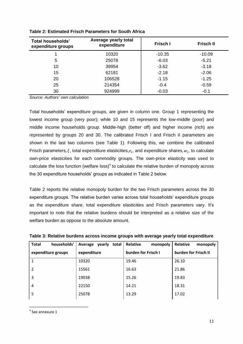
From equation (14), given the calculated average yearly total expenditure and following a

process of trial and error, we calibrate 𝑎 = 11.5 , 𝛼 = 1 and 𝜃 = 500 to generate the

variations in the values of Frisch I parameter that are close to the true theoretical Frisch

(1959) values as shown in Table 1 below. Following William (1978), Frisch II parameter are

calibrated imposing the restrictions as follows:𝑎 = 11.2, 𝛼 = 0.95 and 𝜃 = 777.

11

Table 2: Estimated Frisch Parameters for South Africa

Total households’ expenditure groups

Average yearly total expenditure Frisch I Frisch II

1 10320 -10.35 -10.09

5 25078 -6.03 -5.21

10 39954 -3.62 -3.18

15 62181 -2.18 -2.06

20 106528 -1.15 -1.25

25 214354 -0.4 -0.59

30 924999 -0.03 -0.1

Source: Authors’ own calculation

Total households’ expenditure groups, are given in column one. Group 1 representing the

lowest income group (very poor); while 10 and 15 represents the low-middle (poor) and

middle income households group. Middle-high (better off) and higher income (rich) are

represented by groups 20 and 30. The calibrated Frisch I and Frisch II parameters are

shown in the last two columns (see Table 1). Following this, we combine the calibrated

Frisch parameters, 𝜉, total expenditure elasticities,𝑒𝑖, and expenditure shares, 𝑤𝑖, to calculate

own-price elasticities for each commodity groups. The own-price elasticity was used to

calculate the loss function (welfare loss)4 to calculate the relative burden of monopoly across

the 30 expenditure households’ groups as indicated in Table 2 below.

Table 2 reports the relative monopoly burden for the two Frisch parameters across the 30

expenditure groups. The relative burden varies across total households’ expenditure groups

as the expenditure share, total expenditure elasticities and Frisch parameters vary. It’s

important to note that the relative burdens should be interpreted as a relative size of the

welfare burden as oppose to the absolute amount.

Table 3: Relative burdens across income groups with average yearly total expenditure

Total households’

expenditure groups

Average yearly total

expenditure

Relative monopoly

burden for Frisch I

Relative monopoly

burden for Frisch II

1 10320 19.46 26.10

2 15561 16.63 21.86

3 19038 15.26 19.83

4 22150 14.21 18.31

5 25078 13.29 17.02

4 See annexure 1

12

6 27856 12.63 16.06

7 30756 11.88 15.03

8 33675 11.40 14.32

9 36758 10.93 13.64

10 39954 10.39 12.90

11 43603 9.83 12.14

12 47576 9.36 11.47

13 51820 8.89 10.82

14 56759 8.40 10.15

15 62181 7.91 9.50

16 68190 7.43 8.87

17 75497 6.95 8.23

18 84472 6.41 7.54

19 94568 5.91 6.91

20 106528 5.43 6.30

21 120886 4.96 5.70

22 138046 4.50 5.12

23 157453 4.08 4.60

24 182328 3.66 4.10

25 214354 3.23 3.57

26 251694 2.83 3.08

27 298448 2.48 2.66

28 367321 2.12 2.25

29 476958 1.70 1.78

30 924999 1.00 1.00

Source: Authors own calculation using StatsSA’s IES 2010/2011

The estimated results show a general decline in the relative burden of monopoly as total

expenditure increases across the income groups. The effects of the relative burden of

monopoly power are felt more by lower income group compared to the higher income

groups. These results are consistency with other empirical studies that were conducted.

However, when comparing the results to Creedy & Dixon’s (1998) study of Australia, the

lowest income group, denoted in column 1 in table 3 above, we find a 70% difference the

burden experienced by consumers in the same expenditure class. This indicates the greater

need for an inclusive competition policy that will result in consumers attaining higher

13

consumer welfare outcomes, especially the poor households and general efficiency in the

economy.

7. Conclusion

The paper examined the welfare loss on households with different expenditure (incomes)

shares due to the existence of monopolies. We made use of Creedy & Dixon’s (1998) study

on the burden of monopoly on households and linked it with demand elasticities derived from

Statistics South Africa’s Household Income and Expenditure Survey 2010/2011. As a result,

we demonstrated how the relative burden of monopoly power is borne by lower income

groups as opposed to higher income groups. We find our results to be consistent with other

empirical studies but this effect is even more exacerbated when compared to similar studies

conducted in Australia and Mexico; for example, we find a 70% difference in the burden

which is borne by consumers in the same lower income group. In addition, we find that

welfare loss is felt even at the middle income level. Finally, we were able to infer from the

results that monopoly power has a significant effect on the distribution of welfare and inhibits

efforts to curb inequality and poverty. This highlights a need for an inclusive competition

policy that can minimize the relative burdens by monopoly conduct to improve consumer

welfare, especially for the lower income households.

Further analysis in these study will be conducted across different time period to assess the

impact of competition policy in South Africa over time, using Creedy & Dixon’s (1998)

methodology.

14

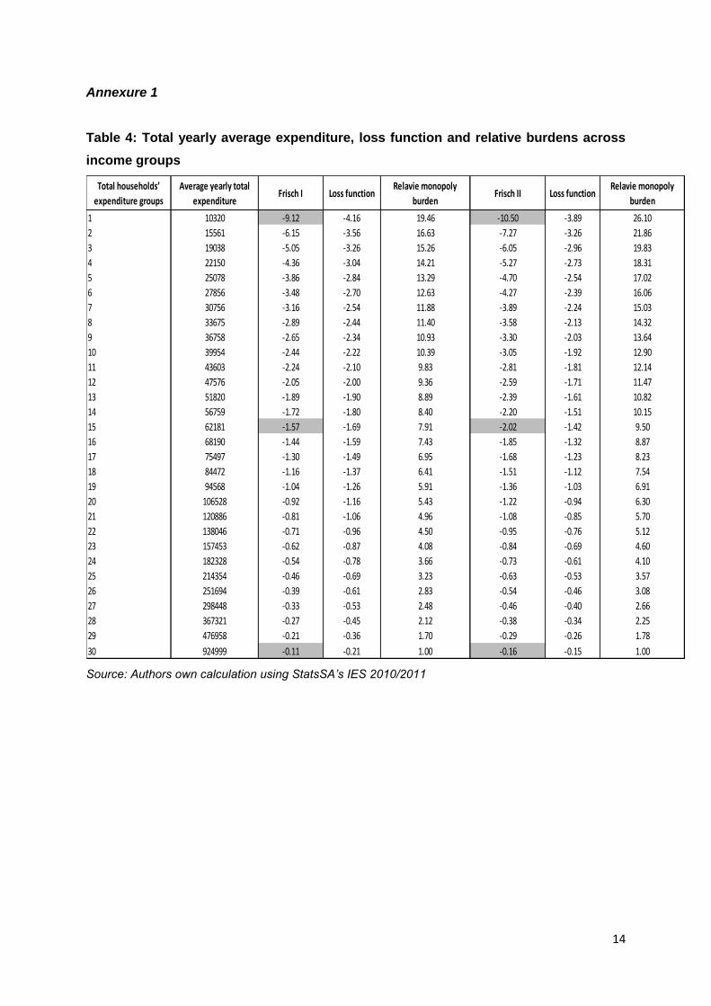
Annexure 1

Table 4: Total yearly average expenditure, loss function and relative burdens across

income groups

Source: Authors own calculation using StatsSA’s IES 2010/2011

Total households’

expenditure groups

Average yearly total

expenditureFrisch I Loss function

Relavie monopoly

burdenFrisch II Loss function

Relavie monopoly

burden

1 10320 -9.12 -4.16 19.46 -10.50 -3.89 26.10

2 15561 -6.15 -3.56 16.63 -7.27 -3.26 21.86

3 19038 -5.05 -3.26 15.26 -6.05 -2.96 19.83

4 22150 -4.36 -3.04 14.21 -5.27 -2.73 18.31

5 25078 -3.86 -2.84 13.29 -4.70 -2.54 17.02

6 27856 -3.48 -2.70 12.63 -4.27 -2.39 16.06

7 30756 -3.16 -2.54 11.88 -3.89 -2.24 15.03

8 33675 -2.89 -2.44 11.40 -3.58 -2.13 14.32

9 36758 -2.65 -2.34 10.93 -3.30 -2.03 13.64

10 39954 -2.44 -2.22 10.39 -3.05 -1.92 12.90

11 43603 -2.24 -2.10 9.83 -2.81 -1.81 12.14

12 47576 -2.05 -2.00 9.36 -2.59 -1.71 11.47

13 51820 -1.89 -1.90 8.89 -2.39 -1.61 10.82

14 56759 -1.72 -1.80 8.40 -2.20 -1.51 10.15

15 62181 -1.57 -1.69 7.91 -2.02 -1.42 9.50

16 68190 -1.44 -1.59 7.43 -1.85 -1.32 8.87

17 75497 -1.30 -1.49 6.95 -1.68 -1.23 8.23

18 84472 -1.16 -1.37 6.41 -1.51 -1.12 7.54

19 94568 -1.04 -1.26 5.91 -1.36 -1.03 6.91

20 106528 -0.92 -1.16 5.43 -1.22 -0.94 6.30

21 120886 -0.81 -1.06 4.96 -1.08 -0.85 5.70

22 138046 -0.71 -0.96 4.50 -0.95 -0.76 5.12

23 157453 -0.62 -0.87 4.08 -0.84 -0.69 4.60

24 182328 -0.54 -0.78 3.66 -0.73 -0.61 4.10

25 214354 -0.46 -0.69 3.23 -0.63 -0.53 3.57

26 251694 -0.39 -0.61 2.83 -0.54 -0.46 3.08

27 298448 -0.33 -0.53 2.48 -0.46 -0.40 2.66

28 367321 -0.27 -0.45 2.12 -0.38 -0.34 2.25

29 476958 -0.21 -0.36 1.70 -0.29 -0.26 1.78

30 924999 -0.11 -0.21 1.00 -0.16 -0.15 1.00

15

Bibliography

1. Agbola, F. W (2003) Estimation of Food Demand Patterns in South Africa Based on a

Survey of Households, Estimation of Food Demand Patterns in South Africa Based

on a Survey of Households, Southern Agricultural Economics Association, Vol 35.

2. Argent, J. and Begazo, T. (2015) Competition in Kenya and its Impact on Income and

Poverty: the Case of Sugar and Maize, working paper, available at

http://econ.worldbank.org/external/default/main?pagePK=64210502&theSitePK=469

372&piPK=64210520&menuPK=64166093&entityID=000158349_20150126105017 .

Accessed on 3 April 2014.

3. Banks et al (1997) Quadratic Engel Curves and Consumer Demand, The Review of

Economics and Statistics, Vol. 79, pp. 527-539.

4. Bopape, L. & Myers, R. (2007), Analysis of household demand for food in South

Africa: Model selection, expenditure endogeneity, and the influence of

sociodemographic effects, in `African Econometrics Society Conference', Cape

Town, South Africa.

5. Competition Act No. 89 of 1998 (as amended), Preamble.

6. Competition Commission vs. Pioneer Foods (Proprietary) Limited (2010) Case no:

15/CR/Feb07 and 50/CR/May 08.

7. Cowling, K and Mueller, C. (1978) The Social Costs of Monopoly Power, The

Economic Journal, Vol. 88, pp. 727-748.

8. Cornwell, A. and Creedy, J. (1997) Environmental Taxes and Economic Welfare:

Reducing Carbon Dioxide Emissions. Aldershot: Edward Elgar.

9. Creedy, J. and Dixon, R. (1998) The Relative Burdon of Monopoly on households

with Different Incomes, Economica, vol 65, pp 93 – 287.

10. Creedy, J. and Dixon, R. (1999) The Distributional Effects of Monopoly, Australian

Economic Papers, vol 38, pp 223 – 37.

11. Deaton, A. (1988) Quality, Quantity and Spatial Variation of Price, American

Economic Review, vol 78, pp 418 – 30.

12. Deaton, A. (1990) Price Elasticities from Survey Data: Extensions and Indonesian

Results, Journal of Econometrics, vol 44, pp 281 – 309.

13. Deaton, A. and Muellbauer, J. (1980) Economics and Consumer Behaviour,

Cambridge University Press.

14. Deaton, A. (1974) A Reconsideration of the Empirical Implications of Additive

Preferences, Economic Journal, vol 84, pp 338 – 48.

15. Dixon, R. (1995) Empirical estimates of the social cost of monopoly: a brief survey.

University of Melbourne Department of Economics Research Paper, no. 490.

16

16. Dunne, J. P. & Edkins, B. (2008), `The demand for food in South Africa', South

African Journal of Economics 76(1), pp.104-117.

17. Frisch, R. (1954) A complete scheme for computing all direct and cross demand

elasticities in a model with many sectors, Econometrica, vol 27, 177 – 96.

18. Govinda, H. et al. (2014) On Measuring the Economic Impact: Savings to the

Consumer Post the Cement Cartel Burst, Pretoria: Competition Commission South

Africa, available at http://www.compcom.co.za/wp-content/uploads/2014/09/On-

measuring-the-economic-impact-savings-to-the-consumer-post-cement-cartel-burst-

CC-15-Year-Conference.pdf. Accessed on 28 March 2015.

19. Grimbeek, S. (2012). Food and Agro-Processing: Enhancing Competitive Outcomes

through Facilitating New Entry, New Agenda, First Quarter: 33-37.

20. Ground, M and Koch,S.F. (2007) Hurdle Models of Alcohol and Tobacco Expenditure

in South African Households, Working Papers 200703. University of Pretoria,

Department of Economics.

21. Koch,S.F. (2010) Fractional Multinomial Response Models With An Application To

Expenditure Shares, Working Papers 201021, University of Pretoria, Department of

Economics.

22. Lerner, A. (1934) The Concept of Monopoly and the Measurement of Monopoly

Power, Review of Economic Studies, vol 1, pp 157 – 75.

23. Lluch, et al. (1977) Patterns in Household Demand and Saving. Oxford: Oxford

University Press.

24. Makhaya, T. and Roberts, S. (2014) The Changing Strategies of Large Corporations

in South Africa Under Democracy and the Role of Competition Law, working paper,

available at

http://static1.squarespace.com/static/52246331e4b0a46e5f1b8ce5/t/54242cdfe4b063

a8a548ce80/1411656927180/CCRED+Working+Paper+02-

2014_+SA+Large+Corps_+MakhayaRoberts.pdf. Accessed on 3 April 2015.

25. Mncube, L. (2013) Strategic Entry Deterrence: Pioneer Foods and Bread Cartel,

Journal of Competition Law and Economics, vol 9, pp 637- 654

26. Mullahy, J. & Robert, S. A. (2010), `No time to lose: Time constraints and physical

activity in the production of health', Review of the Economics of the Household 8, pp.

409-432.

27. Papke, L.E. and Wooldridge, J.M. (1996) Variables with an Application to 401 (K)

Plan Participation Rates, Department of Economics, Michigan State University,

Marshall Hall.

28. Parsons, R. (2009) Zumanomics – Which Way to Shared Prosperity in South Africa?,

Jacana Media, Johannesburg, South Africa.

17

29. Patel, E. (2014) Budget vote speech By Minister of Economic Development, Cape

Town.

30. Posner, R.A. (1975) The Social Costs of Monopoly and Regulation, The Journal of

Political Economy, Vol. 83, pp. 807-828.

31. Proposed Guidelines for Competition Policy (1997) A framework for Competition,

Competitiveness and Development, Department of Trade and Industry, Pretoria.

32. Rimmer, M. (1995) Development of a multi-household version of the Monash model.

Monash University Centre of Policy Studies and the IMPACT Project Working Paper,

no. OP-8 1.

33. Roberts, S. and Makhaya, T. (2013) Expectations and Outcomes: Considering

Competition and Corporate Power in South Africa under Democracy, Review of

African Political Economy, vol 40, pp 556 – 71.

34. Taljaard et al (2003) A linearized almost ideal demand system (la/aids) of the

demand for meat in South Africa, Annual Conference of the Agricultural Economics

Association of South Africa, Pretoria, South Africa.

35. Urzúa, C. M. (2013) Distributive and Regional Effects of Monopoly Power, Economía

Mexicana, vol 22, 279 – 95.

36. Williams, R. (1978). The use of disaggregated cross-section data in explaining shifts

in Australian consumer demand patterns over time. Monash University IMPACT

Project, Preliminaty Working Paper, no. SP-13.