
the application of improved numerical techniques - The ...
255
THE APPLICATION OF IMPROVED NUMERICAL TECHNIQUES TO 1-D MICELLAR/POLYMER FLOODING SIMULATION APPROVED:
-
Upload
khangminh22 -
Category
Documents
-
view
0 -
download
0
Transcript of the application of improved numerical techniques - The ...
THE APPLICATION OF IMPROVED NUMERICAL TECHNIQUES
TO 1-D MICELLAR/POLYMER FLOODING SIMULATION
APPROVED:
THE APPLICATION OF IMPROVED NUMERICAL TECHNIQUES
TO 1-D MICELLAR/POLYMER FLOODING SIMULATION
BY
TAKAMASA OHNO, B.E. Pet.E.
THESIS
Presented to the Faculty of the Graduate School of
The University of Texas at Austin
in Partial Fulfillment
of the Requirements
for the Degree of
MASTER OF SCIENCE IN ENGINEERING
THE UNIVERSITY OF TEXAS AT AUSTIN
August 1981
ACKNOWLEDGEMENT
I would like to express my sincere appreciation and gratitude
to Dr. Gary A. Pope for his supervision and encouragement throughout
this study.
I am also deeply grateful to Dr. K. Sepehrnoori for valuable
assistance and guidance in the numerical analysis and the solution
of differential equations.
Thanks and appreciation are also extended to Dr. L. W. Lake
for his helpful comments and suggestions.
I would also like to thank the Japan Petroleum Exploration
Corporation (JAPEX) for their financial support during this research.
This research was also supported by grants from the Department of
Energy and the following companies: Core Laboratories; Exxon U.S.A.;
INTERCOMP Resources and Engineering; Marathon Oil; Mobil Oil; Shell
Development; Tenneco Oil; Cities Service.
Special appreciation is expressed to my wife, Mihoko, for
her encouragement and understanding which made this work possible.
The University of Texas Austin, Texas
June, 1981
T. Ohno
iii
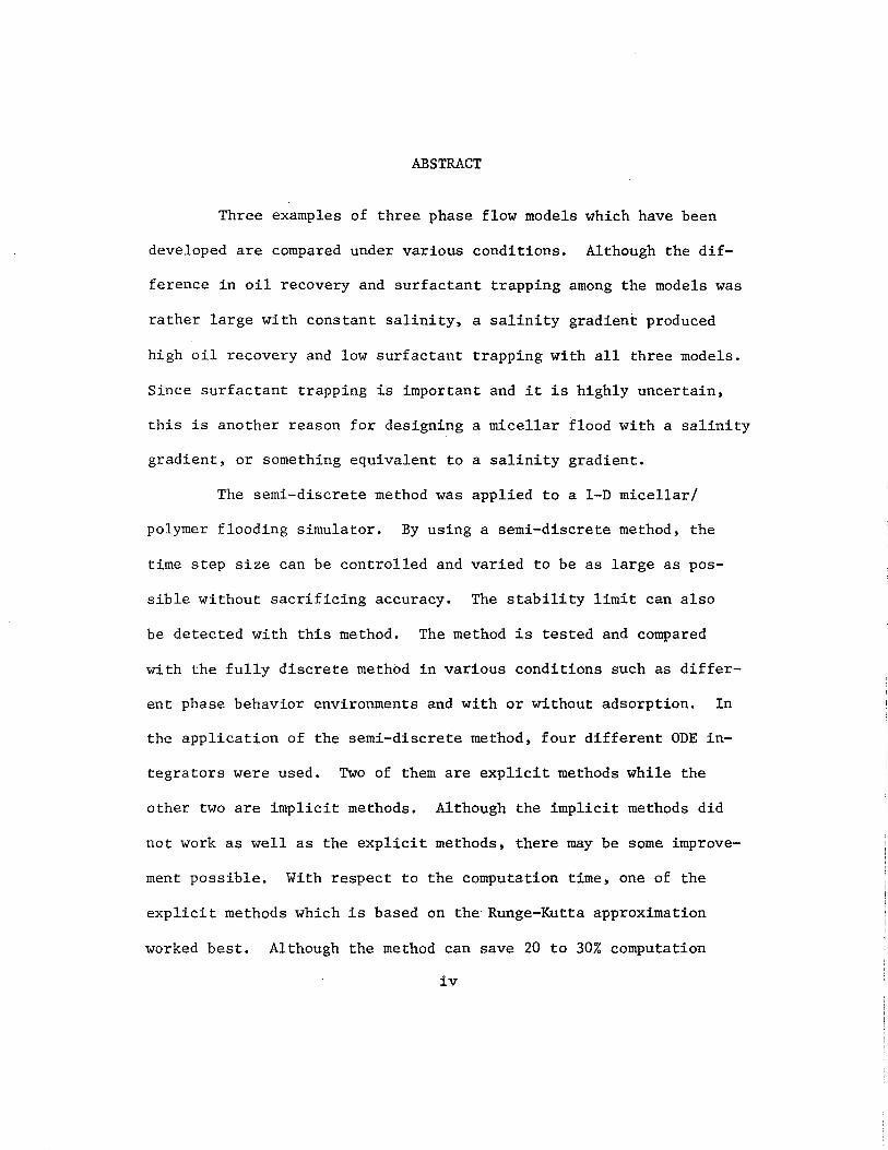
ABSTRACT
Three examples of three phase flow models which have been
developed are compared under various conditions. Although the dif
ference in oil recovery and surfactant trapping among the models was
rather large with constant. salinity, a salinity gradient produced
high oil recovery and low surfactant trapping with all three models.
Since surfactant trapping is important and it is highly uncertain,
this is another reason for designing a micellar flood with a salinity
gradient, or something equivalent to a salinity gradient.
The semi-discrete method was applied to a 1-D micellar/
polymer flooding simulator. By using a semi-discrete method, the
time step size can be controlled and varied to be as large as pos
sible without sacrificing accuracy. The stability limit can also
be detected with this method. The method is tested and compared
with the fully discrete method in various conditions such as differ
ent phase behavior environments and with or without adsorption. In
the application of the semi-discrete method, four different ODE in
tegrators were used. Two of them are explicit methods while the
other two are implicit methods. Although the implicit methods did
not work as well as the explicit methods, there may be some improve
ment possible. With respect to the computation time, one of the
explicit methods which is based on the· Runge-Kutta approximation
worked best. Although the method can save 20 to 30% computation
iv
time under some conditions, compared with the fully-discrete method,
the results are highly problem-dependent. To improve the computation
time, two methods are suggested. One is to check the error only in
the oil or water component rather than all components or any other
one component such as surfactant. The other is to check absolute
error instead of relative error and multiply by a small conservative
factor to the calculated time step size.
The stability was analyzed for the oil bank, and for the
surfactant front. The former imposes a rather constant limitation on
the time step size continuously until the plateau of the oil bank
is completely produced: Although approximate, the stability analysis
for the surfactant front suggests an unconditional local instability,
which is caused by the change in the fractional flow curve due to
the surfactant.
v
Acknowledgement
Abstract
Table of Contents
List of Tables
List of Figures
Chapter
I. INTRODUCTION
TABLE OF CONTENTS
II. LITERATURE SURVEY AND REVIEW OF PREVIOUS WORK
III. DESCRIPTION OF MICELLAR/POLYMER FLOODING
SIMULATOR
3.1 Basic Assumptions and Governing Continuity
Equations
3.2 Auxiliary Functional Relationships
3.2.1 Salinity
iii
iv
vi
ix
xi
Page
1
7
10
10
17
19
3.2.2 Binodal Curve and Distribution Curve 20
3.2.3 Adsorption 24
3.2.4 Phase Viscosity 25
3.2.5 Interfacial Tension 26
3.2.6 Trapping Function 27
3.2.7 Relative Permeability 30
3.2.8 Other Features 32
vi
3.3 Solution Procedure
IV. THREE PHASE FLOW MODEL
4.1 Pope's Model
4.2 Hirasaki's Model
4.3 Lake's Model
4.4 Comparison of Each Model
V. ORDINARY DIFFERENTIAL EQUATION INTEGRATORS
5.1 Runge-Kutta-Fehlberg Methods
5.2 Multi Step Methods
5.3 Stability Region and Stiffness
VI. RESULTS AND DISCUSSIONS
6.1 Basic Input Data and Example Results
6. 2 Comparison of Each Method for Type II (-)
Phase Behavior without Adsorption Case
6.3 Effect of Adsorption and Phase Behavior
6.4 Effect of Each Component on Time Step
Size Selection
6.5 Additional Test Runs and Summary of RK1(2)
and RKl for Type II(-) Phase Behavior Envir
onment without Adsorption
6.6 Stability Requirement before Surfactant Break-
32
44
44
45
48
50
63
64
70
72
82
84
87
93
95
100
thro11gh 101
6.7 Analysis of Stability at Blocks Where Sur-
factant is Present 109
vii

VII. CONCLUSIONS AND RECOMMENDATIONS FOR FUTURE
STUDIES
NOMENCLATURE
APPENDICES
A. PHASE BEHAVIOR CONCEPT
B. DERIVATION OF CONTINUITY EQUATIONS FOR MULTIPHASE
MULTICOMPONENT FLOW
C. COMPUTER PROGRAM
REFERENCES
VITA
viii
171
176
180
185
192
233
239
LIST OF TABLES
Table
3.1 Equations used to calculate phase concentrations
4.1 Comparison of oil recovery and surfactant trapped
(O.l PV of 3% surfactant slug was injected, sal
inity is constant)
4.2 Comparison of oil recovery and surfactant trap
ped
(0.1 PV of 6% surfactant slug was injected.
Salinity is constant.)
4.3 Comparison of oil recovery and surfactant trap
ped for two different salinity gradient (O.l PV
of 3% surfactant slug was injected)
4.4
5.1
6.1
Input data used to compare three phase flow models
Coefficients for RK1(2)
Basic input data used to test semi-discrete method
6.2 Comparison of FDE method and semi-discrete method
with various ODE integrators (Type II(-), no adsorp
tion
6.3 Comparison of FDE and RKl (Type II(-), no adsorp
tion)
6.4 Results of predictor-corrector methods at 0.1 PV
injected
ix
35
52
53
54
55
67
114
117
118
119
6.5 Comparison of FDE, RK1(2), and RKl for Type II(-),
with adsorption
6.6 Comparison of FDE and RKl for Type II(+), no adsorp
tion
120
121
6.7 Comparison of FDE, RK1(2), and RKl for Type II(+), with
adsorption
6.8 Comparison of FDE and RKl for Type III
6.9 Effect of adsorption and phase behavior environment
on the efficiency. of RKl (ERR = 0.01)
6.10 Effect of each component on time step size selec-
122
123
124
tion (RKl, ERR= 0.01, Type II(-), no adsorption) 125
6.11 Improvement in time step size selection by checking
errors for oil component (RKl, ERR = 0.01)
6.12 Test runs with YBIAS = 1.0 (RK1(2) and RKl, Type
126
II(-), no adsorption) 127
6.13 Summary of RK1(2) and RKl (Type II.(-), no adsorption) 128
6.14 Aqueous phase profile of Run 207 at 0.5 PV injection
(Type II(-), no adsorption) 129
6.15 Legend for the total concentration history plots 130
x

LIST OF FIGURES
Figure
Method of lines
Definition of phase number
Effect of G parameters on calculated IFT curve
Effect of G parameters on calculated IFT curve
Effect of G parameters on calculated IFT curve
Effect of G parameters on calculated IFT curve
3.1
3.2
3.3
3.4
3.5
3.6
3.7 Normalized residual saturation versus capillary
number
3.8 Interdependence of variables without shear rate
effect on polymer solution
3.9 Solution procedure in the simulator
4.1 Basic idea of phase trapping employed in
Hirasaki's model
16
36
37
38
39
40
41
42
43
57
4.2 Phase diagrams and interfacial tensions in Type III
phase behavior environment with different salinities 58
4.3 Comparisons of final oil recoveries and surfactant
trappings among three different three phase flow
models (0.1 PV of 3% surfactant slug is injected) 59
4.4 Comparisons of final oil recoveries and surfactant
trappings among three different three phase flow
models (0.1 PV of 6% surfactant slug is injected) 60
xi
4.5 Comparison of production histories among three
different three phase flow models (constant salinity
CSE = 0.82)
4.6 Comparison of production histories among three dif-
61
ferent three phase flow models (salinity gradient) 62
5.1
5.2
5.3
Stability region for RK1(2)
Stability region for Adams' method
Stability region for Gear's methods
6.1 Total concentration profile at 0.25 PV for Run 207
(FDE method, 6tD = 0.001 PV, Type II(-), no adsorp
tion)
6.2
6.3
6.4
Phase saturation profile at 0.25 PV for Run 207
Fractional flow profile at 0.25 PV for Run 207
Microemulsion phase concentraton profile at 0.25 PV
for Run 207
6.5 Oleic phase saturation and its residual saturation
profile at 0.25 PV for Run 207
6.6
6.7
Interfacial tension profile at 0.25 PV for Run 207
Total relative mobility profile at 0.25 PV for
Run 207
6.8 History of total concentration in effluent for Run
207
6.9 History of phase cuts and cumulative oil production
for Run 207
xii
79
80
81
131
132
133
134
135
136
137
138
139
6.10 History of pressure drop (normalized) between pro
ducer and injector for Run 207
6.11 History of total concentration in effluent for
Run 203 (FDE method, 6tD = 0.002, Type II(-), no
adsorption)
6.12 History of total concentration in effluent for
Run 204 (FDE method, 6tD = 0.003, Type II(-), no
adsorption)
6.13 History of total concentration in effluent for Run
206 (FDE method, 6to = 0.004, Type II(-), no
adsorption)
6.14 Histories of total concentration in effluent and
time step size for Run 196 (RK1(2), ERR= 0.00005,
Type II(-), no adsorption)
6Ll5 Histories of total concentration in effluent and time
step size for Run 197 (RK1(2), ERR= 0.0001, Type
II(-), no adsorption)
6.16 Histories of total concentration in effluent and
time step size for Run 198 (RK1(2); ERR= 0.002,
Type II(-), no adsorption)
6.17 Histories of total concentration in effluent and time
step size for Run 498 (Adams' method, ERR= 0.0005,
140
141
142
143
144
145
146
Type II(-), no adsorption) 147
xiii
6.18 Histories of total concentration in effluent and
time step size for Run 496 (Adams' method, ERR =
0.001, Type II(-), no adsorption)
6.19 Histories of total concentration in effluent and
time step size for Run 495 (Adams' method, ERR =
0.01, Type II(-), no adsorption)
6.20 Histories of total concentration in effluent and
time step size for Run 200 (RK.l, ERR = 0.01, Type
II(-), no adsorption)
6.21 Histories of total concentration in effluent and
time step size for Run 201 (RK.l, ERR = 0.02, Type
II(-), no adsorption)
6.22 Histories of total concentration in effluent and
time step size for Run 202 (RK.l, ERR= 0.05, Type
148
149
150
151
II(-), no adsorption) 152
6.23 Histories of total concentration in effluent
and time step size for Run 333 (RK.l, ERR = 0.01,
Type II(-), with adsorption
6.24 Histories of total concentration in effluent and
time step size for Run 411 (RK.l, ERR = 0.01, Type
II(+), no adsorption)
6.25 Histories of total concentration in effluent and
time step size for Run 395 (RK.l, ERR = 0.01,
Type II(+), with adsorption)
xiv
153
154
155

6. 26 Histories of total concentration in effluent and
time step size for Run 442 (RI<l, ERR = 0.01,
Type III, no adsorption) 156
6.27 Histories of total concentration in effluent and
time step size for Run 463 (RKl, ERR = 0.01, Type
III, with adsorption) 157
6. 28 Histories of total concentration in effluent and
time step size for Run 265 (RKl, ERR = 0.01, Type
II(-)' no adsorption, no tracer) 158
6.29 Histories of total concentration in effluent and
time step size for Run 266 (RKl, ERR = 0.01, Type
II(-), no adsorption, error checked only for Cl) 159
6.30 Histories of total concentration in effluent and
time step size for Run 267 (RKl, ERR = 0.01, Type
II(-), no adsorption, error checked only for C2) 160
6.31 Histories of total concentration in effluent and
time step size for Run 268 (RKl, ERR = 0.01, Type
II(-), no adsorption, error checked only for c3 161
6.32 Histories of total concentration in effluent and
time step size for Run 269 (RKl, ERR = 0.01, Type
II(-)' no adsorption, error checked only for C4) 162
6.33 Histories of total concentration in effluent and
time step size for Run 229 (RKl, ERR = 0.01,
waterflooding, no tracer) 163
xv
6.34 Histories of total concentration in effluent and
time step size for Run 260 (RKl, ERR = 0.01,
miscible displacement with tracer)
6.35 Histories of total concentration in effluent and
time step size for Rum 522 (RKl, ERR = 0.01,
Type II(-), with adsorption, error checked only
for c2)
6.36 Histories of total concentration in effluent and
time step size for Run 446 (RKl, ERR = 0.01, Type
III, no adsorption, error checked only for c2)
6.37 Histories of total concentration in effluent and
time step size for Run 629 (RK1(2), ERR= 0.0001,
164
165
166
PCT= 0.25, YBIAS = 1.0, Type II(-), no adsorption) 167
6.38 Histories of total concentration in effluent and
time step size for Run 647 (RK1(2), ERR= 0.0001,
PCT= 0.50, YBIAS = 1.0, Type II(-), no adsorption) 168
6.39
6.40
Stability region for RKl or Forward Euler
Explanation of negative value for f'
xvi
169
170
CHAPTER I
INTRODUCTION
Process background
Micellar/polymer flooding has been recognized as one
of the most promising enhanced oil recovery techniques as well
as co2 injection and thennal recovery. Some people refer to
micellar flooding as a miscible displacement even though this is
not always true. Even if there exist two or three distinct
phases associated with the surfactant process, improved oil re-
covery can be achieved. Three major mechanisms that contribute
to improved oil recovery by micellar flooding have been suggested
as below
(1) miscible displacement
(2) ultra low interfacial tensions1
(3) oil swelling or solubilization2
3 In 1927, Uren and Fahmy concluded that the oil recovery
obtained by flooding has a definite relationship with interfacial
tension between the oil and the displacing fluid. Ever since
extensive research has been done, especially in the laboratory, to
analyze the mechanisms and efficiency of flooding with surfactants
and other chemical agents. . 4
The literature gives a list of
representative references and brief summary of the history. In
spite of this, however, the optimum method is still under investi-
gation both in the laboratory and in the field.
1
In designing and optimizing a micellar flooding pro-
cess, one is confronted with many mechanisms and corresponding
physicochemical properties of the rock and fluid interactions
that affect performance of a micellar flood. Important pro-
perties are phase behavior, interfacial tension, relative per-
meabilities, viscosities, dispersion, adsorption and cation
exchange. Laboratory investigations to analyze process sensiti-
vity to each property are very difficult because they are highly
coupled with one another. Accordingly, several numerical simu
lators for micellar/polymer flooding5-l6 , 67 •68 have been presented
both to aid in the interpretation of laboratory experiments and
to scale it up for field applications.
When one tries to simulate micellar flooding numeri-
cally, special care must be taken of surfactant transport in por-
d . 0 i i 1 bl . i 1 d. . l7 ,ls ous me ia. ne pr nc pa pro em is numer ca ispersion
. 19 20 that may swamp physical dispersion ' , leading to a front appar-
ently much more smeared than it should be. The numerical dispersion
2
is produced from truncation errors when the spatial and/or time deriva-
tives in a differential equation are approximated as difference quo~
tients. The smeared solution may not cause much trouble if the
surfactant slug is injected continuously. However, in actual field
operation, the surfactant slug is usually injected as a finite slug,
sometimes as low as a few percent of the reservoir pore volume, be-
cause of the high cost of chemicals. In such a case, simulated per-
formance may be quite erroneous and lead people to a wrong judgement,
if the numerical dispersion is not treated properly. This is espe-
cially true when the phase behavior environment in the reservoir is
Type II(+).
The dispersion causes the peak surfactant concentration to
decrease, which causes the concentration to fall below the multiphase
boundary earlier, resulting in the earlier loss of one mechanism
of improved oil recovery: miscibility. Furthermore, in the multi-
phase region, when the phase behavior environment is Type II(+),
decreased surfactant concentration results in greater retardation of
the surfactant and loss in the ability to cause oil swelling, another
contribution to higher oil recovery.
Another problem associated with the construction of a micel-
lar/polymer simulator is the lack of knowledge about phase trapping
and flow character .when three phases coexist.
There have been two competing design philosophies for surf ac-
. 4 7 10 7 tant flooding ' ' although, as Larson pointed out, the distinction
is a matter of degree. One is to inject a relatively small pore
volume (about 3-20%) 4 of higher concentration surfactant slug, usually
with a non-zero oil content. The main mechanism of its oil recovery
is miscible displacement: solubilize both oil and water in the reser-
voir leaving no residual oil since there exists no interfacial tension
for single phase flow, until the chemical concentration falls below
the multi phase boundary. The other is to inject a la:rge pore !Volume
(about 15-60%) of lower surfactant concentration slug, usually with
little oil content. The major mechanism of improved oil recovery is
3

4
no longer miscibility in this case. Ultra-low interfacial tension
between the aqueous and oleic phases due to the surfactant reduces
residual oil saturation and increases oil recovery.
1 Healy et al. showed experimental results which indicated the
lowest interfacial tension between the microemulsion and either the
oleic or aqueous phase occurred when three phases coexist. Nelson
2 and Pope also showed higher efficiency of oil recovery in the Type
III phase environment where three. phases coexist. Thus, the transport
characteristics of three phase flow must be considered and included in
the simulator to determine the optimum method of micellar flooding.
Unforitunately, little experimental data which represent three
phase flow in a Type III phase environment have been published. So
we have to make some hypothetical model based upon reasonable assump-
tions. A few models for such three phase flow have been pre-
t d 5,9,37 sen e • Although it is very hard to say which is realistic
from the simulated results, a comparison is made in Chapter IV among
those models just as a reference.
Numerical background
In general, there are two approaches used to solve partial
differential equations. One is the fully-discrete model and the other
is the semi-discrete method. In a fully-discrete method, time deriva-
tives are discretized and approximated by the finite difference expres-
sions, whereas they are left to be continuous in a semi-discrete method.
In both methods, spatial derivatives may be discretized and approximated
as difference quotients: the finite difference methods, or the
problem may be formulated as a variational problem in the spatial
domain: the finite element methods. 21- 25 Furthermore if we
consider equations that involve both parabolic and hyperbolic charac-
ters, like the well known convection diffusion equation, the finite
difference methods can be categorized in two groups; one solves
26-31 32-36 equations as parabolic and the other as hyperbolic.
Fully-discrete finite difference methods that solve prob-
lems as parabolic are the most common techniques in the area of reser-
voir simulation, and have been used in micellar/polymer flooding simu-
lators to solve the continuity equations. Those techniques, however,
exhibit some inherent problems when one tries to solve the case with
5
small dispersion. When the spatial derivatives are approximated by
backward difference expressions, the solution is smeared by numerical
dispersion. When the centered difference approximations are used
instead, the solution oscillates. To eliminate those problems, one may
have to use more grid blocks or nodes which increases computer costs
and may be impractical in some cases.
In this research, some semi-discrete methods are applied to
a micellar/polymer flooding simulator which uses a parabolic techni-
que of finite difference methods. By using a semi-discrete method, the
time step size can be controlled and varied to be as large as possible
without sacrificing accuracy. Thus, it can be expected that the semi-
discrete method may save computation time.
6
When a semi-discrete method is applied to solve partial
differential equations, they are converted to a system of' ordinary
differential equations (ODE's), since the time derivatives remain
continuous. To solve the resulting ODE's, a Runge-Kutta-Fehlberg
(RKF) method, Adams' methods and Gear's backward differentiation
methods were first tested. RKF methods are explicit algorithms
to integrate with respect to time, whereas the other two are implicit
(predictor-corrector) methods, which requires some iterative scheme
to solve non-linear equations. The details of these ODE solvers
are presented in Chapter V.
After the test of all three ODE solvers, another algorithm
which seemed to be more efficient was also examined. This algorithm
consists of a combination of first and second order Runge-Kutta
approximations. A brief description of the algorithm is given.in.
Chapter VI.
The micellar/polymer flooding simulator used in this research
5 38 . 39 was originally presented by Pope et al. Then Wang and Lin made
several improvements. The details of the simulator are described
in Chap.ter III.
CHAPTER II
LITERATURE SURVEY AND REVIEW OF PREVIOUS WORK
In most chemical flooding simulators, continuity equations
are solved for several components. Although the equations are
highly non-linear, their character is quite similar to the well
known linear convection diffusion (C-D) equation. Depending on the
degree of dispersion, the character of the equations ranges from para-
bolic to almost hyperbolic.
Among the chemical flooding simulators which have been pre-
sented, fully discrete finite difference methods that solve equations
as parabolic are the most common techniques. 5-9 Some authors employ
18 11-14 the analysis of Lantz. Other authors use higher order accurate
approximation. 28 , 29 Since these techniques are suitable for parabolic
equations, they have inherent problems when the level of dispersion
is very low. The Lantz's technique may become impractical because of
great computation time, since it requires fine grid spacing to ap-
pr~ximate low dispersion. Furthermore the continuity equations are
usually solved explicitly, which imposes a strict limitation on the
time step size and makes the computation time proportional to the
square of number of spatial grid points. The higher order accurate
methods, on the other hand, require fewer spatial grids to attain the
same level of dispersion. Fine grid spacing, however, is still re-
quired for lower dispersion to avoid oscillation. It also involves
the problem of small time step size due to explicit solution.
7
8
Todd and Chase11 used an automatic time step size control in
a chemical flooding simulator. They varied the step size based on the
relative changes of variables during the last time step. This techni-
que may be called "the method of relative changes" and distinguished
from semi-discrete methods which control time step size based on esti-
mated truncation error made during the last time step.
The method of relative changes is rather widely used in reser-
voir simulation. 40 Coats applied the same kind of method to a steam-
flood simulator and Grabowski et al. 4 used its modified form in a
general purpose thermal model for in situ combustion and steam. How-
ever, these methods only rely on the observation that large changes in
the variables mean more error and small changes mean less error. Al-
though the error control is not rigorous, this method can control sta-
bility. If the stability condition is not met on the way of continuous
integration, the large change in the variables due to instability makes
the time step size smaller, and forces it back toward the stability
region. However, the point is that a stable scheme does not necessarily
mean high accuracy.
Some ordinary differential equation (ODE) solvers have been
applied to solve partial differential equations with the semi-discrete
method. When an ODE-solver is used for time integration, truncation
error made during one time step is estimated and then the time step
size is varied according to the estimated error. The semi-discrete
method has two advantages over fully discrete methods:
1) by changing time step size and the order of integration

9
scheme, truncation error associated with time integration is kept uni-
form while being forced to stay within error tolerance which is usually
specified by users.
2) time step size is controlled to be as large as possible
without sacrificing accuracy.
Sincovec42 introduced Gear's all-purpose ODE-solver43 into
reservoir simulation problems when he applied the semi-discrete method.
Although he had difficulty in solving a highly non-linear problem, he
obtained successful results in other problems. 44 Jensen applied a first
order predictor-corrector method, which is based on Gear's approach,
to automatically select the time-step size in a finite difference
steam injection reservoir simulator. He compared the scheme with
the method of relative changes and showed the superiority of his scheme.
Sepehrnoori and Carey 45 applied several sophisticated ODE-
solver programs to stiff and non-stiff initial-value systems arising
from representative evolution problems. Basic algorithms used in those
programs are Adams' method, Gear's method and the modified (extended
stability region) Runge-Kutta method. The efficiencies of those al-
gorithms are compared for each problem. They found that the per-
formance of each method is highly problem dependent.

CHAPTER III
DESCRIPTION OF MICELLAR/POLYMER FLOODING SIMULATOR
3.1 Basic Assumptions and Governing Continuity Equations
The continuity equations for multiphase multicomponent flow
are derived based on the following assumptions.
(1) Isothermal system.
(2) One-dimensional flow with homogeneous rock properties.
(3) Rock compressibility is negligible.
(4) Gravity and capillary pressure are negligible.
(5) Fluid properties are a function of composition only.
(6) The volume of a mixture is equal to the sum of individual
pure-component volumes: volume does not change upon
mixing.
(7) Pure component densities are constant.
(8) Local thermodynamic equilibrium exists everywhere.
(9) Darcy's law applies.
(10) No chemical reaction occurs (no appearance or disappear-
ance of any species).
Given the above assumptions and some other minor assumptions,
the continuity equations for each component i in dimensionless form
are
3C1. M 3(f.C .. ) L: J 1J
atn + j=l a~ (3.1)
i = 1,2, .•. ,NCOMP
10
where
M I (k./µ.) j=l J J
NCOMP Ci = (1 - I C.)C. + c.
i=l l. l. l.
M c. = I s.c .. l. . 1 J l.J J=
(3.2)
(3. 3)
Definitions (3. 2) and (3.3) give
since
And
NCOMP NCOMP -I c. = 2: c. = 1 l. l. i = 1 i = 1 (3.4)
NCOMP M
I c .. = 2: s. = 1 i = 1 l.J j=l J
C. = volume of component i adsorbed per unit pore volume l.
Cij = concentration of component i in phase j
k. = effective permeability to phase j J
11

µj viscosity of phase j
~ = superficial (Darcy) velocity of total phase
¢ = porosity
L = length of system
x = distance
°uj = dimensionless longitudinal dispersivity
M and NCOMP are the number of phases and components, respectively.
The derivation of Eq. (3.1) is given in Appendix B.
If assumption (11) below is added, we get
ac. M _i + 2: atD j=l
(3.5)
(11) Physical dispersion can be approximated adequately by
numerical dispersion by selecting the appropriate grid
size and time step.
When equation (3.5) is fully discretized using a backward
difference approximation in space and forward difference in time,
the actual equations we solve are
12
C3(f.C •• ) J l.J - 0 (3.6)
where the last term is called numerical dispersion term and for small
M
I: j=l
More detail of this approximation will be discussed later.
(3.7)
Although assumption (11) is based on the analysis of single-
phase flow (linear convection diffusion equation), it may be area
sonable approximation in many cases. Lin39 has tested the numerical
difference between this approximation compared to solving equation
(3.1) with a very large number of grid blocks to minimize numerical
dispersion. He found close agreement, but no way of generalizing
this result to other cases has been developed. When assumption (11)
is employed, the porous medium is, in effect, being modeled as a
series of well-stirred tanks, each of which at each time step dumps
a portion of its contents into the next tank forward according to
the fractional flow rather than saturation of each phase.
In the simulator, equation (3.1) is solved rather than equa-
tion (3.5). However, the former is easily converted to the latter
by only setting aDj = 0 in input data. When aDj > 0 it should be
noted that the solution obtained includes both physical dispersion
and numerical dispersion. In other words, the solution obtained
from equation (3.1) always includes more dispersion compared with
13

the one obtained from equation (3.5) as long as a positive value
of aDj is used. Although negative values of aDj are non-physical,
Lin39 tried some numerical experiments, expecting that numerical
dispersion is cancelled somehow by the negative ~j· The results
seem to be successful to some extent. Some oscillation, however,
is still inevitable when the desired order of effective dispersion
(the sum of numerical and physical dispersion) is low.
14
Because aDj was set to be zero for all test runs, the numerical
approximation of equation (3.5) rather than (3.1) is discussed here.
In other words~assumption (11) remains in this research. The ap
proximation of equation (3.1) is discussed by Lin. 39
Equation (3.5) is solved numerically by either the semi-
discrete or fully discrete finite difference method. In either
case, spatial derivatives are discretized using single-point (one-
point) upstream weighting. For the fully. discrete method, time
derivatives are approximated by forward differences which allow
explicit solutions. For semi-discrete methods, time derivatives
are continuous, rather than discretized, allowing the application
of Ordinary Differential Equation (ODE) solvers (which then con-
tain the time discretization).
Fully discrete finite difference equations .are solved ex-
plicitly as below
b.tD M . (C.)t - -;:--- L {(f.C .. )
1 D u~ j=l J l.J ~ (f.C .. ) " }
J l.J ~ - L\~
(3. 8)

15
Taking the truncation error into account, the actual equations being
solved are
+ HOT = 0 (3. 9)
where HOT means higher order truncation errors. In most cases the
time step size 6tD is forced to be much smaller than 6xD to keep sta
bility because the explicit method is used. Therefore, the dispersion
is controlled by 6xD, or the number of grid blocks.
When semi-discrete finite difference methods are used, equa-
tions (3.10) below are to be solved
(3.10)
where time is retained as a continuous variable. This semi-discrete
approach yields an initial value system of ordinary differential
equations with respect to time. Because every component in one
block affects the right-hand side of equation (3~10) for all com-
ponents in the same block and the next (downstream) block, all con-
centrations in all blocks are coupled. Then the number of equations
involved in the system is given by the product of the number of com-
ponents and the number of spatial grid points. For example, when six
components and forty points are used, a system of two hundred and
forty equations has to be solved. Reordering of each component in
each block is done as follows:
16
(3.11)
where
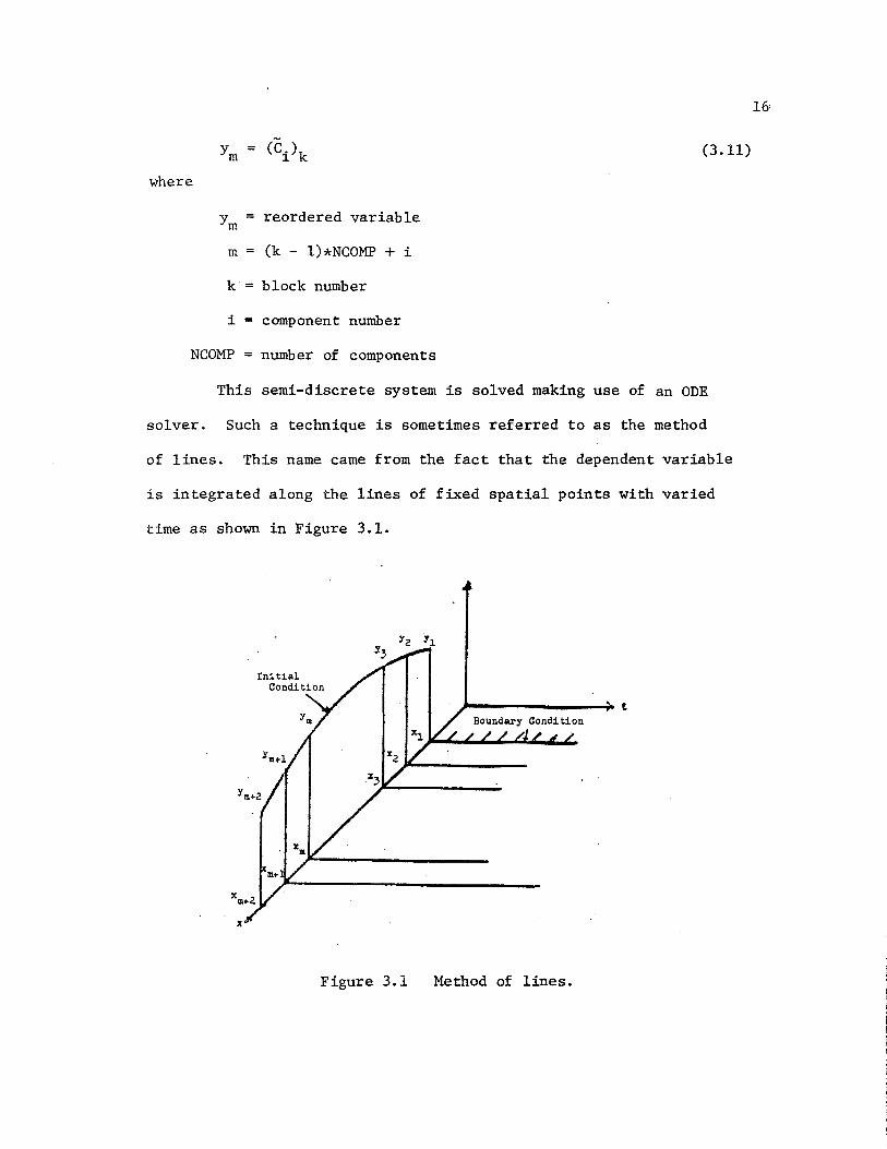
Y reordered variable m
m (k - l)*NCOMP + i
k·= block number
i = component number
NCOMP = number of components
This semi-discrete system is solved making use of an ODE
solver. Such a technique is sometimes referred to as the method
of lines. This name came from the fact that the dependent variable
is integrated along the lines of fixed spatial points with varied
time as shown in Figure 3.1.
Figure 3.1 Method of lines.
Even though the time derivatives remain continuous, their
integration must be done numerically, which means that truncation
error associated with the integration are inevitable. However,
the degree of such truncation errors can be much smailer than the
one produced from fully discrete methods, if compared with the same
time step size. Thus the truncation errors, TE, associated with
semi-discrete methods come mainly from space discretization
TE tixD M
---2- 2: j=l
2 a (f.Ci.) J J (3.12)
Even if a semi-discrete method is used, physical dispersion can be
approximated by numerical dispersion in a similar way as with the
fully discrete method.
Since the derivatives involved in equation (3. 5) are first
order with respect to both time and space, one of each temporal and
spatial boundary conditions are required. Temporal boundary condi-
tion (initial condition) has to be given to the simulator by the
user to start computation. Usually the initial condition is set to
be the post-waterflooding condition. The spatial boundary condition
is taken to be the inflow concentrations during each time step (cor-
responding to the injection of slug or drive).
3.2 Auxiliary functional relationships
In order to solve the continuity equation (3.1), many
functional relationships as well as additional assumptions are needed
17

18
to obtain Cij and fj.
Component number and phase number are determined as follows.
At most seven components are considered: (1) water, (2) oil, (3)
surfactant or surfactant and cosurfactant, (4) polymer, (5) total
anions, (6) calcium ion, and (7) alcohol. The alcohol can be combined
with the surfactant as component three. Adding the surfactant and
alcohol components together is an approximation. The accuracy depends
greatly on the particular system and conditions involved. The maxi
mum number of mobile phases considered is three: (1) aqueous,
(2) oleic, and (3) microemulsion. The last one is defined simply
as the phase containing the highest concentration of surfactant. The
details are shown in Figure 3.2. It should be noted that the number
of phases changes from time to time and place to place, depending on
the total composition (including salinity), with some phase appear
ing and some phase disappearing.
The polymer and electrolytes are assumed to occupy negligible
volume. The adsorption of water, oil, and alcohol is zero. Polymer
(c4
) and calcium (C6) do adsorb, but occupy no voll.lllle. Thus, equa
tion (3.2) is rewritten
(3.13)
The polymer is assumed to be entirely in the most water-rich phase,
whereas the electrolytes are assumed to be uniformly distributed in
the water component.
3.2.1 Effective salinity
Since the physical properties depend on both salinity and
calcium, an effective salinity CSE is defined. When the surfactant
is non-ionic, the effective salinity is given as
(3 .14)
where (c5
- c6
) equals the monovalent cation and S is a weighting
factor which accounts for the difference in effectiveness between
monovalent and divalent cations.
If the surfactant is anionic
(3.15)
wh C . h 1 . f 1 8 •46 0 d ere 8 is t e ca cium-sur actant comp ex concentration an
(c3 - c8 + c5 - c6) equals the monovalent cation.
When only sodium ion is considered to exist as a cation,
c6 can be used as a tracer by setting S equal to unity, instead of
setting c6 equal to zero.
Although not used in this study, it should be noted that
19
h d f . . . f c h b l" d27 i 1 d h f t t t e e inition o SE as een genera ize to nc u e t e sur ac an
and alcohol dilution effects. 1 •48- 50
is different from a for surfactant.
Also, in general S for polymer
65 Just recently, Fil has imple-
66 mented Hirasaki's cation exchange-micelle model which can be used
rather than the "complex model" referred to above. Electrolytes are
then no longer uniformly distributed.
3.2.2 Phase behavior
In this section, equations required to calculate phase con-
centrations and saturations are presented. The independent variables
20
here are CSE' c1 , c2 , and c7 . Since adsorbed surfactant is not con
sidered to affect phase behavior, total concentrations add as follows:
(3.16)
When a phase diagram is considered, c3
arid c7
are sunnned up
to make a single pseudo-component. Thus the pseudo ternary diagram
concept is employed.
Although the simulator is designed to deal with Type II(-),
Type III, and Type II(+) phase environments, only equations for the
Type II(-) and Type II(+) phase environments are presented. When
Type III phase environments arise, coordinate rotation is performed
and plait points for both two-phase nodes and invariant point are
moved continuously according to salinity. 37
(1) Binodal curve and distribution curve
For Type II(-) or Type II(+) phase environment, the Hand
. 51 . 1. d equation is app ie . Regardless of phase number j, the composition
corresponding to the point on the binodal curve satisfies the
21
equation below:
(3.17)
where parameter A is a function of salinity and is discussed later in
more detail. Parameter B is taken to be a constant of minus unity,
which yields a sy.mmetric binodal curve, in all the subsequent discus-
tion. The volume fractions must add to one for the pseudo-ternary, so
= 1 (3.18)
Combining equations (3.17) and (3.18) with B = -1,
(3.19)
(3. 20)
In addition to equation (3.17) the concentrations of the two
equilibrated phases satisfy the following Hand equations:
(3. 21)
Here the definition of phase number is different from that mentioned
before only for convenience. Since only two phases are con-
sidered, left of the plait point is called phase 1 and the right of

22
the plait point is phase 2. Calculation of parameter E as well as
parameter A is given later. Parameter F is taken to be unity in all
subsequent discussion.
(2) Parameter estimation
Parameter A is calculated based on the set of three input
parameters, c3MAXO' c3MAXl' and c3MAX2 , which are physically the maxi
mum height of the binodal curve at CSEN = 0, 1, and 2, respectively.
Here CSEN is normalized salinity: salinity divided by optimal
salinity. In this model, the optimal salinity is defined as the
salinity that yields a Type III phase environment and an oil concen-
tration at the invariant point of 0.5. First, parameters A at the
three salinities are calculated
( 2C3MA.Xk )2
~ = l - C3MAXk k = 0,1,2
Then linear interpolation with respect to CSEN is applied.
A
(3.22)
(3.23a)
(3.23b)
Parameter E can be obtained from the location of the plait
point. Since at the plait point the two phases are exactly the same,
equation (3.21) is rewritten:
(3. 24)
where the subscript p indicates the plait point. Then, solving
(3.24) for E gives
(3.25)
Since the plait point is on the binodal curve, eq~ations (3.19) and
(3.20) are applicable. Thus only c2P and A are required to calculate
parameter E.
23
For Type II(+) and Type II(+) phase environments, the oil con-
centration at the plait point (c2p) is assumed not to change with
salinity, while c1p and c3p change according to equations (3.19) and
(3.20). The value c2p for both Type II(-) and Type II(+) phase en
vironments must be given as input data.
(3) Calculation of phase concentrations and saturations
Suppse CSE and the total concehtrations as well as all input
parameters are given and the phase behavior environment is Type II(+)
or Type II(-). Then the equations used and unknowns involved are
summarized in Table 3.1, which indicates that we need one more equa-
tion to solve the system of equations. Since the two-phase composi-
tions are located on the tie line which goes through total composi-
tion (see Figure A.l), equation (3.26) below must be satisfied.
(3.26)
where the definition of phase number is the same as the one used in
equation (3.21). Now the number of equations and the number of un-
knowns are balanced, which means the equations are solvable somehow.
First, A, c3P, Clp' and E are calculated explicitly. Then some
iterative method is used to solve equations (3.18), (3.19) and (3.21)
for all C .. , if the plait point is not located at the corner. If l.J
the plait point is at the corner, every unknown can be solved ex-
plicitly, since the composition of the excess phase is known.
Once the composition of both phases is obtained, the satura-
tion of each phase is calculated from overall material balance.
i = 1,2,3 (3. 27)
3.2.3 Adsorption
The adsorption isotherms for both surfactant and polymer are
. 52 Langmuir-type
i = 3 or 4 (3.28)
where C~. refers to the concentration of component i in the phase l.J
richest in component i. Or
24
C :C. = max ( C .. ) 1] j = 1,3 1]
i = 3 or 4 (3.29)
Parameters ai and bi should be determined from experimental data.
b. is a constant, while a. can be a function of salinity, which al-1 1
lows adsorption to be salinity dependent.
(3. 30)
In subsequent example calculations, a 4 was assumed to be a
constant, which makes polymer adsorption salinity independent. Fur-
ther assumptions are made as follows. Surfactant adsorption is re-
25
versible with salinity but irreversible with surfactant concentration.
Polymer adsorption is irreversible.
3.2.4 Phase viscosity
where
A new generalized viscosity mode137 was used.
µ = viscosity of water without polymer w
µ = viscosity of oil 0
and the a parameters were assumed to be constants.
When polymer is present in the phase considered, µ is rew
placed by µ , which accounts for the effect of polymer. First the p

concentration of polymer and salinity is taken into account. 39
where (~ - l)b c4 .
R = 1 + ax p J -1<. 1 + b c
4.
p J
Apl' Ap 2' Ap 3 = constant coefficient
s constant exponent p
~ = permeability reduction factor
11anax = maximum value of ~
b = constant coefficient p
(3.32)
(3. 33)
In equation (3.32), the permeability reduction factor is multiplied
to increase viscosity rather than decreasing permeability. From the
viewpoint of mobility, they have the same effect. The permeability
reduction is modeled as permanent (irreversible).
3.2.5 Interfacial tension
1 A set of two empirical equations presented by Reed and Healy
are used to calculate interfacial tensions (IFT's)
G
26
log y = G + 11 wm 12 Gl3(C13/C33) + 1
(3.34a)
logy G22 G21
= + G23(C23fC33) + 1 mo (3.34b)
where
Ywm interfacial tension between aqueous and microemulsion
phase
Y = interfacial tension between microemulsion and oleic mo
phase
and parameters (G's) must be obtained from experimental data.
27
When the phase environment is Type II(-), only equation (3.34b)
is used while type II(+) requires only equation (3.34a). If phase
environment is Type III and three phases coexist, both equations
(3.34a) and (3.34b) are used to obtain two interfacial tensions.
As concerns either Type II(-) node or Type II(+) node of Type III,
one of eqhlations (3.34) is used in a similar way to Type II(-) or
Type II(+) phase environment. Several examples of the effect of the
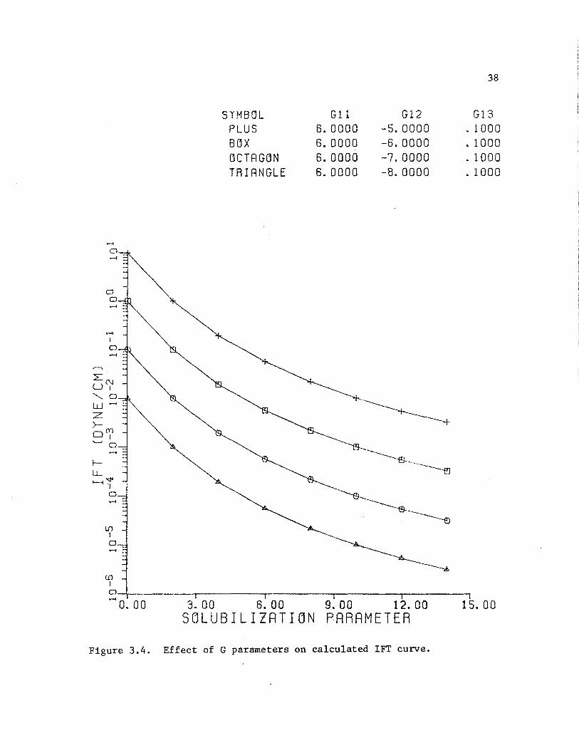
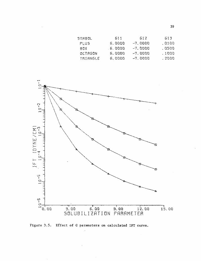
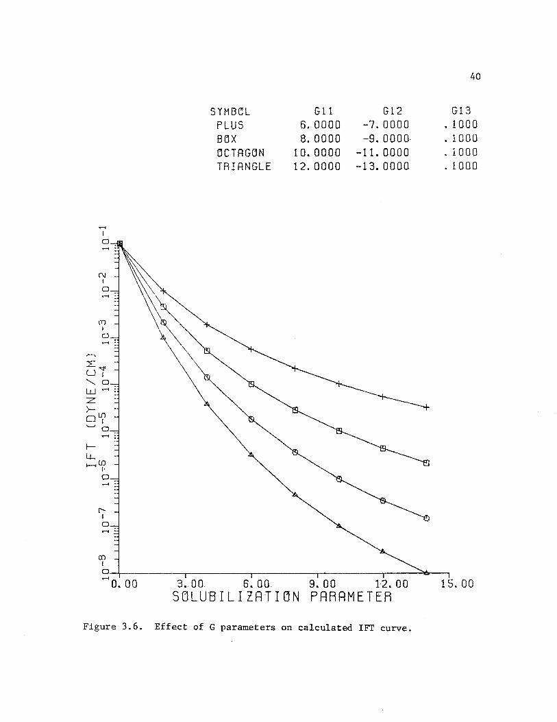
G's on the calculated interfacial tension are shown in Figures 3.3
through 3.6. In these figures, the solubilization parameter desig-
nates the ratio c13Jc33 or c23 /c33 in equations (3.34).
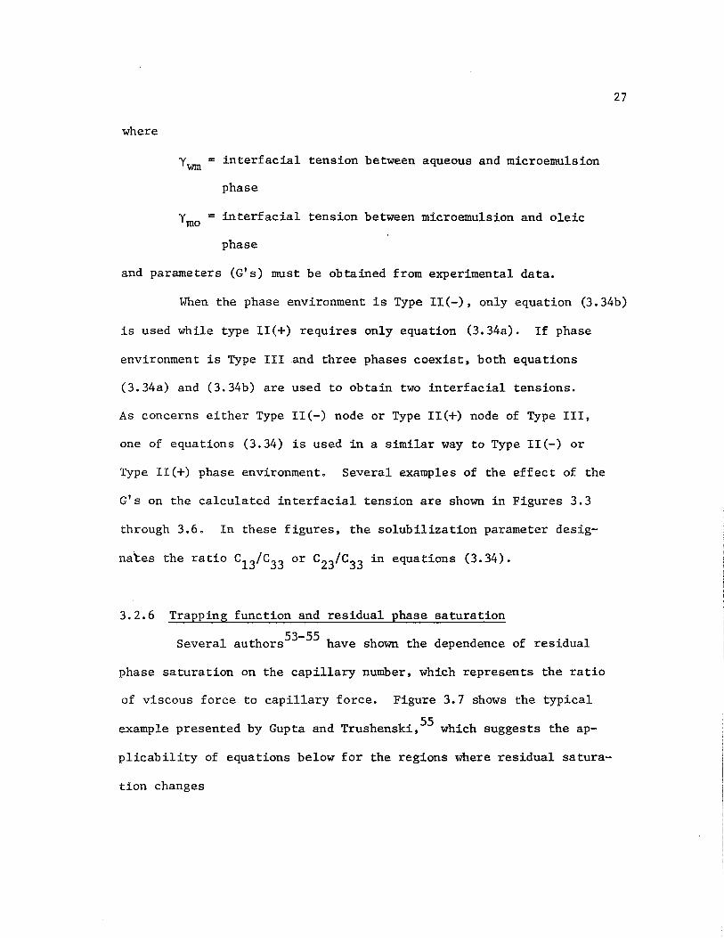
3.2.6 Trapping function and residual phase saturation
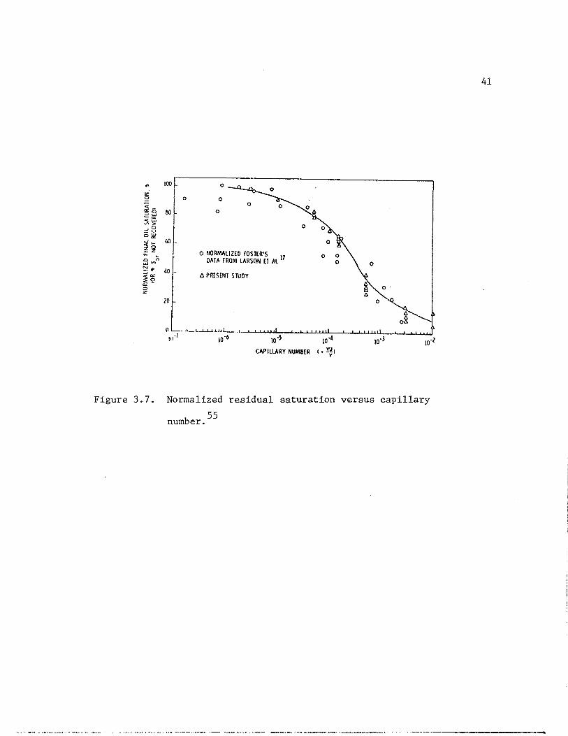
53-55 . Several authors have shown the dependence of residual
phase saturation on the capillary number, which represents the ratio
of viscous force to capillary force. Figure 3.7 shows the typical
example presented by Gupta and Trushenski, 55 which suggests the ap-
plicability of equations below for the regions where residual satura-
tion changes
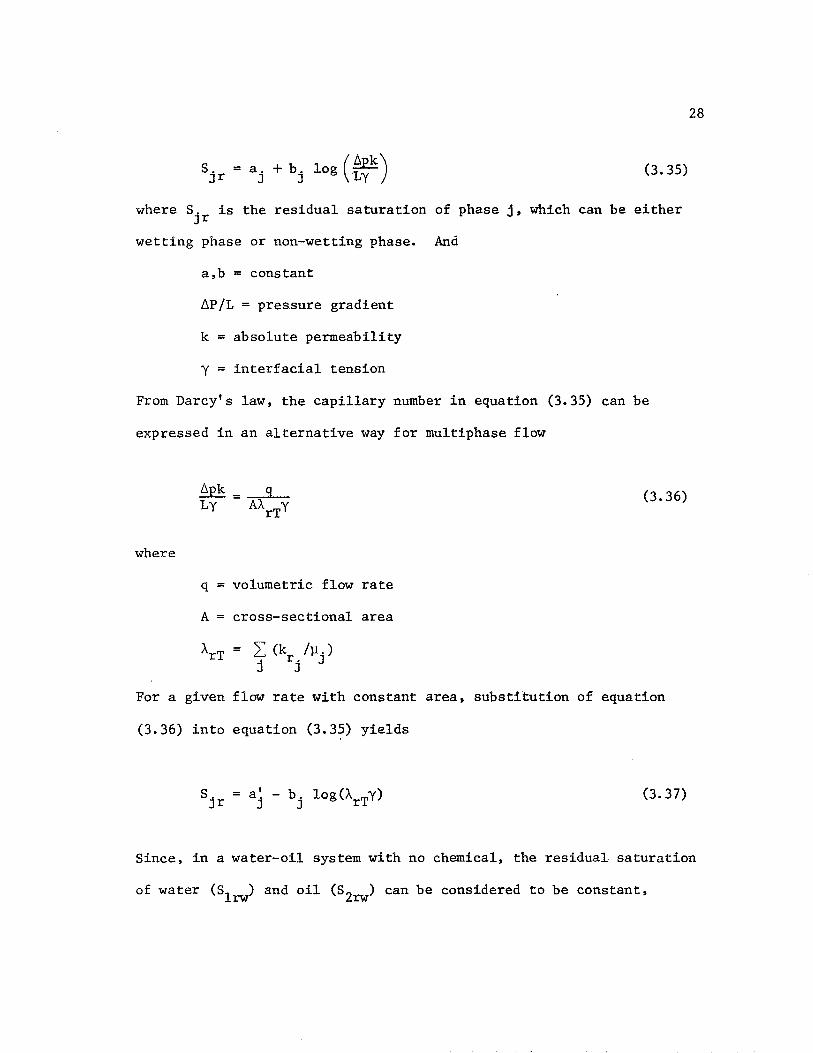
(3.35)
where S. is the residual saturation of phase j, which can be either Jr
wetting phase or non-wetting phase. And
a,b = constant
6P/L = pressure gradient
k = absolute permeability
y = interfacial tension
From Darcy's law, the capillary number in equation (3.35) can be
expressed in an alternative way for multiphase flow
where
q =
A
A.rT
For a given
(3.36) into
s. Jr
volumetric flow
cross-sectional
= 2: (k /µ.) j r. J
J
flow rate with
equation
a~ J
(3.35)
(3. 36)
rate
area
constant area, substitution of equation
yields
(3.37)
28
Since, in a water-oil system with no chemical, the residual saturation
of water (s1rw) and oil (s 2rw) can be considered to be constant,
equations (3.35) can be rewritten
(3. 38)
where sjrw equals to slrw for wetting phase and equals to s2rw for
non-wetting phase. Parameters T's in equation (3.38) depend on
fluid/rock properties such as wettability and have to be determined
from experimental data. When only two phases exist, there is only
one interfacial tension considered, and it is substituted into
equations (3.38) for both wetting phase and non-wetting phase to
calculate residual saturations. Meanwhile for the case where three
phases coexist, phase trapping behavior is still poorly understood.
Although much more experimental work and prudent investigation is
being expected in this area, a few models have been suggested and
will be discussed later.
Since equations (3.38) are applied only to the region where
29
residual saturations change as shown in Figure 3.7, the residual is set
to the water-oil (no-surfactant) value when the calculated residual ex-
ceeds the water-oil value. If ·he calculated residual is negative, the
residual is set to zero. Furthermore, as a special feature of chemi-
cal flooding, saturations can become less than the residual due to the
phase behavior (partitioning or mass transfer). In such cases the
residual saturations are set to the saturations calculated after the
"flash" calculation.
3.2.7 Relative Permeability
The relative permeability model used in this research
was modified from the one used in the original model. The basic
idea is to make relative permeabilities (krj's) approach the proper
limits when surfactant is involved. In this section, only the
equations for two-phase relative permeabilities are presented. For
three-phase flow, three different models will be introduced and
discussed in the next chapter. When there exist only two phases,
the requirements are
(1) k .'s approach their water-oil (no surfactant) values . rJ
as the capillary number decreases
(2) k .'s approach their respective phase saturations rJ
as capillary number increases
There are several cases which involve only two phases: surfactant
free, Type II(-), or Type II(+), phase environment, and either of
the two phase nodes of the Type III phase environment. In these
cases, one phase can be identified as wetting and the other as
non-wetting, presuming that one phase preferentially wets the rock
surface.
The assumed relative permeabilities are
(3.39)
j 1 j'
where
30
S. = saturation of phase j J
Sjr = residual saturation of phase j
k~j = end point relative permeabilities
(krj-value at other phase's residual saturation to
phase j)
e. = "curvature" of relative permeability curve of phase J
j in reduced saturation space
Again in equations (3.39), phase j can be either wetting or non-
wetting phase. When phase j is wetting phase, phase j' is non-·
wetting phase (and vice-versa). S.'s are obtained from equation J
(3.27) in phase behavior calculation while Sjr's are calculated
using equations (3.38).
When a reservoir is preferentially water wet, the aqueous
phase is assumed to be the wetting phase compared with the micro-
emulsion phase in the Type II(+) phase environment, whereas the
microemulsion phase wets and the oleic phase is non-wetting in the
Type II(-) environment.
In order to make relative permeabilities approach the pro-
per limits, linear interpolation of end points and curvatures of
equations (3.39) are performed based on the change in the residual
phase saturations as follows:
0 s.' s.'. =k + Jrw- Jr . s rJW . 1 J r
j :/: j' (3.40)
e. = J
e. JW
(e. - e. ) JC JW
j :/: j I (3.41)
.31
where subscript w designates a water-oil (no surfactant) quantity
and subscript c the infinite capillary number value. Although
all values with subscript c are usually considered to be unity,
they are left to be specified in input data for flexibility.
3.2.8 Other features
In addition to the features which have been described so
far, the simulator involves several other features. Since such
features are not used in this research and they are discussed
elsewhere in detai138 •39 •47 , only the list of such features is
given here.
(1) Inaccessible Pore Volume
(2) Shear rate effect on polymer
(3) Ion exchange
(4) Surfactant complex
(5) Alcohol effect
(6) Dilution effect
3.3 Solution Procedure
Summarizing the functional relations described so far and
governing continuity equations, the interdependence of the major
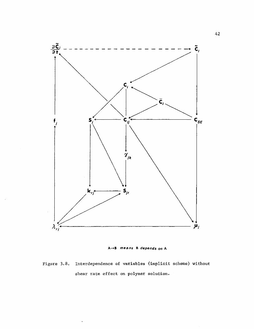
variables is shown in Figure 3.8. All variables are considered at
the same time level except the calculation of Ci from its
32
time derivative, which is indicated by dashed line.
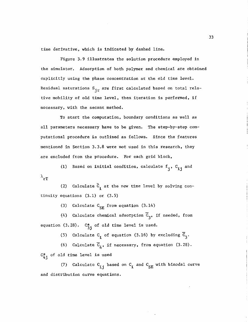
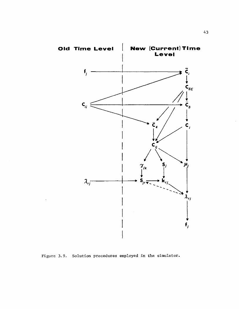
Figure 3.9 illustrates the solution procedure employed in
the simulator. Adsorption of both polymer and chemical are obtained
explicitly using the phase concentration at the old time level.
Residual saturations Sjr are first calculated based on total rela
tive mobility of old time level, then iteration is performed, if
necessary, with the secant method.
To start the computation, boundary conditions as well as
all parameters necessary have to be given. The step-by-step com-
putational procedure is outlined as follows. Since the features
mentioned in Section 3.3.8 were not used in this research, they
are excluded from the procedure. For each grid block,
(1) Based on initial condition, calculate fj, Cij and
(2) Calculate Ci at the new time level by solving con
tinuity equations (3.1) or (3.5)
(3) Calculate CSE from equation (3.14)
(4) Calculate chemical adsorption c3
, if needed, from
equation (3.28). C~j of old time level is used.
(5) Calculate Ci of equation (3.16) by excluding c3
.
(6) Calculate c4
, if necessary, from equation (3.28).
czj of old time level is used
(7) Calculate Cij based on Ci and CSE with binodal curve
and distribution curve equations.
33
(8) Calculate Sj from Ci and Cij making use of
equation (3.27)
(9) Calculate y from equation (3.34)
(10) Calculate µj from equations (3.31) through (3.33)
(11) Cal cu late S . from equation (3. 38) • Jr "-rr of old
time level is used at the first time. Then "-rT obtained at step
(13) is used when iterated.
(12) Calculate krj from equations (3.39) through (3.41)
(13) Calculate "-rj' "-rT and fj based on krj and µj
(14) Compare new "-rT with old "-rr· If the relative dif
ference is larger than some specified value, go back to step (11)
and repeat calculation. Secant method is used to obtain next es-
timate. If the difference is small enough, go to step (2) and start
new time level calculation.
34
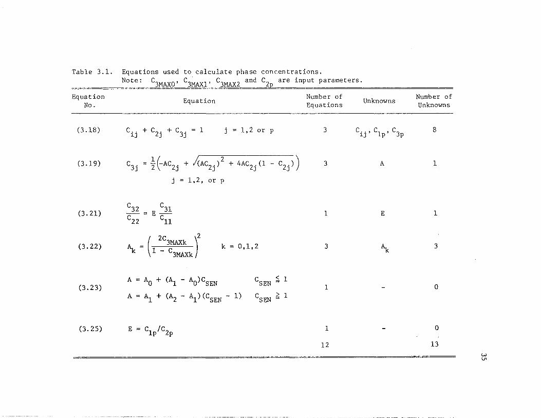
Table 3.1. Equations used to calculate phase concentrations.
Equation No.
(3.18)
(3.19)
(3.21)
(3. 22)
(3. 23)
(3. 25)
Note: c3MAXO' c 3~1 , c3MAX2 and c2p are input parameters.
Equation
c .. + c2 . + c3
. i] J J
1 1,2 or p j
c3 j = i(-Ac2j + /cAc2j) 2
+ 4Ac2j (1 - c 2j))
c32 = c22
j = l, 2, or p
c E _ll
cu
2
( 2C3MAXk )
~ = 1 - c3MAXk k = 0,1,2
A = Ao + (Al - Ao)CSEN
A= Al+ (A2 - Al)(CSEN - 1)
E = Clp/C2p
c < 1 SEN =
c > 1 SEN =
Number of Equations
3
3
1
3
1
1
12
Unknowns
c .. , c1
, c3 1] p p
A
E
~
Number of Unknowns
8
1
1
3
0
0
13 w ln
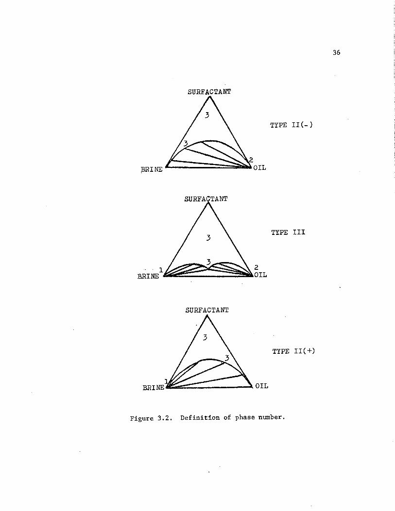
36
SURFACTANT
TYPE II (-)
T~PE III
SURFACTANT
TYPE II(+)
Figure 3.2. Definition of phase number.

L: u "-..
...... 0 ......
0 0
...... I 0
lJ.J N -
z' >- 0 -
.--f -
0 -
I- 01 LL. I
0 1--i ~ :
L.n I
SIMBDL PLUS BrJX DCTRG(rn TRIANGLE
,37
Gll G12 G13 5.0000 -7.0000 . 1000 6.0000 -7.0000 . 1000 7. 0000 -7.0000 . 1000 8.0000 -7.0000 . 100 0
o--.~~~~-.--~~~~~~~~~~~~~~~---'~~ .-t
0. 00 3. 00 6. 00 9. 00 12. 00 15. 00 SOLUBILIZRTION PARAMETER
Figure 3.3. Effect of G parameters on calculated !FT curve.
0 0
.._, I 0
:L:('J U1 '-.... 0 w ...... : z >--0 n;i '-' 0
f-LL ~
1--l ·1
0
If) I 0 .....
(!) I
SIMBOL PLUS BOX DCTRGDN TRIANGLE
38
Gll G12 G13
6. 0000 -5. 0000 . 1000 6. 0000 -6.0000 . 1000 6. 0000 -7. 0000 . 1000 6. 0000 -8. 0000 . 1000
D-+-~~~~·-.--~~~--..--~~~~~~~~~~~~-.._, 0. 00 3. 00 6. 00 9. 00 12. 00 15. 00
SOLUBILIZATION PARAMETER
Figure 3.4. Effect of G parameters on calculated IFT curve.
....... l C.l
('\J l 0
V1 I 0
CD I o__.,__ .......
0. 00
SIMBOL Gll G12 PLUS 5.0000 -7. 0000 BOX .6. 0000 -7. 0000 OCTAGON 6.0000 -7. 0000 TRIANGLE 6.0000 -7.0000
3. 00 6. 00 9.00 12. 00 50LUBILIZRTION PRARMETEA
Figure 3.5. Effect of G parameters on calculated !FT curve.
39
G13
. 0100
. 0500
. 1000
. ·2000
15. 00
....... I a
(\J I a
en I a
2:: .
ui '-.. 0 w ..... ~ z: . >oL( . '-'o
fLL. 1-1 (.D
I· 0
r-t a
()'.) I
SYMBOL PLUS B(j X (jCTRG(jN TRIANGLE
40
Gll G12 G13
6. 0000 -7. 0000 . 1000 8.0000 -9. 0000· . 1000
10. 0000 -11. 0000 . 10 00 12. 0000 -13.0000 . 1000
0--1,.-~~~--~~~~~~~~~~~~~--..--~~lr-~
..... 0. 00 3.00 6.00 9. 00 12. 00 15.00 saLUBILIZATI~N PARAMETER
Figure 3.6. Effect of G parameters on calculated !FT curve.
,,. 100 0 z. 9 0 0 ~ 0
28 80 0
..,5 '-" > :8 Oli! _, ,_ 60 -~~ o NORMALIZED FOSTER'S ... ;; 0 ~ ,,, DATA FROM LARSON ET AL IT ~,,.
40 -~~ 6 PR£SENT STUDY
"' -0 z
20
n -- .1_ L...L.LJ..LJ.J L--'--1u ·I 10-6
I I 1 I I 11 I I I I I I I! I I .....J..-L.-L..L...,.__.__,'-L,~U.JJ
10~ 10~ 10~
CAPILLARY NUMBER I • ~I
Figure 3.7. Normalized residual saturation versus capillary
55 number.
41
42
-oC; ot
----------------- ------+ c I
k,j ____ _
A-B means B depends on A
Figure 3.8. Interdependence of variables (implicit scheme) without
shear rate effect on polymer solution.
Old Time Level New (Current) Time Level
Figure 3.9. Solution procedures employed in the simulator.
43
CHAPTER IV
THREE PHASE FLOW MODEL
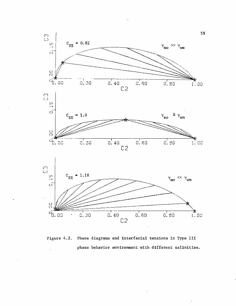
When salinity is in a certain range, phase behavior environ-
ment is called Type III (see Appendix A) and its phase diagram can
involve a three phase region. When three phases coexist, little is
known about the trapping of each phase and their flow character. How-
ever, the modeling of such three phase flow is necessary since the
process is usually used where the lowest interfacial tensions are
achieved, which is in the three phase region. Thus, several authors
have developed models based on various assumptions.
In this chapter, three examples of such three phase flow
models are introduced and comparisons are presented.
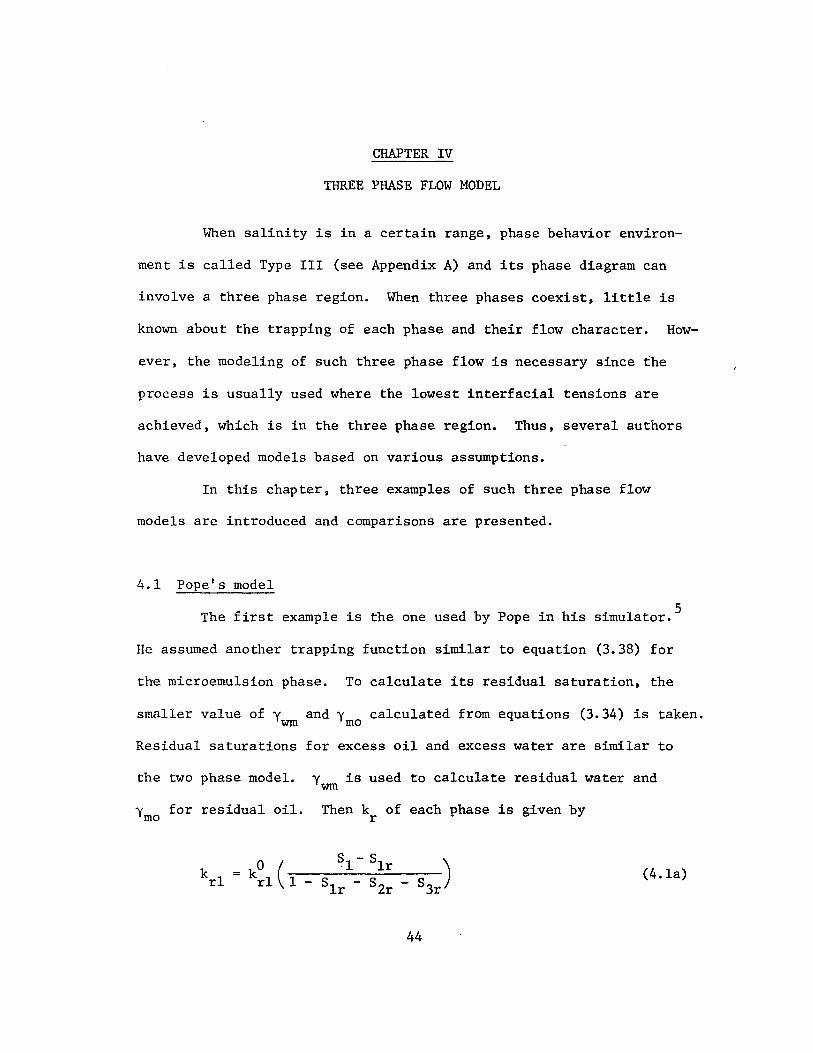
4.1 Pope's model
5 The first example is the one used by Pope in his simulator.
He assumed another trapping function similar to equation (3.38) for
the microemulsion phase. To calculate its residual saturation, the
smaller value of ywm and ymo calculated from equations (3.34) is taken.
Residual saturations for excess oil and excess water are similar to
the two phase model.
Y for residual oil. mo
y is used to calculate residual water and wm
Then k of each phase is given by r
44
(4.la)

45
kr2 ko ( 82 - 82r
83r) (4. lb) =
r2 1 - s - s -lr 2r
83 - 83r e3
kr3 ko ( 83r) (4. le) r3 1 - s - s -lr 2r
where subscripts 1, 2, and 3 designate water, oil, and microemulsion
phase respectively. kO and kO are given by equations (3.40). rl r2
4.2 Hirasaki's model
Another model was presented by Hirasaki9• He calculated the
residual saturation of each phase based on a physical idea, which
is shown in Figure 4.1. In describing the model, an assumption
is made here that a preferentially wtaer wet reservoir is considered.
This asumption is just to make explanation easier and the generality
of the model is not affected by the assumption·.
Figure 4.la leads to equation (4.2) which describes the trap-
ping of excess oil and microemulsion phase by the excess water phase
= f (y ) wm
(4. 2)
where f(y) is the non-wetting phase trapping function, which is
identical to the right hand side of equation (3.38) in the simulator.
Figure 4.lb shows the trapping of excess water and microemulsion
46
phases by the excess oil phase
(4. 3)
where g(y) is the wetting phase trapping function which is given as
equation (3. 38)
From Figures 4.lc and 4.ld
(4. 4)
(4. 5)
After evaluating equations (4.2) through (4.5), the residual
saturation of each phase is determined as follows:
81r
e(ywm) =max g(ymo) - s3
(4.6a)
82r
=max r(ymo) f (y ) - s wm 3
(4. 6b)
f(ywm) - s2
s3r = max 0 (4. 6c)
g(ymo) - s 1
Then assumed relative permeabilities are
(4. 7)
(j = 1, 2,3)
47
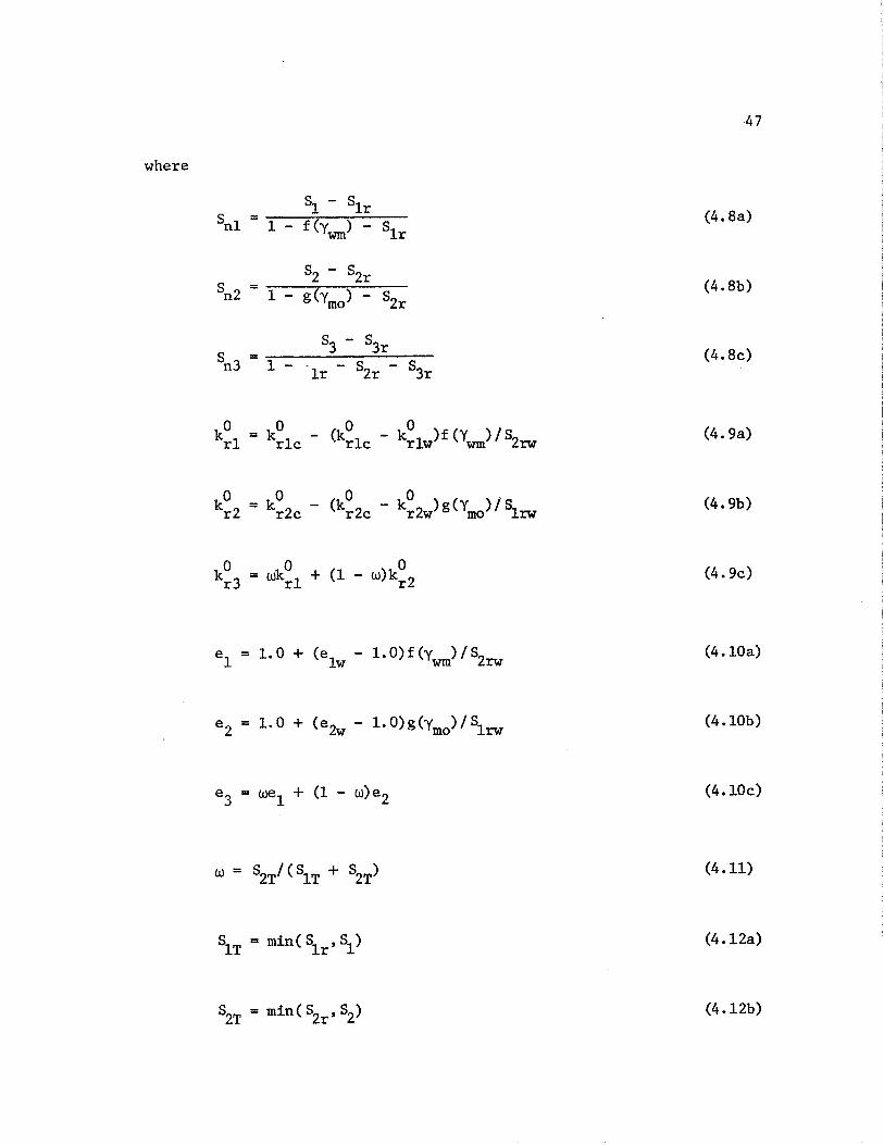
where
s - 81r 8nl = 1 -
1 f(y ) - 81r wm
(4. 8a)
s - 82r s = 2
n2 1 - g(ymo) - 82r (4.8b)
s - 83r s = 3
n3 1 - lr - 82r - 83r (4. 8c)
(4.9a)
(4.9b)
0 0 0 kr3 = wkrl + (1 - w)kr2 (4. 9c)
(4.lOa)
e2
= 1.0 + (e2 - 1.0)g(y )/S1 w mo rw (4. lOb)
(4.lOc)
(4.11)
(4.12a)
(4 .12b)

4.3 37 Lake's model
The basic philosophy employed in the model is that the
48
intermediate wetting phase becomes the wetting phase when the ori-
ginal wetting phase is absent (and vice versa). Hence he first
introduced a simple interpolating function
(4.13)
This function gives G = 0 when s2 = 0 and G = 1 when s1 = 0.
Then the microemulsion residual saturation s3r is determined
(4.14)
where s1
r and s2r are given by equations (3.38).
Assumed relative permeabilities are in the same form as
Hirasaki's model.
(j = 1, 2,3) (4.7)
where
s. - sj S . = --~__,J.___...,,.....,_e-r--=---
nJ 1 - 81r - 82r - 83r j = 1,2,3 (4.15)

49
ko 0 (ko kO )S /S (4.16a) = k -rl rlc rlc - rlw 2r 2rw
0 0 (ko - kO )S /S (4.16b) kr2 = k -r2c r2c r2w lr lrw
ko = GkO + (1 - G)kO (4.16c) 3r rl r2
(4.17a)
(4.17b)
(4.17c)
Considering the fact that saturation can become less than residual
saturation due to phase behavior, the residual saturation of each
phase is defined
SJ. r = min ( S. , S. ) J Jr
j = 1,2,3 (4.18)
Equation (4.18) is substituted in equations (4.15) through (4.17)
as S .• Jr
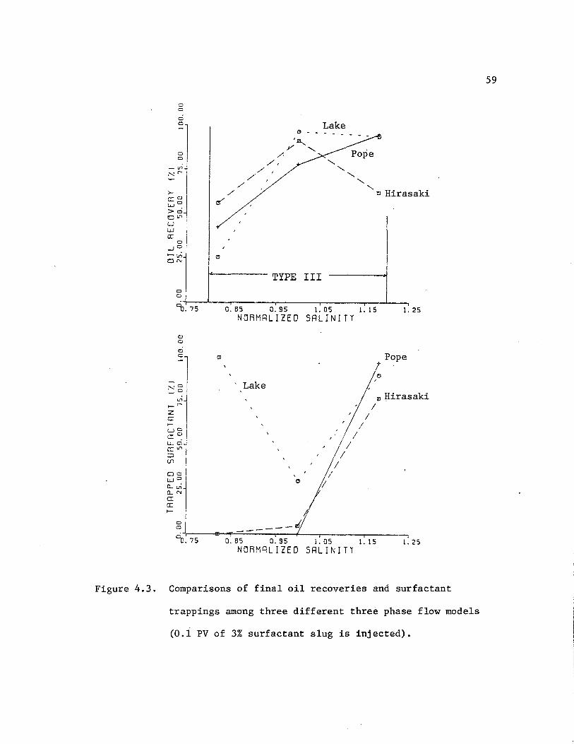
4.4 Comparison of Each Model
Tables 4.1 and 4.2 show the comparison of oil recovery and
the amount of surfactant trapped with the different three-phase flow
models which have been introduced. Table 4.1 shows the results ob
tained with 0.1 PV of 3% surfactant slug injection whereas 0.1 PV of
6% surfactant slug was injected for results given in Table 4.2. In
each table only the flow model was changed for three different
salinities. The same results are plotted as oil recovery versus
salinity and trapped surfactant versus salinity in Figures 4.3 and
4.4. Each salinity represents near lower limit (CSEL), middle, and
near upper limit (CSEU) of Type III phase behavior environment. The
change in salinity affects the shape of multiphase region and inter
facial tensions as shown in Figure 4.2. Salinity was kept constant
or nearly constant for each run. After surfactant slug injection,
1.9 PV of polymer solution was injected in all runs.
The same input data as is given in Table 6.la was used except
that c13
= c23 = 0.05. No adsorption was considered. All other data
are shown in Tables'4.4. No microemulsion phase trapping was con
sidered for Pope's model.
When salinity is near lower limit of Type III (Figure 4.2a),
oil recovery is rather low with all models. All surfactant injected
was trapped with Lake's model whereas the other two models trap no
surfactant.
When salinity is around optimal (Figure 4.2b), all models
but Pope's trap surfactant somewhat. Surfactant trapping is rather
50
51
low and oil recovery is high with all models.
When salinity is near upper limit of Type III (Figure 4.2c),
surfactant trapping is rather high with all models. Pope's and Lake's
model give high oil recovery while Hirasuki's model gives lower oil
recovery.
Although the difference in oil recovery is rather large, es
pecially when the injected amount of surfactant is small, among the
models, Pope's model and Hirasaki's model show similar trend in
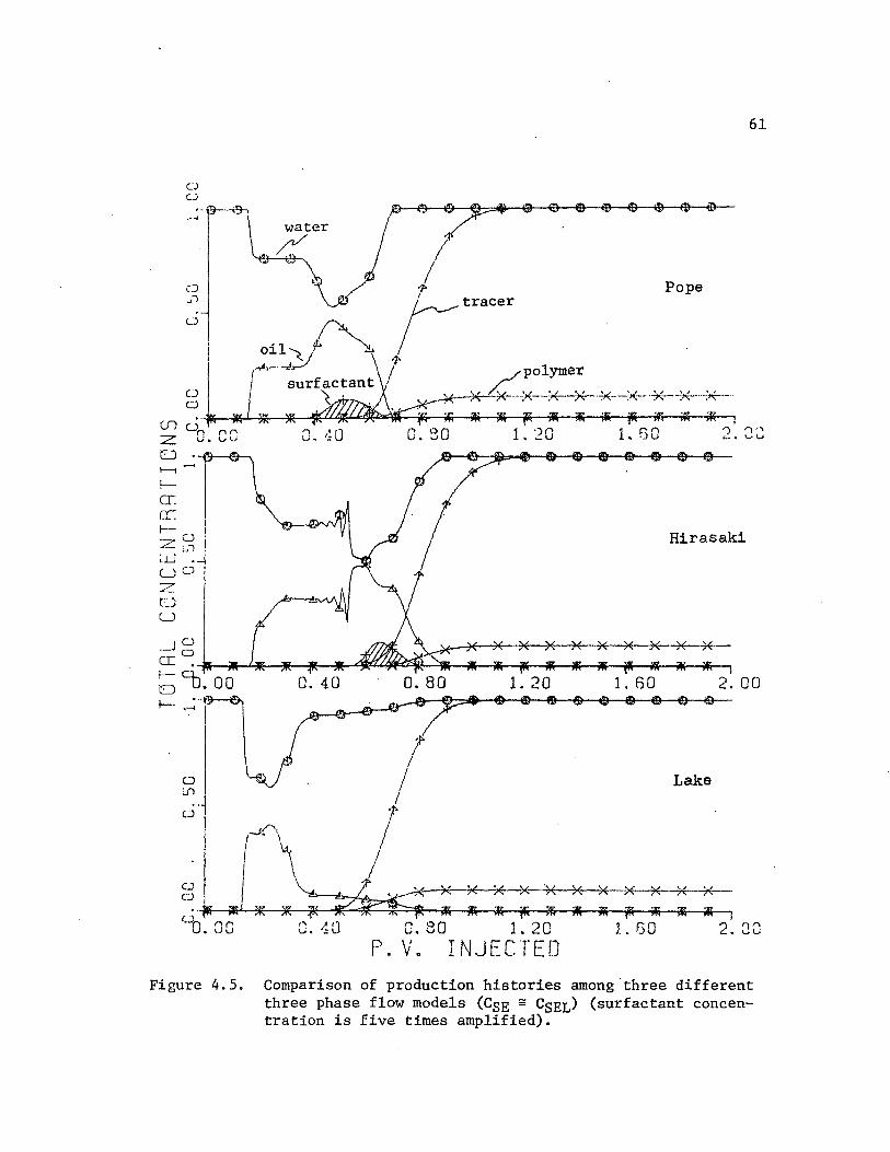
surfactant trapping to each other. Figure 4.5 shows the histories of
total concentration in production for each model with salinity of
0.82 (~CSEL) and 3% surfactant slug. Not only oil production but
surfactant breakthrough time differs among the models.
Table 4.3 shows the comparison for the cases with salinity
gradient. Data set 3S-4 and 3S-5 were used for these runs. 0.1 PV
of 3% surfactant slug was injected. Surfactant trapping was almost
zero in all runs. The difference in oil recovery among the models
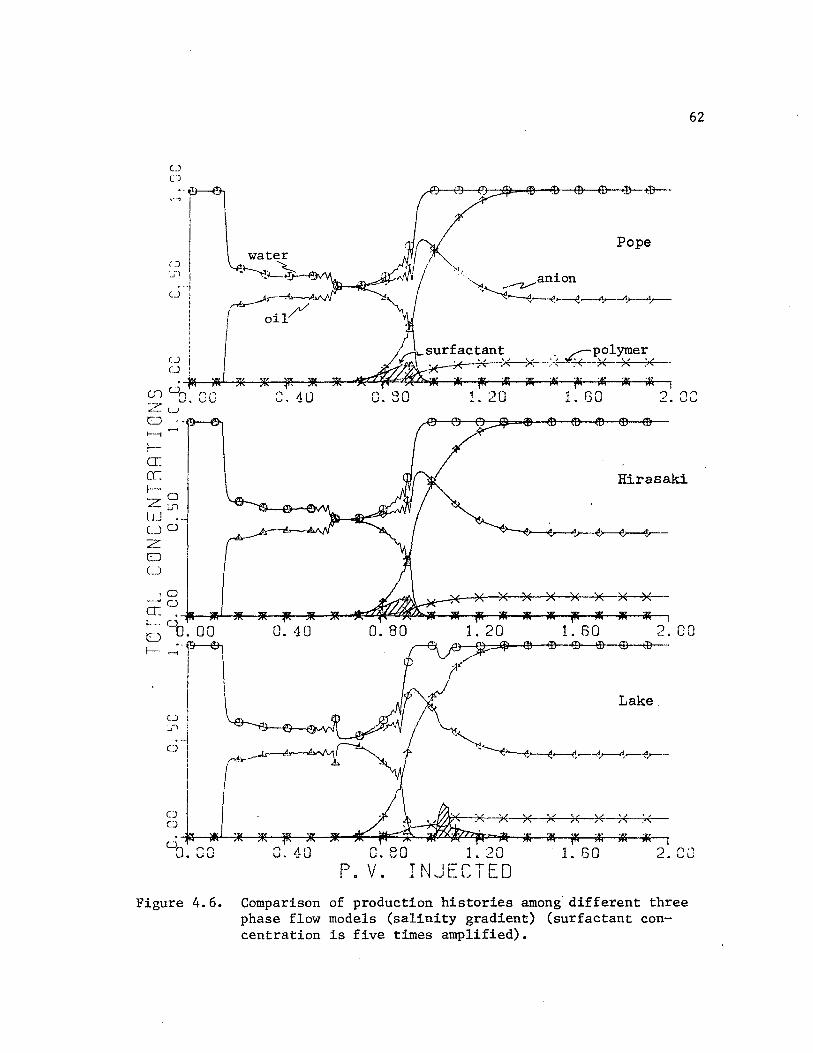
is rather small compared with constant salinity runs. Figure 4.6
shows production history of each model with salinity gradient
(1.4 - 1.0 - 0.6). Although this figure shows there is a significant
difference in surfactant production history, the fact that all models
yield high oil recovery can be another reason for designing a micellar
flood with a salinity gradient.
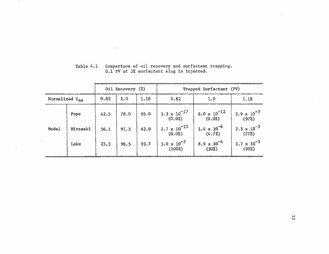
Table 4.1 Comparison of oil recovery and surfactant trapping. 0.1 PV of 3% surfactant slug is injected.
Oil Recovery (%) Trapped Surfactant (PV)
Normalized Cse 0.82 1.0 1.18 0.82 1.0 1.18
Pope 42.5 78.0 95.0 3.3 x l0-17 6.0 x 10⁻¹² 2. 9 x 10 (0. 0%) (0. 0%) (97%)
Model Hirasaki 56.1 91.3 62.0 2.7 x l0-15 1. 4 x 10 -4 2.3 x 10 (0.0%) (4. 7%) (77%)
Lake 25.5 96.5 93.7 3.0 x 10 -3 8.9 x 10 -4 2. 7 x 10 (100%) (30%) (90%)
-3
-3
-3
V1 N

Table 4.2 Comparison of oil recovery and surfactant trapping. 0.1 PV of 6% surfactant slug is injected.
Oil Recovery (%) Trapped Surfactant (PV)
Normalized CSE 0.82 1. 0 1.18 0.82 1.0 1.18
Pope 45.2 88.5 87. 0 1.1 x 10⁻¹⁶ 2. 6 x 10⁻¹⁰ 5.4 x 10 (O. 0%) (O. 0%) (90%)
Model Hirasaki 58.5 94.0 76.0 3.2 x l0-15 2.8 x 10 -4 4.6 x 10 I (0.0%) (4. 7%) (77%)
Lake 47.5 97 .4 89.4 6.0 x 10 -3 6.8 x 10 -4 4. 7 x 10 (100%) (11%) (78%)
-3
-3
-3
V1 w

Table 4.3
Salinity Gradient
Comparison of oil recovery and surfactant trapping for two different salinity gradients. 0.1 PV of 3% surfactant slug is injected.
1. 8-1. 0-0. 2 1. 4-1. 0-0. 6
~ Oil Recovery Surfactant Trapped Oil Recovery Surfactant Trapped (%) (PV) (%) (PV)
1.5 x 10⁻¹⁰ I 2. 5 x 10-lO Pope 90.9 93.0
Hirasaki 87.9 1.1 x 10⁻¹⁰ 90.4 1.6 x 10⁻¹⁰
Lake 84.7 1.1 x 10⁻¹⁰ 86.8 1.6 x 10⁻¹⁰
VI .i::-
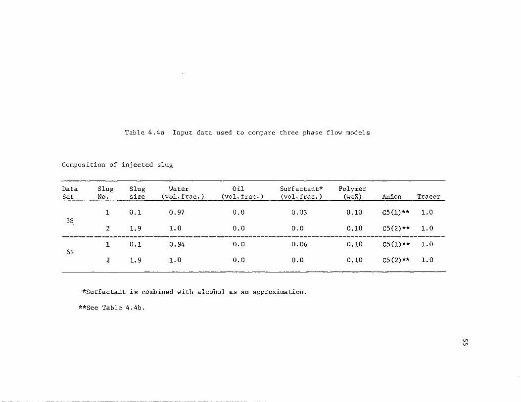
Table 4.4a Input data used to compare three phase flow models
Composition of injected slug
Data Slug Slug Water Oil Surfactant* Polymer Set No. size (vol. frac.) (vol. frac.) (vol. frac.) (wt%)
1 0.1 0. 97 0.0 0.03 0.10 3S
2 1. 9 1. 0 0.0 0.0 0.10
1 0.1 o. 94 0.0 0.06 0.10 6S
2 1. 9 1.0 0.0 o.o 0.10
*Surfactant is combined with alcohol as an approximation.
**See Table 4.4b.
Anion Tracer
C5(1)** 1.0
C5(2)** 1.0
C5(1)** 1.0
C5(2)** 1.0
\Jl \Jl
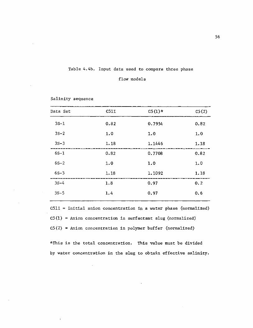
Table 4.4b. Input data used to compare three phase
flow models
Salinity sequence
Data Set C51I cs (l)* C5(2)
3S-l 0.82 0.7954 0.82
3S-2 1.0 1.0 1.0
3S-3 1.18 1.1446 1.18
6S-l 0.82 o. 7708 0.82
6S-2 1.0 1.0 1.0
6S-3 1.18 1.1092 1.18
3S-4 1.8 0.97 0.2
3S-5 1.4 0.97 0.6
C51I = Initial anion concentration in a water phase (normalized)
CS(l)
cs (2)
Anion concentration in surfactant slug (normalized)
Anion concentration in polymer buffer (normalized)
*This is the total concentration. This value must be divided
by water concentration in the slug to obtain effective salinity.
56

(a)
(c)
(b)
(d) MICROEMULSION
Figure 4.1. Basic idea of phase. trapping employed in Hirasaki's model. 9
VI -...J
(!} I (__)
~1 CSE• 0.82
g L/~ . -- - ----- r ----------, 0
0. 00 C. ~?O 0. 40
. CJ
(_)
0 -- ---- ---------. ·- ------,---
C)n 'l " i' • ) Q u .. uu '-' -
[_[) CSE = 1.18
. D
C.GO C2
T-- ----T
0. 40 0. GO C2
58
0. 80 1. 00
~ y wm
1. 00
Figure 4.2. Phase diagrams and interfacial tensions in Type III
phase behavior environment with different salinities.
0 0
0
~l
2; I
::1 >o.J 0 1.:1 I u I w ' 0:::
0 0
~
/ /
/
/, /,
TYPE III
Lake
" " Pope
" .......
" ~ Hirasaki
°a. 75 0.85 0.95 1.05 1.15 1. 25
0 0
0
~l
NORMALIZED SALINITY
' Lake
Pope t
:.... 0
""' Ill Hirasaki ~01 ~~ I ~ I
~~
11 ,~ '//
CL ro a: 0::: ~ ~
~J ______ ei/ c:..~,~~-em--i.,-r-=~~~r1~-+-Z....~--.-,~~~-....,~~~--.,
1.!.75 0.85 0.95 i.05 1.15 1.25 NCRMqLIZEO SALINITY
Figure 4.3. Comparisons of final oil recoveries and surfactant
trappings among three different three phase flow models
(O.i PV of 3% surfactant slug is injected).
59

>-
0 Cl
:::> 0
0 c
cr:: o WO >c::i Cl lJ'>
u w er:
0 .-Jo ..._, ui or..
0 c
°o. 75
0 0
c::i 0
:-.,:0 ._ 0
ui I-,...
z a: t-uo a:~ LL. Cl ::c -.1
::i c.n
ClO :...J Cl
CL .-i a.."' a: c:: I-
0 0
9:J. 75
Cl
al
/
/, /,
/,
0. 85
/ /,
(!I -'a.... -y ..._,
TYPE III
0.95 1. as NuRMRLIZEO SRLINITY
Lake - -0
Pope
Hirasaki
I. I 5 I. 25
,.. Pope
/ !il Hirasaki ' Lake
I j
/1 I;·
/! /'I //
/; I~
'I.
' ~ Ii
--~ ----- '
0. 95 0.95 i. 05 l. 15 i. 25 ~i CR M q L I Z ED SRLIN!TI
Figure 4.4. Comparisons of final oil recoveries and surfactant
trappings among three different three phase flow models
(O .1 PV of 6% surfactant slug is in.!).ected).
60
C) (_)
,.;-1·~-\ water
~~
·-u
>--I
!-a: rr: 1---~ U .... :::_ L J
~Ll . u CJ
:z 0 LJ
u CJ
G. 10
0. 80
I I
I
1. 20
0. 80 1. 20 P. V. INJECTED
61
•") 'I'' r..:. vu
Hirasak.i
1.60 2.00
Lake
)( x
1. 60 2.8C
Figure 4.5. Comparison of production histories among three different three phase flow models (CsE ~ CsEL) (surfactant concentration is five times amplified).
a: cc: 1-
(_)
0
(_)
(_)
C)
z o ~.n
w ·LJO z D u
8. 10 ri on U.vU
Hirasaki
10 -~CJ
a: ._._-aJ_.~~~~~lf;:d.~~~-&----;fi~~~:F----&---&-._;-~ 1-- u
~~J ~ I ·"· "' I r~~~ "'---<~~,__,,_..,,__,,_,,_ ·
I )\ ~1.* * ~ * * ~: )( )\ )( 7<E- ~< )(
;ti ifi if' lfi ~ ~ I
62
uG. CC 0. 40 C.80 1. 20 1.60 2.CC P. V. I ~JJECTED
Figure 4.6. Comparison of production histories among different three phase flow models (salinity gradient) (surfactant concentration is five times amplified).
CHAPTER V
ORDINARY DIFFERENTIAL EQUATION INTEGRATORS
There exist quite a few numerical techniques to solve a system
of first-order ordinary differential equations (ODE's) of the form
dy y' dt - f(y,t) ' (5.1)
where y and f are vectors of length N. The techniques, in general,
can be divided into two categories: single step methods and multistep
61 methods.
For single step methods, no information about the solution for
previous steps is necessary. One representative example of such single
step methods is the Runge-Kutta algorithm. Runge-Kutta methods re-
quire the evaluation of derivative f(y,t) at intermediate points be--
tween the initial and end point of each step.
Multistep methods make use of information about the solution
ob.tained from several previous steps to calculate the solution for the
current step. Thus they generally require a larger amount of compuer
memory than the Runge-Kutta formulas of the same order. Concerning
the computation, however, multistep methods can be rather economical
integrators since they generally require only one or two functions
evaluations per step.
63
5.1 56 Runge-Kutta-Fehlberg methods
Single step mehods for solving y' = f(y,t) require only a
knowledge of the numerical solution y ·1n order to compute the next .n
value Yn+l· This has obvious advantages over the p-step multistep
methods that use several past values {y , •.. ,y }, and that n n-p
require initial values {y1 , ••• ,yp} that have to be calculated by
another method.
The best known one-step methods are the Runge-Kutta methods;
and they are the usual means for calculating the initial values
64
{y1 , ... ,yp} for a (p+l)-step multistep method. The major disadvantage
of the Runge-Kutta methods is that they use many more evaluations of
the derivative f(y,t) to attain the same accuracy, compared with the
multistep methods. At present, there are no variable order Runge-
Kutta methods comparable to the Adams-Bashforth and Adams-Moulton
methods. Runge-Kutta methods are closely related to the Taylor
series expansion of y(t), which is the solution of the initial value
problem, but no differentiations of f is necessary in the use of
the method. 60
The Fehlberg integrators are single-step, fixed-order methods
and time-step size is varied according to the estimated truncation
error made during the last time step. To estimate the truncation
th th error, (p+l) order and p order Runge-Kutta formulas are employed.
The difference between those two approximations is defined to be an
estimate of the leading term of the local truncation error for the
th p order approximation. Error is controlled by keeping the magnitude

65
of the local truncation error within some specified (desired) to-
64 th th lerance. Depending on the algorithm, either the p or (p+l) order
approximation may be used as the solution.
A numerical solution of Equation (5.1) can be obtained by us-
ing either of the following Runge-Kutta-Fehlberg integration formulas
Q,-1 = Yi + Lit L c f + O(l'.itp+2)
k=O k k
(5. 2)
(5. 3)
where m and Q, are the number of function evaluations in the lower order
and higher order formulas, respectively. Subscripts i and i+i indicate
their step level
fo = f(t.,y.) 1 1
(5.4)
k-1 fk = f(t. + C\Lit, y. +Lit I 13k>.f >.)
1 1 >.=O (5. 5)
where Lit is the step size. The constants a, 13, c and c are determined
in the derivation of the algorithm. The superscript A indicates
higher order approximation.
An estimate of the local truncation error, LTE, for the lower-
order solution is obtained as below
r-1 = Litl L (Ck
k=O (5. 6)
66
where
r = max(.!/, ,m)
Let
TOL = ERR*tnax(IYI ,YBIAS) (5. 7)
where ERR is the relative error tolerance. YBIAS is some specified
lower limit to avoid the selection of a step size which is too small.
Here both LTE and TOL are a vector of length N, since y is a
vector in our case. If any component of LTE is larger than the corre-
spending component of TOL, the step size is reduced and calculations
are repeated until the desired accuracy is obtained. If every compo-
nent of LTE is less than the corresponding component of TOL, the step
size is accepted and the next step size to be used is calculated as
follows
.6t new (
TOL.)l/ (p + l)
= PCTM told*. min LTE ~ J=l,N J
(5. 8)
where PCT is a conservative factor, which is intended to prevent ex-
cessive step rejections. PCT may be assigned the value of 0.8 to 0.9 •
.6told is the current step size used. p is the order of approximation.
N is the number of equations.
When a higher order ODE solver is applied to solve the conti-
nuity equation in the simulator, the truncation error produced from
spatial discretization is much larger than the error from time inte-
gration. Consequently the pair of first and second order approximations
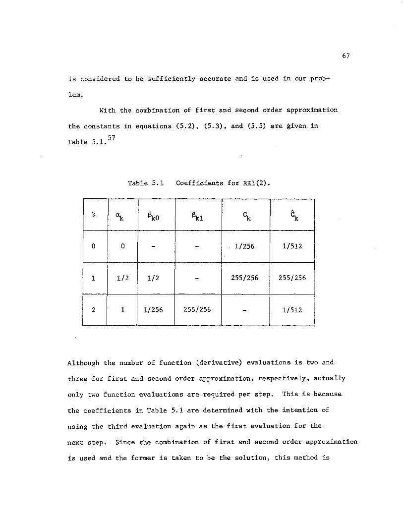
is considered to be sufficiently accurate and is used in our prob-
lem.
With the combination of first and second order approximation
the constants in equations (5.2), (5.3), and (5.5) are given in
57 Table 5.1.
Table 5.1 Coefficients for RK1(2).
A
k ~ f\:o f\:1 ~ ck
0 0 - - 1/256 1/512
1 1/2 1/2 - 255/256 255/256
2 1 1/256 255/256 - 1/512
Although the number of function (derivative) evaluations is two and
67
three for first and second order approximation, respectively, actually
only two function evaluations are required per step. This is because
the coefficients in Table 5.1 are determined with the intention of
using the third evaluation again as the first evaluation for the
next step. Since the combination of first and second order approximation
is used and the former is taken to be the solution, this method is
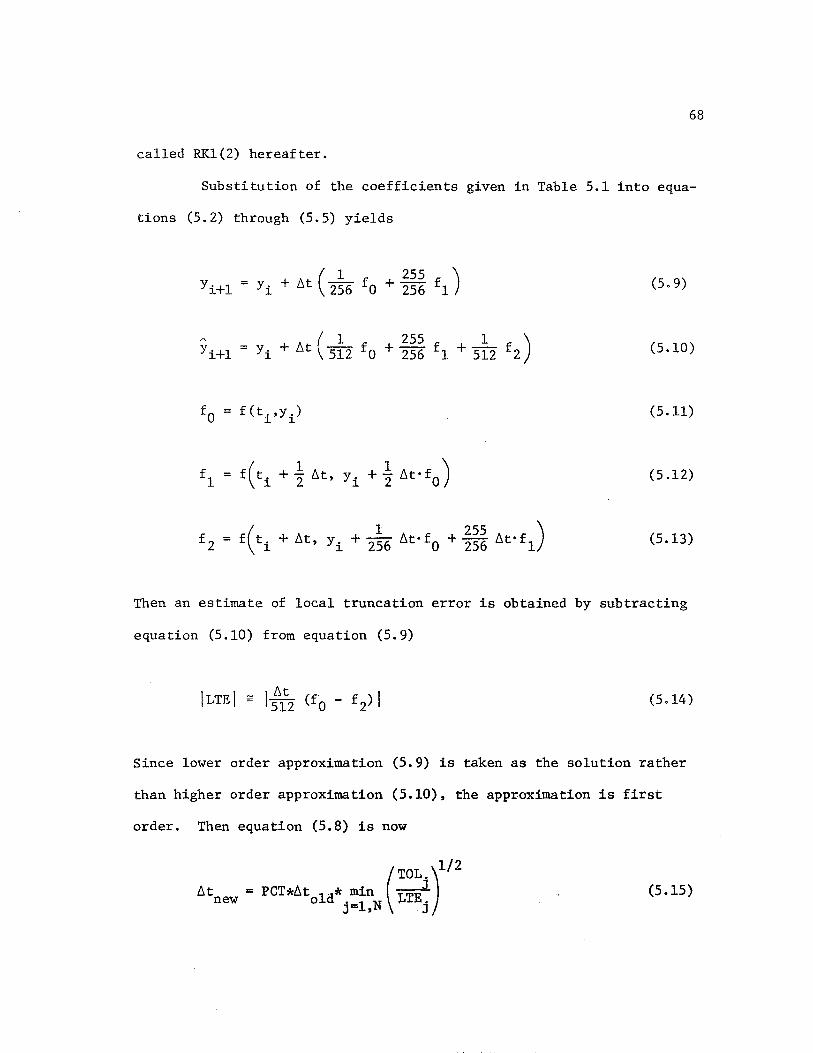
68
called RK1(2) hereafter.
Substitution of the coefficients given in Table 5.1 into equa-
tions (5.2) through (5.5) yields
= y + At ( 1 f + 255 f ) i w 256 0 256 1 (5.9)
(5.10)
f(t.,y.) 1 1
(5.11)
(5.12)
(5.13)
Then an estimate of local truncation error is obtained by subtracting
equation (5.10) from equation (5.9)
(5.14)
Since lower order approximation (5.9) is taken as the solution rather
than higher order approximation (5.10), the approximation is first
order. Then equation (5.8) is now
(TOL.)l/
2
b.t = PCT*b.t 1a* min ____J_LTE new o j=l,N j
(5.15)
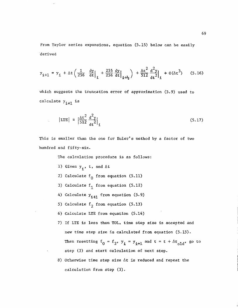
69
From Taylor series expansions, equation (5.15) below can be easily
derived
(5.16)
which suggests the truncation error of approximation (5.9) used to
calculate yi+l is
ILTEI (5.17)
This is smaller than the one for Euler's method by a factor of two
hundred and fifty-six.
The calculation procedure is as follows:
1) Given y., t, and 6t J_
2) Calculate f 0 from equation (5.11)
3) Calculate f 1 from equation (5.12)
4) Calculate Yi+l from equation (5.9)
5) Calculate f 2 from equation (5.13)
6) Calculate LTE from equation (5.14)
7) If LTE is less than TOL, time step size is accepted and
new time step size is calculated from equation (5.15).
Then resetting f 0 = f 2, yi = Yi+l and t = t + 6told' go to
step (3) and start calculation of next step.
8) Otherwise time step size 6t is reduced and repeat the
calculation from step (3).
70
5.2 Multistep Methods
The class of linear multistep methods for ODE's integration
is usually described as follows: Approximate solution values are cal-
culated at t = t 0 ,t1 ,t2 ... where tn = tn-l + ~t, with step size ~t,
according to a formula of the form
k2 + f1t 2: f3,y' .
j=O J n-J (5 .18)
where yk = y(tk)' y~ = y'(tk) = f(yk'~), aj and f3j are coefficients
associated with the particular method. Equation (5.18) is used to
calculate y when previous approximate values of y and y' are known. n
Special considerations have to be made to obtain the several values
needed at the beginning to make equation (5.18) applicable. The most
popular examples of equation (5.18) fall into two specific classes of
methods. One is referred to as "the Adams' methods of order q" and
is obtained by setting a1
= 1, k1
= 1 and k2 = q -1. The other is
the backward differentiation methods (usually called Gear's methods)
of order q which is obtained by setting k1 = q and k2 = 0. When
order is said to be q, it means that if Eq. (5.18) is solved for yn
with all past values being exact, then y will differ from the cor-n
rect solution of Eq. (5.1) .by a truncation error that is O(f1tq+l)
for small ~t.
The biggest advantage of an Adams' integrator over Gear's
methods is that it does not require the evaluation of the Jacobian, nor
solving a large matrix problem in its solution process, since a fixed

71
point iteration is used to solve the non-linear (corrector) equations.
The main disadvantage, on the other hand, is that their stability
regions are small and can often require relatively small time steps
to maintain stability. This disadvantage makes these methods ineffi-
cient for stiff problems.
Gear's methods of order 1 ~ q ~ 6 were shown to have stiff
58 stability by Gear. Their stability region contains a horizontal
strip covering the entire negative real axis in all six cases
(Figure 5.3). The boundary curve crosses the axis, making the method
not stiffly stable for q ~ 7. Newton's method rather than a fixed
point iteration is used to solve corrector equations. A fixed point
iteration imposes time step size limitations to make corrector con-
verge, which destroys the advantage gained by achieving stiff sta-
bility. The expense of calculating the Jacobian matrix 3f/3y can be
further offset by neglecting to re-evaluate it at every step, unless
the existing value of this matrix fails to produce convergence or
the order q is changed.
Sophisticated and highly reliable computer programs have been
developed for solving complicated systems of ODE's, using either Adams'
methods or Gear's stiffly stable methods. Allowing users to specify
which methods be used, these programs automatically select the order q
and time step size keeping the error produced from the integration within
the desired tolerance and maintaining the time step size as large as pos-
sible. 59
In this research, one such program named DGEAR is applied to
micellar/polymer flooding simulation. The code DGEAR implements the

72
Adams' methods of order 1 ~ q ~ 12 and Gear's method of order 1 ~ q ~ 5.
With DGEAR, the user may choose from several different algo
rithms only by specifying two method indicators. The first is called
METH, which indicates the method of integration to be used. The
second is called MITER, which indicates the procedure for solving
the nonlinear equations arising in the method being used. The de
scription of those parameters is given below.
METH = 1, indicates Adams' method
2, indicates backward differentiation (Gear's) method
MITER = 0, implies functional (or fixed point) iteration.
The Jacobian is not needed.
1, implies a chord method (or semistationary Newton
iteration) with the Jacobian supplied by the user.
2, implies a chord method with the Jacobian calculated
internally by finite differences.
3, implies a chord method with the Jacobian replaced
by a diagonal approximation based on a directional
derivative.
5.3 Stability region and stiffness
When an ordinary differential equation is integrated numeri
cally, the stabiliity of the method is often discussed, because it
suggests the quality of the solution or step size required to obtain an
accurate solution. To investigate the stability, only the special equa
tion below and its region of absolute stability are usually considered.
73
y' (5. 19)
Here A is a complex constant having a negative real part. The re
gion of absolute stability is defined60 as the set of all A~t (~t:
step size, therefore real non-negative) for which the numerical solu-
tion y + 0 as t + oo. The larger the region of absolute stability, n n
the less the restriction on ~t in order to have the numerical method
give a numerical solution that is qualitatively the same as the true
solution. If a linear system of ordinary differential equations
y' = Ay is being considered, the eigenvalues A. (i = 1,2, .•• ,N) of l.
matrix A, instead of A in equation (5.19), are used to determine the
step size which gives a stable solution. Furthermore, the stability
of the methods used in solving a system of nonlinear equations can be
determined by considering the eigenvalues of the Jacobian matrix,
()y' /()y.
th When a p order Runge-Kutta scheme with r function evalua-
tions is appiied to the test equation (5.19), an approximate solution
' 61 of the form
= {TIP (A~ t) }y. r i
will be obtained, where
'ITP (A~t) r
p
= ~ j=O
(A~~)j + I y (Mt) q J. q=p+l q
(5. 20)
(5. 21)
74
they , q = p+l, p+2, ••. rare functions of a, B, c (the coefficients q
of the Runge-Kutta formula used in integration of the test equation).
See equation (5.2). np(A6t) is called the stability polynomial. r
region of absolute stability is the area defined by
The
(5. 22)
This ensures that the error does not increase from step to step in
the numerical solution of the test problem. One way of defining a
stability region is to get
or
i8 e
TIP(A6t) = cos8 + isin8 r
i = r-1 (5.23)
By varying 0° < e < 360° and calculating the roots of equation (5.23)
for the small variation of e, one can obtain the boundaries of the
absolute region of stability.
Now let us consider equation (5.9) of RK1(2)
(5.9)
Substituting the test equation f = Ay into equations (5.11) and
75
(5.12)
fo f(t.,y.) l. l.
A.y. l.
(5. 24)
fl f(ti 1 1
= + 2 6t, yi + 2 6tf0)
A.(y i 1 (5. 25) = + 2 6tA.yi)
Then substitution of equations (5.24) and (5.25) into equation (5.9)
gives
This result agrees with equations (5.20) and (5.21) as below
where
255 Y2 = 512
1 j 2 = 2: <>..~~) + 2: y <>-l1t) q
j=O J· q=2 q
To obtain absolute stability region, let
(5. 26)
(5.27)
(5. 28)
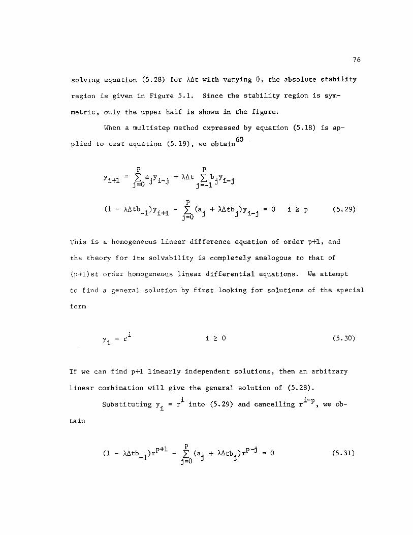
76
solving equation (5.28) for A6t with varying 8, the absolute stability
region is given in Figure 5.1. Since the stability region is sym-
metric, only the upper half is shown in the figure.
When a multistep method expressed by equation (5.18) is ap
plied to test equation (5.19), we obtain60
p p
= L a . y . . + At. t L b . Yi- . j =O J 1 - J j =-1 J J
p
(1 - A6tb_1)yi+l - 2::_ (a. + MtbJ.)Yi.-J" = 0 j=O J
i ~ p (5.29)
This is a homogeneous linear difference equation of order p+l, and
the theory for its solvability is completely analogous to that of
(p+l)st order homogeneous linear differential equations. We attempt
to find a general solution by first looking for solutions of the special
form
i r i ~ 0 (5. 30)
If we can find p+l linearly independent solutions, then an arbitrary
linear combination will give the general solution of (5.28).
tain
Substituting y. = ri into (5.29) and cancelling ri-p, we obi
p (1 - Mtb _
1)rp+l - .L (a. + Al:itb. )rp-j
j=O J J 0 (5. 31)
77
This is called the characteristic equation and the lefthand side is
the characteristic polynomial. The roots are called characteristic
roots. If the roots are all distinct, then the general solution of
equation (5.28) is
p i 2: y. [r. (A~t)]
j=O J J i ~ 0 (5. 32)
where r.(A~t) are characteristic roots, which depend continuously on J
the value of A~t. If r.(A~t) is a root of multiplicity n > 1, then J
the following are n linearly independent solutions of (5.29).
... , (5.33)
These can be used with the solutions arising from the other roots to
generate a general solution for (5.29), comparable to equation (5.32).
From equation (5.32), the region of absolute stability is
equivalent to the area that satisfies
r. (A~t) ~ 1 J
The regions of absolute stability for Adams' methods and
Gear's methods are shown in Figures 5.2 and 5.3 respectively.
(5. 34)
If a system of linear or nonlinear ordinary differential equa-
tions is under consideration, all eigenvalues A. (i = 1,2, ••. N) asso-1
ciated with the matrix must satisfy the absolute stability condition.
Consequently one difficulty may arise when max IAil is much larger i=l,N
than min IA.I. In such a case, a limited stability region may imi=l,N i
pose a severe restriction on the step size. Such a system is called
stiff and the degree of stiffness can be expressed by stiffness
ration SR
SR
max IA. I i=l,N i
= _m_i_..n_...,j A,..-J
i=l,N i
(5.35)
If a system is stiff, it involves both rapidly changing variables
and very slowly changing variables, all of a decaying nature.
Let us consider more specific problems such as semi-discrete
systems arisen from conve:ation-diffusion equations. The more para-
bolic (diffusive) the character of the equation is, the higher the
degree of stiffness. In general, a larger number of grid blocks
yields a stiffer system.
Backward differentiation methods (Gear's methods) are espe-
cially designed for stiff problems. As can be seen in Figure 5.3,
they have infinite regions of absolute stability and offer higher
efficiencies to solve stiff problems.
78
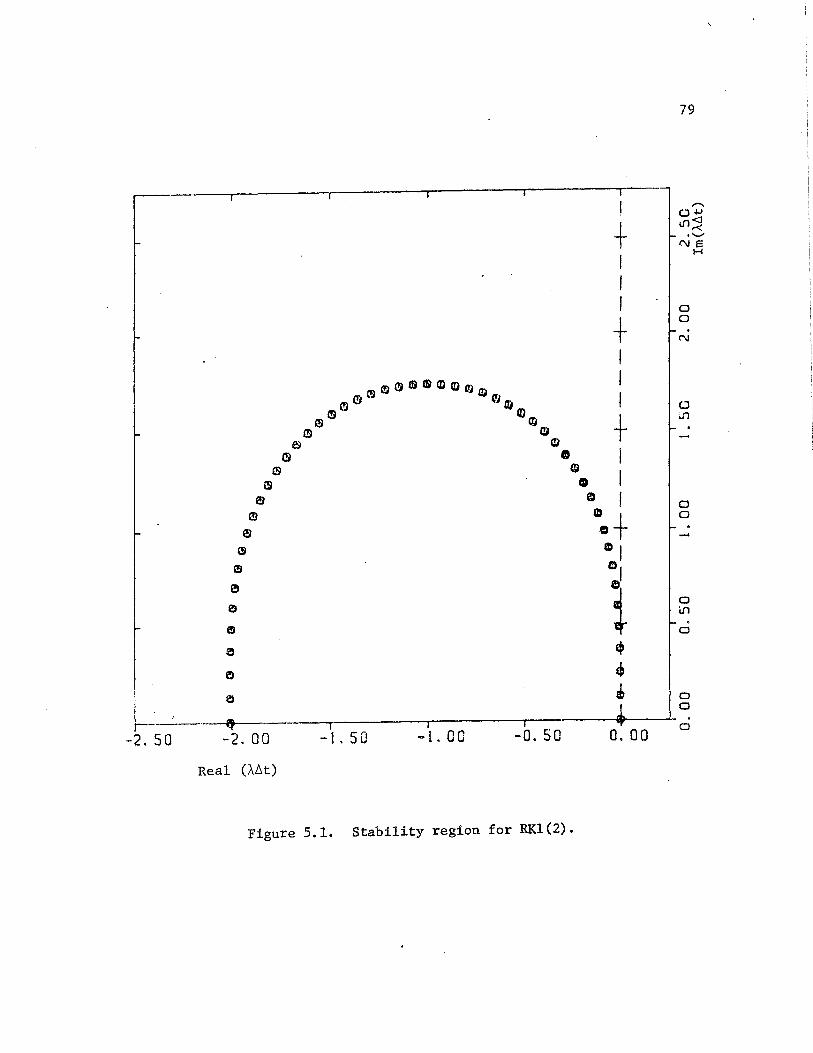
!
+ I I I
+ I I I
+ I I
Q) I O)e+ " I "1
l ~ ~
' -1. 00 -0. 50 0. 00
~~~@~~.--~-r-~--r~~_._~ -1' 50 -2. 50 -2. 00
Real (;\Llt)
Figure 5.1. Stability region for RK.1 (2).
79
a 0 . N
0 i.J1
a 0
a if') . a
0 0
0
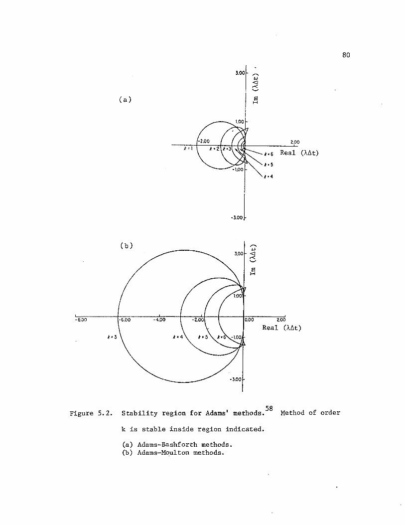
-8.00
k=3
Figure 5. 2.
(a)
k: 1
(b)
-6.00 -4.00 -2.00
""""' .µ 3.00 ~
s H
2.00
k. 6 Real (A.~ t)
0.00 2.00
Real (l.,~t)
58 Stability region for Adams' methods. Method of order
k is stable inside region indicated.
(a) Adams-Bashforth methods. (b) Adams-Moulton methods.
80
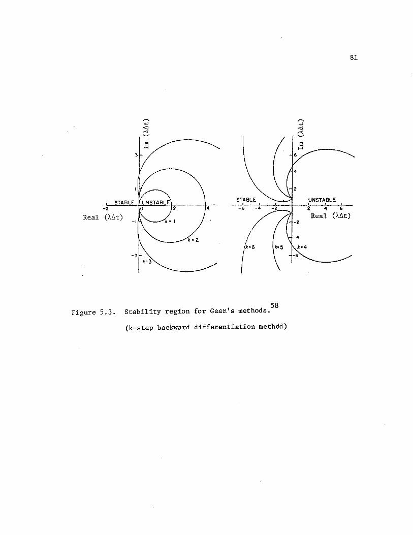
,,...... .µ <J r'< '--'
s H
STABLE STABLE
•2
Real (t .. b.t)
Figure 5.3.
4 -6
k•2
58 Stability region for Gea:rr.' s methods.
(k-step backward differentiation methdd)
81
,,...... .µ <l ..-< '--'
UNSTABLE
2 4 6
Real 0..b.t)
CHAPTER VI
RESULTS AND DISCUSSIONS
In this chapter, the basic input data and a set of com
puted results for a type II(-) phase environment with no adsorp
tion are first presented. The computed results were obtained
from the fully-discrete Euler (FDE) method with constant time step
size of 0.001 Pore Volumes (PV). These plotted results enable us
to understand how the flood is proceeding.
In the next section, results of each method for Type II(-)
phase environment with no adsorption are first presented with some
discussion. Although RK1(2) was the best among semi-discrete methods,
computation time was not improved as had been expected. Then an
~lternative algorithm which is called RK1 is introduced and its
results are compared with FDE method.
The effect of adsorption is shown in Section 6.3 for only
RKl and RK1(2). More computation time was required for both RKl
an<l RK.1(2) when adsorption is involved compared with the no adsorption
cases. Other phase behavior environments were also examined in
this section. The performance of the semi-discrete method got worse
as the phase behavior environment was changed from Type II(-) to
Type II(+), and was worst in the Type III phase behavior environ-
ment.
For the Type II(-) phase behavior environment with no adsorp
tion, the effect of each component on the time st~p size selection
82

was examined (in Section 6.4) using the RK1 method. It was
found that RKl was taking a too conservative (small) time step
size at an early stage of the flood. This is due to rather large
truncation error associated with the time integration at that
stage for the components which did not exist before the micellar
flooding started. When the error was checked only for the water or
oil component, the computation time was improved without affecting
the quality of the solution.
In section 6.5, the results for the case when the absolute
error was specified as the error tolerance instead of the relative
error. By using a smaller value for PCT.in equation (5.8), less
computation time was achieved with absolute error control. A brief
sunnnary of RKl for Type II(-) without adsorption is also given.
Some eigenvalues of the Jacobian matrix before surfactant
breakthorugh are presented in section 6.6. Since the matrix is
characterized as block triangular, it is possible to decouple it in
to submatrices and obtain eigenvalues by analyzing each submatrix.
The eigenvalues presented are obtained from the oil bank blocks
which seem to be governing the stability requirement.
A stability analysis with some assumptions was performed (in
section 6.7) for the blocks where surfactant is present. From this
analysis, it was discovered that an unconditional instability occur
red continually and locally due to the change in residual satura
tion caused by the surfactant. This instability explains why we
have oscillations in the production history even if a small time
83

step is used.
6.1 Basic input data and example results
In this section the basic input data used to compare the
performance of the various semi-discrete methods discussed so far
are presented. Then a set of computed results for Type II(-) phase
environment with no adsorption are shown with some discussion. The
computed results were obtained from the FDE method with constant time
step size of 0.001 PV. These plotted results enable us to under-
stand how the flood is proceeding.
The basic input data are listed in Tables 6.1. Tables
6.la and 6.lb list input data common for all base cases while
Table 6.lc lists the difference in the data for each base case.
A definition of each parameter is given in Appendix C. Some repre-
sentative features of the input data will be discussed later in
this section. Unless otherwise noted, this basic data set is
used for all runs. A somewhat simplified case is considered to
enable easier interpretation of the calculated results. The
main purpose of this research is to investigate the applicability of
the semi-discrete methods to micellar/polymer simulation, and to
compare the perfonnance among different semi-discrete methods. For
RK.1(2) PCT in equation (5.15) and YBIAS in equation (5.7) are fixed
-3 to be 0.8 and 10 , respectively.
The common features for all base cases in Tables 6.1 are as
follows:
84

1) The physical dispersion term is not used assuming
that numerical dispersion can adequately approximate physical dis-
persion.
2) The dimensionless longitudinal dispersivity given as
cnj in equation (3.1) is about 0.0125 since the number of grid blocks
used is forty.
3) Alcohol is combined with chemical to make a single pseudo
component.
4) No ion exchange between clay and mobile phases is con-
sidered.
5) No inaccessible pore volume to polymer or surfactant
is considered.
6) The initial condition is waterflood residual oil satura-
tion.
7) No salinity effect or shear rate effect on polymer solu
tion viscosity is included. Permeability reduction due to polymer
is not considered either.
8) The plait point is located at the corner of the pseudo
ternary diagram, which yields excess phases consisting of a single
pure component (either water or oil)•
9) An aqueous surfactant slug containing 10% (surfactant
+alcohol) and 0.1 wt% polymer is first injected up to 0.1 pore
volume (PV). Then polymer buffer of constant polymer concentration
equal to 0.1 wt % is injected.
10) Calculated viscosities of surfactant slug and polymer
85

buffer are 33 cp and 31 cp, respectively.
11) Tracer is injected in both surfactant and polymer slug.
12) Total injected amount is 2.0 PV.
Figures 6.1 through 6.10 present a set of computed results
for a Type II(-) phase behavior environment with no adsorption (Run
207). The FDE method with a time step size of 0.001 was used. Fig
ures 6.1 through 6.7 show profiles at 0.25 PV injected. Figures 6.8
to 6.10 show the production histories.
Since no adsorption was considered and only microemulsion
and excess oil exist, the fronts of surfactnat, polymer, and tracer
are located at the same position. There are two major fronts in
the profiles. One is at the surfactant front and the other is at
the most upstream grid. The former advances as injection proceeds,
while the latter stays at the same place in this example. At the
surfactant front, interfacial tension is reduced, which leads to
the reduction of non-wetting phase residual saturation. At the most
up_stream grid, oil saturation is extremely low, which is considered
to be the effect of a miscible displacement. However, such low
residual oil saturation is not achieved in this example beyond that
grid because of the dilution of the surfactant.
In Figures 6.2 through 6.4 vertical lines indicate the
appearance or disappearance of surfactant. When the total concentra
tion of (surfactant+ alcohol) is lower than 10-4 , the effect of
surfactant is neglected and no microemulsion phase is considered.
Although the vertical lines separate water phase and microemulsion
86
phase, these two phases are considered to be continuous in Type
II(-) case.
Figure 6.7 shows the profile of total relative mobility.
This figure indicates that physically unstable condition occurs at
the surfactant front. This is caused by the increase in relative
permeabilities both to oil and aqueous (microemulsion) phases due
to surfactant. However, if the mobilities are compared between oil
bank and the middle of surfactant slug, the mobility ratio is about
0.4. Mobility ratio for surfactant slug and polymer buffer is
designed to be about unity. Thus the whole process is stable even
though locally unstable.
6.2 Comparison of each method for Type II(-) phase behavior with
no adsorption
In this section a comparison is made among the fully-dis
crete Euler (FDE) method and the semi-discrete methods discussed
so far. Type II(-) phase behavior environment with no adsorption
(data set A in Table 6.lc) was adopted as the simplest example.
The results are shown in Table 6.2 and in Figures 6.11 through
87
6.19. The legend of total concentration history plots is given in
Table 6.15. This legend is valid for all subsequent total concentra
tion plots. Although RK.1(2) was the best among semi-discrete methods,
computation time was not improved as had been expected. Then an
alternative algorithm which seemed to be more efficient is intro
duced. This algorithm called RKl consists of a combination of first
and second order Runge-Kutta approximations. Its results are also
compared with the FDE method.
In Table 6.2, ERR is the relative error tolerance for semi
discrete methods while constant time step size used is written for
FDE in the same column. IEVA is the number of function (derivative)
evaluations. NREJ indicates how many times the predicted ~tD has
been rejected. NREJ was counted only for RK1(2). CPU time, which is
for CDC Dual Cyber 170/750 at the University of Texas at Austin is
listed just to give an idea of the order of the computer time. One
should compare IEVA rather than CPU time to see the efficiency of
each method, since the semi-discrete methods were progrannned mainly
to see their applicability and flexibility. There may be more room
to decrease CPU time for semi-discrete runs. In the column of
quality in Table 6.2, "good" means the solution obtained looks
comparable to Run 207, which used FDE method with ~tD = 0.001. Fair
quality means the solution oscillates somewhat but is still accep
table. In last column, ER is the total oil recovery as percent of
the initial oil in place. The oil recoveries are presented to show
the effect of the change in numerical dispersion.
Figures 6.11 to 6.13 show the history of total concentration
in the effluent for the FDE method with three different time step
sizes. In Figures 6.14 through 6.16, total concentration histories
are presented at the top and the histories of the time step size
used at the bottom for the RK1(2) method, with varying ERR. Figures
6.17 and 6.19 are the same except for Adams' methods. For Adams'
88
methods, .only the results with the option MITER= 0 are presented
because other options did not give good results. The results
of backward differentiation are also excluded because of their poor
performance. Some discussions on these predictor-corrector methods
will be presented later in this section.
From Table 6.2 one may conclude that the FDE method is
better than the semi-discrete methods tested based on the number of
function evaluations and CPU time. Actually, RK1(2) is not so
efficient as was expected. Neither are Adams' and Gear's methods.
However, one should keep in mind that with these methods the trunca
tion error associated with time integration is controlled and forced
to be smaller than some specified value, which was not done with
the FDE method. This feature may become important when higher or
der accurate approximations for space derivatives or finite element
methods are introduced. Furthermore, the history of the time step
size should not necessarily be constant. Before surfactant break
through, the time step size taken with RK(2) is 0.002 to 0.003 PV,
which coincides with the result obtained from the FDE method.
When the FDE method is used, a time step size larger than 0.003 PV
produces oscillation, which seems to be caused by numerical instabi
lity. After surfactant breakthrough, however, the time step size
more than doubles with RK1(2) and finally increases to DTMAX. DTMAX
is the maximum time step size specified in the input data. After
a time step size is calculated based on the estimated truncation
error, the time step size is compared with DTMAX and the smaller
89

90
value is taken to be the next time step size.
In Table 6.2, an extremely small error tolerance was
listed for RK1(2). This is because RK1(2) produces a very small
truncation error. When a larger error tolerance was used, RK1(2)
selected larger time step sizes due to the small truncation error,
and the solution was no longer stable. Oscillations in both concen-
tration and time step size history occurred.
Although the time step size was increased after surfactant
breakthrough, RK1(2) still required more computation time than
the FDE method. This is because RK1(2) requires two function eva-
luations (equations (S.12) and (5.13)) per step. This means that the
average time step size taken with RK1(2) has to be more than twice
as large as the one for the FDE method. For this reason, another
method called RK1 which requires only one function evaluation per
step was tested. This method discussed below also has time step
size control in a similar way to RK1(2).
Instead of equations (5.9) through (5.13) in Chapter 5,
equations (6.1) through (6.4) below are used to estimate the local
truncation error.
Yi+l = Yi + l:ltfo (6.1)
A = y + t (kf + ~fl) (6. 2) Yi+l i 2 0
fo = f(ti, yi) (6. 3)
fl = f(t. +lit, y. + L':ltf 0) (6.4) l. l.
Approximation (6.1) is exactly the same as Euler's method, while
approximation (6.2) is the trapezoidal method solved with one
iteration using Euler's method as the predictor. Both are a spe-
cial case of Runge-Kutta formulas. Subtracting equation (6.2)
from equation (6.1), the local truncation error LTE is estimated
as below
~(f - f ) 0 1 (6.5)
Since Euler's formula is used as the solution, the truncation error
is two hundred and fifty six times more compared with RK1(2)
jLTEj = Llt2 ~
-2- dt i (6.6)
Its stability region is also the same as the one for the forward
Euler method, which is shown in Figure 6.39.
Some results obtained using RK1 are presented in Table 6.3
where the results of FDE method are again shown for comparison.
Plotted histories are presented in Figures 6.20 through 6.22.
Those results show that RK1 saves computation time of about 20%
compared with FDE method for the same quality. Furthermore the num-
ber of function evaluations is about 40% less for RK1 than the FDE
method.
None of the predictor-corrector methods, neither Adams'
methods nor Gear's method worked as well as RK1(2) or RKl. Although
91

several options were tested with DGEAR, only the results of Adams'
methods with MITER = 0, which implies the functional (fixed point)
iteration, are presented in Table 6.2, because all the other options
did not work as well.
When Adams' methods with MITER = 0 were used, the order
was varied from first to third. Although the average number of func
tion evaluations per step was about two, only one function evaluation
was the most frequent result. This fact indicates that the stability
regions of Adams' predictor method play an important role in the time
step size selection. Since the stability regions of second and
third order Adam's predictors (Figure 5.2a) are smaller than the one
for RK.1(2) (Figure 5.1) or RK1 (Figure 6.39), Adams' methods may have
to take a smaller time step than RK.1(2) or RKl to remain stable.
MITER= 0 was not tested with Gear's methods, since this
iteration scheme imposes a limitation on the time step size which
destroys the advantage of the stiffly stable character of Gear's
methods.
Table 6.4 shows the results obtained with MITER equal to
two. This option uses semi-stationary Newton iteration with the
Jacobian calculated internally by finite differences. When the
MITER = 2 option was tested, the number of grid blocks was decreased
to twenty, because this option requires a large storage for the Jaco
bian matrix. In Table 6.4, ERR designates the relative error tol
erance and ~t;J is the dimensionless time step size. Highest
92
order q means the highest order of the methods used in the computation.

IEVA is the number of function evaluations including the evalua
tion of the Jacobian. NSTEP is the number of steps. NJE is the
number of Jacobian evaluations. Net IEVA is the number of func-
tion evaluations excluding the number of function evaluations used
to obtain the Jacobian matrix. Since 120 function evaluations were
required to get a Jacobian matrix, most of the computation time was
spent to evaluate Jacobian matrices.
The results were obtained only up to 0.1 PV injection be-
cause the solution oscillates, or large error occurred, for all runs
after 0.1 PV injection. This is the time at which the composition
of the injected slug is changed.
Although neither Adams' methods nor Gear's methods worked
as well as the two explicit techniques, it may be too early to con
clude these implicit or semi-implicit methods are not as good.
Since a packaged program was used to impelement the techniques, the
details are not clear, but there may be some improvement possible.
One example is the step size control. DGEAR varies time step size
based on only relative error without YBIAS which was used for the
two explicit methods as in equation (5.7). Since most variables
change between zero and unity, it is risky not to use equation (5.7),
or a combination of relative and absolute error. 62
6.3 Effect of adsorption and phase behavior
In this section the effect of adsorption and phase behavior
on the performance of semi-discrete methods is examined. The
93
difference in input data between the runs presented in this sec
tion and the previous section is the adsorption and/or salinity.
Adams' methods and Gear's method were no longer tested because of
rather poor results obtained in the previous runs and the difficulty
in changing the program to deal with the irreversibility of adsorp
tion.
Table 6.5 shows the results for Type II(-) phase behavior
environment with adsorption. Data set Bin Table 6.lc was used.
Compared with the previous case, !EVA and NREJ increased for both
RK1(2) and RKl. Furthermore, the history of the time step size in
Figure 6.23, which shows the results of Run 333, exhibit more fre
quent oscillation than previously.
Tables 6.6 and 6.7 present the results for Type II(+) phase
behavior with no adsorption (data set C in Table 6.lc) and with
adsorption (data set D in Table 6.lc), respectively. RKl was less
efficient for both cases compared with Type II(-) runs. Figures
6.24 and 6.25 show the performance of RKl with ERR= 0.01 for each
case.
Table 6.8 shows the comparison of FDE and RKl for Type III
phase behavior with and without adsorption (data set F and E). Fig
ures 6.26 and 6.27 show the results of RK1 without adsorption
and with adsorption, respectively. Hirasaki's relative permeability
model was used for all these runs.
Table 6.9 summarizes the effect of adsorption and phase be
havior on the efficiency of R.Kl. All runs were made with ERR= 0.01.
94
The computation time increased as the phase behavior environment
was changed from Type II(-) to Type II(+) to Type III.
Since truncation error for RK1 is rather large compared
with RK1(2), a question arises about the effect of the change in
the time step size ~tD on the numerical dispersion. The numeri
cal dispersion for RKl is expressed by exactly the same equation
as for FDE because the time integrations are identical. When ~tD
95
is small compared with ~XU• ~tD can be neglected as in equation (3.7).
For larger ~tD, however, ~tD may affect the numerical dispersion.
Tables 6.3 and 6.5 through 6.8 suggest oil recovery is not very
sensitive to the change in time step size when the phase behavior is
Type II(-), whereas the time step did have a small effect on the
oil recovery for the Type II(+) case. For the Type III case, the
oil recovery was 100% for all runs.
6.4 Effect of each component on time step size selection
This section contains additional discussion about the time
step size selection. All the results which have been presented so
far were obtained by checking the error for all components. The
effect of each comonent on step size control in chemical flooding
is first discussed. Then simpler problems such as waterflooding
and miscible displacement (single phase flow) are examined. Only
RKl was used and .. ERR was fixed to be 0.01. Thus Run 200 was con
sidered as a reference run for all of the other chemical flooding
runs. A sunnnary of the results is presented in Table 6.10. Figures

6.28 to 6.34 show the total concentration history at the top and
the time step size history at the bottom. Figures 6.28 to 6.32
show chemical flooding results. Figure 6.33 shows a waterflood.
Figure 6.34 shows a miscible flood.
First, the injection of tracer was eliminated in Run 265
(Figure 6.28). Compared with Run 200 (Figure 6.20), a difference
in the time step size and its amplitude of oscillation before sur
factant breakthrough can be observed. Thereafter, the time step
size is identical to Run 200.
In Run 267 (Figure 6.30), the error was checked only for
the oil concentration (C2). The history of the time step size is
quite different from the previous two runs at two different times.
One major difference is before 0.20 PV injection. Run 267 takes a
time step size of around 0.002 PV from the very beginning, whereas
in the previous two runs the time step size increased much more gra
dually. The other difference is after surfactant breakthrough.
The time step size jumps to DTMAX in Run 267, while in the previous
two runs it remained below DTMAX much longer.
The error was checked only for the surfactant concentra
tion (C3) in Run 268 (Figure 6.31). Before surfactant breakthrough,
the time step size gradually increased with little oscillation. The
time step size coincides with the upper edge of the oscillating
time step size in Run 265. After surfactant breakthrough, the time
step size was identical to Run 265.
In Run 269 (Figure 6.32), only the error in the polymer
96

~7
concentration (C4 ) was used to control the time step size. The time
step size before surfactant breakthrough was almost the same as in
Run 268 and increased to DTMAX thereafter. The oscillation in the
concentration history was a little smaller than in Run 268. This may
~ave been because the time step size before surfactant breakthrough
was a little smaller in Run 269 than in Run 268. Run 269 and Run
267 suggest that the time step size should be equal to DTMAX (0.01)
after surfactant breakthrough.
Since Run 267 which checked only the error of the oil com
ponent gave the best result, the same test was done for Type II(-)
phase behavior with adsorption (Run 522) and Type III phase beha
vior with no adsorption (Run 446). A comparison is made with the
runs which checked the errors of all the components in Table 6.11,
and plotted results for Run 522 and 446 are presented in Figures 6.35
and 6.36, respectively. When the error was checked only for c2
(oil), a larger time step size was taken and the quality of the re
sult was still good.
Run 229 (Figure 6.33) is the result of waterflooding with
no tracer injected. In this case the total concentration of water
and oil is identical to water cut and oil cut. Initial condition
was changed to residual water saturation and 100% water (no surfac
tant, no oil) was injected continuously. In this case the problem
reduces to the well known waterflooding equation.
as u w w 3tD = - axu (6.7)
Since the finite difference approximations used are the forward
Euler in time and backward in space, the stability criterion is17
df w
dS w
:;l 1
The maximum value of df /dS is obtained from the value at the w w
(6.8)
flood front. Based on that maximum value, the stability require-
ment can be calculated as ~tD :;l 0.006. Figure 6.33 shows ~tD
was about 0.001 before water breakthrough.
Run 260 (Figure 6.34) is a miscible displacement. The
initial condition was 100% water with no tracer and 100% water
with tracer was injected continuously. Since there exists only a
single phase, df /dS in equation (6.8) is replaced by unity for the w w
stability criterion. Thus, 40 grid blocks gives the stability
requirement of ~ tD :;l 0 .• 025. However, Figure 6. 34 shows that a much
smaller time step size was computed by RKl.
From Runs 229 and 260, it becomes clear that with RKl the
stability requirement was detected only when the time step size ex-
ceeded the stability limit. In other words, error tolerance was
too small for these two runs. If larger error tolerance was used,
RKl should have detected the stability limit and selected a time
step size around the stability limit.
98
Thus, the time step size history in Run 200 (Figure 6.20)
is explained as follows. At the very beginning, a very small time
step size was taken and it increased gradually. This behavior is
due to the truncation error associated with tracer which had the
steepest front. When the tracer was not injected (Run 265, Figure
6.28), larger time step was selected but still similar trend was
observed. This is because of surfactant and polymer which also
had steep (although less than tracer) front. When a steep front
exists, a large truncation error is produced and RK1 selects a small
time step. When the error was checked only for water (Run 266,
Figure 6.29) or oil (Run 267, Figure 6.30) component, which did not
have a steep front, such a small time step was not selected. From
99
the fact that Run 266 and 267 did not show significant oscillation,
the time step size at the beginning in Run 200 was smaller than neces
sary if only stability was desired. The reason the time step size
increased gradually in Runs 200 and 265 is that the front of tracer,
surfactant, and polymer got more and more smeared due to numerical
dispersion.
After a while in Run 200, the time step size history began
to oscillate with larger amplitude as the time step size reached
the stability limit. When the time step size exceeded the stability
limit, it was automatically reduced, however, it is increased
again because of the rather small truncation error in the stable
region.
After surfactnat breakthrough, the time step size in Run 200
100
remained below DTMAX much longer than in Runs 266 and 267.
This is again the effect of surfactant. The truncation error at
the tail of surfactant made RKl select smaller time step size than
DTMAX or stability limit.
The conclusions of this section are as follows. RK1 is
controlling truncation error as it should be. The time step size
is controlled by the component which has the steepest front.
One important fact is that stability and truncation error are dif-
ferent problems. When an ODE integrator is used to control error,
it also controls stability. If, however, one desires only stability,
the ODE integrator may select a time step size smaller than neces-
sary at times.
6.5 Additional test runs and summary of RK1(2) and RKl for
Type II(-) phase behavior environment without adsorption
Some additional test runs were made to attempt to reduce the
computation time. So far the parameters POT and YBIAS have been
-3 fixed to be 0.8 and 10 , respectively. YBIAS was increased to
unity, which makes the error tolerance an absolute error. PCT was
reduced to 0.25 or 0.50 because a larger PCT causes the rejection
of the predicted time step too often, and also give a worse solu-
tion. Some results of both RK1(2) and RK1 are presented in Table
6.12. Plotted results are presented only for Runs 629 and 647 in
Figures 6.37 and 6.38, respectively. With YBIAS = 1.0, the combination
of PCT= 0.25 and ERR= 0.0001 (Run 629) gave the best result
using RK1(2) for both computer time and the quality of the solu
tion. For RKl, PCT = 0.25 and ERR= 0.01 (Run 626) was the
best.
A sunnnary of RK1(2) and RK1 results for Type II(-) phase
behavior without adsorption is given in Table 6.13. Only the best
results are compared. If only oscillation rather than truncation
error is used as the criterion of goodness, the error may be checked
only for the oil component, or the absolute error may be checked
with small PCT, and the computation cost will be less.
6.6 Stability requirement before surfactant breakthrough
101
In this section, the structure of the Jacobian matrix we are
dealing with and its desirable features are first introduced. Then
some eigenvalues before surfactant breakthrough are presented to
derive the stability requirement. Although the analysis is limited to
this special stage, it is important because this is the specific
time period which imposes the most strict limitation on the time
step size.
In order to analyze the stability, we have to express the
system of equations we are dealing with in the same fashion as the
test equation (5.18).
y' (6.9)
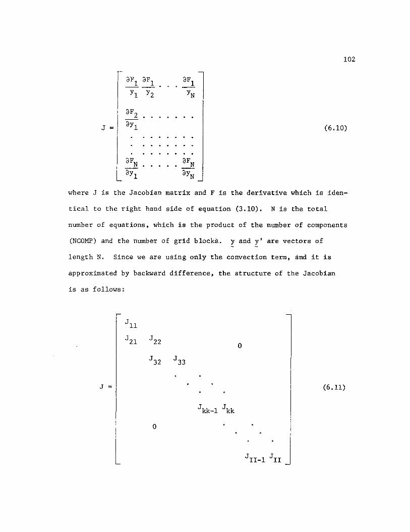
102
()Fl oFl oFl ----
Y1 Yz YN
aF2 . . . . . 0 . J = (lyl (6.10)
where J is the Jacobian matrix and F is the derivative which is iden-
tical to the right hand side of equation (3.10). N is the total
number of equations, which is the product of the number of components
(NCOMP) and the number of grid blocks. y and y' are vectors of
length N. Since we are using only the convection term, and it is
approximated by backward difference, the structure of the Jacobian
is as follows:
0
J = (6 .11)
0

where Jkk and Jkk-l are all NCOMP by NCOMP block matrices. Thus,
the Jacobian is a block lower triangular matrix.
For such a block triangular matrix with its diagonal blocks
all being square matrices, it is possible to prove that the eigen-
• values of the diagonal block matrix Jkk are also the eigenvalues of
the matrix J,
Before surfactant breaktrough, Jkk ahead of the surfactant
front (downstream) can be expressed
ClFm+l ClFm+l 0 0 0 0 3Ym+l 3Ym+2
ClFm+2 ClFm+2 0 0 0 0 3Ym+l 3Ym+l
0 0 0 0 0 0
103
Jkk = (6.12)
0 0 0 0 0 0
ClFm+5 ClFm+S 0 0
ClFm+5 0 3Ym+l 3Ym+2 Clym+S
ClFm+6 ClFm+6 0 0 0
ClFm+6
Clym+l ()ym+2 Clym+6
where
m = (k-lhNCOMP

104
and the subscript m+i indicates component i at kth block.
In the submatrix Jkk above, the alcohol (component 7) is
not included, because it does not affect the eigenvalues. This is
because it only adds zero elements in the seventh columm and the
seventh row. Thus submatrix Jkk is again a block lower triangular
matrix and its eigenvalues are obtained from the following matrices:
aFm+l aFm+l
aym+l aym+2 A = (6.13)
aFm+2 aFm+2
L aym+l aym+2
aFm+5 0
aym+5 B = (6 .14)
0 aFm+6
aym+6
Since there is only a water and an oil phase present (no microemulsion
phase) ahead of the surfactant front, then
Fm+l (6.15a)
(6.15b)
Fm+S (6.lSc)
105
(6.15d)
where
ell = c22 = LO (6.16)
cs1 = CS/Cl (6.17)
c61 = C6/Cl (6.18)
cl = s (6.19) w
c2 l - s (6.20) w
the matrices A and B can be rewritten
l -1
(6.21)
-1 l
l
(6.22)
0
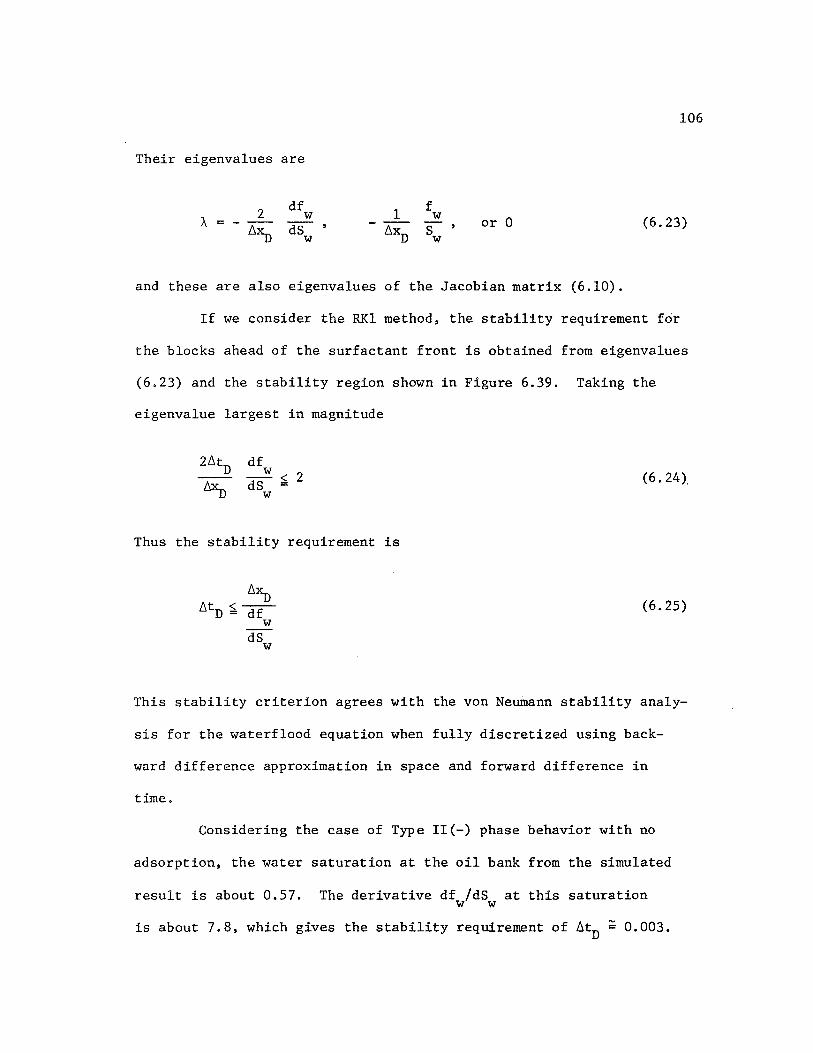
106
Their eigenvalues are
df w
dS w
1 - ti~
f w
s w or 0 (6.23)
and these are also eigenvalues of the Jacobian matrix (6.10).
If we consider the RKl method, the stability requirement for
the blocks ahead of the surfactant front is obtained from eigenvalues
(6.23) and the stability region shown in Figure 6.39. Taking the
eigenvalue largest in magnitude
df w
dS ~ 2 w
Thus the stability requirement is
dS w
(6.24).
(6.25)
This stability criterion agrees with the von Neumann stability analy-
sis for the waterflood equation when fully discretized using back-
ward difference approximation in space and forward difference in
time.
Considering the case of Type II(-) phase behavior with no
adsorption, the water saturation at the oil bank from the simulated
result is about 0.57. The derivative df /dS at this saturation w w
is about 7.8, which gives the stability requirement of fitD ~ 0.003.
The stability requirement estimated from the RKl and FDE runs before
surfactant breakthrough is also ~tD ~ 0.003. The RKl selected the
time step size of around 0.003 (Figure 6.30). The FDE gave oscil-
la ting solution when ~tD ~ 0. 003 (Figure 6.13). From this agreement
it is conjectured that the stability before surfactant breakthrough
is governed by the slope of fractional flow curve at the oil bank
saturation.
When the dispersion term is introduced like in equation
(3.1), the system of equations can be written
107
(6. 26)
where the Jacobian matrix involves the effect of both convection
and dispersion
(6. 27)
The Jacobian matrix JC obtained from convection term is block lower
triangular as before, whereas JD from dispersion is block tridiago-
nal. Thus, the summed Jacobian matrix JT is block tridiagonal and
it may seem impossible to use the advantage of the block triangular
matrix. However, the Jacobian matrix JT still can be divided into
a block lower triangular matrix in a somewhat different way by
taking into account the fact that ac .. /ax... is zero beyond some point l.J 1J
(i.e. in the oil bank).
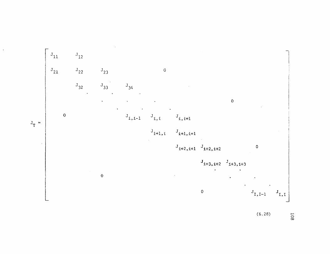
J = T
I Jll
J21
l
Jl2
J22
J 32
0
123 0
J33 J34
J .. 1 1., 1.-
J .. 1.' 1.
Ji+l,i
0
0
J. 1., i+l
Ji+l,i+l
Ji+2,i+l Ji+2,i+2
Ji+3,i+2 1 i+3,i+3
0
0
JI,I-1
(6.28)
-I I
JI,I
I-' 0 co
Then, the eigenvalues of the submatrix Jk,k (k = i+2, .•• I) in
the oil bank are still eigenvalues of the whole matrix JT at the
same time, However, we can no longer conjecture the eigenvalues
still dominate the ones upstream, since the effect of dispersion
there is proportional to ~j/(6~) 2 , where ~j is the dispersivity
coefficient in equation (3.1). For some sufficiently large ~j
or small 6~, the dispersion term behind surfactant front may
dominate the stability requirement.
6.7 Analysis of stability at blocks where surfactant is present
Although stability was analyzed in the previous section for
the oil bank where there is no surfactant, the stability at blocks
where there is surfactant was not analyzed because of the difficulty
of obtaining the Jacobian matrix and its eigenvalues.
In this section, a stability criterion for the waterflood
109
equation is introduced and the stability is analyzed for such blocks.
An attempt is made to explain why oscillation occurs in the produc-
tion history just before and after surfactant breakthrough (Figure
6.9), even when considerably smaller time steps are employed com-
pared to the previous analysis.
Because the nature of equation (3.5) is similar to the water-
flood equation, the stability of the waterflood equation below is
examined.
(6. 29)
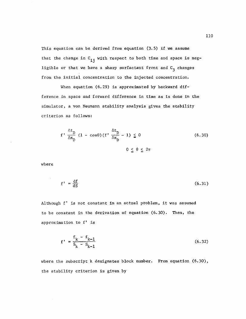
This equation can be derived from equation (3.5) if we assume
that the change in C .. with respect to both time and space is neg-1J
ligible or that we have a sharp surfactant front and c3 changes
from the initial concentration to the injected concentration.
When equation (6.29) is approximated by backward dif-
ference in space and forward difference in time as is done in the
simulator, a van Neumann stability analysis gives the stability
criterion as follows:
110
f' 6tD
(1 - cos8)(f' 6tD
1) < 0 6xD 6xD-
(6.30)
where
f' df =ds
0 < =
e < 2TI
(6.31)
Although f' is not constant in an actual problem, it was assumed
to be constant in the derivation of equation (6.30). Then, the
approximation to f 1 is
f' (6.32)
where the subscript k designates block number. From equation (6.30),
the stability criterion is given by

1) £'6tD ~ 6'1J
2) always unstable
if £' is positive
if £' is negative
111
Although the criterion 2) never arises in waterflooding
because £' is always positive, £' can be negative in micellar flood
ing due to the change in the residual saturation (Figure 6.5) as an
effect of surfactant. Table 6.14 shows the aqueous phase profile of
Run 207 (fully discrete, 6t = 0.001, Type II(-), no adsorption) at
0.5 PV injection. f' is presented in the bottom line and a negative
value appears at dimensionless distance of 0.9 from injector just
upstream of the surfactant front. The appearance of a negative f'
can be explained by comparing two fractional flow curves obtained
from each of the two blocks. Figure 6.40 shows an example. Since
the residual saturation is different for the two blocks, the relative
permeability curves are also different, which yields two different
fractional flow curves, one for each block. It was also confirmed
that a negative value of f' appeared intermittently somewhere behind the
surfactant front. The order of the negative value could be as large
as 10 2•
Although the stability requirement (6.30) was derived for the
finite different approximation backward in space and forward in
time, the same can be true for the formulation of RK1(2).
(5. 9)
112
Recall that the subscripts i and i+l here designate the time level.
Although the time integration is different from the forward Euler, the
derivative f 1 is obtained using forward Euler
(5.11)
f(t. + ~~t. y. + ~~tf0 ) i i
(5.12)
Thus, a larger error is introduced to f 1 and consequently Yi+l in
equation (5.9), which is affected by the error if the stability con-
dition (6.30) is not satisfied.
From Figure 6.40 it can be deduced that if the difference
between the two fractional flow curves is small compared with the dif-
ference between the saturations of each block, the negative f' can
be eliminated. One suggestion can be made at this point. Since frac-
tional flow depends on relative permeabilities, which are functions of
the residual saturations, we should look over the way we determine resi-
dual saturations. In the simulator, residual saturations are given
by equations (3.38). These equations give a linear relationship bet-
ween the residual saturations and the logarithm of the capillary num-
ber. Compared with the experimental data, such as the ones shown in
Figure 3.7, this functional relationship may yield too much change in
the residual saturation at surfactant front, which causes the large
change in the fractional flow. From the viewpoint of both numerical
stability and experimental data fitting, it is suggested that equation
6 (3.38) for the non-wetting phase be changed to another form. However,

it is impossible to eliminate this instability completely as long
as the continuity equations are solved explicitly, because the
change in the fractional flow curve is an essential part of the
micellar/polymer flooding.
113
One question, however, aises. Why is the fractional flow pro
file so smooth as shown in Figure 6.3 in spite of the unstable condi
tion? This is because the unstable condition occurs only locally and
temporarily, although continually. Even if the unstable condition
arises, it becomes stable in a short time and the large error pro
duced in the unstable condition may later die out. Furthermore, the
error that propagates downstream may also die out due to the stable
condition existing there. If, however, the unstable condition occurs
near production block, the error can reach the producer before it dies
out and causes an oscillation in production history.
When the semi-discrete method is used, the time step size
is usually increased to DTMAX after surfactant breakthrough. Sometimes,
however, it is decreased again for a short time, then goes up to D~
and becomes stable (Figure 5.30). This drop in time step size is also
attributed to the instability which has been mentioned above.
Although less significant compared with the effect of surfac
tant, the polymer also changes the shape of the fractional flow curve
by changing the viscosity. Therefore, it may also be necessary to
evaluate the effect of polymer when one considers numerical stability.
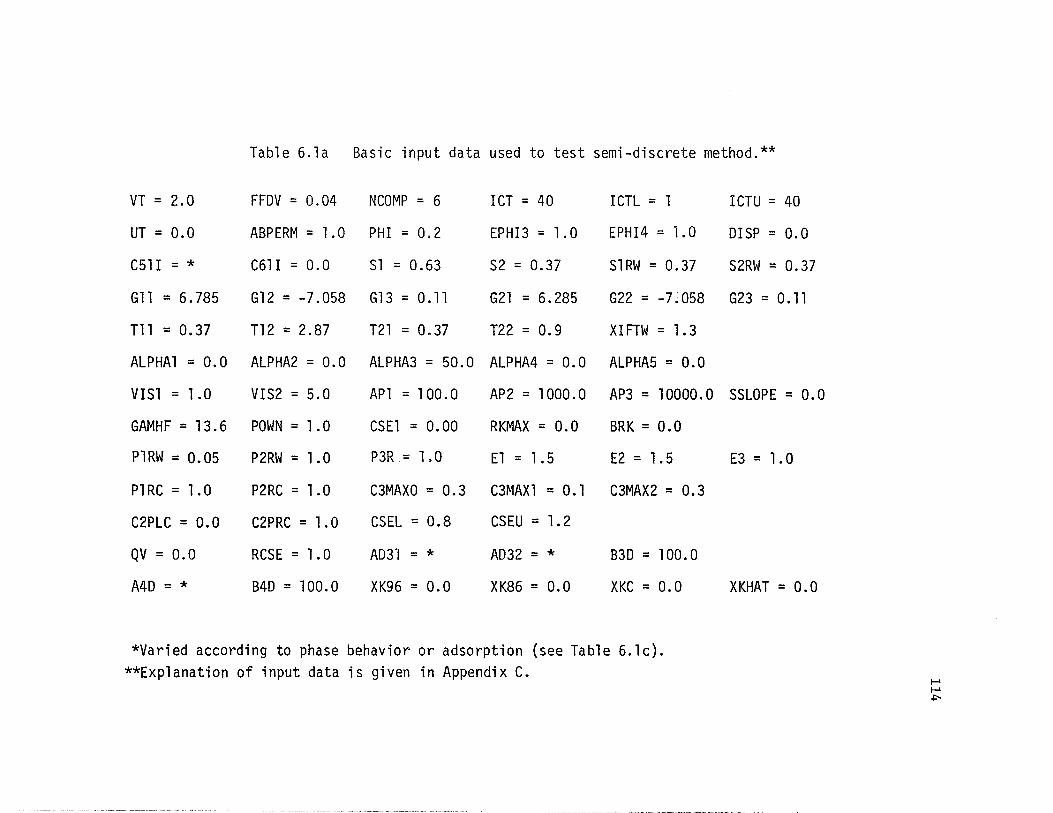
Table 6.la Basic input data used to test semi-discrete method.**
VT = 2.0 FFDV = 0.04 NCOMP = 6 ICT = 40 ICTL = 1
UT = 0.0 ABPERM = 1. 0 PHI = 0.2 EPHI3 = 1.0 EPHI4 = 1. 0
C51I = * C61I = 0.0 Sl = 0.63 S2 = 0.37 SlRW = 0.37
Gll = 6.785 Gl2 = -7.058 Gl 3 = 0 .11 G21 = 6.285 G22 = -7;058
Tll = 0.37 T12 = 2.87 T21 = 0.37 T22 = 0.9 XIFTW = l. 3
ALPHAl = 0.0 ALPHA2 = 0.0 ALPHA3 = 50.0 ALPHA4 = 0.0 ALPHAS = 0.0
VISl = 1.0 VIS2 = 5.0 APl = 100. 0 AP2 = 1000.0 AP3 = 10000.0
GAMHF = 13.6 POWN = 1.0 CSEl = 0.00 RKMAX = 0.0 BRK = 0.0
PlRW = 0.05 P2RW = 1.0 P3R = 1.0 El = 1. 5 E2 = 1.5
PlRC = 1.0 P2RC = 1.0 C3MAXO = 0.3 C3MAX1 = 0.1 C3MAX2 = 0.3
C2PLC = 0.0 C2PRC = 1. 0 CSEL = 0.8 CSEU = 1. 2
QV = 0.0 RCSE = 1.0 AD31 = * AD32 = * B3D = 100.0
A4D = * B4D = 100.0 XK96 = 0.0 XK86 = 0.0 XKC = 0.0
*Varied according to phase behavior or adsorption (see Table 6.lc). **Explanation of input data is given in Appendix C.
ICTU = 40
DISP = 0.0
S2RW = 0.37
G23=0.ll
SSLOPE = 0.0
E3 = 1. 0
XKHAT = 0.0
I-' I-' ~

Table 6.lb Basic input data used to test semi-discrete method.
Composition of injected slug
Surfactant slug Polymer buffer
Slug size (PV) 0. 1
Water (vol. frac.) 0.9
Oil (vol. frac.) 0.0
Surfactant** (vol. frac.) 0. l
Polymer (wt. %) 0.1
Anion (normalized) *
Tracer 1.0
Alcohol 0.0
*Varied according to phase behavior (see Table 6.lc).
**Combined with alcohol as an approximation.
l. 9
1.0
0.0
0.0
o. l
*
1.0
0.0
115
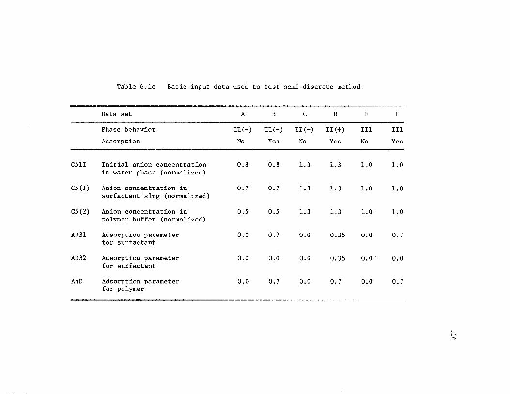
Table 6. le Basic input data used to test semi-discrete method.
Data set A B c D E
Phase behavior II(-) II(-) II(+) II(+) III
Adsorption No Yes No Yes No
CSll Initial anion concentration 0.8 0.8 1. 3 1.3 1.0 in water phase (normalized)
cs (1) Anion concentration in 0.7 0.7 1.3 1. 3 1.0 surfactant slug (normalized)
cs (2) Anion concentration in o.s o.s 1.3 1.3 1.0 polymer buffer (normalized)
AD31 Adsorption parameter 0.0 0.7 0.0 0.3S 0.0 for surfactant
AD32 Adsorption parameter 0.0 o.o 0.0 0.3S 0.0 for surfactant
A4D Adsorption parameter 0.0 0.7 0.0 0.7 o.o for polymer
F
III
Yes
1.0
1.0
1.0
0.7
0.0
0.7
I-' I-' 0\
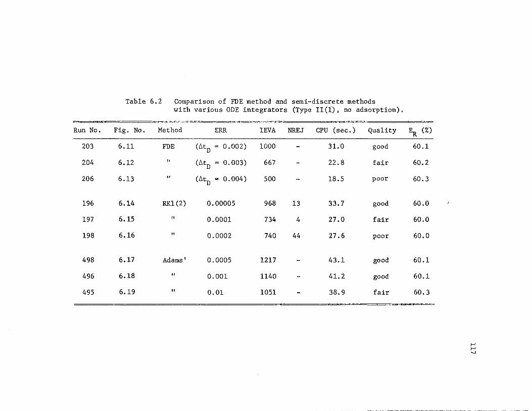
Table 6.2 Comparison of FDE method and semi-discrete methods with various ODE integrators (Type II CU, no adsorption).
Run No. Fig. No. Method ERR IEVA NREJ CPU (sec.) Quality
203 6.11 FDE (LitD = 0.002) 1000 - 31.0 good
204 6.12 II (t.tD = 0. 003) 667 - 22.8 fair
206 6.13 " (LitD = 0.004) 500 - 18.5 poor
196 6.14 RK1(2) 0.00005 968 13 33.7 good
197 6.15 II 0.0001 734 4 27.0 fair
198 6.16 II 0.0002 740 44 27.6 poor
498 6.17 Adams' 0.0005 1217 - 43.l good
496 6.18 II 0.001 1140 - 41.2 good
495 6.19 Ii 0.01 1051 - 38.9 fair
ER (%)
60.1
60.2
60.3
60.0
60.0
60.0
60.1
60.1
60.3
I-' I-' -....!
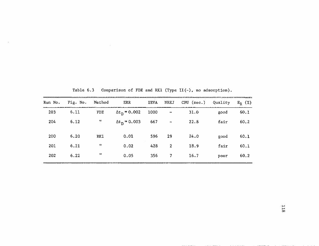
Table 6.3
Run No. Fig. No.
203 6.11
204 6.12
200 6.20
201 6.21
202 6.22
Comparison of FDE and RKl (Type II(-), no adsorption).
Method ERR IEVA NREJ CBU (sec.) Quality
FDE 6tD = 0.002 1000 - 31.0 good
II 6tD = 0.003 667 - 22.8 fair
RKl 0.01 596 29 24.0 good
II 0.02 428 2 18.9 fair
II 0.05 356 7 16.7 poor
ER (%)
60.1
60.2
60.1
60.1
60.2
......
...... co
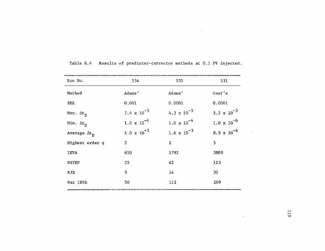
Table 6.4 Results of predictor-corrector methods at 0.1 PV injected.
Run No. 534 535 531
Method Adams' Adams' Gear's
ERR 0.001 0.0001 0.0001
Max. titD 7.4 x 10 -3 4.3 x 10 -3 3.2 x 10 -3
Min. titD 1.0 x 10 -4 1.0 x 10 -4 1.0 x 10 -6
Average titD 4.0 x 10 -3 1.6 x 10 -3 8.9 x 10 -4
Highest order q 2 2 3
!EVA 650 1792 3809
NS TEP 25 62 113
NJE 5 14 30
Net IEVA 50 112 209
f-' f-' l.O
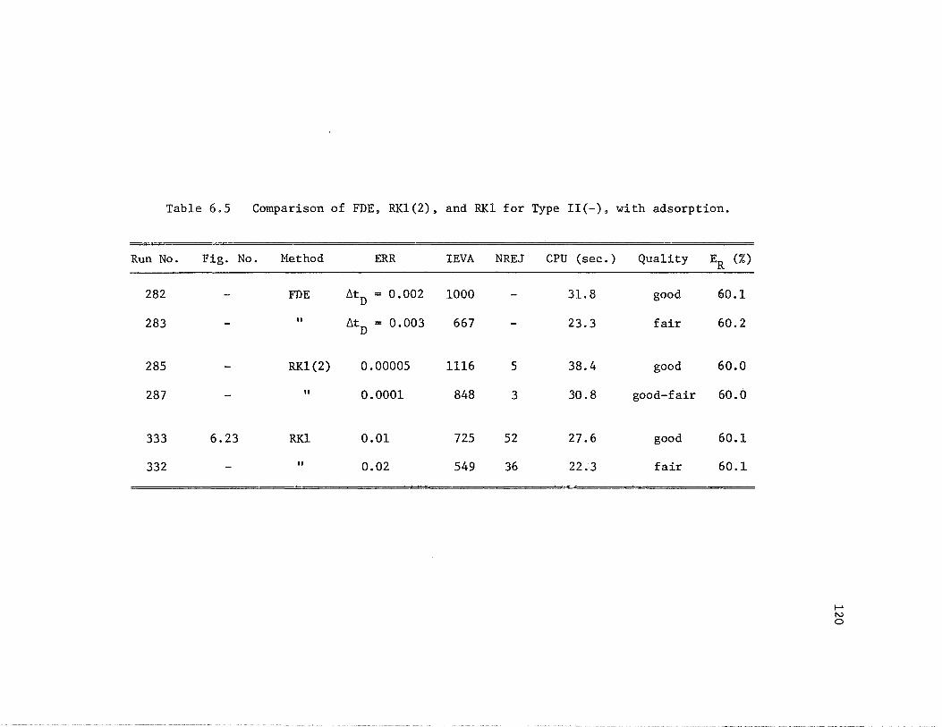
Table 6.5 Comparison of FDE, RK1(2), and RKl for Type II(-), with adsorption.
Run No. Fig. No. Method ERR IEVA NREJ CPU (sec.) Quality ER (%)
282 - FDE MD = 0.002 1000 - 31. 8 good 60.1
283 - II t.tD = 0.003 667 - 23.3 fair 60.2
285 - RK1(2) 0.00005 1116 5 38.4 good 60.0
287 - II 0.0001 848 3 30. 8 good-fair 60.0
333 6.23 RKl 0.01 725 52 27.6 good 60.1
332 - II 0.02 549 36 22.3 fair 60.1
I-" N 0
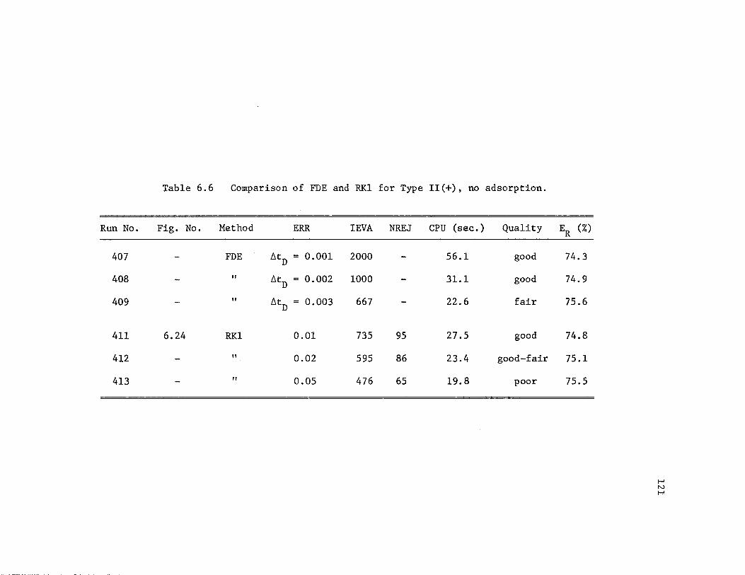
Table 6.6 Comparison of FDE and RKl for Type II(+), no adsorption.
Run No. Fig. No. Method ERR IEVA NREJ CPU (sec.) Quality
407 - FDE LitD = 0.001 2000 - 56.1 good
408 - II L\tD = 0.002 1000 - 31.1 good
409 - II L\tD = 0.003 667 - 22.6 fair
411 6.24 RKl 0.01 735 95 27.5 good
412 - fl 0.02 595 86 23.4 good-fair
413 - II 0.05 476 65 19.8 poor
~ (%)
74.3
74.9
75.6
74.8
75.1
75.5
f--' N H

Table 6.7 Comparison of FDE, RK1(2), and RKl for Type II(+), with adsorption.
Run No. Fig. No. Method ERR IEVA NREJ CPU (sec.) Quality ER (%)
406 - FDE lltD = 0.001 2000 - 56.1 good 51.3
384 - II lltD = 0.002 1000 - 31.0 good 51.8
385 - " lltD = 0.003 667 - 22.8 poor 53.4
395 6.25 RKl 0.01 1005 149 35.8 good 51. 4
389 - " 0.02 778 105 29.1 fair 51. 7
391 - RK1(2) 0.00005 1680 120 53.6 good 51.0
I-' N N

Table 6.8 Comparison of FDE and RKl for Type III.
Run No. Fig. No. Adsorption Method ERR IEVA NREJ CPU (sec.)
445 - No Euler .6tD = 0.001 2000 - 55.5
444 - " II .6tD = 0.002 1000 - 30.9
442 6.26 II RKl 0.01 2760 766 86.9
464 - Yes Euler .6tD = 0.001 2000 - 58.7
465 - II " .6tD = 0.002 1000 - 32.6
463 6.27 II RKl 0.01 2594 466 84.0
Quality
good
fair
good
good
fair
good
Ei (%)
100
100
100
100
100
100
...... N w
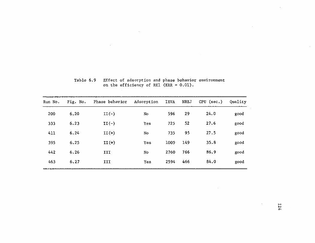
Run No.
200
333
411
395
442
463
Table 6.9 Effect of adsorption and phase behavior environment on the efficiency of RKl (ERR= 0.01).
Fig. No. Phase behavior Adsorption IEVA NREJ CPU (sec.)
6.20 II(-) No 596 29 24.0
6.23 II(-) Yes 725 52 27.6
6.24 II(+) No 735 95 27.5
6.25 II(+) Yes 1005 149 35.8
6.26 III No 2760 766 86.9
6.27 III Yes 2594 466 84.0
Quality
good
good
good
good
good
good
I-' N .i::-
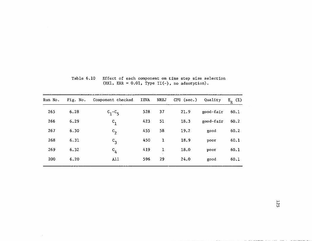
Run No.
265
266
267
268
269
200
Table 6.10 Effect of each component on time step size selection (RKl, ERR= 0.01, Type II(-), no adsorption).
Fig. No. Component checked IEVA NREJ CPU (sec.) Quality
6.28 Cl-CS 528 37 21. 9 good-fair
6.29 cl 423 51 18.3 good-fair
6.30 c2 455 58 19.2 good
6.31 c3 450 1 18.9 poor
6.32 c4 419 1 18.0 poor
6.20 All 596 29 24.0 good
ER (%)
60.1
60.2
60.2
60.1
60.1
60.1
I-' N Vt
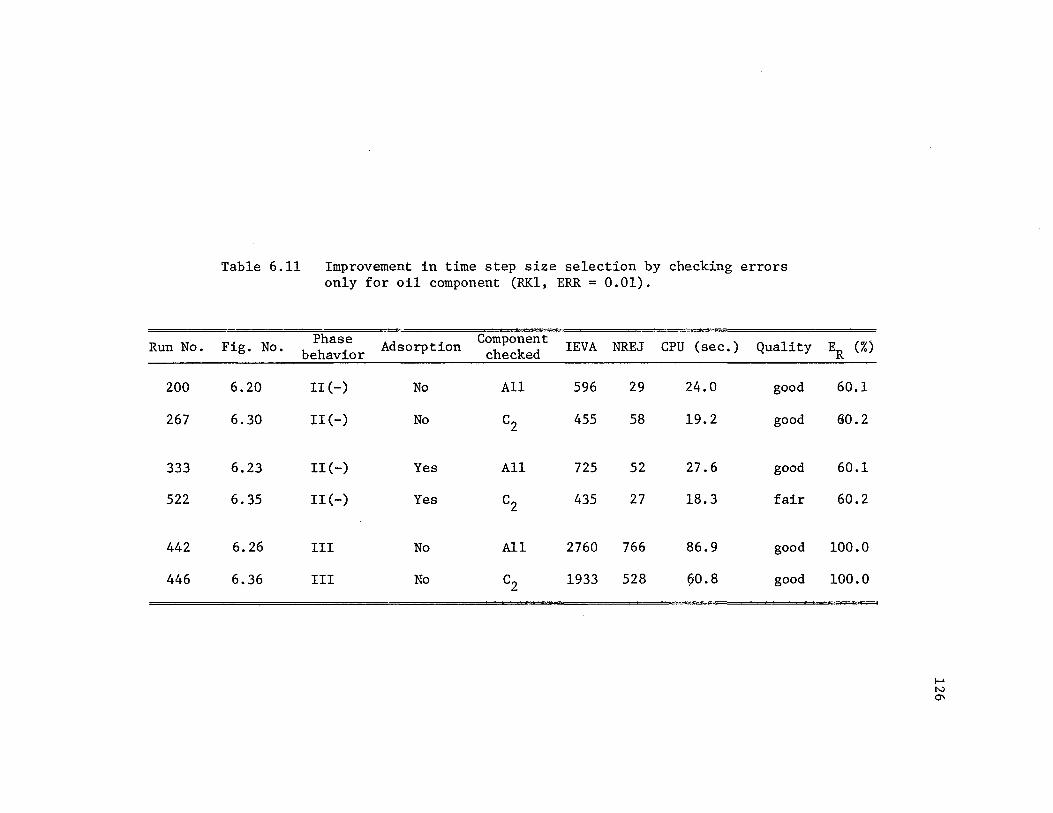
Run No.
200
267
333
522
442
446
Table 6.11 Improvement in time step size selection by checking errors only for oil component (RKl, ERR= 0.01).
Fig. No. Phase Adsorption Component !EVA NREJ CPU (sec.) Quality behavior checked
6.20 II(-) No All 596 29 24.0 good
6.30 II(-) No C2 455 58 19.2 good
6.23 II(-) Yes All 725 52 27.6 good
6.35 II(-) Yes C2 435 27 18.3 fair
6.26 III No All 2760 766 86.9 good
6.36 III No C2 1933 528 90.8 good
ER (%)
60.1
60.2
60.1
60.2
100.0
100.0
1--' N 0\

Table 6.12 Test runs with YBIAS = 1.0 (RK1(2) and RKl, Type II(-), no adsorption).
Run No. Fig. No. Method PCT ERR !EVA NREJ CPU (sec.) Quality
626 - RKl 0.25 0.01 522 0 21.2 good
627 - II II 0.1 336 0 15.5 fair
628 - RK1(2) Ii 0.00005 882 0 30.8 good
629 6.37 II Ii 0.0001 742 0 26.8 good
630 - II II 0.001 572 0 22.0 poor
645 - RKl 0.50 0.01 377 2 16.8 good-fair
646 - RK1(2) II 0.00005 654 9 24.6 good-fair
647 6.38 II II 0.0001 616 3 23.5 poor
...... N -...J
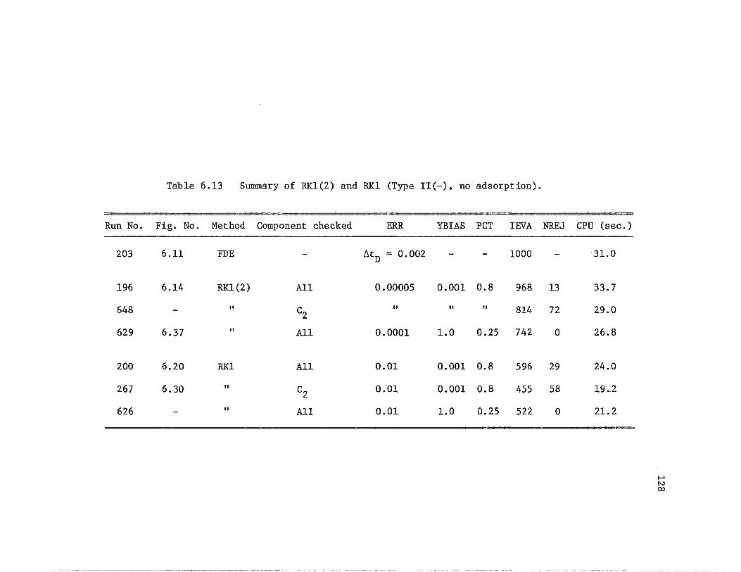
Table 6.13 Summary of RK1(2) and RKl (Type II(-), no adsorption).
Run No. Fig. No. Method Component checked ERR YBIAS PCT !EVA -
203 6.ll FDE - LitD = 0.002 - - 1000
196 6.14 RK1(2) All 0.00005 0.001 0.8 968
648 - II c2
II ti ti 814
629 6.37 II All 0.0001 1.0 0.25 742
200 6.20 RKl All 0.01 0.001 0.8 596
267 6.30 II c2 0.01 0.001 0.8 455
626 - II All 0.01 1.0 0.25 522
NREJ
-
13
72
0
29
58
0
CPU (sec.)
31.0
33.7
29.0
26.8
24.0
19~.2
21.2
I-' N CX>
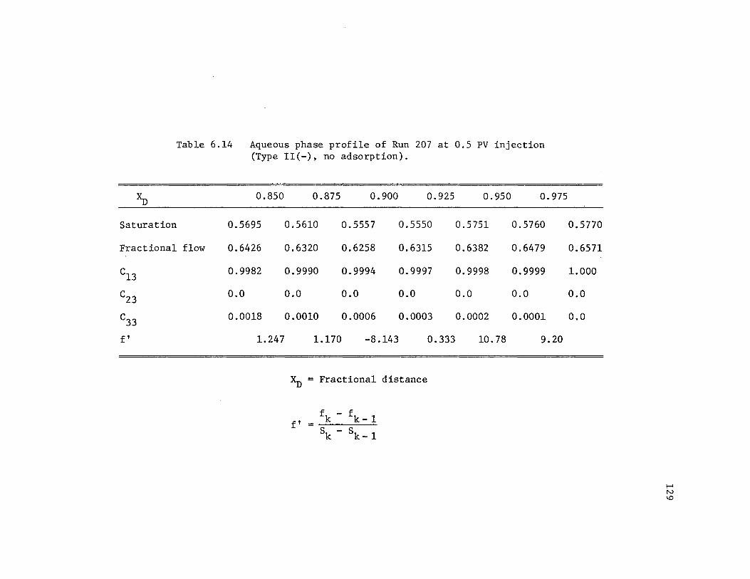
Table 6.14 Aqueous phase profile of Run 207 at 0.5 PV injection (Type II(-), no adsorption).
~ 0.850
Saturation 0.5695
Fractional flow 0.6426
cl3 0.9982
c23 0.0
c33 0.0018
f' 1.247
0.875 0.900 o. 925
0.5610 0. 5557 0.5550
0.6320 0.6258 0.6315
0.9990 0.9994 0.9997
0.0 0.0 0.0
0.0010 0.0006 0.0003
1.170 -8.143 0.333
XD = Fractional distance
f' = fk - fk- 1
8k - 8k- 1
0. 950 0.975
0. 5 751 0.5760
0.6382 0.6479
0.9998 0.9999
o.o 0.0
0.0002 0.0001
10.78 9.20
o. 5770
0.6571
1.000
o.o
o.o
t-' N \.0

Table 6.15 Legend for the total concentration history plots.
Symbol Component
0 Water
6 Oil
+ Surfactant*
x Polymer
0 Anion
4 Tracer
*For all total concentration histoYy plots, surfactant concentration
is five times amplified.
130

z 0
0 0
0 co 0
1-0 a:([) a::c:.) 1-z w (__)
Zo 0 'tjf
u. 0
_J
·IT 1-0 o 1-N .
a
0 0
anion
131
J oil
surfactant (five times amplified)
0.20 0. 40 0.60 0. 80 1. 00 FRRCTitJNRL DISTANCE
Figure 6.1. Total concentration profile at 0.25 PV for Run 207 (FDE method, ~tD = 0.001 PV, Type II(-), no adsorption).
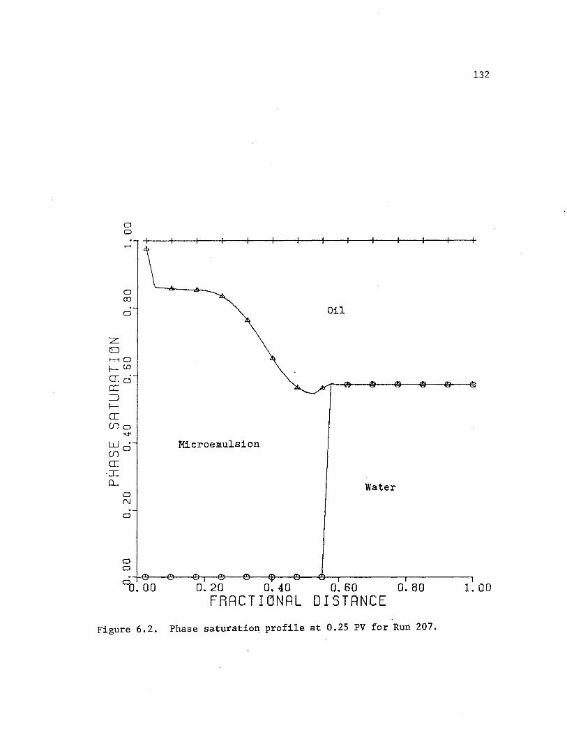
0 a
0 co
a
z 0 ~-10
l- C.D
a: 0 a: ::J l-ee cna
w. (f)o
a: ·::C CL
0 N . 0
a a
Oil
Microemulsion
W~ter
0.20 o. 40 0.60 0.80 FRRCTIONRL DISTANCE
Figure 6.2. Phase saturation profile at 0.25 PV for Run 207.
132
1. 00
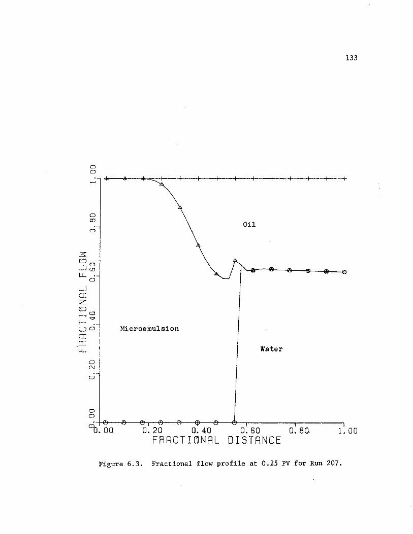
_J a: z 0
a 0
0 (D
0
I-~ 0 .qt
f(__) 0
CI a: LL.
0 0J .. 0
0 a
133
Oil
Microemulsion
Water
00. 00 0. 20 0. 40 0. 60 0. SQ 1. 00
FRACTI~NRL DISTANCE
Figure 6.3. Fractional flow profile at 0.25 PV for Run 207.

0 0
......
0 en
' 0
(/)
zo 0 C.D
1--i 0 la: 0::: lZ o w~
(__) 0 z 0
. (_)
0 N . a
0 0
134
Oil
Water
Surfactant
0. 20 0. 40 o. 60 FRRCTIONRL DISTANCE
Figure 6.4. Microemulsion phase concentration profile at 0.25 PV for Run 207.
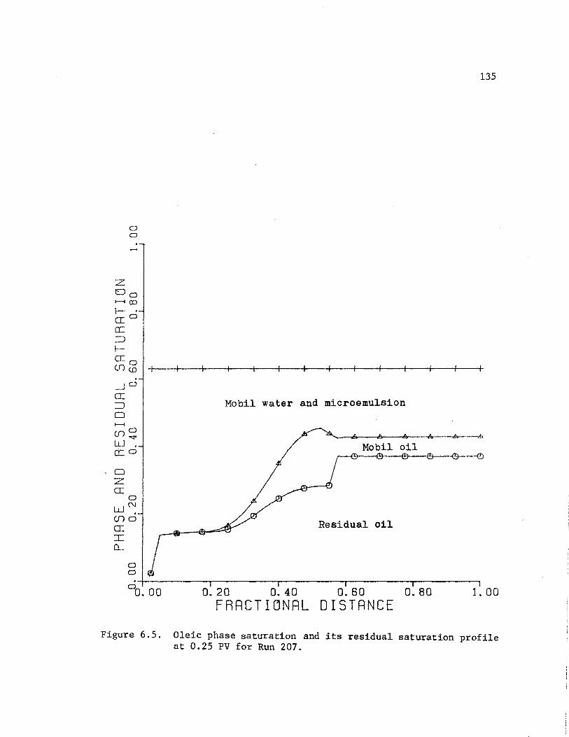
0 0
z Oa ~co
I- . a:o a:: ::J la: (I) 55 . _JO
a: ::J 0 ~
([)o ..q<
Ll.J • a:: 0
0 z a:
0
w~ (()O
a: I Q__
0 0
135
Mobil water and microemulsion
Mobil oil
Residual oil
·.+-.~~~~~~~~~~..,-~~~~-r~~~~--,,-~~~--, 0 o. 00 0. 20 0. 40 0. 60 0. 80 1. 00
FRRCTI~NRL DISTANCE
Figure 6.5. Oleic phase saturation and its residual saturation profile at 0.25 PV for Run 207.

:z: u ......... w z
N 0
>- ..... Oo
z 0
en z w I-
u a: LL a:: w 1-z
...... I
136
01-4-~~~~--.-__:~~~--.~~~~--.~~~~--.~~~~-,
..... 0. 00 0. 20 0. 40 0. 60 0. 80 1. 00 FRACTIONAL DISTANCE
Figure 6.6. Interfacial tension profile at 0.25 PV for Run 207.

......... 00 Wo N, ::i "<!'
<I: E 0:::: 0 z -a
N >- ' I- (Y1
mo 0..q< L,
w >
N
la: 0
,w __J •
LLl .,.... a:
'_J
a: I- 0
oO: 1-0
a 0
137
·~~~~~~~~~~--.~~~~~r-~~~~.--~~~---, 0 o. 00 0. 20 0. 40 0. 60 o. 80 1. 00
FRRCTI0NRL DISTANCE
Figure 6.7. Total relative mobility profile at 0.25 PV for Run 207•
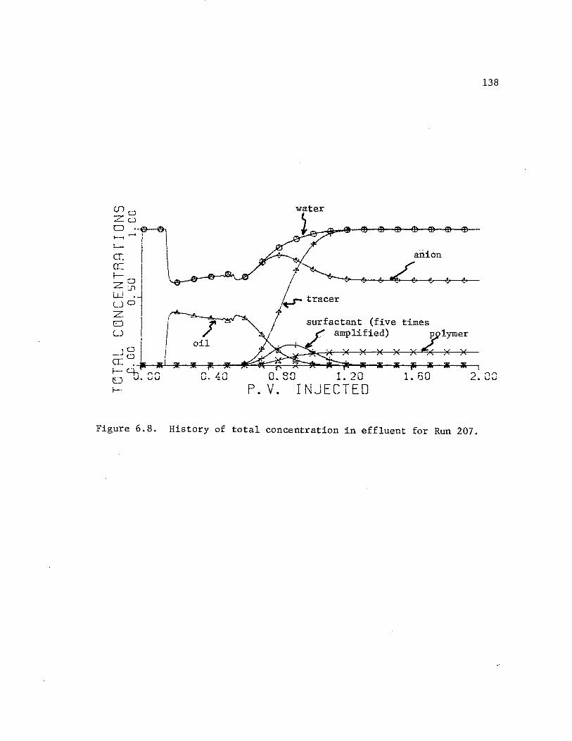
(J)o z CJ
......... .-O·-n
f
anion
~tracer
surfactant (five amplified)
Figure 6.8. History of total concentration in effluent for Run 207.
138
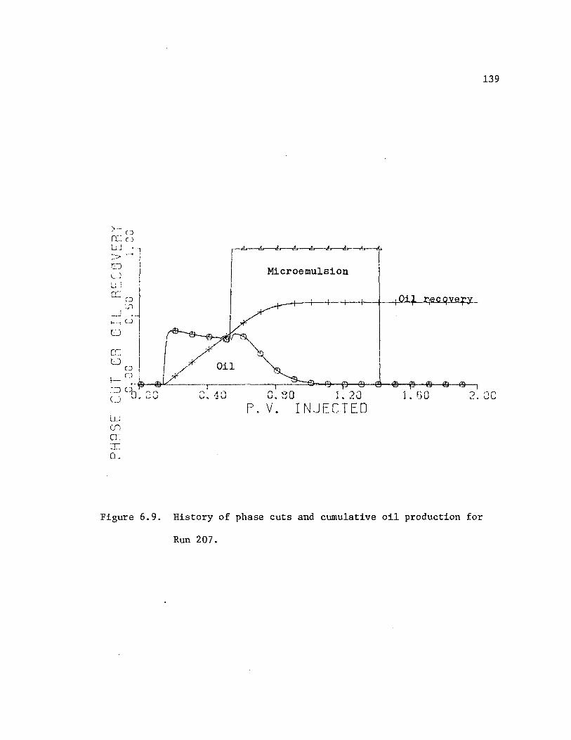
>·- u o.~: c)
'.' '--'---' • .. , :::::> ...... I
(:J (___)
LLJ
a..:: o :.JJ
' _ _J ••
, ... ,Cl
u
Li.J (/')
er: T~ o_
Microemulsion
. .rr Oil
p. v.
Figure 6.9. History of phase cuts and cumulative oil production for
Run 207.
139

CJ n ... u LJ ··1 cc :n I CJ
~~ 01 __ _, i.J'l
(/") .. (.J'l ("\!
L.J .J : o::: I
. u Wu
140
[L Ci. ·J-~
:> . . ·----.---------.,..--------..--------,.------1 ~; 00.88 C.10 0.30 1.20 1.GO 2.CC Cl P. V. I N.JECTED
Figure 6.10. History of pressure drop (normalized) between producer
and injector for Run 207.

fer: cc f-0 z lf)
w. uo z E)
u
141
Figure 6.11. History of total concentration in effluent for Run 203
(FDE method, ~tD = 0.002, Type tI(-), no adsorption).
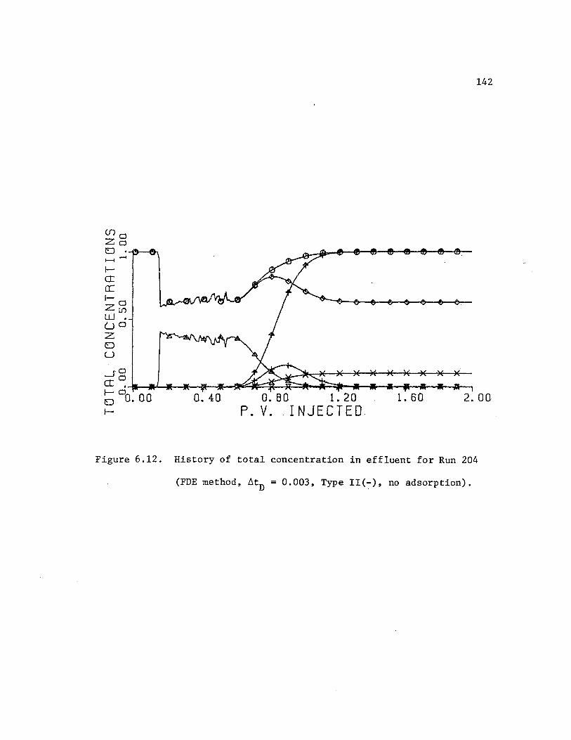
la: a: 1-0 z If)
w. LJO z 0 (_)
142
_Jo ct~----ai.L...:11-.......... --1r--~~~:....-J~~ .. ::::;ii~._ ........ _..~!5-.... -a--. ~ 0o. oo 0.40 0. 80 1. 20 1. 60 2.00 I- P. V. INJECTED
Figure 6.12. History of total concentration in effluent for Run 204
(FDE method, ~tD = 0.003, Type II(-), no adsorption).

en o Zo E> ·~-fll ....
. ....... _... I J---; lld: cc !---' . z~ w. (.Jd z l!J u
'._j d
143
.d CI ·-B--a..J.l.ll~fl.JJ..~"*----~~~~~..ji;.~-11!-iJ~--...-...... _.--illr--, ~do. oo o .. 40 o. so t. 20 . t. 60 2. oo r- P .. V. INJECTED
Figure 6.13. History of total concentration in effluent for Rum 206
(FDE method, ~tD = 0.004, Type II(-), no adsorption).
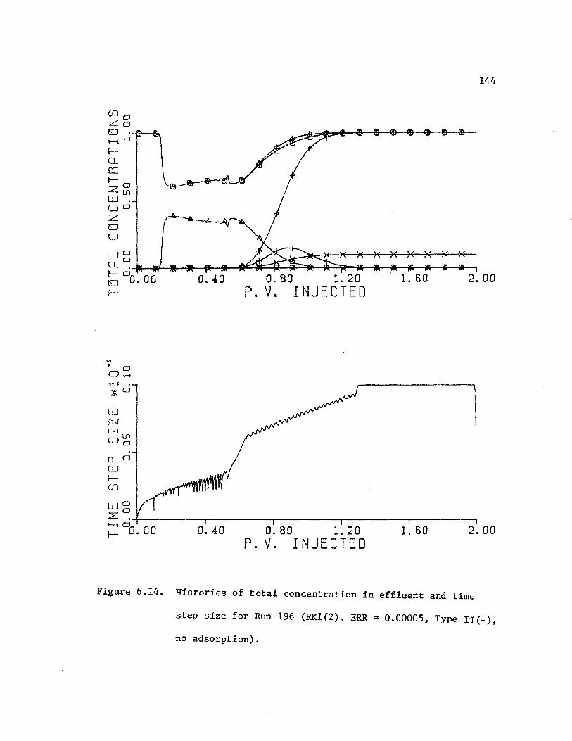
fa: a: f- 0 z lf')
w. LJ 0
z EJ u
~
J .o o ...... ..-I •
*o w N 1--1
en~ o_.o w .I-en
144
wo ~~-+-~~~-~-.-~~~~--,~~~~~r-~~~~.-~~~~, ;:
0 o . 0 0 0. 4 0 0. 8 0 1. 2 0 1. 6 0 2 . 0 0 P. V. INJECTED
Figure 6.14. Histories of total concentration in effluent and time
step size for Run 196 (RK1(2), ERR= 0.00005, Type II(-),
no adsorption).

(f)o Zo u . 1---i
......
f-cr: a::: 1--
0 Zm w LJ CJ
z 0 u
I o o ...... ........ . * w N 1--i
0
(f)~
CL o LU f(f)
wg
145
'
2::: • ...L~~~-~~~~~~-.-~~~~-.~~~-~.-~~~~,
~ 0 o. 0 0 0. 4 0 0. 8 0 1. 2 0 1. 6 0 2. 0 0 P. V. INJECT E 0
Figure 6.15. Histories of total concentration in effluent and time
step size for Run 197 (RK1(2), ERR= 0.0001, Type
II(-), no adsorption).

(Jlo Zo
D ·~--1--1 ......
!CI a: !- 0 z L'"l Lt..J • uo z D u _J 0
146
cr:~Ja__.~!--!IE-*-.... ~~~t=;:::=:*'""..:;::~=-;11f--i ____ .._ ..... __.~I-; ci 0 o . 0 0 0 . 4 0 0 . 8 0 1. 2 0 1. 6 0 2 . 0 0 1- P. V. INJECTED
i' . a 0 ..._.
*a w N 1--!
(f)~ Q_ 0
w l(f)
wa 2::a-t----~~·~-.-~~~~--.~~~~~r--;:
00. 00 o. 40 0.80 1.20
P. V. l NJECTED 1. 60 2. 00
Figure 6.16. Histories of total concentration in effluent and time
step size for Run 198 (RK1(2), ERR= 0.002, Type II(-),
no adsorption).
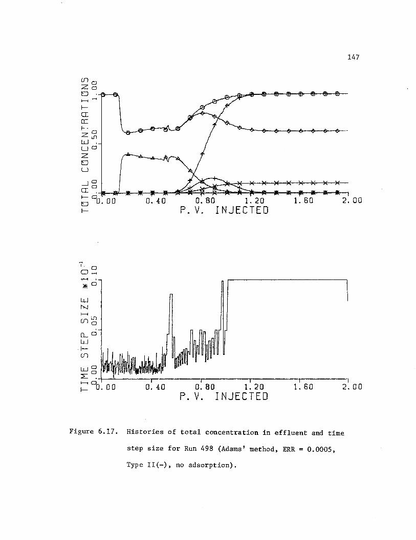
(110 Zo EJ . -\'i--ct. 1--i .....
f-0: a= f- 0 z 1.n w' LJO z EJ u
147
_J 0
a: ~----a"--'------11~.-~~:::::}~~~....-J..::::~ ... ---l--ilft-"il'----il~._, ci 0 o. oo o. 40 O. 80 1. 20 2. 00 f- P. V. INJECTED
I. 0 o .......
*o w N ,__.. en Lf1
0
o._O w
.}-
en
wo ::L.
0-4--L-----.------.-------.-----.-----1
~ 0o.oo 0.40 o.ao 1.20 1.60 2.00 P. V. INJECTED
Figure 6.17. Histories of total concentration in effluent and time
step size for Run 498 (Adams' method, ERR = 0.0005,
Type II(-), no adsorption).
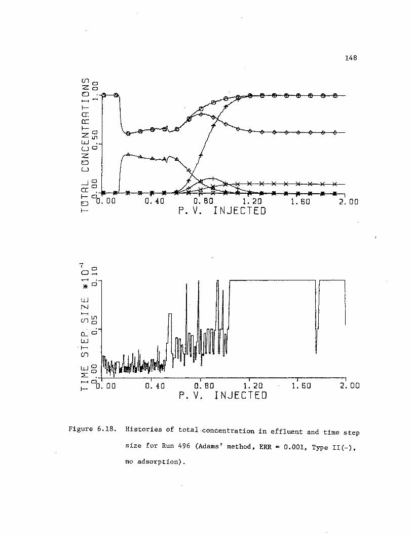
la: er: I-CJ ZLn w. LJ CJ z E)
LJ
_J CJ
148
cr:C::~_.,,.~-----~f--,... ... ~<::::::~~::::::,~~~-.. .......... -.-;""'""" ... _.---;~ 6CJo.oo 0.40 0.80 1.20 1.60 2.00 1- P. V. INJECTED
7 CJ o .... ........ . *o
Q_ Cl
w ·I-m wCJ L:C::-l.-:....'...l..~~~---,.~~~~~.-~~~~ ... ~~~~~r-~~~--, ~ 0o. oo o. 40 o. 80 1. 20 1. 60 2. OD
P. V. INJECTED
Figure 6.18. Histories of total concentration in effluent and time step
size for Run 496 (Adams' method, ERR= 0.001, Type II(-),
no adsorption).
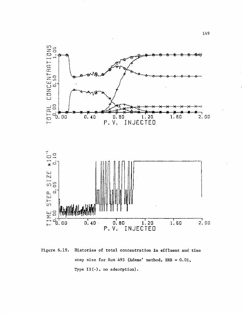
fa: cc f- 0 ZUl w. LJ 0
z 8 LJ
_J 0
CI~...J...--..11J_;.__..__.__;.,_~:::41:::::l~..V::::::::O::..t.4.::::::S:::....,_.,.~._...__.--.11-.._,
149
~ 0 o. 00 0. 40 o. 80 1. 20 1. 60 2.00 f-
I 0 0--< .--1 '
*o w N ;..--;
([)~ (LO
w 1-(f)
P. V. INJECTED
wo :L~-\--'-~~~-.-~~~~--.-~~~~~r--~~~~.,-~~~---, ~ 0 0. 00 o. 40 . o. 80 1. 20
P. V. INJECTED 1. 60 2. OD
Figure 6.19. Histories of total concentration in effluent and time
step size for Run 495 (Adams' method, ERR= 0.01,
Type II(-), no adsorption).
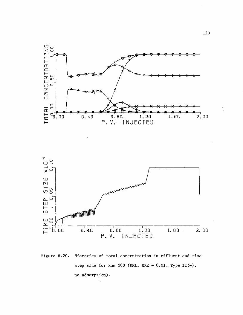
fer a:: fz ~ w. (.jd
z ~ (_)
_Jq .a
a: ·-if..-a~f--*-.... -11£---llfi':::~~__,;~llf-~:::.;;.-;i ............. -a--tl ............. -;
150
6 do. oo 0. 4.0 o .. 80 1. 20 1. 60 2.00 f-
i d o ..... ..-1 •
*o w N
. o._d w fen
P. V •. INJECTED
wd ::E~--~~~~-.-~~~~--.~~~~~.--~~~~...-~~~~~ :=do. oo 0.40 Q. 80 1 r 20 1. 60 2.00
P. V. INJECTED
Figure 6.20. Histories of total concentration in effluent and time
step size for Run 200 (RKl, ERR= 0.01, Type II(-),
no adsorption).

Ula Zo 0 '-rt--ffot
1--t -
1--cc cc 1---z~ w. (_)d
z 0 u _J d )( )(
cc~_..~rL-l~-----~1--_....~~~~~_,~._...__...~1-.a--&--.1i--.a...-
151
~ 0 o. oo o. 40 o. 80 1. 20 L 60 2. 00 I--
w fi-.1 t---1
U1~ a... d w ·~
c.n
0. 40
P. V. INJECTED
o. 80 l. 20 1. 60 2. GO P. V. INJECTED
Figure 6.21. Histories of total concentration in effluent and time
step size for Run 201 (RKl, ERR= 0.02, Type II(-),
no adsorption) •

Id:: er I- . z~ w. (._)d
z E) (_)
_Jd .o
a: ·----M.l--~!-i~--~~~~~t--ijli';:::::: ......... -&--a.--ao.-15--.1r.-ill--
152
6 do. oo 0. 4.0 0. 80 . 1. 20 1. 60 2.00 I-
j d o ..... ~.
*d
w N I-<
([}~ o_d w 1-([}
P. V. INJECTED
wo :E'.o ;:::do~.-o-o~--~o~.-4-o~---o-.~8-o------1~.~-2-0-.-----1~.-so--.----2~.oo
P. V. INJECTED
Figure 6.22. Histories of total concentration in effluent and time
step size for Run 202 (RKl, ERR= 0.05, Type II(-),
no adsorption) •
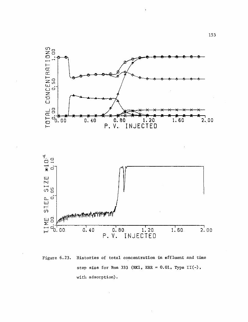
la:: a::: I- 0 z U1 w. uo z ~ u _J 0
a::~..g..-a.J....,i1-+-..... ~f-llD:------~~--~~_,..5--._ ...... __ _,..r-a--a--.
153
6 °o. oo o. 40 0. 80 1. 20 1. 60 2 .. 00 I-
.,..j
'·-. 0 o ..... ....... . .*o
. 0.... 0
w ~ (f\J
P. V. INJECTED
wo ·O
L: ,....,_~~~~-..,-~~~~-.-~~~~-.-~~~~-.-~~~~-.
;: 0
0. OD 0. 40 0. 80 1. 20. 1. 60 2. 00 P. V. INJECTED
Figure 6.23. Histories of total concentration in effluent and time
step size for Run 333 (RKl, ERR= 0.01, Type II(-),
with adsorption).

())0
Zo
El ·r ~,._,
!-CI a: !----,. 0 .c.:.. iJl LLJ . LJO :z 0 u 1~
I __ Jg CI ·-W.--iA~i'!-4--4--411f--l~~_,..__,~~"""---a-_,,~ll--iil--a&-~~:&--a--.
154
6°0. 00 o. 40 0.80 1.20 1. 60 2. 00 !--
7 0 o ......
;al W I :-~-.J I-~
iJl ())0
o_O w
~~~~I ~ 0 0. 0 0 o. 40
P. V. INJECTED
~ -r- -,.---·----------, 0.80 1.20 1.60 2.00
P. V. INJECTED
Figure 6.24. Histories of total concentration in effluent and time
step size for Run 411 (RKl, ERR= 0.01, Type II(+),
no adsorption).
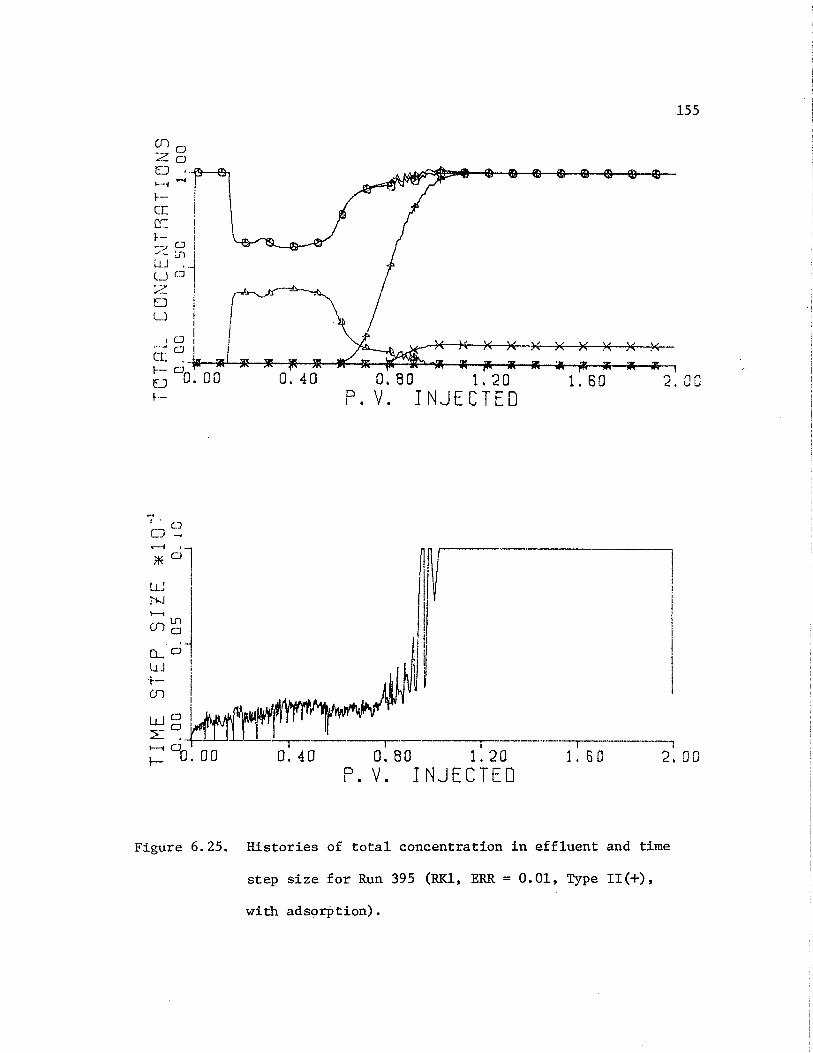
en o -7
""'- 0 0 •-W--t9i 1--i .....
f--0: a::: J-- I -7 o I ""-- :.n I
tj a·~ :z I 0 ; L) i
I
01
I I
.155
-~ o I C[ .,..~~~.-..~-;R--flF--:Jr-~..;::"'""'ifl-iilf-.-........... -ill--lg.._-llW--a--&--. ~ CJD. 00 1--
7 . (_J
o ..... ;ol ~ j Cf)~ .. o._O LLJ 1
-~ I
0. 40 O. BO l. 20 1. 60 2. 00 P. V. INJECTED
wgl.~ ~ 0 +:UJ.L --,---·----------·-----------·--,--------, I- 0.00 0.40 0.80 1.20 1.60 2.00
P. V. INJECTED
Figure 6.25. Histories of total concentration in effluent and time
step size for Run 395 (RKl, ERR= 0.01, Type II(+),
with adsorption).

cno Zo 0 '-C>!-~ t--i r-f
~--
.... I 0 0-< .-~ . -1 m CJ I
I !
LJ._; : '1-J I
I
~~ ~ ! ri. oi LLJ ! 1-- l (J) I
I I
lJ, 0 I -'o'
L:,
1-j 0 o 0 0 1-- •
0. 40 0.80 1.20 1. 60 P. V. INJECTED
0. 40 1. 60
156
2. 00
1 \
---, 2. 00
Figure 6.26. Histories of total concentration in effluent and time
step size for Run 442 (RKl, ERR = O. 01,_ Type III, no
adsorption).
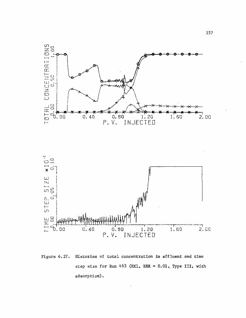
la: a:: f--_,7 0 ..__ w'"l l..LJ • -L) a
L)
LJ
,o --'o a: ·---~~~--4~1(--*"'~~li-~~:L.......;~~-JR~&---&-~'--&--&-~'--&--.
157
~ 0 o. 00 0.40 o. 80 1. 20 1. 60 2.00 1--
-I 0 o ....... ...-f ·-1 *a w ri-...1
~~~I CL o w I- I
(.()
P. V. INJE-CTED
wo 2= ~ i.IMIUIJl_,_"""._! • ..,_,__.___......1-'-'-.__._,_-"-'-'"--'--'-·--'-.....--- ·--~-~ o f-- 0. 00 C.40 o. 80 1. 20 1. 60 2.00
P. V. INJECTED
Figure 6.27. Histories of total concentration in effluent and time
step size for Run 463 (RKl, ERR= 0.01,_ Type III, with
adsorption).
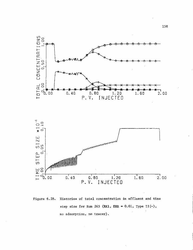
lf>o Zo
0 •-i.---1--1 ......
la: a:: 1-z 5; LU • LJO z 0 u
_JO
er: ~-----al.....i~-4-----41~*""::::je::::::::::j~.ii=::===---i~il--&-_,....-.l&-........ -&-.lll--&-
158
I- 0 0 0. 00 o. 40. 0. 80. 1. 20. 1. 60 2.00 I-
-I 0 0 ....; ...-. . *o
liJ N 1--1
Ul Ul 0 .
o_O w 1-Ul
P. V. I N JEC TE 0
Li.J 0
::L~-'r-~~~~-,...~~~~--.~~~~~...--~~~~-r-~~~~~ 1--10
~ 0. 00 0. 40 0.·80. L 20 1.. 60. 2.00 P. V. INJECTED
Figure 6.28. Histories of total concentration in effluent and time
step size for Run 265 (RKl, ERR= 0.01, Type II(-),
no adsorption, no tracer).
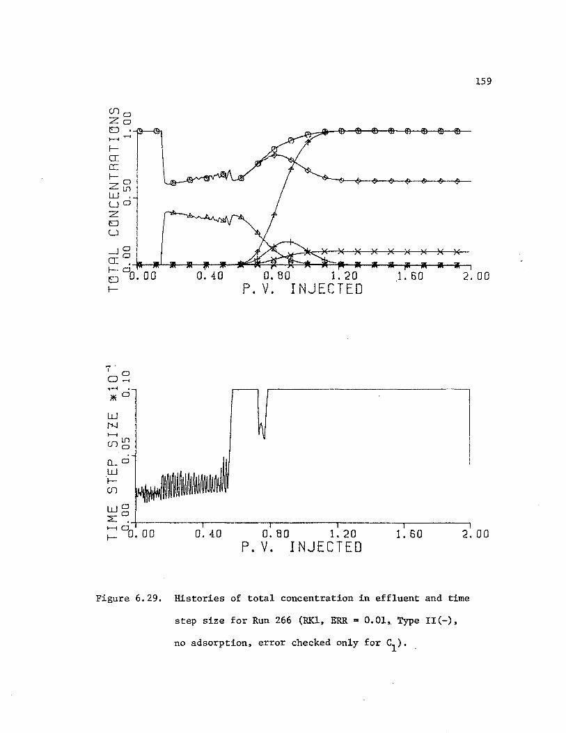
'j' 0 0 ...... T-1 •
*o w N 1--1
en~ Q_ 0
w !en wo a ~.
;::: 0 o. 00
0. 40
o. 40
159
)(
0.80 1.20 1. 60 2. 00 P. V. INJECTED
o. ao i. 20 1. 60 2.00 P. V. INJECTED
Figure 6.29. Histories of total concentration in effluent and time
step size for Run 266 (RK.l, ERR= 0.01~ Type II(-),
no adsorption, error checked only for c1) •.
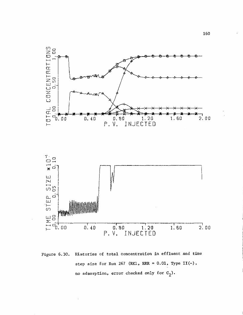
lo:: a:
=: o~' "-- Lil w. LJO z EJ u
7· 0 o ...... .. -1 •
*o
o. 40
0. 40
160
0.'80 1.20 1. 60 2. 00 P. V. JNJECTED
-.- --, 0. 80 1.20 1. 60 2. 00
P. V. INJECTED
Figure 6.30. Histories of total concentration in effluent and time
step size for Run 267 (RKl, ERR= 0.01, Type II(-),
no adsorption, error checked only for c2).
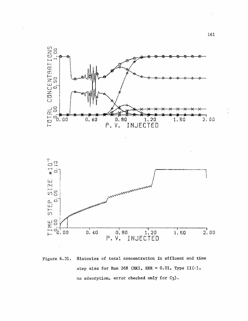
la: er:: I- CJ z [[) w. LJ 0
z EJ u
161
o. 40 o. 80 1. 20 1. 60 2. 00
7 0 o.,..... ,.-; I
* 01 w I N I 1-; i
lf) cno CL o LlJ
·1-(f)
P. V. INJECTED
wo ::?.:o ~ a· -- ---·---i-------r-------~-----T------~
!- 0. 00 0. 40 o. 80 1. 20 1. 60 2. 00 P. V. INJECTED
Figure 6.31. Histories of total concentration in effluent and time
step size for Run 268 (RK.l, ERR= 0.01, Type II(-),
no adsorption, error checked only for C3).

I-rr. er. 1---70 I ""--- \.{) I
lLJ I
LJ cil z !
o I u
7·0 o ..... ..--. '
*o w N 1-i
Ul ~ o_O w 1-cn
o. 40
wo 2::0
. -------r ;:
00. 00 0. 40
162
0.80 1.20 1. 60 2. 00 P. V. 1 NJECTEO
0.80 1.20 1. 60 2. 00 P. V. INJECTED
Figure 6.32. Histories of total concentration in effluent and time
step size for Run 269 (RKl, ERR= 0.01_, Type II(-),
no adsorption, error checked only for c4).

U'l
N C)
Q_~ LtJ • -1-- 0 (,')
lJ.J L: 1-io l- c:: _ -----.II
00. 00
I
0. 40
163
I I I I
0. 80 1. 20 1. 60 2.00 P. V. INJECTED
Figure 6.33. Histories of total concentration in effluent and time
step size for Run 229 (RKl, ERR = 0.01, waterflooding,
no tracer).
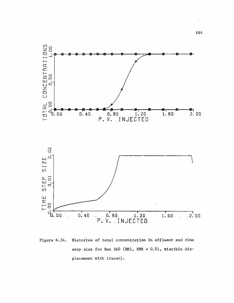
Ula Zo E) •-&---f'Jl--ff--6--ell--1!'J--&--fl!i---<l.'Jo---t!J-~~~-=--~-fl!,__~-e-~--e........ .-I
la: a: 1-0 z IJ')
w. uo z E)
u _JO
a:~ ..... .,.....~ .......... --i'lr--ill-........... ~--~11-~-a.~~--~-ar-.-~-B-~-.1~
164
6 °o. 00 I-
0. 40 0. 80 ' 1. 20 1. 60 2.00
('\J ·o .
wo N
0... ~ w. I- 0 (f)
· P. V. INJECTED
0. 40 0. 80. . 1. 20 1. 60' 2.00 P. V •. INJECTED
Figure 6.34. Histories of total concentration in effluent and time
step size for Run 260 (RKl, ERR = 0.01, miscible dis-
placement with tracer).
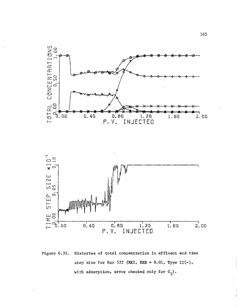
(f)o :Z:o 0 . -i.'1-_,..,,
fa: a:'. f-
:z: ~ w. u a z 0 u
j 0 0 .-4
*a w N ........ (!)~
o......a ·w 1-(f)
wo .a
165
0.40 o. 80 1. 2.0 l. 5·0 2.00 P. V. INJECTED
~ ·--~~~~---.--~~~~--..~~~~~....-~~~~...-~~~----.
;: °o. 00 0.40 0. 80 l. 2.0 1.60 2. 00 P. V. INJECTED
Figure 6.35. Histories of total concentration in effluent and time
step size for Run 522 (RK.l, ERR= 0.01, Type II(-),
with adsorption, error checked only for c2).

l--
IT. ,. a: 1--~a L-. i.JI I
LJ.-1 ' L) CJ
:z 0 u
j. CJ
C.J,.....
';al I II
LU J'l.,J I : l-i I
0. 40 0.80 1.20 P. V. INJECTED
i;; !i~; I ~ ~t _____ I ~w:~~ 1--1 0 ~ I- 0. 00 0. 40 0.80 1.20
P. V. INJECTED
1. 60
1. 60
166
2. 00
-·--, 2.00
Figure 6.36. Histories of total concentration in effluent and time
step size for Run 446 (RKl, ERR= 0.01,_ Type III, no
adsorption, error checked only for c2).
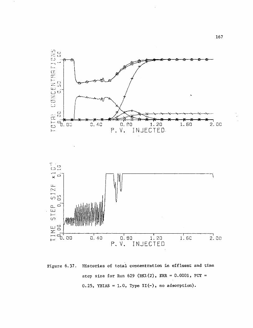
CJ ··~
~i .~JI n·L1 ..•
f-·-··.:.- [') '-··- : ... /1 lJ_j •
LJ o :z t::..J u
' C.) --- L"J
CL ._..~~~_.~1'-~~~~~~::::::;l:=~~~ll-"*"_,.,._,R-_..-iti...._...._,
167
~-~fl 0'' (..J u. '-• 8. 40 0.20 1. 20 1.60 2.00 f-
-· I Cl
0 ..... r-< . -, ~ C.J
p. v. I NJECTEO.
Figure 6.37. Histories of total concentration in effluent and time
step size for Run 629 (RK1(2), ERR= 0.0001, PCT=
0.25, YBIAS = 1.0, Type II(-), no adsorption).

la: 0:::: 1-0 z Ui w. (_)0
z 0 u _J 0
a::~-11--a'/--J.li---4---~f-~~~~~:=#-;;~*""' .... -alr---ll--&--&-~~&---.
168
6 °o. 00 0. 40 0. 80 1. 20 1. 60 2.00 I-
.... I. 0 0 .-. ..-i •
*o
w N t--i
()) ~
o._O w 1-(Jl
P. V. INJECTED
LLJ o 2:~--~~~~-.-~~~~-"T~~~~---,.--~~~~...--~~~---. ~ 0 o. 00 o. 40 0. 80 1. 20 1. 60 2.00
P. V. INJECTED
Figure 6.38. Histories of total concentration in effluent and time
step size for Run 647 (RK1(2), ERR= 0.0001, PCT=
0.50, YBIAS = 1.0, Type II(-), no adsorption).
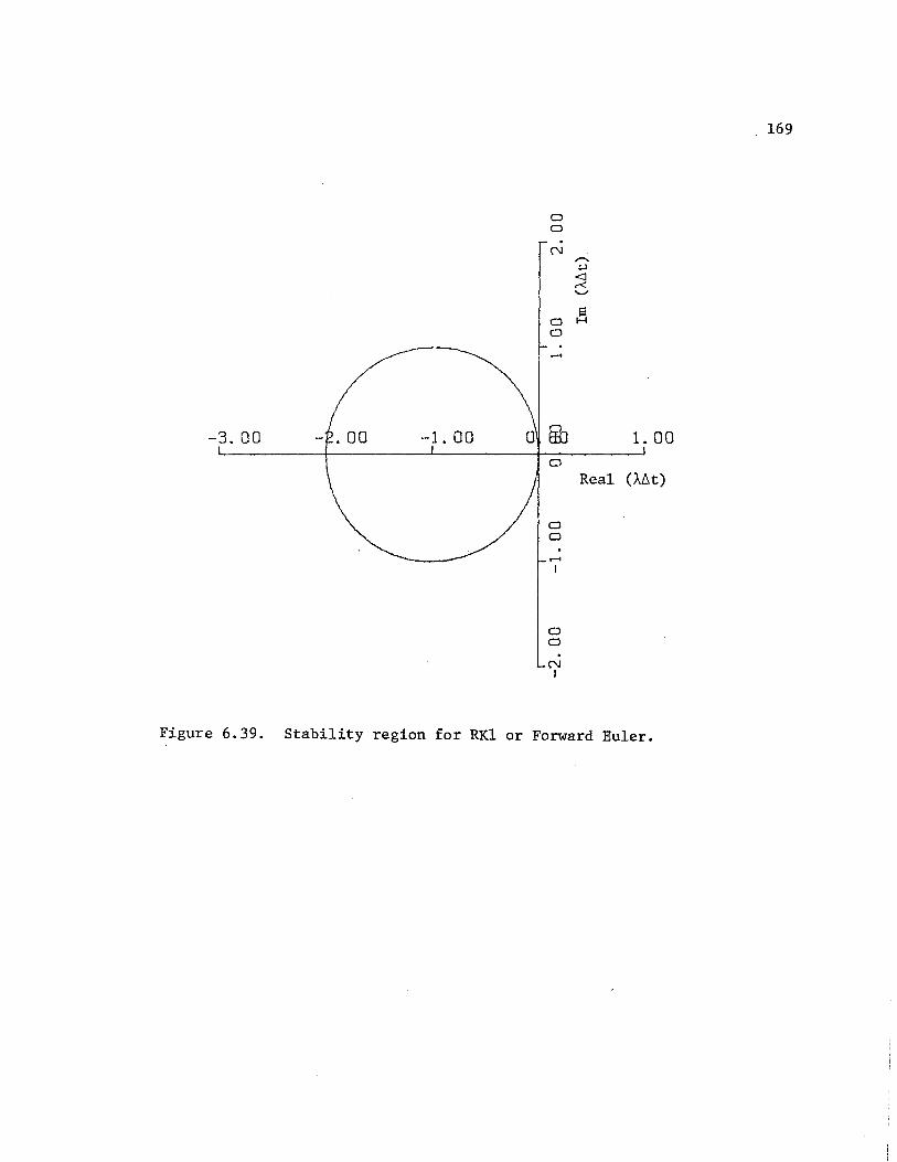
-3. 00 - . 00 -1. 00
0 0 . N
a a .....
....... I
a 0 . N I
,...... .µ <1 .-< '-"
~
1. 00
Real (Mt)
Figure 6.39. Stability region for RKl or Forward Euler.
169

CJ 0
0
0: ro Wo f-0:: 3:
lL.O 0 (Q .
0 3: 0 _J
LL. 0
_J ~
0:: • zo 0
1-U a O::N CL , LL.a
0 0
170
/
0. 20 o. 40 0. 60 0. 80 1. 00 WATER SRTURRTI(jN
Figure 6.40. Explanation of negative value for f'.

CHAPTER VII
CONCLUSIONS AND RECOMMENDATIONS FOR FUTURE STUDY
Some comparisons were made among three different three-phase
flow models. When the salinity was constant, the difference in oil
recovery and surfactant trapping among the models was rather large,
especially if the injected amount of surfactant was small. With
a salinity gradient, there was only a small difference in both oil
recovery and surfactant trapping. Since in all models surfactant
trapping was significant and since it is highly uncertain, this is
still another important reason for designing a micellar flood with a
salinity gradient.
Semi-discrete methods with various ODE integrators were im
plemented in a 1-D micellar/polymer flooding simulator. The ODE
integrators used are 1) Runge-Kutta method: RKl; 2) Runge-Kutta
Fehlberg method: RK1(2); 3) Adams' methods; 4) Backward differen
tiation (Gear's) methods. The first two methods are explicit methods
while the last·two are implicit with a predictor-corrector algorithm.
With respect to computation time, RKl was the best among the
ODE integrators used. Compared with the fully-discrete with forward
time Euler (FDE) method, RKl may save 20 to 30% or more computation
time, although it depends on phase behavior, adsorption, total volume
injected, etc. For some cases such as Type II(+) phase behavior
with adsorption, or Type III phase behavior, FDE required less compu
tation time than RKl. Furthermore, the truncation error associated
171

172
with the time integration for RKl is larger than for other ODE
integrators. The degree of numerical dispersion changes as the time
step size is varied with RKl. 28 However, with Chaudhari's technique ,
it may be possible to eliminate the problem by cancelling the
numerical dispersion at every time step.
Although the computation time with RK.1(2) was not as good as
had been expected, a much smaller error associated with time integra-
tion could be achieved without large computation time. RK1(2) should
be used when a higher order approximation to the spatial derivatives
are applied, or when a finite element technique is introduced to
treat the spatial domain, since these techniques yield much smaller
error in the spatial domain.
To achieve less computation time with RK.l or RK1(2), two methods
are suggested. One is to check the error only in the oil or water com-
ponent with small YBIAS, and with PCT nearly unity. The other is to
make YBIAS equal unity and use smaller PCT.
The semi-discrete methods do have the advantage of automati-
cally selecting a sufficiently small time step to avoid large trun-
cation error and/or instabilities. Since this time step is problem-
dependent, one can avoid a costly trial-and-error determination of
the required value, or the use of an excessively conservative (small)
value. There are of course many problems, conditions, and physical
options not tried during this study for which it would be a great
advantage.

173
Predictor-corrector methods such as Adams' methods or backward
differentiation (Gear's) methods did not work as well as the two
explicit techniques. However, it may be too early to conclude these
implicit or semi-implicit methods are not as good. Since a packaged
program was used to implement the techniques, the details are not
clear, but there may be some improvement possible.
If one desires to test predictor-corrector methods further,
fixed lower order methods should be tried. Since we are dealing with
partial differential equations, it is of no use to achieve a much
higher accuracy in time integration compared with spatial integration.
Furthermore, higher order methods have a smaller stability region,
which may impose more limitation on the time step size.
There was one problem concerning the step size control
employed in DGEAR, which varies time step size based on only relative
error, without YBIAS (see equation (5.7)). Since most variables change
between zero and unity, it is risky not to use YBIAS, or a combination
of relative and absolute error62•
The most difficult problem associated With predictor-correc
tor methods is convergence. Since the equations involved in micellar/
polymer flooding are highly non-linear, much investigation and effort
may be required. If one employes Newton's iteration, one should take
advantage of the sparseness of the Jacobian matrix.
Subprogram DER, which calculates the derivative of each com
ponent at each block, was designed to give flexibil~ty in making use
of any ODE integrator. Then it is easy to replace the ODE integrator.

Another problem concerning the predictor-corrector methods
was the evaluation of adsorption, since the adsorption was :calcu
lated explicitly in the simulator. The procedure should be changed
to evaluate adsorption implicitly.
A stability analysis was done for the oil bank, and the sur
factant front. The former imposes a rather constant limitation on
the time step size continuously until the plateau of the oil bank
174
is completely produced, which coincides with surfactant breakthrough.
The latter yields unconditional instability continually but only
locally. This conclusion is based upon an approximate analysis.
An eigenvalue analysis for the oil bank blocks suggests that
the stability is governed by the slope of the water-oil fractional
flow curve at the oil bank saturation. This analysis seems to give
reasonable criteria for both the fully discrete solution and the semi
discrete solution. The fully discrete solution oscillates to a larger
degree when the stability requirement is not satisfied. The semi
discrete method selects a time step size around the limit of stabil.ity
while the oil bank is being produced, then the time step size is
increased thereafter.
An approximate von Neumann stability analysis for the surfac
tant front blocks showed an unconditional local instability occurred
occasionally, causing an oscillation in the history even with a time
step size as small as 0.001 PV. This instability is caused by the
change in the fractional flow curve due to the redu~tion of inter
facial tension because of the surfactant. It is impossible to
175
eliminate this instability completely, as long as the continuity
equations are solved explicitly, because the change in the frac
tional flow curve is an essential part of micellar/polymer flooding.
However, it may be possible to decrease both the degree of instability
and its frequency by changing the equation that gives the residual
saturation of the non-wetting phase (oil) as a function of the capi
llary number.
When the phase behavior environment is Type III, numerical sta
bility may be more difficult to attain. When total composition is
within the three phase region, extremely low interfacial tension occurs,
which causes a very large change in the fractional flow. Although the
stability was analyzed only for two phase flow, the same result may
apply. Furthermore, in the three phase region, the microemulsion phase
may travel much faster than the other two phases, possibly causing worse
instability. It is rather ironical that low interfacial tension con
tributes to both high oil recovery and to numerical instability during
simulation.
a. J.
A
b p
B
c. J.
CSE
CSEL
CSEU
CSEN
Dij
e. J
e. JC
e. JW
E
F
NOMENCLATURE
adsorption parameters
binodal curve parameter
polymer viscosity parameter
adsorption parameters
penneability reduction parameter
binodal curve parameter
total concentration of component i in mobile phases
concentration of component i in phase j
volume of adsorbed component i per unit pore volume
overall concentration of component i in mobile and
rock phase
effective salinity
lowest effective salinity for Type III phase behavior
highest effective salinity for Type III phase behavior
normalized salinity
effective binary diffusion coefficient of component i
in phase j
relative permeability exponent for phase j
relative permeability exponent for phase j under the
condition of infinite capillary number
relative permeability exponent for oil/water system
distribution curve parameter
distribution curve parameter
176

f. J
Gij
J
k
M
NCOMP
p
q
R~ax
s p
177
fractional flow of phase j
interfactial tension parameters
Jacobian matrix
absolute permeability
relative permeability to phase j
endpoint relative permeability to phase j
endpoint relative permeability to phase j under
the condition of infinite capillary number
endpoint relative permeability to phase j in oil-
water (no-surfactant) system
dispersion coefficient of component i in phase j
longitudinal dispersion coefficient
length of system
total number of phases
total number of components
mass flux of component i
pressure
volumetric flow rate
permeability reduction factor
maximum value of ~
salinity dependence parameter for polymer solution
viscosity
saturation (volume fraction) of phase j
residual saturation of phase j
residual saturation of phase j in water/oil (no
t
u. J
W. l
x
y
Greek
a~j
~j
ai
6
y
6
pj
0
pi
¢
T
ArT
µj
w .. lJ
symbols
178
surfactant) system
time
dimensionless time
desaturation parameters
superficial velocity of phase j
overall mass concentration of component i
distance
dimensionless distance
dependent variable of ordinary differential equation
longitudinal dispersivity
dimensionless dispersivity
microemulsion viscosity parameter
effective salinity parameter
interfacial tension
difference in operator
density of phase j
density of pure component i
porosity
permeable media tortuosity factor
total relative mobility
viscosity of phase j
mass fraction of component i in phase j
Subscripts
i
j
0
p
w
mo
wm
component number
1 water
2 = oil
3 = surfactant
4 = polymer
5 = total anions
6 = calcium ion
7 = alcohol
phase number
1 = aqueous (water-rich)
2 = oleic (oil-rich)
3 = microemulsion
oil
polymer or plait point
water
(surfactant-rich)
microemulsion/oil interface
water/microemulsion interface
179
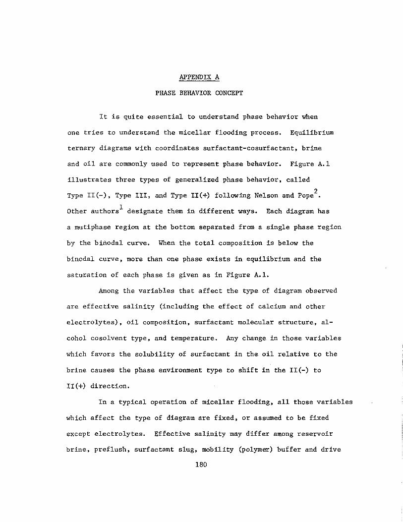
APPENDIX A
PHASE BEHAVIOR CONCEPT
It is quite essential to understand phase behavior when
one tries to understand the micellar flooding process. Equilibrium
ternary diagrams with coordinates surfactant-cosurfactant, brine
and oil are commonly used to represent phase behavior. Figure A.l
illustrates three types of generalized phase behavior, called
Type II(-), Type III, and Type II(+) following Nelson and Pope2•
Other authors1 designate them in different ways. Each diagram has
a mutiphase region at the bottom separated from a single phase region
by the binodal curve. When the total composition is below the
binodal curve, more than one phase exists in equilibrium and the
saturation of each phase is given as in Figure A.l.
Among the variables that affect the typ.e of diagram observed
are effective salinity (including the effect of calcium and other
electrolytes), oil composition, surfactant molecular structure, al-
cohol cosolvent type, and temperature. Any change in those variables
which favors the solubility of surfactant in the oil relative to the
brine causes the phase environment type to shift in the II(-) to
II(+) direction.
In a typical operation of micellar flooding, all those variables
which affect the type of diagram are fixed, or assumed to be fixed
except electrolytes. Effective salinity may differ among reservoir
brine, preflush, surfactant slug, mobility (polymer) buffer and drive
180
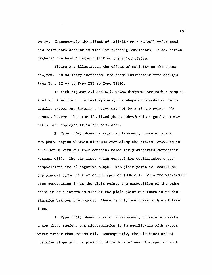
181
water. Consequently the effect of salinity must be well understood
and taken into account in micellar flooding simulators. Also, cation
exchange can have a large effect on the electrolytes.
Figure A.2 illustrates the effect of salinity on the phase
diagram. As salinity increases, the phase environment type changes
from Type II(-) to Type III to Type II(+).
In both Figures A.land A.2, phase diagrams are rather simpli
fied and idealized. In real systems, the shape of binodal curve is
usually skewed and invariant point may not be a single point. We
assume, howver, that the idealized phase behavior is a good approxi
mation and employed it in the simulator.
In Type II(-) phase behavior environment, there exists a
two phase region wherein microemulsion along the binodal curve is in
equilibrium with oil that contains molecularly dispersed surfactant
(excess oil). The tie lines which connect two equilibrated phase
compositions are of negative slope. The plait point is located on
the binodal curve near or on the apex of 100% oil. When the microemul
sion composition is at the plait point, the composition of the other
phase in equilibrium is also at the plait point and there is no dis
tinction between the phases: there is only one phase with no inter
face.
In Type II(+) phase behavior environment, there also exists
a two phase region, but microemulsion is in equilibrium with excess
water rather than excess oil. Consequently, the ti~ lines are of
positive slope and the plait point is located near the apex of 100%

182
brine.
When the phase behavior environment is Type III, there
are three multiphase regions, namely the Type II(+) node, Type
II(-) node, and three phase region. The first two are two phase
regions and the phase behavior is essentially the same as Type II(+)
and Type II(-) as they are called. When total composition is within
the triangle below the two phase regions, three phases appear: micro
emulsion, excess water, and excess oil. The composition of the micro
emulsion is represented by the invariant point. This fact means the
composition of microemulsion does not depend on total composition if it
is in the three phase region, although the saturation of each phase
does.
As salinity increases within the Type III phase behavior
environment, the invariant point moves continuously from the apex
of 100% brine to another apex of 100% oil. Even if the phase behavior
environment is called Type III, Type II(-) phase behavior may domin
ate when salinity is low, and Type II(+) may dominate in higher
salinity. Thus it should be noted that the appearance of only two
phases does not preclude the phase behavior environment being Type
III, because of the Type II(+) and Type II.(-) nodes.
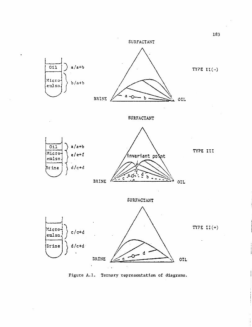
Oil ,__ __ ~icr
e::llsn
) a/a+b
} b/a+b
Oil a/a+b
Micro e.Iillsn
el e:+!
rinc d/c+d
.~~:j) c/~d Brine } d/c+d
SURFACTANT
BRINE OIL
SURFACTANT
BRINE
SURFACTANT
!>RIHE OIL
Figure A.l. Ternary representation of di~grams.
183
TY?E II(-)
TYPE I!!
TYPE II(+)

184
SURFACTANT
BRINE£:..======~~~ OIL ( LOW SAL! NI TY ) (HIGH SALINITY)
'f
(invariant point)
~
(MEDIUM SALI~ITY)
Figure A.2. Effect of salinity on phase diagram
APPENDIX B
DERIVATION OF CONTINUITY EQUATIONS FOR MULTIPHASE MULTICOMPONENT FLOW
63 Lake et al. presented the equations necessary for a com-
plete description of isothermal, multicomponent, multiphase flow in
permeable media, which are shown in Table B.l. The first column
in Table B.l gives the differential form of the equation with its
name in column two. Column three gives the number of independent
scalar equations represented by the equation in column one. Columns
four and five give the identity and the number of dependent var-
iables added to the formulation by the equation in column one.
In Table B.l, i designates a chemical species (i=l, ... N), j desig-
nates a homogeneous flowing phase (j=l, ••• M), S designates the sta-
tionary phase, and D is the number of spatial dimensions (D ~ 3).
From assumptions (2) and (10) in Chapter III, the mass
conservation equation can be written
(B.l)
Since in this simulator phase behavior is calculated based on
the volume fraction of each component, rather than mass fraction,
variables C., C., and C .. are introduced. Each of them designates l. l. l.J
the overall volume fraction of component i, the volume fraction in the
total fluid, and in phase j, respectively.
N -c. = .(1 - L C.)Ci + Ci l. . 1 1 1= (B. 2a)
185
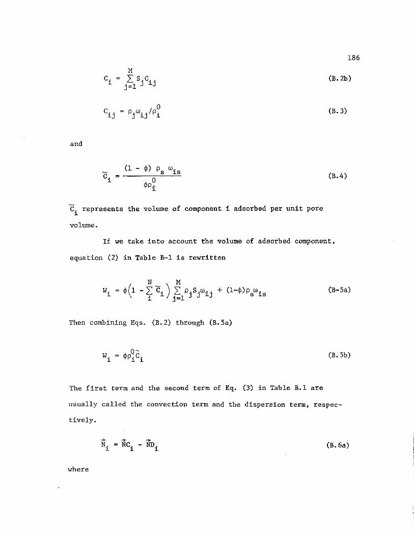
and
c. l.
c .. l.J
c. = l.
=
M 2:: s .c .. . 1 J l.J J=
0 p.w .. /p.
J l.J l.
Ci represents the volume of component i adsorbed per unit pore
volume.
186
(B. 2b)
(B. 3)
(B.4)
If we take into account the volume of adsorbed component,
equation (2) in Table B-1 is rewritten
N M wi. = ¢(1 -2:: c.) 2: p.S.w .. + (1-<f>)p wi
i l. j=l J J l.J s s (B-Sa)
Then combining Eqs. (B.2) through (B.Sa)
(B. Sb)
The first term and the second term of Eq. (3) in Table B.1 are
usually called the convection term and the dispersion term, respec-
tively.
+ + + N. =NC. - ND.
l. 1 1 (B. 6a)
where

-+ ND.
1
M -+ = L: p.w .. u.
j=l J 1J J
M -+
= L: cpp.s.K.. ·Vw .. j=l J J 1] 1]
Combining Eq. (B.3) and (B.7a)
-+ NC.
1
0 M = p. L:
1 . 1 J=
-+ c .. u. 1J J
187
(B. 7a)
(B.8a)
(B.7b)
Since one dimensional flow is being considered, the dispersion coef-+ -+
ficient tensor (K) is replaced by a scalar Ki,ij' the longitudinal
dispersion coefficient, which is usually taken as
D.. an. ju. I K = _2:.J.. + JV] J
n • • ,i..S JV, lJ T '+' •
J
(B.9a)
Since the magnitude of molecular diffusion is much smaller than
the dispersion due to convective flow in most flow problems, the first
term of Eq. (B.9a) may be neglected. Hence
an. ju. j JV] J
<j>S. J
Substituting Eq. (B.9b) into the 1-D expression of Eq. (B.8a)
ND. 1
M ow .. = L PJ.a£J. I uJ. I a~J
j=l
(B.9b)
(B.8b)
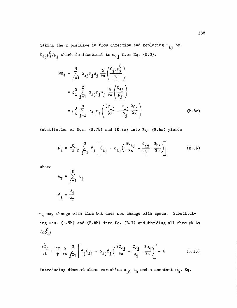
Taking the x positive in flow direction and replacing w .. by 1J
C .. p~/p. which is identical to wiJ. from Eq. (B.3). 1J 1 J
M
ND. = I a.Q,.p.u. 1 j=l J J J
...£... (cijP~) ax p.
J
O M a (~) = p. I a.Q,.p.u. a P 1 j =l J J J x j
=p I au ___ -2:1.....:....J.. 0 M ( acij ci. ap. ) i j =l .Q,j j ax p j ax
Substitution of Eqs. (B. 7b) and (B.8c) into Eq.
where
0 ~ f. [c .. -N. = piuT 1 j=l J 1J
M
UT = I u. j=l J
u. f. = _J_
J UT
( aci. c .. a _2:J.. - 2.J...
.Q,j ax p. J
(B.6a) yie\lds
~)]
188
(B. Sc)
(B. 6b)\
uT may change with time but does not change with space. Substitut
ing Eqs. (B.5b) and (B.6b) into Eq. (B.l) and dividing all through by
0 (¢pi)
-+--"'""' f C - a f _2:.l. _ ___!J_ - = O aci uT a M [ ( aci. ci. apj ~ at <I> ax j~ 1 j ij .Q,j j ax p j ax
(B. lb)
Introducing dimensionless variables xD, tD and a constant ~· Eq.
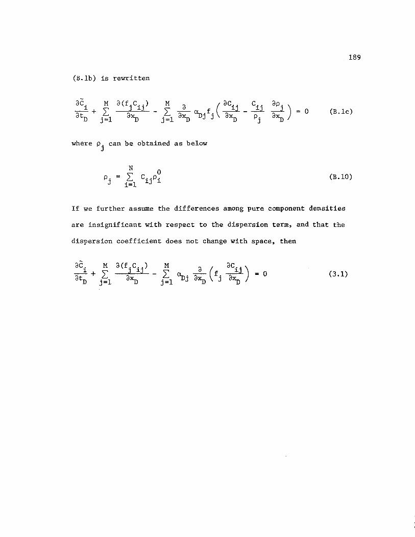
(B.lb) is rewritten
ac. M ac£.c .. ) M ~ ( aci. ci. apj) _i + L: J l.J - L: _a_ f _2:J_ - __!1_ = o atn j=l a~ j=l a~ ~j j axn Pj a~
where p. can be obtained as below J
N
Pj = L: i=l
0 c .. p. l.J l.
189
(B.lc)
(B.10)
If we further assume the differences among pure component densities
are insignificant with respect to the dispersion term, and that the
dispersion coefficient does not change with space, then
(3.1)
Equation
;iw. .. ... l o> r . 17•N. "' R.
l l
M (2) w. "' -ti l: n.s.w .. + (1-¢1) o
5wis
l j= l J J lJ
M +
(3) N. = l
r (p .w . . ;;. - ¢io.s. K.. • 17(1.l .> j• l J lJ J J J lJ lJ
M (4) R i • ¢i l:
j= l s.r .. + 0-cj>}r.
J lJ 1S
N (4a) l: Ri • 0
i= l ":t .....
(5) u. = -).. .k -(17 P. + o.i> J ~ J J
........ (6) A . = A .( S , W, uJ. ,x)
·rJ rJ ....
(7) PJ.- P 0 . = P . (:>, w, x) <. CJ 2,
(8)
(8a)
M (9) l:
j•l
(lOb)
(I) •• = l 1)
s. .. l J
r .. = 0 lJ
Table B.l
Summary of Equations for Isothermal Fluid Flow in Permeable Media
Name
Mass conservation
Accumulation term
Flux term
Source term
Total reaction definition
Darcy's L.aw
Relative mobility
Capillary pressure
Mass fraction definition
Stationary phase mass fraction definition
Saturation definition
Homogeneous kinetic reaction rates
Stationary phase reaction rates
Total phase reaction
Number Independent
Scalar Equations
N
N - l
ND
N-1
MD
M
M-1
M
l
(N-l)M
N-1
M
190
Dependent Variable
Identity Number
2N+N D
C'.,s.,w .. ,w. 2M+M N+N J J l) 1S
u. MD J
M N+N
2M
N ClOc) l:
i= l
Ola)w. lS
Equation
r. • 0 lS
(12) P. ,. P · ( Wt p .) J J J
Name
Stationary phase total reaction definition
Equilibrium relations as phase balances
Stationary phase equilibrium relations as balances
Equation of state
Total independent equations " D(H+N) + 2H N + 4H + 4N
Total dependent variables• D(H+N) + 2HN + 4H + 4N
Number Independent
Scalar Equations
N(H-1)
N
191
Dependent Variable
Identity Number
APPENDIX C
COMPurER PROGRAM
The micellar/polymer flooding simulator used in this research
consists of one main program, twenty five subprograms and one dummy
program. The name of each program and its role is as follows:
MAIN
INPUT
ourPUT
HPRINT
PROF
PRFPLOT
HIS PLOT
SOLVE
SOLVE!
Main program. Drives all subprograms.
Read and print out input data, calculate or specify some
parameters, and set up initial conditions.
Depending on the pore volume injected, call some of sub
programs HPRINT, PROF, PRFPLOT, HISPLOT, and MATBAL.
The boundary condition at injector (injected compositions)
is changed as necessary.
Print out production history and store the values necessary
to plot history.
Print out profile.
Plot profiles.
Plot histories.
Solve continuity equations with fully discrete method.
Cumulative production and relative pressure drop are also
calculated.
Solve continuity equations with semi-discrete method.
Cumulative production and relative pressure drop are also
calculated.
192
FCNJ
RK12
RKl
DGEAR
Dummy subprogram needed when DGEAR is used.
ODE integrator with a RKF algorithm.
ODE integrator with a RK algorithm.
IMSL Library59 • ODE integrator, which allow the use
of either Adams' methods or backward differentiation
methods.
DER Calculate the change in concentration as derivatives with
respect to time.
PROPRTY Calculate viscosities, fractional flows and mobilities
RELPERM Calculate residual saturations and relative permeabilities
POPE Three phase flow model used in original simulator
HIRA Three phase flow model presented by G. Hirasaki
LAKE Three phase flow model presented by L. Lake
193
PHCOMP Calculate phase concentrations and saturations according to
ternary phase behavior. Interfacial tension is also cal
culated.
TI ELI NE
TRY
IONCNG
COMPLEX
CHEMADN
POLYADN
MAT BAL
Find a root of non-linear equation with bisection method
Using the equations of binodal and distribution curves,
calculate phase composition with one degree of freedom
Calculate cation exchange
Calculate cation exchange in case where surfactant complex
forms.
Calculate surfactant adsorption.·
Calculate polymer adsorption
Gives final condition and material balance error

194
As is shown in Figure C •. 1, there are two loops in main
program. Depending on the value of ISOLV specified in input data,
either the semi-discrete method or fully-discrete method is selected
to solve continuity equations. NSTOP is set to be one in subprogram
OUfPUT, when total pore volume desired has been injected.
Figure C.2 and C.3 show which subprogram is called and where,
for fully-discrete and semi-discrete solutions respectively. Most of
the subprograms which are the essential part of the micellar/polymer
flooding simulator are common for both methods. Since subprogram DER
was separated from SOLVE, ODE integrators such as DGEAR, RK12, or RK1
can be easily replaced by other methods.
In subprogram DER, special care is taken for the irrever
sibility of adsorptions. Since predicted time step size may be re
jected and all calculations may be repeated with smaller time step
size, the adsorption calculatd at the last time step are stored and
can be used when the rejection occurs. This is done by assigning
different values to IADS depending on the situation.

Yes
Start
Yes
STOP
SOLVE 1
Is NSTOP =
Yes
Figure C.l. Flow chart of main program.
195
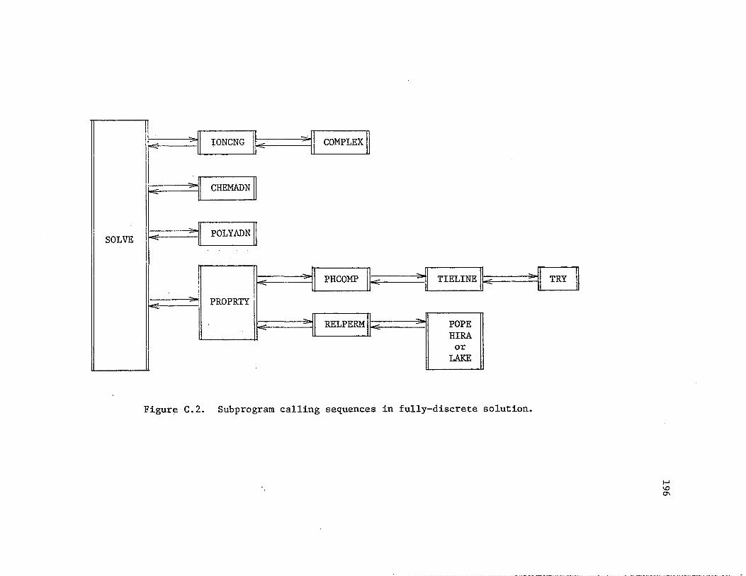
SOLVE
IONCNG
CHEMADN
I
I ii PROPRTY I
COMPLEX
PHCOMP II< 11 TIELINE II< >II TRY 11
RELPERM1 II POPE HIRA or
LAKE
Figure C.2. Subprogram calling sequences in fully-discrete solution.
f-1 \.0
°'
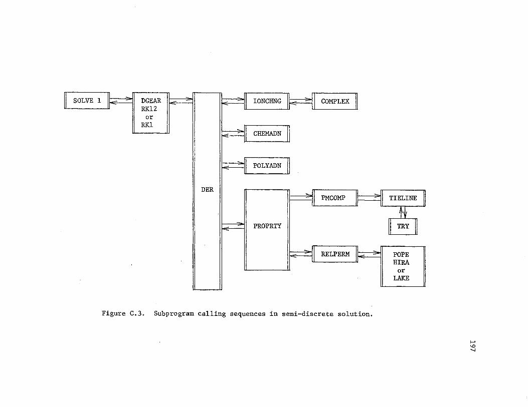
SOLVE 1 DGEAR RK12
or RKl
DER
IONCHNG COMPLEX
CHEMADN
I-<:' II POLYADN
PM COMP
PROPRTY
RE LP ERM
Figure C.3. Subprogram calling sequences in semi-discrete solution.
POPE HIRA
or LAKE
f-' \0 -....J
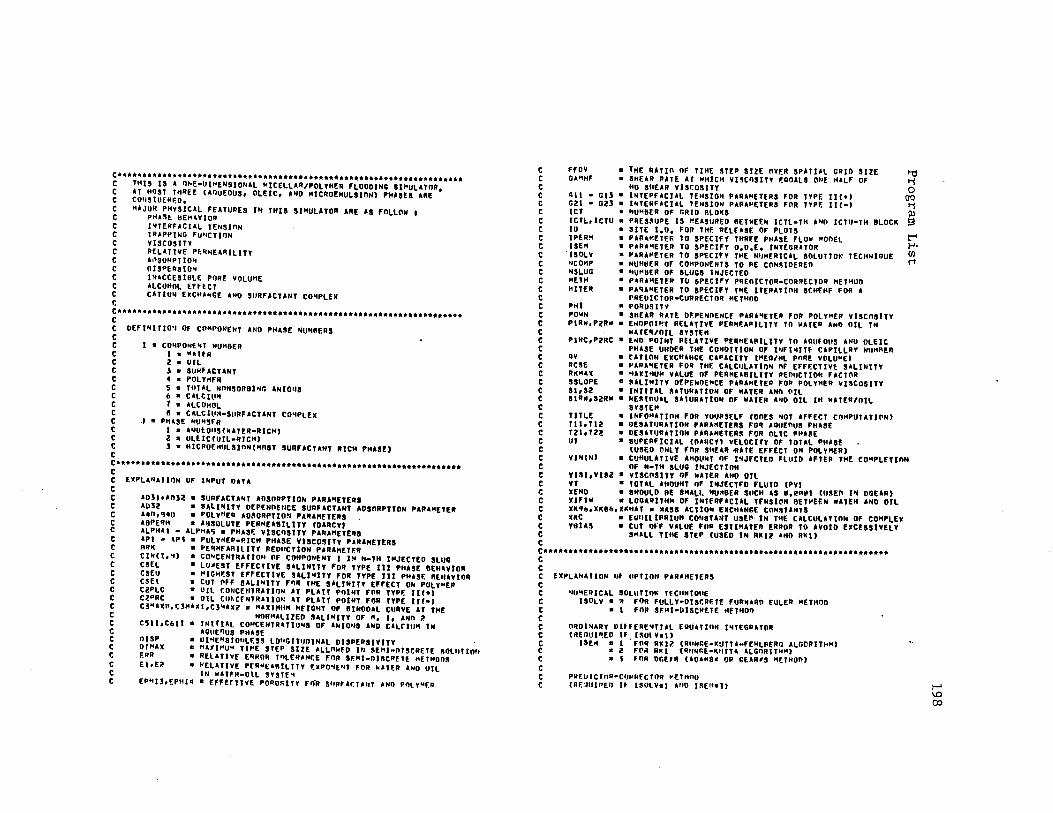
C***********•********************************************************* C THIS IS A 'l~F.·UI~ENSIONAL HICELLAR/POLYMER FLOOOIN; II~ULATOR, C Al H'IST THREf. (AQUEOUS, OLEIC, ANO HICROEMULSION) PHASES Aft£ C CllUSIOEPF.D, C .. AJUR PHYSICAL FEATURES IN THIS SIMULATOR ARE AS FOLLOW t C PHA~t HEHAYIOR C l"TERFACIAL TENftlON C !RAPPING Fu••CTI'IN C VISCOSITY C RELATIVE P~~HEARILITY c AnsoRPTIO .. C \llSPtRSIO" C INACCESIBLE PORE VOLUHE C ALCOHOL EfHCl C CATIUN EXCHA1tGE ANO SllRFACHNT CO .. PLEX r. C•••••••************************************************************** c c c c c c c c c c c c c c c c c
llEfINITID'I Of COl<PONENT ANO PHASE 'fllHMRS
I •
·' .
co .. PONfNl NU .. 8ER I • WAHR Z • UIL .S • SIJHfACTANT 4 • POLYllFR 5 • Till AL NONSORBl'lll ANIOllS It • CALCll111 7 • ALCOHOL 8 a CAlCll•14•SllRF AC TANT CO~PlEX
PHASE NU .. "IFR I • A~UtOUSIWATER•RICHJ l • ULtlt!UIL•RICMl J • MICRDElllJLSION(MOST ftURFACTANT RICH PHASE)
C********************************************************************* c C EXPLANATlllN UF INPUT DATA c c c c c c c c c c c c c c c c c c c c c c c c
AOJl1ADJ2 • SURFACTANT ADSORPTION PARA .. ETERS AUli! • SALINITY DEPENnEHcE SURFACTANT AOSnRPTJON PAPA .. [T(ll a.n,qqp • POLY"E" AO:IORPTICI" PAIUHETERS A8PEllH • A~SULUTE PEHHEABJLJTY IOARCYI ALPHA! - ALPHA~ • PHASF. v1scnsJTY PARAMETEllS API • AP1 • PULY~EP•P.ICM PHASE VISCOSITY PARAMETERS !IA~ • PENHfAfllllTY REtlllCTION PAAAHUER CIN(l,•1) • CO"CENTRATIDH nF l;(IHP0'1ENT I IM N•TH l>!JECTEtl SLIJQ CSEL • LQAEST EfFECTIVE SALINITY Foll TYPE Ill PHASE BEHAVIOll CSEU • HIGHF.Sl EFFECTIVE SALINITY FOR TYPE JIJ PHASE llEHAVIOR CSEI • CUT OFF SALINITY F'IR THE SALINITY EFFECT ON POLYMER CZPLC • Ult r.OllCEtllRATllJN AT PLAIT PlllNT FOR TYPF. II(+) C2PRC • OIL CU~CfNTRATIO~ ~T PLAIT POINT FOR TYPF. Ilf•l CJ"A~l•,r;JHA-l,CJ'4AXl • .. AXIHllH HEIGHT OF lllNOOAL CIJllVE AT THE.
NORHAllZEO SALINITY OF n, 1, ANn ~ C51 l1C6l I • INtllAL CD"CENTRATIU"S OF ANIO•IS ANO ClLrilf'4 IN
AQUEOUS PHASE OISP OIHAX F.RR El,E2
• Ul'IENSJOllLES9 LDhfllTIJDJNAl OISPERSJYITY • HUIHV" Tll'E STEP SIZE ALLONfO Ill MHl•lllSCRETE ftlJlllTIOfl • HElATIVE EnHoR l'ILEMANCE FOR S£Ml·DISCPET£ HETHons • ~EtATIYE PER~f ARILITY F.•PO~£~l F~R kAIER ANO UtL
IN WATfM•OlL SYSTE~ EP'113.EPHIQ • f.FFErTJvE PORO~IH Ff!)f SllRFAr.TAtlY AND P'llY"ER
c c c c c c c c c c c c c c c c c c c c c c c c c c c c c c c c c c c c c c c c c c c c c
FFOV Gl'IHF
• THE RATIO OF TIHE STEP SIZE nYER SPATIAL GRID SIZE 'i;I • SHEAR RATE Al WHICH v1,cnslTY '-QOAL8 ONE HALF OF l"j
lill • NO SHEAR VISCOSITY 0
GlJ • INTEPFACIAl TENSION PARAHET£RS fOR TYPE II(+) ()Q GZI • GZJ • INTERFACIAL TENSION PARA~ETEPS FOR TYPF. II(•) l"j ICT JCTL,ICTU ID
• NUHSER OF r.RIO 8lOKS Ill • PRES:IUPE IS P!EASURF.O BETWEEN ICTL•TH ANP ICTIJ•TH BLOCK El
IPER~
ISE" . ISOLV lfCO~P
NS LUG "ElH HITER
PHI P01'N PJRW,PZR•
• SITE I,D, FOR THF. RELf ASF. OF PLOTS • PAP.AP!ETER TO SPECIF1 lHRF.E PHASE FLOW ~OnEL • PARAMETER TO SPECIFY o.o.E. INTEGRATOR • PARAMETER TO SPECIFY Tl<E NIJMERICAL IOLUTIOll TECHNIQUE • NUHHER OF COMPONENTS TO RE CnN~IOEREll • NUt<8ER OF SLllGS INJECTED • PARAMETER TU SPECIFY PREOICTOR•CORREf.TOR HETHUO • PAqAHETER TO SPECIFY THE ITERATION SCHfMF FOR A
PAEUICTDR•CURRECTOR METHOD • PORUS ITV • SHEAR RATE DF.PElfDENCf PAAAHETE• FOR POl.YMER VISCOSITY • E~OPCllt!T RELATIVE PER,.F.APILITY TCI llATER AND OIL TN
MATER/Oil SY~TEH PlllC,P:?RC • tNO POINT RELATIVE PEAHEAalLJTY TO APUtDllS ANU OLEIC
PHASE UllDER THE CO'IDITION OF lNfl~ITE CAPILLRY NllHRER QY • CATION EXCHANGE CAPACITY IMEQ/HL PORE YOLU~EI RCSE • PARAMETER FOii THF. CALCIJlATIO>I OF EFFF.CTIYl SALINITY RKMAX • HUl .. VH VALVE PF PF.RHEABIL!TY PEDllCTIO'l FACTOR SSLOPE • ~ALINITY DEPENDENCE PARAMETER FOP POLYMER VISCOSITY s1.s2 • INITIAL ftAlURATION OF MATER ANO I'll SIRM,SZRW • llERTOUAL SA1URATION PF ~ATER ANO OJL IH WATER/OIL
TITLE T II 1 Tl2 TZl,TZ:! UT
SYSTEM • llfFOMATIOM FOR YUIJRSELF (DOES NOT AFFECT COHPUUTll'N) • IJESATIJOTIDN PARAMETERS FOR AOOEnuft PHASE • DESATIJPATifJN PARAMETERS FIJR OL 1C PHASE • SUPERFICIAL (PAACY) VELOCITY OF TOTAL PHASf.
(USED ~NlY FOR SHEAR «ATE EFFECT ON POLYMER)
t""' I-'• en rt
VIN(Nl • CUHULATIYE AHOll"T f!F l,.JECTEO FLUID AFTER THE CO"PLETION PF N•TH SLUG lllJECTION
YISl,VJSZ • VISCOSITY OF NATER ANO OJL YT • TOTAL AHOUNT QF INJECTFO FLUID (PVI XEllO • SllOULO BE SHALl NU'4BER SUCH U 11,l!!l'ltll (llftEll (If Dt;EARJ XIFTW • LOGARITHM OF INTfRFACIAl TfNSl~N 8£T~E£N WATER ANO OJL XKq~·•Ke~.x~HAT • MASS ACTION EXCHANGE CON~TANTS •KC • Ellllll ll'AIUH Cll"STA:fT USE" IN THE CALCULATION DF COMPLEX YlllO • CUT OFF VALUE FOR ESTIMATED ERPOR TO AVOID EJC£UIV£L Y
s~•LL TlllE STEP (USED IN Rkll! .. m RKll
C•••••••************•*********************•*************************** c c C HPlANATION llf llPllllll PAAAHETERS c c c c c c c c c c c c c
'lllHEAICAL SOLUTIOt.: Tf.CHNJQllE ISOLV • ~ FDR FULLY•OISCRffE FUR"ARO EULER METHOD
• I FOR Sf.Hl•DISCNETE ~fTHOll
OROl~AAY UlffERE~llAL EQUATION INTEGRATOR UEOUl'l£0 tf UlllV.ll
ISE'4 a I . FOii RKli' (RllNGE•KUTTA•FEHLMRG ALGORIT,..Hl • i! F~i! Rk I (RllNr.E•KllTTA ALGOAITM"I • I f0R OGEIR (A01'4S• OP GEAR•S H£THOn)
PHEUICTOR•Cll~RfCTDA •ETHOO (AF.11111•ED H l~OlY•I AllO I~Ell•Jl f-'
'° CXl
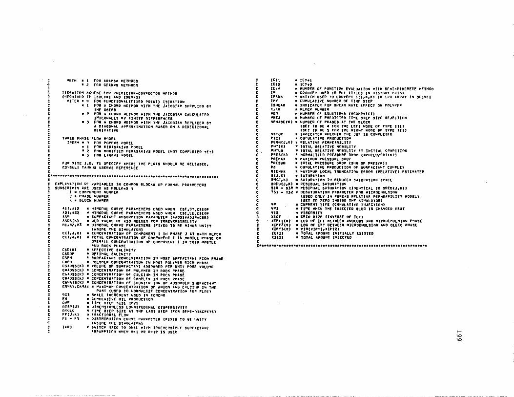
c c c c c c c c c c c c c c c c c c c c c c c
HETH • t FOR AO&HS• HETHOOS • l FOR Gf&R•S HETHOO,
tlER&TION SCllEHE fnR PllElllCT!lR•CO~AECTOR HET~OO (Mf.QIJIAEO U !SOI.Val &NO UEH•!)
HITER • ~ FOR FUNCTION&L(FllED POINT) ITERATION • I FOR A CHORD HETl•on '<IT14 THE JACOBJAll SllPPLlfO 8Y
IHE USERS • 2 fOR A CHORD HETHOO MITH THE JACOBIAN CALCULATED
INTERNALLY RY FINITE DIFFER~NCES • 3 FOR A CHORD HETHOO MITH THf JlCOAllN RF.PLACfO 8Y
A DIAGONAL &PPROllHATION R&SEO ON A OIAfCTIONAL DERIVATIVE
THREE PHASE IPERH a ~
• I • 2 • 3
FLOW fOA FllR FllR FOR
MOEL POPF"•S HOOEL HIRASAkl•S ~OOEL HOOIFIED HIRASlKl•S LAKf.•S "llOEL
HODEL (NOT CO~PlETED YET)
FOR 'ITC 1.0. TO srECIFY MHERE THE PLOTS SHOULD ec R(LEASEO, f.O"ISULT TM.IHlfS USEA•S REFERE~•CE
C********************************************************************* c c c c c c c c c c c c c c c c c c c c c c c c c c c c c c c c c c c c c c
EIPLA~ATION Of VARIABLES JN COHHOH SUH,CRIPH ARE llSEO AS FOLLOWS I
81.0CKS OP FORMAL PARAMETERS
I a CUHPO•IENT NllHAER J a PHASE NlfHl'ER K • Dl.UCk NlfHRER
All,A12 •21,AZ~ AJll AJOS(K) n1,e1,Rl
• HINOl>AL CURVE P&PAHETERS U,ED WHEN csF..cT.CSEl)P • "lllOl'lll CURVE PIRA'1ETEPS USED WHEN CSE 0 LE 0 CS£1)p • SURFlCTlhf IDSO~PTTON PIRlHETER (•AOlltADll•CSE) • UlD VILUf Df A3D NEEDED FOR IRREVF.RSl~ll!JY • l:llNOOAL CIJRVE PAR&11ETERS (FUEil TO !IE HINUS UNITY
INSll'lf. THE SIHllLlTORJ C(l,J,K) • CUNCF.NTRATION !If COllPOllENT l IN PHAllf J AT K•TH llLl'Cll C(l,4,K) • TOUL CllNCENTRATION nF CnHPOllEllT I IN .H08llE PHASE (IR
OVEIUll COllCEIHRATION nF COHPO~EHT I IN POTH HOBflE u.m ROCK PllA~E
CSE(K) • EffECTTVE SALINITY CSEOP • llPTIHAL Sllll<ITT C3PH • ~URFACTANT COHCENTRATION IN HOU SllPFACTA"T PICH PHASE CqPN • l'OLYl1f.P COllCF.NTRATIUN TN HllST POLT'4ER RIC" PHASE CJAl>SS(K) • VOlUHE Of SURFACTA'<T ADSnHflEO PEP UNIT PORE VOLU'IE CUOSS(K) • C0"C£NTRATION OF Pl)LT11ER l" ROCK P"ASE C1>AllS$(K) • CONCEllTAATIOI' llf CALClllH Jtl ROCK PHASE CSAOSS(K) • CO"CENTRITION nf C!lttPLO Ill POCK PHAS[ Cl>~ATS(Kl • CUllC[NJRATIOI• Of CllUNTFR IDN OF AOSORBEP SIJRFlCTAllT C5~U,Cf,t1AI • l'AXIHU'4 CO.,CENTRUllJN OF ANION ANO CALClllH I" THE
!>Cl Ell O~P Ol9P(Jl l>TIJLO FF!J,k) F"I • fl
tans
rAST (USfO TO NORHAl.TZf. CO'<CENTRATIO" FOP Pl.Of! • ~HALL JNCR~14ENT tlSEO f't TO'ICllG • CU"ULATIVE OIL PROOUCTTO!I • llt'E STt.:r SIZE tl'VI • UIHENSfOHLESS LON~ITllDINAL Ol8PERSIVTTY • Tl~E STEP SllE AT Tl1f LAST STEP (FOR Sf~l·OlSCRET£) • fRACTlnNAL flON • llUTRIAllTlnN CIJllYE PAllA1'£TER (l'IX£0 TO ~f 11•HTY
INS!OE THE SIH•ILATRN) • hlTCH ll~EO TO Of.ll WITH IRRfVEASIPlf" SURFACTANT
•O~UPPTtn11 WHEN AKI n~ RK!l' IS USEO
C ICTI • ICT+I C ICTz • ICT+C! C lEVA • HUHBf.R OF FUNCTION EVALUATION WITH SfHl•lllSCAETE H~THOD
. c IH • COUNTEP llSED Tl> PUT TITLES IN HISTORY PRINT C IPASS • ShlTCH USED TO CONVEPT C(l,a,K! TO l•O APNAY IN SOLVfl C IPV • CU14ULATIVE NIJl'RER QF TIHf STEP C ISHEAR • INOICATOR FOP SHEAR RATE EFFECT ON POLY~fR C K1kK • HLOCK ~UH8£R C NE!I • HUl4BfR Of EOU&TlllHS (NCOHP•TCTl C NllEJ • NUH8£R OF PAEDICTEll TIHE STEP SllE R£JECTl~N c llPH&SE(K) • "U"BEN or P14ASlS AT THF 81.0CK C (8£T TO SE a FOR THE LEl'T NOOE OF TYPE 1111 c IS£T Tn 9E 5 FnR THE RIGHT NODE OF TYPE 1111 C NSTIJP s INOICATOR WHETHER THE JO~ IS COHPLEfFO C Pill • CU"UlATIYE PRODUCTION C PERH(J,K) • RELATIVE PERl'ElBILITY C PHT(K) • TOTAL RELATIVE MOBILITY C PHTLll • TOTAL RELATIVE MOBll.ITY AT INITIAL tnNlllT!nN C PRES!Kl • NORHALIZf.D PPESSIJRE ONOP (•PHTLU/PHT(K)) C PHfHAX • l'AXIHUH PRESSURE DROP c PRESUM • TOTAL PRf.SSURE OROP !S•IH or PRfS(K)) C PS • CU"ULATIVE PRODUCTION Of SURFACTANT COl'PLEX C ATEHAX • 11Ul14Ul4 LOCAL TRUNCATION ERROR (PELATIVE) F.STIHATEll C S(J,K) • SATURATIOll C SN(J,K) • SlTUPATION IN REDUCED SITURATlnN SPACE C SREU(J,Kl • RESIDUAL SATIJRATIO'I C SIR • UR • Af.SllltJAL SATUlllTIO'I !ll'IElfTICAL TO SRF.O(J,kl) C TJI • UC! • DESATURATION PARAHET£R FnR MICRQ£HllLSlllN C (USEO OHLY Ill POPE•S llFLATIVE PEllHEA~ll.ITV 1100ELl C (SET To lERO INSIDE THF. Sl"ULATORJ C VP • CURRENT Tl~E (CtJHULATIVE l'4JF.CTION) C VPl • TlH£ NHEN T11E INJECTED Sl.UG IS CHANGED NEXT C VIS • VISCOSITY C UCT • GRID SIZE UNVF.RSE Of ICTI c XJFTI (K) • l.H nF Irr llETMEEN AQUEOUS A"O HJCROEHllllllON P•U~E C XIFTC!(K) • l.OG OF lFT BET~EEN hlCROEHULSlnN ANO OLElt PHASf. C XIFTJ(K) • HlN(XIFTl1XIFTlJ C ZE<ll . • TOTAL A"OUNT l~ITIALLY EXISTED C ll(l) • TOTAL l"OUNT INJF.CTED c C••**************************•****************************************
I-' \0 '\O

P1H!GR&~ ~A IN (I t•PllT, 01.ITl'UT, T APf.~• INPUT, T APH•OUTPllT, PLOTRJ
c-----------------------------------------------------------------------c THIS HAJN PPOGRAH OPIVES All 5UAPR0GR&HS, C OEPENOING ON ISOlY, COllTINUITY EQUATIONS ARE SOLVED EITHER WITH C fUllY•OISCRfTE OR SEMl•OlSCAETf. HfTHOO, C ISOLv • P. FOR FULLY•hlSCAETE HF.THOO C • I FOi> SE"l•OUfRETE HETHOO
c-----------------------------------------------------------------------c Cll~Hf'IH/H& l"llSOl V,HSTl'IP, 10
c CALL l"r•.•T lt(ISOLY,EQ,0)GO TO IA
Z" CAl.L SOLVE! CALL OllTPUT IF(NSTOP,HF.,t)r.o TO 7.A GO TO 3"
1<1 C&Ll SnLVE C&l.l IJllTPllT IF(NSTOP,Nf,l)C:O TO 13
ln COllTI 1111E ~TUP ENI>
SUOROUTI>JF. l'IPllT c--···-··-······-·······-··---······-····-·····--···-···--····-·-······· c THIS sunPPOr:RUI RfAllS A'IO PD("l INP•IT OAT•, C SOME PA•AMETEPS A•E CALCUlATEf'I IN THIS SURP•or:RAH, C lHITllL CONhlTIONS ARf. &lSO SET I~ THIS SUPPROGDAH,
c-----------------------------------------------------------------------c
c
01HE"S ION llTLE!ZI)
CUHHON/HAIH/ISULV,NSTl)P,10 C~HHON/N~/ICT,ICTl,ICTZ,XICT.NCO~P CU"HON/SYSTEH/UT,&RPER~,PHJ,EPHIJ,EPHI•,DtSPJ(Q) COHHOHISEHIOl/hT~A~,~qR,YBl•S,JPA~S CUHHON/SFM!U]/~fQ,(9~M,XEllD,~ETH,HIT~~ C~H~ON/l"/VIN(IOl,CIU(7,l~I CUh~ONISOL/C(7,o,q7),9(3,ozl1Ff(1,G2),NPHASE(I?) COH,.!IN/C~F./CSE(G7l,CSEL,CSEIJ 1 RCSF.1C5EOP CIJH~OH/PHASE/fl,fZ,FJ,~l,8?,R],CZPLC,CZPRC COHHON/A/All,A121AZl1A?2 co-HON/PPOOIN/F.R,P(7),P~.ZJ(7),Z~(7l,S? CUh<ON/AhSORP/t]•nss1•~1.C~A0SS(~0J,C6•0SS!GP),C6HATS(«0) ~OHHON/C~/C~•OSS(•~1.cca1•1.l COMHON/PERM/IP(Rtt,P1Qh1P7RW 1f t,E71PIRC,PZRC CU~HOH/IFT/Gll1Gl2•Gll10?l1G~z,~z3 cu~~ON/XIFT/XJFTl!G2),XIFTZ!•Z>•XlfT3(•21,x1FTW COHHON/TPAPITll1Tl?1T211T2? 1 T31•Tl1.1SIPN,SZRW,PHT(Q~) COHHON/ALPHA/ALPHAt,ALPH&z,ALPHAl1AlPHAa,AlPHA~ Co1<~0N/tsEv1s1v1s1,vJs1.,APt,•PZ1AP],SSLOPE coH11nH1s11Ev 1s1G•t;tff, PO""•Csf 1,RKHAX ,RAK, ts14UA CUH.,ON/CHfHAO/CJPH,AJD,~30
CUHH0~/PrtYA0/CaPH,Ao0,6•0 CUllHON/PllE1\S/Pl4TLU,PllF.llu~,1cn,1cTu,PRES(ll') CUHMOH/HH~/XKC,i•96,XK~~,XKHAT 1 0V CD~HON/ION/ffOv,oc3,K
COHHON/Al0/A]05(Q~),AO]t 1 A0]? CIJlll'ION/l NJECT /OVP 1 VP, VT 1 VP! COHHON/trLOT/C~~·x,C~HAX
C•••***** PE•O lttPUT f'>ATA **•"**** READ t~e,(TITLF.!ll,I•l 1 2G) •EAO 112,NSLl.IG READ 112,l~OlV,t~E~,HETH,HfTER,IPER~,JO REAO 111,0THAX,EAR,f~I•s.xrNn
C INITIAL CONOlTION5 ANO SYST£H YAll!ES
c
Rf.AO , .... VT, FFnv. NCOllP. ICT. ICTL· It TIJ READ ltl,llT,A8PfP~,Ptt!,EPH!3,[PHTl,OISP RE•o lll,C51J,C~ll,sl.SZ,SIA~,szPw
C JFT A~O TPAPPl~C flfNCTJOH P•AAttETFR~ MEAO lll1Gll1Gl21Gll1C?.t1G?2,G?3 l>EAO ~tl,Tll1Tl1.0T?l,T?2,XIFTW
c c P~ASE vlsr.o~ITT P•R•~ETEAS
c
REAO lll,AtPHA1 1 AL~H&Z,•LPHA3 1 &lPHA4 1 ALPHA5 REAU 111,v1s1,v1s2,APl,•P2,•P3,SSLOPF. qEAn It 1.r.A11Hf .PnwM.tSF 1,.qt(H.\x.Antc
C PflATJVf PEP~f AP.ILITY PARAMETfR' ~l&O llt,PtH•,PZ~w,ft,F?.,PIRC,~?~C
c c PHA~l eE~•VIOP PAn&HfffRS
~1-.~0 I l t ,C'\f.tl.Ot,t'.\111'(1 ,C1tUX? N 0 0
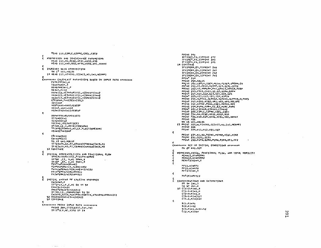
Afao lll,C?PLC,C2PPC,CSEL,r.SEU c . c A~snRPllO~ ANO IONEXCH•~GE PARAMETERS
AE•D 111,ov,ntsE,AOJl,A032,A~O AEAO 111,AaO,Boo,x~q~.YK~~.xKC,XKHAT
c C lNJ~CTED SLUG C~"POSITION
00 lrll U•1 1 t1Slllr. IA WflO ltl,VT~(N),(CIN(l,N),l•l,NCOHP)
c C•••••••• CALC"LA1£ PAPA1<[TEPS BASEO O~ INPUT DATA ••••••••
f t=f 7.CF' JJ:t ...
c
e
l3t•T3-?•£1'.A Hli:f!i»t:R32•t.r l>CJ•l,f•IZ AAea((2o•C,HAXP)/(l 0 •C3H#X~l)•t2 All•(l2o•C3HAXll/(1 0 •C3HtXl)l••2 AA2•f(~ 0 •C)HAX7.ll(l 0 •C3HAX7.ll••2 cS~oP•P,••tCSEU+CS£L) t21 UAP Al?"IAAl•A•~l/C9EOP Atl21,•A~l·A.A?. Al?•l•l2•AAl)/f9£0P
9VP•FFOV/FLQ•Tl!CT) ICll•ICT+I ICTZ•ICT+2 •ICT•l,IFLOATIICT) IF(UT,Lt;1,~£•8)ISH[AR•I IF(APS(POWN•l,P),LE,~.ntllSHEAR•I >l[!atcT•t:COHP
C51··AX•C51 I CM•lX•r.bt I ~O I~ "•lr"Sl.Ur. 1F<c1Nl5,N).CT,C5~•xlC~HAXaCINC5;N) lflCIN(~,N) 0 f.T,C~HAX)C~HAX•CIN(6 1 N)
12 CONT1Nl'E c C IHITl~L PER•EA~ILITI£, AND FRACTIO~AL FLON
SR•(~l•Slq~)/(l,~•SIPW•92RW)
c
lf(SR .LT, ~,M) ~As~,B lf(SP .GT, l,M) $Rat,A P£~H1•P1P~•9Rt•[l P[RM?oP2R~•(l,1•SR)••E2 PhTLUoPEPHf/Vl~l+PEA•2/VIS2 Ff t•PfPhlfVISl/Pl<Tl.U ff~aP[A~?/VIS?/PHTLU
C INlTlll A"Ol'NT nf CA~f.l•JH AOSnR~EO
t
Ct.f AIJc,.,v JflC~ll,LF,~.~) Go Tn 5~ C~•C5ll·t~ll ~q~•·K~6•t?••2/C~ll IFfRV,lT,,•~~~A1)9fl TO 5? CbJAna,~•(~1 *WV+R9~•$QPffQ~*~Y*R~b+Rq6••2lJ
5l RHAT•JMHlT•C9••21C~ll 5;1 COtttlM•JE
C******** PRJMT INPUT tJ-TA ********* PHIMT ?0n,(TlllEfl),la1,7•l lf!l~Ql.V,N(,l)r.o Tl! 14
c
PRINT ?•! 1Flf3[M,fQ,l)PRINT 2~?. lf(l~EH,fU,2)PP{N1 2"3 l~(lSE~,FQ,))PAtNl 205
I• COHllNUE Jf(IPERH,En.~)Pq{HT 2q0 IFllPEP~,EQ,l)PRINT 2GI 1f(IPEAM,fQ,2)PRJNT ?OZ IF(JDEPM;EQ,J)rqtNl ?•3 PRINT ?.I~ PRINT ?SP,~SLU~
PR,~T 2s1.1snLv,JS£H,H[lH.~IT[R,JP~RH,IO PR NT p11,v1,rrov,NcOttP,1cT,ICTL,ICTU PRINT 21?,llT,lRP[RH 0PHl,[PHt3 1 £PHIG,OISP PRINT 21J,r.511,C~IJ,st.s2,SIRW,S?PW PAIN' 21n,~11,c1z,ntl,~?t,~12,~2, PRINT 215rTllrTl?.,121,l?.~,XlfTW PRINT 21~oALrHA1 1 ALPHA2,lLPHl3,ALP~lGoALPHA5 PRINT 111,v1s1,vTs2.•r1.•P2.•P3.~SLOPE P~INT ?IP 0GlHHF,P0WN 1 CSEl 1 RKHAX,RR• PRINT ?19,PIRW,P?PH,~l,E2,PIRC,P?RC PRINI 2?.1 0 CJHAX~ 0 C3MAXl,C3MAX2 PNl~T Z22 1C2PLC 1CZPRC 1CSEL,CSEU PRINT ?za,ov,wcsE,AOJl,AOJ?,ft)D PRINT ?zs.•aD,AaD,XK96,x~e~,XKC,YKHAT PN!NT ?2~ DO 15 N•l1HSLUC
15 PqlNT 727rH1Vl>j(N),(CINIT0Nlol•l 1NCQHP) PAl~l 22~ PRJNl 27.q1AllrAl2oA2lrA2?
PRINT z]P,51,s2,PENHl1PEAH1.,V[Sl.Vl9~ PRINT 231 o ICTL1 ICTU PRt~T ~J2.~1Rw,s2Aw,P1Aw,P?PW,FflrFFl
r. CU .. **** HT l•P INITIAL CflNDITIONS ********
lllJ 2~ UI .tCT c c PEPHEABILITIEs. FRACTIONAL FLn~. ANO TOTAL MOAtllTY c PE~H(l,Kl•PERMI C PEPH(2 1Kl•PERH? C PER~()•M)•~,r. c
c
c
FF(l 0 K)•Ffl FF!loK)•Ff2 ff ( J•K )eri,,,
PHT(K)•Pl'TlU
C CO"tE~IRAllONS ANO SATUQATION, DO '~ 1•1 0 7
c
ou 1r ~Js1,11 311 C(J1J1K)e\•,A
C( l• 1 •K)e:l ,14 C(Z•~1Kl•l,l' Cl!>•l••l•C511 c<~.1.~1·c~11
so ,~1·~1 S(?,MJ~52
S(3,~l•l,P•S1·~? ((2,11,K)-cS~ N
0 I-'
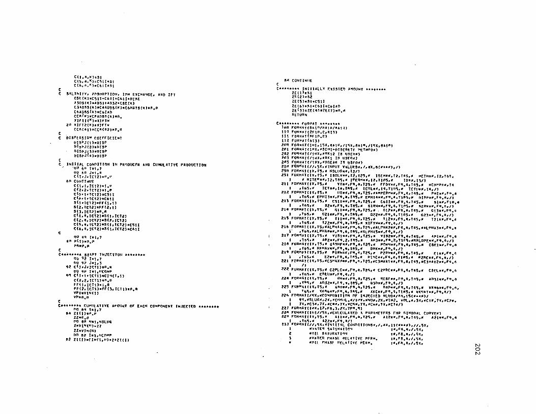
c
C(l,n,~hSI C!~,a,•>•C511•SI C(~,n,K)sC~ll•$t
c S•LThlJY, 1rsoHPTTO~. ION E•CHA .. GE, ANO lfT CSt.IKl•CSll•CblT+Chll•RC~E l3USfK)aA031+A03Z•CSE!K) Cl&OSS(K)•CalDSSIKl•CbHATS!Kl•R•R C6AUSS (K) •Cb! All cc•fK)•C~AOSS(K)•R. xrrr11•1ox1nw
2tt KIFl~!•l••IFTW f.CR(Ol)•CCR(02)•~.n
c . C DISPtRSJON r.O£Fflf.IENT
t>U"JI 1 hO!SP ors,.,1121worsP
~:~:~1:::~::: c C INITIAL COHOITION ltl PR~OUCFR AND CUHULITIV£ PROOUCTION
·nu 1>a T•!, 7
·c
c
oo ,,~ J•t,a C(t,J1lCTZ>•~•''
~II ClitlTTtlllf c11,1,1c121•1." c<2.2.1r.Tzl•l,P cl~•l•TCT2l•C5!1 c<~•l•TCT2l•C611 Sll•ICTZ)cFFllrll S(2,TCT2l•FF!2,ll Sl!o ICT?.)•~,R c<1,4,JCT2)•S<1.rcT2l C(Z,4,fCTZl•S{~,JCT2l C(5,o,TtT2J•S(l11CT2)•C511 t<6,o,1cr21•~<1,1crz1•c~1r
llU •~ 1•111 an PITJ•l.',r
Pf:U='91•"
C••~••*** SJAPT JNJEtTJO~ •******~ llU 1z hl 1 7
c
110 97 J•1.~ q~ tlJ1J1JtTl)•g,q
UO q~ l•t,t 1COt1P ~" t<J•l•ICTll•Cl~(l,ll
c<z.2, 1cn >•"·" FHl1ICTll•l.8 Ff(l,[Clll•FF(3,ICT1l•P•q YP!aYJN(I) Vf's:A.A
c ........ r.u~•.11 ATIYE A~D'JlfT Of EICH CO .. PO"[NT [N.IECT£n •••••••• no e• t•lo7
ea ZllJh<",~ ll•V," l!O 8~ "•1 1 NSLUI; Z•YIN(l'l•Zl ZhVl~{tl) on ez ht ,11cn~P
82 Zl!ll•rl~fJ,~l•Z•Zllll
8A CONllNllE c C•••••••• JNtTIAllY fXJSTE~ -~OllNT ********
ZE!lhSI zt 12loS2 ZEl5l•Sl•C511 ZE!bl•Sl•C~ll+C61&D z~l~l•7.E(Ql•ZE!J)aA,tt RETUR"
C******** Fo~~lT ******** lttA FORHAT(8Al"/RAIM/RAI~) II~ FORMAT(?.Fl~.~,af3) Ill FORHAT(RFl~,P.) 112 fURMg(6J3) 2~A FO~HAT!IHlr15X,9&1r,11sk,e•1q,/l~X,8AIP) 2~1 FORHAf(IPX,•S[ttl•PISCRfTF. ~ETH"O•l 202 FURHAT(/ltt~.•R•1z 18 U~En•) 2"1 FORHAf(/!~X,•RKt I~ US£1l•) 2A5 FURHAT(/l~x.•or.[AR IS uSFO•l ZIA F0RH&f(//o5X1•lllPUT ULUF.S•,l,U,&('**'),/) 25A FOR'4AT(IXoT5r• NSLUGa•,IUl 251 FONH•T(IX,T'io• ISOLY••,rz,125,• ISEH••.12,T•S,• HETH••.1~.T6~.
I • H[Tf.D••.rz,T~5.• [Pf.~"·•·l~.Tl~S.• I0••.11/) 211 FORHAT(IX,T5,• YT••rF9,a,12s.• FfOY••,F9,a,T~5.• NCnHP••·T•
I ,ThS•• ICT••114oT•s.• ICTL••·''•''~~ •• ICTU••1l•1/) 21~ FOR"AT(IX 1 T5,• t1Ta•,fq.n,TZ5 1 •AAPER"c•,Fq•''TQ5,• PMts~,Fo.a
I .To5r• EPHl1••,fq •• ,r~s.• EPHt•••1fq,1,r1Ps,. nl~P-~,fq.~,/) 211 FORHlf(IX,T5r• C511••.rq.•,T25r• Cbll••,F9,a,ras.• Sl••,Ftn.•
1 ,T6S1• S2••,F1,4,TRS.• SlAW••,fq,o,TtP5,• ~ZRW••,Fq,n,/) 21• FQRHlT(lX,T5,• r.tt••1Fq,n,T2~.- r.t?••,Fq~•.T•s,• Gt3••,fq,a I ,,6,.. G21••,F9,0,T~~.- G~2·•·F•,,,Ttns.. r.23••,F•,a,/) ?.15 fORHAT(IX,T5r• Tll••rF9,a,12s.. Tl2••1F9,a,ras,• T?.l••,Fo,a
l ,T~S•• T~Z••1F?,n,T~S,- XIFT~••,FV,4 1 /J 216 FORHAT(IX1T5r•AlP~ll••,F~,~,T2~ 1 •ltPHA~e~,fq,4,yq5,•AlPHl3•'•F4,4
1· ,T65.••lPHAGe•,F~ ••• r~s.••LPH45••·F•,•,IJ 217 FOR~lT(IX,TS.• YJSt••·Fq,o,tzs.• YIS2••,F9,41T•5·• lPl••,F•,a
I ,T~~,- •P2s•,fq.z,r~s,• APl••,FQ·~·'''~·-,~lOPF.••,Fq.~,,. 218 FOAHAJ(l•rT~ •• Gl~HF2•,Fq.1,T2~,. Pnw~ ••• ,, •• ,T45,• CS~1••.Fq,a
I ,Tb~,~ RKHAX••,Fq.q,fft5,• BOKa•,F~.4,/) 21' fOqMIT(tY,TSr• PIR~B# 1 fq.e,Tl5r• PZRk••,Fo.1,ta5,• [1••,Fq.~
I rT6S•• E~••1F9.4,T"5•• Pl~C••,fq.a,TtR5,~ P2RC••,fq••r/) 221 f0~HAJ(IY,T5,•CJ~~X~••1Fq.~,T2,,•CJHA•t•• 1 F9••rT'5,•C3HAX2•• 1 FQ,4
I /l 1.22 FURHAT(IX,T5r• C2PLC••,fq.4,T2~ •• C2PRC••,F9.4,TG5,• CSF.L••,FO,n
I 1Th51• C~l\,a1,Fq,4,/)
1.24 FOR~•T<••1TS1• QY••.FQ.a,r25,. qcsr.aa,F~.•.T~~.· AOJta•,F~.4 I ,Th~,• AOJ2••,J9,1,f65,• blO••,fq.e,/)
125 FUPMlf(IX,T5r• A4D••,fQ•4,T2S1• ~·~••1fq.a,J4~,. WKQ6a•,FQ 1 4, I T~~·· ~K"&••,fq••rTft5 1 • •KC•• 1 fQ.•,TtM5,• -~~ATc•,FQ•~/)
22~ FQRHAT(/~X,•CO~POSITtn" OF l~J~CTEO ~LUG•/ft~,l~{••••l/ t 9'<, •5lUt:lf, 2X, f'Clll11rl. •It a•W, •~O' 1 1,)( r •tHJ • YOl 1111 1 3Y, •CI•~ 7Y, •C?•, t 1x,•c1•,1i,ac••·1w,•c~•,1x,•c4•,1•,•c1•1>
227 FURHAT( l•tX, l:>rF8• }, ?.~, 7F",~I 22~ FUNt1'T(llll//5X,•CAl.Clll'TF.D ~ P&R~'4£TFAS FOR A[NOO&l ClfAYF.•l zzq FON~AT(1Y,TS,• ••••-,Fq.~,T2~.- Al1.••,fQ •• ,r~s.11 A~··-,F~.•
I ,T~~,11 121.s~,Fq.a/) ?H Fl)R~AH //, 5K, •!•II TJ AL CllNOIT ltJNSf 0 / ,U, I I ('*U), 11,~X,
l lll!W•TE'f ~AltJJU.Tlt:i"' 1•,J>" 1 t1,/,lj~, l llOlt SATltRATl1'1'' tlf,,fJ.1,/,t;'( 1
1 •WHER PH•SF. qnntVE PfR'4, 1•,Fe,0,1,5~. 111!1'\tl rHlSf "E'L•ftVf. PEQ"• 1•,f!it•tl•/1'3i'<1
N 0 N

s ·~•TE• v1scns1Tv 1•,Fe,e,1,5x, h •nn VISCOSITY. 1•,H,4,/)
Z31 FORtlAT(5r,•P•Bs•tRE MOP RfCIJPOEn HTNfEN•,13.• ANl)•,n> ~lZ fURMAT(l,5r,
I ••rs1nu•L HATF.R s•TUR•TJON 1•,F8,Q,l,5X, Z •PfSIOUAL Olt. SATllRiTION 1•,F~,4,/,5X,
3 •ENO POINT •Et. PF.RH, F~R WATfR 1•,F~, •• 1,5x, 4 -fNO PUJNJ P~L. Pf.RH. rnR Oil 1•,Fft.4,/,~w. 5 ·~•TER FR•CTJnN•t. FLOW 1•,Fe,e,1,5x, b •nil FRiCTIONAI. flOW 1•,FS,Q)
~·p FORHATl/Sx.•POPE•S HOOEI. I~ usro IF THREE PHASES &PPE&R•) 241 fORH&f (l~X,•HIRASiKl•S HOOF.I. IS USED IF THREE PHASES APPEAR•) Z•Z FURHAf (/5x,• .. OOIFIF.D HIR•S•Kl•S MODEL IS usrn IF THREE PNASES JPPE
•••-> 2•3 FO•t1if (/5W,•lAKE•S Hl)O[l I~ USED IF THREE PHASF.S APPEAR•) Elle>
SUSRntJTl!tE UUTPIJT
c-----------------------------------------------------------------------c DIOl'Et.Ull•G Ot! HO• "1trH P,V, IS INJ£CTE!', THIS SU,PROr.RA14 CAl.L SOME OF C SUHROUllNES LISTE!' ~El~~. C HPRINT I P•lllT PRtJOl•CTllHI OURtNG THF. ll~E l11tREM£11T ANO C SAVE V~l.1!£5 fl)U PLO! C l'ROF I PRlhT PRo1flt.r C l'RFPLUT I PLOT P~OFILE C HISPLUT I Pt.nT t<IST~Ry
C HAT8AI. I CAl.tt•LAT~ ~4TERIAL BALANCE [PROR AT THE T£RHINATl0" C OF 111.l[CTION c EVt:NY ~.01 P,v, PAOPttr.Tlu~ TS PRl~Trn c t•t:~Y •l,zo; r,v. PROF 11.E 15 PRHllEO ~NO PLOTT£!\ c NHEN Sll•G C•n.ct:NJRO '"·" l••JFCTEO Ill CltlNGfD, ROt•Nt:IARV Cl\NOITION c AT INJECTnR I~ CH•~r.ro l•I TlllS SuRPqoGR•H.
c-----------------------------------------------------------------------c
c
cU"""~/HAlll/JSnLV,lt~TOP,JD co~Hnu1Nn11c1,1cr1,1~r2,x1rr,Nto~P CUHHON/IN/VlN(tnl,CIQf7,1 .. I CUHHON/l~J!Cll"VP,VP,yT,VPJ CU~HON/SQL/CIJ,0,07),5(3,02>.FF(,,QZl,~PHASE!•ZI CUMHON/S(ttlOl/ntHAX,ERR,YHlAS,IP•~S cuMHON/S~Hlll~ltfVA,OT~LD,RTE~AX, .. RFJ,l•ns CUHMON/Ul•T/ I H CO~HIJN/DT/XDT(?nu~.11,r11T(2A~z.11,IPV
DATA ISLllG,NSTOP,lPV/1 1 ~,0/ t)Afl YPH,VPPl~.at,1'.l5/
c . C•••••••• SAVE 010lU FOR PLOT (SFHf ·Ol~CRETE HfTllQ~) ••••••••
IFllSOLY,HE,llr.o fn 3~
c
IPhlPV+I X(IT (I pV, I) :VP YUT(IPV,t)sOTOLO
3" Cll1tltNllE
C•*****'* CHECk Mttfft1£~ C01PLETIOH OF JOA ******** l~l(VT•VP),LT,t,uE-llJr.o Tll Ill
c c .......... Ct11"4f.E fJ\'llH-'O~RV cnt.il>tTlO·"' Al l'·!JF.CTtlP IF NfCES"APY ••••••••
c
lf((Vl~!l~LU~)-vPl,GT,l,f•IZ)r,n TO ZR 18LUl:•J~U11:+ I Vl'JaVI"ll$LUG) tPAS"•'' oo 25 1•1, .. ,co: .. P
l5 c11.i,tcHhCt><IJ,tS1.11r.1 Zll Ct1Nfl,.llE
C••······ PSll''' UlST"RY ht'\ SAVE O•ft. ~(fA PLOT •••••••• lf((VPH•VPl,lll,l,E•IZJRETUn>t \tPHtVPH+P • tll CAIL Ml'R!r<T
c C•••••••• rwr"T -.~n oL~T pq~FlLE ••••••••
lf((VPP•VPJ.~1.t.l•t))r[TU~~ vrP:i:VPP+r.?5 (hat•
C"ll P~OF C•t.L PPFrLnt lfttuu~
N 0 w

c C•••1ti11t1t11• COt-4PlETlPN Cf JOT\.••••••••
111 r.Ut1f I NII~ C•LL !<PRIUT CAl.L P~OF
CALL PQFrLOT C•Ll ~UPlllT t•LL l<AT~•L l~(ISULV,EO,l)PQINT IU~,~RFJ,IEVA
1<111 fllHllAT(///151 .. NIOl~P Of llfJfCTION ••1131 I 11 sx. ·~·"•"f.R nf FttNr.T101t [VAL\IATION ••, 15) llSTOPot Rl lU1101 f.f•O
SU~ROUT!Nf. HPRI~T C••••••••••••••••••••••••••••••••••••••••••••••••••••••••••••••••••••••• c THI~ su"RnUJ!NE PRJUT PROOU•TION HISTORY ANO SAVE VALUE~ ron PLOT
c-----------------------------------------------------------------------c
e
c
c
CUHH0N/NO/!CToICTloICT2 0 YICToNC0~P CU"HON/INJECT/ttv•,vP,~T,VPI COH>10N/PPOOIM/~R,P(7),PR,Zl(7l,ZF.17),S? COllHON/PPESS/PlflLIJ, PPESUH, ICTL 1 ICTll, PRES ( U) CO~HON/TPaP/Tll,T12,121,T2?.,T31•T3?.SIP~.s2AW,PHT(Q~) COMHON/SOL/t(714•4?.l,S(J,4?.),ff(3,42),NP14lSf(42) 'OHHON/SEHIO?./IEVa,OTOLO,RTF.~lY1NREJ,IAOS CUHHON/OUT/IH Cll~fll)N/CPLOT /t<;l<A X ,C~Hl X
CUl<HON/HTSt/YHl(SAQ,7),YHq(5Qq 17!,FFP(5A41]),FFPP(5A4,ll CO"HON/Hls21XDH(Se~.1!,PREl4AX,IPT
DATA PRE~AX/l,A/
OlTA JH,TPT/~,11/
C ........ PRTllT PR!>OllCTIO!l HISTORV •••u•u !Ha!M+I
c
lf(IH,»E;IJGO TD I~ PRINT '.l'I PRINT '.lP, YP,(P(ll11•!,7) 1fR,P8,PHT(l),PRfSUH,IEYA llo JA .l•l 1]
l~ PNl"T lOP, J,(C(l1JrfCT2l1l•l•7l,S(J,lCT~l PRJNT ?6•, 1c11,1,1cT2l1l•l17l &u TD 211
lfl CONTl'IUE PN lllT ~5~1 YP,(P (J) .1•I11). ER1 rf!, PHT (I) ,PRESllH, f [YA Du 5P J•l1l
Sit PRINT l•P, J,(C(l,J1fCTl!.I•l.7l1S(J,ICT~l PRINT '.6P, 1r.11.•.1cr21.1s1,7l 1fltM,c:E;7)!H•IO
zn CO .. Tl'll!E
C••••••ta 8AV~ HIStOPY O~TA TO MF. PlOTTf.O ******** IPT•IPT+I
c
nn •All<' 1•117 VHl(JPT1Il•C(l,o,fCT?l XOH(TPT11l•YP
Ult~ CO"TINllE YHO(fPT1ll•YH4(!PT,J)•5,~ tfft~MlX,Gt,~.~)vtt~(fPT,~)•YHQ(lPT,5l/C5Hlr IF!Cb~~•.GT,~,AJYH~(!PT,~l•Y"•(IPT,61/f.~Hax YHl(IPT,ll•C(l131ICT?.l YHJ(TPT•?.l•C(3,J11CT?l+C(7,Jolr.Tll YhJ(tPT1J)•YM31JPT,l)+C(1,~,fCT?.l YH3(!PT14)eYH3(!PT,]J+C(?,J,ICTll ff P(TPf •I l •S ('2, f CT 2) FfP(JPT•'.)eStl,ff.T~)+,(3,Jr.T~l FfP(JPT,])eF.P. FfPP(IPT,l)ePPF.SUH [f (PRffll:IJt-.l':t •PRE"1 1)()J'lifffU.X~PqE~U'4
C******** ~O~"AT •••***** c
~?.~ FUAHIT (IHI) lJ'1 FUAH"' r,, J'W, 2t4\.'P, 7'1,?fiPJ ,t;'t. ?t'PZ, t;x, :tHP], ~x, 2"4'PG. !iW ,?HPS, ';XO' ?f-4P6i N
0 ~
1.s•,zHp7,1px,zHEP,1px,zHP8,15X,8HTOT,hOA,,5x,eHPRESSUR~,,x,•HIEV•I ZtX,f~.),JX,7(lr,Fb,G),SX1f6,~,~x,F~.~.11x,f6~a.~~.,6,4,SY,J5// 3SX,~HPHA3E,6•o27~CONCEt,fPATION OF COMPONENTS,17X,~HPHASE CUT/ •ltX.2HCl.5Y,2HC21SX,,HC3,5X,2HC•,5x,2Hc5,51,2HC6,,x,2HC7l
z•~ fORHAT (~X.J3,7(1X,Fh,l),5x,F~;·.~·.F6;11 ~5~ FOP.HAT 111,1X,f5,31lX17llX.F6,l),5X,F6,l,ftX,F6,l,11x.r~ ••• ~x.F~.·
1.sx,1511 26U FORMAT (6X,3H a,7(tX,F6,a),2(~X.F6,•))
REfUqN F.NO
~IJSROUT INE PP(IF
c-----------------------------------------------------------------------c THIS SU~ROUTJNE PRtttT PPOfllE
c-----------------------------------------------------------------------c c
c
c
c
OtHENSJON GR&l(OPJ,G~A~(Q~),GRA}(O~),XOL(O~)
CDH~ON/ND/tCT1!CTl1ICl1.,Xlr.T.NCOHP COH~ON/C~l/CSE<az),CSEL,CSFU,RCSF.,CSEDP COMMOM1SnL1tt1,a,121,st3,121.rr1',121,»PH•SE<•Z> CO~HON/l~JECl/OVP,VP,VT,VPI co~"""tPf.RMC/P~RM(3,~~).~R~0(3,•~),SN(3,IPl,VtS(3,~e) CO~HON1•nsnRP/C3•nss!•Al,co•nss<•~l.C6•D3S(QP),C~HATS(OA) CO~HON/XTFT/Xtrlt(02) 1 XIFT2112)1XtFT3(•2),XIFT~ co~HON/C~IC~•OSS(IR),CC8(12) COHHn~/PRESS/PHTLU1Pq£SU" 1 TCTl 1 1~1U1PRESlo~l co~"l'N/TRAP/0U"HY(8),PHT(QO)
LIN£•A 14P•GEaftTI• NICT•NPAl!E•• lf(NtCTotT,tCt)NPAGE•HPAGE+I
00 H Nat ,>•PAGE "l•••("•lltl NZ~Nl+l
lftHZ,r.T,lf.TlNZ•ICT
C CALCULATE lfT AttD Dl"F.N~IONLESS OISTANCE FRO" l~JF.CTOR DO oP. l•"l,H2
c
c
lf(NP~•SF.(11,EP,3)CO TO ftl IF! .. PH•Sf(t),EQ,l)GO Tn 02 tf((C(3,a,J)+C(7,1,1)l,Lt,A,~UPl)Gn TO 13 tF<t<3,o,l),lE,U,A)GO TO 13 TF(CSE(l),t;£,C5Ell,m•,NPHA9F.(l),En,l)GO TO IQ CHA2(llotM,q••XIFT?.(tl ~R•ttll•GHAJ(l)a~,n 1;o Tl' O"I
•• CONTTlllJE GHAl(t)•IM,A••XIFTl(t) GRAZ(l)•GPAJ(ll•~,A GO TO Oii
U CIJllTl .. tJF. GMAl(tl•l!RAZ(l)an," r.kAJ(l)•l" 0 M••JlflW 1:11 Tn ae
•2 r:u•<r '"''f. l!UA I ( l)ar.RA2( I hr.IUJ(ll•"•" GO Tn QC
11 CUllTJHllF. GHll(l)•l~.o·•wlFTl(Tl GHtz(IJ•l~,~••X!FT2(t) GRAJf1)•1A.MA•1JFTM
I~ tUL(ll•FlOAl(lf.T•t+ll/FLOAl(ICTl
c PlllNT cnr.ruTEO PE~llLTS tf(LlNf.,EU,llGO TO•~ PPINT ,~,.,VP
Ll~E•I GO I~ 07
N 0 \JI
·C
o co~u>1uE
LlllE•~ PHl>IT IA2
17 CO''Tl~llE PHINT 11 ~. ( XllL( I) ,!lP•USE<I), hNI ,llZ) PRINT 12A,(CSE(ll,CSE(IJ,h>ll,t•2) PRINT 125,(PHTIK),PR~S(K),K•ll1,H21 rAl"T 13~ PRINT lqA,((~IJ,•),J•l13),Kc>l(,N2) l'9 SP let, 11t(l~P
5~ PHIHT 15P 1 J,((C(l,J 1 K),Jal,q),~•Hl,N2) PRINT l6"1((SHfO(J,K),J•l1l)1K•Ht,N?.) ~RIHT t7A,((SH(J,KJ 1Jot 1J),K•Ht1N2) PRINT 1r~,((P[RH(J,K),J•l1J),Kollt,1121 PRINT lqR,((VIS(J,KJ,Jot,Jl,KoNl,>121 PHINT 2~~,((fF(J,KJ,Jot1J),KoN11N2) PRINT ~l~o(GAAl(~J 1 GRl2(K) 1 9RAJ(k) 1 ~•Nl 1 112) PRINT ~?n,(t3Anss1•1.c••n~S(KJ,C~ADSS(K),C~HATS(K),K•Nl1N2) PRINT ?.Jn,1cc&1K>,r.~lOSS(Kl,K•~l.N2)
3~ C1111T INll~
(•••*•••• FOQHAT *****••• r.
11·~ FORNAT(ll•1,1~.•PROFILE AT •,rs;l,• p~v. INJF.CHD•/3X.t61211**)/) 1,2 FOR~AT(/IX 1 13l(IN•)/) II~ FUR~ATllX12Hro,~x.n(7X,F5.~,?.X,8H(~PHASE•,Jl,IN),6X)) 12~ Fo~~AT(tr.~HCSf ,r.SEP,2x.a1sx,f1,4,7x,F1,•.•Xl) 125 FOP"AT(lr,IPNHO~ •• Of.LP,4(5X,F7.•,7X,F7,•,•x>> 13q FORHIT(/IX1SHPHA,E1Sr,a1sx.1H1,6X1IH?1hX11N3,5X,5HTOTlL)) 1•q flJRrlH < 1x,111HUTllRATtoN,112x.1r1,1,7Xl > IS0 FURHIT(5X1IHC1ll•IX14(lX,4F7,4)) t•H FORHITl1x.10HRF.8, SAT, ·•<2x.3F7,a.7X)) 17~ FOR~AJ(IY 1 tAHUOP~, SAT,,4(2X13F7;a,7X)) U" FIJRllAT(tX,tllNA~l. PEqH 14(2X1~F7,417Xll 19ff f0AHATllX.tP.NYJSC0$JTY ·•<zx,JF7,a,7Yl) ZH~ FORHlTllYol~HfAAC, FLON,4(~X.3F7~•.7x)) 21e FORH'Tl/IX1JHIFT,7X,4(~X.?HMH,7X,2HH0,1x,2HwO,•X)/
I IX1IHH(DYNE/CH) ,a(}X,Jf~,5)) 2Z, f0Rt11T(/!IX1•ISX1ZHCl15X.2NC•.sx.zHc~.JX.6HC6HlT9)/
I 1x,1nH&OSOAPTlo~.•(ZX,•F1,•>> ?.31 FuRHAT(lltX.•<~x.zHc~.JX,6HC~Anas.1•X)/
I IX,7HCOHPLEX,3•,•12r,2FT,•,1•x)) RE TUR .. [NO
SU~ROUTINE pqfPLOT
c-----------------------------------------------------------------------c THIS suRRnuTJN£ HAkE PLnTs nf PROFILE .
c-----------------------········-·--·--------------------------·-------~ c
c
c
c
Dlt'E'ISION llPTSl7),lJ~TYP(7) OIK~Ns!ON YSl•?.131,YC<•z.a>,F,11a2,11,rs21•2,11,Fsl1•2.11 OIME~SION YJ<•2,•J1Y•l•2.7J,YH(•11?.J.xr1112,11,xnLl•">·YFF(•21J) OIHEN,10>1 YCSEl12,4J,YTFTl•?.1I)
CO~H~N/HAIN/l51'LY,,.STOP,Tn
tOt1110N/NO/ICl1JCTl1ICTZ1XICT,NCO~P CUHH0N/CSE/CS£(42l 1 C~El,CSfU 1 RCS£ 1 CS,OP COHHl'N/SnL/C( 7, 410?.) 1 S ( \, 4?) ,FF (J,02) ,NPHlM (12) COHHON/INJf.CT/OVP 0 VP 1VT,YPJ cU1111QN/P£RHC/P~RM(3,1~).~RED(J.•~1.~ .. IJ,•e>,YIS(J,•lll COM~0N/AhSORP/CJA0,S(4~l,CaA0SS(•n),CoAOS~l•~>,C6HATS(1Pl COHttON/XIFT /llFTI I 42', XJFTZ! •z), XIFTJl•2l, Xl'111 COMHON/CP/CdlPSS(•~i.cc~!•?.> COHHON/PRE3S/PHTLU1PRESU~.1cTL,ICTU1PRES(•~> CUHHON/TRAP/DU~HY(A) 1 PHT(4P) CUMHON/CPlOT/C~HAK,ChHAX
COMON/Pt. TSIZITf"PU), XL, Yl CO"t1nN/Fiuscl/rF,YF,•O,vo,rx,1v COHH0N/SYH6CC/JSYMCCl21l COH"~N/AXTYP/IXA,IYA COHHON/L I llHOD/LI NMQO 121 l CO~HON/AXlA81./XLA~EL!Jl 1 YLARF.L(3) 1 NXCHlA,NYCHAR,LAAST0 1 ll~TYP,
IS IZT, al zr,, NOEC CO~Hl'tUTITL /NTITLF.,ITITl.15151
C•••••••• SAVE VALUE~ TO BF. PLOTTEO •••••••• 1>0 5POI kal, JCT xOL(K)•XICT•fLOATllCT•Ktl) YS(K 1 1lo~(t,K) YS(K12l•~(t,K)+S(1,K)
c c
c
c
c
vs<(•Jl•YS!Kr2Jt5121()
yH(K1tl•rHT(K)/PHTLU
FS!(K 1tl•,P£0(1,() F$2(K,t)•SPF.O(z,() ~SJ!K 1 1l•SP£0(3 1 K) FSI K12)0S(f1K) FS2(K1lJ•Sl21Kl fSJ(K 12)eS01K) FSt(k 1 JJsl,•SREO(Z 1 k)•SR~DC31K) FS2(K,ll•l,•SREOll1Kl•SRF.O(l1k) F53(K1ll•l,•SRED(l,Kl•SRF.Dll1Kl
YfF(~,l)•FFll,K) yfF(K 12)•FF(l,K)+FF(J,k) yfF(K,lloYFF(k,?.J+FF12 1k)
~~l~:~l=~~J:::=:tC(7,Q,K) Yt(,,~)•YCl•1Zl+Clt,~,K)
YCIK,~l•YC(K,J)tC(?.,•,Kl
vcS£(K,ll•f5F.I•) N 0
°'
c
c
c
vcn!K,21•CSEOP YtSE(K,J)•CSfl yt,E(K,4l•CSHI
v1rr<K,tl•XIFT11•1 Vlff(K,2)•Y!ff2(~)
Y!(K1ll•C(!,J,K) YJ(K,z1•C(],!1K)+C(7,3,K) YJ(K1J)•YJ(K,?.!+Cll111K) VJIK,Q)•Y!(K,J)+C(,.,J,K)
!!O 5<'A2 1•1,llCl)HP XOI CK, IJ.XDLIK) Y4(K,tl•C(!,O,k)
511"2 CUNT IN1!£ Y•!Kr!l•VO(K,])•5,U lflc5H•X,GT.~,P)Y4(K,5l•Y•CK,5)/CSHAW l~lc~HAX,GT,A,R)Y4(~,~)•Y4(K,6)/C6"AY
5"111 CONfJNIJE c C•••••••• PtnT PPOFILE (PRINTER OR ZETA PLOT)
IPLT•I
c c
IX 11 tl' JYsif 00 6r\I~ l•l,NCO~P LINTYPCil•l ISYHCClll•l
6n~u ~PTS(tl•ICT NHA'(?.ttll2
Jf((R,6•VPl,GT,A,AllPLT•1 JF(JPLT,Nt,J)GO TO 6103 IX.IV.z CALL PL0T9(R,0 15LPLOTR)
6teR CO~IJMllE NTllLE•-2 JCL•YLs~.t! XU•Y0si"•t' Xf•Y'F:sn."1 LABTYP•" NtlEC•I ITITLCl1llc9HPPorJtES ITITL (2.l)•QHAT ENCOnE<•.1Pn~.rTITl(J,1))YP ITITL(0,1)•6H P 0 V, lyltLCl12)2!TITLIZ12l•IOH VLAHf.t(2)•VLAKF.L(J)•l0H XLA6fL(l)•lqHfPACTIO~AL
•LA6F.LC2l•l~" nl~TAHCE t.IXCH~Rs2P
TOTAL CnNtEUTRATION VLA8fL(ll•t0Mf01Al CONC YLA~F.l(l)•t~HE~TPATIRM llYC11AR•Z~ NVECTdlCO~P
*******II'
c c
CALL THEPLTCXDl1V41IPLT,~VF.CT 1 NPTS 1 NHAY2 1 LINTYPJ
TOTAL CRNPO!llTION YLA8fL(l)•l~HfOTAL COMP YLA8f.L(2)•7H0STTION llYCHAR•l7
NvEcT•• CALL f4E~LTIXOl,YC1IPLT1NYECT,NPTS 1 N~AW2 1 LINTYP)
c C SALTNITY
c
YLAflf.llll•AHSAl!N!TY YLA8f.Ll21•10H NYC HA~•& Yoo2,•CSEOP/5,~ LINTVPC2l•l!NTYp(Jl•l!NTYP(4)•R l!NHl'0(2)•6 LtNHnoo1•• Ll""°0(4) .. NVECh4 CALL TMEPll(YOJ,YC~E,IPLT1NVECT1HPTS,NHAXl1LINTYP)
~~-=~~. 1•2·•
62~A
c
LINTYP(lhJ LINHOO(ll•2
c
c
PHASE SATllRATIONS YtAaEt(ll•t~HPt<&SE SATll YLA6EL(2l•~HRATION HYCHAR•l6 NVF.Ch} CALL THEPLT(XOl,YS,IPLT1HY£CT1NPTS,NHAX21LINTYPI
C l'ICROE"llLSlON PHA~£ CONCENlPATlON YlAB[L(ll•l~HCONCEHJqAT
YLAHELl2)•0HIONS
c
NYCHAR•ll ITtTL(l17.l•l~HHtCRneHULS tlITL(7.121•1~HION PHASE NVF.Chi CALL THEPLT(XD!,YJ,IPLT 1 NYECT 1 NPTS 1 NHAX2rLl~TVPI
C tNTERfACIAL TF.NSION YLA6f.LCll•t~Ht~TERFACIA YLAl!EL(21•Ul<L Tf.Nl\t'IM YLA6F.L<ll•10HCnvwE1CHI NYCliAR•!l'-
c
ITl TL( I 12ls !l ITL( l12)•1 AH NVECh;t th0 IH•;t f.AtL T4EPLT(YOl 1YIFT 11PLT1MYECT1NPTS1NHAX21LINTYP) Yl t~F.L IJ I"'"" TY hi
lf(IPtT.~E.J)Gn TO 110r CALL PLOTC~OllH 1 Y0U'1 1 <>'1'1) CALL ~£lfA~E(lnl CALL Pl01l\(~,~,5LPLOTR) IY•2 YV.a•.2 Yfa0.A
71gq c
[Ot•TIN•IE
c FRACTIONAL FLllll VlAHF.L(ll•t~HfRA(TtQNAL
YL&SfL(7.)so;H Fl.DA •J'fCH&qttS
N 0 -....!

c c
c
c
c c
c
'IVECTo \ t•ll 1'4EPLT(XOt,YFF,JPLT,NVECT,NPT~,NMAX2,LINTYPI
RESIDUAL ANO PHlSE SlTURlTlON YL•REL(ll•l~HPHASE AUO YLl~f.L(2l•t~HRf.Sl011lL S YLl8FL(3)•oHlTUAAT10~ •lYCHAA•20 lll!Lll,21•1~HM1CROF~UL9 ITJTL(~121•1~H!OH PHASE NV[Ch~ C•LL THEPLT(X01,rs,,IPLT,NVECJ,NPTS,N•AX21LINTYP)
lTITL(l,~l•l~H A~UEOIJS lllTL(?•?l•IPHPHASE NvECta' CALL TH[PLT(XOt,fSl,tPLT,NVECT,NPTS,NMAX~,llNTYP)
lllTl(l,2J•l<'H l'lEIC NVF.Ch~ CALL THEPLTIXOt,•~2,JP~T,NVECT,NPT~,NMAX?,LlNTYPI
TOJAL RELATIVE HO~lLITY IT1TL(l,?l•lTITL(2,2)•1~H YL•SF.L(l)•l~HTOTAL RELA vL•e£L(2)•1~HTIVE MORIL YLlRELOl•,HlTY "YCHAR•.n '4Vf.Ch! lY•ll CALL THEPLT(XP!,YH,1PLT,MVECT,MPT9 1 NKAX2,LINTYP)
IF(lPLTeNE,3)Gn TO 7q0R CALL Pl'lTOOl)K,yOUH,~oo) CALL RElfASE(IPl
"'"'' COMTINIJE tr•~ FUA"AT(Fl,21
P[Tl1AN EHO
SURRnUTINE HlSPlOT C•••••••••••••···-··-·•••••••••••••••••••••••••••••••••••••••··•·••••••• c THIS suAPPOr.RAH PAOOl!CES PLOT~ OF HISTORY,
c-----------------------------------------------------------------------c
c
c
OIME~SlON NPT(7l•LINTYP(•l
CO~HON/HAIN/ISOLV,NSTOP,10
COHHON/HJSt/YHl!S~~,7),yHa(S0A,7l,fFP(~Rl,3),FFPP(5~1,I) COHHOHIHl9~/XDH(5~4,7),PREHAX 1 !PT CQHHON1011xttT<z.,02,11,voT<2"iz,11,1Pv CO"H0NISFHl01/0lHA~,~RR,Y81A,,IPA99 COHHON/INJF.CT1nvP,VP,VT1VPI CUHH0NtPPOO!N/F.R,P(71,P8,ZJ(7),Z£(7),92
r.oHHO~/PLTSIZ/TEHP(•l,XL,Yl cu""""'Fxnscl1~F,yF,xo,vo,1x,1v COMHON/SYM"CC/ISYHr.C(?.I) COHHON/AXTYP/IXA,IYA COl'HON/L JHH00/LlllH00(21) CUHMON/AXlA8l/XlASEL(Jl1YLA8£L(J),NXCHAA,NYCHAR,lA88I01LA8TYP,
UIZT 191ZN,NOF.C COHHON/TITl /NTJTLE11TITL(,,51
C•••••••• PLOT HISTORY (PRINTER PLOT) •••••••• IPLT•I HllAX3•';M DO 0112 1•117
lR92 ~J~~~~!~!;J Jx.11 XLABEL<ll•10HP,V, INJEC XLA8El<2l•3HTEI> YVSF:L(I l•I RH YLABEL(2l•tUHCO~CEHTPAT YLA8F.L(3l•IUHIONS NxCHARol 3 "YCHAA•JA ITITL(t,tl•tl'HHl5TOAIES IT1Tl(2,t)•5HUP TQ ENCOOE(l,tl'RM,TTITL(J,tl) YP ,.YF.CT•4 CALL THE PL T(XOH, YH3, IPLT ,NYE CT ,NPT 1 NllAJ3,l INTYP) NVECT•7 CALL THEPLT(XOH,yHa,tPLT,NYECT,NPT1NHAX3,llNTYP) JF(SZ,LE.~.~)GO TO 9ne ~VfCT•J
YLlH~L(ll•l"HPHA9E CUT YlA8fL(2l•JMHOR Oil REC YLA11£L(3l•!~HUVEAY CALL THEPLTIXUH 1 FFP,IPlT,NVECT 1 NPT,NMAX~,LJNTyP)
'll'A t:O~TINllE YLAllEL(ll•t~H YlAHFl(2)•1~HRfL PRESS YL•8Fl(J)•l~HDROP lllTL(l,l)•IPH IT I Tl<?, 1 Jzl~H Ill !LO, t)st?IH ITITL(O,ll•l~H
HYFCTst C•LL TMlPL TCXOH, FFPl', IPL T ,.,vEr.T ,NPT •""•n,t INTYPI Yll~fLf2l•l~~ll~l ~T£P
N 0 co

c
YLAB~Lf])•l"H~IZF. "HAX)s?~P2 "Pl(Jl•IPY CALL THEPLT(XOT,YOT,IPLT,NYECT 1NPT,NHAX3 1LINTYP)
C•••····· PLnT HISTORY !ZETA PLOT) •••••••• C~LL PLOTS(~,0,5LPLOTR)
c
NTITLE••I IPLh3 tx•z IY•2 )(L•S.•VT yl .• s. X1>•'5,2 Voc1:t.i! l(f·•n. Yr •Y. UMAX3•500 on 2""' 1•1,7
Z110 •IP! I ll•lPT oO tqA 1•118 LlHIYPfl)aJn
19~ ISYHCC(l)aJ •L•~EL(l)•lllHP~Y, IHJEC WLA8EL ( 7.) •]HTEO vL•aEL(Zl•IAH PH•SE COH lTllll?1 I l•511UP TO E~con[1q,,A~~.1TITL!11lll yp 1TllL(A 1 1l•l~H P,V, INJ ITlfL(~,tl•l~H•CTEn NVECTa7 YLAhEL!ll•l~H HtC"O, YLABEL 13 l • JllllC, lllTL(l,llalAHHISTORlES CALL THEPLT(XOH,YH30IPLT0NVECT1NPT1HHAJJ1LINTYP) YLABELtll•JnH TOTAL YLlijfL(2l•10H CONCEHTRA YLABF.L(J)•IAHTJONS . CALL THEPLT(XOH 1YHo,lPLT,NYECT 1NPT,NHAX3,LINTYP)
C PLOT PHASF. CUTS AllO Cll>l•ILATIYE l'Il RECOVERY 1•1s~.LE.M,ll)Gn TO 919
c
NYECTa3 YLABELCll•l~HPHASE CUT YLA8F.L(2)•l"HOR OIL qEC YLA8EL(J)•!~HOVE~Y CALL THEPLT(W0~ 1 FFP,IPLT 1 NVECT,NPT,~HAXJ 1 LINTYP)
91M COllTIN11£
c PLOT RELATIVE PRESSURE nRoP rx•z
c
IY•ff NYE Chi YLAflEL(ll•leH RELATIVF YLAB~LC2l•!llH PRf S5UqE YLARELOl•I AllUPOP IF<PAEHAx ,LF., s.~> rvaz tf(PqEHAX ,LF, 5 0 ~) YO•l,W CALL THEPLT(XOH,FfPP,IPLT,NVECT,~PT,N"AXJ,llNTYP) IFll,OlY,E~.~lGO TQ 4IAA
C PLOT Tl~E STEP SITE
•111n
l~llA
YLARF.L(l)elAH TIHE YLAOELC21•1~H 9TfP SllF. YLABfLO)•l~H NPT(tl•IPV llHA0•211A2 IY•2 YfcA,0 Yo•0•""'2 lf(OTHAX,GT,A,Pl)Yllo~,PA4 IF<OTHai.or.~.~z>vn.~.Bt IF(OTHAX;GT,P,~5)Y0•P,2 LIN hp( I )•A
CALL THEPLT(XOT,YOT,J,J,llPT1N"AX3oLINTYP) CQNTtNllE CALL PL0T(XOUK,ynuH,qqql CALL RElEASE<llll FORMAT('4,2l qffURN ENO
N 0 \0
~ll"ROIJTINf. SOLVE c--------·-4------·········--·---·-············-··-··········~---······-c: Tiii$ SUllPROr.RA" SOLVES C:O'ITINIJJTY EDUlTIOllS, C FllLLY•OUCR£TF fllll~Atln E'JlEll U ltSEll, C CllHllLATIVf. P~OOUCTIO~ A~P Rf.LATIVE PRESSU~E DROP ARE ALSO C:ILCULATEO,
c-----------------------------------------------------------------------
c
COHHOtt/~O/ICT o ICT lo ICTZoWICTt~COMP co~~nN/SVSTE~/UToAKPf.R'1,PHl,EPHIJ,EPHll,ntsPJ(I) CUMMONISOL/C(7o•••2l,s(J,•z>,FF(3,12),NPHASE(•2> COMHOtt/C~E/C8E(42),C9£L,CS£11,RCSE,CSEOP C0HHON/l~O/A30$(AU)olDJl1A032 COHHON/CHEHAO/(]Ptt,l1D,~JD COHHO>l/P'll V lO/CqP11, U0,810 COKN0tt/HH~/XkC 1 Xk1~,kKA~ 1 XKHlT,9V CU"KnttlAOSnRP/C3ADSS(l~l,Ca&OS$(48l,C6A0SS(lt),C6HAT8(49) CUH"ON/CA/CftAOS,(AA),Cr.8(421 CO't'1011/lllJFCT /OVP, VP, VT, VPt co,.HOlltPf'OOlll/f.R ,P ( 11, PB, Zt ( 7) 'Z'-<1> 'Sl! COHHOll/Tll&P/l)UIHIY (A) 1P<IT ( 41') CllllHOll/PPf.55/PHTLt.t, P'IESUH, ICTL, ICTU, PRES ( ''"l CllHHOfl/lt.lN/FfOV' DCl, K
c ........ COllCF.NTRATIOl•3 l'I pqooucnoN ....... .
c
011 JS7 1s1,11co11P c<t.•,rcT2>•"·" DO J57 Jsl, l c<t•••ICTZ>•CIJ,•,1cr21+cc1,J,11•rF<J,1>
J57 CUHTfHllF. CSE(JCT2l•fCl5,e,tCT?.l•C(6,1,1r.T2l•RCSE•C(6,1,1cr2111
IC( I,~, ICT2l
C******** r~~c~ TJHE ST~P 917.E ******** Fft>Vr•FFOV
c
O~PP•UVI' vt'svr+nvF" lf((VP•VP!l,LT;a,~)QO TO 12 ftVPPanvp. VJ.' I •VP vp•yPI ff DVPsffOV•OVPP/OVP
I?. CONTI ttlll;
c ........ cu~lll.ATIVE PRnDllCTIO>I ....... .
c
no P T•l 011COHP ·~ P(l)•P(ll+C(J,a,tcT2)•nvPp
P8•ff(loll•CC8(1J•OVpp•P~ .F.H•P(ll/32
c ........ REDlFlt!F. TOTAL cn11PO~lTlflN BY INCLl•OING ADSORPTION •••••••• llU 3"'; K•lolf.T ~·l,•CJAOSS(•.I C(!,~,K)•C(!,4,K)•X c<z•••Kl•C(2,4,K)•X c<s·••Kl•C(3,4,K)•X•C3,DS9(K) C<7•4•kl•C(7,l,K)•X
]o;5 CIJhTtrllfE c C•••••••• l''ll.VF. r.ornumttY ~t11.14Tto-. ••••••••
00 zq Kk•lolCT • K•1cr+1-n DU 3~ Ta I , llCnHP ffO~•GFUr.t•l1 0 ~
Ou 25 .J•l1l IF Ill ,F.U, 11 GO TO ~R
c C HATERIAL TRANSPORT 8Y OISPfRStON
FFUN•FFU~+DISPJ(Jl•(FFIJ,lltll•(Cll,J,K+!)•C(l,J,K))• lff(J,Kl•IC!l,J,K)•C(l,J,K•l)))•fLDAT(ICTl no To 25
~0 ffUH•FFUN+OISPJ(Jl•(FF(J,2)•(C(l,J,2l•C(t,J,lll• tFF(J,\l•!C(t,J,\)•C(l 1J 12lll•FL0ATllCTl
c C HATERIAL TPANSPO~T RY CONVF.CTION
c c
25 r.fUN•~FUtl•lff(J,11+\)•C(l,J,k+ll•FF(J,Kl•C(t,J,kl) EPNll•I.~
fNACCF.S~fAl_E PORE VOL1/HE5 TO sURFACTANT AllO/OR POLYMER lf(f ,[Q, J) EP~ll•EPH13 If(! ,E~. 4) EPHll•[PHll co ,•.•o•co ,1,111-FFovP•<GFuN.rFuN11EPHr 1 IF<c<1,•.KJ,r.E,•l,E•S)GO TO •e~ PfiJNT 191 1 f,K,C(! 1 1,~)
191 FOR~AT(//lq~,•HEGATIVE CONCE~T•ATION OCCURED AT SUAPRl)ARlH SOLVE•/ I /15Y,2HC(,llolH,l,,121JH) •,£15,7)
nu 910 K~G•ltlCT 9IR P~t'IT '>l~1KNG,(C(ING,4 1 1(•1G) 1 1Ntl•l1NCOHP) ··~ foRHAT(lnX,IJ,7GIG,6)
STOP
""" 36 C•INTIHllE t.:OllTl'fllF.
c C*•****** to~ F.XCHANr.t ********
If (QV ,GE ,R,llAlll )CAl.L IOHCNn c C•••••••• CUF.HJCAL AnsnrtPTJO•' ••••••••
CSE(Kla(C(5,1,K)•C(b,l0Kl+RC~£•C(6,l,l<))/C(l,l1Kl A)U•AD~l+A032•CSf.(k)
c
lf(C(J,1 1 K),LT;!,~F-~)GO TO 28 IF!A~h ,l.T, I,~£-~) QD To <!(I C3PH•A~AXl(C(J,10K),C(J,~,K),C(J,J,Kll lf(NPHAS[(~l,£Q,llC]PHaC(],1 1 K) CALL CHE~AO~(C(3,a,Kl 1 CJAOSS(llltA309(k))
C••••···· REnlflt•E TOTAL toMeOslTION 8Y EXCLUOING AOSORPTION •••••••• ze CToracc1,1,K>+c1z,n,~>•CtJ,1,•>•cc1,•,Kl
c
c
C(l 14,Kl•C(lo41Kl/CTOT c1z,•.~l•C<2.a,K)/CTOT C!J,•,Kl•C(J,4,K)/CTnT t17t41Kl•C(7141Kl/CTUT
lf(C(• 1 •,KJ,LT,1,Pf..~)r.O to 19 IF!AOO ,LT, l~F.-~l GD TU 2~
C•••***** POLY~f.R AO~o~rtt'l~ ******** COPH•,~AXl(C(O,l,Ml,C(4 0 1,K),C(4,J,K)) lF (NP11&sq• J ,E'I, I lCnPt<aC(o, •·•l (ALL P~lYAON(C(lo1oKl,CIAO~S(Kl)
l'I CUttTJll•IE c t•••••••• PttA'fE C".ttlCf-iT~AJtOf.'S AJ.tf\ PRfJP[S>Ttf1' *******•
l:All pqflPllTY c Cit••····· "iLATIVE PP~::J,,llRS:,: n6'nP ••••••••
PHES1Mct'.M
N I-' 0
oo 1~.l Kw1,1r.T PrifS(Kl•PHTLll/PHT(kJ
111•1 PRE S~IHaP•E~Ufl•P•Es ( K) PRESU!iaPPESUH/fLOAT!tCTU•ICTL+ll REIUP~
EllO
SIJRPOllT!tt£ SOLVO
c-----------------------------------------------------------------------c THIS SU~PROGRAll SOLV~S CO"Tl~llITY EDUAT!O~S, c SEHl•OISCRfTE HF.THoO 1 1 1T~ ~HHrl!IC•L o.n;E; l~TEGRlTQR IS USED~ c o.o,E, IHTEr.R•TOR ts ~ElEr.TF.O lCCORnl~G TO 18EH AS FOLL~•SI C !SF.It •I I RK!2 C •2 I Rkl C ·~ I l>GElP
c-----------------------------------------------------------------------c
c
c
c
"'"EN~JON CC(2A3J.l~K(~8RJ,WK(165~R),FFOlO(J),COl0(7,Jl
r.OHMOll/GF.AP/l'UM(5~l,IOllH(}A)
COHHO~/S~HIOll"T~•~,F.Rq,yijl&S,IPASS cO"Hn1t1sr11toUIEVA,OTOLO,RTE~U.~REJ,I•ns COHH~U/$£Hlhl/N£n,1sEH,XFNn,11£rH,HlTFR co~110~1Nn11cr,1cr1,1cr~,w1cr,NcoHP CUHHOlt/Rl'L/C(7 1 4,QZ),S(J,l~),FF(1,42),NP~lS£(4l) CUHHOllll~JECTIOVP,VP,VT,VP! c""""~1P•on1N/£R,P(7),PR,Ztl7),ZE(7),S2 COHHOU/C~EICSE(q~l.CSEl,r.sEu,Ar.Sf,CSEOP COHHl'~/TPlP/OUHHY(A),Pltf(I~)
co1111o;i1P•Ess1PllTllf,PREsu11,1cn,1cru,PRFs<•~> CU~HO~/Cff/C8lUSS(qq),CCffl•?.> E~TER~ll OER,FCNJ DATA IPA~SOl 0 IPlSS,INOEM/B,0 0 ll
C•••••••• ~E•RRANGF. TOTll CONC~NTRATION ARRAY nNLY AT THE 'IPST TIHE ••• IF(!PASSnL.NE.q)GD Tn IR
c
IPlS,1Jl"I 1>() lP 01,rcr l)U ~R t•l1tlCOHP lte<K•ll•~COHP+I
~~ CC(llJ9C(l,1,K) JOI CONTtN11~;
C•••••••• COHP~SITION OF PRQOUCTION •••••••• l•D Jl l•l 0 llCOt4P
c
cu.~. ICT?.)•~ ... '"' J;> .1.1,1 ctt•••!CT2l•C(t,•,tcrz>+C(t,J,tl•FF(J,I)
3l CONT J 11UE CSE(ICT2la(C(5,a,ICT?l•C(6,41ICT?.)+RCSE•C(6,4,ICTZll/
1c<1.a.1cT21
c ........ UVF. OLO VAL•.IES FOR CAlC•flATJON OF CU .. lfllTIVE PRnDuCTION ••••• cc~otn•cr.1111> OU JI, .1 .. 1,3
JI, FfOll'(J)•FF(J,Jl I; C•••····· rHTAtN snturtryN ~ITH SF"l•Dl~CPETE HETHon ••••••••
ff'(l~t;tt.,.:E.1>Go f(t '-"' c C or.HR I~ llSfO
IF ( l'lllf)(. r:o.' )OVP•tt. :iin I JF (OVl•,G~ • (VPl•VP) I I ~OH•2 '>UH (II I :sUTt4,'\ X
r.•ll •Jr.F.AR(~F.A,O~Q.fr.NJ,vP.nvP,Cr.,vE~O,EPP,~F.TH,~ITER,tNnEx, t t.iK,t.•t<, !Ertl lE~lls1PI
N I-' I-'

c
lNOEhJ lf((VP!-YP).r.T;t.E·l~)r,o Tn TR tN~EX•I 'ENO:XfNO+~.~~PI
1<1 CONTl!llJf. PRINT ~""• VP,DVP,l)IJH(ft), tDllH(61 r tEVlr lOUH(T) 1 IDUH(~), INDEX
~p~ fURHtT(8•.•VP,l)VP,HU~ED,OROEA,1Evl,NSlEP,NJE,JNDEX•,5x,Jg15,5,~16J r.o To ~z
C R~IZ oq R~I IS USF.O
c
bl' CnNTt!f11£ lf(OVP.LT.1."E•~)OVP•~.~~l lf(UYP.GT.(vPl·vPllDVP•VPJ-vP lf(lqEM,f?,l)ClLL R~IZ(VP,CC,NEQ,OVP) lf(l~Ett,F0,2lClLL R~l(VP,CC,NEn,nvP)
6;! CUNTI•411E
C•••••••• Q(tATIVE PDESSUR( DROP A~D TOTAL PRESSURE DROP *******" PRESIM•O.~
nu •" ~·1.tcT PHfS(~)•PHTLll/PHT(k)
~11 PHfSllll~PQE511Ht<'RES(0
PRfSU~•Pqf.SUtt/FL04T(ICTU•ICTL+l)
c C•••••••• CUHULATIYE PRQOUCTION ********
IF!ISF.~oF.O,JlDTOLO•OVP ~O S'l I• t .t<COHP
s~ p(Jl•P<11+nTOLO•t(t,~,1c121 P8•FFOLD(l)•CCftl)LD•DTOLO+P~ EH•Pl21/82 NF.TUR>< f.1<0
SU!'ROUTH'E FCIU(N,X 1 V,PO)
c-----------------------------------------------------------------------c THIS 18 A m•~HY PROG~A~ NEEOED WHEN OGEAR (JS~LV•l•ISEH•J) IS USED,
c-----------------------------------------------------------------------AETUAN ENO
N I-' N
su~nm1Tl~E R~IZ(T,x,~,OT)
c---------------------------------------------------------------------·a C T'llS IS ... ll,l',E JlllEllRAT~A ll1Tl1 HEP SIZE CONTqOL, C AIJNGE•KIJTTl-HHLHERG ALGORITH'4 OF FIRST lNI) SECOND OAl)ER U U~E0 0 C CtlHPUSJTtll'I OF PRnOtJt:TIOt< I~ CALCULATfO IN THU S118PROQAAMt
c-----------·--------------------·----------------------·----·------··-~ c
c
c
c
c
c
cO~H0~/9fHt01/0TH•X1ERP,Y8IAS1IPASS -CO~Hl)!lf~E••t OU !EV• ,UTOLO, RTE'10, NREJ, I •os COl<HOll/11(1/ICT, JCT 11 ICT?.1 Xll:T ,NCOHP CUHH()ll/5!•L/C (7, q, 42) rS( ) 1 •?.> 1 FF(J, •;!) ,NPHAS[(U) REAL X(l,,Y(28n),Fl(?.ftn),F?.(?.ft~).FJ(28•) REAL P"l(7) 1 PP?(71 llATA llRf.J/C'/
IF (!PASS ,NF., el GO TO ~ ll'lSS • I HZI • lZ • 1,IZ, Cl • K3t • 1,1256, CZ • H12 • 2~5,125&, 1)1 a CHI • CllJ • t,1~12, CHZ • ?55,li!~6. PCT • ·" . f.8US • 1,F•IZ PMJNT 11!<1,PCT
IWI fORHAf(//l~X,•PCT ao,F~ 0 )) C•ll l)f.R(N,T 1 X,FI)
~ CONT l1111E t AOS•il
I'll zr l•t.MCl)14P PPI ( ll•n,I! no Zit J•l1l
2~ PPt(JlaPPl!tl•FF(J1 ll•C(l 1 J 1 1)
? CUtlfl ~•If. TY a f+AZ•IH t•ll~I • i'Zl•OT nu 2 I • 1,N
?. YI!) s X(ll+RBZl•Fl!I) CALL l)~R(N,TY,Y,FZ)
l'O JP. l•I ,•ttm1P PP2(ll•"'•" IHI );> .fst, l
]~ PP21t)sPP2(1J•FF(J 1 11•C!l 1 J 1 1) J11 C (I,•, ICT?.Ja(PPI (t )+?55,•PPZ!I )}/256,
·ry a '•OT BllJI • P31 •0T A"32 • IHZ• DT !>U J t • I 111
l Y(J) • J(ll+n~Jlofl(l)t~AJ?.•FZ(tl !:ALL Of.R(N,tY,v,FJl DUI • "l•llT Qf~MlX a ERIAS 1)0 • t a loN ATE • •~S!Fl(ll•FJClll•llllt AY s Al!HY!llJ IF (AV ,LT, Yntl~l AV s Y"ll9 PER• ATF/•1
Jf (AF.A ,GT, ATEHAX) RTE~AXoRER CONTlUUE DTOLll • llT OT•OT•JLIJ•PCT. (ERA/ATE•U x) ••• 5 OT a l'11~1 (Dl,OTHAX) IF (NTF.MAX ,LE, EAAI GO TO 7 OT • OT•~9 NllEJ"NREJ+I IAOS•2 Go rn ' T a T+nTOLO 00 15 I a t 1 N Fl(I) • r)(I)
15 1(1) • Y<ll RETURN EHll
N I-' w

SUHRmlTl~E RKl(T,X,",OT) . c-----------------------------------------------------------------------c THI~ IS AN n,o,t, !llT(GQ,TOR ~!TH STEP SIZE COH!ROL~ c ~mcE-~'TTA HffHQn~ or FIRST ANO SECOND OROER ARE USED, c-----------------······················································ c
c
cl111"'1f.1/SEHIOl/OTl1U,(RA,Yll!aS,JPUS CU~HON/~fMIDZ/IEVA,OTDLD,~TEHAX,NREJ,llOS CUH~n11111n1JCT,JCTl,ICT?.,XICT,NCOHP PEAL X(tl,Y(28n),fl(2~0),F?.(?.8"1•'3(288) llA TA llRF..J/~/
If (JP&~~ ,NE, ~I GO TO ~
tPOS • t 1\21 ••?.•1. Cl•I, CHl•CH?•l,I?, 01c1.12. Ptl • 1 8 ~~us • 1.c-12 l'HJNT l1•~ 0 PCT
18~ FOPH&T(//l~X,•PCT ••,fn,JI CALL U~A(H,f,X,f ll
~ co11rl1111E t&l>S•;,
'I CUNTINll( TY • l+AZ•lll -,,82 I a 8ZI •IJT no 2 I • I ,N
2 v<11 a X(tl+~8?.l•Fl(tl CALL ll[H(N,TY,Y,f?.l 1)01 c Ol•llT •t£H•x • r.1•1•s OU I 1 • 1 rt4 &TE• &RSCF!Cll•F~(lll•DOI Av • .nsrvctll IF (&y ,LT, YBJASI &Y • YB!AS RlA • ATE/AY Jf(RER,GT,OT[~AXIRTE~AX•REP
Q r.011TJ111Jf IJT(lLll • 111 "T•DTOLll•PCT•(ERR/~TEHAXI••·' UT • AHl~I (llT,DTMAXl If (PT~M~X ,LE, ERR) GO TO 7 OT • OJ•.ci ~REJ•llllF.,l+t IAUSa;i r:o rn "
·1 T • T+llTl!Ln DO 1'5 t • 1,11 FJ(IJ • F2(1l
J<; X(t) • Y(J) Rl TURI! E"o
sURRnuTltJE DER(N,f,Y,bY) c--···-------------·---------·-·························-··············· C THIS SUSROUTl~E C•LC•QATES CH•~GE (rl COHC£NTRATION AS OERIV&TIVE C W(YH RESPECT 10 TIHE c------------···············---·-·······································
c
c
c
UtMENSIO~ llY(2~R),Y(2~~1.rru~<1.•~l.~Fl~(7,.~, D(ME~s10 .. C3AOnLO(QA),AJOOLO(Q~),C•AllOLD(•~>.c3PHU(•P),CoPHO(OP)
~UH"DNISE"ID2/IEVA 0 DTl)LO,RTF.M&X 0 NRfJ,tAD5 CUM"ON/"0/TCTolCTt,tC!2 0 JICToNCO~P CllMHOlf/SYSTEM/llT, AMPEll~ 0 PHI 1 EPHl1 0 EPM(n,DISPJ (I)
CotHION/SnL/C ( 7, •• a?.), so.·~). rr ( '· •21, NPHASE ( •2l CO"NOH/CSE/CSE(o,l,CSEL,CSEU,RCSE,CSEOP COHHON/A301A30S(~B),&D31oAnl2 cu,..:-1otf1C1tf.•••n1c )Pit, a 10, JJ'.'O CO~tlnN/POLYAD/C:Qf'H, Ol),tlOD CUl'HIJN/HllR/Xr.C, ~·'Ibo XK~h, XKHA T, QV CIJ~MON/A~S~RP/C:JADSS(•~>.C••Dss<•Al,CbA05S(•~>.C•HATSC•~1 COMHON/CP/C6AOSS(aU),CC~I02)
D•TA JEVA/P/ DATA (PA5DER,t&DS/~,~/
IEV .. IEVA+I
Coo••••• SAVE VlL•IES ~HICH StlnllLD Bf llSEO JN CASF. Of RE.IECTION •••••••• lf(IAOS,~E,AIGO TO 5~ Dfl 5?. K•lo!CT CJlDOLO(Kl•C3•USS(KI AJDoLD(Kls&JDS(~I C~ADOLn(Kl•C•ADSS(KI
52 CllNTTNllE 511 CONflNUE
IFCIPASDFR,EA,~ICO TO J~
c . C•••••••• llESET VALUES (N CASE Of REJECTION ********
IF(IAoS.~E.21 r.o TO ~b
c
nu 5~ 01,1cr Cl&ossfKl•Cl•DnL~(~) A)~S(KJ•AlOOLD(K)
5~ C~lDS~(K)•COADQLn(K) '5& cu••TJ ~u~
c ........ q[UT TOTAL tu«PQSlrtou l'ROrl HS SENT fROH llKI?. ....... . <HJ 2" K•t,JCT {H) '" T•J ,MCOHP ll•(K•ll•~CU~P+l cc1,•.~>•v<11> Jflc<1••,Kl.GT,•l,E-~1r.o TO IP PRINT 1~P 1 ) 1 k,r.(t,•,Kl
, .. ~ FURMATf//~X.•lffG•Tl~F. co•1cFNTRAl!DN ntCIJllED JN SUAPRllGllAH DER•// I ""•?~Cl111 1 Jll,ll,,t2,Jt-t) s,ft'5.7//) . C•LL PROF CAl.l PRFrt.111 STl'P
U COUTINl•F c C******** 10'' FXCHA~~E *****•••
lf(Qv.G£.t•.~~~f>C•tl tn~(~G c t••ill'***** Cl-ff HJ CAL 4",,nRPT ftJ'' ***•****
C3f(Wls(f(~.~ 1 ~)·C(6,~,Kl+~C~f•~(6,~,~))/C(J 1 ll,~)
N I-' ~
AJ0•,01l+AOl2•CS[(K) lf(C(J,o,Kl,LT.1.PE·~lGO TO 28 lf(AJO .Ll. l,~E-~l GO TO ?~ CJPH:AHAXl(C(J,1,KJ,C(J,z,MJ,C(l,),Kl) lf(NPHASf(K),En,t)C)PH•C(),4,M) lf(llO~,[Q,01CJPH0(Kl•ClPH
IF ( uos.r !l,ZICJPllsr.)PHO(K) CALL CttE14AON (C (l, 4, K' ,CJAl>l!S ( K), A )OS (K))
c C•••••••• CHAMr:E OEflNITIOH OF TOTAL C!IHPOSlTION C ExCLt.onl"r: .lOSOROEO AMl)llNT OF SURHCTANT •"**"*"~ 28 CTOl•C!t,o,~)+C(Z;a,Kl+C(l,•,Klttl7,a,K)
c
Cll•••Kl•Clt,•,Kl/CTOT t<2••••JsC(2,G,M)/CTOT c<l•••M>•t<1.•,•>1tTnr t<7rQrK)sr.C7,•,~)/tTOT
C••······ POLY~ER &osn~PTtoq ******** lttt(4,4,Kl,LT.t.~F-,l~~ rn z~ IHAGO .IT• 10F•"l Gn Tll ll• C(1,n,K)•C(4,4,Kl•COAQSS(Kl COPH•AMAYl(t(a,t,Kl,C(4,2,K),C(4,),K)) lf(HPHlSf(K),Ell,l)CaPHsC(l,A1K) If (I •ns.Eo,0>CaPllO(Kht•PH IF<I•oS.fn,z>t•PH•COPHO(K) CALL POlYAO"(C(e,o,Kl,taAOSS(Kll
211 r.O~llNllE
c c ........ '•E~ PIUS[ co•tP09tTllJtfS ANO PROPERTIES ....... ..
C•Lt. pqoPRTY c
3n CUNlt>llJf. IPlSllf.P•I
c C•••••••• CllCl 1lAJE OEPIVATIVES ********
on 2'1 1•:1, lr.T olcT+t·T~ nu lb T•1,uct1HP FftfN( I •Kl :sr.flhH I 11<l •~.'1t llU 25 Jzt,J trtK ,fu. 11 ;n rn "~
c HATf.klAL TH•N~PrNT My OtsPCRSIO~ f FUii( I, K lsff!IH( 11 K)•OISP.l(J)•(FF!J, Ktl) •ft( I ,J, Kt! l•C( 11 J 1 Kl)•
tftlJ,K)•(C(l,J,Kl•C(l,J,K•lllJ•fLOATllCTl••Z f;(I l(I ~'S
~a FfUNll,k)•FF~N(l,KJ•nJ~PJ(J)•(Ff(J,2J•(C(l,J,2)•C(t,J,tl>lft(J,1l•<C(l,J,1J-c11.J,p)1)•FLOAT(ICT)••2
c H•T[RIAL TRAN~PnHT Oy to"vEr.110N
c
2'; Gf IJH(l ,K )wr.FU,.(l ,Kl +(FF IJ1UI) •Cfl ,J,Ktl )•Ff (J,KhC(T ,J,K)) 1 .. 1.0AT!lr.tl
F.Yltltxt .11
c l'IACCtS~l~Lr POPt vnt,tl .. ES T(I ~llAFACfANT AllD/011 POLYMER ff(I .ru. ll EPHll•EPHIJ trct ,f.Q, Q) (PHl!•EPHIQ ll:(M•ll•NCOHP+I
JI> l)V ( 11). (GFllN( 1,. l ·FFUH(I, Kl l/F.PHTI .?4 C•J•1Tlt.a1Jf.
IAOS•I RETURN EllU
SUllROlJTT"E PROPRTY
c--·--····--·······-··--------------·--·-·-·····-----------------------· C Tll!S SU'IPRO!;RA't ClLClll.ATE NfH PHASE tn'4PQ~ITIONS ANll PROPERTIES
c-----------------------------------------------------------------------c
c c
n 1HEN~ ION A8PE(IA),PHTOLO(l~l,FlnLottAl,IT(4•)
COMHO~/NO/ICT,ICTt,ICTl,~ICT,NCOttP C0HH0~/SOL/C(7,a,221,s11,q~),FF(1,•2),MPHA8El•Z> COHMOH/C$E/CSE(4'.l,CSf.L,CSEU,RCSF.,CSEOP COHHO~/C~EVIS/VISl1VISZ1APl,AP21APJ,S9LOPE COt<HOlllS''EVIS/GAHHF ,PO"N,CSE 1,AKMAX,ARK, I SMEAR COllHO•l/SYSTEH/\IT I •~PERt<,PHI ,EPltl),[PHia,018PJ(Q) COH~~H/TRAP/Tll•Tl2•TZt,T2l1T311T3~,SlRW,SZRW,PHTl4") COHH{\H/ ALPHA/ ALPl'·I t, ALPHA2, ALPllA11 ALPHU, ALPHAS COMMO~/PfRMC/PER"(],4~l,,Rf.0(),•AJ,SH(l,•eJ,VJS(,,•e> COHMOH/l~Jf.CT/OVP,VP,VT,VPI
IPHHh4'
C•••••••• ~E• PHASE CO~POSITIOHS AHO SATURATIONS •••••••• CALL PHCt)nP
c c c
CALCIJLHF. PllOPERTIF.8
110 21' K•t,ICT CJ7•t<J,41K)+Ct7 14,K) IF(NPllASE(KJ,E1>,1l C'l TO 51 !IO 5a ~•t,3 lf(5(t••Kl.~T.-~.~dl) nn TO 5~ ~lllT!'(l>,?'IA)K
2~~ FuPH,T(l~.···•·ll.~X.•UE~ATIVE SATURATION APPE•REb IN PAoPATY•I RETUR;j
5•1 COHTIN•IE 5t CUllTl~•tE
c C•••••••• ~~TERHINE FOR W~ICH ~HASE VISCOSITY IS CALCULATEO ••••••••
~htlJ&I
c
''2•J lflNP•OSE(KJ,Efl,Jl'lO f{l 1>5 IF(NPH&~F(KJ,EQ,llr.tJ Tn 1>6 lf(C~I LT,n,n~~t)f;~ TO 67 IFICSF.!KJ,~f.,CSEIJ,OR,'IPHAS~(K),En,•)Nl•2 IFltsF.IKl,LE,CSlL,llR,NPH•SE(Kl,Efl,5)Nt•2 l:iJ T" 65
11·1 112•2 '-u TO 1>5
6~ lf(C,7,lT,",A~~l)~2•1 lf(C31.~,.~.~AMJ)~taJ
6'1 <:llfllT~tJE
C P~ASE ~·~~EQ ~HFR~ P~LY~ER fXISTS J~I lf(Nt.~E.l,JP•J
c C ........ P'JLY1tf~ EFFECI tJ•t Vl~COSITY ~XCEPT Sl<EAA RATE EFFE(T ••••••••
VUPPa~l~I tF(C(1,a,~).Lf.t.!•l·'l~O Jn ~8
c P~H·• PEO!ltTJOtt t='At:T0'1 IU(
Pksl.~t(Q~:t4l•l.~l•~Q~tC(•,JP,K)/(t.+8RK•C(G,JP,")l C 5\ll~JTY FFf[Ct
cst}"::u:~1- (Kl
N I-' \.Jl
c
lf(C~E(k) ,LT, C~Ell csE~•CSEI Y!SPP•VISl•R••(t,+(APl•t(a,JP,k)+APZ•t(a,JP,K)••2+APl•C(a,JP,K) 1••1l•C~E~••S~LOPEJ
6~ CUNTl41tE
C•••-•••• P~ASF Yl5COSITIES ******** VlS(l,KlaYIS(Z,K)aVl,(J,K)•I.~
c
IJQ 6q ~s•tt.N2,~] YISPaJISt lf(N,£n,JP)YISPsVl~PP vls(N,Kl•C<t.~,K)•YISP•EXP(lLPHAl•(C(2,N,K)+C(l,N,K)))+
I C(ZrN 1 Kl•VIS2•EXP(ALPHAZ•(C(t,N,K)+C(l,N,K)))+ I C<J,N,Kl•ALPHll•EYP(ALPHAa•Clt,N,Kl+ALPHA,•C(21NrKI)
IF<vl3(N,K),LT,Vl311YIS(N,K)•VISI ~9 CONTl~UE
If(NPH\Sf<•>.E~.•>~o Tn 12~
C•••••••• T~APPl~G fU'ICTlON A'IO RELATIVE PERMEABILITY •••••••• lPHf•·l
c
c
41 CONtl1mE IPHT• !PHT+ I PttTULD(lP~TlaPHT(K) FJOL'l(IPMTlaFf(3,Kl tf(P4TIK),Ll,l,E•41PHT(Kl•l,E••
CALL ~F.LPERH(Kl flll M 19
C S IHGLE Po!ASE fLnw
c
12·1 CUlltfit1E ~REO(t,KleSRf.0(2,~la,REO(],K)aA,ff PENMltrK)aPER"(Z,KlaPEqM(J,Kla~.~ !f(C~T,LJ,q,r~VllPERH(l,Kl•l,ff lf(C]T,GF,tt 0 ffHAl)P£~H(],Kl•l,8
C•••••••• ~liF.AR RATE Efff.CT O~ POLYMER •••••••• I? CUNTJ.i•IE
IYIS•l c C CHlCK -4!T~fR S~EAR ~ATF. ffFECT IS NEEDED
IFtlVI~,lE,1,ANO,~PHASEtK)~NE,l)GO TO 215 IF(JS~f.AR,E~,l)GO To ZIS
c lf(Pf.~~(Jp,K) ,LE, 1,AE·~l GD TO 215 lf(S(JP,k) ,LE. 1.nE-~l r.o TO 215
C S'iEAfl RAIF. hEPEN'lEtlT Y!SC~STTY
c
c
6? CO~TTl'lllE IYIS•IY!~+t QE0•(7,8q~~6E·~••~rEqH/PH!l••V,5 G-~~•Cz4~3•UT/q[QIVH1 lf(NPtA5f(K),~~,llGA•HA•~A~HAC•(Ff(JP,K)•tl/P£RH(JP,K)/S(JP,K))
l ••1.S IF(NP'iASf(K),£11,l)llAHHlaG&HHAC Y!~P•vTSl+(YlSPP-JlSll/(t,n+(GAM~l/GAMHF)••(row'l-1,A))
v1s<JP•Kl•C(l,JP,<)•VISP•E•P(ALP'IAl•(C(Z,JP,K)+C(l,JP,K)))+
1 ~ii:j~:~i::t~~:~=~~:~:r:~:!~~:,~~~~~r~f~~~:;:~:~:JP,K)) lf(YIS(JP,K) ,LE, Y!Sll YISIJP,Kl•Yl,I
?.15 CllNITNllE
C••••···· R~L•Tl•E MnR!LlTY .RAT In •Ho FRACTIONAL fl.OW ••••••••
c
c
PHl"Pf.RH(l,K)/VIS(l,K) PH2•PER~(Z,Kl/YIS(2,K) PH3•PERH(3,K)/VIS(J,K) PHT(Kl•PHl+PltZ+PHl
Ff(l,Kl:PH\/PHT(K) Ff(2,Kl•PH?/PHT(Kl FF<J•<l•l,~•FF(l,Kl·FF(Z,Kl
Co••••••• RECALCULATE VISCOSITY MITH SHEAR RATE EFFECT lf(ISHEAR,EU,l)GO TO 1~
c
lf(C(a,a,Kl.LE.1.E·l~)flO 1n '~ IF(~ER~(JP,Kl,LE.l,E•&,OR,S(JP,K),LE;t;E-~IGn TO 7~ tF<tVIS.LE.l,lNO.~PHASE(K)~NE,llflO TO 62
1~ cONTl1UE
c ........ UPllATE PllT(K) A~n RECALCllLAT'- TRAPP!~ll FUNCTTO'I **•••••• lf(NPH&SF(Kl,En,11no r~ 20•
c
A0PE(JPHT)aPHT(K)•P4TOLO(lPHT) RELPE•AR~(A8PE(!PHT)/PHT'll'l(lPHT)) lf(R~LPE.LT.~.•PllRO rn 2ff• lf(lPHl,CE,lo)r.n Tn ~ff5 If (!Pill ,r,E,2lG'1 Tll II~ r,o 10 4n
8•1 tU'ITl••llE PHT(Kl•PH10LD(lPHTl•A9PE(!PHTlo(PHTOLD(lPHT)•PHTOLDllPHl•lll/
I ORPECIPttTl•A~PE!rPHT•lll GO TO 41!
C U~LE5ll Cll'l'/f.RllEO, PlllNT "ES'AllE A'ID SHOW ITERATION zHS wHITE(~,qqq)VP,K
c
qqq FOR~AT(///\~Xo•PHT UIO NnT CO.,VERGE•ll2W1•YP••rF6,•lllXr• Ka•,!211 I l~X,ZHJPr4Xr6HPHJOLO,qx,•H•MP£,12~•5HFJOLnl
00 qqw IPa!,lPHT qq1 WRITEt•199AllP,PHTOLn(IP),ARPE(IP) 1F10LO(IPl qql! FDRHA1f l~X,12r3El~.7)
STOP Zff4 CUllTI illE
lf(~PH•~~(KJ,EQ,l)!PHT•l lltKhJPHT FlDLO(fPHT+ll•FF!},KJ
c ........ HA~E ALL "n'l•F.XISTINr. vncnlltTY FQUAl ZERO •••••••• lf('IP~A$£(K),En,3)G0 T'l 75 lf(NPH&SE<•J,Ell,llr.O Tn 76
c
lf(C\7,LT,~,o~~ll~O TO 77 If <c~E <~ 1. nE,CSF." ,nR ,NPH•SF. (K > ,Eg,41v 111cz,~1 .w , .. lf(C~F.(K),l.E,C$El,OR,'IPHUF.(K),Ell,5)Yl~(l,K)a0,R GtJ 1n 75
11 vho,•1o11 ... GU T" 75
1~ TFICJT,lT,",A~~1lvlS(Z,Kl•VlS(JrKl•A;0 Jf(C\T,GF,•,PU,llVIS(l,Kl•VIS(?•Kl•R,P
7; CONTT>ll!E 2'1 tU"TJr.111 ~
ff(l~R~l.~l.llGO Jd ~~~
C***"***• PrtJ"'l 'IOe rtF rTE''ATll'lN l"f() Cl')NVEPC[Nt;E' AT IPITH RLOCK ••****** PHt~T Q~,.~P.(~.~-t.ICT)
PWt~T 9~?,(!T(K),K•l,ICTI PKJ~T 1~,,:1D~A1~(~r')
!f'('IP1tA5r(O~),ftl,l)G•I Tll 971 N ~ C\
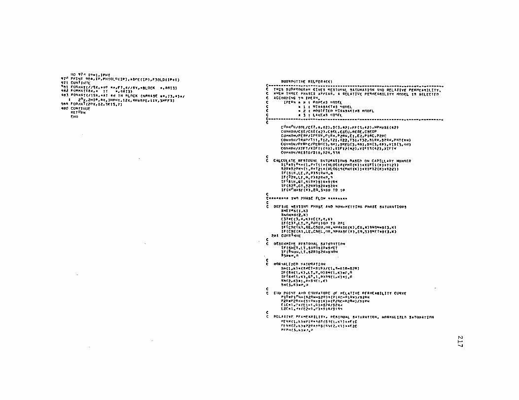
no '17~ 10•1,JPHT '11~ P~l~T q~a,tP,PHTOL»ttP) 1 ABrE(IPl,F30l0!1Ptl) '111 CUtll Jti1J~
::~ ~3=~:~1~~~:··~~ ••~~!A;~~&w,•BLOCK •1•Rl1l '18, F0RHAf(/15k,•lT O~ TH qlOCK (NPHASE ••1131*)*/
I 2nX,2HJP 1 4k,3HPHT,12X,IHA"PEo1lk 13HFfll 'IRq FOR~ATc2~x.12,1~1S,1) ~8ll CUNf!NUE
RETUAtl ENO
SUBllOtJT 111£ RELPER·1CK l
c-----------------------------------------------------------------------c THIS SUflP~OGRAH GIVE~ RESlmtAl SATURATION ANO RELATIVE PERH[AAILITY, C WHEN THREF. PHASES APPEAR, A RELATIVE PERMElA!LITV HODEL IS SELECTEO C ACCORPING Jn IPERH, C lPEPM • P I POPF.•9 HODF.L C • I I HIRASAKT•S •tOl.\El C • 2 I MnDlFJEO HIRASAKt•S HOOF.l c • 3 I L•KE•S •tOllEL
c----------------~---------------------------------------------------·-· c
c
tUH11n~/SOL/C(7,a,az),S(3,0~),ff(3,02)oNPHASE(a?) COttHOtl/CSE/C5E(a2loCSEL,CSEU 0 RCSE,CSEOP CUHHON/PERll/lrF.RH,PfR•,P2Rw,E1,E2,PtRC,P2RC CO"HnH/TllAPITlt,T12,121,r22,TlloTJ2,SIRW,S~RW,PHT(OM) CUNHntl/PfR~C/P[Rtt(3,1n1,s11eo<3,•A),SN(J,a~),V(S(1,1~) tOHH0H/XIFT/XIFTt(ft2),XIFT?(02loXl•T1(02) 1 XIFTW CQHHON/RESTO/SIR 1 52R,,1R
C CALCllLATE RfSIOUAf_ SHURATlnNS AASE!> ON tAPtUUY NUH~F.11 s1N•s1R~•(l.~•Ttl•(ALO~IA(PHT(Kl)+X!•T\(K)tll2)) SZR•5ZPW•(l,A+TZl•(AL0Gt~(PHT(K))+XIFT2(K)+T22ll lf(SlM.LE.~.~)StQ•n.A lf(SZR,LE,a,~)SZR•A,~ lf(SIR,GT,SIRH)SIN•SIRW IF(Slll,GT,~2HHlS2R•S~R• IF(HPHASf.(K),En,31Gu TO ·~
c C•••••••• T~~ PH48E FLOW *•*****• c C OEFWE ~ETTJNr; PHASE AND NON•~ETTIN!I PllASE SATURATIOIJS
swEr•sc1,o
c
St.OH•S(2,K) t37•C(),a,K)tC(7 1 ~,Kl lf(C]1,LJ,A 0 A~Al)~O TO ~Al IF<tSE<Kl,~E.CSE~.nR,MPHASE(K);En,a)SNON•S(J,KI lf(C5E(Kl,LE,CSF.L,nR,~PHASF(K),E~,5JSNF.T•S(],K)
211 I CtJllT I ~llE
C Dl!TElfH(tl!O RfSTOllAL SATU1ATIOI!
c
IFCSMET,LT,SIRl5IR•SMET IF(SNGll,lT,SZRl&ZR•S~Oll S)Rai.t.11
c NOR~•LlzEn ~ATUA•TIOM SN(l,kl•CS•ET•SIRJ/(l,~·~IR•S2Al lf(Sll(l,~l.LJ,A,")SN(l,K)a~,n ff(SM(t1K)•G'•'•~l~~(l,K)tt.n SN(Z,Kl•!,P·S~(t 0 K) ~H(J.M)•~.~
c C E~O POJ~T AMO C~HY&TOPE ~F PELATIVE PfRMEA81LITY CURVE
PtRaPJP~+(~2AH•$2A)•(P\R(•PIAW)/52RH P2N•VZA~o(~l"W•Slffl•(PIAC•P2R~)/~IRH EIC•lo~+IEt•l,~)•3?1f/SlR~ lZ[•t.·•+re2-1.r1•~1~1s•q~
c c llEL•Tl~F. PFP~f.AHILIT•o q~5tnU•L S•TttRATtON, NnRMALllEO S•TUP•TIOM
PEQMCl.~l•PIU••e~cs~11.K•>••[tt rtk~(~,k,2??.P*~a5(~~(2,~\)••F.2C
9~P~(3,~)•~.~
N I-'
"
c
lf(C\7,lT,l',n~Rll~" TQ q9 IF(C~E!KJ,GE,C~EU,UR,NPH,S£(K);En,1)QO rn Zfi PE~H(],K)•rERH!IrKl P[PH(l,Klell,I\ S3Pir~tP
~1Ps!>.f'
''<! ],KJ•~N( I• 0 8N(S 1 t(lef".C" r,U T" ~q
2,, cu•,rt..,ttf. PEPH(],~l•PEOH(ZrKl PlP'4(t!1K)•f·.r. 53w•5?.A Si!P•"'.~ 511(3,Kla~N(l,K) s,..<z,f( ,.,, ... , G•l Tn qq
C•••••••• TllQE£ PH•SE FLOW ••******
c
c
I'' COUTl•lltE lF(lrER~;En,l\)CALL P9PE(K) lf(IPfnH,EO,l)r.•ll HIRA(K) IF!l•ER~.En,zJc•LL QHNn(K) lfl!Pf.OH,F.O,))CALL LAKE(K)
qq COllltrlUE
C RF.llAHE PF.51011AL lllTllRATIONS SAEU(t ,K)•SIR 9wEO(?.,Kl•SZll SNfO(]rK)•~lR PE TURN F.:NO
5U~nnUTJHE POPE(K)
c-----------------------------------------------------------------------c THIS IS A TPPEE PHASE R[LAllYE rEPHEAnlLITY HnOEL, C THI~ MOO[l •A~ U'EO ijV r.,A, POPE IN HI~ OPIGJHAL SlMULATnR,
c-----------------------------------------------------------------------
c
c
CQHMOH/SOL/C ( 7, q, 4z), S ( J, q~), FF ll1 G2), NPHASE I •2l CttPHn~1rERM/IPFR~,r1n~,P2Rw,E1,E2,PIRC,PZPC CO~Hn11/TRAP/Tlt,•12,r21,T2?.,Tll1T3?.rSIPM,S2PW,PHT(IA) CO~Hn~/P[RMC/PERn(],•A),SRE0(3,•Pl,SN(],l~l,VIS(],IA) COHH0N/XIFT/YIFT1(42l1YIFT?.(1211XIFTl(IZ),XlffW CUHHnll/PFSIO/SIR 1 $?A,S\A
P3~•~let.~ SlR•T]l+T3?.•(ALOG\R(PHT(K)l+XlFT3(K)) tF1sc1,K),I t,SIR)SIQ•S<t,K) lflS(Z,Kl,ll,S?RlS?.Q•S(Z,•l ~M•l,n•ISIP+92P+S1R) SN!t,Kl•IS(\,K)·~tRl/S" 9N(Z,Kl•(S(l1K)·S~R)IS" lf(SH(\ 1 Kl,LT 1 P,~lS~(l,K)•n,R lf(S~(l.M).LT.~.n)SN(2,~)•n.M IFISH(\oK),GT 1 1,~l~N(\1Kl•t;~ IFISN(?.1Kl,GT,l,~)SNCZ1Kl•I,~ SN(3,Kl•t,n•(SN(t,r>+SN(~,K)) P!R•PtRH+(~2RH•S2R)•(PIRC•PIRW)/SZRW PZR•PZRH+(RIRH•SIRl•!P?RC•PZRH)/SIRW
•tRH(1 1K)•PtR•S~(l,K)
;~:~!~::~::~::;:~~::~••El llETUAN ENll
N I-' CXl

8UttROUTINE HIRA(K)
c----------------------------------------------------··--·······-······· C THIS 19 A THHf.E PHASE RELATJVE PER~EARlLITY HODfL. C THIS HOOEL MA~ PRF.SENTEry ~y G; HJRA~AKI.
c--·-----------·--···-----·----------------------------------·----------c
c
CO~HON/SOL/C(7,G,Q2),S(J,4~),fF(J,4Zl,NPHA9E(42) CO~•ON/PEqh/fPE~M,PtP• 1 PZRtt,EtrE2 1 PIRC,P~QC COttMON/TPAP/ltl,lt2,T21 1TZZ,Tll1TlZ1SIPW182RWrPHT(4ff) co~~ON/P£R~t/PfRH(,,~1),8RFDIJ,4q),SN(J,10),V18(3,•el CUttHON/XIFT/KIFTl(R2l,XIFT~(42)1KIFTJ(02l,XlfTW COMMON/RfStO/SIR,S2R,S~R
C RESIUllAL SATllRAT!llN S32R•S2Rk•(l.+T21•(ALO~l~(PHl(K))+XIFTl(K)+T22ll SJIR•$JR~•(t,+Ttl•(ALOr,t~(PHT(Kll+X!FT2(Kl+Tt2)l IF(S32R 0 LT 0 0.~)SJZR•~,~
c
1r<sJ1q,LT,A,~)8JIQ•~.P tF(S~2R,r.T,SlH~)SJ?.R•S2RH lf(93tP,r.T.SIR•lSJIR•SIRW S1RPs,]\R•S(]1K) S2RP•S~2R•S(J,K) 53Rl•S32R•5(2,K) S3R2•S11R•~(l,K) SIR•AHIXl(StR,StRP) 52RaAM&Xl($2R192~P)
SJR•AHAXt(SJRl,O,R,S1R2)
C NO~~ALIZEO ~ATURATIO~ SN(l,Kl•19(1,Kl•SIR)/(l 0 •(8l?.R+SIR)l Sh(21K)•(S(2,kl•S2Rl/(l,-(831R+92R)) SN(J,K)•(S(J,Kl•SJR)/(l 0 •(31R+S2R+93R)) lf(~N(l,~l.lT 0 A,~)9N(l 1 K)•~,R
c
IF ($11(2 1 Kl.LT, A, "'l9N(C!, K )•R, ll lf(9H(),K),LT,~.u)S~(31Kl•~~~
C E,.O POJ'IT A••ll CllRYATtlRE OF RELATIVE PERHEIRILITY CURVE SIT••~INl(SIR,s(l,Kl)
c
921•AHIHt(SZP19(2,KJ) NEl•~2Tl(SIT•S?.T) Pl~•rlRC•(PIPC•PIRW)•SJ~RIS2RW P2R•P2~C·(P2PC•P2RWl•S)IRl!lqM P)R•WET•PIP+(l 0 •WEll•P2R F.lt•l,At!El•lo"l•S32Rl82RW E2C•l,~+(£2•1,A)•S31RISIRN E3C•:<EI•~ IC+<l,•>'Ul•ElC
C RELATIIVE PfR~EA61llTY P[RH(t 1K)•PtR•8Nll1Kl••EIC PEH~(2 1 K)•PzR•SN(2,Kl••E2C Pf.R"(J,K)•PJR•SN(3,Kl••f.3C RETURN ENO
SU8Rl'UTl!lf Ol<NO(Kl
c------------------------------------------------·-------•-----····-···· C T~IS 19 A T~~fE PHA~E RfLATlYE PfRHfAPILITY HODEL. c THIS IS • HODJFIEO vrnstUN or HIRASAKI•~ HOOEL, c THIS ~UPPR~~RAH IS ~OT CO~PLETEO YET (NfEO HOPE HOO!f!CATJON),
c-----------------------------------------------------------------------c
c
cU11HON/SOl/C(7,~,42) 1 S(3,4~11Ff(J,az),NPWASEIQZ) CUHMON/PER~/IPERM,PtRM,PZRW,F.1,E21PIPC,P2RC COllHON/TPAPIT11,T12,T21,T22,TJ1.111,s1P•,s2Rw,PHT(~n1 COHMON/PfRMC/P£Rl1(3,a~1.~RF.0(3,•n1,sN(J,4Al,VI9(3,•Al CUflHON/Xlff/XfFTl(02l,XlfT2(02)1~1FTJ(•2),XIFTW C011Hl'N/RF.SID15tR,,2R19]q
C RESIVlllL SATUPATIO'I S3ZR•S?RW•(l,tT21•(1LOGIA(PHT(Kll+XIFll(Kl+Tl2ll S31H•SIAW•(J.+Tll*(ALOGl~(PHT(Kl)+~IFT2(K)+Tl2)1 IF(~J2R,lT.B,~ISJZR•~,P lfCSJIA,LT,U,P)SJID•~.~ lf(S32R,r.T,97.HW)S32R»82RW 1F<s~1A,r.r,s1Pw1s11R•s1qw
c
Sl~•AHIHl(~(l,K)1SIR) S2F•AMIHJ(S(l,KJ,S2Rl SJAl•SJIR•SIR S)R2•9~2R•~2R SJR•IHAXJ(SJRl,o.0,s1R~I lf(S(J1K),LT,SJRISlR•S(3 1K)
C ENO POINT A~() CURVATIJRE tlf Rf.LATIVE PE!IMEIBlLITY CURVE
c
lf((81R+S2Rl,LT,l,f.•4100 TO lff Sl2P.C•AMINl(SJ2R,(93R+SZPl1 931RC•AHJNl(S)JR1(S)~tSIP)) WEJ•S2R/(SIR+92RJ PIR•PIRC•(PIRC•PIRWJ•SJ2RC/92R~ PzR•PzAC•(PZRC•P?RW)•SJIDC/SIAW PJR•WE!•PtR+(l,•HEl)•P2A Elt•l,n+(El•l,Pl•~32RC/S?.Rw EiC•1,~t(E2•1,~l•SltRC/SIRW E3C•WEt•ElC+(l,•NEll•f2C
C N0HHALIZE9 SITUPATION sHUR•l,•(SIR+S?R+S)Rl S~(l,KJ•(S(l,K)•SIRl/SHO~ SH(2,K)•(S(21K)•S2R)/S~un
SN(),Kl•(9(],K)•SJR)/SM93 lf(S"(t,Kl,LT.~.~)SN(J,Kl•n,n lf(S~(?,Kl,LT,A,M)SN(2,~)•q,~ lf(S~(J,~l.lT,n,P)SN(J.K)•n.~
c C AELATllVE PfR~EAQTLITY
PERH(J,K)•rJA•SN(l 1K)••EIC PEAH(2,K)•PlP•~H(Z,Kl••E~C PERM(],K)•P3R•5H(J1k)••E3C RETUAH
lq no 2~ .1a1,1 21 PtP~(J,K)•S(J,K)
RETUPN F. .. ll
N I-' \!:>
SU"R"UTl>tf L•KF(k)
c-----------------------------------------------------------------------c THIS IS A THPEE PHA~E RfLATIVE PfR~fA~lllTY HOCl~L. c THI, ~unEL ~AS nEVELOPPEO BY L. LA~E.
t-------------------------------------------------------------~---------
c
c
Co~H~N/SOL/C ( J, o, •11, s c 3, a 211 FF ( 3, ,2), NPHASE ( •2 l COH~ON/PERH/IPERM,PIR• 1 P?q~,E! 1 E2 1 P!RC,P2RC CO>tH~H/TPAP/Tll,T12,T~l,T22,T311T321SIRW1S2RW,PHT(4A) CO>tHPN/PERHC/P'R~(3,•0)1SRED(3 1 •~),S~(3,1Al,VIS(l,a9) CU>tHON/XlfT/VIFT1(02) 1XIFT2(02)1XIFTl(•2l1XIFTW cn"HON/AESI0/51•,S2R,53R
r.L•~F.•S(?,K)•(l,•SlloK)l/(S(l,klt5(21K)) S3R•$zRt~lAK~•(SIR•S2RJ .
C ACTUAL AE,lnUAL SlTURATIO~ ~JAeAHl~l(~IR1,(l,k)) s2q•AMIN11~2R,S!2,~l) S3••·~ NJ(~3R,~(J,K))
c C l~TERPOLATION FACTORS
SIJP•(S7Rw•S2R)/~2QW
~21P•(~IPH·,IRJ/~I"~ c C E~O POI~! OF RELATIVE P~RHEA~ILITIE,
PIN•PJAk+SllP•(PIRC•P!RWJ PZR•PlPWt~21P•(P2RC-P2RW) P3N•P2PtGLAKF.•(PJR•P2R)
c C CURV•TURE OF PELATIVE PERHEA~tLITY CURVES
EIC•EltSllr•(l,•Ell ~2r.•E2•S?IP•(t,•EZ) f.3C•FZCtPL••F.•CEIC•E?.Cl
c C NOHHALIZEO ~lTUNATtON
SHoe•t,-!SIR+S7RtS3Rl $Hll1K)•(S(loKJ•SIAJ/5"0R ,~12.~1•!S(ZoK1-szA)/SHOR S~(3,Kl•(S!31kJ•S3R)/,M0R
c C RELAJIVF. P[~HEA~ILITl~S
PERH(! 1 K)•PIR•5N(l 1 ~l••E1C
c :~=~ii:::::i::~:l~:=~==~~~ qlTUQN f.NO
Sll"~OUTl"'E PHCnHP
c-------·--····---------------------·----------······-·--------·---····· C THIS SUPPRO~RAH GIVES PHA~E COHP~~ITIO~~, SATURATIONS, ANO JFT 1 c HOO If IEO HA"O EOU•TIOl<S ARE USEO ff) onTAIN PHASE [QUJLBRll•H: C HOST SURFACTANT RICH PHISF. IS OEFINEU AS PHASE 3,
c-----------------------------------------------------------------------
c
c
CQHHnN/N~/ I CT 1ICTI1ICT2,x1cT, HCO~P COHHnN/IFT/GIJ,Gl2oGl3,G2!1G22,G2l co·•~oN/AIA 11, • 12, •21, •n COHHnN/PHl,E/F!,F2 1 F1 1 ~1,82,~l,C2PlC1C2oPC CO~Hf)N/CSE/CSE(Q2l1CSEL.csru.RcSF..C$EOP CO"H~N/SOL/C(J,a,12>.~13,121,fF(],Q2),NPHA~E(all COMHnH/TAYIA,e,G,f,IF•,ALPH4,8F.TA,kK COMMON/XIFT/XIFTl!42) 1XIFT2(4Zl1•ItTJ(GZJ 1XIFTW
00 1~1 K•lolCT~ Kk•K JFIK .~n. ICT!l no TQ IOI
c COt'~INE SllRFACTAllT ANll ALCOl'OL TOGETHfR •s co~PON~~T TH•EF. IF(C(7,4 1K) ,GF., l,0f•~) RSA•C!3 111Kl/C!7 111K) C(3,l,K)•C(J,G 1KltC(7,a,k)
c C ffST FOR CHF.HICll
lf(C(1 141Kl,LT,O,IHIC1) Gn TO &P lf!C~E!K),11,CSEll) GI) TO ell
c C•••••••• TYPE ll(t) BEHAVIOR t HIGH SALINITY ••••••••
41"411tAIZ•CSE(K) IF(C(2,Q1k),LT,0,on1~1 GO TO l5 A]Z•C(J1•1K)/C{21•,K) R]J•(RJZ/AIJ••(l,A/01) cc1,3,kl•RJZ/{R3ZtP1?•PJltR31) ccz,J,K)•l.~•(Rlltl,~l•C(l,J,K) C(3,J,Kl•l,0•C(!13,KJ•C(Z 1 J,k) lf(C(],l1Kl,LT,C!l,4,K)) Go TO 25 HP"lSF. (K) •Z lf(4p5(C2PlCl,r.1,,~~AnJ,ANn,AeSCFll,GT,,PAARJ)GO TO IZ Cf lrl,K)•l•"' c 1.,t,tc>•n ... c<:h t •k>•t:t.u no TO II
12 A•AI A•81 F•FI CJPlC•,5•(•A•CZPLCt((A•C2PLClo•2t4,•••C2PLC•(l,•C2PLCll••,~I r.•(l,•C3PLC•C2PLCl/C2PLC
C ClLCULlTE R~I oR32 AT PLAIT POINT KR•C3PLt/C?~lC•!,E•lh XL•l.~f-7
C C•LCULATE THE CO~CE•ITAATION~ OF C!l"PONENT9 OF TWO PlllSES C•Ll TIELl~f.(XR,xll 00 11 lal,b
13 C<l•'•k)cC(l,2,Kl II llU I'; J•J,~ t'I co,z.•>•q,a
flU I• h~,b OU 14 J•l1312
14 C(l,J,~)•fll,o,kJ•C(t,J,K)/Cll1l,k) S(J,M):(t(l1•,•>•C(!,J,Ml)/(C!lol1•l•C(l131Kl) S(J,•)•l,~·SIJ,K)
N N 0
3(2,•)on.n cc•.1,Kl•C(•,•,•ll~(l,K) c (4, ,, I() •fl.0
C CALCUL•TE INT£RFACIAL TF.NStnN 8F.fWEf.N HICPO£MULSION ANO MATER •IFTl!Kl•GIZtGll/(Gll•Clt,3,Kl/C(3 1 3,K)+I,~) XlfTZl•l•XIFTl!Kl (:Q TO l~P
2Q IFIC•E(KJ.GT.CSELI G~ TO 3~ c c•······· TY•E II(•) nE~•VIOR 1 LO~ SALINITY ·······*
Al•A21+A22•CSE(K) Rll•C(J,4,Kl/C(l,4,K) q]Z•lZ•Ull••nZ C(l,],K)•Rl2f(R32tUlZ•Rll+PJI) C(2,3,Klcl.~•(A3tt1.«)•C(1 1 3 1 M) C(l,,,K)•l,~•C(l,],K)•C(?,3,K)
Jf(C(],l,Kl.LT,C(3 14,K)) GO TO 2~ ~PHAH(Kl•2 JFl&RSIC2PRCl,LT.l.0,A~O~AAS(F2l~GT,~~AA~Pl)GO TO I• ct1,~,K>•~·" C(2,2',k)at.~ c<3,,,K>•o.>!I c;:o to ti!!
I' A•l21tAZ2•f.SEIKI .,."2 F•f2 CJPRCs,5•(•l•C?PPC+((A•C?PRCl••2+1,•A•C2PRC•(l,•C2PRC!l*••5) G•ll,•ClPRC•CZPRC)/C~PRC
ICF.sG•A'H ••F XL•l.919=•7
c CALCULATE T~E CONCEllTRATl~~s nF coHPONENTS OF T~O PHASES CALL !JELl~EIXR,XL) no 2:t st,,.,
2l C(l,3,K)sC(t,l,K) 18 hO U l•t,~
22 c<111••>·~·'-' Ill• 21 1•5.6 no 21 ·'•Zr l
21 tltrJ1Kl•C(l,•,Kl•C(l,J,K)/C(l,l,K) '(J,KJ•IC(l1•rK)•Cllr2rKl)/(C(l13rKl•C!lr21KI) S(~ 1 K)sl,~•S(l,K) . ~H 1 r'<J~O~lt C~Q,3,KJ:cc~ ••• ~,,~<1,M> t(ta 1 LJ 1K)sn.iJ
C CALCULATE l~TE~f&Cl4L TE~Rl~N RETWEEN MtCAOEHULSIO~ A~D OIL K!f l~(K)•G22+G~l/(G23•r.l?rl•K)/C(J,],K)+l,A) Xlflt(•l•~IFT2(K) C:O lf1 JIHll
c C•••••••• TYPE Ill 6EHAVIOA I INTED~ED!ATE SALINITY ******** 3~ C2µ•1CSE!K)·C~FL)/(CSEU•CS~L)
IF(C~ECK)•,5•(CSEU+C'El)l3~1r3~1,3~2 JAi AJ•l?l+A22•CSE(Kl
t;O yn 3~~ 302 A3•&ll+A12•CRE(K) l"l AsA)
fi•~1 ~•fl
CJ~a.~•(•A•Cl~+((A•C~~)••2+4.•A•~~M•(t.·C~M))••.~)
Cl~•l,•C7H•C3~
[f <C?.'1,l T • t ,Af•lOl C=!ttat ,E't:•tPI lf(CIH,LT,J.~~-1~) Cl~•l,0E•l0
IFIC(2,0,KJ.GT.C?.HlGQ 10 on C TtST F~R THM£E PHARES
IF(C(],4 1 Kl.LT,C3M•C(2,0,K)/C2H) GO IQ 5~ c C 1YPE Ill+) LORE
lf(C(2 1 4,Kl,LE;e.~r11 GO Tn 25 ~Pl'A5E(<)H
n]2•C(J,a,K)/C(2,4,~)
q)l•(RJ2/lll••(l,~/~3)
C(l13 1 K)•P32/(R3Z+P3?.•P.ll+R]I) cc2,3,K)•l,O•(R]l+l.~l•Cll.l1K) Cl],),Kl•l.~-cc1.3,K1-c12.~.K) IF(C(],J,KJ,LT,C(J,4,K))r,o Tn 25 IF(A~SICZPLCl,r.T,1,q£•10J(:n Tn l"O C(l,1,K)•l,W C(C', 1,t<Ja;.1•" c<,,1,•>•~ ... c;o 10 ,,.
3M4 C2PL•C2PLC+CCSE(K)•C9EVJ•C2PLC/(CSEU•CSELI CJPL•,5•(•4•CZPL+((A•C2Pll••1.+a,•A•C2PL•<l.•C2Plll••,5l t1PL•1.-r.2rt•CJPL . &LPll•aC]tl/Clt' nETAoSQRT(CZN••2•CJH••1.)/C2H ~•(l,+(lLPl'A•AET&l•C~PL•ClPL)/l~ETA•C2Pl) XR•cJPltclrL-1,E•lb XL•t,~E-7 CALL TIELIUE(~R,XL\
314 00 33 ls1,6 33 c11,z,•>•n,•
tFCC!J,G,k),r.T,CIJ,l,Kll r.n TO 25 no 31 1•5,6 DU 31 JaJ,:1,2
31 CllrJrK)•C(l,4,K)•C(l,J,K)/C(l,4,K) S{l,•l•<r.11,a,kJ•C(l,J,Kl)/(C(lrlrKl•C!lrl1kl) S(3,k)sl,0•Sll,Kl S!Z,K)s<l,P. C!o,1,KJ•C(4,l,K)/S!l1K) C(4,~,tc)aa.1' X1FTl(KJ•nl2+Gll/(r.t1•C(l,J,K)/C(3,l,k)+l,~I Xl'T?(k)•XJFTl(k) Go TO 1e"
19 If(C(J,4,K!,LT,CJH•C!t,a,K)/CIM) GO TO 5n c C TYPE ll(•l LORE
tJPHASE ( K lm'S Rll•C(,,a,~)/C(l,a,~1
R]2•0•~31••~.l c11,J,kl•R1211q12+PlZ•PJ1+0,11 C(?.,3,Kl•l,M•(P31+1,~)•C(l,3,k) C(l,J,Kl•l,~•C(l,J,Kl•C(1,l,K) Jf(C(J,G,K),r.f ,C(J,l,K)) G~ TO Z'S IF<•~s(r.2PPCJ,LT,l,)r.o Tn 'AS Cl 1,2,1<)•'11•'°' C(2,2' 1 1()•1.t1 f:( ,,i!',K)a1t,A GO Ill JI~
1A5 C2PR:C~P~C+ll,•C7PRCl•CCSE<Kl•CSELl/(C~fU•r.SeL) C~VA•.5•<·••C2PR•((A•C~~P)••l+•,•4•C?P~•(t,•C2PRl)••.~) ClPR•t,•CPPA•C3r~
llP11••C}HftlM nET&~5Q~T(Cl~••2tC1~••ll1CtM
G•l!f TA'CI ro/( I,• ( ll.P"•·RF.TA) •CI Po•OPR)
N N 1--'
315 Q3
•I
c c 'ill
SI
c
t
XH•G•Rll•••-t,f•16 >CL1:t.0f•7 CALL T!~LlllE(XR,XL)
OU Q) l•lrb c ( l, 1,-<)2,1,1• DO QI 1•5,6 00 QI J•?.13 t<t•J•Kl•C(J,Q,•l•C(l,J,K)/C(t,•,Kl S(2,Kl•(C(2,•1K)•C(Z,J,Kl)/(C(Z1~••>•C(Z,),Kl} S(),K)•l,•5(7.,K) !Ht,K)a~.0 C(q,,,•)•C(o,4,K)/5(},K) C(a,(' 1 t()ii:tt,A XJfT1(•)•r.22+G~tl(G2\•t(?r3rK)/C(3,3rkl+l,P) XlFTtl~l•XIFT21K)
r.o '" ta"
THPf.E PHASH °'PHASEIK)•) '=< l 1 J ,~):l ,71' C(Z, 1,k )z:A,,1 C(J, 1 1 K)z0,l' t< tr ?.,te)cOI,'°' r. <?.•1,rl()sl .~ C(3,7,t<)sft,~ tlt,3,•l•CIH C(2,J,t<)•CZt1 CO,l,•l•C)H 'lO 51 J•1,) oo H !•~.~ t<t•d•Kl•C(l,Q,Kl•C(t,J,Kl/C(l,4,K) S(2,•l•((t(J,4,K)•C(l,3,Kll•t(2,\,Kl+(l,~·C(J,3,Kll•(C(2;4,Kl
1-c1z,3,•111111,0-c<1,1,K1-c<2,1.K1> S(J,K)e((Cll1•,•1-c11.l1•)l•l1,11-c12,J,K))+(CIZ,•,Kl•C(Z;1,Kll
1•t11,J,kl1111.n-c11,1,K1-c12,1,K11 S(l,K)al~~-S(l,K)•S(~rKl t(o,t,Klot(o,o,K)/~llrK) r. (11,?.,t<ls~." C(A,J,l(Jsrn.\1
CALCULATE TWO INTFRFACIAl TE~SIONS Xlfll(Kl•GIZ+Gtll(r.IJ•Cllr3,kl/C!lr3rKl+l,MJ XIFfZ!~l•G?.Z+GZll(GZJ•C(?,JrK)/C(J,3,Kl+l,AJ XlfT\(Kl•A~!NJ(XJFTl(K)rXIFT2(K)l r.U TO lllP
t•••••••• ~t~GLE PHASE RF.GION I TYPE IT(•lr TYPE 11(+) 1 TYPE III ••••••• ZS ~P~A~ECKl•I
no ?~ 1o1,~ c<t•l••>•C(l,Z,K)•n.~ tCJ,],K)•C(J,•,•)
Z6 tll"Tl"UE
c
:t(l1tC)•r1eP Sl2rK)a'1,P. ,(3,t( )sJ •" t;(I Ttt IRA
C•••***** NO ~~E•·tCAL ******** ~· S(Z,Kl•CC2,a,K)
S(lrK)•l,•S(?,K) ~(J,K)sa.~
lf(S(t,KJ,lT,l,F.•l?.)GO Tn q7 C(lrl,•l•C(J,U,K)/(t(J,o,K)+C(]rOrk))
Cll,J,K)et,~·t()rl1Kl qT Cot1T1NUE
no q" J=sz,~ no qA l•lr'
qg C(t,J,K)z",~
r. c
C(Z,2,k)•l,"1 C(?,t,k):sP,~ no 7<' JuJ,3 t>o 70 1•1,"C01'1P
TA c<t•J••>•e,a 1r<s<1••l,LT,t,E-111r.o '" 12 C(3,t,Kl•C(),q,k)/S(J,K) C(J,J,K)•l,~·Cllrl1Kl t(n,1,•l•r.tn,Q,K)l,(l,K) C(5,1,Kl•C(5,Q,k)/S(11K) t(b,t,Kl•C(b,Q,K)/5(1,k) [f(S(2,Kl,ll,1,E•l2JCQ T~ 74 t1z121Kl•l,I! "PHA~E(kl•2 Xlfll(K)•X!FTZ(K)•XIFTW r.o ro tCJP
12 c<z,z,•l•I,~ 74 NPHASE(K)el
C SEPAHATE SUPFACTANT ~UO ALtrHOL FROM CO~PONENT THREE IYM IFIC17.o,K) ,GE, l,llE-~) en TO l~Z
1113
10~
II" Jilt
oO IAJ JeJ,q c<7•J••he.a GO TO Ifft
~?1!~:K~=~(;,J,K)/(l,+ASA) t13rJrK)at(7,J,Kl•RSA CUNTINllE CONTfNllE ~ETuAN EIJO
N N N
~'J"ROUTl~f TlELl"EfXR;XL)
c------------------------------------------------------------·----------c THIS IS A •O~T·FIN~INr. PROGRAM •!TH BISECTION METHOD, C CNYERGENC[ IS CHC~En WITH THE VALi~ OF FUNCTION FXAPP: C TOLERANCE EPSTIF. IS FIXED IN THIS SU8PROGPAM, C EPSTIE H•Y ~E[O SE CHANG[n,
c---·-----------------------------·····--··-······---------------·-·-··•
l
II'~
1
~
"
EPST IE•~;1m1 IFX•" CALL TRY(XP,FXP) C•LL lRYCX[,FXL) A.Prit(XL+Y"'ll?, JfX•IFx+I IF(!FX,lf.,50lGn TO PHINT 10P FOPHAT(//IPX,•PHAS[ CO'-POSITION nlO NOT CONV~RGE IN TJELJNE•) ~TOP co•· r 1Nu£ CALL TRY(APP1flAPP) lf(FXAPP•FXL)7 1918 XHaAPP FXRsFx l\pp
lf(AOSCFXAPP),LE,fPSTIEl GO TO• r.o TO 2 XL••PP FXLaF)( lpp
lf(ARS(FXAPPl,LE,EPSTIE) Gn TO • GO TO ' CON! INuE RETURN fNrt
SURROUTl"F. TRY(X 1FX)
c-----------------------------------------------------------------------c THIS SUAPROGRA~ GIVES PHASE COHP~SITIONS, C THIS PROGRAM IS US[O wH[N THE PLAI POINT IS N~T AT COPHER, C EQUATIONS OF OINOOAL CURVE ANO OISTAIAUTION CIJAVE AR[ USf.O,
c-----------------------------------------------------------------------c
c
IH
12
cc cc c 2B
c
C0HH0N/SOL/C(7,0,a2),S(3,0Z)1FF(J,aZ)1"PHASECIZl CO~H0NtTRY/A,B,G 1 F,IFX 1 ALPHA 1 8fTA 1 ~K
lh1KK lf(~PHASE(K)•q)IP 1 2e 1 3A Yo(XIA) .. (1,18) Z•G••c-1./r)•X••Ct.l'l lf!Z,GT,l,F•l0)GO To 12 PRINT I"~
IRA ruA~aJ(//l~x.•z IS LESS THAN 1;E-1" TN SUR•rn•TJNE TRY•) STOP CO"JIN11E woA•Z••A C (1 1 ~,K loX/ (x+OY+Y) C(Z,2,Kl•l,•11,+Yl•C(l,2,Kl c<3•21K)•t,-c11,Z,Kl•C(2,2,K) Cll•l••>••llZ+Z•"+k) C(Z 1 11K)al,•ll,+Zl•C(l 1 11K) c(31!1K)•l,P•C(l1l1K)•C(21 11Kl rx•1c11,2,Kl•C(3,q,K))•(C(?.,l,k)•C(2,•,•>l•(C(3,l,K)•C(J,•,K))•
11c12.2,•1-c12,•,•>> Rf'TUPN Y•RJ2(1l X•R3J(I) W•AJ2(3) Z•R31(3) LEFT N'lOF
Y•A•X••B C(Z,t,Kl•X/(X+X•Y+YI C(3,1,Kl•C!211 1K)•Y Cll1l1K)al,•C(?.,1 1k)•C(J,l,K) P•G•!(C(!,l,Kl•C(211 1K)•ALPHA)/(l,•C(J,l,kl+C(7.,1 1K)•(AlPHA•
IRETAlll••F w•OETA•(P+•LPH•tnET•l Z•(W/A)••(I,/~) C(2 131K)aZ/(7+Z•W+W) CIJ1J1Kl•CIZ1J1Kl•W C(t1~ 1 Kl•l,•C(2,l1Kl•C<3131~l FXa(C(J131K)•C(31G1K))•(C(2 1 1 1 kl•Cl2 1 •,K))•(C(~,l,k)•C(3,•,K))•(
1C12 13,K)•CIZ141Kl) ~ETURN
C CALCUTE THf CONC, OF WATER, Olli SURFACTANT IN EACH PHA8F C AT RIGHT NOOE (TYPF TIJ) PHASE BEHAVIOR, C X•RJ~(Z) Y•R31(2) W•A32(3) l•R31(3) c 30 Y•(X/Al••(l,/8)
r!Z1? 1K)•Y/(X+Y•XtY) C(J,?,Kl•CIZ12 1K)•X ((1,2,k)•l.•C(?,?.,MJ•C(J,2,k) Pa((C(~1Z1Kl•ALPHA•C(l,2,k))/G/(t,+C(l12 1 Kl•IALPHA•RETA)•
ICl3 1 2 1 K)))••(l,/F) 7•~ETA•(P+ALPHA/rETAl
~•A•Z••8 C(?,),K)EZ/(l•l•k+~)
cc~.~.~>•cc?,1,~>•~
N N w

t(l 0 3,Kl•l·•C(2 0 J,Kl•C(J 1 J,K) FX•(C(J,2,K)•C(3 0 Q1 K))•(C(2,l 1 K)-C(2,4 1 K))•(C(3,J,Kl•C(]
l,•,K))•(C(2,2,K)•CC2,a,K)) RETURN EhO
SURROUTl~f IONCNG
c-----------------------------------------------------------------------c THl1 ~URPROGRAn GIVES C'TJON f.XCHAN~E RET•EEN CLAY ANO HO•ll PHlSfS
c-----------------------------------------------------------------------c COHHON/SOL/C(7,n,a21,sc1,qz1.FF(J,•Zl.NPHASf(Gl) CUH~QN/A~sn~P/C3AOSs<•~1,CaA05~(•Al1CbADSS!•~l,CbHATS(GA) CnHHON/CR/C8ADS5(4~l,CC8(42l cuttHON/IO~/FFov,oc3,K tDMM0NtHH"tx•c,xK9~.~K~~.xKHAT,Qv COt4f'10N/lif'"l/C5,C3R 0 C,,A,CblOT, 'lRJr '16,FT3 1 f ff), St K,Cft ,CSA JTFR•~
c 'LL CQUCFUTq4TIONS ""~' RE I~ u~tn OF Hf.U/~l CJ••CJAO~S(KJ
c
J•I JFCs<t•Kl,lE,0,BlJ•l Jf(NPHASE(K),(n,J)JsQ C(b,J,K)•C(l,J,K)•C(~,a,K)/C(l,4,K) C(J,J,Kl•CCl,J,Kl•C(3,n,Kl/C(!,4,K) lf(kKC,Lf,l 0 ~E·l~lGO TO 48 lf(C(J,t,Kl,LE,l 0 rf. 0 51GO TO 4R C~R"C8A0SS(K) CC~(K)•CCR(Kl•$(1,K)tFFOV•(CC8(Ktl)•Ff(l,K+IJ• ICC~(K)*FF(l,K))
•e3sC(J,•,•>+Cln+c•a+cce1•1 H~oC(&,•,KltC6AO~S(K)tl,•CCA(K)tC6HATS(Klt2,•C~AOSS(K)
C IUN [XCHAtfr.f ~lfH ~URFACTANT C~HPLEK c USING tlE~TOtf RAPl<SIJN ITF.RATl'1N HETt<on TU FINO THE COQR(T C VALUES OF CJ! ANO C61
ITER•~ CS•C!5.J,K) C3•C(J,4,K)/S(!,Kl r.f>•C(~,),K)
S!Ks~(t,K) 41 CALL COMPLEX(C\,Cbl
F 130•FT] FT1>~sf Tf> C•ll COMPLFX(CJt~C3,Cb) Ff3l•(FT3•FTJ~l/0C} FTf>3•(FT~·FTb~l/~C3 C•tL COMPLfX((J,CbtOCJ) FJ}6•(FTJ•FT30)/0C3 ~Tb~•(FT~·FTf>~)/OCJ nELTA•FT33•FT6,,•FT1~•FT"3 lf(APS(h[LTA),lE,l,9E•5~lG'1 TO 45 UILC}s(FT60•FT,f>·FT3~•FTb6)/~[lTA
llELt"• (FT JP•F Tl>J•FT60•FTHl /OEL TA IH.Ro!TEQtl lf(JTER.~T.s~·>~o TO Q7 JF(A'1S(hELCJ/CJ),LF,~,A<ll,AN'1 0 A8~(nELCb/C~l,LE,W,~•llGO TO 45 Cl•ChnEtCl IF(CJ,LE.~.~~un••~tlCl•(C]•UF.LC3l/Z, Cb•Cb+l•Et Cb lf(C~.Lt.•t.oP~~~··~·)~&=<~~-o~t.(~)12. r.'l TO •I
•S c~·o~S(K)•Cb" C~All~~l•l•C~~ CC"(te )11C• CtJ,n,Klt=t:~•~IM r:(,.,,4,lll'):r:ti•Sl~
N N +:-
C~HATSIK)•C6HAT C(j,t,Kl•C' !If. flJON
QT ~~llF(~,1n12llTE•,r.J,Ch,FT,,FT610ElCl10ElC6 lftl~ •u•~•TllXo•OIO NOT CnNVEoGF. nN c1•,r~,6(IX.1w,Etl,~))
IEoqOR•I •ElUoN
c c JON EXCHANGE ~f.T~Ef.N snotuH ANO CALCIUH ~y c HASS ACTJON, NO su•F•CTANT CnHPlEX, c USING ~fwrn~ NAPHSON ITE••TION HETMOO TO FINO THE CORRECT C C~I Vll!JF 18 n~•C(6,q,~)+C6AO,S!Kl+C6~ATS(K) 18~ Ch•C(h,J,K)
Nf:J 4q C9EC(JrJ,K)tC(~,J,K)·C~
ROh•XK~6•C•••2/C6 CbAs~.5•(2.•0Y+AQb·~n~t(a.~·Qv•R~b+RQb••2)) Rff1T2X~•t-T•Cq••ZIC~
CbHAT•~,5•(Z,0•CJ~+QHlT•~QRT(Q,t•C38•RHAT+RHAT••2)l Cl6,1,<l:Ch•C(l,t,K)/Cl1 1J,K) C(h,2,Kl•Ch•C(l,2,~)/C(t,J,K) C(~,\,Kl•C6•C(l,3,K)/C(l,J,K) C(h,o,<l•Cl6,l 1 Kl•S(1 1 Kl+C(6,2 1 K)•S(2,K)+Cl6 1 3r~l•,(J 1 K) F6•C(6,•,~)+C6n+C6HAT•66 1r1~•.EQ,2) r.o TO 5~ tr.•CHllC~ F ~:tFl:t urez r;o fn tJq
50 FP•IF6·F~)/0Cl tl61J,KJsr.h•F6/fP I lf.~cl TE Rt I 1r1ITfq,r.T,4~) GUT~ •7 lt(C(6,J,Kl.LT;•,n1c16,J,K)•C6/Z; lf(ARS((r.(h,J,~l-ti.l/Cltl,CT,ff,Pff~ll co T~ Q8A C~Al)~S(K) •Cb~
r.~llATSIK)•C61'AT RF. Tllll~ r.1m
SU"ROUTINE COHPlEX!XJ,Xh)
c--------·-·------------·-·--------·---·---------·---·--·-···--------··· t c•ttut•TE THE CONCfHTIOHS OF COHPLEX,SOOIUH,C•LCIUH,SURFACTANT C IN AQUlOUS PHASf. ANO IN ROCK PHA~F
c-----------------------------------------------------------------------c ct1 .. HON11<f'&/MKc,xKo~,x-.1t,xKHAT1QV COMHON/HNq1cs.c3~,c6R,C!>HAT,A8J,~6,FTJ.FT6,s1K,tft,cftA
Cf\•XKC•X~•X3 t<1aXJ+CS•X6•Ce RQ6•XK06•C9••2/X6 "e1tcXKA6•CP••Z/Xto RETAcR?lt+SQRT(R9to•R86) t9~•A,5•(·~ETA+SURT(RETA••2+Q,•OV•Rq6))
Cbe•cq~ .. UR•i. Cb8•1lV•Cto8•Cq8 Rl<ATsXKHAl•t•••2/Xlt Ct>HAT•Q·S•(z,e•tJO+RMAT-80RT(a;•cJA•RHAT+RHAT••2)) C9HA lat31!•C61'AT FT3•t3AtX3•SIK+tA•~IK+CftA•RRl FT6•X6•SIK+t~fttt6HAT+2,•!Cft•91~+C8A)•Alt RETURN ENO
N N lJ1
~~ROUTl~E CHEH&nNcx3,aow3,0LnA3nJ c----·------···-····----------------··-·····-·-···········-·············· C PARTIALLY NFYERSIRLE LANGHUIR•TYPE AO~ORPTION FOR SURFACTANT. c ansnqPTJOll IS RfVfRSl~LE WITH s•LtNttY C RIJT lRREYERSIRLF. HITll StlRHr.TANT COllCENTRATIOll•
E~PL•N•TTON or YARl•RLES ClPH I ~~FACTANT CONCENTRATION IN HOST SUPFACTANT RICH PHASE Alll I SALINITY ~EPf."OFNT PARA"IETER FOP ADSORPTION CALCULATION RlO I SALINITY TNOEPENOENT PARAMETER FOR AO~ORPTION CALCULATION
c c c c c c C Xl I IN • C(3,0,K) I TOTAL ~URFACTANT CONCENTRATION INCLUOING C AOSttR•EO ~URFACTANT ON ~TlTTUNlRY PHASE C I OU! a Ctl,•,~) I TOTAL ~UPFaCTANT CONCENTRATION ONLY TN C "ll•BILE PllASES C lUH I I" • OLD Tft1EL£YEL Sll'IFlCT&NT ADSORPTION C OU! • NEW Tl"l'lEYF.L S11PFACUNT ADSORPTlOt• c 01.oalo I '" • PARl .. f.TfR AlO AT OlO TlHELEYEl C OUT • PARAl•f.TER A30 AT 11£_, Tl"ElEVfl c-----------------------------------··~·-·····-························· c
Cllti~Ofl/CH£MA0/C3PH, A ,O, "10 CJlllS••3~•C3P~/(l,+DJO•C3PH)
C3AOSl•A3D•APX3/0lOl3D l~ICJAUSt 0 r.E 0 AOXl)CllOSl•AOX} or.1•o~ac31os-c1•os1 lf(DC3AO~.LE •• ~eM~l)r.o TD 2 lf(C3•ns .GE. Xll GO TO I Xl•X3•C3AOS APX!•C1AnS GO TO 1 Al•X3WXJ xl•R.n llll TO l
2 vlaxl-tl•OSI AOXJ•ClAOSI
3 OLDAlO•A'O RETURN EttO
SURROUTl~E POLV&~Ntxn,•O••)
C••••••••••••••••••••••••••••••••••••••••••••••••••••••••••••••••••••••• c 1Rllf.VERSIRL£ lAllGt4UJR•TVPE AOSORTIO" FOR Pol V"ER C••••••••••••••••••••••••••••••••••••••••••••••••••••••••••···········•• c
c CUNHOt1/•rtYADIC•PH,AQO,o•o
C4AOSaAQ0•CQPH/tl.+8~0•C•PH) nc••OS•C•A~S-•ox• IF<oc•aDR.LE •• ~~09l)RETURN 1F1oca•D~.GE.xa>GO TR I xox•-DCOAOS 10Xa•cor.-s RETURN AOXa•KOHOXa X1t•0.fJ Rf.TURN END
N N
°'
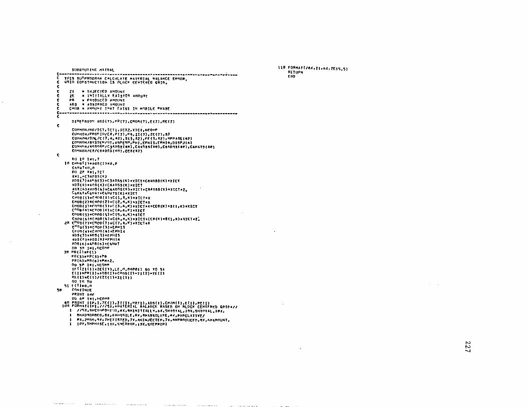
SUARnUTINE HlTAll
c------------------------------------------------------------------~----c Tlll5 sunPRllr.RAH C•Lr.•ILATE HAT~RJAL UL&NCE ERROR, c GRID co••STRHCTION IS llL(ICK CENTf.REO GAio, c C ZI • INJECTED AMOUNT C ZE • INITIALLY EXISTED &HOU~T C PR • PRQOUCf.D lMO~NT C AO~ • lD~OP!IEl> AMOUNT C CHUH • lllOU~T THAT EXTST IN H081Lf. PHASE
c-----------------------------------------------------------------------c
c
c
OlHE~~IOH A05(7),PR(7),CH0A(7),E(7) 0 RE(7)
CO"HON/NO/ICT,rr.r1.rcT?.,XICT,NCO~P CU~HON/PPOO[tt/ER,P(7),P,,Zl(7) 1 ZE(7),S? CO~HON/80LICC7,1,1?.),SCJ,ll),Ff (J,12),NPH&SE(ll) COllHON/SYSTEH/llT, AllPER" 1PHl 1EPHllof PHll,OJSPJ (I) COMHhN/l05QRP/C3&oss<•~>.t1&0S~<·~>,C6lO~S(IP),C6HAT~(IH) COH~ON/C~/C~l058(4~),CC~(ll)
oq 1~ !•1,1 10 CHhQltl•AOS(l)•~.P
CbHATsl-1.l" 00 2~ hl,ICT X•l ,·C~lM5(K) &08(~)a&OSC3)+CJ&05SIK)•XICT+Cft&OSS(K)•XICT l08(4)•&~5(1)+ta&OSS(K)•XICT lO~(~)•AOS(6)+C6A05S(K)•YtrT+Cftl088(K)•XICT•2, CbHATaCbHlTtC~HATSIK)•XICT CH1>8(1)•rH08(lltC(l,4,Kl•XlCT•X CHOQ(ll•CHP~Cl)tC(Z,4,K)•XICT•X CH08!Jl•fHOR(ll+C(3,l,M)•XICT•x•CC8(Kl•S(l,K)•xtCT [HOQ!4l•CH~8(4ltCl•,o,~)•Xltr Ctl08(5)•CHOB!5)+C(5,a,K)•XICT CHP8(6l•C~08(6l+C(~,n,K)•XICT+CC~(K)•SCl,K)•~rcT•2:
Zff cttooc11•CH~S(7)+C(7,1.•)•XICT•X cHOe(J)•CHO~(ll•EPHll tr.Of'!( a) aCHOIJ ( 4 l •f.Pltl 4 lllS(3l .. OS(l)•F.Ptll3 &US(ft)•AOS(a)•FPll!a AO~(~)•AOS(6)tC6HAT
00 l~ ts1,11cOHP JR PR(lhP(I)
PR(J)sPR0)+P8 PR(b)sPR(6)+P~•z.
no 5? t•t .••Cf>HO tF<<zt<l>+ZE(lll,LF.,n,~~P01) GO TO 51 E<ll•PD(J)t&OS!l)tf.M06(tl•Zl(l)•l£(1) R~lll•E(t)/(Zl(t)tl£(J)l
r.u yn ~'' 51 f.(l)s0,11
511 CllNTlNllE l'RINT t~e 1>0 6~ fa1,t•COMP
6Q P~INT llP1lo7E(l)oZlll) 1 PR(l) 1 l0S(t),C~aR(J),E(l) 1 RE!I) IWW FORMAT(l~l.l//5X,•~•TERlll 8ALAllCE R•SEn ON nLOC• CEHTfAEO GPtr•//
I 11~x,qMcn~PO•f~t,ax,qH1NITIAllV,bX,5HTOT•L·l~X,5HTOTll,IRX, ~hAO~OPRF.Oo8X,6H~1JqllEoftY,,H&8,0LUTE,~•,PHPEllTIYE/
~•.2H11n,qx,1H£llSTEo,1•.~HlNJEr.TfP,7Y,~HPRnoucEn.~•.~H•HOUllT, IAY 1 5HPHAS[ 1 t~X,5HERR1JR,J~X,5HERROR)
118 FORH&T(/ftX1llobX,7f.t~,5) RETUP'I ENO
N N -....J

SEMI-DISCRETE ~ITH RKl2 "W AIJSORPTJUM DATA FILE FUR JAPEX2
SEHT•DI~CHETE HFTHOD
llq IS 11si:.o
HlRASAKl~S MUIJtL 1'1 llSED IF HHlES: PH~SES APPEAR
INPUT VALUES
****************
NSLUG: 2
ISOLV: I lSEl4: 2 HFTH: 3
vr: • 4·'3"1 FFOV: 0 0Q\llOI NCD"P" f>
UT: lo'• ~Htl-HA AF>PEkM: I• ll•'llV. PHtc ,21!011
C5JI: .1:1·l~('I C"II= "·"'<lilt'! St= 0&31Hl
r.11= 6.i!ll511 Gl2• -7.1!1580 r.n" • 11111"'
Ttl" .110~ Tl2" 2 087.JDI T21• .11011
Alt'!-l41e Iii. lJ~lllf.! ALPH4?" !l. llfl\!f'I ALPHAJe 51'1.000)!4
vist= l • (.~"l .:.jtA VIS2: s.1rnit10 AP! c 11'111.01'10"
GAMHF: 13.t>lilf!., POW~I: t. i.1'1·~11 CSEt= .1110@
P!Rrl: .l'ISl!i-! P2RW: t .0"100 Et• l 05tl0'1l
C3>1AX;J: .J'-1w}O C,'1AXla • I ''11!111 C 3HAX2: • 311(110!
C2PLC:o r,., • ~n~H" C2PRC: le A;1~~" C!lEL• 0 f100A
1~v .. \'\.~Clt,1(• RCSE: 1.11GJ:l'1 Alllt• 0.0~00
AqO: 0.111•01<1 R<IO: tll1! 0 tMI!'"- lCKqi,11 0 00?1(1\P
C<J'41'0S IT !l'N OF INJECTEO SLllG ******************************
SL'IG Cll'1UL 0 14'1 l "lJ. VUL 0 Cl Ci! C' C<I
I • I >:11.J .Q(.l,t~QI !A, j:l~~.,f~ , l 1HIP0 • 11•t10111 2 •'HH~ t.vH•t·WU r1 0 t·•tl•I>!" 0 0 A'!ill>tl • IV. OlltM~
HITER= 0
tCh QI'
EPHI3= 10 ~P'lt'!
52• .37011
G2h &.2851'
T22• • 91H1P
ALP'iAh 0.'Hllllll
AP2a l0Pll 0 \~P
Rl<MAlCc 1'1 0 Al'll'IP
E?.• t.511'0t>
CSEU• 1.21110ro
AD321: 0.111•;111
XK!\f.a 0.011..H•
cs C" C7
.7""'"'"' I 0N'1"01'
.50"''""' ! 0AOllA00I
I PF.l«~a 1
lCTLI: l
El"q11: t .0'll!l\I
SU!~a .371!1'1
r.22c •7.11581'
lClFTW• t. l!il00
ALPHA Sa 0.0"10!il
AP Jc ''"""'"'~00
8RKz 0.PDll!ll'
PIRC1: 1.011101'
~JD• 11'1'1•1'1001'1!
lCKCm "'·""'"!'\
ro= qa
tCTLlc a0
ClISP11 0.011111111
82H"'c .37111!
r.21= .1100
S!ILOPF.c 0.P.h!IJ0
P2kCa l 00111H'I
Xl\tlAT: 0 0 .alll'IO'I
t>:I :><
~ 'd ~ CD
0 r:: rt 'd r:: rt
N N CX>

C ~LC'ILA H:ll A PAtHMETF.RS FOR III NO'llL CURV'O Al I= •,o_\59 Al2:t ,bR'H A2t:
INITIAL CO~OtTlONS
·~···················· ~ATER SATURATION 'llL SATURATlll11 ~ATEQ ~HASE RELATIVE PF~H• OIL PHASE RtLAlIVE PF.R~, NHF.R VISCOSITY 'JIL VI$coSllV
PHESSURE OROP RECOROF.0 8F.TWEEN
RESIDUAL WATF.R SATllRATJUN RESIDUAL OIL SATllHATJOIJ FND POINT RtL, PER~, Fn~ WATF.R F.NO PUINT REL, PFR~, FnR OtL ~ATE~ FRACTIONAL FLU~ OIL FRACllUNAL FLOW
PCT = ,8P.ll
,b3QIOJ • 3 7~"' ,?'S!iltl
QI, 1'.10n~!
t. ''11"" 5,110n.-i
ANO Qi!
• 37C'QI • ~7"0 ,r,51~0
1.~virrn
t ,1101>0
"·""'"0
,7347 •22• •,&a53
N N \0
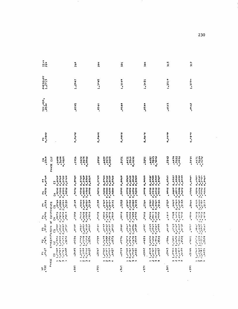
.. >"2 ...,~
-"'
w a: ::>"' .,,_ .,,,.. """' :r . CL -
. u: 0 ... .&J ... .... .,, o:sr ... 0
.. s
"" CL r:> CL .
s
0 "'0 :a.:;-
.... "' -.c
a. "'
~ G ~ts·
iss.cs:s cs. I:'>~~
"""'So:IS~IS u • • •
ts.'5.•fS'!;.
IS' Q G'Sr e:: r:; ~ ~ ~ ':S) ~ 'S
.c f:!". c.. -s· "' u ••••
"'"' IS 1$ " '5-cn ~~Ci.N
.... c ~ ~ -ZU\CC'IS.'!alU\ w u • • • ; ~~
a. !'i::;: ~· 'S" I".': ;,: <'. ...:. ~ ~- ~ s '5' u:a~~~~:.
u • • &.... ...... ~
"' c: .:... r::-:: ~
G t. - P'l'::' ~ s.. ~ ... "" a
u • • '!:. ~
~ ~ ~ :";.
L e-· •. rs w ~ <,1:,.;. ..£;
u (\I~~ "' z u
:..> • • 0 --- "' 'S:; s r.; . r r =-""
- C: ~ .c u • • - ,..
er,
"' "'
... " ... "' .
"' ... .,., ""
s ,,. "' ". "'
~ n.llCIS If\ N,...t!" 0- Cf "'f:',;
- ""'••"s . . ..
" IS'
"' "' . cs
s " s
'" . ... .. "' .
"
ei' 115. e;. cs ~-~ tS. s & :S IS. G: CS>C!WSS
IS' IS' IS: 'S
is. "SS' s '"'~ & G cs. s ~ 'S 15>1S~S
'S' ~ c.. « 'SS.S"'1
"'~ "' It' St s"'
"°' SI ~ ~ :;.•-: ~. f =.-. s ~ ~ ~(';: !!'!; c:.
"' ~ C""i ~ ,....:. -·-:::;. ~ ~ ~- s
f':i5· ~Cs:l '! !" ':' ,... ~ r; ~,\/"I
t" .. ::. ~"'
c: - ~
"' I\) ;:t; ::i: ~- t'\J -1:' ".'"". r: ::!' t\,J ('Ii,·~~ ..c
" ... N
"' " 5
""
., er .... <S> .
s "' ... '" . 1S'
s ,..."""'~ "' "' .... ~ ~ 1:1' U'HS'I l'\I .0 pl''lfS . . .
« C>
I\)
... "' ..... .. .
"'
c;G,·e>.& tS. s~ s C!: s ~ tS. CS;CS.&CS. . . . . ~cs :s:"' iS: s 'S $ l"i:t!;~IS ~(S:"glS c;. ~ c: Ci. . ...
cs "'
""· "· ~ s. :;· c.. -:::: t" ~ ~. _, cO tS. s If\
'!:''!':'c;> ~ ~- c::. :-: ~ 'S":;S5.• cS ~-~I"' .. . . .
c. "-re;, e...c.: ~ ~ 'S $ s t. i:: .. (..; c
c::. :s:i
:.;- 'S
~~~"" ~ ... ~ ~ ~ :;i ~ ::" lf\ " .., 3 r "!',....
:::::J ::... :i-1\J ..... ~ - ~- ,::!" N 'S. 'S..,. .r;,
"' ...
.. ""
C> .. "'
.. ... "' "' .
&
" "' c:. . "'
... .... 0- c V" "'oL" r. - a Lf'\ s N """"C.
"' Ill I\)
N
-L>
" ..... s
. . . "'
~ & ~i:t Q "S C IS ~ 6: ~IS:· ~sis. cs . ... ~ S SIS.
GISS'S II!~~ 6,: c.e:r.:~ C & SS . ...
s"" i:: ~ t!.lf'I 'SC:tSI~
C"· ~ c::: -CCI~ S\I" ....
:;.· S·
!SIG~ :S c: c.:.cr ~ f'!i' s· & 'St':-:' c;. G
~- t.
~ c. s rs ~~~
a.~ c. c:. s ::· 'S" 'S .... ~ -:;, :s:: O' t. '!"". ~ .£ ~$SHI" C::· ~:;.pl\
~ --· !? "';. ~
:<;; ~"" a: "".: c ::J
"' ~ :S" -l:;
-0 ....
. . . -s ~·
~ 'Sl
""
... " "'
" " "' "' .
.. ~-s s . "'
........ "' an.,- c N ::fll\G N .Of"I r.-
c..
.., "' ~ " .
• . . ""
~ 6.~ '""'II!:. ~G- C> s & c:. ~ ~ ~~sis: . . . . CSdS. ~ ~
'&~S~ CC"~ e: (IC.· S t5' IS cs; tS:C$. PS!!. . . . .
!> o;
t: ~ 11! • .& (SOS.O I'.. IS C: «> 'S. IS U'\ ....
0 G
~-c:s. '!: ~ :- '!.. s.: ~cs· ts Ci~"!;'!""
~ c;.
c. ~ !';.~'SS.
~~ c. c.. ~~ ~ -s·
'!<" s. 'S"""' ~-:; ~
~'!;'~·in
s C' ...... ""
f\.' Ci' !'.' ...... «' :,; 5' I'.'.;' LI" ~· ~,,,. tt ~ !'\I' ""!;' "S t\ .c
... ,,,
. . . ·- .:;:. -~
"' "'
.. "' "" .
.., " "' .., .
s " " ~ . ...
l\J crNS> C! .... n.·~· .... Cl'f,l'"I~ f\1 .c .,.., $.
c;
"' .. s . ""
"' "' ... N
.,,
.£:
"' .
... "·
f"" ~~IS; 'S S IS IS: So c;. cs..~
~rs 'S' '5-• • • e
IS :S- e; '$.
'!S C'~·Sr fS c. '5 c;. srs·s~ G. ~ f.. ~ ....
~'IS
11!. '!' C ...... :s,,s-~a: ~ t: c cc ~:,. U"I
cc IS.I~ t::-:G
• "S. :?· s -· ""; c ... "
~ C!
r'. ~ c:... ~ .~ s ~.
e: ~
SS~ . . s ":: (S ....... t\I
::.. r: Gt\: "S:. -S:· :S.:lf'
" "' . . I""\. IS"'::?:' ~ ~~ t.,... "" .. ~ ~ ~ "' !:i.. !::'- ~ >C> . . ...
-cc ..,
-~:.
230
...
..,
s ... ... ...
"' " v s .
" ... .. . s
~ - O'"S: ,,.. ..... f'\lC:
:::r .a "'~ n.· ~I"-:; . . .. <
c. fl.~-~ is s~ c::; ~ ~ (' (5"
s rs·~ cs. .... :S:·'!:'CS :S
s 'S,. s (;.. f. ~ ~C· '!:!~ !S e= t.•.·C... c:: ....
"'· ~ l': "".'"~ ~ .... ~ "!'.;.:£·~
c:.r· -cti"':;:";.tJ"I
I";:<;,; ~~
;;; ~ r: :: ~
!_.C: r-: s::;. 'i
e. ~ ~ <!; ·- -.. ::: ~ . .
':\.!".
"' t ':: n.: "'i~"':- J'
{;,. ·: .. :..-.""' ~ -::.:.
'!' ~=- -.;i. :;I'S~ ,... - r ~
""i" r: .. ,,. . ..c
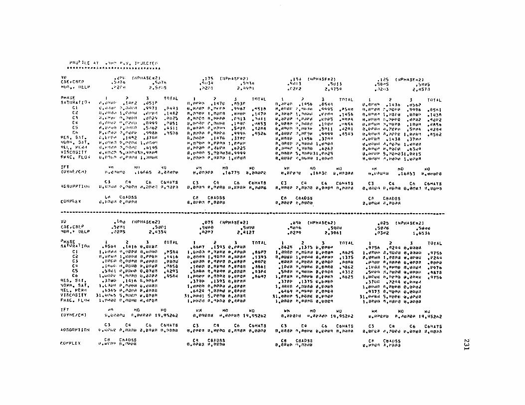
PRtiF ILE AT • 'rn'.'· P.v. l''JECTEP ****•***#****~**********A*******
~ll
CSE1CSl'P MUR,, flt.LP
PHA~E SATIJRAT!IJ<
Cl Ci! c·~
Cq C5 f.h
PES, SH, ~H..1f'H-:. SAT• 111:1., Pbl•1 v I sens IT Y FIHC, FLO,,J
IfT (llYNUCMl
~CSUfH'TlllN
cOHPLtx
(NP11A$[:?. l .Ci"": .5~7o • 5,,.,,., • t' 2::-~1 ;:>. 5,~;,5
v\ , LI~ 1 Wl ~·
~ •• J.hl''£J. ~'~·\1h1 ;.\. t: '~ r'i l" l·Y,ilfll-i'4
~. ~.l~41,.J(1
"' ... ',['! 11')~1 ;;.tt\P.-1 Vt. lJ'·\~.~, 1:) • .,: '·1l~1-\
\1, ~H,~:?i
o,,,'h·.r~
? 3 ,1"~2 ,dS!P
H.:hH'.11 e<iQ71 J e r l 1M 1') et~:-•~,,,
H, :t~t\(1 , ~1!'\2C.,
···,!·~~(~(! ,ftqqq V.,~htf:.(' ,5A&2
,,,~"''' ,9'lllf< ,lll~2 ,.Hllil
lil,Penv. 1.~rii.,rt
t\,P0i~f ,b\Q5 '>, ":.1C'il3l:I, 'IBf'<I "' • (?l•,H\(i 1. \·1t,,~f~
TllTAL
,llQ'l:S ,!QA2 .~'12~
,l'i!SI • a 511 • C\506
'11 MO rlO I·~ '~ ~, "1'·~ (1. ,lblb5 ~.~Aill'l'I
Cl CQ Cb CbHATS u.1.;:tiJl1 Cll,f'M~PI "·'Hh,f·' ~-11.~a"'~"
Lil CuADSS J,f;r.,.,,, ~.o"'~"'
• 175 • "" 3q ,:•21'1
(rlP.,ASF:;:>) ,s·-nq
2,Q'lf't
f·l, ~v"'~' "·~•'lr.1!JI A,0"1111
~."~"~ ~.M'·''~'' 0,l!l'ilfl A,f!:<0ill 11,0'lil"' t",tF11 ~JC'
"·""""' Ci't,l:,~"" 11,l•rW!il
;:> j
,\q7y ,RSJV ~.~~~~ ,qq87 1,n~~~ .~~~~
~,•PFil ,F~ll
:,OH~~ ,1~~~
~.~~~~ .s~z~ r,q11p~ ,qqq~
,1a7~ ,370P ~,C'ilA"' I,~~~·
C',~t~il ,&225 5,?U~~30,qqqq
C',~il~il l,ilC'~A
TllTAL
• ~5111 • \ 11711 • ~IHI ,·A853 , 121'1! ,1152&
>111 1l,16C1'.1Vill
MO "10 ,lb775 0elilA11"0
CJ C4 Cb Ci>HATS ll,0Qllil1 V,P<0.lil 0,11110~ 0 0 ~ldPl0
Cl! CllADSS 0, 0c•f1:>1 I''. 1'101"11
,15~ • c;,111 ,f·?.v2
("'PtHSf:2) ,51~11
2,Q75q
!l,Jl'ilf-' 1-1,0r11w
"'•~"'"(> 0,i1~0P
~.lll"OJl' 0
0;11At•n
"'· illlll"' 11,lllH!~
Pl,i,Ot~p
ti, wtr.u.u., 0,l'IOl0t>
0,00~"
? 3 ,1a5& ,85a11
l!,'~h·AH ,qqq5 t,"."~HHl •"'(H~'-1
"'•"'•<IPid .~:1'115 ",:l'10lll , I ~r."
'" (ll<!i>I'! • 5"'11 ,l,C~l'~l<l ,Cjqqq
,tt1s& .:n"~
''•"'"'"' 1,1!"0'~ ·l 1 'A">I" 1 b2b2 5, ~111'1"1 I , l'!.'25 ~, Ol\,ill! I, i1MH1
TflTAL
,P5a11 .1as& ,CA(il].q
,n~c;q
,a2RI ,11sa1
WH
11,11r"'''il '10 Wu .lbAl('. l<,"'P.11Pl0
C3 C4 Cb CbHATS 0,AAlil~ "•P0n0 0 0 111110~ 1'1 0 C'l0A0
Cll C!iADSS 0, Al!ilP (~, C'll!Hl0
,125 ,50·•5 •. )2,;:S
(NPHA$f:2l ,511~5
2,q57,1
~.fi~~~
H,~"~A
0.~~~~
~.~~~~
~.~r~~M
~.~P~~
~.~(~~~
~.~P~~
~.~~~~
~.~~~t· ~.~~~~
~.~~~~
? 3 ,IQ3b ,d!>b2
r, :·•0"-lil , qqq11 l,1<0M'I ,0r.0r• t1 •• ! .. "''''1 .~Ol~2
'.·l•!.11'1V.0 .lR\:1M ..i,71lli'l'I 0 5<'lHI ;>;,l>IM•0 1,11 .. 11'1 .1~38 ,37•11~
.•,!•o<IC'~J '·'°""" ~.li\'1f1~ .&3¥J4
5,!'f,"'i131,0P.15 :~ • ~11d0!\ot l • k),•'1A
TOPL
,85"'1 .1 Ql!\
•"'"~z ,ilfl5b ,Q28<1 ,!!Sbi!
WM 1.1.•1.?1~~k1
MO wO ,ll>llS3 ll,.,l•0f'0
C3 C4 C~ CbHATS 0.'1~8~ ~."~"" 0.0~0~ ,,00•0
Cll C6ADSS 0, ill'lfl"' i'., 1110il'OI
••••••••••••••••••••••••••••••••••••••••••••••••••••••••••••••••••••••••••••••••••••••••••••••••••••••••••••••••••••••••••••••••w•m
)(i)
CSE1CSti' 'lOA, • IH.LP
PttASE SATURAlJON
Cl C2 Cl cq cs Cb
!?ES. s·tr, 'IOIH•, SAT, qEL, PER11 VI SC OS !TY FflAC, flilrl
IFT (l>YNE/C"1)
ADSORPTION
t:Ot<l'LE X
•I Qll-)
''l~!I I ,;.12115
CNF'HASEc2)
1 • fl5Ua
1 • \1~hH1 ~. t:J'-~ .. J~'
.u'~'·a1
.1 ~\'1t1 • s~.;i
1,utH11' ,3HH•
I, I. ;ir.11• ,blb~
31,111•~.s
I, 1,.1;rn
2 ,tat&
!JI• ~_.0P•1 I• L10,,H 0 •''11~~11 r4,l'ICH11! l'l, 111tll·ll'I ~-'!.(h'""
,\Qlb l'I 1 "'li'Plt "'•'11'1f~~ 5,liln~:i• r1 .~·1e(.1"
, Si!C1 I 2, 113sa
3 0,0crn:i:
", 11iil0ll
16. "'""'' lil,l'Jlilflil II, iJ(·•l!111 lil,0?10(l ,,,0,11";> Pi,!ilt-'bVI ti,ll<HIC1 111,iilf'.l(l(:l
~.0fl0lil
ll,i11'0lil
TOTAL
,flSl!Q ,,1111> ,f.10Akf ,A858 ,Q2q3 • 115114
.. M
0,IHrnr>I) MC WO
~,Ak!O!i!~ 19,952&2
Cl Ca Co CbHHS "' • •H'~Jl~ ~.tt~n~ ~.~00~ tt.~~~~
C.I:\ Cl\ADSS '"'•(>~·r~'t! t1.1•0~,0
,1675 ,51lfil0 0 A2P<7
fNPHASf•2) ,51'1110
2,4127
I ,l!M•7
I ,111•0A 0,000!11 . """"' , 1 Ollll'I
,51'1011 I, lilP."'l'
, 3 711H• 1. '11'1-ltl
,bn2Q .H,lil"'"I
I ,ilV.(h!
2 • \3'13
°'.~~"'~ I ,'!01lA l'!,0!111'0 0,AilO!ll Cl ,A0r~f11
"'·"'~IOlll , 13q3
"·""""' "'• 'l0"'1t1 S.t'0!'H!I "•"111110
3 0,1'1'11111 I', fllP!ilfA 0,111'101'1
"'·"'"""' 1'1 0 0A0f.I i!,01H!fll 0,119'01" 0,0\l'Pll'
"'·"""" il,0"1'1P 11, lllil\!OI i','!1'01"
TOTAL
,llb1117 , 13q3 1 1Hlfl0 .~Bbl ,1131'11 ,llb07
Wf'I 0,il<lfll'li!
MO WO ~,01'1Alil~ lq,q52b2
C3 f.4 Cb C&lil.TS 0,r.O!e0 0,0r00 0,Alil01l ll,0000
CR C8AOSS 0,01'0J 111,01l~ll
,l!l';I! ,c;ll"ll ,11'2!-<q
(NPH•SE•2) ,51l00
2,3qbl
I ,8&2<;
I • "''""' 0,0~Jl6~ , llAllJl'I • I llhlil , 5lillillil
I ,l'!P.01'1 ,371W
I , .~1rnv. ,bQ&q
31 , 110111• I ,0A0V.
2 • 137~
fl 1 liliJPl(I l ,1111"''1 tl,1'01111 A 0 A\HHI <1,<11rn11 l',11111'11
,1375 >l,(llil01:l "•"0"111 5,P0Altl
"·"'"'"'0
3 11,0016" il,l'llfOOI 0,lllPiH4 11,0110i:o 0,01'1£110 0,11\lllilOI 0,E-111111:1 il,1>(110111 0,M'llH'l i',00<00! 16,lllilir!l111
"·"'"0"
TOTAL
,flb25 • 1375 ·"0"'0 ,'18b2 ,Q312 ,flbi!5
WM 0.11~0110
MO WO "'•"i'~t'I" 1'1,q52b2
C3 C'I Cb CbHATS A,f.10l~P A,fllldlil0 0,~A0'1 ~,flf.100
CB C8ADSS 0,01'"~ ll 1 A0~0
f"PHASE:a2) ,P12S , Sih:!I\ ,1'13-12
• 511.,ld I, bS Jb
I ,'1751>
l,t'fl1.k!i'I l!,00IWOI
• l!''llH' , I V.0'1 ,sv.11<1
I, ill'ldil • 3 71ll~
l,lllilfl~
,q373 :u.111•0.i
I•'"~""''
2 3 ,q2~4 ~.00li!lil
~.•01~ 0,0~0'1 l.1'101i10 0,~11100 fll,llJlilflllll 0,0t:00ill 0,l'l'lil0 A,0'111111 ~.~llPA 11,111111111" ~.ar~0 "•~"'"" ,,zuq 11,lillilll~
l',lil0fllll 0,01'0J 0,~0Ail 0 1 0011~ S,"'11r11 lil,dl'W0 <1,"'l!P0 0,~A01!
TOTAL
,q75& ,e211" ,ll0P0 ,r.q1& ,a878 ,'175b
wM lll,140!1'!>!~
MO WO ~.fllil~01l l'l,'1521>2
Cl Ca Cb Con ATS 0,11v0~ -.~lill'!ltl 11,0fllld0 "•"'"~~
C~ Cl!AOSS ld,i'110'1 ~,1'"'9'0
N w f-'
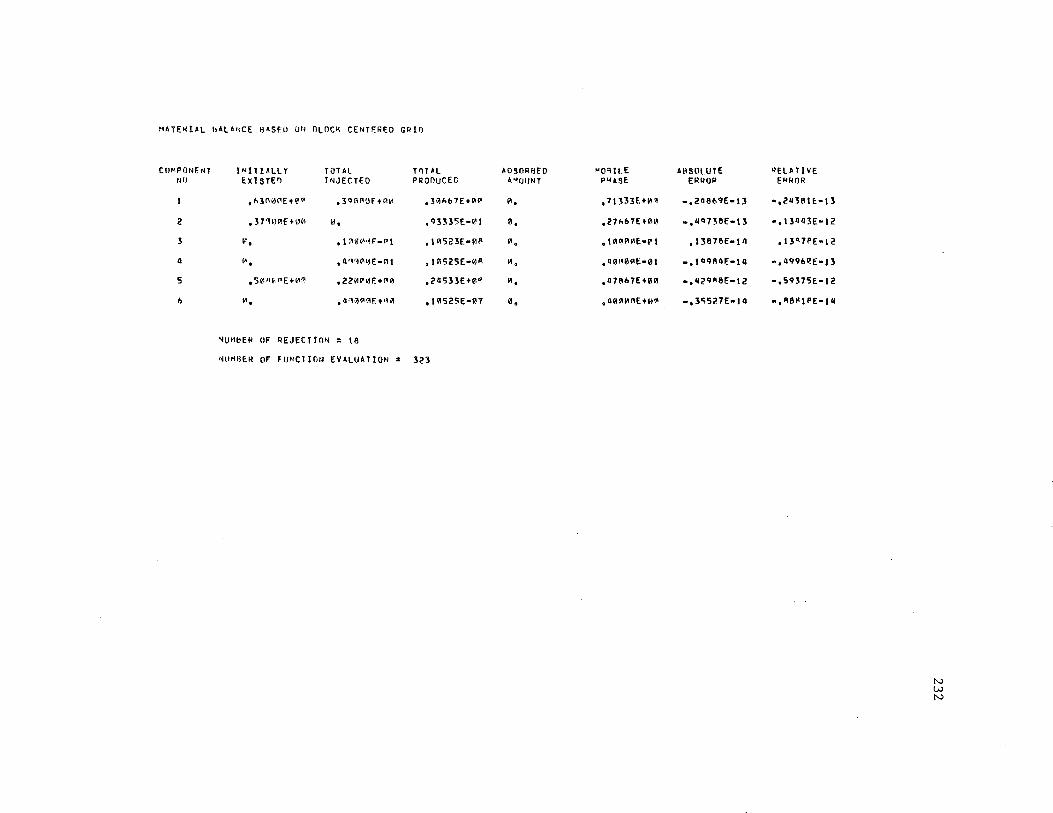
HATEN!AL hALA~CE H~SfD O" ALOCK CENT~REO GRlf)
CU><PONENT INllPLLY TOTAL T'lTAL rJf) EXISTED JNJECTEO PRODUCED
,1>3t1111'EH""' ,J'HH•llE+~" ,31<11>b7E+l'I'
2 , 37"10e>.E +1!'1 "· ,q3'535E•l'I
3 I' " , I ;>0VlvlF·r>t ,!0523(•01'
II ". ,ll"'H'~E·t11 ,IV1525E•0R
5 ,5it,ll~<'E+<ll' ,221ll'l!F.+fl0 ,;>0533E+l'I"'
b "'. • 11·1Vl"'<'IF. ··~Iii , ! 1'1525E•1'7
~UM~ER OF REJECTION : \8
"lli"HE.R OF FU!.!Cl Iritl EVALUATION s 323
AOSORBfO "MILE A'101JNT P4l$E.
ll, , 71'.\33EHl"I
l'I, ,27i.t'17Etlll'I
"· , I A"'IHIE•V t
"'· , llA!H~l'E•01
"'· ,a7M•7E+01l
0 . , 110?1"AE +tt?I
AllSllLUTE ERllOP
.,2Q8b'IE•t3
-,11<1736£-13
, 13878£•!11
., 1aq1111E-111
•,ll;>'IA8E•t2
.,3<;521£-111
"EUTIVE E"RIJR
•,21138H•l3
•, 13Q03E• 12
,13"7PE•12
.,aq'lb~E-13
•, S'll75E• 12
.,R88!PE•!ll
N w N
REFERENCES
1. Reed, R. L. and Healy, R. N. , "Some physicochemical aspects of microemulsion f loading: A review," in Improved Oil Recovery by surfactant and polymer flooding, Shah, D.D. and Schecter, R.S., ed., Academic Press, New York, New York, 1977, 383-437.
2. Nelson, R.C. and Pope, G.A., "Phase relationship in chemical flooding," Soc. Pet. Eng. J. (Oct. 1978), 325-338.
3. Uren, L.C. and Fahmy, E.H., "Factors influencing the recovery of petroleum from unconsolidated sands by waterflooding," Trans. AIME, 1927.
4. van Poolen, H.K., Fundamentals of Enhanced Oil Recovery, Penn Well Books, Tulsa, Oklahoma, 1980.
5. Pope, G.A. and Nelson, R.C., "A chemical flooding compositional simulator," Soc. Pet. Eng. J. (October, 1978), 339-354.
6. Thomas, C.P., Winter, W.K. and Fleming, P.D., III, "Application of a general multiphase, multicomponent chemical flooding model to ternary two-phase surfactant systems," SPE 6727, presented at 52nd Annual Fall Technical Conference of SPE, Denver, Colorado, Oct. 9-12, 1977.
7. Larson, R.G., "The influence of phase behavior on surfactant flooding," Soc. Pet. Eng. J. (Dec. 1979), 411-422.
8. Pope, G.A., Wang, Ben and Tsaur, K., "A sensitivity study of micellar /polymer flooding," Soc. Pet. Eng. J. (Dec. 1979), 357-368.
9. Hirasaki, G.J., van Domselaar, R.R., Nelsori, R.C., "Evaluation of the salinity gradient concept in surfactant flooding," SPE 8825, presented at the First Joint SPE/DOE Symposium on Enhanced Oil Recovery, Tulsa, Oklahoma, April 20-23, 1980.
10. Todd, M.R., Dietrich, J.K. Goldburg, A. and Larson, R.G., "Numerical simulation of competing chemical flood designs," SPE 7077, presented at the Fifth Symposium on Improved Methods for Oil Recovery of SPE, Tulsa, Oklahoma, April 16-19, 1978.
11. Todd, M.R., a.nd Chase, C.A., "A numerical simulation for predicting chemical flood performance," SPE 7689, presented at the Fifth SPE Symposium on Reservoir Simulation,. Denver, Colorado, Feb. 1-2, 1979.
233

234
12. Pang, H. W. and Caudle, B. H., "Modeling of a micellar-polymer process," SPE9009, presented at the SPE Fifth International Symposium on Oilfield and geothermal chemistry, Stanford, California, May 28-30, 1980.
13. Pope, G.A., "Mobility control and scaleup for chemical flooding,'' First Annual Report to DOE, the University of Texas at Austin, Austin, Texas, 1980.
14. Pope, G.A., Hong, C.H., Sepehrnoori, K. and Lake, L.W •. , "Two dimensional simulation of chemical flooding," SPE 9939, presented at SPE California Regional Meeting, Bakersfield, California, March 25-27, 1981.
15. Chase, C.A., "Variational simulation with numerical decoupling and local mesh refinement," SPE 7680, presented at the Fifth SPE Symposium on Reservoir Simulation, Denver, Colorado, Feb. 1-2, 1979.
16. Kazemi, H. and MacMillan, D.J., "A numerical simulation comparison of five spot vs. line drive in micellar-polymei SPE9427, presented at the 55th Annual Fall Technical Conference of SPE, Dallas, Texas, Sept. 21-24, 1980.
17. Peaceman, D.W., Fundamentals of Numerical Reservoir Simulation, Elsevier North-Holland Inc., New York, New York, 1977.
18. Lantz, R.B., "Qualitative evaluation of numerical diffusion (truncation error)," Soc. Pet. Eng. J. (Sept. 1971), 315-320.
19. Perkins, T.K. and Johnston, O.C., "A review of diffusion and dispersion in porous media," Soc. Pet. Eng. J. (March 1963), 70-84.
20. Collins, R. E. , Flow of Fluids Through Porous Materials, the Petroleum Publishing Company, Tulsa, Oklahoma, 1976.
21. Price, H.S., Cavendish, J.C., and Varga, R.S., "Numerical methods of higher-order accuracy for diffusion-convection equations," Soc. Pet. Eng. J. (Sept. 1968), 293~303.
22. Spivak, A., Price, H.S. and Settari, A., "Solution of the equations for multidimensional, two phase, immiscible flow by variational methods," Soc. Pet. Eng. J. (Feb. 1977), 27-41.
23. Settari, A., Price, H.S. and Dupont, T., "Development and application of variational methods for simulation of miscible displacement in porous media," Soc. Pet. Eng. J. (June, 1977), 228-246.
24. Sepehrnoori, K., Carey, G.F. and Knapp, R., "Convectiondiffusion computations," Proceedings of the Third International Conference in Australia on Finite Element Methods, July 1979, The University of New Wales.
25. Jensen, O.K., "Numerical modeling with a moving coordinate system: application to flow through porous media," Ph.D. dissertation, University of Washington, Seattle, Washington, 1980.
26. Peaceman, D.W. and Rachford, R.H., Jr., "Numerical calculation of multidimensional miscible displacement," Soc. Pet. Eng. J. (Dec. 1962), 327-339; Trans., AIME, Vol. 225.
27. Price, H.S., Varga, R.S. and Warren, J.E., "Application of oscillation matrices to diffusion-convection equations," J. of Math. and Phs. (Sept. 1966), Vol. 45, 301-311.
28. Chaudhari, N.M., "An improved numerical technique for solving multidimensional miscible displacement equations," Soc. Pet. Eng. J. (Sept. 1971), 277-284; Trans., AIME, Vol. 251.
29. Todd, M.R., O'Dell, P.M. and Hirasaki, G.J., "Methods for increased accuracy in numerical reservoir simulators," Soc. Pet. Eng. J. (Dec. 1972), 515-530; Trans. AIME, Vol. 253.
30. Laumbach, D.D., "A high-accuracy finite-difference technique for treating the convection-diffusion equation," Soc. Pet. Eng. J. (Dec. 1975), 517-531.
235
31. Yokoyama, Y., "The effects of capillary pressure on displacements in stratified porous media," M.S. thesis, The University of Texas at Austin, Austin, Texas, 1981.
32. Garder, A.O., Jr., Peaceman, D.W., Pozzi, A.I., Jr., "Numerical calculation of nrultidimensional miscible displacement by the method of characteristics," Soc. Pet. Eng. J. (March 1964), 26-36; Trans. AIME, Vol. 231.
33. Nolen, J. S., "Numerical simulation of compositional phenomena in petroleum reservoirs," SPE 4274, presented at the Third Symposium on Numerical Simulation of Reservoir Performance of SPE, Houston, Texas, Jan. 11-12, 1973.
34. Ben-Omran, A.M. and Green, D.W., "A two-dimensional, two phase compositional model which uses a moving point method," SPE 7415, presented at the 53rd Annual Fall Technical Conference of SPE, Houston, Texas, Oct. 1-3, 1978.
35. Naiki, M., "Numerical simulation of polymer flooding including the effects of salinity," Ph.D. dissertation, The University of Texas at Austin, Austin, Texas, 1979.
236
36. Larson, R. G., "Controlling numerical dispersion by variably timed flux updating in two dimensions," SPE9374, presented at the 55th Annual Fall Technical Conference of SPE, Dallas, Texas, Sept. 21-24' 1980.
37. Engelsen, S., Lake, L.W., Ohno, T., Pope, G.A., Sepehrnoori, K. and Wang, B., "A description of a generalized micellar/polymer physical property package," Center for Enhanced Oil and Gas Recovery Research, University of Texas at Austin, Austin, Texas, 1981.
38. Wang, Ben, "A sensitivity study of micellar polymer flooding," M.S. thesis, the University of Texas at Austin, Austin, Texas, 1977.
39. Lin, E., "A study of micellar/polymer flooding using a compositional simulator," Ph.D. dissertation, the University of Texas at Austin, Austin, Texas, 1981.
40. Coats, K.H., "A highly implicit steamflood model," Soc. Pet. Eng. J. (Oct. 1978), 369-383.
41. Grabowski, J.W., Vinsome, P.K., Lin, R.C., Behie, A., and Rubin, B. , "A fully implicit general purpose finite difference thermal model for in situ combustion and steam," SPE8396, presented at the 54th Annual Fall Technical Conference of SPE, Las Vegas, Nevada, Sept. 23-26, 1979.
42. Sincovec, R.F., "Numerical reservoir simulation using an ordinary differential equations integrator," Soc. Pet. Eng. J. (June 1975), 255-264.
43. Hindmarsh, A.C., "GEARB: solution of ordinary differential equations having banded Jacobian," UCID-30059, Lawrence Livermore Laboratory (May 1973).
44. Jensen, O.K., "An automatic timestep selection scheme for reservoir simulation," SPE9373, presented at the 55th Annual Fall Technical Conference of SPE, Dallas, Texas, Sept. 21-24, 1980.
45. Sepehrnoori, K. and Carey, G.F., "Numerical integration of semidiscrete evolution systems," to appear in the Journal of Computer Methods in Applied Mechanics and Engineering.
237
46. Hill, H. J. and Lake, L.W., "Cation exchange in chemical flooding: part 3--experimental," Soc. Pet. Eng. J. (Dec. 1978), 445-456.
47. Engelsen, S., "Micellar/polymer flooding simulation--improvement in modeling and matching of core floods," M.S. thesis, the University of Texas at Austin, Austin, Texas, 1981.
48. Glover, C.L., Puerto, M.C., Maerker, J.M., and Sandvik, E.L., "Surfactant phase behavior and retention in porous media," Soc. Pet. Eng. J. (June 1979), 183-193.
49. Nelson, R.C., "Further studies on phase relationships in chemical flooding," presented at the Third Conference on Surface and colloid science, Stockholm, Sweden, August 20-25, 1979.
50. Nelson, R.C., "The salinity requirement diagram--a useful tool in chemical flooding research and development; :SPE8824, presented at the First Joint SPE/DOE Symposium on Enhanced Oil Recovery, Tulsa, Oklahoma, April 20-23, 1980.
51. Treybal, R.E., Liquid Extraction, 2nd ed., McGraw Hill Book Co., Inc., New York City, 1963, 37.
52. Langmuir, I., J. Am. Chem. Soc., 38, 2267 (1916).
53. Stegemeir, G.L., "Mechanism of entrapment and mobliization of oil in porous media," in Improved Oil Recovery by Surfactant and Polymer Flooding, Shah, D.O. and Schecter, R.S., ed., Academic Press, New York, New York, 1979, 384-437.
54. Taber, J.J., "Dynamic and static forces required to remove a discontinuous oil phase from porous media containing both oil and water," Soc. Pet. Eng. J. (March 1969), 3-12.
55. Gupta, S.P. and Trushenski, S.P., "Micellar flooding--compositional effects on oil displacement," Soc. Pet. Eng. J. (April 1979), 116-128.
56. Fehlberg, E. "'Classical fifth-, sixth-, seventh-, and eighthorder Runge-Kutta formulas with stepsize control," NASA TR R-287, October, 1968.
57. Fehlberg, E., "Low-order classical Runge-Kutta formulas with stepsize control and their application to some heat transfer problems," NASA TR R-315, July, 1969.
58. Gear, C.W., Numerical Initial-Value Problems in Ordinary Differential Equations, Prentice Hall, Englewood Cliffs, N.J., 1971.
59. Algorithm DGEAR, IMSL Library Vol. 1, Edition 7, 1979.
60. Atkinson, K.E., An Introduction to Numerical Analysis, John Wiley & Sons, Inc., 1978.
61. Sepehrnoori, K., "Runge-Kutta fornrulas with extended regions of stability," TICOM Report 78-10, The University of Texas at Austin, Austin, Texas, May 1978.
238
62. Shampine, L., Watts, H., "Practical solution of ordinary differential equations by Runge-Kutta methods," Sandia Labs Tech. Rep. SAND76-0585, Albuquerque, New Mexico, 1976.
63. Lake, L.W., Pope, G.A., Carey, G.F., Sepehrnoori, K., "Isothermal, multiphase, multicomponent fluid-flow in permeable media Part I: Description and mathematical formulation," Center for Enhanced Oil and Gas Recovery Research, The University of Texas at Austin, Austin, Texas,
64. McKenzie, R.E. and Sepehrnoori, K., "An implementation of an eighth order Runge-Kutta-Fehlberg method", IASOM TR78-6, The University of Texas at Austin, Austin, Texas, December 1978.
65. Fil, A., Personal Communication, 1981.
66. Hirasaki, G. J., ''Ion exchange with clays in the presence of surfactant", SPE9279, presented at the 55th Annual Fall Technical Conference of SPE, Dallas, Texas, Sept. 21-24, 1980.
67. Fleming, P.D., III, Thomas, C.P., Winter, W.K., "Formulation of a general multiphase, multicomponent chemical flood model", Soc. Pet. Eng. J. (Feb. 1981), 63-76.
68. Kossac, C.A. and Bilhartz, H.L., Jr., "The sensitivity of micellar flooding to reservoir heterogeneity", SPE5808, presented at Improved Oil Recovery Symposium of SPE, Tulsa, Oklahoma, March 22-24, 1976.

VITA
Takamasa Ohno, son of Yoshiharu Ohno and Tomoko Ohno was
born in Hiroshima, Japan, on February 23, 1952. In April, 1970,
he entered the University of Tokyo. He received the Bachelor of
Engineering degree in Petroleum Engineering in 1974. During the
following five years, he worked for the Japan Petroleum Exploration
Corporation (JAPEX) as a production engineer. In January, 1979, he
entered the Graduate School of the University of Texas at Austin.
He married Mihoko Imaichi in May, 1977 and has one son Takeshi.
Permanent address: c/o Japan Petroleum Exploration Co., Ltd. Production Department No. 6-1, 1-Chome, Ohtemachi, Chiyoda-ku Tokyo, Japan
This thesis was typed by Anderson Typing Service.