The Antarctic Impulsive Transient Antenna ultra-high energy neutrino detector: Design, performance,...

arX

iv:0

812.

1920

v1 [

astr

o-ph

] 10

Dec

200

8

The Antarctic Impulsive Transient Antenna Ultra-high Ener gy Neutrino DetectorDesign, Performance, and Sensitivity for 2006-2007 Balloon Flight

P. W. Gorham1, P. Allison1, S. W. Barwick2, J. J. Beatty3, D. Z. Besson4, W. R. Binns5, C. Chen6,P. Chen6,13, J. M. Clem7, A. Connolly8, P. F. Dowkontt5, M. A. DuVernois10, R. C. Field6,

D. Goldstein2, A. Goodhue9 C. Hast6, C. L. Hebert1, S. Hoover9, M. H. Israel5, J. Kowalski,1

J. G. Learned1, K. M. Liewer11, J. T. Link1,13, E. Lusczek10, S. Matsuno1, B. C. Mercurio3, C. Miki1,P. Miocinovic1, J. Nam2,12, C. J. Naudet11, R. J. Nichol8, K. Palladino3, K. Reil6, A. Romero-Wolf1

M. Rosen1, L. Ruckman1, D. Saltzberg9, D. Seckel7, G. S. Varner1, D. Walz6, Y. Wang12, F. Wu21

(ANITA Collaboration)1 Dept. of Physics and Astronomy, Univ. of Hawaii, Manoa,

HI 96822. 2Univ. of California, Irvine CA 92697.3Dept. of Physics,Ohio State Univ., Columbus, OH 43210.4Dept. of Physics and Astronomy,

Univ. of Kansas, Lawrence, KS 66045.5Dept. of Physics,Washington Univ. in St. Louis, MO 63130.6Stanford Linear Accelerator Center,

Menlo Park, CA, 94025.7Dept. of Physics, University of Delaware,Newark, DE 19716.8Dept. of Physics, University College London, London,

United Kingdom. 9Dept. of Physics and Astronomy, Univ. of California,Los Angeles, CA 90095.10School of Physics and Astronomy, Univ. of Minnesota,

Minneapolis, MN 55455.11Jet Propulsion Laboratory, Pasadena,CA 91109. 12Dept. of Physics, National Taiwan University, Taipei,

Taiwan. 13Currently at NASA Goddard Space Flight Center, Greenbelt, MD, 20771.

We present a detailed report on the experimental details of the Antarctic Impulsive Transient Antenna(ANITA) long duration balloon payload, including the design philosophy and realization, physics simulations,performance of the instrument during its first Antarctic flight completed in January of 2007, and expectationsfor the limiting neutrino detection sensitivity. Neutrinophysics results will be reported separately.

I. INTRODUCTION

Cosmic neutrinos of energy in the Exavolt and higher (1 EeV = 1018 eV) energy range, though as yet undetected,are expected to arise through a host of energetic acceleration and interaction processes at source locations throughoutthe universe. However, in only one of these sources–the distributed interactions of the ultra-high energy cosmic rayflux– does the combination of observational evidence and interaction physics lead to a strong requirement for resultinghigh energy neutrinos. Whatever the sources of the highest energy cosmic rays, their observed presence in the localuniverse, combined with the expectation that their sourcesoccur widely throughout the universe at all epochs, leads tothe conclusion that their interactions with the cosmic microwave background radiation (CMBR)– the so-called GZKprocess (after Greisen, Zatsepin, and Kuzmin [1])– must yield an associated cosmogenic neutrino flux, as first notedby Berezinsky and Zatsepin [2]. These neutrinos are often called the GZK neutrinos, as they arise from the sameinteractions of the ultra-high energy cosmic rays (UHECR) that cause the GZK cutoff, but they are perhaps moreproperly referred to as the BZ neutrinos.

In BZ neutrino production scenarios, current experimentalUHECR measurements invariably point to the presence ofan associated ultra-high energy neutrino flux. For UHECR above several times 1019 eV, intergalactic space is opticallythick to UHECR propagation through the CMBR at a distance scale of several tens of Mpc. Each UHECR source atall epochs is thus subject to local conversion of its hadronic flux to secondary, lower energy particles over a distancescale of order 100 MPc in the current epoch. Neutrinos are theonly secondary particle that may freely propagate tocosmic distances, and the resulting neutrino flux at earth isthus related to the integral over the highest-energy cosmicray history of the universe, to the earliest epoch at which they occur.

Although local sources may also contribute to the EeV-ZeV neutrino flux at earth, the bulk of the flux is generallybelieved to arise from a much wider spectral convolution, and will thus be imprinted with the cosmological sourcedistribution in addition to effects from local sources. This leads to strong motivations to detect the BZ neutrino flux:first, it is required by standard model physics, and thus its absence could signal new physics beyond the standard model.Second, it is the only way to directly observe the UHECR source behavior over cosmic distance scales. Finally, onceestablished, the spectrum and absolute flux of such neutrinos may afford a calibrated “test beam” for both particle

http://arXiv.org/abs/0812.1920v1

2

physics and astrophysics experimentation, providing center-of-momentum energies on target nucleons of 100-1000TeV, an energy scale not likely to be reached by other methodsin the near future.

The Antarctic Impulsive Transient Antenna was designed with the goal of measuring the BZ neutrino flux directly,or limiting it at a level which would provide compelling and useful constraints on the early UHECR source history. TheBZ neutrino flux is potentially very low–of order 1 neutrino per square kilometer per week arriving over 2π steradiansis a typical estimate. This flux presents an extreme challenge to detection, since the low neutrino interaction crosssection also means that any target volume will have an inherently low efficiency for converting any given neutrino.ANITA’s methodology centers on observing the largest possible volume of the most transparent possible target mate-rial: Antarctic ice, which has been demonstrated to provideextremely low-loss transmission of radio signals throughits bulk over much of the continent. ANITA then exploits the Askaryan effect [3], coherent, impulsive radio emissionfrom the charge asymmetry in the electromagnetic componentof a high energy particle cascade in a dielectric medium.

ANITA searches for cascades initiated by a primary neutrinointeracting in the Antarctic ice sheet within its field ofview from the Long-Duration Balloon (LDB) altitude of 35-37km. The observed area of ice from these altitudes isof order 1.5 M km2. Combining this with the electromagnetic field attenuationlength of ice which is of order 1 kmat ANITA’s observation frequency range, ANITA is sensitiveto a target volume of order 1-2 M km3. The acceptance,however, is constrained by the fact that at any location within the target, the allowed solid angle of arrival for a neutrinoto be detectable at the several-hundred-km average distance of the payload is a small fraction of a steradian. Foldingin these constraints, the volumetric acceptance is still oforder hundreds to thousands of km3 steradians over the rangeof energy overlap–1018.5−20 eV–with the BZ neutrino spectrum. This large acceptance, while tempered by the limitedexposure in time provided by a balloon flight, still yields the largest sensitivity of any experiment to date for BZneutrinos. In this report we document the ANITA instrument and our estimates of its sensitivity and performance forthe first flight of the payload, completed in January of 2007. Aseparate report will detail the results on the neutrinoflux.

II. THEORETICAL BASIS FOR ANITA METHODOLOGY.

The concept of detecting high energy particles through the coherent radio emission from the cascade they producecan be traced back over 40 years to Askaryan [3], who argued persuasively for the presence of strong coherent radioemission from these cascades, and even suggested that any large volume of radio-transparent dielectric, such as anice sheet, a geologic saltbed, or the lunar regolith could provide the target material for such interactions and radioemission. In fact all of these approaches are now being pursued [4, 5, 6].

Although significant early efforts were successful in detecting radio emission from high energy particle cascades inthe earth’s atmosphere [7], it is important to emphasize that the cascade radio emission that ANITA detects isunrelatedto the primary mechanism for air shower radio emission.Particle cascades induced by neutrinos in Antarctic ice arevery compact, consisting of a “plug” of relativistic charged particles several cm in diameter and∼ 1 cm thick, whichdevelops at the speed of light over a distance of several meters from the vertex of the neutrino interaction, beforedissipating into residual ionization in the ice. The resulting radio emission is coherent Cherenkov radiation witha particularly clean and simple geometry, providing high information content in the detected pulses. In contrast,the radio emission from air showers is a complex phenomenon entangled with geomagnetic and near field effects.Attempts to understand and exploit this form of air shower emission for cosmic ray studies have been hampered bythis complexity since its discovery in the mid-1960’s, although this effort has seen a recent renaissance [? ].

Surprisingly little work was done on Askaryan’s suggestions that solids such as ice could be important media fordetection until the mid-1980’s, when Gusev and Zheleznykh [10], and Markov & Zheleznykh [11] revisited theseideas. More recently a host of investigators including Zheleznykh [12], Dagkesamansky & Zheleznykh [13], Frichter,Ralston, & McKay [17], Zas, Halzen, & Stanev [14], Alvarez-Muniz & Zas [15], and Razzaque et. al [19] amongothers have taken up these suggestions and confirmed the basic results through more detailed analysis. Of equalimportance, a set of experiments at the Stanford Linear Accelerator center have now clearly confirmed the effect andexplored it in significant detail [6, 16, 20, 21]

A. First Order Energy Threshold & Sensitivity.

To illustrate the methodology, we consider a specific example. The coherent radio Cherenkov emission in an elec-tromagnetice+e− cascade arises from the∼ 20% electron excess in the shower, which is itself produced primarily

3

by Compton scattering and positron annihilation in flight. Considering deep-inelastic scattering charged-current in-teractions of a high energy neutrinoν with a nucleonN, given generically byν + N → ℓ± + X, the charged leptonℓ± escapes while the hadronic debrisX leads to a hadronic cascade. If the initial neutrino has energy energyEν, theresulting hadronic cascade energy willEc = yEν, wherey is the Bjorken inelasticity, with a mean of〈y〉 ≃ 0.22 at veryhigh energies, and a very broad distribution. The average number of electrons and positronsNe+e− near total showermaximum is of order the cascade energy expressed in GeV, or

Ne+e− ≃ Ec

1 GeV. (1)

Consider a case withEν = 1019 eV and a slightly positive fluctuation above the mean givingy = 0.4. This leadsto Ec = 4×1018 eV, giving Ne+e− ∼ 4×109. The radiating charge excess is then of orderNex ≃ 0.2Ne+e−. Single-charged-particle Cherenkov radiation gives a total radiated energy, for tracklengthL over a frequency band fromνminto νmax, of:

Wtot =

(

πhc

α)

L

(

1− 1n2β2

)

(

ν2max−ν2

min

)

(2)

whereα ≃ 1/137 is the fine structure constant,h andc are Planck’s constant and the speed of light, andn andβ are themedium dielectric constant, and the particle velocity relative toc, respectively. For a collection ofN charged particlesradiating coherently (e.g., with mean spacing small compared to the mean radiated wavelength), the total energy willbe of orderWtot = N2w. In solid dielectrics with density comparable to ice or silica sand, the cascade particle bunch iscompact, with transverse dimensions of several cm, and longitudinal dimensions of order 1 cm. Thus coherence willobtain up to several GHz or more.

For a 4×1018 eV cascade,Nex≃ 8×108, andL ≃ 6 m in the vicinity of shower maximum in a medium of density∼ 0.9 with n∼ 1.8 as in Antarctic ice. Taking the mean radio frequency to be 0.6 GHz with an effective bandwidthof 600 MHz, the net radiated energy isWtot = 10−7 J. This energy is emitted into a restricted solid angle defined bythe Cherenkov cone at an angleθc defined by cosθc = (nβ)−1, and a width determined (primarily from diffractionconsiderations) by∆θc ≃ csinθc/(νL). The implied total solid angle of emittance isΩc ≃ 2π∆θcsinθc = 0.36 sr.

The pulse is produced by coherent superposition of the amplitudes of the Cherenkov radiation shock front, whichyields extremely broadband spectral power over the specified frequency range. The intrinsic pulse width is less than100 ps [20], and this pulse thus excites a single temporal mode of the receiver, with characteristic time∆t = (∆ν)−1,or about 1.6 ns in our case here. Radio source intensity in radio astronomy is typically expressed in terms of the fluxdensity Jansky (Jy), where 1 Jy = 10−26 W m−2 Hz−1. The energy per unit solid angle derived above,Wtot/Ωc =2.7× 10−7 J/sr in a 600 MHz bandwidth, produces an instantaneous peak flux density ofSc = 1.4× 107 Jy at themean geometric distanceD = 480 km of the ice in view, after accounting for the fact that atthis distance the geometryconstrains the Fresnel coefficient for transmission through the ice surface to∼ 0.12, since the radiation emerges fromangles close to the total-internal-reflectance (TIR) angle.

The sensitivity of a radio antenna is determined by its collecting aperture and the thermal noise background, calledthe system temperatureTsys. The RMS level of power fluctuations in this thermal noise, expressed in W m−2 Hz−1, isgiven by

∆S =k Tsys

Ae f f√

∆t∆νW m−2 Hz−1 (3)

wherek is Boltzmann’s constant andAe f f is the effective area of the antenna. Note that in our case, because the pulse isband-limited, the term

√∆t∆ν ≃ 1. For ANITA, a single on-board antenna has a frequency-averaged effective area of

0.2 m2. For observations of ice the system temperature is dominated by the ice thermal emissivity withTsys≤ 320 K,assuming∼ 140 K receiver noise temperature. The implied RMS noise level is thus∆S= 2×106 Jy, giving a signal-to-noise ratio of 6.3 in this case. These simple arguments show that the expected threshold for neutrino detection is oforder 1019 eV even to the edges of the observed area viewed by ANITA. In practice, events may be detected at lowerenergies due to fluctuations or interactions closer to the payload, but more detailed simulations of the energy-dependentacceptance of ANITA do not depart greatly from this first-order example.

4

III. INSTRUMENT DESIGN

A. Overview of Technical Approach

As indicated by its acronym, ANITA is conceptually an antenna or antenna array optimized to detect impulsive RFevents with a characteristic signature established by careful modeling and experimental measurements. The array ofantennas should view most of the entire Antarctic ice sheet beneath the balloon, out to the horizon, to retain sensitivityto most of the potential ice volume available for neutrino event production. It should have the ability to triggerwith high efficiency on events of interest, and should have the lowest feasible intrinsic noise levels in its receiversto maximize sensitivity. It should have broad radio spectral coverage and dual-polarization capability to improve itsability to identify the signals and reject the backgrounds.It must have immunity to transient or steady radio-frequencyinterference. It must have enough spatial resolution of thesource of measured pulses to determine if they matchexpected signal sources, and to allow for first-order geolocation and subsequent sky mapping if the event is found tobe consistent with a neutrino. It must make as many distinct and statistically independent measurements as possibleof each impulse that triggers the system covering all available degrees of freedom (spatial, temporal, polarization, andspectral), because the number of potential neutrino eventsamong these triggers may be close to zero, and this potentialrarity of events demands that the information content of each measured event be maximized.

These guiding principles have led to a technical approach that centers around dual-polarization, broadband antennaclusters with overlapping fields-of-view, combined with a trigger system based on a heritage of RF impulse detectioninstruments, both space-based (the FORTE satellite [22, 23]) and ground-based (the GLUE and RICE experiments [4,5]). The need for direction determination, combined with the constraints on usable radio frequency range dictated byice parameters, leads to an overall geometry for both individual antennas and the entire array, that is governed by therequirements for radio pulse interferometry over the spectral band of interest.

The key challenges for ANITA are in the area of background rejection and management of electromagnetic in-terference (EMI). Impulsive interference events are likely to be primarily from anthropogenic sources, and in mostcases do not mimic real cascade Cherenkov radio impulses because they lack many of the required properties suchas polarization-, spectral-, and phase-coherence. A subset of impulsive anthropogenic interference, primarily fromsystems where spark gaps or rapid solid-state switching relays are employed, can produce events which are difficult todistinguish from events of interest to ANITA, and thus the task of pinpointing the origin of any impulsive event is ofhigh importance to the final selection of neutrino candidates. If, after rejection of all impulsive events associated withany known current or prior human activity, there remains a class of events which are distributed across the integratedfield of view of the payload and in time in a way that is inconsistent with human origin, we may then begin to considerthis event class as containing neutrino candidates. Whether they survive with that designation will ultimately dependon our ability to exclude all other known possibilities.

In a previous balloon experiment [24], we found Antarctica to be relatively radio quiet at balloon altitudes once thepayload leaves the vicinity of the largest bases. What continuous wave (CW) interference is present can be managedwith careful trigger configuration and threshold adjustment to servo-adjust for the temporary increases in narrow-bandpower that occasionally are seen. With regard to impulsive interference, we found triggers due to it to be relativelyinfrequent away from the main bases though even the smaller bases did occasionally produce bursts of triggers.

A less well-understood background may arise from ultra-high energy air showers which can produce a tail of radioemission out to ANITA frequencies, but these events, thoughthey may produce triggers, are eliminated on the basisof their direction, arising from above the horizon, and their loss of coherence at VHF and UHF frequencies. However,in all cases above, ANITA may be presented with unexpected challenges.

B. Background Interference Issues.

Because ANITA operates with extremely high radio bandwidthover frequencies that are not reserved for scientificuse, the problem of radio backgrounds, both anthropogenic and natural, is crucial to the development of a robust mis-sion design. We have noted previously that the thermal noisepower [61] provides the ultimate background limitation,for both impulsive and time-averaged measurements, in muchthe same way that photon noise provides one of theultimate limits to optical imaging systems.

Electromagnetic interference may take different forms: near-sinusoidal ”Carrier Wave” (CW) interference can havevery high narrow-band power and saturate the system, or it can appear at a low level, sometimes as a composite ofcontributions from many bands, and effectively act to raisethe aggregate system noise. Impulsive EMI often arisesfrom electronic switching phenomena, and may trigger the system even if it cannot be mistaken for signals of interest,

5

since the trigger should be as inclusive as possible. ANITA has only one chance per true neutrino event to detect andcharacterize the radio wavefront as it passes by the payload; thus it must be as efficient as possible at triggering onanything similar to the events of interest. In the end, it is the information content of a given triggered measurementthat will determine the confidence with which we can ascribe it to a neutrino origin. This conclusion is the primarymission design driver for the type of payload and the number of antennas.

The design of the mission, payload, ballooncraft, and all ancillary instrumentation must therefore be evaluated inthe light of whether it produces EMI, mitigates it, respondsappropriately to it, or facilitates rejection of it. In the end,when all background interference has been rejected, what isleft becomes the substance for ANITA science.

1. Anthropogenic Backgrounds.

Backgrounds from man-made sources do not in general pose a risk of being mistaken for the signals of scientificinterest, unless they arise from locations where no human activity is previously known. As we will show later in thisreport, ANITA’s angular reconstruction ability for terrestrial interference events gives accuracies of order 1 degree orbetter, enabling ground location of event sources to a levelmore than adequate to remove events that originate fromknown camps or anthropogenic sources. Human activity in Antarctica is highly controlled and positions and locationsfor all such activity are logged with high reliability during a season. However, man-made sources can still pose asignificant risk of interfering with the operation of the instrument. Interference from man-made terrestrial or orbitalsources is a ubiquitous problem in all of radio astronomy. Inthis respect ANITA faces a variety of potential interferingsignals with various possible impacts on the data acquisition and analysis.

a. Satellite signals. Orbiting satellite transmitter power is generally low in the bands of interest. For example, theGPS constellation satellites at an altitude of 21000 km, have transmit powers of order 50W in the 1227 MHz and 1575MHz bands, with antenna gains of 11-13 dBi. The implied powerat the earth’s surface is -127 dB W m−2 maximum inthe 1227 MHz band. The implied RMS noise voltage for ANITA, given the antenna’s effective area at this frequency,is of order 0.7µV, far below the RMS thermal noise voltage (∼ 10−15µV RMS) referenced to the receiver inputs.Current satellite systems do not typically operate in ANITA’s band, however there are some legacy systems that canproduce detectable power within ANITA’s band. As we will discuss in a later section, ANITA has encountered somesatellite interference in the 200-300 MHz range, but it has not caused significant performance degradation to date.

Satellites do not in general intentionally produce nanosecond-scale impulsive signals; however, such signals may beproduced by solid-state relay or actuator activity on a satellite that is changing its configuration. Such signals wouldappear to come from above the horizon, but might also show up in reflection off the ice surface. In this latter case,the Fresnel coefficient for such a reflection will in general signficantly boost the horizontal polarization of such areflection, and this characteristic provides a strong discriminator, if the initial above-the-horizon impulse was forsomereason not detected.

b. Terrestrial signals. The primary risk for terrestrial signals is not that they trigger the system. Terrestrialsources often do produce significant impulsive interference, and will trigger our system at significant rates anytimethe payload is within view of such anthropogenic sources. However, such triggers are easily selected against in post-analysis since their directions can be precisely associated with known sources in Antarctica. The greater issue forANITA occurs if there is a strong transmitter in the field of view which saturates the LNA, causing its gain to decreaseso that the sensitivity in that antenna is lost. The present LNA design tolerates up to about 1 dBm output beforesaturation, with an input stage gain of 36 dB. Thus a signal of0.25µW coupled into the antenna would pose a risk ofsaturation and temporary loss of sensitivity.

Since the antenna effective area is of order 0.6 m2 at the low end of the band, ANITA therefore tolerates up to a 0.2MW in-band transmitter at or near the horizon, or a several kWin-band transmitter near the nadir, accounting for theoff-axis response of the ANITA antennas. Most of the higher power radar and other transmitters in use in Antarcticaare primarily at the South Pole and McMurdo stations. Such systems did reduce our sensitivity when the payload wasin close proximity to McMurdo station, and to a lesser degree, when in view of the South Pole station.

2. Other possible backgrounds.

a. Lightning. Lightning is known to produce intense bursts of electromagnetic energy, but these have a spectrumthat falls steeply with frequency, with very little power extending into the UHF and microwave regimes. Althoughlightning does occur over the Southern Ocean [25, 26], it is unknown on the Antarctic continent. We do not expectlightning to comprise a significant background to ANITA.

6

b. Cosmic Ray Air Shower backgrounds.Cosmic ray extensive air showers (EAS) at EeV energies also producean electromagnetic pulse, known from observations since the late 1960’s. The dominant RF emission comes fromsynchrotron radiation in the geomagnetic field. This emission is coherent below about 100 MHz, transitioning topartial coherence above about 200 MHz in the ANITA band. Although there has been a recent increase in activity tomeasure the radio characteristics of EAS events in the coherent regime below 100 MHz [27], there is still little reliableinformation regarding the partially coherent regime whereANITA is sensitive to such events, although in fact severalof the early detections of such events were at 500 MHz [28]. The radio emission from EAS is highly beamed, so theacceptance for such events is naturally suppressed by geometry. They are also expected to have a steeply falling radiospectral signature, and thus an inverted spectrum comparedto events originating from the Askaryan process, whichhas an intrinsic rising spectrum over the frequency region that coherence obtains, and a slow plateau and decline abovethose frequencies.

ANITA may detect such events either by direct signals or reflected signals off the ice surface, in a manner similarto that mentioned above for posible impulses from satellites. The EAS signals are known to be linearly polarized,with the plane of polarization determined by the local geomagnetic field direction. Since the field is largely verticalin the polar regions, there is a tendency for the EAS radio emission to be horizontally polarized for air showers withlarge zenith angles. ANITA’s field-of-view, which has maximum sensitivity near the horizon, thus favors EAS eventswith these large zenith angles. Such events when observed directly arrive from angles above the horizon, but underthe right circumstances they may also be seen in reflection, thus appearing to originate from below the horizon. Theymight thus be confused with neutrino-like events originating from under the ice, if their radio-spectral and polarizationsignature was not considered. In an appendix we will addressthis possible physics background and show why it isstraightforward to separate it from the events of interest.

C. CSBF Support Instrumentation Package.

SCIENCE FLIGHT COMPUTER

LOS

BACKUP NAV SYSTEM

MIP−BASEDIRIDIUM 9601W/ ad INTERFACE

CRITICAL PARAMETERSDOWNLINK

LOS DATA

RECEIVER

"PARTY LINE"

TDRSS

GPS

LOSENCODER

PCM IRIDIUMMODEMTRANSEIVER

TDRSSCMD UPLLINK

DATA DOWNLINK

LOS CMD UPLINKRETRANSMIT(OTH ONLY)

DOWNLINK

IRIDIUMCMD UPLINKDATA DOWNLINK

BACKUP CMDDECODER

RECEIVER

IRIDIUM CMD

ISOLATOR

IRIDIUM SIDECOMM2COMM1

TDRSS SIDE

TRANSMITTER

STACK

GPS

SCIENCEUNIVERSAL

TERMINATIONPACKAGE

(UTP)

COMM2 LOW−RATESCIENCE

INTERFACE

CROSSOVER

DOWNLINKDATA

SCIENCE LOS

TRANSMITTERTRANSCEIVERSUHF CMD

TDRSS HI−RATESCIENCE

INTERFACE

COMM1LOW−RATE

SCIENCEINTERFACE

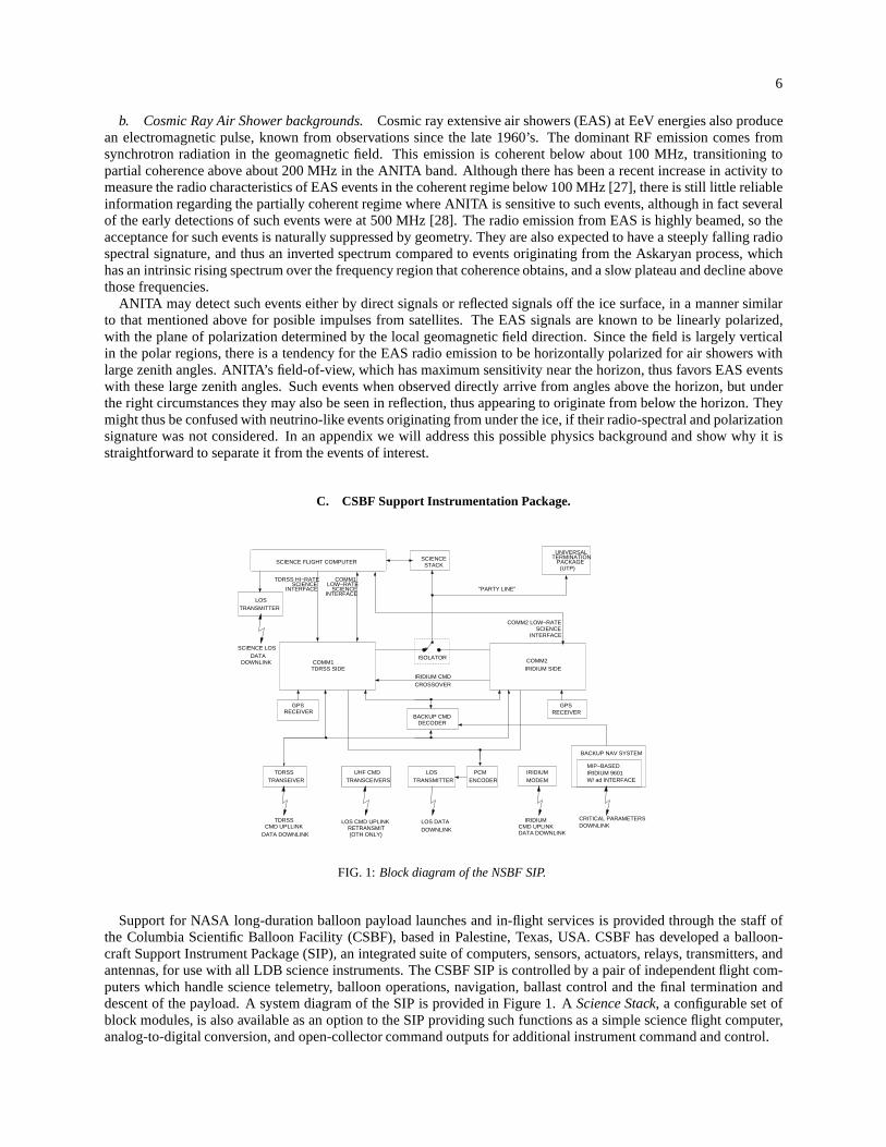
FIG. 1: Block diagram of the NSBF SIP.

Support for NASA long-duration balloon payload launches and in-flight services is provided through the staff ofthe Columbia Scientific Balloon Facility (CSBF), based in Palestine, Texas, USA. CSBF has developed a balloon-craft Support Instrument Package (SIP), an integrated suite of computers, sensors, actuators, relays, transmitters,andantennas, for use with all LDB science instruments. The CSBFSIP is controlled by a pair of independent flight com-puters which handle science telemetry, balloon operations, navigation, ballast control and the final termination anddescent of the payload. A system diagram of the SIP is provided in Figure 1. AScience Stack, a configurable set ofblock modules, is also available as an option to the SIP providing such functions as a simple science flight computer,analog-to-digital conversion, and open-collector command outputs for additional instrument command and control.

7

The SIP also provides the telemetry link between the ANITA flight computer and data acquisition system andground based operations. Data from the ANITA computer is sent over serial lines to the SIP package which handlesrouting and transmission over line-of-sight (LOS), Tracking and Data Relay Satellite System (TDRSS), and IRIDIUMcommunication pathways. ANITA utilizes the NSBF SIP Science Stack to provide the ability to command the flightCPU system off and on and reboot the computer during flight.

With regard to computational resources of the SIP, these aredesigned to fulfill existing LDB requirements, includingpreserving a full archive of all telemetered data that is passed through the SIP from the science instrument. Thisfunction thus provides an additional redundant copy of the telemetered data that can be used if there is telemetry lossor corruption.

One important characteristic of the SIP relevant to ANITA isthat it is not highly shielded from producing local EMI,at least at the extremely low level required for compatibility with ANITA science goals. Of necessity the SIP was thusenclosed in an external Faraday housing, with connectors, and penetrators designed in a manner similar to what wasdone for the ANITA primary electronics instrumentation.

D. Gondola Structure.

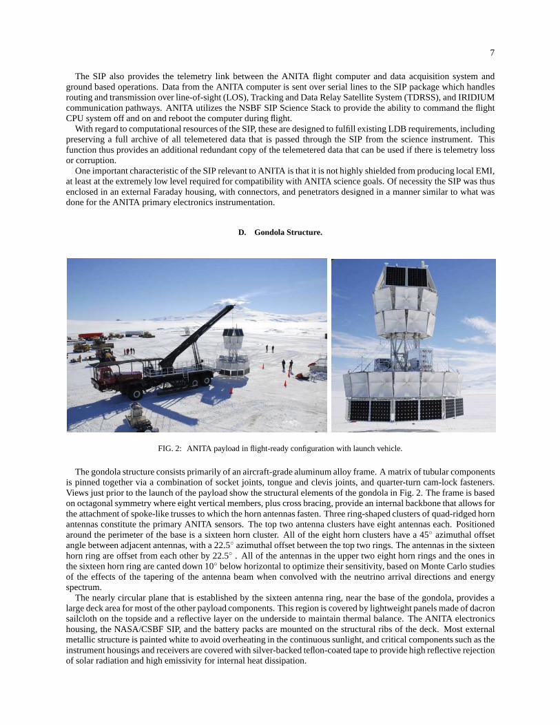
FIG. 2: ANITA payload in flight-ready configuration with launch vehicle.

The gondola structure consists primarily of an aircraft-grade aluminum alloy frame. A matrix of tubular componentsis pinned together via a combination of socket joints, tongue and clevis joints, and quarter-turn cam-lock fasteners.Views just prior to the launch of the payload show the structural elements of the gondola in Fig. 2. The frame is basedon octagonal symmetry where eight vertical members, plus cross bracing, provide an internal backbone that allows forthe attachment of spoke-like trusses to which the horn antennas fasten. Three ring-shaped clusters of quad-ridged hornantennas constitute the primary ANITA sensors. The top two antenna clusters have eight antennas each. Positionedaround the perimeter of the base is a sixteen horn cluster. All of the eight horn clusters have a 45 azimuthal offsetangle between adjacent antennas, with a 22.5 azimuthal offset between the top two rings. The antennas in the sixteenhorn ring are offset from each other by 22.5 . All of the antennas in the upper two eight horn rings and the ones inthe sixteen horn ring are canted down 10 below horizontal to optimize their sensitivity, based on Monte Carlo studiesof the effects of the tapering of the antenna beam when convolved with the neutrino arrival directions and energyspectrum.

The nearly circular plane that is established by the sixteenantenna ring, near the base of the gondola, provides alarge deck area for most of the other payload components. This region is covered by lightweight panels made of dacronsailcloth on the topside and a reflective layer on the underside to maintain thermal balance. The ANITA electronicshousing, the NASA/CSBF SIP, and the battery packs are mounted on the structural ribs of the deck. Most externalmetallic structure is painted white to avoid overheating inthe continuous sunlight, and critical components such as theinstrument housings and receivers are covered with silver-backed teflon-coated tape to provide high reflective rejectionof solar radiation and high emissivity for internal heat dissipation.

8

E. Power subsystem.

The ANITA power system is composed of a photovoltaic (PV) array, a charge controller, batteries, relays, and DC-to-DC converters. The PV array is an omni-directional arrayconsisting of eight panels configured in an octagon, withthe panels hanging vertically (see instrument figure). Although PV panels flown on high-altitude balloons are typicallyoriented at∼ 23 to the horizontal, in Antarctica, the large solar albedo from the ice results in more irradiance incidenton the panels (for most conditions) if they hang vertically.Each panel consists of 84 solar cells electrically connectedin series. They were mounted on frames made of aircraft-grade spruce wood with a coarse webbing (Shearweavestyle1000-P02) stretched on the frames.

The PV arrays were designed and fabricated by SunCat Solar. The solar cells used were Sunpower A-300 cellswith a rated efficiency of 21.5% and dimensions 12.5 cm squareand thickness 260 um. Bypass diodes were placed inparallel with successive groups of 12 cells within a panel (7-diodes/panel) to mitigate the effect of a possible single cellopen circuit failure during flight. Additionally, a blocking diode was placed between each panel output and the chargecontroller to prevent cross-charging of panels with different output voltages resulting from different illuminations andtemperatures. To reduce Fresnel reflection losses for high-refractive index silicon (n=3.46 at 700 nm), the silicon cellshad two anti-reflective (AR) coatings applied. An AR coatingwith refractive index n=1.92 was applied by the solarcell manufacturers. Additionally, during fabrication of the panels by SunCat Solar, a second AR coating with refractiveindex 1.47 was applied. This results in calculated Fresnel losses of 13-14% for incidence angles from 0 to 40.

The maximum power point (MPP) voltage and current generatedby these cells under standard conditions (STC) are0.560V and 5.54A respectively. However, the actual V and I vary considerably depending upon the irradiance and celltemperature. The single-cell temperature coefficient for the voltage is -1.9 mV/C. PV panel temperatures varied overthe range of -10C to +95C, depending upon the irradiance incident upon the cells. The temperatures were measured bysemiconductor temp sensors (AD590) glued to the back of cells. PV array circuit components (diodes) also introducelosses in the output voltage and power. The actual measured PV voltage input to the charge controller during the flightranged from 42.5 to 47 V (in good agreement with estimates using the cell temperature and temperature coefficient)and the current was about 9 A giving a total power of 400 W.

The omni-directional array is inherently an unbalanced system; i.e. the irradiance incident on each panel differs.For a given orientation of the gondola, some panels are directly irradiated by sunlight plus solar albedo from the iceand others are irradiated only indirectly from solar albedo. Additionally, for those that are directly irradiated, thesolar incidence angle is different. This results in individual panels that generate very different currents at any giventime. Because of the differing temperatures, the individual panels also have significantly different output voltages (thevoltage differences are small compared to the current differences) that feed into the charge controller. As mentionedabove, the blocking diodes prevent cross-charging of panels generating different voltages.

When using an unbalanced array, to achieve the maximum poweroutput, it is important to use a charge controllerthat senses and operates at the actual MPP as opposed to one that operates at a constant offset voltage from thearray open-circuit voltage. We used an Outback MX-60 chargecontroller to supply power to the ANITA instrument.Conductive heat sinks were installed on the power FETs and transistors and the heat was conducted to the instrumentradiator plate. We operated in the 24 V mode and flew nine pairsof 12 V Panasonic LC-X1220P (20 AH) lead acidbatteries that were charged by the charge controller and would have provided 12 hours of power in case of PV arrayfailure.

The Instrument Power box consisted of the MX-60 charge controller, solid-state power relays, and Vicor DC/DCconverters for the external radio-frequency conditional module (RFCM) amplifiers. The main power relays for thecPCI crate were controlled by discrete commands from the SIP. All other solid-state relays were controlled by theCPU, either under software control or by commands from the ground. The DC/DC box consisted of Vicor DC/DCconverters which provided the +5, +12, -12, +3.3, +1.5, and 5voltages required by the cPCI crate and peripherals. Allvoltages and currents were read by the housekeeping system.

F. Radio Frequency subsystem

1. Antennas.

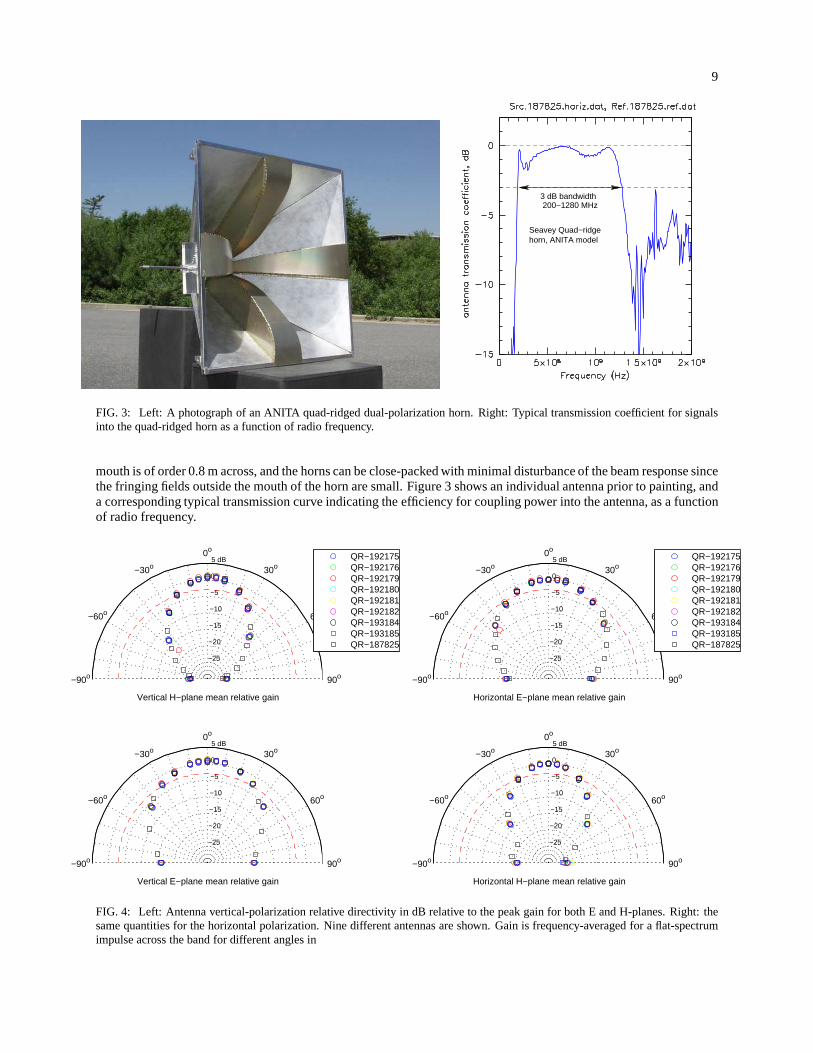
Figure 2 shows the ANITA payload configuration just prior to launch in late 2006 at Williams Field, Antarctica. Theindividual horns are a custom design produced for ANITA by Seavey Engineering, Inc., now a subsidiary of AntennaResearch Associates, Inc. These horns are the primary ANITAantennas, and may be thought of as a flared quad-ridgedwaveguide section; the back of the horn does in fact terminate in a short section of waveguide. The dimension of the

9

3 dB bandwidth200−1280 MHz

Seavey Quad−ridge horn, ANITA model

FIG. 3: Left: A photograph of an ANITA quad-ridged dual-polarization horn. Right: Typical transmission coefficient forsignalsinto the quad-ridged horn as a function of radio frequency.

mouth is of order 0.8 m across, and the horns can be close-packed with minimal disturbance of the beam response sincethe fringing fields outside the mouth of the horn are small. Figure 3 shows an individual antenna prior to painting, anda corresponding typical transmission curve indicating theefficiency for coupling power into the antenna, as a functionof radio frequency.

−25

−20

−15

−10

−5

0

5 dB

90o

60o

30o

0o

−30o

−60o

−90o

Vertical H−plane mean relative gain

−25

−20

−15

−10

−5

0

5 dB

90o

60o

30o

0o

−30o

−60o

−90o

Vertical E−plane mean relative gain

QR−192175QR−192176QR−192179QR−192180QR−192181QR−192182QR−193184QR−193185QR−187825

−25

−20

−15

−10

−5

0

5 dB

90o

60o

30o

0o

−30o

−60o

−90o

Horizontal E−plane mean relative gain


−25

−20

−15

−10

−5

0

5 dB

90o

60o

30o

0o

−30o

−60o

−90o

Horizontal H−plane mean relative gain

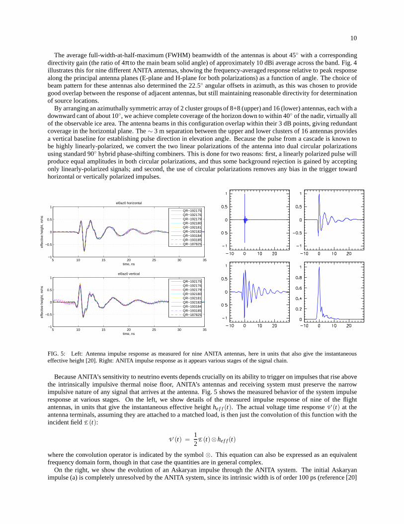
FIG. 4: Left: Antenna vertical-polarization relative directivity in dB relative to the peak gain for both E and H-planes. Right: thesame quantities for the horizontal polarization. Nine different antennas are shown. Gain is frequency-averaged for a flat-spectrumimpulse across the band for different angles in

10

The average full-width-at-half-maximum (FWHM) beamwidthof the antennas is about 45 with a correspondingdirectivity gain (the ratio of 4π to the main beam solid angle) of approximately 10 dBi averageacross the band. Fig. 4illustrates this for nine different ANITA antennas, showing the frequency-averaged response relative to peak responsealong the principal antenna planes (E-plane and H-plane forboth polarizations) as a function of angle. The choice ofbeam pattern for these antennas also determined the 22.5 angular offsets in azimuth, as this was chosen to providegood overlap between the response of adjacent antennas, butstill maintaining reasonable directivity for determinationof source locations.

By arranging an azimuthally symmetric array of 2 cluster groups of 8+8 (upper) and 16 (lower) antennas, each with adownward cant of about 10, we achieve complete coverage of the horizon down to within 40 of the nadir, virtually allof the observable ice area. The antenna beams in this configuration overlap within their 3 dB points, giving redundantcoverage in the horizontal plane. The∼ 3 m separation between the upper and lower clusters of 16 antennas providesa vertical baseline for establishing pulse direction in elevation angle. Because the pulse from a cascade is known tobe highly linearly-polarized, we convert the two linear polarizations of the antenna into dual circular polarizationsusing standard 90 hybrid phase-shifting combiners. This is done for two reasons: first, a linearly polarized pulse willproduce equal amplitudes in both circular polarizations, and thus some background rejection is gained by acceptingonly linearly-polarized signals; and second, the use of circular polarizations removes any bias in the trigger towardhorizontal or vertically polarized impulses.

5 10 15 20 25 30 35−1

−0.5

0

0.5

1el0az0 horizontal

time, ns

effe

ctiv

e he

ight

, m/n

s


5 10 15 20 25 30 35−1

−0.5

0

0.5

1el0az0 vertical

time, ns

effe

ctiv

e he

ight

, m/n

s


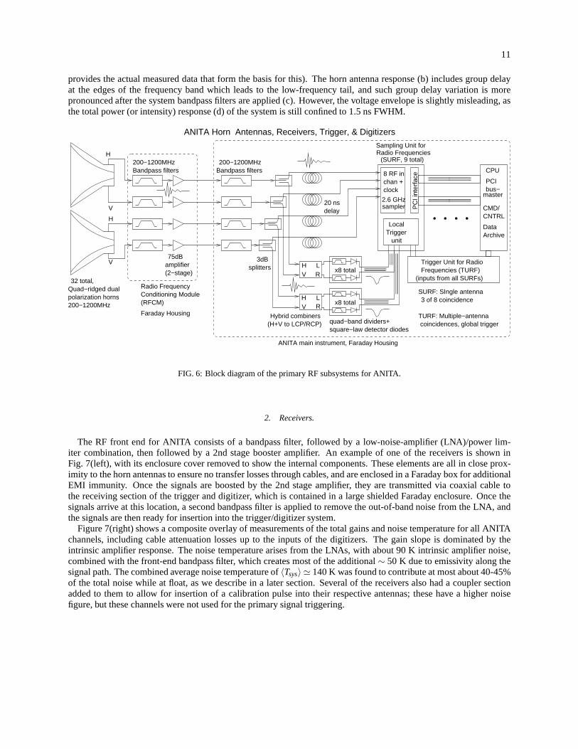
FIG. 5: Left: Antenna impulse response as measured for nine ANITA antennas, here in units that also give the instantaneouseffective height [20]. Right: ANITA impulse response as it appears various stages of the signal chain.

Because ANITA’s sensitivity to neutrino events depends crucially on its ability to trigger on impulses that rise abovethe intrinsically impulsive thermal noise floor, ANITA’s antennas and receiving system must preserve the narrowimpulsive nature of any signal that arrives at the antenna. Fig. 5 shows the measured behavior of the system impulseresponse at various stages. On the left, we show details of the measured impulse response of nine of the flightantennas, in units that give the instantaneous effective height he f f(t). The actual voltage time responseV (t) at theantenna terminals, assuming they are attached to a matched load, is then just the convolution of this function with theincident fieldE (t):

V (t) =12E (t)⊗he f f(t)

where the convolution operator is indicated by the symbol⊗. This equation can also be expressed as an equivalentfrequency domain form, though in that case the quantities are in general complex.

On the right, we show the evolution of an Askaryan impulse through the ANITA system. The initial Askaryanimpulse (a) is completely unresolved by the ANITA system, since its intrinsic width is of order 100 ps (reference [20]

11

provides the actual measured data that form the basis for this). The horn antenna response (b) includes group delayat the edges of the frequency band which leads to the low-frequency tail, and such group delay variation is morepronounced after the system bandpass filters are applied (c). However, the voltage envelope is slightly misleading, asthe total power (or intensity) response (d) of the system is still confined to 1.5 ns FWHM.

HV

LR

HV R

L

x8 total

x8 total

H

V

H

V

200−1200MHzBandpass filters

3dBsplitters

Trigger

sampler2.6 GHz

clock

8 RF inchan +

PC

I int

erfa

ce

Radio Frequencies Sampling Unit for

(SURF, 9 total)

unit

Local

Trigger Unit for RadioFrequencies (TURF)

(inputs from all SURFs)

bus−master

PCI

CPU

CMD/CNTRL

ArchiveData

Hybrid combiners(H+V to LCP/RCP) quad−band dividers+

square−law detector diodes

Bandpass filters200−1200MHz

32 total,Quad−ridged dualpolarization horns200−1200MHz

Radio FrequencyConditioning Module(RFCM)

Faraday Housing

ANITA main instrument, Faraday Housing

20 nsdelay

75dBamplifier(2−stage)

TURF: Multiple−antenna coincidences, global trigger

SURF: SIngle antenna3 of 8 coincidence

ANITA Horn Antennas, Receivers, Trigger, & Digitizers

FIG. 6: Block diagram of the primary RF subsystems for ANITA.

2. Receivers.

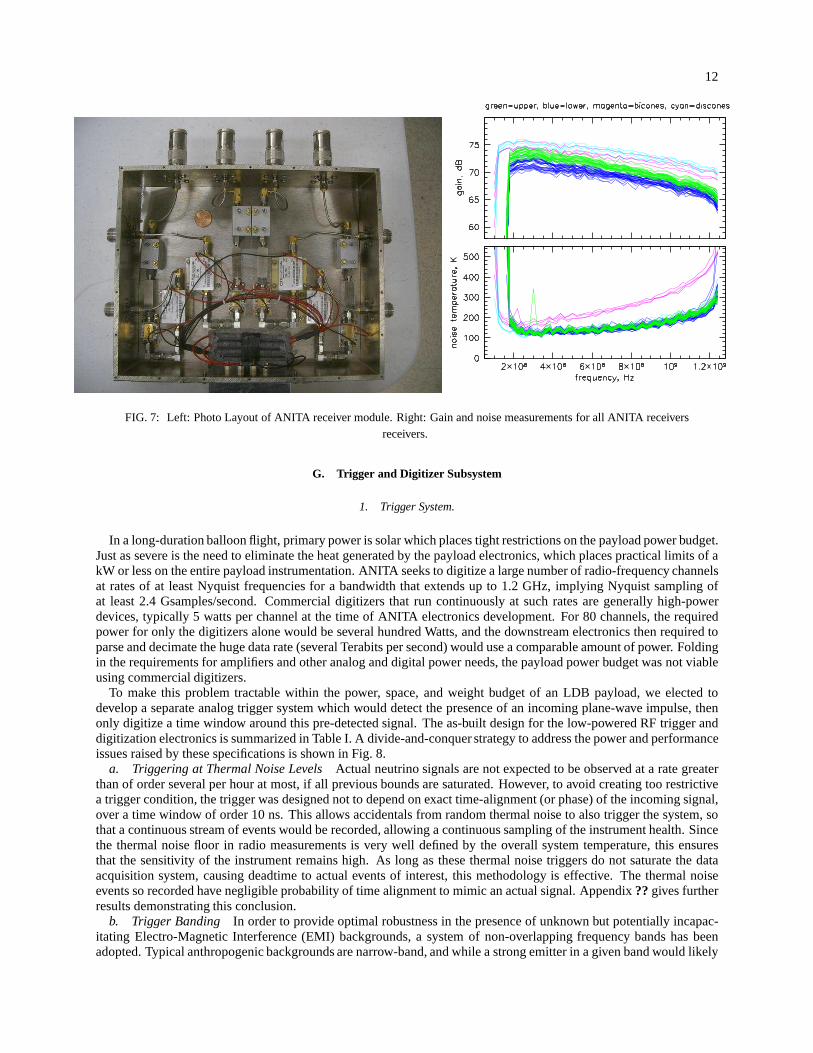
The RF front end for ANITA consists of a bandpass filter, followed by a low-noise-amplifier (LNA)/power lim-iter combination, then followed by a 2nd stage booster amplifier. An example of one of the receivers is shown inFig. 7(left), with its enclosure cover removed to show the internal components. These elements are all in close prox-imity to the horn antennas to ensure no transfer losses through cables, and are enclosed in a Faraday box for additionalEMI immunity. Once the signals are boosted by the 2nd stage amplifier, they are transmitted via coaxial cable tothe receiving section of the trigger and digitizer, which iscontained in a large shielded Faraday enclosure. Once thesignals arrive at this location, a second bandpass filter is applied to remove the out-of-band noise from the LNA, andthe signals are then ready for insertion into the trigger/digitizer system.

Figure 7(right) shows a composite overlay of measurements of the total gains and noise temperature for all ANITAchannels, including cable attenuation losses up to the inputs of the digitizers. The gain slope is dominated by theintrinsic amplifier response. The noise temperature arisesfrom the LNAs, with about 90 K intrinsic amplifier noise,combined with the front-end bandpass filter, which creates most of the additional∼ 50 K due to emissivity along thesignal path. The combined average noise temperature of〈Tsys〉 ≃ 140 K was found to contribute at most about 40-45%of the total noise while at float, as we describe in a later section. Several of the receivers also had a coupler sectionadded to them to allow for insertion of a calibration pulse into their respective antennas; these have a higher noisefigure, but these channels were not used for the primary signal triggering.

12

FIG. 7: Left: Photo Layout of ANITA receiver module. Right: Gain and noise measurements for all ANITA receiversreceivers.

G. Trigger and Digitizer Subsystem

1. Trigger System.

In a long-duration balloon flight, primary power is solar which places tight restrictions on the payload power budget.Just as severe is the need to eliminate the heat generated by the payload electronics, which places practical limits of akW or less on the entire payload instrumentation. ANITA seeks to digitize a large number of radio-frequency channelsat rates of at least Nyquist frequencies for a bandwidth thatextends up to 1.2 GHz, implying Nyquist sampling ofat least 2.4 Gsamples/second. Commercial digitizers that run continuously at such rates are generally high-powerdevices, typically 5 watts per channel at the time of ANITA electronics development. For 80 channels, the requiredpower for only the digitizers alone would be several hundredWatts, and the downstream electronics then required toparse and decimate the huge data rate (several Terabits per second) would use a comparable amount of power. Foldingin the requirements for amplifiers and other analog and digital power needs, the payload power budget was not viableusing commercial digitizers.

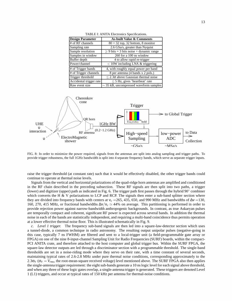
To make this problem tractable within the power, space, and weight budget of an LDB payload, we elected todevelop a separate analog trigger system which would detectthe presence of an incoming plane-wave impulse, thenonly digitize a time window around this pre-detected signal. The as-built design for the low-powered RF trigger anddigitization electronics is summarized in Table I. A divide-and-conquer strategy to address the power and performanceissues raised by these specifications is shown in Fig. 8.

a. Triggering at Thermal Noise LevelsActual neutrino signals are not expected to be observed at a rate greaterthan of order several per hour at most, if all previous boundsare saturated. However, to avoid creating too restrictivea trigger condition, the trigger was designed not to depend on exact time-alignment (or phase) of the incoming signal,over a time window of order 10 ns. This allows accidentals from random thermal noise to also trigger the system, sothat a continuous stream of events would be recorded, allowing a continuous sampling of the instrument health. Sincethe thermal noise floor in radio measurements is very well defined by the overall system temperature, this ensuresthat the sensitivity of the instrument remains high. As longas these thermal noise triggers do not saturate the dataacquisition system, causing deadtime to actual events of interest, this methodology is effective. The thermal noiseevents so recorded have negligible probability of time alignment to mimic an actual signal. Appendix??gives furtherresults demonstrating this conclusion.

b. Trigger Banding In order to provide optimal robustness in the presence of unknown but potentially incapac-itating Electro-Magnetic Interference (EMI) backgrounds, a system of non-overlapping frequency bands has beenadopted. Typical anthropogenic backgrounds are narrow-band, and while a strong emitter in a given band would likely

13

TABLE I: ANITA Electronics Specifications.

Design Parameter As-built Value & Comments# of RF channels 80 = 32 top, 32 bottom, 8 monitorSampling rate 2.6 GSa/s, greater than NyquistSample resolution ≥ 9 bits = 3 bits noise + dynamic rangeSamples in window 260 for a 100 ns windowBuffer depth 4 to allow rapid re-triggerPower/channel < 10W including LNA & triggering

# of Trigger bands 4, with roughly equal power per band# of Trigger channels 8 per antenna (4 bands x 2 pols.)Trigger threshold ≤ 2.3σ above Gaussian thermal noiseAccidental trigger rate ≤ 5 Hz, gives ’heartbeat’ rateRaw event size ∼ 35 kB, uncompressed waveform samples

Collection

High−speedSampling

1GHz BW

(0.2−1.2 GHz)

to Global Trigger

low−powerADC

~MSa/s~GSa/s

Trigger

hold

ElectroMagnetic

Cherenkov

interaction

UHEυ

showerυ

cone

RF antenna

QR hornFreq (GHz)

to Data

FIG. 8: In order to minimize the power required, signals fromthe antennas are split into analog sampling and trigger paths. Toprovide trigger robustness, the full 1GHz bandwidth is split into 4 separate frequency bands, which serve as separate trigger inputs.

raise the trigger threshold (at constant rate) such that it would be effectively disabled, the other trigger bands couldcontinue to operate at thermal noise levels.

Signals from the vertical and horizontal polarizations of the quad-ridge horn antennas are amplified and conditionedin the RF chain described in the preceding subsection. TheseRF signals are then split into two paths, a trigger(lower) and digitizer (upper) path as indicated in Fig. 6. The trigger path first passes through the hybrid 90 combinerwhich converts the H & V polarizations to LCP and RCP. The signals then enter a sub-band splitter section wherethey are divided into frequency bands with centers atνc =265, 435, 650, and 990 MHz and bandwidths of∆ν =130,160, 270, 415 MHz, or fractional bandwidths∆ν/νc ≃ 44% on average. This partitioning is performed in order toprovide rejection power against narrow-bandwidth anthropogenic backgrounds. In contrast, as true Askaryan pulsesare temporally compact and coherent, significant RF power isexpected across several bands. In addition the thermalnoise in each of the bands are statistically independent, and requiring a multi-band coincidence thus permits operationat a lower effective thermal noise floor. This is illustratedschematically in Fig. 9.

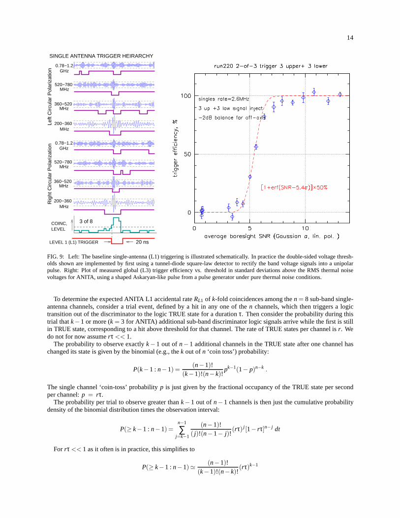
c. Level 1 trigger. The frequency sub-band signals are then led into a square-law-detector section which usesa tunnel-diode, a common technique in radio astronomy. The resulting output unipolar pulses (negative-going inthis case, typically 7 ns FWHM) are filtered and sent to a local-trigger unit (a field-programmable gate array orFPGA) on one of the nine 8-input-channel Sampling Unit for Radio Frequencies (SURF) boards, within the compact-PCI ANITA crate, and therefore attached to the host computerand global trigger bus. Within the SURF FPGA, thesquare-law detector outputs are led through a discriminator section with a programmable threshold. The single-bandthresholds are set in a noise-riding mode where they servo ontheir rate, with a time constant of several seconds,maintaining typical rates of 2.6-2.8 MHz under pure thermalnoise conditions, corresponding approximately to the2.3σV (σV = Vrms, the root-mean-square received voltage) level mentioned above. The SURF FPGA also then appliesthe single-antenna trigger requirement: the eight sub-bands generate a 10 ns logic level for each signal above threshold,and when any three of these logic gates overlap, a single-antenna trigger is generated. These triggers are denoted Level1 (L1) triggers, and occur at typical rates of 150 kHz per antenna for thermal-noise conditions.

14

0.78−1.2GHz

520−780MHz

360−520MHz

200−360MHz

0.78−1.2GHz

520−780MHz

360−520MHz

200−360MHz

Rig

ht C

ircul

ar P

olar

izat

ion

Left

Circ

ular

Pol

ariz

atio

n

COINC,LEVEL

SINGLE ANTENNA TRIGGER HEIRARCHY

3 of 8

20 nsLEVEL 1 (L1) TRIGGER

FIG. 9: Left: The baseline single-antenna (L1) triggering is illustrated schematically. In practice the double-sidedvoltage thresh-olds shown are implemented by first using a tunnel-diode square-law detector to rectify the band voltage signals into a unipolarpulse. Right: Plot of measured global (L3) trigger efficiency vs. threshold in standard deviations above the RMS thermalnoisevoltages for ANITA, using a shaped Askaryan-like pulse froma pulse generator under pure thermal noise conditions.

To determine the expected ANITA L1 accidental rateRL1 of k-fold coincidences among then = 8 sub-band single-antenna channels, consider a trial event, defined by a hit in any one of then channels, which then triggers a logictransition out of the discriminator to the logic TRUE state for a durationτ. Then consider the probability during thistrial thatk−1 or more (k = 3 for ANITA) additional sub-band discriminator logic signals arrive while the first is stillin TRUE state, corresponding to a hit above threshold for that channel. The rate of TRUE states per channel isr. Wedo not for now assumerτ << 1.

The probability to observe exactlyk−1 out ofn−1 additional channels in the TRUE state after one channel haschanged its state is given by the binomial (e.g., thek out ofn ‘coin toss’) probability:

P(k−1 : n−1) =(n−1)!

(k−1)!(n−k)!pk−1(1− p)n−k .

The single channel ‘coin-toss’ probabilityp is just given by the fractional occupancy of the TRUE state per secondper channel:p = rτ.

The probability per trial to observe greater thank−1 out ofn−1 channels is then just the cumulative probabilitydensity of the binomial distribution times the observationinterval:

P(≥ k−1 : n−1) =n−1

∑j=k−1

(n−1)!( j)!(n−1− j)!

(rτ) j [1− rτ]n− j dt

For rτ << 1 as it often is in practice, this simplifies to

P(≥ k−1 : n−1)≃ (n−1)!(k−1)!(n−k)!

(rτ)k−1

15

since only the leading term in the sum contributes significantly and the term 1− rτ ≃ 1.The rate is then determined by multiplying the single-trialprobability by the number of ensemble trials per second,

which is just equal to the total number of channels times the singles rate per channel. The singles rate per channel isgiven simply byr, and the total singles rate across all channels isnr. Thus the total rate in the limit ofrτ << 1, is:

RL1 = nrP(≥ k−1 : n−1)≃ n(n−1)!

(k−1)!(n−k)!rkτk−1 =

(n)!(k)!(n−k)!

krkτk−1 .

d. Level 2 trigger. When a given SURF module detects an L1 trigger, indicating either a possible signal or (mostprobably) a thermal noise fluctuation, it reports this immediately to the Trigger Unit for Radio Frequencies (TURF)module, which occupies a portion of the compact-PCI backplane common to all of the SURF modules. The TURFcontains another FPGA, which determines whether a level 2 (L2) trigger, which corresponds to two L1 events in anyadjacent antennas of either the upper or lower ring, within a20 ns window, has occurred. L2 triggers occur at rate ofabout 2.5 Khz per antenna pair, or about 40 kHz aggregate ratefor thermal noise.

e. Level 3 trigger. If a pair of L2s occur in the upper and lower rings within a 30 nswindow and any up-downpair of the antennas share the same azimuthal sector (known as a “phi sector”), a level 3 (L3) global trigger is issued,and the digitization of the event proceeds. These occur at a rate of about 4-5 Hz for thermal noise. Fig. 9(right) shows ameasurement of the effective threshold for L3 triggers in terms of the peak pulse SNR above thermal noise. Here threeupper and three lower antennas were stimulated with a shapedpulse and the L3 rate was measured as a function ofthe input pulse SNR to estimate the effective global threshold, here in Gaussian standard deviations above the thermalnoise RMS voltage. ANITA begins to respond at about 4σV , reaches of order 50% efficiency at 5.4σV and is fullyefficient at of order∼ 7σV .

In Appendix B 4, we further analyze the rate of accidentals interms of their ability to reconstruct coherently tomimic a true signal event, and we find that the chance probability for this is of order 0.003 events for the ANITA flight,presenting a negligible background.

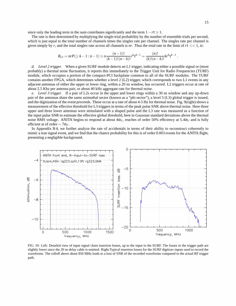
FIG. 10: Left: Detailed view of input signal chain insertionlosses, up to the input to the SURF. The losses in the trigger path areslightly lower since the 20 ns delay cable is omitted. Right:Typical insertion losses for the SURF digitizer inputs usedto record thewaveforms. The rolloff above about 850 MHz leads to a loss of SNR of the recorded waveforms compared to the actual RF triggerpath.

16

2. Digitizer System.

The upper path in Figure 6 is the digitization path. A low-power, high sampling-speed Switched Capacitor Array(SCA) continuously samples the raw RF inputs over the entire1 GHz of analog bandwidth defined by the upstream RFconditioning, at a sample rate of 2.6 Gsamples/s. Sampling is halted and the analog waveform samples held for readoutupon the fulfillment of a trigger condition. The SCA sampler,which does not actually digitize its stored samples untilcommanded to do so for a trigger, uses far lower power than traditional high speed continuous-digitizing samplers(such as oscilloscopes). Without the custom development ofthis technology by G. Varner of the ANITA team, thepower budget for ANITA would have grown substantially, fromof order 1 W/ch to perhaps 10 W per channel for acommercial digitizer as was used for ANITA-lite [24]. In addition, the continuously sampled data would have addeda processing load of order 200 Gbyte/sec to the trigger system.

Fig. 10 shows measurements of the signal chain and SURF channel insertion loss vs. radio frequency. On the left,the losses up to the input of the SURFs are shown; these are primarily cable and second-stage bandpass filter losses.Similar losses apply to the trigger path as well, though slightly lower since there is no 20 ns delay cable in that path. Onthe right, the SURF insertion losses are shown, and these areunique to the waveform recording path. The loss aboveabout 850 MHz tend to significantly reduce the intrinsic peakvoltages in the most impulsive waveforms compared towhat is seen by the analog trigger inputs. These amplitude losses can be corrected to some degree as shown in a latersection, but there is still a net loss of SNR in the deconvolved waveforms compared to what is seen by the trigger path.

It is evident from this plot that ANITA’s digitizers did not fully achieve the design input bandwidth span of 200-1200MHz; the last quarter of this band has reduced response compared to the design goal. The main impact of this is notto reduce the trigger sensitivity of the instrument, since the digitizer does not constrain the input bandwidth of thetrigger system. Rather, the primary impact is in evaluationof potential neutrino candidates, for which we would liketo be able to reconstruct an accurate spectral density for the received radio signal. For the current digitizer system, thereconstructed spectral content above 900 MHz will thus be subject to errors that increase with frequency; however,this frequency region is also the region where ice attenuation is rising quickly [29].

H. Navigation, attitude, & timing

a. Absolute Orientation. In order to geometrically reconstruct neutrino events, accurate position, altitude, abso-lute time, and pointing information are required. To provide such data on an event-by-event basis, a pair of GlobalPositioning System (GPS) units was used. They provide more than sufficient accuracy to fulfill the science require-ments, see Table 20. In addition these units provide the ability to synchronously trigger and read out the systemon an absolute timing mark (such as the nearest second), a feature which is essential to the ground-to-flight calibra-tion sequence, where a ground transmitter needs to be globally synchronized to the system during flight, including apropagation delay offset.

ANITA had a mission-critical requirement for accurate payload orientation knowledge, to ensure that the free-rotation of the payload would not preclude reconstruction of directions for events at the sub-degree level of accuracy.Such measurements were accomplished with a redundant system of 4 sun-sensors, a magnetometer, and a differentialGPS attitude measurement system (Thales Navigation/Magellan ADU5). These systems performed well in flight andmet the mission design goals. In calibration done just priorto ANITA’s 2006 launch, we measured a total(∆φ)RMS=0.071, very close to the limit of the ADU5 sensor specification, andwell within our allocated error budget.

The ADU5 is connected to the flight computer with a pair of RS-232 interfaces; one carries the attitude informationpackets for the housekeeping readout, and the second provides readout when during the UTC second a digital triggerline was set at the ADU5. The second GPS unit, a G12 sensor fromThales, is used to get a second trigger timing pieceof information over one serial line and timing information for the flight computer’s NTP (Network Time Protocol)internal clock. Position and attitude information is updated every second. Also every second the NTP server gets anupdate to keep good overall clock time at the computer. The trigger is also connected directly to GPS time: GPSsecond from the 1-second readout and fraction of a second from the phototiming data block. Additional pointinginformation is derived from the sun sensors and a tip-tilt sensor mounted near the experiment’s center of mass. Theyprovide a simple crosscheck to the attitude data with very different systematics and also offer a measure of redundancy.

17

TABLE II: Navigation, attitude, and timing sensor requirements and provided accuracy.

Parameter Determination method Required Accuracy System Accuracy

Position/Altitude Ordinary GPS 10m horiz./20m vert.5m Horizontal/10m VerticalUTC GPS Phototiming pulse 20ns < 10nsPointing Short-baseline differential GPS0.3 rotation/0.3 tip < 0.07/< 0.14

Pointing Sun-sensorTip-tilt sensor 0.3 rotation/0.3 tip 1/1

IV. FLIGHT SOFTWARE & DATA ACQUISITION

The ANITA-I flight computer was a standard c-PCI single boardcomputer, based on the Intel Mobile Pentium IIICPU. The operating system was Red Hat 9 Linux, which was selected due to driver availability.

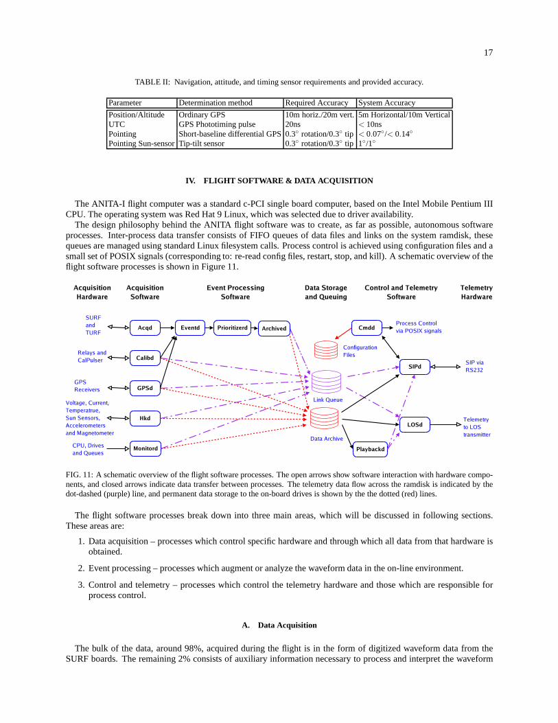
The design philosophy behind the ANITA flight software was tocreate, as far as possible, autonomous softwareprocesses. Inter-process data transfer consists of FIFO queues of data files and links on the system ramdisk, thesequeues are managed using standard Linux filesystem calls. Process control is achieved using configuration files and asmall set of POSIX signals (corresponding to: re-read configfiles, restart, stop, and kill). A schematic overview of theflight software processes is shown in Figure 11.

FIG. 11: A schematic overview of the flight software processes. The open arrows show software interaction with hardware compo-nents, and closed arrows indicate data transfer between processes. The telemetry data flow across the ramdisk is indicated by thedot-dashed (purple) line, and permanent data storage to theon-board drives is shown by the the dotted (red) lines.

The flight software processes break down into three main areas, which will be discussed in following sections.These areas are:

1. Data acquisition – processes which control specific hardware and through which all data from that hardware isobtained.

2. Event processing – processes which augment or analyze thewaveform data in the on-line environment.

3. Control and telemetry – processes which control the telemetry hardware and those which are responsible forprocess control.

A. Data Acquisition

The bulk of the data, around 98%, acquired during the flight isin the form of digitized waveform data from theSURF boards. The remaining 2% consists of auxiliary information necessary to process and interpret the waveform

18

data (payload position, trigger thresholds, etc.) and datathat is used to monitor the health of the instrument duringflight (temperatures, voltages, disk spaces, etc.).

1. Waveform Data

The process that is responsible for the digitization and triggering hardware, the SURF and TURF, is Acqd (theAcquisition Daemon). The Acqd process has four main tasks:

• Acquiring waveform data from the SURFs

• Acquiring trigger and timing data from the TURF (via TURFIO).

• Acquiring housekeeping data from the SURF (scaler rates, read back thresholds, and RF power).

• Setting the thresholds and trigger band masks to control thetrigger, dynamically adjusting the thresholds tomaintain a constant rate.

Once the TURF has triggered an event and the SURFs’ have finished digitizing, the event data is available fortransfer across the c-PCI backplane to the flight computer. The flight computer polls the SURFs to check when anevent has finished digitization and the data is ready to be transferred across the c-PCI backplane.

An event consists of 260 16-bit waveform data words per channel, there are 9 channels per SURF and 9 SURFs inthe c-PCI crate. A complete raw event is approximately 41KB.To achieve better compression, see Section IV B 2, theraw waveform data is pedestal subtracted before being written to the queue for event processing.

2. Trigger Control

In addition to acquiring the waveform and trigger data, Acqdis also responsible for setting the thresholds and triggerband masks that control the trigger. There are three handlesthrough which Acqd can control the trigger:

• The single channel trigger thresholds (256 channels).

• The trigger band masks (8 channels per antenna).

• The antenna trigger mask (32 antennas in total).

The default mode of operation is to have all of the masks off, such that every trigger band and every antenna canparticipate in the trigger. In the thermal regime, i.e. awayfrom anthropogenic RF noise sources such as camps andbases, the trigger control operates by dynamically adjusting the single channel thresholds to ensure that each triggerchannel triggers at the same rate (typically 2-3MHz). The dynamic adjusting of the thresholds is necessary as evenaway from man-made noise sources the RF power in view varies with the temperature of the antenna and its fieldof view, i.e with the position of the sun and galactic center with respect to the antenna. The thresholds are variedusing a simple PID (proportional integral differential) servo loop that was tuned in the laboratory using RFCMs withterminated inputs.

During times when the balloon is in view of large noise sources, such as McMurdo station, a different trigger-ing regime is necessary to avoid swamping the downstream processes with an unmanageable event rate. To allowfor this all of the trigger control options are commandable from the ground, see Section IV C 2 for more details oncommanding. Using these commands some of the available options for controlling the trigger rate are:

• Adjust the global desired single trigger channel rate.

• Adjust individual single channel rates independently.

• Remove individual trigger channels (i.e. frequency bands)from the antenna level (L1) trigger.

• Remove individual antennas from the L2 and L3 triggers.

19

3. Housekeeping Data

In addition to the waveform data, housekeeping data is also continuously captured, both for use in event analysisand also for monitoring the health of the instrument during flight. Table III is a summary of the various types ofhousekeeping data acquired by the flight software processes.

Process Housekeeping Data RateAcqd Trigger rates and average RF power up to 5 HzCalibd Relay status 0.03 HzGPSd GPS position, velocity, attitude, satellites, etc.up to 5 HzHkd Voltages, currents, temperatures, pressures, etc.up to 5 Hz

Monitord CPU and disk drive status 0.03 Hz

TABLE III: The types of housekeeping data acquired by flight software processes.

B. On-line Event Processing

At altitude the bandwidth for downloading data from the payload to the ground systems is very limited, see Sec-tion IV C 1. In order to maximize the usage of this limited resource the events are processed on-line to determine theevent priority and they are compressed and split into a suitable format for telemetry.

1. Prioritization

The Prioritizerd daemon is responsible for determining thepriority of an event. This priority is used to determinethe likelihood of a given event being telemetered to the ground during flight. The prioritizer looks at a number of eventcharacteristics to determine priority. The hierarchical priority determination is described below:

• Priority 9 – If too many waveforms (configurable) have a peak in the FFT spectrum (configurable), the event isgiven this low priority, to veto events from strong narrow band noise sources.

• Priority 8 – If two many channels peak simultaneously, determined via matched filter cross-correlation, the eventis assumed to be generated on-payload and is rejected.

• Priority 7 – Compares the RMS of the beginning and end of waveforms to veto non-impulsive events.

• Priority 6 – This is the default priority. Thermal noise events will be assigned this priority if they are not demotedfor one of the above reasons, or promoted for one of the below reasons.

• Priority 5 – An event is promoted to priority five if it passes the test of N of M (configurable) neighboringantennas peaking within a time window (configurable). Events must satisfy this condition to be c onsidered forpromotion to priorities 1-4.

• Priority 4 – A cross-correlation is performed with boxcar smoothing, and there are peaks in 2-of-2 antennas inone ring and 1-of-2 in the other.

• Priority 3 – A cross-correlation is performed with boxcar smoothing, and there are peaks in 2-of-3 antennas inboth rings.



20

2. Compression

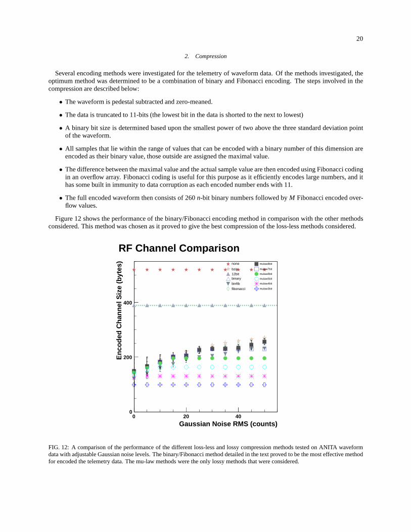
Several encoding methods were investigated for the telemetry of waveform data. Of the methods investigated, theoptimum method was determined to be a combination of binary and Fibonacci encoding. The steps involved in thecompression are described below:

• The waveform is pedestal subtracted and zero-meaned.

• The data is truncated to 11-bits (the lowest bit in the data isshorted to the next to lowest)

• A binary bit size is determined based upon the smallest powerof two above the three standard deviation pointof the waveform.

• All samples that lie within the range of values that can be encoded with a binary number of this dimension areencoded as their binary value, those outside are assigned the maximal value.

• The difference between the maximal value and the actual sample value are then encoded using Fibonacci codingin an overflow array. Fibonacci coding is useful for this purpose as it efficiently encodes large numbers, and ithas some built in immunity to data corruption as each encodednumber ends with 11.

• The full encoded waveform then consists of 260n-bit binary numbers followed byM Fibonacci encoded over-flow values.

Figure 12 shows the performance of the binary/Fibonacci encoding method in comparison with the other methodsconsidered. This method was chosen as it proved to give the best compression of the loss-less methods considered.

Gaussian Noise RMS (counts)0 20 40

Enc

oded

Cha

nnel

Siz

e (b

ytes

)

0

200

400

RF Channel Comparisonnone

bzip12bitbinary

binfib

fibonacci

mulaw8bit

mulaw7bit

mulaw6bit

mulaw5bit

mulaw4bit

mulaw3bit

FIG. 12: A comparison of the performance of the different loss-less and lossy compression methods tested on ANITA waveformdata with adjustable Gaussian noise levels. The binary/Fibonacci method detailed in the text proved to be the most effective methodfor encoded the telemetry data. The mu-law methods were the only lossy methods that were considered.

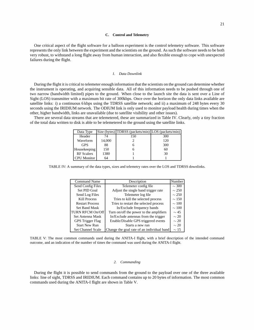
21

C. Control and Telemetry

One critical aspect of the flight software for a balloon experiment is the control telemetry software. This softwarerepresents the only link between the experiment and the scientists on the ground. As such the software needs to be bothvery robust, to withstand a long flight away from human interaction, and also flexible enough to cope with unexpectedfailures during the flight.

1. Data Downlink

During the flight it is critical to telemeter enough information that the scientists on the ground can determine whetherthe instrument is operating, and acquiring sensible data. All of this information needs to be pushed through one oftwo narrow (bandwidth limited) pipes to the ground. When close to the launch site the data is sent over a Line ofSight (LOS) transmitter with a maximum bit rate of 300kbps. Once over the horizon the only data links available aresatellite links: i) a continuous 6 kbps using the TDRSS satellite network; and ii) a maximum of 248 bytes every 30seconds using the IRIDIUM network. The ODIUM link is only used to monitor payload health during times when theother, higher bandwidth, links are unavailable (due to satellite visibility and other issues).

There are several data streams that are telemetered, these are summarized in Table IV. Clearly, only a tiny fractionof the total data written to disk is able to be telemetered to the ground using the satellite links.

Data Type Size (bytes)TDRSS (packets/min)LOS (packets/min)Header 74 150 300

Waveform 14,000 2 120GPS 88 6 300

Housekeeping 150 6 60RF Scalers 1380 1 30

CPU Monitor 64 1 1

TABLE IV: A summary of the data types, sizes and telemetry rates over the LOS and TDRSS downlinks.

Command Name Description NumberSend Config Files Telemeter config file ∼ 300

Set PID Goal Adjust the single band trigger rate ∼ 250Send Log Files Telemeter log file ∼ 250

Kill Process Tries to kill the selected process ∼ 150Restart Process Tries to restart the selected process ∼ 100Set Band Mask In/Exclude frequency bands ∼ 100

TURN RFCM On/Off Turn on/off the power to the amplifiers ∼ 45Set Antenna Mask In/Exclude antennas from the trigger ∼ 20GPS Trigger Flag Enable/Disable GPS triggered events ∼ 20

Start New Run Starts a new run ∼ 20Set Channel Scale Change the goal rate of an individual band∼ 15

TABLE V: The most common commands used during the ANITA-I flight, with a brief description of the intended commandoutcome, and an indication of the number of times the commandwas used during the ANITA-I flight.

2. Commanding

During the flight it is possible to send commands from the ground to the payload over one of the three availablelinks: line of sight, TDRSS and IRIDIUM. Each command contains up to 20 bytes of information. The most commoncommands used during the ANITA-I flight are shown in Table V.

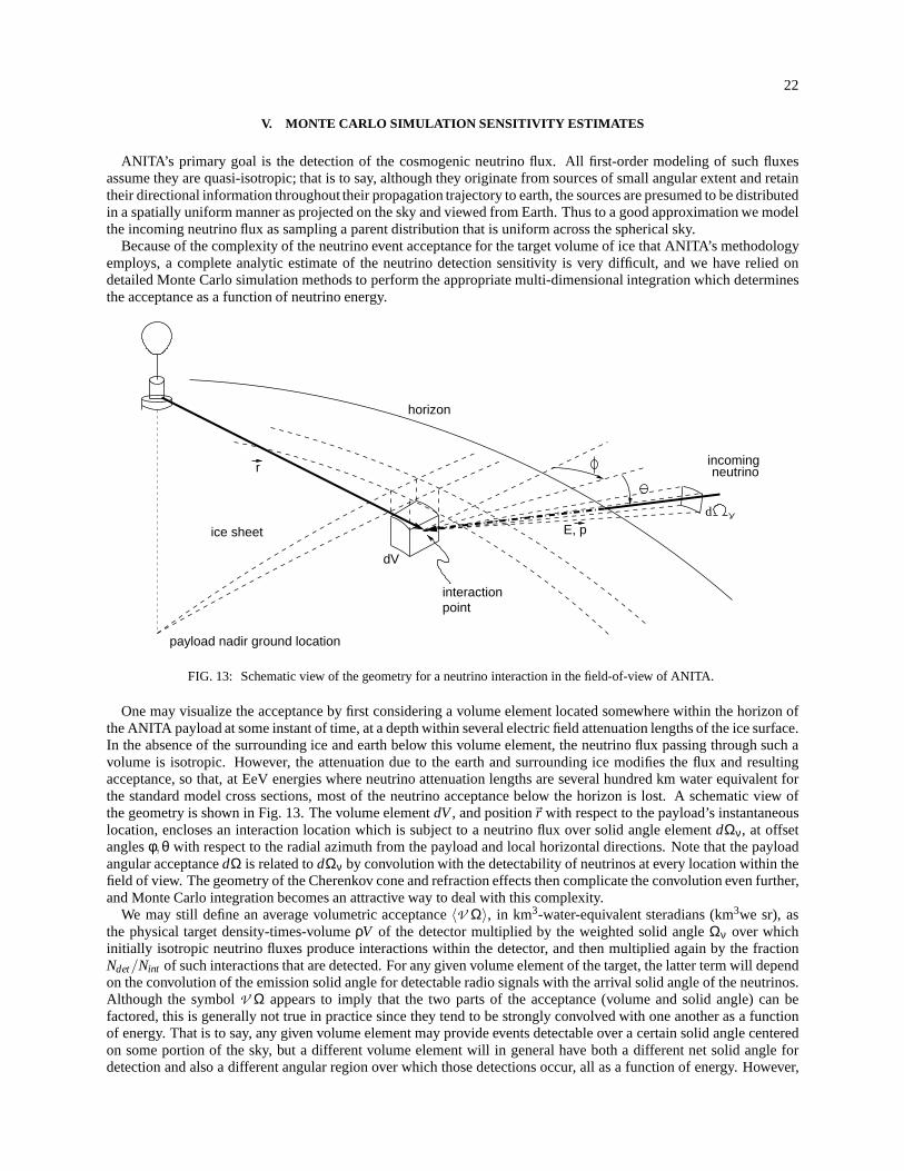
22

V. MONTE CARLO SIMULATION SENSITIVITY ESTIMATES

ANITA’s primary goal is the detection of the cosmogenic neutrino flux. All first-order modeling of such fluxesassume they are quasi-isotropic; that is to say, although they originate from sources of small angular extent and retaintheir directional information throughout their propagation trajectory to earth, the sources are presumed to be distributedin a spatially uniform manner as projected on the sky and viewed from Earth. Thus to a good approximation we modelthe incoming neutrino flux as sampling a parent distributionthat is uniform across the spherical sky.

Because of the complexity of the neutrino event acceptance for the target volume of ice that ANITA’s methodologyemploys, a complete analytic estimate of the neutrino detection sensitivity is very difficult, and we have relied ondetailed Monte Carlo simulation methods to perform the appropriate multi-dimensional integration which determinesthe acceptance as a function of neutrino energy.

d

r

E, p

payload nadir ground location

pointinteraction

dV

ice sheet

neutrinoincoming

horizon

FIG. 13: Schematic view of the geometry for a neutrino interaction in the field-of-view of ANITA.

One may visualize the acceptance by first considering a volume element located somewhere within the horizon ofthe ANITA payload at some instant of time, at a depth within several electric field attenuation lengths of the ice surface.In the absence of the surrounding ice and earth below this volume element, the neutrino flux passing through such avolume is isotropic. However, the attenuation due to the earth and surrounding ice modifies the flux and resultingacceptance, so that, at EeV energies where neutrino attenuation lengths are several hundred km water equivalent forthe standard model cross sections, most of the neutrino acceptance below the horizon is lost. A schematic view ofthe geometry is shown in Fig. 13. The volume elementdV, and position~r with respect to the payload’s instantaneouslocation, encloses an interaction location which is subject to a neutrino flux over solid angle elementdΩν, at offsetanglesφ,θ with respect to the radial azimuth from the payload and localhorizontal directions. Note that the payloadangular acceptancedΩ is related todΩν by convolution with the detectability of neutrinos at everylocation within thefield of view. The geometry of the Cherenkov cone and refraction effects then complicate the convolution even further,and Monte Carlo integration becomes an attractive way to deal with this complexity.

We may still define an average volumetric acceptance〈V Ω〉, in km3-water-equivalent steradians (km3we sr), asthe physical target density-times-volumeρV of the detector multiplied by the weighted solid angleΩν over whichinitially isotropic neutrino fluxes produce interactions within the detector, and then multiplied again by the fractionNdet/Nint of such interactions that are detected. For any given volumeelement of the target, the latter term will dependon the convolution of the emission solid angle for detectable radio signals with the arrival solid angle of the neutrinos.Although the symbolV Ω appears to imply that the two parts of the acceptance (volumeand solid angle) can befactored, this is generally not true in practice since they tend to be strongly convolved with one another as a functionof energy. That is to say, any given volume element may provide events detectable over a certain solid angle centeredon some portion of the sky, but a different volume element will in general have both a different net solid angle fordetection and also a different angular region over which those detections occur, all as a function of energy. However,

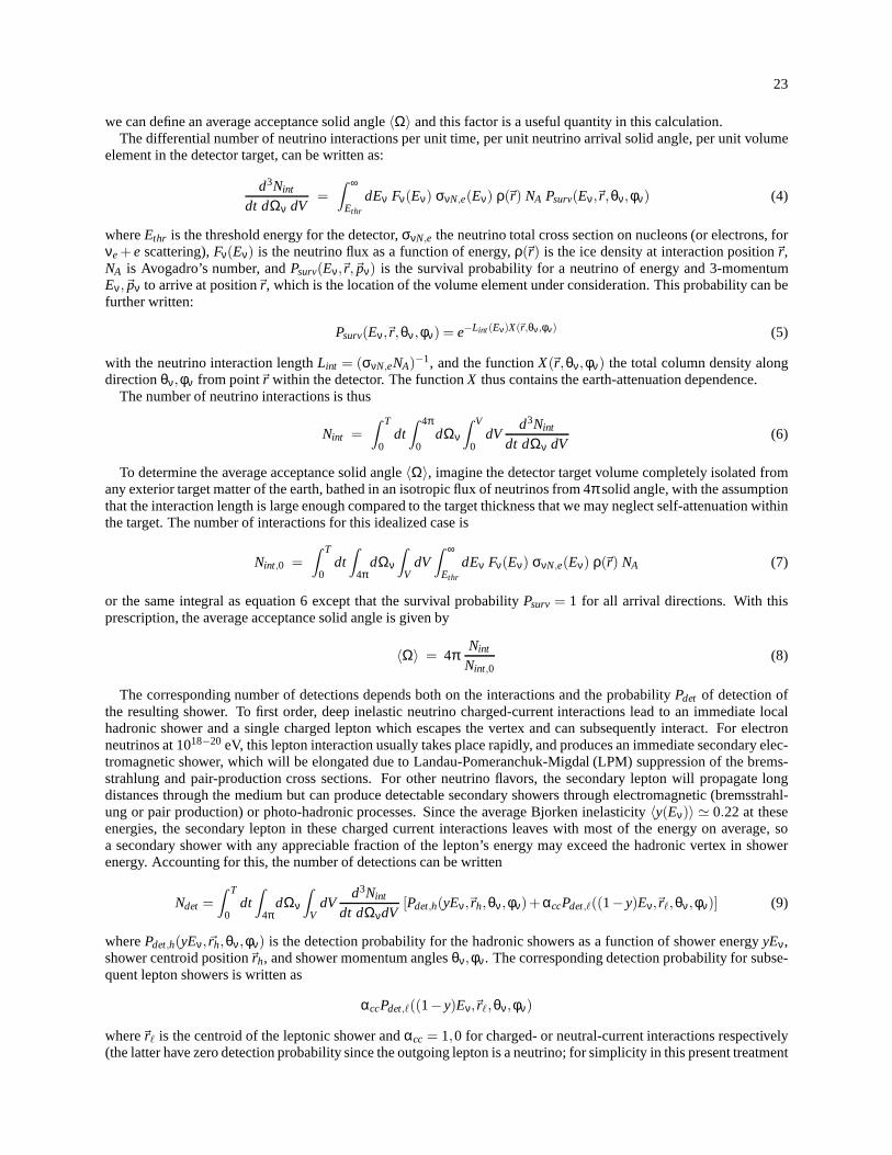
23

we can define an average acceptance solid angle〈Ω〉 and this factor is a useful quantity in this calculation.The differential number of neutrino interactions per unit time, per unit neutrino arrival solid angle, per unit volume

element in the detector target, can be written as:

d3Nint

dt dΩν dV=

Z ∞

Ethr

dEν Fν(Eν) σνN,e(Eν) ρ(~r) NA Psurv(Eν,~r ,θν,φν) (4)

whereEthr is the threshold energy for the detector,σνN,e the neutrino total cross section on nucleons (or electrons,forνe+e scattering),Fν(Eν) is the neutrino flux as a function of energy,ρ(~r) is the ice density at interaction position~r,NA is Avogadro’s number, andPsurv(Eν,~r,~pν) is the survival probability for a neutrino of energy and 3-momentumEν,~pν to arrive at position~r, which is the location of the volume element under consideration. This probability can befurther written:

Psurv(Eν,~r,θν,φν) = e−Lint(Eν)X(~r ,θν,φν) (5)

with the neutrino interaction lengthLint = (σνN,eNA)−1, and the functionX(~r,θν,φν) the total column density alongdirectionθν,φν from point~r within the detector. The functionX thus contains the earth-attenuation dependence.

The number of neutrino interactions is thus

Nint =Z T

0dt

Z 4π

0dΩν

Z V

0dV

d3Nint

dt dΩν dV(6)

To determine the average acceptance solid angle〈Ω〉, imagine the detector target volume completely isolated fromany exterior target matter of the earth, bathed in an isotropic flux of neutrinos from 4π solid angle, with the assumptionthat the interaction length is large enough compared to the target thickness that we may neglect self-attenuation withinthe target. The number of interactions for this idealized case is

Nint,0 =

Z T

0dt

Z

4πdΩν

Z

VdV

Z ∞

Ethr

dEν Fν(Eν) σνN,e(Eν) ρ(~r) NA (7)

or the same integral as equation 6 except that the survival probability Psurv = 1 for all arrival directions. With thisprescription, the average acceptance solid angle is given by

〈Ω〉 = 4πNint

Nint,0(8)

The corresponding number of detections depends both on the interactions and the probabilityPdet of detection ofthe resulting shower. To first order, deep inelastic neutrino charged-current interactions lead to an immediate localhadronic shower and a single charged lepton which escapes the vertex and can subsequently interact. For electronneutrinos at 1018−20 eV, this lepton interaction usually takes place rapidly, and produces an immediate secondary elec-tromagnetic shower, which will be elongated due to Landau-Pomeranchuk-Migdal (LPM) suppression of the brems-strahlung and pair-production cross sections. For other neutrino flavors, the secondary lepton will propagate longdistances through the medium but can produce detectable secondary showers through electromagnetic (bremsstrahl-ung or pair production) or photo-hadronic processes. Sincethe average Bjorken inelasticity〈y(Eν)〉 ≃ 0.22 at theseenergies, the secondary lepton in these charged current interactions leaves with most of the energy on average, soa secondary shower with any appreciable fraction of the lepton’s energy may exceed the hadronic vertex in showerenergy. Accounting for this, the number of detections can bewritten

Ndet =

Z T

0dt

Z

4πdΩν

Z

VdV

d3Nint

dt dΩνdV[Pdet,h(yEν,~rh,θν,φν)+ αccPdet,ℓ((1−y)Eν,~rℓ,θν,φν)] (9)

wherePdet,h(yEν,~rh,θν,φν) is the detection probability for the hadronic showers as a function of shower energyyEν,shower centroid position~rh, and shower momentum anglesθν,φν. The corresponding detection probability for subse-quent lepton showers is written as

αccPdet,ℓ((1−y)Eν,~rℓ,θν,φν)

where~rℓ is the centroid of the leptonic shower andαcc = 1,0 for charged- or neutral-current interactions respectively(the latter have zero detection probability since the outgoing lepton is a neutrino; for simplicity in this present treatment

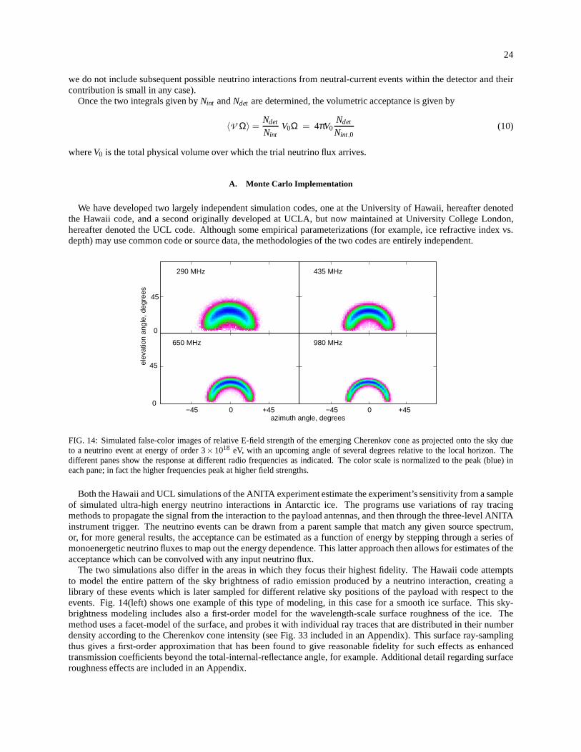
24

we do not include subsequent possible neutrino interactions from neutral-current events within the detector and theircontribution is small in any case).

Once the two integrals given byNint andNdet are determined, the volumetric acceptance is given by

〈V Ω〉 =Ndet

NintV0Ω = 4πV0

Ndet

Nint,0(10)

whereV0 is the total physical volume over which the trial neutrino flux arrives.

A. Monte Carlo Implementation

We have developed two largely independent simulation codes, one at the University of Hawaii, hereafter denotedthe Hawaii code, and a second originally developed at UCLA, but now maintained at University College London,hereafter denoted the UCL code. Although some empirical parameterizations (for example, ice refractive index vs.depth) may use common code or source data, the methodologiesof the two codes are entirely independent.

elev

atio

n an

gle,

deg

rees

azimuth angle, degrees

650 MHz

290 MHz 435 MHz

980 MHz

0

45

0

45

−45 0 0+45 −45 +45

FIG. 14: Simulated false-color images of relative E-field strength of the emerging Cherenkov cone as projected onto the sky dueto a neutrino event at energy of order 3×1018 eV, with an upcoming angle of several degrees relative to thelocal horizon. Thedifferent panes show the response at different radio frequencies as indicated. The color scale is normalized to the peak(blue) ineach pane; in fact the higher frequencies peak at higher fieldstrengths.

Both the Hawaii and UCL simulations of the ANITA experiment estimate the experiment’s sensitivity from a sampleof simulated ultra-high energy neutrino interactions in Antarctic ice. The programs use variations of ray tracingmethods to propagate the signal from the interaction to the payload antennas, and then through the three-level ANITAinstrument trigger. The neutrino events can be drawn from a parent sample that match any given source spectrum,or, for more general results, the acceptance can be estimated as a function of energy by stepping through a series ofmonoenergetic neutrino fluxes to map out the energy dependence. This latter approach then allows for estimates of theacceptance which can be convolved with any input neutrino flux.

The two simulations also differ in the areas in which they focus their highest fidelity. The Hawaii code attemptsto model the entire pattern of the sky brightness of radio emission produced by a neutrino interaction, creating alibrary of these events which is later sampled for differentrelative sky positions of the payload with respect to theevents. Fig. 14(left) shows one example of this type of modeling, in this case for a smooth ice surface. This sky-brightness modeling includes also a first-order model for the wavelength-scale surface roughness of the ice. Themethod uses a facet-model of the surface, and probes it with individual ray traces that are distributed in their numberdensity according to the Cherenkov cone intensity (see Fig.33 included in an Appendix). This surface ray-samplingthus gives a first-order approximation that has been found togive reasonable fidelity for such effects as enhancedtransmission coefficients beyond the total-internal-reflectance angle, for example. Additional detail regarding surfaceroughness effects are included in an Appendix.

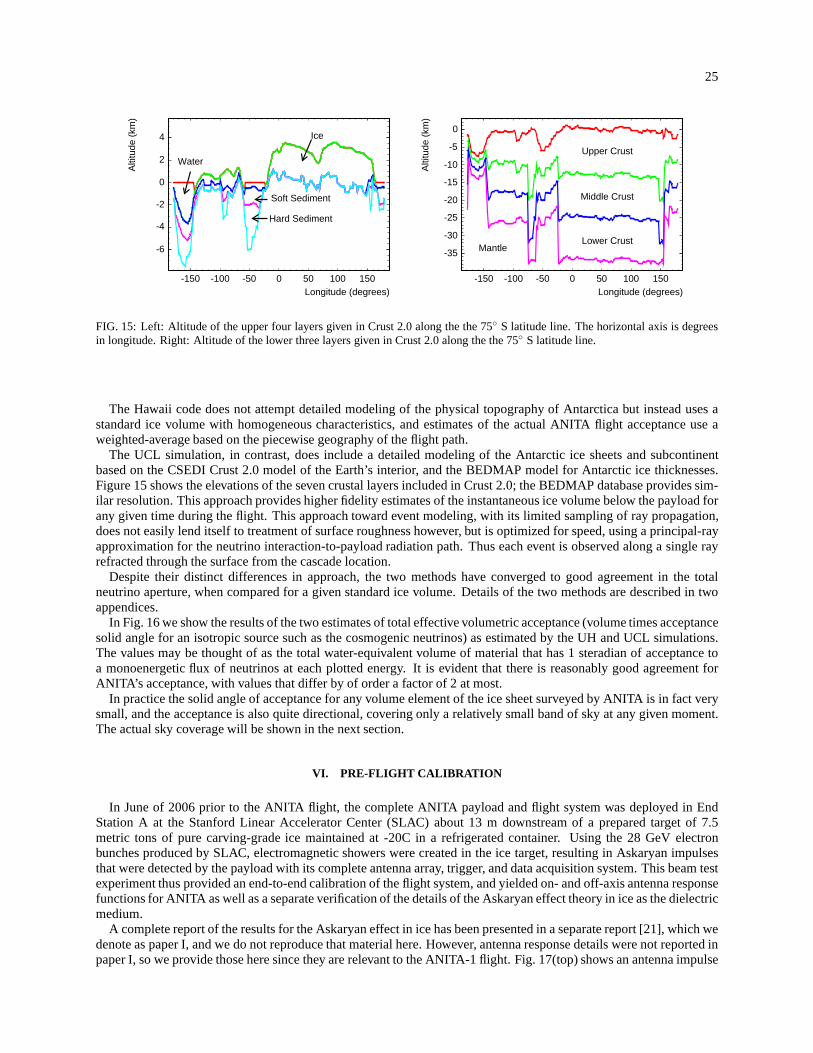
25

Longitude (degrees)-150 -100 -50 0 50 100 150

Alti

tude

(km

)

-6

-4

-2

0

2

4 Ice

Water

Soft Sediment

Hard Sediment

Longitude (degrees)-150 -100 -50 0 50 100 150

Alti

tude

(km

)

-35

-30

-25

-20

-15

-10

-5

0

Upper Crust

Middle Crust

Lower CrustMantle

FIG. 15: Left: Altitude of the upper four layers given in Crust 2.0 along the the 75 S latitude line. The horizontal axis is degreesin longitude. Right: Altitude of the lower three layers given in Crust 2.0 along the the 75 S latitude line.

The Hawaii code does not attempt detailed modeling of the physical topography of Antarctica but instead uses astandard ice volume with homogeneous characteristics, andestimates of the actual ANITA flight acceptance use aweighted-average based on the piecewise geography of the flight path.

The UCL simulation, in contrast, does include a detailed modeling of the Antarctic ice sheets and subcontinentbased on the CSEDI Crust 2.0 model of the Earth’s interior, and the BEDMAP model for Antarctic ice thicknesses.Figure 15 shows the elevations of the seven crustal layers included in Crust 2.0; the BEDMAP database provides sim-ilar resolution. This approach provides higher fidelity estimates of the instantaneous ice volume below the payload forany given time during the flight. This approach toward event modeling, with its limited sampling of ray propagation,does not easily lend itself to treatment of surface roughness however, but is optimized for speed, using a principal-rayapproximation for the neutrino interaction-to-payload radiation path. Thus each event is observed along a single rayrefracted through the surface from the cascade location.

Despite their distinct differences in approach, the two methods have converged to good agreement in the totalneutrino aperture, when compared for a given standard ice volume. Details of the two methods are described in twoappendices.

In Fig. 16 we show the results of the two estimates of total effective volumetric acceptance (volume times acceptancesolid angle for an isotropic source such as the cosmogenic neutrinos) as estimated by the UH and UCL simulations.The values may be thought of as the total water-equivalent volume of material that has 1 steradian of acceptance toa monoenergetic flux of neutrinos at each plotted energy. It is evident that there is reasonably good agreement forANITA’s acceptance, with values that differ by of order a factor of 2 at most.

In practice the solid angle of acceptance for any volume element of the ice sheet surveyed by ANITA is in fact verysmall, and the acceptance is also quite directional, covering only a relatively small band of sky at any given moment.The actual sky coverage will be shown in the next section.

VI. PRE-FLIGHT CALIBRATION

In June of 2006 prior to the ANITA flight, the complete ANITA payload and flight system was deployed in EndStation A at the Stanford Linear Accelerator Center (SLAC) about 13 m downstream of a prepared target of 7.5metric tons of pure carving-grade ice maintained at -20C in arefrigerated container. Using the 28 GeV electronbunches produced by SLAC, electromagnetic showers were created in the ice target, resulting in Askaryan impulsesthat were detected by the payload with its complete antenna array, trigger, and data acquisition system. This beam testexperiment thus provided an end-to-end calibration of the flight system, and yielded on- and off-axis antenna responsefunctions for ANITA as well as a separate verification of the details of the Askaryan effect theory in ice as the dielectricmedium.

A complete report of the results for the Askaryan effect in ice has been presented in a separate report [21], which wedenote as paper I, and we do not reproduce that material here.However, antenna response details were not reported inpaper I, so we provide those here since they are relevant to the ANITA-1 flight. Fig. 17(top) shows an antenna impulse

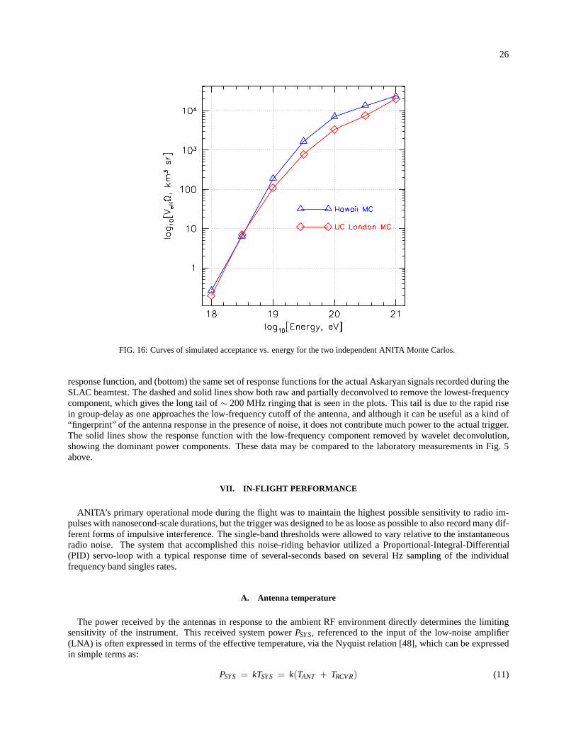
26

FIG. 16: Curves of simulated acceptance vs. energy for the two independent ANITA Monte Carlos.

response function, and (bottom) the same set of response functions for the actual Askaryan signals recorded during theSLAC beamtest. The dashed and solid lines show both raw and partially deconvolved to remove the lowest-frequencycomponent, which gives the long tail of∼ 200 MHz ringing that is seen in the plots. This tail is due to the rapid risein group-delay as one approaches the low-frequency cutoff of the antenna, and although it can be useful as a kind of“fingerprint” of the antenna response in the presence of noise, it does not contribute much power to the actual trigger.The solid lines show the response function with the low-frequency component removed by wavelet deconvolution,showing the dominant power components. These data may be compared to the laboratory measurements in Fig. 5above.

VII. IN-FLIGHT PERFORMANCE

ANITA’s primary operational mode during the flight was to maintain the highest possible sensitivity to radio im-pulses with nanosecond-scale durations, but the trigger was designed to be as loose as possible to also record many dif-ferent forms of impulsive interference. The single-band thresholds were allowed to vary relative to the instantaneousradio noise. The system that accomplished this noise-riding behavior utilized a Proportional-Integral-Differential(PID) servo-loop with a typical response time of several-seconds based on several Hz sampling of the individualfrequency band singles rates.

A. Antenna temperature

The power received by the antennas in response to the ambientRF environment directly determines the limitingsensitivity of the instrument. This received system powerPSYS, referenced to the input of the low-noise amplifier(LNA) is often expressed in terms of the effective temperature, via the Nyquist relation [48], which can be expressedin simple terms as:

PSYS = kTSYS = k(TANT + TRCVR) (11)

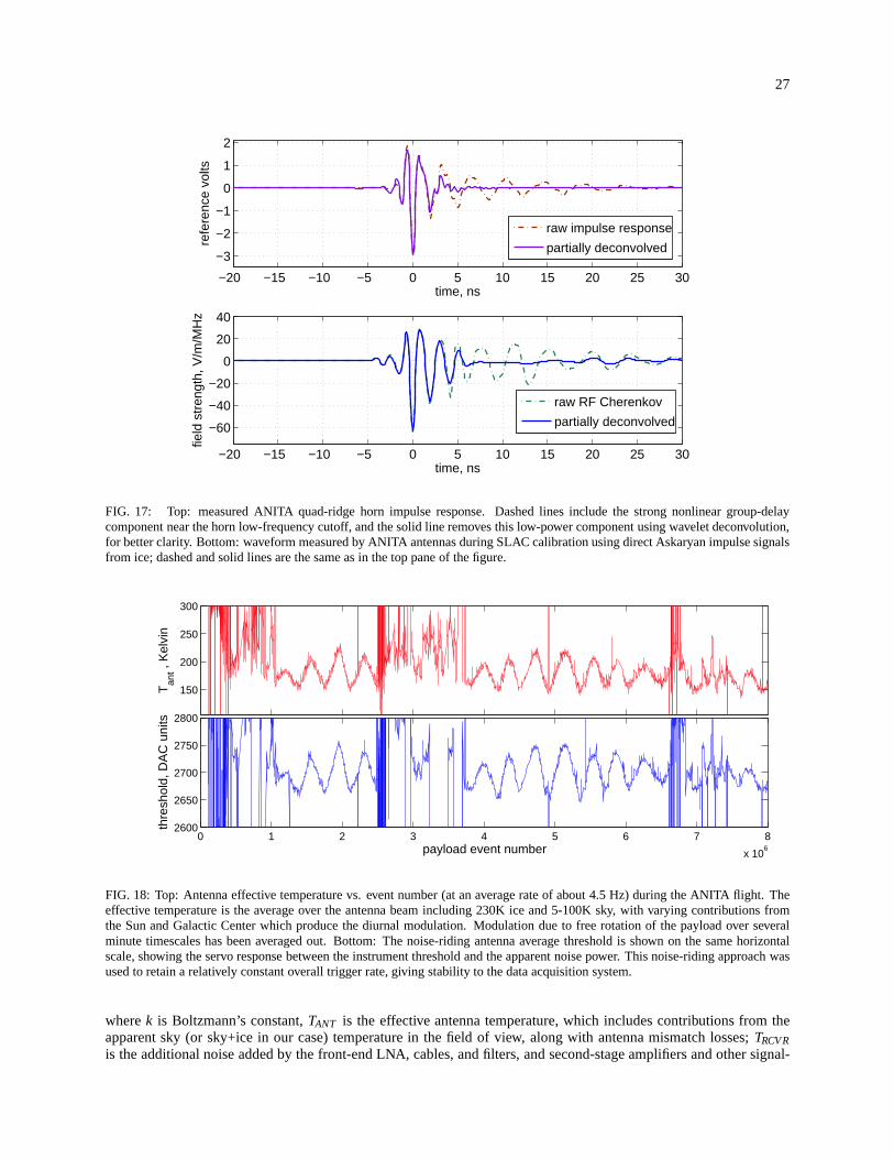
27

−20 −15 −10 −5 0 5 10 15 20 25 30

−3

−2

−1

0

1

2

time, ns

refe

renc

e vo

lts

−20 −15 −10 −5 0 5 10 15 20 25 30

−60

−40

−20

0

20

40

time, ns

field

str

engt

h, V

/m/M

Hz

raw RF Cherenkov

partially deconvolved

raw impulse response

partially deconvolved

FIG. 17: Top: measured ANITA quad-ridge horn impulse response. Dashed lines include the strong nonlinear group-delaycomponent near the horn low-frequency cutoff, and the solidline removes this low-power component using wavelet deconvolution,for better clarity. Bottom: waveform measured by ANITA antennas during SLAC calibration using direct Askaryan impulsesignalsfrom ice; dashed and solid lines are the same as in the top paneof the figure.

1 2 3 4 5 6 7

x 106

150

200

250

300

Tan

t , K

elvi

n

0 1 2 3 4 5 6 7 8

x 106

2600

2650

2700

2750

2800

payload event number

thre

shol

d, D

AC

uni

ts

FIG. 18: Top: Antenna effective temperature vs. event number (at an average rate of about 4.5 Hz) during the ANITA flight. Theeffective temperature is the average over the antenna beam including 230K ice and 5-100K sky, with varying contributions fromthe Sun and Galactic Center which produce the diurnal modulation. Modulation due to free rotation of the payload over severalminute timescales has been averaged out. Bottom: The noise-riding antenna average threshold is shown on the same horizontalscale, showing the servo response between the instrument threshold and the apparent noise power. This noise-riding approach wasused to retain a relatively constant overall trigger rate, giving stability to the data acquisition system.

wherek is Boltzmann’s constant,TANT is the effective antenna temperature, which includes contributions from theapparent sky (or sky+ice in our case) temperature in the fieldof view, along with antenna mismatch losses;TRCVRis the additional noise added by the front-end LNA, cables, and filters, and second-stage amplifiers and other signal-

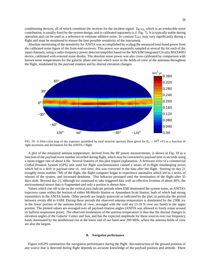
28

conditioning devices, all of which constitute the receiverfor the incident signal.TRCVR, which is an irreducible noisecontribution, is usually fixed by the system design, and is calibrated separately (c.f. Fig. 7). It is typically stable duringoperation and can be used as a reference to estimate additivenoise. In contrastTANT may vary significantly during aflight and must be monitored to ensure the best possible sensitivity of the instrument.

Absolute monitoring of the sensitivity for ANITA was accomplished by scaling the measured total-band power fromthe calibrated noise figure of the front-end receivers. Thispower was separately sampled at several Hz for each of theinput channels, using a radio-frequency power detector/amplifier based on the MAXIM Integrated Circuits MAX4003device, calibrated with external noise diodes. The absolute noise power was also cross-calibrated by comparison withknown noise temperatures for the galactic plane and sun which were in the fields-of-view of the antennas throughoutthe flight, modulated by the payload rotation and by diurnal elevation changes.

FIG. 19: A false-color map of sky exposure quantified by totalneutrino aperture (here given forEν = 1020 eV) as a function ofright-ascension and declination for the ANITA-1 flight.

A plot of the measured antenna temperature, derived from theRF power measurements, is shown in Fig. 18 as afunction of the payload event number recorded during flight,which may be converted to payload time in seconds usinga mean trigger rate of about 4 Hz. Several features of this plot require explanation. A firmware error in a commercialGlobal-Position System (GPS) unit used for flight synchronization caused a series of in-flight timekeeping errorswhich led to a drift in payload time vs. real time; this was corrected in the data after the flight. Starting on day 21(roughly event number 7M) of the flight, the flight computer began to experience anomalies which led to a series ofreboots of the system, and increased deadtime. This behavior persisted until the termination of the flight after 35days aloft. Beyond day 21, although we continued to take triggered data with an effective livetime of about 40%, theenvironmental sensor data is fragmented and only a portion is shown here.

Values which rise off-scale on the vertical axis indicate periods when EMI dominated the system noise, as ANITA’strajectory came within the horizon of either McMurdo Station or Amundsen-Scott Station, both of which had strongtransmitters in the ANITA bands. Other periods are largely quiescent as indicated by the plot; in particular the periodbetween events 4M to 6.6M. During these periods the observedantenna temperature is dominated by the 230K icein the lower portion of the antenna fields of view, averaged with the cold sky (3-10 K over our band) in the upperportion. The plotted values are averaged over all payload rotation angles (ANITA was allowed to freely rotate aroundits balloon suspension point). The observed modulation of the antenna temperature is thus due the diurnal changes inelevation angles of the Galactic Center and Sun, and has the expected amplitude for these sources over our frequencyband, dominated by the nonthermal rise at the lower end of ourband near 200 MHz, where the antenna fields of vieware also the largest.

B. Navigation performance

Figure refGPS summarizes the navigation performance during the flight. Reconstruction of the ground position ofany source that is detected during flight depends on accurateknowledge of the payload position and attitude. There

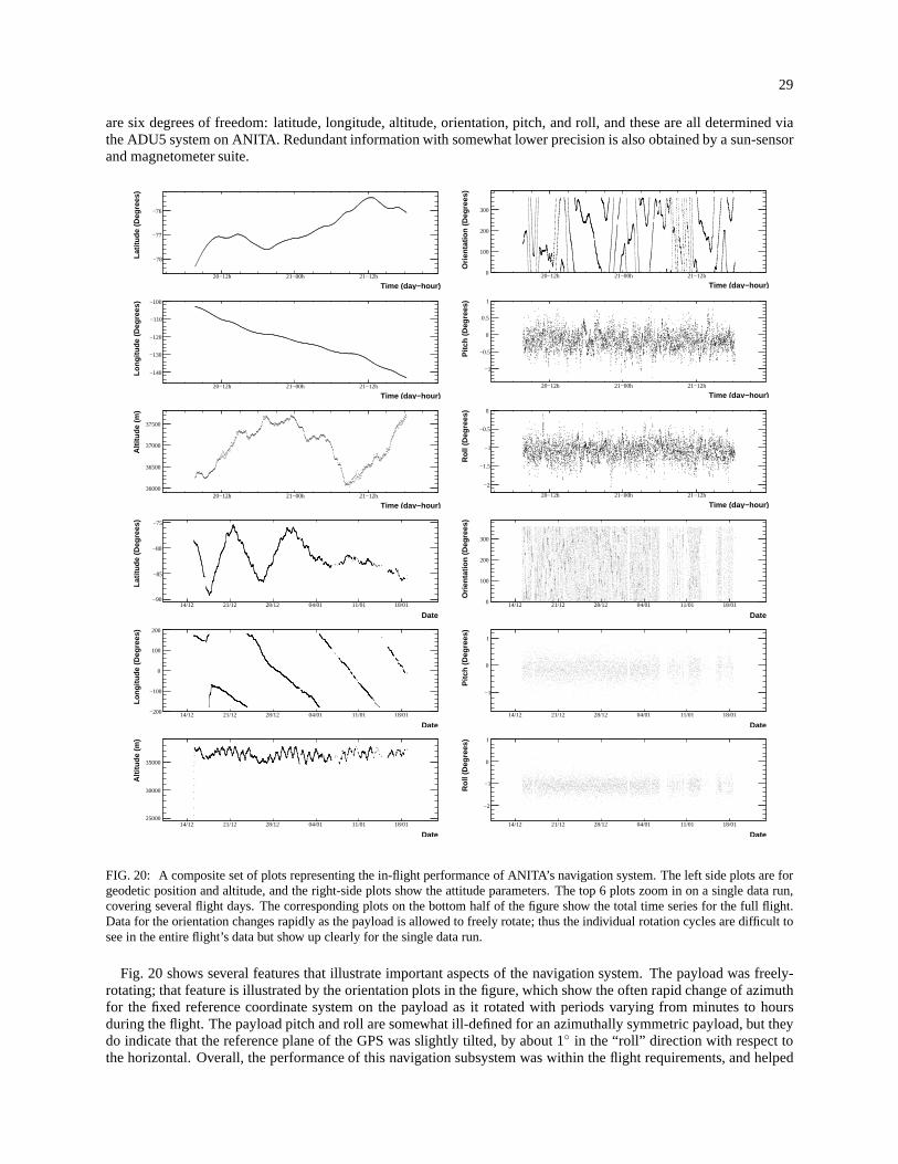
29

are six degrees of freedom: latitude, longitude, altitude,orientation, pitch, and roll, and these are all determined viathe ADU5 system on ANITA. Redundant information with somewhat lower precision is also obtained by a sun-sensorand magnetometer suite.

Time (day−hour)20−12h 21−00h 21−12h

Latit

ude

(Deg

rees

)

−78

−77

−76


Long

itude

(D

egre

es)

−140

−130

−120

−110

−100


Alti

tude

(m

)

36000

36500

37000

37500


Orie

ntat

ion

(Deg

rees

)

0

100

200

300


Pitc

h (D

egre

es)

−1

−0.5

0

0.5

1


Rol

l (D

egre

es)

−2

−1.5

−1

−0.5

0

Date14/12 21/12 28/12 04/01 11/01 18/01

Orie

ntat

ion

(Deg

rees

)

0

100

200

300

Date14/12 21/12 28/12 04/01 11/01 18/01

Pitc

h (D

egre

es)

−1

0

1

Date14/12 21/12 28/12 04/01 11/01 18/01

Rol

l (D

egre

es)

−2

−1

0

1

Date14/12 21/12 28/12 04/01 11/01 18/01

Latit

ude

(Deg

rees

)

−90

−85

−80

−75

Date14/12 21/12 28/12 04/01 11/01 18/01

Long

itude

(D

egre

es)

−200

−100

0

100

200

Date14/12 21/12 28/12 04/01 11/01 18/01

Alti

tude

(m

)

25000

30000

35000

FIG. 20: A composite set of plots representing the in-flight performance of ANITA’s navigation system. The left side plots are forgeodetic position and altitude, and the right-side plots show the attitude parameters. The top 6 plots zoom in on a singledata run,covering several flight days. The corresponding plots on thebottom half of the figure show the total time series for the full flight.Data for the orientation changes rapidly as the payload is allowed to freely rotate; thus the individual rotation cyclesare difficult tosee in the entire flight’s data but show up clearly for the single data run.

Fig. 20 shows several features that illustrate important aspects of the navigation system. The payload was freely-rotating; that feature is illustrated by the orientation plots in the figure, which show the often rapid change of azimuthfor the fixed reference coordinate system on the payload as itrotated with periods varying from minutes to hoursduring the flight. The payload pitch and roll are somewhat ill-defined for an azimuthally symmetric payload, but theydo indicate that the reference plane of the GPS was slightly tilted, by about 1 in the “roll” direction with respect tothe horizontal. Overall, the performance of this navigation subsystem was within the flight requirements, and helped

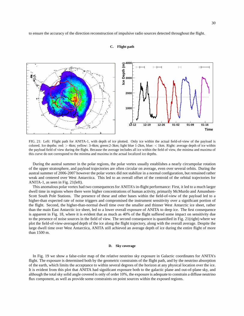
30

to ensure the accuracy of the direction reconstruction of impulsive radio sources detected throughout the flight.

C. Flight path

Time12-12 12-19 12-26 01-02 01-09 01-16

Ice

Dep

th (

m)

0

1000

2000

3000

4000

FIG. 21: Left: Flight path for ANITA-1, with depth of ice plotted. Only ice within the actual field-of-view of the payload iscolored. Ice depths: red:> 4km; yellow: 3-4km; green:2-3km; light blue 1-2km, blue:< 1km. Right: average depth of ice withinthe payload field of view during the flight. Because the average includes all ice within the field of view, the minima and maxima ofthis curve do not correspond to the minima and maxima in the actual localized ice depths.

During the austral summer in the polar regions, the polar vortex usually establishes a nearly circumpolar rotationof the upper stratosphere, and payload trajectories are often circular on average, even over several orbits. During theaustral summer of 2006-2007 however the polar vortex did notstabilize in a normal configuration, but remained ratherweak and centered over West Antarctica. This led to an overall offset of the centroid of the orbital trajectories forANITA-1, as seen in Fig. 21(left).

This anomalous polar vortex had two consequences for ANITA’s in-flight performance: First, it led to a much largerdwell time in regions where there were higher concentrations of human activity, primarily McMurdo and Amundsen-Scott South Pole Stations. The presence of these and other bases within the field-of-view of the payload led to ahigher-than expected rate of noise triggers and compromised the instrument sensitivity over a significant portion ofthe flight. Second, the higher-than-normal dwell time over the smaller and thinner West Antarctic ice sheet, ratherthan the main East Antarctic ice sheet, led to a lower overallexposure of ANITA to deep ice. The first consequenceis apparent in Fig. 18, where it is evident that as much as 40% of the flight suffered some impact on sensitivity dueto the presence of noise sources in the field of view. The second consequence is quantified in Fig. 21(right) where weplot the field-of-view-averaged depth of the ice along the flight trajectory, along with the overall average. Despite thelarge dwell time over West Antarctica, ANITA still achievedan average depth of ice during the entire flight of morethan 1500 m.

D. Sky coverage

In Fig. 19 we show a false-color map of the relative neutrino sky exposure in Galactic coordinates for ANITA’sflight. The exposure is determined both by the geometric constraints of the flight path, and by the neutrino absorptionof the earth, which limits the acceptance to within several degrees of the horizon at any physical location over the ice.It is evident from this plot that ANITA had significant exposure both to the galactic plane and out-of-plane sky, andalthough the total sky solid angle covered is only of order 10%, the exposure is adequate to constrain a diffuse neutrinoflux component, as well as provide some constraints on point sources within the exposed regions.

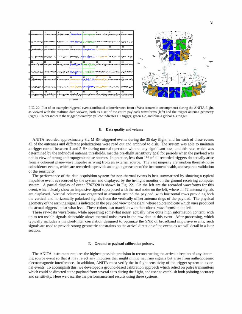
31

V

H

V

H

V

H

V

H

V

1 2 3 4

9 12 15 16

5 6 7 8

131110 14

B2D2B1 D3 B3 D4 B4 D1

100ns

252423

2627

4 5

1314

D3

B2

B3211917 23 25 27 29

18 20 22 24 26 28 30 32

31

FIG. 22: Plot of an example triggered event (attributed to interference from a West Antarctic encampment) during the ANITA flight,as viewed with the realtime data viewers, both as a set of the entire payloads waveforms (left) and the trigger antenna geometry(right). Colors indicate the trigger hierarchy: yellow indicates L1 trigger, green L2, and blue a global L3 trigger.

E. Data quality and volume

ANITA recorded approximately 8.2 M RF-triggered events during the 35 day flight, and for each of these eventsall of the antennas and different polarizations were read out and archived to disk. The system was able to maintaina trigger rate of between 4 and 5 Hz during normal operation without any significant loss, and this rate, which wasdetermined by the individual antenna thresholds, met the pre-flight sensitivity goal for periods when the payload wasnot in view of strong anthropogenic noise sources. In practice, less than 1% of all recorded triggers do actually arisefrom a coherent plane-wave impulse arriving from an external source. The vast majority are random thermal-noisecoincidence events, which are recorded to provide an ongoing measure of the instrument health, and separate validationof the sensitivity.

The performance of the data acquisition system for non-thermal events is best summarized by showing a typicalimpulsive event as recorded by the system and displayed by the in-flight monitor on the ground receiving computersystem. A partial display of event 7767328 is shown in Fig. 22. On the left are the recorded waveforms for thisevent, which clearly show an impulsive signal superposed with thermal noise on the left, where all 72 antenna signalsare displayed. Vertical columns are organized in azimuth around the payload, with horizontal rows providing boththe vertical and horizontally polarized signals from the vertically offset antenna rings of the payload. The physicalgeometry of the arriving signal is indicated in the payload view to the right, where colors indicate which ones producedthe actual triggers and at what level. These colors also match up with the colored waveforms on the left.

These raw-data waveforms, while appearing somewhat noisy,actually have quite high information content, withup to ten usable signals detectable above thermal noise evenin the raw data in this event. After processing, whichtypically includes a matched-filter correlation designed to optimize the SNR of broadband impulsive events, suchsignals are used to provide strong geometric constraints onthe arrival direction of the event, as we will detail in a latersection.

F. Ground-to-payload calibration pulsers.

The ANITA instrument requires the highest possible precision in reconstructing the arrival direction of any incom-ing source event so that it may reject any impulses that mightmimic neutrino signals but arise from anthropogenicelectromagnetic interference. In addition, ANITA must verify the in-flight sensitivity of the trigger system to exter-nal events. To accomplish this, we developed a ground-basedcalibration approach which relied on pulse transmitterswhich could be directed at the payload from several sites during the flight, and used to establish both pointing accuracyand sensitivity. Here we describe the performance and results using these systems.

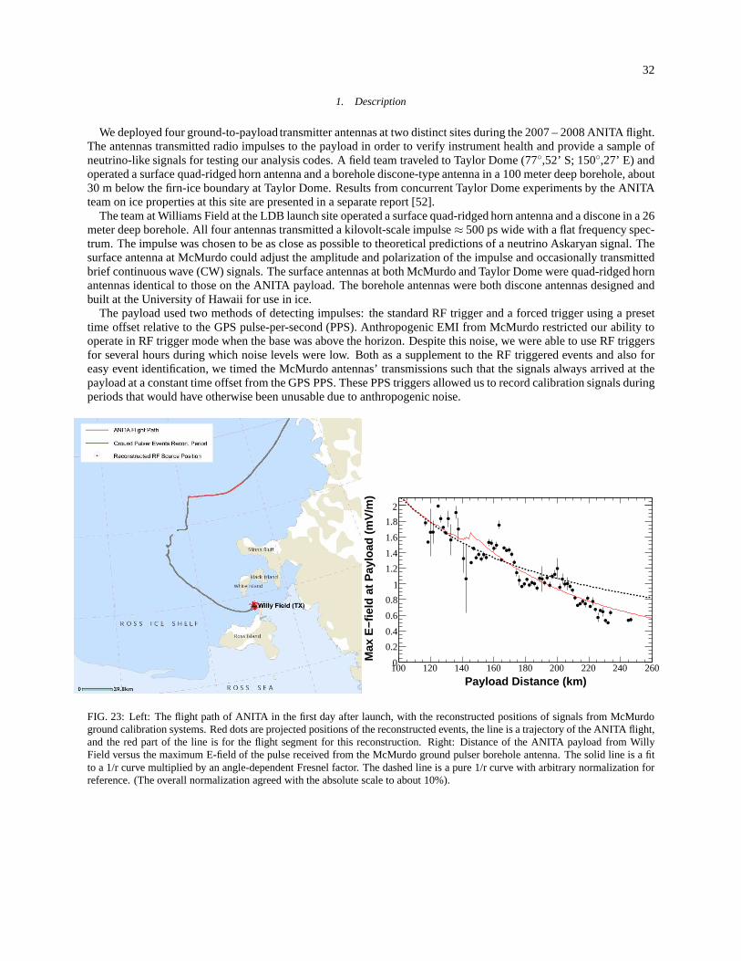
32

1. Description

We deployed four ground-to-payload transmitter antennas at two distinct sites during the 2007 – 2008 ANITA flight.The antennas transmitted radio impulses to the payload in order to verify instrument health and provide a sample ofneutrino-like signals for testing our analysis codes. A field team traveled to Taylor Dome (77,52’ S; 150,27’ E) andoperated a surface quad-ridged horn antenna and a borehole discone-type antenna in a 100 meter deep borehole, about30 m below the firn-ice boundary at Taylor Dome. Results from concurrent Taylor Dome experiments by the ANITAteam on ice properties at this site are presented in a separate report [52].

The team at Williams Field at the LDB launch site operated a surface quad-ridged horn antenna and a discone in a 26meter deep borehole. All four antennas transmitted a kilovolt-scale impulse≈ 500 ps wide with a flat frequency spec-trum. The impulse was chosen to be as close as possible to theoretical predictions of a neutrino Askaryan signal. Thesurface antenna at McMurdo could adjust the amplitude and polarization of the impulse and occasionally transmittedbrief continuous wave (CW) signals. The surface antennas atboth McMurdo and Taylor Dome were quad-ridged hornantennas identical to those on the ANITA payload. The borehole antennas were both discone antennas designed andbuilt at the University of Hawaii for use in ice.

The payload used two methods of detecting impulses: the standard RF trigger and a forced trigger using a presettime offset relative to the GPS pulse-per-second (PPS). Anthropogenic EMI from McMurdo restricted our ability tooperate in RF trigger mode when the base was above the horizon. Despite this noise, we were able to use RF triggersfor several hours during which noise levels were low. Both asa supplement to the RF triggered events and also foreasy event identification, we timed the McMurdo antennas’ transmissions such that the signals always arrived at thepayload at a constant time offset from the GPS PPS. These PPS triggers allowed us to record calibration signals duringperiods that would have otherwise been unusable due to anthropogenic noise.

Payload Distance (km)100 120 140 160 180 200 220 240 260

Max

E−f

ield

at P

aylo

ad (

mV

/m)

0

0.2

0.4

0.6

0.8

1

1.2

1.4

1.6

1.8

2

FIG. 23: Left: The flight path of ANITA in the first day after launch, with the reconstructed positions of signals from McMurdoground calibration systems. Red dots are projected positions of the reconstructed events, the line is a trajectory of the ANITA flight,and the red part of the line is for the flight segment for this reconstruction. Right: Distance of the ANITA payload from WillyField versus the maximum E-field of the pulse received from the McMurdo ground pulser borehole antenna. The solid line is afitto a 1/r curve multiplied by an angle-dependent Fresnel factor. The dashed line is a pure 1/r curve with arbitrary normalization forreference. (The overall normalization agreed with the absolute scale to about 10%).

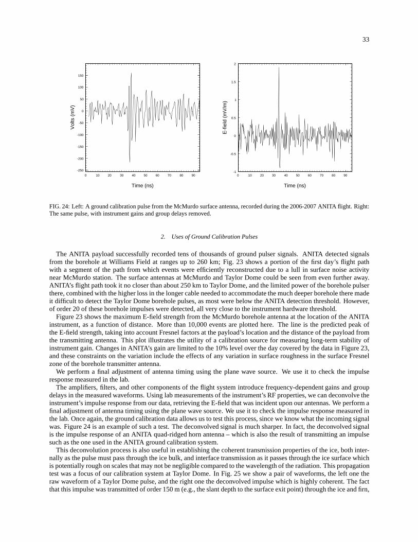
33

Time (ns)

0 10 20 30 40 50 60 70 80 90

Vol

ts (

mV

)

-250

-200

-150

-100

-50

0

50

100

150

Time (ns)

0 10 20 30 40 50 60 70 80 90

E-f

ield

(m

V/m

)

-1

-0.5

0

0.5

1

1.5

2

FIG. 24: Left: A ground calibration pulse from the McMurdo surface antenna, recorded during the 2006-2007 ANITA flight. Right:The same pulse, with instrument gains and group delays removed.

2. Uses of Ground Calibration Pulses

The ANITA payload successfully recorded tens of thousands of ground pulser signals. ANITA detected signalsfrom the borehole at Williams Field at ranges up to 260 km; Fig. 23 shows a portion of the first day’s flight pathwith a segment of the path from which events were efficiently reconstructed due to a lull in surface noise activitynear McMurdo station. The surface antennas at McMurdo and Taylor Dome could be seen from even further away.ANITA’s flight path took it no closer than about 250 km to Taylor Dome, and the limited power of the borehole pulserthere, combined with the higher loss in the longer cable needed to accommodate the much deeper borehole there madeit difficult to detect the Taylor Dome borehole pulses, as most were below the ANITA detection threshold. However,of order 20 of these borehole impulses were detected, all very close to the instrument hardware threshold.

Figure 23 shows the maximum E-field strength from the McMurdoborehole antenna at the location of the ANITAinstrument, as a function of distance. More than 10,000 events are plotted here. The line is the predicted peak ofthe E-field strength, taking into account Fresnel factors atthe payload’s location and the distance of the payload fromthe transmitting antenna. This plot illustrates the utility of a calibration source for measuring long-term stabilityofinstrument gain. Changes in ANITA’s gain are limited to the 10% level over the day covered by the data in Figure 23,and these constraints on the variation include the effects of any variation in surface roughness in the surface Fresnelzone of the borehole transmitter antenna.

We perform a final adjustment of antenna timing using the plane wave source. We use it to check the impulseresponse measured in the lab.

The amplifiers, filters, and other components of the flight system introduce frequency-dependent gains and groupdelays in the measured waveforms. Using lab measurements ofthe instrument’s RF properties, we can deconvolve theinstrument’s impulse response from our data, retrieving the E-field that was incident upon our antennas. We perform afinal adjustment of antenna timing using the plane wave source. We use it to check the impulse response measured inthe lab. Once again, the ground calibration data allows us totest this process, since we know what the incoming signalwas. Figure 24 is an example of such a test. The deconvolved signal is much sharper. In fact, the deconvolved signalis the impulse response of an ANITA quad-ridged horn antenna– which is also the result of transmitting an impulsesuch as the one used in the ANITA ground calibration system.

This deconvolution process is also useful in establishing the coherent transmission properties of the ice, both inter-nally as the pulse must pass through the ice bulk, and interface transmission as it passes through the ice surface whichis potentially rough on scales that may not be negligible compared to the wavelength of the radiation. This propagationtest was a focus of our calibration system at Taylor Dome. In Fig. 25 we show a pair of waveforms, the left one theraw waveform of a Taylor Dome pulse, and the right one the deconvolved impulse which is highly coherent. The factthat this impulse was transmitted of order 150 m (e.g., the slant depth to the surface exit point) through the ice and firn,

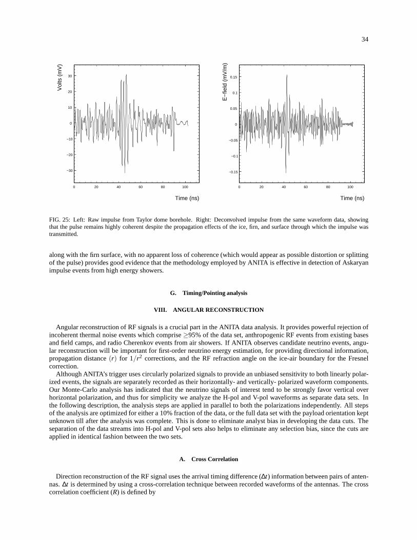
34

Time (ns)

0 20 40 60 80 100

Vol

ts (

mV

)

−30

−20

−10

0

10

20

30

Time (ns)

0 20 40 60 80 100

E−

field

(m

V/m

)

−0.15

−0.1

−0.05

0

0.05

0.1

0.15

FIG. 25: Left: Raw impulse from Taylor dome borehole. Right:Deconvolved impulse from the same waveform data, showingthat the pulse remains highly coherent despite the propagation effects of the ice, firn, and surface through which the impulse wastransmitted.

along with the firn surface, with no apparent loss of coherence (which would appear as possible distortion or splittingof the pulse) provides good evidence that the methodology employed by ANITA is effective in detection of Askaryanimpulse events from high energy showers.

G. Timing/Pointing analysis

VIII. ANGULAR RECONSTRUCTION

Angular reconstruction of RF signals is a crucial part in theANITA data analysis. It provides powerful rejection ofincoherent thermal noise events which comprise≥95% of the data set, anthropogenic RF events from existing basesand field camps, and radio Cherenkov events from air showers.If ANITA observes candidate neutrino events, angu-lar reconstruction will be important for first-order neutrino energy estimation, for providing directional information,propagation distance(r) for 1/r2 corrections, and the RF refraction angle on the ice-air boundary for the Fresnelcorrection.

Although ANITA’s trigger uses circularly polarized signals to provide an unbiased sensitivity to both linearly polar-ized events, the signals are separately recorded as their horizontally- and verticallypolarized waveform components.Our Monte-Carlo analysis has indicated that the neutrino signals of interest tend to be strongly favor vertical overhorizontal polarization, and thus for simplicity we analyze the H-pol and V-pol waveforms as separate data sets. Inthe following description, the analysis steps are applied in parallel to both the polarizations independently. All stepsof the analysis are optimized for either a 10% fraction of thedata, or the full data set with the payload orientation keptunknown till after the analysis was complete. This is done toeliminate analyst bias in developing the data cuts. Theseparation of the data streams into H-pol and V-pol sets alsohelps to eliminate any selection bias, since the cuts areapplied in identical fashion between the two sets.

A. Cross Correlation

Direction reconstruction of the RF signal uses the arrival timing difference (∆t) information between pairs of anten-nas.∆t is determined by using a cross-correlation technique between recorded waveforms of the antennas. The crosscorrelation coefficient (R) is defined by

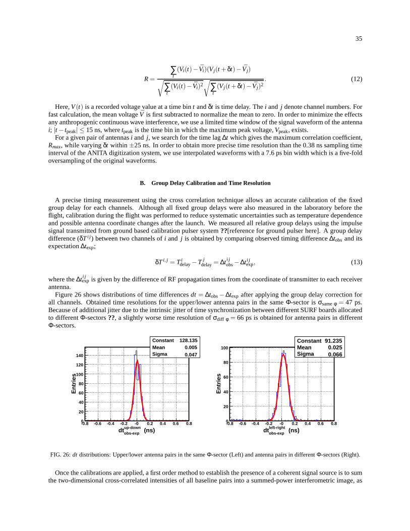
35

R=

∑t(Vi(t)− Vi)(Vj(t + δt)− Vj)

√

∑t(Vi(t)− Vi)2

√

∑t(Vj(t + δt)− Vj)2

. (12)

Here,V(t) is a recorded voltage value at a time bint andδt is time delay. Thei and j denote channel numbers. Forfast calculation, the mean voltageV is first subtracted to normalize the mean to zero. In order to minimize the effectsany anthropogenic continuous wave interference, we use a limited time window of the signal waveform of the antennai; |t − tpeak| ≤ 15 ns, wheretpeak is the time bin in which the maximum peak voltage,Vpeak, exists.

For a given pair of antennasi and j, we search for the time lag∆t which gives the maximum correlation coefficient,Rmax, while varyingδt within ±25 ns. In order to obtain more precise time resolution than the 0.38 ns sampling timeinterval of the ANITA digitization system, we use interpolated waveforms with a 7.6 ps bin width which is a five-foldoversampling of the original waveforms.

B. Group Delay Calibration and Time Resolution

A precise timing measurement using the cross correlation technique allows an accurate calibration of the fixedgroup delay for each channels. Although all fixed group delays were also measured in the laboratory before theflight, calibration during the flight was performed to reducesystematic uncertainties such as temperature dependenceand possible antenna coordinate changes after the launch. We measured all relative group delays using the impulsesignal transmitted from ground based calibration pulser system??[reference for ground pulser here]. A group delaydifference (δT i j ) between two channels ofi and j is obtained by comparing observed timing difference∆tobs and itsexpectation∆texp;

δT i, j = T idelay−T j

delay= ∆t i jobs−∆t i j

exp, (13)

where the∆t i jexp is given by the difference of RF propagation times from the coordinate of transmitter to each receiver

antenna.Figure 26 shows distributions of time differencesdt = ∆tobs−∆texp after applying the group delay correction for

all channels. Obtained time resolutions for the upper/lower antenna pairs in the sameΦ-sector isσsameφ = 47 ps.Because of additional jitter due to the intrinsic jitter of time synchronization between different SURF boards allocatedto differentΦ-sectors??, a slightly worse time resolution ofσdiff φ = 66 ps is obtained for antenna pairs in differentΦ-sectors.

Constant 128.135Mean 0.005Sigma 0.047

(ns)up-downobs-expdt

-0.8 -0.6 -0.4 -0.2 -0 0.2 0.4 0.6 0.8

En

trie

s

0

20

40

60

80

100

120

140



(ns)left-rightobs-expdt

-0.8 -0.6 -0.4 -0.2 -0 0.2 0.4 0.6 0.8

En

trie

s

0

20

40

60

80

100


FIG. 26:dt distributions: Upper/lower antenna pairs in the sameΦ-sector (Left) and antenna pairs in differentΦ-sectors (Right).

Once the calibrations are applied, a first order method to establish the presence of a coherent signal source is to sumthe two-dimensional cross-correlated intensities of all baseline pairs into a summed-power interferometric image, as

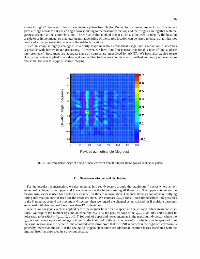
36

shown in Fig. 27. for one of the surface antenna pulses from Taylor Dome. In this procedure each pair of antennasgives a fringe across the sky at an angle corresponding to thebaseline direction, and the fringes sum together with thegreatest strength at the source location. The virtue of thismethod is that it can also be used to identify the locationof sidelobes in the image, so that later quantitative fittingof the source location can be tested to ensure that it has notproduced a misreconstruction at one of the sidelobe locations.

Such an image is highly analogous to a “dirty map” in radio astronomical usage, and a reduction in sidelobesis possible with further image processing. However, we havefound in general that for this type of “pulse-phaseinterferometry,” these maps are adequate since all sourcesare unresolved for ANITA. We have also studied phaseclosure methods as applied to our data, and we find that further work in this area is justified and may yield even morerobust methods for this type of source imaging.

Payload azimuth angle (degrees)

0 50 100 150 200 250 300 350

Ele

vatio

n an

gle

(deg

rees

)

−80

−60

−40

−20

0

20

40

60

80

−0.1

0

0.1

0.2

0.3

0.4

0.5

0.6

0.7

FIG. 27: Interferometric image of a single impulsive event from the Taylor Dome ground calibration pulser.

C. Good event selection and hit cleaning

For the angular reconstruction, we use antennas in threeΦ-sectors around the maximumΦ-sector where an av-erage peak voltage of the upper and lower antennas is the highest among allΦ-sectors. The upper antenna on themaximumΦ-sector is used for a reference channel for the cross correlation. Channels having anomalous or outlyingtiming information are not used for the reconstruction. We compare∆tobss for all possible baselines (15 possible)in the 6 antennas around the maximumΦ-sectors, then we regard the channel as an isolated hit if multiple baselinesassociated with this channel have more than 12 ns deviation.

A selection for good events is applied before the angular fit in order to speed up analysis and reduce misreconstruc-tions. We require the number of good antenna hitsNhit > 5, the peak voltage to beVpeak> 35 mV, and a signal tonoise ratio to be (SNR= Vpeak/Vrms > 3.5) for both of upper and lower antennas in the maximumΦ-sector, where theVrms is a root mean square of voltage obtained in the first third of the recorded waveform which is well-separated fromthe signal region near the center of the recorded waveform. Note that the SNR recorded in the digitizer waveform isgenerally lower than the SNR of the analog RF trigger, since there are additional insertion losses associated with thedigitizer itself, as described in a previous section.

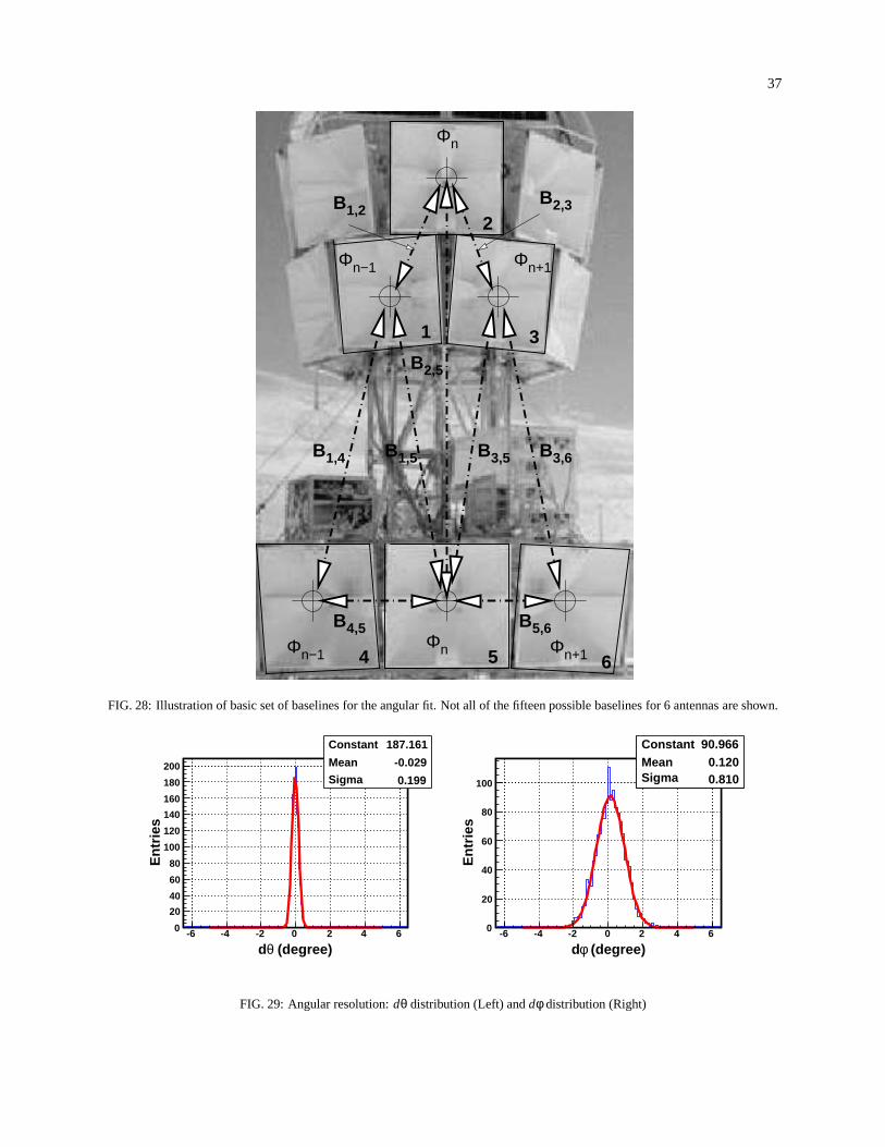
37

Φn+1Φn−1Φn

Φn+1Φn−1

Φn

B4,5 B5,6

B2,5

2

4

B B

BBB

1,2 2,3

3,51,5 3,6

5 6

31

B1,4

FIG. 28: Illustration of basic set of baselines for the angular fit. Not all of the fifteen possible baselines for 6 antennasare shown.

Constant 187.161

Mean -0.029

Sigma 0.199

(degree)θd-6 -4 -2 0 2 4 6

En

trie

s

0

20

40

60

80

100

120

140

160

180

200

Constant 187.161

Mean -0.029

Sigma 0.199


(degree)φd-6 -4 -2 0 2 4 6

En

trie

s

0

20

40

60

80

100


FIG. 29: Angular resolution:dθ distribution (Left) anddφ distribution (Right)

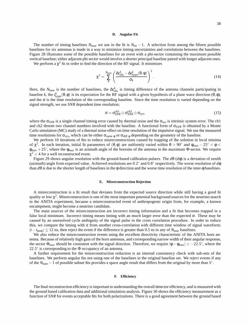
38

D. Angular Fit

The number of timing baselinesNbasewe use in the fit isNhit − 1. A selection from among the fifteen possiblebaselines for six antennas is made in a way to minimize timinguncertainties and correlations between the baselines.Figure 28 illustrates some of the possible baselines for an event with a phi-sector containing the maximum possiblevertical baseline; either adjacent phi sector would involve a shorter principal baseline paired with longer adjacent ones.

We perform aχ2 fit in order to find the direction of the RF signal. It minimizes

χ2 =Nbase

∑k

(

∆tkobs−∆tk

hypo(θ,φ)

σk

)2

. (14)

Here, theNbase is the number of baselines, the∆tkobs is timing difference of the antenna channels participatingin

baselinek, thetkhypo(θ,φ) is its expectation for the RF signal with a given hypothesis of a plane wave direction (θ,φ),

and theσ is the time resolution of the corresponding baseline. Sincethe time resolution is varied depending on thesignal strength, we useSNRdependent time resolution;

σ = σch1SNR⊕σch2

SNR⊕σsys, (15)

where theσSNRis a single channel timing error caused by thermal noise and theσsys is intrinsic system error. The ch1and ch2 denote two channel numbers involved with the baseline. A functional form ofσSNR is obtained by a MonteCarlo simulation (MC) study of a thermal noise effect on timeresolution of the impulsive signal. We use the measuredtime resolutions forσsys, which can be eitherσsameφ or σdiff φ depending on the geometry of the baseline.

We perform 10 iterations of fits to reduce misreconstructions caused by trapping of the solution in local minimaof χ2. In each iteration, initial fit parameters of(θ,φ) are uniformly varied withinθ > 90 andφmax− 25 < φ <φmax+ 25, where theφmax is an azimuth angle of the boresite of the antenna in the maximum Φ-sector. We requireχ2 < 4 for a well reconstructed event.

Figure 29 shows angular resolution with the ground-based calibration pulsers. Thedθ (dφ) is a deviation of zenith(azimuth) angle from expected value. Achieved resolutionsare 0.2 and 0.8 respectively. The worse resolution ofdφthandθ is due to the shorter length of baselines in theφ direction and the worse time resolution of the inter-φ baselines.

E. Misreconstruction Rejection

A misreconstruction is a fit result that deviates from the expected source direction while still having a good fitquality or lowχ2. Misreconstruction is one of the most important potential background sources for the neutrino searchin the ANITA experiment, because a misreconstructed event of anthropogenic origin from, for example, a knownencampment, might become a neutrino candidate.

The main sources of the misreconstruction are incorrect timing information and a fit that becomes trapped in afalse local minimum. Incorrect timing means timing with an much larger error than the expectedσ. These may becaused by an unresolved cycle ambiguity of the signal pulse in the cross correlation procedure. In order to reducethis, we compare the timing with it from another cross-correlation with different time window of signal waveform;|t − tpeak| ≤ 12 ns, then reject the event if the difference is greater than0.5 ns in any ofNbasebaselines.

We also reduce the misreconstruction events using the excellent directivity characteristic of the ANITA horn an-tenna. Because of relatively high gain of the horn antennas,and corresponding narrow width of their angular response,the sectorΦmax should be consistent with the signal direction. Therefore,we require|φ−φmax| < −22.5, where the22.5 is corresponding to theΦ occupancy of an antenna.

A further requirement for the misreconstruction reductionis an internal consistency check with sub-sets of thebaselines. We perform angular fits not using one of the baselines in the original baseline set. We reject events if anyof theNbase−1 of possible subset fits provides a space angle result that differs from the original by more than 5.

F. Efficiency

The final reconstruction efficiency is important to understanding the overall detector efficiency, and is measured withthe ground based calibration data and additional simulation analysis. Figure 30 shows the efficiency measurement as afunction ofSNRfor events acceptable fits for both polarizations. There is agood agreement between the ground based

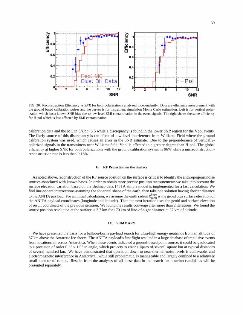
39

FIG. 30: Reconstruction Efficiency vs.SNRfor both polarizations analyzed independently: Dots are efficiency measurement withthe ground based calibration pulses and the curves is for instrument simulation Monte Carlo estimation. Left is for vertical polar-ization which has a known SNR bias due to low-level EMI contamination in the event signals. The right shows the same efficiencyfor H-pol which is less affected by EMI contamination.

calibration data and the MC inSNR> 5.5 while a discrepancy is found in the lowerSNRregion for the Vpol events.The likely source of this discrepancy is the effect of low-level interference from Williams Field where the groundcalibration system was used, which causes an error in the SNRestimate. Due to the preponderance of vertically-polarized signals in the transmitters near Williams field, Vpol is affected to a greater degree than H-pol. The globalefficiency at higher SNR for both polarizations with the ground calibration system is 96% while a misreconstruction-reconstruction rate is less than 0.16%.

G. RF Projection on the Surface

As noted above, reconstruction of the RF source position on the surface is critical to identify the anthropogenic noisesources associated with known bases. In order to obtain moreprecise position measurements we take into account thesurface elevation variation based on the Bedmap data. [43] Asimple model is implemented for a fast calculation. Wefind line-sphere intersections assuming the spherical shape of the earth, then take one solution having shorter distanceto the ANITA payload. For an initial calculation, we assume the earth radiusRhypo

earthis the geoid plus surface elevation ofthe ANITA payload coordinates (longitude and latitude). Then the next iteration uses the geoid and surface elevationof result coordinate of the previous iteration. We found theresults converge after more than 2 iterations. We found thesource position resolution at the surface is 2.7 km for 170 kmof line-of-sight distance at 37 km of altitude.

IX. SUMMARY

We have presented the basis for a balloon-borne payload search for ultra-high energy neutrinos from an altitude of37 km above the Antarctic Ice sheets. The ANITA payload’s first flight resulted in a large database of impulsive eventsfrom locations all across Antarctica. When these events indicated a ground-based point source, it could be geolocatedto a precision of order 0.3×1.0 in angle, which projects to error ellipses of several squarekm at typical distancesof several hundred km. We have demonstrated that operation down to near-thermal-noise levels is achievable, andelectromagnetic interference in Antarctical, while stillproblematic, is manageable and largely confined to a relativelysmall number of camps. Results from the analyses of all thesedata in the search for neutrino candidates will bepresented separately.

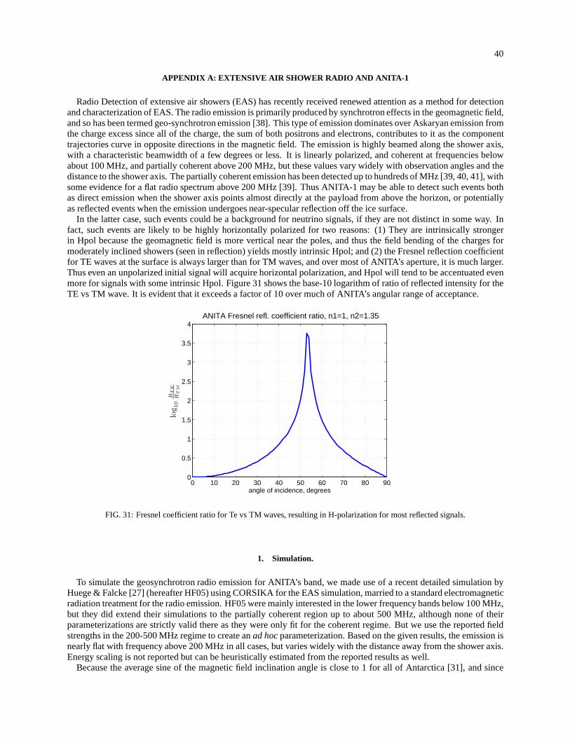
40

APPENDIX A: EXTENSIVE AIR SHOWER RADIO AND ANITA-1

Radio Detection of extensive air showers (EAS) has recentlyreceived renewed attention as a method for detectionand characterization of EAS. The radio emission is primarily produced by synchrotron effects in the geomagnetic field,and so has been termed geo-synchrotron emission [38]. This type of emission dominates over Askaryan emission fromthe charge excess since all of the charge, the sum of both positrons and electrons, contributes to it as the componenttrajectories curve in opposite directions in the magnetic field. The emission is highly beamed along the shower axis,with a characteristic beamwidth of a few degrees or less. It is linearly polarized, and coherent at frequencies belowabout 100 MHz, and partially coherent above 200 MHz, but these values vary widely with observation angles and thedistance to the shower axis. The partially coherent emission has been detected up to hundreds of MHz [39, 40, 41], withsome evidence for a flat radio spectrum above 200 MHz [39]. Thus ANITA-1 may be able to detect such events bothas direct emission when the shower axis points almost directly at the payload from above the horizon, or potentiallyas reflected events when the emission undergoes near-specular reflection off the ice surface.

In the latter case, such events could be a background for neutrino signals, if they are not distinct in some way. Infact, such events are likely to be highly horizontally polarized for two reasons: (1) They are intrinsically strongerin Hpol because the geomagnetic field is more vertical near the poles, and thus the field bending of the charges formoderately inclined showers (seen in reflection) yields mostly intrinsic Hpol; and (2) the Fresnel reflection coefficientfor TE waves at the surface is always larger than for TM waves,and over most of ANITA’s aperture, it is much larger.Thus even an unpolarized initial signal will acquire horizontal polarization, and Hpol will tend to be accentuated evenmore for signals with some intrinsic Hpol. Figure 31 shows the base-10 logarithm of ratio of reflected intensity for theTE vs TM wave. It is evident that it exceeds a factor of 10 over much of ANITA’s angular range of acceptance.

0 10 20 30 40 50 60 70 80 900

0.5

1

1.5

2

2.5

3

3.5

4

angle of incidence, degrees

log 1

0

RT

E

RT

M

ANITA Fresnel refl. coefficient ratio, n1=1, n2=1.35

FIG. 31: Fresnel coefficient ratio for Te vs TM waves, resulting in H-polarization for most reflected signals.

1. Simulation.

To simulate the geosynchrotron radio emission for ANITA’s band, we made use of a recent detailed simulation byHuege & Falcke [27] (hereafter HF05) using CORSIKA for the EAS simulation, married to a standard electromagneticradiation treatment for the radio emission. HF05 were mainly interested in the lower frequency bands below 100 MHz,but they did extend their simulations to the partially coherent region up to about 500 MHz, although none of theirparameterizations are strictly valid there as they were only fit for the coherent regime. But we use the reported fieldstrengths in the 200-500 MHz regime to create anad hocparameterization. Based on the given results, the emissionisnearly flat with frequency above 200 MHz in all cases, but varies widely with the distance away from the shower axis.Energy scaling is not reported but can be heuristically estimated from the reported results as well.

Because the average sine of the magnetic field inclination angle is close to 1 for all of Antarctica [31], and since

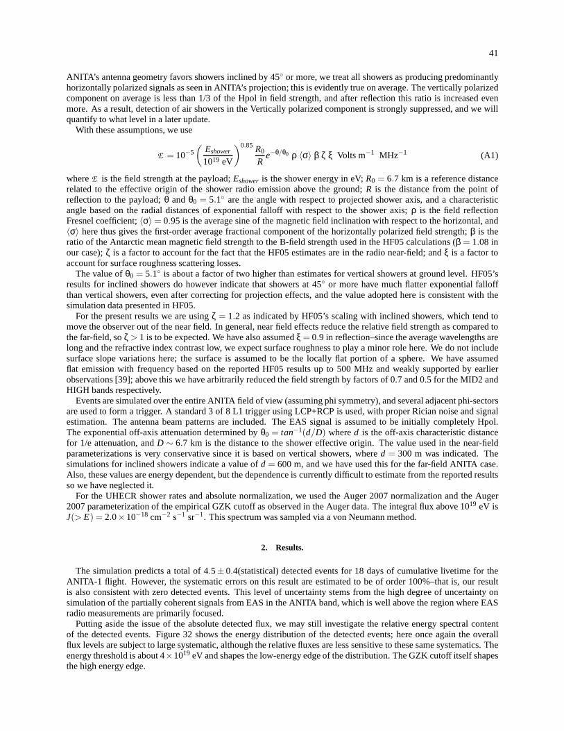
41

ANITA’s antenna geometry favors showers inclined by 45 or more, we treat all showers as producing predominantlyhorizontally polarized signals as seen in ANITA’s projection; this is evidently true on average. The vertically polarizedcomponent on average is less than 1/3 of the Hpol in field strength, and after reflection this ratio is increased evenmore. As a result, detection of air showers in the Verticallypolarized component is strongly suppressed, and we willquantify to what level in a later update.

With these assumptions, we use

E = 10−5(

Eshower

1019 eV

)0.85 R0

Re−θ/θ0 ρ 〈σ〉 β ζ ξ Volts m−1 MHz−1 (A1)

whereE is the field strength at the payload;Eshower is the shower energy in eV;R0 = 6.7 km is a reference distancerelated to the effective origin of the shower radio emissionabove the ground;R is the distance from the point ofreflection to the payload;θ andθ0 = 5.1 are the angle with respect to projected shower axis, and a characteristicangle based on the radial distances of exponential falloff with respect to the shower axis;ρ is the field reflectionFresnel coefficient;〈σ〉 = 0.95 is the average sine of the magnetic field inclination with respect to the horizontal, and〈σ〉 here thus gives the first-order average fractional component of the horizontally polarized field strength;β is theratio of the Antarctic mean magnetic field strength to the B-field strength used in the HF05 calculations (β = 1.08 inour case);ζ is a factor to account for the fact that the HF05 estimates arein the radio near-field; andξ is a factor toaccount for surface roughness scattering losses.

The value ofθ0 = 5.1 is about a factor of two higher than estimates for vertical showers at ground level. HF05’sresults for inclined showers do however indicate that showers at 45 or more have much flatter exponential falloffthan vertical showers, even after correcting for projection effects, and the value adopted here is consistent with thesimulation data presented in HF05.

For the present results we are usingζ = 1.2 as indicated by HF05’s scaling with inclined showers, which tend tomove the observer out of the near field. In general, near field effects reduce the relative field strength as compared tothe far-field, soζ > 1 is to be expected. We have also assumedξ = 0.9 in reflection–since the average wavelengths arelong and the refractive index contrast low, we expect surface roughness to play a minor role here. We do not includesurface slope variations here; the surface is assumed to be the locally flat portion of a sphere. We have assumedflat emission with frequency based on the reported HF05 results up to 500 MHz and weakly supported by earlierobservations [39]; above this we have arbitrarily reduced the field strength by factors of 0.7 and 0.5 for the MID2 andHIGH bands respectively.

Events are simulated over the entire ANITA field of view (assuming phi symmetry), and several adjacent phi-sectorsare used to form a trigger. A standard 3 of 8 L1 trigger using LCP+RCP is used, with proper Rician noise and signalestimation. The antenna beam patterns are included. The EASsignal is assumed to be initially completely Hpol.The exponential off-axis attenuation determined byθ0 = tan−1(d/D) whered is the off-axis characteristic distancefor 1/e attenuation, andD ∼ 6.7 km is the distance to the shower effective origin. The valueused in the near-fieldparameterizations is very conservative since it is based onvertical showers, whered = 300 m was indicated. Thesimulations for inclined showers indicate a value ofd = 600 m, and we have used this for the far-field ANITA case.Also, these values are energy dependent, but the dependenceis currently difficult to estimate from the reported resultsso we have neglected it.

For the UHECR shower rates and absolute normalization, we used the Auger 2007 normalization and the Auger2007 parameterization of the empirical GZK cutoff as observed in the Auger data. The integral flux above 1019 eV isJ(> E) = 2.0×10−18 cm−2 s−1 sr−1. This spectrum was sampled via a von Neumann method.

2. Results.

The simulation predicts a total of 4.5± 0.4(statistical) detected events for 18 days of cumulative livetime for theANITA-1 flight. However, the systematic errors on this result are estimated to be of order 100%–that is, our resultis also consistent with zero detected events. This level of uncertainty stems from the high degree of uncertainty onsimulation of the partially coherent signals from EAS in theANITA band, which is well above the region where EASradio measurements are primarily focused.

Putting aside the issue of the absolute detected flux, we may still investigate the relative energy spectral contentof the detected events. Figure 32 shows the energy distribution of the detected events; here once again the overallflux levels are subject to large systematic, although the relative fluxes are less sensitive to these same systematics. Theenergy threshold is about 4×1019 eV and shapes the low-energy edge of the distribution. The GZK cutoff itself shapesthe high energy edge.

42

FIG. 32: Top: Differential energy distribution of simulated events that are detected by ANITA-1. Bottom: Cumulative energydistribution of events, showing that the detectability turns on in the vicinity of the GZK cutoff.

In summary, ANITA’s sensitivity was adequate to possibly detect a handful of events from extensive air shower radioemission, seen in reflection from the ice surface. The uncertainties in this prediction are dominated by the uncertaintiesin the magnitude of partially coherent emission from EAS radio processes.

APPENDIX B: CHARACTERIZATION OF SURFACE ROUGHNESS AND ITS E FFECT ON NEUTRINO APERTURE

One concern for modeling the detection of neutrinos in the ice is the propagation of the radio emissions from underthe ice to the surface,i.e., the firn, into the air. If the surface of the ice were a smooth boundary, we could simply applythe proper Fresnel coefficient for each polarization at the surface corresponding to an index of refractionn≃ 1.3 to airn = 1. However, the Antarctic winds and other effects serve to carve up the surface, making it rough on many lengthscales.

RF energy propagating from the neutrino interaction to the instrument does not pass through a single point on thesurface of the ice. Rather, all radiation passing through anarea given by the first Fresnel zone on the ice surface cancontribute to the received band-limited impulse. This region is determined by considering the locus of points on thesurface where the pathlength is within a quarter-wavelength of the direct geometric ray for an idealized smooth surface.Straightforward geometric considerations for a simple phase-screen perpendicular to the direction of propagationbetween a transmitter and receiver give a first Fresnel zone radius

RF,1 =

√

cd1d2

〈 f 〉(d1 +d2)

wherec is the velocity of light,〈 f 〉 the mean frequency of the waves, andd1, d2 are the source-to-phase screenand receiver-to-phase screen distances, respectively. Within this radius, any sub-wavelength phase disturbance to thepropagating waves will cause constructive or destructive interference to the beam. Higher order Fresnel zones at largerradii may be important in some cases, but we neglect them here.

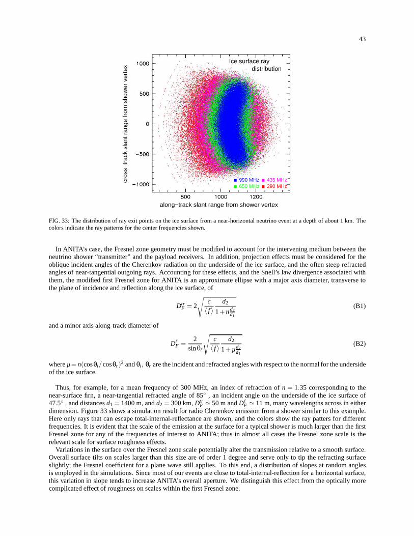
43

cros

s−tr

ack

slan

t ran

ge fr

om s

how

er v

erte

x

along−track slant range from shower vertex

Ice surface raydistribution

990 MHz290 MHz650 MHz435 MHz

FIG. 33: The distribution of ray exit points on the ice surface from a near-horizontal neutrino event at a depth of about 1 km. Thecolors indicate the ray patterns for the center frequenciesshown.

In ANITA’s case, the Fresnel zone geometry must be modified toaccount for the intervening medium between theneutrino shower “transmitter” and the payload receivers. In addition, projection effects must be considered for theoblique incident angles of the Cherenkov radiation on the underside of the ice surface, and the often steep refractedangles of near-tangential outgoing rays. Accounting for these effects, and the Snell’s law divergence associated withthem, the modified first Fresnel zone for ANITA is an approximate ellipse with a major axis diameter, transverse tothe plane of incidence and reflection along the ice surface, of

DtrF = 2

√

c〈 f 〉

d2

1+nd2d1

(B1)

and a minor axis along-track diameter of

DℓF =

2sinθi

√

c〈 f 〉

d2

1+µd2d1

(B2)

whereµ= n(cosθi/cosθr)2 andθi , θr are the incident and refracted angles with respect to the normal for the underside

of the ice surface.

Thus, for example, for a mean frequency of 300 MHz, an index ofrefraction ofn = 1.35 corresponding to thenear-surface firn, a near-tangential refracted angle of 85 , an incident angle on the underside of the ice surface of47.5 , and distancesd1 = 1400 m, andd2 = 300 km,Dtr

F ≃ 50 m andDℓF ≃ 11 m, many wavelengths across in either

dimension. Figure 33 shows a simulation result for radio Cherenkov emission from a shower similar to this example.Here only rays that can escape total-internal-reflectance are shown, and the colors show the ray patters for differentfrequencies. It is evident that the scale of the emission at the surface for a typical shower is much larger than the firstFresnel zone for any of the frequencies of interest to ANITA;thus in almost all cases the Fresnel zone scale is therelevant scale for surface roughness effects.

Variations in the surface over the Fresnel zone scale potentially alter the transmission relative to a smooth surface.Overall surface tilts on scales larger than this size are of order 1 degree and serve only to tip the refracting surfaceslightly; the Fresnel coefficient for a plane wave still applies. To this end, a distribution of slopes at random anglesis employed in the simulations. Since most of our events are close to total-internal-reflection for a horizontal surface,this variation in slope tends to increase ANITA’s overall aperture. We distinguish this effect from the optically morecomplicated effect of roughness on scales within the first Fresnel zone.

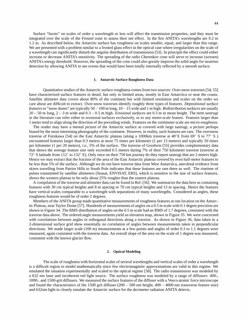
44

Surface “facets” on scales of order a wavelength or less willaffect the tranmission properties, and they must beintegrated over the scale of the Fresnel zone to assess theirnet effect. In the firn ANITA’s wavelengths are 0.2 to1.2 m. As described below, the Antarctic surface has roughness on scales smaller, equal, and larger than this range.We are presented with a problem similar to a frosted glass effect in the optical case where irregularities on the scale ofa wavelength can significantly disturb the angular distribution of transmission [53]. In principle the effect could eitherincrease or decrease ANITA’s sensitivity. The spreading ofthe radio Cherenkov cone will serve to increase (worsen)ANITA’s energy threshold. However, the spreading of the cone could also greatly improve the solid angle for neutrinodetection by allowing ANITA to see events that would have been totally internally reflected by a smooth surface.

1. Antarctic Surface Roughness Data

Quantitative studies of the Antarctic surface roughness comes from two sources: Over-snow traverses [54, 55]have characterized surface features in detail, but only in limited areas, mostly in East Antarctica or near the coasts.Satellite altimeter data covers about 80% of the continent but with limited resolution and scales on the order wecare about are difficult to extract. Over-snow traverses identify roughly three types of features.Depositional surfacefeaturesor “snow dunes” are typically 50−100 m long, 10−15 wide and 1 m high.Redistribution surfacesare usually20−50 m long, 2−3 m wide and 0.3−0.5 m high.Erosional surfacesare 0.3 m in mean height. The termsastrugiin the literature can refer either to erosional surfaces exclusively, or to any meter-scale feature. Features larger than1 meter tend to align along the direction of the prevailing winds. Features on the centimeter scale aremicro-roughness.

The reader may have a mental picture of the Antarctic surfaceas covered with large sastrugi, a picture perhapsbiased by the most interesting photography of the continent. However, in reality, such features are rare. The oversnowtraverse of Furukawa [54] on the East Antarctic plateau (along a 1000km traverse at 40E from 69 S to 77 S )encountered features larger than 0.3 meters at most 75 timesper kilometer (1 per 13 meters) and typically 50 timesper kilometer (1 per 20 meters),i.e., 5% of the surface. The traverse of Goodwin [55] provides complementary datathat shows the average feature size only exceeded 0.5 metersduring 7% of their 750 kilometer traverse (traverse at72 S latitude from 112 to 132 E). Only once on their 750 km journey do they report sastrugi that are 2 meters high.Hence we may extract that the fraction of the area of the East Antarctic plateau covered by even half-meter features tobe less than 5% of the surface. Although we do not have traverse data from West Antarctica, anecdotal evidence fromskiers travelling from Patriot Hills to South Pole indicates that these features are rare there as well. The risetime ofpulses transmitted by satellite altimeters (Seasat, ENVISAT, ERS), which is sensitive to the size of surface features,shows the western plateau to be only about 25% rougher than the eastern plateau.

A compilation of the traverse and altimeter data can be foundin Ref. [56]. We summarize the data here as containingfeatures with 30 cm typical heights and 8 m spacing or 70 cm typical heights and 13 m spacing. Hence the featureshave vertical scales comparable to a wavelength with separations of many wavelengths. Considered as angles, theseroughness features would be of order 2 degrees.

Members of the ANITA group made quantitative measurements of roughness features at one location on the Antarc-tic Plateau, near Taylor Dome [57]. Hundreds of measurements of angles on a 0.5 m scale with 0.1 degree precision areshown in Figure 34. The RMS distribution of angles on the 0.5 mscale had an RMS of 1.7 degrees, consistent with thetraverse data above. The ordered angle measurements yield an elevation map, shown in Figure 35. We were concernedwith correlations between angles in orthoganal directionsalong a traverse. As shown in Figure 36, data taken in a2-dimensional surface grid show essentially no correlation of angles between measurements taken in perpendiculardirections. We made larger scale (100 m) measurements at a few points and angles of order 0.3 to 1.1 degrees weremeasured, again consistent with the traverse data. An overall slope of the area on the scale of 1 degree was measured,consistent with the known glacier flow.

2. Optical Modeling

The scale of roughness with horizontal scales of several wavelengths and vertical scales of order a wavelengthis a difficult region to model mathematically since few electromagnetic approximations are valid in this regime. Weemulated the situation experimentally and scaled to the optical regime [58]. The radio transmission was modeled bya 632 nm laser and incoherent red light source. The surface roughness was modeled by a range of diffusers: 400-,1000-, and 1500-grit diffusers. We measured the surface features of the diffuser with a Veeco atomic force microscopeand found the characteristics of the 1500 grit diffuser (200−500 nm height, 400−4000 nm transverse feature size)and 632nm light to closely emulate the Antarctic surface forthe decimeter radiation ANITA detects.

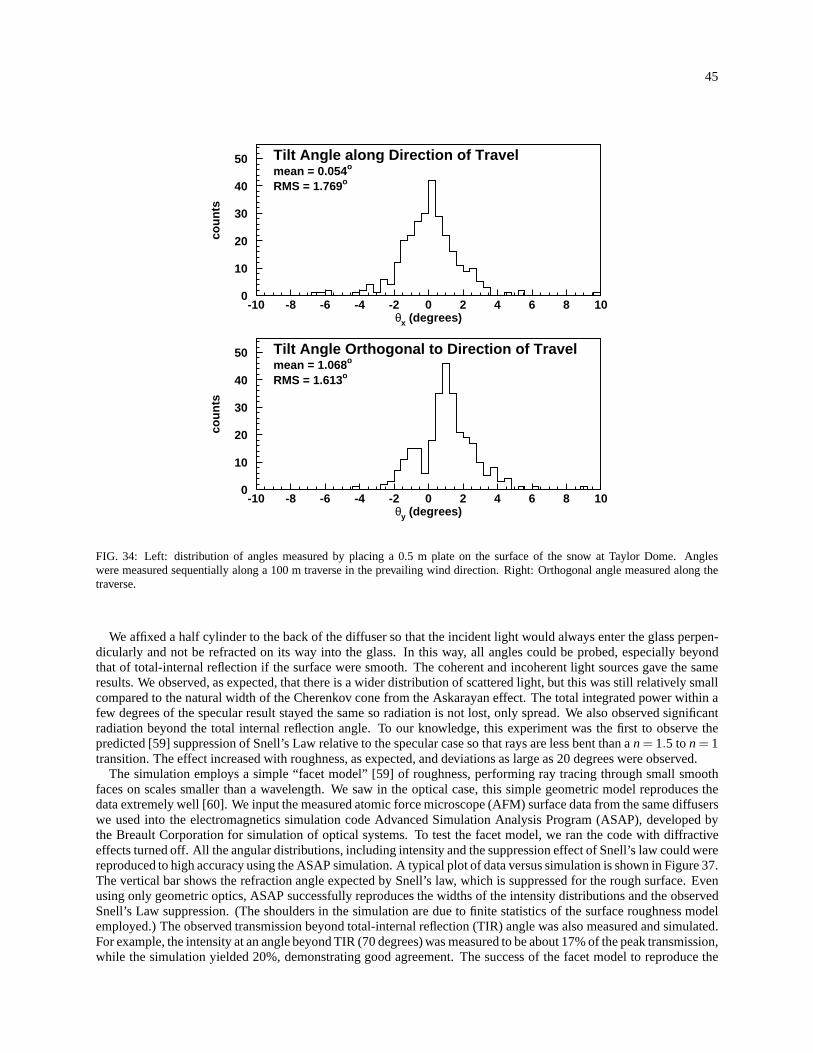
45

0

10

20

30

40

50

-10 -8 -6 -4 -2 0 2 4 6 8 10

Tilt Angle along Direction of Travelmean = 0.054o

RMS = 1.769o

θx (degrees)

cou

nts

0

10

20

30

40

50

-10 -8 -6 -4 -2 0 2 4 6 8 10

Tilt Angle Orthogonal to Direction of Travelmean = 1.068o

RMS = 1.613o

θy (degrees)

cou

nts

FIG. 34: Left: distribution of angles measured by placing a 0.5 m plate on the surface of the snow at Taylor Dome. Angleswere measured sequentially along a 100 m traverse in the prevailing wind direction. Right: Orthogonal angle measured along thetraverse.

We affixed a half cylinder to the back of the diffuser so that the incident light would always enter the glass perpen-dicularly and not be refracted on its way into the glass. In this way, all angles could be probed, especially beyondthat of total-internal reflection if the surface were smooth. The coherent and incoherent light sources gave the sameresults. We observed, as expected, that there is a wider distribution of scattered light, but this was still relatively smallcompared to the natural width of the Cherenkov cone from the Askarayan effect. The total integrated power within afew degrees of the specular result stayed the same so radiation is not lost, only spread. We also observed significantradiation beyond the total internal reflection angle. To ourknowledge, this experiment was the first to observe thepredicted [59] suppression of Snell’s Law relative to the specular case so that rays are less bent than an = 1.5 ton = 1transition. The effect increased with roughness, as expected, and deviations as large as 20 degrees were observed.

The simulation employs a simple “facet model” [59] of roughness, performing ray tracing through small smoothfaces on scales smaller than a wavelength. We saw in the optical case, this simple geometric model reproduces thedata extremely well [60]. We input the measured atomic forcemicroscope (AFM) surface data from the same diffuserswe used into the electromagnetics simulation code AdvancedSimulation Analysis Program (ASAP), developed bythe Breault Corporation for simulation of optical systems.To test the facet model, we ran the code with diffractiveeffects turned off. All the angular distributions, including intensity and the suppression effect of Snell’s law couldwerereproduced to high accuracy using the ASAP simulation. A typical plot of data versus simulation is shown in Figure 37.The vertical bar shows the refraction angle expected by Snell’s law, which is suppressed for the rough surface. Evenusing only geometric optics, ASAP successfully reproducesthe widths of the intensity distributions and the observedSnell’s Law suppression. (The shoulders in the simulation are due to finite statistics of the surface roughness modelemployed.) The observed transmission beyond total-internal reflection (TIR) angle was also measured and simulated.For example, the intensity at an angle beyond TIR (70 degrees) was measured to be about 17% of the peak transmission,while the simulation yielded 20%, demonstrating good agreement. The success of the facet model to reproduce the

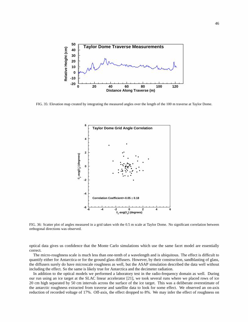
46

-20

-10

0

10

20

30

40

50

0 20 40 60 80 100 120Distance Along Traverse (m)

Rel

ativ

e H

eig

ht

(cm

) Taylor Dome Traverse Measurements

FIG. 35: Elevation map created by integrating the measured angles over the length of the 100 m traverse at Taylor Dome.

-6

-4

-2

0

2

4

6

-6 -4 -2 0 2 4 6θx-avg(θx) (degrees)

θ y-av

g(θ

y) (

deg

rees

)

Taylor Dome Grid Angle Correlation

Correlation Coefficient=-0.05 ± 0.18

FIG. 36: Scatter plot of angles measured in a grid taken with the 0.5 m scale at Taylor Dome. No significant correlation betweenorthogonal directions was observed.

optical data gives us confidence that the Monte Carlo simulations which use the same facet model are essentiallycorrect.

The micro-roughness scale is much less than one-tenth of a wavelength and is ubiquitous. The effect is difficult toquantify either for Antarctica or for the ground glass diffusers. However, by their construction, sandblasting of glass,the diffusers surely do have microscale roughness as well, but the ASAP simulation described the data well withoutincluding the effect. So the same is likely true for Antarctica and the decimeter radiation.

In addition to the optical models we performed a laboratory test in the radio-frequency domain as well. Duringour run using an ice target at the SLAC linear accelerator [21], we took several runs where we placed rows of ice20 cm high separated by 50 cm intervals across the surface of the ice target. This was a deliberate overestimate ofthe antarctic roughness extracted from traverse and satellite data to look for some effect. We observed an on-axisreduction of recorded voltage of 17%. Off-axis, the effect dropped to 8%. We may infer the effect of roughness on

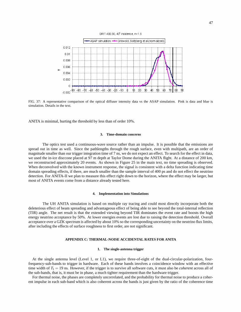
47

FIG. 37: A representative comparison of the optical diffuser intensity data vs the ASAP simulation. Pink is data and blueissimulation. Details in the text.

ANITA is minimal, hurting the threshold by less than of order10%.

3. Time-domain concerns

The optics test used a continuous-wave source rather than animpulse. It is possible that the emissions arespread out in time as well. Since the pathlengths through therough surface, even with multipath, are an order ofmagnitude smaller than our trigger integration time of 7 ns,we do not expect an effect. To search for the effect in data,we used the in-ice disccone placed at 97 m depth at Taylor Domeduring the ANITA flight. At a distance of 200 km,we reconstructed approximately 20 events. As shown in Figure 25 in the main text, no time spreading is observed.When deconvolved with the known instrument response, the signal is consistent with a delta function indicating timedomain spreading effects, if there, are much smaller than the sample interval of 400 ps and do not effect the neutrinodetection. For ANITA-II we plan to measure this effect rightdown to the horizon, where the effect may be larger, butmost of ANITA events come from a distance already tested here.

4. Implementation into Simulations

The UH ANITA simulation is based on multiple ray tracing and could most directly incorporate both thedeleterious effect of beam spreading and advantageous effect of being able to see beyond the total-internal reflection(TIR) angle. The net result is that the extended viewing beyond TIR dominates the event rate and boosts the highenergy neutrino acceptance by 50%. At lower energies eventsare lost due to raising the detection threshold. Overallacceptance over a GZK spectrum is affected by about 10% so thecorresponding uncertainty on the neutrino flux limits,after including the effects of surface roughness to first order, are not significant.

APPENDIX C: THERMAL-NOISE ACCIDENTAL RATES FOR ANITA

1. The single-antenna trigger

At the single antenna level (Level 1, or L1), we require three-of-eight of the dual-circular-polarization, four-frequency-sub-bands to trigger in hardware. Each of these bands involves a coincidence window with an effectivetime width ofT1 = 19 ns. However, if the trigger is to survive all software cuts, it must also becoherentacross all ofthe sub-bands, that is, it must be in phase, a much tighter requirement than the hardware trigger.

For thermal noise, the phases are completely uncorrelated,and the probability for thermal noise to produce a coher-ent impulse in each sub-band which is also coherent across the bands is just given by the ratio of the coherence time

48

τcoh of the full-band impulse to the total coincidence window, multiplied by the number of independent trials for a co-herent signal within the coincidence window to produce the 3of 8 trigger combination. The number of combinationsof N subbands takenM at a time gives a combinatoric factor ofC = N!/(M!(N−M!)), and forN = 8,M = 3 we haveC = 56. For any given combination ofM sub-bands that gives an L1 trigger, there are

(

T1

τcoh

)M

combinations of sub-band signals that can trigger, but onlythose for which the relative locations in the sub-bands areidentical (ignoring constant offsets for sub-band differential delays) can yield a coherent full-band pulse. There arethusT1/τcoh such coherent combinations. The probability of obtaining one such combination is thus

P1 = C

(

τcoh

T1

)M−1

. (C1)

The coherence timeτcoh is estimated by requiring that the signal be phase-coherentacross the full-band, and thusthat the sub-bands have less than aλ/8 phase offset between them for a wavelength at the mean frequency f of theband. Forf ≃ 600 MHz as for ANITA, the delay corresponding to a 1/8-wave phase difference isτcoh≃ 200 ps, whichgivesP1 = 6.2×10−3.

2. The level 2 and 3 trigger: azimuth+elevation constraint

For the L2 trigger, adjacent antennas must each have an L1 trigger with 5 ns of overlap for a 30 ns L1 one-shotoutput, giving an effective coincidence window of aboutT2 ≃ 40 ns. The number of possible combinations of pairsof L1 impulse arrival times that can produce L2 triggers isT2/τaz whereτaz is the azimuthal time resolution for pairof antennas within an azimuthal ring. Similar analysis applies to the elevation constraint via the L3 trigger, whichcouples the upper and lower rings. The coincidence window for L3 triggers is the convolution of the L2 windows, andgivesT3 ≃ 50 ns.

However, the analysis requires an additional azimuth constraint in the other ring, combined with a pair of elevationconstraints for adjacent phi-sector pairs. To estimate thefraction of such combinations of 4-antenna triggers thatadd coherently to give a proper direction reconstruction, we take the ratio of the geometric mean of the elevation andazimuth time resolutions to the total number of combinations of random impulses that can form in the 4T2 coincidencewindows required for an L3. This represents the probabilitythat a single direction (the normal incidence plane wave)can be mimicked by thermal noise:

p2 =

(√τazτel

T2

)4

Multiplying this by the number of independent directions within the antenna beam, and by the number of phi sectorsNφ then gives the total probability at the L3 level.

For a beam withΩ = π∆θ∆φ ≃ π(0.3)(1.0) = 0.94 square degrees, and an antenna main beam solid angle ofΩant ≃ πΦ2/4 for a half-power beam widthΦ ≃ 40, we finally get

P2 = NφKΩant

Ωp2 (C2)

whereK is the fraction of the main antenna beam that is allowed (eg, the fraction below the horizon). For ANITA, thegeometric mean of the timing errors is about 60 ps, and thusP2 ≃ 5.4×10−8, for K = 1.

3. Combined probability

Combining the L1 probability and the L2 probability since they are independent for thermal noise, the total proba-bility for a thermal noise trigger to produce an acceptable direction reconstruction is

Ptot = P1 P2 = (6.2×10−3)× (5.4×10−8) = 3.4×10−10 (C3)

49

or about 0.003 events expected during ANITA’s flight, based on 8.2M triggers.

[1] K. Greisen, Phys. Rev. Lett.16, 748 (1966); G. T. Zatsepin and V. A. Kuzmin, JETP Lett.4, 78 (1966) [Pisma Zh. Eksp. Teor.Fiz. 4, 114 (1966)].

[2] V. S. Beresinsky and G. T. Zatsepin, Phys. Lett. B 28, 423 (1969).[3] G. A. Askaryan, 1962, JETP 14, 441; 1965, JETP 21, 658.[4] P. W. Gorham, C. L. Hebert, K. M. Liewer, C. J. Naudet, D. Saltzberg, D. Williams, Phys. Rev. Lett. 93 (2004) 041101.[5] I. Kravchenko et al., Astropart.Phys. 20 195-213 (2003).[6] P. W. Gorham, D. Saltzberg, R. C. Field,et al., Phys. Rev. D 72, 023002 (2005).[7] J. V. Jelleyet al., Nature 205, 327 (1965); Nuovo CimentoA46, 649 (1966); N. A. Porteret al., Phys. Lett.19, 415 (1965);

S. N. Vernovet al., Pis’ma v ZhETF5, 157 (1967) [Sov. Phys.–JETP Letters5, 126 (1967)]; Can. J. Phys.46, S241 (1968);P. R. Barker, W. E. Hazen, and A. Z. Hendel, Phys. Rev. Lett.18, 51 (1967); W. E. Hazen,et al., ibid. 22, 35 (1969);24, 476(1970); D. Fegan & N. A. Porter, Nature, 1968; H. R. Allan, inProgress in Elementary Particles and Cosmic Ray Physics, v.10, edited by J. G. Wilson and S. G. Wouthuysen (North-Holland, Amsterdam, 1971), p. 171, and references therein.

[8] The IceCube Collaboration: M. Ackermann et al., Nucl. Instrum. Meth. A556 (2006) 169.[9] V. S. Beresinsky and G. T. Zatsepin, Phys. Lett. B 28, 423 (1969); R. Engel, D. Seckel and T. Stanev, Phys. Rev. D 64, 093010

(2001).[10] G. A. Gusev, I. M. Zheleznykh, “On the possibility of detection of neutrinos and muons on the basis of radio radiationof

cascades in natural dielectric media (antarctic ice sheet and so forth),” SOV PHYS USPEKHI, 1984, 27 (7), 550-552.[11] M. A. Markov, I. M. Zheleznykh, Nucl. Instr. Meth. A 248 (1986) 242.[12] I. M. Zheleznykh, 1988, Proc. Neutrino 88, 528.[13] R. D. Dagkesamanskii, & I. M. Zheleznyk, 1989, JETP 50, 233.[14] E. Zas, F. Halzen, & T. Stanev, 1992, Phys Rev D 45, 362.[15] J. Alvarez–Muniz & E. Zas, 1997, Phys. Lett. B, 411, 218.[16] D. Saltzberg, P. Gorham, D. Walz,et al.Phys. Rev. Lett.,86, 2802 (2001).[17] G. M. Frichter, J. P. Ralston, D. W. McKay, Phys. Rev. D 53(1996) 1684-1698.[51] J. Alvarez-Muniz, R.A. Vazquez and E. Zas, “Calculation Methods for Radio Pulses from High Energy Showers,” astro-

ph/0003315.[19] “Coherent Radio Pulses From GEANT Generated Electromagnetic Showers In Ice,” S. Razzaque, S. Seunarine, D. Z. Besson,

D. W. McKay, J. P. Ralston, D. Seckel, Phys.Rev. D65 (2002) 103002; arXiv:astro-ph/0112505[20] P. Miocinovic, R. C. Field, P. W. Gorham,et al., Phys. Rev. D 74, 043002 (2006).[21] ANITA Collaboration: P. W. Gorham, et al., Phys. Rev. Lett. 99 (2007), 171101.[22] A. R. Jacobson, S. O. Knox, R. Franz, & D. C. Enemark, ”FORTE observations of lightning radio-frequency signatures:

Capabilities and basic results,” Radio Science 34, 337, (1999); D. C. Enemark, & M. E. Shipley, ”The FORTE receiver andsub-band triggering unit,” Eighth Ann. Am. Inst. of Aeronautics and Astronautics, Utah State Univ. Conf. on Small Satellites,Logan, UT, 1994; Much information on FORTE can be gathered from http://forte.lanl.gov

[23] N. Lehtinen, P. Gorham, A. Jacobson, & R. Roussel-Dupre, Phys. Rev. D 69 (2004) 013008; astro-ph/030965.[24] The ANITA Collaboration: S. W. Barwicket al., Phys. Rev. Lett. 96 (2006) 171101.[25] A.R. Jacobson, pers. communication, (2001).[26] A. R. Jacobson, K. L. Cummins, M. Carter, et al., ”FORTE radio-frequency observations of lightning strokes detected by

the National Lightning Detection Network,”JGR105, 15, 653 (2000); R. Roussel-Dupre, & A. V. Gurevich, ”On runawaybreakdown and upward propagating discharges,”JGR 101, 2297 (1996); A. V. Gurevich, K.P. Zybin, and R. Roussel-Dupre,”Lightning Initiation by simultaneous effect of runaway breakdown and cosmic ray showers,” submitted toJGR(2001).

[27] T. Huege and H. Falcke, Astropart.Phys. 24 (2005) 116-136; astro-ph/0501580.[28] D. Fegan & N. A. Porter, Nature, 1968.[29] S. Barwick, D. Besson, P. Gorham, D. Saltzberg, J. Glaciol. 51 (2005) 231.[30] http://msp.gsfc.nasa.gov/tdrss/oview.html[31] NOAA NGDC: http://www.ngdc.noaa.gov/geomagmodels/struts/calcGridIGRF[32] G.S. Varner, “The Modern FPGA as Discriminator, TDC andADC”, Journal of Instrumentation, Vol.1, P07001 (2006).[33] R. Engel, D. Seckel, T. Stanev, “Neutrinos from Propagation of Ultrahigh Energy Protons, Phys.Rev. D64:093010[34] S. Kleinfelder, “GHz Waveform Sampling and Digitization Circuit Design and Implementation”, IEEE Trans. Nucl. Sci. 50,

No. 4, pp. 955-962, August 2003.[35] S. Ritt, “The DRS chip: Cheap waveform digitizing in theGHz range.”, Nucl. Instrm. Meth.A 518:470-471 (2004).[36] G. Varneret al., “Monolithic Multi-channel GSa/s Transient Waveform Recorder for Measuring Radio Emissions from High

Energy Particle Cascades”, Proc. SPIE Int. Soc. Opt. Eng. 4858-31, 2003.[37] G.S. Varner, L.L. Ruckman, R.J. Nichol, J. Nam, J. Cao, M. Wilcox and P. Gorham,“Large Analog Bandwidth Recorder and

Digitizer with Ordered Readout (LABRADOR) ASIC,”Nucl. Instr. Meth.A483:447-460 (2007).

http://msp.gsfc.nasa.gov/tdrss/oview.html

50

[38] H. Falcke & P. Gorham 2003, Astropart.Phys. 19 (2003) 477-494.[39] R. E. Spencer, ”Radio Pulses from Cosmic Ray Air Showersat 44, 105, 239, and 408 MHz,” Nature 222, 460 (1969).[40] D. J. Fegan and P. J. Slevin, ”Radio Pulses from Extensive Air Showers at 520 MHz,” Nature 217, 440 (1968).[41] D. J. Fegan and D. M. Jennings, ”UHF Radio Pulses from theZenith Associated with Extensive Air Showers,” Nature 223,

722 (1969).[42] Auger references, ICRCs 2005, 2007: arXiv:0707.2638.[43] Lythe, M. B., D. G. Vaughan, and the BEDMAP Consortium (2001), BEDMAP: A new ice thickness and subglacial topo-

graphic model of Antarctica, J. Geophys. Res., 106(B6), 11,33511,351[44] Bassin, C., Laske, G. and Masters, G., The Current Limits of Resolution for Surface Wave Tomography in North America,

EOS Trans AGU, 81, F897, 2000.[45] Ghandhi,Reno,Quigg,Sarcevic, hep-ph/9512364.[46] SunCat Solar, LLC, 9121 E. Tanque Verde Rd., Tucson AZ 85749.[47] http://www.pol.ac.uk/psmsl/puscience/[48] H. Nyquist, “Thermal Agitation of Electric Charge in Conductors,,” Phys. Rev. 32, 110, (1928).[49] J. Alvarez-Muniz, Phys.Lett.B411:218-224 (1997) astro-ph/9706064.[50] J. Alvarez-Muniz, Phys.Lett.B434:396 (1998) astro-ph/9806098.[51] J. Alvarez-Muniz,et al., Phys. Rev. D74, 023007 (2006) astro-ph/0512337.[52] D.Z. Besson et al. (for the ANITA collaboration) “In situ radioglaciological measurements near Taylor Dome, Antarctica and

implications for ultra-high energy (UHE) neutrino astronomy” Astropart. Phys., Volume 29, Issue 2, March 2008, 130-157[53] M. Nieto-Vesperinaset al., “Light transmission from a randomly rough dielectric diffuser: theoretical and experimental re-

sults,” Optics Letters15, 1261 (1990).[54] T. Furukawa, K. Kamiyama and H. Maeno, “Snow Surface Features along the Traverse Route from the Coast to Dome Fuji

Station, Queen Maud Land, Antarctica,” Proc. NIPR Symp. Polar Meteorol. Glaciol.,10, 13-24 (1996).[55] I. Goodwin, “Snow Accumulation and Surface Topology inthe Katabatic Zone of Eastern Wilkes Land, Antarctica”, Antarctic

Science 2,3, 235-242 (1990).[56] M. Griswold and D. Saltzberg, “Review of Literature Regarding Small-Scale Surface Roughness in Antarctica” ANITA-note

#108http://www.phys.hawaii.edu:8080/anita notes/108.[57] A. Romero-Wolf and D. Saltzberg, “Taylor Dome Snow Surface Roughness,” ANITA-note #330.

http://www.phys.hawaii.edu:8080/anita notes/330.[58] M. Griswold, M. Harrison and D. Saltzberg, “Observation of Light Transmission Through Random Rough Glass Sur-

faces Beyond the critical Angle, J. Op. Soc. Am. A.24, 3207 (2007); More detail is given in the following: B. Daubetal. ANITA-note #77, http://www.phys.hawaii.edu:8080/anita notes/77 and M. Harrisonet al. ANITA-note #101,http://www.phys.hawaii.edu:8080/anita notes/101.

[59] A. Dogariu and G. Boreman, “Facet Model for Photon-FluxTransmission through Rough Dielectric Interfaces”, Optics Letters21, 701 (1996).

[60] Dookayka, K., Ph.D. dissertation, in preparation, University of California, Irvine (2009).[61] PN = kBTsys∆ f , for kB = 1.38×10−23J/K, Tsys= the system noise temperature in Kelvin, and∆ f = the bandwidth in Hz.

The Antarctic Impulsive Transient Antenna ultra-high energy neutrino detector: Design, performance,...

Documents

Transcript of The Antarctic Impulsive Transient Antenna ultra-high energy neutrino detector: Design, performance,...