The Algebra of Timed Processes, ATP: Theory and Application
50
Transcript of The Algebra of Timed Processes, ATP: Theory and Application

The Algebra of Timed Processes ATP: Theory and Application
Xavier Nicollin Joseph Sifakis
Laboratoire de G�enie Informatique
IMAG-Campus B.P. 53X
38041 Grenoble Cedex { FRANCE
phone: (+33) 76-51-48-74
email: [email protected], [email protected]
Abstract
We study a process algebra ATP for the description and analysis of systems of timed
processes. An important feature of the algebra is that its vocabulary of actions contains a
distinguished element �. An occurrence of � is a time event representing progress of time.
The algebra has, apart from standard operators of process algebras like CCS or ACP, a
primitive binary unit-delay operator. For two arguments, processes P and Q, this operator
gives a process which behaves as P if started before the occurrence of a time action and
as Q otherwise. From this operator we de�ne d-unit delay operators that can model delay
constructs of languages, like timeouts or watchdogs. The use of such operators is illustrated
by examples.
ATP is provided with a complete axiomatisation with respect to strong bisimulation
semantics. It is shown that the algebras obtained by adding the various d-unit delay operators
to ATP are conservative extensions of it.
1 Introduction
The paper presents the algebraATP for the modelling and analysis of systems of timed processes.
The algebra uses a notion of discrete global time and suggests a conceptual framework for tackling
the problem of introducing time in description languages. The presentation of this framework
and underlying notions is the objective of the present section.
A system is considered to be a set of interacting sequential components. A component may
evolve by performing actions. The actions can be, either individual actions of the components,
or the result of the simultaneous occurrence of individual actions (communication actions).
Depending on the way the individual actions of a system are composed to obtain its global
behaviour, the majority of the existing models fall into one of the two following categories:
Asynchronous models, where there may be execution sequences with no action of some
deadlock-free component. That is, the execution of an enabled action in a component may
be postponed inde�nitely. The underlying models of most of the existing formalisms for
the description of concurrent systems are asynchronous; programming languages like ADA
and CSP [Hoa78], Petri nets, process algebras like CCS [Mil80] and ACP [BK84,BK86]
adopt explicitly or implicitly asynchronous parallel composition rules.
Synchronous models, where global actions are the result of the simultaneous occurrence of
actions in all the components. That is, no evolution is possible if a component fails to

2 x 1 Introduction
contribute to the realisation of an action, even by executing a trivial one. In this case,
components proceed at the same \speed"; some hardware description languages and process
algebras like SCCS [Mil83] and Meije [AB84] adopt such a mode of functioning.
Both asynchronous and synchronous models adopt extreme cases of scheduling policies: asyn-
chronous models use a completely unconstrained one, consisting in arbitrarily choosing among
possible actions, independently of the identities of the components performing them; synchronous
models use a too constrained one, since actions are performed at the same pace in all components.
To describe real life systems it is desirable to have models where it is possible to control the
delay of execution of actions since the instant they have been enabled. This type of models,
although of paramount practical interest, have not been extensively studied yet. Existing work
for the de�nition of non strictly asynchronous or synchronous models has been carried out in
two directions.
� The �rst one consists in restricting asynchronous models by using constraints discrimi-
nating di�erent types of unfair (in�nite) computations, as for instance in [LPS81]. Such
constraints are usually expressed in temporal logics and their e�ect is to reduce the degree
of asynchrony, as far as they prevent a sequential component from waiting inde�nitely for
execution.
� The second one consists in using timed models, that is, models with a global parameter
called time, to constrain the occurrences of the actions. This parameter is de�ned on a
in�nite totally ordered domain (D;�), which represents a set of \instants" or \dates".
Introducing time allows to associate dates with occurrences of actions. A time constraint
represents the allowed instants of action occurrences.
A fundamental assumption about time is that it is ultimately strictly increasing, that
is, if dates d
0
; d
1
; :::; d
i
; ::: are associated to the in�nite sequence of actions occurrences
a
0
; a
1
; :::; a
i
; :::, then for all i, d
i
� d
i+1
, and moreover, for any d in D, there exists i such
that d < d
i
.
The model for timed systems used for ATP is based on the following principles:
� A timed system is the parallel composition of communicating sequential components (pro-
cesses), all of which may execute a distinguished action, called time action. All the actions
of the system are atomic, i.e., their beginning and end coincide.
� Time progresses by synchronous execution of time actions, that is, time actions can be
performed only if all the components of the system agree to do so.
� An execution sequence is a sequence of steps, a step being determined by two consecutive
occurrences of time actions. Within a step, components may execute, either independently
or in cooperation, a �nite though arbitrarily long sequence of asynchronous actions (ac-
tions other than time actions), after which they all perform synchronously a time action,
corresponding to progress of time for the system. This implies that a component which can
perform no asynchronous action can always perform a time action. Synchronous execution
of a time action is the beginning of a new step.
The functioning described combines both synchronous and asynchronous cooperation in two al-
ternating phases: one where all the components agree for the time to progress, and the other con-
sisting in an eventually terminating asynchronous computation phase during which the progress
of time is blocked (see �gure 1).

x 1 Introduction 3
......
�-step
stepstep
tickticktick
Figure 1: the two phase functioning scheme
Such a mode of two-phase functioning is quite appropriate and natural for modelling reactive
systems. For instance, hardware and systems for real-time control function according to this
principle: time actions determine instants at which inputs are sampled, and from which an
output is elaborated at the end of the asynchronous computation phase. The same principle has
been adopted in the semantics of formalisms for the description of reactive or real-time systems,
like Lustre [CHPP87], Esterel [BC85] and the Statecharts [Har87]. One of the objectives of this
work is to convince that this principle is adequate for timed systems. In fact, it is already clear
that such a functioning scheme
� allows to correlate speeds of components since the ow of asynchronous computation can
be cut by introducing time actions in the appropriate manner.
� introduces an implicit concept of duration, de�ned as the number of steps elapsed. Thus,
one can assign duration to sequences of actions and, as it will be shown, control their
duration by using delay constructs. Clearly, natural integers can be considered as an
appropriate time domain.
Compared to existing work on timed systems, the notion of time introduced has the following
features:
� Time is discrete and its progress is explicitly modelled as an event. In that respect the
approach is di�erent from the one followed by [RR88,DS89,ACD90].
� The assumption about atomicity of actions implies that atomic actions take no time. Such
an assumption simpli�es theoretical development and does not go against generality, since
non atomic actions can be modelled by sequences of atomic ones. It has been pro�tably
adopted by other formalisms like Esterel.
� The time considered is abstract, in the sense that it is used as a parameter to express con-
straints about instants of occurrences of actions. The implementability of such constraints,
taking into account speeds and execution times of processors, is a separate, though not
independent, issue. This distinction between abstract and concrete or physical time is an
important one. It allows simpli�cations that are convenient at conceptual level, as it leads
to simpler and more tractable models. For instance, the assumption that an action may
take zero time, though not realistic for physical time, is quite convenient for abstract time.

4 x 1 Introduction
However, such an abstraction can take into account realisability issues: in any correct im-
plementation, the clock period should be taken greater than the longest execution time of
sequences of ideally zero time actions occurring between two successive executions of time
actions. The assumption about eventual progress of time guarantees that such a bound
exists. Finally, it should be noticed that as a consequence of the abstractness of the notion
of time considered, any action of a system could be taken as a time basis provided that it
obeys the strong synchrony rule in the functioning scheme proposed.
Following standard ideas, a term of ATP represents a process which after executing some action
is transformed into another process. The action vocabulary of the algebra contains a special
element denoting the time action and represented by �, whose execution represents progress of
time. The algebra has, apart from standard operators of process algebras like pre�xing by an
action di�erent from �, non-deterministic choice and parallel composition, a primitive binary
unit-delay operator. For two arguments, processes P and Q, this operator gives a process which
behaves as P if started before the execution of a time action, and behaves as Q otherwise. It
is shown that several d-unit delay constructs, like timeouts and watchdogs used in languages to
describe delay constraints, can be expressed in terms of the unit-delay operator and standard
process algebra operators.
The strong synchrony assumption for time actions is realised by considering that the parallel
composition operator is synchronous for them, while it is asynchronous for all other actions. This
guarantees soundness of the notion of time | time progress is the same for all the components
of a system. Furthermore, it implies that if a sequential component is not controlled by a delay
(cannot execute a time action �), then it must execute some of its actions before any time action
occurs. Thus, synchrony of time allows to satisfy the assumption about zero duration of actions.
Another important assumption about time actions is that they cannot be in con ict, that is,
the transition system representing the behaviour of a timed system is deterministic for time
actions. The combination by the non-deterministic choice operator of two processes with initial
time actions yields a process which can execute a unique time action. After execution of the
latter, the combined process may execute any action possible in each one of the components after
the occurrence of a time event. The reasons for requiring determinism for time actions will be
explained later.
This work, which develops and formalises the ideas presented in previous papers [RSV87,
NRSV90], is organised as follows:.
� In section 2, we present the basic operators of ATP, which generate the Algebra of Sequen-
tial Timed Processes ASTP. An operational semantics and an axiomatisation for each
of these operators is given. The axiomatisation is proven to be sound and complete with
respect to strong bisimulation.
� We introduce in section 3 parallel and encapsulation operators, building so the algebra
ATP. We present their semantics and axiomatisation, and we prove that ATP is a con-
servative extension of ASTP, that is, for any process of ATP there is an equivalent a
process of ASTP.
� Some processes of ATP cannot really be considered as timed processes, since they can
generate behaviours where time cannot progress. The purpose of section 4 is to characterise
well-timed processes, that is processes where the progress of time is inevitable.
� In section 5, three types of operators describing high-level delay constructs are presented:
the start delay operators (or timeout operators), the unbounded start delay operator, and

x 2 Sequential timed processes: the algebra ASTP 5
the execution delay operators (or watchdog operators). Their operational semantics and
axiomatisations are provided. By using the axioms, any process with such high-level con-
structs can be expressed in terms of the low-level operators of ASTP.
� In section 6, three examples of description of timed systems are provided, illustrating
the use of delay constructs: a login procedure, and timed versions of the alternating bit
protocol.
� Finally, we present in section 7 a comparison of ATP with similar work.
2 Sequential timed processes: the algebra ASTP
In this section, we de�ne the algebra of sequential timed processes ASTP, which is the core of
the algebra of timed processes described in section 3.
2.1 Syntax
Let A be a countable set of constants called actions. We distinguish in A a particular element �
and represent by A
�
the set A� f�g. The elements of A
�
are called asynchronous actions. � is
the action representing the progress of time. The symbols �, �
1
, �
2
... and a, a
1
, a
2
... are used
to represent elements of A
�
and A respectively.
Let V be a countable set of variables, whose elements are represented by symbols X, X
1
, X
2
...,
Y , Y
1
, Y
2
... Consider the term algebra P, whose elements are denoted by p, q, r, p
0
, ..., p
1
, ...,
de�ned by the following operators:
� : ! P
� 2 A
�
: P [ V ! P
� : P � P ! P
b c : P � (P [ V)! P
rec : V � P ! P
The operators are given the following meaning:
� � is a constant denoting a blocked or terminated process.
� For all � in A
�
, � is a unary pre�xing operator. It has the same meaning as in CCS [Mil80],
and we write � p instead of �(p).
� � is a binary non-deterministic choice operator.
� b c is a binary operator, called unit-delay. For p, q arguments of b c, we write bpc(q) instead
of b c(p; q). p is called the body, and q the exception of the unit-delay.
� rec is a recursion operator. We write recX � p instead of rec(X; t). The notions of free and
bound occurrences of variables and of closed terms are the same as in [Mil80]. We denote
by Free(p) the set of free variables of a term p.
We call Algebra of Sequential Timed Processes ASTP the sub-algebra of the closed terms of P,
that is, terms p such that Free(p) = ;. The elements of ASTP are denoted by P , Q, R, P
0
, ...,
P
1
, ...

6 x 2 Sequential timed processes: the algebra ASTP
2.2 Operational semantics
We de�ne operational semantics for P (and thus for ASTP) associating with a term a canonical
representative of an equivalence class of labelled transition systems. Labelled transition systems
are de�ned by means of a transition relation on terms. The equivalence relation considered is
strong equivalence. Considering P rather than ASTP is necessary since many proofs in this
section require dealing with open terms.
2.2.1 Transition relation
The transition relation ! is a subset of P �A� 2
V
�P.
We use the standard notation p
a; S
! q for (p; a; S; q) 2!. It expresses the fact that the term p
may perform action a, and the resulting term is q. Moreover, the set S is a recording of the free
variables \encountered" when p performs the action a. We prefer labelling transitions with the
set of the free variables encountered than extending ! on sets of variables; for instance, rather
than writing �X
�
! X, where X is in V, we write �X
(�; fXg)
! �.
To simplify notation, the pair (a; fXg) is denoted by (a;X), and the pair (a; ;) is denoted by a.
We omit the parentheses when (a; S) is a label of !.
The transition relation is de�ned by structural induction, �a la Plotkin [Plo81]. It is the least
relation on P such that:
�
�
! � � p
�
! p �X
�;X
! �
p
�; S
! p
0
p� q
�; S
! p
0
q
�; S
! q
0
p� q
�; S
! q
0
p
�; S
1
! p
0
q
�; S
2
! q
0
p� q
�; S
1
[ S
2
! p
0
� q
0
p
�; S
! p
0
bpc(q)
�; S
! p
0
p
�; S
! p
0
bpc(X)
�; S
! p
0
bpc(q)
�
! q bpc(X)
�;X
! �
p[(recX � p)=X]
a; S
! p
0
recX � p
a; S
! p
0
The notation p[p
0
=X] represents the term p where p
0
is substituted to every free occurrence of
X.
Some remarks about the transition relation:
� The restriction of these rules to closed terms (by suppressing the third, eighth and tenth
rules) de�nes a transition relation where the set S is always empty in the pair (a; S).
Clearly, only this restriction of the transition relation to ASTP is interesting in practice
as it does not make sense associating behaviours to open terms.
� A terminated process � can perform no asynchronous action, but it can let time pass by
performing � actions.
x 2 Sequential timed processes: the algebra ASTP 7
� The process bP c(Q) can perform the same asynchronous initial actions as P , and the
subsequent behaviours are identical. Moreover, bP c(Q) can perform a � action, reaching
process Q. Hence bP c(Q) is the process which behaves as P if it starts (executes an
asynchronous action) before the occurrence of a time action �; if it is not engaged in the
execution of P and � occurs then it behaves as Q. Thus, the unit-delay operator can be
considered as an elementary timeout construct with delay 1.
� The operator � behaves as a standard non-deterministic choice for processes with asyn-
chronous initial actions. Moreover, if P and Q can perform � actions reaching respectively
P
0
and Q
0
, then P �Q can perform a � action reaching P
0
�Q
0
. This is a factorisation
rule for � actions which implies that the transition relation is deterministic for �. It means
that the resolution of a con ict between time actions is postponed until a con ict between
asynchronous actions appears.
Being deterministic with respect to � transitions is an important feature of the algebra. If �
behaved as standard non-deterministic choice with respect to time actions, then the process
P = bP
1
c(Q
1
)� bP
2
c(Q
2
) could perform one of the transitions P
�
! Q
1
or P
�
! Q
2
.
That is, after the �rst occurrence of a time action, there would be no more choice of the
exception Q
i
to be executed.
� Finally, the process P �Q can execute a � action only if both P and Q can do so. This
rule guarantees that � is the zero element for �.
2.2.2 Equivalence relation
De�nition: Strong equivalence [Mil83] is an equivalence relation, denoted by �, de�ned as the
largest strong bisimulation R on P such that:
pR q )
8
<
:
8a 8S 8p
0
[p
a; S
! p
0
) 9q
0
q
a; S
! q
0
and p
0
R q
0
]
8a 8S 8q
0
[q
a; S
! q
0
) 9p
0
p
a; S
! p
0
and q
0
R p
0
]
To express the fact that p is equivalent to q with respect to the semantics of P (resp. ASTP),
we write P j= p � q (resp. ASTP j= p � q), which is abbreviated by p � q when no confusion is
possible
The following proposition tells that � is a congruence on P, and thus on ASTP.
Proposition 1
8p; q; r 2 P; 8X 2 V; p � q )
8
>
>
>
>
>
>
>
>
>
>
<
>
>
>
>
>
>
>
>
>
>
:
� p � � q
r � p � r � q
p� r � q � r
bpc(r) � bqc(r)
bpc(X) � bqc(X)
brc(p) � brc(q)
recX � p � recX � q
The proof can be obtained as an application of a theorem presented in [GV88]. This theorem
asserts that if a transition system speci�cation (a signature, a set of labels and a set of rules) is
in some particular format called tyft/tyxt format, and is not circular, then the strong equivalence
is a congruence. We do not give here the de�nitions of the format and of circularity. In our

8 x 2 Sequential timed processes: the algebra ASTP
case, it is easy to check that every rule of the operational semantics is in tyft/tyxt format, and is
non-circular. So, the theorem holds, and strong equivalence is a congruence.
2.2.3 Models of processes
The semantics induces a transition relation !
=�
on the quotient-algebra P=� (whose elements
are denoted by [p] for the class of p). This relation is de�ned by:
[p]
a; S
!
=�
[q] , p
a; S
! q
Notice that this de�nition makes sense, since � is a bisimulation.
De�nition: the model of a term p of P, denoted by M(p), is the transition system (Q; q
1
;R),
where
� the set of states Q is a subset of P=� containing the elements [p
0
] of P=� which are
reachable from [p], that is, such that [p]
�
!
=�
[p
0
].
� the initial state q
1
is the class of p (that is [p])
� the transition relation R is !
=�
The models are de�ned so that if p � p
0
, then M(p) =M(p
0
).
Remark: In the sequel, we represent the model of a process by a labelled digraph. For sake of
readability, we might take some freedom with this de�nition by giving digraphs whose number
of nodes is not minimal.
In �gure 2, we present the models of some processes.
2.3 Axiomatisation
We propose a set of axioms for ASTP and prove that this axiomatisation is sound and complete
with respect to the semantics given above.
Let � be the least congruence on ASTP induced by the following axioms:
[�1] P � Q � Q � P
[�2] P � (Q � R) � (P � Q) � R
[�3] P � P � P
[�4] P � � � P
[�5] �P � bQc(R) � �P � Q
[�6] bP
1
c(Q
1
) � bP
2
c(Q
2
) � bP
1
� P
2
c(Q
1
� Q
2
)
[b c1] b�c(�) � �
[b c2] bbP c(Q)c(R) � bP c(R)
[rec1] recX � P � P [(recX � P )=X]
[rec2] if P [Q=X] � Q then recX � P � Q

x 2 Sequential timed processes: the algebra ASTP 9
�
1
� � �
2
(�
3
� � �
4
�)
b�
1
�cb�
2
� � �
3
�c(�
4
� � �
5
�)
recX � b�
1
X � �
2
�c(�
3
X)
b�c(�
1
� � �
2
�)
�
� ��
�
�
�
�
1
�
2
�
4
�
3
�
�
�
�
1
�
2
�
3
�
4
�
5
�
2
�
�
�
1
�
2
�
3
�
1
�
�
Figure 2: transition systems modelling some processes
Notice that, in this axiomatisation, we �nd the standard axioms of non-deterministic choice
[�1� 4] and recursion, plus four axioms about the unit-delay operator. In particular, the last
one [b c2] tells that in nested unit-delays, the outermost exception has priority over the inner
ones.
We write ASTP ` P � Q if P and Q are congruent modulo these axioms and we abbreviate
this notation by P � Q when no confusion is possible.
2.3.1 Soundness
We prove that the axioms proposed are sound with respect to operational semantics.
Theorem 1 (Soundness)
8P;Q 2 ASTP; ASTP ` P � Q ) ASTP j= P � Q
Proof. To prove this theorem, it is su�cient to show that � is itself a bisimulation. We present
the proof for the axioms of the unit-delay, that is axioms [�5], [�6], [b c1] and [b c2].
1. [�5] : let R
1
= �P � bQc(R) and R
2
= �P �Q.
Suppose R
1
a
! R
0
. There is no transition by � from �Q. So a 6= �. There are two possibilities:
� �P
a
! R
0
(a = �). Then we have R
2
a
! R
0
and, since � is an equivalence, R
0
� R
0
� bQc(R)
a
! R
0
. Since a 2 A
�
, we must have: Q
a
! R
0
. Then R
2
a
! R
0
, and R
0
� R
0
If we suppose R
2
a
! R
0
, we can prove in the same way that R
1
a
! R
0
.
2. [�6] : let R
1
= bP
1
c(Q
1
)� bP
2
c(Q
2
) and R
2
= bP
1
� P
2
c(Q
1
�Q
2
)

10 x 2 Sequential timed processes: the algebra ASTP
Suppose R
1
a
! R
0
.
� if a = �, we have bP
1
c(Q
1
)
�
! Q
1
and bP
2
c(Q
2
)
�
! Q
2
; so R
1
a
! Q
1
�Q
2
is the only
possibility: R
0
= Q
1
�Q
2
. Furthermore, we have R
2
�
! R
00
where R
00
= Q
1
�Q
2
, and
R
0
� R
00
� if a 2 A
�
, we have P
1
a
! R
0
or P
2
a
! R
0
. Then, P
1
� P
2
a
! R
0
, and �nally R
2
a
! R
0
The case where we suppose R
2
a
! R
0
is similar.
3. [b c1] : let R
1
= b�c(�) and R
2
= �, and suppose R
1
a
! R
0
. We can only have a = �, and
R
1
�
! � (R
0
= �). We have also R
2
�
! �, and � � �.
If we suppose R
2
a
! R
0
, we get the same result.
4. [b c2] : let R
1
= bbP c(Q)c(R) and R
2
= bP c(R), and suppose R
1
a
! R
0
.
� if a = �, we can only have R
1
�
! R, so R
0
= R. We have also R
2
�
! R
00
where R
00
= R,
and then R
0
� R
00
� if a 2 A
�
, we can only have bP c(Q)
a
! R
0
, and then P
a
! R
0
. This implies R
2
a
! R
0
,
and R
0
� R
0
The hypothesis R
2
a
! R
0
leads to the same conclusions.
Since � is commutative and associative (axioms [�1] and [�2]), we use the notations
n
X
i=1
�
i
P
i
or
X
i2I
�
i
P
i
, where I is a �nite non-empty multiset of indices, to represent the process obtained by
combining all the �
i
P
i
's, using the non-deterministic choice operator. We use the meta-variables
P
�
, P
�
1
, P
�
2
,... to represent such terms.
2.3.2 Systems of equations
A system of equations is often used to describe recursively de�ned processes. For instance:
P where
(
P = b�Qc(P ) � b� P c(Q)
Q = P � �Q
means:
\the process P such that there exists Q such that P and Q satisfy the equations modulo �".
The following proposition asserts that such systems of equations have a unique solution modulo�.
Proposition 2
Let
e
X = X
1
; :::;X
m
and
e
Y = Y
1
; :::; Y
n
be distinct elements of V, and let
e
q = q
1
; :::; q
m
be
elements of P, with free variables in h
e
X;
e
Y i. There exist
e
p = p
1
; :::; p
m
, elements of P, with free
variables in
e
Y , such that
p
i
� q
i
[
e
p=
e
X] i = 1::m
Moreover
e
p is unique modulo �.

x 2 Sequential timed processes: the algebra ASTP 11
Proof. The proof is inspired from [Mil84]. We proceed by induction on m.
� m = 1. Let p
1
= recX
1
� q
1
. Then p
1
has free variables in
e
Y , and moreover, by the axiom
[rec1], p
1
� q
1
[p
1
=X
1
]. The unicity modulo � is immediate by using the axiom [rec2].
� Assume the result form, and let
e
q = q
1
; :::; q
m
and q
m+1
be elements of P, with free variables
in
e
X;X
m+1
;
e
Y .
We de�ne
r
m+1
= recX
m+1
� q
m+1
; and
r
i
= q
i
[r
m+1
=X
m+1
] i = 1::m
For i � m, r
i
has free variables in h
e
X;
e
Y i. Therefore, by induction, there exist
e
p = p
1
; :::; p
m
with free variables in
e
Y , such that
p
i
� r
i
[
e
p=
e
X] i = 1::m
Now de�ne
p
m+1
= r
m+1
[
e
p=
e
X]
We have then, for every i � m,
p
i
� q
i
[r
m+1
=X
m+1
][
e
p=
e
X]
� q
i
[(r
m+1
[
e
p=
e
X ;
e
p=
e
X])=X
m+1
]
� q
i
[
e
p=
e
X ; p
m+1
=X
m+1
]
Moreover, since X
m+1
is not free in
e
p, we obtain
p
m+1
= recX
m+1
� (q
m+1
[
e
p=
e
X])
� q
m+1
[
e
p=
e
X ; p
m+1
=X
m+1
] (axiom [rec1])
as required.
To prove the unicity, suppose that the result holds also for
e
p
0
= p
0
1
; :::; p
0
m
and p
0
m+1
, with
free variables in
e
Y . On the one hand, we have
p
0
m+1
� q
m+1
[
e
p
0
=
e
X ; p
0
m+1
=X
m+1
]
� q
m+1
[
e
p
0
=
e
X][p
0
m+1
=X
m+1
]
� recX
m+1
� (q
m+1
[
e
p
0
=
e
X]) (axiom [rec2])
Since X
m+1
is not free in
e
p
0
, we obtain
p
0
m+1
� r
m+1
[
e
p
0
=
e
X]
On the other hand, we use this last equation with the property of
e
p
0
to get, for i �m,
p
0
i
� q
i
[
e
p
0
=
e
X ; (r
m+1
[
e
p
0
=
e
X])=X
m+1
]
� q
i
[r
m+1
=X
m+1
][
e
p
0
=
e
X]
� r
i
[
e
p
0
=
e
X] (de�nition of r
i
)
But we have also p
i
� r
i
[
e
p=
e
X]; therefore, by using induction, we get, for all i � m, p
0
i
� p
i
.
Moreover, by applying these equivalences to the equation p
0
m+1
� r
m+1
[
e
p
0
=
e
X], we obtain
p
0
m+1
� r
m+1
[
e
p=
e
X]
� p
m+1
and this completes the proof

12 x 2 Sequential timed processes: the algebra ASTP
Notice that the case where there are no Y
i
's implies that the p
i
's are elements of ASTP. This
corresponds to the usual application of the proposition to the solution of systems of m equations
with m free variables.
2.3.3 Canonical form
The following proposition de�nes, for every process of ASTP, a canonical form, in terms of a
system of equations.
Proposition 3
Let P be a term of ASTP. Then there exist n � 1 and P
1
; :::; P
n
in ASTP, such that P � P
1
and each P
i
is solution of an equation in one and only one of the forms (1), (2) or (3) de�ned
as follows.
(1) P
i
�
X
j2J
i
�
j
P
j
; 6= J
i
� [1; n]
(2) P
i
� b�c(P
k
i
) k
i
2 [1; n]
(3) P
i
�
6
6
6
4
X
j2J
i
�
j
P
j
7
7
7
5
(P
k
i
) ; 6= J
i
� [1; n]; k
i
2 [1; n]
The proof is given in Annex 1. More precisely, the proposition is extended to open terms, and
the proof is conducted on this extension. Of course, we need to extend also the axiomatisation
to elements of P. For this purpose, we proceed as follows.
� in every axiom, P;Q;R are replaced by p; q; r
� in axiom [�5] (resp. [b c2]), p and r (resp. q and r) may be variables
� the following axiom is added: [b c3] bpc(X) � bpc(�) � b�c(X)
2.3.4 Completeness
The proof of the following completeness theorem is given in Annex 2.
Theorem 2 (Completeness)
Let P and Q be elements of ASTP. Then the following holds:
ASTP j= P � Q) ASTP ` P � Q
2.3.5 Characterisation of the models
The following proposition presents some essential properties of the models.

x 2 Sequential timed processes: the algebra ASTP 13
Proposition 4
The model of a process P is
� �nite
� �nitely branching
� without sink state (every state has at least one successor)
� deterministic with respect to � transitions (every state has at most one outgoing � tran-
sition)
Conversely, any transition system satisfying these properties is equivalent to a model of some
process.
Proof. From proposition 3, we know that there exist n � 1 and P
1
,..., P
n
in ASTP, such that
P � P
1
and every P
i
is solution of an equation in one of the three forms (1), (2) or (3) (see
section 2.3.3). Since the axiomatisation is sound, we have then P � P
1
, and thus P and P
1
have
the same model. We have then to prove the properties for the model of P
1
. This is immediate
by considering what this model is:
M(P
1
) = (Q; q
1
;!); where
� Q � f[P
i
]; i 2 [1::n]g
� q
1
= [P
1
]
� the transition relation ! is de�ned in every state [P
i
] according to the equation satis�ed
by P
i
:
If P
i
�
X
j2J
i
�
j
P
j
, then the outgoing transitions from [P
i
] are
8j 2 J
i
; [P
i
]
�
j
! [P
j
]
If P
i
� b�c(P
k
i
), then the unique outgoing transition from [P
i
] is
[P
i
]
�
! [P
k
i
]
If P
i
�
6
6
6
4
X
j2J
i
�
j
P
j
7
7
7
5
(P
k
i
), then the outgoing transitions from [P
i
] are
8j 2 J
i
; [P
i
]
�
j
! [P
j
]
[P
i
]
�
! [P
k
i
]
The �niteness of M(P ) is given by the �niteness of Q, and the other properties are deduced
from the set of transitions of a state.
Conversely, let T = (Q; q
1
;!) be a transition system (whose transitions are labelled by elements
of A) which is �nite, �nitely branching, without sink state and deterministic with respect to �
transitions.

14 x 3 ATP: the Algebra of Timed Processes
This can be reformulated in: every state has either a �nite number of asynchronous transitions
and no � transition, either only one � transition, or a �nite number of asynchronous transitions
and one � transition. We can then associate to each state q
i
an equation, depending on its
outgoing transitions:
� in the �rst case, we associate the equation
P
i
�
X
j2J
i
�
j
P
j
where for all j, q
i
�
j
! q
j
� in the second case, we associate the equation
P
i
� b�c(P
k
i
)
where q
i
�
! q
k
i
� in the last case, we associate the equation
P
i
�
6
6
6
4
X
j2J
i
�
j
P
j
7
7
7
5
(P
k
i
)
where for all j, q
i
�
j
! q
j
and q
i
�
! q
k
i
The proposition 2 tells that the system of these equations has a solution, that is, the P
i
's exist
and are in ASTP. By applying the same reasoning as in the �rst part of the proof, we obtain
that T is the model of P
1
(modulo bisimulation of states).
3 ATP: the Algebra of Timed Processes
We extendASTP into an Algebra of Timed Processes ATP by introducing a parallel composition
operator k and an encapsulation operator @, in the same way as in ACP [BK84].
We represent by A
?
the set A [ f?g where ? is a new symbol, ? 62 A. To de�ne k, we assume
that A
?
is provided with a binary communication function j such that (A
?
; j) is an abelian
semi-group, with absorbing element ?:
a
1
ja
2
= a
2
ja
1
a
1
j(a
2
ja
3
) = (a
1
ja
2
)ja
3
aj? = ?
This function is used to compose actions occurring simultaneously in di�erent processes. The
symbol ? represents an impossibility of communication.
Moreover, j is such that
�j� = � �j� = ? �
1
j�
2
2 A
�
[ f?g
That is, a communication between two time actions is a time action, no communication is
possible between an asynchronous action and a time action, and a communication between two
asynchronous actions, when possible, is an asynchronous action.

x 3 ATP: the Algebra of Timed Processes 15
3.1 Syntax
ATP is the extension of ASTP de�ned as follows:
Any sequential timed process is a timed process: ASTP � ATP
The operators of ATP are:
� 2 A
�
: ATP! ATP
� : ATP�ATP! ATP
b c : ATP�ATP! ATP
k : ATP�ATP! ATP
@ : ATP� 2
A
�
!ATP
Notice that we do not allow recursion on terms of ATP, in order to get only regular processes.
In fact, a term of the form recX � ((� �) k (� X)) does not de�ne a regular process, because there
is no �nite transition system modelling it.
3.2 Operational semantics
The transition rules for the operators already de�ned in ASTP remain the same. For parallel
composition and encapsulation, the transition relation is de�ned as follows.
P
�
! P
0
P k Q
�
! P
0
k Q
Q
�
! Q
0
P k Q
�
! P k Q
0
P
a
1
! P
0
Q
a
2
! Q
0
a
1
ja
2
6= ?
P k Q
a
1
ja
2
! P
0
k Q
0
P
a
! Q a 62 H
@
H
(P )
a
! @
H
(Q)
(8a 2 A �H) P
a
6�!
@
H
(P )
�
! �
Notice that k behaves as asynchronous parallel composition for actions of A
�
and as synchronous
parallel composition for action �, as illustrated by �gure 3.
The encapsulation of a process P by @
H
prevents P from performing actions belonging to H.
We represent by � the strong equivalence relation on ATP.
Proposition 5
� is a congruence on ATP.
Proof: by using results in [Gro89] about transition systems speci�cations with negative pre-
misses.
The following proposition is of importance, even if it is obvious.
Proposition 6
8P;Q 2 ASTP;ASTP j= P � Q , ATP j= P � Q
Proof. Trivial, since the rules of ASTP hold in ATP, and the rules added in ATP de�ne the
transitions of terms not belonging to ASTP. Hence the transition system modelling an element
of ASTP remains the same as in ASTP.

16 x 3 ATP: the Algebra of Timed Processes
(a)(b) (c)
�
���
�
�
�
��
P Q P
PP k Q�
�
1
�
3
�
1
�
1
�
2
�
2
�
2
=
k k k
=
=
�
Figure 3: parallel composition
(a) asynchronous actions, if �
1
j�
2
= �
3
(b) time actions
(c) asynchronous action and time action
3.3 Axiomatisation
We present now a set of axioms for the operators k and @ which, together with those of ASTP,
are sound for strong congruence.
In order to simplify the axiomatisation, we introduce, as in ACP [BK84], two private operators
bb and j : ATP�ATP!ATP. These operators are called left merge and communication.
We de�ne � as the least congruence on ATP induced by the axioms of paragraph 2.3, plus the
following:
[k1] P k Q � Q k P
[k2] � k P � P
[k3] P
�
k Q
�
� P
�
bbQ
�
� Q
�
bbP
�
� P
�
jQ
�
[k4] P
�
k bQc(R) � P
�
bb bQc(R) � Q bbP
�
� P
�
jQ
[k5] bP
1
c(Q
1
) k bP
2
c(Q
2
) � bP
1
bb bP
2
c(Q
2
) � P
2
bb bP
1
c(Q
1
) � P
1
jP
2
c(Q
1
k Q
2
)
[ bb 1] � bbP � �
[ bb 2] (
X
i2I
�
i
P
i
) bbP �
X
i2I
�
i
(P
i
k P )
[ bb 3] bP c(Q) bbR � P bbR

x 3 ATP: the Algebra of Timed Processes 17
[j1] P jQ � QjP
[j2] �jP
�
� �
[j3] �jbP c(Q) � b�c(Q)
[j4] (
X
i2I
�
i
P
i
)j(
X
j2J
�
j
P
j
) �
X
i2I ; j2J
�
i
j�
j
6=?
(�
i
j�
j
) (P
i
k P
j
)
[j5] P
�
jbQc(R) � P
�
jQ
[j6] bP
1
c(Q
1
)jbP
2
c(Q
2
) � bP
1
jP
2
c(Q
1
k Q
2
)
[@1] @
H
(�) � �
[@2] @
H�f�g
(�P ) � � @
H�f�g
(P )
[@3] @
H[f�g
(�P ) � �
[@4] @
H
X
i2I
�
i
P
i
!
�
X
i2I
@
H
(�
i
P
i
)
[@5] @
H
(bP c(Q)) � b@
H
(P )c(@
H
(Q))
The proof of soundness of the axioms is routine and similar to that of theorem 1.
The following proposition asserts that for any process of ATP there exists a congruent (in the
sense of �) process of ASTP; that is, any term with parallel composition and encapsulation can
be expanded into a congruent one without these operators.
Proposition 7
8P 2 ATP; 9P
0
2 ASTP : P � P
0
The proof of this proposition is given in Annex 3.
A consequence of this proposition is that any term of ATP has a canonical form as speci�ed by
proposition 3.
Since the axiomatisation is sound, we obtain immediately that for any process P of ATP, there
exists a process P
0
of ASTP, such that ATP j= P � P
0
. This implies that the models of ATP
are the same as the models of ASTP. Since proposition 6 tells that the model of an element of
ASTP remains the same in ATP, we conclude that ATP is a conservative extension of ASTP.
We prove now the completeness of the axiomatisation of ATP.
Theorem 3
8P;Q 2 ATP;ATP j= P � Q ) ATP ` P � Q
Proof. From proposition 7, there exist P
0
and Q
0
in ASTP, such that
ATP ` P � P
0
and ATP ` Q � Q
0
Since � is sound in ATP, we get
ATP j= P � P
0
and ATP j= Q � Q
0

18 x 4 Well-timed systems
Since � is a congruence, we obtain ATP j= P
0
� Q
0
.
Proposition 6 gives ASTP j= P
0
� Q
0
.
The completeness of the axiomatisation of ASTP yields ASTP ` P
0
� Q
0
.
We get then trivially ATP j= P
0
� Q
0
.
Finally, since � is a congruence, we obtain ATP ` P � Q.
4 Well-timed systems
It is important to notice that there exist terms of ATP whose behaviours do not satisfy an
important property of timed systems guaranteeing that time progress never stops. A more
precise formulation of the property in terms of model concepts is: in any maximal execution
sequence (trace) � occurs in�nitely often. That is, \always eventually � occurs" in temporal
logic terminology.
We call well-timed processes the terms of ATP whose models satisfy this property.
The processes P
1
= recX � �X and P
2
= recX � b�Xc(X) are not well-timed (�gure 4). The
process P
1
can never execute a � action. Unlike P
1
, P
2
has the possibility to let time progress
| satis�es the property \always possible �" | but there exist execution sequences in which �
does not occur in�nitely often. These sequences are of the form f�;�g
�
�
!
.
Finally, the process P
3
= recX � b� b�c(X)c(X) is well-timed (�gure 4).
P
1
� �
�
P
2
P
3
�
�
�
Figure 4
Determining the well-timedness from the syntactic structure of a process seems rather di�cult, if
not impossible. The main problem comes from the combination of the parallel operator with the
encapsulation. On the one hand, the e�ect of encapsulation is to suppress some asynchronous
transitions, and then to possibly suppress some circuit of asynchronous actions. Hence, a non
well-timed process may become well-timed, when encapsulated. On the other hand, the parallel
composition of two processes has usually other possible actions than those of its components
(the communication actions). It is not trivial to decide whether the resulting process will have
a circuit containing communication actions or not, and whether such a circuit will remain or
disappear if the parallel composition is encapsulated.
However, it is easy to determine if a process P is well-timed, from its canonical form expressed
in terms of a set of equations. Recall that for any term P of ATP, there exist n � 1, and a set
of terms P
1
; :::; P
n
, such that P � P
1
, and each P
i
is solution of an equation in one and only one
of the three forms (1), (2) or (3) de�ned as follows.

x 5 Delay operators 19
(1) P
i
�
X
j2J
i
�
j
P
j
(2) P
i
� b�c(P
k
)
(3) P
i
�
6
6
6
4
X
j2J
i
�
j
P
j
7
7
7
5
(P
k
)
The following rules de�ne the predicate WT(P ) (\well-timed P"), for some term P in canonical
form. It is easy to understand that WT(P ) evaluates to true i� P is well-timed. WT is de�ned in
terms of indexed predicates WT
V;B
, where V and B are subsets of [1; n]. The evaluation starts by
taking WT(P ) = WT
;;;
(P
1
).
WT(P ) = WT
;;;
(P
1
)
if i 2 V and i 62 B then WT
V;B
(P
i
) = false
if i 2 V and i 2 B then WT
V;B
(P
i
) = true
if i 62 V then
if P
i
�
X
j2J
i
�
j
P
j
then WT
V;B
(P
i
) =
^
j2J
i
WT
V [fig;B
(P
j
)
if P
i
� b�c(P
k
) then WT
V;B
(P
i
) = WT
V [fig;V [fig
(P
k
)
if P
i
�
6
6
6
4
X
j2J
�
j
P
j
7
7
7
5
(P
k
) then WT
V;B
(P
i
) =
^
j2J
WT
V [fig;B
(P
j
) ^ WT
V [fig;V [fig
(P
k
)
The rules consist in expressing WT
;;;
(P
1
) in terms of predicates WT
V;B
(P
i
) where P
i
is a successor
of P
1
and V and B are respectively the indices of terms visited in the path from P
1
to P
i
(P
i
excluded) and the indices of terms visited in the path before encountering the last � transition
(notice that we always have B � V ). Thus, if i 2 V and i 62 B then WT
V;B
(P
i
) should be taken
equal to false, since P
i
has already been visited and no � has been encountered in the circuit
from P
i
to P
i
.
5 Delay operators
The aim is to de�ne other constructs involving time than the unit-delay. We present three
families of operators: the start delay within d, the unbounded start delay and the execution delay
within d, where d is a positive integer.
In each case, we proceed as we did for ATP, that is, we extend ASTP with the new operators,
and prove that any term of the extension is equivalent to a term of ASTP.
5.1 Start delay operators
5.1.1 De�nition
For d in IN� f0g, we de�ne binary operators b c
d
, called start delay within d. As for the unit-
delay, we write bP c
d
(Q) instead of b c
d
(P;Q).

20 x 5 Delay operators
We intend to give bP c
d
(Q) the following meaning: bP c
d
(Q) behaves as P if an initial action of
P occurs before the d
th
occurrence of the time action �, otherwise it behaves as Q after the d
th
occurrence of �.
Such a construct may be used to model the control of delay statements in di�erent languages.
For instance, in ADA, there exist statements of the form:
select P
1
or P
2
...
or P
n
or delay d ; Q
end select
whose meaning is \start P
1
or P
2
or ... or P
n
before delay d expires else execute Q". We intend
to model them as terms of the form bP
1
� P
2
� � � � � P
n
c
d
(Q).
5.1.2 Syntax
The extended algebra P
b c
is de�ned by the following operators:
� : ! P
b c
� 2 A
�
: P
b c
[ V ! P
b c
� : P
b c
� P
b c
! P
b c
b c : P
b c
� (P
b c
[ V)! P
b c
rec : V � P
b c
! P
b c
b c
d
: P
b c
� (P
b c
[ V)! P
b c
(d 2 IN� f0g)
The algebra ASTP
b c
is the sub-algebra of closed terms of P
b c
.
5.1.3 Operational semantics
For sake of simplicity, we present only the rules for closed terms (elements of ASTP
b c
).
The semantics of the operators already de�ned in ASTP remain the same. The following rules
de�ne the semantics of the start delay operators.
P
�
! P
0
bP c
d
(Q)
�
! P
0
bP c
1
(Q)
�
! Q
P
�
! P
0
bP c
d+1
(Q)
�
! bP
0
c
d
(Q)
(6 9P
0
) P
�
! P
0
bP c
d+1
(Q)
�
! bP c
d
(Q)
Proving that the induced equivalence � is a congruence is achieved in the same way as for ATP.
A proposition similar to proposition 6 can be presented for P
b c
, that is, for any two terms p and
q of P, P j= p � q , P
b c
j= p � q

x 5 Delay operators 21
5.1.4 Axiomatisation
We present an axiomatisation of ASTP
b c
, obtained by adding to the axioms of section 2, the
following ones.
[b c
d
1] bP c
1
(Q) � bP c(Q)
[b c
d
2] b�c
d+1
(Q) � b�cb�c
d
(Q)
[b c
d
3] bP
�
c
d+1
(Q) � bP
�
cbP
�
c
d
(Q)
[b c
d
4] bbP c(Q)c
d+1
(R) � bP cbQc
d
(R)
Proving soundness of the axioms is routine. Furthermore, the following proposition showing that
ASTP is powerful enough to model start delays, can be proved by induction on d and in a
similar manner as proposition 7.
Proposition 8
For any process P inASTP
b c
, there exists a process P
0
ofASTP such thatASTP
b c
` P � P
0
.
To achieve the proof, we need the axiomatisation of P
b c
instead ofASTP
b c
. The main di�erence
with the axioms above consists in changing the axiom [b c
d
4] into
$
bp
�
c(q)�
X
i2I
b�c(X
i
)
%
d+1
(e) � bp
�
cbqc
d
(e) �
X
i2I
b�c(X
i
)
where one of the two summands in the body of the start delay in the left hand side may be
absent, and e is a term p
0
or a variable X.
5.1.5 Remark
There are several choices for de�ning the meaning of start delay operators. A \natural" one
could be to de�ne them as derived operators:
bP c
1
(Q) = bP c(Q)
bP c
d+1
(Q) = bP cbP c
d
(Q)
These equations correspond to the following operational semantics rules:
P
�
! P
0
bP c
d
(Q)
�
! P
0
bP c
1
(Q)
�
! Q bP c
d+1
(Q)
�
! bP c
d
(Q)
We did not consider this semantics because it does not correspond to the intuitive meaning of
timeout especially in the case of terms with nested delays.
Consider for instance the process P = b�P
0
c(� P
00
). Its initial actions are � before time 1 and
� after time 1. However, if we place P in a start delay operator, for instance in bP c
2
(Q), the
resulting process would not have the ability of executing � if such a semantics is considered.
In fact, it would be equivalent to the process b�P
0
c
2
(Q). According to the semantics adopted,
bP c
2
(Q) is equivalent to b�P
0
cb� P
00
c(Q), that is, its initial actions are � before time 1, � from
time 1 to 2 and the initial actions of Q afterwards (see �gure 5).

22 x 5 Delay operators
5.1.6 Example
We give in �gure 5 the transition system modelling the term bb�P
0
c(� P
00
)c
2
(Q).
�
QP
00
P
0
�
�
�
Figure 5: transition system modelling
bb�P
0
c(� P
00
)c
2
(Q) � b�P
0
cb� P
00
c(Q)
5.2 Unbounded start delay operator
5.2.1 De�nition
We introduce a unary operator bc
!
, called unbounded start delay. For a process P , the meaning
of bP c
!
is taken to be \start P within an arbitrary long delay".
This operator is similar to the \delay operator" of SCCS [Mil83] and can be considered as the
\limit" of start delay operators when their delay parameter tends towards in�nity.
5.2.2 Syntax
The extended algebra P
b c
!
is de�ned by the following operators:
� : ! P
b c
!
� 2 A
�
: P
b c
!
[ V ! P
b c
!
� : P
b c
!
�P
b c
!
! P
b c
!
b c : P
b c
!
� (P
b c
!
[ V)! P
b c
!
rec : V � P
b c
!
! P
b c
!
bc
!
: P
b c
!
! P
b c
!
The algebra ASTP
b c
!
is the sub-algebra of the closed terms of P
b c
!
.
5.2.3 Operational semantics
We present only the rules for closed terms. As for ASTP
b c
, the semantics of the operators
already de�ned in ASTP remain the same. For the unbounded start delay, we add the following
rules.
P
�
! Q
bP c
!
�
! Q
P
�
! Q
bP c
! �
! bQc
!
(6 9Q) P
�
! Q
bP c
! �
! bP c
!

x 5 Delay operators 23
We can again prove that the induced equivalence � is a congruence on P
b c
!
, and that two
equivalent terms of P are equivalent in P
b c
!
.
5.2.4 Axiomatisation
The axiomatisation of ASTP
b c
!
is given by the axioms of section 2, plus the following ones.
[bc
!
1] b�c
!
� �
[bc
!
2] bP
�
c
!
� bP
�
cbP
�
c
!
[bc
!
3] bbP c(Q)c
!
� bP cbQc
!
The proof of soundness is routine, and one can show that any term of ASTP
b c
!
is equivalent
to a process of ASTP, that is, ASTP is powerful enough to model the unbounded start delay
operator.
5.2.5 Examples
1. Figure 6 presents the transition system modelling the term
j
b�P c
2
(� Q)
k
!
.
�
�
�
�
�
P
�
P
Q
Figure 6: transition system modelling
j
b�P c
2
(� Q)
k
!
2. Figure 7 presents di�erent timed versions of a process P
�
having only asynchronous initial
actions. P
�
starts immediately, while b�c
2
(P
�
) has the same behaviour delayed by two
time units. bP
�
c
2
(P
�
) behaves as P
�
and can start at any time from 0 to 2 and anyway
before time 3. Finally, bP
�
c
!
behaves as P
�
but its start can be postponed inde�nitely.
5.3 Execution delay operators
The start delay and the unbounded start delay operators only provide a way to control the start
of a process. We propose now a family of operators allowing to control the execution duration
of a process.
5.3.1 De�nition
For d 2 IN � f0g, we de�ne binary operators d e
d
, called execution delay within d. We use the
notation dP e
d
(Q) instead of d e
d
(P;Q).

24 x 5 Delay operators
P
�
P
�
P
�
�
�
�
�
�
(a)
(b)
(c) (d)
P
�
P
�
P
�
Figure 7: (a) P
�
starts before time 1
(b) b�c
2
(P
�
) starts between time 2 and 3
(c) bP
�
c
2
(P
�
) starts before time 3
(d) bP
�
c
!
starts at any time
We intend to give to dP e
d
(Q) the following meaning: dP e
d
(Q) is the process which behaves as P
until the d
th
occurrence of �, and as Q afterwards. Operationally, it means that P can proceed
to its execution until the d
th
occurrence of �. At this moment Q begins its execution and P is
interrupted if it is not terminated.
Such operators can be used to model constructs of languages where the execution of a process is
allowed until an event occurs. For instance, in the language Esterel [BC85], the construct
do P upto d � ; Q
has the following meaning: \execute P until the d
th
occurrence of the signal �, then execute Q".
With the execution delay operators, this construct can be modeled by dP e
d
(Q).
5.3.2 Syntax
The extended algebra P
d e
is de�ned by the following operators.
� : ! P
d e
� 2 A
�
: P
d e
[ V ! P
d e
� : P
d e
� P
d e
! P
d e
b c : P
d e
� (P
d e
[ V)! P
d e
rec : V � P
d e
! P
d e
d e
d
: P
d e
� (P
d e
[ V)! P
d e
(d 2 IN� f0g)
The algebra ASTP
d e
is the sub-algebra of the closed terms of P
d e
.

x 5 Delay operators 25
5.3.3 Operational semantics
We present again the rules for closed terms only. The semantics of the operators of ASTP
remain the same. For the execution delay operators, we add the following rules.
P
�
! P
0
dP e
d
(Q)
�
! dP
0
e
d
(Q)
P
�
! P
0
dP e
1
(Q)
�
! Q
P
�
! P
0
dP e
d+1
(Q)
�
! dP
0
e
d
(Q)
Again, the induced equivalence � can be proved to be a congruence.
5.3.4 Axiomatisation
To axiomatise ASTP
d e
the following axioms are added to those of ASTP.
[d e
d
1] d�e
d
(Q) � b�c
d
(Q)
[d e
d
2]
&
X
i2I
�
i
P
i
'
d
(Q) �
X
i2I
�
i
dP
i
e
d
(Q)
[d e
d
3] dbP c(Q)e
1
(R) �
j
dP e
1
(R)
k
(R)
[d e
d
4] dbP c(Q)e
d+1
(R) �
j
dP e
d+1
(R)
k
dQe
d
(R)
The proof of the soundness, though a little more complicated than for the start delay, remains
routine.
It can be proved (in the same way as for the start delay operators) that any term ASTP
d e
is
equivalent to a term of ASTP. We infer that ASTP is powerful enough to express execution
delay constructs.
5.3.5 Example
The behaviour representing a process of the form dP e
d
(Q) is obtained by replacing in the ex-
ecution tree of P , the sub-trees reached right after d �-transitions by the execution tree of Q
(�gure 8).
So, in order to �nd the transition system for the term
dP e
3
(Q) =
l
�
1
b�
2
� � �
3
�c
!
� �
4
b�
5
�
6
� � �
7
�c
2
(�
8
�)
m
3
(Q)
one can �nd �rst the transition system for P (�gure 9), \unfold" it upto states reachable from
the initial state right after the execution of 3 �'s and \plug" the transition system of Q into
these states (�gure 10).
5.3.6 Cancel mechanism
Though powerful, the execution delay construct presents an important drawback; in fact, in
the process dP e
d
(Q), the exception Q will always be executed after d time units, whatever the
behaviour of P is.

26 x 5 Delay operators
P
Q Q
�
�
�
�
�
�
Figure 8: behaviour of dP e
3
(Q)
�
�
�
1
�
4
�
5
�
7
�
5
��
�
2
�
3
�
6
�
6
�
7
�
8
Figure 9: transition system modelling the term
�
1
b�
2
� � �
3
�c
!
� �
4
b�
5
�
6
� � �
7
�c
2
(�
8
�)
A variant of this operator could be the termination delay, where the exception Q is executed only
if the process P has not terminated before delay d expires. However, we cannot give a semantics
to such a construct in our framework, since there is no way to operationally know if a process
has terminated, as a �-transition is always possible.
In order to enhance the power of the execution delay operators, we introduce a cancel mechanism:
in the construct dP e
d
(Q), we allow P to cancel the execution delay by executing a special action
called cancel, denoted by �. When P executes �, the process exits the current englobing execution
delay construct and continues executing P .
We suppose that � is an internal action, that is, 8a 2 A; �ja = ?. For every operator but
execution delay operators, it behaves as an action of A
�
, and it is introduced by pre�xing (� P ).
For the execution delay, we add the following rule, where � is an arbitrary internal action di�erent
from �.
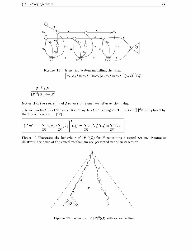
x 5 Delay operators 27
Q
� � �
�
��
� �
�
1
�
2
�
2
�
2
�
3
�
3
�
3
�
4
�
5
�
5
�
6
�
6
�
7
�
7
�
8
Figure 10: transition system modelling the term
l
�
1
b�
2
� � �
3
�c
!
� �
4
b�
5
�
6
� � �
7
�c
2
(�
8
�)
m
3
(Q)
P
�
! P
0
dP e
d
(Q)
�
! P
0
Notice that the execution of � cancels only one level of execution delay.
The axiomatisation of the execution delay has to be changed. The axiom [d e
d
2] is replaced by
the following axiom [d e
d
2
0
]:
[d e
d
2
0
]
2
6
6
6
X
i2I
�
i
P
i
�
X
j2J
� P
j
3
7
7
7
d
(Q) �
X
i2I
�
i
dP
i
e
d
(Q)�
X
j2J
� P
j
Figure 11 illustrates the behaviour of dP e
d
(Q) for P containing a cancel action. Examples
illustrating the use of the cancel mechanism are presented in the next section.
P
Q
�
�
�
�
�
�
Figure 11: behaviour of dP e
3
(Q) with cancel action

28 x 6 Applications
6 Applications
We present three examples illustrating the use of delay operators.
6.1 Example 1: a login procedure
This example illustrates the power of the execution delay operators, when cancel actions are
used. The reader is invited to compare the solution given below with the solutions proposed
in [NRSV90].
Let us consider the description of a login procedure. To start the procedure, the system sends a
login prompt p. Then, the user must enter a valid login response v within l time units. In this
case the login procedure is terminated, and the system enters a session phase, denoted by the
process S. If the login response is invalid i, or if it is not provided before l units of time, the
system rejects the current login request and starts a new one.
This behaviour is described by the process L de�ned as follows:
L = p bv S � i Lc
l
(L)
Figure 12 presents the transition system modelling L in the case where l = 3
�
i
i
�
�
�
v
v
v
i
p
Figure 12: transition system of the login procedure L
We want to control the overall duration of the login procedure by imposing the execution of an
exception E if a valid response has not been entered within d time units.
To model this, we use an execution delay within d to control the process L. Thus, once the delay
has expired, the login procedure is stopped and the exception E is executed.
The process P describing this control is then de�ned by:
P = dLe
d
(E)
However, if we consider the whole system according to the semantics of the execution delay, we
notice that the exception E will always occur, even if a valid response has been provided.
We need then to add a cancel action to the process L, after the execution of v.
The whole system is then described by P , where
P = dLe
d
(E)
L = p bv � S � i Lc
l
(L)

x 6 Applications 29
Notice that the process P is not well-timed. However, it satis�es the property \always possible
�" that is, from any state reachable from the initial state there exists an execution sequence
containing �. Furthermore, the execution sequences without an in�nity of �'s are those with
su�x (p i)
!
.
Hence, if the system is embedded in a \reasonable" environment (the user will eventually let some
time pass after a sequence of valid or invalid responses), we will obtain a well-timed system.
The transition system modelling the whole system P , in the case where l = 3 and d = 7, is given
in �gure 13.
S
p
p
p
p
p
p
i
i
i
i
i
i
i
i
i
i
i
� �
� �
� �
�
�
�
�
��
v
v
v
v
v
v
v
v
vv
vv
i
p
E
�
Figure 13: login procedure with watchdog: process P
6.2 Example 2: the alternating bit protocol with timeout
The following example is a simpli�ed version of a proposal of alternating bit protocol for level
OSI-4 (transmission protocol channel D).
We consider a system (�g. 14) composed with an Transmitter T , a Receiver R and two Media,
M and MM .
-
-
�
��
�
-
-
- -
Receiver
Medium MM
Medium M
Transmitter
?in
tm
0
tm
1
mt
0
mt
1
mr
0
mr
1
rm
0
rm
1
!out
Figure 14: components of the alternating bit protocol
The transmitter sends one message at a time and it cannot proceed to the next transmission

30 x 6 Applications
before either it receives an acknowledgement (the current message has been correctly delivered)
or a �nite delay dt expires.
The media are unsafe, and are respectively used for the transmission of messages and acknowl-
edgements. To detect loss of messages a bit of control is added to messages and acknowledgements
in a standard manner. The delay dt between the time of transmission of a message and the time
of retrial of the same message is greater than the delay dm of its transmission through M , added
to the delay dmm of the transmission of the corresponding acknowledgement, added to the delay
dr of handling of the message by the receiver (dt > dm+ dmm+ dr). This constraint guaran-
tees that a message is retransmitted only if itself, or its acknowledgement, has been lost. In the
version we give, we consider that the receiver handles the message in zero time, that is, dr = 0.
We have then only to assume that dt < dm+ dmm.
6.2.1 Description of the protocol
We consider the vocabulary of actions A = A
�
[ f�g with:
A
�
= f!�g
�2�
[ f?�g
�2�
[ f�g
�2�
[ flm; lmmg
where � = fin; tm
0
; tm
1
;mt
0
;mt
1
;mr
0
;mr
1
; rm
0
; rm
1
; outg.
The communication function j is de�ned by:
a
1
ja
2
= if a
1
= a
2
= � then �
else if a
1
=!� and a
2
=?� then �
else ?
The protocol is de�ned by the term
BITALT = @
H
(T
0
kM
0
kMM
0
k R
0
)
where H = f@tm
0
;@tm
1
;@mt
0
;@mt
1
;@mr
0
;@mr
1
;@rm
0
;@rm
1
= @ 2 f!; ?gg
and T
0
, M
0
, MM
0
and R
0
are the terms describing T , M , MM and R respectively.
6.2.2 The transmitter:
The actions it can perform are,
?in : getting a message to be transmitted
!tm
0
; !tm
1
: sending a message with control bit respectively 0, 1
?mt
0
; ?mt
1
: receiving an acknowledgement with control bit respectively 0, 1
It is described by the system of equations:
T
0
= b?in T
1
c
!
T
1
= !tm
0
T
2
T
2
= b?mt
1
T
1
c
dt
(T
1
) � b?mt
0
T
3
c
dt
(T
1
)
= b?mt
1
T
1
� ?mt
0
T
3
c
dt
(T
1
)

x 6 Applications 31
T
3
= b?in T
4
c
!
T
4
= !tm
1
T
5
T
5
= b?mt
0
T
4
c
dt
(T
4
) � b?mt
1
T
0
c
dt
(T
4
)
= b?mt
0
T
4
� ?mt
1
T
0
c
dt
(T
4
)
The transition system modelling the transmitter in the case dt = 3 is given in �gure 15.
?mt
1
�
�
?mt
0
?mt
0
?mt
0
?mt
1
?mt
1
?mt
1
?mt
1
?mt
1
�
� �
!tm
1
?in
?mt
0
?mt
0
?mt
0
�
��!tm
0
?in
Figure 15: transition system of the transmitter
6.2.3 The medium M :
The actions it can perform are,
?tm
0
; ?tm
1
: receiving message from the transmitter with control bit respectively 0, 1
!mr
0
; !mr
1
: sending message to the receiver with control bit respectively 0,1
lm : losing a message
It is described by the following system of equations:
M
0
= b?tm
0
M
1
c
!
� b?tm
1
M
2
c
!
= b?tm
0
M
1
� ?tm
1
M
2
c
!
M
1
= blmM
0
c
!
� b�c
dm
(!mr
0
M
0
)
= blmM
0
c
dm
(lmM
0
� !mr
0
M
0
)
M
2
= blmM
0
c
!
� b�c
dm
(!mr
1
M
0
)
= blmM
0
c
dm
(lmM
0
� !mr
1
M
0
)
The transition system modelling M in the case dm = 1 is given in �gure 16.
6.2.4 The medium MM :
It is symmetric to M . The actions it can perform are,

32 x 6 Applications
�
!mr
1
!mr
0
��
lmlm
lmlm
?tm
1
?tm
0
Figure 16: transition system of the medium M
?rm
0
; ?rm
1
: receiving acknowledgement from the receiver with control bit respectively 0, 1
!mt
0
; !mt
1
: sending acknowledgement to the transmitter with control bit respectively 0, 1
lmm : losing an acknowledgement
It is described by the following system of equations:
MM
0
= b?rm
0
MM
1
c
!
� b?rm
1
MM
2
c
!
= b?rm
0
MM
1
� ?rm
1
MM
2
c
!
MM
1
= blmmMM
0
c
!
� b�c
dmm
(!mt
0
MM
0
)
= blmmMM
0
c
dmm
(lmmMM
0
� !mt
0
MM
0
)
MM
2
= blmmMM
0
c
!
� b�c
dmm
(!mt
1
MM
0
)
= blmmMM
0
c
dmm
(lmmMM
0
� !mt
1
MM
0
)
The transition system modelling MM in the case dmm = 1 is given in �gure 17.
�
!mt
1
!mt
0
��
lmmlmm
lmmlmm
?rm
1
?rm
0
Figure 17: transition system of the medium MM
6.2.5 The receiver R:
The actions it can perform are,

x 6 Applications 33
?mr
0
; ?mr
1
: receiving messages from medium M with control bit respectively 0, 1
!out : delivering a message received with a correct control bit
!rm
0
; !rm
1
: sending acknowledgement to medium MM with control bit respectively 0, 1
It is described by the following equations:
R
0
= b?mr
0
R
1
c
!
� b?mr
1
R
4
c
!
= b?mr
0
R
1
� ?mr
1
R
4
c
!
R
1
= !outR
2
R
2
= !rm
0
R
3
R
3
= b?mr
0
R
2
c
!
� b?mr
1
R
4
c
!
= b?mr
0
R
2
� ?mr
1
R
4
c
!
R
4
= !outR
5
R
5
= !rm
1
R
6
R
6
= b?mr
1
R
5
c
!
� b?mr
0
R
1
c
!
= b?mr
1
R
5
� ?mr
0
R
1
c
!
The transition system modelling the receiver is given in �gure 18.
�
?mr
0
?mr
1
!out
!out
!rm
0
!rm
1
�
�
?mr
0
?mr
1
?mr
0
?mr
1
Figure 18: transition system of the receiver
6.2.6 The compound system
We would like now to observe the behaviour of BITALT , but we are not really interested in the
value of the control bit on the transitions. On the contrary, we do want to observe the ordering
of those transitions. For this reason we use the relabelling operator [ ] of CCS [Mil80], to obtain
the process BITALT [�], where � is the function
(tm; tm;mr;mr; rm; rm;mt;mt) = (tm
0
; tm
1
;mr
0
;mr
1
; rm
0
; rm
1
;mt
0
;mt
1
)
The transition system modellingBITALT [�] for dm = dmm = 1 and dt = 3 is given in �gure 19.
Notice that while none of the sequential components is well-timed, the compound system is so.

34 x 6 Applications
�
?in
tm
lm
�
�
� lm
� mr
!out
rm�mt
lmm
�
�
lm �
mr
lm
lmm
tm
�
Figure 19: transition system of BITALT [�]
We can abstract from time, by renaming every � transition by � , and reducing the system ob-
tained modulo observational equivalence of CCS [Mil80,Mil83]. We obtain the transition system
given in �gure 20, which corresponds to the behaviour of a system composed of a transmitter
and a receiver, communicating through a bidirectional unsafe medium of capacity 1.
d
d
d d
dd
d d
-
6
- -
?
��
?
�
6
6
?
?in
tm
lm
mr
!out
rmmt
lmm
mr
lm
tm
Figure 20: reduced system of BITALT [�]
6.3 Example 3: the transmitter with timeout and watchdog
In order to illustrate the use of the execution delay operators, we add another feature to the
transmitter of the alternating bit protocol presented in the previous section, to control the
duration of the retry phase.
we suppose that, after receipt of a message to send (?in), the transmitter must handle it within a
delay da (da > dt); otherwise, it considers that the connection is cut and it enters a disconnection
phase D
0
or D
1
, depending on the value of the control bit.
The new transmitter is then described by the following system of equations.

x 7 Related work 35
T
0
= b?in T
1
c
!
T
1
= dT
2
e
da
(D
0
)
T
2
= !tm
0
T
3
T
3
= b?mt
1
T
2
c
dt
(T
2
) � b?mt
0
� T
4
c
dt
(T
2
)
= b?mt
1
T
2
� ?mt
0
� T
4
c
dt
(T
2
)
T
4
= b?in T
5
c
!
T
5
= bT
6
c
da
(D
1
)
T
6
= !tm
1
T
7
T
7
= b?mt
0
T
6
c
dt
(T
6
) � b?mt
1
� T
0
c
dt
(T
6
)
= b?mt
0
T
6
� ?mt
1
� T
0
c
dt
(T
6
)
Notice that the cancel mechanism is used when the right acknowledgement is received.
The transmitter is not a well-timed process by itself, but it is supposed to be embedded in an
environment, such that the compound system is well-timed.
In �gure 21, we give a representation of this transmitter in terms of macro-states, �a la State-
charts [Har87].
da
da
�
�
?in
?in
!tm
0
!tm
1
?mt
0
?mt
1
dt
dt
?mt
1
?mt
0
�
�
T
0
T
1
T
6
T
7
T
4
D
0
D
1
T
5
T
2
T
3
Figure 21: Representation of the transmitter with watchdog
7 Related work
In this section we compare ATP with similar studies about introducing time in process algebras.
Since the amount of work in this area is fast increasing, this presentation may not be complete
and exhaustive. All the studies adopt the principle of extending a standard process algebra by

36 x 7 Related work
adding time constructs. For instance, ATP can be considered as an extension of a combination
of CCS (for pre�xing and recursion) and ACP (for �, choice, parallel and encapsulation), with a
unique feature, the unit-delay operator.
In the following presentation, the classi�cation criterion is the standard algebra extended.
7.1 Extensions of CCS
Hennesy and Regan [HR90] present a process algebra TPL, which is an extension of CCS
with a time action �, playing the role of � in ATP. An important di�erence with our
model is that non-internal actions a other than � may be delayed (a:t
�
! a:t). The
maximal progress assumption is adopted in TPL, that is, pjq may delay only if p and q
cannot communicate; otherwise, the communication is immediate. In ATP, we have not
taken such an assumption for two reasons.
1. We do not have binary rendez-vous as in CCS, so a communication may require any
number of processes to be performed: two processes ready to communicate may need
to wait for a third one to achieve the complete rendez-vous.
2. We can enforce an action to occur before any time action (in � t, no time can pass
before � is performed). We can then express the fact that a given communication
must occur as soon as possible.
The unit-delay of ATP cannot be expressed in TPL. Furthermore, the parallel operator
cannot be expressed in terms of non-deterministic choice, even for �nite processes. For
instance, the term p = a:Nilj�:b:Nil cannot be equivalent to a term with the summand
a:(Nilj�:b:Nil), since the latter can perform the sequence of actions � a yielding process
Nilj�:b:Nil, whereas the process obtained after performing the same sequence from p is
Niljb:Nil, and the processes Nilj�:b:Nil and Niljb:Nil are not equivalent. Thus, it is not
possible to have a law such as the expansion theorem.
Yi [Wan90] describes another extension of CCS, called TCCS (Timed CCS), which is very
close to the proposal of [HR90], in the sense that the process �:P can let time pass before
executing �, whereas �:P cannot. The important di�erence is that this work deals with
continuous time; therefore a set of time events �(t) (where t is a positive real number) is
considered, rather than a time action. The process �(t):P behaves as P after time t has
elapsed.
The model is based upon four assumptions, among which is the persistency assumption:
for any process, if an action � can be performed, then it remains possible after some time
has elapsed. With such an assumption, it is clearly impossible to have an operator similar
to unit-delay, and thus to model timeout constructs. [Wan90] encounters the same problem
as [HR90] for the parallel operator. In a still not published paper the author presents an
expansion theorem. This is possible by adding a new feature to the algebra: a formal date
is bound to actions in pre�xing, and the behaviour after the execution of an action may
depend on the time it is performed.
Moller and Tofts [MT90] also introduce timing constraints in CCS, but with other operators
and assumptions. The resulting calculus is also called TCCS, meaning Temporal CCS.
They have discrete time like [HR90] and ATP. As in [Wan90], they consider a pre�xing
operator (t); (t):P behaves as P after exactly t time units. Contrary to [HR90,Wan90],
and similarly to our model, the process a:P does not let time pass before performing the
action a. Also, the null process 0 does not let time pass and this constitutes an important
di�erence between this algebra and ATP.

x 7 Related work 37
Instead of de�ning an asymmetric operator like the unit-delay, [MT90] has two symmetric
choice operators: a strong choice +, corresponding to the non-deterministic choice ofATP,
and a weak choice operator �. The latter allows to model unit-delay, depending on the
structure of its operands: a:P � (1):Q is equivalent to the process ba:P c(Q) in ATP. The
choice of 0 to be a deadlock process for time actions in [MT90] seems motivated by the will
to provide the weak choice operator with a neutral element.
7.2 Extension of CSP
Reed and Roscoe [RR88] and Davies and Schneider [DS89] add timing information to
CSP, by introducing a delay operator WAIT t, where t is a positive real. This language is
provided denotational semantics in terms of a timed-failure model. An important feature
of the algebra is that the time between any two consecutive events of a sequential process
is greater than a given constant � > 0. Such an assumption guarantees well-timedness
since it implies that a process would engage in only �nitely many events in a bounded
period of time. However, due to this assumption, some laws of untimed CSP are not
preserved and the resulting theory for timed systems cannot be considered as an extension
of untimed CSP. Non-internal actions may be delayed, as in [MT90,Wan90], which prevents
from dealing with urgency. For instance, the sentence \the action a is performed within
3 time units", which is expressed in ATP by baP c
2
(aP ), cannot be translated in Timed
CSP.
7.3 Extensions of ACP
Baeten and Bergstra [BB90] propose an algebra called ACP
�
, incorporating real-time as-
pects in ACP [BK84]. In ACP
�
, a time stamp is added to each action, for instance a(3),
meaning \perform action a at time 3". Time stamps are positive real numbers and rep-
resent absolute time. Also, a version of ACP
�
where action parameters represent relative
time, is given. For instance, a[3] denotes an action a that has to be performed 3 time units
after its enabling: in b[5] � a[3], the action a is performed 3 time units after the occurrence
of b. Many operators are presented with their axiomatisations and operational semantics.
Among them an interesting one is called integration, denoted by
R
v2V
P , where V is a set of
positive real numbers. Such a process is the alternative composition of the processes P [t=v]
for t in V (parametrisation of processes by time is allowed). For instance, the process P (1),
where P (t) =
R
v2[t�0:01;t+0:01]
tick(v) � P (v+ 1) is a clock where some uctuation is allowed
for the ticks, and the errors are cumulated. This operator provides ACP
�
an interesting
power of expression.
Groote [Gro90] proposes another real-time algebra based on ACP, with discrete time. It is
called ACP
t
��
. Time is introduced by an action t, called time step. t acts like any other
atomic action, except that it cannot be hidden (replaced by �), and that there is a strong
synchronisation on time steps for parallel processes. A weak bisimulation semantics is
presented, together with an axiomatisation. There is no rule of factorisation for time
actions, and the model is very simple, close to the one presented in the initial work on
ATP [RSV87].

38 x 8 Conclusion
8 Conclusion
This work proposes a simple process algebra supporting a notion of discrete and global time.
It has been motivated by the study of the semantics of languages with delay constructs and
especially of Estelle and Esterel. Theoretical developments have been carried out with a double
concern about two often con icting criteria: expressiveness in a \natural" and \straightforward"
manner of high level timed constructs and simplicity of the language and of the underlying the-
oretical framework. For sake of simplicity, we chose strong bisimulation semantics rather than
semantics on equivalences supporting abstraction and yielding more complex theories, and re-
stricted to terms representing regular behaviours. Furthermore, the core algebraASTP has been
designed so as to use a set of operators which seems to be minimal for the intended application.
The proposed algebra has several interesting features:
� It suggests a conceptual framework for introducing time as explained in the introduction.
Time progress is modelled by a special action satisfying a strong synchronisation assump-
tion. Our time is abstract as opposed to physical execution time. It can be used either to
correlate the functioning speeds of the components of a system due to synchronous execu-
tion of time actions or to characterise urgency situations due to the possibility of globally
controlling time progress. The only obligation for time is that it always eventually pro-
gresses (property of well-timedness). It seems very di�cult if not impossible, to design a
language describing only well-timed behaviours without adopting assumptions destroying
time abstractness. Assuming for instance, that any action takes a minimal time or that
two consecutive actions are separated by a minimal delay guarantees well-timedness but
reduces abstraction i.e., independence with respect to implementation choices. Accepting
the existence of action sequences of zero time allows keeping the level of abstractness high
by separating speci�cation from implementation issues as explained in the introduction.
However, the price to pay is that well-timedness is not guaranteed and must be checked a
posteriori.
� Several high level delay constructs can be expressed in terms of ATP. Their meaning
has been de�ned so as to capture basic concepts of real-time systems like timeouts and
watchdogs. Whenever we had the choice, their semantics has been de�ned so as to agree
with intuition and preserve generality (see for instance remark 5.1.5).
� The algebraATP can be considered as the extension of a standard process algebra without
time. In fact, consider the language of terms ASP generated by using all the operators of
ASTP but unit-delay. The semantics of this language is de�ned as forASTP by restricting
to relations non labelled by �. ASP with strong equivalence can be completely axiomatised
by the system of axioms obtained by deleting from the axioms of ASTP those containing
occurrences if unit-delay (ASP is the algebra of regular behaviours of Milner [Mil84]). Thus,
ASTP can be considered as the extension of a standard process algebra for the description
of regular sequential behaviours. The restriction of the axioms of ATP in section 3.3, to
those not containing occurrences of unit-delay, is similar to the axiomatisation of parallel
composition and encapsulation in ACP.
� Being deterministic with respect to time, considering the idle process as not blocking for
time, priority of the outermost exception in unit-delays are important features of the se-
mantics of ASTP. They imply that the underlying models are deterministic with respect
to � and without sink states. The �rst feature is a consequence of the intention to interpret
the choice between two unit-delays as a unit-delay whose exception can perform either of
the corresponding exceptions rather than choosing arbitrarily between the two exceptions.

References 39
The other features, guarantee respectively that time progresses despite termination and
strictness of timeouts.
The examples illustrate the adequacy of the delay constructs proposed, as the modelling is simple
and elegant. The combination of the execution delay with the \cancel" action turns out to be
very natural and powerful. It brings ATP closer to Esterel and the Statecharts, and for this it
deserves further study.
References
[AB84] D. Austry and G. Boudol. Alg�ebre de processus et synchronisation. Theoretical
Computer Science, 30, 1984.
[ACD90] R. Alur, C. Courcoubetis, and D. Dill. Model-checking for real-time systems. In
Proceedings of the �fth annual IEEE symposium on Logic In Computer Science,
pages 414{425, Philadelphia, PA., June 1990.
[BB90] J.C.M. Baeten and J.A. Bergstra. Real Time Process Algebra. Technical Report CS-
R9053, Centre for Mathematics and Computer Science, Amsterdam, the Netherlands,
1990.
[BC85] G. Berry and L. Cosserat. The Esterel synchronous programming language and its
mathematical semantics. In LNCS 197: Proceedings CMU Seminar on Concurrency,
Springer-Verlag, 1985.
[BK84] J.A. Bergstra and J.W. Klop. Algebra of Communicating Processes. Technical Re-
port CS-R8420, Centre for Mathematics and Computer Science. Department of Com-
puter Science, 1984.
[BK86] J.A. Bergstra and J.W. Klop. Process algebra : speci�cation and veri�cation in
bisimulation semantics. In M. Hazewinkel, J.K. Lenstra, and L. G. L. T. Meertens,
editors, Proceedings of the CWI Symposium Mathematics and Computer Science II
(CWI Monograph 4), pages 61{94, North Holland, Amsterdam, 1986.
[CHPP87] P. Caspi, N. Halbwachs, D. Pilaud, and J. Plaice. Lustre: a declarative language
for programming synchronous systems. In 14th Symposium on Principles of Program-
ming Languages, Munich, January 1987.
[DS89] J. Davies and S. Schneider. An Introduction to Timed CSP. Technical Report PRG-
75, Oxford University Computing Laboratory, August 1989.
[Gro89] J.F. Groote. Transition system speci�cation with negative premisses. Technical Re-
port CS-R8950, Centre for Mathematics and Computer Science. Department of Com-
puter Science, December 1989.
[Gro90] J.F. Groote. Speci�cation and veri�cation of real time systems in ACP. Technical
Report CS-R9015, Centre for Mathematics and Computer Science. Department of
Computer Science, May 1990.
[GV88] J.F. Groote and F.W. Vaandrager. Structured operational semantics and bisimulation
as a congruence. Technical Report CS-R8845, Centre for Mathematics and Computer
Science. Department of Computer Science, January 1988.

40 References
[Har87] D. Harel. StateCharts : a visual approach to complex systems. Science of Computer
Programming, 8{3:231{275, 1987.
[Hoa78] C.A.R Hoare. Communicating Sequential Processes. CACM, 21(8), 1978.
[HR90] M. Hennessy and T. Regan. A Temporal Process Algebra. Technical Report 2/90,
University of Sussex, April 1990.
[LPS81] D. Lehmann, A. Pnueli, and J. Stavi. Impartiality, justice and fairness: the ethics
of concurrent termination. In S. Even and O. Kariv, editors, LNCS 115. Proceed-
ings of ICALP '81 (Automata, Languages and Programming), Acre (Akko), Israel,
pages 264{277, Springer-Verlag, July 1981.
[Mil80] R. Milner. A Calculus of Communicating Systems. In LNCS 92, Springer Verlag,
1980.
[Mil83] R. Milner. Calculi for Synchrony and Asynchrony. Theoretical Computer Science, 25,
1983.
[Mil84] R. Milner. A Complete Inference System for a Class of Regular Behaviours. Journal
of Computer and System Sciences, 28:439{466, 1984.
[MT90] F. Moller and C. Tofts. A Temporal Calculus of Communicating Processes. In
J.C.M. Baeten and J.W. Klop, editors, LNCS 458. Proceedings of CONCUR '90
(Theories of Concurrency: Uni�cation and Extension), Amsterdam, the Netherlands,
pages 401{415, Springer-Verlag, August 1990.
[NRSV90] X. Nicollin, J.-L. Richier, J. Sifakis, and J. Voiron. ATP: an Algebra for Timed
Processes. In Proceedings of the IFIP TC 2 Working Conference on Programming
Concepts and Methods, Sea of Gallilee, Israel, April 1990.
[Plo81] G.D. Plotkin. A Structural Approach to Operational Semantics. Technical Re-
port DAIMI FN-19,
�
Arhus University. Computer Science Department,
�
Arhus, Den-
mark, 1981.
[RR88] G.M. Reed and A.W. Roscoe. A timed model for Communicating Sequential Pro-
cesses. Theoretical Computer Science, 58 (pp 249{261), 1988.
[RSV87] J-L. Richier, J. Sifakis, and J. Voiron. Une alg�ebre des processus temporis�es. In A.
Arnold, editor, Actes du deuxi�eme colloque C
3
, Angouleme , France, May 1987.
[Wan90] Wang Yi. Real-time behaviour of asynchronous agents. In J.C.M. Baeten and
J.W. Klop, editors, LNCS 458. Proceedings of CONCUR '90 (Theories of Con-
currency: Uni�cation and Extension), Amsterdam, the Netherlands, pages 502{520,
Springer-Verlag, August 1990.

Annex 1. Canonical form 41
Annex 1. Canonical form
We give and prove the proposition de�ning the normal form of a term of P.
Proposition 9
Let p be a term of P, with free variables in
e
Y . Then there exist n � 1 and p
1
; :::; p
n
in P with
free variables in
e
Y , such that p � p
1
and each p
i
is solution of an equation of the form F
1
, F
2
or F
3
de�ned as follows.
(F
1
) p
i
�
X
b2B
i
�
b
p
b
�
X
c2C
i
�
c
Y
c
(F
2
) p
i
� b�c(p
d
i
) �
X
e2E
i
b�c(Y
e
)
(F
3
) p
i
�
6
6
6
4
X
f2F
i
�
f
p
f
�
X
g2G
i
�
g
Y
g
7
7
7
5
(p
h
i
) �
X
j2J
i
b�c(Y
j
)
where B
i
or C
i
, but not both of them, F
i
and G
i
, but not both of them, E
i
, and J
i
, may be
empty, in which case the corresponding sum is considered not to be present.
Proof. Induction on the structure of p.
1. p = �. Let n = 1 and q
1
= b�c(X). According to proposition 2, there exists p
1
with no free
variable, such that p
1
� q
1
[p
1
=X], that is
p
1
� b�c(p
1
)
This equation is in form F
2
. Furthermore, the axiom [b c1] gives us p � b�c(�). Therefore,
p � q
1
[p=X]
p and p
1
are solutions of the same equation; hence, from proposition 2, p � p
1
.
2. p = � p
0
. The free variables of p
0
are the same as those of p. Hence, by induction, there
exist n
0
and p
0
1
; :::p
0
n
0
with free variables in
e
Y , each of them solution of an equation in one
of the 3 forms above-de�ned, such that p
0
� p
0
1
. Now, if we de�ne n = n
0
+ 1, for i = 2::n,
p
i
= p
0
i�1
, and p
1
= �p
0
1
, then each p
i
(i = 1::n) is solution of an equation in form F
1
, F
2
or F
3
, and moreover p � p
1
3. p = �Y
i
is in form F
1
4. p = p
0
� p
00
. The free variables of both p
0
and p
00
are in
e
Y . Hence by induction, there exist
n
0
and p
0
1
; :::; p
0
n
0
such that p
0
� p
0
1
and each p
0
i
is solution of an equation in one of the three
forms, and there exist n
00
and p
00
1
; :::; p
00
n
00
such that p
00
� p
00
1
and each p
00
i
is solution of an
equation in one of the three forms. We have then
p � p
0
1
� p
00
1
As shown above (case 1), we know that there exists p
0
n
0
+1
such that

42 Annex 1. Canonical form
p
0
n
0
+1
� b�c(p
0
n
0
+1
)
and that p
0
n
0
+1
� �. There exists also p
00
n
00
+1
such that
p
00
n
00
+1
� b�c(p
00
n
00
+1
)
and p
00
n
00
+1
� � too.
We de�ne now, for i
0
2 [1; n
0
+ 1] and i
00
2 [1; n
00
+ 1],
p
(i
0
;i
00
)
= p
0
i
0
� p
00
i
00
For all i
0
in [1; n
0
+ 1] and i
00
in [1; n
00
+ 1], we have
p
(i
0
;n
00
+1)
� p
0
i
0
and p
(n
0
+1;i
00
)
� p
00
i
00
By substituting, in the equation of p
0
i
0
(resp. p
00
i
00
), p
(j
0
;n
00
+1)
(resp. p
(n
0
+1;j
00
)
) to every
occurrence of p
0
j
0
(resp. p
00
j
00
), we obtain that if i
0
(resp. i
00
) is equal to n
0
+1 (resp. n
00
+ 1),
then p
(i
0
;i
00
)
is solution of an equation of the same form as p
00
i
00
(resp. p
0
i
0
).
We prove now that for i
0
2 [1; n
0
] and i
00
2 [1; n
00
], p
(i
0
;i
00
)
is solution of an equation in one
of the three forms F
1
, F
2
or F
3
, by considering the forms of the equations concerning p
0
i
0
and p
00
i
00
.
� p
0
i
0
�
X
b
0
2B
0
i
0
�
b
0
p
0
b
0
�
X
c
0
2C
0
i
0
�
c
0
Y
c
0
and p
00
i
00
�
X
b
00
2B
00
i
00
�
b
00
p
00
b
00
�
X
c
00
2C
00
i
00
�
c
00
Y
c
00
.
We have then
p
0
i
0
�
X
b
0
2B
0
i
0
�
b
0
p
(b
0
;n
00
+1)
�
X
c
0
2C
0
i
0
�
c
0
Y
c
0
and
p
00
i
00
�
X
b
00
2B
00
i
00
�
b
00
p
(n
0
+1;b
00
)
�
X
c
00
2C
00
i
00
�
c
00
Y
c
00
We obtain then that, for every pair (i
0
; i
00
), there exist sets B
(i
0
;i
00
)
and C
(i
0
;i
00
)
such
that
p
(i
0
;i
00
)
�
X
(b
0
;b
00
)2B
(i
0
;i
00
)
�
(b
0
;b
00
)
p
(b
0
;b
00
)
�
X
(c
0
;c
00
)2C
(i
0
;i
00
)
�
(c
0
;c
00
)
Y
(c
0
;c
00
)
which is an equation in form F
1
.
� p
0
i
0
�
X
b
0
2B
0
i
0
�
b
0
p
0
b
0
�
X
c
0
2C
0
i
0
�
c
0
Y
c
0
and p
00
i
00
� b�c(p
00
d
00
i
00
)�
X
e
00
2E
00
i
00
b�c(Y
e
00
).
By using the axioms [�2], [�4] and [�5], we obtain then
p
(i
0
;i
00
)
�
X
b
0
2B
0
i
0
�
b
0
p
(b
0
;n
00
+1)
�
X
c
0
2C
0
i
0
�
c
0
Y
c
0
which is an equation in form F
1
.
� if the equation satis�ed by p
0
i
0
is in form F
1
, and the equation satis�ed by p
00
i
00
is in
form F
3
, we obtain for p
(i
0
;i
00
)
an equation in form F
1
, by applying the same axioms
as above.
� if the equations satis�ed by p
0
i
0
and p
00
i
00
are both in form F
2
, then, by applying the
axioms [�1], [�2], [�4] and [�6], we �nd that p
i
0
;i
00
satis�es an equation in form F
2
too.

Annex 1. Canonical form 43
� if the equation satis�ed by p
0
i
0
is in form F
2
, and the equation satis�ed by p
00
i
00
is in
form F
3
, then by applying axioms [�1], [�2], [�4] and [�6], we �nd for p
(i
0
;i
00
)
an
equation in form F
3
.
� if both p
0
i
0
and p
00
i
00
satisfy an equation in form F
3
, then the axioms [�1], [�2] and [�6]
give us for p
(i
0
;i
00
)
an equation in form F
3
� any remaining case is treated like one of the previous cases, by commutativity of �.
Finally we have p � p
(1;1)
, and every p
(i
0
;i
00
)
is solution of an equation in one of the three
forms.
5. p = bp
0
c(p
00
). The free variables of both p
0
and p
00
are in
e
Y . By induction, there exist n
0
and
p
0
1
; :::; p
0
n
0
such that p
0
� p
0
1
and each p
0
i
is solution of an equation in one of the three forms;
there exist also n
00
, p
00
1
; :::; p
00
n
00
such that p
00
� p
00
1
and each p
00
i
is solution of an equation in
one of the three forms.
Let n = n
0
+ n
00
+ 1.
For n
0
+ 2 � i � n
0
+ n
00
+ 1, we de�ne
p
i
= p
00
i�(n
0
+1)
By replacing each p
00
i
by p
n
0
+i+1
in the equations concerning the p
00
j
s, and by manipulating
the indices, we obtain a set of equations in the required forms, satis�ed by the p
i
s for
i 2 [n
0
+ 2; n].
For 2 � i � n
0
+ 1, we de�ne
p
i
= p
0
i�1
As above, if we replace each p
0
i
by p
i+1
in the equations concerning the p
0
j
s, and by manip-
ulating the indices, we obtain a set of equations in the required forms, satis�ed by the p
i
s
for i 2 [2; n
0
+ 1].
Since on the one hand, p
0
� p
0
1
and p
00
� p
00
1
, and on the other hand p
0
1
= p
2
and p
00
1
= p
n
0
+2
,
we get the equation
p � bp
2
c(p
n
0
+2
)
We have now to �nd p
1
solution of an equation in one of the three forms, such that p � p
1
.
For this purpose, we consider the form of the equation satis�ed by p
2
.
� p
2
�
X
b2B
2
�
b
p
b
�
X
c2C
i
�
c
Y
c
.
We de�ne p
1
as solution of the equation
p
1
�
6
6
6
4
X
b2B
2
�
b
p
b
�
X
c2C
i
�
c
Y
c
7
7
7
5
(p
n
0
+2
)
which is in form F
3
. We have immediately
p
1
� bp
2
c(p
n
0
+2
)
� p
2
� b�c(p
d
2
) �
X
e2E
2
b�c(Y
e
).
We de�ne p
1
as solution of the equation
p
1
� b�c(p
n
0
+2
)

44 Annex 1. Canonical form
which is in form F
2
.
By applying the axioms [�6],[b c2] and [�3], we get
bp
2
c(p
0
n
0
+2
) � bb�cp
d
2
c(p
n
0
+2
) �
X
e2E
2
bb�c(Y
e
)c(p
n
0
+2
)
� b�c(p
n
0
+2
) �
X
e2E
2
b�c(p
n
0
+2
)
� b�c(p
n
0
+2
)
and thus
p
1
� bp
2
c(p
n
0
+2
)
� p
2
�
6
6
6
4
X
f2F
2
�
f
p
f
�
X
g2G
2
�
g
Y
g
7
7
7
5
(p
h
2
) �
X
j2J
2
b�c(Y
j
).
We de�ne p
1
as solution of the equation
p
1
�
6
6
6
4
X
f2F
2
�
f
p
f
�
X
g2G
2
�
g
Y
g
7
7
7
5
(p
n
0
+2
)
which is in form F
3
.
The axioms [�6], [b c2] and [�4] give us again
p
1
� bp
2
c(p
n
0
+2
)
In the three cases, we obtain p � p
1
.
6. p = bp
0
c(Y ), where Y is in
e
Y . By induction, there exist n
0
and p
0
1
; :::; p
0
n
0
, such that p
0
� p
0
1
,
and each p
0
i
is solution of an equation in one of the three forms.
The axiom [b c3] gives us
p � bp
0
c(�)� b�c(Y )
Let n = n
0
+ 2. We de�ne p
n
as solution of the equation
p
n
� b�c(p
n
)
which is in form F
2
. As shown previously, we know that p
n
� �; Hence
p � bp
0
c(p
n
)� b�c(Y )
For 2 � i � n
0
+ 1, we de�ne
p
i
= p
0
i�1
By substitution of p
j+1
to each p
0
j
in the equation satis�ed by p
0
i�1
, we get an equation in
one of the three forms, satis�ed by p
i
, and we have
p � bp
2
c(p
n
)� b�c(Y )
In order to �nd an equation satis�ed by some p
1
, such that p � p
1
, we consider the form
of the equation satis�ed by p
2
.
� p
2
�
X
b2B
2
�
b
p
b
�
X
c2C
i
�
c
Y
c
.
We de�ne p
1
as solution of the equation

Annex 1. Canonical form 45
p
1
�
6
6
6
4
X
b2B
2
�
b
p
b
�
X
c2C
i
�
c
Y
c
7
7
7
5
(p
n
) � b�c(Y )
which is in form F
3
. We obtain immediately p � p
1
.
� p
2
� b�c(p
d
2
) �
X
e2E
2
b�c(Y
e
).
We de�ne p
1
as solution of the equation
p
1
� b�c(p
n
) � b�c(Y )
which is in form F
2
. Then by applying the axioms [�6], [b c2] and [�3], we obtain
p � p
1
.
� p
2
�
6
6
6
4
X
f2F
2
�
f
p
f
�
X
g2G
2
�
g
Y
g
7
7
7
5
(p
h
2
) �
X
j2J
2
b�c(Y
j
).
We de�ne p
1
as solution of the equation
p
1
�
6
6
6
4
X
f2F
2
�
f
p
f
�
X
g2G
2
�
g
Y
g
7
7
7
5
(p
n
) � b�c(Y )
By applying the axioms [�6], [b c2] and [oplus4], we obtain once more p � p
1
.
7. p = recX � p
0
. p
0
has free variables in h
e
Y ;Xi. By induction there exist n
0
and p
0
1
; :::; p
0
n
0
with free variables in h
e
Y ;Xi, such that each p
0
i
is solution of an equation in one of the three
forms, and p
0
� p
0
1
. Since � is a congruence, we get p � recX � p
0
1
. By the axiom [rec1], we
know that
p � p
0
1
[p=X]
We de�ne p
1
= p. We have then
p
1
� p
0
1
[p
1
=X] and p � p
1
Let n = 2n
0
.
De�ne, for i in [2; n
0
],
p
i
= p
0
i
[p
1
=X]
and for i in [n
0
+ 1; 2n
0
],
p
i
= p
i�n
0
� p
1
We prove that each p
i
(i 2 [1; n
0
]), which has its free variables in
e
Y , is solution of an
equation in one of the three forms. For i in [n
0
+ 1; 2n
0
], the same result will then be
obtained in the same way as for the case 4. We consider the possible forms of the equation
satis�ed by p
0
i
.
� p
0
i
�
X
b2B
0
i
�
b
p
0
b
�
X
c2C
0
i
�
c
Y
c
.
We get then
p
i
�
X
b2B
0
i
�
b
p
b
�
X
c2C
0
i
X=Y
c
�
c
p
1
�
X
c2C
0
i
X 6=Y
c
�
c
Y
c

46 Annex 2. Completeness of the axiomatisation of ASTP
which is an equation in form F
1
(one of the last two summands may be not present).
� p
0
i
� b�c(p
0
d
i
) �
X
e2E
0
i
b�c(Y
e
).
If X is not among the Y
e
, then we obtain
p
i
� b�c(p
d
i
) �
X
e2E
0
i
b�c(Y
e
)
which is in form F
2
. Otherwise, we get
p
i
� b�c(p
d
i
) �
X
e2E
0
i
X=Y
e
b�c(p
1
) �
X
e2E
0
i
X 6=Y
e
b�c(Y
e
)
� b�c(p
d
i
� p
1
) �
X
e2E
0
i
X 6=Y
e
b�c(Y
e
)
� b�c(p
n
0
+d
i
) �
X
e2E
0
i
X 6=Y
e
b�c(Y
e
)
which is an equation in from F
2
(the last term may be absent).
� p
0
i
�
6
6
6
4
X
f2F
0
i
�
f
p
0
f
�
X
g2G
0
i
�
g
Y
g
7
7
7
5
(p
0
h
i
) �
X
j2J
0
i
b�c(Y
j
).
As above, we obtain, if X is not among the Y
j
:
p
i
�
6
6
6
6
6
6
4
X
f2F
0
i
�
f
p
f
�
X
g2G
0
i
X=Y
g
�
g
p
1
�
X
g2G
0
i
X 6=Y
g
�
g
Y
g
7
7
7
7
7
7
5
(p
h
i
) �
X
j2J
0
i
b�c(Y
j
)
and, in the other case:
p
i
�
6
6
6
6
6
6
4
X
f2F
0
i
�
f
p
f
�
X
g2G
0
i
X=Y
g
�
g
p
1
�
X
g2G
0
i
X 6=Y
g
�
g
Y
g
7
7
7
7
7
7
5
(p
n
0
+h
i
) �
X
j2J
0
i
X 6=Y
j
b�c(Y
j
)
(one of the last two summands of the body of the delay may be absent).
In both cases, we have an equation in form F
3
.
Hence, in every case, p
i
(1 � i � n), whose free variables are in
e
Y , is solution of an equation
in one of the forms F
1
, F
2
or F
3
, and p � p
1
. This concludes the proof.
Annex 2. Completeness of the axiomatisation of ASTP
The completeness theorem (inspired from the one given in [Mil84]) is presented for closed terms
only, but the proof can be easily extended to open terms. The theorem is: if P and Q are
elements of ASTP, then
ASTP j= P � Q)ASTP ` P � Q
Proof. Since P (resp. Q) has no free variables, according to proposition 3, there exists n (resp.
m) and P
1
; . . . ; P
n
(resp. Q
1
; . . . ; Q
m
) in ASTP, such that P � P
1
(resp. Q � Q
1
), and each P
i
(resp. Q
i
) is solution of an equation in one of the forms (1) (2) or (3)

Annex 2. Completeness of the axiomatisation of ASTP 47
First, notice that
� if the equation concerning P
i
is in form (1), then P
i
has no transition by �, and has
transitions by some �s
� if the equation concerning P
i
is in form (2), then P
i
has one transition by �, and no
transition by any �
� if the equation concerning P
i
is in form (3), then P
i
has transitions by � and by some �s
Let I = f(i; i
0
) j P
i
� Q
i
0
g. Since P � P
1
and Q � Q
1
, and since the axiomatisation is sound, we
have P
1
� Q
1
, that is (1; 1) 2 I.
Moreover, when (i; i
0
) 2 I, P
i
and Q
i
0
have equal derivations. Hence, according to the facts
aforementioned, the equations de�ning P
i
and Q
i
0
are in the same form. Therefore, we can make
a partition of I in I
1
, I
2
and I
3
depending on the form of the equations satis�ed by P
i
and Q
i
0
.
� for (i; i
0
) 2 I
1
, we have
P
i
�
X
j2J
i
�
j
P
j
and Q
i
0
�
X
j
0
2J
0
i
0
�
j
0
Q
j
0
Since P
i
� Q
i
0
, there exists a total surjective relation R
1
ii
0
between J
i
and J
0
i
0
, given by
R
1
ii
0
= f(j; j
0
) 2 I j �
j
= �
j
0
g
We de�ne then the following equations, one for each (i; i
0
) 2 I
1
:
X
ii
0
�
X
(j;j
0
)2R
1
ii
0
�
j
X
jj
0
� for (i; i
0
) 2 I
2
, we have
P
i
� b�c(P
k
i
) and Q
i
0
� b�c(Q
k
0
i
0
)
We de�ne then the following equations, one for each (i; i
0
) 2 I
2
:
X
ii
0
� b�c(X
k
i
k
0
i
0
)
� for (i; i
0
) 2 I
3
, we have
P
i
�
6
6
6
4
X
j2J
i
�
j
P
j
7
7
7
5
(P
k
i
) and Q
i
0
�
6
6
6
6
4
X
j
0
2J
0
i
0
�
j
0
Q
j
0
7
7
7
7
5
(Q
k
0
i
0
)
Since P
i
� Q
i
0
, there exists as above a total surjective relation R
3
ii
0
between J
i
and J
0
i
0
,
given by
R
3
ii
0
= f(j; j
0
) 2 I j �
j
= �
j
0
g
We de�ne again a set of equations, one for each (i; i
0
) 2 I
3
:

48 Annex 3. Proof of proposition 7
X
ii
0
�
6
6
6
6
4
X
(j;j
0
)2R
3
ii
0
�
j
X
jj
0
7
7
7
7
5
(X
k
i
k
0
i
0
)
We have then a set of formal equations, one for each (i; i
0
) 2 I. These equations are provably
satis�ed when each X
ii
0
is instantiated to P
i
. In fact, depending on its form, the equation of X
ii
0
becomes
P
i
�
X
(j;j
0
)2R
1
ii
0
�
j
P
j
or
P
i
� b�c(P
k
i
) or
P
i
�
6
6
6
6
4
X
(j;j
0
)2R
3
ii
0
�
j
P
j
7
7
7
7
5
(P
k
i
)
In any case, since R
1
ii
0
and R
3
ii
0
are total, the right hand side of the equation di�ers at most by
repeated summands from the right hand side of the equation that has been proven satis�ed by
P
i
. In the same way, the formal equations are provably satis�ed when each X
ii
0
is instantiated
to Q
i
0
. This is due to the fact that R
1
ii
0
and R
3
ii
0
are surjective.
By applying the unicity assertion of the proposition 2, we obtain then P
1
� Q
1
.
Finally, since P � P
1
and Q � Q
1
, we can conclude that P � Q.
Annex 3. Proof of proposition 7
We recall the proposition:
8P 2 ATP; 9P
0
2 ASTP : P � P
0
We proceed by induction on the structure of P .
� if P 2 ASTP, the result is immediate.
� if P = �P
1
, P = P
1
� P
2
or P = bP
1
c(P
2
), the induction hypothesis applied to P
1
and P
2
leads directly to the result expected.
� if P = P
1
k P
2
. By induction hypothesis, there exist P
0
1
and P
0
2
inASTP, such that P
1
� P
0
1
and P
2
� P
0
2
. Hence P � P
0
1
k P
0
2
.
From proposition 3, there exist n � 1, and P
1
1
; :::; P
1
n
in ASTP, such that P
0
1
� P
1
1
and
each P
1
i
is solution of an equation in one of the forms (1), (2) or (3), recalled hereafter.
(1) P
1
i
�
X
j2J
1
i
�
j
P
1
j
; 6= J
1
i
� [1; n]
(2) P
1
i
� b�c(P
1
k
) k 2 [1; n]

Annex 3. Proof of proposition 7 49
(3) P
1
i
�
6
6
6
6
4
X
j2J
1
i
�
j
P
1
j
7
7
7
7
5
(P
1
k
) ; 6= J
1
i
� [1; n]; k 2 [1; n]
Similarly, there exist m � 1, and P
2
1
; :::; P
2
m
in ASTP, such that P
0
2
� P
2
1
and each P
2
i
is
solution of an equation in one of the forms (1), (2) or (3).
For i 2 [1; n] and l 2 [1;m], de�ne Q
i;l
= P
1
i
k P
2
l
. We have then P � Q
1;1
. We show
now that each T
i;l
is solution of an equation in one of the three forms, depending on the
equations satis�ed by P
1
i
and P
2
l
.
{ P
1
i
�
X
j2J
1
i
�
j
P
1
j
and P
2
l
�
X
h2J
2
l
�
h
P
2
h
.
By using the axioms of parallel composition, we get
Q
i;l
�
X
j2J
1
i
�
j
Q
j;l
�
X
h2J
2
l
�
h
Q
i;h
�
X
j2J
1
i
;h2J
2
l
�
j
j�
h
6=?
(�
j
j�
h
)Q
j;h
which is an equation in form (1).
{ P
1
i
�
X
j2J
1
i
�
j
P
1
j
and P
2
l
� b�c(P
2
k
)
The axioms give us
Q
i;l
�
X
j2J
1
i
�
j
Q
j;l
which is an equation in form (1).
{ P
1
i
�
X
j2J
1
i
�
j
P
1
j
and P
2
l
�
6
6
6
6
4
X
h2J
2
l
�
h
P
2
h
7
7
7
7
5
(P
2
k
).
We obtain then
Q
i;l
�
X
j2J
1
i
�
j
Q
j;l
�
X
h2J
2
l
�
h
Q
i;h
�
X
j2J
1
i
;h2J
2
l
�
j
j�
h
6=?
(�
j
j�
h
)Q
j;h
which is an equation in form (1).
{ t
1
i
� b�c(t
1
k
) and t
2
l
� b�c(t
2
h
)
Then we have
Q
i;l
� b�c(Q
k;h
)
which is an equation in form (2).
{ P
1
i
� b�c(P
1
k
) and P
2
l
�
6
6
6
6
4
X
j2J
2
l
�
j
P
2
j
7
7
7
7
5
(P
2
h
).
By using the axioms, we obtain
Q
i;l
�
6
6
6
6
4
X
j2J
2
l
�
j
Q
i;j
7
7
7
7
5
(Q
k;h
)
which is an equation in form (3).

50 Annex 3. Proof of proposition 7
{ P
1
i
�
6
6
6
6
4
X
j2J
1
i
�
j
P
1
j
7
7
7
7
5
(P
1
k
) and P
2
l
�
6
6
6
6
4
X
h2J
2
l
�
h
P
2
h
7
7
7
7
5
(P
2
s
).
Then we get
Q
i;l
�
6
6
6
6
6
6
6
4
X
j2J
1
i
�
j
Q
j;l
�
X
h2J
2
l
�
h
Q
i;h
�
X
j2J
1
i
;h2J
2
l
�
j
j�
h
6=?
(�
j
j�
h
)Q
j;h
7
7
7
7
7
7
7
5
(Q
k;s
)
which is an equation in form (3).
{ The remaining cases are treated by using the commutativity of k.
By proposition 2, we obtain then that for every pair (i; l), there exists Q
0
i;l
in ASTP, such
that Q
0
i;l
� Q
i;l
. We can then conclude that P � Q
0
1;1
, which is the result expected.
� if P � @
H
(P
1
). By induction hypothesis, there exists P
0
1
in ASTP, such that P
1
� P
0
1
.
From proposition 3, there exist n � 1, and P
1
1
; :::; P
1
p
in ASTP, such that P
0
1
� P
1
1
and
each P
1
i
is solution of an equation in one of the forms (1), (2) or (3). For every i in [1; n],
de�ne Q
i
= @
H
�
P
1
i
�
. By using the axioms of encapsulation, we build the equations satis�ed
by the Q
i
s.
{ if P
1
i
�
X
j2J
1
i
�
j
P
1
j
, then
� if 8j 2 J
1
i
, �
j
2 H, then Q
i
� �, and hence Q
i
� b�c(Q
i
), which is an equation
in form (2).
� else Q
i
�
X
j2J
1
i
;�
j
62H
�
j
Q
j
, which is an equation in form (1).
{ if P
1
i
� b�c(P
1
k
), then
Q
i
� b�c(Q
k
), which is an equation in form (2).
{ if P
1
i
�
6
6
6
6
4
X
j2J
1
i
�
j
P
1
j
7
7
7
7
5
(P
1
k
), then
� if 8j 2 J
1
i
, �
j
2 H, then
Q
i
� b�c(Q
k
), which is an equation in form (2).
� else
Q
i
�
6
6
6
6
6
6
6
4
X
j2J
1
i
�
j
62H
�
j
Q
j
7
7
7
7
7
7
7
5
(Q
k
), which is an equation in form (3).
Again, proposition 2 tells us that for each i, there exists Q
0
i
in ASTP such that Q
0
i
� Q
i
.
We can then conclude that P � Q
0
1
, which is the expected result.