The 1998 floods in Bangladesh: disaster impacts, household coping strategies, and responses
134
The 1998 Floods in Bangladesh Disaster Impacts, Household Coping Strategies, and Response Carlo del Ninno Paul A. Dorosh Lisa C. Smith Dilip K. Roy RESEARCH REPORT 122 INTERNATIONAL FOOD POLICY RESEARCH INSTITUTE WASHINGTON, D.C.
-
Upload
independent -
Category
Documents
-
view
2 -
download
0
Transcript of The 1998 floods in Bangladesh: disaster impacts, household coping strategies, and responses

The 1998 Floods in Bangladesh
Disaster Impacts, Household Coping
Strategies, and Response
Carlo del NinnoPaul A. DoroshLisa C. SmithDilip K. Roy
RESEARCHREPORT 122INTERNATIONAL FOOD POLICY RESEARCH INSTITUTEWASHINGTON, D.C.
Copyright © 2001 International Food Policy Research Institute
All rights reserved. Sections of this report may be reproduced without the expresspermission of but with acknowledgment to the International Food Policy Research Institute.
Library of Congress Cataloging-in-Publication Data
The 1998 floods in Bangladesh : disaster impacts, household coping strategies, and response / Carlo del Ninno . . . [et al.].
p. cm. — (Research report ; 122)Includes bibliographical references.ISBN 0-89629-127-81. Floods—Bangladesh. 2. Food supply—Bangladesh. 3. Food relief—Bangladesh.
4. Disaster relief—Bangladesh. I. Del Ninno, Carlo. II. Research report (International Food Policy Research Institute) ; 122.
HV610 1998.B3 A19 2001363.34′93′095492—dc21 2001055541

Contents
Tables vFigures ixForeword xiAcknowledgments xiiiSummary xv
1. Introduction 1
2. Data and Methods 7
3. Foodgrain Markets and Availability 20
4. Impact of the Floods on Agricultural Production, Employment, and Wealth 42
5. Impact of the Floods on Food Consumption, Food Security, Health, and Nutrition 55
6. Household Coping Strategies 80
7. Impacts of Government Food Relief Operations 93
8. Conclusions and Lessons from the 1998 Floods 101
Appendix A: Distribution and Plots of Category Variables Used for the Flood Exposure Index 105
Appendix B: Supplementary Tables 107
References 111


Tables
1.1 The 1998 floods: Chronology of events 31.2 Bangladesh flood levels and duration, 1988 and 1998 41.3 Estimates of losses and damage in the Bangladesh floods of 1988 and 1998 52.1 List of thanas in the sample 102.2 Construction of the flood exposure index 122.3 Household per capita expenditure by thana and severity of household
flood exposure 132.4 Availability of land and other assets in the period before the floods, by
severity of flood exposure 152.5 Determinants of household flood exposure: Regression results (dependent
variable: flood index 0–16) 162.6 Determinants of household flood exposure: Regression results (dependent
variable: household flood exposure (0 or 1)) 172.7 Determinants of per capita household expenditure: Regression results 183.1 Foodgrain availability and requirements in Bangladesh, 1980/81–1999/2000 213.2 Estimates of the Bangladesh food gap, 1998/99 243.3 Budgeted and actual foodgrain distribution, by channel, 1998/99 273.4 Wholesale rice prices in Bangladesh, 1997/98 and 1998/99 293.5 Estimated rice demand and implicit private stock change, 1996/97–1998/99 323.6 Implicit private stock changes under alternative assumptions for own-price
elasticity of rice demand 333.7 Total production of aman and kharif rice in Bangladesh and India and
percentage deviation from trend, 1971–99 363.8 Rice shortfalls, public stocks, and market prices in Bangladesh,
1974/75–1998/99 384.1 Distribution of farmers’ land by flood depth in a normal year and in 1998,
by survey thana 434.2 Aggregate area, production, and loss of crops on sample farms 454.3 Average area, production, and loss of crops, by flood exposure 464.4 Producing households and loss of agricultural production, by farm size and
flood exposure 474.5 Households’ loss of assets, by asset type and severity of flood exposure 484.6 Flood-exposed households’ loss of assets, by asset type and
expenditure quintile 494.7 Average monthly earnings of workers in current main job in the periods
before, during, and after the floods 514.8 Labor participation rates, by age and gender, November 1998 51
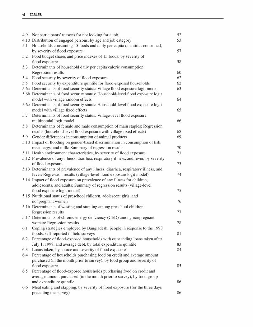
4.9 Nonparticipants’ reasons for not looking for a job 524.10 Distribution of engaged persons, by age and job category 535.1 Households consuming 15 foods and daily per capita quantities consumed,
by severity of flood exposure 575.2 Food budget shares and price indexes of 15 foods, by severity of
flood exposure 585.3 Determinants of household daily per capita calorie consumption:
Regression results 605.4 Food security by severity of flood exposure 625.5 Food security by expenditure quintile for flood-exposed households 625.6a Determinants of food security status: Village flood exposure logit model 635.6b Determinants of food security status: Household-level flood exposure logit
model with village random effects 645.6c Determinants of food security status: Household-level flood exposure logit
model with village fixed effects 655.7 Determinants of food security status: Village-level flood exposure
multinomial logit model 665.8 Determinants of female and male consumption of main staples: Regression
results (household-level flood exposure with village fixed effects) 685.9 Gender differences in consumption of animal products 695.10 Impact of flooding on gender-based discrimination in consumption of fish,
meat, eggs, and milk: Summary of regression results 705.11 Health environment characteristics, by severity of flood exposure 715.12 Prevalence of any illness, diarrhea, respiratory illness, and fever, by severity
of flood exposure 735.13 Determinants of prevalence of any illness, diarrhea, respiratory illness, and
fever: Regression results (village-level flood exposure logit model) 745.14 Impact of flood exposure on prevalence of any illness for children,
adolescents, and adults: Summary of regression results (village-level flood exposure logit model) 75
5.15 Nutritional status of preschool children, adolescent girls, and nonpregnant women 76
5.16 Determinants of wasting and stunting among preschool children: Regression results 77
5.17 Determinants of chronic energy deficiency (CED) among nonpregnant women: Regression results 78
6.1 Coping strategies employed by Bangladeshi people in response to the 1998 floods, self-reported in field surveys 81
6.2 Percentage of flood-exposed households with outstanding loans taken after July 1, 1998, and average debt, by total expenditure quintile 83
6.3 Loans taken, by source and severity of flood exposure 846.4 Percentage of households purchasing food on credit and average amount
purchased (in the month prior to survey), by food group and severity of flood exposure 85
6.5 Percentage of flood-exposed households purchasing food on credit and average amount purchased (in the month prior to survey), by food group and expenditure quintile 86
6.6 Meal eating and skipping, by severity of flood exposure (for the three days preceding the survey) 86
vi TABLES
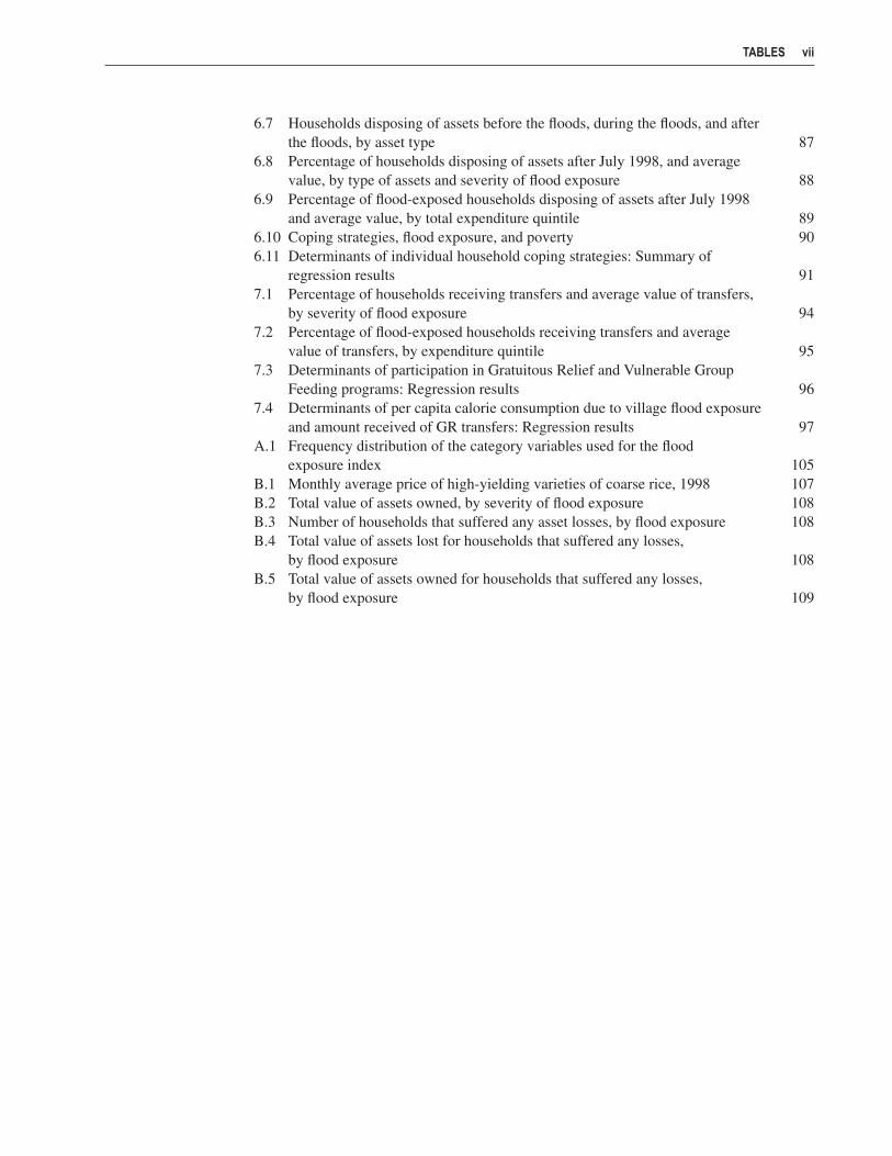
6.7 Households disposing of assets before the floods, during the floods, and after the floods, by asset type 87
6.8 Percentage of households disposing of assets after July 1998, and average value, by type of assets and severity of flood exposure 88
6.9 Percentage of flood-exposed households disposing of assets after July 1998 and average value, by total expenditure quintile 89
6.10 Coping strategies, flood exposure, and poverty 906.11 Determinants of individual household coping strategies: Summary of
regression results 917.1 Percentage of households receiving transfers and average value of transfers,
by severity of flood exposure 947.2 Percentage of flood-exposed households receiving transfers and average
value of transfers, by expenditure quintile 957.3 Determinants of participation in Gratuitous Relief and Vulnerable Group
Feeding programs: Regression results 967.4 Determinants of per capita calorie consumption due to village flood exposure
and amount received of GR transfers: Regression results 97A.1 Frequency distribution of the category variables used for the flood
exposure index 105B.1 Monthly average price of high-yielding varieties of coarse rice, 1998 107B.2 Total value of assets owned, by severity of flood exposure 108B.3 Number of households that suffered any asset losses, by flood exposure 108B.4 Total value of assets lost for households that suffered any losses,
by flood exposure 108B.5 Total value of assets owned for households that suffered any losses,
by flood exposure 109
TABLES vii


Figures
1.1 Flooded area and aman production, 1970–98 52.1 The pathways of flood impact on the domestic availability and household
consumption of foodgrains 82.2 The multiple pathways of flood impacts on household resources and
people’s well-being 92.3 Map of flood-affected areas of Bangladesh as of September 9, 1998, and
thanas selected for the investigation 112.4 Severity of flood exposure and percentage of households in the bottom
40th percentile of per capita expenditure by thana 133.1 Total rice production and availability in Bangladesh, 1976/77–1999/2000 223.2 The government’s budgeted and actual distribution of rice and total
foodgrains, 1998/99 263.3 Rice prices and quantity of private sector rice imports in Bangladesh,
1993–2000 283.4 Variations in wholesale rice prices across districts in Bangladesh, 1998 303.5 Wheat prices, quantity of private sector wheat imports, and net public wheat
distribution in Bangladesh, 1993–2000 313.6 Closing stocks of rice and total foodgrains in Bangladesh, 1995–2000 404.1 Bangladesh crop calendar and seasonal flooding 444.2 Average number of days in the current main job in the periods before, during,
and after the floods 504.3 Labor participation rates, by age and gender, November 1998 525.1 Household daily per capita calorie consumption, by expenditure quintile and
severity of flood exposure 595.2 Distribution of households with consumption above and below the minimum
caloric requirement, by share of expenditure on food 615.3 Female and male consumption of meals containing six staple foods, by
severity of flood exposure 675.4 Comparison of three measures of intrahousehold food distribution across
non-flood-exposed and flood-exposed households 695.5 Prevalence of any illness in previous two weeks, by gender, age group, and
severity of flood exposure 755.6 Wasting and stunting among preschool children, and chronic energy
deficiency among women, by severity of flood exposure 766.1 Percentage of households taking loans, by month and reason in 1998 82A.1 Frequency distribution of households by various variables of flood exposure 106


Foreword
Natural disasters such as prolonged droughts, floods, and cyclones threaten food se-curity in many developing countries, directly reducing agricultural production andfood supply. Moreover, these disasters can disrupt local economies and reduce house-
holds’access to food by destroying infrastructure and private productive assets, reducing em-ployment opportunities, and lessening the profitability of private enterprises. The 1998 floodsin Bangladesh led to a reduction in the main monsoon season rice crop of more than 10 per-cent of targeted production for the entire 1998/99 fiscal year and threatened the food securityof tens of millions of people. But, as this report shows, a combination of well-functioningprivate markets, suitable government policies, public and NGO interventions, and effectiveprivate coping strategies prevented a major disaster.
This report combines a careful analysis of government policy and private foodgrain mar-kets with a detailed survey of 757 households in rural Bangladesh in November and December1998, about two months after the floodwaters receded. The report describes short- and medium-term government policy measures taken to encourage private trade, including an earlier tradeliberalization that permitted private-sector imports of rice from India that stabilized privatemarkets and largely offset the decline in production. The impact of the floods on householdassets, employment, consumption, and nutritional outcomes is analyzed using the micro-levelsurvey data. The study finds that flood-exposed households were, in general, able to avoidsevere declines in food consumption and nutritional status through a combination of private-sector borrowing that averaged almost 6,000 Taka (Tk) per household (equivalent to over 140percent of average monthly expenditures) and targeted government and NGO transfers thataveraged 331 Taka per household.
This research report builds on earlier IFPRI work in Bangladesh analyzing the PublicFoodgrain Distribution System and the behavior of rice and wheat markets. It also extendsIFPRI work on preventing famines, efficiency in targeting of public-sector transfers, copingstrategies, and determinants of nutritional outcomes. Most important, it provides an analysisof how appropriate government policy can both provide incentives for private markets tomaintain food availability and directly reduce the food insecurity of poor disaster-exposedhouseholds through targeted transfers that increase access to food and minimize deteriorationin nutritional status.
Per Pinstrup-AndersenDirector General

Acknowledgments
Alarge number of people made important contributions to this report, particularly incollecting and analyzing the large household data set that is central to much of ourwork.
The data collection was carried out with the support of a Dhaka-based firm, Data Analysisand Technical Assistance (DATA), which assisted in the translation and finalization of thequestionnaire. Its directors, Md. Zahidul Hassan Zihad, Wahidur Rahman Quabili, and Md.Zobair, also trained and organized a team of 20 interviewers who spent many days in diffi-cult conditions.
Special thanks go to the Food Management and Research Support Project (FMRSP)–IFPRI staff, Md. Shahjahan Miah, Pradip Kumar Saha, A. W. Shamsul Arefin, Nurun NaharSiddiqua, Rowshan Nessa Haque, and Shandha Rani Ghosh, who participated in the data col-lection and entered the data in the computers. Abu Bakar Siddique supervised the data entrywork, helped to design the data entry programs, and ran countless checks on the data.
The data analysis on the surveys and secondary data was carried out with the help of avery hard-working team of research assistants: Syed Rashed Al-Zayed, Nishat Afroz MirzaEva, Anarul Kabir, Md. Syful Islam, Abdul Baten Ahmed Munasib, Helena Pachon, AmzadHossain, Md. Aminul Islam Khandaker, and Shameem Mahmoud. Md. Abdulla-Al-Amin,Md. Samsuddin Sumon, and Waheeda Ali Luna provided excellent secretarial support at var-ious stages of the research.
Many people provided helpful suggestions and insights into rice markets, governmentpolicy, household coping strategies, and many other issues, including Raisuddin Ahmed,Ruhul Amin, M. Abdul Aziz, Suresh Babu, Naser Farid, Lawrence Haddad, Nurul Islam,K. A. S. Murshid, Mahfoozur Rahman, Quazi Shahabuddin, Emmanuel Skoufias, and twoanonymous referees.
We also thank the Ministry of Food, Government of the People’s Republic of Bangladeshand the Food Planning and Monitoring Unit (FPMU) for their support of the work the FMRSPproject, and USAID/Dhaka for their financial support.
In addition, we wish to recognize the many people in rural Bangladesh who sufferedthrough the flood, particularly those who patiently participated in our surveys. We hope thatthis work, along with the efforts of many others, will help to enhance their food security.
Finally, we gratefully acknowledge the support of the late Secretary of Food, Mahbub Kabir,who through hard work and dedicated service played a central role in government policy-making during and after the 1998 flood.


Summary
The 1998 floods in Bangladesh, deemed “the flood of the century,” covered more thantwo-thirds of the country and caused 2.04 million metric tons of rice crop losses (equalto 10.45 percent of target production in 1998/99). This flood threatened the health and
lives of millions through food shortages (resulting from crop failure), the loss of purchasingpower for basic necessities, and the potential spread of water-borne disease. Yet, in fact, veryfew flood-related deaths occurred, and reportedly none due to food shortages. Poor house-holds did suffer substantial hardship during and after the floods, but the combination of well-functioning private markets, broadly effective interventions by government, donors, andnongovernmental organizations (NGOs), and private sector borrowing to a large extent main-tained availability and access to food.
This report examines in detail how the floods affected food security in Bangladesh at thenational and household levels and draws lessons for the management of future natural disastersin developing countries. At the heart of this analysis is the food security triad of availability,access, and utilization. Thus, we not only examine food production, imports, government in-terventions, and prices, which determine availability, but place a major focus on households’access to food (which was seriously threatened by loss of assets and income-earning oppor-tunities) and utilization of food (including intrahousehold food distribution). The findings inthis report are largely based on data from a survey of 757 rural households in 7 flood-affectedregions (thanas), supplemented by analysis of secondary data on foodgrain markets and gov-ernment policy.
As described in Chapter 2 (Figures 2.1 and 2.2), the availability of food—particularly riceand wheat, which together account for about 80 percent of the calories in the Bangladeshdiet—is determined by domestic production (which was severely impaired by the floods),government net distribution on the domestic market (in turn determined by the availabilityof stocks, government commercial imports, and food aid), and private sector imports. House-hold access to food, however, requires not only well-functioning markets or effective gov-ernment distribution programs, but also sufficient resources to acquire food (obtained throughcurrent incomes, transfers, savings, or borrowing). Intrahousehold distribution and the healthenvironment ultimately determine individual consumption and nutritional outcomes, as well.
The Impact of the Floods on Foodgrain Markets and the Policy ResponseAt the sectoral level, the government of Bangladesh (GOB) and donor officials were keenlyaware of the potential flood damage to the monsoon season rice crop (aman) and the threat

to foodgrain availability, even while the im-mediate relief operations were under way.The GOB therefore launched an appeal forinternational flood relief and food aid inAugust 1998, anticipating that by the timethe floodwaters receded it would be too lateto replant a large portion of the aman ricearea. Donors ultimately responded with 1.233million metric tons of food aid delivered in1998–99, but, in the short run, governmentdistribution of foodgrains was constrainedby available public stocks. Thus, public food-grain distribution from July through Decem-ber 1998 was only 631,000 metric tons greaterthan planned before the flood.
In spite of only a small increase abovepreviously scheduled supplies through gov-ernment channels in the last six months of1998, markets were stabilized by privatesector imports of rice and wheat. Inflows of1.3 million metric tons of rice from Indiakept prices from rising above import paritylevels following the flood. Evidence fromletters of credit for rice imports shows thatlarge numbers of traders participated in therice import trade (which was mostly over-land), with an average size of contract of710 metric tons in 1994/95. Thus, privatemarkets appear to have worked competi-tively to limit the price increases to only 12.4percent between May–July and August–December 1998 (compared with 58.2 per-cent in the same months in 1974 when afamine occurred) and to maintain availabil-ity of foodgrains. Adequate levels of gov-ernment stocks—659,000 metric tons at thebeginning of September 1998, comparedwith only 347,000 metric tons in September1974—may have also helped stabilize mar-kets by influencing private traders’ expecta-tions of the ability of the government tointervene in local rice markets.
Public stocks and distribution of food-grains were significantly larger following themajor floods in 1988. Several factors suggestthat the need for large public stocks to avertfamines in Bangladesh has decreased con-siderably since 1974 or even 1988, however.Large increases in the size of the boro rice
crop, harvested only five to six months afterthe aman crop, have shortened the period ofuncertainty regarding domestic supply, in-creased foodgrain availability, raised farmerincomes, and reduced prices. Trade liberal-ization in the early 1990s has enabled pri-vate sector imports to help stabilize pricesand total supplies when production shortfallsthreaten domestic supplies, and the availabil-ity of foreign exchange is no longer a severeconstraint on imports. Moreover, 20 yearsof investment in rural infrastructure haveimproved the efficiency of domestic ricemarkets in Bangladesh, so shortages acrossregions within the country can be more easilymet by domestic private (and public) grainflows. In addition, increases in real per capitaincomes and food consumption over timehave added to food security at householdlevels.
Losses of Crops, OtherAssets, and EmploymentDuring the 1998 floods, floodwaters onsample farmers’ fields were almost doubletheir normal levels—137 centimeters com-pared with 73 centimeters. On mediumhighland, floodwaters were on average 88centimeters higher than in normal years andeven high fields that normally are not floodedwere covered by an average of 22 centime-ters of water. This severe flooding led to sub-stantial crop losses, especially to the aus andaman crops. Because of the floods, 69 per-cent of aus production, 82 percent of deep-water (broadcast) aman, and 91 percent oftransplanted aman was lost, representing 24percent of the total value of anticipated agri-cultural production for the year. Overall, ricecrop losses accounted for over half of totalagricultural losses, with vegetables (25 per-cent) and fibers (19 percent) accounting formost of the remaining losses.
In addition to the losses to crops, thefloods damaged or destroyed many house-hold assets, reducing household wealth aswell as future productive capacity. For the55 percent of households that lost assets, theaverage loss was 6,936 taka (Tk), equivalent
xvi SUMMARY
to 16 percent of their pre-flood total value ofassets. In all, 47 percent of households suf-fered damage or loss to housing, the averageloss being Tk 5,675, or 59 percent of thepre-flood value; 17 percent of householdslost trees with an average value of Tk 5,137;15 percent of households lost chickens,though the average loss was only Tk 142.The more severe the level of flood exposure,the larger the proportion of households suf-fering damage to their assets: 78 percent ofthe households exposed to very severe floodsand 69 percent of those exposed to severeflooding lost assets worth on average Tk9,042 and Tk 6,679, respectively.
The rural economy suffered serious dis-ruption from the floods. Average monthlydays of paid work decreased during the floods,but increased in the period after the floods tothe same level as 12 months earlier for allworkers except day laborers. Day laborerswere the most severely affected: their em-ployment fell sharply from 19 days per monthin 1997 to only 11 days per month in Julythrough October 1998. Wage earnings alsofell during the floods and had not recoveredto 1997 levels by October–November 1998.For day laborers, average monthly earningsin the period July–October 1998 were 46 per-cent below those in the same months in 1997,and in October–November 1998 were still18 percent below 1997 levels. This decline innumber of days worked and wage earningsoccurred in the context of a labor market withlittle open unemployment. Thus, underem-ployment increased as people worked fewerdays, but at least most workers found someform of employment.
Impacts on Household Food Security, Health,and NutritionThe decline in crop production, losses of otherassets, and lower employment opportunitiescontributed to increased food insecurity.Food consumption fell, along with house-holds’ abilities to meet their food needs on asustainable basis. Vegetables and many otherfoods were in short supply, and as a conse-
quence the calorie consumption of flood-ex-posed households was 272 calories/person/day fewer than that of households not ex-posed to flooding; 15.6 percent of flood-exposed households became food insecure.We found no evidence that females’ con-sumption of the main staples—rice andwheat—was reduced by more than males’as a result of the floods, or that male fa-voritism in the consumption of animal prod-ucts increased. Thus, the floods did not appearto lead to an increase in discriminationagainst females in food consumption withinhouseholds.
The floods also caused a major deterio-ration in the quality of households’ healthenvironments. They damaged or destroyedpeople’s homes, reduced their access to safewater, and destroyed or damaged their toiletfacilities. These factors, combined with thereduction in food consumption, led to sub-stantial increases in illness, even after thefloodwaters had receded. In the immediatepost-flood period, 9.6 percent of individualsin the sample suffered from diarrhea, and4.7 percent were affected by respiratory ill-nesses. Individuals in all age groups experi-enced a deterioration in health status at thistime, especially those who were severely orvery severely flood exposed. Although ado-lescents had the greatest increase in illness,the most serious health problem posed by thefloods was the increase in children’s illness,because they suffered more serious conse-quences, even threatening their survival.
The floods led to increases in both wast-ing and stunting among preschool children.Severe or very severe flood exposure causedmany children to lose weight and/or to fail togrow at a critical period in their mental andphysical development—55 percent of chil-dren in the sample were stunted and 24 per-cent were wasted. This situation was broughtabout by a combination of factors, includingreduced access to food, the increased diffi-culties of providing proper care for childrenthat came with disruptions in home life, andthe greater exposure of children to contami-nants. We also found some evidence that the
SUMMARY xvii

floods led to an increase in severe chronicenergy deficiency among women.
Household CopingMechanismsHouseholds adjusted to the shock of thefloods in several major ways: reducing expen-ditures, selling assets, borrowing. Borrow-ing was by far the major coping mechanismof the households sampled, in terms of boththe value of the resources and the number ofhouseholds that borrowed. About 60 percentof households in the sample were in debt inthe months immediately following the floods.Average household debt rose to an averageof almost 1.5 months of typical consumptioncompared with only a small percentage ofmonthly consumption in January 1998, abouteight months before the floods. In addition,56.6 percent of flood-exposed householdsin the bottom 3 quintiles resorted to pur-chasing food on credit in the month preced-ing the survey. This borrowing was sufficientto maintain the value of household expendi-tures vis-à-vis pre-flood levels but, becauseof higher prices, poor flood-affected house-holds consumed fewer calories per capitaper day than non-flood-exposed households,suggesting that targeted cash transfers andcredit programs could have been an effectivecomplement to direct food distribution.
Mitigating the Effects of theFloods: Government Food and Cash TransfersOur survey suggests that government directtransfers were well targeted to flood-exposedhouseholds and to the poor. In the initialflood period, immediate relief through theGratuitous Relief program went mainly toseriously flood-exposed households—35.7percent of severely flood-exposed householdsreceived the transfer compared with 9.7 per-cent of non-exposed households. VulnerableGroup Feeding (VGF) transfers, which wereadministered through union-level commit-tees, were better targeted to the poor than tothe flood-exposed households. Among flood-exposed households, 35.4 percent of house-
holds in the bottom quintile received graintransfers compared to 17.8 percent and 7.5percent in the top two quintiles, respectively.
Yet government transfers were small rel-ative to the needs of households, as indicatedby the extent of household borrowing (equalto about six to eight times the level of gov-ernment transfers for poor, flood-exposedhouseholds). To eliminate borrowing wouldhave required a transfer of approximatelyTk 5,000 for each of the 60 percent of house-holds that were in debt in December 1998,several months after the floods. Extrapolat-ing this figure to the national level, the costof such transfers would have been more thanUS$1.5 billion.
Small cash transfers were part of the ini-tial flood relief efforts, but larger cash trans-fers or credit programs were not included inthe medium-term relief to households twoto four months after the floods, even thoughfoodgrain stock constraints limited the ex-pansion of the VGF program during thisperiod.
Policy ImplicationsBoth short-term and long-term policies playedmajor roles in preventing the 1998 floodsfrom resulting in a major food security dis-aster in Bangladesh. Public sector investmentsin agricultural research and extension in the1980s and 1990s, together with mainly pri-vate sector investments in small-scale irriga-tion, led to substantial increases in wheat andboro rice production. This made the countryless vulnerable to floods by increasing totalfoodgrain production in the country, reduc-ing the length of time between major cropsfrom 12 months to only about 6 months, and leading to a shift away from highly flood-susceptible deepwater aman cultivation in themonsoon season to boro cultivation in the dryseason. Continued investment in researchand extension could further increase produc-tion efficiency and reduce the vulnerabilityof the food sector to floods.
In addition, long-term public investmentsin infrastructure (roads, bridges, electricity,and telephones) contributed to efficient mar-
xviii SUMMARY

keting systems that enabled the private sec-tor grain trade to supply markets throughoutthe country following the floods. Govern-ment policies also encouraged private sectorparticipation in the grain trade. In particular,the liberalization of rice and wheat importsin the early 1990s enabled private sectorimports to quickly supply domestic marketsand stabilize prices at their import paritylevels following the floods. Short-term poli-cies such as the removal of the import tariffon rice in early 1998 and instructions to ex-pedite port clearance of private sector food-grain imports also provided clear signals tothe private sector of government support forthis trade. Moreover, these private sectorimports proved to be a far less costly way ofmaintaining foodgrain availability than thedistribution of government commercial im-ports or public stocks, the mechanisms bywhich the government handled productionshortfalls after the 1988 floods, 10 yearsearlier.
Donors responded to the flood situationwith major increases in food aid that eventu-ally permitted a major expansion of targetedfoodgrain distribution through the Vulner-able Group Feeding and Food For Workprograms. However, almost inevitable de-lays and uncertainties in food aid arrivals re-sulted in only a small net increase in publicdistribution beyond preflood plans until De-cember 1998, in part because existing gov-ernment stocks of wheat were insufficient topermit a large expansion in distribution. (Ricestocks were kept in reserve for possible usein stabilizing markets later.) A policy of hold-ing more stocks might not have been a bet-ter option though, given the substantial costsof procuring, handling, and eventually dis-tributing grain. With foodgrain supplies andprices stabilized by private sector imports,targeted cash transfers to supplement directfood transfers could have been used to in-crease household access to food (and otherbasic needs) without increasing market pricesof foodgrains.
Nonetheless, programs already in placeand a rapid expansion of the VGF program
to more than 4 million households enabledpublic foodgrain distribution following thefloods to be well targeted to the poor. Poorwomen and children, many of whom werechronically malnourished, were effectivelytargeted through the VGF program. Greatertargeting of credit programs would have beenuseful, however, given that poor householdsborrowed heavily in the informal privatemarket during the floods, and NGO creditprograms were limited in scope. To avoiddelays and to minimize leakages, these ruralcredit programs for disaster relief should bedesigned and put in place before disastersoccur. Maintaining a structure of social pro-grams that can be scaled up in the event of adisaster is more important than maintaininglarge stocks of food.
To reduce even further the impact of afuture natural disaster like the floods of 1998,it is necessary to improve the scope and thequality of the interventions so as to providefood, water, and shelter at the time of the dis-aster and in its immediate aftermath. Reliefshould be targeted at both the village andindividual levels. This report shows that in-terventions at the village level, such as pro-viding shelter, improving sanitary conditions,and creating economic opportunities, wereeffective in alleviating the adverse impact ofthe floods. We also present evidence thattargeting to individual poor, flood-exposedhouseholds can have a positive impact onthe well-being of individual children. Finally,government policies to foster economicgrowth in rural areas and to provide income-earning alternatives to poor households canboth help to reduce poverty as well as in-crease the capacity of households to with-stand shocks resulting from natural disasters.
ConclusionsThe combined efforts of the government of Bangladesh, donors, NGOs, and flood-affected households themselves, together withprivate trade operating in well-functioningmarkets, were in general extremely success-ful in mitigating the effects of the 1998 floodsat the household level and in avoiding a major
SUMMARY xix

food crisis. Thus, the Bangladesh exampleillustrates the importance of coordinatedactions at the sectoral and household levels,by both public and private sectors, in main-taining the availability of and access to foodto ensure food security following major sup-ply disruptions. Private trade alone mighthave provided sufficient availability of food,though this in itself would not have solvedthe problem of access to food for millions ofhouseholds. Public sector actions enhancedaccess to food by flood-exposed households,though these interventions were too small to
have a major direct effect on overall avail-ability and market prices. Ultimately, foodsecurity in Bangladesh was largely main-tained through an appropriate mix of publicinterventions, private market trade flows,and an extensive system of private borrow-ing. Continued investments in agriculturalresearch, extension, roads, electricity, andother rural infrastructure, along with policiespromoting efficient markets and programs toprovide targeted transfers and credit to poorhouseholds, could further enhance the foodsecurity of the poor.
xx SUMMARY

C H A P T E R 1
Introduction
The nation is faced with a disaster of highest order. All signs, as they become more andmore visible, lead to one conclusion: we are faced with a disaster with catastrophic di-mensions. . . . It is not just another flood; it is THE FLOOD, which all Bangladeshis willremember for generations to come. . . . This will be the reference point for many of ournational events. This will set the standard of our capability or incapability. We’ll measureourselves with this standard in future. So will the rest of the world.
These statements originally appeared in Professor Muhammad Yunus’s article in The DailyStar, a major English-language newspaper in Dhaka, Bangladesh, on September 11, 1998, inthe midst of what has been called “the flood of the century.”1
Fortunately, such a tragedy did not occur. In spite of massive floods that covered morethan two-thirds of the country, causing over 2 million metric tons (MTs) of rice crop losses(equal to 10.5 percent of target rice production in 1998/99) and threatening the health andlives of millions through possible food shortages, loss of purchasing power for basic neces-sities, and the potential spread of water-borne disease, very few flood-related deaths occurred,and reportedly none due to food shortages. Poor households did suffer substantial hardshipduring and after the floods, but the combination of well-functioning private markets, broadlyeffective interventions by government, donors, and nongovernmental organizations (NGOs),and private sector borrowing to a large extent maintained availability and access to food.
This research report documents what is to a large extent a success story about a faminethat did not happen in spite of a massive food production shock. As von Braun, Teklu, andWebb (1999) argue, famines are complex events that involve institutional, organizational, andpolicy failure, not just generalized market- and climate-driven production failure. Moreover,famines must be understood in their long-term context. In the same way, the avoidance of afamine involves more than simply increasing food supply to areas affected by a national dis-aster. Thus, we examine in detail how the flood affected food security in Bangladesh at thenational and household levels, and the response of government, donors, markets, and house-holds to the potential food crisis. A key part of the story is the role of longer-term investmentsin agricultural research, extension, and irrigation, along with earlier policy reforms (namely,
1 Professor Muhammad Yunus was the founder of the Grameen Bank. At about the same time (early September 1998),the British Broadcasting Corporation (BBC) quoted an international agency in reporting that 20 million people inBangladesh might die as a consequence of the floods (Khan and Obaidullah 1999).

the trade liberalization in the early 1990s),which played a major role in making the1998 outcome so much different from that ofthe Bangladesh famine in 1974.
At the heart of this analysis is the foodsecurity triad of availability, access, and uti-lization. The availability of food is naturallyan important issue when a major productionshortfall occurs. As this report will show, pri-vate sector imports played a crucial role inmaintaining the availability of rice and wheatfollowing the 1998 floods. The contributionof food aid to the availability and timing offood aid arrivals is also highlighted.
But, as emphasized by Sen (1981), Drezeand Sen (1989, 1991), and Ravallion (1997),another key determinant of household foodsecurity is households’ food entitlements—their capacity to acquire food legally throughtheir own production, income, savings, andprivate and government transfers (in otherwords, household access to food). Sen (1981),in fact, argues that insufficient entitlementscan lead to famine and that loss of entitle-ments, rather than a significant decline inthe total availability of food, was the majorcause of the Great Bengal famine of 1943,which killed between 1.5 and 3.0 millionpeople.2 The poor are particularly vulnera-ble to natural disasters because of their lackof assets and inadequate food entitlements(World Bank 2000). This study examines howaccess to food was affected by the loss ofassets and income-earning opportunities forflood-exposed households in 1998, using de-tailed income and expenditure data from asurvey of rural households in flood-affectedregions conducted just after the floods.
We do not stop at household access tofood, though. Because sufficient access tofood at the household level does not ensureadequate nutrition, especially for womenand young children, we extend our analysisto cover the utilization of food (includingintrahousehold food distribution). Thus, wealso use household survey data to examine
determinants of nutrition (such as individualfood consumption, caring practices, and over-all health status) as well as nutritional out-comes for children.
Even though the availability of foodwas maintained and targeted programs con-tributed to increasing access to food by thepoor, this report shows that many householdsresorted to borrowing money in informalmarkets as their dominant coping strategy.Credit was also an important coping mecha-nism following the 1988 floods in Bangla-desh, but inadequate access to credit by poorhouseholds at that time adversely affected nu-trition, contributing to reduced child growth(Foster 1995). Thus, we also examine theextent to which poor households were ableto borrow in 1998, and we discuss the impli-cations of these increased debt burdens forthe medium-term welfare of the poor.
The 1998 FloodsFloods are a normal part of the ecology ofBangladesh. The mid-1998 floods in Bang-ladesh were unusual, however, for both theirdepth and duration. Unlike the normal floods,which cover large parts of the country forseveral days or weeks during July and Au-gust, the floods in 1998 lasted until mid-September in many areas, killing hundredsof people and destroying roads, houses, crops,and other assets.
Three major rivers drain into the Bay ofBengal through Bangladesh: the Ganges(known as the Padma in Bangladesh), theBrahmaputra (known as the Jamuna in Bang-ladesh), and the Meghna. Less than 10 per-cent of the 1.55 million km2 catchment areaof these rivers lies within the borders ofBangladesh, so rainfall in neighboring India,Nepal, Bhutan, and China and snowmelt inthe Himalayas are major determinants of theflow of water through Bangladesh. Thesethree major rivers have their peak flows inJuly, August, and September, during the mon-soon season, when they overflow their banks
2 CHAPTER 1
2 The official estimate of famine deaths was 1.5 million. The higher figure is a calculation of excess mortality during thefamine period by Sen (1981), Appendix D.

and deposit fertile silt on the floodplains.These normal annual floods typically coverabout 30 percent of the country at varioustimes. However, in years when the peakwater levels of all three rivers occur at thesame time, as in 1954, 1974, 1987, 1988, and1998, severe floods have occurred.3 In addi-tion to these major river floods, Bangladeshexperiences flashfloods in the eastern andnorthern rivers, generally lasting only a fewdays, local floods due to high rainfall in themonsoon season, and coastal floods due tostorm surges generated by cyclones.4
The 1998 floods began in early July inthe southern part of Bangladesh and contin-
ued over the next three months in variousparts of the country, inundating 68 percent ofthe total area at various times (a detailedchronology of the 1998 floods is presentedin Table 1.1). Initially, flooding (caused byheavy rainfall) was mainly confined to thesoutheastern hilly basin and the Meghnabasin in the northeast of Bangladesh. Duringthe third week of July, however, a heavyon-rush of water in the Brahmaputra, whichflows into Bangladesh from the north, addedto rising levels in the Ganges (Padma) basinin the western part of the country. By July 28,1998, 30 percent of the total area was inun-dated. Then, after two weeks of little change
INTRODUCTION 3
3 Pramanik (1994: 135, 144, 147).4 Shahjahan (1998). See Ali, Hoque, Rahman, and Rashid (1998) for a more in-depth discussion of the hydrology of floods
in Bangladesh and the Flood Action Plan adopted after the 1988 floods.
Table 1.1 The 1998 floods: Chronology of events
Date Event
1998First week of July The Flood Forecasting and Warning Centre (FFWC) of the Bangladesh Water Development Board reports
rising water levels in the major rivers.July 16 First meeting of the Inter-Ministerial Disaster Management Co-ordination Committee (IMDMCC).
Emergency relief operations begin.July 24 First National Disaster Council (NDC) meeting chaired by the Prime Minister.August 13 Second meeting of the IMDMCC. Government plans to cope with the flood situation with internal resources.August 26 The government of Bangladesh appeals for international help to assist flood victims.August 32,000 tons of rice and 1,100 tons of wheat distributed through relief channels: Gratuitous Relief (GR), Test
Relief (TR), and Vulnerable Group Feeding (VGF).September 7 Peak of floods in terms of number of monitoring stations reporting flows above danger levels; 51 percent of
total area of Bangladesh inundated.September 16,575 tons of food aid arrive through World Food Programme; 52,000 tons of rice and 1,800 tons of wheat
distributed through relief channels.September 25 Flood waters recede—all major rivers are below danger level.October 1 Expansion of VGF program to 4 million cards, with 50 percent of the ration in wheat.October 143,000 tons of government commercial wheat imports arrive; 42,500 tons of rice and 32,500 tons of wheat
distributed through relief channels.October 44,344 tons of food aid arrive, bringing total since August 1998 to 61,883 tons.November A total of only 77,000 tons of food aid are available for distribution by end of November. VGF program
continues. Wheat distribution through relief channels (56,700 tons) is now greater than rice distributionthrough relief channels (37,800 tons).
Late November 138,902 tons of food aid arrive, bringing total since August 1998 to 200,785 tons.November–December Aman rice harvest of 7.74 million tons, 1.76 million tons below target.December Expansion of VGF program to 4.2 million cards and increase in the ration size from 16 kg to 20 kg/card
(5 kg rice and 15 kg wheat).December 360,887 tons of food aid arrive, bringing total since August 1998 to 561,672 tons.1999February VGF distribution extended to February through April 1999.May–June Record boro rice harvest of 10.05 million tons leads to drop in national average wholesale coarse rice price
from 14.0 Tk/kg in April to 12.4 Tk/kg in June.
Source: Grameen Trust flood website.

in the flood situation, water levels in thePadma river started rising sharply. Shortlythereafter, other rivers also rose, so that byAugust 30, 1998, 41 percent of the total areawas inundated. The flood situation reachedits peak, in terms of the number of monitor-ing stations reporting flows above dangerlevels, on September 7, 1998, when 51 per-cent of the total area was inundated. Waterlevels fell rapidly thereafter, and by Septem-ber 25, 1998, no monitoring stations reportedflows above danger levels.5
Prior to 1998, the last major floods inBangladesh occurred in 1987 and 1988. In1987, floods covered about 40 percent of theland area, affected about 30 million people,and caused about 1,800 deaths. The floodsin 1988 were even more serious, coveringabout 60 percent of the land area, affectingabout 45 million people, and causing morethan 2,300 deaths.6 In terms of peak waterlevels at various river monitoring stations,the 1998 and 1988 floods were almost iden-tical: they both averaged about 11.45 metersabove danger level (Table 1.2). The majordifference between the two floods was in theduration of the flooding: at the major rivermonitoring stations shown in Table 1.2, thewater was above the danger level for an av-erage of 59 days in 1998, compared with only34 days in 1988.
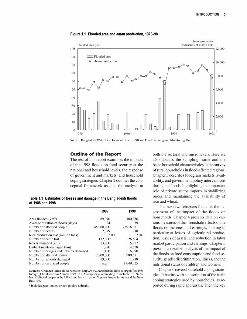
Normal flooding has little adverse effecton rice production in Bangladesh (and, infact, adds to soil fertility), but the long dura-tions of both the 1988 and 1998 floods led tomajor production shortfalls (Figure 1.1). Ini-tially, the 1998 floods caused only relativelyminor damage to standing crops but, as flood-waters persisted into September, the floodingdestroyed seedlings of the main monsoonseason aman rice crop. Ultimately, the floodresulted in a shortfall in aman rice productionof 1.76 million MTs and a total rice produc-tion shortfall of 2.04 million MTs, similar tothe production loss due to floods in 1988.
Official estimates of other losses anddamage in the 1988 and 1998 floods arepresented in Table 1.3. The sudden rise inwater levels in 1988 and the serious floodingwithin the city of Dhaka may account for thehigher number of deaths attributed to theflood in that year and the greater reporteddamage to houses and schools. Nonetheless,the damage to physical infrastructure (roads,embankments, bridges, and culverts) appearsto have been greater in 1998. These com-parisons should be treated with caution,however, because of possible differences indefinitions and data coverage.
4 CHAPTER 1
5 Bangladesh Water Development Board (1998: 28, 29).6 Irrigation Support Project for Asia and the Near East (1993: 1).
Table 1.2 Bangladesh flood levels and duration, 1988 and 1998
Difference1988 1998 1998–1988
Total flood-affected area (km2) 89,970 100,250 10,280Percentage of total area 61 68 7Peak water level (meters)Brahmaputra basin
Bahadurabad (Jamuna) 20.62 20.37 −0.25Aricha (Jamuna) 10.58 10.76 0.18Mymensingh (Old Brahmaputra) 13.69 13.04 −0.65Dhaka (Buriganga) 7.58 7.24 −0.34Narayanganj (Lakhya) 6.71 6.93 0.22
Ganges basinRajshahi (Padma) 19.00 19.68 0.68Goalondo (Padma) 9.83 10.21 0.38Bhagyakul (Padma) 7.43 7.50 0.07
Meghna basinBhairab Bazar (Upper Meghna) 7.66 7.33 −0.33
Average 11.46 11.45 0.00Days above danger levelBrahmaputra basin
Bahadurabad (Jamuna) 27 66 39Aricha (Jamuna) 31 68 37Mymensingh (Old Brahmaputra) 10 33 23Dhaka (Buriganga) 23 57 34Narayanganj (Lakhya) 36 71 35
Ganges basinRajshahi (Padma) 24 28 4Goalondo (Padma) 41 68 27Bahgyakul (Padma) 47 72 25
Meghna basinBhairab Bazar (Upper Meghna) 68 68 0
Average 34 59 25
Source: Bangladesh Water Development Board 1998.
Note: Names of rivers are shown in parentheses next to station names.
Outline of the ReportThe rest of this report examines the impactsof the 1998 floods on food security at thenational and household levels, the responseof government and markets, and householdcoping strategies. Chapter 2 outlines the con-ceptual framework used in the analysis at
both the sectoral and micro levels. Here wealso discuss the sampling frame and thebasic household characteristics in the surveyof rural households in flood-affected regions.Chapter 3 describes foodgrain markets, avail-ability, and government policy interventionsduring the floods, highlighting the importantrole of private sector imports in stabilizingprices and maintaining the availability ofrice and wheat.
The next two chapters focus on the as-sessment of the impact of the floods onhouseholds. Chapter 4 presents data on var-ious measures of the immediate effects of thefloods on incomes and earnings, looking inparticular at losses of agricultural produc-tion, losses of assets, and reduction in labormarket participation and earnings. Chapter 5presents a detailed analysis of the impact ofthe floods on food consumption and food se-curity, gender discrimination, illness, and thenutritional status of children and women.
Chapter 6 covers household coping strate-gies. It begins with a description of the maincoping strategies used by households, as re-ported during rapid appraisals. Then the key
INTRODUCTION 5
Table 1.3 Estimates of losses and damage in the Bangladesh floods of 1988 and 1998
1988 1998
Area flooded (km2) 89,970 100,250Average duration of floods (days) 34 59Number of affected people 45,000,000 30,916,351Number of deaths 2,379 918Rice production lost (million tons) 2.00 2.04Number of cattle lost 172,000a 26,564Roads damaged (km) 13,000 15,927Embankments damaged (km) 1,990 4,528Number of bridges and culverts damaged 1,160 6,890Number of affected houses 7,200,000 980,571Number of schools damaged 19,000 1,718Number of displaced people n.a. 1,049,525
Sources: Grameen Trust flood website: hhtp://www.bangladeshonline.com/gob/flood98/foreign_1.html, cited in Ahmed 1999: 151. Average days of flooding from Table 1.2. Num-ber of affected people in the 1988 flood from Irrigation Support Project for Asia and the NearEast 1993.a Includes goats and other non-poultry animals.
Figure 1.1 Flooded area and aman production, 1970–98
Source: Bangladesh Water Development Board 1998 and Food Planning and Monitoring Unit.

coping strategies—borrowing and purchasesof food on credit, changes in eating behavior,and sales of assets—are discussed and thefactors determining the choice of copingstrategies are analyzed.
Chapter 7 examines the impact of majorgovernment and NGO interventions onhousehold incomes and food consumption.
The chapter highlights the impacts of foodand cash transfers, examining the extent towhich they were targeted to the poor andflood-affected households and their contri-bution to total incomes and expenditures.Finally, Chapter 8 summarizes the findingspresented in earlier chapters and presentspolicy implications.
6 CHAPTER 1

C H A P T E R 2
Data and Methods
The 1998 floods in Bangladesh, and government policy interventions in response to thefloods, affected markets and households through numerous channels. Entire commu-nities and markets experienced damage to infrastructure and disruption of local
economies. Yet this large aggregate shock also affected individuals or households in slightlydifferent ways, depending on the exact location of their houses and fields, their occupations,and other household characteristics. As such, the floods had some of the characteristics of anidiosyncratic shock.7
This chapter begins with the conceptual framework used in this study, which elucidatesthese linkages between the floods, government policy, labor and commodity markets, house-hold incomes and consumption, and nutrition and health outcomes. We describe the micro-level data collection and sampling frame used for the analysis at the household and individuallevel. Finally, we discuss two major issues important for the micro-level analysis in subse-quent chapters: the definition of flood exposure and the extent to which flood exposure iscorrelated with poverty.
Conceptual FrameworkFigure 2.1 describes the relationship between production, markets, and household con-sumption demand for foodgrains. As shown, the availability of foodgrains in the market isdetermined by the level of domestic food production, the level of private imports, and thedistribution of food aid through the public food distribution system (PFDS). The distributionof the PFDS, in turn, is determined by the availability of public stocks at that time, which arethemselves a result of past government procurement, government imports, and food aid inthe form of current and emergency aid. The floods caused major losses of domestic produc-tion and households assets. As a result, food prices rose and the demand for labor fell, low-ering household incomes and ultimately household consumption.
Figure 2.2, which draws on the United Nations International Children Fund’s (UNICEF1990) framework for the causes of malnutrition, shows how the use and allocation of laborand other household resources affect household income and expenditure and ultimatelypeople’s well-being. The allocation and level of expenditure, together with the level of prices
7 For a review of the literature on shocks and poverty, see World Bank (2000).

and level of care and health environment,determine the level of food security and ul-timately the level of health and nutritionalstatus. In particular, Figure 2.2 shows themany pathways through which floods, overwhich people have little or no control, canaffect people’s lives. In this case the floodshad a direct impact on the endowment andthe activities of the household, which affecthousehold behavior, food security, and indi-vidual health and nutritional status in severalways.
First, the floods damaged or destroyedinfrastructure, workplaces, and householdassets, and disrupted the normal functioningof labor, credit, and commodity markets.Landowning farming households were par-ticularly affected because the floodwatersdamaged standing crops and receded only inlate September, thus reducing the time avail-able for planting another crop and reducingthe level of own food production. Nonfarm-ing households were also affected, becausethe floods destroyed the productive assets ofself-employed households, such as weavinglooms and rickshaws. Moreover, market dis-
ruptions caused shortages of critical recurrentinputs (for example, seeds and seedlings) toboth farm and nonfarm production activities.
The reduction in agricultural productionand the slowing down of the economygreatly affected the demand for labor, thusreducing the income-earning opportunitiesof household members. Long-term income(or livelihood) security was compromised bydirect destruction or loss of assets that arestores of value. It was further jeopardized bydepletions of savings or increased indebted-ness, used as a coping strategy in response toshort-term income losses.
The floods were also accompanied byreduced availability of food and other com-modities. This led to higher prices and areduction in the amounts that could be pur-chased by households. At the same time,expenditures on items critical to the propercare of household members, such as clothingor medicines, may have also been smallerthan needed. Thus, food security was com-promised by reduced expenditures on foodresulting from additional constraints onhousehold budgets and rising food prices.
8 CHAPTER 2
Figure 2.1 The pathways of flood impact on the domestic availability and household consumption of foodgrains
Source: Authors.

Finally, the health environment wasgreatly disrupted. Water-borne diseaseswere more prevalent because of contact withcontaminated floodwaters and a lack ofproper sanitation facilities. Moreover, healthinfrastructures were by and large not avail-able. At the same time, the floods led todirect damage to and destruction of house-holds’ domestic assets. The most importantof these were their homes, which were eitherdamaged or not habitable during the periodof the floods. Other assets included waterpumps necessary for accessing clean water,toilet facilities, clothing, cooking equip-ment, eating utensils, and food stocks. Thesefactors, together with a reduction in theavailability of fuel for cooking, disrupteddomestic production (for example, child-care, meal preparation, and house cleaning),which directly affected the quality of carefor household members and the quality ofhouseholds’ health environments.
When food security and the quality of carefor household members are jeopardized, di-etary intakes decline and illness increases,ultimately compromising household mem-bers’ nutritional status. In dire situations,food scarcities may lead households to in-crease discrimination in food consumptionagainst some of their members in order toensure the survival of others. In short, withfloods come multiple, simultaneous shocksto households’ economic resources and theirdaily living environments. Poor householdsin Bangladesh faced difficult tradeoffs indeciding how to cope with the immediatelosses and the deterioration in members’physical well-being because the necessaryresources were undermined.
Data Collection Methodologyand Sampling FrameThe micro-level analysis of this report isbased mostly on The International Food
DATA AND METHODS 9
Figure 2.2 The multiple pathways of flood impacts on household resources and people’swell-being
Source: Adapted from UNICEF 1990.

Policy Research Institute’s Food Manage-ment and Research Support Project (IFPRI-FMRSP) Household Survey 1998, a detailedsurvey of 757 households in seven flood-affected thanas in Bangladesh. Since the pur-pose of the study is to analyze the impact ofthe floods on food security and households’resulting coping strategies, we selected areasthat would give a fair representation of theparts of the country affected by flooding. Weused three main criteria to select the seventhanas. Our first criterion was the severity offlooding, as determined by the BangladeshWater Development Board. It classifiedthanas as “not affected,” “moderately af-fected,” and “severely affected,” dependingon the level and depth of the floodwater. Oursecond criterion was the level of poverty inthe district in which the thanas were located.Thanas with more than 70 percent of thepopulation below the poverty line were clas-sified as poor. Finally, from the thanas se-lected on the first two criteria, we chosethose that had been included in other stud-ies and that would give us a good regionaland geographical balance across the six ad-ministrative divisions of Bangladesh (seeTable 2.1 and Figure 2.3).
We randomly selected households usinga multiple-stage probability sampling tech-nique.8 In the first stage, three unions ineach thana were selected. In the secondstage, six villages were selected from eachunion with probability proportional to the
population in each village. Then, in each vil-lage two clusters (paras) were selectedusing preassigned random numbers. Finally,three households were chosen from all thehouseholds in each cluster using a system-atic random selection process. As a result,we selected approximately 6 households pervillage (36 per union, 108 per thana) for afinal sample size of 757 households in 126villages.
We used three different instruments. Acommunity questionnaire was used to col-lect information at the union level duringthe floods. A village-level survey conductedduring November and December 1998 in64 villages collected information on rurallabor markets. A detailed household ques-tionnaire, administered between the thirdweek in November and the third week inDecember, sought information on the patternof household expenditures, the pattern of landuse by plot, participation in the rural labormarket, ownership and loss of assets, bor-rowing strategy, and anthropometry. Severalsections in the questionnaire contained ret-rospective questions on the situation duringand before the floods.
It is important to point out that, eventhough we concentrated our analysis on thearea of Bangladesh affected by the floods,there were significant differences both be-tween and within the thanas surveyed, andin terms of both the level of exposure to thefloods and the level of economic activity.
10 CHAPTER 2
Table 2.1 List of thanas in the sample
Nonpoor thanas Poor thanas Total
Severely affected Muladi, Barisal District (Barisal) Mohammadpur, Magura District (Khulna)BINP —Shibpur, Narsingdi District (Dhaka)BINP Saturia, Manikganj District (Dhaka)Micro 4
Moderately affected Shahrasti, Chandpur District (Chittagong)BINP Madaripur, Madaripur District (Dhaka)BINP —Derai, Sunamganj District (Sylhet)HKI 3
Total 3 4 7
Source: Authors’ calculations based on the 1998 Household Expenditure Survey (BBS 1998) and Bangladesh Water Development Board (BWDB 1998).
Notes: “BINP” superscript denotes thanas with Bangladesh Integrated Nutrition Project; “Micro” superscript denotes thanas where the International FoodPolicy Research Institute micro-nutrients survey took place; “HKI” superscript denotes thanas used in the Helen Keller International Nutritional SurveillanceSurvey.
8 In Saturia thana this was not done because we were using the random sample used by another IFPRI study.

Figure 2.3 Map of flood-affected areas of Bangladesh as of September 9, 1998, and thanas selected for the investigation
Source: Map of flood-affected areas prepared by GIS Unit from Flood Forecasting and Warning Centre (FFWC) and Bangladesh Water DevelopmentBoard (BWDB).Notes: Number of districts affected, 49; number of thanas affected, 290 (65 with normal flooding, 96 with moderate flooding, 129 with severe flooding).
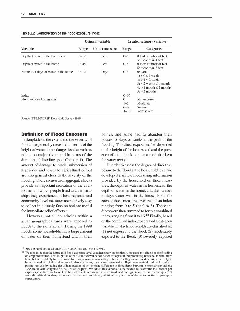
Definition of Flood ExposureIn Bangladesh, the extent and the severity offloods are generally measured in terms of theheight of water above danger level at variouspoints on major rivers and in terms of theduration of flooding (see Chapter 1). Theamount of damage to roads, submersion ofhighways, and losses to agricultural outputare also general clues to the severity of theflooding. These measures of aggregate shocksprovide an important indication of the envi-ronment in which people lived and the hard-ships they experienced. These regional andcommunity-level measures are relatively easyto collect in a timely fashion and are usefulfor immediate relief efforts.9
However, not all households within agiven geographical area were exposed tofloods to the same extent. During the 1998floods, some households had a large amountof water on their homestead and in their
homes, and some had to abandon theirhouses for days or weeks at the peak of theflooding. This direct exposure often dependedon the height of the homestead and the pres-ence of an embankment or a road that keptthe water away.
In order to assess the degree of direct ex-posure to the flood at the household level wedeveloped a simple index using informationprovided by the household on three meas-ures: the depth of water in the homestead, thedepth of water in the home, and the numberof days water was in the house. First, foreach of those measures, we created an indexranging from 0 to 5 (or 0 to 6). These in-dices were then summed to form a combinedindex, ranging from 0 to 16.10 Finally, basedon the combined index, we created a categoryvariable in which households are classified as:(1) not exposed to the flood, (2) moderatelyexposed to the flood, (3) severely exposed
12 CHAPTER 2
9 See the rapid appraisal analysis by del Ninno and Roy (1999a).10 We recognize that the household flood exposure level used here may incompletely measure the effects of the flooding
on crop production. This might be of particular relevance for better-off agricultural producing households with moreland, but is less likely to be an issue for comparisons across villages, because village-level flood exposure is likely tobe associated with field and household damage. In any case, we constructed a village-level agricultural field flood ex-posure variable by taking the village median of the average difference in flood depth between a normal year and the1998 flood year, weighted by the size of the plots. We added this variable to the models to determine the level of percapita expenditure; we found that the coefficients of this variable are small and not significant, that is, the village-levelagricultural field flood exposure variable does not provide any additional explanation of the determination of per capitaexpenditure.
Table 2.2 Construction of the flood exposure index
Original variable Created category variable
Variable Range Unit of measure Range Categories
Depth of water in the homestead 0–12 Feet 0–5 0 to 4: number of feet5: more than 4 feet
Depth of water in the home 0–45 Feet 0–6 0 to 5: number of feet6: more than 5 feet
Number of days of water in the home 0–120 Days 0–5 0: None1: > 0 ≤ 1 week2: > 1 ≤ 2 weeks3: > 2 weeks ≤ 1 month4: > 1 month ≤ 2 months5: > 2 months
Index 0–16Flood-exposed categories 0 Not exposed
1–5 Moderate6–10 Severe
11–16 Very severe
Source: IFPRI-FMRSP, Household Survey 1998.

to the flood, or (4) very severely exposed tothe flood. A summary of the variables usedis reported in Table 2.2. Frequency distri-butions of these variables and of the threesingle indices and the combined index arepresented in Appendix A.
In addition to this measure of house-hold flood exposure we calculated a vil-lage-level variable of flood exposure. Thisvariable, calculated as the village-level me-dian of individual household flood expo-sure, is used mainly in the econometricanalysis to take into account village-levelunobservable characteristics related to the
flood, that is, the effects of village-levelflood exposure.
The resulting frequency distribution ofhousehold-level flood exposure by thana isreported in Figure 2.4 and Table 2.3. Theseshow wide differences across householdswithin thanas in the severity of flood expo-sure as well as large variations across thanas.All together about 50 percent of householdswere exposed severely or very severely tothe flood, while 29 percent were not exposeddirectly to the flood.
Three thanas in the sample were partic-ularly severely affected: Madaripur, Muladi,
DATA AND METHODS 13
Figure 2.4 Severity of flood exposure and percentage of households in the bottom 40th percentileof per capita expenditure by thana
Table 2.3 Household per capita expenditure by thana and severity of household flood exposure
Flood exposurePer capita Bottom 40th
expenditure percentile Not exposed Moderate Severe Very severe AllThana District (Tk/month) (%) (%) (%) (%) (%) (%) Number
Madaripur Madaripur 819.6 38.9 0.0 5.6 31.5 63.0 100 108Muladi Barisal 633.6 56.5 1.9 32.4 50.0 15.7 100 108Shahrasti Chandpur 809.2 38.0 4.6 13.9 43.5 38.0 100 108Derai Sunamganj 716.7 47.2 29.6 38.0 18.5 13.9 100 108Saturia Manikganj 758.4 35.8 51.4 34.9 8.3 5.5 100 109Shibpur Narsingdi 807.2 26.9 52.8 10.2 22.2 14.8 100 108Mohammadpur Magura 769.5 37.0 60.2 17.6 17.6 4.6 100 108Total 759.1 40.0 28.7 21.8 27.3 22.2 100 757
Source: IFPRI-FMRSP, Household Survey 1998.
Source: IFPRI-FMRSP, Household Survey 1998.

and Shahrasti, where 95 percent, 66 percent,and 82 percent of households, respectively,were exposed severely and very severely tothe flood. The relative severity of flood ex-posure across thanas, unions, and villagesas measured here corresponds with the find-ings and observations made at the time of thehousehold survey, as well as with the resultsof a village-level rapid appraisal (del Ninnoand Roy 1999a).
Flood Exposure and PovertyBefore we begin the analysis of the impactof the floods it is important to establishwhether the relatively poor areas covered bythe survey were exposed to the floods morethan richer areas. It is also important to es-tablish whether relatively poor householdswere exposed more than richer households.This is important because in our analysis wedo not want to confound the impact of thefloods with the effects of initial endowmentsand level of income. In other words, we wantto make sure that flood exposure was a trueexogenous shock for each of the households,independently of their initial economic status.
Even though some villages, some unions,and some thanas were exposed more thanothers to the floods, those areas do not appearto be poorer than the other areas. Looking atthe average per capita expenditure by thana,reported in Table 2.3, and the percentages ofhouseholds below the 40th percentile of totalper capita expenditure reported in Figure 2.4,we cannot detect any association betweenflood exposure and poverty at thana level.However, since we are observing per capitaexpenditures after the floods, the possibility
remains that these observed per capita ex-penditures were affected by the floods in thepreceding months.
The best way to assess if poor house-holds were exposed more than richer house-holds would be to directly compare theirexpenditures before and after the floods.Unfortunately, complete data on per capitaexpenditures before the floods were not col-lected because this would have involved arecall period of five or more months.11 Somevariables that can indicate households’ long-term wealth and the level of asset ownershipbefore the floods are available, however.
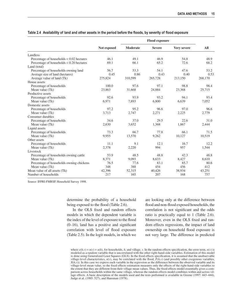
Table 2.4 shows the level of pre-floodownership of several types of assets by levelof exposure to the floods.12 Though, in gen-eral, the total value of assets owned did notvary by flood exposure, the percentage ofhouseholds severely exposed to the flood washigher for those with little (less than 0.20hectares) or no land (less than 0.02 hectares).
To check the hypothesis that there is acorrelation between level of household floodexposure and household endowment (includ-ing land), we ran several regression modelsin which flood exposure is a function of long-term wealth, assumed to be determined byhousehold composition, education, and pre-flood value of assets. The first two equationsare Ordinary Least Squares (OLS) regres-sions, in which we control for a possiblecorrelation between unobservable charac-teristics at the village level and the otherspecified independent variables using bothrandom effects and fixed effects models(Table 2.5).13 We also used the same ex-planatory variables in logit regressions to
14 CHAPTER 2
11 The survey was undertaken in November and December 1998, five months after the flood began in some parts of thecountry in July 1998.
12 Pre-flood asset values were calculated using the value of assets that households would have owned if the floods hadnot occurred. In particular we used two sources of information:
1. The value of the assets owned in November–December 1998 and the percentage of the value lost owing to the floods.This is a valid method for large assets that were not sold or consumed in the period of the floods.
2. The number and value of assets lost, sold, and consumed since July 15, 1998—at the beginning of the flood. Thismeasure is better for smaller assets that might have been sold as a coping strategy by the household to deal with theconsequences of the floods.
13 Random and fixed effects models are common ways to address the role of unobservable heterogeneity in subgroups ofthe data (in this instance, unobservable factors that are common within villages in the sample). Writing the estimatedequation in simplified form, we have:
Y(h,v) = a + bX(h,v) + cF(h,v) + e(h,v)
determine the probability of a householdbeing exposed to the flood (Table 2.6).
In the OLS fixed and random effectsmodels in which the dependent variable isthe index of the level of exposure to the flood(0–16), land has a positive and significantcorrelation with level of flood exposure(Table 2.5). In the logit models, in which we
are looking only at the difference betweenflood and non-flood exposed households, thecorrelation is not significant and the oddsratio is practically equal to 1 (Table 2.6).Moreover, even in the OLS fixed and ran-dom effects regressions, the impact of landownership on household flood exposure isnot very large. The difference in predicted
DATA AND METHODS 15
Table 2.4 Availability of land and other assets in the period before the floods, by severity of flood exposure
Flood exposure
Not exposed Moderate Severe Very severe All
LandlessPercentage of households < 0.02 hectares 46.1 49.1 46.9 54.8 48.9Percentage of households < 0.20 hectares 69.1 66.1 65.2 72.6 68.2
Land (total)Percentage of households owning land 56.7 53.3 54.1 47.6 53.2Average size of land (hectares) 0.45 0.86 0.43 0.40 0.53Average value of land (Tk) 275,824 310,599 265,728 213,150 268,170
House assetsPercentage of households 100.0 97.6 97.1 98.8 98.4Mean value (Tk) 23,863 31,668 24,884 23,368 25,715
Productive assetsPercentage of households 92.6 93.9 93.2 94.1 93.4Mean value (Tk) 6,971 7,893 6,800 6,639 7,052
Domestic assetsPercentage of households 97.2 95.2 96.6 97.0 96.6Mean value (Tk) 3,713 2,747 2,271 2,225 2,779
Consumer durablesPercentage of households 34.6 37.0 29.5 22.6 31.0Mean value (Tk) 2,630 3,652 1,368 1,867 2,444
Liquid assetsPercentage of households 73.3 66.7 77.8 66.1 71.5Mean value (Tk) 9,955 13,570 9,262 10,127 10,519
Other assetsPercentage of households 11.1 9.1 12.1 16.7 12.2Mean value (Tk) 2,378 2,220 994 957 1,544
LivestockPercentage of households owning cattle 53.9 48.5 48.8 42.3 48.8Mean value (Tk) 8,371 9,093 8,633 8,427 8,610Percentage of households owning chickens 76.5 77.6 83.1 85.7 80.6Mean value (Tk) 348 388 454 456 412
Mean value of all assets (Tk) 42,396 52,315 40,426 38,934 43,251Number of households 217 165 207 168 757
Source: IFPRI-FMRSP, Household Survey 1998.
where e(h,v) = n(v) + u(h), for households, h, and village, v. In the random effects specification, the error term, n(v) ismodeled as a random variable that is uncorrelated with the other right-hand-side variables. Estimation of this modelis done using Generalized Least Squares (GLS). In the fixed effects specification, it is assumed that the unobservablevillage-level characteristics, n(v), may be correlated with the flood, F(h,v) (and possibly other exogenous variables,X(h,v)). In this case we express each variable in the regression as the difference between the observed variable and itsvillage-level mean value, so the fixed effects estimation measures only the effects of the right-hand-side variables tothe extent that they are different from their village mean values. Thus, the fixed effects model essentially gives a com-parison across households within the same village, whereas the random effects model combines within and across vil-lage effects. A basic description of the models used and the tests performed is available in Greene (1997: 443–444),Judge et al. (1985: 527), and Hausman (1978).

flood exposure between a household with noland assets and a household with the largestland assets is only 3 points on the 0–16 scale.In the context of rural Bangladesh this resultcan be explained by the fact that householdsthat have more land have the possibility ofbuilding their house on slightly higher groundthan households without any land. This doesnot mean that they were not exposed to theflood, just that they were not as severely ex-posed as households with less land.
The main conclusion from the regres-sion results in Tables 2.5 and 2.6, however,is that pre-flood determinants of wealth do
not explain variations in flood exposureacross households in the sample. Based onthese results, we use the flood exposure vari-able in the following analysis as an inde-pendent variable to explain the impact of thefloods on a series of individual- and house-hold-level outcomes, such as the level ofcaloric consumption, food security, and otherhealth and nutrition outcomes.
In most of our analysis, we use the OLSfixed and random effects models to examinethe impact of the floods on individual- andhousehold-level outcomes. These modelscapture the impact of the level of flood ex-
16 CHAPTER 2
Table 2.5 Determinants of household flood exposure: Regression results (dependent variable:flood index 0–16)
OLS with village OLS with villagerandom effect fixed effect
Description Coefficient t-statistic Coefficient t-statistic
Female-headed household −0.0916 −0.15 0.0292 0.05Age of household head 0.0104 0.73 0.0108 0.76Proportion males: 0–4 years 0.0043 0.26 0.0064 0.39Proportion males: 5–14 years 0.0255 1.63 0.0286 1.83*Proportion males: 15–19 years 0.0072 0.39 0.0085 0.46Proportion males: 20–34 years 0.0014 0.09 0.0058 0.35Proportion males: 35–54 years 0.0231 1.51 0.0260 1.71*Proportion females: 0–4 years 0.0073 0.46 0.0042 0.27Proportion females: 5–14 years 0.0113 0.79 0.0113 0.79Proportion females:15–19 years −0.0027 −0.15 −0.0019 −0.11Proportion females: 20–34 years −0.0128 −0.86 −0.0124 −0.84Proportion females: 35–54 years −0.0200 −1.42 −0.0167 −1.19Household size −0.0621 −0.34 −0.1182 −0.65Number of males: Any primary education −0.1705 −1.14 −0.1797 −1.20Number of males: Any secondary education 0.0498 0.22 0.0210 0.09Number of females: No education 0.0022 0.01 0.0661 0.20Number of females: Any primary education −0.0978 −0.29 −0.0965 −0.29Number of females: Any secondary education 0.3136 0.78 0.3645 0.91Pre-flood value of land (Tk thousands) −0.0120 −2.15* −0.0136 −2.43*Productive asset value (Tk thousands) 0.1119 0.92 0.1103 0.91Liquid asset value (Tk thousands) −0.0139 −0.41 −0.0234 −0.69Housing asset value (Tk thousands) 0.0010 0.03 0.0002 0.01Domestic asset value (Tk thousands) 0.0553 0.13 0.4924 1.17Other assets value (Tk thousands) −1.4218 −1.36 −1.3406 −1.28Credit before1998 (dummy variable) −0.1989 −0.49 −0.0748 −0.18Constant 5.4998 4.30* 5.2820 4.27*
Number of observations 753 753Number of villages 117 117R2 .02 .01Random effects versus fixed effects (p-value)** .01
Source: IFPRI-FMRSP, Household Survey 1998 and authors’ calculations.
* denotes that the coefficient is statistically significant at the 10% level or less. ** values for random versus fixed effects arethe result of the Hausman test.

posure at the household level, taking intoaccount unobservable village characteristics.In some cases, we also use the village floodexposure variable, capturing the direct andindirect effects of the floods common to allhouseholds within a village.
Determinants of Current Per Capita ExpenditureThe above discussion argues that householdexposure to floods can be treated as an ex-ogenous variable in our analysis, since pre-flood household and village characteristicsdo not explain the variation in flood exposure
across households. Thus, in discussing theresults of the survey in subsequent chaptersof this report, we will present tables com-paring various outcomes of interest acrosshouseholds with various levels of flood ex-posure. Likewise, the regression analyseswill treat both household-level and village-level flood exposure variables as exogenousvariables.
In addition, we will compare various out-comes across per capita expenditure quin-tiles because of the policy relevance of thelevel of household incomes (expenditures).We now show that, although per capita ex-
DATA AND METHODS 17
Table 2.6 Determinants of household flood exposure: Regression results (dependent variable:household flood exposure (0 or 1))
Logit with village Logit with villagerandom effect fixed effect
Description Odds ratio z-statistic Odds ratio z-statistic
Female-headed household 1.19 0.25 1.86 0.81Age of household head 0.95 −2.64* 0.96 −2.05*Proportion males: 0–4 years 0.97 −1.14 0.97 −1.20Proportion males: 5–14 years 0.99 −0.32 1.00 −0.14Proportion males: 15–19 years 1.00 −0.19 1.00 0.00Proportion males: 20–34 years 0.99 −0.64 0.99 −0.35Proportion males: 35–54 years 1.03 1.56 1.04 1.65*Proportion females: 0–4 years 0.98 −1.08 0.99 −0.64Proportion females: 5–14years 0.97 −1.90 0.97 −1.42Proportion females:15–19 years 0.96 −1.83* 0.98 −1.03Proportion females: 20–34 years 0.95 −2.93* 0.96 −2.00*Proportion females: 35–54 years 0.95 −2.92* 0.96 −2.08*Household size 1.09 0.34 1.11 0.43Number of males: Any primary education 0.71 −1.64* 0.64 −1.92*Number of males: Any secondary education 1.48 1.23 1.40 1.02Number of females: No education 1.35 0.69 1.17 0.38Number of females: Any primary education 1.11 0.23 0.97 −0.06Number of females: Any secondary education 3.67 2.15* 2.93 1.74*Pre-flood value of land (Tk thousands) 0.99 −1.72* 0.99 −1.18Productive asset value (Tk thousands) 0.90 −0.57 0.76 −1.11Liquid asset value (Tk thousands) 0.98 −0.29 0.83 −0.88Housing asset value (Tk thousands) 1.06 1.04 1.04 0.68Domestic asset value (Tk thousands) 0.67 −0.77 0.96 −0.07Other assets value (Tk thousands) 0.07 −1.84* 0.02 −1.49Credit before1998 (dummy variable) 1.41 0.69 1.52 0.81
Number of observations 753 286Number of villages 117 40χ2 36.8 37.4Prob χ2 0.06 0.05
Source: IFPRI-FMRSP, Household Survey 1998 and authors’ calculations.
* denotes that the coefficient is statistically significant at the 10% level or less.

penditures are endogenous,14 they are notdetermined by either the household or thevillage level of exposure to the floods.
To test the relationship between currentper capita expenditure and long-term wealth
status and the level of exposure, we used amodel in which we explain the level ofcurrent per capita expenditure as a functionof household characteristics (gender, age ofhousehold head, proportion of household
18 CHAPTER 2
Table 2.7 Determinants of per capita household expenditure: Regression results
Household-level flood expenditure
Village-level With village With villageflood exposure random effect fixed effect
Description Coefficient t-statistic Coefficient t-statistic Coefficient t-statistic
Female-headed household −0.3679 −4.76* −0.3752 −4.45* −0.3933 −4.38*Age of household head −0.0027 −1.42 −0.0023 −1.20 −0.0012 −0.59Proportion males: 0–4 years −0.0059 −1.48 −0.0057 −2.46* −0.0052 −2.15*Proportion males: 5–14 years −0.0044 −1.78* −0.0048 −2.22* −0.0055 −2.40*Proportion males: 15–19 years 0.0008 0.27 0.0010 0.39 0.0015 0.55Proportion males: 20–34 years 0.0025 1.01 0.0025 1.10 0.0025 1.03Proportion males: 35–54 years 0.0017 0.83 0.0016 0.77 0.0013 0.56Proportion females: 0–4 years −0.0045 −2.30* −0.0044 −2.06* −0.0044 −1.92*Proportion females: 5–14 years −0.0062 −3.38* −0.0058 −3.00* −0.0047 −2.27*Proportion females:15–19 years −0.0027 −1.14 −0.0025 −1.00 −0.0019 −0.70Proportion females: 20–34 years 0.0004 0.23 0.0008 0.37 0.0014 0.65Proportion females: 35–54 years 0.0021 1.14 0.0020 1.02 0.0015 0.71Household size −0.0553 −1.49 −0.0561 −2.18* −0.0613 −2.21*Number of males: Any primary education 0.0042 0.23 0.0067 0.33 0.0129 0.58Number of males: Any secondary education 0.0366 1.16 0.0374 1.19 0.0431 1.28Number of females: No education −0.0263 −0.48 −0.0313 −0.70 −0.0422 −0.89Number of females: Any primary education 0.0378 0.63 0.0350 0.75 0.0257 0.52Number of females: Any secondary education 0.1245 1.81* 0.1287 2.28* 0.1390 2.35*Pre-flood value of land (Tk thousands) 0.0013 1.44 0.0013 1.74* 0.0012 1.48Productive asset value (Tk thousands) 0.0442 2.37* 0.0447 2.69* 0.0467 2.60*Liquid asset value (Tk thousands) −0.0006 −0.13 0.0004 0.08 0.0017 0.35Housing asset value (Tk thousands) 0.0211 4.39* 0.0201 3.87* 0.0184 3.30*Domestic asset value (Tk thousands) 0.0507 1.04 0.0538 1.01 0.0704 1.15Other assets value (Tk thousands) 0.3972 4.24* 0.4162 2.91* 0.4630 3.04*Credit before1998 (dummy variable) 0.0765 1.33 0.0638 1.17 0.0284 0.48Number of dependent workers −0.0142 −0.49 −0.0102 −0.34 −0.0008 −0.02Number of day laborers −0.0633 −1.99* −0.0661 −2.25* −0.0761 −2.39*Persons engaged in business 0.0116 0.34 0.0120 0.36 0.0154 0.42Persons in own farm 0.0820 2.88* 0.0838 2.86* 0.0841 2.60*Having electricity supply 0.1353 3.26* 0.1432 2.94* 0.1677 3.02*Moderately flood exposed 0.0076 0.14 0.0031 0.07 0.0103 0.17Severely flood exposed 0.0180 0.39 0.0121 0.27 0.0400 0.61Very severely flood exposed 0.0801 1.65* 0.0414 0.88 0.0394 0.55Constant 6.8980 41.69* 6.8944 39.52* 6.8664 36.58*
Number of observations 757 757 757Number of villages 117 117 117R2 .37 .37 .36Random effects versus fixed effects (p-value)** .33
Source: IFPRI-FMRSP, Household Survey 1998 and authors’ calculations.
Note: The dependent variable is the log of per capita expenditure.* denotes that the coefficient is statistically significant at the 10% level or less. ** values for random versus fixed effects are the result of the Hausman test.
14 We treat the issue of endogeneity of per capita expenditures through standard statistical techniques in the regressions,including per capita expenditures as an explanatory variable in subsequent chapters.

members in different age categories, house-hold size, number of members with differenteducational levels, number of people in dif-ferent occupations, and level of pre-floodassets), as well as of the level of exposure tothe floods. The results, presented in Table 2.7,show that flood exposure is not a determi-nant of current per capita expenditure whencontrolling for level of pre-flood assets andother household-level characteristics. Thiswas possible for several reasons. First, despiteflood-exposed households’ lower resources,they were able to maintain at least the samelevel of expenditure, though not the samelevel of consumption because of higher foodprices and additional expenditure neededfor things such as health and fuel. Second, asshown later, households were able to smooththeir expenditure by borrowing and by pur-chasing food on credit. This means that thelevel of current per capita expenditure is agood measure of long-term economic statusand can stand as a proxy of the level ofpoverty. Thus, it can be used to rank house-holds from the poorest in the bottom ex-penditure quintile to the richest in the topquintile. Moreover, because post-flood percapita expenditure indicates both long-termeconomic status and the level of resourcesavailable at the end of the floods, it has rele-vance for targeting flood relief and transfers.
SummaryThe theoretical framework presented in thischapter outlines the pathways by which the1998 floods affected markets, households,and individuals. Particularly important are thepathways emanating from the loss of agri-cultural production, reductions in employ-ment opportunities, and the loss of assets,
which caused major reductions in householdincomes and wealth.
The micro-level data set used in the em-pirical analysis of the impact of the floods onhousehold welfare derives from a householdsurvey in November and December 1998 thatcovered 757 rural households in seven flood-exposed thanas in Bangladesh. At the house-hold level, flood exposure was based on thedepth of water in the homestead, the depth ofwater in the house, and the number of dayswater was in the house.
Ideally, to examine the impact of thefloods, a panel data set with information onhousehold incomes and expenditures bothbefore and after the floods would be used.However, since pre-flood income and expen-diture data are unavailable, it is important todisentangle the effects of pre-flood wealthand incomes from the impacts of the floods.The regression analysis presented in Tables2.5 and 2.6 indicates that pre-flood determi-nants of wealth do not explain variations inflood exposure across households in the sam-ple. Based on these results, we use the floodexposure variable in the following analysisas an independent variable to explain the im-pact of the floods on a series of individual-and household-level outcomes, such as thelevel of caloric consumption, food security,and other health and nutrition outcomes.
Finally, the regression analysis presentedin Table 2.7 indicates that flood exposure isnot a statistically significant determinant ofpost-flood household expenditures; in otherwords, the floods were a true random shockthat affected households independent of theirlevel of wealth. Thus, we can use the level ofcurrent per capita expenditure as a measureof long-term economic status.
DATA AND METHODS 19

C H A P T E R 3
Foodgrain Markets and Availability
The 1998 floods in Bangladesh were a major threat to national food security inBangladesh, not because of the initial damage to standing crops, but because of po-tential damage to the major monsoon season rice crop and rural incomes. This chap-
ter focuses on the behavior of foodgrain (rice and wheat) availability during and after thefloods. We begin with an overview of the importance of rice and wheat in national food avail-ability in Bangladesh and the roles of the private and public sectors in foodgrain marketing.Turning to the markets and government policy at the time of the floods, we discuss initialfood relief efforts, including the contribution of food aid. We then focus on rice and wheatmarkets following the floods, highlighting the massive private sector imports from India. Wefollow this with an analysis of the contribution of private sector imports to food security atthe national level in Bangladesh, discussing alternative estimates of the volume of trade, thestructure of the market, and alternative sources of supply. The chapter concludes with a com-parison of government policies and market behavior in 1998 with those following earlierlarge production shortfalls owing to floods in 1974 and 1988.
Domestic Foodgrain Production and Markets
Domestic Foodgrain ProductionRice dominates agricultural production and food consumption in Bangladesh, accounting for58.3 percent of value-added in agriculture (9.1 percent of total GDP) and 72.8 percent of calo-ries consumed in 1998.15 Over the 1980s and 1990s, domestic rice production slightly outpacedpopulation growth (2.0 versus 1.9 percent per year), enabling annual per capita rice avail-ability to increase from 137.1 kilograms in the 1980s to 144.2 kilograms in the 1990–99period while annual average rice imports declined from 308,000 tons to 160,000 tons (Table3.1). In contrast, per capita wheat availability has declined despite sharp increases in wheatproduction (from 112,000 tons at Independence in 1971 to 1.91 million tons in 1999), be-cause of lower levels of food aid.
15 Unpublished 1997/98 national accounts data (in current prices) from the Bangladesh Bureau of Statistics (BBS) andFood and Agriculture Organization, Food balance sheet, various issues.

Bangladesh annually produces threecrops of rice: aman, typically transplantedin June–July and harvested in November–December, boro, transplanted in December–January and harvested in May–June, andaus, often directly sown in March–April andharvested in July–August. Depending onthe extent of normal seasonal flooding andwater availability through irrigation duringthe dry winter season, two crops of rice areoften grown on the same plot of land. Wheat,which requires cold nights to produce a crop,can be grown only during the winter seasonin Bangladesh, and is typically sown in No-vember–December and harvested in March–
April.16 This sustained increase in rice avail-ability per capita has enabled a long-termdecline in real rice prices, as demand growth,limited by lower per capita demand by urbanhouseholds, relatively slow rural incomegrowth, and changing tastes, has not kept upwith supply (Dorosh 2000).
Most of the increase in rice productionin the 1980s and 1990s was due to increasesin boro production; aman production stag-nated and aus production fell as boro cultiva-tion replaced aus in many areas (Figure 3.1).Prior to the mid-1980s the boro harvest inBangladesh was relatively small—only 20percent of rice production in 1974. A major
FOODGRAIN MARKETS AND AVAILABILITY 21
Table 3.1 Foodgrain availability and requirements in Bangladesh, 1980/81 to 1999/2000
Per Gov-Per Per capita ern-
capita capita food- mentrice Net wheat grain Food com-
Rice Net Pri- Net avail- Wheat Net Pri- Net food- avail- avail- aid mer-pro- PFDS vate rice ability pro- PFDS vate wheat grain ability ability (total cialduc- distri- im- avail- (kg/ duc- distri- im- avail- avail- (kg/ (kg/ food- im-
Year tion bution ports ability capita) tion bution ports ability ability capita) capita) grain) ports
1980/81 13,880 −327 0 12,165 135.3 1,092 852 0 1,835 14,000 20.4 155.7 751 3251981/82 13,629 482 0 12,748 138.7 967 1,282 0 2,153 14,901 23.4 162.1 1,141 1141982/83 14,215 328 0 13,121 139.7 1,095 1,415 0 2,401 15,522 25.6 165.3 976 8681983/84 14,509 358 0 13,416 139.7 1,211 1,427 0 2,517 15,933 26.2 166.0 1,441 6151984/85 14,623 266 0 13,426 136.9 1,464 1,948 0 3,265 16,692 33.3 170.1 1,306 1,2871985/86 15,038 153 0 13,687 136.5 1,042 1,039 0 1,977 15,664 19.7 156.2 1,087 1131986/87 15,406 358 0 14,223 138.8 1,091 1,574 0 2,555 16,779 24.9 163.7 1,425 3421987/88 15,413 180 0 14,052 134.2 1,048 1,948 0 2,891 16,943 27.6 161.8 1,787 1,1301988/89 15,544 326 0 14,316 134.0 1,021 2,199 0 3,117 17,433 29.2 163.2 1,356 7801989/90 17,856 −243 0 15,827 145.3 890 1,447 0 2,248 18,075 20.6 166.0 949 5841990/91 17,852 244 0 16,311 146.9 1,004 1,345 0 2,248 18,559 20.3 167.2 1,540 371991/92 18,252 −180 0 16,246 143.8 1,065 1,509 0 2,468 18,714 21.8 165.6 1,414 1501992/93 18,341 243 0 16,750 145.7 1,176 597 355 2,010 18,761 17.5 163.1 735 931993/94 18,041 202 74 16,512 141.1 1,131 1,008 238 2,338 18,851 20.0 161.1 654 01994/95 16,833 83 583 15,816 132.9 1,245 1,213 430 3,347 19,162 28.1 161.0 935 6201995/96 17,687 240 650 16,808 138.9 1,369 1,133 200 3,215 20,023 26.6 165.5 738 8391996/97 18,883 226 15 17,236 140.1 1,454 550 222 2,096 19,331 17.0 157.2 618 1121997/98 18,854 130 993 18,106 144.8 1,803 875 142 2,640 20,745 21.1 166.0 549 2531998/99 19,905 35 2,661 20,610 162.3 1,908 1,346 804 3,867 24,477 30.5 192.7 1,233 7631999/2000 22,840 120 390 21,066 163.3 1,700 845 745 3,120 24,186 24.2 187.5 895 0Av. 1980/81
–1988/89 14,695 236 0 13,462 137.1 1,115 1,520 0 2,524 15,985 25.6 162.7 1,252 619Av. 1989/90
–1998/99 18,250 98 498 17,022 144.2 1,305 1,102 239 2,648 19,670 22.4 166.5 937 345
Sources: Bangladesh Bureau of Statistics, Marketing Information System (MIS), Directorate General of Food, and authors’ calculations.
Notes: The unit of measure is thousand metric tons unless otherwise noted. Before 1985/86, per capita requirements were calculated at 15.5 oz/day. Before1991/92, private imports of foodgrains were not allowed. The data for 1999/2000 are projected. PFDS = Public food distribution system.
16 See Dorosh (2000) and Zohir (1995) for further discussion of cropping patterns.
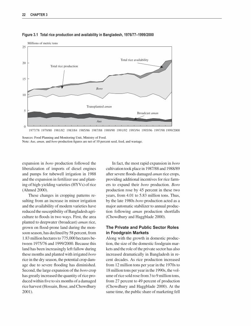
expansion in boro production followed theliberalization of imports of diesel enginesand pumps for tubewell irrigation in 1988and the expansion in fertilizer use and plant-ing of high-yielding varieties (HYVs) of rice(Ahmed 2000).
These changes in cropping patterns re-sulting from an increase in minor irrigationand the availability of modern varieties havereduced the susceptibility of Bangladesh agri-culture to floods in two ways. First, the areaplanted to deepwater (broadcast) aman rice,grown on flood-prone land during the mon-soon season, has declined by 58 percent, from1.83 million hectares to 775,000 hectares be-tween 1975/76 and 1999/2000. Because thisland has been increasingly left fallow duringthese months and planted with irrigated bororice in the dry season, the potential crop dam-age due to severe flooding has diminished.Second, the large expansion of the boro crophas greatly increased the quantity of rice pro-duced within five to six months of a damagedrice harvest (Hossain, Bose, and Chowdhury2001).
In fact, the most rapid expansion in borocultivation took place in 1987/88 and 1988/89after severe floods damaged aman rice crops,providing additional incentives for rice farm-ers to expand their boro production. Boroproduction rose by 45 percent in these twoyears, from 4.01 to 5.83 million tons. Thus,by the late 1980s boro production acted as amajor automatic stabilizer to annual produc-tion following aman production shortfalls(Chowdhury and Haggblade 2000).
The Private and Public Sector Rolesin Foodgrain MarketsAlong with the growth in domestic produc-tion, the size of the domestic foodgrain mar-kets and the role of the private sector has alsoincreased dramatically in Bangladesh in re-cent decades. As rice production increasedfrom 12 million tons per year in the 1970s to18 million tons per year in the 1990s, the vol-ume of rice sold rose from 3 to 9 million tons,from 27 percent to 49 percent of production(Chowdhury and Haggblade 2000). At thesame time, the public share of marketing fell
22 CHAPTER 3
Figure 3.1 Total rice production and availability in Bangladesh, 1976/77–1999/2000
Sources: Food Planning and Monitoring Unit, Ministry of Food.Note: Aus, aman, and boro production figures are net of 10 percent seed, feed, and wastage.

by half, from 15 percent to 7 percent. More-over, the number of marketing agents ex-panded dramatically as well. In the 1960s,there were only about 4,000 itinerant tradersin the former East Pakistan, compared with48,000 in Bangladesh in the 1990s. Similarly,the number of millers doubled from 6,155 inthe 1960s to 11,592 in the 1970s, then in-creased more than fourfold by the 1990s tonearly 51,000.
The large expansion in the number of par-ticipants, the size of the market, investmentsin infrastructure (roads, bridges, electricity,and telecommunications), and a gradual eas-ing of restrictions on private sector trade(including the lifting of a ban on commercialbank credit for foodgrain trade) have re-sulted in a well-functioning private market.Das, Zohir, and Baulch (1997) have shownthat wholesale markets for both rice and wheatare spatially integrated, with over 80 percentof price changes transmitted between pairsof markets within two weeks.17
Though its size relative to the privatemarket has diminished, public sector food-grain distribution in Bangladesh plays an im-portant role in the domestic procurement ofrice and wheat, the management of food aidinflows, public sector targeted distribution,and the maintenance of emergency foodgrainstocks. Foodgrain is typically procured atfixed prices. Most government procurementis done through fixed-price purchases of graindirectly from farmers or traders.18
Until Bangladesh instituted major re-forms in the early 1990s, subsidized sales of grain through ration channels dominatedfoodgrain distribution. Between 1988/89 and1990/91, on average 612,000 tons of rice andwheat were sold through the Rural Rationingand the urban Statutory Rationing channels,or 26.7 percent of total foodgrain distribu-tion (which averaged 2.294 million tons).Total sales, including open market sales and
other programs, accounted for 63.5 percentof distribution in this period, with relief andFood for Work channels accounting for theother 36.5 percent of distribution. Reformsin 1991/92 and 1992/93 closed the Rural Ra-tioning and Statutory Rationing channels, inan effort to improve the targeting of food-grain distribution as well as to reduce fiscalcosts (Ahmed, Haggblade, and Chowdhury2000). As a result, both the percentage andthe total amount of foodgrain distributedthrough targeted and relief channels increasedin the mid to late 1990s, averaging 1.166 mil-lion tons per year from 1995/96 to 1997/98,or 72.8 percent of the 1.603 million tons totalannual average distribution during these threeyears.
With the increasing role of the privatesector in foodgrain markets and a reductionin total public sector foodgrain distribution,government stocks were gradually reducedthrough most of the 1990s. From 1988/89to 1990/91, prior to the closing of rationingchannels, total stocks averaged 1.131 mil-lion tons (566,000 tons of rice and 565,000tons of wheat). From 1995/96 to 1997/98,stocks were on average only 870,000 tons(425,000 tons of rice and 445,000 tons ofwheat), a decline of 261,000 tons. At the startof July 1998, just before the floods, stockswere 630,000 tons, and rose to 711,000 tonsat the start of August as boro procurementcontinued.
Food Aid and PublicFoodgrain DistributionIn late August 1998, it became clear that thefloods would likely lead to a very large short-fall in rice production. The floods had al-ready caused substantial damage to existingcrops, road infrastructure, and other assets.Damage to the aus rice crop, harvested inJuly and August, led to losses of 300,000 tons(16.0 percent of the initial target production,
FOODGRAIN MARKETS AND AVAILABILITY 23
17 Das, Zohir, and Baulch (1998) used data from 1988 through 1996. Goletti (1994: 27–38) also presents evidence of “amoderate degree of market integration” in rice markets using data from 1989/90 to 1991/92.
18 Local tenders have also been used in recent years, particularly when fixed-price procurement has failed to meet gov-ernment targets.
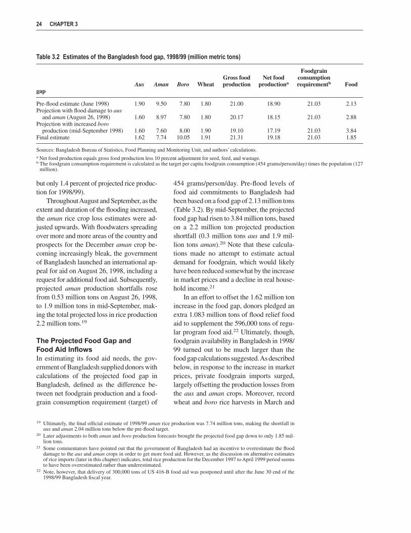
but only 1.4 percent of projected rice produc-tion for 1998/99).
Throughout August and September, as theextent and duration of the flooding increased,the aman rice crop loss estimates were ad-justed upwards. With floodwaters spreadingover more and more areas of the country andprospects for the December aman crop be-coming increasingly bleak, the governmentof Bangladesh launched an international ap-peal for aid on August 26, 1998, including arequest for additional food aid. Subsequently,projected aman production shortfalls rosefrom 0.53 million tons on August 26, 1998,to 1.9 million tons in mid-September, mak-ing the total projected loss in rice production2.2 million tons.19
The Projected Food Gap and Food Aid InflowsIn estimating its food aid needs, the gov-ernment of Bangladesh supplied donors withcalculations of the projected food gap inBangladesh, defined as the difference be-tween net foodgrain production and a food-grain consumption requirement (target) of
454 grams/person/day. Pre-flood levels offood aid commitments to Bangladesh hadbeen based on a food gap of 2.13 million tons(Table 3.2). By mid-September, the projectedfood gap had risen to 3.84 million tons, basedon a 2.2 million ton projected productionshortfall (0.3 million tons aus and 1.9 mil-lion tons aman).20 Note that these calcula-tions made no attempt to estimate actualdemand for foodgrain, which would likelyhave been reduced somewhat by the increasein market prices and a decline in real house-hold income.21
In an effort to offset the 1.62 million tonincrease in the food gap, donors pledged anextra 1.083 million tons of flood relief foodaid to supplement the 596,000 tons of regu-lar program food aid.22 Ultimately, though,foodgrain availability in Bangladesh in 1998/99 turned out to be much larger than thefood gap calculations suggested. As describedbelow, in response to the increase in marketprices, private foodgrain imports surged,largely offsetting the production losses fromthe aus and aman crops. Moreover, recordwheat and boro rice harvests in March and
24 CHAPTER 3
19 Ultimately, the final official estimate of 1998/99 aman rice production was 7.74 million tons, making the shortfall inaus and aman 2.04 million tons below the pre-flood target.
20 Later adjustments to both aman and boro production forecasts brought the projected food gap down to only 1.85 mil-lion tons.
21 Some commentators have pointed out that the government of Bangladesh had an incentive to overestimate the flooddamage to the aus and aman crops in order to get more food aid. However, as the discussion on alternative estimatesof rice imports (later in this chapter) indicates, total rice production for the December 1997 to April 1999 period seemsto have been overestimated rather than underestimated.
22 Note, however, that delivery of 300,000 tons of US 416-B food aid was postponed until after the June 30 end of the1998/99 Bangladesh fiscal year.
Table 3.2 Estimates of the Bangladesh food gap, 1998/99 (million metric tons)
FoodgrainGross food Net food consumption
Aus Aman Boro Wheat production productiona requirementb Foodgap
Pre-flood estimate (June 1998) 1.90 9.50 7.80 1.80 21.00 18.90 21.03 2.13Projection with flood damage to aus
and aman (August 26, 1998) 1.60 8.97 7.80 1.80 20.17 18.15 21.03 2.88Projection with increased boro
production (mid-September 1998) 1.60 7.60 8.00 1.90 19.10 17.19 21.03 3.84Final estimate 1.62 7.74 10.05 1.91 21.31 19.18 21.03 1.85
Sources: Bangladesh Bureau of Statistics, Food Planning and Monitoring Unit, and authors’ calculations.a Net food production equals gross food production less 10 percent adjustment for seed, feed, and wastage.b The foodgrain consumption requirement is calculated as the target per capita foodgrain consumption (454 grams/person/day) times the population (127
million).

May/June 1999, respectively, boosted pro-duction for the fiscal year. Foodgrain fromthe wheat and boro harvests, however, wasof course not yet available for householdsto consume in the six months immediatelyfollowing the floods.
The government of Bangladesh re-sponded to the crisis by supplying food forimmediate relief efforts during the floodsand by helping to coordinate food aid com-mitments and deliveries. At the same time,as part of its price stabilization strategy, thegovernment encouraged private sector im-ports, a policy that helped avoid a food supplyshortage following the floods.
Government Foodgrain DistributionMajor flood relief efforts began in August1998 through the provision of 20,400 tons ofrice through Gratuitous Relief (GR) in flood-affected thanas and an additional 30,800 tonsof rice in September. In addition, the Vulner-able Group Feeding (VGF) program beganon a large scale in August with an initial dis-tribution of 1.3 million cards, which entitledthe holder to 8 kilograms of rice per month.During August and September, 27,500 tonsof rice were distributed through this pro-gram. At 8 kilograms per card, an estimated1.35 million households received VGF ra-tions in August and 2.13 million householdsin September. Almost no wheat was distrib-uted through relief channels in the earlymonths of the floods.
In late September, the World Food Pro-gramme (WFP) strongly urged the govern-ment of Bangladesh to expand the VGFprogram to 4 million cards (households) withan allotment of 32 kilograms of wheat percard. The WFP urged that this expansion takeeffect for both September and October, butthe 141,680 tons of wheat needed for twomonths’distribution would have had to comealmost exclusively from government stocks
because little food aid had arrived.23 Recog-nizing the urgent need for more relief topoor, flood-affected households, the govern-ment of Bangladesh agreed to the expansionin the number of VGF cards to 4 million.However, given that delays in food aid ar-rivals were likely, the allotment was reducedto 8 kilograms of rice and 8 kilograms ofwheat per card for October only, postponinga decision on the November distributionuntil more definite information on food aidarrivals was available.
Initial estimates of foodgrain availabilitygreatly overestimated the arrivals of food-grain because of unforeseen delays in ship-ments and unloading. By the end of October,only 52,000 tons of food aid had actually ar-rived, 71,000 tons less than assumed by theWFP in its late-September analysis. DuringNovember, only an additional 25,000 tons offood aid wheat arrived and were availablefor distribution, so that, by the end of No-vember, cumulative food aid arrivals wereonly 77,000 tons, compared with the WFP-projected 431,000 tons. Fortunately, thegovernment of Bangladesh’s own commer-cial imports of 224,000 tons of wheat arrivedand were unloaded from mid-October to earlyNovember 1998, permitting a continuationof the expanded VGF program in Novemberas well.
The VGF program was again expanded inDecember 1998, to cover 4.2 million house-holds with an increase in the ration size to20 kilograms per card (5 kilograms of riceand 15 kilograms of wheat) for the monthof Ramadan. No distribution of foodgrainsthrough the VGF program took place in Jan-uary, but the program restarted in Februarywith a ration size for February through Aprilof 15 kilograms of wheat and 5 kilograms ofrice per card.
Altogether, planned offtake for 1998/99was increased from 1.718 million tons to
FOODGRAIN MARKETS AND AVAILABILITY 25
23 The government of Bangladesh also explored the possibility of drawing on the food security reserve of the South AsianAssociation for Regional Cooperation (SAARC) or direct purchases from the government of India. However, admin-istrative procedures were found to be very cumbersome and no agreement could be reached on a sales price of grainfor transactions with the government of India, so ultimately no foodgrain came through government-to-governmentchannels.

2.279 million tons. Through December, how-ever, limited government wheat stocks, un-certainties about rice supplies after the amanharvest, and financial constraints limited totaldistribution to 630,000 tons, only 26,000 tonsmore than in the pre-flood government dis-tribution for this period (Figure 3.2). Rice dis-tribution was greater than originally plannedonly in August and September, mainly be-cause of VGF distribution. Thereafter, itwas significantly less than planned, espe-cially in March and April because originallybudgeted open market sales (OMS) did nottake place. The story for wheat is the exactopposite. Actual wheat distribution was belowinitial plans in August and September, andexceeded initial plans every month there-after. To a large extent, additional foodgraindistributed through VGF and other reliefchannels was offset by reductions in previ-ously budgeted OMS rice sales and a post-ponement of planned Food for Education(FFE) disbursements. Later, disbursementsfor Food for Work (FFW) fell behind sched-ule so that total distribution of foodgrainsthrough April 1999 was only 1.578 million
tons, 69 percent of the target for the entirefiscal year.
The VGF program accounted for 29.3percent of the total distribution of foodgrainsfrom July 1998 through April 1999 (that is,up until the 1998 boro rice harvest): 167,000tons of rice and 296,000 tons of wheat. Gra-tuitous Relief accounted for 65,000 tons ofrice and 7,000 tons of wheat, or 4.6 percentof total distribution. Food for Work, whichbegan on a large scale only in January 1999when soil conditions permitted heavy earth-work, accounted for 26.0 percent of distri-bution; Test Relief accounted for another3.2 percent. In all, these four relief channelsaccounted for 63.1 percent of distribution.
For the entire July 1998–June 1999 fiscalyear, Food for Work wheat offtake was690,000 tons, or 32.3 percent of the totalofftake of foodgrains (2.133 million tons).Overall, increases in Food for Work(173,000 tons) and Vulnerable Group Feed-ing (435,000 tons) were the major compo-nents of the 415,000 ton increase in 1998/99food distribution compared with the originalbudget (Table 3.3).
26 CHAPTER 3
Figure 3.2 The government’s budgeted and actual distribution of rice and totalfoodgrains, 1998/99
Source: Food Planning and Monitoring Unit, Ministry of Food.

Rice and Wheat MarketsFollowing the FloodsGovernment rice policy was based on therealization that government imports andfood aid alone would not be sufficient tomake up the projected 1.9 million ton short-fall in foodgrain supplies before the wheatand boro harvests in April–June of 1999.Thus, the government encouraged privatesector imports of rice, a policy that predatedthe floods.
Private Sector Rice ImportsAs shown in Figure 3.3, market prices ofrice had been high in the first half of 1998,even before the floods, because of a poor1997/98 aman rice harvest in November–December 1997. Domestic prices rose swiftlyto import parity levels (equal to the cost ofrice in Indian markets plus transport, han-dling, and a normal profit margin), thusmaking it profitable for the private sector toimport rice from India. Private sector importsof rice had been permitted since 1994,24 butin early 1998 the government of Bangladeshtook deliberate steps to encourage privatesector imports of rice through removal of a
2.5 percent tariff on imports, limitations ongovernment open market rice sales, instruc-tions to expedite clearance of rice importsthrough customs, and a decision not to re-impose anti-hoarding laws. As a result, dur-ing the first five months of 1998, the privatesector imported 894,000 tons of rice fromIndia (according to government of Bangla-desh customs figures), mainly by truck andrail across land borders.
With the onset of the boro rice harvest inMay, the national average wholesale price ofcoarse HYV rice fell from a peak of Tk 14.2per kilogram in April to Tk 12.0 per kilogramin June, and private imports slowed to59,000 tons in June. Soon thereafter, as thefloods began, however, prices again rose toimport parity. By continuing its policy ofencouraging private sector imports, the gov-ernment enabled the private sector to importsubstantial quantities of rice and keep thedomestic market price from rising above im-port parity levels. According to official gov-ernment of Bangladesh estimates, more than200,000 tons of rice per month were im-ported from August 1998 to March 1999,with private rice imports reaching 288,000
FOODGRAIN MARKETS AND AVAILABILITY 27
Table 3.3 Budgeted and actual foodgrain distribution, by channel, 1998/99 (thousand metric tons)
Budget 1998/99 Actual 1998/99
Channel Rice Wheat Total Rice Wheat Total
Priced channelsEssential priorities (EP) 124 85 209 127 85 212Open market sales (OMS) 200 0 200 2 0 2Fair price campaign (FPC) 0 0 0 9 5 14Other priority (OP) 6 6 12 7 5 12Large employee industries (LEI) 0 15 15 0 14 14
Non-priced channelsFood for Work (FFW) 125 400 525 8 690 698Vulnerable Group Development (VGD) 60 120 180 11 193 204Food for Education (FFE) 150 200 350 60 227 287Test Relief (TR) 40 16 56 37 53 90Vulnerable Group Feeding (VGF) 20 10 30 168 297 465Gratuitous Relief (GR) 66 24 90 66 8 74
Others 22 29 51 36 24 60Total 813 905 1,718 530 1,603 2,133
Source: Food Planning and Monitoring Unit, Ministry of Food.
24 Wheat imports were liberalized in 1992/93.

tons in January and 345,000 tons in Febru-ary, 1999.25
Thus, because of the poor 1997/98 amanharvest and the flood-damaged aus and amanharvests in 1998/99, Bangladesh rice prices(wholesale Dhaka) remained close to ex:India import parity prices for most of calen-dar year 1998.26 Wholesale prices after thefloods were in fact remarkably stable. Thenational average wholesale prices of coarserice remained in the range of Tk 14.14–14.83per kilogram from September 1998 throughmid-April 1999.27 With a good boro harvestin April and May, market prices fell by 19percent, from Tk 14.46 per kilogram (amancoarse rice) in the third week of April to Tk
11.74 per kilogram (boro HYV rice) in thesecond week of May, bringing to an end anine-month period of high rice prices andconcerns about post-flood food availability.
Note that the large quantities of privatesector rice imports during 1998 and early1999 were unprecedented in Bangladesh.Prior to 1994, when international trade inrice was liberalized, private sector importswere not permitted. And, for about one anda half years prior to the poor aman harvest in1997/98, rice prices in Bangladesh had beensignificantly below the cost of rice importedfrom India. As a result, there were essentiallyno private sector imports of rice from June1996 to December 1997. The only other pe-
28 CHAPTER 3
Figure 3.3 Rice prices and quantity of private sector rice imports in Bangladesh, 1993–2000
Source: Dorosh 1999a, calculated using data from the Food Planning and Monitoring Unit, Ministry of Food; Market-ing Information System (MIS), Directorate General of Food; CMIE 1998–2000; and Baulch et al. 1998.Notes: Price data for April 2000 are up to the fourth week only; private sector imports are as of April 26, 2000. SinceNovember 1998, the carrying cost has increased by Tk 1.1 per kilogram. Since January 2000, a 5 percent tax has beenimposed on rice imports.
25 The extremely high figures for recorded rice imports in early 1999 may overstate actual rice imports. It is possible thatother commodities were imported using false invoices to avoid import tariffs and other surcharges.
26 In Figure 3.3, a marketing margin of Tk 2.0/kilogram is used to calculate the West Bengal import parity prices shownfor July 1993 to September 1997.
27 Note that Figure 3.3 shows that domestic prices were Tk 0.5–2.0 below ex: Delhi import parity prices from May throughAugust 1998, yet private sector imports continued. The main explanation is that rice exports during this period origi-nated mainly from West Bengal’s rabi (boro) crop, where prices are generally Tk 1.5–2.0/kilogram lower than Delhiprices during this season (as evidenced in the data from 1996 and 1997).
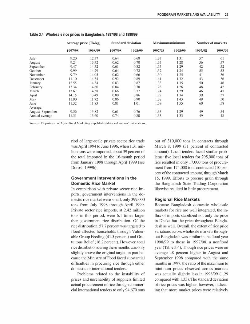
riod of large-scale private sector rice tradewas April 1994 to June 1996, when 1.31 mil-lion tons were imported, about 39 percent ofthe total imported in the 16-month periodfrom January 1998 through April 1999 (seeDorosh 1999b).
Government Interventions in theDomestic Rice MarketIn comparison with private sector rice im-ports, government interventions in the do-mestic rice market were small, only 399,000tons from July 1998 through April 1999.Private sector rice imports, at 2.42 milliontons in this period, were 6.1 times largerthan government rice distribution. Of therice distribution, 57.7 percent was targeted toflood-affected households through Vulner-able Group Feeding (41.5 percent) and Gra-tuitous Relief (16.2 percent). However, totalrice distribution during these months was onlyslightly above the original target, in part be-cause the Ministry of Food faced substantialdifficulties in procuring rice through eitherdomestic or international tenders.
Problems related to the instability ofprices and unreliability of suppliers limitedactual procurement of rice through commer-cial international tenders to only 94,670 tons
out of 310,000 tons in contracts throughMarch 8, 1999 (31 percent of contractedamount). Local tenders faced similar prob-lems: five local tenders for 295,000 tons ofrice resulted in only 17,000 tons of procure-ment from 174,000 tons contracted (10 per-cent of the contracted amount) through March15, 1999. Efforts to procure grain throughthe Bangladesh State Trading Corporationlikewise resulted in little procurement.
Regional Rice MarketsBecause Bangladesh domestic wholesalemarkets for rice are well integrated, the in-flux of imports stabilized not only the pricein Dhaka but the price throughout Bangla-desh as well. Overall, the extent of rice pricevariations across wholesale markets through-out Bangladesh was similar in the flood year1998/99 to those in 1997/98, a nonfloodyear (Table 3.4). Though rice prices were onaverage 48 percent higher in August andSeptember 1998 compared with the samemonths in 1997, the ratio of the maximum tominimum prices observed across marketswas actually slightly less in 1998/99 (1.29compared with 1.33). The standard deviationof rice prices was higher, however, indicat-ing that more market prices were relatively
FOODGRAIN MARKETS AND AVAILABILITY 29
Table 3.4 Wholesale rice prices in Bangladesh, 1997/98 and 1998/99
Average price (Tk/kg) Standard deviation Maximum/minimum Number of markets
1997/98 1998/99 1997/98 1998/99 1997/98 1998/99 1997/98 1998/99
July 9.20 12.37 0.64 0.68 1.37 1.31 57 61August 9.24 13.32 0.62 0.70 1.33 1.28 56 57September 9.47 14.32 0.61 0.82 1.33 1.29 42 52October 9.99 14.29 0.64 0.72 1.32 1.24 55 53November 9.79 14.05 0.62 0.66 1.30 1.25 41 36December 11.10 14.34 0.92 0.89 1.41 1.32 43 36January 12.55 14.34 0.83 0.87 1.33 1.35 50 46February 13.34 14.60 0.84 0.78 1.28 1.26 48 42March 13.67 14.58 0.66 0.77 1.24 1.29 46 47April 14.15 13.49 0.80 0.86 1.27 1.34 39 37May 11.90 11.72 0.86 0.90 1.38 1.43 49 50June 11.32 11.83 0.81 1.01 1.39 1.55 60 58Average:August–September 9.36 13.82 0.61 0.76 1.33 1.29 49 54Annual average 11.31 13.60 0.74 0.80 1.33 1.33 49 48
Sources: Department of Agricultural Marketing unpublished data and authors’ calculations.

far from the mean price in 1998/99 than in1997/98.
Figure 3.4 shows the dispersion ofmonthly average prices across districtswithin the six divisions of Bangladesh inJune, August, and October 1998. Prices rosesharply across all divisions between June andAugust, though the price rise was steepest inRajshahi, Dhaka, and Sylhet. In these majorboro rice-growing divisions, prices weregenerally lower than in the rest of the coun-try at the time of the boro harvest in June, butrose to levels closer to the national average atthe peak of the floods in August. The largestwholesale price variations across districts inAugust and October occurred in Chittagongand Dhaka divisions. Nonetheless, the vari-ations across districts remained relativelysmall—the ratio of the maximum to mini-mum average district price was 1.17 to 1.20 inthese divisions during August and October.
Domestic Wheat MarketsSomewhat surprisingly, the private sectorcontinued to import substantial volumes ofwheat following the floods, even thoughlarge amounts of wheat food aid flowed intoBangladesh and distribution through VGFand Food for Work was expanded. In Janu-ary and February 1999, 90,000 tons of wheatwere imported, raising total wheat importsfrom July 1998 through February 1999 to624,000 tons, 435,000 tons more than inthe same period in 1997/98. As shown in Fig-ure 3.5, domestic wheat prices were slightlybelow calculated import parity prices basedon wheat export prices in the United States(U.S. Hard Red Winter, No. 2, FOB Gulf ofMexico). However, much of the imports inearly 1999 came from other exporters, in-cluding Turkey, Australia, and Central Asiancountries. (The quality and cost of transportdifferences likely account for the deviationbetween calculated import parity and domes-tic prices of wheat.28) Thus, given the largeprivate sector imports, it appears that food
aid inflows did not provide a disincentive fordomestic wheat producers.
Overall, the supply of wheat in Bangla-desh was 3.87 million tons in 1998/99, an in-crease of 46 percent over 1997/98. The largeincrease in apparent wheat consumption maybe explained by several factors: (1) the effectsof high rice prices on wheat consumption (asdetermined by the cross-price elasticity ofdemand for wheat with respect to the riceprice); (2) the adverse income effects of thefloods, which may have induced some house-holds to substitute wheat for rice (given anegative income elasticity of demand forwheat in rural areas); (3) the secular increasein wheat consumption as tastes for wheatchange over time, in part owing to the use ofhigher-protein wheat for milling into flourfor baking; (4) the positive income effects of
30 CHAPTER 3
Figure 3.4 Variations in wholesale rice prices across districts inBangladesh, 1998
Sources: Department of Agricultural Marketing data and authors’ calculations.Notes: This figure shows price variations across districts within each of the six divisionsof Bangladesh. The boxes on this whisker plot denote the range of prices from the 25thpercentile to the 75th percentile the interquartile range (IQR). The median price isshown by the line in the middle of the box. The lines emerging from the box (calledwhiskers) extend to the largest (smallest) data point less (greater) than or equal to the75th (25th) percentile plus (minus) the IQR. J = June, A = August, and O = October.
28 Reportedly, much of the wheat imported by the private sector during the flood was lower-quality “feed” wheat, broughtinto Bangladesh with false papers (personal communication with private sector importers).

wheat transfers to very poor, flood-distressedrural households; and (5) increased use oflower-quality wheat as animal feed.
Private Foodgrain Importsand National Food Security
Alternative Estimates of the Volumeof Rice Imports and AvailabilityThe behavior of market prices in Bangladeshsuggests that rice imports from India were amajor source of supply. The volume of thisrice trade remains somewhat uncertain, how-ever, for two major reasons. First, Bangladeshimport data differ substantially from Indiaexport data. Second, calculations of the totalavailability of rice in Bangladesh are not
consistent with market price movements andestimated rice demand.
Comparisons of Bangladeshi rice importdata and Indian rice export data since theliberalization of the private sector rice tradeby Bangladesh in 1994 indicate a systematicoverstating of rice imports by Bangladeshcompared with exports by India. For example,according to Bangladesh customs data, 3.172million tons of rice were imported fromIndia from April 1998 through March 1999,2.827 million tons (89.1 percent) by the pri-vate sector.29 Indian data on the quantity ofrice exports to Bangladesh30 indicate that in1998/99 exports totaled only 2.215 milliontons, 958,000 tons (30.2 percent) less thanthe Bangladesh customs figures.31
FOODGRAIN MARKETS AND AVAILABILITY 31
Figure 3.5 Wheat prices, quantity of private sector wheat imports, and net public wheatdistribution in Bangladesh, 1993–2000
Sources: Food Planning and Monitoring Unit, Ministry of Food; Department of Agricultural Marketing; Marketing In-formation System (MIS), Directorate General of Food; U.S. Department of Agriculture; and CMIE 1998–2000.Notes: Domestic price data for April 2000 are up to the first week only; private sector imports are as of January 14,2000; and net public food distribution system data are as of March 31, 2000. The import parity price is based on U.S.No. 2 Hard Red Winter and includes import tariffs.
29 The data are presented according to India’s April–March fiscal year in order to permit direct comparison.30 Estimated using the values of basmati and non-basmati rice exports to Bangladesh and the average prices of total In-
dian exports of these two types of rice (Dorosh 2001). Note that non-basmati rice accounted for 99.8 percent of thevalue of rice exports to Bangladesh in 1998/99 (CMIE 1999).
31 Possible explanations for the discrepancies in the data are false customs declarations to avoid import duties on non-rice products, capital flight from Bangladesh, or simply reporting mistakes in one or both countries (Dorosh 2001).Note that smuggling of rice from India is not a likely explanation of the discrepancies since this rice would be unlikelyto enter Bangladesh through official customs channels, and, as shown below, demand calculations indicate that the of-ficial figure for the volume of Bangladesh rice imports appears to be overstated.

Examination of calculated rice availabil-ity and movements in market prices in Bang-ladesh gives another indication of the volumeof rice imports from India in recent years(Table 3.5). In 1996/97, the most recent fis-cal year in which private imports were neg-ligible (only 35,000 tons), net supply—calculated as the sum of net production, netgovernment distribution (offtake less do-mestic procurement), and private imports,assuming no change in private stocks—was17.259 million tons. Using the 1996/97 levelof per capita consumption and the real priceof rice as a base, per capita demand for ricein each period is calculated using the per-centage change in the real price of rice andan assumed own-price elasticity of demand
for rice of −0.15. Then, using the level of pop-ulation in each period, total rice consump-tion is estimated.32 Finally, the differencebetween net supply and the calculated de-mand is reported as the implicit private stockchange.
Thus, for example, real prices of coarserice (national average) in the Decemberthrough April period following the 1996/97aman rice harvest averaged Tk 9.57 per kilo-gram, 0.63 percent higher than the averagereal price for 1996/97. Assuming an own-price elasticity of demand for rice of −0.15,per capita consumption of rice fell by 0.09percent. Total demand for the period is esti-mated at 7.16 million tons, resulting in animplicit private stock change of 1.61 million
32 CHAPTER 3
Table 3.5 Estimated rice demand and implicit private stock change, 1996/97– 1998/99
1996/97 1996/97 1997 1997/98 1998 1998/99Total year aman boro, aus aman boro, aus amanDec.–Nov. Dec.–Apr. May–Nov. Dec.–Apr. May–Nov. Dec.–Apr.
Rice production 18.884 9.550 9.334 8.850 9.595 7.700Aman 9.550 9.550 0.000 8.850 0.000 7.700Boro 7.460 0.000 7.460 0.000 7.979 0.000Aus 1.874 0.000 1.874 0.000 1.616 0.000
Losses, seed, etc. (10 percent) 1.888 0.955 0.933 0.885 0.960 0.770Net production 16.996 8.595 8.401 7.965 8.636 6.930
Domestic procurement (Dec.-Apr.)/(May-Nov.) 0.444 0.201 0.243 0.040 0.322 0.057Offtake from government stocks 0.672 0.365 0.307 0.299 0.365 0.170
Private imports 0.035 0.004 0.031 0.758 1.285 1.472Supply less private stock change 17.259 7.160 10.112 6.999 9.883 7.050
Demand 17.259 7.160 10.112 6.999 9.883 7.050
Implicit private stock changea 0.000 1.603 −1.616 1.983 0.081 1.465Stock change relative to 1996/97b . . . . . . . . . 0.379 1.697 −0.138
Price of rice (Tk/kg) . . . 9.572 9.754 12.982 13.240 14.402Real price (Tk/kg) (1996/97 prices) 9.553 9.572 9.535 12.405 12.367 13.150Per capita demand (kg/period) 70.443 58.686 82.208 56.447 79.063 55.956Change in per capita demand (%) . . . −0.03 0.03 −3.84 −3.80 −4.68
Source: Authors’ calculations.
Notes: The unit of measure is million metric tons unless otherwise noted.a Also includes possible overestimates of production and imports, and underestimates of consumption.b The difference between the implicit stock change in the season specified and the implicit stock change in the same season in 1996/97.
32 Income effects are ignored for three reasons. First, income elasticities of demand for rice are relatively small—about0.4 for rural households and 0.15–0.27 in urban areas (Goletti 1993; Shahabuddin and Zohir 1995). Second, per capitaincomes at a national level did not fall significantly. Third, as shown in Chapter 6, there was substantial borrowing byflood-exposed households.
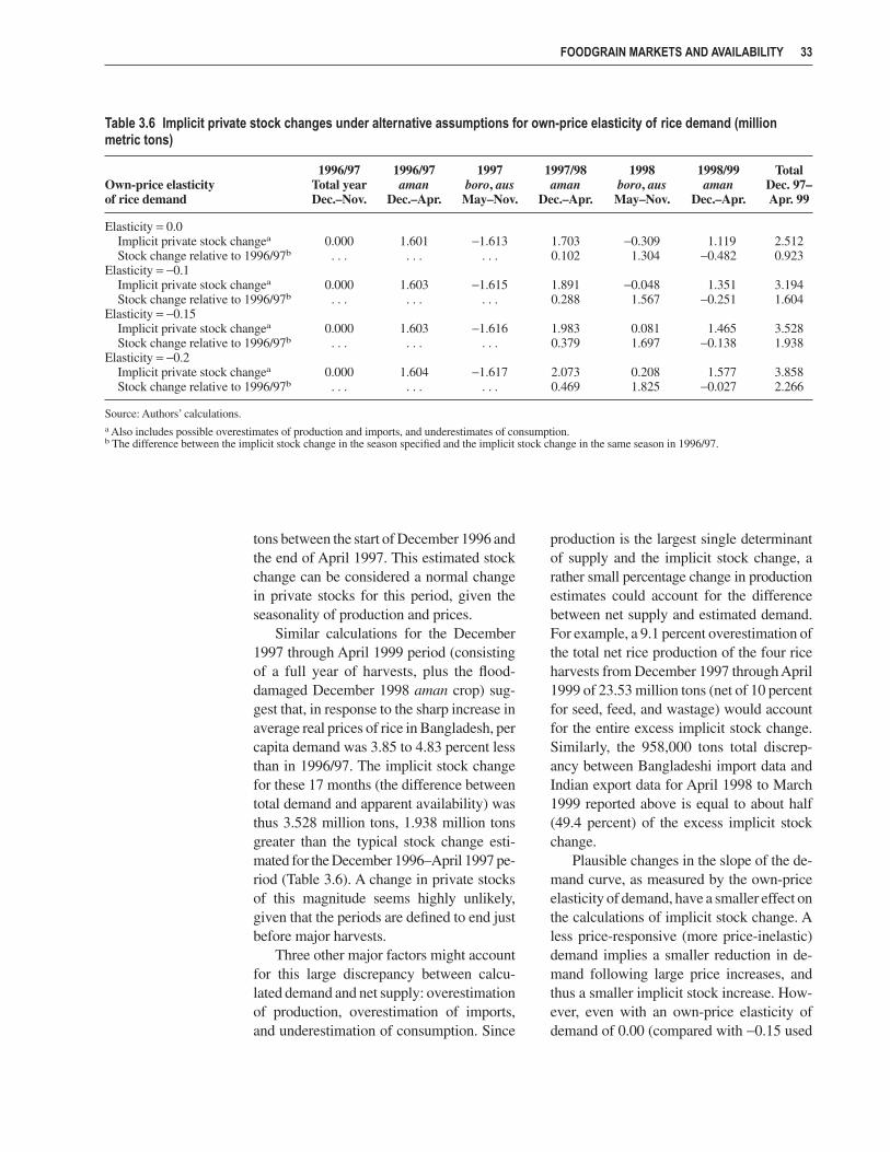
tons between the start of December 1996 andthe end of April 1997. This estimated stockchange can be considered a normal changein private stocks for this period, given theseasonality of production and prices.
Similar calculations for the December1997 through April 1999 period (consistingof a full year of harvests, plus the flood-damaged December 1998 aman crop) sug-gest that, in response to the sharp increase inaverage real prices of rice in Bangladesh, percapita demand was 3.85 to 4.83 percent lessthan in 1996/97. The implicit stock changefor these 17 months (the difference betweentotal demand and apparent availability) wasthus 3.528 million tons, 1.938 million tonsgreater than the typical stock change esti-mated for the December 1996–April 1997 pe-riod (Table 3.6). A change in private stocksof this magnitude seems highly unlikely,given that the periods are defined to end justbefore major harvests.
Three other major factors might accountfor this large discrepancy between calcu-lated demand and net supply: overestimationof production, overestimation of imports,and underestimation of consumption. Since
production is the largest single determinantof supply and the implicit stock change, arather small percentage change in productionestimates could account for the differencebetween net supply and estimated demand.For example, a 9.1 percent overestimation ofthe total net rice production of the four riceharvests from December 1997 through April1999 of 23.53 million tons (net of 10 percentfor seed, feed, and wastage) would accountfor the entire excess implicit stock change.Similarly, the 958,000 tons total discrep-ancy between Bangladeshi import data andIndian export data for April 1998 to March1999 reported above is equal to about half(49.4 percent) of the excess implicit stockchange.
Plausible changes in the slope of the de-mand curve, as measured by the own-priceelasticity of demand, have a smaller effect onthe calculations of implicit stock change. Aless price-responsive (more price-inelastic)demand implies a smaller reduction in de-mand following large price increases, andthus a smaller implicit stock increase. How-ever, even with an own-price elasticity ofdemand of 0.00 (compared with −0.15 used
FOODGRAIN MARKETS AND AVAILABILITY 33
Table 3.6 Implicit private stock changes under alternative assumptions for own-price elasticity of rice demand (millionmetric tons)
1996/97 1996/97 1997 1997/98 1998 1998/99 TotalOwn-price elasticity Total year aman boro, aus aman boro, aus aman Dec. 97–of rice demand Dec.–Nov. Dec.–Apr. May–Nov. Dec.–Apr. May–Nov. Dec.–Apr. Apr. 99
Elasticity = 0.0Implicit private stock changea 0.000 1.601 −1.613 1.703 −0.309 1.119 2.512Stock change relative to 1996/97b . . . . . . . . . 0.102 1.304 −0.482 0.923
Elasticity = −0.1Implicit private stock changea 0.000 1.603 −1.615 1.891 −0.048 1.351 3.194Stock change relative to 1996/97b . . . . . . . . . 0.288 1.567 −0.251 1.604
Elasticity = −0.15Implicit private stock changea 0.000 1.603 −1.616 1.983 0.081 1.465 3.528Stock change relative to 1996/97b . . . . . . . . . 0.379 1.697 −0.138 1.938
Elasticity = −0.2Implicit private stock changea 0.000 1.604 −1.617 2.073 0.208 1.577 3.858Stock change relative to 1996/97b . . . . . . . . . 0.469 1.825 −0.027 2.266
Source: Authors’ calculations.a Also includes possible overestimates of production and imports, and underestimates of consumption.b The difference between the implicit stock change in the season specified and the implicit stock change in the same season in 1996/97.
in Table 3.5), the excess implicit stock changeis still 923,000 tons (Table 3.6).33
In principle other factors could affect thecalculations of implicit stock change, includ-ing demand factors such as shifts in incomeor cross-price effects. But, given that the own-price elasticity of rice appears to be rathersmall, and that little widespread per capitaincome growth was likely in a period thatincluded two major rice production short-falls and a major flood, significant positiveincome effects on demand seem unlikely.Similarly, given the low cross-price effectsof other prices on rice consumption (owingto the large budget share of rice), cross-priceeffects are likely also to be negligible.
The above calculations strongly suggestthat total supply has been overestimated forthe December 1997 through May 1999 pe-riod. An overestimate of Bangladesh riceimports is insufficient in itself to explain thelarge implicit stock change (assuming theseimports were at least as large as stated in theIndian export data). Nonetheless, an over-estimate of imports could account for asmuch as about half of the difference betweennet supply and estimated rice demand.
Market Prices in the Absence of Private Sector ImportsThough the quantity of private sector im-ports from India is uncertain, it is clear thatthis trade substantially augmented Bangla-desh rice supplies in 1997/98 and 1998/99.One measure of the impact of this trade onnational food security in Bangladesh is tocompare actual prices and imports with esti-mates of prices and imports in the absence ofprivate sector imports from India. Given theaverage wholesale price of coarse rice inDhaka of Tk 13.3 per kilogram in 1998/99,
rice imports from December 1997 throughNovember 1998 were 2.043 million tons(according to the Bangladesh customs data).Had rice imports from India not been avail-able, the next lowest cost source for privateimporters would have been Thailand,34 forwhich the import parity price of 15 percentbroken rice in Dhaka in the same period wasTk 16.1 per kilogram. Given this 20.9 per-cent increase in the import parity price, esti-mated rice demand would have fallen bybetween 4.2 and 6.3 percent, assuming anown-price elasticity of rice demand of −0.2to −0.3. In this case, rice imports wouldhave declined by approximately 700,000 to1 million tons.35
If private sector imports were unavailable(or banned) from any source, then, with nochange in government imports, total supplywould have been 12.1 percent less (apart fromprivate stock changes) and rice prices couldhave risen by 40–60 percent, to an averageof between Tk 18.7 and Tk 21.3 per kilo-gram.36 Such an increase in the rice pricelevel would likely have been unacceptableto the government of Bangladesh and publicsector imports would have been increased.However, public sector imports of a magni-tude equal to private sector flows would nothave been feasible.
During the 1998 calendar year alone,private sector imports, mainly from India,reached 2.26 million tons. Had the govern-ment of Bangladesh imported this grain it-self, the average cost of the imported ricedelivered to local delivery points would havebeen approximately Tk 14.9–15.9 per kilo-gram, Tk 1.0–2.0 per kilogram above theprivate sector import costs, owing to addi-tional marketing costs of US$50–100 mil-lion. And, if the government had received a
34 CHAPTER 3
33 Moreover, note that an own-price elasticity of demand of −0.15, though consistent with time-series estimates in Dorosh(1999b), is low compared with cross-section estimates of −0.56 from Goletti (1993).
34 Bangladesh consumes mostly parboiled rice (in the parboiling process, the paddy is first boiled and then milled). Theother major Asian exporter, Vietnam, sold only white (non-parboiled) rice in this period.
35 This calculation assumes no problems with the supply of imports from Thailand, an issue discussed below.36 In the absence of private sector imports, domestic supply would have been 14.839 million tons, a 12.1 percent reduction
in per capita supplies relative to the actual estimated levels. Assuming an elasticity of demand of −0.2 to −0.3, priceswould need to rise by 12.1/0.3 (40 percent) to 12.1/0.2 (60 percent) to equilibrate market supply and demand.

net price of Tk 11.5 per kilogram (the openmarket sales price of Tk 12.0 per kilogramless Tk 0.5 per kilogram OMS dealer’scommission), the total unit subsidy wouldhave been Tk 3.4–4.4 per kilogram, and thetotal fiscal cost would have been US$160–210 million.
The Competitiveness of the PrivateRice Import TradeIn spite of the potentially high costs of mas-sive government imports, such expendituresmight be deemed necessary if there was ev-idence that private traders were manipulat-ing the market. One indication that the ricemarket was competitive in Bangladesh wasthat the margin between wholesale prices inDhaka and India remained relatively lowand stable.37 Data from letters of credit fromboth 1994/95 and 1998 suggest that a largenumber of traders participated in rice im-ports, another indication of a competitivemarket.38
Letters of credit data from 1994/95 indi-cate that most of the rice imported from Indiacame in small lots. The average size of the1,251 shipments of rice in 1994/95 was only707 tons. Letters of credit data from Janu-ary through mid-September 1998 indicatean even smaller average quantity of only268.7 tons per letter of credit for the 3,291letters of credit issued. Moreover, these let-ters of credit were opened by 793 differenttraders, with an average amount of importsper trader of only 1,115 tons of rice. Thelargest 10 traders (in terms of total imports)imported 142,369 tons, or 16 percent of thetotal. Given this broad participation in therice import trade and the small share of thelargest suppliers, it appears that there hasbeen little scope for individuals or a smallgroup of traders to significantly affect marketprices by restricting market supply (Dorosh1999b).
However, private sector imports fromThailand are likely to involve far fewertraders because of economies of scale in seashipments. Whereas cross-border trade in-volves shipments of approximately 10 tonsper truck or 70 tons per railway wagon(generally grouped together in a rack of 24wagons carrying about 1,600 tons), typicalocean shipments involve 10,000–15,000 tonsof rice. Thus, instead of hundreds of partici-pating traders, it is likely that only the largertraders would be able to finance such largeshipments. Of course, competition is still pos-sible even if the number of importers is only5 or 10, but the risk of collusion is high.39
Reliability of the Indian Rice Marketas a Source of SupplyFortunately for Bangladesh, market suppliesof rice in India in 1998/99 were plentiful.Production of the kharif rice crop, whichaccounts for about 85 percent of India’srice production, was 71.84 million tons, onlyabout 0.9 percent below the 1997/98 bumpercrop. Moreover, Food Corporation of Indiarice stocks on October 1, 1998, were quitehigh (8.7 million tons), nearly 3 million tonsabove the buffer stock norm of 6 milliontons for that date. Wheat stocks were evenhigher: 15.8 million tons on September 1,1998.
Large-scale private imports from Indiawere possible in 1998/99 because, with largegovernment stocks of foodgrains and a goodrice harvest, the government of India waswilling to allow exports. Had stocks and/or production been lower, an export quota oreven an export ban could have been imposed.One important factor, then, is the probabilitythat both Bangladesh and India will havepoor rice harvests in the same year.
As shown in Table 3.7, from 1971/72through 1998/99, total production of rice in Bangladesh fell about 5 percent or more
FOODGRAIN MARKETS AND AVAILABILITY 35
37 As indicated in Figure 3.3, the marketing margin for shipment of rice by truck increased by approximately Tk 1.1 perkilogram in November 1998 owing to new weight restrictions on truck loads in both India and Bangladesh.
38 See Murshid (1999) for details of the private sector rice import trade.39 One safeguard against collusion is to encourage international grain companies to participate in the import trade as well.
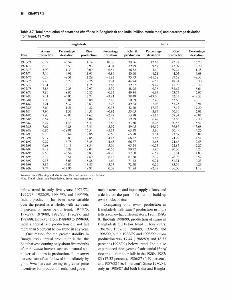
below trend in only five years: 1971/72,1972/73, 1988/89, 1994/95, and 1995/96.India’s production has been more variableover the period as a whole, with six years5 percent or more below trend: 1974/75,1976/77, 1979/80, 1982/83, 1986/87, and1987/88. However, from 1988/89 to 1998/99,India’s annual rice production did not fallmore than 5 percent below trend in any year.
One reason for the greater stability inBangladesh’s annual production is that theboro harvest, coming only about five monthsafter the aman harvest, acts as a natural sta-bilizer of domestic production. Poor amanharvests are often followed immediately bygood boro harvests owing to greater priceincentives for production, enhanced govern-
ment extension and input supply efforts, anda desire on the part of farmers to build upown-stocks of rice.
Comparing only aman production inBangladesh with kharif production in Indiatells a somewhat different story. From 1980/81 through 1998/99, production of aman inBangladesh fell below trend in four years:1981/82, 1987/88, 1988/89, 1994/95, and1998/99, but in 1988/89 and 1998/99, amanproduction was 17.44 (1988/89) and 18.33percent (1998/99) below trend. India alsoexperienced three years of substantial kharifrice production shortfalls in the 1980s: 1982/83 (17.32 percent), 1986/87 (6.49 percent),and 1987/88 (16.41 percent). Since 1980/81,only in 1986/87 did both India and Bangla-
36 CHAPTER 3
Table 3.7 Total production of aman and kharif rice in Bangladesh and India (million metric tons) and percentage deviationfrom trend, 1971–99
Bangladesh India
Aman Percentage Rice Percentage Kharif Percentage Rice PercentageYear production deviation production deviation production deviation production deviation
1970/71 6.22 −3.54 11.14 10.36 39.56 12.63 42.22 16.281971/72 6.12 −6.53 9.93 −4.94 39.99 9.57 43.07 13.201972/73 5.90 −11.33 10.09 −6.54 36.32 −4.10 39.24 −1.381973/74 7.10 4.99 11.91 6.84 40.90 4.21 44.05 6.081974/75 6.29 −8.51 11.29 −1.82 35.93 −11.58 39.58 −8.521975/76 7.45 6.79 12.76 7.74 44.74 6.52 48.74 8.301976/77 7.31 3.13 11.75 −3.63 39.27 −9.49 41.92 −10.321977/78 7.86 9.25 12.97 3.39 48.95 9.36 52.67 8.641978/79 7.89 8.07 12.85 −0.35 49.34 6.94 53.77 7.071979/80 7.11 −3.95 12.74 −3.81 38.49 −19.00 42.33 −18.531980/81 7.96 6.01 13.88 2.10 50.09 2.46 53.63 −0.131981/82 7.21 −5.37 13.63 −2.26 49.24 −2.03 53.25 −3.941982/83 7.60 −1.56 14.22 −0.55 42.70 −17.32 47.12 −17.591983/84 7.94 1.36 14.51 −0.92 55.05 3.84 60.10 2.011984/85 7.93 −0.07 14.62 −2.47 53.78 −1.13 58.34 −3.811985/86 8.54 6.17 15.04 −1.99 59.39 6.49 63.83 2.301986/87 8.27 1.43 15.41 −1.82 53.56 −6.28 60.56 −5.571987/88 7.69 −6.88 15.41 −3.92 49.05 −16.19 56.86 −13.681988/89 6.86 −18.01 15.54 −5.17 63.38 5.80 70.49 4.261989/90 9.20 8.64 17.86 6.66 65.88 7.51 73.57 6.091990/91 9.17 6.89 17.85 4.45 66.32 5.85 74.29 4.511991/92 9.27 6.75 18.25 4.65 66.37 3.65 74.68 2.551992/93 9.68 10.13 18.34 3.09 65.24 −0.25 72.87 −2.271993/94 9.42 5.88 18.04 −0.55 70.72 5.90 80.30 5.241994/95 8.50 −5.54 16.83 −8.96 72.60 6.52 81.81 4.831995/96 8.79 −3.51 17.69 −6.12 67.88 −2.39 76.98 −3.521996/97 9.55 3.65 18.88 −1.60 71.42 0.71 81.31 −0.251997/98 8.85 −5.07 18.85 −3.53 72.50 0.29 83.50 0.291998/99 7.74 −17.96 19.91 0.08 71.84 −2.48 86.00 1.18
Sources: Food Planning and Monitoring Unit and authors’ calculations.Note: Trend values have been derived from linear regression.

desh have a 5 percent or greater shortfall inthe aman/kharif crop. Since that year, India’skharif rice production has been above oronly slightly below trend, and in the twomost recent years of very low aman harvestsin Bangladesh (1988/89 and 1998/99), India’skharif production was 5.80 percent aboveand 2.48 percent below trend. Overall, thecorrelation coefficients of the error terms oflinear time-trend regressions of rice produc-tion are 0.34 for aman and kharif productionand 0.30 for total production in Bangladeshand India.
Past trends are, of course, not perfect pre-dictors of the future. But the lack of correla-tion between poor Indian harvests and poorBangladeshi harvests has an agronomic basis.India’s kharif rice production is spread overa much wider area than Bangladesh’s amanrice production, so weather effects are likelyto vary more across India’s kharif rice-producing zone, reducing the risk of weather-related failure of the entire crop. In partic-ular, high rainfall or excessive snowmelt inthe Himalayas that cause flooding in Bangla-desh and parts of eastern India do not neces-sarily correlate with poor weather in otherregions of India.
In spite of the low correlation of produc-tion shortfalls, it is nonetheless prudent for theBangladeshi government to be prepared forsuch an occurrence. In such a situation, riceimports would likely have to come mainlyfrom Thailand at somewhat higher cost thanimports from India; fewer private traderswould be involved, and shipping schedulesand problems at Chittagong port might hinderthe smooth arrival of rice imports.
A Comparison with EarlierMajor Production ShortfallsAs shown above, private sector importsplayed a major role in stabilizing rice and
wheat markets following the 1998 floods.Government policy in two earlier periods ofmajor foodgrain production shortfalls causedby floods (in 1974 and 1988) depended muchmore on public sector market interventions.In 1974, a large-scale famine, resulting in30,000–100,000 deaths, followed floods thatdamaged aus and aman crops.40 The 1988floods, in contrast, resulted in an even sharperfall in aman production (similar to that in1998) but no famine occurred.
The 1974 famine was characterized by avery sharp rise in nominal (and real) riceprices following the floods in July. Rice pricesin August through November 1974 were onaverage 58.2 percent higher than in Maythrough July 1974. This had disastrous con-sequences for poor households lacking theentitlements to acquire enough of their sta-ple commodity.41 Following the floods in1988/89 and 1998/99, in contrast, rice pricesrose by only 7.0 percent and 12.4 percent,respectively, in these months.
This difference in market price behavioris not explained by the size of the productionshortfall. As shown in Table 3.8, in compar-ison with trend aman rice production, theaman shortfalls in 1988 (18.1 percent) and1998 (18.0 percent) were much larger thanthe 1974 aman shortfall (8.5 percent). Instead,speculative behavior by traders appears tohave played a major role in the price increase.
Ravallion (1985, 1990) provides econo-metric evidence that exaggerated reports ofcrop failure influenced traders’ expectationsand led to “excessive hoarding” of stocks.42
In addition, traders appear to have believed(correctly) that the government would beunable to intervene effectively to stabilizemarket prices in the event of a productionshortfall. Government rice stocks were ex-tremely low at the time of the floods (end-July 1974): only 27,000 tons, equivalent to
FOODGRAIN MARKETS AND AVAILABILITY 37
40 The official death toll from the famine was 30,000 (Alamgir, 1980); unofficial reports were much higher. Sobhan (1979:175) quotes an official figure of 27,000 and an upper nonofficial estimate of 100,000; Lifschultz (1979: 130) gives afigure of 50,000.
41 Wheat prices also rose by 61.2 percent in the same period.42 In his time-series regressions on rice price formation, Ravallion uses the number of newspaper articles about crop short-
ages as a proxy for traders’ expectations about future production shortfalls.
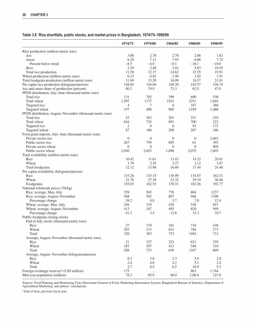
38 CHAPTER 3
Table 3.8 Rice shortfalls, public stocks, and market prices in Bangladesh, 1974/75–1998/99
1974/75 1979/80 1984/85 1988/89 1998/99
Rice production (million metric tons)Aus 3.00 2.78 2.78 2.86 1.62Aman 6.29 7.11 7.93 6.86 7.74
Percent below trend −8.5 −4.0 −0.1 −18.1 −18.0Boro 2.29 2.48 3.91 5.83 10.55Total rice production 11.58 12.37 14.62 15.55 19.91
Wheat production (million metric tons) 0.12 0.82 1.46 1.02 1.91Total foodgrain production (million metric tons) 11.69 13.20 16.09 16.57 21.81Per capita rice production (kilograms/person) 148.05 144.04 149.20 145.57 156.74Aus and aman share of production (percent) 80.3 79.9 73.3 62.5 47.0PFDS distribution, July–June (thousand metric tons)
Total rice 131 702 399 690 530Total wheat 1,597 1737 2163 2251 1,603Targeted rice 4 7 6 167 386Targeted wheat 157 490 905 1259 1,488
PFDS distribution, August–November (thousand metric tons)Total rice 43 263 201 231 216Total wheat 616 725 891 700 223Targeted rice 2 0 0 83 172Targeted wheat 87 186 298 287 186
Food grain imports, July–June (thousand metric tons)Private sector rice 0 0 0 0 2,663Public sector rice 267 759 695 61 393Private sector wheat 0 0 0 0 805Public sector wheat 2,030 2,023 1,898 2,075 1,603
Total availability (million metric tons)Rice 10.42 11.61 13.43 14.32 20.61Wheat 1.70 2.35 3.27 3.12 3.87Total foodgrains 12.12 13.96 16.69 17.44 24.48
Per capita availability (kilograms/person)Rice 133.26 135.15 136.99 134.07 162.31Wheat 21.76 27.38 33.32 29.19 30.46Foodgrains 155.03 162.53 170.31 163.26 192.77
National wholesale prices (Tk/kg)Rice: average, May–July 359 565 778 884 1237Rice: average, August–November 568 565 807 946 1390
Percentage change 58.2 0.0 3.7 7.0 12.4Wheat: average, May–July 256 335 438 538 857Wheat: average, August–November 413 347 495 620 949
Percentage change 61.2 3.4 12.8 15.3 10.7Public foodgrain closing stocks
End of July stocks (thousand metric tons)Rice 27 170 101 710 438Wheat 293 213 651 784 273Total 320 383 752 1494 711
Average, August–November (thousand metric tons)Rice 21 327 223 621 359Wheat 187 397 413 546 310Total 208 723 636 1167 669
Average, August–November (kilograms/person)Rice 0.3 3.8 2.3 5.8 2.8Wheat 2.4 4.6 4.2 5.1 2.4Total 2.7 8.4 6.5 10.9 5.3
Foreign exchange reservesa (US$ million) 175 . . . . . . 863 1,744Mid-year population (million) 78.2 85.9 98.0 1,06.8 127.0
Sources: Food Planning and Monitoring Unit; Directorate General of Food, Marketing Information System; Bangladesh Bureau of Statistics; Department ofAgricultural Marketing; and authors’ calculations.a End of June, previous fiscal year.
0.3 kilograms per person. Moreover, theMinistry of Food had great difficulties im-porting foodgrains because of a shortage offoreign exchange reserves, extremely highworld foodgrain prices, and delays in U.S.food aid deliveries.43 Because of the tightstock situation, total rice distribution duringAugust through November was only 43,000tons.
Osmani (1991) argues that larger publicfoodgrain stocks in 1979/80 and 1984/85 dis-couraged speculative market behavior andlimited price rises following production short-falls in those years. Public foodgrain stocksand distribution appear to have played a majorrole in 1988/89 as well. Total per capitafoodgrain stocks in August through Novem-ber 1998 were 10.9 kilograms per person,about four times those in the same period in1974/75. Moreover, public foodgrain distri-bution from August through November in thatyear was 931,000 tons, 272,000 tons greaterthan in 1974/75.
Hossain (1990), however, presents evi-dence that, during the 1978–90 period, thegovernment of Bangladesh overreacted tonatural disasters by importing more food-grain than needed, leading to an excessivebuild-up of stocks. Only about 50–60 per-cent of the additional imports were used toaugment domestic supply in the year of thenatural disaster, and the increased stocksand distribution in the years immediately fol-lowing a disaster were associated with lowerpaddy prices for farmers. Three main factorscontributed to overestimation of import re-quirements: a tendency of local governmentofficials to overstate production losses inhopes of receiving more aid, a positive sup-ply response of producers in subsequent sea-sons to higher prices, and lower consumer
demand by farmers with reduced incomes.Thus, acquiring and holding additional stocksimplied significant costs to the governmentand to farmers, as the additional importswere often purchased through commercialchannels at a high price, extra storage costswere incurred, and market prices tended tobe depressed in the year following a naturaldisaster.
Stocks in 1998/99 were significantlylarger than in 1974/75 in the crucial Augustthrough November months: 669,000 tons,or 5.3 kilograms per person—twice the percapita stocks of 1974/75, though half thoseof 1988/89 (Figure 3.6). Discouraging pri-vate speculation was a major Ministry ofFood rationale for maintaining a relativelyhigh level of stocks during these crucialmonths in 1998/99.44 Moreover, the Min-istry of Food made numerous efforts to in-crease its stocks through international anddomestic procurement of grain through ten-ders, with little success. Nonetheless, marketswere stabilized with fewer public stocks be-cause of the continued flow of private sectorimports in the months following the flood.45
Several factors suggest that the need forpublic stocks to avert famines in Bangladeshhas considerably decreased since 1974. First,because of the stabilizing influence of boroproduction, total rice production was only5.17 percent below trend in 1988/89 and wasactually 0.08 percent above trend in 1998/99.Total rice production in 1974/75 was 1.82 per-cent below trend. The record 10.55 millionton boro harvest in May/June 1999, only fiveto six months after the failure of the amancrop, shortened the period of uncertainty re-garding domestic supply, increased foodgrainavailability, raised farmer incomes, and re-duced prices.46 Second, as shown above,
FOODGRAIN MARKETS AND AVAILABILITY 39
43 Sobhan (1979) argues that the proximate cause of the famine in 1974 was the withholding of U.S. PL 480 food aid im-ports; a new agreement for food aid for 1973/74 was not reached until July 10, 1974, and grain was not shipped untilOctober 1974. Contributing necessary conditions were the forces of the market (controlled by big farmers and traders)and the refusal of the Bangladesh government to reallocate available food stocks towards rural channels, such as Mod-ified Rationing, and away from favored urban channels (through Statutory Rationing).
44 The sharp fall in rice stocks in early 1998 following the drought-damaged 1997 aman crop was seen by policymakersas a cause of the sharp increase in prices in those months.
45 Early assurances of food aid by donors may also have contributed to calming markets in Bangladesh.46 The record 1.91 million ton wheat harvest in March and April 1999 also added to food availability soon after the aman
crop shortfall.
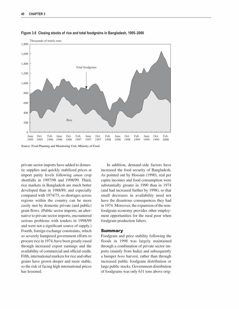
private sector imports have added to domes-tic supplies and quickly stabilized prices atimport parity levels following aman cropshortfalls in 1997/98 and 1998/99. Third,rice markets in Bangladesh are much betterdeveloped than in 1988/89, and especiallycompared with 1974/75, so shortages acrossregions within the country can be moreeasily met by domestic private (and public)grain flows. (Public sector imports, an alter-native to private sector imports, encounteredserious problems with tenders in 1998/99and were not a significant source of supply.)Fourth, foreign exchange constraints, whichso severely hampered government efforts toprocure rice in 1974, have been greatly easedthrough increased export earnings and theavailability of commercial and official credit.Fifth, international markets for rice and othergrains have grown deeper and more stable,so the risk of facing high international priceshas lessened.
In addition, demand-side factors haveincreased the food security of Bangladesh.As pointed out by Hossain (1990), real percapita incomes and food consumption weresubstantially greater in 1990 than in 1974(and had increased further by 1998), so thatsmall decreases in availability need nothave the disastrous consequences they hadin 1974. Moreover, the expansion of the non-foodgrain economy provides other employ-ment opportunities for the rural poor whenfoodgrain production falters.
SummaryFoodgrain and price stability following thefloods in 1998 was largely maintainedthrough a combination of private sector im-ports (mainly from India) and subsequentlya bumper boro harvest, rather than throughincreased public foodgrain distribution orlarge public stocks. Government distributionof foodgrains was only 631 tons above orig-
40 CHAPTER 3
Figure 3.6 Closing stocks of rice and total foodgrains in Bangladesh, 1995–2000
Source: Food Planning and Monitoring Unit, Ministry of Food.

inally scheduled quantities in the last sixmonths of 1998, compared with official esti-mates of more than 1 million tons of privatesector rice imports from India in the sameperiod.
Government policy nonetheless playedan important role in ensuring the availabilityof food. The trade liberalization of the early1990s permitted private sector imports and
concrete measures encouraged private sectorimports during 1998. Moreover, long-termpolicies of investment in infrastructure, agri-cultural research, and extension contributedto well-functioning markets and an expan-sion of boro rice production that reduced thetime between major rice harvests in Bangla-desh from 12 months to 6 months.
FOODGRAIN MARKETS AND AVAILABILITY 41
C H A P T E R 4
Impact of the Floods on AgriculturalProduction, Employment, and Wealth
Almost all households in flooded regions of Bangladesh in September 1998 were af-fected either directly or indirectly. Many households lost standing crops, along withproductive and valuable assets; others could not find employment that would other-
wise have been available if the floods had not been so severe. In this chapter, we assess theimpacts of the floods through loss of agricultural production (particularly for households’main crops), loss of other assets, and loss of income from labor market participation. Alongwith data by level of flood exposure, we present data on direct economic losses from the floodby household per capita expenditures, in order to show the varying effect of flood exposureon poor and nonpoor households.
Agricultural Production and Crop LossesAs noted in the previous chapter, farmers’ choices of cropping patterns in Bangladesh areconstrained by the timing and depth of flooding. In many of the low-lying areas of the coun-try, a meter or more of water covers the land during the monsoon season every year, thus pre-cluding any crop cultivation during that period. In a normal year, 41.0 percent of farmlandcultivated (owned) by the farmers in our sample is covered by more than 90 centimeters ofwater during the monsoon season (Table 4.1). In Derai thana (Sunamganj district in north-east Bangladesh), 48 percent of the land is covered by more than 3 meters of water duringthe monsoon season. On this land, only one crop of boro rice, planted in November or De-cember and harvested in March or April, is possible. Another 31 percent of the area culti-vated in the sample survey was medium lowland and lowland, with average flood depth of0.9 to 3.0 meters. Deepwater aman or aus crops are typically cultivated on this land duringthe monsoon season, with a crop of boro rice or wheat (on the medium lowland) often culti-vated during the dry season (see Figure 4.1). On the medium highland and highland (theremaining 59 percent of the land cultivated by survey farmers), transplanted aman rice dom-inates the cropping pattern from the time of transplanting (normally around August) to har-vest in November or December.
During the 1998 floods, floodwaters on sample farmers’ fields were almost double theirnormal levels—137 centimeters compared with 73 centimeters. On medium highland, flood-
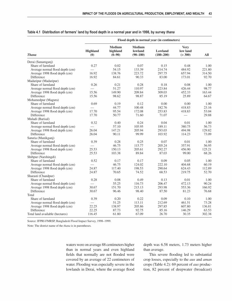
waters were on average 88 centimeters higherthan in normal years and even highlandfields that normally are not flooded werecovered by an average of 22 centimeters ofwater. Flooding was especially severe in thelowlands in Derai, where the average flood
depth was 6.58 meters, 1.73 meters higherthan average.
This severe flooding led to substantialcrop losses, especially to the aus and amancrops (Table 4.2): 69 percent of aus produc-tion, 82 percent of deepwater (broadcast)
IMPACT OF THE FLOODS ON AGRICULTURAL PRODUCTION, EMPLOYMENT, AND WEALTH 43
Table 4.1 Distribution of farmers’ land by flood depth in a normal year and in 1998, by survey thana
Flood depth in normal year (in centimeters)
Medium Medium VeryHighland highland lowland Lowland low land
Thana (0) (0–90) (90–180) (180–200) (> 300) All
Derai (Sunamganj)Share of farmland 0.27 0.02 0.07 0.15 0.48 1.00Average normal flood depth (cm) — 54.15 133.39 214.74 484.92 221.80Average 1998 flood depth (cm) 16.92 138.76 223.72 297.75 657.94 314.50Difference 16.92 84.61 90.33 83.00 173.01 92.70
Madaripur (Madaripur)Share of farmland 0.26 0.21 0.28 0.18 0.08 1.00Average normal flood depth (cm) — 51.27 110.97 223.84 426.44 98.77Average 1998 flood depth (cm) 15.56 149.90 209.84 309.03 452.33 163.44Difference 15.56 98.62 98.87 85.19 25.89 64.67
Mohamedpur (Magura)Share of farmland 0.69 0.19 0.12 0.00 0.00 1.00Average normal flood depth (cm) — 44.77 100.48 182.76 418.83 23.16Average 1998 flood depth (cm) 17.70 95.54 172.08 253.83 418.83 53.04Difference 17.70 50.77 71.60 71.07 — 29.88
Muladi (Barisal)Share of farmland 0.32 0.40 0.24 0.04 0.01 1.00Average normal flood depth (cm) — 57.10 105.95 189.11 380.75 56.73Average 1998 flood depth (cm) 26.04 147.21 205.94 293.03 494.98 129.82Difference 26.04 90.11 99.99 103.92 114.23 73.09
Saturia (Manikganj)Share of farmland 0.39 0.28 0.25 0.07 0.01 1.00Average normal flood depth (cm) — 46.75 115.77 205.24 357.91 56.95Average 1998 flood depth (cm) 25.53 150.13 205.61 292.27 456.90 125.21Difference 25.53 103.38 89.84 87.03 99.00 68.26
Shibpur (Narshingdi)Share of farmland 0.52 0.17 0.17 0.09 0.05 1.00Average normal flood depth (cm) — 46.75 124.02 222.10 404.68 60.19Average 1998 flood depth (cm) 24.87 117.40 198.53 290.64 624.43 112.89Difference 24.87 70.65 74.52 68.53 219.75 52.70
Sharasti (Chandpur)Share of farmland 0.28 0.08 0.49 0.13 0.01 1.00Average normal flood depth (cm) — 55.25 116.73 206.47 472.13 90.24Average 1998 flood depth (cm) 30.67 151.70 215.13 293.98 553.36 166.92Difference 30.67 96.46 98.40 87.50 81.23 76.68
TotalShare of farmland 0.39 0.20 0.22 0.09 0.10 1.00Average normal flood depth (cm) — 51.25 113.11 212.69 461.51 73.28Average 1998 flood depth (cm) 22.25 138.97 205.86 297.85 607.80 136.81Difference 22.25 87.73 92.75 85.16 146.29 63.53
Total land available (hectares) 116.45 61.80 67.09 26.70 30.35 302.38
Source: IFPRI-FMRSP, Bangladesh Flood Impact Survey, 1998–1999.
Note: The district name of the thana is in parentheses.

aman, and 91 percent of transplanted amanwas lost because of the floods, representing24 percent of the total value of anticipatedagricultural production for the year.47 Over-all, rice crop losses accounted for over halfof total agricultural losses, with vegetables(25 percent) and fibers (19 percent) account-ing for most of the remaining losses.
About 70 percent of households in oursample were engaged in some form of agri-cultural production in the 12 months prior tothe survey, and their average agriculturalproduction was Tk 8,277 (Table 4.3). In thesample, 52 percent of all households culti-
vated foodgrains (rice and wheat), althoughonly 38 percent of households actually pro-duced a crop.
The average crop loss for transplantedaman and aus crops was nearly constantacross flood exposure category (moderate,severe, and very severe), with essentially allflood-exposed households suffering nearlytotal losses to transplanted aman. The aver-age crop loss for deepwater aman variedmore substantially, ranging from 56 to 94percent across flood-exposed households,in large part because it is not cultivated onthe very low lands in Derai and other thana
44 CHAPTER 4
Figure 4.1 Bangladesh crop calendar and seasonal flooding
Source: Khan 1999.Notes: Except for wheat, all names refer to rice crops. HYV = high-yielding variety.
47 Official unpublished Bangladesh Bureau of Statistics thana-level aman production estimates for 1998/99 are broadlyconsistent with the survey figures. Six of the thanas reported total failure of aman production, while the seventh(Shibpur thana in Narsingdi district) reported aman production down by 80 percent compared with 1996/97.

where households were nonetheless severelyflooded. Overall crop losses were still broadlysimilar for all farm households that wereexposed to the flood, ranging from 42 to 62percent of expected production. Crop lossesfor farm households not exposed to thefloods were only 23 percent of expected pro-duction, however.48
Only 19 percent of households sampledgrew fibers (jute and sugarcane), but averagelosses were high (62 percent). Overall, 26 per-cent of farmers who cultivated vegetablessuffered losses to their vegetable crops, butaverage losses were only 37 percent. Onereason for the high percentage of farmersgrowing vegetables and the relatively lowpercentage with flood losses was that manyfarmers decided to utilize their cropland forvegetable production just after the flood-waters receded, when it was too late forpaddy cultivation. Price incentives appearedto have played a role here, as well, as theprices of vegetables went up during floodperiod, especially in the flood-affectedareas. Within a few months, however, theprice of vegetables declined as market sup-ply increased.
Table 4.4 reports the values of losses ofagricultural crop production of sample pro-ducing households by size of farm and floodexposure (again excluding the forgone valueof aman cultivation when no crop was trans-planted). Households with smaller farms didnot appear to suffer greater percentage lossesthan households with larger farms. In fact,percentage production losses were highestfor medium-sized farms (0.2–0.6 hectares)and very large farms (1.0 hectares and above).Note, too, there is no correlation betweenseverity of household flood exposure and thesize of landholding. The Spearman rank cor-relation coefficient between flood exposureand quintiles for 757 households is found tobe very small and insignificant, further evi-dence that the severity of flooding was notsignificantly different for the poor than forthe rich.
Ownership and Loss of AssetsAll households in the sample reported own-ership of some type of assets, such as cattle,poultry, and other tangible assets.49 In addi-tion to the losses to crops, 55 percent of the
IMPACT OF THE FLOODS ON AGRICULTURAL PRODUCTION, EMPLOYMENT, AND WEALTH 45
Table 4.2 Aggregate area, production, and loss of crops of sample farms
Area planted Production value Value lost LossCrops (hectares) (Tk thousand) (Tk thousand) (percent)
Transplanted aman 37.9 119.6 1,202.6 91.0Deepwater aman 23.6 101.0 451.4 81.7Aus 27.3 176.3 383.4 68.5Boro 19.0 920.6 160.4 14.8Total rice 107.7 1,317.5 2,197.9 62.5Wheat 7.4 247.0 — —Fibers 25.3 477.3 778.2 62.0Vegetables 140.4 1,735.4 1,007.8 36.7Other 32.7 524.0 45.1 7.9Total 312.8 4,301.1 4,029.0 48.4
Source: IFPRI-FMRSP, Bangladesh Flood Impact Survey, 1998–1999.
48 Note, though, that, since our flood exposure variable is based on measures of flooding at the home, the 70 percent ofhouseholds “not exposed to the flood” that cultivated crops still suffered significant crop losses.
49 Inexpensive agricultural assets include plows, husking mills (diesel operated), and other similar items. Valuable agri-cultural assets include goods such as power tillers, shallow pumps, deep tubewells, threshing machines, and electrichusking mills. Cheap household assets include metal cooking pots and handlooms. Valuable household assets includeitems such as sewing machines and hand tubewells. The data related to number of animals in the livestock categorywere obtained by weighting younger individuals as a fraction of adult animals.

Table 4.3 Average area, production, and loss of crops, by flood exposure
Flood exposure
Main crops Not exposed Moderate Severe Very severe All
Transplanted amanCrop growers (% of households) 30.9 32.1 38.6 24.4 31.8Value of production (Tk/farm household) 595 995 225 156 485Average land planted to crop (hectares/household) 0.10 0.23 0.14 0.20 0.16Average production loss (Tk/farm household) 3,060 6,500 5,357 4,561 4,990Production loss (%) 82.8 86.7 96.0 96.7 91.0
Deepwater amanCrop growers (% of households) 19.8 21.8 24.2 14.3 20.2Value of production (Tk/farm household) 893 502 373 1078 660Average land planted to crop (hectares/household) 0.09 0.17 0.20 0.16 0.15Average production loss (Tk/farm household) 1,206 7,701 3,204 1,342 2,951Production loss (%) 57.5 93.9 89.6 55.5 81.7
AusCrop growers (% of households) 22.1 21.8 23.7 12.5 20.3Value of production (Tk/farm household) 1,714 1,213 815 496 1,145Average land planted to crop (hectares/household) 0.09 0.26 0.20 0.17 0.18Average production loss (Tk/farm household) 1,021 3,579 2,506 2,699 2,490Production loss (%) 37.3 74.7 75.5 84.5 68.5
BoroCrop growers (% of households) 21.2 17.0 14.5 8.9 15.7Value of production (Tk/farm household) 7,926 11,733 4,476 6,212 7,736Average land planted to crop (hectares/household) 0.13 0.18 0.16 0.16 0.15Average production loss (Tk/farm household) 1,682 140 1,712 820 1,348Production loss (%) 17.5 1.2 27.7 11.7 14.8
WheatCrop growers (% of households) 20.3 13.9 13.0 8.3 14.3Value of production (Tk/farm household) 2,596 2,580 1,760 1,850 2,284Average land planted to crop (hectares/household) 0.07 0.05 0.07 0.07 0.07Average production loss (Tk/farm household) — — — — —Production loss (%) — — — — —
All cereals (all rice and wheat)Crop growers (% of households) 50.2 52.1 59.9 42.3 51.5Value of production (Tk/farm household) 5,842 5,841 2,084 2,278 3,998Average land planted to crop (hectares/household) 0.22 0.39 0.30 0.27 0.29Average production loss (Tk/farm household) 3,517 8,773 6,152 4,059 5,636Production loss (%) 37.4 60.0 74.7 64.1 58.4
Fibers (sugarcane and jute)Crop growers (% of households) 28.1 20.6 11.6 13.7 18.8Value of production (Tk/farm household) 1,944 4,554 7,436 1,104 3,361Average land planted to crop (hectares/household) 0.12 0.28 0.14 0.21 0.18Average production loss (Tk/farm household) 189 21,758 486 660 5,480Production loss (%) 8.9 82.7 6.1 37.4 62.0
VegetablesCrop growers (% of households) 52.5 53.9 58.9 47.6 53.5Value of production (Tk/farm household) 4,865 3,497 5,542 2,419 4,285Average land planted to crop (hectares/household) 0.30 0.50 0.33 0.27 0.35Average production loss (Tk/farm household) 425 3,111 5,411 287 2,488Production loss (%) 8.0 47.1 49.4 10.6 36.7
OtherCrop growers (% of households) 36.4 41.8 52.2 36.3 41.9Value of production (Tk/farm household) 1,986 2,211 1,242 1,318 1,653Average land planted to crop (hectares/household) 0.11 0.16 0.08 0.08 0.10Average production loss (Tk/farm household) 93 412 68 25 142Production loss (%) 4.5 15.7 5.2 1.9 7.9
TotalCrop growers (% of households) 72.4 68.5 78.7 61.3 70.8Value of production (Tk/farm household) 9,343 9,920 7,651 4,476 8,015Average land planted to crop (hectares/household) 0.48 0.87 0.55 0.48 0.58Average production loss (Tk/farm household) 2,870 15,925 8,846 3,183 7,517Production loss (%) 23.4 61.6 53.6 41.6 48.4
Sample sizeNumber of farm households 157 113 163 103 536Total number of households 217 165 207 168 757
Source: IFPRI-FMRSP, Bangladesh Flood Impact Survey, 1998–1999.

households surveyed suffered damage to ordestruction of assets, which reduced theirhousehold wealth as well as future produc-tive capacity.
Almost all households reported havingat least one house (main house). More than80 percent of the houses were roofed withtiles, tin, or concrete, and the roofs of theremaining houses (18 percent) were coveredwith bamboo, straw (chhan), leaves, or jutesticks. Less than half of all households ownedtrees, a potentially important source of food aswell as of income (del Ninno and Roy 1999b).
In the sample area, 47.6 percent of house-holds reported owning cattle and more than76 percent owned chickens. Few householdsin the sample owned more than these basicassets, though. Only 15 percent owned aradio and one-fourth of rural households pos-sessed either a radio or a clock. Although40 percent of the households owned smallagricultural equipment, only 3.43 percentowned valuable agricultural assets such asirrigation equipment.
The pattern of ownership of assets by thelevel of welfare and the ownership of landshows that richer households own more as-sets in general, particularly the more valuableassets such as transport vehicles and jewelry.Similarly, households that own more landtend to have more trees, cattle, chickens, andother agricultural assets. About 8 percent of
households owning large trees belong to thelargest landholding group and they have onaverage 20 large trees, compared with the9 large trees of the households with the small-est landholdings (less than 0.02 hectares).Similarly, large landowners owned an aver-age of 4 cattle and 10 chickens, comparedwith 1.5 and 5.6, respectively, for smalllandowners.
Table 4.5 shows the losses of various tan-gible assets by severity of flood exposure.For the 55 percent of households that lostassets, the average loss was Tk 6,936, equiv-alent to 16 percent of the pre-flood totalvalue of assets.
The value of the losses of assets and theproportion to its value varied widely accord-ing to asset, however. The most seriouslosses were for housing. In all, 47 percent ofhouseholds suffered damage or loss to hous-ing, with the average loss equal to Tk 5,675,or 59 percent of pre-flood housing value. Thefloods also caused serious damage to largetrees: 17 percent of households lost tresswith an average value of Tk 5,137. Nearly 15percent of households lost chickens, thoughthe average value of the loss was only Tk142. Note that less than 1 percent of house-holds lost stocks of cereals.
The more severe the level of flood expo-sure, the larger the proportion of householdssuffering damage to their assets—78 percent
IMPACT OF THE FLOODS ON AGRICULTURAL PRODUCTION, EMPLOYMENT, AND WEALTH 47
Table 4.4 Producing households and loss of agricultural production, by farm size and flood exposure (percent)
Not exposed Exposed All
Farmland Farm Production Farm Production Farm Productionavailable (hectares) households loss households loss households loss
0–0.02 24.20 13.6 19.53 37.2 20.90 29.40.02–0.2 21.66 18.1 26.91 30.3 25.37 27.90.2–0.6 35.03 14.9 34.83 58.0 34.89 47.90.6–1.0 10.19 27.1 11.08 39.5 10.82 34.81.0+ 8.92 10.9 7.65 56.7 8.02 48.8Total 100.00 23.4 100.00 55.6 100.00 48.4Number of farm households 157 379 536.00Percentage of farm households 72.35 70.19 70.81Sample size 217 540 757
Source: IFPRI-FMRSP, Bangladesh Flood Impact Survey, 1998–1999.
Note: Percentage loss is calculated as losses as a share of actual production plus losses.

48 CHAPTER 4
Table 4.5 Households’ loss of assets, by asset type and severity of flood exposure
Flood exposure
Type of asset Not exposed Moderate Severe Very severe All
Housing (% of households that lost assets) 7.8 49.7 64.3 74.4 47.2Average value of loss (Tk) 2,509 5,541 5,649 6,221 5,675Share of pre-flood value (%) 56.3 60.0 59.8 59.6 58.8
Productive assets (% of households that lost assets) 9.7 23.6 27.1 28.6 21.7Average value of loss (Tk) 431 1,300 942 1,000 979Share of pre-flood value (%) 15.2 14.4 15.7 16.1 15.3
Cattle (% of households that lost assets) 0.5 7.3 7.2 5.4 4.9Average value of loss (Tk) 1,750 3,406 2,582 3,457 3,040
Goats/sheep (% of households that lost assets) 0.9 2.4 1.9 2.4 1.8Average value of loss (Tk) 850 574 588 500 596
Chickens (% of households that lost assets) 7.8 15.8 17.4 20.8 14.8Average value of loss (Tk) 184 159 115 142 142
Ducks (% of households that lost assets) 1.4 6.7 5.3 7.7 5.0Average value of loss (Tk) 166 75 206 251 180
Agricultural tools (% of households that lost assets) 0.0 1.2 5.3 7.1 3.3Average value of loss (Tk) — 13 26 26 25
Agricultural equipment (% of households that lost assets) 0.0 0.0 0.0 1.2 0.3Average value of loss (Tk) — — — 2,216 2,216
Fishing equipment (% of households that lost assets) 0.5 1.8 2.4 1.8 1.6Average value of loss (Tk) 1,980 793 1,026 239 850
Transport vehicles (% of households that lost assets) 0.0 0.0 0.0 0.6 0.1Average value of loss (Tk) — — — 1,200 1,200
Liquid assets (% of households that lost assets) 6.9 21.2 24.2 23.8 18.5Average value of loss (Tk) 4,692 3,094 2,906 8,428 4,722Share of pre-flood value (%) 17.2 17.6 17.8 17.3 17.5
Large trees (% of households that lost assets) 6.9 18.8 21.3 21.4 16.6Average value of loss (Tk) 4,692 3,427 3,144 9,230 5,137
Jewelry(% of households that lost assets) 0.0 2.4 4.8 6.5 3.7Average value of loss (Tk) — 158 567 308 302
Consumer durables (motorcycles) (% of households that lost assets) 0.5 0.0 0.0 0.6 0.3Average value of loss (Tk) 500 — — 1,000 750Share of pre-flood value (%) 2.1 2.6 1.0 1.1 1.8
Domestic assets (% of households that lost assets) 0.0 6.1 15.5 22.0 10.4Average value of loss (Tk) — 311 177 207 208Share of pre-flood value (%) 8.5 5.1 5.4 5.6 6.2
Cereal stocks (% of households that lost assets) 0.0 0.0 1.9 1.2 0.8Average value of loss (Tk) — — 346 1,605 766
Small household items (% of households that lost assets) 0.0 5.5 9.7 13.7 6.7Average value of loss (Tk) — 205 436 136 265
Large household items (% of households that lost assets) 0.0 3.6 4.3 7.1 3.8Average value of loss (Tk) — 289 94 93 145
Other assets (% of households that lost assets) 0.0 0.0 0.0 3.6 0.8Average value of loss (Tk) — — — 2,182 2,182Share of pre-flood value 0.6 0.4 0.3 0.4 0.4
Total (% of households that lost assets) 18.9 60.6 69.1 78.0 54.8Average value of loss (Tk) 2,990 6,164 6,679 9,042 6,936Share of pre-flood value (%) 7.1 11.8 16.5 23.2 16.0
Number of households 217 165 207 168 757
Source: IFPRI-FMRSP, Household Survey 1998.

of the very severely flood-exposed house-holds and 69 percent of the severely affectedhouseholds lost assets worth on average Tk9,042 and Tk 6,679, respectively. By com-parison, only 19 percent of households de-fined as not exposed to the floods sufferedloss of assets, and their average loss was onlyTk 2,990.
The percentages of households report-ing loss of assets were similar for poorerhouseholds and richer households (Table4.6). For the 73 percent of households inthe first expenditure quintile who lost assets,the average loss was Tk 5,868, comparedwith Tk 8,858 for the 69 percent of house-holds in the top quintile who suffered losses.
IMPACT OF THE FLOODS ON AGRICULTURAL PRODUCTION, EMPLOYMENT, AND WEALTH 49
Table 4.6 Flood-exposed households’ loss of assets, by asset type and expenditure quintile
Type of asset Quintile 1 Quintile 2 Quintile 3 Quintile 4 Quintile 5 All
Housing (% of households that lost assets) 67.26 66.37 62.26 57.43 60.75 62.96Average value of loss (Tk) 4,924 4,713 7,242 6,689 5,994 5,833Share of pre-flood value 60.37 55.13 69.39 62.99 54.84 59.79
Productive assets (% of households that lost assets) 24.78 29.20 27.36 26.73 24.30 26.48Average value of loss (Tk) 1,020 1,291 1,068 940 921 1,059Share of pre-flood value 20.40 19.14 13.88 15.71 13.03 15.33
Cattle (% of households that lost assets) 7.08 9.73 6.60 4.95 4.67 6.67Average value of loss (Tk) 2,601 3,264 2,989 4,012 2,604 3,075
Goats/sheep (% of households that lost assets) 4.42 0.88 2.83 — 2.80 2.22Average value of loss (Tk) 425 450 900 — 457 554
Chickens (% of households that lost assets) 15.93 22.12 14.15 21.78 15.89 17.96Average value of loss (Tk) 130 125 110 116 209 136
Ducks (% of households that lost assets) 7.96 7.08 8.49 5.94 2.80 6.48Average value of loss (Tk) 316 128 182 85 113 182
Agricultural tools (% of households that lost assets) 4.42 6.19 3.77 5.94 2.80 4.63Average value of loss (Tk) 24 21 14 20 57 25
Agricultural equipment (% of households that lost assets) — — — 0.99 0.93 0.37Average value of loss (Tk) — — — 1,431 3,000 2,216
Fishing equipment (% of households that lost assets) 0.88 0.88 3.77 0.99 3.74 2.04Average value of loss (Tk) 300 900 955 712 623 748
Transport vehicles (% of households that lost assets) — 0.88 — — — 0.19Average value of loss (Tk) — 1,200 — — — 1,200
Liquid assets (% of households that lost assets) 19.47 32.74 16.98 19.80 26.17 23.15Average value of loss (Tk) 3,445 4,866 1,855 3,385 8,350 4,726Share of pre-flood value 11.68 17.69 9.98 14.91 24.37 17.57
Large trees (% of households that lost assets) 7.70 27.43 16.04 17.82 23.36 20.56Average value of loss (Tk) 3,727 5,662 1,824 3,607 9,236 5,197
Jewelry (% of households that lost assets) 5.31 7.96 3.77 4.95 4.67 5.37Average value of loss (Tk) 121 507 304 391 308 345
Domestic assets (% of households that lost assets) 14.16 20.35 6.60 14.85 16.82 14.63Average value of loss (Tk) 85 112 168 210 453 208Share of pre-flood value 6.82 6.25 5.45 5.19 4.62 5.34
Cereal stocks (% of households that lost assets) — — 0.94 1.98 2.80 1.11Average value of loss (Tk) — — 78 69 1,459 766
Small household items (% of households that lost assets) 9.73 13.27 4.72 9.90 8.41 9.26Average value of loss (Tk) 132 85 453 331 409 240
Large household items (% of households that lost assets) 4.42 7.08 0.94 6.93 5.61 5.00Average value of loss (Tk) 86 138 200 76 244 138
Other assets (% of households that lost assets) 0.88 0.88 2.83 0.99 — 1.11Average value of loss (Tk) 200 1,200 3,888 25 — 2,182Share of pre-flood value 0.37 0.45 0.28 0.22 0.45 0.36
Total (% of households that lost assets) 72.57 69.91 68.87 65.35 69.16 69.26Average value of loss (Tk) 5,868 7,340 7,605 7,337 8,858 7,369Share of pre-flood value 30.51 23.08 18.51 15.30 11.05 16.90
Number of households 113 113 106 101 107 540
Source: IFPRI-FMRSP, Household Survey 1998.

Poor households’ losses were concentratedmainly in housing and productive assets(such as cattle and poultry); richer house-holds’ losses included large trees as well ashousing. Note also that losses as a propor-tion of pre-flood value were noticeablyhigher for poor households (in quintiles 1and 2) than for richer households (quintile5). Thus, although richer households lostvaluable assets, many poorer householdsexperienced a bigger relative shock as aresult of the floods because they had fewerassets to begin with.
Labor Participation and EarningsThe floods disrupted economic activities aswell as destroying crops and assets. Agricul-tural employment, transport, and the nonfarmeconomy were all affected, not only whilethe floodwaters covered the land, but forseveral months afterward.
As shown in Figure 4.2 and Table 4.7,the average monthly days worked fell in theperiod of the floods and afterwards increasedto the same level as 12 months earlier for allworkers except day laborers.50 The declinein employment during the floods was not verysevere for dependent workers or those em-ployed in cottage industries. For example, de-pendent workers’ employment fell from 27days per month in 1997 to 24 days per monthin July through October 1998. By October–November 1998, they were again employedan average of 27 days per month. Day labor-ers were more severely affected: their em-ployment fell sharply from 19 days per monthin 1997 to only 11 days per month in Julythrough October, 1998. By October–Novem-ber 1998, employment had increased to anaverage of 16 days per month, still 3 daysper month less than the average for Julythrough October 1997.
Similarly, wage earnings also fell in theperiod of the floods and had not recovered to1997 levels by October–November 1998. Fordependent workers, average monthly wageearnings during July–October 1998 were16.5 percent below their average monthlyearnings one year earlier. For day laborers,average monthly earnings in July–October1998 were 46 percent below those in thesame months in 1997, and in October–November 1998 were still 18 percent belowthe 1997 levels. Female earnings were lowerthan male earnings in all labor categories,but the differences over the two periods wereless pronounced than the variations in malemonthly income.
This decline in number of days workedand wage earnings occurred in the contextof a labor market with little open unemploy-ment. Thus, underemployment increasedas workers had fewer work days, but mostworkers found at least some employment.Many people, however, were neither gain-fully employed nor actively searching for
50 CHAPTER 4
50 Working people have been classified as dependent workers, day laborers, business and cottage industry entrepreneurs(those that are engaged in self-employment activities), farmers, and unpaid family laborers. The main difference be-tween dependent workers and day laborers is job regularity. Dependent workers are hired for a fixed amount of time.Day laborers are hired for the day and are found to be multi-occupational, being engaged in agriculture and nonfarmactivities such as commercial, transport, and industrial activities.
Figure 4.2 Average number of days in the current main job in theperiods before, during, and after the floods
Source: IFPRI-FMRSP, Household Survey 1998

jobs in the months immediately followingthe floods.
Table 4.8 and Figure 4.3 show how theparticipation rate in the labor market variedby age and sex. The labor participation ratehas been defined as the ratio of the numberof persons who are either employed or search-ing for employment to the total population inthe 10–65 age group.51 This participation raterepresents the percentage of economicallyactive persons (who include the employed,
those looking for work, and the discouraged)in the population of aged 10–65 years.
We found that the aggregate labor partic-ipation rate was very low (41 percent). Onaverage, participation rates for males werehigher—67 percent, compared with only 14percent for females. The highest participationrates were for males between 25 and 60 yearsof age: 84–94 percent. Female participationrates for those working or actively lookingfor jobs were low, 15–19 percent, even forfemales between 25 and 60 years of age.
Open unemployment was virtually non-existent (below 3 percent), and it appearsthat, in the post-flood period, people in ruralBangladesh were willing to work more andincrease their incomes, especially given thatabout one-third of the population are verypoor and consumed fewer than 1,800 caloriesper capita per day (del Ninno and Roy 1999b).In this situation of low unemployment, yetlow participation, among some age cohorts,it is important to understand why people didnot participate in the labor market.
Table 4.9 shows that males’ main reasonfor not participating was going to school, es-
IMPACT OF THE FLOODS ON AGRICULTURAL PRODUCTION, EMPLOYMENT, AND WEALTH 51
Table 4.7 Average monthly earnings of workers in current main job in the periods before, during, and after the floods
July–October 1997 July–October 1998 October–November 1998
Number Number Number Number Number NumberWorker category of par- Earnings of days of par- Earnings of days of par- Earnings of daysby gender ticipants (Tk) worked ticipants (Tk) worked ticipants (Tk) worked
Dependent workerMale 93 7,486 27.0 91 5,645 23.4 91 2,877 27.5Female 17 1,674 27.2 16 2,439 26.4 16 1,325 26.8Total 110 6,587 27.0 107 5,166 23.9 107 2,645 27.4
Day laborerMale 235 1,160 19.1 234 666 11.1 235 950 15.8Female 11 723 20.3 11 357 11.0 11 590 16.7Total 246 1,140 19.2 245 651 11.1 246 933 15.9
Business and cottage industryMale 101 2,296 23.1 101 1,797 17.8 101 1,931 23.2Female 6 383 15.7 6 258 12.7 7 407 17.7Total 107 2,189 22.6 107 1,710 17.48 108 1,832 22.8
Source: IFPRI-FMRSP, Household Survey 1998.
51 We also used an alternative definition of labor participation, which included discouraged workers. Economically dis-couraged workers were defined as those who were not employed and were not searching for a job because they be-lieved there were no jobs available. The results did not show any difference.
Table 4.8 Labor participation rates, by age and gender, November 1998
Participation rate (%)
Age categories Male Female All Number of persons
10–14 4.3 5.3 10.0 62315–24 54.5 14.1 34.0 69825–34 89.8 14.8 50.3 60335–54 94.2 18.6 60.8 82855–60 83.9 18.9 54.0 16161–65 74.5 15.0 56.7 67Total 66.8 13.8 41.3 2,980
Source: IFPRI-FMRSP, Household Survey 1998.
Note: The participation rate is defined as the percentage of persons working or searching forwork.

pecially in the 10–14 and 15–24 age groups(86 and 77 percent, respectively). Of thegirls aged 10–14 years, 80 percent did not par-ticipate in the labor force because of school-ing. Older women were mostly engaged inhousekeeping activities, especially in the25–60 age groups. Probit regression analysisshows that primary education has a positiveimpact on participation in the labor market,but the values of household-owned land andother productive assets decrease the proba-bility of participation. Coefficients on village-level agriculture flood exposure dummyvariables indicate that the floods had anoverall negative impact on labor marketparticipation. The low participation rate,made worse in villages where agriculture wasseverely exposed to the flood, highlights howcritical was the loss of working days sufferedduring the period of the floods, especially forhouseholds that relied more on selling theirlabor as a main source of income.
Labor Status and EarningsWorkers in rural Bangladesh are engagedmostly in unskilled manual jobs, which canbe performed with little training. More thanone-third of the rural workers in our samplewere day laborers (Table 4.10). Dependent
52 CHAPTER 4
Figure 4.3 Labor participation rates, by age and gender, November 1998
Table 4.9 Nonparticipants’ reasons for not looking for a job
Reason for not looking for job (%)
Age categories No need No jobs Sick Student Housekeeping Other Total Number
All10–14 0.6 1.3 0.2 82.9 10.9 4.2 100 47915–24 1.7 1.2 0.7 42.0 49.5 4.9 100 41225–34 1.1 0.4 0.7 3.7 91.1 3.0 100 27135–54 2.6 1.0 2.6 0.7 92.5 0.7 100 30855–60 3.0 — 10.6 — 77.3 9.1 100 6661–65 7.4 — 22.2 — 66.7 3.7 100 27Total 1.6 1.0 1.7 37.2 54.8 3.7 100 1,563
Male10–14 0.9 1.7 — 85.8 5.6 6.0 100 23315–24 2.3 2.3 0.8 76.5 9.1 9.1 100 13225–34 5.3 — 5.3 31.6 15.8 42.1 100 1935–54 30.0 5.0 20.0 — 40.0 5.0 100 2055–60 16.7 — 25.0 — 50.0 8.3 100 1261–65 — — 33.3 — 66.7 — 100 12Total 3.3 1.9 3.0 71.7 11.7 8.4 100 428
Female10–14 0.4 0.8 0.4 80.1 15.9 2.4 100 24615–24 1.4 0.7 0.7 25.7 68.6 2.9 100 28025–34 0.8 0.4 0.4 1.6 96.8 — 100 25235–54 0.7 0.7 1.4 0.7 96.2 0.4 100 28855–60 — — — — 83.3 9.3 100 5461–65 13.3 — — — 66.7 6.7 100 15Total 1.0 0.6 24.2 24.2 71.1 1.9 100 1,135
Source: IFPRI-FMRSP, Household Survey 1998.
Source: IFPRI-FMRSP, Household Survey 1998.

workers represented only 16 per cent of em-ployed persons. Forty percent of workerswere self-employed in November 1998, themajority of them engaged in nonfarm activ-ities; one-fifth of all rural employed personsworked on their own farm. The figures arequite different for women: more than 42 per-cent were unpaid family workers.
Dependent workers in the sample hadrelatively higher levels of education thanothers, and 14 percent of them had com-pleted 10 or more years of schooling. Thoseemployed in their own business were bettereducated than those engaged on their ownfarm. The proportion of uneducated workersemployed as day laborers was very highcompared with those in other labor statuscategories. About half of the day laborerswere employed in agricultural work. Themanufacturing sector absorbed more thanone-fourth of day laborers, followed by con-
struction (including earthworks and off-farm).The average daily wage rate was higher inconstruction work, transport, and trade jobs(del Ninno and Roy 1999b).
A large majority of dependent workerswere hired in the private sector. The gov-ernment and government projects absorbedone-fourth of dependent workers. Theproportionate use of dependent workerswas larger in the normal period than in theimmediate post-flood period. On the aver-age, more than two-thirds of dependentworkers were employed on a casual (tem-porary) basis. The place of work for two-thirds of dependent workers was outsidetheir home district, while more than 30 percent worked within their own thana; thispattern stayed the same over 1997–98. Thisindicates that people who had a dependentjob did not move during the time of thefloods.
IMPACT OF THE FLOODS ON AGRICULTURAL PRODUCTION, EMPLOYMENT, AND WEALTH 53
Table 4.10 Distribution of engaged persons, by age and job category
Main current type of work (%)
Age categories Dependent Daily laborer Own business Own farm Unpaid Total Number
All10–14 24.6 15.8 15.8 21.1 22.8 100 5715–24 26.4 28.2 13.6 15.5 16.4 100 22025–34 19.1 36.2 24.2 12.3 8.2 100 29335–54 12.5 38.9 23.5 19.2 5.9 100 48955–60 6.0 25.3 20.5 37.4 10.8 100 8361–65 — 18.2 21.2 57.6 3.0 100 33Total 16.5 33.5 21.2 19.2 9.5 100 1,175
Male10–14 27.9 16.3 16.3 25.6 14.0 100 4315–24 26.0 32.4 12.7 19.1 9.8 100 17325–34 19.3 39.0 24.9 14.1 2.8 100 24935–54 12.1 41.1 24.4 21.5 1.0 100 42355–60 6.9 27.4 21.9 42.5 1.4 100 7361–65 — 16.1 22.6 61.3 — 100 31Total 16.2 36.2 21.9 22.2 3.5 992
Female10–14 14.3 14.3 14.3 7.1 50.0 100 1415–24 27.7 12.8 17.0 2.1 40.4 100 4725–34 18.2 20.5 20.5 2.3 38.6 100 4435–54 15.2 24.2 18.2 4.6 37.9 100 6655–60 — 10.0 10.0 — 80.0 100 1061–65 — 50.0 — — 50.0 100 2Total 18.0 19.1 17.5 3.3 42.1 183
Source: IFPRI-FMRSP, Household Survey 1998.

SummaryThe floods of 1998 had a major direct impacton rural households because of the decreasein agricultural production and the losses ofstanding crops and other assets. Overall,agricultural production was reduced by 48percent among survey households, with trans-planted aman and deep water aman croplosses exceeding 80 percent. These large croplosses suggest the need to develop technolo-gies that can shorten the time needed to pro-duce other rice and nonrice crops, therebyincreasing the production possibilities for theperiods before and after the usual flood peri-ods (Hossain, Bose, and Chowdhury 2001).
Damage to houses and losses of othervaluable assets were strongly correlated with
flood exposure. The values of the losses weresignificant for many households and espe-cially for poorer households. Not only didthe poor have fewer assets than richer house-holds, but they suffered bigger losses in per-centage terms as well.
Even though there was little open unem-ployment in the sample thanas, labor partic-ipation rates were very low. The few peoplein each household who relied on finding ajob in the labor market for their livelihoodworked fewer days and suffered losses ofwage earnings during and immediately afterthe floods. Thus, the thinness and unrelia-bility of the labor market increases the vul-nerability of day laborers to large economicshocks such as the 1998 floods.
54 CHAPTER 4
C H A P T E R 5
Impact of the Floods on FoodConsumption, Food Security,Health, and Nutrition
One of the most direct ways in which natural disasters such as floods affect people’slives is through deterioration in their physical well-being, the ultimate outcome ofa myriad of flood-impact pathways as illustrated in Figure 2.2. The state of people’s
physical well-being in November 1998 reflected a combination of flood-related factors inaddition to their pre-flood state. These include (1) the severity of their direct exposure tothe floods; (2) the coping strategies they or their caregivers employed in response to it; and(3) the relief from the government and nongovernmental organizations (NGOs) that they tookadvantage of. In this chapter we examine the impact of the floods on people’s physical well-being, the impact being considered to be the combined result of all of these factors.
The chapter first examines the effects of the floods on food consumption during the pe-riod shortly after the water receded and the ability of households to maintain secure accessto sufficient food for their members on a sustainable basis, that is, household food security.It then takes a look at whether the floods led to any increase in gender inequality in intra-household food distribution. After examining the effects of the floods on the quality of people’shealth environment and on illness, we turn to consideration of their effect on the nutritionalstatus of preschool children and women.
Household Food ConsumptionEven in normal circumstances an exceptionally large percentage of households in Bangla-desh do not consume enough food to meet their members’ dietary energy requirements, closeto 50 percent—55 million people—according to the latest national food expenditures survey(BBS 1998). Additionally, consumption of nutrient-rich animal products is far lower than rec-ommended levels. Micronutrient deficiencies, for example deficiencies of iron, iodine, andvitamin A, are widespread owing to low-quality diets consisting primarily of the main foodstaples, rice and wheat (Bouis and Novenario-Reese 1997; UNICEF-ADB 1997; NPAN 1997;and Ahmed et al. 1998).
During and after the floods there was no national food supply crisis (see Chapter 3). Chap-ter 4 showed, however, that people experienced reduced incomes owing to losses of agricultural

production, lack of employment, and lossesof assets. As a result, field surveys under-taken during the floods reveal that house-holds experienced increased difficulty inaccessing food. They reported less-than-normal food consumption, reduced numberof meals, and/or a reduction in the variety offoods eaten, with many households eatingmeals consisting only of rice (Khan andHaque 1998; World Food Programme (WFP)1998; Hossain and Shuaib 1998; DemocracyWatch 1998).
In addition to the reduced access to re-sources, people faced increases in the priceof rice and other commodities. The rise in theprice of vegetables, because of the destruc-tion of many people’s home gardens and thelack of production as a result of water stand-ing in the fields, was particularly harmful,since vegetables represent the most impor-tant source of micronutrients in the diet.
Another factor contributing to reducedfood consumption was a severe shortage offuel for cooking. Existing sources of fuel weredamp, difficult to obtain, or being used asemergency fodder. Additionally, it was diffi-cult to light fires. Thus, even households thatdid have access to sufficient food had diffi-culty preparing it.52
By the time the floods had ended, mosthouseholds were maintaining a stable levelof total expenditures using a combination ofcoping strategies (see Chapters 4 and 6). Herewe use the household survey data to exam-ine whether, in the floods’ immediate after-math, households nevertheless continued toexperience reduced food consumption. Wealso look at whether the floods led to anychange in the types of foods eaten. To do sowe use data collected on the consumption of256 different foods in the month before thesurvey.
Tables 5.1 and 5.2 list the types of foodsconsumed and compare their importance inthe diet of sample households. Rice is by far
the most important food. Almost all house-holds consumed some rice on a daily basis;it accounted for the majority of calories con-sumed (67 percent; Table 5.1) and the largestbudget share (44 percent; Table 5.2). Theother major staple in the diet, wheat, was con-sumed by about 58 percent of households butplayed a much less important role in terms ofcalories and the food budget. Vegetables andfish are almost universally consumed andhave the next highest budget shares after rice(Table 5.2). Additional important food itemsfrom a nutritional standpoint are meat, eggs,and milk. These foods have a high proteinand micronutrient content, but are not widelyconsumed.
Whereas total food expenditures changedvery little across the flood exposure groups,Table 5.1 shows that the quantities consumedof individual foods did. Rice consumptionappears to decline significantly with in-creased severity of flood exposure: house-holds in the very severely exposed groupconsumed 20 percent less rice than thosenot exposed. Consumption of wheat, whichwas distributed as food aid in the post-floodperiod (see Chapter 7) and was relativelycheaper than rice, registered a substantial in-crease. However, the total quantity of rice andwheat consumed declined across the groups.There was no substantial difference in riceand wheat prices across groups (Table 5.2),53
but the total budget share for these two com-modities declined from 52 percent in thenon-exposed group to 47 percent in the veryseverely exposed group.
Consistent with field reports, a steep de-cline can be found in the consumption ofvegetables—a reduction of 42 percent be-tween the very severely exposed and non-exposed households. This trend was matchedby a steep increase in the price of vegetables(Table 5.2). Although not as strong, the sametrends can be found for fruits. Other foodswith price increases across the groups are
56 CHAPTER 5
52 Sources: HKI 1998a, Khan and Haque 1998, WFP 1998, del Ninno and Roy 1999a, BHC 1998, Hena and Kabir 1998,Rahman and Choudhury 1998.
53 This is consistent with the finding that rice prices increased after the boro harvest and remained high and that they didnot vary very much across regions.
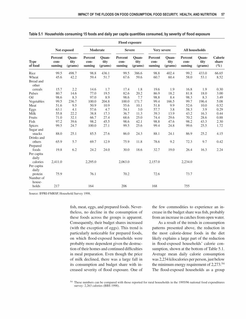
fish, meat, eggs, and prepared foods. Never-theless, no decline in the consumption ofthese foods across the groups is apparent.Consequently, their budget shares increased(with the exception of eggs). This trend isparticularly noticeable for prepared foods,on which flood-exposed households wereprobably more dependent given the destruc-tion of their homes and continued difficultiesin meal preparation. Even though the priceof milk declined, there was a large fall in its consumption and budget share with in-creased severity of flood exposure. One of
the few commodities to experience an in-crease in the budget share was fish, probablyfrom an increase in catches from open water.
As a result of the trends in consumptionpatterns presented above, the reduction inthe most calorie-dense foods in the dietlikely explains a large part of the reductionin flood-exposed households’ calorie con-sumption, shown at the bottom of Table 5.1.Average mean daily calorie consumptionwas 2,234 kilocalories per person, just belowthe minimum energy requirement of 2,273.54
The flood-exposed households as a group
IMPACT OF THE FLOODS ON FOOD CONSUMPTION, FOOD SECURITY, HEALTH, AND NUTRITION 57
Table 5.1 Households consuming 15 foods and daily per capita quantities consumed, by severity of flood exposure
Flood exposure
Not exposed Moderate Severe Very severe All households
Percent Quan- Percent Quan- Percent Quan- Percent Quan- Percent Quan- CalorieType con- tity con- tity con- tity con- tity con- tity shareof food suming (grams) suming (grams) suming (grams) suming (grams) suming (grams) (%)
Rice 99.5 498.7 98.8 436.1 99.5 386.6 98.8 402.4 99.2 433.0 66.65Wheat 45.6 42.2 59.4 51.7 67.6 59.6 60.7 60.4 58.0 53.1 8.52Bread and
other cereals 15.7 2.2 14.6 1.7 17.4 1.8 19.6 1.9 16.8 1.9 0.30
Pulses 80.7 14.6 77.0 19.5 82.6 20.2 86.9 18.2 81.8 18.0 3.00Oil 98.6 8.3 97.0 8.9 98.6 7.7 98.8 8.4 98.3 8.3 3.49Vegetables 99.5 236.7 100.0 204.8 100.0 171.7 99.4 166.5 99.7 196.4 5.08Meat 51.6 9.5 50.9 10.9 55.6 10.1 51.8 9.9 52.6 10.0 0.52Eggs 63.1 4.1 57.6 4.7 54.1 3.0 57.7 3.8 58.3 3.9 0.29Milk 55.8 22.2 38.8 17.3 36.7 11.3 39.3 13.9 43.2 16.3 0.44Fruits 71.0 32.1 66.7 27.4 68.6 25.0 74.4 29.6 70.2 28.6 0.88Fish 97.2 39.6 98.2 45.5 98.6 42.1 98.8 47.6 98.2 43.3 2.30Spices 99.5 24.7 100.0 27.1 99.5 25.6 99.4 24.8 99.6 25.5 1.72Sugar and
snacks 88.0 25.1 85.5 27.6 86.0 24.3 88.1 24.1 86.9 25.2 4.15Drinks and
others 65.9 5.7 69.7 12.9 75.9 11.8 78.6 9.2 72.3 9.7 0.42Prepared
foods 19.8 6.2 24.2 24.0 30.0 18.6 32.7 19.0 26.4 16.3 2.24Per capita
daily calories 2,411.0 2,295.0 2,063.0 2,157.0 2,234.0
Per capita daily protein 75.9 76.1 70.2 72.6 73.7
Number of house-holds 217 164 206 168 755
Source: IFPRI-FMRSP, Household Survey 1998.
54 These numbers can be compared with those reported for rural households in the 1995/96 national food expendituressurvey: 2,263 calories (BBS 1998).
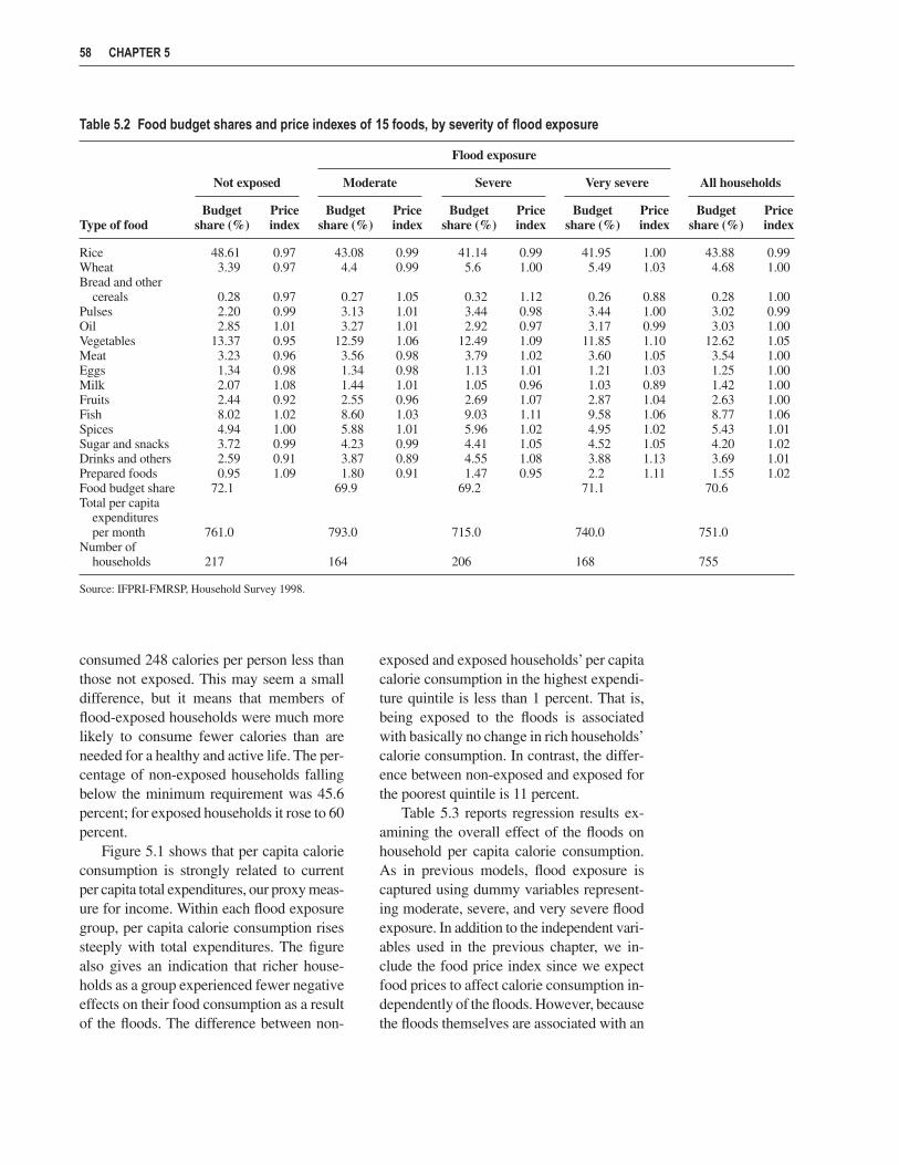
consumed 248 calories per person less thanthose not exposed. This may seem a smalldifference, but it means that members offlood-exposed households were much morelikely to consume fewer calories than areneeded for a healthy and active life. The per-centage of non-exposed households fallingbelow the minimum requirement was 45.6percent; for exposed households it rose to 60percent.
Figure 5.1 shows that per capita calorieconsumption is strongly related to currentper capita total expenditures, our proxy meas-ure for income. Within each flood exposuregroup, per capita calorie consumption risessteeply with total expenditures. The figurealso gives an indication that richer house-holds as a group experienced fewer negativeeffects on their food consumption as a resultof the floods. The difference between non-
exposed and exposed households’ per capitacalorie consumption in the highest expendi-ture quintile is less than 1 percent. That is,being exposed to the floods is associatedwith basically no change in rich households’calorie consumption. In contrast, the differ-ence between non-exposed and exposed forthe poorest quintile is 11 percent.
Table 5.3 reports regression results ex-amining the overall effect of the floods onhousehold per capita calorie consumption.As in previous models, flood exposure iscaptured using dummy variables represent-ing moderate, severe, and very severe floodexposure. In addition to the independent vari-ables used in the previous chapter, we in-clude the food price index since we expectfood prices to affect calorie consumption in-dependently of the floods. However, becausethe floods themselves are associated with an
58 CHAPTER 5
Table 5.2 Food budget shares and price indexes of 15 foods, by severity of flood exposure
Flood exposure
Not exposed Moderate Severe Very severe All households
Budget Price Budget Price Budget Price Budget Price Budget PriceType of food share (%) index share (%) index share (%) index share (%) index share (%) index
Rice 48.61 0.97 43.08 0.99 41.14 0.99 41.95 1.00 43.88 0.99Wheat 3.39 0.97 4.4 0.99 5.6 1.00 5.49 1.03 4.68 1.00Bread and other
cereals 0.28 0.97 0.27 1.05 0.32 1.12 0.26 0.88 0.28 1.00Pulses 2.20 0.99 3.13 1.01 3.44 0.98 3.44 1.00 3.02 0.99Oil 2.85 1.01 3.27 1.01 2.92 0.97 3.17 0.99 3.03 1.00Vegetables 13.37 0.95 12.59 1.06 12.49 1.09 11.85 1.10 12.62 1.05Meat 3.23 0.96 3.56 0.98 3.79 1.02 3.60 1.05 3.54 1.00Eggs 1.34 0.98 1.34 0.98 1.13 1.01 1.21 1.03 1.25 1.00Milk 2.07 1.08 1.44 1.01 1.05 0.96 1.03 0.89 1.42 1.00Fruits 2.44 0.92 2.55 0.96 2.69 1.07 2.87 1.04 2.63 1.00Fish 8.02 1.02 8.60 1.03 9.03 1.11 9.58 1.06 8.77 1.06Spices 4.94 1.00 5.88 1.01 5.96 1.02 4.95 1.02 5.43 1.01Sugar and snacks 3.72 0.99 4.23 0.99 4.41 1.05 4.52 1.05 4.20 1.02Drinks and others 2.59 0.91 3.87 0.89 4.55 1.08 3.88 1.13 3.69 1.01Prepared foods 0.95 1.09 1.80 0.91 1.47 0.95 2.2 1.11 1.55 1.02Food budget share 72.1 69.9 69.2 71.1 70.6Total per capita
expenditures per month 761.0 793.0 715.0 740.0 751.0
Number of households 217 164 206 168 755
Source: IFPRI-FMRSP, Household Survey 1998.
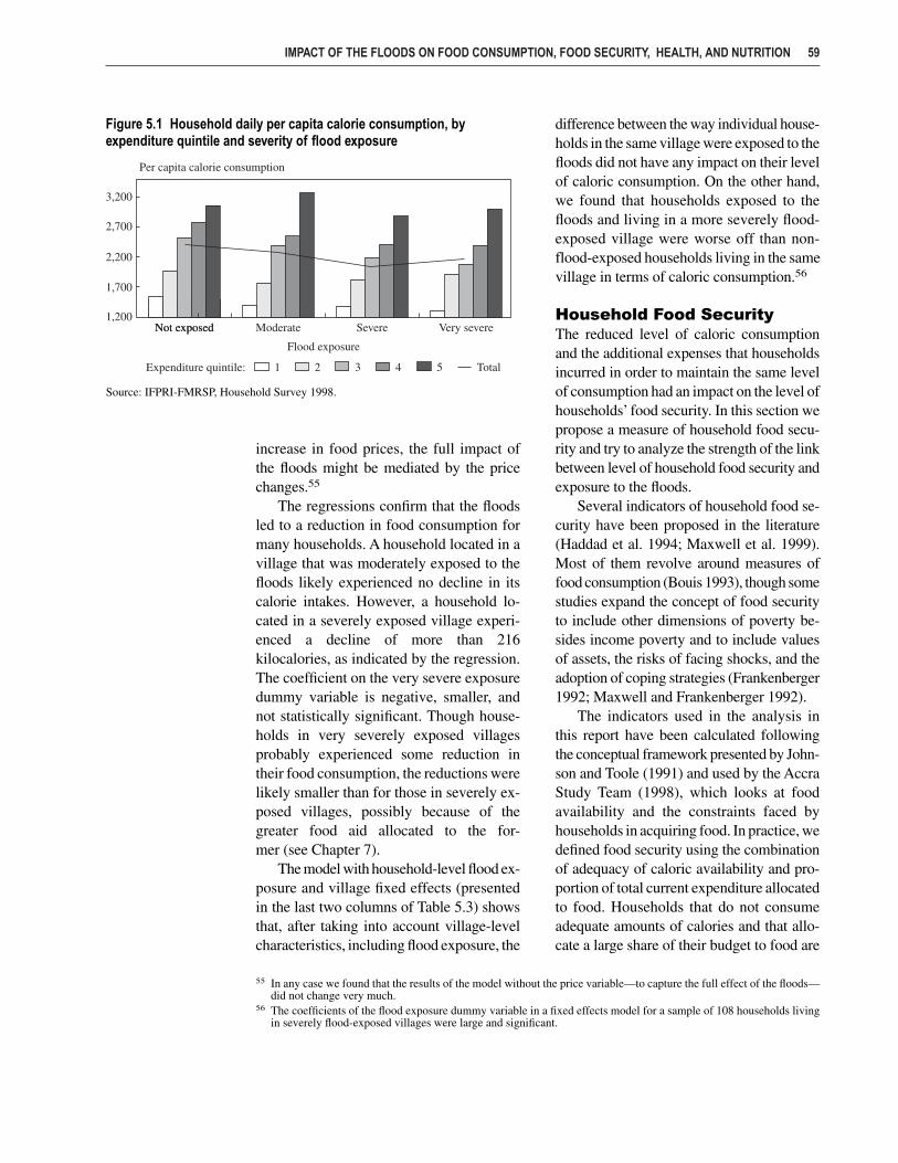
IMPACT OF THE FLOODS ON FOOD CONSUMPTION, FOOD SECURITY, HEALTH, AND NUTRITION 59
Figure 5.1 Household daily per capita calorie consumption, byexpenditure quintile and severity of flood exposure
Source: IFPRI-FMRSP, Household Survey 1998.
55 In any case we found that the results of the model without the price variable—to capture the full effect of the floods—did not change very much.
56 The coefficients of the flood exposure dummy variable in a fixed effects model for a sample of 108 households livingin severely flood-exposed villages were large and significant.
increase in food prices, the full impact ofthe floods might be mediated by the pricechanges.55
The regressions confirm that the floodsled to a reduction in food consumption formany households. A household located in avillage that was moderately exposed to thefloods likely experienced no decline in itscalorie intakes. However, a household lo-cated in a severely exposed village experi-enced a decline of more than 216kilocalories, as indicated by the regression.The coefficient on the very severe exposuredummy variable is negative, smaller, andnot statistically significant. Though house-holds in very severely exposed villagesprobably experienced some reduction intheir food consumption, the reductions werelikely smaller than for those in severely ex-posed villages, possibly because of thegreater food aid allocated to the for-mer (see Chapter 7).
The model with household-level flood ex-posure and village fixed effects (presentedin the last two columns of Table 5.3) showsthat, after taking into account village-levelcharacteristics, including flood exposure, the
difference between the way individual house-holds in the same village were exposed to thefloods did not have any impact on their levelof caloric consumption. On the other hand,we found that households exposed to thefloods and living in a more severely flood-exposed village were worse off than non-flood-exposed households living in the samevillage in terms of caloric consumption.56
Household Food SecurityThe reduced level of caloric consumptionand the additional expenses that householdsincurred in order to maintain the same levelof consumption had an impact on the level ofhouseholds’ food security. In this section wepropose a measure of household food secu-rity and try to analyze the strength of the linkbetween level of household food security andexposure to the floods.
Several indicators of household food se-curity have been proposed in the literature(Haddad et al. 1994; Maxwell et al. 1999).Most of them revolve around measures offood consumption (Bouis 1993), though somestudies expand the concept of food securityto include other dimensions of poverty be-sides income poverty and to include valuesof assets, the risks of facing shocks, and theadoption of coping strategies (Frankenberger1992; Maxwell and Frankenberger 1992).
The indicators used in the analysis inthis report have been calculated followingthe conceptual framework presented by John-son and Toole (1991) and used by the AccraStudy Team (1998), which looks at foodavailability and the constraints faced byhouseholds in acquiring food. In practice, wedefined food security using the combinationof adequacy of caloric availability and pro-portion of total current expenditure allocatedto food. Households that do not consumeadequate amounts of calories and that allo-cate a large share of their budget to food are

defined as food insecure. Similarly, house-holds that consume adequate amounts ofcalories and that allocate a smaller portionof their budget to food are clearly food se-cure. Households that allocate a high propor-tion of their budget to food and that consumeadequate amounts of calories are defined as“vulnerable” because, if the level of total ex-penditure is reduced, their level of caloricconsumption will fall as well, since they havelittle scope for increasing expenditure to meettheir caloric requirements. Finally, house-
holds that do not consume adequate amountsof calories and do not allocate a large portionof their budget to food are defined as “ques-tionable” in regard to food security status.This is because they could increase the levelof expenditure on food to meet their caloricrequirements, but they have other constraintsthat prevent them from doing so or they sim-ply choose not to do so.
The resulting classification of house-holds into the food security categories out-lined above is presented in Figure 5.2 and
60 CHAPTER 5
Table 5.3 Determinants of household daily per capita calorie consumption: Regression results
Household-level flood Village-level exposure with
flood exposure village fixed effects
Coefficient t-statistic Coefficient t-statistic
Female-headed household −599.36 −3.42* −706.81 −4.15*Age of household head −3.77 −0.73 −0.24 −0.06Percent males 0–4 −7.00 −0.51 −5.39 −1.18Percent males 5–14 −3.94 −0.59 −5.14 −1.19Percent males 15–19 −4.68 −0.72 −6.06 −1.18Percent males 20–34 0.05 0.01 0.03 0.01Percent males 35–54 −2.57 −0.55 −3.01 −0.72Percent females 0–4 −13.25 −3.03* −13.02 −3.02*Percent females 5–14 −10.60 −2.55* −10.82 −2.74*Percent females 15–19 −3.95 −0.78 −5.88 −1.17Percent females 20–34 −4.73 −0.85 −5.29 −1.29Percent females 35–54 5.07 1.34 2.41 0.62Household size −110.86 −0.95 −98.83 −1.97*Number of males: Any primary education 36.40 0.80 8.44 0.20Number of males: Any secondary education 52.07 0.93 55.51 0.89Number of females: No education 26.57 0.16 −21.93 −0.25Number of females: Any primary education 49.42 0.29 41.14 0.44Number of females: Any secondary education 76.47 0.44 134.50 1.22Pre-flood value of land (Tk thousand) −0.53 −0.30 −0.39 −0.25Productive asset value (Tk thousand) 78.28 1.88* 89.98 2.69*Liquid asset value (Tk thousand) −4.43 −0.58 −2.40 −0.26Housing asset value (Tk thousand) 39.01 4.03* 31.89 3.03*Domestic asset value (Tk thousand) 178.01 1.24 171.25 1.47Other assets value (Tk thousand) 282.09 1.58 367.69 1.28Food price index −328.77 −0.70 19.91 0.04Moderately flood exposed −10.80 −0.08 3.77 0.03Severely flood exposed −181.80 −1.56 −4.17 −0.03Very severely flood exposed −93.14 −0.65 −49.26 −0.37Constant 3,518.67 7.03* 3,048.38 5.13*R2 .19 .17Number of observations 753 751Number of villages 117 117
Source: IFPRI-FMRSP, Household Survey 1998 and authors’ calculations.
Notes: The food price is represented by an index running from 0.74 to 1.55.* denotes that the coefficient is statistically significant at the 10% level or less.

Tables 5.4 and 5.5. We used a cutoff of 1,818calories, equal to 80 percent of the recom-mended daily intake in Bangladesh (BBS1998), and a cutoff of expenditure allocatedto food equal to 70 percent of the budget(similar to the mean for all households).
Figure 5.2 shows the distribution ofhouseholds above and below the minimumcaloric requirement by their share of expen-diture on food. Looking at the distribution of
households that meet their minimum caloricrequirement, we see that, by allocating an in-creasing share of their budget to food, house-holds are able to maintain an adequate levelof caloric consumption and are thereforemoving from a situation of food security tovulnerability. It is also interesting to note thatover 20 percent of the households allocatebetween 70 and 80 percent of their budget tofood, just past the cutoff of 70 percent.
The distribution of households that donot meet their minimum caloric requirement(Figure 5.2) contains fewer households andtherefore lies under the distribution of house-holds that meet their minimum caloric re-quirement. Moving from right to left in thiscase, we go from households that are foodinsecure towards households that have aquestionable food security status.
It is evident from this graph that a smalladjustment in the cutoff for the budget shareindicator would have a relatively large effecton the number of households classified asfood insecure.
Table 5.4 shows that, although the shareof food expenditure did not change verymuch across categories of flood exposure,the average daily consumption of caloriesdecreased from 2,411 for households notexposed to the floods to 2,097 and 2,158 forhouseholds severely and very severely ex-
IMPACT OF THE FLOODS ON FOOD CONSUMPTION, FOOD SECURITY, HEALTH, AND NUTRITION 61
Figure 5.2 Distribution of households with consumption aboveand below the minimum caloric requirement, by share of expenditureon food
Source: IFPRI-FMRSP, Household Survey 1998.
Table 5.4 Food security by severity of flood exposure
Flood exposure
Not exposed Moderate Severe Very severe Total
Food share of expenditure 72.1 69.9 69.2 71.1 70.6Per capita monthly expenditure 760.9 793.2 715.5 739.8 750.9Per capita daily calories 2,410.7 2,320.3 2,096.7 2,157.2 2,248.9Percent of households spending > 70%
on food 60.4 60.0 54.6 57.1 58.0Percent of households consuming
< 1,818 calories per capita daily 19.4 32.7 38.7 35.7 31.2Food insecure 12.0 15.2 15.5 16.1 14.5Vulnerable 48.4 44.9 39.1 41.1 43.5Food secure 32.3 22.4 22.2 23.2 25.4Questionable 7.4 17.6 23.2 19.6 16.6Number of households 217 165 207 168 757
Source: IFPRI-FMRSP, Household Survey 1998.

posed to the floods, respectively. As a result,only 12.0 percent of the households not ex-posed to the floods are food insecure, com-pared with 16.1 percent of those exposedseverely to the floods, while the percentageof food secure households decreased from32.3 percent for non-exposed households toaround 22 percent for households exposed tothe floods.
The difference in the level of food secu-rity for flood-exposed households acrossexpenditure quintiles is, as expected, quitelarge (Table 5.5). Only 2 percent of the house-holds in the first quintile are food securewhereas practically no households in the toptwo quintiles are food insecure.
To assess the impact of the floods ondifferent levels of food security we ran twosets of models. In the first, we tried to ex-plain the level of each of the outcomes ofthe food security indicators described aboveusing logit models, first using a village-levelflood exposure variable and then using ahousehold-level flood exposure variablewith village random and fixed effects. Inthe second, we modeled the alternativeoutcomes of food security status using amultinomial logit model in which we lookat the probability of food secure house-
holds becoming food insecure, vulnerable,or questionable.
The results of the first set of models(Tables 5.6(a), (b), and (c)) show that theprobability that food security status of house-holds changes to questionable when exposedto the floods increases in all the models.Households exposed to the floods also havea higher probability of being food insecure,even though the coefficient of the modelwith the village-level flood exposure vari-able is significant only with 80 percent prob-ability. Moreover, in the fixed effects modelthe probability that the food security statusof households changes to being secure de-creases, and the probability that it changesto vulnerable increases, if they have beenexposed to the floods. This means that thedifferential flood exposure of householdsfrom the same village had a large impact onthe level of food security.
The results of the multinomial logitmodel (Table 5.7) confirm the results ob-tained above. The probability that the foodsecurity status of food secure householdschanges to questionable or insecure is posi-tive, even though the coefficient of floodexposure for the food insecurity outcome isnot very significant.
62 CHAPTER 5
Table 5.5 Food security by expenditure quintile for flood-exposed households
Quintile 1 Quintile 2 Quintile 3 Quintile 4 Quintile 5 Total
Food share of expenditure 73.2 72.5 71.6 68.5 63.9 70.0Per capita monthly
expenditure 343.1 505.8 648.9 842.6 1434.3 746.8Per capita daily calories 1,367.6 1,836.5 2,194.8 2,460.8 3,140.4 2,183.8Percent of households
spending > 70% on food 66.4 59.3 66.0 50.5 0.4 0.6
Percent of households consuming < 1,818 calories per capita daily 79.7 50.4 24.5 12.9 0.1 0.4
Food insecure 47.8 16.8 9.4 0.0 0.9 15.6Vulnerable 18.6 42.5 56.6 50.5 41.1 41.5Food secure 1.8 7.1 18.9 36.6 51.4 22.6Questionable 31.9 33.6 15.1 12.9 6.5 20.4Number of households 113 113 106 101 107 540
Source: IFPRI-FMRSP, Household Survey 1998.
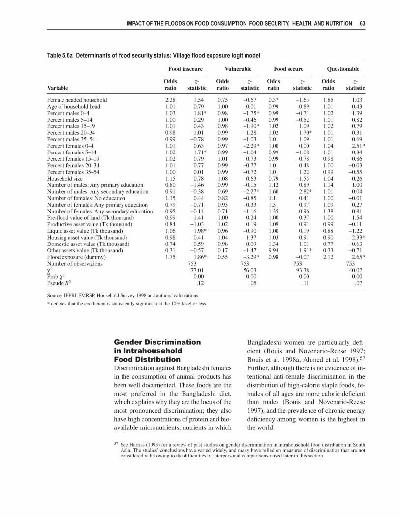
Gender Discrimination in Intrahousehold Food DistributionDiscrimination against Bangladeshi femalesin the consumption of animal products hasbeen well documented. These foods are themost preferred in the Bangladeshi diet,which explains why they are the locus of themost pronounced discrimination; they alsohave high concentrations of protein and bio-available micronutrients, nutrients in which
Bangladeshi women are particularly defi-cient (Bouis and Novenario-Reese 1997;Bouis et al. 1998a; Ahmed et al. 1998).57
Further, although there is no evidence of in-tentional anti-female discrimination in thedistribution of high-calorie staple foods, fe-males of all ages are more calorie deficientthan males (Bouis and Novenario-Reese1997), and the prevalence of chronic energydeficiency among women is the highest inthe world.
IMPACT OF THE FLOODS ON FOOD CONSUMPTION, FOOD SECURITY, HEALTH, AND NUTRITION 63
Table 5.6a Determinants of food security status: Village flood exposure logit model
Food insecure Vulnerable Food secure Questionable
Odds z- Odds z- Odds z- Odds z-Variable ratio statistic ratio statistic ratio statistic ratio statistic
Female headed household 2.28 1.54 0.75 −0.67 0.37 −1.63 1.85 1.03Age of household head 1.01 0.79 1.00 −0.01 0.99 −0.89 1.01 0.43Percent males 0–4 1.03 1.81* 0.98 −1.75* 0.99 −0.71 1.02 1.39Percent males 5–14 1.00 0.29 1.00 −0.46 0.99 −0.52 1.01 0.82Percent males 15–19 1.01 0.43 0.98 −1.90* 1.02 1.09 1.02 0.79Percent males 20–34 0.98 −1.01 0.99 −1.28 1.02 1.70* 1.01 0.31Percent males 35–54 0.99 −0.78 0.99 −1.03 1.01 1.09 1.01 0.69Percent females 0–4 1.01 0.63 0.97 −2.29* 1.00 0.00 1.04 2.51*Percent females 5–14 1.02 1.71* 0.99 −1.04 0.99 −1.08 1.01 0.84Percent females 15–19 1.02 0.79 1.01 0.73 0.99 −0.78 0.98 −0.86Percent females 20–34 1.01 0.77 0.99 −0.77 1.01 0.48 1.00 −0.03Percent females 35–54 1.00 0.01 0.99 −0.72 1.01 1.22 0.99 −0.55Household size 1.15 0.78 1.08 0.63 0.79 −1.55 1.04 0.26Number of males: Any primary education 0.80 −1.46 0.99 −0.15 1.12 0.89 1.14 1.00Number of males: Any secondary education 0.91 −0.38 0.69 −2.27* 1.60 2.82* 1.01 0.04Number of females: No education 1.15 0.44 0.82 −0.85 1.11 0.41 1.00 −0.01Number of females: Any primary education 0.79 −0.71 0.93 −0.33 1.31 0.97 1.09 0.27Number of females: Any secondary education 0.95 −0.11 0.71 −1.16 1.35 0.96 1.38 0.81Pre-flood value of land (Tk thousand) 0.99 −1.41 1.00 −0.24 1.00 0.37 1.00 1.54Productive asset value (Tk thousand) 0.84 −1.03 1.02 0.19 1.09 0.91 0.99 −0.11Liquid asset value (Tk thousand) 1.06 1.98* 0.96 −0.90 1.00 0.19 0.88 −1.22Housing asset value (Tk thousand) 0.98 −0.41 1.04 1.37 1.03 0.91 0.90 −2.33*Domestic asset value (Tk thousand) 0.74 −0.59 0.98 −0.09 1.34 1.01 0.77 −0.63Other assets value (Tk thousand) 0.31 −0.57 0.17 −1.47 9.94 1.91* 0.33 −0.71Flood exposure (dummy) 1.75 1.86* 0.55 −3.29* 0.98 −0.07 2.12 2.65*Number of observations 753 753 753 753χ2 77.01 56.03 93.38 40.02Prob χ2 0.00 0.00 0.00 0.00Pseudo R2 .12 .05 .11 .07
Source: IFPRI-FMRSP, Household Survey 1998 and authors’ calculations.
* denotes that the coefficient is statistically significant at the 10% level or less.
57 See Harriss (1995) for a review of past studies on gender discrimination in intrahousehold food distribution in SouthAsia. The studies’ conclusions have varied widely, and many have relied on measures of discrimination that are notconsidered valid owing to the difficulties of interpersonal comparisons raised later in this section.
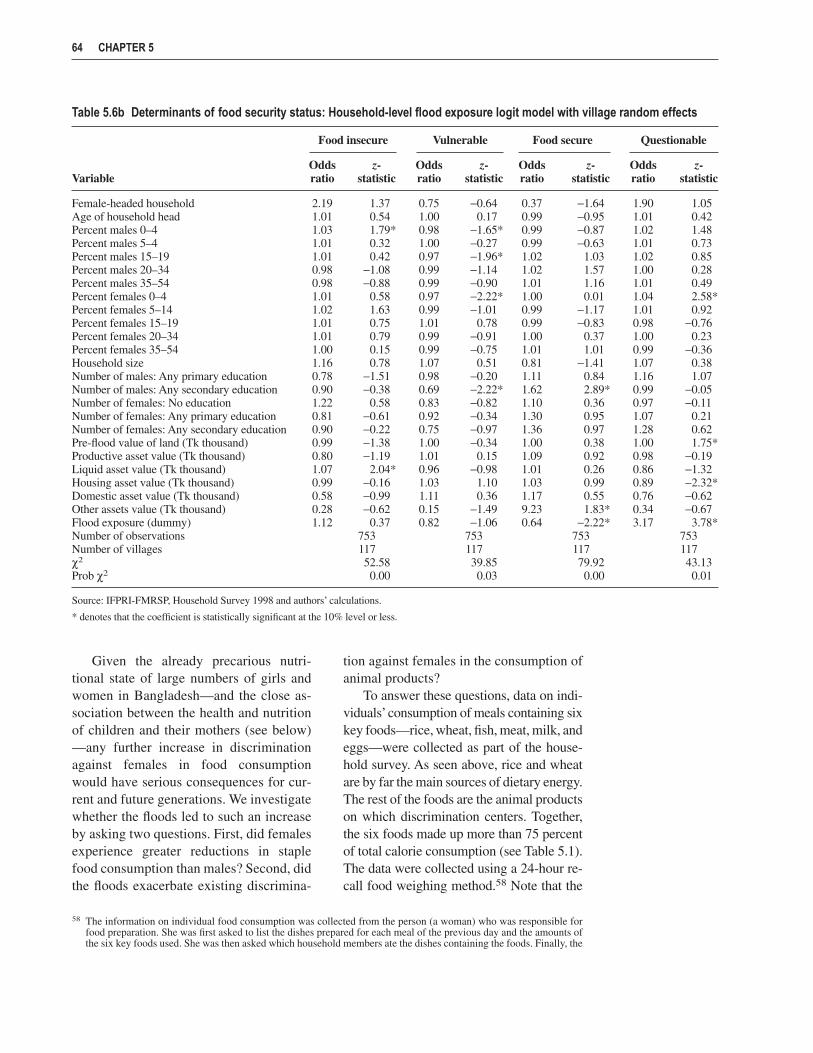
Given the already precarious nutri-tional state of large numbers of girls andwomen in Bangladesh—and the close as-sociation between the health and nutritionof children and their mothers (see below)—any further increase in discriminationagainst females in food consumptionwould have serious consequences for cur-rent and future generations. We investigatewhether the floods led to such an increaseby asking two questions. First, did femalesexperience greater reductions in staplefood consumption than males? Second, didthe floods exacerbate existing discrimina-
tion against females in the consumption ofanimal products?
To answer these questions, data on indi-viduals’consumption of meals containing sixkey foods—rice, wheat, fish, meat, milk, andeggs—were collected as part of the house-hold survey. As seen above, rice and wheatare by far the main sources of dietary energy.The rest of the foods are the animal productson which discrimination centers. Together,the six foods made up more than 75 percentof total calorie consumption (see Table 5.1).The data were collected using a 24-hour re-call food weighing method.58 Note that the
64 CHAPTER 5
Table 5.6b Determinants of food security status: Household-level flood exposure logit model with village random effects
Food insecure Vulnerable Food secure Questionable
Odds z- Odds z- Odds z- Odds z-Variable ratio statistic ratio statistic ratio statistic ratio statistic
Female-headed household 2.19 1.37 0.75 −0.64 0.37 −1.64 1.90 1.05Age of household head 1.01 0.54 1.00 0.17 0.99 −0.95 1.01 0.42Percent males 0–4 1.03 1.79* 0.98 −1.65* 0.99 −0.87 1.02 1.48Percent males 5–4 1.01 0.32 1.00 −0.27 0.99 −0.63 1.01 0.73Percent males 15–19 1.01 0.42 0.97 −1.96* 1.02 1.03 1.02 0.85Percent males 20–34 0.98 −1.08 0.99 −1.14 1.02 1.57 1.00 0.28Percent males 35–54 0.98 −0.88 0.99 −0.90 1.01 1.16 1.01 0.49Percent females 0–4 1.01 0.58 0.97 −2.22* 1.00 0.01 1.04 2.58*Percent females 5–14 1.02 1.63 0.99 −1.01 0.99 −1.17 1.01 0.92Percent females 15–19 1.01 0.75 1.01 0.78 0.99 −0.83 0.98 −0.76Percent females 20–34 1.01 0.79 0.99 −0.91 1.00 0.37 1.00 0.23Percent females 35–54 1.00 0.15 0.99 −0.75 1.01 1.01 0.99 −0.36Household size 1.16 0.78 1.07 0.51 0.81 −1.41 1.07 0.38Number of males: Any primary education 0.78 −1.51 0.98 −0.20 1.11 0.84 1.16 1.07Number of males: Any secondary education 0.90 −0.38 0.69 −2.22* 1.62 2.89* 0.99 −0.05Number of females: No education 1.22 0.58 0.83 −0.82 1.10 0.36 0.97 −0.11Number of females: Any primary education 0.81 −0.61 0.92 −0.34 1.30 0.95 1.07 0.21Number of females: Any secondary education 0.90 −0.22 0.75 −0.97 1.36 0.97 1.28 0.62Pre-flood value of land (Tk thousand) 0.99 −1.38 1.00 −0.34 1.00 0.38 1.00 1.75*Productive asset value (Tk thousand) 0.80 −1.19 1.01 0.15 1.09 0.92 0.98 −0.19Liquid asset value (Tk thousand) 1.07 2.04* 0.96 −0.98 1.01 0.26 0.86 −1.32Housing asset value (Tk thousand) 0.99 −0.16 1.03 1.10 1.03 0.99 0.89 −2.32*Domestic asset value (Tk thousand) 0.58 −0.99 1.11 0.36 1.17 0.55 0.76 −0.62Other assets value (Tk thousand) 0.28 −0.62 0.15 −1.49 9.23 1.83* 0.34 −0.67Flood exposure (dummy) 1.12 0.37 0.82 −1.06 0.64 −2.22* 3.17 3.78*Number of observations 753 753 753 753Number of villages 117 117 117 117χ2 52.58 39.85 79.92 43.13Prob χ2 0.00 0.03 0.00 0.01
Source: IFPRI-FMRSP, Household Survey 1998 and authors’ calculations.
* denotes that the coefficient is statistically significant at the 10% level or less.
58 The information on individual food consumption was collected from the person (a woman) who was responsible forfood preparation. She was first asked to list the dishes prepared for each meal of the previous day and the amounts ofthe six key foods used. She was then asked which household members ate the dishes containing the foods. Finally, the

data used here are the quantities, measuredin grams, that people consumed of “dishes”containing the six foods rather than of thefoods themselves. For rice and wheat, thedishes generally contained only that one food.For the other foods, one dish (for example,fish curry) may have contained other ingre-dients as well (for example, vegetables oroil).59 The sample consisted of 1,613 femalesand 1,647 males over the age of three years.
Turning first to the main staples, Figure5.3(a) shows how female and male con-sumption of rice and wheat combined variesacross the flood exposure severity groups.Both male and female consumption de-clined across the groups. Male consumptionfell precipitously with moderate and severeexposure. Female consumption declinedfrom the non-exposed to the moderately ex-posed group and then remained flat. Table
IMPACT OF THE FLOODS ON FOOD CONSUMPTION, FOOD SECURITY, HEALTH, AND NUTRITION 65
Table 5.6c Determinants of food security status: Household-level flood exposure logit model with village fixed effects
Food insecure Vulnerable Food secure Questionable
Odds z- Odds z- Odds z- Odds z-Variable ratio statistic ratio statistic ratio statistic ratio statistic
Female-headed household 2.11 1.08 0.53 −1.28 0.52 −0.98 2.10 1.05Age of household head 1.00 −0.15 1.01 0.97 1.00 0.07 0.99 −0.48Percent males 0–4 1.04 1.63 0.98 −1.68* 0.99 −0.71 1.02 1.21Percent males 5–14 1.01 0.51 1.00 −0.03 0.99 −0.88 1.00 0.22Percent males 15–19 1.00 0.09 0.97 −2.30* 1.02 1.17 1.02 1.02Percent males 20–34 0.98 −0.84 0.99 −1.01 1.03 1.69* *0.99 −0.30Percent males 35–54 0.98 −0.92 0.99 −0.89 1.02 1.61 1.00 −0.23Percent females 0–4 1.00 0.04 0.98 −1.89* 1.00 0.18 1.03 1.96*Percent females 5–14 1.02 1.26 0.99 −1.25 0.99 −0.79 1.01 0.67Percent females 15–19 1.01 0.61 1.01 0.53 1.00 −0.30 0.99 −0.67Percent females 20–34 1.01 0.71 0.98 −1.55 1.01 0.94 1.01 0.50Percent females 35–54 1.02 0.83 0.99 −1.28 1.01 0.67 1.00 −0.08Household size 1.05 0.20 1.16 1.07 0.75 −1.49 1.08 0.39Number of males: Any primary education 0.74 −1.48 0.92 −0.74 1.20 1.26 1.18 1.07Number of males: Any secondary education 0.90 −0.35 0.68 −2.12* 1.88 3.10* 0.96 −0.17Number of females: No education 1.57 1.16 0.77 −1.04 1.07 0.20 0.97 −0.08Number of females: Any primary education 0.92 −0.22 0.90 −0.40 1.26 0.69 0.99 −0.02Number of females: Any secondary education 0.84 −0.35 0.84 −0.55 1.48 1.04 1.25 0.53Pre-flood value of land (Tk thousand) 0.98 −1.49 1.00 −0.09 1.00 0.03 1.01 1.74*Productive asset value (Tk thousand) 0.75 −1.31 1.01 0.10 1.20 1.44 0.97 −0.24Liquid asset value (Tk thousand) 1.07 1.90* 0.93 −1.13 1.01 0.22 0.89 −0.95Housing asset value (Tk thousand) 1.01 0.19 1.02 0.66 1.02 0.49 0.89 −1.98*Domestic asset value (Tk thousand) 0.72 −0.50 0.82 −0.61 1.38 0.89 0.78 −0.45Other assets value (Tk thousand) 0.11 −0.80 0.18 −1.34 4.11 1.35 0.14 −1.03Flood exposure (dummy) 0.46 −1.43 1.69 1.72* 0.53 −1.96* 2.17 1.71*Number of observations 444 717 657 485Number of villages 69 111 101 75χ2 73.56 53.18 101.37 36.39Prob χ2 0.00 0.00 0.00 0.07
Source: IFPRI-FMRSP, Household Survey 1998 and authors’ calculations.
* denotes that the coefficient is statistically significant at the 10% level or less.
amount eaten of the dishes by each member was determined using direct food weighing or standardized tables of por-tion weights by portion size. If any member was not present at a meal, that person was interviewed to determine thequantities eaten of the six foods. If the person was not available for interview, then the primary respondent was askedto estimate the amount they had eaten.
59 Because our measures of differences between people in food consumption do not rely on direct comparisons of quan-tities or nutrients consumed, this factor does not affect the results of the analysis.

5.8 reports regression results examiningwhether the floods had a differential impacton male and female consumption. Thehousehold-level measure of flood exposurewith village fixed effects specification isemployed. The results confirm that thefloods led to declines in staple food con-sumption for both males and females in allexposure groups, with the greatest declinesbeing associated with moderate exposure.Using the regression coefficients, we esti-mate that the staple consumption of the av-
erage male living in a flood-exposed house-hold declined by 13.6 percent; that of the av-erage female declined by 8.4 percent.60
Thus, for the most important source of calo-ries in the diet, female consumption likelydid not decline by more than that of males.In fact, the opposite may have occurred.This indicates that, after a major disastersuch as the floods, interventions targeted di-rectly to flood-exposed households inBangladesh can be very effective in in-creasing their consumption of staple foods.
66 CHAPTER 5
Table 5.7 Determinants of food security status: Village-level flood exposure multinomial logit model
Questionable Vulnerable Food insecure
Variable Odds ratio z-statistic Odds ratio z-statistic Odds ratio z-statistic
Female-headed household 4.21 1.80* 1.95 1.03 4.59 2.02*Age of household head 1.01 0.89 1.01 0.66 1.02 1.12Percent males 0–4 1.03 1.50 1.00 −0.20 1.03 1.71*Percent males 5–14 1.02 0.92 1.00 0.22 1.01 0.50Percent males 15–19 1.00 0.15 0.98 −1.51 1.00 −0.15Percent males 20–34 0.99 −0.52 0.98 −1.65* 0.97 −1.61Percent males 35–54 1.00 0.05 0.99 −1.13 0.98 −1.13Percent females 0–4 1.03 1.83* 0.99 −1.11 1.01 0.57Percent females 5–14 1.02 1.29 1.00 0.37 1.03 1.84*Percent females 15–19 0.99 −0.24 1.01 0.86 1.02 1.01Percent females 20–34 1.00 −0.24 0.99 −0.64 1.01 0.36Percent females 35–54 0.98 −0.99 0.99 −1.14 0.99 −0.64Household size 1.24 1.05 1.25 1.36 1.36 1.40Number of males: Any primary education 1.01 0.07 0.90 −0.82 0.75 −1.59Number of males: Any secondary education 0.74 −1.26 0.59 −2.84* 0.66 −1.44Number of females: No education 0.95 −0.15 0.85 −0.58 1.03 0.09Number of females: Any primary education 0.87 −0.38 0.78 −0.82 0.66 −1.04Number of females: Any secondary education 1.05 0.12 0.67 −1.18 0.77 −0.51Pre-flood value of land (Tk thousand) 1.01 0.98 1.00 −0.33 0.99 −1.36Productive asset value (Tk thousand) 0.93 −0.54 0.94 −0.64 0.79 −1.24Liquid asset value (Tk thousand) 0.87 −1.21 0.97 −0.69 1.04 1.40Housing asset value (Tk thousand) 0.89 −2.25* 1.00 0.17 0.96 −0.72Domestic asset value (Tk thousand) 0.66 −0.90 0.83 −0.61 0.61 −0.87Other assets value (Tk thousand) 0.14 −1.05 0.09 −1.72* 0.09 −0.98Flood exposure (dummy) 2.00 2.14* 0.75 −1.28 1.69 1.52Number of observations 753LR χ2 206.61Prob > χ2 0.00Pseudo R2 .11
Source: IFPRI-FMRSP, Household Survey 1998 and authors’ calculations.
Note: The base is food security.* denotes that the coefficient is statistically significant at the 10% level or less.
60 These percentages are calculated using a weighted average of the coefficients for the flood exposure severity dummyvariable, where the weights are the proportion of flood-exposed individuals falling into each group.

changed across the flood exposure groups.The latter three foods are grouped togetherbecause of the small numbers of householdsin which they are consumed on a daily basis.As would be expected, male consumptionwas always higher than female consump-tion. Male consumption of fish-containingmeals declined more steeply with flood ex-posure severity than female consumption.Consumption of the three non-fish animalproducts declined across the groups for bothmales and females, but the disparity betweenmale and female consumption was wider forthe very severe exposure group than for thenot-exposed group.
Although these figures are revealing,deliberate discrimination in food consump-tion (or a change in its degree) is difficult todetect by directly comparing nutrient or foodconsumption across groups of people. Prob-lems arise because people of differentgenders, sizes, and activity patterns have dif-ferent consumption requirements, whichare not known for certain (Bouis andNovenario-Reese 1997). Further, a person orgroup of people could eat less food thanneeded simply because they and otherhousehold members are not aware of theirrequirements.
To determine whether the floods led toan increase in discrimination against fe-males in animal product consumption, weused two measures. The first indicates sim-ply whether or not a person consumed aparticular food. The average of the measurefor a group then gives the group’s con-sumption incidence of that food. If the fe-male consumption incidence fell by morethan the male incidence as a consequence ofthe floods, this is telling evidence that dis-crimination in the consumption of that foodhas increased. A second measure, based onthe approach of Bouis et al. (1998b), com-pares the proportions consumed of differ-ent foods across individuals in their ownhousehold. The Individual Relative Con-sumption Share (IRCS) is a ratio of the pro-portion an individual consumes of a food
IMPACT OF THE FLOODS ON FOOD CONSUMPTION, FOOD SECURITY, HEALTH, AND NUTRITION 67
Figure 5.3 Female and male consumption of mealscontaining six staple foods, by severity of flood exposure
a. Rice plus wheat
b. Fish-containing dishes
c. Meat-, egg-, and milk-containing dishes
Turning next to flood impacts on individ-uals’ consumption of animal products, Fig-ures 5.3(b) and 5.3(c) show how female andmale consumption of meals containing fishand those containing meat, eggs, or milk

to the average proportion for all members oftheir household. If the person’s proportion isgreater than the average for a particular food(IRCS > 1), they are considered favored in
the consumption of that food; if it is less(IRCS < 1), they are disfavored.61 A thirdmeasure of whether or not male favoritismexists in a household can then be con-
68 CHAPTER 5
Table 5.8 Determinants of female and male consumption of main staples: Regression results(household-level flood exposure with village fixed effects)
Female Male
Coefficient t-statistic Coefficient t-statistic
Female-headed household 68.90 0.73 110.91 0.79Age of household head −2.19 −1.30 −1.09 −0.55Percent males 5–14 −4.24 −2.64* −0.06 −0.03Percent males 15–19 0.58 0.28 6.95 2.93*Percent males 20–34 −0.03 −0.02 4.69 2.09*Percent males 35–54 0.30 0.13 2.18 0.78Percent males 55+ −0.47 −0.16 2.58 0.77Percent females 0–4 −3.63 −2.18* −0.28 −0.13Percent females 5–14 −3.03 −1.87* −2.19 −1.09Percent females 15–19 −0.79 −0.36 −3.68 −1.33Percent females 20–34 1.14 0.51 1.75 0.63Percent females 35–54 −0.49 −0.22 2.76 1.01Percent females 55+ −1.86 −0.81 −1.80 −0.65Household size 23.95 3.18* 15.39 1.73*Household has educated female 84.65 2.65* 126.10 3.37*Household has educated male −1.07 −0.03 −90.78 −2.19*Pre-flood asset value (Tk thousand) 6.53 2.69* 6.53 2.28*Age 33.48 15.29* 59.27 22.84*Age-squared −0.44 −13.56* −0.72 −19.08*Flood exposure
Moderate −138.18 −2.82* −263.21 −4.41*Severe −90.69 −1.79* −242.38 −3.96*Very severe −116.73 −2.09* −175.96 −2.64*
R2 .169 .316Prob > F 0.000 0.000Significance of village effects (p-value) .000 .000Number of observations 1,613 1,647Number of villages 117 117
Source: IFPRI-FMRSP, Household Survey 1998 and authors’ calculations.
Note: The dependent variable is grams of cooked rice + grams of cooked wheat.* denotes that the coefficient is statistically significant at the 10% level or less.
61 More formally, the individual relative consumption share of any household member i = 1, . . . , n, for food j = 1, . . . ,k, where k is the number of foods in the diet, is defined as:
Xij———–
Σk
j=1Xi
jICRSi
j = ———–, j = 1, . . . k; i = 1, . . . , n.Σn
i=1Xi
j———–
Σn
iΣk
jXi
j
This differs from Bouis et al.’s (1998b) measure, called “Food share over energy share” (FE/ES), in two ways: (a) thenumerator of the FS/ES measure is the individual proportion of total household consumption of a food and the de-nominator is the individual proportion of total household consumption of all foods combined; (b) the FS/ES measureuses calories in the denominator ratio under the presumption that households will maintain relative equality in hungersatiation across their members. We cannot do that here because we have information only on the dishes, for which acalorie conversion is not possible, rather than on the foods. In the absence of the difference due to (b), the two meas-ures are mathematically equivalent.
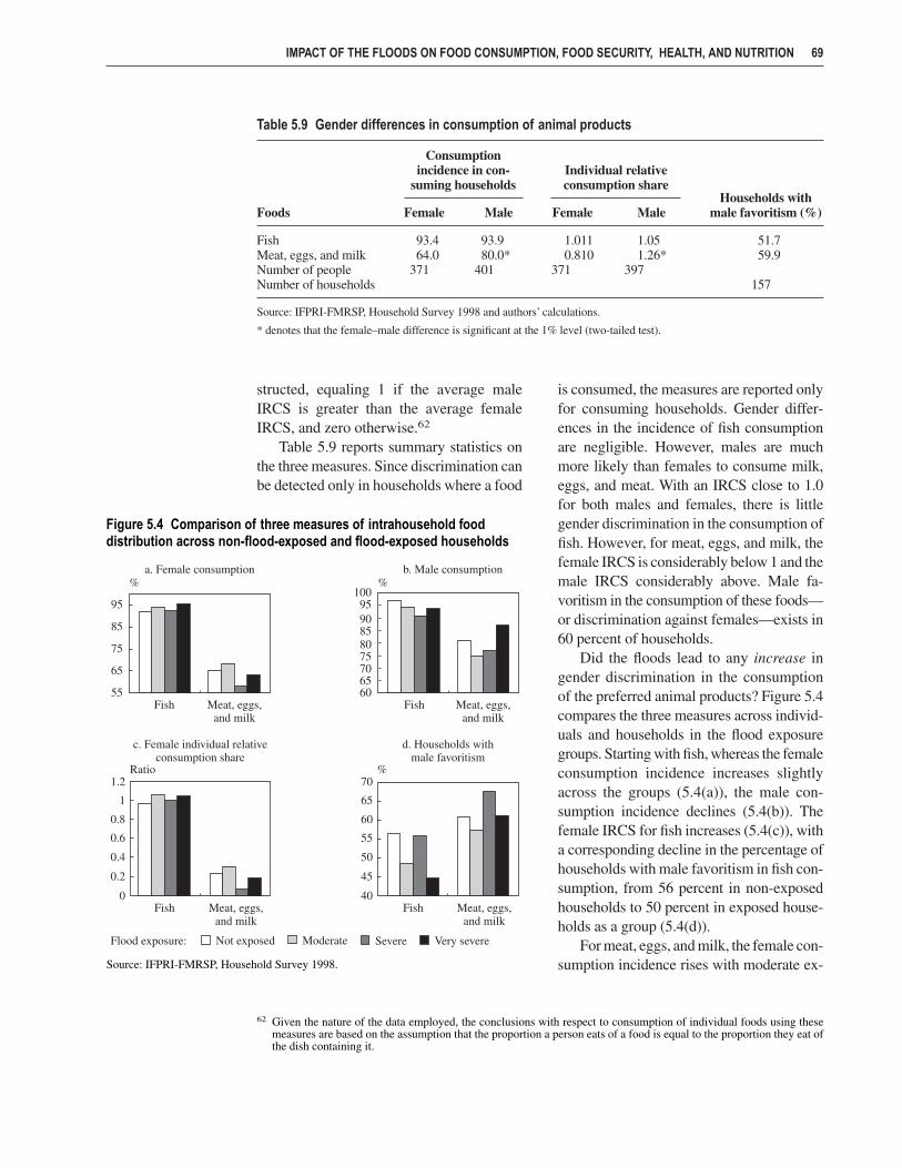
structed, equaling 1 if the average maleIRCS is greater than the average femaleIRCS, and zero otherwise.62
Table 5.9 reports summary statistics onthe three measures. Since discrimination canbe detected only in households where a food
is consumed, the measures are reported onlyfor consuming households. Gender differ-ences in the incidence of fish consumptionare negligible. However, males are muchmore likely than females to consume milk,eggs, and meat. With an IRCS close to 1.0for both males and females, there is littlegender discrimination in the consumption offish. However, for meat, eggs, and milk, thefemale IRCS is considerably below 1 and themale IRCS considerably above. Male fa-voritism in the consumption of these foods—or discrimination against females—exists in60 percent of households.
Did the floods lead to any increase ingender discrimination in the consumptionof the preferred animal products? Figure 5.4compares the three measures across individ-uals and households in the flood exposuregroups. Starting with fish, whereas the femaleconsumption incidence increases slightlyacross the groups (5.4(a)), the male con-sumption incidence declines (5.4(b)). Thefemale IRCS for fish increases (5.4(c)), witha corresponding decline in the percentage ofhouseholds with male favoritism in fish con-sumption, from 56 percent in non-exposedhouseholds to 50 percent in exposed house-holds as a group (5.4(d)).
For meat, eggs, and milk, the female con-sumption incidence rises with moderate ex-
IMPACT OF THE FLOODS ON FOOD CONSUMPTION, FOOD SECURITY, HEALTH, AND NUTRITION 69
Table 5.9 Gender differences in consumption of animal products
Consumptionincidence in con- Individual relative
suming households consumption shareHouseholds with
Foods Female Male Female Male male favoritism (%)
Fish 93.4 93.9 1.011 1.05 51.7Meat, eggs, and milk 64.0 80.0* 0.810 1.26* 59.9Number of people 371 401 371 397Number of households 157
Source: IFPRI-FMRSP, Household Survey 1998 and authors’ calculations.
* denotes that the female–male difference is significant at the 1% level (two-tailed test).
Figure 5.4 Comparison of three measures of intrahousehold fooddistribution across non-flood-exposed and flood-exposed households
62 Given the nature of the data employed, the conclusions with respect to consumption of individual foods using thesemeasures are based on the assumption that the proportion a person eats of a food is equal to the proportion they eat ofthe dish containing it.
Source: IFPRI-FMRSP, Household Survey 1998.

posure but then declines with severe andvery severe exposure. The male incidencefalls but then rises for the very severe group.The female IRCS shows a consistent declin-ing trend. There is a corresponding increasein the percentage of households with malefavoritism. These descriptive results suggestno increase in discrimination against fe-males in the consumption of fish (and per-haps a decrease) but a slight increase indiscrimination in the consumption of themeat, eggs, and milk, which are among themost preferred foods.
Table 5.10 presents the results of thelogit model, in which we examine whetherthe same findings are evident when indi-vidual, household, and village characteris-tics are controlled for. The dependentvariables are (1) whether or not an individ-ual consumed the food, for both males andfemales,63 and (2) whether or not malefavoritism in the consumption of the food
exists in a household. Because of insuffi-cient variation in consumption incidencesamong individuals of the same genderwithin villages, it is possible to employonly the village-level flood exposure meas-ure in these regressions. The household-level flood exposure measure is employedin male favoritism regressions.
The results confirm that the male likeli-hood of consuming fish declined as a resultof the floods, but only in severely exposedvillages. They indicate no change in the fe-male likelihood. Further, the likelihood ofmale favoritism in the consumption of fishdeclined for very severely exposed house-holds. In the case of meat, eggs, and milk, theregression results detect no change in theconsumption incidences for either femalesor males. However, they detect a decline inmale favoritism in the consumption of thesefoods in severely flood-exposed households,contrary to the pattern of Figure 5.4(d).
70 CHAPTER 5
Table 5.10 Impact of flooding on gender-based discrimination in consumption of fish, meat, eggs, and milk: Summary ofregression results
Likelihood ofLikelihood of consuming protein fooda
male favoritismbFemale Male
Flood exposure Odds ratio z-statistic Odds ratio z-statistic Odds ratio z-statistic
FishModerate 1.59 1.24 1.35 0.75 0.84 −0.42Severe 0.75 −0.96 0.53 2.01* 0.74 −0.69Very severe 0.78 −0.66 0.60 −1.38 0.38 −2.06*Prob > χ2 0.47 0.08 0.07Number of people 1,170 1,203Number of households 458
Meat, milk, and eggsModerate 1.55 1.31 0.77 −0.75 0.92 −0.13Severe 1.08 0.27 0.83 −0.57 0.30 −2.14*Very severe 1.14 0.33 1.87 1.15 1.43 0.44Prob > χ2 0.02 0.35 0.00Number of people 369 396Number of households 53
Source: IFPRI-FMRSP, Household Survey 1998 and authors’ calculations.a Village-level flood exposure.b Household flood exposure with village fixed effects.* denotes that the coefficient is statistically significant at the 10% level or less.
63 In addition to the independent variables included in previous regressions, here we include the age and age-squared ofthe individual.
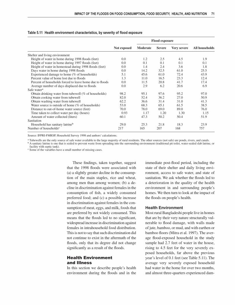
These findings, taken together, suggestthat the 1998 floods were associated with(a) a slightly greater decline in the consump-tion of the main staples, rice and wheat,among men than among women; (b) a de-cline in discrimination against females in theconsumption of fish, a widely consumedpreferred food; and (c) a possible increasein discrimination against females in the con-sumption of meat, eggs, and milk, foods thatare preferred by not widely consumed. Thismeans that the floods led to no significant,widespread increase in discrimination againstfemales in intrahousehold food distribution.This is not to say that such discrimination didnot continue to exist in the aftermath of thefloods, only that its degree did not changesignificantly as a result of the floods.
Health Environment and IllnessIn this section we describe people’s healthenvironment during the floods and in the
immediate post-flood period, including thestate of their shelter and daily living envi-ronment, access to safe water, and state ofsanitation. We ask whether the floods led toa deterioration in the quality of the healthenvironment in and surrounding people’shomes. We then turn to look at the impact ofthe floods on people’s health.
Health EnvironmentMost rural Bangladeshi people live in homesthat are by their very nature structurally vul-nerable to flood damage, with walls madeof jute, bamboo, or mud, and with earthen orbamboo floors (Mitra et al. 1997). The aver-age flood-exposed household in the studysample had 2.7 feet of water in the house,rising to 4.5 feet for the very severely ex-posed households, far above the previousyear’s level of 0.1 feet (see Table 5.11). Theaverage very severely exposed householdhad water in the home for over two months,and almost three-quarters experienced dam-
IMPACT OF THE FLOODS ON FOOD CONSUMPTION, FOOD SECURITY, HEALTH, AND NUTRITION 71
Table 5.11 Health environment characteristics, by severity of flood exposure
Flood exposure
Not exposed Moderate Severe Very severe All households
Shelter and living environmentHeight of water in home during 1998 floods (feet) 0.0 1.2 2.5 4.5 1.9Height of water in home during 1997 floods (feet) 0.0 0.1 0.1 0.1 0.1Height of water in homestead during 1998 floods (feet) 0.0 1.4 2.4 3.6 1.8Days water in home during 1998 floods 0.0 14.2 32.5 61.0 25.5Experienced damage to home (% of households) 5.1 45.6 61.0 72.4 43.9Percent value of home lost due to floods 1.3 11.0 16.5 23.3 12.4Percent of households forced to leave home due to floods 0.0 11.5 20.8 41.7 17.4Average number of days displaced due to floods 0.0 2.9 6.2 20.6 6.9
Safe watera
Obtain drinking water from tubewell (% of households) 98.2 95.1 97.6 95.2 97.0Obtain cooking water from tubewell 82.0 52.4 36.2 27.0 50.9Obtain washing water from tubewell 62.2 36.6 31.4 31.0 41.3Water source is outside of home (% of households) 53.0 68.3 65.1 61.5 38.5Distance to out-of-home water source (feet) 70.0 78.0 69.0 89.0 76.0Time taken to collect water per day (hours) 0.93 1.17 1.20 1.30 1.15Amount of water collected (liters) 60.1 47.3 50.2 50.4 51.9
SanitationHousehold has sanitary latrineb 29.0 25.3 21.8 18.3 23.9
Number of householdsc 217 165 207 168 757
Source: IFPRI-FMRSP, Household Survey 1998 and authors’ calculations.a Tubewells are the only source of safe water available to the large majority of rural residents. The other sources (not safe) are ponds, rivers, and canals.b A sanitary latrine is one that is sealed to prevent waste from spreading into the surrounding environment (traditional pit toilet, water-sealed slab latrine, or
facility with septic tank).c Some of the variables have a small number of missing cases.

age to their home during the floods. Evenmoderately exposed households had muchmore water in their home than in the previ-ous year, and 45 percent had damage to theirhome.
Under these conditions, many peoplewere directly exposed to floodwaters—andthe pathogens they contain—on a dailybasis. The amount of time and energy de-voted to caring for young children and pro-tecting household possessions, includinganimals, was greatly increased. Carrying onregular activities, such as cooking, eating,cleaning, going to work or school, and evensleeping, became more difficult. Manypeople’s homes were so unlivable that theywere forced to leave, relocating to either araised road, a government or NGO shelter,or another home (HKI 1998a). Among theflood-exposed sample households, 24 per-cent had members who were displaced dur-ing the flooding. This number rose to 42percent for very severely exposed house-holds, with the average amount of time dis-placed being three weeks.
One of the most important elements ofa proper health environment is access toadequate safe drinking water. Most house-holds in rural Bangladesh normally get theirdrinking water from tubewells, the safestwater source available (Mitra et al. 1997).Other major sources of water are ponds,rivers, or canals. Flood field reports indicatethat many households’ tubewells were dam-aged or contaminated with floodwater dur-ing the floods. However, many people wereaware of the need for safe water to avoid ill-ness and carried water to their homes fromundamaged tubewells—often traveling greatdistances to do so. Others drank dirty watereither because they could not find any cleanwater or because they lacked the knowledgeor ability to treat it. In some cases, tubewellsthat had been contaminated were not disin-fected; in others, people drank contaminatedwater because fuel was too wet to boil it(BHC 1998; WFP 1998; Hossain and Shuaib1998; Islam 1998).
As shown in Table 5.11, during the timeof the survey in November 1998, mosthouseholds had been able to maintain tube-wells as their main source of drinking water.However, use of tubewell water for cookingand washing dropped precipitously acrossthe flood exposure severity groups. Further,the proportion of households obtaining wateroutside of their home rose from 53 percentof non-exposed households to 62 percent ofvery severely exposed households. The timespent collecting water increased from justunder one hour for non-exposed householdsto about an hour and a quarter for the se-verely exposed households. Consequently,the amount of water collected dropped from60 to 50 liters across these two groups. Thesenumbers indicate that safe water from tube-wells was still scarce and more difficult toobtain than usual even after the floodwatersreceded. Note that the large majority of thewater collected is by females: 20.8 percentby adolescent girls and 70.7 percent by adultwomen.
With regard to sanitation, in normal cir-cumstances most Bangladeshi householdseither rely on open latrines, in which wasteis not prevented from spreading into the sur-rounding environment, or have no sanitationfacility at all (30 percent). The rest use morehygienic, closed latrines, either traditional pittoilets, water-sealed slab latrines, or modernfacilities with septic tanks (Mitra et al. 1997).Flood field reports indicate that during thefloods many open latrines had filled withwater and were overflowing, and that manyclosed latrines were destroyed (BHC 1998;HKI 1998a). Table 5.11 shows that the shareof sample households with closed (sanitary)latrines in fact declined across the floodexposure severity groups, from 29 percentof non-exposed households to 18 percent ofthose very severely exposed.
IllnessThe floods were thus associated with a majordeterioration in the quality of households’health environments, both during the actual
72 CHAPTER 5
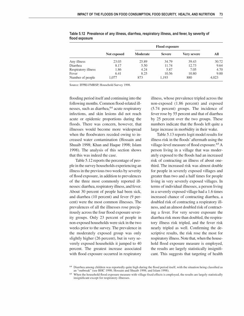
flooding period itself and continuing into thefollowing months. Common flood-related ill-nesses, such as diarrhea,64 acute respiratoryinfections, and skin lesions did not reachacute or epidemic proportions during thefloods. There was concern, however, thatillnesses would become more widespreadwhen the floodwaters receded owing to in-creased water contamination (Hossain andShuaib 1998; Khan and Haque 1998; Islam1998). The analysis of this section showsthat this was indeed the case.
Table 5.12 reports the percentage of peo-ple in the survey households experiencing anillness in the previous two weeks by severityof flood exposure, in addition to prevalencesof the three most commonly reported ill-nesses: diarrhea, respiratory illness, and fever.About 30 percent of people had been sick,and diarrhea (10 percent) and fever (9 per-cent) were the most common illnesses. Theprevalences of all the illnesses rose precip-itously across the four flood exposure sever-ity groups. Only 23 percent of people innon-exposed households were sick in the twoweeks prior to the survey. The prevalence inthe moderately exposed group was onlyslightly higher (26 percent), but in very se-verely exposed households it jumped to 40percent. The greatest increase associatedwith flood exposure occurred in respiratory
illness, whose prevalence tripled across thenon-exposed (1.86 percent) and exposed(5.74 percent) groups. The incidence offever rose by 55 percent and that of diarrheaby 25 percent over the two groups. Thesenumbers indicate that the floods left quite alarge increase in morbidity in their wake.
Table 5.13 reports logit model results forillness risk in the floods’ aftermath using thevillage-level measure of flood exposure.65 Aperson living in a village that was moder-ately exposed to the floods had an increasedrisk of contracting an illness of about one-third. The increased risk was almost doublefor people in severely exposed villages andgreater than two and a half times for peopleliving in very severely exposed villages. Interms of individual illnesses, a person livingin a severely exposed village had a 1.6 timesincreased chance of contracting diarrhea, adoubled risk of contracting a respiratory ill-ness, and an almost doubled risk of contract-ing a fever. For very severe exposure thediarrhea risk more than doubled, the respira-tory illness risk tripled, and the fever risknearly tripled as well. Confirming the de-scriptive results, the risk rose the most forrespiratory illness. Note that, when the house-hold flood exposure measure is employed,the results are largely statistically insignifi-cant. This suggests that targeting of health
IMPACT OF THE FLOODS ON FOOD CONSUMPTION, FOOD SECURITY, HEALTH, AND NUTRITION 73
64 Diarrhea among children was reportedly quite high during the flood period itself, with the situation being classified asan “outbreak” (see BHC 1998; Hossain and Shuaib 1998; and Islam 1998).
65 When the household flood exposure measure with village fixed effects is employed, the results are largely statisticallyinsignificant except for respiratory illnesses.
Table 5.12 Prevalence of any illness, diarrhea, respiratory illness, and fever, by severity offlood exposure
Flood exposure
Not exposed Moderate Severe Very severe All
Any illness 23.03 25.89 34.79 39.43 30.72Diarrhea 8.17 5.50 11.74 12.73 9.64Respiratory illness 1.86 4.24 5.87 7.05 4.70Fever 6.41 8.25 10.56 10.80 9.00Number of people 1,077 873 1,193 880 4,023
Source: IFPRI-FMRSP, Household Survey 1998.

interventions to flood-exposed villages(rather than to individual households) is anefficient mechanism for addressing healthneeds in the aftermath of covariate shockssuch as the floods.
Figure 5.5 shows the prevalence of ill-ness across flood exposure severity groupsby age group and gender. Strong gender dif-ferences in the impact of flood exposure forthe sample as a whole are not apparent. Allage groups exhibit a pattern of increased ill-ness with greater severity of flood exposure.Table 5.14 compares the flood exposure oddsratios derived from logistic regression forchildren (0–10 years), adolescents (10–18),and adults (18 and over) in the sample. Alladults living in flood-exposed villages expe-
rienced increased illness risk. Adolescentsliving in very severely exposed villages wereover three and a half times more likely tocontract an illness than those living in non-exposed villages. Children in severely ex-posed villages had a slightly increased illnessrisk, and for those in very severely exposedvillages the risk more than trebled. Thus, al-though adolescents experienced the greatestincrease in illness risk due to the floods, theconsequences of illness among children aremore serious than among either adolescentsor adults, since illness can put a child’s lifein danger. Acute respiratory infections anddiarrhea, in particular, are major contributorsto child mortality in Bangladesh (Mitra et al.1997). Thus the heightened illness among
74 CHAPTER 5
Table 5.13 Determinants of prevalence of any illness, diarrhea, respiratory illness, and fever: Regression results (village-level flood exposure logit model)
Any illness Diarrhea Respiratory illness Fever
Odds z- Odds z- Odds z- Odds z-ratio statistic ratio statistic ratio statistic ratio statistic
Female-headed household 1.29 0.97 1.36 0.82 0.59 −0.66 0.88 −0.31Age of household head 1.00 −0.81 1.00 0.09 0.99 −1.01 0.99 −0.92Percent males 5–14 0.98 −3.53* 0.99 −1.78* 0.97 −4.15* 0.99 −1.53*Percent males 15–19 0.98 −3.80* 0.99 −1.64 0.99 −0.72 0.98 −2.18*Percent males 20–34 0.98 −3.66* 0.99 −1.59 0.97 −2.87* 0.98 −2.30*Percent males 35–54 0.99 −1.66* 0.98 −1.62 0.98 −1.08 0.99 −1.20Percent males 55+ 0.98 −1.89* 0.98 −1.78* 1.01 0.33 0.99 −1.00Percent females 0–4 0.99 −2.30* 1.00 0.63 0.98 −2.70* 0.99 −2.08*Percent females 5–14 0.98 −3.84* 1.00 −0.66 0.97 −2.96* 0.99 −1.16Percent females 15–19 0.98 −2.92* 0.99 −1.36 0.98 −1.39 0.99 −0.94Percent females 20–34 0.98 −2.43* 0.99 −0.62 1.00 0.11 0.99 −0.87Percent females 35–54 0.98 −2.87* 0.99 −1.05 0.97 −2.03* 1.00 −0.52Percent females 55+ 0.98 −3.91* 0.98 −1.73* 0.96 −3.01* 0.99 −1.02Household size 0.91 −4.35* 0.90 −2.84* 0.97 −0.69 0.85 −4.12*Household has educated female 0.99 −0.08 1.15 1.01 0.56 −3.20* 0.98 −0.12Household has educated male 0.89 −1.30 1.00 −0.01 1.29 1.31 0.75 −2.04*Total pre-flood asset value
(Tk thousand) 1.01 1.89* 1.00 0.37 1.00 −0.07 1.03 3.47*Age 0.99 −1.19 0.96 −5.24* 0.93 −5.83* 1.01 1.54Age-squared 1.00 3.08* 1.00 5.51* 1.00 5.11* 1.00 −0.65Sex 1.08 1.06 0.85 −1.34 1.02 0.09 0.96 −0.39Flood exposure
Moderate 1.30 2.53* 1.16 0.88 0.92 −0.32 1.35 1.74*Severe 1.88 6.88* 1.57 3.14* 2.01 3.32* 1.86 4.07*Very severe 2.77 9.30* 2.15 4.70* 3.28 5.36* 2.82 6.17*
Pseudo R2 .044 .041 .0976 .0472Prob > χ2 0.000 0.000 0.000 0.000Number of observations 4,007 4,007 4,007 4,007
Source: IFPRI-FMRSP, Household Survey 1998 and authors’ calculations.
* denotes that the coefficient is statistically significant at the 10% level or less.

children represents the most serious healthconsequence of the floods.
Nutritional Status of Preschool Children and Women
Preschool ChildrenBangladesh has some of the highest childmalnutrition rates in the world. Even undernormal conditions over half of all preschoolchildren (0- to 5-year-olds) in the country arestunted, signaling that they have experiencedlong-term inadequate nutrition and/or poorhealth. Roughly 15 percent are wasted—hav-ing recently experienced substantial weightloss, usually owing to an acute shortage offood or a severe illness (ACC/SCN 2000;BBS 1997; Mitra et al. 1997).66 Besides beinga cause of much physical and emotional suf-fering, child malnutrition has long-termconsequences for a country’s overall devel-
opment because it impairs cognitive ability,reduces productivity, and increases demandson social services. It is also a leading causeof death among young children (ACC/SCN2000).
One of the reasons child malnutritionrates are so high in Bangladesh is the lackof proper caring practices for children, es-pecially feeding practices (MHFW 1995;UNICEF 1998; UNICEF-ADB 1997). Aftersix months of age, as well as continuedbreastfeeding, children need frequent nutri-tious meals free of pathogens in order tocontinue to grow and thrive. They also needextra feeding during and after illnesses (ACC/SCN 2000). Reports from the flood front in-
IMPACT OF THE FLOODS ON FOOD CONSUMPTION, FOOD SECURITY, HEALTH, AND NUTRITION 75
Figure 5.5 Prevalence of any illness in previous two weeks, by gender,age group, and severity of flood exposure
Table 5.14 Impact of flood exposure onprevalence of any illness for children,adolescents, and adults: Summary ofregression results (village-level floodexposure logit model)
Odds ratio z-statistic
ChildrenFlood exposure
Moderate 1.23 0.99Severe 1.47 2.09*Very severe 3.23 5.34*
Prob > χ2 0.00Number of people 980
AdolescentsFlood exposure
Moderate 1.50 1.42Severe 2.68 4.02*Very severe 3.53 4.43*
Prob > χ2 0.00Number of people 909
AdultsFlood exposure
Moderate 1.30 1.86*Severe 2.02 5.50*Very severe 2.64 6.23*
Prob > χ2 0.000Number of people 1,983
Source: IFPRI-FMRSP, Household Survey 1998 and au-thors’ calculations.
Notes: Child regressions include parents’ ages and educa-tion plus mother’s height as regressors. All other regressionscontain the same variables as listed in Table 5.13.* denotes that the coefficient is statistically significant at the10% level or less.
66 A child is defined as wasted (stunted) if the child’s weight-for-height (height-for-age) z-score is less than −2 standarddeviations from the U.S. National Center for Health Statistics/World Health Organization international reference stan-dard for the child’s age. Severe wasting (stunting) is defined as a z-score of less than −3.
Source: IFPRI-FMRSP, Household Survey 1998.
a. All ages
b. Children, adolescents, and adults

dicate that fulfilling these special needs be-came quite difficult during the floods, whichwould be expected given the damage tohomes and the increased efforts needed toobtain food and cook it, obtain safe water,and maintain a clean living environment.Some mothers had difficulty obtaining orpreparing supplementary food for their chil-dren, and others were producing insufficientbreastmilk owing to their own reduced foodconsumption. Children could not always beprotected from the floodwaters and wereexposed to contaminants in them or becameill from wearing wet clothes (del Ninno andRoy 1999a; Hena and Kabir 1998; Hossainand Shuaib 1998; Khan and Haque 1998;Rahman and Choudhury 1998). Not surpris-ingly, data collected during the flood monthsas part of Bangladesh’s ongoing NutritionSurveillance Project revealed a dramatic in-crease in wasting in the flood-affected areasof the country from June to August 1998,contradicting the normal pattern at that timeof year (HKI 1998b).
The first column of Table 5.15 shows thenutritional status of preschool children inthe study sample. In the period immediatelyfollowing the recession of the floodwaters,24 percent were wasted and 55 percent werestunted. The prevalence of wasting andstunting across the flood exposure severity
groups is shown in Figure 5.6. The wastingrate rose from 21.0 percent for children liv-ing in non-exposed households to 25.3 per-cent for those living in very severely exposedhouseholds. The graph also indicates that thefloods led to an increase in stunting amongchildren in households severely and very se-verely exposed to the floods.67
The logistic regression results using the household-level flood exposure measure
76 CHAPTER 5
Table 5.15 Nutritional status of preschool children, adolescent girls, and nonpregnant women (percent)
Adolescent girls and Preschool children nonpregnant women
Wasting 23.5Severe 3.9
Stunting 55.3Severe 24.0
Body mass index 18.1Chronic energy deficiency (%) 60.4Severe chronic energy deficiency (%) 15.0Number 409 654
Source: IFPRI-FMRSP, Household Survey 1998 and authors’ calculations.
Figure 5.6 Wasting and stunting amongpreschool children, and chronic energydeficiency among women, by severity offlood exposure
Source: IFPRI-FMRSP, Household Survey 1998.Note: CED = chronic energy deficiency.
67 It was somewhat surprising to notice an impact on the rates of stunting only a few months after the end of the floods.This is consistent with the findings of Helen Keller International (HKI 1998a, 1998b) and with our data, which reportan increase in illness at the onset of the floods in July 1998.

(Table 5.16) confirm that the floods led to abig increase in wasting that remained evenafter the floodwaters receded.68 A child liv-ing in a household that was severely exposedto the floods had a seven times greater risk ofbeing wasted than one not exposed at all. Theincreased risk was still quite large for verysevere exposure (almost five times greaterrisk). This indicates that to respond to wast-ing it is necessary to target individual house-
holds rather then relying on village targeting.An example of an intervention would beextra support for lactating mothers and en-suring easily prepared supplementary foodsare available for flood-exposed householdswith preschoolers.
The last column in Table 5.16 presentsthe results for stunting using the village-levelflood exposure measure. They confirm thatthe floods led to a significant increase in
IMPACT OF THE FLOODS ON FOOD CONSUMPTION, FOOD SECURITY, HEALTH, AND NUTRITION 77
Table 5.16 Determinants of wasting and stunting among preschool children: Regression results
Wasting Stuntinga
Household flood exposureVillage flood exposure with village fixed effects Village flood exposure
Odds ratio z-statistic Odds ratio z-statistic Odds ratio z–statistic
Percent males 5–14 1.03 1.36 1.04 1.53 1.01 0.82Percent males 15–19 1.04 1.19 1.10 1.93* 1.05 1.51Percent males 20–34 0.98 −0.59 1.01 0.26 1.02 0.80Percent males 35–54 1.02 0.81 1.05 1.27 1.00 −0.15Percent males 55+ 1.04 0.95 1.11 2.03* 0.95 −1.50Percent females 0–4 1.01 0.62 1.01 0.45 1.04 2.31*Percent females 5–14 1.04 1.96 1.07 2.24* 1.02 1.00Percent females 15–19 1.07 2.06* 1.14 2.70* 1.00 0.01Percent females 20–34 1.05 1.37 1.09 1.81* 1.05 1.67*Percent females 35–54 1.01 0.31 1.00 −0.04 1.02 0.76Percent females 55+ 1.04 1.37 1.08 1.81* 1.00 −0.16Household size 0.85 −1.66* 0.89 −0.77 1.13 1.56Mother’s height 1.01 0.22 1.01 0.19 0.90 −4.37*Mother’s age 1.05 1.18 1.09 1.58 1.04 0.96Father’s age 0.94 −1.80* 0.95 −1.29 1.00 0.01Mother has any education 0.89 −0.38 0.65 −0.90 0.70 −1.28Father has any education 0.90 −0.34 1.10 0.18 0.97 −0.10Pre-flood asset value (Tk thousand) 1.00 −1.15 0.96 −0.80 0.98 −0.85Age (months) 1.03 0.79 1.02 0.41 1.10 3.33*Age-squared 1.00 −0.93 1.00 −0.50 1.00 −2.85*Gender 0.36 −2.21* 0.42 −1.80* 0.42 −2.18*Flood exposure
Moderate 1.14 0.37 2.90 1.26 0.69 −1.15Severe 0.72 −0.96 7.30 2.25* 0.90 −0.36Very severe 0.92 −0.22 4.87 1.76* 2.18 2.04*
Pseudo R2 .080 .144Prob > χ2 0.094 0.079 0.000Number of children 384 247 384Number of villages 60
Source: IFPRI-FMRSP, Household Survey 1998 and authors’ calculations.a When this regression is undertaken using household-level flood exposure and village fixed effects, the observations from 34 villages and 78 households are
dropped because there is no variation across households within villages in the dependent variable. When the household flood exposure measure without vil-lage fixed effects is employed, the flood exposure variables are insignificant except for the moderate exposure dummy, which has a coefficient (odds ratio)of less than one.
* denotes that the coefficient is statistically significant at the 10% level or less.
68 Note that the regression coefficients on the flood exposure variables are not significant when the village-level flood ex-posure measure is employed.

stunting for children living in very severelyexposed villages.69 The impact of the floodson stunting is not surprising because mostof the children that lived in more severelyexposed villages suffered the consequencesof poor sanitation at the onset of the floodsin July 1998, four months before the survey.
WomenAs noted above, the nutritional status ofBangladeshi women is also extremely poor.Bangladesh has the world’s highest known
rate among women of chronic energydeficiency (CED)—signifying that a per-son is underweight owing to insufficientenergy intakes.70 Malnutrition of womenin turn leads to intrauterine growth retar-dation and low birthweight babies. It alsohinders mothers from providing adequatecare to children after they are born(ACC/SCN 2000). The prevalence of CEDamong nonpregnant women aged 19–49years in the study sample is 60 percent(Table 5.15).71
78 CHAPTER 5
Table 5.17 Determinants of chronic energy deficiency (CED) among nonpregnant women:Regression results
Household flood exposureVillage flood exposure with village fixed effects
Odds ratio z-statistic Odds ratio z-statistic
Female-headed household 0.99 −0.02 0.93 −0.11Age of household head 0.99 −0.94 1.01 0.52Percent males 5–14 1.00 0.00 1.00 −0.10Percent males 15–19 1.00 0.15 0.98 −1.08Percent males 20–34 0.99 −1.05 0.98 −0.94Percent males 35–54 1.00 −0.02 0.99 −0.50Percent males 55+ 1.00 0.03 0.97 −1.06Percent females 0–4 1.00 0.39 1.00 −0.08Percent females 5–14 0.99 −1.25 0.97 −2.09*Percent females 15–19 1.01 0.38 0.99 −0.32Percent females 20–34 0.97 −2.01* 0.95 −2.74*Percent females 35–54 0.99 −0.34 0.98 −1.11Percent females 55+ 1.01 0.50 0.98 −0.99Household size 0.93 −1.33 0.84 −2.35*Household has educated female 0.95 −0.25 1.08 0.30Household has educated male 0.78 −1.13 0.69 −1.40Pre-flood asset value (Tk thousand) 0.95 −3.49* 0.95 −2.71*Age 0.75 −2.48* 0.75 −2.05*Age-squared 1.00 2.70* 1.00 2.12*Flood exposure
Moderate 0.917 −0.368 0.519 −1.742*Severe 1.345 1.361 0.476 −1.784*Very severe 1.162 0.553 0.390 −1.968*
Pseudo R2 .072Prob > χ2 0.000 0.003Number of people 650 561Number of villages 97
Source: IFPRI-FMRSP, Household Survey 1998 and authors’ calculations.
* denotes that the coefficient is statistically significant at the 10% level or less.
69 The household-level measure of flood exposure could not be employed in the regression for stunting owing to insuf-ficient variation in stunting across children in villages.
70 A person is classified as being chronically energy deficient if her or his body mass index (weight divided by height-squared) is less than 18.5. A person is severely energy deficient if his or her BMI is less than 16.
71 For comparison, the percentage of nonpregnant women aged 15–49 in Bangladesh among women with children underfive years of age is reported by Mitra et al. (1997) to be 52 percent. It is reported in ACC/SCN (2000) to be 51.3 percentfor women aged 20–49. These numbers are calculated using the 1996–97 Bangladesh Demographic and Health Survey.

Figure 5.6 also shows the prevalence ofCED across the flood exposure severitygroups. Although it drops for moderate ex-posure, it is slightly elevated for severe andvery severe flood exposure. Logistic regres-sion results for CED risk are reported inTable 5.17. The results when the village-level flood exposure measure is employedsuggest that a woman living in a flood-exposed village had no greater risk of be-coming undernourished than those living innon-exposed villages. When the household-level flood exposure measure is employed,the results suggest that the floods led to adecline in undernourishment among womenin households in all three flood exposurecategories, although these results are notstrongly significant. In conclusion, we foundno evidence that the floods had a negativeimpact on women’s nutritional status.
SummaryThe 1998 floods in Bangladesh reducedpeople’s food consumption. It also compro-mised households’ ability to meet their foodneeds on a sustainable basis; in other words,it increased food insecurity. We have foundthat households exposed to the floods prob-ably experienced reduced food consumptionduring the flood period itself, and the major-ity continued to consume less food than usualeven after the floodwaters receded.
In an effort to maintain normal con-sumption of other foods whose prices hadincreased, households reduced their con-sumption of rice (substituting some withwheat). They also reduced their consumptionof three non-staple foods: micronutrient-richvegetables and fruit, whose prices remainedhigher than normal owing to continuedscarcities, and milk. These changes in theirconsumption baskets resulted in a reductionin the level of calories consumed and in-creased the number of households character-ized as questionable in terms of food security(that is, they consumed less than 1,818 calo-ries/person/day but spent less than 70 percentof their budgets on food). Per capita calorieconsumption of households not exposed tothe floods was on average 160–200 calories
per person higher than for households se-verely or very severely exposed to the floods.Other immediate needs in the post-floodperiod may have prevented the questionablehouseholds from increasing their spendingon food, however. We found no evidence thatthe floods led to any widespread increase indiscrimination against females in food con-sumption within households. This is not tosay that females are not discriminatedagainst, only that its degree did not changesignificantly as a result of the floods.
The floods led to a major deterioration inthe quality of households’ health environ-ments. They damaged or destroyed people’shomes, reduced their access to safe water,and destroyed or damaged their toilet fa-cilities. These factors, combined with thereduction in food consumption, led to sub-stantial increases in illness among all agegroups. Although adolescents had the great-est increase in illness, the increase in illnessamong children was an even more serioushealth problem posed by the floods becauseillness has more serious consequences forchildren, even threatening their survival.
We also confirmed that the floods causedmany preschool children to lose weight and/or to fail to grow at a critical period in theirphysical and mental development. This situ-ation was brought about by a combination offactors, including reduced food consump-tion, increased difficulties of providing propercare for children owing to disruptions in homelife, and increases in child illness. We foundno evidence that the floods were harmful towomen’s nutritional status, at least in theirimmediate aftermath.
Our findings that caloric consumptionand other health outcomes were affected byflood exposure measures at village level arean indication that interventions at the villagelevel could have been effective in reducingthe adverse impact of the floods. On theother hand, the degree of individual house-hold flood exposure was a significant deter-minant of individual consumption of staplefoods and of wasting, suggesting a possiblepositive impact of individual targeting inthese cases.
IMPACT OF THE FLOODS ON FOOD CONSUMPTION, FOOD SECURITY, HEALTH, AND NUTRITION 79

C H A P T E R 6
Household Coping Strategies
When households suffer a shock such as the floods, they do not remain passive butemploy several coping strategies. These coping strategies are fallback mechanismsfor when habitual means of meeting needs are disrupted (Frankenberger 1992).
The first thing households do when they suffer a shock is to attempt to minimize risks andmanage losses to ensure some minimal level of sustenance. The second strategy employedby households in distress is divestment, or the gradual disposal of assets. Frankenberger(1992) classifies asset disposal as a coping strategy into several phases, with liquid assets,such as jewelry, being disposed of first, and productive assets later. When productive assetsare disposed of, it becomes more difficult for the person or household to return to a pre-crisisstate. Finally, the household or individual may embark upon distress migration, which is asign of failure to cope with the crisis.
This chapter looks at the kinds of coping strategies that were employed by people duringthe floods of 1998 and in their immediate aftermath. We first report the strategies mentionedby flood-exposed people both in the field interviews of a rapid appraisal done by the FoodManagement and Research Support Project of the International Food Policy Research Insti-tute (IPFRI-FMRSP) during the floods (del Ninno and Roy 1999a) and in other similar studies.Using the household survey, we then quantify some of the coping strategies employed byrural households in Bangladesh to see how widespread they were and whether they weredirectly associated with flood exposure.
Self-Reported Coping StrategiesAt the time of the floods and soon after, several rapid appraisal missions were conducted bythe FMRSP-IFPRI project and by several other organizations. The main goal was to under-stand the extent of the damage caused by the flooding, how well people were doing in thecircumstances, and the type of coping strategies that had been employed. The ultimate pur-pose of those field visits was to improve the immediate alleviation policies that were designedat the time of the floods and in the immediate aftermath.
The results of the rapid appraisal show that the agricultural sector and the labor marketwere hit particularly hard by the floods. In most cases farmers could not plant their usualcrops and did not have enough fodder to feed their livestock. In response to that situationfarmers cultivated alternative crops and found alternative means of feeding their livestock.

Similarly, they found alternative forms ofemployment within the water sector, such asboating and fishing.
One key coping strategy mentioned byalmost all studies is borrowing. According tothe results of the interviews (summarized
in Table 6.1), money was borrowed from allsorts of sources, including moneylenders, rel-atives, and neighbors. Purchasing of food oncredit was also mentioned. Although purchas-ing food on credit is very common in severaldeveloping countries, extensive borrowing
HOUSEHOLD COPING STRATEGIES 81
Table 6.1 Coping strategies employed by Bangladeshi people in response to the 1998 floods, self-reported in field surveys
Coping strategy employed Study
Change agriculture and livestock practicesChange cropping pattern HKI a, b (1998)Cultivate land on lease Hossain and Shuaib (1998)Use emergency fodder (e.g., jackfruit, tree leaves, sugarcane BHC (1998); Save the Children (1998)
tops, banana stems, water hyacinth)Change employment or working pattern
Become engaged in fishing (catch and sell) and boating or WFP (1998); Save the Children (1998)cutting long grass for cattle
Advance labor Khan and Haque (1998); HKI (1998)Borrow moneya Democracy Watch (1998); HKI (1998)
From local money lenders Khan and Haque (1998); Hena and Kabir (1998); WFP (1998); Rahman and Choudhury (1998); Hossain and Shuaib (1998); delNinno and Roy (1999a)
From relatives or neighbors WFP (1998); Rahman and Choudhury (1998); HKI (1998); IFPRI-Sat (1999)
From a nongovernmental organization Rahman and Choudhury (1998); BHC (1998); del Ninno and Roy (1999)
Purchase rice on credit from a farmer Khan and Haque (1998)From a bank BHC (1998); del Ninno and Roy (1999)
Change eating habitsb
Reduce food consumption, including size of meals Khan and Haque (1998); Save the Children (1998); del Ninno and Roy (1999)
Reduce frequency of meals WFP (1998); Save the Children (1998); del Ninno and Roy (1999)Change types of food eaten, including eating jute leaves Save the Children (1998)Starve Save the Children (1998)
Consume assetsEat seed reserves BHC (1998)Use fencing or roofing materials for cooking fuel Khan and Haque (1998); WFP (1998)
Sell assetsDomestic assets (e.g., tin from roof of house, furniture, trees, del Ninno and Roy (1999); Banu and Hussain (1998); WFP (1998);
utensils, clothing) Khan and Haque (1998); Democracy Watch (1998); HKI (1998)Sell rice stocks to buy other essential commodities IFPRI-Saturia (1998)Sell means of transport IFPRI-Saturia (1999); Banu and Hussain (1998); HKI (1998)Sell livestock (cattle, buffalo, chicken, ducks, hens) Khan and Haque (1998); Hena and Kabir (1998); Rahman and
Choudhury (1998); HKI (1998); Save the Children (1998); delNinno and Roy (1999); Banu and Hussain (1998); WFP (1998)
Sell jewelry HKI (1998); Save the Children (1998); del Ninno and Roy (1999);Banu and Hussain (1998)
Sell or mortgage land HKI (1998); Save the Children (1998); del Ninno and Roy (1999);WFP (1998)
OtherDefer monthly installments on loans WFP (1998)Deplete savings Democracy Watch (1998); HKI (1998); Save the Children (1998)Have faith in God (Allah) Save the Children (1998)Move valuables to higher ground, especially cows and buffalo Save the Children (1998); BHC (1998)Float household items (for example, on banana leaves) Save the Children (1998)
Sources: Compiled from the sources cited. IFPRI-Saturia (1999) denotes individual interviews in Saturia, January 1999.a Credit uses: repair damage, buy seeds and food (BHC 1998).b Women ate after men and children; sometimes they ate nothing (del Ninno and Roy 1999a).

is peculiar to Bangladesh and is exploredlater in the chapter.
Another coping strategy was a modifica-tion of eating habits and a reduction in thefrequency of meals consumed when house-holds suffered income loss and failed to getenough credit to purchase the same amountof food. The consumption and sale of do-mestic liquid assets and livestock assetswere also reported as a way of meeting con-sumption needs. Finally, other forms ofcoping consisted of trying to protect assetsand thus minimize losses from the floods,deferring loan payments, and using savings.
The Coping StrategiesIdentified by the Quantitative Analysis
BorrowingThe analysis of the household data set con-firmed that borrowing was one of the maincoping mechanisms used by households inresponse to the floods. The demand for finan-
cial credit during the flood period appearsto have been extensive. The percentage ofhouseholds that took a loan increased duringthe flood period for all uses taken together(Figure 6.1 and Table 6.2), but especially forfood. The percentage of households whotook a loan for food was only 7.0 percent inthe month preceding the onset of flooding.By the last month of flooding (October) thishad increased to 15.9 percent. By that time,more than 60 percent of households exposedto the floods had an outstanding loan of anaverage value of almost Tk 6,000, on loanscontracted after July 1, 1998.72
The majority of the loans were contractedfor purchasing food. In fact more than half ofthe poor households in the bottom two quin-tiles had outstanding loans for food for avalue of almost Tk 3,000, which is close tothe average amount spent in a month by ahousehold to buy food. The percentage ofhouseholds that had outstanding loans forother purposes was much lower, but the av-erage size of the loans for farming and busi-
82 CHAPTER 6
72 There is usually an increase in borrowing in September and October, before the aman harvest, and in March and April,before the boro harvest, but it is clear that in 1998 the extent of borrowing had increased. In fact, as of January 1998very few households had extensive debts, compared with December 1998, when many households were in debt.
Figure 6.1 Percentage of households taking loans, by month and reason in 1998
Source: IFPRI-FMRSP, Household Survey 1998.

ness was larger (between Tk 3,000 and Tk13,000) and they were more often contractedby households in the higher expenditurequintiles. It is interesting to observe that the average size of total outstanding loanswas higher for people in the upper quintiles(Table 6.2). This may be due to greater ac-cess to credit by richer households, in part be-cause they borrowed relatively large amountsfor farming and business reasons. The re-verse is true for poor households, whichborrowed lower amounts and mostly for foodconsumption.
Households that were not exposed to thefloods borrowed money as well, but not inthe same proportion. Only 28 percent ofhouseholds not directly exposed to the floodshad outstanding loans for food during andfollowing the floods. The average size ofloans for all uses was higher for householdsnot exposed to flooding. This was becausethe average size of loans for farming use wasconsistently higher than loans for food con-sumption use, regardless of the category offlood exposure.
Table 6.3 details the sources of loans andtheir interest rates by severity of flood expo-sure. Most of the loans were received fromneighbors and relatives, with 23 percent ofthe households receiving loans from rela-tives and over 31 percent from neighbors.Other loan sources were NGOs, commercialbanks and cooperatives, and local money-lenders (called mahajans).
Across the sample, interest rates rangedwidely, from a low of zero to a high of 120percent. Only 23 percent of loans were at zerointerest rate. Neighbors and relatives weremore likely not to charge any interest thanthe other sources. NGOs charged the lowestinterest rates, while banks and cooperatives,mahajans, and neighbors charged annual in-terest rates of almost 50 percent on average.
It appears that people more exposed tothe floods (Table 6.3) borrowed more, butthey had more access to cheaper loans fromNGOs and in general received more freeloans and paid lower interest rates. Theseresults suggest that, even though people indistress are usually willing to pay higher in-
HOUSEHOLD COPING STRATEGIES 83
Table 6.2 Percentage of flood-exposed households with outstanding loans taken after July 1, 1998, and average debt, bytotal expenditure quintile
Quintile 1 Quintile 2 Quintile 3 Quintile 4 Quintile 5 All
Percent Percent Percent Percent Percent Percentof Average of Average of Average of Average of Average of Average
house- amount house- amount house- amount house- amount house- amount house- amountReason holds (Tk) holds (Tk) holds (Tk) holds (Tk) holds (Tk) holds (Tk)
Food 52.2 2,954 54.9 2,645 46.2 3,205 32.7 3,132 38.3 5,201 45.2 3,328Education/
health 12.4 990 5.3 1,235 6.6 3,228 9.9 2,730 5.6 4,900 8.0 2,339Farming 6.2 8,733 3.5 5,255 7.5 2,656 9.9 6,087 15.0 9,613 8.3 7,068Business 4.4 3,080 12.4 3,999 10.4 9,023 8.9 6,261 8.4 13,386 8.9 7,239Repay loan 2.7 3,258 2.7 5,017 2.8 6,020 4.0 2,513 5.6 8,615 3.5 5,507Marriage
and dowry expenses 0.0 . . . 3.5 7,375 0.9 4,375 1.0 6,000 1.9 4,090 1.5 6,007
Others 11.5 4,271 6.2 6,318 3.8 2,406 12.9 5,702 9.3 9,251 8.7 5,872All 66.4 4,400 69.9 4,268 62.3 5,034 55.4 6,036 61.7 10,141 63.3 5,868Number of
house-holds 113 113 106 101 107 540
Source: IFPRI-FMRSP, Household Survey 1998.

terest rates, not too many people took advan-tage of the situation. It also appears that in-formal sources of credit were more effectivethan traditional microcredit programs (asnoted also in Zaman 1999) at providinghouseholds with the cash necessary to smoothconsumption.
Purchasing Food on CreditFrom the discussion above it is evident thatloans for food were an important copingstrategy for flood-exposed households. Inaddition to the loans for food, we also lookedat the value of food that was purchased oncredit in the month prior to the survey period.This is a reflection of a common practice ofpurchasing basic necessities on credit fromlocal shops, which was confirmed in ouranalysis. Table 6.4 shows that almost 50 per-cent of all households purchased food oncredit in the month of the survey for anaverage of Tk 998. Only 30 percent of thehouseholds not exposed to the floods pur-chased food on credit, compared with 57 per-cent of the households very severely exposedto the floods, which had to purchase rice,pulses, oil, and other products on credit.
Table 6.5 shows the pattern of food pur-chased on credit for flood-exposed house-holds by expenditure quintiles. Althoughthe percentage of people purchasing food oncredit was slightly lower in the upper quin-tiles, they were able to obtain a larger amountof credit (Tk 1,336 in the top quintile), whichcould be used for more expensive foodscompared with poorer people (Tk 774 in thebottom quintile).
Changing Eating BehaviorWhen a household has insufficient access tofood, and faces other constraints, the primarypersons responsible for feeding householdmembers can do one or more of the follow-ing (Maxwell et al. 1999): (a) reduce thenumber of meals eaten in a day or go wholedays without eating; (b) rely on less preferredand less expensive foods; and (c) limit por-tions at meal times.
We have already seen that householdsreduced their food consumption and limitedtheir purchases of relatively expensive foodsin response to the floods (Chapter 5). In orderto determine whether they had reduced thenumber of meals eaten, households were
84 CHAPTER 6
Table 6.3 Loans taken, by source and severity of flood exposure (percent)
Flood exposure
Not exposed Moderate Severe Very severe All
Loans An- Loans An- Loans An- Loans An- Loans An-at nual at nual at nual at nual at nual
zero inter- zero inter- zero inter- zero inter- zero inter-Loans inter- est Loans inter- est Loans inter- est Loans inter- est Loans inter- est
Source taken est rate taken est rate taken est rate taken est rate taken est rate
Big NGO 3.7 0.0 15.8 5.5 0.6 11.1 3.4 0.0 12.4 6.0 0.0 12.4 4.5 0.1 12.9Commercial
bank/ cooperative 6.9 0.0 41.2 5.5 0.0 48.6 11.6 0.5 33.5 10.1 1.8 35.0 8.6 0.5 37.8
Mahajan 4.1 1.8 64.0 17.6 9.1 29.1 14.0 6.8 30.9 7.7 2.4 54.4 10.6 4.9 37.8Neighbors 29.5 15.2 43.9 30.3 15.8 41.1 34.8 20.8 32.3 29.8 12.5 59.7 31.2 16.2 43.1Relatives/
friends 18.4 11.1 26.4 22.4 11.5 41.7 24.2 15.0 19.6 28.0 19.6 22.1 23.0 14.1 26.5All 53.5 21.2 36.1 62.4 23.0 38.4 62.8 23.2 28.9 65.5 25.6 40.1 60.6 23.1 35.5Number of
households 217 165 207 168 757
Source: IFPRI-FMRSP, Household Survey 1998.

asked to report the number of meals eachmember had eaten in the three days prior tothe survey. If a member skipped a meal, therespondent was asked why they had doneso. The results are not reported for childrenunder two years because most were breast-feeding and breastfeeding behaviors were notrecorded in detail.
The incidence of meal skipping for thesample as a whole was 20 percent, which isquite high (Table 6.6). The incidence tendedto increase with increased flood exposureseverity, being 17 percent for the not exposedgroup and rising to 23 percent for the severelyexposed group. It fell slightly between theseverely and very severely exposed groups,to 20 percent, which may be a reflection ofthe latter group’s greater access to aid fromthe government and NGOs. The most com-mon reason by far given for skipping a mealwas “not enough food.” These figures verifythat meal skipping was indeed part of the
menu of coping strategies that some house-holds employed in response to the scarcitiesbrought about by the floods.
Disposal of AssetsDisposal of assets is often mentioned as avery important coping strategy for house-holds exposed to shocks. In fact it is notuncommon for rural households to meet con-sumption requirements by consuming someof their assets or selling them in order to ac-quire the means to purchase other foods.
To isolate the impact of the floods, wecompared the trend in disposal of assets inthree periods: the period before the floods(December 1997 to June 1998), the periodof the floods (July to October 1998), and the month after the floods (November 1998).Table 6.7 shows that more households soldassets during the floods (16.8 percent) thanin the period before or after the floods. Inparticular, more households sold goats (1.9
HOUSEHOLD COPING STRATEGIES 85
Table 6.4 Percentage of households purchasing food on credit and average amount purchased (in the month prior tosurvey), by food group and severity of flood exposure
Flood exposure
Not exposed Moderate Severe Very severe All
Percent Percent Percent Percent Percentof Mean of Mean of Mean of Mean of Mean
house- value house- value house- value house- value house- valueType of food holds (Tk) holds (Tk) holds (Tk) holds (Tk) holds (Tk)
Rice 16.1 1,179 30.3 960 44 951 47.6 950 33.8 984Wheat 2.3 203 13.3 200 16.4 270 13.7 221 11.1 234Bread and other cereals 0.9 62 2.4 89 2.4 50 0.6 40 1.6 64Pulses 4.1 38 12.1 136 27.1 122 20.2 124 15.7 119Oil 7.4 79 16.4 98 28 78 25.6 102 19 89Vegetables 10.1 86 12.1 133 16.9 134 16.7 176 13.9 135Meat 0.5 160 0.6 53 4.3 106 5.4 165 2.6 132Eggs 1.4 68 1.8 23 2.4 55 3 84 2.1 61Milk 2.3 90 1.2 39 5.3 130 3.6 95 3.2 105Fruits 0.5 12 1.2 40 4.8 62 4.8 53 2.8 54Fish 1.4 47 1.8 147 6.3 160 6.5 288 4 194Spices 4.6 49 9.1 226 16.4 168 14.9 153 11.1 160Sugar and snacks 8.8 68 6.1 85 13.5 87 15.5 138 11 98Drinks and other 0.9 136 1.8 163 9.2 222 11.3 106 5.7 163Prepared foods 0.5 255 0.0 . . . 2.9 181 2.4 264 1.5 218Total 29.5 768 44.8 895 59.9 1,055 57.1 1,158 47.3 998Number of households 217 168 207 165 757
Source: IFPRI-FMRSP, Household Survey 1998.

percent), chickens (6.2 percent), and trees(2.3 percent) than in the period before thefloods.
The patterns of disposal across cate-gories of severity of flood exposure werequite different (Table 6.8). Households notexposed to flooding tended to consume alarger share of their assets, mostly cereals and
chickens. Households exposed to floodingtended to sell a larger proportion of their as-sets. For example, 7.3 percent of the house-holds exposed moderately to the floods soldcattle, compared with 3.2 percent of thehouseholds not exposed to the floods. It isalso the case that households exposed mod-erately and severely to the floods were more
86 CHAPTER 6
Table 6.5 Percentage of flood-exposed households purchasing food on credit and average amount purchased (in the monthprior to survey), by food group and expenditure quintile
Quintile 1 Quintile 2 Quintile 3 Quintile 4 Quintile 5 All
Per- Per- Per- Per- Per- Per-cent cent cent cent cent centof Mean of Mean of Mean of Mean of Mean of Mean
house- value house- value house- value house- value house- value house- valueType of food holds (Tk) holds (Tk) holds (Tk) holds (Tk) holds (Tk) holds (Tk)
Rice 44.3 687 45.1 1,028 40.6 992 41.6 1,017 32.7 1,097 40.9 953Wheat 24.8 251 12.4 209 16.0 329 11.9 185 7.5 112 14.6 236Bread and other
cereals 1.8 34 0.9 51 0.0 . . . 1.0 40 5.6 81 1.9 64Pulses 20.4 91 17.7 125 19.8 105 19.8 128 24.3 170 20.4 125Oil 19.5 46 20.4 84 23.6 87 28.7 79 27.1 143 23.7 90Vegetables 10.6 83 15.9 121 17.0 127 16.8 116 16.8 270 15.4 148Meat 2.7 75 1.8 52 5.7 103 3.0 228 4.7 172 3.5 131Eggs 1.8 31 2.7 54 0.9 6 4.0 45 2.8 118 2.4 59Milk 2.7 26 0.0 . . . 7.6 103 2.0 355 5.6 77 3.5 109Fruits 1.8 79 2.7 55 2.8 56 5.9 48 5.6 57 3.7 56Fish 2.7 83 2.7 48 5.7 177 5.0 115 9.4 366 5.0 211Spices 10.6 103 15.0 111 14.2 145 11.9 231 16.8 271 13.7 175Sugar and snacks 6.2 82 12.4 84 9.4 46 12.9 77 18.7 183 11.9 107Drinks and other 6.2 86 7.1 123 9.4 162 4.0 168 11.2 238 7.6 164Prepared foods 0.0 . . . 2.7 91 0.9 17 0.0 . . . 5.6 309 1.9 214Total 55.8 774 57.5 1,029 56.6 1,031 51.5 1,128 50.5 1,336 54.4 1,048Number of
households 113 113 106 101 107 540
Source: IFPRI-FMRSP, Household Survey 1998.
Table 6.6 Meal eating and skipping, by severity of flood exposure (for the three days precedingthe survey)
Flood exposure
Not exposed Moderate Severe Very severe All
Average number of meals eaten 8.7 8.5 8.5 8.6 8.6Average number of meals skipped 0.3 0.5 0.5 0.4 0.4Incidence of meal skipping (%) 17.3 19.4 23.0 19.8 20.0Number of people 970 755 1,073 798 3,596
Source: IFPRI-FMRSP, Household Survey 1998.
Note: This table excludes children under 2 years old, a large number of whom were breastfeeding, and people who were ab-sent from the household in any of the previous three days.
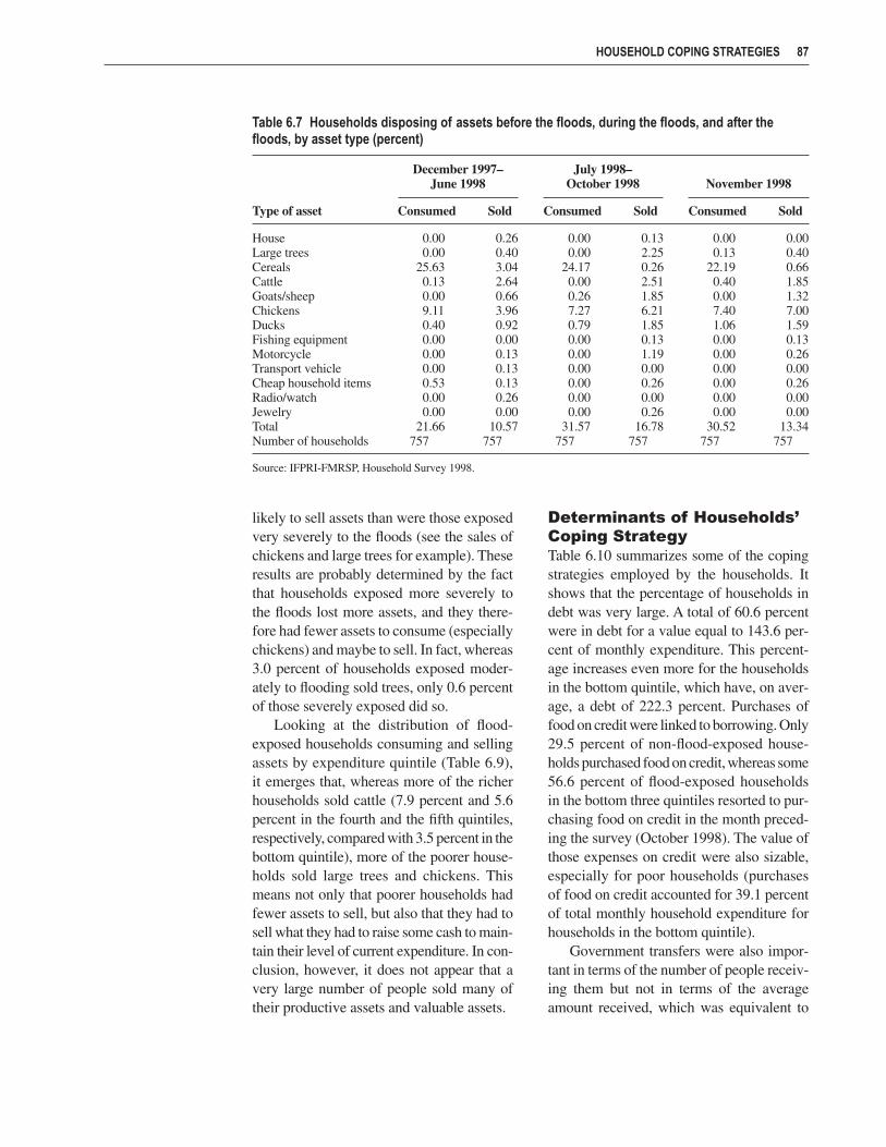
likely to sell assets than were those exposedvery severely to the floods (see the sales ofchickens and large trees for example). Theseresults are probably determined by the factthat households exposed more severely tothe floods lost more assets, and they there-fore had fewer assets to consume (especiallychickens) and maybe to sell. In fact, whereas3.0 percent of households exposed moder-ately to flooding sold trees, only 0.6 percentof those severely exposed did so.
Looking at the distribution of flood-exposed households consuming and sellingassets by expenditure quintile (Table 6.9),it emerges that, whereas more of the richerhouseholds sold cattle (7.9 percent and 5.6percent in the fourth and the fifth quintiles,respectively, compared with 3.5 percent in thebottom quintile), more of the poorer house-holds sold large trees and chickens. Thismeans not only that poorer households hadfewer assets to sell, but also that they had tosell what they had to raise some cash to main-tain their level of current expenditure. In con-clusion, however, it does not appear that avery large number of people sold many oftheir productive assets and valuable assets.
Determinants of Households’Coping StrategyTable 6.10 summarizes some of the copingstrategies employed by the households. Itshows that the percentage of households indebt was very large. A total of 60.6 percentwere in debt for a value equal to 143.6 per-cent of monthly expenditure. This percent-age increases even more for the householdsin the bottom quintile, which have, on aver-age, a debt of 222.3 percent. Purchases offood on credit were linked to borrowing. Only29.5 percent of non-flood-exposed house-holds purchased food on credit, whereas some56.6 percent of flood-exposed householdsin the bottom three quintiles resorted to pur-chasing food on credit in the month preced-ing the survey (October 1998). The value ofthose expenses on credit were also sizable,especially for poor households (purchasesof food on credit accounted for 39.1 percentof total monthly household expenditure forhouseholds in the bottom quintile).
Government transfers were also impor-tant in terms of the number of people receiv-ing them but not in terms of the averageamount received, which was equivalent to
HOUSEHOLD COPING STRATEGIES 87
Table 6.7 Households disposing of assets before the floods, during the floods, and after thefloods, by asset type (percent)
December 1997– July 1998–June 1998 October 1998 November 1998
Type of asset Consumed Sold Consumed Sold Consumed Sold
House 0.00 0.26 0.00 0.13 0.00 0.00Large trees 0.00 0.40 0.00 2.25 0.13 0.40Cereals 25.63 3.04 24.17 0.26 22.19 0.66Cattle 0.13 2.64 0.00 2.51 0.40 1.85Goats/sheep 0.00 0.66 0.26 1.85 0.00 1.32Chickens 9.11 3.96 7.27 6.21 7.40 7.00Ducks 0.40 0.92 0.79 1.85 1.06 1.59Fishing equipment 0.00 0.00 0.00 0.13 0.00 0.13Motorcycle 0.00 0.13 0.00 1.19 0.00 0.26Transport vehicle 0.00 0.13 0.00 0.00 0.00 0.00Cheap household items 0.53 0.13 0.00 0.26 0.00 0.26Radio/watch 0.00 0.26 0.00 0.00 0.00 0.00Jewelry 0.00 0.00 0.00 0.26 0.00 0.00Total 21.66 10.57 31.57 16.78 30.52 13.34Number of households 757 757 757 757 757 757
Source: IFPRI-FMRSP, Household Survey 1998.

only 2.0 percent of total household monthlyexpenditures, especially if compared with thesize of their debts. From a first observation itappears that government transfers were tar-geted more towards the poor than towardsflood-exposed households. In fact, 66.4 per-cent of the households in the bottom quintilereceived transfers, compared with 32.7 per-cent in the top quintile; and 52.6 percent ofthe flood-exposed households received trans-fers, compared with 33.6 percent of non-flood-exposed households (Table 6.10). A
more detailed analysis of the distribution of government transfers will follow in Chap-ter 7.
The last of the coping strategies reportedhere is the selling of assets. Exposed house-holds and non-exposed households sold as-sets in the same proportion (between 20 and22 percent). As we saw before, it was notthe selling of the assets that characterizedthe households exposed to the floods, but thetypes of assets sold. In general, the value ofthe assets sold was around 50 percent of the
88 CHAPTER 6
Table 6.8 Percentage of households disposing of assets after July 1998, and average value, by type of assets and severityof flood exposure
Flood exposure
Not exposed Moderate Severe Very severe All
Percent Percent Percent Percent Percentof of of of of
house- Value house- Value house- Value house- Value house- ValueType of asset holds (Tk) holds (Tk) holds (Tk) holds (Tk) holds (Tk)
ConsumedProductive assets
Cattle 0.5 1,600 0.0 . . . 0.5 1,600 0.6 6,250 0.4 3,150Chickens 21.7 251 10.9 169 6.8 188 0.6 65 10.6 219Ducks 1.8 84 1.8 96 1.5 95 0.6 48 1.5 87
Domestic assetsCereals 41.0 4,024 30.3 3,817 15.9 4,294 16.1 3,352 26.3 3,925
Liquid assetsLarge trees 0.0 . . . 0.6 3,267 0.0 . . . 0.0 . . . 0.1 3,267
Total consumed 45.2 3,794 32.7 3,656 18.8 3,941 17.3 3,340 29.1 3,727SoldProductive assets
Cattle 3.2 2,100 7.3 3,213 3.9 3,550 3.6 6,217 4.4 3,605Goats/sheep 3.2 1,171 4.9 401 2.9 967 1.8 367 3.2 763Chickens 9.2 187 13.3 192 17.4 291 11.3 272 12.8 244Ducks 1.4 90 3.6 116 5.8 340 3.0 591 3.4 308Fishing equipment 0.0 . . . 0.6 600 0.5 500 0.0 . . . 0.3 550
Domestic assetsCereals 1.8 1,463 1.2 1,750 0.5 3,500 0.0 . . . 0.9 1,836Cheap household items 0.0 . . . 0.6 1,300 0.0 . . . 1.8 290 0.5 543
HousingHouse 0.0 . . . 0.6 5,000 0.0 . . . 0.0 . . . 0.1 5,000
Liquid assetsLarge trees 2.3 260 3.0 636 4.4 4,759 0.6 1,500 2.6 2,441Jewelry 0.0 . . . 0.6 700 0.5 1,000 0.0 . . . 0.3 850
Consumer durablesMotorcycle 2.3 6,875 1.8 13,000 1.0 14,125 0.0 . . . 1.3 10,163
Total sold 18.9 932 31.5 1,282 26.1 1,859 17.3 1,878 23.3 1,476Number of households 217 165 207 168 757
Source: IFPRI-FMRSP, Household Survey 1998.

HOUSEHOLD COPING STRATEGIES 89
Table 6.9 Percentage of flood-exposed households disposing of assets after July 1998 and average value, by totalexpenditure quintile
Quintile 1 Quintile 2 Quintile 3 Quintile 4 Quintile 5 All
Percent Percent Percent Percent Percent Percentof of of of of of
Type of house- Value house- Value house- Value house- Value house- Value house- Valueasset holds (Tk) holds (Tk) holds (Tk) holds (Tk) holds (Tk) holds (Tk)
ConsumedProductive assets
Cattle 0.0 . . . 1.8 3,925 0.0 . . . 0.0 . . . 0.0 . . . 0.4 3,925Goats/
sheep 0.9 500 0.9 7,000 0.0 . . . 0.0 0.0 0.4 3,750Chickens 2.7 56 5.3 151 7.5 194 5.9 183 9.3 201 6.1 174Ducks 1.8 48 0.9 96 0.9 48 3.0 127 0.0 . . . 1.3 89
Liquid assetsLarge
trees 0.0 . . . 0.0 . . . 0.0 . . . 1.0 3,267 0.0 . . . 0.2 3,267Domestic assets
Cereals 18.6 3,315 15.9 4,026 20.8 4,049 21.8 3,653 25.2 4,130 20.4 3,846Total
con-sumed 20.4 3,060 21.0 4,206 23.0 3,942 25.7 3,273 27.1 3,914 22.6 3,672
SoldHousing assets
House 0.0 . . . 0.0 . . . 0.0 . . . 1.0 5,000 0.0 . . . 0.2 5,000Productive assets
Cattle 3.5 3,550 4.4 5,600 2.8 2,500 7.9 4,013 5.6 3,743 4.8 4,010Goats/
sheep 5.3 715 3.5 550 5.7 520 0.0 . . . 0.9 500 3.1 595Chickens 16.8 200 21.2 209 13.2 214 13.9 341 5.6 551 14.3 258Ducks 6.2 723 7.1 175 1.9 250 4.0 69 1.9 248 4.3 336Fishing
equip-ment 0.0 . . . 0.0 . . . 0.0 . . . 1.0 600 0.9 500 0.4 550
Liquid assetsLarge
trees 4.4 810 1.8 1,125 1.9 2,050 2.0 1,790 3.7 8,383 2.8 3,168Jewelry 0.9 700 0.0 . . . 0.0 . . . 1.0 1,000 0.0 . . . 0.4 850
Domestic assetsCereals 0.9 200 0.0 . . . 0.0 . . . 1.0 3,500 0.9 3,300 0.6 2,333Cheap
house-holditems 0.0 . . . 0.9 290 0.9 1,300 0.0 . . . 1.9 290 0.7 543
Consumer durablesMotor-
cycle 0.0 . . . 0.9 10,000 1.9 14,125 0.0 . . . 1.9 5,525 0.9 9,840Total sold 30.1 950 29.2 1,305 18.9 1,074 26.7 1,716 19.6 3,733 25.0 1,641Number of
house-holds 113 113 106 101 107 540
Source: IFPRI-FMRSP, Household Survey 1998.
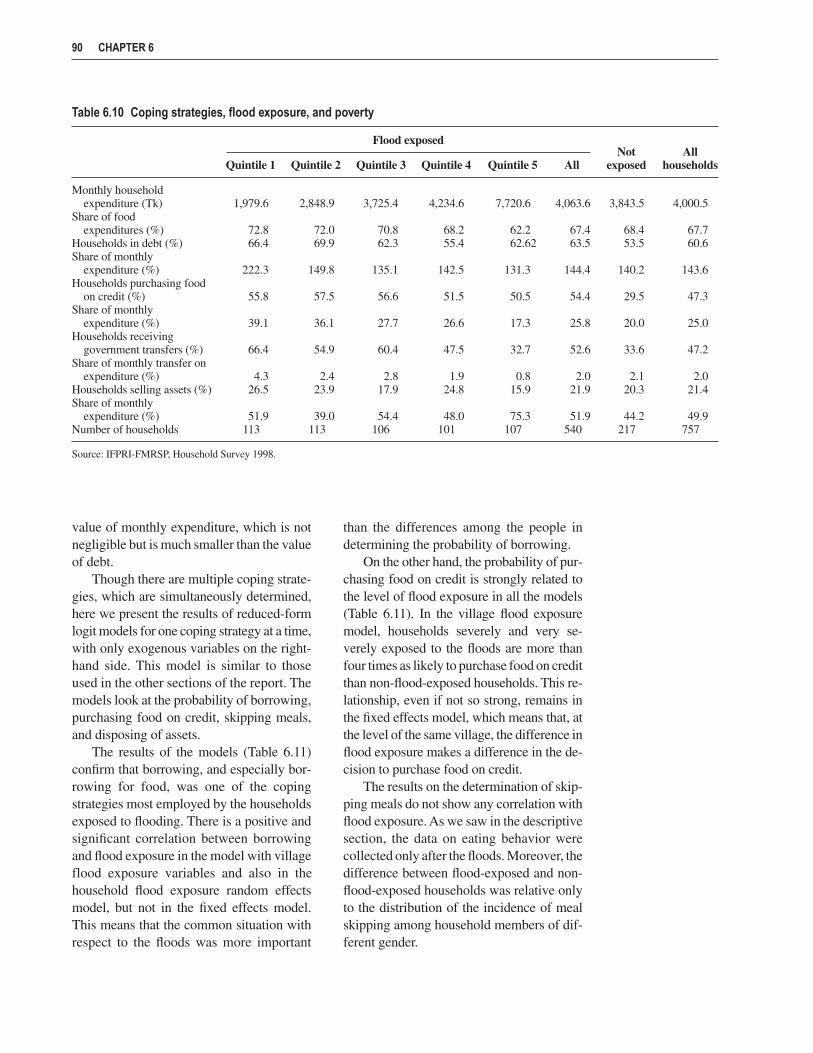
value of monthly expenditure, which is notnegligible but is much smaller than the valueof debt.
Though there are multiple coping strate-gies, which are simultaneously determined,here we present the results of reduced-formlogit models for one coping strategy at a time,with only exogenous variables on the right-hand side. This model is similar to thoseused in the other sections of the report. Themodels look at the probability of borrowing,purchasing food on credit, skipping meals,and disposing of assets.
The results of the models (Table 6.11)confirm that borrowing, and especially bor-rowing for food, was one of the copingstrategies most employed by the householdsexposed to flooding. There is a positive andsignificant correlation between borrowingand flood exposure in the model with villageflood exposure variables and also in thehousehold flood exposure random effectsmodel, but not in the fixed effects model.This means that the common situation withrespect to the floods was more important
than the differences among the people indetermining the probability of borrowing.
On the other hand, the probability of pur-chasing food on credit is strongly related tothe level of flood exposure in all the models(Table 6.11). In the village flood exposuremodel, households severely and very se-verely exposed to the floods are more thanfour times as likely to purchase food on creditthan non-flood-exposed households. This re-lationship, even if not so strong, remains inthe fixed effects model, which means that, atthe level of the same village, the difference inflood exposure makes a difference in the de-cision to purchase food on credit.
The results on the determination of skip-ping meals do not show any correlation withflood exposure. As we saw in the descriptivesection, the data on eating behavior werecollected only after the floods. Moreover, thedifference between flood-exposed and non-flood-exposed households was relative onlyto the distribution of the incidence of mealskipping among household members of dif-ferent gender.
90 CHAPTER 6
Table 6.10 Coping strategies, flood exposure, and poverty
Flood exposedNot All
Quintile 1 Quintile 2 Quintile 3 Quintile 4 Quintile 5 All exposed households
Monthly household expenditure (Tk) 1,979.6 2,848.9 3,725.4 4,234.6 7,720.6 4,063.6 3,843.5 4,000.5
Share of food expenditures (%) 72.8 72.0 70.8 68.2 62.2 67.4 68.4 67.7
Households in debt (%) 66.4 69.9 62.3 55.4 62.62 63.5 53.5 60.6Share of monthly
expenditure (%) 222.3 149.8 135.1 142.5 131.3 144.4 140.2 143.6Households purchasing food
on credit (%) 55.8 57.5 56.6 51.5 50.5 54.4 29.5 47.3Share of monthly
expenditure (%) 39.1 36.1 27.7 26.6 17.3 25.8 20.0 25.0Households receiving
government transfers (%) 66.4 54.9 60.4 47.5 32.7 52.6 33.6 47.2Share of monthly transfer on
expenditure (%) 4.3 2.4 2.8 1.9 0.8 2.0 2.1 2.0Households selling assets (%) 26.5 23.9 17.9 24.8 15.9 21.9 20.3 21.4Share of monthly
expenditure (%) 51.9 39.0 54.4 48.0 75.3 51.9 44.2 49.9Number of households 113 113 106 101 107 540 217 757
Source: IFPRI-FMRSP, Household Survey 1998.

Finally, the regression results providefurther evidence that flood-exposed house-holds did not consume and sell assets to agreater extent than did non-flood-exposedhouseholds. Consumption of assets is in factnegatively correlated with severity of floodexposure in the village flood exposure model,perhaps in part because only households thatdid not lose or sell their assets had the optionto consume them.
Rather than selling assets, flood-exposedhouseholds adopted borrowing or credit pur-chases of food as their predominant copingstrategy—a strategy that, however, left mostof them in debt for an amount equal on av-
erage to almost 150 percent of their currentmonthly expenditures. The choice of bor-rowing rather than sales of assets by flood-exposed households suggests that householdsthat had not lost their assets in the flood hadadequate access to credit. This enabled themto cope with the floods with only limitedsales of liquid assets and to avoid sellingmore valuable assets.
In some ways, these results are a littledifferent from the hypothesis at the begin-ning of the chapter in which we did not ex-pect that borrowing would play such a bigand determinant role. We also found that,although all the coping strategies mentioned
HOUSEHOLD COPING STRATEGIES 91
Table 6.11 Determinants of individual household coping strategies: Summary of regression results
Household flood exposure Household flood exposure
Village flood exposure Random effects Fixed effects
Odds ratio z-statistic Odds ratio z-statistic Odds ratio z-statistic
BorrowingModerate 1.52 1.89* 1.69 1.95* 1.23 0.61Severe 1.75 2.63* 1.15 0.53 0.66 −1.13Very severe 1.28 0.95 1.64 1.78* 1.15 0.35
Prob > χ2 0.00 0.05 0.07Number of observations 753 753 645Purchase of food on credit
Moderate 1.67 2.24* 2.21 2.84* 1.80 1.64Severe 2.92 4.93* 3.53 4.60* 2.23 2.07*Very severe 4.58 5.60* 2.70 3.43* 1.41 0.84
Prob > χ2 0.00 0.00 0.10Number of observations 753 753 645Skipping meals
Moderate 0.47 −1.12 0.87 −0.24 0.70 −0.29Severe 1.22 0.38 0.98 −0.03 0.38 −0.89Very severe 1.17 0.27 0.86 −0.27 0.46 −0.68
Prob > χ2 0.00 0.08 0.01Number of observations 720 753 211Selling assets
Moderate 0.94 −0.25 2.29 2.71* 1.79 1.54Severe 0.99 −0.04 1.40 1.09 1.25 0.55Very severe 0.48 −2.25* 0.96 −0.12 1.10 0.21
Prob > χ2 0.09 0.21 0.14Number of observations 753 753 531Consuming assets
Moderate 0.69 −1.36 0.85 −0.36 1.07 0.12Severe 0.24 −5.00* 0.48 −1.49 1.02 0.02Very severe 0.21 −4.05* 0.59 −1.00 1.36 0.42
Prob > χ2 0.00 0.00 0.00Number of observations 753 753 384
Sources: IFPRI-FMRSP, Household Survey 1998 and authors’ calculations.
* denotes that the coefficient is statistically significant at 10% level or less.
in the rapid appraisals done in the field dur-ing and after the floods were used by someof the households, some were employed moreoften (borrowing) than others (selling assets)and more by poor flood-exposed householdsthan by others.
SummaryIn this chapter we have carried out an analy-sis of the coping strategies used by ruralpeople in Bangladesh to deal with the lossessustained in the aftermath of the floods. Wefound that the coping strategies listed in therapid appraisal reflected the pattern expectedof households affected by a large covariateshock such as the floods. These strategies in-cluded selling assets, borrowing, and reduc-ing food consumption.
The analysis of the household surveyshowed that the predominant form of cop-
ing strategy used by flood-exposed house-holds was to borrow money or to purchasefood on credit. Loans were mostly con-tracted from informal sources to coverconsumption shortfalls and also to get re-sources for productive reasons. This ofcourse had become more necessary, sincethe farming and producing households hadto use their savings and assets to cope withthe hardships of the floods. This means that,even though households were able to useborrowing as a way to smooth their con-sumption, they were left in debt and at fur-ther risk of not recovering from anotherindividual or aggregate shock.
Selling assets, in contrast, was not foundto be a major form of coping strategy. Somepeople did sell some livestock to raise somecash, but this was probably also a way toreduce the expense of caring for them.
92 CHAPTER 6

C H A P T E R 7
Impacts of Government Food Relief Operations
The government of Bangladesh, nongovernmental organizations (NGOs), and privateindividuals implemented numerous programs in order to meet the immediate needs offlood-affected households. These efforts varied over time. They began with immedi-
ate relief efforts involving the provision of shelter, clothing, food, and clean water while thefloodwaters still covered much of the country in August and September 1998. Subsequently,relief efforts gradually gave way to flood rehabilitation programs, involving not only foodtransfers and income support, but rehabilitation of infrastructure, credit for future agricul-tural production, and other development efforts. This chapter focuses mainly on food reliefefforts during the first five months of the flood and post-flood periods (August through De-cember 1998). We explore the effectiveness of the targeting of government programs and al-ternatives to direct food transfers.
Targeting of Government Food Relief and Other TransfersTwo major channels dominated government food relief efforts following the floods: Gratu-itous Relief (GR), designed to provide emergency relief to disaster victims, and VulnerableGroup Feeding (VGF), aimed at assisting households over a longer period (ultimately, fromSeptember 1998 through April 1999).73 Immediate short-term relief through GR was targetedby location. In contrast, the VGF program covered all areas of the country (both flooded andnon-flood-affected areas), and was administratively targeted to poor households through se-lection by local committees (del Ninno and Roy 1999a). The size of these programs was lim-ited, however, both by available wheat stocks (up to early November when governmentcommercial imports and food aid arrivals added to government stocks) and by the financialcost of the programs (covered to a large extent by food aid).
Major flood relief efforts began in August 1998 through the provision of 20,400 metrictons of rice through Gratuitous Relief (GR) in flood-affected thanas and an additional 30,800metric tons of rice in September. In addition, the Vulnerable Group Feeding (VGF) programbegan on a large scale in August with an initial distribution of 1.3 million cards entitling the
73 Food for Work (FFW) programs began on a large scale only in December 1998, following the aman rice harvest whensoils were dry enough to permit manual earthworks to build roads and culverts.

holder to 8 kilograms of rice per month. Dur-ing August and September, a total of 27,500metric tons of rice were distributed throughthis program. At 8 kilograms/card, an esti-mated 1.35 and 2.13 million householdsreceived VGF rations in August and Sep-tember, respectively. Almost no wheat wasdistributed through relief channels in theearly months of the floods. At the urging ofthe World Food Programme (WFP), the gov-ernment of Bangladesh expanded the VGFprogram to 4 million cards with an allotmentof 16 kilograms of grain per card—half riceand half wheat in October, and all wheatthereafter (del Ninno and Dorosh 2001).
Table 7.1 provides evidence of the extentto which these programs were well targetedwith respect to flood exposure. In the seventhanas of the household survey sample of theInternational Food Policy Research InstituteFood Management and Research SupportProject, 47.2 percent of all households re-
ceived some form of government transfers.The GR program was better targeted to-wards flood-exposed households than wasthe VGF program. Only 9.7 percent of GRrecipients, compared with 19.4 percent ofVGF recipients, were not directly exposed tothe floods. On the other hand, among thevery severely exposed households, 35.7 per-cent received GR transfers and 21.4 pecentreceived VGF transfers. Neither programachieved large coverage though: 69.6 per-cent of flood-affected households did not re-ceive GR and 77.2 percent did not receiveVGF. In contrast to the VGF program, trans-fers from NGOs were particularly well tar-geted to households exposed to the floods:22.6 percent of very severely flood-exposedhouseholds received transfers from NGOs,compared with only 3.2 percent of non-flood-exposed households.
Even though the VGF program was notvery well targeted toward flood-exposed
94 CHAPTER 7
Table 7.1 Percentage of households receiving transfers and average value of transfers, byseverity of flood exposure
Flood exposure
Not exposed Moderate Severe Very severe All
Total government transfersPercent 33.6 44.2 53.1 60.1 47.2Value (Tk) 317.7 322.4 318.0 350.2 327.9Gratuitous Relief (GR)
Percent 9.7 23.6 31.4 35.7 24.4Value (Tk) 125.4 125.6 164.2 198.3 162.7
Vulnerable Group Feeding (VGF)Percent 19.4 22.4 24.2 21.4 21.8Value (Tk) 295.4 332.7 290.7 332.0 310.3
Other government transfersPercent 7.4 9.1 12.6 17.3 11.4Value (Tk) 509.3 344.9 327.1 354.3 373.3
NGO transfersPercent 3.2 7.3 12.1 22.6 10.8Value (Tk) 273.1 468.6 315.0 328.0 339.9
Private transfersPercent 8.8 10.9 9.7 7.1 9.1Value (Tk) 5,122.2 5,937.8 6,083.2 3,495.8 5,330.7
Total transfersPercent 41.5 49.1 62.8 70.2 55.4Value (Tk) 1,362.0 1,683.5 1,269.5 771.5 1,229.2
Number of households 217 165 207 168 757
Note: The value of transfers is over the four months from July 15 to November 15, 1998, for receiving households.
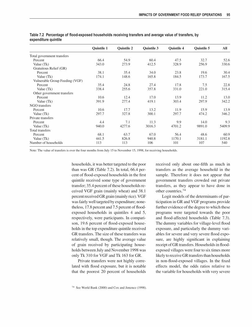
households, it was better targeted to the poorthan was GR (Table 7.2). In total, 66.4 per-cent of flood-exposed households in the firstquintile received some type of governmenttransfer; 35.4 percent of these households re-ceived VGF grain (mainly wheat) and 38.1percent received GR grain (mainly rice). VGFwas fairly well targeted by expenditure; none-theless, 17.8 percent and 7.5 percent of flood-exposed households in quintiles 4 and 5,respectively, were participants. In compari-son, 19.6 percent of flood-exposed house-holds in the top expenditure quintile receivedGR transfers. The size of these transfers wasrelatively small, though. The average valueof grain received by participating house-holds between July and November 1998 wasonly Tk 310 for VGF and Tk 163 for GR.
Private transfers were not highly corre-lated with flood exposure, but it is notablethat the poorest 20 percent of households
received only about one-fifth as much intransfers as the average household in thesample. Therefore it does not appear thatgovernment transfers crowded out privatetransfers, as they appear to have done inother countries.74
Logit models of the determinants of par-ticipation in GR and VGF programs providefurther evidence of the degree to which theseprograms were targeted towards the poorand flood-affected households (Table 7.3).The dummy variables for village-level floodexposure, and particularly the dummy vari-ables for severe and very severe flood expo-sure, are highly significant in explainingreceipt of GR transfers. Households in flood-exposed villages were four to six times morelikely to receive GR transfers than householdsin non-flood-exposed villages. In the fixedeffects model, the odds ratios relative to the variable for households with very severe
IMPACTS OF GOVERNMENT FOOD RELIEF OPERATIONS 95
Table 7.2 Percentage of flood-exposed households receiving transfers and average value of transfers, by expenditure quintile
Quintile 1 Quintile 2 Quintile 3 Quintile 4 Quintile 5 All
Total government transfersPercent 66.4 54.9 60.4 47.5 32.7 52.6Value (Tk) 343.0 273.9 412.5 328.9 256.9 330.6Gratuitous Relief (GR)
Percent 38.1 35.4 34.0 23.8 19.6 30.4Value (Tk) 174.1 148.6 165.8 184.5 173.7 167.5
Vulnerable Group Feeding (VGF)Percent 35.4 24.8 27.4 17.8 7.5 22.8Value (Tk) 338.4 255.6 357.8 331.0 221.0 315.4
Other government transfersPercent 10.6 12.4 17.0 13.9 11.2 13.0Value (Tk) 391.9 277.4 419.1 303.4 297.9 342.2
NGO transfersPercent 10.6 17.7 13.2 11.9 15.9 13.9Value (Tk) 297.7 327.8 300.1 297.7 474.2 346.2
Private transfersPercent 4.4 7.1 11.3 9.9 14.0 9.3Value (Tk) 940.0 4277.6 3016.3 4701.2 9891.0 5409.9
Total transfersPercent 68.1 63.7 67.0 56.4 48.6 60.9Value (Tk) 441.5 826.8 940.8 1170.1 3181.1 1192.8
Number of households 113 113 106 101 107 540
Note: The value of transfers is over the four months from July 15 to November 15, 1998, for receiving households.
74 See World Bank (2000) and Cox and Jimenez (1998).
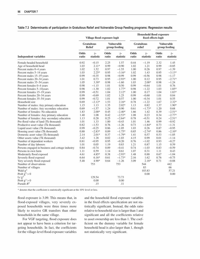
flood exposure is 3.09. This means that, inflood-exposed villages, very severely ex-posed households were three times morelikely to receive GR transfers than otherhouseholds in the same village.
For VGF targeting, flood exposure doesnot appear to have been a criterion for tar-geting households. In fact, the coefficientsfor the village-level flood exposure variables
and the household flood exposure variablesin the fixed effects specification are not sta-tistically significant. Instead, the odds ratiorelative to household size is larger than 1 andsignificant and all the coefficients relativeto asset ownership are less than 1. The coef-ficient on the dummy variable for femalehousehold head is also larger than 1, thoughnot statistically very significant.
96 CHAPTER 7
Table 7.3 Determinants of participation in Gratuitous Relief and Vulnerable Group Feeding programs: Regression results
Household flood exposureVillage flood exposure logit fixed effects logit
Gratuitous Vulnerable Gratuitous VulnerableRelief group feeding relief group feeding
Odds z- Odds z- Odds z- Odds z-Independent variables ratio statistic ratio statistic ratio statistic ratio statistic
Female-headed household 0.92 −0.15 2.25 1.57 0.44 −1.19 2.32 1.45Age of household head 1.03 2.11* 0.99 −0.90 1.02 1.21 0.99 −0.85Percent males 0–4 years 1.02 1.52 0.97 −1.55 1.00 0.26 0.97 −1.39Percent males 5–14 years 1.03 2.25* 0.95 −3.16* 1.02 1.43 0.95 −3.13*Percent males 15–19 years 0.99 −0.35 0.98 −0.99 0.99 −0.56 0.98 −1.17Percent males 20–34 years 1.01 0.73 0.95 −2.93* 1.00 0.12 0.95 −2.71*Percent males 35–54 years 1.05 3.30* 0.98 −1.60 1.03 2.00* 0.98 −1.24Percent females 0–4 years 0.98 −1.15 1.01 0.50 0.99 −0.64 1.01 0.76Percent females 5–14years 0.98 −1.30 1.02 1.77* 0.98 −1.22 1.03 1.85*Percent females 15–19 years 0.99 −0.51 1.04 2.12* 1.00 0.17 1.04 1.83*Percent females 20–34 years 0.99 −0.69 1.02 1.25 0.99 −0.60 1.01 0.84Percent females 35–54 years 0.99 −0.72 1.01 0.57 1.00 −0.34 1.01 0.55Household size 0.69 −2.12* 1.53 2.16* 0.78 −1.22 1.67 2.32*Number of males: Any primary education 1.15 1.13 1.35 2.02* 1.13 0.82 1.37 1.90*Number of males: Any secondary education 0.69 −1.57 1.24 0.90 0.61 −1.73* 1.20 0.68Number of females: No education 1.83 2.00* 0.45 −2.40* 1.66 1.42 0.39 −2.51*Number of females: Any primary education 1.40 1.08 0.42 −2.53* 1.08 0.23 0.34 −2.77*Number of females: Any secondary education 1.13 0.28 0.25 −2.64* 0.78 −0.51 0.24 −2.51*Pre-flood value of land (Tk thousand) 1.01 1.33 1.00 −0.43 1.01 1.46 0.99 −0.92Productive asset value (Tk thousand) 0.82 −1.53 0.76 −1.26 0.73 −1.84* 0.73 −1.31Liquid asset value (Tk thousand) 0.99 −0.25 0.86 −1.05 1.03 0.26 0.87 −0.95Housing asset value (Tk thousand) 0.88 −2.83* 0.89 −1.75* 0.85 −2.74* 0.86 −2.10*Domestic asset value (Tk thousand) 2.14 2.01* 0.37 −1.79* 1.41 0.57 0.53 −1.05Other assets value (Tk thousand) 3.42 1.28 0.02 −1.03 4.15 0.99 0.01 −1.14Number of dependent workers 0.81 −0.95 0.95 −0.20 0.76 −1.02 0.93 −0.27Number of day laborers 1.01 0.05 1.19 0.83 1.21 0.87 1.15 0.59Persons engaged in business and cottage industry 0.84 −0.74 0.89 −0.41 0.74 −1.03 0.83 −0.59Persons in own farm 1.11 0.59 1.14 0.61 1.07 0.31 1.11 0.43Moderately flood exposed 4.61 4.85* 0.38 −2.93* 1.48 0.88 0.67 −1.04Severely flood exposed 6.64 6.16* 0.61 −1.73* 2.16 1.62 0.76 −0.75Very severely flood exposed 5.48 4.90* 0.64 −1.26 3.09 2.18* 0.71 −0.88Number of observations 753 753 544 442Number of villages 83 66Wald χ2 103.83 57.21Prob χ2 > 0 0.00 0.00Lr χ2 129.54 73.73Prob χ2 > 0 0.00 0.00Pseudo R2 .15 .11
* denotes that the coefficient is statistically significant at the 10% level or less.

Impact of Government Food ReliefWe have established that government trans-fers were small but that they played a veryimportant role in helping households, espe-cially in the period of the floods. Did theyhave any impact on other measures of out-come? To answer this question we looked at the impact of GR transfers on per capitacalorie consumption. The results of the modelare reported in Table 7.4.
In the first regression, we run a modi-fied model of the determinants of per capitacalorie consumption as a function of house-hold characteristics, pre-flood assets, and
village flood exposure. In the second modelwe added to these explanatory variables thevalue of GR transfers received. As expected,the value of the coefficient was negativelycorrelated with the amount of calorie con-sumption. This means that, as we have no-ticed in the previous analysis, households thatwere poorer and consumed fewer calorieswere more likely to receive GR transfers.
In order to account for this apparent prob-lem, we use an instrumental variable model(for example, Ravallion and Wodon 2000;Rivers and Vuong 1988). The results of thismodel (Table 7.4) show that the GR transfersdid indeed have a small, but positive, impact
IMPACTS OF GOVERNMENT FOOD RELIEF OPERATIONS 97
Table 7.4 Determinants of per capita calorie consumption due to village flood exposure andamount received in GR transfers: Regression results
Ordinary least 2-stage leastsquares model squares model
Independent variables Coefficient t-statistic Coefficient t-statistic
Female-headed household −614.82 −3.55* −576.58 −2.82*Age of household head −3.47 −0.68 −5.77 −0.96Percent males 0–4 years −7.31 −0.54 −7.49 −0.53Percent males 5–14 years −3.85 −0.59 −7.40 −0.99Percent males 15–19 years −4.59 −0.72 −6.01 −0.82Percent males 20–34 years 0.44 0.07 −0.53 −0.08Percent males 35–54 years −0.79 −0.16 −11.64 −1.49Percent females 0–4 years −13.47 −3.06* −9.04 −1.72*Percent females 5–14years −10.80 −2.65* −6.96 −1.47Percent females15–19 years −3.35 −0.69 −2.37 −0.40Percent females 20–34 years −4.25 −0.78 −4.63 −0.71Percent females 35–54 years 5.21 1.40 12.9 12.54*Household size −100.64 −0.93 −56.16 −0.48Number of males: Any primary education 36.40 0.82 63.17 1.23Number of males: Any secondary education 41.66 0.79 77.97 1.14Number of females: No education 22.47 0.14 −39.46 −0.22Number of females: Any primary education 40.55 0.25 16.55 0.09Number of females: Any secondary education 68.62 0.41 51.03 0.28Pre-flood value of assets (Tk thousand) 30.39 4.61* 33.55 4.37*Moderately flood-exposed −18.13 −0.16 −175.41 −1.26Severely flood-exposed −198.83 −2.07* −516.20 −2.92*Very severely flood-exposed −130.62 −1.03 −405.20 −1.83*Value of GR transfer receiveda −0.74 −2.49* 4.80 1.88*Constant 3,209.07 8.02* 3,138.80 6.73*Number of observations 753 734R2 .18
a Value of GR transfer received has been instrumented using: Female-headed household; age of household head; proportionmales: 0–4 years, 5–14 years, 15–19 years, 20–34 years, 35–54 years; proportion females: 0–4 years, 5–14years, 15–19 years,20–34 years, 35–54 years; household size; number of males: any primary education, any secondary education; number of fe-males: no education, any primary education, any secondary education; pre-flood value of assets (Tk thousand); moderatelyflood-exposed; severely flood-exposed; very severely flood-exposed; number of household members engaged in dependentwork, day work, own farm, or own business; number of buildings; house with a tin roof; availability of electricity; owner-ship of cattle.* denotes that the coefficient is statistically significant at the 10% level or less.

on the level of per capita calorie consump-tion.75 This confirms the hypothesis that the program was well targeted and had apositive impact on the well-being of poorhouseholds.
Cash Transfers for Short-Term Flood ReliefDirect distribution of food and relief sup-plies was vitally important during the floodsand in the immediate post-flood period. Bylate September 1998, the floodwaters hadreceded in most of the country and transportlinks had been reestablished nearly every-where. Yet many people still faced criticalproblems of insufficient food. Unfortunately,as discussed above, because of delayed foodaid arrivals and limited government stocks,the availability of foodgrains in governmentwarehouses was a constraint on the expan-sion of VGF and other programs.
Given that, by late September, poorhouseholds in most of the country had ac-cess to well-supplied markets, their foodconsumption was constrained by lack ofpurchasing power rather than by food avail-ability per se. The months of September andOctober are normally slack periods of labordemand in rural areas, and the floods made iteven more difficult for the rural poor to findemployment. Increasing purchasing powerto affected households was a feasible alter-native to direct food distribution and in-creased food aid in the short run because, inthe post-flood, pre-harvest period (from mid-September to end-November), food supplywas no longer a constraint at the local ornational levels. As discussed above, privatesector imports kept rice prices at import par-ity and markets supplied with rice.
Moreover, much of the 1997/98 boroand 1998/99 aman harvests remained inprivate stocks. The 1998 boro harvest wasabout 8.0 million metric tons, and the flood-damaged aus rice crop was 1.6 million met-ric tons (down by 300,000 metric tons from
the target of 1.9 million metric tons). Thus,about 9.6 million metric tons of rice had beenharvested in Bangladesh from May throughSeptember. In addition, the private sectorhad imported 0.5 million metric tons fromIndia between July and mid-September (andcontinued to import more than 200,000metric tons per month from September 1998through March 1999). Since average nationalrice consumption is about 1.4 million metrictons per month, the 10.1 million metric tonsof total rice supply from the previous boroand aus harvests, combined with importsthrough mid-September (adjusted for losses),could have covered consumption for at leastsix months, that is, until December 1998.Moreover the December aman harvest wasexpected to add another 7.6 million metrictons of rice, and several thousand metric tonsof food aid wheat were scheduled to arriveby December as well.
Thus, following the floods of 1998, ex-cept in the immediate post-flood period,household food security in Bangladesh wasconstrained not by food availability in mar-kets, but by household access to food. How-ever, government distribution of food facedtwo other constraints as well: the availabilityof public foodgrain stocks and the financesfor relief and rehabilitation efforts.
Food aid eventually eased these two con-straints on public distribution. By providingfood, it eased the government stock situa-tion. And, because the food aid was given asa grant, it placed no added burden on thegovernment treasury. Yet, additional use ofcash payments could have enabled the gov-ernment and donors to provide even moreimmediate help to flood victims. Had donorsprovided cash to supplement direct fooddistribution, the total value of the VGF pro-gram could have been substantially increasedwithout endangering government foodgrainstocks.
There were, in effect, three distinct peri-ods following the floods, each with its own
98 CHAPTER 7
75 We also tested the significance of the impact of the predicted value of the GR transfers by adding the predicted valueof the residual of the first-stage regression, which we found to be significantly different from zero.

constraints on household food security andpolicy options. Immediately after the floods(mid-July to mid-September in most regions),household food security was constrainedboth by the availability of foodgrains in localmarkets as well as by purchasing power.With transport networks and markets dis-rupted, the immediate food needs of floodvictims could be met only by direct food dis-tribution. Later, when foodgrain availabilityin markets was no longer a constraint butgovernment foodgrain stocks had not yetbeen replenished through government com-mercial imports or food aid (late Septemberto mid-November), relief efforts were con-strained by government stocks and the finan-cial cost of aid.76 Finally, once governmentstocks had again been built up (mid-Novem-ber), relief efforts were constrained only bythe financial and administrative costs of theprograms.
One argument often advanced againstthe use of cash payments is that leakages arelikely to be larger than in the case of food.This need not occur if transparency is main-tained at both the local and national levels.In order to minimize losses through cashprograms, one option could be to give theNGOs and other local institutions a majorrole in seeing that the money allocated forrelief in a particular locality actually reachespoor flood-affected households. Nonetheless,even if leakages in cash distribution are some-what higher, these costs must be weighedagainst the benefits of increasing the value ofaid to the poor before the arrival of large foodaid shipments.
Implications for Food Aid andTargeting DistributionFood security at the household level dependson the availability of food in markets as wellas on access to food.77 Liberalization of pri-vate sector imports of rice and wheat in theearly 1990s and ensuing government policies
supporting trade in 1998 enabled private im-ports to stabilize market prices and supplies.Government direct distribution programs,though small compared with private imports,nonetheless increased poor households’ ac-cess to food. Given the tight resource con-straints on the size of distribution programs,effective targeting is crucial. Immediaterelief efforts were well targeted to flood-affected households, as were transfers fromNGOs. VGF, a medium-term program, cov-ered non-flood-affected regions and, evenin flood-affected thanas, was not well tar-geted to households directly exposed to thefloods. Nonetheless, according to survey datafrom seven flood-affected thanas, the pro-gram was relatively well targeted to poorhouseholds, with households in the threelowest expenditure quintiles receiving anestimated 75 percent of the foodgrains dis-tributed through this program.
More broadly, the Bangladesh experiencewith the 1998 flood illustrates the dual roleof food aid in increasing availability and pro-viding resources for enhancing the access offood insecure households. In a liberalizedtrade regime where private imports respondto price signals, food aid’s contribution to thetotal availability of food may be minimal.Nonetheless, foreign assistance, in kind or incash, can provide resources for subsidized,targeted distribution to food-insecure house-holds—assistance not otherwise possibleunder tight government budget constraints.
SummaryIn this chapter we have shown that food aidand government transfers were effective inproviding some relief to poor householdsexposed to the floods. These transfers weresmall in size and too limited in coverage,however, to have a major impact on the re-covery of households from the floods. None-theless, Gratuitous Relief transfers werewell targeted towards poor flood-exposed
IMPACTS OF GOVERNMENT FOOD RELIEF OPERATIONS 99
76 In addition, the difficulties of administering a large-scale, targeted emergency program slowed deliveries initially.77 As discussed in Chapter 5, intrahousehold distribution is an important aspect of food security (utilization) for individual
household members.

households and appear to have had an impacton the level of per capita calorie consump-tion. Moreover, these government transfersdid not crowd out private transfers, whichwere received by only a small number ofpeople who were not necessarily poor orexposed to the floods.
We have also shown that the governmentof Bangladesh and the donor communityplayed an important role in procuring theresources necessary for the use and expan-sion of already existing programs. The Bang-ladesh experience, along with other casescited in the World Development Report 2000(World Bank 2000), suggests that it is mucheasier to expand programs that are already
in place at the time of a shock than to designspecific new programs. Unfortunately, inBangladesh the expansion of relief pro-grams in the immediate aftermath of thefloods was constrained by the levels of gov-ernment stocks. Given that private marketswere well supplied by rice and wheat fromdomestic sources as well as by a steady flowof private sector imports, cash transfer pro-grams could have been used instead of grain,especially in the GR program, without lead-ing to increases in foodgrain prices. Suchcash transfers could have been extremely ef-fective, because many households contractedlarge debts in order to buy food.
100 CHAPTER 7

C H A P T E R 8
Conclusions and Lessons from the 1998 Floods
Summary of FindingsThis report has described the extent of the damage caused by the 1998 Bangladesh floods toproduction, transport infrastructure, markets, private assets, and the lives and the well-beingof people. Yet, despite a 2.2 million ton shortfall of aman and aus rice because of the floods,there was no food crisis in Bangladesh. No one died from lack of food, market price increaseswere small (particularly in comparison with the crisis of 1974), and there was no large mi-gration of people to urban areas in search of food. Households did suffer because of thefloods, as documented in this report and elsewhere, but a combination of private market food-grain imports, food aid, public foodgrain distribution and relief, and household coping strate-gies (including borrowing and shifts in food expenditures) kept the floods from becoming atruly major disaster.
The availability of foodgrains in the market in Bangladesh after the floods was maintainedmainly through an increase in imports of rice from India, and to a lesser extent through wheatfrom food aid and government commercial imports. The government of Bangladesh, whichhad launched an appeal for relief efforts in August 1998, was able to increase the distribu-tion of foodgrains in the country by only a small amount in the period immediately after thefloods. However, careful management of public foodgrain stocks may have contributed tomarket stability, by reducing the likelihood of short-term and localized shortages. Becauseof this combination of private sector imports, public foodgrain distribution, and stock policy,the market prices of rice and wheat in late 1998 were only slightly higher than those in theearly part of the year (following a poor rice harvest in December 1997). Moreover, with do-mestic foodgrain markets functioning well, regional price variations were similar to those inother years.
Nevertheless, even though foodgrains were available at a reasonable price, householdsstill did not have access to enough food, because the losses they suffered during the floodsreduced their level of income and wealth. Losses of assets in terms of damage to homes, trees,and small livestock were very large. Income losses were caused by loss of agricultural pro-duction and lack of jobs, especially during the floods, in both the agricultural and the non-agricultural sectors because of the slowing down of the economy. Employment opportunities
picked up again after the floods to a levelsimilar to that of the previous year, but it wasnot enough make up for the income lossessuffered.
The deterioration in the economic situ-ation and the health environment had amajor negative impact on food consump-tion, food security, and health outcomes. Formany households, food consumption wasreduced and food insecurity increased, butthere was no evidence of an increase in thebias in the food allocated to women. A sub-stantial increase in illness, especially diar-rhea and respiratory illnesses, was noticedduring the floods and in the immediate post-flood period. The floods also led to increasesin both wasting and stunting among pre-school children.
In response to reduced employment op-portunities, losses of assets, and higher foodprices, households adjusted by reducing con-sumption and by borrowing. Flood-exposedpoor households adjusted their food expen-ditures by reducing consumption of vegeta-bles and other goods in short supply, andultimately by consuming fewer calories.Most of all, they borrowed heavily fromfriends, neighbors, and local moneylendersto finance food and other expenditures, sug-gesting that additional cash transfers andcredit programs could have enhancedhouseholds’ ability to cope with the floodsand helped them to recover in the mediumterm. Nonetheless, through these copingstrategies and government transfers, privatehouseholds managed to get through a periodof low incomes and higher food prices.
Programs by the government, donors,and nongovernmental organizations (NGOs)brought emergency relief in the initial periodof flooding and increased the access of poor,flood-exposed households to food throughdirect distribution of food and other re-sources. This report shows that direct trans-fers by the government and NGOs during thefloods were well targeted to flood-exposedhouseholds. Government transfers in theperiod after the floods were better targeted
towards poor households than towards areasmore affected by the floods.
Policy ImplicationsBoth short-term and long-term policiesplayed major roles in preventing the 1998floods from resulting in a major food securitydisaster in Bangladesh. Public sector invest-ments in agricultural research and extensionin the 1980s and 1990s, together with mainlyprivate sector investments in small-scale irri-gation, led to substantial increases in wheatand boro rice production, making the countryless at risk from flooding by increasing totalfoodgrain production in the country, reducingthe length of time between major cropsfrom 12 months to only about 6 months,and leading to a shift away from highlyflood-susceptible deepwater aman cultiva-tion in the monsoon season to boro cultiva-tion in the dry season. Continued investmentin research and extension could further in-crease production efficiency and reduce thevulnerability of the food sector to floods.
In addition, long-term public investmentsin infrastructure (roads, bridges, electricity,and telephones) contributed to efficientmarketing systems that enabled the privatesector grain trade to supply markets through-out the country following the floods. Gov-ernment policies also encouraged privatesector participation in the grain trade. Inparticular, the liberalization of rice andwheat imports in the early 1990s enabledprivate sector imports to quickly supply do-mestic markets and stabilize prices at theirimport parity levels following the floods.Short-term policies such as the removal ofthe import tariff on rice in early 1998 andinstructions to expedite port clearance ofprivate sector foodgrain imports also pro-vided clear signals to the private sector ofgovernment support for this trade. Moreover,these private sector imports proved to be afar less costly alternative for maintainingfoodgrain availability than distribution ofgovernment commercial imports or publicstocks, the mechanisms by which the gov-
102 CHAPTER 8

ernment handled the production shortfallsfrom the 1988 floods, 10 years earlier.
Donors responded to the flood situationwith major increases in food aid. Theseeventually permitted a major expansion oftargeted foodgrain distribution through theVulnerable Group Feeding (VGF) andFood for Work (FFW) programs. However,almost inevitable delays and uncertaintiesin food aid arrivals resulted in only a smallnet increase in public distribution beyondpre-flood plans until December 1998, inpart because existing government stocks ofwheat were insufficient for a large expansionin distribution. (Rice stocks were kept in re-serve for possible use in stabilizing marketslater.) Apolicy of holding more stocks mightnot have been a better option, though, givensubstantial costs in procurement of grain,handling, and eventual distribution. Withfoodgrain supplies and prices stabilized byprivate sector imports, targeted cash transfersto supplement direct food transfers couldhave been used to increase household accessto food (and other basic needs) without in-creasing market prices of foodgrains.
Nonetheless, programs already in placeand a rapid expansion of the VGF programto more than 4 million households enabledpublic foodgrain distribution following thefloods to be well targeted to the poor. Poorwomen and children, many of whom werechronically malnourished, were effectivelytargeted through the VGF program. Moretargeted credit programs would have beenuseful, however, given that poor householdsborrowed heavily in the informal privatemarket during the floods and NGO creditprograms were limited in scope. To avoiddelays and to minimize leakages, these ruralcredit programs for disaster relief should bedesigned and put in place before disastersoccur. Maintaining a structure of social pro-grams that can be scaled up in the event of adisaster is more important that maintaininga large stock of food.
To reduce even further the impact of an-other natural disaster like the floods of 1998,
it is necessary to improve the scope and thequality of the interventions so as to providefood, water, and shelter at the time of the dis-aster and in its immediate aftermath. Reliefshould be targeted at both the village and in-dividual levels. This report has shown thatinterventions at the village level, such asproviding shelter, improving sanitary condi-tions, and creating economic opportunities,were effective in alleviating the adverse im-pact of the floods. We have also presentedevidence that targeting to individual poor,flood-exposed households can have a posi-tive impact on the well-being of individualchildren. Finally, government policies tofoster economic growth in rural areas and to provide income-earning alternatives topoor households can both help to reducepoverty as well as increase the capacity ofhouseholds to withstand shocks resultingfrom natural disasters.
ConclusionsThe combined efforts of the government of Bangladesh, donors, NGOs, and flood-affected households themselves, together withprivate trade operating in well-functioningmarkets, were in general extremely success-ful in mitigating the effects of the 1998floods at the household level and avoidinga major food crisis. Thus, the Bangladeshexample illustrates the importance of coor-dinated actions at the sectoral and householdlevels, by both public and private sectors, inmaintaining the availability of and access tofood to ensure food security following majorsupply disruptions. Private trade alone mighthave provided sufficient availability of food,though this would in itself not have solvedthe problem of access to food for millions ofhouseholds. Public sector actions enhancedaccess to food by flood-exposed households,though these interventions were too small tohave a major direct effect on overall avail-ability and market prices. Ultimately, foodsecurity in Bangladesh was largely main-tained through an appropriate mix of publicinterventions, private market trade flows,
CONCLUSIONS AND LESSONS FROM THE 1998 FLOODS 103

and an extensive system of private borrow-ing. Continued investments in agriculturalresearch, extension, roads, electricity, andother rural infrastructure, along with policies
promoting efficient markets and programsto provide targeted transfers and credit topoor households, could help further to en-hance the food security of the poor.
104 CHAPTER 8
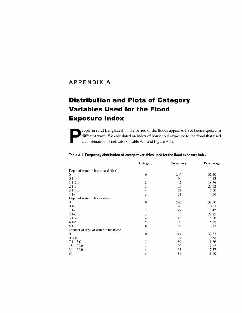
A P P E N D I X A
Distribution and Plots of CategoryVariables Used for the Flood Exposure Index
People in rural Bangladesh in the period of the floods appear to have been exposed indifferent ways. We calculated an index of household exposure to the flood that useda combination of indicators (Table A.1 and Figure A.1).
Table A.1 Frequency distribution of category variables used for the flood exposure index
Category Frequency Percentage
Depth of water in homestead (feet)0 0 246 32.500.1–1.0 1 110 14.531.1–2.0 2 142 18.762.1–3.0 3 175 23.123.1–4.0 4 53 7.004.1+ 5 31 4.10Depth of water in house (feet)0 0 246 32.500.1–1.0 1 80 10.571.1–2.0 2 147 19.422.1–3.0 3 173 22.853.1–4.0 4 43 5.684.1–5.0 5 39 5.155.1+ 6 29 3.83Number of days of water in the home0 0 247 32.630–7.0 1 74 9.787.1–15.0 2 89 11.7615.1–30.0 3 130 17.1730.1–60.0 4 133 17.5760.1+ 5 84 11.10

106 APPENDIX A
Figure A.1 Frequency distribution of households by various variablesof flood exposure

A P P E N D I X B
Supplementary Tables
Table B.1 Monthly average price of high-yielding varieties of coarse rice, 1998 (Tk per kilogram)
Average Standard Maximum/Division price deviation Maximum Minimum minimum
Barisal divisionJune 11.87 0.44 11.75 9.75 1.21August 12.92 0.41 13.67 12.50 1.09October 14.20 0.54 14.78 13.33 1.11
Chittagong divisionJune 11.83 0.42 12.42 10.88 1.14August 13.36 0.71 14.18 12.15 1.17October 14.27 0.85 15.33 13.00 1.18
Dhaka divisionJune 11.25 0.70 12.53 9.76 1.28August 13.45 0.68 15.10 12.56 1.20October 14.33 0.62 15.35 13.06 1.18
Khulna divisionJune 11.18 0.57 11.75 9.75 1.21August 13.02 0.39 13.67 12.50 1.09October 14.09 0.56 14.78 13.33 1.11
Rajshahi divisionJune 10.83 0.63 12.08 9.82 1.23August 12.97 0.56 13.85 12.23 1.13October 14.01 0.60 14.92 13.10 1.14
Sylhet divisionJune 11.53 0.86 12.70 10.79 1.18August 13.94 0.25 14.25 13.64 1.05October 14.67 0.83 15.75 13.77 1.14
All BangladeshJune 11.31 0.69 12.70 9.75 1.30August 13.23 0.62 15.10 12.15 1.24October 14.21 0.65 15.75 13.00 1.21
Source: DAM data and authors’ calculations.

108 APPENDIX B
Table B.2 Total value of assets owned, by severity of flood exposure
Flood exposure
Asset category Not exposed Moderate Severe Very severe All
Productive 6,787 7,604 6,409 4,926 6,448Domestic 2,066 1,659 1,508 1,573 1,716Housing 25,475 28,076 22,661 21,132 24,310Liquid 8,049 12,113 7,679 12,413 9,661Consumer durables 2,619 3,375 1,434 1,911 2,393Others 2,130 1,512 1,148 1,351 1,525Total 40,767 45,476 35,839 35,840 39,352
Source: IFPRI-FMRSP, Household Survey 1998.
Table B.3 Number of households that suffered any asset losses, by flood exposure
Flood exposure
Asset category Not exposed Moderate Severe Very severe All
Productive 21 39 56 48 164Domestic — 10 32 37 79Housing 17 82 133 125 357Liquid 15 35 50 40 140Consumer durables 1 . . . . . . 1 2Others . . . . . . . . . 6 6 Total 41 100 143 131 415
Source: IFPRI-FMRSP, Household Survey 1998.
Table B.4 Total value of assets lost for households that suffered any losses, by flood exposure
Flood exposure
Asset category Not exposed Moderate Severe Very severe All
Productive 413 1,300 942 1,000 979Domestic . . . 311 177 207 208Housing 2,509 5,541 5,649 6,221 5,675Liquid 4,692 3,094 2,906 8,428 4,722Consumer durables 500 . . . . . . 1,000 750Others . . . . . . . . . 2,182 2,182Total 2,990 6,164 6,679 9,042 6,936
Source: IFPRI-FMRSP, Household Survey 1998.
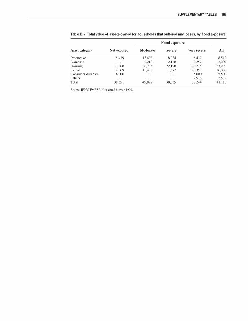
SUPPLEMENTARY TABLES 109
Table B.5 Total value of assets owned for households that suffered any losses, by flood exposure
Flood exposure
Asset category Not exposed Moderate Severe Very severe All
Productive 5,439 13,408 8,034 6,437 8,512Domestic . . . 2,213 2,148 2,257 2,207Housing 13,368 28,735 22,198 22,235 23,292Liquid 12,669 15,432 11,577 26,353 16,880Consumer durables 6,000 . . . . . . 5,000 5,500Others . . . . . . . . . 2,578 2,578 Total 39,551 49,872 38,055 38,244 41,110
Source: IFPRI-FMRSP, Household Survey 1998.


References
Accra Study Team. 1998. Promoting urban food and nutrition security for the vulnerable in the Greater Accrametropolitan area. Final Report of the Accra Urban Food and Nutrition Study to the World HealthOrganization. Legon, Ghana: Noguchi Memorial Institute for Medical Research and Washington, D.C.:International Food Policy Research Institute.
ACC/SCN (United Nations Administrative Committee on Coordination/Subcommittee on Nutrition). 2000.Fourth report on the world nutrition situation. Geneva: ACC/SCN in collaboration with the Interna-tional Food Policy Research Institute.
Ahmed, Faruk, Moududur Rahman Khan, Md Omar Faruque, Shirin Taj, Tasmin Hyderi, and Alan A. Jack-son. 1998. Serum retinol is influenced by social factors and antioxidant nutrients among adolescent girlsin urban Bangladesh. International Journal of Food Sciences and Nutrition 49 (1): 39–45.
Ahmed, R. 2000. Liberalization of agricultural input markets in Bangladesh. In Out of the shadow of famine:Evolving food markets and food policy in Bangladesh, ed. R. Ahmed, S. Haggblade, and T. E. Chowd-hury. Baltimore, Md., U.S.A.: Johns Hopkins University Press for the International Food Policy Re-search Institute.
Ahmed, R., S. Haggblade, and T. E. Chowdhury, eds. 2000. Out of the shadow of famine: Evolving food mar-kets and food policy in Bangladesh. Baltimore, Md., U.S.A.: Johns Hopkins University Press for theInternational Food Policy Research Institute.
Alamgir, M. 1980. Famine in South Asia: Political economy of mass starvation. Cambridge, Mass.:Oelgeschlager, Gunn and Hain.
Ali, Mir M., M. M. Hogue, Rezaur Rahman, and Salim Rashid. 1998. Bangladesh floods: Views from homeand abroad, 1998. Dhaka: University Press.
Bangladesh Water Development Board. 1998. Annual flood report. Flood Forecasting and Warning Centre. Banu, Shireen, and Iftekbar Hussain. 1998. Report on the visit to six flood-affected districts. Dhaka,
Bangladesh.Baulch, Bob, Jayanta Das, W. M. H. Jaim, Naser Farid, and Sajjad Zohir. 1998. The spatial integration and
pricing efficiency of the private sector grain trade in Bangladesh: Phase I and II report. BangladeshInstitute of Development Studies, Bangladesh Agricultural University, and University of Sussex.
BBS (Bangladesh Bureau of Statistics). 1997. Child nutrition survey of Bangladesh 1995-96. Dhaka: Bang-ladesh Bureau of Statistics, Statistics Division, Ministry of Planning.
———. 1998. Household expenditure survey 1995–96. Dhaka: Bangladesh Bureau of Statistics, StatisticsDivision, Ministry of Planning.
———. 1998. Statistical yearbook, 1998. Government of Bangladesh.BHC (British High Commission). 1998. Rapid flood appraisal report. Flood field report undertaken in My-
mensingh, Jamalpur, Siranjganj, Pabna, Bogra, Manikganj and Dhaka districts, September 6–9, 1998,by the First Secretary British High Commission.
Bouis, H. 1993. Food consumption surveys: How random are measurement errors? In Data needs for foodpolicy in developing countries, ed. J. von Braun and D. Puetz. Washington, D.C.: International FoodPolicy Research Institute.
Bouis, H., and M. J. G. Novenario-Reese. 1997. The determinants of demand for micronutrients: An analy-sis of rural households in Bangladesh. Food Consumption and Nutrition Division Discussion PaperNo. 32. Washington D.C.: International Food Policy Research Institute.
Bouis, H., B. de la Briere, L. Guitierrez, K. Hallman, N. Hassan, O. Hels, W. Quabili, A. Quisumbing,S. Thilsted, Z. H. Zihad, and S. Zohir. 1998a. Commercial vegetable and polyculture fish production inBangladesh: Their impacts on income, household resource allocation, and nutrition. Washington, D.C.:International Food Policy Research Institute.
Bouis, H., M. Palabrica-Costello, O. Solon, D. Westbrook, and A. B. Limbo. 1998b. Gender inequality andinvestments in adolescents in the rural Philippines. Research Report 108. Washington, D.C.: Interna-tional Food Policy Research Institute.
Chowdhury, N., and S. Haggblade. 2000. Evolving rice and wheat markets. In Out of the shadow of famine:Evolving food markets and food policy in Bangladesh, ed. R. Ahmed, S. Haggblade, and T. E. Chowd-hury. Baltimore, Md., U.S.A.: Johns Hopkins University Press for the International Food Policy Re-search Institute.
CMIE (Centre for Monitoring Indian Economy). 1998–2000. Monthly review of the Indian economy, variousissues. Mumbai, India.
Cox, D., and E. Jimenez. 1998. Risk-sharing and private transfers: What about urban households. EconomicDevelopment and Cultural Change 46 (3): 621–639.
Das, J., S. Zohir, and B. Baulch. 1997. Spatial integration of foodgrain markets in Bangladesh: Pricing analy-sis. Dhaka: Bangladesh Institute of Development Studies. Manuscript.
del Ninno, C., and P. A. Dorosh. 2001. Averting a food crisis: Private imports and public targeted distributionin Bangladesh after the 1998 flood. Agricultural Economics 25: 1–10.
del Ninno, C., and D. K. Roy. 1999a. Impact of the 1998 flood on labor markets and food security and ef-fectiveness of relief operations in Bangladesh. Food Management and Research Support Project Work-ing Paper 8, Dhaka.
———. 1999b. The 1998 flood and household food security: Evidence from rural Bangladesh. Food Man-agement and Research Support Project Working Paper 9, Dhaka.
Democracy Watch. 1998. Flood and post-flood situation in the rural areas of Bangladesh. Report by Mr.Abul Hossain Ahamed Bhuiyan, advisor to Democracy Watch, Bangladesh Open University.
Department of Agricultural Marketing (DAM), Ministry of Agriculture, Government of Bangladesh. Un-published data.
Directorate General of Food, Ministry of Food, MIS data. Unpublished.Dorosh, P. A. 1999a. Foodgrain markets and policy in the aftermath of the 1998 flood. Food Management
and Research Support Project Working Paper 7, Dhaka. ———. 1999b. The determination of rice prices in Bangladesh: Supply shocks, trade liberalization and
cross-border trade. Food Management and Research Support Project Working Paper 2, Dhaka. ———. 2000. Foodgrain production and imports: Toward self-sufficiency in rice? In Out of the shadow of
famine: Evolving food markets and food policy in Bangladesh, ed. R. Ahmed, S. Haggblade, and T. E.Chowdhury. Baltimore, Md., U.S.A.: Johns Hopkins University Press for the International Food PolicyResearch Institute.
———. 2001. Trade liberalization and national food security: Rice trade between Bangladesh and India. WorldDevelopment 29: 4.
Dreze, J., and A. Sen. 1989. Hunger and public action. Oxford: Clarendon Press.———. 1991. The political economy of hunger, 3 volumes. Oxford: Clarendon Press.FAO (Food and Agriculture Organization of the United Nations). Food balance sheets, various issues. Foster, A. 1995. Prices, credit markets and child growth in low-income rural areas. Economic Journal 105:
551–570.FPMU (Food Planning and Monitoring Unit). 1999. Database on food situation Bangladesh. Dhaka: Ministry
of Food, Government of Bangladesh. Frankenberger, T. 1992. A indicators and data collection methods for assessing household food security. In
Household food security: Concepts, indicators, measurements. A technical review, ed. S. Maxwell andT. Frankenverger. New York and Rome: UNICEF and IFAD.
Goletti, F. 1993. The effects of supply shocks on market integration: An application to rice markets inBangladesh. International Food Policy Research Institute, Washington, D.C. Mimeo.
———. 1994. The changing public role in a rice economy approaching self-sufficiency: The case of Bang-ladesh. Research Report 98. Washington, D.C.: International Food Policy Research Institute.
Greene, W. H. 1997. Econometric analysis, 3d ed. Upper Saddle River, N.J.: Prentice-Hall. Haddad, L., E. Kennedy, and J. Sullivan. 1994. Choices of indicators for food security and nutrition monitor-
ing. Food Policy 19 (3): 329–343.Harriss, B. 1995. The intrafamily distribution of hunger in South Asia. In The political economy of hunger,
ed. J. Dreze, A. Sen, and A. Hussain. Oxford: Oxford University Press.Hausman, J. A. 1978. Specification tests in econometrics. Econometrica 46: 1251–1271. Hena, H., and A. Kabir. 1998. Assessment of food needs for people affected by flood in Bangladesh. Flood
field report undertaken in Shariatpur, Madaripur, Faridpur, Gopalganj, and Rajbari, August 31–September 4, 1998. World Food Programme.
HKI (Helen Keller International). 1998a. Impact of the 1998 floods on rural households in Bangladesh: Aspecial report from the nutrition surveillance project. Dhaka.
———. 1998b. Post flood alert: Malnutrition on the rise in Bangladesh after the worst flood of the century:Potential long-lasting consequences. Dhaka.
Hossain, M. 1990. Natural calamities, instability in production and food policy in Bangladesh. The BangladeshDevelopment Studies 18 (4).
Hossain, M., L. Bose, and A. Chowdhury. 2001. Changes in agriculture and economy in the flood-prone envi-ronment in Bangladesh, 1988 to 2000: Insights from a repeat survey of 16 villages. Paper presented at the
112 REFERENCES

Workshop on Floodprone Rice Systems, January 9–11, 2001, organized by the Bangladesh Rice ResearchInstitute and the International Rice Research Institute. Manuscript.
Hossain, S., and M. Moazzem. 1998. Flood and health. Posting on the Bangladesh flood 1998 internet site(http://bangladeshflood98.org/health/health1.html) reporting results of study undertaken by Save theChildren (UK), Dhaka, Bangladesh.
Hossain, S., and M. Moazzem, and Muhammad Shuaib. 1998. Rapid nutrition assessment during flood 1998:Coping mechanisms and community perception of suitable rehabilitation. Dhaka: Save the ChildrenFund UK.
Irrigation Support Project for Asia and the Near East. 1993. Flood response and guidelines on planning floodproofing. Bangladesh Flood Action Plan FAP 14/ FAP 23. Photocopy.
Islam, Md. Khairul. 1998. Combating health problems in flood 1998: Observations and learning. Dhaka:PLAN International.
Johnson, U., and D. Toole. 1991. Household food security and nutrition: A conceptual analysis. New York:UNICEF. Mimeo.
Judge, G. G., W. E. Griffiths, R. C. Hill, H. Lutkepohl, and T. C. Lee. 1985. The theory and practice of econo-metrics, 2nd ed. New York: John Wiley.
Khan, A. Z., and M. Obaidullah. 1999. Bangladesh floods 1998 and food security. Paper prepared for the Con-ference on Natural Disasters and Policy Response in Asia: Implications for Food Security. Harvard Uni-versity, Cambridge, Mass., April 30–May 1, 1999 (draft). Manuscript.
Khan, S. H., and E. Haque. 1998. Assessment of food needs for people affected by flood 1998 in Bangladesh.Flood field report undertaken in Serajgonj, Bogra, and Gaibandha districts, August 31–September 3,1998. World Food Programme.
Lifschultz, L. 1979. Bangladesh: The unfinished revolution. London: Zed Press.Maxwell, S., and Frankenberger, T. 1992. Household food security: Concepts, indicators, measurements. A
technical review. New York and Rome: UNICEF and IFAD.Maxwell, D., C. Ahiadeke, C. Levin, M. Armar-Klemesu, S. Zakariah, and G. Mary Lamptey. 1999. Alterna-
tive food-security indicators: Revisiting the frequency and severity of “coping strategies.” Food Policy24: 411–429.
MHFW (Ministry of Health and Family Welfare). 1995. Bangladesh country paper on nutrition. Govern-ment of the People’s Republic of Bangladesh in collaboration with the Bangladesh National NutritionCouncil. Dhaka.
Mitra, S. N., A. Al-Sabir, A. R. Cross, and K. Jamil. 1997. Bangladesh demographic and health survey, 1996–1997. Dhaka and Calverton, Md.: National Institute of Population Research and Training (NIPORT),Mitra and Associates, and Macro International, Inc.
Murduch, J. 1999. Between the state and the market: Can informal insurance patch the safety net? WorldBank Research Observer 14 (2): 187–207.
Murshid, K. A. S. 1999. Liberalization and foodgrain imports: The evolution and conduct of the border tradewith India. Food Management and Research Support Project Working Paper 11, Dhaka.
NPAN (Bangladesh National Plan of Action for Nutrition). 1997. Prepared by the Ministry of Health andFamily Welfare, Government of the People’s Republic of Bangladesh in collaboration with the Bang-ladesh National Nutrition Council. Dhaka: Bangladesh National Nutrition Council.
Osmani, S. R. 1991. The food problems of Bangladesh. In The political economy of hunger, volume 3, ed. J.Dreze and A. Sen. Oxford: Clarendon Press.
———. 1995. The food problems of Bangladesh. The political economy of hunger. Dhaka: University Press. Pramanik, M. A. H.. 1994. Natural disasters. In Environment and development in Bangladesh, ed. A. A. Rah-
man, R. Haider, S. Huq, and E. G. Jansen. Vol. 1. Dhaka: University Press.Rahman, H., and S. Choudhury. 1998. Report on flood situation and impact of flood. Flood field report under-
taken in Pabna, Rajshahi, Nawabgan, and Naogaon districts, August 31–Sepember 3, 1998. World FoodProgramme.
Ravallion, M. 1985. The performance of rice markets in Bangladesh during the 1974 famine. EconomicJournal 95.
———. 1990. Markets and famines. Dhaka: University Press.———. 1997. Famines and economics. Journal of Economic Literature 35 (3) (September): 1205–1242. Ravallion, M., and Q. Wodon. 2000. Does child labor displace schooling? Evidence on behavioral responses
to an enrollment subsidy. Economic Journal 110: 158–175.Rivers, D., and Q. H. Vuong. 1988. Limited information estimators and exogeneity tests for simultaneous Pro-
bit models. Journal of Econometrics 39 (3): 347–366.Sen, A. 1981. Poverty and famines. Oxford: Clarendon Press.Shahabuddin, Q., and S. Zohir. 1995. Medium- and long-term projections of foodgrain demand, supply and
trade balance in Bangladesh. The Bangladesh Development Studies 23 (3–4).Shahjahan, M. 1998. Flood disaster management in deltaic plain integrated with rural development. In Bang-
ladesh floods: Views from home and abroad, ed. M. M. Ali, M. M. Hoque, R. Rahman, and S. Rashid.Dhaka: University Press.
REFERENCES 113

Sobhan, R. 1979. Politics of food and famine in Bangladesh. Economics and Political Weekly, December 1,24-28.
UNICEF (United Nations Children’s Fund). 1990. Strategy for improved nutrition of children and womenin developing countries. New York.
———. 1998. Tackling malnutrition in Bangladesh. Panel 14 in State of the World’s Children 1998. New York.UNICEF-ADB (United Nations Children’s Fund and Asian Development Bank). 1997. Reducing child mal-
nutrition in selected Asian countries: Strategies for Bangladesh. Study undertaken by the Institute ofNutrition and Food Science and Department of Economics, University of Dhaka, and Dhaka UrbanCommunity Health Program at the invitation of the United Nations Children’s Fund and the Asian De-velopment Bank.
USDA (United States Department of Agriculture). Rice and wheat outlook, various issues. von Braun, J., T. Teklu, and P. Webb. 1999. Famine in Africa: Causes, responses, and prevention. Baltimore,
Md., U.S.A.: Johns Hopkins University Press for the International Food Policy Research Institute.World Bank. 2000. World development report 2000. Washington, D.C.World Food Programme (WFP). 1998. Field report on flood assessment. Flood field report undertaken in
Mymensingh, Netrakona, Kishoreganj, and Tangail Districts, August 31–September 4, 1998.Zaman, H. 1999. Assessing the impact of microcredit on poverty and vulnerability in Bangladesh. Policy
Research Working Paper 2145. Washington, D.C.: World Bank. Zohir, S. 1995. Problems and prospects of crop diversification in Bangladesh. Bangladesh Development
Studies 21 (September): 73–90.
114 REFERENCES