arX

iv:0

911.

4739

v1 [

hep-

ph]

24

Nov

200

9

Preprint typeset in JHEP style - HYPER VERSION

LPSC09171

Testing Yukawa-unified SUSY during year 1 of LHC:

the role of multiple b-jets, dileptons and missing ET

Howard Baera, Sabine Kramlb, Andre Lessaa and Sezen Sekmenc

aDept. of Physics and Astronomy, University of Oklahoma, Norman, OK 73019, USAbLaboratoire de Physique Subatomique et de Cosmologie, UJF Grenoble 1,

CNRS/IN2P3, INPG, 53 Avenue des Martyrs, F-38026 Grenoble, FrancecDept. of Physics, Florida State University, Tallahassee, FL 32306

E-mail: baer@nhn.ou.edu, sabine.kraml@lpsc.in2p3.fr, lessa@nhn.ou.edu,

sezen.sekmen@cern.ch

Abstract: We examine the prospects for testing SO(10) Yukawa-unified supersymmetric

models during the first year of LHC running at√

s = 7 TeV, assuming integrated luminosity

values of ∼ 0.1–1 fb−1. We consider two cases: the Higgs splitting (HS) and the D-term

splitting (DR3) models. Each generically predicts light gluinos and heavy squarks, with

an inverted scalar mass hierarchy. We hence expect large rates for gluino pair production

followed by decays to final states with large b-jet multiplicity. For 0.2 fb−1 of integrated

luminosity, we find a 5σ discovery reach of mg ∼ 400 GeV even if missing transverse energy,

EmissT , is not a viable cut variable, by examining the multi-b-jet final state. A corroborating

signal should stand out in the opposite-sign (OS) dimuon channel in the case of the HS

model; the DR3 model will require higher integrated luminosity to yield a signal in the

OS dimuon channel. This region may also be probed by the Tevatron with 5–10 fb−1 of

data, if a corresponding search in the multi-b + EmissT channel is performed. With higher

integrated luminosities of ∼ 1 fb−1, using EmissT plus a large multiplicity of b-jets, LHC

should be able to discover Yukawa-unified SUSY with mg . 630 GeV. Thus, the year 1

LHC reach for Yukawa-unified SUSY should be enough to either claim a discovery of the

gluino, or to very nearly rule out this class of models, since higher values of mg lead to

rather poor Yukawa unification.

Keywords: Supersymmetry Phenomenology, Supersymmetric Standard Model, Large

Hadron Collider.

1. Introduction

Grand unified theories (GUTs) find a welcome inclusion of supersymmetry (SUSY) into

their structure in that SUSY tames the gauge hierarchy problem via the well-known can-

cellation of quadratic divergences [1]. In particular, the GUT group SO(10) is highly

motivated in that it allows for– in addition to gauge unification– the unification of all the

matter superfields of each generation into the 16-dimensional spinor representation [2]. The

matter unification only works if the 15 matter superfields of the Minimal Supersymmet-

ric Standard Model (MSSM) are augmented by a SM gauge singlet superfield N ci which

contains a right-hand neutrino (RHN) field. The presence of RHN fields is essential to

describe data from the past decade on neutrino mass and flavor oscillations; in particular a

Majorana mass term near the GUT scale, needed to implement see-saw neutrino masses [3],

should be generated by the breakdown of SO(10) gauge symmetry. In addition to gauge

and matter unification, in the simplest SO(10) SUSY GUT models– wherein both MSSM

Higgs doublets reside in a 10 of SO(10)– one expects Yukawa coupling unification in the

third generation: ft = fb = fτ (= fντ ) at MGUT.

Recently, a variety of studies have examined the MSSM(+RHN) to check whether

the measured values of gauge couplings and third generation fermion masses do indeed

allow for t − b − τ Yukawa coupling unification [4–15]. Essential to the calculation is the

inclusion of 2-loop renormalization group equations [16] (RGEs) and inclusion of weak scale

threshold corrections [17] which occur due to the MSSM → SM transition in effective field

theories. These threshold corrections imply that Yukawa coupling unification depends on

the entire spectrum of SUSY particles, since the SUSY particles enter the various t, b and

τ self-energy diagrams [17].

Assuming universal boundary conditions at the GUT scale, the parameter space of

SO(10)-motivated SUSY consists of

m1/2, m16, m10, M2D, A0, tan β, sign(µ), (1.1)

where m1/2 is the common gaugino mass at MGUT, m16 is the common GUT mass of

all matter scalars, m10 is that of the Higgs soft terms, and M2D parametrizes potential

splittings in the GUT scale Higgs (and possibly matter scalar) soft terms. Such splittings

are expected to arise from the breaking of the SO(10). It has been found that t − b − τ

Yukawa coupling unification can occur in the MSSM within this setup, but only for very

restricted forms of the soft SUSY breaking (SSB) parameters at MGUT. These include, for

the case of µ > 0:

• A20 = 2m2

10 = 4m216,

• m16 ∼ 5 − 15 TeV,

• m1/2 ≪ m16,

• tan β ∼ 50.

– 1 –

These boundary conditions were found in Ref. [18] to give rise to an inverted scalar mass

hierarchy (IMH), wherein first/second generation scalars end up with masses ∼ 10 TeV,

while third generation scalars, Higgs scalars A, H and H± and µ are of order ∼ 1−2 TeV.

A problem with the IMH scheme is that it is inconsistent with radiative electroweak

symmetry breaking (REWSB), unless the Higgs soft terms are split at MGUT [19]: m2Hu

<

m2Hd

, thus giving m2Hu

a head start over m2Hd

in its running towards the weak scale.1 Such

splitting naturally occurs due to D-term (DT) contributions to all scalar masses arising

from the breakdown of SO(10). However, applying the splitting to only the Higgs sector

(“just-so” Higgs splitting, HS)

m2Hu,d

= m210 ∓ 2M2

D (HS model) (1.2)

results in better accuracy of Yukawa unification as compared to full DT splitting. Recently,

it has been shown that DT splitting, combined with the running effect of the neutrino

Yukawa coupling fντ and a small mass splitting between first/second versus third generation

scalars (the DR3 model) can allow for Yukawa coupling unification to a few percent [15].

Both the HS and DR3 schemes lead to sparticle mass spectra characterized by

• mq,ℓ(1, 2) ∼ 10 TeV,

• mq,ℓ(3) and µ ∼ 1 − 3 TeV,

• mg ∼ 300 − 500 GeV,

• mfW1, eZ2∼ 100 − 180 GeV,

• m eZ1∼ 50 − 90 GeV.

Figure 1 shows the location of a large number of Yukawa-unified models in the R vs. mg

plane, for the HS model (red dots) and the DR3 model (blue dots) obtained through a

Markov Chain Monte Carlo (MCMC) scan of the parameter space (for details, see [15]).

Here, the degree of Yukawa unification is quantified as

R =max(ft, fb, fτ )

min(ft, fb, fτ )(1.3)

where ft, fb and fτ are the top, bottom and tau Yukawa couplings, respectively, evaluated

at Q = MGUT. In the DR3 case, if we require R < 1.05, then mg . 450 GeV. In the HS

model, while mg ∼ 300− 500 GeV is favored for low R < 1.05 solutions, it is possible (but

not likely) to have occassional models with mg as large as ∼ 700 GeV.

In models with the above listed superpartner spectrum and a bino-like Z1 state, the

neutralino relic density is computed to be ∼ 102−104 times the measured abundance [9,11],

and the models are seemingly excluded. However, if one invokes the Peccei-Quinn solution

to the strong CP problem [20–24], then an axion/axino supermultiplet is expected in the

theory [25]. With an axino of mass ma ∼ 1 MeV the neutralinos will decay via Z1 → aγ,

1This can be different in non-universal models, see [10,13,14].

– 2 –

Figure 1: Scatter plot of Yukawa unified models in the R vs. mg plane, for solutions in the DR3

model (blue) and the HS model (red).

which greatly reduces the dark matter density by a large factor: ma/m eZ1. Cold dark

matter (CDM) solutions can be found consisting of mainly cold axions and thermally

produced axinos, with a small component of warm axinos arising from Z1 → γa decay,

which occurs on time scales of order 1 sec. Since m16 ∼ 10 TeV, and we expect m16 ∼ mG,

the axion/axino CDM scenario allows for a solution to the gravitino BBN problem, and

can generate re-heat temperatures TR ∼ 106 − 109 GeV, which can allow for baryogenesis

mechanisms such as non-thermal [26] or Affleck-Dine [27] leptogenesis to occur [28].

Since the value of mg is so low in Yukawa-unified SUSY models, we expect the whole

scenario to soon be tested at the CERN LHC.2 LHC has already turned on in Fall, 2009. As

time progresses, the centre-of-mass energy√

s will be increased into the ∼ 7 TeV regime.

An integrated luminosity of 0.1 − 1 fb−1 is expected to be collected.3 Earlier work on

Yukawa-unified SUSY at LHC with√

s = 14 TeV showed the model to be easily testable

at LHC [30]. The LHC SUSY events should be characterized by gluino pair production

followed by three-body decays to states including a high multiplicity of b-jets. In addition,

opposite-sign dileptons with mass between 40 − 80 GeV (i.e. between the γ and Z peaks)

may be evident.

In the intervening past year, while LHC recovered from an unfortunate incident involv-

ing faulty circuits and quenched magnets, the experiments have been measuring millions

of cosmic muon events. This cosmic data has allowed them to fine-tune their detector re-

sponse to muons, and to make great strides in alignment of detector elements. We expect

thus that isolated muons, jets and b-jets should be readily measurable very early on during

LHC running, while reliable electron identification (e ID) and even more so reliable EmissT

measurement, may require additional time to establish.

2Indeed experiments at the Fermilab Tevatron collider may also probe up to mg ∼ 400 − 430 GeV [29].3The quoted physics data to be collected at 7 TeV as of November 2009 is 0.2 fb−1.

– 3 –

6 7 8 9 10 11 12 13 14√s (TeV)

1×102

1×103

1×104

1×105

1×106

σ g~g~ (

fb)

mg~ = 300 GeV

mg~ = 400 GeV

mg~ = 500 GeV

NLOLOLHC Start-up

mq~ ~ 10 TeV

Figure 2: Total cross-section for gluino pair production with mq = 10 TeV versus LHC collider

energy√

s, for mg = 300, 400 and 500 GeV.

In this paper, we expand upon the analysis presented in Ref. [30], and address several

new issues:

• We focus on the LHC potential to discover or rule out Yukawa-unified SUSY during

year 1 of running.4 To this end, we calculate signal and background production rates

for the LHC turn-on energy of√

s = 7 TeV rather than the maximal collider energy of√s = 14 TeV used earlier. Part of the effect of LHC turn-on at lower than expected

energies can be gleaned from Fig. 2, where we plot σ(pp → ggX) vs. collider energy√s, for mg = 300, 400 and 500 GeV, while taking mq = 10 TeV. We show both

LO and NLO QCD results as derived from Prospino [34]. For mg = 400 GeV, LHC

operating at√

s = 7 TeV yields a cross section of σ ∼ 104 fb. It is expected that,

after about 0.1 fb−1 of integrated luminosity, the LHC will move up in energy to

the√

s ∼ 10 TeV regime, where σ ∼ 3 × 104 fb. Ultimately, the LHC should move

up to its design energy of√

s = 14 TeV, where the cross section increases to ∼ 105

fb. Various background rates will also change accordingly. In this paper, we take

a conservative approach, and evaluate all signal and background cross sections at√s = 7 TeV. Increasing the beam energy beyond 7 TeV should only increase the

SUSY reach projections which we calculate here.

• We include as well many more background subprocesses than before, including the

effect of many 2 → 3 and 2 → 4 body subprocesses.

• We particularly hone in on what LHC can accomplish with very low integrated lu-

minosity. After turn-on, some time will be required to examine detector response to

4Some additional analyses of early physics prospects at LHC are contained in Refs. [31–33].

– 4 –

well-known SM processes like W , Z and tt production. To be able to use the classic

SUSY signature of jets + EmissT production, the measurement of Emiss

T – which de-

pends on a knowledge of the entire detector response– will be required. However, in

Ref. [32,33], it is pointed out that LHC experiments can examine multi-jet + isolated

multi-muon events in lieu of jets+EmissT events as a gain for signal over background.

We find that for very low integrated luminosity, using either large isolated muon mul-

tiplicity, or large b-jet multiplicity, allows mg values of up to 400 GeV to be probed

with just 0.2 fb−1 of integrated luminosity. (Note that we expect a similar reach for

the Tevatron in the ≥ 2 − 3 b-jets + EmissT channel with 5 − 10 fb−1 [29].)

• We also discuss the case when EmissT measurements and e ID are established. Here we

find that LHC can explore mg values as high as ∼ 630 GeV with 1 fb−1 of integrated

luminosity. Thus, during year 1 the LHC may well be able to either discover or very

nearly rule out Yukawa-unified SUSY.

The paper is organized as follows. We first establish in Sec. 2 two Yukawa-unified

model lines: one in the HS model and one in the DR3 model. We also examine general

features in sparticle production and decay for these model lines. In Sec. 3, we present

some technical details of our signal and background calculations. In Sec. 4, we present

expectations for early SUSY searches in the multi b-jets channel5 without using EmissT cuts.

We also examine rates for early multi-muon production plus jets without using EmissT . We

find that the HS and DR3 models may be distinguishable by measuring the ratio of OS

dilepton events to multi b-jet events, since both models produce multi-b-jets at a similar

rate. However, while OS dimuons from Z2 decay are abundant in the HS model, they are

relatively scarce in the DR3 model. In Sec. 5.4, we move beyond the 0.1 fb−1 level, and

calculate the LHC reach for the two model lines using as well EmissT and e ID for 1 fb−1

of integrated luminosity. In this case, the 5σ LHC reach should extend to mg ∼ 630 GeV,

enough to cover the bulk of parameter space of these simple Yukawa-unified models. In

Sec. 7, we present our conclusions.

2. HS and DR3 model lines

2.1 Model lines

Using the parameter space in Eq. 1.1, Ref. [28] found a large number of SUSY spectral

solutions with good Yukawa coupling unification in the HS model. We adopt Point B with

R = 1.02 of this paper as a Yukawa-unified benchmark point, and label it as HSb. The

HSb input parameters and mass spectra are listed in Table 1.

To construct a HS model line, we keep most of the above parameters fixed, but allow

m1/2 to vary. This keeps the Yukawa-unification generally low, but allows us to vary

mg ∼ 3.5m eZ2∼ 7m eZ1

continuously. We plot the value of R versus mg in Fig. 3. We see

that at low mg (∼ 325 GeV), R < 1.03, while as mg increases, Yukawa unification gets

worse until mg ∼ 700 GeV, where we find R ∼ 1.13.

5Earlier work emphasizing the utility of the presence of b-jets in SUSY events was provided in Refs. [30,

35].

– 5 –

parameter HSb DR3b

m16(1, 2) 10000 11805.6

m16(3) 10000 10840.1

m10 12053.5 13903.3

MD 3287.1 1850.6

m1/2 43.9442 27.414

A0 −19947.3 −22786.2

tan β 50.398 50.002

R 1.025 1.027

µ 3132.6 2183.4

mg 351.2 321.4

muL9972.1 11914.2

mt12756.5 2421.6

mb13377.1 1359.5

meR10094.7 11968.5

mfW1116.4 114.5

m eZ2113.8 114.2

m eZ149.2 46.5

mA 1825.9 668.3

mh 127.8 128.6

Table 1: Masses in GeV units and parameters for Yukawa-unified benchmark points HSb [28] and

DR3b [15]. For the DR3 model, we use MN3= 1013 GeV.

We also adopt from Ref. [15] a DR3 model line, labelled as DR3b, with parameters in

Table 1. where m16(1, 2, 3), is the scalar mass for the 1st, 2nd and 3th generations and

MN3, fντ , Aντ and mvR3

are the right-handed neutrino mass, Yukawa coupling, A-term

and the scalar mass for the sneutrino. We construct a DR3 model line by again keeping

most parameters fixed, but letting m1/2 to vary. In the DR3 model line, we find R ∼ 1.03

for mg ∼ 325 GeV, while R increases to ∼ 1.15 for mg ∼ 700 GeV.6

Due to the heavy scalar masses in the HS and DR3 model lines, the scalars essentially

decouple at LHC energies. What results is a low energy effective theory where only g,

Z1,2 and W±

1 are the new physics matter states. In the next two sections we discuss the

production cross-sections and decay rates for these states.

2.2 HS and DR3 production cross sections

We plot in Fig. 4 the leading order gg, W1Z2 and W+1 W−

1 production cross sections as a

function of mg for collider energy√

s = 7 TeV. From the figure, we see that gluino pair

production is dominant up to mg ∼ 520 GeV (at NLO, it dominates up to mg ∼ 560 GeV),

with cross sections typically greater than 103 fb, and in excess of 104 fb in the lower gluino

mass range. Thus, even with integrated luminosities as low as 0.1 fb−1, we expect hundreds

6Although Fig. 1 shows that for some special choice of the parameters lower values of R can be obtained

for mg ∼ 700, the model lines chosen here represent the general behavior of the bulk of parameter space.

– 6 –

350 400 450 500 550 600 650 700m

g~(GeV)

1 1

1.01 1.01

1.02 1.02

1.03 1.03

1.04 1.04

1.05 1.05

1.06 1.06

1.07 1.07

1.08 1.08

1.09 1.09

1.1 1.1

1.11 1.11

1.12 1.12

1.13 1.13

1.14 1.14

1.15 1.15

1.16 1.16

R

DR3 HS

Figure 3: Degree of Yukawa unification R (see Eq.1.3) for the models HS and DR3 as a function

of the gluino mass. The model parameters are the same as in Table 1, but with m1/2 varying from

30 to 180 GeV.

of gluino pair events in the upcoming LHC year 1 physics data sample for the HS and DR3

models.

Gluino pair production cross sections at the Fermilab Tevatron collider show a large

increase in rate as mq increases [29]. This is due to suppression of negative interference

terms in the qq → gg subprocess cross section. At the LHC, gluino pair production for

mg ∼ 300−500 GeV is dominated instead by the gg → gg subprocess, which is independent

of mq. Thus, gg cross sections show only a slight (∼10–20%) increase with increasing mq

at the LHC.

2.3 Sparticle branching fractions in the HS and DR3 model lines

Since mg ≪ mq in the HS or DR3 model lines, we will get dominant gluino decays into

three-body modes. The gluino branching ratios will be largely model dependent, but since

ti and bi are always the lightest squarks, and tan β is large [36], the decays will mostly be

restricted to the following channels:

• g → Zi + bb, i = 1, 2

• g → Z1 + tt

• g → W−

1 bt or W+1 bt .

The general feature mg ≪ mq is common to both the HS and DR3 models, since it

relies mostly on the fact that m1/2 ≪ m16. However, the inclusion of the D-term splitting

– 7 –

350 400 450 500 550 600 650 700m

g~(GeV)

1×102

1×103

1×104

σ (f

b)DR3HS√−s = 7 TeV

DR3HS√−s = 7 TeV

W~

1 Z~

2

DR3HS√−s = 7 TeV

DR3HS√−s = 7 TeV

DR3HS√−s = 7 TeV

DR3HS√−s = 7 TeV

DR3HS√−s = 7 TeV

DR3

W~

1 W~

1

HS√−s = 7 TeVg~g~

Figure 4: Leading order total cross-sections for sparticle production in the HS model (solid) and

DR3 model (dashed) as a function of the gluino mass for pp collisions at√

s = 7 TeV. The model

parameters are the same as in Table 1 but with m1/2 varying from 30 to 180 GeV.

for all matter scalars in the DR3 model pushes mbRto lower values, when compared to the

HS model, where mbL∼ mbR

.7 As a result we have:

• DR3: b1 ∼ bR and mb1< mb2

• HS: b1 ∼ bL and mb1∼ mb2

Now, since Z2 is wino-like in both models, it just couples to left-squarks, what suppresses

the g → Z2 + bb decay in the DR3 model and favors it in the HS case. This behavior is

shown in Fig. 5, where the main gluino branching ratios for both models are plotted as

a function of the gluino mass. From Fig. 5 it can also be seen that– in the HS model–

once mg ≫ mt + mfW1the g → W−

1 bt + c.c. channel starts to dominate, since mt1< mb1

(for mg > 500 GeV). We can also see that g → Z1tt becomes relevant for heavy gluinos

(mg > 600 GeV) and it is enhanced in the DR3 model, where t1 is usually lighter than in

the HS model.

From Fig. 5 we see that, for the HSb benchmark case:

• BR(g → Z2 + bb) = 63%

• BR(g → Z1 + bb) = 15%

• BR(g → W1 + bt) = 9% .

On the other hand, the DR3b point has:

7The stop masses and mixing are basically the same in both models, since the D-term splitting is equal

for both tR and tL.

– 8 –

350 400 450 500 550 600 650 700m

g~(GeV)

0

0.1

0.2

0.3

0.4

0.5

0.6

0.7

0.8

0.9

1B

F(g~ )

HS

g~→ W~

1 + qq

g~→ W~

1 + b t

g~→ Z~

1 + b b

g~→ Z~

1 + t t

g~→ Z~

2 + b b

HS

350 400 450 500 550 600 650 700m

g~(GeV)

0

0.1

0.2

0.3

0.4

0.5

0.6

0.7

0.8

0.9

1

BF(

g~ )

DR3g~→ Z~

1 + b b

g~→ W~

1 + b t

g~→ Z~

2 + b b

DR3

g~→ W~

1 + qq

g~→ Z~

1 + t t

Figure 5: Gluino branching ratios for the HS and DR3 model-lines as a function of the gluino

mass. The model parameters are the same as in Table 1, but with m1/2 varying from 30 to 180

GeV.

350 400 450 500 550 600 650 700m

g~(GeV)

0

0.1

0.2

0.3

0.4

0.5

0.6

0.7

0.8

0.9

1

BF(

Z~ 2)

Z~2→ Z

~1 + Z

0

Z~2→ Z

~1 + µ+µ−

Z~2→ Z

~1 + bb

HSHSHSHS

Z~2→ Z

~1 + qq

HSHS

350 400 450 500 550 600 650 700m

g~(GeV)

0

0.1

0.2

0.3

0.4

0.5

0.6

0.7

0.8

0.9

1

BF(

Z~ 2)Z~

2→ Z

~1 + Z

0

Z~2→ Z

~1 + µ+µ−

Z~2→ Z

~1 + bb

DR3

Z~2→ Z

~1 + h

Z~2→ Z

~1 + qq

DR3

Figure 6: Z2 branching ratios for the HS and DR3 model-lines as a function of the gluino mass.

The model parameters are the same as in Table 1, but with m1/2 varying from 30 to 180 GeV.

• BR(g → Z2 + bb) = 11%

• BR(g → Z1 + bb) = 86%

• BR(g → W1 + bt) = 0.3% .

The Z2 and W1 are expected to decay via three body modes:

• Z2 → Z1f f

• W±

1 → Z1f f ′ ,

where the decays are dominated by the intermediate virtual W ∗ and Z∗ diagrams. If

mg & 500 GeV, then the two-body modes W1 → Z1W and Z2 → Z1Z will turn on.

Putting all segments of the cascade decays together, we expect the HSb signal to be rich

in b-jets and opposite-sign/same-flavor (OS/SF) isolated dileptons coming from Z2 → Z1ℓℓ,

with a small rate of SS dileptons coming from g → W1qq′ followed by W1 → ℓνℓZ1 decay.

For the DR3b point, we expect the signal to be rich in b-jets with a harder EmissT spectrum

– 9 –

Cross number of

SM process Generator section events

QCD: 2, 3 and 4 jets (pT > 40 GeV) AlpGen 3.0 × 109 fb 13M

tt: tt + 0, 1 and 2 jets AlpGen 1.6 × 105 fb 5M

bb: bb + 0, 1 and 2 jets AlpGen 8.8 × 107 fb 91M

Z + jets: Z/γ(→ ll, νν) + 0, 1, 2 and 3 jets AlpGen 8.8 × 106 fb 13M

W + jets: W±(→ lν) + 0, 1, 2 and 3 jets AlpGen 1.8 × 107 fb 19M

Z + tt: Z/γ(→ ll, νν) + tt + 0, 1 and 2 jets AlpGen 53 fb 0.6M

Z + bb: Z/γ(→ ll, νν) + bb + 0, 1 and 2 jets AlpGen 2.6 × 103 fb 0.3M

W + bb: W±(→ lν) + bb + 0, 1 and 2 jets AlpGen 6.4 × 103 fb 9M

tttt MadGraph 0.6 fb 1M

ttbb MadGraph 1.0 × 102 fb 0.2M

bbbb MadGraph 1.1 × 104 fb 0.07M

Table 2: Background processes included in this study, their cross sections and number of generated

events.

(when compared to HSb) due to the direct gluino decay to Z1, but with small rates in the

multilepton channels.

3. Event Simulation

In order to study the discovery potential of the LHC at√

s = 7 TeV we used AlpGen [37]

and MadGraph [38] to generate the background hard scattering events and Pythia [39]

for the subsequent showering and hadronization. Table 2 lists the 2 → n subprocesses

included in this study where jets = u, d, s, c and g. For all the processes involving multiple

jets, the MLM matching algorithm [37] was used to avoid double counting. All the above

processes were generated at LO, but a relatively low renormalization and factorization scale

(Q =√

s/6) was used to bring the total cross-sections closer to their NLO values (for more

details see Ref. [33]). The signal events were generated using Isajet 7.79 [40].

A toy detector simulation is then employed with calorimeter cell size ∆η × ∆φ =

0.05× 0.05 and −5 < η < 5 . The HCAL (hadronic calorimetry) energy resolution is taken

to be 80%/√

E + 3% for |η| < 2.6 and FCAL (forward calorimetry) is 100%/√

E + 5% for

|η| > 2.6, where the two terms are combined in quadrature. The ECAL (electromagnetic

calorimetry) energy resolution is assumed to be 3%/√

E + 0.5%. We use the Isajet jet

finding algorithm (cone type) to group the hadronic final states into jets. The jets and

isolated lepton definitions are as follow:

• Jets are required to have R ≡√

∆η2 + ∆φ2 ≤ 0.4 and ET (jet) > 25 GeV.

• Leptons are considered isolated if they have pT (l) > 5 GeV with visible activity

within a cone of ∆R < 0.2 of ΣEcellsT < 5 GeV.

Jets are tagged as b-jets if they contain a B hadron with ET (B) > 15 GeV, η(B) < 3

and ∆R(B, jet) < 0.5. We assume a tagging efficiency of 60% and light quark and gluon

– 10 –

jets can be mis-tagged as a b-jet with a probability 1/150 for ET ≤ 100 GeV, 1/50 for

ET ≥ 250 GeV, with a linear interpolation for 100 GeV ≤ ET ≤ 250 GeV (see R. Kadala

et al. in Ref. [35]).

4. Early searches without EmissT or electron ID

During the early stages of data taking at the LHC with integrated luminosity of order ∼ 0.1

fb−1, it is possible that EmissT and electron identification will not be reliable observables

(see Refs. [32,33]). Therefore we separate our analysis into two stages:

• early searches, where no EmissT cuts are applied and only muons are considered for

the leptonic channels, and

• full analysis, using a minimum EmissT cut and including both e’s and µ’s.

In both cases we assume that the b-jets can be reliably tagged due to their displaced ver-

tices as reconstructed in the micro-vertex detector or via a non-isolated muon tag. For

initial searches we apply the following set of minimal cuts, labelled C0:

C0 cuts:

• Jet cuts: n(jets) ≥ 4 with ET (j) ≥ 50 GeV, η(j) ≤ 3 and for the hardest jet ET (j1) ≥100 GeV,

• Lepton cuts: ET (ℓ) ≥ 10 GeV and η(ℓ) ≤ 2,

• ST ≥ 0.2,

• n(b) ≥ 1,

where ST is the transverse sphericity and for now ℓ = µ only.

4.1 Multi b-jet signal

As discussed in Sec. 2 the points HSb and DR3b are expected to be rich in b-jets and possibly

isolated leptons. In Fig. 7 we plot the b-jet multiplicity for the signal and backgrounds

(BG) after applying the C0 set of cuts. As expected, the BG distribution falls much faster

than the signal. Signal exceeds BG for n(b) ≥ 4, where the BG is dominated by multi b

production (bb and bbbb). We also note that the DR3b case has larger rates for 1 ≤ n(b) ≤ 4

when compared with the HSb point, due to a lighter gluino. However, the HSb benchmark

gives a larger signal for n(b) ≥ 5, since in this case Z2 → Z1bb also contributes, and Z2 are

produced at large rates from gluino cascade decay.

We note here that a signal rate above an expected SM BG level may not be sufficient

to claim a discovery, due to both theoretical and experimental uncertainties in the multi-b

background rate. However, the overall shape of the n(b) distribution should be to some

extent self-normalizing, as one can fix the BG levels in the n(b) = 0, 1, 2 channels, and

look for a harder n(b) distribution in the signal case. Thus, some of the uncertainty is

– 11 –

1 2 3 4 5 6 7 8n(b)

0.1

1

10

100

1000

10000

1e+05

1e+06

1e+07

σ (f

b)

BGHSbDR3bbbbbbbttttttbbQCDttbb + W(lν)bb + Ztt + ZW + jetsZ + jets

Figure 7: b-jet distribution after C0 cuts at the LHC, with√

s = 7 TeV. We show the signal levels

for the HSb (red) and DR3b (green) points along with various SM backgrounds.

Results after C0-based selection

σ(n(b) ≥ 3) σ(n(b) ≥ 4) σ(OS)

HSb 899 fb 176 fb 99 fb

DR3b 1334 fb 243 fb 22 fb

BG 1911 fb 70 fb 11 fb

Table 3: Cross-sections for the n(b) ≥ 3, 4 and OS channels after the C0 cuts for the points HSb,

DR3b and the background.

removed when one looks for an excess in ratios such as σ(n(b) = 3)/σ(n(b) = 1). Table 3

shows the n(b) ≥ 3 and 4 cross-sections for both points and the background. The signal in

the n(b) ≥ 4 channel is at the 200 fb level and is well above SM background levels. Such a

signal may be visible with very low integrated luminosity values ∼ 0.05 fb−1!

As mentioned above, a mere excess in one or more of the multi b-jet channels may not

be sufficient to claim discovery, due to large uncertainties in the normalization of the high

jet multiplicities BGs, such as bb, tt and Z + 2 jets. With this in mind, we present some

signal distributions with distinct shapes from the BG ones, which could help corroborate

a discovery and provide some information on the sparticle masses. As discussed in Sec. 2,

events with n(b) ≥ 4 usually come from g → Zibb decays. Therefore the invariant mass

of the bb pair is expected to have edges at mg − m eZi. This is shown in Figs. 8 and 9,

where max[mb1 b1 ,mb2 b2 ] is plotted8 at the parton level (dashed black line). As expected,

in the DR3b case the mg −m eZ1mass edge is much more evident than the mg −m eZ2

edge,

due to the large g → Z1 + bb branching fraction, while the opposite happens for the HSb

point. At the detector level, the main difficulty in obtaining max[mb1 b1 ,mb2 b2 ] comes from

8Here the index i in bi labels b’s coming from the same gluino.

– 12 –

0 100 200 300 400 500max(m

bb) (GeV)

0

0.25

0.5

0.75

1

1.25

1.5

dσ/d

m (

fb/G

eV)

BGParton level (no cuts) (÷200)HSb + BG

mg~-m

z~1

mg~-m

z~2

mg~-m

z~1

mg~-m

z~2

mg~-m

z~1

mg~-m

z~2

mg~-m

z~1

mg~-m

z~2

mg~-m

z~1

mg~-m

z~2

mg~-m

z~1

mg~-m

z~2

Figure 8: Maximum invariant bb mass at parton level for the HSb point without cuts

(black/dashed) and at detector level for the HSb plus background events (red/solid) with n(b) ≥4, ∆R(b2, b2) < 1 after the C0 cuts (see text). The BG distribution (gray) and the statistical error

bars for 1 fb−1 of integrated luminosity are also shown.

combining the correct b-jets into pairs coming from the same gluino. As pointed out in

Ref. [30], usually the two hardest b-jets come from different gluinos. Furthermore, in most

cases the pair coming from the same g has smaller separation angles. Using these two facts,

we select b1 and b2 as the hardest and second hardest jets and b2 as the remaining jet that

minimizes ∆φ(b2, b2). Also, to avoid event topologies with no small angular separation, we

apply the cut ∆R(b2, b2) < 1, where R =√

∆φ(b2, b2)2 + ∆η(b2, b2)2. Using this procedure

and adding the C0 set of cuts we obtain the solid curves shown in Figs. 8 and 9, where

the BG contribution was added to the signal. We also show the statistical error bars for

1 fb−1 of integrated luminosity. As can be seen, the invariant-mass distributions have the

expected shape, although the mass edges seem to require higher integrated luminosity to

become statistically relevant.

4.2 Dimuon channels

In Fig. 10 we show the muon multiplicity for the HSb and DR3b signal points and the

BG. For n(µ) = 0, 1, the BG is well above the signal, but for n(µ) ≥ 2, signal starts to

dominate over the BG. As expected from the discussion in Sec. 2, the DR3b has much

smaller rates to multileptons. Separating the n(µ) = 2 channel into opposite sign (OS) and

same sign (SS) muons, we see that almost all the signal comes from the OS dimuon case.

Due to the small g → W−

1 tb + c.c. branching fraction, the SS signal is almost 2 orders of

magnitude below the OS one, which makes it irrelevant for luminosities . 1 fb−1. As seen

in Table 3, the OS cross-section for the HSb point is around 100 fb and has a discovery

potential similar to the multi b-jet channel, while the DR3b benchmark will require more

– 13 –

0 100 200 300 400 500max(m

bb) (GeV)

0

0.25

0.5

0.75

1

1.25

1.5

σ/bi

n (f

b/G

eV)

BGParton level (no cuts) (÷200)DR3b + BG

mg~-m

z~1

mg~-m

z~2

mg~-m

z~1

mg~-m

z~2

mg~-m

z~1

mg~-m

z~2

mg~-m

z~1

mg~-m

z~2

mg~-m

z~1

mg~-m

z~2

mg~-m

z~1

mg~-m

z~2

Figure 9: Maximum invariant bb mass at parton level for the DR3b point without cuts

(black/dashed) and at detector level for the DR3b plus background events (green/solid) with n(b) ≥4, ∆R(b2, b2) < 1 after the C0 cuts (see text). The BG distribution (gray) and the statistical error

bars for 1 fb−1 of integrated luminosity are also shown.

0 1 2 3 4 5 6n(µ)

0.1

1

10

100

1000

10000

1e+05

1e+06

σ (f

b)

BGHSbDR3bbbbbbbttttttbbQCDttbb + W(lν)bb + Ztt + ZW + jetsZ + jets

OS SSOS SSOS SS

Figure 10: Muon distribution after C0 cuts at the LHC, with√

s = 7 TeV. We show the signal

levels for the HSb (red) and DR3b (green) points along with various SM backgrounds. In the

n(µ) = 2 bin, the left (pluses) and right (crosses) columns show the background (black) and signal

components for OS (with invariant mass cuts) and SS dimuons.

integrated luminosity to be seen in the OS dimuon channel.

As is well known, the invariant mass of OS muons has a mass edge at m eZ2− m eZ1

,

since most OS muons come from Z2 → Z1µ+µ− decays. In Fig. 11, we show the m(µ+µ−)

– 14 –

50 100 150

m(µ+µ−) (GeV)

0

1

2

3

4

5

6

dσ/d

m (

fb/G

eV)

BGHSb + BGDR3b + BG

mz~

2-m

z~1

mz~

2-m

z~1

Figure 11: OS dimuon invariant mass for the HSb (red) and DR3b (green) points plus background

events after the C0 cuts (see text). The BG distribution (gray) and the statistical error bars for 1

fb−1 of integrated luminosity are also shown.

distribution for the HSb and DR3b points. As discussed in Sec. 2, the DR3b point has

small leptonic rates but may still be visible above background. In both cases, the mass

edges are visible and give the correct m eZ2−m eZ1

values. We also show the statistical error

bars for the combined signal plus background for 1 fb−1 of integrated luminosity. From

Fig. 11, we can see that the HSb point gives a statistically significant edge while the DR3b

case may require higher integrated luminosities.

Finally, we point out that in both the n(b) ≥ 4 and OS dimuon channels the invariant

mass distributions shown in Figs. 8, 9 and 11 have distinct features from the BG, which

should corroborate a discovery claim.

4.3 Early SUSY search: reach results

To estimate the LHC reach in the multi-b and multi-µ channels, we plot in Fig. 12 the signal

cross section for the HS and DR3 model lines versus mg using cuts C0 plus a). n(b) ≥ 3

and b). n(b) ≥ 4, along with the expected BG rate. We also plot the 5σ discovery lines

for integrated luminosity values 0.1 and 0.2 fb−1. The significance in σs is derived from

the p-value corresponding to the number of S+B events in a Poisson distribution with a

mean that equals to the number of background events [41]. For both the HS and DR3

model lines, the approximate 5σ LHC reach extends to mg ∼ 360 GeV for 0.1 fb−1, and

∼ 400 GeV for 0.2 fb−1. We remind the reader that this is comparable to what Tevatron

experiments can achieve using EmissT cuts and > 5 fb−1 of integrated luminosity [29].

The reach using cuts C0 and requiring an OS dimuon pair is shown in Fig. 13. In

this case, the reach in the HS model is similar to the multi-b reach: LHC should explore

to mg ∼ 360 GeV with 0.1 fb−1, and mg ∼ 400 GeV with 0.2 fb−1. In the DR3 model

– 15 –

400 500 600 700m

g~ (GeV)

0

200

400

600

800

1000

1200

1400

1600

1800

2000

2200

σ (

fb)

5σ (0.1 fb-1

)

5σ (0.2 fb-1

)

BGHSDR3

C0 - n(b) ≥ 3

400 500 600 700m

g~ (GeV)

0

50

100

150

200

250

300

σ (

fb)

BGHSDR3

5σ (0.1 fb-1

)

5σ (0.2 fb-1

)

C0 - n(b) ≥ 4

Figure 12: Early LHC reach for Yukawa-unified SUSY using cuts C0 plus nb ≥ 3 and nb ≥ 4.

line, however, there is no reach in the OS dimuon channel at these low values of integrated

luminosity. In fact, the rate of multi-b-jet events compared to the rate for OS dimuon

events would be one way to distinguish early-on whether one might be seeing SUSY in the

HS or the DR3 model case.

We also point out that despite giving the maximum reach for both models, the n(b) ≥ 3

channel has a small signal/BG ratio, what makes it more dependent on the knowledge of

the background.

– 16 –

400 500 600 700m

g~ (GeV)

0

20

40

60

80

100

120

140

σ (

fb)

5σ (0.1 fb-1

)

5σ (0.2 fb-1

)

BGHSDR3

C0 - OS

Figure 13: Early LHC reach for Yukawa-unified SUSY using cuts C0 plus requiring OS dimuons.

5. Analysis including EmissT cut and electron ID

As the experiments accumulate data, knowledge of the detectors and their response to SM

background will improve. Also, at some point in time, the LHC center-of-mass energy will

increase beyond 7 TeV into the 10 TeV range. To be conservative, we will continue our

analysis assuming√

s = 7 TeV. Moving to higher values of√

s should only increase the

possibility of discovering new, high mass matter states.

As detector response becomes better understood, it will be possible to utilize both

EmissT and electrons in the analysis. The Emiss

T variable is well known to be a powerful

discriminator between SUSY and SM events, and is considered to be the “classic” signature

for SUSY. In Fig. 14 we show the EmissT distributions for the BG as well as the HSb and

DR3b points after applying the C0 cuts. As expected, the DR3b signal has a harder EmissT

spectrum than HSb, due to its large g → Z1bb branching ratio.

In order to reduce most of the background and still keep considerably large cross-

sections for the signal, we henceforth:

• include the EmissT > 100 GeV cut and

• include e’s into the C0 leptonic cuts

into our analysis. The cuts C0 augmented with the EmissT cut and inclusion of e’s, but with

no n(b) requirement, will be called C1 cuts:

C1 cuts:

• Jet cuts: n(jets) ≥ 4 with ET (j) ≥ 50 GeV, η(j) ≤ 3 and for the hardest jet ET (j1) ≥100 GeV,

– 17 –

0 100 200 300 400 500 600

ET

miss (GeV)

0.01

0.1

1

10

100

1000

10000

1e+05

dσ/d

ET

mis

s (fb

/GeV

)

BGHSbDR3b

Figure 14: Emiss

T distribution for the BG (gray), HSb (red) and DR3b (green) points after the C0

cuts (see text).

• Lepton cuts: ET (ℓ) ≥ 10 GeV and η(ℓ) ≤ 2,

• ST ≥ 0.2,

• EmissT > 100 GeV,

where ℓ = µ, e.

5.1 Multi b-jet + EmissT channel

The main effect of adding an EmissT cut to our previous analysis is the drastic reduction

of background in the multi b-jet channel. However, the signal will also be significantly

reduced, and so will be the statistics in the invariant mass distributions.

The n(b) distribution after C1 cuts is shown in Fig. 15. Now the signal’s peak at

n(b) =1, 2 is visible above the BG, and the hard distribution in n(b) should be a striking

signature for both the DR3b and HSb models, since the combined signal plus BG distri-

bution becomes approximately flat for 0 ≤ n(b) ≤ 2. The EmissT cut reduces most of the bb

and bbbb backgrounds, leaving tt as the dominant one for n(b) ≥ 1. This results in a consid-

erable reduction of the BG in the n(b) = 1, 2 and 3 bins, where now the signal/background

ratio is larger than one. The cross-sections for n(b) ≥ 3, 4 are shown in Table 4. Due to the

large signal cross-section in these bins, the signal could be visible with less than 0.05 fb−1

of integrated luminosity (in the happy case where an EmissT measurement is immediately

viable)!

The invariant mass distributions from Figs. 8 and 9 are now re-plotted in Figs. 16 and

17 after the EmissT cut is included. Now, due to the drastic reduction in the background, the

mbb distribution is nearly free of BG events. However, the decrease in the signal statistics

– 18 –

0 1 2 3 4 5 6 7 8n(b)

0.1

1

10

100

1000

10000

σ (f

b)

BGHSbDR3bbbbbbbttttttbbQCDttbb + W(lν)bb + Ztt + ZW + jetsZ + jets

Figure 15: b-jet distribution after C1 cuts at the LHC, with√

s = 7 TeV. We show the signal

levels for the HSb (red) and DR3b (green) points along with various SM backgrounds.

Results after C1-based selection

σ(n(b) ≥ 3) σ(n(b) ≥ 4) σ(OS)

HSb 364 fb 68 fb 81 fb

DR3b 782 fb 139 fb 23 fb

BG 16 fb 2 fb 9 fb

Table 4: Cross-sections for the n(b) ≥ 3, 4 and OS channels after the C1 cuts for the points HSb,

DR3b and the background.

makes it impossible to obtain any information on the sparticle masses from the shape of

max[mb1 b1 ,mb2 b2 ].

A quantity that may still reveal some information on the gluino mass scale is the

effective mass, Meff =∑

pT (jets) + EmissT , plotted in Fig. 18 for the HSb and DRb points,

as well as for two points on the HS and DR3 model lines with heavier gluinos (mg = 576 GeV

and mg = 581 GeV, respectively).

5.2 Multi-lepton channels

In Fig. 19, we show the isolated lepton multiplicity distribution after cuts C1. In the

n(ℓ) = 0 channel, the DR3b signal exceeds BG, while in the n(ℓ) = 2 channel, the HSb

signal exceeds BG. In the n(ℓ) = 1 channel, BG from tt production is larger than both

signal cases. One can pull out a better signal rate in the 1ℓ channel by imposing in addition

a MT (ℓ,EmissT ) > 100 GeV cut, as is well known [42].

We divide the n(ℓ) = 2 channel into opposite-sign/same-flavor (OS/SF) events (e+e−

or µ+µ−), and same-sign events. For the OS/SF channel, we see the EmissT cut has little

effect on the signal-to-BG ratio, since the background, mainly tt production, also has large

– 19 –

0 100 200 300 400 500max(m

bb) (GeV)

0

0.25

0.5

dσ/d

m (

fb/G

eV)

BGParton level (no cuts) (÷200)HSb + BG

mg~-m

z~1

mg~-m

z~2

Figure 16: Same as Fig. 8, but including the Emiss

T > 100 GeV cut.

0 100 200 300 400 500max(m

bb) (GeV)

0

0.25

0.5

0.75

σ/bi

n (f

b/G

eV)

BGParton level (no cuts) (÷200)DR3b + BG

mg~-m

z~1

mg~-m

z~2

Figure 17: Same as Fig. 9, but including the Emiss

T > 100 GeV cut.

EmissT . Again, we expect the entire distribution to be self normalizing, since tt is the

dominant BG, and one can fix the total tt cross section by normalizing to the 1ℓ channel.

Then the n(ℓ) distribution should be harder than expected from just SM physics if a SUSY

signal is present.

In Fig. 20, we show the OS/SF dilepton invariant mass distribution after cuts C1.

Now, despite the negligible background, the reduction in the signal makes the mass edges

less visible. In particular, the dilepton invariant mass still shows the m eZ2− m eZ1

edge,

but with a smaller statistical significance as evident from the error bars. Performing a

– 20 –

0 500 1000 1500 2000M

eff (GeV)

0.01

0.1

1σ/

bin

(fb/

GeV

)

BGHSb (m

g~ = 350 GeV)

DR3b (mg~ = 320 GeV)

HS (mg~ = 576 GeV)

DR3 (mg~ = 581 GeV)

n(b) ≥ 3

Figure 18: Effective mass scale of events with n(b) ≥ 3 after C1 cuts for the BG, points HSb and

DRb, and two points on the HS and DR3 model lines with heavier gluinos (mg = 576 GeV and

mg = 581 GeV, respectively).

0 1 2 3 4 5 6n(l)

0.1

1

10

100

1000

10000

σ (f

b)

SSSSOS/SF SS

BGHSbDR3bbbbbbbttttttbbQCDttbb + W(lν)bb + Ztt + ZW + jetsZ + jets

Figure 19: Lepton multiplicity distribution after C1 cuts at the LHC, with√

s = 7 TeV. We show

the signal levels for the HSb (red) and DR3b (green) points along with various SM backgrounds.

In the n(ℓ) = 2 bin, the left (pluses) and right (crosses) columns show the background (black) and

signal components for OS/SF and SS dileptons.

different-flavor subtraction may reduce the already negligible BG even further.

5.3 Jets plus Z → ℓℓ + EmissT signal

We also show in Fig. 20 two additional HS and DR3 cases with mg ∼ 525 GeV. In this case,

– 21 –

50 100 150m(ll) (GeV)

0

1

2

3

4

5

6

dσ/d

m (

fb/G

eV)

BGHSb + BGDR3b + BGHS (m

g~ = 522 GeV)

DR3 (mg~ = 526 GeV)

mz~

2-m

z~1

mz~

2-m

z~1

mz~

2-m

z~1

mz~

2-m

z~1

mz~

2-m

z~1

mz~

2-m

z~1

mz~

2-m

z~1

mz~

2-m

z~1

mz~

2-m

z~1

mz~

2-m

z~1

Figure 20: OS dilepton (µ’s and e’s) invariant mass for the HSb (red) and DR3b (green) points

plus background events after the C1 cuts (see text). The BG distribution (gray) and the statistical

error bars for 1 fb−1 of integrated luminosity are also shown.

according to Fig. 6, the value of m eZ2is high enough that the two-body decay Z2 → Z1Z

is now dominant. We then expect a signature of multiple b-jets plus EmissT plus a dilepton

pair which reconstructs to m(ℓ+ℓ−) ≃ MZ [43]. While signal rates can be very high for

this channel, SM background is low, coming from processes such as tt and Z + tt.

5.4 LHC reach for Yukawa-unified SUSY using EmissT and e ID

Next, we investigate the full LHC reach for Yukawa-unified SUSY along the HS and DR3

model lines. First, we require the cut set C1, which includes EmissT > 100 GeV, and then

require n(b) ≥ 2 or n(b) ≥ 3. The SM background level and 5σ level for 0.2 and 1 fb−1

are shown in the plots of Fig. 21, along with expected signal rates from the HS and DR3

model lines. For the n(b) ≥ 2 case, we find an LHC reach for Yukawa-unifed SUSY out to

mg = 500 (600) GeV for 0.2 (1) fb−1. The reach is largely independent of whether one is

in the HS or the DR3 model.

For n(b) ≥ 3, the SM background is greatly reduced. In this case, we find a reach

to mg = 540 (630) GeV for 0.2 (1) fb−1. Again, the reach in the multi-b-jet channel is

largely independent of the model line, since both give large numbers of b-jets + EmissT in

the final state. We have also calculated the reach in the n(b) ≥ 4 channel; here, the result

is qualitatively similar to that obtained in the n(b) ≥ 2 case.

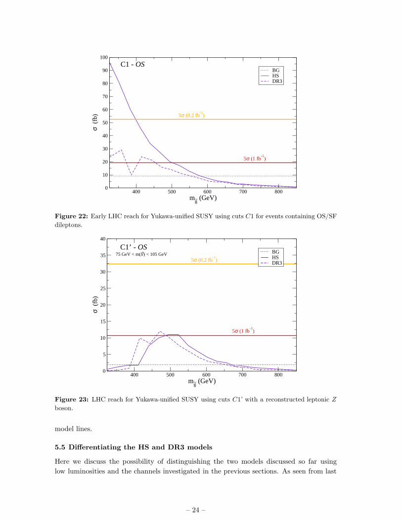
Next, in Fig. 22, we show the LHC reach for Yukawa-unified SUSY using the C1 cuts

plus requiring a pair of OS/SF dileptons. In this case, the LHC reach is model dependent.

For the HS model, where we obtain a high rate for g → bbZ2 decays, we find a reach up

to mg = 400 (500) GeV for 0.2 (1) fb−1 of integrated luminosity. For the DR3 model line,

– 22 –

400 500 600 700 800m

g~ (GeV)

10

100

1000

σ (

fb) 5σ (0.2 fb

-1)

5σ (1 fb-1

)

BGHSDR3

C1 - n(b) ≥ 2

400 500 600 700 800m

g~ (GeV)

10

100

1000

σ (

fb)

5σ (0.2 fb-1

)

5σ (1 fb-1

)

BGHSDR3

C1 - n(b) ≥ 3

Figure 21: Early LHC reach for Yukawa-unified SUSY using cuts C1 plus nb ≥ 2 and nb ≥ 3.

there is no reach for 0.2 fb−1, since here the g → bbZ1 decay is dominant. With 1 fb−1,

however, a signal with 5σ significance should be visible for mg ∼ 300 − 450 GeV.

For mg & 450 GeV, the two body decay mode Z2 → Z1Z opens up and we expect

to reconstruct Z → e+e− and Z → µ+µ− within the class of signal events. Here, we will

adopt cuts C1, but in addition require a OS/SF dilepton pair with 75 GeV< m(ℓ+ℓ−) <

105 GeV (cuts C1′). For this topology– ≥ 4 jets +EmissT + Z → ℓ+ℓ−– the dominant SM

BG comes from tt production. The LHC reach is shown in Fig. 23. As can be seen, no

significant excess is expected with 0.2 fb−1 of data. However, for & 1 fb−1, we find that

this topology can produce a 5σ signal for mg ∼ 450 − 530 GeV for both the HS and DR3

– 23 –

400 500 600 700 800m

g~ (GeV)

0

10

20

30

40

50

60

70

80

90

100

σ (

fb) 5σ (0.2 fb

-1)

5σ (1 fb-1

)

BGHSDR3

C1 - OS

Figure 22: Early LHC reach for Yukawa-unified SUSY using cuts C1 for events containing OS/SF

dileptons.

400 500 600 700 800m

g~ (GeV)

0

5

10

15

20

25

30

35

40

σ (

fb)

5σ (0.2 fb-1

)

5σ (1 fb-1

)

BGHSDR3

75 GeV < m(ll) < 105 GeVC1’ - OS

Figure 23: LHC reach for Yukawa-unified SUSY using cuts C1’ with a reconstructed leptonic Z

boson.

model lines.

5.5 Differentiating the HS and DR3 models

Here we discuss the possibility of distinguishing the two models discussed so far using

low luminosities and the channels investigated in the previous sections. As seen from last

– 24 –

400 500 600 700m

g~ (GeV)

0

0.1

0.2

0.3

0.4

0.5

0.6

HS + BGDR3 + BG

C1 - OS/n(b) ≥ 3

Figure 24: The ratio of the OS and n(b) ≥ 3 cross-sections after C1 cuts for the HS and DR3

model lines plus background as a function of the gluino mass. We also show the statistical error

bars for 1 fb−1.

section results (Figs. 21 and 22) and the discussion in Sec. 2, for low to moderate mg masses

we expect the HS and DR3 models to have rather distinct signatures. The first one is rich

in multi-b jets (n(b) ≥ 4, 5) and OS/SF dileptons coming from the g → Z2 + bb followed

by Z2 → Z/Z∗ + bb/ℓ+ℓ− decays, but has a softer EmissT spectrum due to the two step

cascade decays. On the other hand, the DR3 model is mainly dominated by g → Z1 + bb,

with small cross-sections in the multi-lepton channels, a moderate number of b-jets (n(b) ≥3,4) and a harder Emiss

T spectrum. To explore these features and discuss how well we can

distinguish both models with year one data, we plot in Fig. 24 the ratio of the OS and

n(b) ≥ 3 channels. As expected from the above discussion, we see that the ratio is larger

for the HS model and suppressed in the DR3 case for mg . 600 GeV. As the gluino mass

increases, the W1 + bt and Z1 + bb gluino decay channels become available (see Fig. 5),

increasing the OS channel in both models. From Fig. 24 we see that the OS/3b ratio should

be a good discriminator up to mg ∼ 450 GeV. For mg & 450 GeV, higher luminosities are

required in order to distinguish the models. But with high enough luminosities, we should

be able to tell the models apart up to mg ∼ 600 GeV. For even higher mg values, the signal

features are too similar and the simple OS/3b ratio is no longer useful.

– 25 –

6. Comparison with CDF/CMS multijets + EmissT channel

Next we would like to compare our results for the multi-b-jets + EmissT signature with a

multijets + EmissT analysis for SUSY searches proposed and used by CDF [44] and further

developed in CMS [45]. We implement the following selection.

• n(jets) ≥ 3 (we take jet pT > 50 GeV),

• EmissT ≥ 150 GeV,

• ∆φ( ~EmissT , ~HT ) < 1,

• 0.5 < R2 ≡√

∆φ2(j1, EmissT ) + (π − ∆φ(j2, Emiss

T ))2 < 4,

• 1.5 < Ra1 ≡√

(∆φ(j2, EmissT ))2 + (∆φ(j3, Emiss

T ))2 < 4.25,

• ∆φ(j2, EmissT ) > 0.35,

• ∆φ(ji, EmissT ) > 0.3,

• |η(j1)| < 1.7 ,

• Finally, we require the highest ET object in each signal event to be hadronic, rather

than leptonic 9.

The angular cuts are introduced in multijets + EmissT analyses where no lepton information

is explicitly used in order to guarantee the discrimination of QCD backgrounds which may

have large EmissT arising primarily due to jet mismeasurements. In such events, Emiss

T typi-

cally aligns with the 2nd hardest jet, as the hardest jet has a tendency to be mismeasured

most and eventually becomes the 2nd hardest jet.

The reach results for CDF/CMS multijets + EmissT cuts with no n(b) requirement can

be seen in Fig. 25. The 5σ reach for 0.2 (1) fb−1 of integrated luminosity is found to be

mg ∼ 370 (430) GeV.

In Figure 26, we plot the n(b) signal and background distributions after CDF/CMS

cuts, which share similar characteristics with the distributions after C1 cuts. The dom-

inance of signal starting with n(b) = 1 illustrates the importance of considering b−jet

tagging in the multijets + EmissT analyses. The original CMS analysis made use of the

B−triggers to significantly enhance the signal/BG ratio, while here we directly cut on

n(b). We show in Table 5 the cross sections found after implementing CDF/CMS cuts

with no requirement on n(b) and with n(b) = 1, 2, 3.

9This is an approximation for the leading track isolation step of the indirect lepton veto (ILV) technique

included in the CDF/CMS selection. Normally in multijets EmissT analyses where lepton information is

not explicitly used, W/Z/tt + n jets backgrounds with leptonic W,Z decays can be eliminated by vetoing

the events whose leading track is isolated. We omit the second step of ILV featuring jet electromagnetic

and charged fractions since it is designed to eliminate machine and cosmic backgrounds which we do not

consider here.

– 26 –

400 500 600 700m

g~ (GeV)

0

500

1000

1500

σ (

fb)

5σ (0.2 fb-1

)

5σ (1 fb-1

)

BGHSDR3

CDF/CMS jets + ET

miss cuts

Figure 25: LHC reach for Yukawa-unified SUSY using CDF/CMS multijets + Emiss

T cuts with no

n(b) requirement.

0 1 2 3 4 5 6 7 8n(b)

0.1

1

10

100

1000

10000

σ (f

b)

BGHSbDR3bbbbbbbttttttbbQCDttbb + W(lν)bb + Ztt + ZW + jetsZ + jets

Figure 26: b-jet distribution after CDF/CMS multijets + Emiss

T cuts at the LHC, with√

s = 7

TeV. We show the signal levels for the HSb (red) and DR3b (green) points along with various SM

backgrounds.

As before, we can do much better by requiring a high multiplicity of b-jets. In Fig. 27,

we adopt the same cuts as in Fig. 25, but in addition require n(b) ≥ 3. In this case, the BG

drops by a factor of ∼ 150, while the signal drops merely by a factor of ∼ 7 for mg ∼ 300

GeV. The LHC reach increases to mg ∼ 400 (500) GeV for 0.2 (1) fb−1 of integrated

luminosity.

– 27 –

Results after CDF/CMS multijets + EmissT -based selection

σ(no n(b) req.) σ(n(b) ≥ 1) σ(n(b) ≥ 2) σ(n(b) ≥ 3)

HSb 390 fb 313 fb 167 fb 55 fb

DR3b 849 fb 739 fb 435 fb 140 fb

BG 1132 fb 366 fb 101 fb 7 fb

Table 5: Cross-sections for the channels with no n(b) requirement, n(b) ≥ 1, 2 and 3 after the

CDF/CMS multijets + Emiss

T cuts for the points HSb, DR3b and the background.

400 500 600 700m

g~ (GeV)

1

10

100

1000

σ (

fb)

5σ (0.2 fb-1

)

5σ (1 fb-1

)

5σ (0.2 fb-1

)

5σ (1 fb-1

)

5σ (0.2 fb-1

)

5σ (1 fb-1

)

BGHSDR3

CDF/CMS jets + ET

miss cuts - n(b) ≥ 3CDF/CMS jets + E

T

miss cuts - n(b) ≥ 3CDF/CMS jets + E

T

miss cuts - n(b) ≥ 3

Figure 27: LHC reach for Yukawa-unified SUSY using CDF/CMS multijets + Emiss

T cuts with

nb ≥ 3.

7. Conclusions

In t−b−τ Yukawa-unified SUSY, we expect a characteristic spectrum of superpartners with

first/second generation squarks and sleptons around 10 TeV, third generation sparticles,

heavy Higgs bosons and µ around the few TeV level, and very light gauginos, with mg ∼300−500 GeV (although here we consider even higher values). Thus, at LHC, we expect to

see gluino pair production at a high rate, followed by gluino decays to bbZi or tbW−

1 + c.c..

SUSY searches should therefore exploit the high multiplicity of b-jets expected in this

scenario.

We investigated two model lines– the HS and DR3 cases. The HS case leads to large

rates for OS/SF dileptons in the final state, while DR3 case does not. We computed

numerous 2 → 2, 2 → 3 and 2 → 4 background processes. We found that with just 0.1–

0.2 fb−1 of integrated luminosity, the LHC discovery reach with√

s = 7 TeV extends out to

mg ∼ 400 GeV, even without using EmissT cuts. Crucial use is made of the high multiplicity

of b-jets in the final state. In the case of the HS model, a corroborating signal appears in

the µ+µ− + jets+ ≥ 1 b-jet channel.

– 28 –

L (fb−1) 0.05 0.1 0.2 1

C0

HS 340 GeV 371 GeV 400 GeV 471 GeV

Channel n(b) ≥ 3 n(b) ≥ 3 n(b) ≥ 3 n(b) ≥ 4

DR3 340 GeV 363 GeV 394 GeV 469 GeV

Channel n(b) ≥ 3 n(b) ≥ 3 n(b) ≥ 3 n(b) ≥ 3

C1

HS 436 GeV 480 GeV 526 GeV 630 GeV

Channel n(b) ≥ 3 n(b) ≥ 3 n(b) ≥ 3 n(b) ≥ 3

DR3 460 GeV 506 GeV 545 GeV 630 GeV

Channel n(b) ≥ 3 n(b) ≥ 3 n(b) ≥ 3 n(b) ≥ 3

CDF/CMS

HS - 341 GeV 380 GeV 474 GeV

Channel - n(b) ≥ 1 n(b) ≥ 1 n(b) ≥ 3

DR3 350 GeV 382 GeV 420 GeV 516 GeV

Channel n(b) ≥ 2 n(b) ≥ 2 n(b) ≥ 2 n(b) ≥ 3

Table 6: Gluino 5σ mass reach for the HS and DR3 model lines for different luminosites. We show

the values for the early search (C0 cuts), the full reach (C1 cuts) and the CDF/CMS multijets +

Emiss

T cuts (CDF/CMS). We also show the channel which optimizes the reach.

The LHC reach at very low luminosity and without EmissT is comparable to the Tevatron

reach in the multi-b + EmissT channel with 5–10 fb−1 of data. This may lead to a tight

competition for the discovery or exclusion of the simplest Yukawa-unified SUSY scenario!

Moving beyond about 0.2 fb−1, we expect reliable EmissT resolution and electron iden-

tification to become available. We find that the LHC reach, using√

s = 7 TeV and 1 fb−1

of integrated luminosity, will move into the mg ∼ 600 − 650 GeV range for both the HS

and DR3 model lines, if we require EmissT ≥ 100 GeV along with n(b) ≥ 3. This reach

is presumably sufficient to rule out Yukawa unification in the DR3 case. In the HS case,

somewhat larger values of mg can be allowed, although they seem very improbable. The

LHC reach for 1 fb−1 using the multi-jets + EmissT signature– but making no requirement

on n(b)– turns out to be much lower. A summary of our various results is presented in a

convenient form in Table 6.

At some point LHC energy will be increased to ∼ 10 TeV, and this will allow the

reach to be extended past the values presented here. Thus, our main conclusion is that

LHC stands an excellent chance to either discover Yukawa-unifed SUSY during year 1 of

operation, or exclude almost all its model parameter space!

Last but not least we note that, if the scenario discussed here is realized, a trilepton

signal from Drell-Yang W1Z2 production should appear when moving into the several fb−1

regime, giving direct access to the chargino/neutralino sector.

Note added: While finalizing this manuscript, we found an Atlas note [46] which also

investigates using multiple b-jets to enhance the LHC reach for SUSY in the mSUGRA

model. They examine integrated luminosity values of 0.1 and 1 fb−1, but take√

s = 14

TeV. Their overall results seem quite consistent with the results given here.

– 29 –

Acknowledgments

We thank Harrison Prosper for sharing with us his p-value and significance code. This

research was supported in part by the U.S. Department of Energy grant number DE-FG-

97ER41022, by the Fulbright Program and CAPES (Brazilian Federal Agency for Post-

Graduate Education). The work of SK is supported in part by the French ANR project

ToolsDMColl, BLAN07-2-194882.

References

[1] For recent reviews, see R. Mohapatra, hep-ph/9911272 (1999) and S. Raby, in Rept. Prog.

Phys. 67 (2004) 755.

[2] H. Georgi, in Proceedings of the American Institue of Physics, edited by C. Carlson (1974);

H. Fritzsch and P. Minkowski, Ann. Phys. 93, 193 (1975); M. Gell-Mann, P. Ramond and R.

Slansky, Rev. Mod. Phys. 50, 721 (1978).

[3] P. Minkowski, Phys. Lett. B 67 (1977) 421; M. Gell-Mann, P. Ramond and R. Slansky, in

Supergravity, Proceedings of the Workshop, Stony Brook, NY 1979 (North-Holland,

Amsterdam); T. Yanagida, KEK Report No. 79-18, 1979; R. Mohapatra and G. Senjanovic,

Phys. Rev. Lett. 44 (1980) 912.

[4] B. Ananthanarayan, G. Lazarides and Q. Shafi, Phys. Rev. D 44 (1991) 1613 and Phys. Lett.

B 300 (1993) 245; G. Anderson et al. Phys. Rev. D 47 (1993) 3702 and Phys. Rev. D 49

(1994) 3660; V. Barger, M. Berger and P. Ohmann, Phys. Rev. D 49 (1994) 4908; M.

Carena, M. Olechowski, S. Pokorski and C. Wagner, Ref. [17]; B. Ananthanarayan, Q. Shafi

and X. Wang, Phys. Rev. D 50 (1994) 5980; R. Rattazzi and U. Sarid, Phys. Rev. D 53

(1996) 1553; T. Blazek, M. Carena, S. Raby and C. Wagner, Phys. Rev. D 56 (1997) 6919;

T. Blazek and S. Raby, Phys. Lett. B 392 (1997) 371; T. Blazek and S. Raby, Phys. Rev. D

59 (1999) 095002; T. Blazek, S. Raby and K. Tobe, Phys. Rev. D 60 (1999) 113001 and

Phys. Rev. D 62 (2000) 055001; see also [5].

[5] S. Profumo, Phys. Rev. D 68 (2003) 015006; C. Pallis, Nucl. Phys. B 678 (2004) 398; M.

Gomez, G. Lazarides and C. Pallis, Phys. Rev. D 61 (2000) 123512, Nucl. Phys. B 638

(2002) 165 and Phys. Rev. D 67 (2003) 097701; U. Chattopadhyay, A. Corsetti and P. Nath,

Phys. Rev. D 66 (2002) 035003; M. Gomez, T. Ibrahim, P. Nath and S. Skadhauge, Phys.

Rev. D 72 (2005) 095008.

[6] H. Baer, M. Diaz, J. Ferrandis and X. Tata, Phys. Rev. D 61 (2000) 111701; H. Baer, M.

Brhlik, M. Diaz, J. Ferrandis, P. Mercadante, P. Quintana and X. Tata, Phys. Rev. D 63

(2001) 015007.

[7] H. Baer and J. Ferrandis, Phys. Rev. Lett. 87 (2001) 211803;

[8] T. Blazek, R. Dermisek and S. Raby, Phys. Rev. Lett. 88 (2002) 111804; T. Blazek, R.

Dermisek and S. Raby, Phys. Rev. D 65 (2002) 115004; R. Dermisek, S. Raby, L. Roszkowski

and R. Ruiz de Austri, J. High Energy Phys. 0304 (2003) 037; R. Dermisek, S. Raby, L.

Roszkowski and R. Ruiz de Austri, J. High Energy Phys. 0509 (2005) 029.

[9] D. Auto, H. Baer, C. Balazs, A. Belyaev, J. Ferrandis and X. Tata, J. High Energy Phys.

0306 (2003) 023.

[10] C. Balazs and R. Dermisek, J. High Energy Phys. 0803 (2003) 024.

– 30 –

[11] H. Baer, S. Kraml, S. Sekmen and H. Summy, J. High Energy Phys. 0803 (2008) 056.

[12] W. Altmannshofer, D. Guadagnoli, S. Raby and D. Straub, Phys. Lett. B 668 (2008) 385.

[13] I. Gogoladze, R. Khalid and Q. Shafi, Phys. Rev. D 79 (2009) 115004.

[14] D. Guadagnoli, S. Raby and D. M. Straub, J. High Energy Phys. 0910 (2009) 059.

[15] H. Baer, S. Kraml and S. Sekmen, J. High Energy Phys. 0909 (2009) 005.

[16] S. P. Martin and M. Vaughn, Phys. Rev. D 50 (1994) 2282.

[17] R. Hempfling, Phys. Rev. D 49 (1994) 6168; L. J. Hall, R. Rattazzi and U. Sarid, Phys. Rev.

D 50 (1994) 7048; M. Carena et al., Nucl. Phys. B 426 (1994) 269; D. Pierce, J. Bagger, K.

Matchev and R. Zhang, Nucl. Phys. B 491 (1997) 3.

[18] J. Feng, C. Kolda and N. Polonsky, Nucl. Phys. B 546 (1999) 3; J. Bagger, J. Feng and N.

Polonsky, Nucl. Phys. B 563 (1999) 3; J. Bagger, J. Feng, N. Polonsky and R. Zhang, Phys.

Lett. B 473 (2000) 264. H. Baer,P. Mercadante and X. Tata, Phys. Lett. B 475 (2000) 289;

H. Baer, C. Balazs, M. Brhlik, P. Mercadante, X. Tata and Y. Wang, Phys. Rev. D 64

(2001) 015002.

[19] H. Murayama, M. Olechowski and S. Pokorski, Phys. Lett. B 371 (1996) 57.

[20] R. Peccei and H. Quinn, Phys. Rev. Lett. 38 (1977) 1440 and Phys. Rev. D 16 (1977) 1791.

[21] S. Weinberg, Phys. Rev. Lett. 40 (1978) 223; F. Wilczek, Phys. Rev. Lett. 40 (1978) 279.

[22] J. E. Kim, Phys. Rev. Lett. 43 (1979) 103; M. A. Shifman, A. Vainstein and V. I. Zakharov,

Nucl. Phys. B 166 (1980) 493.

[23] M. Dine, W. Fischler and M. Srednicki, Phys. Lett. B 104 (1981) 199; A. P. Zhitnitskii, Sov.

J. Nucl. 31 (1980) 260.

[24] For recent reviews on axion physics, see J. E. Kim and G. Carosi, arXiv:0807.3125 (2008); P.

Sikivie, hep-ph/0509198; M. Turner, Phys. Rept. 197 (1990) 67.

[25] H. P. Nilles and S. Raby, Nucl. Phys. B 198 (1982) 102; J. E. Kim and H. P. Nilles, Phys.

Lett. B 138 (1984) 150; J. E. Kim, Phys. Lett. B 136 (1984) 378.

[26] G. Lazarides and Q. Shafi, Phys. Lett. B 258 (1991) 305; K. Kumekawa, T. Moroi and T.

Yanagida, Prog. Theor. Phys. 92 (1994) 437; T. Asaka, K. Hamaguchi, M. Kawasaki and T.

Yanagida, Phys. Lett. B 464 (1999) 12.

[27] H. Murayama and T. Yanagida, Phys. Lett. B 322 (1994) 349; M. Dine, L. Randall and S.

Thomas, Nucl. Phys. B 458 (1996) 291.

[28] H. Baer, M. Haider, S. Kraml, S. Sekmen and H. Summy, JCAP0902 (2009) 002.

[29] H. Baer, S. Kraml, S. Sekmen and H. Summy, arXiv:0910.2988 (2009).

[30] H. Baer, S. Kraml, S. Sekmen and H. Summy, J. High Energy Phys. 0810 (2008) 079.

[31] F. Gianotti and M. Mangano, hep-ph/0505221; D. Green, hep-ph/0601038; H. Baer, V.

Barger and G. Shaughnessy, Phys. Rev. D 78 (2008) 095009; J. Hubisz, J. Lykken, M.

Pierini and M. Spiropulu, Phys. Rev. D 78 (2008) 075008; M. Mangano, Eur. Phys. J. C 59

(2009) 373.

[32] H. Baer, H. Prosper and H. Summy, Phys. Rev. D 77 (2008) 055017; H. Baer, A. Lessa and

H. Summy, Phys. Lett. B 674 (2009) 49; J. Edsjo, E. Lundstrom, S. Rydbeck and J. Sjolin,

arXiv:0910.1106 (2009).

– 31 –

[33] H. Baer, V. Barger, A. Lessa and X. Tata, J. High Energy Phys. 0909 (2009) 063.

[34] W. Beenakker, R. Hopker, M. Spira, hep-ph/9611232 (1996).

[35] U. Chattoppadhyay, A. Datta, A. Datta, A. Datta and D.P. Roy, Phys. Lett. B 493 (2000)

127; P. Mercadante, K. Mizukohi and X. Tata, Phys. Rev. D 72 (30005) 035009; S. P. Das et

al. Eur. Phys. J. C 54 (2008) 645; R. Kadala et al. Eur. Phys. J. C 56 (2008) 511

[36] H. Baer, C. H. Chen, M. Drees, F. Paige and X. Tata, Phys. Rev. Lett. 79 (1997) 986 and

Phys. Rev. D 58 (1998) 075008.

[37] M. Mangano, M. Moretti, F. Piccinini, R. Pittau and A. Polosa, J. High Energy Phys. 0307

(2003) 001.

[38] T. Stelzer and W. F. Long, Comput. Phys. Commun. 81 (1994) 357.

[39] T. Sjostrand, S. Mrenna and P. Skands, J. High Energy Phys. 0605 (2006) 026.

[40] ISAJET v7.79, by H. Baer, F. Paige, S. Protopopescu and X. Tata, hep-ph/0312045; for

details on the Isajet spectrum calculation, see H. Baer, J. Ferrandis, S. Kraml and W. Porod,

Phys. Rev. D 73 (2006) 015010.

[41] H. B. Prosper, private code for calculation of significance from p-values.

[42] H. Baer, C. H. Chen, F. Paige and X. Tata, Phys. Rev. D 53 (1996) 6241.

[43] H. Baer, X. Tata and J. Woodside, Phys. Rev. D 42 (1990) 1450; H. Baer, C. Balazs, A.

Belyaev, T. Krupovnickas and X. Tata, J. High Energy Phys. 0306 (2003) 054.

[44] M. Spiropulu, Ph. D. thesis, UMI-99-88600; A. A. Affolder et al. (CDF Collaboration), Phys.

Rev. Lett. 88 (2002) 041801 hep-ex/0106001; S. Sekmen, Ph. D. thesis, CMS TS-2009/025

[45] S. Sekmen, Ph. D. thesis, CMS TS-2009/025

[46] Discovery potential for supersymmetry with b-jet final states with the Atlas detector, (The

Atlas Collaboration), Atlas note ATL-PHYS-PUB-2009-075 (2009).

– 32 –