Testing the performance of a Dynamic Global Ecosystem Model: Water balance

GLOBAL BIOGEOCHEMICAL CYCLES, VOL. 14, NO. 3, PAGES 795-825, SEPTEMBER 2000

Testing the performance of a Dynamic Global Ecosystem Model: Water balance, carbon balance, and vegetation structure

Christopher J. Kucharik, Jonathan A. Foley, Christine Delire, Veronica A. Fisher, Michael T. Coe, John D. Lenters, Christine Young-Molling, l and Navin Ramankutty Climate, People and Environment Program (CPEP), Institute for Environmental Studies, University of Wisconsin, Madison

John M. Norman

Department of Soil Science, University of Wisconsin, Madison

Stith T. Gower

Department of Forest Ecology and Management, University of Wisconsin, Madison

Abstract. While a new class of Dynamic Global Ecosystem Models (DGEMs) has emerged in the past few years as an important tool for describing global biogeochemical cycles and atmosphere- biosphere interactions, these models are still largely untested. Here we analyze the behavior of a new DGEM and compare the results to global-scale observations of water balance, carbon balance, and vegetation structure. In this study, we use version 2 of the Integrated Biosphere Simulator (IBIS), which includes several major improvements and additions to the prototype model developed by Foley et al. [1996]. IBIS is designed to be a comprehensive model of the terrestrial biosphere; the model represents a wide range of processes, including land surface physics, canopy physiology, plant phenology, vegetation dynamics and competition, and carbon and nutrient cycling. The model generates global simulations of the surface water balance (e.g., runoff), the terrestrial carbon balance (e.g., net primary production, net ecosystem exchange, soil carbon, aboveground and belowground litter, and soil CO2 fluxes), and vegetation structure (e.g., biomass, leaf area index, and vegetation compositior0. In order to test the performance of the model, we have assembled a wide range of continer/tal- and global-scale data, including measurements of river discharge, net primary production, vegetation structure, root biomass, soil carbon, litter carbon, and soil CO2 flux. Using these field data and model results for the contemporary biosphere (1965-1994), our evaluation shows that simulated patterns of runoff, NPP, biomass, leaf area index, soil carbon, and total soil CO2 flux agree reasonably well with measurements that have been compiled from numerous ecosystems. These results also compare favorably to other global model results.

1. Introduction

Recently, ecological research has focused on the functioning and dynamic nature of ecosystems, along with their role in the global carbon, nutrient, and water cycles. Part of this focus has resulted in the development of global terrestrial ecosystem models, including models of terrestrial biogeochemistry [e.g., Melillo et al., 1993,' Potter et al., 1993; Parton et al., 1993; Running and Gower, 1991], global vegetation biogeography [e.g.,

INow at Space Science and Engineering Center (SSEC), University of Wisconsin, Madison.

Copyright 2000 by the American Geophysical Union.

Paper number 1999GB001138. 0886-6236/00/1999GB001138512.00

Prentice et al., 1992; Neilson and Marks, 1994; Woodward et al., 1995; Haxeltine and Prentice, 1996], and land-atmosphere exchange processes [e.g., Dickinson et al., 1986; Sellers et al., 1996; Bonan, 1995]. However, these models, which were individually designed with specific goals in mind, consider a limited range of ecosystem processes. Only recently have global ecosystem models been designed to integrate biophysical processes, biogeochemical cycles, and vegetation dynamics into a single, consistent framework [Foley, 1995; Foley et al., 1996; Friend et al., 1997].

Large-scale integrated biosphere models are urgently needed to improve our understanding of how changes in land-use, climate variability, and increases in atmospheric CO2 concentrations might affect the structure and overall functioning of both natural and managed ecosystems across the globe. Such changes in global ecosystems have the potential to dramatically modify the availability of essential natural resources such as water, food,

795

796 KUCHARIK ET AL.: TESTING A DYNAMIC GLOBAL ECOSYSTEM MODEL

timber, and fiber during the next century. Furthermore, any significant changes in the terrestrial biosphere may contribute to additional feedbacks on the climate system through changes in vegetation patterns or changes in the production and consumption of greenhouse gases.

It is therefore of the utmost importance that we analyze the complex interactions among all facets of the biosphere, including atmospheric, vegetative, hydrological, and biogeochemical processes. However, the dynamic interactions that occur within the terrestrial biosphere take place across a continuum of timescales, ranging from seconds to hundreds of years. This system complexity has made the development and validation of integrated models of the terrestrial biosphere a difficult endeavor but one that is essential to global change research.

An integrated model of the Earth's biosphere, the Integrated Biosphere Simulator (or IBIS) [Foley et al., 1996] has been developed as a first step toward gaining an improved understanding of global biospheric processes and studying their potential response to human activity. IBIS is constructed to explicitly link land surface and hydrological processes, terrestrial biogeochemical cycles, and vegetation dynamics within a single, physically consistent framework. Furthermore, IBIS is one of a new generation of global biosphere models, termed Dynamic Global Vegetation Models (or DGVMs) [Steffen et al., 1992,' Walker, 1994,' W. Cramer et al., Dynamic responses of global terrestrial vegetation to changes in CO2 and climate, submitted to Global Change Biology, 1999], that considers transient changes in vegetation composition and structure in response to environmental change. Previous global ecosystem models have typically focused on the equilibrium state of vegetation and could not allow vegetation patterns to change over time.

Here we present a new version of the IBIS model (version 2), which has improved representations of land surface physics, plant physiology, canopy phenology, plant functional type (PFT) differences, and carbon allocation. In addition, IBIS-2 includes a new belowground biogeochemistry submodel [C.J. Kucharik et al., Measurements and modeling of carbon and nitrogen dynamics in managed and natural ecosystems of southern Wisconsin, submitted to Ecosystems, 1999] (hereinafter referred to as Kucharik et al., submitted manuscript, 1999), which is coupled to detritus production (litterfall and fine root turnover).

In this study, we present model simulations of the terrestrial carbon budget (net primary production, vegetation biomass, soil carbon, litter carbon, soil CO2 flux, and microbial biomass), global vegetation patterns, and patterns of runoff. To evaluate the model output across the world s biomes, we use a new global compilation of net primary production (NPP) measurements [S.T. Gower, unpublished data, 1999], a global gridded soil carbon database [International Geosphere-Biosphere Programme - Data and Information System (IGBP-DIS), 1999] and soil CO2 flux data [Raich and Schlesinger, 1992]. Measurements of runoff [Cogley, 1991], microbial biomass [Landsberg and Gower, 1997], fine root biomass [Jackson et al., 1996] and litter carbon [Matthews, 1997] are also used to test the model results.

2. IBIS-2: An Integrated Model of Biospheric Processes

The IBIS model includes, in a single integrated framework, representations of land surface processes (energy, water, and

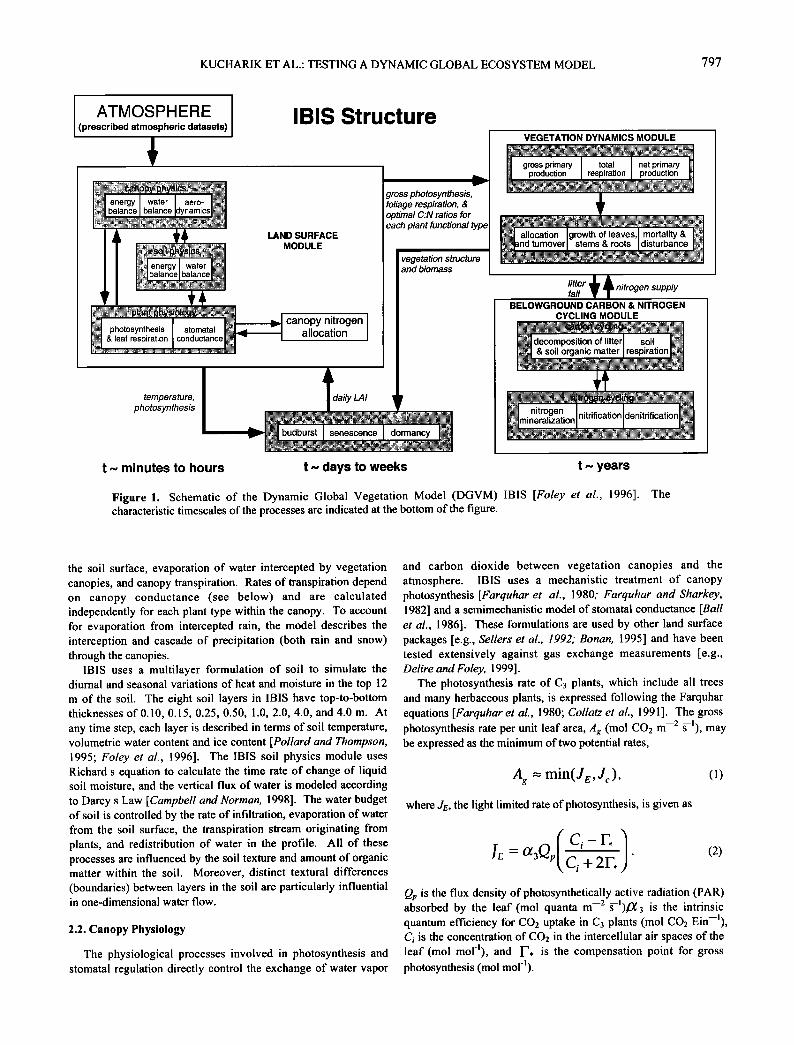
momentum exchange between soil, vegetation, and the atmosphere), canopy physiology (canopy photosynthesis and conductance), vegetation phenology (budburst and senescence), vegetation dynamics (allocation, turnover, and competition between plant types), and terrestrial carbon balance (net primary production, tissue turnover, soil carbon, and organic matter decomposition) [Foley et al., 1996]. These processes are organized in a hierarchical framework and operate at different time steps, ranging from 60 min to 1 year (Figure 1). Such an approach allows for explicit coupling among ecological, biophysical, and physiological processes occurring on different timescales.

A description of the IBIS-1 model is given by Foley et al. [1996], so it is not described in detail here. Instead, we will focus on describing the major improvements, modifications, and additions to IBIS that have been made within the current version of the model.

2.1. Land Surface Physics

The IBIS land surface module, which is based on the land surface transfer model (LSX) package of Thompson and Pollard [1995a,b], simulates the energy, water, carbon, and momentum balance of the soil-vegetation-atmosphere system. The model represents two vegetation canopies (i.e., trees versus shrubs and grasses), eight soil layers, and three layers of snow (when required) (see Figure 2). Following the logic of most land surface packages, IBIS explicitly represents the temperature of the soil (or snow) surface and the vegetation canopies, as well as the temperature and humidity within the canopy air spaces. The radiation balance of the vegetation and the ground and the diffusive and turbulent fluxes of sensible heat and water vapor drive changes in temperature and humidity. In order to resolve the diurnal cycle, the IBIS land surface module uses a relatively short time step (60 min in this study).

IBIS simulates the exchange of both solar and infrared radiation between the atmosphere, the vegetation canopies, and the surface. Solar radiation transfer is simulated following the two-stream approximation, with separate calculations for direct and diffuse radiation in both visible (0.4-0.7 m) and near- infrared (0.7-4.0 m) wavelengths. Compared to LSX and IBIS- 1, the solar radiative transfer scheme of IBIS-2 has been

simplified; sunlit and shaded fractions of the canopies are no longer treated separately. The model now uses the solution of the two-stream approximation following the approach of Sellers et al. [1986] and Bonan [1995]. Infrared radiation is simulated as if each vegetation layer is a semitransparent plane; canopy emissivity depends on foliage density.

Turbulent fluxes and wind speeds through the canopies are modeled using a simple logarithmic profile above and between the canopy layers and a simple diffusive model of air motion within each layer. In contrast to LSX and IBIS-I, which use a logarithmic wind profile below the lowest canopy, IBIS-2 uses an empirical linear function of wind speed to estimate turbulent transfer between the soil (or snow) surface and the lower vegetation canopy. This relation was deduced empirically from extensive studies in wind tunnels and beneath vegetation canopies in the field by Sauer et al. [1995].

The total amount of evapotranspiration from the land surface is treated as the sum of three water vapor fluxes: evaporation from

KUCHARIK ET AL.: TESTING A DYNAMIC GLOBAL ECOSYSTEM MODEL 797

ATMOSPHERE (prescribed atmospheric datasets)

LAND SURFACE MODULE

photosynthesis I stomatal & leaf respiration ]conductance

IBIS Structure

temperature, photosynthesis

canopy nitrogen allocation

t ,,, minutes to hours

gross photosynthesis, foliage respiration, & optimal C:N ratios for each plant functional type

vegetation structure and biomass

• ;iiiiii',i b•dburst senescence dormancy [iiiiiii?•/i?i

t ,,, days to weeks

VEGETATION DYNAMICS MODULE

gross primary I total I net primary product on respiration production

J /allocation Igrowthofleaves,Jmortality& J J nd turnoverJ stems & roots disturbance

fitter 0 nitrogen supply fall

BELOWGROUND CARBON & NITROGEN CYCLING MODULE

i•?}::!•ii•:i] & so I organic matter [ respirat on [•;•::•/•/

I 61• • chn li?i:!i?'i'] . nitrø,.gen.. nlnitrification denitrification[i!ii!i;'i•;;::!!':iii'i'!;•111 i,,ii:,:]mlneraHzauo [ I::::i i':i:.':i•::': i:i':i

t ,,, years

Figure 1. Schematic of the Dynamic Global Vegetation Model (DGVM) IBIS [Foley et al., 1996]. The characteristic timescales of the processes are indicated at the bottom of the figure.

the soil surface, evaporation of water intercepted by vegetation canopies, and canopy transpiration. Rates of transpiration depend on canopy conductance (see below) and are calculated independently for each plant type within the canopy. To account for evaporation from intercepted rain, the model describes the interception and cascade of precipitation (both rain and snow) through the canopies.

IBIS uses a multilayer formulation of soil to simulate the diurnal and seasonal variations of heat and moisture in the top 12 m of the soil. The eight soil layers in IBIS have top-to-bottom thicknesses of 0.10, 0.15, 0.25, 0.50, 1.0, 2.0, 4.0, and 4.0 m. At any time step, each layer is described in terms of soil temperature, volumetric water content and ice content [Pollard and Thompson, 1995; Foley et al., 1996]. The IBIS soil physics module uses Richard s equation to calculate the time rate of change of liquid soil moisture, and the vertical flux of water is modeled according to Darcy s Law [Campbell and Norman, 1998]. The water budget of soil is controlled by the rate of infiltration, evaporation of water from the soil surface, the transpiration stream originating from plants, and redistribution of water in the profile. All of these processes are influenced by the soil texture and amount of organic matter within the soil. Moreover, distinct textural differences

(boundaries) between layers in the soil are particularly influential in one-dimensional water flow.

2.2. Canopy Physiology

The physiological processes involved in photosynthesis and stomatal regulation directly control the exchange of water vapor

and carbon dioxide between vegetation canopies and the atmosphere. IBIS uses a mechanistic treatment of canopy photosynthesis [Farquhar et al., 1980; Farquhar and Sbarkey, 1982] and a semimechanistic model of stomatal conductance [Ball et al., 1986]. These formulations are used by other land surface packages [e.g., Sellers et al., 1992; Bonan, 1995] and have been tested extensively against gas exchange measurements [e.g., Delire and Foley, 1999].

The photosynthesis rate of C3 plants, which include all trees and many herbaceous plants, is expressed following the Farquhar equations [Farquhar et al., 1980; Collatz et al., 1991 ]. The gross photosynthesis rate per unit leaf area, Ag (mol CO2 m --2 •-l), may be expressed as the minimum of two potential rates,

A n = min(Je,Jc), where JE, the light limited rate of photosynthesis, is given as

"* ) J• - øt3QP c i + 2F. ' (2)

Qp is the flux density of photosynthetically active radiation (PAR) absorbed by the leaf (mol quanta m --2 •-1),0•3 is the intrinsic quantum efficiency for CO2 uptake in C3 plants (mol CO2 Ein--1), Ci is the concentration of CO2 in the intercellular air spaces of the leaf (mol mol-1), and I-', is the compensation point for gross photosynthesis (mol mol'l).


physiologically based formulations of canopy photosynthesis and conductance

Tsoil 5 Os OiceS.. .

Tsoil 6 06 0ice6

puddle

15 c_mm____•

5O cm

100 cm ß .

2:00 cm

Tsøi17 07 0ice7 400 cm

Tsoi18 08 0ice8 400 cm

physically-based model of snow temperature, extension and depth

physically-based model of soft •'• temperature, soil moisture and

soil ice with depth

Figure 2. IBIS state description. The basic state description shown here is carried through the entire integrated biosphere model.

lc - v(c, - E) c,+ + [q])' (3) Ko

deis the Rubisco (enzyme) limited rate of photosynthesis, where V,. is the maximum carboxylase capacity of Rubisco (tool CO2 m --2 s--l), and • and Ko are the Michaelis-Menten coefficients (mol mol 'l) for CO2 and 02, respectively. In IBIS-I the maximum Rubisco carboxylation capacity (V,, was predicted by optimizing the net assimilation of carbon by the leaf [Haxeltine and Prentice, 1996]. However, IBIS-2, for the sake of simplicity, prescribes constant values of the maximum Rubisco capacity for the following plant functional types: broadleaf deciduous, broadleaf evergreen, needleleaf deciduous and needleleaf evergreen trees, shrubs, and C3 and C4 grasses.

Following Collatz et al. [ 1992], the photosynthesis rate of C4 plants, which include many tropical and warm-season grasses, is determined from three potential capacities to fix carbon,

A s = min(J,, J•., Jc), (4) where di= a4Op is the light limited rate of photosynthesis, dE = V,,

is the Rubisco limited rate of photosynthesis, and dc = kCi is the CO2 limited rate of photosynthesis at low-CO2 concentrations. The compensation point is assumed to be zero for C4 plants.

Leaf respiration, Rleaf (mol CO 2 m --2 •-1), is determined by

Rleaf -- '•' En, (5)

where T is the leaf respiration cost [Collatz et al., 1991]. The maintenance respiration rates of stem and fine root biomass are given by

Rstem -- •stem&apwoodWstem,if(Tstem) (6) and

Rroot -- •rootWroot, if(Tsoil), (7)

where Cstem and Croot are carbon contained in woody and fine root biomass, respectively, /• is a maintenance respiration coefficient defined at 15f•C (0.0125 • for stem sapwood biomass, 1.250 y-i for fine root biomass) [Sprugel et al., 1995; Amthor, 1984; Ryan et al., 1995], )•sapwood is the sapwood fraction of the total stem biomass (estimated from an assumed sap velocity and


the maximum rate of transpiration), and ~(T) is the Arrenhius temperature function [Lloyd and Taylor, 1994]

E 1 1 f(T)- e (8)

In (8), T is the temperature (13C) of the appropriate tissues (stem temperature, soil temperature in the rooting zone), Eo is a temperature sensitivity factor, and To is a reference temperature.

The net carbon balance for each plant type is calculated by adding all of the carbon fluxes (including gross photosynthesis and maintenance respiration). For each plant type the annual NPP is calculated as

NPP - (1 - r/) f (Ag -- Rleaf -- gstem - groot )dt, (9) where Ag is gross canopy photosynthesis and r/ (0.30) is the fraction of carbon lost due to growth respiration [Amthor, 1984]. Stomatal conductance is simulated following the formulation of Ball et al. [ 1986] and Collatz et al. [ 1991, 1992],

mA n gs,h2o = •ss ms + b, (10)

where gs.h2o is the leaf-level stomatal conductance of water vapor (mol H20 m --2 s--!)•s is the CO2 concentration (mol mol -l) at the leaf surface, hs is the relative humidity at the leaf surface (fraction), and m and b are the slope (nondimensional) and intercept (mol H20 m -2 s 'l) of the conductance-photosynthesis relationship. Following Collatz et al. [1991, 1992], the photosynthesis and stomatal conductance submodels are linked by considering the diffusion of H20 and CO2 between the free atmosphere, the leaf boundary layer, and the stomatal cavity.

In IBIS-1 we scaled photosynthesis and transpiration from the leaf level to the canopy level by calculating those rates separately for sunlit and shaded leaves and then averaging them weighted by the fraction of sunlit and shaded leaves occupying the canopy. In IBIS-2, we use a new and simpler approach for canopy scaling. Our new approach assumes that the net photosynthesis within the canopy is proportional to the absorbed PAR (APAR) within it. This assumption is supported by several field studies [Hirose and Werger, 1987; Field, 1983, 1991; Evans, 1989; Kull and Jarvis, 1995] and has a theoretical basis [Field, 1983; Sands, 1995; Haxeltine and Prentice, 1996].

We use our coupled photosynthesis-stomatal conductance model to calculate net photosynthesis of a leaf at the top of the canopy. The net photosynthesis within the canopy is calculated by scaling it proportional to the APAR within it. The vertical profile of APAR through the canopy, calculated using the two- stream approximation, can be simplified to a simple exponential function of leaf area index (LAI). The analytical integral of this function, multiplied by photosynthesis of the top leaf gives us the canopy-integrated photosynthesis. We then diagnose a canopy- average value of CO2 concentration at the leaf surface (C.0 by using the big leaf approach [Arethor et a!., 1994; Arethor, 1994; Lloyd et al., 1995a, b] and applying a diffusion equation for the leaf level CO2 concentration (not shown) to the canopy level. Canopy-average stomatal conductance is similarly calculated, using the big leaf approach, by applying (10) to the canopy level.

2.3. Phenology

Many plants show an annual cycle of leaf display (e.g., deciduous trees and some shrubs and grasses) and physiological activity (e.g., evergreen trees). Typically, changes in leaf display and physiological activity are triggered by climatic events, where there are one or more unfavorable seasons. IBIS-2 uses a set of

phenology parameterizations that are based on algorithms developed by Botta et al. [2000], which are calibrated against satellite-based measures of leaf activity.

Budburst of winter-deciduous plants is assumed to occur when accumulated growing degree days exceed a certain threshold. We assume (simplifying the approach of Botta et al., 2000) that the threshold is 150 growing degree days (on a-513C base) for shrubs and grasses, and the threshold is 100 growing degree days (on a 013C base) for winter deciduous trees. Leaf fall for trees is initiated when one of the following conditions is met; either the average temperature (using a 10-day running average) falls below 013C or is 513C warmer than the coldest monthly temperature. For grasses and shrubs, leaf fall is initiated when the 10-day running average temperature reaches 013C. This parameterization is a deliberate simplification of several phenology parameterizations that have been suggested in the literature. However, it is possible to make this calculation more process oriented by incorporating the inverse relationship between growing degree-day requirements for budburst and chilling period length [e.g., Murray et al., 1989].

Drought deciduous plants (including tropical deciduous trees, shrubs, and grasses) are assumed to respond to changes in the net canopy carbon budget. The model calculates the mean (using a 10-day running average) net photosynthesis rate of the plant canopies; whenever the 10-day-mean photosynthesis rate becomes negative (indicating that leaf respiration now exceeds gross photosynthesis), the model drops leaves. This algorithm captures the basic dynamics of water stress on the plant canopies and how plants may optimize the canopy carbon budget during droughts by reducing their leaf area [Linder et al., 1987].

2.4. Vegetation Dynamics

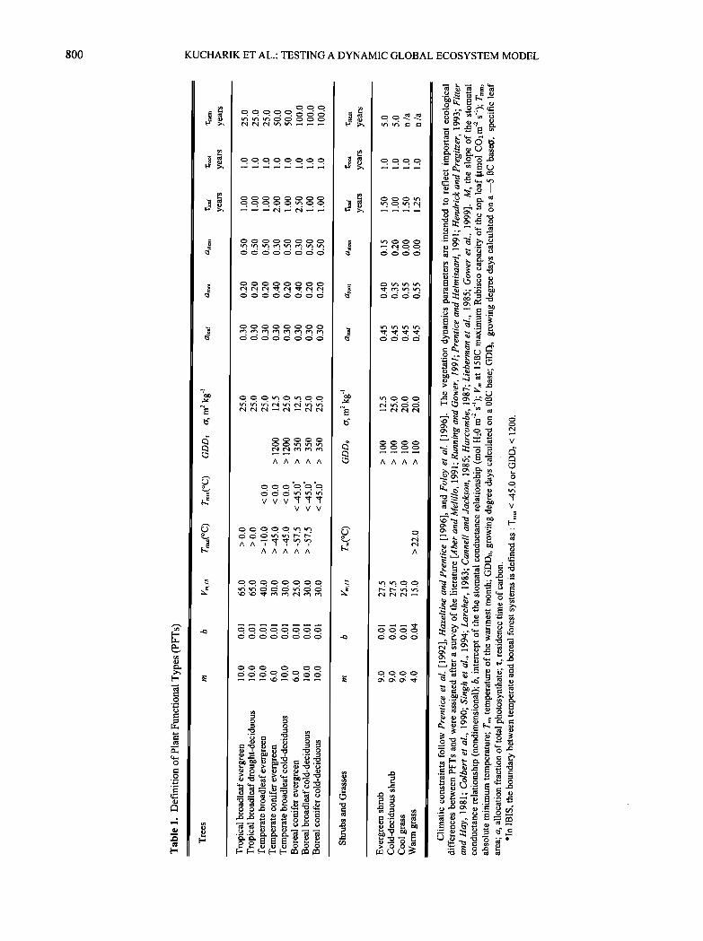
IBIS represents the vegetation cover as a collection of PFTs, where each PFT is characterized in terms of biomass (carbon in leaves, stems, and fine roots) and LAI. The definition of plant functional types is used to differentiate several important characteristics, including basic physiolognomy (trees versus shrubs versus grasses), leaf habit (evergreen versus deciduous), leaf form (broadleaf versus needleleaf), and physiology (C3 versus C4 pathway) (Table 1). The geographic distribution of each plant functional type is determined using a simple set of climatic constraints that determine cold tolerance limits, growing degree- day requirements, and minimum chilling requirements [Prentice et al., 1992; Haxeltine and Prentice, 1996; Foley et al., 1996].

In each grid cell, a number of plant functional types can exist simultaneously. For example, a grid cell in the eastern United States might include temperate broadleaf deciduous trees, temperate needleleaf conifer evergreen trees, evergreen shrubs, deciduous shrubs, and cool grasses. The model explicitly allows trees, shrubs, and grasses to experience different amounts of light and water availability. In addition, plant competition for these two essential resources may be explicitly represented through shading and differences in water uptake [Foley et al., 1996]; the


A A A A A

V V V , , , V V V

A A 'T•', •', • A A A A A

A A A A


competition scheme may be further adapted to include mineral nutrients.

This approach provides a highly simplified representation of vegetation dynamics that is appropriate for global ecosystem modeling. Competition among plant functional types is characterized by the ability of plants to capture common resources (light and water). For example, trees in the upper canopy are able to capture light first and therefore shade shrubs and grasses. However, shrubs and grasses are able to access soil moisture first as it infiltrates through the soil. Thus the model can mechanistically simulate the competition between different plant forms. In addition, the competition between plant types of the same basic form (e.g., trees) is driven by differences in the annual carbon balance resulting from differences in phenology (evergreen versus deciduous), leaf form (needleleaf versus broadleaf), and photosynthetic pathway (C3 versus C4).

IBIS considers each plant functional type in terms of a simple state description. Each PFT is represented in terms of three biomass pools: carbon in leaves, carbon in transport tissues (i.e., predominantly stems), and carbon in fine roots. Carbon in leaves may also be expressed in terms of LAI by multiplying by the specific leaf area (Table 1). Transient changes in biomass poolj of plant functional type i are described as

•Ci,j _ Ci,j oqt -- a i/NPPi - •, (11) ' •'i,j

where ai.j is the fraction of annual NPP allocated to each biomass compartment and •'i.j is the mean residence time (from loss of biomass through mortality, disturbance, and tissue turnover) of each biomass compartment.

Process-based global terrestrial ecosystem models generally use constant ratios of carbon allocation to leaves, roots, and wood and therefore are unable to capture the dynamic nature of carbon allocation that is driven by changes in nutrient and water availability during the various stages of plant growth. Unfortunately, an incomplete understanding of the abiotic and biotic influence on carbon allocation has made it difficult to

implement dynamic carbon allocation into process models [Gower et al., 1999]. In IBIS-2, we have used a new composite data set compiled by Gower et al. [1999] that reports the ratio of belowground NPP to total NPP for major terrestrial biomes (Table 1). Total NPP values that were calculated using estimates of belowground NPP (e.g., estimated as a ratio of aboveground NPP) were excluded from the data set [Gower et al., 1999]. Furthermore, few estimates of belowground NPP exist for tropical biomes thus some degree of uncertainty exists with these values. The general patterns show that the fraction of annual NPP allocated to roots is high in grasses (55%) and shrublands (35%) and about 20% for all other forest PFTs, with the exception of boreal conifers (40%). The fraction of NPP allocated to leaves is 30% for all tree PFTs and 45% for shrubs and grasses in IBIS. Carbon allocation to wood is calculated from the residual NPP not

allocated to leaves and fine roots.

2.5. Soil Biogeochemistry

In the original version of IBIS [Foley et al., 1996] there was no explicit belowground biogeochemistry model to complete flow of carbon between the vegetation, detritus, and soil organic matter

pools. IBIS-2 includes a new soil biogeochemistry module [Kucharik et al., submitted manuscript, 1999] (see Figure 3), which is similar to other previously documented soil biogeochemistry models [Parton et al., 1987, 1993; Verberne et al., 1990].

Following the framework of Verberne et al. [1990], IBIS allows for the growth of microbial biomass to be a direct function of the amount of available substrate (litter return and root turnover, among other more recalcitrant carbon sources in the soil). Furthermore, IBIS allows for microbial growth (and turnover) and the rate of nitrogen mineralization to be dependent on soil textures (particularly clay content). For example, soils higher in clay content have the capability to cause increased physical protection of both the microbial biomass and soil organic matter, which can potentially yield lowered rates of nitrogen mineralization and higher soil carbon densities [Verberne et al., 1990]. The microbial biomass pool in IBIS is regarded as the entire active (highly labile) carbon pool and is kept separate from all other belowground soil carbon pools. By explicitly modeling the microbial dynamics, simulated microbial biomass values can be compared to actual field measurements [e.g., Kucharik et al., submitted manuscript, 1999].

IBIS allows microbial activity to be dependent on an Arrhenius function of physically modeled hourly soil temperatures [Lloyd and Taylor, 1994] and water-filled pore space (WFPS) [Linn and Doran, 1984]. These functions are not part of the model described by Verberne et al. [1990] and are a modification to equations used in the CENTURY model. Additionally, rooting profiles described by Jackson et al. [1996] are used in IBIS to designate where fine roots and soil carbon is most likely to reside in the soil profile to 1 m. These profiles allow soil moisture and temperature values to be weighted by depth accordingly to coincide with the approximate location (depth) of the majority of carbon and microbial biomass. Micorrhizae are not explicitly modeled within IBIS-2.

2.5.1. Flow of carbon and nitrogen. Following Parton et al. [1987] and Verberne et al. [1990], the main partitioning of carbon in 1BIS is between surface and belowground carbon litter pools derived from litterfall (leaf turnover, woody detritus, and fine root turnover) and the more recalcitrant soil organic matter pools (Figure 3). Annual litterfall and fine root turnover from the previous year are divided into equal daily increments (total detritus production divided by total days in year) which are incorporated into the litter pools. This approach is an obvious simplification to actual fine root and leaf phenology; namely root mortality is not a linear function, and future models should include a more sophisticated approach. The detritus is divided between decomposable (DPM, decomposable plant matter), structural (SPM, structural plant matter), and lignified (RPM, resistant plant matter) fractions, each having a specified C:N ratio [Kucharik et al., submitted manuscript, 1999].

Leaves, woody debris, and fine root biomass detritus are treated separately here to divide their respective amounts accordingly between the three litter pool compartments based upon the C:N ratio of each residue type (leaves, wood, or roots), and the C:N ratio of each litter pool compartment [Whitmore et al., 1997]. IBIS-2 follows the equations presented by Whitmore et al. [1997] which calculates the fraction of each residue type in RPM first, then determines the amount of detritus in the SPM pool using the fraction allocated to the RPM pool, with the residual


Figure 3. Schematic of the IBIS soil biogeochemistry submodel. The following symbols are used to identify carbon pools: DPM, decomposable plant matter; SPM, structural plant matter; RPM, resistant (lignin) plant matter; POM, protected slow pool of organic matter (OM); NOM, nonprotected slow pool of OM. Lines and arrows drawn between carbon pools represent flows of carbon, while thick arrows show microbial CO2 respiration occurring with the oxidation of carbon.

detritus assumed to reside in the DPM pool. Following this approach, each plant matter pool (RPM, SPM, and DPM) contains some amount of leaf, fine root, and woody detritus.

IBIS has an aboveground standing litter pool of accumulated decomposable and structural leaf and woody biomass at the soil surface. Similarly, there is a belowground litter pool of decomposing fine root biomass. Generally, these litter pools have the shortest residence times of any carbon pool in the model, of the order of weeks to months [Parton et al., 1987]. Litter in the DPM and SPM carbon pools moves directly to the microbial biomass for decomposition, while the lignified plant biomass (RPM) is transferred to the soil organic matter [l/erberne et al., 1990]. The belowground soil carbon is divided into four compartments (Figure 3): (1) microbial biomass comprises the active carbon pool with a residence time varying from a few hours to months, (2) protected and (3) nonprotected organic matter comprise slow carbon pools [ Parton et al., 1987], with residence times of 10-30 years, and (4) stablized organic matter, representing the most recalcitrant carbon, typically with residence times of more than 1000 years [Verberne et al., 1990]. The carbon to nitrogen ratios for the various carbon pools reported by l/erberne et al. [1990] are used in our model and are assumed to remain constant (Table 2). As carbon in litter and soil organic matter decomposes, it is partitioned between microbial biomass and respiration according to the microbial efficiencies assigned to each transformation (Table 2).

The variables output by the model include total soil carbon and nitrogen, aboveground and belowground litter carbon, total microbial biomass, soil surface CO2 flux, nitrogen mineralization/immobilization, and organic carbon and nitrogen leaching. Amounts of atmospheric nitrogen deposition and nitrogen fixation (both functions of annual precipitation) are also determined in IBIS using empirical equations found in CENTURY [Parton et al., 1987].

2.5.2. Decomposition processes. Soil organic matter decomposition is simulated using a daily time step; hourly values of modeled soil temperature are converted into daily average values. The base decay rates of litter, root, and soil carbon and microbial biomass turnover (defined at 1513C and 60% WFPS; Table 2) are modified by functions of soil temperature and soil moisture. Modifying factors, which are used to simulate the temperature and moisture effects on microbial activity, are calculated using two different sets of soil temperature and moisture values. One set of modifying factors influences the rate of litter decomposition at the soil surface and are based on the daily average 0-10 cm soil temperature (top soil layer in IBIS) and 0-10 cm soil moisture. The second set of factors affects the

turnover rate of microbial biomass and the transformation of

belowground soil carbon between individual pools (fine root detritus, active (microbial), slow, and passive pools). These factors are based on the 0-100 cm soil temperature and soil moisture values, which are depth weighted by the fraction of total


Table 2. Base Rate Constants of Carbon Decomposition, Microbial Efficiency Factors and C:N Ratios Used Within the IBIS Soil Biogeochemistry Model

Transformation/Pool Decomposition Rate, d '• Microbial C:N Efficiency Pool

DPM

leaf litter 0.15 0.40 6 fine roots 0.10 0.40 6 wood 0.00 0.40 6

SPM


RPM


Pbio ==1> Po,, 0.005 1.0 10 Nbi o ==I} Non, 0.045 1.0 10 Po,, :=• Pbio 1.0 x 10 '4 0.25 10 No,, • Nbio 0.001 0.20 15 Pon, :=• So,, 1.0 x 10 '6 1.0 15 No,, :=• So,, 1.0 x 10 '6 1.0 10 Son, 8.0 x 10 -7 0.20 15

The C:N ratio of litterfall and fine root turnover in IBIS is 40 for leaves, 200 for wood and 60 for fine roots, respectively. Here 1 - efficiency is the fraction of carbon oxidation that is released as CO2. Symbols are defined to denote the following C pools: DPM, decomposable plant material; SPM, structural plant material; RPM, resistant (lignin) plant material; Pb•o, protected microbial biomass; N•o, nonprotected microbial biomass; Pon,, protected slow C pool; No,,, nonprotected slow C pool; Son,, stabilized passive C pool.

root biomass in each soil layer following Jackson et al. [1996]. Carbon added to the soil through the decomposition process is not partitioned with respect to soil layers (e.g., decomposition of fine root biomass is not kept track of for each individual soil layer); instead, the total amount of decomposed carbon is aggregated for the total soil profile.

The soil carbon decomposition factors used in IBIS were determined from a simple calibration procedure. First, the model decay constants were modified so that the simulated global totals of soil carbon (to 1 m total depth) were close to reported estimates of 1200-1600 Gigatons (Gt) [e.g., Post et al., 1982; Zinke et al., 1986; Schlesinger, 1991; Eswaran et al., 1993; Sombroek et al., 1993; Batjes, 1996]. Then, the annual amount of leached organic carbon was calibrated to fall within the range measured at various natural and managed ecosystems in Wisconsin (leaching was typically between 0.001-0.005 kg C m -2 yr-l; see Brye et al. [1999]). These simulated values are also representative of both temperate upland forests and swamps and lowland forests, which have reported carbon leaching rates of 0.001-0.014 kg C m -2 yr -1 [Landsberg and Gower, 1997].

3. Model Implementation

We present the results of a 135-year model simulation (1860- 1994) performed on a 113 latitude by 113 longitude global terrestrial

grid, driven by climatological data and soil boundary conditions. The model simulation went through an initial 400-year spin-up procedure where soil carbon, vegetation structure, and biomass were allowed to come to an equilibrium state assumed to exist in 1860. During this initial spin-up period, the soil biogeochemistry and vegetation dynamics were both subjected to separate numerical acceleration procedures. The vegetation dynamics were assumed to occur at 4 times the normal rate (plant competition for light and water, NPP, carbon allocation, and mortality) during years 20-100 of spin-up and 2 times the normal rate during years 101-150.

The initial 400-year model spin-up assumed a preindustrial concentration of atmospheric CO2 (286.6 ppmv) and was driven with 1860-1899 climatology of mean monthly temperature and precipitation (M. Heimann, Max-Planck-lnstitut fuer Biogeochemie, personal communication, 1999), and 1931-1960 climatology of Leeroans and Cramer [ 1990] for monthly average daily temperature range (Tmax-Tmin), the number of days with precipitation each month and potential sunshine hours (W. Cramer, personal communication, 1999). Absolute minimum temperature data, used to determine the extreme geographic limits of several plant types within IBIS, were obtained from P. Bartlein (personal communication, 1998). Monthly-mean estimates of relative humidity and wind speed were compiled from the National Center for Environmental Prediction (NCEP)/National

804 KUCHARIK ET AL.' TESTING A DYNAMIC GLOBAL ECOSYSTEM MODEL

Center for Atmospheric Research (NCAR) reanalyzed meteorological dataset [Kalnay et al., 1996]; we averaged the NCEP/NCAR data from 1958 to 1997 to determine the

climatological values. The simulation begins with zero snow cover and uniform soil temperature (5BC) and soil moisture (50% of pore space). All soil carbon and litter pools also have zero carbon stores to begin, with the soil carbon having reached an equilibrium value by the end of the model spin-up (year 1860) using a numerical acceleration procedure that is discussed below. After spin-up, the model was run for 135 years using transient climate and atmospheric CO2 data from 1860-1994 (M. Heimann, Max-Planck-Institut fuer Biogeochemie, personal communication, 1999) and Leeroans and Cramer [1990] climatology for other meteorological driving variables.

3.1. Weather Generator

IBIS uses a 60-min time step to calculate land-atmosphere exchange processes. To meaningfully convert monthly-mean climate data to this time step, we use a stochastic weather generator based on Richardson [ 1981 ], Richardson and Wright [1984], and Geng et al. [1985]. The Richardson-style weather generator stochastically determines the probability of weather events (on the basis of long-term climatic means). The interrelationships between the random variations in atmospheric parameters (e.g., perturbations in temperature, precipitation, and cloudiness) and their persistence over time are determined from a serial auto-correlative approach. This ensures that a reasonable sequence of atmospheric parameters, mimicking the day-to-day behavior of synoptic weather events, is provided to the model. Spatial correlation between grid cells, however, is not accounted for on hourly to daily timescales. Furthermore, the Richardson- style weather generator explicitly considers the statistical distribution of atmospheric parameters, so extreme weather events can be generated within the model. This is critical to simulating the surface water balance, where extreme rainfall events often produce a large fraction of the runoff.

3.2. Soil Data Sets

We adopted a new global data set [IGBP-DIS, 1999] of soil texture to represent soil conditions across the globe. Using the SoilData software that was included with the data set [IGBP-DIS, 1999], the fraction of sand, silt, and clay were determined for each IBIS soil layer. For soil depths where there was no default data, the value of the layer immediately above was used. This allowed each IBIS grid cell to have a representative fraction of sand, silt, and clay as a function of depth in the soil. This is a significant improvement over the original soil data set used by IBIS [Zobler, 1986], which did not contain soil texture as a function of depth.

To determine the hydraulic and physical properties of the soil layers, we classified soil texture classes into 11 categories following RawIs et al. [1992] and Campbell and Norman [1998] (see Table 3). IBIS matches each soil layer of each grid cell to the most comparable of the 11 soil texture categories. Soil properties assigned to each soil category include porosity (m 3 m-3), field capacity (m 3 m'3), wilting point (m 3 m'3), saturated matric (air- entry) potential (m H20), and the saturated hydraulic conductivity (m s-i). Additionally, following Campbell and Norman [1998], the density of soil material (kg m '3) is computed by


2650 (1 --forgan•c 4- 1300 forgan,c,

and the specific heat of soil material (J kg -• K 't) is given by

(12)

870 (1 '•forgan,c) 4- 1920forganic, (13)

where forgamc is the fraction of organic matter content in the soil. In this version of IBIS, for simplicity, it is assumed that all soil layers contain 1% organic carbon content in these calculations. However, it is possible to modify the physical properties of the soil in terms of the soil organic content, thus allowing soil hydraulic properties to evolve with changes in soil organic matter. This could have important applications in comparing different land use practices, where differences in soil organic matter can cause differences in key soil properties (e.g., density, water holding capacity, and heat capacity).

3.3. Numerical Acceleration of Soil Carbon Dynamics

The amount of soil carbon and nitrogen can be initialized using observed quantities of soil carbon or zero stores of carbon and nitrogen. One notable problem with initializing the model with actual data or current measurements of total litter and soil carbon

densities is that these total quantities are partitioned into several compartments in IBIS (like numerous other biogeochemistry models) (Figure 3). Soil carbon measurements generally do not distinguish between active, slow, and passive carbon pools or distinct litter quality categories. Therefore an initialization procedure would be difficult to implement without causing some degree of uncertainty in the subsequent biogeochemical cycling. Consequently, for model results reported in this study, the soil storage of carbon and nitrogen was initialized at zero.

During a typical IBIS model run, a numerical acceleration procedure is used to simulate approximately 5000 years of actual (geologic) time during a 150-year model integration. To do so, the soil biogeochemistry module in IBIS, which operates on a daily time step, is called 40 times each day with constant soil temperature and moisture (instead of performing just one execution) during the first 100 years in a model run. During the next 50 years of the numerical acceleration (model years 100- 150), a linear decrease in the degree of acceleration occurs until the biogeochemistry model is only called one time each day (normal operation) at year 150 (compared to 40 times at year 100). This progressive decrease applied to the numerical acceleration over time allows for the biogeochemical cycling to adjust gradually to an equilibrium state instead of implementing an abrupt discontinuation of the numerical acceleration at year 150.

4. Results

We present the long-term characteristics of the simulation, based on a 30-year average of model results between years 1965 and1994. These results are intended to represent the average state of present-day ecosystems. Because the model does not explicitly include periodic disturbance mechanisms (e.g., fire, wind, and herbivory), a state of equilibrium (where values of NPP and soil carbon along with vegetation structure do not change significantly over time) would be attained if atmospheric CO2 and climate were assumed to remain constant. In natural ecosystems, however, where disturbance is part of the system, a true steady state condition may never be reached even if other changes in climate

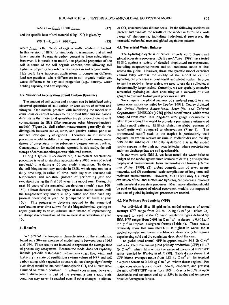
or CO2 concentrations did not occur. In the following sections we present and evaluate the results of the model in terms of a wide range of phenomena, including hydrological processes, the terrestrial carbon balance, and global vegetation patterns.

4.1. Terrestrial Water Balance

The hydrologic cycle is of critical importance to climate and global ecosystem processes. Delire and Foley [ 1999] have tested IBIS-2 against a variety of detailed biophysical measurements, including evapotranspiration and soil moisture, made at sites across the globe. However, these site-specific model exercises cannot fully address the ability of the model to capture hydrological processes at continental and global scales. In order to test the model at these scales, we need to use data collected at fundamentally larger scales. Currently, we use spatially extensive terrestrial hydrological data consisting of a network of river gauges to evaluate hydrological processes in IBIS.

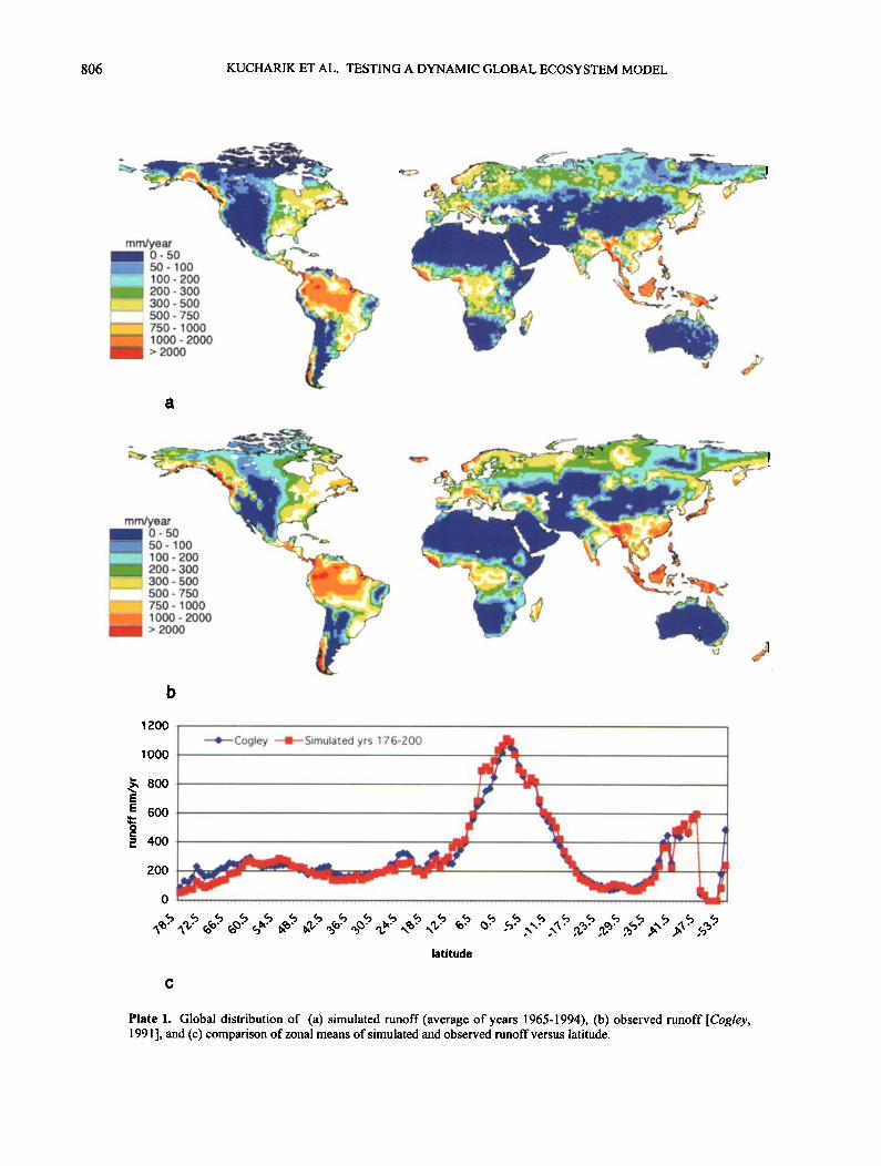
We compare the global patterns of simulated runoff to river gauge observations compiled by Cogley [1991]. Cogley digitized the United Nations Educational, Scientifi'c, and Cultural Organization (UNESCO) [1978] global runoff maps, which were compiled from over 1000 long-term river gauge measurements taken fi'om around the world to provide a preliminary estimate of global runoff patterns. IBIS simulates the global patterns of runoff quite well compared to observations (Plate 1). The pronounced runoff peak in the tropics is particularly well captured, as are the weaker •naxima in midlatitudes and the dry belts of the subtropics. The only systematic bias in the model results appears in the high northem latitudes, where precipitation and river discharge data are still questionable.

In our work with IBIS-2, we have tested the water balance budget of the model against three sources of data: (1) site-specific biophysical measurements from meteorological towers [Delire and Foley, 1999], (2) global compilations of river gauge networks, and (3) continental-scale compilations of long-term soil moisture measurements. However, this is still only a cursory evaluation of the land surface and hydrological processes involved with terrestrial ecosystem processes. Much more attention should be paid to this aspect of global ecosystem models, but improved data sets of global hydrological processes are needed.

4.2. Net Primary Productivity (NPP)

For individual 113 x 113 grid cells, model estimates of annual average NPP range from 0.0 to 1.5 kg C m '2 yr '• (Plate 2a). Averaged for each of the 1-5 basic vegetation types defined by IBIS, NPP ranges from 0.001 kg C m '2 yr '• in deserts to 0.90 kg C m '2 y-r • in tropical evergreen forests (Table 4). These results obviously show that simulated NPP is highest in warm, moist tropical climates and lowest in subtropical deserts or polar regions experiencing cold and dry conditions throughout the year.

The global total annual NPP is approximately 54.3 Gt C yr 't and is 47.3% of the annual gross primary production (GPP) (114.7 Gt C yr'•), which falls within the range of measured NPP/GPP ratios reported by Waring et al. [ 1998]. Table 4 also shows that GPP biome averages range from 1.89 kg C m'2yr -• for tropical evergreen forests to 0.020 kg C m '2 yr -• within desert regions. For major ecosystem types (tropical, boreal, temperate, and grasses) the ratio of NPP/GPP varies from 10% in deserts to 30% in open shrublands and savannas and up to 55% in tundra and temperate broadleaf evergreen forests.


mmb/ear O- 50 50-100 100- 200 200 - 300 300- 500 500- 750 750- 1000 1000-2000 > 2000

mm•ear 0 - 50 50- 100 100 - 200 200 - 300 300 - 500 500- 750 750 - 1000 1000 - 2000 > 2000

1200 ,

ooo

800 .......

600

400

--•--Cogley •Simulated yrs 176-200

2oo in, -.,, . •

latitude

Plate 1. Global distribution of (a) simulated runoff (average of years 1965-1994), (b) observed runoff [Cogley, 1991 ], and (c) comparison of zonal means of simulated and observed runoff versus latitude

KUCHARIK ET AL.' TESTING A DYNAMIC GLOBAL ECOSYSTEM MODEL 807

kg/m•/yr 0 - O. 1 0.4- 0.5 ................ J 0.8 - 0.9 0.1 - 0.2 0.5 - 0.6 •:•: ....... ] 0.9- 1 0.2 - 0.3 0.6 - 0.7 I - 1.1 0.3 - 0.4 • 0.7- 0.8 > 1.1

Plate 2. Distribution of (a) simulated annual net primary productivity (NPP; kg C m -2 yr 'f) and (b) observations compiled by S.T. Gower (unpublished data, 1999).


To evaluate IBIS simulations of annual NPP, we compare the model results to a dataset of field measurements compiled at the University of Wisconsin [S.T. Gower, unpublished data, 1999] (Plate 2b). NPP data were compiled from three major sources: Esser et al. [1997], Cannell [1982], and individual NPP data complied by S.T. Gower [unpublished data, 1999]. These data were processed to remove redundancy among the data sets and quality screened by removing any value that differed more than 3 s.d. from the mean biome value. NPP was calculated as the sum

of wood (stem + branch) + foliage production. Many studies use leaf litterfall as a surrogate for foliage production. Only a small fraction (12%) of the studies have belowground NPP data; to standardize the data we use the aboveground:belowground NPP ratios from Gower ct al. [1999] to approximate total NPP. In this comparison, we use a total of 1882 measurements made at various sites.

In order to describe biome-average variations in NPP, the 1882 field measurements are categorized into one of the 15 IBIS vegetation types (Table 4). However, not all of the 15 IBIS vegetation types had associated NPP field measurements (savanna, polar desert, and open shrublands were omitted), leaving 12 biomes for comparison (Figure 4). There is reasonable agreement between the simulated and observed NPP across most biomes. Simulated and measured NPP differed on average by 39% for the 12 biomes in which comparisons were made; the smallest difference was 4.0% for temperate deciduous forests (403 measurements), while the greatest difference (within a nondesert area) was 89% for boreal mixed forests (44 measurements). Much of the large discrepancy between measurements and simulations in boreal mixed forests could be explained by the fact that the IBIS mixed forest biome classification includes mixed

forests from all regions of the globe. While we believe that this data set represents the most

complete and accurate set of global NPP measurements currently available, caution should still be taken when comparing model simulations and measurements. The IBIS model simulates the

average NPP over a homogeneous 113 x 113 grid cell, while field measurements of NPP are generally made on individual allometric study plots, sometimes as small as 10 m on a side. Furthermore, belowground NPP measurements are exceedingly difficult to make and are sometimes estimated on the basis of assuming a fixed ratio between belowground to aboveground production (e.g., 50:50 contribution to total NPP).

4.3. Vegetation Biomass

The distribution of vegetation biomass (including both aboveground and belowground components), divided into trees and shrubs/grasses, is highlighted in Plates 3a and 3b. In individual l g x 113 grid cells, the simulated total carbon density ranges from 0.01 kg C m '2 in subtropical deserts to 14.1 kg C m '2 in the core of tropical rainforests. The biome-average biomass density ranges from 0.03 kg C m '2 in desert ecosystems to 9.1 kg C m '2 in tropical evergreen forests (Table 4). The global storage of carbon in vegetation biomass is 557.4 Gt C.

We also show the mean residence time of carbon in living biomass (Plate 3c), estimated as the ratio of equilibrium vegetation biomass to NPP. Tropical rainforests, which have relatively large stores of carbon in vegetation, generally have the

shortest residence times (Table 4). Temperate forests and boreal forests generally have the longest residence time of carbon in biomass, around 10-25 years and slightly higher in a few locations; however, this is a difficult value to measure directly.

We also compare simulations of fine root biomass to data compiled by Jackson et al. [1996] (Table 5). Simulated values of the annual average live fine root biomass in IBIS range from a low of 0.004 kg C m '2 in deserts to a high of 0.200 kg C m -2 in temperate needleleaf evergreen forests (Table 4, Table 5); tropical and boreal forests generally have simulated values between 0.08 and 0.20 kg C m -2. The range of live fine root biomass reported by Jackson et al. [1996] is 0.07-0.47 kg C m '2. When biome- average IBIS results are compared to equivalent data compiled by .lackson et al. [1996], temperate and tropical forests generally agree to within 10-25%. The largest discrepancy between model simulations and measurements (outside of desert regions) existed with the IBIS grassland/steppe biome, which yielded a difference of about 71% (Table 5).

The biome classifications differ between Jackson et al. [1996] and lB IS making a direct one-to-one comparison difficult. Only one boreal forest category (including both deciduous and coniferous) was presented by Jackson et al., and grasslands were partitioned into temperate and tropical categories. Furthermore, no distinction is made in the Jackson et al. data set between open and dense shrubland types. For the purpose of this study, the Jackson et al. temperate grassland biome is compared to the IBIS grassland/steppe biome, and the Jackson et al. tropical grassland is compared to the IBIS savanna biome. The shrub data are compared to the dense shrubland biome category in IBIS. Jackson et al. did not present data for mixed forests. For those biomes that do correlate between IBIS and the Jackson et al.

categories (tropical and temperate ecosystems), generally good agreement exists. However, it is obvious that some rather large differences exist in tundra and desert ecosystems (40-75%), and IBIS greatly underestimates (by 71%) grassland fine root biomass reported by Jackson et al. This large difference may be partly due to IBIS having an oversimplified root turnover parameterization; fine roots are assumed to only turnover one time each year. We note however that the simulated values in Table 5 are annual averages, while the data compiled by Jackson et al. are from specific point measurements made during different time periods and may not represent a true annual-average value.

4.4. Leaf Area Index

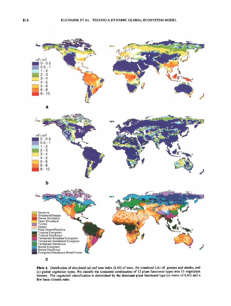
Plate 4a shows the distribution of LAI (defined as single-sided, projected leaf area) for trees. The LAI of trees range from 1.0-4.0 in boreal and tundra regions to 4.0-8.0 in temperate coniferous and deciduous forests to a high of 8.0-11.0 in tropical rainforests. For forested regions in IBIS the biome-average LA! ranges from a high of 6.8 in tropical evergreen forests to a low of about 2.7 for boreal deciduous forests (Table 4). Values of tree LAI in savannas, grasslands, shrublands, deserts, and tundra regions are all less than 1.0. These LAI values for main forested regions are realistic and compare reasonably well to measurements made in several forested areas. Measurements made in boreal forests

during the Boreal Ecosystem-Atmosphere Study (BOREAS) [Gower et al., 1997; Kucharik et al., 1997, 1999; Gower et al., 1999] show that LAI was approximately 2.0 in jack pine forests, 3.5 in aspen, and 6.0 in black spruce stands. LA! has been


1.6

1.4

'1.2

øO.8

,", 0.6

0.4

0.2

Figure 4. Comparison of simulated versus observed NPP values (kg C m '2 yr 'l) [S.T. Gower, unpublished data, 1999] reported on a biome-by-biome basis (average and +/- 1 s.d. are shown). The average and standard deviations of model output reflect variations occurring within each specific biome over the 30-year period (years 1965-1994) and are not intended to show year-to-year differences.

measured to range from 1.3 to 8.4 in temperate coniferous and deciduous forests of the Midwestern and eastern United States

[Fassnacht and Gower, 1997; Landsberg and Gower, 1997; Gower et al., 1999]. LAI can reach values greater than 10 in some evergreen coniferous forests of the Pacific Northwest in the United States [Landsberg and Gower, 1997]. LAI of tropical forests is also variable. LAI has been measured at 5.1-7.5 for

lowland tropical rainforest in Venezuela [Saldarriaga and Luxernoore, 1991], 6.6 for a lowland rainforest in Puerto Rico [Jordan, 1971], 5.5 for an evergreen montane rainforest in Jamaica, 7.5 for a lowland evergreen rainforest in Malaysia [Kira, 1978], and 12.3 for a lowland evergreen rainforest in Thailand [Kira et al., 1964]. Roberts et al. [1996] showed that the LAI values at two sites in the Amazon forest (Manaus and Ji-Paran ) were 6.0 and 4.7, respectively.

The simulated LAI of grasses and shrubs ranges from 1.0-3.0 in tundra and boreal regions to 3.0-6.0 in the grassland and savanna regions of northern Africa, Australia, and the Great Plains region of the United States (Plate 4b). Some locally higher LAIs are apparent in Africa and Australia, where some values approach 8.0 to 10.0. The biome-average grass and shrub LAI in nonforest biomes are highest in savannas (3.3) and obviously very low in desert areas (0.10) (Table 4). In all forest biomes the average LAI of grasses and shrubs is generally less than 1.0. A significant, negative correlation exists between tree LAI and shrub and grass LAI in forest biomes in IBIS. The general pattern is that higher LAI forests that achieve canopy closure (LAI > about

4.0) prevent significant quantities of light from reaching the forest floor, thus inhibiting the development of grasses and shrubs.

A plot of several NPP versus LAI measurements for different forest stands are shown in Figure 5 along with all biome-average values simulated by IBIS. The compiled measurement data are from the following sources: Fassnacht and Gower [1997], who report aboveground NPP versus LA! for evergreen needleleaf, broadleaf deciduous, and mixed forest stands in northern

Wisconsin; Runyon et al. [1994], who report aboveground NPP versus LAI for the Otter transect in the Pacific Northwest

(Oregon); and Saldarriaga and Luxrnoore [1991], who show NPP (aboveground and coarse root) versus LAI tbr a tropical rainforest age sequence in Amazonia. While it is apparent that IBIS simulations and measurement data compare quite well for several ecosystems, some rather interesting patterns associated with the measured data are worth noting. In particular, in both the Runyon et al. [1994] and Saldarriaga and Luxrnoore [1991] measurements, data coincide with the general IBIS relationship until reaching a LAI between 4.0-5.0 (generally when canopy closure occurs in a canopy with randomly distributed foliage elements). However, after canopy closure, NPP per unit LAI declines significantly (Figure 5), which may be related to a decline in NPP occurring with increasing stand age. The interesting relationships between NPP and LAI in both model results and measurements deserve more investigation in future studies.

IBIS assumes that foliage in any grid cell (canopy) has a

g 10 KUCHARIK ET AL.' TESTING A DYNAMIC GLOBAL ECOSYSTEM MODEL

i i i i

KUCHARIK ET AL.: TESTING A DYNAMIC GLOBAL ECOSYSTEM MODEL 81 1

kg/m 2 0-0.1 0.1 - 0.25 0.25 - 0.5 0.5- 1 1-2 2-3 3-4

6-7 ?-9 9-11 11 -13

kg/m 2 0-0.1 0.1 - 0.25 0.25 - 0.5

...... 10.5- 1 1-2 2-3

•]3-4 15-6

..

6-7 7-9

.... 9-11 11 -13

years 0-1 1-3 3-5 5-7

]7-10 10-15 15-20 20- 25 >25

Plate 3. Distribution of simulated biomass (kg C m -2) of (a) trees and (b) grasses and shrubs. (c) Simulated mean carbon residence time (years) in biomass computed as the total vegetation biomass divided by annual NPP.


Table 5. Simulated Annual Average Living Fine Root Biomass Compared to Data Compiled by dackson et al., [1996] on a Biome-by-Biome Basis

IBIS Biome IBIS, dackson et al., [1996], Obs kg C m '2 kg C m '2

Tropical evergreen forest 0.178 (0.035) 0.161 12 Tropical deciduous forest 0.110 (0.031) 0.137 6 Temperate broadleaf evergreen forest 0.164 (0.047) ...... Temperate needleleaf evergreen forest 0.199 (0.039) 0.244 10 Temperate deciduous forest 0.163 (0.032) 0.214 14 Boreal evergreen forest 0.127 (0.034) 0.112 5 a Boreal deciduous forest 0.080 (0.024) 0.112 5 a Evergreen/deciduous mixed forest 0.143 (0.040) ...... Savanna 0.133 (0.080) 0.249 5 • Grassland/steppe 0.135 (0.075) 0.464 21 c Dense shrubland 0.075 (0.032) 0.136 6 a Open shrubland 0.034 (0.022) ...... Tundra 0.096 (0.031) 0.166 5 Desert 0.004 (0.007) 0.063 4 Polar desert/rock/ice 0.007 (0.005) ......

The column "Obs" denotes the number of field measurements used to perform averaging for those biomes. The average and +/- 1 s.d. are shown for IBIS output. Missing data (dashes) denote no measurements made in locations falling within those biome classifications. The average and standard deviations for model output reflect variations occurring within each specific biome over the 30-year period (years 1965-1994) and are not intended to show year- to-year differences.

a No distinction is made by dackson et al. [ 1996] between boreal deciduous and conifers. b IBIS savanna biome is compared to tropical grassland biome by dackson et al. [ 1996]. c IBIS grassland/steppe biome is compared to temperate grassland biome by dackson et al. [ 1996]. a IBIS dense shrubland category is compared to sclerophyllous shrubs and trees by dackson et al. [ 1996].

random distribution, thus the clumping of foliage that generally occurs in boreal forests and influences radiation penetration is ignored [Kucharik et al., 1997; Chen et al., 1997]. This is a significant limitation to many ecosystem models. For example, in some black spruce forests of central Canada, forests stands with LA! greater than 4.0 only achieve 60-70% canopy closure due to clumping [Kucharik et al., 1999]. Future ecosystem models should explicitly consider clumping within the canopy.

4.5. Vegetation Structure

It is often convenient to categorize global patterns of vegetation structure into a simple list of vegetation types (Plate 4c); this allows for an easily interpreted, visual inspection of global vegetation geography. However, while these global vegetation maps are qualitatively useful, it is difficult to meaningfully compare simulated and observed maps of global vegetation patterns. Many of the differences are largely the result of differences in the definition of vegetation types. For example, there are significant semantic problems in defining many vegetation types, including savannas versus grasslands, dense shrublands versus open shrublands, and mixed forests. A comparison (not shown) of ground-based and satellite-based vegetation maps [e.g., Ramankutty and Foley, 1999; DeFries et al., 1998; Haxeltine and Prentice, 1996; Matthews, 1983; Olson, 1983] suggests that there are major differences between existing maps of global vegetation patterns, thereby complicating direct model-to-data comparisons.

A more meaningful way to evaluate simulations of global vegetation structure would be to directly compare vegetation structural attributes with satellite-based measurements. For

example, DeFries et al. [1999] have produced a satellite-based data set which delineates the fraction of vegetation cover in evergreen broadleaf trees, evergreen conifer trees, deciduous broadleaf trees, deciduous conifer trees, herbaceous plants, and bare ground. This data set is directly comparable to our simulation of vegetation structure, without any semantic differences in the description of vegetation cover. However, satellite-based maps represent current vegetation not potential vegetation. Future satellite-based altimetry measurements of vegetation height and biomass could also provide a powerful data set for validating global vegetation models.

To more quantitatively describe the global patterns of vegetation structure, we calculate the fractional cover of evergreen trees, deciduous trees, grasses and shrubs, and bare ground (Plate 5). This quantity is defined by the fully projected foliage cover, approximated by 1 --exp(-0.5eLAJ, where 0.5 is the canopy extinction coefficient. This equation is also directly related to the PAR intercepted by the canopy. The fractional cover for evergreen trees is highest (>90%) in the tropical areas of South America, Africa, and Southeast Asia (Plate 5a). These areas, not surprisingly, have correspondingly high LAI values (> 4.0; Plate 4a) typical of closed forest canopies. Evergreen trees also comprise the majority of the vegetation cover (60-90%) in forested areas of northern Europe through west central Russia,


1.6

1.4 -

1.2 -

0.8-

0.6-

0.4 -

0.2 -

IBIS-2

BF & G [1997]

Runyon et al. [1994]

Tropical Rainforest

AS & L [1991]

A A +

l

l &

l

0 2 4 6 8 10 12

LAI

Figure 5. Biome averages of NPP (total) and LAI for IBIS plotted against measurements of NPP and LAI acquired from the following sources: Fassnacht and Gower, [1997] (evergreen needleleaf, broadleaf deciduous, and mixed forests in northem Wisconsin- only aboveground NPP is accounted for, F & G [1997] in figure legend); Runyon et al. [1994] for the Pacific Northwest United States (Oregon) (only aboveground NPP was measured); various measurements of total NPP (aboveground, fine, and coarse root) and LAI in tropical rainforest locations; and a tropical rainforest age sequence in Amazonia [Saldarriaga and Luxmoore, 1991], where data include both aboveground and course root NPP but exclude fine root NPP (S & L [ 1991 ] in figure legend).

14

east central Canada, and the northwestern United States and British Columbia (Plate 5a).

Forested areas of the eastern United States and central and

southern Europe generally have lower vegetative cover comprised of evergreen trees (10-30%). Deciduous trees form a majority of the vegetative cover in the forested areas of the United States east of the Mississippi River, and in central and southern Europe, which are all areas that experience temperate climates (Plate 5b). Some minimal cover of deciduous trees (10-30%) (e.g., aspen, birch, balsam poplar) is also present in the boreal forest regions of central Manitoba, Saskatchewan, and Alberta. Some dominance (30-40%) of deciduous trees is also apparent in the periphery of tropical forests in both South America and central Africa.

Plate 5c shows the simulated fractional vegetation cover for both grasses and shrubs. Greater than 80% fractional cover generally exists in the grassland and savanna regions of southern South America, southern and north central Africa, India, interior

Australia, and the Great Plains region of the United States. These regions, similar to those high fractional cover areas for forests, have higher LAIs (> 5; Plate 4b). The northem boreal and tundra regions of Canada and Asia are much more open canopies due to colder and drier climates, and only have 40-70% vegetative cover, which corresponds to LAI typically < 3.0 (Plate 4b).

4.6. Soil Organic Matter and Litter

The global total amount of soil carbon (not counting litter) to 1 m depth is simulated to be 1408 Gt C (Table 4). This calibrated value falls within the range (1200-1600 Gt C) reported from compilations of soil carbon data reported in the literature [Post et al., 1982; Zinke et al., 1986; Schlesinger, 1991; Eswaran et al., 1993; Sombroek et al., 1993; Batjes, 1996]. However, it has been suggested that these numbers might be an underestimate due to additional organic carbon stored in the upper permafrost layers in

814 KUCHARIK ET AL,' TESTING A DYNAMIC GLOBAL ECOSYSTEM MODEL

m?-/m 2 0-0.5

..... 0.5- 1

/'• 1-2 2-3 3-4

5-6

8-!0

. \.

m2/m2 0- 0.5 0.5-1

1-2 2-3

3-4 4-5 5-6 6-8 8-10

,- Savanna •. Grassland/Steppe

Dense Shrubland

....... Open Shrubland .... i, Tundra

Desert i' { Polar Desert/Rock/Ice

Tropical Evergreen Tropical Deciduous Temperate Broadleaf Evergreen Temperate Needleleaf Evergreen Temperate Deciduous Boreal Evergreen Boreal Deciduous Evergreen/Deciduous Mixed Forest

, ß n r

Plate 4. Distribution of simulated (a) leaf area index (LAI) of trees, (b) simulated LAI of grasses and shrubs, and (c) global vegetation types. We classify the simulated combination of 12 plant functional types into 15 vegetation biomes. The vegetation classification is determined by the dominant plant functional type (in terms of LAI) and a few basic climatic rules.

g 16 KUCHARIK ET AL.: TESTING A DYNAMIC GLOBAL ECOSYSTEM MODEL

1 o25

'020

o10-

0 5-

[] IBIS []Observed

TT

Figure 6. Biome averages and +/- 1 s.d. of simulated total soil carbon density (kg C m -2) to a depth of 1 m compared with data compiled by IGBP-DIS [ 1999]. The average and standard deviations reflect variations occurring within each specific biome over the 30-year period (years 1965-1994) in model output and for measurement data, respectively. The averages and standard deviations shown for model output are not intended to show year-to-year differences.

some tundra and boreal ecosystems that has not been accounted for [Michaelson et al., 1996].

The spatial variation in soil organic carbon is shown in Plate 6a. For individual 113 x 113 grid cells, total soil carbon ranges from 0.1 kg C m '2 to 53.1 kg C m '2. Tundra and boreal deciduous biomes have the highest biome-average carbon densities, 30.1 and 24.4 kg C m '2, respectively, while desert ecosystems have an average of only 0.4 kg C m '2 (Table 4). The average soil carbon density in the tropical evergreen forests is approximately 9.5 kg C m '2 (Table 4).

Recently, a global compilation of more than a thousand soil profiles with organic carbon content measurements (and other relevant data) was used to construct a map of soil carbon density to a 1 m depth (Plate 6b) [Scholes et al., 1995,' IGBP-DIS, 1999]. This global pedon database is based on the WISE database developed by the International Soil Reference and Information Centre (ISRIC) in Wageningen, Netherlands [Scholes et al., 1995]. Here we compare simulated soil carbon densities to these data (Figure 6). Biome averages and standard deviations for the IGBP-DIS data were constructed by assigning each grid cell in the data set (using 113 resolution) to the corresponding IBIS vegetation classification for that grid cell. Generally, good agreement exists for most vegetation classes with the exception of desert and polar desert regions (Figure 6). As is the case with NPP measurements, soil profiles are plot-scale measurements characterized by extreme variability, while IBIS simulates the average soil carbon density

over an entire, homogeneous, 113 grid cell. It is also possible that the IBIS vegetation type simulated for a particular grid cell is not characteristic of the actual vegetation. This obviously can contribute to the observed differences between model and data.

The global pattern of total standing aboveground litter carbon is shown in Plate 6c. Generally, as is the case with soil carbon storage, high latitudes generally have a larger accumulation of litter carbon even though annual values of NPP are low compared to tropical areas. Because the decomposition of carbon is highly dependent on soil temperature and soil moisture, high latitudes have a slower rate of carbon decay, causing a larger buildup of carbon even though NPP is low in these regions [Landsberg and Gower, 1997].

The total amount of carbon stored in the aboveground litter pool simulated by IBIS is 65.0 Gt C (including woody and nonwoody tissues), while the amount of dead fine root carbon stored is 22 Gt C. Matthews [1997] analyzed both measurements and modeling of detritus production to estimate global litter pools and estimated the aboveground fine litter (nonwoody) pool to be approximately 68 Gt C, with a possible 75 Gt C contained in coarse woody debris (CWD). Mark Harmon (personal communication, 1998) estimates global CWD carbon storage to be 55-60 Gt, with an additional 20-25 Gt in fine surface litter. IBIS output compares favorably with the total carbon storage estimates of Harmon (75-85 Gt) but is roughly half of the value reported by Matthews [1997].

KUCHARIK ET AL.: TESTING A DYNAMIC GLOBAL ECOSYSTEM MODEL g 1'7

For individual grid cells, the simulated aboveground litter carbon ranges from 0.01 to 2.9 kg C m '2 (Plate 6c). On a biome- by-biome basis, desert biomes have the lowest annual average at 0.01 kg C m '2, and boreal deciduous forests having the highest density of aboveground litter, near 1.3 kg C m -2 (Table 4). Belowground litter carbon storage of decomposing fine roots ranged from a high of 1.3 kg C m '2 in boreal regions to a low of 0.01 kg C m -2 in desert regions. Tundra regions, on average, have the highest equilibrium storage of dead fine root carbon, roughly 0.7 kg C m '2.

Plate 6d shows the mean residence time of carbon in litter and

soil organic matter, estimated as the ratio of the equilibrium total of litter and soil carbon to NPP. The spatial pattern of residence time shows that climates with colder temperatures and less precipitation (mainly higher elevation areas and northern latitudes) have mean carbon residence times in the soil and litter between 50-100 years. A few specific biome averages are 81 years in boreal deciduous and 57 years in open shrublands (Table 4). Temperate ecosystems found in central Europe, the Mediterranean region, and parts of central North America and Australia have median residence times around 15-25 years (Table 4). Tropical areas, which characteristically have the highest biomass, LAI, and NPP might deposit the most detritus to the soil through litterfall, but the warm, moist climate of these regions causes rapid decomposition of carbon in the model. These regions generally have carbon residence times in soil and litter less than 20 years on average, with specific biome averages of 11.4 and 16.5 years for tropical evergreen and deciduous forests, respectively (Table 4).

4.7. Microbial Biomass

A key component of the IBIS biogeochemistry model is the living microbial biomass pool. The decomposition of all litterfall and fine root turnover and more recalcitrant soil carbon takes

place through the microbial assimilation of these materials. In general, microbes have a much stronger affinity for labile carbon (recently added litterfall) than recalcitrant soil carbon [Landsberg and Gower, 1997]. As a result, microbial biomass growth and overall density are somewhat correlated to patterns of NPP (litterfall) [Zak et al., 1994] and total soil carbon storage. IBIS is constructed in such a manner that the growth of microbial biomass is directly related to the amount of available substrate and directly influenced by the soil environment affecting the activity of the microbial biomass.

The global distribution of simulated microbial biomass ranges from 0.01 kg C m '2 in unproductive dese• regions of Africa arid the western United States to 0.49 kg C ni '2 in tropical evergreen forests (Plate 7a). Generally, these quantities are similar to values reported by Landsberg and Gower [1997] for different biomes. Moreover, measurements of microbial biomass made in natural prairie systems in Wisconsin during late-spring and early summer [ Wagai et al., 1998; Kucharik et al., submitted manuscript, 1999], which averaged around 0.25-C..50 kg C m -2, also compare reasonably well with IBIS moclel output for the Midwest United States. On a biome-by-biome basis, temperate evergreen broadleaf forests have the highest annual average density, around 0.24 kg C m-2, with tropical forests between 0.12-0.20 kg C m -2 (Table 4). We note that the annual variations in microbial biomass, which are correlated to the timing of litt/•rfall and soil environmental conditions (temperature and moisture) that affect

the decay rate of carbon, are significant and are simulated by the model. The amount of microbial biomass can fluctuate by a factor of 2 during the year in many global ecosystems [Kucharik eta!., submitted manuscript, 1999].

4.8. Soil Respiration and Net Ecosystem Exchange

The efflux of carbon from the soil in IBIS is the sum of two

processes: fine root respiration (autotrophic respiration required for maintenance) and carbon that is respired by the microbial biomass (heterotrophic respiration) during its oxidation of the soil organic matter. The exchange of CO2 between the soil and the atmosphere is the second largest term of some forest carbon budgets, next to gross canopy photosynthesis [Raich and Schlesinger, 1992]. Because climate affects the soil temperature and moisture conditions and the functioning of microbes, climate is a controlling factor in the production of soil CO2 flux [Landsberg and Gower, 1997]. Furthermore, strong positive correlations have been shown to exist between NPP and soil

carbon efflux [Raich and Schlesinger, 1992]. Soil CO2 fluxes generally increase from colder to warmer

latitudes and are highest in biomes that have the highest simulated NPP values (Plate 7b). Quantities of the annual soil carbon flux range from near zero in desert and other unproductive regions of the globe to a high of 1.9 kg C m '2 in tropical rainforests. The distribution of soil carbon flux shows a strong correlation to the spatial distribution of simulated NPP (Plate 2a). The highest biome average occurred in tropical evergreen forests, which have an average annual flux of about 1.15 kg C m '2 (Table 4). The global annual average soil CO2 respiration is 70.2 Gt, which is about 30% higher than global NPP (54.3 Gt). These values are consistent with other estimates of the global total soil carbon flux [Raicb and Schlesinger, 1992].

For the purpose of evaluating model simulations of soil CO2 flux, we used the data set of soil carbon flux measurements compiled by Raich and Schlesinger [1992]. Measurement locations were correlated with the specific IBIS simulated vegetation class so that biome averages and standard deviations of the measurement data could be compared with IBIS results. Unfortunately, not all of the IBIS biomes had representative measurements to compare to (Table 6). Some obvious patterns emerge; namely, IBIS slightly underestimates measured soil CO2 flux in tropical evergreen and temperate broadleaf evergreen biomes and overestimates measured fluxes in other temperate and boreal ecosystems (Table 6). Furthermore, the standard deviations of measurements made in some biomes are larger than the variation simulated by IBIS.

Soil-surface CO2 flux and the partitioning of the flux into separate contributions of roots and microbes is quite difficult to measure because of substantial errors associated with various

methods of measurement, a high degree of spatial variability, and dependence on soil environment and nutrient characteristics [Norman et al., 1992, 1997]. One particular problem is thought to exist with the data set of Raich and Schlesinger [1992]; namely most of the measurements were probably made using a static alkali absorption technique [Raicb and Nadelhoffer, 1989], which underestimates soil CO2 flux, especially at higher rates [Ewel et al., 1987; Haynes and Gower, 1995; Norman et al., 1997]. Thus we can only suggest that IBIS does an adequate job of simulating the exchange of CO2 between the soil-surface and the atmosphere based on the limited data we have for comparison.


o.


kg/m 2 O- 0.05 0.15- 0.2

0.1 - 0.15 l •-•-• 0.25

0.3 - 0.35 0.35 - 0.4 0.4- 0.43

7a

kg/m 2/yr o - o. 1 -• 0.3 - 0.4 0.6 - 0.7 - 0.9 - 1 o.1 - 0.2 0.4 - 0.5 0.7 - 0.8 1 - 1.2

0.2 - 0.3 0.5 - 0.6 t..--] 0.8 - 0.9 -'- 1.2 - 1.4

Plate 7. Distribution of annual average of (a) simulated microbial biomass (kg C m -2) and (b) total soil carbon respiration (kg C m '2 yr-•; fine root and microbial).


Table 6. Comparison of IBIS Simulated Annual Average and Standard Deviation of Soil CO2 Flux With Point-Measurement Data Compiled by Raich and Schlesinger [1992] (R&S).

IBIS Biome IBIS, R & S, Obs kg C m -2 yr -• kg C m '2 yr '•

Tropical evergreen forest 1.15 (0.202) 1.28 (0.20) 10 Tropical deciduous forest 0.69 (0.144) 0.47 (0.09) 1 Temperate broadleaf evergreen forest 0.96 (0.256) 1.36 (0.64) 4 Temperate conifer evergreen forest 0.71 (0.126) 0.37 (0.19) 9 Temperate deciduous forest 0.66 (0.139) 0.53 (0.27) 61 Boreal evergreen forest 0.37 (0.103) 0.16 (0.08) 18 Boreal deciduous forest 0.29 (0.074) ...... Evergreen/deciduous mixed forest 0.50 (0.181) 0.72 (0.36) 11 Savanna 0.61 (0.244) 0.80 (0.20) 1 Grassland/steppe 0.53 (0.252) 0.48 (0.15) 6 Dense shrubland 0.27 (0.111 ) 0.16 (0.03) 1 Open shrubland 0.15 (0.096) 0.22 (0.05) 2 Tundra 0.24 (0.098) 0.15 (0.15) 13 Desert 0.02 (0.029) 0.711 (0.11) 3 Polar desert/rock/ice 0.02 (0.017) ......

Standard deviation +/- 1 is shown. The column denoted "Obs" is the number of field measurements that were

categorized into each IBIS biome. The average and standard deviation reported for Raich and Schlesinger [1992] are classified into IBIS biome categories based on the actual measurement location (latitude, longitude). Missing data (dashes) denote no measurements made in locations falling within those IBIS biome classifications. The average and standard deviations for model output reflect variations occurring within each specific biome over the 30-year period (years 1965-1994) and are not intended to show year-to-year differences.

However, there are some limitations to IBIS that can also help during the winter season in temperate climates, the root explain departure from field measurements. First, soil profiles of contribution to total carbon respired increases significantly as 02 and CO2, which are influenced by gaseous diffusion and the vertical movement of soil air, are not accounted for in IBIS [Fang and Moncrieff, 1999]. The gaseous environment (e.g., concentrations of both O2 and CO2) surrounding microbes might be viewed as being as important as soil moisture and temperature in influencing microbial activity. Furthermore, other factors not parameterized in IBIS such as soil pH, the type of microbial fauna, and presence of heavy metals can also effect CO2 production [Fang and Moncrieff, 1999]. Moreover, the oversimplification of fine root dynamics in IBIS could also contribute to errors in annual estimates of soil CO2 flux. Because

the IBIS fine root respiration is controlled by soil temperature, any errors in describing the annual cycle and timing of fine root turnover could potentially yield significant errors in soil CO2 production.

Landsberg and Gower [1997] report that the average fraction of root respiration to total CO2 flux is about 0.45 but is highly variable (even within the same forest type), ranging from 0.22- 0.62. These values are highly dependent on what time of year the measurements were taken. Figure 7 shows the annual average contribution of fine roots to total soil CO2 flux in IBIS. These

values range from 0.16 in boreal deciduous forests to 0.51 in grassland/steppe biomes, with the average near 0.30. We note that the ratio of root to total carbon respired is highly variable during the year when compared to the annual average. In grassland ecosystems during peak growth periods, the root to total CO2 flux ratio in IBIS can approach 0.70, for example. Field measurements of the partitioning are generally only performed during a few periods or days during the year and might have been measured during the peak of the growing season. Furthermore,

microbial activity declines [Winston et al. 1997]. The annual net ecosystem exchange (NEE) of carbon is defined

as NPP minus heterotrophic respiration; this quantity is used in modeling studies and field experiments to help determine if terrestrial ecosystems are contributing to or mitigating the observed rise in atmospheric CO2. Many modeling studies diagnose the future state of the global terrestrial carbon cycle under future atmospheric CO2 concentrations and climate scenarios at regional and global scales. Here we present the annual average NEE over the 30-year period from 1965-1994, which reflects a period of increasing atmospheric CO2 concentration, and transient climate changes. Model simulations show that grasslands, savannas, open shrublands, and deserts all have negative NEE, meaning these ecosystems are net sources of carbon to the atmosphere, with a range in fluxes between 13-40 g C m -2 yr -•. The remaining IBIS biomes are sequestering carbon during this time (Table 4), with the highest biome average occurring in tropical deciduous forests, where carbon was being sequestered at a rate of 53 g C m -2 yr -•. We note that the annual average global total NEE during 1965-1994 (2.3 Gt C) is approximately equal to reports from the IPCC which estimate a present-day 2 Gt yr -• terrestrial carbon sink (Schimel, 1995; Steffen et al., 1998).

5. Summary and Conclusions

In this study, we present a new version of the IBIS global biosphere model. IBIS-2 has improved canopy physiology formulations, additional plant functional types, more realistic carbon allocation coefficients, and improved parameterizations of


= 07 0 '

o 0.6

o

0.5

0 '•'

0.4 o r, o o

•-•03

mE 0.2

m 0.1

c:: 0

Figure 7. Biome averages and +/- 1 s.d. of the ratio of simulated annual average fine root respiration to total soil carbon respiration. The average and standard deviations reflect variations occurring within each specific biome over the 30-year period (years 1965-1994) and are not intended to show year-to-year differences.

vegetation dynamics and plant phenology. Moreover, the addition of a comprehensive belowground biogeochemistry submodel now allows for the description of belowground biogeochemical processes and simulates the flow of carbon between vegetation, detritus, and the soil organic matter.

While global-scale ecosystem models are becoming increasingly sophisticated, they still suffer from a severe lack of rigorous testing and evaluation. Thankfully, this situation is starting to change. For example, many models are now being compared to detailed biophysical measurements obtained at individual field sites. However, for global- and regional-scale ecosystem models, it is necessary to make these comparisons across a wide range of climate and ecosystem types [e.g., Delire and Foley, 1999]. Unfortunately, many ecosystem types (including both natural and managed systems) have not yet been observed with sophisticated eddy-flux measurement systems.

In two parallel studies designed to test the biophysical, hydrological, and biogeochemical processes simulated in IBIS-2, the model has been tested against several unique sets of detailed measurements [Delire and Foley, 1999; Kucharik et al., submitted manuscript, 1999]. In the Delire and Foley [1999] study, field measurements of soil moisture and temperature and surface energy and carbon fluxes were compared with model simulations for five ecosystems: a soybean crop (HAPEX-Mobilhy), meadow (Cabauw, Netherlands), grassland (Valdai, Russia), prairie (FIFE, Konza prairie, Kansas) and tropical rainforest (ABRACOS, Brazil). In the Kucharik et al. [submitted manuscript, 1999]

study, field measurements of microbial biomass, soil carbon density, soil CO2 flux, and nitrogen mineralization and leaching in agroecosystems under different management practices in the upper Midwest were compared to output generated by IBIS-2. From these two independent studies, we conclude that IBIS-2 is able to accurately simulate biophysical, hydrologic, and b iogeochemical processes occurring at contrasting sites.

Even a much more extensive set of detailed site-specific biophysical measurements from across the globe would not be completely sufficient to evaluate global ecosystem models. It is also necessary to consider more fundamental ecosystem properties, which include aboveground and belowground biomass, leaf area index, net primary production, litter carbon, and soil carbon. These quantities generally define the productivity, longevity, and physical stature of global ecosystems. A much more complete description of terrestrial ecosystem processes can be obtained by combining detailed biophysical measurements of canopy gas-exchange processes with spatially extensive measurements of basic ecosystem properties and biogeochemical stocks. Fortunately, more comprehensive compilations of these data are being developed by a number of research groups and international organizations.

In this study, we use several global-scale compilations of basic ecological and biogeochemical measurements that are now becoming available. Even though most of these data compilations are not fully comprehensive in nature because they do not describe each square kilometer of the Earth s surface, they are still


extremely valuable to our model evaluation process. Using these data, our model evaluation shows that simulated patterns of NPP, biomass, and leaf area index are comparable to other global model results and agree reasonably well with measurements that have been compiled from numerous ecosystems. We also find our simulations of total soil carbon, accumulated litter at the soil

surface, microbial biomass, and total soil CO2 flux compare favorably with various data available both in the literature and in global data compilations.

Generally speaking, it appears that IBIS-2 is able to represent a wide range of ecosystem processes occurring at both local [Delire and Foley, 1999,' Kucharik et al., submitted manuscript, 1999] and global scales. While our evaluation of IBIS-2 represents the most exhaustive test of global ecosystem models performed to date, it is important to note the limitations of this work. For example, our ability to test global ecosystem models against measurements is still hampered by the scarcity of measurements from key biomes and the extreme spatial variability of the measurements (which are difficult to compare to homogeneous model grid cells). Furthermore, we are still limited by the highly biased nature of temporal sampling that is typical of biophysical and ecological measurements. The timing of ecological measurements is critical for model comparisons when dealing with highly dynamic quantities such as standing litter, living fine root biomass, microbial biomass, and the contribution of fine roots to the total soil CO2 efflux.

We believe that future developments in global-scale terrestrial ecosystem modeling must focus on two major objectives. First, global ecosystem models must be much more rigorously tested against a suite of site-specific (e.g., flux tower measurements of carbon, water, and energy exchange) and spatially extensive data (e.g., compilations of field-based and satellite-based measurements that characterize the basic structure of vegetation and other carbon stocks). Second, global ecosystem models need to seriously address important aspects of the Earth s biosphere such as the effects of natural disturbance (e.g., fire, herbivory, and windthrow) and human land use activities [e.g., Ramankutty and Foley, 1998].

Note

The IBIS-2 code is written in Fortran 77, and has been implemented on a variety of Unix-based computing platforms. The code and many of the associated datasets are freely available. For more information, please contact the authors or refer to our web site (http://cpep.aos.wisc.edu).

Acknowledgements. We wish to acknowledge individuals who have helped make this work possible. Climate data were obtained from Wolfgang Cramer (Potsdam Institute for Climate Impacts Research) and Patrick Bartlein (University of Oregon), and a preliminary version of the IGBP-DIS soils data set was provided by Robert Scholes (Division of Forest Science and Technology, Pretoria, South Africa). Gower compiled the NPP data while supported by a NASA grant (NAG5-7298). Guiling Wang (MIT), David Price (Canadian Forest Service), and Debbie Shannon (University of Cape Town) tested preliminary versions of IBIS-2 and were instrumental in the model development. The land surface physics routines of IBIS were based on the LSX land surface model code, which was generously provided by David Pollard (Penn State University) and Starley Thompson (National Center for Atmospheric Research). Colin Prentice (Max Planck

Institute for Biogeochemistry) has given valuable input and advice throughout the development of IBIS. This work was supported by NASA through an Interdisciplinary Science Investigation (IDS) grant (NAG5-3513) and by the NSF through grant ATM- 9711484. Additional support was provided through the Climate, People, and Environment Program (CPEP) of the University of Wisconsin.

References

Amthor, J.S., The role of maintenance respiration in plant growth, Plant Cell Environ., 7, 561-569, 1984.

Amthor, J.S., Scaling CO2 photosynthesis relationships from the leaf to the canopy, Photosynth. Res'., 39, 321-350, 1994.

Arethor, J.S., M.L. Goulden, J.W. Munger, and S.C. Wofsy, Testing a mechanistic model of forest-canopy mass and energy exchange using eddy correlation: Carbon dioxide and ozone uptake by a mixed oak- maple stand, Aust. J. Plant. Physiol., 21,623-651, 1994.

Ball, J.T., I.E. Woodrow, and J.A. Berry, A model predicting stomatal conductance and its contribution to the control of photosynthesis under different environmental conditions, in Progress in Photosynthesis' Research, vol. 4, edited by J. Biggins, pp. 221-224, Martinus Nijhoff, Zoetermeer, Netherlands, 1986.

Batjes, N.H., Total carbon and nitrogen in the soils of the world, Eur. J. Soi! Sci., 47, 151-163, 1996.

Bonan, G.B., Land-atmosphere CO2 exchange simulated by a land surface process model coupled to an atmospheric general circulation model, J. Geophys. Res., 100(D2), 2817-2831, 1995.

Botta, A., N. Viovy, P. Ciais, and P. Friedlingstein, and P. Monfray, A global prognostic scheme of leaf onset using satellite data, Global Change B i o/. in press, 2000.

Brye, K.R., J.M. Norman, L.G. Bundy, and S.T. Gower, An equilibrium tension lysimeter for measuring drainage through soil, Soil Sci. Soc. Am. J., 63, 536-542, 1999.

Campbell, G.S., and J.M. Norman, An Introduction to Environmental Biophysics, 286 pp., Springer-Verlag, New York, 1998.

Cannell, M.G.R., World Forest Biomass and Primary Production Data, Academic, San Diego, Calif., 1982.

Cannell, M.G.R., and J.E. Jackson, Attributes of Trees as Crop P/ants, 592 pp., Inst. OfTerr. Ecol, Abbots Ripton, Huntington, U.K., 1985.

Chen, J.M., P.M. Rich, S.T. Gower, J.M. Norman, and S. Plummer, Leaf area index of boreal forests: Theory, techniques, and measurements, J. Geophys. Res., 102(D24), 29429-29443, 1997.

Cogley, J.G., GGHYDRO --Global hydrological data release 2.0, Trent Clim. Note 91-1, Dep. of Geogr., Trent Univ., Peterborough, Ont., Canada, 1991.

Colbert, S.T., E.J. Jokela, and D.G. Neary, Effects of annual fertilization and sustained weed control on dry matter partitioning, leaf area, and growth efficiency of juvenile loblolly and slash pine, For. Sci., 36, 995-1014, 1990.

Collatz, G.J., J.T. Ball, C. Grivet, and J.A. Berry, Physiological and environmental regulation of stomatal conductance, photosynthesis and transpiration: A model that includes a laminar boundary layer, Agric. Pbr. Meteoro!., 53, 107-136, 1991.

Collatz, G.J., M. Ribas-Carbo, and J.A. Berry, Coupled photsynthesis- stomatal conductance model for leaves of C4 plants, A ust. J. Plant Physiol., 19, 519-538, 1992.

DeFries, R.S., M.C. Hansen, J.R.G. Townshend, and R. Sohlberg, Global land cover classifications at 8 km spatial resolution: The use of training data derived from Landsat imagery in decision tree classifiers, Int. J. Remote Sens., 19, 3141-3168, 1998.

DeFries, R.S., J.R.G. Townshend, and M.C. Hansen, Continuous fields of vegetation characteristics at the global scale at l-km resolution, J. Geophys. Res'., 104(D 14), 16,911 - 16,923, 1999.

Delire, C., and J.A. Foley, Evaluating the performance of a land surface/ecosystem model with biophysical measurements from contrasting environments, J. Geophys. Res., 104(D14), 16,895-16,909, 1999.

Dickinson, R.E., A. Henderson-Sellers, P.J. Kennedy, and M.F. Wilson, Biosphere-Atmosphere Transfer Scheme (BATS) for the NCAR CCM, NCAR/TN-275-STR, Nat. Cent. for Atmos. Res., Boulder, Colo., 1986.

KUCHARIK ET AL.: TESTING A DYNAMIC GLOBAL ECOSYSTEM MODEL g23

Esser, G., H.F.H. Lieth, J.M.O. Scurlock, and R.J. Olson, Worldwide estimates and bibliography of net primary productivity derived from

•re-1982 publications, ORNL/TM-1348.5, 104 pp., Oak Ridge Nat. Lab., Oak Ridge, Tenn., 1997.

Eswaran, H., E. Van den Berg, and P. Reich, Organic carbon in soils of the world, Soil Sci. Soc. Am. d. , .57, 192-194, 1993.

Evans, J.R., Partitioning of nitrogen between and within leaves grown under different irradiances, Aust. d. Plant. Physio!., 16, 533-548, 1989.

Ewel, K.C., W.P. Cropper, and H.L. Gholz, Soil CO2 evolution in Florida slash pine plantations, II, Importance of root respiration, Can. d. For. Res., 17, 330-333, 1987.

Fang, C., and J.B. Moncrieff, A model for soil CO2 production and transport, 1, Model development, Agr. For. Meteorol., 9.5, 225-236, 1999.

Farquhar, G.D., and T.D. Sharkey, Stomatal conductance and photosynthesis, Ann. Rev. Plant Physiol., 33, 317-345, 1982.

Farquhar, G.D., S. von Caemmerer, and J.A. Berry, A biogeochemical model of photosynthetic CO2 assimilation in leaves of C3 species, Planta, 149, 78-90, 1980.

Fassnacht, K.S., and S.T. Gower, Interrelationships among the edaphic and stand characteristics, leaf area index, and aboveground net primary production of upland forest ecosystems in north central Wisconsin, Can. d. For. Res'., 27, 1058-1067, 1997.

Field, C.B., Allocating leaf nitrogen for the maximization of carbon gain: Leaf age as a control on the allocation program, Oecologia, 56, 341- 347, 1983.

Field, C.B., Ecological scaling of carbon gain to stress and resource availability, in Response of Plants to Multiple Stresses, edited by H.A. Mooney, W.E. Winner and E.J. Pell, pp. 35-65, Academic, San Diego, Calif., 1991.

Fitter, A.H., and R.K.M. Hay, Environmental Physiology of Plants, 355 pp., Academic, San Diego, Calif., 1981.

Foley, J.A., Numerical models of the terrestrial biosphere, d. Biogeogr., 22, 837-842, 1995.

Foley, J.A., I.C. Prentice, N. Ramunkutty, S. Levis, D. Pollard, S. Sitch, and A. Haxeltine, An integrated biosphere model of land surface processes, terrestrial carbon balance and vegetation dynamics, Global Biogeochem. Cycles, 10(4), 603-628, 1996.

Friend, A.D., A.K. Stevens, R.G. Knox, and M.G.R. Cannell, A process- based, terrestrial biosphere model of ecosystem dynamics (Hybrid v3.0), Ecol. Mode#., 95(2-3), 249-287, 1997.

Geng, S., F.W.T. Penning De Vries, and I. Supit, A simple method for generating daily rainfall data, Agric. For. Meteoro!., 36, 363-376, 1985.

Gower, S.T., J.G. Vogel, J.M. Norman, C.J. Kucharik, S.J. Steele, and T.K Stow, Carbon distribution and aboveground net primary production in aspen, jack pine, and black spruce stands in Saskatchewan and Manitoba, Canada, d. Geophys. Res., 102(D24)• 29029-29041, 1997.

Gower, S.T., C.J. Kucharik, and J.M. Norman, Direct and indirect estimation of leaf area index, fapar and net primary production of terrestrial ecosystems, Remote Sens. Environ., 70, 29-51, 1999.

Harcombe, P.A., Tree life tables, BioScience, 37, 557-574, 1987. Haxeltine, A., and l.C. Prentice, BIOME3: An equilibrium terrestrial

biosphere model based on ecophysiological constraints, resource availability, and competition among plant functional types, Global Biogeochem. Cycles, 10(4), 693-709, 1996.

Haynes, B.E., and S.T. Gower, Belowground carbon allocation in unfertilized and fertilized red pine plantations in northern Wisconsin, Tree Physio!., 15(5), 317-325, 1995.

Hendrick, R.L., and K.S. Pregitzer, Patterns of fine root mortality in two sugar maple forests, Nature, 361, 59-61, 1993.

Hirose, T., and M.J.A. Werger, Maximizing daily canopy photosynthesis with respect to the leaf nitrogen allocation pattern in the canopy, Oecologia, 72, 520-526, 1987.

International Geosphere-Biosphere Programme - Data and Information System (IGBP-DIS), Global Soil Data Task: Spatial Database of Soil Properties, Toulouse, France, 1999.

Jackson, R.B., J. Canadell, and J.R. Ehleringer, A global analysis of root distributions for terrestrial biomes, Oecologia, 108, 389-411, 1996.

Jordan, C.F., Productivity of tropical forest and its relation to a world pattern of energy storage, d. Eco!., 59, 127-142, 1971.

Kalnay, E., et al., The NCEP/NCAR 40-Year Reanalysis Project, Bull. Am. Meteorl. Soc. 77, 437-471, 1996.

Kira, T., Community architecture and organic matter dynamics in tropical lowland rainforests of Southeast Asia with special reference to Pasoh Forest Malaysia, in Tropical Trees as Living Systems, edited by P.B. Tomlinson and M.H. Zimmermann, Cambridge Univ. Press, New York, 1978.

Kira, T., H. Ogawa, K. Yoda, and K. Ogino, Primary production by a tropical rain forest in southern Thailand, Bot. Mag., 77, 428-429, 1964.

Kucharik, C.J., J.M. Norman, L.M. Murdock, and S.T. Gower, Characterizing canopy nonrandomness with a multiband vegetation imager (MVI), J. Geopbys. Res'., 102(D24), 29455-29473, 1997.

Kucharik, C.J., J.M. Norman and S.T. Gower, Characterization of radiation regimes in nonrandom forest canopies: Theory, measurements, and a simplified modeling approach, Tree Pbysio!., 19, 695-706, 1999.

Kull, O., and P.G. Jarvis, The role of nitrogen in a simple scheme to scale up photosynthesis from leaf to canopy, Plant Cell Environ., 18, 1174- 1182, 1995.

Landsberg, J.J., and S.T. Gower, Applications of Physiological Ecology to Forest Management, 354 pp., Academic, San Diego, Calif., 1997.

Larcher, W., Physiological Plant Ecology, 303 pp., Springer-Verlag, New York, 1983.

Leemans, R., and W.P. Cramer, The IIASA database for mean monthly values of temperature, precipitation and cloudiness on a global terrestrial grid, IIASA WP-90-41, Int. Inst. For Appl. Syst. Anal., Laxenburg, Austria, 1990.

Lieberman, D., M. Lieberman, R. Peralta, and G.S. Hartshorn, Mortality patterns and stand turnover rates in a wet tropical forest in Costa Rica, J. Eco!., 73, 915-924, 1985.

Linder, S.L., M.L. Benson, B.J. Myers, and R.J. Raison, Canopy dynamics and growth of Pinus radiata, l, Effects of irrigation and fertilization during drought, Can. J. For. Res., 17, 1157-1165, 1987.

Linn, D.M., and J.W. Doran, Effect of water-filled pore space on carbon dioxide and nitrous oxide production in tilled and non tilled soils, Soil Sci. Soc. Am. J., 48, 1267-1272, 1984.

Lloyd, J., and J.A. Taylor, On the temperature dependence of soil respiration, Functional Eco!., 8, 315-323, 1994.

Lloyd, J., J. Grace, A.C. Miranda, P. Meir, S.C. Wong, H.S. Miranda, l.R. Wright, J.H.C. Gash, and J. Mcintyre, A simple calibrated model of Amazon rainforest productivity based on leaf biochemical properties, Plant, Cell Environ., 18, 1129-1145, 1995a.

Lloyd, J., S.C. Wong, J.M. Styles, D. Batten, R. Priddle, C. Turnbull, and C.A. McConchie, Measuring and modelling whole-tree gas exchange, Aust. J. Plant Physio!., 22, 987-1000, 1995b.

Matthews, E., Global vegetation and land use: New high resolution data bases for climate studies, J. Clim. Appl. Meteorol., 22, 474-487, 1983.

Matthews, E., Global litter production, pools, and turnover times: Estimates from measurement data and regression models, J. Geophys. Res., 102(D 15), 18771 - 18800, 1997.

Melillo, J.M., A.D. McGuire, D.W. Kicklighter, B. Moore Ill, C.J. Vorosmarty, and A.L. Schloss, Global climate change and terrestrial net primary production, Nature, 363, 234-240, 1993.

Michaelson, G.J., C.L. Ping, and J.M. Kimble, Carbon storage and distribution in tundra soils of Arctic Alaska, USA, Arct. Alp. Res., 28(4), 414-424, 1996.

Murray, M.B., M.G.R. Cannell, and I. Smith, Date of budburst of fifteen tree species in Britain folowing climatic warming, J. Appl., Eco!., 26, 693-700, 1989.

Neilson, R. P., and D. Marks, A global perspective of regional vegetation and hydrologic sensitivities from climatic change, J. Vegetation Sci., .5, 715-730, 1994.

Norman, J.M., R. Garcia, and S.B. Verma, Soil surface CO2 fluxes and the carbon budget of a grassland, J. Geophys. Res., 97(D17), 18845- 18853, 1992.

Norman, J.M., C.J. Kucharik, S.T. Gower, D.D. Baldocchi, P.M. Crill, M. Rayment, K. Savage and R.G. Striegl, A comparison of six methods for measuring soil surface carbon dioxide fluxes, J. Geophys. Res., 102(D24), 28771-28777, 1997.

Olson, J.S., J.A. Watts, and L.J. Allison, Carbon in Live Vegetation of Major World Ecosystems, Oak Ridge Nat. Lab., Oak Ridge, Tenn., 1983.

Parton, W.J., D.S. Schimel, C.V. Cole, and D.S. Ojima, Analysis of factors controlling soil organic matter levels in Great Plains grasslands, Soil Sci. Soc. Am. J., .51, 1173-1179, 1987.


Parton, W.J., et al., Observations and modeling of biomass and soil organic matter dynamics for the grassland biome worldwide, Global Biogeocbem. Cycles', 7(4), 785-809, 1993.

Pollard, D., and S. L. Thompson, Use of a land-surface-transfer scheme (LSX) in a global climate model: The response to doubling stomatal resistance, Global Planet. Change, 1 O, 129-161, 1995.

Post, W.M., W.R. Emanuel, P.J. Zinke, and A.G. Stangenberger, Soil carbon pools and world life zones, Nature, 258, 156-159, 1982.

Potter, C.S., J.T. Randerson, C.B. Field, P.A. Matson, P.M. Vitousek, H.A. Mooney, and S.A. Klooster, Terrestrial ecosystem production: A process model based on global satellite and surface data, Global Biogeocbem. Cycles, 7(4), 811-841, 1993.

Prentice, I.C., and H. Helmisaari, Silvics of north European trees: Compilation, comparisons and implications for forest succession modelling, For. Ecol. Manage., 42, 79-93, 1991.

Prentice, I.C., W. Cramer, S.P. Harrison, R. Leeroans, R.A. Monserud, and A.M. Solomon, A global biome model based on plant physiology and dominance, soil properties and climate, J. Biogeogr., 19, 117-134, 1992.

Raich, J.W., and K.J. Nadelhoffer, Below ground carbon allocation in forest ecosystems: Global trends, Ecology, 70, 1346-1354, 1989.

Raich, J.W., and W.A. Schlesinger, The global carbon dioxide flux in soil respiration and its relationship to vegetation and climate, Tellus, 44B, 81-99, 1992.

Ramankutty, N., and J.A. Foley, Characterizing patterns of global land use: An analysis of global croplands data, Global Biogeochem. Cycles, 12(4), 667-685, 1998.

Ramankutty, N. and J.A. Foley, Estimating historical changes in global land cover: Croplands from 1700 to 1992, Global Biogeocbem. Cycles, 13, 997-1027, 1999.

ß RawIs, W.J., L.R. Ahuja, and D.L. Brakensiek, Estimating soil hydraulic properties from soils data, in Indirect Methods for Estimating Hydraulic Properties of Unsaturated Soils', edited by M. th. Van Genuchthen, F.J. Leij, and L.J. Lund, U.C. Riverside Press, Riverside, Calif., 1992.

Richardson, C.W., and D.A. Wright, WGEN: A model for generating daily weather variables, ARS-8, 83pp., U.S. Dep. of Agric., Agric. Res. Ser b' ., Washington, D.C., 1984.

Richardson, C.W., Stochastic simulation of daily precipitation, temperature, and solar radiation, Water Resour. Res., 17, 182-190, 1981.

Roberts, J.M., O.M.R. Cabral, J.P. da Costa, A.-L.C. McWilliam, and T.D. de A. S, An overview of leaf area index and physiological measurements during ABRACOS, in Amazonian Deforestation and Climate, edited by J.H.C. Gash et al., pp. 287-306, John Wiley, New York, 1996.

Robock, A., K.Y. Vinnikov, C.A. Schlosser, N.A. Speranskaya, and Y. Xue, Use of midlatitude soil moisture and meteorological observations to validate soil moisture simulations with biosphere and bucket models, J. Clim., 8, 15-35, 1995.

Running, S.W., and S.T. Gower, Forest-BGC, a general model of forest ecosystem processes for regional applications, II, Dynamic allocation and nitrogen budgets, Tree Pbysio!., 9, 147-160, 1991.

Runyon, J., R.H. Waring, S.N. Goward, and J.M. Welles, Environmental limits on net primary production and light use efficiency across the Oregon transect, Ecol. Appl., 4, 226-237, 1994.

Ryan, M.G., S.T. Gower, R.M. Hubbard, R.H. Waring, H.L. Gholz, W.P. Cropper Jr., and S.W. Running, Woody tissue maintenance respiration of four conifers in contrasting climates, Oecologia, 101, 133-140, 1995.

Saldarriaga, J.G., and R.J. Luxmoore, Solar energy efficiency during succession of a tropical rain forest in Amazonia, J. Trop. Eco!., 91, 233-242, 1991.

Sands, P.J., Modelling canopy production, I, Optimal distribution of photosynthetic resources, Aust. J. Plant. Pbysio!., 22, 593-601, 1995.

Sauer, T.J., J.M. Norman, C.B. Tanner and T.B. Wilson, Measurement of heat and vapor transfer-coefficients at the soil surface beneath a maize canopy using source plates, Agric. For. Meteorol., 75(1-3), 161-189, 1995.

Schimel, D.S., Terrestrial ecosystems and the carbon-cycle, Global Change Bio!., 1, 77-91, 1995.

Schlesinger, W.H., Biogeochemistry, An Analysis' of Global Change, 443 pp., Academic, San Diego, Calif., 1991.

Scholes, R.J., D. Skole, and J.S. Ingram, A global database of soil properties: Proposal for implementation, IGBP-DIS working pap. 10, GCTE Focus 3 Associate Office, Oxford, UK, 1995.

Sellers, P.J., Y. Mintz, Y.C. Sud, and A. Dalcher, A simple biosphere model (SiB) for use within general circulation models, J. Atmos. Sci., 43, 505-531, 1986.

Sellers, P. J., J. A. Berry, G. J. Collatz, C. B. Field, and F. G. Hall, Canopy reflectance, photosynthesis, and transpiration, III, A reanalysis using improved leaf models and a new canopy integration scheme, Remote Sens. Environ., 42, 187-216, 1992.

Sellers, P.J., et al., Comparison of radiative and physiological effects of doubled atmospheric CO2 on climate, Science, 271, 1402-1406, 1996.

Singh, S.P., B.S. Adhikari, and D.B. Zobel, Biomass, productivity, leaf longevity and forest structure in the central Himalaya, Ecol. Monogr., 64, 401-421, 1994.

Sombroek, W.G., F.O. Nachtergaele, and A. Hebel, Amounts, dynamics and sequestering of carbon in tropical and subtropical soils, Ambio, 22, 417-429, 1993.

Sprugel, D.G., M.G. Ryan, J.R. Brooks, K.A. Vogt, and T.A. Martin, Respiration from the organ level to the stand, in Resource Physiology of Coni•krs, pp. 255-300, Academic, San Diego, Calif., 1995.

Steffen, W.L., B.H. Walker, J.S. Ingram, and G.W. Koch, (Eds.), Global changes and terrestrial ecosystems: The operational plan, Global Change Rep. 21, 95 pp., Int. Geosphere-Biosphere Programme, Stockholm, 1992.

Steffen, W.L., et al., The terrestrial carbon cycle: Implications for the Kyoto Protocol, Science, 280, 1393-1394, 1998.

Thompson, S.L., and D. Pollard, A global climate model (GENESIS) with a land-surface-transfer scheme (LSX), 1, Present-day climate, J. C!im., 8, 732-761, 1995a.

Thompson, S.L., and D. Pollard, A global climate model (GENESIS) with a land-surface-transfer scheme (LSX), 2, CO2 sensitivity, J. C!im., 8, 1104-1121, 1995b.

United Nations Educational, Scientific, and Cultural Organization (UNESCO), World Water Balance and Water Resources of the Earth, edited by V.I. Korzun, 663 pp., Paris, 1978.

Verberne, E.L., J. Hassink, P. De Willigen, J.J.R. Groot, and J.A. Van Veen, Modeling organic matter dynamics in different soils, Neth. J. Agr. Sci., 38, 221-238, 1990.

Vinnikov, K.Y., and I.B. Yeserkepova, Soil moisture: Empirical data and model results, J. C!im., 4, 66-79, 1991.

Wagai, R., K.R. Brye, S.T. Gower, J.M. Norman, and L.G. Bundy, Land use and environmental factors influencing soil surface CO2 flux and microbial biomass in natural and manage ecosystems in southern Wisconsin, Soil Biol. Biochem., 30, 1501 - 1509, 1998.

Walker, B., Landscape to regional-scale responses of terrestrial ecosystems to global change, Ambio, 23, 67-73, 1994.

Waring, R.H., J.J. Landsberg, and M. Williams, Net primary production of forests: A constant fraction of gross primary production?, Tree Physio!., 18, 129-134, 1998.

Whitmore, A.P., H. Klein-Gunnewiek, G.J. Crocker, J. Klir, M. Korschens, and P.R. Poulton, Simulating trends in soil organic carbon in long-term experiments using the Verberne/MOTOR model, Geoderma, 81, 137-151, 1997.

Winston, G.C., E.T. Sundquist, B.B. Stephens, and S.E. Tumbore, Winter CO2 fluxes in a boreal forest, J. Geophys. Res, 102(D24), 28795- 28804, 1997.

Woodward, F.I., T.M. Smith, and W.R. Emanuel, A global land primary productivity and phytogeography model, Global Biogeochem. Cycles, 9(4), 471-490, 1995.

Zak, D.R., D. Tilman, R.P. Paramenter, C.W. Rice, F.M. Fisher, J. Vose, D. Milchunas, and C.W. Martin, Plant production and soil microorganisms in late-successional ecosystems: A continental-scale study, Ecology, 75, 2333-2347, 1994.

Zinke, P.J., A.G. Stangenberger, W.M. Post, W.R. Emanuel, and J.S. Olson, Worldwide organic carbon and nitrogen data, ORNL/TM-8857, Oak Ridge Nat. Lab., Oak Ridge, Tenn., 1986.

Zobler, L., A world soil file for global climate modeling, NASA/TM- 87802, (NASA), Washington, D.C., 1986.


M.T. Coe, C. Delire, V. A. Fisher, J. A. Foley, C. J. Kucharik and J. D. Lenters, Climate, People, and Environment Program (CPEP), Institute for Environmental Studies, University of Wisconsin, 1225 West Dayton Street, Madison, WI 53706. (kucharik•facstaff. wisc.edu)

S. T. Gower, Department of Forest Ecology and Management, University of Wisconsin, 1630 Linden Drive, Madison, Wl 53706.

J. M. Norman, Department of Soil Science, University of Wisconsin, 1525 Observatory Drive, Madison, W1 53706.

C. Young-Molling, Space Science and Engineering Center (SSEC), University of Wisconsin, 1225 West Dayton Street, Madison, WI 53706.

(Received January 25, 1999; revised October 14, 1999; accepted October 14, 1999.)

Testing the performance of a Dynamic Global Ecosystem Model: Water balance

Documents

Transcript of Testing the performance of a Dynamic Global Ecosystem Model: Water balance