Testing hypotheses about direction of causation using cross ...
22
Behavior Genetics, VoL 23, No. 1, 1993 Testing Hypotheses About Direction of Causation Using Cross-Sectional Family Data A. C. Heath, 1 R. C. Kessler, z M. C. Neale, 3 J. K. Hewitt, 3 L. J. Eaves, 3,4 and K. S. Kendler 3,4 Received 2 Apr. 1992--Final 28 May 1992 We review the conditions under which cross-sectional family data (e.g., data on twin pairs or ad'optees and their adoptive and biological relatives) are informative about di- rection of causation. When two correlated traits have rather different modes of inheritance (e.g., family resemblance is determined largely by family background for one trait and by genetic factors for the other trait), cross-sectional family data will allow tests of strong unidirectional causal hypotheses (A and B are correlated "because of the causal influence of A on B'" versus "'because of the causal influence of B on A") and, under some conditions, also of the hypothesis of reciprocal causation. Possible sources of errors of inference are considered. Power analyses are reported which suggest that multiple indi- cator variables will be needed to ensure adequate power of rejecting false models in the presence of realistic levels of measurement error. These methods may prove useful in cases where conventional methods to establish causality, by intervention, by prospective study, or by measurement of instrumental variables, are infeasible economically, ethically or practically. KEY WORDS: Twins; reciprocal causation; genetics. INTRODUCTION It is widely acknowledged that the existence of a correlation between two variables, measured at a single point in time, has no necessary implications about causation (Fisher, 1958). There are many ex- amples in the behavioral sciences where the direc- tion of causation underlying an association between two variables is uncertain, and where reciprocal causation must be suspected. The existence of an association between measures of psychopathology (variable A) and perceived early childhood environ- ment (variable B), for example, might arise because Departments of Psychiatry, Psychology, and Genetics, Washington University School of Medicine, 4940 Audubon Avenue, St. Louis, Missouri 63130. 2 Institute for Social Research, University of Michigan, Ann Arbor, Michigan 48109. 3 Department of Human Genetics, Medical College of Vir- ginia, Richmond, Virginia 23298-0003. 4 Department of Psychiatry, Medical College of Virginia, Richmond, Virginia 23298-0003. 29 the early environment has a direct causal influence on risk of psychopathology (B ~ A) or because current psychopathology is biasing recall of early experiences (A ---> B), or alternatively, both these processes may be operating simultaneously (recip- rocal causation: A ~-- B) (Martin and Heath, 1991; Neale et al., 1993). There may even be no direct causal link between the two variables, with each being influenced by other, unmeasured variables (A ~-- C --> B): inherited temperamental variables, for example, might lead both to a disruption of a child's early environment and to an increased risk of later psychopathology (cf. Bell, 1968). In this paper, we explore the conditions under which even cross-sectional data, on family members, can be used to test such causal hypotheses and review the limitations of this approach. We also explore the sample sizes needed for adequate statistical power to resolve alternative causal hypotheses, for a few instructive parameter sets, to determine how useful it is likely to be in practice. 0001-8244/93/0100-0029507.00/0 1993 Plenum Publishing Corporation
-
Upload
khangminh22 -
Category
Documents
-
view
1 -
download
0
Transcript of Testing hypotheses about direction of causation using cross ...
Behavior Genetics, VoL 23, No. 1, 1993
Testing Hypotheses About Direction of Causation Using Cross-Sectional Family Data
A. C. Heath, 1 R. C. Kessler, z M. C. Neale, 3 J. K. Hewitt , 3 L. J. Eaves, 3,4 and K. S. Kendler 3,4
Received 2 Apr. 1992--Final 28 May 1992
We review the conditions under which cross-sectional family data (e.g., data on twin pairs or ad'optees and their adoptive and biological relatives) are informative about di- rection of causation. When two correlated traits have rather different modes of inheritance (e.g., family resemblance is determined largely by family background for one trait and by genetic factors for the other trait), cross-sectional family data will allow tests of strong unidirectional causal hypotheses (A and B are correlated "because of the causal influence of A on B'" versus "'because of the causal influence of B on A") and, under some conditions, also of the hypothesis of reciprocal causation. Possible sources of errors of inference are considered. Power analyses are reported which suggest that multiple indi- cator variables will be needed to ensure adequate power of rejecting false models in the presence of realistic levels of measurement error. These methods may prove useful in cases where conventional methods to establish causality, by intervention, by prospective study, or by measurement of instrumental variables, are infeasible economically, ethically or practically.
KEY WORDS: Twins; reciprocal causation; genetics.
I N T R O D U C T I O N
It is widely acknowledged that the existence of a correlation between two variables, measured at a single point in time, has no necessary implications about causation (Fisher, 1958). There are many ex- amples in the behavioral sciences where the direc- tion of causation underlying an association between two variables is uncertain, and where reciprocal causation must be suspected. The existence of an association between measures of psychopathology (variable A) and perceived early childhood environ- ment (variable B), for example, might arise because
Departments of Psychiatry, Psychology, and Genetics, Washington University School of Medicine, 4940 Audubon Avenue, St. Louis, Missouri 63130.
2 Institute for Social Research, University of Michigan, Ann Arbor, Michigan 48109.
3 Department of Human Genetics, Medical College of Vir- ginia, Richmond, Virginia 23298-0003.
4 Department of Psychiatry, Medical College of Virginia, Richmond, Virginia 23298-0003.
29
the early environment has a direct causal influence on risk of psychopathology (B ~ A) or because current psychopathology is biasing recall of early experiences (A ---> B), or alternatively, both these processes may be operating simultaneously (recip- rocal causation: A ~-- B) (Martin and Heath, 1991; Neale et al . , 1993). There may even be no direct causal link between the two variables, with each being influenced by other, unmeasured variables (A ~-- C --> B): inherited temperamental variables, for example, might lead both to a disruption of a child 's early environment and to an increased risk of later psychopathology (cf. Bell, 1968). In this paper, we explore the conditions under which even cross-sectional data, on family members, can be used to test such causal hypotheses and review the limitations of this approach. We also explore the sample sizes needed for adequate statistical power to resolve alternative causal hypotheses, for a few instructive parameter sets, to determine how useful it is likely to be in practice.
0001-8244/93/0100-0029507.00/0 �9 1993 Plenum Publishing Corporation
30 Heath, Kessler, Neale, Hewitt, Eaves, and Kendler
Instrumental Variables
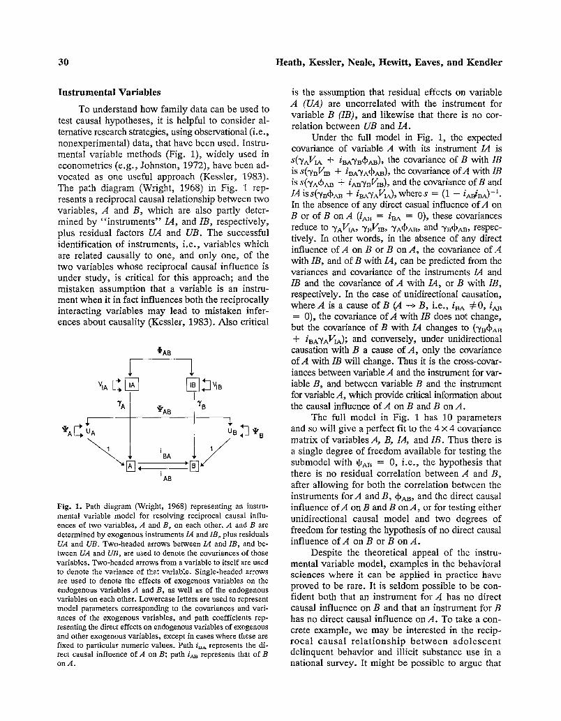
To understand how family data can be used to test causal hypotheses, it is helpful to consider al- ternative research strategies, using observational (i.e., nonexperimental) data, that have been used. Instru- mental variable methods (Fig. 1), widely used in econometrics (e.g., Johnston, 1972), have been ad- vocated as one useful approach (Kessler, 1983). The path diagram (Wright, 1968) in Fig. 1 rep- resents a reciprocal causal relationship between two variables, A and B, which are also partly deter- mined by "instruments"/_4, and IB, respectively, plus residual factors UA and UB. The successful identification of instruments, i.e., variables which are related causally to one, and only one, of the two variables whose reciprocal causal influence is under study, is critical for this approach; and the mistaken assumption that a variable is an instru- ment when it in fact influences both the reciprocally interacting variables may lead to mistaken infer- ences about causality (Kessler, 1983). Also critical
i OAB
BA
i AB
l
~B
Fig. 1. Path diagram (Wright, 1968) representing an instru- mental variable model for resolving reciprocal causal influ- ences of two variables, A and B, on each other. A and B are determined by exogenous instruments/A and 1B, plus residuals UA and UB. Two-headed arrows between/A and IB, and be- tween UA and UB, are used to denote the covariances of those variables. Two-headed arrows from a variable to itself are used to denote the variance of that variable. Single-headed arrows are used to denote the effects of exogenous variables on the endogenous variables A and B, as well as of the endogenous variables on each other. Lowercase l e t t e r s a r e used to represent model parameters corresponding to the covariances and vari- ances of the exogenous variables, and path coefficients rep- resenting the direct effects on endogenous variables of exogenous and other exogenous variables, except in cases where these are fixed to particular numeric values. Path iBA represents the di- rect causal influence of A on B; path iA~ represents that of B on A.
is the assumption that residual effects on variable A (UA) are uncorrelated with the instrument for variable B (IB), and likewise that there is no cor- relation between UB and/A.
Under the full model in Fig. 1, the expected covariance of variable A with its instrument /A is S('yAVIA -I" iBA'YBqbAB), the covariance of B with IB is S(~/BVm a t- iBA~AqbAB), the covariance of A with IB is S(~/AqbAB + iAB'/BVm), and the covariance of B and /A iSS(~/Bd~AB + iBA~/AV~), wheres = (1 -- iAB/BA)--L In the absence of any direct casual influence of A on B or of B on A (/AB = iBA = 0) , these covariances reduce to "/AVIA, "yBVIB, ~/A~)AB, and "yB(~AB, respec- tively. In other words, in the absence of any direct influence of A on B or B on A, the covariance of A with 113, and of B with/A, can be predicted from the variances and covariance of the instruments/A and IB and the covariance of A with/A, or B with 117, respectively. In the case of unidirectional causation, whereA is a cause o r B (A ~ B, i.e., iBA =/=0, iAB = 0), the covariance of A with IB does not change, but the covarianee of B with/,4 changes to ("/B+AB + iBA~/AV~A); and conversely, under unidirectional causation with B a cause of A, only the covariance of A with IB will change. Thus it is the cross-covar- iances between variable A and the instrument for var- iable B, and between variable B and the instrument for variable A, which provide critical information about the causal influence of A on B and B on A.
The full model in Fig. 1 has 10 parameters and so will give a perfect fit to the 4 x 4 covariance matrix of variables .4, B, /,4, and IB. Thus there is a single degree of freedom available for testing the submodel with t~a B = 0, i.e., the hypothesis that there is no residual correlation between A and B, after allowing for both the correlation between the instruments for A and B, +AB, and the direct causal influence of A on B and B o n A , or for testing either unidirectional causal model and two degrees of freedom for testing the hypothesis of no direct causal influence of A on B or B on A.
Despite the theoretical appeal of the instru- mental variable model, examples in the behavioral sciences where it can be applied in practice have proved to be rare. It is seldom possible to be con- fident both that an instrument for A has no direct causal influence on B and that an instrument for B has no direct causal influence on A. To take a con- crete example, we may be interested in the recip- rocal causal re la t ionship be tween adolescent delinquent behavior and illicit substance use in a national survey. It might be possible to argue that
Testing Hypotheses About Direction of Causation 31
a measure of neighborhood or community "drug availability" would be a potential instrument for the illicit substances use variable. It is extremely difficult to conceive of a suitable instrumental var- iable for delinquent behavior which could be as- sumed, with any degree of confidence, to have no direct effect on illicit substance use. Furthermore, it is easy to imagine that certain unmeasured neigh- borhood characteristics might lead both to increased drug availability and use and to increased risk of delinquent behavior, violating the assumption of no correlation between the residual for variable B and the instrument for variable A.
It is sometimes possible to identify an instru- ment for only one variable, which at least makes possible a test of a unidirectional causal hypothesis. For example, if we are interested in the relationship between adolescent smoking and illicit substance use (e.g., Yamaguchi and Kandel, 1984) or be- tween smoking and depression (e.g., Breslau, 1991; Kendler et al., 1992), the assumption that regional differences in the sales tax on cigarettes will be an appropriate instrument for smoking, and uncorre- lated with the residual for depression (or illicit sub- stance use), may sometimes be justifiable, although not if both variables are influenced by local eco- nomic conditions. In these circumstances, the hy- pothesis of no direct causal influence of smoking on illicit substance use (or depression) predicts no covariance between sales tax and illicit substance use (or depression). However, in most examples in the behavioral sciences we must allow for the pos- sibility of reciprocal causation. Another problem confronts the practical application of the instru- mental variable model, even if instruments can be successfully identified: variables A and B and their instruments are unlikely to be measured without error (as is implicit in Fig. 1). However, this prob- lem can often be overcome, by using multiple in- dicator variables (Bollen, 1989) to assess the underlying latent constructs of the model.
Panel Data
Many investigators have explored the use of longitudinal data, most commonly two-wave panel data, to address issues of causality (e.g., Campbell, 1963; Duncan, 1969) and have explored the critical underlying assumptions, violation of which may lead to errors of inference (e.g., Duncan, 1969; Kenny, 1975; Rogosa, 1980; Locasio, 1982). In early pa- pers the relative magnitude of the cross-temporal
cross-trait ("cross-lagged") correlations, i.e., the correlations of A measured at wave 1 (A~;) with B measured at wave 2 (Bt2), and of B measured at wave 1 (Ba) with A measured at wave 2 (A,2), were used to infer the relative strengths of the causal influence of A on B versus B onA: a higher absolute cross-correlation between A,I and B,2 than between Btl and A,2, for example, was taken to imply a pre- dominant causal influence of A on B. This approach can be seriously misleading (see, e.g., the critique by Rogosa, 1980), even when it is recast as a prob- lem of resolving alternative structural equation hy- potheses. Errors of inference may arise because of such issues as (i) differences in measurement error for the two traits, or the existence of correlated errors of measurement for the two traits; (ii) incon- sistency between the causal lags (i.e., the intervals between a change in A and the change in B which this produces, and vice versa) and the time lag be- tween waves of measurement; and (iii) partial or complete determination of the correlation between the two traits by a third unmeasured "mediat ing" variable, C. Such factors can lead to a higher cross- correlation between Aa and Bt2 even when the pre- dominant causal influence is B --* A.
If we consider the instantaneous reciprocal causal influences of A on B and vice versa, we can view the two-wave panel as being a particular in- stance of an instrumental variable model, where measured of A and B at wave 1 function as instru- ments forA and B, respectively, at wave 2 (Kessler, 1983): i.e., we can substituteAtl for/A and B,~ for IB, and A,2 for A and Bt2 for B, in Fig. 1. Thus a critical assumption is that there is no direct influ- ence of A at wave I on B at wave 2, and no direct infuence of B at wave 1 on A at wave 2 (Kessler, 1983). Even if this assumption is satisfied, the ap- proach will break down i fA and B are perfectly or very highly stable over time or if there are serial correlations of errors in A, and in B, which can lead to seriously biased estimates of the reciprocal paths (Kessler and Greenberg, 1981).
Behavioral Genetic Approach
A third possible approach to testing causal hy- potheses in observational data, which is much less widely recognized, utilizes data on family mem- bers, for example, pairs of monozygotic and dizy- gotic twins (Health et al., 198%; Neale et aL, 1989b, 1993; Dully and Martin, 1993; Neale and Cardon, 1992), or adoptees and their adoptive and biological
32 Heath, Kessler, Neale, Hewitt, Eaves, and Kendler
relatives. This approach does not require the suc- cessful identification and measurement of instru- mental variables and can be used with cross-sectional data. It can be used even when two associated var- iables are, except for any measurement error, com- pletely stable over time and, because even cross- sectional data are informative, avoids the problems of serially correlated errors in panel data. This ap- proach may be viewed as a special case of the in- strumental variables method, where we are using genetically informative designs to identify the ef- fects of latent instruments, i.e., the genotypes and environments which determine traits A and B.
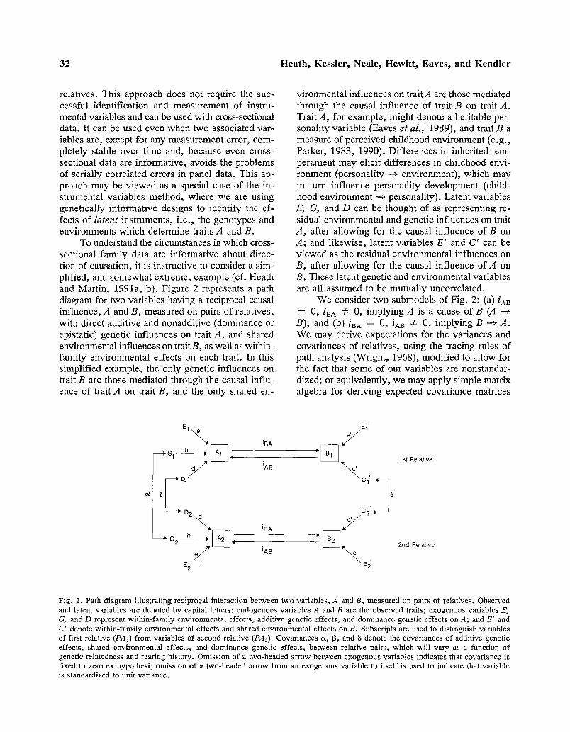
To understand the circumstances in which cross- sectional family data are informative about direc- tion of causation, it is instructive to consider a sim- plified, and somewhat extreme, example (cf. Heath and Martin, 1991a, b). Figure 2 represents a path diagram for two variables having a reciprocal causal influence, A and B, measured on pairs of relatives, with direct additive and nonadditive (dominance or epistatic) genetic influences on trait A, and shared environmental influences on trait B, as well as within- family environmental effects on each trait. In this simplified example, the only genetic influences on trait B are those mediated through the causal influ- ence of trait A on trait B, and the only shared en-
vironmental influences on trait A are those mediated through the causal influence of trait B on trait A. Trait A, for example, might denote a heritable per- sonality variable (Eaves et al., 1989), and trait B a measure of perceived childhood environment (e.g., Parker, 1983, 1990). Differences in inherited tem- perament may elicit differences in childhood envi- ronment (personality ~ environment), which may in turn influence personality development (child- hood environment --~ personality). Latent variables E, G, and D can be thought of as representing re- sidual environmental and genetic influences on trait A, after allowing for the causal influence of B on A; and likewise, latent variables E' and C' can be viewed as the residual environmental influences on B, after allowing for the causal influence of A on B. These latent genetic and environmental variables are all assumed to be mutually uncorrelated.
We consider two submodels of Fig. 2: (a) iAB = 0, iBA 5~ 0, implying A is a cause of B (.4 --*
B); and (b) iBA = 0, iAB 4= 0, implying B --~ A. We may derive expectations for the variances and covariances of relatives, using the tracing rules of path analysis (Wright, 1968), modified to allow for the fact that some of our variables are nonstandar- dized; or equivalently, we may apply simple matrix algebra for deriving expected covariance matrices
E 1 '
E,\ ,oA Y y 'AB
i
S
~ / '~ iAB
E 2 E2
1 st Relative
2nd Relative
Fig. 2. Path diagram illustrating reciprocal interaction between two variables, A and B, measured on pairs of relatives. Observed and latent variables are denoted by capital letters: endogenous variables A and B are the observed traits; exogenous variables E, G, and D represent within-family environmental effects, additive genetic effects, and dominance genetic effects on A; and E' and C' denote within-family environmental effects and shared environmental effects on B. Subscripts are used to distinguish variables of first relative (PAt) from variables of second relative (PA2). Covariances c~, 13, and ~ denote the covariances of additive genetic effects, shared environmental effects, and dominance genetic effects, between relative pairs, which will vary as a function of genetic relatedness and rearing history. Omission of a two-headed arrow between exogenous variables indicates that covariance is fixed to zero ex hypothesi; omission of a two-headed arrow from an exogenous variable to itself is used to indicate that variable is standardized to unit variance.
Testing Hypotheses About Direction of Causation 33
[e.g., using the LISREL model of Joreskog and Sorbom (1988); see also Bollen (1989)]. For the expectation for the cross-covariance of trait A in relative j (Aj), and trait B in relative k (B~), in case (a: A ---> B) we have iBA ( O~hz "+" ~d2), and in case (b: B ---> A) we have iasf3c '2. Thus A --~ B, in this simplified example, predicts a positive cross-co- variance between Aj and B~ in biological relatives, the magnitude of which will depend upon their de- gree of genetic relatedness, but a zero cross-covar- iance in adoptive relatives; whereas B ---> A predicts a positive cross-covariance which does not depend upon genetic relatedness for collateral relatives reared in the same family (e.g., MZ twin pairs, DZ twin pairs, biological or step siblings) and a zero cor- relation for relatives reared in separate families (e.g., separated twin pairs, biological mother and adopted- away offspring).
Although this example represents an extreme case, the same considerations will apply when the relative magnitudes of direct genetic and shared en- vironmental influences (or additive and dominance genetic influences) differ for the two traits. Thus if additive genetic effects are having a stronger direct influence than shared environmental effects on trait A, but shared environmental effects a stronger di- rect influence than genetic effects on trait B, then A ---> B predicts that the cross-covariance between Aj and B~ will be dominated by genetic effects, whereas B --~ A implies that it will be dominated by shared environmental effects. Similar to what we noted for instrumental variable or panel data, in family data we thus find that the cross-correlation between trait A measured in one relative and trait B measured in the second relative provides critical information about causality. However, we must note that in the case where the two traits have identical modes of inheritance (i.e., the proportions of the total variation accounted for by additive genetic, dominance genetic, shared environmental, and within-family environmental effects are identical for the two traits, so that correlations between relatives are the same for the two traits), then family data will be completely uninformative about direction of causation, as we discuss in greater detail later.
METHOD
Basic Genetic Models and Assumptions
Having considered at a somewhat intuitive level how cross-sectional data may be informative about
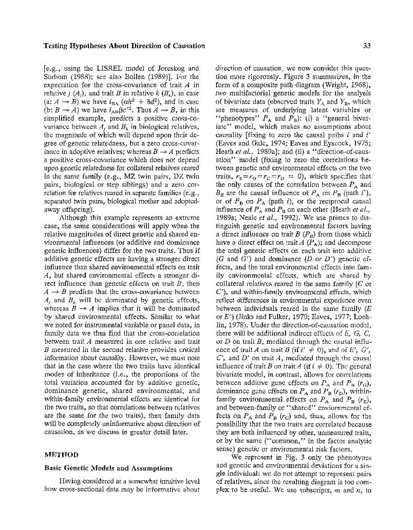
direction of causation, we now consider this ques- tion more rigorously. Figure 3 summarizes, in the form of a composite path diagram (Wright, 1968), two multifactorial genetic models for the analysis of bivariate data (observed traits YA and YB, which are measures of underlying latent variables or "'phenotypes'" PA and PB): (i) a "general bivar- iate" model, which makes no assumptions about causality [fixing to zero the causal paths i and i' (Eaves and Gale, 1974; Eaves and Eysenck, 1975; Heath et al., 1989a]; and (ii) a "direction-of-caus- ation" model (fixing to zero the correlations be- tween genetic and environmental effects on the two traits, rE=rG=rc=rD = 0), which specifies that the only causes of the correlation between PA and BB are the causal influence of Pa on PB (path i'), or of PB on PA (path i), or the reciprocal causal influence Of PA and PB on each other (Heath et aL, 1989a; Neale et al., 1992). We use primes to dis- tinguish genetic and environmental factors having a direct influence on trait B (PB) from those which have a direct effect on traitA (PA); and decompose the total genetic effects on each trait into additive (G and G') and dominance (D or D') genetic ef- fects, and the total environmental effects into fam- ily environmental effects, which are shared by collateral relatives reared in the same family (C or C'), and within-family environmental effects, which reflect differences in environmental experience even between individuals reared in the same family (E or E') (Jinks and Fulker, 1970; Eaves, 197'7; Loeh- lin, 1978). Under the direction-of-causation model, there will be additional indirect effects of E, (3, C, or D on trait B, mediated through the causal influ- ence of trait A on trait B (if i' :P 0), and of E', G', C', and D' on traitA, mediated through the causal influence of trait B on traitA (if i 4: 0). The: general bivariate model, in contrast, allows for correlations between additive gene effects on PA and oP~ (rG), dominance gene effects on PA and PB (rD), within- family environmental effects on PA and PB (rE), and between-family or '%bared'" enviornmental ef- fects on PA and PB (rc) and, thus, allows for the possibility that the two traits are correlated because they are both influenced by other, unmeasured traits, or by the same ( "common," in the factor analytic sense) genetic or environmental risk factors.
We represent in Fig. 3 only the phenotypes and genetic and environmental deviations for a sin- gle individual: we do not attempt to represent pairs of relatives, since the resulting diagram is too com- plex to be useful. We use subscripts, m and n, to
34 Heath, Kessler, Neale, Hewitt, Eaves, and Kendler
r E
r G
l 4" G C D
(~a PA q
re
l ,k E' G' C' D'
I~ PB r, pb
IF 6a A'
[ ]
Fig. 3. Composite path diagram representing (i) general bivariate genetic model and (ii) "direction-of-causation" submodel. YA and YB denote observed variables (measured on a single individual), PA and PB denote the underlying latent traits which these are measuring, and ~, and ~a are the measurement errors for the observed variables. Covariances rE, to, rc, and r~ denote covariances between within-family environmental effects on PA and PB, between additive genetic effects, between shared environmental effects, and between dominance genetic effects. See Fig. 2 and text for definition of other model variables and parameters.
distinguish latent or observed variables of the mth and nth relatives, e.g., with m = 1 and n = 2 for first and second twins from twin pairs of a given zygosity type. In terms of structural equations (e.g., Joreskog and Sorbom, 1988), from Fig. 3 we have
P,v,, = hGm + dD,,, + cC~ + eE~ + iPBm (1)
PB~ = h'Gm' + d'Dm' + C'Cm t -~- e'Er' + i ' P ~ (2)
YAm = MPA,,, + eA (3)
YB~ = h'Ps~ + eB (4)
with corresponding equations for the variables for the nth relative. Here latent genetic and environ- mental variables (G, D, C, E, etc.) are standardized to unit variance, and all variables scaled as devia- tions from zero. Genetic and environmental coef- ficients h, d, c, e, etc., and causal paths i and i ' , are assumed to be the same in relatives of different types (e.g., MZ versus DZ twin pairs). The models in Fig. 3 include measurement error explicitly (er- ror terms CA and eB, with residual variances 0,A and 0,A, respectively), since failure to allow for differ- ences in error variance can easily lead to errors of inference about causality. In applications where we have only a single indicator variable corresponding to each phenotype, we will further fix X = X '= 1,
but this constraint can be relaxed if we have mul- tiple indicator variables, i.e., multiple measures for our constructs.
In order to derive expectations for the within- trait and cross-trait covariances of relative, we need values for the covariances of additive genetic, dom- inance genetic, shared environmental, and within- family environmental effects for each trait (Gin, etc., and G,, etc.), for different types of relationship. By definition, within-family environmental effects (E or E') are uncorrelated between relatives and, also, uncorrelated with familial effects (C, G, D, C', G', or D') for the same individual. Under the simplest model, the covariances between shared en- vironmental effects (C or C') for the same trait (which we denote by 13) will be unity for collateral relatives reared in the same family (e.g., monozygotic or dizygotic twin pairs or biological or adoptive sib- ling pairs) and zero otherwise, and correlations be- tween relatives for shared environmental effects across traits will be 13rc under the general bivariate model and zero under the direction-of-causation submodel. More elaborate environmental models may also be tested, provided that appropriate con- stellations of relatives are studied (e.g., Eaves et aL, 1978; Fulker, 1982, 1988; Heath et aL, 1985), models which could incorporate such complications as differences in similarity of environmental ex- posure of twins versus sibling pairs, parent-to-off- spring environmental transmission, offspring-to-
Testing Hypotheses About Direction of Causation 35
parent environmental transmission, nonrandom placement of adoptees, and reciprocal sibling en- vironmental influences (Cavalli-Sforza and Feld- man, 1981; Cloninger et al., 1979; Eaves, 1976; Eaves et al., 1978; Carey, 1986; Fulker, 1982; Heath, 1983; Heath et al., 1989a).
From genetic theory (Fisher, 1918; Falconer, 1960; Mather and Jinks, 1971; Bulmer, 1980), the correlation between the additive genetic deviations of relatives, within traits, which we denote a , will be equal to the coefficient of relationship, under random mating, i.e., unity for monozygotic twin pairs, 0.5 for first-degree relatives, 0.25 for half- sibling pairs, etc., and zero for genetically unre- lated individuals; and the correlation of dominance genetic effects (8) will be unity for monozygotic twin pairs, 0.25 for dizygotic twin pairs, and zero for most other relationships; while the correlation between the additive genetic effects in one relative and dominance effects in the same relative or in another relative, will be zero. The corresponding correlation between additive genetic effects (or dominance effects) on trait A in relative m and ad- ditive genetic effects (or dominance effects) on trait B in relative n will be c~r a (and 8rD) under the general bivariate model but, again, zero under the direction-of-causation submodel. The assumption of random mating, i.e., that there is no tendency for like to marry like with respect to the variables under study, is easily relaxed (e.g. Fisher, 1918; Rice et aL, 1978; Cloninger et al., 1979; Eaves et al., 1978; Heath and Eaves, 1985; Fulker, 1988; Cardon et al., 1991) but is retained here to simplify- presentation. For the representation of the additive genetic variance (h 2) and the dominance genetic variance (d 2) in terms of allele frequencies and av- erage allele effects at individual loci, see Mather and Jinks (1971). In principle, terms for epistatic interactions between genetic loci [additive x ad- ditive, additive x dominance etc. (Mather and Jinks, 1971; Bulmer, 1980)] could be included in Eq. A. (1) and (2), but in practice resolution of the effects of genetic dominance and genetic epistasis for mul- tifactorial traits, in human populations, requires ex- tremely large sample sizes (Heath, 1983). In what follows, we make the additional simplifying as- sumptions of no genotype-environment correlation and no genotype x environment interaction, noting that these assumptions, too, can be relaxed if ap- propriate experimental designs are used (Eaves et al., 1977; Fulker, 1982; Heath et al., 1989a; Plomin et aL, 1977).
Hypothesis Testing
The application of methods of structural equa- tion modeling to testing genetic and environmental models, using twin and other family data, has been reviewed extensively elsewhere (Martin and Eaves, 1977; Eaves et aL, 1978; Fulker, 1982; Heath et al., 1989a; Neale et al., 1989a). In the simplest case where data are available on collateral relative pairs (e.g., monozygotic and dizygotic twin pairs reared together and twin pairs reared apart), sepa- rate summary covariance or correlation matrices are computed for each group of relatives, and a series of nested models is fitted, in a multiple-group analysis, by maximum-likelihood (Joreskog and Sorbom, 1988), asymptotic weighted least-squares (Browne, 1984), or other fitting functions, yielding efficient estimates of model parameters. Expected covariance matrices will differ for different groups of relatives because of differences in the covari- ances of genetic and environmental factors (i.e., constants oL, 13, and 8), but genetic and environ- mental parameters h, h', d, d', and etc., are con- strained to be equal across different relative groups, as well as between first and second members of same-sex relative pairs. A chi-square statistic is used to assess the overall goodness of fit of a model, and likelihood-ratio or chi-square difference tests are used to compare the fit of a general model with nested submodels, in order to identify the most par- simonious model consistent with the data (Jores- kog, 1978; Eaves et al., 1978; Neale et aL, 1989b). When more elaborate experimental designs are used, such as studying adoptees and their biological and adoptive siblings and parents (e.g., Fulker and DeFries, 1983), or twins reared together and their siblings and offspring (e.g., Eaves et al., 1992), the number of different family structures may be almost as large as the number of families, requiring that models be fitted directly to the observed raw data by max~mum-like-- lihood (e.g., Lange et al., 1976; Eaves et aL, 1978, 1989). In such analyses likelihood-ratio comparisons of the fit of a general model and submodels are made in the usual fashion.
We have described the full model in Fig. 3 as a "composite model ," in order to recognize that the full model is indeterminate. In fact, i~ can be shown that the direction-of-causation model is a submodel of the general bivariate genetic model. To avoid confusion, we use subscripts a and b for genetic and environmental parameters under the general bivariate model (i.e., ha, etc., to replace h,
36 Heath, Kessler, Neale, Hewitt, Eaves, and Kendler
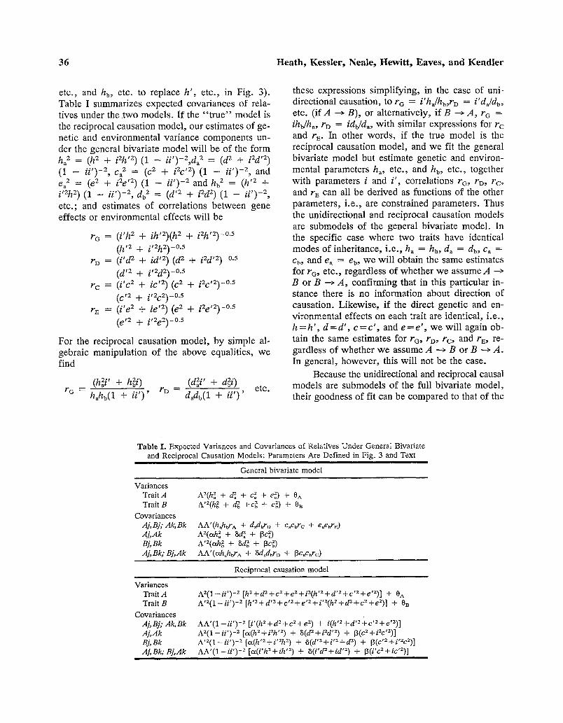
etc., and hb, etc. to replace h ' , etc., in Fig. 3). Table I summarizes expected covariances of rela- tives under the two models. If the " t r u e " model is the reciprocal causation model , our estimates of ge- netic and environmental variance components un- der the general bivariate model will be of the form ha 2 = (h 2 + i2h'2)(1 - i i ' ) -2 ,da 2 = (d 2 + i2d'2) (1 - i i ') -2, Ca 2 = (C 2 + i2C'2) (1 -- i i ') -2, and ea 2 = (e 2 + i2e '2)(1 -- i i ') -2 and hu E = (h '2 + i'2h2) (1 - i i , ) -2, db 2 = (d,a + i2d 2) (1 - i i ' ) -2, etc.; and estimates of correlations between gene effects or environmental effects will be
r G
r D =
r e =
r E =
(i 'h z + ih'Z)(h 2 + i2h'2) -~
(h 'z + i'2h2)-o.5 ( i 'd 2 + id '2) (d 2 + i2d'2)-o-5
(d '2 + i'2d2)-~ (i 'c 2 + ic '2) (C 2 + i2c'2)-~
(c '2 + i'2c2)-~ (i 'e z + ie '2) (e z + i~e'Z) -o.5
(e 'z + i'2eZ) -~
For the reciprocal causation model , by simple al- gebraic manipulation of the above equalities, we find
(h~i' + hZui) (d~i' + d~i) rG -- hahb(1 + i i ' ) ' rD -- dadb(1 + i i ' ) ' etc.
these expressions simplifying, in the case of uni- directional causation, to r o = i 'ha/hb,rD = i 'da/d b, etc. (if A --~ B), or alternatively, if B ~ A, r o = ihb/ha, r D = idb/da, with similar expressions for rc and rE. In other words, if the true model is the reciprocal causation model, and we fit the general bivariate model but estimate genetic and environ- mental parameters ha, etc., and hb, etc., together with parameters i and i ' , correlations r e , rD, rc , and rE can all be derived as functions of the other parameters, i .e . , are constrained parameters. Thus the unidirectional and reciprocal causation models are submodels of the general bivariate model. In the specific case where two traits have identical modes of inheritance, i .e . , ha = hb, da = db, ca = Cb, and ea = eb, we will obtain the same estimates for rG, etc., regardless of whether we assume A --~ B or B --~ A, confirming that in this particular in- stance there is no information about direction of causation. Likewise, if the direct genetic and en- vironmental effects on each trait are identical, i .e . , h = h ' , d = d ' , c = c ' , and e = e ' , we will again ob- tain the same estimates for r G, rD, r o and rE, re- gardless of whether we assume A --~ B or B ~ A. In general, however, this will not be the case.
Because the unidirectional and reciprocal causal models are submodels of the full bivariate model, their goodness of fit can be compared to that of the
T a b l e I . Expected Variances and Covariances of Relatives Under General Bivariate and Reciprocal Causation Models: Parameters Are Defined in Fig. 3 and Text
General bivariate model
Variances Trait A Trait B
Covariances Aj, Bj; Ak, Bk Aj, Ak Bj, Bk Aj, Bk; Bj, Ak
A2(h~ + dZ~ + c2~ + e~) + 0A A'2(h~ + d~ +c~ + e~) + 0B
AA'(h~ht~A + ddtc'D + c~c~rc + e~ev"E) A2(ah 2 + ~d~ + 13c~) A ' ~ ( ~ + ~d~ + 13c~) AA'(e&fld'A + 8dflbrD + 13c.Cd'c)
Reciprocal causation model
Variances Trait A Trait B
Covariances Aj, Bj; Ak, Bk Aj, Ak Bj, Bk A],Bk; Bj, Ak
A 2 ( 1 - i i ' ) -~ [hZ+d2+ca+e2+i2(h'2+d'2+c'2+e'Z)] + 0A A ' 2 ( 1 - i i ' ) -z [h'2+d'2+c'2+e'2+i'2(h2+d2+cZ+e2)] + OB
A A ' ( 1 - i i ' ) -z [i '(h2+d2+c2+e 2) + i(h'2+d'2+c'2+e'2)] A z ( 1 - i i ' ) -e [tx(hZ+i2h '2) + ~(d2+i2d'2) + f3(c2+i2c'2)] A ' 2 ( 1 - i i ' ) -2 [tx(h'2+i'2h 2) + ~(d'2+i'2+d 2) + ~(c'2+i'2r A A ' ( 1 - - i i ' ) -2 [ct(i'h2 +ih '2) + 6(i'd2 +id '2) + f3(i'c2+ic'2)]
Testing Hypotheses About Direction of Causation 37
full bivariate model by likelihood-ratio chi-square test, with the numbers of degrees of freedom equal to the number of genetic and environmental corre- lations estimated in the bivariate model minus the number of causal paths estimated in the causal model. An important implication of this is that in order to test the reciprocal causation model against the gen- eral bivariate model, we need to have at least three "sources of variation" [in the traditional terminol- ogy of quantitative genetic (Mather and Jinks, 1971; Jinks and Fulker, 1970; Eaves, 1977)] influencing the two traits, either directly or indirectly, counting within-family environment, additive genetic ef- fects, dominance genetic effects, and shared envi- ronment each as one source of variation. (It is not necessary that each trait be directly influenced by three sources of variation, for example, the genetic influences on B may be those mediated through the causal influence of A on B, as in Fig. 2). If there are only two "sources of variation" in the two traits, e.g., if both traits are influenced by additive genetic and within-family environmental effects, the recip- rocal causation model will give the same fit to the data as the general bivariate model, and no test of the model will be available.
An Important Limitation
The fact that the reciprocal causation model is a submodel of the general bivariate model empha- sizes an important difference between the infer- ences about causality which can be drawn using instrumental variables and the inferences which can be drawn from family data. Using an instrumental variable approach, in addition to the direct effects of A on B and B on A, it is possible to estimate a residual correlation between the reciprocally inter- acting variables (~aB in Fig. 1). Thus it is possible to test the hypothesis that the correlation between A and B arises solely because of the reciprocal causal influence of A on B and of B on A, plus the cor- relation between the instruments forA and B (qbAB), i.e., that "IraB = 0. In family data, in contrast, at least in the bivariate case, we are restricted to test- ing hypotheses of the form "the ONLY cause of the correlation between PA and PB is the causal influence of PA on P~ (or the reciprocal causal in- fluence of PA and PB on each other)." In what follows, we use the phrase "testing the causal hy- pothesis A ~ B (or A ~ B) " as a short-hand for these strong causal hypotheses. If A and B are cor- related, both because of their reciprocal causal in-
fluence and also because both variables are influenced by other unmeasured variables, this will cause fail- ure of the reciprocal causation model (if the latter influences are sufficiently important). The latter case cannot be distinguished from the general bivariate model in family data on a single pair of variables but may still be tractable if our hypothesis specifies a causal chain (A ~ B ~ C ~ D, etc.) with an additional contribution of other unmeasured varia- bles to correlations between variables A, B, C, D, etc. The same problem is encountered in trying to draw inferences about causality from panel data, where partial determination of A and B by an un- measured latent variable, C, can again lead to errors of inference about causality.
The Problem o f Measurement Error
In general, we cannot assume that our varia- bles are measured without error. The example of smoking status, i.e., whether or not an individual ever smoked (Heath et aL, !993), and age at death provides a rare counterinstance where measurement error effects may be minor. Under the general bi- variate model, if we ignore measurement error when it is present, and if errors of measurement are un- correlated between family members (and therefore contribute to within-family variance but not to fam- ily resemblance), this will inflate estimates of ea 2
and eb z and lead to an underestimate of rE (Eaves and Eysenck, 1975), but other parameters will be unbiased. Similarly, in the context of the reciprocal causation and unidirectional causation submodels, ignoring measurement error will lead to inflated es- timates of e 2 and e 'z. However, since the expec- tation for the within-person ( i .e . , phenotypic) covariance of traits A and B (Aj with Bj and Ak with Bk in Table I) includes terms in i 'e 2 and ie '2 (see Table I), ignoring measurement error will also lead to biased estimates of all the other parameters of the direction-of-causation model.
In the case of unidirectional causal models, only a single error term is critical, namely, the error variance for trait A i fA --~ B or the error variance for trait B if B ~ A. If the direction of causation is A --~ B (with i = 0, i'=P 0), then the expectation for the phenotypic covariance of A and B will in- clude only the expression i 'e z. Omitting the error term for B will inflate the estimate of e '2 by the error variance for B, but other parameter estimates will be unbiased, provided that an error variance for trait A is included in the model. Omission of
38 Heath, Kessler, Neale, Hewitt, Eaves, and Kendler
the error variance for A will, however, lead to biased parameter estimates, even if an error variance is estimated for B.
We reported above expectations for the genetic and environmental correlations of the general bi- variate model for the case where the true model is the reciprocal causation model, for example,
(e2i ' + e~i)
rE = eaeb(1 + i i ' )
with similar expressions for ra, rD, and rc. Thus even in the case where we do not have data about measurement error, it is possible to test a unidirec- tional causal model allowing for measurement error ("unidirectional causation with error" model), pro- vided that we have at least three "sources of vari- ation" influencing the two traits, either directly or indirectly. Including a single error variance in a unidirectional causation model has the effect of re- laxing the equality constraint relating r E to param- eters e,, eb, and i (or i '). If there are three sources of variance for each trait, e.g., both trait A and trait B are influenced by additive gene action, shared environmental effects, and within-family environ- mental effects, there will remain one degree of free- dom for test ing the goodness of fit of each unidirectional causation with error model against the fit of the general bivariate model, which in ef- fect is testing whether the equalities rG = i ' h J h b and r c = i ' c j c b (ifA --> B) or, alternatively ro = ihu/h , and r e = icu/c , ( i fB --> A) are both satisfied, and two degrees of freedom if there are four sources of variation. If there are only two sources of vari- ation for traits A and B, e.g., within-family envi- ronmental effects plus additive genetic effects on both traits or within-family environmental effects plus shared environmental effects on both traits, however, the general bivariate model will include only two correlations, rE and either r G or rc. Re- laxing the constraint on r z , by estimating an error variance for one variable, will be equivalent to fit- ting the general bivariate model. If there are only two sources of variation, therefore, the two "uni- directional causation plus measurement e r ror" models will, in general, give identically good fits to the data and will give the same fit as the general bivariate model. In this case we can proceed to test causal hypotheses only if we know that both traits are measured without error or if we have additional information about error variances for the two traits and can exploit this in a multiple indicator causal model.
In the case of the reciprocal causation model, within-family environmental variances for both traits occur in the expectation for the within-person co- variance of the two traits. If no other data about error variances are available, estimation of an error variance for one trait will relax the equality con- straint on rE. Regardless of how many sources of variation are influencing the two traits, no further information is available to estimate an error vari- ance for the second trait. Thus it will be possible to test reciprocal causation models only if we are prepared to assume that the error variances for the two traits are either zero or equal in absolute mag- nitude [it appears that relatively small differences in the magnitude of the error variances for A and B will produce only a minor bias to estimates of other parameters, if the error variances are assumed equal (Neale and Cardon, 1992)] or if additional information is available to estimate the effects of measurement error for each trait, for example, by fitting a multiple indicator model. If error variances can be assumed to be zero, the reciprocal causation model will be just identified if there are only two sources of variation, and at least three sources of variability will be required in order to permit a like- lihood-ratio chi-square test, on one degree of free- dom, against the general bivariate model. If error variances are nonzero but can be assumed to be equal, four sources of variability will be required to permit a test of the reciprocal causation plus error model against the general bivariate model. The se- quence of causal models that can be tested and de- grees of freedom for testing each model against the general bivariate model are summarized in Table III.
Multiple Indicator and Multivariate Genetic Models
In studies of samples of unrelated individuals, generalization of the instrumental variable or panel models to allow for multiple measures ("indica- tors") of traits A and B and their instruments is comparatively straightforward and is illustrated in standard texts on structural equation modeling (e.g., Bollen, 1989). The use of multiple indicator vari- ables in family studies enjoys the same advantages as in the more traditional approaches to testing causal hypotheses, i.e., it allows the formulation of ex- plicit assumptions about measurement error and testing of at least some of these assumptions; for example, depending upon how many indicator var-
Testing Hypotheses About Direction of Causation 39
iables are assessed, it may be possible to allow for correlated errors of measurement between certain indicators (Costner and Schoenberg, 1973). In fam- ily data, the use of multiple indicator variables also makes it possible to allow for correlated errors of measurement between family members for each in- dicator variable (Martin and Eaves, 1977). We have noted in the previous section that multiple indicator data are needed to allow estimation of reciprocal causal effects, except in cases where error variances are known precisely from external sources. In this section, therefore, we first present a multiple in- dicator generalization of the direction of causation model for family data and then compare this model to less restrictive multivariate genetic models.
Multiple Indicator D O C Model
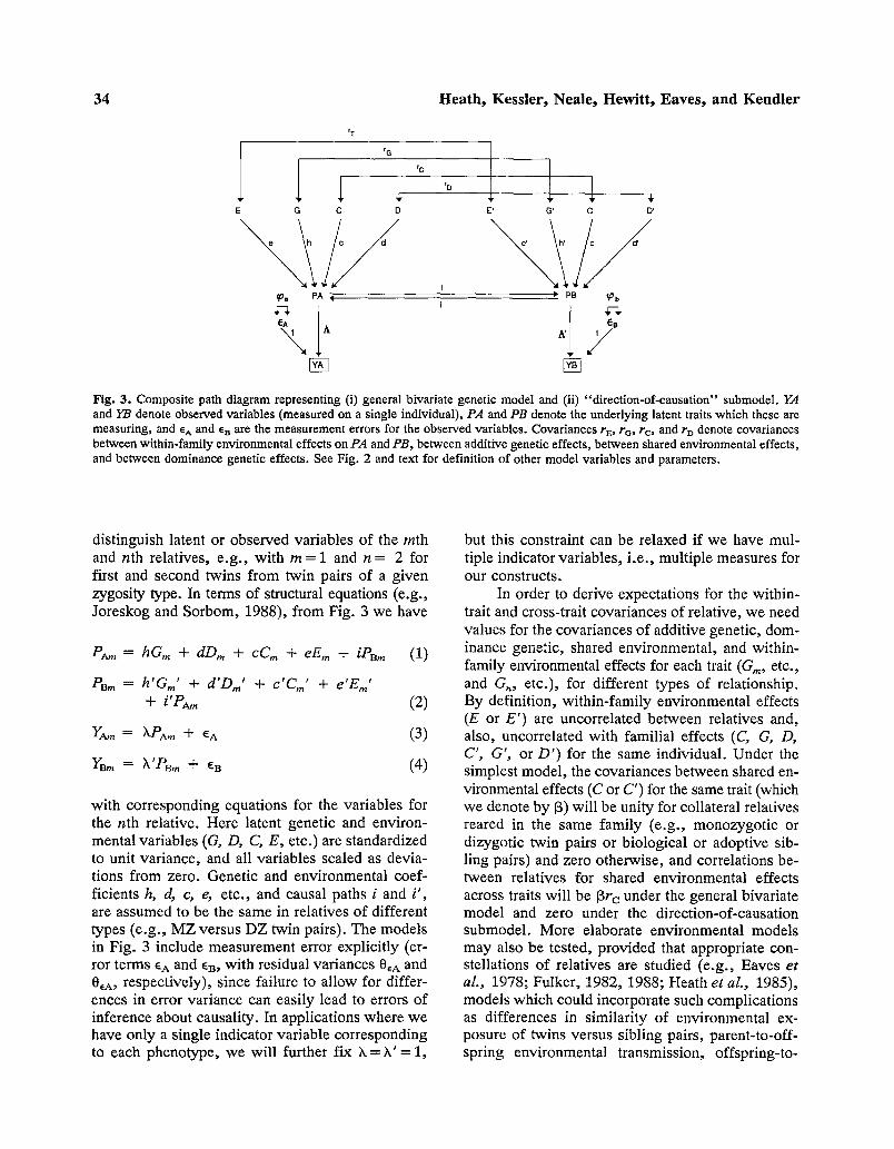
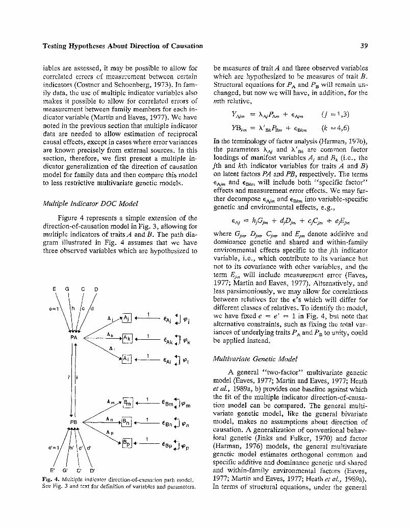
Figure 4 represents a simple extension of the direction-of-causation model in Fig. 3, allowing for multiple indicators of traits A and B. The path dia- gram illustrated in Fig. 4 assumes that we have three observed variables which are hypothesized to
E G C D
EAj ~ ~j
�9 ,t- (~AI ~ to I
PB 4 1
e' 1 c : - - eBp,~I ~p
E' G' C' D'
Fig. 4. Multiple indicator direction-of-causation path model. See Fig. 3 and text for definition of variables and parameters.
be measures of trait A and three observed variables which are hypothesized to be measures of trait B. Structural equations for PA and PB will remain un- changed, but now we will have, in addition, for the ruth relative,
Yajm = Xm.Pa,, + EAjm ( j = 1,3)
}"B/on = X'BkPBm + eBk m (k =4,6)
In the terminology of factor analysis (Harman, 1976), the parameters kay and k'Bk are common factor loadings of manifest variables Aj and Bk (i.e., the jth and kth indicator variables for traits A and B) on latent factors PA and PB, respectively. The terms eAj m and eB~ will include both "specific factor" effects and measurement error effects. We may fur- ther decompose eaj~ and e ~ into variable-specific genetic and environmental effects, e.g.,
e~. = hjGj,,, + djDjm + cjCjm + ejEjm
where @'m, Ds'm, Cj,o and Eim denote additive and dominance genetic and shared and within-family environmental effects specific to the jth indicator variable, i.e., which contribute to its variance but not to its covariance with other variables, and the term Ej,, will include measurement error (Eaves, 1977; Martin and Eaves, 1977). Alternatively, and less parsimoniously, we may allow for correlations between relatives for the e's which will differ for different classes of relatives. To identify the model, we have fixed e = e' = 1 in Fig. 4, but note that alternative constrain% such as fixing the total var- iances of underlying traits PA and PB to unity, could be applied instead.
Multivariate Genetic Model
A general "two-factor" multivariate genetic model (Eaves, 1977; Martin and Eaves, 1977; Heath et aL, 1989a, b) provides one baseline against which the fit of the multiple indicator direction-of-causa- tion model can be compared. The general multi- variate genetic model, like the general bivariate model, makes no assumptions about direction of causation. A generalization of conventional behav- ioral genetic (Jinks and Fulker, 1970) and factor (Harman, 1976) models, the general multivariate genetic model estimates orthogonal common and specific additive and dominance genetic and shared and within-family environmental factors (Eaves, 1977; Martin and Eaves, 1977; Heath et aL, 1989a). In terms of structural equations, under the general
40 Heath, Kessler, Neale, Hewitt, Eaves, and Kendler
model we will have (omitting subscripts for rela- tives)
YAj = hjaGa -Jr- hjbG b "AI- 4aDa -1- 4bDb "4- CjaC a + 9bCb + ey,E, + esbE b + eAj
where Ga and Gu denote the first and second ad- ditive genetic common factors, D, and Db the first and second dominance genetic common factors, and so on; hjo, hj~, djo, djb, etc., are the additive and dominance genetic loadings of the jth item on the first and second additive and dominance genetic common factors; and eAj. denotes the sum of the specific factor and measurement error effects for thejth item. The issue of factor rotation which arises in conventional factor analysis (e.g., Harman, 1976) will apply equally to factors estimated under the multivariate genetic model, except that factors corresponding to different sources of variability cannot be rotated jointly, i.e., we must rotate sep- arately additive genetic common factors, domi- nance genetic common factors, shared environmental common factors, and within-family environmental common factors. Covariances of the genetic and environmental factors between relatives may be ex- pressed in terms of constants cx and ~ (which de- pend upon genetic relatedness) and B (which depends upon rearing experience), as before, with the as- sumption of orthogonal genetic and environmental factors implying no cross-covariances between the first additive genetic factor in one relative and the second additive genetic factor in the second rela- tive, etc. In terms of the parameters of the general multivariate genetic model, the expectation for the variance of observed variable Ym. will be
Var(YAs-) = h~ + hj 2 + h~ + d~Za + d~Zu + d~ 2 + c~ + cYb + c 2 + e~ + e j~b + e j
the expectation for the within-person covariance of observed variables Y~ and Yak will be
CoV(YAjYA.k) = hjahka -[- hjbhkb "1- 4adka -I- 4bdkb + c.i~c~, + CybCkb + ey~ek~ + ejbeku
the expectation for the covariance between the ruth and the nth relatives for YAj will be
Cov(Y .mYAj-n) = cr + hj 2 + + + dJ b + d} + + c j \ +
and the expectation for the covariance between Ym. measured in relative m and YAk measured in relative n will be
Cov(Y, jmY .) = (hjahka + h uhkb) + a(4ad a + 4bd ) + t3(cj.c . + cj c, )
As in the single indicator case, we also give (in Table II) expressions for the parameters of the gen- eral multivariate genetic model in terms of the pa- rameters of the multiple indicator reciprocal causation model, which will apply when the latter is the "true" model,
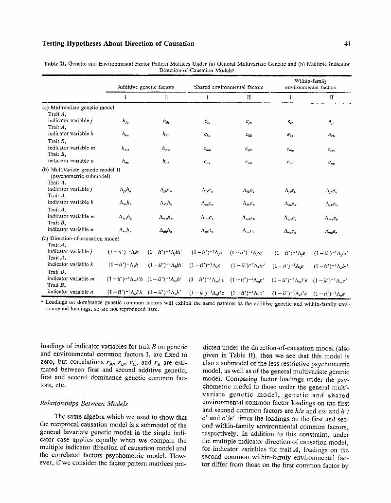
The general multivariate genetic model im- poses no constraints on the genetic and environ- mental common factor structures; it does not constrain the pattern of genetic factor loadings to bear any relationship to the pattern of environmen- tal factor loadings. A more restrictive version of this model, which has been variously described as the "psychomet r ic" (McArdle and Goldsmith, 1990), "common pathway" (Kendler et al., 1987), or "latent phenotype" (Heath et al., 1989a, b) model, while still making no assumptions about di- rection of causation, imposes the constraint that ge- netic and shared environmental loadings on each factor differ from the corresponding within-family environmental factor laodings only by a scale factor (Martin and Eaves, 1977). This is the pattern that we would expect to observe if indicator variables load on " 'phenotypic" factors (e.g., personality factors), which in turn are determined by orthogo- nal genetic and environmental effects. In Table II we present common factor loadings, in the form of additive genetic, shared environmental, and within- family environmental factor pattern matrices, for the general multivariate and psychometric genetic models. As in the case of the multiple indicator direction-of-causation model, the psychometric model may be identified by fixing e = e ' = 1 or by constraining the variances of the underlying phe- notypic factors, PA and PB, to unity. In contrast to the general multivariate model, factor loadings un- der the psychometric model cannot in general be rotated (e.g., Hewitt, unpublished): the constraint that the genetic and environmental effects (G or G', C or C', etc.) on intervening latent phenotypes PA and PB are uncorrelated identifies a unique factor solution. Finally, we may note that by combining the general bivariate model in Fig. 3 (with i = i' = 0) with the multiple indicator variable component of the model in Fig. 4, we may also derive a correlated factors version of the psychometric model (Mc- Ardle and Goldsmith, 1990). Under this model, loadings of indicator variables for trait PA on ge- netic and environmental common factors II, and
Testing Hypotheses About Direction of Causation 41
Table II . Genetic and Environmental Factor Pattern Matrices Under (a) General Multivariate Genetic and (b) Multiple Indicator Direction-of-Causation Models ~
Within-family Additive genetic factors Shared environmental factors environmental factors
I II I II I II
(a) Multivariate genetic model Trait A, indicator variable j h~. h.m Cja Cdb ei~ gjb Trait A, indicator variable k hk~ hkb Cka Ckb eka ekb
Trait B, indicator variable m hma hmb era. Crab e., . e,.b Trait B. indicator variable n h.a hnb Cna Crib en a en b
(b) Multivariate genetic model iI (psychometric submodel)
Trait A. indicator variable j Aj.h. Ajbhb Ajac a AjbCb Aj.e. Ajbe b Trait A, indicator variable k Ak.h. Akbh b Ak~c. Akbc~ Ak.e. Akbeb Trait A. indicator variable m A,..h a A , . ~ AmaC a hmbC b A,..ea A,~beb Trait B. indicator variable n A.~ha A.~b A.~c. AnbC b A.~ea A.beb
(C) Direction-of-causation model Trait A, indicator variable j (1 - i i ' ) - l A j h (1 - i i ' ) - I A ~ d h ' (1 - i i ' ) - X A F (1 - i i ' ) - ~ A j c ' (1 - i i ' ) - X A ~ e (1 - i i ' ) - ~ A f i e ' Trait A. indicator variable k (1 - i i ' ) - A k h (1-i i ' ) -~Akih ' (1--ii ')-~Akc (1--ii ')-~Akic ' (1--ii ')-~Ake (1 - - i i ' ) -~Ak ie '
Trait B ,
indicator variable m (1- i i ' ) -~Ami 'h ( 1 - i i ' ) - l A ~ h ' (1--ii ')-lAmi'C (1 - i i ' ) - lAmc ' (1 - i i ' ) - lAmi ' e ( 1 - i i ' ) - I A ~ e ' Trait B,
indicator variable n (1-ii ' )-XA~i'h ( 1 - i i ' ) - l A . h ' (1 - i i ' ) - lA~ i ' c (1 - i i ' ) - lA~c ' (1- i i ' ) -~A~i 'e (1 - i i ' ) - IA~e ' u l i
l
a Loadings on dominance genetic common factors will exhibit the same patterns as the additive genetic and within-family envi- ronmental loadings, so are not reproduced here.
loadings of indicator variables for trait B on genetic and environmental common factors I, are fixed to zero, but correlations rA, rD, rc, and rE are esti- mated between first and second additive genetic, first and second dominance genetic common fac- tors, etc.
Relationships Between Models
The same algebra which we used to show that the reciprocal causation model is a submodel of the general bivariate genetic model in the single indi- cator case applies equally when we compare the multiple indicator direction of causation model and the correlated factors psychometric model. How- ever, if we consider the factor pattern matrices pre-
dicted under the direction-of-causation model (also given in Table II), then we see that this model is also a submodel of the less restrictive psychometric model, as well as of the general multivariate genetic model. Comparing factor loadings under the psy- chometric model to those under the general multi- va r ia te gene t ic mode l , gene t i c and shared environmental common factor loadings on the first and second common factors are hie and c/e and h'/ e' and c'/e' times the loadings on the first and sec- ond within-family environmental common factors, respectively. In addition to this constraint, under the multiple indicator direction of causation model, for indicator variables for trait A, loadings on the second common within-family environmental fac- tor differ from those on the first common factor by
42 Heath, Kessler, Neale, Hewitt, Eaves, and Kendler
a factor of (ie'/e), while for indicator variables for trait B, loadings on the first common within-family environmental factor differ from those on the sec- ond common factor by a constant multiple (i'e/e'), with similar constraints applying to genetic and shared environmental common factor loadings. As a submodel of the psychometric model, the multiple indicator direction-of-causation model will also de- fine a unique factor solution. Expectations for the variances and covariances of relatives under the psychometric and multiple indicator direction-of- causation models may be derived from those for the general multivariate genetic model by making the appropriate substitutions for common factor loadings from Table II; specific factor effects will be parameterized identically under these models.
Measurement Error
From these considerations we can see how the use of multiple indicator variables will reduce the problem of measurement error, including correlated errors of measurement , in test ing causal hy- potheses. If measurement error is variable specific, application of the multiple indicator direction-of- causation model to cross-sectional family data will provide statistical tests of the goodness of fit of the reciprocal causation model (A ~e B) compared to correlated factors, psychometric, or general multi- variate genetic models, provided that there are at least three sources of variability, and also tests of the unidirectional causal models (A ~ B or B --~ A), even when there are only two sources of vari- ation (e.g., additive genetic plus within-family en- vironmental effects) in A and B. If there are only two sources of variability, the reciprocal causation model will be confounded with the correlated psy- chometric factors model, the same result that we noted in the single indicator case. Measurement er- ror correlations for the same indicator variable be- tween family members will bias estimates of the variable-specific genetic and environmental param- eters but will not affect estimates of common factor loadings and, hence, will not bias inferences about direction of causation. If measurement errors are correlated across indicator variables, but the cross- variable error correlations between family members are zero, it will still be possible to test the reciprocal and unidirectional causal models if there are at least three sources of variability (or four in the case of the reciprocal causation model). In this case, in- stead of constraining additive and dominance and
shared environmental common factor loadings to be multiple of within-family environmental common factor loadings, we will estimate, say, dominance genetic and shared environmental common factor loadings to be multiples of the additive genetic common factor loadings but impose no constraints on the within-family environmental common factor loadings. Finally, if there are correlations between measurement errors across different indicator vari- ables between family members, as well as within persons, then we may be able to incorporate these in our model, following the approach of Costner and Schoenberg (1973), provided that we have as- sessed a sufficiently large number of indicator var- iables and that the number of indicator variables for which such cross-indicator familial correlations oc- cur is small.
Hypothesis Testing
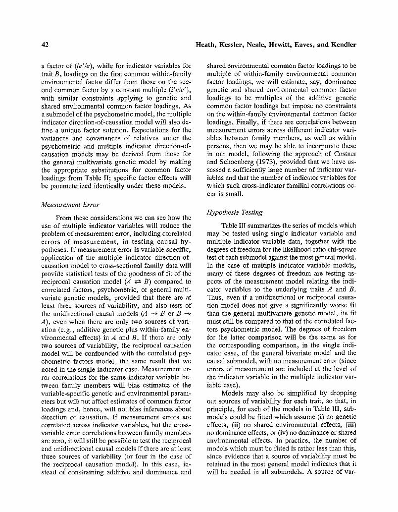
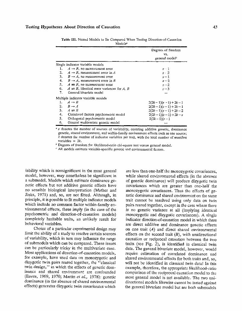
Table III summarizes the series of models which may be tested using single indicator variable and multiple indicator variable data, together with the degrees of freedom for the likelihood-ratio chi-square test of each submodel against the most general model. In the case of multiple indicator variable models, many of these degrees of freedom are testing as- pects of the measurement model relating the indi- cator variables to the underlying traits A and B. Thus, even if a unidirectional or reciprocal causa- tion model does not give a significantly worse fit than the general multivariate genetic model, its fit must still be compared to that of the correlated fac- tors psychometric model. The degrees of freedom for the latter comparison will be the same as for the corresponding comparison, in the single indi- cator case, of the general bivariate model and the causal submodel, with no measurement error (since errors of measurement are included at the level of the indicator variable in the multiple indicator var- iable case).
Models may also be simplified by dropping out sources of variability for each trait, so that, in principle, for each of the models in Table III, sub- models could be fitted which assume (i) no genetic effects, (ii) no shared environmental effects, (iii) no dominance effects, or (iv) no dominance or shared environmental effects. In practice, the number of models which must be fitted is rather less than this, since evidence that a source of variability must be retained in the most general model indicates that it will be needed in all submodels. A source of var-
Testing Hypotheses About Direction of Causation 43
Table III. Nested Models to Be Compared When Testing Direction-of-Causation Models a
| |1
Degrees of freedom V S .
general modeP
Single indicator variable models 1. A --'- B, no measurement error 2. A ~ B, measurement error in A 3. B ---* A, no measurement error 4. B ~ A , measurement error in B 5. A ~ B, no measurement error 6. A ~:~ B, identical error variances for A, B 7. General bivariate model
Multiple indicator variable models 1. A "+ B
2. B --+ A 3. A ~ e B
4. Correlated factors psychometric model 5. Orthogonal psychometric mode/ 6. General multivariate genetic model
s - I s - 2 s - 1 s - 2 s - 2 s - 3
2(2k - 1)(s - 1) + 2k - 1 2(2k - 1)(s - 1) + 2k - 1 2(2k - 1)(s - 1) + 2k - 2 2(2k- 1)(s- 1) +2k-s 2 ( ~ - 1)(s- 1
a s denotes the number of sources of variability, counting additive genetic, dominance genetic, shared environment, and within-family environment effects each as one source; k denotes the number of indicator variables per trait, with the total number of manifest variables = 2k.
b Degrees of freedom for likelihood-ratio chi-square test versus general model. c All models estimate variable-specific genetic and environmental factors.
lability which is nonsignificant in the most general model, however, may nonetheless be significant in a submodel. Models which estimate dominance ge- netic effects but not additive genetic effects have no sensible biological interpretation (Mather and Jinks, 1971) and, so, are not fitted. Although, in principle, it is possible to fit multiple indicator models which include no common factor within-family en- vironmental effects, these imply (in the case of the psychometric and direction-of-causation models) completely heritable traits, an unlikely result for behavioral variables.
Choice of a particular experimental design may limit the ability of a study to resolve certain sources of variability, which in turn may influence the range of submodels which can be compared. These issues can be particularly tricky in the multivariate case. Most applications of direction-of-causation models, for example, have used data on monozygotic and dizygotic twin pairs reared together, the "classical twin design," in which the effects of genetic dom- inance and shared environment are confounded (Eaves, 1969, 1970; Martin et aL, 1978): genetic dominance (in the absence of shared environmental effects) generates dizygotic twin covariances which
are less than one-half the monozygotic covariances, while shared environmental effects (in the absence of genetic dominance) will produce dizygotic twin covariances which are greater than one-]half the monozygotic covariances. Thus the effects of ge- netic dominance and shared environment on the same trait cannot be resolved using only data on twin pairs reared together, except in the case where there is no genetic variance at all (implying identical monozygotic and dizygotic covariances). A single indicator direction-of-causation model in which there are direct additive and dominance genetic effects on one trait (A) and direct shared environmental effects on the second trait (B), with unidirectional causation or reciprocal causation between the two traits (see Fig. 2), is identified in classical twin data. The general bivariate model, however, would require estimation of correlated dominance and shared environmental effects for both traits and, so, will not be identified in classical twin data[ In this example, therefore, the appropriate likelihood-ratio comparison of the reciprocal causation model to the most general model is not available. The two uni- directional models likewise cannot be tested against the general bivariate model but are both submodels
44 Heath, Kessler, Neale, Hewitt, Eaves, and Kendler
of the reciprocal causation model, so that likeli- hood-ratio comparisons with that model can be made. For the same example, but assuming multiple in- dicator variables, the correlated factors psychomet- ric model will not be identified, by the same reasoning that applies to the general bivariate model with single indicator variables. The orthogonal fac- tors psychometric model, with one factor allowing for genetic dominance and the second for shared environmental effects, will be identified and, thus, permits a test of the reciprocal causation model as well as of the two unidirectional causal models. Using multiple relationships to ensure that the ma- jor sources of variability are unconfounded (Fulker, 1982; Heath, 1983; Heath et al., 1985) will help avoid such complications.
Power Analyses
Demonstration that it is feasible, in principle, to test strong causal hypotheses using cross-sec- tional family data need not imply that it is feasible in practice. We present in this section details of power analyses using the noncentral chi-square dis- tribution (Martin et al., 1978; Heath and Eaves, 1985; Heath et al., 1985; Matsueda and Bielby, 1986; Satorra and Saris, 1985), which were con- ducted for a limited range of parameter values, and considered only the power of the most widely used experimental design, the classical twin design. These suffice to demonstrate the conditions under which resolution of hypotheses about direction of causa- tion is likely to be most feasible. For a given true model (e.g., A --+ B), and given population param- eter values, we generated numerical values for the expected covariances for monozygotic and dizy- gotic twin pairs reared together. Genetic and en- vironmental parameter values were chosen to give total variances for PA and PB, in the absence of any causaul influence of PA on PB, or vice versa, of unity. (We have taken this approach, rather than standardizing parameter estimates after allowing for the causal effects of B on A, or vice versa, since it simplifies presentation of results for the case of re- ciprocal interaction: see below.) A false model (e.g., B ~ A or B ~ A with measurement error in B) was fitted to the data, assuming equal numbers of monozygotic and dizygotic twin pairs and an arbi- trary total sample size, N, and the goodness-of-fit chi-square, C, was recorded. Since the true model, and all models of which the true model is a sub- model, would give a perfect fit to the observed
data, the statistic C is also a likelihood-ratio chi- square for testing the false model against a more general model of which both the true and the false models are submodels, with degrees of freedom, x, equal to the number of parameters of the more gen- eral model which have been fixed to zero or unity under the false model. The sample sizes required for 80% probability of rejecting the false model, at the 5% significance level, given the population pa- rameters used under the true model, were compared (see Martin et al., 1978; Satorra and Saris, 1985) as
NC' /C where C' is the noncentral chi-square parameter C(o.05.so.~) obtained from the table of noncentral chi- squares (Pearson and Hartley, 1972).
In our analyses of statistical power, we con- sidered first the case where only a single indicator variable is used for each trait. We considered both the case where both traits are measured without error and then the more realistic case where 20% of the observed variance in trait A, and also 20% of the observed variance in trait B, is attributable to error variance. In model-fitting, however, in every case the models fitted included a false unidirec- tional model with measurement error, since in some cases this required larger sample sizes to reject than the false model assuming no measurement error (e.g., cases 1 and 2 when the true model was A ~ B). We examined four cases: (1) direct effects of ad- ditive and dominance gene action on trait A and of shared environment on trait B but with no direct shared environmental influence on trait A and no direct genetic influence on trait B; (2) direct addi- tive genetic effects only on trait A and direct shared environmental effects only on trait B; (3) direct ad- ditive genetic and dominance effects on trait A and direct additive genetic and shared environmental ef- fects on trait B; and (4) direct additive genetic and shared environmental effects on both traits A and B, with genetic effects having a relatively greater impact on trait A, and shared environmental effects on trait B. In each case we compared the statistical power when nonshared environment is accounting for 25% of the variance and also, in the case of true models without measurement error, 50% of the variance.
Illustrative power analyses were also con- ducted under the multiple indicator model, assum- ing three indicator variables for each trait. These used the same sets of parameters values as under the measurement error analyses and assumed that
Testing Hypotheses About Direction of Causation 45
measurement error variance is the only source of specific factor variance for the indicator variables, accounting for only 20% of the variance. These are very strong assumptions, since empirically it has usually been found that variable-specific genetic and shared environmental influences are also found (e.g., Martin and Eaves, 1977; Eaves e t a l . , 1989).
R E S U L T S
Table IV summarizes the number of twin pairs required, assuming equal numbers of monozygotic and dizygotic twin pairs reared together are used in a study, for 80% power of rejecting a false unidi- rectional causal hypothesis, at the 5% significance level, when the true population model is the alter- native unidirectional causal model. It demonstrates very clearly that the power of the twin design to falsify unidirectional causal models is greatest when the two correlated traits have very different modes of inheritance. To provide some perspective for the sample sizes reported in Table IV, a sample size of 200-500 twin pairs is achievable for a laboratory study in which twin pairs are participating in an experimental protocol (e.g., Martin e t a l . , 1985a, b; Scheiken e t a l . , 1989), 1000 or more twin pairs in an interview-based study (e.g., Kendler e t al . , 1991), and as many as 5000 or more twin pairs in an mailed questionnaire survey (e.g., Eaves e t a l . , 1992; Eisen e t a l . , 1991). We consider first cases where measurement error is negligible. The worst case is that where both traits are influenced by both additive genetic and shared environmental effects, albeit to differing degrees (case 1.4). For this case our ability to reject the false unidirectional causal model even in questionnaire survey data depends upon within-family environmental effects having a relatively modest impact (e 2 = e '2 = 0.25) and the causal influence being at least moderately strong (1 > 0.25 or i ' > 0.25) or, if there is a stronger influence of within-family environmental variance (e 2 = e '2 = 0.5), requires that the causal influence be very strong indeed (i > 0.5 or i ' > 0.5). In the first two cases, where there are no direct genetic influences on trait B, and direct genetic but no di- rect shared environmental effects on traitA, if within- family environment effects are weak, required sam- ple sizes are within a range that can be achieved in laboratory studies if i or i ' >_ 0.3 and are certainly achievable in interview studies if i or i ' -> 0.15. In the third case, where there are direct additive ge- netic effects on both traits, but direct nonadditive
(dominance) effects on trait A and direct shared environmental effects on trait B, sample sizes are within the feasible range for interview-based stud- ies if e 2 = e '2 = 0.25 and i -> 0.25 or i ' -> 0.25, or if e 2 = e '2 = 0.5 and i _> 0.4 or i ' _ 0.4. hi all cases, increasing the proportion of variance ac- counted for by within-family environment (and therefore decreasing twin pair resemblance) greatly increases the required sample sizes.
Once we allow for levels of measurement error that are realistic for many psychometric traits (or even optimistic!), i.e., with 20% of the observed variance in each trait being explained by measurement error, sample sizes move beyond the level that would be feasible for laboratory-based experimental studies. When the two traits have essentially similar modes of inheritance (case II.4), but with differences in the relative magnitude of genetic and shared environ- mental effects, even for large-scale questionnaire sur- veys the required sample sizes are impractically large unless the unidirectional causal influence is very large (i _> 0.4 or i ' >_ 0.4). However, when modes of inheritance are somewhat different (cases ILI- IL3) , sample sizes are well within the feasible range for mailed questionnaire studies and, at values of i or i '
>- 0.3 (cases II.1 and II.2) or 0.4 (case II.3), are feasible for interview-based studies.
It is instructive to consider the case where the true model involves reciprocal causation between the two traits and where, under the true model, the two traits are measured without error. It turns out that for the parameters given in Table IV for the case of no measurement error, which were chosen so that (e z + h a + d a + c 2) = l a n d (e' a + h,2 + c '2) = 1, the goodness-of fit chi-square for re-
jecting the simpleA -~ B model, or the same model allowing for measurement error, does not depend upon the value of i ' and is the same as the chi- square for rejecting the simple A --~ B model when the true model is B ~ A; and likewise, the good- ness-of-fit chi-square for rejecting the B --~A model does not depend upon the value of i and is the same as the chi-square for rejecting the simple B --~ A model when the true model is A --~ B. Thus the sample sizes required for rejecting either simple un- idirectional causation model, allowing for the pos- sibility of measurement error, can be read directly from Table IV; for example, under case 1.1, with e 2 = 0.25 and i = i ' = 0 . 3 , 313 pairs are required to reject the false unidirectional model A --~ B, and 248 pairs are required to reject the unidirectional model B --~ A.
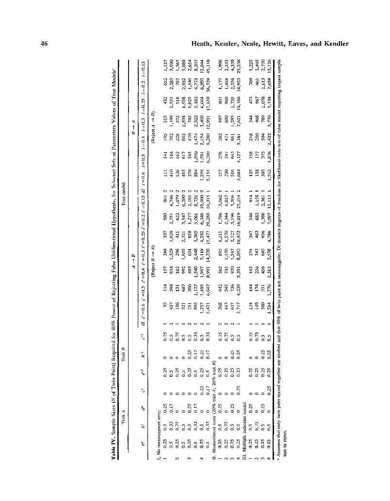
46 Heath, Kessler, Neale, Hewitt, Eaves, and Kendler
>
O
C
0~
o
o
..=
Z
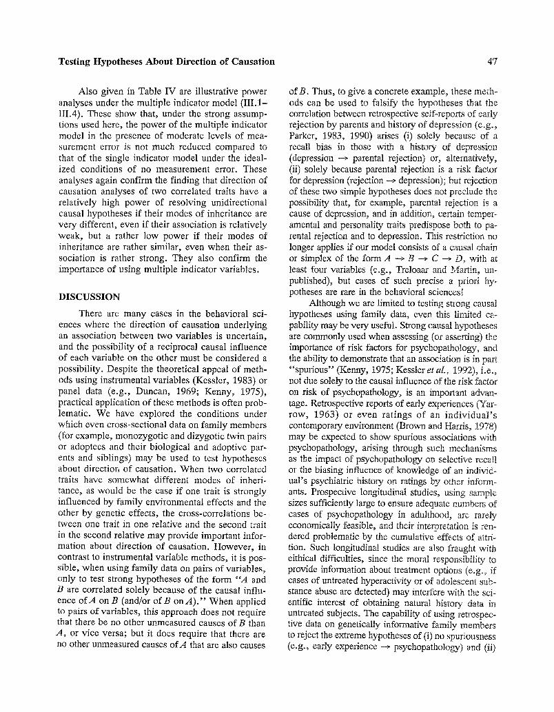
Testing Hypotheses About Direction of Causation 47
Also given in Table IV are illustrative power analyses under the multiple indicator model (III. 1- III.4). These show that, under the strong assump- tions used here, the power of the multiple indicator model in the presence of moderate levels of mea- surement error is not much reduced compared to that of the single indicator model under the ideal- ized conditions of no measurement error. These analyses again confirm the finding that direction of causation analyses of two correlated traits have a relatively high power of resolving unidirectional causal hypotheses if their modes of inheritance are very different, even if their association is relatively weak, but a rather low power if their modes of inheritance are rather similar, even when their as- sociation is rather strong. They also confirm the importance of using multiple indicator variables.
DISCUSSION
There are many cases in the behavioral sci- ences where the direction of causation underlying an association between two variables is uncertain, and the possibility of a reciprocal causal influence of each variable on the other must be considered a possibility. Despite the theoretical appeal of meth- ods using instrumental variables (Kessler, 1983) or panel data (e.g., Duncan, 1969; Kenny, 1975), practical application of these methods is often prob- lematic. We have explored the conditions under which even cross-sectional data on family members (for example, monozygotic and dizygotic twin pairs or adoptees and their biological and adoptive par- ents and siblings) may be used to test hypotheses about direction of causation. When two correlated traits have somewhat different modes of inheri- tance, as would be the case if one trait is strongly influenced by family environmental effects and the other by genetic effects, the cross-correlations be- tween one trait in one relative and the second trait in the second relative may provide important infor- mation about direction of causation. However, in contrast to instrumental variable methods, it is pos- sible, when using family data on pairs of variables, only to test strong hypotheses of the form "'4 and B are correlated solely because of the causal influ- ence of A on B (and/or o fB o n A ) . " When applied to pairs of variables, this approach does not require that there be no other unmeasured causes of B than A, or vice versa; but it does require that there are no other unmeasured causes of A that are also causes
of B. Thus, to give a concrete example, these meth- ods can be used to falsify the hypotheses that the correlation between retrospective self-reports of early rejection by parents and history of depression (e.g., Parker, 1983, 1990) arises (i) solely because of a recall bias in those with a history of depression (depression --, parental rejection) or, alternatively, (ii) solely because parental rejection is a risk factor for depression (rejection --~ depression); but rejection of these two simple hypotheses does not preclude the possibility that, for example, parental rejection is a cause of depression, and in addition, certain temper- amental and personality traits predispose both to pa- rental rejection and to depression. This restriction no longer applies if our model consists of a causal chain or simplex of the form A --~ B --~ C ~ D, with at least four variables (e.g., Treloaar and Martin, un~ published), but cases of such precise a priori hy- potheses are rare in the behavioral sciences!
Although we are limited to testing strong causal hypotheses using family data, even this limited ca~ pability may be very useful. Strong causal hypotheses are commonly used when assessing (or asserting) the importance of risk factors for psychopathology, and the ability to demonstrate that an association is in part "'spurious" (Kenny, 1975; Kessler et al., 1992), i.e., not due solely to the causal influence of the risk factor on risk of psychopathology, is an important advan- tage. Retrospective reports of early experiences (Yar- row, 1963) or even ratings of an individual 's contemporary environment (Brown and Ha~is, 1978) may be expected to show spurious associations with psychopathology, arising through such mechanisms as the impact of psychopathology on selective recall or the biasing influence of knowledge of an individ- ual's psychiatric history on ratings by other inform- ants. Prospective longitudinal studies, using sample sizes sufficiently large to ensure adequate numbers of cases of psychopathology in adulthood, are rarely economically feasible, and their interpretation is ren- dered problematic by the cumulative effects of attri- tion. Such longitudinal studies are also fraught with eithical difficulties, since the moral responsibility to provide information about treatment options (e.g., if cases of untreated hyperactivity or of adolescent sub- stance abuse are detected) may interfere with the sci- entific interest of obtaining natural history data in untreated subjects. The capability of using retrospec- tive data on genetically informative family members to reject the extreme hypotheses of (i) no spuriousness (e.g., early experience ~ psychopathology) and (ii)
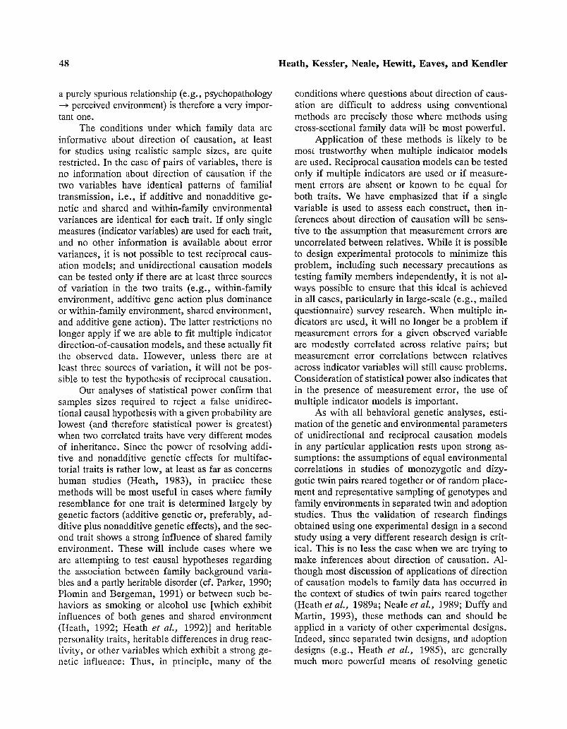
48 Heath, Kessler, Neale, Hewitt, Eaves, and Kendler
a purely spurious relationship (e.g., psychopathology --~ perceived environment) is therefore a very impor- tant one.
The conditions under which family data are informative about direction of causation, at least for studies using realistic sample sizes, are quite restricted. In the case of pairs of variables, there is no information about direction of causation if the two variables have identical patterns of familial transmission, i.e., if additive and nonadditive ge- netic and shared and within-family environmental variances are identical for each trait. If only single measures (indicator variables) are used for each trait, and no other information is available about error variances, it is not possible to test reciprocal caus- ation models; and unidirectional causation models can be tested only if there are at least three sources of variation in the two traits (e.g., within-family environment, additive gene action plus dominance or within-family environment, shared environment, and additive gene action). The latter restrictions no longer apply if we are able to fit multiple indicator direction-of-causation models, and these actually fit the observed data. However, unless there are at least three sources of variation, it will not be pos- sible to test the hypothesis of reciprocal causation.
Our analyses of statistical power confirm that samples sizes required to reject a false unidirec- tional causal hypothesis with a given probability are lowest (and therefore statistical power is greatest) when two correlated traits have very different modes of inheritance. Since the power of resolving addi- tive and nonadditive genetic effects for multifac- torial traits is rather low, at least as far as concerns human studies (Heath, 1983), in practice these methods will be most useful in cases where family resemblance for one trait is determined largely by genetic factors (additive genetic or, preferably, ad- ditive plus nonadditive genetic effects), and the sec- ond trait shows a strong influence of shared family environment. These will include cases where we are attempting to test causal hypotheses regarding the association between family background varia- bles and a partly heritable disorder (cf. Parker, 1990; Plomin and Bergeman, 1991) or between such be- haviors as smoking or alcohol use [which exhibit influences of both genes and shared environment (Heath, 1992; Heath et al., 1992)] and heritable personality traits, heritable differences in drug reac- tivity, or other variables which exhibit a strong ge- netic influence: Thus, in principle, many of the
conditions where questions about direction of caus- ation are difficult to address using conventional methods are precisely those where methods using cross-sectional family data will be most powerful.
Application of these methods is likely to be most trustworthy when multiple indicator models are used. Reciprocal causation models can be tested only if multiple indicators are used or if measure- ment errors are absent or known to be equal for both traits. We have emphasized that if a single variable is used to assess each construct, then in- ferences about direction of causation will be sens- tive to the assumption that measurement errors are uncorrelated between relatives. While it is possible to design experimental protocols to minimize this problem, including such necessary precautions as testing family members independently, it is not al- ways possible to ensure that this ideal is achieved in all cases, particularly in large-scale (e.g., mailed questionnaire) survey research. When multiple in- dicators are used, it will no longer be a problem if measurement errors for a given observed variable are modestly correlated across relative pairs; but measurement error correlations between relatives across indicator variables will still cause problems. Consideration of statistical power also indicates that in the presence of measurement error, the use of multiple indicator models is important.
As with all behavioral genetic analyses, esti- mation of the genetic and environmental parameters of unidirectional and reciprocal causation models in any particular application rests upon strong as- sumptions: the assumptions of equal environmental correlations in studies of monozygotic and dizy- gotic twin pairs reared together or of random place- ment and representative sampling of genotypes and family environments in separated twin and adoption studies. Thus the validation of research findings obtained using one experimental design in a second study using a very different research design is crit- ical. This is no less the case when we are trying to make inferences about direction of causation. Al- though most discussion of applications of direction of causation models to family data has occurred in the context of studies of twin pairs reared together (Heath et al., 1989a; Neale et al., 1989; Duffy and Martin, 1993), these methods can and should be applied in a variety of other experimental designs. Indeed, since separated twin designs, and adoption designs (e.g., Heath et al., 1985), are generally much more powerful means of resolving genetic
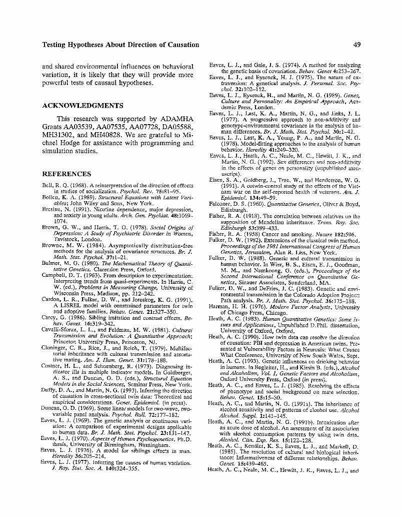
Testing Hypotheses About Direction of Causation 49
and shared environmental influences on behavioral variation, it is likely that they will provide more powerful tests of causaul hypotheses.
ACKNOWLEDGMENTS
This research was suppor ted b y A D A M H A
Grants A A 0 3 5 3 9 , A A 0 7 5 3 5 , A A 0 7 7 2 8 , D A 0 5 5 8 8 , M H 3 1 3 0 2 , and M H 4 0 8 2 8 . W e are grateful to Mi- chael Hodge for ass is tance wi th p r o g r a m m i n g and s imula t ion s tudies .
R E F E R E N C E S
Bell, R. Q. (1968). A reinterpretation of the direction of effects in studies of socialization. Psychol. Rev. 75:81-95.
Bollen, K. A. (1989). Structural Equations with Latent Vari- ables; John Wiley and Sons, New York.
Breslau, N. (1991). Nicotine dependence, major depression, and anxiety in young adults. Arch. Gen. Psychiat. 48:106% 1074.
Brown, G. W., and Harris, T. O. (1978). Social Origins of Depression: A Study of Psychiatric Disorder in Women, Tavistock, London.
Browne, M. W. (1984). Asymptotically distribution-free methods for the analysis of covariance structures. Br. J. Math. Star. PsychoL 37:1-21.
Bulmer, M. G. (1980). The Mathematical Theory of Quanti.. tative Genetics, Clarendon Press, Oxford.
Campbell, D. T. (1963). From description to experimentation: Interpreting trends from quasi-experiments. In Harris, C. W. (ed.), Problems in Measuring Change, University of Wisconsin Press, Madison, pp. 212-242.
Cardon, L. R., Fulker, D. W., and Joreskog, K. G. (1991). A LISREL model with constrained parameters for twin and adoptive families. Behav. Genet. 21:32%350.
Carey, G. (1986). Sibling imitation and contrast effects. Be- hay. Genet. 16:319-342.
Cavalli-Sforza, L. L., and Feldman, M. W. (1981). Cultural Transmission and Evolution: A Quantitative Approach; Princeton University Press, Princeton, NJ.
Cloninger, C. R., Rice, J., and Reich, T. (1979). Multifac- torial inheritance with cultural transmission and assorta- rive mating. Am. J. Hum. Genet. 31:178-188.
Costner, H. L., and Schoenberg, R. (1973). Diagnosing in- dicator ills in multiple indicator models. In Goldberger, A. S., and Duncan, O. D. (eds.), Structural Equation Models in the Social Sciences, Seminar Press, New York.
Duffy, D. A., and Martin, N. G. (1993). Inferring the direction of causation in cross-sectional twin data: Theoretical and empirical considerations. Genet. Epidemiol. (in press).
Duncan, O. D. (1969). Some linear models for two-wave, two- variable panel analysis. Psychol. Bull. 72:17%182.
Eaves, L. J. (1969). The genetic analysis or continuous vari- ation: A comparison of experimental designs applicable to human data. Br. J. Math. Stat. Psychol. 23:131-147.
Eaves, L. J. (1970). Aspects of Human Psychogenetics. Ph.D. thesis, University of Birmingham, Birmingham.
Eaves, L. J. (1976). A model for siblings effects in man. Heredity 36:205-214.
Eaves, L. J. (1977). Inferring the causes of human variation. J. Roy. Stat. Soc. A. 140:324-355.
Eaves, L. J., and Gale, J. S. (1974). A method for analyzing the genetic basis of covariation. Behav. Genet 4:253-267.
Eaves, L. J., and Eysenck, H. J. (1975). The nature of ex- traversion: A genetical analysis. J. Personal. Soc. Psy- choL 32:102-112.
Eaves, L. J., Eysenck, H., and Martin, N. G. (1989). Genes, Culture and Personality: An Empirical Approach, Aca- demic Press, London.
Eaves, L. J., Last, K. A., Martin, N. G., and Jinks, J. L. (1977). A progressive approach to non-additivity and genotype-environmental covariance in the analysis of hu- man differences. Br. J. Math. Star. PsychoL 30:1-42.
Eaves, L. J., Last, K. A., Young, P. A., and Martin, N. G. (1978). Model-fitting approaches to the analysis of human behavior. Heredity 41:249-320.
Eaves, L. J., Heath, A. C., Neale, M. C., Hewitt, J. K., and Martin, N. G. (1992). Sex differences and non-additivity in the effects of genes on personality (unpublished man- uscript).
Eisen, S. A., Goldberg, J., True, W., and Henderson, W. G. (1991). A cotwin-control study of the effects of the Viet- nam war on the self-reported health of veterans. Am. J. Epidemiol. 134:49-59.
Falconer, D. S. (1960). Quantitative Genetics, Oliver & Boyd, Edinburgh.
Fisher, R. A. (1918). The correlation between relatives on the supposition of Mendelian inheritance. Trans..Roy. Soc. Edinburgh 53:399-433.
Fisher, R. A. (1958) Cancer and smoking. Nature 182:596. Fulker, D. W. (1982). Extensions of the classical twin method.
Proceedings of the 1981 International Congress qf Human Genetics, Jerusalem, Alan R. Liss, New York:.
Fulker, D. W. (1988). Genetic and cultural transmission in human behavior. In Wier, B. S., Eisen, E. J., Goodman, M. M., and Namkoong, G. (eds.), Proceedings of the Second International Conference on Quantitative Ge- netics, Sinauer Associates, Sunderland, MA.
Fulker, D. W., and DeFries, J. C. (1983). Genetic and envi- ronmental transmission in the Colorado Adoption Project: Path analysis. Br. J. Math. Stat. Psychol. 36:175-188.
Harman, H. H. (1976). Modern Factor Analysis, University of Chicago Press, Chicago.
Heath, A. C. (1983). Human Quantitative Genetics: Some Is- sues and Applications, Unpublished D.PhiL dissertation, University of Oxford, Oxford.
Heath, A. C. (1990). How twin data can resolve the direction of causation: PBI and depression in American twins, Pre- sented at Vulnerability Factors in Neurosis: What Causes What Conference, University of New South Wales, Sept.
Heath, A. C. (1993). Genetic influences on drinking behavior in humans. In Begleiter, H., and Kissin B. (eds.), Alcohol and Alcoholism, VoL 1, Genetic Factors and Alcoholism, Oxford University Press, Oxford (in press).
Heath, A. C., and Eaves, L. J. (1985). Resolving the effects of phenotype and social background on mate selection. Behav. Genet. 15:15-30.
Heath, A. C., and Martin, N. G. (1991a). The inheritance of alcohol sensitivity and of patterns of alcohol use. Alcohol Alcohol. SuppL 1:141-145.
Heath, A. C., and Martin, N. G. (1991b). Intoxication after an acute dose of alcohol. An assessment of its association with alcohol consumption patterns by using twin data. Alcohol. Clin. Exp. Res. 15:122-128.
Heath, A. C., Kendier, K. S., Eaves, L. J., and Markell, D. (1985). The resolution of cultural and biological inheri- tance: Informativeness of different relationships. Behav. Genet. 15:439-465.
Heath, A. C., Neale, M. C., Hewitt, J. K., Eaves, L. J., and
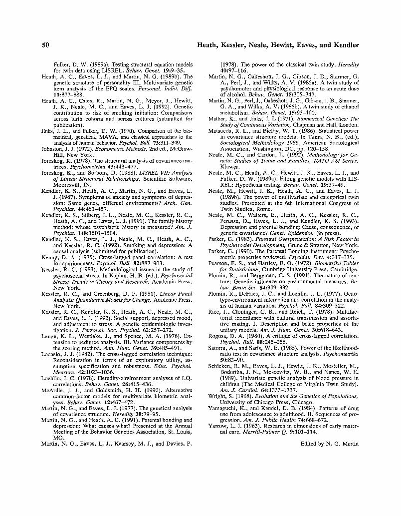
50 H e a t h , K e s s l e r , N e a l e , H e w i t t , E a v e s , and Kendler
Fulker, D. W. (1989a). Testing structural equation models for twin data using LISREL. Behav. Genet. 19:9-35.
Heath, A. C., Eaves, L. J., and Martin, N. G. (1989b). The genetic structure of personality III. Multivariate genetic item analysis of the EPQ scales. Personal Indiv. Diff. 10:877-888.
Heath, A. C., Cates, R., Martin, N. G., Meyer, J., Hewitt, J. K., Neale, M. C., and Eaves, L. J. (1992). Genetic contribution to risk of smoking initiation: Comparisons across birth cohorts and across cultures (submitted for publication).
Jinks, J. L., and Fulker, D. W. (1970). Comparison of the bio- metrical, genetical, MAVA, and classical approaches to the analysis of human behavior. PsychoL Bull 73:311-349.
Johnston, J. J. (1972). Econometric Methods, 2nd ed., McGraw- Hill, New York.
Joreskog, K. (1978). The structural analysis of covariance ma- trices. Psychometrika 43:443--477.
Joreskog, K., and Sorbom, D. (1988). LISREL VII: Analysis of Linear Structural Relationships, Scientific Software, Mooresvill, IN.
Kendler, K. S., Heath, A. C., Martin, N. G., and Eaves, L. J. (1987). Symptoms of anxiety and symptoms of depres- sion: Same genes, different environments? Arch. Gen. Psychiat. 44:451---457.
Kendler, K. S., Silberg, J. L., Neale, M. C., Kessler, R. C., Heath, A. C., and Eaves, L. J. (1991). The family history method: whose psychiatric history is measured? Am. J. Psychiat. 148:1501-1504.
Kendler, K. S., Eaves, L. J., Neale, M. C., Heath, A. C., and Kessler, R. C. (1992). Smoking and depression: A causal analysis (submitted for publication).
Kenny, D. A. (1975). Cross-lagged panel correlation: A test for spuriousness. PsychoL Bull. 82:887-903.
Kessler, R. C. (1983). Methodological issues in the study of psychosocial stress. In Kaplan, H. B. (ed.), Psychosocial Stress: Trends in Theory and Research, Academic Press, New York.
Kessler, R. C., and Greenberg, D. F. (1981). Linear Panel Analysis: Quantitative Mode&for Change, Academic Press, New York.
Kessler, R. C., Kendler, K. S., Heath, A. C., Neale, M. C., and Eaves, L. J. (1992). Social support, depressed mood, and adjustment to stress: A genetic epidemiologic inves- tigation. 3". Personal Soc. PsychoL 62:257-272.
Lange, K. L., Westlake, J., and Spence, M. A. (1976). Ex- tension to pedigree analysis. III. Variance components by the scoring method. Ann. Hum. Genet. 39:485-491.
Locasio, J. J. (1982). The cross-lagged correlation technique: Reconsideration in terms of an exploratory utility, as- sumption specification and robustness. Educ. PsychoL Measure. 42:1023-1036.
Loehlin, J. C. (1978). Heredity-environment analyses of I.Q. correlations. Behav. Genet. 26:415-436.
McArdle, J. J., and Goldsmith, H. H. (1990). Alternative common-factor models for multivariate biometric anal- yses. Behav. Genet. 12:467---472.
Martin, N. G., and Eaves, L. J. (1977). The genetical analysis of covariance structure. Heredity 38:79-95.
Martin, N. G., and Heath, A. C. (1991). Parental bonding and depression: What causes what? Presented at the Annual Meeting of the Behavior Genetics Association, St. Louis, MO.
Martin, N. G., Eaves, L. J., Kearsey, M. J., and Davies, P.
(1978). The power of the classical twin study. Heredity 40:97-116.
Martin, N. G., Oakeshott, J. G., Gibson, J. B., Starmer, G. A., Perl, J., and Wilks, A. V. (1985a). A twin study of psychomotor and physiological response to an acute dose of alcohol. Behav. Genet. 15:305-347.
Martin, N. G., Perl, J., Oakeshott, J. G., Gibson, J. B., Starmer, G. A., and Wilks, A. V. (1985b). A twin study of ethanol metabolism. Behav. Genet. 15:93-100.
Mather, K., and Jinks, J. L (1971). Biometrical Genetics: The Study of Continuous Variation, Chapman and Hall, London.
Matsueda, R. L., and Bielby, W. T. (1986). Statistical power in covariance structure models. In Tuma, N. B., (ed.), Sociological Methodology 1986, American Sociological Association, Washington, DC, pp. 120-158.
Neale, M. C., and Cardon, L. (1992). Methodology for Ge- netic Studies of Twins and Families, NATO AS1 Series, Kluwer.
Neale, M. C., Heath, A. C., Hewitt, J. K., Eaves, L. J., and Fulker, D. W. (1989a). Fitting genetic models with LIS- REL: Hypothesis testing. Behav. Genet. 19:37-49.
Neale, M., Hewitt, J. K., Heath, A. C., and Eaves, L. J. (1989b). The power of multivariate and categorical twin studies. Presented at the 6th International Congress of Twin Studies, Rome.
Neale, M. C., Waiters, E., Heath, A. C., Kessler, R. C., Perusse, D., Eaves, L. J., and Kendler, K. S. (1993). Depression and parental bonding: Cause, consequence, or genetic covariance? Genet. EpidemioL (in press).
Parker, G. (1983). Parental Overprotection: A Risk Factor in PsychosocialDevelopment, Grune & Stratton, New York.
Parker, G. (1990). The Parental Bonding Instrument: Psycho- metric properties reviewed. Psychiat. Dev. 4:317-335.
Pearson, E. S., and Hartley, E. 0 . (1972). Biometrika Tables for Statisticians, Cambrige University Press, Cambridge.
Plomin, R., and Bergeman, C. S. (1991). The nature of nur- ture: Genetic influence on environmental measures. Be- hay. Brain Sci. 84:309-332.
Plomin, R., DeFries, J. C., and Loehlin, J. L. (1977). Geno- type-environment interaction and correlation in the analy- sis of human variation. PsychoL Bull. 84:309-322.
Rice, J., Cloninger, C. R., and Reich, T. (1978). Multifac- torial inheritance with cultural transmission and assorta- rive mating. I. Description and basic properties of the unitary models. Am. J. Hum. Genet. 30:618-643.
Rogosa, D. A. (1980). A critique of cross-lagged correlation. PsychoL Bull. 88:245-258.
Satorra, A., and Saris, W. E. (1985). Power of the likelihood- ratio test in covariance structure analysis. Psychometrika 50:83-90.
Schieken, R. M., Eaves, L. J., Hewitt, J. K., Mosteller, M., Bodurtha, J. N., Moscowitz, W. B., and Nance, W. E. (1989). Univariate genetic analysis of blood pressure in children (The Medical College of Virginia Twin Study). Am. J. CardioL 64:1333-1337.
Wright, S. (1968). Evolution and the Genetics of Populations, University of Chicago Press, Chicago.
Yamaguchi, K., and Kandel, D. B. (1984). Patterns of drug use from adolescence to adulthood. II. Sequences of pro- gression. Am. J. Public Health 74:668-672.
Yarrow, L. J. (1963). Research in dimensions of early mater- nal care. Merrill-Palmer Q. 9:101-114.
Edited by N. G. Martin