Test Questions, Economic Outcomes, and Inequality

Eric Nielsen Board of Governors of the Federal Reserve System

System Working Paper 19-07 April 2019

The views expressed herein are those of the authors and not necessarily those of the Federal Reserve Bank of Minneapolis or the Federal Reserve System. This paper was originally published as Finance and Economics Discussion Series 2019-013 by the Board of Governors of the Federal Reserve System. This paper may be revised. The most current version is available at https://doi.org/10.17016/FEDS.2019.013. __________________________________________________________________________________________

Opportunity and Inclusive Growth Institute Federal Reserve Bank of Minneapolis • 90 Hennepin Avenue • Minneapolis, MN 55480-0291

https://www.minneapolisfed.org/institute

Finance and Economics Discussion SeriesDivisions of Research & Statistics and Monetary Affairs

Federal Reserve Board, Washington, D.C.

Test Questions, Economic Outcomes, and Inequality

Eric Nielsen

2019-013

Please cite this paper as:Nielsen, Eric (2019). “Test Questions, Economic Outcomes, and Inequality,” Finance andEconomics Discussion Series 2019-013. Washington: Board of Governors of the FederalReserve System, https://doi.org/10.17016/FEDS.2019.013.

NOTE: Staff working papers in the Finance and Economics Discussion Series (FEDS) are preliminarymaterials circulated to stimulate discussion and critical comment. The analysis and conclusions set forthare those of the authors and do not indicate concurrence by other members of the research staff or theBoard of Governors. References in publications to the Finance and Economics Discussion Series (other thanacknowledgement) should be cleared with the author(s) to protect the tentative character of these papers.

Test Questions, Economic Outcomes, andInequality

Eric Nielsen*

Federal Reserve Board of Governors

This draft: February 20, 2019Most recent draft: here

AbstractStandard achievement scales aggregate test questions without considering their

relationship to economic outcomes. This paper uses question-level data to improvethe measurement of achievement in two ways. First, the paper constructs alternativeachievement scales by relating individual questions directly to school completion andlabor market outcomes. Second, the paper leverages the question data to constructmultiple such scales in order to correct for biases stemming from measurement error.These new achievement scales rank students differently than standard scales andtypically yield achievement gaps by race, gender, and household income that are largerby 0.1 to 0.5 standard deviations. Differential performance on test questions can fullyexplain black-white differences in both wages and lifetime earnings and can explainroughly half of the difference in these outcomes between youth from high- versuslow-income households. By contrast, test questions do not explain gender differencesin labor market outcomes.

Keywords: human capital, inequality, achievement gaps, measurement errorJEL Codes: I.24, I.26, C.2

1 Introduction

Human capital is fundamental to understanding labor market success, health, and many

other economic outcomes. Group differences in human capital play a key role in common*Bryce Turner and Danielle Nemschoff provided excellent research assistance. This paper benefited from

discussions with Ralf Meisenzahl, Steve Laufer, Neil Bhutta, and seminar participants at the Federal ReserveBoard and the NBER Education Program Meeting. The views and opinions expressed in this paper aresolely those of the author and do not reflect those of the Board of Governors or the Federal Reserve System.Contact: eric.r.nielsen@frb.gov

1

explanations for group differences in economic outcomes. A key question therefore is

to what extent human capital differences drive observed inequalities. Human capital,

however, is not directly observable. Researchers and policy makers therefore often turn to

achievement test scores calculated using standard psychometric methods as proxies for

human capital. These scores correlate with economic outcomes across a variety of contexts,

motivating their use as direct measures of human capital.

Standard psychometric achievement scales measure human capital imperfectly because

the skills they emphasize need not correspond to the skills most valuable for economic

outcomes. Every test scale can be thought of as a method for combining individual test

items (questions) into a single index. (I will stick with the terminology “items” throughout

the remainder of the text.) Psychometric methods combine items without reference to the

economic importance of the skills the items measure. Such methods may therefore yield

biased estimates of human capital inequality if different groups perform differentially

better or worse on items that are systematically related to later success. This is not a failing

of psychometric methods per se – the problem lies using them for a purpose for which

they were not designed.

In this paper, I develop new achievement scales that more accurately measure human

capital. Using recently available data on individual Armed Forces Qualifying Test (AFQT)

items from the National Longitudinal Survey of Youth 1979 (NLSY79), I assess which

items are most relevant for predicting various long-run economic outcomes including

high school completion, college completion, wages at age 30, and total lifetime earnings. I

construct “item-anchored” scores by weighting test items in proportion to how strongly

they correlate with these school completion and labor market outcomes, conditional on

the other item responses. In other words, I assign to each item a “skill price” based on that

item’s ability to predict outcomes. I then use these skill prices to compare human capital

(achievement) differences across different demographic groups. This use of item data

is novel – even where outcomes have been used to anchor scores (Cunha and Heckman

2

(2008); Bond and Lang (2018); Chetty et al. (2014); Jackson (2018), and many others), item

data have not been available or have not been used.1

I additionally use the item data in a novel way to assess measurement error in the

item-anchored scales. Understanding this measurement error is important for calculating

mean achievement gaps – simply taking the naive mean difference in the item-anchored

scores between two groups will result in estimates that are biased towards zero. I adapt

the empirical approach in Bond and Lang (2018), who use lagged scores and instrumental

variables methods to undo this downward bias. I follow a similar approach, but instead of

lagged scores, I leverage the item data to estimate multiple item-anchored scales which can

then be used to construct the necessary instruments. This method allows me to estimate

the reliabilities (signal-to-noise ratios) of the item-anchored scales.

After adjusting for measurement error, I find that achievement gaps calculated using

the item-anchored scales are typically, though not always, much larger than gaps calculated

using the NLSY79-given scales. For instance, I estimate that white/black and high-/low-

income (defined here as the top and bottom parental income quintiles) math and reading

gaps are all around 1 standard deviation (sd) using the NLSY79-given scales, roughly in

line with prior literature (Neal and Johnson (1996); Reardon (2011); Downey and Yuan

(2005), and many others). By contrast, the high-/low-income gaps are 0.2 sd larger and

the white/black gaps are 0.2-0.5 sd larger when I anchor on wages at age 30 or lifetime

earnings. Anchoring to high school completion leads to more modest, though still sizable,

increases on the order of 0.06-0.20 sd. Item-anchoring does not increase all of the gaps,

however – the college anchored white/black math gap is a full 0.2 sd smaller than the gap

calculated using given math scores.

1Jackson (2018) studies teacher value-added on noncognitive dimensions not captured by achievementtest scores using an analytic framework that recognizes the possibility of a disconnect between the skills em-phasized by test scores and the skills that generate later-life outcomes. Polachek et al. (2015) take a differentapproach by estimating human capital production function parameters for each survey respondent in theNLSY79. They then relate these “human capital” ability measures to standard measures of cognitive andnoncognitive skills. The NLSY79 item-level data is used by Schofield (2014) to argue that the measurementerror in the IRT-derived AFQT scores is non-normal.

3

Achievement does not have natural units, so in some sense the most fundamental way

to compare different test scales is through their induced rank orderings of students. Even

if the cardinal properties of two scales are different, they might nonetheless rank students

equally. However, the item-anchored scales I estimate rank students very differently than

the NLSY79-provided scales. Individual student’s rankings may differ by 10-20 percentile

points or more between the item-anchored and given scales. Some students do well on

items that are predictive of later success but poorly on uninformative items, resulting in a

low given score, while for other students the situation is reversed. The item-anchored and

given scales frequently disagree fundamentally about which students are doing well and

which are doing poorly.

The item-anchored gaps can be directly compared to the actual outcome gaps. Con-

sistent with prior literature using standard psychometric test scales (Lang and Manove,

2011), test items predict larger white/black gaps in school completion than are actually

observed. By contrast, the item-anchored and actual white/black lifetime earnings and

wage at age 30 gaps are very similar – the sizable racial differences in these labor market

outcomes can be more or less fully explained by differential item responses. This result

strengthens the headline conclusion in Neal and Johnson (1996); I both explain a greater

share of the early-adult wage gap, and I additionally explain the gap in lifetime earnings,

an outcome not studied in that paper.2 Notably, I obtain these labor market results using

only white men to construct the item-anchored scales, so that my findings do not depend

on racial differences in how items correlate with outcomes.

The item-anchored scales do less well at explaining outcome differences for youth

from high- and low-income households. The item-anchored scales modestly under-predict

school completion differences while dramatically under-predicting wage and total labor

market earnings gaps for youth from the top versus bottom quintiles of the household

income distribution. The differences are largest for total earnings, suggesting that, con-

2To be clear, Neal and Johnson could not have studied lifetime earnings because the NLSY79 respondentswere too young to accurately estimate this outcome when their paper was written.

4

ditional on test items, youth from high-income households both earn higher wages and

work more hours. In short, youth from high-income households do substantially better in

the labor market than their test items alone would predict.

Finally, I show that the item-anchored scores resolve the “reading puzzle” – the phe-

nomenon in which reading scores, though positively correlated with wages, are weakly or

even negatively correlated conditional on math scores (Sanders, 2016; Kinsler and Pavan,

2015; Arcidiacono, 2004). Joint regressions of wages at age 30 on item-anchored reading

and math scores suggest a sizable role for reading conditional on math, in contrast to

what regressions using given scores find. Reading skills do seem to have explanatory

power above and beyond their correlation with math skills, but this is not visible when

reading items are combined as they are in standard psychometric models. Nonetheless, the

item-anchored reading coefficients are still only about half as large as the math coefficients

for most outcome anchors and most regression specifications.

The rest of the paper is organized as follows: Section 2 discusses the test item and

outcome data in the NLSY79, while Section 3 presents preliminary evidence that these

items correlate quite differently with different outcomes. Section 4 discusses the general

empirical and conceptual framework. Sections 5 - 6 present the main empirical estimates,

while Section 7 addresses the reading puzzle. Section 8 concludes. Appendix A contains

all of the tables and figures referenced in the paper.

2 NLSY79 Data

The NLSY79 is a nationally representative survey that follows a sample of individuals

aged 14-22 in 1979 through to the present. Each round of the survey collects extensive

information on educational and labor market outcomes that allows me to construct school

completion, wage, and lifetime earnings variables. Additionally, survey respondents took

a series of achievement tests, the Armed Services Vocational Aptitude Battery (ASVAB), in

5

the base year of the survey. Item response data that code each item as correct or incorrect

for each survey respondent are available for the math and reading components of the

ASVAB. I now describe each of these pieces, the test items and later-life outcomes, in

detail.

The ASVAB consists of a series of subject- and skill-specific tests which are primarily

used by the United States military in making enlistment and personnel decisions. I make

use of the item response data from the math and reading components of the ASVAB that

together comprise the oft-studied Armed Forces Qualifying Test (AFQT). The math items

come from the arithmetic reasoning (30 items) and mathematics knowledge (25 items)

ASVAB component tests, while the reading items come from the paragraph comprehension

(15 items) and word knowledge (35 items) components.3 Thus, in total, I use 50 reading

items and 55 math items to construct the item-anchored scales. I drop the subsample of the

initial sampling frame that was designed to be representative of the military population,

as the ASVAB is intended specifically for military recruits. However, my results change

very little if this group is included.

The math and reading ASVAB items in the NLSY79 are particularly well-suited to

anchoring to economic outcomes. The tests were administered to youth on the cusp of

adulthood – completing high school, enrolling in college, starting to work full time, and

so forth. As such, the item responses may be viewed as summary measures of the skills

these youth took into adulthood. Moreover, the ASVAB was a low-stakes and unfamiliar

test for most of the the NLSY79 sample, particularly with the military subsample already

dropped. The item responses therefore are unlikely to reflect differential coaching/practice

by race and socioeconomic background as might be a concern with a more widely-used,

high-stakes assessment.

I use longitudinal data in the NLSY79 to construct various school completion and labor

3The constituent ASVAB components defining the AFQT changed after the administration of the test inthe NLSY79. I use the current definition of math and reading, rather than the definition which held in 1980.

6

earnings outcomes.4 For school completion, I use the highest grade completed reported at

any point in the first 15 years of the survey. I define “high school” as an indicator for 12 or

more grades completed and “college” as 16 or more grades completed.

The first labor market outcome I construct is average hourly wage at age 30 (wage_30).

I divide total annual labor income by total hours worked for each survey round. I then

average over the three rounds closest to each individual’s age-30 round to to smooth out

transitory wage/earnings fluctuations. I restrict myself to 30 because almost all schooling

is completed by this age. Additionally, 30 falls after the typical crossing point past which

more educated adults earn more on average than less educated adults.

The second labor market outcome I construct is the present discounted value of lifetime

labor income (pdv_labor). The construction of pdv_labor is complicated because I do not

observe labor income in all years for all survey respondents, either due to missing data,

unemployment, or labor-force non-participation. To deal with such missing observations,

I adopt a “pessimistic” imputation rule which assigns to each missing value the minimum

labor income observed for the individual over the life of the survey. This rule is not

meant to be realistic; rather, it will tend to compress the earnings distribution.5 The

NLSY79 respondents are only in their late 40’s in the most recent survey round; I therefore

assume that each individual’s earnings growth after the latest survey round follows the

education-specific growth rates from a pseudo-panel of male earnings constructed from

the 2005 American Community Survey. Additionally, I assume each respondent retires 20

years after the most recent survey round, when the respondents are in their late sixties.6 I

discount future income exponentially at a 5% annual rate.

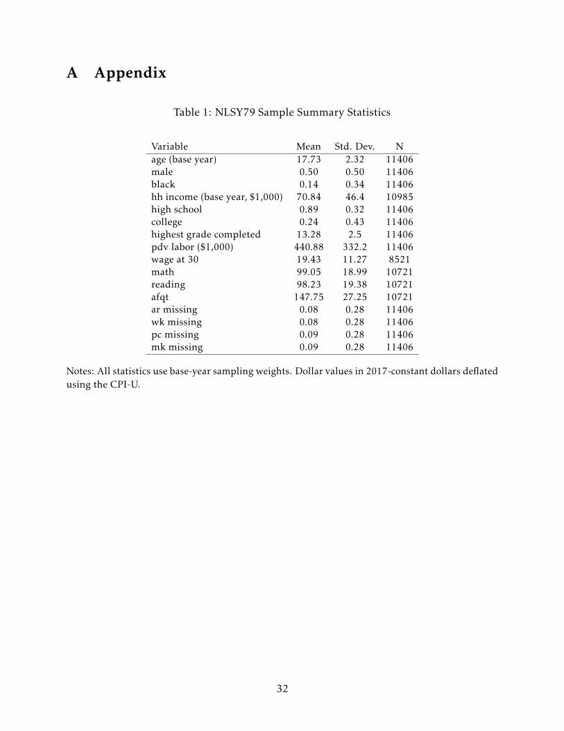
Table 1 presents the summary statistics of the main variables used in the analysis. The

calculations here and elsewhere use cross-sectional weights designed to make the sample

4Please refer to Nielsen (2015b) for more details.5In Nielsen (2015b), I study this measure along with others which adopt alternative fill-in rules. Though

different in levels, the resulting income measures using different fill-in rules are strongly correlated witheach other. I therefore stick with pessimistic imputation to simplify the discussion.

6A final complication is that the NLSY79 moved to a biennial format after 1994. I impute labor earningsfor the odd-numbered years using linear interpolation after applying the pessimistic imputation rule.

7

nationally representative. My final analysis sample consists of 11,406 youth.7 The college

completion rate in this sample is about 24%, while the high school completion rate is 89%.

The average hourly wage earned at age 30 is about $19.43 with a standard deviation of

$11.27. The pdv_labor variable has an average of $440,880. Roughly 9% of the sample is

missing each of the ASVAB components – I drop these roughly 1,500 individuals from the

anchoring analysis.8

3 Item-Outcome Correlations

Before delving into the anchoring analysis, I first present some simple evidence that test

items differ widely in how strongly they predict economic outcomes. I then show that the

predictive items are not easily identified using the parameters that characterize each item

in item response theory (IRT), the popular psychometric framework used to construct the

math and reading scales in the NLSY79.

Figure 1 shows the distributions of the estimated coefficients for bivariate regressions of

indicators for each test item on school completion and labor market outcomes (in natural

logs). The panels of Figure 1 show that the items are all positively correlated with every

outcome. However, there is quite a range in the estimated coefficients. For instance, using

college completion as the outcome yields math item coefficient estimates that range from

0.1 to 0.3. For each outcome, one can easily reject 0 for most item coefficients, and one can

also easily reject that all of the coefficients are equal.9 Comparing the distributions, there

7I use the full range of ages in my analysis to get as large a sample as possible. However, restricting theanalysis sample to youth less than 18 years old at the survey start yields similar empirical results but withlower estimated reliability in the item-anchored scales.

8These individuals are also all missing IRT-estimated ASVAB component scores. In cases where the itemsare not entirely missing, I set the missing items to 0, corresponding to “incorrect.” For individuals whotook the assessment (so that not all items are missing), blank (unanswered) items are coded as missing bythe NLSY79. The assumption I make therefore is that leaving a question blank and getting the questionincorrect are equivalent.

9Regressions that include all items simultaneously yield similar conclusions, although of course theindividual item coefficients are smaller and some are negative. Similarly, plotting the R2 for each bivariateregression used in Figure 1 shows that the share of variance explained by each item also varies widely.

8

are more math than reading items that are strongly correlated with college completion.

The situation for high school completion and lifetime earnings is reversed – reading items

seem to be particularly predictive of these outcomes. For ln(wage_30), the reading item

distribution has greater variance than the math distribution, with more low-correlation

and more high-correlation items.

Items that are predictive of one outcome are often not predictive of other outcomes.

This is clear in Figure 2, which plots the item-level coefficients for different outcomes

against each other. The top panel shows that the college item coefficients are essentially

uncorrelated with the high school item coefficients. Even the math items in the right tail

with college coefficient estimates greater than 0.25 have high school coefficients no higher

or lower than the average. By contrast, the bottom panel shows that the ln(wage_30) and

ln(pdv_labor) item coefficients are positively correlated – the items that predict lifetime

earnings also, on average, predict wages at age 30. Even here there is substantial variation,

with some items strongly predictive of only one of these two labor market outcomes.

A natural question is whether the highly predictive items have any discernible com-

monalities. My ability to investigate this question is very limited – the only item-level

information available in the NLSY79 comes from the estimated IRT parameters that are

used in the construction of the given scales.10 In detail, the ASVAB scales are constructed

using the three parameter logistic (3PL) IRT model, which supposes that a student with

achievement θ answers item i with probability (i.e., has item response function)

P (Di = 1|θ,αi ,βi ,γi) = γi +1−γi

1 + e−αi(θ−βi ).

The parameters (αi ,βi ,γi) characterize the item. The discrimination, αi , gives the max-

imum slope of the item response function – the higher is αi , the more sharply does the

item distinguish between individuals with similar θs. The item difficulty, βi , gives the

10The IRT parameters are not included as variables in the NLSY data download program, Rather, Itranscribed them manually from the NLSY79 codebook.

9

location of this maximum slope – difficult (high-β) items distinguish between high-θ

individuals. Finally, γi gives the guessing probability – the probability that a test taker

with minimal achievement answers the item correctly. Importantly, these IRT parameters

are not connected to the topics or skills covered by the item and are not estimated using

any data on economic outcomes. Two items that have the same parameters will be treated

equivalently, regardless of how differentially well they predict outcomes.

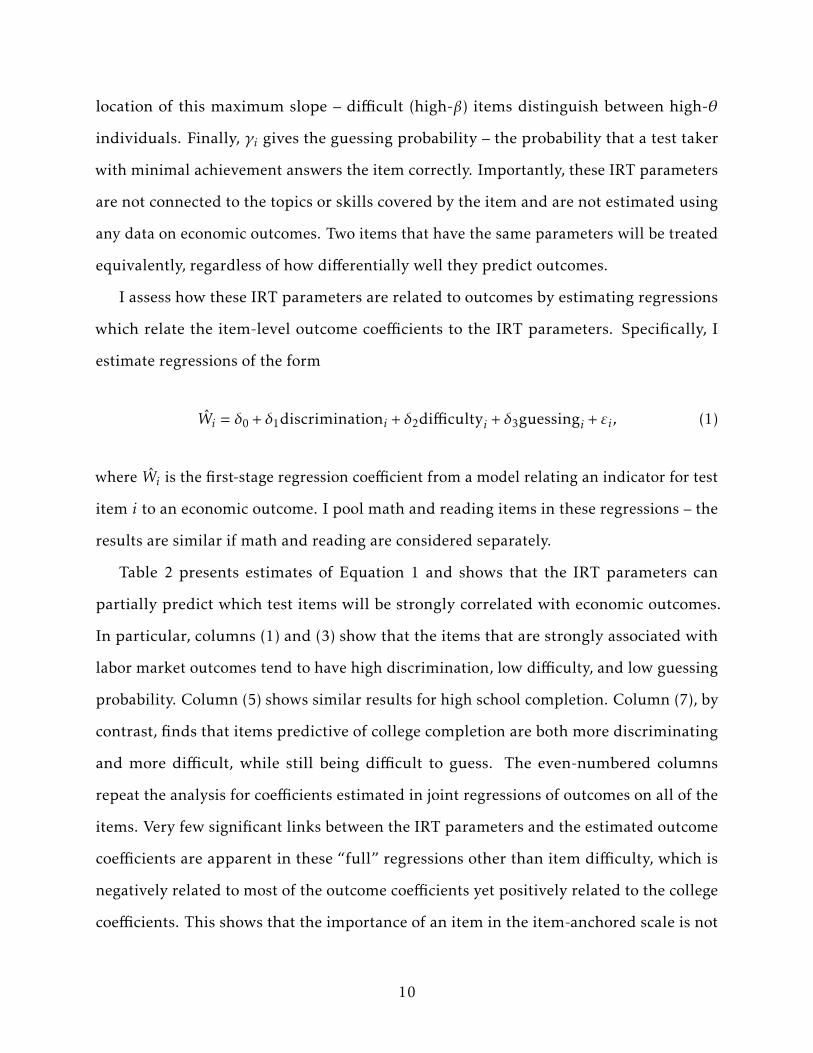
I assess how these IRT parameters are related to outcomes by estimating regressions

which relate the item-level outcome coefficients to the IRT parameters. Specifically, I

estimate regressions of the form

Wi = δ0 + δ1discriminationi + δ2difficultyi + δ3guessingi + εi , (1)

where Wi is the first-stage regression coefficient from a model relating an indicator for test

item i to an economic outcome. I pool math and reading items in these regressions – the

results are similar if math and reading are considered separately.

Table 2 presents estimates of Equation 1 and shows that the IRT parameters can

partially predict which test items will be strongly correlated with economic outcomes.

In particular, columns (1) and (3) show that the items that are strongly associated with

labor market outcomes tend to have high discrimination, low difficulty, and low guessing

probability. Column (5) shows similar results for high school completion. Column (7), by

contrast, finds that items predictive of college completion are both more discriminating

and more difficult, while still being difficult to guess. The even-numbered columns

repeat the analysis for coefficients estimated in joint regressions of outcomes on all of the

items. Very few significant links between the IRT parameters and the estimated outcome

coefficients are apparent in these “full” regressions other than item difficulty, which is

negatively related to most of the outcome coefficients yet positively related to the college

coefficients. This shows that the importance of an item in the item-anchored scale is not

10

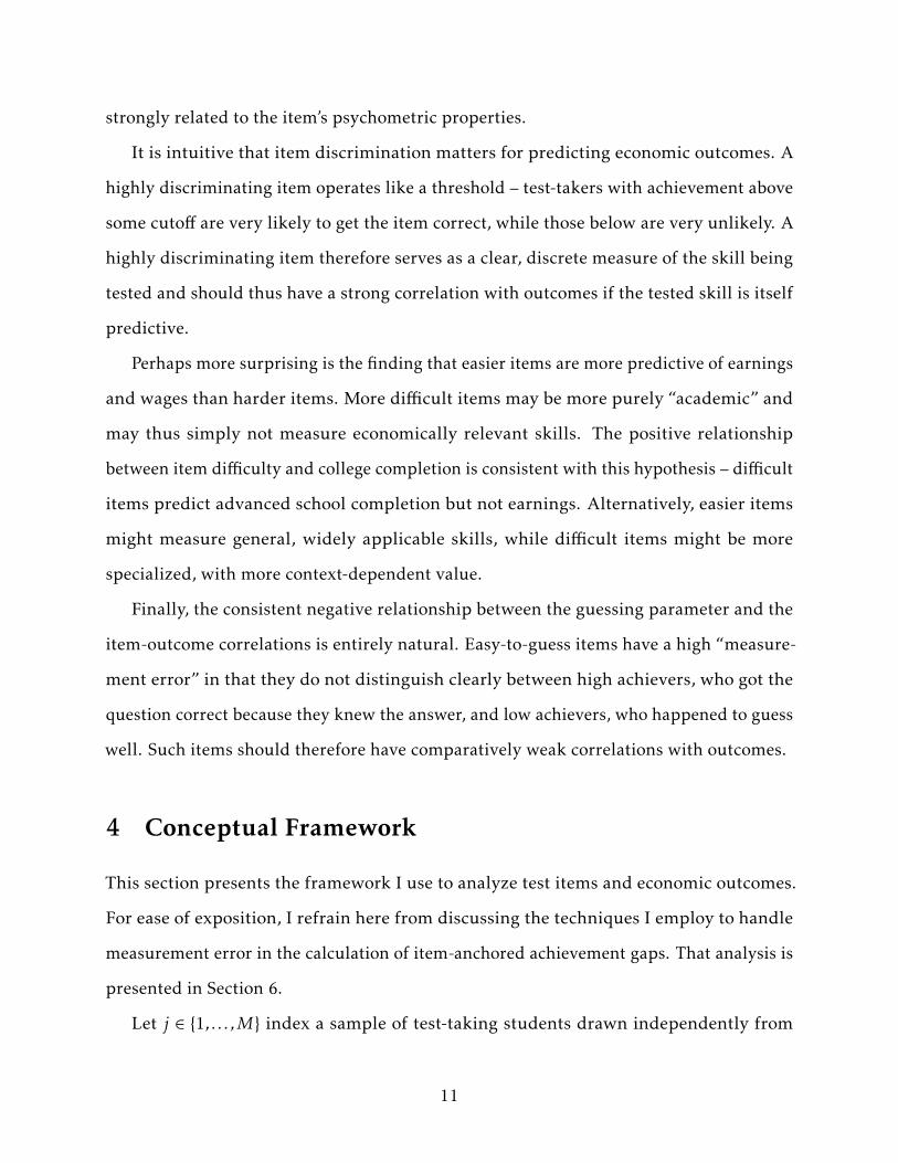
strongly related to the item’s psychometric properties.

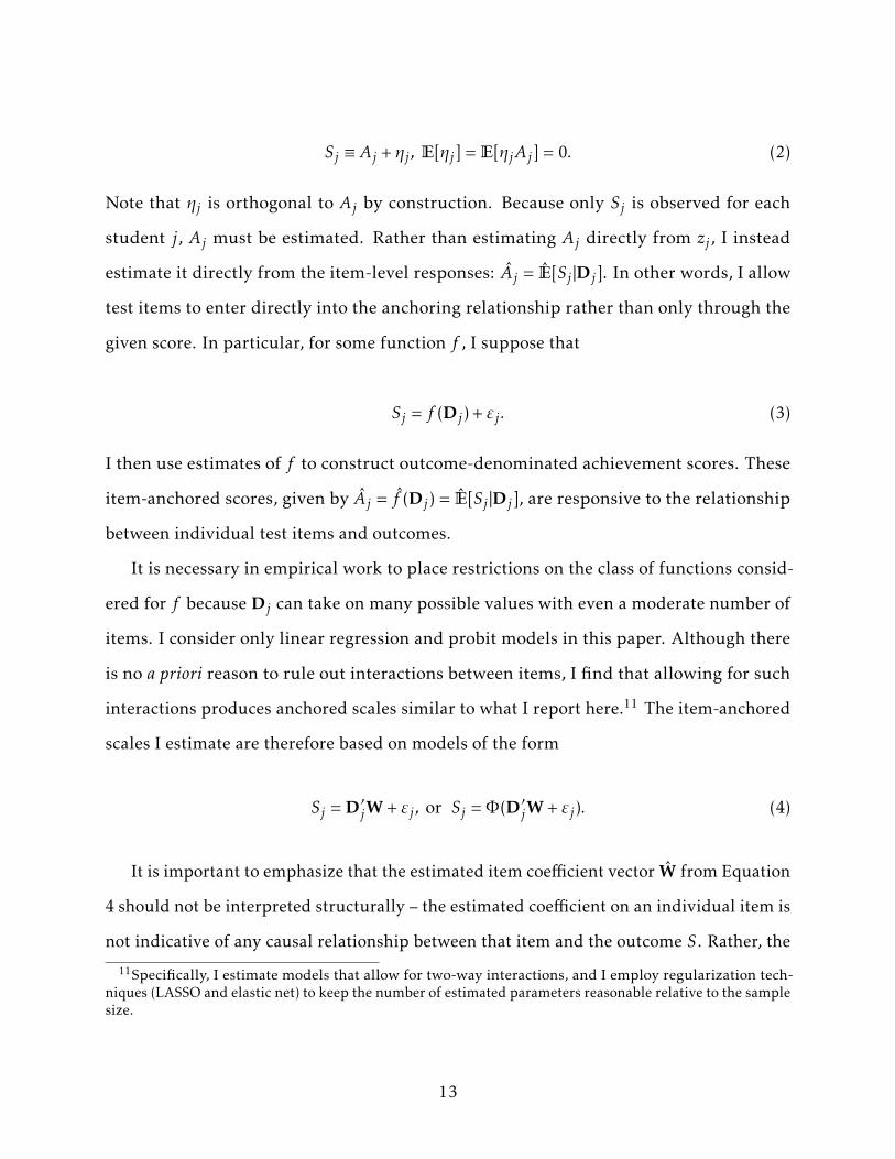
It is intuitive that item discrimination matters for predicting economic outcomes. A

highly discriminating item operates like a threshold – test-takers with achievement above

some cutoff are very likely to get the item correct, while those below are very unlikely. A

highly discriminating item therefore serves as a clear, discrete measure of the skill being

tested and should thus have a strong correlation with outcomes if the tested skill is itself

predictive.

Perhaps more surprising is the finding that easier items are more predictive of earnings

and wages than harder items. More difficult items may be more purely “academic” and

may thus simply not measure economically relevant skills. The positive relationship

between item difficulty and college completion is consistent with this hypothesis – difficult

items predict advanced school completion but not earnings. Alternatively, easier items

might measure general, widely applicable skills, while difficult items might be more

specialized, with more context-dependent value.

Finally, the consistent negative relationship between the guessing parameter and the

item-outcome correlations is entirely natural. Easy-to-guess items have a high “measure-

ment error” in that they do not distinguish clearly between high achievers, who got the

question correct because they knew the answer, and low achievers, who happened to guess

well. Such items should therefore have comparatively weak correlations with outcomes.

4 Conceptual Framework

This section presents the framework I use to analyze test items and economic outcomes.

For ease of exposition, I refrain here from discussing the techniques I employ to handle

measurement error in the calculation of item-anchored achievement gaps. That analysis is

presented in Section 6.

Let j ∈ {1, . . . ,M} index a sample of test-taking students drawn independently from

11

some population, and let Sj denote the economic outcome of interest for student j. All

other observable characteristics of the student (race, gender, family background, etc.) are

denoted by Xj . Students take an achievement test with N dichotomous items. Let Dj

denote the vector of item responses from student j: Dj = [D1,j , . . . ,DN,j] where Di,j = 1 if j

gets question i correct, and 0 otherwise. These items are combined using some framework

(item response theory in the NLSY79) to produce a standardized (mean 0, standard

deviation 1) test score zj . It is these given scores that are often treated in social science

and policy analysis as direct measures of human capital rather than as estimated proxies.

The use of such scores introduces two distinct problems, both of which are remedied by

item-level anchoring.

First, achievement has no natural scale – there is no way to determine whether a given

score represents a lot of achievement or relatively little. Anchoring scores by estimating

the relationship between zj and the outcome Sj solves this indeterminacy by rescaling so

that test scores are in directly interpretable units. Interpretability is not the only reason

to prefer the anchored scale, however. If the transformation from the given scale to the

anchored scale is nonlinear, as is often the case empirically, statistics calculated using

the two scales may disagree dramatically – they may even differ in sign (Nielsen, 2015a;

Schroeder and Yitzhaki, 2017; Bond and Lang, 2013).

Second, and the key insight in this paper, the given scores represent a particular choice

about how to map each of the 2N possible sequences of item responses to a scalar measure

of achievement. Since this map is chosen without reference to economic outcomes, the

scoring procedure may obscure useful information about human capital contained in the

item responses. Note that anchoring given scores to outcomes (zj to Sj), as has been done

in prior literature, does not address this second concern.

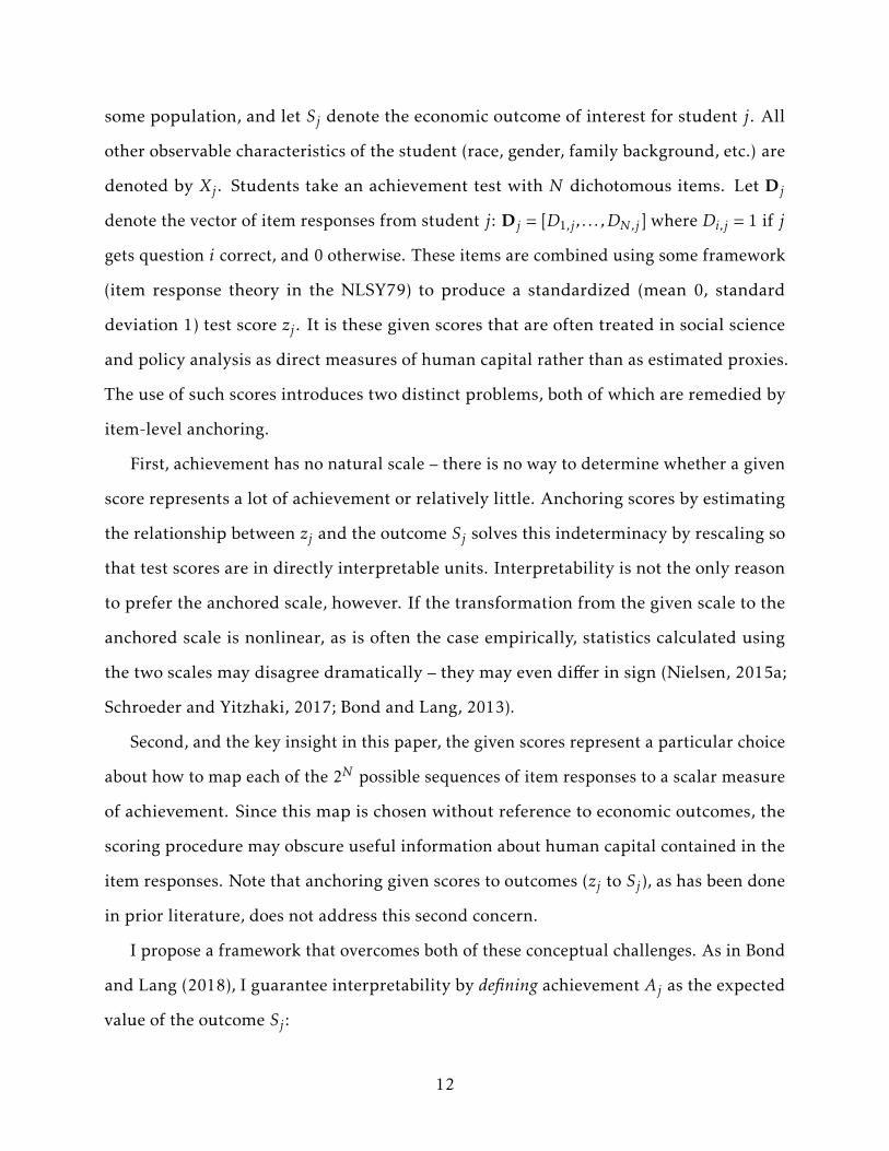
I propose a framework that overcomes both of these conceptual challenges. As in Bond

and Lang (2018), I guarantee interpretability by defining achievement Aj as the expected

value of the outcome Sj :

12

Sj ≡ Aj + ηj , E[ηj] = E[ηjAj] = 0. (2)

Note that ηj is orthogonal to Aj by construction. Because only Sj is observed for each

student j, Aj must be estimated. Rather than estimating Aj directly from zj , I instead

estimate it directly from the item-level responses: Aj = E[Sj |Dj]. In other words, I allow

test items to enter directly into the anchoring relationship rather than only through the

given score. In particular, for some function f , I suppose that

Sj = f (Dj) + εj . (3)

I then use estimates of f to construct outcome-denominated achievement scores. These

item-anchored scores, given by Aj = f (Dj) = E[Sj |Dj], are responsive to the relationship

between individual test items and outcomes.

It is necessary in empirical work to place restrictions on the class of functions consid-

ered for f because Dj can take on many possible values with even a moderate number of

items. I consider only linear regression and probit models in this paper. Although there

is no a priori reason to rule out interactions between items, I find that allowing for such

interactions produces anchored scales similar to what I report here.11 The item-anchored

scales I estimate are therefore based on models of the form

Sj = D′jW+ εj , or Sj = Φ(D′jW+ εj). (4)

It is important to emphasize that the estimated item coefficient vector W from Equation

4 should not be interpreted structurally – the estimated coefficient on an individual item is

not indicative of any causal relationship between that item and the outcome S. Rather, the

11Specifically, I estimate models that allow for two-way interactions, and I employ regularization tech-niques (LASSO and elastic net) to keep the number of estimated parameters reasonable relative to the samplesize.

13

goal is simply to estimate E[Sj |Dj] flexibly.12 Individual elements of W are unconstrained

and may therefore be negative, even though it may not be plausible that the true causal

effect of any of these items should be less than zero.

5 Empirical Results – Rank Comparisons

I compare in this section the rank orderings induced by various item-anchored test scales to

the rank orderings induced by the NLSY79-given scales. I also compare the item-anchored

scales to “given-anchored” scales that use regression and probit models to relate the

given scores to outcomes. This exercise produces two important results. First, economic

outcomes are not linearly related to the given scores. Second, the item-anchored scales

rank students very differently than the given scales.

Figure 3 plots the item-anchored scores against the given scores. The x-axis for each

panel plots the given scores in standard deviation units. The y-axis plots the mean (solid

black line) as well as the middle-50% and middle-90% ranges of the item-anchored scores,

in standard deviation units, for each ventile of the given score distribution. For comparison,

the figure also shows the mean of the given-anchored scores (dashed line) in each ventile.

The first thing to note in Figure 3 is that the item-anchored and given-anchored scales

have nonlinear relationships to the given scales, particularly for high school and college

completion. As noted in previous literature (Bond and Lang, 2013; Schroeder and Yitzhaki,

2017; Jacob and Rothstein, 2016; Nielsen, 2015a), this nonlinearity means that standard

calculations (mean differences, OLS, etc.) using the given scale may produce severely

biased estimates. Notably, the item-anchored and given-anchored scales line up very well

at the mean for each ventile of the given score distribution.

The nonlinearities in the school completion scales are intuitive. The college math and

12In fact, the only reason to assume a linear model, or any model at all, is because the sample size is notlarge enough for non-parametric anchoring. Given a very, very large sample, the anchored scale could beestimated simply as the sample average of S for each possible realization of item responses.

14

reading scales have convex relationships to the given scales; differences in achievement at

the bottom ends of the given scales do not translate to differences in college completion,

while differences at the top do. The situation is reversed for high school – improvements at

the bottom ends of the given scales translate strongly changes in high school completion,

while improvements in the top are not very valuable. Low-achievement youth are not

likely to be on the margin for completing college, so the college scales should be flat for

such students. At the same time, these students are likely to be on the high school margin,

explaining the steep anchored relationship for below-mean given scores.

The item-anchored scales are closer to being linearly related to the given scales for

ln(wage_30) and ln(pdv_labor). Of course, this means that the relationship between

observed scores and lifetime earnings or wages in levels is convex. Improvements at the

top of the given math and reading scales yield out-sized gains in predicted wages and

lifetime earnings.

The middle 50% and 90% ranges in each panel of Figure 3 show that there is a

fairly wide distribution of item-anchored scores associated with each given score ventile.

Individuals whose item responses led to the same (or similar) given score might have

very different predicted outcomes based on their particular item responses. For college

completion, this variation is greater at the top of the observed score distribution. For

instance, among students with given math scores about 1 sd above the mean, the middle

90% of the item-anchored scores cover almost 2 sd on the item-anchored scale, while

for those 1 sd below the mean, the corresponding range is only about 0.2 sd. Some

apparently high-performing youth are actually forecast to have very low rates of college

completion, while others are substantially more likely to finish than their given scores

would indicate. Low-performing youth, however, are always forecast to have low rates

of college completion. The pattern for high school is reversed – there is a lot of variation

in the item-anchored scores at the bottom of the given scale and very little variation

at the top. In contrast, the middle 50% and 90% ranges of the log labor scales appear

15

to be fairly constant across the given score distributions, although they are a bit more

spread out in reading for lower given scores. The range of item-anchored scores in each

given score ventile again tends to be quite large. As a representative example, the range

of log(pdv_labor) scores for youth at the mean of the given reading distribution covers

about 2 sd. Some youth with low observed scores are predicted to have high labor market

earnings, while others with high observed scores are forecast to perform fairly poorly in

the labor market.

The range of item-anchored scores depicted in Figure 3 implies that they rank students

differently than the given scores. This is not true for the given-anchored scales, as these

are just monotone transformations of the given scores. The item-anchored scores do not

just disagree with the given scores about how valuable achievement is, they disagree

fundamentally about which students are performing well and which students are not.

The relatively wide 90% ranges depicted in Figure 3 suggest that the ranking differences

between the item-anchored and given scales might be quite substantial. Indeed, Figure

4, which plots the absolute value of the difference in percentiles according to the item-

anchored and given scales, shows that it is not uncommon for the rankings to differ by

10 - 20 percentile points or more between the two. Notably, the labor outcome scales

display more rank shuffling than the school completion scales. This is intuitive, as math

and reading test items should be more closely aligned to academic performance than to

success in the labor market.

6 Empirical Results – Achievement Gaps

I now turn to the measurement of achievement gaps using the item-anchored test scales. I

first show how to leverage the item data to construct multiple, independent item-anchored

scales in order to estimate the amount of measurement error in said scales. That is, I use

the item data in two ways: first to estimate the item-anchored scales and second to estimate

16

the reliability (signal-to-noise ratio) of these scales. After adjusting for measurement error,

I find that the item-anchored scales generally show much more achievement inequality

than the NLSY79-given scales. Moreover, I find that the item-anchored scales can explain

significant fractions of the observed differences in school completion and labor market

success by race and parental income.

6.1 Mean Achievement Gaps and Measurement Error

The item-anchored test scales are estimated with error. This error biases achievement gaps

estimated using the item-anchored scales towards zero. I adapt the approach in Bond

and Lang (2018) to handle this problem. The basic idea is to construct two independent

anchored scales that can be used in an instrumental variables setting to undo the bias

generated by the measurement error. The strategy of using instruments to recover the

relevant “shrinkage term” (to be explained below) is from Bond and Lang’s work. My

innovation lies in leveraging the item data to construct the necessary instruments.

Let h and l denote two groups of students whose achievement we want to compare.

The goal is to estimate ∆Ah,l ≡ Ah − Al , where Ag is the average achievement of group g.

Each individual’s achievement is measured with error: Aj = Aj + νj . If A ∼N (A,σ2A) and if

νj ∼N (0,σ2ν ) iid in the population,13

E[Sj |Aj] =σ2A

σ2A + σ2

νAj +

σ2ν

σ2A + σ2

νA. (5)

Equation 5 says that the expected outcome of student j conditional on the item-anchored

achievement Aj is “shrunk” towards the population mean A. This is intuitive – tests are

noisy, so the best guess about a student’s true achievement gives weight to both the realized

score and the population expected value, with the observed score weighted more heavily

the less noisy it is.

13See Bond and Lang (2018) for an extensive discussion and demonstration of the robustness of the generalapproach outlined here to violations in the normality assumption.

17

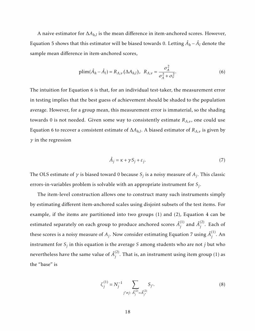
A naive estimator for ∆Ah,l is the mean difference in item-anchored scores. However,

Equation 5 shows that this estimator will be biased towards 0. Letting Ah − Al denote the

sample mean difference in item-anchored scores,

plim(Ah − Al) = RA,ν(∆Ah,l

), RA,ν =

σ2A

σ2A + σ2

ν. (6)

The intuition for Equation 6 is that, for an individual test-taker, the measurement error

in testing implies that the best guess of achievement should be shaded to the population

average. However, for a group mean, this measurement error is immaterial, so the shading

towards 0 is not needed. Given some way to consistently estimate RA,ν , one could use

Equation 6 to recover a consistent estimate of ∆Ah,l . A biased estimator of RA,ν is given by

γ in the regression

Aj = κ+γSj + εj . (7)

The OLS estimate of γ is biased toward 0 because Sj is a noisy measure of Aj . This classic

errors-in-variables problem is solvable with an appropriate instrument for Sj .

The item-level construction allows one to construct many such instruments simply

by estimating different item-anchored scales using disjoint subsets of the test items. For

example, if the items are partitioned into two groups (1) and (2), Equation 4 can be

estimated separately on each group to produce anchored scores A(1)j and A(2)

j . Each of

these scores is a noisy measure of Aj . Now consider estimating Equation 7 using A(1)j . An

instrument for Sj in this equation is the average S among students who are not j but who

nevertheless have the same value of A(2)j . That is, an instrument using item group (1) as

the “base” is

ζ(1)j =N−1

j

∑j ′,j: A(2)

j =A(2)j′

Sj ′ . (8)

18

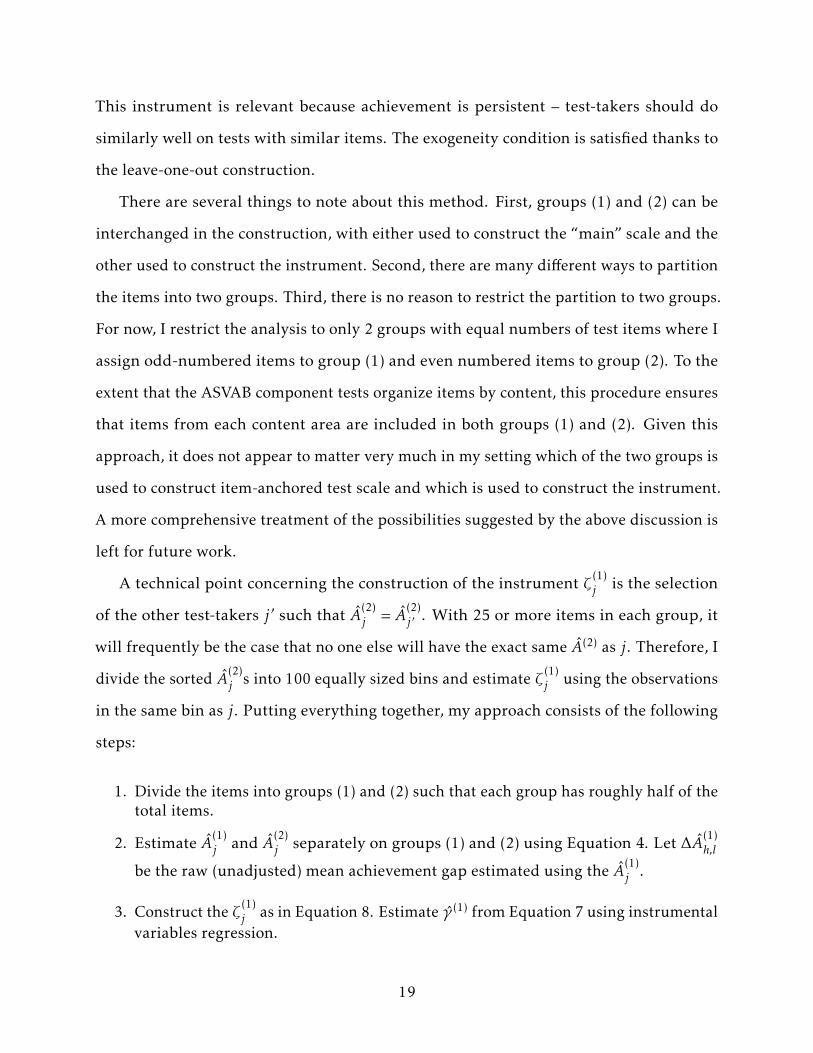
This instrument is relevant because achievement is persistent – test-takers should do

similarly well on tests with similar items. The exogeneity condition is satisfied thanks to

the leave-one-out construction.

There are several things to note about this method. First, groups (1) and (2) can be

interchanged in the construction, with either used to construct the “main” scale and the

other used to construct the instrument. Second, there are many different ways to partition

the items into two groups. Third, there is no reason to restrict the partition to two groups.

For now, I restrict the analysis to only 2 groups with equal numbers of test items where I

assign odd-numbered items to group (1) and even numbered items to group (2). To the

extent that the ASVAB component tests organize items by content, this procedure ensures

that items from each content area are included in both groups (1) and (2). Given this

approach, it does not appear to matter very much in my setting which of the two groups is

used to construct item-anchored test scale and which is used to construct the instrument.

A more comprehensive treatment of the possibilities suggested by the above discussion is

left for future work.

A technical point concerning the construction of the instrument ζ(1)j is the selection

of the other test-takers j ′ such that A(2)j = A(2)

j ′ . With 25 or more items in each group, it

will frequently be the case that no one else will have the exact same A(2) as j. Therefore, I

divide the sorted A(2)j s into 100 equally sized bins and estimate ζ(1)

j using the observations

in the same bin as j. Putting everything together, my approach consists of the following

steps:

1. Divide the items into groups (1) and (2) such that each group has roughly half of thetotal items.

2. Estimate A(1)j and A(2)

j separately on groups (1) and (2) using Equation 4. Let ∆A(1)h,l

be the raw (unadjusted) mean achievement gap estimated using the A(1)j .

3. Construct the ζ(1)j as in Equation 8. Estimate γ (1) from Equation 7 using instrumental

variables regression.

19

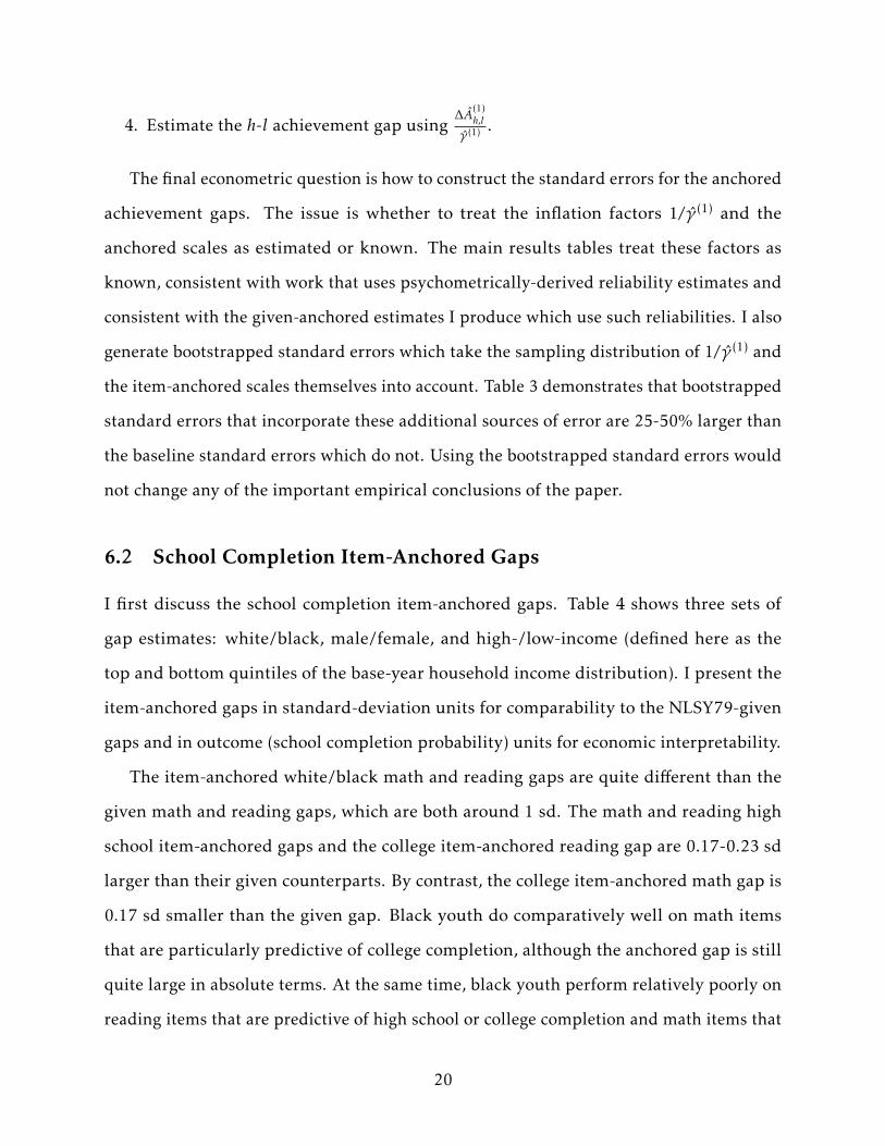
4. Estimate the h-l achievement gap using∆A

(1)h,l

γ (1) .

The final econometric question is how to construct the standard errors for the anchored

achievement gaps. The issue is whether to treat the inflation factors 1/γ (1) and the

anchored scales as estimated or known. The main results tables treat these factors as

known, consistent with work that uses psychometrically-derived reliability estimates and

consistent with the given-anchored estimates I produce which use such reliabilities. I also

generate bootstrapped standard errors which take the sampling distribution of 1/γ (1) and

the item-anchored scales themselves into account. Table 3 demonstrates that bootstrapped

standard errors that incorporate these additional sources of error are 25-50% larger than

the baseline standard errors which do not. Using the bootstrapped standard errors would

not change any of the important empirical conclusions of the paper.

6.2 School Completion Item-Anchored Gaps

I first discuss the school completion item-anchored gaps. Table 4 shows three sets of

gap estimates: white/black, male/female, and high-/low-income (defined here as the

top and bottom quintiles of the base-year household income distribution). I present the

item-anchored gaps in standard-deviation units for comparability to the NLSY79-given

gaps and in outcome (school completion probability) units for economic interpretability.

The item-anchored white/black math and reading gaps are quite different than the

given math and reading gaps, which are both around 1 sd. The math and reading high

school item-anchored gaps and the college item-anchored reading gap are 0.17-0.23 sd

larger than their given counterparts. By contrast, the college item-anchored math gap is

0.17 sd smaller than the given gap. Black youth do comparatively well on math items

that are particularly predictive of college completion, although the anchored gap is still

quite large in absolute terms. At the same time, black youth perform relatively poorly on

reading items that are predictive of high school or college completion and math items that

20

are predictive of high school completion.

Turning to gender differences, the given scores imply that males have a 0.18 sd ad-

vantage in math and a 0.11 sd deficit in reading, roughly consistent with prior literature

(Fryer and Levitt (2010); Dee (2007); Le and Nguyen (2018), and many others). Anchoring

to school completion at the item level lowers the male advantage in math – the college-

anchored gap is 0.13 sd and the high school-anchored gap is only 0.05 sd. Similarly,

item-anchoring to high school completion shrinks the female advantage in reading to 0.08

sd, while item-anchoring to college completion removes the female advantage entirely

– the gap shifts to an insignificant 0.01 sd. Achievement scales which emphasize items

associated with school completion reduce, or in some cases remove, apparent male-female

achievement differences.

Item-anchoring to school completion also shifts the estimated achievement gaps be-

tween youth from high- and low-income households. Specifically, Table 4 shows the given

and item-anchored gaps for students in the top and bottom quintiles of the base-year

household income distribution. Given scores show achievement gaps of about 1 sd in

math and reading, while the high school item-anchored gaps are roughly 0.10 sd larger.

The college results again show a divergence between math and reading; the college item-

anchored math gap is about 0.05 sd smaller than the corresponding given gap, while the

college item-anchored reading gap is 0.30 sd larger.

Table 4 also presents the estimated reliabilities for the item-anchored scales. The math

reliabilities are 0.81 for high school and 0.87 for college; these are both quite close to the

0.85 reliability reported in the NLSY79. The high school reading reliability, at 0.86, is

larger than the reported value of 0.81, while the college reading reliability is smaller, at

0.74. A consistent finding is that the item-anchored reliabilities are different from, and

often smaller than, the reliabilities reported by the NLSY79 and also quite different for

the same test items across different anchoring outcomes.14

14These reliabilities are mostly larger than what Bond and Lang (2018) find anchoring to high schoolcompletion with prior-year lagged test scores used to adjust for shrinkage. One possible explanation for

21

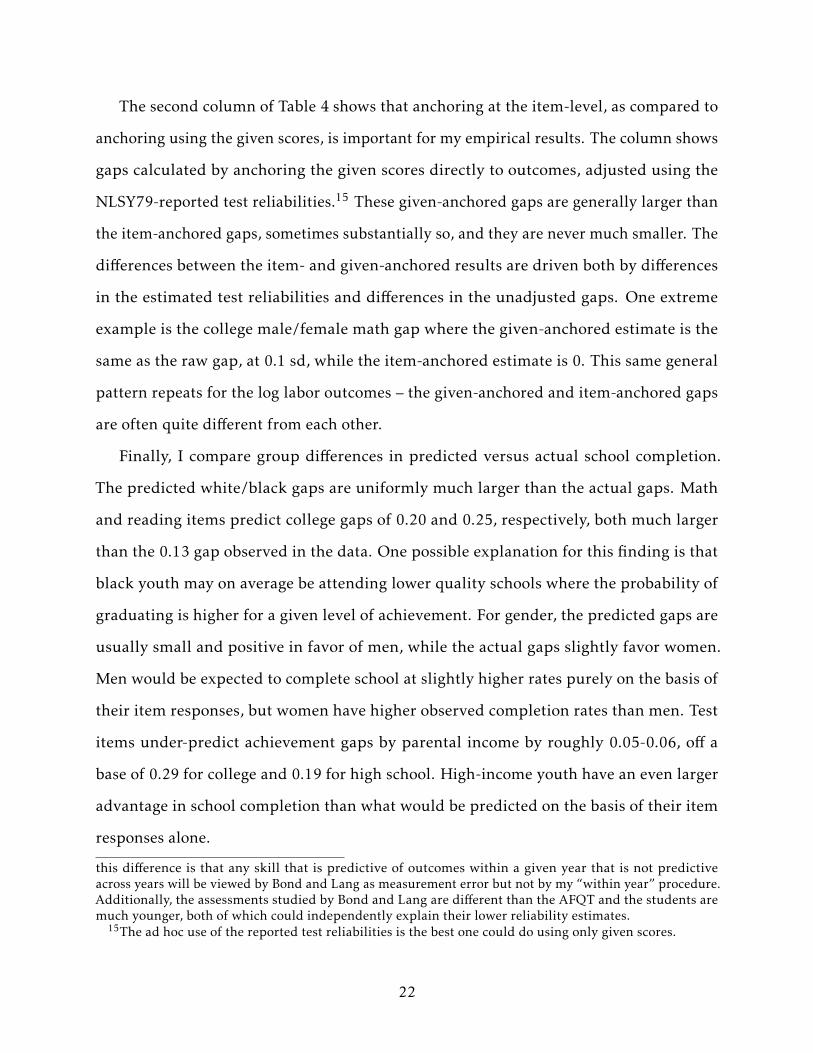
The second column of Table 4 shows that anchoring at the item-level, as compared to

anchoring using the given scores, is important for my empirical results. The column shows

gaps calculated by anchoring the given scores directly to outcomes, adjusted using the

NLSY79-reported test reliabilities.15 These given-anchored gaps are generally larger than

the item-anchored gaps, sometimes substantially so, and they are never much smaller. The

differences between the item- and given-anchored results are driven both by differences

in the estimated test reliabilities and differences in the unadjusted gaps. One extreme

example is the college male/female math gap where the given-anchored estimate is the

same as the raw gap, at 0.1 sd, while the item-anchored estimate is 0. This same general

pattern repeats for the log labor outcomes – the given-anchored and item-anchored gaps

are often quite different from each other.

Finally, I compare group differences in predicted versus actual school completion.

The predicted white/black gaps are uniformly much larger than the actual gaps. Math

and reading items predict college gaps of 0.20 and 0.25, respectively, both much larger

than the 0.13 gap observed in the data. One possible explanation for this finding is that

black youth may on average be attending lower quality schools where the probability of

graduating is higher for a given level of achievement. For gender, the predicted gaps are

usually small and positive in favor of men, while the actual gaps slightly favor women.

Men would be expected to complete school at slightly higher rates purely on the basis of

their item responses, but women have higher observed completion rates than men. Test

items under-predict achievement gaps by parental income by roughly 0.05-0.06, off a

base of 0.29 for college and 0.19 for high school. High-income youth have an even larger

advantage in school completion than what would be predicted on the basis of their item

responses alone.

this difference is that any skill that is predictive of outcomes within a given year that is not predictiveacross years will be viewed by Bond and Lang as measurement error but not by my “within year” procedure.Additionally, the assessments studied by Bond and Lang are different than the AFQT and the students aremuch younger, both of which could independently explain their lower reliability estimates.

15The ad hoc use of the reported test reliabilities is the best one could do using only given scores.

22

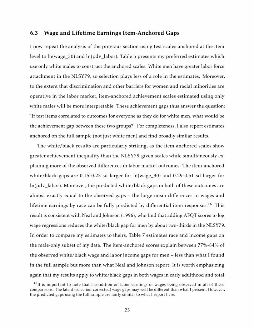
6.3 Wage and Lifetime Earnings Item-Anchored Gaps

I now repeat the analysis of the previous section using test scales anchored at the item

level to ln(wage_30) and ln(pdv_labor). Table 5 presents my preferred estimates which

use only white males to construct the anchored scales. White men have greater labor force

attachment in the NLSY79, so selection plays less of a role in the estimates. Moreover,

to the extent that discrimination and other barriers for women and racial minorities are

operative in the labor market, item-anchored achievement scales estimated using only

white males will be more interpretable. These achievement gaps thus answer the question:

“If test items correlated to outcomes for everyone as they do for white men, what would be

the achievement gap between these two groups?” For completeness, I also report estimates

anchored on the full sample (not just white men) and find broadly similar results.

The white/black results are particularly striking, as the item-anchored scales show

greater achievement inequality than the NLSY79-given scales while simultaneously ex-

plaining more of the observed differences in labor market outcomes. The item-anchored

white/black gaps are 0.15-0.23 sd larger for ln(wage_30) and 0.29-0.51 sd larger for

ln(pdv_labor). Moreover, the predicted white/black gaps in both of these outcomes are

almost exactly equal to the observed gaps – the large mean differences in wages and

lifetime earnings by race can be fully predicted by differential item responses.16 This

result is consistent with Neal and Johnson (1996), who find that adding AFQT scores to log

wage regressions reduces the white/black gap for men by about two-thirds in the NLSY79.

In order to compare my estimates to theirs, Table 7 estimates race and income gaps on

the male-only subset of my data. The item-anchored scores explain between 77%-84% of

the observed white/black wage and labor income gaps for men – less than what I found

in the full sample but more than what Neal and Johnson report. It is worth emphasizing

again that my results apply to white/black gaps in both wages in early adulthood and total

16It is important to note that I condition on labor earnings of wages being observed in all of thesecomparisons. The latent (selection-corrected) wage gaps may well be different than what I present. However,the predicted gaps using the full sample are fairly similar to what I report here.

23

lifetime earnings, whereas Neal and Johnson (1996) present results only for early-adult

wages due to the young age of the NLSY79 respondents in the mid-1990s.

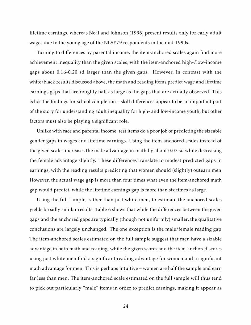
Turning to differences by parental income, the item-anchored scales again find more

achievement inequality than the given scales, with the item-anchored high-/low-income

gaps about 0.16-0.20 sd larger than the given gaps. However, in contrast with the

white/black results discussed above, the math and reading items predict wage and lifetime

earnings gaps that are roughly half as large as the gaps that are actually observed. This

echos the findings for school completion – skill differences appear to be an important part

of the story for understanding adult inequality for high- and low-income youth, but other

factors must also be playing a significant role.

Unlike with race and parental income, test items do a poor job of predicting the sizeable

gender gaps in wages and lifetime earnings. Using the item-anchored scales instead of

the given scales increases the male advantage in math by about 0.07 sd while decreasing

the female advantage slightly. These differences translate to modest predicted gaps in

earnings, with the reading results predicting that women should (slightly) outearn men.

However, the actual wage gap is more than four times what even the item-anchored math

gap would predict, while the lifetime earnings gap is more than six times as large.

Using the full sample, rather than just white men, to estimate the anchored scales

yields broadly similar results. Table 6 shows that while the differences between the given

gaps and the anchored gaps are typically (though not uniformly) smaller, the qualitative

conclusions are largely unchanged. The one exception is the male/female reading gap.

The item-anchored scales estimated on the full sample suggest that men have a sizable

advantage in both math and reading, while the given scores and the item-anchored scores

using just white men find a significant reading advantage for women and a significant

math advantage for men. This is perhaps intuitive – women are half the sample and earn

far less than men. The item-anchored scale estimated on the full sample will thus tend

to pick out particularly “male” items in order to predict earnings, making it appear as

24

though men have a sizable advantage in both reading and math.

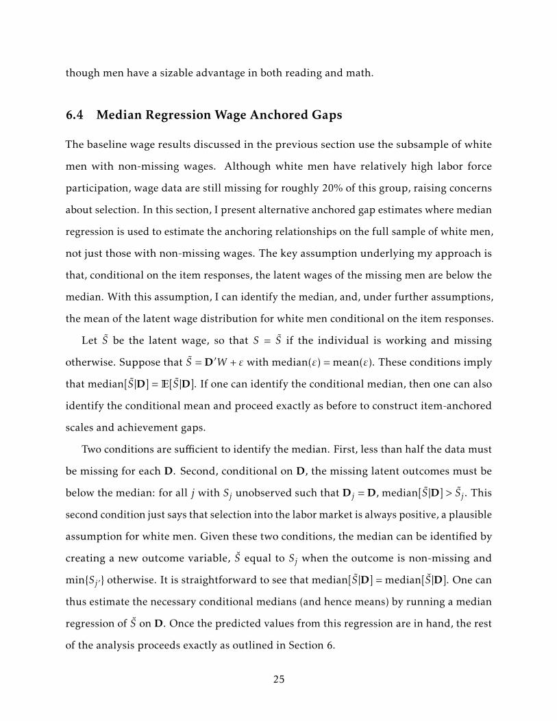
6.4 Median Regression Wage Anchored Gaps

The baseline wage results discussed in the previous section use the subsample of white

men with non-missing wages. Although white men have relatively high labor force

participation, wage data are still missing for roughly 20% of this group, raising concerns

about selection. In this section, I present alternative anchored gap estimates where median

regression is used to estimate the anchoring relationships on the full sample of white men,

not just those with non-missing wages. The key assumption underlying my approach is

that, conditional on the item responses, the latent wages of the missing men are below the

median. With this assumption, I can identify the median, and, under further assumptions,

the mean of the latent wage distribution for white men conditional on the item responses.

Let S be the latent wage, so that S = S if the individual is working and missing

otherwise. Suppose that S = D′W + ε with median(ε) = mean(ε). These conditions imply

that median[S |D] = E[S |D]. If one can identify the conditional median, then one can also

identify the conditional mean and proceed exactly as before to construct item-anchored

scales and achievement gaps.

Two conditions are sufficient to identify the median. First, less than half the data must

be missing for each D. Second, conditional on D, the missing latent outcomes must be

below the median: for all j with Sj unobserved such that Dj = D, median[S |D] > Sj . This

second condition just says that selection into the labor market is always positive, a plausible

assumption for white men. Given these two conditions, the median can be identified by

creating a new outcome variable, S equal to Sj when the outcome is non-missing and

min{Sj ′ } otherwise. It is straightforward to see that median[S |D] = median[S |D]. One can

thus estimate the necessary conditional medians (and hence means) by running a median

regression of S on D. Once the predicted values from this regression are in hand, the rest

of the analysis proceeds exactly as outlined in Section 6.

25

Table 8 presents the ln(wage_30) item-anchored gaps estimated on the white male

sample using median regression. As before, the item-anchored gaps are typically sub-

stantially larger than the given gaps. Notably, the median-anchored math gaps tend to be

much larger than the regression-anchored gaps, with the white/black math gap ballooning

from 1.21 sd to 1.48 sd and the high-/low-income gap increasing from 1.19 sd to 1.44

sd. These larger math gaps are partially due to the lower estimated reliability of the

median-anchored math scale (0.64 vs 0.75). The median-anchored reading estimates,

despite a similarly lower reliability, are generally much closer to the regression-anchored

estimates. Overall, these results do not suggest that selection is driving my main findings.

Turning to the actual versus predicted comparisons, the reading item responses again

perfectly predict the black/white log wage gap while predicting a bit less than half of the

high/low-income gap. However, for math, item responses now predict a log wage gap that

is about 0.1 larger that what is actually observed. Similarly, math items predict a higher

share of the high-/low-income log wage gap (about two-thirds versus one half previously).

7 The Reading Puzzle and Item-Anchoring

Prior research (Sanders, 2016; Kinsler and Pavan, 2015) has noted that in multivariate

regressions of labor outcomes on math and reading scores, the coefficients on reading are

often much smaller than the coefficients on math. In some cases, the reading coefficients

are even significantly negative. These findings are puzzling – reading and math skills

are distinct, and reading skills seem like they should be quite valuable economically.

This section demonstrates that using item-anchored scores can resolve this puzzle. Item-

anchored math and reading scores both have large and statistically significant coefficient

estimates in the types of joint regressions that give rise to the reading puzzle. Nonetheless,

the coefficient estimates on item-anchored reading achievement are still quite a bit smaller

than those on item-anchored math.

26

I assess the effect of item anchoring on the reading puzzle by estimating for different

definitions of math and reading (given, item-anchored, etc.) models of the form

ln(wage_30) = α + β1math + β2reading + controls + ε.

Table 9 presents the math and reading regression coefficients for various model specifica-

tions that include or exclude parental income and highest grade completed dummies as

additional controls. Echoing prior literature, columns (1) and (4) show that the estimated

coefficients using the given scores are large and statistically significant for math and small

and insignificant for reading. A one standard deviation increase in the given math score is

associated with a 0.1-0.18 increase in ln(wage_30), while the same increase in the given

reading score corresponds to a -0.01 to 0.03 change in ln(wage_30). Given-anchored

scores do not resolve the puzzle – columns (2) and (5) show that given-anchored math is

significantly associated with ln(wage_30), while given-anchored reading is not.17

Item-anchored scores, however, do resolve the reading puzzle. Columns (3) and (6) in

Table 9 show that the item-anchored math coefficients are very similar to the given-scale

coefficients, while the item-anchored reading estimates are much larger: a one standard

deviation in item-anchored reading corresponds to a 0.05-0.09 increase in ln(wage_30).

Although these reading estimates are about half the size of the math estimates, they are

still large and are statistically distinguishable from 0 at a 1% level.

These results are not tautological – the math and reading scales are constructed inde-

pendently of each other. It could have been the case that the component of item-anchored

reading orthogonal to item-anchored math was uncorrelated with ln(wage_30). Nonethe-

less, each scale is constructed to be maximally predictive of ln(wage_30). This may make

their significance less surprising. However, Table 10 shows that using school completion

item-anchored scales yields similar results. In particular, columns (2) and (4) show that

17The given-anchored scales use linear regression, which Figure 3 suggests should fit the data quite well.Indeed, using quadratic or cubic models to anchor the given scores alters the results very little.

27

high school and college item-anchored scales result in smaller, though still significant,

math and reading estimates.18 Finally, columns (3) and (5) show that the reading puzzle

persists using school completion given-anchored scores. The scales in these columns are

non-linear (probit) transformations of the given scores, but they are order-preserving. In

each case, the reading coefficient is small and not distinguishable from 0, while math

remains significantly positive.

The results in this section also highlight the more general point that the item-anchored

scales relate to each other and to various outcomes differently than the given scales.

Item-anchoring therefore has the potential to change not just achievement gap estimates.

Any calculation using test scores as an outcome or as a control might yield strikingly

different results with item-anchored scores. Findings such as the reading puzzle, which

have been interpreted as saying something interesting about the relationship between

math and reading skills and economic outcomes, may in fact only reflect arbitrary and

poorly motivated measurement choices.

8 Discussion and Conclusion

In this paper, I argue that test scales anchored at the item-level to economic outcomes

are more plausible measures of human capital than the standard psychometric scales

widely used in social science and policy analysis. I show that the choice of scale, item-

anchored or psychometric, matters in a variety of settings. Item-anchored scales rank

students very differently and yield gaps by race, gender, and parental income that are

typically 15-50% larger in standard deviation terms. Item-anchored scales can explain

the entire white/black earnings gap but only half of the earnings gap between youth

from high- and low-income households. Finally, item-anchored scales can resolve the

“reading puzzle” in that item-anchored reading scores have significant explanatory power

18The smaller college-anchored reading estimates may reflect the weaker relationship between readingitems and college completion.

28

for labor market outcomes beyond their correlation with item-anchored math, in contrast

to psychometric reading and math scales. These empirical results make use of a novel

method for calculating test reliability that leverages item-level data to construct multiple,

independent, item-anchored scales.

Overall, the results in this paper suggest that social scientists and policy makers would

do well to consider more closely the alignment between the achievement scales they

are using and the economic outcomes that they are ultimately interested in. Although

psychometric achievement scales are related to economic outcomes, they are not designed

with these outcomes in mind. Such scales are thus imperfect measures of human capital

and their use appears to obscure important patterns in data.

Although my focus in this paper is on math and reading achievement, similar critiques

apply to standard measures of noncognitive skills. As these skills are thought to be

important in determining later-life outcomes, a natural question is to what degree our

understanding of these skills is being driven by the economically arbitrary aggregation of

individual noncognitive items.

Policy interventions are frequently evaluated by their causal effects on standard psy-

chometric scores. My results further suggest that a focus on such effects may be misplaced.

An intervention might improve observed scores by shifting items that are not predictive

of later success. Conversely, an intervention that improves items that are predictive of

success may appear to be a failure if those items are not emphasized by the psychometric

scale. Moreover, causal effects estimated on psychometric scales may mask economically

important heterogeneity by race, gender, and socioeconomic status. This discussion sug-

gests yet again that economists and policy makers would do well to focus greater effort

on the construction of achievement scales that are more closely aligned with economic

outcomes.

29

References

Arcidiacono, P. (2004). Ability Sorting and the Returns to College Major. Journal ofEconometrics, 121(1):343 – 375. Higher Education (Annals Issue).

Bond, T. and Lang, K. (2013). The Evolution of the Black-White Test Score Gap in GradesK-3: The Fragility of Results. Review of Economics and Statistics, 95:1468–1479.

Bond, T. and Lang, K. (2018). The Black-White Education-Scaled Test-Score Gap in GradesK-7. Journal of Human Resources (forthcoming).

Chetty, R., Friedman, J. N., and Rockoff, J. E. (2014). Measuring the Impacts of Teachers II:Teacher Value-Added and Student Outcomes in Adulthood. American Economic Review,104(9):2633–79.

Cunha, F. and Heckman, J. J. (2008). Formulating, Identifying, and Estimating the Tech-nology of Cognitive and Noncognitive Skill Formation. Journal of Human Resources,43:738–782.

Dee, T. S. (2007). Teachers and the Gender Gaps in Student Achievement. The Journal ofHuman Resources, 42(3):528–554.

Downey, D. B. and Yuan, A. S. V. (2005). Sex Differences in School Performance DuringHigh School: Puzzling Patterns and Possible Explanations. The Sociological Quarterly,46, 2.

Fryer, R. G. and Levitt, S. D. (2010). An Empirical Analysis of the Gender Gap in Mathe-matics. American Economic Journal: Applied Economics, 2, 2:201–240.

Jackson, K. C. (2018). What Do Test Scores Miss? The Importance of Teacher Effects onNon-Test Score Outcomes. Journal of Political Economy, 126(5):2072–2107.

Jacob, B. and Rothstein, J. (2016). The Measurement of Student Ability in Modern Assess-ment Systems. Journal of Economic Perspectives, 30:85–108.

Kinsler, J. and Pavan, R. (2015). The Specificity of General Human Capital: Evidence fromCollege Major Choice. Journal of Labor Economics, 33(4):933–972.

Lang, K. and Manove, M. (2011). Education and Labor Market Discrimination. TheAmerican Economic Review, 101(4):1467–1496.

Le, H. T. and Nguyen, H. T. (2018). The Evolution of the Gender Test Score Gap ThroughSeventh Grade: New Insights from Australia Using Unconditional Quantile Regressionand Decomposition. IZA Journal of Labor Economics, 7(1):2.

Neal, D. A. and Johnson, W. R. (1996). The Role of Premarket Factors in Black-White WageDifferences. The Journal of Political Economy, 104:869–895.

30

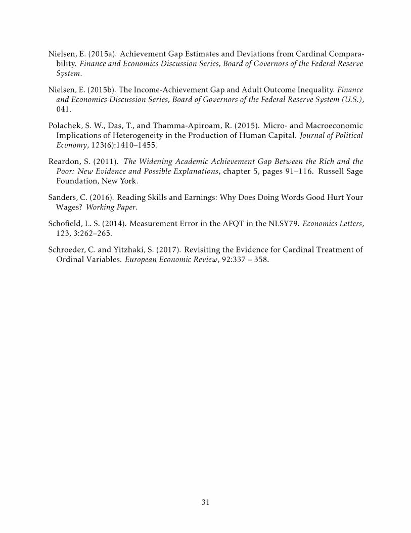
Nielsen, E. (2015a). Achievement Gap Estimates and Deviations from Cardinal Compara-bility. Finance and Economics Discussion Series, Board of Governors of the Federal ReserveSystem.

Nielsen, E. (2015b). The Income-Achievement Gap and Adult Outcome Inequality. Financeand Economics Discussion Series, Board of Governors of the Federal Reserve System (U.S.),041.

Polachek, S. W., Das, T., and Thamma-Apiroam, R. (2015). Micro- and MacroeconomicImplications of Heterogeneity in the Production of Human Capital. Journal of PoliticalEconomy, 123(6):1410–1455.

Reardon, S. (2011). The Widening Academic Achievement Gap Between the Rich and thePoor: New Evidence and Possible Explanations, chapter 5, pages 91–116. Russell SageFoundation, New York.

Sanders, C. (2016). Reading Skills and Earnings: Why Does Doing Words Good Hurt YourWages? Working Paper.

Schofield, L. S. (2014). Measurement Error in the AFQT in the NLSY79. Economics Letters,123, 3:262–265.

Schroeder, C. and Yitzhaki, S. (2017). Revisiting the Evidence for Cardinal Treatment ofOrdinal Variables. European Economic Review, 92:337 – 358.

31

A Appendix

Table 1: NLSY79 Sample Summary Statistics

Variable Mean Std. Dev. Nage (base year) 17.73 2.32 11406male 0.50 0.50 11406black 0.14 0.34 11406hh income (base year, $1,000) 70.84 46.4 10985high school 0.89 0.32 11406college 0.24 0.43 11406highest grade completed 13.28 2.5 11406pdv labor ($1,000) 440.88 332.2 11406wage at 30 19.43 11.27 8521math 99.05 18.99 10721reading 98.23 19.38 10721afqt 147.75 27.25 10721ar missing 0.08 0.28 11406wk missing 0.08 0.28 11406pc missing 0.09 0.28 11406mk missing 0.09 0.28 11406

Notes: All statistics use base-year sampling weights. Dollar values in 2017-constant dollars deflatedusing the CPI-U.

32

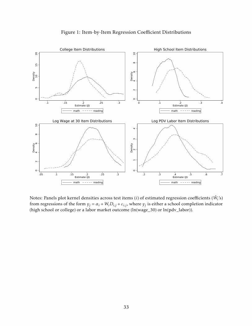
Figure 1: Item-by-Item Regression Coefficient Distributions0

510

1520

Den

sity

.1 .15 .2 .25 .3Estimate (β)

math reading

College Item Distributions

02

46

810

Den

sity

0 .1 .2 .3 .4Estimate (β)

math reading

High School Item Distributions

02

46

810

Den

sity

.05 .1 .15 .2 .25 .3Estimate (β)

math reading

Log Wage at 30 Item Distributions

01

23

4D

ensi

ty

.2 .3 .4 .5 .6 .7Estimate (β)

math reading

Log PDV Labor Item Distributions

Notes: Panels plot kernel densities across test items (i) of estimated regression coefficients (Wi ’s)from regressions of the form yj = αi +WiDi,j + εi,j , where yj is either a school completion indicator(high school or college) or a labor market outcome (ln(wage_30) or ln(pdv_labor)).

33

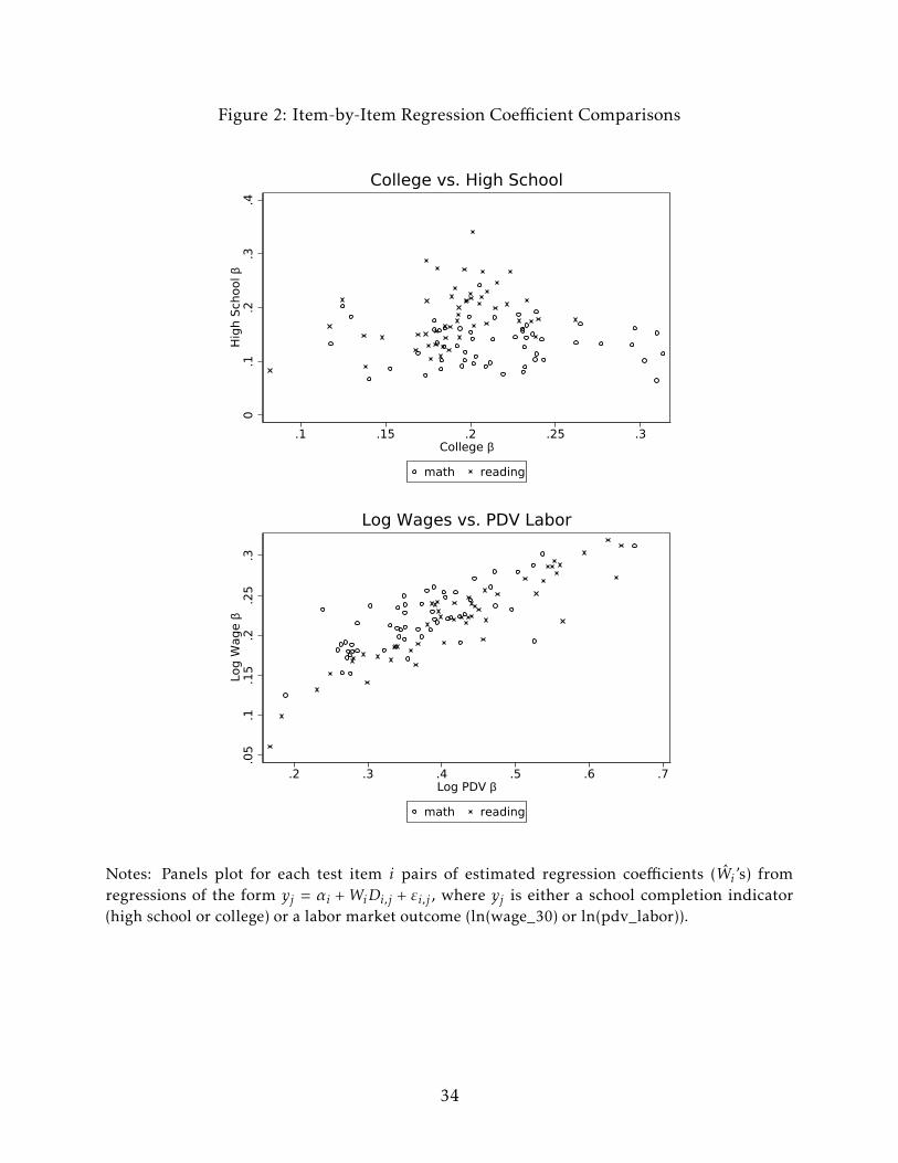
Figure 2: Item-by-Item Regression Coefficient Comparisons

0.1

.2.3

.4H

igh

Scho

ol β

.1 .15 .2 .25 .3College β

math reading

College vs. High School

.05

.1.1

5.2

.25

.3Lo

g W

age

β

.2 .3 .4 .5 .6 .7Log PDV β

math reading

Log Wages vs. PDV Labor

Notes: Panels plot for each test item i pairs of estimated regression coefficients (Wi ’s) fromregressions of the form yj = αi +WiDi,j + εi,j , where yj is either a school completion indicator(high school or college) or a labor market outcome (ln(wage_30) or ln(pdv_labor)).

34

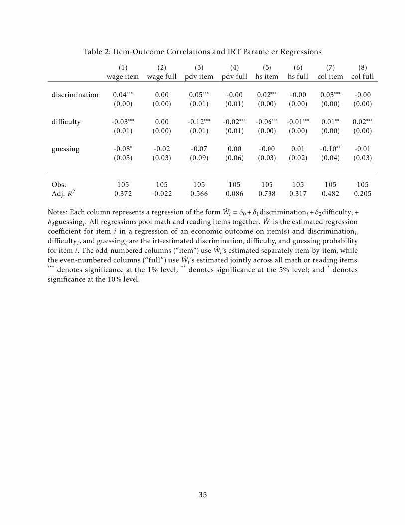
Table 2: Item-Outcome Correlations and IRT Parameter Regressions

(1) (2) (3) (4) (5) (6) (7) (8)wage item wage full pdv item pdv full hs item hs full col item col full

discrimination 0.04∗∗∗ 0.00 0.05∗∗∗ -0.00 0.02∗∗∗ -0.00 0.03∗∗∗ -0.00(0.00) (0.00) (0.01) (0.01) (0.00) (0.00) (0.00) (0.00)

difficulty -0.03∗∗∗ 0.00 -0.12∗∗∗ -0.02∗∗∗ -0.06∗∗∗ -0.01∗∗∗ 0.01∗∗ 0.02∗∗∗

(0.01) (0.00) (0.01) (0.01) (0.00) (0.00) (0.00) (0.00)

guessing -0.08∗ -0.02 -0.07 0.00 -0.00 0.01 -0.10∗∗ -0.01(0.05) (0.03) (0.09) (0.06) (0.03) (0.02) (0.04) (0.03)

Obs. 105 105 105 105 105 105 105 105Adj. R2 0.372 -0.022 0.566 0.086 0.738 0.317 0.482 0.205

Notes: Each column represents a regression of the form Wi = δ0 +δ1discriminationi +δ2difficultyi +δ3guessingi . All regressions pool math and reading items together. Wi is the estimated regressioncoefficient for item i in a regression of an economic outcome on item(s) and discriminationi ,difficultyi , and guessingi are the irt-estimated discrimination, difficulty, and guessing probabilityfor item i. The odd-numbered columns (“item”) use Wi ’s estimated separately item-by-item, whilethe even-numbered columns (“full”) use Wi ’s estimated jointly across all math or reading items.*** denotes significance at the 1% level; ** denotes significance at the 5% level; and * denotessignificance at the 10% level.

35

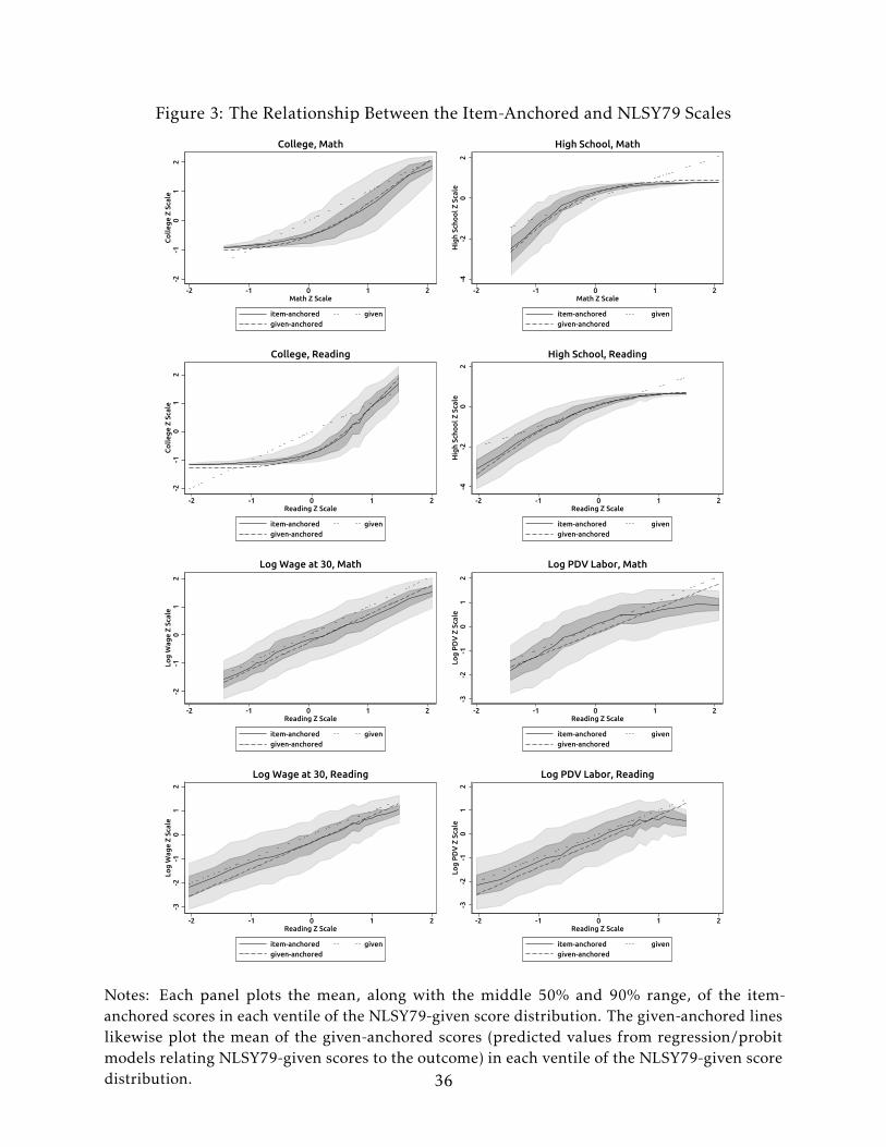
Figure 3: The Relationship Between the Item-Anchored and NLSY79 Scales

-2-1

01

2C

olle

ge Z

Sca

le

-2 -1 0 1 2Math Z Scale

item-anchored givengiven-anchored

College, Math

-4-2

02

Hig

h Sc

hoo

l Z S

cale

-2 -1 0 1 2Math Z Scale

item-anchored givengiven-anchored

High School, Math

-2-1

01

2C

olle

ge Z

Sca

le

-2 -1 0 1 2Reading Z Scale

item-anchored givengiven-anchored

College, Reading

-4-2

02

Hig

h Sc

hoo

l Z S

cale

-2 -1 0 1 2Reading Z Scale

item-anchored givengiven-anchored

High School, Reading

-2-1

01

2Lo

g W

age

Z Sc

ale

-2 -1 0 1 2Reading Z Scale

item-anchored givengiven-anchored

Log Wage at 30, Math

-3-2

-10

12

Log

PD

V Z

Sca

le

-2 -1 0 1 2Reading Z Scale

item-anchored givengiven-anchored

Log PDV Labor, Math

-3-2

-10

12

Log

Wag

e Z

Scal

e

-2 -1 0 1 2Reading Z Scale

item-anchored givengiven-anchored

Log Wage at 30, Reading

-3-2

-10

12

Log

PD

V Z

Sca

le

-2 -1 0 1 2Reading Z Scale

item-anchored givengiven-anchored

Log PDV Labor, Reading

Notes: Each panel plots the mean, along with the middle 50% and 90% range, of the item-anchored scores in each ventile of the NLSY79-given score distribution. The given-anchored lineslikewise plot the mean of the given-anchored scores (predicted values from regression/probitmodels relating NLSY79-given scores to the outcome) in each ventile of the NLSY79-given scoredistribution. 36

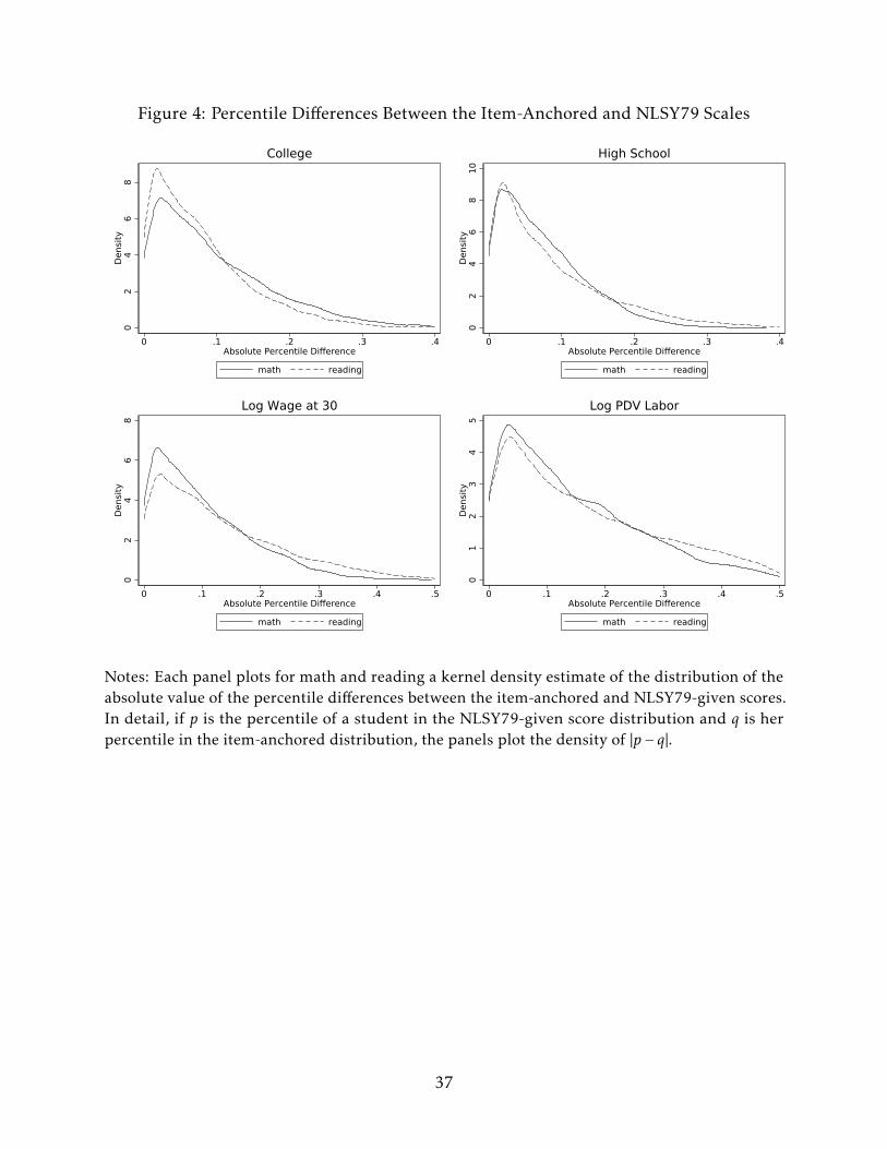
Figure 4: Percentile Differences Between the Item-Anchored and NLSY79 Scales0

24

68

Den

sity

0 .1 .2 .3 .4Absolute Percentile Difference

math reading

College

02

46

810

Den

sity

0 .1 .2 .3 .4Absolute Percentile Difference

math reading

High School

02

46

8D

ensi

ty

0 .1 .2 .3 .4 .5Absolute Percentile Difference

math reading

Log Wage at 30

01

23

45

Den

sity

0 .1 .2 .3 .4 .5Absolute Percentile Difference

math reading

Log PDV Labor

Notes: Each panel plots for math and reading a kernel density estimate of the distribution of theabsolute value of the percentile differences between the item-anchored and NLSY79-given scores.In detail, if p is the percentile of a student in the NLSY79-given score distribution and q is herpercentile in the item-anchored distribution, the panels plot the density of |p − q|.

37

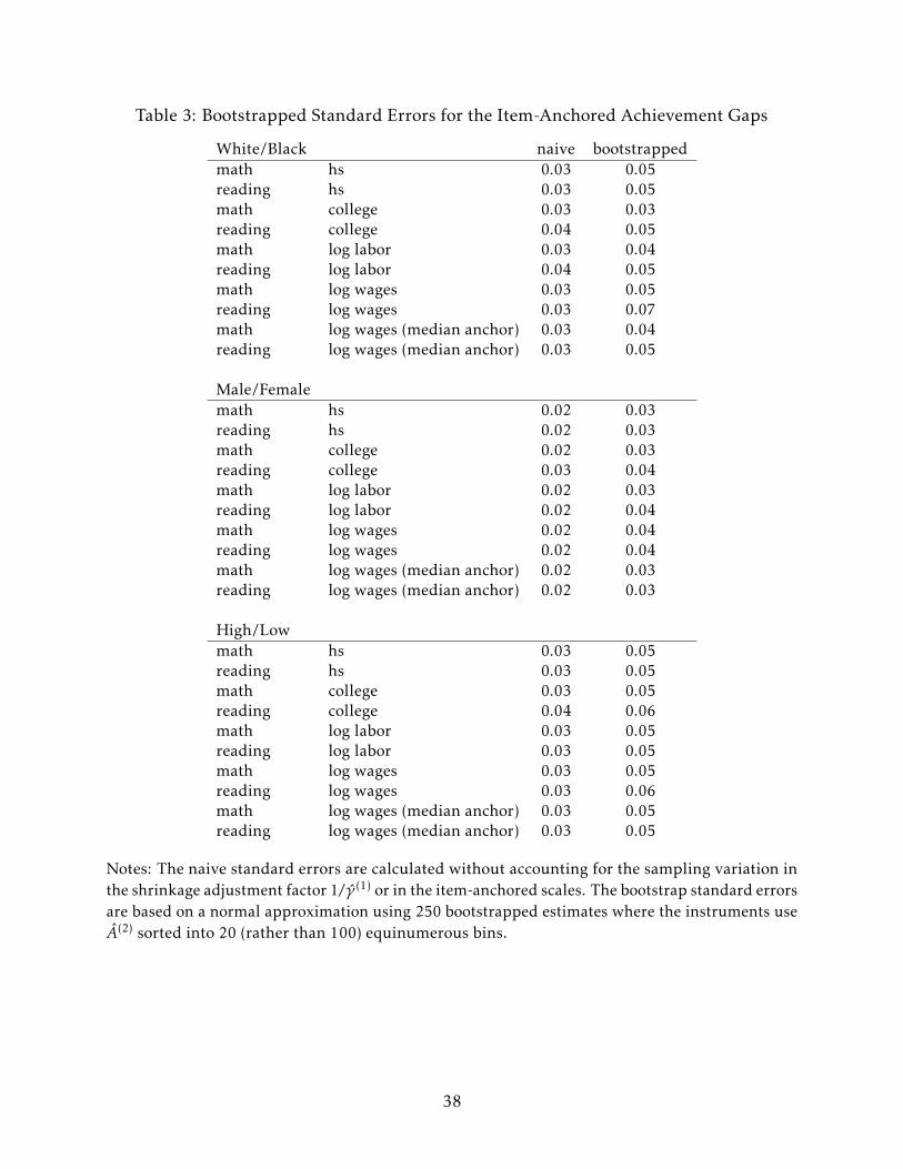
Table 3: Bootstrapped Standard Errors for the Item-Anchored Achievement Gaps

White/Black naive bootstrappedmath hs 0.03 0.05reading hs 0.03 0.05math college 0.03 0.03reading college 0.04 0.05math log labor 0.03 0.04reading log labor 0.04 0.05math log wages 0.03 0.05reading log wages 0.03 0.07math log wages (median anchor) 0.03 0.04reading log wages (median anchor) 0.03 0.05

Male/Femalemath hs 0.02 0.03reading hs 0.02 0.03math college 0.02 0.03reading college 0.03 0.04math log labor 0.02 0.03reading log labor 0.02 0.04math log wages 0.02 0.04reading log wages 0.02 0.04math log wages (median anchor) 0.02 0.03reading log wages (median anchor) 0.02 0.03

High/Lowmath hs 0.03 0.05reading hs 0.03 0.05math college 0.03 0.05reading college 0.04 0.06math log labor 0.03 0.05reading log labor 0.03 0.05math log wages 0.03 0.05reading log wages 0.03 0.06math log wages (median anchor) 0.03 0.05reading log wages (median anchor) 0.03 0.05

Notes: The naive standard errors are calculated without accounting for the sampling variation inthe shrinkage adjustment factor 1/γ (1) or in the item-anchored scales. The bootstrap standard errorsare based on a normal approximation using 250 bootstrapped estimates where the instruments useA(2) sorted into 20 (rather than 100) equinumerous bins.

38

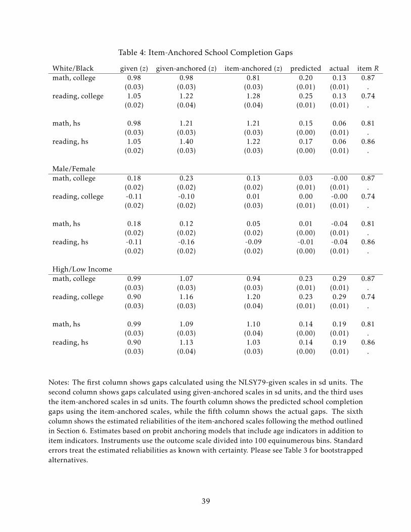
Table 4: Item-Anchored School Completion Gaps

White/Black given (z) given-anchored (z) item-anchored (z) predicted actual item Rmath, college 0.98 0.98 0.81 0.20 0.13 0.87

(0.03) (0.03) (0.03) (0.01) (0.01) .reading, college 1.05 1.22 1.28 0.25 0.13 0.74

(0.02) (0.04) (0.04) (0.01) (0.01) .

math, hs 0.98 1.21 1.21 0.15 0.06 0.81(0.03) (0.03) (0.03) (0.00) (0.01) .

reading, hs 1.05 1.40 1.22 0.17 0.06 0.86(0.02) (0.03) (0.03) (0.00) (0.01) .

Male/Femalemath, college 0.18 0.23 0.13 0.03 -0.00 0.87

(0.02) (0.02) (0.02) (0.01) (0.01) .reading, college -0.11 -0.10 0.01 0.00 -0.00 0.74

(0.02) (0.02) (0.03) (0.01) (0.01) .

math, hs 0.18 0.12 0.05 0.01 -0.04 0.81(0.02) (0.02) (0.02) (0.00) (0.01) .

reading, hs -0.11 -0.16 -0.09 -0.01 -0.04 0.86(0.02) (0.02) (0.02) (0.00) (0.01) .

High/Low Incomemath, college 0.99 1.07 0.94 0.23 0.29 0.87

(0.03) (0.03) (0.03) (0.01) (0.01) .reading, college 0.90 1.16 1.20 0.23 0.29 0.74

(0.03) (0.03) (0.04) (0.01) (0.01) .

math, hs 0.99 1.09 1.10 0.14 0.19 0.81(0.03) (0.03) (0.04) (0.00) (0.01) .

reading, hs 0.90 1.13 1.03 0.14 0.19 0.86(0.03) (0.04) (0.03) (0.00) (0.01) .

Notes: The first column shows gaps calculated using the NLSY79-given scales in sd units. Thesecond column shows gaps calculated using given-anchored scales in sd units, and the third usesthe item-anchored scales in sd units. The fourth column shows the predicted school completiongaps using the item-anchored scales, while the fifth column shows the actual gaps. The sixthcolumn shows the estimated reliabilities of the item-anchored scales following the method outlinedin Section 6. Estimates based on probit anchoring models that include age indicators in addition toitem indicators. Instruments use the outcome scale divided into 100 equinumerous bins. Standarderrors treat the estimated reliabilities as known with certainty. Please see Table 3 for bootstrappedalternatives.

39

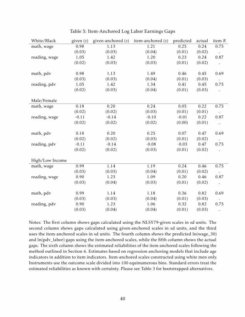
Table 5: Item-Anchored Log Labor Earnings Gaps

White/Black given (z) given-anchored (z) item-anchored (z) predicted actual item Rmath, wage 0.98 1.13 1.21 0.25 0.24 0.75

(0.03) (0.03) (0.04) (0.01) (0.02) .reading, wage 1.05 1.42 1.20 0.23 0.24 0.87

(0.02) (0.03) (0.03) (0.01) (0.02) .

math, pdv 0.98 1.13 1.49 0.46 0.45 0.69(0.03) (0.03) (0.04) (0.01) (0.03) .

reading, pdv 1.05 1.42 1.34 0.41 0.45 0.75(0.02) (0.03) (0.04) (0.01) (0.03) .

Male/Femalemath, wage 0.18 0.20 0.24 0.05 0.22 0.75

(0.02) (0.02) (0.03) (0.01) (0.01) .reading, wage -0.11 -0.14 -0.10 -0.01 0.22 0.87

(0.02) (0.02) (0.02) (0.00) (0.01) .

math, pdv 0.18 0.20 0.25 0.07 0.47 0.69(0.02) (0.02) (0.03) (0.01) (0.02) .

reading, pdv -0.11 -0.14 -0.08 -0.03 0.47 0.75(0.02) (0.02) (0.03) (0.01) (0.02) .

High/Low Incomemath, wage 0.99 1.14 1.19 0.24 0.46 0.75

(0.03) (0.03) (0.04) (0.01) (0.02) .reading, wage 0.90 1.23 1.09 0.20 0.46 0.87

(0.03) (0.04) (0.03) (0.01) (0.02) .

math, pdv 0.99 1.14 1.18 0.36 0.82 0.69(0.03) (0.03) (0.04) (0.01) (0.03) .

reading, pdv 0.90 1.23 1.06 0.32 0.82 0.75(0.03) (0.04) (0.04) (0.01) (0.03) .

Notes: The first column shows gaps calculated using the NLSY79-given scales in sd units. Thesecond column shows gaps calculated using given-anchored scales in sd units, and the thirduses the item-anchored scales in sd units. The fourth column shows the predicted ln(wage_30)and ln(pdv_labor) gaps using the item-anchored scales, while the fifth column shows the actualgaps. The sixth column shows the estimated reliabilities of the item-anchored scales following themethod outlined in Section 6. Estimates based on regression anchoring models that include ageindicators in addition to item indicators. Item-anchored scales constructed using white men only.Instruments use the outcome scale divided into 100 equinumerous bins. Standard errors treat theestimated reliabilities as known with certainty. Please see Table 3 for bootstrapped alternatives.

40

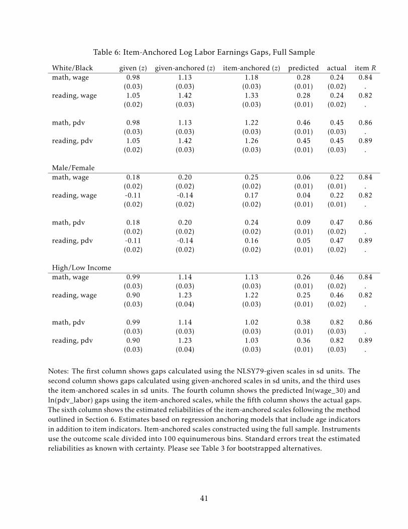
Table 6: Item-Anchored Log Labor Earnings Gaps, Full Sample

White/Black given (z) given-anchored (z) item-anchored (z) predicted actual item Rmath, wage 0.98 1.13 1.18 0.28 0.24 0.84

(0.03) (0.03) (0.03) (0.01) (0.02) .reading, wage 1.05 1.42 1.33 0.28 0.24 0.82

(0.02) (0.03) (0.03) (0.01) (0.02) .

math, pdv 0.98 1.13 1.22 0.46 0.45 0.86(0.03) (0.03) (0.03) (0.01) (0.03) .

reading, pdv 1.05 1.42 1.26 0.45 0.45 0.89(0.02) (0.03) (0.03) (0.01) (0.03) .

Male/Femalemath, wage 0.18 0.20 0.25 0.06 0.22 0.84

(0.02) (0.02) (0.02) (0.01) (0.01) .reading, wage -0.11 -0.14 0.17 0.04 0.22 0.82

(0.02) (0.02) (0.02) (0.01) (0.01) .

math, pdv 0.18 0.20 0.24 0.09 0.47 0.86(0.02) (0.02) (0.02) (0.01) (0.02) .

reading, pdv -0.11 -0.14 0.16 0.05 0.47 0.89(0.02) (0.02) (0.02) (0.01) (0.02) .

High/Low Incomemath, wage 0.99 1.14 1.13 0.26 0.46 0.84

(0.03) (0.03) (0.03) (0.01) (0.02) .reading, wage 0.90 1.23 1.22 0.25 0.46 0.82

(0.03) (0.04) (0.03) (0.01) (0.02) .

math, pdv 0.99 1.14 1.02 0.38 0.82 0.86(0.03) (0.03) (0.03) (0.01) (0.03) .

reading, pdv 0.90 1.23 1.03 0.36 0.82 0.89(0.03) (0.04) (0.03) (0.01) (0.03) .

Notes: The first column shows gaps calculated using the NLSY79-given scales in sd units. Thesecond column shows gaps calculated using given-anchored scales in sd units, and the third usesthe item-anchored scales in sd units. The fourth column shows the predicted ln(wage_30) andln(pdv_labor) gaps using the item-anchored scales, while the fifth column shows the actual gaps.The sixth column shows the estimated reliabilities of the item-anchored scales following the methodoutlined in Section 6. Estimates based on regression anchoring models that include age indicatorsin addition to item indicators. Item-anchored scales constructed using the full sample. Instrumentsuse the outcome scale divided into 100 equinumerous bins. Standard errors treat the estimatedreliabilities as known with certainty. Please see Table 3 for bootstrapped alternatives.

41

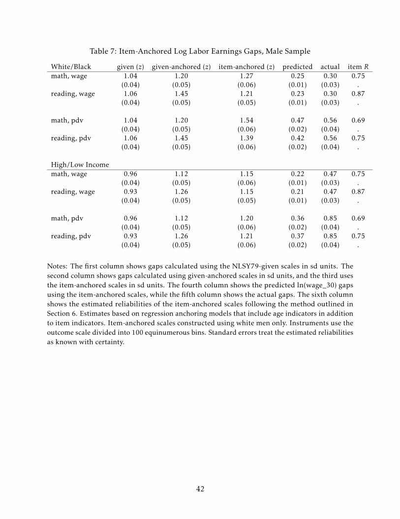
Table 7: Item-Anchored Log Labor Earnings Gaps, Male Sample

White/Black given (z) given-anchored (z) item-anchored (z) predicted actual item Rmath, wage 1.04 1.20 1.27 0.25 0.30 0.75

(0.04) (0.05) (0.06) (0.01) (0.03) .reading, wage 1.06 1.45 1.21 0.23 0.30 0.87

(0.04) (0.05) (0.05) (0.01) (0.03) .

math, pdv 1.04 1.20 1.54 0.47 0.56 0.69(0.04) (0.05) (0.06) (0.02) (0.04) .

reading, pdv 1.06 1.45 1.39 0.42 0.56 0.75(0.04) (0.05) (0.06) (0.02) (0.04) .

High/Low Incomemath, wage 0.96 1.12 1.15 0.22 0.47 0.75

(0.04) (0.05) (0.06) (0.01) (0.03) .reading, wage 0.93 1.26 1.15 0.21 0.47 0.87

(0.04) (0.05) (0.05) (0.01) (0.03) .

math, pdv 0.96 1.12 1.20 0.36 0.85 0.69(0.04) (0.05) (0.06) (0.02) (0.04) .

reading, pdv 0.93 1.26 1.21 0.37 0.85 0.75(0.04) (0.05) (0.06) (0.02) (0.04) .

Notes: The first column shows gaps calculated using the NLSY79-given scales in sd units. Thesecond column shows gaps calculated using given-anchored scales in sd units, and the third usesthe item-anchored scales in sd units. The fourth column shows the predicted ln(wage_30) gapsusing the item-anchored scales, while the fifth column shows the actual gaps. The sixth columnshows the estimated reliabilities of the item-anchored scales following the method outlined inSection 6. Estimates based on regression anchoring models that include age indicators in additionto item indicators. Item-anchored scales constructed using white men only. Instruments use theoutcome scale divided into 100 equinumerous bins. Standard errors treat the estimated reliabilitiesas known with certainty.

42

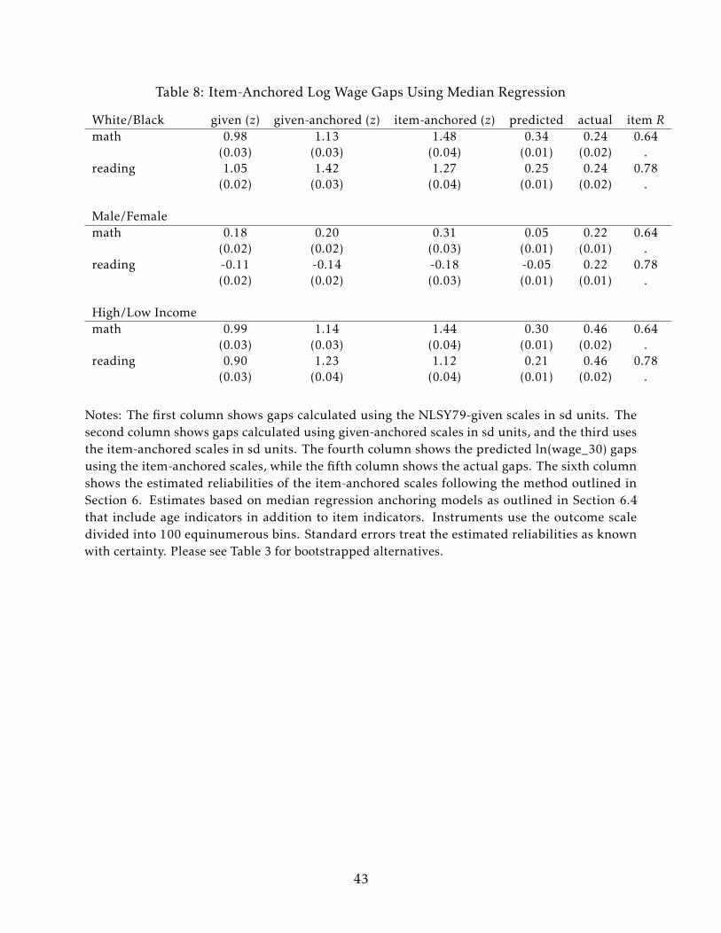
Table 8: Item-Anchored Log Wage Gaps Using Median Regression

White/Black given (z) given-anchored (z) item-anchored (z) predicted actual item Rmath 0.98 1.13 1.48 0.34 0.24 0.64

(0.03) (0.03) (0.04) (0.01) (0.02) .reading 1.05 1.42 1.27 0.25 0.24 0.78

(0.02) (0.03) (0.04) (0.01) (0.02) .

Male/Femalemath 0.18 0.20 0.31 0.05 0.22 0.64

(0.02) (0.02) (0.03) (0.01) (0.01) .reading -0.11 -0.14 -0.18 -0.05 0.22 0.78

(0.02) (0.02) (0.03) (0.01) (0.01) .

High/Low Incomemath 0.99 1.14 1.44 0.30 0.46 0.64

(0.03) (0.03) (0.04) (0.01) (0.02) .reading 0.90 1.23 1.12 0.21 0.46 0.78

(0.03) (0.04) (0.04) (0.01) (0.02) .

Notes: The first column shows gaps calculated using the NLSY79-given scales in sd units. Thesecond column shows gaps calculated using given-anchored scales in sd units, and the third usesthe item-anchored scales in sd units. The fourth column shows the predicted ln(wage_30) gapsusing the item-anchored scales, while the fifth column shows the actual gaps. The sixth columnshows the estimated reliabilities of the item-anchored scales following the method outlined inSection 6. Estimates based on median regression anchoring models as outlined in Section 6.4that include age indicators in addition to item indicators. Instruments use the outcome scaledivided into 100 equinumerous bins. Standard errors treat the estimated reliabilities as knownwith certainty. Please see Table 3 for bootstrapped alternatives.

43

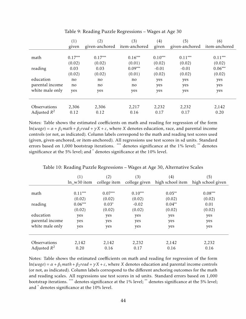
Table 9: Reading Puzzle Regressions – Wages at Age 30

(1) (2) (3) (4) (5) (6)given given-anchored item-anchored given given-anchored item-anchored

math 0.17∗∗∗ 0.17∗∗∗ 0.16∗∗∗ 0.10∗∗∗ 0.11∗∗∗ 0.11∗∗∗

(0.02) (0.02) (0.01) (0.02) (0.02) (0.02)reading 0.03 0.03 0.09∗∗∗ -0.01 -0.01 0.06∗∗∗

(0.02) (0.02) (0.01) (0.02) (0.02) (0.02)education no no no yes yes yesparental income no no no yes yes yeswhite male only yes yes yes yes yes yes

Observations 2,306 2,306 2,217 2,232 2,232 2,142Adjusted R2 0.12 0.12 0.16 0.17 0.17 0.20

Notes: Table shows the estimated coefficients on math and reading for regression of the formln(wage) = α + β1math+ β2read + γX + ε, where X denotes education, race, and parental incomecontrols (or not, as indicated). Column labels correspond to the math and reading test scores used(given, given-anchored, or item-anchored). All regressions use test scores in sd units. Standarderrors based on 1,000 bootstrap iterations. *** denotes significance at the 1% level; ** denotessignificance at the 5% level; and * denotes significance at the 10% level.

Table 10: Reading Puzzle Regressions – Wages at Age 30, Alternative Scales

(1) (2) (3) (4) (5)ln_w30 item college item college given high school item high school given

math 0.11∗∗∗ 0.07∗∗∗ 0.10∗∗∗ 0.05∗∗ 0.08∗∗∗

(0.02) (0.02) (0.02) (0.02) (0.02)reading 0.06∗∗∗ 0.03∗ -0.02 0.04∗∗ 0.01

(0.02) (0.02) (0.02) (0.02) (0.02)education yes yes yes yes yesparental income yes yes yes yes yeswhite male only yes yes yes yes yes

Observations 2,142 2,142 2,232 2,142 2,232Adjusted R2 0.20 0.16 0.17 0.16 0.16

Notes: Table shows the estimated coefficients on math and reading for regression of the formln(wage) = α + β1math+ β2read +γX + ε, where X denotes education and parental income controls(or not, as indicated). Column labels correspond to the different anchoring outcomes for the mathand reading scales. All regressions use test scores in sd units. Standard errors based on 1,000bootstrap iterations. *** denotes significance at the 1% level; ** denotes significance at the 5% level;and * denotes significance at the 10% level.

44