ESSLLI 2012Student SessionProceedings———————————

Preface

The 24rd European Summer School in Logic, Language, and Information (ESS-LLI) took is taking place on August 6-17, Opole, Poland, under the auspices ofFoLLI. This volume contains the proceedings of the 17th Student Session1, anannual event which takes place within ESSLLI. It contains 21 papers addressinga wide range of topics in logic, language, and computation. These papers wereselected from a large number of excellent submissions on the basis of reports byexpert reviewers in the relevant areas.

Thanks are due to the area experts and to the two previous chairs, Mar-ija Slavkovik (2010) and Daniel Lassiter (2011), for their advice and support,and to Janusz Czelakowski, Urszula Wybraniec-Skardowska and the rest of theESSLLI 2012 Organizing Committee. Special recognition goes to Springer fortheir continuing support of the Student Session. Most importantly, thanks to allthose who submitted papers, and to the many reviewers who generously gavetheir time to provide thoughtful feedback on each submission.

Rasmus K. RendsvigChair, ESSLLI 2012 Student Session

Copenhagen, August 2012

1This volume is a working copy. Though nearly complete, minor changes may occurin the final version.

Organization

Chair: Rasmus K. Rendsvig

Co-Chairs: Niels Beuck (Language and Computation)Margot Colinet (Logic and Language)Maxim Haddad (Logic and Computation)Anders Johannsen (Language and Computation)Dominik Klein (Logic and Computation)Matthjis Westera (Logic and Language)

Area Experts: Ann Copestake (Language and Computation)Friederike Moltmann (Logic and Language)Eric Pacuit (Logic and Computation)

Table of Contents

Preface . . . . . . . . . . . . . . . . . . . . . . . . . . . . . . . . . . . . . . . . . . . . . . . . . . . . . . . . . . . i

Organization . . . . . . . . . . . . . . . . . . . . . . . . . . . . . . . . . . . . . . . . . . . . . . . . . . . . . . ii

Aligning Geospatial Ontologies Logically . . . . . . . . . . . . . . . . . . . . . . . . . . . . . 1Heshan Du

Doing argumentation using theories in graph normal form . . . . . . . . . . . . . . 14Sjur Dyrkolbotn

The Expressive Power of Swap Logic . . . . . . . . . . . . . . . . . . . . . . . . . . . . . . . . 25Raul Fervari

Reasoning on Procedural Programs using Description Logics withConcrete Domains . . . . . . . . . . . . . . . . . . . . . . . . . . . . . . . . . . . . . . . . . . . . . . . . 35

Ronald de Haan

Small Steps in Heuristics for the Russian Cards Problem Protocols . . . . . . 47Ignacio Hernandez-Anton

Markov Logic Networks for Spatial Language in Reference Resolution . . . . 59Casey Kennington

Using Conditional Probabilities and Vowel Collocations of a Corpus ofOrthographic Representations to Evaluate Nonce Words . . . . . . . . . . . . . . . 71

Ozkan Kılıc

A Dynamic Probabilistic Approach to Epistemic Modality . . . . . . . . . . . . . 80Manuel Kriz

Computing with Numbers, Cognition and the Epistemic Value of Iconicity 92Jose Gustavo Morales

The Force of Innovation . . . . . . . . . . . . . . . . . . . . . . . . . . . . . . . . . . . . . . . . . . . 102Muhlenbernd, Nick & Adam

Existential definability of modal frame classes . . . . . . . . . . . . . . . . . . . . . . . . 114Tin Perkov

Spotting and improving modularity in large scale grammar development . 122Simon Petitjean

Questions of Trust . . . . . . . . . . . . . . . . . . . . . . . . . . . . . . . . . . . . . . . . . . . . . . . . 132Jason Quinley and Christopher Ahern

iv

Checking Admissibility in Finite Algebras . . . . . . . . . . . . . . . . . . . . . . . . . . . . 145Christoph Rothlisberger

Scalar Properties of Degree Modification in Karitiana: Evidence forIndeterminate Scales . . . . . . . . . . . . . . . . . . . . . . . . . . . . . . . . . . . . . . . . . . . . . . 155

Luciana Sanchez Mendes

PCFG extraction and sentence analysis. . . . . . . . . . . . . . . . . . . . . . . . . . . . . . 164Noemie-Fleur Sandillon-Rezer

An Interaction Grammar for English Verbs . . . . . . . . . . . . . . . . . . . . . . . . . . . 174Shohreh Tabatabayi Seifi

Toward a Discourse Structure Account of Speech and Attitude reports . . . 185Antoine Venant

Some, speaker knowledge, and subkinds . . . . . . . . . . . . . . . . . . . . . . . . . . . . . . 196Andrew Weir

Tableau-based decision procedure for hybrid logic with satisfactionoperators, universal modality and difference modality . . . . . . . . . . . . . . . . . . 209

Micha l Zawidzki

A Frame-Based Semantics of Locative Alternation in LTAG . . . . . . . . . . . . 221Yulia Zinova

Aligning Geospatial Ontologies Logically

Heshan Du

The University of Nottingham, UK

Abstract. Information sharing and updates have become increasinglyimportant in the rapidly changing world. However, owing to the dis-tributed and decentralized nature of information collection and storage,it is not easy to use information from different sources synergistically.Ontology plays as an important role in establishing formal descriptionsof a domain of discourse. In geographic information science, the rapiddevelopments of crowd-sourced geospatial databases challenge and alsobring opportunities to the current geospatial information developmentframework. In this paper, a new semi-automatic method is proposed toalign disparate geospatial ontologies, based on description logic and do-main experts’ knowledge.

1 Introduction

Information sharing and updates have become increasingly important in therapidly changing world, with a large amount of disparate information available.However, owing to the distributed and decentralized nature of information de-velopment, it is not easy to fully capture the information content in differentsources. A same expression can have different meanings in different context,and different expressions may refer to the same meaning. Such issues are quitecommon when disparate and related information sources exchange their data.

Ontology plays an important role in information sharing. Ontology, orig-inated in the work of Aristotle, is a branch of philosophy which studies theexistence of entities [41]. In computer science, ontology is an explicit formalspecification of a shared conceptualization [14]. Compared to its origin, com-puter science ontology is not only about existence, but also about meaning,and making meanings as clear as possible [41]. Ontologies are often employedas important means for establishing explicit formal vocabulary shared amongapplications.

Description logics are a family of formalisms for representing the knowledgeof an application domain [2]. They firstly define the relevant concepts (termi-nology), and then use these concepts to specify properties of objects in thedomain [2]. Compared to traditional first-order logic, description logics providetools for the manipulations of compound and complex concepts [7]. Descrip-tion logics support inference patterns, including classification of concepts andindividuals, which are often used by humans to structure and understand theworld [2]. When dealing with ontology issues, description logics can be used asthe logical underpinning.

2 Heshan Du

The rapid developments in geographic information science emphasize the im-portance of geospatial information sharing. Spatial Data Infrastructures (SDI)refers to an institutional and technical foundation of policies, standards and pro-cedures that enable organizations at multiple levels and scales to discover, eval-uate, use and maintain geospatial data [28]. Over the last few years, the currenttop-down approach to SDI has been challenged by the rapid pace of techno-logical development [17]. There is a need to address the separation of nationaland international SDI from crowd-sourced geospatial databases [1]. Relying onvolunteers for data collection, crowd-sourced data is less expensive than authen-ticated data. In addition, although typically not as complete in its coverage oras consistent in its geometric or metadata quality as authenticated data, crowd-sourced data may provide a rich source of complementary information with thebenefit of often more recent and frequent updates than that of authenticateddata [18]. It is desirable to use authenticated and crowd-sourced geospatial datasynergistically.

Compared to other ontologies, geospatial ontologies have several special prop-erties. Firstly, many words within geospatial ontologies are often more widelyused in daily life, and there is less consensus about their definitions. For example,the word ‘creek’ can refer to a river in Australia, while cannot in the US. Theword ‘field’ has different meanings (e.g. a branch of knowledge, a piece of land,etc.) for different people in different contexts. There are no precise formal defi-nitions which can tell ‘river’ and ‘stream’, ‘lake’ and ‘pond’ apart. In addition,geospatial ontologies often do not have a huge number of classes as biomedicalor bioinformatics ontologies do, but may have many instances, referring to realworld objects, whose locations, at least in theory, are verifiable. With respectto these properties and the underspecification of geospatial ontologies, no fullyautomated system can ensure the correctness and completeness of generatedmappings. Therefore, experts are inevitably needed to make decisions, for ex-ample on the correctness of correspondences, based on their domain knowledge,which is often implicit in the individual ontologies. This research will finally leadto the minimisation of the human intervention.

This project aims to explore logic-based approaches to aligning disparate andrelated geospatial ontologies to obtain harmonized and maximized informationcontent. Ontologies are disparate if they are created independently. Ontologiesare related if they contain more than one common concept. Aligning means es-tablishing relations between the vocabularies of two ontologies [9]. The desiredoutput will be a collection of verified such relations, for query answering overmultiple ontologies. If ontologies cannot be aligned logically, a deficiency reportwill be produced explaining reasons and providing suggestions about furtheractions to take in order to align them. In this paper, we propose a new semi-automatic method to align disparate geospatial ontologies, based on descriptionlogic and domain experts’ knowledge. It is assumed that original informationwithin ontologies is believed all the time as premises, whilst generated infor-mation, including disjointness axioms and mappings, is believed by default asassumptions, which may be retracted later. Differing from other existing meth-

Aligning Geospatial Ontologies Logically 3

ods, generated disjointness axioms are seen as assumptions, which are retractableduring the overall aligning process. Disparate ontologies are aligned by finding acoherent and consistent assumption set with respect to them. Based on this mainidea, algorithms are designed to align ontologies at the terminology level and theinstance level. With respect to the special properties of geospatial ontologies, analgorithm is designed for refining correspondences between geospatial individualstaking their geometries and semantics into account.

The rest of the paper is organized as follows. The related work is summarizedin Section 2. Section 3 introduces the geospatial ontologies we use, and explainssome results generated by a state-of-the-art system called S-Match [12]. Ourmethod is discussed in Section 4. Finally, it provides conclusions in Section 5.

2 Related Work

Ontology matching is the task of finding correspondences between entities fromdifferent ontologies [11]. A correspondence represents a semantic relation, such asinclusion or equivalence. A mapping is defined as a set of these correspondences[25]. Many ontology matching methods and systems have been proposed anddeveloped in recent years [11] [35], based on shared upper ontologies, if available,or using other kinds of information, such as lexical and structural information,user input, external resources and prior matches [30]. The existing methodscan be classified into three broad categories [4]. Syntactic methods rely on asyntactic analysis of the linguistic expressions to generate mappings. Thoughthese methods are direct and effective, semantic relations between entities cannotbe captured. Pragmatic methods infer the semantic relations between conceptsfrom associated instance data. Though they work well when the instance datais representative and overlapping, this kind of methods use a strong form ofinduction, thus lack correctness and completeness. Conceptual methods comparethe lexical representation of concepts to compute mappings. Socially negotiatedmeanings (e.g. dictionaries) are often used when generating relations, makingthe problem very complicated.

Many methods are hybrid, combining different approaches and making useof structural, lexical, domain or instance-based knowledge. Most of them ap-ply heuristics-based or machine learning techniques to various characteristicsof ontology. However, mappings generated by these methods often contain log-ical contradictions. Some systems, such as CtxMatch [5] and its extension S-Match [12], and more recently, Automated Semantic Mapping of Ontologieswith Validation (ASMOV) [20], Knowledge Organization System Implicit Map-ping (KOSIMap) [33], logiC-based ONtology inTEgratioN Tool using MAPpings(ContentMap) [22], LogMap [21], and Combinational Optimization for Data In-tegration (CODI) [29], seem to be exceptions, since they employ logical reason-ing for either mapping generation or verification. Due to limited space, not allof them are discussed in detail.

CtxMatch and its extension S-Match are early logic-based attempts for ontol-ogy matching. While most of the other methods compute linguistic or structural

4 Heshan Du

similarities, CtxMatch shifts the semantic alignment problem to deducing re-lations between logical formulae [5, 6]. Relevant lexical (concepts denoted bywords), world (relations between concepts) and structural knowledge is repre-sented as logical formulae, and logical reasoning is employed to infer differentkinds of semantic relations [34]. WordNet [27], an external resource, is employedto provide both lexical and world knowledge. The S-Match system re-implementsand extends CtxMatch. Taking two tree-like structures (e.g. hierarchies) as input,it computes the strongest semantic relations between every pair of concepts [12].The semantic matching has two main steps. Firstly, at element level, relationsbetween labels are calculated, and then, at structure level, it generates relationsbetween concepts, whose semantics are constructed based on the semantics oflabels [36]. The structure level matching task is converted into propositional va-lidity problems, and the standard DPLL-based SAT solver [3] is employed tocheck the unsatisfiability of propositional formulae [13]. However, S-Match onlyuses information in the tree-like structures extracted from ontologies, which isinsufficient to guarantee the overall coherence of ontologies after applying themapping relations. More recently, some matching tools have been developed,involving semantic verification into the alignment process.

LogMap [21] is a logic-based and scalable ontology matching tool. It ad-dresses the challenges when dealing with large-scale bio-medical ontologies withtens (even hundreds) of thousands of classes. It employs lexical and structuralmethods to compute an initial set of mapping relations as the starting point forfurther discovery of mapping relations. The core of LogMap is an iterative pro-cess which alternates repair and discovery steps. In the repair step, unsatisfiableclasses will be detected using propositional Horn representation and satisfia-bility checking, and be repaired using a greedy diagnosis algorithm. However,the propositional Horn satisfiability checking is sound but incomplete, and theunderlying semantics is restricted to propositional logic, and thus cannot guar-antee the coherence of the mapping between more expressive ontologies. In thediscovery step, new mapping relations will be generated based on the similaritybetween classes which are semantically related to matched classes. ISUB [37] isemployed to compute the similarity scores. Mapping relations which are newlydiscovered are active, and only active mapping relations can be eliminated inthe repair step, whilst mapping relations found in earlier iterations are seen asestablished or valid. In other words, each mapping relation will be checked once,against the available information at that time, which, however, cannot guaranteeits correctness when new information is discovered later.

Combinational Optimization for Data Integration (CODI) [29] is a probabilis-tic logical alignment system. It is based on Markov logic [10], which combinesfirst-order logic with undirected probabilistic graphical models. As the main ad-vantages over other existing matching approaches, Markov logic can combinehard logical axioms and soft uncertain formulae for potential correspondences.Cardinality constraints, coherence constraints and stability constraints are for-malized using logical axioms and similarity measures. The matching problem istransformed to a maximum-a-posteriori optimization problem subject to these

Aligning Geospatial Ontologies Logically 5

constraints. The GUROBI optimizer [15] is employed to solve the optimizationproblems. According to Noessner and Niepert [29], CODI reduces incoherenceduring the alignment process for the first time, compared to all other existingmethods repairing alignments afterwards. CODI is based on the rationale offinding the most likely mapping by maximizing the sum of similarity-weightedprobabilities for potential correspondences. It can be argued that during the op-timization process, some valid correspondences can be thrown away. In addition,the input coherence constraints will influence the resulting mapping, however,in practice, many ontologies are underspecified, within which valid disjointnessaxioms are not always available.

In addition, there is some recent work on debugging and repairing ontologiesand mappings in ontology networks [24] [32] [40] [23], which is still at an earlystage. However, all of them use disjointness axioms as premises, rather thanassumptions, and none of the matching systems discussed above have addressedthe special properties of geospatial information fully. Several ontology-drivenmethods have been developed for integrating geospatial terminologies. Most ofthem are based on similarity measures or a predefined top-level ontology, andlogical reasoning is only employed when formal ontologies commit to the sametop-level ontology [8]. However, when ontologies are developed independently,the common top-level ontology is not always available. Additionally, there existsome other methods, such as [38] and [19], following the pragmatic approach tolink geospatial schemas or ontologies, inferring the terminology correspondencesfrom the instances correspondences. As discussed above, relying on a very strongform of induction from particular to the universal, this approach will lead to thelack of correctness and completeness [4]. Therefore, more research is required tofill in the gap, exploring logic-based approaches to aligning disparate geospatialontologies.

3 Disparate Geospatial Ontologies

The Ordnance Survey of Great Britain (OSGB) ontology [16] and the Open-StreetMap (OSM) controlled vocabularies [31] are selected to undertake ini-tial research. OSGB and OSM are representatives of authenticated and crowd-sourced geospatial information sources respectively. OSGB is the national topo-graphic mapping agency of Great Britain. It has built ontologies for Hydrologyand for Buildings and Places [16]. OSM is a collaborative project aimed to cre-ate a free editable map of the world [31]. It employs the bottom-up approach,relying on volunteers to collect the data. Currently, OSM does not have a stan-dard ontology, but maintains a collection of commonly used tags for main mapfeatures [31]. An OSM feature ontology is generated automatically from the ex-isting classification of main features. Both ontologies are written in the OWL 2Web Ontology Language [39]. The OSGB Buildings and Places ontology has 692classes and 1230 logical axioms, and its DL expressivity is ALCHOIQ. There are663 classes and 677 logical axioms in the OSM ontology, whose DL expressivityis AL. Both ontologies, containing no disjointness axioms, are coherent.

6 Heshan Du

To understand the ontologies more deeply, S-Match is employed to generaterelations between concepts from them. To distinguish concepts from differentontologies, let us label each concept with the abbreviated name of the ontologyit belongs to, such as OSGB : School and OSM : School. All the labelledconcepts will be treated as belonging to one super ontology. A relation thencan be represented as an axiom within which all the concepts are labelled, likeOSGB : School w OSM : School.

Some of the mapping axioms generated by S-Match seem reasonable, suchas OSGB : Roof ≡ OSM : Roof , OSGB : Service w OSM : Service, andOSGB : Accommodation w OSM : Accommodation. However, there are alsosome problematic relations. For example, OSGB : Thing ≡ OSM : Nothingis derived, because the string ‘Thing’ is considered to be close enough by thestring-based matcher 1 for stating that it is equivalent to the string ‘Nothing’.The relation OSGB : Person w OSM : GuestHouse is generated because,‘GuestHouse’ is split to ‘Guest’ and ‘House’, and ‘House’ is treated as a person’sname, referring to a particular individual of ‘Person’. The relation OSGB :Person w OSM : Dentist seems reasonable, just looking at it alone. However,OSM : Dentist v OSM : Healthcare, and OSM : Healthcare v OSM :Amenity. TheOSM : Dentist is used for tagging a place where a dentist practiceor surgery is located, rather than referring to a person who is a dentist. In thiscase, S-Match seems too restrictive to deal with the informal use of terms andtheir variable meanings in crowd-sourced databases, such as OSM.

4 Method

Ontology alignment has attracted the attention of people working in severalresearch fields, such as linguistics, philosophy, psychology and computer science.To fully understand and solve the problem, relying on only one approach isinadequate. Different approaches may play different important roles and solvedifferent aspects of the problem effectively. This project focuses on the logic-based approach, and explores what logic can do and how far logic can go whenaligning disparate geospatial ontologies.

To represent and reason with two ontologies Oi and Oj , where i, j are theirnames, as well as the matching relations between them, as if they all belongto one super ontology Oi ∪ Oj , we label all atomic concepts and roles in eachontology by the name of the ontology. The ontology Oi is the set {ϕi : ϕ ∈ Oi},where ϕ denotes a logical formula. A logical formula ϕi is labelled inductivelyas follows.

– Ai = i : A, for atomic concept A;– Ri = i : R, for atomic role R;– (¬B)i = ¬Bi;– (B u C)i = Bi u Ci;

1When matching labels of concepts, S-Match employs string-based, sense-based andgloss-based matchers [13].

Aligning Geospatial Ontologies Logically 7

– (B t C)i = Bi t Ci;– {o}i = {oi}, for nominal {o}, individual name o;– (∀R.B)i = ∀Ri.Bi;– (∃R.B)i = ∃Ri.Bi;– (≥ n R.C)i =≥ n Ri.Ci– (≤ n R.C)i =≤ n Ri.Ci– (= n R.C)i == n Ri.Ci

– (R−)i = (Ri)−;– (R+)i = (Ri)+;– (B v C)i = Bi v Ci– (S v T )i = Si v T i

where B,C denote concept descriptions, S, T denote roles. Similarly, we label allindividual names in each ontology by the ontology name:

– ai = i : a;– (C(a))i = Ci(ai)– (R(a, b))i = Ri(ai, bi)

where a, b denote individual names.A terminology mapping is a set of correspondences between classes from

different ontologies. A terminology correspondence is represented as one of thetwo basic forms:

Bi v Cj (1)

Bi w Cj (2)

where B,C denote class descriptions. The relation (1) states that the class Bfrom the ontology i is more specific than or equivalent to the class C from theontology j. The relation (2) states that the class B from the ontology i is moregeneral than or equivalent to the class C from the ontology j. The equivalencerelation (3) holds if and only if (1) and (2) both hold.

Bi ≡ Cj (3)

It states that the concept B from the ontology i and the concept C from theontology j are equivalent.

A disjointness axiom states that two or more classes are pairwise disjoint,having no common element. For example, Person and Place are disjoint. Thedisjointness axioms in ontologies play an important role in debugging ontologymappings. However, within the original geospatial ontologies, disjointness ax-ioms are not always available or sufficient. Adding disjointness axioms manually,especially for large ontologies, is time-consuming and error-prone. Many existingsystems employ more automatic approaches, either assuming the disjointness ofsiblings (e.g. KOSIMap [33]), or employing machine learning techniques to detectdisjointness (e.g. [26]). After the disjointness axioms are generated by whatevermeans, all existing ontology matching or debugging methods, to the best of ourknowledge, use them as premises, believing their validity through the overall fol-lowing process, though the input disjointness axioms can be insufficient or too

8 Heshan Du

restrictive. Differing from these methods, we use generated disjointness axiomsas assumptions, rather than premises, and ensure the assumption set is coherent.A disjointness assumption is represented as:

B v ¬C (4)

where B,C denote class descriptions either from ontology i or ontology j. Wefollow the terminology from [26], and adapt them to this context.

Definition 1 (Coherence). An ontology O is coherent if there is no class Csuch that O |= C v ⊥. Otherwise, it is incoherent.

Definition 2 (Coherence of an Assumption Set). An assumption set Asis incoherent with respect to an ontology O, if O ∪ As is incoherent, but O iscoherent. Otherwise, it is coherent with respect to an ontology O.

Definition 3 (Minimal Incoherent Assumption Set). Given a set of as-sumptions As, a set C ⊆ As is a minimal incoherent assumption set (MIA) iffC is incoherent and each C

′ ⊂ C is coherent.

A minimal incoherent assumption set can be fixed by removing any axiomfrom it. When a MIA contains more than one element, one needs to decide whichaxiom to remove. Most of the existing methods remove the one either with thelowest confidence value or which is the least relevant. However, it can be arguedthat there is no consensus with respect to the measure of the degree of confidenceor relevance. In addition, the confidence values or the relevance degrees mightbe unavailable, difficult to compute or compare. In such cases, it seems sensibleto allow domain experts to make such decisions.

When aligning ontologies using a terminology mapping, Definition 2 is ex-tended from one ontology O to two ontologies O1 and O2, given that the unionof two ontologies O1∪O2 is an ontology. Based on these definitions, Algorithm 1is designed as follows 2. An assumption in a minimal incoherent assumption setcan be a disjointness axiom or a terminology correspondence axiom. The set ofminimal incoherent assumption sets will be visualized clearly (Line 7). Domainexperts are consulted to decide which assumption(s) to retract (Line 8). A repairaction can be retracting or adding an assumption axiom. Users are allowed totake several repair actions at one time.

ALGORITHM 1: Terminology Level AlignmentInput: O1, O2: coherent ontologies

Ds: a disjointness assumption setMst: a terminology mapping between O1 and O2

Output: As: a coherent assumption set with respect to O1 ∪O2

1. O := O1 ∪O2

2. As := Ds ∪Mst

3. assert O is coherent

2In an algorithm, lines marked with ∗ may require manual intervention.

Aligning Geospatial Ontologies Logically 9

4. O := O ∪As5. while O is incoherent do6. Smia := MIA(O)7. visualization(Smia)8*. repair(O,Smia)9. update(As)10. end while11. return As

Following the algorithm above, even if the problematic relations generated by S-Match are introduced, they can be retracted, given the disjointness assumptionssuch as OSGB : Person v ¬OSM : Accommodation and OSGB : Person v¬OSM : Amenity.

An instance level mapping is a set of individual correspondences. An indi-vidual correspondence is represented in one of the following forms:

(ai, bj) ∈ sameAs (5)

(ai, bj) ∈ partOf (6)

where a, b denote individual names. The relation (4) states that the individualname a from the ontology i and the individual name b from the ontology j referto the same object. The relation (5) states that the individual name a from theontology i refers to an object which is a part of the object the individual nameb from the ontology j refers to.

When working with geospatial instances, Algorithm 2 is designed to refinethe initial instance level mapping using geometry, lexical and cardinality prop-erties.

ALGORITHM 2: Refining GeoInstance MappingInput: Msa: an initial instance level mapping for geospatial individualsOutput: Msa: the refined input Msa

1. for each individual correspondence m in Msa do2. a1 := m.individual1, a2 := m.individual23. if a1.geometry, a2.geometry are not matched then4. remove(Msa,m)5. else if a1.lexicons, a2.lexicons are not matched then6. remove(Msa,m)7. end if8. end for9. for each individual b appearing more than once in Msa do10. Msb := allCorrespondencesInvolving(b)11. repair(Msa,Msb)12. end for13. return Msa

10 Heshan Du

Given a set of correspondences linking geospatial individuals from different on-tologies, Algorithm 2 applies three main constraints, these are, geometry, lexicaland cardinality. Firstly, a correspondence is invalid if the geometries of the linkedindividuals are not matched (Line 3-4). For example, when the geometries areboth polygons, if they are spatially disjoint, they cannot be matched. Secondly, acorrespondence is invalid if the lexicons, i.e. meaningful labels indicating identity,cannot be matched (Line 5-6). The lexical matching required should be robustenough to tolerate partial differences in labelling. For example, a full name andits abbreviation should be matched. Thirdly, if an individual is involved in sev-eral different ‘sameAs’ correspondences, then these correspondences need to berepaired (Line 9-12), for example, by changing the relation from ‘sameAs’ to‘partOf’. The three constraints complement each other to cope with the follow-ing possibilities. Different geospatial individuals may share the same label or thesame location in an ontology. In addition, the same geospatial individual may berepresented as a whole in one ontology, whilst as several parts of it in the other.

The algorithm for aligning instances is generated by extending the assump-tion set to include instance correspondences (output of Algorithm 2 ) and chang-ing coherence checking to consistency checking in Algorithm 1. Similarly, domainexperts are consulted to make decisions to repair inconsistencies. Consider theexample below.

Example 1. OSGB : 1000002308476718 refers to a OSGB : HealthCentrelabelled as ‘SNEINTON HEALTH CENTRE’. OSM : 62134030 refers to aOSM : Clinic labelled also as ‘SNEINTON HEALTH CENTRE’. Their ge-ometries are very similar. However, the existence of the following assumptionscan lead to inconsistency.

(OSGB : 1000002308476718, OSM : 62134030) ∈ sameAs (7)

OSGB : Clinic ≡ OSM : Clinic (8)

OSGB : Clinic v ¬OSGB : HealthCentre (9)

Domain experts are consulted to decide which assumption(s) to retract. To keepthe individual correspondence (7), it is reasonable to retract (9). This differsfrom all other methods, which use (9) as a premise, and therefore will eitherremove (7) or (8), though both are reasonable.

This method has been implemented as a system. Its performance is being evalu-ated, compared to other existing systems, such as S-Match, CODI and LogMap.

5 Conclusion

To facilitate the geospatial information sharing and updates, it is importantto harmonize disparate and related geospatial ontologies. This paper discussesproblems involved, and presents a new logic-based method to deal with them.Future work includes employing a truth maintenance system to track logicaldependencies and qualitative spatial reasoning to check topological consistencyof geospatial data.

Aligning Geospatial Ontologies Logically 11

References

1. Anand, S., Morley, J., Jiang, W., Du, H., Jackson, M.J., Hart, G.: When worldscollide: Combining Ordnance Survey and OpenStreetMap data. In: Association forGeographic Information (AGI) GeoCommunity ’10 Conference (2010)

2. Baader, F., Calvanese, D., McGuinness, D.L., Nardi, D., Patel-Schneider, P.F.(eds.): The Description Logic Handbook. Cambridge University Press (2007)

3. Berre, D.L., Parrain, A.: The Sat4j Library, release 2.2. Journal on Satisfiability,Boolean Modeling and Computation 7(2-3), 59–64 (2010)

4. Bouquet, P.: Contexts and ontologies in schema matching. In: Context andOntology Representation and Reasoning (2007), http://ceur-ws.org/Vol-298/paper2.pdf

5. Bouquet, P., Serafini, L., Zanobini, S.: Semantic Coordination: A New Approachand an Application. In: International Semantic Web Conference. pp. 130–145(2003), http://disi.unitn.it/~bouquet/papers/ISWC2003-CtxMatch.pdf

6. Bouquet, P., Serafini, L., Zanobini, S.: Peer-to-Peer Semantic Coordination. WebSemantics: Science, Services and Agents on the World Wide Web 2(1) (2004),http://www.websemanticsjournal.org/index.php/ps/article/view/54

7. Brachman, R.J., Levesque, H.J.: Knowledge Representation and Reasoning. TheMorgan Kaufmann Series in Artificial Intelligence, Morgan Kaufmann (2004),http://books.google.co.uk/books?id=OuPtLaA5QjoC

8. Buccella, A., Cechich, A., Fillottrani, P.: Ontology-Driven Geographic Informa-tion Integration: A Survey of Current Approaches. Computers and Geosciences35(4), 710 – 723 (2009), http://www.sciencedirect.com/science/article/pii/S0098300408002021

9. Choi, N., Song, I.Y., Han, H.: A survey on ontology mapping. SIGMOD Record35, 34–41 (September 2006), http://doi.acm.org/10.1145/1168092.1168097

10. Domingos, P., Lowd, D., Kok, S., Poon, H., Richardson, M., Singla, P.: Just AddWeights: Markov Logic for the Semantic Web. In: Uncertainty Reasoning for theSemantic Web I, ISWC International Workshops, URSW 2005-2007, Revised Se-lected and Invited Papers. pp. 1–25 (2008)

11. Euzenat, J., Shvaiko, P.: Ontology Matching. Springer-Verlag, Heidelberg (DE)(2007), http://www.springerlink.com/content/978-3-540-49611-3#section=

273178&page=1

12. Giunchiglia, F., Shvaiko, P., Yatskevich, M.: S-Match: an Algorithm and an Imple-mentation of Semantic Matching. In: European Semantic Web Conference (ESWS).pp. 61–75 (2004)

13. Giunchiglia, F., Yatskevich, M., Shvaiko, P.: Semantic Matching: Algorithms andImplementation. Journal on Data Semantics IX 9, 1–38 (2007)

14. Gruber, T.R.: A translation approach to portable ontology specifications. Knowl-edge Acquisition 5, 199–220 (1993), http://citeseer.ist.psu.edu/viewdoc/

summary?doi=10.1.1.101.7493

15. Gurobi Optimization Inc.: Gurobi Optimizer Reference Manual.http://www.gurobi.com (2012), http://www.gurobi.com

16. Hart, G., Dolbear, C., Kovacs, K., Guy, A.: Ordnance Survey Ontologies.http://www.ordnancesurvey.co.uk/oswebsite/ontology (2008)

17. Jackson, M.J.: The Impact of Open Data, Open Source Software and Open Stan-dards on the Evolution of National SDI’s. In: Third Open Source GIS Conference(21-22 June 2011), http://uiwapmds01.nottingham.ac.uk/qcsplace/ondemand/events11/a5a1e446858f4867b77716111a/player.HTM

12 Heshan Du

18. Jackson, M.J., Rahemtulla, H., Morley, J.: The Synergistic Use of Authenticatedand Crowd-Sourced Data for Emergency Response. In: 2nd International Work-shop on Validation of Geo-Information Products for Crisis Management (VAL-gEO). Ispra, Italy (11-13 October 2010), http://globesec.jrc.ec.europa.eu/

workshops/valgeo-2010/proceedings19. Jain, P., Hitzler, P., Sheth, A.P., Verma, K., Yeh, P.Z.: Ontology Alignment for

Linked Open Data. In: International Semantic Web Conference (1). pp. 402–417(2010)

20. Jean-Mary, Y.R., Shironoshita, E.P., Kabuka, M.R.: ASMOV: results for OAEI2010. In: the 5th International Workshop on Ontology Matching (OM-2010) (2010)

21. Jimenez-Ruiz, E., Grau, B.C.: LogMap: Logic-Based and Scalable Ontology Match-ing. In: International Semantic Web Conference (1). pp. 273–288 (2011)

22. Jimenez-Ruiz, E., Grau, B.C., Horrocks, I., Llavori, R.B.: Ontology IntegrationUsing Mappings: Towards Getting the Right Logical Consequences. In: The 6thEuropean Semantic Web Conference (ESWC). pp. 173–187 (2009)

23. Lambrix, P., Liu, Q.: Debugging is-a Structure in Networked Taxonomies.In: the 4th International Workshop on Semantic Web Applications andTools for the Life Sciences. pp. 58–65. SWAT4LS ’11, ACM, New York,NY, USA (2011), http://doi.acm.org/10.1145/2166896.2166914,http://www.informatik.uni-trier.de/~ley/db/indices/a-tree/l/Lambrix:Patrick.html

24. Meilicke, C., Stuckenschmidt, H.: An Efficient Method for Computing AlignmentDiagnoses. In: Third International Conference on Web Reasoning and Rule Sys-tems. pp. 182–196 (2009)

25. Meilicke, C., Stuckenschmidt, H., Tamilin, A.: Reasoning Support for MappingRevision. Journal of Logic and Computation 19(5), 807–829 (2008), http://disi.unitn.it/~p2p/RelatedWork/Matching/Meilicke08reasoning.pdf

26. Meilicke, C., Volker, J., Stuckenschmidt, H.: Learning Disjointness for DebuggingMappings between Lightweight Ontologies. In: Proceedings of the 16th interna-tional conference on Knowledge Engineering: Practice and Patterns. pp. 93–108.EKAW ’08, Springer-Verlag, Berlin, Heidelberg (2008), http://dx.doi.org/10.1007/978-3-540-87696-0_11

27. Miller, G.A.: WordNet: a lexical database for English. Communications of the ACM38, 39–41 (November 1995), http://dl.acm.org/citation.cfm?doid=219717.

21974828. Nebert, D.D.: Developing Spatial Data Infrastructures: The SDI Cookbook. Global

Spatial Data Infrastructure Association (GSDI) (2004)29. Niepert, M., Meilicke, C., Stuckenschmidt, H.: A Probabilistic-Logical Framework

for Ontology Matching. In: American Association for Artificial Intelligence (2010)30. Noy, N., Stuckenschmidt, H.: Ontology alignment: An annotated bibliography.

In: Semantic Interoperability and Integration. Schloss Dagstuhl (2005), http:

//citeseerx.ist.psu.edu/viewdoc/summary?doi=10.1.1.93.257431. OpenStreetMap: The Free Wiki World Map. http://www.openstreetmap.org

(2012)32. Qi, G., Ji, Q., Haase, P.: A Conflict-Based Operator for Mapping Revision:

Theory and Implementation. In: Proceedings of the 8th International Seman-tic Web Conference. pp. 521–536. ISWC ’09, Springer-Verlag, Berlin, Heidel-berg (2009), http://dx.doi.org/10.1007/978-3-642-04930-9_33,http://www.springerlink.com/content/0v25w11500867103/fulltext.pdf

33. Reul, Q., Pan, J.Z.: KOSIMap: Use of Description Logic Reasoning to Align Het-erogeneous Ontologies. In: the 23rd International Workshop on Description Logics(DL 2010) (2010)

Aligning Geospatial Ontologies Logically 13

34. Serafini, L., Zanobini, S., Sceffer, S., Bouquet, P.: Matching Hierarchical Classi-fications with Attributes. In: European Semantic Web Conference (ESWC). pp.4–18 (2006)

35. Shvaiko, P., Euzenat, J.: Ontology Matching: State of the Art and Future Chal-lenges. IEEE Transactions on Knowledge and Data Engineering (2012)

36. Shvaiko, P., Giunchiglia, F., Yatskevich, M.: Semantic Matching with S-Match,vol. Part 2, pp. 183–202 (2010)

37. Stoilos, G., Stamou, G.B., Kollias, S.D.: A String Metric for Ontology Alignment.In: International Semantic Web Conference. pp. 624–637 (2005)

38. Volz, S., Walter, V.: Linking Different Geospatial Databases by Explicit Re-lations. In: Proceedings of the XX th International Society for Photogramme-try and Remote Sensing (ISPRS) Congress, Comm. IV. pp. 152–157 (2004),http://www.isprs.org/proceedings/XXXV/congress/comm4/papers/332.pdf

39. W3C: OWL 2 Web Ontology Language. http://www.w3.org/TR/owl2-overview(2009)

40. Wang, P., Xu, B.: Debugging Ontology Mappings: A Static Approach. Comput-ers and Artificial Intelligence 27(1), 21–36 (2008), http://disi.unitn.it/~p2p/RelatedWork/Matching/MappingDebug_CAI.pdf

41. Welty, C.A.: Ontology research. AI Magazine 24(3), 11–12 (2003), http://www.aaai.org/ojs/index.php/aimagazine/article/view/1714

Doing argumentation using theories in graphnormal form

Sjur Dyrkolbotn

Department of InformaticsUniversity of Bergen, Norwaysjur.dyrkolbotn@ii.uib.no

Abstract. We explore some links between abstract argumentation, logicand kernels in digraphs. Viewing argumentation frameworks as proposi-tional theories in graph normal form, we observe that the stable seman-tics for argumentation can be given equivalently in terms of satisfactionand logical consequence in classical logic. We go on to show that thecomplete semantics can be formulated using Lukasiewicz three-valuedlogic.

1 Introduction

Abstract argumentation in the style of Dung [11], has gained much popularityin the AI-community, see [3] for an overview. Dung introduced argumentationframeworks, networks of abstract arguments that are not assumed to have anyparticular internal structure. All that arguments can do is attack one another,and extension based semantics for argumentation identify sets of arguments thatare in some sense successful. Given a set A of arguments, some requirements areintuitively natural to stipulate. If, for instance, a, b ∈ A and one of a and b attacksthe other, then it seems problematic to accept A as successful - A effectivelyundermines itself. There are several other more or less natural constraints onemight consider, some of which cannot be mutually satisfied, and this has givenrise to several different semantics for argumentation frameworks, each able tocapture some, but not all, intuitive requirements, see e.g. [2] for an overview andcomparison of various approaches. In this paper we introduce argumentationtheories, a representation of argumentation frameworks as propositional theoriesin graph normal form, a novel normal form for theories in propositional logic [4],closely connected to directed graphs.

In section 2 we give the necessary definitions from argumentation theory andwe observe that stable sets in argumentation frameworks, satisfying assignmentsto their representations as theories, and kernels in the directed graphs obtainedby reversing their attacks, are all one and the same. In section 3 we work with therepresentation of frameworks as theories, showing that the definition of a com-plete extension can be given equivalently in terms of satisfaction in Lukasiewiczthree-valued logic L3.

Doing argumentation using theories in graph normal form 15

2 Preliminaries

An argumentation framework, framework for short, is a finite digraph, F =〈A,R〉, with A a set of vertices, called arguments, and R ⊆ A × A a set ofdirected edges, called the attack relation. For 〈a, a′〉 ∈ R we say that the argu-ment a attacks the argument a′. We use the notation R+(x) = {y | 〈x, y〉 ∈ R}and R−(y) = {x | 〈x, y〉 ∈ R}. This notation extends point-wise to sets, e.g.R−(X) =

⋃x∈X R−(x). We use the convention that R+(∅) = R−(∅) = ∅.

The most well-known semantics for argumentation, first introduced in [11]and [6] (semi-stable semantics), are given in the following definition.

Definition 21 Given any argumentation framework F = 〈A,R〉 and a subsetA ⊆ A, we define D(A) = {x ∈ A | R−(x) ⊆ R+(A)}, the set of verticesdefended by A. We say that

– A is conflict-free if R+(A) ⊆ A \A, i.e. if there are no two arguments in Athat attack each other.

– A is admissible if it is conflict free and A ⊆ D(A). The set of all admissiblesets in F is denoted a(F).

– A is complete if it is conflict free and A = D(A). The set of all completesets in F is denoted c(F).

– A is the grounded set if it is complete and there is no complete set B ⊆ A

such that B ⊂ A, it is denoted g(F).– A is preferred if it is admissible and not strictly contained in any admissible

set. The set of all preferred sets in F is denoted p(F).– A is stable if R+(A) = A \A. The set of all stable sets in F is denoted s(F)– A is semi-stable if it is admissible and there is no admissible set B such thatA ∪ R+(A) ⊂ B ∪ R+(B). The set of all semi-stable sets in F is denoted byss(F).

For any S ∈ {a, c, g, p, s, ss}, one also says that A ∈ S(F) is an extension (of thetype prescribed by S). Given a framework F and an argument a ∈ A, we saythat a is credulously accepted with respect to some S ∈ {a, c, g, p, s, ss} just incase there is some set A ∈ S(F) such that a ∈ A. If a ∈ A for every A ∈ S(F), wesay that A is skeptically accepted with respect to S. If an argument is neithercredulously nor skeptically accepted with respect to a semantics, it is rejected.1

Intuitively, if an argument is credulously accepted, then it is involved in some lineof argument that is successful; it is potentially useful, and should be consideredfurther. If an argument is skeptically accepted, it is involved in all successful linesof arguments; it is beyond reproach, and arguing against it should be considereduseless.

Notice that it follows from Definition 21 that the empty set is admissible andthat all stable sets are semi-stable, all semi-stable sets are preferred, all preferredsets are complete and all complete sets are admissible. Also, it is not hard to seethat the grounded extension is contained in every complete set of arguments.

1Arguments that are credulously but not skeptically accepted are typically calleddefensible

16 Sjur Dyrkolbotn

In Figure 1, we give two argumentation frameworks, F and F′, that serve asexamples. In the framework F, every argument is attacked by some argument,

F : F′ :

a 77 bww

��c

__ j:: boo

��

aoo h dd i dd

c 66 dww //

@@

e##//

OO

fQQ 77 g

OO

vv

Fig. 1. Two argumentation frameworks

and from this it follows that we have g(F) = ∅, i.e., the grounded extension isthe empty set. The non-empty conflict-free sets are the singletons {a}, {b} and{c}, but we observe that a does not defend himself against the attack he receivesfrom c (since there is no attack (a, c)), and that c does not defend himself againstthe attack he receives from b. So the only possible non-empty admissible set is{b}. It is indeed admissible; b is attacked only by a and he defends himself,attacking a in return. In fact, since b also attacks c, the set {b} is the uniquestable set of this framework. It follows that s(F) = p(F) = ss(F) = {{b}} anda(F) = c(F) = {∅, {b}}. For a more subtle example, consider F′. The first thing tonotice here is that we have an unattacked argument a, so the grounded extensionis non-empty. In fact, the framework is such that all semantics from Definition 21behave differently. It might look a bit unruly, but there are many self-attackingarguments that can be ruled out immediately (since they are not in any conflict-free sets), and it is easy to verify that the extensions of F′ under the differentsemantics are the following:

g(F′) = {a}, s(F′) = ∅, ss(F′) = {{a, d, g}}a(F′) = {∅, {a}, {a, c}, {a, c, e}, {d}, {a, d}, {a, d, g}, {d, g}}p(F′) = {{a, d, g}, {a, c, e}}, c(F′) = {{a}, {a, d, g}, {a, c, e}, {a, d}}

Notice that s(F′) = ∅ - no stable set exists in the framework. That stablesets are not guaranteed to exist is a major objection against what is otherwise afairly conclusive notion of success - an internally consistent set of arguments thatdefeats all others. Other semantics for argumentation can - to quite some extent- be seen as attempts at arriving at a reasonable notion of success that is weakenough so that interesting extensions always exists, while still strong enough sothat it is adequate for applications and have interesting theoretical properties.As we will see later, this is intimately related to the problem of inconsistencyhandling in logic, with stable sets not existing in a framework precisely whenthe corresponding propositional theory is not classically consistent.

Argumentation has close links to established concepts in both graph theoryand logic. We start by briefly accounting for the link with what is known as

Doing argumentation using theories in graph normal form 17

kernels in the theory of directed graphs. Given a directed graph (digraph) D =〈D,N〉 with N ⊆ D ×D, a set K ⊆ D is a kernel in D if

N−(K) = D \K

Kernels were introduced by Von Neumann and Morgenstern in [18] in the contextof cooperative games, but have since attracted quite a bit of interest from graph-theorists, see [5] for a recent overview. The connection to argumentation should

be apparent. If we let←−D denote the digraph obtained by reversing all edges in

D, then it is not hard to see that a kernel in D is a stable set in←−D and vice versa.

In kernel theory, one also considers local kernels [17], which are sets L ⊆ D suchthat

N+(L) ⊆ N−(L) ⊆ D \ L

It is easy to verify that a local kernel in D is an admissible set in←−D and vice versa.

These two observations seem valuable to argumentation, since in graph theory,several interesting results and techniques have been found, especially concerningthe question of finding structural conditions that ensure the existence of kernels,see e.g. [9, 10, 15]. Still, as far as we are aware, the connection to argumentationhas never been systematically explored.2

In this paper, we will describe some connections between argumentation andlogic, and we will not explore the link with kernels any further. What is importantfor us, is that digraphs inspire a normal form for propositional theories where anassignment is satisfying iff it gives rise to a kernel in the corresponding digraph,see [4, 19] for two recent papers that explore this link. We remark that theobservation we make here is in some sense implicit already in the original paperby Dung [11], who connects argumentation to logic programming. Still, the directrepresentation of argumentation frameworks as propositional theories is morestraightforward and also seems useful, as suggested by the results we obtain inSection 3, and the fact that they can be established so easily.

A propositional formula, φ, is said to be in graph normal form iff φ = x ↔∧y∈X ¬y for propositional letters {x} ∪X. In [4] it is shown that this is indeed

a normal form for propositional logic, every propositional theory has an equi-satisfiable one containing only formulas of this form.3 The correspondence withdigraphs is detailed in [4, 19]. Instead of reversing edges in order to connect it toargumentation, we give our own formulation that can be applied directly. Givena framework F, we define the argumentation theory TF as follows:

TF = {x↔∧

y∈R−(x)

¬y | x ∈ A} (1)

2The connection has been noted, for instance in [8], where the authors remark thatsome of their results concerning symmetric argumentation frameworks (all attacks aremutual) follow from basic results in kernel theory.

3Equisatisfiable means that for every satisfying assignment to one there is a satis-fying assignment to the other, i.e., the assignments are not necessarily the same (theaddition of new propositional letters must be permitted)

18 Sjur Dyrkolbotn

For instance, the argumentation theory for the framework F depicted in Figure1, consists of the following equivalences:

a↔ ¬b ∧ ¬c, b↔ ¬a, c↔ ¬b

We observe that the only satisfying assignment in classical logic is δ : A →{0,1} such that δ(a) = δ(c) = 0 and δ(b) = 1, corresponding to the fact thatthe only successful line of argument under stable semantics is the set containingthe argument b, defeating a and c.

Argumentation theories are written using graph normal form, and we canalso move in the opposite direction. The construction seems to be of indepen-dent interest, so we will present it here. It provides, in particular, a simple wayin which results and techniques from argumentation can be applied to logic.Solving SAT, for instance, becomes the search for a stable set, while the othersemantics for argumentation could provide new and useful ways in which toextract information from inconsistent theories.

For a positive natural number n, let [n] = {1, . . . , n}. Then, for any the-ory, T = {x1 ↔

∧x∈X1

¬x, . . . , xn ↔∧x∈Xn

¬x}, we define an argumentationframework FT = 〈FT ,RT 〉 as follows

AT =⋃i∈[n] ({xi} ∪Xi ∪ {x | x ∈ Xi ∧ ∀i ∈ [n] : x 6= xi})

RT = (⋃i∈[n]{(x, xi) | x ∈ Xi}) ∪ {(x, x), (x, x) | x ∈ AT } (2)

We introduce a fresh argument x for every propositional letter x that doesnot occur to the left of any equivalence. The reason is that we do not want toforce acceptance of x when viewed as an argument. Rather, x should be openfor both acceptance and rejection, depending on the rest of the theory. This isachieved by adding the symmetric attack {(x, x), (x, x)}.

Let I = {x | x ∈ A} denote all the arguments from FT that do not correspondto propositional letters used in T. Given a function α : X → Y , let α|Z denoteits restriction to domain Z ⊆ X. Also, given δ : X → {0,1}, we let δ denote theboolean evaluation of formulas induced by δ according to classical logic.

Given a stable set E ⊆ FT , consider δE : A→ {0,1} defined by δE(x) = 1 iffx ∈ E (meaning that δE(x) = 0 for all x ∈ AT \E). It is not hard to show thatδE |AT \I is a satisfying assignment for T in classical logic, i.e., that δE(φ) = 1 forall φ ∈ T . Similarly, if we are given a satisfying assignment δ : AT \ I → {0,1},we obtain the stable set Eδ = {x ∈ AT | δ(x) = 1} ∪ {x ∈ I | δ(x) = 0}.

The constructions given in this section are completely analogous to the onesgiven in [4] in order to establish equivalence between theories in graph normalform and kernels in digraphs. Therefore, we will simply summarize, withouta formal proof, one obvious consequence for argumentation. We let |= denotethe satisfaction relation in classical propositional logic, and we let ⊥ denotecontradiction in classical logic.

Theorem 24 Given an argumentation framework F, and an argument a ∈ A

(1) F admits a stable extension iff TF 6|= ⊥ (i.e. iff TF is satisfiable)

Doing argumentation using theories in graph normal form 19

(2) a ∈ A is credulously accepted with respect to stable semantics iff {a}∪TF 6|= ⊥(3) a ∈ A is skeptically accepted with respect to stable semantics iff TF |= a

When we succeed in giving semantics for argumentation in terms of logicalconsequence and consistency, we no longer need to consider just atomic argu-ments and statements about them specified in some informal or semi-formalway. Rather, one can now use logic, and form a propositional formula whichcan then be evaluated against the theory corresponding to the framework. Forinstance, given a framework F with a ∈ A, we have that a is not credulouslyaccepted with respect to stable semantics iff TF is a model of ¬a, i.e., iff wehave TF |= ¬a. For another example, consider how one may write simply a→ bto indicate that every successful line of argument which involves accepting amust also involve accepting b. More generally, when we succeed in providinga formulation in terms of a known logic, we can use reasoning systems devel-oped for this logic both to address standard notions from argumentation suchas credulous and skeptical acceptance, and also to check how arbitrary proposi-tional formulas fare with respect to an argumentation theory; formulas that cannow be seen as statements about interaction among arguments in the underly-ing argumentation framework. Conversely, we may use techniques developed inargumentation theory to analyze logical theories in graph normal form - some-thing that might prove particularly useful for algorithmic problems, since thedigraph structure of argumentation frameworks should prove particularly usefulin this regard. We remark that interesting results have already been obtainedwhich exploits digraph-properties for tackling algorithmic problems concerningthe semantic properties of argumentation frameworks, see e.g., [12, 13].

It seems, in light of this, that the search for nice logical accounts of argumen-tation is a highly worthwhile direction of research. In fact, it has recently beentaken up by logicians coming at argumentation from a more theoretical, lessapplication-oriented, angle, see e.g., [7, 16]. Conceptually, we differ from theseapproaches in that we rely on the link with known concepts in digraph theoryand the representation of frameworks as propositional theories, rather than onthe use of modal logic.

3 Argumentation and Lukasiewicz logic L3

In this section we will characterize the complete extensions logically. This ne-cessitates a move away from classical logic. In Caminada and Gabbay [7], acharacterization is provided using modal logic and a complicated modal versionof Equation 1. In this section we show that complete extensions can be character-ized much more simply using Lukasiewicz three valued logic L3. This observationis also made in [14], but there it is formalized only with respect to local kernelsand a new logic for reasoning about paradoxes. The details and consequencesare not worked out in the context of argumentation.

Here, we directly link L3 to argumentation by showing that any satisfyingassignment to TF gives rise to a complete extension in F and vice versa. The

20 Sjur Dyrkolbotn

argument we give proceeds by showing that an assignment is satisfying iff itis what is known in argumentation theory as a complete Caminada labeling.While not technically challenging, this result seems nice, since it implies thatskeptical and credulous acceptance of arguments with respect to the completesemantics reduces to logical consequence and satisfiability in L3. We remark,in particular, that Lukasiewicz three-valued logic admits a nice proof theory,see e.g., [1]. We also remark that since the grounded extension is complete andalso contained in every complete extension, characterizing skeptical acceptancewith respect to complete semantics amounts to completely characterizing thegrounded extension.

Given a propositional language over connectives {¬,∧,→} and propositionalalphabet A, the semantics of logic L3 is defined as follows.

Definition 31 Given an assignment δ : A → {0, 1/2, 1} its extension, δ, isdefined inductively on complexity of formulas.

– δ(a) = δ(a) for all a ∈ A

– δ(¬φ) = 1− δ(φ)– δ(φ→ ψ) = min{1, (1− α(φ)) + α(φ)}– δ(φ ∧ ψ) = min{α(φ), α(ψ)}

The consequence relation of Lukasiewicz logic is |= L⊆ 2L × L, defined suchthat Φ |= L φ iff for all δ : A → {0, 1/2, 1}, we have that δ(φ) = 1 wheneverδ(ψ) = 1 for all ψ ∈ Φ,

Notice that φ→ ψ obtains semantic value 1 (”true”) under some assignmentjust in case ψ does not receive a lower semantic value than φ. Defining φ↔ ψ =(φ → ψ) ∧ (ψ → φ) as usual, one also notices that φ ↔ ψ obtains the value 1just in case φ and ψ obtain the same semantic value.

Next we define the complete Caminada labellings, not using the originaldefinition, but the equivalence stated and proven in [7, Proposition 1, p. 6-7]

Definition 32 A function δ : A → {0, 1/2, 1} is a complete Caminada labelingiff for all x ∈ A we have:

– If δ(x) = 1 then for all y ∈ R−(x) : δ(y) = 0– If δ(x) = 0 then there is y ∈ R−(x) : δ(y) = 1– If δ(x) = 1/2 then there is y ∈ R−(x) such that δ(y) = 1/2 and there is noz ∈ R−(x) such that δ(z) = 1

In [7, Theorem 2], the authors prove that if δ : A→ {0, 1/2, 1} is a completeCaminada labeling then δ1 = {x ∈ A | δ(x) = 1} is a complete extensionfor F. They also show that if E ⊆ A is a complete extension, then there isa corresponding complete Caminada labeling δE : A → {0, 1/2, 1}, defined asfollows:

– δE(x) = 1 for all x ∈ E– δE(x) = 0 for all x ∈ R+(E)

Doing argumentation using theories in graph normal form 21

– δE(x) = 1/2 for all x ∈ A \ (E ∪ R+(E))

In the following, we prove that a complete Caminada labeling can be equiv-alently defined as a satisfying assignment for TF in the logic L3. This showsthat the results from [7] have direct logical content, and that we do not need tointroduce modal logic to characterize complete extensions logically.

Theorem 33 Given an argumentation framework F, we have that δ : A →{0, 1/2, 1} is a complete Caminada labeling iff δ(φ) = 1 for all φ ∈ TF.

Proof. ⇒) Assume that δ : A → {0, 1/2, 1} is a complete Caminada labelingand consider an arbitrary φ = x ↔ ∧

y∈R−(x) ¬y ∈ TF. We need to show that

δ(x↔ ∧y∈R−(x) ¬y) = 1. There are three cases:

– δ(x) = 1. Since δ is a complete Caminada labeling we have, for all y ∈ R−(x),δ(y) = 0. It follows that δ(¬y) = 1 for all y ∈ R−(x). Since all conjuncts aretrue, we conclude that δ(

∧y∈R−(x) ¬y) = 1 = δ(x) = δ(x). So δ(φ) = 1 as

desired.

– δ(x) = 0. Since δ is a complete Caminada labeling it follows that there issome y ∈ R−(x) such that δ(y) = 1. Then δ(¬y) = 0, so it follows thatδ(∧y∈R−(x) ¬y) = 0 = δ(x) = δ(x). So δ(φ) = 1 as desired.

– δ(x) = 1/2. Since δ is a complete Caminada labeling, there is some y ∈ R−(x)such that δ(y) = 1/2. It also follows that there is no z ∈ R−(x) such thatδ(z) = 1. From this we conclude that 1/2 = min{δ(y) | y ∈ R−(x)} whichmeans δ(

∧y∈R−(x) ¬y) = 1/2 = δ(x) = δ(x). So δ(φ) = 1 as desired.

⇐) Assume that δ : A → {0, 1/2, 1} is a satisfying assignment for TF, i.e. thatδ(φ) = 1 for all φ ∈ TF. Consider arbitrary φ = x ↔ ∧

y∈R−(x) ¬y ∈ TF. Againthere are three cases:

– δ(x) = 1. Since δ(φ) = 1, we have δ(∧y∈R−(x) ¬y) = 1. It follows that

δ(¬y) = 1 and therefore δ(y) = 0 for all y ∈ R−(x). So the criterion ofDefinition 32 is met in this case.

– δ(x) = 0. Since δ(φ) = 1, we have δ(∧y∈R−(x) ¬y) = 0. It follows that

δ(¬y) = 0, and therefore δ(y) = 1 for some y ∈ R−(x). So the criterion ofDefinition 32 is met.

– δ(x) = 1/2. Since δ(φ) = 1, we have δ(∧y∈R−(x) ¬y) = 1/2. This means that

1/2 = min{δ(¬y) | y ∈ R−(x)}. So there must be some y ∈ R−(x) suchthat δ(¬y) = 1/2, which means δ(y) = 1/2. Also, it follows that there is noz ∈ R−(x) such that δ(¬z) = 0. So there is no z ∈ R−(x) such that δ(z) = 1,meaning that the criterion of Definition 32 is met in this case as well.

2

We conclude by stating the following corollary, which sums up the immediateconsequences for argumentation. We let ⊥ denote contradiction in L3.

22 Sjur Dyrkolbotn

Corollary 34 Given an argumentation framework F. An argument a ∈ A isskeptically accepted with respect to complete semantics iff TF |= L a and credu-lously accepted iff TF ∪ {a} 6|= L ⊥.

Proof. For the first claim, remember that a ∈ A is said to be skepticallyaccepted with respect to complete semantics iff for all complete extensionsE ⊆ A we have a ∈ E iff δ(a) = 1 for all complete Caminada labellingsδ : A→ {0, 1/2, 1}. By Theorem 33 this is the same as saying that δ(a) = 1 forall δ such that δ(φ) = 1 for all φ ∈ TF. By Definition 31, this is the same asTF |= L a. The second claim follows similarly. 2

As already noted, the logical approach means that we can form complexstatements to express various claims about arguments and their interaction inthe framework. For the case of complete semantics, we may write, for instance,a ↔ ¬a to indicate that the argument a can be neither defeated nor accepted.It is not hard to see that this formula is true in a model TF iff neither a nor anyof its attackers is credulously accepted with respect to the complete semantics.So it does capture the intended meaning, and we believe that the formula isa beautiful representation of an argument having malfunctioned, becoming in-stead a paradox: an argument such that accepting it is logically equivalent withdefeating it!

Using a logical language to talk about argumentation provides clarity, butalso sheds light on subtleties that we might not otherwise come to fully appreci-ate. As an example, consider again the framework F′ from Figure 1. With somethought, we see that in order for both h and i to be defeated, it is necessary to used to defeat h (since using e will defeat g - the only attacker of i except i itself).But if we try the formula (¬h∧¬i)→ d and check if it follows logically from TF′

in L3, we find that it does not. The explanation for this is that implication in L3treats an argument that is neither accepted nor defeated as closer to truth thanan argument that is defeated. Since there is a complete set ({a,c,e}) such thatd is defeated while i is neither accepted nor defeated, it follows from this that acountermodel to the implication can be found. Still, it is possible to express aclaim that correctly describes the state of affairs that obtains. In fact, after somethought, it is seen that the claim we stated informally - that you must accept dto defeat both h and i - while true, actually serves to misrepresent the situationat hand. For what we actually have is something stronger, namely that in orderfor h and i to obtain any of the two classical values (true/false or, if you like,defeated/accepted), we have to accept d. This we can express by the implication(¬(h ↔ ¬h) ∧ ¬(i ↔ ¬i)) → d, and now we observe that this implication doesindeed follow logically from TF′. Also, we obtain the further logical consequence(¬(h ↔ ¬h) ∧ ¬(i ↔ ¬i)) → (¬h ∧ ¬i) which is also stronger than the originalintuition that we had. Thus, what seemed at first sight a shortcoming of thelogical approach really suggested a more precise analysis of the situation, onethat we might not as easily have arrived at without a logical formulation.

Doing argumentation using theories in graph normal form 23

4 Conclusion

In this paper we have observed how argumentation frameworks can be viewedas propositional theories in graph normal form. We have shown that this makesit possible to capture the stable and complete semantics using classical andthree-valued Lukasiewicz logic respectively. Moreover, we have argued that ar-gumentation theories provide a nice way in which to talk about argumentationin a logical language. It is much more straightforward than the modal approachfrom [7], and exploring it further seems worthwhile. For a possible first step infuture work, we remark that both the preferred and semi-stable sets seem to in-volve notions of maximal consistency that it should be possible, and interesting,to express in terms of logic.

References

1. Arnon Avron. Natural 3Valued Logics - Characterization and Proof Theory. Jour-nal of Symbolic Logic, 56:276–294, 1991.

2. Pietro Baroni and Massimiliano Giacomin. On principle-based evaluation ofextension-based argumentation semantics. Artificial Intelligence, 171(10–15):675–700, 2007.

3. T.J.M. Bench-Capon and Paul E. Dunne. Argumentation in artificial intelligence.Artificial Intelligence, 171(10–15):619–641, 2007.

4. Marc Bezem, Clemens Grabmayer, and Micha l Walicki. Expressive power of di-graph solvability. Annals of Pure and Applied Logic, 2011. [to appear].

5. Endre Boros and Vladimir Gurvich. Perfect graphs, kernels and cooperative games.Discrete Mathematics, 306:2336–2354, 2006.

6. Martin Caminada. Semi-stable semantics. In Proceedings of the 2006 conference onComputational Models of Argument: Proceedings of COMMA 2006, pages 121–130.IOS Press, 2006.

7. Martin W. A. Caminada and Dov M. Gabbay. A logical account of formal argu-mentation. Studia Logica, 93(2-3):109–145, 2009.

8. Sylvie Coste-marquis, Caroline Devred, and Pierre Marquis. Symmetric argumen-tation frameworks. In Proc. 8th European Conf. on Symbolic and QuantitativeApproaches to Reasoning With Uncertainty (ECSQARU), volume 3571 of LNAI,pages 317–328. Springer-Verlag, 2005.

9. Pierre Duchet. Graphes noyau-parfaits, II. Annals of Discrete Mathematics, 9:93–101, 1980.

10. Pierre Duchet and Henry Meyniel. Une generalisation du theoreme de Richard-son sur l’existence de noyaux dans les graphes orientes. Discrete Mathematics,43(1):21–27, 1983.

11. Phan Minh Dung. On the acceptability of arguments and its fundamental rolein nonmonotonic reasoning, logic programming and n-person games. ArtificialIntelligence, 77:321–357, 1995.

12. Paul E. Dunne. Computational properties of argument systems satisfying graph-theoretic constraints. Artif. Intell., 171(10-15):701–729, 2007.

13. Wolfgang Dvorak, Reinhard Pichler, and Stefan Woltran. Towards fixed-parametertractable algorithms for abstract argumentation. Artif. Intell., 186:1–37, 2012.

14. Sjur Dyrkolbotn and Micha l Walicki. Propositional discourse logic. (submitted),2011. www.ii.uib.no/ michal/graph-paradox.pdf.

24 Sjur Dyrkolbotn

15. Hortensia Galeana-Sanchez and Victor Neumann-Lara. On kernels and semikernelsof digraphs. Discrete Mathematics, 48(1):67–76, 1984.

16. Davide Grossi. On the logic of argumentation theory. In Proceedings of the 9thInternational Conference on Autonomous Agents and Multiagent Systems: volume1 - Volume 1, AAMAS ’10, pages 409–416, Richland, SC, 2010. International Foun-dation for Autonomous Agents and Multiagent Systems.

17. Victor Neumann-Lara. Seminucleos de una digrafica. Technical report, Anales delInstituto de Matematicas II, Universidad Nacional Autonoma Mexico, 1971.

18. John von Neumann and Oscar Morgenstern. Theory of Games and EconomicBehavior. Princeton University Press, 1944 (1947).

19. Micha l Walicki and Sjur Dyrkolbotn. Finding kernels or solving SAT. Journal ofDiscrete Algorithms, 10:146–164, 2012.

The Expressive Power of Swap Logic

Raul Fervari

FaMAF, Universidad Nacional de Cordoba, Argentinafervari@famaf.unc.edu.ar

Abstract. Modal logics are appropriate to describe properties of graphs.But usually these are static properties. We investigate dynamic modaloperators that can change the model during evaluation. We define the

logic SL by extending the basic modal language with the�3 modality,

which is a diamond operator that has the ability to invert pairs of re-lated elements in the domain while traversing an edge of the accessibilityrelation. We will investigate the expressive power of SL, define a suitablenotion of bisimulation and compare SL with other dynamic logics.

Keywords: Modal logic, dynamic logics, hybrid logic, bisimulation, expressiv-ity.

1 Introduction

There are many notions in language and science that have a modal character,e.g. the classical notion of necessity and possibility. Modal logics [5, 6] are logicsdesigned to deal with these notions. In general, they are adequate to describecertain patterns of behaviour of the real world. For this reason, modal logics arenot just useful in mathematics or computer science; they are used in philosophy,linguistics, artificial intelligence and game theory, to name a few.

Intuitively, modal logics extend the classical logical systems with operatorsthat represent the modal character of some situation. In particular, the basicmodal logic (BML) is an extension of propositional logic, with a new operator.We now define formally the syntax and semantics of BML.

Definition 1 (Syntax). Let PROP be an infinite, countable set of propositionalsymbols. The set FORM of BML formulas over PROP is defined as:

FORM ::= p | ¬ϕ | ϕ ∧ ψ | 3ϕ,

where p ∈ PROP and ϕ,ψ ∈ FORM. We use 2ϕ as a shorthand for ¬3¬ϕ, while⊥, > and ϕ ∨ ψ are defined as usual.

Definition 2 (Semantics). A model M is a triple M = 〈W,R, V 〉, where W isa non-empty set; R ⊆W×W is the accessibility relation; and V : PROP→ P(W )is a valuation. Let w be a state in M, the pair (M, w) is called a pointed model;

26 Raul Fervari

we will usually drop parenthesis and write M, w. Given a pointed model M, wand a formula ϕ we say that M, w satisfies ϕ (M, w |= ϕ) when

M, w |= p iff w ∈ V (p)M, w |= ¬ϕ iff M, w 6|= ϕM, w |= ϕ ∧ ψ iff M, w |= ϕ and M, w |= ψM, w |= 3ϕ iff for some v ∈W s.t. (w, v) ∈ R,M, v |= ϕ.

ϕ is satisfiable if for some pointed model M, w we have M, w |= ϕ.

As shown in Definition 2, modal logics describe characteristics of relationalstructures. But these are static characteristics of the structure, i.e. propertiesnever change after the application of certain operations. If we want to describedynamic aspects of a given situation, e.g. how the relations between a set of ele-ments evolve through time or through the application of certain operations, theuse of modal logics (or actually, any logic with classical semantics) becomes lessclear. We can always resort to modeling the whole space of possible evolutions ofthe system as a graph, but this soon becomes unwieldy. It would be more elegantto use truly dynamic modal logics with operators that can mimic the changesthat structure will undergo. This is not a new idea, and a clear example of thiskind of logics is the sabotage logic SML introduced by van Benthem in [4].

Consider the following sabotage game. It is played on a graph with two play-ers, Runner and Blocker. Runner can move on the graph from node to accessiblenode, starting from a designated point, and with the goal of reaching a givenfinal point. He should move one edge at a time. Blocker, on the other hand, candelete one edge from the graph, every time it is his turn. Of course, Runnerwins if he manages to move from the origin to the final point in the graph, whileBlocker wins otherwise. van Benthem proposes transforming the sabotage gameinto a modal logic; this idea has been studied in several other works [8, 11]. Inparticular, they defined the operator of sabotage as:

M, w |= –3ϕ iff there is a pair (v, u) of M such that M{(v,u)}, w |= ϕ,

where ME = 〈W,R \ E, V 〉, with E ⊆ R.It is clear that the –3 operator changes the model in which a formula is evalua-

ted. As van Benthem puts it, –3 is an “external” modality that takes evaluationto another model, obtained from the current one by deleting some transition. Ithas been proved that solving the sabotage game is PSpace-hard [4], while themodel checking problem of the associated modal logic is PSpace-complete andthe satisfiability problem is undecidable [8, 9]. It has been investigated in thesearticles that the logic fails to have two nice model theoretical properties: thefinite model property (if a formula is satisfiable, then it is satisfiable in a finitemodel) and the tree model property (every satisfiable formula is satisfied in theroot of a tree-like model).

Another family of model changing logics is memory logics [1, 3, 10]. Thesemantics of these languages is specified on models that come equipped with a setof states called the memory. The simplest memory logic includes a modality r©

The Expressive Power of Swap Logic 27

that stores the current point of evaluation into memory, and a modality k© thatverifies whether the current state of evaluation has been memorized. The memorycan be seen as a special proposition symbol whose extension grows wheneverthe r© modality is used. In contrast with sabotage logics, the basic memorylogic expands the model with an ever increasing set of memorized elements. Thegeneral properties of memory logics are similar to those of sabotage logics: aPSpace-complete model checking problem, an undecidable satisfiability problem,and failure of both the finite model and the tree model properties.

In this article, we will investigate a model changing operator that in thegeneral case doesn’t shrink nor expand the model. Instead, it has the ability to

swap the direction of a traversed arrow. The�3 operator is a 3 operator — to be

true at a state w it requires the existence of an accessible state v where evaluationwill continue— but it changes the accessibility relation during evaluation —thepair (w, v) is deleted, and the pair (v, w) is added to the accessibility relation.

A picture will help understand the dynamics of�3. The formula

�33> is true

in a model with two related states:

w

�33>

v w v

3>

As we can see in the picture, evaluation starts at state w with the arrow pointing

from w to v, but after evaluating the�3 operator, it continues at state v with

the arrow now pointing from v to w. In this article, we will study the expressivepower of SL and will compare it with BML and some dynamic logics.

2 Swap Logic

Now we introduce syntax and semantics for SL. We will define first some notationthat will help us describe models with swapped accessibility relations.

Definition 3. Let R and S be two binary relations over a set W . We definethe relation RS = (R \ S−1) ∪ S. When S is a singleton {(v, w)} we write Rvw

instead of R{(v,w)}.

Intuitively RS stands for R with some edges swapped around (S contains theedges in their final position). The following property is easy to verify:

Proposition 1. Let R,S, S′ ⊆W 2 be binary relations over an arbitrary set W ,

then (RS)S′

= RSS′

.

We extend BML with a new operator�3. For (v, w) ∈ R−1, let Mvw =

〈W,Rvw, V 〉. Similarly, for S ⊆ R−1, MS = 〈W,RS , V 〉. Then we define thesemantics of the new operator as follows:

M, w |= �3ϕ iff for some v ∈W s.t. (w, v) ∈ R, Mvw, v |= ϕ.

The semantic condition for�3 looks quite innocent but, as we will see in the

following example, it is actually very expressive.

28 Raul Fervari

Example 1. Define 20ϕ as ϕ, 2n+1ϕ as 22nϕ, and let 2(n)ϕ be a shorthand for∧1≤i≤n2

iϕ. The formula ϕ = p∧2(3)¬p∧�333p is true at a state w in a model,only if w has a reflexive successor. Notice that no equivalent formula exists inthe basic modal language (satisfiable formulas in the basic modal language canalways be satisfied at the root of a tree model).

Let us analyse the formula in detail. Suppose we evaluate ϕ at some state wof an arbitrary model. The ‘static’ part of the formula p∧2(3)¬p makes sure thatp is true in w and that no p state is reachable within a three steps neighbourhoodof w (in particular, the evaluation point cannot be reflexive). Now, the ‘dynamic’

part of the formula�333p will do the rest. Because

�333p is true at w, there

should be an R-successor v where 33p holds once the accessibility relation hasbeen updated to Rvw. Now, v has to reach a p-state in exactly two Rvw-steps tosatisfy 33p. But the only p state sufficiently close for this to happen is w whichis reachable in one step. As w is not reflexive, v has to be reflexive so that wecan linger at v for one loop and reach p in the correct number of states.

Example 1 shows that the tree model property fails for SL. It should be awarning about the expressivity of SL, which is certainly above that of the BML.

3 Bisimulation and Expressive Power

In most modal logics, bisimulations are binary relations linking elements of thedomains that have the same atomic information, and preserving the relationalstructure of the model [6]. This will not suffice for SL where we also need to

capture the dynamic behaviour of the�3 operator. The proper notion of SL-

bisimulations links states together with the context of potentially swapped edges.

Definition 4 (Swap Bisimulations). Given models M = 〈W,R, V 〉 and M′ =〈W ′, R′, V ′〉, together with points w ∈W and w′ ∈W ′ we say that they are bisi-milar and write M, w -M′, w′ if there is a relation Z ⊆ (W ×P(W 2))× (W ′ ×P(W ′2)) such that (w,R)Z(w′, R′) satisfying the following conditions.Whenever (w, S)Z(w′, S′) then

(Atomic Harmony) for all p ∈ PROP, M, w |= p iff M′, w′ |= p;(Zig) If wSv, there is v′∈W ′ s.t. w′S′v′ and (v, S)Z(v′, S′);(Zag) If w′S′v′, there is v∈W s.t. wSv and (v, S)Z(v′, S′);(S-Zig) If wSv, there is v′∈W ′ s.t. w′S′v′ and (v, Svw)Z(v′, S′v

′w′);(S-Zag) If w′S′v′, there is v∈W s.t. wSv and (v, Svw)Z(v′, S′v

′w′).

Theorem 1 (Invariance for Swap Logic.). Let M = 〈W,R, V 〉 and M′ =〈W ′, R′, V ′〉 two models, w ∈ W , w′ ∈ W ′, S ⊆ R−1 and S′ ⊆ R′−1. If M, w -M′, w′ then for any formula ϕ ∈ SL, MS , w |= ϕ iff M′S

′, w′ |= ϕ.

Proof. The proof is by structural induction on SL formulas. The base case holdsby Atomic Harmony, and the ∧ and ¬ cases are trivial.

The Expressive Power of Swap Logic 29

[3ϕ case:] Let M = 〈W,R, V 〉 and M′ = 〈W ′, R′, V ′〉. Suppose M, w |= 3ϕ.Then there is v in W s.t. wRv and M, v |= ϕ. Since Z is a bisimulation, by(zig) we have v′ ∈ W ′ s.t. w′R′v′ and (v,R)Z(v′, R′). By inductive hypothesis,M′, v′ |= ϕ and by definition M′, w′ |= 3ϕ. For the other direction use (zag).

[�3ϕ case:] For the left to the right direction suppose M, w |= �

3ϕ. Then thereis v ∈ W s.t. wRv and Mvw, v |= ϕ. Because Z is a bisimulation, by (S-zig)we have v′ ∈W ′ s.t. w′R′v′ and (v,Rvw)Z(v′, R′v

′w′). By inductive hypothesis,

M′v′w′ , v′ |= ϕ and by definition M′, w′ |= �

3ϕ. For the other direction use (S-zag). ut

Example 2. The two models in row A of Table 1 are SL-bisimilar. The simplestway to check this is to recast the notion of SL-bisimulation as an Ehrenfeucht-Fraısse game as the one used for BML, but where Spoiler can also swap arrowswhen moving from a node to an adjacent node. It is clear that Duplicator has awinning strategy.

Aw w′ v′

M1 M2

Bw w′ v′

M1 M2

C

w v

ν

w′ v′

ν′µ′M1 M2

Dw w′ v′

M1 M2

Table 1. Table of comparison between models.

Example 3. There is no SL-bisimulation between the models in row B of Table 1.

Indeed the formula�332⊥ is satisfied in M2, w

′ and not in M1, w. Notice thatthe models are BML-bisimilar.

We are now ready to investigate the expressive power of SL.

Definition 5 (L ≤ L′). We say that L′ is at least as expressive as L (notationL ≤ L′) if there is a function Tr between formulas of L and L′ such that forevery model M and every formula ϕ of L we have that M |=L ϕ iff M |=L′ Tr(ϕ).M is seen as a model of L on the left and as a model of L′ on the right, and weuse in each case the appropriate semantic relation |=L or |=L′ as required.

We say that L′ is strictly more expressive than L (notation L < L′) if L ≤ L′

but not L′ ≤ L. And we say that L and L′ are uncomparable (notation L 6= L′)if L � L′ and L′ � L.

30 Raul Fervari

The definition above requires that both logics evaluate their formulas overthe same class of models. However, we can abuse of this detail when operatorsof some logic do not interact with the part of the model that is different ofthe other one. For example, memory logics operate over models that containsan aditional set to store visited states (a memory), and in our results we willevaluate formulas with an initial empty memory. When we evaluate SL-formulasover memory logics models with an empty memory, we can as well forget aboutthat memory and treat them as standard Kripke models. The same occurs withhybrid models (where there are nominals and ↓ operator in the language).

Our first result is fairly straightforward as it builds upon Example 3: BML

is strictly less expressive than SL.

Theorem 2. BML < SL.

Proof. We have to provide a translation from BML formulas to SL. This istrivial as BML is a fragment of SL. To prove SL � BML consider the modelsin row B of Table 1. They are bisimilar for BML but, as we already mentioned,

the SL formula�332⊥ distinguishes them. ut

Now we will compare SL with the hybrid logic H(:, ↓), whose operator ↓ is adynamic operator.

Definition 6 (Hybrid Logic H(:, ↓)). Let the signature 〈PROP,NOM〉 be given,with NOM ⊆ PROP. We extend BML with two new operators n:ϕ and ↓n.ϕ,where p ∈ PROP, n ∈ NOM and ϕ,ψ ∈ FORM.

A hybrid model M is a triple 〈W,R, V 〉 as usual, but V : PROP → P(W ) issuch that V (p) is a singleton if p ∈ NOM. Let w be a state in M, the semanticsof the new operators is defined as:

〈W,R, V 〉, w |= n:ϕ iff 〈W,R, V 〉, v |= ϕ where V (n) = {v}〈W,R, V 〉, w |= ↓n.ϕ iff 〈W,R, V wn 〉, w |= ϕ,

where V wn is defined by V wn (n) = {w} and V wn (m) = V (m) when m 6= n.

Formulas like ↓n.ϕ, can be intuitively read as “after naming the currentstate n, ϕ holds”. For instance, ↓n.♦n means “the current state is reflexive”,and �↓n.♦n means “all accessible states are reflexive”

Theorem 3. SL < H(:, ↓).

Proof. We will define an adequate translation from SL to H(:, ↓). As models ofH(:, ↓) have a fixed frame, we will encode the configuration of the model (i.e.,the current state of swapped links) at the syntactic level. To do so, we will takeadvantage of the binder ↓ and nominals to name the pair of points of the modelwhere a swap should occur.

Let F be a non-empty set of pairs of nominals. Intuitively, this set will play asimilar role than the set S of Definition 3. However, it contains purely syntacticinformation in the form of pair of nominals, as opposed to a direct description

The Expressive Power of Swap Logic 31

of swapped edge of the model. Moreover, it stores swapped links in the orderof their former state. That is, F (as in “forbidden”) represents the set of linksthat cannot be taken any more. We use F to keep track of the configuration ofthe model in which a subformula must be satisfied. In fact, we will make heavyuse of nominals to exactly determine if there are links that we should not take,when translating modal logic connectors.

The complexity of the translation lies in the operators 3 and�3. The trans-

lation of 3ϕ subformulas considers two cases:

– either the diamond is satisfied using a successor by a link that either hasnot been swapped, or is a swapped reflexive link. To know which accessibleworlds in the hybrid model should not be accessible in the swap model,we first have to determine where we are. That is, for every forbidden pair(x, y) ∈ F , decide if x is true or not at the current point. Then for all truex, we enforce that either ¬y is true at the destination point, or x is true(for the reflexive case). Of course, the translation of ϕ has to be true at thatdestination point.

– or the diamond is satisfied by taking a swapped edge (y, x). In this case thecurrent point of evaluation should be y and we should continue evaluationat x.

The cases for�3 subformulas are similar, but we should record that the used link

is now swapped:

– either�3 is satisfied by traversing a new edge, in which case we name it (x, y)

and we add it to the set F .– or

�3 is satisfied by taking an already swapped edge (x, y) ∈ F , in which case

the current point of evaluation is y, we should continue at x and remove(x, y) from F .

Formally then, the equivalence-preserving translation from SL to H(:, ↓) isdefined as follows:

Definition 7. Let F ⊆ NOM × NOM. Define ( )′F from formulas of SL toformulas of H(:, ↓) as

Let F ⊆ NOM × NOM. Define ( )′F from formulas of SL to formulas ofH(:, ↓) as

(p)′F = p(¬ϕ)′F = ¬(ϕ)′F(ψ ∧ ϕ)′F = (ψ)′F ∧ (ϕ)′F(♦ϕ)′F =

∧c∈P(F ) (

∧xy∈F (¬)xy 6∈cx) → ♦((

∧xy∈c ¬y ∨ x) ∧ (ϕ)′F )

∨ ∨xy∈F y ∧ x:(ϕ)′F

(�3ϕ)′F =

∧c∈P(F ) (

∧xy∈F (¬)xy 6∈cx) → ↓i♦(↓j(∧xy∈c ¬y ∨ x) ∧ (ϕ)′F∪ij)

∨ ∨xy∈F y ∧ x:(ϕ)′F\xy

where i and j are nominals that do not appear in F .

32 Raul Fervari

We introduced two SL-bisimilar models in Example 2. Finally the formula↓x.♦¬x distinguishes them, being true in M2, w

′ and false in M1, w. ut

Summing up, SL is strictly in between BML and H(:, ↓). Let us now compareSL with a family of dynamic modal logics called memory logics. Memory logics [1,10] are modal logics with the ability to store the current state of evaluation intoa set, and to consult whether the current state of evaluation belongs to this set.This set is also called the memory.

Definition 8 (Memory Logics). The set FORM of formulas of ML( r©, k©)over PROP is defined as in Definition 1 but adding a new zero-ary operator k©and a new unary operator r©ϕ. The same holds for ML(〈〈r〉〉, k©), but adding〈〈r〉〉ϕ and deleting the classical 3.

A model M = 〈W,R, V, S〉 is an extension of an SL model with a memoryS ⊆W . Let w be a state in M, we define satisfiability as:

〈W,R, V, S〉, w |= k© iff w ∈ S〈W,R, V, S〉, w |= r©ϕ iff 〈W,R, V, S ∪ {w}〉, w |= ϕ〈W,R, V, S〉, w |= 〈〈r〉〉ϕ iff 〈W,R, V, S〉, w |= r©♦ϕ.

A formula ϕ of ML( r©, k©) or ML(〈〈r〉〉, k©) is satisfiable if there exists amodel 〈W,R, V, ∅〉 such that 〈W,R, V, ∅〉, w |= ϕ.

In the definition of satisfiability, the empty initial memory ensures thatno point of the model satisfies the unary predicate k© unless a formula r©ϕor 〈〈r〉〉ϕ has previously been evaluated there. The memory logic ML(〈〈r〉〉, k©)does not have the ♦ operator, and its expressive power is strictly weaker thanML( r©, k©) [3, 10]. We now show that the expressive power of SL is uncompa-rable with both ML( r©, k©) and ML(〈〈r〉〉, k©).

Theorem 4. SL 6≥ML(〈〈r〉〉, k©).

Proof. As we mentioned, no SL formula distinguishes the models in row A ofTable 1, but 〈〈r〉〉¬ k© is satisfiable in M2, w

′ but not in M1, w. ut

Theorem 5. ML( r©, k©) 6≥ SL.

Proof. The models in row C of Table 1 are bisimilar in ML( r©, k©). Indeedthey are BML bisimilar and acyclic, hence k© is always false after taking anaccessibility relation.

The formula�3�33332⊥ is satisfiable in M2, w

′ but not in M1, w. ut

Corollary 1. The expressive powers of ML( r©, k©) and SL are uncomparable.The same holds for ML(〈〈r〉〉, k©) and SL.

Proof. From Theorems 4 and 5, given that ML(〈〈r〉〉, k©) <ML( r©, k©) [3].ut

We now compare the expressive powers of ML( r©, k©) and SL with the sabotagemodal logic SML.

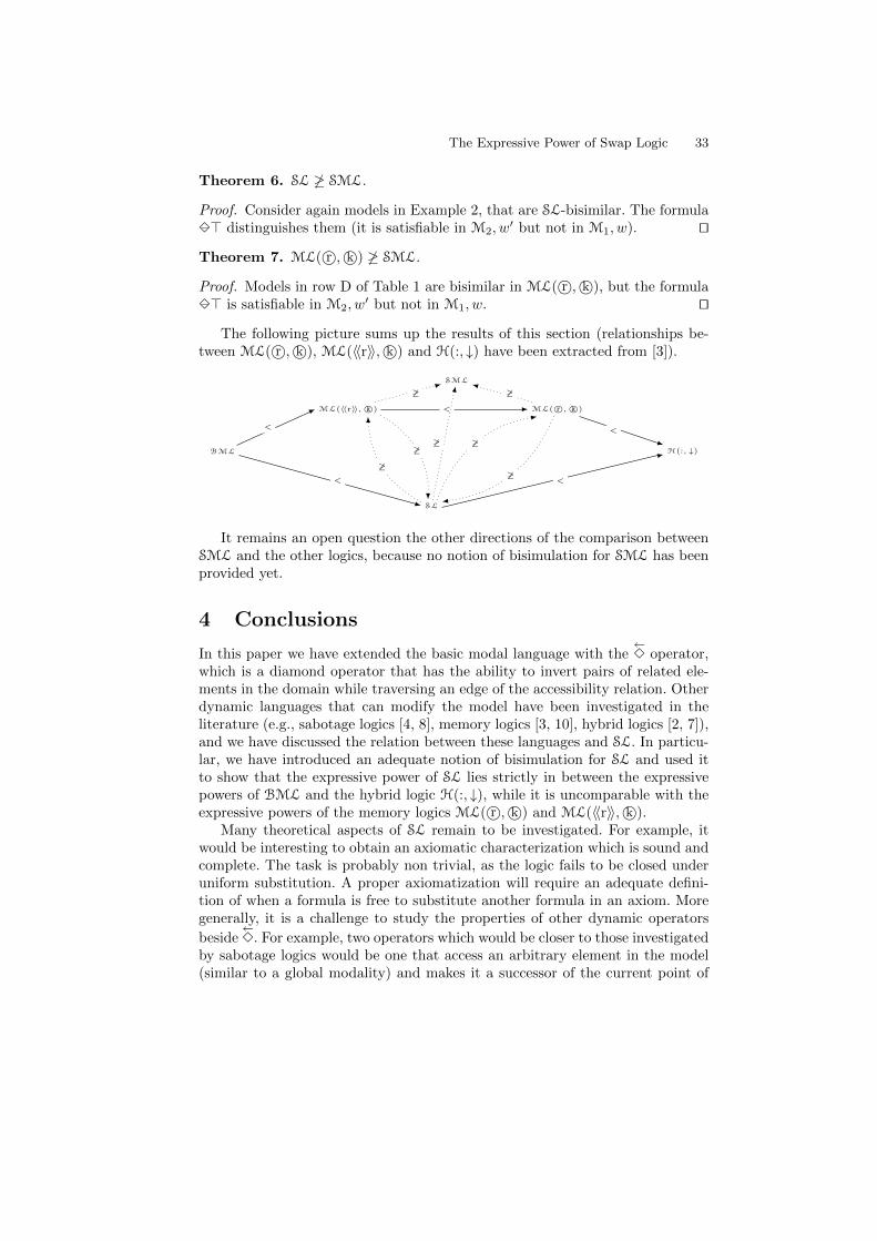
The Expressive Power of Swap Logic 33

Theorem 6. SL 6≥ SML.

Proof. Consider again models in Example 2, that are SL-bisimilar. The formula–3> distinguishes them (it is satisfiable in M2, w

′ but not in M1, w). ut

Theorem 7. ML( r©, k©) 6≥ SML.

Proof. Models in row D of Table 1 are bisimilar in ML( r©, k©), but the formula–3> is satisfiable in M2, w

′ but not in M1, w. ut

The following picture sums up the results of this section (relationships be-tween ML( r©, k©), ML(〈〈r〉〉, k©) and H(:, ↓) have been extracted from [3]).

BML

ML(〈〈r〉〉, k©) ML( r©, k©)

H(:, ↓)

SL

SML

<

<

<

< <

6≥

6≥6≥

6≥

6≥

6≥

6≥

It remains an open question the other directions of the comparison betweenSML and the other logics, because no notion of bisimulation for SML has beenprovided yet.

4 Conclusions

In this paper we have extended the basic modal language with the�3 operator,

which is a diamond operator that has the ability to invert pairs of related ele-ments in the domain while traversing an edge of the accessibility relation. Otherdynamic languages that can modify the model have been investigated in theliterature (e.g., sabotage logics [4, 8], memory logics [3, 10], hybrid logics [2, 7]),and we have discussed the relation between these languages and SL. In particu-lar, we have introduced an adequate notion of bisimulation for SL and used itto show that the expressive power of SL lies strictly in between the expressivepowers of BML and the hybrid logic H(:, ↓), while it is uncomparable with theexpressive powers of the memory logics ML( r©, k©) and ML(〈〈r〉〉, k©).

Many theoretical aspects of SL remain to be investigated. For example, itwould be interesting to obtain an axiomatic characterization which is sound andcomplete. The task is probably non trivial, as the logic fails to be closed underuniform substitution. A proper axiomatization will require an adequate defini-tion of when a formula is free to substitute another formula in an axiom. Moregenerally, it is a challenge to study the properties of other dynamic operators

beside�3. For example, two operators which would be closer to those investigated

by sabotage logics would be one that access an arbitrary element in the model(similar to a global modality) and makes it a successor of the current point of

34 Raul Fervari

evaluation, complemented with one that access a successor of the current pointof evaluation and deletes the edge between the two. Investigating further exam-ples of this kind of operator will let us have a clearer picture of the gains andlosses of working with logics which can dynamically modify the model.

Acknowledgments:

This work was partially supported by grants ANPCyT-PICT-2008-306, ANPCyT-PIC-2010-688, the FP7-PEOPLE-2011-IRSES Project “Mobility between Eu-rope and Argentina applying Logics to Systems” (MEALS) and the LaboratoireInternationale Associe “INFINIS”.

References

1. Areces, C.: Hybrid logics: The old and the new. In: Arrazola, X., Larrazabal, J.(eds.) Proc. of LogKCA-07. pp. 15–29. San Sebastian, Spain (2007)

2. Areces, C., ten Cate, B.: Hybrid logics. In: Blackburn, P., Wolter, F., van Benthem,J. (eds.) Handbook of Modal Logics, pp. 821–868. Elsevier (2006)

3. Areces, C., Figueira, D., Figueira, S., Mera, S.: The expressive power of memorylogics. The Review of Symbolic Logic 4(2), 290–318 (2011)

4. van Benthem, J.: An essay on sabotage and obstruction. In: Mechanizing Mathe-matical Reasoning. pp. 268–276 (2005)

5. Blackburn, P., van Benthem, J.: Modal logic: A semantic perspective. In: Handbookof Modal Logic. Elsevier North-Holland (2006)

6. Blackburn, P., de Rijke, M., Venema, Y.: Modal Logic, Cambridge Tracts in The-oretical Comp. Scie., vol. 53. Cambridge University Press (2001)

7. Blackburn, P., Seligman, J.: Hybrid languages. Journal of Logic, Language andInformation 4, 251–272 (1995)

8. Loding, C., Rohde, P.: Model checking and satisfiability for sabotage modal logic.In: Pandya, P., Radhakrishnan, J. (eds.) FSTTCS. LNCS, vol. 2914, pp. 302–313.Springer (2003)

9. Loding, C., Rohde, P.: Solving the sabotage game is PSPACE-hard. In: Mathemat-ical Foundations of Computer Science 2003, Lecture Notes in Computer Science,vol. 2747, pp. 531–540. Springer, Berlin (2003)

10. Mera, S.: Modal Memory Logics. Ph.D. thesis, Univ. de Buenos Aires and UFRSTMIA - Ecole Doctorale IAEM Lorraine Dep. de Form. Doct. en Informat. (2009)

11. Rohde, P.: On games and logics over dynamically changing structures. Ph.D. thesis,RWTH Aachen (2006)

Reasoning on Procedural Programsusing Description Logics with Concrete Domains

Ronald de Haan

Technische Universitat Wien

Abstract. Existing approaches to assigning semantics to proceduralprogramming languages do not easily allow automatic reasoning overprograms. We assign a model theoretic semantics to programs of a sim-ple procedural language, by encoding them into description logics withconcrete domains. This allows us to flexibly express several reasoningproblems over procedural programs, and to solve them efficiently usingexisting reasoning algorithms, for certain fragments of the programminglanguage. Furthermore, it allows us to explore for what further fragmentsof the programming language reasoning problems are decidable.

1 Introduction

There has been much research investigating the formal semantics of (proce-dural) programs. This has resulted in several different approaches (see for in-stance [5, 6]). Such approaches include defining several notions of semanticsfor programs (e.g. operational semantics, denotational semantics, axiomatic se-mantics) and investigating the relations between these different notions. Theseapproaches to investigating the semantics of programming languages are veryuseful for proving the correctness of compilers, for instance. However, it is verydifficult to automatically solve reasoning problems on procedural programs (e.g.deciding whether two programs are equivalent) using such kinds of semantics.Also, there is no unified approach to express and automatically solve variousdifferent reasoning problems, based on these existing notions of semantics ofprogramming languages.

We propose an approach that solves these problems. We assign a model theo-retic semantics to procedural programs. In particular, we will encode proceduralprograms as description logic knowledge bases. Description logics are widely usedformalisms to reason about large and complex knowledge bases [1], and thereare many efficient reasoners available for description logics. We will show that bymeans of this encoding of programs into description logic knowledge bases, wecan express reasoning problems over programs in the description logic language,and in this way reduce such reasoning problems to description logic reasoning.This allows us to leverage the performance of existing reasoning algorithms forour reasoning problems. Furthermore, we illustrate how this approach can behelpful in identifying fragments of programming languages for which these rea-soning problems are decidable, and analyzing the computational complexity ofsuch reasoning.

36 Ronald de Haan

The paper is structured as follows. We begin with briefly repeating how thesyntax and the semantics of the prototypical description logic ALC can be ex-tended with concrete domains, resulting in the description logic ALC(D), beforedefining a simple representative procedural programming language While. Then,we show how programs of this programming language can be encoded into thedescription logic ALC(D) in a semantically faithful way. Also, we illustrate howthis allows us to encode reasoning problems over While programs into ALC(D)reasoning problems. Finally, we will discuss the benefit of this method, in com-bination with suggestions for further research.

2 Preliminaries

A concrete domain D is a pair (∆D, ΦD), where ∆D is a set and ΦD a set ofpredicate names. Each predicate name P ∈ ΦD is associated with an arity n andan n-ary predicate PD ⊆ ∆n

D. A predicate conjunction of the form

c =∧

i≤k

(x(i)0 , . . . , x(i)

ni) : Pi,

where Pi is an ni-ary predicate, for all i ≤ k, and the x(i)j are variables, is

satisfiable iff there exists a function δ mapping the variables in c to elements

of ∆D such that (δ(x(i)0 ), . . . , δ(x

(i)ni )) ∈ PD

i , for all i ≤ k. A concrete domainis called admissible iff its set of predicate names is closed under negation andcontains a name >D for ∆D, and the satisfiability problem for finite conjunctionsof predicates is decidable.

An example of an admissible concrete domain is N = (N, ΦN ), where ΦNcontains unary predicates >N and ρn, and binary predicates ρ, for ρ ∈ {=, 6=, <,≤, >,≥}, and ternary predicates +,−, ?, \, and the required negations ofpredicates. All predicates are given the usual interpretation (here ρn holds for avalue x iff x ρ n holds).

We will use the description logic ALC(D) [2], which is the extension of theprototypical description logic ALC [7] with concrete domains. For an overviewof description logics with concrete domains, see [3].

We get the logic ALC(D), for a given concrete domain, by augmenting ALC

with abstract features (roles interpreted as functional relations), concrete fea-tures (interpreted as a partial function from the logical domain into the concretedomain), and a new concept constructor that allows to describe constraints onconcrete values using predicates from the concrete domain. More concretely, wecan construct concepts ∃u1, . . . , uk.P and u↑, for u, u1, . . . , uk paths and P ∈ ΨD

a k-ary predicate. A path is a sequence f1 . . . fng, where f1, . . . , fn (for n ≥ 0)are abstract features and g is a concrete feature.

Paths are interpreted as (partial) functions from the logical domain intothe concrete domain, by taking the composition of the interpretation of theircomponents. Concepts ∃u1, . . . , uk.P are interpreted as the set of objects thatare in the domain of the interpretation of all ui, such that the resulting concrete

Reasoning on Procedural Programs using Description Logic 37

objects satisfy the predicate P . Concepts u↑ are interpreted as those objectsthat are not in the domain of the interpretation of u. For a complete, formaldefinition of the syntax and semantics of ALC(D), see [2, 3], for instance.

3 The Programming Language While

3.1 Syntax

We define the syntax of the simple representative procedural programming lan-guage While (defined and used for similar purposes in [5, 6]) with the followinggrammar (we use right-associative bracketing). Let X be a countably infinite setof variables. We let n range over values in N1, x over X, a over expressions ofcategory AExp, b over expressions of category BExp, and p over expressionsof category Prog.

a ::= n | x | a+ a | a ? a | a− ab ::= > | ⊥ | a = a | a ≤ a | ¬b | b ∧ bp ::= x := a | skip | p; p | if b then p else p | while b do p

We consider programs as expressions of category Prog. We denote the set ofvariables occurring in a program p with V ar(p), the set of subterms of p ofcategory BExp with Bool(p), and the set of subterms of p of category AExpwith Arith(p). Furthermore, with cl(p) we denote the smallest set of programssuch that:

– cl(p) is closed under subterms, i.e., if p1 ∈ cl(p), p2 ∈ Sub(p) and p2 ∈ Prog,then p2 ∈ cl(p); and

– if while b do p1 ∈ cl(p), then also p1; while b do p1 ∈ cl(p) ∈ cl(p).

3.2 Operational Semantics

Given a finite subset of variables X ⊆ X, we define the set of states over X,denoted with StateX , as the set of total mappings µ : X → N.

We define the function BX that interprets expressions of category BExp asa function from StateX to B.

BX(s, a1 σ a2) = AX(s, a1) σ AX(s, a2) for σ ∈ {=,≤}BX(s,¬b) = ¬BX(s, b)

BX(s, b1 ∧ b2) = BX(s, b1) ∧BX(s, b2)

1In this paper, we restrict ourselves to natural numbers, but the approach can beextended straightforwardly to other concrete domains.

38 Ronald de Haan

We define the function AX that interprets expressions of category AExp as afunction from StateX to N.

AX(s, n) = n for n ∈ NAX(s, x) = state(x) for x ∈ X

AX(s, a1 ρ a2) = AX(s, a1) ρ AX(s, a2) for ρ ∈ {+, ?}AX(s, a1 − a2) = AX(s, a1)−AX(s, a2) if AX(s, a1)−AX(s, a2) ≥ 0AX(s, a1 − a2) = 0 if AX(s, a1)−AX(s, a2) < 0

For s ∈ StateX , x ∈ X and n ∈ N, we define s[x 7→ n](y) = n, if x = y, ands[x 7→ n](y) = s(y) if x 6= y.

For a program p and a set X such that var(p) ⊆ X ⊆ X, we define theoperational semantics as follows. We consider the transition system (Γ, T,⇒),where Γ = {(q, s) | q ∈ cl(p), s ∈ StateX}, T = StateX , and ⇒ ⊆ Γ × (Γ ∪ T ).

We define the relation ⇒ as the smallest relation such that for each s ∈StateX , for each a ∈ AExp, and for each b ∈ BExp

– we have (skip, s)⇒ s;– we have (x := a, s)⇒ s[x 7→ AX(a, s)];– (p1, s)⇒ (p′1, s

′) implies (p1; p2, s)⇒ (p′1; p2, s′);

– (p1, s)⇒ s′ implies (p1; p2, s)⇒ (p2, s′);

– we have (if b then p1 else p2, s)⇒ (p1, s), if PX(b, s) = >;– we have (if b then p1 else p2, s)⇒ (p2, s), if PX(b, s) = ⊥; and– we have (while b do p, s)⇒ (if b then (p; while b do p) else skip, s).

Note that⇒ is deterministic, i.e., for any s, t, t′, if s⇒ t and s⇒ t′, then t = t′.We say that p terminates on s with outcome t if (p, s) ⇒∗ t for t ∈ T . We saythat p does not terminate on s if there is no t ∈ T such that (p, s) ⇒∗ t. Wetake notice of the fact that if p does not terminate on s, then there is an infinitesequence (p, s)⇒ (p′, s′)⇒ . . . starting from (p, s).

3.3 Normal Form

In order to simplify our encoding of While programs into the description logicALC(D) later, we define a notion of normal forms for While programs. Considerthe following substitutions, preserving the operational semantics of programs,for a fresh variable x, for ρ ∈ {+, ?,−}, and π ∈ {=,≤}:

ϕ[x := a1 ρ a2] ; x1 := a1 ; ϕ[x := x1 ρ a2] if a1 6∈ X

ϕ[x := a1 ρ a2] ; x2 := a2 ; ϕ[x := a1 ρ x2] if a2 6∈ X

ϕ[a1 π a2] ; x1 := a1 ; ϕ[x1 π a2] if a1 6∈ X

ϕ[a1 π a2] ; x2 := a2 ; ϕ[a1 π x2] if a2 6∈ X

p; p; skip if p not of the form q; skip

Using the transformations on programs given by the above substitutions, we cantransform any program p to an operationally equivalent program p′ such thatthe following holds:

Reasoning on Procedural Programs using Description Logic 39

– each subexpression of p′ of category AExp is either of the form x ρ y, forx, y ∈ X and ρ ∈ {+, ?,−}, or of the form n for n ∈ N;

– for each subexpression of p′ of category BExp of the form t ρ s, for ρ ∈ {=,≤}, holds t, s ∈ X; and

– either p′ = skip, or p′ is of the form e; skip.

We will say that programs that satisfy this particular condition are in normalform.

4 Encoding Programs into ALC(D)

We model programs in the language While using description logic and its model-theoretic semantics. The concrete (i.e. numerical) values in the programminglanguage correspond to concrete values in the description logic. States are repre-sented by objects, and programs are represented by concepts. We represent theexecution of programs on states by a (functional) role nextState. In particular, fora given program p with V ar(p) = {x1, . . . , xn}, we denote states s ∈ StateV ar(p)with objects that have concrete features valueOfxi

.An execution of a program p will then be modelled by means of a nextState

sequence of objects. The objects in this sequence represent the states occurringin the particular execution of the program. Whenever in this execution of theprogram there occurs a state s such that the execution is continued from thisstate s with the intermediate program p′, the object corresponding to s is anelement of the concept Cp′ . Also, whenever this execution terminates, the finalobject in this sequence is an element of the concept Cskip.

4.1 Encoding

Take an arbitrary program p, i.e., an expression of category Prog. W.l.o.g., weassume p is in normal form. We define an ALC(D) TBox Tp as follows. We useconcept names Cq for each q ∈ cl(p), and concept names Db for each b ∈ Bool(p).

For each variable x ∈ V ar(p), we create a concrete feature valueOfx, and werequire

> v ¬valueOfx↑ (1)

We let nextState be an abstract feature and for Cskip we require:

Cskip v ¬∃nextState.> (2)

For each b ∈ Bool(p), we require the following, where x1, x2 range over X, andb1, b2 range over Bool(p):

Dx1=x2≡ ∃(valueOfx1

)(valueOfx2). = (3)

Dx1≤x2≡ ∃(valueOfx1

)(valueOfx2). ≤ (4)

D¬b1 ≡ ¬Db1 (5)

Db1∧b2 ≡ Db1 uDb2 (6)

40 Ronald de Haan

Furthermore, we let D> denote > and D⊥ denote ⊥. Then, for each q ∈ cl(p)of the form p1; p2 we require the following for Cq, where p1, p2, q1, q2 range overcl(p), x, y1, y2 range over X, a ranges over Arith(p),

C(x:=a);p2v ∃nextState.> u ∃nextState.Cp2

(7)

Cskip;p2v Cp2

(8)

C(x:=n);p2v ∃(nextState valueOfx). =n (9)

C(x:=y);p2v ∃(nextState valueOfx)(valueOfy). = (10)

C(x:=y1+y2);p2v ∃(nextState valueOfx)(valueOfy1

)(valueOfy2).+ (11)

C(x:=y1−y2);p2v (¬∃(valueOfy2

)(valueOfy1).≤ t

∃(valueOfy1)(nextState valueOfx)(valueOfy2

).+) u(¬∃(valueOfy2

)(valueOfy1).> t

∃(nextState valueOfx).=0) (12)

C(x:=y1?y2);p2v ∃(nextState valueOfx)(valueOfy1

)(valueOfy2).? (13)

C(x:=a);p2v ∃(valueOfy)(nextState valueOfy). = for y 6= x (14)

C(if b then q1 else q2);p2v (¬Db t Cq1;p2

) u (Db t Cq2;p2) (15)

C(while b do q);p2v (¬Db t Cq;(while b do q);p2

) u (Db t Cp2) (16)

Notice that, in general, the TBox Tp is not acyclic, since Axioms (7), (8),(15) and (16) can together induce a cycle.

4.2 Correctness

In order to use the above encoding of a program p into an ALC(D) TBox Tp toreduce reasoning problems over programs into ALC(D) reasoning, we show thefollowing correspondence between the operational semantics of p and the modeltheoretic semantics of Tp.

Lemma 1. For any program p, any X such that V ar(p) ⊆ X ⊆ X, any states ∈ StateX , any b ∈ Bool(p), and for any model I = (∆I, ·I) of Tp, we havethat d ∈ ∆I and (d, s(xi)) ∈ valueOfIxi

for all 1 ≤ i ≤ n implies that d ∈ CIb iff

BX(b, s) = >.

Proof (sketch). By induction on the structure of b. All cases follow directly fromthe fact that Axioms (3)-(6) hold.

Theorem 1. For any program p, any X such that V ar(p) ⊆ X ⊆ X, any states ∈ StateX such that p terminates on s with outcome t, and for any modelI = (∆I, ·I) of Tp we have that d ∈ CI

p and (d, s(xi)) ∈ valueOfIxifor all 1 ≤ i ≤ n

implies that e ∈ CIskip and (e, t(xi)) ∈ valueOfIxi

for all 1 ≤ i ≤ n, for some

e ∈ ∆I.

Proof. By induction on the length of the ⇒-derivation (p, s) ⇒k t. Assumed ∈ CI

p and (d, s(xi)) ∈ valueOfIxifor all 1 ≤ i ≤ n, for some d ∈ ∆I. The base

Reasoning on Procedural Programs using Description Logic 41

case k = 0 holds vacuously. In the case for k = 1, we know p = skip, sincep is in normal form. Therefore, we know s = t, and thus e = d witnesses theimplication.

In the inductive case, we distinguish several cases. Case p = skip; q. We know(p, s)⇒ (q, s)⇒k−1 t. Since I satisfies Tp, by Axiom (8), we know d ∈ CI

q . Theresult now follows directly by the induction hypothesis.

Case p = (x := a); q. We know (p, s) ⇒ (q, s′) ⇒k−1 t, and s′ = s[x 7→AX(a, s)]. Since I satisfies Tp, by Axioms (7), (9)-(13) and (14), we know theremust exist a d′ ∈ CI

q such that (d′, s′(xi)) ∈ valueOfIxifor all 1 ≤ i ≤ n. Then by

the induction hypothesis, the result follows directly.Case p = (if b then p1 else p2); q. Assume BX(b, s) = >. Then (p, s) ⇒

(p1; q, s) ⇒k−1 t. By Lemma 1, we know d ∈ DIb . Then, by the fact that Ax-

iom (15) holds, we know d ∈ CIp1;q. The result now follows directly by the

induction hypothesis. For BX(b, s) = ⊥ an analogous argument holds.Case p = (while b do p1); q. Assume BX(b, s) = >. Then (p, s)⇒2 (p1; p, s)⇒k−2

t. By Lemma 1, we know d ∈ DIb . Then, by the fact that Axiom (16) holds, we

know d ∈ Cp1;p. The result now follows directly by the induction hypothesis.If, however, in the same case holds BX(b, s) = ⊥, then (p, s)⇒3 (q, s)⇒k−3

t. By Lemma 1, we know d 6∈ DIb . By the fact that Axiom (16) holds, we know

d ∈ CIq . The result now follows directly by the induction hypothesis.

Theorem 2. For any program p, any X such that V ar(p) ⊆ X ⊆ X any state{x1 7→ c1, . . . , xn 7→ cn} = s ∈ StateX such that p does not terminate on s, thereexists a model I = (∆I, ·I) of Tp such that for some d ∈ ∆I we have d ∈ CI

p ,

(d, ci) ∈ valueOfIxi, for all 1 ≤ i ≤ n, and CI

skip = ∅.

Proof. Since p does not terminate on s, we know there exists an infinite ⇒-sequence (pi, si) ⇒ (pi+1, si+1), for i ∈ N, where (p1, s1) = (p, s). Consider thefollowing interpretation I = (∆I, ·I), where ∆I = {(pi, si) | i ∈ N}. For q ∈ cl(p),we let CI

q = {(pi, si) | pi = q}. For b ∈ Bool(p), we let DIb = {(pi, si) | i ∈

N,PX(b, s) = >}. For each x ∈ X, we let valueOfIx = {((pi, si), si(x)) | i ∈ N}.We let nextStateI = {((pi, si), (pi+1, si+1)) | i ∈ N}.

The definition of I implies that CIskip = ∅. Assume (pk, sk) ∈ CI

skip. Thenpk = skip, and thus (pk, sk) ⇒ sk, which contradicts our assumption of non-termination.

Clearly, I satisfies Axiom (1). Since CIskip = ∅, I also satisfies Axiom (2). It is

easy to verify, that by the definition of DIb we get that I satisfies Axioms (3)-(6).

To see that I satisfies Axioms (7)-(16), we take an arbitrary object (pj , sj)in the interpretation an arbitrary class CI

q , and we distinguish several cases.Consider pj = skip; q. Then by the constraints on ⇒, pj+1 = q and sj+1 = sj .This witnesses that the subsumption in Axiom (8) holds.

Consider pj = (x := a); q. Then by the constraints on ⇒, pj+1 = q andsj+1 = sj [x 7→ AX(a, sj)]. By definition of I, we know ((pj , sj), (pj+1, sj+1)) ∈nextStateI. It is now easy to verify that the subsumptions in Axioms (7), (9)-(13) and (14) are satisfied.

42 Ronald de Haan

Consider pj = (if b then p′1 else p′2); q. Assume BX(b, sj) = >. Then(pj , sj) ∈ DI

b . Also, by the constraints on ⇒, pj+1 = p′1; q and sj+1 = sj . Itis easy to verify that, in this case, the subsumption in Axiom (15) holds. Thecase for BX(b, sj) = ⊥ is completely analogous.

Consider pj = (while b do p′); q. If BX(b, sj) = >, then (pj , sj) ∈ DIb

and pj+1 = p′; pj and sj+1 = sj . If BX(b, sj) = ⊥, then (pj , sj) 6∈ DIb and

pj+1 = skip; q and sj+1 = sj . It is easy to verify that, in either case, thesubsumption in Axiom (16) holds.

Theorem 3. For any program p, any X such that V ar(p) ⊆ X ⊆ X any state{x1 7→ c1, . . . , xn 7→ cn} = s ∈ StateX such that p terminate on s, there existsa model I = (∆I, ·I) of Tp such that for some d ∈ ∆I we have d ∈ CI

p , (d, ci) ∈valueOfIxi

, for all 1 ≤ i ≤ n.

Proof (Sketch). We know there exists (p, s)⇒k (p′, s′)⇒ t. Analogously to theproof of Theorem 2, we can construct a model I from the sequence (p, s) ⇒k

(p′, s′). By similar arguments to those in the proof of Theorem 2 it follows thatI |= Tp. Then, (p, s) ∈ CI

p witnesses the further constraints on I.

Note that the syntax and operational semantics of While can be adapted tovarious concrete domains with varying operators. The encoding into ALC(D)can be adapted correspondingly, and a corresponding correlation between theoperational semantics and the model theoretic semantics can be proven.

4.3 Example

To illustrate the method described above, of encoding While programs intoALC(D) TBoxes, we will consider an example. Let p0 be the following pro-gram in normal form, that computes the factorial of the value stored in variablex and outputs this in variable y. Note that variable z is simply used to refer tothe constant value 1.

p0 = (y := 1; z := 1; while x > z do (y := y ? x; x := x− z); skip)

Furthermore, we will use the following abbreviations to refer to subprograms ofp0.

p1 = (z := 1; while x > z do (y := y ? x; x := x− z); skip)p2 = (while x > z do (y := y ? x; x := x− z); skip)p3 = (y := y ? x; x := x− z)p4 = (x := x− z)

Reasoning on Procedural Programs using Description Logic 43

We can now construct the ALC(D) TBox Tp0 , in the fashion described above.

Tp0 = { > v ¬valueOfx↑,> v ¬valueOfy↑,> v ¬valueOfz↑,

Cskip v ¬∃nextState.>,Dx<z ≡ ∃(valueOfx)(valueOfz).<,

C(y:=1);p1v ∃nextState.> u ∃nextState.Cp1 ,

C(z:=1);p2v ∃nextState.> u ∃nextState.Cp2 ,

C(y:=1);p1v ∃(nextState valueOfy).=1,

C(y:=1);p1v ∃(valueOfx)(nextState valueOfx).=,

C(y:=1);p1v ∃(valueOfz)(nextState valueOfz).=,

C(z:=1);p2v ∃(nextState valueOfz).=1,

C(z:=1);p2v ∃(valueOfx)(nextState valueOfx).=,

C(z:=1);p2v ∃(valueOfy)(nextState valueOfy).=,

Cp2v (¬Dx<z t Cp3;p2

) u (Dx<z t Cskip), (†)C(y:=y?x);p4;p2

v ∃nextState.> u ∃nextState.Cp4;p2, (†)

C(x:=x−z);p2v ∃nextState.> u ∃nextState.Cp2

, (†)C(y:=y?x);p4;p2

v ∃(nextState valueOfy)(valueOfy)(valueOfx).?,C(y:=y?x);p4;p2

v ∃(valueOfx)(nextState valueOfx).=,C(y:=y?x);p4;p2

v ∃(valueOfz)(nextState valueOfz).=,C(x:=x−z);p2

v (¬∃(valueOfz)(valueOfx).≤ t∃(valueOfx)(nextState valueOfx)(valueOfz).+) u(¬∃(valueOfz)(valueOfx).> t∃(nextState valueOfx).=0),

C(x:=x−z);p2v ∃(valueOfy)(nextState valueOfy).=,

C(x:=x−z);p2v ∃(valueOfz)(nextState valueOfz).= }

Note that Tp0 is not acyclic, since there are inclusion axioms (a) with Cp2as lhs

and Cp3;p2in the rhs, (b) with Cp3;p2

as lhs and Cp4;p2in the rhs, and (c) with

Cp4;p2 as lhs and Cp2 in the rhs. These axioms are marked with the symbol †.It is straightforward to construct models of the TBox Tp0 . One can simply

take an execution of the program p0, and transform this execution into a modelof Tp0 according to the intuition behind the encoding described above.

5 Reasoning Problems

Theorems 1, 2 and 3 allow us to use the encoding of While programs into ALC(D)to reduce several reasoning problems over While programs to reasoning problemsover ALC(D). For instance, termination of a program p reduces to unsatisfiabilityof the ABox Ap = {o1 : Cp} with respect to the TBox Tp ∪ {Cskip v ⊥}.

Also, we are able to encode abduction problems over While problems inthe description logic ALCO(D), which is ALC(D) extended with nominals. Thequestion what input states for a program p could have led to the (partial) outputstate s, for dom(s) ⊆ V ar(p), reduces to finding models for Ap = {i : Cp, o :

44 Ronald de Haan

Cskip} ∪ {(o, s(x)) : valueOfx | x ∈ dom(s)} and Tp, where Cskip is required tobe a nominal concept.

Another example is checking whether two (terminating) programs p1 and p2

are equivalent. Without loss of generality, we can assume V ar(p1) = V ar(p2).This equivalence check can be reduced to the problem of ALCO(D) unsatis-fiability of the ABox Ap1,p2 = {o : Cp1

, o : Cp2, s : Ctest} with respect to

the TBox Sp1 ∪ Sp2 ∪ Teq, where Spi is Tpi with Cskip replaced by Ciskip, andTeq = {Ctest ≡ (∃.(res1 valueOfx1)(res2 valueOfx1). 6= t · · · t ∃.(res1 valueOfxn)(res2 valueOfxn

). 6=) u ∃res1.C1skip u ∃res2.C2

skip}, for res1, res2 abstract features,

and C1skip, C

2skip and Ctest nominal concepts.

Naturally, this approach allows us to encode more intricate reasoning prob-lems over While programs into description logic reasoning problems. Descriptionlogic offers us a very flexible formalism to express a variety of reasoning problemsover While programs.

5.1 Decidability

A bit of care has to be taken with this powerful and general approach. Theproblems we consider generally balance on the bounds of decidability.

A concrete domain D is called arithmetic if its values contain the naturalnumbers, and it contains predicates for equality, equality with zero and incre-mentation. Unfortunately, satisfiability of ALC(D) concepts for arithmetic con-crete domains D with respect to general TBoxes is undecidable [4]. So, for manycases, our approach doesn’t directly result in a decision procedure.

This is no surprise, however. We know that we cannot decide equivalence ofWhile programs in general. For instance for the concrete domain Z (with additionand equality) we can easily encode the undecidable problem of whether a givenDiophantine equation Φ(x1, . . . , xn) = 0 has an integer solution (the subject ofHilbert’s Tenth Problem) as a reasoning problem over While programs. Similarly,it can be proven that equivalence of While programs with concrete domain N isundecidable.

Nevertheless, several decidable fragments of the While language can be ob-tained by either restricting the concrete domains or by forbidding statementsof the form (while b do p). By forbidding these while-statements, we end upwith acyclic TBoxes. We know that reasoning with respect to acyclic TBoxesis decidable for ALC(D). Restricting the concrete domain (and keeping while-statements), does not change the fact that we are dealing with general TBoxes.In this case, the concrete domain needs to be restricted quite severely, to getdecidability.

5.2 Examples

We can use the example from Section 4.3 to illustrate how to encode severalreasoning problems over While programs into ALC(D) reasoning problems. Forinstance, we can encode the problem of checking whether p0 is terminating as

Reasoning on Procedural Programs using Description Logic 45

the unsatisfiability problem of the ABox {o1 : Cp0} with respect to the TBoxTp ∪ {Cskip v ⊥}.

Using the expressivity of the description logic ALC(D), we can in fact ex-press a variety of different semantic properties to be checked automatically. Forinstance, in this fashion, we can express the problem whether p0 does not ter-minate with an output value for y that is less than or equal to 20 for all inputvalues for x that are greater than or equal to 4. This problem can be reducedto the unsatisfiability of the ABox {o1 : Cp0 u ∃(hasValuex).≥4} with respect tothe TBox Tp ∪ {Cskip v ∃(hasValuey).≤20}.

These examples of expressing reasoning problems in the ALC(D) languageillustrate the flexibility we get in expressing different reasoning problems. Wecan reduce the decision of any semantic property of While programs that isexpressible using the modelling of While programs in the ALC(D) language toreasoning on ALC(D).

6 Further Research

The results presented in this paper are only the beginning of a larger inquiryinvestigating the possibilities and bounds of approaching automated reasoningover (procedural) programming languages by means of assigning model-theoreticsemantics to programs. We suggest a number of directions for further researchneeded to get a better understanding of the topic.

Similar encodings of programming languages into the description logic ALC(D)could also be devised also for other procedural programming languages, as wellas for declarative programming languages. It needs to be investigated to whatextent this method is extendable to such other languages. Suitable programminglanguages for which this could be investigated as a next step include extensionsof the programming language While with language constructs for nondetermin-ism or parallellism, procedural programming languages that are based on goto-statements rather than while-statements, and simple, representative functionaland logic programming languages that operate on similar domains (e.g. numer-ical values). Once the method presented in this paper has been applied to suchlanguages, it will also be possible to investigate to what extent reasoning prob-lems on multiple programs of different programming languages (e.g. the equiv-alence problem of a While program and a program of a goto-based language)can be encoded in this framework.

Another important direction for further research is identifying larger frag-ments of the programming language While for which reasoning problems onprograms such as the ones we considered in this paper are decidable. By encod-ing programs into description logics, we get a conceptually simpler setting toinvestigate such questions. Programming languages can have a variety of differ-ent constructs behaving in various ways. Reasoning over such diverse structurescan get rather messy and complex. On the other hand, practically all reasoningproblems for description logics can be reduced to finding models for descriptionlogic knowledge bases (i.e. reduced to the satisfiability problem). The problem

46 Ronald de Haan

of finding such models is conceptually simple, and the semantic definition ofthe description logic language guides the search for models. Such a conceptuallysimpler setting might make it easier to identify decidable fragments. In additionto this conceptual simplification of the problem, we could use results and tech-niques from the field of description logic when investigating the decidability ofsuch fragments. For those fragments of the programming languages that lead todecidable reasoning problems, we can investigate the computational complexityof these reasoning problems.

7 Conclusions

We assigned a model theoretic semantics to programs of the simple procedurallanguage While, by encoding them into the description logic ALC(D). This al-lowed us to express a variety of reasoning problems over While programs usingthe expressivity of the description logic ALC(D). Furthermore, for a number ofrestricted fragments of the programming language While, this directly results ina method of solving such reasoning problems using existing (description logic)algorithms. Furthermore, this encoding leads to a new approach of exploringwhat fragments of the programming language allow for decidable reasoning overprograms. Further research includes a further characterization of fragments ofthe language that allow decidable reasoning, and extending this approach todifferent procedural (and declarative) programming languages.

References

1. Baader, F., Calvanese, D., McGuinness, D., Nardi, D., Patel-Schneider, P.: TheDescription Logic Handbook: Theory, Implementation and Applications. CambridgeUniversity Press (2003)

2. Baader, F., Hanschke, P.: A scheme for integrating concrete domains into conceptlanguages. In: Proceedings of the 12th international joint conference on Artificialintelligence - Volume 1. pp. 452–457. IJCAI’91, Morgan Kaufmann Publishers Inc.,San Francisco, CA, USA (1991)

3. Lutz, C.: Description logics with concrete domains—a survey. In: Advances in ModalLogics Volume 4. King’s College Publications (2003)

4. Lutz, C.: NExpTime-complete description logics with concrete domains. ACMTrans. Comput. Logic 5(4), 669–705 (Oct 2004)

5. Nielson, F., Nielson, H.R., Hankin, C.: Principles of Program Analysis. Springer-Verlag New York, Inc., Secaucus, NJ, USA (1999)

6. Nielson, H.R., Nielson, F.: Semantics with Applications: A Formal Introduction.John Wiley & Sons, Inc., New York, NY, USA (1992)

7. Schmidt-Schaubß, M., Smolka, G.: Attributive concept descriptions with comple-ments. Artif. Intell. 48(1), 1–26 (Feb 1991)

Small Steps in Heuristics for the Russian CardsProblem Protocols

Ignacio Hernandez-Anton

Dept. Philosophy, Logic and Philosophy of ScienceUniversity of Seville (Spain)

iha(at)us.es

Abstract. This work1 presents a couple of algorithmic techniques appli-ed to the Russian Cards Problem. This problem represent an idealizedscenario where Dynamic Epistemic Logic [4, 5, 8] plays an important rolein secure communications analysis. This logic is in a lower layer belowthe protocol desing tasks acting as a specification and verification formaltool. This work focusses not on the logical aspects but rather on the pro-tocol design/searching problem. It is important to have present the epis-temic formal notions of that logic to fully understand the epistemic func-tions developed here. Secure protocols found in this card game scenariomay be a good starting point for developing some aspects towards uncon-ditional information security. Hill-Climbing and Genetic Algorithms arestudied as searching techniques aimed to find optimal announcementsthat can be part of a secure communication protocol. Some problems asthe dimension and complexity of the search space are pointed out.

Keywords: Evolutionary computing, genetic algorithm, epistemic pro-tocols, information security.

1 Introduction

We present an algorithmic approach to search unconditionally secure protocols ofcommunicating agents within the well-known Russian Cards Problem scenario.In public/private key approaches as AES (Advanced Encription Standard), RSA(Rivest, Shamir, Adleman technique), DSA (Digital Signature Algorithm) orECC (Elliptic Curve Cryptography), secret information if safeguarded becauseof the high complexity of computational operations to decrypt the message, forinstance, RSA uses the IFD, the Integer Factorization Problem [10, 11]. Insteadof the computational hardness for security assurance, we focus on an information-based approach to protocol design in this work. We model the communicatingagents as cards players and the communicating secret is the ownership of thecards in the game. In this scenario it is possible to define good protocols regard-less of the computational complexity of cryptographic techniques [4, 5, 7].

1This work shares some content with [9] but add the Hill-Climber section and someconlusion remarks important to understand the nature of the search and the solutionspace.

48 Ignacio Hernandez-Anton

We just study the security aspects of communication in order to avoid eaves-dropping; other models of attacker are intentionally ommited here, we are awareof the importance of considering them for future works in order to gain ro-bustness though. We study how to guarantee the privacy of the message whichshould only be shared by those principal agents we legitimated. This will occurregardless of other agents listening passively to the information passed. Thereis a logical approach where this problem is formalized using dynamic epistemiclogic [4, 5].

We employ genetic algorithms to search for card deal protocols [12, 16, 17].Genetic algorithms are a bio-inspired family of computational techniques whichhave natural evolution as a model for encoding some critical aspects of solutionsas chromosomes-like data structures [3, 15]. An initial population is transformedby genetically inspired operations in order to produce new generations. The mostimportant ones are selection (of the fittest), crossing-over, and mutation,the latter ones add variety to the search producing the exploration of the solutionspace. We use JAVA to specify the russian cards problem and a genetic enginecalled jgap to search for protocols. For further details on the genetic engine seehttp://jgap.sourceforge.net/.

2 The Russian Cards Problem

From a pack of seven known cards (for instance 0-6) two players (a, b)each draw three cards and a third player (c) gets the remaining card.How can the two first players (those with three cards) openly (publicly)inform each other about their cards without cyphering the messages andwithout the third player learning from any of their cards who holds it?

Although this presentation of the problem has 7 cards in the stack and thedeal distribution is 3.3.1 (agent a draws three cards, b draws three and c drawsjust one), one may consider other scenarios, e.g., a 10-cards stack with a 4.4.2deal. To become familiar with a basic game scenario, let us call agents a, b andc. The cards are named 0, ..., 6. Deals distributions (size) are noted as integerstrings, for instance 3.3.1. Legitimated principals are a and b while c is theeavesdropper. We suppose the actual deal is 012.345.6 w.l.o.g. Communication isdone by truthful and public announcements, see [13, 14]. A public announcementfor an agent a is a set of a’s possible set of hands (we use a simplified notation todenote set of hands, e.g., {012, 125, 156} instead of {{0, 1, 2}, {1, 2, 5}, {1, 5, 6}}).

A secure announcement in this scenario should keep c ignorant throughoutthe entire communication and guarantee common knowledge of this agent’s igno-rance. According to that approach, a good protocol comprises an announcementsequence that verifies that:

Informativeness 1: Principals a and b know each other cards.Informativeness 2: It is common knowledge, at least for the principals, that

they do know each other’s cards.Security 1: The intruder, c, remains ignorant always.

Heuristics in Protocol Search 49

Security 2: It is common knowledge for all agents that the intruder remainsignorant.

Knowledge-based: Protocol steps are modelled as public announcements.

The reason we split the informativeness and security requirements into twoparts can be found in [5]. A protocol is then a finite sequence of instructionsdetermining sequences of announcements. Each agent chooses an announcementconditional on that agent’s knowledge. The protocol is assumed to be commonknowledge among all agents following Kerckhoff’s principle.

One knowledge-based protocol that consitutes a solution for the riddle is asfollows. Suppose that the actual deal of cards is that agent a has {0, 1, 2}, b has{3, 4, 5} and c has {6}.

– a says: My hand is one of {012, 046, 136, 145, 235}.– Then, b says: c’s card is 6.

After this, it is common knowledge to the three agents that a knows the handof b, that b knows the hand of a, and that c is ignorant of the ownership of anycard not held by itself. For further details on the notion of common knowledgesee [6].

We can also see these two sequences as the execution of a knowledge-basedprotocol. Given a’s hand of cards, there is a (non-deterministic) way to produceher announcement, to which b responds by announcing c’s card. The protocol isknowledge-based, because the agents initially only know their own hand of cards,and have public knowledge of the deck of cards and how many cards each agenthas drawn from the pack. It can be viewed as an unconditionally secure protocol,as c cannot learn any of the cards of a and b, no matter their computationalresources. The security is therefore not conditional on the high complexity ofsome computation.

3 Russian Hill-Climbers

Let’s begin with a simple metaheuristic technique called Hill-Climbing. It is avery simple algorithm that give us the oportunity to study the primitive be-haviour of the problem representation and the nature of the search space. TheGenetic Algorithms can be partially viewed as a sophistication of hill-climbing asoptimization technique. The latter constitutes a point of reference because, be-ing simpler, it can give clues about the need of using more sophisticated (hence,more resource-consuming) algorithms. Hill-Climbing is related to gradient as-cent, but it does not require you to know the strength of the gradient or even itsdirection: you just iteratively test new candidate solutions in the region of yourcurrent candidate and adopt the new ones if they are better. This enables youto climb up the hill until you reach a local optimum. To have a first flavor abouthow this technique would work on the russian card problem, we implemented aspecific Hill-Climber (see Algorithm 1) with the next parameters:

50 Ignacio Hernandez-Anton

– 100 executions over 3.3.1.– 100000 evaluations allowed

Algorithm 1 Russian Hill-Climber 1 (RHC1)

1: ANN ← All-hand-in initialization2: repeat3: ANN ′ ← BFM1(ANN)4: if Quality(ANN ’) > Quality(ANN) then5: ANN ← ANN ′

6: end if7: until 100000 generations or good protocol found8: return x

Algorithm 2 Single Bit Flip Mutator (BFM1)

1: h← Random(PossibleHandsForANN)2: if h ∈ ANN then3: ANN ′ ← Remove h from ANN4: else5: ANN ′ ← Include h in ANN6: end if7: return ANN ′

The initialization chosen for RHC1 produces an announcement with all handsin and a single Bit Flip Mutator BFP1 described in Algorithm 2. A randomhand from all possible hand to be included into the announcement is selectedto proceed as the if conditional states removing it if present or including itotherwise.

After 100 executions for 3.3.1 we obtained the next results: the average num-ber of protocol evaluations (in red) was 39288.16 with a minimum of 1716 anda maximum of 130321. Find attached the whole experiment graphics in Figu-re 1, see in the horizontal axis the excution number and in the vertical one thegeneration where the RHC1 found a global optimal solution.

4 Modelling cards protocols with Genetic Algo-rithms

The final objective of modelling cards protocols with genetic algorithms is to findprotocols for card deal sizes where an analytic solution is lacking. We reinvesti-gate protocols for 3.3.1 with genetic algorithms in order to study the behaviourof the relationship between the problem representation and the fitness func-tion used. This way we will be able to polish them for more complex scenarios.The use of genetic algorithms requires to satisfy two conditions: possible solu-tions can be represented by chromosomes and an evaluation function can be

Heuristics in Protocol Search 51

Fig. 1. 100 runs of RHC1 over 3.3.1; BFM1

defined in order to assign a value to each chromosome. Regarding this encodingrepresentation we observe that the set of possible hands of an agent can be ar-ranged in lexicographic order, e.g., for Russian Cards, the 35 hands are listedas 012, 013, . . . , 456. Then we assign a binary gene to each possible hand. Anannouncement is then represented by a 35-bitstring. To illustrate a mapping likethis see Figure 2 (a), we can encode several announcements into one chromosomeas in Figure 2 (b) representing this way an composite protocol. In the 3.3.1 caseas it is proved that there is a minimal protocol where just one announcement isneeded, we restrict the encoding representation to just agent a announcement,but if several announcements are required, this representation is flexible enoughto be adapted to it.

To evolve the population a fitness function assigns to each announcement avalue. As the protocols are knowledge-based, this function needs some epistemicaspects to be considered (implemented). As we are looking for a two-step protocol[2], we only need one announcement. The fitness function evaluates possibleannouncements. Note that if D is the set of cards, these announcements areelements of P(P(D)) with certain properties.

The first epistemic function is compCardsGivenAnnounce(Ann,Hand) whichreturns, for a given announcement Ann, the set of possible hands that an agenthaving Hand considers for the agent making the announcement:

52 Ignacio Hernandez-Anton

(a) Mapping announcements

(b) Allele decoding

Fig. 2. Chromosome general structure

compCardsGivenAnnounce : P(P(D))× P(D) 7→ P(P(D))compCardsGivenAnnounce(Ann,Hand) = {h ∈ Ann | h ∩Hand = ∅}

Now we define whatAgentLearnsFromAnnounce(Ann,Hand) that returnsthe set of cards that an agent having Hand learns from the agent. The functionis defined as:

Heuristics in Protocol Search 53

Algorithm 3 Genetic algorithm schema1: t← 02: Population initialization P (0) : {p1(0), . . . pk(0)}3: Evaluation of P (0): Φ(p1(0)), . . . , Φ(pk(0))4: while θ(P (t) 6= true) do5: Recombination P ′(t)← r(P (t))6: Mutation P ′(t)← m(P ′(t))7: Evaluation P ′(t) : Φ(p′1(0)), . . . , Φ(p′m(0))8: Selection P (t+ 1)← s(P ′(t))9: end while

10: return P (t+ s)

whatAgentLearnsFromAnnounce : P(P(D))× P(D) 7→ P(D)whatAgentLearnsFromAnnounce(Ann,Hand) =⋂

compCardsGivenAnnounce(Ann,Hand)

As an example, consider that, in the 3.3.1 setting with deal 012.345.6, aannounces that her hand is one of {012, 016, 234}. Then, a’s compatible handsfor b are {012, 016} and b learns that a has {0, 1} in this case. However an agentmay learn cards not only from the agent making the announcement, but alsofrom the remaining one. In our example, as c’s hand is {6}, c can also applythe previous function to learn that a holds card 2. But not that a’s compatiblehands for c are {012, 234}, so c learns that b holds cards 5. So c learns two cards,one from a and the other from b. The following function calculates this:

howManyAgentLearnsFromDeal : P(P(D))× P(D) 7→ NhowManyAgentLearnsFromDeal(Ann,Hand) =

|whatAgentLearnsFromAnnounce(Ann,Hand)|+|D| − |Hand| − |⋃ compCardsGivenAnnounce(Ann,Hand)|

In the fitness function we have to consider not only one deal (as that in ourexample) but all possible deals, in order to ensure that the announcement isunconditionally secure. The following function calculates, for a given announce-ment Ann and an agent having x cards, the minimum number of cards that theagent learns from the deal, by considering all possible agent’s hands consistentwith Ann:

minLearn : P(P(D))× N 7→ NminLearn(Ann, x) = min({howManyAgentLearnsFromDeal(Ann,H) |

H ⊆ D, |H| = x, compCardsGivenAnnounce(Ann,H) 6= ∅})In the same way, we can define a function maxLearn to calculate the maxi-

mum number of cards that an agent may learn. Then, the fitness function, giventhat the size of the deal is n.m.k, is defined as:

fitness : P(P(D))× N× N 7→ Zfitness(Ann,wI, wS) = wI ·minLearn(Ann,m)− wS ·maxLearn(Ann, k)

54 Ignacio Hernandez-Anton

The two values wI and wS are two natural numbers which measure the rele-vance of b’s knowledge and c’s ignorance, respectively. Obviously, the maximumvalue of the fitness function is obtained when b learns n+k cards (all a’s and c’scards) and c learns nothing. Then, the value of the fitness function is wI(n+k).The minimum value is −wS(n+m).

In the Java implementation we work with jgap’s chromosomes, that are se-quences of binary values. Prior to apply the fitness function we need to decodethe binary sequence into an announcement, as explained above. As the fitnessfunction is only allowed to return non-negative values, S(n + m) is added toevery result of our previous fitness function.

5 Weighing informativeness and ignorance

It seems reasonable to suppose that there is a correspondence between weighinginformativeness and security, on the one hand, and the efficiency in time of thesearch, on the other hand. In this section we demonstrate by statistical analysisthat this is not the case.

Weighing the fitness function with wI and wS we can influence the search,prioritizing one aspect or the other. If we consider informativeness more impor-tant than security, the algorithm lets survise to the next generation announce-ments where c could learn some cards. But if we focus on security and wish toavoid that situation, we will prioritize the security weight in order to devaluatethe announcement where c can learn.

Apart from the number of experiments, the size of the populations, and thenumber of generations set in the algorithm, the different weight combinationsalso allow us to create different scenarios and configurations. Those will be use-ful to collect data for statistical analysis. We wish to determine if there is acombination of weights that makes the search go faster.

The results of the algorithm search are stored and a statistic data analyzergoes through them in order to find relevant information. Figure 3 shows an3.3.1-case sample summary of the output of this analysis.

The first line of Figure 3 represents the weights that have the best meansearch time. Those weights could be good candidates to weigh other card deals(than 3.3.1), in order to investigate if there is a relation between weighing andsearch time. Expression minTime sPR TimeOfSearching 465 denotes the lowesttime, in millis, (the fastest protocol found) in the experiment that is associatedto the announcement [[0, 2, 5], [0, 4, 6], [1, 3, 4], [1, 5, 6], [2,

3, 6]] that has the weight wI = wInformativeness: 9, wS = wSecurity: 9.We also see similar parameters for the protocol with the highest search time. Atthe end, the search time range and mean of the entire experiment.

There are also other 7-cards distributions where the genetic approach cansearch for protocols. Considering the constraints among a, b, c cards presentedin [1], we obtain just two 7-cards scenarios where there exist protocols to search,namely: 3.3.1 and 4.2.1. Another case is 2.4.1. Then, there is no protocol where

Heuristics in Protocol Search 55

Best weighing MEAN preformance: 7,1

minTime sPR TimeOfSearching 465,

announcement: [[0, 2, 5], [0, 4, 6], [1, 3, 4], [1, 5, 6], [2, 3, 6]],

wInformativeness: 9,

wSecurity: 9,

Deal: 3.3.1

maxTime sPR TimeOfSearching 48875,

announcement: [[0, 1, 2], [0, 3, 4], [0, 3, 6], [1, 2, 6], [1, 3, 5],

[1, 3, 6], [2, 3, 4], [2, 3, 5], [4, 5, 6]],

wInformativeness: 6,

wSecurity: 7,

Deal: 3.3.1

(max-min) range time sPR 48410.0

Whole experiment mean timeOfSearching: 4031.433

Data analyzer timing: 915

Fig. 3. Stats analyzer output for 30-runs experiment wI,wS = [1..10]

first a makes the announcement. But swapping the roles of a and b we can applya 4.2.1 protocol.

The first experiment we did was a 30-runs from 1 to 10 different combinationsof weights. We can represent that as (SC 30, 500, 200, wI, wS, 3, 3, 1) where:

– SC stands for scenario configuration– 500 is the maximun number of generations allowed to evolve– 200 is the initial population size– 30 means thirty runs of the algorithm– wI is the weight for informativeness– wS is the weight for security– 3, 3, 1 is the deal distribution

Notice that wI and wS will vary from 1 to 10, generating different scenariosconfigurations in order to search for weight with the fastest result. The first threeresults from a 30-run sample experiments with wI = 4 and wS = 7 are depictedin Figure 4.

[[0, 2, 5], [0, 3, 4], [1, 3, 5], [1, 4, 6], [2, 3, 6]]:

58.0, 58.0, 73, 6464, 4, 0, 500, 200

[[0, 1, 6], [0, 2, 3], [1, 2, 4], [2, 5, 6], [3, 4, 5]]:

58.0, 58.0, 24, 2587, 4, 0, 500, 200

[[0, 1, 5], [0, 3, 4], [1, 2, 6], [2, 4, 5], [3, 5, 6]]:

58.0, 58.0, 48, 4478, 4, 0, 500, 200

. . .

Fig. 4. Partial output of SC 30, 500, 200, 4, 7, 3, 3, 1

Each two lines represent the execution of the serach for a 3.3.1 scenario. Forexample, considering the first protocol result, those figures mean:

56 Ignacio Hernandez-Anton

– [[0, 2, 5], [0, 3, 4], [1, 3, 5], [1, 4, 6], [2, 3, 6]] is the an-nouncement sequence. So a annouces {025, 034, 135, 146, 236}.

– 58.0 means the value the fitness functions assigned to that protocol.– 58.0 (the second occurrence) represents the maximum fitness value that can

be reached for any protocol.– 73 is the generation where this protocol was found.– 6464 is the time of searching in milliseconds.– 4 means the minimum number of cards b can learn using this protocol.– 0 is the maximum number of cards c can learn.– 500 is the maximun number of generations allowed to evolve.– 200 is the initial population size.

We executed a 30-runs experiment varying both weights from 1 to 10 generat-ing a total of 30× 10× 10 = 3000 protocol results. Figure 5 depicts informationabout the runtime for different weights for 3.3.1: on the left, the relation be-tween the differents weights assignments and the search mean time of those; onthe right, the standard deviation extracted from the first. At first sight one caninfer there is not a regular relation among those parameters. Hence we thinkthere is no use in extracting the best weights for ignorance and informativenessfrom this experiment and scale them up to larger deals.

(a) weighing and mean time (b) weighing and deviation time

Fig. 5. 3.3.1 weighing and mean stats graphics

6 Conclusions and future work

We confirmed the possibiliy of modelling unconditionally secure protocols searchusing Genetic Algorithms. The statistical analyzer showed the non-regular re-lation between weighing protocol (main) requirements and the mean time ofsearching. Althouth the genetic engine has been used for small deals, it has nowbeen studied in order to improve the time/memory efficiency to use it for largerdeals where several announcements comprise a protocol and a huge number ofoperations is presumed to be executed. In fact considering the exponential na-ture of the search space based on the cards distribution, our actual concern

Heuristics in Protocol Search 57

is focussed on a possible future guidance of the fitness function and the othervariation operators i.e: think that a 5.5.1 scenario with a binary announcementrepresentation has a search space cardinality around 2462. Using the RHC1 wecan observe the epistatic nature of the search space where a slight modificationof the chromosome leads to a huge penalty on the solution fitness assignment.We project new features regarding not just the statistical analysis over the pro-tocols found but the search for symmetry properties in protocols, features like anon-exhaustive fitness function and alternative protocol representation that cangive a clue about a possible analytic solution for larger and more complex deals.

References

1. Albert, M., Aldred, R., Atkinson, M., van Ditmarsch, H., Handley, C.: Safe com-munication for card players by combinatorial designs for two-step protocols. Aus-tralasian Journal of Combinatorics 33, 33–46 (2005)

2. Albert, M., Cordon, A., van Ditmarsch, H., Fernandez, D., Joosten, J., Soler, F.:Secure communication of local states in interpreted systems. In: Abraham, A.,Corchado, J., Gonzalez, S., De Paz Santana, J. (eds.) International Symposiumon Distributed Computing and Artificial Intelligence. pp. 117–124. Advances inIntelligent and Soft Computing, Vol. 91, Springer (2011)

3. Coello, C.A.C., Lamont, G.B., Veldhuizen, D.A.V.: Evolutionary Algorithmsfor Solving Multi-Objective Problems (Genetic and Evolutionary Computation).Springer-Verlag New York, Inc., Secaucus, NJ, USA (2006)

4. van Ditmarsch, H.: The Russian cards problem. Studia Logica 75, 31–62 (2003)5. van Ditmarsch, H., van der Hoek, W., Kooi, B.: Dynamic Epistemic Logic, Synthese

Library, vol. 337. Springer (2007)6. Fagin, R., Halpern, J., Moses, Y., Vardi, M.: Reasoning about Knowledge. MIT

Press, Cambridge MA (1995)7. Fischer, M., Wright, R.: Bounds on secret key exchange using a random deal of

cards. Journal of Cryptology 9(2), 71–99 (1996)8. Gochet, P., Gribomont, P.: Epistemic logic. In: Gabbay, D.M., Woods, J. (eds.)

Logic and the Modalities in the Twentieth Century. Handbook of the History ofLogic, vol. 7, pp. 99–195. North-Holland (2006)

9. Hernandez-Anton, I., Soler-Toscano, F., van Ditmarsch, H.P.: Unconditionally se-cure protocols with genetic algorithms. In: PAAMS (Special Sessions). pp. 121–128(2012)

10. Kumar, A., Ghose, M.K.: Overview of information security using genetic algorithmand chaos. Information Security Journal: A Global Perspective 18(6), 306–315(2009)

11. Menezes, A.J., Vanstone, S.A., Oorschot, P.C.V.: Handbook of Applied Cryptog-raphy. CRC Press, Inc., Boca Raton, FL, USA, 1st edn. (1996)

12. Ocenasek, P.: Evolutionary approach in the security protocols design. In: Blyth,A. (ed.) EC2ND 2005, pp. 147–156. Springer London (2006)

13. Plaza, J.: Logics of public communications. In: Emrich, M., Pfeifer, M., Hadzikadic,M., Ras, Z. (eds.) Proceedings of the 4th International Symposium on Method-ologies for Intelligent Systems: Poster Session Program. pp. 201–216. Oak RidgeNational Laboratory (1989)

14. Plaza, J.: Logics of public communications. Synthese 158(2), 165–179 (Sep 2007),http://dx.doi.org/10.1007/s11229-007-9168-7

58 Ignacio Hernandez-Anton

15. Sivanandam, S.N., Deepa, S.N.: Introduction to Genetic Algorithms. Springer Pub-lishing Company, Incorporated, 1st edn. (2007)

16. Whitley, D.: A genetic algorithm tutorial. Statistics and Computing 4, 65–85 (1994)17. Zarza, L., Pegueroles, J., Soriano, M.: Evaluation function for synthesizing security

protocols by means of genetic algorithms. In: Second international Conference onAvailability, Reliability and Securiy (ARES’07). IEEE (2007)

Markov Logic Networks forSpatial Language in Reference Resolution

Casey Kennington

Dialogue Systems Group, CITECFaculty of Linguistics and Literary StudiesUniversitat Bielefeld, Bielefeld, Germany

ckennington@cit-ec.uni-bielefeld.dewww.caseyreddkennington.com

Abstract. This paper presents an approach for automatically learningreference resolution, which involves using natural language expressions,including spatial language descriptions, to refer to an object in a con-text. This is useful in conversational systems that need to understand thecontext of an utterance, like multi-modal or embodied dialogue systems.Markov Logic Networks are explored as a way of jointly inferring a ref-erence object from an utterance with some simple utterance structure,and properties from the real world context. An introduction to mlns,with a small example, is given. Reference resolution and the role of spa-tial language are introduced. Different aspects of combining an utterancewith properties of a context are explored. It is concluded that mlns arepromising in resolving a contextual reference object.

Keywords: reference resolution, spatial language, markov logic net-works

1 Introduction

When we speak in a dialogue setting, we are often co-located (situated) in spaceand refer to objects in that space. Besides using salient properties to refer toan object, like its color, shape, and size, the language which is often used torefer to those objects make up spatial language; that is, where the object isrelative to some frame of reference, or as relative to other objects in that space.Understanding spatial language has application in fields like dialogue systems,multi-modal systems, and robotics, and makes up a part of natural languageunderstanding (nlu) in situated environments.

Work done in reference resolution has focused mainly on word-level ap-proaches (see [16]), without specific focus on spatial language. [20] constructa visual grammar for reference resolution with some degree of success. [18] looksat incremental reference resolution, but also only looks at words. In this paper,we extend the work of reference resolution by focusing on real world propertiesand bridge them with utterances that use spatial language, with a small amountof linguistic structure. We created a statistical model trained on generated data

60 Casey Kennington

and apply Markov Logic Networks (mlns, [14]) as the machine learning techniquein the experiments. It is shown that these models are significantly better thanthe baseline and that spatial language can be learned and applied to referenceresolution using mlns.

Plan of this paper: In the following section, mlns are defined and a simpleexample is given. The last part of the section will define reference resolution,with particular attention to spatial language and how it pertains to the task ofthis paper. In section 2, the domain, task, data, and procedure are explained.The experiment section then shows how well the system performs in referenceresolution, as well as some visual representations of how well the system learnedabout spatial language.

1.1 Markov Logic Networks

Markov Logic Networks have recently received attention in language processingfields like coreference resolution [3], semantic role labeling [13], and web informa-tion extraction [17]. As defined by [14], a Markov Logic Network is a first-orderknowledge base with a weight attached to each formula (see also Markov Ran-dom Fields [10], which make up mlns). This knowledge base is a declaration ofpredicates and typed arguments, along with weighted first-order logic (fol) for-mulas which define the type of relations between those predicates. This becomesa template to a mln network. Evidence in the form of instances of the predicatescan also be given either for training the network, or for direct inference. mlnsare a type of graphical model, where the nodes are not directed, an example ofwhich can be found in Figure 2.

As an example mln, consider the following statement: If you write some-thing down, you are twice as likely to remember it. We can represent this by thepredicates Write(person) and Remember(person). This can be formulated as:2 Write(x)⇒ Remember(x). This defines a relationship between Write and Re-member. The argument in both Write and Remember have the type person andfor this example, we will introduce only one constant: Mary. Building all possibleformulas given this information requires all combinations of positive and nega-tive predicates in the formula, resulting in four formulas, all with weight 2, whichwill be referred to as worlds. It is then necessary to determine which of thosefour formulas are satisfied by the original formula of Write(x)⇒ Remember(x).It is satisfied when Write is negative or when Remember is positive, or both.The only time it is not satisfied is when Write(Mary)⇒ ¬Positive(Mary).

After a set of worlds is created, one can perform inference by calculating aprobability:

P (X = x) =1

Ze∑

j wjfj(x) (1)

Where Z, also known as the partition function, is the normalizing constantgiven by:

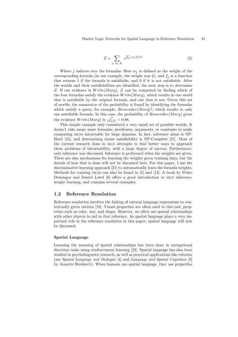
Markov Logic Networks for Spatial Language in Reference Resolution 61

Z =∑

x in X

e∑

j wjfj(x) (2)

Where j indexes over the formulas. Here wj is defined as the weight of thecorresponding formula (in our example, the weight was 2), and fj is a functionthat returns 1 if the formula is satisfiable, and 0 if it is not satisfiable. Afterthe worlds and their satisfiabilities are identified, the next step is to determineZ. If our evidence is Write(Mary), Z can be computed by finding which ofthe four formulas satisfy the evidence Write(Mary), which results in one worldthat is satisfiable by the original formula, and one that is not. Given this setof worlds, the numerator of the probability is found by identifying the formulaswhich satisfy a query, for example, Remember(Mary)?, which results in onlyone satisfiable formula. In this case, the probability of Remember(Mary) given

the evidence Write(Mary) is e2

e2+e0 = 0.88.This simple example only considered a very small set of possible worlds. It

doesn’t take many more formulas, predicates, arguments, or constants to makecomputing mlns intractable for large domains. In fact, inference alone is NP-Hard [15], and determining clause satisfiability is NP-Complete [21]. Most ofthe current research done in mln attempts to find better ways to approachthese problems of intractability, with a large degree of success. Furthermore,only inference was discussed. Inference is performed when the weights are given.There are also mechanisms for learning the weights given training data, but thedetails of how that is done will not be discussed here. For this paper, I use thediscriminative learning approach [21] to automatically learn the formula weights.Methods for training mlns can also be found in [5] and [12]. A book by PedroDomingos and Daniel Lowd [6] offers a good introduction to mln inference,weight learning, and contains several examples.

1.2 Reference Resolution

Reference resolution involves the linking of natural language expressions to con-textually given entities [18]. Visual properties are often used to this end, prop-erties such as color, size, and shape. However, we often use spatial relationshipswith other objects to aid in that reference. As spatial language plays a very im-portant role in the reference resolution in this paper, spatial language will nowbe discussed.

Spatial Language

Learning the meaning of spatial relationships has been done in navigationaldirection tasks using reinforcement learning [22]. Spatial language has also beenstudied in psycholinguistic research, as well as practical applications like robotics(see Spatial Language and Dialogue [4] and Language and Spatial Cognition [8]by Annette Herskovit). When humans use spatial language, they use properties

62 Casey Kennington

of the objects to which they are referring, such as color, shape, relative positionto another salient object, or relative position with respect to some axis [23].

Spatial language involves the language humans use to describe space and theobjects in that space. Humans require a common understanding of absolute andrelative spatial descriptions in order to communicate effectively. Words such asleft, right, top, bottom, and middle can represent absolute descriptions. Relativemeans that objects identified relative to another, perhaps more visually salientobject. This is where prepositions are often used; on top of, below, next to, tothe left of, beside. Even if we can gesture by pointing or looking at an object, westill usually need to be able to articulate the linguistic description of the objectsuch that the hearer of the utterance can uniquely identify the object to whichwe are referring. This linguistic description becomes even more important whena human is interfaced with a computer and language is the only medium forcommunication from human to computer, which is the experimental setting forthis paper.

It is essential to establish a frame of reference when using spatial language.It has been shown that alignment of the reference point is an ongoing processacross utterances, depending on the context [24]. [11] and [22] use two maincategories for the frame of reference: egocentric where the speaker is the frameof reference, and allocentric were the coordinates are not based on the speaker.In this paper, we will assume a single frame of allocentric reference. Specifically,both the hearer and the speaker use the same frame of reference.

2 Two-Dimensional Spatial Learning

In this section, the domain, task, data, and procedure of the experiment whichwill use mln to automatically learn reference resolution, particularly using spa-tial language, are defined. By giving accuracies of successfully referred objects,we show that mlns can be used successfully in reference resolution, as well assome figures that show the extent that spatial language was learned.

2.1 Domain, Task, Data, and Procedure

Domain

In this study, we used the Pentomino puzzle piece domain. A Pentomino boardis visually represented in rows and columns with pieces viewable by a human.On the computer side, pieces are identified with unique arbitrary identifiers. Theproperties of the pieces which are visually distinguishable by a human (color,shape, row, column, relation to other pieces) are accessible also to the computer.In this way, the board and pieces effectively become a shared visual context be-tween the human and the computer, as described in [20]. An example Pentominoboard can be seen in Figure 1.

Perspective is not being studied in this paper, so assumptions need to bemade about the frame of reference. The Pentomino board defines a fixed frameof reference which is a board on a computer screen. Also, given the nature of

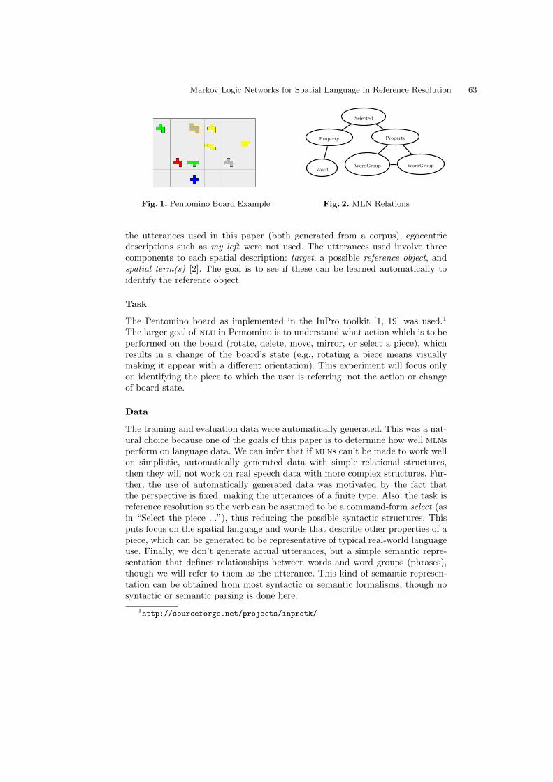
Markov Logic Networks for Spatial Language in Reference Resolution 63

Fig. 1. Pentomino Board Example

Selected

Property

Word

Property

WordGroup WordGroup

Fig. 2. MLN Relations

the utterances used in this paper (both generated from a corpus), egocentricdescriptions such as my left were not used. The utterances used involve threecomponents to each spatial description: target, a possible reference object, andspatial term(s) [2]. The goal is to see if these can be learned automatically toidentify the reference object.

Task

The Pentomino board as implemented in the InPro toolkit [1, 19] was used.1

The larger goal of nlu in Pentomino is to understand what action which is to beperformed on the board (rotate, delete, move, mirror, or select a piece), whichresults in a change of the board’s state (e.g., rotating a piece means visuallymaking it appear with a different orientation). This experiment will focus onlyon identifying the piece to which the user is referring, not the action or changeof board state.

Data

The training and evaluation data were automatically generated. This was a nat-ural choice because one of the goals of this paper is to determine how well mlnsperform on language data. We can infer that if mlns can’t be made to work wellon simplistic, automatically generated data with simple relational structures,then they will not work on real speech data with more complex structures. Fur-ther, the use of automatically generated data was motivated by the fact thatthe perspective is fixed, making the utterances of a finite type. Also, the task isreference resolution so the verb can be assumed to be a command-form select (asin “Select the piece ...”), thus reducing the possible syntactic structures. Thisputs focus on the spatial language and words that describe other properties of apiece, which can be generated to be representative of typical real-world languageuse. Finally, we don’t generate actual utterances, but a simple semantic repre-sentation that defines relationships between words and word groups (phrases),though we will refer to them as the utterance. This kind of semantic represen-tation can be obtained from most syntactic or semantic formalisms, though nosyntactic or semantic parsing is done here.

1http://sourceforge.net/projects/inprotk/

64 Casey Kennington

The training data were generated by creating one thousand boards. Eachboard was randomly assigned 3-5 rows and 3-5 columns (number of rows andcolumns need not be the same), creating a small variability in the dimensions ofthe boards which allowed for generality. The number of pieces was also randomlyassigned, between 4 and 6 pieces for training where the maximum number ofpieces must be no larger than the number fields in the smallest possible board.Each piece was assigned a random color, shape, row, and column, and of coursemultiple pieces could not occupy the same space. After each piece was in place,one was chosen randomly to be the selected piece, the piece that was referred.A pseudo-utterance that described that piece was then generated in the formof a simple semantic representation. The pseudo-utterance contained words thatdescribed the shape, color, absolute, and relative descriptions. There were a totalof 5 colors and 7 shapes. I used the following absolute spatial descriptions: left,right, top, bottom, middle, corner, and the following relative spatial descriptions:above, higher than, on top of, next to, beside, below, under, beneath, on the leftof, and on the right of. The shape, color, and all absolute spatial descriptionswere treated as a bag of words. The words in a relative spatial description weretreated as a word group, which corresponds to a small amount of linguisticstructure (grouped, for example, as prepositional phrases).

An example of this is given in Figure 3. Here, the selected piece is a red crosssomewhere near the middle, below a gray cross which is in the middle of the toprow. The generated pseudo-utterance would be something like select the middlered cross below the gray cross in the top middle, where red, middle, and cross aretreated as simple words, and below the gray cross in the top middle is treated asa word group.

The evaluation set was similarly generated, but used 100 boards, with rowand column lengths between 3 and 7, and the number of pieces was between 4and 9. The range of rows and columns, and the range of possible number of pieceswas larger than in training. For each evaluation experiment, the evaluation setwas randomly generated, so each one was different.

Part of the effort in using mlns is determining what should be specified aspredicates (e.g. Color, Shape, Row, etc) and what should be learned automati-cally. In this paper, only one abstract predicate, Property, that implicitly doesthe typing into different features was used. The example in Figure 3 shows asingle Piece, and multiple Property predicates for that piece. Where numberswould cause confusion, they can simply be annotated with a unique propertytype (e.g. column 1 = 1C). The properties used as represented in Figure 3 weretype, color, % horizontal from center, % vertical from center, row, and column.The predicates Word and WordGroup represent the words, and group of words,respectively, as previously explained. The final argument for all the predicatesis the board identifier, which separated states of the board and correspondingselected pieces and utterances from other boards. The second argument in Word-Group, groupID, is a unique identifier that is the same across a group of words.In Figure 3, the identifier is simply 1, but if more WordGroups existed, then

Markov Logic Networks for Spatial Language in Reference Resolution 65

they would be represented by a different number. A typical representation of aboard would have many pieces and more word groups for the utterance.

Figure 3 also shows the actual mln template that was used for training.Lines 1-5 are the predicate definitions and argument types and 6-7 define therelations via fol formulas. The + before an argument in a formula tells the mlnto learn from each constant in the training data, which is necessary when dealingwith natural language because it must learn how to interpret individual wordsas individual symbolic features. The result is that words and word groups aremapped to properties.

mln template1 Piece(piece, boardID)2 Property(piece, prop, boardID)3 Word(word, boardID)4 WordGroup(gWord, groupID, boardID)5 Selected(piece, boardID)6 Word(+w, b)∧Property(p,+p1, b)⇒Selected(p, b)

7 WordGroup(+w1, e, b)∧WordGroup(+w2, e, b)∧Property(p,+p1, b)⇒ Selected(p, b)

Fig. 3. mln template and example for selectthe middle red cross below the gray cross inthe top middle

examplePiece(tile-7,-1)

Property(tile-7,X,-1)

Property(tile-7,red,-1)

Property(tile-7,0H,-1)

Property(tile-7,-67V,-1)

Property(tile-7,2R,-1)

Property(tile-7,1C,-1)

Word(red,-1)

Word(cross,-1)

Word(center,-1)

WordGroup(below,1,-1)

WordGroup(gray,1,-1)

WordGroup(cross,1,-1)

WordGroup(top,1,-1)

WordGroup(middle,1,-1)

Procedure

The Alchemy system [5] for mln learning and inference was used for these exper-iments.2 The board and pseudo-utterances were represented as evidence to themln, as well as which piece was selected. Discriminative training with Select asthe predicate to query was used. As mln is a way of defining a relation betweenvarious predicates, those predicates need to represent meaningful informationfrom the Pentomino board, as well as the utterance and how the utterance re-lates to the board, as shown in Figure 3.

To test, a board is similarly randomly generated as in training, and a piece isagain randomly selected. However, the selected piece is what was being inferredabout by the mln, so it was kept hidden. The pseudo-utterance was generated inthe same way as in training. Using the state of the board and the utterance, themln system then inferred which piece was being described by that utterance. Ifthe piece with the highest probability matched the selected piece, it was marked

2http://alchemy.cs.washington.edu/

66 Casey Kennington

as correct. If there was a tie, then the first one returned by the query was chosen.This is therefore a simple measure of accuracy. In this scenario, the majority classbaseline would be 25%, where 4 is the minimum number of possible pieces duringevaluation.

2.2 Experiment: Absolute and Relative Spatial Understand-ing

Table 1 shows various training and evaluation settings that were used. Each rowrepresents the parts of the utterance and board properties that were represented.The Full column was trained on one set of boards with all possible descriptions(shape, color, relative spatial, absolute spatial, row, column) and that trainedmodel was used to evaluate for both rows in the column. Even though, wordslike row and column are often used to distinguish pieces in this kind of setting,those words are left out of evaluation unless specifically stated because they areeasy features to learn as they map easily to their corresponding piece properties.The Ind column (short for Individual) in the table shows the results when eachrow’s setting was trained individually, and subsequently evaluated.

Description Full% Ind%

shape, color 70 92absolute spatial with rows and columns 87 97absolute spatial 65 69relative spatial 35 59shape, color, absolute spatial 92 100absolute and relative spatial 34 82all 58 88

Table 1. Various Select Accuracy Results; Full represents a single trained model withall features and evaluated only on the features of the row, Ind represents a differentmodel trained and evaluated on the features of the corresponding row.

Though the main goal of this paper is to show that a mln can effectively learnspatial language reference resolution, it is also useful to see how a mln performsin different settings, as shown in Table 1. Overall, alchemy and mln performabove baseline in all areas. Most interesting to note is the fact that when alltypes were used (shape, color, absolute, and relative spatial), the accuracy wasonly 58%. This is possibly due to the fact that it was trained on a system whichincluded the rows and columns (information that was not used at evaluation).This is evidenced by the fact that the Ind column for the same row gave 88%and was trained on similar settings, only minus rows and columns, forcing themodel to learn how to resolve without rows and columns as piece properties. It isfurther interesting to note that shape, color, and absolute spatial received highaccuracies for both systems. However, a system with relative spatial knowledge

Markov Logic Networks for Spatial Language in Reference Resolution 67

will be more robust to real language input in a real-world environment, despitethe somewhat lower probability.

2.3 Board Distributions

Another way of showing how well the mln learned about spatial language is tolook at a graphical representation of the probabilities of each piece in the boardas a gradient, where the darker in color, the higher the probability. Some of thesegradient boards (using a 5x5 board) are displayed, where all fields are taken bya piece with the same color and shape, thus nullifying them as distinguishingfeatures. First, a look at absolute spatial language. An example of absolute top-left, and absolute centre-right are represented in Figures 4 and 5 respectively.These show that the absolute language was well learned, especially for a specificpoint like top-left in Figure 5.

Fig. 4. Center Right Fig. 5. Top Left

Relative spatial language is a little more difficult to visualize in a gradient,but certain relative relations can be isolated by looking at a gradient map withits corresponding board, where the board is not completely filled. The board andgradient map for the relation above can be found in Figures 6 and 7. For a pieceto be above another piece, it simply needed to be in a higher row than that piece,regardless of the column. The notion of above is learned, but the distributionover the pieces is somewhat unexpected. Any piece that is above another pieceshould have some probability, with the darker gradients starting at the higherpieces, decreasing with the rows. The concept of above here is generally learned,though there is need for improving the model when it comes to relative spatialrelationships.

After the submission of this paper, we used the principles that were learnedhere and applied them to real, non-generated Pentomino data collected in aWizard-of-Oz study [7, 18] in a situated setting of natural language understand-ing. That work resulted in a paper [9] in which we used mlns not only forreference resolution, but to predict a semantic frame which also included theaction to take on the referred piece, and the desired state of the board after the

68 Casey Kennington

action was complete (for example, the utterance rotate the blue cross clockwisewould have rotate as the action, the blue cross as the referred piece, and theresulting state of the board would be that it appears 90 degrees to the right).Experiments were performed on hand-annotated speech, as well as automaticallytranscribed speech, evaluated incrementally (word-level increments), and on fullutterances. We concluded that information from the visual context (pentominoboard), the utterance (which included a syntactic context-free parser and corre-sponding semantic representation), and previous discourse context perform well,in terms of frame accuracy, in the Pentomino domain.

Fig. 6. above Board Fig. 7. above Map

3 Conclusions and Future Work

Markov Logic Networks are effective in reference resolution in a two-dimensionaldomain like Pentomino. They can effectively learn a mapping between an utter-ance and real world object properties, including utterances that contain spatiallanguage descriptions.

Future work involves using what was learned via this task and implementingit into a larger natural language understanding framework. We will continueto use mlns, and further incorporate other real-world information, such as eyegaze and gestural information from the human. We will extend this to domainsbeyond Pentomino, domains which use real world spatial representations, andapply it in interactive settings.

References

1. Baumann, T., Schlangen, D.: The InproTK 2012 Release. In: Proceedings of Hu-man Language Technologies: The 2012 Annual Conference of the North AmericanChapter of the Association for Computational Linguistics on - NAACL ’12 (2012)

2. Carlson, L.A., Hill, P.L.: Formulating Spatial Descriptions across Various DialogueContexts. In: Spatial Language and Dialogue, pp. 89–103 (2009)

Markov Logic Networks for Spatial Language in Reference Resolution 69

3. Chen, F.: Coreference Resolution with Markov Logic. Association for the Advance-ment of Artificial Intelligence (2009)

4. Coventry, K.R., Tenbrink, T., Bateman, J. (eds.): Spatial language and dialogue,vol. 3. Oxford University Press (2009)

5. Domingos, P., Kok, S., Poon, H., Richardson, M.: Unifying logical and statisticalAI. American Association of Artificial Intelligence (2006)

6. Domingos, P., Lowd, D.: Markov Logic An Interface Layer for Artificial Intelligence.Morgan & Claypool (2009)

7. Fernandez, R., Lucht, T., Schlangen, D.: Referring under restricted interactivityconditions. In: Proceedings of the 8th SIGdial Workshop on Discourse and Dia-logue. pp. 136–139 (2007)

8. Herskovits, A.: Language and Spatial Cognition. Cambridge University Press(2009)

9. Kennington, C., Schlangen, D.: Markov Logic Networks for Situated IncrementalNatural Language Understanding. In: Proceedings of SIGdial 2012. Association forComputational Linguistics, Seoul, Korea (2012)

10. Kindermann, R., Snell, J.L.: Markov random fields and their applications (1980)11. Levinson, S.C.: Space in Language and Cognition. Explorations in Cognitive Di-

versity, vol. 5. Cambridge University Press (2003)12. Lowd, D., Domingos, P.: Efficient weight learning for Markov logic networks.

Knowledge Discovery in Databases: PKDD 2007 pp. 200–211 (2007)13. Meza-Ruiz, I., Riedel, S.: Jointly identifying predicates, arguments and senses using

Markov logic. In: Proceedings of Human Language Technologies: The 2009 AnnualConference of the North American Chapter of the Association for ComputationalLinguistics on - NAACL ’09. p. 155. No. June, Association for ComputationalLinguistics, Morristown, NJ, USA (2009)

14. Richardson, M., Domingos, P.: Markov logic networks. Machine Learning 62(1-2),107–136 (2006)

15. Roth, D.: On the hardness of approximate reasoning. Artificial Intelligence 82(1-2),273–302 (1996)

16. Roy, D.: Grounding words in perception and action: computational insights. Trendsin Cognitive Sciences 9(8), 389–396 (Aug 2005)

17. Satpal, S., Bhadra, S., Rajeev, S.S., Prithviraj, R.: Web Information ExtractionUsing Markov Logic Networks. Learning pp. 1406–1414 (2011)

18. Schlangen, D., Baumann, T., Atterer, M.: Incremental Reference Resolution: TheTask, Metrics for Evaluation, and a Bayesian Filtering Model that is Sensitive toDisfluencies. In: Proceedings of SIGdial 2009 the 10th Annual SIGDIAL Meetingon Discourse and Dialogue. pp. 30–37. No. September (2009)

19. Schlangen, D., Skantze, G.: A general, abstract model of incremental dialogueprocessing. Proceedings of the 12th Conference of the European Chapter of theAssociation for Computational Linguistics on - EACL ’09 (April), 710–718 (2009)

20. Siebert, A., Schlangen, D.: A Simple Method for Resolution of Definite Reference ina Shared Visual Context. In: Proceedings of the 9th SIGdial Workshop on Discourseand Dialogue. pp. 84–87. No. June, Association for Computational Linguistics(2008)

21. Singla, P., Domingos, P.: Discriminative Training of Markov Logic Networks. Com-puting 20(2), 868–873 (2005)

22. Vogel, A., Jurafsky, D.: Learning to Follow Navigational Directions. In: Proceedingsof the 48th Annual Meeting of the Association for Computational Linguistic. pp.806–814 (2010)

70 Casey Kennington

23. Vorwerg, C.: Consistency in Successive Spatial Utterances. In: Coventry, K.R.,Tenbrink, T., Bateman, J.A. (eds.) Spatial Language and Dialogue, chap. 4, pp.40–55. Oxford University Press (2009)

24. Watson, M.E., Pickering, M.J., Branigan, H.P.: Alignment of Reference Frames inDialogue. In: Cognitive Science Society (2004)

Using Conditional Probabilities and VowelCollocations of a Corpus of OrthographicRepresentations to Evaluate Nonce Words

Ozkan Kılıc

Department of Cognitive Science, Informatics Institute, Middle East TechnicalUniversity, Ankara, Turkey

e-mail: okilic@ii.metu.edu.tr

Abstract. Nonce words are widely used in linguistic research to evalu-ate areas such as the acquisition of vowel harmony and consonant voic-ing, naturalness judgment of loanwords, and children’s acquisition ofmorphemes. Researchers usually create lists of nonce words intuitivelyby considering the phonotactic features of the target languages. In thisstudy, a corpus of Turkish orthographic representations is used to proposea measure for the nonce word appropriateness for linearly concatenativelanguages. The conditional probabilities of orthographic co-occurrencesand pairwise vowel collocations within the same word boundaries areused to evaluate a list of nonce words in terms of whether they would berejected, moderately accepted or fully accepted. A group of 50 Turkishnative speakers were asked to evaluate the same list of nonce words. Boththe method and the participants displayed similar results.

Keywords: Nonce words, Orthographic representations, Conditional probabil-ities.

1 Introduction

Nonce words are frequently employed in linguistic studies to evaluate areas suchas well-formedness [1], morphological productivity [2] and development [3], judg-ment of semantic similarity [4], and vowel harmony [5]. Nonce words are alsoused to understand the process of adopting loan words. The majority of loanedwords undergo certain phonetic changes to more resemble the lexical entries ofthe language into which they will be adopted [6]. For example, television inTurkish becomes televizyon /televızjon/ because /jon/ is more frequent than/Zın/ in Turkish1. Similarly, train is adopted as tren /tren/ because, similarto diphthongs, vowel-to-vowel co-occurrences are not usually allowed in Turkish

1In the METU-Turkish Corpus, there are 181 occurrences with the segment /Zın/of which only 30 are at the terminating word boundaries. On the other hand, there are5,945 occurrences with the segment /jon/ of which 3,190 are at the terminating wordboundaries, excluding the word televizyon.

72 Ozkan Kılıc

non-compound words. This phenomenon shows that the speakers of a languageare aware of the possible sound frequencies and collocations of their native lan-guages, and they can make judgements on the naturalness of loan words, recentlyinvented words and nonce words by using their knowledge of the existing Turk-ish lexis. Thus, the acceptability of nonce words is a logical decision based onknown-word statistics.

The acceptability of nonce words can be investigated by experimental in-vestigations through phonotactic properties or factor-based analysis [7]. In theexperimental investigations, it is observed that the participants accepted orrejected nonce words according to probable combinations of sounds [1, 8]. Infactor-based analysis, the acceptability of nonce words is evaluated through theco-occurrences of syllables or consonant clusters locally [9] or non-locally [10–12]or through nucleus-coda combination probabilities [13].

In this study, the acceptability of nonce words was assessed using the condi-tional probabilities of the bigram co-occurrences of the orthographic represen-tations locally and the pairwise collocations of the vowels within the same wordboundaries. Similar methods within the context of phonotactic modeling hadbeen used for Finnish vowel harmony [14]. Yet in this study, the local bigramphonotactic modeling was used to evaluate Turkish nonce words. Two thresholdvalues were set for the decision to reject, moderately accept and fully accept.The threshold values were computed according to the length of each input string.For the evaluation of the conditional and collocation probabilities, the METU-Turkish Corpus containing about two million words was employed [15]. The listof nonce words was created intuitively. The same list of nonce words evaluatedby the method was also given to 50 Turkish native speakers to judge the level ofacceptability of each word. The 25 male and 25 female Turkish native speakers,had an average age is 31.26 (s = 4.11).The results from the native speakers werevery similar to the results provided by the statistical method. In this paper, briefinformation about Turkish language and plausibility of conditional probabilitieswill be given then details of the method and the results will be presented.

2 Turkish Language and Conditional Probabil-ity

Turkish has 8 vowels and 21 consonants, and it is agglutinative with a consid-erably complex morphology [16, 17]. While communicating, the word internalstructure in Turkish is required to be segmented because Turkish morphosyn-tax plays a central role in semantic analysis. For example, although Turkish isconsidered as an SOV language, the sentences are usually in a free order. Thus,the subject and object of a verb can only be determined by the morphologicalmarkers as in (1) rather than the word order.

(1) Kopek adam-ı ısırdı. Kopeg-i adam ısırdı.Dog man-Acc bit Dog-ACC man bit

Using Conditional Probabilities to Evaluate Nonce Words 73

The dog bit the man. The man bit the dog.

The description of Turkish word structure depends heavily on morphophono-logical constraints and morphotactics. In Turkish morphotactics, the continua-tion of a morpheme is determined by the preceding morpheme or by the stemas in (2).

(2) ev-de-ki *ev-ki-dehouse-Loc-RelThe one in the house

These morphotactic constraints in Turkish are captured by statistical mod-els based on conditional probabilities [18, 19]. In addition to morphotactics, themorphophonology of Turkish needs a brief explanation because nonce words haveto mimic this morphophonology.

Vowel harmony is dominantly effective in Turkish morphophonology in orderto preserve the roundedness and the frontness of vowels within the same wordboundaries. While a morpheme with a vowel is concatenated to a string, itsvowel is modified with respect to the roundedness and frontness properties ofthe most recent vowel in the string as in (3).

(3) ev-ler oda-lar bil-di duy-duhouse - Plu room - Plu know - Past hear - Pasthouses rooms knew heard

Another important phenomenon in Turkish morphophonology is voicing. Ifsome of the strings terminating with the voiceless consonant, ‘p, t, k, c’, arefollowed by the suffixes starting with vowels, then the consonants are voiced as‘b, d, g, c’ as in (4).

(4) sonuc sonuc-um kanat kanad-ıresult result -1S.Poss wing wing - Acc

my result he wing

Consonant assimilation is also important in Turkish morphophonology. Theinitial consonants of some morphemes undergo an assimilation operation if theyare attached to the strings terminating in the voiceless consonants, ‘p, t, k, c, f,s, s, h, g’, as in the surface forms of the Turkish past tense -DI in (5).

(5) at-tı konus-tuthrow - Past speak - Pastthrew spoke

The final Turkish morphophonological phenomena that need to be brieflymentioned are deletion and epenthesis occurring as in (6).

74 Ozkan Kılıc

(6) hak hakk-ım isim ism-imright right - 1S.Poss name name - 1S.Poss

my right my name

The Turkish morphophonological phenomena described above occur in theco-occurrences of the orthographic representations in the concatenating positionsexcept in vowel harmony and the deletion. This results in high conditional prob-abilities evaluated using the frequencies of the pairs of consecutive orthographicrepresentations. Since the vowel harmony and deletion take place after or beforethe concatenation positions, their pairwise collocations within the same wordboundaries are also required to be utilized in the statistical model.

The transition probability between A and B is simply based on the condi-tional probability statistics as in (7).

(7) P (B|A) = (frequency of AB) / (frequency of A)

Infants are reported to successfully discriminate speech segments using tran-sitional probabilities of syllable pairs [20, 21]. Adults also make use of transi-tional probabilities between word classes to acquire syntactic rules [22]. Similarly,transition probabilities are dominantly used in unsupervised morphological seg-mentation and disambiguation [18, 19], [23–25].

Statistical approaches to linguistics support the empiricist view; and theyprovide an explanatory account of linguistic phenomena such as the decrease inperformance errors and language variations. Considering the properties of theTurkish language, using the conditional probabilities of orthographic represen-tations and the collocations of vowels within the same word boundaries is aplausible method to decide whether nonce words or loan words will be rejected,moderately accepted or accepted

3 The Method

Let s be a string such that s = u1u2. . .un, where ui is a letter in the Turkishalphabet. The string s is unified with the empty strings σ and ε such that s= σu1u2. . .unε, where σ denotes the initial word boundary and ε denotes theterminal word boundary. The overall transition probability of the string s isevaluated from the METU-Turkish Corpus using Formula 1.

Pt(s) =

n+1∏

1

P (ui|ui−1) (1)

For example, using the Formula 1, P (a|σ) gives the probability of the stringsstarting with the letter a, and P (b|a) estimates the probability of the substring abin the corpus. Now let v be a subset of the string s such that v = ui,1uj,2 . . . uk,m

Using Conditional Probabilities to Evaluate Nonce Words 75

where uk,m is the mth vowel in the kth location of the string s. The overall vowelcollocations of the string s are estimated from the substring of vowels v usingFormula 2.

Pc(v) =

m∏

2

g(vi−1vi)

f(vi−1)if |v| > 1

Pc(v) =f(vi)

CorpusSizeif |v| = 1 (2)

In the Formula 2, the function f(vi) gives the frequency of the words thatcontain the vowel vi as a substring in the corpus. The function g(vi−1vi) gives thefrequency of words in which the vowels vi−1 and vi are collocating not necessarilyin immediately consecutive positions but within the same word boundaries. Theacceptability probability of the string s is calculated by Pa(s) = Pt(s)Pc(v). Theacceptability decision of the string s in the method is made by using the Formula3.

Accept if Pa(s) ≥ 10−(t+v)

Moderately accept if 10−(t+v+1) ≤ Pa(s) < 10−(t+v) (3)

Reject if 10−(t+v+1) > Pa(s)

where t is the number of transitions (which is the length of the string + 1)and v is the number of the vowel collocations (which is the number of the vowels- 1) in the string. If the string s has only one vowel, then v = 1.

The method was applied to the list of nonce words given in the followingsection. The same list was also given to the 50 Turkish native speakers to evaluatethe acceptability of each item. The comparison of the results from the methodand the native speakers is given below.

4 Results

The nonce word talar is evaluated as in (8)

(8)

Pa(talar) = Pt(σtalarε)xPc(aa)

= P (t|σ)P (a|t)P (l|a)P (a|l)P (r|a)P (ε|r)xPc(aa)

= 7.66e− 06xPc(aa) = 7.66e− 06 ∗ 4.75e− 01 = 3.63e− 06

Since Pa(talar) ≥ 10−(6+1), in which 6 conditional probability estimationsand 1 vowel collocation are evaluated, the nonce word talar is accepted. Theword list was evaluated by the 50 selected Turkish speakers. The distribution ofthe native speaker responses and the results of the method are given in Table 1.

76 Ozkan Kılıc

Table 1. The results of the method and the results of the participants (Bold textindicates a strong similarity of the results)

Responses of the ParticipantsNonce Words Results of the Method Reject Moderately Accept Accept

ogtar Reject 96% 4%soykıl Reject 96% 4%talar Accept 100%teluti Reject 64% 28% 8%prelus Reject 84% 14% 2%

katutak ModeratelyAccept 8% 50% 42%par Accept 14% 86%

ocgos Reject 100%jeklurt Reject 100%bosems Reject 88% 12%trugat Reject 96% 4%

cakeyas Reject 92% 8%corottu Reject 74% 16% 10%doyyal Reject 78% 22%effol Reject 92% 8%aznı Reject 32% 60% 8%

fretanit Reject 64% 30% 6%erttice ModeratelyAccept 36% 64%goytar Reject 38% 52% 10%

hekkuruk Reject 41% 47% 12%henatiya ModeratelyAccept 36% 64%taberarul Reject 84% 16%

govuk Reject 30% 44% 26%sor ModeratelyAccept 78% 22%

perolus Reject 84% 16%kletird Reject 98% 2%ojucı Reject 100%

urtanig Reject 94% 6%lezgaji Reject 100%lamafi ModeratelyAccept 64% 36%nort Reject 38% 42% 20%netik Accept 18% 82%

mesipir ModeratelyAccept 24% 76%oblan ModeratelyAccept 58% 42%oftik Reject 62% 34% 4%ozola ModeratelyAccept 32% 60% 8%ayora Accept 72% 28%sengri ModeratelyAccept 32% 68%

sakkutan Reject 58% 34% 8%sepilt Reject 78% 22%sur ModeratelyAccept 78% 22%

puhaptı ModeratelyAccept 38% 44% 18%upapık Reject 54% 28% 18%

ulu Reject 28% 52% 20%yukta ModeratelyAccept 74% 26%zerafip Reject 54% 34% 12%upgur Reject 70% 16% 14%

kujmat Reject 90% 10%lertic Reject 94% 6%duleri Accept 64% 36%

Using Conditional Probabilities to Evaluate Nonce Words 77

For 82% of the words the Turkish native speaker’s responses are in agree-ment with the results from the method. The method failed to simulate the re-sponses from the participants in 18% of the results.

5 Discussions and Conclusion

The acceptability of loan words and nonce words is mainly determined by thephonological properties of the target language and the current approaches aresyllable-based [7–13]. Since there are no lexical entries for nonce words, themethod in this study tries to estimate the acceptability of the words using thebigram conditional probabilities and collocations of the orthographic representa-tions within the word boundaries, which is a simplified way of inducing Turkishmorphophonology.

The nonce word ulu was rejected by the method but accepted by the par-ticipants. A possible reason might be that the nonce word ulu sounds similarto an existing Turkish word olu ’death’. Similarly, the responses for the nonceword nort were in disagreement. This nonce word has a similar pronunciationto an English word north and the most of the participants also knew Englishas a foreign language. Therefore, the participants might also make use of theirforeign language knowledge to evaluate nonce words.

Although the method does not assume to utilize any property of Turkishphonology and it does not implement any phonologic filtering mechanism, it isable to mimic, in a remarkable way, a large number of the responses from theparticipants. Indeed, this study does not propose that acceptability is based onraw orthographical representations rather than syllables and phonemes. Instead,it underlines that simple pairwise conditional properties and vowel collocationsfrom a corpus can give an estimation of the acceptability of a list of nonce words.This can be used by researchers that need an evaluation for the nonce words fortheir studies when no phonologically annotated corpus with syllables exists.

6 Limitations and development

The method needs to be tested with larger word lists. The method is successfulbecause there is a close correspondence between phonotactics and orthotactics inTurkish. It requires improvements in terms of the morphophonological propertiesof target languages. The method uses exact orthographic representations. Thus,it requires an additional phonological similarity measure for the representationsto increase the success rate.

The threshold values for the acceptability decisions depend on word lengths.They also need to be improved with respect to the target languages. The methodalso needs to be tested and adapted for the languages with ablaut or umlautphenomena such as English and German, and the templatic languages such asArabic and Hebrew.

78 Ozkan Kılıc

References

1. Hammond, M. : Gradience, phonotactics, and the lexicon in English phonology. Int.J. of English Studies 4 (2004) 1–24

2. Anshen, F., Aronoff, M.: Producing morphologically complex words. Linguistics 26(1988) 641–655

3. Dabrowska, E.: Low-level schemas or general rules? The role of diminutives in theacquisition of Polish case inflections. Language Sciences 28 (2006) 120–135

4. MacDonald, S., Ramscar, M. : Testing the distributional hypothesis: The influenceof context on judgements of semantic similarity. Proc. of the 23rd Annual Conferenceof the Cognitive Science Society, University of Edinburgh (2001)

5. Pycha, A., Novak, P., Shosted, R., Shin, E.: Phonological rule-learning and its im-plications for a theory of vowel harmony. Proc. of WCCFL 22, G. Garding and M.Tsujimura (Eds.) (2003) 423–435

6. Kawahara, S: OCP is active in loanwords and nonce words: Evidence from natural-ness judgment studies. Lingua (to appear)

7. Albright, A.: From clusters to words: Grammatical models of nonce word accept-ability. Handout of talk presented at 82nd LSA, Chicago, January 3 (2008)

8. Shademan, S.: From clusters to words: Grammatical models of nonce word accept-ability. Grammar and Analogy in Phonotactic Well-formedness Judgments. Ph. D.thesis, University of California, Los Angeles (2007)

9. Hay, J., Pierrehumbert, J., Beckman, M.: Speech perception, well-formedness andthe statistics of the lexicon. In: J. Local, R. Ogden, and R. Temple (Eds.), Pho-netic Interpretation: Papersbin Laboratory Phonology VI. Cambridge: CambridgeUniversity Press (2004)

10. Frisch, S. A., Zawaydeh, B. A.: The psychological reality of OCP-Place in Arabic.Language 77 (2001) 91–106

11. Koo, H., Callahan, L.: Tier-adjacency is not a necessary condition for learningphonotactic dependencies. Language and Cognitive Processes 77 (2011) 1–8

12. Finley, S.: Testing the limits of long-distance learning: learning beyond a three-segment window. Cognitive Science 36 (2012) 740–756

13. Treiman, R., Kessler, B., Knewasser, S., Tincoff, R., and Bowman, M.: Englishspeakers’ sensitivity to phonotactic patterns. In: M. B. Broe and J. Pierrehumbert(eds.), Papers in Laboratory Phonology V: Acquisition and the Lexicon. Cambridge:Cambridge University Press (2000) 269–282

14. Goldsmith, J., Riggle, J.: Information theoretic approaches to phonological struc-ture: the case of Finnish vowel harmony. Natural Language & Linguistic Theory (toappear)

15. Say, B., Zeyrek, D., Oflazer, K., Ozge, U.: Development of a corpus and a treebankfor present-day written Turkish. Proc. of the Eleventh International Conference ofTurkish Linguistics (2002)

16. Goksel, A., Kerslake, C.: Turkish: A Comprehensive Grammar. Routledge: Londonand New York (2005)

17. Lewis, G: Turkish Grammar, Second edition. Oxford: University Press (2000)18. Kılıc, O., Bozsahin, C.: Semi-supervised morpheme segmentation without mor-

phological analysis. Pro. of the LREC 2012 Workshop on Language Resources andTechnologies for Turkic Languages, Istanbul, Turkey (2012)

19. Yatbaz, M. A., Yuret, D.: Unsupervised morphological disambiguation using sta-tistical language models. Pro. of the NIPS 2009 Workshop on Grammar Induction,Representation of Language and Language Learning, Whistler, Canada (2009)

Using Conditional Probabilities to Evaluate Nonce Words 79

20. Aslin, R.N., Saffran, J.R., Newport, E.L.: Computation of conditional probabilitystatistics by human infants. Psychological Science 9 (1998) 321–324

21. Gomez, R. L.: Variability and detection of invariant structure. Psychological Sci-ence 13 (2002) 431–436

22. Kaschak, M. P., Saffran, J. R.: Idiomatic syntactic constructions and languagelearning. Cognitive Science 30 (2006) 43–63

23. Creutz, M., Lagus, K.: Unsupervised models for morpheme segmentation and mor-phology learning. ACM Tran. on Speech and Language Processing 4(1) (2007)

24. Bernhard, D.: Unsupervised morphological segmentation based on segment pre-dictability and word segments alignment. Proc. of 2nd Pascal Challenges Workshop(2006) 19–24

25. Demberg, V.: A language-independent unsupervised model for morphological seg-mentation. Ann. Meet. of Assoc. for Computational Linguistics 45(1) (2007) 920–927

A Dynamic Probabilistic Approach to EpistemicModality∗

Manuel Kriz

University of Vienna

Abstract. This paper develops a very simple probabilistic dynamic for-malism for a semantics of epistemic modal expressions that is essen-tially expressivist in nature, with a notion of information states basedon probability spaces. It differs from existing approaches to this task (inparticular [22] and [?]) in certain features that make it more appropriatefor modelling actual conversational behavior, especially as regards igno-rance and unawareness. It will be argued that the latter is importantfor an adequate treatment of the alleged non-monotonicity of condition-als. Directions for further research that follow from the approach will bepointed out.

Introduction

Recent work ( [19], [20], [11]) has emphasized the importance of probability inepistemic modality in natural language. At the same time, there is a traditionin dynamic semantics (e. g. [16], [6], more recently [13]) which is successful indealing with the subjective, non-truth conditional aspects of their meaning andits non-monotonicity in conversation. In this paper, we make a first attempt atdoing the obvious thing and bringing them together. We will explore a possibilitythat has also been hinted at in [22], and developped quite fully, though with adifferent focus, in [12]: we will give a semantics for epistemic modals that isboth probabilistic and essentially dynamic, using sets of probability functions tomodel information. In section 1, we will define our simple technical apparatus. Inthe next section, we will explore some applications to the behavior of epistemicmodals in discourse and some linguistically relevant aspects of internal statesof speakers and hearers. Section 3 concerns the non-monotonic properties ofconditionals, and in the final section, we point to some further limitations of ourmodel and directions for future research that follow from our approach.

1 A Toy Model

Definition 1. A probability space over possible worlds is a triple 〈S,S , P 〉,where S is a set of worlds, S is some Boolean algebra over S, and P is a prob-ability function on S .

∗My thanks are due to Viola Schmitt, Daniel Buring, and especially JohannesSchmitt for stimulating and encouraging conversations.

A Dynamic Probabilistic Approach to Epistemic Modality 81

Let our language L be a simple propositional language with modal operators3, 2 and 4 (the latter for probably) and a conditional connective �. We call aformula non-modal if it contains none of these.

Definition 2. A model for L is a pair 〈W, J·K〉, where W is a set of possibleworlds and J·K an interpretation function that assigns to every non-modal formulaof the language a subset of W , subject to the usual conditions for ∧ and ∨.

Definition 3. We define an information state (or context) c to be a pair〈S ,P〉, where S is a boolean algebra over W and P is a set of functions Psuch that 〈W,S , P 〉 is a probability space.

A preliminary definition of update, which serves to illustrate what propertieswe want it to have, is given in the following:

Definition 4. (to be revised) If φ is a non-modal formula, then the update ofa context c is defined as follows:1

c[φ] := {P (·|φ)|P ∈ c ∧ P (φ) 6= 0}c[3φ] := {P ∈ c|P (φ) > 0}c[2φ] := {P ∈ c|P (φ) = 1}c[4φ] := {P ∈ c|P (φ) > .5}

c[φ � ψ] := {P ∈ c|{P}[φ][ψ] = {P}[φ]}

Definition 5. A formula φ is accepted in an information state c (c � φ) ifc[φ] = c 6= ∅. It is consistent with c if c[φ] 6= ∅ and inconsistent if it is notconsistent. It is compatible with c if there is a sequence ∆ (which may includeφ) of formulae such that successive update with the members of ∆ yields a c′ inwhich φ is accepted. φ is incompatible with c if it is not compatible.

The recursive definition of negation in such a system is a tricky matter due tothe qualitative difference between conditionalization and eliminative update. It isnot even clear that the definition of negation really needs to be given recursivelyinstead of as a set of rules for negative update, as in [13] (cf. also [10]). However, inour case a recursive definition can be given by adapting the procedure developedin [12].

We use a slightly simplified version of Schmitt’s notion of a Bayesian closureof a set of probability functions. It is the set that contains all the functions inthe original set, and all those that are the result of conditionalizing a functionin the original set on some non-modal sentence in the language.

Definition 6. The Bayesian closure ccl of a context c is defined as

{P |∃P ′ ∈ c : ∃φ ∈ L : P (·) = P ′(·|φ)}.1We write P (φ) for P (JφK). Furthermore, since S is not affected by updates at this

point, we will for ease of exposition pretend that a context is just a set of probabilityfunctions.

82 Manuel Kriz

Schmitt proves that the function (·)∗ is the reverse of the Bayesian closurefunction if c fulfills the condition of weak regularity : if a function in c assigns 1to any formula φ, then all functions in c do. Our contexts are, in general, notweakly regular, but as will be clear in a moment, that is not a problem for ourfinal definition of update.

Definition 7. The ∗-function returns for every set C of probability functionsthat is closed under conditionalization in the above sense the unique weakly reg-ular set of probability functions that C is the Bayesian closure of.

C∗ = {P ∈ C|¬∃P ′ ∈ C : ∃φ ∈ L : P (·) = P ′(·|φ)}

On the level of Bayesian closures, a recursive definition for negation can begiven. These are Schmitt’s update rules:

Definition 8. The update of a Bayesian closure C with a formula is defined asfollows, where φ is a non-modal formula and ψ is an arbitrary formula.

C ↑ φ := {P ∈ C|∃P ′ ∈ C : P (·) = P ′(·|φ)}C ↑ ¬ψ := {P ∈ C|∃y ⊆ C : P ∈ y ∧ ycl ↑ φ = ∅}C ↑ 3φ := {P ∈ C|C ↑ ¬φ 6= C}C ↑ 2φ := {P ∈ C|C ↑ φ = C}C ↑ 4φ := {P ∈ C|∀P ∈ C∗ : P (φ) > .5}

C ↑ (φ � ψ) := {P ∈ c|(C ↑ φ) ↑ ψ = C ↑ φ}

But Bayesian closures are not what correctly represents our information, andfurthermore, the update with modals here is only a test. What we will do is tomake the update of a context distributive: we take the singleton of every functionin P , form the Bayesian closure of it, apply Schmitt’s rules to it, feed it to the∗-function, and collect all the results.

Definition 9. The update of a context c with an arbitrary formula φ (writtenc[φ]) is given by the following:

c[φ] =⋃{P|∃P ∈ c : P = ({P}cl ↑ φ)∗}

The effects of this update are generally as in Definition 4. Now the negationof a formula φ is accepted in c iff φ is inconsistent with c.2

Norm of Assertion. A speaker S may assert φ iff φ is accepted in their infor-mation state cS .

Norm of Contradiction. A hearer H may contradict a speaker’s assertion ofφ iff φ is incompatible with their information state cH .

2We cannot, however, derive the fact, pointed out in [14], that the negation ofa conditional is actually the negation of the consequent. Neither are the neg-raisingproperties of probable explained. This is a defect that the present approach shares withall comparable ones that I am aware of.

A Dynamic Probabilistic Approach to Epistemic Modality 83

2 Some Applications

2.1 Question Sensitivity

These definitions allow us to capture elegantly a number of linguistic phenomena.The first (perhaps more of a cognitive phenomenon) is what is called questionsensitivity in [21]. There are people who don’t know about the existence of atown by the name of Topeka. It seems very plausible to say that they are entirelyinsensitive to the question of whether it’s raining in Topeka. The possibilityof encoding this falls out directly from our use of probability spaces. Nothingforces S to be the whole power set of W , so there may well be propositions thatthe probability functions in P are not defined on.3 Note that this means thatsensitivity is not closed under logical consequence, although due to our use ofproper probability spaces over possible worlds, we do, of course, still incur theproblem of logical omniscience and, as it were, logical omnisensitivity.

2.2 Ignorance about Possibilities

Using sets of probability functions is the standard way of capturing that proba-bility assignments are typically vague (cf. e. g. [7], among many others): someonewho says that it’s probably raining doesn’t have to have a specific probability,say, .7, in mind.4 But there is an interesting special case: writing P(φ) for theset of values assigned to φ by some P ∈P, we can consider the possibility thatP(φ) = [0, 1]. An agent with such an information state seems strange at first:she is sensitive to φ, and she doesn’t have any evidence to exclude it. Still, shedoesn’t believe that φ is possible. But we can use this to make sense of certainacts of communication that Yalcin ( [21]) subsumes under question sensitivity,but which we would like to distinguish from for reasons that will become clearlater (cf. footnote 10). For instance, in well-known examples from [1], a personwho is anxiously awaiting the results of John’s cancer test may be disposed tosay “I don’t know whether John might have cancer, we’re still waiting for thetest results.” Of course, John’s having cancer is consistent and compatible withher information state, and she has considered the question, which means sheis sensitive to it. In fact, the person could just as well say “Yes, John mighthave cancer, that’s why they’re running a test.” But by saying she doesn’t knowwhether John might have cancer, she portrays herself as accepting neither thathe might nor that he might not have cancer; in our terms, this means that she

3A reviewer suggested that this might just be a case of a familiarity presuppositionof a proper name. But that is not an alternative explanation: the fact that his prob-ability function is undefined for sentences involving the name is just an effect of theagent’s being unfamiliar with it! In addition, it is a well-known fact from the literatureof belief that it does often not seem appropriate to ascribe beliefs about a matter thatthe agent is simply not thinking of, even if she would have no trouble forming themwere the proposition to come to his mind. See section 3 for some further discussion ofthis.

4Naturally, there is also higher-order vagueness, which will be ignored.

84 Manuel Kriz

presents herself as being in an information state where the range of probabilitiesassigned to John’s having cancer is [0, 1] (or [0, 1)). Similarly, a speaker whoassigns probabilities (0, 1] to φ is disposed to say that she doesn’t know howprobable φ is (at least if the interval is dense).

It could be suggested that possibility operators embedded under know haveno semantic effect (at least at the level of at-issue content), so that an agentwho says she doesn’t know if something is possible is just expressing that she isignorant as to whether it does in fact obtain. However, evidence for an analysisalong the lines presented above comes from the fact that while the agent may, ina given situation, either say that something is possible or that she doesn’t knowif it’s possible, she can’t say both at the same time; she has to decide how topresent herself:

(1) ??John might have cancer, so they ran a test to rule that out. I haven’tseen the results yet, so I don’t know if he might have cancer.

Our analysis is similar in spirit to the treatment that the phenomenon receivesin [17]. However, Willer, using a non-probabilistic system, has to introducespecial-purpose machinery: for him, information states are sets of sets of worlds,i. e. sets of Stalnakerian contexts, which is not something that is readily in-terpretable. In contrast, in our probabilistic framework, we have the requisitetechnical apparatus in place because it also models the vagueness of probabil-ity. The only question that remains is what it means for an agent to assign toa proposition a vague probability represented by an interval that include bothextreme (0 or 1) and intermediate values. Isn’t there simply a fact of the mat-ter about whether or not their evidence excludes the possibility? Yes, there is;and if pushed, the agent will probably agree that the proposition under discus-sion is a possibility after all. But by presenting herself, for the purpose of theconversation, as assigning to φ (e. g. that John has cancer) such a weird set ofprobability values, she expresses a disposition: should an issue come up the res-olution of which depends on whether φ is possible or not (e. g. the question ofwhether certain precautions should be taken), the agent would not just assumethe possibility, but rather try to get hold of the lab report before deciding any-thing. Only if she could not obtain the lab report would she resort to assumingthat John’s having cancer is, after all, possible, and proceed to action directly.5

The crucial thing here is that an agent’s information state only encodes her dis-positions (or the dispositions she wants to portray herself as having) at a giventime, and it may change not only as a result of utterances of others, but alsobe manipulated by processes internal to the agent. It is, however, very unclearto what extent such internal processes are amenable to logical modeling; theycertainly aren’t at this point.

5Note that in order for this to work technically, the person’s probability estimateabout the contents of the lab report also have to be totally vague. But that seemsabout right: she is not disposed to speculate about the lab report. Rather, if questionsabout its content come up, she would try to settle them by having a look at it.

A Dynamic Probabilistic Approach to Epistemic Modality 85

2.3 Contradiction and the Search for Evidence

The reader may have been puzzled by the norm of contradiction given above;the usual way to state it is, of course, to say that a hearer may (or even must)contradict an assertion of φ if φ is inconsistent with their information state. Thereare, however, some cases where a hearer can neither accept an assertion norcontradict it. Assume that A assign’s to John’s having been there probabilitiesin the interval [.6, .9].

(2) A: Smith is probably the murderer.B: He must be.A1: Why?A2:??I see.A3:??No.

We can make sense of this if we assume that A is in an information state wherethe range of probabilities assigned to John’s having been there (which we ab-breviate as χ) is, say, [.6, .8]. If he updated with 2χ, he would end up with theabsurd context, so he cannot just accept B’s assertion. On the other hand, hecannot contradict it either, because his information state is, presumably, notincompatible with 2χ: from an information state that accepts the negation of amodal formula, one can, in the usual case, reach one that accepts its unnegatedversion through update with certain non-modal formulae, i. e. conditionalizationon the right kind of evidence. That is why, in the most typical case, the onlyroute open to A is to ask for such evidence.

As predicted, unmodalized assertion behaves differently:

(3) A: John was probably there.B: Yes, he was there.A1: I see.

To be sure, there are cases that can be updated with 2φ directly, viz. if thehearer’s information state contains a P such that P (φ) = 1. In that case, wewould expect her to just accept the assertion. Indeed, if a hearer is very weaklyopinionated about φ, or thinks it possible that φ follows from what she knows,then such a reaction seems appropriate intuitively. Only when the hearer doeshave an opinion about the probability of φ, the question for evidence is necessary.

Of course, the classic kind of examples of “subjective” use of epistemic modalsare covered by our theory as well, as well as the usual asymmetries.

(4) A: Your keys might be in the car.B: No, they can’t be, I still had them when we came into the house.B’: #Okay, but I know that they’re not there.

(after [3])

Here, speaker A asserts a possibility on the basis of her own information state,and speaker B, following the norm of rejection, denies it. Her information stateassigns probability 0 to the keys’ being in the car, so she cannot update in any

86 Manuel Kriz

way to make A’s assertion accepted in his information state, thus fulfilling thenorm of rejection. What she cannot do is accept A’s assertion and point out thatshe, on the other hand, knows better — such a reaction is just not sanctioned bythe norms of conversation.

(5) a. A: John might be/is probably in the garden. B: He’s not.b. #A: John isn’t in the garden. B: He might be.etc.

Our system also includes the explanation from [6] for why the sequence in (5a)is infelicitous when uttered by a single speaker: it is not possible to be in aninformation state that accepts both of these statements, so the norm of assertionwould be violated.6 But with two speakers involved, there is no problem, becauseA can update with the information from B and end up in a state where she nolonger accepts his initial assertion.

In (5b), this is not an option. Of course, (5b) is not an impossible sequence inactual discourse, but the point is that B is prompting A to revise her informationstate — by removing the information that John isn’t in the garden — and notmerely to update.

2.4 A Word on Worlds

The technical setup we have seen might look very similar to that of [22]. However,we believe it is only as similar as any system that deals with the same phenomenawill be. The crucial difference is that for Yalcin, information states are not setsof probability functions, but sets of pairs 〈s, P 〉, where s is a set of worlds, the“live possibilities”, and P is a probability function so that P (s) = 1. For him, theonly expression that properly uses a probability function is probably ; possibilityand necessity modals merely quantify over the elements of s, and update witha non-modal formula restricts s (with concomitant conditionalization of P ). Byhaving suitable variation within a context, it is possible to reproduce the totalvagueness we used to model a person who claimed not to know if something ispossible. But insensitivity is now lost on us; or rather, it is restricted to probable.There is, however, no way that 3φ or 2φ could be undefined in Yalcin’s system.

Yalcin’s reason for sticking with a quantificational semantics for modals, isgiven in [18]: there are events that have, as a mathematical fact, probability 0without being impossible: if we pick a number from the interval [0, 1] completelyat random, then the probability of that number being any particular number is0; still, it is, by hypothesis, possible for every number to be picked. We have gonewith [11] in identifying possibility with non-zero probability. Lassiter’s reply toYalcin’s objection is that in natural language, there is always granularity. If we

6Contra Yalcin ( [22]), who considers sequences like (5a) dubious without takinginto account the question of whether they are uttered by one or two speakers. Thatis why Yalcin is hesitant about recommending a system like the present one, wherethe update with non-modal formulae is non-eliminative, although his formalism couldaccommodate that in a way similar to our own.

A Dynamic Probabilistic Approach to Epistemic Modality 87

want to assess the probability of the randomly picked number being .5, they donot think of it as absolutely precise; there will always be some numbers that areindistinguishable from it. We can, as it were, be arbitrarily, but not infinitely,precise. Therefore, natural language statements are never about a continuoussample space in the intended way — only about arbitrarily precise sample spaces.We are sympathetic to this point of view; but we may note that, as a last resort,we would even be prepared to postulate infinitesimal probabilities in order toharvest the benefits of doing away with quantification over worlds. Primarily,this allows us the notion of insensitivity we have developed, which will be put tofurther use in the next section. A secondary reason to disfavor possible worlds isthat they may eventually get in the way of avoiding logical omniscience (cf. [4],where probabilities are assigned directly to sentences).

3 Conditionals and Sensitivity

There is a well-known kind of conjunctions of conditionals which are not re-versible, sometimes called Sobel sequences. The classic example is this:

(6) If the USA were to throw its nukes into the sea tomorrow, there would bewar. Of course, if the USA and all the other superpowers were to throwtheir nukes into the sea tomorrow there would be peace.

(7) #If the USA and all the other superpowers were to throw their nukes intothe sea tomorrow, there would be peace. Of course, if the USA were tothrow its nukes into the sea tomorrow, there would be war.

Sobel sequences are generally discussed in the context of counterfactual condi-tionals, but they are just as possible with epistemic conditionals as with coun-terfactuals.7 In a few thousand years, a historian researching the history of thetwentieth century, and so oblivious of human nature that she actually considersthe possibility of any country throwing its weapons into the sea, could utter:

(8) If the USA threw its nukes into the sea, there was war. Of course, if theUSA and all the other superpowers threw their nukes into the sea, therewas peace.

(9) #If the USA and all the other superpowers threw their nukes into the sea,there was peace. Of course, if the USA threw its nukes into the sea, therewas war.

Intuitively, it is clear what happens here: at first, the speaker didn’t even considerthe possibility that all superpowers could throw their weapons into the sea. Thenit comes to her attention and she corrects herself.

The traditional analysis (e. g. [2], [5]) is formulated in terms of domain ofquantification: the domain of quantification for a conditional is not the wholeset of possible worlds, but a certain subset not including any possibilities that

7The existence of indicative Sobel sequences is in fact acknowledged in [5].

88 Manuel Kriz

one considers too remote or just forgets to think about, and while the domaincan be widened in the course of a conversation, it cannot (at least not withoutsignificantly more effort) be narrowed, hence the irreversibility.8

Theories based on domain widening have a problem: they cannot distinguishbetween disregarding the possibility of φ (i. e. failure to consider it) and acceptingthat φ is impossible. Assume that in a context9 c1, a speaker has accepted ifφ, ψ. At the same time, she is disposed to accept if φ and χ, then ¬ψ (whichis the situation in Sobel sequences), update with which would put her in theinformation state c2. On the domain restriction theory, it follows that in c1, noχ-worlds are in the relevant domain. But then in c1, ¬3χ is accepted, and so isif φ, ¬χ. But this is not what we want: a speaker who has failed to consider apossibility is not necessarily disposed to accept its negation.

Conversely, domain restriction theories predict that propositions deemed tobe impossible can still feature as the antecedent of a subsequent conditional. Butsequences like the following have a strong contradictory flavor:

(10) #The USA can’t have thrown their weapons into the sea, because humannature wouldn’t have allowed them to; of course, if they did, there waspeace.

It suggests itself to apply the ideas in [8] to this, where pragmatic halos are as-sumed for domains of modal quantification. We do not doubt that the empiricalconnection between conditionals and imprecision is correct (cf. also [9]), but suchan analysis is only as good as the pragmatic halos framework, which has trou-ble incorporating negation and providing an explanation for the directionalityeffects.

In our approach, there is a notion of insensitivity that captures the fact thatdisregarding a possibility is to disregard its negation and various combinationsof it with others as well.10 While we cannot analyze complete Sobel sequence,we believe that the manner of failure here is very interesting.

Our update rules do not change S , which means that we cannot model be-coming sensitive to a question in the course of a conversation. This is obviouslyinadequate. In fact, when a question is mentioned in a conversation that weweren’t sensitive to, we adjust our information state often (though not always)silently. In our formalization, this would mean that if an agent is insensitiveto φ and φ (or some modalized version of it) is mentioned, they extend S tothe smallest superset of itself that contains JφK and still fulfills all the closure

8Schulz’s ( [13]) analysis derives the non-monotonicity of counterfactual conditionalsin a different way and fails to predict this dynamic, directional effect.

9Of course, in these theories, a context is something different than in ours.10This is the reason why we want to distinguish insensitivity to φ from P(φ) = [0, 1].

The first conjunct of a Sobel sequence behaves, in a way, as if the probability of thedisregarded possibility were 0; this couldn’t be captured if insensitivity were just totalvagueness of the probability. On our conception, however, insensitivity does not surviveeven mention of the possibility (and neither do conditionals survive the mention of anexception!), which makes it unfit for the explanation of the DeRose kind of examples.

A Dynamic Probabilistic Approach to Epistemic Modality 89

conditions that come with being part of a probability space. Of course, the prob-ability functions in P would have to be altered so as to assign some value toφ. This could be done by just extending them (which will result in some con-straints on the probability of the new φ), but this is quite obviously inadequate:upon becoming aware of a possibility, we sometimes lower the probability weassign to other possibilities. This is also what is needed in Sobel sequences. Forassume that in c,� φ � ψ is accepted and φ and ψ are non-modal formulae,so that P(ψ|φ) = 1. As long we are not allowed to alter existing probabilityassignments, that will not change no matter what probability we assign to thenew possibility χ, since P(φ|φ ∧ χ) = 1, and so P(ψ|φ ∧ χ). But the conditionalthat prompted us to become sensitive to χ was (φ ∧ χ) � ψ, with which ourcontext is then inconsistent.

What is missing is a representation of the background knowledge on the basisof which we alter probability assignments when we become aware of an additionalpossibility; presumably the kind of information that is encoded in generic condi-tionals.11 The modeling of this is a challenging task: one may suspect with [10]that this is actually an issue of activation in the associative memory of thespeaker/hearer.

4 Further Limitations and Outlook

There are other issues we cannot treat with our simplistic approach; in particu-lar, the evidential effect of modals. While 2φ and φ have different update effectsand deniability conditions, they still have identical acceptance conditions, and soshould be assertable by an agent in the same circumstances (and be interchange-able under attitude operators and in the consequent of conditionals). However,as noted in [15], this is not true:

(11) Context: Rain is falling outside and the agent is looking out of the window.

a. It’s raining outside.b. #It must be raining outside.

Evidential effects are equally present under attitude operators:

(12) a. Peter believes that aliens were here.b. Peter believes that aliens must have been here.

(12b) clearly implies that Peter’s belief about the presence of aliens is inferred,and that he neither actually saw, nor, indeed, hallucinated them. (12a) is neutralabout either possibility. That 2φ and φ are therefore not in complementarydistribution either is what makes the incorporation of the evidential impact ofmodals very non-trivial. One can of course extend information states to includea special body of directly evidenced propositions, but the intricate interplay

11Of course, one could just use an ordered set of contexts with successively largerevent spaces S , but that would be entirely uninteresting.

90 Manuel Kriz

of implicatures and presuppositions with respect to these will then have to beexplored. This we leave to future research as well.

In summary, we have demonstrated that the probabilistic dynamic approachhas a number of useful features. Modeling an information state as a vague prob-ability space over possible worlds, we have provided a conspicuous picture of theworkings of modals in conversation regarding acceptance, rejection and to someextent the information conferred by them, and makes use of the formal possibil-ity of a totally vague probability distribution to model an agent who presentsherself having no commitment at all as to the probability of a proposition. Fur-thermore, a superior account of question sensitivity falls out directly from theformal tools that are employed.

We have reached the limits of our simple model at two points, giving riseto questions for further research. First, the evidential effect of modals is notcaptured, which points to the necessity of extending information states to desig-nate some propositions of special status so that evidential presuppositions maybe formulated. Second, while we have seen that our notion of insensitivity is infact superior to that employed in standard accounts of Sobel sequences of con-ditionals, we have not ourselves provided an analysis of these. It turned out thatin order to treat the dynamics of sensitivity that are involved, a representationof generic probabilistic knowledge is needed, and it stands to reason that thisultimately leads us deep into cognitive science.

References

1. DeRose, K.: Epistemic possibilities. The Philosophical Review 100, 581–605 (1991)2. von Fintel, K.: Counterfactuals in a dynamic context. In: Kenstowicz, M. (ed.) Ken

Hale: A Life in Language. MIT Press, Cambridge (2001)3. von Fintel, K., Gillies, A.: ’might’ made right. In: Weatherson, B., Egan, A. (eds.)

Epistemic Modality. Oxford University Press (2011)4. Gaifman, H.: Reasoning with limited resources and assigning probabilities to arith-

metical statements. Synthese 140, 97–119 (2004)5. Gillies, A.: Counterfactual scorekeeping. Linguistics and Philosophy 30, 329–360

(2007)6. Groenendijk, J., Stokhof, M., Veltman, F.: Coreference and modality in multi-

speaker discourse. In: Kamp, H., Partee, B. (eds.) Context Dependence in theAnalysis of Linguistic Meaning. I. M. S., Stuttgart (1997)

7. Joyce, J.M.: How probabilities reflect evidence. Philosophical Perspectives 19, 153–178 (2005)

8. Klecha, P.: Shifting modal domains: An imprecision-based account. Paper pre-sented at LSA 2012 (2012)

9. Kriz, M., Schmitt, V.: Semantic slack in plural predication. Talk at the SemanticsWorkshop, Vienna (May 2012)

10. van Lambalgen, M., Stenning, K.: Human Reasoning and Cognitive Science. MITPress (2008)

11. Lassiter, D.: Measurement and Modality: The Scalar Basis of Modal Semantics.Ph.D. thesis, NYU (2011)

12. Schmitt, J.: Iffy Confidence. Ph.D. thesis, USC (2012)

A Dynamic Probabilistic Approach to Epistemic Modality 91

13. Schulz, K.: Minimal Models in Semantics and Pragmatics: Free Choice, Exhaus-tivity, and Conditionals. Ph.D. thesis, University of Amsterdam (2007)

14. Stalnaker, R.: A defense of conditional excluded middle. In: Stalnaker, R., Harper,W., Pearce, G. (eds.) Ifs: Conditionals, Belief, Decision, Chance and Time, pp.87–104. Reidel, Dordrecht (1981)

15. Swanson, E.: How not to theorize about the language of subjective uncertainty.In: Weatherson, B., Egan, A. (eds.) Epistemic Modality. Oxford University Press(2011)

16. Veltman, F.: Defaults in update semantics. Journal of Philosophical Logic 25(3),221–261 (1996)

17. Willer, M.: Dynamics of epistemic modality. Philosophical Review (forthcoming)18. Yalcin, S.: Epistemic modals. Mind 116, 983–937 (2007)19. Yalcin, S.: Modality and Enquiry. Ph.D. thesis, MIT (2008)20. Yalcin, S.: Probability operators. Philosophy Compass 5(11), 916–37 (2010)21. Yalcin, S.: Nonfactualism about epistemic modality. In: Weatherson, B., Egan, A.

(eds.) Epistemic Modals. Oxford University Press (2011)22. Yalcin, S.: Context probabilism. Proceedings of the 18th Amsterdam Colloquium

(2012)

Computing with Numbers, Cognition and theEpistemic Value of Iconicity

Jose Gustavo Morales

National University of Cordoba & National Research Council (CONICET)

Abstract. In my paper I will rely on research by Grosholz (2007) con-sidering, in particular, her thesis of the irreducibility of iconic represen-tation in mathematics. Against this background, my aim is to discussthe epistemic value of iconicity in the case of different representationsof numbers in elementary arithmetic. In order to make my point, I willbring in a case study selected from Leibniz’s work with notations and thelessons Leibniz draws in the context of his number-theoretic considera-tions.

Keywords: Iconic Representation, Notations, Visual Reasoning, Num-bers, Epistemic Value

1 Introduction

According to the standard view in twentieth century philosophy of logic andmathematics, reasoning in the formal sciences is best characterized as purelysyntactic so that 1) the body of mathematical knowledge can be seen as builtup systematically and 2) a purely syntactic presentation guarantees formal rigorand transparency by making explicit all relevant epistemic contents in provingmathematical results. Full-explicitness goes hand in hand with the eliminationof any reference to the context of work.1 From such assumptions follows thatfigures and, more generally, iconic ingredients are to be eliminated from a fullysystematic presentation.

This view of the role of representation in the formal sciences has been calledinto question by a number of recent investigations. According to a critical line ofresearch developed by Grosholz (2007), the research mathematician engages informal reasoning that is broadly conceived as sets of problem-solving activitieswhich make use of an irreducible variety of modes of representation or workingtools such as notations, tables, figures, etc. but also discursive reasoning in nat-ural language. Such modes of representation depend on the specific context ofwork as well as acquired cognitive abilities of the agent which include backgroundknowledge that remains largely implicit. As the critics point out “syntactic re-constructions” of formal reasoning may be complemented by formal semanticsbut the price to pay is the elimination of discursive language and forms of know-how relevant to the successful use of notations and other working tools, as well

1For a discussion of the standard view see [6], [5], and [4].

Computing with Numbers, Cognition and the Epistemic Value of Iconicity 93

as rich dialogical aspects of mathematical practice leading to innovation. In par-ticular, the syntactic view requires that figures be eliminated in favor of a onedimensional formal reconstruction which is purely symbolic.

2 Aim of My Paper

In my paper I will rely on research by Grosholz (2007) considering, in particular,her thesis of the irreducibility of iconic representation in mathematics. Againstthis background, my aim is to discuss the epistemic value of iconicity in thecase of different representations of numbers in elementary arithmetic. In orderto make my point, I will bring in a case study selected from Leibniz’s workwith notations and the lessons Leibniz draws in the context of his number-theoretic considerations. The reason for my selection of this particular case studyis twofold. Firstly, throughout his work as a mathematician, Leibniz emphasizesthe importance of visual reasoning while relying on a variety of tools whichdisplay rich iconic aspects in the implementation of problem-solving activities.Secondly, Leibniz discusses the peculiar iconicity of representations of numbers;in particular, he illuminates the issue of the epistemic value of different numericalsystems by discussing the cognitive benefits of the binary system vis-a-vis thesystem of Arabic numerals. For Leibniz some notations are more fruitful thanothers, moreover, simplicity and economy is amongst the epistemic virtues ofnotational systems. In the case under consideration – my case study – Leibnizargues for the view that the iconic aspects present in binary notation revealstructural relations of natural numbers that are concealed in other numericalmodes of representation such as the system of Arabic numerals.

3 The Idea of Iconic Representation

Let me start by focusing on the idea of iconic representation. Representationsmay be iconic, symbolic and indexical depending upon their role in reasoningwith signs in specific contexts of work.2 According to the received view repre-sentations are iconic when they resemble the things they represent. In the caseof arithmetic this characterization appears as doubtful because of its appeal toa vague idea of similarity which would seem untenable when representations ofnumbers are involved. But Grosholz argues that in mathematics iconicity is oftenan irreducible ingredient, as she writes,

In many cases, the iconic representation is indispensable. This is of-ten, though not always, because shape is irreducible; in many importantcases, the canonical representation of a mathematical entity is or in-volves a basic geometrical figure. At the same time, representations thatare ‘faithful to’ the things they represent may often be quite symbolic,

2This tripartite distinction goes back to Charles Peirce’s theory of signs. For adiscussion of the distinction, see [6, p. 25].

94 J. G. Morales

and the likenesses they manifest may not be inherently visual or spa-tial, though the representations are, and articulate likeness by visual orspatial means [6, p. 262].

In order to determine whether a representation is iconic or symbolic, the dis-cursive context of research needs to be taken into account in each particular case,in other words, iconicity cannot simply be read off the representation in isolationof the context of use. We find here a more subtle understanding of “iconicity”than the traditional view. Let me focus on the idea that representations “ar-ticulate likeness by visual or spatial means” in the case of arithmetic. Grosholzsuggests that even highly abstract symbolic reasoning goes hand in hand withcertain forms of visualizations. To many this sounds polemical at best. Grantedto the critic that “shape is irreducible” in geometry as it is the case with geomet-rical figures. But what is the role of iconicity in the representation of numbers,and more generally, what is involved in visualizing in arithmetic?

Giardino (2010) offers a useful characterization of the cognitive activity of“visualizing” in the formal sciences. In visualizing, she explains, we are decodingarticulated information which is embedded in a representation, such articulationis a specific kind of spatial organization that lends unicity to a representationturning it intelligible. In other words, spatial organization is not just a matterof physical display on the surface (paper or table) but “intelligible spatiality”which may require substantial background knowledge:

(. . . ) to give a visualization is to give a contribution to the organizationof the available information (. . . ) in visualizing, we are referring also tobackground knowledge with the aim of getting to a global and synopticrepresentation of the problem [3, p. 37].

According to this perspective, the ability to read off what is referred to ina representation depends on some background knowledge and expertise of thereader. Such cognitive act is successful only if the user is able to decode theencrypted information of a representation while establishing a meaningful re-lationship between the representation and the relevant background knowledgewhich often remains implicit. The starting poing of this process is brought aboutby representations that are iconic in a rudimentary way, namely, they have spa-tial isolation and organize information by spatial and visual means; and they areindivisible things. Borrowing Goodman’s terms we may say that representationshave ‘graphic suggestiveness’.

4 The Role of Iconicity in the Representation ofNumbers

Against this background, I will bring in my case study in order to consider therole that iconicity plays in the representation of natural numbers both by Arabicnumerals (0, 1, . . . , 9) and by binary numerals (0, 1). In a number of fragments,

Computing with Numbers, Cognition and the Epistemic Value of Iconicity 95

Leibniz discusses both notational systems. He compares them with regard tousefulness for computation and heuristic value leading to discovery of novelties.I begin by asking about the interest in choosing a particular representation ofnumbers in the context of arithmetical problem-solving activities. Once more, Iwill rely here on the Leibnizian view as discussed by Grosholz. According to thisview the use of different modes of representation in the formal sciences allowsus to explore “productive and explanatory conditions of intelligibility for thethings we are thinking about” [7, p. 333].3 The objects of study of mathematicsare abstract (“intelligible”), but they are not transparent but problematic, andthey are inexhaustible requiring mathematical analysis which will clarify andfurther develop conceptual structures aided by the appropriate working tools.4

In the case of number-theoretic research different modes of representation mayreveal different aspects of things leading to discovery of new properties and thedesign of more elaborated tools.

5 Representation of Numbers

From this perspective, let us now consider the case of the representation ofnatural numbers. A natural number is, Grosholz writes, “either the unit or amultiplicity of units in one number” [6, p. 262]. Following this idea a very iconicrepresentation of six could look like this:

//////

On the one hand, this “picture” contains – or shows – the multiplicity of unitscontained in the number six. On the other hand, the unity of the number six isexpressed by some strategy of differentiation from the rest of objects surroundingit on the page (or surface). In this particular case, the six strokes are spatiallyorganized to achieve this aim. But this works only with small numbers and ifwe want to represent, for instance, the number twenty-four, the iconicity of thestrokes collapses partly because the reader cannot easily visualize the numberthat was meant to be thereby represented. In opposition to this rudimentaryrepresentation of numbers by means of strokes, take the Arabic numeral “6”which does not reveal the multiplicity of units contained in the natural numbersix but exhibits instead the unity of the number itself. Arabic numerals exhibiteach number as a unity and just for this reason they are iconic too. If whatis at stake are big numbers, representation by strokes becomes useless and theweaker iconicity of Arabic numerals appears as more productive in problem solv-ing activities such as basic computing with numbers. In other words, iconicityis a matter of degree depending on each context of work as well as backgroundknowledge relevant to the problem-solving activity. When it comes to arithmeti-cal operations the “graphic suggestiveness” of strokes may not be the last word

3The roots of this perpective are, as Grosholz recognizes, in Leinbiz’s theory ofexpression developed around 1676-1684.

4See [6, p. 47 and p. 130].

96 J. G. Morales

while the “maneuverability” of Arabic numerals seems more decisive as it allowsus to operate with precision and easiness. In Arabic notation each individualmark is “dense” in the sense that in each character there is a lot of informationcodified in highly compressed way.

6 Leibniz and His Preference for the Binary Sys-tem

In this section, I will look at Leibniz’s discussion of the binary notation broadlyexposed in “Explication de l’arithmetique binaire” (1703). I consider this casestudy of great interest because it brings to light specific aspects which are centralto the topic of my paper, in particular, the epistemic value of iconicity in therepresentation of number systems in specific problem-solving contexts of work.Leibniz emphasizes what he sees as the cognitive virtues of his favorite notationalsystem in arithmetic, the binary notation. This notation displays some propertiesof numbers by means of only two characters, namely, 0 and 1 and the followingfour rules: 1+1 = 10, 1+0 = 1 (addition) and 1 ·1 = 1, 1 ·0 = 0 (multiplication).In binary notation when we reach two, we must start again; thus, in this notationtwo is expressed by 10, four by 100, eight by 1000 and so on.

Time and again Leibniz points to the values of this binary notation, econ-omy and simplicity of the system. All of arithmetic can be expressed by onlytwo characters and a few rules for the manipulation of them. Having presentedthe law for the construction of the system, Leibniz explains the benefits of itcomparing it with the more familiar decimal system:

Mais au lieu de la progression de dix en dix, j’ai employe depuis plusieursannees la progression la plus simple de toutes, qui va de deux en deux;ayant trouve qu’elle sert a la perfection de la science des Nombres [10,Vol. VII, p. 223].

For Leibniz, the economy and simplicity of his binary system seems to runcontrary to the decimal system of Arabic numeration. Simplicity and easinessgo hand in hand, as in every operation with binary notation the elements of thesystem are made fully explicit, while in Arabic notation we must always appealto memory:

Et toutes ces operations sont si aisees (. . . ) [o]n n’a point besoin nonplus de rien apprendre par coeur ici, comme il faut faire dans le calculordinaire, ou il faut scavoir, par exemple, que 6 et 7 pris ensemble font13; et que 5 multiplie par 3 donne 15 (. . . ) Mais ici tout cela se trouveet se prouve de source... [10, Vol. VII, p. 225].

Consider the case of three multiplied by three. In order to solve this case bymeans of the decimal system, Leibniz argues, we need to appeal to memory; wemust recall the multiplication table for 3 which gives us the correct outcome, and

Computing with Numbers, Cognition and the Epistemic Value of Iconicity 97

the same goes for any numeral of the Arabic system from 0 to 9. In contrast,the same operation made within the binary system always makes explicit allapplications of the rules for any operation we perform. In this case we do not needto rely upon memory but only on the combination of characters fully deployedon the page. Thus, in decimal we know by memory that 3 · 3 = 9 while in binarynotation we “see” it (Fig. 1), where “11” expresses the natural number threeand “1001” stands for the number nine.

Fig. 1. Leibniz, Mathematische Schriften, VII, ed. Gerhardt, p. 225.

Moreover, Leibniz insists, the binary system reveals structural relations amongcharacters, and in the same text “Explication de l’arithmetique binaire”, Leib-niz goes on to note that in virtue of the economy and simplicity of the binarysystem we are able to easily visualize structural relations between numbers thusuncovering novelties. The example he presents here to illustrate his point is thatof geometric progression of ratio two:

On voit ici d’un coup d’oeil la raison d’une propriete celebre de la pro-gression Geometrique double en Nombres entiers. . . [10, Vol. VII, p. 224,italics included in quoted edition].

Let us take the following geometric progression “deux-en-deux” of naturalnumbers 7, 14, 28. Next, we express those numbers as sums of powers of two.Accordingly, within the decimal system of Arabic numerals we then have thefollowing progressions:

a)4 + 2 + 1 = 7

b)8 + 4 + 2 = 14

98 J. G. Morales

c)16 + 8 + 4 = 28

Finally, we proceed to decompose a), b) and c) into powers of two:a’)

20 + 21 + 22 = 20 · 7b’)

21 + 22 + 23 = 21 · 7c’)

22 + 23 + 24 = 22 · 7In the first case, the three lines do not provide any information about the

pattern that lead to a), b), c). Instead, those lines require familiarity with allelements of the system as well as familiarity with the operation in question(addition).

Similarly in the second case, the three lines do not provide any informationabout the pattern underlying the progression. In each of the three lines, the rightside of a’), b’), c’) does not indicate the outcome. We must find out how to expressthe outcome as power of two. In all three cases we find that the outcome cannotbe expressed as power of two and that it is therefore necessary to introduce anew element: the factor 7. Of course, we must know the multiplication table forseven as well.

Let us now go back to the binary notation and consider how the spatialdistribution of a), b), c) is expressed by binaries (see Fig. 2).

In opposition to the decimal system of Arabic numerals, within the binarysystem it is unnecessary to analyze the case in two separate steps. This is sobecause the characters and the order they exhibit on the page make visible thepattern underlying the progression. We only need to know the rules for additionand the system characters (“0” and “1”).

Finally, Leibniz points to another feature of binaries in relation with theconstruction of the system. It is the simplicity and economy of the binary thataccording to him brings forth a remarkable periodicity and order. In makingthis point the author again emphasizes visual aspects and spatial configurationof characters:

(. . . ) les nombres etant reduits aux plus simples principes, comme 0 &1, il paroıt partout un ordre merveilleux. Par exemple, dans la Tablememe des Nombres, on voit en chaque colonne regner des periodes quirecommencent toujours [10, Vol. VII, p. 226, italics included in quotededition].

Leibniz groups together numbers that fall under 21, 22, 23, etc. I include belowa segment of a larger table used by Leibniz to show three groups of numbers(surrounded by vertical and horizontals lines), namely, 0, 1; 2, 3 and 4 – 7. Eachgroup is a cycle which is iterated in the next cycle, and so on ad infinitum as wecan easily see.5

5 [10, Vol. VII, p. 224].

Computing with Numbers, Cognition and the Epistemic Value of Iconicity 99

Fig. 2. Geometric progression of ratio two as expressed by binaries.

Fig. 3. Leibniz, Mathematische Schriften, VII, ed. Gerhardt, p. 225.

100 J. G. Morales

7 Conclusion

For Leibniz mathematical research starts with the search for suitable signs(“characters”) and the design of good notations (or “characteristics”) by meansof which structural relations of intelligible objects of study could be explored; agood “characteristic” should allow us to uncover different aspects of things bymeans of a sort of reasoning with signs. When Leibniz remarks this in a brief textof 1683-1684 his example of a “more perfect characteristic” is the binary nota-tion vis-a-vis the decimal system.6 In order to understand Leibniz preference forthe binary system, we recall here, it is useful to focus on the importance of visualreasoning in problem-solving contexts of work. According to Leibniz, problem-solving activities and the discovery of new properties is the goal of mathematicalanalysis in the case of number theory, one of the areas of research he was mostinterested in pursuing. Such goal strongly motivates the design of notational sys-tems with a view to obtain fruitful results. As already pointed out, for Leibnizthe binary system is characterized by its simplicity and economy so that in eachoperation every element (“0”, “1”) is displayed for the eye to see without anyneed to rely on memory as in the case of operating with Arabic numerals. Leibnizobserved that in certain contexts of work the spatial distribution of such binaryelements reveals patterns which are relevant to the resolution of the problemunder consideration, or to the discovery of new properties that would otherwiseremain hidden. Such is the case of the geometrical progression “deux-en-deux”,which as we have just noted, can be easily seen only when expressed by means ofthe binary system. No doubt that for practical considerations of everyday life thedecimal system of Arabic numerals may be easier to calculate with, nonethelessLeibniz was fascinated by the binary as facilitating algorithmic structures whichlike the calculus engaged the issue of infinite series.

To conclude, one of the things we can learn from my case study is that incomputing with numbers – a way of “reasoning with signs” – we always requiresystems of signs or characters but some of them are more fruitful than others,some are easier to calculate with but beyond the specific epistemic virtues theymay have, all of them include important iconic features that are most relevantto cognition. This conclusion, in particular, calls into question the old idea thatworking with algorithmic structures – computing with numbers – is a purelymechanical affaire which excludes iconicity.

Acknowledgments.

I should like to thank Norma Goethe for extended comments and suggestions.Many thanks go also to two anonymous referees for helpful observations.

6Exempli gratia perfectior est caracterıstica numerorum bimalis quam decimalesvel alia quaecunque, quia in bimali – ex characteribus – omnia demonstrari possuntquae de numeris asseruntur, in decimali vero non item. [2, p. 284].

Computing with Numbers, Cognition and the Epistemic Value of Iconicity 101

References

1. Bender, A.: Fingers as a Tool for Counting – Naturally Fixed or Culturally Flexible?Front. Psychology 2:256. doi: 10.3389/fpsyg.2011.00256 (2011)

2. Couturat, L.: Leibniz, Opuscules et Fragments Inedits. Paris, Alcan (1903).Reprinted by Olms, Hildesheim (1961)

3. Giardino, V.: Intuition and Visualization in Mathematical Problem Solving. Pub-lished online: 9 February 2010 – Springer Science+Business Media B. V. Topoi,29:29–39 (2010)

4. Goethe, N. B., Friend, M.: Confronting Ideals of Proof with the Ways of Proving ofthe Research Mathematician. Studia Logica 96 (2), Dordrecht: Springer, p. 273–288(2010)

5. Goethe, N. B.: Revisiting the Question about Proof: Philosophical Theory, History,and Mathematical Practice. Manuscrito, Vol. 31 (1), CLE, Campinas S.P. p. 361–386(2008)

6. Grosholz, E.: Representation and productive ambiguity in mathematics and the sci-ences. Oxford New York (2007)

7. Grosholz, E.: Reference and Analysis: The Representation of Time in Galileo, New-ton, and Leibniz. Arthur O. Lovejoy Lecture , Journal of the History of Ideas, Volume72, Number 3 (July 2011) pp. 333–350 (2010)

8. Ippoliti, E.: Inferenze Ampliative. Visualizzazione, Analogia e RappresentazioniMultiple. Morrisville, North Carolina, USA (2008)

9. Lakoff, G., Nunez.: Where Mathematics Comes From. How the Embodied MindBrings Mathematics into Being. Basic Books, The Perseus Books Group (2000)

10. Leibniz GW.: E.: Mathematische Schriften. Vol. I – VII (1849–1863). Reprinted byOlms, Hildesheim (1962)

The Force of Innovation

Emergence and Extinction of Messages in Signaling Games

Roland Muhlenbernd1, Jonas David Nick1, and Christian Adam1

University of Tubingen

Abstract. Lewis [L1] invented signaling games to show that meaningconvention can arise simply from regularities in communicative behav-ior. The precondition for the emergence of such conventions are so-calledperfect signaling systems. In a series of articles the emergence of such sig-naling systems was addressed by combining signaling games with learningdynamics; and not uncommonly researchers examined the circumstancesaggravating the emergence of perfect signaling. It could be shown thatespecially by increasing the number of states, messages and actions fora signaling game perfect signaling becomes more and more improbable.This paper contributes to the question how the capability of innovationthrough emergence of new messages and extinction of unused messageswould change these outcomes. Our results show that innovation in factsupports the emergence of perfect signaling.

1 Introduction

With the objective to explore the evolution of semantic meaning, signaling gamesrecently became a leading model for this purpose. In line with this trend re-searchers used simulations to explore agents’ behavior in repeated signalinggames. Within this field of study two different lines of research are apparent:i) the simulation of a repeated 2-player signaling game combined with agent-based learning dynamics, in the majority of cases with the dynamics reinforce-ment learning (e.g. [B1], [BZ1], [S1]) and ii) evolutionary models by simulatingpopulation behavior, wherein signaling games are usually combined with thepopulation-based replicator dynamics (e.g. [HH1], [HSRZ1]). To fill the gap be-tween both accounts, recent work deals with applying repeated signaling gamescombined with agent-based dynamics on social network structures or at leastmulti-agents accounts (e.g. [Z1], [W1], [M1], [MF1]). With this paper we wantto make a contribution to this line of research.

Barrett ( [B1]) could show that i) for the simplest variant of a signalinggame, called Lewis game, combined with a basic version of the learning dynamicreinforcement learning in a 2-player repeated game conventions of meaningfullanguage use emerge in any case, but ii) by extending the domains1 of the sig-naling game those conventions become more and more improbable. Furthermore

1With domains we refer to the sets of states, messages and action, which will beintroduced in the following section.

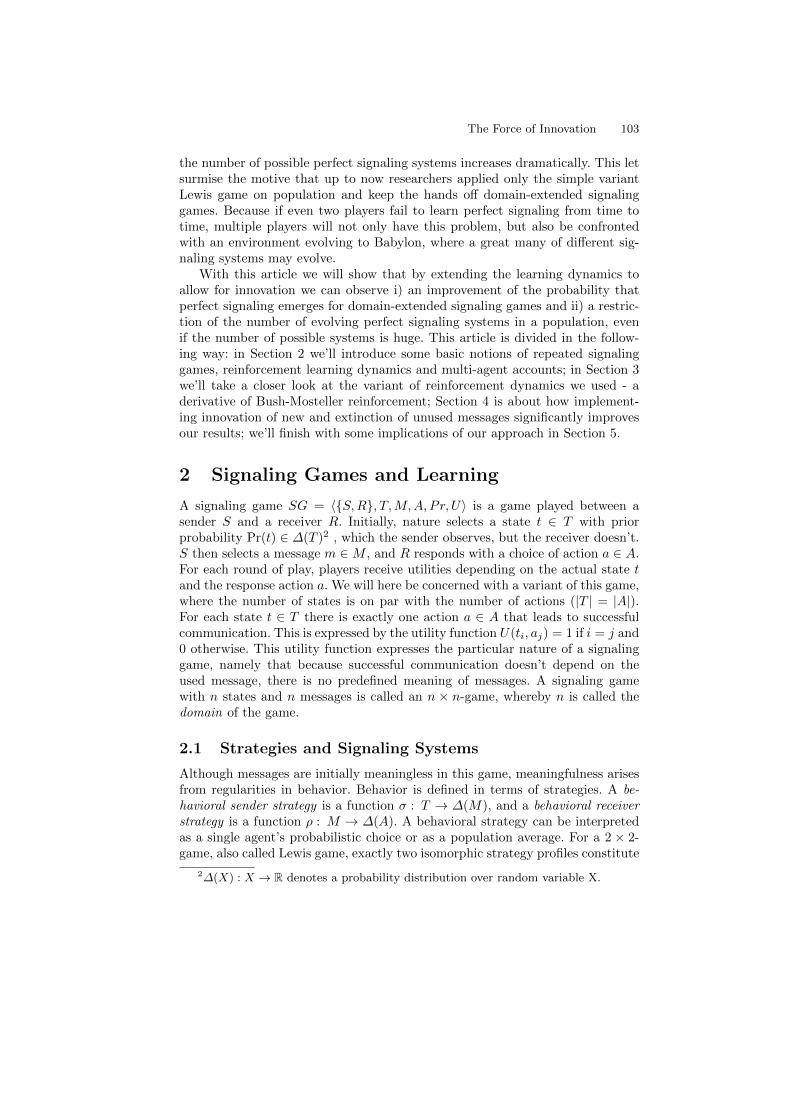
The Force of Innovation 103

the number of possible perfect signaling systems increases dramatically. This letsurmise the motive that up to now researchers applied only the simple variantLewis game on population and keep the hands off domain-extended signalinggames. Because if even two players fail to learn perfect signaling from time totime, multiple players will not only have this problem, but also be confrontedwith an environment evolving to Babylon, where a great many of different sig-naling systems may evolve.

With this article we will show that by extending the learning dynamics toallow for innovation we can observe i) an improvement of the probability thatperfect signaling emerges for domain-extended signaling games and ii) a restric-tion of the number of evolving perfect signaling systems in a population, evenif the number of possible systems is huge. This article is divided in the follow-ing way: in Section 2 we’ll introduce some basic notions of repeated signalinggames, reinforcement learning dynamics and multi-agent accounts; in Section 3we’ll take a closer look at the variant of reinforcement dynamics we used - aderivative of Bush-Mosteller reinforcement; Section 4 is about how implement-ing innovation of new and extinction of unused messages significantly improvesour results; we’ll finish with some implications of our approach in Section 5.

2 Signaling Games and Learning

A signaling game SG = 〈{S,R}, T,M,A, Pr, U〉 is a game played between asender S and a receiver R. Initially, nature selects a state t ∈ T with priorprobability Pr(t) ∈ ∆(T )2 , which the sender observes, but the receiver doesn’t.S then selects a message m ∈M , and R responds with a choice of action a ∈ A.For each round of play, players receive utilities depending on the actual state tand the response action a. We will here be concerned with a variant of this game,where the number of states is on par with the number of actions (|T | = |A|).For each state t ∈ T there is exactly one action a ∈ A that leads to successfulcommunication. This is expressed by the utility function U(ti, aj) = 1 if i = j and0 otherwise. This utility function expresses the particular nature of a signalinggame, namely that because successful communication doesn’t depend on theused message, there is no predefined meaning of messages. A signaling gamewith n states and n messages is called an n × n-game, whereby n is called thedomain of the game.

2.1 Strategies and Signaling Systems

Although messages are initially meaningless in this game, meaningfulness arisesfrom regularities in behavior. Behavior is defined in terms of strategies. A be-havioral sender strategy is a function σ : T → ∆(M), and a behavioral receiverstrategy is a function ρ : M → ∆(A). A behavioral strategy can be interpretedas a single agent’s probabilistic choice or as a population average. For a 2 × 2-game, also called Lewis game, exactly two isomorphic strategy profiles constitute

2∆(X) : X → R denotes a probability distribution over random variable X.

104 Muhlenbernd, Nick & Adam

L1:t1

t2

m1

m2

a1

a2L2:

t1

t2

m1

m2

a1

a2

Fig. 1. Two perfect signaling systems of a 2× 2-game, consisting of a pure sender andreceiver strategy.

a perfect signaling system. In these, strategies are pure (i.e. action choices haveprobabilities 1 or 0) and messages associate states and actions uniquely, as de-picted in Figure 1.

It is easy to show that for an n × n-game the number of perfect signalingsystems is n!. This means that while for a Lewis game we get the 2 signalingsystems as mentioned above, for a 3 × 3-game we get 6, for a 4 × 4-game 24,and for a 8× 8-game more than 40,000 perfect signaling systems. Moreover forn× n-games with n > 2 there is a possibility of partial pooling equilibria, whichtransmit information in a fraction of all possible cases.

2.2 Models of Reinforcement Learning

The simplest model of reinforcement learning is Roth-Erev reinforcement (see[RE1]) and can be captured by a simple model based on urns, known as Polyaurns, which works in the following way: an urn contains balls of different types,each type corresponding to an action choice. Now drawing a ball means to per-form the appropriate action. An action choice can be successful or unsuccessfuland in the former case, the number of balls of the appropriate act will be in-creased by one, such that the probability for this action choice is increased forsubsequent draws. All in all this model ensures that the probability of making aparticular decision depends on the number of balls in the urn and therefore onthe success of past action choices. This leads to the effect that the more success-ful an action choice is, the more probable it becomes to be elected in followingdraws.

But Roth-Erev reinforcement has the property that after a while the learningeffect3 slows down: while the number of additional balls for a successful actionis a static number α, in the general case α = 1, as mentioned above, the overallnumber of balls in the urn is increasing over time. E.g. if the number of ball inthe urn at time τ is n, the number at a later time τ + ε must be m ≥ n. Thusthe learning effect is changing from α/n to α/m and therefore can only decreaseover time.

Bush-Mosteller reinforcement (see [BM1]) is similar to Roth-Erev reinforce-ment, but without slowing the learning effect down. After a reinforcement theoverall number of balls in an urn is adjusted to a fixed value c, while preservingthe ratio of the different balls. Thus the number of balls in the urn at time τ is

3The learning effect is the ratio of additional balls for a successful action choice tothe overall number of balls.

The Force of Innovation 105

c and the number at a later time τ + ε is c and consequently the learning effectstays stable over time at α/c.

A further modification is the adaption of negative reinforcement : while inthe standard account unsuccessful actions have no effect on the urn value, withnegative reinforcement unsuccessful communication is punished by decreasingthe number of balls leading to an unsuccessful action.

By combining Bush-Mosteller reinforcement with negative reinforcement, theresulting learning dynamic follows the concept of lateral inhibition. In particular,a successful action will not only increase its probability, but also decrease theprobability of competing actions. In our account lateral inhibition applies tonegative reinforcement as well: for an unsuccessful action the number of theappropriate balls will be decreased, while the number of each other type of ballwill be increased.

2.3 Applying Reinforcement Learning on Repeated Sig-naling Games

To apply reinforcement learning to signaling games, sender and receiver bothhave urns for different states and messages and make their decision by drawinga ball from the appropriate urn. We assume the states are equally distributed.The sender has an urn 0t for each state t ∈ T , which contains balls for differentmessages m ∈ M . The number of balls of type m in urn 0t designated withm(0t), the overall number of balls in urn 0t with |0t|. If the sender is facedwith a state t she draws a ball from urn 0t and sends message m, if the ball isof type m. Accordingly the receiver has an urn 0m for each message m ∈ M ,which contains balls for different actions a ∈ A, whereby the number of balls oftype a in urn 0m designated with a(0m), the overall number of balls in urn 0mwith |0m|. For a receiver message m the receiver draws a ball from urn 0m andplays the action a, if the ball is of type a. Thus the sender’s behavioral strategyσ and receiver’s behavioral strategy ρ can be defined in the following way:

σ(m|t) =m(0t)

|0t|(1) ρ(a|m) =

a(0m)

|0m|(2)

The learning dynamics are realized by changing the urn content dependenton the communicative success. For a Roth-Erev reinforcement account with apositive update value α ∈ N > 0 and a lateral inhibition value γ ∈ N ≥ 0 thefollowing update process is executed after each round of play: if communicationvia t, m and a is successful, the number of balls in the sender’s urn 0t is increasedby α balls of typem and reduced by γ balls of typem′ 6= m. Similarly, the numberof balls in the receiver’s urn 0m is increased by α balls of type a and reducedby γ balls of type a′ 6= a.

Furthermore for an account with negative reinforcement urn contents alsochange in the case of unsuccessful communication for the negative update valueβ ∈ N ≥ 0 in the following way: if communication via t, m and a is unsuccessful,the number of balls in the sender’s urn 0t is decreased by β balls of type m andand increased by γ balls of type m′ 6= m; the number of balls in the receiver’s

106 Muhlenbernd, Nick & Adam

urn 0m is decreased by β balls of type a and increased by γ balls of type a′ 6= a.The lateral inhibition value γ ensures that the probability of an action can getzero and it speeds up the learning process.

We extended the Bush-Mosteller reinforcement for applying it to games withmore than two messages. The content of the appropriate sender and receiver urnswill be adjusted to a predefined value in the following way: for the given valuec of fixed urn content it is assumed that before a round of play the urn contentof all sender and receiver urns |0| = c. After a round of play it may be the casethat the urn content |0| = d 6= c. Now the number ni of each type of ball iis multiplied by c/d.4 For two messages the Bush-Mosteller is equivalent to ourextension by setting the learning parameter of the original model to φ = c·α

c+α .

2.4 Multi-Agent Accounts

It is interesting not only to examine the classical 2-players sender-receiver game,but the behavior of agents in a society (e.g. [Z1], [W1], [M1], [MF1]): more than2 agents interact with each other and switch between sender and receiver role. Inthis way an agent can learn a sender and a receiver strategy as well. Now if sucha combination forms a signaling system, it is called a signaling language and thecorresponding agent is called a learner. Thus the number of different possiblesignaling languages is defined by the number of possible signaling systems andtherefore for a n × n-game there are n! different languages an agent can learn.Furthermore if an agent’s combination of sender and receiver strategy forms apooling system, it is called a pooling language. After all it is easy to show that thenumber of possible pooling languages outvalues the number of possible signalinglanguages for any kind of n× n-game.

3 Simulating Bush-Mosteller

Barrett (see [B1]) simulated repeated signaling games with Roth-Erev reinforce-ment in the classical sender-receiver variant and computed the run failure rate(RFR). The RFR is the proportion of runs not ending with communicationvia a perfect signaling system. Barrett started 105 runs for n × n-games withn ∈ {2, 3, 4, 8}. His results show that 100% (RFR = 0) of 2 × 2-games weresuccessful. But for n × n-games with n > 2, the RFR increases rapidly(Figure2, left).

To compare different dynamics, we started two lines of simulation runs forBush-Mosteller reinforcement in the sender-receiver variant with urn contentparameter c = 20 and reinforcement value α = 1. For the second line we addi-tionally used lateral inhibition with value γ = 1/|T |. We tested the same gameslike Barrett and correspondingly 105 runs per game. In comparison with Bar-rett’s findings our simulation outcomes i) resulted also in a RFR of 0 for the2× 2-game, but ii) revealed an improvement with Bush-Mosteller reinforcement

4In this account urn contents and numbers of balls are real numbers

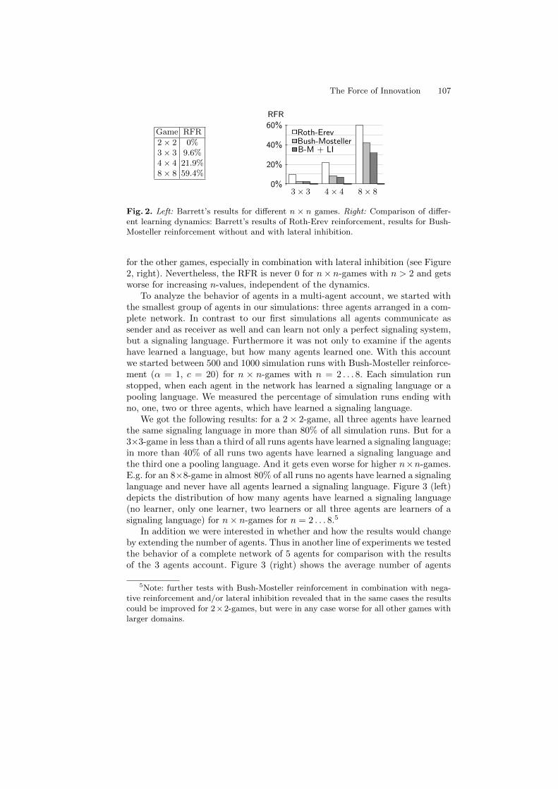
The Force of Innovation 107

Game RFR

2× 2 0%3× 3 9.6%4× 4 21.9%8× 8 59.4%

RFR

0%

20%

40%

60%

3× 3 4× 4 8× 8

B-M + LIBush-MostellerRoth-Erev

Fig. 2. Left: Barrett’s results for different n × n games. Right: Comparison of differ-ent learning dynamics: Barrett’s results of Roth-Erev reinforcement, results for Bush-Mosteller reinforcement without and with lateral inhibition.

for the other games, especially in combination with lateral inhibition (see Figure2, right). Nevertheless, the RFR is never 0 for n× n-games with n > 2 and getsworse for increasing n-values, independent of the dynamics.

To analyze the behavior of agents in a multi-agent account, we started withthe smallest group of agents in our simulations: three agents arranged in a com-plete network. In contrast to our first simulations all agents communicate assender and as receiver as well and can learn not only a perfect signaling system,but a signaling language. Furthermore it was not only to examine if the agentshave learned a language, but how many agents learned one. With this accountwe started between 500 and 1000 simulation runs with Bush-Mosteller reinforce-ment (α = 1, c = 20) for n × n-games with n = 2 . . . 8. Each simulation runstopped, when each agent in the network has learned a signaling language or apooling language. We measured the percentage of simulation runs ending withno, one, two or three agents, which have learned a signaling language.

We got the following results: for a 2× 2-game, all three agents have learnedthe same signaling language in more than 80% of all simulation runs. But for a3×3-game in less than a third of all runs agents have learned a signaling language;in more than 40% of all runs two agents have learned a signaling language andthe third one a pooling language. And it gets even worse for higher n×n-games.E.g. for an 8×8-game in almost 80% of all runs no agents have learned a signalinglanguage and never have all agents learned a signaling language. Figure 3 (left)depicts the distribution of how many agents have learned a signaling language(no learner, only one learner, two learners or all three agents are learners of asignaling language) for n× n-games for n = 2 . . . 8.5

In addition we were interested in whether and how the results would changeby extending the number of agents. Thus in another line of experiments we testedthe behavior of a complete network of 5 agents for comparison with the resultsof the 3 agents account. Figure 3 (right) shows the average number of agents

5Note: further tests with Bush-Mosteller reinforcement in combination with nega-tive reinforcement and/or lateral inhibition revealed that in the same cases the resultscould be improved for 2×2-games, but were in any case worse for all other games withlarger domains.

108 Muhlenbernd, Nick & Adam

2×2 3×3 4×4 5×5 6×6 7×7 8×80%

20%

40%

60%

80%

100%

012

3

01

2

3

0

1

2

3

01

2

3

0

1

2

3

0

1

23

0

1

23

1 no learners1 1 learner2 2 learners3 3 learners

2×2 3×3 4×4 5×5 6×6 7×7 8×80%

20%

40%

60%

80%

100%

5 agents account3 agents account

Fig. 3. Left: Percentage of simulation runs ending with a specific number of learnersos signaling languages in a network with three agents for different n × n-games withn = 1 . . . 8. Right: Average percentage of agents learning a signaling language over allruns for different n×n-games with n = 1 . . . 8. Comparison of the results of a completenetwork of 3 agents (white circles) and 5 agents (black circles).

who learned a signaling language per run for different n× n-games. As you cansee for 2 × 2-games and 3 × 3-games the enhancement of population size leadsto a higher average percentage of agents learning a signaling language. But forgames with larger domains the results are by and large the same.

The results for the classical sender-receiver game reveal that by extendinglearning accounts the probability of the emergence of perfect signaling systemscan be improved but nevertheless is never one for an n × n-game, if n is largeenough. Furthermore the results for the multi-agent account with only threeagents show that even for a 2×2-game not in any case all agents learn a language.And for games with larger domains, results get worse. Furthermore results don’tget better or worse by changing the number of agents, as shown in a multi-agentaccount with 5 agents. But how could natural languages arise by assuming themhaving emerged from n× n-games with a huge n-value and in a society of muchmore interlocutors? We’ll show that by allowing for the extinction of unusedmessages and the emergence of new messages, perfect signaling systems emergefor huge n-values and multiple agents in any case. In other words, we’ll showthat stabilization needs innovation.

4 Innovation

The idea of innovation in our account is that messages can become extinct andnew messages can emerge, thus the number of messages during a repeated playcan vary, whereas the number of states is fixed. The idea of innovation andextinction for reinforcement learning applied on signaling games stems fromSkyrms (2010), whereby to our knowledge it is completely new i) to combine itwith Bush-Mosteller reinforcement plus negative reinforcement and ii) to use itfor multi-agent accounts.

The Force of Innovation 109

The process of the emergence of new messages works like this: additionallyto the balls for each message type each sender urn has an amount of innova-tive balls (according to Skyrms we call them black balls). If drawing a blackball the sender sends a completely new message, not ever used by any agent ofthe population. Because the receiver has no receiver urn of the new message,he chooses a random action. If action and state matches, the new message isadopted in the set of known messages of both interlocutors in the following way:i) both agents get a receiver urn for the new message, wherein the balls for allactions are equiprobable distributed, ii) both agents’ sender urns are filled witha predefined amount of balls of the new message and iii) the sender and receiverurn involved in this round are updated according to the learning dynamic. If thenewly invented message doesn’t lead to successful communication, the messagewill be discarded and there will be no change in the agents strategies.

As mentioned before, messages can become extinct, and that happens inthe following way: because of lateral inhibition, infrequently used or unusedmessages’ value of balls in the sender urns will get lower and lower. At a pointwhen the number of balls of a message is 0 for all sender urns, the messageisn’t existent in the active use of the agent (i.o.w. she cannot send the messageanymore), and will also be removed from the agent’s passive use by deletingthe appropriate receiver urn. At this point the message isn’t in this agent’s setof known messages. Besides, there is no other interference between sender andreceiver urn of one agent.

Some further notes:

– it is possible that an agent can receive a message that is not in her set ofknown messages. In this case she adopts the new message like described forthe case of innovation. Note that in a multi-agent setup this allows for aspread of new messages

– the black balls are also affected by lateral inhibition. That means that thenumber of black balls can decrease and increase during runtime; it can es-pecially be zero

– a game with innovation has a dynamic number of messages starting with 0messages, but ends with |M | = |T |. Thus we call an innovation game withn states and n ultimate messages an n× n∗-game

4.1 The Force of Innovation

The total number of black balls of an agent’s sender urns describes his personalforce of innovation. Note that black balls can only increase by lateral inhibitionin the case of unsuccessful communication and decrease by lateral inhibition inthe case of successful communication. This interrelationship leads to the follow-ing dynamics: successful communication lowers the personal force of innovation,whereas unsuccessful communication raises the personal force of innovation. Ifwe define the global force of innovation for a group of connected agents X asthe average personal force of innovation over all x ∈ X, then the following holds:the better the communication between agents in a group X, the lower the global

110 Muhlenbernd, Nick & Adam

Game 2× 2∗ 3× 3∗ 4× 4∗ 5× 5∗ 6× 6∗ 7× 7∗ 8× 8∗

3 agents 1,052 2,120 4,064 9,640 21,712 136,110 > 500,0005 agents 2,093 5,080 18,053 192,840 > 500,000 > 500,000 > 500,000

Table 1. Runtime Table for n× n∗-games with n = 2 . . . 8; for a complete network of3 agents and 5 agents.

force of innovation of this group and vice versa. In other words, this accountrealizes a plausible social dynamics: if communication works, then there is noneed to change and therefore a low (or zero) value of the force of innovation,whereby if communication doesn’t work, the force of innovation rises.

4.2 Learning Languages by Innovation: A Question of Time

We could show in section 3 that the percentage of agents learning a signalinglanguage in a multi-agent context is being decreased by increasing the domainsize of the game. To find out whether innovation can improve these results westarted simulation runs with the following settings:

– network types: complete network with 3 agents and with 5 agents– learning dynamics: Bush-Mosteller reinforcement with negative reinforce-

ment and lateral inhibition value (α = 1, β = 1, γ = 1/|T |) and innovation– initial state: every urn of the sender is filled with black balls and the receiver

does not have any a priori urn.– experiments: 100 simulation runs per n× n∗-game with n = 2 . . . 8– break condition: simulation stops if the communicative success of every

agents exceeds 99% or the runtime passes the runtime limit of 500,000 com-munication steps (= runtime)

These simulation runs gave the following results: i) for the 3-agents accountin combination with n×n∗-games for n = 2 . . . 7 and the 5-agents in combinationwith n × n∗-games for n = 2 . . . 5 all agents have learned a signaling languagein each simulation run and ii) for the remaining account-game combinations allsimulation runs exceeded the runtime limit (see Table 1). We expect that for theremaining combination all agents will learn a signaling language as well, but ittakes extremely long.

All in all we could show that the integration of innovation and extinction ofmessages leads to a final situation where all agents have learned the same sig-naling language, if the runtime doesn’t exceed the limit. Nevertheless we expectthe same result for account-game combinations where simulations steps of theseruns exceeded our limit for a manageable runtime.

4.3 The Development of Signaling Languages by Innova-tion

As our experiments in the last section showed, by applying Bush-Mosteller rein-forcement learning with innovation all agents learn the same signaling language

The Force of Innovation 111

force of innovationnumber of messagescommunicative

success

50 100 150 200 250 300 350036912151821242730

-.5-.4-.3-.2-.10.1.2.3.4.5.6.7.8.91

Fig. 4. Simulation run of a 3 × 3∗-game with innovation in a 3-agents population.Communicative success, number of used messages and force of innovation of all agentsin the population; number of simulation steps at x-axis.

for a small group of agents and any n × n∗-game with n = 2 . . . 7. Let’s take acloser look at how a 3 × 3∗-game develops during a simulation run by analyz-ing i) one randomly chosen agent’s parameters and ii) parameters of the wholepopulation. Three parameters are of interest to us:

– communication success: utility value averaged over the last 20 communica-tion steps averaged over all agents in the population

– number of messages in use: number of actually used messages in the wholepopulation

– force of innovation: absolute number of black balls averaged over all agents

Figure 4 shows the resulting values for the whole population: in the beginningall the agents try out a lot of messages, which reduces the number of black ballsin the urns because balls for the new messages are added and then the urncontent is normalized. Note that for the first communication steps the force ofinnovation drops rapidly, while the number of messages rises until it reaches 21messages here. As you can see in the course of the success-graph, the work isnot done here. Once they have more or less agreed on which messages might beuseful, the agents are trying them out and it is only when finally a subset ofthose messages is probabilistically favored that the success is increasing, whilethe number of known messages decreases, until the success finally reaches aperfect 1 on average, while the number of messages equals that of the states (3)and the force of innovation is zero.

What you can see in the figures as well is that even though there is noone-to-one correspondence between the number of messages and the averagesuccess, their graphs do show some sort of mirroring on the micro level. Theinterrelationship of innovation force and average success is not well visible inFigure 4, because of the coarse scaling of the force of innovation value. Figure

112 Muhlenbernd, Nick & Adam

force of innovationcommunicative

success

100 150 200 250 300 3500

0.3

0.6

0.9

1.2

1.5

-.3-.2-.10.1.2.3.4.5.6.7.8.91

Fig. 5. Simulation run of a 3 × 3∗-game with innovation in a 3-agents population.Comparison of communicative success and force of innovation; number of simulationsteps at x-axis.

5 shows the force of innovation and the communication success between step 50and 350 of the simulation run, already depicted in Figure 4, whereas the force ofinnovation value is 20 times more fine-grained. Here the interrelationship betweenboth values is clearly recognizable, one measure’s peak is simultaneously theother measure’s valley. Admittedly the mirroring is not perfect, but it improvesby increasing the number of agents.

5 Conclusion and Outlook

Let’s recap: We started out with comparing Roth-Erev and Bush-Mosteller rein-forcement, finding that Bush-Mosteller yields better results for repeated signal-ing games. Extending Bush-Mosteller with lateral inhibition lead to even betterresults, but far from perfect. And results were even worse for multi-agent accountwith 3 or 5 agents: with increasing n less agents develop a signaling language inthe first place, especially pooling strategies turned out to be a common outcome.In a next step we extended the classical Bush-Mosteller reinforcement by addingnegative reinforcement and therefore achieving lateral inhibition, innovation andextinction. We found that these tweaks result in perfect communication between3 agents in n×n∗-games for n < 8 and between 5 agents for n < 6, since highervalues for n or the number of agents require much higher runtime that exceedour limit. Especially the force of innovation seems to be responsible for thisachievement, since it makes sure that new messages are introduced when com-munication is not successful, while the combination of negative reinforcementand lateral inhibition takes care of all unused or useless messages to becomeextinct. Consequently, the result is an agreement on one single perfect signalinglanguage with no other messages that might interfere.

The purpose of this direction of research is mostly about finding reasonableextensions of simple learning algorithms that lead to more explanatory results,

The Force of Innovation 113

assuming that more sophisticated learning dynamics might be more adequateto eventually describe human language behavior. We think the extensions weintroduced in this article are of that kind, especially negative reinforcement,since we’re rather certain that failure has a learning-effect, and innovation andextinction, because it seems unreasonable to assume that all messages are avail-able right from the start and that everything is kept in the lexicon, even if ithas only once been successfully used. Further research in this direction shouldclarify how memory restrictions could be modeled and how sender and receiverroles of one agent should influence each other. What remains to be shown is thatour results in fact hold for higher numbers of agents and states. It would furtherbe interesting to see what influence different, again more realistic network-types(say small-world or scale-free networks) have on the results and what happensif two or more languages interact.

References

CE1. Clarke, F., Ekeland, I.: Nonlinear oscillations and boundary-value problems forHamiltonian systems. Arch. Rat. Mech. Anal. 78 (1982) 315–333

L1. Lewis, David: Convention. Cambridge: Harvard University Press (1969)B1. Barret, Jeffrey A.: The Evolution of Coding in Signaling Games. Theory and

Decision 67 (2009), pp. 223–237BZ1. Barret, Jeffrey A., Zollman, Kevin J. S.: The Role of Forgetting in the Evolution

and Learning of Language. Journal of Experimental and Theoretical ArtificialIntelligence 21.4 (2009), pp. 293–309

BM1. Bush, Robert, Mosteller, Frederick: Stochastic Models of Learning. New York:John Wiley & Sons (1955)

HH1. Hofbauer, Josef, Huttegger, Simon M.: Feasibility of communication in binarysignaling games. Journal of Theoretical Biology 254.4 (2008), pp. 843–849

HSRZ1. Huttegger, Simon M., Skyrms, Brian, Rory, Smead, Zollman, Kevin J.: Evolu-tionary dynamics of Lewis signaling games: signaling systems vs. partial pool-ing. Synthese 172.1 (2010), pp. 177–191

HZ1. Huttegger, Simon M., Zollman, Kevin J.: Signaling Games: Dynamics of Evo-lution and Learning. Language, Games, and Evolution. Ed. by Anton Benz etal. LNAI 6207. Springer (2011), pp. 160–176

M1. Muhlenbernd, Roland: Learning with Neighbours. Synthese 183.S1 (2011), pp.87–109

MF1. Muhlenbernd, Roland, Franke, Michael: Signaling Conventions: Who LearnsWhat Where and When in a Social Network. Proceedings of EvoLang IX (2011)

RE1. Roth, Alvin, Erev, Ido: Learning in extensive-form games: experimental dataand simple dynamic models in the intermediate term. Games and EconomicBehaviour 8 (1995), pp. 164–212

S1. Skyrms, Brian: Signals: Evolution, Learning & Information. Oxford: OxfordUniversity Press (2010)

W1. Wagner, Elliott: Communication and Structured Correlation. Erkenntnis 71.3(2009), pp. 377–393

Z1. Zollman, Kevin J. S.: Talking to neighbors: The evolution of regional meaning.Philosophy of Science 72.1 (2005), pp. 69–85.

Existential definability of modal frame classes

Tin Perkov

Polytechnic of Zagreb, Croatiatin.perkov@tvz.hr

Abstract. A class of Kripke frames is called modally definable if thereis a set of modal formulas such that the class consists exactly of frameson which every formula from that set is valid, i. e. globally true underany valuation. Here, existential definability of Kripke frame classes isdefined analogously, by demanding that each formula from a defining setis satisfiable under any valuation. This is equivalent to the definability bythe existential fragment of modal language enriched with the universalmodality. A model theoretic characterization of this type of definabilityis given.

Keywords: modal logic, model theory, modal definability

1 Introduction

Some questions about the power of modal logic to express properties of relationalstructures are addressed in this paper. For the sake of notational simplicity, onlythe basic propositional modal language (BML) is considered in this paper. Let Φbe a set of propositional variables. The syntax of BML is given by

ϕ ::= p | ⊥ |ϕ1 ∨ ϕ2 | ¬ϕ |3ϕ,

where p ∈ Φ. We define other connectives and 2 as usual. Namely, 2ϕ := ¬3¬ϕ.Only the Kripke semantics is considered in this paper. The basic notions and

results are only briefly recalled here (see [1] for details if needed). A Kripke framefor the basic modal language is a relational structure F = (W,R), where W 6= ∅and R ⊆W ×W . A Kripke model based on a frame F is M = (W,R, V ), whereV : Φ→ 2W is a mapping called valuation. For w ∈W , we call (M, w) a pointedmodel.

The truth of a formula is defined locally and inductively as usual, and denotedM, w ϕ. Namely, a formula of a form 3ϕ is true at w ∈ W if M, u ϕ forsome u such that Rwu. A valuation is naturally extended to all modal formulasby putting V (ϕ) = {w ∈W : M, w ϕ}.

We say that a formula is globally true on M if it is true at every w ∈W , andwe denote this by M ϕ. On the other hand, a formula is called satisfiable inM if it is true at some w ∈W .

If a formula ϕ is true at w under any valuation on a frame F, we writeF, w ϕ. We say that a formula is valid on a frame F if we have M ϕ for

Existential definability of modal frame classes 115

any model M based on F. This is denoted F ϕ. A class K of Kripke frames ismodally definable if there is a set Σ of formulas such that K consists exactly offrames on which every formula from Σ is valid, i. e. K = {F : F Σ}. If this isthe case, we say that K is defined by Σ and denote K = Fr(Σ).

Model theoretic closure conditions that are necessary and sufficient for anelementary class of frames (i. e. first-order definable property of relational struc-tures) to be modally definable are given by the famous Goldblatt-ThomasonTheorem.

Theorem (Goldblatt-Thomason [3]). An elementary class K of frames isdefinable by a set of modal formulas if and only if K is closed under surjec-tive bounded morphisms, disjoint unions and generated subframes, and reflectsultrafilter extensions.

All of the frame constructions used in the theorem – bounded morphisms,disjoint unions, generated subframes and ultrafilter extensions – are presentedin detail in [1] (the same notation is used in this paper). Just to be clear, we saythat a class K reflects a construction if its complement Kc, that is the class ofall Kripke frames not in K, is closed under that construction.

Now, an alternative notion of definability is proposed here as follows.

Definition. A class K of Kripke frames is called modally ∃-definable if there isa set Σ of modal formulas such that for any Kripke frame F we have: F ∈ K ifand only if each ϕ ∈ Σ is satisfiable in M, for any model M based on F. If thisis the case, we denote K = Fr∃(Σ).

The definition does not require that all formulas of Σ are satisfied at thesame point – it suffices that each formula of Σ is satisfied at some point.

In the sequel, a notation Mod(F ) is used for a class of structures defined by afirst-order formula F . Similarly, if Σ = {ϕ} is a singleton set of modal formulas,we write Fr∃(ϕ) instead of Fr∃({ϕ}).

Example 1. It is well-known that the formula p → 3p defines reflexivity, i. e.Fr(p → 3p) = Mod(∀xRxx). Now, it is easy to see that Fr∃(p → 3p) is theclass of all frames such that R 6= ∅, that is Fr∃(p→ 3p) = Mod(∃x∃yRxy). Thisclass is not modally definable in the usual sense, since it is clearly not closedunder generated subframes. Note that the condition R 6= ∅ is ∃-definable also bya simpler formula 3>.

The main result of this paper is the following characterization.

Theorem 1. Let K be an elementary class of Kripke frames. Then K is modally∃-definable if and only if it is closed under surjective bounded morphisms andreflects generated subframes and ultrafilter extensions.

This is an analogue of a similar characterization of existentially definableKripke model classes, given in [6].

116 Tin Perkov

2 First and second-order standard translations

The starting point of correspondence between first-order and modal logic is thestandard translation, a mapping that translates each modal formula ϕ to thefirst-order formula STx(ϕ), as follows:

STx(p) = Px, for each p ∈ Φ,

STx(⊥) = ⊥,

STx(¬ϕ) = ¬STx(ϕ),

STx(ϕ ∨ ψ) = STx(ϕ) ∨ STx(ψ),

STx(3ϕ) = ∃y(Rxy ∧ STy(ϕ)).

Clearly, we have M, w ϕ if and only if M |= STx(ϕ)[w], and M ϕif and only if M |= ∀xSTx(ϕ). But, validity of a formula on a frame gener-ally is not first-order expressible, since we need to quantify over valuations.We have a second-order standard translation, that is, F ϕ if and only ifF |= ∀P1 . . . ∀Pn∀xSTx(ϕ), where P1, . . . , Pn are monadic second-order variables,one for each propositional variable occurring in ϕ. So, the notion of modal de-finability is equivalent to the definability by a set of second-order formulas ofthe form ∀P1 . . . ∀Pn∀xSTx(ϕ). However, in many cases a formula of this type isequivalent to a first-order formula. Namely, this holds for any Sahlqvist formula(the definition is omitted here – see [7] or [1]), for which a first-order frame corre-spondent is effectively computable. On the other hand, the Goldblatt-ThomasonTheorem characterizes those first-order properties that are modally definable.

Now, ∃-definability is clearly also equivalent to the definability by a typeof second-order formulas – those of the form ∀P1 . . . ∀Pn∃xSTx(ϕ). Consideranother example of a modally ∃-definable class.

Example 2. The condition F = ∃x∀y(Rxy → ∃zRyz) is not modally definable,since it is not closed under generated subframes, but it is modally ∃-definableby the formula ϕ = p→ 23p.

To prove this, we need to show Fr∃(ϕ) = Mod(F ). But F = (W,R) ∈ Fr∃(ϕ)if and only if F |= ∀P∃x(Px → ∀y(Rxy → ∃z(Ryz ∧ Pz))). So in particular,under the assignment which assigns the entire W to the second-order variableP , we get F |= ∃x∀y(Rxy → ∃zRyz), thus F ∈ Mod(F ). The reverse inclusion isproved similarly.

Other changes of quantifiers or the order of first and second-order quantifierswould result in other types of definability, perhaps also worthy of exploring. Infact, this has already been done by Venema [9] and Hollenberg [5], who con-sider negative definability, which corresponds to second-order formulas of theform ∀x∃P1 . . . ∃PnSTx(¬ϕ). A class of frames negatively defined by Σ is de-noted Fr−(Σ). A general characterization of negative definability has not beenobtained, and neither has a characterization of elementary classes which are neg-atively definable – it even remains unknown if all negatively definable classes arein fact elementary. But, to digress a little from the main point of this paper, weeasily get the following fairly broad result.

Existential definability of modal frame classes 117

Proposition 1. Let ϕ be a modal formula which has a first-order local cor-respondent, i. e. there is a first-order formula F (x) such that for any frameF = (W,R) and any w ∈ W we have F, w ϕ if and only if F |= F (x)[w]. (Inparticular, this holds for any Sahlqvist formula.)

Then we have Fr−(ϕ) = Mod(∀x¬F (x)).

Proof. We have F ∈ Fr−(ϕ) if and only if F |= ∀x∃P1 . . . ∃PnSTx(¬ϕ) if and onlyif F 6|= ∃x∀P1 . . . ∀PnSTx(ϕ). But this means that there is no w ∈ W such thatF |= ∀P1 . . . ∀PnSTx(ϕ)[w]. The latter holds if and only if F, w ϕ, which is byassumption equivalent to F |= F (x)[w]. The fact that such w does not exist, isequivalent to F ∈ Mod(∀x¬F (x)). ut

So for example, since p → 3p locally corresponds to Rxx, we have thatp→ 3p negatively defines irreflexivity, which is not modally definable property,since it is not preserved under surjective bounded morphisms.

3 Model-theoretic constructions

This section can be used, if needed, for a quick reference of the basic facts aboutconstructions used in the main theorem. Otherwise it can be omitted.

A bisimulation between Kripke models M = (W,R, V ) and M′ = (W ′, R′, V ′)is a relation Z ⊆W ×W ′ such that:

(at) if wZw′ then we have: w ∈ V (p) if and only if w′ ∈ V ′(p), for all p ∈ Φ,(forth) if wZw′ and Rwv, then there is v′ such that vZv′ and R′w′v′,(back) if wZw′ and R′w′v′, then there is v such that vZv′ and Rwv.The basic property of bisimulations is that (at) extends to all formulas: if

wZw′ then M, w ϕ if and only if M′, w′ ϕ, i. e. (M, w) and (M′, w′) aremodally equivalent. We get the definition of bisimulation between frames byomitting the condition (at).

A bounded morphism from a frame F = (W,R) to F′ = (W ′, R′) is a functionf : W →W ′ such that:

(forth) Rwv implies R′f(w)f(v),(back) if R′f(w)v′, then there is v such that v′ = f(v) and Rwv.Clearly, a bounded morphism is a bisimulation that is also a function.A generated subframe of F = (W,R) is a frame F′ = (W ′, R′) where W ′ ⊆W

such that w ∈W ′ and Rwv implies v ∈W ′, and R′ = R∩(W ′×W ′). A generatedsubmodel of M = (W,R, V ) is a model based on a generated subframe, with thevaluation V ′(p) = V (p)∩W ′, for all p ∈ Φ. It is easy to see that the global truthof a modal formula is preserved on a generated submodel.

To define the ultraproducts and ultrafilter extensions, we need the notion ofultrafilters. An ultrafilter over a set I 6= ∅ is a family U ⊆ P(I) such that:

(1) I ∈ U ,(2) if A,B ∈ U , then A ∩B ∈ U ,(3) if A ∈ U and A ⊆ B ⊆ I, then B ∈ U ,(4) for all A ⊆ I we have: A ∈ U if and only if I \A /∈ U .

118 Tin Perkov

The existence of ultrafilters is provided by a fact that any family of subsetswhich has the finite intersection property (that is, each finite intersection isnon-empty) can be extended to an ultrafilter (see e. g. [2]).

Let {Mi = (Wi, Ri, Vi) : i ∈ I} be a family of Kripke models and let Ube an ultrafilter over I. The ultraproduct of this family over U is the model∏U Mi = (W,R, V ) such that:

(1) W is the set of equivalence classes fU of the following relation defined onthe Cartesian product of the family: f ∼ g if and only if {i ∈ I : f(i) = g(i)} ∈ U ,

(2) fURgU if and only if {i ∈ I : f(i)Rig(i)} ∈ U ,

(3) fU ∈ V (p) if and only if {i ∈ I : f(i) ∈ Vi(p)} ∈ U , for all p.

The basic property of ultraproducts is that (3) extends to all formulas.

Proposition 2. Let {Mi : i ∈ I} be a family of Kripke models and let U be anultrafilter over I.

Then we have∏U Mi, f

U ϕ if and only if {i ∈ I : Mi, f(i) ϕ} ∈ U , forany fU . Furthermore, we have

∏U Mi ϕ if and only if {i ∈ I : Mi ϕ} ∈ U .

This is an analogue of the Los Fundamental Theorem on ultraproducts fromthe first-order model theory (see [2] for this, and [1] for the proof of the modalanalogue). The Los Theorem also implies that an elementary class of models isclosed under ultraproducts.

An ultraproduct such that Mi = M for all i ∈ I is called an ultrapower ofM and denoted

∏U M. From the Los Theorem it follows that any ultrapower

of a model is elementarily equivalent to the model, that is, the same first-ordersentences are true on M and

∏U M. Definition of an ultraproduct of a family of

frames is obtained by omitting the clause regarding valuation.

Another notion needed in the proof of the main theorem is modal satura-tion, the modal analogue of ω-saturation from the classical model theory. Thedefinition of saturation is omitted here, since we only need some facts which itimplies. Most importantly, saturation implies a converse of the basic property ofbisimulations, which generally does not hold. In fact, modal equivalence betweenpoints of modally saturated models is a bisimulation. Also, we use the fact thatany ω-saturated Kripke model is also modally saturated (see [1] for proofs ofthese facts).

Finally, the ultrafilter extension of a model M = (W,R, V ) is the modelueM = (Uf(W ), Rue, V ue), where Uf(W ) is the set of all ultrafilters over W ,Rueuv holds if and only if A ∈ v implies m3(A) ∈ u, where m3(A) denotes theset of all w ∈ W such that Rwa for some a ∈ A, and u ∈ V ue(p) if and onlyif V (p) ∈ u. The basic property is that this extends to any modal formula, i. e.we have u ∈ V ue(ϕ) if and only if V (ϕ) ∈ u (see [1]). From this it easily followsthat the global truth of a modal formula is preserved on the ultrafilter extension.Another important fact is that the ultrafilter extension of a model is modallysaturated (see [1]).

The ultrafilter extension of a frame F = (W,R) is ueF = (Uf(W ), Rue).

Existential definability of modal frame classes 119

4 Proof of the main theorem

In this section Theorem 1 is proved in detail. Arguments and techniques usedin the proof are similar to the ones used in the proof of Goldblatt-Thomasontheorem as presented in [1], so the reader might find it interesting to comparethese proofs to note analogies and differences.

Proof (of Theorem 1). Let K = Fr∃(Σ). Let F = (W,R) ∈ K and let f be asurjective bounded morphism from F to some F′ = (W ′, R′). Take any ϕ ∈ Σ andany model M′ = (W ′, R′, V ′) based on F′. Put V (p) = {w ∈W : f(w) ∈ V ′(p)}.Then V is a well defined valuation on F. Put M = (W,R, V ). Since F ∈ K, thereexists w ∈ W such that M, w ϕ. But then M′, f(w) ϕ. This proves that K

is closed under surjective bounded morphisms.To prove that K reflects generated subframes and ultrafilter extensions, let

F = (W,R) /∈ K. This means that there is ϕ ∈ Σ and a model M = (W,R, V )based on F such that M ¬ϕ. Let F′ = (W ′, R′) be a generated subframe ofF. Define V ′(p) = V (p) ∩W ′, for all p. Then we have M′ ¬ϕ, which provesF′ /∈ K, as desired. Also, ueM is a model based on the ultrafilter extension ueFand we have ueM ¬ϕ, which proves ueF /∈ K.

For the converse, let K be an elementary class of frames that is closed undersurjective bounded morphisms and reflects generated subframes and ultrafilterextensions. Denote by Σ the set of all formulas that are satisfiable in all modelsbased on all frames in K. Then K ⊆ Fr∃(Σ) and it remains to prove the reverseinclusion.

Let F = (W,R) ∈ Fr∃(Σ). Let Φ be a set of propositional variables thatcontains a propositional variable pA for each A ⊆W . Let M = (W,R, V ), whereV (pA) = A for all A ⊆ W . Denote by ∆ the set of all modal formulas over Φwhich are globally true on M. Now, for any finite δ ⊆ ∆ there is Fδ ∈ K anda model Mδ based on Fδ such that Mδ δ. Otherwise, since ∆ is closed underconjunctions, there is ϕ ∈ ∆ such that ¬ϕ ∈ Σ, thus ¬ϕ is satisfiable in M,which contradicts M ∆.

Now, let I be the family of all finite subsets of ∆. For each ϕ ∈ ∆, putϕ = {δ ∈ I : ϕ ∈ δ}. The family {ϕ : ϕ ∈ ∆} clearly has the finite intersectionproperty, so it can be extended to an ultrafilter U over I. But for all ϕ ∈ ∆we have {δ ∈ I : Mδ ϕ} ⊇ ϕ and ϕ ∈ U , thus {δ ∈ I : Mδ ϕ} ∈ U ,so the Proposition 2 implies

∏U Mδ ϕ. The model

∏U Mδ is based on the

frame∏U Fδ. Since K is elementary, it is also closed under ultraproducts, so∏

U Fδ ∈ K. It remains to prove that there is a surjective bounded morphismfrom some ultrapower of

∏U Fδ to a generated subframe of ueF. Then the as-

sumed properties of K imply that F ∈ K, as desired.The classical model theory provides that there is an ω-saturated ultrapower

of∏U Mδ (cf. [2]). Let M∆ be such an ultrapower. We have that M∆ is modally

saturated. Also, it is elementarily equivalent to∏U Mδ, so using standard trans-

lation we obtain M∆ ∆. The model M∆ is based on a frame F∆, which isan ultrapower of

∏U Fδ. Now define a mapping from F∆ to ueF by putting

f(w) = {A ⊆W : M∆, w pA}.

120 Tin Perkov

First we need to prove that f is well-defined, i. e. that f(w) is indeed anultrafilter over W .

(1) We easily obtain W ∈ f(w), since pW ∈ ∆ by the definition of V .(2) If A,B ∈ f(w), then M∆, w pA ∧ pB . Clearly, M pA ∧ pB ↔ pA∩B .

Thus M∆ pA ∧ pB ↔ pA∩B , so M∆, w pA∩B , i. e. A ∩B ∈ f(w).(3) If A ∈ f(w) and A ⊆ B ⊆ W , then from the definition of V it follows

M pA → pB . But then also M∆ pA → pB , hence M∆, w pB , so B ∈ f(w).(4) For all A ⊆ W we have M pA ↔ ¬pW\A, which similarly as in the

previous points implies A ∈ f(w) if and only if W \A /∈ f(w), as desired.Assume for the moment that we have: u = f(w) if and only if (ueM, u) and

(M∆, w) are modally equivalent. Since ueM and M∆ are modally saturated, themodal equivalence between their points is a bisimulation. So f is a bisimulation,but it is also a function, which means that it is a bounded morphism from F∆to ueF. But then the corestriction of f to its image is a surjective boundedmorphism from an ultrapower of

∏U Fδ to a generated subframe of ueF, which

we needed.So to conclude the proof, it remains to show that u = f(w) holds if and only

if (ueM, u) and (M∆, w) are modally equivalent. Let u = f(w). Then we haveueM, u ϕ if and only if V (ϕ) ∈ u, which is by the definition of f equivalent toM∆, w pV (ϕ). But the definition of V clearly implies M ϕ↔ pV (ϕ), so alsoM∆ ϕ↔ pV (ϕ), which provides the needed modal equivalence.

For the converse, the assumption implies that we have ueM, u pA if andonly if M∆, w pA, for all A ⊆W . This means that V (pA) = A ∈ u if and onlyif A ∈ f(w), i. e. u = f(w).

ut

5 Conclusion: link to the universal modality

Although the approach of this paper is to define ∃-definability as a metalingualnotion, it should be noted that it can be included in the language itself. Thatis, the satisfiability of a modal formula under any valuation on a frame canbe expressed by a formula of the modal language enriched with the universalmodality (BMLU). The syntax is an extension of the basic modal language bynew modal operator Aϕ, and we can also define its dual Eϕ := ¬A¬ϕ. We callA the universal modality, and E the existential modality. The semantics of thenew operators is standard modal semantics, with respect to the universal binaryrelation W×W on a frame F = (W,R). This means that the standard translationof universal and existential operators is as follows (cf. [4] and [8]):

STx(Eϕ) = ∃ySTy(ϕ),STx(Aϕ) = ∀ySTy(ϕ).Now, let K be a class of Kripke frames. Clearly, K is modally ∃-definable

if and only if it is definable by a set of formulas of the existential fragment ofBMLU, i. e. by a set of formulas of the form Eϕ, where ϕ is a formula of BML.This immediately follows from the clear fact that for any frame F and any ϕwe have F Eϕ if and only if F |= ∀P1 . . . ∀Pn∃ySTy(ϕ), where P1, . . . , Pn

Existential definability of modal frame classes 121

correspond to propositional variables that occur in ϕ, and the letter holds if andonly if ϕ is satisfiable under any valuation on F.

Goranko and Passy [4] gave a characterization that an elementary class ismodally definable in BMLU if and only if it is closed under surjective boundedmorphisms and reflects ultrafilter extension. So, from the main theorem of thispaper we conclude that reflecting generated subframes, not surprisingly, is whatdistinguishes existential fragment within this language, at least with respect toelementary classes. Also, the usual notion of modal definability clearly coincideswith the universal fragment of BMLU, hence the Goldblatt-Thomason Theoremtells us that closure under generated subframes and disjoint unions is essentialfor this fragment.

As for some further questions that might be worth exploring, for example,similarly to the notion of ±-definability from [5], we can say that a class offrames is modally ∀∃-definable if there is a pair (Σ1, Σ2) of sets of formulas suchthat a class consists exactly of frames on which every formula from Σ1 is validand every formula from Σ2 is satisfiable under any valuation, and try to obtaina characterization theorem. This also coincides with a fragment of BMLU, andgeneralizes both usual modal definability and ∃-definability. Furthermore, wemay be able to obtain general characterization theorems for these fragments,without the assumption of the first-order definability.

On the other hand, a question to be addressed is which modally ∃-definableclasses are elementary, and is there an effective procedure analogous to the one forSahlqvist formulas, to obtain a first-order formula equivalent to a second-ordertranslation ∀P1 . . . ∀Pn∃xSTx(ϕ) for some sufficiently large and interesting classof modal formulas.

References

1. J. Blackburn, M. de Rijke, Y. Venema: Modal Logic. Cambridge University Press(2001)

2. C. C. Chang, H. J. Keisler: Model Theory. Elsevier (1990)3. R. I. Goldblatt, S. K. Thomason: Axiomatic classes in propositional modal logic.

In: J. Crossley (ed.) Algebra and logic, pp. 163–173. Springer (1974)4. V. Goranko, S. Passy: Using the Universal Modality: Gains and Questions. Journal

of Logic and Computation, 2, 5-30 (1992)5. M. Hollenberg: Characterizations of Negative Definability in Modal Logic. Studia

Logica, 60, 357–386 (1998)6. T. Perkov: Towards a generalization of modal definability. In: D. Lassiter, M.

Slavkovik (eds.) New Directions in Logic, Language, and Computation, pp 130–139.Springer (2012)

7. H. Sahlqvist: Completeness and correspondence in the first and second order se-mantics for modal logic. In: S. Kanger (ed.) Proceedings of the Third ScandinavianLogic Symposium, Uppsala 1973, pp. 110–143. Amsterdam: North-Holland (1975)

8. J. van Benthem: The range of modal logic. Journal of Applied Non-Classical Logics,9, 407–442 (1999)

9. Y. Venema: Derivation rules as anti-axioms in modal logic. Journal of SymbolicLogic, 58, 1003–1034 (1993)

Spotting and improving modularity in largescale grammar development

Simon Petitjean

LIFO, University of Orleans

Abstract. XMG (eXtensible MetaGrammar) is a metagrammar com-piler which has already been used for the design of large scale Tree Ad-joining Grammars and Interaction Grammars. Due to the heterogeneityin this field (different grammar formalisms, different languages, etc), aparticularly interesting aspect to explore is modularity. In this paper, wediscuss the different spots where this modularity can be considered in agrammar development, and its integration to XMG.

1 Introduction

Nowadays, a lot a applications have to deal with languages and consequentlyneed to manipulate their descriptions. Linguists are also interested in this kindof resources, for study or comparison. For these purposes, formal grammarsproduction has became a necessity. Our work focuses on large scale grammars,that is to say grammars which represent a significant part of the language.

The main issue with these resources is their size (thousands of structures),which causes their production and maintenance to be really complex and timeconsuming tasks. Moreover, these resources have some specificities (language,grammatical framework) that make each one unique.

Since a handwriting of thousands of structures represents a huge amount ofwork, part of the process has to be automatized. A totally automatic solutioncould consist in a acquisition from treebanks, which is a widely used technique.Semi automatic approaches are alternatives that give an important role to thelinguist: they consist in building automatically the whole grammar from informa-tion on its structure. The approach we chose is based on a description language,called metagrammar [1]. The idea behind metagrammars is to capture linguisticgeneralization, and to use abstractions to describe the grammar.

The context that initially inspired metagrammars was the one of Tree Ad-joining Grammars (TAG) [8]. This formalism consists in tree rewriting, with twospecific rewriting operations: adjunction and substitution. An adjunction is thereplacement of an internal node by a an auxiliary tree (one of its leaf nodes islabelled with ? and called foot node) with root and foot node having the samesyntactic category as the internal node. A substitution is the replacement ofa leaf node (marked with ↓) by a tree with a root having the same syntacticcategory as this leaf node. The principle is to apply these operations to a set ofelementary trees to match the sentence we want to parse. TAG is said to have

Spotting and improving modularity in large scale grammar development 123

a extended domain of locality, because those operations (especially adjunction)and the depth of the trees allow to represent long distance relations betweennodes: two nodes of the same elementary tree can after derivation end up atan arbitrary distance from each other. Here, we will only manipulate LTAG(lexicalized-TAG), which means each elementary tree is associated with at leastone lexical element.

What can we do to lower the amount of work implied by the conception ofthe grammar ? Let us take a look at some rules:

S

N ↓ V� N ↓

Sally sings a song

N

N? S

C S

that N↓ V�

the song that Sally sings

Fig. 1. Verb with canonical subject and canonical or extracted object

Those two trees share some common points: part of the structure is thesame (the subject is placed before the verb in both circled parts), and the agree-ment constraints, given in feature structures associated to nodes (not representedhere), are similar. This kind of redundancy is one of the key motivations for theuse of abstractions. These abstractions are descriptions of the redundant frag-ments we can use everywhere they are needed.

Metagrammars are based on the manipulation of those linguistic generaliza-tions. They consist in generating the whole grammar from an abstract descrip-tion, permitting to reason about language at an abstract level. The metagram-matical language we will deal with here is XMG (eXtensible MetaGrammar) 1,introduced in [4]. A new project, XMG-2 2, started in 2010 to achieve the initialgoal of the compiler, extensibility, which has not been realized yet: XMG-1 onlysupports tree based grammars (two formalisms, Tree Adjoining Grammars andInteraction Grammars), and includes two levels of description, the syntactic oneand the semantic one. Our goal is to go towards two levels of modularity: wewant it to be possible to assemble a grammar in a modular way, thanks to ametagrammar assembled in a modular way.

We will begin pointing out the modularity on the grammar side in section 2.In section 3, we will focus on a new level of modularity, a metagrammatical one.In section 4, we will give an overview of what has been done, and what remainsto be done. Finally, we will conclude and give some perspectives.

1https://sourcesup.cru.fr/xmg/2https://launchpad.net/xmg

124 Simon Petitjean

2 Assembling grammars in a modular way

XMG consists in defining fragments of the grammar, and controlling how thesefragments can combine to produce the whole grammar. The following figureshows the intuition of the combination of fragments to produce a tree for tran-sitive verbs. It is done by combining three tree fragments, one for the subject(in its canonical form, that we noticed redundant previously), one for the object(relative) and one for the active form.

N

N? S

C S

which N↓ V�

S

N↓ V

S

V�

N

N? S

C S

which N↓

= + +

Transitive CanSubj Active RelObj

To build a lexicon, the metagrammar is first executed in an indeterministicway to produce descriptions. Then these descriptions are solved to produce themodels which will be added to the lexicon.

2.1 The control language and the dimension system

The main particularity of XMG is that it allows to see the metagrammar as alogical program, using logical operators.

The abstractions (possibly with parameters) we manipulate are called classes.They contain conjunctions and disjunctions of descriptions (tree fragments de-scriptions for TAG), or calls to other classes. This is formalized by the followingcontrol language:

Class := Name[p1 , . . . , pn ]→ Content

Content := 〈Dim〉{Desc} | Name[. . . ] | Content ∨ Content

| Content ∧ Content

For example, we can produce the two trees of the figure 1 by defining the treefragments for canonical subject, verbal morphology, canonical object and rela-tivized object, and these combinations:

Object → CanObj ∨ RelObj

Transitive → CanSubj ∧ Active ∧ Object

This part of metagrammar says that an object can either be a canonical objector a relative object, and that the transitive mode is created by getting togethera canonical subject, an active form and one of the two object realizations.

Spotting and improving modularity in large scale grammar development 125

Notice that descriptions are accumulated within dimensions, which allow toseparate types of data. Sharing is still possible between dimensions, by meansof another dimension we call interface. In XMG’s TAG compiler for example,the syn dimension accumulates tree descriptions while the sem dimension ac-cumulates predicates representing the semantics. Each dimension comes with adescription language, adapted to the type of data it will contain. For each typeof description we need to accumulate, we have to use a different description lan-guages. The first version of XMG provides a tree description langague (for TAGor Interaction Grammars) associated with the syn dimension and a language forsemantics associated with the sem dimension.

A tree description language

For trees in TAG, we use the following tree description language:

Desc := x→ y | x→+ y | x→∗ y | x ≺ y | x ≺+ y | x ≺∗ y | x[f :E]

| x(p:E) | Desc ∧ Desc

where x and y are node variables, → and ≺ dominance and precedence betweennodes (+ and ∗ respectively standing for transitive and reflexive transitive clo-sures). ’:’ is the association between a property p or a feature f and an expressionE. Properties are constraints specific to the formalism (the fact that a node isa substitution node for example), while features contain linguistic information,such as syntactic categories, number or gender.

When accumulated, the tree description in the syntactic dimension is stillpartial. The TAG elementary trees that compose the grammar are the modelsfor this partial description. They are built by a tree description solver, basedon constraints to ensure the well-formedness of the solutions. XMG computesminimal models, that is to say models where only the nodes of the descriptionexist (no additional node is created).Here is a toy metagrammar, composed of three description classes (represent-ing canonical subject, relative object, active form) and one combination class(transitive mode):

CanSubj →〈syn〉{(s1[cat : S]→ v1[cat : V ]) ∧ (s1 → n1(mark : subst)[cat : N ])

∧ (n1 ≺ v1)}RelObj →〈syn〉{(n2[cat = N ]→ n3(mark = adj)[cat = N ]) ∧ (n2 → s2[cat = S])

∧ (n3 ≺ s2) ∧ (s2 → c) ∧ (s2 → s1[cat = S]) ∧ (c ≺ s1)

∧ (c→ wh[cat = wh]) ∧ (s1 → n1[cat = n])}Active→〈syn〉{(s1 → v2[cat : V ])}

Transitive→CanSubj ∧RelObj ∧Active

The minimal models for the classes named CanSubj, Active and Object arethe trees with matching names on the previous figure. The tree Transitive is aminimal model for the description accumulated in class Transitive.

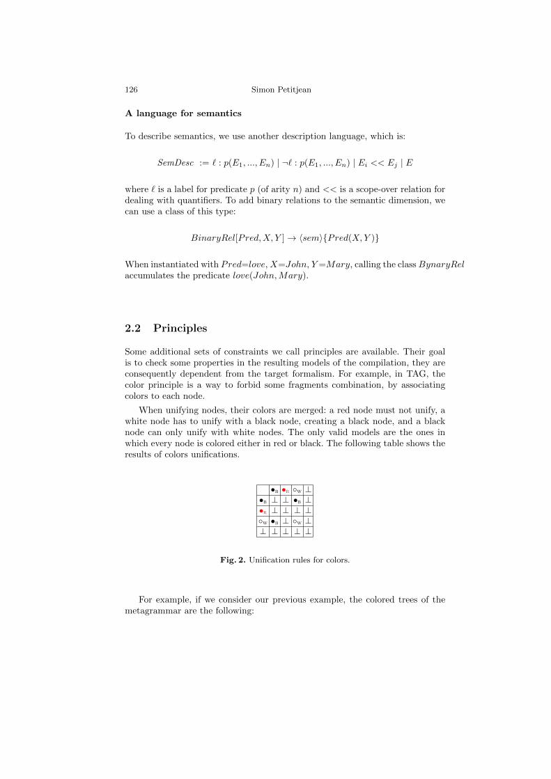
126 Simon Petitjean

A language for semantics

To describe semantics, we use another description language, which is:

SemDesc := ` : p(E1, ..., En) | ¬` : p(E1, ..., En) | Ei << Ej | E

where ` is a label for predicate p (of arity n) and << is a scope-over relation fordealing with quantifiers. To add binary relations to the semantic dimension, wecan use a class of this type:

BinaryRel[Pred,X, Y ]→ 〈sem〉{Pred(X,Y )}

When instantiated with Pred=love,X=John, Y=Mary, calling the classBynaryRelaccumulates the predicate love(John,Mary).

2.2 Principles

Some additional sets of constraints we call principles are available. Their goalis to check some properties in the resulting models of the compilation, they areconsequently dependent from the target formalism. For example, in TAG, thecolor principle is a way to forbid some fragments combination, by associatingcolors to each node.

When unifying nodes, their colors are merged: a red node must not unify, awhite node has to unify with a black node, creating a black node, and a blacknode can only unify with white nodes. The only valid models are the ones inwhich every node is colored either in red or black. The following table shows theresults of colors unifications.

•b •r ◦w ⊥•b ⊥ ⊥ •b ⊥•r ⊥ ⊥ ⊥ ⊥◦w •b ⊥ ◦w ⊥⊥ ⊥ ⊥ ⊥ ⊥

Fig. 2. Unification rules for colors.

For example, if we consider our previous example, the colored trees of themetagrammar are the following:

Spotting and improving modularity in large scale grammar development 127

S◦W

N•B V◦W

CanSubj

N•R

N•R S•R

C•R

Wh•R

S◦W

N◦W

RelObj

S•B

V•B

Active

→

N•R

N•R S•R

C•R

Wh•R

S•B

N•B V•B

The tree description solver (ignoring the colors) will produce models wherethe nodes labelled S of CanSubj and Active unify with any of the two nodeslabelled S in RelObj, where the nodes labelled V do not unify, etc. But whenfiltering with the colors principle, the only remaining model is the one of theright, which is linguistically valid, contrary to the others.

We can also cite the rank principle: we use it to add constraints on theordering of nodes in the models of the description. In French for example, cliticsare necessarily ordered, so we associate a rank property to some nodes, withvalues that will force the right order.

3 Assembling metagrammars in a modular way

The main aim of the XMG-2 project is to make it possible for the linguist todesign new metagrammatical scopes, that can accomodate any linguistic theory.A simple way to realize this ambition is to provide a set of bricks the user canpick to build the compiler he needs. Those bricks could be used to design newdimensions, with new description languages or new principles.

3.1 A modular architecture

XMG compiler comes with a modular processing chain. Most of this chain is astandard compiling chain, including a tokenizer for the metagrammar, a parser,an unfolder, etc.

The particularity of XMG is to make it possible to chose the modules thatsuits the best his metagrammar. By this mean, descriptions accumulated indifferent dimensions can be handled differently. For example, the end of the pro-cessing chain for TAG is a tree description solver, that builds the grammar’selementary trees from the descriptions accumulated in the syntactic dimension.The user can chose the kind of output the compiler will produce: he can inter-actively observe the grammar he produced, or produce an XML description ofthe grammar. This description can be used by a parser (for example TuLiPA [9]3 for TAG, or LeoPar 4 for IG).

3https://sourcesup.cru.fr/tulipa/4http://wikilligramme.loria.fr/doku.php?id=leopar:leopar

128 Simon Petitjean

3.2 Representation modules

As we wish to build a tool which is as universal as possible, being independentfrom the formalism is a priority. To achieve this goal, we need to be able todescribe any type of structure into XMG. We saw the dimension system wasuseful to separate syntax from semantics. It could also be used to separate treedescriptions from constraints based descriptions, as long as we have a dedicateddimension, with a dedicated description language.

In [6], description languages for two formalisms, namely Lexical FunctionalGrammars (LFG) and Property Grammars (PG), are proposed. Here, we willfocus on Property Grammars, because they differ from TAG in many aspects. PGare not based on tree rewriting but on a local constraints system: the properties.A property concerns a node and applies constraints over its children nodes.One of the interesting aspects of PG is the ability to analyse non grammaticalutterances. When parsing a utterance, its grammaticality score is lowered atevery violated property. Here, we will consider these six properties:

Obligation A : 4B at least one B childUniqueness A : B! at most one B childLinearity A : B ≺ C B child precedes C childRequirement A : B ⇒ C if a B child, then also a C childExclusion A : B 6⇔ C B and C children are mutually exclusiveConstituency A : S children must have categories in S

A real size PG consists in a inheritance hierarchy of linguistic constructions.These constructions are composed of feature structures and a set of properties.Variables are manipulated on both sides, and can be used to share data betweenthem. Figure 3 represents a part of the hierarchy built in [7] for French. The V-n

V (Verb)

INTR

[ID—NATURE

[SCAT 1 .SCAT

]]const. V :

1

[CAT V

SCAT ¬ (aux-etre ∨ aux-avoir)

]V-m (Verb with modality) inherits V ; V-n

INTR

SYN

INTRO

[RECT 1

DEP Prep

]uniqueness Prep!

requirement 1 ⇒Prep

linearity 1 ≺Prep

V-n (Verb with negation) inherits V

INTR

SYN

NEGA

[RECT 1

DEP Adv-n

]uniqueness

Adv-ngAdv-np !

requirement 1 ⇒Adv-n

linearity Adv-ng≺ 1

Adv-ng≺Adv-npAdv-np≺ 1 .[MODE inf ]

1 .[MODE ¬inf ] ≺Adv-np

Fig. 3. Fragment of a PG for French (basic verbal constructions)

construction of the figure says that in verbs with negation in French, negationimplies the presence of an adverb ne labelled with category Adv−ng (ne) and/oran adverb labelled with category Adv−np (like pas). We also have a uniqueness

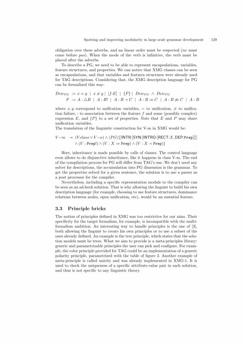
Spotting and improving modularity in large scale grammar development 129

obligation over these adverbs, and an linear order must be respected (ne mustcome before pas). When the mode of the verb is infinitive, the verb must beplaced after the adverbs.

To describe a PG, we need to be able to represent encapsulations, variables,feature structures, and properties. We can notice that XMG classes can be seenas encapsulations, and that variables and features structures were already usedfor TAG descriptions. Considering that, the XMG description language for PGcan be formalized this way:

DescPG := x = y | x 6= y | [f :E] | {P} | DescPG ∧ DescPG

P := A : 4B | A : B! | A : B ≺ C | A : B ⇒ C | A : B 6⇔ C | A : B

where x, y correspond to unification variables, = to unification, 6= to unifica-tion failure, : to association between the feature f and some (possibly complex)expression E, and {P} to a set of properties. Note that E and P may shareunification variables.The translation of the linguistic construction for V-m in XMG would be:

V−m → (V class ∨ V−n) ∧ 〈PG〉{[INTR:[SYN:[INTRO:[RECT:X,DEP:Prep]]]]

∧ (V : Prep!) ∧ (V : X ⇒ Prep) ∧ (V : X ≺ Prep)}

Here, inheritance is made possible by calls of classes. The control languageeven allows to do disjunctive inheritance, like it happens in class V-m. The endof the compilation process for PG will differ from TAG’s one. We don’t need anysolver for descriptions, the accumulation into PG dimension is the grammar. Toget the properties solved for a given sentence, the solution is to use a parser asa post processor for the compiler.

Nevertheless, including a specific representation module to the compiler canbe seen as an ad-hock solution. That is why allowing the linguist to build his owndescription language (for example, choosing to use feature structures, dominancerelations between nodes, open unification, etc), would be an essential feature.

3.3 Principle bricks

The notion of principles defined in XMG was too restrictive for our aims. Theirspecificity for the target formalism, for example, is incompatible with the multi-formalism ambition. An interesting way to handle principles is the one of [3],both allowing the linguist to create his own principles or to use a subset of theones already defined. An example is the tree principle, which states that the solu-tion models must be trees. What we aim to provide is a meta-principles library:generic and parametrizable principles the user can pick and configure. For exam-ple, the color principle provided for TAG could be an implementation of a genericpolarity principle, parametrized with the table of figure 2. Another example ofmeta-principle is called unicity and was already implemented in XMG-1. It isused to check the uniqueness of a specific attribute-value pair in each solution,and thus is not specific to any linguistic theory.

130 Simon Petitjean

3.4 Dynamic definition of a metagrammar

To build his own metagrammatical scope, one should only have to select thedimensions he needs and the properties he wants to check on them. Buildinga dimension would consist in picking bricks out from a library to create a newdescription language. With this feature, a user could redefine the property gram-mars description we proposed earlier. The advantage here is that the specific partof the compiler is written automatically, and new features could be added just forexperiments. Defining the principles would just consist in taking meta-principlesout from the library and instantiate them.

Building a metagrammar compiler in this way allows to deal with a largerange of linguistic theories, or even to quickly experiment while creating a newgrammar formalism.

4 Current state of the work

XMG project started in 2003 with a first tool, that has been used to produce largeTAG grammars for French [2], German [10] and English, and a large InteractionGrammar for French [11]. The compiler was written is Oz/Mozart, a languagewhich is not maintained any more and not compatible with today’s architectures(64 bits). It was also important to restart from scratch, in order to build acompiler more in adequation with its ambitions : modularity and extensibility.

Consequently, a new implementation started in 2010, in YAP (Yet AnotherProlog) with bindings with Gecode for constraints solving. XMG-2 is currentlythe tool used for modeling the syntax and morphology of Ikota, a bantu lan-guage [5], and is getting close to total compatibility with the previous largemetagrammars. It also includes a dimension for basic property grammar de-scription. The work focuses now on a parser generator which, from a descriptionof a description language, produces the parser rules for this language. The firstapplication could be the dynamic generation of a language dedicated to morpho-logic descriptions. We also wish to implement quickly some generic principles,beginning with the tree principle.

5 Conclusion

In this paper, we showed how modularity, together with a metagrammaticalapproach, eases the development of a large scale grammar. This modularity isessential for reaching the main goal of XMG, that is to say extensibility. Gettingto that means taking a big step towards multi-formalism and multi-languagegrammar development, and then offers new possibilities for sharing data betweendifferent types of grammar, or even for comparing them.

Now, what we would like to create is a way to express the definition ofdimensions and meta-principles. This could begin by formalizing a descriptionlanguage for description languages. We also aim to provide more checking tools

Spotting and improving modularity in large scale grammar development 131

to the user, beginning with the type checking of the properties and the featurestructures we manipulate in a lot of grammar formalisms.

References

1. Candito, M.: A Principle-Based Hierarchical Representation of LTAGs. In: Pro-ceedings of COLING 96. Copenhagen, Denmark (1996)

2. Crabbe, B.: Representation informatique de grammaires fortement lexicalisees :Application a la grammaire d’arbres adjoints. Ph.D. thesis, Universite Nancy 2(2005)

3. Debusmann, R.: Extensible Dependency Grammar: A Modular Grammar Formal-ism Based On Multigraph Description. Ph.D. thesis, Saarland University (4 2006)

4. Duchier, D., Le Roux, J., Parmentier, Y.: The Metagrammar Compiler: An NLPApplication with a Multi-paradigm Architecture. In: Proceedings of the 2nd Oz-Mozart Conference, MOZ 2004. Charleroi, Belgium (2004)

5. Duchier, D., Magnana Ekoukou, B., Parmentier, Y., Petitjean, S., Schang, E.: De-scribing Morphologically-rich Languages using Metagrammars: a Look at Verbs inIkota. In: Workshop on ”Language technology for normalisation of less-resourcedlanguages”, 8th SALTMIL Workshop on Minority Languages and the 4th work-shop on African Language Technology. Istanbul, Turkey (2012), http://hal.

archives-ouvertes.fr/hal-00688643/en/

6. Duchier, D., Parmentier, Y., Petitjean, S.: Cross-framework grammar engineeringusing constraint-driven metagrammars. In: CSLP’11. Karlsruhe, Allemagne (2011),http://hal.archives-ouvertes.fr/hal-00614661/en/

7. Guenot, M.L.: Elements de grammaire du francais pour une theorie descriptive etformelle de la langue. Ph.D. thesis, Universite de Provence (2006)

8. Joshi, A.K., Schabes, Y.: Tree adjoining grammars. In: Rozenberg, G., Salomaa,A. (eds.) Handbook of Formal Languages. Springer Verlag, Berlin (1997)

9. Kallmeyer, L., Maier, W., Parmentier, Y., Dellert, J.: Tulipa - parsing extensionsof tag with range concatenation grammars (June 2009), first Polish-German Work-shop on Research Cooperation in Computer Science

10. Kallmeyer, L., Lichte, T., Maier, W., Parmentier, Y., Dellert, J.: Developing att-mctag for german with an rcg-based parser. In: LREC. ELRA (2008)

11. Perrier, G.: A French Interaction Grammar. In: RANLP. Borovets, Bulgaria (2007),http://hal.inria.fr/inria-00184108/en/

Questions of Trust

Jason Quinley1 and Christopher Ahern2

1 University of Tubingenjason.quinley@student.uni-tuebingen.de

2 University of Pennsylvaniacahern@ling.upenn.edu

Abstract. We consider the application of Game Theory in the model-ing of different strategies of politeness. In particular, we examine howdifferences in the linguistic form of requests and proposals map ontothe structure of the game being played by interlocutors. We show howconsiderations of social wants [1, 2] and coordination and cooperationmotivate these differences. First, we adapt the notion of other-regardingpreferences [3, 4] to show how linguistic systems with the ability to en-code politeness strategies allow for requests and cooperation between awider range of individuals. Finally, we connect the distinction betweenrequests and proposals to the notion of a self-enforcing equilibrium [5].

1 Introduction

Questions in their many forms are central to social interaction. Asking someonefor a dollar, or if they would like to see a movie, are commonplace yet revelatory.The indicate how we use language not only to convey information, but also tonegotiate relationships. A clear case of these distinctions can be had in the useof the modals will and would in the following requests:

(1) Will/Would you lend me a dollar?(2) Will/Would you open the door?(3) Will/Would you turn that music down?(4) Will/Would you marry me?

Consider asking these questions of a stranger. It would be impolite to omitthe modal. Moreover, between the two modals we also sense a difference in effect.In the first two cases would is the more polite form of request. In the third eitheris acceptable, modulo the degree to which the music affects the speaker. In thelast, will seems the more appropriate form. Moreover, would allows for comedicresponse: I would if you were rich/handsome/x!

Why are such questions necessary? One reason is that scarcity and ambiguitydrive interaction. We have neither unlimited resources nor unlimited informationwith which to achieve our ends. This leads to the need for cooperation, and withit, strategies to address its fragility. As humans have access to language, they areavailed of multiple avenues of cooperation. Studying these allows for a fruitfulcombination of theories of language and rational interaction.

Questions of Trust 133

In what follows, we examine the use of modals in requests and proposals. Weshow how modals, and other politeness strategies, when thought of in terms ofother-regarding preferences, allow for expanded interaction between individuals.We also show how and why the use of the modal will in requests is binding,whereas would is not necessarily so. We begin by presenting the relevant notionsfrom politeness- and game theory, then turn to our analysis of requests in theseterms and suggest future directions.

2 Politeness Theory and Speech Acts

Beginning from Goffman’s [1] notion of face, Brown and Levinson [2] articulatedan ur-theory of politeness, which has prompted much subsequent theoretical andempirical work. Face is the term given to an individual’s basic needs, character-ized broadly as the need for autonomy (negative face) and acceptance (positiveface). Broadly, positive face can be thought of as the wants of the individual,including the desire that those wants be desirable to or approved of by oth-ers. Negative face includes both the freedom of action and the freedom fromimposition.

Preferences of one agent may conflict with those of others, incentivizing themto make requests, issue threats, or offer proposals. In cases where a requestmust be made, speakers must commit a face-threatening act (FTA). In order tomitigate the weight of a FTA, speakers may use several strategies, as laid out inFigure 1.

Fig. 1. Brown and Levinson’s Politeness Strategies: As we move upwards on thegraph, the potential for a face-threatening act (FTA) increases.

At the two extremes, a speaker might avoid making the FTA altogether, orstate it in a direct manner. In between there are various degrees of deference to

134 Jason Quinley and Christopher Ahern

the hearer’s face wants: indirect speech that is “off the record” and addressing thehearer’s positive or negative face. As a concrete example, consider the situationof having left one’s wallet at the office while going out to lunch with a group.Here the relevant FTA might be taken as requesting some money from a friend.The various strategies of doing so could be implemented as:

(1) Don’t do FTA: Don’t ask for money.(2) Off Record:3“Oh no! I forgot my wallet in my office!”(3) Negative Politeness:“You don’t have to, but would you mind lending me

a bit of money?”(4) Positive Politeness:“Congratulations on the raise! Want to lend me some

money.”

The goal of the speaker is to craft the appropriate message to convey theintent and the weight of the FTA. The greater an imposition a FTA carries,the more care needs to be taken. However, too much politeness is inappropriategiven certain FTAs. It would seem odd to be asked, rather circuitously, “Excuseme Sir/Ma’am, but I was hoping that it might be possible if it’s not too muchtrouble that you would be able to tell me the time.” Similarly, when expediencyis called for, “Please, if you could, move out of the way of that speeding car,”would be inappropriate. Thus we might think of different forms of politeness asstrategic responses to situations where face may be threatened. Again, the goalof the speaker is to select the appropriate form for the FTA in question; neithertoo much nor too little deference can be paid. With this notion of strategy inmind we turn to the game-theoretic framework that will figure in our analysis.

3 Basic Game Theory

Game theory gives a mathematical model of strategic interaction between agents.We begin by presenting canonical examples from the field. Crucially, we focuson the difference between cooperation and coordination in sequential play. Se-quential play allows for an optimal outcome under rational behavior in cases ofcoordination, but not for cooperation.

Formally, a sequential game is a tuple 〈N,O,Aj , Ui〉. N is the set of playersin the game. O is a sequence over N that determines the order of play; forj ∈ O, Aj is the set of actions available to the jth player in the order of play.Finally, Ui is a preference for player i over the set of possible paths of play.The payoffs are represented as numeric values, where higher values are taken tobe more preferred outcomes. The Prisoner’s Dilemma (PD) offers the canonicalexample of choosing between cooperation and defection. The game reflects ascenario wherein two prisoners must choose between cooperatively staying silent(C), telling the police nothing about their crime, or defecting on each other (D)and confessing the details to the police. Jointly, both prisoners do better if they

3See Pinker et al. [6] as well as Mialon [7] for game-theoretic treatments of indirectspeech.

Questions of Trust 135

remain silent, but individually, they do better by ratting out their accomplice.We represent the structure of the Prisoner’s Dilemma in extensive form in Figure2. Each node in the game is labeled with the letter of the player whose turn itis to take an action, O = 〈X,Y 〉. The payoffs, as determined by the utilityfunctions, are listed as (UX , UY ) at the bottom of the tree.

Fig. 2. A Sequential PD Fig. 3. A Sequential PCG

We use the notion of a rollback equilibrium to examine expected behavior inthe game. The reasoning proceeds as follows. We begin by considering the lowestnodes in the game and putting in bold the best action available. For any nodewhere Y can make a choice, she should choose D as it is always the better option.Knowing that this is the case, X should always choose D, as it always the bestoption based on what Y will do. That is, cooperation will only ever be met withdefection, so it should never be explored. We will refer to those instances whereplayers have diverging interests but come together to yield the optimal outcomefor all as instances of cooperation. In instances of cooperation, as in the PD,reaching the best outcome for the players as a group requires some sacrifice interms of individual payoff. That is, each player must forgo the temptation payoffof defecting in order to maintain cooperation.

In contrast, in cases of coordination, players’ incentives do not conflict. Con-sider the case of a Pure Coordination Game (PCG) in Figure 3. Here playersare ambivalent between the actions they take, they only prefer to take the sameaction. An example might be a scenario where two friends want to meet up forlunch at noon. If one player suggests a restaurant, then the other should indeedgo to that restaurant. If X plays A (B), then Y should play A (B). Sequen-tial games allow for the optimal outcome for both players in pure coordinationgames.

These game structures allow us to distinguish between the notions of coop-eration and coordination. We might think of the first as exemplified in the Pris-oner’s Dilemma, and the latter in the case of Pure Coordination Games. Withthis background in place, we now turn to the analysis of modals in requests andexamine the different rationales for polite behavior.

136 Jason Quinley and Christopher Ahern

4 Trust and Modals

In this section we show how face-addressing forms allow for requests between awider range of individuals. This serves as a broad motivation for using such formswith strangers. We then turn to a distinction between requests in general andmarriage proposals in particular, where we argue for a distinction between thedifferent sorts of speech acts involved as they relate to the notion of self-enforcingequilibria.

4.1 Requests as Extended Trust Games

Quinley [8] adapts Trust Games [9] as a model of requests. We borrow tech-niques and insights from this approach and introduce Extended Trust Games tocapture the sequential dynamics of requests. We note the effects of repetition,reputation, and observation on polite forms in requests, but suggest that theyare not sufficient to fully explain the use of politeness strategies. Instead, wepropose other-regarding preferences as a means to explain the use of modals andother forms of linguistic politeness in a variety of situations.

Trust games are an appropriate model for requests due to several factors.First, individuals are rarely if ever entirely self-sufficient. Moreover, agents pos-sess different aptitudes and abilities, and this asymmetry prompts requests. Re-quests entail a loss of face on the part of the requester; so to speak, the requestermakes a face “payment” to the requestee. Finally, the requestee is not obligatedto grant the request, presenting the agent in need with the risk of both a loss offace and having their request denied.

Trust games depict a scenario where Player X has an initial option to defer toPlayer Y for a potentially larger payoff for both. We extend this notion further,incorporating a third step in the order of play. Here the play of the game isshown in extensive form in Figure 4 and consists of the first player asking or notasking for some favor, the second player granting or not granting the request,and the requester thanking or not thanking the requestee. We considered a moredetailed motivation of the utility structure below.

If X does not ask (¬A), then the status quo remains and X is left to her owndevices. Let cx be the cost to X to achieve the desired outcome. Let cy be thecost to Y to achieve the same outcome. As noted before, assume an asymmetryin ability or disposition such that cy < cx; Y is in a better position than X tobring about X’s desired state of affairs. If X does ask (A) for help, using a politerequest, Y should experience some boost in self-esteem based on the attentionreceived. That is, by acting in accordance with Y ’s face wants, X increases Y ’sface. Let the amount of face paid by X to Y in the request be fr. Let mr bea multiplicative factor that acts upon fr to determine the payoff to Y . If talkis cheap, then flattery is certainly sweet; a little bit of face goes a long way, sowe assume that mr > 1. Even if Y chooses not to grant the request, Y stillcomes away with some benefit based on the face paid by X, mrfr. If Y deniesthe request (¬G), X has incurred the face cost of asking without receiving anybenefits, and must also bear the cost of performing the action, cx. If Y chooses

Questions of Trust 137

to grant the request (G), then Y incurs some cost of the action, but still receivesthe benefit of face from X. Let the benefit to X of Y granting the request bebx. In general, we assume that bx < cx. If the request is granted, then X has anopportunity to express to Y some sort of thanks (T ) or not (¬T ). This expressionof thanks, again, comes at some cost ft, and, again, carries with it some facebenefit to Y as determined by a factor mt > 1.

Fig. 4. Request Trust Game: Player X can choose to Ask (A) something fromPlayer Y , who can then choose to Grant (G) the favor. Player X can choose to Thank(T ) or not Thank (¬T ) player Y .

We are faced with the same problem as the prisoner’s dilemma; requests areFTAs that require cooperation. X prefers ¬T to T , Y prefers ¬G to ¬T , and Xprefers ¬A to ¬G. Thus, if we are only maximizing individual utility, it nevermakes sense in a one-shot scenario to ask, grant, or thank, even though bothplayers might prefer the interaction under certain assumptions. We thus considerthe effect of repetition, reputation, and observation on the outcome.

4.2 Repetition and Reputation

Under various conditions, repetition engenders cooperation [10]. More specifi-cally, with a given probability of another round of play, group welfare becomesindividual welfare; i.e. a PD becomes a Stag Hunt [11]. In a Stag Hunt, play-ers’ interest are highly aligned, and the only pitfall is the possibility of mis-coordination. Importantly, in a Stag Hunt players wish to coordinate, but maynot necessarily know how when playing simultaneously. In Figure 5, the StagHunt structure assumes that players have aligned preferences, and shared pref-erences over outcomes.

Here, as in the case of coordination games, sequential play allows the playersto achieve the optimal outcome. That is, if the first player plays Stag, then thesecond player should as well. Repetition transforms a Prisoner’s Dilemma toa Stag Hunt. However, repetition cannot be all there is to the outcome of the

138 Jason Quinley and Christopher Ahern

Stag Rabbit

Stag 4,4 0,1

Rabbit 1,0 1,1

Fig. 5. Stag Hunt (SH):in strategic form

Fig. 6. Stag Hunt (SH):in extensive form

interactions we consider here. People are polite to strangers they will never seeagain.

The effects of reputation and observation on different strategies in trustgames are explored in Quinley [8]. Namely, asking requests of other agents isrational when there is a sufficient likelihood that the request will be grantedbased on the requestee’s reputation. Or, in the case here, granting requests isrational when there is sufficient likelihood that X will play T . If Y has sufficientexperience or knowledge about the behavior of X with regards to Pr(T ), thenthis suffices to render granting the request rational strategy or not. The novelcontribution of Quinley is the inclusion of face effects due to third-party obser-vation. In line with experimental results [12], such observation, framed as a loss(gain) in face for Y when denying (granting) a request, is shown to ensure thatrequests are asked and granted by and large. This can be extended similarly toX’s actions when choosing to thank Y or not.

4.3 Other-Regarding: Reciprocity Without Repetition

While reputation and observation offer rationales for asking and granting re-quests, they are unlikely to explain all of the behavior we observe. Modals areused to make requests in one-shot interactions where nothing is known about theother individual and there are no third-party observers. In fact, the polite useof modals is even more expected in these sorts of situations. This suggests thatreputation and observation are not alone in explaining the behavior observedin requests A rationale for politeness strategies in such situations can be foundwhen we consider other-regarding preferences.

There exists a wealth of theoretical work on [13–15], and behavioral [16, 17]and neurobiological evidence [18] of other-regarding preferences. Here we adaptthe notion of sympathy as advanced by Sally [3, 4] to explain the observedbehavior. The central notion is that of a sympathy distribution over the payoffsof all the agents involved in the game. For each agent, there is a distribution,δi ∈ ∆(U), such that

∑j δi(Uj) = 1, which determines how much that agent

cares about her own payoffs and those of others. For example, the perfectly self-

Questions of Trust 139

interested agent of classical Economic theory is such that δi(Uj) = 0 for all j 6= i.A selfless agent would be such that δi(Ui) = 0.

Here we consider the limiting case of a single interlocutor. Based on thesympathy distribution and the utility function U of the original game, we definea new utility function V .

Vi = δi(Ui) · Ui + (1− δi(Ui)) · Uj (1)

The impact of other-regarding preferences can be seen in the following. Con-sider what values would suffice to make thanking rational for X in the ExtendedTrust Game of Figure 4. Namely, we wish to determine the condition underwhich the sympathy distribution of X renders thanking (T ) preferable to notthanking (¬T ). This holds just when:

Vx(¬T ) < Vx(T )

1

1 +mt< δx(Uy)

(2)

Given that mt > 1, the highest threshold will be bounded from above by 12 .

As mt increases, the threshold approaches 0. The greater the benefit to Y forthanking, the less X has to care about Y ’s payoff to do so. This undoes someof the unraveling effect of divergent preferences. We move on to determine theconditions on Y ’s preferences that suffice to allow for cooperation. That is, wewish to determine when Y prefers T to ¬G.

Vy(¬G) < Vy(T )

(cy −mtft)

(cy −mtft) + bx + cx − ft< δy(Ux)

(3)

There several important points to consider. First, the thresholds we haveoutlined here are the conditions under which the underlying game of cooperationis transformed into one of coordination. That is, if these thresholds are surpassed,then the game is one of coordination rather than cooperation, and we shouldexpect requests to be made, granted, and thanks expressed. If X’s condition onthanking is not met, then the request should be granted if Y prefers ¬T to ¬G,which is true just when:

Vy(¬G) < Vy(¬T )cy

cy + bx + cx< δy(Ux)

(4)

Otherwise, we should expect requests not to be made.Second, we find that if mtft > cy, then the request should be granted for any-

one, regardless of the sympathy distribution. We might be tempted to think ofT in terms of expressing a future commitment to cooperation. While T has this

140 Jason Quinley and Christopher Ahern

flavor, it does not have this force; thanks, like talk, are cheap. For the expressionof thanks to outweigh the cost, cy, would require either something particularlyimportant to Y , or some strong guarantee on the part of X. Again, future guar-antees are not available in the case of single interactions with strangers.

Third, note that cx−ft > cy−mtft given that cx > cy and m > 1. Moreover,note that bx > cx, and thus bx > cy−mtft. As such, as we collapse the non-fixedvalues towards zero, we see that 1

3 serves as an upper bound on the threshold. Theuse of a face addressing form, such as the polite use of modals, allows for a lowerthreshold of other-regarding preferences for requestees compared to requesters.This makes intuitive sense as requesters are more inherently self-interested.

Finally, the use of politeness strategies that address face allow for a lowerthreshold than a system without such forms. Consider a faceless Trust Game,where ft = fr = 0 for the payoffs in Figure 4. We can think of this as a systemwhere no transfers of face are possible. The structure of the game reduces toa choice on the part of Y between granting or not granting the request. Thecorresponding threshold of other-regarding preference can be given as follows:

Vy′(¬G) < Vy′(G)cy

cy + bx + cx< δy′(Ux′)

(5)

From Eq. (3) and (5) we know that a system with face requires a lowersympathy threshold than one without face just when:

δy(Ux) < δy′(Ux′)cy

bx + cx< mt

(6)

Given cy < cx, we know thatcy

bx+cx< 1. Since, mt > 1, it is always the

case that a system with face requires a lower threshold than a system without,thus allowing for requests between a wider range of individuals. In this sense,when considered in the context of other-regarding preferences, face allows forcooperation by smoothing out the payoffs of the interlocutors. By “investing” ineach other’s face, we can guarantee cooperation more easily, even with peoplewe do not know.

4.4 Proposals and Credible Signaling

In contrast with requests, proposals encode an interaction potentially to the ben-efit of both participants. Returning to marriage, we noted the use of modals incertain contexts differs. For purposes of both humor and invoking the undercur-rent of common knowledge, we observed that would allows for a certain amountof disavowal whereas will does not. For example, the following dialogues can becompleted for comedic effect:

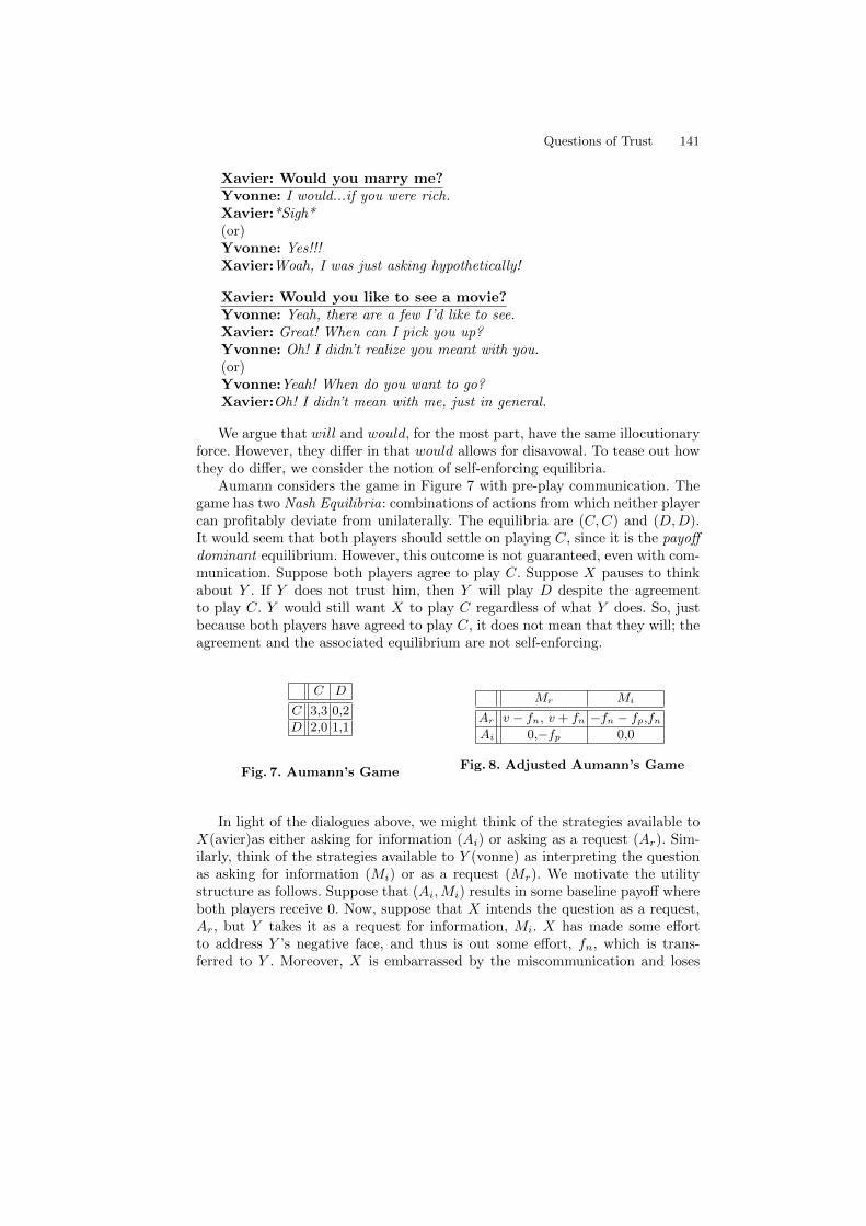
Questions of Trust 141

Xavier: Would you marry me?Yvonne: I would...if you were rich.Xavier:*Sigh*(or)Yvonne: Yes!!!Xavier:Woah, I was just asking hypothetically!

Xavier: Would you like to see a movie?Yvonne: Yeah, there are a few I’d like to see.Xavier: Great! When can I pick you up?Yvonne: Oh! I didn’t realize you meant with you.(or)Yvonne:Yeah! When do you want to go?Xavier:Oh! I didn’t mean with me, just in general.

We argue that will and would, for the most part, have the same illocutionaryforce. However, they differ in that would allows for disavowal. To tease out howthey do differ, we consider the notion of self-enforcing equilibria.

Aumann considers the game in Figure 7 with pre-play communication. Thegame has two Nash Equilibria: combinations of actions from which neither playercan profitably deviate from unilaterally. The equilibria are (C,C) and (D,D).It would seem that both players should settle on playing C, since it is the payoffdominant equilibrium. However, this outcome is not guaranteed, even with com-munication. Suppose both players agree to play C. Suppose X pauses to thinkabout Y . If Y does not trust him, then Y will play D despite the agreementto play C. Y would still want X to play C regardless of what Y does. So, justbecause both players have agreed to play C, it does not mean that they will; theagreement and the associated equilibrium are not self-enforcing.

C D

C 3,3 0,2

D 2,0 1,1

Fig. 7. Aumann’s Game

Mr Mi

Ar v − fn, v + fn −fn − fp,fnAi 0,−fp 0,0

Fig. 8. Adjusted Aumann’s Game

In light of the dialogues above, we might think of the strategies available toX(avier)as either asking for information (Ai) or asking as a request (Ar). Sim-ilarly, think of the strategies available to Y (vonne) as interpreting the questionas asking for information (Mi) or as a request (Mr). We motivate the utilitystructure as follows. Suppose that (Ai,Mi) results in some baseline payoff whereboth players receive 0. Now, suppose that X intends the question as a request,Ar, but Y takes it as a request for information, Mi. X has made some effortto address Y ’s negative face, and thus is out some effort, fn, which is trans-ferred to Y . Moreover, X is embarrassed by the miscommunication and loses

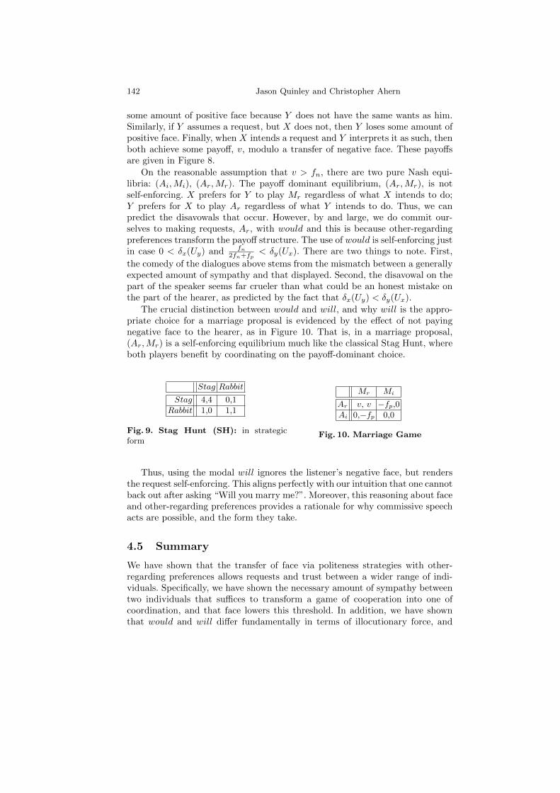
142 Jason Quinley and Christopher Ahern

some amount of positive face because Y does not have the same wants as him.Similarly, if Y assumes a request, but X does not, then Y loses some amount ofpositive face. Finally, when X intends a request and Y interprets it as such, thenboth achieve some payoff, v, modulo a transfer of negative face. These payoffsare given in Figure 8.

On the reasonable assumption that v > fn, there are two pure Nash equi-libria: (Ai,Mi), (Ar,Mr). The payoff dominant equilibrium, (Ar,Mr), is notself-enforcing. X prefers for Y to play Mr regardless of what X intends to do;Y prefers for X to play Ar regardless of what Y intends to do. Thus, we canpredict the disavowals that occur. However, by and large, we do commit our-selves to making requests, Ar, with would and this is because other-regardingpreferences transform the payoff structure. The use of would is self-enforcing justin case 0 < δx(Uy) and fn

2fn+fp< δy(Ux). There are two things to note. First,

the comedy of the dialogues above stems from the mismatch between a generallyexpected amount of sympathy and that displayed. Second, the disavowal on thepart of the speaker seems far crueler than what could be an honest mistake onthe part of the hearer, as predicted by the fact that δx(Uy) < δy(Ux).

The crucial distinction between would and will, and why will is the appro-priate choice for a marriage proposal is evidenced by the effect of not payingnegative face to the hearer, as in Figure 10. That is, in a marriage proposal,(Ar,Mr) is a self-enforcing equilibrium much like the classical Stag Hunt, whereboth players benefit by coordinating on the payoff-dominant choice.

Stag Rabbit

Stag 4,4 0,1

Rabbit 1,0 1,1

Fig. 9. Stag Hunt (SH): in strategicform

Mr Mi

Ar v, v −fp,0Ai 0,−fp 0,0

Fig. 10. Marriage Game

Thus, using the modal will ignores the listener’s negative face, but rendersthe request self-enforcing. This aligns perfectly with our intuition that one cannotback out after asking “Will you marry me?”. Moreover, this reasoning about faceand other-regarding preferences provides a rationale for why commissive speechacts are possible, and the form they take.

4.5 Summary

We have shown that the transfer of face via politeness strategies with other-regarding preferences allows requests and trust between a wider range of indi-viduals. Specifically, we have shown the necessary amount of sympathy betweentwo individuals that suffices to transform a game of cooperation into one ofcoordination, and that face lowers this threshold. In addition, we have shownthat would and will differ fundamentally in terms of illocutionary force, and

Questions of Trust 143

the underlying structure of the interaction. would allows for disavowal and isnot necessarily self-enforcing, whereas will as a commissive speech act commitsthe speaker to a course of action. In parallel to results from dynamic epistemiclogic [19], saying will creates common knowledge between the participants of thehearer’s commitment to future action, and thus it is only rational in the casethat both participants have a benefit towards taking that action and that theaction cannot be repeated.

5 Conclusion

This work follows in the vein of approaches to pragmatics and politeness froma strategic viewpoint. It defines the conditions under which politeness strategiesare rational in those situations where repetition, reputation, and observation donot hold. A central result is that a system with face allows for a greater level oftrust between agents with other-regarding preferences. Also, it outlines how themodals will and would map onto fundamentally different game structures andpredicts both the humorous possibilities of denial and the real power of socially-binding statements. Future directions include extending the current analysis tothreats such as Will you cut that music out! and requests for information Willyou be here later?, and providing a broader theoretical framework for the descrip-tion of speech acts. The results presented here demonstrate the growing abilityof game-theoretic methods to model pragmatic phenomena, including politeness.Moreover, though reciprocity and coordination existed outside of and prior tolanguage, language nonetheless serves as an efficient tool for managing them inrelationships.

References

1. Goffman, E.: Interaction Ritual: Essays on Face-to-Face Behavior. 1st pantheonbooks edn. Pantheon, New York (1982)

2. Brown, P., Levinson, S.C.: Politeness: Some universals in language use. CambridgeUniversity Press, Cambridge (1978)

3. Sally, D.: A general theory of sympathy, mind-reading, and social inter- action,with an application to the prisoners’ dilemma. Social Science Information 39(4)(2000) 567–634

4. Sally, D.: On sympathy and games. Journal of Economic Behavior and Organiza-tion 44(1) (2001) 1–30

5. Aumann, R.J.: 34. In: Nash Equilibria Are Not Self-Enforcing. Elsevier (1990)667–677

6. the National Academy of Sciences of the United States of America: The logic ofindirect speech, the National Academy of Sciences of the United States of America(2007)

7. Mialon, H., Mialon, S.: Go figure: The strategy of nonliteral speech. (2012)8. Quinley, J.: Trust games as a model for requests. ESSLLI 2010 and ESSLLI 2011

Student Sessions. Selected Papers (2012) 221–233

144 Jason Quinley and Christopher Ahern

9. Berg, J., Dickhaut, J., McCabe, K.: Trust, reciprocity, and social history. Gamesand Economic Behavior 10(1) (July 1995) 122–142

10. Mailath, G.J., Samuelson, L.: Repeated games and reputations: long-run relation-ships. Oxford University Press, Oxford (2006)

11. Skyrms, B.: The Stag Hunt and the Evolution of Social Structure. CambridgeUniversity Press, Cambridge (2004)

12. Fehr, E., Fischbacher, U.: Third-party punishment and social norms. Experimental0409002, EconWPA (September 2004)

13. Rabin, M.: Incorporating fairness into game theory and economics. AmericanEconomic Review 83(5) (December 1993) 1281–1302

14. Fehr, E., Schmidt, K.M.: A theory of fairness, competition and cooperation. CEPRDiscussion Papers 1812, C.E.P.R. Discussion Papers (March 1998)

15. Levine, D.K.: Modeling altruism and spitefulness in experiment. Review of Eco-nomic Dynamics 1(3) (July 1998) 593–622

16. Fehr, E., Schmidt, K.M.: Theories of fairness and reciprocity - evidence and eco-nomic applications. CEPR Discussion Papers 2703, C.E.P.R. Discussion Papers(February 2001)

17. Camerer, C.: Behavioral Game Theory: Experiments in Strategic Interaction.Princeton University Press, Princeton (2003)

18. Fehr, E.: 15. In: Social Preferences and the Brain. Academic Press (2008)19. Baltag, A., Moss, L.S., Solecki, S.: The logic of public announcements, common

knowledge and private suspicions. Technical Report TR534, Indiana University,Bloomington (November 1999)

Checking Admissibility in Finite Algebras

Christoph Rothlisberger∗

Mathematics Institute, University of BernSidlerstrasse 5, 3012 Bern, Switzerland

christoph.roethlisberger@math.unibe.ch

Abstract. Checking if a quasiequation is admissible in a finite algebrais a decidable problem, but the naive approach, i.e., checking validity inthe corresponding free algebra, is computationally unfeasible. We givean algorithm for obtaining smaller algebras to check admissibility and arange of examples to demonstrate the advantages of this approach.

1 Introduction

Rules and axioms are the building blocks of a logic. Axioms are the assumptionsof the logic, whereas rules are used to derive new facts from previously derivedfacts. Rules are usually formulated as IF-THEN statements, e.g. “IF x is aninteger and x is positive THEN x + 1 is a natural number”. More generally,a rule is a set of premises followed by a conclusion. In logic, the premises andthe conclusion are formulas. In algebra they are usually equations, as in thecancellation rule “IF x + y = x + z THEN y = z”. Axioms are rules without apremise and can be read as, e.g., “x + y = y + x always holds”. In algebra oneoften uses Σ to denote a finite set of equations and calles the rule “IF Σ THENϕ ≈ ψ”, written Σ ⇒ ϕ ≈ ψ, a quasiequation. A quasiequation Σ ⇒ ϕ ≈ ψ iscalled valid in the finite algebra A if whenever every equation in Σ is true in Afor a specific choice of elements of A for the variables occuring in Σ ∪ {ϕ ≈ ψ},then also ϕ ≈ ψ is true in A for this choice.

Checking validity in finite algebras (similarly, derivability in finite-valuedlogics) has been studied extensively in the literature, and may be considered a“solved problem” in the sense that there exist both general methods for obtainingproof systems for checking validity (tableaux, resolution, multisequents, etc.) andstandard optimization techniques for such systems (lemma generation, indexing,etc.) (see, e.g., [1, 12, 24]). A rule which can be added to a given system withoutproducing new valid equations is called admissible. This notion was introducedby Lorenzen in 1955 [18], but the property of being admissible was already usedby Gentzen twenty years earlier [7]. Admissibility has been studied intensively inthe context of intermediate and transitive modal logics and their algebras [6, 8,9, 13, 15, 21], leading also to proof systems for checking admissibility [2, 10, 14],and certain many-valued logics and their algebras [5, 16, 17, 19, 21], but a generaltheory for this latter case has so far been lacking.

∗Supported by Swiss National Science Foundation grant 20002 129507.

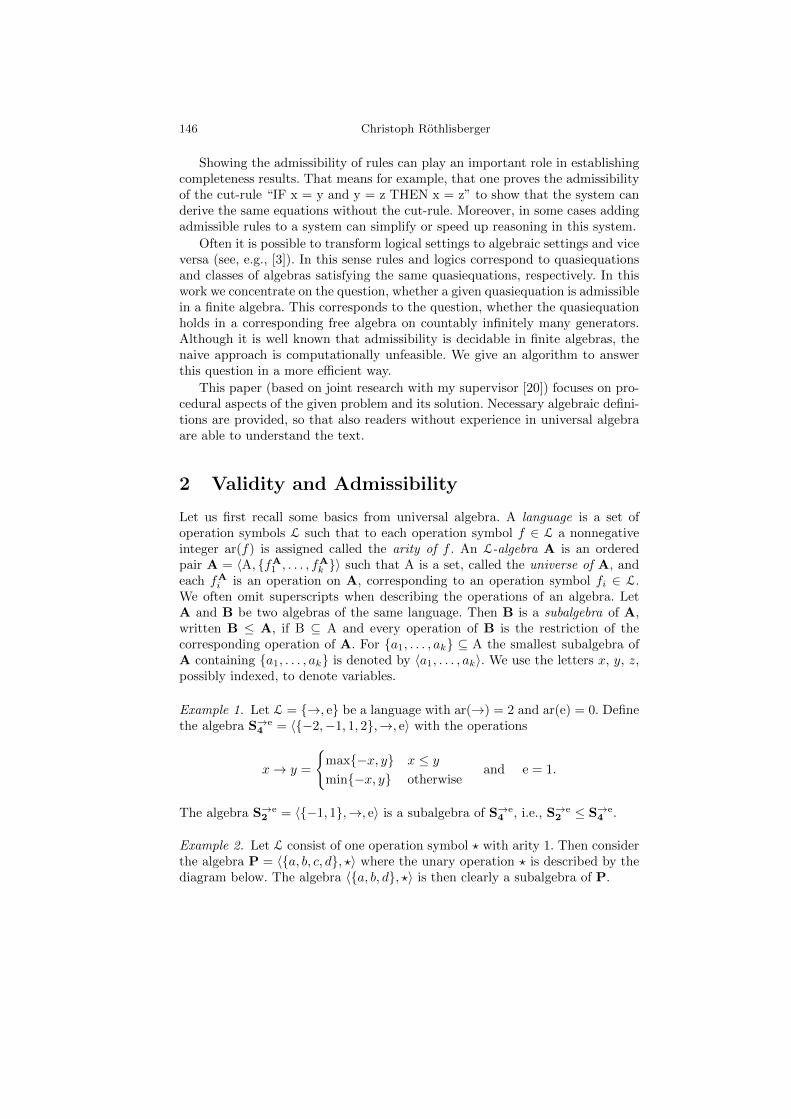
146 Christoph Rothlisberger

Showing the admissibility of rules can play an important role in establishingcompleteness results. That means for example, that one proves the admissibilityof the cut-rule “IF x = y and y = z THEN x = z” to show that the system canderive the same equations without the cut-rule. Moreover, in some cases addingadmissible rules to a system can simplify or speed up reasoning in this system.

Often it is possible to transform logical settings to algebraic settings and viceversa (see, e.g., [3]). In this sense rules and logics correspond to quasiequationsand classes of algebras satisfying the same quasiequations, respectively. In thiswork we concentrate on the question, whether a given quasiequation is admissiblein a finite algebra. This corresponds to the question, whether the quasiequationholds in a corresponding free algebra on countably infinitely many generators.Although it is well known that admissibility is decidable in finite algebras, thenaive approach is computationally unfeasible. We give an algorithm to answerthis question in a more efficient way.

This paper (based on joint research with my supervisor [20]) focuses on pro-cedural aspects of the given problem and its solution. Necessary algebraic defini-tions are provided, so that also readers without experience in universal algebraare able to understand the text.

2 Validity and Admissibility

Let us first recall some basics from universal algebra. A language is a set ofoperation symbols L such that to each operation symbol f ∈ L a nonnegativeinteger ar(f) is assigned called the arity of f . An L-algebra A is an orderedpair A = 〈A, {fA

1 , . . . , fAk }〉 such that A is a set, called the universe of A, and

each fAi is an operation on A, corresponding to an operation symbol fi ∈ L.

We often omit superscripts when describing the operations of an algebra. LetA and B be two algebras of the same language. Then B is a subalgebra of A,written B ≤ A, if B ⊆ A and every operation of B is the restriction of thecorresponding operation of A. For {a1, . . . , ak} ⊆ A the smallest subalgebra ofA containing {a1, . . . , ak} is denoted by 〈a1, . . . , ak〉. We use the letters x, y, z,possibly indexed, to denote variables.

Example 1. Let L = {→, e} be a language with ar(→) = 2 and ar(e) = 0. Definethe algebra S→e

4 = 〈{−2,−1, 1, 2},→, e〉 with the operations

x→ y =

{max{−x, y} x ≤ ymin{−x, y} otherwise

and e = 1.

The algebra S→e2 = 〈{−1, 1},→, e〉 is a subalgebra of S→e

4 , i.e., S→e2 ≤ S→e

4 .

Example 2. Let L consist of one operation symbol ? with arity 1. Then considerthe algebra P = 〈{a, b, c, d}, ?〉 where the unary operation ? is described by thediagram below. The algebra 〈{a, b, d}, ?〉 is then clearly a subalgebra of P.

Checking Admissibility in Finite Algebras 147

aP

b

c d

The set TmL of L-terms is inductively defined: every variable is an L-termand if ϕ1, . . . , ϕn are L-terms and the operation symbol f ∈ L has arity n,then also f(ϕ1, . . . , ϕn) is an L-term. We denote the term algebra over count-ably infinitely many variables by TmL (i.e., for each f ∈ L with ar(f) = n,ϕ1, . . . , ϕn ∈ TmL, fTmL(ϕ1, . . . , ϕn) is just the L-term f(ϕ1, . . . , ϕn)) and letϕ,ψ stand for arbitrary members of the universe TmL. An L-equation is a pairof L-terms, written ϕ ≈ ψ. If Σ is a finite set of L-equations, we call Σ ⇒ ϕ ≈ ψan L-quasiequation. As usual, if the language is clear from the context we mayomit the prefix L.

Example 3. Terms in the language of Example 1 are, e.g., x, x→ x or (x→ e)→y whereas terms corresponding to Example 2 have the form ?(x) or ?(?(?(y))).The following is a quasiequation in the language of Example 1

{x ≈ y → x, x→ e ≈ y} ⇒ x ≈ e.

A homomorphism h between two algebras A and B of the same languageL is a map h : A → B between their universes that preserves all the opera-tions, i.e., for all a1, . . . , an ∈ A and every operation f ∈ L with ar(f) = n,h(fA(a1, . . . , an)) = fB(h(a1), . . . , h(an)). The homomorphism h : A → B iscalled surjective if for all b ∈ B, there exists an a ∈ A such that h(a) = b. Twoalgebras A and B are said to be isomorphic, if there exists a surjective homo-morphism h : A → B with h(a) 6= h(b) for all a 6= b. The algebra C with theuniverse C = {h(a) : a ∈ A} ⊆ B and the restrictions of the operations of B toC as operations is called a homomorphic image of A, written C ∈ H(A).

We say that the quasiequation Σ ⇒ ϕ ≈ ψ is valid in A or “holds in A”,written Σ |=A ϕ ≈ ψ, if for every homomorphism h : TmL → A, h(ϕ′) =h(ψ′) for all ϕ′ ≈ ψ′ ∈ Σ implies h(ϕ) = h(ψ).

Example 4. The quasiequation of Example 3 is not valid in S→e4 since the homo-

morphism h : TmL → S→e4 with h(x) = −1 and h(y) = 1 satisfies h(x) = h(y →

x) and h(x→ e) = h(y), but not h(x) = h(e).

We also need the well-known fact (see, e.g., [4]) that taking homomorphicimages and subalgebras preserves equations and quasiequations, respectively.

Lemma 1. Let A be an algebra and Σ∪{ϕ ≈ ψ} a finite set of equations. Then

(a) |=A ϕ ≈ ψ implies |=B ϕ ≈ ψ for all B ∈ H(A).(b) Σ |=A ϕ ≈ ψ implies Σ |=B ϕ ≈ ψ for all B ≤ A.

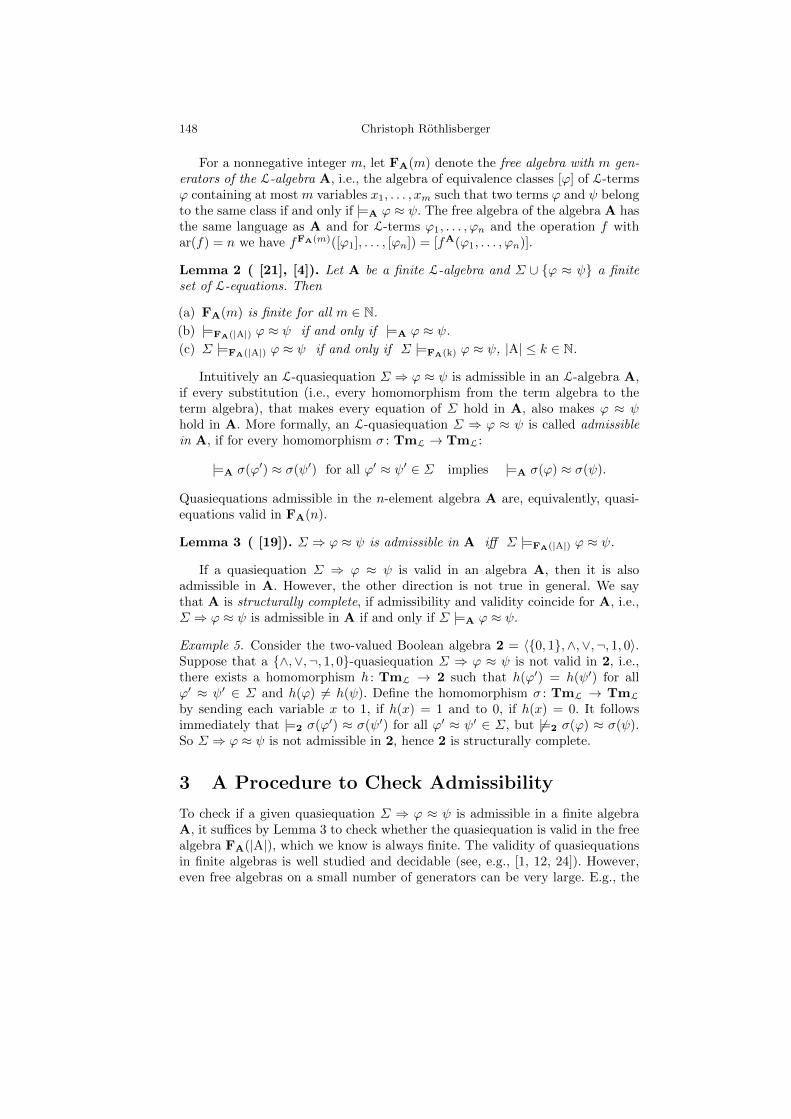
148 Christoph Rothlisberger

For a nonnegative integer m, let FA(m) denote the free algebra with m gen-erators of the L-algebra A, i.e., the algebra of equivalence classes [ϕ] of L-termsϕ containing at most m variables x1, . . . , xm such that two terms ϕ and ψ belongto the same class if and only if |=A ϕ ≈ ψ. The free algebra of the algebra A hasthe same language as A and for L-terms ϕ1, . . . , ϕn and the operation f withar(f) = n we have fFA(m)([ϕ1], . . . , [ϕn]) = [fA(ϕ1, . . . , ϕn)].

Lemma 2 ( [21], [4]). Let A be a finite L-algebra and Σ ∪ {ϕ ≈ ψ} a finiteset of L-equations. Then

(a) FA(m) is finite for all m ∈ N.

(b) |=FA(|A|) ϕ ≈ ψ if and only if |=A ϕ ≈ ψ.

(c) Σ |=FA(|A|) ϕ ≈ ψ if and only if Σ |=FA(k) ϕ ≈ ψ, |A| ≤ k ∈ N.

Intuitively an L-quasiequation Σ ⇒ ϕ ≈ ψ is admissible in an L-algebra A,if every substitution (i.e., every homomorphism from the term algebra to theterm algebra), that makes every equation of Σ hold in A, also makes ϕ ≈ ψhold in A. More formally, an L-quasiequation Σ ⇒ ϕ ≈ ψ is called admissiblein A, if for every homomorphism σ : TmL → TmL:

|=A σ(ϕ′) ≈ σ(ψ′) for all ϕ′ ≈ ψ′ ∈ Σ implies |=A σ(ϕ) ≈ σ(ψ).

Quasiequations admissible in the n-element algebra A are, equivalently, quasi-equations valid in FA(n).

Lemma 3 ( [19]). Σ ⇒ ϕ ≈ ψ is admissible in A iff Σ |=FA(|A|) ϕ ≈ ψ.

If a quasiequation Σ ⇒ ϕ ≈ ψ is valid in an algebra A, then it is alsoadmissible in A. However, the other direction is not true in general. We saythat A is structurally complete, if admissibility and validity coincide for A, i.e.,Σ ⇒ ϕ ≈ ψ is admissible in A if and only if Σ |=A ϕ ≈ ψ.

Example 5. Consider the two-valued Boolean algebra 2 = 〈{0, 1},∧,∨,¬, 1, 0〉.Suppose that a {∧,∨,¬, 1, 0}-quasiequation Σ ⇒ ϕ ≈ ψ is not valid in 2, i.e.,there exists a homomorphism h : TmL → 2 such that h(ϕ′) = h(ψ′) for allϕ′ ≈ ψ′ ∈ Σ and h(ϕ) 6= h(ψ). Define the homomorphism σ : TmL → TmL

by sending each variable x to 1, if h(x) = 1 and to 0, if h(x) = 0. It followsimmediately that |=2 σ(ϕ′) ≈ σ(ψ′) for all ϕ′ ≈ ψ′ ∈ Σ, but 6|=2 σ(ϕ) ≈ σ(ψ).So Σ ⇒ ϕ ≈ ψ is not admissible in 2, hence 2 is structurally complete.

3 A Procedure to Check Admissibility

To check if a given quasiequation Σ ⇒ ϕ ≈ ψ is admissible in a finite algebraA, it suffices by Lemma 3 to check whether the quasiequation is valid in the freealgebra FA(|A|), which we know is always finite. The validity of quasiequationsin finite algebras is well studied and decidable (see, e.g., [1, 12, 24]). However,even free algebras on a small number of generators can be very large. E.g., the

Checking Admissibility in Finite Algebras 149

free algebra FS→e4

(2) has 453 elements, where S→e4 is the algebra of Example 1.

We therefore seek smaller algebras B such that, as for FA(|A|):

Σ ⇒ ϕ ≈ ψ is admissible in A ⇐⇒ Σ |=B ϕ ≈ ψ.

Proposition 1. Let A,B be L-algebras such that B is a subalgebra of FA(|A|)and A is a homomorphic image of B. Then Σ ⇒ ϕ ≈ ψ is admissible in A iffΣ |=B ϕ ≈ ψ.

Proof. Let Σ ⇒ ϕ ≈ ψ be admissible in A. So Σ |=FA(|A|) ϕ ≈ ψ by Lemma 3and then Σ |=B ϕ ≈ ψ by Lemma 1. For the other direction suppose thatΣ |=B ϕ ≈ ψ and |=A σ(ϕ′) ≈ σ(ψ′) for all ϕ′ ≈ ψ′ ∈ Σ. Then |=FA(n) σ(ϕ′) ≈σ(ψ′) for all ϕ′ ≈ ψ′ ∈ Σ by Lemma 2 and therefore |=B σ(ϕ′) ≈ σ(ψ′) forall ϕ′ ≈ ψ′ ∈ Σ by Lemma 1. But then |=B σ(ϕ) ≈ σ(ψ) and since A is ahomomorphic image of B, |=A σ(ϕ) ≈ σ(ψ) by Lemma 1. ut

Note that every subalgebra B of a subalgebra C of the free algebra FA(|A|),i.e., B ≤ C ≤ FA(|A|), is a subalgebra of FA(|A|). So since FA(m1) ≤ FA(m2)for all m1 ≤ m2 (see, e.g., [4]), we possibly do not need |A| generators. Thissuggests the following procedure when A is finite:

(i) Find the smallest free algebra FA(m) such that A ∈ H(FA(m)).

(ii) Compute subalgebras B of FA(m), increasing in their size, and check foreach whether A ∈ H(B).

(iii) Derive a proof system for a smallest B with the properties of (ii).

Steps (i) and (ii) of the procedure have been implemented using macros imple-mented for the Algebra Workbench [23]. Step (iii) can be implemented directlymaking use of a system such as MUltlog/MUltseq [11, 22].

We now give some explanation how to implement the first two steps of theprocedure. For a given A, we want to find the smallest free algebra FA(m)(m ≤ |A|) such that A is a homomorphic image of FA(m). The idea is tocalculate first FA(0) and to check whether A ∈ H(FA(0)). Stop if this is thecase, otherwise calculate FA(1) and check whether A ∈ H(FA(1)) and so on.

Suppose that, given a finite algebra A = 〈{a1, . . . , an}, f1, . . . , fk〉, we wantto calculate the elements of FA(m). Recall that the elements of the free algebracan be seen as equivalence classes of terms. Therefore we need to know all theterms that are definable using the given generators. To decide whether two termsϕ and ψ are the same, i.e., |=A ϕ ≈ ψ, we would have to check all the possiblehomomorphisms h : TmL → A. So we simulate the truth table checking bystoring the elements by sequences of elements of A.

We represent the m generators of FA(m) by sequences 〈πi(a1), . . . , πi(anm)〉where a1, . . . , anm are the elements of Am and πi, i = 1, . . . ,m the i-th projection-map from Am to A and collect them in a set G. Then we run the functionDefinableTerms (see Fig. 1) to get the elements of FA(m), stored as sequencesof length nm in the set F .

150 Christoph Rothlisberger

function DefinableTerms(G, {f1, . . . , fk})F ← Grepeat

F0 ← Ffor all f ∈ {f1, . . . , fk} do

F ← F ∪ { 〈f(g1), . . . , f(gar(f))〉 : g1, . . . , gar(f) ∈ F }end for

until F0 == Freturn F

end function

Fig. 1. Algorithm to generate all the definable terms, given a set of generators G

Example 6. Suppose that we want to calculate the elements of the free algebrafor the algebra P = 〈{a, b, c, d}, ?〉 defined in Example 2. We certainly needgenerators for the free algebra since P has no constants, i.e., no nullary opera-tions. So the first step will be to calculate FP(1): our generator is the sequence(a, b, c, d). Running the function DefinableTerms((a, b, c, d), {?}) gives us F ={(a, b, c, d), (b, a, b, b), (a, b, a, a)}. It is easy to see that there cannot be a surjec-tive homomorphism from FP(1) to A since A has four elements. So we have tocalculate the algebra FP(2) with generators (a, a, a, a, b, b, b, b, c, c, c, c, d, d, d, d)and (a, b, c, d, a, b, c, d, a, b, c, d, a, b, c, d), which will give us a six element algebrathat fulfills the requirement of the homomorphism.

The second step of the procedure requires us to calculate subalgebras ofthe free algebra, increasing in their size. We could, at least theoretically, checkA ∈ H(B) for all B ≤ FA(m). But since we are interested in the smallestalgebras with this property, we generate the subalgebras by increasing theirsize and always testing whether they satisfy the property. The principles forthe calculation of subalgebras are those of DefinableTerms defined in Fig. 1.Using the generating elements as arguments for the operations, we increase theset of “reached” elements as long as we get new elements.

We first calculate all the one-generated subalgebras of the free algebra FA(m),i.e., 〈ϕ〉 for ϕ ∈ FA(m) and store their sizes |〈ϕ〉|. Now we know that the size ofthe two-generated subalgebra 〈ϕ1, ϕ2〉 of FA(m) is at least max{|〈ϕ1〉|, |〈ϕ2〉|}.Suppose that k = min{|〈ϕ〉| : ϕ ∈ FA(m)}. If there is more than one ϕ ∈ FA(m)with |〈ϕ〉| = k, then we generate all the algebras (increasing the number of gen-erators) 〈ϕ1, . . . , ϕr〉 with max{|t1|, . . . , |tr|} ≤ k, again testing if there exists asurjective homomorphism to A and storing their sizes. We then proceed simi-larly for k′ = min{|〈ϕ〉| : ϕ ∈ FA(m), |〈ϕ〉| > k}. As soon as we find an algebraB with A ∈ H(B) we have an upper-bound for the size of the algebras to test(note that this upper-bound always exists since it cannot exceed the size of thefree algebra FA(m)). However, we then have to continue until we know thatevery combination of generators will lead to a subalgebra B′ with B ≤ B′.

It is not hard to see that step (i) is sound and terminating since we use theoperations of the generating algebra A to calculating new, finite sequences ofelements of A. So there are at most |A||A|m sequences. The soundness of step (ii)

Checking Admissibility in Finite Algebras 151

is, similar to the previous step, given by the construction of the subalgebras andthe used bounds of the cardinalities of the algebras. The algorithm terminatessince there are only finitely many subalgebras of the free algebra.

Example 7. Consider the algebra S→¬3 = 〈{−1, 0, 1},→,¬〉, where → is definedas in Example 1 and ¬x = −x. Note that an equation of the form ϕ ≈ ϕ → ϕholds in S→¬3 iff ϕ is a theorem of the {→,¬}-fragment of the logic RM. Now,following our procedure, we obtain:

(i) S→¬3 6∈ H(FS→¬3(1)), but S→¬3 ∈ H(FS→¬3

(2)).

(ii) FS→¬3(2) has 264 elements and the smallest subalgebras B ≤ FS→¬3

(2) withS→¬3 ∈ H(B) have 6 elements.

The fact that we first check the smaller subalgebras is useful here: We only hadto check the 264 one-generated algebras, 15 two-generated and 3 three-generatedalgebras rather than all the 5134 possible subalgebras of FS→¬3

(2).

Example 8. Small changes in the universe or language of an algebra can dra-matically change the size and structure of its free algebra. Consider the algebraS→¬e

4 = 〈{−2,−1, 1, 2},→,¬, e〉 where → and ¬ are defined as in Example 7and =

¯1. Although this algebra is only slightly different to S→e

4 and S→¬3 of theExamples 1 and 7, the appropriate free algebra is much smaller and only needsone generator:

(i) S→¬e4 6∈ H(FS→¬e

4(0)), but S→¬e

4 ∈ H(FS→¬e4

(1)).

(ii) FS→¬e4

(1) has 18 elements and the smallest subalgebras B ≤ FS→¬e4

(1) withS→¬e

4 ∈ H(B) have 6 elements.

Example 9. In some cases, it is possible to establish structural completenessresults for the algebra A using the described procedure. The smallest B ≤FA(m) with A ∈ H(B) may be an isomorphic copy of A itself. In particular,known structural completeness results have been confirmed for

L→3 = 〈{0, 12 , 1},→ L〉 the 3-element Komori C-algebra

B1 = 〈{0, 12 , 1},min,max,¬G〉 the 3-element Stone algebra

G3 = 〈{0, 12 , 1},min,max,→G〉 the 3-element positive Godel algebra

S→3 = 〈{−1, 0, 1},→S〉 the 3-element implicational Sugihara monoid

where x → L y = min(1, 1 − x + y), x →G y is y if x > y, otherwise 1,¬Gx = x →G 0, and →S is the operation → of S→¬3 from Example 7. A newstructural completeness result has also been established for the psuedocomple-mented distributive lattice B2 obtained by adding a top element to the 4-elementBoolean algebra.

Example 10. There are even cases where we do not need any generators for thefree algebra since the constants alone suffice. Consider the 5-valued Post algebraP5 = 〈{0, 1, 2, 3, 4},∧,∨,′ , 0, 1〉 where 〈{0, 1, 2, 3, 4},∧,∨〉 builds a 5-chain with0 < 4 < 3 < 2 < 1 and 0′ = 1, 1′ = 2, 2′ = 3, 3′ = 4, 4′ = 0. This algebrabuilds the algebraic counterpart to the Post logic P5. Running our procedure werecognize that P5 is isomorphic to FP5(0), i.e., P5 is also structurally complete.

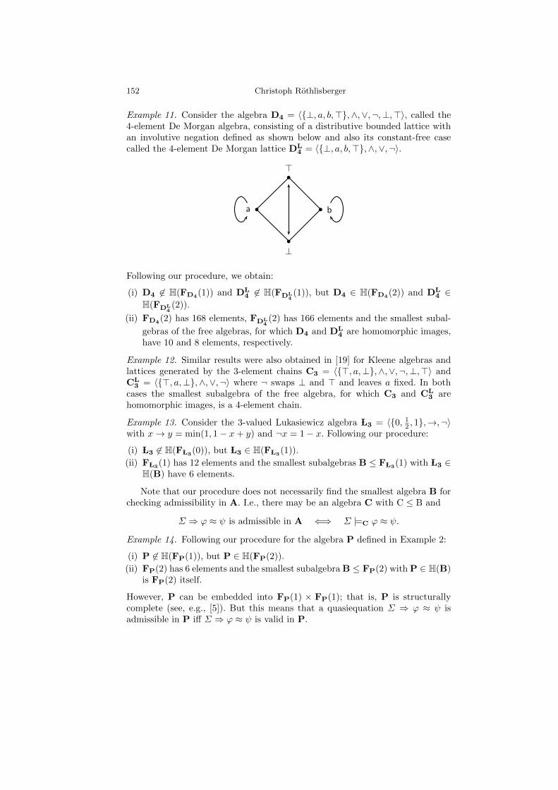
152 Christoph Rothlisberger

Example 11. Consider the algebra D4 = 〈{⊥, a, b,>},∧,∨,¬,⊥,>〉, called the4-element De Morgan algebra, consisting of a distributive bounded lattice withan involutive negation defined as shown below and also its constant-free casecalled the 4-element De Morgan lattice DL

4 = 〈{⊥, a, b,>},∧,∨,¬〉.

b

b b

b

⊥

a b

⊤

Following our procedure, we obtain:

(i) D4 6∈ H(FD4(1)) and DL4 6∈ H(FDL

4(1)), but D4 ∈ H(FD4(2)) and DL

4 ∈H(FDL

4(2)).

(ii) FD4(2) has 168 elements, FDL4(2) has 166 elements and the smallest subal-

gebras of the free algebras, for which D4 and DL4 are homomorphic images,

have 10 and 8 elements, respectively.

Example 12. Similar results were also obtained in [19] for Kleene algebras andlattices generated by the 3-element chains C3 = 〈{>, a,⊥},∧,∨,¬,⊥,>〉 andCL

3 = 〈{>, a,⊥},∧,∨,¬〉 where ¬ swaps ⊥ and > and leaves a fixed. In bothcases the smallest subalgebra of the free algebra, for which C3 and CL

3 arehomomorphic images, is a 4-element chain.

Example 13. Consider the 3-valued Lukasiewicz algebra L3 = 〈{0, 12 , 1},→,¬〉

with x→ y = min(1, 1− x+ y) and ¬x = 1− x. Following our procedure:

(i) L3 6∈ H(F L3(0)), but L3 ∈ H(F L3(1)).

(ii) F L3(1) has 12 elements and the smallest subalgebras B ≤ F L3(1) with L3 ∈H(B) have 6 elements.

Note that our procedure does not necessarily find the smallest algebra B forchecking admissibility in A. I.e., there may be an algebra C with C ≤ B and

Σ ⇒ ϕ ≈ ψ is admissible in A ⇐⇒ Σ |=C ϕ ≈ ψ.

Example 14. Following our procedure for the algebra P defined in Example 2:

(i) P 6∈ H(FP(1)), but P ∈ H(FP(2)).

(ii) FP(2) has 6 elements and the smallest subalgebra B ≤ FP(2) with P ∈ H(B)is FP(2) itself.

However, P can be embedded into FP(1) × FP(1); that is, P is structurallycomplete (see, e.g., [5]). But this means that a quasiequation Σ ⇒ ϕ ≈ ψ isadmissible in P iff Σ ⇒ ϕ ≈ ψ is valid in P.

Checking Admissibility in Finite Algebras 153

A |A| Quasivariety Q(A) |Free algebra| |Output algebra| L3 3 algebras for L3 (Ex. 13) |FA(1)| = 12 6

B1 3 Stone algebras (Ex. 9) |FA(1)| = 6 3

C3 3 Kleene algebras (Ex. 12) |FA(1)| = 6 4

L→3 3 algebras for L→3 (Ex. 9) |FA(2)| = 40 3

CL3 3 Kleene lattices (Ex. 12) |FA(2)| = 82 4

S→¬3 3 algebras for RM→¬ (Ex. 7) |FA(2)| = 264 6

S→3 3 algebras for RM→ (Ex. 9) |FA(2)| = 60 3

G3 3 algebras for G3 (Ex. 9) |FA(2)| = 18 3

DL4 4 De Morgan lattices (Ex. 11) |FA(2)| = 166 8

D4 4 De Morgan algebras (Ex. 11) |FA(2)| = 168 10

P 4 Q(P) (Ex. 2) |FA(2)| = 6 6

S→¬e4 4 Q(S→¬e4 ) (Ex. 8) |FA(1)| = 18 6

B2 5 Q(B2) (Ex. 9) |FA(1)| = 7 5

P5 5 algebras for P5 (Ex. 10) |FA(0)| = 5 5

Table 1. Algebras for checking admissibility

This last issue, but also possibilities of improving the given procedure forchecking admissibility (e.g., ruling out symmetric cases of generators when cal-culating a free algebra) will be the subject of future work. The given examplesfor our procedure are summarized in Table 1.

References

1. M. Baaz, C. G. Fermuller, and G. Salzer. Automated Deduction for Many-ValuedLogics. In Handbook of Automated Reasoning, volume II, chapter 20, pages 1355–1402. Elsevier Science B.V., 2001.

2. S. Babenyshev, V. Rybakov, R. A. Schmidt, and D. Tishkovsky. A Tableau Methodfor Checking Rule Admissibility in S4. In Proceedings of UNIF 2009, volume 262of ENTCS, pages 17–32, 2010.

3. W. J. Blok and D. Pigozzi. Algebraizable Logics. Number 396 in Memoirs of theAmerican Mathematical Society volume 77. American Mathematical Society, 1989.

4. S. Burris and H. P. Sankappanavar. A Course in Universal Algebra, volume 78 ofGraduate Texts in Mathematics. Springer-Verlag, New York, 1981.

5. P. Cintula and G. Metcalfe. Structural Completeness in Fuzzy Logics. Notre DameJournal of Formal Logic, 50(2):153–183, 2009.

6. P. Cintula and G. Metcalfe. Admissible Rules in the implication-negation fragmentof intuitionistic logic. Annals of Pure and Applied Logic, 162(10):162–171, 2010.

7. G. Gentzen. Untersuchungen uber das Logische Schliessen. Math. Zeitschrift,39:176–210,405–431, 1935.

8. S. Ghilardi. Unification in Intuitionistic Logic. Journal of Symbolic Logic,64(2):859–880, 1999.

9. S. Ghilardi. Best Solving Modal Equations. Annals of Pure and Applied Logic,102(3):184–198, 2000.

10. S. Ghilardi. A resolution/tableaux algorithm for projective approximations in IPC.Logic Journal of the IGPL, 10(3):227–241, 2002.

154 Christoph Rothlisberger

11. A. J. Gil and G. Salzer. Homepage of MUltseq. http://www.logic.at/multseq.12. R. Hahnle. Automated Deduction in Multiple-Valued Logics. OUP, 1993.13. R. Iemhoff. On the Admissible Rules of Intuitionistic Propositional Logic. Journal

of Symbolic Logic, 66(1):281–294, 2001.14. R. Iemhoff and G. Metcalfe. Proof Theory for Admissible Rules. Annals of Pure

and Applied Logic, 159(1–2):171–186, 2009.15. E. Jerabek. Admissible Rules of Modal Logics. Journal of Logic and Computation,

15:411–431, 2005.16. E. Jerabek. Admissible rules of Lukasiewicz logic. Journal of Logic and Computa-

tion, 20(2):425–447, 2010.17. E. Jerabek. Bases of admissible rules of Lukasiewicz logic. Journal of Logic and

Computation, 20(6):1149–1163, 2010.18. P. Lorenzen. Einfuhrung in die operative Logik und Mathematik, volume 78 of

Grundlehren der mathematischen Wissenschaften. Springer, 1955.19. G. Metcalfe and C. Rothlisberger. Admissibility in De Morgan algebras. Soft

Computing, to appear.20. G. Metcalfe and C. Rothlisberger. Unifiability and Admissibility in Finite Algebras.

In Proceedings of CiE 2012, volume 7318 of LNCS, pages 485–495. Springer, 2012.21. V.V. Rybakov. Admissibility of Logical Inference Rules, volume 136 of Studies in

Logic and the Foundations of Mathematics. Elsevier, Amsterdam, 1997.22. G. Salzer. Homepage of MUltlog. http://www.logic.at/multlog.23. M. Sprenger. Algebra Workbench. http://www.algebraworkbench.net.24. R. Zach. Proof theory of finite-valued logics. Master’s thesis, Technische Univer-

sitat Wien, 1993.

Scalar Properties of Degree Modification inKaritiana: Evidence for Indeterminate Scales

Luciana Sanchez Mendes

Universidade de Sao Paulo (Fapesp/Capes/CNPq) and Universite Paris 8sanchez.mendes@gmail.com

Abstract. The aim of this article is to give evidence for the existenceof a new parameter for the typology of degree predicates: the indetermi-nacy of scales. The arguments are based in the analysis of the semanticbehavior of the degree modifier pitat in Karitiana - a native brazilianlanguage.

1 Introduction

This paper focusses on the scalar properties of a specific verbal construction inKaritiana: degree modification with the adverb pitat ‘a lot’ in sentences like (1)1.

(1) Tasoman

∅-na-pytim’adn-∅3-decl-work-nfut

pitat.a.lot

‘The man worked a lot’

Pitat is a degree modifier that has some particular characteristics. It only com-bines with atelic verbal predicates, and the modified sentences are adequate in arange of situations related to a high degree in many dimensions, such as durationin time, number of occurrences, intensity, speed, and distance.The main claims of this paper are (i) pitat in Karitiana does not behave likeother degree modifiers such as beaucoup in French or a lot in English; (ii) thedata from Karitiana support a degree-scale semantics for degree modiification,and (iii) the traditional typology of gradable predicates based on the closure ofthe scales and their relation with a standard of comparison can be improved byintroducing a further dimension: the distinction between determinate and inde-terminate scales.

2 Degree Modification in Karitiana

The aim of this Sect. is to present the distribution of pitat ‘a lot’ in Kari-tiana. Only atelic verbal predicates can be modified by pitat. Sentences (2) and

1Karitiana is a native language of the Ariken family, Tupi stock, spoken by about320 people on a demarcated area in the northwest of Brazil (Storto and Vander Velden[2005]).

156 Luciana Sanchez Mendes

(3) with activity and stative predicates are grammatical. Accomplishment andachievement predicates as in sentences (4) and (5), on the other hand, cannotbe modified by pitat.

(2) MilenaMilena

∅-na-aka-t3-decl-cop-nfut

i-tarak-tpart-walk-abs.

pitat.a.lot

‘Milena walked a lot’

(3) InacioInacio

∅-na-aka-t3-decl-cop-nfut

i-osedn-∅part-be.happy-abs.

pitat.a.lot

‘Inacio was happy a lot’

(4) *InacioInacio

∅-na-aka-t3-decl-cop-nfut

i-tat-∅part-go-abs.

pitata.lot

PortoPorto

VelhoVelho

pip.to

‘Inacio went a lot to Porto Velho city’

(5) *InacioInacio

∅-na-aka-t3-decl-cop-nfut

i-horop-∅part-reach-abs.

pitata.lot

eptree

opytop

ty.obl

‘Inacio reached a lot the top of the tree’

The distribution above is similar to what we find with a lot in English (asdescribed in Caudal and Nicolas [2005]).

(6) Yanning walked a lot.

(7) *Yanning ate his pancake a lot.

(Caudal and Nicolas [2005], p.5)

Nevertheless pitat has an unexpected characteristic: it can be easily used in amuch wider range of interpretations. Thus, sentence (2) can be used to describethe following situations: (i) Milena walked for a long time; (ii) Milena walkeda lot of times; (iii) Milena walked in high speed; (iv) Milena walked for a longdistance; (v) Milena walked with pleasure. And sentence (3) felicitously describessituations in which: (i) Inacio was happy for a long time; (ii) Inacio was happya lot of times; (iii) Inacio was very happy.So, an appropriate analysis for pitat has to account for these two characteristics:(i) the distribution with only atelic predicates; and (ii) the diversity of possibleinterpretations. The analysis proposed in the next Sects. attemps to capturethese two features.

3 Degree Modification in Karitiana Cannot beExplained by the Mass/Count Distinction inthe Verbal Domain

Degree modifiers conveying high degree are usually sensitive to the mass/countdistinction in the domain they modify. Much and many are the classical example(Chierchia [1998]). One could be tempted to suggest that the distribution of pitat

Degree Modification in Karitiana 157

can be explained by this regularity. The degree adverb beaucoup in French, forexample, was investigated by Doetjes [2007] in these terms. The author followsBach [1986] in arguing that the same mass/count distinction we find in thenominal domain can be found in the different types of verbal predicates. Roughlythe proposal is that telic verbal phrases (accomplishments and achievements) canbe considered countable predicates and atelic (activities and states) can be takenas massive.Beaucoup has a different behavior depending on the kind of predicate that itmodifies. When it is used with a telic predicate, as in example (8), the sentencehas an iterative interpretation, by which many events occurred. In sentences withatelic predicates, as in (9), the sentence can have an iterative interpretation ora degree interpretation (Doetjes [2007]).

(8) PierrePierre

vagoes

beaucoupa.lot

auto.the

Louvre.Louvre

‘Pierre goes to the Louvre a lot (many times)’

(9) IlIt

ahas

plurained

beaucoup.a.lot

‘It has rained a lot (many times or intensively)’

According to Doetjes [2007], the iterative interpretation of sentences with beau-coup has its origin in the count feature of the predicate. So in sentences like (8)the fact that only iterative interpretation is available is explained by the countnature of the predicate aller au Louvre ‘to go to the Louvre’. Regarding thesentences with atelic predicates, like pleuvoir ‘to rain’ in (9), when they have adegree interpretation, it is on account of the massive nature of the verbal pre-dicate, but when they have an iterative interpretation, it is because the massivepredicate shifted from mass to count. This type–adjustment is the price to payfor the assumption that the iterative interpretation in sentences with degree ad-verbs has its origin in the count nature of the predicate.This analysis is not adequate to explain the Karitiana data. Firstly, there aremore than only two readings associated with degree modification in Karitiana.All the interpretations available for sentences with pitat are equally importantand none of them should be explained by an exception rule, like ‘shift the pre-dicate’ from mass to count. It is not the case that one of the readings is availableby one rule and the others by another one. Beaucoup has a binary behavior(concerning its interpretations), so it makes sense to capture it by a binary rule(mass/count distinction). Pitat has not a binary behavior with atelic verbs, thenit should not be explained by a property like the mass/count distinction.As the next Sect. will show, the iterative interpretation can be considered as be-ing part of the degree modification. I will argue that iterativity in sentences withpitat is built on one of the possible scales associated with degree modification,and it is not an operation on the verbal domain that competes with the degreeone.

158 Luciana Sanchez Mendes

4 Degree Modification in Karitiana and Degree-Scale Structures

The aim of this Sect. is to argue that scalar structures are the proper way to dealwith degree modification in atelic constructions in Karitiana. It will be shownthat a degree-scale semantics can account for both the distribution and meaningof pitat.Degree modification can be understood as an operation on gradable predicates.Following Kennedy [1999], I will consider gradable predicates as predicates thathave a degree argument and a scalar structure2. Kennedy and McNally [2005]argue that there are two parameters that are crucial to the typology of degreepredicates: the closure of their scales and their relation to a standard of com-parison.The first parameter divides the scales into open and closed ones. Open scales donot have a minimum or a maximum degree lexically determined. The adjectivehigh, for example, has an open scale since it has no lexically defined minimumor maximum degree. On the other hand, closed scales have a well determinedminimum and maximum degree. For example, full and empty are closed scalesadjectives. The scales related with these adjectives have a minimum degree, as-sociated to empty and a maximum one associated to full.The second important parameter of the typology of degree predicates is describedby their relation to the context. Relative degree predicates are dependent on acontextual standard of comparison in order to be interpreted; absolute ones, bycontrast, do not have a context dependent standard of comparison. For instance,the adjective high is a relative predicate because its denotation in a sentencevaries according to the context. On the other hand, an adjective such as closeddoes not have the standard of comparison defined by the context. Kennedy andMcNally [2005] claim that there is an relation between the parameters - gradableadjectives that have totally open scales have relative standards, whereas gradableadjectives that have totally or partially closed scales have absolute standards.Since I am dealing with degree modification of verb phrases, this typology, whichis widely used in the studies of gradable adjectives, must be apllied to the verbaldomain. Caudal and Nicolas [2005] assume that there is a relation between eventstructure and scale closure. They apply the distinction open/closed to the verbaldomain and claim that telic verbal predicates, since they have a final point givenby the telos, can be considered as having closed scales. On the other hand, atelicpredicates are open scale predicates since they do not have a lexically definedend point (telos).As it was shown in Sect. 2, pitat can be used only with atelic verbal predicates.We may rephrase the restriction by saying that it applies only to open scalepredicates. This is precisely the same restriction of the degree modifier very in

2A scale is a set of degrees ordered along a dimension. It can be understoodmetaphorically as a ruler formed by degrees ordered in a certain dimension (that canbe, for instance, weight, temperature, length).

Degree Modification in Karitiana 159

English as described in Kennedy and McNally [2005]3.

(10) Kim was very worried by the diagnosis.

(11) ??Beck is very acquainted with the facts of the case.

So far this is the distribution of pitat according to a theory that assumes scalarstructures. In what follows, I will develop a proposal to account for how themultiple readings associated to the sentences with pitat are built.Intuitively, there is a difference between degree modification of the adjectivaland in the verbal domain. When one says ‘Mary is very beautiful’, it is clearthat the dimension of the scale involved in the interpretation of the sentence iseasily made available by the adjective: the sentence is evaluated relative to ascale of beauty. But when one say in Karitiana ‘Taso napytim’adn pitat ’ (‘Theman worked a lot’), the proper scale for the evaluation of the truth conditionsof the sentence is not obvious, but must be filled by context.This intuition can be formally captured by the theory of degree and scalar struc-tures. The scales formed in constructions with adjectives are scales available inthe lexicon (cf. Kennedy [1999]). This explains the similarity between the ad-jectives and the scales related to them. High is related to the scale of height,happy is associated to the happiness scale, and so on. Activity verbs, in turn, likethe verb to work do not lexically encode a scale. There is no “workness” scalelexically associated to the verbal predicate. However, this does not mean thatverbal constructions of this type cannot be associated to a scale. The proposalsubmit is that the scales in these cases are contextually constructed rather thangiven by the lexicon.I assume, following Dowty [1979], that activities are dynamic predicates involv-ing complex changes, that is a combination of changes in several possible dimen-sions4.The variety of the dimensions associated to complex change predicates isresponsible for the variable range of scales related to these predicates and there-fore for the multiple readings of the sentences in which they appear.The variety of dimensions can be formally captured by the tools provided in theworks on degree-scales by what Kennedy and McNally [2005] called indetermi-nacy. Indeterminacy is the capacity of a predicate to be compatible with scalesof various dimensions. The different measurable dimensions of an event denotedby an atelic verbal predicate – as duration in time, number of occurrences, num-ber of participants, intensity, etc. – can be used to fill in the dimensions of thescales.

3See Kennedy and McNally [2005] for details.4In fact, I extend the idea of complex change predicates to all activity and stative

verbs in Karitiana since they have the same behavior in pitat ’s constructions.

160 Luciana Sanchez Mendes

4.1 Formalization Proposal for Degree Modification withPitat

This Sect. intends to present my proposal of formalization for the degree mod-ifier pitat. As stated before the idea I adopt is that scales associated to atelicpredicates (activity and states) are not given in the lexicon, but are providedby context. Since pitat only modifies atelic predicates, it only operates on con-textual scales. Since scales are sets of degrees, this suggests that the degree thatthis adverb selects is not present in the lexical representation of the predicates itmodifies. See below the traditional lexical entry for to walk in (12) and compareto beautiful in (13).

(12) JwalkK= λe. walk(e)5

(13) JbeautifulK= λd. λx. beauty(x) = d

However, in order to be modified by pitat, the degree argument must bepresent somehow in verbs like tarak ‘to walk’. I assume following Caudal andNicolas [2005] that atelic predicates may have a degree argument, although it isnot present in the lexicon. Pinon [2000] claims that there is possible to give adegree argument to verbal predicates in the course of the semantic compositionby a degree function. Following his idea I postulate a function DegP – in (14)– that takes a simple predicate of events and returns a relation between degreesand events6. To capture the indeterminacy of the scale, a measure function µ isused as a variable for dimensions (cf. Krifka [1998], Thomas [2009]).

(14) JDegPK= λP〈s,t〉. λd. λe. P(e) & µ (e) = d

In (10) µ can be replaced by temporal duration, event cardinality, speed, distanceor intensity7. The DegP function has a double role. Besides adding a degreeargument to the predicate, it also functions as a restriction in the domain ofpitat. Since pitat can occur only in sentences with predicates of open scales, Iassume that DegP is a function that can be applied only to open scale predicates.I propose the following lexical entry for pitat :

5I assume a neo-davidsonian semantic of events that consider verbs as predicatesof events (cf. Parsons [1990]). Furthermore, I follow Kratzer [1996] in the assumptionthat the external argument is inserted in the syntax.

6The crucial difference between the degree function I postulate and the oneseggested in Pinon [2000] is that his formula maps events, objects and degrees of ac-complishment predicates. The degree function I suggested in (10) can be applied onlyto atelic verbal predicates and it says nothing to the relation between the objects andthe events or degrees. Its purpose is to give a degree argument and a variable of scaleto the predicate.

7In the way the formula is given it is over-generating because all verbs can beassociated to any dimension. The next step of the investigation will be to find lexicalconstraints to fix this, since, of course, not all verbs have distance and high speedreadings, for instance.

Degree Modification in Karitiana 161

(15) JpitatK= λG〈d,〈s,t〉〉. λe. ∃d. [ d ≥ N & G (d) (e) ]where: N = normal degree of the scale

So the formalization proposed here exploits the idea in Caudal and Nicolas [2005]that the degree modifiers can restructure or introduce scales during the deriva-tion combining lexical, syntatic and semantic information.

4.2 Some Consequences of the Proposal

In this Sect., some consequences of the proposal presented above are discussed.The first one relies on the iterative versus degree interpretations (as discussedin Sect. 3). Returning to Karitiana data, with the assumption of indeterminacyof scales it is possible to explain the iterative reading as part of the degree mod-ification, without postulating a type-shifting rule on the predicate as suggestedby Doetjes [2007]. Thus unlike Doetjes [2007] iterativity is considered a subtypeof degree modification, and not an operation that competes with it. In fact, inthe proposal assumed in that there is no degree interpretation. There is a de-gree modification and there are iterative and intensity interpretations that aregenerated by the degree operation.The second consequence of the idea that constructions involving gradable ad-jectives have scales whose dimension is lexically specified; while constructionsinvolving verbs have contextual ones is that degree modification in the formerconstructions is less complex than in the latter. The application of a degree ad-verb like very to an adjective like beautiful is just an operation of modificationon the lexicalized scale of beauty. The degree modification of a verb, on the otherhand, involves a few more steps. For something like to run a lot be interpreted,it is necessary that the appropriate scale of the verb is formed and only then theconstruction can be evaluated. In this very distinction lies the difference betweenEnglish very and a lot. Insofar as very is a modifier that can be applied onlyto lexical scales, a lot is an adverb that forces the predicate to have a degreeargument in order to be used. The assumption that degree modification in theadjectival domain is less complex than modification in the verbal domain is sup-ported by other works in the degree-scale literature. Bochnak [2010] analyzesthe degree modifier half and posits some semantic functions that are necessaryto the modification of verbs and are not used to modify adjectives8.The last consequence that will be discussed is the importance of indeterminacyto the typology of degree predicates. Starting from the idea that constructionsinvolving gradable adjectives such as beautiful have scales available in the lex-icon, while constructions involving verbs like the ones I am dealing with havescales built in the context, the first issue that arises is a problem in the descrip-tion of the distribution of pitat. Previously I claimed that pitat selects open scalepredicates. But, in fact, the predicates that are modified by pitat do not have ascalar structure before the modification. So it is necessary to slightly reformu-late that claim. In fact, pitat selects predicates that can have an indeterminate

8See Bochnak [2010] for details.

162 Luciana Sanchez Mendes

scale and this is the relevant property for both its distribution and meaning. Theindeterminacy of scales is as important to the scales’ typology as their closureand their relation to the standard of comparison. This is the main theoreticalcontribution of this work: besides the well-know parameters of open/closed andrelative/absolute predicates, the indeterminate/determinate property is also im-portant.In fact, since there is a one-to-one correspondence between the two parametersdescribed in Kennedy and Mcnally [2005], there is no reason to consider them astwo different parameters. They can be treated as a single parameter describedin two different ways. The relative vs. absolute distinction is a characteristic ofdegree predicates whereas the open vs. closed distinction is a characteristic oftheir scalar structure. On the ther hand, indeterminacy is an independent pa-rameter since it allows for crossed combinations with the other(s).The table resumes the proposal with examples (adjectives and verbs)9:

(In)determinacy Adjctive Verb

Open Scale Determinate high to melt (atelic reading)

Relative Predicate Indeterminate big to run

Closed Scale Determinate full to melt (telic reading)

Absolute Predicate

The proposal is that if a gradable predicate is absolute and it has a closedscale, it necessarily has a determinate scalar strucutre, there is, its scale is givenby lexicon. If a predicate is relative, it can have a determinate or an indeterminatescale. The adjective high is the classical example os an open scale adjective withdeterminate scale (scale of height). The verbs trated in this paper as to run, onthe other hand, are open scale predicates with indeterminate scales (scales ofspeed, distance, iterativity, intensity, etc.).

5 Conclusions

This paper argues that the number of parameters that classify degree predicatesmust be enlarged in order to include also the determinate/indeterminate dis-tinction. Thus the degree modification with pitat in Karitiana can be properlyanalized in a degree-scale semantics. The analysis proposed assumes that atelicpredicates are verbs of complex changes that are composed by changes in sev-eral possible dimensions (speed, distance, iterativity, intensity) whichh are madeavailable by the scales’ inderteminacy.The proposal has some consequences. First, iterative interpretations in sentenceswith pitat are properly described by a degree modification operation, withoutthe postulation of a type-shifting rule on the predicates. Secondly, the predic-tions that degree modification in the verbal domain is in a certain way morecomplex than in the adjectival domain is in accordance with other works in thesame field. And finally, the investigation of degree modification with pitat in

9For degree achievements ambiguity see Hay et al. [1999]

Degree Modification in Karitiana 163

Karitiana helped to reach a new theoretical claim: the determinacy of scales isas important to their typology as their closure and their dependence from thecontextual standart.

References

1986. Bach, E.: The Algebra of Events. Linguistics and Philosophy 9 (1986) 5–162010. Bochnak, M. R.: Two sources of scalarity within the verb phrase. Paper presented

at Workshop on Subatomic Semantics of Event Predicates. (2010)2005. Caudal, P., Nicolas, D.: “Types of degrees and types of event structures”. In

C. Maienborn and A. Wollstein, eds., Event arguments: foundations and arguments.Max Niemeyer Verlag, Tubingen. (2005) 277–299

1998. Chierchia, G.: Plurality of mass nouns and the notion of semantic parameter. InS. Rothstein, ed., Events and Grammar. Kluwer, Dordrecht. (1998) 53–103

2007. Doetjes, J.: Adverbs and quantification: degree versus frequency. Lingua 117(2007) 685–720

1979. Dowty, D.R.: Word Meaning and Montague Grammar. Reidel, Dordrecht. (1979)1999. Hay, J., Kennedy, C., Levin, B.: Scalar Structure Underlies Telicity in Degree

Achievements, SALT 9 (1999) 127–144.1999. Kennedy, C.: Projecting the adjective: The syntax and semantics of gradability

and comparison. NewYork: Garland. [Santa Cruz: University of California, SantaCruz dissertation, 1997.] (1999)

2005. Kennedy, C., McNally, L.: Scale Structure, Degree Modification, and the Seman-tic Typology of Gradable Predicates. Language 81 (2005) 345–381

1996. Kratzer, A.: “Severing the External Argument from its Verb”. In Rooryck, J.and L. Zaring. (eds.) Phrase Structure and the Lexicon. Dordrecht, Kluwer. (1996)109–137

1998. Krifka, M.: “The Origins of telicity”. In Susan Rothstein (ed.) Events and Gram-mar. Dordrecht: Kluwer. (1998) 197–236

1990. Parsons, T.: Events in the Semantics of English: A Sttudy in Subatomic Seman-tics. MIT Press: Cambridge, MA. (1990)

2000. Pinon, C.: Happening gradually. In Conathan, L. J.; Good, J.; Kavitskaya, D.Wulf, A. B. and Yu, A. C. L. (eds.) Proceedings of the Twenty-Sixth Annual Meetingof the Berkeley Linguistics Society. (2000) 445-456

2005. Storto, L., Vander Velden, F.F.: Karitiana. Povos Indıigenas do Brasil.http://www.socioambiental.org/pib/epi/karitiana/karitiana.shtm (2005)

2009. Thomas, G.: Comparison across domains in Mbya. In Proceedings of WSCLA14 Vancouver: Department of Linguistics, University of British Columbia. (2009)

PCFG extraction and pre-typed sentenceanalysis

Noemie-Fleur Sandillon-Rezernfsr@labri.fr

LaBRI, CNRS351 cours de la Liberation, 33405 Talence

Abstract. We explain how we extracted a PCFG (probabilistic context-free grammar) from the Paris VII treebank. First we transform the syn-tactic trees of the corpus in derivation trees. The transformation is donewith a generalized tree transducer, a variation from the usual top-downtree transducers, and gives as result some derivation trees for an ABgrammar, which is a subset of a Lambek grammar, containing only theleft and right elimination rules. We then have to extract a PCFG fromthe derivation tree. For this, we assume that the derivation trees are rep-resentative of the grammar. The extracted grammar is used, through aslightly modified CYK algorithm that takes in account the probabilities,for sentences analysis. It enables us to know if a sentence is include inthe language described by the grammar.

1 Introduction

This article describes a method to extract a PCFG from the Paris VII treebank[1]. The first step is the transformation of the syntactic trees of the treebankinto derivation trees representative of an AB grammar [13], which correspondsto the elimination rules of Lambek Calculus, as shown in Fig. 1. We chose anAB grammar because we want our approach to be potentially compatible withsome usual learning algorithms, like the one of Buszkowski and Penn [4] orKanazawa [12]. Once we have the derivation trees, we extracted the PCFG fromthem, and use it for sentence analysis. This analysis helps us to know how wecan improve our grammar and all the processing line used to get it, by analyzingwhy some correct sentences cannot be parsed or why some incorrect ones arestill parsed. In a more long-viewed aim, parsing french sentences can be usefor grammatical checking, and with semantic information over a lexicon, thegrammar could be used for generate coherent sentences.

The Paris VII treebank [1] contains sentences from the newspaper Le Monde,analyzed and annotated by the Laboratoire de linguistique de Paris VII. The flatshape of trees does not allow the direct application of a usual learning algorithm,so we decided to use a generalized tree transducer. For our work, we use a subpartof the treebank, on a parenthesized form, composed by 12, 351 sentences. Evenif the whole treebank was in an XML form, the parenthesized form is easier

PCFG extraction and sentence analysis 165

A/B B

A[/E]

B B\AA

[\E]

Fig. 1. Elimination rules of Lambek Calculus. An AB grammar is composed of instan-tiations of these two rules, where A and B are Lambek types.

to treat with the transducer. The 504 sentences left aside will be an evaluationtreebank that we use as a control group.

Another new treebank, Sequoia [5], which is composed by 3, 200 sentencescoming from different horizons, will also be used for experimentation. It is an-notated using the same convention as the French Treebank.

This article will firstly overfly the transducer we use to transform syntactictrees into derivation trees, then we will focus on PCFG extraction. In a thirdpart, we will detail the experimental results, obtained by using our PCFG tofind the best analysis for a sentence, via the CYK algorithm [19].

2 Generalized Tree Transducer

It exists many way to make a syntactic analysis of a treebank, as we can seewith the work of Hockenmaier [8], or Klein and Manning [10], but they were notapplicable over the French Treebank or they did not gave simple AB grammar.

The transducer we created is the central point of the grammar extractionprocess. Indeed, the binarization of syntactic trees parametrize the extractedgrammar. We based our works on usual derivation rules of an AB grammar usedin computational linguistic and the annotations of the treebank itself [2]. Theannotations give two types of information about the trees :

POS-tag: the Part-Of-Speech tags, booked for the pre-terminal nodes, indi-cates the POS-tag of the daughter node. For example NC will be used forCommon Noun, DET for a determinant, etc.

Phrasal types: the nodes which are not a terminal or a pre-terminal node areannotated with their syntactic categories and sometime the role of the node.A NP-SUJ node will correspond to a Noun Phrase used as a subject for thesentence.

For the usual derivation rules, they are instantiation of elimination rules of Lam-bek calculus (see Fig. 1). We based ourselves on other annotation methods : aNP node will have the type np, a sentence type will be s, a preposition phrasetaken as an argument will have the type pp, and so on.

A transducer, like defined by TATA [7], is an automaton which read an inputand write something on output. It can be applied to trees and transform theshape of them. The transducers have some feature especially important for ourwork. Indeed, they are non erasing (it ensures us that we do not lost informationsduring the transduction), linear (the transduction will not change the order ofthe words in the sentence) and ε-free (gives more control over the transduction).

166 Sandillon-Rezer

The G transducer, developed by Sandillon-Rezer in [17], has additional featuresthat feet better with the global shape of the treebank:

Recursivity: Our transducer can apply a rule to a node, looking only on itslabel but with an arbitrary arity. It generalize the usual definition of trans-duction rule, by matching node with an arbitrary number of daughters. Thestudy of each specific case of the rule can transform the recursive rule intoa set of ordinary rules.

Parametrization: We allow the rules to have some generic nodes which re-place a node from a finite set of nodes. This quantification is equivalent towrite each instantiation of the generic node.

Priority system: As our transducer needs to be deterministic, we decided toapply the rules always in a given order. It ensures us to have only one outputtree.

The transduction rules have been written from a systematic analysis of thedifferent shapes we could find in the treebank. As an example, a syntactic treefrom the treebank and its transduction is shown Fig. 2.

SENT

VN

CLS-SUJ

On

V

ouvre

PP-P OBJ

P

sur

NP

NPP

la Cinq

PONCT

,

COORD

CC

mais

Sint

VN

CLS-SUJ

on

V

glisse

AdP-MOD

ADV

assez

ADV

vite

PONCT

.

TEXT txt

SENT s

VN s

CLS-SUJ np

On

np\s

V (np\s)/pp

ouvre

PP-P OBJ pp

P pp/np

sur

NP np

NPP np

la Cinq

s\s

PONCT (s\s)/(s\s)

,

COORD s\s

CC (s\s)/s

mais

Sint s

VN s

CLS-SUJ np

on

V np\s

glisse

AdP-MOD s\s

ADV (s\s)/(s\s)

assez

ADV s\s

vite

PONCT s\txt

.

Fig. 2. Syntactic tree and derivation tree for the sentence: ”On ouvre sur la Cinq, maison glisse assez vite.” (We open on la Cinq, but we slip fast enough.).

3 Grammar extraction

Even if the lexicon, extracted from the derivation trees, is representative enoughof an AB grammar, and gives a probabilistic distribution of different types for

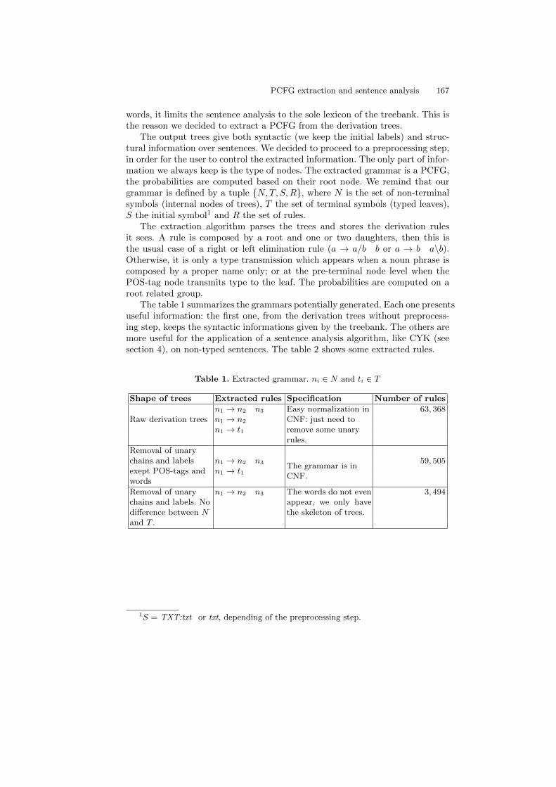
PCFG extraction and sentence analysis 167

words, it limits the sentence analysis to the sole lexicon of the treebank. This isthe reason we decided to extract a PCFG from the derivation trees.

The output trees give both syntactic (we keep the initial labels) and struc-tural information over sentences. We decided to proceed to a preprocessing step,in order for the user to control the extracted information. The only part of infor-mation we always keep is the type of nodes. The extracted grammar is a PCFG,the probabilities are computed based on their root node. We remind that ourgrammar is defined by a tuple {N,T, S,R}, where N is the set of non-terminalsymbols (internal nodes of trees), T the set of terminal symbols (typed leaves),S the initial symbol1 and R the set of rules.

The extraction algorithm parses the trees and stores the derivation rulesit sees. A rule is composed by a root and one or two daughters, then this isthe usual case of a right or left elimination rule (a → a/b b or a → b a\b).Otherwise, it is only a type transmission which appears when a noun phrase iscomposed by a proper name only; or at the pre-terminal node level when thePOS-tag node transmits type to the leaf. The probabilities are computed on aroot related group.

The table 1 summarizes the grammars potentially generated. Each one presentsuseful information: the first one, from the derivation trees without preprocess-ing step, keeps the syntactic informations given by the treebank. The others aremore useful for the application of a sentence analysis algorithm, like CYK (seesection 4), on non-typed sentences. The table 2 shows some extracted rules.

Table 1. Extracted grammar. ni ∈ N and ti ∈ T

Shape of trees Extracted rules Specification Number of rules

Raw derivation treesn1 → n2 n3 Easy normalization in

CNF: just need toremove some unaryrules.

63, 368n1 → n2

n1 → t1

Removal of unarychains and labelsexept POS-tags andwords

n1 → n2 n3The grammar is inCNF.

59, 505n1 → t1

Removal of unarychains and labels. Nodifference between Nand T .

n1 → n2 n3 The words do not evenappear, we only havethe skeleton of trees.

3, 494

1S = TXT:txt or txt, depending of the preprocessing step.

168 Sandillon-Rezer

Table 2. Example of rules extracted from various input trees.

Raw derivation trees

Rule exampleNP:np → NPP:np 1.01e−1

NP:np → DET:np/n NC:n 2.02e−1

Removal of unary chains and labels but POS-tags and words

Rule example:(np\si)/(np\sp) → VINF:(np\si)/(np\sp) 9.53e−1

:(np\s)/(np\sp) → CLR:clr :clr\((np\s)/(np\sp)) 2.88e−2

Removal of unary chains and labels.

Rule example

np → np/n n 8.02e−1

s → np np\s 3.81e−1

s → s s\s 2.65e−1

the sentence has a ”sentence modifier” at its end.s → np\sp (np\sp)\s 1.13e−3

the type np\sp corresponds to a past participle, used as anargument of the whole sentence.

4 Sentence analysis

The analysis process can be subdivided in two parts. On the one hand, we have totype the words, while staying as close as possible to standard Lambek derivations.On the other hand, the needed rules must belong to the input grammar.

4.1 Word typing

By gathering the leaves of the derivation trees, we have a lexicon, as we can seeFig. 3. However, a typing system based only on this lexicon reduces the possibilityof parsing to the sentences composed by words from the French Treebank. Wedecided to type words with the Supertagger (see Moot [15, 16]), which enabledus to validate the Supertagger results and to analyze sentences which did notoccur in the Paris VII treebank.

The Supertagger is trained with the lexicon extracted from the transducedderivation trees.

5968:le:det: - 5437:np/n, 140:(n\n)/n, 79:(s/s)/n, 68:(s\s)/n

Fig. 3. Extract of the lexicon. It gives the occurrence in the derivation trees, thePOS-tag of the words and the associated types. Here, the determiner ”le” occurs 5968times in the derivation trees, and the most probable type is np/n, the usual one fora determiner at the beginning of a noun phrase. The three other types correspond tonoun phrases used as modifiers.

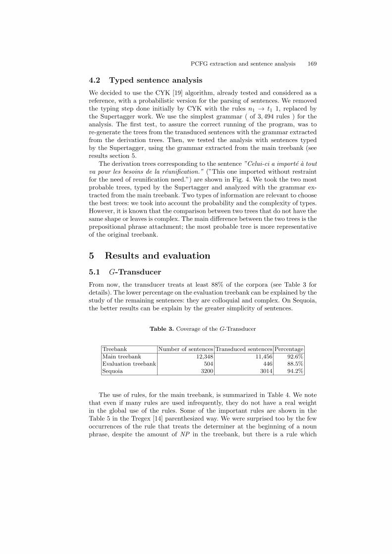
PCFG extraction and sentence analysis 169

4.2 Typed sentence analysis

We decided to use the CYK [19] algorithm, already tested and considered as areference, with a probabilistic version for the parsing of sentences. We removedthe typing step done initially by CYK with the rules n1 → t1 1, replaced bythe Supertagger work. We use the simplest grammar ( of 3, 494 rules ) for theanalysis. The first test, to assure the correct running of the program, was tore-generate the trees from the transduced sentences with the grammar extractedfrom the derivation trees. Then, we tested the analysis with sentences typedby the Supertagger, using the grammar extracted from the main treebank (seeresults section 5.

The derivation trees corresponding to the sentence ”Celui-ci a importe a toutva pour les besoins de la reunification.” (”This one imported without restraintfor the need of reunification need.”) are shown in Fig. 4. We took the two mostprobable trees, typed by the Supertagger and analyzed with the grammar ex-tracted from the main treebank. Two types of information are relevant to choosethe best trees: we took into account the probability and the complexity of types.However, it is known that the comparison between two trees that do not have thesame shape or leaves is complex. The main difference between the two trees is theprepositional phrase attachment; the most probable tree is more representativeof the original treebank.

5 Results and evaluation

5.1 G-Transducer

From now, the transducer treats at least 88% of the corpora (see Table 3 fordetails). The lower percentage on the evaluation treebank can be explained by thestudy of the remaining sentences: they are colloquial and complex. On Sequoia,the better results can be explain by the greater simplicity of sentences.

Table 3. Coverage of the G-Transducer

Treebank Number of sentences Transduced sentences Percentage

Main treebank 12,348 11,456 92.6%Evaluation treebank 504 446 88.5%Sequoia 3200 3014 94.2%

The use of rules, for the main treebank, is summarized in Table 4. We notethat even if many rules are used infrequently, they do not have a real weightin the global use of the rules. Some of the important rules are shown in theTable 5 in the Tregex [14] parenthesized way. We were surprised too by the fewoccurrences of the rule that treats the determiner at the beginning of a nounphrase, despite the amount of NP in the treebank, but there is a rule which

170 Sandillon-Rezer

txt

s

s

s

Celui-ci np np\s

a (np\s)/(np\sp) importe np\sp

a tout va s\s

s\s

pour (s\s)/np np

les np/n n

besoins n n\n

de (n\n)/np np

la np/n reunification n

. s\txt

txt

s

Celui-ci np np\s

a (np\s)/(np\sp) np\sp

(np\sp)/pp

importe (np\sp)/pp a tout va ((np\sp)/pp)\((np\sp)/pp) pp

pour pp/np np

les np/n n

besoins n n\n

de (n\n)/np np

la np/n reunification n

. s\txt

Fig. 4. Probability of the first tree: 5.12e−05; probability of the second one: 2.29e−08.

treats only the case of a noun phrase composed by a determinant and a noun,called 8, 892 times.

The derivation trees of the three corpora allow us to extract three differentgrammars, and in addition, lexicon were created, containing words and theirformulas. The lexicon covers 96.6% of the words of the Paris VII treebank, i.e.26, 765 words on 27, 589, and for Sequoia, it covers 95.1%, i.e. 18, 350 word on19, 284.

Table 4. Summary of the rule usage.

Number of rules Minimal and maximal occurrence. Number of applications

1,148 between 1 and 20 5, 818473 between 21 and 1, 000 68, 44041 between 1, 001 and 10, 000 125,4054 greater than 10, 000 60, 779

PCFG extraction and sentence analysis 171

Table 5. Some important rules of the transducer, including the four most important.

input pattern output pattern applications

( NP:* NC PP ) ( NP:* NC:n PP:n\* ) 17, 767(NP:* DET tree ) ( NP:* DET:np/n NP:n ) 16, 232(PP:* P NP ) (PP:* P:*/np NP:np) 16, 037(SENT tree PONCT ) (TEXT:txt SENT:s PONCT:s\ txt ) 10, 819(NP:* tree (COORD CC NP)) (NP:* (:* NP:*

(COORD:*\* CC:(*\*)/np NP:np))) 2, 511(SENT:* NP-SUJ VN NP-OBJ ) (SENT:* NP-SUJ:np

(:np\* VN:(np\*)/np NP-OBJ:np)) 1, 820

NP :∗CC : (∗\∗)/np NP : np

COORD : ∗\∗[/E]

NP : ∗ [\E]

Fig. 5. Rule for the coordination between two NP, as shown in Table 5.

5.2 Sentence parsing

The parsing of typed sentences is done with the grammar extracted from themain treebank, which is the most covering one. Each treebank has been divided intwo part, the transduced one and the non-transduced one. For the Supertagger,we used a β equal to 0.01: even if the supertagging and the parsing steps areslower, the results are much better than a β of 0.05. The results are gathered inTable 6. We note that non-transduced sentences are nevertheless analyzed, evenif the results are less accurate than for the other sentences.

We also tested the precision of the Supertagger (for the whole tests, see [18]):the Supertagger can adjust the number of types given to a word, with the βparameter. It enables to select formula which the confidence of the Supertaggeris at least β times the confidence of the first supertag. We summarize the timespent to analyze the fragment of 440 sentences of the evaluation corpus, theeffectiveness of the algorithm by modifying β in Table 7. The high number oftypes is due to the limitations of AB-grammar. When the Supertagger is usedfor multimodal categorial grammars, the average number of formulas is around2.4 with a β equal to 0.01 and 4.5 with β = 0.001; the correctness is better too,with respectively a rate of 98.2% and 98.8%.

6 Conclusion and prospects

In this article, we have briefly introduced the G-transducer principle, that weused to transform syntactic trees into derivation trees of an AB grammar. Thenwe explained how we extracted a PCFG and used it in the sentence analysis. Theexperimental results of the CYK algorithm used with typed sentences enabledus to compare the annotation from the transducer and the Supertagger.

172 Sandillon-Rezer

Table 6. Results.

Origin of sentences Number of sentences Success Rate

Main treebank 11,456 90.1%Evaluation treebank 446 83.6%Sequoia treebank 3,014 95.5%

Non transduced main treebank 892 62.5%Non transduced evaluation treebank 98 52.0%Non transduced Sequoia treebank 198 94.4%

Table 7. Summary of time spent, given the average number of types for a word. Thecorrectness of types is evaluated by the Supertagger.

Average number of types Correctness Execution time Analyzed sentences

1 (β = 1) 76.9% 0.31 sec 30.2%1.8 (β = 0.1) 87.0% 0.78 sec 65.7%2.4 (β = 0.05) 88.9% 1.22 sec 72.7%4.5 (β = 0.01) 91.7% 4.27 sec 83.6%10.6 (β = 0.001) 93.4% 20.18 sec 96.8%19.2 (β = 0.0001) 93.8% 55.32 sec 98.0%

However, the work is still ongoing, and opens many horizons. Of course, wewant to extend the coverage of the transducer to exceed 95% and simplify thetypes of words. The main problem is that only complex cases remain, but weshould be able to find derivation trees, given that we can analyze a part of themwith the CYK algorithm. In order to improve parsing precision, we intend tointegrate modern techniques such as those of [3, 20] into our parser. Using theCharniak method [6], we would like to transform our grammar into a highlylexicalized grammar.

Given that AB grammars may seem limiting in the case of a complex lan-guage, we wish to transform our transducer into a tree to graph transducer. Thisway, we would be able to use the whole Lambek calculus.

The XML version of the Treebank gives more informations on the words, likethe tense of verbs. A major evolution would be to reflect this information intoour transducer, even if it implies many transformation for it.

Our work and programs are available on [21], under GNU General PublicLicence.

References

1. Abeille, A., Clement, L., Toussenel, F.: Building a treebank for French. Treebanks,Kluwer, Dordrecht (2003).

2. Abeille, A., Clement, L., Toussenel, F.: Annotation Morpho-syntaxique.http://llf.linguist.jussieu.fr (2003).

3. Auli M. and Lopez A.: Efficient CCG Parsing: A* versus Adaptive Supertagging.In Proceedings of the Association for Computational Linguistics (2011).

PCFG extraction and sentence analysis 173

4. Buszkowski, W., Penn, G.: Categorial grammars determined from linguistic data byunification. Studia Logica (1990).

5. Candito M. and Seddah D.: Le corpusSequoia : annotation syntaxique et exploita-tion pour l’adaptation d’analyseur par pont lexical TALN’2012 proceedings, Greno-ble, France (2012).

6. Charniak E. A maximum-entropy-inspired parser. In Proceedings of the 1st AnnualMeeting of the North American Chapter of the ACL (NAACL), Seattle (2000).

7. Comon, H., Dauchet, M., Jacquemard, F., Lugiez, D., Tison, S., Tommasi, M.: Treeautomata techniques and applications (1997).

8. Hockenmaier J.: Data and Models for Statistical Parsing with Combinatory Cate-gorial Grammar. PhD thesis, 2003.

9. Hopcroft J.E. and Ullman J.D.: Introduction to Automata Theory, Languages, andComputation. Addison-Wesley Publishing Company (1979).

10. Klein D. and Manning C.: Accurate Unlexicalized Parsing. In Proceedings of theAssociation for Computational Linguistics (2003).

11. Knuth D.E.: The Art of Computer Programming Volume 2: Seminumerical Algo-rithms (3rd ed.) Addison-Wesley Professional (1997).

12. Kanazawa, M.: Learnable Classes of Categorial Grammars. Center for the Studyof Language and Information (1998).

13. Lambek, J.: The Mathematics of Sentence Structure. (1958).14. Levy R., Andrew G.: Tregex and Tsurgeon: tools for querying and manipulating

tree data structures. http://nlp.stanford.edu/software/tregex.shtml (2006).15. Moot, R.: Automated extraction of type-logical supertags from the Spoken Dutch

Corpus. Complexity of Lexical Descriptions and its Relevance to Natural LanguageProcessing: A Supertagging Approach (2010).

16. Moot, R.: Semi-automated Extraction of a Wide-Coverage Type-Logical GrammarFor French. Proceedings TALN 2010, Montreal (2010).

17. Sandillon-Rezer, N.F.: Learning categorial grammar with tree transducers. ESSLLIStudent Session Proceedings (2011).

18. Sandillon-Rezer, N-F.: Extraction de PCFG et analyse de phrases pre-typeesRecital 2012, Grenoble (2012).

19. Younger D.H.: Context Free Grammar processing in n3. (1968).20. Zang Y. and Clarck S.: Shift-Reduce CCG Parsing. In Proceedings of the Associ-

ation for Computational Linguistics (2011).21. Sandillon-Rezer, N.F.: http://www.labri.fr/perso/nfsr/ (2012).

An Interaction Grammar for English Verbs

Shohreh Tabatabayi Seifi

INRIA / Universite de Lorraine, BP 23954506 Vandoeuvre-les-Nancy cedex

Abstract. This paper accounts for the construction of a grammar forEnglish verbs using Interaction Grammars. Interaction Grammar is agrammatical formalism based on the two key notions: polarities and con-straint system. A polarity expresses an available resource or a lack ofresource and is used to discriminate between saturated and unsaturatedsyntactic structures. A grammar is viewed as a system of constraints ofdifferent kinds: structural, feature and polarity constraints, which shouldbe satisfied by the parse trees of sentences. We have developed a gram-mar for English verbs in affirmative clauses and finally we evaluated ourgrammar on the portion of a test suite of sentences, the English TSNLP,with LEOPAR parser which is a parser devoted to Interaction Gram-mars.

Keywords: Grammatical formalism, interaction grammar, tree descrip-tion, polarity, unification grammar

1 Introduction

The goal of this work is to construct an Interaction Grammar for English verbs.Interaction Grammar(IG) [1] is a very powerful formalism which has the advan-tages of both Lexical Functional Grammar (LFG) [5] and Categorial Grammar(CG) [3] and [4]. From LFG, it takes the flexibility with the mechanism of uni-fication to perform syntactic composition. From CG, it takes the resource sensi-tivity to control syntactic composition with polarities. It is inspired by chemicalreactions. In this formalism each lexicalized elementary tree acts as a potentiallyactive element which can participate in a reaction with another tree. Two nodesof different trees can merge if they are able to neutralise each other’s active po-larities and make stable combination. Whenever all the polarities are neutralisedcorrectly to build a unique tree, the obtained tree would be the parse tree of thesentence.

Guillaume and Perrier [9] investigated the principle underlying IG formalismfrom more theoretical point of view. In general we can see that in IG polaritiesare attached to the features where as in CG they are attached to the constituentsthemselves. The other more essential difference lies in the frameworks of thesetwo formalism: CG are usually formalized in generative deductive frameworkwhile IG is formalized in a model–theoretic framework. Pullum and Scholz high-lighted the advantages of changing the framework [8].

An Interaction Grammar for English Verbs 175

Currently a very detailed French Grammar with quite high coverage has beendeveloped in IG formalism [9]. This work is an attempt to construct a portionof English grammar using the same formalism.

2 Interaction Grammars

In order to get a view of how Interaction Grammars work, the following notionsare required.

2.1 Tree Description

A tree description is a tree like structure which uses the notion of underspecifica-tion relations to describe a family of trees instead of only one tree [7]. This allowsto make an unlimited number of trees from a unique underspecified tree repre-sentation. A tree which does not have any underspecified relation is a model. Forinstance, one tree description with an underspecified dominance link, illustratedin the left side of Fig. 1, can produce three (and more) different models.

Fig. 1. A description tree with three of its models.

2.2 Feature Structure

IG associates features with the nodes of tree descriptions to put constraints andprevent building ungrammatical parse trees. Feature structure models the inter-nal structure of the language where grammatical properties are represented. Notonly do feature structures prevent building ungrammatical sentences, but alsothey carry valuable linguistics information. Using feature structure to constructa grammar is a salient characteristics of a formalism like LFG but unlike LFGthere is no recursive feature in IG and feature structures have only one level.

176 An Interaction Grammar for English Verbs

2.3 Polarities and Saturated Models

Polarities are one of the basic notions in Interaction Grammars. A polarizedfeature is used to control the process of merging nodes of trees to be combined.Different kinds of polarities are used in IG. There are features with positive ornegative polarities meaning an available resource to be consumed or an expectedresource to be provided respectively. A neutral feature indicates a feature whichis not to be consumed but just to participate in a simple unification process whilecombining with other nodes. A saturated feature is the result of combination ofa positive and a negative feature and can be unified with no more positive ornegative feature.

Finally there are virtual features which should be merged with real featuresduring the parsing process including positive, negative, neutral and saturatedfeatures. Virtual polarities are used to express required contexts. Positive, neg-ative and virtual features constitute the active polarities because they need tocombine with other polarities.In Fig. 2 features with positive (–>), negative (<–) and virtual (∼) polarities canbe seen in the tree descriptions associated with the words been and arranged.Saturated features indicated with symbol <==> and neutral features indicatedwith symbol = or == can be seen in the non-completed parse tree in the leftside of Fig. 2. The horizontal arrows between nodes indicate linear precedenceconstraints and comes in two forms: large precedence (- - >)which means therecan be several nodes between these two node and immediate precedence (–>)which obstacles locating any other node between these two nodes.

Tree descriptions along with polarized feature structure are called polarizedtree descriptions or PTDs. The composition process is defined as a sequence ofPTD superpositions controlled by polarities. When two nodes merge, their fea-tures will be unified according to the standard process of unification with theextra limitations coming from the rules of combination for polarities. Saturatedtrees are those completely specified trees which have no active polarities any-more. The goal of parsing is to generate all saturated trees from the set of inputPTDs which come from a particular IG grammar.

2.4 Grammar

An IG grammar is defined by a finite set of PTDs which are called the elementaryPTDs or EPTDs of the grammar. Each EPTD has one (or more) leaf which islinked with a word of a lexicon and is called an anchored node. This means thatthe grammar is strictly lexicalized and there is no EPTD without any anchor.In practice there is more than one EPTD for each lexical entry in the grammarwith respect to its different syntactic properties.The parser of an IG grammar has two main roles. First to select the EPTDs ofthe words in the input sentence from the set of EPTDs inside the grammar thento build all valid minimal models with the use of these EPTDs.

Fig. 2 and Fig. 3 show an example of building a model for the sentence Theinterview has been arranged. The first figure is a snapshot of the intermediate

An Interaction Grammar for English Verbs 177

Fig. 2. A non-complete parse tree on the top with two of its EPTDs on the bottomwaiting to be used to make a saturated model for the sentence The interview has beenarranged.

178 An Interaction Grammar for English Verbs

Fig. 3. A parse tree (model) for the sentence The interview has been arranged.

An Interaction Grammar for English Verbs 179

results during parsing process; a non-completed parse tree with unsaturatednodes along with the EPTDs of the rest of the words of the sentence. The secondfigure shows the result yielded by combining the EPTDs of the remaining wordswith the non-completed tree: it is one valid model, the parse tree of the inputsentence.

3 Building grammars with wide coverage

Tackling with real language problems needs a large scale lexicalized grammarwhich is hard to build and without using automatic tools it is an overwhelmingtask. The main reason for that is the huge degree of grammatical and lexicalredundancy. For instance in IG, several PTDs may share same subtrees which isdue to the grammatical redundancy of syntactic structures. Moreover differentlexical entries share the same elementary PTDs owing to the fact that they are inthe same syntactic category. These redundancies turn even a small modificationof the grammar into a big change in large amount of grammar trees. In orderto conquer these obstacles eXtensible MetaGrammar (XMG) [6] is used as afacilitating tool to write the IG grammar. XMG is a tool for constructing largescale grammars. The main feature of XMG is to distinguish between sourcegrammar and object grammar. A source grammar is a collection of statementswritten in a human readable language which produces object grammars whichare usable by NLP systems.

3.1 Source grammar and object grammar

The terms source grammar and object grammar here are analogous with thesource and object codes in programming languages. In the current task first wewrote the source grammar and then we compiled it with XMG into the objectgrammar which is encoded in XML. XMG is widely used in construction ofgrammars in two formalisms: IG and TAG [2].In source grammar, each small fragment of tree structure is written in an indi-vidual class.

By use of class disjunction, conjunction and inheritance, more complex classescan be built. The compilation of terminal classes of the source grammar producesthe EPTDs of the object grammar. Each EPTD does not contain any lexicalentry yet, but has a detailed description of the word which is going to be nestedin its anchor node.

3.2 Linking the grammar with the lexicon

The characteristics of the appropriate word to be settled in an anchor node ofan EPTD is described in the EPTD interface. An interface is a feature structuredescribing the words which are able to anchor the EPTD. Every entry in thelexicon is a pair of a word and a feature structure hence a word can anchor an

180 An Interaction Grammar for English Verbs

Fig. 4. The process tool chain

EPTD if its feature structure is unifiable with the EPTD’s interface in the exactsame means of unification we have in node merging.

The whole process chain is illustrated in Fig. 4 and the highlighted box isthe part that has been developed in our work.

4 The Grammar of English Verbs

To build a complete Interaction Grammar for a specific language which can beable to parse any possible sentence, we need a set of EPTDs for wide rangeof words from different categories like verb, auxiliary, noun, adjective, adverb,prepositions, determiner, pronoun etc. Our main effort was on the constructionof a grammar for verbs in affirmative clauses (e.g. different tenses, moods andvoices). We have used a small grammar for noun phrase, pronouns, prepositionsand adjectives to provide appropriate EPTDs to parse a sentence [11].The central focus in writing a grammar with IG formalism is to find a wayto write classes in a manner that with the use of heredity, conjunction anddisjunction all different grammar trees needed in a complete grammar can beobtainable.

4.1 An Sketch of The Major Modules

Five major modules contribute building the EPTDs for verbs. Module VerbalK-ernel is the kernel of all lexical and auxiliary verbs. It implements different pos-sible voices and moods of the verbs and also it provides syntactic functions of averb phrase (e.g. head, subject, modifier and etc). A subclass in a module is anintermediate tree description that we use along with operators such as heredity,conjunction and disjunction to build the final tree descriptions.

There are seventeen subclasses in module VerbalKernel. For instance wemodel the long distance dependency between a verb and its subject with the useof underspecification relation. All tree descriptions of the verbs which are coming

An Interaction Grammar for English Verbs 181

out of this module have a subject node which is an empty node for imperativeverbs and a non empty node for all other verbs.

Fig. 5. A schema of relations between some of classes in the module VerbalKernel.

Fig. 5 aims to illustrate different relations between some of classes in themodule VerbalKernel. Some classes are inherited from another one and someare built out of the disjunction of two or more other classes.

Whenever there is no complement nodes in the verb tree, auxiliaries arefollowing the same pattern as non auxiliary verbs therefore class Auxiliary isinherited from VerbalKernel. The EPTD associated with the auxiliary been inFig. 2 is an example of an auxiliary EPTD. Eight subclasses are in class auxiliaryimplementing all different kinds of auxiliaries. We treated to ,the infinite marker,like auxiliaries in the current grammar. The main reason for this approach is thecomplementary distribution between to and modal auxiliaries e.g. they neverappear together but they appear in the exact same position in the sentence andboth force the verb after them to be in the bare infinitive form.

Module Complements builds all different kinds of verb complements. Itcontains 20 different classes and all number, category and function of verb com-plements are defined in this module.

VerbalKernel and Complements will merge together in order to make anew module Diathesis with 20 classes which describes different diathesis alongwith different verb complements e.g. 13 classes for active verbs and 7 classesfor passive verbs. For instance to build an EPTD for an active verb with adirect object a tree describing a predicate node with one complement of type

182 An Interaction Grammar for English Verbs

noun phrase will merge to a tree associated with active verb and give back theappropriate PTD with active verbs with direct nominal object. Finally moduleVerb with 15 classes will implement trees for different verb families accordingto their subcategorization frame. For example the family of transitive verbscan anchor the tree associated with active verbs with direct object and thetree associated with passive verbs. So the class for transitive verbs will be thedisjunction of two classes of module Diathesis. The PTDs which are comingout of module Verb and module Auxiliary are elementary PTDs and used toattach to the lexicon.

5 Evaluation Results

The English TSNLP (Test Suite for Natural Language Processing) [12] projecthas aimed to compose a tool for Natural Language Evaluation purposes. It is adatabase of phrases which carry different linguistic phenomena to be used as areference for evaluation tasks. These phrases are divided into several categoriesaccording to different linguistic phenomena. Each category has both grammaticaland ungrammatical examples to provide an infrastructure not only for determin-ing the true positives (success in parsing the grammatical sentences), but alsofor counting the true negative (failure to parse ungrammatical sentences).

The English TSNLP has 15 different categories and 3 of those contain phe-nomena exclusively related to verbs which was the subject of this research. How-ever those three categories also contain some other structure which was not in-cluded in the current grammar and sentences of those form were put out as wellincluding phrasal verbs, sentences having there as their subject and sentencescontaining relative clauses. (e.g. That she leave is requested by him.) We haveused LEOPAR parser [10] to construct the models for the input sentences andthe result of evaluation of the current grammar can bee seen in table 1.

Grammatical Ungrammatical

Total Number 148 832Parsing Success 115 50Parsing Failure 33 782

Precision 86.7% 94%Table 1. Evaluation results of the proposed IG grammar on portion of English TSNLP

5.1 Result Analysis

The major reason of failure in parsing grammatical sentences is that the con-struction of verbs up to now requires that every verb tree has a subject nodewhich should be filled with a real subject while parsing the sentence. However

An Interaction Grammar for English Verbs 183

there are situations in which a verb acts like a noun or an adjective and thereis no such a subject node in its grammar tree. (e.g. He finds the office closed.)Owing to the fact that we were focusing on construction of the verbs of the mainVP of the sentence, other grammatical phenomena which are related to verbswere not properly treated and this failure should not be regarded as a weaknessof the framework. In appropriate time all this structures can be constructed inthe grammar which is one of the goals in the future works.

The other failure is to mistakenly parse some ungrammatical sentences. Oneof the main reasons, among other defeats, is that there are some sentences thatare not correct because of semantic issues which is not recognizable by ourgrammar.

6 Conclusions and Future Works

Interaction grammars is a powerful formalism that has advantages of both uni-fication grammars and categorial grammars at the same time. Writing a widecoverage grammar for the English language needs a huge effort and this workcan be regarded as the starting point of such a project. Using tools like XMGto accomplish this goal is quite helpful and makes the writing and then the tun-ing of the grammar a lot more easier than before. Moreover, a high degree offactorization is possible when we separate source grammar and object grammarwhich leads to more efficiency.

The potential future aims of this project are first to continue to constructa complete grammar for English incorporating all different phenomena in orderto parse any grammatical English sentence and second try to cope with the stillopen problems like coordination in the sentences within the same framework.

On the other hand English TSNLP is a relatively simple set of sentencesand is not quite similar to real corpora. Therefore some steps further would beto enrich the grammar some how we would be able to cope with real corporalike newspaper or spoken language corpora where the structure of sentences aremore complicated and our grammar should be able to handle several non quitegrammatical sentences too .

References

1. Perrier, G.: Interaction grammars. In 18th International Conference on Computa-tional Linguistics, CoLing 2000, Sarrebrucken, pages 600–606. (2000)

2. Crabbe, B.: Grammatical development with XMG. LACL 05. (2005)

3. Retore, C.: The Logic of Categorial Grammars. ESSLLI 2000, Birmingham.(2000)

4. Steedman, M.: Categorial Grammars. A short encyclopedia entry for MIT Encyclo-pedia of Cognitive Science. (1999)

5. Bresnan, J.: Lexical-Functional Syntax. ESSLLI 2000, Birmingham.(2000)

6. Duchier, D., Le Roux, J., Parmentier,Y.: The Metagrammar Compiler: an NLP Ap-plication with a Multi-paradigm Architecture. In Second International Mozart/OzConference, MOZ 2004, Charleroi, Belgium, pages 175–187 (2004)

184 An Interaction Grammar for English Verbs

7. Marcus, M.C., Hindle, D., Fleck. M.M. : D-Theory: Talking about Talking aboutTrees. In 21st Annual Meeting of the Association for Computational Linguistics,pages 129–136.(1983)

8. Pullum,G.K., Scholz, B.C. : On the Distinction between Model–Theoretic andGenerative–Enumerative Syntactic Frameworks. In Logical Aspects of Computa-tional Linguistics, LACL 2001, Le Croisic, France, volume 2099 of Lecture Notes inComputer Science, pages 17–43. Springer Verlag. (2001)

9. Guillaume,B., Perrier, G.: Interaction Grammars. INRIA Research Report 6621:http://hal.inria.fr/inria-00288376/ (2008)

10. Guillaume,B., Le Roux,J., Marchand, J., Perrier,G., Fort,K., Planul,J.:A Tool–chain for Grammarians. CoLING 08, Manchester. (2008)

11. Planul, J.: Construction d’une Grammaire d’Interaction pour l’anglais. Memoire,presente et soutenu publiquement le 27 juin. (2008)

12. Lehmann,S., Oepen, S., Regnier–Prost,S., Netter,K., Lux,V., Klein,J., Falkedal,K.,Fouvry,F., Estival, D., Dauphin, E., Compagnion, H., Baur, J., Balkan, L.,Arnold,D.: TSNLP– Test Suite for Natural language Processing. In Proceedingsof COLING 1996, Kopenhagen. (1996)

Toward a Discourse Structure Account of Speechand Attitude reports

Antoine Venant1,2

1 Laboratoire Parole et Langage2 Ecole Normale Superieure de Cachan

Abstract. This paper addresses the question of propositional attitudereports within Segmented Discourse Representation Theory (SDRT). Inline with most SDRT discussions on attitudes reports, we argue that thereported attitude should be segmented in the same way as the rest of thediscourse is. We identify several issues that are raised by the segmenta-tion of attitude reports. First, the nature of some relations crossing theboundaries between main and embedded speech remains unclear. More-over, such constructions are introducing a conflict between SDRT’s RightFrontier Constraint (RFC) and well established facts about accessibilityfrom factual to modal contexts. We propose two solutions for adaptingdiscourse structure to overcome these conflicts. The first one introducesa new ingredient in the theory while the second one is more conservativeand relies on continuation-style semantics for SDRT.

1 Introduction

From a semantic perspective, attitudes reports require to solve several notoriouspuzzles. Among these, are a lot of problems triggered by definites: Substitutionof directly co-referential expressions is generally not allowed under the scope ofan attitude verb and neither does existential generalization(see the shortest spyproblem raised by [8]). Closely related to those are effects of attitudes verbs ondiscourse referents availability. For instance factive epistemic verbs like ’to know’allow referents introduced under their scope to be then referred from outside theirscope, while non factive like ’to believe’ do not. These two issues are related tocontext which has naturally led to several accounts involving dynamic semanticssuch as [1, 9].

From the modeling text coherence perspective, we need to understand howreporting someone’s propositional attitude interacts with the overall discoursestructure. The dynamic framework of Segmented Discourse Representation The-ory (SDRT) [3] allows to address both perspectives simultaneously by lookingat the interaction between discourse structure and anaphoric phenomena. How-ever there is in SDRT no semantic contribution for attitudes report that is asprecise as the ones cited above and formulated within Discourse RepresentationTheory (DRT) [7]. Since SDRT builds over a lower-level formalism (DRT), andenriches it by adding rhetorical relations, one may wonder whether DRT-style

186 Antoine Venant

accounts could be straightforwardly embedded in SDRT. One condition for thisis that SDRT keeps the benefits of the work done in the chosen low-level logic,and uses its ability to handle discourse relation to model a more accurate inter-face between semantics and pragmatics.3 We want to address then the questionof how does SDRT’s treatment of embedded speech acts keeps up with such aconsideration.

We attach a particular attention to examples in the spirit of 1 for they involveirruption of the factive context into the modal context at the discourse level. Wethink that such anaphoric links are not fully modelled by the current analysesof attitude reports in SDRT. Distinguishing between Intentional/Evidential usesof reportative verbs still do not allow them in some intensional cases while DRTbased approaches would very likely allow event correference from an embeddedDRS to the main DRS.

Example 1. The criminal parked his car somewhere near the airport. So detec-tives think that afterwards he tried to get into a plane.

After briefly introducing SDRT in section 2, we argue in section 3 for seg-mentation of reported constructions. Section 4 deals with relations that links areported speech act to a factual one. It shows that the discursive structure ofintensional reports is closed to incoming relations, but still can bear anaphoriclinks to the context. On this basis it exhibits a family of relations for whichRFC makes bad predictions. Section 5 presents two ways of restoring the rightaccessibility conditions while still benefiting from SDRT specificities.

2 Segmented Discourse Representation Structures

SDRT assumes that to analyze discourse one has to segment into meaningfulunits that shall be linked to each other by means of discourse relations. Eachsegment is called an elementary discourse unit (edu). The level of segmenta-tion is merely the clause level (where a clause can be understood as somethingcontaining an event or a state)4.

Each discourse unit is assigned a label (πi,...πn) in the language of SDRSsand a corresponding formula in a given language for representation of atomicclauses (K1,...,Kn)5. These labels will serve as arguments of rhetorical relations,like narration(πi, πj) or explanation(πi, πj). Additional labels are associatedwith complex structured content made of rhetorical relations and other subordi-nated labels. Such labels with complex content will be called complex discourseunits and recursively used as argument of other relations. A SDRS is a triple〈A,F, Last〉 where A is a set of labels (A), F a function mapping labels to con-tents (either lower-level language such as DRS or discourse relations in case of

3This is indeed what the theory aims at doing while extending DRT’s definition ofaccessibility.

4How fine-grained segmentation should is still under discussions. The present workis also a contribution at this level since we argue for segmenting attitudes.

5This is the lower-level language and associated representations.

Toward a Discourse Structure Account of Speech and Attitude reports 187

complex constituents) and Last the information of the last segment introduced.(See [3]:p.138 for the precise definition).

SDRT makes a structural distinction between coordinating and subordinatingrelations. The former, like narration, confer an equal status to their two argu-ments. The latter introduce a hierarchy between the related constituents. Sucha distinction allows to define the so-called Right Frontier constraint. The RightFrontier is the set of labels RF = {π | π ≺∗ Last} where ≺∗ is the transitive clo-sure of the dominance relation ≺ defined by π ≺ α iff α is a complex consitutentwhich immediately outscopes π or there is subordinating edge R(α, π) in someconstituent γ. The Right Frontier Constraint stipulates that labels accessible fordiscourse continuation are those of the Right Frontier, while the ones accessiblefor correference have to be DRS-accessible on the right frontier.

For instance, the structure of [John visited his friend]a. [Then he went to thecinema]b. [He watched Pirates of the Caribbean]c is narration(πa, elaboration(πb, πc))elaboration is a subordinating and narration a coordinating relation, thereforethe right frontier is {πb, πc} and the discourse could not be felicitously continuedby They talked for a long time which intends to attach to a.

πa π1

πb

πc

narration

elaboration

Fig. 1. SDRS example

Figure 1 gives a graphical representation of this example, with the conventionthat coordinating relation are drawn horrizontally, subordinating one vertically,complex constituents are linked with dashed edges to their subconstituents, andnodes of the right frontier are red.

The truth conditional content of an SDRS, as in DRT, is expressed in termsof context-change potential (i.e relation between world-assignment pairs), and isrecursively computed using the semantic constraints associated with each rhetor-ical relation, finally relying on the lower-level logical forms.

In this framework, we now move to the discourse structure of attitude andspeech reports.

3 Segmentation and treatment of the matrix clause

There are at least two reasons for capturing the interaction between attitudes orspeech reports and discourse structure. First, we need to account for discourse

188 Antoine Venant

phenomena both inside the reports and across their boundaries. Then the treat-ment of intentional and evidential uses of attitude reports in the way of [6] alsorequire segmentation.

About the first point, example 2 is not felicitous, because the pronoun ’it’cannot easily refer to the salmon in the given context. Such a behaviour ispredicted by RFC. Therefore, even if the semantics of attitudes generally involvesquantification over intensions or contents, and thus erases to some extent thestructure of the logical form of the original speech act, the discourse structureof the report is needed anyway to build the logical form of the speech report.

Example 2. #John told me that Marry had a wonderful evening last night. Hesaid [she ate salmon]a [and then won a dancing competitionb] [and that it wasbeautiful pink.]b

On the other hand, in example 3 the reported speech introduces a narrationbetween two events while the non-reported discourse asserts a causal relation(result) between the two same events. The contrast introduced by but is howevercoherent, partially because it is supported by the isomorphic structures of thereported speech and the non-reported one. SDRT treatment of contrast as ascalar relation, following [2, 3] provides such an analysis, assuming that thestructure of the embedded speech is accessible.

Example 3. John says that he left after Mary did but he left because she did.

About the segmentation of the matrix, we may consider the matrix clauseas nothing more than a kind of logical operator6. However, that would be inac-curate since the matrix clause can be fairly sophisticated. It generally includesa communication event or a mental state that can be modified by adverbs orprepositional phrases and therefore would be difficult to model as simple logicaloperator. Since removing the matrix-clause from the discourse representation isnot an option neither segmenting attitude reports forces us to deal with thismatrix-clause segment.

[6] addresses several issues raised by such a treatment of reported speech.The approach consists in segmenting apart matrix clause and reported speechand in identifying the relation between these elements themselves but also theirrelations with the surrounding context. It distinguishes between two uses ofreportative verbs, namely evidential where the embedded content is asserted bythe main speaker and intensional where the content of the report is not assertedby the main speaker. In evidential uses, the matrix clause is subordinated tothe embedded content by a veridical evidence relation.7 In intensional uses, theembedded content is subordinated to the matrix via a relation of attributionwhich is non-veridical. Such a distinction makes very profitable the separationof the matrix clause and the reported speech, accounting for cases like 4.

6This would still requires to modify the SDRT framework since all logical opera-tors are delegated either to the lower-level logical forms or to the semantic effects ofdiscourse relations.

7To be satisfied, veridical relations require their arguments to be true in the model.Non veridical relations do not have this requirement. [3]

Toward a Discourse Structure Account of Speech and Attitude reports 189

Example 4. (1) [The neighbours are gone.]a [John told me that]b [they went onvacation in an expensive hotel.]c [I called it this morning.]d

(2) [The neighbours are gone.]a [John told me that]b [they went on vacation inan expensive hotel.]c [But he lied]e .

As [6] argues, we can see in the first example above that c is asserted bythe speaker since d is carrying an anaphoric link to the hotel eventhough it hasfirst been introduced under the scope of the attitude8. On the contrary, in 4.2,the author disagree with what is reported, and the existence of the hotel is notensured anywhere outside the scope of the attitude. Therefore The hotel shallnot be referred to later in the discourse. [6] also argues that the compositionalsemantics of both the reported speech and the matrix clause do not change froman intensional to an evidential report. And the matrix clause can neither bedeleted without loss of compositional content in the one nor the other case. Butthe way the two parts of speech are related can change. Fu rthermore, sincethe two first sentences are the same in both examples, the decision of choosingthe one or the other might only be a matter of context, as such it is essentiallyinformation packaging, and in SDRT, this level is kept aside from the logic ofinformation content.

Following this analysis, in the first example, d will be related to c by a veridi-cal relation of narration, forcing the evidential reading. So c will be related tob with the veridical Evidence(c, b) and to a with a veridical relation of expla-nation. In the second example however, continuation e is attached to the wholereport with a contrast and yields an intensional reading (attaching e to the em-bedded clause only would entails that John said something incoherent, which isless likely the intended meaning) and b is related to c using the non-veridicalattribution(b, c). The two different type of structures are sketched below. (Leftcolumn is evidential, right one is intensional. We also give some of the semanticsconditions associated with the two relations involved).

F(πb) =φ

A(x, φ)F′(πb) =

φ

A(x, φ)

F(πtop) = Re(πa, πc) ∧ evidence(πc, πb) F′(π′top) = Ri(πa, πb) ∧ attribution(πb, πc)Φevidence(πc,πb) ⇒ Kπc ∧Kπb ∧ φ ∼ˆπc Φattribution(πb,πc) ⇒ Kπb ∧ φ ∼ˆπc

Where ∼ may be understood as an equivalence relation between SDRS contents.

How this content and∼ are defined actually remains an open question. Basically content

could be understood as the context change potential. However, blocking substitution of

logically equivalent expressions under the scope of an attitude verb may require some

amount of structure being kept in the notion of content( [1]).

8At least if we assume that d is not part of what John said here, but in that casethat it would be a very odd reading.

190 Antoine Venant

4 Relations across boundaries

As [5] remarks, the picture becomes more complicated when relations comes tocross the boundaries of an embedded speech act such as in 5.

Example 5. [Fred will go to Dax for Christmas]a. [Jane claims that]b [Afterwards,he will go to Pau]c.

Afterwards introduces a veridical relation of narration. If we invoke the ev-idential/intensional distinction and assume an evidential reading, this exampledoes not pose any problem since the discourse producer (DP ) is thought toassert the content πc and thus can use a veridical relation for relating it tothe context. However, with an intensional reading the speaker does not claimnarration(πa, πc) since he does not assert the content of πc. But he still cancommit to Jane committing to such a relation. To solve this problem, [5] set upa new paradigm for discourse analysis that examines reported relations againstseveral sources. For instance, 5 will be analyzed as follows:

The discourse producer is certain of the main eventuallity ea in a but he doesnot know anything about the one in c. Jane is attributed to be certain about themain eventuality in c, and, after the source of the narration is identified to beingJane, the picture is completed with the statements of Jane being certain of eatoo, as well as ea and ec being in a temporal sequence. Semantically speaking,such examples require some further discussion. First, we cannot always identifya source for a relation. Consider a two level deep embedding as in 6. AssertingnarrationFred’s wife(πa, πd) in this case would make us unable to distinguish be-tween 6 and the same without b. With 6 the writer does not commit to Fred’swife committing that he will go to Pau.

Example 6. [Fred will go to Dax for Christmas]a. [Jane told me that]b [accordingto his wife,]c [afterwards, he will go to Pau]d.

Besides, interpreting narrationJ(πa, πc) ∧ attribution(πb, πc) requires someprecisions that the framework does not provide. To this end, we may switch toa dialogical framework in which each individual would receive its own SDRS.However, reducing reported speech and other voicing effects to dialogue is notwhat we want to do (especially if we want to be able to account for 6). An-other way to provide an interpretation would be to use [10] semantics, R(a, b): JC(Speaker(b),Ka) ∧C(Speaker(b),Kb) ∧C(Speaker(b), φR(a,b))K where C isa commitment relation and R a veridical relation. But once again the structureis misleading, and with this account, the narration producer must be under-stood as being Jane, which is strange since even when being reported, its pro-ducer remains the main producer. And we would end up with a fomulla entailingC(Jane, φnarration(πa,πb)) instead of something like C(W,C(Jane, φnarration(πa,πb)))that would be needed to account for example 6 with this semantics. Our conclu-sion thus is that the problem originates from the structure which does not modelthe right scope of attribution which should includes the narration relation. This

Toward a Discourse Structure Account of Speech and Attitude reports 191

can be done in SDRT by introducing a complex segment for representing theembedded content9:

A = {πtop, πa, πb, γ, πc}F(πtop) = attribution(πb, γ) F(γ) = narration(πa, πc)

(1)

Equation 1 is actually missing a non-embedded left-veridical coherence rela-tion between πa and another segment. As it stands our structure semantics doesnot imply that the main discourse producer claims the content of a. However,more generally there must be some relation (R) introduced by the main producerand that links πa with the speech act of reporting Jane’s claim (at least with anintensional reading). Attribution being subordinating in the intensional case, Rcannot be coordinating without the RFC being violated in 5. So it seems thatR should be a subordinating like background. However cases like 7 are source ofproblems.

Example 7. (1) [The train arrived 3 hours late.] [then the company announcedthat] [in consequence, the passengers would be refunded]. [But as a matterof fact, they never were.]

(2) [John had a deadline at midnight yesterday.] [So we all though that after-wards he would go to bed.] [But he did not.]

(3) [Yesterday, John fell three times in a row.] [Mary then told him that] [it wasprobably because he drank to much.] [He did not believe her.]

All these examples involve an intensional attitude report and in all of them,lexical markers mark either a narration or a result between the first segment andthe matrix clause of the report. Finally, they also all seem to support anaphoriclinks between the reported content and the first segment. Both result and narra-tion are thought to be coordinating relations. So even if we use the subordinatingbackground between πa and πb in 5, we cannot account for these links withoutviolating RFC.

Examples in 7 thus allow us to see that the Intensional/Evidential treatmentcomes with the side effect of sometimes preventing from linking to the previousdiscourse. But they are very specific in the sense that they enforce an explicitrhetorical link from the previous discourse on the two level (the main discourse,and the embedded one) at the same time. The problem may however be moregeneral if these links may as well be implicit.

Example 8. (1) [The factory blew up.]a [John told me]b [there were a lot ofdangerous chemicals in there.]c

(2) [The factory blew up.]a [John thinks]b [there were a lot of dangerous chemi-cals in there.]c

9Representing SDRS as directed acyclic graphs as it is often done is very confusingin this case, because a graph based representation does not distinguish which complexsegment actually hosts such a cross-relation. The graphs for our structure and theproblematic one are the same.

192 Antoine Venant

(3) [The factory blew up.]a [John thinks]b [there were a lot of dangerous chemi-cals in there.]c [But sam thinks]d [someone lighted a fire.]e

Examples in 8 intend to illustrate this. The first one does not seem to requirean implicit relation between a and c. The possible explanation of the explosionby the presence of chemicals is not a mandatory part of what John said. ActuallyJohn might have said that to the writer even before the explosion happened, andthe writer is making the link himself from what John previously said. The twoother examples on the other hands may carry such implicit links between a andthe reported content b: There is at least one plausible reading for the secondexample involving a coordinating relation between a and b which fits very wellan implicit explanation between a and c. The explosion actually made Johnthink of a plausible explanation, which is that they are dangerous chemicals inthe usine, and that these chemicals may have cause the explosion. Finally, thelast example requires implicit explanation relations to make a better sense ofthe con trast relation that links b and c. The beliefs of John and Sam are fullycompatible, unless what John and Sam respectively said is explanation(a, c) andexplanation(a, e), in which case they are not.

All together, this threatens to make SDRT better understanding of anaphoriclinks in attitude reports only come at the price of some wrong predictions in someintensional cases.

5 Restoring accessibility

We have shown that SDRT damages more standard but essentially correct ac-counts of anaphoric links going between modal and factual contexts. An accountof attitude reports in DRT for instance, would not have this behaviour. Exam-ples like 7 would introduce reference to events in the main DRS from the modalcontext, which is permitted. We would like such a behaviour, but with SDRTtreatment of accessibility still applying inside the reported speech. To this end,we could drop the attribution relation, falling back to a DRT like treatment.The structure of one of our problematic report in SDRT would thus be sketchedby Rcoord(πa, πatt) with F(πatt) = Kπb

∧A(x, φ)∧φ ∼ˆπc. This structure allowsreferents in πc to attach or refer to elements in πa.10 This builds on intensional re-port being ” closed” discursive structures. We showed in section 4 that a relationcannot really penetrate the report from the factual context without (a ”copy”of) its left argument and itself being embedded under the attitude. Moreover,attachment to the matrix clause and attachment to a complex segment made ofboth the matrix clause and the report are semantically and dynamically equiv-alent. This allows us to abstract the complete speech act of reporting under acomplex segment πatt. This approach however requires to adapt the languagefor inferring the relations because the intensional and evidential cases are now

10Such an approach actually needs to slightly modify the syntax of the SDRS lan-guage

Toward a Discourse Structure Account of Speech and Attitude reports 193

asymmetric. One has to state that the content of a segment πmat in the eviden-tial case is equal to a part of the content of the abstracted complex segment πattin the intensional case.

That is why we propose below a more conservative approach that makesuse of continuation-syle semantics [4]. Continuation style semantics representsa discourse as a λ−abstraction of type JΓ K = γ → ((γ → l → t) → l → t)where γ is the type of input contexts. A discourse thus asks for (i) an inputcontext i of type γ containing the effects of processing the previous discourse;(ii) a continuation o of type γ → l → t representing the discourse to come and;(iii) a label π, the label of the SDRS representing the whole discourse.

To represent chunks of an SDRS, a language is used where every n−arybecomes an n + 1-ary predicate, the extra argument stands for the label thathosts the predicate: A label π with F(π) = R(π1, π2) will be represented as∃π1∃π2∃πR(π1, π2, π).

We will assume that the context contains a structural representation of theSDRS for the previous discourse such that the following functions may be de-fined:

(1) sell : γ → l that selects a label for attachment.(2) ν : γ → l→ γ that performs the SDRT update operation on the context [3],

defined in terms of SDRT’s language for inferring relations. Given a labelπ, it basically picks up a relation and two other labels π1, π2 in the contextand add the relation R(π1, π, π2) to the context.

Finally, we will use the following version of the binder rule to join a discourseand a sentence:

JD.SK = λioπ ∃πDJDKi(λi′ ∃πS JSK i′ o πS))

The main idea, is to refine [6] proposal of a lexical entry for attitude reportsusing continuation-style semantics to overcome the right-frontier problems. Sinceevidential and intensional readings only differ by the way the matrix clause andthe embedded content are related, one simple solution is to postpone attach-ment of the matrix clause until the embedded content has been dealt with andall attachment to previous context have been done. But it must be performedbefore the following discourse is processed in order to still benefit from the inten-sional/evidential distinction. This might be done by modifying the continuationof the report in such a way that it proceeds to the attachment of the matrixclause before applying the real continuation.

Let us assume an attitude α in a discourse ”x α that φ” and that syntaxdelivers us a parse leading to α(x, φ). We add the lexical entry given in 2 for anattitude verbe α, with A a modal operator corresponding to attitude α.

JαK = λxλsλioπmatt∃φA(x, φ, πmatt)∧∃πs φ ∼ πs∧s i [λi′o(ν(ν(i′, πmatt), πs))] πs(2)

194 Antoine Venant

Let us now have a look back to [The train arrived late]a. [Then the companyannouced that]b [the passengers should thus be refunded]c.

We assume for a a lexical entry like:

λioπ ∃x train(x, π) ∧ Late(x, π) ∧ o ν(i, π)

.In this entry the update operation ν(i) will deliver a context i′ containing

the structure πa | F (πa) = [x | train(x) ∧ late(x)], and maybe a relation linkingπa to the previous context. Assuming the lexical entry for Thus is

JthusK = λioπs s i (λi′Result(selL(i′), π, selL(i′)) ∧ o i′)

We end up with the following entry for the embeded content c:

λioπ∃y, z ∧ The Passengers(y, π) ∧Be Refunded(y, π)

∧Result(selL(i), π, selL(i)) ∧ o i

The lexical entry for to announce (our α here) will be given the company asits first argument and the interpretation of c as its second. Which should yieldafter beta reduction:

λioπmatt∃φA(The company, φ, πmatt) ∧ ∃πs φ ∼ πs∧ ∃y, z ∧ The Passengers(y, πs) ∧Be Refunded(y, πs)

∧Result(selL(i), πs, selL(i)) ∧ o(ν(ν(i, πmatt), πs))

When composing with JaK, this entry will receive the context i′ containingthe structure πa | F (πa) = [x | train(x) ∧ late(x)], unmodified, as input contextand thus be able to select πa as first argument for the result relation withoutRFC violation. Importantly, successive call to the ν function will perform theintensional/evidential choice and choose a relation to link the report to thepreceding discourse before processing the continuation.

6 Conclusion

Segmenting discourse structure cannot be avoided, but as we have shown, thediscourse structure of segmented reports is not straightforward. We have thusgiven a more precise picture of what it should be and why. It remains to give aprecise semantics to those reports, and especially to decide what is the contentˆπ of a SDRS and what amount of structure it carries.

References

1. Asher, N.: A typology for attitude verbs and their anaphoric properties. Linguisticsand Philosophy 10(2), 125–197 (1987)

Toward a Discourse Structure Account of Speech and Attitude reports 195

2. Asher, N., Hardt, D., Busquets, J., Sabatier, I.P.: Discourse parallelism, ellipsis,and ambiguity. Journal of Semantics 18, 200–1 (2001)

3. Asher, N., Lascarides, A.: Logics of Conversation (Studies in Natural LanguageProcessing). Cambridge University Press (Jun 2005), http://www.worldcat.org/isbn/0521659515

4. Asher, N., Pogodalla, S.: SDRT and Continuation Semantics. In: Onada, T., Bekki,D., McCready, E. (eds.) New Frontiers in Artificial Intelligence JSAI-isAI 2010Workshops, LENLS, JURISIN, AMBN, ISS, Tokyo, Japan, November 18-19, 2010,Revised Selected Papers, LNCS, vol. 6797, pp. 3–15. Springer (2011), http://hal.inria.fr/inria-00565744

5. Danlos, L., Rambow, O.: Discourse relations and propositional attitudes. Con-straint in Discourse (CID) (2011)

6. Hunter, J., Asher, N., Reese, B., Denis, P.: Evidentiality and intensionality: Twouses of reportative constructions in discourse. In: Proceedings of the Workshop onConstraints in Discourse. pp. 99–106. Maynooth: National University of Ireland(2006)

7. Kamp, H., Reyle, U.: From Discourse to Logic: Introduction to Model-theoretic Se-mantics of Natural Language, Formal Logic and Discourse Representation Theory,Studies in Linguistics and Philosophy, vol. 42. Kluwer, Dordrecht (1993)

8. Kaplan, D.: Quantifying in. Synthese 19(1-2), 178–214 (1968)9. Maier, E.: Presupposing acquaintance: a unified semantics for de dicto, de re

and de se belief reports. Linguistics and Philosophy 32(5) (2010), http://www.

springerlink.com/index/10.1007/s10988-010-9065-2

10. Vieu, L.: On the semantics of discourse relations. Constraint in Discourse (CID)(2011)

Some, speaker knowledge, and subkinds∗

Andrew Weir

University of Massachusetts Amherst

Abstract. I provide an analysis of sentences with some combining withsubkind-denoting NPs, such as Some plant is growing through the wall ofmy room. In such sentences, there is epistemic uncertainty concerning thesubkind, but not concerning the actual witness of the claim. I make use ofthe semantics proposed by [Alonso-Ovalle and Menendez-Benito, 2010b]for the Spanish epistemic indefinite algun, combined with the polysemy ofcommon nouns between being individual-denoting and subkind-denoting[Krifka, 1995, Kratzer, 2008], to provide an analysis of such sentences.

Keywords: some, epistemic indefinites, kinds, subkinds

1 Introduction

The English determiner some, when combined with a singular noun phrase,seems to carry a meaning of speaker ignorance as to the witness of the existentialclaim being made [Becker, 1999, Farkas, 2002, Alonso-Ovalle and Menendez-Benito, 2003].

(1) a. Some ball bearing in this pile is actually made of a different mate-rial from all the others. But they all look identical, so I can’t tellwhich one./#Namely, that one there that’s a different color fromthe others.

b. The hackers implanted a virus into some file on this computer. Butthere’s no telling which file./#It’s the file I’m pointing out to youright now.

In these cases, we can see that the speaker of the sentence cannot know who orwhat the referent of the some NP phrase is. Following such a phrase with anidentifying statement (such as a ‘namely, . . . ’ statement) is infelicitous.

However, there are some cases of the use of some, exemplified in (2), wherethe meaning appears to be subtly different. The intuition about these cases isthat the speaker’s lack of knowledge in saying some P is not really connected toknowledge of which P is being referred to. Rather, the speaker does not knowwhat kind of P the referent is.

(2) a. I saw some contraption in the copy room this morning.

∗I would like to thank Angelika Kratzer and two anonymous ESSLLI reviewers forextremely useful comments on this material. All errors are of course mine.

Some, speaker knowledge, and subkinds 197

b. I came home to find some plant growing through a hole in my wall.c. Doctor, some growth appeared on my arm. Should I be worried?

These cases, on the reading of interest here, cannot be paraphrased as meaning(for example) ‘I saw a contraption in the copy room and I don’t know whichcontraption it was’. Rather, the meaning seems to be something more like ‘Isaw a contraption in the copy room and I don’t know what kind of contraptionit was’; and similarly for the other examples in (2). This is not just a matterof knowing what the name of the contraption is; I will argue that some can besensitive to a lack of knowledge of a name in the case when it is in constructionwith a human-denoting NP, but not when it combines with a thing- or subkind-denoting NP. I will postulate a denotation for some based on the semanticsproposed by [Alonso-Ovalle and Menendez-Benito, 2010b] for Spanish algun.The two readings, the ‘unknown entity’ and the ‘unknown kind’ reading, comeabout via polysemy of the common noun. Following [Krifka, 1995] and [Kratzer,2008], I will propose that a noun like contraption can represent either a propertyof individual contraptions or a property of subkinds of contraption. I will thenargue that some can quantify over either of these; it also has built into it apartitive semantics, accounting for the fact that some contraption is in the officewill have the truth conditions that some part of a subkind of contraption isin the office (and not a subkind itself). Firstly, I discuss the type of epistemicuncertainty that holds when some is used, before turning to how Alonso-Ovalleand Menendez-Benito’s semantics for algun can be used to model some.

2 Uncertainty about things and people

We know from examples like the following (from [Alonso-Ovalle and Menendez-Benito, 2003]) that some in English is not generally incompatible with ostension.That is, a sentence like (3) is acceptable even if you can ‘point to’ the professorin question.

(3) Look! Some professor is dancing lambada on his table! [Alonso-Ovalle andMenendez-Benito, 2003, (9)]

Some other epistemic uncertainty is targeted by some in (3). [Alonso-Ovalle andMenendez-Benito, 2003] suggest the professor’s name, which is possible but notthe only possibility, as (4) shows:

(4) Look! Some professor wearing a name badge saying ‘John Smith’ is danc-ing the lambada!1

[Aloni and Port, 2010] discuss cross-linguistic variation in epistemic determin-ers of the some kind (for example, Spanish algun, German irgendein, Italian unqualche, Romanian vreun). There is cross-linguistic variation in whether exam-

1We assume that name badges are perfectly reliable. Some is still licensed even inthat situation.

198 Andrew Weir

ples like (3) are licensed; Spanish algun, for example, is not licit in examples like(3). However, in cases like (3) in English, which are licit, there appear to be avariety of identification modes which some could indicate uncertainty about. Pos-sibly some is sensitive to all the ways that there are of ‘knowing who’ [Boer andLycan, 1986] or ‘knowing what’, argued to be contextually determined by [Aloni,2001].

If this were the end of the story, the examples of the form I saw some con-traption in the copy room, which are the ones which motivate this paper, wouldnot be interesting. Some in such examples might just denote lack of knowledgeof the name of the subkind of contraption. However, I will argue that when somecombines with NPs which denote things, rather than people, the subtleties dis-cussed above disappear. With things, ‘differentiation’ – being able to distinguishthe witness of the claim from other things in the extension of the NP – is the onlyidentification mode which is relevant for some. Having established diagnosticsto show this, I will go on to show that the ‘unknown subkind’ reading patternswith ‘unknown things’ rather than ‘unknown people’.

Prima facie, ‘picking out’ seems to be the identification mode for thing-denoting NPs as opposed to human-denoting NPs, as the below examples show.2

(5) a. Some professor is dancing the lambada!b. I saw some guy hanging about outside.

(6) a. ??Some statue is in the middle of the square. [looking at it]b. ??There’s some letter in my mailbox. [looking at it]

Being able to ‘pick out’ the referent appears to delicense some with thing-denoting NPs in (6). One could argue that this simply represents there beingmany more means of ‘knowing’ applicable to humans than to things; so for ex-ample humans have names while things generally don’t. However, even whenthings have names, some does not seem to be able to target uncertainty aboutthe name, as the below examples show.

(7) Two diplomats from Peru are delegates to a conference you are at. Oneis a man and one a woman. You see them both several times, and knowthat they’re both from Peru, but never catch their names.

a. At dinner, I was sat across from a/some delegate from Peru.

(8) You are lost. You know that the city you’re in has only two squares. Youkeep coming across both squares. You can tell them apart because onehas a fountain and the other doesn’t, but you can’t see any street signs.You end up in the fountainless square in the city. Your friend phones you:

a. A: Where are you?B: I’m in a/?#some square in the city.

2The examples in (6) are marginal rather than fully unacceptable, for reasons I willdiscuss in section 4.

Some, speaker knowledge, and subkinds 199

Some appears able to signify lack of knowledge of the name in (7), but not eas-ily in (8), even though city squares do usually have names. Given these data, Ipropose that the epistemic condition which some is sensitive to, when in con-struction with a thing-denoting NP, is uniformly that in (9). This will delicensesome in situations like (8), where the speaker can differentiate the city squares,even though he does not know their names.3

(9) Differentiation condition on ‘some NPthing’A speaker uses ‘some NPthing’ to signal that she could not, if presentedwith the extension of NP, ‘pick out’ the witness of the existential claim.

I do not want to speculate here about precisely how the contrast between human-denoting and thing-denoting NPs is to be modeled. An obvious way wouldbe to posit homophony (or polysemy) between two somes, one which selectsa [+human] argument and one which does not. That is an unattractively unpar-simonious solution and hopefully further work can shed light on whether andhow the two somes can be unified. That the distinction should be grammaticallyencoded, however (rather than following from some general constraint on epis-temic relations towards people versus towards things), seems to be supported bycontrasts like that between (7) and (8). For present purposes, it suffices to notethat the contrast does exist.

3 Modeling the epistemic condition: [Alonso-Ovalleand Menendez-Benito, 2010b]

How can we model in the semantics the ‘differentiation’ condition given in (9)?One way is that developed by [Alonso-Ovalle and Menendez-Benito, 2010b](henceforth, AM) for the Spanish indefinite determiner algun. Algun carries withit an implicature of speaker lack of knowledge, seemingly similar to the ‘unknownentity’ readings of English some discussed above. For example, asking a speakerto identify the referent of algun NP is an infelicitous conversational contribution,as shown in (10) (AM’s (8)).

(10) a. JuanJuan

tienehas

queto

estarbe

enin

algunaalguna

habitacionroom

deof

lathe

casa.house

‘Juan must be in a room of the house.’

3This ‘differentiation’ condition is subtly different from ostension, being able to‘point at’ the referent. Ostension can’t be exactly what is at play, because of thefelicity of examples like:

(i) [A has been drugged and kidnapped; he wakes up, looks around, and exclaims:]I’m trapped in some subway station!

Here, the poor kidnappee can point at the subway station perfectly well; what he isnot in a position to do is distinguish the one he’s in from other things in the extensionof ‘subway station’.

200 Andrew Weir

b. #¿Enin

cual?which

(‘In which one?’)

These contrast with examples where the determiner un is used. In such cases,there is no epistemic uncertainty, as shown in (11) (AM’s (10)).

(11) a. JuanJuan

tienehas

queto

estarbe

enin

unauna

habitacionroom

deof

lathe

casa.house

‘Juan must be in a room of the house.’b. ¿En

incual?which

‘In which one?’

AM propose that algun is a standard existential quantifier, taking a restrictorand a scope; as is un. However, both of these determiners also combine witha subset selection function f . The purpose of these subset selection functionsis to restrict the domain of the quantifier to some subset, following proposalsby [Schwarzschild, 2002]. AM propose that algun places a presuppositional re-striction on the function in question: it is an antisingleton function. Un does notdo this. Below is a definition of an antisingleton subset selector function, andAM’s definitions of un and algun (AM’s (50, 54)).4

(12) Let f be a function which takes a set X and returns a subset of X.f is an antisingleton function iff, for all X in the domain of f , |f(X)| > 1.

(13) a. JunK = λf〈et,et〉λP〈e,t〉λQ〈e,t〉.∃x[f(P )(x) & Q(x)]b. JalgunK = λfλPλQ : antisingleton(f).∃x[f(P )(x) & Q(x)]

AM argue that algun is in pragmatic competition with un. Un can in principleallow for an exhaustivity inference to be drawn; a speaker hearing (11) could,potentially, believe that the subset of rooms being quantified over is a singletonset. Algun, with its extra presupposition, precludes this possibility; on hearinga sentence like (10), the listener deduces that the speaker avoided using unspecifically to avoid the possibility that the listener could draw the inferencethat the speaker was restricting the domain of rooms to a singleton set. Giventhis reasoning, it follows that algun is used to indicate that the speaker is activelyunable to restrict the domain of rooms to a singleton set; that is, the speakerdoes not know which room Juan is in.

AM (pp. 16f.) argue that the ‘antisingleton’ presupposition is justified asalgun cannot combine with NPs which must denote singleton sets, as in ‘Juanbought un/#algun book that was the most expensive in the bookstore.’ Thisseems also to be true of English examples such as Mary bought a/?#some ringthat was the most expensive in the jeweler’s. This ‘antisingleton’ presuppositioncan also, I argue, model the ‘differentiation’ constraint on English some, at least

4Following AM, and [Heim and Kratzer, 1998], I place presuppositional restrictionson the well-formedness of an expression between the colon and the period.

Some, speaker knowledge, and subkinds 201

when some pairs with thing-denoting NPs. So, as a preliminary move, we cantake over AM’s definition of algun to some:

(14) JsomeK = λf〈et,et〉λP〈e,t〉λQ〈e,t〉 : antisingleton(f).∃x[f(P )(x) & Q(x)]

4 Kinds and subkinds

Having proposed this definition for some, I turn to the ‘unknown subkind’ read-ing of some NP. As noted above, the initial contrast in e.g. (2b), repeated as (15)below, would not be surprising if subkinds patterned with ‘people’ with respectto their combination with some, rather than ‘things’.

(15) There’s some plant growing through the wall of my room.

In this section, I will argue that subkind-denoting NPs do, however, generallypattern with ‘things’ in combination with some. The argument consists in show-ing that being able to distinguish subkinds from one another is sufficient tode-license some, even if other epistemic uncertainties (e.g. the name) remain. Toshow this, we turn to the following examples.

(16) Able to distinguish subkindsKatniss, having grown up on her wits, is intimately familiar with all theplants in her district, and how they can be used for medicinal purposes.She’s never had any formal schooling or parental teaching of herbal lore,though, so she doesn’t know any of their names. She applies one to healGale’s burns.Gale: What’s that?Katniss: A/?#some plant that’s good at soothing burns.

(17) Unable to distinguish subkindsKatniss is in the Hunger Games Arena, far from home, where there arenew types of plant that she’s never seen before. She discovers throughexperimentation that one type is good for healing burns. She applies itto heal Rue’s burns.Rue: What’s that?Katniss: A/some plant that’s good at soothing burns.

Here, the crucial point is that, in (16), Katniss is able to differentiate subkindsfrom each other, and categorize the entities (the actual plants) into each subkind,as appropriate. Even if she doesn’t know the subkinds’ names, some is still notlicensed. However, if Katniss cannot differentiate the subkinds with certainty, asin (17), some on the subkind reading is again licensed.

I now turn to an analysis of common nouns which will allow us to derive the‘unknown subkind’ reading. Nouns like plant appear to be polysemous betweendenoting individual plants and subkinds of plants, as shown in (18):

(18) That plant {was watered yesterday/is widespread}.

202 Andrew Weir

I will summarize a means of achieving this polysemy compositionally, proposedby [Krifka, 1995] and [Kratzer, 2008]. We start from the assumption that a kind,for example the kind PLANT, is no more than the mereological sum of all plantsin the world. See e.g. [Chierchia, 1998, 349]: ‘It seems natural to identify a kindin any given world (or situation) with the totality of its instances.’5 [Kratzer,2008] argues that the noun root

√plant denotes this sum of all plants, which

I will notate with ΣPlant. This root is not pronounced alone, however. Theword plant which we actually pronounce includes a classifier, which in English issilent. There are two classifiers in English: one combines with a kind and returnsa property of individuals which are parts of the kind; the other combines witha kind and returns a property of subkinds of the kind. (19), (20) show how thisworks. ‘Π’ is the part relation, as in [Link, 1983].

(19) (Kratzer’s (2), adapted)

a. J√

plantK = ΣPlantb. JCLindK = λxλy.kind(x) & individual(y) & yΠx

(takes a kind and returns the property of being an individal memberof that kind)

c. JCLkindK = λxλy.kind(x) & kind(y) & yΠx(takes a kind and returns the property of being a subkind of thatkind)

In (20), we see how this system can provide a subkind reading for a DP like thatplant. The NP formed by the combination of the root

√plant and the classifier

CLkind is pronounced as plant.

(20) a. DP

NP

√plantCLkind

D

that

b. Function Application on JCLkindK and J√

plantK:λy.kind(ΣPlant) & kind(y) & yΠ(ΣPlant)= λy.kind(y) & yΠ(ΣPlant)6

c. JthatK = λP〈e,t〉.ιx[P (x)]7

5In fact, Chierchia argues that kinds are not entity-type, type e, but individualconcept type, type 〈s, e〉 – a function from situations to entities. Here, I work with afully extensional semantics, and so treat kinds simply as the entities which would, ina fuller treatment, be the result of applying a Chierchia-type kind to the world (orsituation) of evaluation w0.

6I abbreviate by removing from the truth conditions the restriction on ΣPlant thatit be a kind. I simply assume from now on that CLkind combines only with kinds,without writing it explicitly into its denotation.

7I am ignoring the deictic contribution of that here and simply identifying it withthe.

Some, speaker knowledge, and subkinds 203

d. Function Application on (b) and (c): ιx[kind(x) & xΠ(ΣPlant)]‘The contextually salient subkind of plant’

The word plant can either denote the property of being an individual plant, orthe property of being a subkind of plant. Given this, it is not surprising thatsome might combine with plant and yield an ‘unknown kind’ reading, ratherthan lack of certainty as to the witness of the existential claim. In a sentencelike Some plant is growing through my wall, we want some to make an existentialclaim about a plant, the witness to which claim the speaker might well be able todistinguish from other members of JplantK; and at the same time express speakerignorance about the kind of plant. Below is a revised proposal for the denota-tion of some, based on AM’s proposal for algun, but with a crucial underlinedaddition.

(21) JsomeK = λf〈et,et〉λP〈e,t〉λQ〈e,t〉 : antisingleton(f).∃x[(f(P ))(x)& ∃y[yΠx & Q(y)]]

In this denotation, the quantifier’s scope, Q, is not applied to the x that therestrictor P applies to. Rather, there is a subpart of x which Q applies to. Sosome P is a Q means that there is a part of a P that is a Q. The work doneby the underlined addition is to allow some to felicitously combine with kind-type arguments, but to end up quantifying, not over subkinds themselves, butover instantiations of subkinds (here equated with parts of those subkinds). Ifwe apply this some to a noun root combined with CLkind, we get the readingthat is at issue here, as shown below. For perspicuity, I have indicated someplaces where I replace lambda-abstraction notation for properties (understoodextensionally as sets of entities) with set notation, as the lambda notation forthe set of subkinds in (23a) is not very transparent when embedded in a largerexpression such as (23b).

(22) DP

NP

√plantCLkind

D’

fD

some

(23) a. JNPK = λy.kind(y) & yΠ(ΣPlant)= {ΣIvy,ΣCreeper,ΣRhododendron, . . .} (using set notation)

b. JDPK = λQ.∃x[(f(λy.kind(y) & yΠ(ΣPlant))(x)) & ∃z[zΠx&Q(z)]]= λQ.∃x[x ∈ f({ΣIvy,ΣCreeper,ΣRhododendron, . . .}) & ∃z[zΠx& z ∈ Q]] (using set notation)Presupposition: antisingleton(f)

(24) Jsome plant is growing through my wallK =∃x[(f(λy.kind(y) & yΠ(ΣPlant))(x)) & ∃z[zΠx & growsInWall(z)]]

204 Andrew Weir

‘There is some subkind of plants x, and there is something z that is apart of that subkind of plants, and z is growing through my wall, andthe speaker wants to signal that the set of subkinds of plants to which xbelongs is not a singleton.’

The pragmatic effect of (24) is such that there is no signal that the speaker doesnot know which plant is at issue. It is not the case that the speaker is signalingthat she cannot narrow the set of plants down to a singleton set. Rather, she issignaling that she is not whittling the set of subkinds of plant ({ΣIvy, ΣCreeper,ΣRhododendron, . . . }) down to a singleton. We use the same reasoning as usedby AM to analyze algun: on hearing some plant, the listener deduces that thespeaker chose some (rather than a, which has no anti-singleton presupposition)in order to signal that she actively could not restrict the set of possible subkindsthat the plant could fall into to a singleton set.

This analysis also predicts the marginal (not fully ungrammatical) statusof sentences like ??There’s some statue in the town square (while looking atthe statue). Such sentences are good exactly to the extent that we can imagineuncertainty about the subkind involved; that is, they are good to the extent thatstatue can mean kind of statue (see [Carlson, 1977] for discussion of which nounscan easily receive a kind reading).

5 Some with individuals

In cases like some file is infected, there does seem to be an epistemic effectconcerning individuals, very much parallel to Spanish algun. Do we need yet moresomes in English; one to combine with properties of kinds, and one combiningwith properties of individuals? I will argue that this is not the case. There isonly one some (at least when it combines with thing-denoting NPs), with thesemantics given above. Below, I show the result of combining this some with aproperty of individuals, another possible meaning for a common noun.

(25) a. DP

NP

√fileCLind

D’

fD

someb. JNPK = λy.individual(y) & yΠ(ΣFile)8

= {file1,file2,file3, . . .} (in set notation)c. JDPK = λQ∃x[(f(λy.individual(y) & yΠ(ΣFile)))(x) & ∃z[zΠx &

Q(z)]

8Again, I abbreviate by omitting the statement that ΣFile is a kind.

Some, speaker knowledge, and subkinds 205

= λQ∃x[x ∈ f({file1,file2,file3, . . .}) & ∃z[zΠx & z ∈ Q]](in set notation)Presupposition: antisingleton(f)

(26) Jsome file is infectedK = ∃x[(f(λy.individual(y) & yΠ(ΣFile)))(x)& ∃z[zΠx & infected(z)]]‘There is some individual x which is a mereological part of the file-kind(i.e. x is a file), and there is a z which is a mereological part of x, and zis infected, and the speaker wants to signal that the set of individual filesto which x belongs is not a singleton.’

If we say there is an individual x which is a file, and a z such that zΠx, then– because x is an individual and so has no proper mereological parts – z mustbe an improper mereological part of x, that is, z = x. The semantics then isprecisely equivalent to the semantics proposed by AM for algun. A sentence likesome file is infected means that there is an x which is a member of a subsetof individual files, and x is infected, and the speaker wishes to signal that thesubset of individual files is not a singleton set; that is, the speaker cannot specifywhich files is the witness to the existential claim. We therefore derive both the‘unknown individual’ and ‘unknown kind’ readings with the same denotation forsome.

6 Notes on plurality

Consider the semantics for a sentence like some contraption is in the office (onthe ‘unknown kind’ reading).

(27) Jsome contraption is in the officeK =∃x[(f(λy.kind(y) & yΠ(ΣContraption))(x)) & ∃z[zΠx & inTheOffice(z)]]

Let us say that one choice of contraption is ‘hole punch’. Then we could have,for example, the situation where ∃z[zΠ(ΣHolePunch) & inTheOffice(z)] is trueas one verifying instance of (27). We do not actually have any requirement thatz in (27) be atomic, despite the singular morphology on the noun contraption.On the basis of the following examples, I suggest that in fact the ‘unknown-kind’reading of some is indeed number-neutral.

(28) A: What’s this warehouse for?B: There’s some contraption in there. There are shelves upon shelves ofthe things, all the same. I don’t know what they are, though.

(29) [I take a delivery of 100 plants, but they are not the type I ordered; theyare all the same type of plant, but I don’t recognize what type.]A: Did you get the plants you ordered?B: They did deliver some plant. I have 100 of the things clogging up theoffice. But I’ve no idea what they are, they’re not what I ordered.

206 Andrew Weir

Some can range over pluralities; the restriction on cases like (28), is that all thethings in the plurality belong to the same subkind. If this is not the case, thenthe examples above become sharply bad.

(30) A: What’s this warehouse for?B: #There’s some contraption in there. Three shelves for three differentthings, but I don’t know what any of them are.

(31) [I take a delivery of 100 plants, not the type I ordered, and not all thesame type of plant; I don’t recognize any of the types of plants.]A: Did you get the plants you ordered?B: #They did deliver some plant.

These examples suggest that the semantics for some proposed here is on the righttrack; on the ‘unknown kind’ reading, some NP is number-neutral with respectto the entities quantified over, but makes reference to one specific subkind ofthe denotation of the NP. Note that some file is infected, the individual reading,is not number-neutral with respect to entities in the same way:

(32) Some file is infected. I don’t know which one/#which ones.

The (unknown) referent of some file cannot be plural. However, this is accountedfor by the semantics of the individual classifier CLind, which, when combined witha root like

√file, returns a set of individual files. Some file is infected asserts that

there is (some part of) some member of that set which is infected. We therebyachieve the result that some file is infected only makes reference to individuals,in contrast with the ‘unknown kind’ reading of a phrase like some plant.

7 Conclusion

I have argued that the ‘unknown individual’ meaning of some file is infectedand the ‘unknown subkind’ reading of some contraption is in the office can beaccounted for by a unitary analysis of some, whose denotation includes a partitivesemantics allowing it to combine with properties of kinds. The ambiguity is nota property of some itself, but rather due to the polysemy of noun phrases likeplant, contraption between subkind-type readings and individual-type readings,following [Krifka, 1995] and [Kratzer, 2008].

Various questions remain. For example, does some with plural NPs (as insome files are infected, namely these ones), which has no epistemic effect, admitof the same analysis as some with singular NPs? [Alonso-Ovalle and Menendez-Benito, 2010a] propose an analysis of Spanish algunos (the plural form of algun),which also does not have an epistemic effect, where the antisingleton constraint

Some, speaker knowledge, and subkinds 207

is retained in the denotation but the epistemic effect is not present.9 Whetherthe account can be transplanted to English is a question I leave for future work.

Furthermore, the question raised in section 2 concerning the source of the dif-ference between some when paired with human-denoting NPs and thing-denotingNPs remains open. This ‘split’ does not seem to be cross-linguistic – for exam-ple, algun is not felicitous in [Alonso-Ovalle and Menendez-Benito, 2003]’s ‘lam-bada professor’ example. That these splits are not reproducible across languagesseems to indicate that the nature of the constraint is grammatical, rather thana ‘deeper’ (mental/cognitive) constraint on epistemic relations. Cross-linguisticwork will be crucial here (see [Aloni and Port, 2010] for an overview). I leavethese as open questions, however.

References

Aloni, 2001. Aloni, M. (2001). Quantification under conceptual covers. PhD thesis,University of Amsterdam.

Aloni and Port, 2010. Aloni, M. and Port, A. (2010). Epistemic indefinites cross-linguistically. Presented at NELS 41. http://staff.science.uva.nl/~maloni/

NELS2010-handout.pdf.Alonso-Ovalle and Menendez-Benito, 2003. Alonso-Ovalle, L. and Menendez-Benito,

P. (2003). Some epistemic indefinites. In Kadowaki, M. and Kawahara, S., editors,Proceedings of NELS 34, pages 1–12. Amherst, MA: GLSA.

Alonso-Ovalle and Menendez-Benito, 2010a. Alonso-Ovalle, L. and Menendez-Benito,P. (2010a). Domain restriction, modal implicatures and plurality: Spanish algunos.Journal of Semantics, 28(2):211–40.

Alonso-Ovalle and Menendez-Benito, 2010b. Alonso-Ovalle, L. and Menendez-Benito,P. (2010b). Modal indefinites. Natural Language Semantics, 18:1–31.

Becker, 1999. Becker, M. (1999). The some indefinites. In Storto, G., editor, Syntaxat Sunset 2, UCLA Working Papers in Linguistics 3, pages 1–13.

Boer and Lycan, 1986. Boer, S. E. and Lycan, W. G. (1986). Knowing who. Cam-bridge, MA: MIT Press.

Carlson, 1977. Carlson, G. N. (1977). Reference to kinds in English. PhD thesis,University of Massachusetts Amherst.

Chierchia, 1998. Chierchia, G. (1998). Reference to kinds across languages. NaturalLanguage Semantics, 6:339–405.

Farkas, 2002. Farkas, D. (2002). Varieties of indefinites. In Jackson, B., editor, Pro-ceedings of SALT 12, pages 59–83. Ithaca, NY: CLC Publications, Cornell University.

Heim and Kratzer, 1998. Heim, I. and Kratzer, A. (1998). Semantics in generativegrammar. Malden: Blackwell.

9 [Alonso-Ovalle and Menendez-Benito, 2010a] assume a number-neutral seman-tics for plural, in which case the set {John, Mary, John+Mary} can be the subsetof ‘students’ picked out by ‘algunos students’. Crucially, while this set contains onlyone plural individual (John+Mary), the set is not a singleton, and so is licit as thedomain of algunos. It is possible, then, for the speaker to not narrow down the set ofstudents to a singleton set and yet have only one witness (here, John and Mary) inmind. Algunos is then predicted not to have an epistemic effect. See [Alonso-Ovalleand Menendez-Benito, 2010a] for the full details.

208 Andrew Weir

Kratzer, 2008. Kratzer, A. (2008). On the plurality of verbs. In Dolling, J., Heyde-Zybatow, T., and Schafer, M., editors, Event structures in linguistic form and inter-pretation, pages 269–300. Berlin: Walter de Gruyter.

Krifka, 1995. Krifka, M. (1995). Common nouns: a contrastive analysis of Chineseand English. In Carlson, G. N. and Pelletier, F. J., editors, The generic book, pages398–411. Chicago: University of Chicago Press.

Link, 1983. Link, G. (1983). The logical analysis of plurals and mass terms: A latticetheoretic approach. In Bauerle, R., Schwarze, C., and von Stechow, A., editors,Meaning, use and the interpretation of language. Berlin: de Gruyter.

Schwarzschild, 2002. Schwarzschild, R. (2002). Singleton indefinites. Journal of Se-mantics, 19(3):289–314.

Tableau-based decision procedure for hybridlogic with satisfaction operators, universal

modality and difference modality

Micha l Zawidzki12

1 Department of Logic, University of Lodz16/18 Kopcinskiego St., 90-232 Lodz, Poland

2 School of Computer Science, The University of ManchesterOxford Road, Manchester M13 9PL, United Kingdom

michal.zawidzki@gmail.com

Abstract. Hybrid logics are extensions of standard modal logics, whichsignificantly increase the expressive power of the latter. Since most ofhybrid logics are known to be decidable, decision procedures for them isa widely investigated field of research. So far, several tableau calculi forhybrid logics have been presented in the literature. In this paper we in-troduce a sound, complete and terminating tableau calculus TH(@,E,D) forhybrid logics with satisfaction operators, universal modality and differ-ence modality. TH(@,E,D) not only uniformly covers relatively wide rangeof various hybrid logics but it is also conceptually simple and enableseffective search for a minimal model for a satisfiable formula. TH(@,E,D)

exploits the unrestricted blocking mechanism introduced as an explicit,sound tableau rule.

Keywords: hybrid logics, modal logics, tableau algorithms, decisionprocedures, automated reasoning

1 Introduction

Hybrid logics are powerful extensions of modal logics which allow referring toparticular states of a model without using meta-language. In order to achieveit, the language of standard modal logics is enriched with the countably infiniteset of propositional expressions called nominals (we fix the notation nom ={i, j, k, . . . } to stand for the set of nominals), disjoint from the set of proposi-tional variables prop. Each nominal is true at exactly one world and thereforecan serve both as a label and as a formula. Supplying a language with nominalssignificantly strengthens its expressive power. In the presented paper we alsoconsider further modifications of hybrid logic obtained by adding the so-calledsatisfaction operators, the universal modality and the difference modality. Thesatisfaction operators of the form @i allow stating that a particular formulaholds at a world labelled by i. The universal modality E expresses the fact thatthere exists a world in a domain, at which a particular formula holds. The dif-

210 Micha l Zawidzki

ference modality D stands for the fact that a particular formula holds at a worlddifferent from the current one.

Some hybrid logics additionally contain a different sort of expressions, thestate variables, which allow quantifying over worlds, and additional operatorslike the down-arrow operator or the state quantifiers. However, these logics areproven to be undecidable (cf. [1]) so, in principle, they cannot be subjected toa terminating tableau-based decision procedure. We therefore confine ourselvesonly to the forgoing decidable hybrid logic.

In the present paper we introduce a sound, complete and terminating tableaucalculus TH(@,E,D) for hybrid logics with @, E and D operators. Our approach, un-like that in [7] and [3], is focused on the uniform treatment of all aforementionedlogics, conceptual simplicity and minimality of models generated by TH(@,E,D).Basing on [10], we introduce the unrestricted blocking mechanism that satisfiesthese conditions.

In Section 2 a characterisation of the logic H(@,E,D) is provided. In Sec-tion 3 we introduce the tableau calculus TH(@,E,D) and we describe the decisionprocedure for H(@,E,D). In Section 4 we prove soundness and completeness ofTH(@,E,D) and Section 5 provides a closer look at the termination problem forTH(@,E,D). We conclude the paper in Section 6.

2 Hybrid logic

Syntax

Let O ∈ {@,E,D}. By H(O) we will denote the hybrid logic with operator(s) O.

We recursively define the set form of well-formed formulas of the logicH(@,E,D) in the following manner:

form 3 ϕ := p | i | ¬ψ | ψ ∧ χ | 3ψ | @iψ | Eψ | Dψ,

where p ∈ prop, i ∈ nom and ψ, χ ∈ form.

Other connectives and operators are defined in a standard way. Both E andD have dual operators. @ is self-dual. We abbreviate ¬E¬ as A.

Semantics

A model M for hybrid logic H(@,E,D) is a triple 〈W,R, V 〉 where:

W 6= ∅ is called a domain,

R ⊆W 2 is called an accessibility relation,

V : prop ∪ nom −→ P(W ) such that for each i ∈ nom V (i) is a singletonset; V is called a valuation function.

Tableau-based decision procedure for hybrid logics 211

Relation |= (forcing) is defined inductively:

M, w |= p

M, w |= i

M, w |= ¬ϕM, w |= ϕ ∧ ψM, w |= 3ϕ

M, w |= @iϕ

M, w |= Eϕ

M, w |= Dϕ

⇔⇔⇔⇔⇔⇔⇔⇔

w ∈ V (p), p ∈ prop;

{w} = V (i), i ∈ nom;

M, w 6|= ϕ;

M, w |= ϕ ∧M, w |= ψ;

∃z ∈W (wRz ∧M, z |= ϕ);

{z} = v(i) ∧M, z |= ϕ;

∃z ∈W (M, z |= ϕ);

∃z ∈W (z ˙6= w ∧M, z |= ϕ),

where ⇔,∃, ∧, |=, = are meta-language symbols. Henceforth, we will call theexpressions containing these meta-language symbols the domain expressions.

3 Synthesising tableau calculus for the logic H(@,E,D)

Tableau calculi

Two main types of tableau calculi for hybrid logics are present in the literature,namely the prefixed and the internalised calculi. The prefixed calculi consist inintroducing another sort of expressions, namely prefixes. They serve as labelsfor worlds, which, unlike nominals, are of meta-linguistic provenience. Anothertype of meta-language expressions occurring in prefixed tableaux are the acces-sibility expressions. The equality between two prefixes is expressed implicitly byimposing on them the satisfaction of the same nominal. Apparently, prefixedcalculi are less complex than internalised calculi. Besides, basic hybrid logic H

is not supplied with sufficient expressive power to internalise its own semantics.It therefore requires the domain expressions occurring in the calculus. The mostwidely known prefixed tableau calculi for hybrid logics come from Tzakova [12],Bolander and Brauner (who improved Tzakova’s calculus to the terminatingversion) [5], Kaminski and Smolka [8]. The tableau calculus for hybrid logicsobtained than the synthesised framework from [10] is also subsumed under theprefixed calculi class.

Internalised calculi for hybrid logics take advantage of the high expressivepower of these logics which allows encoding the domain expressions within thelanguage. Although internalisation of the logic allows dispensing with certainrules present in prefixed tableau calculi, it also jeopardises termination of thecalculus by, e.g., using pure axioms (not including other formulas but nominals)to characterise frame conditions (cf. [3]).

In this section we present an internalised tableau calculus covering hybridlogics with the satisfaction operators, the universal modality and the differencemodality. It resembles Blackburn’s calculus from [2] modified by Bolander andBrauner in [5] and by Blackburn and Bolander in [3]. However, certain rules havebeen added (e.g. the rules for D).

212 Micha l Zawidzki

Rules for the connectives:

(¬)i : ¬jj : j

(¬¬)i : ¬¬ϕi : ϕ

(∧)i : ϕ ∧ ψi : ϕ, i : ψ

(¬∧)i : ¬(ϕ ∧ ψ)

i : ¬ϕ | i : ¬ψ

(3)∗i : 3ϕ

i : 3j, j : ϕ(¬3)

i : ¬3ϕ, i : 3j

j : ¬ϕ (@)i : @jϕ

j : ϕ(¬@)

i : ¬@jϕ

j : ¬ϕ

(E)∗i : Eϕ

j : ϕ(¬E)

i : ¬Eϕ, j : j

j : ¬ϕ (D)∗i : Dϕ

i : ¬j, j : ϕ(¬D)

i : ¬Dϕ, j : j

i : j | j : ¬ϕ

Equality rules:

(ref)i : ϕ

i : i(sub)

i : j, i : ϕ

j : ϕ

Closure rule and unrestricted blocking rule:

(⊥)i : ϕ, i : ¬ϕ⊥

(ub)i : i, j : j

i : j | i : ¬j∗ Nominals in the conclusions are fresh on the branch.

Fig. 1. Rules for the calculus TH(@,E,D)

Encoding the domain expressions

In [2] Blackburn made an observation that the language of hybrid logic with@ operators is sufficiently rich to express semantics within itself. As we men-tioned in Section 2, there are three types of the domain expressions: satisfactionstatements (M, w |= ϕ), accessibility statements (wRv) and equality statements(w=v). Hybrid equivalents of the forgoing expressions are shown below.

H(M, w |= ϕ) = @iwϕ

H(R(w, v)) = @iw3jv

H(w=v) = @iwjv

H(M, w 6|= ϕ) = @iw¬ϕH(¬R(w, v)) = @iw¬3jvH(w ˙6=v) = @ix¬jy

Both E and D operators allow mimicking @ operators: @iϕ := E(i ∧ ϕ) and@iϕ := (i ∧ ϕ) ∨ D(i ∧ ϕ). Therefore, in the calculus we use the notation i : ϕ,rather than @iϕ, to keep its universal character. This colon notation will standfor one of the forgoing expressions, depending on a considered logic, except forthe fact that whenever a logic includes @ operators, i : ϕ means @iϕ.

Tableau calculus

Figure 1 presents the rules of the tableau calculus TH(@,E,D) for the logic H(@,E,D).Boolean rules are straightforward and require no additional comments. (3),

(E) and (D) are rules introducing new labels, which was marked as the side-condition for them. In the case of (¬E) and (¬D) the standard side-conditionof former occurrence of a label on a branch was replaced by introducing anexplicit premiss stating that a particular nominal has appeared as a label on

Tableau-based decision procedure for hybrid logics 213

a branch. The rule (ref) is a reflexivity rule that introduces to a branch theexplicit information that a nominal occurred as a label within a branch. (sub)expresses the substitutability of two nominals as labels, provided that one ofthem is labelled by the other. The (⊥) rule is self-evident. The (ub) rule is avariant of the analytical cut rule applied to nominals. Intuitively, if two labelsappear on a branch, they either label two distinct worlds or the same world.Thus, (ub) allows comparing any pair of labels that appeared on a branch. Asit will turn out before long, this possibility is essential for termination of thewhole calculus. The rule (¬D) deserves a wider comment. In [3] Blackburn andBolander notice that the (¬D) rule of the form

i : ¬Dϕ, i : ¬jj : ¬ϕ

breaks the completeness of the whole calculus. In [8] Kaminski and Smolka for-mulate (¬D) correctly but they do not explain why no such modification likefrom [3] can be applied to (¬D). In [10] Schmidt and Tishkovsky introduce the(†) condition which decides whether the refinement can be applied to a rule:

Theorem 1 ( [10]). Let T be a tableau calculus. Let β be the rule of the formX0

X1|···|Xnand let TR be a refined version of T. Suppose that B is an arbitrary open

and fully-expanded branch in a TR-tableau.Let F = {ϕ1, . . . , ϕl} be a set of all

K(En)-formulas from B reflected in M(B). Then the refined ruleX0,¬Xi1

,...,¬Xij

Xij+1|···|Xin

is admissible (i.e. the resulting calculus TR is still complete) satisfies the follow-ing condition is satisfied:

If X0(ϕi1 , . . . , ϕik) ∈ B

then M(B) |= Xm(ϕi1 , . . . , ϕik), for some m ∈ {1, . . . , n}. (†)

(†) holds for (¬3) in most modal and description logics but, as it turns out,it fails for (¬D).

Before we provide a proper method of constructing a tableau, we need tointroduce several preliminary definitions.

Definition 1. We call a branch of a TH(@,E,D) tableau closed if the closure rulewas applied on it. If a branch is not closed, it is open. An open branch is fullyexpanded if no other rules are applicable on it.

Definition 2. Let nom(B) be a set of nominals occurring as labels on a fullyexpanded branch B of a TH(@,E,D) tableau for a given input formula. We introducethe !B relation over nom(B) which we define in the following way:

i!B j iff i : j ∈ B.

Proposition 1. !B is the equivalence relation.

214 Micha l Zawidzki

Proof. Reflexivity is ensured by the (ref) rule. For symmetry assume that i : j ison B. By (ref) we obtain i : i and after applying (sub) to these two premises weobtain j : i. For transitivity suppose that i : j and j : k are on B. By symmetrywe have that j : i is also on B. We therefore take j : i and j : k as premises of(sub) and obtain i : k.

Definition 3. A rule of the TH(@,E,D) is applied eagerly in a tableau iff wheneverit is applicable, it is applied.

Definition 4. Let ≺B be an ordering on nom(B) defined as follows:

i ≺B j iff i : i occurred on B earlier than j : j.

Note that ≺B is well-founded and linear since no rule introduces more than 1labelling nominal as a conclusion.

Definition 5. To each TH(@,E,D) rule we affix the priority number. It indicateswhat the order of application of particular rules should be. The lower the numberis, the sooner the rule should be applied. We have: (ref), (¬): 1, (ub): 2, (sub):3,(¬¬), (∧), (¬∧): 4, (¬3), (¬E), (¬D): 5, (3), (E), (D): 6.

Now we are ready to provide the tableau construction algorithm. As usual,we do it inductively.

Definition 6 (Tableau construction algorithm). Basic step: For a giveninput formula ϕ put i : ¬ϕ at the initial node. i is a nominal not occurring in ϕ.

Inductive step: Suppose that you performed n steps of a derivation. In then+ 1th step apply the rules of TH(@,E,D) eagerly respecting the priority orderinggiven in Definition 5 and fulfilling the following conditions:

(c1) if the application of a rule results in a formula that is already present on abranch, do not perform this application;

(c2) rules of priority 5 and 6 can only by applied to labels that are the leastelements (with respect to ≺B) of the equivalence class (with respect to!B);

(c3) the (3) must not be applied to formulas of the form i : 3j. We call them theaccessibility formulas;

(c4) apply the (⊥) rule whenever it is possible.

If after the n+ 1th step of derivation:

(a) all tableau branches are closed, stop and return: theorem,

(b) there are open branches in a tableau and no further rules are applicable (re-specting conditions (c1)-(c4)), stop and return: non-theorem;

(c) there are open branches in a tableau and further rules are applicable (respect-ing conditions (c1)-(c4)), proceed to the n+ 2th step.

We will explain the way the (ub) rule works more carefully in Section 5.

Tableau-based decision procedure for hybrid logics 215

4 Soundness and Completeness of TH(@,E,D)

In the current section we state and prove soundness and completeness of theforgoing calculus. First, we formulate the following

Definition 7. We call a tableau calculus T sound if and only if for each satisfi-able input formula ϕ each tableau T(ϕ) is open, i.e., there exists a fully expandedbranch on which no closure rule was applied. A tableau calculus is called com-plete if and only if for each unsatisfiable input formula ϕ there exists a closedtableau, i.e. a tableau where a closure rule was applied on each branch.

For soundness it amounts to proving that particular rules preserve satisfi-ability. For completeness we take the contrapositive of the condition given inDefinition 7 and demonstrate that if there exists an open, fully expanded branchB in a tableau for ϕ then there exists a model for ϕ.

Theorem 2. TH(@,E,D) is sound.

Proof. By easy verification of all the rules.

Suppose that B is an open, fully expanded branch in a TH(@,E,D) tableau forϕ. We define a model M(B) = 〈W,R, V 〉 derived from B in the following way:

W = {[i]!B| i : i ∈ B};

R = {([i]!B, [j]!B

) | i : 3j :∈ B};V = {(i, [i]!B

) | i : i ∈ B} ∪ {(p, U) | p ∈ prop, p occurred in B andU = {[i]!B

| i : p ∈ B}}.Lemma 1. Suppose that B is an open, fully expanded branch in a TH(@,E,D)

tableau for ϕ. Then if i : ψ ∈ B then M(B), [i]!B|= ψ.

Proof. By induction on the complexity of ψ. Since all cases save ψ = Dχ andψ = ¬Dχ are covered by proofs given in [3] and [5], we only consider missingcases.

Case: ψ = Dχ. We have i : Dχ ∈ B. After applying (D) we obtain i : ¬j ∈ B

and j : χ ∈ B. By the inductive hypothesis we have that M(B), [j]!B|= χ.

It suffices to show that [i]!Band [j]!B

are distinct. Suppose that they arethe same equivalence class. But then, by Def. 2, i : j ∈ B, which contradictsthe fact that B is open.

Case: ψ = ¬Dχ. We have i : ¬Dχ ∈ B. If no labels different than i occurred onB, it means that W = {[i]!B

} and therefore M(B), [i]!B|= ¬Dχ trivially

holds. Suppose that L is a set of labels different than i, which occurredin B. Pick an arbitrary label j from L. After applying (¬D) to ¬Dχ weobtain that either i : j ∈ B or j : ¬χ ∈ B. If the former is the case,by the inductive hypothesis we obtain that [i]!B

= [j]!B. If the latter

holds, then by the inductive hypothesis, M(B), [j]!B|= ¬χ. Both cases are

subsumed by M(B), [i]!B|= ¬Dχ. Since j was picked arbitrarily, we obtain

the conclusion.

Theorem 3. TH(@,E,D) is complete.

Proof. By Definition 7 and Lemma 1.

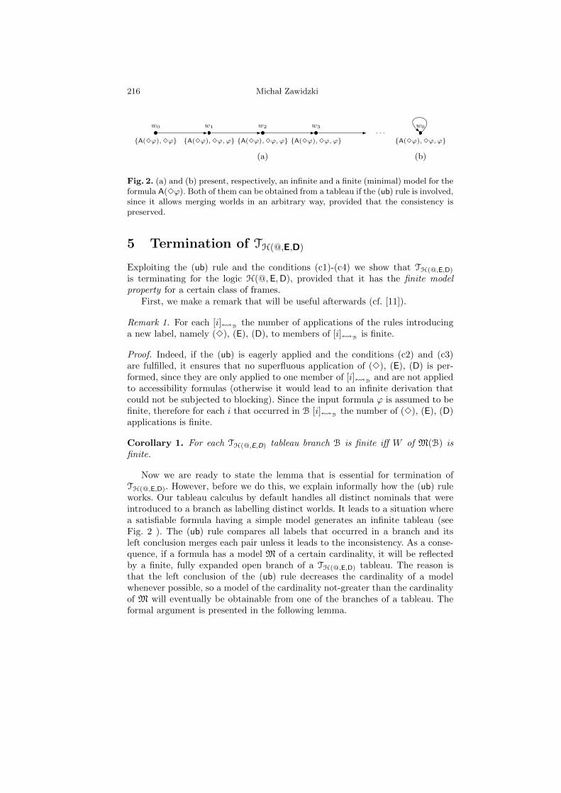
216 Micha l Zawidzki

w0

{A(3ϕ),3ϕ}

w1

{A(3ϕ),3ϕ, ϕ}

w2

{A(3ϕ),3ϕ, ϕ}

w3

{A(3ϕ),3ϕ, ϕ}. . .

(a)

w0

{A(3ϕ),3ϕ, ϕ}

(b)

Fig. 2. (a) and (b) present, respectively, an infinite and a finite (minimal) model for theformula A(3ϕ). Both of them can be obtained from a tableau if the (ub) rule is involved,since it allows merging worlds in an arbitrary way, provided that the consistency ispreserved.

5 Termination of TH(@,E,D)

Exploiting the (ub) rule and the conditions (c1)-(c4) we show that TH(@,E,D)

is terminating for the logic H(@,E,D), provided that it has the finite modelproperty for a certain class of frames.

First, we make a remark that will be useful afterwards (cf. [11]).

Remark 1. For each [i]!Bthe number of applications of the rules introducing

a new label, namely (3), (E), (D), to members of [i]!Bis finite.

Proof. Indeed, if the (ub) is eagerly applied and the conditions (c2) and (c3)are fulfilled, it ensures that no superfluous application of (3), (E), (D) is per-formed, since they are only applied to one member of [i]!B

and are not appliedto accessibility formulas (otherwise it would lead to an infinite derivation thatcould not be subjected to blocking). Since the input formula ϕ is assumed to befinite, therefore for each i that occurred in B [i]!B

the number of (3), (E), (D)applications is finite.

Corollary 1. For each TH(@,E,D) tableau branch B is finite iff W of M(B) isfinite.

Now we are ready to state the lemma that is essential for termination ofTH(@,E,D). However, before we do this, we explain informally how the (ub) ruleworks. Our tableau calculus by default handles all distinct nominals that wereintroduced to a branch as labelling distinct worlds. It leads to a situation wherea satisfiable formula having a simple model generates an infinite tableau (seeFig. 2 ). The (ub) rule compares all labels that occurred in a branch and itsleft conclusion merges each pair unless it leads to the inconsistency. As a conse-quence, if a formula has a model M of a certain cardinality, it will be reflectedby a finite, fully expanded open branch of a TH(@,E,D) tableau. The reason isthat the left conclusion of the (ub) rule decreases the cardinality of a modelwhenever possible, so a model of the cardinality not-greater than the cardinalityof M will eventually be obtainable from one of the branches of a tableau. Theformal argument is presented in the following lemma.

Tableau-based decision procedure for hybrid logics 217

Lemma 2. Suppose that a finite model N = 〈W ′, R′, V ′〉 satisfies a formula ϕ.Then there exists an open branch B in a TH(@,E,D) tableau and M(B) = 〈W,R, V 〉such that Card(W ) ≤ Card(W ′).

Proof. We proceed by induction on the number of steps in the derivation. Duringthe derivation we construct a branch B in such a way that M(B) is partiallyisomorphic to N (cf. [11]).Basic step: ϕ is satisfiable on N, so there must exist w ∈W ′ such that N, w |=ϕ. If also N, w |= i such that i does not occur in ϕ, we put at the initial nodeof the derivation i : ϕ. If no such nominal holds in w, we conservatively extendN by adding fresh nominal i to w and put at the initial node of the derivationi : ϕ.Inductive step: Application of each tableau rule should be considered as aseparate case. Nevertheless, only four rules seem to be essential for this proof,namely (3), (E), (D) and (ub), i.e. rules that either introduce a new label to abranch or identify labels already present on a branch. We consider each of them.

Case: (3). Suppose that a formula 3ψ occurred at the nth node of the deriva-tion. It means that we associated the label i of this node with a world inW ′ that satisfies 3ψ and i. What follows, there must exist a world v suchthat wRv and N, v |= ψ. If v does not satisfy any nominal l that has notyet occurred on the branch either as a label or as a subformula, we conser-vatively extend N by ascribing l to v. Applying (3) to 3ψ we obtain i : 3jand j : ψ. We put l in place of j.

Case: (E). Suppose that a formula Eψ occurred at the nth node of the derivation.It means that we associated the label i of this node with a world in W ′ thatsatisfies Eψ and i. Therefore, there exists a world v such that N, v |= ψ. If vdoes not satisfy any nominal l that has not yet occurred on a branch eitheras a label or as a subformula, we conservatively extend N by ascribing l tov. Applying (E) to Eψ we obtain j : ψ. We put l in place of j.

Case: (D). Suppose that a formula Dψ occurred at the nth node of the deriva-tion. It means that we affixed the label i of this node to a world in W ′ thatsatisfies Dψ and i. Therefore, there exists a world v such that N, v |= ψ∧¬i.If v does not satisfy any nominal l that has not yet occurred on a brancheither as a label or as a subformula, we conservatively extend N by ascribingl to v. Applying (D). to Dψ we obtain j : ¬i and j : ψ. We put l in place ofj.

Case: (ub). Suppose that during the derivation two labels i and j have beenintroduced to B. By the inductive hypothesis we mapped these labels toworlds w and v of (the conservative extension of) W ′. Either the world wsatisfies i ∧ j (which would mean that w and v are the same world) or itsatisfies i ∧ ¬j (which indicates that w and v are distinct). If the former isthe case, we pick the left conclusion of (ub) and add it to B, if the latter isthe case, we choose the right conclusion of (ub) and add it to B.

Since B is open, we can construct a model M(B) = 〈W,R, V 〉 out of it. Nowwe show that Card(W ) ≤ Card(W ′) (we consider N as already conservatively

218 Micha l Zawidzki

extended in progress of constructing B). We set a function f : W ′ −→ W asfollows

f(w) =

[i]!B, if there is i : i ∈ B such that i was affixed

to w during the derivation

arbitrary element of W, otherwise

f is injective and if we cut it to these elements of W ′ to which we assigned anominal during the derivation, it is also an isomorphism. That concludes theproof.

To conclude our considerations it is sufficient to prove that the logic H(@,E,D)has the finite model property. The following proposition deals with it.

Proposition 2. The logic H(@,E,D) has the effective finite model propertywith the bounding function µ = 2Card(Sub(ϕ))+1, where Sub(ϕ) is a set of allsubformulas of a formula φ.

Proof. We use the standard, filtration-based argument. Suppose that a formulaϕ is satisfied on a (possibly infinite) model M = 〈W,R, V 〉. It means that thereexists w ∈ W such that M, w |= ϕ.We show that there exists a finite model M′

that satisfies ϕ and whose cardinality does not exceed 2Card(Sub(ϕ))+1.

First, we set the relation !ϕ on W in the following way:

w!ϕ v iff for all ψ ∈ Sub(ϕ) M, w |= ψ iff M, v |= ψ.

It is straightforward that !ϕ is the equivalence relation

Now we are ready to construct our finite model that will satisfy φ. Let M′ =〈W ′, R′, V ′〉 such that:

W ′ = W/!ϕ]W/!ϕ

;

R′ = {(|v|!ϕ, |u|!ϕ

) : R(v, u)};V ′(p) = {|v|!ϕ : v ∈ V (p)} for all proposition letters in ϕ;

V ′(i) = {|v|!ϕ : v ∈ V (i)} for all nominals in ϕ.

We prove that M′ satisfies ϕ by induction on the complexity of subformulas ofϕ. Since the proof for the modal part of H(@,E,D) is well known (cf. [4]) and thecase of ψ = i follows immediately from the definition of V ′, we confine ourselvesto proving the cases of @iχ, Eχ and Dχ.

Case: ψ = @iχ. Suppose that M, v |= @iχ. It means that χ holds at a world uat which also i holds. This world is transformed to a singleton equivalenceclass {u} in W ′. By the inductive hypothesis it follows that M′, {u} |= i andM′, {u} |= χ. Hence M′, |v| |= @iχ.

Case: ψ = Eχ. Suppose that M, v |= Eχ. It means that there exists a world u atwhich χ holds. By the inductive hypothesis M′, |u| |= χ. Hence M′, |v| |= Eχ.

Tableau-based decision procedure for hybrid logics 219

Case: ψ = Dχ. Suppose that M, v |= Dχ. It means that there exists a world udifferent than v, at which χ holds. By the inductive hypothesis M′, |u| |= χ.Two complementary cases might occur. If |v| 6= |u|, then we obtain M′, |v| |=χ. If, however, |v| = |u|, it means that χ is also satisfied by a copy of |v|that we pasted to W ′ at the stage of the construction of M′. Since |v| andits copy are distinct, we obtain M′, |v| |= χ.

Observe that pasting a distinct copy of W/!ϕto W ′ is only necessary if D is

involved. Therefore, in other cases the bounding function µ = 2Card(Sub(ϕ)).

Consequently, we obtain the following result:

Theorem 4. TH(@,E,D) is terminating.

Proof. Follows from Corollary 1, Lemma 2 and Proposition 2.

Obviously, the bounding function µ from Proposition 2 can be reduced (cf. [1,9]), however, the main aim of this paper is not optimising the complexity ofTH(@,E,D). Besides, the filtration-based argument can be easily adapted for dif-ferent types of frames. Thus, we formulate the following strategy-condition forperforming the derivation in TH(@,E,D):

(tm) Expand a branch of TH(@,E,D)-tableau until the number of equivalence classesof individuals in B exceeds the bound given by µ function. Then stop.

It turns our tableau calculus into a deterministic decision procedure.

6 Concluding remarks

In this paper we presented an internalised tableau-based decision procedure forthe logic H(@,E,D). Tableau calculus TH(@,E,D) was proven to be sound, com-plete and terminating. In the existing literature of the subject several approachesto systematic treatment of decision procedures for hybrid logics can be found.We recall two of them. In [3] and [5] Blackburn, Bolander and Brauner pro-vide a terminating internalised tableau-based decision procedure for the logicH(@,E). However, their main concern is different from ours. Their attempts arefocused on tailoring a suitable tableau calculus for each logic separately. There-fore, they introduce two different blocking mechanisms, namely subset blockingand equality blocking for the logics H(@) and H(@,E) and modify the notionof urfather subject to a particular logic. The resulting calculus is conceptuallycomplex but seems to avoid any superfluous performances of the rules. In [7]Gotzmann, Kaminski and Smolka describe Spartacus, which is a tableau proverfor hybrid logics with @ operators and universal modality. Thanks to the appli-cation of advanced blocking and optimisation techniques, namely pattern-basedblocking and lazy branching the system is very efficient in terms of complexity.

The decision procedure introduced in this paper presents the approach whichis different from the aforementioned. It introduces (ub) as an explicit tableau rule

220 Micha l Zawidzki

which is sound and, together with the conditions (c1)-(c4), ensures terminationof the whole calculus. (ub) allows a direct comparison of every pair of labels thatoccurred on a branch and, therefore, subsumes any other blocking mechanisms.(ub) is a generic rule which means that it generates every possible configurationof labels occurring on a branch. In comparison to [3] and [7] many of theseconfigurations are superfluous. However, the huge advantage of this approach isconceptual simplicity which allows to avoid introducing complicated strategies ofsearching for a pair of labels that are liable to blocking mechanism. Additionally,for each satisfiable formula ϕ (ub) ensures that a minimal model for ϕ (in termsof a domain size) will be generated, which cannot be guaranteed by the systemsof [3] and [7]. Moreover, TH(@,E,D) provides a uniform approach to all hybridlogics mentioned in the paper and covers the case of difference modality which isomitted in [3]. A possible direction of future work may be investigating whetherthe applications of the (ub) rule can be optimised.

Acknowledgements

The research reported in this paper is a part of the project financed fromthe funds supplied by the National Science Centre, Poland (decision no. DEC-2011/01/N/HS1/01979).

References

1. Areces C., Blackburn P., Marx M.: A road-map on complexity for hybrid logics.Proc. of the 8th Annual Conference of the European Association for ComputerScience Logic (CSL 1999), Madrid, Spain, 307–321

2. Blackburn P.: Internalizing labelled deduction. J. Log. Comput. 10(1), 137—168(2000)

3. Blackburn P., Bolander T.: Termination for Hybrid Tableaus. J. Log. Comput.17(3), 517–554 (2007)

4. Blackburn P., Venema Y., de Rijke M.: Modal Logics. Cambridge University Press(2002)

5. Bolander T., Brauner T.: Tableau-based Decision Procedures for Hybrid Logic. J.Log. Comput. 16, 737–763 (2006)

6. Brauner T.: Hybrid Logic and its Proof-Theory Springer (2011)7. Gotzmann D., Kaminski M., Smolka G.: Spartacus: A Tableau Prover for Hybrid

Logic. Electron. Notes Ther. Comput. Sci. 262, 127-139 (2010)8. Kaminski M., Smolka G.: Terminating Tableau Systems for Hybrid Logic with

Difference and Converse. J. Log. Lang. Inf. 18, 437–464 (2009)9. Mundhenk M., Schneider T.: Undecidability of Multi-modal Hybrid Logics. Elec-

tron. Notes Ther. Comput. Sci. 174, 29–43 (2007)10. Schmidt, R. A., Tishkovsky, D.: Automated Synthesis of Tableau Calculi. Log.

Meth. Comput. Sci. 7(2), 1–32 (2011)11. Schmidt R.A., Tishkovsky D.: Using Tableau to Decide Description Logics with Full

Role Negation and Identity. http://www.mettel-prover.org/papers/ALBOid.pdf(2012)

12. Tzakova M.: Tableau Calculi for Hybrid Logics. LNCS 1617, 278–292 (1999)

A Frame-Based Semantics of LocativeAlternation in LTAG

Yulia Zinova

Heinrich Heine University Dusseldorfzinova@phil.uni-duesseldorf.de

Abstract. In this paper I present the analysis of locative alternationphenomena in Russian and English. This analysis follows the approachproposed in [13] and uses LTAG and Frame Semantics. The combinationof a syntactic theory with an extended domain of locality and framesprovides a powerful mechanism for argument linking. Metagrammar fac-torization allows to determine not only lexical, but also constructionalmeaning that is essential for locative alternation analysis.

1 Introduction

There is a number of formalisms that capture the idea that the meaning of averb-based construction depends both on the lexical meaning of the verb andon the construction in which the verb is used ( [8], [19]). The question is howexactly the components of the meaning are distributed and how they combine.In [13] a combination of Lexicalized Tree Adjoining Grammars ( [9]) and FrameSemantics is introduced. It is shown that the resulting framework is very flexiblewith respect to the factorisation and combination of lexical and constructionalunits on the syntax and semantics level and is also suitable for computationalprocessing.Though there already exist a number of different approaches to semantic con-struction using LTAG ( [10], [5], [12]) and approaches that combine other syn-tactic formalisms with Frame Semantics ( [3], [4]), the novel combination of anLTAG and Frame Semantics benefits from both extended domain of locality andunderspecification allowed by frames.In this paper I want to present the analysis of locative alternation that benefitsof flexibility offered by the novel framework.

2 Tree Adjoining Grammar

Tree Adjoining Grammar (TAG, [9]) is a tree-rewriting grammar formalism. Itconsists of a finite set of elementary trees with labelled nodes with two operationson them: substitution and adjunction. All elementary trees are either auxiliarytrees or initial trees. An auxiliary tree is a tree which has exactly one foot node -a leaf that is marked with an asterisk. Leaf nodes can be labelled with terminals

222 Yulia Zinova

and other nodes are labelled only with non-terminals. The derivation processstarts from an initial tree and in the final derived tree all the leaves must belabelled by terminals.Substitution allows to replace a non-terminal leaf with a new tree and adjunctionis used for replacing an internal node with an auxiliary tree. Adjunction to thenode labelled X is allowed if the root and foot nodes of the adjoining auxiliarytree have the same label X. It is also possible to indicate nodes where adjunctionis obligatory or not allowed with OA and NA subscripts respectively.Figure 1 shows an example of a derivation: the initial tree for Mary substitutesinto the subject slot of the elementary tree for laughs, and the sometimes aux-iliary tree for the VP modifier adjoins to the VP node. Feature-structure based

S

NP NP VP VP

Mary V Adv VP*

laughs sometimes

derived tree:

S

NP VP

Mary Adv VP

sometimes V

laughs

Fig. 1. Example of a TAG derivation

TAG, or FTAG, is a variant of TAG in which elementary trees are enriched withfeature structures ( [20]). In an FTAG each node has a top feature structureand all the nodes except substitution nodes have a bottom feature structure.Feature unification happens during the derivation process when adjunction andsubstitution take place. Due to the extended domain of locality, nodes withinone elementary tree can share features, allowing to express constraints amongdependent nodes easily.For natural languages a specific version of TAG called lexicalized TAG, or LTAGis used. In an LTAG, each elementary tree must have at least one non-emptylexical item, called lexical anchor. The second important principle for a natu-ral language TAG is that every elementary tree where the lexical anchor is apredicate must contain slots (leaves with non-terminal labels) for all argumentsof this predicate, including the subject, and for nothing else (theta-criterion forTAG, [6]).The facts that LTAGs have extended domains of locality and that elementarytrees are lexicalized and contain slots for all the predicate’s arguments, makethem good candidates for combination with frame-based compositional seman-tics ( [13]). In the approach proposed in [13], a single semantic representation(a semantic frame in this case) is linked to the entire elementary tree. Whencoupling an elementary tree with a semantic frame, syntactic arguments can

A Frame-Based Semantics of Locative Alternation in LTAG 223

be directly linked to their counterpart in the semantics. Described approach issimilar to ones in [7] and [14], but uses different kind of semantic representa-tion. Semantic composition is then modeled by unification which is a result ofperforming adjunction and substitution. Figure 2 provides a simple illustrationof syntactic and semantic composition. In this example, substitutions triggerunifications between 1 and 3 and 2 and 4 which leads to correct insertion ofargument frames into the frame of loves.Linguistic generalizations in TAGs are captured by a metagrammar. There are

S

NP NP[I=1 ] VP NP

John V NP[I=2 ] Mary

3

[person

NAME John

] loves love

EXPERIENCER 1

THEME 2

4

[person

NAME Mary

]

Fig. 2. Syntactic and semantic composition for John loves Mary

two steps of factorization, which are important for this paper:

• unanchored elementary trees are specified separately from lexical anchors;• trees are organized into tree families which represent different realizations of

one subcategorization frame.

This allows to define a meaning for sets of unanchored elementary trees, i.e., ameaning of constructions.

3 The Data

3.1 Previous approaches

(1) and (2) show basic examples of locative alternation in English and Russian.Despite the fact that in English both constructions have a PP and it can beomitted without losing the specific construction meaning, let us call the firstvariant ((1a), (2a)) prepositional phrase construction, or PPC and the secondvariant ((1b), (2b)) - instrumental case construction, or ICC for convenience ofreferring to them.

(1) a. John 1 loaded the hay 2 into the truck 3 . (PPC)b. John 1 loaded the truck 3 with hay 2 . (ICC)

(2) a. Ivan 1

Ivan

zagruzilloaded

seno 2

hayacc,def

vin

vagon 3 .

wagongen,indef/def .Ivan loaded the hay into a/the wagon.

224 Yulia Zinova

b. Ivan 1

Ivan

zagruzilloaded

vagon 3

wagonacc,def

senom 2 .

hayinstr,indef .Ivan loaded the wagon with hay.

PPCs are traditionally analyzed as having a change of location meaning andICCs - as having a change of state meaning ( [11], [16], [8]). An analysis for (1)following [11] is provided in (3). It demonstrates that there is a difference betweenthe two constructions, but only the difference in the perspective is shown.

(3) a. X CAUSE [BECOME [hay BE ON truck]]b. X CAUSE [BECOME [truck z BE [WITH [hay BE ON z]]]]

The analysis proposed in [16], which can be found under (4), provides moredetailed information about the difference between PPCs and ICCs. (4a) tells usthat the hay changes its location as a result of the loading event, while (4b)describes that the result is a change in the state of the wagon. One can noticethat in (3) there is no explicit reference to the verb itself and the only componentthat is taken from the verb meaning is that the result of the loading is that theTHEME is on the LOCATION in the end.

(4) a. [[x ACT] CAUSE [y BECOME Ploc z] [LOAD]MANNER]b. [[x ACT] CAUSE [z BECOME []STATE WITH-RESPECT-TO y]

[LOAD]MANNER]

Using frame semantics, one can assign two frames in 3 to the two differentconstructions. For the PPC, one has to remove the concrete verb load and replaceit with change of location effect. So the first frame tells us that the activity ofthe Actor (X) causes the Theme (Y) to change its location to the Goal (Z). Forthe ICC’s frame in order to introduce the Manner one can simply embed thecaused change of location frame under the manner atribute. The second framein this case would mean that the activity of the Actor (X) causes the Theme (Z)to change its state by means of changing the location of the third argument (Y)to Z.

3.2 Detailed Russian and English Data

The question that arises if one looks carefully at what the sentences in (1) and(2) mean is whether it is really the case that there is no change of state in PPCexamples? In fact, any loading activity leads to both a change of location of thecontent and some change of state of the container (if it is specified), and thedifference between two constructions is that

• different components of the effect become more salient;• in the case of ICC initial and result states of the container are specified.

In order to understand how the meaning of verbs and constructions should berepresented let us look at the whole range of the verbs allowing locative alter-nation that one can find in English and Russian. [18] provides the following

A Frame-Based Semantics of Locative Alternation in LTAG 225

0

causation

cause 4

[activity

actor 1

]

effect 5

change-of-loc

theme 2

goal 3

1

0

causation

cause 4

[activity

actor 1

]

effect 5

change of state

theme 3

manner 6

causation

cause 7

[activity

actor 1

]

effect 8

change of loc

theme 2

goal 3

1

Fig. 3. Frame semantics for PPC and ICC

classification for English:

Content-oriented classes:

(a) simultaneous forceful contact and motion of a mass against a surface (brush,drape, spread, etc.);

(b) vertical arrangement on a horizontal surface (heap, pile, stack);(c) force is imparted to a mass, causing ballistic motion in a specified spatial

distribution along a trajectory (inject, splash, spray, etc.);(d) mass is caused to move in a widespread or non directed distribution (scatter,

seed, sow, etc.).

Container-oriented classes:

(e) a mass is forced into a container against the limit of its capacity (crowd,jam, stuff, etc.);

(f) a mass of size, shape, or type defined by the intended use of a contained isput into the container, enabling it to accomplish its function (load, pack,stock).

From the description of verb classes that allow locative alternation in Englishone can see that the result state of the container in case of ICC is such that theaction cannot be performed any longer. There is no result state common for allthe cases, so it depends on the verb, i.e. on how the change of location happens.The easiest way to solve this would be to assume different construction meaningsfor different verb classes (e.g. one with the Effect of the Theme being full andthe other one with the Effect of the Theme being covered), but let us first lookat some Russian data.In Russian a lot of verbs allow only one of the constructions, i.e. a changeof construction requires a change of verb prefix (a list can be found in [1]).However, some of the verbs from the list remain the same in both prepositional

226 Yulia Zinova

and instrumental constructions. Such verbs can be organised in three groups:the first one is similar to the (f) group in English (see example (2)), the secondone is similar to group (a) in English, like in (5), and the third class is like acombination of the first and the second: a mass is put into a container, enablingit to accomplish its function, or on a container, covering its surface (6).With the vebs from the third group an interesting effect can be observed: whilein the case of PPC example (6a) there is a preposition which tells us that thecontent goes in the container, in the case of ICC example (6b) two differentreadings are possible: the content can be put in the container or the content cancover the container. In both cases there is a clear result state: either the containeris full or the container’s surface is fully covered with content. This means thatthe verb zasypat’ (’to fill/to cover’) does not provide information about howthe theme is positioned at the goal. In case of PPC this information comesfrom the preposition used (both v (’in’) and na (’on’) are possible) and in ICCthe ambiguity can be resolved only using world knowledge. So (6) demonstratesconclusively that there should be one construction accounting for different resultstates of the theme and allowing to get different interpretations of one verb dueto underspecification of how the change of location process goes.

(5) a. OnHe

namazaldistributed

maslobutteracc,def

naon

hleb.breadacc,indef

He distributed butter over a piece of bread.b. On

Henamazalcovered

hlebbreadacc,def

maslom.butterinstr,indef

He covered a piece of bread with butter.

(6) a. OnHe

zasypalput

saharsuggaracc,def

vin

banku.canacc,indef/def

He put sugar in a/the tin.b. On

Hezasypalcovered/filled

bankutinacc,def

saharom.sugarinstr,indef

He covered/filled the tin with sugar.

4 Locative Alternation: The Analysis

4.1 Syntactic representation

In the previous section we were looking only at ”full” examples, where bothcontainer and content are present. However, the constructions that are beingdiscussed can be used when only the direct object of the verb is present; inthis case, they will have the same difference in semantics. Using LTAG andmetagrammar decomposition one can obtain the tree family in 4 for the PPCand tree family in 5 for the ICC (the second NPINSTR stands for both NP ininstrumental case in Russian and PP with preposition ”with” in English).

A Frame-Based Semantics of Locative Alternation in LTAG 227

S

NP[I=1 ] VP

V⋄[S=0 ] NP[I=2 ] PP[I=3 ]

S

NP[I=1 ] VP

V⋄[S=0 ] NP[I=2 ]

Fig. 4. Unanchored trees for the PPC

S

NP[I=1 ] VP

V⋄[S=0 ] NP[I=3 ] NPINSTR[I=2 ]

S

NP[I=1 ] VP

V⋄[S=0 ] NP[I=3 ]

Fig. 5. Unanchored trees for the ICC

4.2 Scales and Proposed Frame Semantics

In the case of the PPC, the semantics of the whole phrase can be compositionalyderived from the semantics of the verb and its arguments, while in the case of theICC there is a part of the meaning, that comes from the construction itself. Thegoal now is to provide such semantics for the ICC and verbs allowing locativealternation such that in combination they form the desired frame representationof the semantics of a sentence.Following ideas in [17] where one can find a discussion of the representation ofattributes, events, and results while implementing Fillmore’s Frame Semantics( [2]) I introduce attributes of initial and result state and a scale which is deter-mined by its type, start and end points. The change of state is either a decreaseor an increase of the value on an ordered scale (discussion of analysis of scalarchange can be found in [15]). The direction is given by the values of atributesENDP and STARTP (end and start points), which replaces the LESSER atributeof ordering proposed in [17]. Some of the verbs specify a concrete initial or resultstate (INIT and RESULT respectively), but load does not have any initial orresult state specified within its semantics, so it just determines the scale andtwo values on it. Summarizing the ideas, one obtains the following scheme:

• in the verb both change of location and change of state effects are specified;• MANNER attribute is not needed because it is already described in the

change of location subframe;• change of state is described by scale, initial state, and result state;• SCALE atribute can have a type such as ”degree of fullness” that is a subtype

of the type ”scale” and thus replaces it during the unification;• initial and result states are values on the scale;• the ICC specifies that initial and result states are equal to the start and end

points of the scale, respectively.

Figure 7 shows a lexical frame for the verb load. As one can see, when all thearguments are filled, the right meaning for the whole PPC follows automatically.

228 Yulia Zinova

0

causation

effect

scalar change of state

theme 3

scale 7

scale

startp 5

endp 6

init

state

entity 3

scale 7

value 5

result

state

entity 3

scale 7

value 6

1

Fig. 6. Frame for the ICC

0

causation

actor 1

theme 2

goal 3

cause

[activity

actor 1

]

effect

change of location

theme 2

goal 3

,

scalar change of state

theme 3

scale 7

degree of fullness

startp empty

endp full

init

state

entity 3

scale 7

value 8

result

state

entity 3

scale 7

value 9

1Fig. 7. Frame representation of the verb load

The semantics of the ICC is a caused change of state meaning that gets furtherconstrained when a specific lexical anchor is inserted. Figure 6 shows how theunanchored tree for the ICC is linked to its semantic frame. The correct argumentlinking happens because I features in the syntactic tree and the thematic roles inthe semantic frame are identical. This is done in a local way (within the domainof an elementary tree) because of LTAG’s extanded domain of locality. The Sfeature of the V node serves for unification of the lexical frame for the verb andthe constructional frame. When a lexical anchor is inserted, this feature unifieswith the S feature of the lexical item. The result of this unification for the ICCwith a lexical anchor load is shown in Fig. 8.

5 Conclusion

This is a case study for combining an LTAG with Frame Semantics, in whichI have described a model for locative alternation in English and Russian. Thisanalysis uses LTAG’s mechanism of separation between unanchored elementarytrees and lexical anchors to separate the contribution of the lexical meaningfrom the contribution of construction and follows the ideas expressed in [13].Another advantage of combination of an LTAG with Frame Semantics is thatLTAG’s extended domain of locality allows direct linking of thematic roles ofthe arguments with corresponding syntatctic slots. As this framework is a newone, there are a lot of open questions and a wider range of semantic phenomenashould be examined.

A Frame-Based Semantics of Locative Alternation in LTAG 229

0

causation

actor 1

theme 2

goal 3

cause

[activity

actor 1

]

effect

change of location

theme 2

goal 3

,

scalar change of state

theme 3

scale 7

degree of fullness

startp empty

endp full

init

state

entity 3

scale 7

value empty

result

state

entity 3

scale 7

value full

1Fig. 8. Resulting frame for the ICC and the verb load

References

1. Dudchuk, P.: Locativnaja alternacija i struktura glagol’noj gruppy [Locative Alter-nation and the structure of VP]. diploma thesis, Moscow State University (2006)

2. Fillmore, C.J.: Frame semantics. In: of Korea, T.L.S. (ed.) Linguistics in the Morn-ing Calm, pp. 111–137. Hanshin Publishing Co., Seoul (1982)

3. Frank, A.: Generalizations over corpus-induced frame assignment rules. In: Pro-ceedings of the LREC 2004 Workshop on (2004)

4. Frank, A.: Question answering from structured knowledge sources. Journal of Ap-plied Logic 5(1), 20 – 48 (2007)

5. Frank, A., van Genabith, J.: GlueTag. Linear logic based semantics for LTAG –and what it teaches us about LFG and LTAG. In: Butt, M., King, T.H. (eds.)Proceedings of the LFG01 Conference. Hong Kong (2001)

6. Frank, R.: Syntactic Locality and Tree Adjoining Grammar: Grammatical, Acqui-sition and Processing Perspectives. Ph.D. thesis, University of Pennsylvania (1992)

7. Gardent, C., Kallmeyer, L.: Semantic Construction in FTAG. In: Proceedings ofEACL 2003. pp. 123–130. Budapest (2003)

8. Goldberg, A.E.: Constructions. A Construction Grammar Approach to ArgumentStructure. Cognitive Theory of Language and Culture, The University of ChicagoPress, Chicago and London (1995)

9. Joshi, A.K., Schabes, Y.: Tree-Adjoning Grammars. In: Rozenberg, G., Salomaa,A. (eds.) Handbook of Formal Languages, pp. 69–123. Springer, Berlin (1997)

10. Joshi, A.K., Vijay-Shanker, K.: Compositional semantics with lexicalized Tree-Adjoining Grammar (LTAG): How much underspecification is necessary? In:

230 Yulia Zinova

Blunt, H.C., Thijsse, E.G.C. (eds.) Proceedings of the Third International Work-shop on Computational Semantics (IWCS-3). pp. 131–145. Tilburg (1999)

11. Kageyama, T.: Denominal verbs and relative salience in lexical conceptual struc-ture. In: Kageyama, T. (ed.) Verb semantics and syntactic structure, pp. 45–96.Kurioso Publishers, Tokyo (1997)

12. Kallmeyer, L., Joshi, A.K.: Factoring Predicate Argument and Scope Semantics:Underspecified Semantics with LTAG. Research on Language and Computation1(1–2), 3–58 (2003)

13. Kallmeyer, L., Osswald, R.: A frame-based semantics of the dative alternationin lexicalized tree adjoining grammars (2012), submitted to Empirical Issues inSyntax and Semantics 9

14. Kallmeyer, L., Romero, M.: Scope and situation binding in LTAG using semanticunification. Research on Language and Computation 6(1), 3–52 (2008)

15. Kennedy, C., Levin, B.: Measure of change: The adjectival core of degree achieve-ments. In: McNally, L., Kennedy, C. (eds.) Adjectives and adverbs. syntax, seman-tics, and discourse. Oxford University Press, Oxford (2008)

16. Levin, B., Rappaport Hovav, M.: Morphology and lexical semantics. In: Spencer,A., Zwicky, A.M. (eds.) Handbook of morphology, pp. 248–271. Blackwell Publish-ers, Oxford (1998)

17. Osswald, R., Van Valin, Jr., R.: Framenet, frame structure, and thesyntax-semantics interface (2012), http://www.phil-fak.uni-duesseldorf.

de/fileadmin/Redaktion/Institute/Allgemeine_Sprachwissenschaft/

Dokumente/Rainer_Osswald/FrameStructure-Osswald-VanValin-2012-02-20.

pdf, manuskript Heinrich-Heine Universitat18. Pinker, S.: Learnability and cognition: The aquisition of argument structure. MIT

Press, Cambridge, MA (1989)19. Van Valin, R.D., LaPolla, R.J.: Syntax. Cambridge University Press, Cambridge

(1997)20. Vijay-Shanker, K., Joshi, A.K.: Feature structures based tree adjoining grammar.

In: Proceedings of COLING. pp. 714–719. Budapest (1988)