TESS Hunt for Young and Maturing Exoplanets(THYME). VI. An 11 Myr Giant Planet Transitinga Very-low-mass Star in Lower Centaurus Crux

The MIT Faculty has made this article openly available. Please share how this access benefits you. Your story matters.

Citation Vanderburg, Andrew and Seager, Sara. 2022. "TESS Hunt for Youngand Maturing Exoplanets (THYME). VI. An 11 Myr Giant PlanetTransiting a Very-low-mass Star in Lower Centaurus Crux." TheAstronomical Journal, 163 (4).

As Published 10.3847/1538-3881/ac511d

Publisher American Astronomical Society

Version Final published version

Citable link https://hdl.handle.net/1721.1/142261

Terms of Use Creative Commons Attribution 4.0 International License

Detailed Terms https://creativecommons.org/licenses/by/4.0

TESS Hunt for Young and Maturing Exoplanets (THYME). VI. An 11Myr Giant PlanetTransiting a Very-low-mass Star in Lower Centaurus Crux

Andrew W. Mann1 , Mackenna L. Wood1 , Stephen P. Schmidt1, Madyson G. Barber1,30, James E. Owen2 ,Benjamin M. Tofflemire3,31 , Elisabeth R. Newton4 , Eric E. Mamajek5,6 , Jonathan L. Bush1, Gregory N. Mace3 ,

Adam L. Kraus3 , Pa Chia Thao1,32 , Andrew Vanderburg7 , Joe Llama8 , Christopher M. Johns-Krull9 , L. Prato8 ,Asa G. Stahl9 , Shih-Yun Tang8,10 , Matthew J. Fields1, Karen A. Collins11 , Kevin I. Collins12 , Tianjun Gan13 ,

Eric L. N. Jensen14 , Jacob Kamler15, Richard P. Schwarz16 , Elise Furlan17 , Crystal L. Gnilka18, Steve B. Howell18 ,Kathryn V. Lester18 , Dylan A. Owens1, Olga Suarez19 , Djamel Mekarnia19 , Tristan Guillot19 , Lyu Abe19,

Amaury H. M. J. Triaud20 , Marshall C. Johnson21 , Reilly P. Milburn1, Aaron C. Rizzuto3 , Samuel N. Quinn11 ,Ronan Kerr3 , George R. Ricker7 , Roland Vanderspek7 , David W. Latham11 , Sara Seager7,22,23, Joshua N. Winn24 ,

Jon M. Jenkins25 , Natalia M. Guerrero26 , Avi Shporer7 , Joshua E. Schlieder27 , Brian McLean28 , and Bill Wohler18,291 Department of Physics and Astronomy, The University of North Carolina at Chapel Hill, Chapel Hill, NC 27599, USA; awmann@unc.edu

2 Astrophysics Group, Imperial College London, Blackett Laboratory, Prince Consort Road, London SW7 2AZ, UK3 Department of Astronomy, The University of Texas at Austin, Austin, TX 78712, USA4 Department of Physics and Astronomy, Dartmouth College, Hanover, NH 03755, USA

5 Jet Propulsion Laboratory, California Institute of Technology, 4800 Oak Grove Drive, Pasadena, CA 91109, USA6 Department of Physics & Astronomy, University of Rochester, 500 Wilson Boulevard, Rochester, NY 14627, USA

7 Department of Physics and Kavli Institute for Astrophysics and Space Research, Massachusetts Institute of Technology, Cambridge, MA 02139, USA8 Lowell Observatory, 1400 West Mars Hill Road, Flagstaff, AZ 86001, USA

9 Department of Physics and Astronomy, Rice University, 6100 Main Street, Houston, TX 77005, USA10 Department of Astronomy and Planetary Sciences, Northern Arizona University, Flagstaff, AZ 86011, USA

11 Center for Astrophysics | Harvard & Smithsonian, 60 Garden Street, Cambridge, MA 02138, USA12 George Mason University, 4400 University Drive, Fairfax, VA 22030 USA

13 Department of Astronomy and Tsinghua Centre for Astrophysics, Tsinghua University, Beijing 100084, Peopleʼs Republic of China14 Department of Physics & Astronomy, Swarthmore College, Swarthmore, PA 19081, USA

15 John F. Kennedy High School, 3000 Bellmore Avenue, Bellmore, NY 11710, USA16 Patashnick Voorheesville Observatory, Voorheesville, NY 12186, USA

17 NASA Exoplanet Science Institute, Caltech/IPAC, Mail Code 100-22, 1200 E. California Boulevard, Pasadena, CA 91125, USA18 NASA Ames Research Center, Moffett Field, CA 94035, USA

19 Université Côte d’Azur, Observatoire de la Côte d’Azur, CNRS, Laboratoire Lagrange, Bd de l’Observatoire, CS 34229, F-06304 Nice cedex 4, France20 School of Physics & Astronomy, University of Birmingham, Edgbaston, Birmingham, B15 2TT, UK

21 Las Cumbres Observatory, 6740 Cortona Drive, Ste. 102, Goleta, CA 93117, USA22 Department of Earth, Atmospheric and Planetary Sciences, Massachusetts Institute of Technology, Cambridge, MA 02139, USA

23 Department of Aeronautics and Astronautics, MIT, 77 Massachusetts Avenue, Cambridge, MA 02139, USA24 Department of Astrophysical Sciences, Princeton University, 4 Ivy Lane, Princeton, NJ 08544, USA

25 NASA Ames Research Center, Moffett Field, CA 94035, USA26 Department of Astronomy, University of Florida, Gainesville, FL 32811, USA

27 NASA Goddard Space Flight Center, 8800 Greenbelt Road, Greenbelt, MD 20771, US28 Space Telescope Science Institute, 3700 San Martin Drive, Baltimore, MD, 21218, USA

29 SETI Institute, Mountain View, CA 94043, USAReceived 2021 October 18; revised 2021 December 28; accepted 2022 January 20; published 2022 March 9

Abstract

Mature super-Earths and sub-Neptunes are predicted to be; Jovian radius when younger than 10Myr. Thus, weexpect to find 5–15 R⊕ planets around young stars even if their older counterparts harbor none. We report thediscovery and validation of TOI 1227b, a 0.85± 0.05 RJ (9.5 R⊕) planet transiting a very-low-mass star(0.170± 0.015Me) every 27.4 days. TOI 1227ʼs kinematics and strong lithium absorption confirm that it is amember of a previously discovered subgroup in the Lower Centaurus Crux OB association, which we designate theMusca group. We derive an age of 11± 2Myr for Musca, based on lithium, rotation, and the color–magnitudediagram of Musca members. The TESS data and ground-based follow-up show a deep (2.5%) transit. We usemultiwavelength transit observations and radial velocities from the IGRINS spectrograph to validate the signal asplanetary in nature, and we obtain an upper limit on the planet mass of ;0.5MJ. Because such large planets areexceptionally rare around mature low-mass stars, we suggest that TOI 1227b is still contracting and will eventuallyturn into one of the more common <5 R⊕ planets.

The Astronomical Journal, 163:156 (26pp), 2022 April https://doi.org/10.3847/1538-3881/ac511d© 2022. The American Astronomical Society. All rights reserved.

30 UNC Chancellor’s Science Scholar.31 51 Pegasi b Fellow.32 NSF GRFP Fellow.

Original content from this work may be used under the termsof the Creative Commons Attribution 4.0 licence. Any further

distribution of this work must maintain attribution to the author(s) and the titleof the work, journal citation and DOI.

1

Unified Astronomy Thesaurus concepts: Pre-main sequence stars (1290); Transits (1711); Exoplanet evolution(491); Exoplanet formation (492); Stellar associations (1582); Stellar ages (1581); OB associations (1140); Timedomain astronomy (2109); Time series analysis (1916); Late-type stars (909); Low mass stars (2050)

Supporting material: machine-readable tables

1. Introduction

Young planets offer a window into the early stages of planetformation and evolution. Planets younger than 100Myr areparticularly useful for this work, as planetary systems likelyevolve most rapidly in the first few hundred million years afterformation (Owen & Wu 2013; Lopez & Fortney 2013).Populations of such planets are critical to understandingplanetary migration (Nelson et al. 2017), photoevaporation(Raymond et al. 2008; Owen & Lai 2018), and atmosphericchemistry (e.g., Segura et al. 2005; Gao & Zhang 2020). Giventhe timescale for planet formation (1–10Myr; Yin et al. 2002;Alibert et al. 2005), planets aged 30Myr can even tell usabout the conditions of planets right after their formation.

The number of known young transiting planets has grownsignificantly in recent years (e.g., Obermeier et al. 2016; Davidet al. 2018; Benatti et al. 2019; Newton et al. 2021). Thisgrowth was primarily driven by a combination of the K2 andTESS missions surveying nearby young clusters and star-forming regions (Ricker et al. 2014; Van Cleve et al. 2016),improvements in filtering variability in young stars (e.g.,Aigrain et al. 2016; Rizzuto et al. 2017), and more completeidentification of young stellar associations from Gaia kine-matics (e.g., Cantat-Gaudin et al. 2018; Kerr et al. 2021).Despite this progress, there are still only a handful of transitingplanets at the youngest ages of 30Myr (Plavchan et al. 1919;Rizzuto et al. 2020; Mann et al. 2016b; David et al.2016, 2019a) and a few candidate nontransiting planets fromradial velocity (RV) surveys (e.g., Johns-Krull et al. 2016;Donati et al. 2017).

Models predict that gas giant planets younger than <50Myrwill be larger and brighter than their older counterparts (Linderet al. 2019). At 10–20Myr, progenitors of mature Jovian-massplanets are expected to be 1.2–1.6 RJ and sub-Neptunes∼ 1 RJ

(Linder et al. 2019; Owen 2020). Completeness curves fromthe best search pipelines (Rizzuto et al. 2017) and the discoveryof much smaller planets (e.g., Mann et al. 2018; Zhou et al.2020) demonstrate that giant planets are readily detectable evenin the presence of complex stellar variability common to youngstars. Thus far, transit surveys of young stars identified only afew Jovian-radius planets in the youngest associations (Rizzutoet al. 2020; David et al. 2019b; Bouma et al. 2020).

As part of the TESS Hunt for Young and MaturingExoplanets survey (THYME; Newton et al. 2019), our teamsearches TESS data using a specialized pipeline to identifyyoung planets missed by standard searches (e.g., Rizzuto et al.2020) and checks previously identified planet candidates forsigns of membership in a young association (e.g., Mann et al.2020; Newton et al. 2021). We identified TOI 1227 (2MASSJ12270432–7227064, TIC 360156606) as a member of a youngassociation, with a planet candidate (TOI 1227.01) identified bythe TESS mission, and astrometry consistent with membershipin the Lower Centaurus Crux (LCC) region of the Scorpius-Centaurus (Sco-Cen) OB association (Goldman et al. 2018;Damiani et al. 2019). The TESS-identified transit signal is;2% deep, suggesting a Jovian-sized planet orbiting a pre-main-sequence low-mass star. As giant planets with periods

<100 days are rare around older stars of similar mass (<1%Bonfils et al. 2013), validation of this planet would providestrong evidence of radius evolution.In this work, we present validation, characterization, and age

estimates for TOI 1227b, a 0.85 RJ planet orbiting a ;11Myrpre-main-sequence M5V star (0.17 Me) every 27.26 days. InSection 2, we detail the photometric and spectroscopic follow-up of the planet and host star. We demonstrate that the star is amember of a recently identified substructure of LCC and derivean updated age of 11± 2Myr for the parent population inSection 3. We estimate parameters for the host star in Section 4,estimate parameters of the planet in Section 5, and combinethese with our ground-based follow-up to statistically validatethe planet in Section 6. We place the large size of TOI 1227b incontext with its age and host star mass and explore its likelyevolution in Section 7. We conclude in Section 8 with asummary and discussion of follow-up and implications forfuture searches for young exoplanets.

2. Observations

2.1. TESS Photometry

TOI 1227 was observed by the TESS mission (Ricker et al.2014) from UT 2019 April 22 through 2019 June 19 (Sectors11 and 12) and then again from 2021 April 28 through 2021May 26 (Sector 38). In all three sectors, the target fell onCamera 3. The first two sectors had 2-minute cadence data aspart of a search for planets around M dwarfs (G011180; PIDressing). Sector 38 had 20 s cadence data, as it was known tobe a young TESS object of interest (TOI) at that phase(G03141; PI Newton). We initially used the 2-minute cadencefor all analysis for computational efficiency and TESS cosmic-ray mitigation33 (not included in 20 s data), but we also ran aseparate analysis using the Sector 38 20 s data (see Section 5).In both cases, we used the Pre-Search Data ConditioningSimple Aperture Photometry (PDCSAP; Smith et al. 2012;Stumpe et al. 2012, 2014) TESS light curve produced by theScience Process Operations Center (SPOC; Jenkins et al. 2016)and available through the Mikulski Archive for SpaceTelescopes (MAST).34

2.2. Identification of the Transit Signal

The planet signal, TOI 1227.01, was first detected in a jointtransit search of sectors 11 and 12 (one transit in each) with anadaptive wavelet-based detector (Jenkins 2002; Jenkins et al.2010). The candidate was fitted with a limb-darkened lightcurve (Li et al. 2019) and passed all performed diagnostic tests(Twicken et al. 2018). Although the difference imagecentroiding failed to converge, the difference images indicatethat the transit source location was consistent with the locationof the host star, TOI 1227. A search of the residual light curve

33 https://archive.stsci.edu/files/live/sites/mast/files/home/missions-and-data/active-missions/tess/_documents/TESS_Instrument_Handbook_v0.1.pdf34 https://mast.stsci.edu/portal/Mashup/Clients/Mast/Portal.html

2

The Astronomical Journal, 163:156 (26pp), 2022 April Mann et al.

failed to identify additional transiting planet signatures. TheTESS Science Office reviewed the diagnostic test results andissued an alert for this planet candidate as a TESS object ofinterest (TOI) on 2019 August 26 (Guerrero et al. 2021). Athird transit was detected in the Sector 38 TESS data, consistentwith the expected period and depth.

We searched for additional planets using the Notch andLoCoR pipelines, as described in Rizzuto et al. (2017).35 Thisincluded using the significance of adding a trapezoidal Notch tothe light-curve detrending, as characterized by the Bayesianinformation criterion (BIC). The method was more effectivethan periodic methods for finding planets with 3 transits, aswas the case for HIP 67522b (Rizzuto et al. 2020). The transitswere quite clear from the BIC test. However, no additionalsignificant signals were detected.

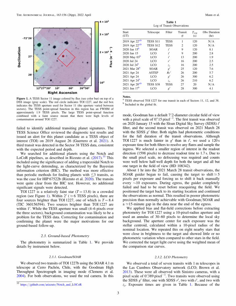
TOI 1227 is a relatively faint star (T= 13.8) in a crowdedregion (see Figure 1). Within 2′ (; 6 TESS pixels), there arefour sources brighter than TOI 1227, one of which is T= 8.4(TIC 360156594). Two sources brighter than TOI 1227 arewithin 1′. While the TESS aperture was small (4–6 pixels overthe three sectors), background contamination was likely to be aproblem for the TESS data. Correcting for contamination andconfirming the planet were the major motivations for ourground-based follow-up.

2.3. Ground-based Photometry

The photometry is summarized in Table 1. We providedetails by instrument below.

2.3.1. Goodman/SOAR

We observed two transits of TOI 1227b using the SOAR 4.1mtelescope at Cerro Pachón, Chile, with the Goodman HighThroughput Spectrograph in imaging mode (Clemens et al.2004). For both observations, we used the red camera. In this

mode, Goodman has a default 7 2-diameter circular field of viewwith a pixel scale of 0 15 pixel−1. The first transit was observedon 2020 January 15 with the Sloan Digital Sky Survey (SDSS) i′filter, and the second transit was observed on 2021 March 28with the SDSS g′ filter. Both nights had photometric conditionsfor the full duration of the transit observations. AlthoughTOI 1227 is much fainter in g′ than in i′, we used a 120 sexposure time for both filters to resolve any flares and sample theingress. We selected a smaller region of interest in the readoutdirection (1598 pixels) to decrease readout time to 1.7 s. Due tothe small pixel scale, no defocusing was required and countswere well below half-well depth for both the target and all butone target in the field of view (HD 108342).About 1 hr into the 2021 March 28 transit observations, the

SOAR guider began to fail, causing the target to shift; 5pixels per exposure and forcing us to shift it back manuallyevery ∼10 exposures. During egress, the guider completelyfailed and had to be reset before reacquiring the field. Wepositioned the target back to its starting location and continuedthe observations as normal. This resulted in poorer photometricprecision than normally achievable with Goodman/SOAR anda ;15-minute gap in the data near the end of the egress.We applied bias and flat-field corrections before extracting

photometry for TOI 1227 using a 10-pixel-radius aperture andused an annulus of 30–60 pixels to determine the local skybackground. The aperture center for each exposure was thestellar centroid, calculated within a 10-pixel radius of thenominal location. We repeated this on eight nearby stars thatwere close in brightness to the target and showed little or nophotometric variation when compared to other stars in the field.We corrected the target light curve using the weighted mean ofthe comparison star curves.

2.3.2. LCO Photometry

We observed a total of seven transits with 1 m telescopes inthe Las Cumbres Observatory network (LCO; Brown et al.2013). These were all observed with Sinistro cameras, with apixel scale of 0 389 pixel−1. Two transits were observed usingthe SDSS g′ filter, one with SDSS r′, two with ¢i , and two withzs. Exposure times are given in Table 1. Because of the

Figure 1. A TESS Sector 11 image colored by flux (see color bar) on top of aDSS image (gray scale). The red circle indicates TOI 1227, and the red boxindicates the TESS aperture used for Sector 11 (the aperture varied betweensectors). The TESS point-spread function in this region has an FWHM ofapproximately 1.9 TESS pixels. The large TESS point-spread functioncombined with a faint source meant that there were high levels ofcontamination around TOI 1227.

Table 1Log of Transit Observations

Start Telescope Filter Transit Texp Obs Duration(UT) # (s) (hr)

2019 Apr 22a,b TESS S11 TESS 1 120 N/A2019 Apr 22a,b TESS S12 TESS 2 120 N/A2020 Jan 15b SOAR i’ 9 120 8.12020 Jan 15 LCO i’ 9 200 2.82020 May 03b LCO i’ 13 200 1.92020 Jul 24 LCO r’ 16 200 2.52020 Jul 24b LCO zs 16 200 2.52021 Mar 28b SOAR g′ 25 120 7.62021 Apr 24 ASTEP Rc’ 26 200 5.72021 Apr 24 LCO g′ 26 300 6.22021 Apr 24b LCO zs 26 210 6.22021 Apr 28a,b TESS S38 TESS 27 20 N/A2021 Jun 17b LCO g′ 28 300 4.1

Notes.a TESS observed TOI 1227 for one transit in each of Sectors 11, 12, and 38.b Included in the global fit.

35 https://github.com/arizzuto/Notch_and_LOCoR

3

The Astronomical Journal, 163:156 (26pp), 2022 April Mann et al.

difficulty of scheduling observations of a long-period planet(∼27 days) and weather interruptions, all LCO observationscovered only part of the transit.

The images were initially calibrated by the standard LCOGTBANZAI pipeline (McCully et al. 2018). We then performedaperture photometry on all data sets using the AstroImageJpackage (AIJ; Collins et al. 2017). The aperture varied based onthe seeing conditions at the observatory, but we generally used acircular aperture with a radius of 6–10 pixels for the source and anannulus with an inner radius of 15–20 pixels and an outer radiusof 25–30 pixels for the sky background. For all observations, wecentered the apertures on the source and weighted pixels withinthe aperture equally. Because the event was detected on thesource, the usual check of nearby sources for evidence of aneclipsing binary was not necessary. Light curves of nearbysources are available with the extracted light curves and furtherdetails on the follow-up at ExoFOP-TESS36 (ExoFOP 2019).

Except for a 2021 April 24 g′ transit, all photometry showedthe expected transit behavior. Two transits had poor coverage(no out-of-transit baseline) but still showed a shape consistentwith ingress. We discuss the 2021 April 24 transit in moredetail in Section 6.4.

2.3.3. ASTEP Photometry

On UTC 2021 April 24, one additional transit was observedwith the Antarctica Search for Transiting ExoPlanets (ASTEP)program on the East Antarctic plateau (Guillot et al. 2015;Mékarnia et al. 2016). The 0.4 m telescope is equipped with anFLI Proline science camera with a KAF-16801E, 4096× 4096front-illuminated CCD. The camera has an image scale of0 93 pixel−1, resulting in a 1°× 1° corrected field of view. Thefocal instrument dichroic plate splits the beam into a bluewavelength channel for guiding, and a nonfiltered red sciencechannel roughly matches an Rc transmission curve.

Due to the extremely low data transmission rate at theConcordia Station, the data are processed on-site using anautomated IDL-based pipeline described in Abe et al. (2013).The calibrated light curve is reported via email, and the rawlight curves of about 1000 stars are transferred to Europe on aserver in Rome, Italy, and are then available for deeperanalysis. These data files contain each star’s flux computedthrough 10 fixed circular aperture radii so that optimal lightcurves can be extracted. For TOI 1227, a 9.3-pixel-radiusaperture gave the best result.

TOI 1227 was observed under mixed conditions, with awindy clear sky and air temperatures between −62°C and−66°C. The Moon was ∼90% full and present during theobservation. A strong wind (∼6 m s−1) led to telescope guidingissues at the beginning of the observation and prevented usfrom observing the ingress. The data points corresponding tothese issues were removed from the analysis. However, theresulting light curve showed the expected egress.

2.4. Corrections for Second-order Extinction

Since atmospheric extinction is strongly color dependent,changes in air mass produce color-dependent flux losses thatdepend on the spectral energy distribution (SED) of the target.These color terms are weaker in redder and narrower passbands(Young et al. 1991). The effect is often small, as comparison

stars typically span a range of colors, and observations aretimed for favorable air mass. However, TOI 1227 was unusualbecause of both its long orbital period (27.3 days) and its redcolor; of stars <5′ from the target and differing by <1 mag inG, the reddest has a Gaia color of BP− RP= 2.1, whileTOI 1227 has BP− RP= 3.3.Because we had few options for mitigating second-order

extinction (color terms), we corrected for the effect followingMann et al. (2011). To summarize, we estimated Teff for allcomparison stars based on their Gaia colors and the tables fromPecaut & Mamajek (2013).37 We then combined the relevantBT-SETTL models (assuming solar metallicity) with an air-mass-dependent model of the atmosphere above the observingsite (Rothman et al. 2009) and the appropriate filter profile. Theoutput was a predicted change in flux from second-orderextinction alone. The trend was negligible (<1 mmag) for i′and zs observations, so we did not apply a correction. The effectwas small but nonnegligible for r (>1 mmag) and significantfor g′-band observations (as large as 5 mmag), so we applied itto those data sets.

2.5. Spectroscopy

2.5.1. Goodman/SOAR

We observed TOI 1227 with the Goodmanspectrograph (Clemens et al. 2004) on the Southern Astro-physical Research (SOAR) 4.1 m telescope located at CerroPachón, Chile, on two nights. We used the red camera, the1200 line mm–1 grating in the M5 setup, and the 0 46 slitrotated to the parallactic angle. This setup gave a resolution ofR; 5880 spanning 6150–7500Å.We obtained the first spectrum on 2019 December 12 (UT)

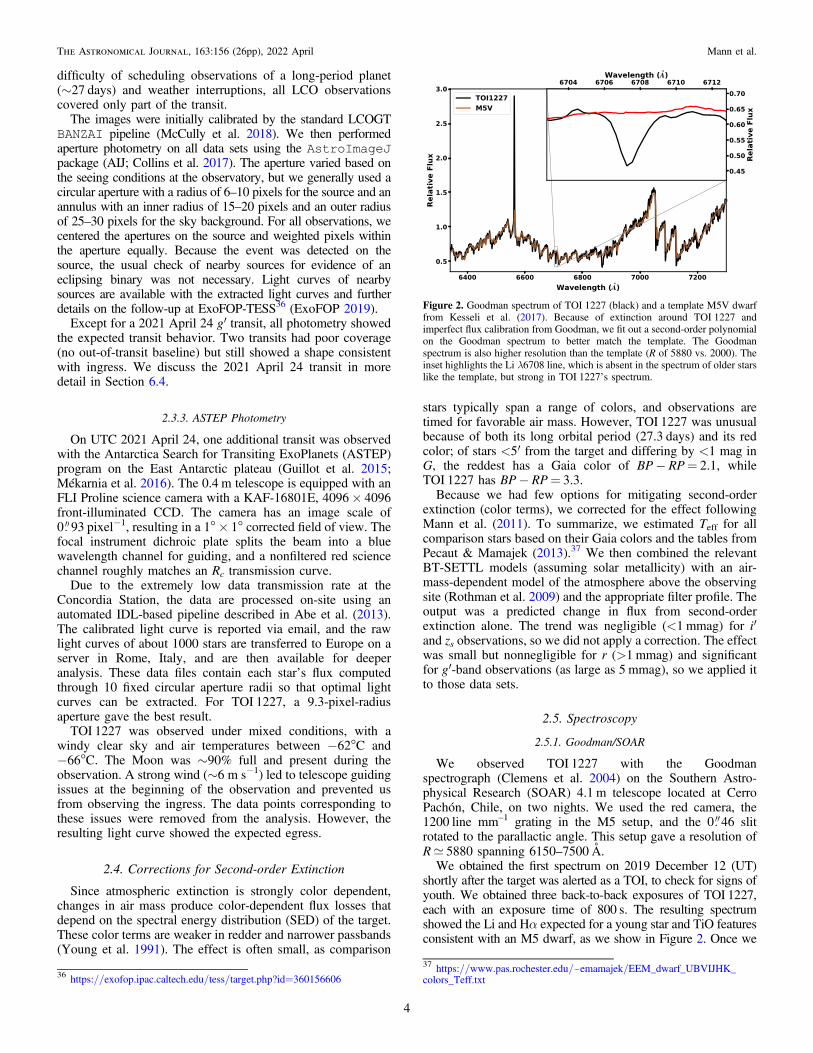
shortly after the target was alerted as a TOI, to check for signs ofyouth. We obtained three back-to-back exposures of TOI 1227,each with an exposure time of 800 s. The resulting spectrumshowed the Li and Hα expected for a young star and TiO featuresconsistent with an M5 dwarf, as we show in Figure 2. Once we

Figure 2. Goodman spectrum of TOI 1227 (black) and a template M5V dwarffrom Kesseli et al. (2017). Because of extinction around TOI 1227 andimperfect flux calibration from Goodman, we fit out a second-order polynomialon the Goodman spectrum to better match the template. The Goodmanspectrum is also higher resolution than the template (R of 5880 vs. 2000). Theinset highlights the Li λ6708 line, which is absent in the spectrum of older starslike the template, but strong in TOI 1227’s spectrum.

36 https://exofop.ipac.caltech.edu/tess/target.php?id=360156606

37 https://www.pas.rochester.edu/~emamajek/EEM_dwarf_UBVIJHK_colors_Teff.txt

4

The Astronomical Journal, 163:156 (26pp), 2022 April Mann et al.

confirmed the planetary signal (based on ground-based transits),we obtained an additional spectrum on 2021 February 23 (UT)under clear conditions. Our goal was a spectrum with a signal-to-noise ratio (S/N)? 100 pixel–1 across the full wavelength range,to use for stellar characterization (Section 4). To this end, weused an exposure time of 1800 s for five back-to-back exposures.

To better determine the age of TOI 1227, we also observed13 nearby stars that are likely part of the same grouping in LCCas TOI 1227 (see Section 3). The 13 targets observed withGoodman were selected from the parent sample to map outlithium levels from M0–M5, which can constrain the age of thepopulation. These targets were observed between 2021February 23 and 24 April 2021 using an identical setup tothe observations for TOI 1227. Exposure times were set toensure an S/N greater than 50 (per pixel) around the Li line andvaried from 90 to 420 s per exposure, with at least fiveexposures per star for outlier (cosmic-ray) removal.

Using custom scripts, we performed bias subtraction, flat-fielding, optimal extraction of the spectra, and mapping pixelsto wavelengths using a fifth-order polynomial derived from theNe lamp spectra obtained right before or after each spectrum.Where possible, we applied a small linear correction to thewavelength solution based on the sky emission or absorptionlines. We stacked the individual extracted spectra using therobust weighted mean. For flux calibration, we used an archivalcorrection based on spectrophotometric standards taken over ayear. Due to variations on nightly or hourly scales, thiscorrection is only good to ;10%.

2.5.2. HRS/SALT

We observed TOI 1227 with the Southern African LargeTelescope (Buckley et al. 2006) High ResolutionSpectrograph (Crause et al. 2014) on six nights (2020 May08–2020 June 17). On each of the six visits, we obtained threeback-to-back exposures. We used the high-resolution modewith an integration time of 800 s per exposure. The resultingspectral resolution was R∼ 46,000. The HRS data werereduced using the MIDAS pipeline (Kniazev et al. 2016),which performs flat-fielding, bias subtraction, extraction ofeach spectrum, and wavelength calibration with arc lampexposures.

We measured RVs from the SALT spectra by computingspectral line broadening functions (BFs; Rucinski 1992) withthe saphires Python package38 (Tofflemire et al. 2019). TheBF results were computed from the linear inversion of anobserved spectrum with a narrow-lined template. We computedthe BF for 16 individual spectral orders in the SALT red armthat range from 6400 to 8900Å; the remaining orders hadstrong telluric contamination. We used a 3100 K, log g= 4.5PHOENIX model as our narrow-lined template (Husser et al.2013). The BFs only contained one profile; we did not detect asecondary star. The BFs from each order were then combined,weighted by the S/N. We fit the combined BF with arotationally broadened profile to determine the stellar RV and

*v isin . RVs from each epoch, corrected for barycentricmotion, are presented in Table 2. The mean and standarddeviation of the *v isin measurements were 17.5± 0.3 km s−1,although this does not include corrections for activity/magneticbroadening or macroturbulence (∼1–3 km s−1; Sokal et al.1919).

2.5.3. IGRINS/Gemini-S

We observed TOI 1227 a total of 11 times from 2020December 31 to 2021 April 24 with the Immersion GratingInfrared Spectrometer (IGRINS; Park et al. 2014; Mace et al.2016b, 2018) while on the Gemini-South observatory (programID GS-2020B-FT-101). IGRINS uses a silicon immersiongrating (Yuk et al. 2010) to achieve high resolving power(R; 45,000) and simultaneous coverage of both H and Kbands (1.48–2.48 μm) on two separate Hawaii-2RG detectors.IGRINS is stable enough to achieve RV precision of40 m s−1 (or better) using telluric lines for wavelengthcalibration (Mace et al. 2016a; Stahl et al. 2021).All observations were done following commonly used

strategies for point-source observations with IGRINS.39 Eachtarget was placed at two positions along the slit (A and B),taking an exposure at each position in an ABBA pattern.Individual exposure times were between 120 and 425 s, and the(total) times per epoch were between 720 and 2280 s to achievepeak S/N 100 per resolution element in the K band. To helpremove telluric lines, we observed A0V standards within 1 hrand 0.1 air masses of the observation of TOI 1227.We reduced IGRINS spectra using version 2.2 of the

publicly available IGRINS pipeline package40 (Lee et al.2017), performing flat-fielding, background removal, orderextraction, distortion correction, wavelength calibration, andtelluric correction using the A0V standards and an A-staratmospheric model. We used the spectrum right before telluriccorrection to improve the wavelength solution and provide azero-point for the RVs.We extracted the RVs of TOI 1227 using the IGRINS RV

code41 (Tang et al. 2021) with a 3000 K PHOENIX model

Table 2Radial Velocity Measurements of TOI 1227

JD −2,450,000 v (km s−1) σv (km s−1)a Instrument

8978.2812 12.33 0.14 HRS8985.3302 11.32 0.32 HRS9000.2566 13.39 0.24 HRS9006.3086 12.07 0.29 HRS9010.3192 11.86 0.37 HRS9018.2586 14.33 0.42 HRS9215.7831 13.221 0.034 IGRINS9217.7999 13.278 0.038 IGRINS9218.7799 13.332 0.044 IGRINS9226.8620 13.252 0.051 IGRINS9227.8498 13.295 0.043 IGRINS9233.8262 13.229 0.037 IGRINS9262.6350 13.411 0.043 IGRINS9267.7740 13.474 0.038 IGRINS9312.5170 13.402 0.060 IGRINS9318.5862 13.592 0.043 IGRINS9329.6748 13.289 0.034 IGRINS

Note.a IGRINS velocity errors are relative; the error on systemic velocity ofTOI 1227 is 13.3 ± 0.3 km s−1 and is dominated by the zero-point calibration.HRS velocities are absolute and include the zero-point calibration.

(This table is available in machine-readable form.)

38 https://github.com/tofflemire/saphires

39 https://sites.google.com/site/igrinsatgemini/proposing-and-observing40 https://github.com/igrins/plp41 https://github.com/shihyuntang/igrins_rv

5

The Astronomical Journal, 163:156 (26pp), 2022 April Mann et al.

(Husser et al. 2013) and the TelFit code to create a synthetictelluric spectrum (Gullikson et al. 2014). Barycentric-correctedRVs from each epoch are listed in Table 2. IGRINS RVprovided an estimate of the rotational broadening ( *v isin= 16.65± 0.24 km s−1) and the star’s systemic velocity(13.3± 0.3 km s−1), the calibration of which is detailed inStahl et al. (2021).

2.6. High-contrast Imaging

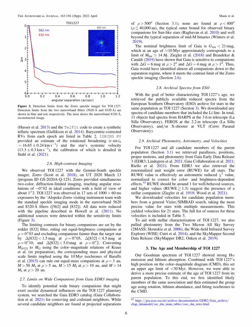
We observed TOI 1227 with the Gemini-South speckleimager, Zorro (Scott et al. 2018), on UT 2020 March 13(program ID GS-2020A-Q-125). Zorro provided simultaneoustwo-color, diffraction-limited imaging, reaching angular reso-lutions of ∼0 02 in ideal conditions with a field of view ofabout 1 2. TOI 1227 was observed in 17 sets of 1000× 60 msexposures by the ‘Alopeke-Zorro visiting instrument team withthe standard speckle imaging mode in the narrowband 5620and 8320Å filters ([562] and [832]). All data were reducedwith the pipeline described in Howell et al. (2011). Noadditional sources were detected within the sensitivity limits(Figure 3).

The limiting contrasts for binary companions are set by theredder [832] filter, ruling out equal-brightness companions atρ= 0 03 and excluding companions fainter than the target starby Δ[832]< 1.5 mag at ρ= 0 05, Δ[832]< 4.5 mag atρ= 0 10, and Δ[832]< 5.0 mag at ρ= 0 2. ConvertingM[832] to MG using the color–magnitude relations of Krauset al. (in preparation), the corresponding mass and physicalscale limits implied using the 10Myr isochrones of Baraffeet al. (2015) can rule out equal-mass companions at ρ= 3 au,M> 50 MJ at ρ> 5 au, M> 15 MJ at ρ> 10 au, and M> 14MJ at ρ> 20 au.

2.7. Limits on Wide Companions from Gaia EDR3 imaging

To identify potential wide binary companions that mightexert secular dynamical influences on the TOI 1227 planetarysystem, we searched the Gaia EDR3 catalog (Gaia Collabora-tion et al. 2021) for comoving and codistant neighbors. Whileseveral candidate neighbors are found at projected separations

of ρ> 500″ (Section 3.1), none are found at ρ< 400″(ρ 40,000 au), the typical outer bound for observed binarycompanions for Sun-like stars (Raghavan et al. 2010) and wellbeyond the typical separation of mid-M binaries (Winters et al.2019).The nominal brightness limit of Gaia is <G 21lim mag,

which at an age of ;10Myr approximately corresponds to alimit of M M14 Jlim . Ziegler et al. (2018) and Brandeker &Cataldi (2019) have shown that Gaia is sensitive to companionswith ΔG= 6 mag at ρ> 2″ and ΔG= 4 mag at ρ> 1″. Thus,Gaia would have identified almost all companions down to theseparation regime, where it meets the contrast limit of the Zorrospeckle imaging (Section 2.6).

2.8. Archival Spectra from ESO

With the goal of better characterizing TOI 1227’s age, weretrieved the publicly available reduced spectra from theEuropean Southern Observatory (ESO) archive for stars in thesame population as TOI 1227 (Section 3). We downloaded anyspectra of candidate members that included the Li line. In total,11 objects had spectra from HARPS at the 3.6 m telescope (LaSilla Observatory), FEROS at the 2.2 m telescope (La SillaObservatory), and/or X-shooter at VLT (Cerro ParanalObservatory).

2.9. Archival Photometry, Astrometry, and Velocities

For TOI 1227 and all candidate members of the parentpopulation (Section 3.1) we retrieved parallaxes, positions,proper motions, and photometry from Gaia Early Data Release3 (EDR3; Lindegren et al. 2021; Gaia Collaboration et al. 2021;Riello et al. 2021). From EDR3 we also retrieved therenormalized unit weight error (RUWE) for all stars. TheRUWE value is effectively an astrometric reduced χ2 value,normalized to correct for color- and brightness-dependenteffects.42 RUWE should be around 1 for well-behaved sources,and higher values (RUWE 1.3) suggest the presence of astellar companion (Ziegler et al. 1919; Wood et al. 2021).We downloaded velocities for candidate population mem-

bers from a general Vizier/SIMBAD search, taking the mostprecise value for stars with multiple measurements. Thisyielded velocities for 21 stars. The full list of sources for thesevelocities is included in Table 5.To aid with stellar characterization of TOI 1227, we also

pulled photometry from the Two Micron All Sky Survey(2MASS; Skrutskie et al. 2006), the Wide-field Infrared SurveyExplorer (WISE; Cutri et al. 2014), and the SkyMapper SecondData Release (SkyMapper DR2; Onken et al. 2019).

3. The Age and Membership of TOI 1227

Our Goodman spectrum of TOI 1227 showed strong Hαemission and lithium absorption. Combined with TOI 1227’shigh position on the color–magnitude diagram (CMD), this setan upper age limit of <30Myr. However, we were able toderive a more precise estimate of the age of TOI 1227 from itsparent population. To this end, we first identified likelymembers of the same association and then estimated the groupage using rotation, lithium abundance, and fitting isochrones tothe CMD.

Figure 3. Detection limits from the Zorro speckle imager for TOI 1227.Detection limits from the two narrowband filters (5620 Å and 8320 Å) areshown in blue and red, respectively. The inset shows the narrowband 8320 Å,reconstructed image.

42 https://gea.esac.esa.int/archive/documentation/GDR2/Gaia_archive/chap_datamodel/sec_dm_main_tables/ssec_dm_ruwe.html

6

The Astronomical Journal, 163:156 (26pp), 2022 April Mann et al.

3.1. The Parent Association of TOI 1227

To identify any comoving and coeval population toTOI 1227, we first used the BANYAN-Σ tool (Gagné et al.2018),43 providing as input the IGRINS systemic velocity andthe Gaia EDR3 position, parallax, and proper motion. Thisyielded a membership probability of 99.3% for ò Cha, with0.4% for LCC and 0.3% for the field. However, TOI 1227 is;25 pc away from the core of ò Cha, while nearly all knownmembers of ò Cha are packed in a sphere 5 pc across(Murphy et al. 2013; see also Figure 4). The BANYANalgorithm preferred placing ò Cha over LCC likely becauseof better agreement in UVW despite poor XYZ agreement.However, the current BANYAN model did not account formore recent findings of significant velocity substructure inLCC (Goldman et al. 2018; Kerr et al. 2021), which changesthe UVW model for LCC and hence the membershipprobabilities.

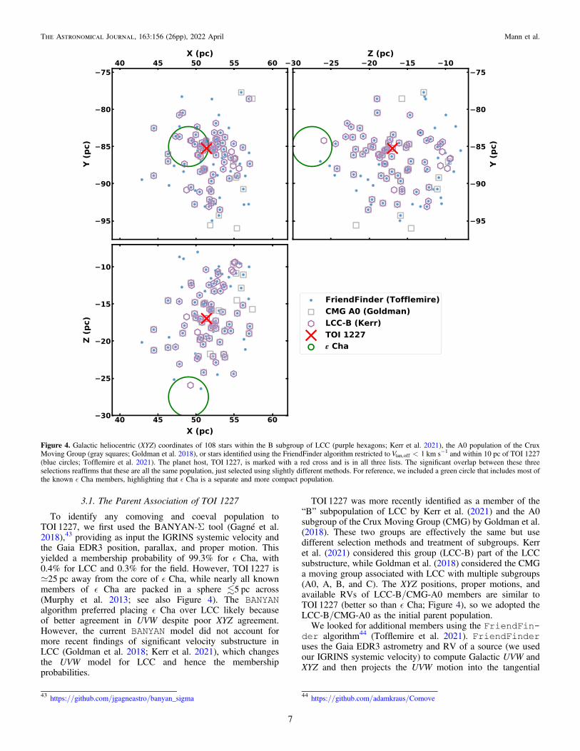
TOI 1227 was more recently identified as a member of the“B” subpopulation of LCC by Kerr et al. (2021) and the A0subgroup of the Crux Moving Group (CMG) by Goldman et al.(2018). These two groups are effectively the same but usedifferent selection methods and treatment of subgroups. Kerret al. (2021) considered this group (LCC-B) part of the LCCsubstructure, while Goldman et al. (2018) considered the CMGa moving group associated with LCC with multiple subgroups(A0, A, B, and C). The XYZ positions, proper motions, andavailable RVs of LCC-B/CMG-A0 members are similar toTOI 1227 (better so than ò Cha; Figure 4), so we adopted theLCC-B/CMG-A0 as the initial parent population.We looked for additional members using the FriendFin-

der algorithm44 (Tofflemire et al. 2021). FriendFinderuses the Gaia EDR3 astrometry and RV of a source (we usedour IGRINS systemic velocity) to compute Galactic UVW andXYZ and then projects the UVW motion into the tangential

Figure 4. Galactic heliocentric (XYZ) coordinates of 108 stars within the B subgroup of LCC (purple hexagons; Kerr et al. 2021), the A0 population of the CruxMoving Group (gray squares; Goldman et al. 2018), or stars identified using the FriendFinder algorithm restricted to <V 1tan,off km s−1 and within 10 pc of TOI 1227(blue circles; Tofflemire et al. 2021). The planet host, TOI 1227, is marked with a red cross and is in all three lists. The significant overlap between these threeselections reaffirms that these are all the same population, just selected using slightly different methods. For reference, we included a green circle that includes most ofthe known ò Cha members, highlighting that ò Cha is a separate and more compact population.

43 https://github.com/jgagneastro/banyan_sigma 44 https://github.com/adamkraus/Comove

7

The Astronomical Journal, 163:156 (26pp), 2022 April Mann et al.

velocities that would be expected for nearby stars if they wereto share the same space motion. We selected stars withseparations <10 pc from TOI 1227 and tangential velocities<1 km s−1 from the expected values calculated by Friend-Finder. These cuts were based on the fact that 1 km s−1 ;1 pcMyr−1 and an estimated age for the population of;10Myr. We estimated that these cuts would yield 2 fieldinterlopers based on the background population of Gaia stars.

The three candidate membership lists—those from Goldmanet al. (2018), Kerr et al. (2021), and this work—have significantoverlap in both Galactic position and proper motion (Figures 4and 5). Of the 108 stars in any of the three lists, 40 were in allthree, and 27 were in two of the three. Further, most of the starsmissing from Goldman et al. (2018) were missing preciseparallaxes in Gaia DR2 (the former used DR2, while the othertwo selections used EDR3). Many of the stars in theFriendFinder list but not in Kerr et al. (2021) wereremoved by one of the quality cuts imposed by the latter work(e.g., BP/RP flux excess). The FriendFinder list was alsomissing a small number of objects slightly farther away fromTOI 1227 because of our separation cut.

To be inclusive, we adopted the combination of all three listsas the membership list for TOI 1227’s association; these 108stars are listed in Table 5.

The resulting population has two (contradictory) names inthe literature, both of which are difficult to remember. Giventhe presence of a young transiting planet, it deserves a morememorable name than “A0” or “B.” Most of the members landwithin the Musca constellation, so we refer to the merged groupof stars as the Musca group (or just Musca).

TOI 1227 resides at the center of Musca, based on bothGalactic position (Figure 4) and proper motion (Figure 5). Themean velocity of the members with literature RVs(12.8 km s−1) is also in good agreement with the value forTOI 1227. A randomly selected star that matches Musca inXYZ has a =1% probability of matching Musca in propermotion and RV by chance. The CMD also indicates acommon age for stars in the population (Figure 6), withTOI 1227 matching the sequence. Combined with thepresence of lithium in its spectrum, TOI 1227’s membershipin Musca is unambiguous.

3.2. Rotation

To better measure the age of Musca (and hence TOI 1227),we measured rotation periods for all candidate members usingTESS Full-Frame Images (FFIs) downloaded from theMikulski Archive for Space Telescopes (MAST). First, wecreated initial light curves from the FFI cutouts centered oneach candidate member. After background subtraction, we usedthe unpopular package (Hattori et al. 2021) to generate aCausal Pixel Model (CPM) of the telescope systematics foreach star, which we subtracted from the initial light curve. Weused the CPM curves because it does a better job preservinglong-period signals than PDCSAP (Stello et al. 2016; Wanget al. 2017).We searched the resulting single-sector light curves for

rotation periods between 0.1 and 30 days using the Lomb–Scargle algorithm (Horne & Baliunas 1986), repeating for eachavailable sector. We selected the rotation period from the sectorthat returned the largest Lomb–Scargle power. As a check, wephase-folded the resulting light curves along that rotationperiod to inspect each measurement by eye. A few stars hadmultiple peaks in their Lomb–Scargle periodograms, whichmight indicate an unresolved binary. In such cases, we took thestronger signal (which was always the shorter period). Eachrotation measurement was assigned a quality score during thevisual inspection following Rampalli et al. (2021), with Q0indicating an obvious rotation signal, Q1 a questionable signal,Q2 a spurious detection, and Q3 a light curve dominated bynoise. In total, we measured usable rotation periods (Q0 or Q1)for 90 stars out of a sample of 108. Of the remaining 18, 11were too faint to retrieve a reliable light curve, one showed aclear dipper pattern (and was identified as such by Tajiri et al.2020), three had high flux contamination from nearby stars, andthe remaining three had no significant period detection.Rotation period measurements are included in Table 5. Thehigh detection rate is consistent with a young population andsuggests a low rate of field-star interlopers in our selection.The rotation period distribution (Figure 7) is consistent with

the spread seen in the 10Myr Upper Scorpius association(Rebull et al. 2018), and marginally consistent with the tighter

Figure 5. Galactic coordinates (l, b) of stars around TOI 1227, with arrowsindicating the direction and magnitude of the proper motion for each star.Likely members of Musca (Section 3.1) are colored by their BP − RP color. Allstars within 10 pc of TOI 1227 (excluding candidate members) are shown asgray arrows. TOI 1227 is thicker with a black outline.

Figure 6. CMD of stars in Musca (stars associated with TOI 1227), withsymbols by the selection method or reference. We removed stars with poorastrometric fits from Gaia (RUWE > 1.5; Gaia Collaboration et al. 2021).TOI 1227 is marked as a red cross and lands within the tight sequence. Theblue line indicates an empirical main sequence for reference (Pecaut &Mamajek 2013).

8

The Astronomical Journal, 163:156 (26pp), 2022 April Mann et al.

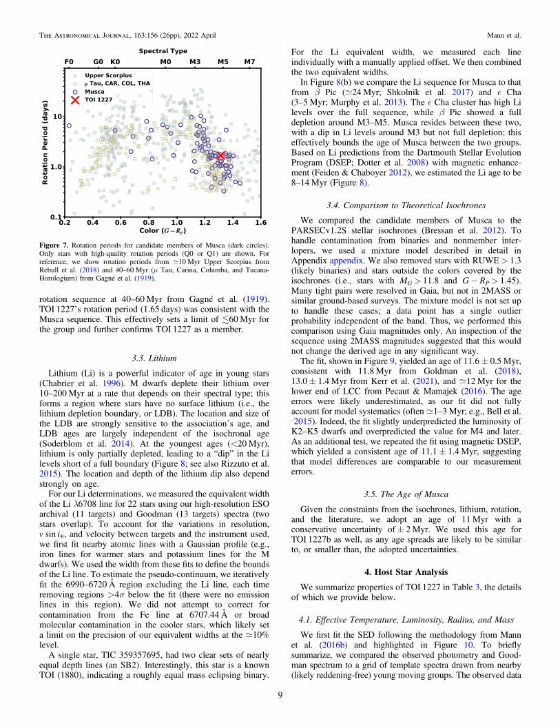
rotation sequence at 40–60Myr from Gagné et al. (1919).TOI 1227’s rotation period (1.65 days) was consistent with theMusca sequence. This effectively sets a limit of 60Myr forthe group and further confirms TOI 1227 as a member.

3.3. Lithium

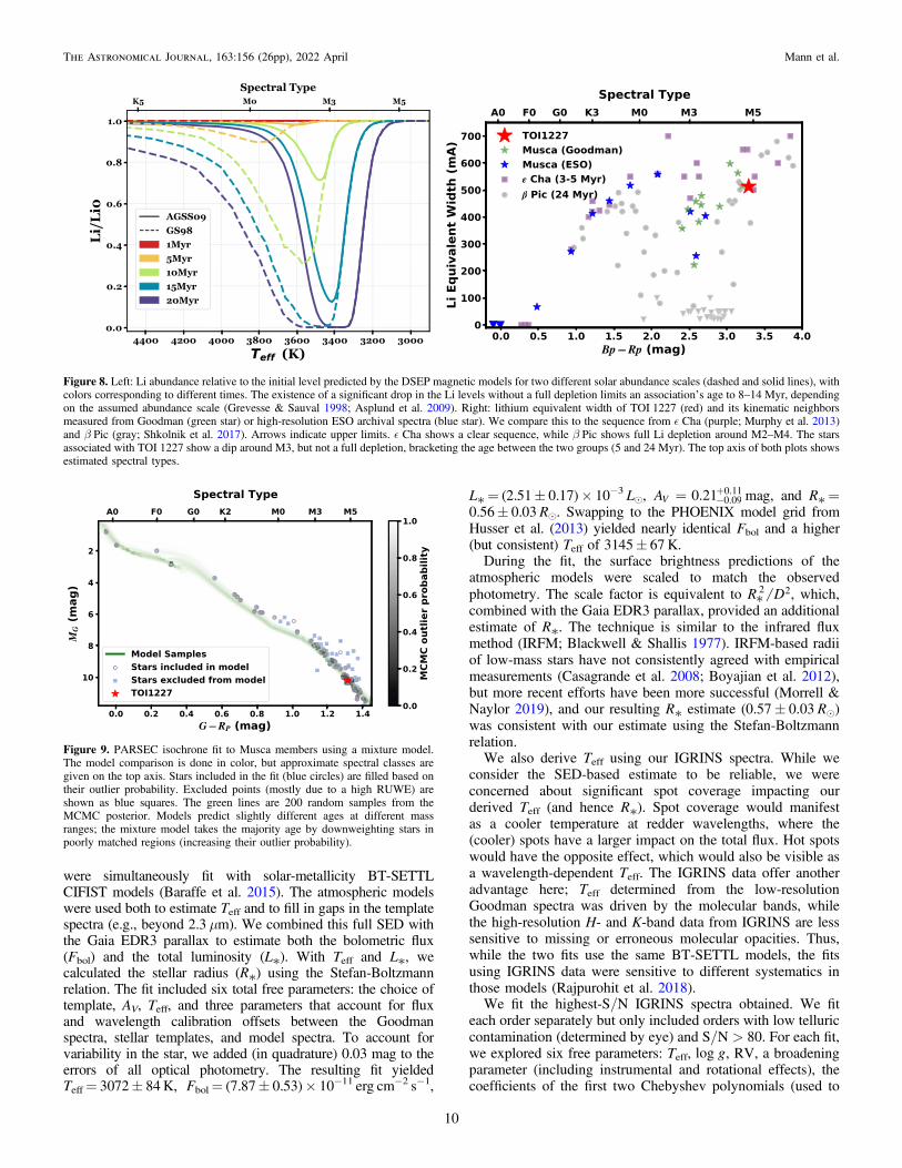
Lithium (Li) is a powerful indicator of age in young stars(Chabrier et al. 1996). M dwarfs deplete their lithium over10–200Myr at a rate that depends on their spectral type; thisforms a region where stars have no surface lithium (i.e., thelithium depletion boundary, or LDB). The location and size ofthe LDB are strongly sensitive to the association’s age, andLDB ages are largely independent of the isochronal age(Soderblom et al. 2014). At the youngest ages (<20Myr),lithium is only partially depleted, leading to a “dip” in the Lilevels short of a full boundary (Figure 8; see also Rizzuto et al.2015). The location and depth of the lithium dip also dependstrongly on age.

For our Li determinations, we measured the equivalent widthof the Li λ6708 line for 22 stars using our high-resolution ESOarchival (11 targets) and Goodman (13 targets) spectra (twostars overlap). To account for the variations in resolution,

*v isin , and velocity between targets and the instrument used,we first fit nearby atomic lines with a Gaussian profile (e.g.,iron lines for warmer stars and potassium lines for the Mdwarfs). We used the width from these fits to define the boundsof the Li line. To estimate the pseudo-continuum, we iterativelyfit the 6990–6720Å region excluding the Li line, each timeremoving regions >4σ below the fit (there were no emissionlines in this region). We did not attempt to correct forcontamination from the Fe line at 6707.44Å or broadmolecular contamination in the cooler stars, which likely seta limit on the precision of our equivalent widths at the ;10%level.

A single star, TIC 359357695, had two clear sets of nearlyequal depth lines (an SB2). Interestingly, this star is a knownTOI (1880), indicating a roughly equal mass eclipsing binary.

For the Li equivalent width, we measured each lineindividually with a manually applied offset. We then combinedthe two equivalent widths.In Figure 8(b) we compare the Li sequence for Musca to that

from β Pic (;24Myr; Shkolnik et al. 2017) and ò Cha(3–5Myr; Murphy et al. 2013). The ò Cha cluster has high Lilevels over the full sequence, while β Pic showed a fulldepletion around M3–M5. Musca resides between these two,with a dip in Li levels around M3 but not full depletion; thiseffectively bounds the age of Musca between the two groups.Based on Li predictions from the Dartmouth Stellar EvolutionProgram (DSEP; Dotter et al. 2008) with magnetic enhance-ment (Feiden & Chaboyer 2012), we estimated the Li age to be8–14Myr (Figure 8).

3.4. Comparison to Theoretical Isochrones

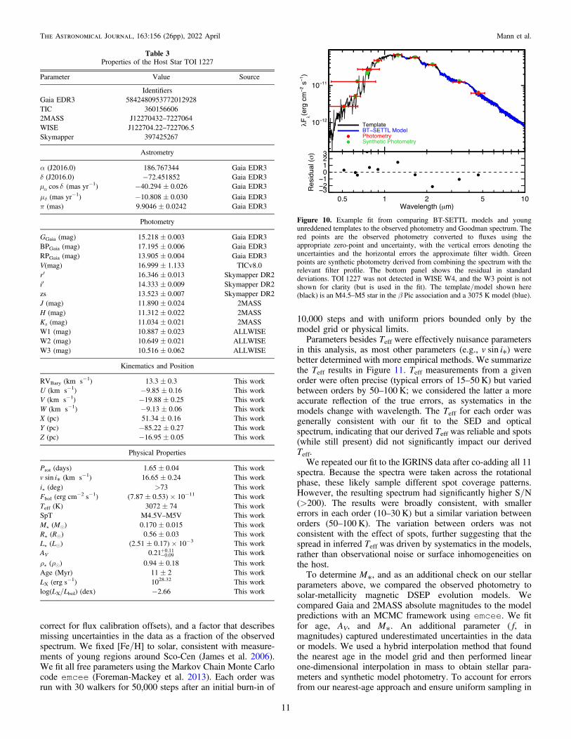
We compared the candidate members of Musca to thePARSECv1.2S stellar isochrones (Bressan et al. 2012). Tohandle contamination from binaries and nonmember inter-lopers, we used a mixture model described in detail inAppendix appendix. We also removed stars with RUWE> 1.3(likely binaries) and stars outside the colors covered by theisochrones (i.e., stars with MG> 11.8 and G− RP> 1.45).Many tight pairs were resolved in Gaia, but not in 2MASS orsimilar ground-based surveys. The mixture model is not set upto handle these cases; a data point has a single outlierprobability independent of the band. Thus, we performed thiscomparison using Gaia magnitudes only. An inspection of thesequence using 2MASS magnitudes suggested that this wouldnot change the derived age in any significant way.The fit, shown in Figure 9, yielded an age of 11.6± 0.5 Myr,

consistent with 11.8 Myr from Goldman et al. (2018),13.0± 1.4 Myr from Kerr et al. (2021), and ;12Myr for thelower end of LCC from Pecaut & Mamajek (2016). The ageerrors were likely underestimated, as our fit did not fullyaccount for model systematics (often ;1–3Myr; e.g., Bell et al.2015). Indeed, the fit slightly underpredicted the luminosity ofK2–K5 dwarfs and overpredicted the value for M4 and later.As an additional test, we repeated the fit using magnetic DSEP,which yielded a consistent age of 11.1± 1.4 Myr, suggestingthat model differences are comparable to our measurementerrors.

3.5. The Age of Musca

Given the constraints from the isochrones, lithium, rotation,and the literature, we adopt an age of 11Myr with aconservative uncertainty of± 2Myr. We used this age forTOI 1227b as well, as any age spreads are likely to be similarto, or smaller than, the adopted uncertainties.

4. Host Star Analysis

We summarize properties of TOI 1227 in Table 3, the detailsof which we provide below.

4.1. Effective Temperature, Luminosity, Radius, and Mass

We first fit the SED following the methodology from Mannet al. (2016b) and highlighted in Figure 10. To brieflysummarize, we compared the observed photometry and Good-man spectrum to a grid of template spectra drawn from nearby(likely reddening-free) young moving groups. The observed data

Figure 7. Rotation periods for candidate members of Musca (dark circles).Only stars with high-quality rotation periods (Q0 or Q1) are shown. Forreference, we show rotation periods from ;10 Myr Upper Scorpius fromRebull et al. (2018) and 40–60 Myr (μ Tau, Carina, Columba, and Tucana-Horologium) from Gagné et al. (1919).

9

The Astronomical Journal, 163:156 (26pp), 2022 April Mann et al.

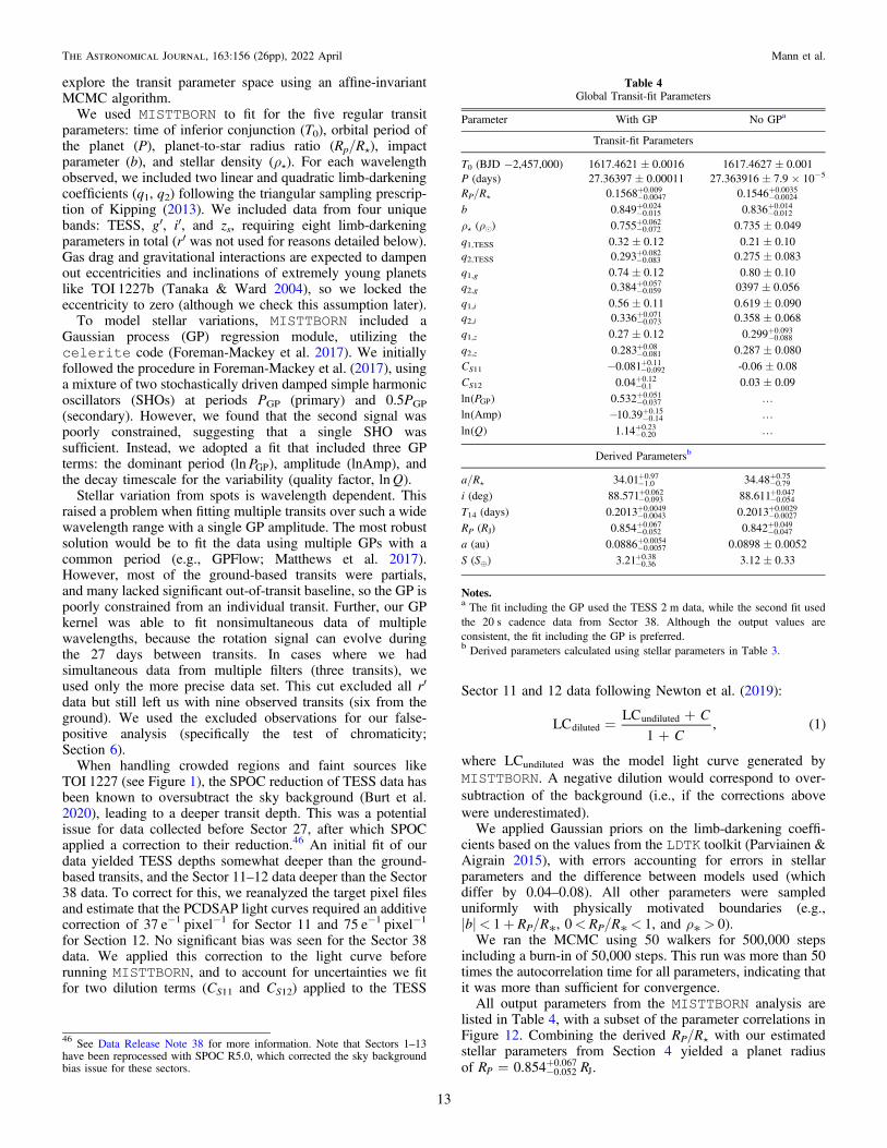
were simultaneously fit with solar-metallicity BT-SETTLCIFIST models (Baraffe et al. 2015). The atmospheric modelswere used both to estimate Teff and to fill in gaps in the templatespectra (e.g., beyond 2.3 μm). We combined this full SED withthe Gaia EDR3 parallax to estimate both the bolometric flux(Fbol) and the total luminosity (L*). With Teff and L*, wecalculated the stellar radius (R*) using the Stefan-Boltzmannrelation. The fit included six total free parameters: the choice oftemplate, AV, Teff, and three parameters that account for fluxand wavelength calibration offsets between the Goodmanspectra, stellar templates, and model spectra. To account forvariability in the star, we added (in quadrature) 0.03 mag to theerrors of all optical photometry. The resulting fit yieldedTeff= 3072± 84K, Fbol= (7.87± 0.53)× 10−11 erg cm−2 s−1,

L*= (2.51± 0.17)× 10−3 Le, = -+A 0.21V 0.09

0.11 mag, and R*=0.56± 0.03 Re. Swapping to the PHOENIX model grid fromHusser et al. (2013) yielded nearly identical Fbol and a higher(but consistent) Teff of 3145± 67 K.During the fit, the surface brightness predictions of the

atmospheric models were scaled to match the observedphotometry. The scale factor is equivalent to *

R D2 2, which,combined with the Gaia EDR3 parallax, provided an additionalestimate of R*. The technique is similar to the infrared fluxmethod (IRFM; Blackwell & Shallis 1977). IRFM-based radiiof low-mass stars have not consistently agreed with empiricalmeasurements (Casagrande et al. 2008; Boyajian et al. 2012),but more recent efforts have been more successful (Morrell &Naylor 2019), and our resulting R* estimate (0.57± 0.03 Re)was consistent with our estimate using the Stefan-Boltzmannrelation.We also derive Teff using our IGRINS spectra. While we

consider the SED-based estimate to be reliable, we wereconcerned about significant spot coverage impacting ourderived Teff (and hence R*). Spot coverage would manifestas a cooler temperature at redder wavelengths, where the(cooler) spots have a larger impact on the total flux. Hot spotswould have the opposite effect, which would also be visible asa wavelength-dependent Teff. The IGRINS data offer anotheradvantage here; Teff determined from the low-resolutionGoodman spectra was driven by the molecular bands, whilethe high-resolution H- and K-band data from IGRINS are lesssensitive to missing or erroneous molecular opacities. Thus,while the two fits use the same BT-SETTL models, the fitsusing IGRINS data were sensitive to different systematics inthose models (Rajpurohit et al. 2018).We fit the highest-S/N IGRINS spectra obtained. We fit

each order separately but only included orders with low telluriccontamination (determined by eye) and S/N > 80. For each fit,we explored six free parameters: Teff, glog , RV, a broadeningparameter (including instrumental and rotational effects), thecoefficients of the first two Chebyshev polynomials (used to

Figure 8. Left: Li abundance relative to the initial level predicted by the DSEP magnetic models for two different solar abundance scales (dashed and solid lines), withcolors corresponding to different times. The existence of a significant drop in the Li levels without a full depletion limits an association’s age to 8–14 Myr, dependingon the assumed abundance scale (Grevesse & Sauval 1998; Asplund et al. 2009). Right: lithium equivalent width of TOI 1227 (red) and its kinematic neighborsmeasured from Goodman (green star) or high-resolution ESO archival spectra (blue star). We compare this to the sequence from ò Cha (purple; Murphy et al. 2013)and β Pic (gray; Shkolnik et al. 2017). Arrows indicate upper limits. ò Cha shows a clear sequence, while β Pic shows full Li depletion around M2–M4. The starsassociated with TOI 1227 show a dip around M3, but not a full depletion, bracketing the age between the two groups (5 and 24 Myr). The top axis of both plots showsestimated spectral types.

Figure 9. PARSEC isochrone fit to Musca members using a mixture model.The model comparison is done in color, but approximate spectral classes aregiven on the top axis. Stars included in the fit (blue circles) are filled based ontheir outlier probability. Excluded points (mostly due to a high RUWE) areshown as blue squares. The green lines are 200 random samples from theMCMC posterior. Models predict slightly different ages at different massranges; the mixture model takes the majority age by downweighting stars inpoorly matched regions (increasing their outlier probability).

10

The Astronomical Journal, 163:156 (26pp), 2022 April Mann et al.

correct for flux calibration offsets), and a factor that describesmissing uncertainties in the data as a fraction of the observedspectrum. We fixed [Fe/H] to solar, consistent with measure-ments of young regions around Sco-Cen (James et al. 2006).We fit all free parameters using the Markov Chain Monte Carlocode emcee (Foreman-Mackey et al. 2013). Each order wasrun with 30 walkers for 50,000 steps after an initial burn-in of

10,000 steps and with uniform priors bounded only by themodel grid or physical limits.Parameters besides Teff were effectively nuisance parameters

in this analysis, as most other parameters (e.g., *v isin ) werebetter determined with more empirical methods. We summarizethe Teff results in Figure 11. Teff measurements from a givenorder were often precise (typical errors of 15–50 K) but variedbetween orders by 50–100 K; we considered the latter a moreaccurate reflection of the true errors, as systematics in themodels change with wavelength. The Teff for each order wasgenerally consistent with our fit to the SED and opticalspectrum, indicating that our derived Teff was reliable and spots(while still present) did not significantly impact our derivedTeff.We repeated our fit to the IGRINS data after co-adding all 11

spectra. Because the spectra were taken across the rotationalphase, these likely sample different spot coverage patterns.However, the resulting spectrum had significantly higher S/N(>200). The results were broadly consistent, with smallererrors in each order (10–30 K) but a similar variation betweenorders (50–100 K). The variation between orders was notconsistent with the effect of spots, further suggesting that thespread in inferred Teff was driven by systematics in the models,rather than observational noise or surface inhomogeneities onthe host.To determine M*, and as an additional check on our stellar

parameters above, we compared the observed photometry tosolar-metallicity magnetic DSEP evolution models. Wecompared Gaia and 2MASS absolute magnitudes to the modelpredictions with an MCMC framework using emcee. We fitfor age, AV, and M*. An additional parameter ( f, inmagnitudes) captured underestimated uncertainties in the dataor models. We used a hybrid interpolation method that foundthe nearest age in the model grid and then performed linearone-dimensional interpolation in mass to obtain stellar para-meters and synthetic model photometry. To account for errorsfrom our nearest-age approach and ensure uniform sampling in

Table 3Properties of the Host Star TOI 1227

Parameter Value Source

IdentifiersGaia EDR3 5842480953772012928TIC 3601566062MASS J12270432–7227064WISE J122704.22–722706.5Skymapper 397425267

Astrometry

α (J2016.0) 186.767344 Gaia EDR3δ (J2016.0) −72.451852 Gaia EDR3m da cos (mas yr−1) −40.294 ± 0.026 Gaia EDR3

μδ (mas yr−1) −10.808 ± 0.030 Gaia EDR3π (mas) 9.9046 ± 0.0242 Gaia EDR3

Photometry

GGaia (mag) 15.218 ± 0.003 Gaia EDR3BPGaia (mag) 17.195 ± 0.006 Gaia EDR3RPGaia (mag) 13.905 ± 0.004 Gaia EDR3V(mag) 16.999 ± 1.133 TICv8.0r′ 16.346 ± 0.013 Skymapper DR2i′ 14.333 ± 0.009 Skymapper DR2zs 13.523 ± 0.007 Skymapper DR2J (mag) 11.890 ± 0.024 2MASSH (mag) 11.312 ± 0.022 2MASSKs (mag) 11.034 ± 0.021 2MASSW1 (mag) 10.887 ± 0.023 ALLWISEW2 (mag) 10.649 ± 0.021 ALLWISEW3 (mag) 10.516 ± 0.062 ALLWISE

Kinematics and Position

RVBary (km s−1) 13.3 ± 0.3 This workU (km s−1) −9.85 ± 0.16 This workV (km s−1) −19.88 ± 0.25 This workW (km s−1) −9.13 ± 0.06 This workX (pc) 51.34 ± 0.16 This workY (pc) −85.22 ± 0.27 This workZ (pc) −16.95 ± 0.05 This work

Physical Properties

Prot (days) 1.65 ± 0.04 This work

*v isin (km s−1) 16.65 ± 0.24 This workiå (deg) >73 This workFbol (erg cm

−2 s−1) (7.87 ± 0.53) × 10−11 This workTeff (K) 3072 ± 74 This workSpT M4.5V–M5V This workMå (Me) 0.170 ± 0.015 This workRå (Re) 0.56 ± 0.03 This workLå (Le) (2.51 ± 0.17) × 10−3 This workAV -

+0.21 0.090.11 This work

ρå (ρe) 0.94 ± 0.18 This workAge (Myr) 11 ± 2 This workLX (erg s−1) 1028.32 This worklog(LX/Lbol) (dex) −2.66 This work

Figure 10. Example fit from comparing BT-SETTL models and youngunreddened templates to the observed photometry and Goodman spectrum. Thered points are the observed photometry converted to fluxes using theappropriate zero-point and uncertainty, with the vertical errors denoting theuncertainties and the horizontal errors the approximate filter width. Greenpoints are synthetic photometry derived from combining the spectrum with therelevant filter profile. The bottom panel shows the residual in standarddeviations. TOI 1227 was not detected in WISE W4, and the W3 point is notshown for clarity (but is used in the fit). The template/model shown here(black) is an M4.5–M5 star in the β Pic association and a 3075 K model (blue).

11

The Astronomical Journal, 163:156 (26pp), 2022 April Mann et al.

age, we pre-interpolated bilinearly in age and mass using theisochrones package (Morton 2015). The interpolated gridwas far denser (0.1 Myr and 0.01 Me) than expected errors. Toredden the model photometry, we used synphot (Lim 1919),following the extinction law from Cardelli et al. (1989). Weplaced Gaussian priors for age (11± 2Myr; derived from thepopulation), AV (0.21± 0.1 mag; from the SED fit), and Teff(3072± 74 K; from the SED fit). All other parameters evolvedunder uniform priors. From the best-fit posteriors, we were ableto interpolate additional posteriors on other stellar parametersfrom the evolutionary model, including R* and Teff.

The fit yielded age= 11.5± 1.0 Myr, M* = 0.165±0.010Me, AV= 0.148± 0.074 mag, R* = 0.554± 0.007 Re,and Teff= 3050± 20 K. Changing the Teff prior to uniformyielded consistent but less precise parameters (e.g.,M* = 0.170± 0.015 Me). As an additional test, we repeatedthe analysis using the PARSEC models, which yieldedparameters somewhat discrepant with our SED and populationanalysis (age= 14.9± 2.1Myr, Teff= 2900± 30 K, andM* = 0.20± 0.01Me). PARSEC did not reproduce theobserved colors of the coolest stars in Musca, which manifestedas systematically high luminosities for a fixed color past;M4(see Figure 9). Thus, we prefer the magnetic DSEP fit.However, we adopted the more conservative mass (M* =0.170± 0.015Me), which was 2σ consistent with the PARSECvalue.

4.2. Rotation Period, Rotational Broadening, and StellarInclination

Canto Martins et al. (1919) reported a rotation period (Prot)of 1.663± 0.028 days for TOI 1227 using TESS data. Ouranalysis of rotation periods in Section 3 yielded a consistent1.65± 0.04 days, which we adopted for our analysis. Wecomputed *v isin as part of extracting RVs from IGRINS/Gemini and HRS/SALT spectra. The mean value from theIGRINS data was 16.65± 0.24 km s−1, while the SALT datayielded a marginally inconsistent value of 17.8± 0.3 km s−1.We adopted the former value, as the IGRINS data havesignificantly higher S/N and are less impacted by spots ormolecular line contamination.

We used the combination of *v isin , Prot, and R* to estimatethe stellar inclination (i*) and hence test whether the stellar spinand planetary orbit are consistent with alignment. A basicversion of this calculation can be done by estimating the V termin *v isin using V= 2πR*/Prot, although in practice it requiresadditional statistical corrections, including the fact that we can

only measure alignment projected onto the sky. To this end, wefollowed the formalism from Masuda & Winn (2020). Theresulting stellar inclination was consistent with alignment withthe planet, yielding a limit on inclination of i* > 73° at 95%confidence and i* > 77° at 68% confidence.

4.3. X-Ray Luminosity

TOI 1227 was detected in X-rays in a ROSAT pointing of theglobular cluster NGC 4372 in 1993 (Johnston & Verbunt 1996).The X-ray source was listed as #6 in NGC 4372 (identified inSIMBAD as [JVH96] NGC 4372 6); however, the quoted valueswere not usable here, as they quote an X-ray flux assuming thatthe source is at the distance to NGC 4372 and only gave upperlimits on the hardness ratios. The X-ray detection was reanalyzedby Voges et al. (2000) in the 2nd ROSAT PSPC Catalog, whichidentifies the X-ray source as 2RXP J122703.8−722702,situated 4 9 away from TOI 1227 with a positional errorof± 9″ (i.e., consistent with TOI 1227 being the sourceof the X-rays). They list a soft X-ray count rate of fX=(1.967± 0.626)× 10−3 counts s−1 with hardness ratiosHR1= 0.06± 0.32 and HR2= 0.58± 0.32 with an effectiveexposure time of 7399 s observed over UT 1993 September 4–6.Using the energy conversion factor equation of Fleming et al.(1995), this count rate and HR1 hardness ratio translate to a softX-ray energy flux of fX= 1.70± 10−14 erg s−1 cm−2, which atthe distance to TOI 1227 translates to a soft X-ray luminosity ofLX= 1028.32 erg s−1.Given our estimate of the star’s bolometric luminosity

(Table 3), this translates to a fractional X-ray luminosity oflog(LX/Lbol)=−2.66. This is within the range of activitylevels stars in the saturated regime display. However, X-raylevels tell us little about TOI 1227’s age; M5V stars remain inthe saturated well into field ages (West et al. 2015; Newtonet al. 2017).

5. Transit Analysis

We fit the TESS, SOAR, and LCO photometry simulta-neously using the MISTTBORN (MCMC Interface for Synth-esis of Transits, Tomography, Binaries, and Others of aRelevant Nature) fitting code45 first described in Mann et al.(2016a) and expanded on in Johnson et al. (2018). MIS-TTBORN uses BATMAN (Kreidberg 2015) to generate modellight curves and emcee (Foreman-Mackey et al. 2013) to

Figure 11. Marginal probability distributions on Teff (“violin” plot; Waskom et al. 1919) for 24 IGRINS orders fit independently over the H band (left) and K band(right). Each violin has an equal area distributed according to the MCMC posterior, so narrow/tall violins represent larger uncertainties than wider/shorter ones. Theblue bar represents the 1σ distribution from our optical spectrum and SED fit.

45 https://github.com/captain-exoplanet/misttborn

12

The Astronomical Journal, 163:156 (26pp), 2022 April Mann et al.

explore the transit parameter space using an affine-invariantMCMC algorithm.

We used MISTTBORN to fit for the five regular transitparameters: time of inferior conjunction (T0), orbital period ofthe planet (P), planet-to-star radius ratio (Rp/Rå), impactparameter (b), and stellar density (ρå). For each wavelengthobserved, we included two linear and quadratic limb-darkeningcoefficients (q1, q2) following the triangular sampling prescrip-tion of Kipping (2013). We included data from four uniquebands: TESS, g′, i′, and zs, requiring eight limb-darkeningparameters in total (r′ was not used for reasons detailed below).Gas drag and gravitational interactions are expected to dampenout eccentricities and inclinations of extremely young planetslike TOI 1227b (Tanaka & Ward 2004), so we locked theeccentricity to zero (although we check this assumption later).

To model stellar variations, MISTTBORN included aGaussian process (GP) regression module, utilizing thecelerite code (Foreman-Mackey et al. 2017). We initiallyfollowed the procedure in Foreman-Mackey et al. (2017), usinga mixture of two stochastically driven damped simple harmonicoscillators (SHOs) at periods PGP (primary) and 0.5PGP

(secondary). However, we found that the second signal waspoorly constrained, suggesting that a single SHO wassufficient. Instead, we adopted a fit that included three GPterms: the dominant period ( Pln GP), amplitude (lnAmp), andthe decay timescale for the variability (quality factor, Qln ).

Stellar variation from spots is wavelength dependent. Thisraised a problem when fitting multiple transits over such a widewavelength range with a single GP amplitude. The most robustsolution would be to fit the data using multiple GPs with acommon period (e.g., GPFlow; Matthews et al. 2017).However, most of the ground-based transits were partials,and many lacked significant out-of-transit baseline, so the GP ispoorly constrained from an individual transit. Further, our GPkernel was able to fit nonsimultaneous data of multiplewavelengths, because the rotation signal can evolve duringthe 27 days between transits. In cases where we hadsimultaneous data from multiple filters (three transits), weused only the more precise data set. This cut excluded all r′data but still left us with nine observed transits (six from theground). We used the excluded observations for our false-positive analysis (specifically the test of chromaticity;Section 6).

When handling crowded regions and faint sources likeTOI 1227 (see Figure 1), the SPOC reduction of TESS data hasbeen known to oversubtract the sky background (Burt et al.2020), leading to a deeper transit depth. This was a potentialissue for data collected before Sector 27, after which SPOCapplied a correction to their reduction.46 An initial fit of ourdata yielded TESS depths somewhat deeper than the ground-based transits, and the Sector 11–12 data deeper than the Sector38 data. To correct for this, we reanalyzed the target pixel filesand estimate that the PCDSAP light curves required an additivecorrection of 37 e−1 pixel−1 for Sector 11 and 75 e−1 pixel−1

for Section 12. No significant bias was seen for the Sector 38data. We applied this correction to the light curve beforerunning MISTTBORN, and to account for uncertainties we fitfor two dilution terms (CS11 and CS12) applied to the TESS

Sector 11 and 12 data following Newton et al. (2019):

( )=+

+C

CLC

LC

1, 1diluted

undiluted

where LCundiluted was the model light curve generated byMISTTBORN. A negative dilution would correspond to over-subtraction of the background (i.e., if the corrections abovewere underestimated).We applied Gaussian priors on the limb-darkening coeffi-

cients based on the values from the LDTK toolkit (Parviainen &Aigrain 2015), with errors accounting for errors in stellarparameters and the difference between models used (whichdiffer by 0.04–0.08). All other parameters were sampleduniformly with physically motivated boundaries (e.g.,|b|< 1+ RP/R*, 0< RP/R* < 1, and ρ* > 0).We ran the MCMC using 50 walkers for 500,000 steps

including a burn-in of 50,000 steps. This run was more than 50times the autocorrelation time for all parameters, indicating thatit was more than sufficient for convergence.All output parameters from the MISTTBORN analysis are

listed in Table 4, with a subset of the parameter correlations inFigure 12. Combining the derived RP/Rå with our estimatedstellar parameters from Section 4 yielded a planet radiusof = -

+R R0.854P 0.0520.067

J.

Table 4Global Transit-fit Parameters

Parameter With GP No GPa

Transit-fit Parameters

T0 (BJD −2,457,000) 1617.4621 ± 0.0016 1617.4627 ± 0.001P (days) 27.36397 ± 0.00011 27.363916 ± 7.9 × 10−5

RP/Rå -+0.1568 0.0047

0.009-+0.1546 0.0024

0.0035

b -+0.849 0.015

0.024-+0.836 0.012

0.014

ρå (ρe) -+0.755 0.072

0.062 0.735 ± 0.049

q1,TESS 0.32 ± 0.12 0.21 ± 0.10q2,TESS -

+0.293 0.0830.082 0.275 ± 0.083

q1,g 0.74 ± 0.12 0.80 ± 0.10q2,g -

+0.384 0.0590.057 0397 ± 0.056

q1,i 0.56 ± 0.11 0.619 ± 0.090q2,i -

+0.336 0.0730.071 0.358 ± 0.068

q1,z 0.27 ± 0.12 -+0.299 0.088

0.093

q2,z -+0.283 0.081

0.08 0.287 ± 0.080

CS11 − -+0.081 0.092

0.11 -0.06 ± 0.08

CS12 -+0.04 0.1

0.12 0.03 ± 0.09

( )Pln GP -+0.532 0.037

0.051 K( )ln Amp − -

+10.39 0.140.15 K

( )Qln -+1.14 0.20

0.23 K

Derived Parametersb

a/Rå -+34.01 1.0

0.97-+34.48 0.79

0.75

i (deg) -+88.571 0.093

0.062-+88.611 0.054

0.047

T14 (days) -+0.2013 0.0043

0.0049-+0.2013 0.0027

0.0029

RP (RJ) -+0.854 0.052

0.067-+0.842 0.047

0.049

a (au) -+0.0886 0.0057

0.0054 0.0898 ± 0.0052

S (S⊕) -+3.21 0.36

0.38 3.12 ± 0.33

Notes.a The fit including the GP used the TESS 2 m data, while the second fit usedthe 20 s cadence data from Sector 38. Although the output values areconsistent, the fit including the GP is preferred.b Derived parameters calculated using stellar parameters in Table 3.

46 See Data Release Note 38 for more information. Note that Sectors 1–13have been reprocessed with SPOC R5.0, which corrected the sky backgroundbias issue for these sectors.

13

The Astronomical Journal, 163:156 (26pp), 2022 April Mann et al.

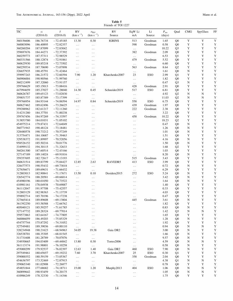
Table 5Friends of TOI 1227

TIC α δ RV σRV RV EqW Li Li Prot Qual CMG SpyGlass FF(J2016.0) (J2016.0) (km s−1) (km s−1) Source mA Source (days)

360156606 186.76734 −72.45185 13.30 0.30 IGRINS 513 Goodman 1.65 Q0 Y Y Y360003096 186.40895 −72.82357 K K 598 Goodman 0.58 Q0 Y Y Y360260204 187.87099 −72.83042 K K K 10.22 Q3 Y Y Y359697676 184.44271 −72.37392 K K 382 Goodman 2.09 Q0 Y Y Y360259773 187.57311 −72.98529 K K K 6.53 Q1 Y Y Y360331566 188.12874 −72.91861 K K 479 Goodman 5.52 Q0 Y Y Y360625930 189.85218 −72.73502 K K K 6.60 Q0 Y Y Y360259534 187.70690 −73.07898 K K 563 Goodman 8.64 Q2 Y Y Y326657935 188.45791 −71.42464 K K K 1.61 Q0 N Y Y359997243 186.21572 −72.60394 7.90 1.20 Kharchenko2007 23 ESO 2.99 Q1 Y Y Y360906004 190.90566 −71.99760 K K K 1.82 Q0 Y Y Y360212499 187.32060 −73.91157 K K K 0.47 Q3 N Y Y359766629 185.15013 −73.88416 K K 428 Goodman 2.91 Q0 Y Y Y447994659 185.27027 −71.28040 14.30 0.45 Schneider2019 517 ESO 6.81 Q0 Y Y Y360626787 189.65123 −73.02830 K K K 4.92 Q2 N N Y359851737 185.87389 −73.17399 K K K 11.03 Q2 N N Y359766954 184.93144 −74.06594 14.97 0.84 Schneider2019 558 ESO 6.75 Q0 Y Y Y360627462 189.62496 −73.26625 K K 439 Goodman 1.97 Q0 Y Y Y359288962 182.61217 −72.11260 K K 222 Goodman 2.38 Q0 Y Y Y314231280 184.37701 −71.00238 K K K 3.22 Q0 Y Y Y359767456 184.97269 −74.33597 K K 458 Goodman 10.22 Q0 Y Y Y313853780 184.01031 −71.05102 K K K 18.23 Q2 Y Y Y454975214 179.87431 −72.64049 K K K 0.47 Q0 N Y Y360771943 190.48124 −73.18481 K K K 1.26 Q0 N Y Y328480578 190.73212 −70.57249 K K K 1.01 Q0 N Y Y313754471 184.10687 −71.39463 K K K 1.51 Q0 Y Y Y329538372 191.89997 −70.52056 K K K 4.16 Q0 N Y Y958526152 185.50216 −70.01776 K K K 1.50 Q0 N Y Y334999132 194.30115 −71.32633 K K K 1.68 Q2 Y Y Y360261300 187.60514 −72.43166 K K K 1.03 Q0 Y Y Y327147189 189.14024 −69.91816 K K K 8.20 Q0 N Y Y359357695 182.72617 −75.13193 K K 515 Goodman 3.43 Q0 Y Y Y360631514 189.83799 −75.04427 12.85 2.63 RAVEDR5 413 ESO 3.99 Q0 Y Y Y328477573 190.55432 −69.73018 K K K 0.72 Q0 N Y Y327656671 189.69631 −71.66432 K K K 6.29 Q0 Y Y Y312803013 182.90841 −71.17671 13.50 0.10 Desidera2015 272 ESO 5.24 Q0 N Y Y326542774 188.20581 −69.66814 K K K 3.42 Q0 N Y Y454980196 180.01050 −74.73522 K K K 1.64 Q0 N Y Y410981161 178.04938 −70.69887 K K K 1.40 Q0 Y Y Y361112047 191.97708 −75.42557 K K K 0.33 Q0 Y Y Y312803129 182.98363 −71.13739 K K K 4.03 Q0 Y Y Y359892714 185.70196 −74.17238 K K K 0.47 Q0 Y Y Y327665414 189.89608 −69.13804 K K 445 Goodman 3.61 Q0 N Y Y361392250 193.58588 −72.66762 K K K 1.82 Q0 Y Y Y405040121 185.59257 −71.61785 K K K 0.83 Q0 N Y Y327147732 189.28324 −69.77014 K K K 1.42 Q3 N N Y359573863 183.64167 −74.77805 K K K 1.65 Q0 Y Y Y360086059 186.49203 −75.85329 K K K 1.28 Q0 N Y Y454757744 175.87292 −74.31052 K K K 1.92 Q0 Y Y Y327549481 189.39036 −69.00110 K K K 0.94 Q0 N N Y328234948 190.21623 −68.94963 34.05 19.38 Gaia DR2 K 3.00 Q0 N Y Y326538701 188.35305 −68.81545 K K K 1.66 Q0 N Y Y311731608 181.28789 −70.07076 K K K 9.57 Q0 N Y Y334930665 194.03409 −69.44842 13.80 0.30 Torres2006 K 4.59 Q0 N N Y361113174 191.98801 −76.10258 K K K 0.58 Q0 N Y Y455000299 179.92537 −76.02397 12.63 1.40 Gaia DR2 460 ESO 7.90 Q0 N Y Y297549461 180.65657 −69.19232 7.60 3.70 Kharchenko2007 25 ESO 0.30 Q1 Y Y Y359000352 180.59159 −73.05367 K K 358 Goodman 2.04 Q0 Y Y Y454636797 173.52469 −72.87915 K K K 4.38 Q1 N N Y359065340 181.02908 −72.26877 K K K 0.78 Q0 Y Y Y454851844 177.68682 −74.18711 15.00 1.20 Murphy2013 404 ESO 1.06 Q0 N N Y360899642 190.93459 −74.20175 K K K 1.05 Q0 N N Y410986249 178.32330 −71.14346 K K K 1.75 Q0 Y Y Y

14

The Astronomical Journal, 163:156 (26pp), 2022 April Mann et al.

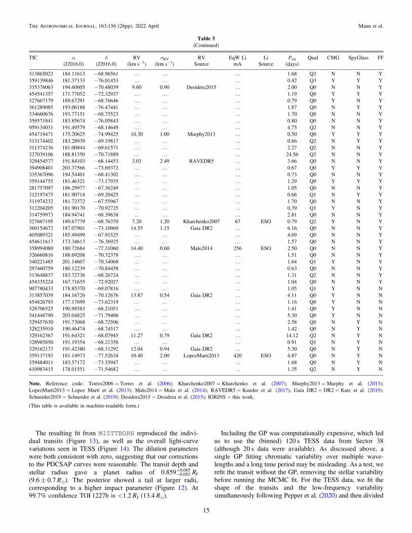
The resulting fit from MISTTBORN reproduced the indivi-dual transits (Figure 13), as well as the overall light-curvevariations seen in TESS (Figure 14). The dilution parameterswere both consistent with zero, suggesting that our correctionsto the PDCSAP curves were reasonable. The transit depth andstellar radius gave a planet radius of -

+ R0.859 J0.0520.065

(9.6± 0.7 R⊕). The posterior showed a tail at larger radii,corresponding to a higher impact parameter (Figure 12). At99.7% confidence TOI 1227b is <1.2 RJ (13.4 R⊕).

Including the GP was computationally expensive, which ledus to use the (binned) 120 s TESS data from Sector 38(although 20 s data were available). As discussed above, asingle GP fitting chromatic variability over multiple wave-lengths and a long time period may be misleading. As a test, werefit the transit without the GP, removing the stellar variabilitybefore running the MCMC fit. For the TESS data, we fit theshape of the transits and the low-frequency variabilitysimultaneously following Pepper et al. (2020) and then divided

Table 5(Continued)

TIC α δ RV σRV RV EqW Li Li Prot Qual CMG SpyGlass FF(J2016.0) (J2016.0) (km s−1) (km s−1) Source mA Source (days)

313865023 184.11613 −68.96561 K K K 1.68 Q3 N N Y359139846 181.37133 −76.01453 K K K 0.42 Q3 Y Y Y335376063 194.60605 −70.48039 9.60 0.90 Desidera2015 K 2.00 Q0 N N Y454541357 171.77052 −72.32937 K K K 1.19 Q0 Y Y Y327667179 189.67291 −68.76646 K K K 0.79 Q0 Y N Y361289085 193.06188 −76.47441 K K K 1.87 Q0 N Y Y334660676 193.77151 −68.75523 K K K 1.70 Q0 N N Y359571841 183.85674 −76.05843 K K K 0.80 Q0 N N Y959134031 191.49579 −68.14649 K K K 4.75 Q2 N N Y454718471 175.20625 −74.99425 10.30 1.00 Murphy2013 K 0.50 Q0 Y Y Y313174402 183.28939 −69.19817 K K K 0.66 Q2 N Y Y311374236 181.00944 −69.61571 K K K 2.27 Q2 N N Y327039106 188.81350 −70.71889 K K K 24.56 Q2 N N Y329454577 191.84103 −68.14453 3.03 2.49 RAVEDR5 K 3.66 Q0 N N Y394908401 203.37566 −73.69372 K K K 0.67 Q0 Y Y Y335367096 194.54401 −68.41302 K K K 0.73 Q0 N N Y359144755 181.46321 −73.17935 K K K 1.29 Q0 Y Y Y281757097 186.29977 −67.36249 K K K 1.05 Q0 N N Y312197475 181.90714 −69.20425 K K K 0.66 Q1 N Y Y311974232 181.72372 −67.55967 K K K 1.70 Q0 N N Y312204205 181.90170 −70.92725 K K K 0.39 Q1 Y N Y314759973 184.94741 −68.39638 K K K 2.81 Q0 N N Y327667195 189.67779 −68.76370 7.20 1.20 Kharchenko2007 67 ESO 0.79 Q2 Y N Y360154672 187.07901 −73.10969 14.55 1.15 Gaia DR2 K 6.16 Q0 N N Y405089321 185.49499 −67.91525 K K K 4.69 Q0 N N Y454611617 173.34613 −76.36925 K K K 1.57 Q0 N N Y358994080 180.72684 −77.31060 14.40 0.60 Malo2014 256 ESO 2.50 Q0 N N Y326660816 188.69208 −70.32378 K K K 1.51 Q0 N N Y340221485 201.14607 −70.34068 K K K 1.64 Q1 Y N Y297460759 180.12239 −70.84458 K K K 0.63 Q0 N N Y313648837 183.72736 −68.26724 K K K 1.31 Q2 N N Y454335224 167.71655 −72.92027 K K K 1.04 Q0 N N Y907780433 178.85370 −69.07816 K K K 1.05 Q1 Y N N313857039 184.16726 −70.12676 13.87 0.54 Gaia DR2 K 4.11 Q0 Y N N454826793 177.17699 −73.62319 K K K 1.16 Q0 Y N N328706525 190.98583 −68.21051 K K K 1.41 Q0 Y N N341448790 203.04825 −71.79406 K K K 5.30 Q0 Y N N329457630 191.73068 −68.72506 K K K 2.58 Q0 N Y N328235910 190.46474 −68.74517 K K K 1.42 Q0 N Y N329162367 191.64321 −68.07945 11.27 0.79 Gaia DR2 K 14.12 Q2 N Y N328985850 191.19354 −68.21358 K K K 0.91 Q1 N Y N329162173 191.42380 −68.11292 12.04 0.94 Gaia DR2 K 5.30 Q0 N Y N359137193 181.14973 −77.52634 10.40 2.00 LopezMarti2013 420 ESO 4.87 Q0 N Y N359484011 183.57172 −73.35947 K K K 1.68 Q0 N Y N410983415 178.01551 −71.54682 K K K 1.35 Q2 N Y N

Note. Reference code: Torres2006 = Torres et al. (2006); Kharchenko2007 = Kharchenko et al. (2007); Murphy2013 =Murphy et al. (2013);LopezMarti2013 = Lopez Martí et al. (2013); Malo2014 = Malo et al. (2014); RAVEDR5 = Kunder et al. (2017); Gaia DR2 = DR2 = Katz et al. (2019);Schneider2019 = Schneider et al. (2019); Desidera2015 = Desidera et al. (2015); IGRINS = this work.

(This table is available in machine-readable form.)

15

The Astronomical Journal, 163:156 (26pp), 2022 April Mann et al.

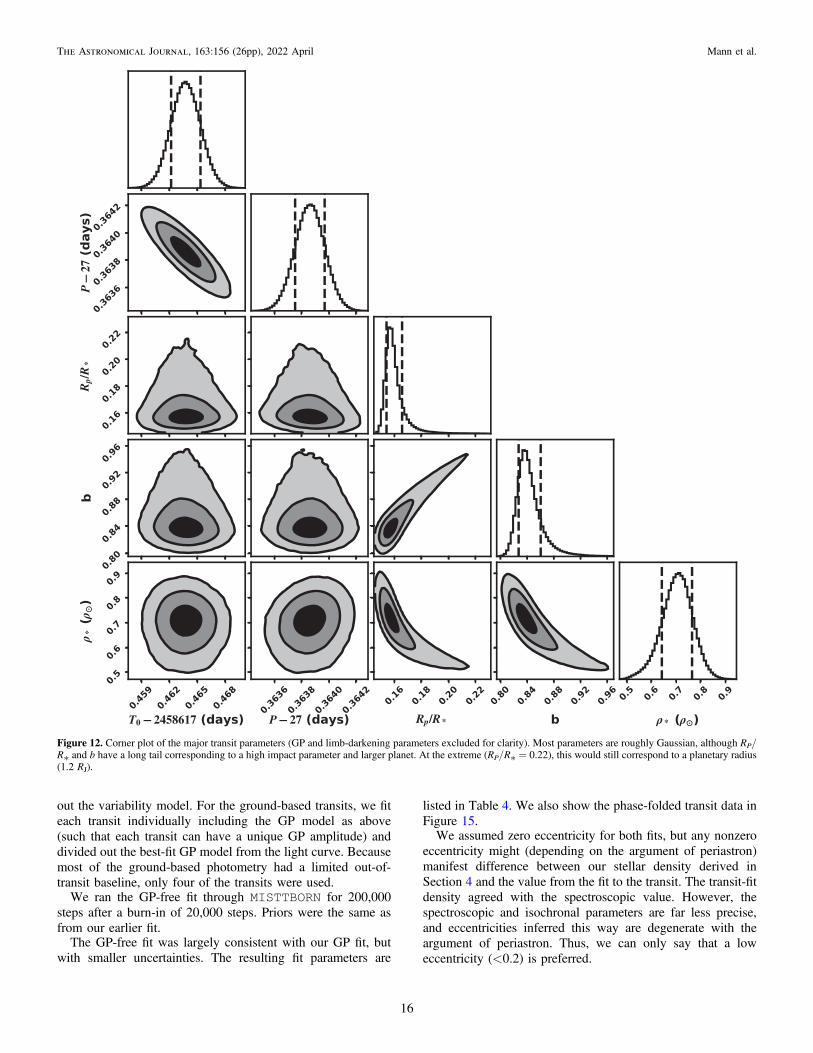
out the variability model. For the ground-based transits, we fiteach transit individually including the GP model as above(such that each transit can have a unique GP amplitude) anddivided out the best-fit GP model from the light curve. Becausemost of the ground-based photometry had a limited out-of-transit baseline, only four of the transits were used.

We ran the GP-free fit through MISTTBORN for 200,000steps after a burn-in of 20,000 steps. Priors were the same asfrom our earlier fit.

The GP-free fit was largely consistent with our GP fit, butwith smaller uncertainties. The resulting fit parameters are

listed in Table 4. We also show the phase-folded transit data inFigure 15.We assumed zero eccentricity for both fits, but any nonzero

eccentricity might (depending on the argument of periastron)manifest difference between our stellar density derived inSection 4 and the value from the fit to the transit. The transit-fitdensity agreed with the spectroscopic value. However, thespectroscopic and isochronal parameters are far less precise,and eccentricities inferred this way are degenerate with theargument of periastron. Thus, we can only say that a loweccentricity (<0.2) is preferred.

Figure 12. Corner plot of the major transit parameters (GP and limb-darkening parameters excluded for clarity). Most parameters are roughly Gaussian, although RP/R* and b have a long tail corresponding to a high impact parameter and larger planet. At the extreme (RP/R* = 0.22), this would still correspond to a planetary radius(1.2 RJ).

16

The Astronomical Journal, 163:156 (26pp), 2022 April Mann et al.

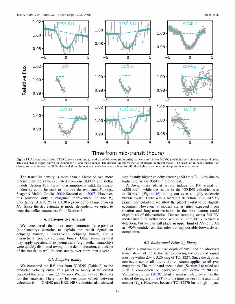
The transit-fit density is more than a factor of two moreprecise than the value estimated from our SED fit and stellarmodels (Section 4). If the e= 0 assumption is valid, the transit-fit density could be used to improve the estimated R* (e.g.,Seager & Mallén-Ornelas 2003; Sozzetti et al. 2007). However,this provided only a marginal improvement on the R*uncertainty (0.0250 Re vs. 0.030 Re) owing to a large error onM*. Since the M* estimate is model dependent, we opted tokeep the stellar parameters from Section 4.

6. False-positive Analysis

We considered the three most common false-positive(nonplanetary) scenarios to explain the transit signal: aneclipsing binary, a background eclipsing binary, and ahierarchical (bound) eclipsing binary. Other scenarios thatmay apply specifically to young stars (e.g., stellar variability)were quickly dismissed owing to the depth, duration, and shapeof the transit, as well its consistency over more than a year.

6.1. Eclipsing Binary

We compared the RV data from IGRINS (Table 2) to thepredicted velocity curve of a planet or binary at the orbitalperiod of the outer planet (27.4 days). We did not use HRS datafor this analysis. There may be zero-point offsets betweenvelocities from IGRINS and HRS. HRS velocities also showed

significantly higher velocity scatter (>500 m s−1), likely due tohigher stellar variability in the optical.A Jovian-mass planet would induce an RV signal of

;220 m s−1, while the scatter in the IGRINS velocities was;130 m s−1 (Figure 16), ruling out even a highly eccentricbrown dwarf. There was a marginal detection of a ∼0.5MJ

planet, particularly if we allow the planet’s orbit to be slightlyeccentric. However, a modest stellar jitter expected fromrotation and long-term variation in the spot pattern couldexplain all of this variation. Denser sampling and a full RVmodel including stellar noise would be more likely to yield adetection, but we can still place an upper limit of MP< 1.7MJ

at >95% confidence. This rules out any possible brown dwarfcompanion.

6.2. Background Eclipsing Binary

Given a maximum eclipse depth of 50% and an observedtransit depth of 2.5%, the star producing the observed signalmust be within Δm< 3.26 mag of TOI 1227. Since the depth isconsistent across all filters, this constraint applies to all grizmagnitudes. The multiband speckle data (Section 2.6) ruled outsuch a companion or background star down to 90 mas.Vanderburg et al. (2019) detail a similar metric based on theratio of the ingress time (T12) to the time between first and thirdcontact (T13). However, because TOI 1227b has a high impact

Figure 13. All nine transits from TESS (three transits) and ground-based follow-up (six transits) that were used in our MCMC global fit, shown in chronological order.The cyan shaded region shows the combined GP and transit model. The dashed line shows the GP fit absent the transit model. The scales of all panels match. Forclarity, we have binned the TESS data and show the scatter in each bin as error bars; for all other light curves, one point represents one exposure.

17

The Astronomical Journal, 163:156 (26pp), 2022 April Mann et al.

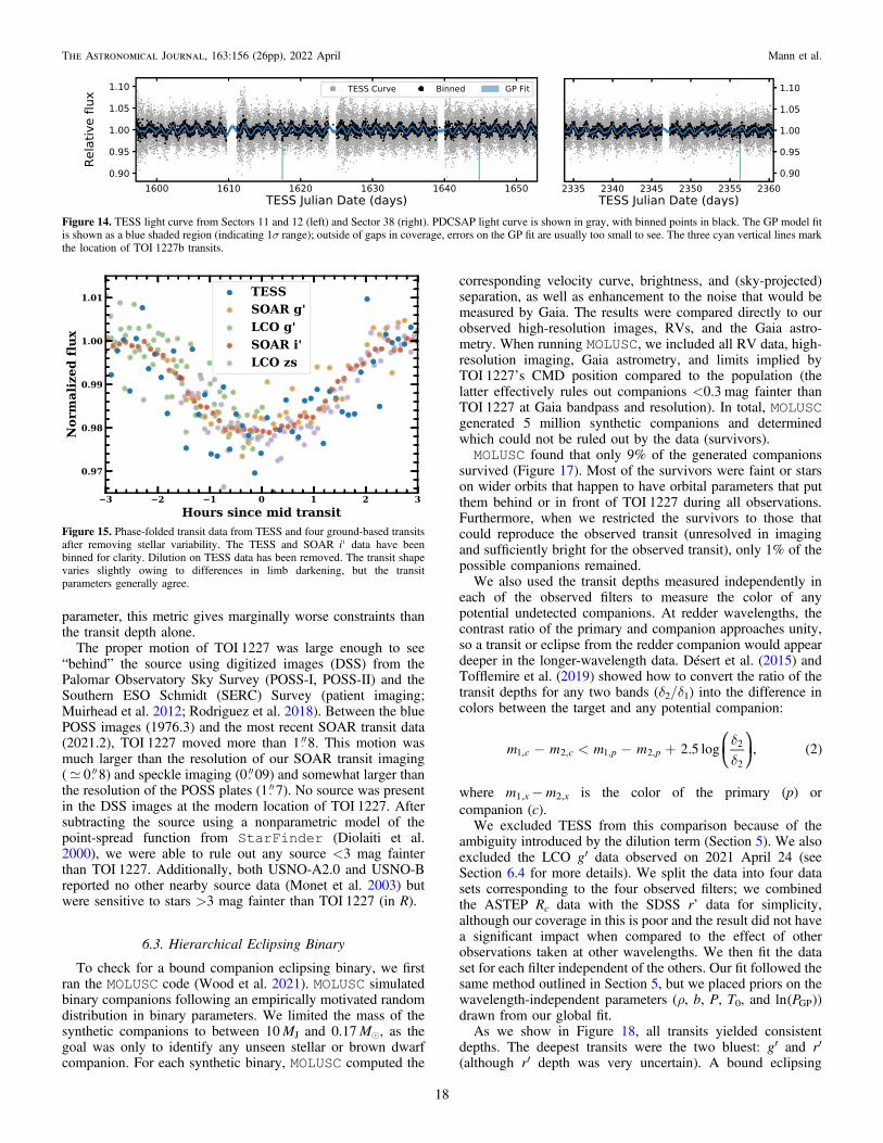
parameter, this metric gives marginally worse constraints thanthe transit depth alone.

The proper motion of TOI 1227 was large enough to see“behind” the source using digitized images (DSS) from thePalomar Observatory Sky Survey (POSS-I, POSS-II) and theSouthern ESO Schmidt (SERC) Survey (patient imaging;Muirhead et al. 2012; Rodriguez et al. 2018). Between the bluePOSS images (1976.3) and the most recent SOAR transit data(2021.2), TOI 1227 moved more than 1 8. This motion wasmuch larger than the resolution of our SOAR transit imaging(; 0 8) and speckle imaging (0 09) and somewhat larger thanthe resolution of the POSS plates (1 7). No source was presentin the DSS images at the modern location of TOI 1227. Aftersubtracting the source using a nonparametric model of thepoint-spread function from StarFinder (Diolaiti et al.2000), we were able to rule out any source <3 mag fainterthan TOI 1227. Additionally, both USNO-A2.0 and USNO-Breported no other nearby source data (Monet et al. 2003) butwere sensitive to stars >3 mag fainter than TOI 1227 (in R).

6.3. Hierarchical Eclipsing Binary

To check for a bound companion eclipsing binary, we firstran the MOLUSC code (Wood et al. 2021). MOLUSC simulatedbinary companions following an empirically motivated randomdistribution in binary parameters. We limited the mass of thesynthetic companions to between 10MJ and 0.17Me, as thegoal was only to identify any unseen stellar or brown dwarfcompanion. For each synthetic binary, MOLUSC computed the

corresponding velocity curve, brightness, and (sky-projected)separation, as well as enhancement to the noise that would bemeasured by Gaia. The results were compared directly to ourobserved high-resolution images, RVs, and the Gaia astro-metry. When running MOLUSC, we included all RV data, high-resolution imaging, Gaia astrometry, and limits implied byTOI 1227’s CMD position compared to the population (thelatter effectively rules out companions <0.3 mag fainter thanTOI 1227 at Gaia bandpass and resolution). In total, MOLUSCgenerated 5 million synthetic companions and determinedwhich could not be ruled out by the data (survivors).MOLUSC found that only 9% of the generated companions

survived (Figure 17). Most of the survivors were faint or starson wider orbits that happen to have orbital parameters that putthem behind or in front of TOI 1227 during all observations.Furthermore, when we restricted the survivors to those thatcould reproduce the observed transit (unresolved in imagingand sufficiently bright for the observed transit), only 1% of thepossible companions remained.We also used the transit depths measured independently in

each of the observed filters to measure the color of anypotential undetected companions. At redder wavelengths, thecontrast ratio of the primary and companion approaches unity,so a transit or eclipse from the redder companion would appeardeeper in the longer-wavelength data. Désert et al. (2015) andTofflemire et al. (2019) showed how to convert the ratio of thetransit depths for any two bands (δ2/δ1) into the difference incolors between the target and any potential companion:

⎜ ⎟⎛⎝

⎞⎠

( )dd

- < - +m m m m 2.5 log , 2c c p p1, 2, 1, 2,2

2

where m1,x−m2,x is the color of the primary (p) orcompanion (c).We excluded TESS from this comparison because of the

ambiguity introduced by the dilution term (Section 5). We alsoexcluded the LCO g′ data observed on 2021 April 24 (seeSection 6.4 for more details). We split the data into four datasets corresponding to the four observed filters; we combinedthe ASTEP Rc data with the SDSS r’ data for simplicity,although our coverage in this is poor and the result did not havea significant impact when compared to the effect of otherobservations taken at other wavelengths. We then fit the dataset for each filter independent of the others. Our fit followed thesame method outlined in Section 5, but we placed priors on thewavelength-independent parameters (ρ, b, P, T0, and ( )Pln GP )drawn from our global fit.As we show in Figure 18, all transits yielded consistent

depths. The deepest transits were the two bluest: g′ and r′(although r′ depth was very uncertain). A bound eclipsing

Figure 14. TESS light curve from Sectors 11 and 12 (left) and Sector 38 (right). PDCSAP light curve is shown in gray, with binned points in black. The GP model fitis shown as a blue shaded region (indicating 1σ range); outside of gaps in coverage, errors on the GP fit are usually too small to see. The three cyan vertical lines markthe location of TOI 1227b transits.

Figure 15. Phase-folded transit data from TESS and four ground-based transitsafter removing stellar variability. The TESS and SOAR ¢i data have beenbinned for clarity. Dilution on TESS data has been removed. The transit shapevaries slightly owing to differences in limb darkening, but the transitparameters generally agree.

18

The Astronomical Journal, 163:156 (26pp), 2022 April Mann et al.

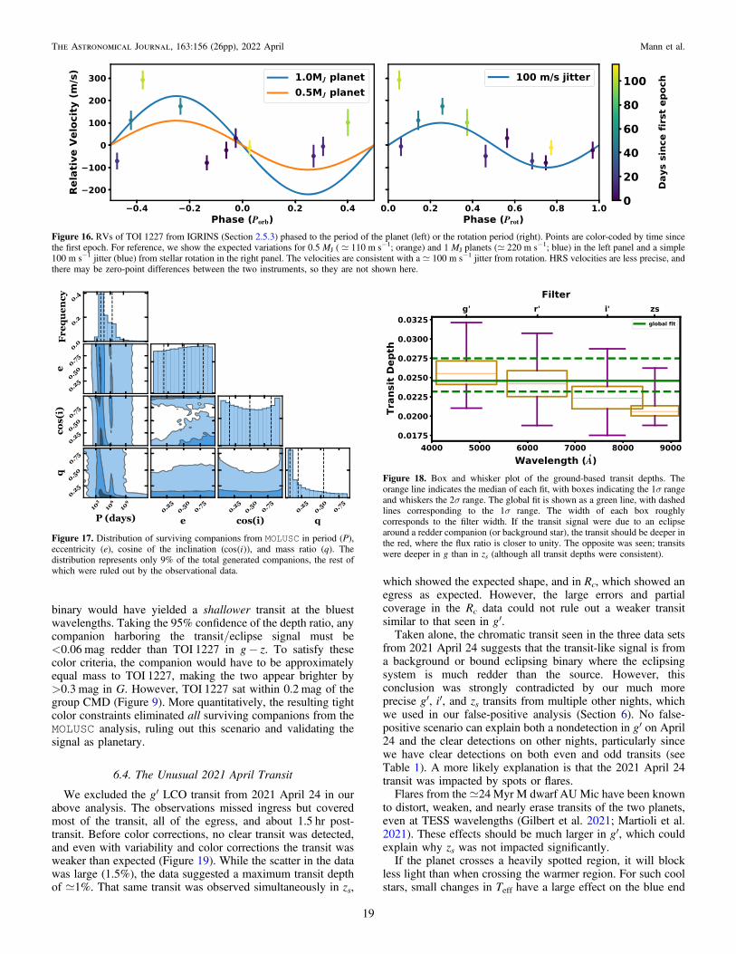
binary would have yielded a shallower transit at the bluestwavelengths. Taking the 95% confidence of the depth ratio, anycompanion harboring the transit/eclipse signal must be<0.06 mag redder than TOI 1227 in g− z. To satisfy thesecolor criteria, the companion would have to be approximatelyequal mass to TOI 1227, making the two appear brighter by>0.3 mag in G. However, TOI 1227 sat within 0.2 mag of thegroup CMD (Figure 9). More quantitatively, the resulting tightcolor constraints eliminated all surviving companions from theMOLUSC analysis, ruling out this scenario and validating thesignal as planetary.

6.4. The Unusual 2021 April Transit

We excluded the g′ LCO transit from 2021 April 24 in ourabove analysis. The observations missed ingress but coveredmost of the transit, all of the egress, and about 1.5 hr post-transit. Before color corrections, no clear transit was detected,and even with variability and color corrections the transit wasweaker than expected (Figure 19). While the scatter in the datawas large (1.5%), the data suggested a maximum transit depthof ;1%. That same transit was observed simultaneously in zs,

which showed the expected shape, and in Rc, which showed anegress as expected. However, the large errors and partialcoverage in the Rc data could not rule out a weaker transitsimilar to that seen in g′.Taken alone, the chromatic transit seen in the three data sets

from 2021 April 24 suggests that the transit-like signal is froma background or bound eclipsing binary where the eclipsingsystem is much redder than the source. However, thisconclusion was strongly contradicted by our much moreprecise g′, i′, and zs transits from multiple other nights, whichwe used in our false-positive analysis (Section 6). No false-positive scenario can explain both a nondetection in g′ on April24 and the clear detections on other nights, particularly sincewe have clear detections on both even and odd transits (seeTable 1). A more likely explanation is that the 2021 April 24transit was impacted by spots or flares.Flares from the ;24Myr M dwarf AU Mic have been known

to distort, weaken, and nearly erase transits of the two planets,even at TESS wavelengths (Gilbert et al. 2021; Martioli et al.2021). These effects should be much larger in g′, which couldexplain why zs was not impacted significantly.If the planet crosses a heavily spotted region, it will block

less light than when crossing the warmer region. For such coolstars, small changes in Teff have a large effect on the blue end

Figure 16. RVs of TOI 1227 from IGRINS (Section 2.5.3) phased to the period of the planet (left) or the rotation period (right). Points are color-coded by time sincethe first epoch. For reference, we show the expected variations for 0.5 MJ ( ; 110 m s−1; orange) and 1 MJ planets (; 220 m s−1; blue) in the left panel and a simple100 m s−1 jitter (blue) from stellar rotation in the right panel. The velocities are consistent with a ; 100 m s−1 jitter from rotation. HRS velocities are less precise, andthere may be zero-point differences between the two instruments, so they are not shown here.

Figure 17. Distribution of surviving companions from MOLUSC in period (P),eccentricity (e), cosine of the inclination ( ( )icos ), and mass ratio (q). Thedistribution represents only 9% of the total generated companions, the rest ofwhich were ruled out by the observational data.

Figure 18. Box and whisker plot of the ground-based transit depths. Theorange line indicates the median of each fit, with boxes indicating the 1σ rangeand whiskers the 2σ range. The global fit is shown as a green line, with dashedlines corresponding to the 1σ range. The width of each box roughlycorresponds to the filter width. If the transit signal were due to an eclipsearound a redder companion (or background star), the transit should be deeper inthe red, where the flux ratio is closer to unity. The opposite was seen; transitswere deeper in g than in zs (although all transit depths were consistent).

19

The Astronomical Journal, 163:156 (26pp), 2022 April Mann et al.

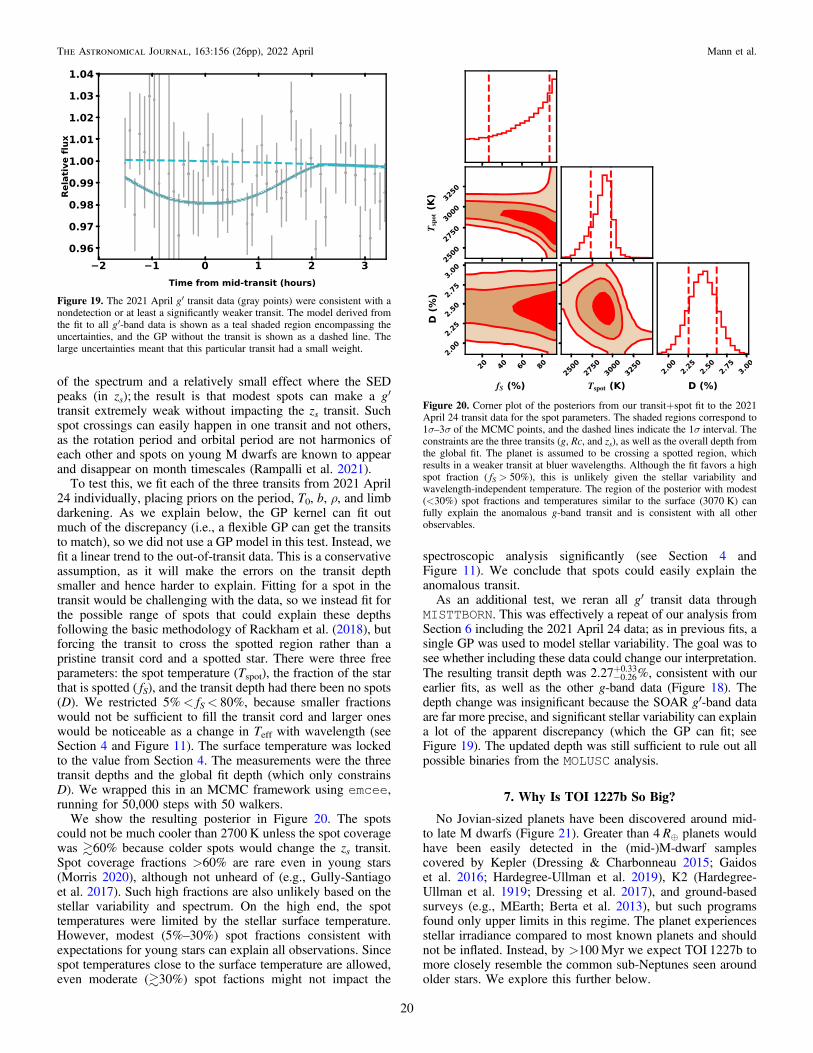
of the spectrum and a relatively small effect where the SEDpeaks (in zs); the result is that modest spots can make a g′transit extremely weak without impacting the zs transit. Suchspot crossings can easily happen in one transit and not others,as the rotation period and orbital period are not harmonics ofeach other and spots on young M dwarfs are known to appearand disappear on month timescales (Rampalli et al. 2021).

To test this, we fit each of the three transits from 2021 April24 individually, placing priors on the period, T0, b, ρ, and limbdarkening. As we explain below, the GP kernel can fit outmuch of the discrepancy (i.e., a flexible GP can get the transitsto match), so we did not use a GP model in this test. Instead, wefit a linear trend to the out-of-transit data. This is a conservativeassumption, as it will make the errors on the transit depthsmaller and hence harder to explain. Fitting for a spot in thetransit would be challenging with the data, so we instead fit forthe possible range of spots that could explain these depthsfollowing the basic methodology of Rackham et al. (2018), butforcing the transit to cross the spotted region rather than apristine transit cord and a spotted star. There were three freeparameters: the spot temperature (Tspot), the fraction of the starthat is spotted ( fS), and the transit depth had there been no spots(D). We restricted 5%< fS< 80%, because smaller fractionswould not be sufficient to fill the transit cord and larger oneswould be noticeable as a change in Teff with wavelength (seeSection 4 and Figure 11). The surface temperature was lockedto the value from Section 4. The measurements were the threetransit depths and the global fit depth (which only constrainsD). We wrapped this in an MCMC framework using emcee,running for 50,000 steps with 50 walkers.

We show the resulting posterior in Figure 20. The spotscould not be much cooler than 2700 K unless the spot coveragewas 60% because colder spots would change the zs transit.Spot coverage fractions >60% are rare even in young stars(Morris 2020), although not unheard of (e.g., Gully-Santiagoet al. 2017). Such high fractions are also unlikely based on thestellar variability and spectrum. On the high end, the spottemperatures were limited by the stellar surface temperature.However, modest (5%–30%) spot fractions consistent withexpectations for young stars can explain all observations. Sincespot temperatures close to the surface temperature are allowed,even moderate (30%) spot factions might not impact the

spectroscopic analysis significantly (see Section 4 andFigure 11). We conclude that spots could easily explain theanomalous transit.As an additional test, we reran all g′ transit data through

MISTTBORN. This was effectively a repeat of our analysis fromSection 6 including the 2021 April 24 data; as in previous fits, asingle GP was used to model stellar variability. The goal was tosee whether including these data could change our interpretation.The resulting transit depth was -

+2.27 %0.260.33 , consistent with our

earlier fits, as well as the other g-band data (Figure 18). Thedepth change was insignificant because the SOAR g′-band dataare far more precise, and significant stellar variability can explaina lot of the apparent discrepancy (which the GP can fit; seeFigure 19). The updated depth was still sufficient to rule out allpossible binaries from the MOLUSC analysis.

7. Why Is TOI 1227b So Big?

No Jovian-sized planets have been discovered around mid-to late M dwarfs (Figure 21). Greater than 4 R⊕ planets wouldhave been easily detected in the (mid-)M-dwarf samplescovered by Kepler (Dressing & Charbonneau 2015; Gaidoset al. 2016; Hardegree-Ullman et al. 2019), K2 (Hardegree-Ullman et al. 1919; Dressing et al. 2017), and ground-basedsurveys (e.g., MEarth; Berta et al. 2013), but such programsfound only upper limits in this regime. The planet experiencesstellar irradiance compared to most known planets and shouldnot be inflated. Instead, by >100Myr we expect TOI 1227b tomore closely resemble the common sub-Neptunes seen aroundolder stars. We explore this further below.

Figure 19. The 2021 April g′ transit data (gray points) were consistent with anondetection or at least a significantly weaker transit. The model derived fromthe fit to all g′-band data is shown as a teal shaded region encompassing theuncertainties, and the GP without the transit is shown as a dashed line. Thelarge uncertainties meant that this particular transit had a small weight.

Figure 20. Corner plot of the posteriors from our transit+spot fit to the 2021April 24 transit data for the spot parameters. The shaded regions correspond to1σ–3σ of the MCMC points, and the dashed lines indicate the 1σ interval. Theconstraints are the three transits (g, Rc, and zs), as well as the overall depth fromthe global fit. The planet is assumed to be crossing a spotted region, whichresults in a weaker transit at bluer wavelengths. Although the fit favors a highspot fraction ( fS > 50%), this is unlikely given the stellar variability andwavelength-independent temperature. The region of the posterior with modest(<30%) spot fractions and temperatures similar to the surface (3070 K) canfully explain the anomalous g-band transit and is consistent with all otherobservables.

20

The Astronomical Journal, 163:156 (26pp), 2022 April Mann et al.

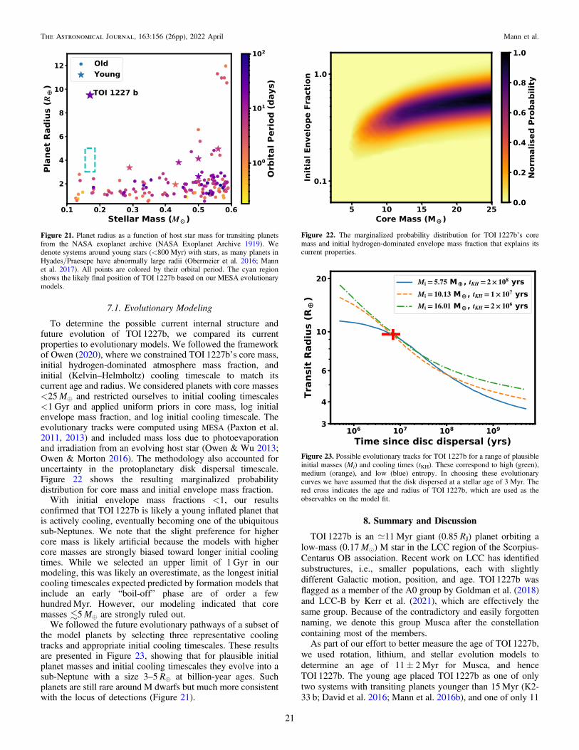
7.1. Evolutionary Modeling

To determine the possible current internal structure andfuture evolution of TOI 1227b, we compared its currentproperties to evolutionary models. We followed the frameworkof Owen (2020), where we constrained TOI 1227b’s core mass,initial hydrogen-dominated atmosphere mass fraction, andinitial (Kelvin–Helmholtz) cooling timescale to match itscurrent age and radius. We considered planets with core masses<25M⊕ and restricted ourselves to initial cooling timescales<1 Gyr and applied uniform priors in core mass, log initialenvelope mass fraction, and log initial cooling timescale. Theevolutionary tracks were computed using MESA (Paxton et al.2011, 2013) and included mass loss due to photoevaporationand irradiation from an evolving host star (Owen & Wu 2013;Owen & Morton 2016). The methodology also accounted foruncertainty in the protoplanetary disk dispersal timescale.Figure 22 shows the resulting marginalized probabilitydistribution for core mass and initial envelope mass fraction.

With initial envelope mass fractions <1, our resultsconfirmed that TOI 1227b is likely a young inflated planet thatis actively cooling, eventually becoming one of the ubiquitoussub-Neptunes. We note that the slight preference for highercore mass is likely artificial because the models with highercore masses are strongly biased toward longer initial coolingtimes. While we selected an upper limit of 1 Gyr in ourmodeling, this was likely an overestimate, as the longest initialcooling timescales expected predicted by formation models thatinclude an early “boil-off” phase are of order a fewhundredMyr. However, our modeling indicated that coremasses 5M⊕ are strongly ruled out.

We followed the future evolutionary pathways of a subset ofthe model planets by selecting three representative coolingtracks and appropriate initial cooling timescales. These resultsare presented in Figure 23, showing that for plausible initialplanet masses and initial cooling timescales they evolve into asub-Neptune with a size 3–5 R⊕ at billion-year ages. Suchplanets are still rare around M dwarfs but much more consistentwith the locus of detections (Figure 21).

8. Summary and Discussion

TOI 1227b is an ;11Myr giant (0.85 RJ) planet orbiting alow-mass (0.17Me) M star in the LCC region of the Scorpius-Centarus OB association. Recent work on LCC has identifiedsubstructures, i.e., smaller populations, each with slightlydifferent Galactic motion, position, and age. TOI 1227b wasflagged as a member of the A0 group by Goldman et al. (2018)and LCC-B by Kerr et al. (2021), which are effectively thesame group. Because of the contradictory and easily forgottennaming, we denote this group Musca after the constellationcontaining most of the members.As part of our effort to better measure the age of TOI 1227b,

we used rotation, lithium, and stellar evolution models todetermine an age of 11± 2Myr for Musca, and henceTOI 1227b. The young age placed TOI 1227b as one of onlytwo systems with transiting planets younger than 15Myr (K2-33 b; David et al. 2016; Mann et al. 2016b), and one of only 11

Figure 21. Planet radius as a function of host star mass for transiting planetsfrom the NASA exoplanet archive (NASA Exoplanet Archive 1919). Wedenote systems around young stars (<800 Myr) with stars, as many planets inHyades/Praesepe have abnormally large radii (Obermeier et al. 2016; Mannet al. 2017). All points are colored by their orbital period. The cyan regionshows the likely final position of TOI 1227b based on our MESA evolutionarymodels.

Figure 22. The marginalized probability distribution for TOI 1227b’s coremass and initial hydrogen-dominated envelope mass fraction that explains itscurrent properties.

Figure 23. Possible evolutionary tracks for TOI 1227b for a range of plausibleinitial masses (Mi) and cooling times (tKH). These correspond to high (green),medium (orange), and low (blue) entropy. In choosing these evolutionarycurves we have assumed that the disk dispersed at a stellar age of 3 Myr. Thered cross indicates the age and radius of TOI 1227b, which are used as theobservables on the model fit.

21

The Astronomical Journal, 163:156 (26pp), 2022 April Mann et al.

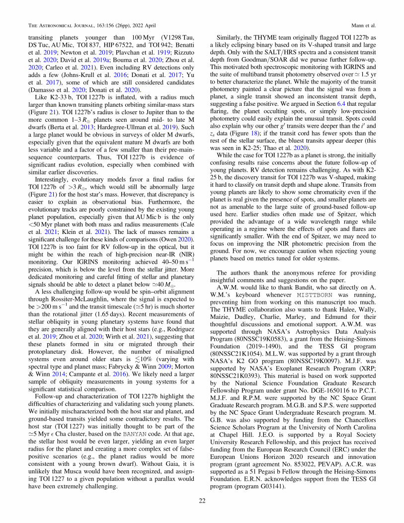
transiting planets younger than 100Myr (V1298 Tau,DS Tuc, AUMic, TOI 837, HIP 67522, and TOI 942; Benattiet al. 2019; Newton et al. 2019; Plavchan et al. 1919; Rizzutoet al. 2020; David et al. 2019a; Bouma et al. 2020; Zhou et al.2020; Carleo et al. 2021). Even including RV detections onlyadds a few (Johns-Krull et al. 2016; Donati et al. 2017; Yuet al. 2017), some of which are still considered candidates(Damasso et al. 2020; Donati et al. 2020).

Like K2-33 b, TOI 1227b is inflated, with a radius muchlarger than known transiting planets orbiting similar-mass stars(Figure 21). TOI 1227b’s radius is closer to Jupiter than to themore common 1–3 R⊕ planets seen around mid- to late Mdwarfs (Berta et al. 2013; Hardegree-Ullman et al. 2019). Sucha large planet would be obvious in surveys of older M dwarfs,especially given that the equivalent mature M dwarfs are bothless variable and a factor of a few smaller than their pre-main-sequence counterparts. Thus, TOI 1227b is evidence ofsignificant radius evolution, especially when combined withsimilar earlier discoveries.

Interestingly, evolutionary models favor a final radius forTOI 1227b of >3 R⊕, which would still be abnormally large(Figure 21) for the host star’s mass. However, that discrepancy iseasier to explain as observational bias. Furthermore, theevolutionary tracks are poorly constrained by the existing youngplanet population, especially given that AUMic b is the only<50Myr planet with both mass and radius measurements (Caleet al. 2021; Klein et al. 2021). The lack of masses remains asignificant challenge for these kinds of comparisons (Owen 2020).TOI 1227b is too faint for RV follow-up in the optical, but itmight be within the reach of high-precision near-IR (NIR)monitoring. Our IGRINS monitoring achieved 40–50m s−1

precision, which is below the level from the stellar jitter. Morededicated monitoring and careful fitting of stellar and planetarysignals should be able to detect a planet below ;40M⊕.

A less challenging follow-up would be spin–orbit alignmentthrough Rossiter-McLaughlin, where the signal is expected tobe >200 m s−1 and the transit timescale (;5 hr) is much shorterthan the rotational jitter (1.65 days). Recent measurements ofstellar obliquity in young planetary systems have found thatthey are generally aligned with their host stars (e.g., Rodriguezet al. 2019; Zhou et al. 2020; Wirth et al. 2021), suggesting thatthese planets formed in situ or migrated through theirprotoplanetary disk. However, the number of misalignedsystems even around older stars is 10% (varying withspectral type and planet mass; Fabrycky & Winn 2009; Morton& Winn 2014; Campante et al. 2016). We likely need a largersample of obliquity measurements in young systems for asignificant statistical comparison.

Follow-up and characterization of TOI 1227b highlight thedifficulties of characterizing and validating such young planets.We initially mischaracterized both the host star and planet, andground-based transits yielded some contradictory results. Thehost star (TOI 1227) was initially thought to be part of the;5Myr ò Cha cluster, based on the BANYAN code. At that age,the stellar host would be even larger, yielding an even largerradius for the planet and creating a more complex set of false-positive scenarios (e.g., the planet radius would be moreconsistent with a young brown dwarf). Without Gaia, it isunlikely that Musca would have been recognized, and assign-ing TOI 1227 to a given population without a parallax wouldhave been extremely challenging.

Similarly, the THYME team originally flagged TOI 1227b asa likely eclipsing binary based on its V-shaped transit and largedepth. Only with the SALT/HRS spectra and a consistent transitdepth from Goodman/SOAR did we pursue further follow-up.This motivated both spectroscopic monitoring with IGRINS andthe suite of multiband transit photometry observed over; 1.5 yrto better characterize the planet. While the majority of the transitphotometry painted a clear picture that the signal was from aplanet, a single transit showed an inconsistent transit depth,suggesting a false positive. We argued in Section 6.4 that regularflaring, the planet occulting spots, or simply low-precisionphotometry could easily explain the unusual transit. Spots couldalso explain why our other g′ transits were deeper than the ¢i andzs data (Figure 18); if the transit cord has fewer spots than therest of the stellar surface, the bluest transits appear deeper (thiswas seen in K2-25; Thao et al. 2020).While the case for TOI 1227b as a planet is strong, the initially

confusing results raise concerns about the future follow-up ofyoung planets. RV detection remains challenging. As with K2-25 b, the discovery transit for TOI 1227b was V-shaped, makingit hard to classify on transit depth and shape alone. Transits fromyoung planets are likely to show some chromaticity even if theplanet is real given the presence of spots, and smaller planets arenot as amenable to the large suite of ground-based follow-upused here. Earlier studies often made use of Spitzer, whichprovided the advantage of a wide wavelength range whileoperating in a regime where the effects of spots and flares aresignificantly smaller. With the end of Spitzer, we may need tofocus on improving the NIR photometric precision from theground. For now, we encourage caution when rejecting youngplanets based on metrics tuned for older systems.

The authors thank the anonymous referee for providinginsightful comments and suggestions on the paper.A.W.M. would like to thank Bandit, who sat directly on A.

W.M.’s keyboard whenever MISTTBORN was running,preventing him from working on this manuscript too much.The THYME collaboration also wants to thank Halee, Wally,Maizie, Dudley, Charlie, Marley, and Edmund for theirthoughtful discussions and emotional support. A.W.M. wassupported through NASA’s Astrophysics Data AnalysisProgram (80NSSC19K0583), a grant from the Heising-SimonsFoundation (2019–1490), and the TESS GI program(80NSSC21K1054). M.L.W. was supported by a grant throughNASA’s K2 GO program (80NSSC19K0097). M.J.F. wassupported by NASA’s Exoplanet Research Program (XRP;80NSSC21K0393). This material is based on work supportedby the National Science Foundation Graduate ResearchFellowship Program under grant No. DGE-1650116 to P.C.T.M.J.F. and R.P.M. were supported by the NC Space GrantGraduate Research program. M.G.B. and S.P.S. were supportedby the NC Space Grant Undergraduate Research program. M.G.B. was also supported by funding from the ChancellorsScience Scholars Program at the University of North Carolinaat Chapel Hill. J.E.O. is supported by a Royal SocietyUniversity Research Fellowship, and this project has receivedfunding from the European Research Council (ERC) under theEuropean Unions Horizon 2020 research and innovationprogram (grant agreement No. 853022, PEVAP). A.C.R. wassupported as a 51 Pegasi b Fellow through the Heising-SimonsFoundation. E.R.N. acknowledges support from the TESS GIprogram (program G03141).

22

The Astronomical Journal, 163:156 (26pp), 2022 April Mann et al.

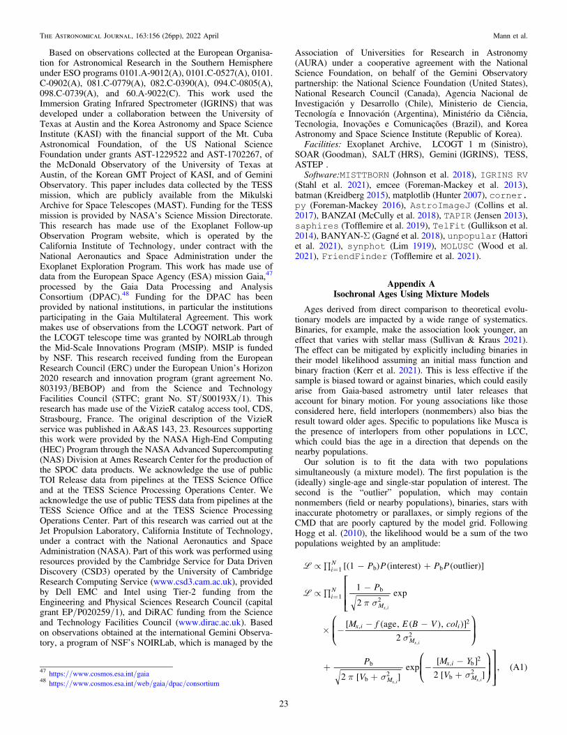
Based on observations collected at the European Organisa-tion for Astronomical Research in the Southern Hemisphereunder ESO programs 0101.A-9012(A), 0101.C-0527(A), 0101.C-0902(A), 081.C-0779(A), 082.C-0390(A), 094.C-0805(A),098.C-0739(A), and 60.A-9022(C). This work used theImmersion Grating Infrared Spectrometer (IGRINS) that wasdeveloped under a collaboration between the University ofTexas at Austin and the Korea Astronomy and Space ScienceInstitute (KASI) with the financial support of the Mt. CubaAstronomical Foundation, of the US National ScienceFoundation under grants AST-1229522 and AST-1702267, ofthe McDonald Observatory of the University of Texas atAustin, of the Korean GMT Project of KASI, and of GeminiObservatory. This paper includes data collected by the TESSmission, which are publicly available from the MikulskiArchive for Space Telescopes (MAST). Funding for the TESSmission is provided by NASA’s Science Mission Directorate.This research has made use of the Exoplanet Follow-upObservation Program website, which is operated by theCalifornia Institute of Technology, under contract with theNational Aeronautics and Space Administration under theExoplanet Exploration Program. This work has made use ofdata from the European Space Agency (ESA) mission Gaia,47

processed by the Gaia Data Processing and AnalysisConsortium (DPAC).48 Funding for the DPAC has beenprovided by national institutions, in particular the institutionsparticipating in the Gaia Multilateral Agreement. This workmakes use of observations from the LCOGT network. Part ofthe LCOGT telescope time was granted by NOIRLab throughthe Mid-Scale Innovations Program (MSIP). MSIP is fundedby NSF. This research received funding from the EuropeanResearch Council (ERC) under the European Union’s Horizon2020 research and innovation program (grant agreement No.803193/BEBOP) and from the Science and TechnologyFacilities Council (STFC; grant No. ST/S00193X/1). Thisresearch has made use of the VizieR catalog access tool, CDS,Strasbourg, France. The original description of the VizieRservice was published in A&AS 143, 23. Resources supportingthis work were provided by the NASA High-End Computing(HEC) Program through the NASA Advanced Supercomputing(NAS) Division at Ames Research Center for the production ofthe SPOC data products. We acknowledge the use of publicTOI Release data from pipelines at the TESS Science Officeand at the TESS Science Processing Operations Center. Weacknowledge the use of public TESS data from pipelines at theTESS Science Office and at the TESS Science ProcessingOperations Center. Part of this research was carried out at theJet Propulsion Laboratory, California Institute of Technology,under a contract with the National Aeronautics and SpaceAdministration (NASA). Part of this work was performed usingresources provided by the Cambridge Service for Data DrivenDiscovery (CSD3) operated by the University of CambridgeResearch Computing Service (www.csd3.cam.ac.uk), providedby Dell EMC and Intel using Tier-2 funding from theEngineering and Physical Sciences Research Council (capitalgrant EP/P020259/1), and DiRAC funding from the Scienceand Technology Facilities Council (www.dirac.ac.uk). Basedon observations obtained at the international Gemini Observa-tory, a program of NSFʼs NOIRLab, which is managed by the

Association of Universities for Research in Astronomy(AURA) under a cooperative agreement with the NationalScience Foundation, on behalf of the Gemini Observatorypartnership: the National Science Foundation (United States),National Research Council (Canada), Agencia Nacional deInvestigación y Desarrollo (Chile), Ministerio de Ciencia,Tecnología e Innovación (Argentina), Ministério da Ciência,Tecnologia, Inovações e Comunicações (Brazil), and KoreaAstronomy and Space Science Institute (Republic of Korea).Facilities: Exoplanet Archive, LCOGT 1 m (Sinistro),

SOAR (Goodman), SALT (HRS), Gemini (IGRINS), TESS,ASTEP .Software:MISTTBORN (Johnson et al. 2018), IGRINS RV

(Stahl et al. 2021), emcee (Foreman-Mackey et al. 2013),batman (Kreidberg 2015), matplotlib (Hunter 2007), corner.py (Foreman-Mackey 2016), AstroImageJ (Collins et al.2017), BANZAI (McCully et al. 2018), TAPIR (Jensen 2013),saphires (Tofflemire et al. 2019), TelFit (Gullikson et al.2014), BANYAN-Σ (Gagné et al. 2018), unpopular (Hattoriet al. 2021), synphot (Lim 1919), MOLUSC (Wood et al.2021), FriendFinder (Tofflemire et al. 2021).

Appendix AIsochronal Ages Using Mixture Models

Ages derived from direct comparison to theoretical evolu-tionary models are impacted by a wide range of systematics.Binaries, for example, make the association look younger, aneffect that varies with stellar mass (Sullivan & Kraus 2021).The effect can be mitigated by explicitly including binaries intheir model likelihood assuming an initial mass function andbinary fraction (Kerr et al. 2021). This is less effective if thesample is biased toward or against binaries, which could easilyarise from Gaia-based astrometry until later releases thataccount for binary motion. For young associations like thoseconsidered here, field interlopers (nonmembers) also bias theresult toward older ages. Specific to populations like Musca isthe presence of interlopers from other populations in LCC,which could bias the age in a direction that depends on thenearby populations.Our solution is to fit the data with two populations

simultaneously (a mixture model). The first population is the(ideally) single-age and single-star population of interest. Thesecond is the “outlier” population, which may containnonmembers (field or nearby populations), binaries, stars withinaccurate photometry or parallaxes, or simply regions of theCMD that are poorly captured by the model grid. FollowingHogg et al. (2010), the likelihood would be a sum of the twopopulations weighted by an amplitude:

⎡

⎣

⎢⎢

⎛

⎝⎜

⎞

⎠⎟

⎛

⎝⎜

⎞

⎠⎟

⎤

⎦

⎥⎥

[( ) ( ) ( )]

[ ( ( ) )]

[ ]

[ ][ ]

( )

p s

s

p s s

µ - +

µ -

´ -- -

++

--+

=

=

P P P P

P

M f E B V col

P

V

M Y

V

1 interest outlier

1

2exp

age, ,

2

2exp

2, A1

iN

iN

M

x i i

M

M

x i

M

1 b b

1b

2

,2

2

b

b2

, b2

b2

x i

x i

x i x i

,

,

, ,

L

L

47 https://www.cosmos.esa.int/gaia48 https://www.cosmos.esa.int/web/gaia/dpac/consortium

23

The Astronomical Journal, 163:156 (26pp), 2022 April Mann et al.

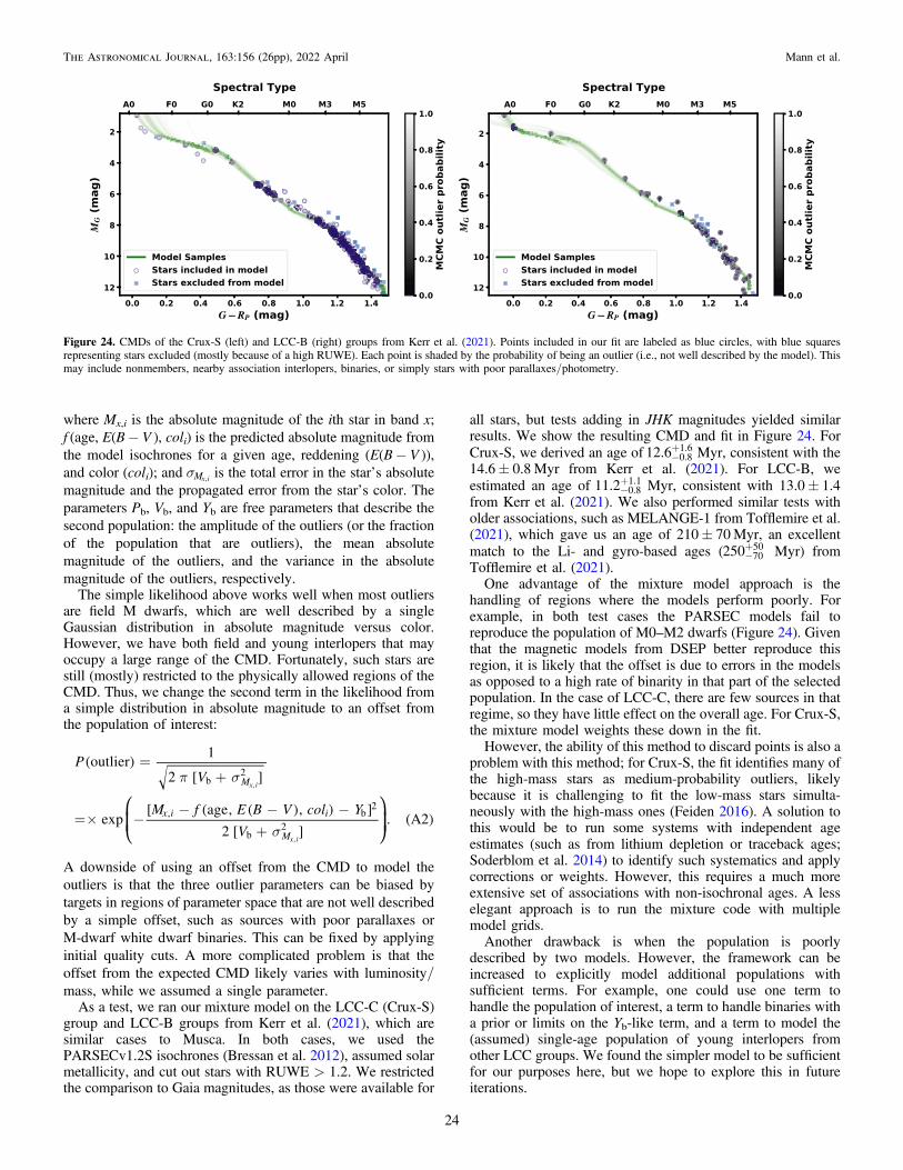
where Mx,i is the absolute magnitude of the ith star in band x;f (age, E(B− V ), coli) is the predicted absolute magnitude fromthe model isochrones for a given age, reddening (E(B− V )),and color (coli); and sMx i, is the total error in the star’s absolutemagnitude and the propagated error from the star’s color. Theparameters Pb, Vb, and Yb are free parameters that describe thesecond population: the amplitude of the outliers (or the fractionof the population that are outliers), the mean absolutemagnitude of the outliers, and the variance in the absolutemagnitude of the outliers, respectively.

The simple likelihood above works well when most outliersare field M dwarfs, which are well described by a singleGaussian distribution in absolute magnitude versus color.However, we have both field and young interlopers that mayoccupy a large range of the CMD. Fortunately, such stars arestill (mostly) restricted to the physically allowed regions of theCMD. Thus, we change the second term in the likelihood froma simple distribution in absolute magnitude to an offset fromthe population of interest:

⎛

⎝⎜

⎞

⎠⎟

( )[ ]

[ ( ( ) ) ][ ]

( )

p s

s

=+

=´ -- - -

+

PV

M f E B V col Y

V

outlier1

2

expage, ,

2. A2

M

x i i

M

b2

, b2

b2

x i

x i

,

,

A downside of using an offset from the CMD to model theoutliers is that the three outlier parameters can be biased bytargets in regions of parameter space that are not well describedby a simple offset, such as sources with poor parallaxes orM-dwarf white dwarf binaries. This can be fixed by applyinginitial quality cuts. A more complicated problem is that theoffset from the expected CMD likely varies with luminosity/mass, while we assumed a single parameter.

As a test, we ran our mixture model on the LCC-C (Crux-S)group and LCC-B groups from Kerr et al. (2021), which aresimilar cases to Musca. In both cases, we used thePARSECv1.2S isochrones (Bressan et al. 2012), assumed solarmetallicity, and cut out stars with RUWE > 1.2. We restrictedthe comparison to Gaia magnitudes, as those were available for

all stars, but tests adding in JHK magnitudes yielded similarresults. We show the resulting CMD and fit in Figure 24. ForCrux-S, we derived an age of -

+12.6 0.81.6 Myr, consistent with the

14.6± 0.8 Myr from Kerr et al. (2021). For LCC-B, weestimated an age of -

+11.2 0.81.1 Myr, consistent with 13.0± 1.4

from Kerr et al. (2021). We also performed similar tests witholder associations, such as MELANGE-1 from Tofflemire et al.(2021), which gave us an age of 210± 70Myr, an excellentmatch to the Li- and gyro-based ages ( -

+250 7050 Myr) from

Tofflemire et al. (2021).One advantage of the mixture model approach is the

handling of regions where the models perform poorly. Forexample, in both test cases the PARSEC models fail toreproduce the population of M0–M2 dwarfs (Figure 24). Giventhat the magnetic models from DSEP better reproduce thisregion, it is likely that the offset is due to errors in the modelsas opposed to a high rate of binarity in that part of the selectedpopulation. In the case of LCC-C, there are few sources in thatregime, so they have little effect on the overall age. For Crux-S,the mixture model weights these down in the fit.However, the ability of this method to discard points is also a

problem with this method; for Crux-S, the fit identifies many ofthe high-mass stars as medium-probability outliers, likelybecause it is challenging to fit the low-mass stars simulta-neously with the high-mass ones (Feiden 2016). A solution tothis would be to run some systems with independent ageestimates (such as from lithium depletion or traceback ages;Soderblom et al. 2014) to identify such systematics and applycorrections or weights. However, this requires a much moreextensive set of associations with non-isochronal ages. A lesselegant approach is to run the mixture code with multiplemodel grids.Another drawback is when the population is poorly

described by two models. However, the framework can beincreased to explicitly model additional populations withsufficient terms. For example, one could use one term tohandle the population of interest, a term to handle binaries witha prior or limits on the Yb-like term, and a term to model the(assumed) single-age population of young interlopers fromother LCC groups. We found the simpler model to be sufficientfor our purposes here, but we hope to explore this in futureiterations.

Figure 24. CMDs of the Crux-S (left) and LCC-B (right) groups from Kerr et al. (2021). Points included in our fit are labeled as blue circles, with blue squaresrepresenting stars excluded (mostly because of a high RUWE). Each point is shaded by the probability of being an outlier (i.e., not well described by the model). Thismay include nonmembers, nearby association interlopers, binaries, or simply stars with poor parallaxes/photometry.

24

The Astronomical Journal, 163:156 (26pp), 2022 April Mann et al.

ORCID iDs

Andrew W. Mann https://orcid.org/0000-0003-3654-1602Mackenna L. Wood https://orcid.org/0000-0001-7336-7725James E. Owen https://orcid.org/0000-0002-4856-7837Benjamin M. Tofflemire https://orcid.org/0000-0003-2053-0749Elisabeth R. Newton https://orcid.org/0000-0003-4150-841XEric E. Mamajek https://orcid.org/0000-0003-2008-1488Gregory N. Mace https://orcid.org/0000-0001-7875-6391Adam L. Kraus https://orcid.org/0000-0001-9811-568XPa Chia Thao https://orcid.org/0000-0001-5729-6576Andrew Vanderburg https://orcid.org/0000-0001-7246-5438Joe Llama https://orcid.org/0000-0003-4450-0368Christopher M. Johns-Krull https://orcid.org/0000-0002-8828-6386L. Prato https://orcid.org/0000-0001-7998-226XAsa G. Stahl https://orcid.org/0000-0002-0848-6960Shih-Yun Tang https://orcid.org/0000-0003-4247-1401Karen A. Collins https://orcid.org/0000-0001-6588-9574Kevin I. Collins https://orcid.org/0000-0003-2781-3207Tianjun Gan https://orcid.org/0000-0002-4503-9705Eric L. N. Jensen https://orcid.org/0000-0002-4625-7333Richard P. Schwarz https://orcid.org/0000-0001-8227-1020Elise Furlan https://orcid.org/0000-0001-9800-6248Steve B. Howell https://orcid.org/0000-0002-2532-2853Kathryn V. Lester https://orcid.org/0000-0002-9903-9911Olga Suarez https://orcid.org/0000-0002-3503-3617Djamel Mekarnia https://orcid.org/0000-0001-5000-7292Tristan Guillot https://orcid.org/0000-0002-7188-8428Amaury H. M. J. Triaud https://orcid.org/0000-0002-5510-8751Marshall C. Johnson https://orcid.org/0000-0002-5099-8185Aaron C. Rizzuto https://orcid.org/0000-0001-9982-1332Samuel N. Quinn https://orcid.org/0000-0002-8964-8377Ronan Kerr https://orcid.org/0000-0002-6549-9792George R. Ricker https://orcid.org/0000-0003-2058-6662Roland Vanderspek https://orcid.org/0000-0001-6763-6562David W. Latham https://orcid.org/0000-0001-9911-7388Joshua N. Winn https://orcid.org/0000-0002-4265-047XJon M. Jenkins https://orcid.org/0000-0002-4715-9460Natalia M. Guerrero https://orcid.org/0000-0002-5169-9427Avi Shporer https://orcid.org/0000-0002-1836-3120Joshua E. Schlieder https://orcid.org/0000-0001-5347-7062Brian McLean https://orcid.org/0000-0002-8058-643X

References

Abe, L., Gonçalves, I., Agabi, A., et al. 2013, A&A, 553, A49Aigrain, S., Parviainen, H., & Pope, B. J. S. 2016, MNRAS, 459, 2408Alibert, Y., Mordasini, C., Benz, W., & Winisdoerffer, C. 2005, A&A,

434, 343Asplund, M., Grevesse, N., Sauval, A. J., & Scott, P. 2009, ARA&A, 47, 481Baraffe, I., Homeier, D., Allard, F., & Chabrier, G. 2015, A&A, 577, A42Bell, C. P. M., Mamajek, E. E., & Naylor, T. 2015, MNRAS, 454, 593Benatti, S., Nardiello, D., Malavolta, L., et al. 2019, A&A, 630, A81Berta, Z. K., Irwin, J., & Charbonneau, D. 2013, ApJ, 775, 91Blackwell, D. E., & Shallis, M. J. 1977, MNRAS, 180, 177Bonfils, X., Delfosse, X., Udry, S., et al. 2013, A&A, 549, A109Bouma, L. G., Hartman, J. D., Brahm, R., et al. 2020, AJ, 160, 239Boyajian, T. S., von Braun, K., van Belle, G., et al. 2012, ApJ, 757, 112Brandeker, A., & Cataldi, G. 2019, A&A, 621, A86

Bressan, A., Marigo, P., Girardi, L., et al. 2012, MNRAS, 427, 127Brown, T. M., Baliber, N., Bianco, F. B., et al. 2013, PASP, 125, 1031Buckley, D. A. H., Swart, G. P., & Meiring, J. G. 2006, Proc. SPIE, 6267,

62670ZBurt, J. A., Nielsen, L. D., Quinn, S. N., et al. 2020, AJ, 160, 153Cale, B., Reefe, M., Plavchan, P., et al. 2021, AJ, 162, 295Campante, T. L., Lund, M. N., Kuszlewicz, J. S., et al. 2016, ApJ, 819, 85Cantat-Gaudin, T., Jordi, C., Vallenari, A., et al. 2018, A&A, 618, A93Canto Martins, B. L., Gomes, R. L., Messias, Y. S., et al. 1919, ApJS, 250, 20Cardelli, J. A., Clayton, G. C., & Mathis, J. S. 1989, ApJ, 345, 245Carleo, I., Desidera, S., Nardiello, D., et al. 2021, A&A, 645, A71Casagrande, L., Flynn, C., & Bessell, M. 2008, MNRAS, 389, 585Chabrier, G., Baraffe, I., & Plez, B. 1996, ApJL, 459, L91Clemens, J. C., Crain, J. A., & Anderson, R. 2004, Proc. SPIE, 5492, 331Collins, K. A., Kielkopf, J. F., Stassun, K. G., & Hessman, F. V. 2017, AJ,

153, 77Crause, L. A., Sharples, R. M., Bramall, D. G., et al. 2014, Proc. SPIE, 9147,

91476TCutri, R. M., Skrutskie, M. F., van Dyk, S., et al. 2014, yCat, II, 328Damasso, M., Lanza, A. F., Benatti, S., et al. 2020, A&A, 642, A133Damiani, F., Prisinzano, L., Pillitteri, I., Micela, G., & Sciortino, S. 2019,

A&A, 623, A112David, T. J., Cody, A. M., Hedges, C. L., et al. 2019b, AJ, 158, 79David, T. J., Hillenbrand, L. A., Petigura, E. A., et al. 2016, Natur, 534, 658David, T. J., Mamajek, E. E., Vanderburg, A., et al. 2018, AJ, 156, 302David, T. J., Petigura, E. A., Luger, R., et al. 2019a, ApJL, 885, L12Désert, J.-M., Charbonneau, D., Torres, G., et al. 2015, ApJ, 804, 59Desidera, S., Covino, E., Messina, S., et al. 2015, A&A, 573, A126Diolaiti, E., Bendinelli, O., Bonaccini, D., et al. 2000, A&AS, 147, 335Donati, J. F., Bouvier, J., Alencar, S. H., et al. 2020, MNRAS, 491, 5660Donati, J.-F., Yu, L., Moutou, C., et al. 2017, MNRAS, 465, 3343Dotter, A., Chaboyer, B., Jevremović, D., et al. 2008, ApJS, 178, 89Dressing, C. D., & Charbonneau, D. 2015, ApJ, 807, 45Dressing, C. D., Vanderburg, A., Schlieder, J. E., et al. 2017, AJ, 154, 207ExoFOP 2019, Exoplanet Follow-up Observing Program—TESS, v2021-08,

IPAC, doi:10.26134/EXOFOP3Fabrycky, D. C., & Winn, J. N. 2009, ApJ, 696, 1230Feiden, G. A. 2016, A&A, 593, A99Feiden, G. A., & Chaboyer, B. 2012, ApJ, 761, 30Fleming, T. A., Schmitt, J. H. M. M., & Giampapa, M. S. 1995, ApJ, 450,

401Foreman-Mackey, D. 2016, JOSS, 1Foreman-Mackey, D., Agol, E., Ambikasaran, S., & Angus, R. 2017, AJ,

154, 220Foreman-Mackey, D., Hogg, D. W., Lang, D., & Goodman, J. 2013, PASP,

125, 306Gaia Collaboration, Brown, A. G. A., Vallenari, A., et al. 2021, A&A, 649, A1Gagné, J., David, T. J., Mamajek, E. E., et al. 1919, ApJ, 903, 96Gagné, J., Mamajek, E. E., Malo, L., et al. 2018, ApJ, 856, 23Gaidos, E., Mann, A. W., Kraus, A. L., & Ireland, M. 2016, MNRAS,

457, 2877Gao, P., & Zhang, X. 2020, ApJ, 890, 93Gilbert, E. A., Barclay, T., Quintana, E. V., et al. 2021, arXiv:2109.03924Goldman, B., Röser, S., Schilbach, E., Moór, A. C., & Henning, T. 2018, ApJ,

868, 32Grevesse, N., & Sauval, A. J. 1998, SSRv, 85, 161Guerrero, N. M., Seager, S., Huang, C. X., et al. 2021, ApJS, 254, 39Guillot, T., Abe, L., Agabi, A., et al. 2015, AN, 336, 638Gullikson, K., Dodson-Robinson, S., & Kraus, A. 2014, AJ, 148, 53Gully-Santiago, M. A., Herczeg, G. J., Czekala, I., et al. 2017, ApJ, 836, 200Hardegree-Ullman, K. K., Cushing, M. C., Muirhead, P. S., &

Christiansen, J. L. 2019, AJ, 158, 75Hardegree-Ullman, K. K., Zink, J. K., Christiansen, J. L., et al. 1919, ApJS,

247, 28Hattori, S., Foreman-Mackey, D., Hogg, D. W., et al. 2021, arXiv:2106.15063Hogg, D. W., Bovy, J., & Lang, D. 2010, arXiv:1008.4686Horne, J. H., & Baliunas, S. L. 1986, ApJ, 302, 757Howell, S. B., Everett, M. E., Sherry, W., Horch, E., & Ciardi, D. R. 2011, AJ,

142, 19Hunter, J. D. 2007, CSE, 9, 90Husser, T.-O., Wende-von Berg, S., Dreizler, S., et al. 2013, A&A, 553, A6James, D. J., Melo, C., Santos, N. C., & Bouvier, J. 2006, A&A, 446, 971Jenkins, J. M. 2002, ApJ, 575, 493Jenkins, J. M., Chandrasekaran, H., McCauliff, S. D., et al. 2010, Proc. SPIE,

7740, 77400DJenkins, J. M., Twicken, J. D., McCauliff, S., et al. 2016, Proc. SPIE, 9913,

99133E

25

The Astronomical Journal, 163:156 (26pp), 2022 April Mann et al.

Jensen, E. 2013, Tapir: A web interface for transit/eclipse observability,Astrophysics Source Code Library, Astrophysics Source Code Library,ascl:1306.007

Johns-Krull, C. M., McLane, J. N., Prato, L., et al. 2016, ApJ, 826, 206Johnson, M. C., Dai, F., Justesen, A. B., et al. 2018, MNRAS, 481, 596Johnston, H. M., & Verbunt, F. 1996, A&A, 312, 80Katz, D., Sartoretti, P., Cropper, M., et al. 2019, A&A, 622, A205Kerr, R. M. P., Rizzuto, A. C., Kraus, A. L., & Offner, S. S. R. 2021, ApJ,

917, 23Kesseli, A. Y., West, A. A., Veyette, M., et al. 2017, ApJS, 230, 16Kharchenko, N. V., Scholz, R. D., Piskunov, A. E., Röser, S., & Schilbach, E.

2007, AN, 328, 889Kipping, D. M. 2013, MNRAS, 435, 2152Klein, B., Donati, J.-F., Moutou, C., et al. 2021, MNRAS, 502, 188Kniazev, A. Y., Gvaramadze, V. V., & Berdnikov, L. N. 2016, MNRAS,

459, 3068Kreidberg, L. 2015, PASP, 127, 1161Kunder, A., Kordopatis, G., Steinmetz, M., et al. 2017, AJ, 153, 75Lee, J.-J., Gullikson, K., & Kaplan, K. 2017, igrins/plp 2.2.0, Zenodo, doi:10.

5281/zenodo.845059Li, J., Tenenbaum, P., Twicken, J. D., et al. 2019, PASP, 131, 024506Lim, P. L. 1919, synphot, 1.0.1, Zenodo, doi:10.5281/zenodo.3971036Lindegren, L., Klioner, S. A., Hernández, J., et al. 2021, A&A, 649, A2Linder, E. F., Mordasini, C., Mollière, P., et al. 2019, A&A, 623, A85Lopez, E. D., & Fortney, J. J. 2013, ApJ, 776, 2Lopez Martí, B., Jimenez Esteban, F., Bayo, A., et al. 2013, A&A, 551, A46Mace, G., Jaffe, D., Park, C., & Lee, J.-J. 2016a, tellar radial velocities with

IGRINS at McDonald Observatory, Zenodo, doi:10.5281/zenodo.56434Mace, G., Kim, H., Jaffe, D. T., et al. 2016b, Proc. SPIE, 9908, 99080CMace, G., Sokal, K., Lee, J.-J., et al. 2018, Proc. SPIE, 10702, 107020QMalo, L., Artigau, É., Doyon, R., et al. 2014, ApJ, 788, 81Mann, A. W., Gaidos, E., & Aldering, G. 2011, PASP, 123, 1273Mann, A. W., Gaidos, E., Mace, G. N., et al. 2016a, ApJ, 818, 46Mann, A. W., Gaidos, E., Vanderburg, A., et al. 2017, AJ, 153, 64Mann, A. W., Johnson, M. C., Vanderburg, A., et al. 2020, AJ, 160, 179Mann, A. W., Newton, E. R., Rizzuto, A. C., et al. 2016b, AJ, 152, 61Mann, A. W., Vanderburg, A., Rizzuto, A. C., et al. 2018, AJ, 155, 4Martioli, E., Hébrard, G., Correia, A. C. M., Laskar, J., &

Lecavelier des Etangs, A. 2021, A&A, 649, A177Masuda, K., & Winn, J. N. 2020, AJ, 159, 81Matthews, A. G. D. G., van der Wilk, M., Nickson, T., et al. 2017, J. Mach.

Learn. Res., 18, 1McCully, C., Volgenau, N. H., Harbeck, D.-R., et al. 2018, Proc. SPIE, 10707,

107070KMékarnia, D., Guillot, T., Rivet, J. P., et al. 2016, MNRAS, 463, 45Monet, D. G., Levine, S. E., Canzian, B., et al. 2003, AJ, 125, 984Morrell, S., & Naylor, T. 2019, MNRAS, 489, 2615Morris, B. M. 2020, ApJ, 893, 67Morton, T. D. 2015, Isochrones: Stellar model Grid Package, Astrophysics

Source Code Library, ascl:1503.010Morton, T. D., & Winn, J. N. 2014, ApJ, 796, 47Muirhead, P. S., Johnson, J. A., Apps, K., et al. 2012, ApJ, 747, 144Murphy, S. J., Lawson, W. A., & Bessell, M. S. 2013, MNRAS, 435, 1325NASA Exoplanet Archive 1919, Planetary Systems, NExScI-Caltech/IPAC,

doi:10.26133/NEA12Nelson, B. E., Ford, E. B., & Rasio, F. A. 2017, AJ, 154, 106Newton, E. R., Irwin, J., Charbonneau, D., et al. 2017, ApJ, 834, 85Newton, E. R., Mann, A. W., Kraus, A. L., et al. 2021, AJ, 161, 65Newton, E. R., Mann, A. W., Tofflemire, B. M., et al. 2019, ApJL, 880, L17Obermeier, C., Henning, T., Schlieder, J. E., et al. 2016, AJ, 152, 223Onken, C. A., Wolf, C., Bessell, M. S., et al. 2019, PASA, 36, e033Owen, J. E. 2020, MNRAS, 498, 5030Owen, J. E., & Lai, D. 2018, MNRAS, 479, 5012Owen, J. E., & Morton, T. D. 2016, ApJL, 819, L10Owen, J. E., & Wu, Y. 2013, ApJ, 775, 105Park, C., Jaffe, D. T., Yuk, I.-S., et al. 2014, Proc. SPIE, 9147, 91471DParviainen, H., & Aigrain, S. 2015, MNRAS, 453, 3821Paxton, B., Bildsten, L., Dotter, A., et al. 2011, ApJS, 192, 3Paxton, B., Cantiello, M., Arras, P., et al. 2013, ApJS, 208, 4

Pecaut, M. J., & Mamajek, E. E. 2013, ApJS, 208, 9Pecaut, M. J., & Mamajek, E. E. 2016, MNRAS, 461, 794Pepper, J., Kane, S. R., Rodriguez, J. E., et al. 2020, AJ, 159, 243Plavchan, P., Barclay, T., Gagné, J., et al. 1919, Natur, 582, 497Rackham, B. V., Apai, D., & Giampapa, M. S. 2018, ApJ, 853, 122Raghavan, D., McAlister, H. A., Henry, T. J., et al. 2010, ApJS, 190, 1Rajpurohit, A. S., Allard, F., Teixeira, G. D. C., et al. 2018, A&A, 610, A19Rampalli, R., Agüeros, M. A., Curtis, J. L., et al. 2021, ApJ, 921, 167Raymond, S. N., Barnes, R., & Mandell, A. M. 2008, MNRAS, 384, 663Rebull, L. M., Stauffer, J. R., Cody, A. M., et al. 2018, AJ, 155, 196Ricker, G. R., Winn, J. N., Vanderspek, R., et al. 2014, Proc. SPIE, 9143, 20Riello, M., De Angeli, F., Evans, D. W., et al. 2021, A&A, 649, A3Rizzuto, A. C., Ireland, M. J., & Kraus, A. L. 2015, MNRAS, 448, 2737Rizzuto, A. C., Mann, A. W., Vanderburg, A., Kraus, A. L., & Covey, K. R.

2017, AJ, 154, 224Rizzuto, A. C., Newton, E. R., Mann, A. W., et al. 2020, AJ, 160, 33Rodriguez, J. E., Eastman, J. D., Zhou, G., et al. 2019, AJ, 158, 197Rodriguez, J. E., Vanderburg, A., Eastman, J. D., et al. 2018, AJ, 155, 72Rothman, L. S., Gordon, I. E., Barbe, A., et al. 2009, J. Quant. Spec. Radiat.

Transf., 110, 533Rucinski, S. M. 1992, AJ, 104, 1968Schneider, A. C., Shkolnik, E. L., Allers, K. N., et al. 2019, AJ, 157, 234Scott, N. J., Howell, S. B., Horch, E. P., & Everett, M. E. 2018, PASP, 130,

054502Seager, S., & Mallén-Ornelas, G. 2003, ApJ, 585, 1038Segura, A., Kasting, J. F., Meadows, V., et al. 2005, AsBio, 5, 706Shkolnik, E. L., Allers, K. N., Kraus, A. L., Liu, M. C., & Flagg, L. 2017, AJ,

154, 69Skrutskie, M. F., Cutri, R. M., Stiening, R., et al. 2006, AJ, 131, 1163Smith, J. C., Stumpe, M. C., Van Cleve, J. E., et al. 2012, PASP, 124, 1000Soderblom, D. R., Hillenbrand, L. A., Jeffries, R. D., Mamajek, E. E., &

Naylor, T. 2014, in Protostars and Planets VI, ed. H. Beuther et al. (Tucson,AZ: Univ. of Arizona Press), 219

Sokal, K. R., Johns-Krull, C. M., Mace, G. N., et al. 1919, ApJ, 888, 116Sozzetti, A., Torres, G., Charbonneau, D., et al. 2007, ApJ, 664, 1190Stahl, A. G., Tang, S.-Y., Johns-Krull, C. M., et al. 2021, AJ, 161, 283Stello, D., Vanderburg, A., Casagrande, L., et al. 2016, ApJ, 832, 133Stumpe, M. C., Smith, J. C., Catanzarite, J. H., et al. 2014, PASP, 126, 100Stumpe, M. C., Smith, J. C., Van Cleve, J. E., et al. 2012, PASP, 124, 985Sullivan, K., & Kraus, A. L. 2021, ApJ, 912, 137Tajiri, T., Kawahara, H., Aizawa, M., et al. 2020, ApJS, 251, 18Tanaka, H., & Ward, W. R. 2004, ApJ, 602, 388Tang, S.-Y., Stahl, A., Johns-Krull, C., Prato, L., & Llama, J. 2021, JOSS,

6, 3095Thao, P. C., Mann, A. W., Johnson, M. C., et al. 2020, AJ, 159, 32Tofflemire, B. M., Mathieu, R. D., & Johns-Krull, C. M. 2019, AJ, 158, 245Tofflemire, B. M., Rizzuto, A. C., Newton, E. R., et al. 2021, AJ, 161, 171Torres, C. A. O., Quast, G. R., da Silva, L., et al. 2006, A&A, 460, 695Twicken, J. D., Catanzarite, J. H., Clarke, B. D., et al. 2018, PASP, 130,

064502Van Cleve, J. E., Howell, S. B., Smith, J. C., et al. 2016, PASP, 128,

075002Vanderburg, A., Huang, C. X., Rodriguez, J. E., et al. 2019, ApJL, 881, L19Voges, W., Aschenbach, B., Boller, T., et al. 2000, IAU Circ., 7432, 3Wang, D., Hogg, D. W., Foreman-Mackey, D., & Schölkopf, B. 2017,

arXiv:1710.02428Waskom, M., Botvinnik, O., Gelbart, M., et al. 1919, mwaskom/seaborn,

v0.11.0, Zenodo, doi:10.5281/zenodo.592845West, A. A., Weisenburger, K. L., Irwin, J., et al. 2015, ApJ, 812, 3Winters, J. G., Henry, T. J., Jao, W.-C., et al. 2019, AJ, 157, 216Wirth, C. P., Zhou, G., Quinn, S. N., et al. 2021, ApJL, 917, L34Wood, M. L., Mann, A. W., & Kraus, A. L. 2021, AJ, 162, 128Yin, Q., Jacobsen, S. B., Yamashita, K., et al. 2002, Natur, 418, 949Young, A. T., Genet, R. M., Boyd, L. J., et al. 1991, PASP, 103, 221Yu, L., Donati, J. F., Hébrard, E. M., et al. 2017, MNRAS, 467, 1342Yuk, I.-S., Jaffe, D. T., Barnes, S., et al. 2010, Proc. SPIE, 7735, 77351MZhou, G., Quinn, S. N., Irwin, J., et al. 2020, AJ, 161, 2Ziegler, C., Law, N. M., Baranec, C., et al. 2018, AJ, 156, 259Ziegler, C., Tokovinin, A., Briceño, C., et al. 1919, AJ, 159, 19

26

The Astronomical Journal, 163:156 (26pp), 2022 April Mann et al.