lable at ScienceDirect

Applied Geography 58 (2015) 141e152

Contents lists avai

Applied Geography

journal homepage: www.elsevier .com/locate/apgeog

Temporal stability of model parameters in crime rate analysis:An empirical examination

Li He a, *, Antonio P�aez a, Desheng Liu b, Shiguo Jiang c

a School of Geography and Earth Sciences, McMaster University, 1280 Main Street West, Hamilton, Ontario L8S 4K1, Canadab Department of Geography, The Ohio State University, 1036 Derby Hall, 154 North Oval Mall, Columbus, OH 43210-1361, USAc Department of Geography and Planning, State University of New York at Albany, 1400 Washington Ave, Albany, NY 12222, USA

a r t i c l e i n f o

Article history:Available online

Keywords:Spatial crime analysisSingle-year crimeMulti-year averageSeemingly unrelated regression

* Corresponding author. Tel.: þ1 905 525 9140x420E-mail addresses: hel36@mcmaster.ca (L. He), pa

liu.738@osu.edu (D. Liu), sjiang2@albany.edu (S. Jiang

http://dx.doi.org/10.1016/j.apgeog.2015.02.0020143-6228/© 2015 Elsevier Ltd. All rights reserved.

a b s t r a c t

Two common practices in modeling of crime when crime data is available for multiple years are usingsingle-year crime data corresponding to census data and taking the average of crime rate (or count) overmultiple years. Current theoretical and empirical literature provides little, if any, rationale in supportof either practice. Averaging multiple years is purported to reduce heterogeneity and minimize themeasurement error in the year-to-year emergence of crime. However, it is unclear how useful theanalysis of averaged and smoothed data is for revealing the relationship between crimes and socio-demographic and economic characteristics of every single year. In order to more clearly understandthese two approaches, this paper applies a seemingly unrelated regression model to assess the temporalstability of model parameters. The model accounts for spatial autocorrelation among crime rates andsocial disorganization variables at the block group level.

© 2015 Elsevier Ltd. All rights reserved.

Introduction

A frequent task in spatial modeling of crime is the selection of adependent variable, either single-year or multi-year average ofcrime. A number of studies prefer to use a single year and corre-sponding census data in regression analysis (e.g., Andresen, 2006a;Bjerk, 2010; Chamlin & Cochran, 2004). The purported reason forthis, in addition to data availability, is that a gap between the year ofcensus data and crime data may hide potential relationships be-tween crimes and socio-economic characteristics (Andresen,2006a). Meanwhile, others prefer to smooth crime data by takingthe average of crime rates (or counts) over multiple years, in orderto reduce the influence of volatility and fluctuation in the year-to-year occurrence of crime. This is, by far, the most common prac-tice; see for example, Browning et al. (2000), Cahill and Mulligan(2003, 2007), Erdogan, Yalçin, and Dereli (2013), Light and Harris(2012), Messner and Golden (1992), Peterson, Krivo, and Harris(2000), Sampson (1985, 1987), and Ye and Wu (2011); for a re-view see Krivo and Peterson (1996). Admittedly, crime patterns

82; fax: þ1 905 546 0463.ezha@mcmaster.ca (A. P�aez),).

may vary over multiple years, and the location of crime events canalso markedly shift over an area's landscape from year to year. Inthis case, taking average of crimes may help to reduce volatility,wash off the potential effect of outliers, and demonstrate the meancharacteristics of crime over a specific time period. To date, how-ever, there is no evidence to support either approach (i.e. single-year or averaging). Lacking a statistical examination of the data, itis unclear to what extent the analysis of these averaged andsmoothed secondary data would be useful for revealing the asso-ciation between crimes and correlates of crime. Averaged crimedata may be different with any single-year data, which does notrepresent any real crime process and may fail to provide mean-ingful information for understanding the spatial and temporalpattern of crime. This question is of interest and has implicationsfor researchers to make appropriate modeling decisions.

Of particular interest is the potential temporal instability ofcrime patterns. Criminologists have long been aware of this issue,and within the literature, a frequent strategy used to statisticallyexamine this temporal fluctuation is the difference of means test(e.g., Cahill&Mulligan, 2003; Novak, Hartman, Holsinger,& Turner,1999). For instance, Cahill and Mulligan (2003) employed a five-year average because the single-year patterns were significantlydifferent (higher or lower) from the five-year average. Admittedly,the difference of means test can test for differences betweenmeans

L. He et al. / Applied Geography 58 (2015) 141e152142

from several separate groups of crime data. However, in regressionanalysis of crime, the appropriateness of using single-year or multi-year average crime data should not be purely determined by theappearance of annual fluctuations in crime data itself, but thetemporal stability of crime process and characteristics, in otherwords, the temporal stability of relationships between socio-economic characteristics and crime. This is to say, yearly variationof crime data within a certain range may be accounted for by socio-economic characteristics derived from decennial census data.Therefore, it is necessary to examine the extent to which claims ofsocio-economic invariance are sensitive to the temporal dynamicsof crime data.

This paper attempts to fill this gap in the literature by empiri-cally investigating the temporal stability of model parameters incrime rate analysis, and further assessing the appropriateness ofusing single-year or multi-year average data in spatial analysis ofcrime. The case study is violent crime in Columbus, Ohio, usingsocio-economic data derived from the U.S. Census 2000. Weemploy seemingly unrelated regressions (SUR) (Davidson &MacKinnon, 1993; Zellner, 1962) to jointly estimate the relation-ship between 5 single years (1998e2002) and five-year averageviolent crime rates and socio-demographic variables at the blockgroup level. TheWald statistic test is then used to test the temporalstability of estimated model parameters. With regard to the SURand Wald test results, if parameters of one group are not signifi-cantly different from those of other groups, we can conclude thatthe crime characteristics are stable across the period considered,and if the average group's performance is worse than other singleyear groups, there is no basis for using the average measure.Otherwise, the crime characteristics are heterogenous in the studyregion, and if the average group performs better than other groups,using average measure may help to reduce the volatility and fluc-tuation within the data.

Context and data sources

Crime data

Our analysis relies on two sets of data, that is, crime data of thecity of Columbus and decennial census data. With a population of711,470 in 2000, Columbus is the capital and the largest city in thestate of Ohio, and the 15th largest city in the U.S. Previousresearch by Browning et al. (2010) indicated that the city of Co-lumbus has characteristics that reflect a wide range of places inthe United States from the perspective of population composition,economic functions, commercial and industrial functions.Detailed daily crime data comes from the Columbus Division ofPolice, and covers a period of 9 years (from 1994 to 2002). In-formation provided by the dataset includes location of crimeincident, date and time when crime happened, date when crimewas cleared, Uniform Crime Reporting (UCR) code, and type ofcrime, among other attributes. Over 160 disaggregated types ofcrime are available in this large dataset. Criminal offenses aregrouped in two main categories in criminology (Ellis & Walsh,2000), that is, violent crime and property crime. Following FBI'sUCR Program, violent crime is composed of four offenses: murderand non-negligent manslaughter, forcible rape, robbery, andaggravated assault. In our dataset, there are in excess of 4000violent crimes each year.

The dataset provides an accuracy of 95 per cent success rate forthe geocoding of violent crime. Remaining unmatched points areaddresses erroneously coded by police personnel. With such a highrate of successful matches and the randomness of unmatchedpoints, there are no reasonable concerns about bias in the analysis(Ratcliffe, 2004).

In crime modeling, a large gap between census data and crimedata may lead to a failure to explain crime patterns, and the po-tential relationships between crimes and neighborhood socio-demographic and economic characteristics may be biased(Andresen, 2006a). The most relevant census data for this crimedataset is Census 2000. Therefore, to reduce the magnitude of thisgap, the final dataset is selected to include 5 years of data (1998,1999, 2000, 2001 and 2002). The reason of using 5 years of data isbecause our data is limited to 2002, so five years includes, inaddition to census year data, the two preceding and subsequentyears. There are 22,987 violent crimes in total over 5 years: 4099 in1998, 4415 in 1999, 4647 in 2000, 4944 in 2001, and 4882 in 2002.The violent crime rates in Columbus, which are calculated bydividing the number of violent crimes by the total residentialpopulation of the study area, have steadily increased from 6.87 per1000 population in 1998, to 7.39 per 1000 population in 1999, 7.78per 1000 population in 2000 and 8.28 per 1000 population in 2001.In 2002 the violent crime rate in Columbus was 8.17 per 1000population.

Census data

The second dataset is obtained from two institutions. One is theUS Census Bureau, which provides Summary File 3 (SF3). The SF3consists of Census 2000 general demographic, social, economic andhousing characteristics compiled from a sample of approximately19million housing units (about 1 in 6 households) that received theCensus 2000 long-form questionnaire. The SF3 provides indepen-dent variables at census block group level. The other data source isthe National Historical Geographic Information System (MinnesotaPopulation Center, 2011), which was launched in 2007 and ismaintained by theMinnesota Population Center at the University ofMinnesota. It is a historical GIS project to create and freelydisseminate a database incorporating all available aggregate censusinformation for the U.S. between 1790 and 2010. We use it to createsupplementary socio-economic variables.

Spatial unit of analysis

There are numerous ways to create zoning systems (P�aez &Scott, 2004), therefore, the modifiable areal unit problem (MAUP)has always been a typical issue in spatial analysis when aggregategeographical data is used. Likewise, the choice of spatial unit (scale)can significantly affect the result of crime analysis (Andresen &Malleson, 2013; Langford & Unwin, 1994). The MAUP can affectindices created from aggregate areal data (P�aez & Scott, 2004).Appropriate spatial unit can help reducing the effect of MAUP andecological fallacy in crime data and socio-economic indicators(Andresen, 2006a; Andresen&Malleson, 2011). Smaller census unitis preferable to large unit because data can be less aggregated andaveraged (Oberwittler & Wikstr€om, 2009). Frequently usedgeographic units in spatial crime analysis are: census tract (e.g.,Browning et al., 2010), census block group (e.g., Cahill & Mulligan,2003), census block (e.g., Bernasco, Block, & Ruiter, 2013),dissemination area (e.g., Law & Quick, 2013), enumeration area(e.g., Andresen, 2006a, 2006b), face block (e.g., Schweitzer, Kim, &Mackin, 1999), street block and more micro spatial units such asstreet segment (e.g., Weisburd, Groff, & Yang, 2012). Census tractand census block are respectively the largest and smallest censusunit in the U.S. Previous research suggests that crime analysis car-ried out at census tract level may obscure much of the geographicvariability that captures violent crime (Cahill & Mulligan, 2003).But census data are not available at census block level. Face block,street block and street segment are commonly used for studyingmicro built environmental characteristics.

L. He et al. / Applied Geography 58 (2015) 141e152 143

Consequently, in this research we use census block group (BG)which is between the level of census tract and the census block andis the smallest geographical unit for which the U.S. Census Bureautabulates and publishes sample data. Typically, a BG has a popu-lation of 600 to 3000 people. In this paper, the study area does notcover the whole city and the reason is twofold. The first is thecontingency of BGs. There are some “holes” (suburbs) in BGs inColumbus. Crime records in these BGs are generally not maintainedby Columbus Division of Police which is our crime data source, thusthey are excluded from the study area. The other reason is that theU.S. census sets a threshold (100 people in a specific geographicunit) for data availability, which means that census data is onlyavailable for those census units having a population more than 100(U.S. Census Bureau, 2003). In our dataset, four randomly distrib-uted BGs have to be excluded because data are not available forthem. As a result, those continuous BGs with available census dataare selected as the study area, and there are finally 567 BGs in thestudy area, out of a total of 571.

Methods

Exploratory spatial data analysis

One of the most common and important tasks in ExploratorySpatial Data Analysis (ESDA) is examining spatial autocorrelation inthe data (Rangel, Diniz-Filho, & Bini, 2010). Social science variablesare usually positively spatially autocorrelated due to the way phe-nomena are geographically organized (Griffith, 2003). Therefore, itis necessary to explore the presence of spatial autocorrelationamong our variables first. The global Moran's I statistic introducedby Moran (1950) is the most popular measure of spatial autocor-relation, and it takes the form (see Griffith & Amrhein, 1991):

I ¼ nPiP

jwij

PiP

jwij�Xi � X

��Xj � X

�P

i�Xi � X

�2 (1)

where n is the total number of spatial features, Xi and Xj are valuesfor feature i and j, X is the mean of X, ðXi � XÞ indicates the devi-ation of i's feature value Xi from its mean X, andwij are the elementsof the spatial weight matrix, indicating the spatial weight betweenfeature i and j.

Moran's I represents a linear association between a feature valueand the spatially weighted average of neighboring values (Ratcliffe,2010). The expected value of Moran's I statistic is �1/(n�1), whichtends to zero as the sample size increases. An I coefficient largerthan �1/(n�1) indicates positive spatial autocorrelation, and lessthan �1/(n�1) indicates negative spatial autocorrelation, and aMoran's I approaching �1/(n�1) indicates an absence of spatialautocorrelation (Griffith & Amrhein, 1991). Hypothesis testingagainst the null hypothesis of spatial independence can be evalu-ated by a z-score and p-value. The z-score values associated with a95 percent confidence level are �1.96 and þ1.96 standard de-viations, indicating that if the computed z-score fall between �1.96and þ1.96, the p-value is larger than 0.05, and the spatial auto-correlation is not statistically significant, the observed patterncould very likely be the result of random spatial processes.

Seemingly unrelated regression

We use multiple equation models to estimate yearly relation-ships between socio-economic characteristics and violent crime,and use a testing method to investigate the stability of these re-lationships across years. Although we could estimate models foreach single year separately and test stability of parameters of each

model, it is possible that the models will not be independent due tocross-equation error correlations. Therefore, it is appropriate totake these correlations into account. Zellner's seemingly unrelatedregression (Zellner, 1962) is used to estimate models of violentcrime rate as a function of a host of social disorganization variables.

As one type of multiple equation regression, seemingly unre-lated regression (SUR) is defined as a generalization of a linearregression model that consists of several regression equations. InSUR, a set of equations that have their own dependent and inde-pendent variables have cross-equation error correlation, i.e. sharinginterdependent unmeasured causes (Light& Harris, 2012). The SURis performed in two steps. Firstly, ordinary least squares (OLS) isperformed to estimate the variance and covariance of cross-equation error term. Secondly, generalized least squares (GLS) isused in the equation system for cross-equation error correlation.Error term's variance and covariance obtained from the residuals ofprevious OLS regression are used to estimate model parameters.Compared to OLS, SUR is able to provide more efficient and preciseestimates of model parameters and standard errors by compre-hensively employing all the information in the equation system andconsidering the interdependent unmeasured causes which cansimilarly influence violent crime in different years (Zellner, 1962).In addition, it provides a unified framework to test the hypothesisof parameter volatility across equations.

SUR is defined in the following way. Assume that there are Mequations in the system. Then, the ith equation is as follows:

yi ¼ Xibi þ εi; i ¼ 1; …; M (2)

where i represents the equation number, the i'th equation has asingle dependent variable yi which is an R�1 vector (R is theobservation index), Xi is an R�ki design matrix, where ki is thenumber of regressors, bi is a ki�1 vector of the regression co-efficients, and εi is an R�1 vector which indicates random errorterms. All these M vector equations can be stacked, and the SURsystem then becomes (Zellner, 1962):

2664y1y2«yM

3775 ¼

2664X1 0 / 00 X2 / 0« « 1 «0 0 / XM

37752664b1b2«bM

3775þ

2664ε1ε2«εM

3775 (3)

Equations (2) and (3) can be written more compactly as:

y ¼ Xbþ ε; ε � Nð0; UÞ (4)

where y is an MR�1 vector, X is an MR�k matrix, b is a k�1 vectorand k ¼ PM

i¼1ki, and ε is an MR�1 vector of disturbances.The model assumes that the error terms ε have cross-equation

correlations, that is:

E�εisεjt

� ¼ �sij if s ¼ t;0 else

where εis and εjt are the error terms of the s'th observation of the i'thequation and the t'th observation of the j'th equation.

The MR�1 disturbance vector can be assumed to have avariance-covariance matrix as follows:

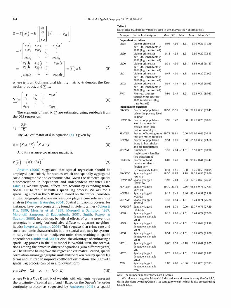
Table 1Descriptive statistics for variables used in the analysis (567 observations).

Acronym Variable description Mean S.D. Min. Max. Moran's Ia

Dependent variablesVR98 Violent crime rate

per 1000 inhabitants in1998 (log transformed)

0.05 4.56 �11.51 6.10 0.29 (11.59)

VR99 Violent crime rateper 1000 inhabitants in1999 (log transformed)

0.13 4.53 �11.51 5.80 0.20 (7.88)

VR00 Violent crime rateper 1000 inhabitants in2000 (log transformed)

0.31 4.39 �11.51 6.66 0.23 (9.18)

VR01 Violent crime rateper 1000 inhabitants in2001 (log transformed)

0.47 4.30 �11.51 6.91 0.20 (7.90)

VR02 Violent crime rateper 1000 inhabitants in2002 (log transformed)

0.55 4.13 �11.51 6.10 0.23 (9.02)

AVG Five-year averageviolent crime rate per1000 inhabitants (logtransformed)

0.91 3.49 �11.51 6.32 0.24 (9.08)

Independent variablesPOVRTY Percent of population

below the poverty levelin 1999

18.52 15.91 0.00 76.81 0.53 (19.45)

UEMPLOY Percent of populationage 16 and over incivilian labor forcethat is unemployed

3.99 3.42 0.00 30.77 0.25 (10.07)

RENTER Percent of housing unitsthat are renter occupied

49.77 28.81 0.00 100.00 0.43 (16.18)

NOFAM Percent of populationliving in householdsand are nonrelatives

9.34 8.75 0.00 65.18 0.59 (23.68)

SIGFAM Number ofsingle-parent families(log transformed)

3.35 2.14 �11.51 5.98 0.29 (10.96)

FOREIGN Percent of totalpopulation that isforeign born

6.09 8.40 0.00 95.86 0.44 (16.47)

HI Heterogeneity Index 0.33 0.16 0.00 0.76 0.50 (18.95)POVRTYL Spatially lagged

POVRTY18.30 11.97 1.18 59.35 0.83 (29.66)

UEMPLOYL Spatially laggedUEMPLOY

3.97 2.04 0.34 12.36 0.69 (26.51)

RENTERL Spatially laggedRENTER

49.70 20.14 10.56 98.68 0.78 (27.51)

NOFAML Spatially laggedNOFAM

9.15 6.49 3.46 43.43 0.91 (35.59)

SIGFAML Spatially laggedSIGFAM

3.38 1.54 �11.51 5.24 0.71 (26.78)

FOREIGNL Spatially laggedFOREIGN

6.08 5.71 0.00 49.77 0.76 (27.49)

VR98L Spatially laggeddependent variableVR98

0.19 2.80 �11.51 3.44 0.72 (27.09)

VR99L Spatially laggeddependent variableVR99

0.38 2.57 �11.51 3.56 0.64 (23.89)

VR00L Spatially laggeddependent variableVR00

0.54 2.55 �11.51 3.69 0.72 (25.06)

VR01L Spatially laggeddependent variableVR01

0.66 2.38 �9.18 3.73 0.67 (25.05)

VR02L Spatially laggeddependent variableVR02

0.79 2.26 �11.51 3.86 0.69 (25.87)

AVGL Spatially laggeddependent variableAVG

1.09 2.00 �8.96 3.61 0.73 (27.83)

Note: The numbers in parentheses are z-scores.a We calculate the global Moran's I Index values and z-scores using GeoDa 1.4.0,

this is also done by using Queen's 1st contiguity weight which is also created usingGeoDa 1.4.0.

L. He et al. / Applied Geography 58 (2015) 141e152144

U ¼ E�εε

0� ¼ E

26642664ε1ε2«εM

3775� ε0

1 / ε

0M

�3775

¼ E

2664ε1ε

01 ε1ε

02 / ε1ε

0M

ε2ε01 ε2ε

02 / «

« « 1 «εMε

01 / / εMε

0M

3775

¼

2664s11IR s12IR / s1MIRs21IR s22IR / «« « 1 «

sM1IR / / sMMIR

3775 ¼

X5IR (5)

where IR is an R-dimensional identity matrix, 5 denotes the Kro-necker product, and

Pis:

X≡

2664s11 s12 / s1Ms21 s22 / «« « 1 «

sM1 / / sMM

3775 (6)

The elements of matrixP

are estimated using residuals fromthe OLS regression:

bsij ¼bε 0ibεjR

(7)

The GLS estimator of b in equation (4) is given by:

bb ¼�X

0U�1X

��1X

0U�1y (8)

And its variance-covariance matrix is:

V�bb� ¼

�X

0U�1X

��1(9)

Anselin (2006) suggested that spatial regression should beemployed particularly for studies which use spatially aggregatedsocio-demographic and economic data. Given the detected spatialautocorrelation in dependent and independent variables (seeTable 1), we take spatial effects into account by extending tradi-tional SUR to the SUR with a spatial lag process. We assume aspatial lag effect in the SUR model based on theoretical consider-ations. Geographical space increasingly plays a core role in crimeanalysis (Messner & Anselin, 2004). Spatial diffusion processes, forinstance, have been consistently found in violent crimes (Cohen &Tita, 1999; Messner et al., 1999; Morenoff & Sampson, 1997;Morenoff, Sampson, & Raudenbush, 2001; Smith, Frazee, &Davison, 2000). In addition, beneficial effects of crime preventionstrategies in a neighborhood also diffuse to adjacent neighbor-hoods (Bowers & Johnson, 2003). This suggests that crime rate andsocio-economic characteristics in one spatial unit may be system-atically related to those in adjacent units, thus resulting in spatialdependence (Smith et al., 2000). Also, the advantage of embracing aspatial lag process in the SUR model is twofold. First, the correla-tions among the errors in different equations (also different years)will be utilized to improve the regression estimates. Second, spatialcorrelation among geographic units will be taken care by spatial lagterms and utilized to improve coefficient estimation. The SUR withspatial lag process can be in a following form:

y ¼ lWyþ Xbþ ε; ε � Nð0; UÞ (10)

where W is a R by R matrix of weights with elements wij representthe proximity of spatial unit i and j. Based on the Queen's 1st ordercontiguity protocol as suggested by Andresen (2011), a spatial

L. He et al. / Applied Geography 58 (2015) 141e152 145

weight matrix is created using GeoDa 1.4.0 (Anselin, Syabri, & Kho,2006). The coefficient l quantifies the relationship between crimerate y in one BG and crime rates in contiguous BGs. A statisticallysignificant l can be interpreted as that a spatial diffusion process ofcrime rate is detected (Doreian, 1980). We calculate the spatial lagof dependent variable yL ¼ Wy and spatial lag of all independentvariables, and apply them in the estimation of the SUR model. Thevariable yL can be understood as the “violent crime potential”similar to the “street robbery potential” studied in Smith et al.(2000). As suggested by Tita and Radil (2010), it is feasible tocombine the response lag and predictor lag terms in a single model.We use the SUR model with spatial lag process to simultaneouslyestimate equations using crime rates of different years as depen-dent variables and all independent variables selected above, inorder to obtain the model parameters of each group (i.e. eachequation in the model system).

Wald statistic test

A key feature of SUR is that we can test differences betweenpredictors across equations. Based on the estimated parameters ofthe SUR models, we use the Wald statistic test to investigatewhether the correlates of crime vary in their effects on violentcrime over time (Clogg, Petkova, & Haritou, 1995). The null hy-pothesis (H0) is that the parameter (bi) for one independent vari-able in one equation is statistically equal to that of another equation(bj), that is:

H0: bi ¼ bj

HA: bisbj

This is the same as testing the following hypothesis:

H0: bi � bj ¼ 0

HA: bi � bjs0

For testing the null hypothesis, a general formula for thecomputation of the Wald statistic is as follows:

W ¼�bbi � bbj

�’hvar

�bbi

�þ var

�bbj

�i�1�bbi � bbj

�(11)

where bi and bj are the parameter vectors including all parameterestimates for two equations, var ð,Þ is the estimated variance-covariance matrix for the parameters. The Wald statistic isasymptotically distributed as c2 distribution under the nullhypothesis.

If the test fails to reject the null hypothesis at an acceptable levelof confidence, it can be interpreted to mean that the parameter ofone independent variable in one equation is not significantlydifferent from that corresponding to the same independent vari-able in other equations. Therefore, the relationship between crimerates and socio-economic characteristics are stable across years,and if the average group's performance is worse than other singleyear groups, there will be no point in using multi-year averagecrime rate. Whereas, if the null hypothesis can be rejected at asignificant level, model parameters of one equation are signifi-cantly different from those of others, it can be interpreted to meanthat the relationship is significantly heterogenous over years. Inthis case, if the average group performs better than other groups,using multi-year average crime rate may help to minimize theimpact of annual fluctuations and reduce the potential bias of asingle high or low crime year.

Analysis and results

Dependent variables

The present research investigates the appropriateness ofdependent variable selection by examining the temporal stability ofcorrelations between socio-economic indicators and violent crimerates. The intent is to test the parameter stability of well-provedsocio-economic variables in each single year in order to examineif the criminal processes and characteristics are stable across years.Six dependent variables are used: violent crime rate of the year of1998, 1999, 2000, 2001, 2002, and five-year average. The reason weinvestigate violent crime in this study is simply because of the dataavailability. The reason we use crime rate rather than count is thatcrime count which measures the quantity of criminal activity is aquite restrictive measure. Andresen (2006a) pointed out that as anabsolute term it does not give an indication of why crime happensmore in certain places but less in others. We employ the measure ofcrime rate to evaluate the risk of crime by controlling for thepopulation. The rate is measured per 1000 residential populationliving in the BG. Violent crime rate in this study is composed of allfour violent offenses: murder and non-negligent manslaughter,forcible rape (including intent to rape), robbery, and aggravatedassault. The distribution of crime rate is long tailed, and as a matterof practice it is transformed using the natural logarithm (Smithet al., 2000). The transformation also ensures that back trans-formed estimates of crime rate are strictly positive. Table 1 gives theacronyms (VR98, VR99, VR00, VR01, VR02, AVG), definitions anddescriptive statistics for these dependent variables.

Independent variables

The independent variables in this research are selected based onthe social disorganization theory (Shaw&McKay,1942; Sampson&Groves, 1989), one of the most important theories in criminology.Social disorganization refers to “the inability of local communitiesto realize the common values of their residents” (Bursik, 1988, p.521). Rooted in social ecology (Park, Burgess, & McKenzie, 1967),social disorganization theory looks for explanations of criminalactivity in general characteristics of the social structure and socialcontrol onwhich offenders and victims are embedded. Over the lastseveral decades, a large body of studies has emerged and sought totest the empirical validity of the theory by using multivariate sta-tistical modeling approaches and various crime data sources. Theyhave consistently shown that socio-economic deprivation, resi-dential mobility (or population turnover), family disruption, andethnic heterogeneity lead to community social disorganization,which in turn, increases violent crime rates (Andresen, 2006a,2006b; Cahill & Mulligan, 2003; Charron, 2009; Porter & Purser,2010; Sampson, 1985).

We use a series of variables to capture the four structural ele-ments of the theory: socio-economic deprivation, residentialmobility, family disruption, and ethnic heterogeneity. All elementshave been recognized to characterize socially disorganized anddistressed areas, and have been identified as main sources of socialdisorganization (Cahill, 2004; Law & Quick, 2013). All variablesbelow are proxy measures of the theory and have been informed byan extensive review of the relevant literature (e.g., Andresen,2006a, 2006b; Cahill & Mulligan, 2003; Law & Quick, 2013;McCord & Ratcliffe, 2007; Sun, Triplett, & Gainey, 2004; Ye & Wu,2011). Socio-economic deprivation is measured as percentage ofpopulation below the poverty level and percentage of unemployedpopulation. Residential mobility is represented by percentage ofrenter occupied housing units and percentage of population livingin households and are nonrelatives. Family disruption is measured

L. He et al. / Applied Geography 58 (2015) 141e152146

through number of single-parent families. Ethnic heterogeneity iscaptured by percentage of foreign born population and racial het-erogeneity measured by means of the Heterogeneity Index (seeequation (12)) which is designed to capture the degree of racialheterogeneity in each BG (Blau, 1977; Cahill & Mulligan, 2003;Sampson & Groves, 1989).

Heterogeneity Index ¼ 1�X

p2i (12)

where i indicates the number of racial group, pi is the proportion ofthepopulation inagivengroup (Sampson&Groves,1989). The indexis defined as a function of the different racial groups within a givenarea, andconsidersbothnumberof racial groups andpopulation sizeof each group. The range of the index is (0,1), withinwhich 0meansmaximumhomogeneity, and 1meansmaximumheterogeneity.Weuse all 5 different racial groups to generate the index, i.e. White,Black or African American, American Indian and Alaska Native,Asian, and Native Hawaiian and Other Pacific Islander.

In spatial analysis of crime, it is important to consider the spatialdependency in the data. BGs are relatively small geographic units,thus socio-economic characteristics of any BG may not only affectits own crime rate but also crime rates of its neighboring BGs. Forthis purpose, we also consider the spatial lag of explanatory vari-ables for spatial modeling. Spatial weightmatrix is calculated basedon the Queen's 1st order contiguity by using GeoDa 1.4.0. Table 1provides descriptive statistics of all these explanatory variables.

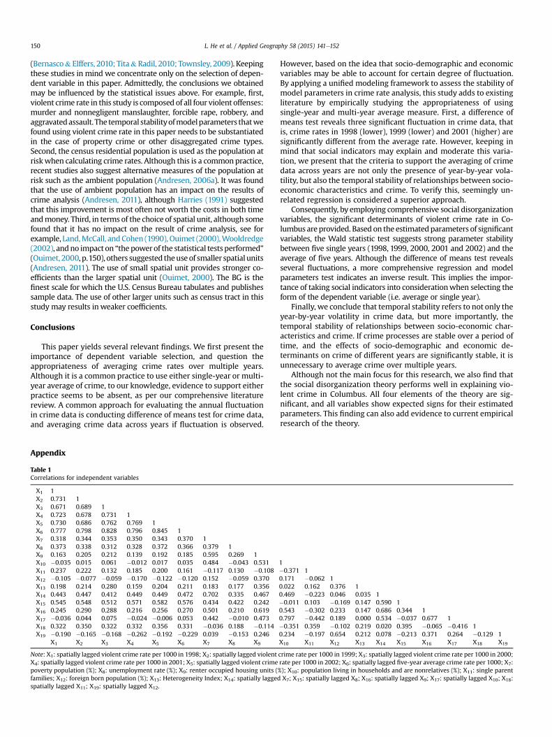
The correlations test (see Table 1 in the Appendix) for all inde-pendent variables indicates that none of the pair-wise correlationsbetween explanatory variables is larger than 0.8, which is a com-mon threshold for the issue of collinearity (Andresen, 2006a). Thevariable of poverty population has a strong positive relationship(0.702) with the spatial lag of itself, the variable of population livingin households and are nonrelatives has a strong positive relation-ship (0.797) with the spatial lag of itself. Both are standard re-lationships. In addition, the correlations among all six spatiallylagged dependent variables are strong. Particularly, the correlationsbetween the spatially lagged 5-year average crime rate and other 5single years are all strong. However, considering the stable patternsof the geographic distribution of crime rates in 5 years and 5-yearaverage (see Fig. 1), these high correlations can be seen as stan-dard relationships.

Empirical results

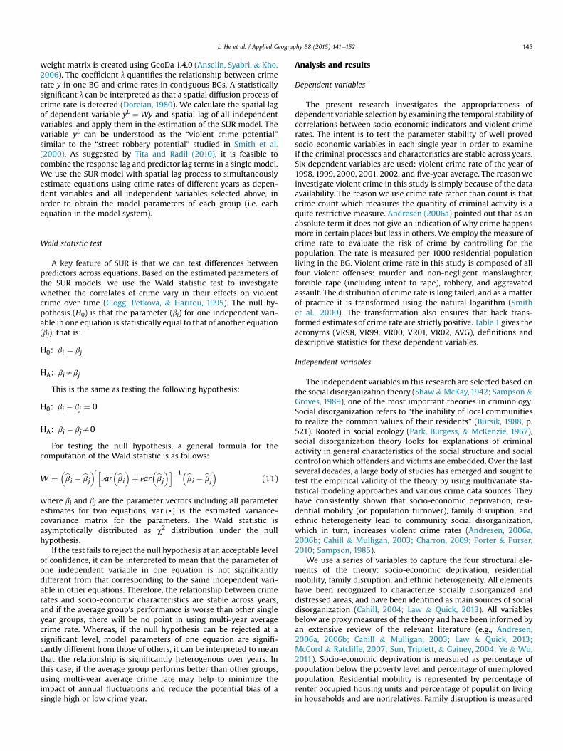
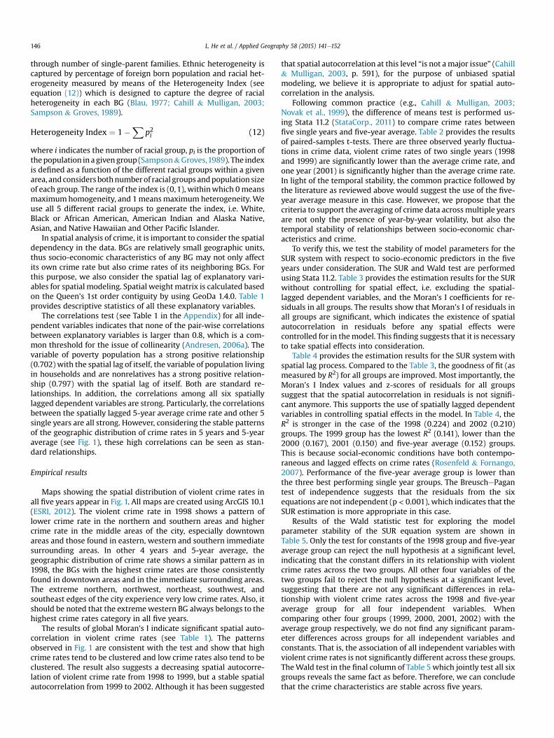
Maps showing the spatial distribution of violent crime rates inall five years appear in Fig. 1. All maps are created using ArcGIS 10.1(ESRI, 2012). The violent crime rate in 1998 shows a pattern oflower crime rate in the northern and southern areas and highercrime rate in the middle areas of the city, especially downtownareas and those found in eastern, western and southern immediatesurrounding areas. In other 4 years and 5-year average, thegeographic distribution of crime rate shows a similar pattern as in1998, the BGs with the highest crime rates are those consistentlyfound in downtown areas and in the immediate surrounding areas.The extreme northern, northwest, northeast, southwest, andsoutheast edges of the city experience very low crime rates. Also, itshould be noted that the extremewestern BG always belongs to thehighest crime rates category in all five years.

The results of global Moran's I indicate significant spatial auto-correlation in violent crime rates (see Table 1). The patternsobserved in Fig. 1 are consistent with the test and show that highcrime rates tend to be clustered and low crime rates also tend to beclustered. The result also suggests a decreasing spatial autocorre-lation of violent crime rate from 1998 to 1999, but a stable spatialautocorrelation from 1999 to 2002. Although it has been suggested

that spatial autocorrelation at this level “is not amajor issue” (Cahill& Mulligan, 2003, p. 591), for the purpose of unbiased spatialmodeling, we believe it is appropriate to adjust for spatial auto-correlation in the analysis.

Following common practice (e.g., Cahill & Mulligan, 2003;Novak et al., 1999), the difference of means test is performed us-ing Stata 11.2 (StataCorp., 2011) to compare crime rates betweenfive single years and five-year average. Table 2 provides the resultsof paired-samples t-tests. There are three observed yearly fluctua-tions in crime data, violent crime rates of two single years (1998and 1999) are significantly lower than the average crime rate, andone year (2001) is significantly higher than the average crime rate.In light of the temporal stability, the common practice followed bythe literature as reviewed above would suggest the use of the five-year average measure in this case. However, we propose that thecriteria to support the averaging of crime data across multiple yearsare not only the presence of year-by-year volatility, but also thetemporal stability of relationships between socio-economic char-acteristics and crime.

To verify this, we test the stability of model parameters for theSUR system with respect to socio-economic predictors in the fiveyears under consideration. The SUR and Wald test are performedusing Stata 11.2. Table 3 provides the estimation results for the SURwithout controlling for spatial effect, i.e. excluding the spatial-lagged dependent variables, and the Moran's I coefficients for re-siduals in all groups. The results show that Moran's I of residuals inall groups are significant, which indicates the existence of spatialautocorrelation in residuals before any spatial effects werecontrolled for in themodel. This finding suggests that it is necessaryto take spatial effects into consideration.

Table 4 provides the estimation results for the SUR systemwithspatial lag process. Compared to the Table 3, the goodness of fit (asmeasured by R2) for all groups are improved. Most importantly, theMoran's I Index values and z-scores of residuals for all groupssuggest that the spatial autocorrelation in residuals is not signifi-cant anymore. This supports the use of spatially lagged dependentvariables in controlling spatial effects in the model. In Table 4, theR2 is stronger in the case of the 1998 (0.224) and 2002 (0.210)groups. The 1999 group has the lowest R2 (0.141), lower than the2000 (0.167), 2001 (0.150) and five-year average (0.152) groups.This is because social-economic conditions have both contempo-raneous and lagged effects on crime rates (Rosenfeld & Fornango,2007). Performance of the five-year average group is lower thanthe three best performing single year groups. The BreuschePagantest of independence suggests that the residuals from the sixequations are not independent (p < 0.001), which indicates that theSUR estimation is more appropriate in this case.

Results of the Wald statistic test for exploring the modelparameter stability of the SUR equation system are shown inTable 5. Only the test for constants of the 1998 group and five-yearaverage group can reject the null hypothesis at a significant level,indicating that the constant differs in its relationship with violentcrime rates across the two groups. All other four variables of thetwo groups fail to reject the null hypothesis at a significant level,suggesting that there are not any significant differences in rela-tionship with violent crime rates across the 1998 and five-yearaverage group for all four independent variables. Whencomparing other four groups (1999, 2000, 2001, 2002) with theaverage group respectively, we do not find any significant param-eter differences across groups for all independent variables andconstants. That is, the association of all independent variables withviolent crime rates is not significantly different across these groups.TheWald test in the final column of Table 5 which jointly test all sixgroups reveals the same fact as before. Therefore, we can concludethat the crime characteristics are stable across five years.

Fig. 1. Violent crime rates per 1000 in Columbus in five single years and five-year average.

L. He et al. / Applied Geography 58 (2015) 141e152 147

Discussion

A synthesis of the results of SUR model and Wald test leads toseveral relevant conclusions. Of particular importance is that,although the difference of means test suggests significant yearlyvolatility in crime data, both the SUR model and Wald test showdifferent results. Tables 4 and 5 suggest that there are not anysignificant differences in relationship with violent crime ratesacross all single year groups and five-year average group for all four

significant explanatory variables. The results also indicate thatthere is a considerable stability in the signs of the explanatoryvariables across all groups. In other words, the crime characteristicsare stable across five years. This finding yields twofold implications.The first is in regard to the appropriateness of averaging crime dataacross multiple years. The second is in regard to the selection ofdependent variables in spatial analysis of crime.

In previous studies, the main criterion for averaging crime dataacross multiple years is the presence of annual fluctuation, that is, if

Fig. 1. (continued).

Table 2Results of t-tests of crime rates between five single years and five-year average.

Comparison Group t p-Value

Single year 5-year average

M S.D. n M S.D. n

1998 vs. Avga 9.04 20.73 567 10.20 25.17 567 �4.60 <0.0011999 vs. Avg 9.44 17.59 567 10.20 25.17 567 �1.80 0.0372000 vs. Avg 10.78 34.19 567 10.20 25.17 567 1.35 0.1782001 vs. Avg 11.68 43.04 567 10.20 25.17 567 1.84 0.0332002 vs. Avg 10.51 21.96 567 10.20 25.17 567 1.12 0.265

a Avg stands for the 5-year average group.

Table 3Parameter estimates from the SUR without spatial lag and Moran's I of residuals.

Variables 1998 1999 2000

Constant �3.212*** �3.462*** �2.854***POVRTY e e e

UEMPLOY 0.275*** 0.318*** 0.313***RENTER e e e

NOFAM e e e

SIGFAM 0.542*** 0.472*** 0.351**FOREIGN e e e

HI e e e

POVRTYL e e e

UEMPLOYL e e e

RENTERL e e e

NOFAML 0.093* 0.126** 0.124**SIGFAML e e e

FOREIGNL �0.132** �0.114** �0.109**Moran's Ia 0.173 (6.435) 0.069 (2.928) 0.135 (5.6R2 0.111*** 0.109*** 0.097***Nb 567 567 567

Note: *p < 0.05; **p < 0.01; ***p < 0.001.a We calculate the global Moran's I Index values and z-scores (the numbers in parenthe

weight.b N is the number of observation.

L. He et al. / Applied Geography 58 (2015) 141e152148

it is observed by using the difference of means test, crime data ofmultiple years should be averaged. However, our findings reveal thatthe criteria to support the averaging of crime data should be not onlythe presence of year-by-year volatility, but also the temporal stabilityof relationships between socio-economic characteristics and crime.

Our findings also reveal that averaging crime data across mul-tiple years is not necessarily superior to single year crime rate.Previous studies suggest that in case of the annual fluctuation,using average crime rate is able to reduce the influence of fluctu-ation in the year-to-year occurrence of crime. But this paper an-swers an important question of this practice, that is, how useful willthe analysis of these averaged data be for revealing the relationshipbetween crimes and socio-demographic and economic

2001 2002 AVG

�1.667** �2.637*** �1.084*e e e

0.274*** 0.307*** 0.226***e e e

e e e

0.335** 0.433*** 0.273**e e e

e e e

e e e

e e e

e e e

0.091** 0.118*** 0.091**e e e

�0.190*** �0.132*** �0.134***78) 0.085 (3.411) 0.111 (4.516) 0.106 (4.264)

0.120*** 0.128*** 0.109***567 567 567

ses) for residuals using GeoDa 1.4.0, this is also done by using Queen's 1st contiguity

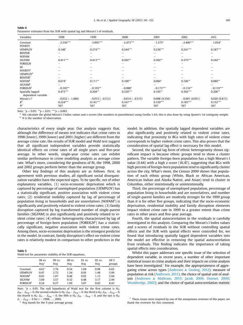
Table 4Parameter estimates from the SUR with spatial lag and Moran's I of residuals.

Variables 1998 1999 2000 2001 2002 AVG

Constant �2.356*** �3.095*** �2.473*** �1.575* �2.409*** �1.034*POVRTY e e e e e e

UEMPLOY 0.148* 0.274*** 0.244*** 0.236*** 0.241*** 0.187***RENTER e e e e e e

NOFAM e e e e e e

SIGFAM 0.411*** 0.413*** 0.292** 0.302** 0.375*** 0.242**FOREIGN e e e e e e

HI e e e e e e

POVRTYL e e e e e e

UEMPLOYL e e e e e e

RENTERL e e e e e e

NOFAML 0.074* 0.111** 0.100** 0.084* 0.106** 0.080**SIGFAML e e e e e e

FOREIGNL �0.103** �0.103** �0.088* �0.173*** �0.116** �0.119***Spatially lagged

dependent variable0.473*** 0.204** 0.339*** 0.195** 0.302*** 0.206**

Moran's Ia �0.032 (�1.080) �0.015 (�0.512) �0.014 (�0.515) 0.008 (0.350) �0.001 (0.051) 0.020 (0.872)R2 0.224*** 0.141*** 0.167*** 0.150*** 0.185*** 0.152***Nb 567 567 567 567 567 567

Note: *p < 0.05; **p < 0.01; ***p < 0.001.a We calculate the global Moran's I Index values and z-scores (the numbers in parentheses) using GeoDa 1.4.0, this is also done by using Queen's 1st contiguity weight.b N is the number of observation.

L. He et al. / Applied Geography 58 (2015) 141e152 149

characteristics of every single year. Our analysis suggests that,although the difference of means test indicates that crime rates in1998 (lower), 1999 (lower) and 2001 (higher) are different from theaverage crime rate, the results of SUR model and Wald test suggestthat all significant independent variables provide statisticallyidentical effects on crime rates of all single years and five-yearaverage. In other words, single-year crime rates can exhibitsimilar performance in crime modeling analysis as average crimerate. What's more, considering the goodness of fit, the 1998, 2000and 2002 groups perform better than the average group.

Other key findings of this analysis are as follows. First, inagreement with previous studies, all significant social disorgani-zation variables have the expected signs. To be specific, net of otherexplanatory variables, (1) socio-economic deprivation which iscaptured by percentage of unemployed population (UEMPLOY) hasa statistically significant, positive association with violent crimerates; (2) residential mobility captured by lag of percentage ofpopulation living in households and are nonrelatives (NOFAML) issignificantly and positively related to violent crime rates; (3) familydisruption captured by log transformed number of single-parentfamilies (SIGFAM) is also significantly and positively related to vi-olent crime rates; (4) ethnic heterogeneity characterized by lag ofpercentage of foreign-born population (FOREIGNL) has a statisti-cally significant, negative association with violent crime rates.Among them, socio-economic deprivation is the strongest predictorin the model. In contrast, family disruption's effect on violent crimerates is relatively modest in comparison to other predictors in the

Table 5Wald test for parameter stability of the SUR equations.

98 vs.Avga

99 vs.Avg

00 vs.Avg

01 vs.Avg

02 vs.Avg

All 5groups

Constant 4.61* 3.76 0.54 1.04 0.98 6.65UEMPLOY 0.47 2.72 1.24 0.95 1.48 5.99NOFAML 0.03 1.07 0.48 0.02 1.15 5.94SIGFAM 3.09 3.57 0.32 0.48 3.17 2.44FOREIGNL 0.24 0.27 1.09 3.07 0.02 8.43

Note: *p < 0.05. The null hypothesis of Wald test for the first column is H0:b98 � bAvg¼ 0, the second column is H0: b99 � bAvg¼ 0, the third is H0: b00 � bAvg¼ 0,the fourth is H0: b01 � bAvg ¼ 0, the fifth is H0: b02 � bAvg ¼ 0, and the last is H0:bt � bAvg ¼ 0 for t ¼ 1998, …, 2002.

a Avg stands for the 5-year average group.

model. In addition, the spatially lagged dependent variables arealso significantly and positively related to violent crime rates,indicating that proximity to BGs with high rates of violent crimecorresponds to higher violent crime rates. This also proves that theconsideration of spatial lag effect is necessary for this model.

Second, the spatial lag form of ethnic heterogeneity shows sig-nificant impact is because ethnic groups tend to show a clusterpattern. The variable foreign-born population has a high Moran's Ivalue (0.44) with a high z-score (16.47), suggesting that BGs withhigh percent of foreign-born population tend to significantly clusteracross the city. What's more, the Census 2000 shows that popula-tion of each ethnic group (White, Black or African American,American Indian and Alaska Native, and Asian) tend to cluster inColumbus, either intentionally or unintentionally.

Third, the percentage of unemployed population, percentage ofpopulation living in households and are nonrelatives, and numberof single-parent families are modestly stronger for the 1999 groupthan it is for other five groups, indicating that the socio-economicdeprivation, residential mobility and family disruption elementsimpact violent crime rate in 1999 to a greater extent than crimerates in other years and five-year average.

Fourth, the spatial autocorrelation in the residuals is carefullyinvestigated in this analysis. Comparing the Moran's I Index valuesand z-scores of residuals in the SUR without controlling spatialeffects and the SUR with spatial effects were controlled for, wefound that introducing spatially lagged dependent variables intothe model are effective in removing the spatial autocorrelationfrom residuals. This finding indicates the importance of takingspatial effects into consideration.

Whilst this paper addresses one specific issue of the selection ofdependent variable, in recent years, a number of other importantstatistical issues in crime analysis and their impacts on crime analysishave been investigated.1 For example, the appropriateness of aggre-gating crime across types (Andresen & Linning, 2012); measure ofpopulation at risk (Andresen, 2011); the choice of spatial unit of anal-ysis (Andresen & Malleson, 2013; Jacob, 2006; Ouimet, 2000;Wooldredge, 2002); and the choice of spatial autocorrelation statistic

1 These issues were inspired by one of the anonymous reviewer of this paper, wethank the reviewer for this comment.

L. He et al. / Applied Geography 58 (2015) 141e152150

(Bernasco& Elffers, 2010; Tita&Radil, 2010; Townsley, 2009). Keepingthese studies in mind we concentrate only on the selection of depen-dent variable in this paper. Admittedly, the conclusions we obtainedmay be influenced by the statistical issues above. For example, first,violent crime rate in this study is composed of all four violent offenses:murder and nonnegligent manslaughter, forcible rape, robbery, andaggravatedassault. The temporal stabilityofmodelparameters thatwefound using violent crime rate in this paper needs to be substantiatedin the case of property crime or other disaggregated crime types.Second, the census residential population is used as the population atriskwhen calculating crime rates. Although this is a commonpractice,recent studies also suggest alternative measures of the population atrisk such as the ambient population (Andresen, 2006a). It was foundthat the use of ambient population has an impact on the results ofcrime analysis (Andresen, 2011), although Harries (1991) suggestedthat this improvement is most often not worth the costs in both timeandmoney. Third, in terms of the choice of spatial unit, although somefound that it has no impact on the result of crime analysis, see forexample, Land,McCall, andCohen (1990), Ouimet (2000),Wooldredge(2002), andno impact on “the powerof the statistical tests performed”(Ouimet, 2000,p.150), others suggested theuseof smaller spatial units(Andresen, 2011). The use of small spatial unit provides stronger co-efficients than the larger spatial unit (Ouimet, 2000). The BG is thefinest scale for which the U.S. Census Bureau tabulates and publishessample data. The use of other larger units such as census tract in thisstudy may results inweaker coefficients.

Conclusions

This paper yields several relevant findings. We first present theimportance of dependent variable selection, and question theappropriateness of averaging crime rates over multiple years.Although it is a common practice to use either single-year or multi-year average of crime, to our knowledge, evidence to support eitherpractice seems to be absent, as per our comprehensive literaturereview. A common approach for evaluating the annual fluctuationin crime data is conducting difference of means test for crime data,and averaging crime data across years if fluctuation is observed.

Appendix

Table 1Correlations for independent variables

X1 1X2 0.731 1X3 0.671 0.689 1X4 0.723 0.678 0.731 1X5 0.730 0.686 0.762 0.769 1X6 0.777 0.798 0.828 0.796 0.845 1X7 0.318 0.344 0.353 0.350 0.343 0.370 1X8 0.373 0.338 0.312 0.328 0.372 0.366 0.379 1X9 0.163 0.205 0.212 0.139 0.192 0.185 0.595 0.269 1X10 �0.035 0.015 0.061 �0.012 0.017 0.035 0.484 �0.043 0.531X11 0.237 0.222 0.132 0.185 0.200 0.161 �0.117 0.130 �0.108X12 �0.105 �0.077 �0.059 �0.170 �0.122 �0.120 0.152 �0.059 0.370X13 0.198 0.214 0.280 0.159 0.204 0.211 0.183 0.177 0.356X14 0.443 0.447 0.412 0.449 0.449 0.472 0.702 0.335 0.467X15 0.545 0.548 0.512 0.571 0.582 0.576 0.434 0.422 0.242X16 0.245 0.290 0.288 0.216 0.256 0.270 0.501 0.210 0.619X17 �0.036 0.044 0.075 �0.024 �0.006 0.053 0.442 �0.010 0.473X18 0.322 0.350 0.322 0.332 0.356 0.331 �0.036 0.188 �0.114X19 �0.190 �0.165 �0.168 �0.262 �0.192 �0.229 0.039 �0.153 0.246

X1 X2 X3 X4 X5 X6 X7 X8 X9

Note: X1: spatially lagged violent crime rate per 1000 in 1998; X2: spatially lagged violentX4: spatially lagged violent crime rate per 1000 in 2001; X5: spatially lagged violent crimepoverty population (%); X8: unemployment rate (%); X9: renter occupied housing units (families; X12: foreign born population (%); X13: Heterogeneity Index; X14: spatially laggedspatially lagged X11; X19: spatially lagged X12.

However, based on the idea that socio-demographic and economicvariables may be able to account for certain degree of fluctuation.By applying a unified modeling framework to assess the stability ofmodel parameters in crime rate analysis, this study adds to existingliterature by empirically studying the appropriateness of usingsingle-year and multi-year average measure. First, a difference ofmeans test reveals three significant fluctuation in crime data, thatis, crime rates in 1998 (lower), 1999 (lower) and 2001 (higher) aresignificantly different from the average rate. However, keeping inmind that social indicators may explain and moderate this varia-tion, we present that the criteria to support the averaging of crimedata across years are not only the presence of year-by-year vola-tility, but also the temporal stability of relationships between socio-economic characteristics and crime. To verify this, seemingly un-related regression is considered a superior approach.

Consequently, by employing comprehensive social disorganizationvariables, the significant determinants of violent crime rate in Co-lumbus areprovided. Based on the estimatedparameters of significantvariables, the Wald statistic test suggests strong parameter stabilitybetween five single years (1998, 1999, 2000, 2001 and 2002) and theaverage of five years. Although the difference of means test revealsseveral fluctuations, a more comprehensive regression and modelparameters test indicates an inverse result. This implies the impor-tance of taking social indicators into considerationwhen selecting theform of the dependent variable (i.e. average or single year).

Finally, we conclude that temporal stability refers to not only theyear-by-year volatility in crime data, but more importantly, thetemporal stability of relationships between socio-economic char-acteristics and crime. If crime processes are stable over a period oftime, and the effects of socio-demographic and economic de-terminants on crime of different years are significantly stable, it isunnecessary to average crime over multiple years.

Although not the main focus for this research, we also find thatthe social disorganization theory performs well in explaining vio-lent crime in Columbus. All four elements of the theory are sig-nificant, and all variables show expected signs for their estimatedparameters. This finding can also add evidence to current empiricalresearch of the theory.

1�0.371 10.171 �0.062 10.022 0.162 0.376 10.469 �0.223 0.046 0.035 1�0.011 0.103 �0.169 0.147 0.590 10.543 �0.302 0.233 0.147 0.686 0.344 10.797 �0.442 0.189 0.000 0.534 �0.037 0.677 1�0.351 0.359 �0.102 0.219 0.020 0.395 �0.065 �0.416 10.234 �0.197 0.654 0.212 0.078 �0.213 0.371 0.264 �0.129 1X10 X11 X12 X13 X14 X15 X16 X17 X18 X19

crime rate per 1000 in 1999; X3: spatially lagged violent crime rate per 1000 in 2000;rate per 1000 in 2002; X6: spatially lagged five-year average crime rate per 1000; X7:%); X10: population living in households and are nonrelatives (%); X11: single parentX7; X15: spatially lagged X8; X16: spatially lagged X9; X17: spatially lagged X10; X18:

L. He et al. / Applied Geography 58 (2015) 141e152 151

References

Andresen, M. A. (2006a). Crime measures and the spatial analysis of criminal ac-tivity. British Journal of Criminology, 46(2), 258e285.

Andresen, M. A. (2006b). A spatial analysis of crime in Vancouver, British Columbia:a synthesis of social disorganization and routine activity theory. The CanadianGeographer/Le G�eographe canadien, 50(4), 487e502.

Andresen, M. A. (2011). The ambient population and crime analysis. The ProfessionalGeographer, 63(2), 193e212.

Andresen, M. A., & Linning, S. J. (2012). The (in) appropriateness of aggregatingacross crime types. Applied Geography, 35(1), 275e282.

Andresen, M. A., & Malleson, N. (2011). Testing the stability of crime patterns:implications for theory and policy. Journal of Research in Crime and Delinquency,48(1), 58e82.

Andresen, M. A., & Malleson, N. (2013). Spatial heterogeneity in crime analysis. InCrime modeling and mapping using geospatial technologies (pp. 3e23).Netherlands: Springer.

Anselin, L. (2006). Spatial econometrics. In T. C. Mills, & K. Patterson (Eds.),Econometrics theory: Vol. 1. Palgrave handbook of econometrics (pp. 901e941).Basingstoke: Palgrave Macmillan.

Anselin, L., Syabri, I., & Kho, Y. (2006). GeoDa: an introduction to spatial dataanalysis. Geographical Analysis, 38(1), 5e22.

Bernasco, W., Block, R., & Ruiter, S. (2013). Go where the money is: modelingstreet robbers' location choices. Journal of Economic Geography, 13(1),119e143.

Bernasco, W., & Elffers, H. (2010). Statistical analysis of spatial crime data (chapter33). In A. Piquero, & D. Weisburd (Eds.), Handbook of quantitative criminology(pp. 699e724). Springer.

Bjerk, D. (2010). Thieves, thugs, and neighborhood poverty. Journal of Urban Eco-nomics, 68(3), 231e246.

Blau, P. M. (1977). Inequality and heterogeneity: a primitive theory of social structure.New York: Free Press.

Bowers, K. J., & Johnson, S. D. (2003). Measuring the geographical displacement anddiffusion of benefit effects of crime prevention activity. Journal of QuantitativeCriminology, 19(3), 275e301.

Browning, C. R., Byron, R. A., Calder, C. A., Krivo, L. J., Kwan, M. P., Lee, J. Y., et al.(2010). Commercial density, residential concentration, and crime: land usepatterns and violence in neighborhood context. Journal of Research in Crime andDelinquency, 47(3), 329e357.

Bursik, R. J. (1988). Social disorganization and theories of crime and delinquency:problems and prospects. Criminology, 26(4), 519e552.

Cahill, M. E. (2004). Geographies of urban crime: an intraurban study of crime inNashville, TN, Portland, OR and Tucson, AZ (Doctoral dissertation). University ofArizona.

Cahill, M. E., & Mulligan, G. F. (2003). The determinants of crime in Tucson, Arizona.Urban Geography, 24(7), 582e610.

Cahill, M. E., & Mulligan, G. F. (2007). Using geographically weighted regression toexplore local crime patterns. Social Science Computer Review, 25(2), 174e193.

Chamlin, M. B., & Cochran, J. K. (2004). Excursus on the population size-crimerelationship. Western Criminology Review, 5, 119.

Charron, M. (2009). Neighbourhood characteristics and the distribution of police-re-ported crime in the city of Toronto. Statistics Canada, Canadian Centre for JusticeStatistics.

Clogg, C. C., Petkova, E., & Haritou, A. (1995). Statistical methods for comparingregression coefficients between models. American Journal of Sociology,1261e1293.

Cohen, J., & Tita, G. (1999). Diffusion in homicide: exploring a general method fordetecting spatial diffusion processes. Journal of Quantitative Criminology, 15(4),451e493.

Davidson, R., & MacKinnon, J. G. (1993). Estimation and inference in econometrics.Cambridge, Massachusetts: Harvard University Press.

Doreian, P. (1980). Linear models with spatially distributed data spatial distur-bances or spatial effects? Sociological Methods & Research, 9(1), 29e60.

Ellis, L., & Walsh, A. (2000). Criminology: a global perspective. Boston, MA: Allyn andBacon.

Erdogan, S., Yalçin, M., & Dereli, M. A. (2013). Exploratory spatial analysis of crimesagainst property in Turkey. Crime, Law and Social Change, 59(1), 63e78.

ESRI (Environmental Science Research Institute). (2012). ArcGIS 10.1. Redlands, CA,USA.

Griffith, D. A. (2003). Spatial autocorrelation and spatial filtering: gaining under-standing through theory and scientific visualization. Berlin: Springer-Verlag.

Griffith, D. A., & Amrhein, C. G. (1991). Statistical analysis for geographers. EnglewoodCliffs, NJ: Prentice Hall.

Harries, K. D. (1991). Alternative denominators in conventional crime rates. InP. Brantingham, & P. Brantingham (Eds.), Environmental criminology (2nd ed.).(pp. 147e165). London: Sage.

Jacob, J. C. (2006). Male and female youth crime in Canadian communities:assessing the applicability of social disorganization theory. Canadian Journal ofCriminology and Criminal Justice, 48(1), 31e60.

Krivo, L. J., & Peterson, R. D. (1996). Extremely disadvantaged neighborhoods andurban crime. Social Forces, 75(2), 619e648.

Land, K. C., McCall, P. L., & Cohen, L. E. (1990). Structural covariates of homiciderates: are there any invariances across time and social space? American Journalof Sociology, 922e963.

Langford, M., & Unwin, D. J. (1994). Generating and mapping population densitysurfaces within a geographical information system. The Cartographic Journal,31(1), 21e26.

Law, J., & Quick, M. (2013). Exploring links between juvenile offenders and socialdisorganization at a large map scale: a Bayesian spatial modeling approach.Journal of Geographical Systems, 15(1), 89e113.

Light, M. T., & Harris, C. T. (2012). Race, space, and violence: exploring spatialdependence in structural covariates of white and black violent crime in UScounties. Journal of Quantitative Criminology, 28(4), 559e586.

McCord, E. S., & Ratcliffe, J. H. (2007). A micro-spatial analysis of the demographicand criminogenic environment of drug markets in Philadelphia. Australian &New Zealand Journal of Criminology, 40(1), 43e63.

Messner, S. F., & Anselin, L. (2004). Spatial analyses of homicide with areal data. InSpatially integrated social science (pp. 127e144).

Messner, S. F., Anselin, L., Baller, R. D., Hawkins, D. F., Deane, G., & Tolnay, S. E.(1999). The spatial patterning of county homicide rates: an application ofexploratory spatial data analysis. Journal of Quantitative Criminology, 15(4),423e450.

Messner, S. F., & Golden, R. M. (1992). Racial inequality and racially disaggregatedhomicide rates: an assessment of alternative theoretical explanations. Crimi-nology, 30(3), 421e448.

Minnesota Population Center. (2011). National historical geographic informationsystem: version 2.0. Minneapolis, MN: University of Minnesota. https://www.nhgis.org/.

Moran, P. A. (1950). Notes on continuous stochastic phenomena. Biometrika, 17e23.Morenoff, J. D., & Sampson, R. J. (1997). Violent crime and the spatial dynamics of

neighborhood transition: Chicago, 1970e1990. Social Forces, 76(1), 31e64.Morenoff, J. D., Sampson, R. J., & Raudenbush, S. W. (2001). Neighborhood

inequality, collective efficacy, and the spatial dynamics of urban violence.Criminology, 39(3), 517e558.

Novak, K. J., Hartman, J. L., Holsinger, A. M., & Turner, M. G. (1999). The effects ofaggressive policing of disorder on serious crime. Policing: An InternationalJournal of Police Strategies & Management, 22(2), 171e194.

Oberwittler, D., & Wikstr€om, P. O. H. (2009). Why small is better: advancing thestudy of the role of behavioral contexts in crime causation. In Putting crime in itsplace (pp. 35e59). New York: Springer.

Ouimet, M. (2000). Aggregation bias in ecological research: how social disorgani-zation and criminal opportunities shape the spatial distribution of juveniledelinquency in Montreal. Canadian Review of Criminology, 42, 135e156.

P�aez, A., & Scott, D. M. (2004). Spatial statistics for urban analysis: a review oftechniques with examples. GeoJournal, 61(1), 53e67.

Park, R. E., Burgess, E. W., & McKenzie, R. D. (1967). The city. Chicago: University ofChicago Press.

Peterson, R. D., Krivo, L. J., & Harris, M. A. (2000). Disadvantage and neighborhoodviolent crime: do local institutions matter? Journal of Research in Crime andDelinquency, 37(1), 31e63.

Porter, J. R., & Purser, C. W. (2010). Social disorganization, marriage, and reportedcrime: a spatial econometrics examination of family formation and criminaloffending. Journal of Criminal Justice, 38(5), 942e950.

Rangel, T. F., Diniz-Filho, J. A. F., & Bini, L. M. (2010). SAM: a comprehensive appli-cation for spatial analysis in macroecology. Ecography, 33(1), 46e50.

Ratcliffe, J. H. (2004). Geocoding crime and a first estimate of a minimum acceptablehit rate. International Journal of Geographical Information Science, 18(1), 61e72.

Ratcliffe, J. (2010). Crime mapping: spatial and temporal challenges. In A. R. Piquero,& D. Weisburd (Eds.), Handbook of quantitative criminology (pp. 5e24). NewYork: Springer.

Rosenfeld, R., & Fornango, R. (2007). The impact of economic conditions on robberyand property crime: the role of consumer sentiment. Criminology, 45(4),735e769. Chicago.

Sampson, R. J. (1985). Race and criminal violence: a demographically disaggregatedanalysis of urban homicide. Crime & Delinquency, 31(1), 47e82.

Sampson, R. J. (1987). Urban black violence: the effect of male joblessness andfamily disruption. American Journal of Sociology, 348e382.

Sampson, R. J., & Groves, W. B. (1989). Community structure and crime: testingsocial-disorganization theory. American Journal of Sociology, 774e802.

Schweitzer, J. H., Kim, J. W., & Mackin, J. R. (1999). The impact of the built envi-ronment on crime and fear of crime in urban neighborhoods. Journal of UrbanTechnology, 6(3), 59e73.

Shaw, C. R., & McKay, H. D. (1942). Juvenile delinquency and urban areas. Chicago:University of Chicago Press.

Smith, W. R., Frazee, S. G., & Davison, E. L. (2000). Furthering the integration ofroutine activity and social disorganization theories: small units of analysis andthe study of street robbery as a diffusion process. Criminology, 38(2), 489e524.

StataCorp. (2011). Stata statistical software: release 12. College Station, TX: Stata Corp LP.Sun, I. Y., Triplett, R., & Gainey, R. R. (2004). Neighborhood characteristics and

crime: a test of Sampson and Groves' model of social disorganization. WesternCriminology Review, 5, 1.

Tita, G. E., & Radil, S. M. (2010). Spatial regression models in criminology: modelingsocial processes in the spatial weights matrix (chapter 6). In A. R. Piquero, &D. Weisburd (Eds.), Handbook of quantitative criminology (pp. 101e121). NewYork: Springer.

Townsley, M. (2009). Spatial autocorrelation and impacts on criminology.Geographical Analysis, 41(4), 452e461.

U.S. Census Bureau. (2003). Census of population and housing, summary file 4:technical documentation (p. 2000).

L. He et al. / Applied Geography 58 (2015) 141e152152

Weisburd, D. L., Groff, E. R., & Yang, S. M. (2012). The criminology of place: streetsegments and our understanding of the crime problem. Oxford University Press.

Wooldredge, J. (2002). Examining the (ir)relevance of aggregation bias for multi-level studies of neighborhoods and crime with an example comparing censustracts to official neighborhoods in Cincinnati. Criminology, 40(3), 681e710.

Ye, X., & Wu, L. (2011). Analyzing the dynamics of homicide patterns in Chicago:ESDA and spatial panel approaches. Applied Geography, 31(2), 800e807.

Zellner, A. (1962). An efficient method of estimating seemingly unrelated re-gressions and tests for aggregation bias. Journal of the American Statistical As-sociation, 57(298), 348e368.