Temporal Mechanics (D): Time-Space Metrics - viXra.org

of 35

EQUUS AEROSPACE PTY LTD © 2021

Temporal Mechanics (D): Time-Space Metrics

Stephen H. Jarvis

email: [email protected]

©2021 Equus Aerospace Pty Ltd

Abstract: Here is presented the first of two additional instalments to what was initially envisaged to be a series of

three papers, namely “Temporal Mechanics (A): Time-Space Constants”, “Temporal Mechanics (B): Time-space

Circuits”, and “Temporal Mechanics (C): Time-Space Manifolds”, here as Time-Space Metrics and in a subsequent

paper as Time-Space Logistics. The importance of this fourth paper in this series of five upholds the need to detail

what is recognized as an underlying theme through its three lead-up papers, namely time-space metrics being integral

to the ideas of time-space constants, time-space circuits, and time-space manifolds, and what those “metrics” are,

how those “metrics” can be demonstrated to exist from the microscopic scale (and elementary particle level) to the

macroscopic scale (cosmological distances). Here therefore will be communicated the idea of a principle of relativity

that conveys how the small scale relates with the large scale, how the elementary particle level works on a

cosmological scale, and how that transference of metrics can be properly and consistently accounted for in the

context of the previously presented time-space constants, circuits, and manifolds. In demonstration of these metrics

will be derived the age of the perceived universe and the distance of the closest star to Sol, using the a priori metrics

of Temporal Mechanics.

Keywords: temporal mechanics; temporal calculus; non-local; time-point; magnetic quantum shell; metric; Bohr

radius

1. Introduction

The utility of scales and measurements, “metrics” as can be simply known, is a way quite simply

to “measure” reality, to measure space, to measure time, to measure the qualities of objects in space and

time, in a standardised “metric” fashion. Commonly this is done with the basic metric system, namely the

use of an arbitrarily defined measurement standard such as the metre for distance.

http://orcid.org/0000-0003-3869-7694 (ORCiD)

Web:www.equusspace.com

mailto:[email protected]

http://orcid.org/0000-0003-3869-7694

http://www.equusspace.com/

of 35


What shall be presented in this paper is the actual metric system utilised by Temporal Mechanics

[1-33] for time and space in terms of the dimensional relationship between time and space, and how the

dimensions of time and space are measured as per the basis of the accepted metric of distance, here as

the known value for the 𝐵𝑜ℎ𝑟 𝑟𝑎𝑑𝑖𝑢𝑠 as 5.292 ∙ 10−11𝑚, from which using Temporal Mechanics, as

shall be demonstrated, all other equations and constants for particle and field phenomena can be

derived.

Given Temporal Mechanics proposes a new a priori for time and space, a diversion to how

Einstein linked space with time using mathematics, the mathematics of Temporal Mechanics here will be

laid out on an a priori basis, using something more fundamental than light as a standard with space,

namely "time".

Here, "time" is used as a way of measuring space, not light alone measuring mass/inertia (as per

Special and general Relativity), although the speed of light (𝑐) is still used (derived) as a constant for the

interaction between time and space as a metric to measure events in space, as per a temporal definition

of points in space, such as a locality in space communicating with each other at 𝑐.

This new process solves theoretic problems Einstein’s Special and General theories of Relativity

cannot, and derives all known equations and constants of atomic phenomena (including vacuum energy),

together with conforming to the known and required set of metrics and measurements of the elementary

particles, together with the known dimensions of the solar system and associated phenomena of the

stars. In other words, it solves the problem of Einstein's quaternionic spacetime and associated

cosmological constant discrepancy with the ΛCDM model’s metric expansion of space, by initiating the a

priori of space with time (not light), thus being able to go sub-light , or more precisely sub-EM, with its

theoretic exercise of numbers and equations.

Following this paper, “Time-Space Logistics” will be presented to highlight the overall process of

logic that Temporal Mechanics has expedited, and comparing this system of logic to that of Einstein’s

Special and General relativity, Quantum Mechanics, and then Standard Model of the atom, demonstrating

the limitations of Einstein’s theories of relativity.

2. Time-Space Circuits, Constants, and Manifolds

Temporal Mechanics (and 𝑡𝑒𝑚𝑝𝑜𝑟𝑎𝑙 𝑐𝑎𝑙𝑐𝑢𝑙𝑢𝑠) proposes via its theoretic modelling a holistic

joining of known microscopic fundamental principles and associated values locally for the physics of this

reality and then applies the same fundamental logic and reasoning to cosmology, to the greater

macroscopic scale, a process much like using a repeating pattern/algorithm as timestamps in space with

the task of merging that pattern with known fundamental laws of the particles and their field forces, as

extended all the way to cosmological phenomena.

The three preceding papers in this series of 5 papers are therefore required reading; given this

is a series of five papers (papers 31-35) that aim to summarise papers 1-30 [1-30], papers 31-33 [31-33]

of 35


prepare for what is to be now presented for the general metrics of time and space, from the microscopic

scale to the macroscopic.

As presented in paper 31 “Temporal Mechanics (A): Time-Space Circuits” [31], Temporal

Mechanics presented the idea of time-space constants:

The motive here is five-fold:

• To present a new basis for the physical use of mathematics, namely as a time-equation, based on

the human perception temporal awareness ability, laying the foundation for a physics that conforms

to our human temporal perception ability.

• To then re-work all of what current spatial mathematics lays claim to by using this new mathematical

formalism.

• To, by this process, thereby link the field forces under the one mathematical process, namely upon

this new temporal calculus formalism.

• To achieve such by not needing unproveable entities, entities such as dark energy and dark matter.

• To then present a new more accurate cosmological model, or rather, one more substantiated than

the ΛCDM model.

As this paper shall present, time represents a perception-limited 2-d spherical wave-front manifold

based on a fundamental time-space circuit (𝑇𝑆𝜑) that naturally derives a 3-d volume in its passage,

manifesting phenomena that the 𝑇𝑆𝜑 primarily gives rise to by its specific interference patterns in space as

a 2-d spherical-front phenomenon. Subsequently, a new model for cosmology is mandated, as one that

involves the use of no unconfirmed ingredients or qualities (such as dark matter and dark energy).

The mathematics employed here is not given free-reign as otherwise described by the certain

function of spatial geometry via physics’ common calculus approach of infinitesimals (partial, or complete),

yet abides by the common basic principles of time in relation to space according to the ability of human

perception; the mistake that physics makes in giving mathematics free reign with space is not made here by

this new 𝑡𝑒𝑚𝑝𝑜𝑟𝑎𝑙 𝑐𝑎𝑙𝑐𝑢𝑙𝑢𝑠 process, yet guided by the constraints of human temporal perception abilities.

It will therefore be noticed that through the theoretic building process of the temporal algorithm with

space there is eventuated a specific mathematics, namely clear temporal steps of time-space

interdimensional mechanics, temporal steps for each specific energy and mass phenomena in space as

based on those relevant phenomena qualities, those temporal steps of inter-dimensional (time and space)

development for particles and their field force carriers, a specific inter-dimensional relationship of time with

space, yielding the known equations for phenomena as understood by contemporary metric-space physics

theory and associated mathematical equation formalisms. Consequently by this process, each phenomenon

in space will be demonstrated to have a specific requirement to fulfill under the umbrella of the time-

algorithm, the time-algorithm in prescribing a 1-d time-space circuit (𝑇𝑆𝜑) temporal event resulting in a

primary 2-d region of temporal activity in space enshrouding 3-d space, giving the 2-d temporal event the

appearance of volume with associated known physical attributes of energy, light, and mass, as it only can.

Further to this in paper 31, page 8 presented the following ([31]: p8):

of 35


As a broad description, it was proposed that the idea of time represents a sea of time-points that

give rise to the idea of 3-d space, time-points that give space its 3-d character. The idea of how the time-

points interact with 3-d space then became formalised as time-space dimensional mechanics, presented

through papers 20-30 [20-30]. There, the time-points were explained in the context of how they form basic

elementary/subatomic/atomic particles, and why, focussing primarily on how time as the time-points is

divided into a stream of time-now time-points, time-point streams. This was initially presented in paper 20

as the arrow of a triple set of time-now time-points [20]: p11-13), the time-equation as a most basic time-

space circuit (𝑇𝑆𝜑).

The summary there is that time-points as a time-before event are non-local, and they become local

as time-now points via the time-equation time-space circuit (𝑇𝑆𝜑) mechanism, a mechanism which

inadvertently creates an uncertainty between time and space termed the time-space uncertainty principle

(TSU) ([20]: p13), which most basically leads to a fundamental construction of a cloud of time-points in their

streaming. This then lead as a development of the 𝑡𝑒𝑚𝑝𝑜𝑟𝑎𝑙 𝑐𝑎𝑙𝑐𝑢𝑙𝑢𝑠 of the time-space template (TST)

(atomic template) ([23]: 17-20), ultimately leading to (as per the previous paper’s proposal) a Magnetic

Quantum Shell (𝑀𝑄𝑆) ([30]: p18-20) which appears to be the overall atomic lynch pin, supporting the value

of the CMBR ( and associated vacuum energy), the permittivity constant, and permeability constant, all in

the correct context of the electron shell model according to the Rydberg equation for electron shell modelling,

the atomic shell model, together with proposing a value for a recently discovered value of energy tagged by

researchers at CERN as particle X17 ([30]: p18-19). Also derived was the nature of motion of these time-

space templates as described in chapter 7 of paper 30 ([30: p20-21), together with the idea of light

polarisation in the 𝑀𝑄𝑆 explaining the nature of the helical motion of light ([30]: p20).

What makes the time-before time-points as time-now time-points (time now as 𝑡𝑁 = 1) is the issue,

and how they behave in an overall field of time-points, leading to an overall universal model, not contradicting

the known cosmological problems as presented in paper 17 ([17]: p3-4). The “circuit” nature of the time-

space circuit (𝑇𝑆𝜑) itself was presented in paper 6, “The Relativity of Time” ([6] p2-4). Ultimately though, the

answer to that question of the flow of time-now points as the time-space circuit (𝑇𝑆𝜑) requires an entire

landscape of the process to unfold as an overall balanced steady state universal equation of time-points

lending their description to the ideas of energy, light, and mass.

Paper 32, “Temporal Mechanics (B): Time-Space Constants”, then presented the case for time-

space constants ([32]: p5):

Temporal Mechanics and associated 𝑡𝑒𝑚𝑝𝑜𝑟𝑎𝑙 𝑐𝑎𝑙𝑐𝑢𝑙𝑢𝑠 have presented the case of re-defining the

first principles of time and space, using “time” as the thing that measures space, as per a time-algorithm that

is more closely related to the human temporal perception ability than mass. Here it is found that in using

such a time-equation that “𝑐” is not just a constant yet a way time measures space, namely as associated to

time-points in space allowing the transmission of energy through space, through the vacuum, at “𝑐”. Simply,

“𝑐” is the most fundamental component to the time-point theory as how a time-point is requested to quantify

the vacuum of space it is being associated to.

For instance, to measure a distance in space requires (if space is a dimensionless vacuum, no

scale, other than our own 3-d perceptive constraints) “two” time-points while then having a line in time drawn

between two time-points. How can a time-point measure distance in space? How can a line be drawn

between those two time points as a value of measuring space? Simply, for a time-point to bear reference to

another time-point reference is to entertain a new concept of time as a duration of time in assuming the idea

of 35


of “speed”, namely spatial distance per however many units of time are being determined as time-points,

timestamps, to be crossed through. This was presented in paper 20 figure 6 ([20]: p13, fig6):

Paper 33, “Temporal Mechanics (C): Time-Space Metrics”, then presented the case of the time-

space manifolds ([33]: p6):

Despite the obvious comparative difficulty, there are nonetheless basic principles that can be

proposed to exist by Temporal Mechanics, and they do exist, basic manifolds and associated behaviour

of light with those manifolds of space.

So, the purpose of this paper is to present those basic principles in play on the cosmological

stage of time and space in setting the temporal algorithm, the 𝑡𝑒𝑚𝑝𝑜𝑟𝑎𝑙 𝑐𝑎𝑙𝑐𝑢𝑙𝑢𝑠, in motion, on that

grand scale of manifolds.

The key points to consider as derived by 𝑡𝑒𝑚𝑝𝑜𝑟𝑎𝑙 𝑐𝑎𝑙𝑐𝑢𝑙𝑢𝑠 represent the three following

classes of time-space phenomena characterisation:

(i) Time-space Principles ([25]: p38-41)

(ii) Time-space “Principles of Simplicity” ([30]: p11-13)

(iii) Time-Space Circuits, Constants, and Manifolds [31-32]

The task of the most recent paper was to define the ultimate manifold termed the Black Expanse

([33]: p5-8) within which all phenomena of time and space would exist, a concept much like the Big Bang

and black hole theory as one, except here the concept is one of making the proposed initial expansion of

the proposed Big Bang an otherwise continual steady state event, as though contained within a void,

contained within a veritable black hole, within a greater outer 𝐸 = 𝑓 limited Black Expanse.

Essentially, all the basic concepts for time-space were laid down as time-space circuits (paper 31

[31]) detailing the basic interoperation between time and space, time-space constants (paper 32 [32]) that

emerge from the basic interoperation of time and space, constants such as 𝑐, and thirdly time-space

manifolds (paper 33 [33]), how the combination of the time-space circuits and time-space constants

results in time-space manifolds, veritable 2-dimensional spherical surface areas where the appearance

of reality manifests as particle phenomena with associated illumination qualities.

Despite the general simplicity itself of those three features of circuits, constants, and manifolds,

there existed a primary basis for all those three principles to be derived from, stated in paper 30 as the “5

Principles of Simplicity” ([30], p12-13):

(A) Space is an infinite void, a nothing, that when considered alone has no in-built ruler or measurement

mechanism to measure its dimensional scope or size, other than time.

(B) Time, or Temporality, is the concept of a uniform “time-now” event in space that is preceded by a pre-

now (time-before) event of time-points and followed by an unknown time-after realm; the time-before

realm in being non-local as an infinite array of infinitesimal time-points in symmetry with one another, a

non-locality of time-points (time-before) in a uniform field of time-after potential time-points via time-

of 35


now, creating an arrow from time-before into time-after via a perceptible local datum reference time-

now realm.

(C) A datum frame of reference in the time-now realm, namely a locality, is what our consciousness naturally

assumes, within this entire structure, as how there becomes the idea of a measurement process in

space by identifying a network of non-spatial (non-local) time-points to prescribe a locality in space

(reference in space), as upheld by the perception-based time-equation (arrow) leading to a mandate for

3-d space.

(D) Energy, the concept of transmission of a time-point datum-reference from one time-point datum-frame

of reference to another at a “fixed”/constant speed, is how one datum reference acknowledges another

via this transmission of energy, as the arrow of time, as non-local time-point energy transmission at a

constant rate (commonly understood as light).

(E) Mass being the result of a time-point pairing, as one time-point joined to another as a new datum

reference, as a destructive interference resonance (DIR) energy transmission (folding-over of data-

transmission), as a time-point DIR interference producing the idea of a unique locality in space by this

interference of time-points, a destruction of non-locality to produce locality, a locality which as mass

associates with space to present with the need for itself to represent a uniform drive of spatial

homogeneity as thus a general mass-force of attraction as the force of gravity (as shall be explained).

Related to the 5 principles of simplicity, was the following as presented in paper 33 ([33]: p7):

Through all the developments of the interoperation of time and space (through the derivation of the

CMBR, vacuum energy, vacuum permittivity, vacuum permeability, fine structure constant, qualities and

metrics of the particles (charges, weights) and associated field forces, atomic/subatomic/elementary particle

metrics), it became possible to propose how light operates outside the confines of an atomic reference, as

a wave in an aether of time-points, non-local time-points, non-local time-points as compared to the defined

locality of space. This led to the proposal of an ultimate 𝐸 = 𝑓 manifold in space ([13]: p9-13, eq6-8) ([32]:

p10-18), as the greater limiting sphere light would reach in its passage through space.

Yet of course nothing is so simple to propose in so few words, as shall be highlighted shortly.

One thing that can be proposed, and rather elementary nonetheless, is that beyond the 𝐸 = 𝑓

manifold would logically be a void of time and space, a vast blackness of time and space, an absence of

dimensionality, meaning that there would be no distance to measure between points on and outwardly

beyond that 𝐸 = 𝑓 (Oort Cloud/sphere) manifold, and thus according to the proposed 𝑡𝑒𝑚𝑝𝑜𝑟𝑎𝑙 𝑐𝑎𝑙𝑐𝑢𝑙𝑢𝑠

holding “𝑐” as the construct of measuring distance in a time-point aether, there would be no light beyond

that 𝐸 = 𝑓 Oort Cloud (or for conventionality, 𝐸𝑝𝑜𝑐ℎ).

What really needs to be achieved though is how all of this represents a general overall schematic,

from the 𝐸 = 𝑓 manifold holding out the Black Expanse to a realm of non-local time-points incurring a 3-

d space within which is projected a more subsequent 2-d reality of spherical surface area phenomena.

of 35


3. The fundamental metrics of time and space

Merriam Webster defines a “metric” as [34]:

3: a mathematical function that associates a real nonnegative number analogous to distance

with each pair of elements in a set such that the number is zero only if the two elements are

identical, the number is the same regardless of the order in which the two elements are

taken, and the number associated with one pair of elements plus that associated with one

member of the pair and a third element is equal to or greater than the number associated

with the other member of the pair and the third element

Temporal Mechanics explains this feature of metric analysis in physics in further detail, as

presented in paper 31 ([31]: p4):

Physics is most basically a study of physical phenomena. The lineage of physics theory takes

root from measuring physical phenomena using numbers and geometry, as a way to capture the

dimensions of space, 3-dimensions primarily. This has been the case for millennia. The range of

concepts physics seeks to describe with mathematics and associated geometries that transform from

one place in 3-d space to another include the idea of mass, inertia, force, light, and energy, what

constitutes mass and energy and light, and how that can be measured with mathematics, to then

determine if that mathematics associated to physical phenomena can predict new phenomena and thus

demonstrate that there is an underlying mathematics behind physical phenomena, behind reality, almost

implying a type of mathematical order to reality, a type of mathematical determinism.

Along this process though of measuring and seemingly trying to anticipate the nature of reality,

of creating laws that describe symmetries in nature, consistencies of phenomena and associated laws,

has been the need to create a start-date for physical phenomena as the current big bang model (ΛCDM)

describes. The primary reason for the ΛCDM model is to explain the observed redshift effect of light from

the stars, the only mechanism of explanation there being by giving space a mathematical feature, and

thus explaining the redshift effect of light as a metric expansion of space.

There, is the assumption of mathematics taking precedence with space as a metric, as a metric

expansion of space, as a process of space expanding, to explain the redshift of light. Secondary to this

is the idea of time, together with light being dragged along by the metric expansion of space from the big

bang event. The big bang model though requires a huge amount of energy, 10121 more than what is

observed of the current energy level of space (CMBR), thus requiring a thing called “dark energy”,

together with requiring a thing called “dark matter” to keep galaxies from flying apart in the context of this

metric expansion of space.

In short, the ΛCDM model proposes an explanation for the redshift effect via the tagging of

space with a mathematical grid, making essentially space mathematical. To achieve this though, that

theory has to employ phenomena not found, not evident, of the order of 80% of what it proposes should

be accountable care of the required inclusions of dark matter and dark energy. Yet most of physics

hammers away at that proposal and associated fundamental theoretic start point without question. That

should be a problem, yet that problem is overlooked in the exercise of the hope that evidence for dark

of 35


energy and dark matter can be found, primarily through mathematical theory as much as the issue in

question of the expansion of space is described purely metrically, as a metric expansion of space.

Quite simply, contemporary physics uses the idea of a metric and tags it to space, to then use

such a process as a primary feature of space, namely a metric, to then explain the redshift effect as an

expansion of that metric of space, called the “metric expansion of space”, as it only can if space is a

veritable “nothing” that would only have mathematics itself to define it. Physics thence reasons that it is

the metric of space that must be expanding, giving thus mathematics the driver’s seat to primarily

explaining all physical phenomena from the event that caused the metric expansion of space, proposed

by physics as the Big Bang, all together called the ΛCDM model.

3.1 The Temporal Mechanics metric

Temporal Mechanics forwards the basic principle of time-points in space as the primary

dimensional construct from which space can be mathematically derived, and thence all the constants,

scales, and associated properties of fields and particles. Temporal Mechanics does not make space a

primary metric, yet time.

The “metric” being defined here therefore is subjected to a massive interlinking of time-points in

space, yet primarily as a unitary universal time-now metric.

What therefore is the actual metric of time-points in space?

The metric of the time points is that these time-points would each represent their own “point”

existence, and thus in theory there would exist an infinite number of time-points, primarily in a

dimensionless void of space. It is difficult to visualise just yet, however such is the initial proposal, namely

that there would exist an infinite realm of time-points in space. Further to this, as these time-points have

yet to be tagged to the known 3-dimensional limitations of space, these time-points can be stated to be

“non-local”, yet a universal uniform field of time-points, namely that they have yet to be localised to a

definitive region of 3-d space, however represent the concept of a uniform field of time-points. This is

presented in figure 1.

This infinite realm of time-points in space is then proposed to be “annexed” to a concept of human

perception, the human perception ability with time.

Figure 1: a general uniform realm

of time-points (here as the white

pixels), as a uniform field of time-

points characterising a “uniform”

universal time.

of 35


Why use human perception to annex and explain these non-local time-points? Why not? The

essence of theory presumes a level of consciousness, of intellect, as the codex of theory itself.

For instance, these time-points are immaterial, just like consciousness is immaterial; the whole

purpose of this presentation is, in a way, to make an understanding of time-points relevant to human

consciousness relayed as a theory of these time-points and how they relate to space and all associated

phenomena. So, such has been decided as the path, namely using a temporal feature of human

consciousness to explain this infinite realm of non-local time-points.

This idea of the temporal ability of human perception was presented in paper 1 [1], the whole

process summarised in paper 30, p7-10 ([30]: p7-10), as follows:

After much trial and error and theoretic modelling and testing in Temporal Mechanics [1]-[29], the

proposed algorithm for time represents an equation best modelled on the human perception ability of time,

naturally, which is then applied to an infinite empty space, and then that algorithm for time is pushed to

derive what it does via that process that is relevant to the basics of that perception ability and associated

perception-based time-space constraints. More specifically:

o The temporal-algorithm (arrow) itself as an equation is to be granted the symmetry-breaking

trait requirement.

o What that arrow-algorithm is applied to is granted symmetry status as the symmetry of time-

points in space.

Simply, the overall idea of symmetry, of the principle of relativity, is considered as the feature of

non-local time-points in space, and the way those time-points interact above and beyond their basic time-

point status as a field of time-points is a process of symmetry-breaking. On top of this though, the arrow-

algorithm is proposed to conform to known restrictions of human temporal perception, namely that the future

is an unknown realm, and reality exists in time-now, and yet the key operator of the time-equation is the

continued potentiality (as a time-after feature) and yet also certainty of a time-before time-point, as presented

initially in paper 1 ([1]: p3-10).

Such is the mechanism of 𝑡𝑒𝑚𝑝𝑜𝑟𝑎𝑙 𝑐𝑎𝑙𝑐𝑢𝑙𝑢𝑠.

Effectively, 𝑡𝑒𝑚𝑝𝑜𝑟𝑎𝑙 𝑐𝑎𝑙𝑐𝑢𝑙𝑢𝑠 is a key applied to an infinite realm of space, a key which generates

concepts in space and time relevant to the human perception ability, concepts that are then checked with

commonly understood concepts of physics; the specifics of that 𝑡𝑒𝑚𝑝𝑜𝑟𝑎𝑙 𝑐𝑎𝑙𝑐𝑢𝑙𝑢𝑠 abide primarily by what

is humanly possible in terms of the human conscious ability of time, namely the arrow of time, and secondly

how that time-algorithm needs to accommodate for the idea of symmetries and symmetry-breaking.

Thus, given what needs to be achieved, what precise algorithm needs to be employed?

As a standard for time, as a mathematics, clearly a minimum of two variables are required to form

an equation, as sets. Paper 27, Time Scaling Space ([27]: p2-8), presents a summary of the context of

mathematics in physics when used to measure objects in space. However, it is paper 8, Golden Ratio Axioms

of Time and Space ([8]: p3), that gives a clear example of refining the time-equation down to its most basic

features, as follows:

In mathematics, an equation is a statement that asserts the equality of two expressions. To

present an “absolute” equation for time requires a type of equality to be established between two

of 35


expressions/properties of time. What can we say about “time” that has two properties using both “1” (as

𝑡𝑁) and 𝑡𝐵, as an expression of equality?

If time is a singularity, we can relate time-before to time-after along a basic linear mathematical

construct as via 𝑡𝑁. This has been the Achilles heel it seems of our logic of time, so let us break it down

further. For instance, we know that placing 𝑡𝐵 next to 𝑡𝑁 requires a negative sign for 𝑡𝐵 (equation 1) given

𝑡𝐵 is a “backward/negative” step compared to 𝑡𝑁.

(−𝑡𝐵) + 1 = fundamental property A equation 1.

Yet, if time is a singularity, we can present the case that 𝑡𝑁 can also be “per” (−𝑡𝐵) as another

equation as technically 𝑡𝐵 would already be contained within the 𝑡𝑁 construct, as it would have already

happened (equation 2).

1

(−𝑡𝐵)= fundamental property B equation 2.

Thus, if these two features represent fundamental properties of time, and time itself is a

singularity, then fundamental property A must equate to fundamental property B (equation 3.)

(−𝑡𝐵) + 1 = 1

(−𝑡𝐵) equation 3.

From equation 3, we arrive at the following (equations 4-5).

𝑡𝐵2 − 𝑡𝐵 = 1 equation 4.

𝑡𝐵 + 1 = 𝑡𝐵2 equation 5.

Equation 5 is interesting, as essentially it suggests that if we consider an “arrow of time” equation that is

absolute, and we add the past as a “positive value” (as it would be in considering an arrow of time equation)

to 𝑡𝑁, as past + present, only logically we would arrive at the future, let us call 𝑡𝐴 (equation 6.)

𝑡𝐵 + 1 = 𝑡𝐴 equation 6.

Yet as we know, 𝑡𝐵2 = 𝑡𝐴 (equation 7.)

𝑡𝐵2 = 𝑡𝐴 equation 7.

This time-equation explains the golden ratio being integral to the arrow of time.

This equation process was presented in paper 1 ([1]: p4) via a different mechanism, the “perceptive”

model mechanism as follows:

If light is “energy” and reality as we know it operates according to a process of entropy [6],

namely increasing randomness, then “time” has an interesting feature that requires more

investigating as it flows from tB to tA; if indeed the future is unknown, then we can suggest the

following:

𝑡𝐴 = ? (2)

of 35


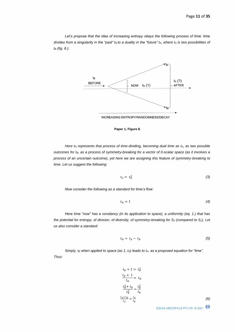
Let’s propose that the idea of increasing entropy obeys the following process of time: time

divides from a singularity in the “past” tB to a duality in the “future” tA, where tA is two possibilities of

tB (fig. 8.):

Here tN represents that process of time-dividing, becoming dual time as tA, as two possible

outcomes for tB, as a process of symmetry-breaking for a vector of 0-scalar space (as it involves a

process of an uncertain outcome), yet here we are assigning this feature of symmetry-breaking to

time. Let us suggest the following:

𝑡𝐴 = 𝑡𝐵2 (3)

Now consider the following as a standard for time’s flow:

𝑡𝑁 = 1 (4)

Here time “now” has a constancy (in its application to space), a uniformity (eq. 1.) that has

the potential for entropy, of division, of diversity, of symmetry-breaking for S2 (compared to S1). Let

us also consider a standard:

𝑡𝑁 = 𝑡𝐴 − 𝑡𝐵 (5)

Simply, tB when applied to space (as 1, tN) leads to tA, as a proposed equation for “time”.

Thus:

𝑡𝐵 + 1 = 𝑡𝐵2

𝑡𝐵 + 1

𝑡𝐵= 𝑡𝐵

𝑡𝐵2+ 𝑡𝐵

𝑡𝐵2 =

𝑡𝐵2

𝑡𝐵

𝑡𝐴+ 𝑡𝐵

𝑡𝐴=

𝑡𝐴

𝑡𝐵 (6)

Paper 1, Figure 8.

of 35


Both processes result in the same golden ratio equation.

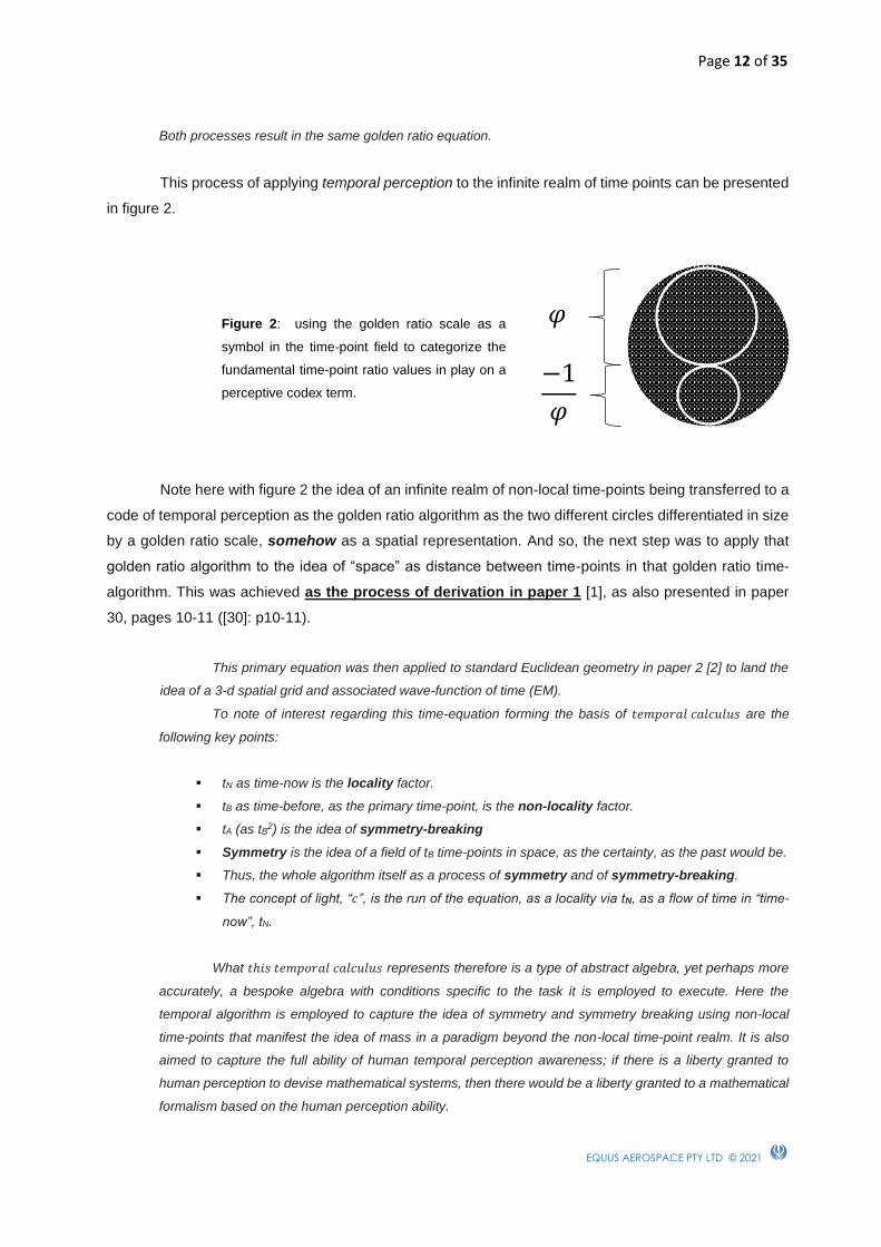
This process of applying temporal perception to the infinite realm of time points can be presented

in figure 2.

Note here with figure 2 the idea of an infinite realm of non-local time-points being transferred to a

code of temporal perception as the golden ratio algorithm as the two different circles differentiated in size

by a golden ratio scale, somehow as a spatial representation. And so, the next step was to apply that

golden ratio algorithm to the idea of “space” as distance between time-points in that golden ratio time-

algorithm. This was achieved as the process of derivation in paper 1 [1], as also presented in paper

30, pages 10-11 ([30]: p10-11).

This primary equation was then applied to standard Euclidean geometry in paper 2 [2] to land the

idea of a 3-d spatial grid and associated wave-function of time (EM).

To note of interest regarding this time-equation forming the basis of 𝑡𝑒𝑚𝑝𝑜𝑟𝑎𝑙 𝑐𝑎𝑙𝑐𝑢𝑙𝑢𝑠 are the

following key points:

▪ tN as time-now is the locality factor.

▪ tB as time-before, as the primary time-point, is the non-locality factor.

▪ tA (as tB2) is the idea of symmetry-breaking

▪ Symmetry is the idea of a field of tB time-points in space, as the certainty, as the past would be.

▪ Thus, the whole algorithm itself as a process of symmetry and of symmetry-breaking.

▪ The concept of light, “𝑐”, is the run of the equation, as a locality via tN, as a flow of time in “time-

now”, tN.

What 𝑡ℎ𝑖𝑠 𝑡𝑒𝑚𝑝𝑜𝑟𝑎𝑙 𝑐𝑎𝑙𝑐𝑢𝑙𝑢𝑠 represents therefore is a type of abstract algebra, yet perhaps more

accurately, a bespoke algebra with conditions specific to the task it is employed to execute. Here the

temporal algorithm is employed to capture the idea of symmetry and symmetry breaking using non-local

time-points that manifest the idea of mass in a paradigm beyond the non-local time-point realm. It is also

aimed to capture the full ability of human temporal perception awareness; if there is a liberty granted to

human perception to devise mathematical systems, then there would be a liberty granted to a mathematical

formalism based on the human perception ability.

Figure 2: using the golden ratio scale as a

symbol in the time-point field to categorize the

fundamental time-point ratio values in play on a

perceptive codex term.

𝜑

−1

𝜑

of 35


3.2 Temporal Mechanics Metric Building

What had to happen as the next theoretic step is the remarkable thing, namely the inclusion of

the concept of a circle, of the surface area of a sphere to be more precise, as the propagation of the

surface area of a sphere from each non-local time-point in space to account and therefore derive 3-d

space, as the process of derivation in paper 2 [2].

The next theoretic step to make was to present the case that the idea of “consciousness”,

assumed here in the idea of temporal perception as the golden ratio equation, is the “perfection” of that

circle, the “perfection” of that sphere, the need for that equation for “𝜋” to “fit” to make the assumption of

temporal perception as the golden ratio equation actually work. Such was paper 3 [3].

In short, papers 1-3 [1-3] laid down the foundations for a theoretic building process from the non-

local time-points to space, to then derive the idea of physical phenomena, particles and field forces, and

their associated constants and properties in regard to this interoperation between the non-local time-

points and derived 3-d space. Such was paper 4 [4].

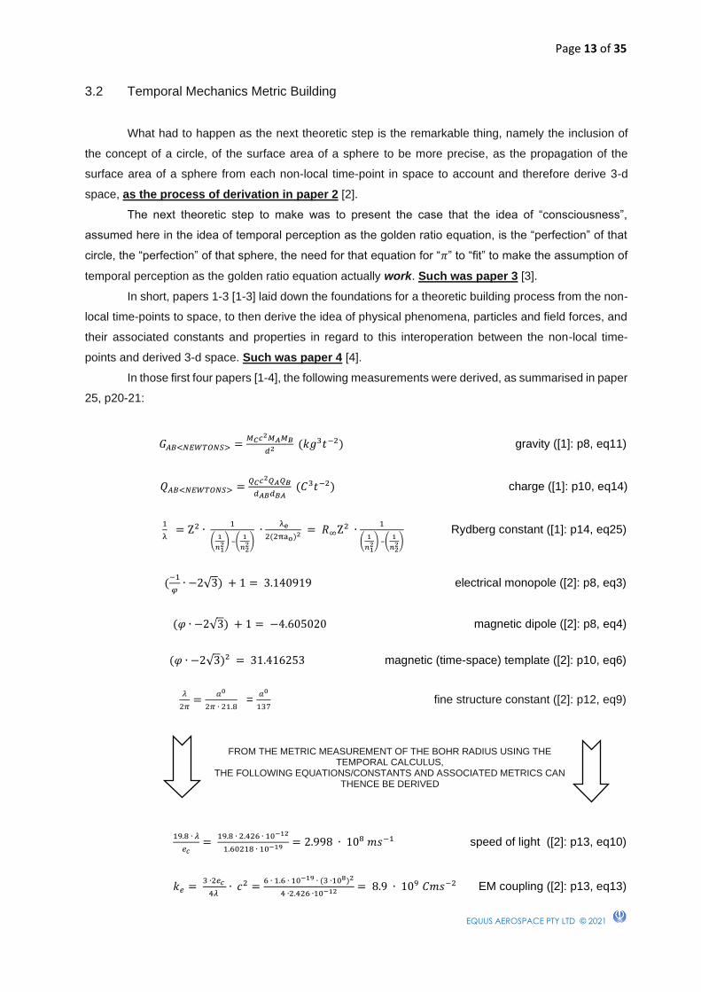
In those first four papers [1-4], the following measurements were derived, as summarised in paper

25, p20-21:

𝐺𝐴𝐵<𝑁𝐸𝑊𝑇𝑂𝑁𝑆> =𝑀𝐶𝑐2𝑀𝐴𝑀𝐵

𝑑2 (𝑘𝑔3𝑡−2) gravity ([1]: p8, eq11)

𝑄𝐴𝐵<𝑁𝐸𝑊𝑇𝑂𝑁𝑆> =𝑄𝐶𝑐2𝑄𝐴𝑄𝐵

𝑑𝐴𝐵𝑑𝐵𝐴 (𝐶3𝑡−2) charge ([1]: p10, eq14)

1

λ = Z2 ∙

1

(1

𝑛12) –(

1

𝑛22)

∙ λe

2(2πao)2 = 𝑅∞Z2 ∙1

(1

𝑛12) –(

1

𝑛22)

Rydberg constant ([1]: p14, eq25)

(−1

𝜑∙ −2√3) + 1 = 3.140919 electrical monopole ([2]: p8, eq3)

(𝜑 ∙ −2√3) + 1 = −4.605020 magnetic dipole ([2]: p8, eq4)

(𝜑 ∙ −2√3)² = 31.416253 magnetic (time-space) template ([2]: p10, eq6)

𝜆

2𝜋=

𝑎0

2𝜋 ∙ 21.8 =

𝑎0

137 fine structure constant ([2]: p12, eq9)

FROM THE METRIC MEASUREMENT OF THE BOHR RADIUS USING THE

TEMPORAL CALCULUS, THE FOLLOWING EQUATIONS/CONSTANTS AND ASSOCIATED METRICS CAN

THENCE BE DERIVED

19.8 ∙ 𝜆

𝑒𝑐=

19.8 ∙ 2.426 ∙ 10−12

1.60218 ∙ 10−19 = 2.998 ∙ 108 𝑚𝑠−1 speed of light ([2]: p13, eq10)

𝑘𝑒 = 3 ∙2𝑒𝑐

4𝜆 ∙ 𝑐2 =

6 ∙ 1.6 ∙ 10−19 ∙ (3 ∙108)2

4 ∙2.426 ∙10−12 = 8.9 ∙ 109 𝐶𝑚𝑠−2 EM coupling ([2]: p13, eq13)

of 35


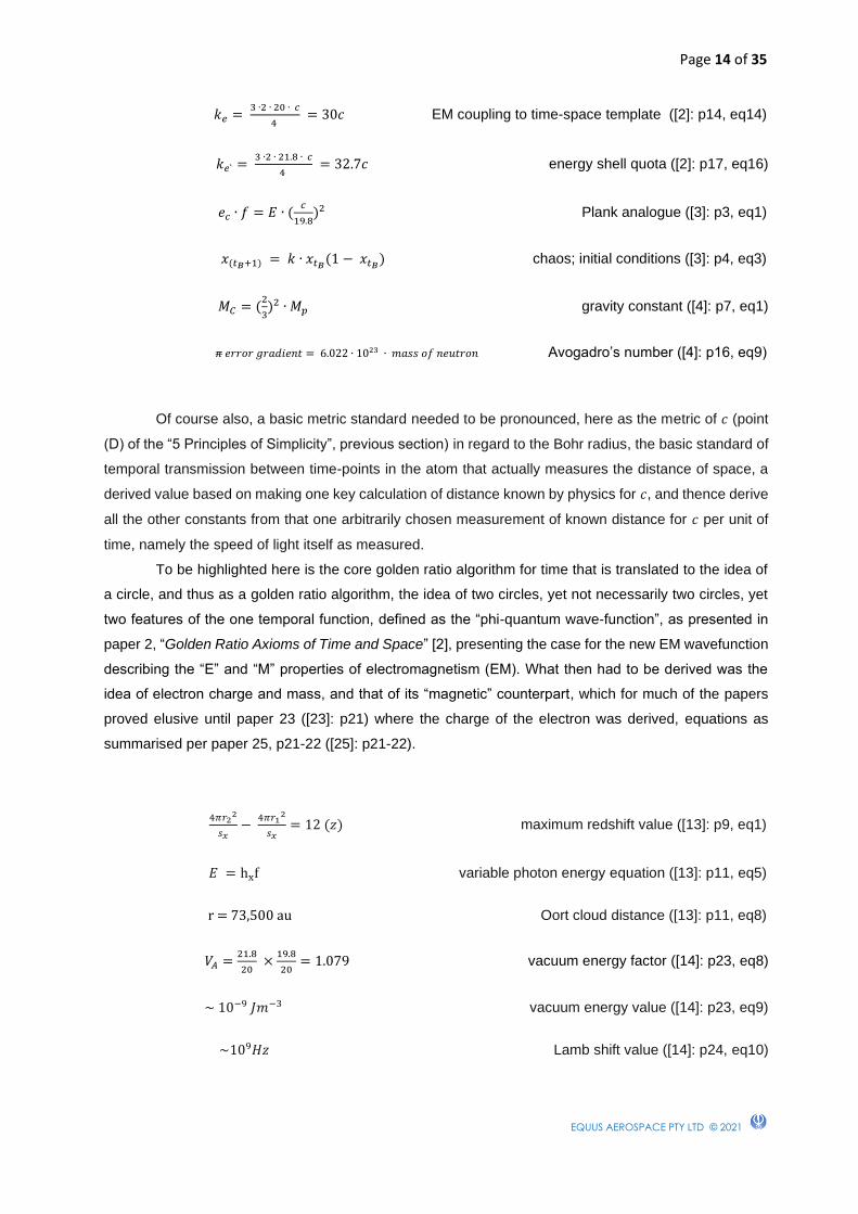
𝑘𝑒 = 3 ∙2 ∙ 20 ∙ 𝑐

4 = 30𝑐 EM coupling to time-space template ([2]: p14, eq14)

𝑘𝑒` = 3 ∙2 ∙ 21.8 ∙ 𝑐

4 = 32.7𝑐 energy shell quota ([2]: p17, eq16)

𝑒𝑐 ∙ 𝑓 = 𝐸 ∙ (𝑐

19.8)2 Plank analogue ([3]: p3, eq1)

𝑥(𝑡𝐵+1) = 𝑘 ∙ 𝑥𝑡𝐵(1 − 𝑥𝑡𝐵

) chaos; initial conditions ([3]: p4, eq3)

𝑀𝐶 = (2

3)2 ∙ 𝑀𝑝

gravity constant ([4]: p7, eq1)

𝜋 𝑒𝑟𝑟𝑜𝑟 𝑔𝑟𝑎𝑑𝑖𝑒𝑛𝑡 = 6.022 ∙ 1023 ∙ 𝑚𝑎𝑠𝑠 𝑜𝑓 𝑛𝑒𝑢𝑡𝑟𝑜𝑛 Avogadro’s number ([4]: p16, eq9)

Of course also, a basic metric standard needed to be pronounced, here as the metric of 𝑐 (point

(D) of the “5 Principles of Simplicity”, previous section) in regard to the Bohr radius, the basic standard of

temporal transmission between time-points in the atom that actually measures the distance of space, a

derived value based on making one key calculation of distance known by physics for 𝑐, and thence derive

all the other constants from that one arbitrarily chosen measurement of known distance for 𝑐 per unit of

time, namely the speed of light itself as measured.

To be highlighted here is the core golden ratio algorithm for time that is translated to the idea of

a circle, and thus as a golden ratio algorithm, the idea of two circles, yet not necessarily two circles, yet

two features of the one temporal function, defined as the “phi-quantum wave-function”, as presented in

paper 2, “Golden Ratio Axioms of Time and Space” [2], presenting the case for the new EM wavefunction

describing the “E” and “M” properties of electromagnetism (EM). What then had to be derived was the

idea of electron charge and mass, and that of its “magnetic” counterpart, which for much of the papers

proved elusive until paper 23 ([23]: p21) where the charge of the electron was derived, equations as

summarised per paper 25, p21-22 ([25]: p21-22).

4𝜋𝑟22

𝑠𝑥−

4𝜋𝑟12

𝑠𝑥= 12 (𝑧) maximum redshift value ([13]: p9, eq1)

𝐸 = hxf variable photon energy equation ([13]: p11, eq5)

r = 73,500 au Oort cloud distance ([13]: p11, eq8)

𝑉𝐴 =21.8

20 ×

19.8

20= 1.079 vacuum energy factor ([14]: p23, eq8)

~ 10−9 𝐽𝑚−3 vacuum energy value ([14]: p23, eq9)

~109𝐻𝑧 Lamb shift value ([14]: p24, eq10)

of 35


tB = √21.8 ∙1.079

NA = 6.25 ∙ 10−12 s cosmological CMBR value ([14]: p25, eq12)

2.7 ×22

21.8= 2.725 (𝑡𝑒𝑚𝑝𝑒𝑟𝑎𝑡𝑢𝑟𝑒) lowest temperature (CMBR) ([14]: p25, eq13)

𝑒 = 𝑚 ∙ 𝑐2. Einstein’s equation ([14]: p26, eq18)

532 × 1.079 = 574 𝑎𝑟𝑐𝑠𝑒𝑐𝑜𝑛𝑑𝑠 𝑝𝑒𝑟 𝑐𝑒𝑛𝑡𝑢𝑟𝑦 Perihelion of Mercury ([14]: p28, eq19)

𝜋

4= 1 −

1

3+

1

5−

1

7+

1

9… 𝑒𝑡𝑐 𝜋 algorithm ([15]: p7, eq4)

𝑒2 + 𝜑2 ~ (√19.8

20 𝜋)

2

general energy equation ([15]: p11, eq8)

√2 + √3 ≅ 𝜋 𝜋 approximation ([16]: p8, eq1)

𝑒2 < 𝑬𝑵𝑻𝑹𝑶𝑷𝒀 > + 𝜑2 < 𝑬𝑵𝑻𝑹𝑶𝑷𝒀 > ≅ (√19.8

20 𝜋)

2

< 𝑬𝑵𝑻𝑯𝑨𝑳𝑷𝒀 > energy equation ([20]: p10, eq2)

𝑚 ∙ 𝑑

𝑡 = 𝑓𝑢𝑛𝑑𝑎𝑚𝑒𝑛𝑡𝑎𝑙 𝑝𝑟𝑜𝑝𝑒𝑟𝑡𝑦 1 momentum ([23]: p21, eq2)

𝑒 ∙ 𝑡

𝑑 = 𝑓𝑢𝑛𝑑𝑎𝑚𝑒𝑛𝑡𝑎𝑙 𝑝𝑟𝑜𝑝𝑒𝑟𝑡𝑦 2 charge ([23]: p21, eq3)

≅ 1.67 ∗ 10-27𝑘𝑔 proton/neutron mass from charge ([23]: p22)

𝜀0 =1

4𝜋 ×

1

𝑄𝐶 ∙ 𝑐2 = 1

4𝜋 ∙ 𝑘𝑒 vacuum permittivity ([23]: p30, eq5)

𝜀0 = 1

𝜇0 ∙ 𝑐2 vacuum permeability ([23]: p30, eq7)

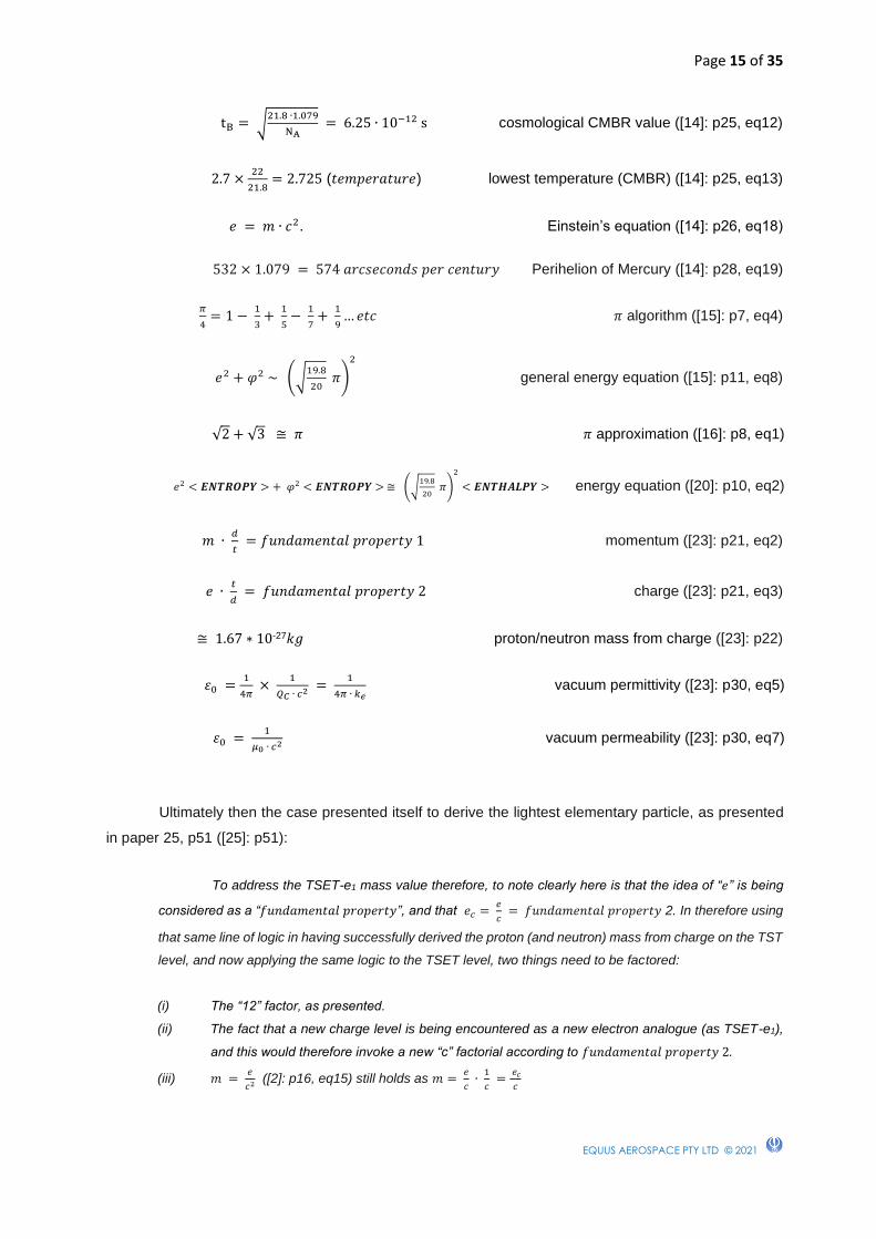
Ultimately then the case presented itself to derive the lightest elementary particle, as presented

in paper 25, p51 ([25]: p51):

To address the TSET-e1 mass value therefore, to note clearly here is that the idea of “𝑒” is being

considered as a “𝑓𝑢𝑛𝑑𝑎𝑚𝑒𝑛𝑡𝑎𝑙 𝑝𝑟𝑜𝑝𝑒𝑟𝑡𝑦”, and that 𝑒𝑐 = 𝑒

𝑐 = 𝑓𝑢𝑛𝑑𝑎𝑚𝑒𝑛𝑡𝑎𝑙 𝑝𝑟𝑜𝑝𝑒𝑟𝑡𝑦 2. In therefore using

that same line of logic in having successfully derived the proton (and neutron) mass from charge on the TST

level, and now applying the same logic to the TSET level, two things need to be factored:

(i) The “12” factor, as presented.

(ii) The fact that a new charge level is being encountered as a new electron analogue (as TSET-e1),

and this would therefore invoke a new “c” factorial according to 𝑓𝑢𝑛𝑑𝑎𝑚𝑒𝑛𝑡𝑎𝑙 𝑝𝑟𝑜𝑝𝑒𝑟𝑡𝑦 2.

(iii) 𝑚 = 𝑒

𝑐2 ([2]: p16, eq15) still holds as 𝑚 = 𝑒

𝑐 ∙

1

𝑐 =

𝑒𝑐

𝑐

of 35


Therefore, the equation for the mass of TSET-e1, the value of the mass gap 𝑚𝑀𝐺, would be as

follows:

𝑚𝑀𝐺 = 𝑒𝑐

𝑐 ∙

1

12 ∙

1

𝑐= 1.5 ∙ 10−37𝑘𝑔 (10)

This would be the value for TSET-e1 as confirmed by researchers from UCL, Universidade Federal

do Rio de Janeiro, Institut d'Astrophysique de Paris and Universidade de Sao Paulo [26].

Through this entire process, all the particle and field features of the characters of these equations,

their persona, were accurately derived with this golden ratio 𝑡𝑒𝑚𝑝𝑜𝑟𝑎𝑙 𝑐𝑎𝑙𝑐𝑢𝑙𝑢𝑠 codex and compared to

known particle and field phenomena matching the same phenomenal description. Yet something very

interesting evolved, namely the idea of reality actually representing an image upon the surface area of a

sphere, a 2-d spherical manifold. The importance of this was realised in paper 30, “Non-Local Time-Point

Theory: Magnetic Quantum Shell (MQS) Modelling” [30], with the derivation of the X17 particle, pages 18-

19 ([30]: p18-19), and the importance there of the magnetic 2-d shell construct as a key phenomenal

manifold in reality related to EM and particle phenomena.

According to paper 2 ([2]: p17), there exists a scale in play for the magnetic template EM-coupling

dynamic of 32.7, as an adjusted EM-coupling factor, as by definition of the 𝑒 and 𝑚 time-points, thus time-

points which are linked via the phi-quantum wave-function ([2]: p4-11), a condition that would fix not only the

electron number per shell at a maximum value, yet define the concept of a shell itself as a spherical surface

area; such is what is proposed for the uniform magnetic quantum shell surface area structure, namely this

theoretic maximum value factored to the energy of a single electron, as though although the electrons can

be of any number in the atom, the electron feature abides by a code of being uniformly held by the 32.7 EM-

coupling factor of the 𝑀𝑄𝑆, almost like an axis the electron builds around as a value for atomic modelling of

EM-coupling stability for each electron, of course in the constraints of the Hyperfine structure of the shells

and associated inclusion of the Rydberg equation.

Therefore, this primary 32.7 EM-coupling factor would be applied to each electron as a value of

energy-mass, as a quantum representation of the shell, and thus surface area, as it can only represent, and

therefore the proposal is that equation 1 and 2 apply for the energy value of the magnetic shell for each

electron as a mass value for the magnetic component of the 32.7 EM-coupling factor:

32.7 ∙ 𝑒𝑙𝑒𝑐𝑡𝑟𝑜𝑛 𝑚𝑎𝑠𝑠 = 𝑀𝑄𝑆 𝑠ℎ𝑒𝑙𝑙 𝑢𝑛𝑖𝑡 𝑚𝑎𝑠𝑠 (1.)

32.7 ∙ 0.511 𝑀𝑒𝑉𝑐−2 = 16.7 𝑀𝑒𝑉𝑐−2 (2.)

Research by the “𝐼𝑛𝑠𝑡𝑖𝑡𝑢𝑡𝑒 𝑜𝑓 𝑁𝑢𝑐𝑙𝑒𝑎𝑟 𝑅𝑒𝑠𝑒𝑎𝑟𝑐ℎ (𝐴𝑡𝑜𝑚𝑘𝑖)” through work at 𝐶𝐸𝑅𝑁 has uncovered

a value for such an energy in the atom of 16.7 𝑀𝑒𝑉, ascribing this value to a particle named 𝑋17 [32][33][34].

𝐴𝑡𝑜𝑚𝑘𝑖 has though not identified this as the magnetic shell confining an electron in the atom though, as that

theory has not been formulated by contemporary modelling, and thus the energy value remains a mystery

to the physics community.

of 35


3.3 Temporal Mechanics metric synchronisation

The importance of this magnetic quantum shell (𝑀𝑄𝑆) system [30] was then taken to this current

series of five papers (time-space circuits, constants, manifolds, metrics, and logistics), to describe how

ultimately these manifolds, these surface areas, would work to the level of the proposed 𝐸 = 𝑓 feature of

light in space, as Temporal Mechanics derived, all the way to the proposed Black Expanse beyond the

Oort cloud. This was the purpose of papers 32-33 [32-33], specifically the previous paper, “Temporal

Mechanics (C): Time-Space Manifolds”, chapter 4, “The Macroscopic Manifolds” ([33]: p8-17).

To then compact all of such into a diagram from the level of the infinite non-local time-point realm,

consider figure 3.

As the diagrams present, the more fundamental 2-d realms (manifolds) become apparent, as the

primary dimensional realm providing the features of the elementary, subatomic, and atomic particle

phenomena, presenting the phenomena of the greater macroscopic manifolds of the Heliopause, Bow

Shock, and Oort Cloud.

All of such can be described as an equation from an infinite time-point aether (𝑇∞) projected to

what would appear to be a 3-d spatial realm (𝑆3) (note that 4-d spacetime is being by-passed here, as a

Figure 3: an amalgamation of the non-local time-point golden ratio field (1.; from figure 2), accompanied to

the microscopic scale (2.; ([33]: p11,fig2)), and then applied to the macroscopic scale (3.; (25]: p48, fig15)).

1.

2.

3.

of 35


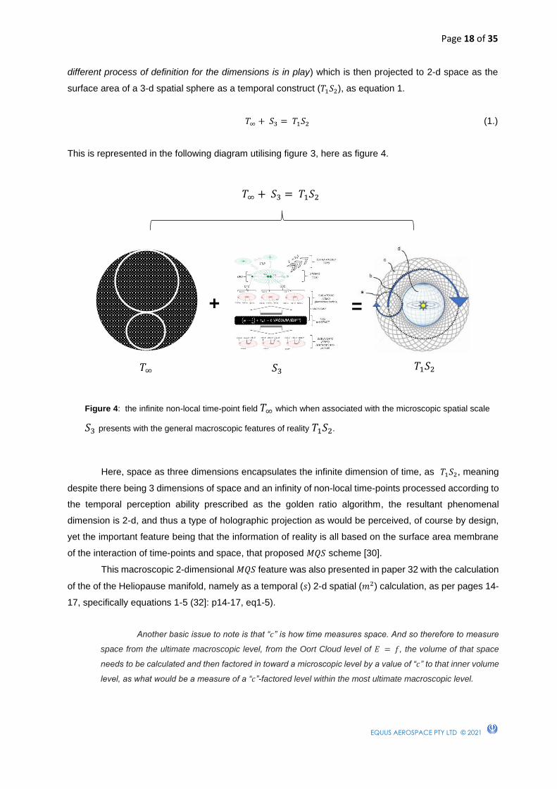
different process of definition for the dimensions is in play) which is then projected to 2-d space as the

surface area of a 3-d spatial sphere as a temporal construct (𝑇1𝑆2), as equation 1.

𝑇∞ + 𝑆3 = 𝑇1𝑆2 (1.)

This is represented in the following diagram utilising figure 3, here as figure 4.

Here, space as three dimensions encapsulates the infinite dimension of time, as 𝑇1𝑆2, meaning

despite there being 3 dimensions of space and an infinity of non-local time-points processed according to

the temporal perception ability prescribed as the golden ratio algorithm, the resultant phenomenal

dimension is 2-d, and thus a type of holographic projection as would be perceived, of course by design,

yet the important feature being that the information of reality is all based on the surface area membrane

of the interaction of time-points and space, that proposed 𝑀𝑄𝑆 scheme [30].

This macroscopic 2-dimensional 𝑀𝑄𝑆 feature was also presented in paper 32 with the calculation

of the of the Heliopause manifold, namely as a temporal (𝑠) 2-d spatial (𝑚2) calculation, as per pages 14-

17, specifically equations 1-5 (32]: p14-17, eq1-5).

Another basic issue to note is that “𝑐” is how time measures space. And so therefore to measure

space from the ultimate macroscopic level, from the Oort Cloud level of 𝐸 = 𝑓, the volume of that space

needs to be calculated and then factored in toward a microscopic level by a value of “𝑐” to that inner volume

level, as what would be a measure of a “𝑐”-factored level within the most ultimate macroscopic level.

Figure 4: the infinite non-local time-point field 𝑇∞ which when associated with the microscopic spatial scale

𝑆3 presents with the general macroscopic features of reality 𝑇1𝑆2.

+

=

𝑇∞ + 𝑆3 = 𝑇1𝑆2

𝑇∞

𝑆3

𝑇1𝑆2

of 35


This idea was presented in paper 25 ([25]: p50-51) regarding the microscopic level in the manner

of calculating the mass of the lightest elementary particle in calculating what exists as mass below the

structure of a subatomic mass, using a factor of “𝑐” and “12” for the mass of the proton, stepping below that.

Here though the process of the macroscopic scale is different to the microscopic scale, as it can

only be, as they are two very different things; the thinking is to use a basic scaling of “𝑐” with the value of

energy in terms of volume, and not mass (mass, as was used on the microscopic scale), namely the volume

of the Solar System to the Oort cloud, specifically as 4

3𝜋𝑟𝑂

3 where 𝑟𝑂 is the distance of 𝑆𝑂𝐿 to the Oort cloud,

derived to be 1.1 ∙ 1016 𝑚 (73,500 𝑎𝑢), as per equation 1:

4

3𝜋𝑟𝑂

3 = 4 ∙ 𝜋 ∙(1.1 ∙ 1016)3

3= 5.58 ∙ 1048 𝑚3 (1)

This value is then proposed to be factored back a value of “𝑐”, taken within itself, as “𝑐” is the

standard of measurement between time-points measuring space.

So, the calculation here aims to derive what the next manifold would be from the overall ultimate

manifold of 𝐸 = 𝑓, from that ultimate macroscopic manifold of 𝐸 = 𝑓, as follows:

5.58 ∙1048

𝑐= 1.86 ∙ 1040 (2)

The value of “𝑟” for this value, this new value for r, say 𝑟𝐻, then equates to the following:

4

3𝜋𝑟𝐻

3 = 1.86 ∙ 1040 (3)

𝑟𝐻 = 1.643 ∙ 1013 𝑚 (4)

𝑟𝐻 = 110 𝑎𝑢 (5)

This value would represent the basic time-space manifold within the macroscopic 𝐸 = 𝑓 manifold.

Therefore, if the 𝐸 = 𝑓 manifold represents the process of mass disintegrating to a macroscopic

sub-light level, to a macroscopic elementary particle level, as a particle zone in time-space, then this new

manifold of distance 𝑟𝐻 from 𝑆𝑂𝐿 would represent the basic subatomic level, a plasma level, as per the

following diagram.

Paper 32, Figure 1: a universal scale from a source of light as the Sun outwards in a spherical wavefront of light

a distance of 𝑟𝑂 = 73,500 𝑎𝑢, tracked back a time-scale measurement of “c” to the Heliopause as 𝑟𝐻 = 110 𝑎𝑢.

of 35


Astrophysics knows 𝑟𝐻 as the Heliopause [35].

Once again, 𝑟𝐻 would represent the basic scaling from the macroscopic 𝐸 = 𝑓 level to a universal

level of “𝑐” within that zone, to the next most basic level, and here this is proposed to be the macroscopic

subatomic level, a level of quantum stagnation, where in all appearance the plasma-styled solar wind would

appear to measure equally with any apparent interstellar wind, leading to a type of static plasma sphere.

Thus notably, at and beyond this Heliopause would be a marked increase in plasma particle activity. To what

point though?

There is still the issue of factoring the value of “12” on the Oort Cloud level, that required ultimate

macroscopic 𝐸 = 𝑓 level, as presented in paper 13 ([13]: p11-12) to fulfil the general entropy-enthalpy

equation for energy, as was appropriated on the microscopic level in paper 25([25]: p50-51).

The thinking here with this Oort cloud macroscopic manifold and associated Heliopause manifold

is that the value of “12” would be factored “into” “𝑐” by a certain mechanism inverse to what was proposed

on the microscopic level, namely as a process of enhancing the Heliopause by a factor of 12 regarding

volume. Note that this process would be an inverse application to the process used on the elementary

particle level, for here is a new process, a macroscopic process, not a microscopic process, and thus the

process of application of the “12” factorial would be inverse to how it was applied on the microscopic scale,

despite still using “𝑐” as a measurement standard between time-points in space as was used on the

microscopic scale.

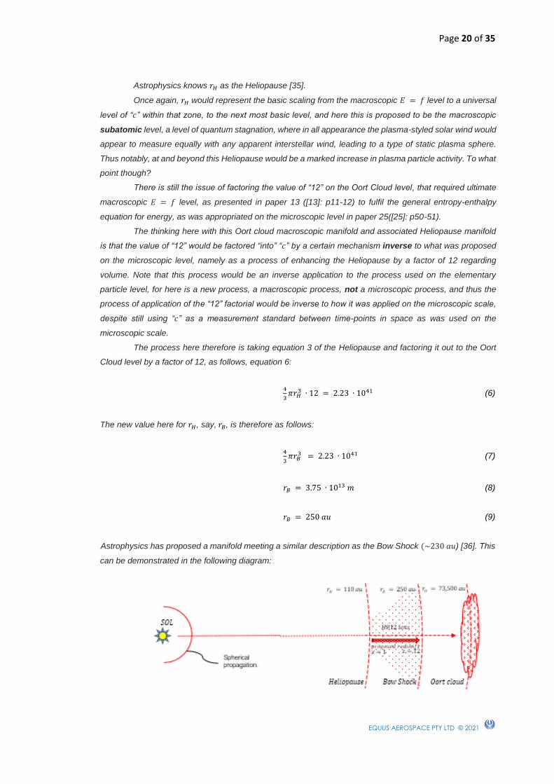
The process here therefore is taking equation 3 of the Heliopause and factoring it out to the Oort

Cloud level by a factor of 12, as follows, equation 6:

4

3𝜋𝑟𝐻

3 ∙ 12 = 2.23 ∙ 1041 (6)

The new value here for 𝑟𝐻, say, 𝑟𝐵, is therefore as follows:

4

3𝜋𝑟𝐵

3 = 2.23 ∙ 1041 (7)

𝑟𝐵 = 3.75 ∙ 1013 𝑚 (8)

𝑟𝐵 = 250 𝑎𝑢 (9)

Astrophysics has proposed a manifold meeting a similar description as the Bow Shock (~230 𝑎𝑢) [36]. This

can be demonstrated in the following diagram:

of 35


The thinking of this region is that it represents, in theory, a general layer where the CMBR bleeds down as

the 𝑧 = 1 > 𝑧 = 12 redshift process, from the Heliopause to the Bow Shock, noting that “c” is being

accompanied here with “12” as a measure of distance between time-points in space, here as a factor of “12”,

yet not only this, yet doing this while light and associated plasma behaves like a type of pressure “shock”

front to the space beyond which (towards the Oort cloud) where matter in theory would disintegrate, and

light lose its integrity.

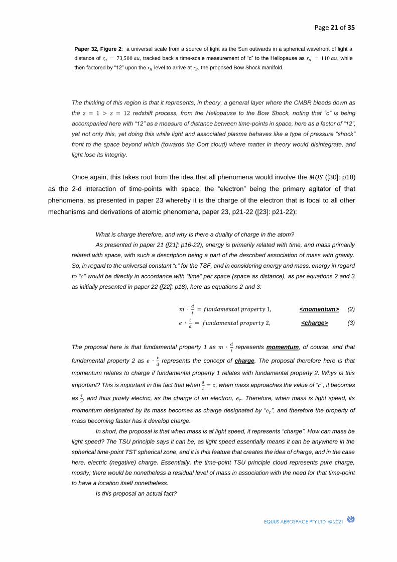
Once again, this takes root from the idea that all phenomena would involve the 𝑀𝑄𝑆 ([30]: p18)

as the 2-d interaction of time-points with space, the “electron” being the primary agitator of that

phenomena, as presented in paper 23 whereby it is the charge of the electron that is focal to all other

mechanisms and derivations of atomic phenomena, paper 23, p21-22 ([23]: p21-22):

What is charge therefore, and why is there a duality of charge in the atom?

As presented in paper 21 ([21]: p16-22), energy is primarily related with time, and mass primarily

related with space, with such a description being a part of the described association of mass with gravity.

So, in regard to the universal constant “𝑐” for the TSF, and in considering energy and mass, energy in regard

to “𝑐” would be directly in accordance with “time” per space (space as distance), as per equations 2 and 3

as initially presented in paper 22 ([22]: p18), here as equations 2 and 3:

𝑚 ∙ 𝑑

𝑡 = 𝑓𝑢𝑛𝑑𝑎𝑚𝑒𝑛𝑡𝑎𝑙 𝑝𝑟𝑜𝑝𝑒𝑟𝑡𝑦 1, <momentum> (2)

𝑒 ∙ 𝑡

𝑑 = 𝑓𝑢𝑛𝑑𝑎𝑚𝑒𝑛𝑡𝑎𝑙 𝑝𝑟𝑜𝑝𝑒𝑟𝑡𝑦 2, <charge> (3)

The proposal here is that fundamental property 1 as 𝑚 ∙ 𝑑

𝑡 represents momentum, of course, and that

fundamental property 2 as 𝑒 ∙ 𝑡

𝑑 represents the concept of charge. The proposal therefore here is that

momentum relates to charge if fundamental property 1 relates with fundamental property 2. Whys is this

important? This is important in the fact that when 𝑑

𝑡= 𝑐, when mass approaches the value of “𝑐”, it becomes

as 𝑒

𝑐, and thus purely electric, as the charge of an electron, 𝑒𝑐. Therefore, when mass is light speed, its

momentum designated by its mass becomes as charge designated by “𝑒𝑐”, and therefore the property of

mass becoming faster has it develop charge.

In short, the proposal is that when mass is at light speed, it represents “charge”. How can mass be

light speed? The TSU principle says it can be, as light speed essentially means it can be anywhere in the

spherical time-point TST spherical zone, and it is this feature that creates the idea of charge, and in the case

here, electric (negative) charge. Essentially, the time-point TSU principle cloud represents pure charge,

mostly; there would be nonetheless a residual level of mass in association with the need for that time-point

to have a location itself nonetheless.

Is this proposal an actual fact?

Paper 32, Figure 2: a universal scale from a source of light as the Sun outwards in a spherical wavefront of light a

distance of 𝑟𝑂 = 73,500 𝑎𝑢, tracked back a time-scale measurement of “c” to the Heliopause as 𝑟𝐻 = 110 𝑎𝑢, while

then factored by “12” upon the 𝑟𝐻 level to arrive at 𝑟𝐵, the proposed Bow Shock manifold.

of 35


According to paper 2 ([2]: p13, eq11)], 𝑒𝑐 = 19.8 ∙ 𝜆

𝑐 = 1.60218 ∙ 10−19 𝐶, an actual fact. Charge

therefore would exist as the electron cloud associated to a magnetic time-point, while also needing to be

balanced with a positive charge of equal value to the electron, as such a balance of charge would need to

exist as the property of the TSF and associated TST representing a type of overall neutral footing basis.

6.5 Proton, Neutron, and Electron mass

It would be now possible to calculate the mass of the proton (and neutron) if it is considered that

such a basic time-point particle as mass when taken up to near light speed produces the charge equivalent

to that of an electron. For instance:

• If particle speed and wavelength are known, distance and time:

▪ the charge can be calculated as 𝑒𝑐 = 19.8 ∙ 𝜆

𝑐 ([2]: p13, eq11)

▪ and so too its mass from which the electron as a charge came (in using

𝑚 = 𝑒

𝑐2 ([2]: p16, eq15) and 𝑒𝑐 =

𝑒

𝑐 = 𝑓𝑢𝑛𝑑𝑎𝑚𝑒𝑛𝑡𝑎𝑙 𝑝𝑟𝑜𝑝𝑒𝑟𝑡𝑦 2, eq3):

▪ thus 𝑚 equates to ≅ 5.3 ∗ 10-28𝑘𝑔

▪ Factor this by 𝜋 and the mass of a proton (or neutron) can be calculated. Why a

factor of 𝜋? The mass of the electron would have been “per” 𝜋, the actual spherical

reference it is upon as the time-point cloud (TSG), yet the mass of the central time-

point would not be per 𝜋 and thus the 5.3 ∗ 10-28𝑘𝑔 value needs to be factored with

𝜋, giving:

▪ ≅ 1.67 ∗ 10-27𝑘𝑔

Essentially, Temporal Mechanics proposes that the phenomena of the stars is actually a

projection intrinsic to the greater manifolds of this solar system reality, the manifolds of the Heliopause,

Bow Shock, and Oort Cloud.

To note is that Temporal Mechanics never sought out to explain the phenomena of the stars from

data in the context of the proposed ΛCDM model and those assumptions, from astrophysics, the

phenomena of the redshift effect in particular, yet to derive the basis for their existence, as with first

deriving the basis for the existence of particles and their associated field force attributes. To achieve this,

Temporal Mechanics has had to re-define the a priori of time and space, to then demonstrate the

interoperation of time and space as proven and known particle phenomena and associated field effects,

according to all the relevant metrics and associated constants prescribed to that phenomena. Such has

been the case presented in this paper thus far.

To demonstrate the validity of such, Temporal Mechanics will now explain an added feature to

the great manifolds of reality, from the Heliopause manifold to the Bow Shock manifold to the Oort Cloud

manifold, namely how the 𝑇1𝑆2 dimensional realm presents the case for the metric of the nearest star, that

associated distance to 𝑆𝑂𝐿, and why what would appear to be the closest star would be that calculated

distance, together with then deriving the age of the proposed time-space system as it would present itself

as a feature of a “longest” cycle of time.

of 35


To achieve such, one new manifold needs to be presented as based on the 𝐸 = ℎ𝑓 principle, on

the concept of light itself as it appears to our awareness, light that is atomic based. As shall be

demonstrated, this new manifold joins all the other greater 𝐸 = 𝑓 manifolds, with ultimately this new

manifold presenting the phenomena we understand of the stars.

4. Cosmological metrics

In developing upon the idea of the macroscopic 𝐸 = 𝑓 based manifolds of the previous paper,

“Temporal Mechanics (C): Time-Space Manifolds” [33], distances were initially calculated for 𝑟𝐻

(Heliopause manifold) and 𝑟𝐵 (Bow Shock manifold) as relative to 𝑟𝑂 (𝐸 = 𝑓, Oort Cloud manifold), as

initially presented in paper 32 “Temporal Mechanics (B): Time-Space Circuits” [32] and then further

expanded upon in paper 33 [33], in accounting for a proposed theory for the redshift effect. To further that

theoretic design, what needs to be finally presented for the system of manifolds is a manifold projected

from the central 𝐸 = ℎ𝑓 region, a focal manifold it would seem, focal to the other 𝐸 = 𝑓 based manifolds

(𝑟𝑂, 𝑟𝐻, and 𝑟𝐵), here in this case from 𝑆𝑂𝐿, from the general/predominant 𝐸 = ℎ𝑓 temporal reference,

𝑆𝑂𝐿.

4.1 The 𝑟𝐸 Manifold

Let us present the case therefore that the 𝑐-metric (a requirement here for 𝑡𝑒𝑚𝑝𝑜𝑟𝑎𝑙 𝑐𝑎𝑙𝑐𝑢𝑙𝑢𝑠,

namely using 𝑐 as a way to measure distance in space) manifold extending from 𝑆𝑂𝐿 represents 𝑟𝐸, an

altogether new manifold, yet acting as the focal 𝐸 = ℎ𝑓 manifold for the 𝐸 = 𝑓 based manifolds, where

the 𝐸 = 𝑓 based manifolds come into proper 𝐸 = ℎ𝑓 focus, and therefore most likely the manifold upon

which the holographic universe comes into focus, as a display of 𝐸 = ℎ𝑓 light.

In being consistent with using 𝑐 as a way to measure distance, let us suggest that the value of

this new manifold would be calculated in accounting for the distance light travels from the sun (𝑆𝑂𝐿)

relative to the fixed 𝐸 = 𝑓 reference. Indeed, how?

Let us calculate this new manifold using the Earth reference, and therefore consider it, say, as

𝑟E; 𝑟E quite simply is proposed to represent a primary focus of light of 𝑆𝑂𝐿 as viewed from Earth (𝐸).

In adapting to the fixed 𝑟𝑂 principle, let us say that 𝑟E would also need to be a fixed temporal

reference from Earth, and therefore how far light would travel for one full cycle of the Earth around

𝑺𝑶𝑳, as a measure, namely a process of time that accounts for Earth returning to its same location relative

to 𝑆𝑂𝐿 according to the proposed fixed 𝐸 = 𝑓 manifold of 𝑟O, most basically.

Indeed, the question should be asked, “how would one revolution of Earth seem relevant to

measure distance for 𝑐?”. It must be, as this is the measurement reference being considered, namely

from Earth as a general “fixed” construct, and thus in being fixed the measurement must represent the

time between those fixations, as a year, and thus as the distance light travels in one Earth year, in the

context of the overall fixed reference of 𝑟O, of the Oort Cloud manifold.

of 35


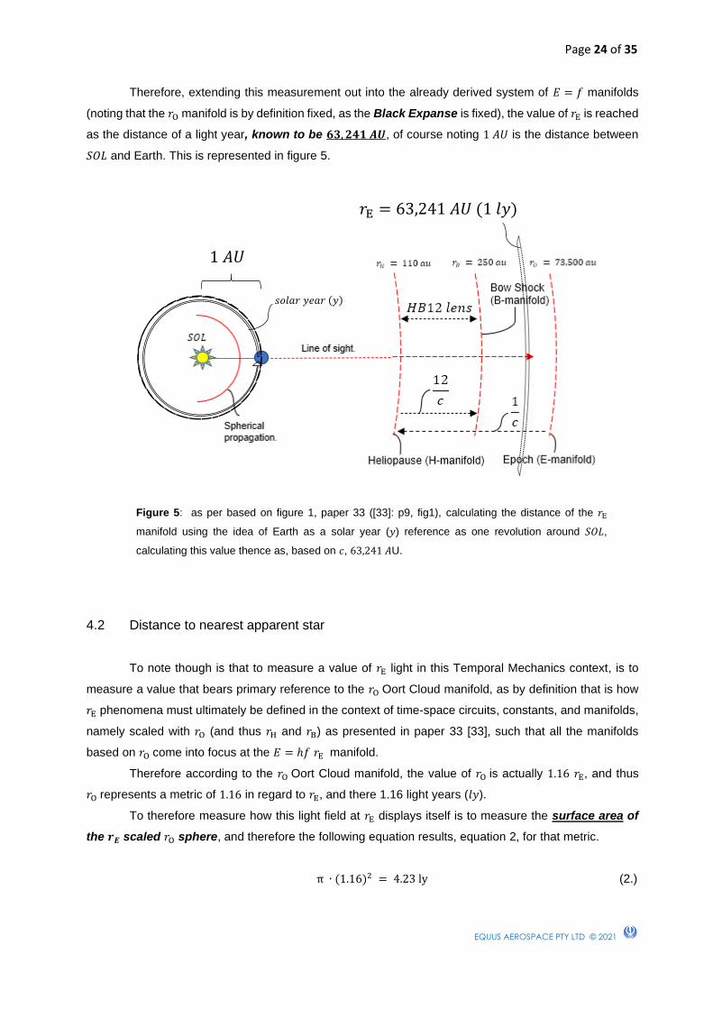
Therefore, extending this measurement out into the already derived system of 𝐸 = 𝑓 manifolds

(noting that the 𝑟O manifold is by definition fixed, as the Black Expanse is fixed), the value of 𝑟E is reached

as the distance of a light year, known to be 𝟔𝟑, 𝟐𝟒𝟏 𝑨𝑼, of course noting 1 𝐴𝑈 is the distance between

𝑆𝑂𝐿 and Earth. This is represented in figure 5.

4.2 Distance to nearest apparent star

To note though is that to measure a value of 𝑟E light in this Temporal Mechanics context, is to

measure a value that bears primary reference to the 𝑟O Oort Cloud manifold, as by definition that is how

𝑟E phenomena must ultimately be defined in the context of time-space circuits, constants, and manifolds,

namely scaled with 𝑟O (and thus 𝑟H and 𝑟B) as presented in paper 33 [33], such that all the manifolds

based on 𝑟O come into focus at the 𝐸 = ℎ𝑓 𝑟E manifold.

Therefore according to the 𝑟O Oort Cloud manifold, the value of 𝑟O is actually 1.16 𝑟E, and thus

𝑟O represents a metric of 1.16 in regard to 𝑟E, and there 1.16 light years (𝑙𝑦).

To therefore measure how this light field at 𝑟E displays itself is to measure the surface area of

the 𝒓𝑬 scaled 𝑟O sphere, and therefore the following equation results, equation 2, for that metric.

π ∙ (1.16)2 = 4.23 ly (2.)

Figure 5: as per based on figure 1, paper 33 ([33]: p9, fig1), calculating the distance of the 𝑟E

manifold using the idea of Earth as a solar year (𝑦) reference as one revolution around 𝑆𝑂𝐿,

calculating this value thence as, based on 𝑐, 63,241 𝐴U.

𝑟E = 63,241 𝐴𝑈 (1 𝑙𝑦)

1 𝐴𝑈

𝑠𝑜𝑙𝑎𝑟 𝑦𝑒𝑎𝑟 (𝑦)

of 35


What this means is that there are 4.23 light years measured as a metric in regard to the reference

of Earth for the idea of light perceived in the 𝑟E to the 𝑟O(𝑟H𝑟B) manifold systems as a virtual (holographic,

namely manifold-filtered) 𝑆𝑂𝐿 entity, as defined from a 𝑆𝑂𝐿 entity basis, as highlighted in figure 6.

This proposed 𝑆𝑂𝐿-Earth based phenomenon per this 𝑟E manifold would represent a virtual

phenomenon, a virtual 𝑆𝑂𝐿, as such is the basis of definition here, and therefore would appear itself as a

presence of light as 𝑆𝑂𝐿 appears to the reference of Earth, yet here according to what would be an

automatically adjusted process of illumination metrics in terms of size and brightness, parallax, and so

on, as can only be the case, with all the required 𝑟O based time-space circuits of the 𝑟H and 𝑟B manifolds

in play, as a “focus” of light phenomena dictated by the time-space circuits in play at the Heliopause (𝑟H)

and to the Bow Shock (𝑟B), as presented in paper 33 [33]. In other words, the 4.244 𝑙𝑦 value would be, as

Temporal Mechanics derives, the closest distance as light years to what would appear to be the nearest

virtual 𝑆𝑂𝐿 from this 𝑆𝑂𝐿 and the reference here on Earth, the most fundamental reference nonetheless

and therefore closest reference for the 𝑆𝑂𝐿 𝑟E manifold in reference to the 𝑟O Oort Cloud manifold, as a

particular holographic virtual 𝑆𝑂𝐿 image.

4.3 Distance to furthest apparent star (age of system)

The next theoretic task is acknowledging greater steps in this process, that beyond this most

fundamental 𝑟E manifold step would exist more distant placements of light activity modelled on the 𝑐 based

𝑆𝑂𝐿 and Earth relationship, according to this 𝑟E manifold.

Figure 6: Calculating the light year (𝑙𝑦) distance of 𝑆𝑂𝐿 to the nearest 𝑟E based virtual 𝑆𝑂𝐿.

4.23 𝑙𝑦

𝑟𝐸 𝑚𝑎𝑛𝑖𝑓𝑜𝑙𝑑

𝑣𝑖𝑟𝑡𝑢𝑎𝑙 𝑖𝑚𝑎𝑔𝑒

𝑆𝑂𝐿

of 35


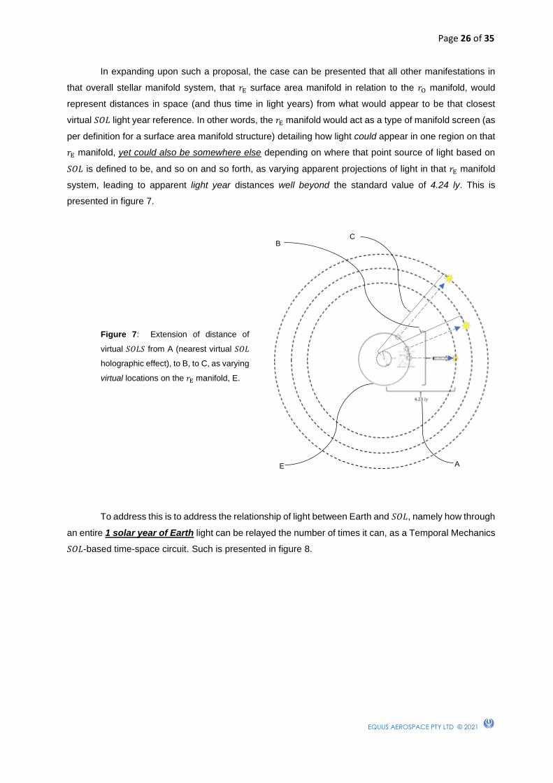
In expanding upon such a proposal, the case can be presented that all other manifestations in

that overall stellar manifold system, that 𝑟E surface area manifold in relation to the 𝑟O manifold, would

represent distances in space (and thus time in light years) from what would appear to be that closest

virtual 𝑆𝑂𝐿 light year reference. In other words, the 𝑟E manifold would act as a type of manifold screen (as

per definition for a surface area manifold structure) detailing how light could appear in one region on that

𝑟E manifold, yet could also be somewhere else depending on where that point source of light based on

𝑆𝑂𝐿 is defined to be, and so on and so forth, as varying apparent projections of light in that 𝑟E manifold

system, leading to apparent light year distances well beyond the standard value of 4.24 ly. This is

presented in figure 7.

To address this is to address the relationship of light between Earth and 𝑆𝑂𝐿, namely how through

an entire 1 solar year of Earth light can be relayed the number of times it can, as a Temporal Mechanics

𝑆𝑂𝐿-based time-space circuit. Such is presented in figure 8.

Figure 7: Extension of distance of

virtual 𝑆𝑂𝐿𝑆 from A (nearest virtual 𝑆𝑂𝐿

holographic effect), to B, to C, as varying

virtual locations on the 𝑟E manifold, E.

A

B

C

E

of 35


For instance, in view of figure 8, the maximum distance of light from 𝑆𝑂𝐿 in light years would be

calculated based on the accumulated interaction of light between 𝑆𝑂𝐿 and Earth in one Earth solar

revolution period.

Can this maximum value be calculated, namely the maximum light year distance in this scheme

of light running from 𝑆𝑂𝐿 to Earth and then returning to 𝑆𝑂𝐿 from Earth as a basic time-space circuit for

this new manifold proposal, namely in regard to the 𝑟E manifold and thence what is presented as a

holographic image as per figure 7?

It should be, as it would be primarily relevant to the number of times light can travel from 𝑆𝑂𝐿 to

Earth and back again, a solar time-space circuit in regard to Earth, during a full Earth solar cycle (~365

days), a 𝑆𝑂𝐿-Earth time-space circuit, which would then be measured as distance.

According to known observations, the number of times light travels to the Earth and back again

from 𝑆𝑂𝐿 is about 980 seconds, given it takes light 490 seconds for light to travel from 𝑆𝑂𝐿 to the Earth.

Given there are 31536000 seconds in a year, this equates to 32,179 times, namely 31536000

980=

32,179.

As a temporal spherical manifold factor though, as must be the case, if this number of steps

(32,179) represents a virtual accumulated 𝑨𝑼-based radius for an overall 𝒓𝐄 manifold, as it must, and

then equated as 𝜋𝑟E2 (𝑟E as the 𝑆𝑂𝐿 𝑐-metric time-space circuit distance, as between Earth and 𝑆𝑂𝐿, as

it must be for Temporal Mechanics) there is the value of 3.253 billion if 𝑟E = 32,179, as per equation 3.

𝜋 ∙ (32,179)2 = 3.253 ∙ 109 (3.)

Figure 8: taking into context the time-space circuits in play as a 𝑐-metric between 𝑆𝑂𝐿 and

Earth for 1 year.

1 𝑠𝑜𝑙𝑎𝑟 𝑦𝑒𝑎𝑟

𝐸𝑎𝑟𝑡ℎ

(progressive

movement around

𝑆𝑂𝐿)

𝑆𝑂𝐿-Earth light

cycle (as a time-

space circuit)

of 35


The issue now is factoring that 3.253 ∙ 109 value with the 4.24 𝑙𝑦, as must also be the case (4.24

being the standard 𝑟O adjusted measurement for this 𝑟E manifold scheme, as a basic standard context

here for the location of a virtual 𝑆𝑂𝐿 on this proposed manifold).

This overall value therefore would represent the maximum virtual 𝑆𝑂𝐿 distance of light from the

Earth as the number of times light from 𝑆𝑂𝐿 to Earth and back occurs during one Earth solar revolution

(year), as applied through this 𝑟E filter, as per equation 4.

3.253 ∙ 109 ∙ 4.24 = 13.8 ∙ 109 𝑙𝑦 (4.)

This value is 13.8 billion light years, namely that when the 𝑟E manifold is geared using all the

time-space circuit loops of light between Earth and 𝑆𝑂𝐿 as per the metric of 𝑐, and then standardised to

the apparent distance of the nearest virtual 𝑆𝑂𝐿, the apparent age of the observed time-space system, or

as Temporal Mechanics understands, the value for the apparent distance of the apparent furthest 𝑆𝑂𝐿-

Earth event manifestation, namely 13.8 billion years, is calculable.

4.4 Number of apparent stars in Milky Way, and galaxies

What of the apparent number of stars in the perceived galaxy, in the Milky Way, the Milky Way

structure as derived in paper 33 ([33]: p16-17)?

This would represent the 13.8 billion value, as a measure of distance regarding 𝑐, as described,

as a basic value of virtual/apparent (holographic) 𝑆𝑂𝐿 activity, of virtual extended activity of light between

𝑆𝑂𝐿 and Earth factored to the 𝑟E manifold, and then factored with the 𝑟H manifold to produce the

𝑟H manifold adjusted stellar light effect of the Milky Way.

However, for the 𝑟H manifold and associated 𝐻𝑐𝑀𝑄𝑆 ring phenomena ([33]: p13-14), that ring

phenomena requires an additional factor for this 𝑟E process of light, namely an EM coupling factor to an

overall time-space template, to that overall 𝑟H time-space manifold, as from an 𝐸 = ℎ𝑓 (𝑟E) manifold to the

𝐸 = 𝑓 based 𝑟H manifold, and the thinking here (in being consistent with the process of logic of Temporal

Mechanics) is that this would be an analogue of the 𝑘𝑒 equation ([2]: p14,eq14), namely 𝑘𝑒 = 3 ∙2 ∙ 20 ∙ 𝑐

4 =

30𝑐 (except on this larger/macroscopic scale), yet here with the coupling of the 𝑟E scheme to the 𝑟H

scheme 𝑐 is already factored into that association, by definition (with the 𝑟O manifold), so the factor used

here is only “30”.

Thus the following equation for the number of these 𝑆𝑂𝐿 light points becomes evident for the

Milky Way 𝐻𝑐𝑀𝑄𝑆 ring, as per equation 5:

30 ∙ 13.8 ∙ 109 = 414 ∙ 109 (5.)

This then proposes the number of apparent stars (virtual 𝑆𝑂𝐿𝑆) in the observed Milky Way Galaxy

as ~414 billion, noting that this would also need to be a 𝑟E (virtual 𝑆𝑂𝐿) phenomena.

of 35


According to Temporal Mechanics, it would therefore be logical as per paper 33 ([33]: p16-17), to

thence present the number of galaxies based on the known number of points of 𝑆𝑂𝐿 light activity in the

𝐻𝑐𝑀𝑄𝑆 ring scheme.

And so, according to paper 33 ([33]: p16-17), the number of perceived galaxies in the perceived

universe would represent the perceived extension of the 𝑟H manifold to the 𝑟B manifold, and this would

represent a value in the same ballpark as the number of stars in this galaxy, namely ~ 414 billion, given

the process defined to be in play there.

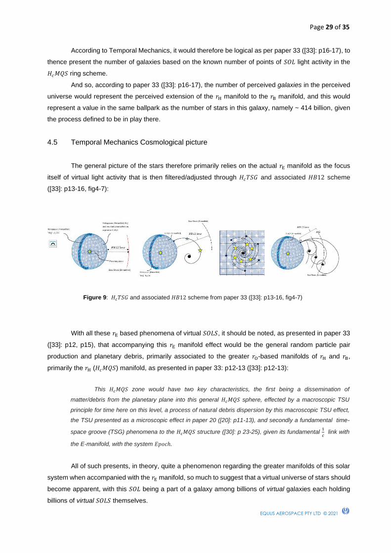
4.5 Temporal Mechanics Cosmological picture

The general picture of the stars therefore primarily relies on the actual 𝑟E manifold as the focus

itself of virtual light activity that is then filtered/adjusted through 𝐻𝑐𝑇𝑆𝐺 and associated 𝐻𝐵12 scheme

([33]: p13-16, fig4-7):

With all these 𝑟E based phenomena of virtual 𝑆𝑂𝐿𝑆, it should be noted, as presented in paper 33

([33]: p12, p15), that accompanying this 𝑟E manifold effect would be the general random particle pair

production and planetary debris, primarily associated to the greater 𝑟O-based manifolds of 𝑟H and 𝑟B,

primarily the 𝑟H (𝐻𝑐𝑀𝑄𝑆) manifold, as presented in paper 33: p12-13 ([33]: p12-13):

This 𝐻𝑐𝑀𝑄𝑆 zone would have two key characteristics, the first being a dissemination of

matter/debris from the planetary plane into this general 𝐻𝑐𝑀𝑄𝑆 sphere, effected by a macroscopic TSU

principle for time here on this level, a process of natural debris dispersion by this macroscopic TSU effect,

the TSU presented as a microscopic effect in paper 20 ([20]: p11-13), and secondly a fundamental time-

space groove (TSG) phenomena to the 𝐻𝑐𝑀𝑄𝑆 structure ([30]: p 23-25), given its fundamental 1

𝑐 link with

the E-manifold, with the system 𝐸𝑝𝑜𝑐ℎ.

All of such presents, in theory, quite a phenomenon regarding the greater manifolds of this solar

system when accompanied with the 𝑟E manifold, so much to suggest that a virtual universe of stars should

become apparent, with this 𝑆𝑂𝐿 being a part of a galaxy among billions of virtual galaxies each holding

billions of virtual 𝑆𝑂𝐿𝑆 themselves.

Figure 9: 𝐻𝑐𝑇𝑆𝐺 and associated 𝐻𝐵12 scheme from paper 33 ([33]: p13-16, fig4-7)

of 35


Yet the question must be asked, “is Temporal Mechanics close to estimates made by

contemporary astrophysics through its own systems of observation and measurement?”

The following is what is considered today by astrophysics via observation and calculation:

• the number of galaxies to be estimated between 200 billion to 2 trillion, depending on how the

data is being processed.

• the number of stars in the Milky Way to approximately number 400 billion.

• the age of the Universe to be 13.8 billion years, as according to the metric expansion of space

ΛCDM model and associated star-light data available.

• Proxima Centauri is measured to be the closest star from 𝑆𝑂𝐿 at 4.246 𝐴𝑈.

Temporal Mechanics is spot-on with the apparent age of the Universe, the distance to the closest

star, Proxima Centauri, the number of stars perceived in this apparent galaxy of 𝑆𝑂𝐿, and in the ballpark

of what is proposed to be the number of galaxies in the apparent universe of stars.

It should be mentioned though that the cosmological model employed by contemporary

astrophysics (2021) is the ΛCDM model, a model which has large problems with its general calculations

for the metric expansion of space and associated energy requirements, namely not successfully

explaining the cosmological constant in the manner Temporal Mechanics has, namely as per correctly

deriving the vacuum energy value ([13]: p23, eq9), vacuum permittivity ([23]: p30, eq5), and vacuum

permeability ([23]: p30, eq7), nor being able to account for the Axis of Evil, the Flatness problem, and the

Horizon problems, all of which Temporal Mechanics has resolved.

The model of cosmology presented by Temporal Mechanics laid the groundwork via the time-

space manifolds of the previous paper, yet required the inclusion of the 𝑟E manifold to uphold the standard

atomic 𝐸 = ℎ𝑓 effect of light, as presented here.

To ask if the stars are solar systems as images therefore, indeed they are as images, as they are

based on the 𝑟E process, yet the real question is if they are real physical solar systems like our own.

Temporal Mechanics has explained what they are, and why they are what they are, and how their

phenomena is what it is, as based on all the required metrics this local reality of ours relies on. The most

important feature of cosmology that Temporal Mechanics has explained, has laid groundwork for, is the

redshift effect and thus what would be an apparent expansion of space in regard to light, while not

conflicting with the vacuum energy value, and thereby resolving the cosmological constant problem, while

also resolving the Axis of Evil problem.

Quite simply, there would exist a 𝑟E focus of 𝐸 = ℎ𝑓 quantified light associated to the 𝐸 = 𝑓 𝑟H and

𝑟B manifolds (and associated time-space circuitry effects), primarily via an EM coupling factor in play

between the 𝑟E and 𝑟H manifolds.

4.6 The Geocentric Model: solving the “Axis of Evil problem

The big issue here therefore is why the 𝑟E manifold and thus Earth-𝑆𝑂𝐿 reference is primary for

the manifestation/focus of the stars. Why not use a Mars-𝑆𝑂𝐿 reference or a Venus-𝑆𝑂𝐿 reference? It

of 35


would just seem that, with all things considered, Earth is the calculated reference-zone for the stars to be

centralised to, almost making the Earth in reference to 𝑆𝑂𝐿 as the centre of the time-space system, so to

speak, if not Earth itself as the ultimate centre, in theory, the ultimate sweet spot of conscious exercise if

indeed as Temporal Mechanics proposes that consciousness is an emergent and required feature of the

relationship between time and space, as presented in paper 3 [3], “The Emergence of Consciousness

from Chaos”. This therefore suggests that “life”, consciousness, would only be found on Earth, not Mars

or anywhere else, unless of course the entire system makes a fundamental change to its entire

perceivable structure.

The scientific achievement here though is explaining and solving the known “Axis of Evil” problem.

The “Axis of Evil” problem prescribes that there must be a type of Geocentric (Earth-central) cosmological

model in play, as follows [35]:

But when you look at CMB map, you also see that the structure that is observed, is in fact, in a

weird way, correlated with the plane of the earth around the sun. Is this Copernicus coming back

to haunt us? That’s crazy. We’re looking out at the whole universe. There’s no way there should

be a correlation of structure with our motion of the earth around the sun — the plane of the earth

around the sun — the ecliptic. That would say we are truly the center of the universe.

Lawrence Krauss – Physicist/Cosmologist, Ambrose Swasey Professor of

Physics, Chairman of the Physics Department of Case Western Reserve

University

Here, Temporal Mechanics has solved this problem in understanding how Earth is centralised to

the metrics of the appearance of the stars and associated vacuum energy phenomena, calculated by

𝑡𝑒𝑚𝑝𝑜𝑟𝑎𝑙 𝑐𝑎𝑙𝑐𝑢𝑙𝑢𝑠 to be the known measured relatively uniform value.

Previously Temporal Mechanics proposed a type of dynamic solar system, of planets slowly

moving out from the sun to the outer manifolds, a proposal, as a way to explain how planets would be

formed, namely at 𝑆𝑂𝐿 via cyclic supernova type events, and that the planets would through time slowly

migrate outwards ultimately becoming debris. Yet, it would seem that there must always exist a sweet-

spot, Earth, for consciousness, for life, a source reference to perceive reality best, given how accurately

the entire star-scape is accounted for from the Earth reference, making the Earth reference a necessary

if not eternal reference.

Thus, the presentation of theory here now delivers a more startling suggestion, namely that

everything, the planets, the stars, is likely entirely steady-state, and the only thing that changes through

time would be upon the general platforms that must exist, cycles, that could not exist if not for everything

not existing. Of course there would be variations to this cycle, how 𝑆𝑂𝐿 could still nonetheless provide

debris for the outer manifolds, and how all of such would be a steady state system, by design, still

nonetheless with the appearance of the arrow of time as entropy; of course also, general symmetry-

breaking based variations take place with the process of particle pair production, a type of natural chaos

(within this proposed albeit overall order).

of 35


4.7 The Earth cycle through time

The question now therefore focusses on the linearity of historical events, for instance from a

prehistoric age to today, as though with temporal linearity our appearance as life presumes to be the first

time we as humans have been here from a previous prehistorical era, all of which must be questioned.

The question there is whether or not prehistory was merely a cycle of change itself compared to today,

as a part of cycles that carry on eternally. The other question is of course regarding past civilisations and

do any remnants exist in the form of what would be considered as alien life, and more to such, why it

would be important to honour the cycles of time, of the passage of time and the required changes,

suggesting therefore that the idea is to keep everything real and contextual here on Earth in time, namely

upholding required cycles and associated life, all of such derivations sure to provide for deep discussion,

especially with need to keep the integrity of the celestial objects intact, including Earth.

Finally, calculating the age of Earth, of this solar system, would entail a process of calculating the

age of the 𝑟E scheme, that EM appearance associated to time-space circuits, and thus to particle matter,

which itself as an EM phenomenon would be calculated by measuring the calculated age of the furthest

proposed star phenomenon, namely 13.8 billion light years, here as years. Although science calculates

this value to be roughly 4.54 billion years, the issue is how matter would present a “maximum” radiocarbon

dating and what that value logically would be, noting that a “maximum” value would represent a level of

maximum decay and therefore be unreadable; 4.54 billion years would thus appear to be a measurement

based on what is readable. Ultimately the idea of dating the time-space reference of Earth via a radioactive

decay process would represent, must represent, a feature synonymous with how the greater manifolds fit

with each other, how this relates to the Earth and 𝑆𝑂𝐿, and thus how the overall system would work as a

holistic entity. Once again, as is evident by Temporal Mechanics, the phenomena of the stars if not reality

itself is no simple “line of sight” phenomena (despite being thoughtfully based on a metric expansion of

space as per the ΛCDM model), yet something far more fundamental to the actual nature of interaction

between the dimensions of time and space, phenomena this series of five papers aims to highlight (time-

space circuits, constants, manifolds, metrics, and logistics), in summarising the general work of Temporal

Mechanics.

5. Conclusion

It would all seem quite fantastic to have a theory based on the human ability of temporal

perception using the metric of the Bohr radius to then derive what is perceived generally of reality as

within those parameters of definition, namely Temporal Mechanics deriving all that physics measures, all

apparent philosophical points of view aside, except for using a different a priori, a more fundamental a

priori for time, with the inclusion of a temporal perception codex, solving what contemporary physics’

models get stuck in, namely the cosmological constant, Horizon, Flatness, “Axis of Evil”, and so on,

problems. Yet indeed is not the concept of television quite fantastic, of relaying 3-d images that can be

presented in 2-d form, to our living rooms, conveying a 3-d type show?

of 35


If there is room for a philosophical point of view here, in many regards we as a species must

adapt to our reality, despite what theory presents this way or that, despite the fact that many theories

suggest we do just that, namely adapt to reality, to whatever reality our conscious mind has us be focussed

on. Indeed, it is no oddity we stargaze while also staring at plasma screens, if not at the same time. The

question is “what natural construct unbeknown to most of us has us accustomed, desiring, to do such,

what are we actually adapting to we are not cognizant of?”. As presented in this paper, that would appear

to be the highly virtual/holographic 𝑟E manifold, and how it presents the manifestation of the stars, as

programmed by the three key 𝐸 = 𝑓 manifolds (𝑟O , 𝑟H, and 𝑟B), as though performing as a macroscopic

scaled virtual screen transmitting virtual images of solar systems.

And so, is there any problem in our adapting to any greater manifolds of reality contemporary

physics has yet to acknowledge, greater “holographic manifolds”, greater 2-d screens presenting reality

to us as though modelled on our own solar system, our own sun, presenting to us as the case here has it

as the stars, as 3-d images like our own sun and solar systems, yet holographic images nonetheless?

We have adapted quite well to the idea of plasma screen technology and associated transmission of the

one reality we perceive in our daily lives from one location to the next via 2-d screen displays. The model

of cosmology presented here by Temporal Mechanics is no different to what we are familiar with.

In conclusion, Temporal Mechanic presents the fundamentals of time and space and those

interactions according to our human temporal perception ability, yet that model can only ultimately be

judged on what it can prove locally in a way the current ΛCDM model (primarily based on Einstein’s

Special and General relativity, and associated strings of physics schooling, and there are many, key of

such being Quantum Mechanics and the Standard Model of particles) cannot. What can be demonstrated

as per Temporal Mechanics nonetheless as proof closer to home, laboratory proof, proof central to the

Temporal Mechanics unique EMDIR effect and associated particle pair production phenomenon

description, is the subject of a subsequent paper. Prior such, an upcoming paper, paper 5 in this series

of Temporal Mechanics papers (paper 5 titled time-space logistics), will explore how it is possible for a

code of temporal perception to derive the distance to the nearest apparent star and the age of the

universe, how such a thing could be possible, or was it a mere fluke, as with all the derivations of the

equations and constants for particle and associated field force phenomena, and not just how it is possible,

yet why it needs to be possible.

Conflicts of Interest

The author declares no conflicts of interest.

of 35


References

1. Jarvis S. H. (2017), Gravity’s Emergence from Electrodynamics,

DOI: 10.13140/RG.2.2.35132.28804/1, https://vixra.org/abs/1704.0169

2. Jarvis S. H. (2017), Golden Ratio Axioms of Time and Space, DOI:

10.13140/RG.2.2.30099.12327/1, http://vixra.org/abs/1706.0488

3. Jarvis S. H. (2017), The Emergence of Consciousness from Chaos, DOI:


4. Jarvis S. H. (2017), Phi-Quantum Wave-Function Crystal Dynamics, DOI:


5. Jarvis S. H. (2017), Time as Energy, DOI: 10.13140/RG.2.2.23466.88009/3,

http://vixra.org/abs/1711.0419

6. Jarvis S. H. (2018), The Relativity of Time, DOI: 10.13140/RG.2.2.13400.55044/3,


7. Jarvis S. H. (2019), Golden Ratio Entropic Gravity: Gravitational Singularity Field Testing, DOI:


8. Jarvis S. H. (2019), The Golden Ratio Time Algorithm, DOI: 10.13140/RG.2.2.35399.14246/2,


9. Jarvis S. H. (2019), The Physics Chimera, DOI: 10.13140/RG.2.2.28499.02084/1,


10. Jarvis S. H. (2019), The Conception of Time, DOI: 10.13140/RG.2.2.10258.71363/1,


11. Jarvis S. H. (2019), Space, and the propagation of Light, DOI:


12. Jarvis S. H. (2019), Space, and the Nature of Gravity, DOI: 10.13140/RG.2.2.17320.93443,


13. Jarvis S. H. (2019), Space, and the Redshift Effect, DOI: 10.13140/RG.2.2.14287.43683/1,


14. Jarvis S. H. (2019), Solving The Cosmological Constant Problem, DOI:


15. Jarvis S. H. (2020), Hybrid Time Theory: “Euler’s Formula” and the “Phi-Algorithm”, DOI:


16. Jarvis S. H. (2020), The Hybrid Time Clock as a Function of Gravity,

DOI: 10.13140/RG.2.2.27053.64487/1, http://vixra.org/abs/2001.0401

17. Jarvis S. H. (2020), Hybrid Time Theory: Cosmology and Quantum Gravity (I),


18. Jarvis S. H. (2020), Scientific Principles of Space, Time, and Perception,


19. Jarvis S. H. (2020), Hybrid Time Theory: Cosmology and Quantum Gravity (II),

DOI: 10.13140/RG.2.2.23972.22405, http://vixra.org/abs/2005.0053

https://www.researchgate.net/deref/http%3A%2F%2Fdx.doi.org%2F10.13140%2FRG.2.2.35132.28804%2F1?_sg%5B0%5D=GXuatXf8LjBUf4QyBkryiAfDd2HRSE8Fx--TZiPQeITixEQcYj6GgCHIggLq8WmOyapqp_-x-fBlnWBHijO6EiaGKQ.fxbwTCy5HxlA2ET6IyANHXTv0kZXNfcjJsb7mx8cA3vKzKV4w1QbYaCnnIee996nSAx_krR0-UN7ajpE5ejBXg

https://vixra.org/abs/1704.0169

https://www.researchgate.net/deref/http%3A%2F%2Fdx.doi.org%2F10.13140%2FRG.2.2.30099.12327%2F1?_sg%5B0%5D=vHAhYhaNM_rJSVAkybQiqP8IG2gS5prv9t0Ibm8bmUINOfRXHE_tW1D0dwY0EOO7UZvxSdXaAUa_vX-3fmoFYOdpbQ.IWQRHtgo4Mr2NJsyma32-ZG45722AP4dd1BQq99gBDWmpf5nYPekfhRCBcyXYgZJ76fc6kZWU-d6yTMyIHWWmQ


https://www.researchgate.net/deref/http%3A%2F%2Fdx.doi.org%2F10.13140%2FRG.2.2.23388.23683%2F1?_sg%5B0%5D=mfdrj1QEE6y3hXVGTy-lC1YkrlLFXsr0DWlyS9hEGOxU0IYQZcrAHdwvBLwgyGWRRpL8rYwu5y2ofxKLYAYeAcZb-Q.YZtYwWvVQd6WPAsBfsN4DB3bgQbTVGgMkRV0YLSWBpra7RZZfTFwhmMMUJbLJGGGRg_WZodLFdB8osG4dvC0rA


https://www.researchgate.net/deref/http%3A%2F%2Fdx.doi.org%2F10.13140%2FRG.2.2.10045.10726%2F3?_sg%5B0%5D=1ci62mUE-HyknsNhFQfuJpS27rrCKFOJmAXqgvpy3-rUY0k3Fp2DCZqra-g94MCgoFvakvC86EiF_lAj1rQBll1j7g.Q62bNNk0oDIyCyKcj-U6XQ6HBah-gh78kVkFNcPiPZwiEUdlEA1PsEfd5EPyj9sSPB7eP-Gg6wd-jT-XXKvlAw


https://www.researchgate.net/deref/http%3A%2F%2Fdx.doi.org%2F10.13140%2FRG.2.2.23466.88009%2F3?_sg%5B0%5D=9N3ROIuLWlA_UHJCZn1jcOaHGRdjzwTEi2Lfn3J2O6887Yx1h0myA_Is2X9cbO0087BMVngq-a1QDitElWYnKH8qUg.8fbGW1JXYGg8QDvxVejDWEV88CxRw4aJDC8Hng5udzFt1mLfTrg6itYxq862huD6TotjJMDCasxRwUSxCMEnhg


https://www.researchgate.net/deref/http%3A%2F%2Fdx.doi.org%2F10.13140%2FRG.2.2.13400.55044%2F3?_sg%5B0%5D=ziZ_BdkEymDWTLtlVNWHWqccelwHIEtt1uag3bzZW9gV_276flH16btIswL9OaFLyAshgZVOLx0trUeVC_CdUDJzjQ.nRQvoOtaLfIvtRx3wcUp8OX6Nfn6rFaneyNea76wELDOLTisQ4rqRP8l_MJHTVJYaO-o4c0RMvAsv1wf4lfLTA


https://www.researchgate.net/deref/http%3A%2F%2Fdx.doi.org%2F10.13140%2FRG.2.2.35399.14246%2F1?_sg%5B0%5D=wxMTnyuGcg_bcTuQue9mZJgZQwfleIp1k4mx03R1s2am-k5sMdm6eavXwwf12bwqUlPMLQNA4H-wc2aBbM1y230OcA.dMchrRtMGpVXj8sAUA_iVz7ZCV0p33HeP36OfAfVknQ3rZ5M_qUOFt2VgTeY7E5sBsBy1JZUBpxo20ZEBX9Hyw


https://www.researchgate.net/deref/http%3A%2F%2Fdx.doi.org%2F10.13140%2FRG.2.2.35399.14246%2F2?_sg%5B0%5D=g9whbvsQoEaSF7tL-XP8pfbfxqGpSw6gfRtgIe4rCk_rma791vB1e6dmRmUXXJu9P0k1lwEWNCK6I1sSNevqrjyh1A.jPnnx4hU1hOHDuhXmWr8IfAysO48wP1J0AXkJ5eBR9pFEmU4Rg4H4B0QblwefSl9LY1zbqKzPtREvUcX4fMIyg


https://www.researchgate.net/deref/http%3A%2F%2Fdx.doi.org%2F10.13140%2FRG.2.2.28499.02084%2F1?_sg%5B0%5D=dxoNyUFipVYgV0r7H6JPU8iRBqyIgnM30RWrnWcXkHfT_Y1kdkfVnZSMt1UsbJMw8WvIOtFGcdUfMY7fSHOZhj96dA.AXK9HnNXcugx8x2LUonhdFjGw9rNq19e1L_hJ8B7VQp9bwMFrDOshOGGzW0rqwixCZtJEqwAeSne5abV1TIQMQ


https://www.researchgate.net/deref/http%3A%2F%2Fdx.doi.org%2F10.13140%2FRG.2.2.10258.71363%2F1?_sg%5B0%5D=Kmdjo8lYyA-9bXO09p0Czg7RJemv6C59BL_DpvS-RPmnGgYvm1Oh8uq6w52QFkdVou3j-kiSrPRXqMwkcoc7QvLZVQ.T-hI3SoumzrCQoq03gDvq4ahdu8cUpx6dPAU01PZ7__MoJoT7mqUsaQidKJ8cthcPdY1YN0OWqyZ8i5PaN3Hmw


https://www.researchgate.net/deref/http%3A%2F%2Fdx.doi.org%2F10.13140%2FRG.2.2.15833.67689%2F1?_sg%5B0%5D=j125EH06F90N4tcU7yvQnC2tompUmKFx-jfQb29gd52F_1-GP65vCMOYbQX8V6MHJ4MXN5Q-MiSDELoZXjhMVq6irw.1iMHofsJqnLnp9PACya5-suabZH_FT193PPV-WbXR0GTF4iICJSaHX7A7Owoutb1iUqNsK48b9VROheLngxrNA


https://www.researchgate.net/deref/http%3A%2F%2Fdx.doi.org%2F10.13140%2FRG.2.2.17320.93443?_sg%5B0%5D=qAtUV97gDBEpgtX3zwRRjZzUZXndMNXhsB6I8PbwNwbm52cfqvOuf0DmlIPexGl5q7vsz3u-IT3eaa-z0UpCdLWkog.vDFdMlVnQZogqEd-AvrUjPrwPzMIMd7RCubqBf2cwmlwY2eFAHNCTkeimceY3pndlpoK0l6zL1BgPsny9U-b2Q


https://www.researchgate.net/deref/http%3A%2F%2Fdx.doi.org%2F10.13140%2FRG.2.2.14287.43683%2F1?_sg%5B0%5D=iT97CswPXluKsOWwe-aWxKFRTthNjbd62CrJc5mCUba-xjsQGiF26tT8OkxfB42Eukr7mR-E_cwlxECuQTVesADmlw.J-a3Gzu9ntbydQ6ZXcoA6LjAI2cbGQRgAlfmt9B6bA7L3mT6DzniL_PF2ohFLsVdoMpJ76hUtK_MGGXfrQBDeA


https://www.researchgate.net/deref/http%3A%2F%2Fdx.doi.org%2F10.13140%2FRG.2.2.25730.63686%2F2?_sg%5B0%5D=hrK8P-iKzVEXd-TrxR3QpRk95Q45uIns7L2W4jQyV4xmbyCCl3KxCR5zlrQGY5F23gDSnA66HMVKxl13YpIgCl-Tkg.MmxmwIt4_2b9x_eL4VNBhon_Ils5qDsYqp_XA6P77Gg9y4bVxjOwQ3yTMpTGzz-dciuzAHsask-kkIRa6e7zRQ


https://www.researchgate.net/deref/http%3A%2F%2Fdx.doi.org%2F10.13140%2FRG.2.2.13078.91205%2F2?_sg%5B0%5D=ygFMJS2TJWc_w1D7tDXzjJDdb8rSim923-_9zvpMQoyFI6aSfgarILqr7D5W1YwkTn1mNZyomyqZ_NgVUGs8vHGDdQ.Vw8nnUqIopbuq46Bk8JR_rLP7mWsxgY0rpbrK64Qqv583PmEebcKOMozM5hZYmfLOVaBENrLr4fFtyQlBNu7HA


https://www.researchgate.net/deref/http%3A%2F%2Fdx.doi.org%2F10.13140%2FRG.2.2.27053.64487%2F1?_sg%5B0%5D=DlZ1NdSezbI7KrRpzjCaen7JlgzM6xjXWD3ozY1XLisso5KH6t6ykbI4sSWpDsURtOqxzrDzq4LwMcmQT7QkmaitxA.eOZLN1We6h9PtCoMlGMXuyFYKUjhQMzVj1RkRrS9od6CU6l0_dr5tHjib1MUNQQv6ADx_7hQsHyWGgl3tKdlDQ


https://www.researchgate.net/deref/http%3A%2F%2Fdx.doi.org%2F10.13140%2FRG.2.2.20045.79847%2F1?_sg%5B0%5D=TzZ1gT2WHwWfBUUZWzKMgqmr-aipotC6kmyhyWM3-YoIYtaq1ac7tW1qU_Dj-plWoyrAcpfStYcBlxFjrDy__BpBhw.b9g_9d-QDiuOJWcyKlIW1W6_d1GEVLWCmy-Cc1IPXJE4IVkKppRjF30VhVKHxx69PPPaCFfkWwGwv3eQqvv5xg


https://www.researchgate.net/deref/http%3A%2F%2Fdx.doi.org%2F10.13140%2FRG.2.2.16207.84648%2F1?_sg%5B0%5D=F1j4GhPUP8WN5BtPtYXbni2eL7hnjtAa0zFbHrNzqwOIaKoI8yIG_ADHR6ulQvhrDbuAFhAtqoQSwWNyr-6paG9PWw.Tc_OApzbLEU3MU_tWcsKGd0qzXnEvoGfglNaHF7cyGlPLuEuKlmMOq4JOmTqghJld7ilGf4Bvh5piYZYPOUmZg


https://www.researchgate.net/deref/http%3A%2F%2Fdx.doi.org%2F10.13140%2FRG.2.2.23972.22405?_sg%5B0%5D=FGHrjCwgyeJbbmWZORoF2KANlmFD2W77QLbQsxwLb-EzVWIJEEtk3Q6CqsshJ7Q0pRtXY8E1RtLFvPsWK3cmwsEIRA.j3jxi08DIWjDBO981qUXK1DFswcIf3Bei-Tv1OesTE9u0HuNDw5Lref2NGi1cmxKT_n1Ad0fxxKnh8Svl13N8w


of 35


20. Jarvis S. H. (2020), Mathematical Principles of Time and Energy,


21. Jarvis S. H. (2020), Dimensional Mechanics of Time and Space,


22. Jarvis S. H. (2020), Dimensional Thermodynamics, DOI 10.13140/RG.2.2.29715.71202/2,


23. Jarvis S. H. (2020), Time-Space Wave-Mechanics, DOI 10.13140/RG.2.2.10565.68320/3,


24. Jarvis S. H. (2020), Temporal Calculus (The Calculus of Time-points in Space),


25. Jarvis S. H. (2020), Temporal Calculus: solving the “Yang-Mills Existence and Mass Gap”

problem., DOI: 10.13140/RG.2.2.33774.43843/2, http://vixra.org/abs/2008.0226?ref=11562969

26. Jarvis S. H. (2020), Temporal Calculus: Time Scaling Space,


27. Jarvis S. H. (2020), Temporal Calculus: Resolving Elementary Particle Formation and

Confinement, DOI: 10.13140/RG.2.2.20191.07844, https://vixra.org/abs/2009.0177

28. Jarvis S. H. (2020), Temporal Calculus: Resolving Einstein’s Theory of Relativity (Special and

General), DOI: 10.13140/RG.2.2.12474.21447/1, https://vixra.org/abs/2010.0017

29. Jarvis S. H. (2020), Time and Non-Locality: Resolving Bell’s Theorem,

DOI: 10.13140/RG.2.2.12651.98086 (researchgate.net), https://vixra.org/abs/2011.0002

30. Jarvis S. H. (2020), Non-Local Time-Point Theory: Magnetic Quantum Shell (MQS) Modelling,


31. Jarvis S. H. (2021), Temporal Mechanics (A): Time-Space Circuits,

DOI: 10.13140/RG.2.2.28879.10407, https://vixra.org/abs/2101.0022

32. Jarvis S. H. (2021), Temporal Mechanics (B): Time-Space Constants,


33. Jarvis S. H. (2021), Temporal Mechanics (C): Time-Space Manifolds,


34. https://www.merriam-webster.com/dictionary/metric, webpage accessed 15th March 2021

35. https://www.edge.org/conversation/lawrence_m_krauss-the-energy-of-empty-space-that-isnt-

zero

https://www.researchgate.net/deref/http%3A%2F%2Fdx.doi.org%2F10.13140%2FRG.2.2.34441.67683%2F3?_sg%5B0%5D=xDPbtEjLjbfxATbppKMWvnjtBSkWQTMrm8owluaZjXJ6W-g3yjajQzt9389uCQvf1-7uUqnWzAjMZ0i6qi4hH4Iz7Q.gXim5TtUvCSebk1WqAi3seOyZsM7UopDmjTZRxMp4sbNYJjMlvOVa9Bon2y6lR5torv2-fzPu7gS_kZSii9zow


https://www.researchgate.net/deref/http%3A%2F%2Fdx.doi.org%2F10.13140%2FRG.2.2.21001.88169%2F1?_sg%5B0%5D=0vCQDKeh0_-o6uZ0ULFeTfis84kZ8bcfbADda732RRQOA_roqD70G-F0iU-Lms-608Vjrhl-A9o322Ycz0ftA9Hm3w.GoBvM79EABvLRjaLk6Ty2QRUgm71AI8EAo8jae511VNCIK2R6pg3rqV4Fwd7q8Q3wLaTjU0jU00nFCzj06720w


https://www.researchgate.net/deref/http%3A%2F%2Fdx.doi.org%2F10.13140%2FRG.2.2.29715.71202%2F2?_sg%5B0%5D=-cxbWJjGI2KifytE9rK-YB618R9oWJ0mTsJGjX6GtW4BCdI8rfMV4uy_lgoJBNZptdP3iIS6xuUGA6QantJgDn9-6Q.6H4PHOkQjcOnJn8XitVFvJAarZgDnFFctd3bO46D_w2aZOFkX4QodalW60EC0MzxlZAtji2gr0BF20MhwVOiag


https://www.researchgate.net/deref/http%3A%2F%2Fdx.doi.org%2F10.13140%2FRG.2.2.10565.68320%2F3?_sg%5B0%5D=VZoU9bXGn_aUpSERqdQkUUrhpA6C8Vye80RZEaLBouH4PrD7ZzHZNEBonkt37zf39MdjWuQbvXaPDUDh5ozTK0T_6g.8GtkONs1AlfSLvW1wkaU8u5dVra-XpA602KHnbkCtQ1iKpecQiB0Lk7Avwv7xoLeHYEE_0vwqP22XvmBiKuaqw


https://www.researchgate.net/deref/http%3A%2F%2Fdx.doi.org%2F10.13140%2FRG.2.2.15362.09929%2F3?_sg%5B0%5D=TT0OKIB3iDubEr1-gq7nZv4Vl33JH-KZMSkBXbh2Z1jhKcf0gDccjzkt_mKotq9R83QdnxSHKCKCf7Yv6I23On9iYA.Rp9aPoOYCdubXmHqN55HHZaUdfuOHlANcknKgnMqpbL_-87eJtWRkKswYaP5PkD3lNYiKf9R4qDnnw6PVv2Xvg


https://www.researchgate.net/deref/http%3A%2F%2Fdx.doi.org%2F10.13140%2FRG.2.2.33774.43843%2F2?_sg%5B0%5D=BN95hchovX-tLnw6yxgSc1dQ6j9bSHA301gTuKPZUJDaNX1WU-9St_Kh7OPRhjurwlhRpATvJxgWwQJOc3aAX5xk1w.8663tlrDf1mKHpYk_9v6LqdzyeCoxUFJGNkBTebwDJAW-Jy5nG6IMUn-A_O5kkTpsSqAv5vA2623AB9t15ihzw

http://vixra.org/abs/2008.0226?ref=11562969

https://www.researchgate.net/deref/http%3A%2F%2Fdx.doi.org%2F10.13140%2FRG.2.2.28539.75043%2F2?_sg%5B0%5D=_t9_4sNxsznWeGNXC0F00C9J7L-36Wli6Rv-UHuhgORBxRSrBYQf1lFeZss29MYmox4cc-OM0R1glLT1dkla1L28sg.fGPhg0CRXdH-E0CBtCVoMimlIgosoDyZkij27TR0wqTBJXeIW93qUkrhK_Pw785HXWd_bFYIKR-qM03tm6qjWA


https://www.researchgate.net/deref/http%3A%2F%2Fdx.doi.org%2F10.13140%2FRG.2.2.20191.07844?_sg%5B0%5D=Fp6426dC72B2udYZIP9VzatkuBGY-ZFjiDf8bCxWL-GCDNF51ARy-IViW_FfhF0ztnfNAFnoHivwM9RB-GzkanCKaQ.D3OPW2qOSAV41Mu0n-Tm00So6O-6-f62Y88-v7SLHno3CLVKEuVvNRzPc3Z_6W0otVsuSs3VLg6Xg51eH7vEeA


https://www.researchgate.net/deref/http%3A%2F%2Fdx.doi.org%2F10.13140%2FRG.2.2.12474.21447%2F1?_sg%5B0%5D=0cOv0qUTA4_A4Jw0uPEkZydk6Qii7kHqbDRg9Ovtj-zCeA_w979Vl6HoVwRk9CXpzdpq58ZD88Tbu1Us6eKCF_0IVA.mEayhskJhFON5TNBpKnT1_g6bq__ssSKlD30n_ZDt6MNFGsvsdQ8sCHaC-2U5FnnLjfCjWTpGTKGMbJKEZKBRg


https://www.researchgate.net/deref/http%3A%2F%2Fdx.doi.org%2F10.13140%2FRG.2.2.12651.98086?_sg%5B0%5D=yjFl4-JTCglu5YHhsLPAyh2v9J0mwcU45zXjV98DG8xyQsPYKXZeOGUoUz2PuhNN5yG5StdS-bm00AljGHXn3ZqPQA.8F_7k2wzHdeRv_cSNUSqjfdOk46RjLifwb_R-C_4-V_CnUD6tPTJ6okK_EuSMRBq80DN9JNPdJ_Pyzp8u-Ip2g


file:///C:/Users/shjar/Desktop/paper%2032/10.13140/RG.2.2.11032.83206/2


https://www.researchgate.net/deref/http%3A%2F%2Fdx.doi.org%2F10.13140%2FRG.2.2.28879.10407?_sg%5B0%5D=xcRNsx3Zoo2ZPM696Yc--xn5rshEphwuE7N3QGtx6xKs1mE0jS3TDQ0hNFS5RhDcTM1HN0q25rhp3JxgN9aYi18__g.WQ7yoopLF-XAYZ9sYQwmkfoTScsCjJGvft0RMyrpgl-4FRftp3f9JUAIygGyz0V8zFGa8GpmTiW3pbrSXLwi5Q


https://www.researchgate.net/deref/http%3A%2F%2Fdx.doi.org%2F10.13140%2FRG.2.2.31751.21925%2F2?_sg%5B0%5D=BEt850OMy5Qq0FDPLkvePMtnDx5XcrL5Qt0giC5oCU2Z1DlO5hSQ9gZw1biqUcZZP9Bb7DC6SmQY1jZ4cPf1647-ow.v2v2JIhbIazepDUwtXQdnyfAeB-Zbv_Gv0Rc3vRTfShhI9G8qpkCiQcmtomvEz4BP-62LsvmmbHKowAVtYAlZw


https://www.researchgate.net/deref/http%3A%2F%2Fdx.doi.org%2F10.13140%2FRG.2.2.30214.70720%2F1?_sg%5B0%5D=i6yqwm9HYn7rXw5j1sFqgi6D16EOspmyj3w1Tml3LaV8IaLK9BMFFnE9OXRnGAws0dabgjNTBgjIRGAdI4sgLaGWLA.HgRp4kwjE_v8On9W0Wef_bOwN5f2th4fJYRHc1H2ah0fYk4VYaqJ1FvirZk3wgvjHYgdzWqu3U7s5RDKprBAag


https://www.merriam-webster.com/dictionary/metric

https://www.edge.org/conversation/lawrence_m_krauss-the-energy-of-empty-space-that-isnt-zero

https://www.edge.org/conversation/lawrence_m_krauss-the-energy-of-empty-space-that-isnt-zero

Temporal Mechanics (D): Time-Space Metrics - viXra.org

Documents

Transcript of Temporal Mechanics (D): Time-Space Metrics - viXra.org