Technology Development for Nuclear Fuel Cycle Waste ...
558
KR0000050 KAERI/RR-1907/98 7H U 1 Technology Development for Nuclear Fuel Cycle Waste Treatment Development of Decontamination, Decommissioning and Environmental Restoration Technology «r 3 1/30
-
Upload
khangminh22 -
Category
Documents
-
view
1 -
download
0
Transcript of Technology Development for Nuclear Fuel Cycle Waste ...

KR0000050
KAERI/RR-1907/98
7HU1
Technology Development for Nuclear FuelCycle Waste Treatment
Development of Decontamination, Decommissioning andEnvironmental Restoration Technology
«r
3 1 / 3 0
KAERI/RR-1907/98
Technology Development for Nuclear FuelCycle Waste Treatment
Development of Decontamination, Decommissioning andEnvironmental Restoration Technology
7l
If flSf
S! &
1999. 3.
0|
O Ofc
I.
II.
13.7] (250 kW, TRIGA Mark-II)
TRIGA Mark-III
2^17] (2 MW,
"A
TRIGA Mark-II ^ I I I
^ - 5 . ^ 3.711
C02
7171
TRIGA Mark I I I
TRIGA MARK 7fl
7}
III.
1^- TRIGA <&-?S.
TRIGA
C02
C02
co2
<H47](granular filter)^]
^ Slfe- HEPA 4
7}
^ X I

TRIGA
- Cs-137
- TRIGA
IV.
TRIGA
^r Co-60
^ B f l o i e i l ^ 304
(Unrestricted release)
IV

£ S , ^#4^(Chemical flushing) tioVaJ-£|
EDTA
71
C02
400 24
Hr
44
: 45 Kg/cm2*]
loose ^ fixed
10mm«q
98%
4

-f-
so
non-Newtonian o]tf shear thinning
- TRIGA
150 m -
L3. TRIGA
V.
-f-TRIGA
VI

3. 4
^ r TRIGA
sol - gel
ffe TRIGA
vnNEXT PAGE(S)
left BLANK
SUMMARY
I. Project Title
Development of Decontamination, Decommissioning and Environmental
Restoration Technology
II. Objective and Importance of the Project
Part 1. Development of Decontamination and Repair Technology for
Nuclear Fuel cycle Facilities
For the purpose of aquiring the technologies in relation
to the decontamination, repair and decommissioning of the domestic
nuclear fuel cycle facilities, Korea Atomic Energy Research
Institute has a plan to develop and demonstrate the decontamination
and decommissioning technologies by using the retired Korea Research
Reactor #1 (250 kW, TRIGA Mark-II) and Korea Research Reactor #2 (2
MW, TRIGA Mark-Ill) which were located at the Seoul site. The
objective of this study is to develop the technologies such as the
reactor coolant system decontamination and the concrete
decontamination, and to demonstrate these technologies by
application to the TRIGA Mark-II research reactor during the
decommissioning activity of it.
The most recent AEC decided the dismantling of TRIGA Mark III
Reactor. Therefore dismantling system technology be
establishing/applying. Of dismantling concrete surface cutting is
the most technology due to waste quantity. So the concrete cutting
apparatus characteristic analysis and the selection of all sorts of
technology is needed. And the dust treatment technology development
IX

be needing in order to prevent decontamination of environment.
Decontamination during the life time of nuclear facilities is
becoming increasingly necessary, to reduce dose to personnel during
repair and maintenance, conventional decontamination processes can
be subdivided into three main categories: chemical decontamination
using chemical solutions for dissolving the radioactivity; water or
other liquids spraying at high pressure ; and solid blasting using
sand, alumina or other solids. These conventional decontamination
methods leave a secondary liquid or solid waste needing disposal.
CO2 blasting decontamination technology can solve this problem, and
has been applied and studied in Europe and USA since 1991. In
domestic, the development of decontamination technology to eliminate
or minimize the use of decontamination chemicalsis becoming
incresingly necessary in order to reduce the dose exposure to
operator and to effectively operate the facility for nuclear fuel
cycle.
Part 2. Development of Dismantling Technology
With the aging of nation's nuclear facilities, dismantling
of a nuclear facility requires technology of proven reliability
mainly because of the hazardous outcome of malpractice of empirical
technology. The presented R&D effect is aimed at providing timely
development of basic dismantling technologies and equipment for on
site testing. These are the development of the under water ranging
robotic vehicle for inspection task of a TRIGA MARK III reactor, and
the analysis of dismantling processes and equipments using the
graphic simulator.
Part 3. Development of Environmental Restoration Technology
The objective of this study is to develop decontamination
technologies applicable to soil or contaminated urban surfaces for
an unrestricted release of decommissioned site of nuclear facility
or to the contaminated area as a result of a nuclear accident and
the other incidents involving the spread of radioactive waste. These
technologies will help ensure that cleanups of contaminated
environment can be performed as safely and quickly as possible.
III. Scope and Contents of the Project
Part 1. Development of Decontamination and Repair Technology for
Nuclear Fuel cycle Facilities
In order to develop the TRIGA research reactor coolant
system decontamination technology, a study for obtaining the basic
technology was performed this year. The structural features, design
and operation data of the TRIGA reactor were analyzed. The analysis
on the application methods of decontamination technology to the
TRIGA reactor, sampling and radiochemical analysis of the
contaminated specimens, fundamental characteristic tests of
decontamination reagents by using aluminum material, and design and
the manufacture of the system decontamination test equipment etc.
were performed.
CO2 Blasting Decontamination Technology Development :
Technical review on the CO2 blasting decontamination
technology
Investigation of production method of a simulated
contamination specimens and characterization of
contamination
- Testing of CO2 blasting decontamination in labaratory scale
This year's R&D analized the generation dust characteristic in
XI
decontamination and decommissioning and developed and analized
pre-filter, midium filter and HEPA filter because of decontamination
and decommissioning system is demanded high removal efficiency of
the generation dust. Through the characteristic analysis of dust
treatment, the effective system is presented and is performed
performance test for minimun cyclone.
Part 2. Development of Dismantling Technology
The R&D efforts of the under water ranging robotic vehicle
are focused on the development of an robotic vehicle which is
capable of precise inspection of contamination of reactor wall
through remotely controlled actuation. For this, a self balanced
vehicle actuated by propellers is fabricated, which consists of
small sized control boards, an absolute position detector, and a
radiation detector. Also, the algorithm for autonomous navigation is
developed and its performance is tested at the swimming pool and the
reactor pool of the research reactor.
The dismantling tools and equipments are selected which are
suitable for remote dismantling processes of the research reactor.
Also, the applicability of these tools to the remote dismantling
processes of the research reactor is analyzed using the graphic
simulator.
Part 3. Development of Environmental Restoration Technology
1. Soil decontamination technology development
- Basic study on the electrokinetic soil decontamination
- Basic study on the soil washing method
- Design and manufacturing of soil decontamination equipment
2. Dry decontamination technology development for an urban
surface
Xll

- Performance improvement of clay decontamination agent and
physicochemical analysis on the clay decontamination agent
- Demonstration of dry decontamination agent using building
materials contaminated with Cs-137
- Design and manufacturing of urban surface dry decontamination
equipment
3. Soil decontamination performance assessment technology
development
- Measurement of input parameters for the application of soil
decontamination performance assessment model
- Prediction of the spreading phenomena of radioactivity around
the TRIGA research reactor
IV. Results of the Project
Part 1. Development of Decontamination and Repair Technology for
Nuclear Fuel cycle Facilities
As a result of the contamination characterization of the
TRIGA reactor coolant system, it was found that the major
contaminants are Co-60 and Cs-137, but the radiation level of it is
very low. The fundamental dissolution data on the aluminum coolant
system material of the TRIGA reator and stainless steel 304 were
obtained from the dissolution tests by using various decontamination
reagents. The results of these tests indicated that fluoboric acid
based decontamination reagent is more effective than other reagents
such as mineral, organic acids or a mixture of these for the
dissolution of aluminium material under the condition of dilute
concentration and low temperature. Also, this reagent could be
applied to the decontamination for the unrestricted release and
XHl

recycle of materials. The coolant system decontamination test
equipment which was designed and manufactured in this year will be
used in next year's tests for comparing the process characteristics
and selection of the process condition.
CO2 Blasting Decontamination Technology Development
a. From the technical review on the CO2 blasting decontamination
technology, the following results were confirmed: CO2 blasting
decontamination technology is a dry process that generates no
secondary waste streams, and a non-destructive method. The use of
CO2 blasting proved very effective at removing loose contamination,
but of significantly effectiveness on fixed contamination.
b. Investigation of production method of a simulated
contamination specimens and characterization of contamination: The
production method of a simulated contamination
specimens was optimized for time and temperature, with
the result that a temperature of 400 C for 24hr was
selected.
c. Testing of CO2 blasting decontamination in laboratory scale:
The highest decontamination efficiency(removal % of 98% above) for
CO2 blasting was obtained at conditions using a blasting pressures
of 45 Kg/cm , a stand-off distance of about 10mm during 2min.
This year's R&D performed the characteristic analysis of
concrete surface cutting and dust treatment system and constructed
electric heating cutting machine and minimum cyclone and performed
test performance improvement of cyclone. For the dust treatment,
that's output widely applied the common dust generation system.
Part 2. Development of Dismantling Technology
The test result of the wall ranging vehicle in underwater
xiv

environment shows that the vehicle can easily navigate into the
arbitrary directions while maintaining its balanced position. The
non-linear predictive controller shows good tracking performance and
the absolute position detector measures the vehicle position within
its tolerant accuracy. Also, the test result at the research reactor
shows that the vehicle firmly attached the wall while measuring the
contamination level of the wall. The optimal sequence of the
dismantling process of the research reactor is obtained by using the
3-D graphic simulator. Also, the analysis result of the graphic
simulation shows that the selected tools can be used for the
remote dismantling processes.
Part 3. Development of Environmental Restoration Technology
1. Soil decontamination technology development
- Removal of more than 80% of cesium ion on soil by applying
the electrokinetic decontamination technology for 72 hours
- Elucidation of cobalt ion leaching mechanism by chelating
agent from soil
- Performance test of soil decontamination equipment
2. Dry decontamination technology development for an urban
surface
- Identification of the characteristics of the developed dry
decontamination agent as non-Newtonian and shear thinning
fluid
- the order of dry decontamination efficiency is wood> red
brick > weight concrete > fire brick > silicate brick
- Performance test of urban surface dry decontamination
equipment
3. Soil decontamination performance assessment technology
development
XV
- The section influenced most critically by redionuclides is
150 m between TRIGA reactor building and a stream
- Radionuclides leaked from TRIGA reactor due to the unexpected
accident was estimated not to influence the area in the
vicinity of TRIGA reactor
V. Proposal for Application
Part 1. Development of Decontamination and Repair Technology for
Nuclear Fuel cycle Facilities
Through the demonstrative applications of the coolant
system and concrete decontamination technologies, and dust treatment
technology, it will be contributted to the cleaning of TRIGA Mark II
coolant system and concrete surface during decommissioning project
of TRIGA. In the future, these technologies could be applied to the
decontamination of commercial nuclear power plants and nuclear
facilities decommissioning.
Part 2. Development of Dismantling Technology
To commercialize the wall ranging vehicle, various
application areas are examined such as the inspection process of
spent fuel storage pools, the decontamination process of the liquid
waste tanks, and the inspection and maintenance processes of the
bridge columns. The graphic simulation technology of dismantling
process can be used as an useful tool for designing the detailed
dismantling processes as well as a training tool for the radiation
workers by providing the virtual models of the nuclear facilities.
Part 3. Development of Environmental Restoration Technology
XVI

The results of study on the development of soil
decontamination technology could be applied to decontaminate
radioactively contaminated soil around the nuclear facility and
prepared to against the nuclear accidents by manufacturing the soil
decontamination equipment. And the results could be used to the
areas contaminated with heavy metal ions. The developed soil
decontamination technology could be used to apply the restoration of
decommissioned area of the TRIGA research reactor.
The results of study on the development of urban surface
decontamination agent could be applied to decontaminate
radioactively contaminate urban surface and prepared to nuclear
accidents by the manufacturing of decontamination equipment. And the
results could be used a new ceramic manufacturing process involving
sol-gel process which control reaction rate. The developed dry
decontamination agent could be used to apply not only urban surface
but also other contaminate surface.
The results of study on the development of assessment technology
of the contaminated area could be applied to assess the contaminated
area by radionuclide around the nuclear facility and to predict
residual radioactive concentration after soil remediation. Also,
The developed assessment technology could be used to apply the
assessment of the contaminated area around the TRIGA research
reactor.
xvuNEXT PAGE(S)
left BLANK
TOTAL CONTENTS
PART 1. DEVELOPMENT OF DECONTAMINATION AND REPAIR TECHNOLOGY
FOR NUCLEAR FUEL CYCLE FACILITIES 1
Chapter 1. Introduction 19
Chapter 2. Development of TRIGA Research Reactor Coolant
System Decontamination Technology 23
Section 1. Introduction 23
Section 2. State of the art 24
Section 3. Contents and results 35
Section 4. Conclusions 101
Chapter 3. CO2 solid blasting decontamination technology 103
Section 1. Introduction 103
Section 2. State of the art on CO2 solid blasting
decontamination 103
Section 3. Contents and results 115
Section 4. Conclusions 124
Chapter 4. Concrete decontamination technology development ••••125
Section 1. Introduction 125
Section 2. State of the art 125
Section 3. Contents and results 191
Section 4. Conclusions 224
Chapter 5. Attainment degree on the research target and
contribution degree to the other area 229
Section 1. Development of TRIGA research reactor coolant
system decontamination technology • 229
Section 2. CO2 solid blasting decontamination technology 229
xix

Section 3. Concrete decontamination technology
development 229
Chapter 6. Application plan of the results 231
Section 1. Development of TRIGA research reactor coolant
system decontamination technology 231
Section 2. CO2 solid blasting decontamination technology 231
Section 3. Concrete decontamination technology
development 231
Chapter 7. References 233
PART 2. DEVELOPMENT OF DISMANTLING TECHNOLOGY 237
Chapter 1. Introduction 249
Chapter 2. Underwater wall raging radiation inspection robot ••••251
Section 1. Introduction 251
Section 2. Design and fabrication of Underwater wall raging
radiation inspection robot 252
Section 3. Development of control algorithm 283
Section 4. Performance test of wall raging radiation
inspection robot 306
Section 5. Concluding remarks 331
Chapter 3. Selection of dismantling equipment and
graphic simulation of dismantling process 333
Section 1. Introduction 333
Section 2. Selection of dismantling equipment 334
Section 3. Graphic simulation of reactor dismantling
process 340
Section 4. Concluding remarks 354
Chapter 4. Conclusion 355
XX

Chapter 5. References • 357
PART 3. DEVELOPMENT OF ENVIRONMENTAL RESTORATION
TECHNOLOGY 361
Chapter 1. Introduction 377
Chapter 2. State of the art 379
Section 1. Understanding of the state of the art 379
Section 2. Comparison and discussion of detail
technologies 380
Chapter 3. Contents and results 385
Section 1. Soil decontamination 385
Section 2. Dry decontamination of urban surface 435
Section 3. Soil remediation performance assessment and
radionuclide migration modeling around the
TRIGA 477
Chapter 4. Attainment degree on the research target and
contribution degree to the other area 541
Chapter 5. Application plan of the results 543
Chapter 6. References 545
xxi
NEXT PAGE(S)left BLANK

jll-
4 1 ^ 4 ^ : 19
4 2 # TRIGA g^-S 7^I#^ll^7l# 7fl 23
4 1 *i 4 £ 23
4 2 ^ ^Ml • *J 7l#7fl^ ^% 24
*)1 3 ^ ^9-7fl^: ^*$ q-g- ^ ^21- 35
*fl 4 ^ ^ -g- 101
11 3 # C02 ^ 4 ^]<g7]^ ?m 103
^ | ] 1 | A-) & 103
^) 2 ^ CO2 £*M<* ^ H • <i\ 7)^7m ^ % 103
^) 3 ^ g ^ H i * ^r*l uB-§- ^ ^ H54 4 | | -g: 124
4 4 % ^ 3 e l S ^ |^7]# 7flt 125
4 1 | M -g 125
125
g 9 2f 191
4 4 | | § 224
4 5 # ^^-7f| - ^-S ^^§S. ^ cfl^7l<HS 229
4 1 *l TRIGA ^ ^ - ^ ^ ^ - 4 ^ 7 ] ^ 7fl^ 229
4 2 | CO2 £ 4 4<*7|# 7Btii 229
4 3 | s.£ie]J=L 4 ^ 7 1 ^ 7B«i 229
4 6 # ^^-711^ ^ 4 ^ f %-§-X|^ 231
4 1 ^ TRIGA ^ ^ - ^ 7^1^-4^71^- 7fl11; 231
xxm

2 ^ C02 I 4 4 ^ 7 | t 7m •••— 231
231
233
237
1 ^ 4 ^ • .......249
2 # ^'jHMg , $ . ^ ^ 4 $%] 7m • — 251
*fl 1 ^ 4 ^ - • • 251
^*|| O 'SJ XJ| t>| "^^liTil^Q- • LiOO
31] c ^ :<£-§. 9^1• ^ n i ^ j » - f *^+ y _' « • • • • . • • • • « . . . • • • . . . • « . • • • « • • • • • • . • • • • • . . . . . . . . . . . 4 . . . . . . . . . . . . . 4 . . . . . . . . . * ! • • • • > • • • * • • j ^ ^
A 1 4 ^ - 333
"-334
340
• 11 4 - ^ ' § • & ' <J54
4 ^ ^ ^ - • 355
5 # ^-a^-*i 357
- 361
...377
379
379
380
XXIV

4
5
385
385
435
7||^ 477
7]<*|j£ 541
543
545
XXV

1 ^ n^y\M^
: 0|
o l
0| 7|
0| ^
• l -
NEXT PAGE(S)left BLANK
CONTENTS
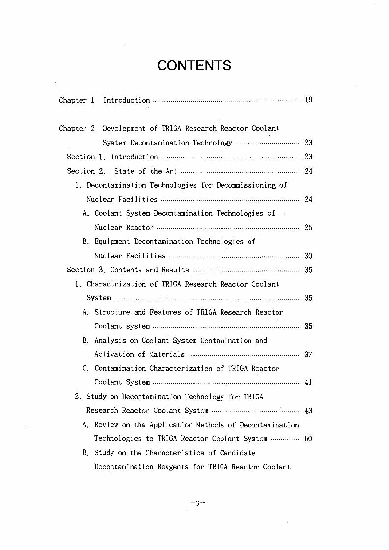
Chapter 1 Introduction 19
Chapter 2 Development of TRIGA Research Reactor Coolant
System Decontamination Technology 23
Section 1. Introduction 23
Section 2. State of the Art 24
1. Decontamination Technologies for Decommissioning of
Nuclear Facilities 24
A. Coolant System Decontamination Technologies of
Nuclear Reactor 25
B. Equipment Decontamination Technologies of
Nuclear Facilities 30
Section 3. Contents and Results 35
1. Charactrization of TRIGA Research Reactor Coolant
System 35
A. Structure and Features of TRIGA Research Reactor
Coolant system 35
B. Analysis on Coolant System Contamination and
Activation of Materials 37
C. Contamination Characterization of TRIGA Reactor
Coolant System 41
2. Study on Decontamination Technology for TRIGA
Research Reactor Coolant System 43
A. Review on the Application Methods of Decontamination
Technologies to TRIGA Reactor Coolant System 50
B. Study on the Characteristics of Candidate
Decontamination Reagents for TRIGA Reactor Coolant
- 3 -

System • 52
C. Manufacture of Test Loop for Coolant System
Decontamination 73
3. Design and Manufacture of Decontamination Kit for
TRIGA Coolant System Application 81
A. Design of Decontamination Kit 81
B. Manufacture of Decontamination Kit 86
C. Decontamination Procedure and Operation of
Decontamination Kit 96
Section 4. Conclusions 101
Chapter 3 CO2 Solid Blasting Decontamination Technology 103
Section 1. Introduction 103
Section 2. State of the Art on CO2 Solid Blasting
Decontamination 103
Section 3. Contents and Results 115
1. Experimental Procedure 115
A. Preparation of the Simulated Contamination
Specimen 115
B. CO2 Solid Blasting Decontamination Test 115
C. CO2 Solid Blasting Decontamination Apparatus 115
D. Experimental Analysis 117
2. Results and Discussions 117
A. Contamination Characteristics of the Simulated
Specimen 117
B. Characteristics of CO2 Solid Blasting
Decontamination 121
Section 4. Conclusions 124
Chapter 4 Concrete Decontamination Technology Development •••125
- 4 -

Section 1. Introduction 125
Section 2. State of the Art 125
1. Dust Treatment and Concrete Cutting Technology 125
A. State of the Art on Dust Treatment Technology 125
B. State of the Art on Concrete Decontamination
Technology 178
Section 3. Contents and Results 191
1. Efficiency Experiment of Minimum Cyclone 191
A. Conformation of Experimental Apparatus "191
B. Design and Construction of Complex Dust
Treatment Apparatus 198
C. Design and Construction of Electric Concrete
Cutting Machine 198
D. Design and Construction of Remote Controlled
Concrete Cutting Machine 204
2. Results and Discussions 206
A. State of the Art on Dust Treatment Technology 206
B. Available Particle Range Degree 210
C. Efficiency Experiment of Minimum Cyclone 210
D. Results and Discussion 224
Section 4. Conclusions 224
Chapter 5 Attainment Degree on the Research Target and
Contribution Degree to the Other Area 229
Section 1. Development of TRIGA Research Reactor Coolant
System Decontamination Technology 229
Section 2. CO2 Solid Blasting Decontamination Technology 229
Section 3. Concrete Decontamination Technology
Development 229
- 5 -

Chapter 6 Application Plan of the Results ••••• 231
Section 1. Development of TRIGA Research Reactor Coolant
System Decontamination Technology • 231
Section 2. CO2 Solid Blasting Decontamination Technology 231
Section 3. Concrete Decontamination Technology
Development 231
Chapter 7 References • 233
-6-

JE.
M & 19
4 2 # TRIGA #^3. 7f§-*tf<*7]# 7H^ 23
1 1 1 ^ 23
24
24
7}. #*}$.$) 7fl^fl<g7l£- 25
U. ^ } ^ 4 ^ 7|7]4^7l# 30
3 | ^^-7)1^ ^r*J a-§- ^ ^ ^ 35
1. TRIGA £ ^ . ^ 4 ^ ] # ^ ^ -^ £*} 35
7}. TRIGA g ^ - 3 . ^ 4 ^ ] # ^ ^ - ^ Ri ^-^ 35
U. ^ 4 ^ 1 ^ i ^ 91 aoV4^ ^ ^ ^ r^ 37cf. TRIGA ^ ^ - ^ ^ 4 ^ ) # ^ ^ . ^ ^ ^ ^Af 41
2. TRIGA <&^-£. 7 ^ ] ^ 4 ^ 7 l ^ ^ 9 - 43
7\. <&^-S. 4 ^ 1 ^ - 4 ^ y o ^ 3-% 50
• 52
73
3. *M-§- ^^-4«g^l ^X| 9J 4 4 81
QA 81
4 4 86
^r^ "A 4-g^f 96
^ 4 | I ۥ 101
4 3 4 co2 £ 4 4 ^ 7 1 ^ 7B^ 103
4 1 I 4 ۥ 103
- 7 -

4 2 £ C02 # 4 4 £ ^ B • £] 7}^?m ^ % 103
4 3 *l <&^-7Vi ^r*3 V-B-8- 9J £2f 115
i. co2 M i ^ ^ -s^s7}. S^-S-^ X\3&*\ *§£, 115
T-K CO2 # 4 4 £ ^ ^ -115
^}. co2 # 4 4 ^ ^ l H5
B>. *1^#*J • -117
2. ^ ^ ^ ^ f ^ 3-*t .117
7>. 4 ^ 1 ^ A ^ ^ J g 117
i-h CO2 # 4 4 ^ " ^ ^ 121
1 4 | | ^ • 124
125
125
125
| ] 9i l l ^ - 125
7\. ^ 1 * 1 * 1 7 1 ^ * ! % ^ 125
4^]^%^^ 178
^ 191
4 1 # ^ ^ 191
7f. ^ ^ ^ 1 9-^ 191
W ^ ^ l * | ] ^ 1 ^ 7 j ] / 1 ^ • 198
^3.5]M. ^ ^ > ^ 1 ^Til/43]- 198
^ a . e l ^ &&#*] A^]/^14 204
2. ^21- 5J J l # • 206
l l 2f 206
210
210

5h ^ 91 -2-% 224
4 ^ ^ ^ 224
^ 91 H ^ ^ 229
TRIGA <£^-S 7f§*fl<g7l^- 7^ 229
C02 £ 4 *||<g7l# 7lf^ 229
| 4 ^ ] ^ Hi 229
231
1 t TRIGA ol^-S X | ^ 4 ^ 7 ] ^ - 7flt 231
2 | C02 £ -4 *fl£7l# 4 y i 231
231
233
- 9 -
NEXT PAGE(S)left BLANK

Table 1-1 BWR PWR£) <ti*H4?fl 3 . ^ ^ - ^ ^ 27
Table 1-2 JPDR <&%} *-J4>W . ^ ^ * f r M £ 3 a ^ s * ^2f .. 28
Table 1-3 Specifications of TRIGA Research Reactors 36
Table 1-4 Shutdown Inventory of Radionuclides in Neutron-
Activated Aluminium Liner of TRIGA Mark-II
Reactor,(Ci/cm3) 42
Table 1-5 MCA Results of the Samples Taken from TRIGA
Research Reactors 49
Table 1-6 Composition of Aluminium-6061 Alloy 60
Table 1-7 Demonstration Work Schedule on Coolant System
Decontamination of TRIGA Research Reactor •••• 85
Table 1-8 ^afl^^lSj ^ S L # £ 1 ^^ % 4<£ 91
Table 1-9 *l|g#*l *W*>SJ nfi- -g- 98
Table 2-1 Decontamonation results in Surry PWRs 112
Table 2-2 Recent CO2 blasting projects-nuclear
applications 114
Table 2-3 Contamination conditions for simulated
specimens 116
Table 3-1 Collection Rate of Particle • 128
Table 3-2 ^ $-<g^- 4°l#^^t ii l *l r*l 132Table 3-3 4°1#^I ^ W * ] ^ S - 139
Table 3-4 ^ - * H 4 ^ $$]<t\ ^^>^<H1 $X<>\M *$^S- 147
Table 3-5 vpf- ^ S J M * ! ^S. 151
Table 3-6 nf^Tj]^^ 7\}*y 152
Table 3-7 4 ° 1 # ^ ^ 1 SX^M 6 H ^ ^ ^ 155
Table 3-8 4O1#^ W l 6«^^^ 162
Table 3-9 Rating Judgement as to the Relative Potential of
-11-

Each Concept Tested in the Cyclonic Wind Tunnel ••••167
Table 3-10 Heating Rods - ^ 201
Table 3-11 Power Controllers - ^ 201
Table 3-12 -&3.B]S. fi£*fl£ 7]^- H].2.^ 225
Table 3-13 ^-3.5]^. S ^ ^ # e l ^ 4 ^ 1 ^ 7\£ HlJ2.^-^ 226
Table 3-14 -&a.elS ^-^#^1 *1|*)ll[7] 7l^ wl^-^:^ 227
i *\

Fig. 1-1 Flow Diagram of TRIGA Mark-II Reactor Coolant
System 38
Fig. 1-2 Photograph of TRIGA Mark-II Reactor Coolant
System 39
Fig. 1-3 Photograph of TRIGA Mark-III Reactor Coolant
System 40
Fig. 1-4 Photograph of Heat Exchanger Installed in
TRIGA Mark-II Reactor Coolant System 44
Fig. 1-5 Photograph of Demineralizer Installed in TRIGA
Mark-III Reactor Coolant System 45
Fig. 1-6 Photographs of Contaminated Pipe Sample Taken from
TRIGA Mark-II Reactor Coolant System 46
Fig. 1-7 MCA Spectrum of the Contaminated Sample Taken from
TRIGA Mark-II Reactor Coolant System 47
Fig. 1-8 MCA Spectrum of the Contaminated Sample Taken from
TRIGA Mark-III Reactor Coolant System 48
Fig. 1-9 Effect of Fluoboric Acid Concentration on
Dissolution Rate of Al-99.9%(open) and Al-6061
(solid) at Various Temperature 55
Fig. 1-10 Effect of Sulfuric Acid Concentration on
Dissolution Rate of Al-99.9%(open) and Al-6061
(solid) at Various Temperature 56
Fig. 1-11 Effect of Nitric Acid Concentration on
Dissolution Rate of Al-99.9%(open) and Al-6061
(solid) at Various Temperature 57
Fig. 1-12 Effect of Oxalic Acid Concentration on
Dissolution Rate of Al-99.9^(open) and
-13-

Al-6061 (solid) at Various Temperature 58
Fig. 1-13 Effect of EDTA Concentration on Dissolution Rate
of Al-99.9%(open) and Al-6061(solid) at Various
Temperature 59
Fig. 1-14 Effect of Temperature on Dissolution Rate of
Al-99.9%(open) and Al-6061(solid) in the Dilute
KAERI Decontamination Solution 61
Fig. 1-15 Effect of Cerium(IV) Ion Addition on Dissolution
Rate of Aluminium in Sulfuric Acid Solution at
28°C and 80 °C. Mole Ratio of Ce(IV)/SA= 0.04 63
Fig. 1-16 Effect of Cerium(IV) Ion Addition on Dissolution
Rate of Aluminium in Nitric Acid Solution at
28°C and 80°C. Mole Ratio of Ce(IV)/NA= 0.04 64
Fig. 1-17 Effect of Concentration on Dissolution Rate of
304 S.S.in Fluoboric Acid Solution for Various
Temperatures 65
Fig. 1-18 Effect of Concentration on Dissolution Rate of
304 S.S. in Sulfuric Acid Solution for Various
Temperatures 66
Fig. 1-19 Linear Dependence of Dissolution Rate of Aluminium
on Fluoboric Acid Concentration at Various
Temperatures 67
Fig. 1-20 Linear Dependence of Dissolution Rate of Aluminium
on Sulfuric Acid Concentration at Various
Temperatures 68
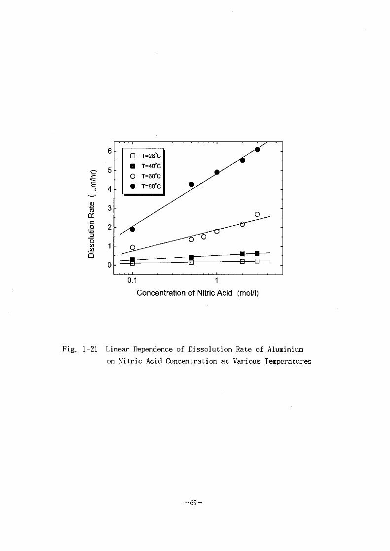
Fig. 1-21 Linear Dependence of Dissolution Rate of Aluminium
on Nitric Acid Concentration at Various
Temperatures 69
Fig. 1-22 Effect of Temperature on Dissolution Rate of
Aluminium at Various Concentrations of Fluoboric
-14-

Acid Solution 70
Fig. 1-23 Effect of Temperature on Dissolution Rate of
Aluminium at Various Concentrations of Sulfuric
Acid Solution 71
Fig. 1-24 Effect of Temperature on Dissolution Rate of
Aluminium at Various Concentrations of Nitric
Acid Solution 72
Fig. 1-25 Linear Dependence of Fluoboric Acid Concentration
on Dissolution Rate of Al-6061 at Various
Temperature 74
Fig. 1-26 Linear Dependence of Sulfuric Acid Concentration
on Dissolution Rate of Al-6061 at Various
Temperature 75
Fig. 1-27 Linear Dependence of Nitric Acid Concentration
on Dissolution Rate of Al-6061 at Various
Temperature 76
Fig. 1-28 Linear Dependence of Oxalic Acid Concentration on
Dissolution Rate of Al-6061 at Various
Temperature 77
Fig. 1-29 Effect of Concentration on Dissolution Rate of
Al-99.9% at 28°C for Various Candidate
Decontamination Reagents 78
Fig. 1-30 Effect of Concentration on Dissolution Rate of
Al-99.9% at 40°C for Various Candidate
Decontamination Reagents 79
Fig. 1-31 Effect of Concentration on Dissolution Rate of
Al-6061 at 401C for Various Candidate
Decontamination Reagents 80
Fig. 1-32 Schematic Diagram of System Decontamination Test
Loop 82
-15-

Fig. 1-33 Photograph of System Decontamination Test Loop 83
Fig. 1-34 P & ID of Coolant System Decontamination Kit •••• 87
Fig. 1-35 Drawing of Demineralizer in Coolant System
Decontamination Kit 88
Fig. 1-36 Drawing of Model Heat Exchanger in Coolant System
Decontamination Kit 89
Fig. 1-37 Layout Drawing of Coolant System Decontamination
Kit • 90
Fig. 1-38 Control Panel Circuit of Coolant System
Decontamination Kit 97
Fig. 1-39 Photograph of Coolant System Decontamination Kit •• 99
Fig. 2-1. Experimental equipment for solid CO2
decontamination •• 118
Fig. 2-2. Residual amount for simulated specimens • 120
Fig. 2-3. Residual amount for simulated specimens 123
Fig. 3-1. Paticle Size Accumulation Curve 127
Fig. 3-2. Cyclone Entrance Block • - — 130
Fig. 3-3. Cyclone Configulation 132
Fig. 3-4. The Kind of the Dust Hopper • • 135
Fig. 3-5. ^ H ^ l S ^ S l ^ K i ...138
Fig. 3-6. ^ ^ 3 &£. 140
Fig. 3-7. 4 ° 1 # ^ I &S.Q ^S.c]} tflst ^ 2 ^ 3 141
Fig. 3-8. ^^Sj-, -g-f- ^3L ^Sl-ffofl cfl*]: ^ * p g ........141
Fig. 3-9. 4 ° l # « i -M*t <£*}$ £ ^ 142
Fig. 3-10. 4 ° 1 # * ^ ^ ^ ti*}^ ••• 143Fig. 3-11. 4 ° I # M <H3j 7}x] ^^V^oll^^ <y- .-145
Fig. 3-12. 4°1#€-£| S.^ VA *Ki2l- ^J£ 149
Fig. 3-13. ^ ^ ^ ^ - ^ - ^ 1 - 7H2 AH#^r^] ^*> ^n}^)^ . . . .150
Fig. 3-14. ^ % ^ - # ^ # 7} 1 4°l#^c>fl t W ^ 4 ^ ) ^ . . . . 1 5 0
Fig. 3-15. ^ ^ ^ 4 ^S. 154
- 1 6 -

Fig. 3-16. ti^H^gl 4 ° ] # ^ r 5 :# 158
Fig. 3-17. rvgj; ^^f^-^d 160
Fig. 3-18. C& JSL^^Kd 160
Fig. 3-19. 4°]-K *1^£^ 164
Fig. 3-20. Sand Filter Configulation 168
Fig. 3-21. 4i*g 4°1#^" ^^1/^14 192
Fig. 3-22. 4°l#^r ^ ] SSa^3 ^#S 193
Fig. 3-23. 4 ° 1 # € ^ t y } S.H^ JL#51 194
Fig. 3-24. 4°1# - ^Vy^#*l A^S. 195
Fig. 3-25. ^}5l*m 4£# ^*H^1 197
Fig. 3-26. £7]7}<iq *tf<g#*l 199
Fig. 3-27. f^ i el l 205
Fig. 3-28. Comparison of Temperature Capability 207
Fig. 3-29. Comparison of Face Velocity 207
Fig. 3-30. Comparison of Dust Treatment Capability 208
Fig. 3-31. Collector Size Comparison • 208
Fig. 3-32. I*lel S. 209
Fig. 3-33. s)-a.# <y4^s:£ 212
Fig. 3-34. H ^ f - n ] ^ <y*fg-Ss. 213
Fig. 3-35. 5 H 1 *!*}^:SJE 214
Fig. 3-36. S|-3.# &£.o\] n ^ £^JL-§- 215
Fig. 3-37. -il;Sl- -f-n| SLO]} xt}^ S ^ ^ # 216
Fig. 3-38. #4}-^ £<H1 nf€- S ^ ^ # 217
Fig. 3-39. -tfSfca-il -3£.<H| ^}€: S ^ J L ^ - 218
Fig. 3-40. tfSJ-^nl-fe- <£f£.6fl n^g. 3E^5L-i- 219
Fig. 3-41. *>SH ^d\] TL}^ 3:$3L-£ 220
Fig. 3-42. r l 4## ^^l^Hl ni^ S^^# 220
Fig. 3-43. 60%, 10 ni/soi|A-|5] tiov#^l ^^fg-SS. 221
Fig. 3-44. 10%, 10 m/s<HW£| ^ # ^ 1 6 « ^ } ^ S £ 222
Fig. 3-45. 60%, 10 m/s<5M£) ^ # ^ ^ 1 <y*}^S£ 223
- 1 7 - I NEXTPAGE(S)I left BLANK
M
91-b 30
(250 kW, TRIGA Mark-II)
(2 MW, TRIGA M a r k - I l l ) # ° l -§-*H 1999^
1^7)(TRIGA Mark-ID
2517](TRIGA
TRIGA Mark-II
TRIGA Mark-II^
7f^5]^L SI^- Ao^-§" ^ 4 ^ a
^ XI 4 1 fl^cH[][l-l~l-4], TRIGA
, TRIGA Mark-II ^ ^ - ^ ^ 1 u ^ 4 9J
1999^
- 1 9 -

. C02
co2
co2 co2
4TRIGA Mark I I I
4
717]
7]71
, DUPIC ^ g , KALIMER
hot particulate
- 2 0 -

sodium# 4-g-tfe KALIMER
ix}5}
^^7l(granular f i l terW
- 2 1 -NEXT PAGE(S)
left BLANK

2 s- TRIGA
TRIGA
>, TRIGA
[1-1.2]
1317] (TRIGA Mark-I I )^
|p.^ o|
7} # 71 ^#<L
o)
6Tuf. - i 1JM7}- -f si
TRIGA Mark-II
- 2 3 -

l ^ h 1999^ 3W*] 2*}
2)
i fe^] , «»]
o|
- 2 4 -

o] 7]71
7171
4.
7K
- 2 5 -
3.71) ^oj j l - t ^ K BWR
. Table 1-
fe Cr
$171 n6H 37}
±= F e , N i , C r ^ + ^ ) l J ] ^ ^ ^
o | < 5 | e ^ CAN-DECON, NS-1 , LOMI
Cr
( N P )
(2)
JPDR*] ^ ^ [ ^ <y^7f|-t 47fl*]
Table l
(7\) CAN-DECON
- 2 6 -

Table 1-1
FeNiCr
£| %
BWR4 ?ms\ <y 1-^4^1
BWR
80-907-101-10
«-Fe2O3(^£)Fe304
NiFe2O4
F e 3 0 4 ( ^ - A ^ )ct -Fe203
NiFe2O4
FeCr2O4
1 B.A^\ ^
PWR
2 0 -2 5 -1 5 -
F e 3 0 4 ( ^
NiFe2O4
FeCr2O4
FeCr2O4
Fe2Cr04
NiCr2O4
406045
*£)
- 2 7 -

Table 1-2 JPDR <&%} *-J4?H 3-§-3 1 ^ 1 £.#3}
"11 T~T * ^ l
CAN-DECON
* * * ! *
LND-1O1A
0. lw»s
- 1 2 0 °C24hl m / s
NP/NS-1 m o d i f i e d
NP fHN03
[KMnO4
0.6w%fO. 5w/o10. lw/o
~ 120136h
lm/s
NS-1
0. 7w%
~120"C24h
lm/s
W-Ce(IV)
REDOX x\]<g
H2S04+Ce4*
0.25M 2mM
70~80°C106h
0.3m/s
7]m^
B4C <&*•}
20w%
^ - &35h
4.8-6. 7m/s
3-90 90-740 300-1,200 200-1,660^ 5 - 9 ^ S 520 ^ ^ 900 5§5- 1,100
15%)
- 2 8 -
DF 3 - 1 1
Cu
NP/NS-1
l, NP(0.5 wt% ^ ^ > / O.lwt*
NP/NS-1 5 . S
500
DF 90-740,
, o)
A S ^ 900
Cr
Ce4+ /Ce3+
DF 300-1,200,
m/s
4.5
01
- 2 9 -

K o]S. Hi^l^ Cr
^r
4.8-6.7
1,1001-
4A]
lBq/cm2
Ce(IV)ofl
^ Cs-1375]
0.5M 2M
DF 200-1 ,660 ,
(Rapsodie)^
REDOX
0.01M
20,
60°C
strippable
(7})
£ gun S ^ lancet
^ 70-1,400
150-700 Pa*]
DF 50-1,0001-
^ 200 Pa
1,400 Pa O| 4
30-45 l/min^l4 DF l,000#
pa 7}
-g-S.
-30-

(Strippable coating)
, #(Brush)
7]71 S^Jl^-Jf^ uH - ^c^l o|H.7]7Mlfe ^-§-6] o^cf. 2 4
-g-
DF
(Uf)
l f e ^ , DF 10
0.1M
200-1,500 m2 $S.$] 7}7]*\]
-31-

(2)
(7f)
-§--§-*} 04
3.7]}
r 240 .2-0 .5 A/cm2,
103~104
horning^
- 3 2 -

Ce(IV) REDOX 3L
4t(Ce+4/Ce+3 =1M H2S04 + 0.05M Ce4t(Ce+4/Ce+3 =
^ s o > ^ CEA 2M H2S04-§-
1.6M
DF 1 0 - 1 5 , # DF 1 , 0 0 0 - 1 ,
1.4Bq/cm2
Gal igur iano -c- 3% 5%
60°C, 30min
- 3 3 -
Savana river^l -^-e]JLij-71^- 7 ^ 4 ^ ^ ] 4 ^ canister
glass £*m103~105 dpm
^ glass frit-i- J L S ^ - ^ ^ S *1I£WSS.>H 2 4
, 24
blast)
5-20, # e } ^ ^ ^ ^ H | ^ ^ ^7]#oi | cH«B 10-100
>i CEA
fe 24C02 ^ 4 a ^ S ^ I G25] eU ) 14 1 # M f r ^ 4 1 ^
^ # %7}$) 3M NaOH
H2SO4 + 3M H3P04#
435g/m2^A-l ^ H N ^ ^ 7 . 2 1/m2, ^ l ^ J L ^ f ^ DF 500i§
- 3 4 -

Pu
^ 4^^-Hfe ^ r ^17]#^ 4%
fe 200~300g^| ^ - ^ 4 500ppm*] PuO2-|- ^ ^
ZL# Ar ^-^71 -§*M ^ 7 1 5 . 7><i -g-g-A]^^- «g*fjl( 5|tfl 109
^ 7 ] ^ e B ^ . -g-g-
s(iookg
1. TRIGA
7>. TRIGA
(TRIGA
1962^ 0.1 MWthS. 7}-^# A|4«rH 1969^^] 0.25
2S.7] (TRIGA Mark-Ill)fe 1972^^] 2 MWthS
^ § - 4 4 34^d VA 24id ^^> 7Hf-51$-lr:h Table
fe TRIGA g
TRIGA
91
- 3 5 -

Table 1-3. Specifications of TRIGA Research Reactors
Reactor name
Reactor type
Thermal power
Neutron flux (max)[nv]
FUEL
U-235 Concentration
Cladding materialChemical
compositionModerator
Coolant
Control rod
Fuel loading(U-235)
Volume of pool water
Research reactor unit-1,TRIGA Mark II
Pool type
250 kW
1 x 10'3
20 %
Aluminium
U-ZrHi.o Alloy
ZrH, H2O
H2O
B4C
2.96 kg
17,146 L
Research reactor unit-2,TRIGA Mark Hi
Pool type
2 MW2,000 MW, 2.8 msec pulse
6.5X1OW
(Pulse, 2.0 X10'6)
20 and 70 %
SUS-304
Er-U-ZrH,.6 Alloy
ZrHi.6, H2O
H2O
B4C
12.6 kg
153,000 L
- 3 6 -

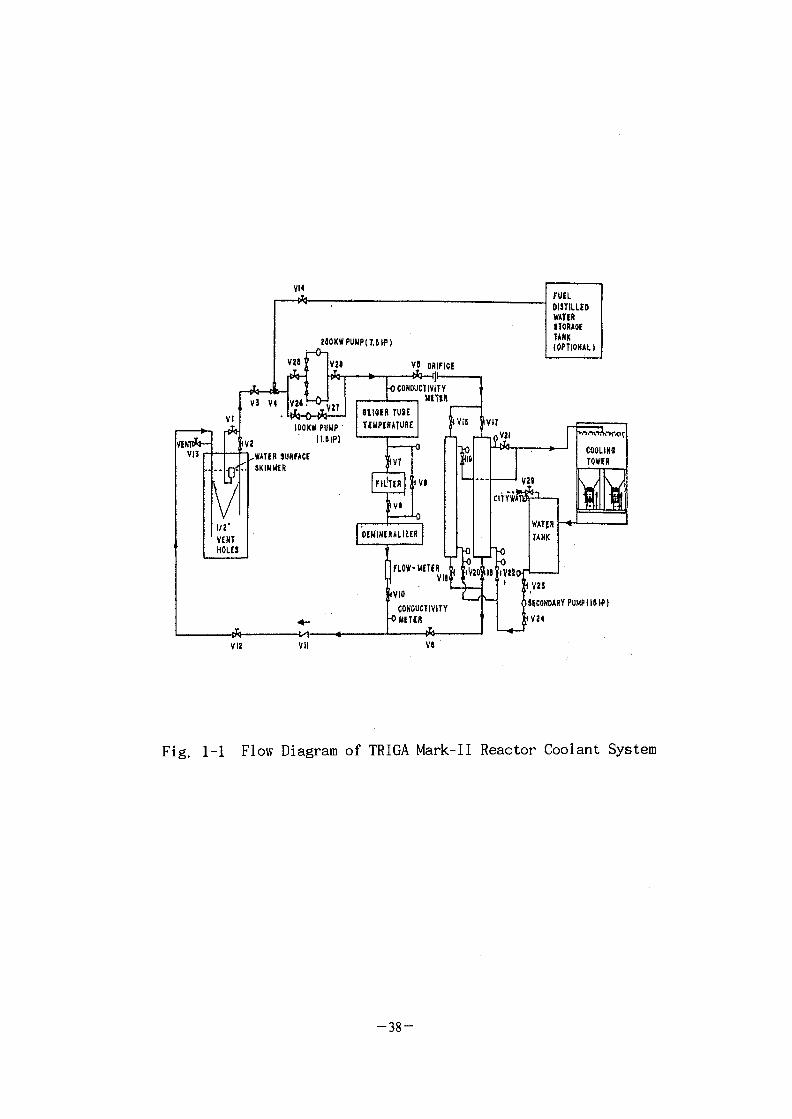
. Fig. 1-loflfe TRIGA Flow
diagram^- 27ffSj
^ 100
11! 250 kw
^ 250 kW
250 kW
Fig. 1-2
Fig.
(Pool),
n}(Skimmer),
^#7), 1 1
17,000 153,000 . TRIGA
43°C
^: FerriteTft
TRIGA Mark-II
- 3 7 -
fLOW-MITM[ v i eIVIO
CONDUCTIVITY
( V2J
JECONOARYPUMPIIUP]
Fig. 1-1 Flow Diagram of TRIGA Mark-II Reactor Coolant System
- 3 8 -

Fig. 1-2 Photograph of TRIGA Mark-11 Reactor Coolant System
- 3 9 -

Fig. 1-3 Photograph of TRIGA Mark-Ill Reactor Coolant System
-40-
#444(Hner) ^JsL-b
Co-58, Co-60, Fe-55, Mn-54, Zn-65
Ni-63
fe ANISN
H S ^ Tfl-f-oj Cs-137, Eu-152 ^ Eu-154
[1-5]. 1JL7H
-2,3]. Table
Table 1-
. TRIGA
TRIGA
2(1/2)"
- 4 1 -

Table 1-4. Shutdown Inventory of Radionuclides in Neutron-Activated
Aluminium Liner of TRIGA Mark-II Reactor (Ci/cm )
Radionuclide
Cr-51
Mn-54
Fe-55
Fe-59
Co-60
Zn-65
Side
4.0E-16
1.4E-15
4.4E-11
8.6E-17
3.3E-13
1.3E-12
Floor:
8.2E-16
2.9E-15
9.1E-11
1.8E-16
6.9E-13
2.7E-12
-42-

SCH40 ^ r n ) ^ - Hjf^(^[o|, 3i0nnn) ^ ^IjL-f(Elbow)t-
(Fig. 1-45] # ^$] afl^fl), <£ -jlL 2£7]o |H*r ^
1(1/2)" SCH40
Fig. l-6<fe 04^-S. 15L7HIA] *fl*l^ 2(1/2)" SCH40
^ # %<^«i 4£o]uK Fig.
1^71 ^ 2 ^ 7 1 ^
(MCA)# ^A]^r}^A^, ZL ^ | 3 f # Fig. 1-7, Fig. 1-8 9J Table
^ ^ ^ TRIGA «1^-S 13.7] ^ 25L7}$>]
^r Co-60 *i Cs
t * ! f ^ S Mn-54# H|^-
Eu-152 J£fe Eu-154
TRIGA
2. TRIGA
- 4 3 -

Fig. 1-4 Photograph of Heat Exchanger Installed in TRIGA Mark-II
Reactor Coolant System
-44-

Fig. 1-5 Photograph of Demineralizer Installed in TRIGA Mark-II
Reactor Coolant System
-45-

Fig. 1-6 Photographs of Contaminated Pipe Sample Taken from
TRIGA Mark-II Reactor Coolant System
-46-

Saaple : elbow § 1
Data collected at 1Bn17:17 on 23-SEP-97Real TlK : BOOSSceidsSeconds Live Tihive JiSe SecoWKlO SecondsDetector :
Calibration :
FILE NAHE : B164MH1 DR5BlNtSK9ADiTECS6a8589399?
14400
Fig. 1-7 MCA Spectrum of the Contaminated Sample Taken from
TRIGA Mark-II Reactor Coolant System
-47-

Sample : pipe 20 c» 6 1
Data collected at 12:05:16 on 23-SEP-9?Real Tine : 20029.42 Seconds Live Tirce : 20000 SecondsDetector :
Calibrat ion :
KII.E NAUE : »: pipe10' |
DRAhlNS QSTE : DS-2B-1997
12000 14400
Fig. 1-8 MCA Spectrum of the Contaminated Sample Taken from
TRIGA Mark-III Reactor Coolant System
-48-

Table 1-5. MCA Results of the Samples Taken from TRIGA Research
Reactors
Samples
Elbow
Pipe
Radionuclides
Co-60
Cs-137
Eu-152
Co-60
Cs-137Mn-54Eu-152Eu-154Ce-144
Energy
(keV)1332.51173.2661.6
1408.0
1332.51173.2661.6834.81408.01274.4133.5
Activity
(cps)0.060.060.07
0.02
0.52
0.551.440.070.030.030.04
Remark
Sample was
taken from
TM-II coolant
system
Sample was
taken from
TM-III coolant
system
* Background
* Count time
Co-60 (1332.5 keV) 0.014 cpsCo-60 (1173.2 keV) 0.016 cpsElbow-50,000 (sec), Pipe-20,000 (sec)
-49-

7}. g^s. ^ 4 7 ^
^ ojnj
TRIGA ^-T-S^l uJ44 :f- (Cooling
circuit) *fl<g<4fe 3W^Hi~§- 4-§"t!: 4^(Chemical flushing)
el-
TRICAR ^ " ^
sasafe
safe ^4^H 6 f l * W I 6-}=## ^7^}^ . ^ s # 90°c
safe
TRIGA
- 5 0 -

^r TRIGA
(1)
^ ( c l a d d i n g ) * !
(gel)
5a
-Le]u} o|
(2)
Inserter
- 5 1 -

24 ^l^^o) a.7il TC #•§• ^ 3 3 Inserter*
EDTA
90°C7f
71-4>
, o] ,rf|
fe 7|7l
[1-5-1-8]
-§-*]fe 7m "A
TR1GA
- 5 2 -
6061
^ B ] ^ J ^ ] ^ 7 O > 304
nfl
(1)
3X
0.1mole/L~3
ic acid,
HBF4),
Ethylenediaminetetraacetic acid(EDTA), • -yy- ];(oxalic acid)
^ £ 99.9%
type 304 25mm?? Xlannt^ 3.7]S.
28-80
- 5 3 -
. Table l-6oflfe
. 0.5* °W # ^ * f e A i ^ - ^ ^ Fe, Mg ^ Si
(2) ^ ^ ^5} £ ^-^
Fig. 1-9 ~ Fig. l
. Fig. l-9fe !-S*^!:<4 ^ - ^ ^ ^ - n l ^ nj ^^-nl^- 6061
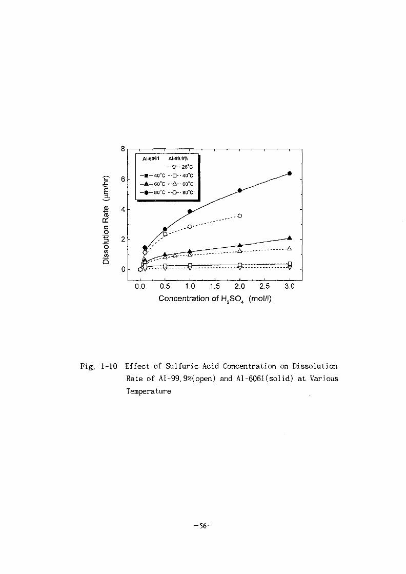
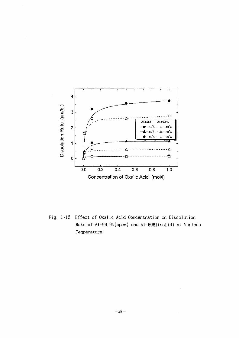
^1 tfl*H T^MVH ^^°1^K Fig. 1-10^ %^
4°]^- , Fig. 1-ll^r ^ - g - ^ , Fig. 1-12-b ^-^^-g-64, Fig
EDTA -g-^# 4-§-^}^ l-^-f^: A J ^ 4 ^ ^ a o ^ ^ - S -§-«
M.^ Hj-Af ^o] <y-^-nl^ 6061 4 ^ 7 }
3.4 ^^gSl^cK a ] ^ "t-f-n]^. 6061
Table l-6^]-H # ^ ^ ^ H>5} ^o] o]
HBlJL, Fig. 1-14^ ^ I ^ S . KAERI 4 ^ 1 -g-64(EDTA 1.12 g/L,
Citric acid 0.21 g/L Rj Ascorbic acid 0.18 g/L*] ^ * J # ; #•
0.15
6061^1
3.4 T-Mlv!:^^ ^ ^ 80°C<>M ^>f-n|^- 6061^1
0.16 ^m/hrS, ^ ^ ^ ^ 1 ^ - ^ 0.09 ^m/hrS ^ - ^ £ ] ^ K% Q RED0X
Rj KAERI
- 5 4 -

$(0
c
J3OV)CO
b
uuu
800
600
400
200
0
/ Z^^
AI-6061 Al-99.9%
- V- • 28°C- • - 4 0 ° C --D--40°C
-A- 60°C - -A- • 60°C
- • - 80°C - -O- - 80°C
-
-
_
_.^V A
0.0 0.5 1.0 1.5 2.0 2.5
Concentration of HBF4 (mol/l)
3.0
Fig. 1-9 Effect of Fluoboric Acid Concentration on Dissolution
Rate of Al-99.9%(open) and Al-6061(solid) at Various
Temperature
-55-
E
CO
a:co•5
6 -
4 -
2 -
0 -
-
-
1 • 1 1
AI-6061 AI-99.9%
- -V- - 28°C
- • - 4 0 ° C --D--40°C
- A - 6 0 ° C -A--60°C
- » - 8 0 ° C --O--80°C
X^"°
J&t~—£1 JR"—'
i • i • i • i
^ —
0.0 0.5 1.0 1.5 2.0 2.5 3.0
Concentration of H 2SO 4 (mol/l)
Fig. 1-10 Effect of Sulfuric Acid Concentration on Dissolution
Rate of Al-99.9%(open) and Al-6061(solid) at Various
Temperature
- 5 6 -

CD
co
oCO
AI-6061 AI-99.9%
-•V--28"C
- • - 4 0 ° C --D--40°C
- A - 6 0 ° C --A--60°C
— 80°C --O--80°C
0 -
0.5 1.0 1.5 2.0 2.5
Concentration of HNO (mol/l)
Fig. 1-11 Effect of Nitric Acid Concentration on Dissolution
Rate of Al-99.9^(open) and Al-6061(solid) at Various
Temperature
- 5 7 -
"I
I 1o(A
wb
oAI-6061 AI-99.9%
- • - 4 0 ° C --D--40°C
- A - 6 0 ° C --A--60°C
- • - 8 0 ° C --O--80°C
0.0 0.2 0.4 0.6 0.8 1.0Concentration of Oxalic Acid (mol/l)
Fig. 1-12 Effect of Oxalic Acid Concentration on Dissolution
Rate of Al-99.9%(open) and Al-6061(solid) at Various
Temperature
- 5 8 -

0.10
JZ
I
ion
Rat
eol
ut
0.08
0.06
0.04
0.02
Q0.00 -
AI-60G1 AI-99.9%
- 4 0 ° C --D--40'C
—A—60°C --A--60°C
—•—80°C --O--80°C
0.00 0.02 0.04 0.06 0.08
Concentration of EDTA (mol/l)
0.10
Fig. 1-13 Effect of EDTA Concentration on Dissolution Rate
of Al-99.9%(open) and Al-6061(solid) at Various
Temperature
-59-
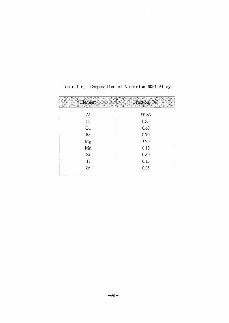
Table 1-6. Composition of Aluminium-6061 Alloy
Element
Al
Cr
Cu
Fe
Mg
Mn
Si
Ti
Zn
Fraction (%)
95.85
0.35
0.40
0.70
1.20
0.15
0.80
0.15
0.25
-60-

I
0.16
0.12
ra 0.08
2. 0.04o
bo.oo
-•-AI-6061--O-Al-99.9%
20 40 60 80
Temperature (°C)
Fig. 1-14 Effect of Temperature on Dissolution Rate of Al-99.9%(open) and Al-6061(solid) in the Dilute KAERIDecontamination Solution
- 6 1 -

. Fig.
1-15 ^ Fig. 1-166*1 i_j.El-\fl ^ 4 ^ o ] ^ A > £ %A>CH] Afl-t(IV)o] 0.04
ZLSJ
, Fig. 1-17 iJ Fig. l-186fl i Bfvfl ^BlI^tBl]^^,}- 304
mole/L ^ £ # 71 ^ S . uV .
80 °C, ^fS. 3.0 mole/L S ^ W #5f-fA>^ ^^-fe 6f 7.3 /m/hrS.
^ < 36 fm/hrS. ^5\°] 5^}
^ - T - 80 °C, %•£. 3.0 mole/L
>i7ov 304^ -g-*U^s.fe 0.05
t\X\ «l^--§-c^( Semi-log) Sf^efl ~Le} i ^ K Fig.
1-19 ~ Fig. 1
4
Arrhenius' plot# Fig. 1-22 ~ Fig. 1-24^1
t\. 4
rtf] tfl*> %^^-^lM^HEa)^- Fig. 1-22 ~ Fig. 1-243 7 I #
4 4 , Ea (l-S|-3-^>) = 5.46 kcal/mol, Ea (%*>) = 5.80
kcal/mol H Ea (-^^1:) = 5.91 kcal/mol^.
v = [A • exp(-Ea/RT)] • log [C] (1-1)
- 6 2 -

(D
o
10
8
6
4h
- 2 -O Z h
-
i • i • i •
— • - T=28°C + Ce(IV)
- • - T = 8 0 ° C + Ce(IV)
--D--T=28°C
--O--T=80°C
tdD—grr—--H
1 . 1 i 1 •
1 ' 1 ' 1 ' 1
_ o
---H 5 .i i i > \ i i
0.0 0.5 1.0 1.5 2.0 2.5 3.0
Concentration of Sulfuric Acid (mol/l)
Fig. 1-15 Effect of Cerium(IV) Ion Addition on Dissolution Rate of
Aluminium in Sulfuric Acid Solution at 28°C and 80°C.
Mole Ratio of Ce(IV)/SA= 0.04.
- 6 3 -

E
B
co« 2 -
CO
b
- T=28 C + Ce(IV)
-T=80°C + Ce(IV)
D--T=28"C
O--T=80°C
0 -
0.0 0.5 1.0 1.5 2.0 2.5 3.0
Concentration of Nitric Acid (mol/l)
Fig. 1-16 Effect of Cerium(IV) Ion Addition on Dissolution Rate ofAluminium in Nitric Acid Solution at 28°C and 80°C.
Mole Ratio of Ce(IV)/NA= 0.04.
- 6 4 -

&
i 2Hi
\—T=40 C
--O--T=60°C
—•-T=80°C
O
0.0 0.5 1.0 1.5 2.0 2.5 3.0
Concentration of Fluoboric Acid (mol/l)
Fig. 1-17 Effect of Concentration on Dissolution Rate of 304 S. S.
in Fluoboric Acid Solution for Various Temperatures
-65-

E=3.
a:co
o(0
40
35
30
25
20
15
10
5
0
-5
1 ' 1 •
- --•-•-T=40°C
--O--T=60°C
- • - T = 8 0 ° C
_
:
a — — - • • H - ' - " B -
1 . 1 .
i • i • i • i • i
/ . - - • " ' " " "4------ * :i . i . i . i . i
0.0 0.5 1.0 1.5 2.0 2.5 3.0
Concentration of Sulfuric Acid (mol/l)
Fig. 1-18 Effect of Concentration on Dissolution Rate of 304 S.S.
in Sulfuric Acid Solution for Various Temperatures
-66-

a:o
500
400 •
300 -
200 •
75 100-
0 •
-
•
••o
T=28°C
T=40°C
T=60°C
T=80°C
B—B-
y
-m—-a—
/
^ © -
—•-B-
-
-a—
0.1 1
Concentration of Fluoboric Acid (mol/l)
Fig. 1-19 Linear Dependence of Dissolution Rate of Aluminium
on Fluoboric Acid Concentration at Various
Temperatures
• 6 7 -

I 2h
o= 1 -o(A/
0 -
0.1 1
Concentration of Sulfuric Acid (mol/l)
Fig. 1-20 Linear Dependence of Dissolution Rate of Aluminium
on Sulfuric Acid Concentration at Various
Temperatures
-68-
3
6-
5 -
4
3
I 21 1
0-
• . . 1
-
••0
•
-
. . . 1
T=28°C
T=40°C
T=60°C
T=80°C
/
1 1 '
——•— •"D B-
-
-a—
0.1 1Concentration of Nitric Acid (mol/l)
Fig. 1-21 Linear Dependence of Dissolution Rate of Aluminium
on Nitric Acid Concentration at Various Temperatures
-69-

1000
£Z
gowwb
100
10
O 0.5MHBF,1 M HBF4
A 3 M HBF.
2.8 3.0
1/Tx1033.2 3.4
Fig. 1-22 Effect of Temperature on Dissolution Rate of Aluminium
at Various Concentrations of Fluoboric Acid Solution
-70-

£CO
o
" o</>CO
b
2.8 3.0
1/Tx103
Fig. 1-23 Effect of Temperature on Dissolution Rate of Aluminium
at Various Concentrations of Sulfuric Acid Solution
-71-

szE
£CO
o
"o
10
1
0.1
xx.
0 0.5 M HNO3
D 2 M HNO3
A 3 M HNO3
% ^ ^
XXXKX
2.8 3.0
1/Tx1033.2 3.4
Fig. 1-24 Effect of Temperature on Dissolution Rate of Aluminium
at Various Concentrations of Nitric Acid Solution
-72-

kcal/moljsl
^ %SL Fig. 1-25 ~ Fig. 1-27 6061
log
6061
6061^
7f*fjL alt:}. Fig. l-28
6061^] -§•*!!
log
- 3 1 cHl
$5LS. 3.7(1
28°C 9J
^- 6061
, Fig. 1-29 ~ Fig.
(HBF4)
-g-^S.
- 7 3 -

00
OHcg*«•-<
"owv>b
800
600
400
200
0
•
_
1
D
•O
•
-
:::g. . . i
T=28°C
T=40°C
T=60°C
T=80°C
,.."""0
" •TT" TT *
#
•"ri"
-
9-*°'"
0.1 1
Concentration of H B F (mol/l)
Fig. 1-25 Linear Dependence of Fluoboric Acid Concentration on
Dissolution Rate of Al-6061 at Various Temperature
-74-

x:E
6 -
a:
3 2^COCO
0 -
••O
•
B
T=28°C
T=40°C
T=60°C
T=80°C
. . - - ' ' '
JO. -0—'
* - » - - -
#
o
—ft"
•
•
o
•ft—
0.1 1Concentration of H 2SO 4 (mol/l)
Fig. 1-26 Linear Dependence of Sulfuric Acid Concentration on
Dissolution Rate of Al-6061 at Various Temperature
-75-

co
15
10
5
0
•
D
•O
•
-
-
O
. -
T=28°C
T=40°C
T=60°C
T=80°C
...
•
q...
ifm
o
• " " •. . 1
•
q.
•TT"
•
-
-
. .O - -
•0.1 1
Concentration of H N O (mol/l)
Fig. 1-27 Linear Dependence of Nitric Acid Concentration on
Dissolution Rate of Al-6061 at Various Temperature
-76-

.cE
2g
o
AI-6061
• 40°C
A 60°C
• 80°C
AI-99.9%
•A
O
40°C
60°C
80°C
0.01 0.1 1
Concentration of Oxalic Acid (mol/l)
Fig. 1-28 Linear Dependence of Oxalic Acid Concentration on
Dissolution Rate of Al-6061 at Various Temperature
- 7 7 -
a:o
"o
b
20
15
10
5
0
i ' l ' l ' l • l • l • l
Q -
/
- • - HBF,- O - H2SO4
--D--HNO3- A - H2SO4-Ce(IV)
- V - HNO3-Ce(IV)
/
-
-
0.0 0.5 1.0 1.5 2.0 2.5
Concentration (mol/l)
3.0
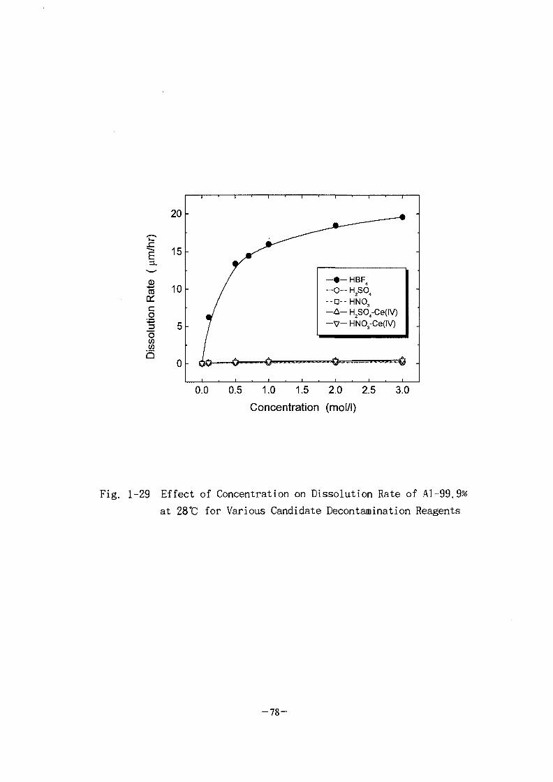
Fig. 1-29 Effect of Concentration on Dissolution Rate of Al-99.9*
at 28°C for Various Candidate Decontamination Reagents
-78-
£TO
a:cg
0.5 1.0 1.5 2.0 2.5
Concentration (mol/l)
3.0
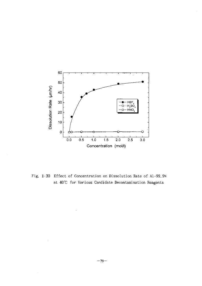
Fig. 1-30 Effect of Concentration on Dissolution Rate of Al-99.9%
at 40°C for Various Candidate Decontamination Reagents
-79-

&CO
q
owwb
140
120
100
80
60
40
20
0
-
• y —O— H2SO4
—D— HNO3
>->
^ * -
n
0.0 0.5 1.0 1.5 2.0 2.5
Concentration (mol/l)3.0
Fig. 1-31 Effect of Concentration on Dissolution Rate of Al-6061
at 40°C for Various Candidate Decontamination Reagents
-80-

(2)
Fig.
Fig.
71
3. ^-
7>. 4
(1)
(TRIGA
250kW
(2)
(7})
13171 (TRIGA
-81-

SpecimenChamber
Fig. 1-32 Schematic Diagram of System Decontamination Test Loop
-82-
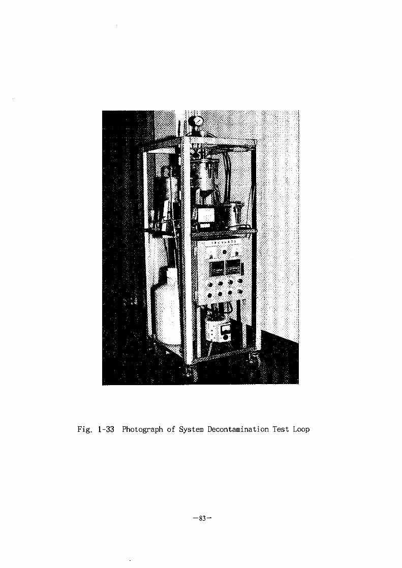
Fig. 1-33 Photograph of System Decontamination Test Loop
- 8 3 -

skid
71
13171
1999\4 1-7).
250kW
EDTA
4, 80°C
60°C
471
(3)
- 8 4 -

Table 1-7. Demonstration Work Schedule on Coolant System
Decontamination of TRIGA Research Reactor
Activities
o Fundamental technology development• Analysis of TRIGA reactor coolant system• Contamination characterization• Reagent development test• Fabrication of coolant system decontamination
test loop• Reagent decontamination test
oApplication technology development• Decontamination process establishment test• Design and ordering manufacture of coolant
system decontamination equipmento Demonstration of coolant system
decontamination technology• Test operation of decontamination equipment• In-situ decontamination application to TRIGA
mark-II reactor
Year
1997 1998 1999
- 8 5 -
Fig. l-34ofl
fe 4.^# Fig. 1
Fig. 1-35
1 skid #
Fig.
44
( l )
44 fe 4
4444-8- ^-4 ^ 7W
. 44,
44-8-4
Table 1-8^1
4 - r1! 4 4 4 ^
- 8 6 -

M
SB
S i
s
0
© aft
?
118
|
ss3a? \r w v* tfl in
©-
(L
Fig. 1-34 P & ID of Coolant System Decontamination Kit
- 8 7 -

3
31
no,a
\
Fig. 1-35 Drawing of Demineralizer in Coolant System
Decontamination Kit

oseeI
3
I
Fig. 1-36 Drawing of Model Heat Exchanger in Coolant System
Decontamination Kit
-89-

Fig. 1-37 Layout Drawing of Coolant System Decontamination Kit
-90-

Table 1-8
No
1
2
3
4
5
6
7
8
9
10
11
12
€7l7><g7l
.E.'Sl.H^l
^ 7 l
-g-££^7l
^3*1 #*>
- $3 | : ^*^o)l ^°]^1 #*}.- H7l: D=380mmp, H=450mm- tfl^-g-^: 50 L- 4S.- SUS 304
- X-l l 7^1^. 7|ti7l ^
^ ^ 31fe «}^-^ -g-71- H7l: D=600mm?', H=870mm- tfl •¥--§-^: 200L- zflS.: PE ^fe PP- qq-. ^ ^ ^- -§- =: 7 kW (220VAC-§-)- ^^^-^HS.: SUS 304- 7><i7ll- ^ r£^H^- <&*\7} ^ ^ m
^ESl -g-7Hl ^3)o.S. =3"#- ^Efl: ?flE.el^^ (H^#A-2 # a )- 3-7]: 114mm¥>x400mm(*|-f^)
89mm <p x300mm(?>S.2l 1)- ^ ^ ^ - ^ S . : SUS 304
- 3.7]: 90mmpx300mm(S}-T-;;8)- ^ ^ ^ - ^ a : ^4^ /SUS 304- -fr^H: 2~20L/min- ^°JJ-¥-^a: vfl'ti-^^S./SUS 304- ^Efl ^ 3.7]: ^-a/shell&tube ^ ,
D=350mm?>, H=1500mm(£^#A-3 %3i)
- AS.'- ^ °1-3.1- °iZ}^<&%.-- 2(1/2)" s M S ^- %n ^ 3.7}: Shell & tube^,
Shells OD=140mmp, H=400mm- •SJE^ft /•}<&: 1/2°!*] SUS304
- <83: * ^ 7>^i!- -fr^: ~10 L/min- ^^^-^fla: SUS 304- # € : 220VAC/60Hz- ti^«fl^-: 1/2" 4°1S- ^Efl % 3.7}: T£2}£: 3§^sl Skid
- 4S.- SUS 304 (t=lmm)- ^ I M l«fl 71^^-ft-^l- TIC: PID ^lH7l(MDC-10)- RTD: Pt 100i3
(^^-¥- B ] 1 = S . S ^ )
- f efl 5 a7l: £^#A-4 ^-2- °J^^^(220VAC) ^ r ^ ^ l -- T^i-a on/off ^3*1- ^ 5 . on/off i f l a ]- ^7l7}^7l on/off i ^ ^ l- -a:5La^7l(TIC) ^ 1 -1741 (TI) # ^
^ ^
1
2
2
2
1
1
1
1
1
1
1
1
«1 3.
-#sa*i*§ ^ ^
7H1 ^-^
-4^*^1-8-
«fl*°l -8-<>lft ?•2 / ^^1^1 1-8- 4^^- ^ sus^^J-
DS-205
-#t*11J fi-H.4SS}- ^«.sl7 l ^ ^ -JM.&.
-Shell# «fl -:1/2 1 1 SUS304 4°1S
-$ll^a^£,S. IS:' CSW-0042
-Skid 3.71 :W2100XDl 100mm
-RTDTT #7}7}<£
s}^! ^ 1
- 9 1 -

71 ^ #
s k i d " o.]
4
100mm
X-J47],
1200mm
4 9-A^O.^^.BI A ]
4 4 "*=5W"#
Skid*] *f|H2 5| 2^1 ^5] 4
304)
1 1 £ ^A] 1/2"
304)
304
S.)fe Fig. l-34dfl
# Fig. l-35<>fl
Fig. l-36ofl
4 S M 3 ^ 1 Mfl^lSl- Fig. l-37ofl
- 9 2 -
304 >i
Skid l-g- H v%
1-35
(safety ifiji),
sa
.fe 7}<i7l
304
-93-
^ 304
4 rcj-
3.7]if-
2(1/2)' 4 ° 1 ^
- 9 4 -

ir PP
- Skid*] 4l^> 44-§- =a ^ A ] ^ of) £_^ *]
vent-g-
^ flexible hose
on/off,
on/off, 27flS] on/off,
£:# 4-&5L
Fig.
7]7|
-95-

4& PVC Duct Si
output 4fe 4
^ . 717]
Fig. 1-38^1,
Table
(2)
Fig.
7}<£7}
(1)
(Inlet)if
- 9 6 -

2P 220V
2P 20A NFB
FS 1
(2)
C3PL41
-O O- -o o-
Fig. 1-38 Control Panel Circuit of Coolant System Decontamination
Kit
-97-

Table 1-9
No
1
2
3
4
5
6
8
Voltage meter
Ampere meter
•8:SL X]A] *5
ON/OFF ^ 1 * 1
PM
VI
AI
TIC
TI
SW1SW2SW3
- Analog type (4^)
- Analog type (42})- MDC-10- Digital type- Range : 0-100 °C- Digital type- Range : 0-100 °C- -^^-^(Main power) on/off- ^ ^ : ^ ! S on/off- ^7]7}^7] on/off- D150XH600XW500 mm
1
1
1
1
1
111
1
Hi 31
- 9 8 -
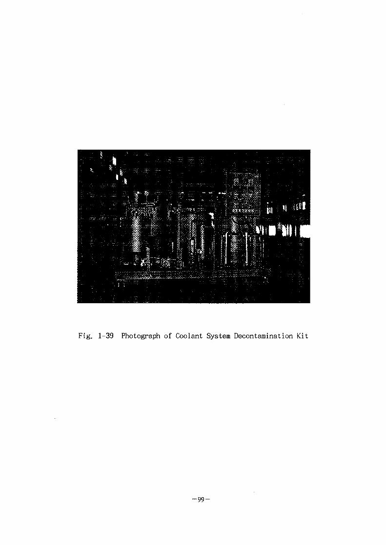
Fig. 1-39 Photograph of Coolant System Decontamination Kit
-99-

13.7})$ 7}-g- 220V, 20AS]
(2)
EDTA
- EDTA : 4.48 g/L
: 0.84 g/L
S.til : : 0.72 g/L
: 0.01 g/L
(3)
-100-
44
44
13171 (TRIGA Mark-II)7|-
TRIGA
Co-60 ^J
- 1 0 1 -

> I ^ 304
(Unrestricted release
^ (Chemica l flushing)
EDTA
71
71 Ef
- 1 0 2 -
3 # C02
C02
>g-f
7}
lfe C02
co2 co2
2 ^ co2
1.
- 1 0 3 -
co2 #
dry i
6.-L]- dry ice^l A\3L7\ -§-O]^ *6\] DCJ-B} o]
^U}. ^«14 dry i
7] A ] ^ } ^ ^ . ^ i ^ o H s . dry ice^ ^
. a l4 . 1945VI njSll^-ofl^fe O^BI $] grease
dry ice!- * J ^ * B 1 M , '63^ 5^, Reginald Lindall^
)^! ^ 4 co2 oJ4t- 4-§-^fe »^SLS. ^M- 4\***}%&. 72, Edwin Ricefe dry ice*] J L ^ ^ 4 #
J* £?&*}% o_x$, 77H1 8^, Calvin
OSHA(Occupational safety & Health Act, *] <£ ^ - ^ ^ . ^ i 1 ^ ) ^ EPA(Energy
Policy Act, e^m^] ^ ^ ^ , 9 2 ^ ) ^4^<>fl rcfsf ^1^7l#^A-| dry ice#
4 dry ice ^}7}^ 7fl^# ^-?-^fe «H^ $\A}7} >g^S|$io.af, dry
ice pelletizerif ^ 4 ^ ] 7 > ^>^ 4 ^ ^
l ^ l ^ f S 7 } 3.JL JL7}^A^, 200psi
}. II ^ C02 £ 4 7 ] # o ] ^^^°11 ^SK J I ^ S dry ice pelletso) 7fl
7l^6fl 4-g-S]1?! ^ ^ S . shaved block dry ice Jiuj- t:-]^-
c] ^ | 2 , 5]e5] i c # ^ ^ 7 ] ^ ^ 80psi5]SlSit:}. pellets^
Dry icefe^ 0.03vol.
carbon hydrates*] -^-^t> l>4i
104-

Sj C027|-
C02 tf^Xfe- *Vf-ofl 25,000^^:1- ^ ^ ^r S l - M , o| <£sj 95%
dry icefe -109°F^
j l ] ^ 3 - ^ ^ vapors.
(blasting media)^
4^1^^1 4^§-5|fe co2i] # ^ ^ * m X N 4-§-^fe ^2} ^^ -^ , FDA,EPA * fl 11 I]H^K |*
C02 fe i U 4 4 4. C027> ^ M ^ o f l °l-§-£|fe
nfl < ic-l*l 4 ^ ^ C027f ^ 3 - f e %°) o\t\x$ ^eH5] C02
2. C02 afl
C02#
- dry ice pel lets0]i-} j2_B]3ijii.4|- - f- ]; ^•'H^cJ^H] ^\^ - ^ ^ ^ I T T dry
ice snow -§-.£) JL-^t media-It
C02#
C02(Supercritical fluid carbon dioxide : SFC02)#
;} macroscopic pe l l e t s ^
•S]i?r'5m, dry ice
snow
-105-

coa
. SFC Tife
7f. pellets
pellets7jj£|
pellet
. *|^. 3.7)5] pellet 4 ^
• ^^«> S^^ l^ pellets*^
• pellet^
pellet
macroscopic dry ice pellets
. Snow
snow £ C02
snow
snow
microscopic snow stream^]
^•£ ^l^-*] large snow flakes stream^
4^r snow spray system^ <£*}$ &^-fr7]
3.7]7} a. snow fiake stream^
snow spray7]
3.7]7\
3.715} snow
microscopic snow stream^
C02 source7}
7\*£$\C02 source^,
co2
- 1 0 6 -

C02 af l£#*]-b SFC #*1»J Jicf
SFC
SFCiLrf
^ ^ T f f C02 (Superc r i t i ca l f lu id C02, SFC)
SFCO2 ^ l 7 ( ( f e C02^ - g - n ^ >§^2f ^
. <>l£r 31°C, 72.8atm 0)
^ . ^ , SFC02 ^ l f e
SFC02
^ t > 7)7] ,
. SFC02 ^ 1 1 ^ > ^ ^ ] ^ ^
3.
(5. latm, -56.7°C)o|^ ^7J l^(cr i t ica l pt. 72.8atm, 31.
- ^ ^ o] A > ^ 7 | A O V ^ 6 J | ^ ^ . ^ s j . ^ ^ ^
C02 ^
71 co2oia, 0} ai
C0 2 #
- 1 0 7 -

, C02
fe dry ice
CO2 press.-enthalpy diagram?] Mollier^S.
C02 feed 1 }
snow
C02 cylinder^) liquid C02 7}
C02)7f o r i f i c e ^
C02
7)
C02 source#
57}
yield b ^
> C02 source*] orifice
7]-
(SftOpsi) 2.^
y i e l d s ^6«o]c}. rcj-eM JL^J- C02
^^*f^, source*] ^S., ^-^ofl
^BU a e ] j L snow*]
dry ice 3.71, ^ £
C02
>b^f. <>]
orifice nozzle
co2 snow *(|££ C02 sourcel- 4
4. Medial]
Dry ice
- 1 0 8 -
dry ice block
granules^ & £ ^ 4 -
^ ^ . ^ sugar-crystal 37] S] dry ice granules^]
dry ice
dry ice p e l l e t #
p e l l e t # ^r4*WM- *&&-*] #}*] £-£r%-7M p e l l e t #
. °11- p e l l e t s ^ Ji^f- 0.08-0.12"(2.03-3.05mm)^ ^
0.4"(2.54-10.16mm)^ ^o]M. ^%cf. o) «J-^ofl $a°1>H, dry
QQ 64Ac}" C02# snowS. flashing*! ^ snow# J
t:}. snowfe pellet.^..!. ^ ] ^ nuggetsf ^- 7l7fl^
efl^iS. d i e | | f-sfl i ^ - pellet % B H S ##(extrusion)^i: j- .
$1pellet-
C02
0 . 1 -
^r 7}
media
. 4
5. -4Dry ice
soda bias ting 21- 4
mediafe C02
-pellet^
800HB
sand blasting, plastic bead blasting
7f«y-:g-7]vf- ^ - ^ t : } ^ inert 7}^S. ^r^
K c]
medial, dry i
nfl-f
3-4mili 4°H1 pellet
C027l-
, dry ice ^ 2^}
-109-
., dry ice
^o]z\. C02 <g*\±r
4 T T ^r-E.^ air stream
fe ^ e j , C02 6
HT4fe -109°F(-78°C )S]
H S coating typeofl ^ ^ * f ^ 4 *•}£.& coating^] ^
>4. dry
"T
6.
1981 id<>leH Savannah River
l^^o] ^ 1 ^ , ^ - ^ ^ ^ A C ^ co2
71 # ^ *}q-s. ^ 1
NDC4(Non Destructive Cleaning Inc. )if TTI Eng. A } ^ 1990\l
surry PWR(Virginia Electric Power)*] ^ ^ S J i ^ l ? ! ^ ] : ^o\] C02 -g-
Al~§--erMtool# ^^ zQlWSlK}. ^ l ^ ^ ^ Table 2-
hard too l^ 100%7} 1000dpm/100cm2ol^}7M
o]i} %>7ll chain falls, power hand tool ^ ^ofl afloj^ ^
o] 9ife ^ 4 ^ 4 ^ ^ ^%^^^1 -f- -, !«- ^131 #71 a ^7l manway
- n o -

£# }m£: ^M°} 3~5mrem/h
l f e H E P A 1 1 B l n > o | ^ } i K
Winco ICPP( Idaho Chemical Processing plan
storage area, FSA)^S.-?-Bl affTJ^ RSM stainless steelofl £fl?>
*]-7l ^*H S 4 ? > ^2 f FSA stainless steel •§
^ ^ S 4 ^ ^ l f FSAstainless steely afl ofl 4-g-^ ^ ^ ^ - ^ C02
ICPP 3s}l7l#^el^aHl *\^*} ^ ^ 7 ]
dipping) °
J ^ j j ^ ^ I ^ ^ j l ^ , H ^ l f l ^ ] soft
C02 ^ 4 ^ 1 ^°1 4 ^ ^ 4 >
7H^^ turbine/C02
O] 5 1 1 ^ 1 ^ ^ dry ice pellet#. JL^S|^. wheels.
pe l l e t ^
Winco(Westinghouse Idaho Nuclear Company Inc. H14fe
-§• ^ S | ^1<^^# H]J3L24?> ^ ^ loose AgaflTHfe
i co2
fixed & loose
-§• ^ S | ^1<^^# H]J3L2:4?> ^ ^ loose
e^S. *M,
a ^ ^ ^ , C02
^]^(everyday type cleaning)^]
Qfl-f ^4^ 6r i o l ^ ^ K °|ism ^ # 4 ^ # ^*l| °1 ^ ^ ^ ^ fixed
-111-

Table 2-1. Decontamonation results in Surry PWRs.
* *
Hand tools
Power tool
Chain falls
Spec i a1 ca1i bra ted
equip.
Valves/Pumps parts
Instrument/gauges
Monitors
Cables&hoses
Resipirators
1
2-32-3
10-20
1-3
2-6
varies
1
2-3
1-3
10-20 ft/min
2-3
• loose
• fixed
• loose
• loose
• loose
* fixed
• loose
• fixed
• loose
• -r-H];f:• fixed
• loose
• loose
• loose
i, oil,
-, oil,
>er 100cmZJ
lOOOdpm
~r~M ^ paint
. lOOcpm
lOOOdpm
lOOOdpm
lOOOdpm
. lOOcpm
. lOOOdpm
lOOcpm
. lOOOdpm
-?-*] paint
. lOOcpm
: lOOOdpm
. lOOOdpm
: lOOOdpm
-112-

loose
C02 £ 4 ^ 1 ^ ^ . && <££] fixed
Cs, Zr f - ^S . i<gs} SUS 304L tool<>M
fe 0.125" 5J 0.080"^] pellet d i e #
zflfif^]- A^-f^-oll 45} OT^f die size7}
C02 pellet
filters ^ enclosure
C02 pellet ^ 4 ^ j | ^ ^ 1 1 - *J*]*M 7l^ 4 ^ ^ ^ S . ^A^5|fe sodium waste
Oceaneering International Co. fe R0VC02(The Remote Operated Vehicle
with C02 Blasting) SLSJ.^4: ^ B ^a .S lH H f ^ ^ # jL2f^^-S. ^ 1 ^ ^ ^r
. ROVCO2 S S J l ^ 2^711 ^-S. ^f^l R0VC02 ^ 1 7 } 3.3.
coating^ J L ^ A S -il^*}7fl ^]«g^ ^ StI r<>I ^ 6J5 |5i
4 . ^T, ^ S i M ^r Slfe loose ,2.<g£| 98% .BJJL fixed ^.<g*l 75%# 1
^ S . 4 €-3.e]S ^ s ^ l ^ ] r;fl*H 52.5
tl|>tfSl 85% }^] ^m £ )
$ 0.72 /f2 g
Tecnubel Afe ' 9 1 ^ O|E|) C02 blasting
31 Sa4. , 3fl7]-i- 6i^7](supercompactor), 4 ^
» Mettrology table, Hot cells, Fertilizer production
plant 31 JET (The Joint European Tours) vacuum vessels -§-ofl
Table 2-2if
113-
Table 2-2. Recent CO2 blasting projects-nuclear applications
Facility
Nuclear service
centre
Fuel plant
Fuel plant
JET Culham
Research centre
Research centre
Isotopeproduction,
Cell 27-28
Isotopeproduction,
Cell 28
Fertilizerplant
Materialsupporting
thecontamination
Painted
carb steel
Concrete/epoxy
Brick/painted
Inconel/Inox
Painted
carb steel
Painted
carb steel
Stainless steel
Lead/epoxy
Stainless steel
polypropylene
contaminant
All fissionproducts
UO2 enriched
UO2 enriched
H3Co-60
Co-60
Various fission
products
Various fission
products
Ra-226
Decontaminat ion
factor
3 to 158
12 to 35
53
0 to 14
1.8 to 73
2 to 5
1.3 to 3.6
10 to 100
Measurement
Wipe reading
Direct reading
Direct reading
Wipe reading
Direct reading
Wipe reading
Direct reading
Direct reading
Direct reading
-114-

4 3. C02
7f. £
C02 -S-
" 4?*H, Table 2-
39mm, ^-^1 6mm . 7f^-^H grinding ^ polishing*H ^ % N 4
M l r 4 1 1 ^ H H ^ 7 ^ 4 ^ SUS304
. C02
SUS304 ^ H ^ # CoJSq- Cs-^-S ^ . ^ A ] ^ , i ^ ^ «_Af6i.^(10) 25, 45kg/cm2),
.S, 1.0, 1.5, 3.5, 5.0, lO.Omin), ^ - 7 ^ 1 ( 5 , 10, 15 mm),
.85, 2.9mm) -§^J- ^ ^ C02
, C02 £ 4 4 £ g #
co2
co2 ^ - A J - 4 ^ 7 1 ^ £ 4 W 4 ^ ^ ^ u}4 ^ 1 , co2
1 ^ C02 medium^-ir pelletsf snow# # ^ Sit}.
H 4 pellet
- 1 1 5 -

Table 2-3. Contamination conditions for simulated specimens
Loose SL^
Fixed
IT
1ST
Cl & C2 (- 1 ^ ^ ^ ^ temp.=50C, t=48Hr)
Cll (temp.=650C, t=24Hr)
\ Time\(Hr)
Temp(C)\
400
550
650
8
C3
C8
24
C4
C7
C9
48
C5
CIO
72
C6
-116-

system^] u|*j| *sl*l * | £ C02 snow system^- ^Tfl • * f l ^ H ^ % N 4~§-
C02 s n o w ^ 9£ ^ r 4 ^ * f e Fig. 2-l^f <>1 disassembly if C02
cylinder^. - 7 - ^ 4 . 4-g-S} C 0 2 ^ ^7}SL<* 7}^^ %±&t*}7] ^ * j |
3.&S. C027]- ^ . ^ - ^ 4 . J t # assembly^ 0.80mm£| orifice
J <£:£ f i t t ing^S.
Joule-Thomson
C02
C02 ^ ^ # ^ ° > ^ ^
} ^ ^ # # | ^ f } ^- C02
^-#1- JL " co2
C027} ^ - ° - ^ 3 ^
co2
X-ray Fluorescence(XRF)^o]
4-§-^i XRF^l-b Siemens^]; SRS-303 modelS.^
Rh target^-
2. -S
7K
- 1 1 7 -

PTFE lined flexible stainless tube
pressure valve
pressure gage & regulater
PJFENonleseccndonfce C G O T i n g
Bombeliquid orgas phasecarbon dioxide
Fig. 2-1 Experimental equipment for solid CO2 decontamination
- 1 1 8 -

3.79
r Silt:}
C02 ^ r 4 ^ 1 ^ ^ ° l loose^.^ ^ - ^ o}iJ|e} fi
Table 2 - H
. 4000 ppm^ Coif Cs^^--§-^ 2.5ml# 7}?>
] ^ H I ^ O ) } ^ ^ > Co
5 0 % ^ > I 1 1 4 U
5% nln>(Cs : 2%, Co
4.0-4.796)u)ro] xh^Z\o] i ^ ^ ^ ^ . S . ^ -¥-^^?> ^ r £ ^ #
650C, 8 ^ ) ^ : ^ ^ : ? i < H M 5 . Cs2} Co^l .<g ^ ^ - % f e AA 21%,
7} Cs^^3] 4^^f ^^-^o] 1 4 ^ ^ ^2f# -E|-M|&uK -y^| fixed
Co,
- 1 1 9 -

100
80
0 s
OECO
"co
"(0
Q:
60
40
20
7
XXXX
XXXXXXXXXX•X
XXXXXXXXXy
\\\\\\
<;
X
XXXXXXXXxx
s]\\\\\s
Cs ^ B n o wash V/\ wash
Co K>d no wash | \ \ 1 washi
\
XXXXXXXy
XX
XX
XX
XX
XX
)
\\\\\\\
7
yXXXXXXXXXXXXXXX
\\\\\\ I
XXVX
XX
XX
XX
XX
XJ
\
•
•
•
yxXXXXX
xXXX
xXXXXX
•
C3 C4 C5 C6 C8 C9 C10 C11
Fig. 2-2. specimens.
-120-

7241^
244 #
4
co2
400C5]
co2
SUS304
co2 , co2
C02
Fig.
C02 3,7}
C02
C02 snow7}
%*}5L
121-

4 ^ J L ^ } 2^£ | ^ 4 ^ 1 H|*D 3.7]}
co2
25 kg/cm2oflA-| 45 kg/cnfe ^
^ 4 f e ^ :4 C027l-
71S] 7} HA%># ^ n
10
C02
- 1 2 2 -
70
60
50
40
DF3020
10
0
70r
60
50
40
mum•1I••••
23
10
0
0.5 tfrrin) 3.5
•
ftft/A'//'//7/,
A/
ftY/yftft,VA'/AV/,//'/,'//
m'/,ftft
35 45 10 20L(rrrrj>
Fig. 2-3. Residual amount for simulated specimens.
-123-
co2 co2
. C02
fixed ^^^.T:!-^ loose £.<*$)fixed
2. 400 C*] -8:5Lo\}M 24
3. C02 *H, C02 -
- -44^ 45
loose Rj fixed
98%
-124-
7H 1 J -
fe TRIGA Mark I I I
S|£S
1.
7K
(l)
- 1 2 5 -

DUPIC, KALIMER, S/F
, Fission Moly, '
(AT, Kr, Xe), ^l yi^ 7]^(I, Cs, Ru, T), ^ - ^ ^ ^ # ( C o , Mn)
Zr, Cu, Ge, Nb, Rh, Pb, Na, Cl, P, S, Ir -§-o|nJ,
H^l 3-1-cr <s^r-^ JPDR(Japan Power Demonstration Reactor)
Sand-blaster*] ^g-f nl4*> ^^1*] i H ^ o ] 7}% -fe^-t^, JE|cfl 0.5 mm
^ ^ ] ^ ^ ^ ^ J i ^ : 14^ ^°1 FloorScabbler# f ^ ^ f f ^ > t 4
126-

0 0.1 0.2 0.3 0.4 0.5
Particle Size(mm)
Fig. 3.1. Particle Size Accumulation Curve.
- 1 2 7 -
Table 3-1. Collection Rate of Particle
Method
Shot-Blaster
Sand-Blaster
Floor Scabbier
Wall Scabbier
Needle Gun
Particle Generation(g)
19,893
7,246
18,352
13,157
62
Dispersed Particles(g)
126
687
5,550
147
16
Collection Ratio(%)
99.4
91.3
76.8
98.9
79.5
^Pg^f DUP1C, Fission Moly,
91 Cso]
SL h, Kr/Xe, C-14, Cs, Ru, Cl2, C02
Particulate7}
Hot Part i cu la te ^ ^ j ^ - ^
Hot Pa r t i cu l a t e 1=M§Tr 3.7\]
-£• DOG/VOG, sfl 7] ^\ e] -^ JLS. n 2 -^ :^ ^r SlI
1-fe- Voloxidation, -§-Sf|c2i •;o";§) -§-^H, ^ S ] , -n-
B.S. Kr, Xe, C-14, I2/N0x, Ru
DUP1C ^ S/F ^V
Hot
sodium
KALIMER
- 1 2 8 -

part)
3.71
3-143.
- 1 2 9 -

Fig. 3.2. Cyclone Entrance Block
- 1 3 0 -
3-7% #42
#9" 1-1-f- 4°l°fl # 4 ^(deflection vane)#4 ° ) t € # 1 1 ^ o ] 51^4 ^cK ojif ^ ^
and Cone)
cr 1.2-3.6 m
^ 90
fe 50-130 mm
50-150 mm
H20
4
Jtcf
- 1 3 1 -
Dc Body Dia.b Inlet Width
DB Outlet Dia.
aSh
H Overall Height B
Inlet HeightOutlet LengthCylinder HeightDust OutletDia.
Fig. 3.3. Cyclone Configulation.
Table 3-2.
71JL
Dc
Hc
Bc
Sc
Dc
Lc
Zc
JL £•§• &^7]
1.00.50.20.50.51.52.5
1.00.750.8750.8750.751.52.5
Lapple1.00.50.250.6250.5
2.02.0
3.
7}
- 1 3 2 -

4
. o] o)
tl|7] 3E171
- 1 3 3 -

o|
7}
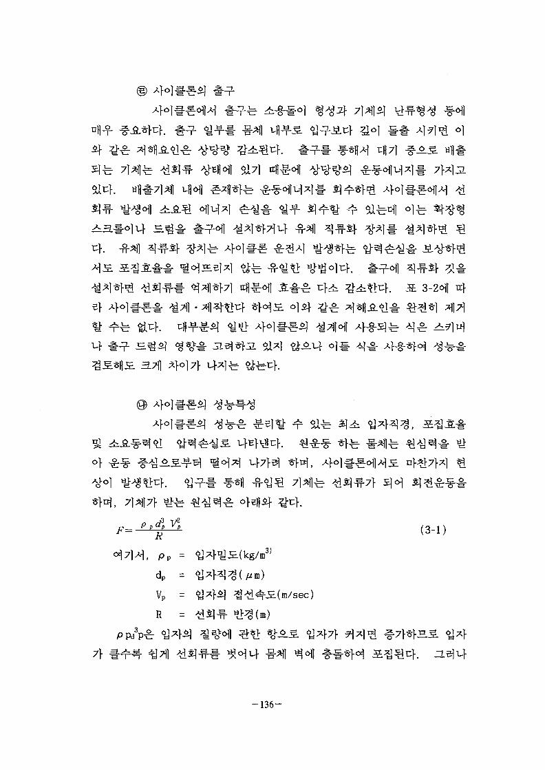
- 1 3 4 -

Slide Gate
a. Single Slide Gate c. Discharge Screw Feeder
("••Si: . «
&»l
b. Rotary Valve d. Automatic Flap Valve
Fig. 3.4. The Kinds of the Dust Hopper.
- 1 3 5 -
$17}
7}
dp
Vp
R
- 1 3 6 -

47] 4i
, [dp]cut =
nt =
Vj =
p p .
B -
Pa =
1/2
(m/sec)
kg/m3
kg/m3
±;V% o |
3-5^
nt
nt=5#
- 1 3 7 -

Particle Dia
Fig. 3.5.
- 1 3 8 -
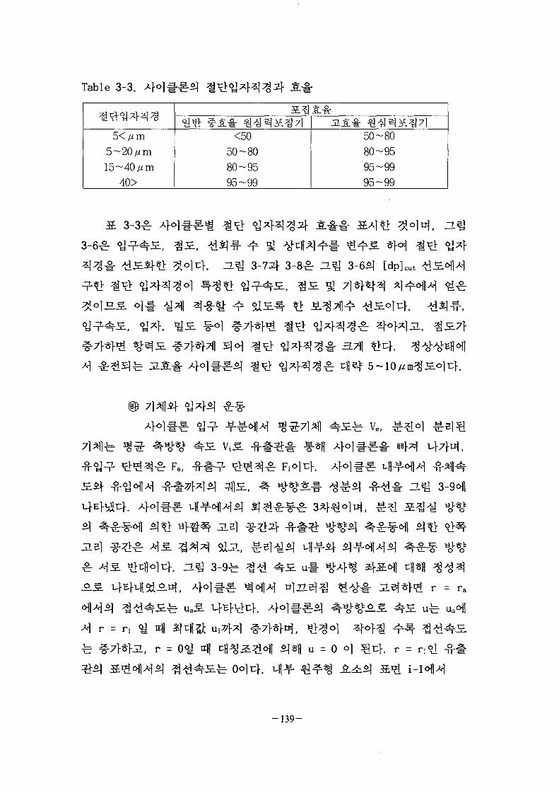
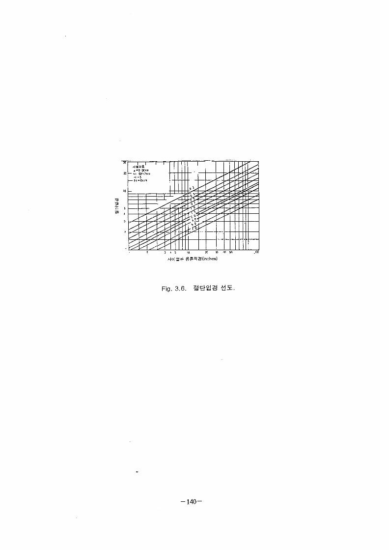
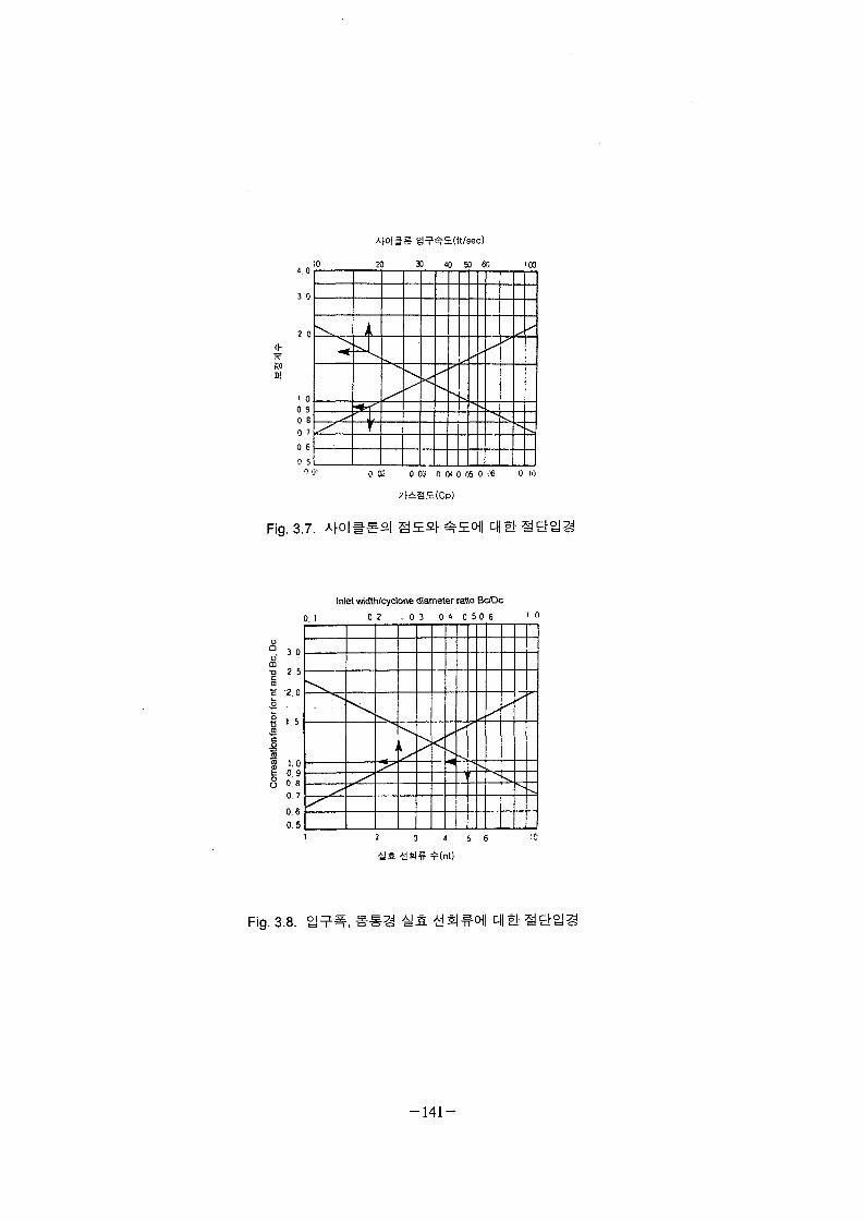
Table 3-3.
5</im5-20/^m15-40 m
40>
<5050-8080-9595-99
III- € 3£ 7l50-8080-9595-9995-99
n ^ 3-74 3-8^ O. [dp]cut
Ve
^ r F e ,
r = ra
r = r,
r - u = 0 . r = r;
- 1 3 9 -
To"
JO
10
TOSitfJ 5
j
3
— VI
— Bt
IIS
5011/5
-Oc /
^
cc
1
/
/•**
E _- ?
* "*
f
»v
<K- ,
^-
*•*
'-
f *
'&
inches)
Fig. 3.6.
- 1 4 0 -
3 0
2 0
I 00 90 80 70 6i •>
0
• * •
20
rf
30 40 Hi 60
-
00
0 0! 0 03 n M 0 05 0 -.'6 0 10
Fig. 3.7.
Inlet width/cydone diameter ratio Bc/Dc
0 J 0 2 . 0 3 0 * 0 5 0 6 '
3 0
2 5
• 2 . 0
1 5
1.00.90 80.7
0.6
0.5
\ .
^y^y
> <
1
[
y
!
Fig. 3.8. ^a
- 1 4 1 -
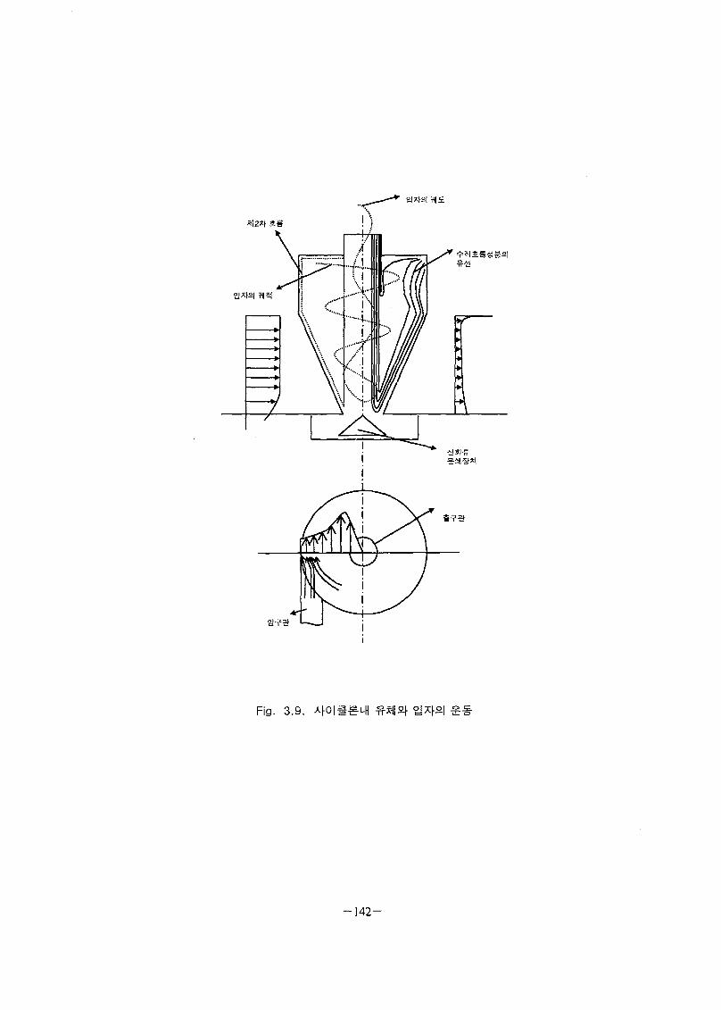
Fig. 3.9.
- 1 4 2 -
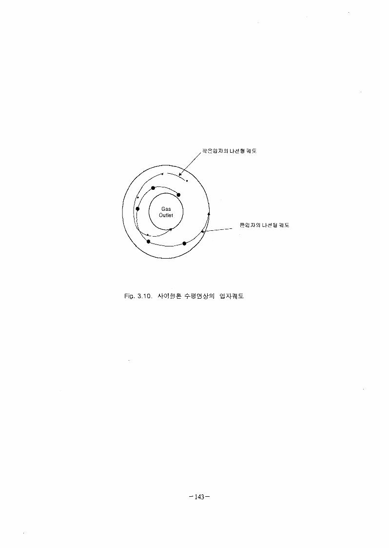
Fig. 3.10.
- 1 4 3 -
44.
71 fe
r r (3-3)
r,
ZLQ 3-951
.2*} S: 4
24 ^ ^ ^24 ^ ^ ^
3-non
AP*
- 1 4 4 -
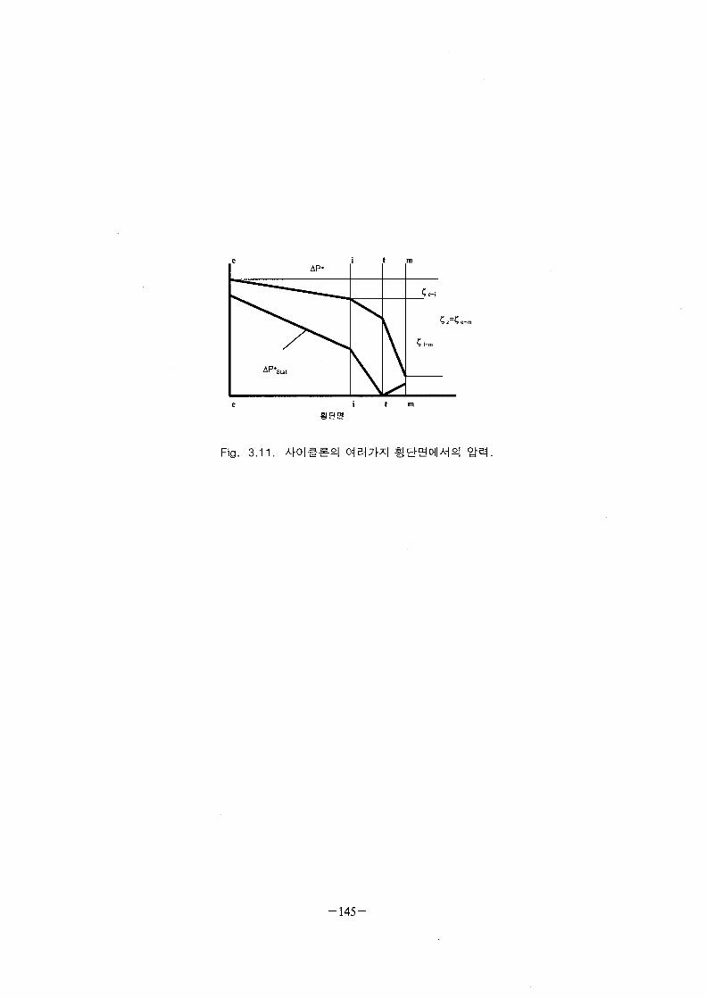
eAP-
AP'stat
i
\
t
\
m
C-i
Cl-m
Fig. 3.11.
- 1 4 5 -
* P P( 3 ~ 4 )
.* Pstat Pm.stat (3-5)
t-m i - t
7]
- 1 4 6 -

Table 3-4. $X<>H
',=FJFi
= •¥-
V
V Vi
itch, 2 h*
V Vi
(3-6)
(3-7)
(3-8)
(3-9)
(3-10)
(3-11)
(3-12)
(3-13)
(3-14)
- 1 4 7 -

^ r ^ 3-12<»fl
o] vro]
# 3EE 3-
(3-29)^
e-eij- i-i
- 1 4 8 -

Fig. 3.12.
149-

2
$6
t
* 2fin 2
Dsr IO
ae
2
a3
\
\\
\
1
1i
•&*
1:
NT
t
r'
i
I
b
1
:.
• _ . ; 5
i 6 8 10 2 I S I 10 2 4 SReynolds Number
Fig. 3.13. S S S
)O86
c
a tos a
1
A-
^-
-
a '
*-*
„
A:• — .
* /r iK.l
,
c
; .
1
i0
*
s
t 6 eio2 2 AS e to3 2 i e 6 to'Reynolds Number
Fig. 3.14.
- 1 5 0 -

Table 3-5.
r =
r* ua
r =
(3-15)
(3-16)
«,-/«*,<0.2
ui#
r =
aT= 1.0-(0.54-0.153lF*e?{W
^7l|(swirl vane
(3-17)
(3-18)
(3-19)
(3-20)
0.85 (3-22)
0.95 (3-23)
- 1 5 1 -
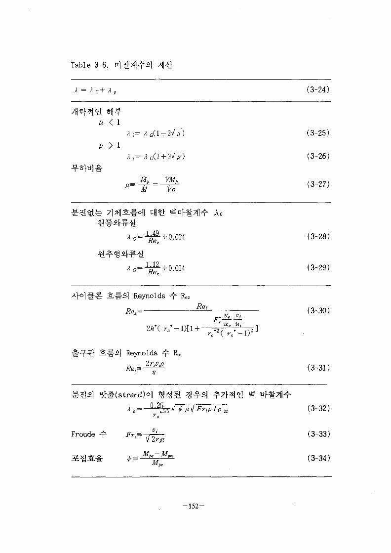
Table 3-6. n
A = A G+ A p (3-24)
fi < 1
fi > 1
3/7)
M
(3-25)
(3-26)
(3-27)
1.49Rez
1.12
+ 0.004
+ 0.004
(3-28)
(3-29)
$] Reynolds ^ Re
Re,=
2k*( ra*-
Reynolds ^ Rei
(3-30)
(3-31)
Froude Fr{=-
0.25
2Tig
ps (3-32)
(3-33)
(3-34)
- 1 5 2 -

dpwr
1 dp2.pt.u
18 rv
, ZLB|JL wr(u5L
(3-35)
(3-36)
(3-37)
- 1 5 3 -

asm
Fig. 3.15. &&
- 1 5 4 -

Table 3-7. A p .
(3-38)
' - . = (Pe+ P u?/2)-(pm+ P vf/2)
(3-39)
(3-40)
(3-41)
(3-42)
(3-43)
(3-44)
(3-45)
(3-46)
(3-47)
(3-48)
(3-49)
155-
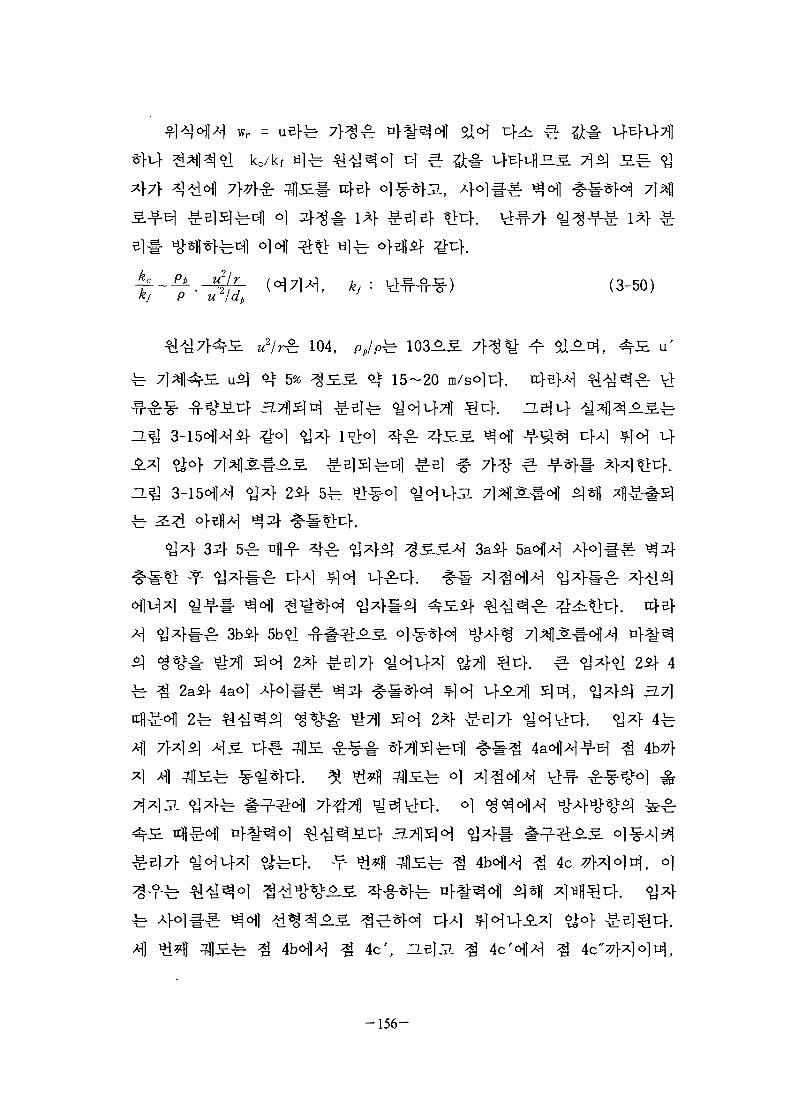
Wr = u e f e 7 p * ^
fedl 6] . vMf7f ^ ^ -
( 3 - 5 0 )
104, p,/pfe
<$ 15-20
u '
71*1);§L#J> 7}^
3.7}
M]
01
4c
4c',
- 1 5 6 -

4c'
24*H7J- oj
€- 2*} ^rBlfe
Lapple
© Leith-Liech }
Leith-Liech^
^ l ^ 3.71 Af
l oil-A 4 4 1 - ^4(3-51)^1
? ; - = 1 - E X P [ - 2 ( O ) 1 / 2 M + 2 ] (3-51)
C = 4°1#€--^ 4"r-S-tKCyclone dimmension factor)
^ = *§H§-1£l r( impact ion parameter)
n = ^i51^-4^r(vortex exponent)
- 1 5 7 -

00
80
60
40
20
-
/ /
J
/
1! I; 1i
1r
7•'
^ m
•* . * • "" " -
/ •
/ _ _
1
. - - ^ ^ '
pcivrson ond whitbv
-OIS(I956)
-O IS ( l 95 i ;
- 01S (1970)
_ teilh and Lichi 01?
1
•
-
(1965)
-
(1972)
Fig. 3.16.
- 1 5 8 -
(3-52)3.
(3-52)
(3-53)
^/:
n
2} Rp/R0
Lapple
Leith liechif
Lapple
-159-

ii) Lapple
d,P O
[ dp] ^
cut[dp]cutX
—J—l
7/
n ? o
—T
1 /
1
1
*
Y-t-
~t/ />i
0
/ /
i//ff/ • /
if
Wf//\if
—
' 6
Fig. 3.17.
u
sta5
" * Tr
_ —
•
,
/
^ ^
..
"
• i - I P - -
—-0 1 -
I
Fig. 3.18.
- 1 6 0 -
?i(Lapple)
(3-54)
kg/m3
Pm
g
o]r.}. K c ^ 16,
*l(3-55)
(f ( 3 " 5 5 )
Q :
- 1 6 1 -

JP=K'cpgV2i<>|t:>.
xcfl K'cfe 0.013-0.024^1
6-21
^4. 4
Table 3-8.
^ £ 4 1 mmHaO
200-250100-15050-100
100- V a _1 0 0 - vb) \Cai
: a, b 2,^2]
C : a,
( 3 _ 5 6 )
( 3 - 5 7 )
162-
170~230g/m3
4
2-58^
1 0 0 - v b
v ••
Qa
a, b : 2^^. a, b
1 0 0 - v
100- Va
a,
( 3 _ 5 8 )
fe *} (3-59)
(3-59)
(3-60)
163-
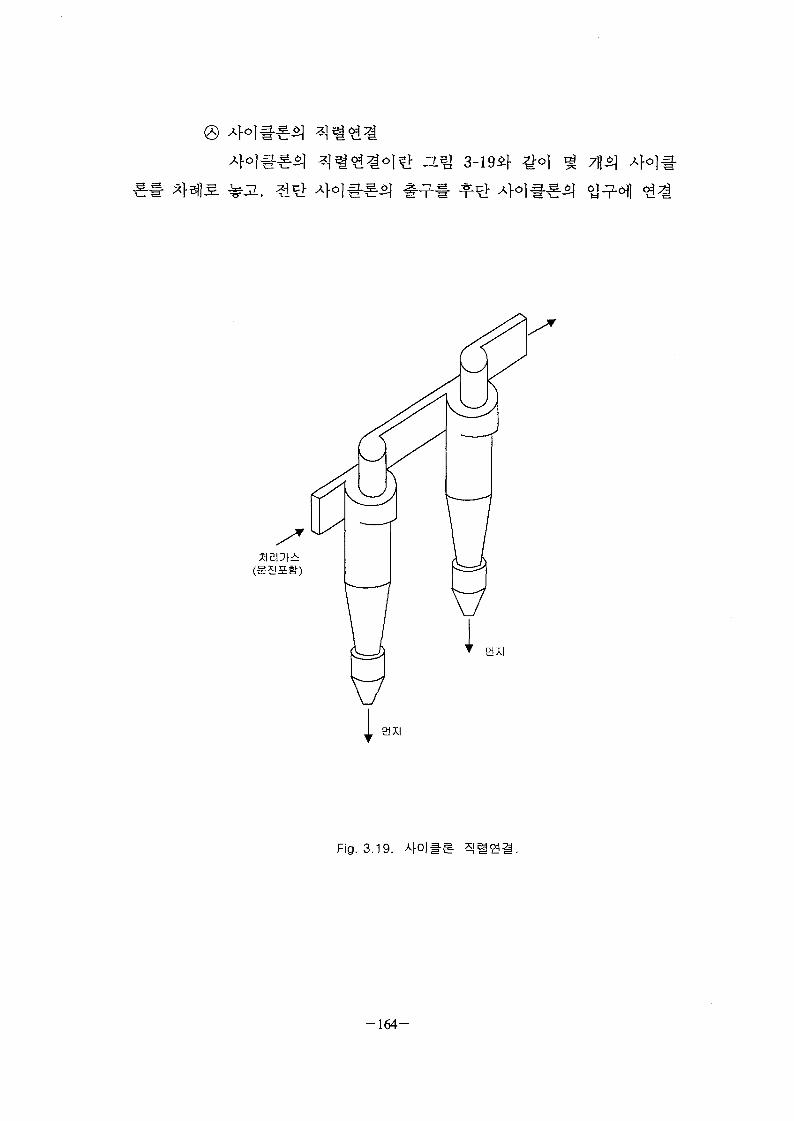
3-194}
a xi
Fig. 3.19. M0\
- 1 6 4 -

n]4tl: ^47}
7]7}
^ 4
4(3-61)5.
v = v p+ 9,(100- (3-61)
-. o|
20
, 5-10
H20, JL
mVmin
50-10 mm H20, # J L #
-^r 250 mm H20
<>1 # J L , ©]
100-150 mm
^ 14-28
67H 7 W ^ 7}
7]^]5o>o| 700-800 mVmin
- 1 6 5 -

ojn]
3.7]]
smooth rotating wall, porous rotating wall,
grooved rotating wall, acoustic field, electrostatic field^
166-
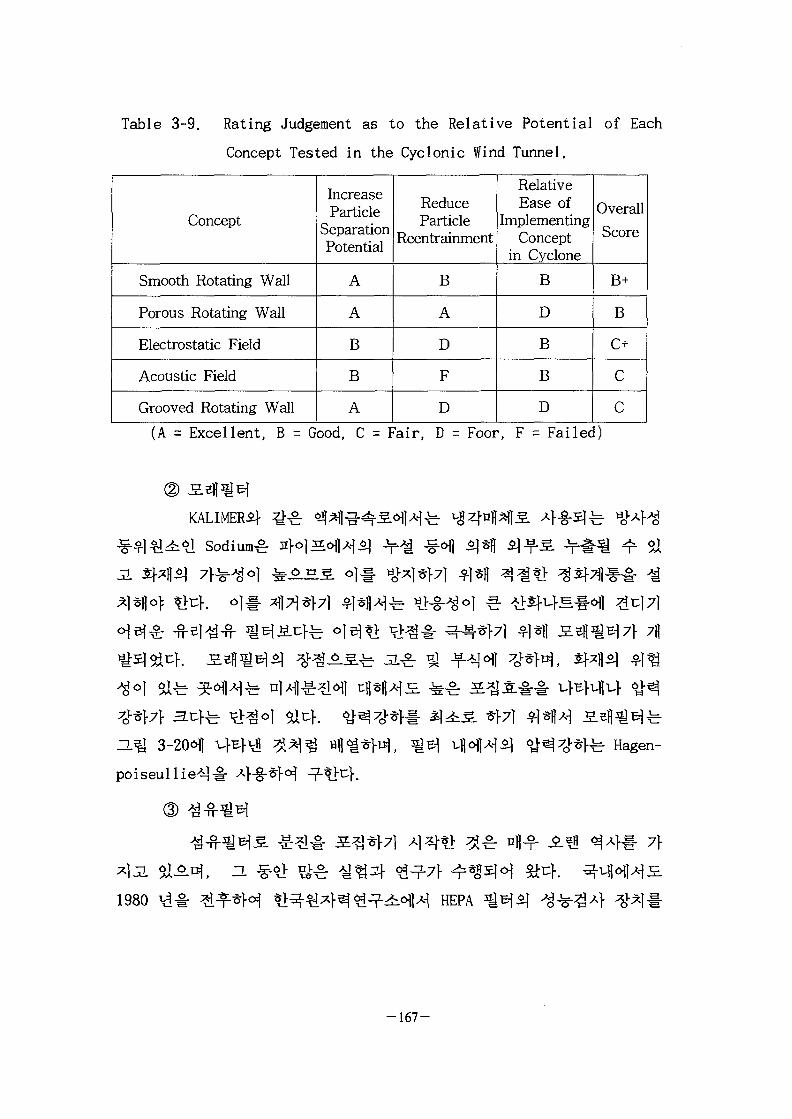
Table 3-9. Rating Judgement as to the Relative Potential of Each
Concept Tested in the Cyclonic Wind Tunnel.
Concept
Smooth Rotating Wall
Porous Rotating Wall
Electrostatic Field
Acoustic Field
Grooved Rotating Wall
IncreaseParticle
SeparationPotential
A
A
B
B
A
ReduceParticle
Reentrainment
B
A
D
F
D
RelativeEase of
ImplementingConcept
in Cyclone
B
D
B
B
D
Overall
Score
B+
B
C+
cc
(A = Excellent, B = Good, C = Fair, D = Foor, F = Failed)
KALIMER4}
Sodium^ -Hi
1 o>
Stl
Hagen-
1980 HEPA
-167-

HEPA
Dirty Gas
3.0-9.7 mm
3.0 mm
1.58 mm
0.28-1.58 mm
0.28 mm
3.0 mm
Cleaned Gas
Fig. 3.20. Sand Filter Configulation.
- 1 6 8 -
3.7)7} 9]^d\] 4 4
3.717}
°-£- 0.3
HEPA ^ ^ ^ A ^ ^ ^ 4 # £l*H 0 . 3 fm DOP H # # M g H l
>l ^ f l ^ ^ 1 )±r 0 . 3
7), -
46JK. W. Leei l - B. Y. H. Li
(penetration)
717}
-§-•£• Spielman4 Goren[3-18] TJ| Dawson[3-19]^°l
Kuwabara-Happel 5]
Stechkina[2-20] £!
Kuwabara -n-^-^'S" l"§"^r]'0'} Friedlander-S]
44
371 ^
- 1 6 9 -
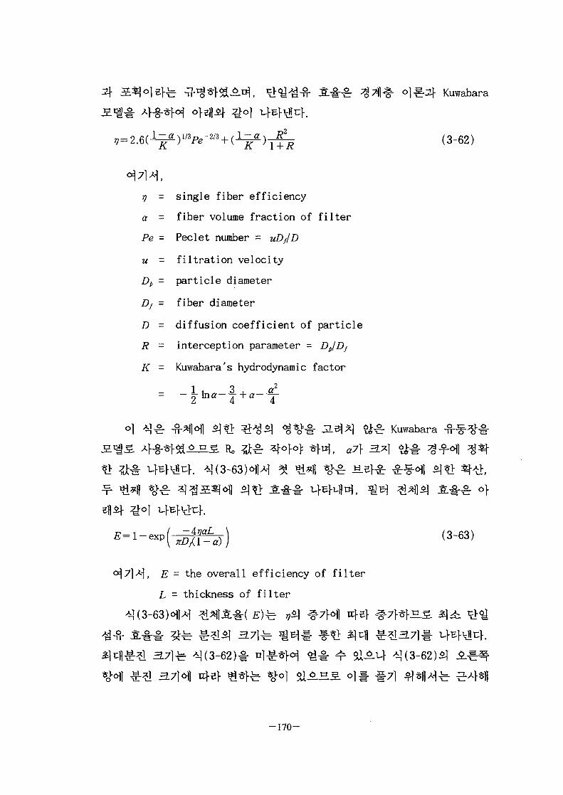
Kuwabara
(3-62)
7 = single fiber efficiency
<z = fiber volume fraction of filter
Pe - Peclet number = uD/lD
u - filtration velocity
Dp - particle diameter
Df - fiber diameter
D - diffusion coefficient of particle
R - interception parameter = DplDf
K - Kuwabara's hydrodynamic factor
#•& Kuwabara
ASLS Re ^ ^ 4 o f o > *}*J, a7\
of
(3~63)
£ - the overall efficiency of filter
L - thickness of filter
37]6j|
-170-

7}
, k - Boltzmann constant
T - absolute Temp.
H - gas viscocity
C - slip correction factor
Kuwabara- Weber^ o|] A-]
(3-65)
, A = mean free path of gas molecules
a, b, c - 2.492, 0.84 and 0.435 according to Fuchs
1) 4 C=l (3-66)
4 C=(a+«^-=3.33-^- (3-67)
^ - ) 1 / 2 (3-68)
for (A/Dp)< 0.075 (3-69)
for 0.075<U/Z^K1.3 (3-70)
for (A/DJ>1.3 (3-71)
- a (3-72)
- 1 7 1 -

•a fi uU/ZX)<0.075 (3-73)
for 0.075<UW<1.3 (3-74)
for UAD,)>1.3 (3-75)
3.7)7}
J2>iPM^i-(Solid volume fraction, a)7\
3.7)7}
^- 0.075<(/l/Z)J>)<1.3
1 /Q
= 2.35U 7—) ( ~ M
rc}e}
- 1 7 2 -

^Tfl Slfe
0^47 } ^ 1 ^ 5 ] ^ -§•<?>
-173-

Baggaleyofl
^ * } # ^ S j £ ^ r Tardosi*
Gutfinger[3-22] ^ Lee [
H. Mori ^ ^ ^
Kuwabara-Happel ^ S
^l^f<^ cfoo>*> ^S.if -S^?> 3.71*] PSL, stearic acid, sodium
chlorideif silver iodide^ # ^ 1 4 o^e| S 7 } ^ ^^ f^^ l cfl*fl
N. Kimura ^ & ^ ^ ^
fe^) Einstein
[3-26].
V®c=(l + kNRa-®c)L5)VeDi (3-78)
- 1 7 4 -

5*103
] # ^ B Happel-Kuwabara
f Kuwabara 2.vg)
SEt> 7]^] slip
Knudsen^jt
D. W. Cooper^ quality factor#
1- 4
Brown
.Pe~m (3-79)
3 sphere efficiency due to Brownian diffusion
a - volume fraction of granular bed
5 a 5 a
Pe - Peclect number ( = —fr)
u = flow velocity
dg = diameter of the collecting bed sphere
dp = particle diameter
D - diffusion coefficient of particle ( = £ j ^
K - Boltzmann constant
T - absolute temperature
C - Cummingham slip correction factor
fj. - gas viscosity
-175-

S F (3-80)» 77 R=s ingle sphere efficiency due to interception
R = interception parameter ( =dp/dg)
X = ( l + 2 a ) / ( 3 - 3 c )
(3-80)^ ^ S ^ ^ l « H < I ^ - f r^M" Kuwabara^
18/*
(3-82)
(3-83)
(3-84)
= <t>gl2,xl2 (3-85)
}7l 4 ^ ^ ! *1 (3-24)51
- 1 7 6 -

(3-84)# *}(
(3-86)
(3_87)Zl LA
(2-81 )£•
( 3 " 8 8 )
51 ?> S ^ - ^
Tardos %<>\] 3]^ r}^ ^^6\) $]*% £ ^ J L u ] - Gebhart ^ ^ r VG7\
3.7}6\]
7] 4 ^ : ^ ! aq^JL^-eHI] ufl«> 7]<H^ nfl-f ^ r> . Gutfinger^ Tardosofl
*> 7] <Hfe Skokes ^ o | 0.1 o]
Gebhart ^ i f Gutfingerif Tardos^l £Jt! ^^11 ^^f0!] ^-§-*fe Stokes
(3-89)
^(3-79),
(3-80)3f (3-88)5]
( 3 - 9 0 )
-177-

S)
=171
(3-89) 1
+ i (3-94)
(1)
, Scabbier, Milling, Drill-Spall, Paving
breaker and chipping hammer^- Expansive grout^-S.
(7})
Vacuum cleaning (VC)
-178-

7}
Brushing, washing, scrubbing
S^-(Fixative/Stabilizer coatings)
-§-§•
glycol),
(Stripping coatings)
-179-

ight ablation)
<& <>M*1 S
}. o]
pinch plasma lamp
laser, xenon flash
ot i)Ooo-2,oo(rc
90dB
1/4
^(Microwave scabb ling)
Oak Ridge Y-12
71
(Flaming)
- 1 8 0 -

4
(Flame scarifying)
o| 7 1 ^ ^
PCB#
fe C02 J£4r N0x
4
spalling
o] 7 ) ^
^^] 3.
- 1 8 1 -

(2)
Scabbier
H ^ «J Spall
^ ^ £ i s . 3e lH S^<H1 30cm£|
spaller# ^o
5cm ^
(e}) Shot Blaster
(nf) Sand Blaster
shot blaster^) «]«){ jL-§-ol
(H}) Cryogenic
C02 7 } ^ # °|-§-5r}o={ Dry Ice
150 PSI ^
)^" Dry
- 1 8 2 -
#^H1 An}-B Dry IceS]
1HH
(3)
^(chisel)
- 1 8 3 -

*r 71
o]
1-
Sit:}.
- 1 8 4 -

O »d
©l«g-
600'C
iLS. ^ 71
(4)
(7}) TMI
1979^ n]^- TMI (Three Mile Island)^^^^
4
-185-
Cs-1374
and dry abrasive blasting technique)2f
, o] 7 1 ^ ^
MOOSE Bj-
EPRI(Electric Power Research Institute)<H]4
100 ftVhr
head
-186-

<^*l(on-board vacuum system )5H°)
r €4^^ (wi re l e s s )
( hard-wi red )
6171
West Valley Demonstartion Project(WVDP)^
3} 3.3.el je
"M00SE"e>
1/16 1
- 1 8 7 -
fe
fe
4-§-*H & 4 * l ^ 3 . *ll?m ^ safe
HEPA(High Efficiency Particulate Air)-Vacuum ^ ] ^SI
(uf) PNL |
PNLoflA-] 1990 4 DOE l ^ ] ^ * H Hanford^] Slfe Hot cell
324^ 325 ^ ^ ^ 1 4^*H*H H S l ^ l - ^«g*}Slt:>. o] ^ ^ n ^ ^ | ^
A}^6fi i i#£i fe ^ . £ # ^4iXl^7l *J*H air lock
cover blocks^- ^-g-*fe ^M, *? Si*flfe
# ^BH(Waste forms)*} ^ ^ ^ - ^ * f e cfl
Cell# ^1 |*H 44-§-^fe^ m^M ALARA
PNL J 324y4^ufl£| aJ-A}5]-^ ^4qo]B 0 i Al-gofl^^. air lock 7^^
v> 1960^ -f 4-g-*H 4^^^-^-^- ^ 1 1 - ^*>^>.Air lock
A i r
ALARA ^ >
-188-

grout# £chipping^ hydromilling*> ^ Hydraulic spall i
fe 3j, c) #£,©- n]
Sll-b ^ ^ ° 1 1 1". PNLtHJA-] 7]| -*> hydraulic concrete
spallerl- 4-§-* |-^^ 3], 3j;g 2.5cm ?Jo| ^ 5 c m^ jfL^^. n | B | ^ J T .
spaller# ^-^ofl ^ H ^ ^ 4^§- 68.9MPa^ hydraulic pump£f push rod
# o|-§-*H HJ- -ofl push rod7} Sl^*]-7|[ *> ufg- »J^ wedge7> ^-^^1
bit7} ^3.B|H ^ # ttl)e|^^ ^^>*>U}. ^ i f l ^ 3.3.Bl^ ^o^e] 3.71
20.3cm ^g£7f 5] Siu}. o]4 ^.T§ ^ > ^ ^ 20.3cm7f 7 } ^ ^
.t^ push rod^f bitAfo]^ -g- Vo aersol lubricant#
^^el# 113 L -g-7H H f e
10 man-hr©] &J5.T-} 4 ^ ° 1 4 ^ 5 ] ^ ^ 6.
2.5cm
Post-refurbishment analysis
«1|^-*fe 4 ^ ^ ^ ^ ^ 10^©)cj-o-^ *t<$x}7\ * ^ ^ # ©1
^ 3i]^-# £|dL§. ^7] ^^©isd*.^
^ 80 mrem/hr©! u} .
Cs-137 ^ Sr
©>S.JE. Saw#
©fl ?fl^HAl^ ^ ^ * } ^ f e cfl,
- 1 8 9 -
inventory^ 50%, Sr-90£| ^ - f 30%7f sfl^M
^r 1.0 ~ 1.5 mmS.
C-CellSj
50 r a d / h r o ] ^ ^
foam cleaner^- 34.5MPa^ water flush iS.>M 200
JPDR 5{{^1S^.J1
Japan Power Demonstartion Reactor(JPDR)
-& 1981
JPDR5]
^ 1995^
JPDR |a 471
> i ^ - Diamond sawing and coring^} Abrasive water jet
- 1 9 0 -

3.7(1 sand-blaster, Shot-balster, Floor
-scabbier, Wall-scabbier, Needle gun Jg- 5 7j-*|5j ^«11- l-8-*f$i^.^
JPDR£) *||£*1|*Mo1fe ^ 5 . Shot-blaster, Scabbier Sand-blaster||-
7}. ^
(1)
^ 3-214
ZL J 3-225} ^ ^
fe ss.ai«# n l 3-234
(2)
ZL^' 3-24^1
^14I^-% Compressorl-
Reciever l 1 H ^
37B ^^*|-5iA^, Air Dryer^-7)
(uf) £ ^
Air DryerSL
-S-7] $m Water bath
-191-

(Humidifier)^
Mixed Bed# Hygrometer
^: humidifier ofl ^ ^ «-# 4-§-
Dc body dia. (60)a inlet height:(30)b inlet width(12)SC
Nnmpnr.laturfl
DhH
outlet length(30) Bchamber height(90)
outlet dia. (30)cylinder height: (90)overall height: (240)dust outlet dia. (22.5)
Fig. 3.21.
- 1 9 2 -

I Reqiired overall efficiency
I Compare particle size distribution
I Correct overall efficiency
I Select fT, fP
Calculate Vj/v,
NO=NO-1 orDc-Dc+0.1 o
M M
1Find Dc, vs
Pick cyclone design ratios1
Calculate Q,1
Calculate No. of cyclone
iCalculate v,
Calculate n, G, x1
Calculate grade efficiency
-^=CI]airpartjcleI^::=*-
Calculate overall efficiency1
Calculate pressure drop
Print output
Fig. 3.22. The Cyclone Design Program Flowchart.
- 1 9 3 -

Input Design Ratio
Input Particle Distribution
Cal. Natural Length Volume
Cal. Core Dia.
Cal. Cyclone Volume
Cal. Cyclone Vol. Const.
Cal. Cyclone Configuration Factor
Cal. Saltation Velocity
Cal. Vortex Exponent
Cal. Cyclone Grade Efficiency
1Cal. Overall Efficiency
1
Fig. 3.23. The Program Flowchart of the Cyclone Efficiency Evaluation.
- 1 9 4 -

Compressor
Silica Gel Column
Air PumpIntergrated Flow Meter
Fig. 3.24.
- 1 9 5 -

By-pass
7] £ S # JL7] JH*fl filter paper# ££*|-&-S.n|, S^ 1 !^ . filter
papers] J2.^7|- -g-oj j-s. . filter paper case#
5. Blower# ^ ^
(3)
Dry Oven^l \$JL 244^>
1~3 yum, -^Sf W * ] ^ 5 //
^r^l^ 6o^ 4 4 3g «?^s^ 0-60% 7}45] ^£^2f^f 2-15 m/s
filter papers] S^1^, ^- Afol^-S.^.
4l*l|^ filter paper*]
IS0T0N II -g-^M- 4-g-*><H Coulter Multisizer
7~15mm
- 1 9 6 -

ParticulateLaden Outer-Vortex
SeparatorPlate
Hopper
CleanInner-Vortex
Turbulence Impact
CollectedParticulate
Fig. 3.25.
- 1 9 7 -

HEPA 0)7]
HEPA
^ DOP ^ ^ 0.3[m
99.97%7f fe
5JHEPA
(l)
(2)
(7}) Steel Bar Heating M/C
© Power : AC 220V 10 1, 2KVA
© Output : 0 ~ 10V, 100A
.ni, 4
-198-

Load Cable : 3M (Remote Cable 3.6m)
Fig. 3.26.
- 1 9 9 -

(3) Control System : Loading Time, Over Heating Controller,
Power Meter, Ampere Meter, Volt Meter, Safety System
(I-}) Heating Rods & Control
® Capacity : 161.333 Resi
© Channel Point : 50P
(3) Safety System : 2 Interlock
(D PID Auto Tuning
© Display : Setting = 0.5% +1 digit
© Feedback Control
(£}) Concrete
© Capacity : 595x595x300
® Power : AC 220V
(3) Up & Down : PID Auto Tuning
(D Display : Setting = 0.5% +ldigit
(§) Feedback Control
© Stroke : 200mm
(ef) 1 z\W*4*} ti^^l^Heating Rods -jf f Power ControlIer5j Tf^# S 3-10 1-
3-nofl 4 4
-200-
Table 3-10. Heating Rods
Diameter
Length
Heating Length
Cold Length
Volts(V)
Resistance
12.3
150
50
100
220
161.33
Table 3-11. Power Controllers
Power Supply
Control Point
Cable
AC 220V 10 12KVA
1-Point
3 Ea
AC 220V 10
50-Point
50 Ea
Heating Rods
Heating Rods^ 14~36W/cnf£J ^ £
Power Controllers
Power Controllers^- Heating Rods-H
$X
(3)
Heating Rodsif Power Controllers^-
- 2 0 1 -
(4) 4 3.
Heating Rodsij- Power Controllers^] 4-§-*fe *1|.§.-b < i ^ ) 7]
Ni-Cr
(5) ^ ^
Heating Rodsl- 25°C ± 5°C
90% ±2%, ^$) -&S. 25°C ±
Heating Rods ij-f- S^<^1 -f-^^I ^r^:# ifK I.|JJL
-f e\7\ $X^ H ] ^ ^ -^^-^-^1 4 ° ! ^ ^ ^ 4%v^r 500V
4 fw
(14)
X[o}6\] ^^ ^bj- 1500V Jl^- **## 7f^}^# ttfl
i.06«H
(6) ^8-5"
-202-

Power Controllers^- Heating Rods# t[^$] *\}o]
(A) 4
4
Heating Rods o\)
(7) Concrete
*m ;?i<fcl~ 150V s.3\ 'S'Ffe 7A 1.5 mA
Concrete
(7\)
Heating rods
heating rods<H] r^?> power7F U}E}L.|-O]:
(v-F) heating
(8) -3.e]S % press M/C
-203-

(1)
(2)
(3)
(4)
3-27^)
2,250 mm
2,200 mm
850 mm
550 Kg
^ 7O>(STS 304)
scabbler
fe X-% LM 7>o|H,
, 4
(5)
50/«m O]AOVO1 ^ «}BA| short blast i ^ sand blast
-204-

; LM Shaft & Ball Bush X
Y * Ball Screw
Timing Belt & Pully
Servo Motor
Fig. 3.27.
- 2 0 5 -
2. £
< H4 4 S]BH tflft < ^ 7 J ^ J=-^ ^oj-iL^oj 4
44
woven ceramic bag)<H2f7],
velocity), -&S]^-5L(col lection efficiency), ^Z] B.7]
(colletor s ize)^ | tfitl wlJ3.ig7f# ^f^uf. ZL^o\] 3£MQ 6-M-b CY :
Cyclone, ESP : Electrostatic Precipitator, FB : Fabric Filter, WCB :
Woven Ceramic Bag, GB : Granular Bed, CFC : Ceramic Fil ter Candle-^-
744 ^\i&c\. 4
. 4
o] ZL^O\]A] 4 0 ] ^ g . ^ . 12 m/s
5. *]•*] t iSlt^.^, 0.04 ~ 0.3
a ^ 3-30*1)^
3-3KH1 «J2HW ^ 1 -f^Km3)^ ^ e m ^ Sllfe 7^1 -§-eo>(m3/s)#
- 2 0 6 -

3-32^
°F1000
800 -
600 -
400 -
200
—
nCY ESP FB WGB GB CFC
Fig. 3.28. Comparison of Temperature Capability.
m/s20.0
0.30 -
0.10
0.09
0.08
0.07
0.06
0.05
0.04
-
n n
0.26
CY ESP FB WCB GB CFC
Fig. 3.29. Comparison of Face Velocity.
- 2 0 7 -

100
99
98
70
69
CY ESP FB WCB GB CFC
Fig. 3. 30. Comparison od Dust Treatment Capability.
10
CY ESP FB WGB GB CFC
Fig. 3. 31. Collector Size Comparison.
- 2 0 8 -
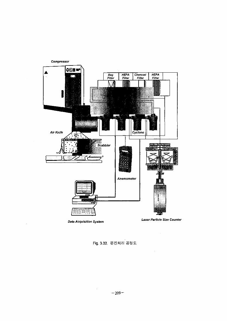
Compressor
HEPAFilter
Data Acquisition SystemLaser Particle Size Counter
Fig. 3.32. ^ 3 * 1 Bl
- 2 0 9 -

Coulter Multisizer^.
ZL | 3-33 ~ 3-35Af ^ ^ S # 4 4 v J 4 . a ^ 3-334l~3mm *]cfl
30%^
~L^1 3-344 95%
7 } ^
l:^-^, ^ ^ 3-354
(l)
H^J 3-36 ~ 3-384
0.045 g
^r 98.5% ol^-o^
filter
Ac^, H ^ 3-3644 ^-fe4 «B#6o>ol 0.004
60%
fe 0.043gA5.
10HB ^ £ ^7BM- ^ ^ ^ 1 ^ . ^ , ^ l ^ ^ ^ - n ] ^ ^ ^-f-b a ^ 3-37
^o] 5* 1 4 61= 0.038 g OIJL 60 %°i 4 ^ 0.024 g *.$.
(2)
3-39 ~ 3-414
^J44 ife
- 2 1 0 -

o.O45g
98.5% 4 ^
^ 3-40^
O.025g 7
(3)
10
ZL^[ 3-42^)
(4)
n ^ 3-43 ~10 m/s
71
- 2 1 1 -

Particle Size(nm)
Fig. 3.33.
- 2 1 2 -

1.95 73.05 83.15
Particle Size( jjm)
Fig. 3.34.
- 2 1 3 -

0 10 21 33 43 53 63 73 83
Particle Size(nm)
Fig. 3.35.
- 2 1 4 -

tS 0.020
0.015
0.005
Fig. 3.36.
- 2 1 5 -

0.012
10 15
Velocity(m/s)20
Fig. 3.37.
- 2 1 6 -

3
V)
Q
0.040 r
0.035
0.030
0.025
0.020
0.015
0.010
0.005
0.000
1 0
Velocity(m/s)
1 5 2 0
Fig. 3.38. ct|-
- 2 1 7 -
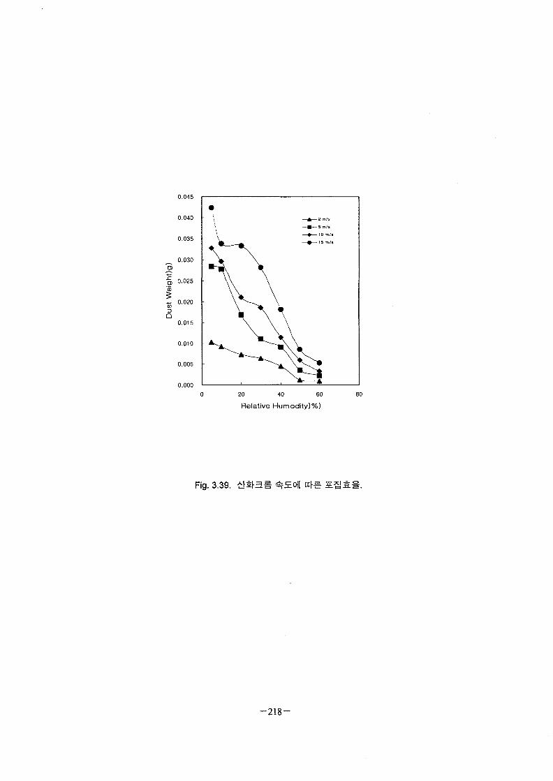
0.045
0.040
0.035
0.030
•§, 0.025
0.020
Q0.015
0.010
0.005
0.00020 40 60
Relative Humodity)%)
80
Fig. 3.39.
- 2 1 8 -

0.012
0.01 h
0.008 *-•3
g>'a) 0.006
\
0.004 h
0.002 ,-
5 m/s10 m/s15 m/s
0 10 20 30 40 50 60 70
Relative Humidity(%)
Fig. 3.40.
- 2 1 9 -

0.000 -
Fig. 3.41.
5.0 r-
4.9 [•
CD
i
Du
st'
4.8
4.7
4.6
4.5
4.4
4.3
4.2
/
-
-
-
5 7 9
Hopper
! 1
11 13
Size(mm)
V
\
\I
I
I15 1
Fig. 3.42.
- 2 2 0 -

nt(
%
o0CLOE
o>
100
90
60
70
60
50
40
30
20
10
0 I
f[•
• ! /
•I /. f fl
A ,i ;' •
/ ' ' /
u ili '
i ' •
] •
1
-TVPi
}
—•—Fe—*—Cr
• Al
40 60
Particle Sfee(mm)
Fig. 3.43. 60%, 10 m/sO\\M^\
-221-

20 40 60
Particle Size(mm)
Fig. 3.44. 10%, 10m/soflA-|o|
- 2 2 2 -

c0o5a.aE
O
70
60
50
40
30
20Cr
Al
20 40 60 80
particle Size(mm)
Fig. 3.45. 60%, 10m/sO||A-i°[
- 2 2 3 -

71
t:\t\5L
7fl
3-12 ~ 3-14<>fi
4
2.
3.
4.
- 2 2 4 -
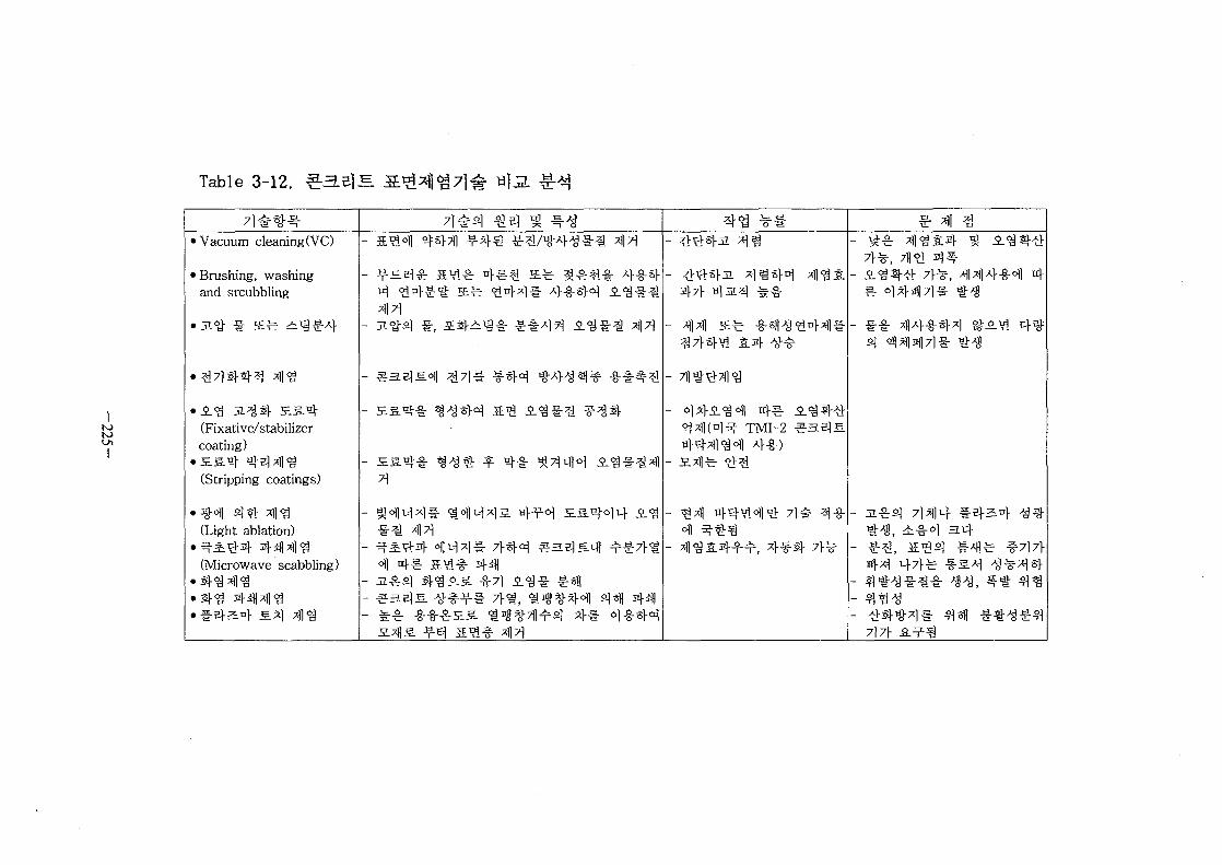
Table 3-12. ti];2.
7]£U-3-• Vacuum cleaning(VC)
• Brushing, washingand srcubbling
(Fixative/stabilizercoating)
(Stripping coatings)
(Light ablation)
(Microwave scabbling)
• s(-3 441*113
- **4 #.
71
°ll 4# 5.- jl^rfil 3]-
- 5H.e)E. -
7l#°l ^e] ^ - ^7)1 ^-T;]-^1 ^•^l/lg-A}^-g-^ ^ T ]
M*l!" 7rsf<^ §3SlE.lfl ^^•7l-'g'S^ 441
2} 71- B
- 11*11
j i ^I^BI- '3! xfl 3 S.
£fe •§-=ll'^l?lDr*ll-l-S 5 l 4 >ov^
^ TMI-2 ^3HlJ=3 i 4-8-)
- ^£ *l
" 5% %
—i O c>\JxL.\^ -—| '
w}A 4 '
7)71- A-
§• *ll ^33L4 S .3 tV
^7|J , ,H1^^
S)l7ll- I H
•5-°! 3 4

Table 3-13.
• £?PM5'$( Grinding)
• Hf §' spall
'Shot blaster
'Sand blaster
•i- ftj! spalleri- ^o] ^ ^ t}" -S 4 ^
_ 3x<y-3i^ •7l'?'o11 S-Sfl- -S- "s}o %-^[ °-?Jt^-S- 4 ^
- Shor blaster^! «1 «fl a 4 ^-§-
. & *0 ^

afeinl
K
If
Hi
CO
Q)
B)
PI-J
w|n)
Jb
5
fir
oT
-dmIN
D)r
"FT
oU
•HTNi
B'K
Djo^°
< - i *
i
•m
*>i
•Kb
K-1
n>l
i5°
H-i
•*T
<°BJjlU
d-
o T ' 'UHJIT
I
no
of
d-N°
1
ntfo)
Sir
&
oln)
fl"l>j
oTl?J
i
Djo
o|d
-<i1
Jb
1
TO"
•Kb
!
Ord*•oT
flu
hise
l
•R°
^f
or,
f\"qirr-io^z.
•!(|r
o ^
i
5»r-io
B|
I
•J'Hb
K
sTip'!(|flf
Mi
o|p
o^
r-io
oT
a|
a|
U'i
i
•^i)
i li
rrl
IP|J
dJ
i
•10)
1I t
1
T"ijo"
ojffl
o^
o|n)
jjo
w|75"
ret
1
1
i
SBalo
'o'ljo"
Bl'Ho
1
ajo^-T
IwiI
JIJ
<lm#>
1
7S"ojn)
•pi
liR"
ojni
olWW
d-o(r
1
pjo
r-|o o i
^ i o J ^
oT^1"1
d j jW IN
nTJU
p"lio"
i
X r-|J
pj| ?. j
i
•RJ
*>ri
_
lt|BI
Tff"
IflITlJ
o"J-r—
oJ"
1
Pjo
oT
i \
w1
: < -
if-J
i
I
#
JlJ
TJ
•Rr
i
OrR
o|n)
TJ
JU
op7^-j
1
r-io
of
1
•ft
•<1 '
TtLlJJ-P
i
olj
BlB
o|m750
n-
wi75"
If|J
1
T —
1
•S"
- %
ftJcjo
^Jo"
1 1
s
dJ
1
•K-1
K I *o*V
KlW
1 1
r-jo.|op
DJ-J'p"
1 1
JW
r W
-Ito*
1
o|W
oU
oS
1
o|ni
TO"
•nb
wl75"
flj
iui
HiiflU
<!_
1
2•su
1
Pill!
olnS0
* * >UIJ'KJ'S"
1
J7?
1
tHrT^r
•^Kb
•ao"d-
0o|n)
*W"
° ^1
TO
r-io
W
I*"
1
II
<AW1 1
ajoajo
Kb Kb
<i-<r-
1 1
1 nib
"fa ">ISPI
o ) J ^
ItlW 'lo]j
i^o|n)
^ TilD
oT3l|j
ulorlci
1 1
•$>
oT
PiCp"
w^'Sn^in?
1 1
olJo
r-la
ob
wl
75"
rrl
r|J
a(o
elmwl
-p-
Kl
75"win)
1
wl
- p -
Kl
E75"0 H|n!
1
°b
AHoj
-5-
1
8
1
$
•<
ffijo
wlrJ
%
dJ
wl75"
1
•55D
WJll)lo
W
w1
*K "o"
7t BTB|
1
yj| J iTJiL'lo'Sr
1
Ifijo
mini
nit
"rTKh
°o
5. Scabbler\§.-£~5!£I
2*}
6.
fe JLS.71)
7. 98.5%
7}
8.
9.
sa-a-
10. 4 ^ HEPA
11.
- 2 2 8 -

TRIGA
TRIGA
TRIGA
2 ^ C02
3j-§- parameter^
C02
7}
-229-

TRIGA
- 2 3 0 -

1 4 TRIGA
TRIGA <?l
X\
71
2 ^ C02
— 231 —
NEXT PAGE(S)left BLANK

7
1-1. - M T ^ * *f, "^9-8- #*K§. 3E11S. W , KAERI/RR-1286/93 (1993).
1-2. % £f, "<£ --§- #*K§. 3EJ15. W , KAERI/RR-1437/94 (1994).
1-3. *\<>m SJ, "#*}3. ^.*H^l7l^ 7H^". KAER/RR-575/86 (1986).
1-4. *\<>m 3], "TRIGA MARK II <&^-£. M^M *%# *H^ ^
^^•", KAERI/IM- 92/87 (1987).
1-5. IAEA-TR-373, "Decommissioning Techniques for Research
Reactors", IAEA (1994).
1-6. IAEA-TR-351, "Planning and Management for the Decommissioning
of Research Reactors and Other Small Nuclear Facilities", IAEA
(1993).
1-7. NEA Group of Experts, "Decontamination Methods as Related to
Decommissioning of Nuclear Facilities", NEA/OECD (1981).
1-8. IMechE Conference, "Decommissioning of Major Radioactive
Facilities", Proceed, of the Institute of Mechanical Engineers
International Conference, London, 11-12, Oct., 1988 (1988).
1-9. IAEA, "Decontamination of Nuclear Facilities to Permit
Operation, Inspection, Maintenance, Modification or Plant
Decommissioning", Technical Reports Series No. 249, IAEA,
Vienna (1985).
3-i.mpR%^, mi-mmm(D^m^m, U > ^ ^ D V , P. 41, APHI1993.
3-2. E. Muschelknautz : Chem.Ing.Techn. 44, 63, 1972.
3-3. E. Muschelknauz. N. Rink : Zyklonabscheider. Handb Fortbildung-
slehrgang "Mehrphasenstromungen", VDI-Bildungswerk, 1975.
3-4. E. Muschelknautz : Hochshchulkurs II. Mechanische
Verfahrenstechnik, Verfahrenstechnil 6 (1972) 3, pp. I/IV.
3-5. E. Muschelknaytz K. Brunner : Chem.Ing.Techn. 39, 531, 1967.
3-6. W. Barth : Brennstoff-Warme-Kraft 8, 1 1956.
- 2 3 3 -

3-7. E. Muschelknauz, W. Lrambrock : Chetn. ing.Techn., 42, 247 1970.
3-8. W. Barth, L. Leineweber : Staub-Reinhaltung Luft 24, 41, 1964.
3-9. A. Ogawa : J. College Eng., Nikon Univ., Series A, 19, 157,
1978.
3-10. T. Hikichi, A. Ogawa : ibid. 19, 167, 1978.
3-11. Y. Fuzita, A. Ogawa : ibid., 19, 185, 1978.
3-12. Y. Fujita, A. Ogawa : ibid., 20, 79, 1979.
3-13. T. Hikichi, A. Ogawa : ibid., 20, 155, 1979.
3-14. R.Spilger : Methodik Uberfuhrung wissenschaftlicher
Informationen aus dem Gebiet der Verfarenstechnik in
problemorieentierte Rechenprogramme, Disseration, Techn.
Univers. Berlin, 1978.
ojij-^]^ ^%^gAf7l^ofl 3*?> £•?-", KAERI/RR-322/91, 1982.
-f-n-^4 *IM <*t -", ^>^«J-S], vol. 16(1), 29, 1984.
3-17. K. W. Lee and B.Y.H.U. Liu, "Om the minimum efficiency and the
most penetrating particle size for fibrous filter", J. Air.
Pollution Cont. Ass., Vol. 30, No. 4, 1980
3-18. L. Spielman and S.L. Goren, "Model for predicting pressure
drop and filtration efficiency in fibrous media", Envir. Sci.
Tech. Vol. 2, No. 4, p279, 1968.
3-19. S.V. Davison, "Theory of collection of airborne particles by
fibrous filter", Ph.D. thesis, the harvard school of public
health, Boston, MA, 1969.
3-20. I. B. Sechkina, A. A. Kirsch and N. A. Fuchs, "Studies on
fibrous aerosol filters-IV. Calculation of aerosol deposition
in model filters in the range of maximum penetration", Ann.
Occup. Hyg. Vol. 12, No. 1, 1969.
3-21. H. C. Yeh and B. Y. H. Liu, "Aerosol filtration by fibrous
^234-
filters - I. Theoretical, Aero. Sci., Vol 5. pl91, 1974.
3-22. Gutfinger, C. and Tardos, G. I., Atmos. Environ., Vol. 13,
p853, 1979.
3-23. K. W. Lee and Gieseke, J. A., Envir. Sci. Tech. Vol. 13, p466,
1979.
3-24. H. Mori, etc., Int. Chem. Eng., Vol. 27, No. 2, 1987.
3-25. N. Kimura, etc., Int. Chem. Eng., Vol. 25, No. 1, 1984.
3-26. N. Kimura, etc., Int. Chem. Eng., Vol. 25, No. 1., 1985.
3-27. K. W. Lee, J. Aero. Sci. Vol. 9, 1978.
3-28. Douglas W. Cooper, J. Air Poll. Cont. Ass. Vol. 32, No. 2,
1982.
3-29. Rosin, P., etc., Ver. Deut. Ing., Vol. 76, No. 18, p433, 1932.
3-30. Leith, D., AIChE Sym. Ser., Vol. 68, No. 126, pl26, 1972.
3-31. Zenz, F. A., Ind. & Engr. Chem. Fund., Vol. 13, p65, 1964.
3-32. Kalen, B. etc., AIChE Sym. Ser. Vol. 70, No. 137, p388, 1974
3-33. Kelsall D. F., Chem. Eng. Ser. Sci., Vol. 2, p254, 1953.
3-34. Bradley D., etc. Trans. Inst. Chem. Engr., Vol. 37, p34, 1959.
3-35. K. Rietema, Chem. Eng. Sci. Vol. 15, p298, 1961.
- 2 3 5 -NEXT PAGE(S)
left BLANK

1=1
HI-—I
el-
o|
- 237 - NEXT PAGE(S)left BLANK

C O N T E N T S
Chapter 1. Introduction 249
Chapter 2. Underwater wall raging radiation inspection robot 251
Section 1. Introduction 251
Section 2. Design and fabrication of Underwater wall raging
radiation inspection robot 251
Section 3. Development of control algorithm 283
Section 4. Performance test of wall raging radiation inspection
Robot 306
Section 5. Concluding remarks 331
Chapter 3. Selection of dismantling equipment and
graphic simulation of dismantling process 333
Section 1. Introduction 333
Section 2. Selection of dismantling equipment 334
Section 3. Graphic simulation of reactor dismantling process 340
Section 4. Concluding remarks 354
Chapter 4. Conclusion 355
Chapter 5. References 357
- 2 3 9 -NEXT PAGE(S)
left BLANK

249
^ ^ g £ 3 4 #*1 A»i 251
1 3* 4^- 251
2 1 ^ ^ # * 1 7(| 1 4 251
1. ^ ^ ^ l £r*H 251
2. ^ ? I 7 | 255
3. Laser local izer 261
4. ^ # «o^Rl ^ S # 269
5. *M-f- 270
6. 314^2: 281
3 | ^M<tJLSl# 283
1. 3& ^ ^ n "A H9 -^ 284
2. ^ l ^ l & a H <y-3-^]# 2903. 7OV6]*> H ] ^ ^ ^ 1 ^ - ^ H -^JLBl-i- 297
4 ^ ^ ^ ^ * | ^ ] ^ ^ ^ ^ 306
1. j e . # l ^ ^ ^ ^ 306
2. ^£^«8#*1S1 ^ ^ - ^ ^ 317
3. TRIGA-III <^9-S - § - ^ ^ 325
5 l ^ ^ 331
- 2 4 1 -

333
333
*fl*fl#a] 334
340
3402. ^ ^ - - g - € ^ } ^ ^ ZLeH^ S.t3}eoT 343
3. «H^)1^-^ 3-&S.4 347
354
355
357
- 2 4 2 -

Table 1 ^ # ^ £ ^ #*1 4<tf 254Table 2 H^§)5] 4<£ 256
Table 3 - g ^ 2.&\ *}<$ 259
Table 4 ^tfl^^]6]Ai *}+**<>) ^Tfl 4<tf 268
Table 5 ^ W ^H§7l 4<>o> 269
Table 6 #-§- }o]7] A } ^ 273
Table 7 ^ B ! * W ,e.J£^ ^ S B ] S ^ xjs . 273
Table 8 * H ] ^ H ^-H5J rH|S5] ^ ^ *},£ 274
Table 9 ^^ l7 l 4 ^ 307
Table 10 4AoV ^1^1^ ^ ^ 4 313
Table 11 $J*1*I*J ^ ^ 4 314
Table 12 TRIGA-III - .- W ^ 4 ^ ^ 327
Table 13 - A ] ^ ^^^§-^(^4^ &7], #*}$. q ^ ^ * ] , ^ ^
9-^# % 44^B *) 335
Table 14 7 ]T | |#*1 ^ ^ ^ - ^ ( s f o ] ^ ^ - , E | 3 . , 7]7(f - f # ) 336
Table 15 ^3.2.]^. ^ - S # ^ ^ ^ ^ ( ^ l - ^ . ^ ^ - pool ^ ) 337
Table 16 g^~g- ^ x } ^ *B^^-^ ^ ^ ^ -fcA -H] 339
- 243 -NEXT PAGE(S)
left BLANK
Fig. 1 ^ # ^ ^«g S^-^f ^ 7J|^JE 253
Fig. 2 ^ ^3 ^ #*1 «£. 253
Fig. 3 ^ ^*g#*l • 255
Fig. 4 S.^ ^ # ^ t > ^ ^ ^ £ - 257
Fig. 5 ^ * 1 - ^ *[7fl;£ 259
Fig. 6 ^?!7] 260
Fig. 7 37fl£] «VA}^]# o]-g-«> 7 ] ^ ^ ^)^<?1^ A ] > ^ ^B] 261
Fig. 8 e W * i >b.?11M 7flsi=£ 263
Fig. 9 ^tl)$.|*loH X\^sJi ^e] 264
Fig. 10 01, $2 ^f-B] a, ^ # 9-^fe -y-JLBl 265
Fig. 11 ^ t f l ^ l ^ H ^^^-^1 BH^ ^d£ 266Fig. 12 ^g-f- %£.£. 267
Fig. 13 zlWQ *)*} <&*\ ,i\}o}x\ >=.7jm 268
Fig. 14 ^ # yoUKi 4 ^ S.# ^ ^ l £ 270
Fig. 15 ^ ^ H d 4 ^ S.# 270
Fig. 16 ^-§-^1^71^ l-^HdS • 271
Fig. 17 3*B]*W iLH SlSJc. 277
Fig. 18 *R1*1H AH SjSS. 278
Fig. 19 J2.B] H B H ^ AH SJ5JS. • 279
Fig. 20 flol JLH S # 280
Fig. 21 £ A } ^ « ) 7fl > ^}S. • 282
Fig. 22 J S A H - ^ • 282
Fig. 23 ^ S ^ H } 4-§-*fe ^ 283
Fig. 24 ^ # S ^ - £ ) 5fS7^1 284
Fig. 25 S.%: s fS^| i f ^cfl s|.S7fl 285
Fig. 26 S.* 4 S ^ H 1 A ^ 4fl^^# -$-4 • 288
Fig. 27 f^!-^ ^]^^^-4<H #^idS. 289
- 2 4 5 -

Fig. 28 § ^ - £ 1 3D CAD SM • 292
Fig. 29 S £ - S j *j*g:?H 293
Fig. 30 $.#2) 3H<HM^(2fl*I£3 313, PID*H7l) 294
Fig. 31 5.^5} 3 | 3 ^ # ^ ( #•§"&*! 313. PID^H7l) • 294
Fig. 32 JH -<q 3 I 3 J H M ^ ( # W # 313, PID^H7]) •• 295
Fig. 33 3.%$) i m ^ ^ i ^ ^ $&, *]#*1£ *W7)) .....295
Fig. 34 ££•£] 3 l 3 < M ^ ( ; W 4 l i l 313. *1#*1£ *H7l) 296
Fig. 35 3.%$) 3 1 3 ^ ^ ( ^ 8 3 ^ 313, Al#*lg afloat) 296
Fig. 36 2 . ^ 7 ^ 1 - ^^-*1 <gJL $ai- 3-M PI ^ H ^ 4 304
Fig. 37 fi^^^l- J2.# ^-f^ PI *H:£2f •• 304
Fig. 38 H]^i^ 6l |^ol7l^ a W ^ -305
Fig. 39 7oi-6l*> a ] ^ ^ cH14 ]<H7l ^1|<H^4 305
Fig. 40 ^ ^ 1 ^ ^ ^ ^ ^ 1 • 307
Fig . 41 ^ * I ^ ^ - ^ ^ ^ ^ ^ • ( ^ Ho
> % ) : ) 308
Fig. 4 2 ^ 5 1 3 ^ - ^ ^ ^ ( ^ I H ) 1 ) • 308
Fig. 43 ^U«o> ^^13} ^^«o> ^*}<H ^-f^ # ^ ^ # 309
Fig. 44 ^Efl^*lSl*! *}+**$] xW ^ ^ % ^ 314
Fig. 45 ej|o|;*f ^?Hu |^ ^ A > 4 <flA|^ ^Bl«L^|o |^ 315
Fig. 46 *Iel«.i!H>a ^ 1 ^ 4 ^*1 l^1 ^ ^ ^ 1 ^ 315
Fig. 47 BiM*!^ ^*Y& ^ ^ ••- -316Fig. 48 ^ < > M £ | ^«VA> ^1-g- tValAfs]- 3i6
Fig. 49 ^ # 4\*]<*m ^ ^ %>g 317
Fig. 50 ^ ^ - £ | ^ ^ ^ ^ • • 318
Fig. 51 ^§^g ^ £ ] ## 319
Fig. 52 ^£-$:S>) ^^Bf l - iS .1- ^ t > ^ ^ r ^ ^ -320
Fig. 53 ^ 5 L ^ 3 ^ N ! ^ « 8 - a « 322
Fig. 54 ^ f J L ^ ^^%> * | ^ ^ - . . • 323
Fig. 55 TRIGA-III ^ J S L ^ 4 ^ $1*1 • 326
Fig. 56 TRIGA-III <&^£. «**££| ^ ^ 1 tioU]->«i ^ ^ t ...328
Fig. 57 ii-g ^ ^ ^ ] ^ 4 ^ ^ ^-^(SPIS, ^ ^ 6 m) 329
-246~

Fig. 58 #^-3. ^3L ^ ^ 5 ] # 4 ^ 1 ? ^ ( A l , ^ 5 m) 329
Fig. 59 ^ * l ^ - b ^ 4 ^ ^ M H * ^ ( S P I O , ^ 6 m) 330
Fig. 60 g^-S. ^ E ^Sj # 4 * 1 *£ ^P§(SP9, 4 ^ 6 m) 330
Fig. 61 HiflB} ^>i>S4 4 ^ ^ n2-^ 342
Fig. 62 £^-g- ^44^-^ -eH«l S i 344
Fig. 63 Bridge Transporter ^H) S ^ 345
Fig. 64 TRIGA MARK III £9~g- ^ 4 ^ . 4 ^ ^ S^ | 346
Fig. 65a <&^-£. 1317](TM-II) *fl^|^-^ #*KE.4-l 348
Fig. 65b <&^-£. 1JL7](TM-II) ^H^l^-^ ^-i>S4~2 349
Fig. 66a <&^-3. 23l7l(TM-III) S f N ^ >il£4-l 350
Fig. 66b <&^-3. 23L7KTM-III) §1|^1^-^ ^ ^ S 4 " 2 351
Fig. 67 Mechanical shear# «l-§-*> internal pipe tf{7\ -^ 352
Fig. 68 Plasma arc torch# o|-g-^ ^ liner *fl7f -g- g 353
- 247 -
NEXT PAGE(S)left BLANK
1962^ TRIGA MARK
40%
TRIGA
safe 4s)-
-249-

MARK
- 2 5 0 -
XT O >*-.
- 2 5 1 -
4
1.
o]
7}
Fig. 1 ^
Fig. 2fe
- 2 5 2 -

l-M o|
Fig.
Fig. 2.
- 2 5 3 -
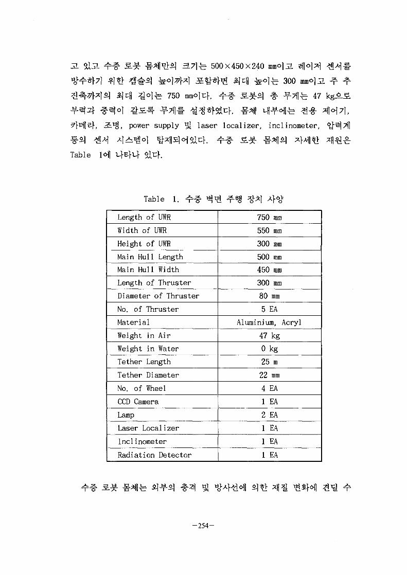
3. ^ 500X450X240
Table
^ 300
750 mmojuh lfe 47 kgJ*
power supply Rj laser local izer, inclinometer,
Table 1. 3*1Length of UWR
Width of UWR
Height of UWR
Main Hull Length
Main Hull Width
Length of Thruster
Diameter of Thruster
No. of Thruster
Material
Weight in Air
Weight in Water
Tether Length
Tether Diameter
No. of Wheel
CCD Camera
Lamp
Laser Localizer
Inclinometer
Radiation Detector
750 mm
550 mm
300 mm
500 mm
450 mm
300 mm
80 mm
5 EA
Aluminium, Acryl
47 kg
0 kg
25 m
22 mm
4 EA
1 EA
2 EA
1 EA
1 EA
1 EA
-254-

rf2} *}T£O.
bcr 15 fe 0-ring
mm
. Fig. 3 ^
Fig. 3.
2.
7]S.
2-3- 10
30
- 2 5 5 -

128 10 cmoju}. o]ofl Table 2
Table 2. S
Propeller Diameter
Hub Diameter
Pitch
Pitch Ratio (P0.7R/D)
Section Type
Skew Rate
Material
No. of Blade
128 mm
42 mm
100 mm
0.8
Kaplan Type Constant Pitch Propeller
0
Plastic
4
(2 .1 )
A=0.032 m3,
p=1000 kg/m3,
V=Vnax=30 c m / s S o |
O]
CD=0.4,
^ tg-^^- fi, = 5.4
- 2 5 6 -
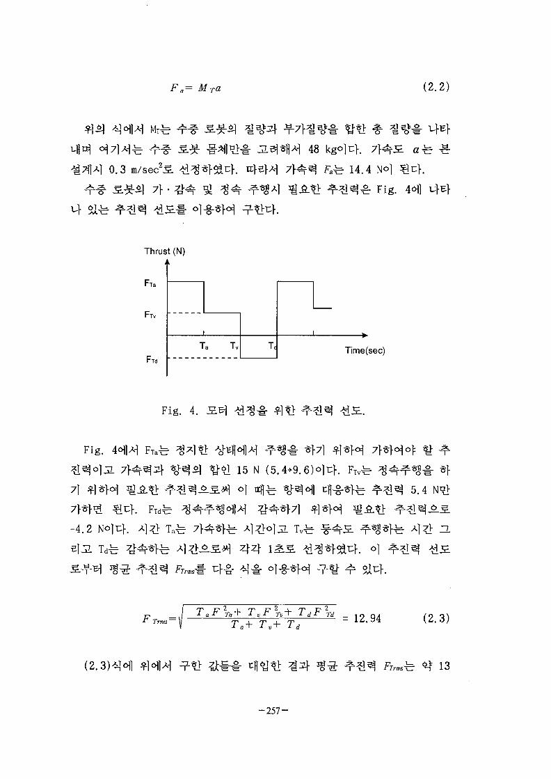
F a= MTa (2.2)
0.3
7f
Thrust (N)
FTa
FTV
FTd
Ta Tv Tc
Fig. 4.
Fig.
7] ^ *
7>
-4.2
48
fe 14.4^ Fig.
Time(sec)
15 N (5.4+9.6HC}. Fiv
5.4
-*S.*| 44
Trms-TaF Ta+ TVF Tv+ TdF
Td _T +1 a~
T,1.94 (2.3)
fe <$ 13
- 2 5 7 -

Sjsfl
( 2 - 4 )
13 N), p ^
kg/m3), Dfe SS-^e]^} xl^-(0.13 m)-§- ^fB^jL, CTfe
0.25# A]-g-«r> t:K o) ^v
^ n ^ 810 j }
T KQDF Trms /o rS
^ ^ . 0.025^
uf. ir|-eH -7-*H^l-b ^ ^ : S.^^i S H f e 0.169
0.17
A|-6ot . T a b l e 3 o j | T^-EI-T^ ^ K Table 3<>fl
if ^ 1 SB|fe ^.f- ^ 3 S | ^ ^ 7 } 3000
^i<^ 810 rprn^] ^ S . ^ - 3:1 ^•^•7]# 4 - § M > K
M i ^ ^ 1 ^ 1 ^ > ^ ^ f e Fig
fe 5 7H
£ B l ^ Table 3 ^ ^ o ] ^ . ^ 7 1 ^^°fl>M ^ t > -§-s<M ^ - b SANYOAfi]
V406-0H1- ^^«f5it:f. se j i ] s ] ^ # ^ ^ * f 7 ] ^ *
NIDEC SYMP04-21
- 2 5 8 -

Fig.
•b 300
Mechanical Seal#
Jclf 3 ) ^ ^ 80
132 mm,
. Fig. 6(a)-b
Fig. 6(c)b
50 mm, 3
, Fig.
44
Table 3. -tfMotor Type
Rated Speed
Rated Torque
Rated Current
Rated Capacity
Weight
Length
SANYO DC SERVO MOTOR
3000 rpm
1.8 kgf • cm
4.1 A
60 W
0.45 kg
104 mm
Fig. 5.
-259-

(a)
(b)
(c) ^ ^ ^
Fig. 6.
\i '" i
• 2 6 0 -

3. Laser localizer
7}.
position)if ^
61 71] * } ^ ^ , *j-7lSj ^ U l * ] (absolute
Fig.
7]51
Fig. 7.
-261-

c)
inclinometer)!-
ilt angle
sensor), ^|o|^| >i?im( laser scanner), 2 7l|5|
(retro-reflector),
^ ^ M ^-^r^I 9-^fe Fig.
^m A I A ^ ^(spot) %BB^ ^ |O |
spl i t ter)!
45°
-262-

, 4*14
Fig. 8.
Fig. 9fe
#4 ^ At:} 7] E}
Fig. {x,
{x, y}#
A, 4 ^ :
# 4S-7}
. o|
- 2 6 3 -

inclinometer^?-^eading angle) 0
Stl K Inclinometer^-
Vertical wall
A, B:{X, Y}{x, y}:
a,
-reflector)
l^Z^Inclinometer^.
Fig. 9.
Fig.
, _ Dtan(<f> + a)-H)x tan((f>+a)+tan(7r-<f>-a-
dY— dxt?cn.(x— $— a— fi)(2.6)
- 2 6 4 -

Fig.
0 )*=• 344
BSJ
Fig. 10. 0i, 02
02 (0 i. 02 < 2*r)
4sa
- 2 6 5 -

4. ZIZ\B.
a 4 0^Fig. lO^r
A4
(photo coupler) }-L.]-7f7ll
IS. tif^uf. o] A ] ^ ^
4 ^ Fig.
^ Fig. 124
51^, °1 # # £ OP Ampl-
(comparator)!- <>]-§-*M ^ ^ t l ^ r ^ ^ l ^ threshold^-
4 #^^! J l f e 80196 CPU^ HSI (High Speed Input)
Home Sensor
1 _
Encoder
jinjuuutrin. 0 1 2 3
counter reset
Photo TR
e2
A 0 1 2 3
counter reset
Fig. -id:
-266-
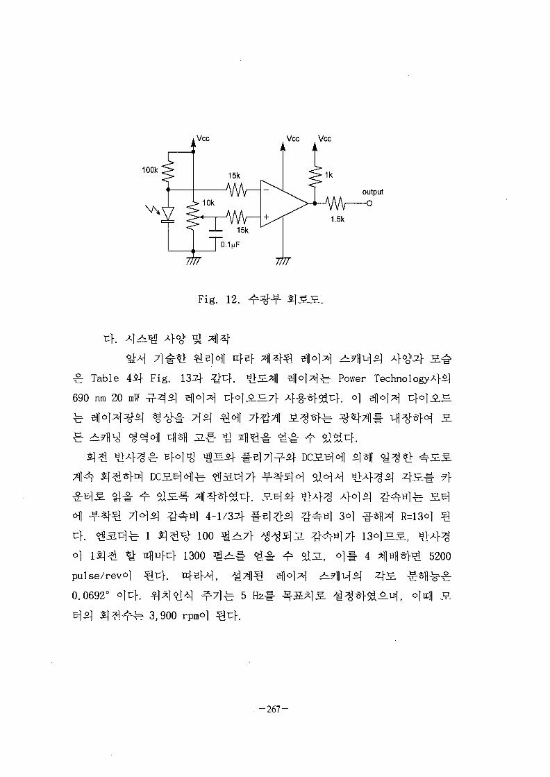
Vcc Vcc Vcc
100k
output
Fig. 12. ^ - f S]S.S..
4.nil-el-
£• Table 4 4 Fig. 134 ^ 4 .
690 nm 20 mW
3144 ^ 4 4 4^4 s.^J ^ . Power Techno logy A}*]
i 4-1/344 ^ ioo ^ ^
^ 4 4 1300 ^>i#
R=i3<>}
4 1 - 4 5200
0.0692° 4 4 . 44^14 ^4fe 54 4 4 ^ ^ f e 3,900 rpmo] Qv\.
S
- 2 6 7 -
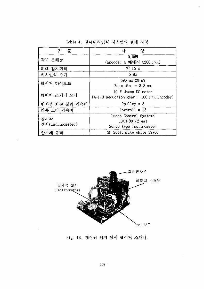
Table 4.
B M * 1 ^?1M S.BJ
^ 4 (Incl inometer)
0.069
(Encoder 4 *H«M 5200 P/R)^ 15 m5 Hz
690 nm 20 mWBeam dia. - 3.8 mm
10 W Maxon DC motor(4-1/3 Reduction gear + 100 P/R Encoder)
Rpulley = 3
Roverall = 13
Lucas Control SystemsLSXH-90 (2 ea)
Servo type inclinometer3M Scotchlite white 3970G
(Inclinoms^er) g/
CPU a n
Fig. 13. $1*1
- 2 6 8 -

4.
FH 40G
#4*1njo| A}-§-5]^ EBERL1NE4
cf^- Table 5^)4 ^-^RS-232
Table 5.
Model
Detector Type
Size
Detector Dimension
Measuring Range
Energy Range
Battery
FH40G (ESM Eberline)
Proportional counter type
195 mm x 73 mm x 42 mm
25 mm
100 nSv ~ 10 Sv
33 KeV ~ 3 MeV
2 lithium cells 1.5 V
Fig.
83(L)X55(D)
5 mm3]
55(w)x
10
. Fig.
Fig.
-269-

4 1=3 O
CotlimatorfJ}
/'i^J-1
10mm
Strw
3mm
195mm
.inr .i ' i
80mm
73m(r
50mm "$
r16rrn)
45mm
Fig. 14.
^
Fig. 15.
5.
7}.
3.7] 7}
MIW?)
- 2 7 0 -

nfl- 0)7]
^ 7 1 ^ - RS-232C
CPU 1 H# Fig.
(hierarchical structure)JL
e]^|c^7l(supervisory controller) JiJS.7}- &JL H of fl
'lower-level controller)7f
DPRAM
Lower-levelController
#1
OperatingConsole
RS-232C
SupervisoryController
DPRAM
Lower-levelController
#2
Motor •Driver
UnderwaterRobot
DPRAM
Lower-levelController
#3
MotorDriver
Fig. 16.
-271-

fe 2 HRS-232CS ^l^ffe 4
416 bit
converterl-
Intel*] 80C196KC CPU# o)-g-?>r:f. o]
£-tf, 256 ^ > ^ ) ^ PWM port^ 10 bit A/D
, 5].
Table 6 4
CPU JLH
rvisory control) CPU
Intel 80C196KC CPU
Fig. 174
28C256(R0M)
. 80196 CPU^ 16-bit^
64 Kbyte*}
32 Kbyte*]
- 3
-272-

address^}- data bus extension^ 7}*}JL $X^\. <
$}*\ 1 Kbyte-g-^ DPRAM - Afg-*}HS. 3.^ 3 KbyteS]
Kbyte!- DPRAMofl ^r Table
Table 6.
-7 t3
CPU
Memory
Communication
Power
CPU
Memory
Features
CommunicationPowerN-MOSFETPhoto-couplerDC-DCconverter
Intel 80C196KC(Clock freq.: 20 MHz)
32k8 EEPROM (ATMEL 28C256)RS-232C
DPRAM (IDT 7130) x 3
5 V 0.3 AIntel 80C196KC
(Clock freq.: 20 MHz)
32k8 EEPROM (ATMEL 28C256)24-bit Encoder Counter(LS7166) x 2
10-bit A/D Conversion (80196)256 step PWM output (80196)
RS-232C and DPRAM (IDT 7130)5 V 0.3 A
HARRIS-IRFP150TOSHIBA-TLP250
LAMDA-PPD1R5 48-1515
Table 7. 1 H 5 ]
o o
ROM
RAM
DPRAM No.1
DPRAM No.2
DPRAM No.3
- j~- A 6H 6g\ " — O "~1
H00000-H07FFF
H08000-H0F3FF
H0F400-H0F7FF
H0F800-H0FBFF
H0FC0O-HOFFFF
8 bit
8 bit
8 bit
8 bit
8 bit
til JL
0-32 K
32-61 K
61-62 K
62-63 K
63-64 K
- 2 7 3 -

CPU j e . ^
CPU E. 44 \$.<i\
32
DPRAM2]- 2 7H*] 7166 encoder counter^
Fig.
ROM°K§- £ S a a j
^ t l 1 Kbyte-g-
^ Table 8
Table 8.
ROM
DPRAM
LS7166 No.1
LS7166 No.2
H00000-H07FFF
H08000-H083FF
H0A000-H0BFFF
HOCOOO-HODFFF
8 bit
8 bit
8 bit
8 bit
«] JL
0-32 K
32-33 K
40-48 K
48-56 K
4 CPU i £
CPU ^.Hfe
2 7f l l -
Ug: RS-232C
2) 2H - 3 - ^ ^ tiov%^%-§- ^?l7l 2 7H1-
3| ^15l# 80196 1 A/D ^%7j S S I ;
3)
- 2 7 4 -
PI
CPUS] gAVofl £}*1| ^JSfl*]^, CPUvfl*] PWM port l - <>l-§-*H
PWM 3g>i7}- ^ ^ ^ t f . PWM ^ ^ S
7166 *flS^ ^ } ^ ^ f e 24 bit ^}
^ ^ ^ H ^ 1 ^ vfl^-^^.S. up-countif down-count# ^ } ^ ^ -
H ^^°11 nj-ef 4 ^ ) H | { ^ ] ^ ^ Sl-b 7 1 ^ 1 - ^ ^ J L $X°-r$, CPU
71665] # ^ i^|^l>iEiS^-B| 3*1 £) < a ^ ^ t l byte
read/write#
cpuif
(control word)^- ^
eh 5J&1 Hef
H 1 R l l ! ^ ^ ^ ] I PWM
Fig. 19^ HE S.5H
^ H ^ 300
MOSFET r H a r r i s ^ IRFP150o|4. o j ^ . 40 A, 100
^ ^ ^ &fe N-channel power M0SFETo|u}-, N-channel M0SFET#
t:}. M0SFET5] JEsfl^] ^ > 4 ^ - VccAj- &
o] Vcc7f ^S.•^• M0SFET# O n ^ l f e %°]tf. ° l ^ ^ r N-channel MOSFET l
\£- N-channel MOSFET
- 2 7 5 -

4.5-7
DC_DC
4 MOSFET*] Tllo]^^- ^^6^1 o | ^ * H PWM>*d 7} High
LowS. # ^ # nflfe, ^Itfl^ ^ ^ - o | ^>g*]-7lI^*H N-channel
TLP250O]Bfe PHOTO-COUPLER
- 10-35
4.
^ . ^ 4 3 7jf ^ ] efl^ J<H ij_5. riB]jL 37H^ 2-tf SB}o]a1 J i B f
4 4 ^ 4 ^ « t : } . Fig. 20^ o]^7fl 4 4 ^ 1 1<>1 ^ 1 ^ ^
a l4 . Fig. 20(a)iq ^ 1 4*£ 4 ^ ^ - ^ ^ 3.7180X80
^ aqcfl ^ o | ^ 12 mmoli:}. Fig. 20(b)^ *}$ s)]^
r°l-b 15 mmolcK Fig.
^ 80X60 mmol L ^ o | ^ 25
L6203 ^ B H ^ f e ^ ^ l ^ # ^ d )
- L6203 E 5
- 2 7 6 -

P1.2XTAL2 P1.3/PWM1
P1.4/PWM2!NMI P1.5/BRB3JREADY P1.6/HLDR:
P1.7/HOIUj
RESET P3.0;AD0|P3.17AD1
PO.0/ACHCP3-2/AD2P0-KACH1P3-3/AD3;P0.2/ACH2P3.4/AD4;
0-T P0.3IACH2P3.5/AO5B-r, P0.4/ACH4P3.6/AD6
3B-, P0.6/ACH6G— P0.7/ACH/P4.0/AD8;
P4.1/AD9- P2.0/TXOP4.2/AD10T P2.1/RXCP4.3/AD11
0- i P2.2/EXIW1.4/AD120-J.P2.3/T2CEM.57AD13B-J;P2.4/T2RSTI.6;AD141
0-J P2.5/PWNB».7;AD150-J P2.6/T2UP-DN0— P2.7/T2CAELBKEIT
O-| HSI.O0-SHSI.1
BHE/WKH-iflWR/WRT:
R0
0-^HSI.3/HSO.5 INSTBUSW1DTH
JVREFr VCC HSO.O- VPP HSO.1
r-J, ANGNO
'vssVSSVSSEA
HSO.2LSHSO.3 ^6
- 80C196KC
CONNECT TO SUB
ROBOT CONTROLLER SUPERVIS
tUocument Number
Fig. 17.
- 2 7 7 -

XTAL1 P1.0P1 1PI.2
XTAL2 P1.3/PWM1PI 4/PWM2
NM1 P1.5/BRECT
Q-f PO.ZllB
RESET P3.0/ACX)P3.1/AD1
POO/ACHO P3 2/AD2P0.1/ACH1 P3.3/AD3P0.2/ACH2 P3AIAO4
'ACH3 P3.5/AD5P0.4/ACH4 P3.6/AD6P0 5/ACH5 P3 7/AD7P0.6/ACH6P0.7/ACH7 P4 0/AD6
P4.1/AD9P2.O/TXD P4 2/AD10P2.1/RXD P4.3/AD11P2.2/EXINTP4.4/AD12P2.3/T2CLKP4 5/AD13P2.4/T2RSTP4.6/AD14P2.5/PWM0P4 7/AD15P2.6H-2UP-DNP2.7yT2CAPTCEEOUT
HS1.0 WR/WRUHSI 1HSI.2/HSO.4ALE/A0VHSI.3/HSO.5 INST
BUSW1DTHVREFVCCVPP
ANGNOVSSVSSVSSEA
HSO.OHSO.lHSO2HSO3
IOBOT CONTROLLER SUB 1 2 3
Fig. 18.
- 2 7 8 -

pwivp~>
VS=36Vmax0
J1
C0N2
Motor Power
Vcc=5V0
J2
CON2
~ Logic Power
J3
CON2
FROM SUB
Logic powers}3 6V, 4A7} Jl-i-
Lfe S.^- 1 itle
sizeA
Jale
MOTOR DRIVER
Document Number
Wednesday, November •prii ot 0
-ievIV
Fig. 19.
- 2 7 9 -

(a)
(b)
(c)
Fig. 20.
- 2 8 0 -
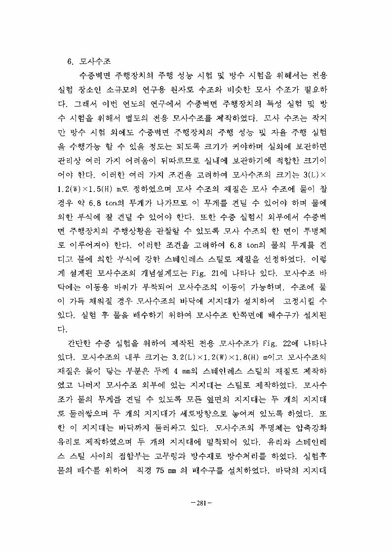
6.
4. a
n>
-2.4 ^ - b
1 . 2 ( W ) X 1 . 5 ( H )
3- f ^ 6.8
71]
.7]
3.7]fe- 3(L)x
6.8 toni] 1-5]
^ Fig.
Fig.
ufl-f- 3 .7 ] f e 3 . 2 ( L ) x l . 2 ( W ) x i . 8 ( H )
75 mm
- 2 8 1 -
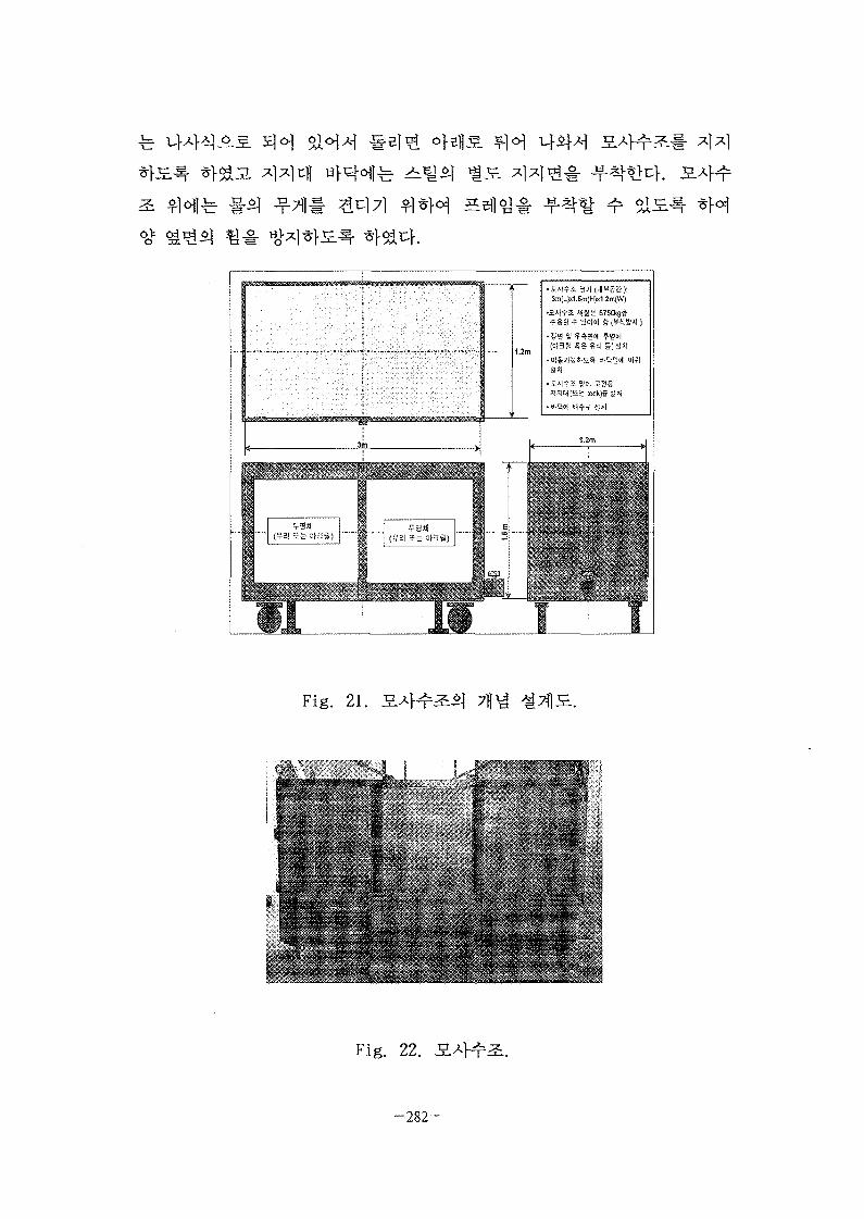
444
1.2m
3m(L)xl.5m|H)x1.2m(W)
•S3 * T«fS«l ?
41*1
gat
. . r . _ 1
Fig. 21.
Fig. 22.
- 2 8 2
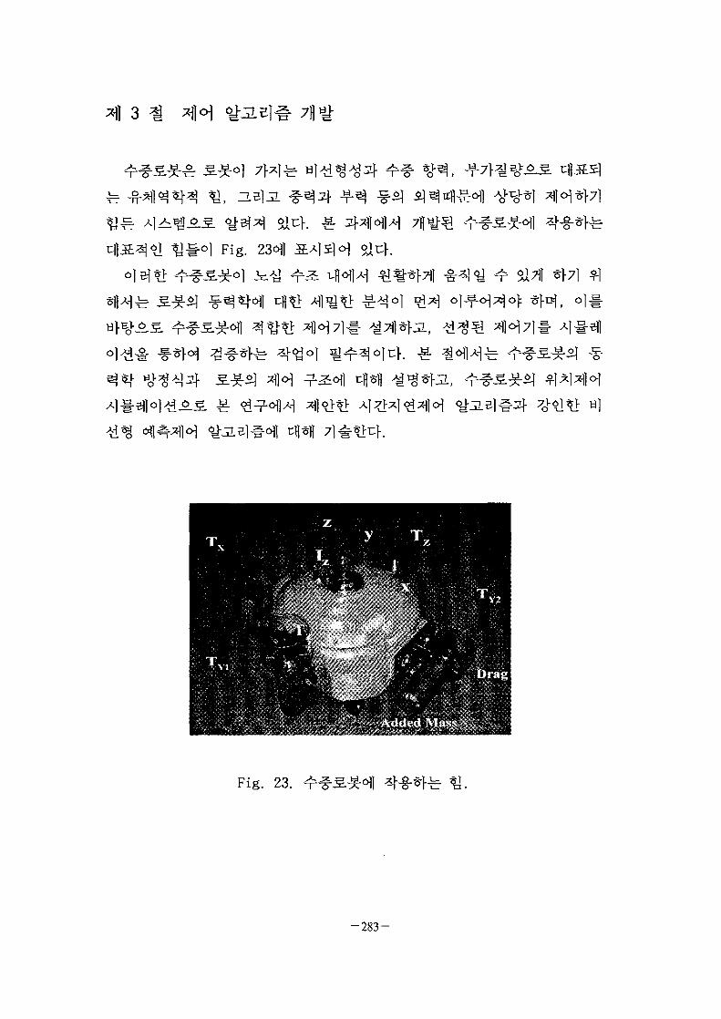
Fig.
Fig. 23.
- 2 8 3 -
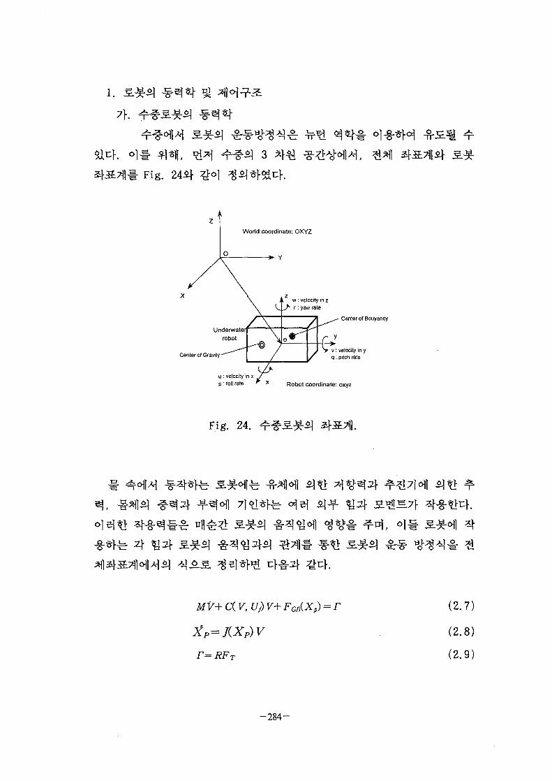
7f.
Fig.
World coordinate: OXYZ
-> Y
Center of Bouyancy
Center of Gravity
u : velocity in xp: roll rate r x R o b o t coordinate: oxyz
Fig. 24.
fe 4
MV+ C( V, Uf) V+ FG£XP)
XP=J(XP)V
r=RFT
(2.7)
(2.8)
(2.9)
- 2 8 4 -

^[u , v, w, p, q,
6x63-)
inertia)^)- Ma(added mass)^ ^
rigid body
H5]J1 C-
6x6
SfSS.
fe 6x6^
Fig. 2 5 ^
X , Y
0
x, y
u, vrT L T2, T3
Fig. 25.
A
^ + (w+ ywr)wr- Yw \ v\ v+Y= mycu+ mxcv+mr(xcu+ycv) — Nrr | r | r+NT
- 2 8 5 -

x
A
Yv- , ZL
NT=l(T2-T3)si (2.11)
X= ucos <j> — ys inY= Msin (Z> — ycos'<j> = r
(2.12)
, 8, 9]ofl
- 2 8 6 -

r Q(t) + Q(t)=Q(t) (2.13)
6\] H)*1| nfl-f ^ ^
r (2.14)
3 . B M ^4 , CT= 1.67 x 10"3 [N/(rad/s)2] 5 ^fcAS.
4 , CT= 2.93 x 10"3 [N/(rad/s)2]
t - L A t , I t , 0 t J •
••fe- F i g
- 2 8 7 -

ey = -{Xt - (Yt -
(2.15)
yfe 4 4
Fig. 2 7 ^
0
Desired trajectory ""T"1 • ' J ^
p•^r^ Current vehicleaJ posture
• f f s - Target vehicle
k.
Xt X
Fig. 26.
- 2 8 8 -

PathTrackingController
Thrusters AUV f—•
Localizationsensorsystem
Fig. 27.
lfe Fig. 26,
XT(k) = KPxex(k) + Kh ex(k)
(2.16)
KPy, Kp f]^r
[KIx, KIy, Ki f]fe
PID
- 2 8 9 -

2.
[10].
XT(k) = 2 $ - 1) - Exk{k- 1).
). (2 .17)
+ NT(k-
^ , wnx, wny, w n f ^ 4
Ey, Etffe ^1
fe 4
Ey,
MIMO X\
44 l f T2f T30I
7)5]
(2.18)
(2.11)
, Q2 )
^ *} (2.11)4- i1 (2.14)5.^-^1
- 2 9 0 -
cT TK "
(2.19)
] ^ ^ o ) 3D CAD
Fig. 2 8 ^ ^ ^ ] ^ > ] ^ ^ # 3D
m=Al.Vkg, xc = -A.lmm, yc=1.2>mm,
Xii=Yur=7Mkg, Yv=Xvr=7A5kg,
Xuu= 18.24W m, Yvv=25.20kglm,
Nr=l.251kg-m2, Nrr=l.l%kglm2
^r Fig.
changing path) -
instant turning path)
^1^(circular turning path)
^ ut - 0.13
0.5, 1.0, 1.5 m
"• 45, 90, 135°
: 0.5, 0.85 m
Fig. 30~
-291-

30, 33).
o a
ig. 31, 34).
3.71]
^r
sa4(Fig. 32, 35).
Fig. 28. 3D CAD 5L*£.
- 2 9 2 -
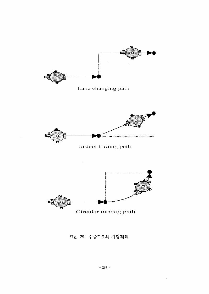
I.anc changing path
Instant turning path
Oircular turning path
Fig. 29.
- 2 9 3 -

2.0
1.5 -
1.0 -
~ 0.5 -
0.0
-0.5
r3
case
case
casei
1:
2:
3:
Yd =
r <
<a.
a.
I II
II
0.5m
1.0m
1.5m
0.0 0.5 1.0 1.5 2.0 2.5 3.0
X-coordicate (X), m
3.5 4.0
Fig. 30. PID*H7l).
6
dina
te (Y
'-coo
r
2.0
1.5
1.0
0.5
0.0
\
N. 3
1 . 1 . 1
2
/
/
' case 1: (j>
case 2: <)>d
case 3: <J>i . i . d
/
/
= 45°
= 90°
= 135°
0.0 0.5 1.0 1.5 2.0 2.5 3.0
X-coordicate (X), m
3.5 4.0
Fig. 31. , PID*W7l).
- 2 9 4 -

2.0 ,
1.5
E
p 1.0
8o£ o.o
-0.5
case 1: curvature = 0.85 m
case 2: curvature = 0.5 m
0.0 0.5 1.0 1.5 2.0
X-coordicate (X), m
2.5 3.0
Fig. 32.
a|
o
8
2.0
1.5 -
1.0 -
0.0
-0.5
-
I . I .
/ 3
I2
M/ case 1: Y = 0.5m
case 2: Yd = 1.0m
case 3: Yd = 1.5m
0.0 0.5 1.0 1.5 2.0 2.5 3.0
X-coordicate (X), m
3.5 4.0
Fig. 33.
- 2 9 5 -

I•ao
2.0
1.5
1.0
0.5
0 0
\
I . I . I .
2
/
/
/ 1
/ case 1: 4>d
case 2: <)>
case 3:§
/
/
= 45°
= 90°
= 135°
0.0 0.5 1.0 1.5 2.0 2.5 3.0
X-coordicate (X), m
3.5 4.0
Fig. 34.
2.0
1.5
1.0
| o ,o
8> - 0.0
-0.5
case 1; curvature = 0.85 m
case 2: curvature = 0.5 m
0.0 0.5 1.0 1.5 2.0
X-coordicate (X), m
2.5 3.0
Fig.35.
- 2 9 6 -
3.
17}
Mx(t)+ CDx(t)\x(i)\= FT(t) (2.20)
CD coefficient)O|JL Fr ^
= u,(t) (2.21a)
(2.21b)
4
- 2 9 7 -
(2.22a)
(2.22b)
x *r AoW^J5l x=[x x]Tif ^ o | %$]5]JL f ^
h7f n]^5] ^ ^ - 7f^ 4 , Cf^-^j^ T a y l o r series
^ h7\
-298 -
(2.23)
-(f+gu). (2.24)
2: °I<^ xd(t) = [xd(t) xd(t)]T # 7 ] ^ ^Bim^efjL % ic||, xd(t)

r ^ H ^ u*(t)sU (for all te[0,T])7|- «lH
xd(t+h) £ JEE*> iT (2.25)Af
7]
du(t) ~u-
(2.24)3f *] (2.25)1- *] (2.27)eHUo]
A2
h
e(t) = x ( t ) - xd(t), e ( t )=x( t ) - xd(t).
-299-
(2.25)
(x(t+h)~ xd(t+h))2 + Au(t)2} (2.26)
4^/ ^ -^ ( f l l (2.28)
(2.22aH ^fe *H*1 f*} g7} W W g *} (2.28H
(2.29)
^-Bm f
u(t) = j^-[e(i) + he(t) + -^-} f- xd(t)] (2.30)
= f+gu=(}+ Af)
(2.31)
o
(2.32a)
, Vt (2.32b)
- 3 0 0 -
«(/)= uc(t)+ us(i) (2.33)
4
•§•
=g( uc(t)-u*c(f)+ us(t)).
u *+
e= [e e]T, b= [0 g]T, H.
(2.34)
(2.35)
0 12 __2_^ 2 A
Lyapunov
P = PT > 0 (2.36a)
P ^ ^ ^ . c ^
(2.36a)#
= -Q , Q > 0.
*] (2.35)1- &H'
(2.36b)
- 3 0 1 -

=-4f eTQe+ eTPb{ uc-u*c)+ eTPbus. (2.37)
u,=-sgn(eTPb) | 2 c | l j n (2.38)
) ^ s>0 s<0
7}
(2.39)
t=( -sgn(s)\
| ~(s/ slim) s , i m
s = eTPb
(2.20)ofl aife M^ CD
=14
0.00167 N/s2^. 0.00293 N/s2
= 25+l5sm(\x\f)
(2.41a)
(2.41b)
-302-

CT(f) = 0.00167 + 0.0005cos(d for forward thrust (2.41c)
CT(t) = 0.00293 + 0.0005cos(f) for backward thrust. (2.41d)
FA*
•"* min
Mmin ^ 4 4 ^^H^f ^ ^ ^ 1 - M I M J ! ^t^r Mmax=120
A=0.25 m o]3. T = 10 sec°lt;K
Fig. 36^- ^ # ^ ^
Fig
. Fig. 38^ l ^ ^ ^ #
Fig. 39-b ^ ^
o]-o\. Fig. 384
^ m , Fig.
- 3 0 3 -
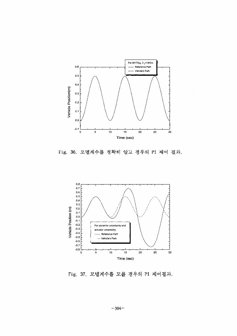
0.6
0.5
0.4
§ 0.3
0.2
0.0
-0.1
ForM=70kg, Ca=14N/m
Reference Path
Vehicle's Path
10 15 20
Time (sec)
25 30
Fig. 36. PI
co
0.80.70.60.50.40.30.20.10.0
g -0.1O- -0.2| -0.3^ -0.4> -0.S
-0.6
-0.7
-0.8
For paramter uncertainty and
actuator uncertainty
Reference Path
Vehicle's Path
10 15 20 25 30
Time (sec)
Fig. 37. PI
- 3 0 4 -

0.6
0.5 -
0.4 -
0.3 -
0.2 -
•a o.i -
0.0 L
-0.1
O
moa.
I
ftwDesired path |
Vehicle's path 1 '
i . i . i
10 20 30
Time (sec)
40 50 60
Fig. 38.
co
1D.Sio
I
0.3 -
0.2 -
• = 0 . 1 -
0.0
-0.1
Desired path
Vehicle's path by robust NPC
Vehicle's path by NPC
-^<— Vehicle's path by SMC
1 \I \i \ i \ i \ / V
10 20 30 40
Time (sec)
50
Fig. 39.
- 3 0 5 -

A.
Fig. Jib
b I m x 0 . 8 m x 0 . 6 m
^ 7 1 ]
71 (power supply)^
44el#(ripple)o)
Fig. 414 42b4 0.00167 (N
Vrad2sVrad2), ^ ^ o ^ 4 0.00293 (N
- 3 0 6 -

75 %
ig. 43).
Table 9.
DiameterHub DiameterPitchSection TypeMaterialNo. of BladesTypeRated OutputRated SpeedRated TorqueRated VoltageRated CurrentSizeEncoder Resolution
TypeReduction rate
130 mm42 mm100 mm
Kaplan typePlastic
4DC Servo Motor
60 W3,000 rpm1.8 kgf-cm
24 V4.3 A
41110 mm (Encoder SL^)
1,000 P/R
Planetary Gear
1 : 3
Fig. 40.
- 3 0 7 -

10-
6-
u> 4 -
2 -
20 40 60
Propeller Speed [rad/s]
80
.(fi[rad/s]) vs. ^
FT = 0.00167 * Qz
[N])
Fig. 41.
1 2 -
10-
£• 4 -
2 -
20 30 40 50
Propeller Speed [rad/s]
60 70
rad/s]) vs.
FT = 0.00293 *
[N])
Fig. 42.
- 3 0 8 -
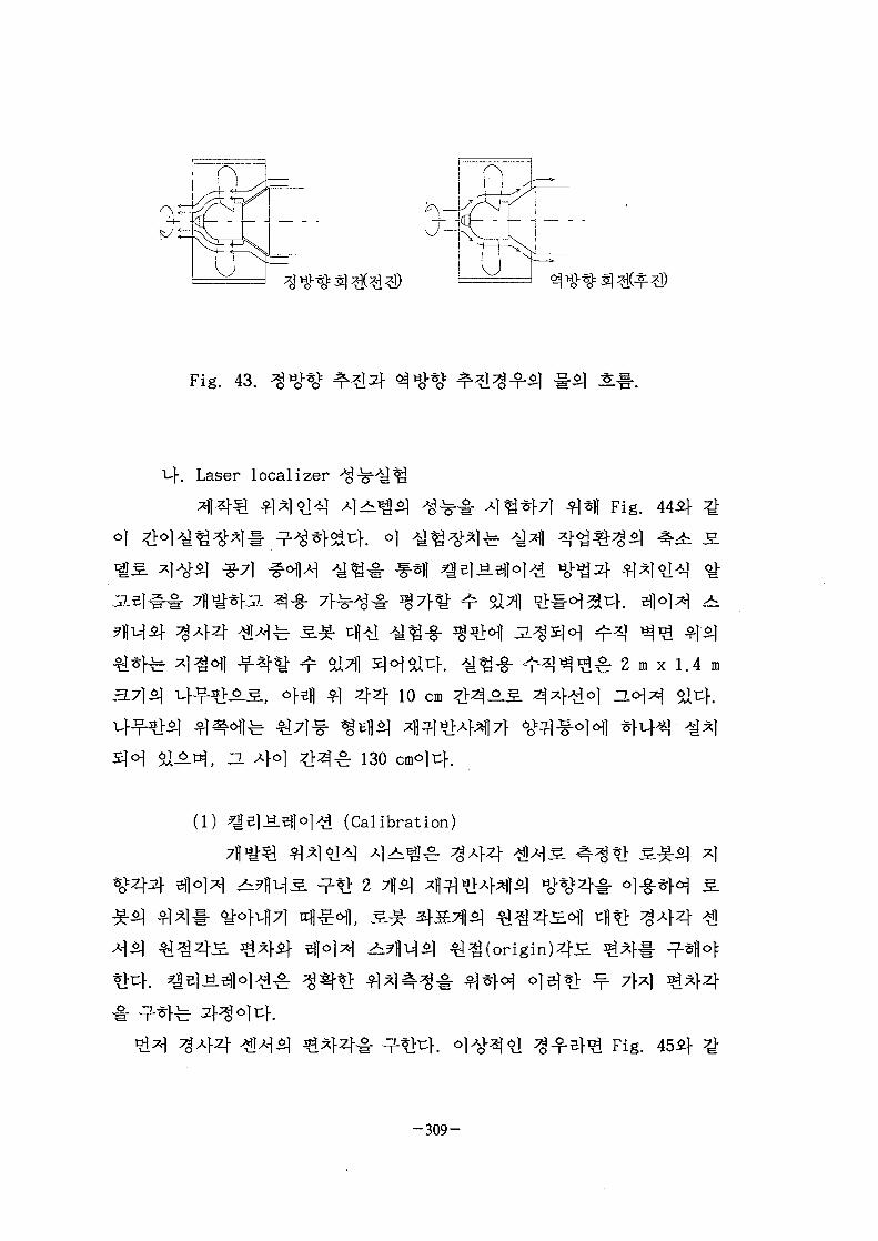
Fig. 43.
K Laser local izer
4 ^ 7 ] sfm Fig. 445}
3.7}$] 4 4 10 cm 4^-
Afo| 130
£ 2 m x 1.4 m
(1) ^JelH.5|]o]^ (Calibration)
Fig.
-309-

o] Oo]
*J*]43l§- £ 0 V7f LjSfo) Sfuf. ^ejJE
o. Fig.
(2<42)
nit
£ s
<p2- <p j < 7T
i i ) p 2 - <P \ > n
- 3 1 0 -
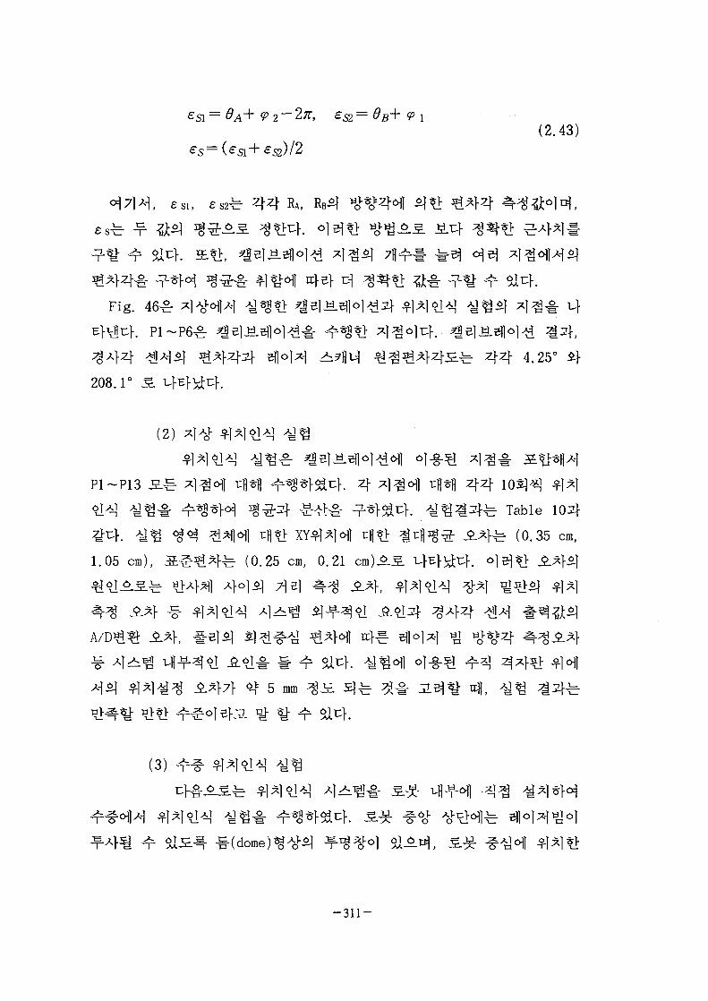
= 6B+ <p(2.43)
, £si, £s2fe 4 4
7J1
Fig. 46^
^ 4 4 4.25°
208.1
(2)
. A 44^-fe Table
fe (0.35 cm,1.05 cm), (0.25 cm, 0.21 cm)A
5 mm
(3)
- 3 1 1 -

-^r Fig.
Fig.
fetl Fig.
. Fig.
2 . 5 m P2
-312 -
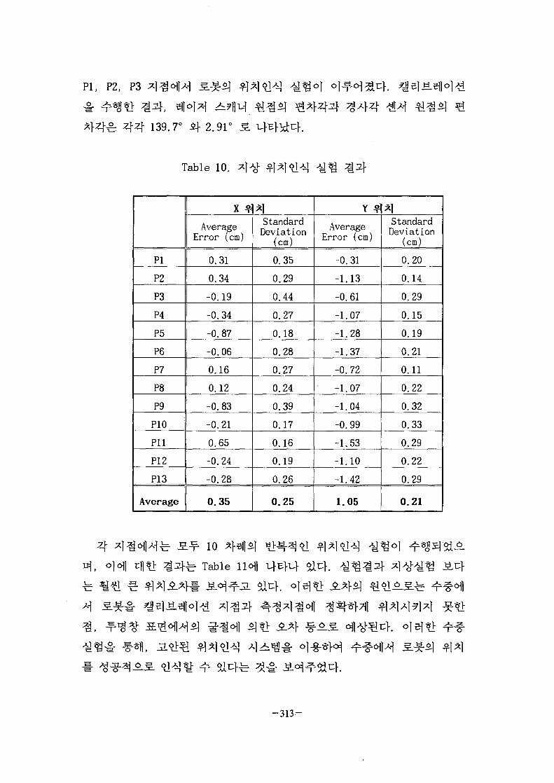
PI, P2, P3
4 4 139.7° £f 2.91
Table 10. 4AoV
PI
P2
P3
P4
P5
P6
P7
P8
P9
P10
Pll
P12
P13
Average
x $1*1Average
Error (cm)
0.31
0.34
-0.19
-0.34
-0. 87
-0.06
0.16
0.12
-0.83
-0.21
0.65
-0.24
-0.28
0.35
StandardDeviation
(cm)
0.35
0.29
0.44
0.27
0.18
0.28
0.27
0.24
0.39
0.17
0.16
0.19
0.26
0.25
AverageError (cm)
-0.31
-1.13
-0.61
-1.07
-1.28
-1.37
-0.72
-1.07
-1.04
-0.99
-1.53
-1.10
-1.42
1.05
StandardDeviation
(cm)
0.20
0.14
0.29
0.15
0.19
0.21
0.11
0.22
0.32
0.33
0.29
0.22
0.29
0.21
4°H
^f io %
fe Table
- 3 1 3 -
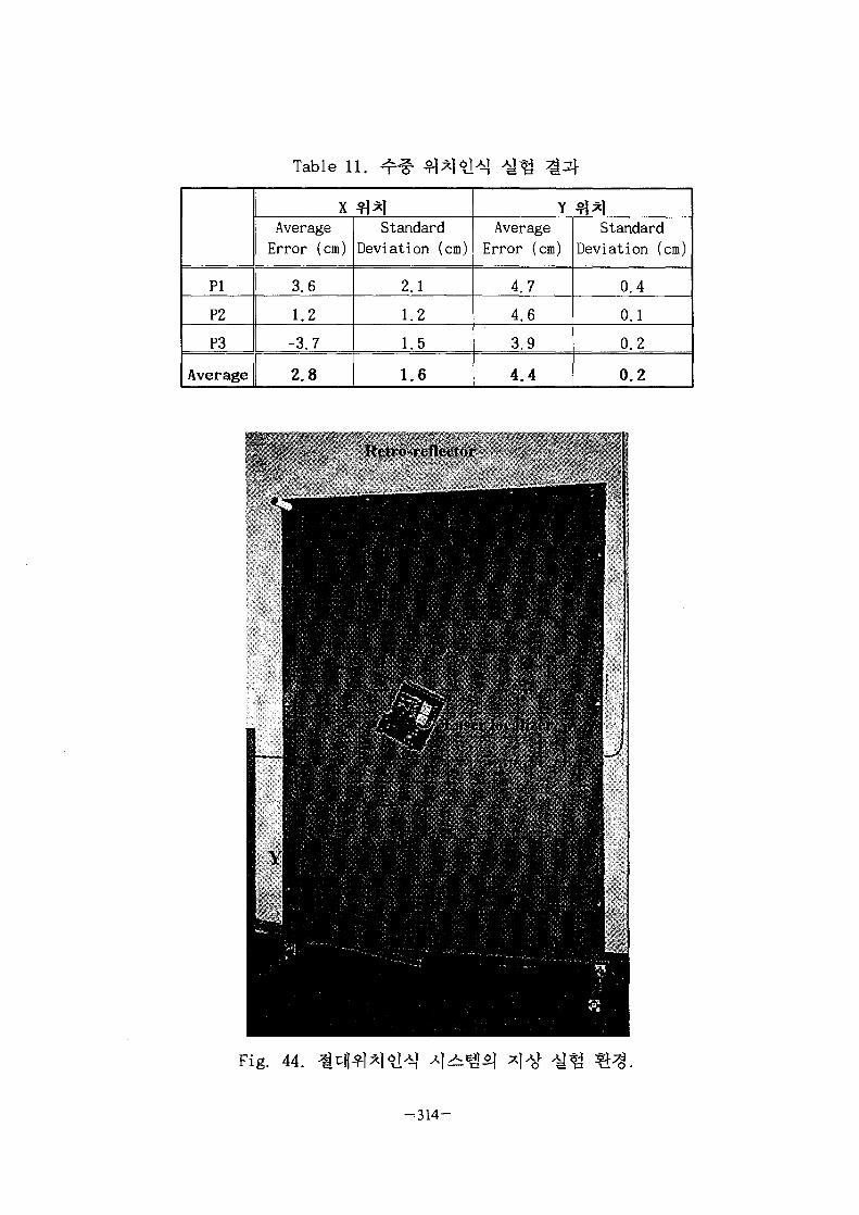
Table 11.
PI
P2
P3
Average
XAverageError (cm)
3.6
1.2
-3.7
2.8
$1*1Standard
Deviation (cm)
2.1
1.2
1.5
1.6
YAverage
Error (cm)
4.7
4.6
3.9
4.4
$1*1Standard
Deviation (cm)
0.4
0.1
0.2
0.2
Kctrn-rtflcctor
Fig. 44.
-314 -
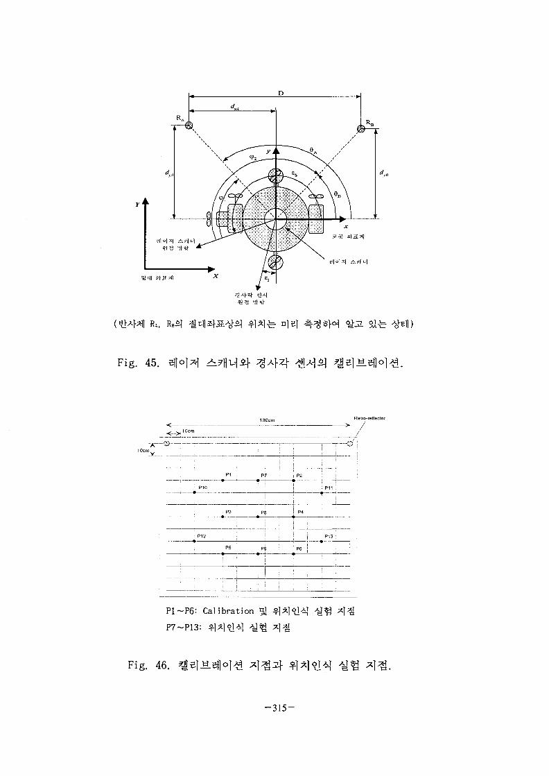
RA.
Fig. 45.
Retro-reflector
:mVL „_
P12
P5 P8Q |
i i
: i i
• P6
P13
P1-P6: Calibration
P7-P13: ^
Fig. 46. ^5]«.
-315-

sas
(a)
Fig. 47. -A}~§-
-9=1
\
Fig. 48.
- 3 1 6 -

Cylindrical
Reflector
246.4cm
X
Cylindrical
Reflector
0
P, (92.4cm, 36.0cm)
P2 (123.2cm, 36.0cm)
P, (154.0cm, 36.0cm)
Fig. 49. 1*1
2.
5 mi]
7f.
- 3 1 7 -

JOS. 5
m x 5
. Fig. 5 0 ^
ig. 51).
- 5 m
Fig. 50.
- 3 1 8 -

Fig.
6] 0 m 5 m
F. Fig .
5 m
oi l -
- 3 1 9 -

Fig. a»
30
Fig.
4 >HS., Fig.
a) t = Osec
Fig. 52.
- 3 2 0 -

b) t = 7.5sec
c) t = 15sec
Fig. 52.
- 3 2 1 -

a) t = Osec
b) t = 7.5sec
Fig. 53.
- 3 2 2 -
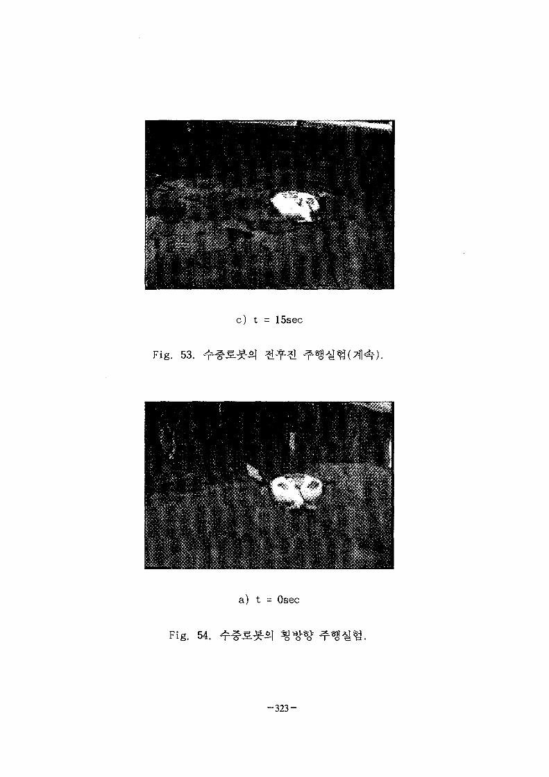
c) t = 15sec
Fig. 53.
a) t = Osec
Fig. 54.
- 3 2 3 -
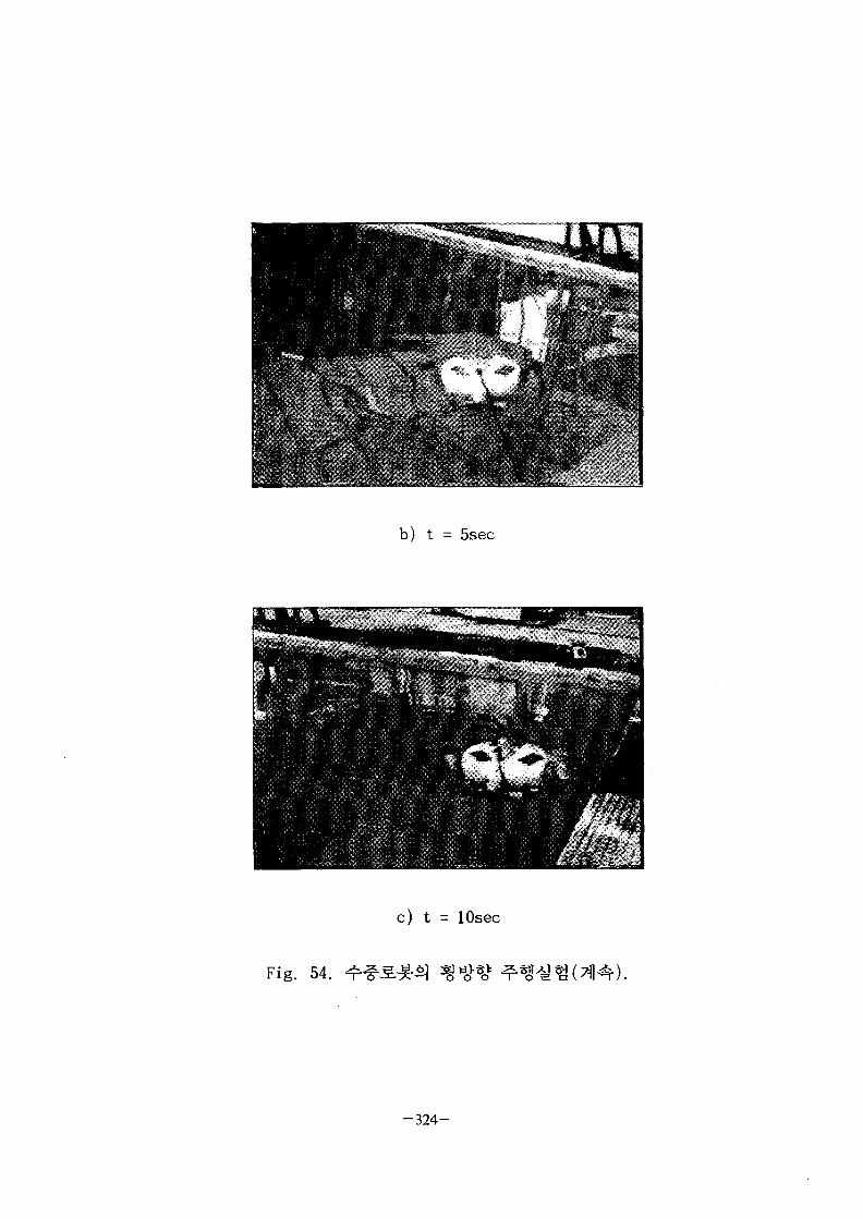
b) t = 5sec
c) t = lOsec
Fig. 54.
-324-

3. TRIGA-III
TRIGA-III
TRIGA-III
Fig. 55^4^]- o) Al, A2, Bl, B2
6 mV\x] 50 cm^ 7 ^ A S ^^1 SL
, rack/duct ^ ^ 4 5 .
TRIGA-III < £ ^ ^-§-^^6fl4fe ^ 52711 ^
^^t> 4 4^^ ^ 4 ^ ^ &£: Table
2.5 cm 7}
- 3 2 5 -
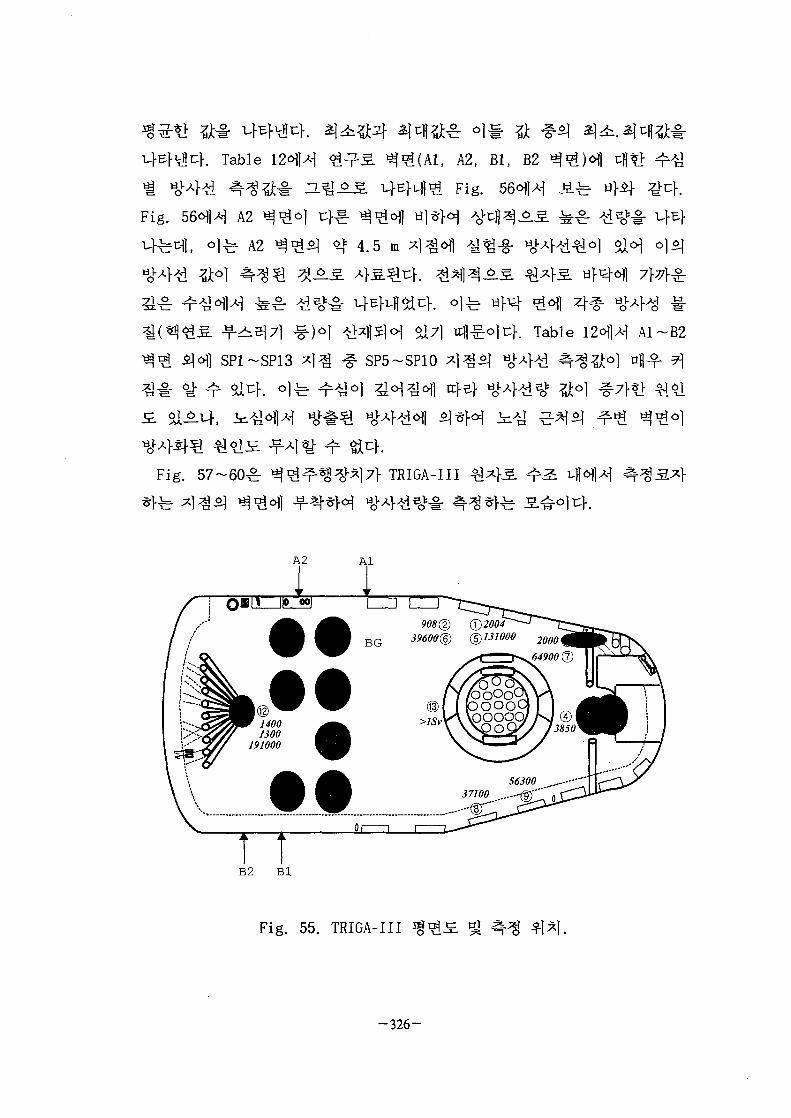
. Table , A2, Bl, B2
Fig. 566JH
Fig. 56^14 A2
A2 4 .5 m
Zi-2- 4=-
. Table
SP1-SP13 SP5-SP10
Fig. TRIGA-III
A1-B2
B2 Bl
Fig. 55. TRIGA-III
-326-

Table 12. TRIGA-III
BG
A1S
A2S
B1S
B2°j
Sol(m)2.5
1.0
1.5
2.0
2.5
3.0
3.5
4.0
4.5
5.0
5.5
6.0
1.0
1.5
2.0
2.5
3.0
3.5
4.0
4.5
5.0
5.5
6.0
1.0
1.5
3.5
4.0
4.5
5.0
5.5
6.0
1.0
3.0
3.5
4.0
4.5
5.0
5.5
6.0
(nSv)90
105
120
115
127
103
313
298
300
294
332
1440
115
120
195
284
3030
6770
38300
55800
20100
953
650
105
87.5
417
337
2260
36500
72700
29100
88
102
107
103
128
226
659
1440
(uSv)7.84E-02
1.01E-01
1.03E-01
1.15E-01
1.21E-01
9.88E-02
3.13E-01
2.91E-01
2.65E-01
2.39E-01
2.84E-01
1.10E+00
1.10E-01
1.15E-01
1.42E-01
2.70E-01
2.25E+00
6.24E+00
2.78E+01
5.14E+01
2.01 E+01
9.29E-01
6.48E-01
8.50E-02
8.61E-02
1.01E-01
3.08E-01
2.19E+00
3.61 E+01
6.97E+01
2.87E+01
8.38E-02
9.82E-02
9.76E-02
9.99E-02
1.17E-01
2.13E-01
6.48E-01
1.43E+00
(uSv)1.04E-01
1.22E-01
1.35E-01
1.30E-01
1.32E-01
1.07E-01
3.40E-01
3.09E-01
3.47E-01
3.00E-01
3.73E-01
1.45E+00
1.16E-01
1.23E-01
2.00E-01
4.12E-01
3.07E+00
6.80E+00
4.04E+01
5.63E+01
2.08E+01
1.54E+00
8.98E-01
1.08E-01
9.99E-02
1.17E-01
3.95E-01
2.26E+00
4.06E+01
7.27E+01
3.00E+01
8.89E-02
1.09E-01
1.12E-01
1.16E-01
1.33E-01
2.37E-01
7.75E-01
1.61E+00
«/ J2
-327-

Table 12. TRIGA-III
SP1
SP2
SP3
SP4
SP5
SP6
SP7
SP8
SP9
SP1O
SP11
SP12
SP13
20/(m)5.0
5.0
5.0
5.0
6.0
6.0
6.0
6.0
6.0
6.0
5.0
4.0
(nSv)2004
908
2000
3850
131000
39600
64900
37100
56300
191000
1300
1400
9.99E+08
(uSv)1.96E+00
7.46E-01
1.85E+00
3.79E+00
1.29E+02
3.91 E+01
6.45E+01
3.41 E+01
5.11 E+01
1.86E+02
1.22E+00
1.35E+00
1.04E-01
*/W(uSv)
2.06E+00
9.26E-01
2.09E+00
3.94E+00
1.36E+02
4.57E+01
6.75E+01
3.72E+01
5.95E+01
2.11E+02
1.40E+00
1.49E+00
9.99E+05
«/ JZ
?Wl^i(isv)» ytH^
100000.00(WmRemJ
10000.00
1000.00
100.00
10.00
—+—A1&- -m - A2&!—*—B1&I- ® •- B2&
1 -
/.o/OS11510588
- i
/ .5 '120120
,87.5
TR
775
IGA
127
284
^ ^
103
3030
102
& Ah
5 .5
313
6770417107
4.0
298
38300337
103
:.,© "
4.5
-A—
5.0
55800 201002260 36500128
-A—B1S - © -B2S '
5.5
55;?P55
1440650
72700\29100659 1440
Sol(m)
Fig. 56. TRIGA-III
- 3 2 8 -
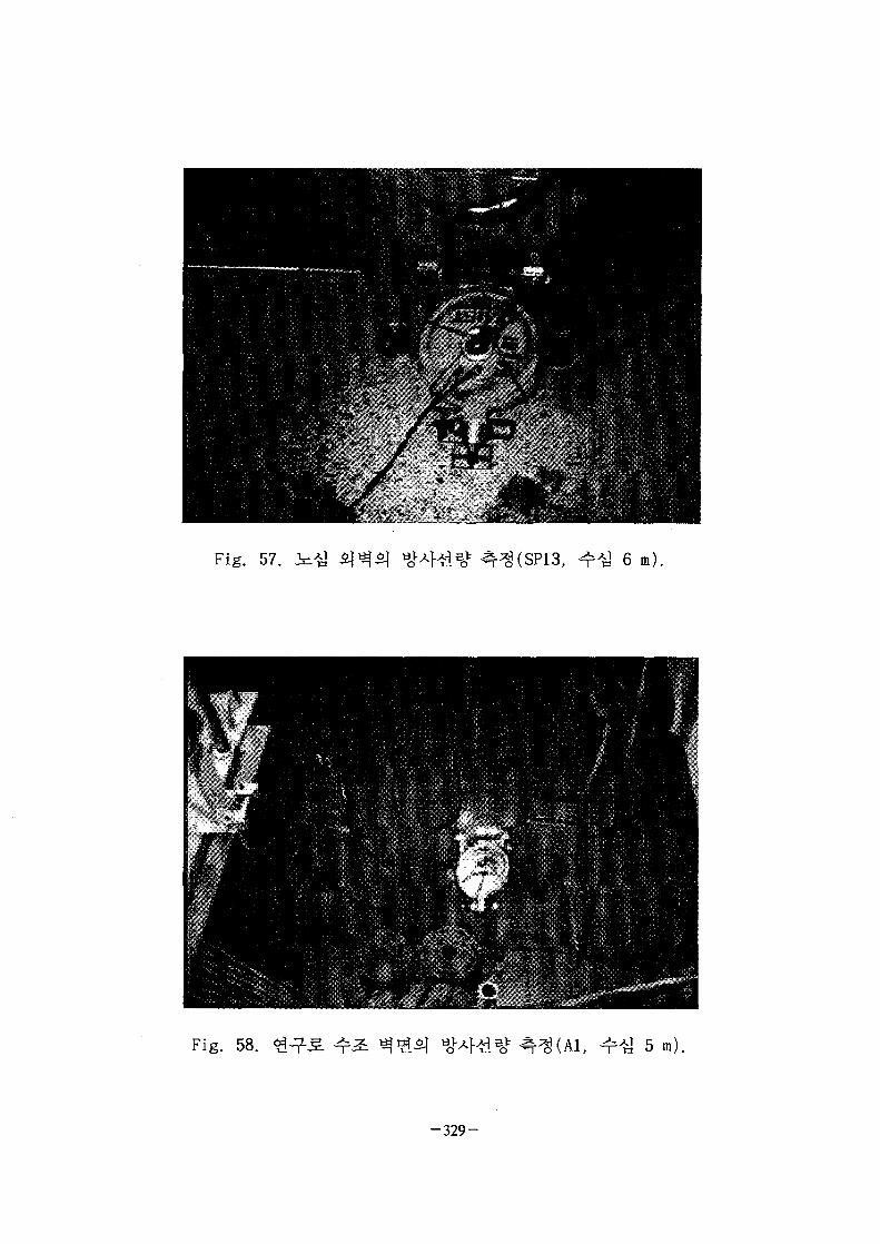
Fig. 57. h=.M 6 m).
Fig. 58. 5 m).
- 3 2 9 -

Fig. 59. 6 m).
Fig. 60. 6 m).
- 3 3 0 -

TRIGA-III
61514.
3.711 ^^11, ^^I7l , laser local izer,
force)#
7} 47B, 2|^ol 130mm,
, 7] 7113} A] ^(mechanical seal) J S
thruster)^
^ ^ ^ o ^ S - ^^15]^ alfe 2 7lf ^?l7l(front
and rear thruster)^ S.^2) xm^°-3.S>) $]# ^ f e ^^ofl-M^ ^r*$
in thruster)^ S.
}(absolute position)if
(posture)!- *I*J*|-7l 4\i% ^ ^ •ofl-M JL6>*> laser local izer X\£
^ ^ 4 4 ^ * i ( t i l t angle sensor), eflo]^ ^ ^ i ^ , 27fl*|
(retro-reflector),
- 3 3 1 -
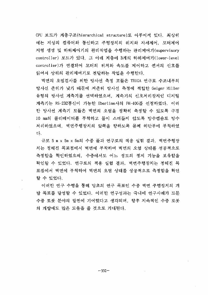
CPU S.B.7} X|4H?-S(hierarchical structure)^
fe ^SJaW 7] (supervisory
controller) ^H7} $14. ^ ° H 7|l#ol) 37H*] ^RHH^Klower-level
controller)7} ^
TRIGA i ^ ^
| ^^-*> Geiger Miller
1 ] f FH-40G
10
5 m x 5m x
- 3 3 2 -

s i SH*
71
MARK I I ^ TRIGA MARK I I I ) * ]
- 3 3 3 -
-§-7),
7)7)1
. rcj-BH ^ TRIGA MARK II if III
, 16] 5J ^-<H Gundremingen
DOE ^ Decommissioning Handbook[21], -§•
Table 13,
4
Table
}, Vessel Internals liner^
#^- Plasma Arc
Mechanical Nibbler
, Table Pipe, Tank Sfl
Mechanical Shear^f *> aov%1:(Hl4 Disc Cutter7}
fe Circular
Saw
-334-

Table 13.
Arc Saw* 36"
Oxygen
Burner*
Thermic
Lance*
Explosive
Cutting*
Laser
Mechanical
Nibbler
Plasma
Arc*
gasl-
7}
C02
^ • 8 -
liner
A
liner
O
Arc)
-335-
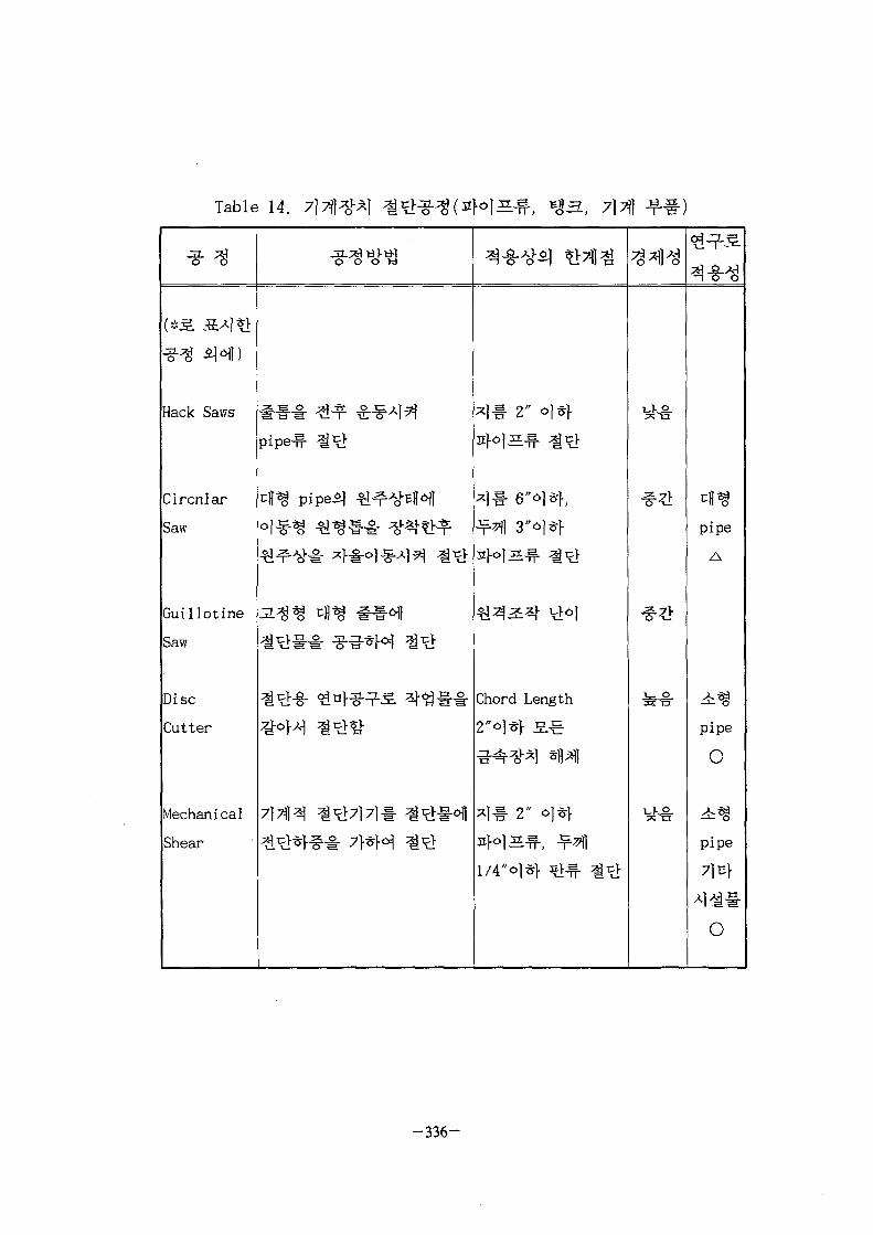
Table 14.
Hack Saws
Circniar
Saw
Guillotine
Saw
Disc
Cutter
Mechanical
Shear
pipe-W- ^ ^
m pipe*! * H ^ H
^1-t 2" o]*f
W f € *
-)# 6'ol*>.
Chord Length
2*o) *> S ^
*| a. 2" O|*|-
pipe
A
pipe
O
pipe
71E}
O
- 3 3 6 -

Table 15. pool
o o
Controlled
Blasting
Wrecking
Ball/Slab
Backhoe
Mounted
Rams
Flame
Cutting
Thermic
Lance
Rock
Splitter
BRISAR
Compound
Water Jet
*1W» »4te T|* 4*
^ 6 V-/S. ^ n^ T?p 1— 1 | ngp
^ * ^ a *
A
A
- 3 3 7 -
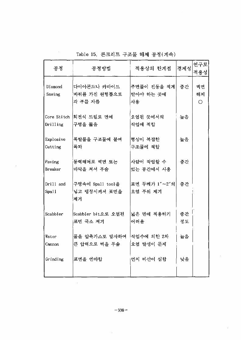
Table 15.
Diamond
Sawing
Core Stitch
Drilling
Explosive
Cutting
Paving
Breaker
Drill and
Spall
Scabbier
Water
Cannon
Grinding
2* * ^ *
-7-tg -e | Spall tool#
Scabbier bit^-S. SL<gQ
•a
On x*]l
o
- 3 3 8 -

flat form -§• <^e| 7}*\7\
bridge transporter7} °]n] ^
-^u}, TRIGA
-, bridge transporter^]
kg
TX>e> ^ e ] ^ l Table 16*]]^ i
Table 16. <£-
^^s. a^- - ]T]
ii^-f ^7]
^ H i-a# 47]
^ ^ S . Tank Liner 47]
Plasma arc
Mechanical
Shear(^%) Disc
cutter (^i^)
Circular saw(tH^)
Plasma arc
Mechanical Shear
Plasma arc
Diamond saw
Water jet
Controlled blasting
31^47]
Crane
Manipulator
Crane
Manipulator
Crane
Manipulator
Crane
Crane
Excavator
-339-

ofl
7}.
T2-0!]^^- Silicon Graphics^f-^l Workstation Onyx# h§-*>$g[t:}-. o]
fe R10000 «1^7| Reality Engine^- ^||
S^^H IGRIP
Deneb Robot i c s^WH 7^^} ^-g- i H I ^ M IGRIP (Interactive
Graphics Robot Instruction Program)^ ^V§-*}SSlcK
IGRIP^ 7 l ^ ^ t:}^-^- ^-^r ^ o | air}. [25]
- Part Modeller : Surface Modelling y<H-2] CAD
g • # «1# 4 ^ ^ 4^^1 (Polygon)*] ^^ -^ . ^ ^ - ^ ^ ^
*> CATIA, CADAM, AUTOCAD, Wave Front *§• Ef 7 l # 5 ^ CAD
Animation^!
-340-

4
*]
User Programming 7]-^
<H GSL (Graphic Simulation Language)
Line Interpreter)!
, CLI (Command
: C
(LLTI, Low Level Telerobotic Interface)^
Fig.
-341-

Fig. 61. H
Host workstationSGI Onyx
Graphic Modeller
Motion simulator
Off-line programmer
UNIX OS C-languogeinterface(LLTI)
Motor controllerRobotCameraSensorMotor controller
TW:
"ACAD
. Fig.
4
4 ^ 1 (replay)*fe
nje]
Animation-^- H
record)*|f
01
- 3 4 2 -
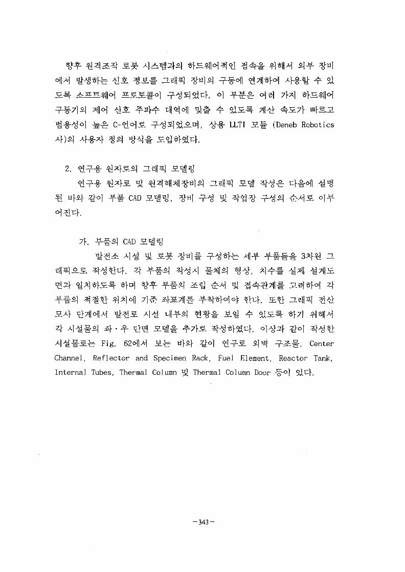
LLTI S # (Deneb Robotics
2.
CAD
7f. -f-g-S CAD
4
4 ^]^#^ 4--f >^ 1 ^ # ^ - ^ Fig. 6 2 ^ ] ^ J£^. B f ^ ^o) < ^ ^ ^ 5 ] ^ -7-2:-i-, Center
Channel, Reflector and Specimen Rack, Fuel Element, Reactor Tank,
Internal Tubes, Thermal Column ^ Thermal Column Door -%-°]
- 3 4 3 -

(a)
If1
Core and reflector
BBwB^ * • -
g (EM' S
(c) Center channel
Fig. 62. <£^
(b) Fuel element
ifflmm11
(d) Reactor internals
zj-
4
4
- 5 - ^ ^ <>1
oil" #*)*]
Center Channel, Reflector and
-344-

Specimen Rack, Fuel Element, Reactor Tank, Internal Tubes, Thermal
Column ^ Thermal Column DOOHEH $ 1 - ^ SflaH^HJ-S. 3 - ^ S i , Bridge
Transporter * ^h§ 4^f&4 ^ M 1^1 4§3*
Transporter-^- JsL-
Trolley<>|j -f"4*l't-H
- •*> SchillingAf^l Titan 7 S.^
3] ^ Bridge
^r Slh Trolleyofl
^ > 4^-§- s ^
transporter-^- _<H
d^}. Fig.
:f. Bridge
-^1 Boom^-
^ ^ ° 1 7}
6 3 ^ o]$\
Fig. 63. Bridge Transporter
Fig.
-g-o)
4
- 3 4 5 -

Fig. 64. TRIGA MARK III
-346-
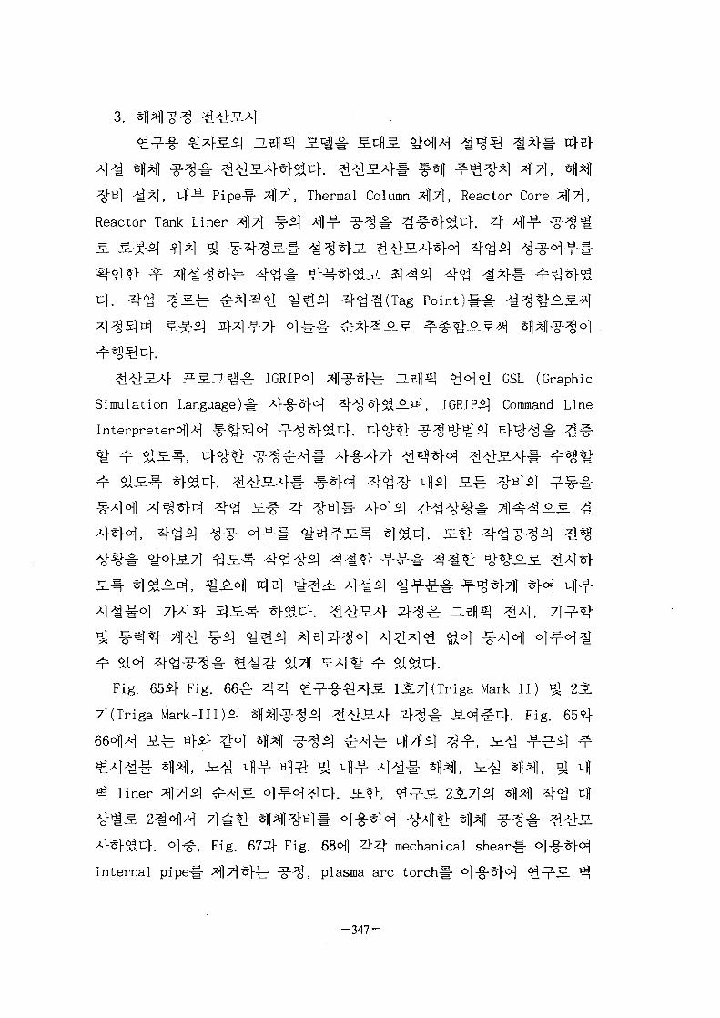
3.
^ a ) , ufl-f- Pipe^ff
Reactor Tank Liner ^7]
Thermal Column , Reactor Core *\}7\,
4 fl-f-
(Tag Point
^ ^ 4 ^5.^L5fl^ IGRIPo]
Simulation Language)^
Interpreter^^
m <d°]^l GSL (Graphic
, IGRIP^I Command Line
4
5]
Fig. 65if Fig. 66^: 4 4
7](Triga Mark-Ill)^
l5.7l(Triga Mark-II)
t:j-. Fi
*H*H.23L7}*)^ l iner z\]7]S>]
^ l ^ . ^ } . °1#, Fig. 672} Fig. 68^] 4 4 mechanical shear
internal pipe# *fl7t*ffe g- g, plasma arc torch# 61>§-*M
- 3 4 7 -
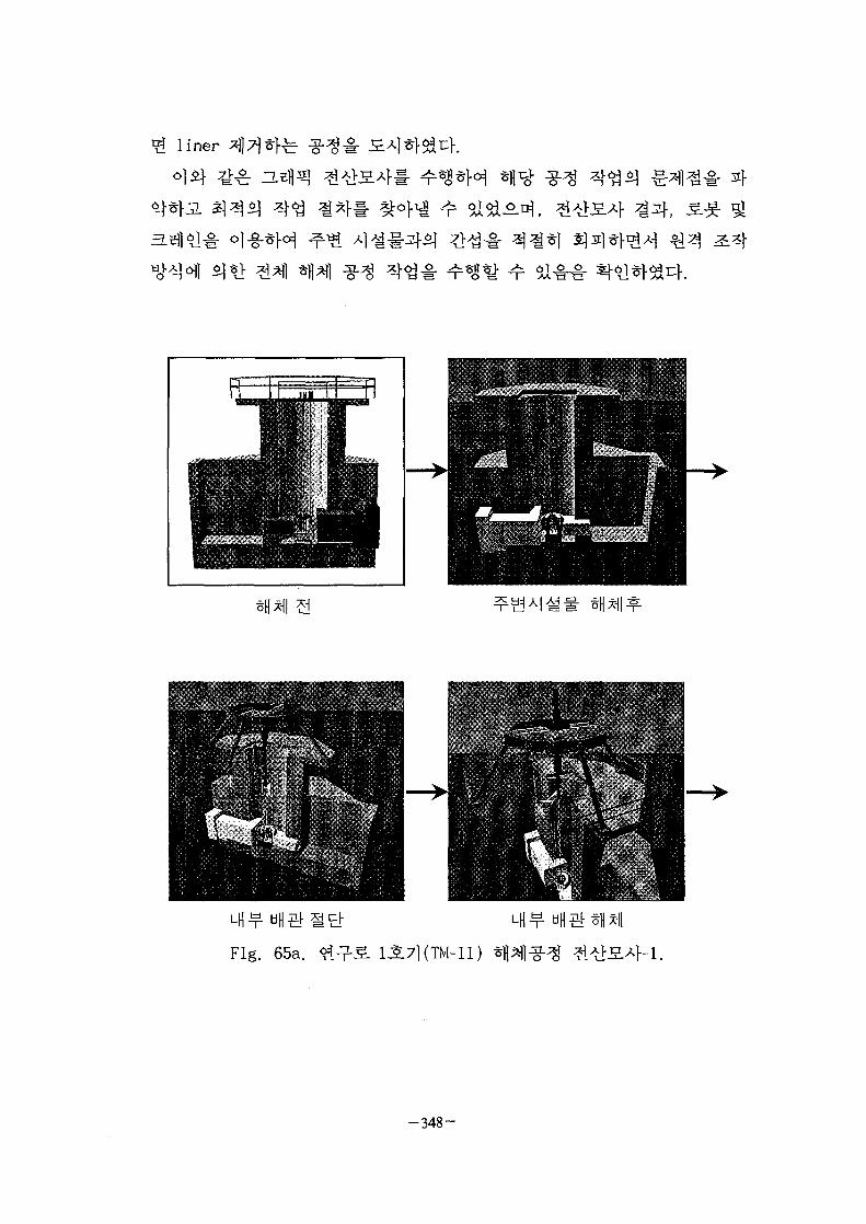
liner
4
Fig. 65a. 1JL7KTM-II)
- 3 4 8 -

mn
I IPiT" \
" 1 3
Fig. 65b. 1S7KTM-II)
- 3 4 9 -

Fig. 66a. 2JL7KTM-III)
- 3 5 0 -

Fig. 66b. 23L7KTM-III)
- 3 5 1 -

mechanical shear
Fig. 67. Mechanical s h e a r # <:>]<§-*> internal pipe *f[7]
- 3 5 2 -

Fig. 68. Plasma arc torch# °|-§-*> ^ liner
-353 -
- 3 5 4 -

*fl 4
TRIGA MARK
3.711 , laser localizer, 4^71
l(absolute position)^ ^>4(posture)
fe laser localizer#
^ EBERLINE
FH 40G
- 3 5 5 -

711
TRIGA
- 3 5 6 -

[I] ^ J i ^ UDC 629.182,
?>^-7]X|«i^-4i JjH| A } 7 l ^ ^ 9 - ^ , 1991.
[2] J. Yuh, Learning Control for Underwater Robotic Vehicles, IEEE
Control Systems, pp.39-46, April, 1994.
[3] US Patent 4,811,228, ."Method of Navigating an Automated Guided
Vehicle," Mar. 7, 1989.
[4] Lucas Electronics, Operations Manual: Inclinometers, 1996.
[5] »JlM, ° I W , C<d<>i5. Tfl *±= 80C196KC, tfl<g4. 1995.
[6] J. Yuh, "Learning Control for Underwater Robotic Vehicles",
IEEE Control Sytems Magazine, Apr. 1994.
[7] L.L. Whitcomb and D.R. Yoerger, Comparative Experiments in the
Dynamics and Model-based Control of Marine Thrusters, Proc.
MTS/ IEEE Oceans 95, October 9-12 1995, San Diego, CA.
[8] L.L. Whitcomb and D.R. Yoerger, Preliminary Experiments in the
Model-Based Dynamic Control of Marine Thrusters, Proc. IEEE
Int. Conf. on Robotics and Automation, pp. 2166-2173, 1996.
[9] A.J. Healey, S.M. Rock, S. Cody, D. Miles, and J.P. Brown,
"Toward an Improved Understanding of Thruster Dynamics for
Underwater Vehicles," IEEE journal of Oceanic Engineering, Vol.
20, No. 4, pp. 354-361, 1995
[10] Younger-Toumi, K. and Ito, 0., A Time Delay Controller for
Systems with Unknown Dynamics, ASME J. of Dynamic Systems,
Measurement, and Control, vol.112, pp.133-142, March 1990.
[II] P. Lu, "Optimal Predictive Control of Continuous Nonlinear
Systems", Int. J. of Control, vol. 62, No. 3, pp.633-649, 1995
[12] Hsia, T. C. and Gao, L. S., Robot Manipulator Control using
Decentralized Linear Time-invariant Time-Delayed Joint
-357 -

Controllers, Proc. IEEE conf. on Robotics and Automation, pp.
2070-2075, 1990.
[13] G. Y. Park, J. S. Yoon, and Y. S. Park, "Robust Nonlinear
Predictive Control of Underwater Wall-Climbing Robot",
Institute of Control, Automation, and System Engineer, vol.4,
no.6, pp.772-779, 1998.
", '97 Korea Automatic Control Conference, FA1-12-3,
PP.237-240, 1997.
[15] A. Baker, I.R. Birss, and G.F. Fish, "Remote Handling Equipment
for the Decommissioning of the Windscale Advanced Gas Cooled
Reactor," Proc. of Seminar on Remote Handling in Nuclear
Facilities, pp.581-597, 1984.
[16] L. Costa, et.al, "Remote Operation in Decommissioning,"
Decommissioning of Nuclear Power Plants, 1989.
[17] N. Eikelpasch et. al., "The KRB A Boiling Water Reactor pilot
dismantling project," Euro Courses-Greifswald, Sept., 1996.
[18] N. Eikelpasch et. al. , "Status of decommissioning at
Gundremmingen unit A," Kerntechnik 56, No.6, pp.367-371, 1991.
[19] N. Eikelpasch et. al., "Eliot Dismantling of the KRB A Boiling
Water Reactor, " Int. Conf on the Decommissioning of Nuclear
Installations, Sept., 1994.
[20] N. Eikelpasch et. al., "Remote techniques for the underwater
dismantling of reactor internals at the nuclear power plant
Gundremmingen unit A, " BNES, Remote Techniques for Hazardous
Environment, pp.14-19, 1995.
[21] Decommissioning Handbook, U.S. Department of Energy, U.S.
Government Printing Office, 1980.
[22] J.J. Fisher, "Applying Robots in Nuclear Applications," RI/SME
Robots Conf., June, 1985.
-358 -

[23] G. Clement, J. Vertut, A. Cregut, P. Antione, and J. Guittet,
"Remote Handling and Transfer Techniques in Dismantling
Strategy," Proc. of the Seminar on Remote Handling in Nuclear
Facilities, pp.556-569, 1984.
[24] K.H. Schaller, "Possible Advances in Remotely Controlled
Operations in the Field of Decommissioning of Nuclear
Installations," Proc. of the Seminar on Remote Handling in
Nuclear Facilities, pp.570-580, 1984.
[25] Deneb Robotics, IGRIP Version 2.3 User Manual, Pittsburgh,
1993.
- 3 5 9 -
NEXT PAGE(S)left BLANK
td ^ n
si
o|
— 3 6 1 -
NEXT PAGE(S)left BLANK

CONTENTS
Chapter 1. INTRODUCTION 377
Chapter 2. STATE OF THE ART 379
Section 1. Understanding of the state of the art 379
Section 2. Comparison and discussion of detail technologies...380
1. Comparison of detai 1 technologies 380
2.Main technical items 380
A. Foreign countries 380
B. Korea 382
Chapter 3. CONTENT AND RESULT. 385
Section 1. Soil decontamination 385
1. Introduction 385
2. Main Item 386
A. Electrokinetic soil decontamination 386
B. Soil washing 412
C. Decontamination equipment 425
3. Concluding remarks 433
Section 2. Dry decontamination of urban surface 435
1. Introduction 435
2. Theory 436
A. Ion exchanger 436
B. Surface contact angle and surface tension of
Decontamination agent 438
C. Rheology 439
3. Urban surface decontamination equipment 440
A. Equipment characteristics and principle 440
B. Equipment arrangement 440
C. Drawing of equipment arrangement 443
- 3 6 3 -

D. Photograph of equipment 443
E. Components and usage of equipment 448
4. Experimental 449
A. Makeup of decontamination agent 449
B. Basic property 451
C. Rheology 453
D. Measurement of surface contact angle 454
E. Preparation of hot specimen 454
F. Decontamination test 455
5. Result and discussion 455
A. Basic Property 455
B. Rheology of clay decontamination agent 463
C. Interfacial property of clay decontamination agent 466
D. Relationship between flowing property and interfacial
property of clay decontamination agent 466
E. Decontamination test 469
6. Concluding remarks 476
Section 3. Soil remediation performance assessment and
radionuclide migration modeling around the TRIGA
research reactor 477
1. Migration of contaminants in the unsaturated zone 477
A. Comparison with the saturated zone 477
B. Hydraulic property of the porous media 478
2. Comparison and analysis of codes 482
A. Input parameter 482
B. Analytical model 485
C. Mathematical model 491
3. Application of decontamination assessment model 493
A. Input parameter measuring method 493
B. Boundary condition establishment method 496
-364-
4. Development of one-dimension non-equilibrium sorption
model 498
5. Residual radioactivity dose analysis after remediation...508
6. Radionuclide migration modeling around the TRIGA research
reactor 518
A. Topography and the underground water table 518
B. Measurement of on-site hydraulic parameters 520
C. Modeling of underground water flowing system 525
D. Radionuclide migration system prediction modeling 532
7. Concluding remark 538
Chapter 4. ATTAINMENT DEGREE ON THE RESEARCH TARGET AND CONTRIBUTION
DEGREE TO THE OTHER AREA 541
Chapter 5. APPLICATION PLAN OF THE RESULT 543
Chapter 6. REFERENCES 545
- 3 6 5 -
NEXT PAGE(S)left BLANK

1 # M £ 377
2 # ^H.SJ 7]^A^ £ % ....379
379
380
H]J2. 380
2. ^ § ^ 1 1 ^ A 7 ]# Lfl-g- 380
7}. $m 380
v}. ^ 382
^ ^^-711 ^ * ^ H ^ - T£ %3\ 385
1 ^ A^S^ 4^71^ 7^ 385
1. *1 . . ' 385
2. ^- § 386
7\. ^-^.7]^ S^]<^7l^ 386
^ ^ > 412
^ l ^ ^ 1 4 ...4253. ^ 433
1 2 | £.*] S ^ ?m 4 ^ 7 1 ^ 7Bt 435
1. M & 4352. <*] -4 JL% 436
7\. °}£: 3. : 11 436
fl£«£| ^ ^ ^ 438
...439
3. SA]S^ ^-i} I ^ ^ l 440
7}. #*1 ^-^ ^ 7^SL 440
^f. ^ 1 TH§ 440K 443
443
448
- 3 6 7 -

4. ^ ^ 449
7j. ;** jg. ^) < [] ^[]3: 449
U. 7 ] £ #A^ 451
t}. - f r ^ ^ 453
5}. S.1^ -^ r^l" ^ ^ 454QL tJWl.yM j£_64 A J ^ -^liS. 454
«>. ^ 1 ^ ^ ^ 455
5. ^ 4 9l 3L% 455
7f. 7}^: # ^ 455
463
466
466
4. 4^ ^ ^ 4696. ^ £• 476
477
477
7}. 3L$\X\<^3}$] ^[O]^ 477
"M". ^ ^ o " ^ 0 ! ^ - ^ "T'5!^-^) 478
2 S ^ 1 ^ ] ^ '*§^rJ%7}S-xzl y]o2.~E"^4... 4827]. B^7|.^^<5i sj AV-^-SS 482
~i\. ^xlS.1^ ti]^^^ 485
5. ^ 1 ^ ^^-^f^ 21-^- ^ 508
6. TRIGA ^ * i ' ^ ^ o l ^ <W S ^ s j 518
7}. *1% 9l ^1^}^1 518
- 3 6 8 -
H"
t l
?'}
7 ^
4 -Q
5 #
6 #
520525
532
538
H£ 541
543
545
- 3 6 9 -
NEXT PAGE(S)left BLANK

Table 3-1. Chemical Composition of Kaolin Clay 398
Table 3-2. Physical Property of Kaol in Clay 398
Table 3-3. Parameter Range of Electrokinetic Decontamination
Process 404
Table 3-4. Physicochemical Properties of Soil 415
Table 3-5. Oxide Composition of Soil 415
Table 3-6. Physical Properties of Certain Cations 437
Table 3-7. Components of Decontamination Kit 448
Table 3-8. Manufacturing Composition of Decontamination Agent. ..452
Table 3-9. Properties of Clay Studied 457
Table 3-10. Composition of Tested Specimen 462
Table 3-11. Power-law Parameters of Modified Clay Suspensions as
Fitted with Equation(3-1) 465
Table 3-12. Input and Output data of Each Code 484
Table 3-13. Status of Codes for Assessment of Soil Decontami-
nation 486
Table 3-14. Component Content of Soi 1 503
Table 3-15. Density, Porosity, Water Content, and pH of Soil 503
Table 3-16. Inhalation Dose Conversion Coefficients 515
Table 3-17. Ingestion Dose Conversion Coefficients(mSv/Bq) 516
Table 3-18. Hydraulic Conductivity of Each Layer 521
Table 3-19. Porosity and Moisture Content of Each Layer 522
Table 3-20. Dispersivity of Sediments 522
Table 3-21. Diffusion Coefficient of Concrete 523
Table 3-22. Distribution Coefficient of Radioactive Nuclides and
Phenol 524
Table 3-23. A Half Life of Nuclides 525
- 3 7 1 -NEXT PAGE(S)
left BLANK

Fig. 3-1. Electrokinetic Transport Phenomena 387
Fig. 3-2. Experimental Apparatus for Soil Decontamination 400
Fig. 3-3. Logo Screen for Monitoring the Soil Decontamination..402
Fig. 3-4. Monitoring Screen for Soil Decontamination ..402
Fig. 3-5. Screen for Analyzing the Experimental Parameter 403
Fig. 3-6. Double Plot of Voltage and Current against Time 405
Fig. 3-7. Accumulated Effluent Volume against Time 406
Fig. 3-8. The Movement of Front against Time at 30 V 408
Fig. 3-9. Change of Cs+ ion Concentration according to the Length
from the Cathode 410
Fig. 3-10. Cs+ ion Concentration of Effluent against Time 411
Fig. 3-11. Sexidendate Octahedral Model of the Co-EDTA ion 416
Fig. 3-12. Amount of Adsorbed Co against Time 420
Fig. 3-13. Desorption of Co according to the Concentration of EDTA
under Various pH 421
Fig. 3-14. Amount of Desorbed Co against pH under Various
Temperature 423
Fig. 3-15. Amount of Dissolved Fe against pH under Various
Temperature 424
Fig. 3-16. Competitive Reaction Mechanism between Co Ion and Fe
Ion on EDTA in Soi 1 Solution 425
Fig. 3-17. Arrangement Drawing of Soil Decontamination Equipment..428
Fig. 3-18. P & ID of Soil Decontamination Equipment 429
Fig. 3-19. Control Circuit of Soil Decontamination Equipment....430
Fig. 3-20. Photograph of Soil Decontamination Equipment(Top and Side
View) 431
Fig. 3-21. Schematic Drawing of Urban Surface Decontamination
Kit. 444
-3 7 3 -
Fig, 3-22. Photograph of Urban Surface Decontamination Kit 445
Fig. 3-23. Photograph of Urban Surface Decontamination Kit (Side
View) 446
Fig. 3-24. Photograph of Spraying Operation 447
Fig. 3-25. Photographs of Specimen; (1) Weight-Concrete (2) Fired
Brick (3) Red Brick (4) Silicate Brick (5) Wood 455
Fig. 3-26. Optical Microphotographs of Silicate Brick(l) and Fire
Brick(2) 459
Fig. 3-27. Optical Microphotographs of Red Brick(3), Weight crete(4)
and Wood(5) 460
Fig. 3-28. X-Ray Diffraction Pattern of Hectorite 461
Fig. 3-29. Non-Newtonian Viscosity of Decontamination Agents... .464
Fig. 3-30. Surface Contact Angle according to Hectorite
Contents 467
Fig. 3-31. Viscosity Parameter n and Surface Contact Angle According
to Hectori te Contents 468
Fig. 3-32. Activity Ratio of Residual to Initial Cs-137 according to
Decontamination Cycle Using HT-type Decontamination Agent
(Contaminated with liquid Cs-137) 471
Fig. 3-33. Activity Ratio of Residual to Initial Cs-137 according to
Decontamination Cycle Using Na-type Decontamination Agent
(Contaminated with liquid Cs-137) ...472
Fig. 3-34. Activity Ratio of Residual to Initial Cs-137 according to
Decontamination Cycle Using HT-type Decontamination Agent
(Contaminated with liquid Cs-137 and Dust) 473
Fig. 3-35. Activity Ratio of Residual to Initial Cs-137 according to
Decontamination Cycle Using Na-type Decontamination Agent
(Contaminated with liquid Cs-137 and Dust) 474
Fig. 3-36. Activity Ratio of Residual to Initial Cs-137 of
contaminated with liquid Cs-137 respect to dust and
liquid Cs-137 according to decontamination(HT-Type)..475
Fig. 3-37. Typical Soi 1 -water Retention Curve 479
Fig. 3-38. Tensiometer Used to Measure Soil-water Potential
-374-

in the Field,,,,, 480
Fig. 3-39. Relationship of Hydraulic Conductivity to Matric
Potential for Wetting and Dying Cycle Illustrating
Hysteresis 481
Fig. 3-40. Unsaturated Hydraulic Conductivity as a Function of Water
Content for Three Temperatures 481
Fig. 3-41. Relative Permeability vs. Moisture Content for Sand,
Clay, Si 1 ty Loam, and Sandy Loam 489
Fig. 3-42. Use of Pressure-head Gradient Boundary Condition to
Simulate a Portion of the Unsaturated Zone 490
Fig. 3-43. Linear Sorption Isotherm with S versus C 494
Fig. 3-44. Nonlinear Sorption Isotherm with S versus C. 495
Fig. 3-45. (a) Nonlinear Langmuir Sorption Isotherm will Reach a
Maximum Sorption Value When S is Plotted versus C
(b) The Langmuir Sorption Isotherm can be Made Linear
by Plotting C/S versus C 497
Fig. 3-46. Apparatus for Solvent Flushing 499
Fig. 3-47. Equilibrium Sorption Coefficient of Co Solution with
the Soil 504
Fig. 3-48. Co Sorption Ratio in the Soil versus Time 505
Fig. 3-49. Experimental results Remediating the Soil of High
Hydraul ic Conductivi ty by Water 506
Fig. 3-50. Experimental and Model Prediction Results Remediating the
Soil of Low Hydraulic Conductivity by Water 506
Fig. 3-51. Experimental Results Remediating the Soil of Low
Hydraulic Conductivity by EDTA Solution 507
Fig. 3-52. Location and topographical Map of Study Area 518
Fig. 3-53. Configuration of Water Table and 4 Layers 519
Fig. 3-54. Kind of Rock and Soil in Study Area 520
Fig. 3-55. (a) Constant-head Test Equipment (b) Falling-head Test
-37 5 -

Equipment 521
Fig. 3-56. Distribution Coefficient Measurement Procedure ..523
Fig. 3-57. Base Map of Study Area 526
Fig. 3-58. Finite Element Net about Study Area 527
Fig. 3-59. Groundwater Flow Modeling in 1 Layer of Study
Area 528
Fig. 3-60. Groundwater Flow Modeling in 2 Layer of Study.
Area 529
Fig. 3-61. Groundwater Flow Modeling in 3 Layer of Study Area...530
Fig. 3-62. Groundwater Flow Modeling in 4 Layer of Study Area...531117
Fig. 3-63. Cs Transport Modeling in 1 Layer of Study Areaafter 5 Years 5331 17
Fig. 3-64. Cs Transport Modeling around Reactor along Time. ...535
Fig. 3-65. 90Sr Transport Modeling around Reactor along Time 536
Fig. 3-66. 60Co Transport Modeling around Reactor along Time 537
-376-

1 S- M
3.3. 4^r
Hanford Site
o] A
m3
n)^- ofl, «I
TRIGA
TRIGA
Cs, Sr,
NH4+
CEC
15 NH4+
TRIGA
TRIGA
TRIGA MODFLOW
TRIGA MT3D
Cs, Co
— 377-NEXT PAGE(S)
left BLANK

ANL, Oak Ridge National Lab., Sandia National Lab., PNNL,
Los Alamos^ ^ t J g ^ f c o M *#*}& SL<& £<£ ^ 1 ^ 7 ] # # 7^ #ofl &
cf. Oak Ridge National Lab. 1996^ E M * 1 ^ * J ,S_<g -*l(K-25 site)
Hanford site*] ^ - ^ # JH*H 1996\1 Flour Daniel Afif %>^ 5\1^> 50<^ $
, KIST
nfl-f ^uf. -f el i^efe ^^1 ^-3.7}
3 D < ^
safe ^AS. sra^nK -f el u}ef£ TRIGA
711
- 3 7 9 -

fe 1995
ICRP 6fr§-
71^ 4-¥- % ^
^ ^ ^ ^ l
^ e l
^>^-^4-^ 711 -
^ 7 }
^r ^ 7} ^
S-<gT£7l]
7 ] ^ ^^^17^1
7Hy^ ^7^1
7 f l ^ ^Tf l
7^ *t*H
^r $ 7] ^ * ^ 71 ^^-^ ^H, ^1
^-^ 4 , ^1
^ 1 ^711
2.
7}.
25
- 3 8 0 -

biodegradation #
- bioventing •#
- soil vapor extraction t|{
soil flushing -fr
soldification/stabi 1 ization t:l|
vitrification -fr
Thermally enhanced soil vapor extraction t:|{
solvent flushing -fr
slurry phase biological treatment £§
controlled slurry phase biological treatment tf|
electrokinetic method •§•
land farming #
soil washing tj]
dehalogenation •§•
chemical reduction/oxidation •§•
low temperature thermal desorption •§•
incineration cfl
o Deterministic
o Stochastic
o Saturation Zone
o Unsaturation Zone
- 3 8 1 -

fe- soilwashing, solvent flushing ^ electrokinetic soil decontamination ^
•§• 7 f l ^ M # ^ soil washing ofl $a<H>H-b bench ^ - S ^ ^l^^l-t
4 l .n|, electrokinetic soil decontamination *g£-
biodegradation
bioventing
soil vapor extraction
soil flushing
soldification/stabilization
vitrification
Thermally enhanced soil vapor extraction
solvent flushing
slurry phase biological treatment
controlled slurry phase biological treatment
electrokinetic method
land farming
soil washing
dehalogenation
chemical reduction/oxidation
low temperature thermal desorption
incineration
-382-

o Deterministic S.
& Stochastic S.^
o Saturation Zone S
o Unsaturation Zone
*}•
— 383 —
NEXT PAGE(S)left BLANK

^ 1
1. 44
e . 4 . Chernobyl ^ 4 ^ 4:2., ^.Bj-^ Goiania,
km2 45 cm
fe 71 igr,
1&-S- ^g-^7]^(electrokinetic)
7 } ^
sa
TRIGA 2002
Cs, Sr, Co o ) ^ - ^
4
- 3 8 5 -

'-'• i__ ii_
7}.
. o]
electromigration ), ^,71 'tHF! electroosmosis ), ^.71 ^-^( electro-
phoresis) o| <&z.\. $_7]
3-1 -8: ^ ^ 7 } ^ O)^^AO>^. ^.o^ ^t ;^ £7]
4~§-(drag interaction)^! 5l*fl 4 ^ -
-fr^t^ ^ ^ ^ r o|-f^(double layer)
^ -S 1 " 10 urn 51
l 51 ?> cfl - ^-£( convective liquid
velocity ) ^ JL*fl S^^ l ^E} ^ ^ ( 5 ), ^^] ^-afl( gradient of
electrical potential)^ ^-51 ft°LS. $S>)V} Z^&Q *\7}^
(electric field strength, E H t)]3ltM. ^l^^l 3.71 AJ- H]J2.*H
&£ ° l##( th in double layer)^} tfl*Jf,
S.fe Helmholtz-Smoluchowski
-386-

Ueo = £?E/J1 (1)
Eiectrophoresismovement of parades
ElectricalDoubleLayer
Electromigdationmovement of ions
Fig. 3-1. Electrokinetic Transport Phenomena
ti]
Ueffi = VZFE (2)
(mobility), F fe
7}
.tLS. -B-S.(pressure-driven)5j-b
-38 7 -

3.7M °]
3.7}o\]
Jit* €-
(imperfection) ^ ^ S]^ ^}^ 7}x\7\]
potential)
10 - 100 mV S)
< )] Tfl ^ . < g # ^ £ ^ - i - W i:B^-( electroosmotic
convection ) if # 7 ] °]^-ofl 5 ] ^ ^^]^ ] 2,^}^ -g-sf{
(transport) £ "L
H20 - • 2H+ + 1/2 02 + 2 e" E° = + 1.23 V (3)
H20 + 2 e" - • 2 OH" + H2 E° = - 0.83 V (4)
- 3 8 8 -
2*} tiKg-o]
2 H+ + 2 e~ -+ H2 t (5)
Men+ + n e" -* Me(s) (6)
-i, Me -
4,
2) ° m ^ wH^[3-l, 2]
7\) H 6O ^ PH
pH
fe ^ % ^ © ^7l^-tifl(electric gradients) ofl y\
ionic migration), (2) ^7] - --f- ^ # ^ ] 7|6]*>
ionic migration)
o]
- 3 8 9 -

7}
E ZiC; = 0 (7)
Z i ^
= [H+] [OH'] (8)
«|*j[ ufEfufe o]
AH u
, D; ^ %^>^1^, ui fe *l-^#5l oj^-s., F fe Faraday
^ , T fe Wll"^ 4^r(tortuosity) oji:].. #
B S , pH 7} ^ ^ f K r ^I^lfe # 4 * f e
; ^-xl #££c^l 51 *U ^ ^ £ j p . ^ pH 7}
(mobility) ofl
PH 7f
. pH 7} ^ 4 .
%\ f i ^ pH
- 3 9 0 -

n+ + nOH" -»• M ( O H ) n j
pH o\)M bizincate °
(10)
2+Zn2+ + 30FT •-> HZnO2" + H20
, 371-
(11)
p H
"^ PH 7}
*H °1:§-*M pH 7}
3L pH 7}
focusingjojel-
PH 7}
. pH
fume
0.001 M 3] % ^ > o l ^ ^ - PH 7} 4
106
^ : 75-95
13
Calcium zincate if calcium chromite ^-S. ^7 ]
- 3 9 1 -

} 0.001 M
37} 3.^$] -§-«HS-^ 102 ~ 103
B pH ^ S H - ^ ^ * } 7 l ^]sfl Af-g-5)^ ^ 1 ^ 1 ^ ^ : bromophenol
blue(pH 3 o]*H>Mfe i-5o^, pH7} 4.8 <>1^6fl^^ ^ ^ : ^ ) ^ Phenol
red(PH 6.8 o j ^ H ^ f e ^^J-, PH7]- 8.4 o)^6f lA^ ^ ^ ^ ) o ) ^ } . ^ ^
5^ ^ 1 A | ^ ^ PH 3 o]*HM-b i^eov, 3 - 6 . 8 ofl>H-b ^ ^ ( g r e e n color),
PH 7}
pH
^ S . pH f
^ ^ pH # ^ o ] £6ol= ^HlJlL ^
Pourbaix diagram $] ^ pH
pH
^ Nernst -i]# 4"§-*H
nF Ili [reduced species]vRT 1 I!; [oxidized species]v
-392-

oxidized species + ne —* reduced species (13)
potential ) #
Nernst ^ ^ .
Cr3+ + 4H20 -> HCrO4" + 7 H+ + 3e E° = +1.35 V (14)
^ t h 1 ^ ferric
pH J ^ ^ f % € ^ H tH*H Pourbaix diagram
Stic}. A>5f5l ^ - f <?] 67}
37} £L# ^>5}1-^ g-q- 5:^*} ^ pH
^ojul-. 37} 3 . ^ - ^
- 3 9 3 -
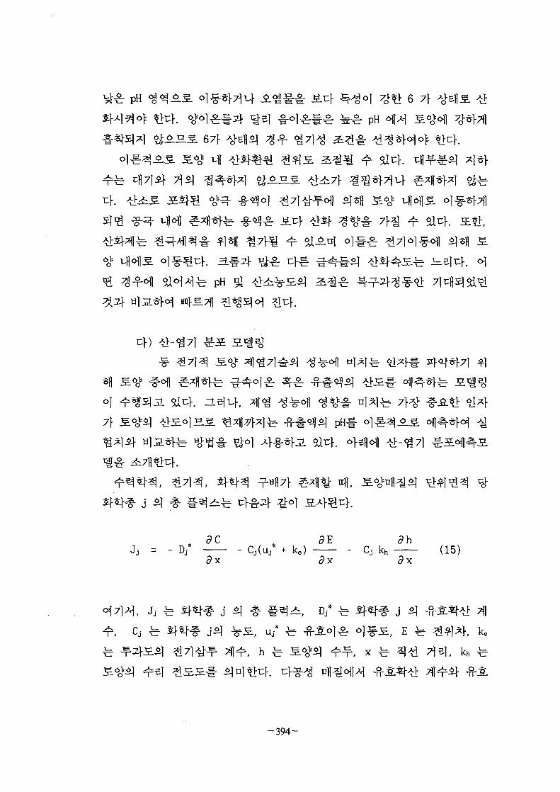
pH <$<*±
JEL5. 67f
Jit;]- 6 7}
fe pH
7} pH#
t dcD/ CJ(UJ*
3x dx
dhj kh (15)
dx
£, u/ fe ^-^o)^ o^JE, E ^ &$*}, ke
- 3 9 4 -

4 ^ 7 ^ Dj ^ o |£ oj-f-s. UJ
61
= Dj I n (16)
D * z • FU j * = UJ I n = (17)
RT
tortuosity
dt= - V • Jj + nRj (18)
•§-
18 o) 4 l
9E 3E aQ[(U j* + ke) + kh ] + nRj (19)
dDj j
d t dx dx dx dx
, H+
- 3 9 5 -

H20 <-> H+ + OH" (20)
ZLtfES., H+ 2} OH" o ) ^ ^ ty^ o ] § o]^-(coupled t ranspor t ) -^
°1£^7} ^l^S]o]x|^ ^o] ^Qo]t\. H*
Kretardation factor) <H1 *11 ^ ^ 5 | ^ ^ ttj,
a U cy LH d LH
- PH+ + DAH+ ( 2 1 )3X2
OH"
d COH 3 COH 9 COH
d T0H" ax 2 d x- POH" + DAOH" (22)
Pj ^ Sj-^-f1 J °fl tfl*l Peclet number
f. D/y -fe- Damkohler number
^ ^ ^ (14) 4 ] ^
CH+ • COH" = Kw ( 2 3 )
10"14 o ]H
. Faraday ^4}ofl rcfs},
- 3 9 6 -

<£•=*• ^ H ^ flux boundary
condition^ ^S]*K2. -fi- > [4:^ (finite element method)^
pH
#^l pH »!5Hr ^ «
3)
(1) Cesium chloride(CsCl)
Merck 4 $ ] ^ S 99.5 % O|AV^| GR
^ 168.36 o)uK
(2) Bromophenol blue(CigHioBr405S)
Showa chemicals Inc. $] ^--g- ^1
o>^. 669.97 o]c>.
(3) Phenol red(Ci9H14O5S)
Junsei Chemical Co. 3] ^gX
354.38 ojcf.
(4) Kaolin
Showa chemicals Inc. 5] 1-g- A]
#e l^ ^ -^# S 3-2 ofl ^
(1) 0.01 M Cs
(2) 0.01 M Cs -§-«<f 100 ml, 150 g ^ Kaolin, 5 ml S] *]*]<$
(Bromophenol blueif Phenol ^ ^ " - § - < ^ ) # - 3 : ^ * ^ ^ tS" t ! :4 .
(3) 5-^*1-71] ^ ^ ^ S<>OU]S# tapping isMM &7] ce l l ofl
^H^r^K * f l ^ # kaolin £ ^ A | ^ - ^ 122 ± 2g ^$] ).
(4) ^ ^ <^^
(5) ^«U ^ ^
(6) A l # ^ ^ c f l n ^ ^ 7 ] ^ ^ * # « } S 1 -¥•=] ^ P H # ^
- 3 9 7 -

Table 3-1. Chemical Composition of Kaolin Clay.
^ tf &SiO 2
A12O3
Fe2O3
CaO
MgO
H20
72.1019.570.390.800.540.70
100.00
Table 3-2. Physical Property of Kaolin Clay
Parameters
^-§-*J} pH
Value
6.8
300 mesh
7.01 m2/g
0.37 g/cm3
(7)
(10) Kaolin
Cs
0.45
(8) 7HA] 72(9) 71 cell S.-fel kaolin
pH
fe Cs
^-H 3-2^On-line
-398-

(1) *1-
S . ^ 4 ^ #*}£) 31°]^ 41 mData acquisition) ]S. PLC
(Programmable Logic Controller)!-
Hl^-7l^ ^ PC
71^ ^o) 1 7 O ^ ?14^H ^ jo ju} . PLC*] -7-^^ A } ^
CPU JS.1-, ^ H S 2 # ^ ^ * H CPU S #
H ^ 3-2 *1 ^ ^ H l ^ ^ - ^oj 80-10 V <q tllo]e|3- ^O]-1-O|JL CPU S # ^ r ^ l ^ ^ o ] ^ ^ ) E . ( I / F unit)
# ^f-sfH PC^I t-iio]B|i- ^ ^ t l ^ K ° 1 4 CPU s # ^ } PC 4 | ^
RS-232C S. -f-^lSI^, 4<^ SZL^-i- ^ ^ T j u l - CPU S' rrl a i lr lHll i-l >1 O Cl 1 1 *J -71.^1 rtl p j p j].C>l:_O_
CPU £ . #
% ] : FPU81A
=-;£ : lms/step
Lsfl v%2.Z] -g-so> : 10.5K step
g I/O ^ ^ : aitfl 1600^
n i/o ^ : 3}cf 100^
-^399-
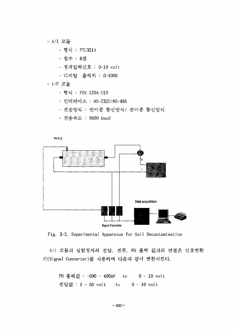
A/i
I/F
FTU321A
: 0-10 volt
1 : 0-4000
FFK 120A-C10
!^ : RS-232C/RS-485
: 9600 baud
Signal Converter
Fig. 3-2. Experimental Apparatus for Soil Decontamination
A/I S#2} -y^
7}(Signal Converter)#
PH
PH # ^ ^ : -600 - 400mV to 0 - 1 0 volt
= 1 - 5 0 volt to 0 - 1 0 volt
- 4 0 0 -
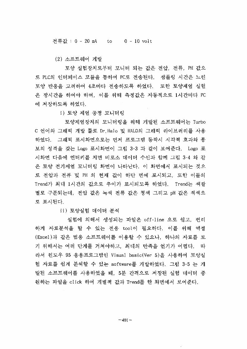
: 0 - 20 mA t o 0 - 1 0 v o l t
(2) -tSJE
^ ^ i l ^ ^ & &Q ^^ PH &SL
4i=S^|<H-b Turbo
Dr.Halo % HALO He|[5] ej-o]M.tf B]#
Logo S A l J ^ o l HQ 3-3 21- ^ o | ^.<H^4. LogoZL^ 3-4 if
PH SJ ^ 4 ^o] ^ t > ^ofl
Trend7> ajcfl 1A|^>^ ^-^ .5 . -^o]7} 1 A 1 5 ] £ 4 v}&^}. Trendy ^ ^
^ ^ ^ ^ nelJL PH ^ ^ ^ ^ ^ .
i i )
^ ^ ] ^ f l ] |fe- 4 < y ^ off-line
toolo] ^^ .^uK
(Excel )2f ^ ^ ^-g- ^SH^1<H# o)-§-^ ^ ^ ^ . 1 ^ . , ^ U ^ ^ S # J£
7] ^Sfl^-b ^51 ^ ^ ] 1 - T ^ ^ o ^ a , ^ 4 * ] n>^.^. ^ 7 | 7 | . c^^c}. rcf
95 -g-g-iESa^^l visual basic(Ver 5 )# 4-§-^M S 6O ^
software!- 7H^F$ii:K a^J 3-5 fe 7H
click *M 7 f l ^ ^^1- Trend
- 4 0 1 -

Fig. 3-3. Logo Screen for Monitoring the Soil Decontamination.
W94.. 8.1b-16. 0.36
Current value
i TTJH
Fig. 3-4. Monitoring Screen for Soil Decontamination.
-402-
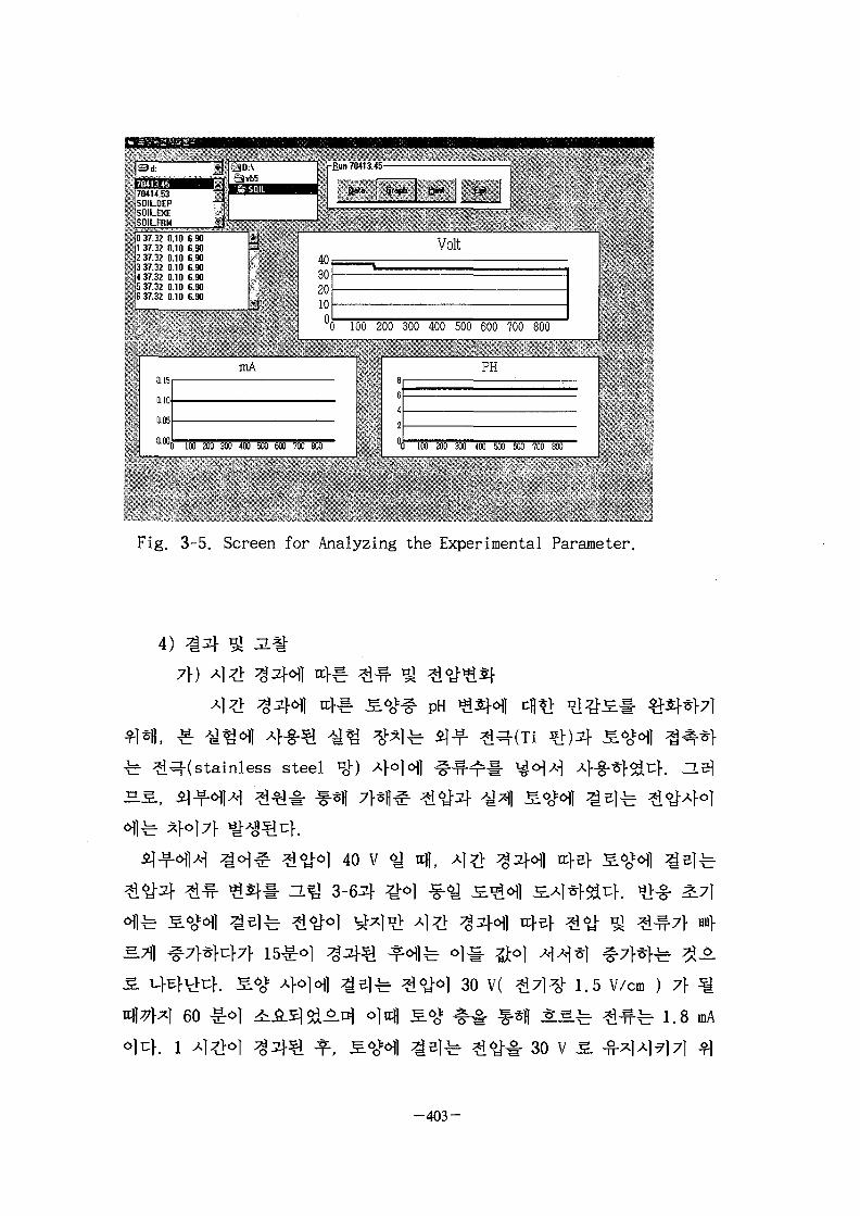
rRun 70*13 « -
70414 53SOU DFPSOU E ft1011 fflM " j
. 0 1 / \> 1110 b901137 3? 0 10 6 90?V V 1110 billj3 37 J2 010 6 9014 37 V 0 10 6 905 37 3? 010 6 90G37 32 010 6 90
tt
ftata Graph Hint Eat
"'jit
! --1.::•
uJiO 300 400 500 600 700 800
1 •
1 '
l i t
11.Ill
'.A
Fig. 3-5. Screen for Analyzing the Experimental Parameter.
4)
7})
fe ^q-(stainless steel
40 v «y 4 ,
60
27]
30 V( ^ 7 1 ^ - 1 . 5 V/cm ) 7> %|f ^ s . ^ s . ^ j 8 mA
3 0 V S ]
- 4 0 3 -

^ l 30 ± l v 3]
(electroosmotic advective flow )o]s}
Helmholtz-Smoluchowski
Table 3-3. Parameter Range of ElectrokineticDecontamination Process
Parameter
Electrode spacingAppliedApplied
potentialelectric field
Cross sectional areaCurrentCurrent density
0
00.05
10563
Range
20 cm~ 40 V~ 2 V/cm.14 cm2
~ 2. 3 mA0.37 mA/cm2
-404-
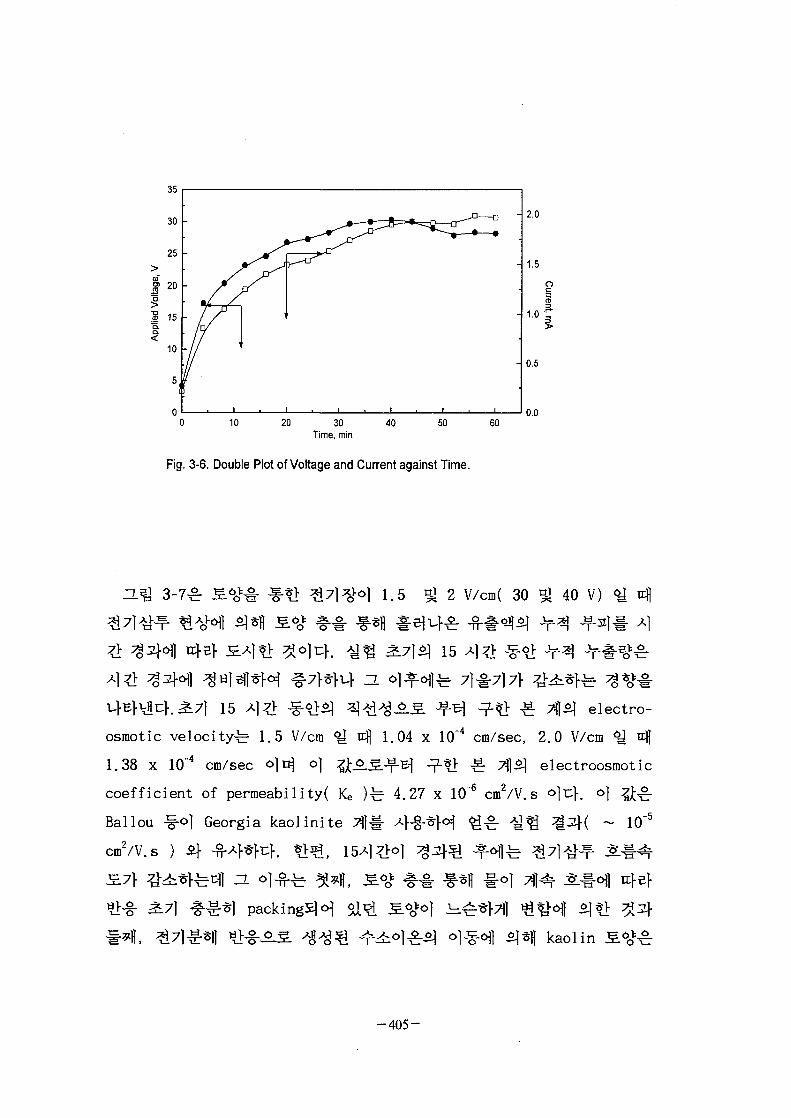
30Time, min
50
Fig. 3-6. Double Plot of Voltage and Current against Time.
60
life}.
1.5 2 V/cm( 30 *? 40 V)
%•*>15
3i7| 15 -*]%S ^f-^rS) -^^^g^-jiL ^T"^| -j2-^} -^ ^1-S] e l ec t ro -
osmotic veloci ty^- 1.5 V/cm ^ tcj) 1.04 x 10"4 cm/sec, 2.0 V/cm < tcfl
1.38 x 10"4 cm/sec o]n| o) ^jvg.-f-B] T2-?]; ^ 7 ]5] electroosmotic
coefficient of permeability( Ke )-b 4.27 x 10"6 cm2/V. s o]t:>. o] $g-
Ballou
cm2/V.s
Georgia kaolinite 7}] 10-5
«>-§- packings]^
kaolin S6O>^
- 4 0 5 -

acid/base front
(3), (4)
cr electromigration ^ electroosmotic flow o)t}.
ionic mobility fe 3.6 x 10~3 cm2/Vs,
10~3 cm2/Vs o|t:>.
-47.6 x 10"\
-tl:porosity
-n-jL ionic mobility
4.3 x 10~4 cm2/Vs S. •
ionic mobility
turtuosity factor
1.8
e ^ 4.27 xlO-6
10 15
Time, hr
20 25
Fig. 3-7. Accumulated Effluent Volume against Time.
( 9.3 x 10⁵ cmVs) if ( 5.3 x 1(T cmVs)
-406-

electromigrationofl
electromigration J5.
l^r ^ 6 H V O 1 30 V <y n| A]^> ^ o f l nfg. acid ^ base
H ^ 3-8 <HT S.Al*}-5it:f. * J ^ 2 i 7 H f e acid ^ base*] o
base front 5] ol^^£7|- acid front o]^^^<^| H]*1( £
K Bromophenol blue 7} pH = 3 °]^l"61]^fe Jt^, phenol red
7} pH = 8.4 o]^-6fl^-b ^-^r ^ - ^ S . W ^ H r # ^ ^ ^ 4 , base
front 1 o}^.^.^7} nj f 5£S|-^ oj-fi-fe- acid front if base front7f >
^ ^ ^ 10 ^1#°1 ^^f£lSi-i- it)] acid front ^ 12 cm, base front ^>
5.3 cm 7} o]%.-Q<ftc\. Acid front $] o]^-^^7} base front ofl
2.3 HB WJ -cll O}^. O ] ^ ^ 1 ( ~ 1.7 afl ) off H]*H 3 . ^ . o ] ^ ^y ^ ^ l ^ 1 - ^ ^ ^ 7 ] ^ ^ MAoV, S 6 ^ *}*flS] ^ ^ ^ ^ ^ transport
number ^ H ^ f ^ ^ r 4 ^ ^ ^ I ^ H
porosity# n &.£. 7}^^ ir(f, (19)
l-fe 7]e] xofl $I<H-H^ flux*] 7 | e H r t}^ £ 2 } ^ g| sj-«|-
. ^r^iol^r^l electromigration 2f electo-
osmotic advective flow - - - # ^ ^ ^ ^ ^^-^-S. ^ *|^MRt r
electromigration ^ ^ ^ r electoosmotic advective flow «Hf Hi
pH 7} 4.3
*fe Cselectromigration 6fl $X°]M ^^|S>-§- 5J Cl
electromigration «1 ^ ^ ^ ^ 1
acid front 7f base frontSj
-407-

25 30
Fig. 3-8. The movement of Front According to the Time[ at 30 V] .
- 4 0 8 -

Cs+
10, 20 V ( 0.5, 1 V/cm ) * \
3 cm ^ ^
72
XRF
Cs+
ofl
20 V
10 V
72 Aj
Cs+ o ] ^
72 A]?>O|
Cs+ o]
4 ^.
Z L ^ 3-9
18 cm
15 cm o ] ^ ^ < ^
, 20 V ofl Wl§H 10 V
. ^-, ( 2 )
Cs+
H+
Cs+
0}
Cs+
, Cs+
i e ] 2 pH
Cs+ o j ^ o .
2} *]3.*}&t}. 10 V 5^ $.<go]}M 72
Cs+ o|^-6| 29.1 *, 20 V S]
# AA
3-10
3 cm
Cs+
\^ 53.04 % 7}
20, 30, 40 V cfl*f|
40 V
- 4 0 9 -

42
K ae|L+, 30 gj 40 V
30, 40 V
J 3-2 ofl
Cs+
73%, 80%
, 20
7}
tt||
Hfif
30 V 72
S 10 15
Length from the Cathode, cm
Fig. 3-9. Change of Cs ion Concentration According toLength from the Cathode.
- 4 1 0 -

oX5
g"|c8
iw0
25
2 0
15
10
5
01
/
/A /
/ <i
/V'—- / V/ 7
/ /K
° a
/ A\\\\A
\
a \
—a— 20 v—O— 30 V— a — 40 V
-
- A
^ ~ - -a
Time, hr
Fig. 3-10. Cs Ion Concentration of Effiuent against Time.
2+Sr
| f e 7 l # ^ Cs+
40 V <HW 72 A]^>^. a
> j ^ - Sr
AA S ^
4 cm OJAOV ^
ZL5]JL, 40 V ofl H]*lf 10 V
Sr2+
. 10, 20,
336
r2+ fe Sr2
40 V
Sr 2+
Sr
336
2+
- 4 1 1 -

DOE(Department of Energy)5f
7}
.^ hydrochloric acidi} -^r
$1*H hot sulfuric acid
sodium hypochloritei} ^ ^
E D T A(3-4.5)
DTPA, Ci t r i c acid. . )•§•
-412-

Co-60, Sr-90, Cs-137, Ce-144 ILB\JL Ru-106
60co £
^ H ^ S6o>c»] 60Co
soil washing ^,
Soil washing^
pH Jh&
. Soil Washing^] 4-§"5|fe ^ " ^ 1 ^ - ^ NTA,
c i t r i c acid ^ EDTA -§•©] $luf.
Co if ^ ^ ^oj-g-^- c l^r^r pH 4 ~ 5 ^ ^ 1 ^ ^ ^>^ ^2<HH EDTA
PH si*fe
#oj:g.<t o | ^ g . pH
7} ^>^^©H 4ef1 oj [^^ PH fe
Mnn+ + nOH" - • M(OH)n I
pH 7} tf-Sf- ^7>*}7(f 5J£ bizincate
Zn2+ + 30H" ^ HZnO2" + H20
- 4 1 3 -

Co2t oj^fi. Zn °]£-3\ n}&7}*]3. ^-g-64 ^M ^2-$. & # 4 PH 7}
£ f ^ W *hS: ^ fc£ PHa B U , Co2+ o ] ^ ^ EDTA7J-
(equimolar)
(6) EDTA i f
Co2+ o ] ^ S . PH
Men+ + EDTA -»• Me -EDTAn"4 , K =ffEirrA4" • Kf
Co2t o|^-eH} «T*B Co3+ o | ^ o | EDTA
", Co2t ol£3|- Co3+ o]^.5| o > ^ £ A O ^ - . 4 ^ log K =
17.97 4 logK = 43.49o]HS. Co2+
^ f e Co3+ o l ^ * . S . ^5f^l?l ^ EDTA 2}
Co o ] ^ ^]7 i^fe ^ ^ S - SI4 . o ] 4 , Co3+
Co2+ ^I^r^.5
N-donor g r o u p ^ l EDTA, NH3 - ^ r amine ^ ^ f « > - § - A | ^ O > «>I: | -
EDTA
( 3-6 )
Co2+ o ] ^ - , F e - o x i d e , H e ] 3 . EDTA
2) -y^
7\) sg
(1)
co 2 +
5.58, organic matter 3.5*)-§- ^-^*}3L 100 mesh
- 4 1 4 -

3-4
XRF (Model: SIEMENS SRS 303)# °1«§-*M
Table 3-4. Physicochemical Properties of Soil.
Property
Unit
Soil A
pH(1:5)
5.58
CEC
mnol( + )/kg
102
sand
43
silt
33
clay
— - %
24
0.
3
M.
.5
WaterContent
3.2
Texture
L : loam soil
Table 3-5. Oxide Composition of Soil.
SiO2 A12O3 Fe 2 0 3 FeO K20 P2O5 CaO CuO 71
56.06 21.51 8.14 9.98 2.01 0.974 0.839 0.105 0.382
(2)
&°M tH*> -g- ,^^- ^ ^ # $M Cobalt-Chloride-
Hexahydrate (CoCl2 • 6H20: Mw=237.93g/mol ) # 4-g-*}Sl31, *|-Sf4S>H
EDTA (Ethylene diaminetetraacetic Acid Diammonium sal t (C10H12N2O3
(NH4)2H2-H20; Mw =344.32g/mol))#
Co2+ EDTA5]
(3)
50meshif 100mesh
H2O2 (30%)
^ Hot P l a t ed
20-30^
H2O2I- 2-35]
-415-
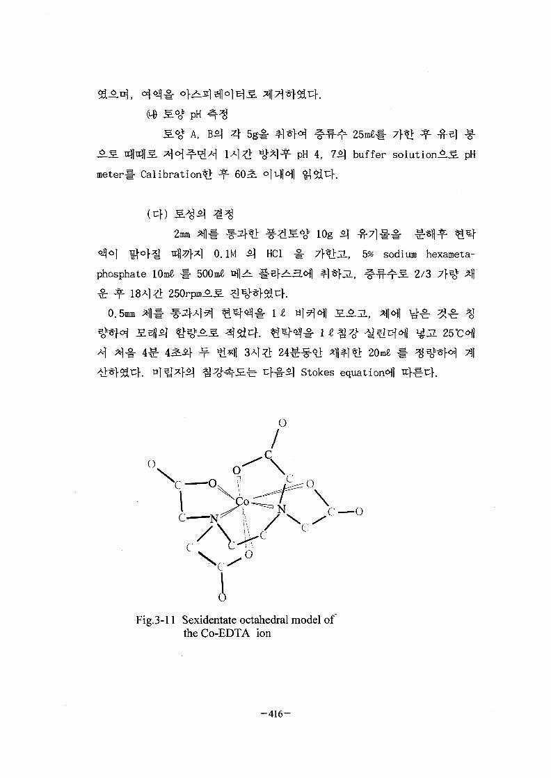
to £<£ pH 4 ^A, B<q 4 -g-
pH 4, 75] buffer solution^.5. pH
Calibrationt!:
phosphate
0.5mm
2mm *fl# ^ ^ * > ^ ^ . S ^ 10g
0.1M 5] HC1
500mC tifl^ #e]--£i
sodium hexameta-
2/3
l i
25°c<>fl
Stokes equation^] nfg^h
O
0\ c —-o c 3 0
-o
Fig.3-11 Sexidentate octahedral model ofthe Co-EDTA ion
- 4 1 6 -

V
g
D
d
#<*?.£(cm/sec)
(cm)
_9_ x gh.2 r\D-d)g
(l)
acetate, pH5
carbonate #
20% hydrogen peroxide
0.1M NaCl S
100 mesh g
1M sodium
(2)
Co2tFe
co2+ = 5.5 ofH 72
£ AAS (Analyst 300; Perkin Elmer)# o]
-417-

= Vsoi(Cc-CM)/Wads
i7 : The amount of Metal species adsorbed
(g of Metal / g of adsorbent)
Vsoi : The volume of solution
CM : Metal concentration in the adsorbent supernatant
Cc : The concentration in the control solution
Wads : The weight of adsorbent
i —
• f '• Fraction adsorbed
(g of Metal adsorbed / g of ini t ial Metal)
(3)
ty-AJ-^Ofg^ j g : * ^ ^ ^ - f i f n f ^ ; 7 H S . buffer
PHI- 2L^}^,3., 6a^«> c l ^ : 4 £ # $-x]*}7] J?-l*l| 0.1 M
^ ^ ^ & water bath shaker tflofl*] 200 rpm $] Z^.o\\M ^
^ ^ r 3000 rpm £ S . 10^:^: #<£ ^el*> ^ 0.45/um f i l ter
s. v\x\ <H2]-«H 4-g-*l-S£^}. co2+ o | ^ ^ ^ * ] - ^ ^ ^ r 35 ntfM PH 3,
4, 5, 6 £| S^^lA-1 ^ ^ * } 5 i ^ . ^ , EDTA ^SLfe 0.05M, 6^1 ?> ^ - ^ «K§-
* I & 4 . Al^>Ti ^ rH^^-^ l ^f€r ^ ^ ^ 0.05M EDTA # 4"§-*H 25, 45,
55°C ofl^ 4 4 ^ r * I ^ ^ ^ K EUTA ^ -^J£ ^ifofl cfl^}^fe 35°C, pH=4
0.03M, 0. 07M, 0.1M 3. EDTA $] ^ S # ^^f^f^ 4 4 ^ r W f c
^SrS^ 25, 35, 55°C S. ^.^}^3. <$q°l) ^*H*fb Fe, Co
^ AAS(M 1100B ; Perkin Elmer)#
- 4 1 8 -
3)
3-12^ 4 4 72 A|?> 5J ^7] 24 >M?>
^ - ^ ^ ^ 5 f # i M W . 72
f 72 -M^*}*)^ ^*$ *££ 1.87 X 10"4mole
24
^ % j - so>5] 81.8
BET 1- 4-§-t> »I S ^ 3 | ^-^A) £oo> vfl^ :g.q.o| ^ ^
f ^ 4 , *>-§- 2 7 ] 6
Co 2 +
site
^ 1 - ^ s i t e ofl Co2+
s i t e «Hf ^ ^ ^ 1 Co2+
o2tvfl Co2t o]£.*\ ^^^r slow rate adsorption^
O.^ 3-13 ^r 25 °C^1^ pH ^ EDTA ^-S. ^ 7 H 1 ttj-^- Co2t o]
u>. EDTA 5J ^-S.7} 0.02 M S. # 7 f ^ ttfl^M Co2+
EDTA i f 5 1
. EDTA ^ ^ H 4 4
) fe^K ^., EDTA
(Distribution coefficient) o| ^ H ^ H EDTA %•£.
H r Co2+
711 ^ 4 . J£*>, 0.02 M 0]^$] EDTA
^ 24
- 4 1 9 -

, pH 7}
2 1.0
oo
0.5
O.CM
10 » 30 W 60
I , i _
10 15Time(h)
20 25
2+ .Fig. 3-12. Amount of Adsorbed Co ion against Time
EDTA
EDTA ^
Fe-oxide «2 EDTA, Co2+
\ L~ T-i T T Y T A 2~CoEDTA'", FeEDTA'", Fe(0H)2) CoEDTA"
Co
-420-
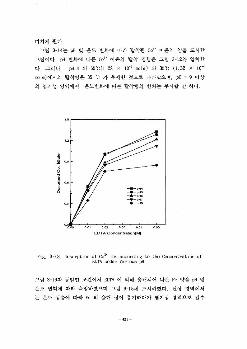
pH
PH
PH=4 ] 5513(1.22 x 10"4 mole) i f 35°C (1.32 X 10"4
35 °C 7} ^M)*} %SL£. LfEfJs to^ , pH = 9 O)AOV
0.01 0.02 0.03 0.04
EDTA Concentration[M]0.05
Fig. 3-13. Desorption of Co2+ ion according to the Concentration ofEDTA under Various pH.
EDTA Fe p H
-421-
pH - 4 *J
Fe 5] <#£• 55 °C<>\]*\ 5X10"4 mole S 2.82X10 4 mole *] 35*0 ofl
^ FeO 5} &
pH=4 ^ 4 55 ° C ^ 1 ^ ^ W ^ o ] 35 °C ofl
6\] Hl*l| ^uf jL ^ f e ^ ^ r EDTA ofl ^sfl ^S | -g . ^ B B ^ . ^ ^ Co2+
CoEDTA2"
EDTA ofl Vj*> Co2+ o j ^ - i j S6o>6^g_^.Bj iy-:*J-£.f A}-g-Sl EDTA
pH,
4 7 ] tiKg-cHM, Fe-oxide ^ -g-*fl
Co2+ o l ^ , a e l J L EDTA ^ ^ ^ « > - § - # f-*f<H ^ g - ^ ^^A- ] Co2t
, pH ^ i f (H+ o ] ^ - ^ Fe-oxide
if S^oM ^ * j - ^ Co2+ o } ^ - ^ . ^ . ^ ^ © . s ^ ^ ^ # ^SfAl^lcf) ofl irf
CoEDTA2" ofl 5l*l| ^z$Q ShS- (0 2f ^A]ofl FeO
Fe2t S. °}-&ty- (2) 5] JL, (1) 5} CoEDTA2" # ^
r^I (3) 5 |
CoEDTA2" = Co2+ + EDTA4" (1)
FeO + 2H+ = Fe2t + H20 (2)
Fe2+ + H20 + Co2+ + EDTA4"= FeEDTA2" (3)
FeO + 2H+ + EDTA4"= FeEDTA2" + H20 (4)
h FeO o\] cfl«> PH ^L^fo)] xt}^ H+ *\ ^% Fe-oxide
2f ^ ^ «!-§- (4)oj f A | o | o l ^ o j ^ A S (1) *]5J CoEDTA2" i f
-^l 5|*H EDTA off 5|*> S ^ ^ S . ^ - e | 5 | Co2+
- 4 2 2 -

1.4
1.3
0>O
0O 1.2
10W
Q
1.1
1.04 5
« . i
6 7
pH8 9 10 11
Fig. 3-14. Amount of Desorbed Co + ion agains pH underVarious Temperature.
-423-

2t .Fig. 3-15. Amount of Dissolved Fe ion against pH under Various
Temperature.
-424-

EDTACoEDTA2-
(Co, Ni, Zn..)Metal Complex
cS+
FeEDTA
SoilH+
Fe2+or3+
Metal-Oxide(Fe, Si, AL)
dissolution
Fig. 3-16. Competitive Reaction Mechanism between Co2+ ion and Fen
ion on EDTA in Soil Solution.
A.(l) 7tf.fi.
7} screw feeder
(2) 4
4 TT seamless « .
-425-

STS316
x
butterfly valve 7}
160
sampling
PH
, tiJ:-§-7l 7}<i
thermocoupl
60 °C
-§-<>]*} flange
1/4" f-JL ?J valve
20 mm ^ ^ 1 - ^ ^
band heater ^
3" butterfly valvef-
screw feeder^}
screw feeder
Sat:>. screw feeder^
. screw feeder^ 1/2HP*]
100 - 200°C
screw
feeder^
3 -T-^^-
*>SlcK screw feeder
- STS 3/8"
3/8" ^ H .
-426-

, Sl-g-7]
«>-§-7l
^ ^ ON/OFF, «K§-7]
screw feeder tfl<f ^ £ *]*W ^ ^r
], screw feeder 4f.£ ^
PH
-L^! 3-16, P
& ID ZLQ 3-17, # ^ .^ 3-18 ofl 4 43-19 5J 3-20 ^] ^
- 4 2 7 -
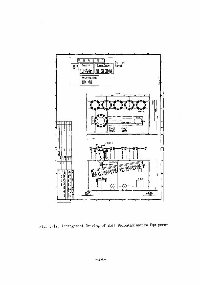
a § %\\
warnsw
Reactor Screw Feader
frTI ITS fraKlS'
Hetarino Pumo
ControlPanel
Fig. 3-17. Arrangement Drawing of Soil Decontamination Equipment.
-428-

Fig. 3-18. P & ID of Soil Decontamination Equipment.
-429-

3P 220V
2P20A NFB
-O I o-
-O O-
(Sh
-o 1 o , o a1 f P!
-o a
-o o-M2
Fig. . Control Circuit of Soil D econtaminati on Kit.
Fig. 3-19. Control Circuit of Soil Decontamination Equipment.
-430-

Fig. 3-20. Photograph of Soil Decontamination Equipment(Top View).
-431-

Fig. 3-20. Photograph of Soil Decontamination Equipment(Side View).
-432-

3.
7f.
Sr 2t
f. 40 V B] 72^1
80
336
Sr2t
fe Cs+
k a o l i n S ^ ^
^-^ Sr2+4 0 v
c m
U. 2+EDTA S] Co '
, EDTA
uf. EDTA(Hi|- N a ) ^ Fe-oxide ^ ^
. H 5 1 U EDTA7f
60Co
irfl
CoEDTA2"
, CoEDTA2" 7} F e - o x i d e
, ZLnfl Co2t
Fe *1 EDTA
% 3
Fe3+ i £ i r Fe2+
a e j H S . , EDTA *
1 A ^ ^ r EDTA
- 4 3 3 -

7}
o ^ 7f<i7l7} screw feeder ofl
- 4 3 4 -

2
1.4
4:2.
(free standing water) 7f ufeo>
CEC (Cation Exchange Capacity) &SJ ^ 15
-435-

^ (Cs-137)
Ji7|
Na-%
(JIC34)
2.
7}.
(ion exchange selectivity) ^.7]
z fe ionic charge 0)3. r^r
^ 27}
«]vg) ^r
(z /r2
z / r2
fe 3steric hinderance
3.71
-436-

pH
caesium
3-6
^ complex
repulsion
Table 3-6. Physical Properties of Certain Cations
Cation
Cs+
K+
Na+
Ca2+
NH4+
Ionic Radius(A)
Crystalline
1.69
1.33
0.97
0.99
1.43
Hydrated
2.35
2.50
3.60
6.10
2.45
CrystallineSurface Charge
z/r2
0.35
0.57
1.06
2.04
0.49
z
0.9960
1.0083
0.9974
1.9940
1.0020
Partial MolarVolume
(cmVmol)
15.9
3.6
-6.6
-26.6
12.4
-437-

51
wetting d\]
liquid channel -§
$1^ liquid channel^
(surface contact angle)
wetting ^ - £ # LjEKfl-b 4&S.4 ^ 4 4 ° 1 4 # ^ ^ - ^^-^^<>| ?\
(active site) # 7}^ ^ $I4[3
^ ] drop
fe ^^-S. wettability ^^g#
v TLV
^ 9/SL
Gibbs' Free Energy fe
AG = AA ( r SL - 7 sv ) + AA r LV cos ( 0 - A 6 )
$ • Contact Angle
/SL : Solid/Liquid Interfacial Tension
- 4 3 8 -

ysv : Solid/Gas Interfacial Tension
y LV : Liquid/Gas Interfacial Tension
A : Contact Area
° M £ r AG = 0, A 0 = 0 o | H S
0 = rsL -/SV + /LV COS#
V 7]- S>
rsv = r s
/LV = /L
r S = / SL + 7 L COS ^
Young equation o]ej-JL
(Rheology) 7 ^ ^ ^
(viscoelastic)
3-22]. ^ « > ^ ^ S . ^ f > ^ -8-^fe &^S. (shear
rate) 7f ^7f^ ttfl ^ £ f e ^ 4 i * f e ^ % ^ ^ ^ 1 ^ . £ j i7 l ^[J£7]-7o|
^ y ^ | log v o\\ K\M- i o g y ^
"power-law"
(3-1)
-439-

7} ; viscosity, [Pa. s]
m ; consistency index, [Pa.sn]
y : shear rate, [s'1]
n ; power-low exponent, [ - ]
£4* m £ n # 7^1 JL ^ U ^ , n o] i ^
;£) 7f SJo} Newtonian -fraf|<*3 ^ - T - ° H , n o| 1
"Pseudoplastic" J £ ^ "shear thinning" -B-*Ht}. H^\JL n o| 1
"dialatant" or "shear thickening" -%-$\}7} Qv}.
3.
OO ^71 el 3-g-
O
l^t^ 4
- 4 4 0 -

$1°H 4 ^r seamless ^ i
1) Pre-mixing Tank
pre-mixing tank fe
3.S>7]-t
1 *H-5
STS316 (1.
ojcf. ^ 3 g ^
^ 10 cm o) 5 cm
10 cm $)
flange
a o] Jj
uf.
outlet
5cm ^ 3/4"
5 cm 1/2" -«.
2) Reactor
reactor -fe- pre-mixing tank •§-;*»£
-441-

STS316 ( i ) # 4
, 3.7]fe- 200(vH^) x 300(^0])
flange ^ ( ^ J2.yj7]# ^-^*>JL
S ^ o ) 5cm ^ 3/4" fl-H.# 9 - ^ # *3L -g-
5cm $}*M 7jo| 5cm^ 1/2" ^ « .
^ # }}] $?t outlet
5cm 3] 3/4" ^ a . # ^ - ^ # #JL - g - ^ ^ f i ^ -
5 cm ^ojofl 7^o] 5cm^ 3/4" ^ « -
3)
4)
4
5)
- 4 4 2 -

n|o)
fg- Zl^ 4-21 ofl uj-
[^ ZL^ 4-22
4-24 off
- 4 4 3 -

Bentonile & Additive Tankwith Vibrator
Chemical Tank
0 Q B
Sprayer(Dry Decontamination
Agent)
Mixer
Air Compressor
Fig. 3-21. Schematic Drawing of Urban Surface Decontamination Kit.
-444-

1. Control Panel 2. Reactor 3. Pre-mixing Tank 4. Mono-
pump 5. Air Compressor 6. Sprayer 7. Chemical Tank
Fig. 3-22. Photograph of Urban Surface Decontamination Kit.
-445-

- ) - •
1. Reactor 2. Pre-mixing Tank 3. Mono-pump
4. Metering Pump 5. Chemical Tank
Fig. 3-23. Photograph of Urban Surface Decontamination Kit (SideView).
-446-

Fig. 3-24. Photograph of Spraying Operation.
-447-

"A
Table 3-7. Components of Decontamination Kit.
l
2
3
4
5
6
7
JX tri xO ^ 1 2 |
JS.ii ^ H : SUS, 1 mVhr,
{%m, DS-20)
cc/min,
SUS 304, 2 se t
Chemical Tank: 20 L
Nalgene(2318-0050)
Air Compressor: 1 Hp,
Oil less Type,
^(YOMD-40)
^ . ^ 7 ] : Flange Type,
360 rpm, 0.2 KW
£ ^ 1 ) : 1200x750x800, ^^> 1.2t
Ball Valve, SUS316, %",
%" (SS-63TS8)
set
set
set
set
set
set
ea
TjJ IIS TCjl £*}3 ~3Ul t 3 > L -O
-448-

4.
7}.
(free standing water) 7f
"A
CEC :&£} «^ 80
*]*1| gelling
hectorite# -
S^[3-24, 4-25]
9}7} $}
h e c t o r i t e [ Nao.eviMg, L i ) 6 Si8O20(OH, F ) 4
] ^ % 1 4 § | ^ ^ ^ l ^ r # ammonium
l-hydroxidel- A}-g-^H -OH q-^# -<H*}Ssl4. °1 -f- £ , hectorite,
NH40H Ri ^-^^] 4
4"A
-449-

^ r 3.7)}
S[3-20] 7\S. ^
7] ^
® ^ S / #%\] -g-<sJ} = 1 / 8.7
© ^ S / hectorite = 2
O H J-)
© hectorite -§-«*] (3 %) *]]Z.
@ hectorite -§-^ (3 %) 1 methyl alcohol
NH4OH
ID© hectorite -g-^ {3 %) *§£.
2) hectorite -g-< (3 %) o\] NH4OH
^7\o\] methyl alcohol
HI)
© hectorite
NH4OH
hectorite ^
ll51-b 4^tiov^^- -§" 1 ^ 4 37M
- 4 5 0 -

I), II) $)
HI)
4 ^ ^
3-7 o\] M-EKJlsiM, ^ ^ «cj- i n ) ^
III) ^ ^•^•oll^ ^ ^ s ^ 3 £ £ i | H hectorite
hectorite - ^^-^r ^ r ^ o ^ 4^t>^>. 3L ^ NH40H (29 Vol.
^ Tixoton ^ S . o|
X-id 5 ] ^ ^ : ^ , ^•^•^r^ 9J EGME (ethylene glycol monoethyl
ether) ofl 5]?>
- 4 5 1 -

Table 3-8. Manufacturing Composition of Decontamination Agent.
SampleNo.
1
2
3
4
5
6
7
8
9
10
11
Composition (wt%)
Bentonite
4.762
5.085
5.344
5.556
5.733
5.882
6.011
6.122
6.220
6.306
6.383
Hectorite
2.273
2.016
1.812
1.645
1.506
1.389
1.289
1.202
1.126
1.059
1
NH4OH(29 %)
7.143
6.356
5.725
5.208
4.777
4.412
4.098
3.827
3.589
3.378
3.192
85.714
86.441
87.023
87.50
87.898
88.235
88.525
88.776
88.995
89.189
89.362
. Van Olphen %• [3-20]
m2/g«LS.
BET
750 m2/g A
. BET
-^^ of 60
: 810 mVg
-452-
~ 3-28]. <y
Carter [3-29] 7} - * 5 . EGME
EGME
30
(60
2 . 5 m l ^ EGME#
EGME
259 mtorr ^
250 mtorr
EGME ^ 7 > ^ A]S. ^-711# v§°] ^ Q EGME
^lSofl ^f-^^ EGME <£# ^ ^ ^-#el^u}o)JE 1 g ^
monolayer^ ^ f e ^ ^ A t l °]^r EGME <£ ( = 1/810 g/m2 = 0.000286
hectorite ofl cfl*> X-
325 nfl4j ^ (sieve)
^ u K X--?d Sl^^r^^l alH^i 4-§-€ 7]7lfe Rigaku
Denki A}*] Reigerflex 7]^-o)r.\. X-^.^ 30 kV ^ - ^ ^ 3 f 15 mA*] ^ ^ -
*H1^1 CuKa ^^^.S-f-^ ti^A]^^.t^ «}4( semi-angle) 20 # 10 -
80 JE7H 1 J£/min 5]
4.
Shear Rate)^ ^Sfofl t t}^
4 ^ f j l 4 ^^u> . ^^6fl 4-g-S} 7l7lfe Concentric
Cylinder Viscometer (Brookfield, Model DV-I1+, Small Sample Adapter)
- 4 5 3 -
^ 1 tappingofl ^ * H *W*}-£Ul 4
oj7] JH*M £*] ^14^ 2.5 £
(shear rate)
wettability
Contact Angle Meter ( FACE, Model: CA-X ) # <>|-§-*M
(Acryl Plate) ofl micro-syringe 3. M& drop •§•
^ 4 # CCD -fc H °m monitor
3 point method ofl ^ H ^^"4# -^*}^4. l^^lfe 4 ^ 3
mm -tg S ^ sampl
nf.
(JIC34) ^
7J-S. -MIS. 4 5 cm, ^*fl# 1 cm
S-fEJ ^ o | 4 mm | blanket^ ^ e j $ ^ ^
. Cs-137 ^ H § -S-^ 7.41 x 10³ Bq/cm3# Aj^xg- 2 . 5
cm3
5
£ - 7 . 4 1 x 10³ Bq/cm3 S>] Cs-137 -§-«?ofl 325 mesh
0.2 wt% £] ^ ^ t o ] ^-$-5
- 4 5 4 -
blanket
(2) (3) (4) (5)
Fig. 3-25. Photographs of Specimen; (1) Weight-Concrete (2) Fired
Brick (3) Red Brick (4) Silicate Brick (5) Wood.
Sealer Ratemeter SR7) ~L
dectector, Nuc. Enterprise Ltd.,
4 cm3
704?
5.
tft*}
Na20
3-9 ofl1 wt
. o|
4.2 wt
-455-

77.5 meq/100 g
82 % <>M EGME
665 m2/g
Fe203 ^ ^ ^ o ] 61
n ] ^ (HIROX A}, Model; KH-2200) ojj ^*> ^ ^ ^ - # ZL ] 3-26
4 4 ^-l-BKii^K n ^ 3-16. £ ^fi)?WJE ^ # *A i-H^^
] ^ ^ § ^ 1 ^ - f 4f 0.2 - 0.5 mm
(JIC34) ^ ^ - H r >yeMo|js ^ f i n f e ^ . tg^ . ^ l n > c | j^}^ o.l -
0.2 mm l 3.7] S] crack c| njo|
O.^ 3-27 ^ ^ S : ^ # , ^ ^ l ^ fffl
crack o]
5] 3 - f ^ 0.1
0.3 mm ^ ^-tgo] u } ^
crack o|
A}-§-^ hectoriteoil t%Q X-^ ^ ^ ^ ^ 4 ( Rigaku Denki Co.,
Reigerflex, CuKa ^ ^ A}-§-) ^ 2 ^ t ^ - ^ 3-22 < ] 4-E)OJ|&u]-. ^ ^ 1
X-ti S)^6o1:'o1'c>fl ^H*}0^ JCPDS (Joint Committee on Power Diffraction
Standards) 5J mineral powder diffraction f i le [3-29] ^f H]j2.^-^4 *)•
- 4 5 6 -

Table 3-9. Properties of Clay Studied
Constituent
Composition (%)
SiO2
TiO2
A12O3
Fe2O3
MgO
CaO
Na20
K2O
MnO
CEC* (meq/lOOg Clay)
S** (m2/g)
MT*** (%)
Value
50.4
0.6
15.2
4.3
3.4
2.4
4.2
0.7
0.1
77.5
665.0
82
* CEC
#* S
: Cation exchange capacity
•' Surface area, by ethylene glycol
monoethyl ether (EGME) method
: Montmorillonite content, by theoretical
montmorillonite surface area and EGME
surface area
-457-
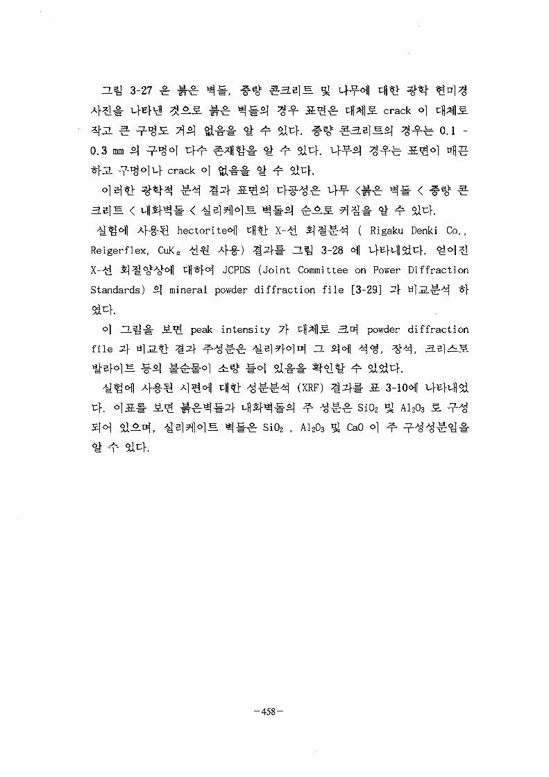
3L.Q 3-27 £ -g-£ ^ , ^ ^ ^ + M
crack o]
^ ^-f^- 0.1 -
0.3 mm SJ -?-^o| ztf> ^1f^ ^ 14 P) ^fcrack o| ^ ^
hectoriteoi] cHt> X-^i 5 } ^ ^ ( Rigaku Denki Co.,
Reigerflex, CuKc ^d^4 Afg-) ^ 5 f # Z L ^ 3-28 <H1 M-B}-v|5iuK c^^]
X-*i 5 ] ^ ^ o M ^B^}0^ JCPDS (Joint Committee on Power Diffraction
Standards) S] mineral powder diffraction file [3-29] 3} H]iL^:^ *F
o] ZL J-g- ^ . ^ peak intensity 7} tflafliiL 3 . ^ powder diffraction
f i l e af w]j3.*> ^2 f ^^-S-g
^ (XRF)
"^ ^ ^ ^ ^ SiO2 % A12O3
E ^ § ^ . sio2 , AI2O3 ^ Cao
- 4 5 8 -

{1)
Tit).-
Fig. 3-26. Optical Microphotographs of Silicate Brick(l) and Fire
Brick(2).
-459-

(ft
Fig. 3-27. Optical Microphotographs of Red Brick(3), Weight crete(4)
and Wood(5).
-460-
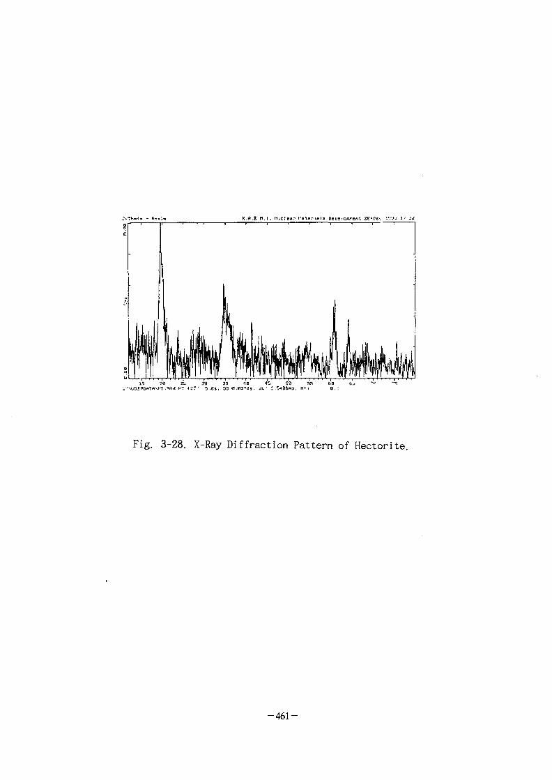
K.G.E H . I , M^clB#r l ' i t r i a l s Ueusioprenl 2C-Pc. VJ'Ju 1- JJ
-c -•=
Fig. 3-28. X-Ray Diffraction Pattern of Hectorite.
-461-

Table 3-10. Compositions of Tested Specimen.
Sio2
A12O3
Fe2O3
K2OMgOTiO2
Na2OCaOP2O5BaOMnOZ1-O2
SrOPt
Rb2OPbO2
CuOZnOV2O5
ClSO3
CO2
RedBrick
69.80019.6803.6483.1000.7840.5850.4140.4040.0720.0410.0250.0200.0150.0110.0090.0090.009
--
FireBrick
69.50026.300
1.8801.5100.1870.261
-0.1290.0640.0220.0320.0200.035
---
0.008--
SilicateBrick
57.70014.8004.5803.1902.6400.6110.872
13.5000.1720.0510.0770.0200.0390.0170.0070.0150.0170.006
-
WeightConcrete
16.6002.760
61.2300.5005.6000.198
-11.5000.072
-0.122
-0.013
----
0.0120.023
D TJD 1
66.821.52.530.4872.9
0.2732.412.82
0.0750.0150.0570.0180.0380.015
-0.0070.007
--
0.0690.068
ri 1
67.30.141
0.0379
28.40.0217
2.250.1940.23
----
0.0133-----
0.0940.65
0.711
-462-

flocculation series test ^ J f #*)! A]£.ofl EflSJH -rM^r *4HH
log v o\\ ^H*H log r 3 & £ S . H^[ 3-29
o| ZL JoflX} STD 3. *$MQ MS-^r hectorite 7}
s"1
<y- ^ 61 uf. ti>i^ hectorite 7}
hectorite
forg. "power- law' *J*1 ^ (3-1)
i l - ^ ^ ^0.015 o]t\S.^\ ±*}7} 7]$]
S 3-11 ofl U E M ^ U K o] SS-f-^ m & £
hectorite ^
hectorite 7} ^-°r^ ^ ^ l^fe non-Newtonian ^-^|] 7i-^#
n ?Jto] 1 oj-sH13} ^ i ^ ^ - * - ^ . ^ £ 7 f ^-fc*fe shear thinning fluid
- 4 6 3 -

Shear Rate [ s"1]
Fig. 3-29. Non-Newtonian Viscosity of Decontamination Agents.
-464-

Table 3-11. Power-law Parameters of Modified Clay Suspensions as
Fitted with Equation (3-1).
Sample No.
1
2
3
4
5
6
7
8
9
10
11
m [Pa sn]
26.6685
23.7848
20.4480
18.7668
17.1471
15.3918
14.0932
13.6502
12.6964
10.8966
9.1405
n [ - ]
0.0538
0.0713
0.0656
0.0656
0.0778
0.0820
0.0799
0.0992
0.1109
0.1450
0.1474
-465-

hectorite
4 3-30
wettability 7]-
hectorite
-, hectorite
hectorite
n
o] -L^o
No>
^-^ 3-31 o\]
wettability 7}
-466-
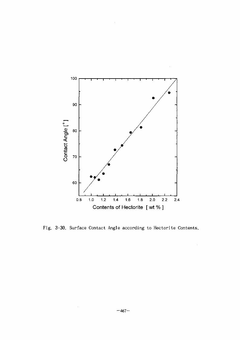
100
0.8 1.0 1.2 1.4 1.6 1.8 2.0 2.2 2.4
Contents of Hectorite [ wt % ]
Fig. 3-30. Surface Contact Angle according to Hectorite Contents.
- 4 6 7 -

0.16 100
0.041.0 1.5 2.0
Contents of HT [ wt% ]
ooi9.
D.W.
Fig. 3-31. Viscosity Parameter n and Surface Contact Angle According
to Hectorite Contents.
-468-

4
M 52 %,
3-32 ^ 3-33 ofl 4
H ^ 3-24) 4
38
61 *, | h g : ^ # 57 *,
H ^ 1 - 24 % <&c\.
7]
3-33)
4 S\ *\}
B]M. 48 28
58 %, M ^ : ^ # 54 %,
^ ^ § 16 %
51fe ^ ^
liquid channel
fe liquid channel^
s i t e #
^ #^§711 51^.
- 4 6 9 -
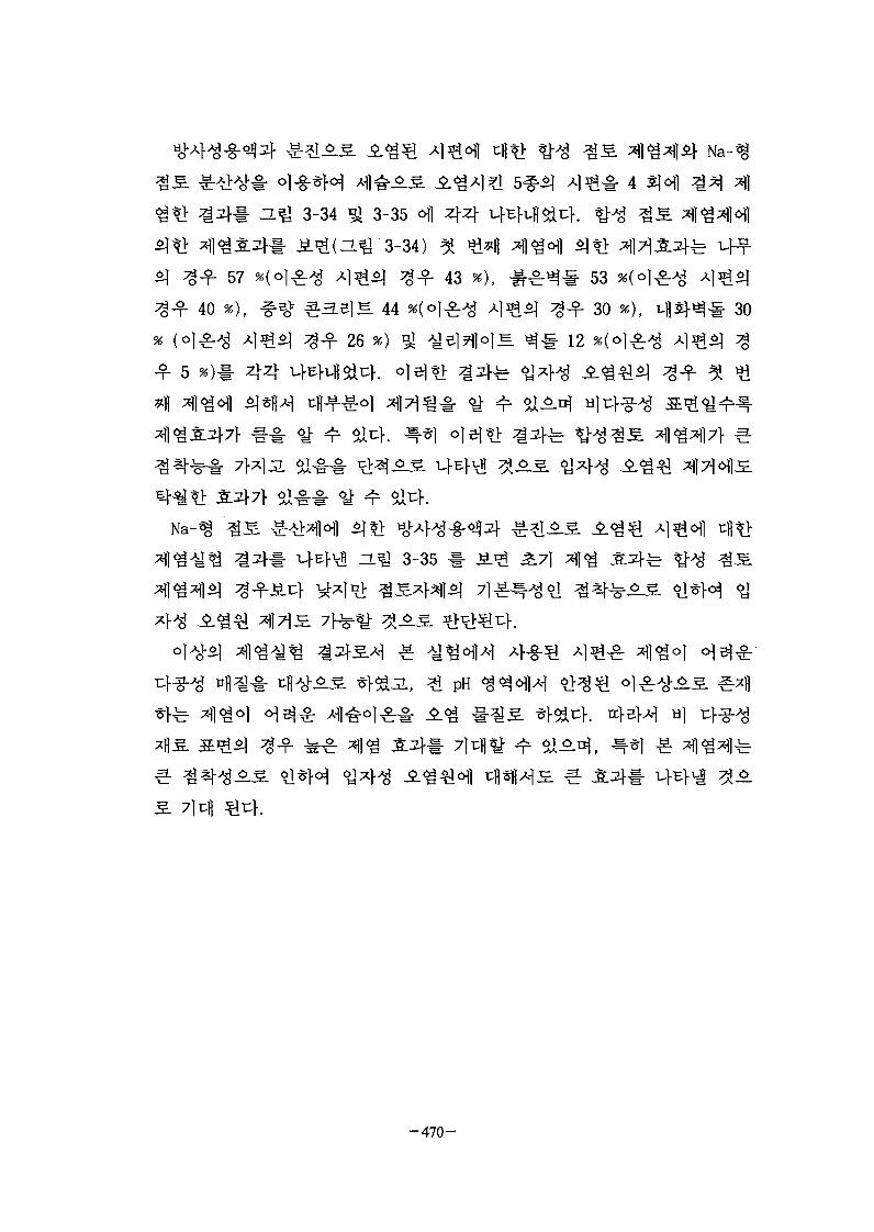
<* 3-34 £ 3-35 o\) 4 4
^-^ 3-34) $57
40 %),
4 3 as), ^ - ^
H 44
26 *)
53 %(o
30 * ) ,
12
30
ti
^ - ^ 3-35
PH
7]c||
- 4 7 0 -

100
h- 90CO
</>
2 8003
O 70
0313
ioo
f
03
rv
vity
1
60
50
40
30
—O— Silicate Brick
- A - Fire Brick
—V— W-Concrete
- O - Red Brick)
—•— Wood
1 2 3 4
Decontamination Cycle [ - ]
Fig. 3-32. Activity Ratio of Residual to Initial Cs-137 according to
Decontamination Cycle Using HT-type Decontamination Agent
( Contaminated with liquid Cs-137).
-471-

coI
COO
.Is
o
"coZJ
0)
oroo03
DH
o<
100
90
80
70
60
50
40
30
-o— Silicate Brick-A— Fire Brick-v— W-Concrete-•— Red Brick)-n—Wood
1 2 3 4
Decontamination Cycle [ - j
Fig. 3-33. Activity Ratio of Residual to Initial Cs-137 according to
Decontamination Cycle Using Na-type Decontamination Agent
( Contaminated with liquid Cs-137).
-472-

100
00 90
ntia
l Cs
al to
IrR
esid
u;
"oo
Rat
80
70
60
50
•ti 40
30
-O— Silicate Brick
-A- Fire Brick
-y-W-Concrete
- • - Red Brick)
-D— Wood
1 2 3 4
Decontamination Cycle [ - ]
Fig. 3-34. Activity Ratio of Residual to Initial Cs-137 according to
Decontamination Cycle Using HT-type Decontamination Agent (
Contaminated with liquid Cs-137 and Dust).
-473-

CO
(J)O
o<
100
90
~ 80'Eo*!-'— 70(013TJ0)
(D
a:
60
o.2 50
£ 40
30
—O— Silicate Brick- A - F i r e Brick—V— W-Co ncrete- • - R e d Brick)- D - W o o d
1 2 3 4
Decontamination Cycle [ - ]
Fig. 3-35. Activity Ratio of Residual to Initial Cs-137 according to
Decontamination Cycle Using Na-type Decontamination Agent
(Contaminated with liquid Cs-137 and Dust).
-474-
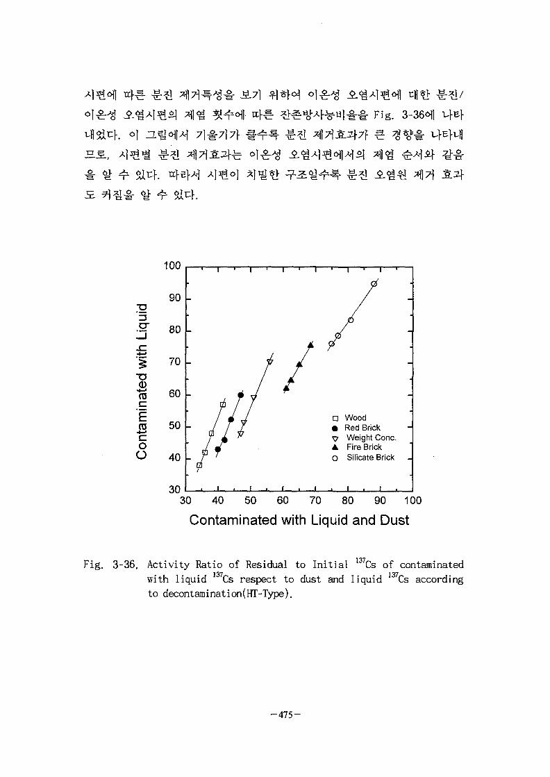
Fig.
100
90
Liq
with
mat
ed
Ero
Con
i
80
70
60
50
40
30
• Wood• Red BrickV Weight Cone.• Fire BrickO Silicate Brick
30 40 50 60 70 80 90 100
Contaminated with Liquid and Dust
137rFig. 3-36. Activity Ratio of Residual to Initial Cs of contaminatedwith liquid ] Cs respect to dust and liquid ' 7Cs accordingto decontamination(HT-Type).
-475-

6.
hectoritel-
CEC 15
fe- non-NewtonianoH shear thinning
"power-law"^
hectorite n
wettability 7} # ^
61 x,
Cs-137
57 x, #%> rHBlS 52 *, 38 %
24
- 4 7 6 -

£ 3.7\] 2?
S ^r^-1- ^r fct^K ^ , 5 ^ 1 ^ (Saturation Zone)^
(Unsaturation Zone or Vadose Zone)°|t:h a^^-^H
1<^(Vadose
f-*H ^]^}^r^l(Water Table)7?\x]
^r Nonaqueous, Liquid, Gaseous Phased.
S-fB] ^ l ^ ^ ^ l ^ M ^ ^1<^^S. S^l^^^-ol t ^ t r f e 9-^>(Capillary
Fringe)^ 3E^?>i:>. o| a . 4 ^ 4 ^ - ^-^>^; ^ ^ ^ S^]<^o]i:}. ^.sSf
^|^S] ^ A ^ ^-^-^^(Pore Water Pressure)©! NagativeSfe ^ O|JL
o] x | ^ ^ *]5H^ ^^r Perched Water Tabled
o|
- 4 7 7 -

7]o]W[3-31]. #3ESftfl6fl>Hfe S ^ ^ ^ (Surface Tension)
°\] -&£{ 6 i ^ (Negative Pressure)^ i-M\H4.
(Capilary Potential) JEE - Matric Potential, <l>,
^ # ^ ^ - Matric Potential*] ^
^ S ^ ^ - ^ ^ ^ l (Soil-Moisture
Potential), 0,fe Matric Potential, Graviational Potential, Osmotic
Potential, Electrochemical Potential^] ti"0]1^. Osmotic Potential2}
Electro- chemical Potential^
Osmotic Potential^} Electrochemical Potential^-
%• S ^ w ^ ^ ^ - l f e Matricij- Graviational Potential^} ^.
0= <i> ( 6 )g + zg
2) S. -1- ^-^d
l fl Matric Potential(Sj^
K a ^ 3-37^
HW o 1, ^^H]fe ^ 5 . S A l W . Matric
Potentialo| ^ x l ^ ^ . S ^ ^ ^ ^ e f £ S.%^ SSf^EH
uf Matric Potentialoj nfl-f- 3. ^% ^ s . ufEf^ afl
o]ttfl.$] Matric Potential^- Bubbling Pressure(hb)
K Matric Potential^] ^o]-^*)] VC}B} ^ - ^
, Matric Potential^]
3)
Matric Potential^ ^^<H]^1 TensiometerS.
-478-
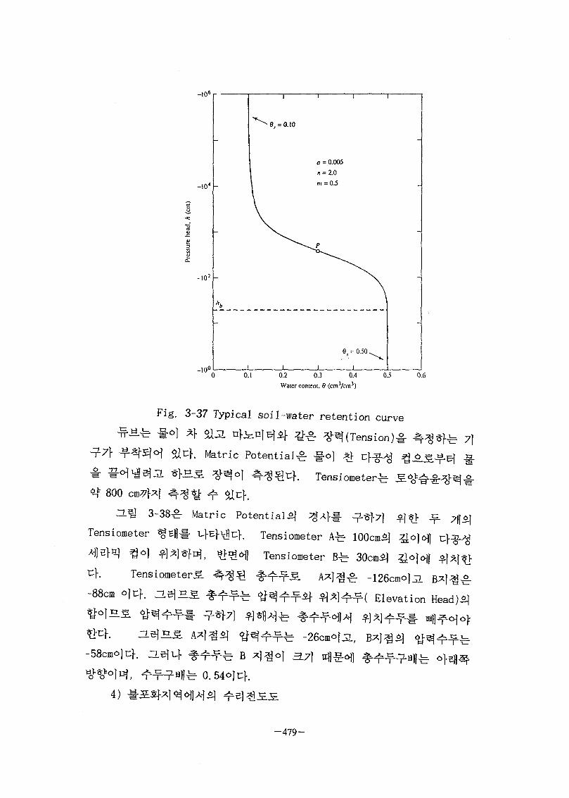
-10 4
MO2
mO
-
1 1
a
n
m
V
1 1
= 0.005
= 2.0
= 0.5
e
i
-
i
0 0.1 0.2 0.3 0.4Water content, 6 (em'/cm')
Fig. 3-37 Typical soil-water retention
0.5 0.6
curve
674. Matric Potent ia l^ # o | -Q c|~§.>g
h Tensiometerfe
te 7}
<% 800 cm*f*l ^ - ^
H^J 3-38^: Matric Potential*] %X[^ ^}7] SftQ JjL 7]|o|
Tensiometer ^Bfll- ufEf^rl-. Tensiometer A^ lOOcm l
4e}nl ^ o | ^1^]^H, w>^6fl Tensiometer B ^
t:f. Tensiometer^ ^
-88cm ejef. ZLe]HS Elevation Head)^
58cmo)t:}. a .
4)
^ B
0.54O) uf.
fe -26cmo]jL,) 3.7] ^ ^ . ^
-479-

o o "Dead-end"
.<=>••
• • . 6
•imU^99:• • • . - . - O - • . ; • . • •
- * P o r o u s c u p •• - ' • •' • • r*.-. •'
. - • • . - . • • . : • . • • • : o ° - . . ; . ^ . ^ .
o • • .
. \ C ° • • •
&o o : o: &
Fig. 3-38 Tensiometer used to measure soil-water potential
in the field
o]
K=
K= K(
^ Matric Potential^
n % ! 3-39^ Matric Potential^]
- 4 8 0 -

^u]-. H ^ 3-40^
-300
-250
-200
I -150
-100 -
-50 -
I x 10" 2x 10" 3 x JO"4 4x 10"Hydraulic conduciivity <cm/sec)
Fig. 3-39 Relationship of hydraulic conductivity to matric potential
for wetting and dying cycle illustrating hysteresis
A 2Co 25C• 45 C
Hanford sandy loam
I I
0.3 0.46 (cmtycm3)
Fig. 3-40 Unsaturated hydraulic conductivity as a function of water
content for three temperatures
- 4 8 1 -

2.
7}.
Fick Lawofl
ep
cstV
9D=aV+dD*
3 ,r 3\Content, U/U)
Density, M/L3)
Darcy Velocity(L/T)
V» : t4HKDivergence)
V : 9-alf(Gradient)
D : r^l7jl^(Dispersion Coefficient, L2/T)
A: #^-g-J]^-^(Material Decay Constant, T)
Q : Water Source/Sink rate(M/T)
Ci : Source/Sink*] ^ . ^ # ^ ^ £ ( M / L 3 )
D*: ^-^>^I^r(Molecular Diffusion Coefficient, L2/T)
a '• -§-^l^]^r( Longitunal or Transverse Dispersivity)
e = vw/ vT105°C a ^
2) ^J£(Bulk Density, p )
-482-

Bulk Density^ ^ 3 W M £ | ^^^-3)cH| cfl*>
3)
^•(Adsorption), ^SJ-g-^HChemisorption),
(Absorption), °]^rJaL%( Ion Exchange)
^ 37H
, Freundlich^*}- ^Bfl, Longmuir^^"
7}) ^ ^ ^ B |
S = KdC
istribution, L/kg)
S = KCN
K, N :
a :
4) ^-^]^r(Dispersion,
Dispersion)ef
^(Transverse Dispersion, L2/T)e}
- ^ g - ^ ^ ^ S . ^ 1 Dynamic Dispersity(L)
5)
- 4 8 3 -
Table 3-12. Input and
cy-a>nfl
^ )
(6D
V
^ ] •g-].^.^. | - ^ -_^( ^=-^- )
^ ^ • ^
^Ldt : Darcy ^-S.
^.4i : Darcy ^-S.
Output data of eachDeterministi
0
0
0
o
o
0
0
0
0
Stochastic
0
0
0
0
o
0
0
0
0
0
0
^ode
0
0
0
0
o
0
0
0
0
0
0
0
0
0
o
o
o :
(Radioactive Decay)°]n}, E^Mr
dC\ _._ In2
>S|-^^(Hydrocarbon)#
iodegradation)<
-484-

Spatial
Variability!- i ^ * M I
^ [3-32,33,34],
M0DFL0W[3-36], MT3D[3-37], TRAFRAP[3-38] f ^ ^ 5.H
#43M-[3-39,40] .
91 «J*I|^ «*7l*l S f^
, A91
91
1) 3DFEMWATER/3DLEWASTE
- 4 8 5 -

7\)
3DFEMWATER(A Three-dimensional Finite Element Model of
Table 3-13 Status of codes for assessment of soil decontamination
nl-3-
= * > .
"'**• T H ^
3DLEWASTE
FE3DGW
FRACMAN
TRAFRAP
MODFLOW
SWIFT
SUTRA-ANE
BioF&T 3-D
PORFLOW
NAPSAC
METIS
MOTIF
GWHRT
HYDRASTAR
3DSEEP
FERM
FREESURF
FEFLOW
aE.vfl-8-4-S"^, 3
4^,3
4* ,3
"i^-,2or3
4 ^ , 3
Hiasi-
^ T - , 3
4 ^ ^ 2
3
Q
4-?-^2or3
4"W" 2
or3
Wellhead ProtectionArea(WHPA)Sutter-Basin,California(1979)Stripa, "a^- PNC(1990)Waste IsolationProject(1982)Stream-Aquifer(1988)Hazardous WasteSite(1987)
Idaho NationalEngineeringLaboratory (1990)Stripa(1990)
INTERVAL Project(1987)
ResearchLaboratory(1984)
Fjallveden, SFR(1988)SKB 91 Project(1991)
-
-
—
Veitsivaara(1992, 31
Pennsylvania StateUniversityPacific NorthwestLaboratoryGolder AssociateIncorporationInternational GroundwaterModel CenterU.S. Geological Survey
Sandia NationalLaboratoryClifford I. Voss Of theUSGSSci. Software Group
Analytic andComputational ResearchIncorperationHarwell Laboratory
Centre d'InformatiqueGeologique
Whiteshell Laboratory
Swedish Nuclear WasteManagement CoperationSwedish Nuclear WasteManagement Coperation
HLW ManagementLaboratory JAERK1986)Central Research Instituteof Electric Power Industry
Motor Columbus
Consulting Engineers
Nuclear EngineeringLaboratory
H]31
EPA/600/R-92/223PNL-2939
ISSN
IGWMC
USGS
NUREG/CR-3328
ISSN
ISSN
TO CMlO OlN
ISSN
SKB(TR88-10)SKB(TR92-12)
JAERI-M86-09)GEOVAL-90
ISSN
YJT-92-33E
WATER Flow through Saturated-Unsaturated Media)
J^§. ^ H ^ ^ f e ^ISJE.01^, «>i*N 3DLEWASTE(A Hybrid
Three-Pimensional Lagrangian-Eulerian Finite Element Model of WASTE
Transport through Saturated-Unsaturated Media)^
-486-

Sinkif Source!- J L 3 ^ fc,
JL-fe- Dirichlet( Fixed-head SL^ Concentration), Specified-flux,
Neumann(Specified-pressure-head gradient J£^- Specified-dispersive
flux), ZLZ]3L Variable^- 4-g"^: r StteK 3DFEMWATERoflA-|Af Variable
S.-b ^^^KEvaporation), ^^(Infiltration), ^[^(Seepage) -§-o| $i
JL, 3DLEWASTE^]A-^ Mass Infiltration 3t^ Advection J§-o| S^-^-1^,
, Freundlich, ^ f e Langmuir Isotherm^ -*]-§-*fe •§•*}-, ^-t>, J3.B]
3DFEMWATER^ Variably-saturated
(Moisture) &§-£• M^^i°\^M, -f#(Well Production),
(Drought Condition), -^(Rainfall), -^^^(Evapotranspiration)
3-$%t ^r 51 -T-. 3DLEWASTEfe -§-*H^ - $ - ^ # ^ (Dissolved Conta
minants-^ ©1-^i- ^7f*f7l J?|*H 4-§-*f^, 3DFEMWATERofl
•§-^>S.(Flow Data)!-
3DFEMWATER^1
K( s* ) - krKs
^ , L)
Q : Source/Sink(L3/T/L3)
Q : Source/Sink(L3/T/L3)
-487-

Ks :
kr ^r ^ t f l J M ^ . 3 . £<££} SH>HW *}£} 0.0 -f-BJ 1.0
van Genuchten ^ ( 1 9 8 0 ) #
kr=ef[i-{\-
* =( [l + {a\h-ha\YrY for h<ha* ' 1 for
6W~W & WY
n— 6
^5,Y: Soil-specific Exponents
ha : Air Entry Pressure Head(L)
a '• Soil-specific Coefficient(l/L)
Sand, Clay, Silty Loam, and Sandy Loam£]
^ ZL^ 3-414
nfl-or0!] (Drainage
Potentialofl
-488-

Specific Yield)3f
1.0
10
3.3a afld 3i8t£
10
10
io "*B
10
1 0 • * . :
LEGEND
j i i i i i i i I
10 1.0
Fig. 3-41 Relative permeability vs. moisture content for sand,
clay, silty loam, and sandy loam
( Specific Storage)£f
o| 3 C ^ A ) 4-g- 7fe«> ^Tll^^l^r Fixed-Head(Dirichlet),
Specified-Flux(Cauchy), Specified-Pressure-Head Gradient(Neumann),
ae]JL Variable(Head-Dependent Flow) ^ ^ l ^ ^ i w 0 ] ^ . Fixed-Head ^g
h = on Bd
hd =
Bd =
Specified-flux(Cauchy) § ^ 1 ^
Profiled
w • krKs Bc
- 4 8 9 -

n =
qc = Flux*!,*
3DFEMWATER<H1 tfl*> Default Boundary^ qc=0 ° 1 4 .
^ ^ ^ : Specif ied-Pressure-Head Gradient (Neumann)
-n • krKs- v<p = qn{xb,yb,zb,t)on Bn
Bn = Specif ied-Pressure-Head Gradient
nn ARID \ l
%
r J r l M V ,
I
M r ' • 1 M
GroundSurface
-
Water Table
Fig. 3-42 Use of pressure-head gradient boundary condition to
simulate a portion of the unsaturated zone.
- 4 9 0 -
>. Capillary Fri
-n-^NI- OT^HHI 1 * * 1 ^ *1^K£ Specified-Pressure-Head
Gradient %7§3LH
3-42).
Speci fied-Pressure-Head Gradient
tif^|-^^]tt[^- Gravity Drainage Boundary7} Qt\. o|7^^- Horizontal
Bottom Boundary^ 4 ^ ^ &*&£ qn=krKs
4:2. ^ tiH^^^AS 7}^sl Outflow Boundary Condition^
Cf.
, o]
Absorption Isotherm^] 5 *1| ^
7} : Consolidated first-order decay term
7i : First-order decay rate constant for liquid phase
7j s First-order decay rate constant for solid phase
£ : Consolidated zero order source term
£i Zero-order source term for liquid phase
£ s Zero-order source term for solid phase
- 4 9 1 -

. Van Genuchten^ |1 f l ^ ! ^
Column^
C(z,0)=Ci(z)
z=0 *1 S6O> Column
ao, t)=co(t)
Advectionij- Diffusion tf] $)*$ £<£ Column
=0 , t >t0, z=0
Columno]
-492-

x exp -2 i(r/z— vt
ADrf t
xerfc
0)4,
dz
2D J
3.
3-43).
S = KdC
S :
C :
mg/kg)
- 4 9 3 -

Kd : ^rtifl^l^(Distribution, L/kg)
Advection-Dispersion
dC _D d2C dC Pb d(KdQdt dx2 dx 6 dt
dC dC
Factor)ef
c"
(\V i i i i I i I I I I
Fig. 3-43 Linear sorption isotherm with S versus C
uf) Freundlich
- 4 9 4 -

. ^ Freundlich Sorption Isotherm^l^, o]
S = KCN
Freundlich
Sorption
cf(H^ 3-44).
Fig. 3-44 Nonlinear sorption isotherm with S versus C
log5=logif+7VlogC
l o g S t - a B f l ^ i l l ^ ^
%°)t-}(3.m 3-45). Freundlich Sorption
Isotherm^]
1+ ^ -Yff
Spreading Front ° 1 ^ , IM-t-} -2]-^.^ Self-sharpening^]
Freundlich Sorption Isotherm^ °i 3) 1JrW"£| S
- j-c>|] 7}^ ^ 5 ] -^-§-5]°] - f. ° | Isotherm-2]
- 4 9 5 -

3. >y o]e}# %^*H 4-§- 4
Uf) Langmuir
Langmuir
C _ 1 , C
a '• ;
Langmuir ii-^H?£^£- °F5H-2I
S= 1 + aC
Langmuir :§-
i .... Pb t aB
Langmuir
3-45).
(1) Specific V a l u e ( ^ ( ±§-S.), (2)Specified
JL (3) Value-dependent
-496-

0 ' I I I I I I I I I I
c_c*
i I I i i i I
C(b)
Fig. 3-45 (a) Nonlinear Langmuir sorption isotherm will reach a
maximum sorption value when S is plotted versus C
(b) The Langmuir sorption isotherm can be made linear
by plotting C/S versus C
-497-

4.
7}.
^ Solvent Flushingyo^
ten, ^.^^j^o} cjl-f ^^- 4 , ^.elJL ,£.££<£
^ l " ^ o l ^1^1^ 4 Solvent Flushing^^# 4"§"*H
3-43j.
^ S # 4-g-^H - ^ - ^ S ^ ^ Solvent Flushing^; tcfi
T3| m>S7
7] # ^
. Brusseau^f Rao
4 >«1-e.7fl o]^^- 4 Hl^^^^o] ^Ag*H, o] u l ^ ^ * : ^ ^ 040I
Jf^^M-^^-tKIntraggregate Matter Diffusion)^
(Intraorganic Matter Diffusion)olB}^L ^^5![r:}-r3-45f46j. £• t ^ :^ ]4
^ Solvent Flushingtio^# 4-§-*M, 3-^^S. ^ . ^ ^ £.<£& Solvent^.
-498-
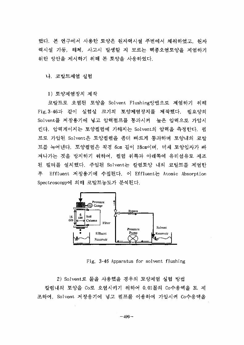
Solvent F l u s h i n g ^ ^
Fig.3-46^}-
Solvent^
Solvent
] ^ Solvents
6cm £o]
^ Effluent
Spectroscopyofl
Solvent^ ^
. °1 Effluent^ Atomic Absorption
Fig. 3-46 Apparatus for solvent flushing
2) Solvents
3L
Solvent
-499-

. 1 ^-q-^-3i](Pore Volume)
7] ^*fl ** 134^o) ^]^)5|HS ^ 12
uf. t ^ j l S . uW 134^ O|AOV C o ^^ .6^^ . ^^Alt l^K Solvents.
52.^3=1- ^|<St> ^ Effluent
. °1 Effluent-b -g-7H] ^±°} Atomic Absorption SpectroscopyS.
3) Solvents. EDTA-g- 1-
^ vfl £ ^ # a ^ l S . A^A|^7l JH*1I 0.01#£f Co^-^-i- 3L
, Solvent^ #-§-71 °ti ^^ - ^ S # o ] ^ } ^ 7}#A|*| Co^-§-^#
^<y*M ^ ^ l t l ^ K 1 ^ - ^ - ^ ) # ^^^1^171 ^*H ^ 134^-o] ^ l^ s jHS . ^ 12
1 3 4 ^ o ] # Co^-g-^ ^6HU)t[i:1-. Solvents. EDTA-g-<>J}#
^ Effluent
. o| Effluent^- -§-7]ofl ^lof Atomic Absorption SpectroscopyS.
1) °a^}^ Hl^^l1^- -8- oW 3
Solvent^
- 5 0 0 -

^JELS-Solvent
o] Solvent^
ti]
k2
Si ^ S2i
C feInstantaneous <g^£} ^.^#^-^i(M/M)o]r:K S2^ Rate-Limited^<^£\
. Kp ^ ^ ^ ^ ^ ^ - r 0 ! ^ . ki 3\ k2fe 4 4
trjf,
Si =F Kp C
dS2 /dt = ki Si-k2 S2
Si = k2 S2 S2 =F Kp C
ki/k2 =
f
- 5 0 1 -

oR6C an-2—C.~^r0D~7
W=p{k2-X)S2
F : fraction of instantaneous sorption domains
R : retardation factor
S2 : sorbed concentration in rate-limited domain(M/M)
k2 '• reverse first-order sorption rate coefficient^"1)
C : concentration in solution(M/L3)
t : time(T)
v : pore water velocity(L/T)
D : hydrodynamic dispersion coefficient(L2/T)
X ' radioactive decay constant(T"1)
x ; distance in column(L)
Kp '• equilibrium sorption coefficient(L3/M)
p '• dry bulk density
8 '• volumetric water content
FORTRAN 77 <&<>]$. *H3*1-$EU2-, Linear Basis Function^-
Galerkin ^ - * > ^ L ^ ^ # 4-§-M-^-^, ^ 1 ^ ] ^ ^ - ^«fl Implicit
Difference Scheme^ 4-§-M^-, Matrix# 7fl >Sf7l ^sfl Thomas
Algorithm^-
2) 3-^i
7\)
€ ^ H *]£ ^ ^ -f-^1^]^ * H 1 ^ £ ^ 1 - XRF (X-ray fluore-
scence)# ^ H &<$# %3} £<#<q ^ ^ ^ ^ r ^ Table3-14^|- ^o ) 68.1%
16. 7%°] A12O3 &
110
-502-

Table 3-14. Component Content of Soil
Component Content(%)
SiO2 68.1
AI2O3 16.7
K2O 8.27
Fe2O3 2.2
P2O5 1.63
CaO 1.51
Table -
bulk
] x 100
100
Table 3-15. Density, Porosity, Water Content, and pH of Soil
Dry bulk density (g/ cm3) 1.55
Porisity (%) 36.27
Water Content (%)
pH
12.00
4.30
8.46xlO"4. 2.00mm
-50 3 -

£ f e 0.133 cm/min o]uf. 1.18mm *U(N0.16)
J£fe 2.31xlO"3cm/mino)jL, ^ - ^ - ^ S ^ 0.327 cm/min
Bf)
3-47j
£ 0gata(1970)£|
Mathematica 5
1.5 m2/min
JS
Fig.
0.0 .1 .2 .3 .4 .5 .6 .7 .8 .9 1.0 1.1 1.2 1.3
Solute Concectration (g/l)
3-47. Equilibrium sorption coefficient of Co solution with
the soil
AA(Atomic
440.01mol, 0.005mol, 0.0025mol
200ml *]
^ o.3O^ Fig.3-48^
instantaneous sorption ratio)
-504-
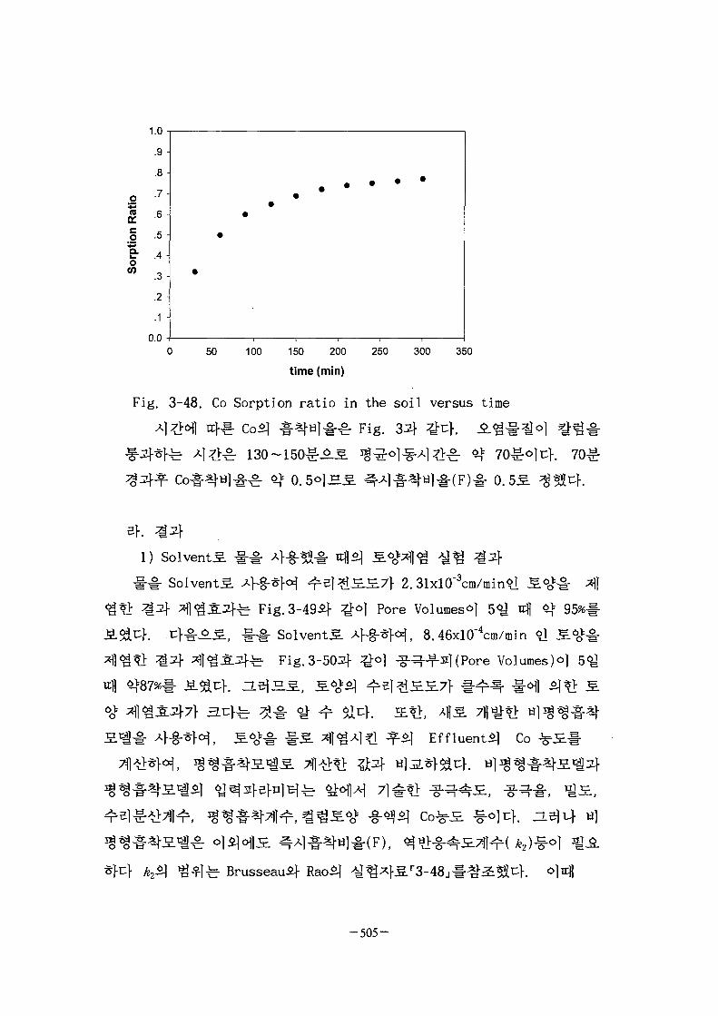
co1o
CO
Fig.
0 50 100 150 200 250 300 350
time (min)
3-48. Co Sorption ratio in the soil versus time
h& Fig. 34
1) Solvents !~I
Solvents
fe Fig. 3-494 ;
Solvents
Fig. 3-503} £0]
7f 2.31xl0"3cm/min6] ^
Pore Volumeso] 5 ^ 4 6 | 95%
, 8.46xlO"4cm/min <?]
-s) (Pore Volumes)^]
Brusseau^}
Effluent^ Co
. z i e l ^ a]
- 5 0 5 -

1.2
corocQ>
ucoo0)
lati
coOH
1 . 1 •
1 . 0 <.9 -
.8 -
.7 -
.6 -
.5 -
.4 -
.3 -
.2 -
.1 -
0.00.0 1.0 1.5 2 . 0 2 . 5 3 . 0 3 .5 4 .0 4 . 5 5 .0
Pore Volumes
Fig. 3-49. Experimental results remediating the soil of high
hydraulic conductivity by water
o
co
Io
1.2 T -
1.1 -1 .0 < • -.9 -.8 -.7 -.6 -.5 -.4 -.3 -.2.1 -
0.0 - -0.0
Equilibrium model value
Nonequilibrium model value
/ .Experimental value »
.. •
.5 1.0 1.5 2.0 2.5 3.0 3.5 4.0 4.5 5.0
Pore Volumes
Fig.3-50. Experimental and model prediction results remediating the
soil of low hydraulic conductivity by water
Fig. 3-504 °l
2) Solvents.
- 5 0 6 -
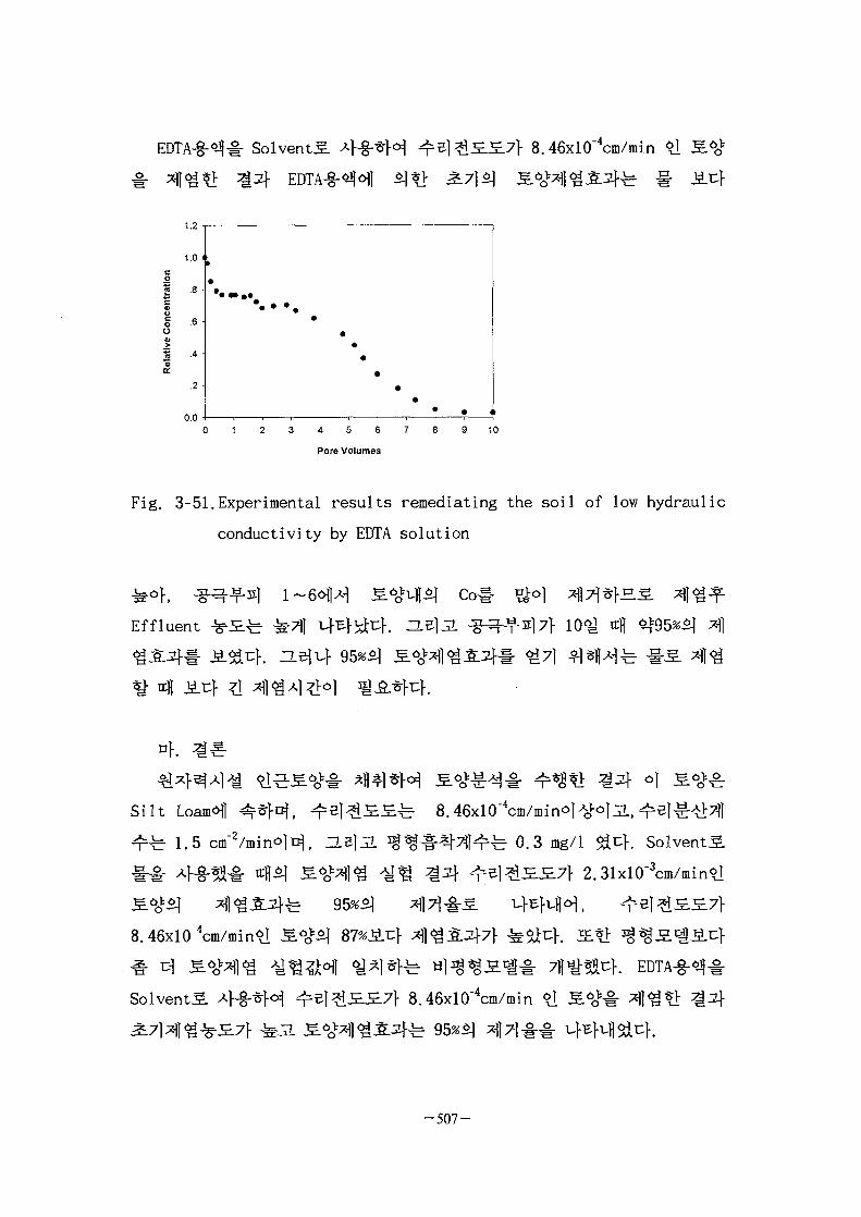
EDTA-§-6J|# S o l v e n t s ~48.46xlO~4cm/min
I
oo
0 1 2 3 4 5 6 7 8 9 10
Fig. 3-51.Experimental results remediating the soil of low hydraulic
conductivity by EDTA solution
Effluent ^ £ f e ^711
f
. -LejJL 10^ 4 ^95*^
Sil t Loam ]
^ b 1.5 cm"
8.46xlO"4cm/min*I
Solvents
8. 46xl0"4cm/min^lAo1-o|j7, e | ^ -
fe 0.3 mg/1 514. Solvents
2.31xlO-3cm/min^I
8.46xlO"4cm/min
- 5 0 7 -

5.
7\. 7fl.fi.
4
TRIGA MARK*} SflSfl 3.
71
7 ] ^4*1
NRCL-1- EPA
ICRP Publication
- 5 0 8 -

Uf. ICRP
7} £if
fe 9*4
ICRP 60
7]
4-1 *H As Low As Resonable Achievable (ALARA)7fl
-509-

37(1
1) IAEA
IAEAfe »W$ #^^1 *U A^^i -MSI ^4^1" ^t> 7]
IAEA-TECD0C-987
(cleanup criteria)
7}) Justification
1-}) Optimization
9J ^4^<H1 ai<H4 ^l^sf 4<^# ^flA|
-510-
Protection of the individual and the use of dose constraints
7}
2) US DOE
DOE Order 5400.51-
1 Ao^)^ffe 10 CFR Part 834# ^ } ) 4 ^-f-^^lJL Sl^f. DOE Order<>M
fe 6JyJ ^H^^] tHt> 2.^ tioV4^^%^^--f-^^[ 7H6J ^ ^ t > S . ^ ] # 100
mrem/yr S. f?>*FJL $I^.nf 2. t ^ e ^ 7 f ^ ^ i ^ ^ ^ ^ 4 U ^
^ > l f e 30mrem/yrS.
site
©
(D
©
©
-511-

3) US EPA
514.
4) US NRC
n]^-£| ^ 4 4 ^ -^-4 <M^S)of l^ 10 CFR Part 20, "Standard for
Protection Against Protection Radiation"# tfp^K^. ^-^]
51 nj-u} 5171
514.
. 51
4.
- 5 1 2 -

2)
XI S^ofl *l?f[ sit:}.
3711 37}*) J l
A}-g-(Unrestricted use
Stlfe
i- ^ 4X\
- 5 1 3 -

3)
7f)
(Sv)
T =
DFExt,i - ^ ^ - i ^) 5}?> 51-
(Sv y'VBq cm"2)
(Bq/g)
^r ICRP
surfaced.
-514-

Dinh =
Ub =
Csi =
A -
p =
(m3/y)
(g/cm3)
. (g/cm3)
(sv)
(Sv/Bq)
(Bq/cm3)
(Bq/cm3)
Table 3-16. Inhalation dose conversion coefficients
Mn54C06OSr9O
Cs134Cs137U235U238
Pu238Pu239Am241
1.50E-062.90E-05 ;
1.50E-046.80E-064.80E-067.70E-037.30E-034.30E-024.70E-023.90E-02:
ICRP 30Inhalation (mSv/Bq)
1.70E-064.10E-O53.40E-041.30E-05I8.70E-06'3.20E-023.20E-02;1.20E-01 |1.20E-011.20E-01 '
NUREG/CR-5512
1.81E-06!5.91E-05'3.51E-041.25E-058.63E-063.32E-023.20E-021.06E-011.16E-011.20E-01
RESRAD
1.73E-06I4.05E-053.51E-041.27E-058.65E-06"3.24E-023.24E-021.24E-01 '1.38E-011.41E-01
Uf)
ICRP 6 8 £ ICRP 60
ICRP 60
- 5 1 5 -

„ „ r
= Fa-Ua\Bp-Cs)
DCF i n g
U =
CP -
Ca =
C s =
BP =
kg-1-soil)
Fa =
( k g y_
(Sv y-
Bq-l)
(Bq kg-1) ,
(Bq kg-1) ,
(Bq kg-1).
kg-1-wet wt per Bq
(d kg-1)
Table 3-17 Ingestion Dose Conversion Coefficients (mSv/Bq)
Co60
Sr90
Cs134
Cs137
U235
U238
Pu238
Pu239
Am241
ICRP 68
3.40E-06
2.80E-05
1.90E-05
1.30E-05
4.60E-05
4.40E-05
2.30E-04
2.50E-04
2.00E-04
ICRP 30
7.00E-06
4.00E-05
2.00E-05
1.40E-05
6.90E-05
6.90E-05
9.30E-04
9.60E-04
9.80E-04
NUREG/CR-5512
7.28E-06
3.85E-05
1.98E-05
1.35E-05
7.19E-05
6.88E-05
8.65E-04
9.56E-04
9.84E-04
RESRAD
7.03E-06
3.78E-05
2.00E-05
1.35E-05
6.76E-05
6.76E-05
1.03E-03
1.16E-03
1.22E-03
- 5 1 6 -

60
ICRP 68£- ICRP 60
ICRP
(Allowable Residual Contamination Levels)
4) u]4t>^ 4-8-
oj-g-
30mrem
-517-

6. TRIGA
TRIGA
, ©]
TRIGA
r ^HyJ- 80~100m£| ^
100~200m ^ - ^ ^ ] 4)*\qr ^ ^ 127° 04'
31' ' . O)
-52if
fe o^ 1.6fe ^ 3.0
3.8 km2 o
200 400m
Key Map
South Korea
Study
Fig. 3-52 Location and topographical map of study area
-518-

3moli:>.
^ 3-532}
30~100mS
Fig. 3-53 Configuration of water table and 4 layers
-519-

715]
144
^ - f^ 3-534
o ^ ^ - ^ 3-544 ^°1 ^ ] S ^ ^ ; <* 7 cm
3- ^^r ^ H ^ 4 ^ ( S i l t y Sandstone)^.^
Clay Layer
Silty SandstoneLayer
Fig. 3-54 Kind of rock and soil in study area
1) re]^S-E.(Hydraulic Conductivity)
L7\
AH
-520-
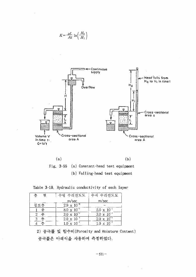
At
Volume Vin time t =Q = V/t
•*— Continuoussupply
Overflow
Cross-sectionalarea A
Heod'falls fromH o to H, in time!
Cross -sectionalarea a
Cross-sectionalarea A
(a) (b)
Fig. 3-55 (a) Constant-head test equipment
(b) Falling-head test equipment
Table 3-18. Hydraulic conductivity of each layer
1 *2 %3 %•
4 %•
m/sec2.9 x 10"8
8.0 x 10"'3.0 x 10"'2.0 x 10"'1.0 x 10"'
m/sec-
5.0 x 10"'3.0 x 10"'2.0 x 10"'1.0 x 10"'
2) 3)(Porosity and Moisture Content)
-521-

Ph ^ Bulk Density^. Oven 1 fl
- f - s l^ U¥<H ^r°l -T"W. Psfe Solid Particle Density
1 Oven SLS. QSLQ X\SL$) -f^^i- Solid Particle Volume . L-j-Y^ ^
o] ^-*>U}. Solid Particle Volume^ -i-6]
# 4
Table 3-19. Porosity and moisture content of each layer
^ £ *1 #2 *3 %4 *
29.320141210
16.712.7---
3) ^H^*]^Dispersivity)
{sediments)#^)
- Table 3-204
Silty Sandstoneif H|£
l^^[1988, 3-49]^
Silty Sandstone^] ^^r^^l^fe 30m
Table 3-20. Dispersivity of sediments
Alsace, France alluvialsedimentsRocky Mtn. Arsenalalluvial sedimentsCalifornia alluvialsedimentsArkansas River Valleycoalluvial sediments
f^^mm)12
30.5
30.5
30.5
4
30.5
9.1
30.5
#^7i5l(m)
305
305
660
4) iffusion Coefficient)
-522-

[1995, 3-50]ofl^T ^1^-^.3- Table 3-
Table 3-21 Diffusion coefficient of concrete
CsSrCo
^3 l^ (m z / s e c )1.0 x 10"IZ
1.0 x 10"n
3.0 x 10"i4
5)
3-564
Coefficient)
Stock Solution^-
. i jgs. *>i:Hl000ppm). c ^ l
Stock Solution$!
5.10. 20. 40 oom
2K
[7...
5, 10, 20,
I
r
r
Fig. 3-56 Distribution coefficient measurement procedure
40ppm# *tiS*M. olicfl, 40ppm^ Stock Solution^- 25HB
2«lf
- 5 2 3 -
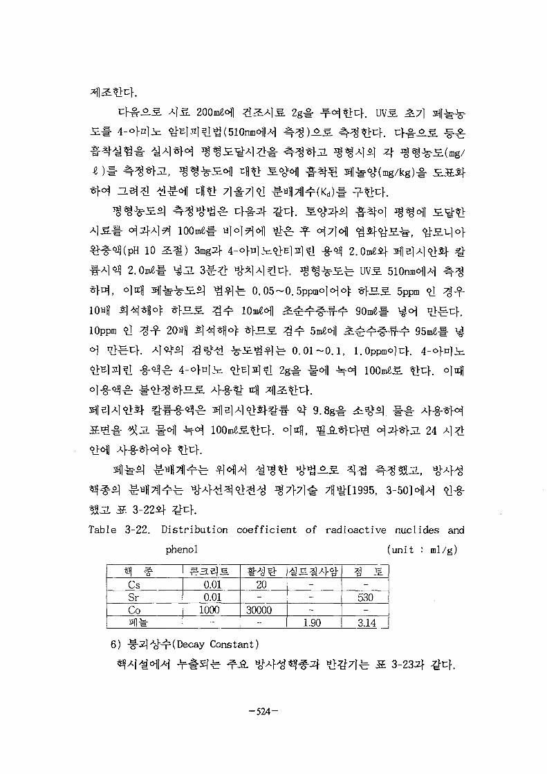
5:71
)AS.
4
10 2.
5ppm
10H|)
lOppm
0 . 0 1 - 0 . 1 , 1.0ppmo]t:K
24
Ma S 3-22 -
Table 3-22. Dis t r ibut ion coefficient of radioact ive nuclides and
phenol (unit : ml/g)
CsSrCo2)1 ^
0.010.01
1000-
20-
30000-
--
1.90
-530
-3.14
6) -3]^KKDecay Constant)
fe fi 3-234
-524-

Table 3-23 A half life of radioactive nuclides
60Co
^ ^ 7 l ( y r )3029.1
5.27
A (1/yr)2.31E-2
2.38E-2
1.31E-1
l)
TRIGA
7]
MODFLOWJS.1^(A MODular three-dimensional
water FLOW model)<§• o]^-*]-^^.^, o] 3.
finite-difference ground-
ox ax ay
, Kx, Ky, Kz :
h :
Ss :
t :
_dh_\ i _J5_ r rr dh sdt
2)
3)
Base Map)
-1*11
Map)# Auto
3.7] fe 3,000 x 1,600m °W,
3-574
XY
- 5 2 5 -

Fig. 3-57 Base map of study area
*J»5. 60 x 32 = 1,920 ?m 4 - § - * f & - ^ ,
4
]^ 50m<>)
3-584
4) ^
^ S 7}
100~200m 12
7° 04' 31'
47]
5)
- 5 2 6 -

-LZ9-
' 8 'Z ^
'Z '
Is
voiaxraOST
ft to
voiai ^
'piOT 'p i9 ^
V0IH1 ^
voiai
g (z
(9
Xpn^s T.noqe au uaraaja a^xuij gg-g "Si
1\
y
\\
1
\
\E l KZ
)
fI
J
\
I
\
\
i\
\\\
j
I
j
/J
1
-—\\
1
-
\
—
\
-
—
}
\\)
/
jjI\
f
\
\s,

0.00 400.00 800.00 1200.00 1600.00 2000.00 2400.00 2800.001600.00
1200.00
800.00
400.00
0.00
[ 1600.00
1200.00
800.00
400.00
0.00 400.00 800.00 1200.00 1600.00 2000.00 2400.00 2800.000.00
Equipotential Line Groundwater Flow Direction
Fig- 3-59. Groundwater flow modeling in 1 layer of study area

1600.000.00 400.00 800.00 1200.00 1600.00 2000.00 2400.00 2800.00
1200.00 -
800.00 -
400.00 -
0.000.00
-
-f y'l
\&
- v\
//l
/
v
I
/ ?\ *\v, 1. >
• 1 1 .1 1 1
\ ' 1 H
/ :
y ~ ^
\ 1
/ /V S
1/— —
/ /^- " / I/'sl -- ^ y
\ \ ^
\
1 "
\ _
/y ^ ,
\ ^\
/
- ^ \
f f
* ,
t I/ p
-* //
I
50
' \.
/0'
\-s
lili]
^<r — — -
, * /
\ \
\ I l\
^
. J-V"
- .
/
s /N /
\
//
Til
' % ;
Z7.;
- -_/
1i \
f~ ~~
(
u•ni /
>
— 1 -
1
f\ N -- 40
-i***Y / -" <>'
1 ^ V s
I; \
,' \, \
\
i • i
f V IP' \1 \^ ^ \ ** ****
/ C ( V" \ ' $^J(1
" v 3 ^- /
°-. - '
|\\\ \ V I
1
i
i
„ "
D —_ . *io"
30
1
1 1
*^~ ' »^ _,
/* \1
1
1
—
„
\ ^\
/ \
\ -\\
\V
\/ \
i i \
1600.00
- 1200.00
- 800.00
- 400.00
400.00 800.00 1200.00 1600.00 2000.00 2400.00 2800.000.00
Equipotential Line -• Groundwater Flow Direction
Fig. 3-60. Groundwater flow modeling in 2 layer of study area

oI
1600.00
1200.00 -
800.00 -
400.00 -
0.00
)0I
—
—
A-_ V
h
/\\}
Iy
\ s
?
400.00
/
/* \ C
i ^»\*\ y i i A T '
800.001 < ^ ^
, \ s \
/''<^'-
) ] \ ^^
/ I " ~ 4 C
' ' \ s
J, \
f I
1 1
'\ \ / \\ V >
AS. y " " ^^ /
/
1 /V
1
•-\,
;
r
/
/
•
M
1200.00I
- — °V5
r^= rs^ *
/ 7 4? ^
"\ IF?'" if I!
- - - 'jL,<*• — _ » ^
t
1i
\§-~-
' / /
; / ^
\V/
V;
I
6001
ft)," ^ x-
/
_ /
so •
• ^ -
%
\\\ |
.001
1 {J\ 1
^ V Si- " " /
'''/J::'t^ ,.-
i
; i
2000.00
^ •
2400.00
— — i • '
syi 1 /
^ i1 \
\
\
i ~
2800.00
\A!\
—
—
—V
\\
\ \
o.oo
1600.00
- 1200.00
- 800.00
- 400.00
400.00 800.00 1200.00 1600.00 2000.00 2400.00 2800.000.00
Equipotential Line Groundwater Flow Direction
Fig. 3-61. Groundwater flow modeling in 3 layer of study area
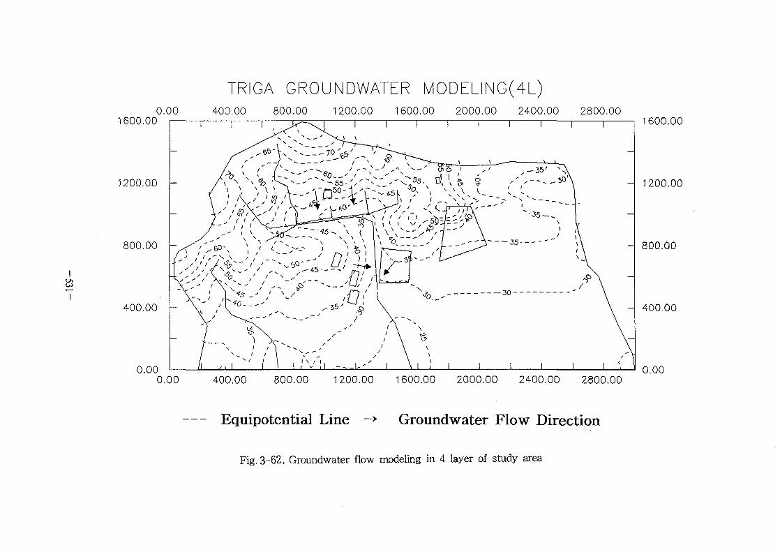
TRIGA GROUNDWATER MODELING(4L)0.00 400.00 800.00 1200.00 1600.00 2000.00 2400.00 2800.00
1600.00
1200.00
800.00
400.00
0.00
T T 600.00
1200.00
800.00
400.00
0.00 400.00 800.00 1200.00 1600.00 2000.00 2400.00 2800.000.00
Equipotential Line Groundwater Flow Direction
Fig. 3-62. Groundwater flow modeling in 4 layer of study area
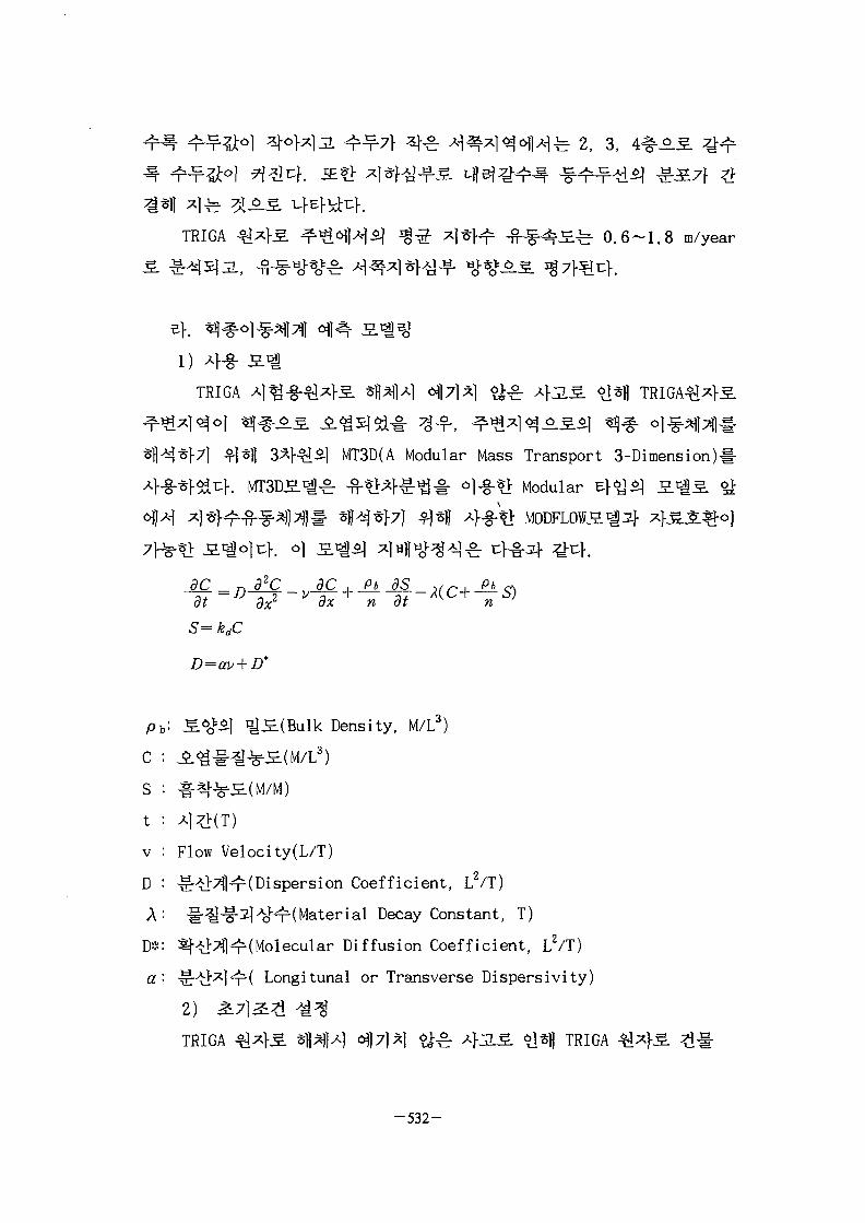
} A ^ j ^ ^ i . 2, 3, i^-SL
TRIGA ^^fS ^-^ofl^^l Jg-5: j*Hr -n-f4^r 0.6-1.8 m/year
TRIGA
41 *H 3 1- -Sl MT3D(A Modular Mass Transport 3-Dimension)#
Modular E } ^ ^
. o]
_3x dx n at n
S= kjC
D=av+D*
D
A
a
Pb: S^-^l ^S.(Bulk Density, M/L )
C
S
t
Flow Velocity(L/T)2ispersion Coefficient, L /T)
Decay Constant, T)
£7fl*r(Molecular Diffusion Coefficient, LVT)
Longitunal or Transverse Dispersivity)
2)
TRIGA #*}3. ^B^]A] <$7]%] *££: *}3LS. 6]*H TRIGA
- 5 3 2 -
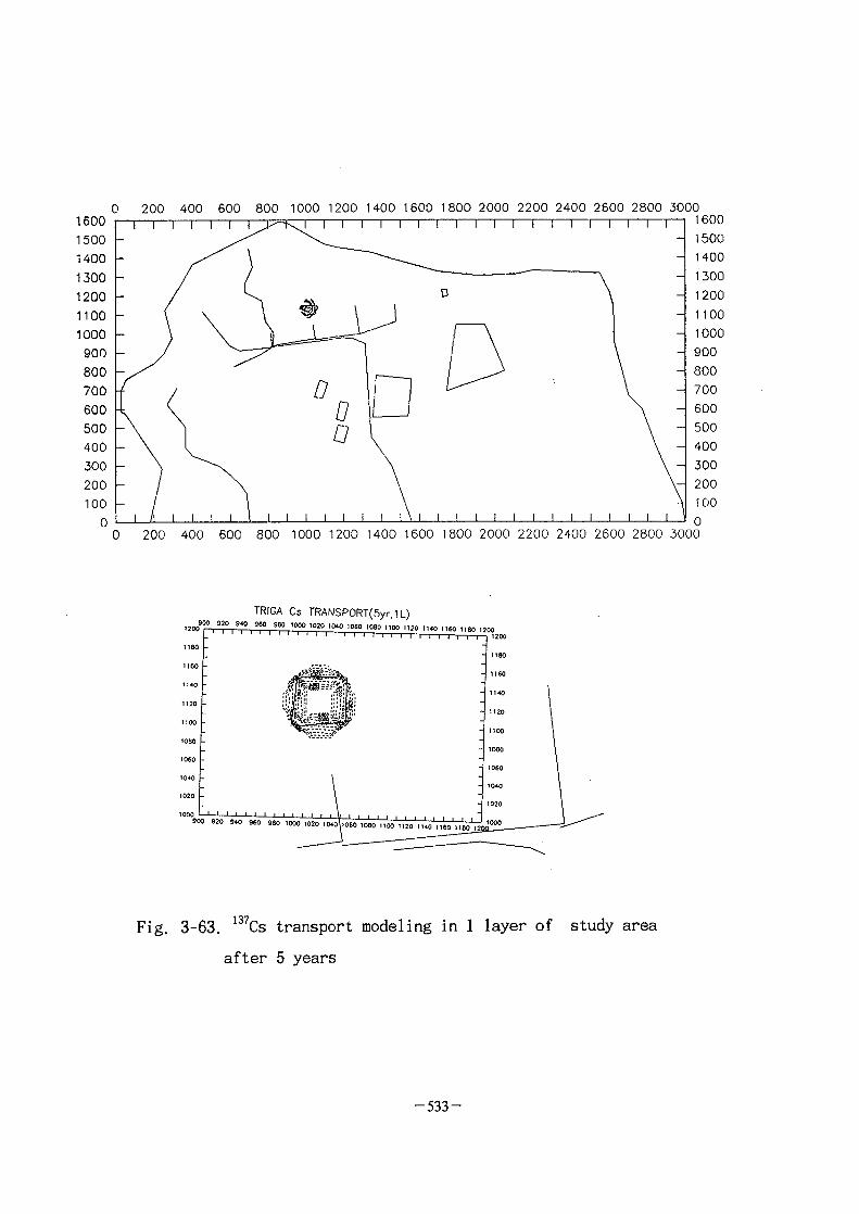
1600
1500
1400
1300
1200
1100
1000
900
800
700
600
500
400
300
200
100
0
200 400 600 800 1000 1200 1400 1600 1800 2000 2200 2400 2600 2800 3000
1 1 1 1 1 1
1 1
1
I
1 1
- \ ]
1 / I 1 I I I
k~KI 1 1 1
D0a
i i i i i i
i i i i i
D
J f
1 1 \ I 1 1
1 1 1
~ \
1 1 1
! I 1
I I I
1 1 1 1
I\
1 I 1 I
1
I I
I I
I 1
1 1
1
1
1
1600
1500
1400
1300
1200
1100
1000
900
800
700
600
500
400
300
200
100
00 200 400 600 800 1000 1200 1400 1600 1800 2000 2200 2400 2600 2800 3000
TRIGA Cs TRANSP0RT(5yr,1L)900 920 940 960 960 10OO 1020 1040 1060 1O80 1100 1120 1140 1160 HBO
1200 |—i—|—|—i—i—i—i—i—i—i—i—i—'—•—'
960 980 1000 102O I04oli060 1080 1100 1120 1140 1160 1180
Fig. 3-63. 137Cs transport modeling in 1 layer of study area
after 5 years
-533-

137Cs, 9 0Sr,
, 30\!
3)
4)
51
5)
TRIGA 1.051
3-63(a)5j-
3-64 ~ H
TRIGA
3 - 6 6 ^ 137Cs, 90Sr,
, 30
15m
0.003014. 2
^ 0.011^1 JL, 0.018<>l^f 0.025JL
10m «i
^ ^ 0.001
3-65^
JL, 10
-534-
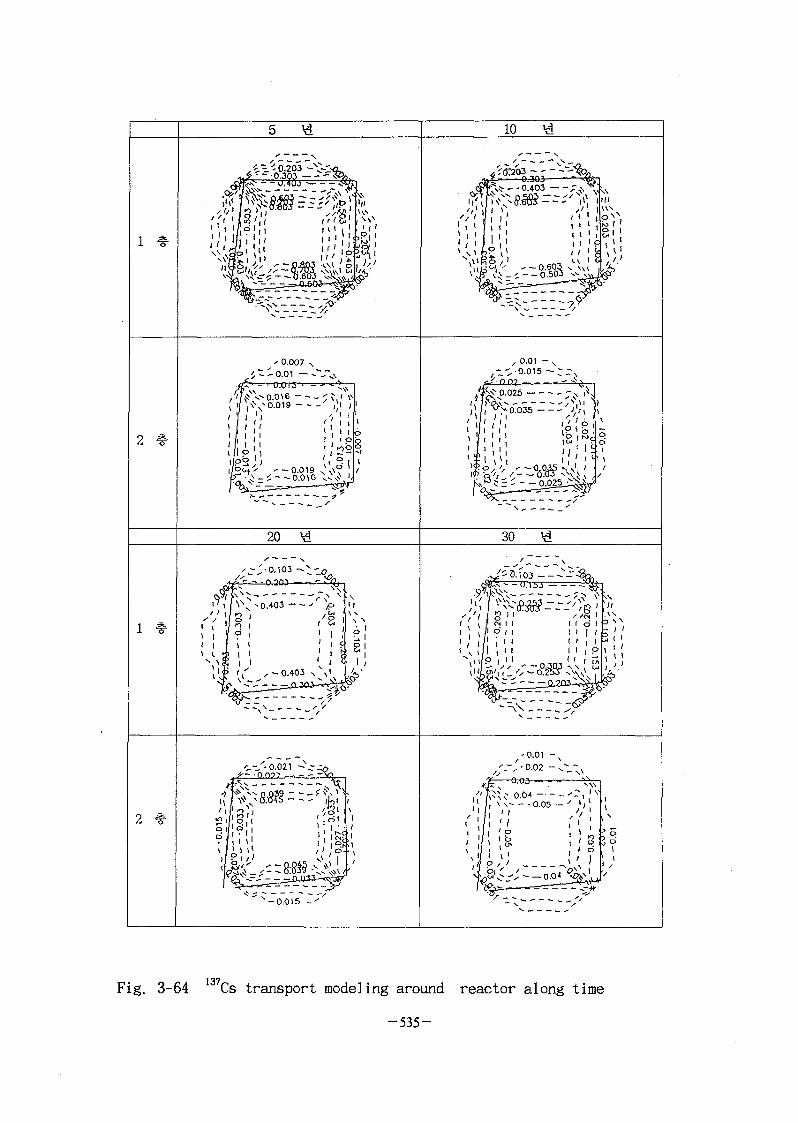
1 %•
/',~-J'0.203 -"C-C-O,,
0.40Ji — - - •&>
10
0.007 , 0.01 - ,- - -0.015 - — , ,
20 30
-0.015 - '
0.01 - ,
• 0.00 '
J
137,-Fig. 3-64 lo'Cs transport modeling around reactor along time
- 5 3 5 -
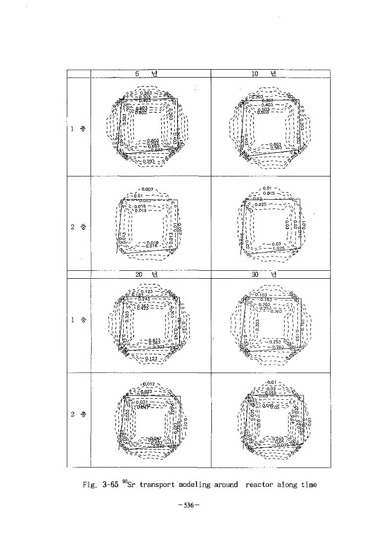
«• 5 £1X203 -iVv
10
-0.007
•-0.01 — - - -
,0.01 - %
*, 0.015 1 - N
20 30
I I I o' i ' h.
• S \ - - -
ftrr^3w
90,Fig. 3-65 Sr transport modeling around reactor along time
- 5 3 6 -

\i 10
• 3i-005
20 30
, 0.003 <-- --, 0.008 -^.- -s
. ''/"- -0.013 -y.
4E-006- -
60,Fig. 3-66. Co transport modeling around reactor along time
-53 7 -

^ 6> o.3O°H,
^ M <% 15m
0.025JL ^ %} ^ f t 4 t ^ 4 ^ l #
]] x]^^*) ^^^ S^^l^LHl £*\ ^ 0.01^14. *>^, 3
^ £ ^ 0.001 M
HQ 3-66^ 60CocHl 5]* l ^ ^ | ] ^ |
^ # ^ 4 ^ ^ 1 ^ ^ 5 ^ ^ ^ i$^5L±r <$ 0.19olJL, 10
fe <$ O.Q2°]JL, <
i f | ^ 13m
fe ^ 0.0030) 1
^4S.?l# ^Tfl^W^i 5^$\ %S.±= <% 0.000045 ] ., 10
fe ^ 0.00004^1 rt|, 2 0 \ 4 ^ ^ ^ 0.000015^13. 30Vd ffe 0.000004^
] ^ ^ ^ ^ ^ ^ ^J-ifc^K ^ ^ , 3 # 4 4
^ o.ooooi ]} 4 } # 4
7.
7f.
Spatial Variability!- i^*f7l^*H ^ b g ^ ^ # £.<&# 3 H f 7fl
I, Van Genuchten-£- ^l yfl H ^
[£ 3 7 H ^Efl^. tfe ^ $x4. ^-, ( l )
- 5 3 8 -

Specific Value(^Mr-,
(3) Value-dependent
, (2)Specified Flux(-fH£, *##*£ ), ZLB\JL
£ S i l t Loam<H]
1.5 cm"2/min<>l^,
fe 8.
0.3 mg/1 SJuK Solvent
"32.31xlO"3cm/min
918.46xlO"4cm/min<y
Solvents. "48.46xlO"4cm/ioin
3.711
. TRIGA
150m 9-^I^-
^ 0.6-1.8
n}. TRIGA
15m <> 150~200m
TRIGA ^
i ^ 7fl
— 539-NEXT PAGE(S)
left BLANK

1997\d
2000 ^ TRIGA
fe TRIGA
' 3 .
-U, 1999
r^ 1999^ 4
*U TRIGA A
TRIGA
^^(solvent flushing
*> bench -S
TRIGA
°H
7}
bench
3.7)1
TRIGA
- 5 4 1 -
NEXT PAGE(S)left BLANK

TRIGA , 2)
, 3)
sol - gel
, 2)
4)
^ TRIGA
j-g-
- 5 4 3 -
NEXT PAGE(S)left BLANK

6
3-1. R. E. Hicks and S. Tondorf, "Electrorestoration of Metal
Contaminated Soils", Environ. Sci. Technol., Vol. 28, No.
12, pp. 2203-2210(1994).
3-2. Y. B. Acar, A. N. Alshawabkeh and R. J. Gale, "Fundamentals
of Extracting Species from Soils by Electrokinetics", WASTE
MANAGEMENT, Vol. 13, pp. 141-151(1993).
3-3. Davis, A. P., "Washing of Zinc(II) from Contaminated Soil
Column", J. Envir. Engr., 27(2), pp. 174-185(1995).
3-4. Kari, F. G., Xue, H., and Sigg, L., "Speciation of EDTA in
Natural Waters:Exchange Kinetics of Fe-EDTA in Rever Water",
Environ. Sci. Technol, 29(1), pp. 59-68(1995).
3-5. Gall, E. J. , and Farley, K. J., "Evaluation of Nickel Removal
From Savannah River Site Soil By EDTA and Ethylendiamine",
Nuclear and Hazardous Waste Management Spectrum'94, pp.
675-680(1994).
3-6. Girvin, D. C., Gassman, P. L., and Bolton, B., "Adsorption of
Aqueous Cobalt EDTA by d -A12O3", Soil Sci. Soc. AM. J., 57,
47-57 (1993).
3-7. Nishita, H., and Essington, E.H., "Effect of chelating agents
on the movement of fission products in soils", Soil Sci.,
103(3), 168-176(1966).
3-8. Wilkins, R. G., and Yelin, R. E., "The Probable Structures of
Cobalt(II)-EDTA Type Complexes in Aqueous Solution from
Oxidation Experiments", J. Amer. Chem. Soc., 92(5),
pp.1191-1194(1970).
3-9. Motrits, W.C., Gushikem, Y., and Nasimento, 0. R., "Adsorption
and structure of MC12 (M = Co2+, Cu2+, Zn2+, Cd2+, and Hg2t)
-545-
Complex species on a chemically Modified Silica Gel Surface
with 1,4 - Diazabicyclo(2.2.2) Octane", J. Colloid Interface
Sci. 150(1), pp.115-120(1991).
3-10. Warwick, P., Shaw, P., Williams, G. M., and Hooker, P. J.,
"Preliminary Studies of Cobalt Complexation in Groundwater",
Radiochimica Acta, 44, pp.55-63(1988).
3-11. Hicks, R. E., and Tondorf, S., "Electrorestoration of
Contaminated Soils, Environ. Sci. Technol., 28(12),
pp.2203-2210(1994).
3-12. Szrvsody, J. E., Zachara, J. M., and Bruckhart, P. L.,
"Adsorption - Desorption Reactions Affecting the Distribution
and Stability of ConEDTA in Iron Oxide-Coated Sand", J.
Environ. Sci. Technol., 28(9), pp.1706-1716 (1994).
3-13. B. G. AHN, H. J. WON, W. Z. OH : Decontamination of Building
Surface Using Clay Suspension", J. of Nuc. Sci. and Tech. pp.
787 - 793, Aug. (1995).
3-14. R0ED J. : Run-Off from and Weathering of Roof Material
Following the Chernobyl Accident, Radiat. Prot. Dosim., 21
59, (1987).
3-15. ROED J. : Deposition and Removal of Radioactive Substances in
an Urban Area, Final Report of the NKA, Project AKTU-245,
Riso National Laboratory(1990).
3-16. SANDALLS, F. J. : Removal of Radiocaesium from Urban Surfaces
Contaminated as the Results of Nuclear Accident, AERE R
122355(1987).
3-17. DE WITT H. , GOLDAMMER W., BRENK H. D., HILLE R., JACOBS H.,
FRENKLER K., : Decontamination of Urban Areas after Nuclear
Accident, Proc. of Symp. on Recovery, Operations in the event
of Nuclear Accident or Radiological Emergency, IAEA,
Vienna, 6-10 November(1989).
-546-
3-18. BENGAL P. R., MASON R. C. : Results of the Gross
Decontamination Experiment and Implications for Future
Decontamination Activity, Proc. of ANS/CNA Conf. on
Decontamination of Nuclear Facilities, Niagara Falls,
September(1982).
3-19. LEWIS, W. B. : The Accident to the NRX Reactor on December
12, 1952, AECL-232, Atomic Energy of Canada Ltd.,
0ntario(1953).
3-20. VAN OLPHEN H. : "An Introduction to Clay Colloid Chemistry
for Clay Technologists, Geologists and Soil Scientists", 2nd
ed., Krieger Pub. Co.(1977).
3-21. DE BOER J. H. : "The Structure and Properties of Porous
Materials", Butterworth, New York(1958).
3-22. VAN OLPHEN H. : The Rheological Behavior of Clay-Water
System, American Perfumer, 77, 45(1962).
3-23. BIRD R. B., ARMSTRONG R. C. and HASSAGER 0. : "Dynamics of
Polymeric Liquids", Vol. 1, 2nd ed. , John Wiley & Sons Inc.,
New York(1987).
3-24. TEMPLE, C. P.: "Paint Flow and Pigment Dispersion", 2nd ed. ,
John Wiley & Sons Inc., New York(1987).
3-25. POURBAIX M. : "Atlas of Electrochemical Equilibria in Aqueous
Solution", National Association of Corrosion Engineers,
Houston, Texas, U.S.A(1974).
3-26. RYAN W. : "Properties of Ceramic Raw Materials", (1968),
Pergamon Press, Oxford.
3-27. WEAVER C. E. : Geothermal Alternation of Clay Minerals and
Shales, ONWI-21 (1979).
3-28. BRADY N. C. : "The Nature and Properties of Soils", (1974),
Macmillan Pub. Co., New York.
3-29. CARTER D. L., HEILMAN M. D. and GONZALEZ C. L. : Ethylene
-547-

Glycol Monoethyl Ether for Determing Surface Area of Silicate
Minerals, Soil Sci.,, 100, 356 - 360 (1965).
3-30. JCPDS, Powder Diffraction Data File, Index No. 12-219, 13-135,
13-256, 29-1498, U.S. Joint Committee on Powder Diffraction
Standards, Pennsylvania (1972).
3-31. Fetter, C. W. , Applied Hydrogeology. 2d ed., Macmillan
Publishing Conpany, pp. 588(1988), XMoreno, L. and Neretnieks,
I., Flow and nuclide transport in fractured meadia. J. of
Contaminant Hydrology, 13, 49(1993).
3-32. Cushey, M.A., Bellin, A., and Rubin, Y. Generation of three
dimensional flow fields for statistically anisotropic
heterogeneous porous media, Stoch. Hyd. Hydraul., 9,
89.(1995).
3-33. Gelhar, L. W., and Azness, C. L. Three-dimensional stochastic
analysis of macrodispersion in aquifers. Water Resour Res.
19(1), 161-180(1993).
3-34. Jang, Y. S., Sitar, N., and Der Kiureghian, A., Reliability
analysis of contaminant transport in saturated porous meadia.
Water Resources Res., Amer AGU, 30, 2435(1994).
3-35. Wierenga, P. J., and van Genutchen, M. TH. Solute transport
through small and large unsaturated plainfield sand. Water
Resour. Res., 14, 528-588(1989).
3-36. McDonald, M. G., and Harbaugh, A. W. A modular
three-dimensional finite-difference ground-water flow model.
U.S. Geological Survey(1988).
3-37. Zheng, C., A modular three-dimensional transport model for
simulation of advection, dispersion and chemical reactions of
contaminants in ground water system, S. S. Papadopulos &
Associates, Inc(1990).
3-38. Huyakorn, P. S., A two-dimensional finite element code for
-548-
simulating fluid flow and transport of radionuclides in
fractured porous media with water table boundary conditions,
Hydrogeologic, Inc.(1987).
3-39.
3-40.
3-41. Yeh, G. T. FEMWATER : A finite element model of water flow
through saturated-unsaturated porous media-first revision. Oak
Ridge National Lab., ORNL-5567/RL(1987).
3-42. van Genuchten, M. T., A Closed-form Equation for Predicting
the Hydraulic Conductivity of Unsaturated Soils, Soil Sci. Soc.
J. 44:892-898(1980).
3-43. EPA, In Siut Soil Flushing, Engineering Bulletin,
EPA/540/2-91/021 (1991).
3-44.Brusseau, M L., and Rao, P. S. C. "The Influence of
Sorbate-Organic Matter Interaction on Sorption Nonequilibrium",
Chemosphere, 18(9/10), 1691-1706 (1989).
3-45. Augustijn, D. C. M., Jessup, R. E., Rao, P. S. C., and Wood A.
L. "Remediation of Contaminated Soils by Solvent Flushing",
Journal of Environmental Engineering, Vol.120, No.1, pp 42-56
(1994)
3-46. Brusseau, M. L., Jessup, R. E., and Rao, P. S. C.
"Nonequilibrium Sorption of Organic Chemicals: Elucidation of
Rate-Limiting Processes'", Environ. Sci. Technol., 25(1), pp
134-142 (1991).
3-47. *pg^, "^-M^tr.-il-fSSW, PP.29.
3-48. Nkedi-Kizza P., Brusseau M.L., Rao S. P. C., and Hornsby A.
G.,"Nonequilibrium Sorption during Displacement of Hydrophobic
Organic Chemicals and Ca through Soil Column with Aqueous and
-549-
Mixed Solvents",Environ. Sci. Technol. 23(7), pp.814-820(1989)
3-49. ?H}# , ^ ^ e ] * ) ^ , -ii-^&SW, PP. 38-39(1988).
3-50.
- 5 5 0 -

KAERI/RR-1907/96
• »
nil o|
*lc
(10EK
is*
, i
XI
1 ^
15-2C
1 ®l2 ")3. &
!?l°-i-
r|] g
550
a
*ll §J S
^ • 7 | A N^•7|A|4
)
1
IS
P-
)•
A-j X|
^|Ej-7j^!-SJLA
x-ll'gsil^l §J
oiasi, ^ ^
o4 ^-Xl-: 2j5|£
O|7M
M7I8
dsi -K ) . _
S.^17|# 7H# c
L2.|E., -g-S, s||Ji
s .
Pig
5H*II i
r. at?
O| 0AA C3
a .
J
%<
a-
1 C
J
=
, a asr. "fe!^5
i, O|*T
X|-BNoj^
) ), HA'S'
SJLA-
, 1 ^
3 Ah & i
A'
inA-ias INIS
71.^. jii ui-
[ ) 3. 7 I
1 0,
S,
1999.
29.7
AH
H
3.
Cm.
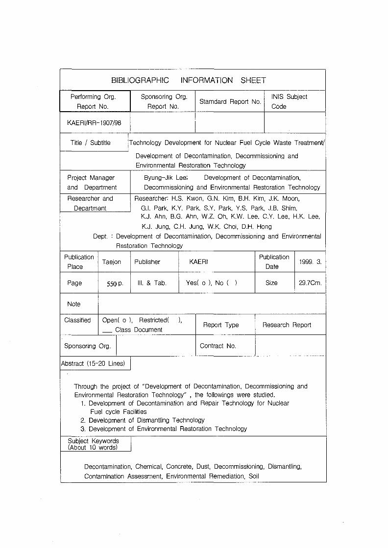
BIBLIOGRAPHIC INFORMATION SHEET
Performing Org.
Report No.
Sponsoring Org.
Report No.Stamdard Report No.
IMS Subject
Code
KAERI/RR-1907/98
Title / Subtitle Technology Development for Nuclear Fuel Cycle Waste Treatment/
Development of Decontamination, Decommissioning andEnvironmental Restoration Technology
Project Manager
and Department
Byung-Jik Lee; Development of Decontamination,
Decommissioning and Environmental Restoration Technology
Researcher and
Department
Researcher: H.S. Kwon, G.N. Kim, B.H. Kim, J.K. Moon,G.I. Park, K.Y. Park. S.Y. Park, Y.S. Park, J.B. Shim,K.J. Ahn, B.G. Ahn, W.Z. Oh, K.W. Lee, C.Y. Lee, H.K. Lee,
KJ. Jung, C.H. Jung, W.K. Choi, D.H. Hong
Dept. : Development of Decontamination, Decommissioning and Environmental
Restoration Technology
Publication
PlaceTaejon Publisher KAERI
Publication
Date1999. 3.
Page 550 P- III. & Tab. Yes( o ), No Size 29.7Cm.
Note
Classified Open( o ), Restricted!
Class DocumentReport Type Research Report
Sponsoring Org. Contract No.
Abstract (15-20 Lines)
Through the project of "Development of Decontamination, Decommissioning andEnvironmental Restoration Technology" , the followings were studied.
1. Development of Decontamination and Repair Technology for NuclearFuel cycle Facilities
2. Development of Dismantling Technology3. Development of Environmental Restoration Technology
Subject Keywords(About 10 words)
Decontamination, Chemical, Concrete, Dust, Decommissioning, Dismantling,
Contamination Assessment, Environmental Remediation, Soil