Technique and Muscle Activity of the Water Polo Eggbeater ...

This thesis has been submitted in fulfilment of the requirements for a postgraduate degree

(e.g. PhD, MPhil, DClinPsychol) at the University of Edinburgh. Please note the following

terms and conditions of use:

This work is protected by copyright and other intellectual property rights, which are

retained by the thesis author, unless otherwise stated.

A copy can be downloaded for personal non-commercial research or study, without

prior permission or charge.

This thesis cannot be reproduced or quoted extensively from without first obtaining

permission in writing from the author.

The content must not be changed in any way or sold commercially in any format or

medium without the formal permission of the author.

When referring to this work, full bibliographic details including the author, title,

awarding institution and date of the thesis must be given.

Technique and Muscle Activity of the Water Polo Eggbeater Kick at

Different Levels of Fatigue

Nuno Oliveira

Doctor of Philosophy

The University of Edinburgh

2014

I

Technique and Muscle Activity of the Water Polo Eggbeater Kick at Different

Levels of Fatigue

The eggbeater kick is a skill used frequently in water polo and synchronized swimming to

elevate the upper body for shooting, passing, blocking or compete with the opponent for position

in the water. The hips, knees, and ankles are involved in creating favourable orientations of the

feet so that propulsive forces in the vertical direction can be created. Literature reporting the

technique of the eggbeater kick is scarce and limited to description of kinematics or muscle

activity. The relationship of the kinematics to the demands on specific muscles has not been

established. The purpose of this study was to analyze the kinematics and muscle activity of the

water polo eggbeater kick in fatigued and unfatigued states to provide foundational knowledge

on which training programs can be based. Twelve water polo players were tested executing the

eggbeater kick in the vertical position while trying to maintain as high a position as possible for

the duration of the test. The test was terminated when the player could not keep the top of the

sternum marker above water. Anthropometric data were collected using the ‘eZone’ method.

Three dimensional coordinates for the lower limbs and two dimensional coordinates of the above

water top of the sternum marker were obtained. Surface electromyography recorded the muscle

activity of the Tibialis Anterior, Rectus Femoris and Biceps Femoris muscles on both legs.

Differences between fatigued and unfatigued conditions and between dominant and non-

dominant sides were tested using a two factor ANOVA with repeated measures. Differences

within subjects were also investigated on a subject by subject basis with regard to muscle

activity. Results indicated differences for kinematic and muscle activity variables between

fatigue levels. The amplitude of anatomic angles and speed of the feet decreased with fatigue.

Significant differences were found between dominant and non-dominant sides for the ankle

motion. The non-dominant ankle was more inverted and adducted than the dominant ankle

during the knee flexion phase of the cycle. The Rectus Femoris muscle had consistent patterns

across subjects, while Tibialis Anterior and Biceps Femoris muscles were more subject specific

in their responses. The Rectus Femoris and the Biceps Femoris have an agonist/antagonist

relationship during knee flexion and extension. The Tibialis Anterior was active for long periods

in the cycle while dorsiflexing and inverting the foot. As a consequence activity in these muscles

decreased with fatigue. These findings point towards the necessity for players and coaches to

address specific motions and muscles during the training of the eggbeater technique. Future

work should focus on developing eggbeater kick training programs that address specific strength

and flexibility.

II

Technique and Muscle Activity of the Water Polo Eggbeater Kick at

Different Levels of Fatigue

The University of Edinburgh

Thesis submitted for the degree of Doctor of Philosophy to The University of Edinburgh.

I hereby declare that this thesis is my own work, that it has not been submitted for any other

academic award, or part thereof, at this or any other educational institute.

Student: Date:

III

Acknowledgements

I would like to acknowledge the contribution of many people to this project.

First, I would like to thank Prof. Ross Sanders for the guidance and mentoring throughout my

thesis. I would like to thank you for encouraging my research and for allowing me to grow as a

research scientist.

I would like to express my special appreciation to Dr. Simon Coleman and Dr. Dave Sounders

for the advice and insightful comments in the writing of this thesis.

To all the CARE team, namely Marlies Declerck, Jacki Thow, Tomohiro Gonjo, Chuang-Yaun

Chiu and Jon Kelly. It was great to be part of the team and I can say I have learned a lot from

each one of you.

To all the water polo players that participated in this study, your commitment was truly amazing!

Finally, I would like to thank my parents – Manuel and Margarida – for being always there

throughout these years, and Sarah for her personal support and great patience at all times.

IV

Table of Contents

1 Introduction ............................................................................................................................ 2

1.1 Purpose of the Study ...................................................................................................... 5

2 Review of the Literature ........................................................................................................ 7

2.1 The Eggbeater Kick ....................................................................................................... 7

2.2 The Issue of Side Dominance and Asymmetries ......................................................... 12

2.3 Methodological Issues.................................................................................................. 14

2.3.1 Anatomical Descriptors ........................................................................................ 14

2.3.2 Movement Description ......................................................................................... 15

2.3.3 Joint Angles ......................................................................................................... 17

2.3.4 Kinematics ........................................................................................................... 18

2.3.5 Kinetics ................................................................................................................ 28

2.3.6 Electromyography ................................................................................................ 37

2.4 Summary of Literature Review .................................................................................... 49

3 Methods................................................................................................................................ 51

3.1 Participants ................................................................................................................... 51

3.2 Participant Preparation ................................................................................................. 52

3.2.1 Skin Markers ........................................................................................................ 52

3.2.2 Surface Electromyography ................................................................................... 55

3.3 Experimental Design .................................................................................................... 56

3.3.1 Swimming Pool Details ....................................................................................... 56

3.3.2 Camera Settings ................................................................................................... 56

3.3.3 Calibration Frame ................................................................................................ 58

3.4 Testing Set Up .............................................................................................................. 58

3.5 Testing Procedure ........................................................................................................ 61

3.6 Data Collection Methods ............................................................................................. 62


3.6.2 Maximum Voluntary Isometric Contractions ...................................................... 63

3.6.3 Anthropometric Data............................................................................................ 64

3.6.4 Weight + Buoyancy Measurement ....................................................................... 65

3.6.5 3D Kinematics Dynamic Validation .................................................................... 66

V

3.7 Data Processing ............................................................................................................ 66

3.7.1 Eggbeater Kick Trial Digitising ........................................................................... 66

3.7.2 Height Assessment ............................................................................................... 68

3.7.3 Weight + Buoyancy Assessment .......................................................................... 69

3.8 Calculations of Variables ............................................................................................. 69

3.8.1 Joint Angles ......................................................................................................... 70

3.8.2 Foot Speed ........................................................................................................... 73

3.8.3 Pitch Angles ......................................................................................................... 75

3.8.4 Sweepback Angles ............................................................................................... 76

3.8.5 Vertical Component of the Force ......................................................................... 77


3.9 Reliability ..................................................................................................................... 81

3.10 Statistical Analysis ....................................................................................................... 82

4 Results .................................................................................................................................. 86

4.1 3D Kinematics Dynamic Validity ................................................................................ 86

4.2 Reliability of Calculated Variables .............................................................................. 86

4.3 Comparisons Between Fatigue Level and Dominance ................................................ 92

4.3.1 Average Vertical Force ........................................................................................ 92

4.3.2 Mean Maximum Vertical Force ........................................................................... 93

4.3.3 Hip Joint ............................................................................................................... 94

4.3.4 Knee Joint .......................................................................................................... 100

4.3.5 Ankle Joint ......................................................................................................... 102

4.3.6 Joint Angular Velocity ....................................................................................... 108

4.3.7 Feet Pitch Angles ............................................................................................... 111

4.3.8 Average Foot Sweepback Angles ...................................................................... 113

4.3.9 Average Foot Speed ........................................................................................... 114

4.3.10 Feet Motion ........................................................................................................ 115

4.3.11 Summary Table .................................................................................................. 116

4.4 Muscle Activity .......................................................................................................... 118

4.4.1 Tibialis Anterior ................................................................................................. 118

4.4.2 Rectus Femoris ................................................................................................... 124

4.4.3 Biceps Femoris ................................................................................................... 131

VI

4.4.4 Summary Table .................................................................................................. 137

4.5 Correlations between Vertical Force and Studied Variables ..................................... 137

5 Discussion .......................................................................................................................... 142

5.1 Factors Influencing Performance when not Fatigued ................................................ 142

5.2 Dominant vs Non-Dominant Side .............................................................................. 154

5.3 Implications for Training to Improve Performance ................................................... 160

5.3.1 Role of the Muscles in the Cycle ....................................................................... 160

5.3.2 Specific Training for the Eggbeater Kick .......................................................... 169

6 Conclusions ........................................................................................................................ 173

6.1 Technique and Performance....................................................................................... 173

6.2 Fatigue........................................................................................................................ 174

6.3 Dominance ................................................................................................................. 175

6.4 Practical Applications ................................................................................................ 176

6.5 Limitations and Future Work ..................................................................................... 178

7 Bibliography ...................................................................................................................... 182

8 Appendix A ........................................................................................................................ 198

9 Appendix B ........................................................................................................................ 206

10 Appendix C .................................................................................................................... 209

VII

List of Figures

Figure 2.1. Associations between the variables being studied. Adapted from Sanders (1999a) .. 8

Figure 2.2. Illustration of the anatomical position....................................................................... 14

Figure 2.3. Xyz rotation sequence ................................................................................................ 26

Figure 2.4. Illustration of Hanavan’s segment model. ................................................................. 32

Figure 2.5. Illustration of Hatze’s segment model. ...................................................................... 33

Figure 2.6. Yeadon’s segments and subsegments (adapted from Dembia (2011)). .................... 34

Figure 2.7. Illustration of Jensen’s elliptical model (from Jensen (1978)). .................................. 36

Figure 2.8. Illustration of the action potential mechanism. ........................................................ 39

Figure 3.1. Individual muscle surface EMG waterproofing final stage. ....................................... 55

Figure 3.2. Final result of participant preparation. Markers and EMG waterproofing. .............. 56

Figure 3.3. Position of the underwater (1-4) and above water cameras (5). .............................. 59

Figure 3.4. An underwater view of calibration frame from camera 1 perspective. .................... 60

Figure 3.5. Above view of calibration frame from camera 5 perspective. .................................. 60

Figure 3.6. Above view of the player during the eggbeater kick trial. ......................................... 61

Figure 3.7. Synchronization device. ............................................................................................. 63

Figure 3.8. Representation of the electric impulse from the synchronization device. The red

arrow shows the time when the electric impulse was created. .................................................. 63

Figure 3.9. Camera view and digitising screen for weight + buoyancy assessment .................... 66

Figure 3.10. Camera view and digitising screen for height assessment ...................................... 68

Figure 3.11. Second degree regression equation calculated for the weight + buoyancy. ........... 69

Figure 3.12. Representation of the body markers and the lower limb coordinate frames. ........ 71

Figure 3.13. Foot pitch angles at 30° and 0°. ............................................................................... 76

Figure 3.14. Illustration of sweepback angles. Black arrows indicates different sweepback

angles. .......................................................................................................................................... 77

Figure 4.1. Average Vertical Force produced for the three fatigue conditions studied. Error bars

represent the group’s standard deviation. .................................................................................. 93

Figure 4.2. Maximum vertical force produced for the three conditions studied. Error bars

represent the group’s standard deviation. .................................................................................. 94

Figure 4.3. Average Right Tibialis Anterior activity for the three fatigue conditions. Error bars

represent the group’s standard deviation. ................................................................................ 119

Figure 4.4. Average Left Tibialis Anterior activity normalized to MVC for the three fatigue

conditions. Error bars represent the group’s standard deviation. ............................................ 120

Figure 4.5. Average Left Tibialis Anterior normalized to peak of the cycle for the three fatigue


Figure 4.6. Right Tibialis Anterior activity pattern for non-fatigued and fatigued conditions. Solid

line represents the mean, dotted line the 95% confidence interval of the true mean. ............ 122

Figure 4.7. Individual activation times of the Right Tibialis Anterior for the non-fatigue condition

following the double-threshold method. .................................................................................. 122

VIII

Figure 4.8 Left Tibialis Anterior activity pattern for non-fatigued and fatigued conditions. Solid

line represents the mean, dotted line the 95% confidence interval of the true mean. ............ 123

Figure 4.9 Individual activation times of the Left Tibialis Anterior for the non-fatigue condition


Figure 4.10. Average Right Rectus Femoris and Left Rectus Femoris activity for the three fatigue


Figure 4.11. Average Left Rectus Femoris activity normalized to MVC for the three fatigue


Figure 4.12. Average Left Rectus Femoris normalized to peak of the cycle for the three fatigue


Figure 4.13. Right Rectus Femoris activity pattern for non-fatigued and fatigued conditions.

Solid line represents the mean, dotted line the 95% confidence interval. ............................... 128

Figure 4.14. Individual activation times of the Right Rectus Femoris for the non-fatigue

condition following the double-threshold method. .................................................................. 129

Figure 4.15. Left Rectus Femoris activity pattern for non-fatigued and fatigued conditions. Solid

line represents the mean, dotted line the 95% confidence interval. ........................................ 130

Figure 4.16. Individual activation times of the Left Rectus Femoris for the non-fatigue condition


Figure 4.17. Average Left Biceps Femoris activity for the three fatigue conditions. Error bars

represent the group’s standard deviation. ................................................................................ 131

Figure 4.18. Average Left Biceps Femoris activity normalized to MVC for the three fatigue


Figure 4.19. Average Left Biceps Femoris activity normalized to peak of the cycle for the three

fatigue conditions. Error bars represent the group’s standard deviation. ................................ 133

Figure 4.20. Right Biceps Femoris activity pattern for non-fatigued and fatigued conditions.

Solid line represents the mean, dotted line the 95% confidence interval. ............................... 134

Figure 4.21. Individual activation times of the Right Biceps Femoris for the non-fatigue

condition following the double-threshold method. .................................................................. 135

Figure 4.22. Left Biceps Femoris activity pattern for non-fatigued and fatigued conditions. Solid

line represents the mean, dotted line the 95% confidence interval. ........................................ 136

Figure 4.23. Individual activation times of the Left Biceps Femoris for the non-fatigue condition


Figure 5.1. Dominant side hip abduction, flexion, internal rotation, and knee flexion during the

non-fatigued cycle across all subjects. ....................................................................................... 144

Figure 5.2. Knee flexion-extension angular velocity (AV) across all subjects during the non-

fatigued cycle (solid lines). Vertical Force during the cycle (dashed line). Dotted lines indicate

the 95% confidence interval of the true mean. ......................................................................... 145

Figure 5.3. Knee flexion-extension angular velocity (solid lines) and foot speed (dashed lines)

for the non-fatigued cycle across all subjects. ........................................................................... 148

IX

Figure 5.4. Feet pitch angles for dominant and non-dominant side during the non-fatigued cycle

across all subjects. Dotted lines indicate the 95% confidence interval. .................................... 148

Figure 5.5. Feet sweepback angles for dominant and non-dominant side during the non-

fatigued cycle for a typical subject. Black lines show when the flow changes from medial to

lateral and vice-versa. ................................................................................................................ 149

Figure 5.6. Vertical force produced during the cycle for non-fatigued and fatigued conditions

across all subjects. Dotted lines indicate the 95% confidence interval of the true mean. ........ 151

Figure 5.7. Dominant side hip abduction, flexion, and internal rotation for the non-fatigued (NF)

and fatigued (F) cycle across all subjects. .................................................................................. 153

Figure 5.8. Mean vertical force produced during the non-fatigued eggbeater kick cycle across all

subjects. Stick figures show position of the lower limbs at 16%, 40%, 68% and 94% of the time

in the cycle. ................................................................................................................................ 156

Figure 5.9 Mean ankle angles for dominant (DS) and non-dominant (NDS) side during the non-

fatigued cycle across all subjects. .............................................................................................. 157

Figure 5.10 Hip angles for dominant (DS) and non-dominant (NDS) side during the non-fatigued

cycle across all subjects. ............................................................................................................ 159

Figure 5.11 Illustration of moments in the cycle where the Right Tibialis Anterior is most active.

Blue represents the right side and red the left. Green indicates the anterior part of the foot. 161

Figure 5.12 Right ankle inversion, plantar flexion and adduction with Right Tibialis Anterior

normalized activity during the cycle for non-fatigued condition. Mean TA activity is represented

by the solid line and dotted lines indicate the 95% confidence interval. .................................. 162

Figure 5.13 Left ankle inversion, plantarflexion and adduction and Left Tibialis Anterior activity

during the cycle for non-fatigued condition. Mean TA activity is represented by the solid lines

and dotted lines indicate the 95% confidence interval. ............................................................ 163

Figure 5.14 Illustration of time in the cycle where the Right Rectus Femoris was most active.

Blue represents the right side and red the left. Green indicates the anterior part of the foot. 163

Figure 5.15 Dominant (DS) knee flexion angular velocity (AV), Rectus Femoris and Biceps

Femoris activity during the cycle for non-fatigued (NF) and fatigued (F) condition. Dotted lines

indicate the 95% confidence interval of the true mean. ........................................................... 165

Figure 5.16 Non-dominant (NDS) knee flexion angular velocity (AV), Rectus Femoris and Biceps


indicate the 95% confidence interval of the true mean. ........................................................... 166

Figure 5.17 Illustration of moments in the cycle where the Right Biceps Femoris is most active.

Blue represents the right side. Green indicates the anterior part of the foot. ......................... 168

Figure 5.18 Dominant (RBF) and non-dominant (LBF) Biceps Femoris activity for non-fatigued

and fatigued conditions across all subjects. Black lines are an estimate indication of when the

Biceps Femoris alternated from a main antagonist (ANT) role to a main agonist. ................... 169

X

List of Tables

Table 3.1 Location of the body markers for digitizing ................................................................ 53

Table 3.2. Location of the additional body markers for the Ezone. ............................................. 54

Table 3.3. MVIC test protocol. .................................................................................................... 64

Table 4.1. Reliability results for nine cycles at NF and F conditions. ......................................... 87

Table 4.2. Mean (N) and standard deviation of average vertical force for non-fatigued (NF), 50%

time point (50% TP) and fatigued (F) conditions. ....................................................................... 92

Table 4.3. Mean (N) and standard deviation of maximum vertical force for non-fatigued (NF),

50% time point (50% TP) and fatigued (F) conditions. ............................................................... 93

Table 4.4. Mean (°) and standard deviation of average hip abduction, flexion and internal

rotation for, non-fatigued (NF), 50% time point (50% TP) and fatigued (F) conditions and both

sides. ............................................................................................................................................ 95

Table 4.5. Mean (°) and standard deviation of maximum hip abduction, flexion and internal

rotation for non-fatigued (NF), 50% time point (50% TP) and fatigued (F) conditions and both

sides. ............................................................................................................................................ 96

Table 4.6. Mean (°) and standard deviation of minimum hip abduction, flexion and internal


sides. ............................................................................................................................................ 97

Table 4.7. Mean (°) and standard deviation of range of motion hip abduction, flexion and

internal rotation for non-fatigued (NF), 50% time point (50% TP) and fatigued (F) conditions

and both sides. .............................................................................................................................. 99

Table 4.8. Mean (°) and standard deviation of average knee flexion for non-fatigued (NF), 50%

time point (50% TP) and fatigued (F) conditions and both sides. ............................................. 100

Table 4.9. Mean (°) and standard deviation of maximum knee flexion for non-fatigued (NF),

50% time point (50% TP) and fatigued (F) conditions and both sides. ..................................... 100

Table 4.10. Mean (°) and standard deviation of minimum knee flexion for non-fatigued (NF),

50% time point (50% TP) and fatigued (F) conditions and both sides. ..................................... 101

Table 4.11. Mean (°) and standard deviation of knee flexion range of motion for non-fatigued

(NF), 50% time point (50% TP) and fatigued (F) conditions and both sides. ........................... 102

Table 4.12. Mean (°) and standard deviation of average ankle inversion, plantarflexion and

adduction for, non-fatigued (NF), 50% time point (50% TP) and fatigued (F) conditions and both

sides. .......................................................................................................................................... 103

Table 4.13. Mean (°) and standard deviation of maximum ankle inversion, plantarflexion and


sides. .......................................................................................................................................... 104

Table 4.14. Mean (°) and standard deviation of minimum ankle inversion, plantarflexion and


sides. .......................................................................................................................................... 105

Table 4.15. Mean (°) and standard deviation of the ankle’s inversion, planatrflexion and

adduction range of motion for non-fatigued (NF), 50% time point (50% TP) and fatigued (F)

conditions and both sides. .......................................................................................................... 107

XI

Table 4.16. Mean (°/s) and standard deviation of angular velocity for the hip abduction-

adduction, flexion-extension, and rotation for, non-fatigued (NF), 50% time point (50% TP) and

fatigued (F) conditions and both sides. ...................................................................................... 108

Table 4.17. Mean (°/s) and standard deviation knee flexion-extension angular velocity for non-

fatigued (NF), 50% time point (50% TP) and fatigued (F) conditions and both sides. ............. 109

Table 4.18. Mean (°/s) and standard deviation of angular velocity for the ankle inversion-

eversion, plantarflexion-dorsiflexion, and abduction-adduction for, non-fatigued (NF), 50% time

point (50% TP) and fatigued (F) conditions and both sides. ...................................................... 110

Table 4.19. Mean (°) and standard deviation of average, maximum and minimum foot pitch

angles for, non-fatigued (NF), 50% time point (50% TP) and fatigued (F) conditions and both

sides. .......................................................................................................................................... 112

Table 4.20. Mean (%) and standard deviation of percentage of positive feet pitch angles for non-


Table 4.21. Mean (°) and standard deviation of average sweepback angles of the feet for non-


Table 4.22. Mean (m/s) and standard deviation of average foot speed for non-fatigued (NF), 50%

time point (50% TP) and fatigued (F) conditions and both sides. ............................................. 114

Table 4.23. Mean (%) and standard deviation of average anterior-posterior, vertical and medio-

lateral motion components of the feet for, non-fatigued (NF), 50% time point (50% TP) and

fatigued (F) conditions and both sides. ...................................................................................... 115

Table 4.24. Main effect (ME) fatigue, main effect dominance and interaction between fatigue

and dominance. Statistical differences (p<0.05) are indicated in bold. ..................................... 116


and dominance. Crossed out cells indicate to no statistical test. Statistical differences (p<0.05)

are indicated in bold. .................................................................................................................. 137

Table 4.26. Correlation (r) between calculated variables and vertical force normalized to body

weight for the three fatigue levels. *indicates p < 0.01 significance level. ............................... 138

XII

List of Abbreviations

NF Non-fatigued

TP Time Point

F Fatigued

EMG Electromyography

Max Maximum

Min Minimum

TA Tibialis Anterior

RF Rectus Femoris

BF Biceps Femoris

MVC Muscle Voluntary Contraction

MVIC Muscle Voluntary Isometric Contraction

COM Centre of Mass

ROM Range of Motion

BSP Body Segment Parameters

Avg Average

eZone Elliptical Zone Method

APAS Ariel Performance Analysis System

3D Three dimensional

SD Standard Deviation

N Number

DLT Direct Linear Transformation

1

Chapter One: Introduction

2

1 Introduction

The eggbeater kick is a skill in water polo used to raise the upper body out of the water

in order to execute a wide range of technical skills (shooting, passing, blocking) or to

compete with the opponent for position in the water (Bratusa et al., 2003). The hips,

knees, and ankles are involved in creating favourable orientations of the feet so that

small pitch angles (the water hits the underside of the foot at an acute angle) can be

created, thereby generating propulsive forces (Sanders, 1999b).

Compared with most sport skills, little work has been done concerning the eggbeater

kick. Current literature reveals a lack of depth about its biomechanics, physiology, and

consequently, its training methodology. Most existing studies are based on analysis of

the kinematics (Sanders, 1999a, Homma and Homma, 2005) focusing on the movement

of the lower limbs. Sanders (1999a) focused on the role of the feet, relating specific

variables in the execution of the eggbeater kick (foot velocity, pitch and sweepback

angles of the feet, and foot paths) with the height attained. Homma and Homma (2005)

compared the motion of the lower limbs between different levels of performance

(excellent-poor). Both studies provided important information about the kinematics of

the movement. However, to further improve understanding of the relationship between

technique and performance, analysis of kinetics and muscles activity needs to be

conducted taking into account the height and the mass of the players.

3

The search of literature did not yield any studies indicating the instantaneous force being

produced during the eggbeater kick. This information is critical to investigate three main

questions, 1) the link between technique and performance 2) the fatigue induced changes

in the eggbeater kick technique and 3) asymmetries that might be present in the

movement.

Logically, the measure of performance should be the vertical force produced during the

cycle. In accordance with the definition of fatigue as ‘failure to maintain the required or

expected power output’ (Fitts, 1994), changes in the ability to generate vertical force is a

viable external indicator of fatigue. Given that the force produced depends on the

technique used, and that force diminishes with fatigue, there is a clear link between

technique, performance, and fatigue. Thus it is of interest to investigate how technique

affects performance (force produced) and how technique changes with fatigue (decrease

in force). This knowledge would establish a foundation from which specific training

programs could be designed.

Further, to understand the fatigue process and its influence on technique the activity of

the muscles should be quantified. Based on knowledge of the actions used in the

eggbeater kick in combination with knowledge of muscle functional anatomy Sanders

(2002) suggested which muscles should be trained. However, the level of muscle

activity and the durations of activity of each muscle within the eggbeater kick cycle

must be quantified to understand fully the demands on the muscles involved. This would

inform strength and conditioning programs to improve eggbeater kick performance and

4

endurance. Two main features of muscle activity are important to understand their roles

in the performance of the eggbeater kick:

- The initiation (on-offset times) of muscle activation. This indicates the timing

sequence of one or more muscles when performing an action (De Luca, 1997).

- The amplitude of the EMG signal relative to MVC reflects the force contribution

of individual muscles or muscle groups (De Luca, 1997). This information can

highlight the importance of particular muscles in critical phases of the cycle.

Thus, research that links muscle activity to the 3D kinematics and to the vertical force

produced has valuable implications for training.

Current training programs do not appear to be underpinned by a scientific rationale

based on knowledge of the eggbeater kick. Anecdotal evidence from water polo coaches

indicates that the training of the eggbeater kick is directed under very general guidelines

that are not supported with scientific evidence. They include both the strength exercises

used and their planning. In addition, some coaches and players believe that dry land

strength training for the lower limbs might be counterproductive to performing the

eggbeater kick. The lack of evidence makes it hard to dispel that belief. The most

common form of training for development of an effective eggbeater kick is squats.

However, there is little evidence that squats improve eggbeater kick performance. It is

known that squats are effective in developing strength and endurance of the hip and knee

extensors (Young et al., 1998, Cormie et al., 2007). While hip and knee extensions occur

during the eggbeater kick, many other actions are involved including internal and

external rotation of the hip, hip abduction and adduction, hip and knee flexion, ankle

5

plantar and dorsiflexion, and ankle inversion and eversion (Sanders, 1999a, Homma and

Homma, 2005). Thus, squats would not be expected, in isolation, to develop optimal

strength and endurance of the muscles involved in the eggbeater kick actions. Thus,

linking analysis of muscle function with 3D kinematics and with the production of

vertical forces could provide an accurate description of variables associated with

performance, and changes associated with fatigue.

Consequently, one of the outcomes of this study is foundational information to develop

strength and conditioning programs that address the specific demands of the eggbeater

kick. Researchers and coaches can look to improve specific strength and conditioning

training programs for the eggbeater kick based on scientific evidence.

1.1 Purpose of the Study

The purpose of this study was to analyse the kinematics and muscle activity of the water

polo eggbeater kick in fatigued and unfatigued states to provide foundational knowledge

on which training programs can be based.

6

Chapter Two: Review of the Literature

7

2 Review of the Literature

To address the purposes of this study literature has been reviewed that relates to both

performance of the eggbeater kick as well as research that informs the development of

appropriate methodological approaches to investigating the skill. However, due to the

paucity of literature dedicated to the study of the eggbeater kick our knowledge and

understanding of the skill is limited. Therefore, the search for related literature has been

extended to include literature that is relevant by virtue of commonality of particular

aspects of performance in cyclical tasks performed in aquatic environments. In the first

section of the review current knowledge of the eggbeater kick is presented. The second

section deals with the issue of side dominance and asymmetry. The third section deals

with issues relating to the methods that could be employed to address the purposes of

this research.

2.1 The Eggbeater Kick

The eggbeater kick is a complex and unusual movement typically executed in water polo

and synchronized swimming. It is an essential technique for water polo and

synchronized swimming where it is mostly executed with high intensity while

performing other essential skills such as shooting, passing, and blocking.

The main objective of the eggbeater kick is to raise the body to assist in the performance

of shooting, blocking, and passing and increase the likelihood of successful outcomes in

those tasks. The height achievable in the water can be explained as the result of the

interaction of variables controlled by the player (Fig. 2.1). Height has been used an

8

indicator of performance and mentioned as an important factor in the efficiency of other

water polo skills (i.e. shooting, passing, goalkeeper actions) (Davis and Blanksby, 1977,

Platanou and Thanopoulos, 2002, Smith, 1998).

The height attained is the result of the upward/downward impulse produced during the

kick. The hips, knees, and ankles are involved in creating favourable orientations of the

feet, so that the water hits the underside of the foot at an acute angle, allowing the

swimmer to generate vertical forces with their lower limbs (Sanders, 1999a). In addition,

foot velocity during the cycle seems to be highly correlated with the height attained

(Sanders, 1999a). Thus, muscle activity and fatigue are important variables controlling

the two previous factors.

Height

Upward Impulse Downward Impulse

Magnitude of

Force

Time of Force Time of Force Magnitude of

Force

Negative components

of lift and drag

Buoyancy of

submerged mass

Positive components of

lift and drag

Speed of the Limbs Orientation of the

Limbs

Joint actions Joint angles

Gravitational

force

EMG

3D Kinematics

X-sectional area of

limbs

Muscle Activity

Fatigue

ROM

Figure 2.1. Associations between the variables being studied. Adapted from Sanders (1999a)

9

In general, the eggbeater kick consists of a combination of hip flexion and extension, hip

adduction and abduction, internal and external rotation, and knee flexion and extension

(Sanders, 2002). Motions of the ankle are important (e.g. dorsi-flexion, plantar-flexion,

eversion and inversion) to create favourable angles of pitch through as much of the

kicking cycle as possible. Effective performers tend to maximize the period of positive

pitch by dorsi-flexing the feet during their anterior motion, plantar-flexing the feet

during their posterior motion and everting the feet during the period of lateral motion

(Sanders, 1999a). Creating small angles between the water surface and the planes of

motion of the ankles is also related to skilled performance (Homma and Homma, 2005).

Therefore, appropriate orientation of the body segments is fundamental for good

performance and seems to require good levels of flexibility and strength in the

joints/muscles involved.

There is a paucity of literature relating to the biomechanics and physiology of the

eggbeater kick, and consequently, methods of training to optimise performance. Most

existing studies focus on the kinematic of the lower limbs (Sanders, 1999a, Homma and

Homma, 2005, Klauck et al., 2006) and no studies on fatigue and its implications have

been reported. Sanders (1999a) performed a kinematic analysis of the eggbeater kick

giving great attention the role of the feet, relating specific variables in the execution of

the eggbeater kick including foot velocity, pitch and sweepback angles, with the height

attained. However, the angles of the hip, knee and ankle joints that are responsible for

the orientation of the feet were not calculated, limiting the information available to

describe the technique associated with best performance. On the other hand, Homma and

Homma (2005) compared the motion of the lower limbs calculating variables such as

10

distance profiles for the knees and the heels from the greater trochanter, height of the

knees, angle profile between the right and left thigh, foot motion planes or angular

velocities of the hip, knee, and ankle, across different levels of performance (excellent-

poor) in a sample of synchronized swimmers of international level. Both studies address

important questions about the kinematics of the movement but their calculated variables

allow a limited representation of the motion of the lower limbs as the totally of degrees

of freedom for each joint are not accounted for. Additionally, both studies focused on

investigating the technique associated with best performance and do not address the

effect of fatigue or assymetries in the movement. Furthermore, performance of the

eggbeater kick has been determined by height achieved and does not take into account

the stature and mass of the swimmers.

Muscle activity has been scarcely investigated in the eggbeater kick. Oliveira et al.

(2010) reported normalized muscle activity values of six muscles for four female water

polo players, and Klauck et al. (2006) investigated the muscle coordination of three

muscles in one male water polo goalkeeper. Further research is required to investigate

the relationship between muscle activity and technique variables, and its association

with sustainability of performance and delay of fatigue.

The variation and intermittent nature of water polo make the assessment and

interpretation of physiological responses by the players in training and competition

technically difficult (Smith, 1998). Water polo players have been described to perform

activities at >80 VO2max and >90% HRmax involving the eggbeater kick 53% of the time

in the water (Smith, 1998, Platanou and Geladas, 2006, Platanou and Thanopoulos,

2002). Additionally, activities that require the execution of the eggbeater kick (contacts,

11

passing, faking, shooting) showed mean durations below 10s (9.8 ± 0.7 for contacts and

2.6 ± 0.2 for ball skills)(Platanou and Geladas, 2006). However, players have shown for

approximately 85% of the time, total velocities of movement in the horizontal plane that

reflect a high demand from the anaerobic alactic system, a high demand on the aerobic

system for the replenishment of creatine phosphate and a lesser emphasis on anaerobic

lactic metabolism for energy provision (Smith, 1998).

The question of neuromuscular fatigue and its effects in the eggbeater kick technique has

not been addressed in the literature. However, fatigue has been shown to change IEMG

in highly active muscles involved in water sculling movements (Rouard et al., 1997) or

change surface EMG parameters in upper body muscles during front crawl (Figueiredo

et al., 2013a) and breaststroke (Conceicao et al., 2014) associated with changes in the

kinematics. These authors reported changes in aquatic cyclical movements that show

some relation to the eggbeater kick, supporting the importance of investigating the effect

of fatigue in the muscle activity and kinematics of the eggbeater kick.

There is also a paucity of studies that have yielded information about the strength and

conditioning training required for improving performance of the eggbeater kick. Because

muscle activity demands and movement patterns are not clear, the role of particular

muscles in the movement has been suggested on the basis of the kinematics of the

motion, and the anatomical function of the individual muscles. However, to date, no data

have been reported regarding the magnitudes and duration of activity of the involved

muscles during the eggbeater kick.

To coach towards improved performance of the eggbeater kick it is necessary to learn

the specific movement blueprint and, for designing appropriate training programs, the

12

characteristic muscle activity patterns (Kraemer et al., 1998). As in any sport skill, the

eggbeater kick has specific demands on the muscles. Therefore, strength training

programs should be designed to meet those demands. The current picture of strength

training in water polo indicates a contrast between upper body/core and lower body

exercises. Upper body exercises tend to occupy a greater part of strength training

programs with the two major goals being to increase strength levels and to reduce the

incidence of injury. Little attention has been given to the lower limbs even though the

eggbeater kick is a fundamental skill in the game and is used for 45 to 55% of the game

(Bratusa et al., 2003, Smith, 1998).

2.2 The Issue of Side Dominance and Asymmetries

One of the purposes of this study is to investigate differences between the dominant and

non-dominant lower limb during the eggbeater kick. Similar to other bilateral activities

where dominant and non-dominant sides have equivalent roles and could have identical

spatio-temporal movement patterns (e.g. gait, running, swimming), to maximize

performance in the eggbeater kick, players should have the lower limbs on both sides

contributing optimally to maximize propulsion. However, even though congruent actions

would appear to be ideal, asymmetries can exist. For example, despite breaststroke’s

symmetrical nature that does not encourage uneven development in terms of the

demands of the activity, side dominance causes asymmetries in the kinematics of the leg

kick among most breaststroke swimmers (Czabanski, 1975, Czabanski and Koszcyc,

1979, Sanders et al., 2012b, Sanders et al., 2012a). Asymmetries between dominant and

13

non-dominant sides have been reported for many other bilateral activities such as gait

(Sadeghi et al., 2000, Herzog et al., 1989, Leroy et al., 2000), running (Zifchock et al.,

2006) or backstroke swimming (Seifert et al., 2005, Formosa et al., 2014).

The lateralization of motor skills is a developmental process influenced throughout

childhood and lifespan by several factors: genetic and early environmental (Palmer and

Strobeck, 1986, Parson, 1990), developmental (Auerback and Ruff, 2006, Ducher et al.,

2005), disease (Chung et al., 2008), injuries (Schiltz et al., 2009, Swaine, 1997, Hunt et

al., 2004) or technique demands of a specific activity (Kobayashi et al., 2010, Downwar

and Sauers, 2005, Seifert et al., 2008, Sanders, 2013, Sanders et al., 2012c).

When considering what variables might affect the height attained in the eggbeater kick,

reference to the model illustrated in Figure 2.1 is useful. Asymmetries can affect both

downward impulse and propulsion (i.e. upward impulse) which, together with

physiological capacity of the player, are the key determinants of performance. The

pattern of force production of the right and left sides might differ due to differences in in

limb and foot orientation, range of motion, and speed of motion. These factors must be

considered for each of the cycles (dominant and non-dominant) in conjunction with the

vertical force patterns.

14

2.3 Methodological Issues

2.3.1 Anatomical Descriptors

Given the importance of being able to describe clearly and unambiguously the eggbeater

kick motion and its relationship to the player’s body, a brief review of the conventions

for describing body orientations and motions is useful.

A segmental position or joint movement is typically expressed relative to a designated

starting position. This reference position is called the anatomical position. In this

position, the body is in an erect stance with the head facing forward, arms at the side of

the trunk with palms facing forward, and the legs together with the feet pointing forward

(Fig. 2.2) (Tortora and Derrickson, 2008, Hamill and Knutzen, 2003).

Figure 2.2. Illustration of the anatomical position.

15

The human body can be divided in three different planes (Gray, 2010). Considering the

anatomical position as reference, the coronal or frontal plane divides the body

lengthwise, anterior from posterior (front to back); the sagittal plane passes from ventral

(front) to dorsal (rear) dividing the body into right and left halves; and, the transverse

plane divides the body into superior and inferior (above and below) parts. It is

perpendicular to the coronal and sagittal planes.

The term ‘medial’ refers to a position relatively close to the midline of the body or a

movement that moves toward the midline. The opposite of medial is ‘lateral’, which is, a

position relatively far from the midline or a movement way from the midline. ‘Proximal’

and ‘distal’ are used to describe the relative position with respect to a designated

reference point, where proximal represents a position closer to the reference point and

distal the position farther from the reference point. The reference point is generally a

primary axis of the body passing through its mass centre. The term ipsilateral describes

activity or location of a segment or landmark positioned on the same side as a particular

reference point. Actions, positions, and landmark locations on the opposite side can be

designated as contralateral. When actions take place on both sides of the body they are

named bilateral (Hall, 1995).

2.3.2 Movement Description

To discuss joint position, we must define the ‘relative angle’ between two segments. A

‘relative angle’ is the included angle between two segments (Robertson et al., 2004).

Movement of body segments are classified by the direction in which the affected

16

structures are moved. For all positions and movements it is assumed that the body is in

its anatomical position. The anatomical motions used are (Hamill and Knutzen, 2003):

- Flexion (bending movement that decreases the angle between two segments).

- Extension (straightening movement that increases the angle between body

segments).

- Abduction (motion that pulls a segment away from the midline of the body).

- Adduction (motion that pulls a segment toward the midline of the body).

- Internal or medial rotation

- External or lateral rotation

- Elevation (movement in a superior direction)

- Depression (movement in an inferior direction)

- Pronation (rotation of the forearm that moves the palm from an anterior-facing

position to a posterior-facing position, or palm facing down. Different from

medial rotation as this must be performed when the arm is half flexed.)

- Supination (opposite of pronation)

- Dorsiflexion (flexion of the entire foot superiorly)

- Plantarflexion (extension of the entire foot inferiorly)

- Eversion (movement of the sole of the foot away from the median plane)

- Inversion (movement of the sole towards the median plane)

These terms are specific for comparisons made in the anatomical position, or with

reference to the anatomical planes. Thus, allowing the identification and comparison of

different motions and stages in the eggbeater kick cycle.

17

2.3.3 Joint Angles

Given the involvement of several joints (i.e. hip, knee and ankle) in the eggbeater kick

technique, the movement can be described in terms of joint angles. Determining the

angles in the different joints throughout the movement is critical to understand the

movement, and differences between fatigue levels or dominance that might occur.

To perform accurate observations of motion a reference system is necessary (Hay, 1985,

Hall, 1995). The use of joint movements relative to the fundamental or anatomical

starting positions can be used as a reference system. A reference frame is arbitrary and

can be within or outside of the body. It is placed at a designated spot and is established

by axes that intersect at 90° angles at a common point named ‘origin’. To describe

angular motion, an ‘absolute’ or a ‘relative’ frame of reference can be used. When the

axes intersect in the centre of the joint and movement of a segment is described with

respect to that joint we are referring to the ‘absolute’ reference frame. A ‘relative

reference frame’ is one in which the movement of a segment is described relative to the

adjacent segment. Absolute angles follow the right-hand-rule, which specifies that

positive rotations are counter clockwise and negative rotations are clockwise. Curving

the fingers of the right hand in the direction of the angle or rotation and then comparing

the direction of the thumb to the reference axes determine the sign of an angle or

rotation about a particular axis. If the thumb points in the direction of a positive axis,

then the angle or rotation is positive.

18

Segment angles can be quantified using two conventions. The first measures angles

ranging from 0 to 360°, the second allows a range from +180 to -180°. For both

conventions a problem arises when a segment crosses the 0/360° line or the ±180° line.

To solve this problem it is assumed that no angle changes more than 180° from one

frame to the other (Robertson et al., 2004, Hamill and Knutzen, 2003).

2.3.4 Kinematics

Given the biomechanical nature of this study and its goals, an analysis of kinematics

needs to be conducted.

2.3.4.1 Three-Dimensional Kinematics

Kinematics is the study of the motion of bodies or systems of bodies disregarding the

causes of motion. It is used to describe and quantify the linear and angular position of

bodies and their time derivatives (Robertson et al., 2004). Three-dimensional (3D)

kinematics is its application in 3D space. Collection of 3D position data of body

landmarks is the first stage of the process and it involves the setup of a multi-camera

motion analysis system. In this system each camera provides a set of two-dimensional

(2D) coordinates that can be transformed into three-dimensional (3D) spatial

coordinates. In this study, the technique by which the two-dimensional coordinates are

transformed into 3D coordinates is the direct linear transformation (Abdel-Aziz and

Karara, 1971).

19

2.3.4.1.1 Direct Linear Transformation

The direct linear transformation (DLT) method proposed by Abdel-Aziz and Karara

(1971) is a widely used method to transform 2D coordinates into 3D coordinates by the

use of a multi-camera setup and a calibrated space within which the motion takes place.

On comparing with the other methods, the DLT technique has the advantages of being

relatively simple and accurate, and it permits great flexibility in camera setup (Chen et

al., 1994, Hatze, 1988, Marzan and Karara, 1975, Miller et al., 1980, Shapiro, 1978).

The linear relationship between the 2D coordinates of each body mark and its

representation in 3D space is then established. This technique requires a set of control

points (points with known coordinates in real units in 3D space) that define a fixed

coordinate system. From the 2D coordinates of the n control points a set of two

equations (1) (2), solved for 11 DLT coefficients is developed for each camera. The

DLT parameters establish the relationship between 3D space and the 2D camera view

(Allard et al., 1995, Robertson et al., 2004, Chen et al., 1994).

(1) xi + L1Xi + L2Yi + L3Zi + L4 + L9xiXi + L10xiYi + L11xiZi = 0

(2) yi + L5xi + L6Yi + L7Zi + L8 + L9yiXi + L10yiYi + L11yiZi = 0

i = number of control points

xi and yi = digitized 2D coordinates for the ith

control point

Xi, Yi and Zi = space coordinates of the ith

control point

L1 to L11 = DLT coefficients

20

As long as there are at least six control points, the least-squares method can be used to

determine the standard 11 DLT parameters. If there are less than six control points, the

11 DLT parameters will be undetermined (Miller et al., 1980).

2.3.4.1.2 Nonlinear Systematic Errors

In the practical context the theoretical image coordinates cannot be determined because

of the presence of systematic errors caused by lens distortion, non-orthogonality of

video/image axes and other sources of linear, and non-linear and asymmetrical lens

distortion. Points across the field of view do not have the same amplification factor,

meaning that the actual transformation between the three-dimensional space and the

two-dimensional image plane is a nonlinear transformation (Chen et al., 1994, Hatze,

1988). In attempting to correct these sources of error some authors (Hatze, 1980, Chen et

al., 1994) have proposed a modified DLT (MDLT) algorithm to satisfy certain

orthogonality conditions in the form of a non-linear constraint.

2.3.4.1.3 Advantages of 3D Analysis

Although 2D analysis is simpler and cheaper (as fewer cameras and other equipment are

needed, less digitising time is required and fewer methodological problems are present),

movements have to be executed in a pre-selected movement plane and measurements of

movements out of the plane perpendicular to the camera are not accurate (Bartlett,

1997). Yeadon and Challis (1990) stated that this limitation can be important even for

21

movements that seem to be mainly two dimensional, such as the long jump. As

mentioned previously, the use of 3D analysis minimises the errors that occur in the

calculation of variables and, therefore, increases the accuracy and reliability of a study

(Keskinen and Keskinen, 1997). Bartlett (1997) suggested further advantages of 3D

analysis:

- It can show the body’s true spatial motions and is closer to the reality of the

movements studied.

- It allows inter-segment angles to be calculated accurately, without viewing distortions.

It also allows the calculation of other angles which cannot be easily obtained from a

single camera view in many cases.

- It enables the reconstruction of simulated views of the performance other than those

seen by the cameras, an extremely useful aid to movement analysis and evaluation.

In conclusion, 3D methodologies should be used by researchers whenever possible in

conducting a biomechanical study, particularly when the objective is the accurate and

detailed investigation of movements that occur in several planes such as the eggbeater

kick.

2.3.4.2 Local Coordinate System

To analyse the movement and anatomical movements of the lower limb segments

involved in the eggbeater kick (i.e. trunk, thighs, leg and foot) it is necessary to establish

coordinate systems in those segments.

22

To measure the motion of skeletal structures three non-collinear markers must be used to

define the plane of each segment of interest. Four main configurations of markers are

frequently used (Robertson et al., 2004, Hamill and Knutzen, 2003):

- Markers mounted on bone pins

- Skin-mounted markers on specific anatomical landmarks

- Arrays of markers on a rigid surface that is attached to the body

- Combination of markers on anatomical landmarks and arrays of markers

The most accurate marker system is where markers are mounted on bone pins (Fuller et

al., 1997, Reinschmidt et al., 1997), the least accurate marker system uses markers

placed directly on the skin (Fuller et al., 1997, Karlsson and Tranberg, 1999,

Reinschmidt et al., 1997). No matter what system is used, it is essential that movement

artefacts from the weight of the marker or the movement of the marker attachment

device relative to the bones are minimized (Karlsson and Tranberg, 1999).

The marker configuration applied to a body or segment allows creating a local

coordinate system. Coordinate systems are systems used to determine the positions or

orientation of a point or other geometric element. In spatial or 3D motion analyses there

are numerous conventions for reporting the position of a body in space. The most

common methods to calculate this are Cartesian coordinates and unit vectors. In the

Cartesian coordinate system a position vector has three mutually orthogonal coordinates

that uniquely distinguish the point in space. Unit vectors are defined as vectors of unit

length along each of the axes of the coordinate system. A vector can be changed to a unit

vector by dividing each component by the length of the vector.

23

2.3.4.3 Transformations between Reference Systems

The orientation of a body or segment moving in three-dimensional space can be

transformed into different reference systems. The process by which the coordinates in

one reference frame are converted to another coordinate system is called

‘transformation’. This process can be linear or rotational (Robertson et al., 2004). Linear

transformation consists of describing the relative positions of origin of two coordinate

systems by a vector , the components of are , , and (1).

(1) [

]

When there is no rotation in the transformation between two local coordinate systems,

converting the coordinates of a point P in the initial coordinate system to point in the

final coordinate system can be accomplished by (2)

(2)

When rotation is present between three-dimensional reference systems the coordinates

can be converted by calculating the rotation transformation matrix. If the vector

components of one coordinate system, are represented by the unit vector matrix (3)

24

(3) [ ]

[

]

And those for another coordinate system (4)

(4) [ ]

[

]

The rotation transformation matrix [ ] (5) is calculated by taking the dot product of a

unit vector matrix from one coordinate system and the unit vector matrix of another

coordinate system.

(5) [ ] [

]

2.3.4.4 Joint Angles

Different methods can be used to determine the relative orientation of two coordinate

systems (Chao, 1980, Grood and Suntay, 1983, Spoor and Veldpaus, 1980, Woltring,

1991). The most used methods are the Cardan/Euler Angles (Apkarian et al., 1989,

25

Kabada et al., 1990, Davis et al., 1991, Engsberg et al., 1988), joint coordinate system

(Grood and Suntay, 1983, Soutas-Little et al., 1987) and helical angles (Woltring, 1991).

The principle behind Cardan/Euler angles and joint coordinate system techniques is the

same and neither of them appears to have any obvious advantages or disadvantages over

each other (Robertson et al., 2004).

2.3.4.4.1 Cardan/Euler Angles

Cardan/Euler angles are calculated by the projections of the vectors of one coordinate

system on the orthogonal planes of another coordinate system. The orientation of a

coordinate system in space is determined using three independent projection angles that

correspond to three rotational degrees of freedom. Since these rotations must be

performed in a specific order because they are not commutative, several rotation

sequences can be used. However, sequences usually take the same order, the first

rotation is about an axis in one coordinate system, the second is about a floating axis,

and the third about an axis fixed in the final coordinate system. A common Cardan

rotation sequence used in biomechanics is a Xyz sequence (An and Chao, 1991, Cole et

al., 1993, Apkarian et al., 1989, Kabada et al., 1990). This sequence involves, first (α),

rotation about the medially directed axis (X); second (β), rotation about the anteriorly

directed axis (y); and third (γ), about the vertical axis (z) (Fig. 2.3).

26

Figure 2.3. Xyz rotation sequence

Cardan/Euler angles are widely used in biomechanics and provide a well understood

anatomical representation of the joint movement. On the other hand, the sequence

dependence or gimbal lock (when the second rotation results in mathematical

singularity) problems might be seen as a disadvantage.

2.3.4.4.2 Joint Coordinate Systems

The joint coordinate system technique gives all three rotations between body segments a

functional anatomical meaning. It can be defined as a Joint Coordinate System described

by two segment-fixed axes and a mutually orthogonal floating axis. It was proposed by

Grood and Suntay (1983) to eliminate the temporal sequence dependency of Euler angle

techniques and to encourage the use of clinically relevant models. The joint coordinate

system is defined by two independent body-fixed axes and the common perpendicular.

Angular rotation of the bodies is about one or more of these spatial axes. The major

drawback to the joint coordinate system technique is that an orthogonal coordinate

system is not guaranteed (Robertson et al., 2004, Hamill and Knutzen, 2003).

27

2.3.4.4.3 Helical Angles

The Helical angles approach consists of defining a position vector and an orientation

vector. Thus, any finite movement from a reference position can be described in terms of

a rotation about and translation along a single axis (helical axis) in space. This axis may

not coincide with any of the defined axes of the local coordinate system, giving the

instantaneous position and orientation of one local coordinate system with respect to the

other (Spoor and Veldpaus, 1980).

2.3.4.5 Reference Systems in the Eggbeater Kick

To investigate the eggbeater kick technique it is required the use of references systems.

Sanders (1999a) and Homma and Homma (2005) reported several hip, knee, and ankle

joint motions (e.g. flexion-extension, abduction-adduction, internal-external rotation,

inversion-eversion) involved in the eggbeater kick movement. These motions can be

described using reference systems that can indicate the position and orientation of each

lower limb segment (i.e. thigh, shank, foot). That allows determining the relative

orientation between the reference systems of two lower limb segments, and providing an

accurate description of the specific motions involved in the eggbeater kick and their

anatomical meaning.

28

2.3.5 Kinetics

Kinetics, particularly methods to calculate the centre of mass (COM) of a body, are

essential in this study to determine the position of the lower limbs system’s COM

(thighs, legs, feet) during the eggbeater kick. An accurate calculation of the COM allows

calculation of the vertical force produced during the eggbeater kick cycle to establish a

performance indicator that can be associated with other variables.

2.3.5.1 Methods of Calculating COM

Body segment parameter data including segment masses, and segment mass centre

locations relative to the segment endpoints, are required to calculate the centre of mass.

The techniques available to obtain estimates of these parameters include studies of

cadavers, mathematical models, and data from radiation and MRI techniques.

2.3.5.1.1 Data from Cadavers

Dissection techniques have been used to advance the understanding of human

physiological and biomechanical functions. Details of the planes of dissection recorded

by Dempster (1955), resulted in a degree of standardisation of methodologies for

subsequent research. By studying eight Caucasian male cadavers (52-83yrs; mass:

49.43-72.11 kg), Dempster quantified both segmental centres of gravity with a balance

plate and volumes using immersion methods. The mass moments of inertia of each

29

segment were calculated around the transverse (through the centre of mass) and parallel

axes (through the centre of the proximal joint) by a free swinging pendulum system.

Using similar techniques, Clauser et al. (1969) dissected thirteen Caucasian male

cadavers (49.31 ± 13.69yrs; 172.72 ± 5.94 cm; 66.52 ± 8.7 kg) and calculated the

segmental mass, volume and centre of mass. This author calculated a series of regression

equations that could estimate segmental parameters, based on his anthropometric

measurements. These included the length, circumference and breadth/ depth of each

body segment. Additionally, one hundred and sixteen anthropometric measurements and

segmental properties using methods similar to Clauser et al. (1969) were calculated from

both the entire cadaver and individual segments. Some of the results from this study

were compared to data collected by Santschi et al. (1963) on living subjects and it was

concluded that a satisfactory level of agreement exists between the two datasets.

Chandler et al. (1975) considered their data should be interpreted with caution and not

be assumed to reflect population parameters due to the limited subject sample. However,

others authors still consider their data the most valid estimates of the segment moments

of inertia available that can be used as a criterion for comparing other estimates (Miller

and Nelson, 1973, Jensen and Nassas, 1988).

2.3.5.1.1.1 Limitations with Cadaver Data

Many concerns have been identifies with respect to the interpretation and

implementation of data from cadaver studies. Differences between the density of tissues

in cadavers and living subjects (Katch and Gold, 1976, Zatsiorsky, 2002) have been

30

highlighted in the literature. This would raise questions about using cadaver data in

living subjects. Additionally, the limited sample size and diversity with respect to race,

age, height or weight may not be representative of the average adult population.

Therefore, when impossible to obtain direct data from subjects, cadaver data can be used

cautiously to estimate the segmental properties (Katch and Gold, 1976, Plagenhoef et al.,

1983).

2.3.5.1.2 Additional Techniques and Computations to Calculate Body Segment

Parameters

Regression equations have been formulated to try to overcome the difficulty of

ascertaining segmental characteristics from living subjects. Based on certain

anthropometric measurements, these equations calculate the appropriate segmental

information with minimal subject intrusion. Initially a fixed relationship determined

from cadaver data between the segment and that of the total body was assumed. This

approach is very fast and easy to use (Sprigings et al., 1987) since it does not need any

prior anthropometric measurements on the subject being analysed. Using the cadaver

data of Dempster (1955), Barter (1957) presented regression equations that predicted the

segment mass as a function of total body weight. With the use of direct proportions or

regression equations, obtaining information on body segment parameters was simplified.

However, the limited number of Caucasian adult male cadavers (with the exception of

Zatsiorsky and Seluyanov (1983) used in most studies is a reason to interpret data with

caution.

Radiation techniques based on the principle that photon transmission is dependent on the

mass and composition of the body have been used to estimate segment mass. Zatsiorsky

31

and Seluyanov (1983) developed the gamma-mass scanning technique to quantify the

segment mass and its distribution directly. The radiation was measured before and after

it passed through the body, providing an indication of the segment density. de Leva

(1996) highlighted the limitations of Zatsiorsky and Seluyanov (1983) results, noting

that this kind of data is rarely preferred to cadaver data, due to the use of bony

landmarks as reference points for locating the segmental centre of mass and defining

segment lengths. Computed Tomography (CT) is an alternate radioactive technique used

to measure in vivo segmental inertial parameters. Studies have shown that there is

generally good agreement between the CT-derived bone, muscle and fat density values

in comparison to traditional methods as described previously (Ackland et al., 1988,

Huang and Wu, 1976). Ackland et al. (1988) found that there was a 1.9% difference

between the CT-derived density values and the hydrostatic weighing values for a

cadaver leg when comparing it to CT scans. Similarly, Rodrigue and Gagnon (1983)

calculated density and volume within the range of 0.1-4.8% and 5.4-35.9% respectively,

of the values obtained by direct measurement.

Using magnetic resonance imaging (MRI) Mungiole and Martin (1990) examined the

lower leg inertial properties for 12 adult male athletes (age: 28.59 ± 3.41yrs; mass: 66.24

± 3.72 kg; height: 177.69 ± 4.54 cm). Their estimates, especially the centre of mass data,

closely agreed with other methods.

Based on mathematical modelling techniques Ackland et al. (1988) showed that the

assumption of segment uniform density was invalid based on the 10% variation in

density along the segment length. However, it only produced minor errors when

estimating inertial parameters of leg segments. Mungiole and Martin (1990) supported

32

this argument when observed less variation in segment density (2.3%) along the

longitudinal axes of the leg.

2.3.5.1.3 Human Body Models

The first human body model was developed by Hanavan (1964) to calculate the

segmental and total body principal moments of inertia and centre of mass location. It

consisted of a 15-segment computerised model (Fig. 2.4) and incorporated Barter (1957)

regression equations, based on 12 cadavers, to estimate the segment masses. Twenty-

five anthropometric measurements, including body weight, height, segment lengths and

girths were required to be inputted to personalise the model for each subject.

Figure 2.4. Illustration of Hanavan’s segment model.

33

The oversimplified geometrical shapes and uniform density assumption constitute the

main limitations for this model (Bartlett, 1999, Jensen, 1978).

A later model developed by Hatze (1980) was made subject-specific by inputting 242

anthropometric measurements for each subject. It allowed for sex differences by use of

different density functions and mass distributions and the use of more complex segment

structures that were neither simple nor symmetrical (Bartlett, 1999) (Fig. 2.5).

Figure 2.5. Illustration of Hatze’s segment model.

Overall accuracy of the model was approximately 3%, and subject to a maximum error

of about 5% for each of the 17 segments, average error results between the measured

and computed total body mass which was reported as 0.06%. Accuracy and fast

34

computation time were recognised as the main advantages of this method (Hatze, 1980,

Sprigings et al., 1987). The major drawback of this method is the time required (approx.

80mins/subject) to gather the 242 subject-specific anthropometric measurements (Hatze,

1980, Sprigings et al., 1987, Bartlett, 1999).

More recently Yeadon (1990) developed a model that divided the body into 11-segments

and subdivided the body into 39 stadium solids, and 1 semi-ellipsoid for the cranium

(Fig.2.6), and included 95 anthropometric measurements (34 lengths, 41 perimeters, 17

widths and 3 depths). This model is recognized as having an acceptable level of

accuracy without being constrained by the time consuming subject specific

measurements from Hatze (1980).

Figure 2.6. Yeadon’s segments and subsegments (adapted from Dembia (2011)).

35

2.3.5.1.3.1 Jensen’s Elliptical Zone Method

The Matlab programme (Deffeyes and Sanders, 2005) used to calculate the body

segment parameters in this study is based on the Jensen’s ‘elliptical zone’ method. For

this reason, the description of Jensen (1978) initial and modified models is done

separately.

Jensen (1978) developed a 16-segment model where segments were composed of

elliptical zones 2cm wide (Fig. 2.7). This allowed a more precise recognition of the

segment’s shape. Segment densities were assumed and used with the calculated segment

volumes to give the segment masses. Two photographs were taken of the subject lying in

a prone anatomical reference position, one from the frontal view and the other from the

lateral view. Next, the segments were sectioned into 2cm ellipses and radii is calculated

from both the front and lateral views. Using the formulas developed by Jensen (1978)

the volume, mass, centre of mass location and moments of inertia of each elliptical

cylinder were calculated. Segment mass is obtained by summing the masses of the

elliptical zones within each segment and the location of the segments centre of mass is

calculated by summing the moments of the elliptical zones using the positions of the

centroid of the cylinders with respect to the proximal endpoint as the moment arm

(Deffeyes and Sanders, 2005). Finally, the moment of inertia of the segments for the

anteroposterior, mediolateral and proximal-distal axes of the segment are calculated by

summing the local and remote moment of inertia terms in accordance with the parallel

axis theorem (Deffeyes and Sanders, 2005).

36

Figure 2.7. Illustration of Jensen’s elliptical model (from Jensen (1978)).

Sanders et al. (1991) applied the elliptical zone method to measure whole body mass of

two male and two female subjects and found that the estimates were within ± 3%, which

is within the similar range of error previously reported by Jensen (1978) of 1.16, 1.17,

and 1.82 %, and are within the standard deviations reported by Jensen and Nassas (1988)

of 2.63 % for the males. Wicke and Lopers (2003) validity study of Jensen’s elliptical

zone method volume functions tested 20 subjects: 10 males (24.3 ± 1.4yrs; 178.8 ± 6.6

cm; 75.4 ± 9.5 kg) and 10 females (23.8 ± 1.4yrs; 161.4 ± 6.1 cm; 62.7 ± 10.9 kg) and

concluded that the volumes of several segments, as well as the whole body provide valid

volume estimates.

Using the same technique established by Jensen (1978) with the exception of the

subject’s body position (upper limb body segments are not aligned vertically), Deffeyes

37

and Sanders (2005) developed a Matlab software (eZone) that combines the functions of

digitising digital photographs to obtain the diameters of the ellipses, with the ability to

calculate the body segment parameters data. Subsequent studies evaluating this software

reported the whole body mass within 5% of its actual value (Deffeyes and Sanders,

2005) and mean differences between calculated and real values for the whole body mass

as -0.2 ± 0.9 kg or -3 ± 1.3% (expressed as a percentage of the real body mass values)

(Psycharakis, 2006).

The abovementioned studies indicate that the eZone software offers an accurate method

of obtaining anthropometric data. Combined with precise digitising it can calculate the

centre of mass position of the whole body or particular body segments and derive the

respective velocity and acceleration. In this study, the vertical force produced during the

eggbeater kick, was calculated using the acceleration of the lower limb system which is

determined using the calculated position of its centre of mass.

2.3.6 Electromyography

One of the purposes of this study is to investigate the muscle activity of lower limb

muscles during the eggbeater kick. This knowledge allows improving the performance

and training of the eggbeater kick. Electromyography is the tool that can detect and

record the muscle activity. Consequently, it is necessary to understand the EMG signal,

particularities of its application in the water and its relationship with force and fatigue.

38

2.3.6.1 The EMG Signal

Muscles constitute approximately 45% of body weight (Huxley, 1965, Brooks et al.,

1996). Skeletal muscle is an important tissue for bioenergetics homeostasis during rest

and exercise, it is not only the major site of energy transduction, but it is also a major

site of energy storage (McArdle et al., 2001). Skeletal muscle is the fundamental basis of

human biodynamics. Human movement through the action of muscles requires

conversion of the chemical energy in adenosine triphosphate (ATP) to mechanical

energy. The muscle action begins at the neuromuscular junction when a motor unit pool

is recruited with an electrical impulse by the motor neuron. The action potential (Fig.

2.8) causes the depolarization of the T-tubule system and Ca2+

is released from the

lateral sacs of the sarcoplasmic reticulum, triggering the excitation-contraction coupling

mechanism (Langley and Telford, 1980, McArdle et al., 2001). Since multiple muscle

fibres are innervated by a single motor neuron, the firing of a motor neuron results in the

near-simultaneous discharge of many muscle fibres. The summed activity of all this

muscle fibres results in the generation of a motor unit action potential. The amplitude of

the motor unit action potential is determined by the individual muscle fibre action

potentials, summed both temporally and spatially. The action potentials responsible for

recruiting the motor units and the respective contraction in the skeletal muscle are the

signals recorded by electromyography.

39

Figure 2.8. Illustration of the action potential mechanism.

The EMG signal is the electrical manifestation of the neuromuscular activation

associated with a contracting muscle (Basmajian, 1978). At any point in time, the EMG

signal is a composite electrical sum of all of the active motor units. A large peak in the

EMG signal might be the result of the activation of two or more motor units separated

by a short interval. As the signal has both positive and negative components, when the

signal crosses the baseline, a positive phase of one motor unit action potential is likely

balanced by the negative phase of another (Yao et al., 2000).

2.3.6.2 Factors Affecting the EMG Signal

Many factors directly affect the EMG signal (De Luca, 1997). These include

physiological, anatomical of biochemical factors such as the number of active motor

units (affects the amplitude of the signal) (Yao et al., 2000) fibre type (Kupa et al.,

1995), blood flow (Larsson et al., 1995), depth and location of the active fibres with

respect to the electrode detection surfaces or the amount of tissue between the surface of

40

the muscle and the electrode (De la Barrera and Milner, 1994, Lindstrom and Petersen,

1983). Some of these factors are also related with the muscle fiber conduction velocity.

The muscle fibre conduction velocity has been shown to strongly influence the EMG

signal (Arendt-Nielsen and Zwarts, 1989, Zwarts and Arendt-Nielsen, 1988, Arendt-

Nielsen and Mills, 1985). Muscle fibre conduction velocity has been shown to depend

upon a number of muscle fibre characteristics such as the intramuscular milieu (Juel,

1988), temperature (Stalberg, 1966), muscle fibre diameter and muscle morphology

(Stalberg, 1966, Gantchev et al., 1992, Li and Sakamoto, 1996), muscle length (Arendt-

Nielsen et al., 1992, Kossev et al., 1992), fibre type (Hopf et al., 1974, Sadoyama et al.,

1988) or muscle fatigue (Sadoyama et al., 1985, Zwarts and Arendt-Nielsen, 1988).

Extrinsic factors that can affect the EMG signal are controlled by the investigator and

are associated with the electrode structure, its placement on the surface of the skin above

the muscle, electrode configuration such as the area and shape of the electrode detection

surfaces (Zipp, 1978) or the distance between the electrodes detection surfaces

(Fuglevand et al., 1992). Additionally the location of the electrode on the muscle surface

(Mesin et al., 2009, Rainoldi et al., 2004, Campanini et al., 2007) and the orientation of

the detection surface with respect to the muscle fibres have been shown to affect the

value of the measured conduction velocity of the action potentials and, consequently the

amplitude of the signal (Zedka et al., 1997, Weir et al., 1999).

In the process of recording an EMG signal, the source of the generated signal can come

additionally from any electrical fields or artifacts that occur around an electrode and lead

cables (electronics components, ambient noise from sources of electromagnetic

41

radiation, motion artifacts or movement of the cable connecting the electrode to the

amplifier) (Huigen et al., 2002).

2.3.6.3 Issues with EMG Recording in the Eggbeater Kick

To record quality EMG signal during the eggbeater kick two critical particularities of the

present study need to be addressed: 1) the eggbeater kick is an intense, dynamic

movement that involves several joints and motions, and 2) the signal was detected

underwater.

To record the muscle activity of the particular muscles of interest it is important to

reduce the amount of ‘crosstalk’ (i.e. muscle activity from muscles nearby) detected by

the electrodes. In the eggbeater kick where several muscles in the lower limb are active

at the same time during the cycle this issue is critical for good quality of the EMG signal

of particular muscles. The use of double-differential electrodes was specifically designed

to reduce the presence of EMG crosstalk emanating from muscles underneath and

adjacent to the muscle of interest. It works on the principle that a signal originating from

a source further away (some other muscle) will arrive at adjacent detection surfaces with

less relative latency than a signal which originates from the muscle beneath the

electrode. By performing two subtractions, the signals with short relative latency (those

originating from distant sources) cancel out. This causes the output amplitude of the

signal to be approximately 1.5 times larger than the single differential electrode (De

Luca et al., 2012, De Luca and Merletti, 1988). Additionally, because the EMG system

used in this study is wireless, possible artifact around the cables were eliminated.

42

In general, recording an EMG signal in a water environment is no different from the

common methodology of surface EMG, but there are certain specifics in that case. The

EMG signal is an electrical impulse very sensitive to changes in conductivity that can be

affected by the contact of water with the EMG sensors and electrodes, making it

essential to isolate it from the water. Great attention has been paid in the literature to the

issue of the different effect of water and dry environments on the nature of the EMG

recording itself (Kelly et al., 2000, Masumoto et al., 2004, Masumoto et al., 2005,

Rainoldi et al., 2004, Veneziano et al., 2006), with several works reporting decrease in

the EMG signal in the underwater environment (Clarys et al., 1985, Fujisawa et al.,

1998, Kelly et al., 2000, Poyhonen et al., 1999, Poyhonen et al., 2001) and others

(Rainoldi et al., 2004, Veneziano et al., 2006) showing no decrease in the signal

amplitude as long as the electrodes were protected by water-resistant taping. In their

work, Rainoldi et al. (2004) demonstrated (1) that water leakages can cause a huge

decrement in the sEMG signals; (2) that electrodes have to be properly protected in

order to provide reliable results. This leads to complex experimental set ups to minimize

the exposure of the equipment to the water and restricted waterproofing techniques that

significantly limit the duration of test protocols (lifespan of the waterproofing). These

two issues have been the main difficulties to perform underwater EMG measurements

and implement appropriate standards.

Most underwater EMG studies have focused on: isometric contractions and the

differences between the dry and underwater signal (Rainoldi et al., 2004, Pinto et al.,

2010, Carvalho et al., 2010), dynamic knee extension-flexion (Poyhonen et al., 1999,

Poyhonen et al., 2001, Tovin et al., 1994, Coulange et al., 2006), in water walking

43

(Masumoto et al., 2004, Masumoto et al., 2005, Miyoshi et al., 2004, Chevutschi et al.,

2007, Jung et al., 2010) and running (Kaneda et al., 2008, Silvers and Dolny, 2011). In

sports, underwater EMG recordings have been used to study freestyle swimming (Caty

et al., 2007, Clarys et al., 1983, Rouard and Clarys, 1995, Yoshizawa et al., 1983),

sculling motions (Rouard et al., 1997), flip turn (Araujo et al., 2010) and backstroke start

(Hohmann et al., 2008, De Jesus et al., 2011). The most frequently used waterproofing

technique to isolate the EMG electrodes has been described as covering the electrodes

with only water-resistant taping and transparent adhesive film (Chevutschi et al., 2007,

Hohmann et al., 2008, De Jesus et al., 2011, Kaneda et al., 2008, Silvers and Dolny,

2011, Poyhonen et al., 2001) or with additional foam pads (Masumoto et al., 2004) to

prevent water from contacting the skin-electrode interface and to prevent electrical

leakage during the tests. Even though most of the abovementioned studies consist of

stationary activities (i.e. isometric contraction studies), very limited (e.g. knee or elbow

extension) or moderate velocity movements that are hard to compare with the maximum

intensity eggbeater kick performed in this study, the swimming studies at higher

intensities and more aggressive to the electrode isolation indicate that successful water

proofing techniques are available.

2.3.6.4 EMG/Force Relationship

The EMG signal recorded during the eggbeater kick can provide useful information

about the role of the studied muscles in the cycle. The amplitude of the signal can

indicate when a particular muscle is more active and producing more force. However,

44

the observation that the EMG signal amplitude generally increases as the force and/or

contraction velocity of the muscle increases only provides a qualitative indication of a

relationship between the variables (De Luca, 1997). This relationship is hard to establish

due to a complex interaction of anatomical, physiological, detection, and calculation

factors. Cross talk and the stationarity (maintaining signal characteristics in time) of the

signal are the main issues when establishing this relationship. Signal stationarity is

greatly affected by two factors: (a) stability of the electrode position with respect to

active muscle fibers (movement would affect the amplitude of the motor unit action

potentials and possibly bring the electrode to the territory of an active motor unit not

previously detected), and (b) stability of the motor unit activation pattern (De Luca et al.,

1996). In its turn, surface EMG crosstalk is the EMG signal detected over a non-active

muscle and generated by a nearby muscle, it is present in most contractions and efforts

can be made to eliminate or minimize it (e.g. double differential electrodes).

In isometric contractions the EMG/Force relationship becomes monotonic but still

remains problematic to establish a linear one. First, because the detection volume of the

electrode is smaller than the volume of the muscle, the number of motor unit action

potentials detected by the electrode is less than the number active in the muscle. For

fixed-size electrodes, this problem is more pronounced in larger muscles. Secondly, as

the muscle force output increases beyond the level of a newly recruited motor unit, the

firing rate of the recruited motor unit increases but the force contribution of the motor

unit does not increase. As each motor unit action potential continues to provide energy

to the EMG signal, the force contribution saturates to a near constant value. This

45

nonlinear relationship causes the amplitude of the EMG signal to increase more than the

force output (De Luca et al., 1996).

The reports on the relationship between EMG magnitude and muscular force are

controversial. This relationship has been described as linear by some authors (Lippold,

1952, Knowlton et al., 1956, Moritani and deVries, 1978, Kawazoe et al., 1981, Milner-

Brown and Stein, 1975, Bouisset and Maton, 1972, Jacobs and van Ingen Schenau,

1992, Milner-Brown et al., 1975), but other studies have reported non-linear

relationships between force and EMG amplitude (Lawrence and De Luca, 1983, Alkner

et al., 2000, Metral and Cassar, 1981, Stokes et al., 1987, Maton and Bouisset, 1977,

Thorstensson et al., 1976, Woods and Biglandritchie, 1983).

In an anisometric contraction, the relationship between signal amplitude and muscle

force is affected by various mechanical, physiological, anatomical, and electrical

modifications that occur throughout the contraction. Several factors limit the force/EMG

signal relationship: a) in most joints, the length of the moment arm changes with muscle

length b) as the length of the muscle fibers changes so does the force generated by the

fiber c) the inertia components of the net torque (De Luca, 1997) and d) the force-length

relationship of the muscle fibers varies nonlinearly, and the shapes of the motor units

action potentials that construct the EMG signal are altered because the relative position

of the electrode fixed on the skin surface changes with respect to the contracting muscle

fibers (De Luca and Forrest, 1973).

The force-EMG relationship in dynamic contractions has been studied by several

investigators. Using the elbow extensors, Aoki et al. (1986) reported a linear relationship

between kinematic variables such as peak velocity and acceleration, and EMG

46

amplitude. Similar relationships have been obtained for the elbow flexors (Barnes, 1980,

Bouisset and Maton, 1972, Komi, 1973) and plantarflexors (Bigland and Lippold, 1954).

Other studies have reported a nonlinear force-EMG relationship during rapid

contractions in the first dorsal interosseous (Bronks and Brown, 1987) or no relationship

between amplitude and angular velocity in knee extensor muscles (Gerdle et al., 1988).

As the muscle shortens, the EMG-force relationship becomes nonlinear (Currier, 1972,

Edwards and Lippold, 1956) meaning that more linear relationships are observed at

longer muscle lengths. This can explain the variation of the EMG-force relationship

slope with joint angle (Bouisset, 1973).

The evidence indicates that for dynamic activities such as the eggbeater kick the EMG

signal amplitude should be interpreted with caution. Quantitative comparisons between

muscles or between subjects are not possible and any assumption of the force being

produced can be misleading. Additionally, because the eggbeater kick in this study is

executed at maximum intensity all the time, it would be expected that fatigue levels

result in a decrease of force that is not accompanied by an equal decrease of EMG

amplitude.

2.3.6.5 EMG and Fatigue

One of the main purposes of this study is to compare the muscle activity of six muscles

at different fatigue levels. That requires an understanding of the relationship between

muscle fatigue and the EMG signal, and the different methods available for signal

processing and analysis for that purpose.

47

Surface electromyography signals are usually processed by using some data reduction

techniques to obtain quantities describing their amplitude and dominating frequency

(Farina and Merletti, 2000). When force produced by a muscle (or moment of force

produced at a joint) is kept unchanged with time, fatigue results in a downward shift

of the frequency spectrum of the signal and increase in the signal amplitude

(Ferdjallah et al., 2000, Tarata, 2003). The most common procedure is to monitor the

relative changes in the mean and median power frequencies and to relate these measures

to the initial value or non-fatigue state mean and median power frequencies. The shift

towards lower frequencies of the EMG signal frequency spectrum has been used as an

estimator of muscle fatigue (Kaljumae et al., 1994, Gerdle et al., 1989, So et al., 2002,

Lindstrom et al., 1974, Tesch et al., 1983). This definition of fatigue is always correct

when an isometric muscle contraction protocol at a given performance is used. It was

noted that the relationship between EMG power frequency and fatigue development, as

observed in isometric protocols, cannot be simply applied in dynamic exercise (Jansen et

al., 1997).

One limitation of spectral analysis of the EMG signal to investigate fatigue is the

underlying assumption that the signal is stationary. This is because the spectral analysis

requires recording of the EMG signal over a substantial time period meaning the

temporal aspect of the signal changes (Karlson et al., 1999). When the muscle contracts

in dynamic conditions, the myoelectric signal generated by the muscle may no longer be

considered as a stationary process. If the signal is not stationary, classical spectral

estimation techniques should not be used because the classical signal analysis techniques

cannot cater for the movement component of the signal, and noise (Karlsson and Gerdle,

48

2001). Stability of the electrode position with respect to the active muscle fibers and the

decrease of muscle fiber conduction velocity with greater muscle length are the main

reasons (De Luca, 1997, Morimoto, 1986, Kamen and Caldwell, 1996).

Fatigue also has a relationship with the amplitude of the EMG signal. The changes in

EMG amplitude during fatiguing isometric contractions are well documented. During a

maximal isometric contraction, EMG amplitude declines (Bigland-Ritchie, 1979, Gerdle

and Fugl-Meyer, 1992, Moritani et al., 1986, Stephens and Taylor, 1972). This decline is

due to decreases in motor unit firing rate (Bigland-Ritchie et al., 1983), neuromuscular

propagation failure (Bellemare and Garzaniti, 1988) and the slowing of conduction

velocity produced by the added K+ ions and the depletion of the Na

+ inside the muscle

fiber.

During sustained submaximal contractions, EMG amplitude is initially stable but then

increases (Krogh-Lund and Jorgensen, 1991). This is due to the need for increased motor

unit recruitment to maintain the required force (Fuglevand et al., 1993, Krogh-Lund,

1993, Maton and Gamet, 1989).

Similar to the spectral characteristics, the interpretation of EMG signals from dynamic

contractions is much more difficult because movement introduces additional factors that

affect their characteristics. Muscle force capacity is highly dependent on fiber length and

is also inversely related to shortening (concentric) velocity (Hill, 1938, Wilkie, 1950)

and directly related to lengthening (eccentric) velocity (Joyce et al., 1969, Komi, 1973).

Generally, EMG amplitude has been observed to increase during repetitive, dynamic

submaximal efforts (Arendt-Nielsen and Sinkjaer, 1991, Bouissou et al., 1989, Tesch et

al., 1990) and decrease during maximal efforts (Gerdle et al., 1987, Komi and Tesch,

49

1979). Given the maximal and dynamic nature of the eggbeater kick movement

performed during the test it is expected that a decrease of the amplitude of the EMG

signal should be related with increasing fatigue and this should be evident across the

fatigue levels.

2.4 Summary of Literature Review

While there are some indications of what characteristics in the eggbeater kick technique

are associated with performance, the relationship between them and their relative impact

in the production of vertical force during the cycle remain unclear. Additionally, there

are no reports in the extant literature about fatigue induced changes in the eggbeater kick

technique, differences between the dominant and non-dominant lower limbs during the

movement, or the particular role of the muscles involved in the cycle. Having this

information would allow improvement in the technique and conditioning of the

eggbeater kick through bespoke training programs.

To investigate these issues it is necessary to quantify the vertical force produced during

the cycle, and surface EMG to assess the role of particular muscles in the eggbeater kick

cycle.

50

Chapter Three: Methods

51

3 Methods

This chapter describes the methodological approaches used to address the previously

stated purposes of this study. It covers the subject preparation, set up, data collection

procedures, data analysis and statistical analysis of the kinematic, kinetic and EMG data.

3.1 Participants

Twelve national level male water polo players (aged: 22.41 ± 1.50 years; body mass:

81.25 ± 6.08 kg; height: 184.75 ± 5.11 cm) from two Scottish water polo clubs were

tested. Participants were required to be in full training and competition, and free of

injury or any limiting medical condition.

Before all testing sessions participants were provided with a volunteer information sheet

(Appendix A), which contained a brief purpose of the study, the requirements of the

participants, and the testing protocols. The possible risks the subject might experience

and the benefits for their participation were also outlined. Subsequent to reading the

volunteer information document, and the investigator addressing any concerns expressed

by the participants, each player signed the supplied informed consent form (Appendix

B).

All testing procedures were approved by the University of Edinburgh Ethics Committee.

To protect the players’ identities, individual data was anonymized. Thus, a number given

to each player is used throughout this thesis.

52

3.2 Participant Preparation

3.2.1 Skin Markers

All participants wore brief water polo trunks so that all joints were clearly visible and

easy to identify. Subjects’ height and body mass measurements were recorded using a

stadiometer and weighing scales (Seca 780-2317008).

Participants were marked before the testing protocols for two purposes: i) to track the

movement of the player’s lower limbs for 3D kinematics calculations and ii) to enable

the calculation of the inertial properties of the limbs using the elliptical zone method

(Ezone) (Jensen, 1976, Deffeyes and Sanders, 2005).

To increase accuracy and reliability of digitizing and subsequent calculations,

participants were marked with skin markers (black) consisting of wax based cream

(Grimas Crème Make up) applied by a 45mm diameter sponge. For better visibility

during the digitizing process for the foot (1st interphalangeal and 5

th metatarsophalangeal

joints) and ankle (lateral malleolus - fibula and medial malleolus - tibia) joints, red and

black plastic spherical markers (2cm diameter ) were attached using adhesive tape

(Leukotape-P) and hot glue. Although this kind of marker can produce more drag during

the movement, it was determined during pilot work that given the speed of the feet, for

clear visibility of foot markers it was necessary to use ball markers. Table 3.1 describes

the markers used for the 3D kinematics.

53

Table 3.1 Location of the body markers for digitizing

Marker Location Type of marker Number of markers

Pelvis Iliac crest Wax based cream 1

Hip Great trochanter Wax based cream 1

Thigh

Half way in the line from hip

marker to lateral knee

marker

Black Ball 1

Knee

(Medial marker/

Lateral marker)

Medial side of the knee Wax based cream

2

Lateral side of the knee Wax based cream

Shank

Half way in the line from

lateral knee marker to

lateral ankle marker

Black Ball 1

Heel Calcaneus bone Wax based cream 1

Ankle

(Medial marker /

Lateral marker)

Medial malleolus - tibia Red Ball

2

Lateral malleolus - fibula Red Ball

Foot

(Medial marker/

Lateral marker)

1st

Interphalangeal Black Ball 1

5th

Metatarsophalangeal Black Ball 1

For the Ezone method calculations, markers additional to those applied as black wax

based crème described above were necessary to define specific the upper body segments.

Since these markers were not used for the testing trials, black tape was used. These

additional markers were placed at the following locations: mandible angle, 2nd cervical

54

vertebra, 7th cervical vertebra, axes of the head of each humerus, acromioclavicular

joint, hip and the line of the xiphoid process, olecranon process of ulna, wrist axis, 3rd

distal phalanx, greater tubercle of the humerus and vertex. Table 3.2 shows the

additional markers used for the Ezone protocol.

Table 3.2. Location of the additional body markers for the Ezone.

Marker Location

Vertex Vertex

Mandible Mandible angle

Chin 2nd Cervical Vertebra

Neck 7th Cervical Vertebra

Trunk Xiphoid Process Line

Shoulder Humeral Axis

Shoulder Acromioclavicular Joint

Shoulder Greater Tubercle of the Humerus

Elbow Olecranon Process of Ulna

Wrist Wrist Axis

Hand 3rd Distal Phalanx

For the calculations of the height achieved and the weight + buoyancy a black tape on a

white tape background was placed in the superior part of the sternum (manubrium).

Overlaying the two tapes assured maximum contrast between both tapes and improved

the durability of the tapes on the skin.

55

3.2.2 Surface Electromyography

For the surface electromyography (sEMG) collection, before the testing session,

participants’ skin was shaved and cleaned with alcohol swabs at the intended location of

the sEMG sensors. After the skin was prepared electrodes were placed over each muscle

following SENIAM (1999) and Hermens et al. (2000) recommendations (see Appendix

B). Finally, each electrode was covered using Opsite Flexifix film to waterproof the area

and taped with adhesive tape (Leukotape-P) for durability and resistance to movement

(Figueiredo et al., 2013b, Figueiredo et al., 2013a) (Fig. 3.1). The muscles analysed

using this method were: Right Tibialis Anterior, Right Rectus Femoris, Right Biceps

Femoris, Left Tibialis Anterior, Left Rectus Femoris, Left Biceps Femoris. Figure 3.2

shows the final stage of participant preparation.

Figure 3.1. Individual muscle surface EMG waterproofing final stage.

56

Figure 3.2. Final result of participant preparation. Markers and EMG waterproofing.

3.3 Experimental Design

3.3.1 Swimming Pool Details

Data were collected in a 25m x 13.25m x 2m indoor swimming pool at 27C water

temperature. Evenly diffused and distributed lighting at 1000 Lux was provided by large

lights and reflectors.

3.3.2 Camera Settings

Five (4 cameras below and 1 above the water surface) portable ELMO PTC-450C

cameras (PAL 470,000 pixels, 470 TV lines (H) x 420 TV lines (V) resolution, internal

57

sync. System, 1lx min. lumination), recorded the movement. These cameras were inside

a waterproof box that could be attached in any place on the swimming pool wall thereby

enabling optimal positioning to capture all markers by at least two cameras throughout

the kick cycle. Camera sampling frequency was set at 25 frames per second, with an

electronic shutter speed of 1/250 seconds, to reduce the blurring of the image that occurs

when recording fast underwater movements. A frequency of 25Hz was considered

adequate because most human movements have been reported to occur at less than 6Hz

(fastest eggbeater kick cycle took approximately 0.45s (2.2Hz))(Bartlett, 1997), hence

following the Nyquist Theorem. Additionally, being a movement totally executed

underwater it is not subject to the typical high-frequency motions/vibrations resultant

from impacts/shocks in dry land activities. In four sessions a ‘gen-locked’ JVC KY32

CCD camera (PAL 440,000pixels, 580 TV lines resolution, internal sync. system, 7.5lx

min. lumination), with the same setup, was used to replace one of the portable cameras,

this was due to water leaking into the portable camera box which diminished the picture

quality. This type of camera is permanently fixed in the water in built boxes in the pool

walls. Transparent perspex protective screens which normally shield that camera were

removed for video data collection to reduce errors due to distortion and refraction

(Kwon, 1999, Kwon and Casebolt, 2006). Each camera had an individual time code

generator and was connected to a recorder. All time code generators were synchronized.

The video recorded from the five cameras was synchronized to the same time using time

codes imprinted on the video frames.

58

3.3.3 Calibration Frame

The 3D calibration frame (Psycharakis et al., 2005) was adapted from the one used by

Psycharakis and Sanders (2009) and McCabe (2008). In this study only one third (1.5m

length, 1.5m height and 1m width) of the original frame (4.5m length, 1.5m height and

1m width) was used because there was minimal movement in the X direction. Thus the

frame dimensions for this study were (1.5m length, 1.5m height and 1m width). Using a

smaller version made it easier to transport and set up. Also, the cameras were zoomed to

this reduced space to achieve even greater accuracy and reliability of 3D coordinate

calculation than that established by Psycharakis et al. (2005).

The legs supporting the calibration frame were shortened, resulting in the calibration

frame being lower in the water. These changes were appropriate because when executing

the eggbeater kick subjects adopt a vertical position with their lower limbs deeper than

when swimming.

3.4 Testing Set Up

The cameras were placed in the pool as shown in Figure 3.3. Underwater cameras were

placed at different heights to avoid errors with respect to the camera axes being in the

same plane as the axes of the calibration frame plane and while ensuring that all control

points were clearly visible (Fig. 3.4). The above water camera was placed at an elevated

position (1m) to the water level (Fig. 3.5). All cameras were set up with a field of view

enclosing the whole calibration frame plus some extra space (approx. 0.5m), to allow for

the participant moving slightly from his initial position during the test.

59

After the camera set up the calibration frame was recorded for a period of 10s for

calibration purposes. The calibration frame was then taken out of the water. During the

test trial the players occupied the 3D calibrated space. To achieve that position, players

were instructed to be aligned with the above water camera and four cones on the

poolside aligned with the outer planes of the calibration frame.

Figure 3.3. Position of the underwater (1-4) and above water cameras (5).

60

Figure 3.4. An underwater view of calibration frame from camera 1 perspective.

Figure 3.5. Above view of calibration frame from camera 5 perspective.

61

3.5 Testing Procedure

The data collection for each participant required one session (morning 9am-1pm).

Participants had limited time (approx. 2min) to warm up before the eggbeater test trial.

This was due to the short lifespan of the sEMG waterproofing and the necessity to keep

the electrodes dry. After the warm up each player performed the eggbeater kick trial.

Players were asked to hold their position at maximum height with the arms vertically

extended out of the water until told to stop (Fig. 3.6), ‘raise and hold your body as high

as possible out of the water in the vertical position with your arms up’. The test would

be completed (player was told to stop) when the player could not keep the black tape

(top of the sternum) above the water surface (participants were not aware of this).

During the trial players were reminded to keep their arms still and received verbal

encouragement to hold the position as high as possible.

Figure 3.6. Above view of the player during the eggbeater kick trial.

62

3.6 Data Collection Methods


Surface electromyography (sEMG) was used to record the activity of three muscles on

each leg (Tibialis Anterior, Biceps Femoris, Rectus Femoris). These muscles were

chosen based on two factors: i) their anatomical function and perceived role in the

execution of the eggbeater kick (Sanders, 2002) and ii) their anatomical location, since

the use of surface electromyography requires muscles to be superficial. The sEMG

signal was recorded using a wireless double-differential 16-channel sEMG system

(KinePro) with a sampling rate of 1600Hz and with bandpass frequencies of 20Hz and

500Hz. Synchronization with the video was achieved using a synchronization device

created at The University of Edinburgh (Figure 3.7). This device has two main parts: 1)

a small box with an on/off button and an attachment for one of the sEMG sensors, and 2)

a small box with a Light-Emitting Diode (LED) (Figure 3.6). When turning on (pressing

the on/off button) the device, an electrical impulse was sent to the sEMG sensor (Figure

3.8) at the same time the LED went on. A camera placed in front of the LED box

recorded the exact frame and respective time code of the event. This synchronized the

video and EMG signal with an accuracy of ½ frame (± 0.02s).

63

Figure 3.7. Synchronization device.

Figure 3.8. Representation of the electric impulse from the synchronization device. The red

arrow shows the time when the electric impulse was created.

3.6.2 Maximum Voluntary Isometric Contractions

After the swimming pool test the sEMG signal for the Maximum Voluntary Isometric

Contraction (MVIC) of each muscle was recorded using a Biodex dynamometer. This

method provided an easier way to establish standard body position for the participant,

Synchronization sample

64

better control of the joint angle during the contraction and the recording of the force

produced. Angles and duration of the contractions are described in table 3.3.

Table 3.3. MVIC test protocol.

Muscle Number of

contractions Duration (s)

Rest between

contractions (s) Movement

Angle of

contraction

(degrees)

Rectus Femoris 2 5 15 Extension of

the knee 90

Biceps Femoris 2 5 15 Flexion of the

knee 90

Tibialis Anterior 2 5 15 Dorsiflexion

of the foot 15

3.6.3 Anthropometric Data

Anthropometric data were calculated using the MATLAB software developed by

Deffeyes and Sanders (2005). This software uses the elliptical zone method of Jensen

(1976) which has been validated previously (Jensen, 1978, Yokoi et al., 1985, Jensen,

1986, Jensen and Nassas, 1988, Sanders et al., 1991, Wicke and Lopers, 2003) to

calculate anthropometric data and the COM.

The anthropometric data collection method used in this study was very similar to the one

used by McCabe (2008). This updated version requires three photographs taken

simultaneously (frontal view and both side views) instead of two.

65

The two types of cameras used in this study were the Sony TX10 (16.2 megapixel) and

the Panasonic HC-V100 (2.1 megapixel). With the exception of using one camera on

both sides of the participant, set up and collection were identical to those used by

McCabe (2008).

3.6.4 Weight + Buoyancy Measurement

In order to calculate the vertical force being produced during the eggbeater kick the

weight + buoyancy had to be calculated. To calculate the weight + buoyancy participants

were suspended in the vertical position using a swimming pool hoist and a harness

(Figure 3.9). The harness was attached to the hoist through a load cell (transducer:

10.0v, maximum drop in each supply lead 0.25v; analogue to digital conversion: 5ɥV

per digit to 135 ɥV in three ranges sensitivity, ±0.05% of full scale linearity, reading rate

of 3 per second) that indicated the weight (KgF). A video camera was placed in front of

the participant so that the black tape on the top of the sternum, the water surface and the

load cell display were in view. Each participant was lowered very slowly until the black

tape was no longer visible. This produced a video file where the height (distance from

the black tape to water surface) and the corresponding weight + buoyancy (displayed in

the load cell display x 9.8m/s2) could be determined in each frame.

66

Figure 3.9. Camera view and digitising screen for weight + buoyancy assessment

3.6.5 3D Kinematics Dynamic Validation

A T shape wand with two markers at 48cm from each other was used to perform a

dynamic validity test in the calibration space. Applying the same camera set up used to

test each subject the wand was passed through the whole calibration space. The two

markers were digitised in 131 frames across the calibration space.

3.7 Data Processing

3.7.1 Eggbeater Kick Trial Digitising

The use of four underwater cameras maximized the accuracy and visibility of the

submerged markers, meaning that each marker was clearly visible by at least two

cameras. The Ariel Performance Analysis System (APAS) version 13.3.0.3 from Ariel

Dynamics Inc. was used to digitize the body markers of each frame and of each camera

view and to calculate the 3D coordinates using the Direct Linear Transformation (DLT)

(Abdel-Aziz and Karara, 1971) equations generated from the known coordinates of the

67

calibration frame. The first step of this process was to select (trim) the parts of the trial

of interest. In this study the first nine cycles of the trial (first nine cycles after the

indication to start the test is given and the participant stabilizes his position) correspond

to the non-fatigued condition, the last nine cycles of the trial (last nine cycles before the

black tape is no longer visible) correspond to the fatigued condition, and the nine cycles

in the middle of that interval of time (first nine – last nine) correspond to the 50% time

point condition. The beginning of a cycle was determined as the frame with largest

extension of the knee. In order to prevent possible inaccuracies selecting this instant and

to avoid inaccuracies at the ends of the data set due to signal processing and filtering

procedures five extra frames at the beginning and at the end of the nine cycle selection

were added.

The specified body markers were digitised in the following order: right 1st

interphalangeal, right 5th

metatarsophalangeal, right calcaneus bone, right medial

malleolus – tibia, right lateral malleolus – fibula, right shank, right knee, right thigh,

right great trochanter, right iliac crest, left 1st interphalangeal, left 5

th

metatarsophalangeal, left calcaneus bone, left medial malleolus – tibia, left lateral

malleolus – fibula, left shank, left knee, left thigh, left great trochanter, left iliac crest,

sternum. When the digitising process was completed, the x, y and z coordinates for each

body marker at every frame were output by APAS.

68

3.7.2 Height Assessment

To determine the height attained during the selected nine cycles the video from the

above camera (camera 5) was used. Using a MATLAB program three points were

digitised for each frame: the top edge of the black tape, the bottom edge of the black

tape and the water surface (Fig. 3.10). The width of the black tape was known (1.9cm)

and the height (cm) was calculated to account for possible movement in the frontal and

lateral planes during the eggbeater kick trial:

where:

Figure 3.10. Camera view and digitising screen for height assessment

69

3.7.3 Weight + Buoyancy Assessment

To calculate the weight + buoyancy force during the selected nine cycles a MATLAB

program was used. In that program four input values were inserted for every frame

during the lowering of the participant: 1) value displayed from the load cell 2) top of

black tape 3) bottom of black tape 4) water surface. When the digitising was completed

a 2nd

degree regression equation (height/weight+buoyancy) for best fit, was calculated

for each participant using the polyfit function (Figure 3.11). This allowed determining

the weight + buoyancy supported by each participant during the eggbeater kick trail.

Figure 3.11. Second degree regression equation calculated for the weight + buoyancy.

3.8 Calculations of Variables

All raw video data were processed in MATLAB. To remove noise a 4th

-order

Butterworth digital filter with a cut off frequency of 6Hz was used (Bartlett, 1997,

Antonsson and Mann, 1985, McCabe, 2008). Given the differences in sampling

70

frequency between the sEMG (1600Hz) and the video data (25Hz), the latter was

interpolated using a cubic spline, continuous at the 2nd

derivative, function in MATLAB.

This method was appropriate since the plots of the filtered data were compared with the

interpolated data and proven identical.

After dividing the data into individual cycles, each cycle was normalized to a 101 points

percentile using a Fourier transform retaining 20 harmonics. These points represented

the eggbeater kick cycle as a percentage (0 to 100 percent) allowing comparison

between and within subjects of movement and EMG patterns.

3.8.1 Joint Angles

To calculate the anatomic angles (flexion/extension, abduction/adduction,

external/internal rotation) during the eggbeater kick, coordinate frames were established

in the lower limb segments.

3.8.1.1 Coordinate Frames Transformations

Four coordinate frames were created in four different segments of the lower limb: pelvis,

thigh, shank and foot (Fig. 3.12). The moving coordinate frame at the pelvis was formed

by the hip (left-right) vector (x1), the iliac crest-hip vector (z1), and the cross-product

vector of x1 and z1 (y1).

The moving coordinate frame for the thigh was formed by the hip-knee vector (z2),

cross-product vector of middle femur-hip and middle femur-knee vectors (y2), and the

cross-product vector of z2 and y2 (x2).

71

The moving coordinate frame for the shank was formed by the knee-ankle vector (z3),

the cross-product vector of middle shank-knee and middle shank-ankle vectors (y3), and

the cross-product vector of z3 and y3 (x3). The moving coordinate frame for the foot

was formed by the 1st interphalangeal-heel vector (y4); the cross-product vector of the 1

st

interphalangeal-heel vector and the 5th

metatarsophalangeal-heel vector (z4); the cross-

product vector of y4 and z4 (x4).

Figure 3.12. Representation of the body markers and the lower limb coordinate frames.

The sequence of rotation for the hip was flexion/extension (T1) followed by

abduction/adduction (T2) then internal/external rotation (T3). The ankle followed the

72

same sequence but different terminology was adopted: plantarflexion/dorsiflexion (T1),

inversion/evertion (T2) and adduction/abduction (T3). Following this sequence the

resulting transformation matrix (T) was calculated:

[

]

From this rotation matrix a solution θ1 (flex/ext), θ2 (abd/add) and θ3 (int/ext rot) for

the hip joint, θ1 (flex/ext) for the knee joint, and θ1 (plantarflex/dorsiflex), θ2

(inversion/eversion) and θ3 (adduction/abduction) for the ankle joint was calculated:

))

) ))

) ))

The output variables for the mean concerning the movement of both sides were

calculated using the following formula:

73

The output variables for the maximum value concerning the movement of both sides

were calculated using the following formula:

3.8.1.2 Angular Velocities

Angular velocities were calculated using the coordinate frames of each body segment.

Angular velocity vector ω = (ωx, ωy, ωz) was extracted from the skew-symmetric matrix

S = S(ω):

) [

]

Where ω is the angular velocity of the rotating frame with respect to the fixed frame

) is the differential of the rotation matrix as follows:

)

)

Where R is the rotation matrix and t is the time interval between frames.

3.8.2 Foot Speed

To calculate the speed of the foot, the centre of the foot was determined as the mean of

the three foot markers used (1st interphalangeal joint, 5

th metatarsophalangeal joint and

heel). X, Y, and Z component velocities were obtained by differentiation with respect to

74

time of the respective foot center coordinates. With the player upright and the

mediolateral axis aligned with the X axis of the calibrated space, the Z velocity vectors

described anteroposterior motions, the Y velocity vectors described vertical motions,

and the X velocity vectors represent medio-lateral motions. The score for foot speed was

calculated by summing, across the whole eggbeater kick cycle, the instantaneous foot

speeds (Sanders, 1999a). The score for foot speed over an n samples cycle was:

(∑

)

Where is the resultant foot velocity for the nth

sample.

As calculated by Sanders (1999a), the percentage of velocity components was the sum,

across the cycle, of the squared instantaneous velocity components expressed as a

percentage of the sum of the squares of the foot speed. Being:

The contributions of the motions in the X, Y, and Z directions were:

75

(∑

)

(∑

)

(∑

)

Then, the percentage contributions were:

3.8.3 Pitch Angles

The definition of pitch and sweepback angles followed the technique described by

Schleihauf (1979) for the hand in swimming, and later applied to the eggbeater kick by

Sanders (1999a). Thus, pitch ( ), expressed in degrees, was defined by the angle

between the plane of the foot and the direction of water flow (i.e. along the line of the

foot velocity vector ( )):

76

(

[

])

was the vector normal to the plane of the foot determined as the cross-product of the

vectors joining the heel marker to each of the phalangeal joint markers. Pitch angle

(ranging from -90º to 90º) was positive when water flow hit the plantar surface of the

foot and negative when the water flow hit the dorsal surface of the foot (Fig. 3.13).

Figure 3.13. Foot pitch angles at 30° and 0°.

3.8.4 Sweepback Angles

Sweepback angle ( ), expressed in degrees, defines the angle from which water flow is

coming. To calculate the sweepback angle an internal reference frame for the foot was

defined. The x axis was defined as the line from the heel marker to the midpoint of the

two phalangeal markers, and y was determined as the cross product of the x vector and N

(the normal to the foot plane). Sweepback angle was then the angle between the y axis

vector of the foot plane and the projection of the foot velocity vector onto that plane

(Sanders, 1999b, Sanders, 1999a)(Fig. 3.14):

77

( [ ( )

| |])

where:

and

Figure 3.14. Illustration of sweepback angles. Black arrows indicates different sweepback

angles.

3.8.5 Vertical Component of the Force

In this study the vertical force produced during the eggbeater kick was calculated as

performance indicator. Although the height attained was assessed, such methods are

limited to the position of one anatomic marker (i.e. vertex, trochanter) and do not

account for the subject’s mass or buoyancy factors. Additionally, by calculating the

instantaneous net force during the eggbeater kick anthropometrics of individual subjects

78

are taken into account and it offers a detailed continuous indication of net force that can

be linked to the body actions and orientations.

The vertical force produced during the eggbeater kick was calculated using the

following formula:

) ) ) )

i = sample number

The weight + buoyancy was calculated by determining the height (3.7.2) at each sample

and inserting it in the 2nd

degree regression equation previously calculated on 3.7.3 for

each specific player.

The FST system corresponds to the foot, shank and thigh system. The mass of the whole

system was calculated by adding the segment masses obtained from Ezone. Each

coordinate of the system’s COM was determined by summing the segmental mass-

moments and dividing by the mass of the whole system:

) ))

79

Where x1 is the x coordinate of the proximal marker of the segment, x2 is the distal

marker of the segment and cmfd is the centre of mass fractional distance calculated with

the Ezone method.

The same process was conducted to calculate and for the n samples of

each eggbeater kick cyle. Having calculated the coordinates of the FST COM the

vertical acceleration of the system was calculated using the central difference method:

) )

i = sample number

sf = sample frequency

The head, arms and trunk (HAT) was considered as a one body complex since players

were instructed to keep their arms and head completely still, resulting in very limited

segmental motion. It was represented by the point digitised at the top of the black tape

(point mass). Thus, the vertical HAT acceleration can be calculated using the height

calculated previously:

) )

i = sample number

sf = sample frequency

80


3.8.6.1 Amplitude of the EMG Signal

To determine its amplitude the EMG signal was analysed using a MATLAB program.

An offset component was removed by subtracting the mean. The signal was full-wave

rectified and a linear envelope of the raw data was created using a 4th

-order Butterworth

low-pass filter with a 20Hz cut-off frequency.

3.8.6.2 Activation Timing

The activation timing of each muscle was determined in the mean cycle which was

calculated by averaging the 9 cycles for every percentile point.

The activation timing of each individual muscle was calculated in MATLAB using a

double threshold method. An initial cut off value for signal amplitude was determined as

20% of the maximum value in the cycle. When the EMG signal exceeded this level for

at least 10% of the cycle the start and finish of that continuous period above the 20%

threshold was considered the onset and offset respectively of the muscle activity.

3.8.6.3 Normalized Signal

To compare the muscle activity within and between subjects the EMG signal was

normalized to the MVIC.

81

3.8.6.3.1 Normalized to Maximum Voluntary Isometric Contraction

The maximum value from the recorded MVIC signal of each muscle was used as

reference value to calculate the normalized to MVIC EMG:

)

3.8.6.3.2 Normalized to Maximum Value in the Cycle

The maximum EMG signal value from the linear envelope in each cycle ( )was

used as reference value for the respective cycle.

)

3.9 Reliability

To assess the reliability of the digitising process responsible for the kinematic variables,

one single eggbeater kick cycle at two different moments in the trial (non-fatigued,

fatigued) was digitised nine times for all four underwater camera views. For each of the

kinematic and kinetic variables, the standard deviation and 95% error limits (

) of the nine repeat digitisations were used as an indication of the reliability.

82

3.10 Statistical Analysis

The processed data were analysed using the Statistical Package for Social Sciences

(SPSS) version 20.0. Descriptive statistics including the mean, and standard deviations

were calculated for all the data in Microsoft Office Excel 2010 software.

A two factor repeated measures ANOVA with fatigued level (non-fatigued, 50% time

point, fatigued) and dominance (dominant, non-dominant) as factors was performed. The

differences between fatigued levels and dominance as well as the interactions between

these, were tested with the alpha level of 0.05. Post hoc analysis was also performed and

a Bonferroni adjustment made for multiple comparisons.

In statistical analysis using a repeated measures ANOVA the criterion of sphericity, that

is, homogeneity of variance and homogeneity of covariance must be met. Homogeneity

of covariance means that the relationships, or correlations, on the dependent variable

among all of the three repeated measures are equal. However, when only two repeated

measures are employed, this assumption is not applicable, because there are too few

points to establish a correlation coefficient.

To complement the above, a 95% Confidence Interval (CI) of the true mean was

quantified for each variable. The upper and lower CI boundaries were presented on the

graphs instead of the standard error bars to indicate the range in which the true value of

the variable fell 95% of the time. All CI calculations were quantified using Microsoft

Office Excel 2010 software, using the formula:

)

83

Whereby is the mean, T is the T-score for the particular confidence level of interest

and SE is the standard error. The SE is calculated as:

SE = SD / √

Where SD is the standard deviation and n is the number of cycles/subjects.

The effect size (d) for each variable was also calculated to measure the magnitude of

change between fatigue levels and to assess the magnitude of the differences between

dominance. The general effect size formula is given as:

Effect Size = (Mean1 – Mean2) / Standard Deviation

To calculate the effect size of the differences in means between fatigue levels the SD of

the pre-test was used (Hopkins, 2000). To calculate the effect size of the differences in

means between dominant and non-dominant side a ‘pooled’ standard deviation, which is

the average of the standard deviations of both datasets, was used (Coe, 2002). The

criteria for interpreting the absolute effect size, was based on Cohen (1992) suggestion

that effect sizes of 0.2 are small, 0.5 are moderate and 0.8 are large. Hopkins (2002) has

extended this scale to a new one where 0.2 are small, 0.6 are moderate, 1.2 are large, 2.0

are very large and 4.0 are nearly perfect.

84

The Pearson product-moment correlation coefficient (r) was calculated using SPSS to

measure the linear correlation (dependence) between kinematic, muscle activity

and performance (vertical force normalized to body weight) variables.

85

Chapter Four: Results

86

4 Results

In this section, the results of the kinetic, kinematic and muscle activity variables from

different levels of fatigue during the eggbeater kick trial (non-fatigued, 50% time point

and fatigued) are presented. Tables and graphs are used to illustrate the results and to

highlight the differences between the different levels of fatigue and performance.

4.1 3D Kinematics Dynamic Validity

The results from the dynamic validity test showed a root mean squared error of 6.56mm

which corresponds to an average 1.31% of error between the true value (480mm) and the

distance calculated from the digitized data.

4.2 Reliability of Calculated Variables

Table 4.1 presents the results from the reliability calculations, based on the same

eggbeater kick cycle at NF and F state digitised nine times. The 95% confidence

intervals show the range in which 95% of samples of that particular variable would fall

and the percentage error the standard deviation as percentage of the mean. Standard

deviation values were considered small relative to the magnitude of the variable being

measured.

87

Table 4.1. Reliability results for nine cycles at NF and F conditions.

Non Fatigued Fatigued

hgfhVariable Mean Standard

Deviation

95% Confidence

Interval Percentage

Error Mean

Standard

Deviation

95% Confidence

Interval Percentage

Error Lower Upper Lower Upper

Avg Vertical Force (N) 278.0 0.37 277.1 278.8 0.1 202.8 0.15 202.4 203.1 0.1

Max Vertical Force (N) 469.7 7.25 453.0 486.4 1.5 283.6 3.91 274.6 292.6 1.4

Avg RHip Abduction (°) 17.1 0.39 16.2 18.1 2.3 8.45 0.38 7.57 9.33 4.5

Avg LHip Abduction (°) 12.1 0.57 10.8 13.4 4.7 7.94 0.44 6.91 8.96 5.5

Avg RHip Flexion (°) 54.2 0.17 53.8 54.6 0.3 48.6 0.35 47.8 49.4 0.7

Avg LHip Flexion (°) 49.5 1.19 46.7 52.2 2.4 45.2 0.96 43.0 47.5 2.1

Avg RHip Internal Rot (°) 4.8 1.27 1.9 7.8 26.5 8.47 0.87 6.46 10.4 10.3

Avg LHip Internal Rot (°) 28.0 1.34 25.0 31.1 4.8 44.9 1.42 41.6 48.2 3.2

Avg RKnee Flexion (°) 94.2 0.14 93.3 94.6 0.1 92.4 0.09 92.2 92.6 0.1

Avg LKnee Flexion (°) 91.7 0.45 90.7 92.8 0.5 93.4 0.31 92.7 94.1 0.3

Avg RAnkle Plantarflexion (°) 20.3 0.28 19.7 21.0 1.4 21.8 0.33 21.0 22.6 1.5

Avg LAnkle Plantarflexion (°) 17.4 0.54 16.1 18.6 3.1 16.0 0.28 15.3 16.6 1.8

Avg RAnkle Inversion (°) -3.2 0.30 -3.9 -2.5 9.4 2.11 0.35 1.28 2.93 16.6

Avg LAnkle Inversion (°) 4.2 0.35 3.4 5.0 8.3 13.7 0.28 13.0 14.3 2.0

Avg RAnkle Adduction (°) 22.3 1.01 20.0 24.7 4.5 18.7 0.61 17.2 20.1 3.3

88

Avg LAnkle Adduction (°) 30.0 0.55 28.7 31.2 1.8 28.1 0.69 26.5 29.7 2.5

Max RHip Abduction (°) 24.4 0.49 23.3 25.6 2.0 12.9 0.61 11.5 14.3 4.7

Max LHip Abduction (°) 19.3 1.15 16.6 22.0 6.0 14.0 0.55 12.7 15.3 3.9

Max RHip Flexion (°) 77.9 0.54 76.7 79.2 0.7 71.9 0.80 70.1 73.8 1.1

Max LHip Flexion (°) 71.5 1.23 68.7 74.4 1.7 71.9 2.16 67.0 76.9 3.0

Max RHip Internal Rot (°) 27.1 1.37 23.2 30.3 5.1 37.3 1.63 33.5 41.1 4.4

Max LHip Internal Rot (°) 53.0 1.64 49.2 56.8 3.1 72.7 2.16 67.7 77.7 3.0

Max RKnee Flexion (°) 131.7 0.23 131.2 132.2 0.2 125.5 0.34 124.7 126.3 0.3

Max LKnee Flexion (°) 136.6 1.52 133.1 140.1 1.1 137.5 2.47 131.8 143.2 1.8

Max RAnkle Plaflx (°) 43.5 1.10 40.9 46.0 2.5 42.8 0.63 41.3 44.3 1.5

Max LAnkle Plaflx (°) 40.6 0.70 39.0 42.2 1.7 37.1 1.13 34.5 39.8 3.0

Max RAnkle Inversion (°) 18.8 1.14 16.2 21.4 6.1 21.4 0.88 19.4 23.5 4.1

Max LAnkle Inversion (°) 37.9 0.62 36.4 39.3 1.6 36.4 0.44 35.4 37.5 1.2

Max RAnkle Adduction (°) 51.2 1.61 47.4 54.9 3.1 42.2 1.51 38.7 45.7 3.6

Max LAnkle Adduction (°) 68.2 0.72 66.5 69.9 1.1 60.9 0.87 58.9 63.0 1.4

Min RHip Abduction (°) 11.4 1.03 9.03 13.8 9.0 4.76 0.82 2.87 6.66 17.2

Min LHip Abduction (°) 3.30 0.87 1.27 5.32 26.4 -1.88 0.58 -3.23 -0.53 30.9

Min RHip Flexion (°) 34.7 0.44 33.7 35.8 1.3 28.6 0.66 27.0 30.1 2.3

Min LHip Flexion (°) 29.7 1.01 27.4 32.1 3.4 26.4 0.53 25.1 27.6 2.0

Min RHip Internal Rot (°) -29.8 2.33 -35.2 -24.4 7.8 -35.1 1.25 -35.0 -32.2 3.6

89

Min LHip Internal Rot (°) -13.8 1.83 -18.0 -9.60 13.3 -6.08 2.15 -11.0 -1.12 35.4

Min RKnee Flexion (°) 52.4 0.36 51.5 53.2 0.7 53.1 0.26 52.5 53.8 0.5

Min LKnee Flexion (°) 42.6 1.26 39.7 45.6 3.0 47.8 0.53 46.6 49.1 1.1

Min RAnkle Plaflx (°) -4.90 1.16 -7.59 -2.21 23.7 -0.63 0.76 -2.40 1.13 120.6

Min LAnkle Plaflx (°) -14.6 0.94 -16.8 -12.4 6.4 -13.5 0.37 -14.3 -12.6 2.7

Min RAnkle Inversion (°) -26.5 0.60 -27.9 -25.1 2.3 -17.8 0.47 -18.9 -16.7 2.6

Min LAnkle Inversion (°) -17.6 1.05 -20.1 -15.2 6.0 -4.1 0.63 -5.59 -2.65 15.4

Min RAnkle Adduction (°) -2.68 1.59 -6.35 0.99 59.3 -3.20 1.48 -6.62 0.20 46.3

Min LAnkle Adduction (°) 10.3 1.12 7.79 12.9 10.9 17.6 1.14 15.0 20.3 6.5

RHip Abduction Range (°) 13.0 1.04 10.6 15.4 8.0 8.19 0.80 6.34 10.0 9.8

LHip Abduction Range (°) 16.0 0.88 14.0 18.0 5.5 15.9 0.85 13.9 17.8 5.3

RHip Flexion Range (°) 43.1 0.74 41.4 44.8 1.7 43.3 0.99 41.0 45.6 2.3

LHip Flexion Range (°) 41.8 1.34 38.7 44.9 3.2 45.5 1.99 40.9 50.1 4.4

RHip Internal Rot Range (°) 57.0 2.39 51.5 62.5 4.2 72.5 1.85 68.2 76.8 2.6

LHip Internal Rot Range (°) 66.9 2.83 60.3 73.4 4.2 78.8 2.79 72.3 85.2 3.5

RKnee Flexion Range (°) 79.3 0.45 78.2 80.3 0.6 72.3 0.47 71.2 73.2 0.7

LKnee Flexion Range (°) 93.9 1.21 91.1 96.7 1.3 89.6 2.75 83.3 96.0 3.1

RAnkle Plaflx Range (°) 48.4 2.08 43.6 53.2 4.3 43.4 1.14 40.8 46.1 2.6

LAnkle Plaflx Range (°) 55.6 1.49 52.1 59.0 2.7 50.7 1.32 47.6 53.7 2.6

RAnkle Inversion Range (°) 45.4 2.08 43.6 53.2 4.6 39.3 1.06 36.8 41.7 2.7

90

LAnkle Inversion Range (°) 55.2 0.92 53.1 57.4 1.7 40.6 0.93 38.4 42.7 2.3

RAnkle Adduction Range (°) 48.5 2.29 43.2 53.8 4.7 39.0 1.72 35.0 43.0 4.4

LAnkle Adduction Range (°) 78.6 1.30 75.6 81.6 1.7 78.6 1.51 75.1 82.1 1.9

Avg RFoot Pitch Angle (°) -11.1 0.29 -11.8 -10.4 2.6 -7.59 0.14 -7.93 -7.25 -1.8

Avg LFoot Pitch Angle (°) 7.72 0.23 7.18 8.27 3.0 6.65 0.10 6.41 6.90 1.5

Max RFoot Pitch Angle (°) 23.1 0.36 22.2 23.9 1.6 31.6 0.32 30.8 32.3 1.0

Max LFoot Pitch Angle (°) 41.4 0.34 40.6 42.2 0.8 43.8 0.33 43.0 44.6 0.8

Min RFoot Pitch Angle (°) -52.0 0.84 -54.0 -50.1 1.6 -54.8 0.59 -56.2 -53.4 -1.1

Min RFoot Pitch Angle (°) -37.6 0.19 -38.0 -37.1 0.5 -48.7 0.26 -49.3 -48.0 -0.5

Time of Pos Pitch Rfoot (%) 39.0 0.86 37.0 40.9 2.2 43.5 0.52 42.3 44.7 1.2

Time of Pos Pitch Lfoot (%) 56.2 0.97 53.9 58.4 1.7 59.8 0.33 59.1 60.6 0.6

RF Medio-Lateral Motion (%) 35.1 0.17 34.7 35.5 0.5 46.7 0.17 46.3 47.1 0.4

LF Medio-Lateral Motion (%) 25.4 0.13 25.1 25.7 0.5 36.1 0.22 35.6 36.7 0.6

RFoot Vertical Motion (%) 34.5 0.10 34.3 34.8 0.3 28.5 0.08 28.3 28.6 0.3

LFoot Vertical Motion (%) 37.8 0.09 37.6 38.1 0.2 31.2 0.11 31.0 31.5 0.4

RF Ant-Pos Motion (%) 30.2 0.15 29.8 30.5 0.5 24.7 0.20 24.2 25.1 0.8

LF Ant-Pos Motion (%) 34.6 0.10 34.4 34.9 0.3 34.9 0.11 34.7 35.2 0.3

Average Rfoot Speed (m/s) 2.80 0.003 2.79 2.80 0.1 2.05 0.003 2.04 2.06 0.1

Average Lfoot Speed (m/s) 2.78 0.002 2.77 2.78 0.1 2.09 0.002 2.08 2.10 0.1

Avg RH Abd Ang Vel (rad·s-1

) 2.8 0.06 2.7 2.9 2.1 1.7 0.07 1.6 1.8 4.1

91

Avg LH Abd Ang Vel (rad·s-1

) 4.5 0.09 4.4 4.6 2.0 2.61 0.1 2.51 2.71 3.8

Avg RH Flx Ang Vel (rad·s-1

) 4.4 0.1 4.3 4.5 2.3 3.3 0.05 3.2 3.4 1.5

Avg LH Flx Ang Vel (rad·s-1

) 4.4 0.1 4.3 4.5 2.3 3.3 0.1 3.2 3.4 3.0

Avg RH Rot Ang Vel (rad·s-1

) 3.9 0.1 3.8 4.0 2.6 3.9 0.1 3.8 4.0 2.6

Avg LH Rot Ang Vel (rad·s-1

) 7.9 0.07 7.8 8.0 0.9 5.7 0.06 5.6 5.8 1.1

Avg RK Flx Ang Vel (rad·s-1

) 4.9 0.05 4.8 5.0 1.0 3.7 0.03 3.7 3.7 0.8

Avg LK Flx Ang Vel (rad·s-1

) 8.9 0.1 8.8 9.0 1.1 6.1 0.09 6.0 6.2 1.5

Avg RAnk Inv Ang Vel (rad·s-1

) 3.2 0.08 3.1 3.3 2.5 2.4 0.04 2.4 2.4 1.7

Avg LAnk Inv Ang Vel (rad·s-1

) 5.1 0.1 5.0 5.2 2.0 4.0 0.03 4.0 4.0 0.8

Avg RAnk Plaflx Ang Vel (rad·s-1

) 5.4 0.1 5.3 5.5 1.9 4.0 0.05 3.9 4.1 1.3

Avg LAnk Plaflx Ang Vel (rad·s-1

) 6.1 0.1 6.0 6.2 1.6 4.1 0.07 4.0 4.2 1.7

Avg RAnkle Add Ang Vel (rad·s-1

) 7.9 0.08 7.8 8.0 1.0 5.5 0.04 5.5 5.5 0.7

Avg LAnkle Add Ang Vel (rad·s-1

) 4.8 0.04 4.8 4.8 0.8 3.9 0.04 3.9 3.9 1.0

92

4.3 Comparisons between Fatigue Level and Dominance

Section 4.3 presents the results for each fatigue state and for both sides. The value for

each state represents the mean for the 12 subjects. Each subject score is the mean of the

average, maximum or minimum value for each particular variable during the cycle for

nine cycles. Error bars represent the standard deviation of the group.

The time to fatigue (i.e. from non-fatigued condition to fatigued condition) across all

subjects was 30.66 ± 4.09s.

4.3.1 Average Vertical Force

Table 4.2 shows the mean of the twelve participants’ average vertical force during the

cycle.

Table 4.2. Mean (N) and standard deviation of average vertical force for non-fatigued (NF), 50%

time point (50% TP) and fatigued (F) conditions. * indicates statistical differences.

NF 50% TP F

Average Vertical

Force (N) 212.2 ± 27.6** 184.5 ± 21.6** 164.3 ± 22.2**

There was a statistical difference between fatigue conditions as determined by one-way

repeated measures ANOVA (F1.351,14.85 = 48.952, p < 0.001, η2 = 0.817). A Bonferroni

post-hoc test revealed that the vertical force produced was statistically significantly

lower in the F condition (p < 0.001, d = 1.90) and at the 50% TP (p < 0.001, d = 1.11)

compared to the NF condition. 50% TP was statistically significantly higher than F

condition (p = 0.001, d = 0.92) (Fig. 4.1).

93

Figure 4.1. Average Vertical Force produced for the three fatigue conditions studied. Error bars

represent the group’s standard deviation.

4.3.2 Mean Maximum Vertical Force

Table 4.3 shows the mean of the twelve participants’ maximum vertical force during the

cycle.

Table 4.3. Mean (N) and standard deviation of maximum vertical force for non-fatigued (NF),

50% time point (50% TP) and fatigued (F) conditions. * indicates statistical differences.

NF 50% TP F

Maximum Vertical

Force (N) 353.0 ± 58.7** 297.1 ± 56.6* 259.1 ± 30.2*

There was a statistical difference between fatigue conditions as determined by one-way

repeated measures ANOVA (F2,22 = 39.649, p < 0.001, η2 = 0.783). A Bonferroni post-

0

50

100

150

200

250

300

Non Fatigued 50% Time Point Fatigued

Ve

rtic

al F

orc

e (

N)

94

hoc test revealed that the maximum vertical force produced was statistically significantly

lower in the F condition (p < 0.001, d = 2.01) and at the 50% TP (p = 0.01, d = 0.96)

compared to the NF condition. There was no statistically significant difference between

the 50% TP and F condition (p = 0.015, d = 0.83) (Fig. 4.2).

Figure 4.2. Maximum vertical force produced for the three conditions studied. Error bars


4.3.3 Hip Joint

4.3.3.1 Average Angles

Table 4.4 shows the mean of the twelve participants’ average angle for hip abduction,

flexion and internal rotation during the cycle.

0

50

100

150

200

250

300

350

400

450


Ve

rtic

al F

orc

e (

N)

95

Table 4.4. Mean (°) and standard deviation of average hip abduction, flexion and internal

rotation for, non-fatigued (NF), 50% time point (50% TP) and fatigued (F) conditions and both

sides. † indicates statistical differences between fatigue conditions.

Abduction Flexion Internal Rotation

NF 50%

TP F NF

50%

TP F NF

50%

TP F

Dominant

side (°)

34.0 ±

7.6†

32.3 ±

7.1†

31.0 ±

5.7††

46.7 ±

9.7†

45.0 ±

8.6

43.2 ±

7.5†

20.6 ±

11.8†

23.0 ±

11.5

23.3 ±

11.9†

Non-

dominant

side (°)

34.0 ±

7.8†

32.7 ±

6.6†

31.2 ±

6.6††

44.4 ±

11.4†

40.8 ±

10.0

40.5 ±

9.3†

20.0 ±

8.3†

22.9 ±

10.4

24.4 ±

10.3†

There was no statistically significant interaction between fatigue conditions and

dominance for hip abduction (F2,22 = 0.197, p = 0.823, η2 = 0.018). Significant

differences were found between fatigue conditions (F2,22 = 10.120, p = 0.001, η2 =

0.479) but not between sides (F1,11 = 0.013, p = 0.910, η2 = 0.001). Post hoc Bonferroni

test revealed that NF was statistically significantly higher than F (p = 0.012, d = 0.43)

and 50% TP was statistically significantly higher than F (p = 0.037, d = 0.22).


dominance for hip flexion (F2,22 = 2.313, p = 0.123, η2 = 0.174). There were statistically

significant differences between conditions (F2,22 = 7.758, p = 0.003, η2 = 0.414) but not

between sides (F1,11 = 3.792, p = 0.077, η2 = 0.256). A post hoc Bonferroni test revealed

NF was statistically significantly higher than F condition (p = 0.027, d = 0.38).

There was no statistically significant interaction between hip internal rotation fatigue

conditions and dominance (F2,22 = 0.509, p = 0.608, η2 = 0.044). There was statistically

significant differences between conditions (F2,22 = 7.601, p = 0.003, η2 = 0.409) but not

96

between sides (F1,11 = 0.002, p = 0.969, η2 < 0.001). A post hoc Bonferroni test revealed


4.3.3.2 Maximum Angles

Table 4.5 shows the mean of the twelve participants’ maximum angle for hip abduction,


Table 4.5. Mean (°) and standard deviation of maximum hip abduction, flexion and internal


sides. * indicates statistical differences between sides. † indicates statistical differences between

fatigue conditions.


NF 50%

TP F NF

50%

TP F NF

50%

TP F

Dominant

side (°)

40.0 ±

7.9†

38.3 ±

8.9

36.9 ±

6.8†

64.5 ±

13.4†

63.1 ±

12.6

60.7 ±

11.5†

41.3 ±

10.5*†

45.2 ±

10.6*

45.4 ±

10.5*†

Non-

dominant

side (°)

41.5 ±

9.1†

40.3 ±

8.3

38.9 ±

8.0†

63.8 ±

15.2†

58.0 ±

12.0

57.2 ±

10.6†

52.3 ±

9.91*†

55.6 ±

10.4*

56.6 ±

10.7*†


dominance for maximum hip abduction (F2,22 = 0.094, p = 0.911, η2 = 0.008). There

were differences between conditions (F2,22 = 9.048, p = 0.001, η2 = 0.451) but not




dominance for maximum hip flexion (F1.236,13.596 = 3.030, p = 0.099, η2 = 0.216). There

97



NF was statistically significantly higher than F conditions (p = 0.02, d = 0.41).


dominance for the maximum hip internal rotation (F1.338,14.716 = 0.058, p = 0.877, η2 =

0.005). There were differences between conditions (F2,22 = 7.015, p = 0.004, η2 = 0.389)

and between sides (F1,11 = 9.615, p = 0.010, η2 = 0.466). A post hoc Bonferroni test

revealed NF was statistically significantly higher than F conditions (p = 0.04, d = 0.35).

4.3.3.3 Minimum Angles

Table 4.6 shows the mean of the twelve participants’ minimum angle for hip abduction,


Table 4.6. Mean (°) and standard deviation of minimum hip abduction, flexion and internal


sides. † indicates statistical differences between fatigue conditions.


NF 50%

TP F NF

50%

TP F NF

50%

TP F

Dominant

side (°)

8.59 ±

7.9†

7.06 ±

6.9

5.77 ±

5.7†

33.3 ±

7.4††

30.7 ±

6.1†

29.2 ±

5.0†

-5.62 ±

20.9

-5.68 ±

19.3

-3.50 ±

19.4

Non-

dominant

side (°)

6.09 ±

7.9†

4.56 ±

7.0

2.98 ±

5.5†

29.2 ±

8.4††

26.6 ±

7.0†

26.3 ±

6.8†

-18.6 ±

7.7

-16.7 ±

11.7

-13.0 ±

10.0


dominance for minimum hip abduction (F2,22 = 0.088, p = 0.916, η2 = 0.008). There

98





dominance for minimum hip flexion (F1.963,21.598 = 1.979, p = 0.163, η2 = 0.152). There

were differences between conditions (F1.412,15.537 = 11.586, p = 0.002, η2 = 0.513) and


NF was statistically significantly higher than F (p = 0.014, d = 0.49) and 50% TP (p =

0.009, d = 0.35) conditions.

There was no statistically significant interaction between fatigue condition and

dominance for the minimum hip internal rotation (F1.746,19.207 = 0.742, p = 0.472, η2 =

0.063). There were no differences between conditions (F1.350,14.852 = 3.149, p = 0.087, η2

= 0.223) nor between sides (F1,11 = 3.438, p = 0.091, η2 = 0.238).

4.3.3.4 Hip Range of Motion

Table 4.7 shows the mean of the twelve participants’ range of motion for hip abduction,


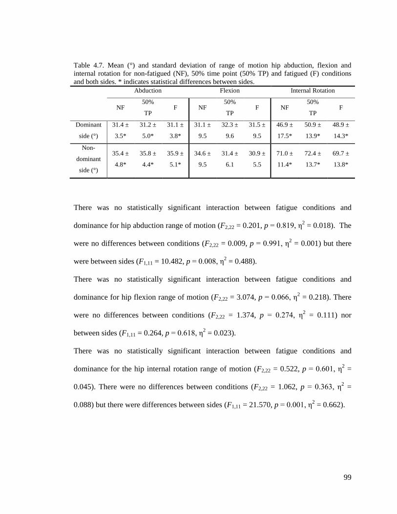
99

Table 4.7. Mean (°) and standard deviation of range of motion hip abduction, flexion and

internal rotation for non-fatigued (NF), 50% time point (50% TP) and fatigued (F) conditions

and both sides. * indicates statistical differences between sides.


NF 50%

TP F NF

50%

TP F NF

50%

TP F

Dominant

side (°)

31.4 ±

3.5*

31.2 ±

5.0*

31.1 ±

3.8*

31.1 ±

9.5

32.3 ±

9.6

31.5 ±

9.5

46.9 ±

17.5*

50.9 ±

13.9*

48.9 ±

14.3*

Non-

dominant

side (°)

35.4 ±

4.8*

35.8 ±

4.4*

35.9 ±

5.1*

34.6 ±

9.5

31.4 ±

6.1

30.9 ±

5.5

71.0 ±

11.4*

72.4 ±

13.7*

69.7 ±

13.8*


dominance for hip abduction range of motion (F2,22 = 0.201, p = 0.819, η2 = 0.018). The

were no differences between conditions (F2,22 = 0.009, p = 0.991, η2 = 0.001) but there

were between sides (F1,11 = 10.482, p = 0.008, η2 = 0.488).


dominance for hip flexion range of motion (F2,22 = 3.074, p = 0.066, η2 = 0.218). There

were no differences between conditions (F2,22 = 1.374, p = 0.274, η2 = 0.111) nor

between sides (F1,11 = 0.264, p = 0.618, η2 = 0.023).


dominance for the hip internal rotation range of motion (F2,22 = 0.522, p = 0.601, η2 =

0.045). There were no differences between conditions (F2,22 = 1.062, p = 0.363, η2 =

0.088) but there were differences between sides (F1,11 = 21.570, p = 0.001, η2 = 0.662).

100

4.3.4 Knee Joint


Table 4.8 shows the mean of the twelve participants’ average knee flexion during the

cycle.

Table 4.8. Mean (°) and standard deviation of average knee flexion for non-fatigued (NF), 50%

time point (50% TP) and fatigued (F) conditions and both sides.

NF 50% TP F

Dominant side (°) 91.0 ± 4.6 89.9 ± 4.4 89.0 ± 4.4

Non-dominant side (°) 90.9 ± 5.6 89.3 ± 6.3 89.0 ± 4.5

There was no significant interaction between fatigue conditions and dominance for

average knee flexion (F2,22 = 0.321, p = 0.729, η2 = 0.028). There was a significant main

effect on the fatigue conditions (F2,22 = 4.800, p = 0.019, η2 = 0.304). A post hoc

Bonferroni test revealed no significant differences between levels. There was no

significant main effect on dominance (F1,11 = 0.045, p = 0.836, η2 = 0.004).


Table 4.9 shows the mean of the twelve participants’ average knee flexion during the

cycle.

Table 4.9. Mean (°) and standard deviation of maximum knee flexion for non-fatigued (NF),

50% time point (50% TP) and fatigued (F) conditions and both sides. * indicates statistical

differences between sides.

NF 50% TP F

Dominant side (°) 139.5 ± 6.2* 137.5 ± 7.1 135.2 ± 6.5*

Non-dominant side (°) 145.2 ± 8.0* 144.0 ± 8.1 142.0 ± 7.7*

101

There was no significant interaction between fatigue conditions and dominance (F2,22 =

0.634, p = 0.540, η2 = 0.054). There were differences between conditions (F2,22 = 8.595,

p = 0.002, η2 = 0.439), but not between sides (F1,11 = 5.230, p = 0.043, η

2 = 0.322). A

post hoc Bonferroni test revealed NF was statistically significantly higher than F

condition (p = 0.011, d = 0.48).


Table 4.10 shows the mean of the twelve participants’ minimum knee flexion during the

cycle.

Table 4.10. Mean (°) and standard deviation of minimum knee flexion for non-fatigued (NF),

50% time point (50% TP) and fatigued (F) conditions and both sides.

NF 50% TP F

Dominant side (°) 37.0 ± 9.3 35.6 ± 8.5 36.4 ± 9.0

Non-dominant side (°) 38.7 ± 10.9 35.8 ± 11.4 36.9 ± 9.6

A two way repeated measures ANOVA showed no significant interaction between

fatigue conditions and dominance for average knee flexion (F2,22 = 0.752, p = 0.483, η2

= 0.064). There was no significant main effect on the fatigue conditions (F2,22 = 2.600, p

= 0.097, η2 = 0.191) nor significant main effect on dominance (F1,11 = 0.076, p = 0.788,

η2 = 0.007).

102

4.3.4.4 Knee Range of Motion

Table 4.11 shows the mean of the twelve participants’ range of motion for knee flexion

during the cycle.

Table 4.11. Mean (°) and standard deviation of knee flexion range of motion for non-fatigued

(NF), 50% time point (50% TP) and fatigued (F) conditions and both sides. † indicates statistical

differences between fatigue conditions.

NF 50% TP F

Dominant side (°) 102.5 ± 11.8† 101.9 ± 12.6 98.7 ± 12.9†

Non-dominant side (°) 106.4 ± 16.2† 108.1 ± 15.9 105.0 ± 15.6†


dominance for knee flexion range of motion (F2,22 = 1.811, p = 0.187, η2 = 0.141). There

was a significant difference between fatigue conditions (F2,22 = 3.943, p = 0.034, η2 =

0.264) but not between sides (F1,11 = 1.059, p = 0.326, η2 = 0.088). A post hoc

Bonferroni test revealed NF was statistically significantly higher than F condition (p =

0.045, d = 0.17).

4.3.5 Ankle Joint

The complex morphology of the ankle joint results in a complex axis of rotation of the

ankle. The coexistence of the ‘true ankle joint’ (consisting of the tibia, fibula, and talus)

and the subtalar joint, creates longitudinal and oblique axes of rotation that make

motions of the ankle concurrent (i.e. inversion and evertion motions are naturally

accompanied with abduction and adduction of the ankle). This should be kept in mind

when interpreting ankle results.

103


Table 4.12 shows the mean of the twelve participants’ average angle for ankle

abduction, flexion and external rotation during the cycle.

Table 4.12. Mean (°) and standard deviation of average ankle inversion, plantarflexion and



fatigue conditions.

Inversion Plantarflexion Adduction

NF 50%

TP F NF

50%

TP F NF

50%

TP F

Dominant

side (°)

-0.77 ±

4.2*††

2.93 ±

4.0*†

3.43 ±

3.8*†

22.1 ±

7.2*

22.8 ±

7.0*

22.7 ±

6.5*

16.5 ±

11.3*

17.4 ±

10.8*

16.3 ±

10.3*

Non-

dominant

side (°)

5.26 ±

4.9*††

7.78 ±

5.1*†

9.00 ±

4.7*†

19.3 ±

2.6*

18.7 ±

2.9*

19.9 ±

2.9*

26.7 ±

10.8*

24.5 ±

10.8*

25.9 ±

10.1*

There was no statistically significant interaction between ankle inversion fatigue

conditions and dominance (F2,22 = 2.425, p = 0.112, η2 = 0.181). There were differences

between fatigue conditions (F2,22 = 28.760, p < 0.001, η2 = 0.723) and between sides

(F1,11 = 9.263, p = 0.011, η2 = 0.457). A Bonferroni post hoc test revealed NF was

statistically significantly higher than F (p < 0.001, d = 0.75) and 50% TP (p < 0.001, d =

0.58) conditions.

There was no statistically significant interaction between ankle plantarflexion fatigue

conditions and dominance (F2,22 = 1.738, p = 0.199, η2 = 0.136). There were no

differences between conditions (F2,22 = 0.011, p = 0.989, η2 = 0.001), but there were

differences between sides (F1,11 = 5.195, p = 0.044, η2 = 0.321).

104

There was a statistically significant interaction between ankle adduction fatigue

conditions and dominance (F2,22 = 6.189, p = 0.007, η2 = 0.360). There were no

differences between fatigue conditions (F2,22 = 0.643, p = 0.535, η2 = 0.055), but there

were differences between sides (F1,11 = 5.718, p = 0.036, η2 = 0.342).


Table 4.13 shows the mean of the twelve participants’ maximum angle for ankle


Table 4.13. Mean (°) and standard deviation of maximum ankle inversion, plantarflexion and


sides. * indicates statistical differences between sides.


NF 50%

TP F NF

50%

TP F NF

50%

TP F

Dominant

side (°)

16.5 ±

9.2*

20.2 ±

8.2*

18.5 ±

6.7*

45.8 ±

7.1

45.7 ±

7.1

44.3 ±

6.1

33.4 ±

15.5*

35.3 ±

13.3*

33.1±

12.8*

Non-

dominant

side (°)

34.1 ±

7.7*

33.7 ±

7.1*

33.8 ±

6.9*

43.2 ±

5.0

42.0 ±

5.4

42.0 ±

5.1

54.9 ±

11.8*

51.7 ±

13.5*

53.5 ±

9.7*

There was no statistically significant interaction between maximum ankle inversion

fatigue conditions and dominance (F2,22 = 3.441, p = 0.050, η2 = 0.238). There were no

differences between fatigue conditions (F2,22 = 2.293, p = 0.125, η2 = 0.172), but there

were differences between sides (F1,11 = 28.372, p < 0.001, η2 = 0.721).

There was no statistically significant interaction between maximum ankle plantarflexion


105

differences between conditions (F2,22 = 2.979, p = 0.072, η2 = 0.213) nor between sides

(F1,11 = 1.244, p = 0.288, η2 = 0.102).

There was a statistically significant interaction between maximum ankle adduction


significant differences between conditions (F2,22 = 0.433, p = 0.654, η2 = 0.038), but

there were differences between sides (F1,11 = 18.623, p = 0.001, η2 = 0.629).


Table 4.14 shows the mean of the twelve participants’ minimum angle for ankle


Table 4.14. Mean (°) and standard deviation of minimum ankle inversion, plantarflexion and



fatigue conditions.


NF 50%

TP F NF

50%

TP F NF

50%

TP F

Dominant

side (°)

-5.61 ±

8.6*

-4.42 ±

8.1*

-4.83 ±

8.1*

-17.9 ±

6.8††

-14.5 ±

6.3††

-12.4 ±

5.2††

-2.32 ±

12.3

-1.56

± 11.5

-0.41±

10.5

Non-

dominant

side (°)

-12.5 ±

5.8*

-13.3 ±

5.6*

-13.1 ±

4.9*

-18.5 ±

6.5††

-14.4 ±

6.5††

-13.3 ±

5.9††

-5.67 ±

12.6

-7.62 ±

12.3

-7.71 ±

11.2

There was no statistically significant interaction between minimum ankle inversion

fatigue conditions and dominance (F1.302,14.323 = 3.739, p = 0.065, η2 = 0.254). There

106

were no differences between fatigue conditions (F1.332,14.652 = 0.086, p = 0.841, η2 =

0.008) but there were differences between sides (F1,11 = 19.254, p = 0.001, η2 = 0.636).

There was no statistically significant interaction between minimum ankle plantarflexion

fatigue conditions and dominance (F2,22 = 0.693, p = 0.511, η2 = 0.059). There were

differences between conditions (F2,22 = 42.609, p < 0.001, η2 = 0.795) but not between

sides (F1,11 = 0.032, p = 0.861, η2 = 0.003). A post hoc Bonferroni test revealed NF was

statistically significantly higher than F conditions (p < 0.001, d = 0.89) and 50% TP (p <

0.001, d = 0.58) conditions, 50% TP was statistically significantly higher than F (p =

0.048, d = 0.27).

There was a statistically significant interaction between minimum ankle adduction

fatigue conditions and dominance (F1.454,15.992 = 3.580, p = 0.064, η2 = 0.246). There was

no differences between fatigue conditions (F1.400,15.395 = 0.203, p = 0.740, η2 = 0.018) nor


4.3.5.4 Ankle Range of Motion

Table 4.15 shows the mean of the twelve participants’ range of motion angle for ankle

inversion, plantarflexion and adduction during the cycle.

107

Table 4.15. Mean (°) and standard deviation of the ankle’s inversion, planatrflexion and

adduction range of motion for non-fatigued (NF), 50% time point (50% TP) and fatigued (F)

conditions and both sides. * indicates statistical differences between sides. † indicates statistical



NF 50%

TP F NF

50%

TP F NF

50%

TP F

Dominant

side (°)

22.2 ±

6.2*

24.7 ±

5.1*

23.4 ±

3.6*

63.8 ±

12.1††

60.3 ±

12.1†

56.7 ±

10.4†

35.7 ±

17.3*

36.8 ±

16.0*

33.6 ±

14.6*

Non-

dominant

side (°)

46.7 ±

7.0*

47.1 ±

8.1*

46.9 ±

7.1*

61.8 ±

9.6††

56.5 ±

10.3†

55.3 ±

9.0†

60.6 ±

15.9*

59.3 ±

18.5*

61.2 ±

16.0*


dominance for ankle inversion range of motion (F2,22 = 0.597, p = 0.559, η2 = 0.051).

There were no differences between conditions (F2,22 = 1.598, p = 0.225, η2 = 0.127) but

there were between sides (F1,11 = 98.353, p < 0.001, η2 = 0.999).


dominance for ankle plantarflexion range of motion (F2,22 = 1.130, p = 0.341, η2 =

0.093). There were differences between conditions (F2,22 = 28.750, p < 0.001, η2 =

0.723) but not between sides (F1,11 = 0.298, p = 0.596, η2 = 0.026). A post hoc

Bonferroni test revealed NF was statistically significantly higher than F (p < 0.001, d =

0.66) and 50% TP (p = 0.01, d = 0.40) conditions.


dominance for ankle adduction range of motion (F2,22 = 2.192, p = 0.135, η2 = 0.166).

There were no differences between fatigue conditions (F2,22 = 0.409, p = 0.669, η2 =

0.036) but there were between sides (F1,11 = 16.681, p = 0.002, η2 = 0.603).

108

4.3.6 Joint Angular Velocity

4.3.6.1 Hip Motions

Table 4.16 shows the mean of the twelve participants’ angular velocity for the hip

abduction-adduction, flexion-extension, and rotation during the cycle.

Table 4.16. Mean (rad·s-1

) and standard deviation of angular velocity for the hip abduction-

adduction, flexion-extension, and rotation for, non-fatigued (NF), 50% time point (50% TP) and

fatigued (F) conditions and both sides. * indicates statistical differences between sides. †

indicates statistical differences between fatigue conditions.

Hip Abduction Hip Flexion Hip Rotation

NF 50%

TP F NF

50%

TP F NF

50%

TP F

Dominant

side (rad·s-1

)

4.8 ±

1.0*††

1.8 ±

0.5*†

1.86 ±

0.4*†

3.4 ±

0.8*††

3.3 ±

0.5*†

3.0 ±

0.4*†

2.2 ±

1.0*†

2.1 ±

0.9*†

2.0 ±

1.1*††

Non-dominant

side (rad·s-1

)

3.8 ±

0.8*††

3.3 ±

0.7*†

3.2 ±

0.6*†

3.9 ±

0.5*††

3.6 ±

0.4*†

3.4 ±

0.4*†

5.8 ±

0.8*†

5.2 ±

0.7*†

4.6 ±

0.6*††

There was a statistically significant interaction between hip abduction-adduction angular

velocity fatigue conditions and dominance (F1.151,12.662 = 43.415, p < 0.001, η2 = 0.798).

There were differences between fatigue conditions (F1.375,15.124 = 82.640, p < 0.001, η2 =

0.883) and between sides (F1,11 = 21.273, p = 0.001, η2 = 0.659). A post hoc Bonferroni

tests revealed NF was statistically significantly higher than F (p < 0.001, d = 1.87) and

between 50% TP (p < 0.001, d = 1.68) conditions.

There was no statistically significant interaction between hip flexion-extension angular

velocity fatigue conditions and dominance (F2,22 = 1.242, p = 0.308, η2 = 0.101). There

were differences between conditions (F2,22 = 10.399, p = 0.001, η2 = 0.486) and between

sides (F1,11 = 5.620, p = 0.037, η2 = 0.338). A post hoc Bonferroni tests revealed NF was

109

statistically significantly higher than F (p = 0.013, d = 0.78) and 50% TP (p = 0.015, d =

0.28) conditions.

There was a significant interaction between hip rotation angular velocity fatigue

conditions and dominance (F1.888,20.769 = 28.205, p < 0.001, η2 = 0.719). There were

differences between conditions (F1.501,16.601 = 30.799, p < 0.001, η2 = 0.737) and between

sides (F1,11 = 141.824, p < 0.001, η2 = 0.928). A post hoc Bonferroni test revealed NF

was statistically significantly higher than F (p < 0.001, d = 0.41) and 50% TP (p = 0.013,

d = 0.19) conditions. F was statistically significantly lower than 50% TP (p < 0.001, d =

0.23).

4.3.6.2 Knee Motion

Table 4.17 shows the mean of the twelve participants’ angular velocity for the knee

flexion-extension during the cycle.


) and standard deviation knee flexion-extension angular velocity for

non-fatigued (NF), 50% time point (50% TP) and fatigued (F) conditions and both sides. *

indicates statistical differences between sides. † indicates statistical differences between fatigue

conditions.

NF 50% TP F

Dominant side (rad·s-1

) 4.7 ± 0.4*†† 4.2 ± 0.4*†† 3.9 ± 0.4*††

Non-dominant side (rad·s-1

) 6.2 ± 1.0*†† 5.5 ± 0.7*†† 5.2 ± 0.7*††

There was no statistically significant interaction between knee flexion angular velocity


differences between conditions (F2,22 = 32.703, p < 0.001, η2 = 0.748), and differences

110

between sides (F1,11 = 44.512, p < 0.001, η2 = 0.802). A post hoc Bonferroni test

revealed NF was statistically significantly higher than F (p < 0.001, d = 0.96) and 50%

TP (p = 0.006, d = 0.40) conditions. F was statistically significantly lower than 50% TP

(p = 0.002, d = 0.60).

4.3.6.3 Ankle Motions

Table 4.18 shows the mean of the twelve participants’ angular velocity for the ankle

inversion-eversion, plantarflexion-dorsiflexion, and abduction-adduction during the

cycle.


) and standard deviation of angular velocity for the ankle inversion-

eversion, plantarflexion-dorsiflexion, and abduction-adduction for, non-fatigued (NF), 50% time

point (50% TP) and fatigued (F) conditions and both sides. * indicates statistical differences

between sides. † indicates statistical differences between fatigue conditions.

Ankle Inv-Eve Ankle Pla-Dor Ankle Abd-Add

NF 50%

TP F NF

50%

TP F NF

50%

TP F

Dominant

side (rad·s-1

)

3.1 ±

0.4*††

2.8 ±

0.5*††

2.4 ±

0.3*††

4.9 ±

1.0*††

4.5 ±

0.9*††

4.1 ±

0.6*††

5.8 ±

1.0*††

5.3 ±

0.7*††

5.0 ±

0.6*††

Non-

dominant

side (rad·s-1

)

4.8 ±

0.5*††

4.4 ±

0.6*††

3.9 ±

0.4*††

4.3 ±

0.6*††

3.7 ±

0.6*††

3.4 ±

0.5*††

4.8 ±

1.0*††

4.6 ±

1.0*††

4.3 ±

0.8*††

There was no statistically significant interaction between ankle inversion-eversion

angular velocity conditions and dominance (F2,22 = 2.374, p = 0.117, η2 = 0.178). There

were differences between fatigue conditions (F2,22 = 47.177, p < 0.001, η2 = 0.811) and

between sides (F1,11 = 74.515, p < 0.001, η2 = 0.871). A post hoc Bonferroni test

revealed differences between NF and F conditions (p < 0.001, d = 0.84), between NF

111

and the 50% TP (p < 0.001, d = 0.38), and between F and the 50% TP (p < 0.001, d =

0.43).

There was statistically significant interaction between ankle plantarflexion-dorsiflexion

angular velocity fatigue conditions and dominance (F2,22 = 0.382, p = 0.687, η2 = 0.034).

There were differences between conditions (F2,22 = 26.265, p < 0.001, η2 = 0.705) and

between sides (F1,11 = 17.146, p = 0.002, η2 = 0.609). A post hoc Bonferroni test

revealed differences between NF and F conditions (p < 0.001, d = 1.06), between NF

and the 50% TP (p = 0.005, d = 0.54), and between F and the 50% TP (p = 0.014, d =

0.47).

There was a statistically significant interaction between ankle abduction-adduction

angular velocity fatigue conditions and dominance (F2,22 = 3.844, p = 0.037, η2 = 0.259).

There were differences between fatigue conditions (F2,22 = 17.681, p < 0.001, η2 =

0.616) and differences between sides (F1,11 = 16.133, p = 0.002, η2 = 0.595). A post hoc

Bonferroni tests revealed differences between NF and F conditions (p = 0.002, d = 0.68),

between NF and the 50% TP (p = 0.023, d = 0.33), and between F and the 50% TP (p =

0.010, d = 0.36).

4.3.7 Feet Pitch Angles

4.3.7.1 Average, Maximum and Minimum

Table 4.19 shows the mean of the twelve participants’ average, maximum and minimum

foot pitch angles during the cycle.

112

Table 4.19. Mean (°) and standard deviation of average, maximum and minimum foot pitch

angles for, non-fatigued (NF), 50% time point (50% TP) and fatigued (F) conditions and both

sides. * indicates statistical differences between sides.

Average Maximum Minimum

NF 50%

TP F NF

50%

TP F NF

50%

TP F

Dominant

side (°)

11.5 ±

3.7*

11.1 ±

3.7*

9.8 ±

3.4*

53.8 ±

11.0*

51.6 ±

10.3*

50.0 ±

8.5*

-30.0 ±

5.6*

-31.9 ±

7.1*

-33.4 ±

7.0*

Non-

dominant

side (°)

9.1 ±

4.6*

9.6 ±

3.7*

7.7 ±

5.1*

60.7 ±

9.2*

61.0 ±

8.5*

60.1 ±

9.7*

-41.44

± 10.9*

-38.6 ±

8.7*

-43.7 ±

14.2*

There was no statistically significant interaction between average feet pitch angles




There was no statistically significant interaction between maximum feet pitch angles


differences between conditions (F1.191,13.098 = 1.516, p = 0.246, η2 = 0.121) but there


There was no statistically significant interaction between minimum feet pitch angles


differences between conditions (F1.244,13.687 = 1.921, p = 0.189, η2 = 0.149), but there


113

4.3.7.2 Positive Pitch Angle Time

Table 4.20 shows the mean of the twelve participants’ percentage of positive feet pitch

angles during the cycle.

Table 4.20. Mean (%) and standard deviation of percentage of positive feet pitch angles for non-

fatigued (NF), 50% time point (50% TP) and fatigued (F) conditions and both sides. * indicates

statistical differences between sides.

NF 50% TP F

Dominant side (%) 64.9 ± 3.9* 65.3 ± 4.8* 64.4 ± 4.9*

Non-dominant side (%) 62.4 ± 6.1* 62.2 ± 4.2* 60.6 ± 3.3*

There was no significant interaction between the percentage of positive feet pitch angles



differences between sides (F1,11 = 6.538, p = 0.027, η2 = 0.373).

4.3.8 Average Foot Sweepback Angles

Table 4.21 shows the mean of the twelve participants’ average sweepback angles of the

feet during the cycle.

Table 4.21. Mean (°) and standard deviation of average sweepback angles of the feet for non-

fatigued (NF), 50% time point (50% TP) and fatigued (F) conditions and both sides. † indicates

statistical differences between fatigue conditions.

NF 50% TP F

Dominant side (°) 185.4 ± 4.9† 188.3 ± 5.2† 190.3 ± 5.7††

Non-dominant side (°) 188.6 ± 11.7† 190.1 ± 10.1† 193.9 ± 10.5††

114

There was no significant interaction between average sweepback angles of the feet


significant differences between conditions (F2,22 = 11.501, p < 0.001, η2 = 0.511), but

there were no differences between sides (F1,11 = 1.207, p = 0.295, η2 = 0.099). A post

hoc Bonferroni test revealed NF was statistically significantly higher than F condition (p

= 0.006, d = 0.58), and 50% TP was statistically significantly higher than F (p = 0.023, d

= 0.34).

4.3.9 Average Foot Speed

Table 4.22 shows the mean of the twelve participants’ average foot speed during the

cycle.

Table 4.22. Mean (m/s) and standard deviation of average foot speed for non-fatigued (NF), 50%

time point (50% TP) and fatigued (F) conditions and both sides. † indicates statistical differences

between fatigue conditions.

NF 50% TP F

Dominant side (m/s) 2.80 ± 0.1†† 2.55 ± 0.1†† 2.34 ± 0.1††

Non-dominant side (m/s) 2.77 ± 0.1†† 2.54 ± 0.1†† 2.32 ± 0.1††

There was no significant interaction between average foot speed fatigue conditions and

dominance (F2,22 = 0.470, p = 0.631, η2 = 0.041). There were significant differences

between conditions (F1.064,11.709 = 78.458, p < 0.001, η2 = 0.877), but there were no

differences between sides (F1,11 = 1.038, p = 0.330, η2 = 0.086). A post hoc Bonferroni

test revealed NF was statistically significantly higher than F (p < 0.01, d = 2.99) and

115

50% TP (p < 0.01, d = 1.64). 50% TP was statistically significantly higher than F (p <

0.01, d = 1.46).

4.3.10 Feet Motion

Table 4.23 shows the mean of the twelve participants’ average anterior-posterior,

vertical and medio-lateral motion components of the feet during the cycle.

Table 4.23. Mean (%) and standard deviation of average anterior-posterior, vertical and medio-

lateral motion components of the feet for, non-fatigued (NF), 50% time point (50% TP) and

fatigued (F) conditions and both sides.

Anterior-Posterior Motion Vertical Motion Medio-Lateral Motion

NF 50%

TP F NF

50%

TP F NF

50%

TP F

Dominant

side (%)

32.8 ±

5.2

35.2 ±

6.0

35.7 ±

4.9

37.9 ±

5.6

35.9 ±

5.9

35.7 ±

4.8

29.1 ±

5.8

28.8 ±

3.7

28.5 ±

4.7

Non-

dominant

side (%)

33.3 ±

7.6

35.5 ±

6.1

36.2 ±

8.2

38.0 ±

7.6

36.2 ±

7.7

35.3 ±

7.5

26.8 ±

5.9

27.3 ±

5.8

27.8 ±

6.5

There was no statistically significant interaction between the anterior-posterior motion

component fatigue conditions and dominance (F1.355,14.903 = 0.010, p = 0.064, η2 =


0.166) nor between sides (F1,11 = 0.042, p = 0.841, η2 = 0.004).

There was no statistically significant interaction between the vertical motion component


differences between conditions (F2,22 = 1.161, p = 0.332, η2 = 0.095) nor between sides

(F1,11 = 0.001, p = 0.982, η2 < 0.001).

116

There was no statistically significant interaction between the medio-lateral motion

component fatigue conditions and dominance (F1.308,14.387 = 0.746, p = 0.437, η2 =


0.002) nor sides (F1,11 = 0.652, p = 0.437, η2 = 0.056).

4.3.11 Summary Table

Table 4.24 shows the main effect on fatigue, main effect on dominance and interaction

between fatigue and dominance values for all kinematic variables.


and dominance. Statistical differences (p<0.05) are indicated in bold.

Variable ME Fatigue ME Dominance Interaction

Average Hip Abduction p = 0.001, η2 = 0.479 p = 0.910, η

2 = 0.001 p = 0.823, η

2 = 0.018

Average Hip Flexion p = 0.003, η2 = 0.414 p = 0.077, η

2 = 0.256 p = 0.123, η

2 = 0.174

Avg Hip Internal Rotation p = 0.003, η2 = 0.409 p = 0.969, η

2 < 0.001 p = 0.608, η

2 = 0.044

Average Knee Flexion p = 0.019, η2 = 0.304 p = 0.836, η

2 = 0.004 p = 0.729, η

2 = 0.028

Avg Ankle Plantarflexion p = 0.989, η2 = 0.001 p = 0.044, η

2 = 0.321 p = 0.199, η

2 = 0.136

Average Ankle Inversion p < 0.001, η2 = 0.723 p = 0.011, η

2 = 0.457 p = 0.112, η

2 = 0.181

Average Ankle Adduction p = 0.535, η2 = 0.055 p = 0.036, η

2 = 0.342 p = 0.007, η

2 = 0.360

Max Hip Abduction p = 0.001, η2 = 0.451 p = 0.351, η

2 = 0.079 p = 0.911, η

2 = 0.008

Max Hip Flexion p = 0.003, η2 = 0.406 p = 0.093, η

2 = 0.235 p = 0.099, η

2 = 0.216

Max Hip Internal Rotation p = 0.004, η2 = 0.389 p = 0.010, η

2 = 0.466 p = 0.877, η

2 = 0.005

Max Knee Flexion p = 0.002, η2 = 0.439 p = 0.043, η

2 = 0.322 p = 0.540, η

2 = 0.054

Max Ankle Plantarflexion p = 0.072, η2 = 0.213 p = 0.288, η

2 = 0.102 p = 0.410, η

2 = 0.078

Max Ankle Inversion p = 0.125, η2 = 0.172 p < 0.001, η

2 = 0.721 p = 0.050, η

2 = 0.238

Max Ankle Adduction p = 0.654, η2 = 0.038 p = 0.001, η

2 = 0.629 p = 0.028, η

2 = 0.277

Min Hip Abduction p = 0.003, η2 = 0.404 p = 0.182, η

2 = 0.156 p = 0.916, η

2 = 0.008

Min Hip Flexion p = 0.002, η2 = 0.513 p = 0.015, η

2 = 0.428 p = 0.163, η

2 = 0.152

Min Hip Internal Rotation p = 0.087, η2 = 0.223 p = 0.091, η

2 = 0.238 p = 0.472, η

2 = 0.063

117

Min Knee Flexion p = 0.097, η2 = 0.191 p = 0.788, η

2 = 0.007 p = 0.483, η

2 = 0.064

Min Ankle Plantarflexion p < 0.001, η2 = 0.795 p = 0.861, η

2 = 0.003 p = 0.511, η

2 = 0.059

Min Ankle Inversion p = 0.841, η2 = 0.008 p = 0.001, η

2 = 0.636 p = 0.065, η

2 = 0.254

Min Ankle Adduction p = 0.740, η2 = 0.018 p = 0.135, η

2 = 0.192 p = 0.064, η

2 = 0.246

Hip Abduction Range p = 0.991, η2 = 0.001 p = 0.008, η

2 = 0.488 p = 0.819, η

2 = 0.018

Hip Flexion Range p = 0.274, η2 = 0.111 p = 0.618, η

2 = 0.023 p = 0.066, η

2 = 0.218

Hip Internal Rot Range p = 0.363, η2 = 0.088 p = 0.001, η

2 = 0.662 p = 0.601, η

2 = 0.045

Knee Flexion Range p = 0.034, η2 = 0.264 p = 0.326, η

2 = 0.088 p = 0.187, η

2 = 0.141

Ankle Plaflexion Range p < 0.001, η2 = 0.723 p = 0.596, η

2 = 0.026 p = 0.341, η

2 = 0.093

Ankle Inversion Range p = 0.225, η2 = 0.127 p < 0.001, η

2 = 0.999 p = 0.559, η

2 = 0.051

Ankle Adduction Range p = 0.669, η2 = 0.036 p = 0.002, η

2 = 0.603 p = 0.135, η

2 = 0.166

Average Foot Pitch Angle p = 0.052, η2 = 0.236 p = 0.031, η

2 = 0.358 p = 0.816, η

2 = 0.018

Maximum Foot Pitch Angle p = 0.246, η2 = 0.121 p = 0.007, η

2 = 0.504 p = 0.313, η

2 = 0.100

Minimum Foot Pitch Angle p = 0.189, η2 = 0.149 p = 0.001, η

2 = 0.642 p = 0.247, η

2 = 0.120

Time of Positive Pitch Foot p = 0.119, η2 = 0.176 p = 0.027, η

2 = 0.373 p = 0.752, η

2 = 0.026

Avg Foot Sweepback Ang p < 0.001, η2 = 0.511 p = 0.295, η

2 = 0.099 p = 0.415, η

2 = 0.077

Foot Medio-Lateral Motion p = 0.974, η2 = 0.002 p = 0.437, η

2 = 0.056 p = 0.437, η

2 = 0.064

Foot Vertical Motion p = 0.332, η2 = 0.095 p = 0.982, η

2 < 0.001 p = 0.791, η

2 = 0.021

Foot Ant-Pos Motion p = 0.135, η2 = 0.166 p = 0.841, η

2 = 0.004 p = 0.064, η

2 = 0.001

Average foot Speed p < 0.001, η2 = 0.877 p = 0.330, η

2 = 0.086 p = 0.631, η

2 = 0.041

Avg Hip Abduction Ang Vel p < 0.001, η2 = 0.883 p = 0.001, η

2 = 0.659 p < 0.001, η

2 = 0.798

Avg Hip Flexion Ang Vel p = 0.001, η2 = 0.486 p = 0.037, η

2 = 0.338 p = 0.308, η

2 = 0.101

Avg Hip Rotation Ang Vel p < 0.001, η2 = 0.737 p < 0.001, η

2 = 0.928 p < 0.001, η

2 = 0.719

Avg Knee Flexion Ang Vel p < 0.001, η2 = 0.748 p < 0.001, η

2 = 0.802 p = 0.073, η

2 = 0.212

Avg Ankle Inversion Ang Vel p < 0.001, η2 = 0.811 p < 0.001, η

2 = 0.871 p = 0.117, η

2 = 0.178

Avg Ank Plaflexion Ang Vel p < 0.001, η2 = 0.705 p = 0.002, η

2 = 0.609 p = 0.687, η

2 = 0.034

Avg Ankle Add Ang Vel p < 0.001, η2 = 0.616 p = 0.002, η

2 = 0.595 p = 0.037, η

2 = 0.259

118

4.4 Muscle Activity

Section 4.4 presents the results for each fatigue level for each individual muscle tested.

The value for each state represents the mean for the 12 subjects. Each subject score is

the mean of the average for each particular variable during the cycle for nine cycles.

Error bars represent 95% confidence interval of the true mean.

Repeated measures ANOVA tests were used for the average muscle activity that was not

compared between sides. Repeated measures two-way ANOVA tests were used for the

average normalized muscle activity.

4.4.1 Tibialis Anterior

4.4.1.1 Average Activity

A repeated measures ANOVA for the average Right Tibialis Anterior activity showed

significant differences between fatigue conditions (F1.286,12.862 = 13.337, p = 0.002, η2 =

0.572). A post hoc Bonferroni test revealed NF was statistically significantly higher than

F conditions (p = 0.007, d = 0.80) and 50% TP (p = 0.047, d = 0.50). 50% TP was

statistically significantly higher than F (p = 0.011, d = 0.40) (Fig. 4.3).

There was a significant main effect between average Left Tibialis Anterior activity

between fatigue conditions (F1.282,12.818 = 18.989, p < 0.001, η2 = 0.655). A post hoc

Bonferroni test revealed NF was statistically significantly higher than F (p = 0.001, d =

0.98) and the 50% TP (p = 0.013, d = 0.68) conditions. 50% TP was statistically

significantly higher than F (p = 0.027, d = 0.41) (Fig. 4.3).

119

Figure 4.3. Average Right Tibialis Anterior activity for the three fatigue conditions. Error bars

represent the group’s standard deviation. indicates statistical differences between fatigue

conditions.

4.4.1.2 Normalized to MVC

There was no statistically significant interaction between the Tibialis Anterior activity

normalized to MVC fatigue conditions and dominance (F2,20 = 1.021, p = 0.383, η2 =

0.113). There were differences between fatigue conditions (F2,20 = 20.636, p < 0.001, η2

= 0.721), but not between sides (F1,10 = 0.697, p = 0.428, η2 = 0.080). Post hoc

Bonferroni tests revealed NF was statistically significantly higher than F (p = 0.003, d =

0.89) and 50% TP (p = 0.011, d = 0.59) conditions. F was statistically significantly

lower than 50% TP (p = 0.015, d = 0.37) (Fig. 4.4).

0

0.05

0.1

0.15

0.2

0.25

0.3

0.35

Non Fatigued 50% TimePoint

Fatigued Non Fatigued 50% TimePoint

Fatigued

Right Tibialis Anterior Left Tibialis Anterior

Mu

scle

Act

ivit

y (m

V)

120

Figure 4.4. Average Left Tibialis Anterior activity normalized to MVC for the three fatigue

conditions. Error bars represent the group’s standard deviation. indicates statistical differences


4.4.1.3 Normalized to Peak of the Cycle

There was no statistically significant interaction between the Tibialis Anterior activity

normalized to peak of the cycle fatigue conditions and dominance (F2,20 = 0.105, p =

0.901, η2 = 0.011). There were differences between fatigue conditions (F2,20 = 28.715, p

< 0.001, η2 = 0.761), but not between sides (F1,10 = 0.333, p = 0.578, η

2 = 0.036). Post

hoc Bonferroni tests revealed NF was statistically significantly higher than F (p < 0.001,

d = 0.82) and 50% TP (p = 0.005, d = 0.47) conditions (Fig. 4.5).

0

0.2

0.4

0.6

0.8

1

1.2

1.4


No

rmal

ize

d V

alu

e


121

Figure 4.5. Average Left Tibialis Anterior normalized to peak of the cycle for the three fatigue



4.4.1.4 Pattern of Muscle Activity

The group’s level of muscle activity is constant during the cycle (Fig. 4.6), with no

significant peak or low periods of activity. Looking at individual data (appendix C),

subjects 1, 2, 3, 4, 7 and 8 show lower activity from 55 to 70% of the cycle. This is

supported by the individual activations timings (Fig. 4.7). Other subjects (6, 9, 10, 11

and 12) do not follow this trend and seem to have more individualized patterns of

muscle activity for the Right Tibialis Anterior. Larger 95% confidence interval from 80

to 90% in the fatigued condition results from some subjects (1, 2, 3, 4, 6, 9 and 12)

showing a peak of activity during that period. There is a general trend of decrease in

amplitude as the subjects become fatigued. Figure 4.6 shows no significant differences

0

0.1

0.2

0.3

0.4

0.5

0.6


No

rmal

ize

d V

alu

e


122

between the patterns of muscle activity between fatigue conditions (NF and F). Figure

4.7 shows the individual activation timings for the Right Tibialis Anterior muscle for the

NF condition.

Figure 4.6. Right Tibialis Anterior activity pattern for non-fatigued and fatigued conditions.

Solid line represents the mean, dotted line the 95% confidence interval of the true mean.

Figure 4.7. Individual activation times of the Right Tibialis Anterior for the non-fatigue

condition following the double-threshold method.

0

0.1

0.2

0.3

0.4

0.5

0.6

0.7

0 25 50 75 100

Mu

scle

Act

ivit

y (m

V)

Time in the Cycle (%)

Non-Fatigued Fatigued

0123456789

101112

0 25 50 75 100

Sub

ject


123

The Left Tibialis Anterior group’s level of muscle activity seems to have two moments

of higher activity, 20 – 40% and 80 – 95%. Subjects 1, 10, 11 and 12 support the group’s

trend. However, other subjects seem to adopt individualized patterns of muscle activity.

Figure 4.8 shows no significant differences between the patterns of muscle activity

between NF and F conditions. At the same time, when comparing conditions, all

subjects seem to maintain the same pattern for F condition with a decrease in amplitude.

Figure 4.9 shows the individual activation timings for the Left Tibialis Anterior muscle

for NF condition.

Figure 4.8 Left Tibialis Anterior activity pattern for non-fatigued and fatigued conditions. Solid

line represents the mean, dotted line the 95% confidence interval of the true mean.

0

0.05

0.1

0.15

0.2

0.25

0.3

0.35

0.4

0.45

0 25 50 75 100

Mu

scle

Act

ivit

y (m

V)


Non-fatigued Fatigued

124

Figure 4.9 Individual activation times of the Left Tibialis Anterior for the non-fatigue condition

following the double-threshold method.

4.4.2 Rectus Femoris


A repeated measures ANOVA for average Right Rectus Femoris activity showed no


0.187) (Fig. 4.10) .

There was a significant main effect between average Left Rectus Femoris activity

between fatigue conditions (F2,22 = 3.756, p = 0.039, η2 = 0.255). A post hoc Bonferroni

test revealed no statistically significant differences between fatigue conditions (Fig.

4.10).

0

1

2

3

4

5

6

7

8

9

10

11

12

0 25 50 75 100

Sub

ject


125

Figure 4.10. Average Right Rectus Femoris and Left Rectus Femoris activity for the three

fatigue conditions. Error bars represent the group’s standard deviation.

4.4.2.2 Normalize to MVC

There was no statistically significant interaction between the Rectus Femoris activity


0.024). There were no differences between fatigue conditions (F2,22 = 2.316, p = 0.122,

η2 = 0.174) nor between sides (F1,11 = 0.069, p = 0.797, η

2 = 0.006) (Fig. 4.11).

0

0.02

0.04

0.06

0.08

0.1

0.12

0.14

0.16

0.18

0.2



Fatigued

Right Rectus Femoris Left Rectus Femoris

Mu

scle

Act

ivit

y (m

V)

126

Figure 4.11. Average Left Rectus Femoris activity normalized to MVC for the three fatigue

conditions. Error bars represent the group’s standard deviation.


There was no statistically significant interaction between the Rectus Femoris activity


0.713, η2 = 0.030). There were differences between fatigue conditions (F2,22 = 13.624, p

< 0.001, η2 = 0.553), but not between sides (F1,11 = 0.226, p = 0.644, η

2 = 0.020). A post

hoc Bonferroni test revealed NF was statistically significantly higher than F (p = 0.005,

d = 1.38) and 50% TP (p = 0.038, d = 0.87) conditions. F was statistically significantly

lower than 50% TP (p = 0.004, d = 0.49) (Fig. 4.12).

0

0.1

0.2

0.3

0.4

0.5

0.6

0.7

0.8

0.9

1


No

rmal

ize

d V

alu

e


127

Figure 4.12. Average Left Rectus Femoris normalized to peak of the cycle for the three fatigue




The group’s level of muscle activity of the Right Rectus Femoris seems to have two

distinct phases, one period corresponding to the initial (0 – 30%) and final (70 – 100%)

parts of the cycle, and one period where the muscle activity increase from 30 to 70% of

the cycle (Fig. 4.13). This is supported by the individual activations timing (Fig. 4.14).

Figure 4.13 shows significant differences between the patterns of muscle activity

between NF and F conditions. There seems to be a delay for the fatigued condition

during the activation phase (30 – 45%). This is supported when looking at the individual

data (appendix C). All subjects with the exception of subject 11 show this trend. Figure

0

0.05

0.1

0.15

0.2

0.25

0.3

0.35


No

rmal

ize

d V

alu

e


128

4.14 shows the individual activation timings for the Right Rectus Femoris muscle for the

F condition.

Figure 4.13. Right Rectus Femoris activity pattern for non-fatigued and fatigued conditions.

Solid line represents the mean, dotted line the 95% confidence interval.

0

0.1

0.2

0.3

0.4

0.5

0.6

0 25 50 75 100

Mu

scle

Act

ivit

y (m

V)



129

Figure 4.14. Individual activation times of the Right Rectus Femoris for the non-fatigue


The group’s level of muscle activity of the Left Rectus Femoris seems to have two

distinct phases, one period corresponding to the initial (0 – 25%) and final (75 – 100%)

parts of the cycle where the activity is high, and one period, from 30 to 70% of the time

in the cycle, where the muscle activity decreases (Fig. 4.15). Individual data (appendix

C) shows that all shows that all subjects follow the same pattern. Figure 4.15 shows no

significant differences between the patterns of muscle activity between NF and F

conditions. When looking at individual data, however, subjects 1, 2, 3, 5, 6, 7, 8 and 12

show the same fatigued trend observed for the Right Rectus Femoris (activation delay).

Figure 4.16 shows the individual activation timings for the Left Rectus Femoris muscle

for the NF condition.

0

1

2

3

4

5

6

7

8

9

10

11

12

0 25 50 75 100

Sub

ject


130

Figure 4.15. Left Rectus Femoris activity pattern for non-fatigued and fatigued conditions. Solid

line represents the mean, dotted line the 95% confidence interval.

Figure 4.16. Individual activation times of the Left Rectus Femoris for the non-fatigue condition


0

0.05

0.1

0.15

0.2

0.25

0.3

0.35

0.4

0.45

0.5

0 25 50 75 100

Mu

scle

Act

ivit

y (m

V)



0

1

2

3

4

5

6

7

8

9

10

11

12

0 25 50 75 100

Sub

ject


131

4.4.3 Biceps Femoris


A repeated measures ANOVA for average Right Biceps Femoris activity showed no


0.243) (Fig. 4.17).

There was a significant main effect between average Left Biceps Femoris activity

between fatigue conditions (F2,18 = 3.863, p = 0.043, η2 = 0.326). Post hoc Bonferroni

tests revealed no statistically significant differences between fatigue conditions (Fig.

4.17).

Figure 4.17. Average Left Biceps Femoris activity for the three fatigue conditions. Error bars


0

0.05

0.1

0.15

0.2

0.25



Fatigued


Mu

scle

Act

ivit

y (m

V)

132

4.4.3.2 Normalize to MVC

There was no statistically significant interaction between the Biceps Femoris activity


0.068). There were differences between fatigue conditions (F2,14 = 7.595, p = 0.006, η2 =

0.520), but not between sides (F1,7 = 1.565, p = 0.251, η2 = 0.183). Post hoc Bonferroni

tests did not reveal any significant differences between conditions (Fig. 4.18).

Figure 4.18. Average Left Biceps Femoris activity normalized to MVC for the three fatigue

conditions. Error bars represent the group’s standard deviation.

0

0.2

0.4

0.6

0.8

1

1.2


No

rmal

ize

d V

alu

e

Right Biceps Femoris Left Biceps Femoris

133


There was no statistically significant interaction between the Biceps Femoris activity


0.817, η2 = 0.028). There were differences between fatigue conditions (F2,14 = 9.989, p <

0.002, η2 = 0.588), but not between sides (F1,7 = 1.685, p = 0.235, η

2 = 0.194). Post hoc

Bonferroni tests revealed NF was statistically significantly higher than F (p = 0.007, d =

0.54) and 50% TP (p = 0.014, d = 0.49) conditions (Fig. 4.19).

Figure 4.19. Average Left Biceps Femoris activity normalized to peak of the cycle for the three

fatigue conditions. Error bars represent the group’s standard deviation. indicates statistical


0

0.05

0.1

0.15

0.2

0.25

0.3

0.35

0.4

0.45

0.5


No

rmal

ize

d V

alu

e

Right Biceps Femoris Left Biceps Femoris

134


The group’s level of muscle activity seems to have three periods of high activity and two

periods of low activity (Fig. 4.20). The general pattern consists of higher activity during

the initial (0 – 25%) and final (80 – 100%) phases of the cycle with low peaks of activity

around 25 – 30% and 70 – 80%. Looking at individual data (appendix C) this is

supported by subjects 1, 2, 3, 5, 8, 9 and 10. Subject 4 and 11 showed higher activity in

the middle of the cycle (30 – 70%). Figure 4.21 shows no significant differences

between the patterns of muscle activity between fatigue conditions (NF and F). Figure

4.40 shows the individual activation timings for the Right Biceps Femoris muscle for the

NF condition.

Figure 4.20. Right Biceps Femoris activity pattern for non-fatigued and fatigued conditions.

Solid line represents the mean, dotted line the 95% confidence interval.

0

0.05

0.1

0.15

0.2

0.25

0.3

0.35

0.4

0 25 50 75 100

Mu

scle

Act

ivit

y (m

V)



135

Figure 4.21. Individual activation times of the Right Biceps Femoris for the non-fatigue


The group’s level of muscle activity seems to have a phase of higher activity

corresponding to the period from 25 to 70% of the time in the cycle (Fig. 4.22). Looking

at individual data (appendix C) this is patent in subjects 2, 8, 9 and 12. Other subjects

showed more individualized patterns of muscle activity. Figure 4.22 shows no

significant differences between the patterns of muscle activity between fatigue

conditions (NF and F). Figure 4.23 shows the individual activation timings for the Left

Biceps Femoris muscle for the NF condition.

0

1

2345

6

78

9

1011

12

0 25 50 75 100

Sub

ject


136

Figure 4.22. Left Biceps Femoris activity pattern for non-fatigued and fatigued conditions. Solid

line represents the mean, dotted line the 95% confidence interval.

Figure 4.23. Individual activation times of the Left Biceps Femoris for the non-fatigue condition


0

0.05

0.1

0.15

0.2

0.25

0.3

0.35

0 25 50 75 100

Mu

scle

Act

ivit

y (m

V)



0

1

2

3

4

5

6

7

8

9

10

11

12

0 25 50 75 100

Sub

ject


137

4.4.4 Summary Table

Table 4.25 shows the main effect on fatigue, main effect on dominance and interaction

between fatigue and dominance values for the normalized muscle activity variables. Non

normalized activity shows the main effect on fatigue for each side.


and dominance. Crossed out cells indicate no statistical test. Statistical differences (p<0.05) are

indicated in bold.

Variable ME Fatigue ME Dominance Interaction

Avg Right TA Activity p = 0.002, η2 = 0.572

Avg Left TA Activity p < 0.001, η2 = 0.655

Avg MVC TA Activity p < 0.001, η2 = 0.721 p = 0.428, η

2 = 0.080 p = 0.383, η

2 = 0.113

Avg Peak Cycle TA Activity p < 0.001, η2 = 0.761 p = 0.578, η

2 = 0.036 p = 0.901, η

2 = 0.011

Avg Right RF Activity p = 0.128, η2 = 0.187

Avg Left RF Activity p = 0.039, η2 = 0.255

Avg MVC RF Activity p = 0.122, η2 = 0.174 p = 0.797, η

2 = 0.006 p = 0.766, η

2 = 0.024

Avg Peak Cycle RF Activity p < 0.001, η2 = 0.553 p = 0.644, η

2 = 0.020 p = 0.713, η

2 = 0.030

Avg Right BF Activity p = 0.118, η2 = 0.243

Avg Left BF Activity p = 0.043, η2 = 0.326

Avg MVC BF Activity p = 0.006, η2 = 0.520 p = 0.251, η

2 = 0.183 p = 0.610, η

2 = 0.068

Avg Peak Cycle BF Activity p < 0.002, η2 = 0.588 p = 0.235, η

2 = 0.194 p = 0.817, η

2 = 0.028

4.5 Correlations between Vertical Force and Studied Variables

Table 4.26 shows the correlation values between vertical force normalized to body

weight and the variables calculated in this study for the three fatigue levels.

138

Table 4.26. Correlation (r) between calculated variables and vertical force normalized to body

weight for the three fatigue levels. *indicates p < 0.01 significance level.

Variable Non-fatigued 50% Time Point Fatigued

Average RHip Abduction (°) 0.593, p = 0.042 0.150, p = 0.642 -0.247, p = 0.440

Average LHip Abduction (°) 0.461, p = 0.135 0.256, p = 0.422 -0.060, p = 0.854

Average RHip Flexion (°) 0.682, p = 0.015 0.551, p = 0.063 0.106, p = 0.743

Average LHip Flexion (°) 0.669, p = 0.017 0.382, p = 0.221 0.110, p = 0.733

Average RHip Internal Rotation (°) 0.346, p = 0.270 0.416, p = 0.178 0.110, p = 0.734

Average LHip Internal Rotation (°) 0.151, p = 0.640 0.122, p = 0.705 -0.107, p = 0.740

Average RKnee Flexion (°) 0.662, p = 0.042 0.446, p = 0.146 0.004, p = 0.990

Average LKnee Flexion (°) 0.695, p = 0.012 0.422, p = 0.172 0.193, p = 0.547

Average RAnkle Plantarflexion (°) 0.048, p = 0.882 -0.173, p = 0.592 -0.580, p = 0.048

Average LAnkle Plantarflexion (°) -0.137, p = 0.670 -0.283, p = 0.373 -0.631, p = 0.028

Average RAnkle Inversion (°) 0.133, p = 0.681 -0.265, p = 0.406 0.105, p = 0.746

Average LAnkle Inversion (°) -0.126, p = 0.695 -0.161, p = 0.617 0.113, p = 0.726

Average RAnkle Adduction (°) 0.289, p = 0.362 0.147, p = 0.648 0.158, p = 0.624

Average LAnkle Adduction (°) 0.126, p = 0.695 0.147, p = 0.649 0.339, p = 0.280

Max RHip Abduction (°) 0.736*, p = 0.006 0.183, p = 0.569 -0.089, p = 0.784

Max LHip Abduction (°) 0.513, p = 0.088 0.372, p = 0.233 -0.008, p = 0.979

Max RHip Flexion (°) 0.739*, p = 0.006 0.576, p = 0.050 0.221, p = 0.491

Max LHip Flexion (°) 0.813*, p = 0.001 0.453, p = 0.140 -0.004, p = 0.990

Max RHip Internal Rotation (°) 0.362, p = 0.248 0.312, p = 0.323 -0.084, p = 0.795

Max LHip Internal Rotation (°) 0.112, p = 0.729 0.072, p = 0.823 -0.395, p = 0.204

Max RKnee Flexion (°) 0.328, p = 0.165 0.01, p = 0.988 0.273, p = 0.391

Max LKnee Flexion (°) 0.215, p = 0.503 0.046, p = 0.888 0.032, p = 0.922

Max RAnkle Plantarflexion (°) 0.106, p = 0.744 0.068, p = 0.833 -0.677, p = 0.016

Max LAnkle Plantarflexion (°) 0.027, p = 0.933 0.080, p = 0.804 -0.258, p = 0.418

Max RAnkle Inversion (°) 0.294, p = 0.353 0.237, p = 0.458 -0.083, p = 0.798

Max LAnkle Inversion (°) -0.227, p = 0.477 0.029, p = 0.929 0.015, p = 0.964

Max RAnkle Adduction (°) 0.310, p = 0.327 0.316, p = 0.317 0.204, p = 0.526

Max LAnkle Adduction (°) 0.240, p = 0.253 0.592, p = 0.042 0.646, p = 0.023

Min RHip Abduction (°) 0.483, p = 0.112 0.118, p = 0.714 -0.372, p = 0.234

Min LHip Abduction (°) 0.355, p = 0.258 0.152, p = 0.637 -0.252, p = 0.429

Min RHip Flexion (°) 0.556, p = 0.061 0.358, p = 0.254 -0.005, p = 0.988

Min LHip Flexion (°) 0.614, p = 0.034 0.249, p = 0.434 -0.140, p = 0.665

Min RHip Internal Rotation (°) 0.317, p = 0.315 0.437, p = 0.155 -0.079, p = 0.807

139

Min LHip Internal Rotation (°) 0.089, p = 0.783 0.394, p = 0.205 -0.472, p = 0.121

Min RKnee Flexion (°) 0.485, p = 0.110 0.510, p = 0.090 -0.002, p = 0.994

Min LKnee Flexion (°) 0.639, p = 0.025 0.503, p = 0.096 0.289, p = 0.362

Min RAnkle Plantarflexion (°) -0.503, p = 0.095 -0.360, p = 0.251 0.210, p = 0.511

Min LAnkle Plantarflexion (°) -0.067, p = 0.836 -0.192, p = 0.549 -0.061, p = 0.850

Min RAnkle Inversion (°) 0.071, p = 0.827 0.017, p = 0.958 -0.189, p = 0.556

Min LAnkle Inversion (°) -0.070, p = 0.828 -0.367, p = 0.241 -0.438, p = 0.642

Min RAnkle Adduction (°) 0.042, p = 0.897 -0.009, p = 0.978 0.311, p = 0.325

Min LAnkle Adduction (°) 0.131, p = 0.684 -0.013, p = 0.968 0.095, p = 0.769

RHip Abduction Range (°) 0.569, p = 0.054 0.162, p = 0.615 0.391, p = 0.209

LHip Abduction Range (°) 0.379, p = 0.224 0.458, p = 0.134 0.262, p = 0.410

RHip Flexion Range (°) 0.606, p = 0.037 0.531, p = 0.076 0.271, p = 0.395

LHip Flexion Range (°) 0.759*, p = 0.004 0.607, p = 0.036 0.165, p = 0.608

RHip Internal Rotation Range (°) 0.162, p = 0.615 0.366, p = 0.241 0.169, p = 0.600

LHip Internal Rotation Range (°) -0.157, p = 0.626 0.392, p = 0.207 0.650, p = 0.022

RKnee Flexion Range (°) -0.158, p = 0.042 -0.345, p = 0.272 0.139, p = 0.667

LKnee Flexion Range (°) -0.535, p = 0.073 -0.385, p = 0.216 -0.163, p = 0.613

RAnkle Plantarflexion Range (°) 0.344, p = 0.273 0.148, p = 0.646 -0.425, p = 0.169

LAnkle Plantarflexion Range (°) 0.060, p = 0.853 0.165, p = 0.608 -0.062, p = 0.642

RAnkle Inversion Range (°) 0.336, p = 0.286 0.411, p = 0.184 0.268, p = 0.400

LAnkle Inversion Range (°) -0.189, p = 0.556 0.278, p = 0.382 0.319, p = 0.313

RAnkle Adduction Range (°) 0.248, p = 0.437 0.270, p = 0.396 -0.037, p = 0.909

LAnkle Adduction Range (°) 0.074, p = 0.819 0.441, p = 0.151 0.328, p = 0.297

RFoot Average Pitch Angles (°) 0.465, p = 0.128 0.166, p = 0.606 -0.374, p = 0.231

LFoot Average Pitch Angles (°) 0.046, p = 0.887 -0.457, p = 0.072 -0.414, p = 0.181

RFoot Maximum Pitch Angles (°) 0.464, p = 0.129 0.222, p = 0.488 -0.310, p = 0.327

LFoot Maximum Pitch Angles (°) 0.299, p = 0.345 0.086, p = 0.790 0.154, p = 0.633

RFoot Minimum Pitch Angles (°) -0.63, p = 0.846 -0.004, p = 0.989 -0.401, p = 0.196

LFoot Minimum Pitch Angles (°) -0.312, p = 0.323 -0.459, p = 0.133 -0.332, p = 0.292

Time of Positive Pitch Rfoot (%) 0.395, p = 0.203 0.297, p = 0.348 -0.041, p = 0.901

Time of Positive Pitch Lfoot (%) 0.009, p = 0.977 0.231, p = 0.470 -0.296, p = 0.350

RFoot Average Sweepback Angle (°) 0.162, p = 0.616 -0.048, p = 0.882 -0.175, p = 0.585

LFoot Average Sweepback Angle (°) 0.056, p = 0.863 -0.181, p = 0.572 -0.143, p = 0.658

RFoot Medio-Lateral Motion (%) 0.118, p = 0.716 0.386, p = 0.216 0.361, p = 0.248

LFoot Medio-Lateral Motion (%) 0.055, p = 0.865 0.240, p = 0.452 0.284, p = 0.371

RFoot Vertical Motion (%) -0.472, p = 0.121 -0.480, p = 0.114 -0.100, p = 0.758

140

LFoot Vertical Motion (%) -0.654, p = 0.021 -0.748*, p = 0.005 -0.335, p = 0.288

RFoot Anterior-Posterior Motion (%) 0.118, p = 0.716 0.139, p = 0.668 -0.273, p = 0.391

LFoot Anterior-Posterior Motion (%) 0.390, p = 0.210 0.515, p = 0.087 0.207, p = 0.519

Average Rfoot Speed (m/s) 0.433, p = 0.160 0.121, p = 0.708 0.556, p = 0.061

Average Lfoot Speed (m/s) 0.364, p = 0.245 0.060, p = 0.853 0.462, p = 0.130

Avg RHip Abduction Ang Vel (°/s) 0.155, p = 0.631 0.051, p = 0.874 0.190, p = 0.554

Avg LHip Abduction Ang Vel (°/s) 0.085, p = 0.793 0.370, p = 0.236 0.031, p = 0.924

Avg RHip Flexion Ang Vel (°/s) 0.378, p = 0.226 0.650, p = 0.022 0.329, p = 0.297

Avg LHip Flexion Ang Vel (°/s) 0.587, p = 0.045 0.439, p = 0.154 0.009, p = 0.977

Avg RHip Rotation Ang Vel (°/s) 0.430, p = 0.163 0.509, p = 0.091 0.321, p = 0.309

Avg LHip Rotation Ang Vel (°/s) 0.203, p = 0.526 0.017, p = 0.959 -0.097, p = 0.763

Avg RKnee Flexion Ang Vel (°/s) 0.613, p = 0.058 0.448, p = 0.144 0.126, p = 0.696

Avg LKnee Flexion Ang Vel (°/s) 0.746*,p = 0.005 0.718*, p = 0.009 0.460, p = 0.132

Avg RAnkle Inversion Ang Vel (°/s) 0.362, p = 0.247 0.577, p = 0.049 0.490, p = 0.106

Avg LAnkle Inversion Ang Vel (°/s) -0.026, p = 0.935 0.190, p = 0.554 -0.053, p = 0.870

Avg RAnk Plantarflexion Ang Vel (°/s) 0.301, p = 0.342 0.430, p = 0.163 0.030, p = 0.926

Avg LAnk Plantarflexion Ang Vel (°/s) 0.603, p = 0.038 0.446, p = 0.147 0.169, p = 0.599

Avg RAnkle Adduction Ang Vel (°/s) 0.253, p = 0.005 0.133, p = 0.680 0.072, p = 0.824

Avg LAnkle Adduction Ang Vel (°/s) 0.155, p = 0.631 0.394, p = 0.206 0.007, p = 0.982

EMG

RTA normalized to MVC -0.135, p = 0.709 -0.386, p = 0.271 -0.155, p = 0.668

RRF normalized to MVC -0.163, p = 0.612 -0.447, p = 0.145 -0.011, p = 0.973

RBF normalized to MVC -0.312, p = 0.380 -0.236, p = 0.512 -0.030, p = 0.935

LTA normalized to MVC -0.586, p = 0.058 -0.568, p = 0.068 -0.139, p = 0.683

LRF normalized to MVC -0.201, p = 0.531 -0.249, p = 0.435 -0.147, p = 0.649

LBF normalized to MVC -0.642, p = 0.045 -0.484, p = 0.157 -0.464, p = 0.177

RTA normalized to peak cycle -0.017, p = 0.961 -0.149, p = 0.663 -0.179, p = 0.599

RRF normalized to peak cycle 0.446, p = 0.147 0.392, p = 0.207 0.486, p = 0.110

RBF normalized to peak cycle 0.094, p = 0.795 -0.142, p = 0.696 -0.266, p = 0.458

LTA normalized to peak cycle -0.047, p = 0.892 -0.040, p = 0.907 -0.091, p = 0.791

LRF normalized to peak cycle 0.295, p = 0.352 0.147, p = 0.648 0.579, p = 0.049

LBF normalized to peak cycle -0.325, p = 0.352 -0.328, p = 0.354 -0.209, p = 0.563

141

Chapter Five: Discussion

142

5 Discussion

The purpose of this study was to analyze the kinematics and muscle activity of the water


on which training programs can be based. In the previous chapter, the results of this

study were presented in relation to fatigue conditions, dominance, and the interaction

between fatigue conditions and dominance.

In this chapter the variables studied across different fatigue levels and dominance are

discussed relative to the implications they have for development of eggbeater kick

technique and training. In addition, the relationship between specific variables and

eggbeater kick performance will be discussed.

5.1 Factors Influencing Performance when not Fatigued

The average vertical force normalized to body weight was the performance indicator in

this study.

The results revealed some important implications with respect to which aspects of the

eggbeater kick motion are associated with high level performance and distinguish

between players in terms of ability. However, given the large number of correlations

investigated and the small sample size in this study, correlations should be interpreted

with caution as a value representing the degree of linear association between a particular

variable and performance level, and a measure of explained variance. Based on the

correlations it is apparent that better players were characterized by keeping the hips

143

more abducted (average angle: dominant, r=0.593 and non-dominant, r=0.461; max

angle: dominant, r=0.736 and non-dominant, r=0.513), flexed (average angle: dominant,

r=0.682 and non-dominant, r=0.669; max angle: dominant, r=0.739 and non-dominant,

r=0.813); having larger hip flexion range of motion (dominant, r=0.606; non-dominant,

r=0.759) throughout the cycle; and having foot paths with less vertical motion than

players with lower levels of performance (dominant, r=-0.472; non-dominant, r=-0.654).

Average knee flexion was also significantly correlated with performance (dominant,

r=0.662; non-dominant, r=0.695) giving an advantage to players that keep their knees

more flexed during the cycle. However, larger average knee flexion positively correlated

with performance seems to come from lower maximum knee extension (dominant,

r=0.485; non-dominant, r=0.639) and not from larger maximum knee flexion values

(r=0.328, r=0.215). This result agrees with Sanders (1999a) who noted that excessive

extension would be a disadvantage because of the difficulty of recovering the foot

without having substantial magnitude and duration of negative pitch. Despite the large

maximum abduction, flexion and internal rotation angles of the hip, ranges of motion

were small. In contrast, ranges of knee angular motion were large. Additionally, average

abduction and flexion of the hip were negatively correlated (not statistically significant

or the dominant side) with vertical motion of the feet, r=-0.351 (dominant) and r=-0.523

(non-dominant) for abduction, and r=-0.392 (dominant) and r=-0.617 (non-dominant)

for flexion. Therefore, considering all of the above, it is reasonable to interpret that the

main function of the hip is to keep the thighs oriented in positions that enable effective

motion of the feet. In its turn, the knees due to their large range of motion are important

144

to move the feet (Fig. 5.1). Consequently, it is apparent that the role of the hips is to

promote horizontal - and more effective - motion of the feet.

During the cycle, vertical force corresponded temporally with knee angular velocity.

Small values of knee angular velocity corresponded to the minimum values of vertical

force and large values of knee angular velocity corresponded closely to the peaks of

vertical force (Fig. 5.2). Positive correlations, across the different levels of fatigue,

between normalized vertical force and knee flexion angular velocity supported this

finding (dominant side, r=0.613; non-dominant side r=0.746, p=0.005).

Figure 5.1. Dominant side hip abduction, flexion, internal rotation, and knee flexion during the

non-fatigued cycle across all subjects.

-20

0

20

40

60

80

100

120

140

160

0 25 50 75 100

An

gle

(°)


DS Hip Abduction DS Hip Flexion DS Hip Internal Rotation DS Knee Flexion

145

Figure 5.2. Knee flexion-extension angular velocity (AV) across all subjects during the non-

fatigued cycle (solid lines). Vertical Force during the cycle (dashed line). Dotted lines indicate

the 95% confidence interval of the true mean.

Given that foot motion depends strongly on knee angular velocity, and that the force

acting on an object moving in water is related to its speed in accordance with the

relationship (French, 1970, Clarys, 1979, Toussaint et al., 1988):

where

is the density of water

is the velocity of the fluid

is the drag/lift coefficient

A is the cross-sectional area

0

50

100

150

200

250

300

-600

-400

-200

0

200

400

600

0 25 50 75 100

Ve

rtic

al F

orc

e (

N)

An

gula

r V

elo

city

(°/

s)


Dominant Side Non-dominant Side Vertical Force

146

It is expected that knee angular velocity would be related to vertical force (Fig. 5.3).

However, only small positive correlations were found for vertical force and foot speed

(dominant side, r=0.433; non-dominant side r=0.364). Sanders (1999a) reported a strong

linear relationship between the squared foot speeds and the height maintained in the

‘hold’ (r = 0.82, p < 0.01). However, given that height maintained and vertical force are

not the same performance variable, the findings of the two studies are difficult to

compare and an attempt to do so could be misleading. In particular, the relationship

between force generated by an object moving in water and its speed is not linear.

Furthermore, all players, not merely the ones with higher normalized vertical force, had

considerable foot speeds compared with Sanders (1999a), thereby restricting the

variation among predictor and outcome variables. In the present study, average foot

velocities ranged from 2.56m/s to 2.92m/s in the non-fatigued condition. Additionally,

the anthropometric characteristics of the players, particularly the length of the lower

limb body segments, can be a factor influencing the eggbeater kick performance. Longer

shanks and thighs can be favorable to create longer foot trajectories, and the size of the

feet can influence its cross sectional area and be beneficial to the production of lift/drag

forces.

Because of the sculling nature of the eggbeater kick, in which the swimmer tries to

utilize lift forces rather than drag (Sanders, 1998), high foot speeds combined with small

positive pitch angles to create favorable lift forces would be expected. This was found to

be the case in this study in which positive pitch angles were dominant throughout the

cycle (65%). The period of positive pitch started when the knee was near maximum

flexion and the foot was being moved laterally, posteriorly and upwards. Because the

147

ankle was plantarflexed while still inverted and abducted from the previous phase, the

ability to create positive pitch angles at this stage depended largely on the ability to

quickly dorsiflex and evert the ankle. As this motion continued with the ankle becoming

increasingly dorsiflexed, larger positive pitch angles were attained.

This motion was interrupted by the maximum flexion of the knee. As the knee started

extending, while the foot maintains its previous orientation, pitch angles started to

decrease until close to zero. At this point, negative pitch angles were avoided (pitch

angles start increasing again) by a change of motion of the foot. The foot started moving

medially instead of laterally and downwards instead of upwards. At the same time, the

ankle became more everted and less adducted, resulting in increasingly larger positive

pitch angles as the knee was being extended.

During the last part of the medial/downwards motion, when the foot started moving

posteriorly instead of anteriorly, the ankle was inverted and plantarflexed to adapt to the

change in the anterior-posterior motion and prolong the period of positive pitch. Pitch

angles became negative when the knee was flexing with the ankle still inverted and

plantarflexed (Fig. 5.4).

The period of negative pitch observed by Sanders (1999a), was also identified during the

phase of knee flexion (inwards phase). The inability of players to create positive pitch

angles during the whole cycle was due to physical limitations on the inversion-eversion

and adduction-abduction ranges of motion of the ankle. These limited the ankle to

orientate the foot in effective ways that create positive pitch angles during the period of

the cycle when the knee was flexing.

148

Figure 5.3. Knee flexion-extension angular velocity (solid lines) and foot speed (dashed lines)

for the non-fatigued cycle across all subjects.

Figure 5.4. Feet pitch angles for dominant and non-dominant side during the non-fatigued cycle

across all subjects. Dotted lines indicate the 95% confidence interval.

Because the periods of positive pitch corresponded to times in the cycle of medial water

flow in the feet it is apparent that the foot is able to create positive pitch angles in the

0

0.5

1

1.5

2

2.5

3

3.5

4

-600

-400

-200

0

200

400

600

0 25 50 75 100

Foo

t Sp

ee

d (

m/s

)

An

gula

r V

elo

city

(°/

s)


Dominant Knee Flexion AV Non-dominant Knee Flexion AV

Dominant Foot Speed Non-dominant foot speed

-60

-40

-20

0

20

40

60

0 25 50 75 100An

gle

(°)


NF Dominant Side PA NF Non-dominant Side PA

149

cycle more easily when the flow is moving from the medial to lateral side of the foot.

This corresponds to the time in the cycle where the knee is being extended and foot

speeds are high.

During the non-fatigued cycle players keep the sweepback angle on the medial side

(between 0°/90° and 270°/360°) of the foot for about 55% of the time in the cycle (Fig.

5.5). Sanders (1999a) reported that his subjects kept the flow mostly on the medial side

of the foot for about 66% of the time of the cycle.

Assuming that the eggbeater kick is mainly a sculling movement where the production

of lift forces should be advantaged, the vertical force, angular velocities, and pitch angle

data indicate that the phase in the cycle during which the knee was being extended (until

maximum extension) was the most propulsive phase in the cycle.

Figure 5.5. Feet sweepback angles for dominant and non-dominant side during the non-fatigued

cycle for a typical subject. Black lines show when the flow changes from medial to lateral and

vice-versa.

0

50

100

150

200

250

300

350

400

0 25 50 75 100

An

gle

(°)


Dominant Side Non-dominant Side

Medial

Lateral

Medial

150

The above highlights the importance of technique and foot speed to performance.

Players that performed better kept their hips abducted and flexed to reduce the vertical

motion of the feet. In its turn, reducing vertical motion of the feet was essential to

maximize the percentage of time in the cycle of positive pitch angles. This was

supported by the significant negative correlation between vertical motion and the

percentage of time of positive pitch angles in the cycle (dominant side, r=-0.704; non-

dominant side r=-0.630). Minimizing vertical motion would increase the use of anterior-

posterior and medio-lateral motions and increase the time during which the ankle can

enable positive pitch angles of the feet. This is important because some negative pitch

angle during the phase of knee flexion (phase with most vertical motion) is unavoidable,

since the ankle is unable to dorsiflex enough. Additionally, high speed of the feet,

created mainly by the extension of the knee is essential to produce larger propulsive

forces.

5.1. Fatigue Induced Changes in the Eggbeater Kick Cycle

The vertical force produced during the eggbeater kick cycle decreases with fatigue (Fig.

5.6). Reduced vertical force with fatigue was observed throughout the whole cycle, and

particularly during the time near the positive force peaks for which the difference

between fatigue conditions was consistently significant statistically. This corresponded

to the part in the cycle during which the knee was being extended. This change in

performance can be explained by some of the changes that occur in the movement with

fatigue.

151

Figure 5.6. Vertical force produced during the cycle for non-fatigued and fatigued conditions

across all subjects. Dotted lines indicate the 95% confidence interval of the true mean.

One of the main indicators of fatigue was the decrease of cycle rate. With fatigue,

players tended to increase the duration of the cycle – 0.51s (SD = 0.03) for non-fatigued,

0.56s (SD = 0.03) for the mid time point, and 0.59s (SD = 0.03) for the fatigued

condition – while maintaining the range of motion for most motions with the exception

of knee flexion-extension. Increasing the cycle time differs from other cyclical aquatic

sports such as swimming (Arellano et al., 1994, Chatard et al., 2001a, Chatard et al.,

2001b, Chatard et al., 2001c, Chatard et al., 2001d, Pelayo et al., 1996) where cycle time

decreases. This difference in fatigue adaptations of the movement between swimming

strokes and the water polo eggbeater kick might be explained by two factors:

- The above water recovery in swimming strokes affords the opportunity to

increase stroke rate with only small increases in resistance to the motion.

0

50

100

150

200

250

300

350

0 25 50 75 100

Ve

rtic

al F

orc

e (

N)



152

This means that reducing recovery time is an efficient way to increase

stroke frequency.

- The pull phase of the swimming stroke can be shortened by decreasing

the range of motion or by changing the orientation of the hand to reduce

the resistive force so that stroke rate can be maintained despite fatigue.

In contrast, the range of joint motion and resistance to motion cannot be changed readily

in the egg-beater kick without further adverse effects on performance. The hip needs to

rotate internally and adduct to create favorable pitch angles and that happens when the

knee is flexed. At the same time, the knee needs a large range of motion to create high

foot speed and take advantage of the favorable pitch angles arranged when the knee is

flexed.

Although the range of motion was maintained, amplitude of anatomical angles tended to

decrease with increasing fatigue. Average angles reduced when fatigued for all

movements with the exceptions of ankle plantar flexion and adduction. However, this

did not result in a decrease of range of motion of the hip. Instead, players conserved

their range of motion by having smaller minimum and maximum angles. Despite the fact

that reducing both maximum and minimum ankle angle while conserving range of

motion has been identified as a strategy present in running (Christina et al., 2001),

fatigue has been mainly related to declines in range of motion of the lower limbs for

activities such as squats (Hooper et al., 2013), posture during lifting exercises (Sparto et

al., 1997), and jump and side-step skills (Cortes et al., 2012).

153

Figure 5.7 shows that the hip maintained range of motion for abduction, flexion and

internal rotation across fatigue levels. With fatigue, maximum hip abduction and flexion

moves towards the neutral anatomic position (0°) as this reduces demand on the

muscles. By contrast internal rotation of the hip increases with fatigue, that is, away

from 0°. Increasing internal rotation might be an adaptation of the hip joint to

compensate for the inability to abduct and flex with fatigue, meaning that internally

rotating the hip, while not as effective in the technique, might be less demanding in

terms of muscle activity than abducting and flexing the hips.

Figure 5.7. Dominant side hip abduction, flexion, and internal rotation for the non-fatigued (NF)

and fatigued (F) cycle across all subjects.

The knee reduced its range of motion with fatigue by decreasing its maximum flexion

while maintaining its maximum extension, suggesting that the phase of the cycle where

-10

0

10

20

30

40

50

60

70

0 25 50 75 100

An

gle

(°)


NF Abduction NF Flexion NF Internal Flexion

F Abduction F Flexion F Internal Rotation

154

the knee was flexed might have been more demanding than the phase when the knee was

extended.

Range of ankle motion was reduced with fatigue by decreasing maximum dorsiflexion.

This difficulty in dorsiflexing the foot when fatigued might explain the strong negative

correlations (dominant, r=-0.580; non-dominant, r=-0.631) for fatigued condition

between normalized vertical force and average ankle plantar flexion angle.

Despite the differences between fatigue levels in the eggbeater kick technique,

particularly in terms of amplitude of the movement and sweepback angles, the resultant

feet pitch angles remained unchanged across fatigued states. Although average

sweepback angles tended to increase with fatigue, relative durations of medial and

lateral flow remained unchanged. The fact that changes induced by fatigue in the

anatomical angles of the lower limbs did not result in changes in pitch angles is

surprising. It would be expected that changes in the orientation of the thighs, legs and

feet due to fatigue would result in a significant change of feet pitch angles. Instead,

players seem to adapt to the effects of fatigue on the hip and knee joint angles to

conserve the same pitch angles throughout the cycle. Thus, the decrease in performance

was not related to a decrease in ability to maintain appropriate pitch angles.

5.2 Dominant vs Non-Dominant Side

Figure 5.8 shows the vertical force produced throughout the non-fatigued eggbeater kick

cycle (the same two peak pattern is maintained for other fatigue levels) across all

subjects. Although no significant differences were observed (p = 0.054), there was a

155

difference in the magnitude of the vertical force produced between the two halves of the

cycle. Larger maximum and minima of vertical force during the first half (0 – 50% of

the time in the cycle) suggest an asymmetry in the contributions of the dominant and

non-dominant sides to the vertical force produced. Similar movement asymmetries in

other cyclical activities such running (Karamanidis et al., 2003), cycling (Smak et al.,

1999, Carpes et al., 2007) or swimming (Barden et al., 2011, dos Santos et al., 2013,

Seifert et al., 2008, Sanders, 2013) have been reported. In the eggbeater kick the

maximum periods of force were generated when one knee was fully extended (40% and

94% in the time) and the opposite knee was being flexed. The two minimum values

(16% and 68% in the time) occurred when one knee was at the beginning of flexion and

the opposite knee was starting its extension. In the first part of the cycle (0 – 50%), when

the dominant knee was being flexed and the non-dominant knee was extending, the

vertical force produced was larger than during the second half (50 – 100%), when the

dominant knee was extending and the non-dominant knee was being flexed. Because

both sides moved at the same time in opposite phases, these differences could be due to

either increased propulsion during knee extension of the non-dominant side or increased

propulsion during the recovery phase of knee flexion of the dominant side.

156

Figure 5.8. Mean vertical force produced during the non-fatigued eggbeater kick cycle across all

subjects. Stick figures show position of the lower limbs at 16%, 40%, 68% and 94% of the time

in the cycle.

Significant differences in technique between dominant and non-dominant side were

evident mainly in the hip and ankle motions. In the case of the hip, although both sides

had identical average angles, the non-dominant side had a larger rotation range of

motion with increased maximum and decreased minimum (more negative) (Fig. 5.9). It

is likely that these differences in kinematics contributed to the differences in patterns of

force production during the first and second halves of the eggbeater kick cycle.

The different movement patterns between sides can be explained by differences in the

motion of the dominant and non-dominant ankle during the knee flexion phase of the

cycle (Fig. 5.9).

100

120

140

160

180

200

220

240

260

280

0 25 50 75 100

Ve

rtic

al F

orc

e (

N)


157

Figure 5.9 Mean ankle angles for dominant (DS) and non-dominant (NDS) side during the non-

fatigued cycle across all subjects.

By the end of knee extension, when the foot was moving medially and starting to move

upwards, some adduction and inversion of the foot was required to create positive pitch

angles. However, while the dominant ankle was able to keep the foot adducted and

inverted just enough to create positive pitch angles, the non-dominant ankle adducted

and inverted the foot totally. This created larger positive pitch angles for the non-

dominant side than the dominant side (Fig. 5.4). While this would not create any

disadvantage during that phase, the large adduction and inversion would have been a

disadvantage during the next phase, that is, the part of the cycle where the knee was

flexed with the foot was starting to move outwards. This is because the ankle must be

abducted and everted to produce positive angles of pitch during the outward movement

of the foot. Because the dominant ankle was less adducted and inverted than the non-

-20

-10

0

10

20

30

40

50

60

0 25 50 75 100

An

gle

(°)


DS Ankle Inversion DS Ankle Plantarflexion DS Ankle Adduction

NDS Ankle Inversion NDS Ankle Plantarflexion NDS Ankle Adduction

158

dominant foot at the equivalent time in its cycle it was able to make the transition to

abduction and eversion more quickly than the non-dominant foot. This meant that the

non-dominant foot had larger negative pitch angles and for a longer duration than the

dominant foot during the equivalent phases immediately following the transition

between the medial and lateral movement of the foot. The more rapid transition of the

dominant ankle facilitated its abduction and eversion when moving the foot laterally and

downwards during knee extension, thereby creating positive pitch angles earlier in that

period than the non-dominant ankle.

Another consequence of the differences between ankle motions is the different range of

rotation of the hip between the dominant and non-dominant side (Fig. 5.10). When the

knee was flexed, the medial-lateral motion of the foot was controlled by the rotation of

the hip (i.e. internally rotating the hip with the knee flexed would move the foot

outwards and vice-versa). Because the non-dominant ankle was more adducted and

inverted than the dominant ankle during knee flexion, it required more time to abduct

and evert for the beginning of the knee extension phase. The time to execute this action

was controlled by the rotation of the hip. At the beginning of knee flexion the ankle was

adducted and inverted, and, because the hip was externally rotated, the foot was located

medially at this time of the cycle. By the time the ankle was abducted and everted with

the knee flexed, the hip was internally rotated and the foot located on the laterally.

Because the non-dominant ankle was initially more adducted and inverted than the

dominant ankle, the non-dominant hip rotated more internally and externally to increase

the medial-lateral path of the non-dominant foot and allow more time for it to abduct and

evert for the phase of knee flexion. The knee flexion phase is a critical period in the

159

cycle during which the ankle needs to be abducted and everted as much as possible to

ensure positive pitch angles that, in combination with high foot speeds as the foot moves

laterally, result in the most propulsive phase in the cycle. The dominant ankle, on the

other hand, because it was less adducted and inverted than the non-dominant one

required less time to abduct and evert resulting in less hip rotation range of motion for

the dominant hip.

Figure 5.10 Hip angles for dominant (DS) and non-dominant (NDS) side during the non-fatigued

cycle across all subjects.

The difference between the motions each side executes to bring the ankle everted and

abducted in preparation for the knee extension is an interesting finding from the motor

control prespective. While the non-dominant side ‘preferred’ to execute one quick ‘all or

nothing’ abduction-adduction and inversion-eversion motion of the ankle, the dominant

-30

-20

-10

0

10

20

30

40

50

60

70

0 25 50 75 100

An

gle

(°)


DS Hip Abduction DS Hip Flexion DS Hip Internal Rotation

NDS Hip Abduction NDS Hip Flexion NDS Hip Internal Rotation

160

side showed smoother, more refined motions, and controlled them more independently

to its advantage. Adopting different motor strategies for the dominant and non-dominant

side has been reported particularly for the upper limb extremity (hand) (Annett et al.,

1979, Steenhuis and Bryden, 1989, Triggs et al., 2000) and arm (Sainburg and

Kalakanis, 2000, Bagesteiro and Sainburg, 2002, Sainburg, 2002).

The abovementioned supports the idea that the vertical force asymmetries observed in

Figure 5.8 are related with the knee flexion phase when the foot is moving outwards.

Despite the differences in the orientations of the hip and ankle across the cycle both

sides manage to have the ankle identically abducted and everted for the propulsive knee

extension phase, however, the longer adduction and inversion of the non-dominant foot

results in larger negative pitch angles during the knee flexion phase.

5.3 Implications for Training to Improve Performance

5.3.1 Role of the Muscles in the Cycle

In order to interpret the movement and recognize the most demanding periods of the

cycle, it is essential to understand the role of the tested muscles during the cycle. This

will allow designing training programs and exercises that can focus not only on

important muscles for the eggbeater kick cycle but also maximize their role in the cycle

when their action is important to create propulsive forces.

The Tibialis Anterior actions are dorsiflexion and inversion of the ankle (Basmajian,

1978). In the eggbeater kick cycle it is mostly active when the knee is being flexed and

161

the foot is inverted, plantarflexed and adducted (Fig. 5.11a), and when the ankle is

everted, dorsiflexed and abducted at the beginning of knee extension (Fig. 5.11b).

Figure 5.11 Illustration of moments in the cycle where the Right Tibialis Anterior is most active.

Blue represents the right side and red the left. Green indicates the anterior part of the foot.

The first period of activity might be explained by its role in inverting the ankle when the

ankle is plantar flexed during the part of the cycle where the knee is extended and

moving medially. The second period of activity corresponds to the period during which

the ankle is dorsiflexed when the knee is extending and moving outwards (Fig. 5.11a-

5.11b). Tibialis Anterior was close to maximum MVC for long periods in the cycle. This

supports the suggestion of Sanders (2002) that this muscle would play an important role

when the foot is moved upward, backward and outward towards the end of the period of

knee flexion. Average muscle activity of the Tibialis Anterior decreased with fatigue.

This is a further indication of the demand on this muscle and the necessity to maintain

high levels of activation during the whole cycle to optimise performance. Thus, the

evidence suggests that because this muscle was involved in the cycle with constant

162

levels of high activity it also fatigued more than muscles characterized by bursts of

activity. Normalized activity decreased significantly with fatigue (an average normalized

to MVC activity of 88% when not fatigued, and an average normalized to MVC activity

of 70% when fatigued). The major consequence of this decline in activity was a decrease

in the minimum plantar flexion angles of the ankle. In other words, the ankle lost the

capacity to dorsi flex during the part of the cycle when the knee was extending and the

foot was moving outwards (Fig. 5.11b). Because dorsiflexion of the ankle during this

phase of the cycle is advantageous to create positive pitch angles, it is apparent that the

fatigue of the Tibialis Anterior was one of the causes of the decline of performance with

fatigue.

Figure 5.12 Right ankle inversion, plantar flexion and adduction with Right Tibialis Anterior

normalized activity during the cycle for non-fatigued condition. Mean TA activity is represented

by the solid line and dotted lines indicate the 95% confidence interval.

0

0.2

0.4

0.6

0.8

1

1.2

1.4

1.6

-20

-10

0

10

20

30

40

50

0 25 50 75 100

No

rmal

ize

d t

o M

VC

Mu

scle

Act

ivit

y

An

gle

(%

)


Right Ankle Inversion Right Ankle Plantarflexion Right Ankle Adduction Right TA

163

Figure 5.13 Left ankle inversion, plantarflexion and adduction and Left Tibialis Anterior activity

during the cycle for non-fatigued condition. Mean TA activity is represented by the solid lines

and dotted lines indicate the 95% confidence interval.

The Rectus Femoris’ actions are knee extension and hip flexion (Basmajian, 1978). It

was active during the part in the cycle when the knee was near the end of its flexion and

moving into the extension phase (Fig. 5.14).

Figure 5.14 Illustration of time in the cycle where the Right Rectus Femoris was most active.

Blue represents the right side and red the left. Green indicates the anterior part of the foot.

0

0.2

0.4

0.6

0.8

1

1.2

1.4

1.6

-20

-10

0

10

20

30

40

50

60

0 25 50 75 100

No

rmal

ize

d M

VC

Mu

scle

Act

ivit

y

An

gle

(°)


Left Ankle Inversion Left Ankle Plantarflexion Left Ankle Adduction Left TA

164

The peak Rectus Femoris activity coincided closely with peak knee flexion angular

velocity. The high angular velocities involved in flexing the knee activate the Rectus

Femoris to initially decelerate the flexion of the knee and initiate the extension. The

evidence suggests that this muscle played a coactivation agonist/antagonist role (Hallett

and Marsden, 1979, Lesticnne, 1979, Marsden et al., 1983, Aagaard et al., 1995, Hallett

et al., 1975) in the cycle by working together with the Biceps Femoris. Figure 5.15

shows that the highest muscle activity was recorded when the knee flexion angular

velocity decreased and knee extension angular velocity increased. Additionally, when

comparing with the fatigued condition, the delay of Rectus Femoris activation observed

with fatigue might have been a consequence of the reduced knee flexion angular velocity

for the same condition. Activation delay of the antagonist muscle due to longer duration

of the movement (reduced angular velocity of the movement) has been reported for the

flexion/extension of the elbow when studying the Biceps Brachii’s and the Triceps

Brachii’s agonist/antagonist relationship (Barnett and Harding, 1955, Brown and Cooke,

1981, Marsden et al., 1983, Bouisset and Lestienne, 1974) and isokinetic knee

extensions (Quad/Hamstrings) (Weir et al., 1998). Furthermore, the timing of the

antagonist muscle as a function of the agonist (Biceps Femoris) burst (Marsden et al.,

1983) and torque output (Wierzbicka et al., 1986) has also been established in the elbow.

Because the Rectus Femoris has an agonist/antagonist relationship with the Biceps

Femoris, the reduced torque produced by the Biceps Femoris with fatigue resulted in

reduced flexion angular velocity and consequently a delay in the activation of the

165

antagonist (Rectus Femoris). Moreover, the significant decrease in average muscle

activity with fatigue found for the Biceps Femoris but not for the Rectus Femoris

supported this idea. Additionally, since the antagonist is the major responsible for the

time (stop motion) of the movement (Wierzbicka et al., 1986), the intense burst of

activity by the Rectus Femoris indicates that during the cycle the performer tried to

minimize the flexed position of the knee, further indicating that this position was not a

favorable one to create propulsive forces. This evidence supports the idea of a critical

knee flexion phase during the cycle that should be addressed in terms of muscle

activation and response with the purpose of minimizing the time the percentage of time

of this phase during the cycle, minimize the negative pitch angles created at this stage

and maximize the duration of positive ones.

Figure 5.15 Dominant (DS) knee flexion angular velocity (AV), Rectus Femoris and Biceps


indicate the 95% confidence interval of the true mean.

0

0.05

0.1

0.15

0.2

0.25

0.3

0.35

0.4

0.45

0.5

-600

-400

-200

0

200

400

600

0 25 50 75 100

Mu

scle

Act

ivit

y (m

V)

An

gula

r V

elo

city

(°/

s)


DS Knee AV NF DS Knee AV F Rectus Femoris NF

Rectus Femoris F Biceps Femoris NF Biceps Femoris F

166

Figure 5.16 Non-dominant (NDS) knee flexion angular velocity (AV), Rectus Femoris and

Biceps Femoris activity during the cycle for non-fatigued (NF) and fatigued (F) condition.

Dotted lines indicate the 95% confidence interval of the true mean.

High levels of activity for the Rectus Femoris when the knee is flexed at more than 90°

have been reported for other activities (Escamilla et al., 2001, Wretenberg et al., 1993,

McCaw and Melrose, 1999, Escamilla et al., 1998, Isear et al., 1997). Highest activity

normalized to MVIC goes beyond the MVIC recorded (100%). While this was not

expected, it can be explained due to three factors:

1. The dynamic nature of the contraction and its similar features to a ballistic

movement (e.g. throwing, kicking…). In this type of movement, muscle

activity normalized to MVIC values have been frequently over 100%

(Brophy et al., 2007, Dorge et al., 1999, DiGiovine et al., 1992, Shaffer et al.,

1993, Smith et al., 2004, Kellis and Katis, 2007).

0

0.05

0.1

0.15

0.2

0.25

0.3

0.35

0.4

-800

-600

-400

-200

0

200

400

600

800

0 25 50 75 100

Mu

scle

Act

ivit

y (m

V)

An

gula

r V

elo

city

(°/

s)


NDS Knee AV NF NDS Knee AV F Rectus Femoris NF

Rectus Femoris F Biceps Femoris NF Biceps Femoris F

167

2. The fact that the MVIC tests had to be performed after the eggbeater kick test

in order to preserve the quality of the waterproofing procedure, might have

resulted in reduced MVCs due to fatigue at the time of the MVIC tests.

3. The extreme flexion of the knee (140°) might add some artifact activity by

stretching the waterproof covering the sensor.

The Biceps Femoris actions are knee flexion and hip extension, but it also laterally

rotates the leg when the knee is flexed (Basmajian, 1978).

The Biceps Femoris was most active near the time of maximum knee extension (Fig.

5.17). The evidence suggests that the Biceps Femoris, through an agonist/antagonist

relationship, was involved with the Rectus Femoris in the flexion/extension of the knee

during the eggbeater kick. Similar to the Rectus Femoris, the Biceps Femoris was most

active when it was acting as an antagonist-agonist. It acted as an antagonist at the end of

the knee extension to decelerate the motion and acted as an agonist immediately after

when initiating the knee flexion motion. Additionally, greater antagonist hamstring co-

activation towards full knee extension (10-30°) than in midrange of joint movement (40-

70°) has been reported (Aagaard et al., 2000). This agrees with the findings of the

present study and suggests that the Biceps Femoris is more important in stabilizing and

controlling the extension/flexion of the knee in the cycle when it is extended than when

it is at midrange and flexed.

168

Figure 5.17 Illustration of moments in the cycle where the Right Biceps Femoris is most active.

Blue represents the right side. Green indicates the anterior part of the foot.

Normalized activity of the Biceps Femoris was close to MVC level when the knee was

ending extension and starting to be flexed (Fig. 5.17). Muscle activity across fatigue

levels revealed a similar behavior to the Rectus Femoris whereby declines in muscle

activity due to fatigue occurred when the Biceps Femoris was acting as an antagonist

(Fig. 5.18).

169

Figure 5.18 Dominant (RBF) and non-dominant (LBF) Biceps Femoris activity for non-fatigued

and fatigued conditions across all subjects. Black lines are an estimate indication of when the

Biceps Femoris alternated from a main antagonist (ANT) role to a main agonist.

5.3.2 Specific Training for the Eggbeater Kick

The previous discussion suggests the necessity of specific training to improve the

eggbeater kick. Players and coaches should address the particularities of the eggbeater

kick technique in terms of orientation and actions of the lower limbs, but also the role of

individual muscles in the movement in relation to the demands on their endurance and

power.

Players should train their technique to keep their hips abducted and flexed. Having the

thighs in such positions will allow the feet to create more horizontal motions rather than

vertical motions. Similar data were reported by Homma and Homma (2005), who

0

0.05

0.1

0.15

0.2

0.25

0 25 50 75 100

Mu

scle

Act

ivit

y (m

V)


Left BF F Left BF NF Right BF NF Right BF F

LBF ANT LBF AG RBF ANT RBF AG

170

suggested that eggbeater kick performers should keep the knees ‘high and wide’. This

was achieved by the players in this study by abduction and flexion of the hip. Endurance

of the hip abductors (Gluteus group) and flexors (Iliopsoas and Rectus Femoris) and

good flexibility would allow the hip to be abducted and flexed during the eggbeater kick

cycle to meet those demands.

Knee extension movements should be fast but not maximum, to allow the feet to attain

high speeds and reduce the amount of vertical motion. The agonist/antagonist

relationship between the knee extensor (Rectus Femoris) and the knee flexor (Biceps

Femoris) should be considered when designing endurance and strength exercises for

those muscle groups. The Rectus Femoris and Biceps Femoris muscle activity patterns

suggest the addition of plyometric exercises to training programs. This type of exercise

reproduces the short and intense agonist/antagonist activity of the knee extensors and

flexors (Wang et al., 2001, Schmid et al., 2010) characteristic of the eggbeater kick.

Having both muscle groups (Quadriceps and Hamstrings) performing short intense

bursts of eccentric/concentric contractions is important. Thus, plyometric

extension/flexion of the knee with explosive motions, particularly when the knee is

almost fully flexed and almost fully extended, would be beneficial. The use of

plyometric training has been proven to increase the development and increase of

explosive power (Mehdipour et al., 2008) or agonist-antagonist coactivation (Chimera et

al., 2004, Lephart et al., 2005). Additionally, power of the knee extensors (Quadriceps)

should be maximized particularly at larger degrees of flexion of the knee (100° - 140°)

and with the hip internally rotated. This suggests the use of short but intense eggbeater

kick repetitions in the pool but also of specific dry land exercises. This can be

171

accomplished by the use of elastic bands resisting knee extension while the hip is

abducted, flexed and internally rotated, or particularly deep squats with a wide stance.

Players also need to address the difficulty of dosrflexing the ankle when the Tibialis

Anterior becomes fatigued. While improvements in endurance can be achieved by

executing the eggbeater kick for long periods of time, this training should be

complemented with land-based exercises including elastic band or weight exercises that

can provide heavier loads resisting the dorsiflexion of the foot. Adaptation to increased

loads in dry-land training could allow the Tibialis Anterior to work at lower submaximal

intensities during the performance of the eggbeater kick in the water, thereby improving

endurance and eggbeater kick performance in competition. Furthermore, additional

attention should be given to asymmetries in the movement. Because of limitations in the

orientation of the non-dominant foot, players tend to have an inefficient non-dominant

knee flexion that creates more negative pitch angles than the dominant side. This is

accompanied by a larger rotation range of motion for the non-dominant hip. This can be

corrected by directing more attention to the excessive adduction of the non-dominant

foot, particularly during the learning stages of the movement when it should be easier to

correct.

172

Chapter Six: Conclusions

173

6 Conclusions

The purpose of this study was to analyse the kinematics and muscle activity of the water


on which training programs can be based.

The main findings and implications for each of the three purposes of this study, as well

as the limitations of this study and recommendations for future work are outlined and

described in this section.

6.1 Technique and Performance

The instantaneous vertical force produced during the eggbeater kick was used as a

performance indicator. Players that produced more average vertical force normalized to

body weight were considered the better performers.

Similar to Sanders (1999a) and Homma and Homma (2005), better performance was

related to increased abduction and flexion of the hips during the cycle. Performance was

also associated with foot paths being mostly horizontal rather than vertical. The small

range of motion of hip flexion and abduction indicate that these motions are primarily

responsible for orientating and keeping the thighs in favorable positions for the

movement of the feet. On the other hand, hip internal and external rotation and knee

flexion had a major role in moving the feet in the medio-lateral and anterio-posterior

motions respectively.

Eggbeater performance was also associated with knee flexion and knee extension. Knee

extension was the main action producing foot speed. The highest foot speeds in the cycle

174

were achieved when the knee was extending and were accompanied by positive pitch

angles created with medial flow on the feet. This was concluded to be the most

propulsive part of the eggbeater kick cycle. However, large knee extension would be a

disadvantage because of the difficulty of recovering the foot without having substantial

magnitude and duration of negative pitch. Large knee flexion was important to increase

knee range of motion and time of positive pitch during knee extension.

The period of negative pitch was observed during knee flexion and could be minimized

by the ability to quickly dorsiflex, abduct and evert the ankle when the knee is near

maximum knee flexion.

6.2 Fatigue

Fatigue reduced the vertical force observed throughout the whole cycle, particularly

during the time near the positive force peaks for which the difference between fatigue

conditions was consistently statistically significant. This corresponded to the part in the

cycle during which the knee was being extended.

The reduced vertical force produced across fatigue levels was a consequence of

decreased foot speed which also resulted in increasing duration of the cycle, and changes

in the amplitude and range of joint motions. Players kept their hip abduction and flexion

range of motion by decreasing their maximum and minimum angles, and increased hip

internal rotation.

The knee reduced its range of motion with fatigue by decreasing its maximum flexion

while maintaining its maximum extension, suggesting that the phase of the cycle where

175

the knee was flexed might have been more demanding than the phase when the knee was

extended. When the knee was flexed the Rectus Femoris was highly involved in

agonist/antagonist activity with the Biceps Femoris, when the knee was extended only

the Biceps Femoris increased activity.

Range of motion of the ankle was reduced with fatigue by decreasing maximum

dorsiflexion. The difficulty in dorsiflexing the foot when fatigued was shown to be

detrimental to performance and can be explained by the reduced activity of the Tibialis

Anterior with fatigue. Despite the differences between fatigue levels in the eggbeater

kick technique, particularly in terms of amplitude of the movement and sweepback

angles, the resultant feet pitch angles remained unchanged across fatigued states. Thus,

the decrease in performance was not related to a decrease in ability to maintain

appropriate pitch angles.

6.3 Dominance

The pattern of vertical force produced during the eggbeater kick cycle showed

asymmetries between the equivalent phases in the cycle of the dominant and non-

dominant limbs. This asymmetry can be explained by differences in the technique of the

dominant and non-dominant side, particularly during the phase of knee flexion.

Differences in controlling the inversion of the ankle resulted in the non-dominant foot

being moved laterally with the ankle more inverted and adducted than the dominant side.

This caused the non-dominant foot to have a longer period of negative pitch than the

dominant foot during this phase.

176

The dominant and non-dominant hips had similar average angles, but the non-dominant

side had a larger range of internal and external rotational motion. This seemed to be

related to the large inversion of the non-dominant ankle. The non-dominant hip

compensated the less efficient non-dominant ankle motions by increasing its rotation,

thereby giving more time for the ankle to evert and abduct. This contrasted with the

smoother, more refined motions of the dominant ankle during the phase of knee flexion

that resulted in longer positive pitch angles than the non-dominant side.

6.4 Practical Applications

The findings in this study revealed some factors related to maximum eggbeater kick

performance when fatigued and not fatigued that have important implications in the

training and instruction of the eggbeater kick.

During the eggbeater kick the hips should be kept largely abducted and flexed while

going through a large rotation range of motion. The combination and amplitude of these

motions is not common in other activities, suggesting the need to address these specific

hip actions in the training of the eggbeater kick. Although muscles in the hip region

were not tested in this study, this evidence indicates that training these muscles is

fundamental to maximize eggbeater kick performance. Because several muscles can be

both hip adductors and internal rotators simultaneously (e.g. Adductor Longus, Adductor

Magnus…) or hip abductors and internal rotators (e.g. Gluteus Medius, Gluteus

Minimus…) it is important to develop both flexibility and strength in these muscles. In

order to keep the hips abducted, hip abductors such as the Gluteus Medius, Gluteus

177

Minimus, or the Tensor Fascia Latae should be trained for endurance and strength. On

the other hand, flexibility of hip adductors like the Adductor Longus, Adductor Magnus,

Pectineus or Gracilis should be increased to facilitate hip abduction. Another

fundamental action of the hip is internal and external rotation. It is responsible for the

medial-lateral motion of the feet, thus contributing to foot speed. Therefore, it is

important to develop power and strength of the muscles involved in the internal and

external rotation of the hip.

The action of the knee is critical to improve performance in the eggbeater kick. The

knee’s major role in the eggbeater kick cycle is to give amplitude and speed to the feet

motion. Knee extension/flexion through the action of the Rectus Femoris and Biceps

Femoris proved to be critical for foot speed and minimizing non propulsive periods in

the cycle when the knee flexes. The phase of knee extension, because of the high foot

speeds and positive pitch angles created by the feet is also the most propulsive phase in

the cycle.

Although endurance and some flexibility can be addressed during the usual water

training sessions through the execution of the movement for long periods of time, this

should be complemented with maximal intensity eggbeater kick sets and with dry land

exercises. High intensity eggbeater kick sets with short repetitions can address the

specific strength and power required to execute the eggbeater kick under maximum

effort. Dry land exercises for the lower limbs are recommended to reinforce the

flexibility and strength of muscle groups involved in the movement. In this particular

topic, squats with a wide stance seem to be appropriate. A wide stance (with feet wider

that shoulder line) will have the hips abducted throughout hip and knee

178

flexion/extension and, if executed as a plyometric exercise, can resemble the

agonist/antagonist activity of the Rectus Femoris and Biceps Femoris observed in this

study. Another important action that could benefit from specific strength exercises is the

internal and external rotation of the hip. Internally and externally rotating the hip with

the knee flexed and with elastic bands providing resistance at the ankle might be a good

way to strengthen the hip rotators and improve this motion.

The ankle had smaller ranges of motion than the hip and knee joints. As the muscle

activity of the Tibialis Anterior significantly decreased with fatigue, reducing the ability

of the ankle to dorsiflex and invert. This evidence supports the water training exercises

for endurance and strength previously recommended. Dry land exercises to develop

strength in the Tibialis Anterior should consist of dorsiflexion, inversion and abduction

of the ankle under the resistance of elastic bands.

Another important finding of this study was the asymmetry between the dominant and

non-dominant ankle motions. The larger inversion and adduction of the non-dominant

ankle results in a longer period of negative pitch angles during the cycle for the non-

dominant foot. This pattern of the non-dominant ankle can result from a wide variety of

factors and should be addressed and corrected particularly during the phase of

instruction when it is easier to modify motor behaviors.

6.5 Limitations and Future Work

This study investigated the eggbeater kick technique between three different fatigue

levels and found differences between them. However, it is speculated that looking into

179

fatigue from a more continuous perspective – by analyzing longer periods of time or

periods at closer intervals – could provide useful information about the fatigue process

in the eggbeater kick including information about when changes occur and which ones

happen first.

In this study the water polo eggbeater kick was investigated using surface

electromyography. One of the difficulties of applying surface electromyography in the

water is the limited time the sensors can be waterproofed. This limited the duration of

the warm up in this study to two minutes. Additionally, the maximum isometric

voluntary contraction tests had to be performed after the water trial, this might have

resulted in reduced activation of the muscles tested.

In this study the eggbeater kick in the vertical position was examined. However, the

eggbeater kick in water polo is executed under many different contexts. It can be

performed in different positions or while executing other skills (passing, shooting,

blocking, jumping…). Investigating these variations of the eggbeater kick can deepen

the information about its training and provide a more complete picture of the skill. It

would be possible to examine whether the technique and muscle demands between

variants differ.

All the subjects recruited in this study had the right leg as dominant. This can be a

limitation when interpreting the dominance data. It is suggested that to further

investigate this issue a larger sample with subjects both right and left leg dominant

should be used. Additionally, it is suggested that the data and results obtained from this

study, may be examined from a motor control perspective in order to shed light on the

aforementioned questions. In particular, the application of the dynamical systems theory

180

which has frequently been used to analyse athletic performance across many sports, due

to its emphasis on processes of coordination and control in human movement systems,

may prove useful (Bartlett et al., 1996, Glazier et al., 2002).

181

Bibliography

182

7 Bibliography

AAGAARD, P., SIMONSEN, E. B., ANDERSEN, J. L., MAGNUSSON, S. P., BOJSEN-

MOLLER, F. & DYHRE-POULSEN, P. 2000. Antagonist muscle coactivation during

isokinetic knee extension. Scand J Med Sci Sports, 10, 58-67.

AAGAARD, P., SIMONSEN, E. B., TROLLE, M., BANGSBO, J. & KLAUSEN, K. 1995.

Isokinetic hamstring/quadriceps strength ratio: influence from joint angular velocity,

gravity correction and contraction mode. Acta Physiologica Scandinavica, 154, 421-427.

ABDEL-AZIZ, Y. I. & KARARA, H. M. 1971. Direct linear transformation from comparator

coordinates into object space coordinates in close-range photogrammetry. American

Society for Photogrammetry Symposium on Close Range Photogrammetry. Falls

Church, VA: American Society for Photogrammetry.

ACKLAND, T. R., HENSON, P. W. & BAILEY, D. A. 1988. The Uniform Density Assumption

- Its Effect Upon the Estimation of Body Segment Inertial Parameters. International

Journal of Sport Biomechanics, 4, 146-155.

ALKNER, B. A., TESCH, P. A. & BERG, H. E. 2000. Quadriceps EMG/force relationship in

knee extension and leg press. Med Sci Sports Exerc, 32, 459-63.

ALLARD, P., STOKES, I. & JEAN-PIERRE, B. 1995. Three-Dimensional Analysis of Human

Movement, Champaign, IL, Human Kinetics.

AN, K. N. & CHAO, E. Y. S. 1991. Kinematic analysis. In: AN, K. N., BERGER, R. A. &

COONEY, W. P. (eds.) Biomechanics of the Wrist Joint. New York, NY: Springer-

Verlag.

ANNETT, J., ANNETT, M., HUDSON, P. T. & TURNER, A. 1979. The control of movement

in the preferred and non-preferred hands. Q J Exp Psychol, 31, 641-52.

ANTONSSON, E. K. & MANN, R. W. 1985. The frequency content of human gait. Journal of

Biomechanics, 18, 39-47.

AOKI, F., NAGASAKI, H. & NAKAMURA, R. 1986. The relation of integrated EMG of the

triceps brachii to force in rapid elbow extension. Tohoku J Exp Med, 149, 287-91.

APKARIAN, J., NAUMANN, S. & CAIRNS, B. 1989. A three-dimensional kinematic and

dynamic model of the lower limb. J Biomech, 22, 143-55.

ARAUJO, L., PEREIRA, S., GATTI, R., FREITAS, E., JACOMEL, G., ROESLER, H. &

VILLAS-BOAS, J. 2010. Analysis of the lateral push-off in the freestyle flip turn. J

Sports Sci, 28, 1175-81.

ARELLANO, R., BROWN, P., CAPPAERT, J. & NELSON, R. C. 1994. Analysis of 50-M,

100-M, and 200-M Freestyle Swimmers at the 1992 Olympic Games. Journal of Applied

Biomechanics, 10, 189-199.

ARENDT-NIELSEN, L., GANTCHEV, N. & SINKJAER, T. 1992. The influence of muscle

length on muscle fiber conduction velocity and development of muscle fatigue. .

Electroencephalography and Clinical Neurophysiology,, 85, 166-172.

ARENDT-NIELSEN, L. & MILLS, K. R. 1985. The relationship between mean power

frequency of the EMG spectrum and muscle fibre conduction velocity.

Electroencephalography and Clinical Neurophysiology, 60, 130-134.

ARENDT-NIELSEN, L. & SINKJAER, T. 1991. Quantification of human dynamic muscle

fatigue by electromyography and kinematic profiles. J Electromyogr Kinesiol, 1, 1-8.

ARENDT-NIELSEN, L. & ZWARTS, M. 1989. Measurement of muscle fiber conduction

velocity in humans: techniques and applications. J Clin Neurophysiol, 6, 173-90.

183

AUERBACK, B. M. & RUFF, C. B. 2006. Limb bone bilateral asymmetry: variability and

commonality among modern humans. Journal of Human Evolution, 50, 203‐218.

BAGESTEIRO, L. B. & SAINBURG, R. L. 2002. Handedness: dominant arm advantages in

control of limb dynamics. J Neurophysiol, 88, 2408-21.

BARDEN, J. M., KELL, R. T. & KOBSAR, D. 2011. The effect of critical speed and exercise

intensity on stroke phase duration and bilateral asymmetry in 200-m front crawl

swimming. J Sports Sci, 29, 517-26.

BARNES, W. S. 1980. The Relationship of Motor-Unit Activation to Isokinetic Muscular-

Contraction at Different Contractile Velocities. Physical Therapy, 60, 1152-1158.

BARNETT, C. H. & HARDING, D. 1955. The activity of antagonist muscles during voluntary

movement. Ann Phys Med, 2, 290-3.

BARTER, J. T. 1957. Estimation of the Mass of Body Segments. WADC Technical Report.

Wright-Patterson Air Force Base, Ohio: Wright Air Development Center.

BARTLETT, R. 1997. Introduction to Sports Biomechanics, London, E & FN Spon.

BARTLETT, R. 1999. Sports biomechanics: reducing injury and improving performance,

London, E & FN Spon.

BARTLETT, R. M., STOCKILL, N. P., ELLIOTT, B. C. & BURNETT, A. F. 1996. The

biomechanics of fast bowling in men's cricket: a review. J Sports Sci, 14, 403-24.

BASMAJIAN, J. V. 1978. Muscles Alive, Baltimore, MD, The Williams & Wilkins Company.

BELLEMARE, F. & GARZANITI, N. 1988. Failure of neuromuscular propagation during

human maximal voluntary contraction. J Appl Physiol (1985), 64, 1084-93.

BIGLAND-RITCHIE, B. 1979. Factors contributing to quantitative surface electromyographic

recording and how they are affected by fatigue. . American Review of Respiratory

Disease, 119, 95-97.

BIGLAND-RITCHIE, B., JOHANSSON, R., LIPPOLD, O. C., SMITH, S. & WOODS, J. J.

1983. Changes in motoneurone firing rates during sustained maximal voluntary

contractions. J Physiol, 340, 335-46.

BIGLAND, B. & LIPPOLD, O. C. J. 1954. The Relation between Force, Velocity and Integrated

Electrical Activity in Human Muscles. Journal of Physiology-London, 123, 214-224.

BOUISSET, S. 1973. EMG and muscle force in normal motor activities. In: DESMEDT, J. E.

(ed.) New developments in electromyography and clinical neurophysiology,. Basel:

Karger.

BOUISSET, S. & LESTIENNE, F. 1974. The organization of a simple voluntary movement as

analysed from its kinematic properties. Brain Research, 71, 451-457.

BOUISSET, S. & MATON, B. 1972. Quantitative Relationship between Surface Emg and

Intramuscular Electromyographic Activity in Voluntary Movement. American Journal

of Physical Medicine & Rehabilitation, 51, 285-295.

BOUISSOU, P., ESTRADE, P. Y., GOUBEL, F., GUEZENNEC, C. Y. & SERRURIER, B.

1989. Surface EMG power spectrum and intramuscular pH in human vastus lateralis

muscle during dynamic exercise. J Appl Physiol (1985), 67, 1245-9.

BRATUSA, Z., MATKOVIĆ, I. & DOPSAJ, M. 2003. Model characteristics of water polo

players’ activities in vertical position during game. IX International Simposium

Biomechanics and Medicine in Swimming. Saint Ettiene, France: University of Sanint-

Etienne.

BRONKS, R. & BROWN, J. M. 1987. IEMG/force relationships in rapidily contracting human

hand muscles. Electromyography and Clinical Neurophysiology, 27, 509-515.

BROOKS, G. A., FAHEY, T. D. & WHITE, T. P. 1996. Exercise Physiology: Human

Bioenergetics and its Applications, Mountain View, CA, Mayfield Publishing.

184

BROPHY, R. H., BACKUS, S. I., PANSY, B. S., LYMAN, S. & WILLIAMS, R. J. 2007.

Lower extremity muscle activation and alignment during the soccer instep and side-foot

kicks. J Orthop Sports Phys Ther, 37, 260-8.

BROWN, S. H. & COOKE, J. D. 1981. Amplitude- and instruction-dependent modulation of

movement-related electromyogram activity in humans. J Physiol, 316, 97-107.

CAMPANINI, I., MERLO, A., DEGOLA, P., MERLETTI, R., VEZZOSI, G. & FARINA, D.

2007. Effect of electrode location on EMG signal envelope in leg muscles during gait. J

Electromyogr Kinesiol, 17, 515-26.

CARPES, F. P., ROSSATO, M., FARIA, I. E. & BOLLI MOTA, C. 2007. Bilateral pedaling

asymmetry during a simulated 40-km cycling time-trial. J Sports Med Phys Fitness, 47,

51-7.

CARVALHO, R. G. D., AMORIM, C. F., PERACIO, L. H. R., COELHO, H. F., VIEIRA, A.

C., MENZEL, H. J. K. & SZMUCHROWSKI, L. A. 2010. Analysis of various

conditions in order to measure electromyography of isometric contractions in water and

on air. Journal of Electromyography and Kinesiology, 20, 988-993.

CATY, V., AUJOUANNET, Y., HINTZY, F., BONIFAZI, M., CLARYS, J. P. & ROUARD, A.

H. 2007. Wrist stabilisation and forearm muscle coactivation during freestyle

swimming. Journal of Electromyography and Kinesiology, 17, 285-291.

CHANDLER, R. F., CLAUSER, C. E., MCCONVILLE, J. T., REYNOLDS, H. M. & YOUNG,

J. M. 1975. Investigation of inertial properties of the human body. AMRL Technical

Report Wright-Patterson Air Force Base, OH.

CHAO, E. Y. 1980. Justification of triaxial goniometer for the measurement of joint rotation. J

Biomech, 13, 989-1006.

CHATARD, J. C., CAUDAL, N., COSSOR, J. & MASON, B. Specific strategy for the

medallists versus finalists and semi-finalists in the men's 200m breaststroke at the

Sidney Olympic games. In: BLACKWELL, J. R. & SANDERS, R. H., eds. XIX

International Symposium on Biomechanics in Sports, 2001a San Francisco: University

of San Francisco. 10-13.

CHATARD, J. C., CAUDAL, N., COSSOR, J. & MASON, B. Specific strategy for the

medallists versus finalists and semi-finalists in the women's 200m breaststroke at the

Sidney Olympic games. In: BLACKWELL, J. R. & SANDERS, R. H., eds. XIX

International Symposium on Biomechanics in Sports, 2001b San Francisco, CA.

University of San Francisco, 14-17.

CHATARD, J. C., GIROLD, S., COSSOR, J. & MASON, B. Specific strategy for the medallists

versus finalists and semi-finalists in the men's 200m freestyle at the Sidney Olympic

games. In: BLACKWELL, J. R. & SANDERS, R. H., eds. XIX International

Symposium on Biomechanics in Sports, 2001c San Francisco, CA. University of San

Francisco, 57-60.

CHATARD, J. C., GIROLD, S., COSSOR, J. & MASON, B. Specific strategy for the medallists

versus finalists and semi-finalists in the women's 200m backstroke at the Sidney

Olympic games. In: H, B. J. R. S. R., ed. XIX International Symposium on

Biomechanics in Sports, 2001d San Francisco, CA. University of San Francisco, 6-9.

CHEN, L., ARMSTRONG, C. W. & RAFTOPOULOS, D. D. 1994. An investigation on the

accuracy of three-dimensional space reconstruction using the direct linear

transformation technique. Journal of Biomechanics, 27, 493-500.

CHEVUTSCHI, A., LENSEL, G., VAAST, D. & THEVENON, A. 2007. An

Electromyographic Study of Human Gait both in Water and on Dry Ground. Journal

Physiology Anthropology, 26, 467-473.

185

CHIMERA, N. J., SWANIK, K. A., SWANIK, C. B. & STRAUB, S. J. 2004. Effects of

Plyometric Training on Muscle-Activation Strategies and Performance in Female

Athletes. J Athl Train, 39, 24-31.

CHRISTINA, K. A., WHITE, S. C. & GILCHRIST, L. A. 2001. Effect of localized muscle

fatigue on vertical ground reaction forces and ankle joint motion during running. Hum

Mov Sci, 20, 257-76.

CHUNG, L. H., REMELIUS, J. G., VAN EMMERIK, R. E. & KENT-BRAUN, J. A. 2008. Leg

power asymmetry and postural control in women with multiple sclerosis. Med Sci Sports

Exerc, 40, 1717-24.

CLARYS, J. P. 1979. Human morphology and hydrodynamics. Swimming III. Baltimore, MD:

University Park Press.

CLARYS, J. P., MASSEZ, C., VAN DEN BROECK, M., PIETTE, G. & ROBEAUX, R. 1983.

Total telemetric surface EMG of the front crawl. Biomechanics VIII. Champaign, IL:

Human Kinetics.

CLARYS, J. P., ROBEAUX, R. & DELBEKE, G. 1985. Telemetrical versus conventional EMG

in air and water. In: WINTER, N. R., HAYES, R. & PATLA, A. E. (eds.)

Biomechanics, vol IX. . Champaign, IL: Human kinetics.

CLAUSER, C. E., MCCONVILLE, J. T. & YOUNG, J. M. 1969. Weight, volume and centre of

mass of segments of the human body. AMRL Technical Report. Wright-Patterson Air

Force Base, OH.

COE, R. 2002. It's the effect size, stupid: what effect size is and why it is important. Annual

Conference of the British Educational Research Association. University of Exeter,

England.

COHEN, J. 1992. ‘A power primer’. Psychological Bulletin, 112, 155-159.

COLE, G. K., NIGG, B. M., RONSKY, J. L. & YEADON, M. R. 1993. Application of the joint

coordinate system to three-dimensional joint attitude and movement representation: a

standardization proposal. J Biomech Eng, 115, 344-9.

CONCEICAO, A., SILVA, A. J., BARBOSA, T., KARSAI, I. & LOURO, H. 2014.

Neuromuscular fatigue during 200 m breaststroke. J Sports Sci Med, 13, 200-10.

CORMIE, P., MCCAULLEY, G. O. & MCBRIDE, J. M. 2007. Power versus strength-power

jump squat training: influence on the load-power relationship. Med Sci Sports Exerc, 39,

996-1003.

CORTES, N., QUAMMEN, D., LUCCI, S., GRESKA, E. & ONATE, J. 2012. A functional

agility short-term fatigue protocol changes lower extremity mechanics. J Sports Sci, 30,

797-805.

COULANGE, M., HUG, F., KIPSON, N., ROBINET, C., DESRUELLE, A. V., MELIN, B.,

JIMENEZ, C., GALLAND, F. & JAMMES, Y. 2006. Consequences of prolonged total

body immersion in cold water on muscle performance and EMG activity. Pflugers Arch,

452, 91-101.

CURRIER, D. P. 1972. Maximal isometric tension of the elbow extensors at varied positions.

Assessment of extensor components by quantitative electromyography. Physical

Therapy, 52, 1265-1276.

CZABANSKI, B. 1975. Asymmetry of lower limbs in breastroke swimming. In: LEWILLIE, L.

& CLARYS, J. P. (eds.) Swimming II. Baltimore, MD: University Park Press.

CZABANSKI, B. & KOSZCYC, T. 1979. Relationship of stroke asymmetry and speed of

breastroke swimming. In: TERAUDS, J. & BEDINGFIELD, E. W. (eds.) Swimming III.

Baltimore, MD: University Park Press.

DAVIS, R. B., OUNPUU, S., TYBURSKI, D. & GAGE, J. R. 1991. A Gait Analysis Data-

Collection and Reduction Technique. Human Movement Science, 10, 575-587.

186

DAVIS, T. & BLANKSBY, B. A. 1977. A cinematographic analysis of the overhand water polo

throw. J Sports Med Phys Fitness, 17, 5-16.

DE JESUS, K., DE JESUS, K., FIGUEIREDO, P., GONÇALVES, P., PEREIRA, S., VILLAS-

BOAS, J. P. & FERNANDES, R. 2011. Electromyographic Analysis of two Different

Feet Positions in Backstroke Start. . Portuguese Journal of Sport Sciences, 11, 191-194.

DE LA BARRERA, E. J. & MILNER, T. E. 1994. The effect of skinfold thickness on the

selectivity of surface EMG. . Electroencephalography and Clinical Neurophysiology,

93, 91-99.

DE LEVA, P. 1996. Adjustments to Zatsiorsky-Seluyanov's segment inertia parameters. J

Biomech, 29, 1223-30.

DE LUCA, C. J. 1997. The use of surface electromyography in biomechanics. Journal of

Applied Biomechanics, 13, 135-163.

DE LUCA, C. J., FOLEY, P. I. & ERIM, Z. 1996. Motor unit control properties in voluntary

isometric isotonic contractions. Journal of Neurophysiology, , 76, 1503-1516.

DE LUCA, C. J. & FORREST, W. I. 1973. Force analysis of individual muscles acting

simultaneously on the shoulder joint during isometric abduction. . Journal of

Biomechanics,, 6, 385-393.

DE LUCA, C. J., KUZNETSOV, M., GILMORE, L. D. & ROY, S. H. 2012. Inter-electrode

spacing of surface EMG sensors: reduction of crosstalk contamination during voluntary

contractions. J Biomech, 45, 555-61.

DE LUCA, C. J. & MERLETTI, R. 1988. Surface myoelectric signal cross-talk among muscles

of the leg. Electroencephalography and Clinical Neurophysiology, 69, 568-575.

DEFFEYES, J. & SANDERS, R. H. Elliptical zone body segment modelling software:

digitising, modelling and body segment parameter calculation. In: WANG, Q., ed.

XXIII International Symposium on Biomechanics in Sports, 2005 Beijing. The China

Institute of Sports Science.

DEMBIA, C. 2011.

DEMPSTER, W. T. 1955. Space requirements of the seated operator. WADC Technical Report

(55-159). Wright-Patterson Air Force Base, OH.

DIGIOVINE, N. M., JOBE, F. W., PINK, M. & PERRY, J. 1992. An electromyography analysis

of the upper extremity in pitching. Journal of Shoulder and Elbow Surgery, 1, 15-25.

DORGE, H. C., ANDERSEN, T. B., SORENSEN, H., SIMONSEN, E. B., AAGAARD, H.,

DYHRE-POULSEN, P. & KLAUSEN, K. 1999. EMG activity of the iliopsoas muscle

and leg kinetics during the soccer place kick. Scand J Med Sci Sports, 9, 195-200.

DOS SANTOS, K. B., PEREIRA, G., PAPOTI, M., BENTO, P. C. & RODACKI, A. 2013.

Propulsive force asymmetry during tethered-swimming. Int J Sports Med, 34, 606-11.

DOWNWAR, J. M. & SAUERS, E. L. 2005. Clinical measures of shoulder mobility in the

professional baseball player. Journal of Athletic Training, 40, 23‐29.

DUCHER, G., JAFFRE, C., ARLETTAZ, A., BENHAMOU, C. & COURTEIX, D. 2005.

Effects of long term tennis playing on the muscle‐bone relationship in the dominant and

non‐dominant forearms. Canadian Journal of Applied Physiology, 30, 3‐17.

EDWARDS, R. G. & LIPPOLD, O. C. J. 1956. The Relation between Force and Integrated

Electrical Activity in Fatigued Muscle. Journal of Physiology-London, 132, 677-681.

ENGSBERG, J., GRIMSTONE, S. K. & WACKWITZ, J. 1988. Predicting talocalcaneal joint

attitudes from talocalcaneal/talocrural joint attitudes. Journal of Orthopedic Research, 6,

749-757.

ESCAMILLA, R. F., FLEISIG, G. S., ZHENG, N., BARRENTINE, S. W., WILK, K. E. &

ANDREWS, J. R. 1998. Biomechanics of the knee during closed kinetic chain and open

kinetic chain exercises. Med Sci Sports Exerc, 30, 556-69.

187

ESCAMILLA, R. F., FLEISIG, G. S., ZHENG, N., LANDER, J. E., BARRENTINE, S. W.,

ANDREWS, J. R., BERGEMANN, B. W. & MOORMAN, C. T., 3RD 2001. Effects of

technique variations on knee biomechanics during the squat and leg press. Med Sci

Sports Exerc, 33, 1552-66.

FARINA, D. & MERLETTI, R. 2000. Comparison of algorithms for estimation of EMG

variables during voluntary isometric contractions. J Electromyogr Kinesiol, 10, 337-49.

FERDJALLAH, M., WERTSCH, J. J. & SHAKER, R. 2000. Spectral analysis of surface

electromyography (EMG) of upper esophageal sphincter-opening muscles during head

lift exercise. J Rehabil Res Dev, 37, 335-40.

FIGUEIREDO, P., ROUARD, A., VILAS-BOAS, J. P. & FERNANDES, R. J. 2013a. Upper-

and lower-limb muscular fatigue during the 200-m front crawl. Applied Physiology,

Nutrition, and Metabolism, 38, 716-724.

FIGUEIREDO, P., SANDERS, R., GORSKI, T., VILAS-BOAS, J. P. & FERNANDES, R. J.

2013b. Kinematic and Electromyographic Changes During 200 m Front Crawl at Race

Pace. International Journal of Sports Medicine, 34, 49-55.

FITTS, R. H. 1994. Cellular mechanisms of muscle fatigue.

FORMOSA, D. P., SAYERSA, M. G. L. & BURKETTA, B. 2014. Stroke-coordination and

symmetry of elite backstroke swimmers using a comparison between net drag force and

timing protocols. Journal of Sports Sciences, 32, 220-228.

FRENCH, A. P. 1970. Newtonian Mechanics (The M.I.T. Introductory Physics Series) New

York, W. W. Norton & Company Inc.

FUGLEVAND, A. J., WINTER, D. A., PATLA, A. E. & STASHUK, D. 1992. Detection of

motor unit action potentials with surface electrodes: influence of electrode size and

spacing. Biol Cybern, 67, 143-53.

FUGLEVAND, A. J., ZACKOWSKI, K. M., HUEY, K. A. & ENOKA, R. M. 1993. Impairment

of Neuromuscular Propagation during Human Fatiguing Contractions at Submaximal

Forces. Journal of Physiology-London, 460, 549-572.

FUJISAWA, H., SUENAGA, N. & MINAMI, A. 1998. Electromyographic study during

isometric exercise of the shoulder in head-out water immersion. J Shoulder Elbow Surg,

7, 491-4.

FULLER, J., LIU, L. J., MURPHY, M. C. & MANN, R. W. 1997. A comparison of lower-

extremity skeletal kinematics measured using skin- and pin-mounted markers. Human

Movement Science, 16, 219-242.

GANTCHEV, N., KOSSEV, A., GYDIKOV, A. & GERASIMENKO, Y. 1992. Relation

between the motor units recruitment threshold and their potentials propagation velocity

at isometric activity. Electromyography and Clinical Neurophysiology, 32, 221-228.

GERDLE, B., ELERT, J. & HENRIKSSON-LARSEN, K. 1989. Muscular fatigue during

repeated isokinetic shoulder forward flexions in young females. Eur J Appl Physiol

Occup Physiol, 58, 666-73.

GERDLE, B. & FUGL-MEYER, A. R. 1992. Is the mean power frequency shift of the EMG a

selective indicator of fatigue of the fast twitch motor units? Acta Physiologica

Scandinavica, 145, 129-138.

GERDLE, B., HEDBERG, R., JONSSON, B. & FUGL-MEYER, A. R. 1987. Mean power

frequency and integrated electromyogram of repeated isokinetic plantar flexions. Acta

Physiol Scand, 130, 501-6.

GERDLE, B., WRETLING, M. L. & HENRIKSSON-LARSEN, K. 1988. Do the fiber type

proportion and the angular velocity influence the mean power frequency of the

electromyogram? Acta Physiologica Scandinavica Supplementum, 134, 341-346.

188

GLAZIER, P. S., DAVIDS, K. & BARTLETT, R. M. 2002. Grip force dynamics in cricket

batting. In: K. DAVIDS, G. S., S.J. BENNETT, J. VAN DER KAMP (ed.) Interceptive

Actions in Sport: Information and Movement. London: Taylor and Francis.

GRAY, J. 2010. Gray's anatomy, Random House LLC.

GROOD, E. S. & SUNTAY, W. J. 1983. A joint coordination system for the clinical description

of three-dimensional motions: Application to the knee. Journal of Biomechanical

Engineering, 105, 136-144.

HALL, S. 1995. Basic Biomechanics St Louis, MO, Mosby-Year Book.

HALLETT, M. & MARSDEN, C. D. 1979. Ballistic flexion movements of the human thumb. J

Physiol, 294, 33-50.

HALLETT, M., SHAHANI, B. T. & YOUNG, R. R. 1975. EMG analysis of stereotyped

voluntary movements in man. J Neurol Neurosurg Psychiatry, 38, 1154-62.

HAMILL, J. & KNUTZEN, K. M. 2003. Biomechanical Basis of Human Movement, Baltimore,

MD, Lippincott Williams & Wilkins.

HANAVAN, E. P. 1964. A mathematical model of the human body. AMRL Technical Report

Wright-Patterson Air Force Base, OH.

HATZE, H. 1980. A mathematical model for the computational determination of parameter

values of anthropometric segments. . Journal of Biomechanics, 13, 833-843.

HATZE, H. 1988. High-precision three dimensional photogrammetric calibration and object

space reconstruction using a modified DLT-approach. Journal of Biomechanics, 21,

533-538.

HAY, J. G. 1985. The Biomechanics of Sports Techniques, Englewood Cliffs, NJ, Prentice-Hall.

HERMENS, H. J., FRERIKS, B., DISSELHORST-KLUG, C. & RAU, G. 2000. Development

of recommendations for SEMG sensors and sensor placement procedures. J


HERZOG, W., NIGG, B. M., READ, L. J. & OLSSON, E. 1989. Asymmetries in ground

reaction force patterns in normal human gait. Med Sci Sports Exerc, 21, 110-4.

HILL, A. V. 1938. The heat of shortening and the dynamic constants of muscle. Proceedings of

the Royal Society Series B-Biological Sciences, 126, 136-195.

HOHMANN, A., FEHR, U., KIRSTEN, R. & KRUEGER, T. 2008. Biomechanical Analysis of

the Backstroke Start Technique in Swimming. Bewegung und Training, 2, 28-33.

HOMMA, M. & HOMMA, M. 2005. Coaching points for the technique of the eggbeater kick in

synchronized swimming based on three-dimensional motion analysis. Sports Biomech,

4, 73-87.

HOOPER, D. R., SZIVAK, T. K., DISTEFANO, L. J., COMSTOCK, B. A., DUNN-LEWIS, C.,

APICELLA, J. M., KELLY, N. A., CREIGHTON, B. C., VOLEK, J. S., MARESH, C.

M. & KRAEMER, W. J. 2013. Effects of resistance training fatigue on joint

biomechanics. J Strength Cond Res, 27, 146-53.

HOPF, H. C., HERBORT, R. L., GNASS, M., GUNTHER, H. & LOWITZSC.K 1974. Fast and

Slow Contraction Times Associated with Fast and Slow Spike Conduction of Skeletal-

Muscle Fibers in Normal Subjects and in Spastic Hemiparesis. Zeitschrift Fur

Neurologie, 206, 193-202.

HOPKINS, W. G. 2000. Effect statistics. In: A New View of Statistics [Online]. Available:

newstats.org/effect.html.

HOPKINS, W. G. 2002. A scale of magnitudes for effect statistics In: A New View of Statistics

[Online]. Available: newstats.org/effectmag.html [Accessed November 2013].

HUANG, H. K. & WU, S. C. 1976. The evaluation of mass densities of the human body in vivo.

Computers in Biology and Medicine, 6, 337-343.

189

HUIGEN, E., PEPER, A. & GRIMBERGEN, C. A. 2002. Investigation into the origin of the

noise of surface electrodes. Medical & Biological Engineering & Computing, 40, 332-

338.

HUNT, M. A., SANDERSON, D. J., MOFFET, H. & INGLIS, T. J. 2004. Interlimb asymmetry

in persons with and without an ACL deficiency during stationary cycling. Archives of

Physical Medicine and Rehabilitation, 85, 1475‐1478.

HUXLEY, H. E. 1965. The mechanism of muscular contraction. Sci Am, 213, 18-27.

ISEAR, J. A., JR., ERICKSON, J. C. & WORRELL, T. W. 1997. EMG analysis of lower

extremity muscle recruitment patterns during an unloaded squat. Med Sci Sports Exerc,

29, 532-9.

JACOBS, R. & VAN INGEN SCHENAU, G. J. 1992. Control of an external force in leg

extensions in humans. J Physiol, 457, 611-26.

JANSEN, R., AMENT, W., VERKERKE, G. J. & HOF, A. L. 1997. Median power frequency of

the surface electromyogram and blood lactate concentration in incremental cycle

ergometry. Eur J Appl Physiol Occup Physiol, 75, 102-8.

JENSEN, R. K. 1976. Model for body segment parameters. In: KOMI, P. V. (ed.) Biomechanics

VB. Baltimore, MD: University Park Press.

JENSEN, R. K. 1978. Estimation of the biomechanical properties of three body types using a

photgrammetric method. Journal of Biomechanics, 11, 349-358.

JENSEN, R. K. 1986. Body segment mass, radius and radius of gyration proportions of children.

J Biomech, 19, 359-68.

JENSEN, R. K. & NASSAS, G. 1988. Growth of segment principal moments of inertia between

four and twenty years. Medicine and Science in Sports and Exercise, 20, 594-604.

JOYCE, G. C., RACK, P. M. H. & WESTBURY, D. R. 1969. The mechnaical properties of cat

soleus muscle during controlled lengthening and shortening movements. J. Physiol.

Lond., 204, 461-467.

JUEL, C. 1988. Muscle action potential propagation velocity changes during activity. Muscle

Nerve, 11, 714-9.

JUNG, T., LEE, D., CHARALAMBOUS, C. & VRONGISTINOS, K. 2010. The influence of

applying additional weight to the affected leg on gait patterns during aquatic treadmill

walking in people poststroke. Arch Phys Med Rehabil, 91, 129-36.

KABADA, M. P., RAMAKRISHNAN, H. K. & WOOTTEN, M. E. 1990. Measurement of

Lower Extremity Kinematics During Level Walking. Journal of Orthopaedic

Reasearch, 8, 383-392.

KALJUMAE, U., HANNINEN, O. & AIRAKSINEN, O. 1994. Knee extensor fatigability and

strength after bicycle ergometer training. Arch Phys Med Rehabil, 75, 564-7.

KAMEN, G. & CALDWELL, G. E. 1996. Physiology and interpretation of the electromyogram.

J Clin Neurophysiol, 13, 366-84.

KANEDA, K., WAKABAYASHI, H., SATO, D., UEKUSA, T. & NOMURA, T. 2008. Lower

extremity muscle activity during deep-water running on self-determined pace. J


KARAMANIDIS, K., ARAMPATZIS, A. & BRUGGEMANN, G. P. 2003. Symmetry and

reproducibility of kinematic parameters during various running techniques. Medicine

and Science in Sports and Exercise, 35, 1009-1016.

KARLSON, S., YU, J. & AKAY, M. 1999. Enhancement of spectral analysis of myoelectric

signals during static contractions using wavelet methods. IEEE Transactions on

Biomedical Engineering, 46, 670-684.

KARLSSON, D. & TRANBERG, R. 1999. On skin movement artefact-resonant frequencies of

skin markers attached to the leg. Human Movement Science, 18, 627-635.

190

KARLSSON, S. & GERDLE, B. 2001. Mean frequency and signal amplitude of the surface

EMG of the quadriceps muscles increase with increasing torque - a study using the

continuous wavelet transform. Journal of Electromyography and Kinesiology, 11, 131-

140.

KATCH, V. & GOLD, E. 1976. Normative data for body segment weights, volumes, and

densities in cadaver and living subjects. Res Q, 47, 542-7.

KAWAZOE, Y., KOTANI, H., MAETANI, T., HAMADA, T. & YATANI, H. 1981. Integrated

electromyography activity and biting force during rapid isometric contraction of fatigued

masseter muscle in man. Archives of Oral Biology, 26, 795-801.

KELLIS, E. & KATIS, A. 2007. The relationship between isokinetic knee extension and flexion

strength with soccer kick kinematics: an electromyographic evaluation. Journal of

Sports Medicine and Physical Fitness, 47, 385-394.

KELLY, B. T., ROSKIN, L. A., KIRKENDALL, D. T. & SPEER, K. P. 2000. Shoulder muscle

activation during aquatic and dry land exercises in nonimpaired subjects. J Orthop

Sports Phys Ther, 30, 204-10.

KESKINEN, O. P. & KESKINEN, K. L. Velocity profiles of competitive swimmers and

triathlonists during an all-out 100-m swim. In: ERIKSSON, B. O. & GULLSTRAND,

L., eds. XII FINA World Congress on Sports Medicine, 1997 Goteborg, Sweden., 351-

356.

KLAUCK, J., DANIEL, K. & BAYAT, M. 2006. Goalkeeper’s eggbeater kick in waterpolo:

hinematics, dynamics and muscular coordination. In: VILAS-BOAS, J. P., ALVES, F.

& MARQUES, A. S. (eds.) Xth International symposium biomechanics and medicine in

swimming. Porto: Port J Sport Sci.

KNOWLTON, G. C., HINES, T. F., KEEVER, K. V. & BENNETT, R. L. 1956. Relation

between electromyogram voltage and load. . Journal of Applied Physiology, 9, 472-476.

KOBAYASHI, Y., KUBO, J., MATSUO, A., MATSUBAYASHI, T., KOBAYASHI, K. &

ISHII, N. 2010. Bilateral asymmetry in joint torque during squat exercise performed by

long jumpers. J Strength Cond Res, 24, 2826-30.

KOMI, P. V. 1973. Relationship between muscle tension, EMG and velocity of contraction

under concentric and eccentric work. In: DESMEDT, J. E. (ed.) New Developments in

Electromyography and Clinical Neurophysiology. Basel: Karger.

KOMI, P. V. & TESCH, P. 1979. EMG frequency spectrum, muscle structure, and fatigue

during dynamic contractions in man. Eur J Appl Physiol Occup Physiol, 42, 41-50.

KOSSEV, A., GANTCHEV, N., GYDIKOV, A., GERASIMENKO, Y. & CHRISTOVA, P.

1992. The effect of muscle fiber length change on motor units potentials propagation

velocity. Electromyogr Clin Neurophysiol, 32, 287-94.

KRAEMER, W. J., DUNCAN, N. D. & VOLEK, J. S. 1998. Resistance training and elite

athletes: adaptations and program considerations. J Orthop Sports Phys Ther, 28, 110-9.

KROGH-LUND, C. 1993. Myo-electric fatigue and force failure from submaximal static elbow

flexion sustained to exhaustion. Eur J Appl Physiol Occup Physiol, 67, 389-401.

KROGH-LUND, C. & JORGENSEN, K. 1991. Changes in conduction velocity, median

frequency, and root mean square-amplitude of the electromyogram during 25% maximal

voluntary contraction of the triceps brachii muscle, to limit of endurance. Eur J Appl

Physiol Occup Physiol, 63, 60-9.

KUPA, E. J., ROY, S. H., KANDARIAN, S. C. & DE LUCA, C. J. 1995. Effects of muscle

fiber type and size on EMG median frequency and conduction velocity. J Appl Physiol

(1985), 79, 23-32.

KWON, Y. H. 1999. Object plane deformation due to refraction in two-dimensional underwater

motion analysis. Journal of Applied Biomechanics, 15, 396-403.

191

KWON, Y. H. & CASEBOLT, J. B. 2006. Effects of light refraction on the accuracy of camera

calibration and reconstruction in underwater motion analysis. Sports Biomechanics, 5,

95-120.

LANGLEY, L. L. & TELFORD, I. R. 1980. Dynamic Anatomy and Physiology New York,

McGraw-Hill.

LARSSON, S. E., LARSSON, R., ZHANG, Q., CAI, H. & OBERG, P. A. 1995. Effects of

psychophysiological stress on trapezius muscles blood flow and electromyography

during static load. Eur J Appl Physiol Occup Physiol, 71, 493-8.

LAWRENCE, J. H. & DE LUCA, C. J. 1983. Myoelectric signal versus force relationship in

different human muscles. J Appl Physiol Respir Environ Exerc Physiol, 54, 1653-9.

LEPHART, S. M., ABT, J. P., FERRIS, C. M., SELL, T. C., NAGAI, T., MYERS, J. B. &

IRRGANG, J. J. 2005. Neuromuscular and biomechanical characteristic changes in high

school athletes: a plyometric versus basic resistance program. Br J Sports Med, 39, 932-

8.

LEROY, D., POLIN, D., TOURNY-CHOLLET, C. & WEBER, J. 2000. Spatial and temporal

gait variable differences between basketball, swimming and soccer players.

International Journal of Sports Medicine, 21, 158-162.

LESTICNNE, F. 1979. Effects of inertial load and velocity on the braking process of voluntary

limb movcments. Experimental Brain Research, 35, 407-418.

LI, W. & SAKAMOTO, K. 1996. The influence of location of electrode on muscle fiber

conduction velocity and EMG power spectrum during voluntary isomeric contraction

measured with surface array electrodes. Applied Human Science, 15, 25-32.

LINDSTROM, L., MAGNUSSON, R. & PETERSEN, I. 1974. Muscle load influence on myo-

electric signal characteristics. Scand J Rehabil Med, 0, 127-48.

LINDSTROM, L. & PETERSEN, I. 1983. Power spectrum analysis of EMG signals and its

applications. In: DESMEDT, J. E. (ed.) Computer-aided electromyography. Basel:

Karger.

LIPPOLD, O. C. J. 1952. The Relation between Integrated Action Potentials in a Human Muscle

and Its Isometric Tension. Journal of Physiology-London, 117, 492-499.

MARSDEN, C. D., OBESO, J. A. & ROTHWELL, J. C. 1983. The function of the antagonist

muscle during fast limb movements in man. J Physiol, 335, 1-13.

MARZAN, T. & KARARA, H. M. 1975. A computer program for direct linear transformation of

the colinearity condition and some applications of it. American Society for

Photogrammetry Symposium on Close Range Photogrammetry. Falls Church, VA:

American Society for Photogrammetry.

MASUMOTO, K., TAKASUGI, S., HOTTA, N., FUJISHIMA, K. & IWAMOTO, Y. 2004.

Electromyographic analysis of walking in water in healthy humans. J Physiol Anthropol

Appl Human Sci, 23, 119-27.

MASUMOTO, K., TAKASUGI, S., HOTTA, N., FUJISHIMA, K. & IWAMOTO, Y. 2005.

Muscle activity and heart rate response during backward walking in water and on dry

land. Eur J Appl Physiol, 94, 54-61.

MATON, B. & BOUISSET, S. 1977. The distribution of activity among the muscles of a single

group during isometric contraction. European Journal of Applied Physiology, 37, 101-

109.

MATON, B. & GAMET, D. 1989. The fatigability of two agonistic muscles in human isometric

voluntary submaximal contraction: an EMG study. II. Motor unit firing rate and

recruitment. Eur J Appl Physiol Occup Physiol, 58, 369-74.

MCARDLE, W. D., KATCH, F. & KATCH, V. 2001. Exercise Physiology: Energy, Nutrition

and Human Performance, Baltimore, MD, Lippincott Williams and Wilkins.

192

MCCABE, C. 2008. Effects of 50m and 400m Race Paces on Three-Dimensional Kinematics

and Linear Kinetics of Sprint and Distance Front Crawl Swimmers. Edinburgh:

University of Edinburgh.

MCCAW, S. T. & MELROSE, D. R. 1999. Stance width and bar load effects on leg muscle

activity during the parallel squat. Med Sci Sports Exerc, 31, 428-36.

MEHDIPOUR, A. R., FERDOWSI, M. H., ALIJANI, A. & GOHARPEY, S. 2008. A Study of

Electromyography of Lower Extremities and Comparison of Efects of Plyometric and

Isotonic Weight Training. Human Movement, 9, 103-106.

MESIN, L., MERLETTI, R. & RAINOLDI, A. 2009. Surface EMG: the issue of electrode

location. J Electromyogr Kinesiol, 19, 719-26.

METRAL, S. & CASSAR, G. 1981. Relationship between force and integrated EMG activity

during voluntary isometric anisometric contraction. . European Journal of Applied

Physiology, 46, 185-198.

MILLER, D. I. & NELSON, R. C. 1973. Biomechanics of sport- a research approach.,

Baltimore, Md, Lea & Febiger.

MILLER, N. R., SHAPIRO, R. & MCLAUGHLIN, T. M. 1980. A Technique for Obtaining

Spatial Kinematic Parameters of Segments of Biomechanical Systems from

Cinematographic Data. Journal of Biomechanics, 13, 535-&.

MILNER-BROWN, H. S. & STEIN, R. B. 1975. The relation between the surface

electromyogram and muscular force. Journal of Physiology (London), 246, 549-569.

MILNER-BROWN, H. S., STEIN, R. B. & LEE, R. G. 1975. Synchronization of human motor

units: possible roles of exercise and supraspinal reflexes. Electroencephalogr Clin

Neurophysiol, 38, 245-54.

MIYOSHI, T., SHIROTA, T., YAMAMOTO, S., NAKAZAWA, K. & AKAI, M. 2004. Effect

of the walking speed to the lower limb joint angular displacements, joint moments and

ground reaction forces during walking in water. Disabil Rehabil, 26, 724-32.

MORIMOTO, S. 1986. Effect of length change in muscle fibers on conduction velocity in

human motor units. Jpn J Physiol, 36, 773-82.

MORITANI, T. & DEVRIES, H. A. 1978. Reexamination of the relationship between the

surface integrated electromyogram and force of isometric contraction. American Journal

of Physical Medicine, 57, 263-277.

MORITANI, T., MURO, M. & NAGATA, A. 1986. Intramuscular and surface electromyogram

changes during muscle fatigue. J Appl Physiol (1985), 60, 1179-85.

MUNGIOLE, M. & MARTIN, P. E. 1990. Estimating segment inertial properties: comparison

of magnetic resonance imaging with existing methods. J Biomech, 23, 1039-46.

OLIVEIRA, N., FERNANDES, R. J., SARMENTO, M., LIBERAL, S., FIGUEIREDO, P. A.,

GONÇALVES, P. & VILLAS-BOAS, J. P. 2010. Muscle Activity During the Typical

Water Polo Eggbeater Kick. International Journal of Aquatic Research & Education, 4,

163-174.

PALMER, A. R. & STROBECK, C. 1986. Fluctuating Asymmetry - Measurement, Analysis,

Patterns. Annual Review of Ecology and Systematics, 17, 391-421.

PARSON, A. R. 1990. Fluctuating asymmetry: An epigenetic measure of stress. Biological

Review, 65, 131‐145.

PELAYO, P., SIDNEY, M., KHERIF, T., CHOLLET, D. & TOURNY, C. 1996. Stroking

characteristics in freestyle swimming and relationships with anthropometric

characteristics. Journal of Applied Biomechanics, 12, 197-206.

PINTO, S. S., LIEDTKE, G. V., ALBERTON, C. L., DA SILVA, E. M., CADORE, E. L. &

KRUEL, L. F. 2010. Electromyographic signal and force comparisons during maximal

193

voluntary isometric contraction in water and on dry land. Eur J Appl Physiol, 110, 1075-

82.

PLAGENHOEF, S., EVANS, F. G. & ABDELNOUR, T. 1983. Anatomical Data for Analyzing

Human Motion. Research Quarterly for Exercise and Sport, 54, 169-178.

PLATANOU, T. & GELADAS, N. 2006. The influence of game duration and playing position

on intensity of exercise during match-play in elite water polo players. Journal of Sports

Sciences, 24, 1173-1181.

PLATANOU, T. & THANOPOULOS, V. 2002. Time analysis of the goalkeeper's movements in

water polo. Kinesiology, 34, 94-102.

POYHONEN, T., KESKINEN, K. L., HAUTALA, A., SAVOLAINEN, J. & MALKIA, E. A.

1999. Human isometric force production and electromyogram activity of knee extensor

muscle in water and on dry land. Eur J Appl Physiol, 80, 52-56.

POYHONEN, T., KESKINEN, K. L., KYROLAINEN, H., HAUTALA, A., SAVOLAINEN, J.

& MALKIA, E. 2001. Neuromuscular function during therapeutic knee exercise under

water and on dry land. Arch Phys Med Rehabil, 82, 1446-52.

PSYCHARAKIS, S. 2006. A 3D analysis of intra-cycle kinematics during 200m freestyle

swimming. Edinburgh: University of Edinburgh.

PSYCHARAKIS, S. G. & SANDERS, R. H. 2009. Validity of the use of a fixed point for

intracycle velocity calculations in swimming. Journal of Science and Medicine in Sport,

12, 262-265.

PSYCHARAKIS, S. G., SANDERS, R. H. & MILL, F. A calibration frame for 3D analysis of

swimming. In: WANG, Q., ed. XXIII International Symposium on Biomechanics in

Sports, 2005 Beijing. The China Institute of Sports Science, 901-904.

RAINOLDI, A., CESCON, C., BOTTIN, A., CASALE, R. & CARUSO, I. 2004. Surface EMG

alterations induced by underwater recording. J Electromyogr Kinesiol, 14, 325-31.

REINSCHMIDT, C., VAN DEN BOGERT, A. J., NIGG, B. M., LUNDBERG, A. & MURPHY,

N. 1997. Effect of skin movement on the analysis of skeletal knee joint motion during

running. J Biomech, 30, 729-32.

ROBERTSON, D., CALDWELL, G., HAMILL, J., KAMEN, G. & WHITTLESEY, S. 2004.

Research Methods in Biomechanics, Champaign, IL, Human Kinetics.

RODRIGUE, D. & GAGNON, M. 1983. The evaluation of forearm density with axial

tomography. J Biomech, 16, 907-13.

ROUARD, A. H., BILLAT, R. P., DESCHODT, V. & CLARYS, J. P. 1997. Muscular

activations during repetitions of sculling movements up to exhaustion in swimming.

Arch Physiol Biochem, 105, 655-62.

ROUARD, A. H. & CLARYS, J. P. 1995. Cocontraction in the elbow and shoulder muscles

during rapid cyclic movements in an aquatic environment. J Electromyogr Kinesiol, 5,

177-83.

SADEGHI, H., ALLARD, P., PRINCE, F. & LABELLE, H. 2000. Symmetry and limb

dominance in able-bodied gait: a review. Gait Posture, 12, 34-45.

SADOYAMA, T., MASUDA, T. & MIYANO, H. 1985. Optimal conditions for the

measurement of muscle fibre conduction velocity using surface electrodes arrays.

Medical and Biological Engineering and Computing, 23, 339-342.

SADOYAMA, T., MASUDA, T., MIYATA, H. & KATSUTA, S. 1988. Fibre conduction

velocity and fibre composition in human vastus lateralis. Eur J Appl Physiol Occup

Physiol, 57, 767-71.

SAINBURG, R. L. 2002. Evidence for a dynamic-dominance hypothesis of handedness.

Experimental Brain Research, 142, 241-258.

194

SAINBURG, R. L. & KALAKANIS, D. 2000. Differences in control of limb dynamics during

dominant and nondominant arm reaching. J Neurophysiol, 83, 2661-75.

SANDERS, R. H. Lifting Performance in Aquatic Sports. In: H. J. RIEHLE, M. M. V., ed. XVI

International Symposium on Biomechanics in Sports, 1998 Konstanz, Spain.

SANDERS, R. H. 1999a. Analysis of the eggbeater kick used to maintain height in water polo.

Journal of Applied Biomechanics, 15, 284-291.

SANDERS, R. H. 1999b. A model of kinematic variables determining height achieved in water

polo boosts. Journal of Applied Biomechanics, 15, 270-283.

SANDERS, R. H. 2002. RE: Strength, flexibility and timing in the eggbeater kick.

SANDERS, R. H. 2013. How do asymmetries affect swimming performance? Journal of

Swimming Research, 21.

SANDERS, R. H., ALCOCK, A., DONALD, N., RIACH, I., WRIGHT, L. & FAIRWEATHER,

M. 2012a. The swimming asymmetry puzzle: Putting the pieces together. Sports Science

Conference. Denizli, Turkey.

SANDERS, R. H., ALCOCK, A. & FAIRWEATHER, M. 2012b. Is correction of asymmetries

important in swimming? . FINA World Medicine Conference. Istanbul, Turkey.

SANDERS, R. H., THOW, J., ALCOCK, A., FAIRWEATHER, M., RIACH, I. & MATHER, F.

2012c. How can asymmetries in swimming be measured? Journal of Swimming Science,

19.

SANDERS, R. H., WILSON, B. D. & JENSEN, R. K. 1991. Accuracy of Derived Ground

Reaction Force Curves for a Rigid Link Human-Body Model. International Journal of

Sport Biomechanics, 7, 330-343.

SANTSCHI, J., DUBOIS, J. & OMOTO, C. 1963. Moments of inertia and centres of gravity of

the living human body. WADC Technical Report. Dayton, OH: Wright-Patterson Air

Force Base.

SCHILTZ, M., LEHANCE, C., MAQUET, D., BURY, T., CRIELAARD, J. M. & CROISIER,

J. L. 2009. Explosive strength imbalances in professional basketball players. J Athl

Train, 44, 39-47.

SCHLEIHAUF, R. E. 1979. A hydrodynamic analysis of swimming propulsion. In: TERAUDS,

J. & BEDINGFIELD, E. W. (eds.) Swimming III. Baltimore, MD: University Park Press.

SCHMID, S., MOFFAT, M. & GUTIERREZ, G. M. 2010. Effect of knee joint cooling on the

electromyographic activity of lower extremity muscles during a plyometric exercise. J


SEIFERT, L., CHEHENSSE, A., TOURNY-CHOLLET, C., LEMAITRE, F. & CHOLLET, D.

2008. Effect of breathing pattern on arm coordination symmetry in front crawl. J

Strength Cond Res, 22, 1670-6.

SEIFERT, L., CHOLLET, D. & ALLARD, P. 2005. Arm coordination symmetry and breathing

effect in front crawl. Hum Mov Sci, 24, 234-56.

SENIAM 1999. European recommendations for surface electromyography, results of the

SENIAM project. , Roessingh Research and Development b.v.

SHAFFER, B., JOBE, F. W., PINK, M. & PERRY, J. 1993. Baseball batting. An

electromyographic study. Clin Orthop Relat Res, 292, 285-93.

SHAPIRO, R. 1978. Direct linear transformation method for three-dimensional cinematography.

Res Q, 49, 197-205.

SILVERS, W. M. & DOLNY, D. G. 2011. Comparison and reproducibility of sEMG during

manual muscle testing on land and in water. J Electromyogr Kinesiol, 21, 95-101.

SMAK, W., NEPTUNE, R. R. & HULL, M. L. 1999. The influence of pedaling rate on bilateral

asymmetry in cycling. J Biomech, 32, 899-906.

SMITH, H. K. 1998. Applied physiology of water polo. Sports Med, 26, 317-34.

195

SMITH, J., PADGETT, D. J., DAHM, D. L., KAUFMAN, K. R., HARRINGTON, S. P.,

MORROW, D. A. & IRBY, S. E. 2004. Electromyographic activity in the immobilized

shoulder girdle musculature during contralateral upper limb movements. J Shoulder

Elbow Surg, 13, 583-8.

SO, R., CHAN, K. M. & SIU, O. 2002. EMG power frequency spectrum shifts during repeated

isokinetic knee and arm movements. Res Q Exerc Sport, 73, 98-106.

SOUTAS-LITTLE, R. W., BEAVIS, G. C., VERSTRAETE, M. C. & MARKUS, T. L. 1987.

Analysis of foot motion during running using a joint co-ordinate system. Medicine and

Science in Sports and Exercise, 19, 391-393.

SPARTO, P. J., PARNIANPOUR, M., REINSEL, T. E. & SIMON, S. 1997. The effect of

fatigue on multijoint kinematics, coordination, and postural stability during a repetitive

lifting test. J Orthop Sports Phys Ther, 25, 3-12.

SPOOR, C. W. & VELDPAUS, F. E. 1980. Rigid body motion calculated from special

coordinates of markers. Journal of Biomechanics, 13, 391-393.

SPRIGINGS, E. J., BURKO, D. B., WATSON, G. & LAVERTY, W. H. 1987. An evaluation of

three segmental methods used to predict the location of the total body CG for human

airborne movements. Journal of Human Movement Studies, 13, 57-68.

STALBERG, E. 1966. Propagation velocity in human muscle fibers in situ. Acta Physiol Scand

Suppl, 287, 1-112.

STEENHUIS, R. E. & BRYDEN, M. P. 1989. Different Dimensions of Hand Preference That

Relate to Skilled and Unskilled Activities. Cortex, 25, 289-304.

STEPHENS, J. A. & TAYLOR, A. 1972. Fatigue of maintained voluntary muscle contraction in

man. J Physiol, 220, 1-18.

STOKES, I. A., RUSH, S., MOFFROID, M., JOHNSON, G. B. & HAUGH, L. D. 1987. Trunk

extensor EMG-torque relationship. Spine (Phila Pa 1976), 12, 770-6.

SWAINE, I. L. 1997. Time course of changes in bilateral arm power of swimmers during

recovery from injury using a swim bench. British Journal of Sports Medicine, 31, 213-

216.

TARATA, M. T. 2003. Mechanomyography versus electromyography, in monitoring the

muscular fatigue. Biomed Eng Online, 2, 3.

TESCH, P. A., DUDLEY, G. A., DUVOISIN, M. R., HATHER, B. M. & HARRIS, R. T. 1990.

Force and EMG signal patterns during repeated bouts of concentric or eccentric muscle

actions. Acta Physiol Scand, 138, 263-71.

TESCH, P. A., KOMI, P. V., JACOBS, I., KARLSSON, J. & VIITASALO, J. T. 1983.

Influence of lactate accumulation of EMG frequency spectrum during repeated

concentric contractions. Acta Physiologica Scandinavica, 119, 61-67.

THORSTENSSON, A., KARLSSON, J., VIITASALO, J. H., LUHTANEN, P. & KOMI, P. V.

1976. Effect of strength training on EMG of human skeletal muscle. Acta Physiol Scand,

98, 232-6.

TORTORA, J. G. & DERRICKSON, B. H. 2008. Principles of Anatomy and Physiology,

Hoboken, NJ, Wiley.

TOUSSAINT, H. M., DE GROOT, G., SAVELBERG, H. H., VERVOORN, K.,

HOLLANDER, A. P. & VAN INGEN SCHENAU, G. J. 1988. Active drag related to

velocity in male and female swimmers. J Biomech, 21, 435-8.

TOVIN, B. J., WOLF, S. L., GREENFIELD, B. H., CROUSE, J. & WOODFIN, B. A. 1994.

Comparison of the effects of exercise in water and on land on the rehabilitation of

patients with intra-articular anterior cruciate ligament reconstructions. Phys Ther, 74,

710-9.

196

TRIGGS, W. J., CALVANIO, R., LEVINE, M., HEATON, R. K. & HEILMAN, K. M. 2000.

Predicting hand preference with performance on motor tasks. Cortex, 36, 679-89.

VENEZIANO, W. H., DA ROCHA, A. F., GONCALVES, C. A., PENA, A. G., CARMO, J. C.,

NASCIMENTO, F. A. & RAINOLDI, A. 2006. Confounding factors in water EMG

recordings: an approach to a definitive standard. Med Biol Eng Comput, 44, 348-51.

WANG, H., LIU, T., CHEN, C. & SHIANG, T. Comparision of the EMG activity between

passive repeated plyometric half squat and traditional isotonic half squat. In:

SANDERS, R. H. & BLACKWELL, J. R., eds. XIX International Symposium on

Biomechanics in Sports, 2001 San Francisco, CA.

WEIR, J. P., KEEFE, D. A., EATON, J. F., AUGUSTINE, R. T. & TOBIN, D. M. 1998. Effect

of fatigue on hamstring coactivation during isokinetic knee extensions. Eur J Appl

Physiol Occup Physiol, 78, 555-9.

WEIR, J. P., MAHONEY, K. P., HAAN, K. G. & DAVIS, A. 1999. Influence of Electrode

Orientation on Electromyographic Fatigue Indices of the Vastus Lateralis. Journal of

Exercise Physiology, 2, 15-20.

WICKE, J. & LOPERS, B. 2003. Validation of the volume function within Jensen's (1978)

elliptical cylinder model. Journal of Applied Biomechanics, 19, 3-12.

WIERZBICKA, M. M., WIEGNER, A. W. & SHAHANI, B. T. 1986. Role of agonist and

antagonist muscles in fast arm movements in man. Exp Brain Res, 63, 331-40.

WILKIE, D. R. 1950. The relation between force and velocity in human muscle. Journal

Physiology London, 110, 249-280.

WOLTRING, H. J. 1991. Representation and calculation of 3D joint movement. Human

Movement Science, 10, 603-616.

WOODS, J. J. & BIGLANDRITCHIE, B. 1983. Linear and Non-Linear Surface Emg Force

Relationships in Human Muscles - an Anatomical Functional Argument for the

Existence of Both. American Journal of Physical Medicine & Rehabilitation, 62, 287-

299.

WRETENBERG, P., FENG, Y. & LINDBERG, F. 1993. Joint moments of force and quadriceps

muscle activity during squatting exercise. Scandinavian Journal of Medicine & Science

in Sports, 3, 244-250.

YAO, W., FUGLEVAND, R. J. & ENOKA, R. M. 2000. Motor-unit synchronization increases

EMG amplitude and decreases force steadiness of simulated contractions. J

Neurophysiol, 83, 441-52.

YEADON, M. R. 1990. The simulation of aerial movement--II. A mathematical inertia model of

the human body. J Biomech, 23, 67-74.

YEADON, M. R. & CHALLIS, J. H. 1990. Future directions for performance related research in

sports biomechanics. The Sports Council London.

YOKOI, T., SHIBUKAWA, K., AE, M., ISHIJIMA, S. & HASHIHARA, Y. 1985. Body

segment parameters of Japanese Children. In: PATLA, A. E. (ed.) Biomechanics IX-B.

Champaign, Il: Human Kinetics.

YOSHIZAWA, M., OKAMOTO, T. & KUMAMOTO, M. 1983. Effects of EMG-biofeedback

training on swimming. Biomechanics VIII-B. Champaign, IL: Human Kinetics.

YOUNG, W. B., JENNER, A. & GRIFFITHS, K. 1998. Acute enhancement of power

performance from heavy load squats. Journal of Strength and Conditioning Research,

12, 82-84.

ZATSIORSKY, V. & SELUYANOV, V. 1983. The mass and inertia characteristics of the main

segments of the human body. . In: H. MATSUI, A. K. K. (ed.) Biomechanics VIII-B.

Illinois: Human Kinetics.

ZATSIORSKY, V. M. 2002. Kinetics of Human Motion., Illinois, Human Kinetics.

197

ZEDKA, M., KUMAR, S. & NARAYAN, Y. 1997. Comparison of surface EMG signals

between electrode types, interelectrode distances and electrode orientations in isometric

exercise of the erector spinae muscle. Electromyography and Clinical Neurophysiology,

37, 439-447.

ZIFCHOCK, R. A., DAVIS, I. & HAMILL, J. 2006. Kinetic asymmetry in female runners with

and without retrospective tibial stress fractures. Journal of Biomechanics, 39, 2792-

2797.

ZIPP, P. 1978. Effect of electrode parameters on the bandwidth of the surface e.m.g. power-

density spectrum. Med Biol Eng Comput, 16, 537-41.

ZWARTS, M. J. & ARENDT-NIELSEN, L. 1988. The influence of force and circulation on

average muscle fiber conduction velocity during local muscle fatigue. European Journal

of Applied Physiology and Occupational Physiology, 58, 278-283.

198

8 Appendix A

199

Appendix A: Players’ data and consent sheets

1.1 Players’ information sheet

Dear water polo player,

I am seeking your involvement in a study designed to examine the technique and muscle

activity of the eggbeater kick in water polo. This is the topic of my PhD. The eggbeater kick is an

essential technique used in water polo that can directly and indirectly affect the performance

of other components of the game (fighting for a position in the water, passing, shooting,

blocking…). Performance of the eggbeater kick is the result of a variety of factors and is often

limited by fatigue, a factor you will often associate with tiredness, pain and an inability to

sustain optimal performance. Despite the knowledge that fatigue can influence the muscles’

ability to contract effectively as well as control technical actions, both of which are vital for

optimal eggbeater kick performance, little is known about these effects in the movement.

Therefore the general aim of this study is to investigate the movement of the lower limbs and

respective muscle activities that are associated with the performance of the eggbeater kick. By

investigating the movement of the legs we can calculate velocities, angles and forces produced

by the movement. Muscle activity from electromyography will assess the activity of 3 different

muscles in each leg and determine variables such as magnitude of the contractions, activation

timings or indication of fatigue.

Requirements of each participant

The testing will be conducted over 2-3 weeks and you will be required to be available for one

test session over this period. The duration of each session is estimated to be around 4 hour and

will be allocated to fit around your training and personal routine and lifestyle.

200

During each session you will be videotaped for subsequent analysis. To aid this process you will

be marked with black marker paint (applied by a sponge) and eight 2cm diameter balls (taped

on you) on joint and anatomical markers. You will also be required to have surface electrodes

(sensors that record the electrical activity produced by the muscles) placed upon your skin to

record activity levels of certain muscles, again for subsequent analysis. This will require the

placement of Flexifix waterproof covering and adhesive tape to waterproof each electrode (Fig.

1). For this preparation to be more effective it is recommended that you shave your legs on the

day before your session, this will allow the taping and waterproof material to stick better to

your legs. In addition, you should wear fitted trunks as opposed to training shorts so that each

joint marker can be easily identified.

Figure 1. Legs fully prepared with the sensors and body markers.

Potential benefits for your participation

201

On completion of the study, an individual report with the results and findings will be made

available to each player. This report will consist of the data from your testing session, videos

from your trials and possible suggestions for the improvement of your performance.

Additional Information

Each testing session will be carried out in the St Leonards Land swimming pool. If you decide to

take part in the study, you will be fully briefed in terms of the nature of the task, the procedure

and layout of the pool. You will be required to give informed consent and complete a medical

questionnaire and information sheet detailing aspects of your water polo history, injury history

and personal details. All information obtained will remain strictly confidential. In any

subsequent use of the data, any identifiable information will be removed. You should be made

aware that you are under no obligation to complete the testing sessions and are at a liberty to

withdraw at any time.

If you have any further questions or concerns at any point throughout the duration of the

study, please do not hesitate to contact me.

Researcher: Nuno Oliveira

Telephone: 07736921030

E-mail: [email protected]

Sincerely,

Nuno Oliveira (Experimenter)

Professor Ross Sanders (Thesis Supervisor)

mailto:[email protected]

202

1.2 Informed Consent Form

I (print name clearly)………………………………………………………………………………… hereby give my

consent to participate in the exercise test(s) explained to me. I fully understand the following

aspects of this study:

The procedures involved and the purpose, details and requirements of the study as well as the possible benefits.

That I will be required to provide some personal information, water polo history and medical details prior to participation

That underwater and above water views of my eggbeater kick execution will be recorded using video cameras.

That electric sensor’s will be placed on the surface of my skin, non-invasively, to measure muscular activity.

That I have been informed of the possible risks or discomfort associated with this study and its design.

I can withdraw my involvement at any stage of the study without prejudice.

That the researchers will answer any questions regarding the procedures.

That I have responsibilities as a participant in informing the researcher of any problems during the investigation and I am aware of these.

I have been informed that any information or data I provide will be kept strictly confidential and that my identity will be kept anonymous in any presentation of this material.

My participation in the analysis is not in response to financial or other inducements.

I acknowledge I have received a copy of this form and that I have read and understood the

instructions regarding my participation in this study and agree to fulfil these.

I DO/ DO NOT grant permission for physiological measures to be taken, including heart rate and

muscular activity.

Date………/…………/…………

Subjects Full Signature………………………………………………………………………………………………………..

Print Name………………………………………………………………………………………………………………………….

Experimenters Signature………………………………………………………………………………………………………

203

1.3 Players’ data information

1. Name:

2. D.O.B:

3. Age:

4. Height (cm):

5. Weight (kg):

6. Dominant limb (Arm):

7. Dominant limb (Leg):

8. Number of training sessions per week/ hours training per week:

9. Have you suffered from any previous injuries/pain which affected your playing

(Please indicate for all injuries/pain)

Where was the injury located/ which side of the body:…………………………………………

Did you have to cease training? For how long:………………………………………

How long were you in rehabilitation for this injury/pain:………………………………………

Has the injury or pain re-occurred:……………………………………………………………………….

10. What is your water polo experience/history:……………………………………………………………..

………………………………………………………………………………………………………………………………………………

………………………………………………………………………………………………………………………..

11. What is your main position/s in the game (center forward, wing…):…………………………..

………………………………………………………………………………………………………………………………………..

Additional information for day of test Session:

12. What activities/training were you involved in two days prior to this

test?.....................

……………………………………………………………………………………………………………………………………………………

………………………………………………………………………………………………………………………………

204

1.4 Medical Questionnaire

Before participating in the experimental protocol that has been outlined to you we would like

to establish that the exercise is safe for you. Therefore please complete the following

questionnaire. All information given will be treated as strictly confidential.

1. Name:

2. During your water polo career have you participated in a fatiguing ‘anaerobic’ set at maximum effort as part of your training?

Yes/No

3. If yes, did you have any lasting discomfort or unusual after effects or symptoms other than some muscle soreness following that test?

Yes/No If yes, give details:

4. Have you had to consult your doctor in the last six months?

Yes/No

5. Have you experienced chest pain when performing physical activity?

Yes/No

6. Have you experienced chest pain when you were not doing physical activity?

Yes/No

7. Is there a history of early onset heart disease in your family?

Yes/No

8. Do you lose your balance because of dizziness or do you ever lose consciousness?

Yes/No

9. Do you have any form of muscular/ joint injury that could be made worse by a change in your physical activity?


205

10. Do you have or have you suffered from any of the following conditions that could be made worse by a change in your physical activity?

Diabetes Heart condition/complaints

Asthma Hepatitis

Bronchitis Blood pressure problems

Viral/bacterial infection

11. Are you presently taking any medication, particularly for blood pressure problems or a heart condition?


12. Have you had, for any reason, to suspend your normal training for the past two weeks prior to this test?


13. Is there anything to prevent you from successfully completing the tests that have been outlined to you?


I declare that the above information is correct at the time of

completing this questionnaire.

Date: ………/…………/………… Signature of Supervisor: Researcher: Nuno Oliveira Supervisor: Prof. Ross Sanders

Telephone: 07736921030 Telephone:

E-mail: [email protected] E-mail: [email protected]

Thank you Nuno Oliveira (Experimenter)

Professor Ross Sanders (Thesis Supervisor)

206

9 Appendix B

207

Rectus Femoris

Function Extension of the knee joint and flexion of the

hip joint.

Location

The electrodes need to be placed at 50% on

the line from the anterior spina iliaca superior

to the superior part of the patella

Orientation

of the

electrodes

In the direction of the line from the anterior

spina iliaca superior to the superior part of

the patella.

Test

Sitting on a table with the knees in slight

flexion and the upper body slightly bend

backward. Extend the knee without rotating

the thigh while applying pressure against the

leg above the ankle in the direction of

flexion.

Biceps Femoris

Function

Flexion and lateral rotation of the knee joint.

The long head also extends and assists in

lateral rotation of the hip joint.

Location

The electrodes need to be placed at 50% on

the line between the ischial tuberosity and the

lateral epicondyle of the tibia.

Orientation

of the

electrodes

In the direction of the line between the ischial

tuberosity and the lateral epicondyle of the

tibia.

Test

Lying on the belly with the face down with

the thigh down on the table and the knees

flexed (to less than 90 degrees) with the thigh

in slight lateral rotation and the leg in slight

lateral rotation with respect to the thigh. Press

against the leg proximal to the ankle in the

direction of knee extension.

208

Tibialis Anterior

Function Dorsiflexion of the ankle joint and assistance

in inversion of the foot.

Location

The electrodes need to be placed at 1/3 on

the line between the tip of the fibula and the

tip of the medial malleolus.

Orientation

of the

electrodes

In the direction of the line between the tip of

the fibula and the tip of the medial

malleolus.

Test

Supine or sitting. Support the leg just above

the ankle joint with the ankle joint in

dorsiflexion and the foot in inversion

without extension of the great toe. Apply

pressure against the medial side, dorsal

surface of the foot in the direction of plantar

flexion of the ankle joint and eversion of the

foot.

209

10 Appendix C

Technique and Muscle Activity of the Water Polo Eggbeater ...

Documents

Transcript of Technique and Muscle Activity of the Water Polo Eggbeater ...