ISR develops, applies and teaches advanced methodologies of design and analysis to solve complex, hierarchical,heterogeneous and dynamic problems of engineering technology and systems for industry and government.

ISR is a permanent institute of the University of Maryland, within the Glenn L. Martin Institute of Technol-ogy/A. James Clark School of Engineering. It is a National Science Foundation Engineering Research Center.

Web site http://www.isr.umd.edu

I RINSTITUTE FOR SYSTEMS RESEARCH

TECHNICAL RESEARCH REPORT

A Feature Based Approach to Automated Design of Multi-Piece Sacrificial Molds

by Savinder Dhaliwal, Satyandra K. Gupta, Jun Huang,Malay Kumar

T.R. 2000-23

1

A Feature Based Approach to Automated Design of Multi-Piece SacrificialMolds

Savinder Dhaliwal, Satyandra K. Gupta1, Jun Huang, Malay Kumar

Mechanical Engineering Department and Institute for Systems Research

University of MarylandCollege Park, MD 20742

Abstract

This paper describes a feature-based approach to automated design of multi-piece sacrificialmolds. We use multi-piece sacrificial molds to create complex 3D polymer/ceramic parts. Multi-piece molds refer to molds that contain more than two mold components or subassemblies. Ourmethodology has the following three benefits over the state-of-the-art. First, by using multi-piecemolds we can create complex 3D objects that are impossible to create using traditional two piecemolds. Second, we make use of sacrificial molds. Therefore, using multi-piece sacrificial molds,we can create parts that pose disassembly problems for permanent molds. Third, mold design stepsare significantly automated in our methodology. Therefore, we can create the functional part fromthe CAD model of the part in a matter of hours and so our approach can be used in small batchmanufacturing environments.

The basic idea behind our mold design algorithm is as following. We first form the desired grossmold shape based on the feature based description of the part geometry. If the desired gross moldshape is not manufacturable as a single piece, we decompose the gross mold shape into simplershapes to make sure that each component is manufacturable using CNC machining. During thedecomposition step, we account for tool accessibility to make sure that (1) each component ismanufacturable, and (2) components can be assembled together to form the gross mold shape.Finally, we add assembly features to mold component shapes to facilitate easy assembly of moldcomponents and eliminate unnecessary degree of freedoms from the final mold assembly.

1 Introduction

Molds are required in a large number of manufacturing operations such as metal casting, die making, injectionmolding, ceramic and polymer processing etc. Molded and cast parts are used extensively because they produce net-shape parts that require minimal secondary operations. On the basis of the number of pieces in a mold, molds can bedivided into the following two categories:

1. Two Piece Molds: These molds consist of two pieces, a mold top and bottom. The two mold halves areseparated at the surface known as the parting surface. Two piece molds are the most commonly used moldsbecause they are easy to design and manufacture. However, they cannot be used to produce complex parts.Since there is only one parting surface in a two-piece mold, it imposes restrictions on the kind of parts that canbe cast in such molds. Two piece molds often require cores to handle undercuts in parts. Undercuts areprojections or recesses in the component which are unfavorably inclined with respect to the draw vector, andwhich hinder the removal of the part from the mold. The draw vector is the direction in which the mold top isremoved. Figure 1 shows a part having an undercut. The shaded part is the undercut and it hinders the removalof the part from the mold.

2. Multi-Piece Molds: These molds refer to molds having more than two pieces. These molds can producecomplex parts that cannot be made using two piece molds. They enable the use of molding for making parts thatwere previously manufactured using other processes. Since they have more than two pieces, multi-piece moldshave more than one parting surface. This enables the mold to be decomposed along different directions and thuscan be used to make complex parts. Figure 2(a) shows an example of a part that requires a multi piece mold.This part consists of three sections, a rotor, a cylindrical connector, and a top piece.

1 Author to whom all correspondence should be addressed.

2

The mold component for the rotor can be removed only in the -Z direction since the blades restrict themotion of the mold in any other direction. However the mold for the part top would need to be partitioned intwo parts since there are two cylinders that need to be removed in opposite directions (X and -X directions).Thus this part cannot be produced using a two piece mold. A possible multi piece mold for the part is shown inFigure 2(b). This consists of a three piece mold, a mold bottom for the rotor that is removed in the -Z direction,and two identical mold parts for the remaining part, one that is removed in +X direction and the other that isremoved in -X direction.

Even though multi-piece molds enable the production of complex parts, they still present the problem of molddisassembly. After the part has been cast, the mold has to be separated from the part. Though it is generally not aproblem for temporary mold castings such as sand casting, it does pose problems for permanent mold castings.Figure 3 shows a part that cannot be cast using a permanent mold since mold for the cavity cannot be disassembledfrom the part once it is cast. This is because the mold components cannot be removed from the part. Sacrificialmolds can be used to circumvent this problem. Sacrificial molds refer to molds that can be destroyed after the parthas been produced. They are generally made of low melting point materials such as wax or ABS and are typicallydestroyed by heating the mold-part assembly. Moreover, the wax molds can be easily machined making them veryeasy to manufacture at high production rates. Sacrificial multi-piece molds find use in a number of manufacturingdomains. Examples include:

1. Manufacture of polymer parts: They are used for making polymer parts. Polymer parts made up of materialssuch as polyurethanes solidify at room temperatures. They have typically a higher melting point than wax usedfor making the mold. Since the quality of the parts is not dependent on the material properties of the mold (e.g.,porosity of mold), sacrificial molds made of wax provide an excellent alternative to traditional molds.

2. Gelcasting of ceramic parts: Another application domain for sacrificial multi-piece molds is gelcasting.Gelcasting is emerging as a popular method for making high performance ceramic parts for a wide variety of

Parting Surface

(a): Part

Upper half of mold

Lower half of mold

(b): Mold

Draw Vector

UndercutUndercut

Draw Vector

Part

Upper half of mold

Lower half of mold

(c): Undercuts hindering mold disassembly

Figure 1: A part having an undercut

3

Figure 2: Part with multi-piece mold

(b): Multi-piece mold of part

Part C

Part A

Part B

Part B

Part A

Part C

Y

X

Z

(a): Part

aerospace, automotive, and industrial applications. Gelcasting produces large, complex shaped parts that arestrong enough to be machined if necessary. The process is simple, economical and uses conventionalequipment. Low melting temperatures in gelcasting enable use of sacrificial molds.

This paper describes a feature based approach to automated design of multi-piece sacrificial molds. The basic ideabehind our mold decomposition algorithm is as following. We first form the desired gross mold shape based on the

(a): Part (b): Mold (c): The middle mold piece cannot be removedafter the part is cast

Figure 3: A part and its multi piece mold that cannot be disassembled afterthe part has been cast

Mold componentcannot be removed

4

feature based description of the part geometry. If the desired gross mold shape is not manufacturable as a singlepiece, we decompose the gross mold shape into simpler shapes to make sure that each component is manufacturableusing CNC machining. During the decomposition step, we account for tool accessibility to make sure that (1) eachcomponent is manufacturable, and (2) components can be assembled together to form the gross mold shape. Finally,we add assembly features to mold component shapes to facilitate easy assembly of mold components and eliminateunnecessary degree of freedoms from the final mold assembly.

The remainder of this paper has been organized in the following manner. Section 2 reviews the related work inthe area of automated mold decomposition. Section 3 presents the background and overview of approach. Section 4describes the feature based decomposition algorithm. Section 5 describes the accessibility based decompositionalgorithm. Section 6 describes the algorithm for reducing the mold components by eliminating over decomposition.Section 7 describes the algorithm for adding assembly features to the mold assembly. Section 8 discusses the systemimplementation and describes few example parts. Finally, Section 9 presents the conclusions of our research.

2 Review of Related Work

In the past, mold development has been a cumbersome, labor intensive process requiring a significant amount ofsubjective guesswork [Bern97]. Mold quality was normally determined by the skills of the designer. The designerused to analyze the part and then determine how the liquid would flow in the mold, depending on how the mold isgated and where the runners are placed. Nowadays, software tools are helping designers in the mold design process[Chen93a]. Software tools have been developed which can do the complete mold design for simple injection moldedparts. Given a CAD model of the part to be cast, the output is a 3D model of the mold. In addition to this, thesesoftware can be used to calculate mold design parameters such as cooling time of the part, the draw area of the part,the ejection force, and the part shrinkage. Part shrinkage calculations are especially useful because they eliminatethe need to produce shrink corrected drawings. Most of the work related to the integration of CAD with mold designhas been for solid modeling, addition of shrink factors, mold base design and flow analysis for gating design. Thesimulation of the plastic flow in the molding process gives indications as to the pressure and temperaturedistributions and the cycle time, which is required for the determination of the gating, runner and cooling system tobe used. The use of a standard solid modeler for the definition of libraries of runners, gates and mold plates has alsobeen reported. It is also possible to generate the tool paths for NC manufacture of the mold. Other features of molddesign software include the ability to create mirror designs for balanced molds or to create multiple copies of themold geometry for multi-cavity applications. They also incorporate structural, thermal and hydraulic considerationsinto the design process.

For the sake of brevity, we only present the status of current research in the field of mold decomposition. InSection 2.1, we describe the parting surface selection for two piece molds. Parting surfaces determine the locationswhere the mold is decomposed. In Section 2.2, we discuss about automated decomposition of multi-piece molds.

2.1 Parting Surface Selection for Two-Piece Molds

One of the most significant design aspects that greatly influence mold manufacturing costs is the choice of thesurface separating the two halves of the mold or die, referred to as the parting surface. The selection of the partingsurface and the parting directions is important since it affects all subsequent steps in the design of the mold.

Most of the work done in the past is concentrated on parting line selection for two piece permanent molds. Dueto this, the presence of undercuts plays a significant role in determining the parting line. Some of the researchershave discussed the cases in which cores are incorporated into the molds to take care of undercuts. Since we areinterested in developing multi piece sacrificial molds, undercuts do not pose a problem. The primary concern is theaccessibility of each of the individual mold components for machining. However, parting surface design approachprovides valuable insight into the mold design process. In the remaining part of this section, we discuss differentapproaches for mold parting surface selection.

Ravi and Srinivasan [Ravi90] have developed a set of nine optimization functions that determine the bestlocation for a specified draw direction. Some of the principal optimization functions are maximizing the projectedarea on the parting plane, selecting a parting plane having the highest degree of flatness, minimizing the draw,minimizing the draft, minimizing the volume of undercut, maximizing dimensional stability and minimizing flash.The parting directions considered by them consist of only the principal axis.

5

Hui and Tan [Hui92] define an optimum parting surface as one that minimizes the number of side cores andalso has the minimum area in shear contact between the mold plate and the molded part. They have considered thenormals of planar surfaces and the axes of cylindrical surfaces as possible parting directions.

Chen et al. [Chen93b] aim to find a pair of parting directions, which minimizes the number of required cores.They divide a part into convex and concave regions and have used the notion of visibility maps to determine thespherical polygons that represent the set of directions from which each region is accessible. A common intersectionof all these spherically convex polygons is used to determine whether a side core is needed or not. If the intersectionis non-null, this implies that a direction exists which results in a two-piece mold. If the intersection is null, adirection is selected that lies in the maximum number of polygons.

Weinstein and Manoochehri [Wein96, Wein97] build upon the work of Chen et al. They also use visibilitymaps to determine if a feasible direction exists that results in a two-piece mold. If no such direction exists, then aparting direction is selected which minimizes the objective function. The objective function is defined as a functionof the flatness of the parting line, draw depth, number of undercuts, number of side cores required to form theundercuts, and the machining complexity. They have defined a constraint set which consists of the followingconstraints: a minimum draft angle for each surface, preventing flash from designated surfaces and maintainingcritical dimensions. Their method can also be used to incrementally calculate the draw direction range and partingline location for a part, as features are added during the design process. This allows the designer to modify thefeatures during the design process and obtain an acceptable draw direction and parting line location.

2.2 Automated Decomposition of Multi-Piece Molds

Krishnan [Kris97] describes automated two-piece and multi-piece mold design for injection molding. The part isconstructed by stacking 2.5D primitives called C-entities along the Z direction through either a Constructive SolidGeometry (CSG) or Destructive Solid Geometry (DSG) operation. A C-entity is manufacturable if there are no thinwalls created by the shape of the island and cavity profiles and there are no thin walls created by the position of thecavity profile with respect to the island profile. Each entity also has an accessibility attribute that is calculated withrespect to its parent entity. The accessibility attribute is used to determine whether a two piece mold can be used. If atwo piece mold cannot be used to make the injection mold part, it is checked whether a multi-piece mold can beused or not. A multi-piece mold is defined as one that has two or more pieces, and the direction of separation of themold components is orthogonal to the Z direction, i.e. the direction in which the part was created. The moldseparation is restricted to the X and Y direction.

Krishnan’s research is in automating two-piece and multi-piece mold design for injection molding. Since theinjection molds are permanent molds, disassemblability of mold plays an important factor in determining the partingsurface and parting direction. Moreover, since the primitives considered are only 2.5D solids that are stacked alongthe Z direction, the complexity of the part is limited. The parting surface directions are also constrained to be alongthe X axis direction or the Y axis direction.

3 Background and Overview

3.1 Feature Based Part Representation

In a feature based representation of a part, the part is constructed from a set of primitives. The primitives can beselected from either a pre-defined library of shapes or they may be user-defined primitives subject to the shapeconstraints described in Section 3.2. The pre-defined library consists of basic primitives such as a rectangular block,cylinder etc. These primitives are created at the origin of the reference frame. A transformation matrix is provided totransform the primitives to their respective positions. The transformations supported are rotation and translationtransformations.

The part can be represented by a tree structure in which the nodes represent the primitives while the edgesdenote the relationship between the primitives. The relationship can be a regularized Boolean union or subtractionoperation. The relationship is represented by a directed line segment whose head points to a child primitive (i.e. aprimitive that is added to or subtracted from another primitive) and the tail points to the parent primitive (i.e. aprimitive to which a child primitive is added or subtracted). Figure 4 shows an example part and Figure 5 shows thefeature tree for the part.

3.2 Problem Formulation

6

This paper describes an algorithm for doing multi-piece sacrificial mold design. The input is a feature basedrepresentation of the part. The part is constructed by sequentially combining the primitives in the order specified inthe input file. The primitives can either be added to or subtracted from their parent primitive. The primitives consistof either a solid from a pre-defined library of shapes or any solid represented in the boundary representation thatsatisfies the restrictions imposed in Section 3.3.

The output is an N piece assembly M = {m1, m2, …, mN} of solid models of mold components where each moldcomponent is represented by its boundary representation. M needs to satisfy the following conditions:

1. Each mi∈M is a connected solid.

2. MS = UN

iim

1=

such that the internal shell of MS corresponds exactly to the boundary of the part.

3. Boundary of each mi∈M is completely accessible to a cutting tool.

3.3 Restrictions/Assumptions

The following restrictions are imposed on the feature based representation of the part:

1. The primitives should consist of at least one planar face along which they are added to or subtracted from theparent primitive.

2. The primitives do not share more than one planar face with their parent.

3. After the part has been constructed from its feature based representation, it does not have any internal shells andhas only one lump. A shell is a set of connected faces while a lump represents a connected solid.

Figure 4: Feature based representation of part

Primitive 2

Primitive 7

Primitive 6

Primitive 3

Primitive 5

Primitive 4

Primitive 1

Primitive

Primitive 10Primitive

Primitive 8

(a): Feature based representation of part

(b): Part

face f1

face f3

face f2

7

4. All the subtractive features can only be leaf nodes in the feature based representation.

3.4 Overview of Mold Decomposition Algorithm

This section discusses the approach followed in doing mold decomposition. It can be divided into six steps:

1. Preprocessing: As described earlier, each part consists of a feature based representation of the part. As a firststep a validation check is performed on all the primitives to ensure that they satisfy the restrictions discussed inSection 3.3. If the feature based representation is valid, the part is scaled uniformly so that the cavity size of themold accounts for the shrinkage in the part. Then the gross mold is created by subtracting the scaled part from alarge rectangular block that completely encloses the part.

2. Feature Based Decomposition: A feature based decomposition of the mold is done to obtain individual moldcomponents for each of the primitives constituting the part. All decompositions are performed along planarfaces. This is a problem simplification process since it is easier to do geometric reasoning on individual moldcomponents for primitives as compared to the gross mold. Section 4 discusses the algorithm for performingfeature-based decomposition.

3. Accessibility Based Decomposition: Once the feature based decomposition is completed, some of the individualmold components may need to be further decomposed due to accessibility constraints. These mold components

Figure 5: Feature tree for part

Node 9:

Primitive 9

Node 10:

Primitive 10

Node 11:

Primitive 11

Subtract

Add

Add

Add

Add Add

Add

Add

Subtract

Add

Node 8:

Primitive 8

Node 7:

Primitive 7

Node 6:

Primitive 6

Node 3:

Primitive 3

Node 2:

Primitive 2Node 5:

Primitive 5

Root Node 1:

Primitive 1

Node 4:

Primitive 4

8

may not be completely accessible to the cutting tool in the specified set of directions. An accessibility check isperformed on all the mold components and further decomposition is done for mold components that are notcompletely accessible. Section 5 discusses the algorithm for performing accessibility-based decomposition.

4. Recombination to Reduce Mold Components: Once the decomposition has been completed, some of theindividual mold components may be combined if the resulting mold component is completely accessible. This isachieved by doing the accessibility analysis for each possible combination. The list of possible combinationsconsists of all those mold components that share a common face. Section 6 discusses the algorithm forcombining mold components.

5. Addition of Assembly Features: Once the mold recombination is completed, assembly features are added to themold components in the mold assembly.

6. Postprocessing: After the mold assembly for the part has been designed, the user has to select a moldcomponent for creating the sprue. A sprue is a passage through which the liquid material is poured into the moldenclosure.

Figure 6 shows an overview of the mold design and fabrication process.

Figure 6: Steps in mold design and part fabrication

Assemble Mold

Design and Manufacture Mold Components

Scale CAD Model

CAD Model

Fabricate Part

9

4 Feature Based Decomposition

A preprocessing step is performed before the feature based decomposition of the mold is initiated. It consists of thefollowing steps:

1. Verification: The feature based representation of the part is checked to determine if it is a valid representation ornot. This step ensures that the feature based representation does not violate the restrictions imposed on the inputthat are discussed in Section 3.3.

2. Initialization: The boundary representation of the part is constructed using the feature based representation ofthe part.

3. Scaling of Part: After the boundary representation of the part is created from its feature based representation,the part is scaled so that the cavity size of the mold accounts for the shrinkage in the part. We use isotropicscaling factors to scale the part. If P represents the point set corresponding to the solid model of the part andα is the scaling factor, the new part is given by αP.

The input to the algorithm is a feature based representation of the part. This feature based representation is used tobuild the feature tree for the part. This feature tree can be represented by a double (N, E) where N is a set of nodes inthe feature tree and E represents the set of edges. The output is a set of mold components M such that each moldcomponent represents the solid model of a primitive.

The feature based decomposition process can be divided into the following steps:

Figure 7: Feature tree for part with subtractive nodesremoved

Node 10:Primitive 10

Node 11:Primitive 11

Add

Add

Add

Add Add

Add

Add

Add

Node 8:Primitive 8

Node 7:Primitive 7

Node 6:Primitive 6

Node 3:Primitive 3

Node 2:Primitive 2

Root Node 1:Primitive 1

Node 5:Primitive 5

10

1. Removing Subtractive Features from theFeature Tree: All the nodes representingsubtractive primitives are removed from thefeature tree. This is done because all thesubtractive features form inserts in the moldand thus can be added after the molddecomposition is completed. Figure 7shows the feature tree for a part in which allthe nodes that correspond to subtractiveprimitives are removed.

2. Gross Mold Formation: The scaled part isused to form its gross mold shape. Wecreate the desired gross mold shape bysubtracting the solid model of the scaledpart from the solid model of the moldenclosure. The mold enclosure consideredin our implementation is a rectangular solidmodel that completely encloses the scaledpart. Figure 8 shows the gross mold shapeof the part shown in Figure 4. During thisstep we also initialize the set M thatcontains mold components after decomposition. M is initialized to contain one solid model that corresponds togross mold shape of the part.

3. Decomposition: We need to construct a set T that contains all the feature trees in the data structure. Initially itcontains only the feature tree of the part. While the set T contains a tree t that is not a primary tree (i.e. has morethan one node), perform the following steps:

a. Select the mold component m for the tree t from M.

b. Identify all candidate parting planes and sort them based on a priority criteria (Section 4.1 describes theprocedure for identifying and sorting the parting planes).

c. Select the best candidate parting plane and check if it is a valid cutting plane (Section 4.2 presents theprocedure for validating a candidate parting plane). If no valid parting plane can be found, the tree cannotbe decomposed. The user is notified and the program terminates.

d. If a valid parting plane p is found, the mold is cut along the plane (The procedure for performing this step isdescribed in Section 4.3).

e. If the valid parting plane is shared by more than two nodes, the mold components may need to be furtherdecomposed (Section 4.4 describes the procedure for performing this step).

4. All the subtractive primitives are added to the set M after being scaled by the scaling factor α.

4.1 Identifying the Candidate Parting Planes

The candidate planes are identified and sorted in the following manner:

1. The highest priority is given to the parting planes that are shared by exactly one leaf node and one other node.Figure 9 shows an example of such a plane.

2. If the candidate parting plane is shared by exactly two nodes and none of the nodes is a leaf node, then thisparting plane is given the middle priority. This is shown in Figure 10.

3. The lowest priority is given to a candidate parting plane that is shared by more than two nodes. Figure 11shows an example of such a plane.

If any of above described categories contain more than one plane, then the planes are arbitrarily sorted in thatcategory.

Figure 8: Gross mold of part

11

4.2 Validating a Candidate Parting Plane

A candidate parting plane is a valid parting plane if its non-regularized intersection with all the primitives that do notshare this plane is a null set. Figure 12 shows an example of a valid and an invalid cutting plane. An invalid cutting

Figure 9: A cutting plane along face f3 shared by twosubparts, one of which is a primitive

Figure 10: A cutting plane along face f2 shared bytwo subparts, none of which is a primitive

(a): Feature based representationof part

(c): Cutting plane shared by morethan two subparts

(d): Result of mold decomposition

(b): Part

Figure 11: A cutting plane shared by more than two subparts

12

plane may become a valid cutting plane at some later stage of mold decomposition. For example, the candidateplane in Figure 12(b) becomes a valid cutting plane after the part has been decomposed along the plane given inFigure 13.

4.3 Updating the Mold Component Set and Feature Trees

Once a valid cutting plane p cuts the mold component m, the current tree t that is being decomposed needs to beupdated. This decomposition will also result in new trees that are added to the set of trees T. The following stepsneed to be performed:

1. m is cut into two mold components that are added to M while the mold m is removed from M.

(a): Valid cutting plane along face f3 (b): Invalid cutting plane along face f1

Figure 12: A valid and invalid cutting plane

(a): First cut along face f2 (b): Result of decomposition

(d): Result of decomposition(c): Second cut along face f1

Figure 13: An invalid cutting plane becomes valid after cutting along another plane

13

2. If the parting plane is shared by exactly two nodes,identify the parent and child nodes. The child node isremoved from the list of children nodes for the parentnode. Create a new tree with the child node as its rootnode and add it to T.

3. If the parting plane is shared by more than two nodes,construct a set G that contains all these nodes. Identifythe parent node that will still belong to the original treet after the decomposition. Remove from the list ofchildren nodes for this node all those nodes that lie inG. For all the other nodes in G do the following:

• Remove from the list of children nodes for thisnode all those nodes that lie in G.

• Create a new tree with this node as its root nodeand add it to T.

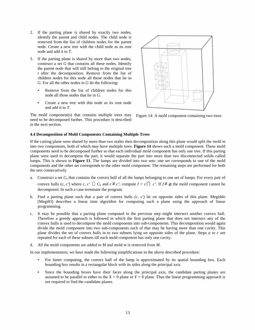
The mold component(s) that contains multiple trees mayneed to be decomposed further. This procedure is describedin the next section.

4.4 Decomposition of Mold Components Containing Multiple Trees

If the cutting plane were shared by more than two nodes then decomposition along this plane would split the mold minto two components, both of which may have multiple trees. Figure 14 shows such a mold component. These moldcomponents need to be decomposed further so that each individual mold component has only one tree. If this partingplane were used to decompose the part, it would separate the part into more than two disconnected solids calledlumps. This is shown in Figure 11. The lumps are divided into two sets: one set corresponds to one of the moldcomponents and the other set corresponds to the other mold component. The remaining steps are performed for boththe sets consecutively.

a. Construct a set Ch that contains the convex hull of all the lumps belonging to one set of lumps. For every pair of

convex hulls (c, c’) where c, c’ ∈ Ch and c≠ c’, compute I = cI c’. If I ≠ φ, the mold component cannot bedecomposed. In such a case terminate the program.

b. Find a parting plane such that a pair of convex hulls (c, c') lie on opposite sides of this plane. Megiddo[Megi83] describes a linear time algorithm for computing such a plane using the approach of linearprogramming.

c. It may be possible that a parting plane computed in the previous step might intersect another convex hull.Therefore a greedy approach is followed in which the first parting plane that does not intersect any of theconvex hulls is used to decompose the mold components into sub-components. This decomposition would againdivide the mold component into two sub-components each of that may be having more than one cavity. Thisplane divides the set of convex hulls in to two subsets lying on opposite sides of the plane. Steps a to c arerepeated for each of these subsets till each mold component has only one cavity.

d. All the mold components are added to M and mold m is removed from M.

In our implementation, we have made the following simplifications in the above described procedure:

• For faster computing, the convex hull of the lump is approximated by its spatial bounding box. Eachbounding box results in a rectangular block with its sides along the principal axis.

• Since the bounding boxes have their faces along the principal axis, the candidate parting planes areassumed to be parallel to either to the X = 0 plane or Y = 0 plane. Thus the linear programming approach isnot required to find the candidate planes.

Figure 14: A mold component containing two trees

14

5 Accessibility Based Decomposition

In the previous section we presented an algorithm for doing feature based decomposition of the mold. The result ofthe feature based mold decomposition is a set of mold components where each mold component contains the cavityfor a particular primitive of a part. An accessibility analysis has to be performed for individual mold components toensure that they can be machined on a CNC machine. If some mold components are not completely accessible,further decomposition based on accessibility will be required. We perform two stages of accessibility analysis. In thefirst stage, a global accessibility analysis of the mold components is done to ensure that each mold component iscompletely machinable by a cutting tool of semi-infinite length and zero diameter. Section 5.1 describes theprocedure for detecting accessibility problems based on the semi-infinite accessibility criteria and Section 5.2presents the accessibility based decomposition algorithm for alleviating semi-infinite accessibility problems. Thesecond stage of accessibility based decomposition involves detecting accessibility problems due to non-zero cuttingtool diameter. Section 5.3 describes the procedure for detecting accessibility problems due to non-zero cutting tooldiameter while Section 5.4 presents the algorithm for accessibility based decomposition for alleviating accessibilityproblems due to a non-zero tool diameter.

5.1 Detecting Accessiblity Problems Based on Semi-Infinite Accessiblity Criteria

5.1.1 Definitions of Semi-Infinite Accessibility

• Semi-infinite accessibility of a point in a given direction: A point belonging to a geometric entity is said to havesemi-infinite accessibility in a given direction if a ray of semi-infinite length can be drawn from it in the givendirection without intersecting any other part of the geometric entity. Figure 15 illustrates the concept of semi-infinite accessibility graphically. If the cutting tool is assumed to be of semi-infinite length and zero radius, then thedirection from which a point is accessible represents a direction from which it is machinable.

• Semi-infinite Accessibility of a face in a Given Direction: A face is said to have semi-infinite accessibility in agiven direction if all the points constituting the face have semi-infinite accessibility in the given direction.

• Global accessibility cone of a point: Global accessibility cone of a point represents the set of unit vectors alongwhich the point has semi-infinite accessibility.

• Global accessibility cone of a surface: Global accessibility cone of a surface represents the set of unit vectorsalong which the entire surface has semi-infinite accessibility.

Direction not semi-infinitelyaccessible

Semi-infinitely accessibledirection

Figure 15: Semi-infinite accessibility of a point

15

5.1.2 A Procedure for Computing Exact Inaccessibility

Given two planar triangular facets f and f’ , the set of directions from which f is inaccessible (and accessible) can becomputed using the method given by Dhaliwal [Dhal00]. Once again, let the set of directions from which f isinaccessible due to f’ be given by I and the set of directions from which f is accessible be given by V. The followingprocedure computes the set of directions from which f is inaccessible due to f’ .

procedure INACCESSIBLE(f, f’)

1. Construct unit spheres at the three vertices of the facet f. Project f’ on these spheres and let the projections bedenoted by f’ P1, f’ P2 and f’ P3. If any vertex of f’ lies at the center of sphere, then do not include that vertex in theprojection.

2. f’ P1, f’ P2 and f’ P3 are spherical triangles (or arc if the two facets share vertices) on the sphere and would result inmaximum of nine vertices on the unit sphere.

3. Find the convex hull CV of the vertices computed in the previous step.

4. I = CV.

(I is a convex spherical polygon representing the set of directions from which f is inaccessible due to f’ .)

5.1.3 Overview of Generation of Global Accessibility Cones for Various Facets in an Object

In order to generate the global accessibility cones for various facets in an object, a fecetised representation of theobject is first created. For a polyhedral object, the facetised representation is its exact geometric representation. Fora body having curved surfaces, the number of facets in a given facetised representation is dependent on the accuracyrequirements specified and also the maximum facet size specified by the user. The higher the accuracy requirement,the greater the number of facets in the facetised representation. The object is now represented in terms of facetsrather than faces. An object consisting of triangular facets has two types of facets: convex-hull facets and non-convex hull-facets. Convex-hull facets are defined in the following manner. We take the convex hull of the part.Convex-hull facets are those facets on the part that are also on the convex hull. All the facets on the part other thanconvex-hull facets are called non-convex-hull facets.

A convex-hull facet is always exactly accessible from the hemisphere created by using its direction normal asthe pole. However, the shape of the global accessibility cone of a non-convex-hull facet is generally much morecomplex due to the blocking by other facets. In Section 5.1.2, we described a procedure for finding the exactinaccessibility region for a facet due to another facet. In this section we describe how that procedure can be used toidentify the global accessibility cones for all the non-convex-hull facets in the object.

5.1.4 Finding the Global Accessibility Cones for Non-Convex-Hull Facets

We initially assume a non-convex-hull facet f is accessible from all the orientations described by the hemisphere Hcreated by the facet’s direction normal as its pole. Procedure INITIALIZE performs this initialization for all non-convex-hull facets. We use a data structure called Access_Status to represent global accessibility cones.Access_Status represents a matrix. Rows of this matrix represent spherical triangles. Columns of this matrixrepresent various facets. Various entries in the matrix describe whether a facet is accessible from a spherical triangleor not. Each entry in the matrix stores a set of facets due to which the given facet is inaccessible from the set ofdirections represented by the spherical triangle. For example if jth facet is accessible from ith spherical triangle, entrythat corresponds to ith row and jth column contains a null set. On the other hand, if jth facet is not accessible from ith

spherical triangle, the entry that corresponds to ith row and jth column contains the set of facets due to which thisfacet is inaccessible. We use procedure UPDATE to find a facet’s inaccessibility region due to the influence of otherfacets in the set. Procedure UPDATE calls procedure INACCESSIBLE to find the inaccessibility region for variousfacets.

INITIALIZE takes the set of non-convex-hull facets Fn of the object as an argument. It decomposes the surface ofa unit sphere into a finite number of spherical triangles. In the decomposition, each hemisphere is equally dividedinto τ strips, and each strip i is further decomposed into δi spherical triangles. The values of τ and δi are determinedsuch that the areas of the spherical triangles are kept uniform, within solution accuracy.

16

INITIALIZE uniquely classifies the spherical triangles according to the initial accessibility status of each facet.This initial accessibility information is stored in matrix Access_Status and will be later updated by the iterativeprocedure UPDATE.

Inaccessibility region of a non-convex-hull facet can be determined by only considering the influence of othernon-convex-hull facets in the object. This property exists because of the following reason. A semi-infinite rayemanating from a point within a non-convex-hull facet either does not intersect any facet in the object or intersects anon-convex-hull facet [Chen93b]. Therefore to determine the complete inaccessibility region of a non-convex-hullfacet, it is sufficient to only examine the influence of other non-convex-hull facets in the object.

procedure INITIALIZE (Fn)

1. Form the set of spherical triangles S by dividing each hemisphere of a unit sphere into τ strips, and each strip iinto δi spherical triangles. τ is selected by the user.

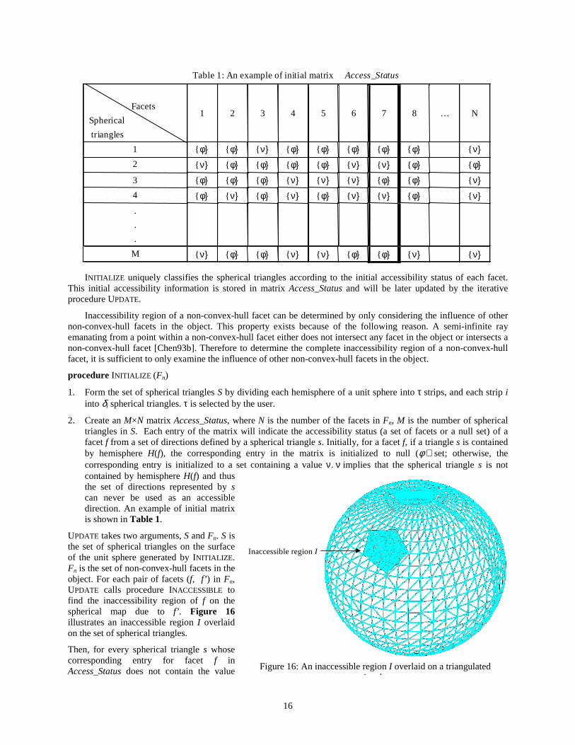
2. Create an M×N matrix Access_Status, where N is the number of the facets in Fn, M is the number of sphericaltriangles in S. Each entry of the matrix will indicate the accessibility status (a set of facets or a null set) of afacet f from a set of directions defined by a spherical triangle s. Initially, for a facet f, if a triangle s is containedby hemisphere H(f), the corresponding entry in the matrix is initialized to null (φ ) set; otherwise, thecorresponding entry is initialized to a set containing a value ν. ν implies that the spherical triangle s is notcontained by hemisphere H(f) and thusthe set of directions represented by scan never be used as an accessibledirection. An example of initial matrixis shown in Table 1.

UPDATE takes two arguments, S and Fn. S isthe set of spherical triangles on the surfaceof the unit sphere generated by INITIALIZE.Fn is the set of non-convex-hull facets in theobject. For each pair of facets (f, f’ ) in Fn,UPDATE calls procedure INACCESSIBLE tofind the inaccessibility region of f on thespherical map due to f’ . Figure 16illustrates an inaccessible region I overlaidon the set of spherical triangles.

Then, for every spherical triangle s whosecorresponding entry for facet f inAccess_Status does not contain the value

Facets

Spherical

triangles

1 2 3 4 5 6 7 8 … N

1 { φ} { φ} { ν} { φ} { φ} { φ} { φ} { φ} { ν}2 { ν} { φ} { φ} { φ} { φ} { ν} { ν} { φ} { φ}

3 { φ} { φ} { φ} { ν} { ν} { ν} { φ} { φ} { ν}4 { φ} { ν} { φ} { ν} { φ} { ν} { ν} { φ} { ν}.

.

.

M { ν} { φ} { φ} { ν} { ν} { φ} { φ} { ν} { ν}

Table 1: An example of initial matrix Access_Status

Inaccessible region I

Figure 16: An inaccessible region I overlaid on a triangulatedit h

17

ν (i.e. s is contained by H(f)), if the Boolean intersection of s with I is not a null set, update Access_Status by addingf’ in list of facets that make f inaccessible in the set of directions represented by s. Boolean operations on sphericaltriangles are performed by first converting spherical polygons to planar polygons using central projection [Lent49].After this step we apply standard planar polygon intersection algorithms. Table 2 is an example of an intermediateresult while updating Access_Status shown in Table 1. It shows the addition of facet f3 in all those columns for facetf5 where the Boolean intersection of I (obtained by calling INACCESSIBLE (f5, f3)) with s (where the correspondingentry does not include ν) results in a not null set.

procedure UPDATE(S, Fn)

For every pair of facets (f, f’ ) in Fn, do the following:

• Call INACCESSIBLE (f, f’ ), which returns I, the convex spherical polygon representing the inaccessibility regionof f due to f’ .

• For every spherical triangle s in S, if the corresponding entry for facet f in Access_Status does not containν, compute C = I ∩ s. If C ≠ φ, update the entry for facet f in Access_Status for the row s by adding f’ to set offacets that make f inaccessible in set of directions represented by s.

5.2 Decomposition Algorithm to Alleviate Accessibility Problems

In the Section 5.1.4 we developed a procedure for computing the global accessibility cones for all the non-convexhull facets of an object. These cones can be used to analyze if an accessibility based decomposition of a moldcomponent is required or not. The first step in this process would be to obtain the global accessibility cones for eachmold component. The next step is to determine if all the facets for a mold component are accessible in somedirection. In Section 5.2.1 procedure CHECKACCESSIBILITY describes the procedure for doing this test.

If there exist some facets in a mold component that are not accessible in any direction, the mold component hasto be decomposed. A set of directions D is constructed that contains the unit normals of the candidate parting planes.At present, the set of directions for a mold component comprise of the six principal directions (i.e. ZYX ±±± ,, ),

face normals for all the planar faces of the primitive for the mold component (each mold component represents themold cavity for a particular primitive) and a set of user defined directions. This set of directions can be easilyaugmented.

Once the set of directions for a mold component have been determined, the next step involves creating a matrixDirection_Status similar to Access_Status for storing the set of facets that block a facet f in a direction d in D.Procedure CREATEMATRIX described in Section 5.2.2 creates this matrix. Each entry in this matrix representswhether a facet is accessible in the given direction or not.

Facets

Spherical

Triangles

1 2 3 4 5 r… N

1 { φ} {f 3,f4,f5} {φ} { φ} {f 2,f3} { ν}

2 {f 4,f2} {f 5,f3} {f 2,f7} { ν} {f 2,f3} {f r,f r+1}

3 {f 5,f2} {f 3,f4} { ν} {f 6,f7} {f r,f r+1} {f n-1,f7}

4 { φ} { ν} {φ} { ν} { ν} { ν}

.

.

M { φ} { φ} {ν} { ν} { φ} {f n-2,fn}

Table 2: An example of updating matrix Access_Status

18

Since we have a set parting planes represented by their unit normals (set D), we need to develop a procedure forselecting the best parting plane for doing the decomposition. The procedure described in Section 5.2.3 sorts thecandidate parting planes and decomposes the mold component along the best candidate plane. It first callsCHECKACCESSIBILITY to determine if the mold component is completely accessible or not. If the mold component isnot completely accessible it calls CREATEMATRIX to create the matrix Direction_Status. It then selects the bestparting plane to decompose the mold component.

5.2.1 Checking if the Mold Component is Completely Accessible

The procedure CHECKACCESSIBILITY checks if the mold component is completely accessible. It uses the matrixAccess_Status to perform this test. For each column in this matrix, if there exits at least one entry that contains a nullset, it implies that the entire mold component is completely accessible. However, if there are columns that do notcontain a single null set, the facet represented by the column is completely inaccessible. The mold component needsto be decomposed to make it accessible. This procedure returns a status (True/False) that specifies whether the moldcomponent is completely accessible or not.

procedure CHECKACCESSIBILITY

1. For every column in Access_Status do the following:

• Search for the first entry in the matrix that is a null set.

• If an entry is found, then continue.

• Else break the loop and return False.

2. Return True.

5.2.2 Creating Matrix Direction_Status

CREATEMATRIX takes the set of non-convex-hull facets Fn of the mold component and the set of directions D asarguments. It creates the matrix Direction_Status for classifying the accessibility of a facet in a given direction. It isinitially assumed that all the facets are accessible in the set of directions D. ν implies that the direction d is notcontained by hemisphere H(f) and thus can never be used as an accessible direction.

procedure CREATEMATRIX(Fn, D)

1. Create a Md×N matrix Direction_Status, where N is the number of the facets in Fn, Md is the number ofdirections in D. Each entry of the matrix will indicate the accessibility status (a set of facets or a null set) of afacet f from a direction d in D. Initially, for a facet f, if a direction d is contained by hemisphere H(f), thecorresponding entry in the matrix is initialized to null set; otherwise, the corresponding entry is initialized to aset containing a value ν.

2. For every pair of facets (f, f’ ) in Fn, do the following:

3. Call INACCESSIBLE (f, f’ ), which returns I, the convex spherical polygon representing the inaccessibility regionof f due to f’ .

• For every direction d in D, if the corresponding entry for facet f in Directions_Status does not contain ν, ifd∩ I ≠ φ, update the entry for facet f in Direction_Status for the row d by adding f’ to set of facets thatmake f inaccessible in the direction d.

5.2.3 Accessibility Based Decomposition

A mold component needs to be decomposed if the procedure CHECKACCESSIBILITY returns False. In such a case, theuser specifies the maximum allowable cuts that may be performed on the mold component. The procedureCREATEMATRIX is then called to create a matrix Directions_Status. The next step is to identify all the columns inmatrix Direction_Status that do not contain a single null set. These columns represent the facets that are completelyinaccessible.

19

From the set D, those directions that represent the face normals of the primitive corresponding to the moldcomponent are given highest priority. This is because this decomposition would be along the natural edges of thepart. Therefore no visible parting line will be present in the part.

The following strategy is applied to find a suitable parting plane for partitioning the mold component:

1. A facet f is selected from the list of completely inaccessible facets that is being blocked by the least number offacets.

2. A direction d is selected from D that does not contain ν in the entry for f in Direction_Status. If there are morethan one such direction, a direction is selected that represents a face normal of the primitive corresponding tothe mold component. If there are more than one such direction that represent the face normals, a direction isarbitrarily selected from among them. If no such direction exists, then any direction is arbitrarily selected.

3. If no direction exists that does not contain ν , then any direction is arbitrarily selected.

4. The facet f and all the facets that are making f inaccessible are projected onto a line l whose direction is along d.This is shown in Figure 17. Let lf be the line segment on l that represents the projection of f and lo be the linesegment on l that represents the projection of all the other facets. If lf and lo overlap, this direction is not asuitable direction. Select the next direction.

5. If lf and lo do not overlap then:

• If the direction represents a face normal of the primitive corresponding to the mold component, projectthe plane representing the face of the primitive on the line. If the projection of the plane lies in the gap(including the end points), select the plane as the parting plane.

• Else the mid point of the gap g between lf and lo is computed. A cutting plane represented by normal dand root point g is used to decompose the mold component.

The approach described above may not be the most optimum partition of the mold component. Since the userspecifies the maximum allowable cuts for a mold component, it does not guarantee that the mold component can bedecomposed such that it is completely accessible. Since we only look at facet-facet interaction for determining thecutting plane, we are not looking for a one-cut solution that will make the mold component accessible. Theimplementation of this algorithm also provides a provision for the user to input a partition plane for decomposing amold component.

Line l

lf : Projection of inaccesible facet

on line l

lo : Projection of facets causing

inaccesibility on line l

Gap g

Direction d

Figure 17: Projection of inaccessible facet and facets causing its inaccessibility on a line lrepresenting a direction d from set D.

Facets causinginaccessibility

Inaccessible facet

20

5.3 Detecting Accessibility Problems due to Non-Zero Cutting Tool Diameter

Mold components are typically machined using cylindrical milling cutters. Therefore, even if the entire boundary ofthe mold component is accessible using the accessibility criteria described in the previous sections, the moldcomponent may not be machinable using any finite diameter cutter. Figure 18 shows an example of such cases.

We use the following approach to detect locally unmachinable regions:

1. We label edges as convex or concave by performing the following procedure for all edges:

• Suppose face f1 and face f2 intersect at edge e. Let 1nr

and 2nr

be the outer normal vector of the two faces

respectively, and er

be the direction vector for edge e in the edge loop of face f1. The edge e is concave if

er

is opposite to ( 1nr

× 2nr

). Otherwise the edge is convex.

2. For every concave edge we measure the angle between the faces that form the edge.

• If the angle is less then 90 degrees then the edge is labeled as an acute concave edge and consideredunmachinable.

• If the angle is 90° or more, we extend the edge on both ends by arcs whose radius is equal to the minimum

tool diameter and the arc angle is 2

π radians. The tangent to the arc at the point where it touches the edge

is collinear with the edge. We consider two arcs at each end. These two arcs are in the same plane as thetwo faces that form the edge. One end of the arc touches the end of the edge and the other end is placed onaway from the face that is not coplanar with the arc. If the extended edge intersects with the part, then theedge is labeled as concave edge with a closed end.

5.4 Decomposition for Concave Edges

If the mold component contains any acute concave edge or a closed concave edge, we need to decompose the moldcomponent. We know that an acute concave edge (i.e. an edge with an angle between its adjacent faces less than90°) is always unmachinable due to the finite diameter of the cutting tool. In order to eliminate thismanufacturability problem, the only solution is to cut the object along either of the two faces so that the acuteconcave edge is eliminated.

For a closed concave obtuse edge (i.e. an edge with angle between its adjacent faces greater than or equal to90°, and at least one of whose ends is closed), there are also multiple solutions for making it machinable with onecut on the object. Similarly to the acute edge case, we can cut the object along either of the two adjacent faces toeliminate the concave edge. For an obtuse edge with only one closed end, there exists another solution – cuttingalong the third face, which makes that end closed. As shown in Figure 19, edge AB is a closed obtuse edge with aclosed end at B. We have three one-cut decomposition solutions to make it machinable: (1) cutting along face f1, (2)cutting along face f4, and (3) cutting along face f2. The first two solutions eliminate the concave edge, and the third

(b): A part having a closed concave edge

Closed concave edge

(a): A part having an acute concave edge

Figure 18: Parts that are not completely accessible by a finite sized cutting tool

Acute concave edge

21

solution simply makes the end at B open. For an obtuse edge with both ends closed, as edge BF shown in Figure19, there are only two one-cut solutions, namely, cutting along face f2 or cutting along face f4, both of whicheliminate the concave edge.

Based on the above observations, we have developed a greedy algorithm to perform decomposition due tounmachinable concave edges.

1. For each of the unmachinable concave edges in the mold component, list all the candidate faces along which aone-cut solution can make it machinable.

2. Among the list, pick the face that appears the maximum number of times and cut the object along it.

The status of an edge may change after each cut. For example, an obtuse edge with both ends closed may have oneof the ends opened after a cut. Thus, we need to re-check the status of the all the edges. This decompositionprocedure runs recursively until all the edges become machinable.

Consider the example in Figure 19,we list all the candidate cutting planesfor each of the unmachinable concaveedges:

AB – f1, f2, f 4

BF – f2, f4

BD – f1, f2, f4

FH – f2, f3, f4

EF – f3, f4, f2

Therefore, we have the following facelist [f1, f2, f4, f2, f4, f1, f2, f4, , f2, f3, f4,f3, f4, f2]. Both f2 and f4 appear fivetimes, which is the maximum in this list.Therefore, cutting the object along eitherf2 or f4 will make the maximum numberof unmachinable edges machinable. Inthis particular example, all the edgesbecome machinable after a cut alongeither f2 or f4. If there is still at least oneconcave edge remaining unmachinableafter the cut, the above describedprocedure is applied recursively until alledges become machinable.

6 Reducing Mold Components byEliminating Over Decomposition

The feature based decomposition mightresult in mold components that can be

A

BC

D

E

FG

H

f1

f4

f2

f3

Figure 19: Decomposition for concave edges

m1

m2

m9

m5

m7

m6

m4

m3

m8

m11

m10

Figure 20: Mold components of part shown in Figure 4

22

combined without affecting the overall accessibility of the combination. Figure 20 shows the mold components ofthe part shown in Figure 4. Since the feature based representation of the part consists of eleven primitives, thefeature based decomposition of the mold results in eleven mold components. As there is no accessibility baseddecomposition in this example, the total number of mold components is eleven. However, some of the moldcomponents can be easily combined without affecting the overall accessibility of the combined mold component.This section describes the conditions and provides an algorithm for doing recombination of mold components.

6.1 Conditions for Feasibility of Recombination

A pair of mold components that share a common planar face is a candidate pair for recombination if it satisfies thefollowing conditions:

1. The recombination of the mold components should not result in acute concave edges or closed concave edges.In Section 5.3 we have described the procedure for identifying acute concave edges and closed concave edges.This condition invalidates the recombination of mold components shown in Figure 21.

2. The recombination of the mold components should not affect the global accessibility of the combined moldcomponent. In Section 5.2.1 we have described the procedure for checking if a mold component is completelyaccessible. This procedure is used to check the accessibility of the combined mold component. If the combinedmold component is not completelyaccessible, this combination is not valid.Figure 22 shows a pair of moldcomponents that cannot be combinedbecause they do not satisfy this condition.

6.2 Overview of Recombination Algorithm

We follow a feasibility based approach torecombine the mold components. It tries toeliminate over decomposition as it identifies ittill no further recombination is possible.However, this approach does not necessarilyminimize the total number of moldcomponents. There may be other ways ofcombining the mold components that result inan optimal number of mold components.However, the approach may be easilyextended to produce the optimal result bybacktracking during the search process. Thedifferent steps involved in the mold

(a): A mold combination resulting inan acute concave edge

Closed concave edgeAcute concave edge

(b): A mold combination resulting in aclosed concave edge

Figure 21: Invalid mold combinations due to acute or closed concave edges

Cavity not completelyaccessible

Figure 22: A mold combination resulting in inaccessible regions

23

recombination are as follows:

1. Determine which mold components share a commonplanar face. A contact graph is created that representsthe connectivity of the mold components. The contactfor the mold components in Figure 20 is shown inFigure 23.

2. Construct a set C initialized to a null set whose eachelement c is an unordered pair of mold components(cm1, cm2) that can be combined. For every pair ofmold components that are connected in the contactgraph, do the following:

• Perform the validation checks described inSection 6.1 to determine if the pair of moldcomponents can be combined. If the pair can becombined add it to C.

For the contact graph shown in Figure 23, C is givenby

C = {{m2, m5}, {m4, m5}, {m9, m10}, {m7, m10}}

3. While C is not empty, do the following:

• Select an element c from C and unite the pair ofmold components (cm1, cm2) contained in c toproduce a new mold component mnew. Remove cfrom C.

• For every element d in C that contains either cm1

or cm2 do the following:

• Replace cm1 or cm2 by mnew in d and perform the validation checks described in Section 6.1 todetermine if the pair of mold components contained in d can be combined. If the pair of moldcomponents cannot be combined, remove d from C.

6.3 Checking Recombination Feasibility for a Mold Component Pair

The algorithm described in the previous section can be used to recombine all possible pairs of mold components.However, the procedure described in Section 6.2 that is required for validating a combination of mold components iscomputationally expensive since the generation of the accessibility matrix requires performing pair-wiseintersections of all the facets in the facetised representation of the mold component. It also requires performing anintersection of an inaccessible region for a facet due to another facet with all the spherical triangles on the unitsphere. Therefore, a set of heuristics have been developed that can be used to combine two mold componentswithout generating a new accessibility matrix for every candidate combination of mold components.

We have developed two heuristics for identifying the pair of mold components that can be combined withoutcreating a new accessibility matrix for the combined mold component. These heuristics are described in this section.

1. Heuristic 1: For any pair of mold components (m1, m2) that are connected in the contact graph, let 1nr

and 2nr

( 2nr

= - 1nr

) be the two opposite normal vectors of the common planar face f along which we want to combine

the mold components. A 2D view of the representative example is shown in Figure 24. The unit sphere thatrepresents all the directions in space is divided by f into two hemispheres, h1 and h2. A sufficient condition forvalidating the combination of these mold components is given below:

• If an accessibility direction 1vr

exists for all the facets in the facetised representation of m1 such that

1vr

. 1nr

0≥ and an accessibility direction 2vr

exists for all the facets in the facetised representation of m2

m2

m3

m1 m5 m4

m8

m7

m6

m11

m10 m9

Figure 23: Contact graph of the mold components

24

such that 2vr

. 2nr

0≥ , then the mold components can be combined. In such a case, every facet in m1 will be

accessible in at least one direction that lies on hemisphere h1 while every facet in m2 will be accessible in atleast one direction that lies on hemisphere h2. Therefore, m1 and m2 can be combined without creating anyaccessibility problems.

2. Heuristic 2: Let m and m’ be two mold components that correspond to 2.5D primitives such that m∪ p isconvex (where p is the primitive that corresponds to m ) and m’ ∪ p’ is convex (where p’ is the primitive thatcorresponds to m’). m and m’ can be combined if the following condition is satisfied.

• The infinite sweep of the profile of p does not intersect with m’ and the infinite sweep of the profile of p’does not intersect with m.

This condition ensures that the concave regions of m and m’ do not have any accessibility problems due tocombination. The convex regions of m and m’ do not have any accessibility problems due to the argumentpresented in Heuristic 1. This is shown in Figure 25.

m2

2nr

1nr

f

m1

Mold component m1 is completely accessiblein set of direction given by h1

Mold component m2 is completely accessiblein set of direction given by h2

f

Hemisphere h1

Hemisphere h2

Figure 24: Mold components completely accessible in set of directions lying in different hemispheres

m’

f

m

Concave region corresponding to part p

Figure 25: Mold components m and m’ combining along face f

25

7 Adding Assembly Features into Mold Components

The addition of assembly features to the mold assembly consists of two steps: (1) selecting the appropriate pairs ofmold components that need assembly features, and (2) adding assembly features at appropriate positions on thesemold components. These steps are described in Section 7.1 and Section 7.2 respectively.

7.1 Selecting the Component Pairs to Add Assembly Features

The primary reason for adding assembly features to mold components is to constrain the degrees of freedom of eachmold component such that all the mold components in the assembly have either no relative motion or translationalmotion only in the positive Z direction. To achieve this, an assembly feature in the form of a hole-pin combination isadded to a pair of mold components along their contact face. Addition of assembly features to mold componentsincreases the mold component manufacturing time. We have considered the set-up time for machining as the mainfactor that contributes to the total manufacturing time. An algorithm following a greedy heuristic has beendeveloped that reduces the total setup time by orienting features such that multiple assembly features can beproduced in the same setup.

Various contacts in an assembly of mold components can be represented by a graph G (V, E). Each moldcomponent is represented by a vertex v in set V. If any two mold components, say v1 and v2, share a common face,an edge e (v1, v2) is added to the set E. Since multiple assembly features on the same planar face of a moldcomponent can be manufactured in a single setup, our algorithm tries to put as many assembly features as possibleon a single contact face. We use a variation of the spanning tree algorithm that results in a solution in which moldcomponents (represented by vertices in the graph), get kinematically constrained with respect to each other in apattern of a spanning tree of the graph. Each edge in the spanning tree kinematically constraints two moldcomponents by adding a pair of hole-pin combination on the contact face that corresponds to the edge.

We construct the spanning tree T (S, X) using the procedure ASSEMBLY-TREE described below. Afterconstructing the spanning tree, we add a pair of hole-pin combination on the contact faces corresponding to eachedge in the tree. Technique for determining the locations of hole-pin features on the contact faces is described inSection 7.2.

procedure ASSEMBLY-TREE (G (V, E), T(S, X))

1. Initiatlize S = Φ and X = Φ.

2. Color all e ∈ E such that all edges lying in the same contact plane have the same color.

3. Find a vertex r ∈ V that has the highest number of edges of the same color. Add r into set S and make this theroot node of tree T.

4. Let V’ be the set of nodes in V that are common with the set S. Find v in V’ that has the highest number of thecrossing edges of the same color for partition (V’, V – V’). We say that an edge e ∈ E is a crossing edge for thepartition (V’, V – V’) if one of its vertices is in V’ and the other is in V – V’. Let Ev be the set of highestcardinality of crossing edges of the same color for node v.

5. Add all edges in Ev into X, and all vertices in (V – V’) into S that are connected by Ev to v.

6. If S ≠ V, go to 4. Otherwise, stop.

7.2 Adding Assembly Features

In order to add assembly features (i.e., two pin-hole pairs) to a pair of mold components that need to be assembled,we initially compute the shape of their contact region to determine which mold component has the pins and whichmold component has the holes. This is performed comparing the areas of faces that contain the contact region. Thecomponent that has larger face area is assigned the hole assembly feature and the other component is assigned thepin assembly feature. Then we use procedure DETERMINE_PINS (described later in this section) to determine thepositions of the pins. Finally we create the pin-hole pairs at the positions found in the previous step and attach themto the corresponding mold components.

26

Figure 26 shows an example of a pair of mold components that need to be assembled. BodyA and BodyB sharea common planar face. The initialization procedure computes their contact region through a non-regularizedintersection. The component that has the holes is returned as HoleBody while the component that has the pins isreturned as PinBody. The procedure also transforms the contact region onto the X-Y (Z=0) plane and returns it asBodyI (a body that has only one planar face). BodyI will be analyzed further in procedure DETERMINE_PINS as a 2-Dentity to determine the positions of the pin-hole pairs. Figure 27 shows a contact region transformed onto the X-Yplane.

We use procedure DETERMINE_PINS to find the positions of the two pins. DETERMINE_PINS takes BodyI as anargument, which is the body resulting from transforming the contact region onto the X-Y plane. DETERMINE_PINS

finds the edges and loops of the contact region. It then calls MESHING to generate a set of grid points on the planewhere each point represents a candidate position to put the pin. The sub-procedure LOCATE_PINS then traverses allthe candidate positions, checking their validity and finding two valid positions for pins of a desired radius so that thetwo pins are placed at the maximum possible distance between them. DETERMINE_PINS returns these positions asPinPos1 and PinPos2.

procedure DETERMINE_PINS (BodyI)

1. Retrieve the information of all the loops and edges of the assembly region, and store it in a data structure Profl.

2. Call MESHING (Profl), which returns a set of grid points Sp.

3. Call LOCATE_PINS (Sp, Profl), which returns PinPos1 and PinPos2.

MESHING first computes a rectangle bounding the contact region and then generates an orthogonal grid on therectangular area at a reasonable resolution. All the crossing points on the grids represent the candidate positions toplace a pin. This procedure takes Profl as an argument. Figure 28 shows the grid on the example contact region.

procedure MESHING (Profl)

1. Calculate the bounding rectangle of Profl, the profile of the contact region.

2. Mesh the rectangle with an orthogonal grid. The space width of the grid should be small as compared to thediameter of the pin. The set of all the candidate positions is returned as Sp.

LOCATE_PINS takes Sp, the set of candidate positions, and Profl, the profile of the contact region, as two arguments.The procedure filters out all the invalid positions that lie outside Prof. It then calls procedure PIN_SIZE for each ofthe remaining positions to determine the maximum possible radius of the pin at that position. If the maximum

BodyA

BodyB

Figure 26: Example of BodyA and BodyB Assembly

Figure28: Meshing the Assembly RegionFigure 27: Assembly Region Transformed onto X-Y Plane

27

possible radius is smaller than the desired radius of the pin, then the position is also invalid. The pair of position thatis farthest apart is returned as PinPos1 and PinPos2.

procedure LOCATE_PINS (Sp, Profl)

1. For every candidate position p in set Sp, do the following:

• If p is outside profile Profl, then delete this position.

• Otherwise, call PIN_SIZE (P, Profl). It returns the maximum possible radius of a pin at position P. If thereturned radius is smaller than the desired radius of the pin times a specified ratio (between 0 and 1), deletethis position.

2. For all valid pin positions, calculate the pair-wise distance. Return the pair with the greatest distance as PinPos1and PinPos2.

PIN_SIZE takes p, a valid candidate position, and Profl, the profile of the assembly region, as two arguments. Theprocedure calculates the distance from p to each edge of the profile. The distance from position p to an edge e isdefined as the length of the shortest line segment that can be drawn from p to a point on e. Since the radius of thepin at position p should be no greater than the smallest of the distances obtained, this smallest distance is returned asthe maximum radius of the pin.

procedure PIN_SIZE (p, Profl)

1. For every edge e in profile Profl, calculate the distance from p to e.

2. Return Pinr, the maximum radius of the pin at p, which is the smallest distance from p to the various edges.

Figure 29 shows an example of the pin locations. Figure 30 shows the pair of mold components after addingassembly features.

Figure 29: Locating the two pins Figure 30: Creating Assembly Features

28

8 System Implementation and Examples

8.1 System Architecture

The system architecture of our implementation is shown in Figure 31. The system consists of two main componentseach of which have multiple modules for performing various tasks. These two components are:

1. Graphical User Interface (GUI): The graphical user interface is implemented in Java. Java 3D, a package inJava 2, is used to render solid models of parts.

2. Geometric Reasoning Component: The geometric reasoning is done in C++/ACIS. ACIS is a 3D geometricmodeler provided by Spatial Technologies.

The communication between the components is through a file based system. A set of keywords have been definedthat enable the communication between these components. Each component contains a module that monitors a statusfile, which is used for reading and writing the messages between the components. A log file is created that maintainsa record of all the communication between the GUI and the geometric reasoning component.

8.2 Example Run of the System

In this section we present an example run of the system. The different steps in the implementation are as follows:

1. Using the GUI, the user selects a file that contains the feature based representation of the part.

ValidateInput

DisplayPart

CreateGeometry

Java FileParser C++ File

Parser

Preprocessing

Accesibility BasedDecomposition

Feature BasedDecomposition

Utilities

File handlingsystem

InputCAD part

GUIComponent

Geometric ReasoningComponent

Figure 31: System architecture

29

2. This file is then used by the Geometric Reasoning component. If the feature based representation of the part isvalid, the part will be created and shown to the user. This is shown in Figure 32. The user will be prompted toscale the part if she/he desires.

Figure 32: Solid model of part

Figure 33: Wireframe model of gross mold

30

3. After the user has input the scaling factor for the part, a wireframe model of the mold is displayed. This isshown in Figure 33.

4. By clicking on the Decompose Mold button, the user initiates the decomposition of the mold. A decomposedmold for the part is shown in Figure 34.

8.3 Example Parts

We have used our implementation to design and manufacture parts requiring multi-piece molds. In this section wepresent a few example parts whose molds were designed using our system. The mold components for these moldswere manufactured on a 3-Axis CNC milling machine. After the mold components were made, the mold wasassembled manually using the assembly features incorporated on each mold component. The parts were made ofpolyurethane. Section 8.4 describes the polymer part fabrication process.

1. Example Part 1- Indexer: Figure 35 shows the solid model of an indexer. The multi-piece mold for the indexerwas made using our system. The mold consisted of four mold components. The assembly features were addedto the mold components after the decomposition was done by the system. This was done to ensure an easyassembly of the mold components. Figure 36 shows the mold components of the mold. Figure 37 shows thepolyurethane part that was made in this mold.

2. Example Part 2-Multi-Stage Rotor: Figure 38 shows thesolid model of a multi-stage rotor. The mold for the rotorconsisted of seventeen mold components. Figure 39shows the mold components for this mold. Assemblyfeatures were incorporated to the mold components toensure an easy assembly. Figure 40 shows thepolyurethane part that was made in this mold.

8.4 Polymer Part Fabrication

Polyurethanes can be used to fabricate complex parts thatrequire multi-piece molds. Polyurethanes (PURs) are a group ofpolymers with highly versatile properties and a broad range ofcommercial applications. PURs can be manufactured in anextremely wide range of grades, in polymer stiffness from veryflexible elastomers to rigid hard plastics. The manufacturergenerally sells the PUR chemical components, usually in theform of liquids, and may also provide information to enable theuser to make the PUR. The user mixes together the PUR

(a): Assembled mold (b): Disassembled mold

Figure 34: Decomposed mold

Figure 35: Solid model of indexer

31

chemicals that then react to make the required polymer product. Thus they can be tailored with remarkableaccuracy to meet the needs of a particular application. Most of the PURs cure at room temp so no specialcuring facility is needed for these parts.

Complex polymer parts are easy to manufacture by casting PUR into multi-piece wax molds. The multi-piecemolds are first fabricated from machinable wax on a CNC machine. After the mold components are machined at themachining facility, they are cleaned using acetone to remove dust particles that may get trapped in the mold cavities.Cleaning of dust particles is required to get a good surface finish. The mold components are assembled togetherusing the designed assembly features. Then PUR components are mixed in the specified ratio by weight or volumeand poured into the mold. The cast part is then left to set for the required demolding time. The demolding timetypically varies from 2 hours to 10 hours depending on the grade of PUR used. The cast part is demolded byremoving the wax mold components and the fabricated part is then cured for the ultimate cure time. The ultimatecure time varies from 2 days to 10 days.

Figure 36: Mold for the part Figure 37: Part

Figure 38: Solid model of multi-stage rotor

Figure 39: Mold for the part

32

PURs are very easy to cast as most of the widely used PURs are in the liquid state at room temperature.However, care must be taken to ensure the fabrication of good quality polymer parts. The PUR components shouldbe mixed and poured very quickly otherwise PUR may get cured partially before it could be poured into the molds.In such a case, it will not flow into the molds properly and that may result in under-filling in some portions of themold. When mold components form a horizontal partitioning, these pieces need to be clamped together properly toavoid leakage of material under gravity through the gap between mold components.

9 Conclusions

This paper presents a systematic approach for doing automated design of multi-piece sacrificial molds. These moldscan be used to make complex shaped parts that cannot be made using two-piece molds. Manufacturing techniquessuch as gelcasting and polyurethane manufacturing can be used to make parts using these molds. A novel approachhas been developed for doing decomposition of a mold. The mold decomposition process has been divided into foursteps:

1. The first step involves a feature-based decomposition of the part. The input to the algorithm is a feature basedrepresentation of the part. This decomposition results in different mold components for each primitive. Theprimary reason for doing feature based decomposition is to simplify the problem of mold decomposition since itis easy to do geometric reasoning with a mold components that represent individual primitives.

2. The next step is an accessibility-based decomposition of those mold components that are not completelyaccessible. Accessibility analysis is performed on all mold components and those mold components that are notcompletely accessible are further decomposed.

3. The feature-based decomposition might result in over decomposition of the mold. This step performs a pair-wise analysis of all mold components that share a common planar face and combines those mold componentsthat can be combined without compromising their accessibility.

4. Finally assembly features are added into various mold components to facilitate assembly of the mold.

A system has been developed based on the above approach for designing multi-piece sacrificial molds. This systemhas been used to design multi-piece molds for several parts. The mold components of these molds have beenmachined on a 3-Axis CNC milling machine and the parts has been fabricated using polyurethanes. The successfulfabrication of these parts shows that such a system can be used to design multi-piece sacrificial molds for complexshaped parts that cannot be produced using two-piece molds.

There are a number of potential benefits of automating the design of multi-piece molds. The principal benefitsare enumerated below.

1. Mold design is a laborious process that requires significant time from the mold designer. This is aggravated inthe case of multi-piece molds. Automated mold design significantly reduces the mold design time.

Figure 40: Part

33

2. This approach allows us to manufacture parts that could not be produced earlier using two-piece molds. Thus itexpands the design space for parts that can be produced using casting processes such as gelcasting andpolyurethane manufacturing.

3. Since this approach automatically produces solid models of mold components, it can be integrated with CAMsystems to generate the cutter path plans for manufacturing the individual mold components. Thus an integratedsystem can be developed that can simultaneously design and generate the cutter path plans for manufacturingthe individual mold components in a mold assembly.

10 References

[Chen93a] L.-L. Chen, S.-Y. Chou and T. C. Woo, “Separating and intersecting spherical polygons: computingmachinability on three-, four-, and five-axis numerically controlled machines”, ACM Transactions on Graphics,1993, Vol. 12, No. 4, 305-326

[Chen93b] L. L. Chen, S.-Y. Chou and T. C. Woo, “Parting directions for mould and die design”, Computer-AidedDesign, Vol. 25, pp. 763-767, 1993.

[Dhal00] S. Dhaliwal, S. K. Gupta and J. Huang, “Computing exact global accessibility cones for polyhedralobjects”, Accepted for publication for the 2000 ASME DETC/DFM Conference, September 10-13, Baltimore, USA.

[Hui92] K. C. Hui and S.T. Tan, “Mould Design with Sweep Operations – a Heuristic Search Approach”. ComputerAided Design, Vol. 24(2), 1992.

[Kris97] S. Krishnan, “Design for Manufacture: An Integrated System for Injection Molding and Milling”, PhDPaper, Mechanical Engineering, University of Maryland, College Park, 1997.

[Lent49] J. G. Lenthem, “Spherical trigonometry, for the use of colleges and schools”, Macmillian Pub., London,1949

[Megi83] N. Megiddo, “Linear-Time Algorithm for Linear Programming in R3 and Related Problems”, Society forIndustrial and Applied Mathematics, Vol. 12, No. 4, November 1983.

[Ravi90] B. Ravi and M. N. Srinivasan, Decision Criteria for Computer-Aided Parting Surface Design. ComputerAided Design, Vol. 22(1), 1990.

[Wein96] M.Weinstein and S.Manoochehri, “Geometric Influence of a Molded Part on the Draw Direction Rangeand Parting Line Locations”, Journal of Mechanical Design Vol. 118, March 1996.

[Wein97] M.Weinstein and S.Manoochehri, “Optimum Parting Line Design of Molded and Cast Parts forManufacturability”, Journal of Manufacturing Systems, Vol. 16(1), 1997.