SACLANT ASW RESEARCH CENTRE REPORT - CiteSeerX

o a. 0)

U F- Z <

u <

LIBRARY RESEARCH REPORTS DIVISION NAVAL POSTGRADUATE SCHOOL MONTEREY, CALIFORNIA 93943

SACLANTCEN Report SR - 75

SACLANT ASW

RESEARCH CENTRE

REPORT

VARIABILITY AND MIXING OF THE SURFACE LAYER

IN THE TYRRHENIAN SEA:

MILEX-80, FINAL REPORT

by

JON MOEN

15 JANUARY 1984

NORTH

ATLANTIC

TREATY

ORGANIZATION

LA SPEZIA, ITALY

This document is unclassified. The Information it contains is published subject to the conditions of the legend printed on the inside cover. Short quotations from it may be made in other publications If credit is given to the author(s). Except for working copies for research purposes or for use in official NATO publications, reproduction requires the authorization of the Director of SACLANTCEN.

Published by

5TI

This document is released to a NATO Government at the direction of the SACLANTCEN subject to the following conditions:

1. The recipient NATO Government agrees to use its best endeavours to ensure that the information herein disclosed, whether or not it bears a security classification, is not dealt with in any manner (a) contrary to the intent of the provisions of the Charter of the Centre, or (b) prejudicial to the rights of the owner thereof to obtain patent, copyright, or other like statutory protection therefor.

2. If the technical information was originally released to the Centre by a NATO Government subject to restrictions clearly marked on this document the recipient NATO Government agrees to use Its best endeavours to abide by the terms of the restrictions so imposed by the releasing Government.

•

m --U ... -12 - .—.44 .... --20 .... — 33 ...

2 OF S 4 - AD NUi1BEF<;! 6141929 2 •- FIELDS AND GROUPSs 8/10.. 8/3 5 - CORP OF? ATE AUTHOR s SACLAf ■"■ 6 - UNCLASSIFIED TITLEs MARIABILITY AND [IIXING OF THE

IN THE TYRRHENIAN SEA,, i1ILEX-80.. 9 - [) E S i; RIP T' 1U E H 0 T' E s f-1N A L K E P T . ,

10 ■••• PERSONAL Ai.JTHORH!! MOEN.J., "

REPORT DATE: JAN IS.. 1994 P A 'd i M A i i l.l N i 13 4 P REPORT NUNBERs SACLANTCEN-SR~7S R £ F 0R T CL A S31FIC A T10 N;: UN i: i... A S S1FI E: LIMITATION CODESs 1

SURFACE LAYER

SACLANTCEN REPORT SR-75

NORTH ATLANTIC TREATY ORGANIZATION

SACLANT ASW Research Centre Viale San Bartolomeo 400, 1-19026 San Bartolomeo (SP), Italy.

national 0187 560940 tel: international + 39 187 560940

telex: 271148 SACENT I

VARIABILITY AND MIXING OF THE SURFACE LAYER IN THE TYRRHENIAN SEA: MILEX-80, FINAL REPORT

by

Jon Moen

15 January 1984

This report has been prepared as part of Project 04.

APPROVED FOR DISTRIBUTION

RALPH R. GOODMAN Director

SACLANTCEN SR-75

TABLE OF CONTENTS

Pages

ABSTRACT .1

INTRODUCTION 3

1 DESCRIPTION OF EXPERIMENT 5 1.1 Area 5 1.2 Method 5 1.3 Onboard measurements 8 1.4 Data recording and preparation 9

2 ANALYSIS AND INTERPRETATION : SPATIAL DESCRIPTION 11 2.1 Vertical sections 11 2.2 Horizontal sections 12 2.3 SST profiles 15 2.4 Current measurements 21 2.5 Errors in current estimates and measurements 21

3 ANALYSIS AND INTERPRETATION: TEMPORAL DESCRIPTION 2i 3.1 Thermistor chain data 25 3.2 Current meter data 27 3.3 Lamgmuir circulations 28 3.4 Wind data 28 3.5 Dynamic stability 29

4 ATMOSPHERIC FORCING 82 4.1 Surface heat fluxes 82 4.2 Surface layer heat balance and up-welling 8$ 4.3 Ekman pumping 90 4.4 Sub-surface response 93 4.5 Mixed layer modelling 95

5 SPECTRAL ANALYSIS 99 5.1 Thermistor chain spectra 99 5.2 Current meter rotary spectra 109 5.3 Wind and current coherence spectra 116

SUMMARY AND CONCLUSIONS 121

REFERENCES 124

APPENDIX A - A VERTICAL VORTICITY BALANCE IN NON-DIMENSIONAL FORM 127

SACLANTCEN SR-75

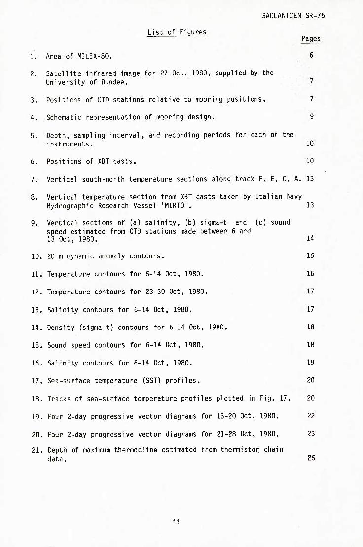
List of Figures Pages

1. Area of MILEX-80. . .. fi

2. Satellite infrared image for 27 Oct, 1980, supplied by the University of Dundee. .'. '7'

3. Positions of CTD stations relative to mooring positions. 7

4. Schematic representation of mooring design. 9

5. Depth, sampling interval, and recording periods for each of the instruments. 10

6. Positions of XBT casts. 10

7. Vertical south-north temperature sections along track F, E, C, A. 13

8. Vertical temperature section from XBT casts taken by Italian Navy Hydrographic Research Vessel 'MIRTO'. 13

9. Vertical sections of (a) salinity, (b) sigma-t and (c) sound speed estimated from CTD stations made between 6 and 13 Oct, 1980. 14

10. 20 m dynamic anomaly contours. 16

11. Temperature contours for 6-14 Oct, 1980. 16

12. Temperature contours for 23-30 Oct, 1980. , 17

13. Salinity contours for 6-14 Oct, 1980. 17

14. Density (sigma-t) contours for 6-14 Oct, 1980. 18

15. Sound speed contours for 6-14 Oct, 1980. 18

16. Salinity contours for 6-14 Oct, 1980. 19

17. Sea-surface temperature (SST) profiles. 20

18. Tracks of sea-surface temperature profiles plotted in Fig, 17. 20

19. Four 2-day progressive vector diagrams for 13-20 Oct, 1980. 22

20. Four 2-day progressive vector diagrams for 21-28 Oct, 1980. 23

21. Depth of maximum thermocline estimated from thermistor chain data. 26

n

SACLANTCEN SR-75

List of Figures (cont'd) Pages

22. Bathytherms measured by the thermistor chain at Position A. 31

23. Bathytherms measured by the thermistor chain at Position B. 34

24. Bathytherms measured by the thermistor chain at Position C. 41

25. Bathytherms measured by the thermistor chain at Position D. 49

26. Bathytherms measured by the thermistor chain at Position E. 56

27. Bathytherms measured by the thermistor chain at Position F, 63

28. Currents measured by NBA565 at Position B (63 m). 69

29. Currents measured by NBA565 at Position D (60 m). 69

30. Currents measured by NBA567 at Position F (88 m). 70

31. Currents measured by NBA568 at Position A (58 m). 70

32. Currents measured by NBA570 at Position E (54 m). 71

33. Currents measured by NBA569 at Position C (54 m). 71

34. Currents measured by VACM357 at Position C (32 m). 72



37. Currents measured by NB3 at Position C (4 m). 73

38. Winds measured by meteo-chain MC707 at Position A (height 3.5 m). 74

39. Wind speed, mixed-layer depth, current shear, buoyancy frequency, and Richardson number at Position C (4 to 14 m). 75




43. Components in the surface heat flux for Positions A and F. 84

44. Summer averaged wind stress over the Mediterranean <10>. 91

lit

SACLANTCEN SR-75

List of Figures (cont'd) Pages

45. Schematic representation of EKMAN pumping and subsurface response. 91

46. Mean annual wind-stress curl over Mediterranean <10>. 98

47. Comparison of 1-D mixed-layer model with data for vertical temperature profiles and for mixed-layer depth. 98

48. Thermistor frequency response functions estimated from three different impulses. 100

49. Thermistor chain temperature variance spectra for each thermistor and for chain average at Position A. 102

50. Thermistor chain temperature variance spectra for each thermistor and for chain average at Position B. 102

51. Thermistor chain temperature variance spectra for each thermistor and for chain average at Position C. 103

52. Thermistor chain temperature variance spectra for each thermistor and for chain average at Position D. 103

53. Thermistor chain temperature variance spectra for each thermistor and for chain average at Position E. 104

54. Thermistor chain temperature variance spectra for each thermistor and for chain average at Position F. 104

55. Rotary spectra and coefficients for NBA current meters at moorings B, D, F, and A. Ill

56. Rotary spectra and coefficients for NBA current meters at moorings C and E, the NIEL BROWN 3-axis current meter at mooring C and the upper most VACM current meter also at C. 112

57. Rotary spectra and coefficients for VACM current meters at mooring C, the average for VACM and NIEL BROWN current meters at C and the average for all NBA current meters excluding mooring F. 113

58. Coherence and phase spectra comparing wind speed at Position A with current speed at Positions B, D, F, A and C. 117

59. Coherence and phase spectra comparing wind speed at Position A with speed at Positions E and C (4 current meters at C). 118

IV

SACLANTCEN SR-75

VARIABILITY AND MIXING OF THE SURFACE LAYER IN THE TYRRHENIAN SEA:

MILEX-80, FINAL REPORT

by

Jon Moen

ABSTRACT

Data from the 1980 Tyrrhenian Sea mixed-layer experiment (MILEX-80) are reported. Results from the experiment are presented and discussed. The high south-north gradients in the mixed-layer depth are explained by an Ekman pumping mechanism (upwelling and downwelling) caused by a maximum in the west wind blowing through the Bonifacio Strait. It is also argued that this band of wind maximum (or jet) is chiefly responsible for the pair of counter-rotating eddies observed to be quasi-permanent features of this zone. Measured currents in the area were found to be up to twice as great as the currents estimated from the density field. This suggests a strong barotropic component to the currents in the north Tyrrhenian Sea. Some results from mixed-layer models are presented and compared with the data. These illustrate the need to generalize one-dimensional mixed-layer models to 3-dimensions to properly model the mixed layer in areas, such as the MILEX-80 zone, where there is a high spatial variability in the wind field. The wind-stress curl is estimated using two independent methods and compared with historical data for the same area. The first method involves estimating the upwelling and downwelling required to obtain a heat balance in the region. The second method results from a relation between inertial period temperature variance in the thermocline and inertial pulsations in the Ekman mass flux divergence caused by wind stress curl. The two methods show good agreement with each other and with the historical data. The same divergence pulsations are invoked, although less successfully, to explain the observed inertial peaks in the anticlockwise rotary spectra below the thermocline.

SACLANTCEN SR-75

INTRODUCTION

The surface mixed layer and the highly stratified layers beneath it together form a complex surface boundary layer to the deep ocean.

Incoming energy from the atmosphere is initially stored in this 'surface layer' in the forms of potential energy, kinetic energy, and heat energy. These vary in time due to the local rates of conversion from one form to another and due to their local fluxes across both the upper boundary with the atmosphere and the lower boundary with the deeper ocean. They vary in space due to spatial variations in the boundary fluxes and due to the dynamic response scales of both the surface layer itself and of the deeper ocean.

Locally, and on short time scales, it is important to understand these thermal and dynamical processes of the surface layer in order, for example, to improve the formulation of top boundary conditions for ocean circulation modelling (usually achieved by modified one-dimensional mixed-layer models), or to improve the interpretation of sea-surface images sensed remotely by satellite. On longer time scales these processes have an important effect on climate and long-range weather prediction. In addi- tion, the surface layer and its variability are important in sound propagation loss models, sonar performance models, ambient-noise models, and in calculating the performances of hull-mounted sonars and sonobuoys.

Several large international experiments to study the surface layer of the ocean have taken place during the past decade. Amongst these were the MILE 1977 experiment in the North Pacific (see <1> and <2> for example) and the JASIN 1978 experiment in the North Atlantic <3>. Research in the Mediterranean has concentrated on measurements taken from and around the French Bouee Laboratoire moored in the Gulf of Lions during the 1970's. From this the most useful data set, in terms of mixed-layer experiments, was that of the COFRASOV II expedition in 1976. This data set, used for model testing by Klein <4>, was quite short (only 10 days during July) and no account was taken of upwelling effects. The main purpose of Klein's model was to demonstrate the importance of meteorological variability in time, whereas in the present report we are more concerned with spatial variability.

The surface layer in the Mediterranean differs from that of the open ocean in two important ways: firstly, the meteorological forcing in the Mediterranean has a far greater variability in space than in the open ocean and, secondly, below the seasonal thermocline the vertical stratitifaction is very low in the Mediterranean compared with that in the open ocean. Evidence of this can be seen in the atlas by Robinson, Bauer & Schroeder <5> where, with the exceptions of the Alboran Sea, waters off the western part of the north African coast, and regions of the Agean Sea, the thermocline virtually disappears in the Mediterranean during winter.

The high meteorological variability, due to the great variety of wind systems found around the Mediterranean coastline, causes a similarly high

SACLANTCEN SR-75

spatial variability in the mixed-layer depth. Such variability arises as a balance between the local rate of deepening that, following Kraus & Turner <6>, is proportional to the cube of the wind speed, and an upwelling or Ekman pumping mechanism that is proportional to the product of the wind speed and its large scale (order of 100 km) variations. The balance, then, is between local and non-local (i.e. large-scale) forcing and the resulting variability, which is confined entirely to the surface layer, is by far the most striking to be found in the Mediterranean. The Mediterranean surface layer thus takes on a special importance that it might not have, say, in the open ocean where a thermocline and generally greater vertical structure can be found.

SACLANTCEN SR-75

1 DESCRIPTION OF EXPERIMENT

1.1 Area

A mixed-layer experiment (hereafter referred to as MILEX-80) was conducted in the north Tyrrhenian Sea in October 1980. Its main purpose was to investigate spatial and temporal variability of the surface layer during the period of transition from summer to winter conditions. The area of the experiment, shown in Fig. 1, was an approximately 200 km square zone laying to the east of Corsica, the Strait of Bonifacio, and Sardinia. Previous measurements in this area <7> had indicated high variability in the mixed-layer depth, with a relatively shallow, cold mixed layer to the north of the zone and a relatively deep, warm mixed layer to the south.

Satellite infrared images, such as the one shown in Fig. 2 indicate the presence during the summer and autumn of a large cold patch of water to the east of Corsica and the Strait of Bonifacio. In winter the cold patch remains but is less well defined due both to the merging of its northern and eastern boundaries with the extended zone of coastally up-welled water off the west of Italy and to surface cooling of all the Mediterranean waters. The persistence of the frontal zone separating the cold water from the warmer water to the south has been studied using satellite infrared images by Philippe & Harang <8>.

Dynamic topography estimates by Krivosheya & Ovchinnikov <9>, using data collected by French and Italian hydrographic research vessels during the 1950's, indicate the presence of a permanent cyclonic eddy to the west and north of the Bonifacio Strait, corresponding to the region of cold water, and a smaller, less intense anticyclonic eddy in the warmer water to the south. The authors attributed these eddies to forcing by the wind-stress curl (estimated from mean geostrophic wind) arising from a band of maximum of the northwest wind through the Bonifacio Strait during the summer months July to September. However, no explanation was given as to why these eddies should remain throughout the winter in the apparent absence of this wind maximum.

A recent analysis of wind-stress patterns over the Mediterranean has been made by May <10> in which surface stresses calculated from wind vector observations by shipping were averaged into 0.2° squares for each month of the year. These data, approximately one million observations covering the 20 years from 1950 to 1970, indicate a band of wind-stress maximum directed more eastward from the Strait of Bonifacio than that cited by Krivosheya & Ovchinnikov <9>. The data also show the persistence of the band throughout the year.

1.2 Method

The method of the experiment was to monitor the deepening of the mixed layer and erosion of the thermocline using an arrangement of taut moored thermistor chains and current meters. Six mooring sites A, B, C, D, E & F were established at the positions indicated in Fig. 3. These positions can

SACLANTCEN SR-75

North

FIG. 1 AREA OF MI LEX 80

SACLANTCEN SR-75

FIG. 2 SATELLITE INFRARED IMAGE FOR 27 OCT, 1980, SUPPLIED BY THE UNIVERSITY OF DUNDEE. Light shades represent colder temperature. Letters A-F indicate the mooring positions and the line the track used for vertical sections.

FIG. 3 POSITIONS OF CTD STATIONS RELATIVE TO ICORING POSITIONS.

7

SACLANTCEN SR-75

also be seen relative to the cold water patch in the satellite image of Fig. 2. Each mooring consisted of a Bendix surface float anchored by approximately 100 m of 3 rmi steel cable for attachment of instruments, a variable length (depending on water depth) of stretched 6 mm nylon Samson rope, and approximately 100 m of 3 mm steel cable attached in line with buoyancy spheres, an acoustic releaser, and an anchor (see Fig. 4). One Aanderaa thermistor chain of 11 thermistors was attached to the upper steel cable of each mooring and adjusted, on site, to span the mixed-layer/upper-thermocline region. The depth of each thermistor relative to the uppermost was 9.7, 12.7, 15.7, 18.7, 21.7, 24.7, 27.7, 32.7, 37.7 and 42.7 m. The sampling interval was set to 10 min. One NBA current meter was attached in-line under each thermistor chain and set to sample at 5-min intervals.

Two additional taut moorings, C2 and C3, each of two current meters, were deployed at position C (see Fig. 4). One of these, C3, consisted of a Neil-Brown 3-axis acoustic current meter (sampling interval 1 min at 4 m) and an EG&G VACM (vector-averaging) current meter, sampling interval 1.875 min at 14 m. The other was comprised of VACM current meters at 23 m and 32 m, both sampling at 1.875 min. The total of five current meters at position C were arranged to span the mixed layer and upper thermocline with the aim of measuring vertical shear during deepening periods.

Wind speed, wind direction, air temperature, sea-surface temperature, and barometric pressure were measured by an Anderaa meteo-chain mounted at a height of 3.5 m on the surface float of mooring A (Fig. 4). The recording periods for the instruments, together with their depths, sampling intervals, and mooring identification are given in Fig. 5.

1.3 Onboard Measurements

The moorings were deployed and recovered using the SACLANTCEN research vessel MARIA PAOLINA G. (MPG). During the deployment phase 19 CTD stations were taken to a depth of 500 m and 162 XBT casts made to 300 m. During the recovery phase 17 CTD stations and 88 XBT casts were made. An additional 52 XBT casts were made by the Italian Navy hydrographic research vessel MIRTO during an intermediary phase that included surveillance of the moorings. All CTD positions are shown in Fig. 3. The positions of the XBT measurements, which were taken along the ship's track between mooring positions and CTD stations, are shown in Fig. 6.

Wind speed and direction at 10 m were recorded from the ship's meteo-chain and sea-surface (4 m depth) temperature (SST) was recorded by a thermistor projecting down through a tubular opening near the ship's well.

The measurement periods for the CTD, XBT, and SST measurements are shown in Fig. 5. Also included in that figure, as an indication of the weather conditions during the experiment, are the wind speed and direction measured by ship's anemometer until 13 October and thereafter by the meteo-chain at mooring A. It can be seen that at least three storms occurred during the experiment, in which the wind speed was greater than 10 m/s. These were roughly during the periods 9-11, 16-19, and 25-27 October.

8

SACLANTCEN SR-75

Also available from the MIRTO ship's log, at approximately 1 h intervals, are wind speed & direction, barometric pressure, and wet & dry air temperature.

1.4 Data Recording and Preparation

Data from the moored instruments were recorded on magnetic-tape cassettes, transcribed onto 8-track HP tapes, transferred to UNIVAC disc storage, and then prepared for analysis by the replacement of 'bad' data values and truncation.

Onboard acquisition of XBT & CTD data was by use of SACLANTCEN's lOS system (integrated oceanographic system) on a Hewlett Packard 21MX computer. Data were stored on HP 8-track tapes and later transferred to UNIVAC 1106 disc storage where they were cleaned by the removal of spikes and bad profiles.

Apparent wind speeds & directions and sea-surface (4 m) temperatures were recorded on strip charts and later digitized and corrected before storage on disc.

The XBT data collected by the Italian Navy were also digitized and transferred to UNIVAC disc storage.

AANDERAA METEO CHAIN

BOTTOM

AANDERAA THERMISTOR CHAIN

<=y—NBA CURRENT METER

STEEL CABLE

EG&G VACM CURRENT METER EG&G VACM

'CURRENT METER

SCRAP SHIP CHAIN

NYLON CABLE -

STEEL CABLE

3 GLASS SPHERES AMF RELEASER TRANSPONDER

STEEL CABLE

3 GLASS SPHERES AMF RELEASER TRANSPONDER

FIG. 4 SCHEMATIC REPRESENTATION OF MOORING DESIGN.

SACLANTCEN SR-75

UOORINQ

SITE

* INSTRUMENTS DEPTH

(m)

SAMPLING

INTERVAL

(min)

OCTOBER 1980 tj /' B 9 10 11 12 13 14 15 16 17 18 19 20 21 22 23 24 25 26 ?7 ?a ?9 3n

A NBAsea MC707

58.0

-3.5

10.0

5.0 10.0 ^ 1^ = zz - i- = I

B TC357 NBA56S

12.9-55.6

63.0

10.0

6.0 a. z ■" — — — -

C3

TC148 NBASeS

4.3-47.0

54.0

10.0

5.0

■ ^ z ^ ^ "" ^ — — - VACM356

VACM367

23.0

32.0

1.876

1.875

1

4 n Z! "■ z ̂ ,„^ ̂ ^ — - NB3

VACM355

4.0

14.0

1.0

1.875 ■ ^ ■" .. — ^^ ^ ^^ _

D TC459 NBAsee

9.0-51.7

60.0

10.0

5.0

■n ^ "■ ̂ "" ,^ z -

E TCI 64 NBA570

18.3-61.0

68.0

10.0

5.0 _ ^ "■ ̂ z "■ — —

F TC342 NBA567

37.0-79.7

ee.o 10.0

5.0 ■■ "■ ^ ^^^ —

k -

SST (Palol

1 1 1 1 r—-

1 ■1 1 1

XBT 3 1

6 1 52 66 > I'l 13) 1< . ,^ ̂ ; MIBTI MflTC 20: 218

1 "U 2J4 l: Xi

CTD 1 ■ 1 4

11

I 10 12 1"

1 15

16

I 19 \

" 273^ 33

• 20-E TC = AANDEBAA THERMISTOR CHAIN ^,- -

NBA = CURRENT METER E ^ ;

yy^QI^-EGIQ vector averagino Z current meter Q 10—z

NB3 = NIet Brown 3-axi8 current meter — -

MC = AANDEHAA METEO-CHAIN 5 5 —J

0-^

:ShTps f'\ /\ . , - Anemometer \ 1 \ /I J

r r 1 1 1 r A.'

3.5m Surface Buoy ,

'■ ...1 . 1 . .. ., 1

FIG. 5 DEPTH, SAMPLING INTERVAL, AND RECORDING PERIODS FOR EACH OF THE INSTRUMENTS. Wind speed indicates weather conditions during the various phases of MiLEX 80.

XBT TRACKS MILEX 80

A r ̂̂ *--*^. I V, i

^♦-^ ., *

\„ N *~~~-*-^ \1 ^/ * c\ X

J-381

>t .-.__l

FT\ 7 ^ +

\ ^--^ \ \io

\ \ ^ +

PHASE 11 ---of 12

163

;::k -^ 172 ••—1=«177

.o\ ISB

/- ; /

h

^•'^S, [m

EO

I \ h \ '

PI ■ 130

HASE III

I I 231 O F

FIG. 6 POSITIONS OF XBT CASTS (a) Phase I, (b) Phase II and (c) Phase III.

10

SACLANTCEN SR-75

2 ANALYSIS AND INTERPRETATION: SPATIAL DESCRIPTION ^ .

2.1 Vertical Sections

The Selected vertical sections of temperature, salinity, density, and sound speed shown contoured in Figs. 7, 8 and 9 illustrate the spatial charac- teristics of these variables in the upper layer in the MILEX-80 zone.

Figure 7a is a south-north vertical section of temperature calculated from XBT data taken between 12 and 13 Oct. It shows a strong south-north gradient in the mixed layer—being relatively shallow and cold (approx. 15 m & 19.5°C) to the north and relatively deep and warm (approx. 50 m & 21.5°C) to the south. The same general structure remains (Fig. 7b) after the passage of two fairly intense storms of several days duration and wind speeds in excess of 10 m/s. The new structure shows that, in the cold water region to the north, the mixed layer has deepened by about 13 m and cooled by about 2.5°C, whereas in the warm water to the south the deepening was about 10 m and the cooling only TC.

It is a good measure of the spatial variability that the south-north difference in mixed-layer depth is two or three times greater than the change in layer depth at either location caused by two weeks of intensive wind mixing.

Based on the respective depths of the two mixed layers, the difference in deepening rate between north and south is much less than might be expected. Shallow mixed layers deepen more rapidly than deep ones, because for shallow mixed layers a greater fraction of the turbulent 'mixing' energy, created near the surface, arrives at the mixed-layer/ thermocline-interface zone. Furthermore, the wind-driven inertially oscillating bulk (or slab) flow of a shallow mixed layer is far greater than that of a deep one, and this means that a relatively larger production of turbulent mixing energy can be expected in the mixed-layer/thermocline-shear zone for shallow mixed layers <11>.

Better estimates for deepening and cooling, in which high-frequency variations in time have not been smoothed, can be determined from the thermistor chain data presented in the next chapter. These indicate a general deepening and cooling of the mixed layer in the north of about 11.5 m and 2.1°C respectively and in the south of about 6 m and TC respectively. Although this represents a greater relative increase in depth for the more shallow mixed layer to the north than for the deeper one to the south, the north-south ratio for deepening rates is still far too low.

Let this ratio be denoted by R. Then, using the above values of 11.5 m and 6 m, we obtain the value R=2 for the 2-week period. If now we consider the deepening rate due to the downward penetration of turbulence created near the surface <6>:

dh U3 dt "^ f^If » (Eq. 1)

11

SACLANTCEN SR-75

where U is the wind speed, h the depth of the mixed layer, and r the thermocline gradient below the jump zone. We can write:

Ahi h2 U3 T2 R . ._1_J , (Eq. 2)

Aho h2 U3 Fi * 12

where the subscript 1 refers to the north, 2 to the south and we have assumed the wind speed at the two locations to be the same. Taking hi = 25 m and h2 = 50 m, Eq. 2 gives a value of R = 4. Note that we have not considered the mechanism due to Pollard, Rhines & Thompson <11> mentioned earlier, which may in fact be more important than the Kraus & Turner mechanism <6> for the shallow mixed layer to the north. In this case the value of R = 4 would be an underestimate of the deepening rates ratio. It is, however, sufficiently high, compared with the measured value of R = 2, to indicate that some process other than mixing is important in the MILEX-80 zone. This process, which will be developed more fully in a later chapter on Ekman pumping, is clearly one of upwelling to the north and/or downwelling to the south. In view of the presence of a large cold patch observed in the area throughout the year, the emphasis should be on upwelling.

Two further examples of the south-north and southeast-northwest structure can be seen in the vertical sections of Fig. 8. These are taken from XBT casts taken during phase II of MILEX-80 when the MIRTO steamed south and southeast from A to F and then returned along approximately the same course towards A. The two sections are thus separated in time by a maximum to the north of one day and it can be seen that during this period the cold water has advected southward, apparently sharpening the frontal boundary separating north from south. The southern portion of the section in Fig. 8b, however, contains some east-west structure, with warmer water lying to the west of F. It would appear that during this period, 14-15 Oct, cold water was advecting in from the north or northwest and this can explain why the mixed layer at F has decreased from the 50 to 60 m level seen on both 12 and 24 Oct, shown in Fig. 7, to a depth of only 35 m. This advection event can also be seen on the thermistor chain data displayed in the next chapter, where it will be discussed in more detail.

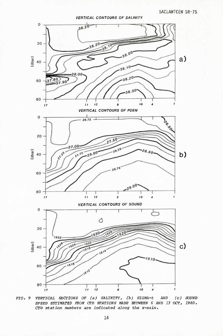
Vertical south-north sections of salinity, density, and sound speed for phase I are shown in Fig. 9a,b,c. These are less accurate than the temperature sections, both because fewer CTD stations were available than XBT casts and because the data were spread over one week in which an appre- ciable wind mixing and cooling took place. Nevertheless, they give a good indication of the spatial gradients involved. The change in sound speed is striking — changing from 1530 m/s at the 50 m level in the south to 1512 m/s in the north. Such an 18 m/s change over 90 km could have a significant effect on acoustic propagation losses and ambient-noise models.

2.2 Horizontal Sections

Dynamic anomalies relative to the 450 m depth level were calculated for each CTD station by the usual method of transformation from z to pressure

12

SACLANTCEN SR-75

TEMPERATURE CONTOURS [°C] XBT SECTION F-E-C-A

NORTH

ii 111 I I (I I I I I I ;\'

I b)

0 10 20 30 40 SO km

FIG. 7 VERTICAL 33UTH-N0RTH TEMPERATURE SECTIONS ALONG TRACK F, E, C, A. (a) 12-13 Get, 1980, (b) 23-29 Oct, 1980. XBT cast numbers are indicated along the x-axis.

TEMPERATURE CONTOURS (°C]

XBT SECTION (MlRTO) SOUTH NORTH

a)

0 10 20 30 40 50 km 14'1S October 1980

FIG. 8 VERTICAL TEMPERATURE SECTION FROM XBT CASTS TAKEN BY ITALIAN NAVY HYDROGRAPHIC RESEARCH VESSEL 'MIRTO'. (a) 14-15 Oct, 1980, (b) 15 Oct, 1980. XBT cast numbers are indicated along the x-axis.

13

SACLANTCEN SR-75 VERTICAL CONTOURS OF SALINITY

a)

17 11 12 8 10 4

VERTICAL CONTOURS OF PDEN

b)

17 11 12 B 10 4

VERTICAL CONTOURS OF SOUND

c)

FIG. 9 VERTICAL SECTIONS OF (a) SALINITY, (b) SIGMA-t AND (c) SOUND SPEED ESTIMATED FROM CTD STATIONS MADE EETffEEN 6 AND 13 OCT, 1980. CTD station TTumbers are indicated along the x-axis.

14

SACLANTCEN SR-75

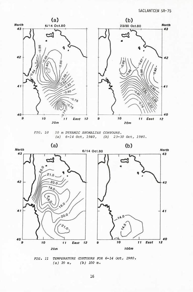
co-ordinates and integration of specific volume anomaly, 6 = a(T,S,p)- a(0,35,p), between the reference pressure of 450 dbar and the desired pressure surface. Contours of dynamic anomaly, in dynamic metres, for the 20 dbar surface are shown in Fig. 10 in which Fig. 10a represents phase I, the mooring deployment phase of the experiment, and Fig. 10b represents phase III, the mooring recovery phase. These show a cyclonic gyre underlying the cold water patch and evidence of an anticyclonic motion to the south. The results are thus consistent with those of Krivosheya and Ovchinnikov <9>.

Geostrophic currents calculated from the dynamic anomaly estimates were found to agree well in direction with measured currents (to be illustrated later) but to be about half the speed. This is an interesting result, since although some discrepancy between the actual current and that calculated from the density field is expected in the Mediterranean, no measurements have been reported in the literature. Also, that this discrepancy should be so high is surprising. Further discussion of this result will appear in Ch. 4,

Comparing Figs. lOa and b we see that the gyre appears to have either moved or to have partially broken up during the two weeks of stormy weather between measurements. An insufficient spatial coverage of CTD stations pre- vents this ambiguity from being resolved.

Figures 11 to 16 present horizontal contours of the temperature, salinity, density, and sound speed at different depths. The salinity, density and sound speed contours of Figs. 13, 14 and 15, respectively, were estimated from the CTD data and are for the depths 20 m (or 30 m) & 100 m. The temperature contours of Figs. 11 and 12 are from greater coverage provided by the XBT data from phases I and III respectively; they show that the anomalies in temperature, which form the major contribution to the density field, have virtually disappeared below 100 m. The density contribution to the geostrophic flow is thus confined to a relatively thin surface layer and it is this layer that, for most of the Mediterranean, contains the bulk of the variability in the state variables and in sound speed. Figure 16 shows that the anomalies in salinity go somewhat deeper than those of temperature but that they also effectively disappear by 300 m.

2.3 SST profiles

Figure 17 plots the sea-surface (4 m) temperatures recorded along the horizontal tracks indicated in Fig. 18.

These records further illustrate the general impressions of a south-north temperature change of about 3°C, as shown in profiles 3, 5 & 15, and of a cooling of this surface water throughout the experiment by about 3°C as seen by comparing profiles 1 to 6 with 7 to 15. They also illustrate a strong frontal zone separating the warm and cold water, as seen in profiles 5, 7, 13 and, especially, 15, which shows a change in temperature of 2°C in about 2 km. Such fronts are also evident after quantitative analysis of satellite infrared images of the area <12> but these will not be presented here.

15

SACLANTCEN SR-75

North (a)

6/14 Oct.80

11 East 12 11 East 12 20m 20m

FIG. 10 20 m DYNAMIC ANOMALIES CONTOURS. (a) 6-14 Oct, 1980, (b) 23-30 Get, 1980.

6/14 Oct.80

11 East 12 9 11 East 12

20m 100m

FIG. 11 TEMPERATURE CONTOURS FDR 6-14 Oct, 1980.

(a) 20 m, (b) 100 m.

16

SACLANTCEN SR-75

23/30 Oct.80

11 East 12

100m

FIG. 12 TEMPERATURE CONTOURS FOR 23-30 Oct, 1980. (a) 20 m, (b) 100 m.

(a) North 6/14 Oct.80

FIG. 13 SALINITY CONTOURS FOR 6-14 Oc±, 1980. (a) 20 m, (b) 100 m.

17

SACLANTCEN SR-75


FIG. 14 DENSITY (sigma-t) CONTOURS FOR 6-14 Oct, 1980. (a) 30 m, (h) 100 m.


FIG. 15 SOUND SPEED CONTOURS FOR 6-14 Oct, 1980.

(a) 20 m, (b) 100 m.

18

SACLANTCEN SR-75

FIG. 16 SALINITY CONTOURS FDR 6-14 Oct, 1980. (a) 200 m, (b) 300 m.

19

SACLANTCEN SR-75

• Day (Oclobar ia<0)-Tlm« (QMT)

5 100 125 ISO

22.

» o

20' o o •* 10 O

le- V vj-

22-

^ 20- o '—«^\

K) 6 a ■0

n d o

IB- < , , , , r

11

14

■

.. 15 n

o ^ »

- o L a

' a

FIG. 17 SEA-SURFACE TEMPERATURE (SST) PROFILES. Numbers represent tracks indicated in Fig. 18.

10- 11'

FIG. 18 TRACKS OF SEA-SURFACE TEMPERATURE PROFILES PLOTTED IN FIG. 17.

20

SACLANTCEN SR-75

A theory for the formation of fronts in areas of non-zero wind-stress curl and weak coupling of the mixed layer with the atmosphere can be found in Welander <13>. The theory was applied to large (~ 1000 km) scales but if one can assume a sufficiently weak coupling of the mixed layer with atmosphere at smaller scale (e.g. cooling greater in warm water region) the mechanism might also be applied in the MILEX-80 zone.

2.4 Current Measurements

Currents were measured approximately below the thermocline (~ 70 m level) at each of the mooring positions. Other current measurements were also made at mooring position C, but since currents will also be discussed as temporal phenomena in Ch. 3 these will not be illustrated here. The measurements to be presented here give a spatial impression and have been included for that reason.

Figures 19 and 20 are progressive vector diagrams for each of the mooring positions, with each of the eight maps representing a 2-day period and each progressive vector sub-divided into 12 h intervals. Figure 19 covers the period 13-20 Get and Fig. 20 covers 21-28 Oct. This representation thus gives both spatial and temporal information for the MILEX-80 zone. The directions of the currents are consistent with the eddy structure indicated earlier by the surface contours of dynamic anomaly -a cyclonic eddy to the north and an anticyclonic one to the south. The magnitude for several of the 2-day periods approaches 50 cm/s, which is considerably higher than the estimated geostrophic currents. This observation was tested more carefully by comparing the geostrophic current relative to 450 m, computed from the CTD profiles surrounding each mooring position, with values of the measured current, when available. Since baroclinic adjustment can take in the order of a day or more, the measured currents were low-pass filtered to 60 h before comparison was made in order to make them more representative of the density currents. Table 1 shows the comparison, together with additional information such as lag time between CTD and current measurement (often CTD stations were taken at the mooring position before deployment or after recovery of the current meter), type of current meter, and depth of current meter. There appears to be reasonably good agreement in direction, generally within about 20° except for position D which showed a 47° difference, but the speeds of the measured currents are about twice as high as those of the estimated currents.

2.5 Errors in current estimates and measurements

Errors in the estimated geostrophic current may occur from the choice of a rather shallow reference level of 450 m. Geostrophic estimates by Krivosheya & Ovchinnikov <9> for the same area as MILEX-80, but using a reference level of 1000 m, indicate that the flow at 450 m can be as high as 25 % of that at the surface.

Another source of error in the comparison is in the use of surface-moored NBA current meters. This error arises because of the vertical oscillations of the mooring line to which the current meter is attached; these can be quite large when seas are high. Since the drag on the current meter is not

21

SACLANTCEN SR-75

FIG. 19 FOUR 2-DAY PROGRESSIVE VECTOR DIAGRAMS FOR 13-20 Oct, 1980. Divisions on vectors are at 12 h intervals.

22

SACLANTCEN SR-75

43

".^--•A V. B

or

/ /

41

11° 40"

12°

FIG. 20 FOUR 2-DAY PROGRESSIVE VECTOR DIAGRAMS FDR 21-28 Oct, 1980. Divisions on vectors are at 12 h intervals.

23

SACLANTCEN SR-75

symmetric (higher drag on the tail fins than on the nose) and since the current meter is free to rotate ± 10° in the vertical plane, these vertical oscillations tend always to increase the rotor rotations and create an overestimation of the mean current.

The magnitude of this 'pumping' error is difficult to estimate since we know neither the coupling of current meter tilt with vertical oscillations nor the cosine response of the NBA rotor. Furthermore, the amplitude and frequency of the vertical oscillations are not known, since the surface waves which they are forced to follow (surface float and current meter con- nected by steel cable) were not measured. We can only note from Table 1 that the VACM current meters, which are less prove to pumping, indicate currents of the same order or higher than the NBA current meters. The current measured by the VACM at 32 m on 8 Oct, for example, was twice that of the NBA at 54 m. Both current meters were below the Ekman layer during this period and so should not be measuring the wind-driven current. In any case, the winds during this period, as during other periods when CTD measurements were taken, were very light and the pumping of the NBA current meters would therefore have been low. The NBA569 and VACM357 current meters can be compared by using the stick diagrams presented in Sect. 3.2. Since the NBA should be measuring consistently lower than the VACM (which is near the surface) but is in fact measuring slightly higher we can deduce that it is indeed overestimating the current.

Other comparisons between measured currents and geostrophic estimates will be made for the MILEX-80 zone and the Balearic sea, but these will be presented elsewhere.

TABLE 1

COMPARISON OF ESTIMATED GEOSTROPHIC CURRENTS WITH MEASURED CURRENTS

Lag time indicates the time difference between measured (filtered) current and estimated geostrophic current

MEASURED CURRENT GEOSTROPHIC ESTIMATE

TIME LAG MOORING CURRENT DEPTH MAGNITUDE DIRECTION MAGNITUDE DIRECTION

METER (m) (cni/s) (degrees) (cm/s) (degrees) (hrs)

C VACM 14 33.8 163.2 16.5 163.4 -12

VACM 23 24.8 152.6 13.5 167.2 -17

VACM 32 30.5 178.3 11.2 169.8 -17

NBA 54 14.9 177.7 7.5 173.1 0

B NBA 63 13.1 324.0 6.3 339.6 0

D NBA 60 11.2 83.8 3.1 61.2 0

E NBA 68 6.4 65.0 10.2 18.3 + 7

C VACM 14 24.7 142.6 14.2 132.5 + 72

VACM 23 14.7 157.2 12.8 124.0 + 36

VACM 32 17.1 149.4 10.5 130.4 + 36

NBA 54 16.0 152.0 5.7 125.1 + 36

24

SACLANTCEN SR-75

3 ANALYSIS AND INTERPRETATION: TEMPORAL DESCRIPTION

3.1 Thermistor chain data

In response to a number of passing storms that occurred during the three weeks of MILEX-80, the mixed layer deepened by about 15 m and cooled by about 3°C. An indication of the variability during this period is shown by Fig. 21, which plots the depth of the maximum thermocline gradient as estimated from the thermistor chain data. Effectively this is a measure of the mixed-layer depth, since it refers to the thin temperature jump zone at the base of the mixed layer. The depths were estimated from smoothed contours of the thermistor-chain data such that any variability above about the inertial frequency does not appear. Variability at and above the inertial frequency will be discussed later.

There are several striking features about Fig. 21. Firstly, as mentioned in the previous section, despite the passage of four storms all with wind speeds exceeding 10 m/s, the maximum change in layer depth at any mooring was still only about half that of the south-north (F-A) change. This is a measure of the high spatial variability. Secondly, the rate of deepening varies considerably with mooring position. There was virtually no deepening at position D, for example, while during the same period at E the layer deepened by about 20 m. Such a result is a certain indication of upwelling at or upstream from position D. Thirdly, some considerable large-scale variations in the layer depth can be seen, particularly at mooring position F. Here between 14 and 17 Oct the depth varied from 63 m to 39 m and back to 71 m, with a similar variation occuring later between 28 and 29 Oct. Closer examination of these events (to appear later) reveals that the mixed layer itself varied by somewhat less than these extreme values and that the variations were probably due to advection effects — either southward advection of the colder, more shallow mixed layer to the north, or, southeastward advection of mixed water formed in a region of convergence between cold northern and warmer southern waters.

Figures 22 to 27* present a detailed day-by-day description of the temperature structure within the mixed-layer/thermocline zone at each of the six mooring positions. The contours were estimated using a cubic spline interpolation (with tension factor 5) between thermistors for each time step and then using a linear interpolation in time between successive profiles. Upper thermistor and lower thermistor temperature values are written at their corresponding depth/time positions at 4 h intervals and, since the interval between isotherms is fixed at 0.5°C, the absolute value of an isotherm is readily deduced.

The Nyquist frequency for these data is 3 cycle/h, but since the declared time response for the thermistor is 1 min some aliasing has clearly occurred. However, it will be demonstrated in Sect. 5.1, on temperature spectra, that the extent of this aliasing is quite limited and can not significantly affect the interpretation of these contours.

Various periods of quite strong inertial internal waves (of 18 h period at this latitude) can be seen in most of the records. These vertical oscilla-

T/ie (^^guAei fiz{^znAzd to -in tkU, chaptoA aA.2, on pp. 31-81

25

SACLANTCEN SR-75

THERMOCLINE DEPTH TC DATA

10

0)

0)

a. Q

CO

■30

■50 —

70

TC 459 \

\\

:\\ /' ^ TC 357

I I I I I I I I I I I I I I I I I I I I I I SHIP WIND

g 20

g 0

I WIND MC707 h a

j^^% I I I I I

10 I I I I I r I i I I I I

20 25 31

OCTOBER 1980

6 15

FIG. 21 DEPTH OF MAXIMUM THERMOCLINE ESTIMATED FROM THERMISTOR CHAIN DATA. 6-31 Oct, 1980.

26

SACLANTCEN SR-75

tions of the thermocline are quite common in the Mediterranean and usually follow sudden increases in wind speed (see <14> <15> <16>, for example). Some examples are evident in Fig. 24 for mooring C on 11, 15 and 19 Oct. In some cases inertial oscillations appear to follow sharp decreases in wind speed — for example on 22, 25 and 28 Oct at mooring B, as shown in Fig. 23. In other cases, however, inertial oscillations seem to appear unforced by sudden changes in wind speed. Two such examples are at mooring E (Fig. 26) on 13 Oct and at mooring F on 23 Oct (Fig. 27). It is possible that the local winds at E & F on these particular days did indeed change rapidly. If this did happen, however, one would expect some evidence of the variation to show up at position A, only 150 km to the north.

We will see in Sect. 5.1 that the inertial oscillations are well demonstrated in the temperature variance spectra. We will also see evidence there of high variance at the unexpected frequency of about 8 h. Since this does not correspond to either the inertial or tidal frequencies, it is probably due to some non-linear interaction between the two. A good example of this variance can be seen at mooring D (Fig. 25) on 14 Oct which shows a fairly energetic oscillation with a period between about 7.5 and 8 h.

Re-examining the large vertical excursion of the thermocline at position F shown in Fig. 21, we notice that during 14-17 Oct (Fig. 27) that the mixed layer shallowed, due not so much to an upward movement of the whole thermocline but more to a rarefaction of the isotherms. This event seems most likely to be the result of southeastward advection of waters mixed horizon- tally somewhere upstream from F by convergence of the cold northern and warm southern waters. A likely location for this is near mooring position E. Assuming a cyclonic eddy to the north and anticyclonic eddy to the south, as described in Sect. 2.2, then a convergence zone would be expected near position E. Indeed, we see evidence of such a convergence during 14-16 Oct (Fig. 25) where warmer water appears to be advecting in over the colder water. The vertical temperature sections taken on 14 and 15 Oct (Fig. 8) also indicate a convergence near position E.

3.2 Current-meter data

Some of the current-meter data were presented in Sect. 2.4 in the form of progressive vector diagrams (Figs. 19, 20). These data are now represented, together with other current-meter data, in the form of stick diagrams in Fig. 28 to 37. The vector components were first low-pass filtered to about 6 h and then plotted as one stick ewery hour. This method was chosen as it gives a better impression of magnitude, direction, and sense of rotation than other representations.

Inertial oscillations can be seen for all the current meters, with the strongest occurring nearest the surface. Compare Figs. 28 to 33, which show currents measured generally below the thermocline at each of the mooring positions, with Figs. 34 to 37, which show currents measured generally within the mixed layer at position C. The current measured by the NBA current meter at 54 m at position C (Fig. 33) appears to be higher than that measured at 32 m by the VACM current meter (Fig. 34). This is probably due to the pumping of the NBA current meter discussed in Sect. 2.5.

27

SACLANTCEN SR-75

A Niel-Brown 3-axis acoustic current meter was moored at 4 m depth at position C in an attempt not only to measure the mean current at this depth (Fig. 44) but also to test for the presence of Langmuir circulations.

3.3 Test for Langmuir Circulations

Langmuir circulations refer to the vortex structure, sometimes occurring in the mixed layer, of counter-rotating cell pairs with axes that are horizontal and aligned approximately in the wind direction. They often, but not necessarily always, give rise to the parallel bands of visible substances collecting in the convergence lines that are frequently referred to as windrows. The most commonly accepted theory for the generation of Langmuir circulations is an interaction between surface waves and the wind drift current, (see <17> <18> <19> <20>, for example). Their importance is in the high efficiency with which they transport heat, momentum, and turbulent kinetic energy downwards through the mixed layer <18>, but little is known as to how often they occur. If they are as common as the above-mentioned theories seem to imply they would consitute a serious omission in the present state of mixed-layer modelling. On the other hand, should they occur only in certain locations and on the rare occasions when windrows have actually been observed, they may be treated as anomalies or even ignored in their over-all effect on surface-layer dynamics.

Had Langmuir circulations been present in the MILEX-80 zone, their vertical velocities (up to 3 or 4 cm/s for well-developed cells) ought to have shown up in the 4m vertical velocity measurement of the Neil-Brown current meter. The three components were high-pass filtered to 3 h and rotary and kinetic energy spectra examined for peaks in the 2 min to 3 h range. An advecting Langmuir circulation structure would, at some frequency related to the advection speed and cell dimensions, cause a signal in the rotary spectra for the velocity component pairs (u,v) or (v,w). No clear signals were observed in the spectra and so it is concluded that Langmuir circulations did not occur, at least at mooring position C, during the 11 day recording period of the Niel-Brown current meter.

3.4 Wind data

Although wind speed plots have been included in many of the figures as an indication of weather conditions, the vector wind is best represented by the stick diagrams shown in Fig. 38. This shows that the wind was blowing quite consistently from the east throughout the experiment. During 7-13 Oct the wind was measured on-board ship at 20 m height and for the remainder of the experiment, 13-30 Oct, the wind was measured at a height of 3.5 m by instruments mounted on the surface buoy at A. The higher value of the ship-measured wind is due partly to the greater height of the ship's anemometer. The main reason, however, is that mooring A was more sheltered than the zone downwind of the Bonifacio Strait where the ship was working during 7-13 Oct. Indeed, these data can be taken as further evidence that the wind is much stronger off the Bonifacio Strait than it is to the north and it is this variation in wind stress that will be invoked later to explain the existence of the cold upwelled water in the north of the zone.

28

SACLANTCEN SR-75

3.5 Dynamic stability

Turbulent entrainment of the colder water in the thermocline into the mixed layer, and hence mixed-layer deepening, takes place if the local Richardson number

£[ Ri = - 9 «,— „ (Eq. 3)

drops below 0.25. Here a is the coefficient of thermal expansion, u_ the horizontal velocity vector, T the temperature, g the acceleration due to gravity, and z the vertical axis. This mechanism is important, for example, in the Pollard, Rhines and Thompson model <11>, where it is assumed that the mixed layer moves as a slab over the thermocline, which it then entrains when the shear at the base of the mixed layer becomes sufficiently large.

Eddy viscosity models of mixed-layer deepening parameterize the turbulent diffusion by use of an empirical function K that depends on R-j and, if higher order turbulence closures are used (<21>, for example), on q , the turbulent kinetic energy. One very simple empirical form for K due to Munk & Anderson <22> will be used in Sect. 4.5. The purpose of this section is to present estimates of the Richardson number at different depths throughout the MILEX-80 experiment so that periods of mixing can be identified. These estimates were made using data from the five current meters and thermistor chain at position C and then using Eq. 3 in the form

Ri =\ . (Eq. 4) S2

where N is the Brunt-Vaisala frequency and S the shear. The values of S^ and N^ were calculated by the expressions

(ui - U2)2 + (vi - V2)2 S2 = , (Eq. 5)

(zi - Z2)2

with the suffixes i and 2 referring to the upper and lower current meters respectively, and

Ifi - ' °''" - '""^' , (Eq. 6) ^n - Zn+i

29

SACLANTCEN SR-75

with n and n+1 referring to the two thermistors nearest the mid point (zi+Z2)/2 between current meters. Since thermistors were closer together than current meters (see Sect. 1.2) the value of S, as a vertical mean value over a relatively large interval, compared with N, as a vertical mean value over a relatively small interval, tends to cause Eq. 3 to be an overestimate of Rq. In the estimates of R^ to be presented in this section, therefore, turbulent mixing might well be occurring for values of Rj greater than 0.25. For example, entrainment is defined to occur in the Pollard, Rhines & Thompson model <11> when the bulk Richarson number falls below unity. Since the estimates to be presented here lie somewhere between the bulk and local Richardson number, the choice of critical Richardson number ought to lie somewhere between 1.0 and 0.25.

Figures 39 to 42 illustrate the estimates of Richardson number for each of four depths, together with the wind speed, mixed-layer depth, estimates of current shear, and estimates of the Brunt-Va'isala frequency throughout the MILEX-80 period. Initially the mixed layer was at about the 14 m level (Fig. 39) so that the 4 m and 14 m current meters were both within the mixed layer. This implies, as can be seen in the plot of N, that the stratification was low but that the shear near the layer base was high and, as expected, the Richardson number was well below the critical value. Occasionally, however, the mixed layer shallowed, the thermistor at 14 m fell within the thermocline, and the values of N and R^ both increased, causing greater stability at this level. After 14 Oct the mixed layer deepened, the shear maintained its relatively high value of 0.01 to 0.02 rad/s and, apart from a short period on 15 Oct, the 4 to 14 m layer became one of turbulent production.

Figure 40 shows N, S and Ri estimates for the 14 to 23 m level. During 9 Oct the mixed layer still had not deepened beyond 18 m and the estimates of N and S were both high, indicating the high temperature and velocity gradients across the mixed-layer/thermocline interface zone. It is interesting to note that whenever the mixed layer dropped below the lower- most current meter the value of S decreased to its much lower, mixed- layer value of between 0.005 & 0.01 rad/s. An example of this is when the mixed layer deepened to below the 23 m current meter on 18 Oct.

30

TC570 0.5-DEG ISOTHERMS

SACLANTCEN SR-75

13/10/80 HOURS (GMT )

3 12 15

14/10/80

-60.0

15/10/80 0 3 6 3 12 15 18 21 24

^ Q 1 1 t 1 I I I I I t 1 I I t I I I I 1 I t t I I t I 1 t I t I 1 I t I I t I I I I I 1 I I I I I ■ I t I I I 1 I I I I I I t I I I t

in ^ -20.0- >- UJ

Q. -40.0-

-GO.O

20.13 20.10 20.20 20.08

K 13.37

-V"""^ VX J^v^ 13.35 13.90 13.37 13.32 14.20

FIG. 22 BATHYTHERMS MEASURED BY THE THERMISTOR CHAIN AT POSITION A. Printed numbers indicate temperature and position for the upper and lower thermistors at 4 h intervals. a) 13-15 Oct 1980.

31


SACLANTCEN SR-75

lG/10/80 0 3 B

HOURS ;GMT )

9 12 15

17/10/80

-GO.O

8/10/80 0

LU -20.0-

Ul z:

D- UJ

-40.0-

-BO.O

' I ■ ' ' ' ' I ' 9 12 15

I I I 1 1 I ■ ■ ■ ' I ' ■ 1 I I I 21 24

13.49 X

19.49 19.34 19.26 19.34 X

19.39 X

FIG. 22 BATHYTHERMS MEASURED BY THE THERMISTOR CHAIN AT POSITION A. Printed numbers indicate temperature and position for the upper and lower thermistors at 4 h intervals, b) 16-18 Oct 1980.

32

SACLANTCEN SR-75

TC570 Q.B-DEG ISOTHERMS

19/10/80 0 3 G

HOURS t GMT)

9 12 15

-GO.O

I I 1 I I I I 1 1 ' I ■ I ' ' ' I ' ' I ' ■ ■ ■ ■ ■ ' ■ 1 ' 18 21 24

11111 11111 I

ia.7S 18.43 18.40 K

IB. II 17.54 17.10

14.17 14.07 14.27 14.27

20/10/80

if) UJ -20.0

^

UJ o -40.0-

-60.0

16.30 16.76 16.98 16.38 16.8S X X X X M

X X 14.12 14.17

0 3 6 9 12 15 18 21 24 Q ' t ' t ' ' ' t 1 I ' ' ' ' ' ■ ' I ' ' ' ' ' ' ' ' I ' ' I ' ' I I t I i I I t I I I p I I I I I I I i . I [

FIG. 22 BATHYTHERMS MEASURED BY THE THERMISTOR CHAIN AT POSITION A.

Printed numbers indicate temperature and position for the upper and lower thermistors at 4 h intervals, c) 19-20 Oct 1980.

33

SACLANTCEN SR-75


12/10/90 0 3 B

HOURS (GMT 1

9 12 15

Lu -20 .0- h- UI T.

a

-40.0-

-GO.O

LJ_I

18 21 I I I 1 I 1 I I I I ' 1 1 t 1 I I t 1 I t 1 1 1 t I t I 1 1 ■■'''■ 1 ''■'''■■ t '

24

X X 13.30 13.95

13/10/80 12 15 18 21

' ' ' ' ' I ' I ' ■ I ' ' ' I ' 1 ' ' I ' ' ■ ' ' 1 ' « ■ ' ' ' I ' I ' ' ' ' ' ' ' ' I ' ' ' ' I ■ M t ■ ' ' ' ' ' ' t I ' ■ ■ ,' ■ I. I 24

X X 14.00 14.03

14/10/80 0 3 G

-.0-

^ -20.0'

LU a -40.0

-SO.O'

I I ' I ■ ' ' ' ' ' 1 ' 12 15 18 21

' ■ ■ ■ 1 I ' ' ' I ■ ' ' 1 ' ' ' ' ' ' ' ' i « 24

FIG. 23 BATHYTHERMS MEASURED BY THE THERMISTOR CHAIN AT POSITION B. Printed numbers indicate temperature and position for the upper and lower thermistors at 4 h intervals, a) 12-14 Oat 1980.

34

SACLANTCEN SR-75


15/10/80 0 3 G

t ' * t 1 I 1 1 I 1 ] L I I I I I 1 1 [ I I I I I I I

HOURS ( GMT )

a 12 15 18 21 I I 1 1.1,l.I i. I '''■'' I ' I '■■'''' I )'*''' t I I I » I

24

(8.43

lG/10/80 0 3 6 12 15 18 21

Q _ I ' I I I I r [ I I I r I ] I r r I I I I I I I I 1 I I I I 1 I r I I I I I I I I I I r I I I I I I I I 1,1 I I I I I I r I I I I I I I I I 1 24

K M 14.17 U.07

17/10/80 0 3 6

-60.0'

i-Li OJ 12

L.jn._ii-i.i.i j-X.t-i..i.I I, r, M r i.t 15 18 21 24

I '■''*'■' I ■''■''«' I ■■■■■'

18.26 18.17 18.02

X 13.88

FIG. 23 BATHYTHERMS MEASURED BY THE THERMISTOR CHAIN AT POSITION B. Printed numbers indicate temperature and position for the upper and lower thermistors at 4 h intervals. b) 15-17 Oct 1980.

35

SACLANTCEN SR-75

TC357 0.5-DEG ISDTHERnS

18/10/80 0 3 6

HOURS (GMT )

9 12 15

-BO.O

19/10/80 0 3 6

■ 0 I I '"■ 12

.. I ■ 15

I ill

18 21 I.l.lx.l.ll X.t Ll-i-l-

24

M 13.S8

20/10/80 0 3 B 12

uj -20.0-

■£

UJ a

-40.0-

-SO.O'

I 1 1 > ' < I t t I I I I 1 I [ I 1 1 I 1 I 1 f ) L I 1 I

15 IS 21 '■''''''''■'■'''' I. Ill III ii

24 » t I I t I t I

FIG. 23 BATHYTHERMS MEASURED BY THE THERMITOR CHAIN AT POSITION B. Printed numbers indicate temperature and position for the upper and lower thermistors at 4 h intervals. c) 18-20 Oct 1980.

36


SACLANTCEN SR-75

21/10/80 0

HOURS (GMT

12 -.0-

CO LU -20.0- I—

-40.0-

-60.0'

15 18 21 ' I I '' I ' I I I I 1 I I I I I 1 I I I I I r I I I I I r I I I I I I I I I I I I I I I I I I I I I I I I , I I 1 ■■ I ■ I ,, ,

24

17.60 17.4S M

n.3S X

17.10 X

le.sE X

16.81 X

22/10/80 0 3 G 12 15 18 21

_ ^ Q 1 I 1 r 1 1 I I I 1 t I I I I I I I I I I I I I t r t I t I I t I I I ! I I I I [ I I I 1 I 1 I I I ] I t I I 1 1 [ t I r I I I t 1

24

23/10/80 0 3

Q _ „J I I 1 1 I r I 1

-60.0-

S 9 12 15 18 21 * ' ' ' ' ' ' ' 1 ' ' ' ' t ' ' ' ^ I ' ' I ' ' I ' 1 « t I 1 I t t I I I 1 I I , I t I I I 1 t t I I 1 I I 1 I I t I I . y

24

M 13.39

VAA K

14.10 K

14.07 X

14.07 K K

M.17 14.00

FIG. 23 BATHYTHERMS MEASURED BY THE THERMISTOR CHAIN AT POSITION B. Printed numbers indicate temperature and position for the upper and lower thermistors at 4 h intervals, d) 21-23 Oct 1980.

37


SACLANTCEN SR-75

24/10/80 0 3 B

11111111 111 11.

HOURS (GMT

9 12 15 .0—^

-60.0

1 ■'>''''''■■ t '' '

18 L„i. L J I 1,.] ,1 1.1 1 I

25/10/80

-.0-

CO

^ -20.0- I— UJ

UJ a

-40.0'

-GQ.O'

I I * * I ■ I r F I I I I I I I t I I I ^ 12

.. I. 15 IB irliiriiiiili

21 24

21 24 I I I 1 I I H-l.i_L

26/10/80

0- "'""

CO

UJ -20.OH en t-

UJ o

-40.0'

-60.0'

' 1 *'■■'' I

9 12 LJ-J-l-t-] ,1 J..M Ll I

15 18 ■ I I '''■''■' 1 '

21 24

16.16 IS.07 M

16.04 16.t4 I5.S2 X M X

15.79

13.88 13.38 13.88 13.30

FIG. 23 BATHYTHERMS MEASURED BY THE THERMISTOR CHAIN AT POSITION B. Printed numbers indicate temperature and position for the upper and lower thermistors at 4 h intervals. e) 24-26 Oct 1980.

38

SACLANTCEN SR-75


27/10/80 0 3 6

-SO.O

' ' ' ' I ■ ' ' I ■ ■ ' ' ' ' ■ ■ I » ' ' ' ' * ' ' I '

HOURS (GMT )

9 12 15 OJ

19 21 24 '■■''''«''«''''«■'''■'■■'''■'■*«■ 11111 ■■■« I

M 16.74

K ts.s?

M IS.67

K IS.65

K IS.SS

K

H.71 U.20 13.33 M.47 14.35 13.88

28/10/80 0 3 6

— _ n., ' ■ ■ ' ■ ' ' I 1' ' 111 I ' 11« ' I I ' ' 1 ' I ■ ' ' ^' 12 15 18 21

' t I ' ■ I ' ' I « ' ' ' ' I ' ' ' ' ■ ' ' I

24

IS.04

v^ IS.74

K IS. 87

X IS.70 16.04

M

29/10/80 0 3 6 12 15 18

-.0-

-60.0

,.1,-1-1 ■i..i,i,..t l.i i.j I i.i I..I.11 1.1 j 1,111 Li-1-i-i-i..i-j-i-LjLi.i.j .111-1,11,11,111111 21 24

1 ■ 111111111111111

15.47

FIG. 23 BATHYTHERMS MEASURED BY THE THERMISTOR CHAIN AT POSITION B.

Printed numbers indicate temperature and position for the upper and lower thermistors at 4 h intervals, f) 27-29 Oct 1980.

39

SACLANTCEN SR-75


30/10/80 HOURS (GMT

0 3 G 3 12 IS 19 21 24 , Q_ 1 1 I 1 1 I I I I I I I I I I I I I 1 I ■ I 1 ■ I I 1 .. I I I I ■ I !■ I ■ , ■ , , , , , I . . I . . ■ , , I

^ -20.0-

m

-40.0-.

-60.0' 14.07 13.83 13.SS 13.83

FIG. 23 BATHYTHERMS MEASURED BY THE THERMISTOR CHAIN AT POSITION B. Printed numbers indicate temperature and position for the upper and lower thermistors at 4 h intervals,

g) 30 Oct 1980.

m

TC14a 0.5-DEG ISOTHERMS

SACLANTCEN SR-75

'7/10/80 0 3

' I I I I ' ' ' I ' ' ' ■

UJ -20.0 Q: t- LU z: ~- X

Q_ -40.0 LU Q

-GO.O'

I I. ..

HOURS (GMT 1

3 12 15 LIJ ub

18 I.I.

24

22.72 22.65

./Wv-': 14.63

8/10/80 0 3 6 9 12 15 18 21 24

' ' ' ' ' ' ' ' I ' ' I I ' ' ' I 1 ' ' ' ' 1 I I I I T I r . I 1 I I I 1 I I I I I I r I 1 I I 1 I ] L I ] I I I I ] I t I I t ] [ I 1 t I [

-60.0'

22.45 X

22.33 22.36 22.23 X

22.33 X

22.31 X

X X 14.23 14.38 14.73

3/10/80

CO LjJ -20.0 Lf. 1— UJ 7Z '— X

-40.0 Ul

-60.0'

FIG. 24 BATHYTHERMS MEASURED BY THE THERMISTOR CHAIN AT POSITION C. Printed numbers indicate temperature and position for the upper and lower thermistors at 4 h intervals. a) 7-9 Oat 1980.

41

SACLANTCEN SR-75


10/10/80 0 3

HOURS ;GMT 1

3 12 15

UJ -20.0' a: I— UJ

LJ_ 11 ■' ■ ■ I''

18 21 24 1 t I T 1 t 1 I r t I I I I I . 1 1 I I I I I t 1 I I

21.28 20.89 20.64 20.45 20.32 20.25 X X

Q_

O

^40.0-

-GO.O

11/10/80 12 15

-GO.n.

18 21 24 I ' ' ' ' ' I ' ' I ' ' ' ' ' '

12/10/80

-60.0

Fig. 24 BATHYTHERMS MEASURED BY THE THERMISTOR CHAIN AT POSITION C. Printed numbers indicate temperature and position for the upper and lower thermistors at 4 h intervals, b) 10-12 Oat 1980.

42


SACLANTCEN SR-75

13/10/80

-GO.O

HOURS (GMT]

3 12 15 If

13.89 X

13.SO

14/10/80

-BO.C'

13.60

15/10/80

-60.0-

13.62 13.40 13.89

FIG. 24 BATHYTHERMS MEASURED BY THE THERMISTOR CHAIN AT POSITION C. Printed numbers indicate temperature and position for the upper and lower thermistors at 4 h intervals. c) 13-15 Oct 1980.

43

SACLANTCEN SR-75


iG/io/ao HOURS (GMT

Q- LU □

-GO.O-

13.7S X

13.34 13.83 14.06 13.92 13.34

17/10/80

-GO.O'

13.97 13.SS

18/10/80

-.0

u -20.0'

-GO.O-

3 6 I, 1J, 1 Lt-L-I.i 1 I, i I. I I 1 1

9 12 ] i i.l.l.J. ;-L.LJ.L.LJ

15 18 21 1 1 1 1 I 1 I ' I I I I 1 I I I 1 I I I I I

24

13.51 19.27 X X

13.39 19.47 X X

19.SI X

19.71 X

X X 14.43 14.41

FIG. 24 BATHYTHERMS MEASURED BY THE THERMISTOR CHAIN AT POSITION C. Printed numbers indicate temperature and position for the upper and lower thermistors at 4 h intervals,

d) 16-18 Oct 1980.

44

SACLANTCEN SR-75


19/10/80 0 3

■.0-

^ -20-0

^-

Q

-40.0-

-GO.O'

B 11 111

HOURS (GMT )

12 15 18 21 24 I ' I ' ■ ' I I ' I 1 I I J r t ■ I I 1 r I I t t I I I I I r r I I

19.63 13.32 13.22 13.39 X K

13.54 X

IS.S'I

20/10/80 0

-60.0

3 6 3 12 15 18 21 24 ' I ' I I ' ' I ' ' ' I I I t I I t 1 I I I 1 I I I T I I I t I I r I I I I I I I I t I I I t I I I I I I I [ I

13.43 13.32 19.32 19.32 13.22 tS.lS X X X X X X

21/10/80

-.0 0 3 6 9 12 15 18 21 24

I I '' '' I' I I ''' I ' I'' I I' '' 11' I ' ■''' ' 1'' I I ''' 11'' I ' ■' I I I'''' I''' I' ■ I ' ■ ' ■ '

UJ -20.OH (—

a

-40.0-

-BO.O

18.73 X

18.se 18.39 18.31 XXX

18.07 17.7S X X

14.37 14.24

FIG. 24 BATHYTHERMS MEASURED BY THE THERMISTOR CHAIN AT POSITION C. Printed numbers indicate temperature and position for the upper and lower thermistors at 4 h intervals,

e) 19-21 Oct 1980.

45

SACLANTCEN SR-75


22/10/80 HOURS (GMT

LL)

X

Q_ UJ a

10.0-

-40.0-.

-GO.n

14.24 <4.4S

23/10/80

to LU -20.0 t- UJ

-40.0-

-GO.O

24/10/80 0 3 12 15 18 21

-GO.O

' 1 I I I I '' I 11 I I [ 111 I 18.14 18.04 17.37 18.04 18.04

X X 17.BS

X

FIG. 24 BATHYTHERMS MEASURED BY THE THERMISTOR CHAIN AT POSITION C.

Printed numbers indicate temperature and position for the upper and lower thermistors at 4 h intervals,

f) 22-24 Oct 1980.

46

SACLANTCEN SR-75

■C148 0.5-DEG ISOTHERMS

25/10/80 0 3 B

... I I I I I I I I ■ I I r I ■

HOURS (GMT

^ -20.0-

-BO.O

12 I I I r I I

15 21 24 ' I I ' ' I 1 r I r I 1 t t I t t I I I I r r 1

17.32 17.30 17.73 X

17.04 X

1B.5S X

15.31 X

14.31 15.90 IS.00

26/10/80 0 3 B

' ■ I I 11' I I'' 1 I

LO LiJ -20 .0 a: h- UJ X.

CL LLI a

-40.0-

-60.0'

9 12 15 18 21 ' I ' I I I I I I ■ I ' ' I ' I I t ' 1 ' 1 ■ I ■ I ' I I ' ' ' I ' ' ' I 1 '

24

1S.3B X

16.33 X

16.70 X

16.18 X

IE.69 X

16.18 X

X 14.82

-J-^V

16.02

27/10/80 0 3

en ^ -20.0-

^ -40.0- Ui o

-60.0

6 9 12 15 'I r 1 r F I I I I ] ] I I I I I r I I I t I

18 a I I I I I I I I I I 1 r I I M I I i [ I I I

21 u

24

16.57 X

16.50 16.IB X X

16.38 X

16.55 X

16.87 X

A^-V Vu\ /u X -^\ x'- 15.51 16.05 15.££ 15.98

X 15.09

FIG. 24 BATHYTHERMS MEASURED BY THE THERMISTOR CHAIN AT POSITION C. Printed numbers indicate temperature and position for the upper

and lower thermistors at 4 h intervals,

g) 25-27 Oct 1980.

47

SACLANTCEN SR-75


28/10/80 HOURS (GMT

to UJ

I- m T.

-20.0-

-40-0

-60.0

21 24 ■ ilti 11II

FTG. 24 BATHYTHERMS MEASURED BY THE THERMISTOR CHAIN AT POSITION C. Printed numbers indicate temperature and position for the upper and lower thermistors at 4 h intervals,

h) 28 Oct 1980.

48

SACLANTCEN SR-75


1 1/10/80 HOURS (GMT )

0 3 G 9 12 15 18 21 24

LO UJ -20.0 Ui »— UJ z: ^— X

n -40.0 Ixl Q

-BO.O

' ''' 1111 I I I ■ I ' ' ' ' ■ I 1 1 1 I I I I r 1 I I I 1 1 I

19.70 19.60 19.50 19.50 X X

13.98 13.93

12/10/80

■.0-

en LU -20.0 OL I— LU 71

Q_ UJ a

-40.0

-GO.O

9 12 15 I I I I I L I I I M I ll I

18 21 ' 1 I 1 I I I t t

24

19.38 X

19.40 X

19.33 19.31 X X

19.18 X

19.04 X

X 14.08

X 14.00

X 14. 12

' X 14.08

X 14. 12

X 14.22

-.0

13/10/80 0 3 B

■ ■'''■ I ■■'''■■■ I'

LiJ -20.0

Q_

a. -40.0

-GO.O

12 15 ..l.rii.iiilM

18 21 I 1.1 I I I I 1 I 1 I I [ I 1 1 1 I I I

24

18.94 18.91 X X

18.86 X ■

19.01 X

18.59 X

18.45 X

FIG. 25 BATHYTHERMS MEASURED BY THE THERMISTOR CHAIN AT POSITION D. Printed numbers indicate temperature and position for upper and lower thermistors at 4 b intervals, a) 11-13 Oct 1980.

49

SACLANTCEN SR-75


14/10/80 0

HOURS (GMT )

9 12 15 18 21 24 LJ 1.1-I-,I-L-L I ' ' ' ' ' 1 ' ' 1 ' ' ' ' ' I ■ ' 1 ' ' ■ ■ ■ ■ ■ 1 I ' I I 1 1 t I I I I

15/10/80 0

m -20, I— Hi TZ

a. -40.

-BO.O'

3 G L.i_i. 1 J I [ I I I 1 r I I I I I I

9 12 15 18 21 24 I I I 1 ' ' ' ' ' ' 1 ' ' It I 1 ■ I I I I ] I ' I ' ■ I ■ ' ■ ' I

lG/10/80 0 3 6 9 12 15 18 21 24

, Q - I I I I r I I I I I I I I I I I I I r I j I I j I I I I I I I I I I I I I I I , I III, I , I ,

CD

^-20.

-60.0

18.32 18.37 X

18.49 18.42 18.40 18.35 n X

FIG, 25 BATHYTHERMS MEASURED BY THE THERMISTOR CHAIN AT POSITION D.

Printed numbers indicate temperature and position for upper and lower thermistors at 4 h intervals, b) 14-16 Oct 1980.

50


SACLANTCEN SR-75

17/10/80 0 3 6

HOURS (GMT

9 12 15

-GO.O

LI-J-I J, 1-1-1 L.J J-l i-ILI I, 1-Li.L.I-l.l.l-l.l-L.LlJ .1 J I I 1 1 I 1 18 21

18/10/80

-.0 0 3 G 3 12 15

I'11'1'111 I■■''■I■■''■■■■1' I ''■■■' I ''''''■' I'

en ^ -20.0- I—

Q_ 1x1 □

-40.0

-GO.O

19/10/80

24

18 21 r 1 I I I I t I I t I 1 I r I I 1 I I I

24

0 3 G 9 12 15 18 21 24 Q . ■! 1 1 1, 1 l-l.I-t,l-l,.l-i.J-l.i.J i I 1 1 1,1 ,i lil.l t i. 1 ,i..l.l..l 1 J 1 1 1 1 1 1 1 1 1 1 1 1, M 1.1 1 J.I..1.L-L J. I.I-t.l 1.IJ..1 1 I L L

-60.0

ia.Z2 18.35 18.15 18.13 18.10 17.88 X M X M X X

FIG. 25 EATHYTHERMS MEASURED BY THE THERMISTOR CHAIN AT POSITION D. Printed numbers indicate temperature and position for upper and lower thermistors at 4 h intervals, c) 17-19 Oct 1980.

51

SACLANTCEN SR-75


20/10/80 0 3 G

-BO.O'

LXXJ

HOURS (GMT )

9 12 15 18 21 I I ' ' ' 1 I I I I I 1 I I I I I I I I I r t I 1 I I I I I j I I t I t I I I I I I

24 1 I I I 1 t I I

18.54 13.08 ta.oa 18.84

14.QQ

21/10/80 0 3

Q I I I I I 1.1, 1 1 1 I I

CO

^ -20. 1—

a. -40.0-

-SO.O-

G 3 12 15 18 21 24 I I ' I ' ' ' ' ■ ' I ' ' ■ ■ I I ' ' I ' ' I I ' ' ■ ' I I I I t ' ' I I I < I I I > I I ' I I t I I I t I 1

22/10/80 0 3

,0 llTrlii rrhi II M

-GO.O

12 I-IXL.

15 18 21 24 ■ ' I ''''''■' I'' 1111111.1

18.64 18.62 18.S4 18.45 M

18.45 X

18.42

FIG. 25 BATHYTHERMS MEASURED BY THE THERMISTOR CHAIN AT POSITION D. Printed numbers indicate temperature and position for upper and lower thermistors at 4 h intervals. d) 20-22 Oct 1980.

52

SACLANTCEN SR-75


23/10/80 0 3 6

HOURS (GMT )

9 12 15

id -20.0-

a. LU Q

-40.0-

-BO.O 24/10/80

0

LU a: I— UJ

I I—

U o

-20.0-

-40.0-

-60.0

3 6 9 12 15 18 21 24 ill' [ I I r I I I I I I I I 1 I I I I I I 1 I I I I I I I I I I I I I I I I I I I I I I . I I I I I I I . 11 I .

18.22 X

18.20 18.32 X

18.S4 18.40 18.40 K K X

X 13.61

X 13.68

X 13.68

X 13.63

X 13.S6

X 13.63

25/10/80 12 15 18 21 24

CD UJ cc I— LU

X I—

LU □

-20.0

-40.0-

-60.0

FIG. 25 BATHYTHERMS MEASURED BY THE THERMISTOR CHAIN AT POSITION D. Printed numbers indicate temperature and position for upper and lower thermistors at 4 h intervals, e) 23-25 Get 1980.

53

SACLANTCEN SR-75


26/10/80 HOURS ;GMT

0 3 E 9 12 15 18 21 Q I I I I I I r I . I I I I I 1 1 I I I I I I I I I t I I 1 I 1 I t t I I I 1 I L I I I t I I I I I 1 1 I I I 1 I 1 ill

-eo.o

24 I lilt.

16.as 16.87 X

16.BO 16.76 X

16.S5 X

16.70 X

X K 13.61 13.61

X 13.63

X 13.66

X 13.S3

X 13.S6

27/10/80

in ^ -20.

CL LU □

-40.0-

-GO.O

3 6 9 12 15 18 21 24 11111111 ■ 1111 ■ 111111' ■ 1 ■ 11' ■ I ■'' ■' I ■' t ■ I' I''' ■ 1''' I'''' 1'' ■'''''

16.77 16.70 X X

16.7S X

17.07 X

17.07 16.90 X X

X 13.61

X 13.66

X 13.59

X 13.S9

X 13.59

X 13.63

28/10/80

-.0 0 3 S 9 12 15 19 21 24

1111111»11111 111111 11 11111111111111111111 111111111111111111

UJ

I— LU

-20.0-

LU -40.0

-GO.O

X 13.53

X 13.63

X 13.61

X 13.59

X 13.53

X 13.61

FIG. 25 BATHYTHERMS MEASURED BY THE THERMISTOR CHAIN AT POSITION D. Printed numbers indicate temperature and position for upper and lower thermistors at 4 h intervals. f) 26-28 Oct 1980.

54

SACLANTCEN SR-75


29/10/80 HOURS (GMT

-.0 0 3 6 9 12 15 18 21 24 11111 11111111111111111111111111111111 ■ 11 ■ 11 11111111

17.07 X

13.6t

-60.0^

(6.80 X

16.43 X

16.48 X

X 13.61

X 13.SS

X 13.E6

FIG. 25 BRTHYTHERMS MEASURED BY THE THERMISTOR CHAIN AT POSITION D. Printed numbers indicate temperature and position for upper and lower thermistors at 4 b intervals. g) 29 Oct 1980.

55

SACLANTCEN SR-75

TCi64 0.5-DEG ISOTHERMS

10/10/80 HOURS t GMT

■10.0-

UJ -30.0- 1-

x:-

s: -50.0' LU a

0 3 S 9 12 15 f t I t I ■ I I 1 I I 1 I 1 * I I I ' t t t I I I I I t I I I t I I I 1 r 1 1 1 1

-70.0-

18 21 I ■ I t I I I t t t t 1 t

24

20.11 M

14.87

is.es M

I4.2B

19.77

M.ze

11/10/80 □ 3

■10 .0-4" """'""'

^ -30.0- t- ui

Ut a

-50-0-

-70.0'

9 12 15 18 21 24

IS.34 K

zo.ie 20.14 U

20.26 K

20.43 K

20.43

14.38

12/10/80

UJ

h- UI

■lO.O-

-30.0-

LU Q

-50.0-

-70.0

3 L-i.r I f I I 1

e 9 12 15 [ I I 1 I I I I M > I ■'■■'''' I ■'*''''' t I I

18 21 I > I » ' « I t < I 1 1-t-

24

20.14 X

20.33 K

20.SO 20.50 K

20.41 20.18 K H

14.38

FIG. 26 BATHYTHERMS MEASURED BY THE THERMISTOR CHAIN AT POSITION E. Printed numbers indicate temperature and position for upper and

lower thermistors at 4 h intervals, a) 10-12 Oct 1980.

56


SACLANTCEN SR-75

13/10/80 0 3 6

-10 .0 -I'l I M I I il.i r I I II I li

HOURS (GMT )

9 12 15

^-30, t-

0-

a

-50.0

-70.0

iXi t I I L 1 I I 1 I I I I I 1 I 1 I 1 I 1 t I I I [ * ''■ 'I '1 M '''■''■ I *''■■''■'« ' 18 21 24

20.04 M

13.34 K

13.87 K

13.93 M

IS.74 K

13.2S M

14/10/80

-10 0

-70.0

3 6 3 12 15 [ I I 1 1 t t I t I I 1 I I I 1 I t 1 I « I I T I t I t I ■ ^ ' ' ' ' ■ ' 1 '

18 I t I I I 1 t I ' I

21 24 ■ ihlll M

14.9« 14.33 14.94 is.es 14.31

15/10/80

-10 0

,0-h^

-70.0

3 6 9 12 15 18 21 24 ■ 1 t ' I ' ■ ' ' ' I ' ■ ' ' ' ' ' ' I ' t t r 1 t I I I t 1 1 I I 1 I ■ I > I I t I I I I I 1 1 1 I 1 I I I I I I I I I I I I

FIG. 26 BATHYTHERMS MEASURED BY THE THERMISTOR CHAIN AT POSITION E. Printed numbers indicate temperature and position for upper and lower thermistors at 4 b intervals, b) 13-15 Oct 1980.

57

SACLANTCEN SR-75

TC1G4 0.5-DEG ISOTHERMS

16/10/80 0 3 6

HOURS (GMT

9 12 15 18 21 ^ Q _ Q I I I I I I I I I I I I r [ r I I I I I I I I I I I I I I I I I I 1 I I I I I I 1 I I I I I 1 I i i r i i i i i I i ■

CO UJ

a, u a

-30.0-

-50.0-

-70.0'

24

16.01 le.U 15.79 16.18 IS.09 16.09

17/10/80 0 3 6 9 12 15 18 21 24

05 LU a: I- UJ

a, LU a

-30.0-

-50.0-

-70.0'

IB.31 16.13 16.38 16.18 16.67 16.18

18/10/RG 0 3 G 9 12 15 18 21 24

-1 n. n ■ I' 1111111111111111111 [ 1111111111 111111111 > 11

-70.0

21.00 Z0.S8

15.39 16.26 16.87 16.72 16.77 17.28

FIG. 26 BATHYTHERMS MEASURED BY THE THERMISTOR CHAIN AT POSITION E. Printed numbers indicate temperature and position for upper and lower thermistors at 4 h intervals, c) 16-18 Oct 1980.

58

SACLANTCEN SR-75


19/10/80 0 3 G

" t 0 . 0 - '''■'''' I'' I«' ■

i±i a: t-

z:

a, £3

-30.0'

-50.0-

-70.0'

HOURS (GMT )

9 12 15 18 21 24 ' I''' ■'''' I *''' ■'' ■ I'' 1111111111111111. t f 11111

K Zt.07

M it.44

M «1.41 «t.IS

M

r

17.84 n.83 17.OS 17.06

20/10/80 0 3 6 3 12 15 18 21

-^ Q . Q I ■ ' ' I I ■ I I I ' I ' ' ' ' ' ■ I ' ■ I I I I I ■ I ■ ■ ' i ■ ' I 1 I ■ ■ ■ ' ' 1 I ' I ■ I I I ■ I I ' I ' ' I ■ I I I r I 1 1

UI

t-

-30.0-

UJ a -50.0

-70.0'

24

lt.24 it.12 t\.tZ ft.OS to.37 tO-M « K X M K M

n.3S 17.06 17.26

21/10/80 0 3 G

. J^ Q ^ Q -{.i I I 1 I ] I I I I 1.1 1 ] 1 I I |_L.,i..i.i 1 ,t i.i

UJ -30.0-

Q, m o -50.0-

-70.0-

12 15 18 21 24 ■ ■ I 11111 1111111.1.1111111.1

20.97 21.00 20.32 21.12 21.17 21.07 K M X

17.SS 17.16 16.11 17.06 16.31 16.87

FIG. 26 BATHYTHERMS fdEASURED BY THE THERMISTOR CHAIN AT POSITION E. Printed numbers indicate temperature and position for upper and lower thermistors at 4 h intervals, d) 19-21 Oct 1980.

59

SACLANTCEN SR-75


-10.0-

22/1 0/80 HOURS ( GM'^ )

0 3 S 3 t2 15 18 21 24 ■J ' l-t ' 1 ' ' ' ' I ' ' l-l.L.I 1 I I ]] I I t I I I ]] 1 I I 1 I I I I ] I I 1 I t I I I I I I I I t t I

LO LU -^n IX 1- LU i; ^- X 1- 0- -50 LU a

.0-

-70.0-

20.92 20.SO » 20.53

K 20.38

K 20.58

K 20.48

K

15.50 15.40

23/10/80 0

-10.0'

LO

CL. LU D

-50.0-

-70.0

3 G 9 12 15 18 21 24 ' ' I ■ ' ' I ' ' ' ' 1 ' I ' I 1 I [ r I I I I 1 I t I I t I I I I I I I t 1 I ■ I ■■ I I I 1 I I I I I I

15.40 IB.55 15.74

24/10/80 0 3 B 9 12 15 18 21 24

"10-0 —'■'''''' I ■''''''■ I '''■'''' ^ '■■''''■ I '''''■'■*'■■■■■■'* * 11111111.'

CO

UJ -30.0- en h- LU

CL LU a

-50.0-

-70.0

16.91 16.26 16.3B IS.99

FIG. 26 BATHYTHERMS MEASURED BY THE THERMISTOR CHAIN AT POSITION E. Printed numbers indicate temperature and position for upper and lower thermistors at 4 h intervals. e) 22-24 Oct 1980.

50

SACLANTCEN SR-75


25/10/80 0 3

HOURS (GMT )

.0.0-

-70.0

-10.0

6 3 12 15 18 21 24 I 11' I I I ' ■' 11 ' ■ I' I '' I 11 11 1111 11 1111111111 ,

19.B4 19. 16 M

13. IB 19.15 18.93 18.93 X

18.B7 1S.5S

26/10/80

-70.0 27/10/80

•10.0-

LU -30.OH I— u 7Z

a. LU D

-50.0

-70.0

3 6 9 I I I I 1 I I I I t I I r I I 1 I I I 1 1 '' I

12 15 18 21 24 ■ ■ 1 I ' I I ■ ' ' ■ I I I I I t t I I r 1 I I I I I I I I

13.82 X

19.79 X

19.74 X

19.74 X

19.79 X

19.64 X

16.67 15.82

FIG. 26 BATHYTHERMS MEASURED BY THE THERMISTOR CHAIN AT POSITION E. Printed numbers indicate temperature and position for upper and lower thermistors at 4 h intervals. f) 25-27 Oct 1980.

61

SACLANTCEN SR-75


•10.0

28/10/80 0 3 B

111 ] 111111111111111

en LLJ -30.OH

-70.0

HOURS (GMT )

9 12 15 18 21 ''■ I ■'■■''■' I *■■■■■■■ I '■''■■■' I ■''■■''' I ■

24 1111

19.64 X

il.SA X

15.Qt

FIG. 26 BATHYTHERMS MEASURED BY THE THERMISTOR CHAIN AT POSITION E. Printed numbers indicate temperature and position for upper and lower thermistors at 4 h intervals, g) 28 Oct 1980.

62


SACLANTCEN SR-75

13/10/80 0 3

HOURS (GMT

-30.0'

CO

UJ -50.0- I—

a. LU a

-70.0

-90.0

-30.0

G 15 18 21 I I h I I I I .. I 11

14/10/80

-90.0

15/10/80

24

-90.0-

FIG. 27 BATHYTHERMS MEASURED BY THE THERMISTOR CHAIN AT POSITION F. Printed numbers indicate temperature and position for upper and lower thermistors at 4 h intervals. a) 13-15 Oct 1980.

63

SACLANTCEN SR-75


lS/10/80 0

-30.0

-90.0-

HOURS (GMT 12 15 21 24

' I I '' I I I I ' I I I I I I I I I I I I I I J I I I I I I I I I I I I . f r 1 I I I I . , I , 1,1.1.

19.51

14.4t U.70 14.70

17/10/80

-90.0-

IS.02 IS.14 14.97 16.22 IS.68

18/10/80

-90.0'

15.43

FIG. 27 BATHYTHERMS MEASURED By THE THERMISTOR CHAIN AT POSITION F. Printed numbers indicate temperature and position for upper and lower thermistors at 4 h intervals, b) 16-18 Oct 1980.

64

SACLANTCEN SR-75

"C342 0.5-DEG ISOTHERMS

19/10/80 HOURS (GMT

-90.0-

IS.43 is.az 15.02

20/10/80

-90.0-

21/10/80 0

-30.0

-90.0-

12 15 1! I I I ' I I I I I I I I I I I I I I I I I I I I I r r I I r I I I [ I I I I 1 I i I I I r I I I , I I , , , , I I . I I , , I , , , I

24

15.39 14.70 15.04

FIG. 27 BATHYTHERMS MEASURED BY THE THERMISTOR CHAIN AT POSITION F. Printed numbers indicate temperature and position for upper and lower thermistors at 4 h intervals, a) 19-21 Oct 1980.

m

SACLANTCEN SR-75

■C342 0.5-DEG ISOTHERMS

22/10/80 HOURS (GMT )

-30.0 0 3 e 9 12

1 I I I 1 : I I I r T I I 1 i I I I I r 1 I 1 I I r I I I I 1 I ] I I I I I

-90.0

15 18 21 24 1 I 1 1 1 1 1 1 1 1 1 I 1 I 1 1 ] 1. 1 L1 1.1 ■[_H_L-L

20.08 20.0V X X

23/10/80 0 3 S 9 12

"30-0 —'' ■ ■''' ■ I' ' '' ' ■ ' ' t' I '' I' ' 11'' I I' ''' 11 I

tn LU -50.0 Q: 1— LU 2:

X

Q_ -70.0 LU □

-90.0-

15 18 21 24 ' I I ■' I' I I '' I ■' 1 ''' ■' I' I'

20.03 13.81 13.91 19.83 13.86 19.53 _ 1<^ X K M K X

IS.12 15.16 15.36 16.22 16.51

24/10/80

-90.0'

15.48 15.83 16.51 16.37 16.44 16.13

FIG, 27 BATHYTHERMS MEASURED BY THE THERMISTOR CHAIN AT POSITION F. Printed numbers indicate temperature and position for upper and

lower thermistors at 4 b intervals. d) 22-24 Oct 1980.

66


SACLANTCEN SR-75

25/10/80 HOURS (GMT )

30.0-

-30.0-

3 B 9 12 15 18 21 24 ' I I I'I' I I I I''I I I'''I•'I''I I'I'I I I''I I 1'■'I I I'11''' I I I ' 11' '1

19.88 19.79

17.17 K

18.23 j^-t^^y-^^^^^^^;^^^ X

17.84 17.OS 16.32 18.SS

2G/10/80 0 3 B 9 12 15 18 21 24

-90.0

20.33 20.30 20.18 20.20 20.13 20.08 M X M K X X

17.32 IS.78 16.02 16.07 15.24

27/10/80 0

-30.0'

t/5 ^ -50.0' t— LU

Q-

D

-70.0-

-90.0

I I I I■ I I I I 11 111 .. I 11 I . 1.1

12 15 18 21 24 I ' I' I I I ' ' I ' I' ' I' I I I I I ■' 11 '' ' 11

20.03 19.98 X X

19.38 18.S9 X X

19.54 X

18.88 X

FIG. 27 BATHYTHERMS MEASURED BY THE THERMISTOR CHAIN AT POSITION F.

Printed numbers indicate temperature and position for upper and lower thermistors at 4 h intervals.

e) 25-27 Oct 1980.

67


SACLANTCEN SR-75

28/10/80 0 3 6

-30.0-

-30.0'

OJ

HOURS (GMT

3 12 15 18 21 '11' 1111111 'I I' 1 ' ' I ' ' I I I 1 ' I I ■ ' ' I I I ' I I t I r . . . I I IT

15.58 t6.22

29/10/80

24

15.03 15.41 17.n 19.37

-30.0 12 15 18 21

^ ' t ' ' ' ' ' I I ' ' ' ' I I ' ' I ' I ' ' ■ ' ■ I I ' I

-30.0

FIG. 27 BATHYTHERMS MEASURED BY THE THERMISTOR CHAIN AT POSITION F. Printed numbers indicate temperature and position for upper and lower thermistors at 4 h intervals. f) 28-29 Oct 1980.

68

SACLANTCEN SR-75

MILEX80 NBA5G5 LPFGH

] 1 1 T T 1 1 T 1 1 T 1 1 1 I T 1 1 1 T I [ 1 1 1 1 1 r 1 1 1 T T M I 1

OCT N OCT

7 ;,

10

AWWwih 13

13 V\\\\\\\\\\\\M\\\\1I//M\\\\lllll^^^ /^ IG

.s%\\i«\\lM\\lfei\\k. 19

,9%\\ ii^^j^\\\\\!i^S\\ IflAW /k^w 22

22 \\llll\\\\\\\\U\\\\\\\\\\\\lUux\^\\\\\ ll\m\\\\\U\^\ 25

.A\ /il?^M!^^\\taw.x\Mi/ 28

28 /l,_^;Si;^\\lll.,„„*sS;i\\\l\W~,.,.//mi 31

0 50 CM/S

FIG. 28 CURRENTS MEASURED By NBA565 XT POSITION B (63 m).

MILEX80 NBA5GG LPFGH

I I I I I I ] I 1 I 1 I I 1 I I I I I I I I I I I I I I I T ] I I I T T I

OCT N OCT

10

-H--E

10

13

16

19 _»!^^^^%i;=_^

22 _-«ife-^////x^. / l//yl^^,^/Jy^ -^ 25

Z'i,-^\l/^l/MMk^\/..:^^\\/.^^^iA\\\\\/^-^„ 28

28 ^. '^~^'l/ll' ^'^"''' '^-v/1 31

0 50 CM/S

' I ' ' ' i I I ' I ■ I I ' ■ I I I I ■ ' ' ■ I I 1 I I I ) I I ' I ' I

FIG. 29 CURRENTS MEASURED BY NBA565 AT POSITION D (60 m),

69

SACLANTCEN SR-75

MILEX80 NBA5G7 LPFBH

1 I I I I I I I 1 I I I I I I I I I I I I I I I j 1 I I I I [ I I I I I I

OCT N OCT

10

13

IG

19

28

H-E

l\w,llll,'

p i//m^^\mh

10

13

IG

19

22

77 25

28 25-^;£i;j...„

31

0 50 CM/S

I I I ,, I I I I I I I , , I

FIG. 30 CURRENTS MEASURED EY NBA567 AT POSITION F (88 m).

MILEX80 NBA5B8 LPFBH

[ I I I I I I I 1 I I I I I I I I 1 I I I I I I I I I I I I [ 1 I 1 I 1 I

OCT N OCT

1

10

13

16

19

I

-^l

"«Miiii//''''(illliiii/(iiyii/////iii\\f///iiu\\\\\\\\\\wi|^^^

10

13

16

\^||ll\\^/)\lf//|\W\wi 19

\w%\^^?w^ "W^/lh

22 V W

i^ 22

25

28 I; //.^...^j^asWl; / •;l'^!v^^,,

;;^^._,^,, 28

31

0 50 CM/S

I I ] I I I 1 I I 1 i 1 I I I 1 I I I I I I I I I I [ i I I I I

FIG. 31 CURRENTS MEASURED m NBA568 AT POSITION A (58 m).

70

SACLANTCEN SR-75

MILEX80 NBA570 LPFGH

I I I I I I I I I I I I 1 I !'''''! OCT N OCT

10

to

2Z

25

28

iil///is=-_,,^\\W, 25

1

ft\ll(//l IWMki

31

0 50 CM/S

I I I I I ' I I I I I I t I I I I I ] I [ 1 1 I [ I I

FIG. 32 CURRENTS MEASURED By NBA570 AT POSITION E (54 m).

MILEX80 NBA5G9 LPFBH

|l 1 1 . .{ 1 1 1 1 1 1 1 1 1 1 1 |< 1 1 M| 1 MM |I 1 1 1 1 1

OCT N QCT /

7 II///l^^^W////ln\\\\\l|| W/imillll '°

'° iiwi "^///^"^mM^nw/i M'' '' piim^^^''^^^^^^^^^ '' ^'^^^^^IWW^^'/'i^'^'

" ^\\\m^"^ f/\^f//\^r' ^^ \^y///ii\\w\iiin\\\\\\\\iu\\\\\\\\\^^^

, 1 / .

26 —rf

0 50 CM/S

1 1 t 1 1 1 1 1 1 1 1 1 1 1 1 1 1 1 1 1 1 1 1 1 1 I 1 1 1 1 1 1 1 i 1 1 1

iTG. 33 CURRENTS MEASURED BT NBA569 AT POSITION C (54 m).

71

SACLANTCEN SR-75

MILEX80 VACM357 LPFGH

OCT

-|-TT-TTTJ-I 11 1 1 1 1 I 1 1 1 1 1 1 1 1 1 1 1 1 1 1 1 1 1 1 1 1 1 1

N OCT t

7 _\ ' wwm " 10

IF^^IIIIIIII///^'''^^^^^ 13 wmmmM^^^m''''''^m^'' IS ^^^^^^mw^^\\\\\\^\\^)i wx''

19 f/i\^lip^-^////^-^\l i\\\m'' 22

liMW//iiwiii\\\\\\'^;^^^ '' 25 i---x\^^ ^^^^ ^^^^\/-^^\ 28

28 \\\\\\^

0 50 CM/S

FIG. 34 CURRENTS MEASURED m VACM357 AT POSITION C (32 m).

MILEX80 VACM35G LPFGH

1 I I I I I I I I I I I I I I I I I I I I I I 1 [[ I I I I I I I I I I I—~

DCT N OCT

10

-HT-E

10

13

IG

19

22

25

28

^iiymiiiir'w^

\\m\m\-^

'///I

i //iw^^ll^

13

16

19

22

25

28

31

0 50 CM/S

I I I > I I t t I I t I I 1 r I I I I I I 1 1 I ] t I

FIG. 35 CURRENTS MEASURED BY VACM356 AT POSITION C (23 m).

72

SACLANTCEN SR-75

MILEX80 VACM355 LPFGH

1 1 ' 1 1 ' 1 1 1 ' 1 ' 1 ' 1 1 ' ' ' ' ' !

OCT N OCT

7

^, ////"^"W/Ill'"

'°\ii/f//ii\\\r^^/'^^//\V^ " w/m^mj \\\\\\^ iii\x—^x??.*-«<

'^ ~^*^p^''^^^/i^--'''*w/'^-^^« '^

" pii\\^/'>\\w//'\\^//ii\^^^^

'' ^^^\\liiii""l\\'^^^^lll\^^"^'"""^^''

^^ \i\\\^<^ate>^^'''^^ \^^ ^^

0 50 CM/5

1 1 1 I 1 1 i j 1 1 1 1 1 1 1 i I j 1 1 I 1 1 1 1 1 t j 1 1 1 1

FIG. 36 CURRENTS MEASURED m VACM355 K£ POSITION C (14 m).

MILEXaO NB3 LPFEH

[ I' 1 I I 1 I I 1 I ri r 1

OCT N

I I 1 I I I I r ■: I r I I' I I I " " ' I

-e-E

10

13

16

19

'""^'^////lll '^-^/z^-

^|\x -*^//-^\^^X\^

OCT

10

13

IB

19

22

0 50 CM/S

I I I I I I I I I I I I I I r I I I I r I I I I I J I I I I I I I I I J I

FIG. 37 CURRENTS MEASURED BY NB3 AT POSITION C (4 m).

n

SACLANTCEN SR-75

MILEX80 MC707 WIND (LPF4H )

■[nminm[Mininni|iMiimiH]tnnimM]iiiii"i'y'ininiim]—

OCT

7 ^///A^^:^^*..:^

OCT

0

.- 13 ^\\\\\\\

,. M,/yJJMMMMklli ,s \JAJ7/Miidl/Mi//Mik

22 j7ll/Al/////,.„^\\\-~..,//^...,^^l/^lk\n^^^^^/M\.^ 25

\\/MLiJI/Mk\l/JllMM^^ 25

28 ^l\\\V.„,,.v////(H- /////ll,....,ll//M,

^ 2B

31 />E

N-J- 25 M/S

liinmiml ilirn ] li 11 ] i [i il i [I I lllll 11] I III ll

FIG. 38 WINDS MEASURED BY METEO-CHAIN MC707 AT POSITION A (height 3.5 m). Wind from 7 to 13 Oct 1980 measured by ships einemometer at 20 m height,

74

SACLANTCEN SR-75

aCTQBER 1960

^ H -02 1 t (4-14M)

OCTOBER laSO

FIG. 39 WIND SPEED, MIXED LAYER DEPTH, CURRENT SHEAR, BUOYANCY FREQUENCY,

AND RICHARDSON NUMBER AT POSITION C (4 to 14 m). a) 8-13 Oct 1980. b) 14-20 Oct 1980.

75

SACLANTCEN SR-75

OCTOBER 1980

FTG. 40 WIND SPEED, MIXED-LAYER DEPTH, CURRENT SHEAR, BUOYANCY FREQUENCY, AND RICHARDSON NUMBER AT POSITION C (14 to 23 m).

a) 7-12 Oct 1980.

OCTOBER 1980

FIG. 40 WIND SPEED, MIXED-LAYER DEPTH, CURRENT SHEAR, BUOYANCY FREQUENCY,

AND RICHARDSON NUMBER AT POSITION C (14 to 23 m), h) 13-18 Oct 1980.

76

SACLANTCEN SR-75

OCTOBER 1980


AND RICHARDSON NUMBER AT POSITION C (14 to 23 m), c) 19-24 Oct 1980.

r\.f^

^i^v-, v \

\ I v.'

T"

OCTOBER 1980

FIG. 40 WIND SPEED, MIXED-LAYER DEPTH, CURRENT SHEAR, BUOYANCY FREQUENCY, AND RICHARDSON NUMBER AT POSITION C (14 to 23 m), d) 25-30 Oct 1980.

77

2.S

2.0

1.5

1.0-

.5-

.0

SACLANTCEN SR-75

'■-^--*r~..n^^f

[23

JJWWJJIIWA-

OCTOBER 13B0

FTG. 41 WIND SPEED, MIXED LAYER DEPTH, CURRENT SHEAR, BUOYANCY FREQUENCY,

AND RICHARDSON NUMBER AT POSITION C (23 to 32 m). a) 7-12 Oct 1980.

\^'^'%n\/r>

—VAV*' ■A-WIALJVJ' V]

[ 23-32M1

'■u^.**ijJ*i,lll^^

OCTOBER 1980


AND RICHARDSON NUMBER AT POSITION C (23 to 32 m). b) 13-18 Oct 1980.

78

SACLANTCEN SR-75

''V'>A^

I ll^^^jnyv/Kj^"^ ^^. y^

( 23-32M ' 1, - ;

kJ 21 22 23

OCTOBER 1980

FIG. 41 WIND SPEED, MIXED-LAYER DEPTH, CURRENT SHEAR, BUOYANCY FREQUENCY, AND RICHARDSON NUMBER AT POSITION C (23 to 32 m). c) 19-24 Oct 1980.

20.0'

IS.O

^ 10.0

^ S.O

.0 .r\/y- r -30

z h -40-5

-so

\ I

.04

2 ^ .02-

.00

.04

"T"

27M

T"

I njti./'\KVtrV. ,-fWvi . .1. lHl«l''*^(W^

" ] 14 123-32M1

OCTOBER ISBO

FIG. 41 WIND SPEED, MIXED-LAYER DEPTH, CURRENT SHEAR, BUOYANCY FREQUENCY, AND RICHARDSON NUMBER AT POSITION C (23 to 32 m). d) 25-30 Oct 1980.

79

SACLANTCEN SR-75

-^--Â^y^yy-yvAJ .04-

.02-

.00- Vi ûf^r'--'''-'-"-^r~^^^r^^

.04-1

1

' .00

2.5

2.0

1.5

1.0-

1 32-54M ) [

.0

OCTOBER 1980

FIG. 42 WIND SPEED, MIXED LAYER DEPTH, CURRENT SHEAR, BUOYANCY FREQUENCY, AND RICHARDSON NUMBER AT POSITION C (32 to 54 m).

a) 7-12 Oct 1980.

:Ân\/r^

43M

JtMirii.<ni<\r"-~—/^y/^^vvvv^Mv^^v,••'''«V^'^■;'V^

OCTOBER 1980


AND RICHARDSON NUMBER AT POSITION C (32 to 54 m).

b) 13-18 Oct 1980.

80

SACLANTCEN SR-75

1 3 JO 21 22 23 24 25

;;; is-o- _ - 10.0- I ,J\ u.^^y^ AS A /' ' 5.0- I AH \J ' -^ V\ / j^ .. fW :

VII V "^V-VA./ ̂ VvA/^/ 1 1 1 1 1

2.0'

1 .5-

1 .0-

1; OCTOBER 1980


AND RICHARDSON NUMBER AT POSITION C (32 to 54 m). c) 19-24 Oct 1980.

r\^r-

h^\/N

i-":-wwvv-s/>A/^ I 32-54M )

I •-AJXA^v^ 2.0

^ 28

OCTOBER 19B0

FIG. 42 WIND SPEED, MIXED-LAYER DEPTH, CURRENT SHEAR, BUOYANCY FREQUENCY, AND RICHARDSON NUMBER AT POSITION C (32 to 54 m). d) 25-30 Oct 1980.

81

SACLANTCEN SR-75

ATMOSPHERIC FORCING

4.1 Surface heat fluxes

In this section we consider changes in the heat content of the surface layer. We will show how the estimated surface heat fluxes do not account for the observed changes in heat content and that this anomaly must be explained by the occurrence of upwelling and'downwelling. An Ekman pumping mechanism is proposed.

The rate of heat exchange between the atmosphere and ocean can be sub- divided into a number of contributions given by

Q = Qs + Ql + Qp - Qi , (Eq. 7)

where the subscripts s, 1, r and i refer to sensible heat exchange, latent heat of evaporation, radiative heat loss, and irradiative heating respectively. The first contribution to Eq. 7 can be estimated by use of the bulk aerodynamic formula (see <23> for example)

% - Cj Pa S^'s - ^a) ^10 ' (Eq. 8)

where U^Q is the wind speed at 10 m, Tg is the air temperature, Tg the sea surface temperature, p^ the air density, Cp the specific heat of air at constant pressure, and Cj an empirically determined coefficient taken here to be 0.002.

Since humidity measurements were not made during MILEX-80 the evaporative heat loss Q] of Eq. 7 must be estimated from the sensible heat loss using the Bowen ratio — the ratio of sensible heat fluxes to latent heat fluxes. The Bowen ratio has an empirically determined form dependent mainly on the air/sea temperature difference and, to a lesser extent, on the wind speed <24>). For the range of interest here the form chosen was

0.16 - 0.089 (Ta-Ts), . [Tg-Tg <-1.0]

B = - 0.147(Ta-Ts)3 - 0.4(Ta-Ts)2 - 0.483(Ta-Ts). [- KTa-Tg < 0.5]

0.16 - 0.89 (Ta-Ts). [Ta-Tg > 0.5]

(Eq. 9)

The evaporative heat loss is then

Ql = Qs/B. (Eq. 10)

The non-radiative heat flux Qs + Q-, was then estimated using Eqs. 7, 8 /i 9 together with the measurements of wind speed, air temperature, and sea sur-

82

SACLANTCEN SR-75

face temperature recorded by the meteo-chain at position A. It was assumed that the wind speed Uio was approximately equal to the measured value at 3.5 m. The result for the 17 days of measurements is plotted in Fig. 43a. The second profile of this figure refers to the non-radiative heat flux estimated for position F. This estimate is based on measurements of wind speed and air temperature at position A and sea-surface temperature measured by the uppermost thermistor (37 m depth) at position F. Although the air temperatures at A and F should be approximately the same, the wind speed at F, according to historical data, should be greater than at A. Also, the 37 m temperature is a deep mixed-layer value that will generally be less than the surface temperature. These underestimates for wind speed and sea-surface temperature therefore imply an underestimate for the rate of cooling at F and the profile in Fig. 43a should accordingly be regarded as a lower bound.

We now consider the radiative heat flux contributions Qp and Qi in Eq. 7. Unfortunately, time series for these fluxes cannot be accurately estimated since we lack a detailed knowledge of cloud cover during the experiment. However, for the purposes of the argument to be developed here, it will be sufficient to show that spatial variations in the mean (time averaged) radiative heat fluxes are not significant. It is well known (see <25> for example) that climatological averages of the net infrared radiation flux Qp vary strikingly little with temperature. We do not expect, therefore, that the south-north gradient in sea-surface temperature in the MILEX-80 zone will cause a significant variation in the radiative heat flux. We shall assume a spatial uniformity both in the mean cloud cover and in the surface albedo over the MILEX-80 zone.

The radiative cooling can be written, after Wyrtki <26>, in the form

Op = naT^ (0.39 - 0.05 e^/2) (1 - 0.7 n) + 4 naT3(Ts-Ta), (Eq. 11)

in which n is the emissivity of sea water, usually taken to equal 0.985, a the Stefan-Boltzmann constant equal to 5.76 * 10"^ W/m^, eg the water vapour pressure in the air a few metres above the sea surface, n the fractional cloud cover, and Tg and Tg the temperatures measured in degrees Kelvin. The term in T^ represents a small correction for

stability of the air above the sea. Since the humidity was not measured we must again use the Bowen ratio to estimate the water vapour correction term in eg.

By approximations involving the ratio between the bulk aerodynamic formulae, such as Eq. 8, for sensible and evaporative heat fluxes, the Bowen ratio can be written in the form <27>:

B = 0.65 |I^ ' (Eq. 12)

where eg is the water vapour pressure in the air at the sea surface, which is assumed always to be saturated. Using an integrated form of the

83

SACLANTCEN SR-75

400

E 300 o CO \ 200 (0 r-.

5^ 100

0

100

NON-RADIATIVE HEAT FLUX

12

r r-rr-T r-r-TT"i i r-r TT TI T I I r I I T I I I I I f r r rx I I t I IT T-T-T T T T T T T T I I I T I T I I I T I TV r"n~

16 20 24 28 October 1980

400

g 300 H

o S^ 200

{2 b 100

0 -\

-100

RADIATIVE HEAT FLUX COMPONENTS

12 I" r

16

I 1 1 I I I I I II r-r T I r !■ I I I 1 I ir r i-T-T I i i i T i IT

20

b)

I [ I I 1 1 I I I I r r 1 1 I 11 1 I T I 1 I t I I IT T I I r T-

24 28 October 1980

FIG. 43 COMPONENTS IN THE SURFACE HEAT FLUX FJR POSITIONS A AND F.

(a) non-radiative (sensible + latent) heat flux, (b) coefficients in the expression for radiative (incoming and out-going) beat fluxes (cloud cover corrections not included - see text)

84

SACLANTCEN SR-75

Clausius-Clapeyron equation (see <28> or <29>) eg can be written as a function of temperature as

eo exp L I ^MVO

l_ Ts

(Eq. 13)

The values eg and TQ of Eq. 13 are reference values found experimentally to be 6.11 mbar and 273°K respectively. The constant L is the latent heat of vapourization for water, equal to 2.55 * 10^ J/kg at 20°C, and Ry is the gas constant for water vapour, equal to 461.5 J/kg/°K^

Equation 11 can then be re-written as

Qr = qp (1 - 0.7n2) + qc ,

where

qr = 0.985 a Tj (0.39 -0.5 ei/2)

with eg calculated by use of Eqs. 13, 12 & 9 and

(Eq. 14)

(Eq. 15)

qc = 0.394 a T3(TS - T^) (Eq. 16)

Values of qp and qc are plotted in Fig. 43b for both positions it can be seen that in comparison with the non-radiative heat vary insignificantly, both with position and with time.

The irradiance from the sun can be written in the form <30>:

Qi = qi (1 - 0.68 n) ,

A and F and fluxes they

(Eq. 17)

where qi is a daily average of incoming radiation of the sea surface that depends on the latitude and time of year. Using tables obtained by Berliand <31> and discussed in Ivanoff <32>, a linear form for q^ for the month of October and at 41°N can be extracted and expressed by

qi = 237 - 1.88t (Eq. 18)

with t the time in days of October. The constant varies with latitude by about 5.4 W/m^ per degree, giving rise to the small difference observed in qi between positions A and F plotted in Fig. 43b. Time integrals of Eqs. 8, 10, 14 and 17 will now be used in consideration of the total heat balance for the surface layer.

85

SACLANTCEN SR-75

4.2 Surface-layer heat balance and upwelling

The heat balance for the surface layer can be represented by

r) T 3 T P ^p ^ + P Cp ujr^hT + P Cp w — - VV2T = 0 , (Eq. 19)

where the subscript h signifies a horizontal vector, z is positive upwards, and v is the molecular diffusion coefficient. Then, replacing

the variables w and T by w+w' and f+T' respectively, where the overbar represents a mean over several hours and the prime a turbulent fluctuation, Eq. 19 can be averaged and integrated vertically to give

p

0 _

/ U| ■D z=-D

Cp 1- / T dz + p Cp / U|i.Vh T dz

0 3T

+ P Cpy w — dz + p Cp(w'T')o - p Cp(w'T').D

0 _ 0 _

- P Cp / Kh V2 T dz - p Cp V / V2 T dz = 0 , (Eq. 20) z=-D z=-D

in the derivation of which the continuity condition

^•u = 0 (Eq. 21)

and the parameterization

u'hT' = -kh^hT (Eq. 22)

have been applied.

The first term of Eq. 20 represents the rate of change of heat content per unit area for the surface layer of depth D, the second term the horizontal advection, the third term the vertical advection (upwelling and downwelling), the fourth term the turbulent heat flux at the surface, which is set equal to Q of Eq. 7, the fifth term the turbulent flux of heat through the lower boundary z = -D , which is set to zero, and the last two terms represent the horizontal turbulent diffusion and the molecular diffusion of heat, both of which can be neglected in comparison with other terms.

86

SACLANTCEN SR-75

In the MILEX-80 data we shall be interested in the mean heat balance over a 13-day period and so we can introduce a long time average, which we define, for some variable i)), as

.<<!)>= i / <l)dt , (Eq. 23) t=0

where T is of the order of 13 days. The balance of Eq. 20 then reduces to

AH ° ° TT — - - / P Cp <Uh.VhT> dz - <p Cp / w — dz> - <Q> , (Eq. 24)

where

AH

z=-D ^z=-D 3z

0 0 P Cp / T(T) dz - P Cp / T(o) d2

z=-D "^ z=-D

Assuming that the cold water patch is caused by upwelling and not by horizontal advection from some distant source, the measured change in heat content AH well within the cold patch will be independent of position. Without loss of generality, therefore, we can choose a position such that the mean advection is zero and the righthand side of Eq. 24 reduces to upwelling and surface-flux terms. If now we consider a typical Mediterranean mixed-layer geometry with layer of depth d, a region of strong thermocline (often referred to as the temperature jump zone) of thickness 6 , and then a region of progressively weakening temperature gradient with depth, Eq. 24 can be written approximately as

^ = - <p Cp / w — dz> - <Q> . (Eq. 25) ^ ^z=-d-6 8z

Defining mean representative values w* and r* for the 6-layer such that

< / w ^ dz> = 6 w* r* , (Eq. 26) z=-d-6 8z

we can write, using Eq. 25,

W* = -^^/^ - <Q> . (Eq. 27) p Cn 6 r

The mean heat flux can be separated into two components

<Q> = <QNR> + <QR> (Eq. 28)

87

SACLANTCEN SR-75

with the subscripts NR and R referring to non-radiative and radiative respectively. Except for <QR>, all the parameters of Eq. 27 are either known or can be estimated. The parameter <QR> is not known because it is strongly dependent on cloud cover, which was not measured during MILEX-80. However, if we can assume that <QR> does not vary significantly in space then we can make an estimate of the difference in w* between two locations. By Eqs. 14 and 17 the total radiative heat fluxes can be written

QR = qp (1-0.7 n2) + qc - qi (1-0.68 n) . (Eq. 29)

The coefficients qp, q^. and q^ ^ plotted in Fig. 43b, can be seen to vary by insignificant amounts between north and south in comparison with the non- radiative heat flux terms (plotted in Fig. 43a). Furthermore, the coefficients qp and q^ are approximately constant in time for the 13-day period 14-27 Oct. The difference in <QR> between north and south can therefore be reduced to the expression

<QR>N - <QR>S " 0.7<qp>(<n2>s-<n2>N) - 0.68<qi>(<n>s-<n>N) . (Eq. 30)

We now make the assumption that the mean and variance for the cloud cover over the 13-day period do not vary significantly in space and the righthand side of Eq. 30 can be equated to zero.

The difference in w* between north and south can therefore be written

w* - w* = (AH$-AHN)/T + <QNR>S - <QNR>N ^ (^q^ 3^^

^ ^ P Cp 6 r*

where we have also assumed that 6 and r* have not varied significantly between north and south. This assumption is purely for convenience since separate values for r* and 6 for north and south are available from the data. All the quantities on the righthand side of Eq. 31 can now be estimated.

Mean values for the non-radiative heat flux are estimated by integration of the profiles in Fig. 43a over the 13-day period. These give

<QNR>S = 89 W/m2

<QNR>N = 53 W/m2 (Eq. 32)

To estimate AH, XBT casts were divided into four groups: two groups in the cold water patch in the north corresponding to the beginning and end of the selected 13-day period and two similar groups in the warmer water to the south. The temperature profiles were integrated from a depth of 120 m to the surface, giving values of

0 Hi = P Cp / Ti dz , (Eq. 33)

z=-120

88

SACLANTCEN SR-75

which were then averaged within each group to give an estimate of surface- layer heat content. Differences over the period for the north and south were found to be

AH^/T = -133 W/m2

AHS/T = 116 W/m2 (Eq. 34)

These values imply a net gain in heat in the south that could be due to radiative heating or downwelling or both.

It is interesting to note at this point that the net radiative heat flux is negative, meaning that insolation exceeds back radiation even for 100% cloud cover. From Eq. 29 and values deduced from Fig. 43b the mean radiative heat flux for the relevant period can be written

QR = -56 n2 + 136 n - 100 (Eq. 35)

For n = 1 (complete cloud cover) QR = -20 W/m^ and for n = 0 (no clouds) Qp = -100 W/m^. Comparing these fluxes with the non-radiative fluxes given in Eq. 32 shows that there is a range of mean cloud covers that would produce a mean surface-heat flux of zero.

Using the values of Eqs. 32 and 34, together with the typical values of 6 = 10 m, r* = 4°C/10 m, q = 1027 kg/m3, and Cp = 1010 J/kg/°K, the mean vertical velocity difference between north and south can be calculated by Eq. 31 to give

w*N - w*2 =5.9 m/day (Eq. 36)

Using the two extreme cases QR = -20 W/m^ and Qp = -100 W/m^ deduced from Eq. 35, Eq. 27 shows that the upwelling velocity w*f,j in the north lies in the range 2.1 to 3.8 m/day and the downwelling w*- in the south lies in the range -3.9 to -2.2 m/day. ^

One source of error in these estimates lies in the use of the Bowen ratio technique to estimate vertical humidity gradients above the sea surface. Other error sources are in having chosen positions A and F for the estima- tion of the heat fluxes (A is too far northwest and F is not far enough south), in the assumptions that the wind speed at F is equal to the wind speed at A, and in the use of a deep mixed-layer temperature to approximate the sea-surface temperature at F. By far the greatest source of error, however, is in the high variance of the estimates for heat-content anomaly AH/T made from XBT profiles. These are of the same order as the mean

value estimates and are probably due both to insufficient numbers of XBT's used in the estimates and to poorly defined distinctions between north and south groupings.

89

SACLANTCEN SR-75

4.3 Ekman pumping

In this section we propose that the upwelling and downwelling velocities estimated in the previous sections are due to Ekman pumping caused by the wind jet blowing through the Strait of Bonifacio. Historical data <10> show that for most of the year the wind in the north Tyrrhenian Sea blows from the west and that the intensity of this wind is much greater in the area to the east of the Bonifacio Strait than it is either to the north, which is partially sheltered by Corsica, or to the south which, although similarly sheltered by Sardinia, appears to be south of the influence of the Mistral. An example is shown in Fig. 44. The figure, taken from <10>, represents the summer average wind-stress field estimated from 20 years of shipping wind measurements.

Figure 45 is a schematic representation of the Ekman pumping mechanism. When the wind blows over the sea surface the top layer, in which the stresses are high (in our case confined to the mixed layer), begins to move in the direction of the wind. Because of the rotation of the earth the motion deflects to the right and after a time this results in a net mass flux (or Ekman flux) to the right of the wind direction. When the wind varies in space, as it does across the jet in Fig. 45, the Ekman flux is greater at the maximum wind stress than at the minimum outside the jet. This leads to a divergence zone to the north that causes upwelling and a convergence zone to the south that results in downwelling.

Figure 45 also shows a schematic cross-section, indicating the vorticity response in the deeper sub-surface water. This response will be invoked later in Sect. 4.4 to explain, in part at least, the existence of the counter-rotating meso-scale eddies observed in the area. Indeed, it is because we wish to examine the vorticity imparted to the water by the wind that we derive the Ekman pumping expression through the vorticity balance rather than the more illuminating description through the momentum balance.

The vertical (normal) component of the vorticity equation on the rotating earth can be written in non-dimensional form as (see App. A or <33> for further explanation)

R D?. + 3v + Ro(co.V)w +-^ " Dt " - az

1 /8P aP _8p iP\ .E^(VHX V2 UH) p2 \^ax ay ay ax/ " V " H -"/

Ev (VH X ^)= 0, (Eq. 37)

90

SACLANTCEN SR-75

SUMMER WIND STRESS AVERAGE FOR POINTS WITH MORE THAN 100 OBSERVATIONS

SUMMER P- 1.0 DYNE/cm^

FIG. 44 SUMMER AVERAGED WIND STRESS OVER THE MEDITERRANEAN <10>

0 ^ ^' 0 0 © ©

© ©

A

® ®

0 0

o

0

FIG. 45 SCHEMATIC REPRESENTATION OF EKMAN PUMPING AND SUBSURFACE RESPONSE.

91

SACLANTCEN SR-75

with the dimensionless Rossby number Rg, curvature parameter 3, and hori zontal and vertical Ekman numbers Ej^ and Ey, respectively, defined by

Ro u fL

3 3oL

fo

EH _ AH

fL2

Ev Av

fD2

(Eq. 38)

In Eq. 37, p is the vertical vorticity relative to the earth's surface, - (0 the relative vorticity vector, (x,y,z,) a right-handed cartesian coordinate system with z the upward normal axis, (u,v,w) the corresponding orthogonal velocity components, p the density, p the pressure, and the subscript H signifies horizontal components. In the relations of Eq. 38, f is the normal component of the earth's vorticity (the Coriolis parameter), gg ^^^ south-north gradient in the linear approximation to the variation of f with latitude (f = fg + POY). U is a horizontal velocity scale, L a horizontal length scale, D a vertical length scale ( « L), and A^ and Ay are the turbulent eddy viscosity coefficients for the horizontal and vertical respectively.

The fifth term of Eq. 37 is a vorticity production term due to the barocli- nicity of the fluid. Although this term is formally of order unity it has been shown by Pedlosky <33> that if the Rossby number is small ( « 1) the value of this term will also be small and can be neglected.

In our case the horizontal length scale is that associated with mean south- north variations in wind stress, which is about 100 km, a typical velocity scale for the Ekman layer is about 10 cm/s, and the local value of f is 10-'*/s. These give a value of RQ = 0.01. The parameter 3 is equal to (cot 6Q)L/ro» ^''^'^ ^0 ^^^ latitude and TQ the earth's radius, and has the value 0.018. Since also the horizontal Ekman number is of the order of D2/L2 less than the vertical (a factor of 10-8 fgp the Ekman layer) we are left with only the fourth and last terms of Eq. 37.

In dimensional form and integrating over the depth d of the mixed layer gives

P f w^=_d = ^H X (P Av^) ^^^ , (Eq. 39)

where we have assumed that the turbulent stress below the mixed layer is negligible and that Wz=o ""s zero. The term in brackets is the horizontal turbulent-stress vector in the water at the sea surface and so must be

92

SACLANTCEN SR-75

equal to the tangential wind stress r_. The upwelling velocity is thus given by

w,_ . = — curl T . z—d pf -

Assuming south-north wind variations as indicated in Fig. 45 this reduces to

fp 8y

where y is the northward (or cross jet) coordinate and x the eastward (or downwind) coordinate.

The mean wind-stress curl over the northern portion can be written as

9^ (Uio+6Uio)2 - (Uio-6Uio)^

a---'-'' u-2 which gives

8TX _ - 8 Pa Cp Uio 6Uio /F^ A^\ . , (Eq. 41) 8y L

where U^Q is the mean wind speed over the region, 6Uio the wind speed variation amplitude across the jet, L the jet wavelength, pg the air density, and CQ the drag coefficient. Taking pg = 1.22 kg/m^, CD = 1.5 * 10-3, L = 100 km, Uio = 8 m/s and 6Uio = 2 m/s (i.e. 4 m/s

difference between jet maximum and minimum) gives TTx/ay = -2.34*10-^N/m3. The mean upwelling velocity is then, by Eq. 40,

w_c| = 2.1 m/day . (Eq. 42)

This value is to be compared with the estimated value (range 2.1 to 3.8 m/day) of the previous section. In view of the historical data the requirement of a wind speed 4 m/s higher off the Bonifacio Strait than off the east coasts of Corsica and Sardinia appears quite possible.

4.4 Sub-surface response

Descriptively, the sub-surface layer will respond to Ekman pumping in the following way:

93

SACLANTCEN SR-75

Upwelling water leaving the sub-surface layer will cause a fluid deficit (low pressure) and hence create there a zone of horizontal convergence. The slowly converging water will deflect to the right of its motion due to the earth's rotation and thus begin to circulate in a cyclonic motion around the upwelling zone. Similarly, in the sub-surface layer, downwelling water will cause a zone of horizontal divergence (under high pressure) with the outward flowing water veering constantly to the right of its motion and circulating in an anticyclonic motion.

To what extent these large vortex motions can grow and reach the propor- tions observed in the eddies of the MILEX-80 zone (i.e. to what extent the wind-stress curl is a generating mechanism for these eddies) can only be determined through a careful examination of the terms in the vorticity balance, Eq. 37. For simplicity we will assume a homogeneous fluid and thus avoid the problem here of baroclinic production of vorticity. Also we will assume a flat bottom and zero vertical velocity at the top and bottomn boundaries. If at the lowest order a geostrophic balance is assumed (i.e. the Rossby number is small), then as shown in Pedlosky <33>, the velocity components u, v, and hence t. , will be independent of z in the interior region. Vertical integration of Eq. 37 from the bottom to the free surface then gives

D5_

Dt R. Rr v2? +

Rr 3Z z=-l ToL

PU2D V|-| X T (Eq. 43)

where TQ is a scale surface wind stress perturbation.

The third term of Eq. 37 has been neglected, since it can be written as

R. 9u 8w 3v 9w , ^ 9w Tz ^ ' Tz Tx "^ ^ Tz

V and X, are independent of z to the lowest order in the w is zero at the boundaries. The vertical length scale D now with the total depth and is approximately equal to 1 km We shall assume that the time-averaged velocity near the bot-

and since u, interior and is associated in our case. tom is in reality much less and the time-averaged velocity near the top is in reality much greater than the average velocity over the whole depth.

Although the second term on the lefthand side of Eq. 43 is of the same order as the first it will be small if spatially averaged over the eddy. The principal balance in this case would, in the early stages, be between the tendency for the vorticity to increase (the partial derivative contribution to the first term on the lefthand side of Eq. 43) and the production by the curl of the wind stress. Eventually, of course, growth would be limited by friction and the balance would be between the wind-stress term and the third and fourth terms on the lefthand side of Eq. 43. The former balance is expressed by setting

U^D (Eq. 44)

94

SACLANTCEN SR-75

For TQ = 0.025 N/m^ (a perturbation corresponding to 2 m/s wind speed), p = 1027 kg/m^, L = 100 km, and D = 1 km gives a velocity scale of

U = 0.05 m/s . (Eq. 45)

Although many approximations have been used to arrive at Eq. 45 and any effects of bathymetry and mean circulation have been ignored, this value is remarkably high considering it is depth averaged. It would appear, therefore, that the mean wind-stress curl in the MILEX-80 zone is capable of generating the two counter-rotating eddies known to be present there. Furthermore, generation of the eddies by wind-stress curl would account for the seemingly high barotropic component implied by the current measurements discussed earlier in Sects. 2.4 and 2.5.

4.5 Mixed-layer modelling

To properly model the mixed layer in the MILEX-80 zone account should be taken of the upwelling velocities due to the Ekman pumping described in Sect. 4.3. A model representing upwelling effects on the depth of the mixed layer was developed by De Szoeke <34>. The model assumed very large scale variations in the wind stress, as found in the Pacific between the Westerly and Trade winds. Here we can apply the same analysis to the much smaller scale of the wind jet blowing through the Bonifacio Strait.

We consider the deepening rate of the mixed layer due to Kraus and Turner <6> written as

dh 4mo(T/p) ' dt = r h^ a g ' (^^- ^^)

where mg is an empirically determined constant (=1.2), r is the thermocline gradient below the jump zone, a is the coefficient of thermal expansion for sea water, and g is the acceleration due to gravity. The mixed layer will stabilize at some depth h.^ where the rate of deepening (Eq. 46) balances the Ekman up-welling given by Eq. 40. Combining these two yields ,

I -ill 4moT ' f

^ragpV^ 8Tx/ay ^-d ». -a/2 4moT ' f \ (Eq. 47)

Using the appropriate values r = 0.5°C/ni, ag = 0.002 m/sV°C,

T = 0.1 N/m^ (i.e. 8 m/s wind speed), and Bt^/By as in Eq. 41 gives

h_d = 15 m . (Eq. 48)

A time scale for the adjustment is found using w_d= 2.7 m/day, estimated by Eq. 42 to give

T = h_c|/w_c| = 7 days . (Eq. 49)

95

SACLANTCEN SR-75

The value of 15 m is close to the measured value of the mixed-layer depth found in the cold water region at the beginning of the MILEX-80 experiment (end of summer season) and the time scale of 7 days is close to that of passing depression systems in this area. Although this model will not be developed any further here it appears to be the right sort of model to explain the main variations in the depth and temperature of the mixed layer observed in the north Tyrrhenian Sea.

Other areas of high wind-stress curl, and where similarly high spatial variations in the mixed layer might therefore be expected, can be seen in a plot of mean annual wind-stress curl due to May <10> shown in Fig. 46. These areas (and associated wind systems) are: the Gulf of Lions (Mistral); northeastern Agean (Etesians); western Alboran Sea (Vendeval , Liberator or Levanter); southern Adriatic or northern Aegean (Sirocco, Gregale and Maestro); northern Adriatic (Bora) and possibly other places not showing up on such a smoothed, annually averaged and non synoptic pic- ture. Other coastal regions not in the Mediterranean but where winds are, as in the Mediterranean, channelled onto the ocean by gaps in mountain ranges may also be areas of high variability in the mixed layer.

Despite the high variability in the MILEX-80 zone shown earlier in Sect. 3.1, both in the plots of depth of maximum thermocline in Fig. 21 and in the thermistor-chain isotherms plotted in Figs. 22 to 27 (variability caused in the low-frequency sub-inertial range by advection and upwelling effects), it is instructive to look at the performance of a one-dimensional mixed-layer model.

How well, for example, can such a model predict the general trend of layer deepening in the MILEX-80 zone without taking into account the effects of upwelling and advection?.

The model chosen is a grid point or differential model using a simple empirical turbulence closure due to Munk and Anderson <22> that is dependent on the local Richardson number. The diagnostic equations for the model are:

M _ f V = Km ifil 9t az2

11 + fu = Kn, ^ (Eq. 50) 9t 9z2

9T KT 92T

9t 9z

where u & v are horizontal velocity components, z is the vertical coordinate, T is temperature, and K^ and Kj are eddy viscosity coefficients for momentum and heat respectively.

The turbulence closure is:

•V2 Km = K°(l + lORi) m

96

SACLANTCEN SR-75

Ri = -a g — / \ ^=\ 3 z a z

where the superscript o refers to a constant value, R-j is the local

gradient Richardson number, and a is the coefficient for thermal expansion. The boundary conditions are, at the surface:

and below the thermocline;

9u Km ^ = (0. 0)

KT — = 0 , 9Z

(Eq. 53)

where T^ and Ty are the horizontal components of the surface wind stress and Qo is the surface heat flux. The estimates of wind stress and heat flux (non-radiative component only) were both calculated from bulk aerodynamic formulae (see Sect. 4.1) with the drag coefficients Cj„ and Cj set to 0.002. The constants K^, and Ky were both set to 0.02 m^/s. Equations 49 to 52 were coded numerically using a "leap-frog" numerical scheme. The model was run for a 17-day period and compared with the measurements at position C, as shown in Fig. 47.

Agreement between the model output and the general trend of the data is quite good but the values of K^, Kj, C^ and Cj required for this agreement are somewhat high. The Munk & Anderson turbulence closure <22> gave better results than another form tried, since it allowed for higher values of K,^ and Kj within the thermocline. Looking at Fig. 28 it can be seen that the reasonably good agreement found was largely due to the choice of position C for the comparison; if, for example, position D had been chosen the agreement would have been poor.

This sort of model might be used successfully in an area such as MILEX-80 if it were adapted to include an upwelling term and applied at a number of grid points in the horizontal. Such a generalization to three dimensions would allow the upwelling velocity w to be estimated from divergence in the Ekman layer. This approach has been tried successfully on a larger scale by De Szoeke <34> using a bulk mixed-layer model.

97

SACLANTCEN SR-75

CONTOURED ANNUAL WIND STRESS CURL

FIG, 46 MEAN ANNUAL WIND-STRESS CURL OVER MEDITERRANEAN <10>.

TCI48 FILTERED DATA TEMPERATURE (30h)

12 14 16 18 20 22 24°C

MODEL OUTPUT TC 148 12 14 16 18 20 22 24°C

0 I I I I I I I I ,1,.

ML DEPTH TCI48 [LPF30h) 10 12 14 16 18 20 22 24 260ctober 80

0 4 I I I I I I I I I I I I I \ I I i I—I

-20-

-40-

-60-

FIG. 47 COMPARISON OF 1-D MIXED-LAYER MODEL WITH DATA FOR VERTICAL TEMPERATURE PROFILES (top and middle) AND FDR MIXED-LAYER DEPTH (bottom),

98

SACLANTCEN SR-75

SPECTRAL ANALYSIS

5.1 Thermistor-chain spectra

Before presenting the temperature variance spectra for the thermistor chain data it is appropriate to point out that a certain degree of aliasing is to be expected.

Aliasing can occur when the sampling frequency is lower than the frequency associated with the time response of the measuring instrument (see <35>, p. 228, for example). The frequencies that alias (i.e. fold back their energy to the resolvable spectrum below the Nyquist frequency) are given by the range

where At is the sampling frequency and 6t is the time response of the instrument. Since the specified time response for the thermistor is 1 min and the sampling interval was set at 10 min, the aliasing range is 3 < a < 120 cycle/h.

Examining the buoyancy frequency for the thermocline at position C, presented earlier in Sect. 3.5, we see that internal waves could occur in the thermocline at frequencies as high as 34 cycle/h - although these would have low energy. As the aliasing frequencies lie within the same range as the high-frequency internal waves, the thermistor frequency response was more carefully examined. Departure from the ideal exponential response of the thermistor might be expected to be caused by the different wrapping materials used in forming the chain.

An impulse of finite width was applied to the thermistor by alternately plunging the instrument into two baths of different temperature and measuring the impulse response. The time series of the responses were digitized and fourier transformed and the frequency response function H was calculated from

H(a) = I ^M1^ I , (Eq. 55) |Gx(a)|

where Gxy(a) is the cross spectrum of the impulse x with the response y

and Gx {a) is the autospectrum of the impulse.

Figure 48 shows the impulse and response time series for three different impulse widths, together with corresponding frequency response functions estimated according to Eq. 55. The high-frequency cutoff for the wrapped thermistor appears somewhat better than the 120 cycle/h value assumed from the time response. At 10 cycle/h the frequency response is only 0.25 and the effective aliasing range is thus reduced to between 3 and 10 cycle/h.

99

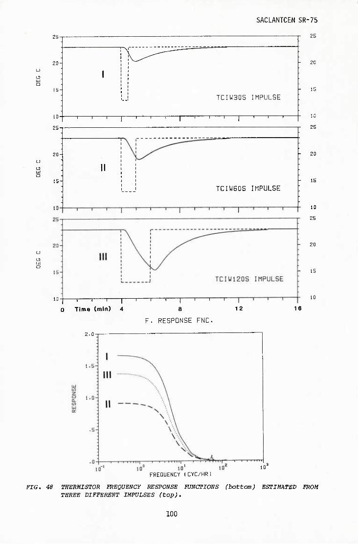
SACLANTCEN SR-75

a

L3 UJ D

LU Q

25-

20-

15-

10-

25-

20-

15-

TCIW30S IMPULSE

T 1 -r -\ 1 r -[ 1 r -T 1 T

TCIWGOS IMPULSE

25

20

15

10

25

20

\- 15

10

25

20

h 15

1 1 1 1 1 1 1 1 1 I r

0 Time (min) 4 $ 12

F. RESPONSE FNC.

10

16

2.0

—1 1—I—I—m

ID FREQUENCY tCYC/HR 1

FIG. 48 THERMISTOR FREQUENCY RESPONSE FUNCTIONS (bottom) ESTIMATED FROM THREE DIFFERENT IMPULSES (top).

100

SACLANTCEN SR-75

Vertical motions of the mooring line occur at frequencies well above this 3 to 10 cycle/h range because the mooring line is taut nylon and the buoy is essentially surface-following. Internal waves in this frequency range (and buoyancy frequency range) measured by Brekhovskikh et al <36> and presented in Phillips <37>, p.203), show vertical displacement spectra of the isotherms decreasing with frequency to the power of -2.7. Similar spectra for a lower frequency range measured by Cairns <38>, also presented in <37>, decrease with frequency to the power -2. From the evidence of these two spectra any aliasing in the spectrum from the internal waves in the 3 to 10 cycle/h range will have only a minor effect.

Temperature variance spectra for each of the mooring positions A to F are presented in Figs. 49 to 54.

To estimate spectra the data were detrended by least squares and multiplied by a cosine taper window before fourier transforming. Confidence in the raw spectral estimates was increased by averaging the raw estimates over adjacent frequency bands. The number of bands was set to seven for the spectra of the individual thermistors and to three for the averaged spectra of the thermistor chain. Towards higher frequencies the number of bands averaged was progressively increased in order to avoid congestion on the logarithmic frequency axis. Accordingly, the confidence in higher frequency estimates is also increased, as can be seen on the 90% confidence interval limits displayed on the top left of each figure. For the purpose of display most of the spectra have been cut at the low-frequency end by linear interpolation between the first two estimates (i.e. all spectra begin at the frequency of 0.01 cycle/h).

Although, as noted earlier, aliasing ought not to be serious for isotherm displacement spectra, it does appear to be occurring for the temperature variance spectra. It appears as a rapid increase in variance towards the Nyquist frequency, as clearly evidenced, for example, in the first four thermistors of mooring F (Fig. 54). Other good examples occur in thermistor T4 of mooring E (Fig. 53) and in thermistor TIO of mooring C (Fig. 50), although here it is difficult to distinguish between aliased internal waves from the 3 to 10 cycle/h range and resolvable internal waves occurring around the 1 and 2 cycle/h bands. Aliasing for some frequency, a , is caused by the frequencies 2na[\| + a, where aM is the Nyquist frequency and n an integer. Taking a = 1 cycle/h and ON = 3 cycle/h the aliasing frequencies will be 5, 7, 11, 13, ... cycle/h. Similarly for a = 2 cycle/h the aliasing frequencies will be 4, 8, 10, 14 ... cycle/h. Since, as clearly shown in Fig. 49, the buoyancy frequency range at 42 m depth (depth of thermistor TIO for mooring C) lies within the 4 to 11 cycle/h range, and since the peak of internal wave energy is at the buoyancy frequency, we deduce that at least one of the two peaks (a = 1, 2 cycle/h) in the TIO spectrum is from aliased internal waves. It is easily seen, however, that for a spectrum proportional to a-2 the aliased contribution of a large internal-wave peak at about 6 cycle/h would be virtually indetectable below 0.1 cycle/h. In support of this all the spectra show a proportionality of a'^, with r between -5/3 and -2.

The averaged spectrum of the chain is much smoother than the separate thermistor spectra and is therefore a good indicator of the spectral peaks. However, confidence in these peaks is not necessarily increased through the

101

SACLANTCEN SR-75

WAVE PERIOD (HRS)

10 Inrii I

10 10 I Ii..

10

SO'/

FREQUENCY (CYC/HR)

TC 570 A

FREQUENCY (CYC/HR) I '"I - '

FIG. 49

THERMISTOR CHAIN TEMPERATURE VARIANCE SPECTRA FOR EACH THERMISTOR AND FOR

CHAIN AVERAGE AT POSITION A.

WAVE PERIOD (HRS)

10 Im

10 10 . I , I..,.

10 III I

L, I., !„■" 10 10 10 10

FREQUENCY (CYC/HR)

-| 1 I MMIII r-TTTTTTIj 1 I | Mill

10"^ 10"' 10° lo' FREQUENCY (CYC/HR)

BOX

FREQUENCY (CYC/HR)

TC 357 B

FREQUENCY (CYC/HR) (-I-TTTTTT

FIG. 50 THERMISTOR CHAIN TEMPERATURE VARIANCE SPECTRA FOR EACH THERMISTOR AND FOR

CHAIN AVERAGE AT POSITION B.

10 10 10 10 FREQUENCY (CYC/HR)

]—I I (I mil—I 11 null—I I I mill

lo' 10"' lo'' 10' FREQUENCY (CYC/HR)

102

SACLANTCEN SR-75

WAVE PERIOD (HRS)

lo' lo' 10° Id' lllllH I I III I':ii.i : I I

BOX'

FREQUENCY (CYC/HR)

TC 148 C,

FREQUENCY (CYC/HR) TTTIl TTTTTTTTl n nTTTI]

_l-l _'o I I

FIG. 51

THERMISTOR CHAIN TEMPERATURE VARIANCE SPECTRA FOR EACH THERMISTOR AND FOR

r CHAIN AVERAGE AT POSITION C.

WAVE PERIOD (HRS)

10^ lo' 10° Id'

I I I

"I, I id' 10 lo" 10

FREOUENCY (CYC/HR)

I ' '"""I ' ' 'I 10"' 10"' 10° 10' FREQUENCY (CYC/HR) FREQUENCY (CYC/HR)

FIG. 52 10 THERMISTOR CHAIN TEMPERATURE VARIANCE SPECTRA FOR EACH THERMISTOR AND FOR CHAIN AVERAGE AT POSITION D.

TC 459 D

FREQUENCY (CYC/HR) I I I iiiiii[—I I iMiiij—I I iiMn|

10 10 10 10

FREQUENCY (CYC/HR)

~| I I I Mill] 1 I I lllllj 1 I I Mill ~

Id' Id' 10° 10' FREQUENCY (CYC/HR)

103

SACLANTCEN SR-75

WAVE PERIOD (HRS)

lo' 10' 10° 10' I' luill ■ I I I I

90%

FREQUENCY (CYC/HR) TTTTTl r'TflllTH

to 10 , 10 r 10

TC 164 E

FREQUENCY (CYC/HR) rrrm]—1 t tiiiiT|—1 1 iiiiiij

10 r

10' 10"' 10° 10' FREQUENCY (CYC/HR)

r FIG. 53 THERMISTOR CHAIN TEMPERATURE VARIANCE SPECTRA FDR EACH THERMISTOR AND FDR CHAIN AVERAGE AT POSITION E.

WAVE PERIOD (HRS)

10' 10' 10° Id' tuilU I I liliULLJ liimi I I I TC 342 F

1 I nmi—I I [ niiM—1 1 1IIITI

Id' W' 10° 10' FREQUENCY (CYC/HR)

SOX

10 10

FREQUENCY (CYC/HR) FREQUENCY (CYC/HR) I—I ' Miiii[—I I iiinij—I I MTlii] (—I I iiliii|—I I llllll|—I I 111111)

■"' ■"' "■° 10' , id' id' 10° 10' r '0

FIG. 54 10 THERMISTOR CHAIN TEMPERATURE VARIANCE

SPECTRA FOR EACH THERMISTOR AND FOR CHAIN AVERAGE AT POSITION F.

CHAIN \VERAGE

w' id' 10° 10' FREQUENCY (CYC/HR)

-| 1 I I lllll| 1 I I Mill] 1 I I Kill "

\6' Id' 10° 10' FREQUENCY (CYC/HR)

104

SACLANTCEN SR-75

averaging, since the thermistors of the chain were not measuring statisti- cally independent events.

All the spectra show a peak at the inertial frequency. As discussed in Sect. 3.1, strong inertial oscillations occur after a rapid increase in wind speed. These have been observed and discussed by Pollard <15> and Gonella <39>, who both found the oscillations to be confined effectively to the surface mixed layer.

A theory for the vertical oscillations at the inertial or near inertial frequency has been developed by Pollard <15>. In the models explored, generation of the vertical oscillations was seen to depend on horizontal variations (not necessarily local) in the applied wind stress.

In the following we emphasize this dependence and relate the amplitude of the vertical oscillations to the curl of the local wind stress. The treat- ment is not rigorous, as in <15>, but is presented purely to illustrate a mechanism that appears to be operating locally n the MILEX-80 zone.

In the thermocline, temperature fluctuations at the inertial frequency will occur primarily through advective action of the inertial oscillations (tlH , ^) on spatial gradients in the mean temperature field. This can be represented more specifically by the second two terms of the temperature balance

^ + UH.VHT + w|I +1IH VH T + wil = 0 , (Eq. 56)

where the tilde denotes oscillation at the inertial frequency, the over-bar denotes an average over several inertial periods, and the subscript H refers to horizontal components.

Equation 56 can now be used to relate temperature variance at the inertial frequency to inertial pulsations in the Ekman mass flux divergence and, consequently, to the local wind-stress curl. To develop this connection it is convenient to write the horizontal advection terms of Eq. 56 as

iiH . VHT « - (_UH . V?) ^ . (Eq. 57)

where ? is the depth of a sloping isotherm at, say, the maximum thermocline. The tilde and over-bar symbols will be re-introduced later but variables in Eq. 57 should be considered low-pass filtered to several hours.

The Ekman mass flux divergence is obtained by vertical integration of the continuity equation

^H . UH +|Y = 0 . (Eq. 58)

lOS

SACLANTCEN SR-75

between z = ^ and z = 0 to give

VH . UH = w^ - iiH,c • Vc , (Eq. 59)

where 0

UH = / UH dz . (Eq. 60; z=?

Combining Eqs. 56, 57, & 59 gives, for the local rate of change of temperature,

|I = - CH . U„) |I . (Eq. 61)

The inertial oscillations U^ satisfy the vertically integrated momentum balance

iUH + f k X UH =:-^ ^ (Eq. 62) at

where k is a unit vertical vector, T_H the horizontal wind-stress vector and f is the local inertial frequency. The extra term u 8^/8t from integration of the time derivative in Eq. 62 has been neglected, since it is small compared with the terms retained. Taking the wind stress to be a step function applied suddenly at time t = 0 and to be in the x-direction only (i.e. west wind in the MILEX-80 zone), leads to the well-known solution

U = — sin ft

V = — (cos ft-1)

(Eq. 63)

pf

that defines both the clockwise rotating inertial oscillations and the Ekman mass flux. Taking the divergence of Eq. 63 and allowing TX to be a function of y only (i.e. we assume 3TX/8X « 9Tx/9y) gives, for the inertial frequency pulsations in the Ekman mass flux divergence.

VH-UH = —-^ cos ft . (Eq. 64) pf 8y

106

SACLANTCEN SR-75

Then substituting Eq. 64 into Eq. 61 and integrating in time gives

T = -1_ !I^iI sin ft . (Eq. 65) f2p 3y 3Z

Finally, equating the amplitude term in brackets with the measured ampli' tude from the spectrum we obtain

f2p dy 3z

ay = f^P 2Aa Sj(f) / jj

(Eq. 66)

where Sx(f) is the spectral density estimate of temperature variance at frequency f and Aa is the frequency bandwidth of the estimate before smoothing in frequency.

Table 2 shows the modulus values of wind-stress curl calculated from Eq. 56 and the corresponding Ekman pumping velocity for each of the six mooring positions. The value S-r(f) was taken as the chain maximum and the value

34^/9z was set equal to the representative value of l°C/m. The wind-stress curl is higher to the north of the Bonifacio Strait than to the south and the range of values adds strong support to the model assumed in Sect. 4.3. The values in the table do not distinguish between upwelling and downwelling but in view of the earlier calculations of Sect. 4.2 it seems pro- bable that the value at F, at least, is for downwelling.

It should be pointed out that the solution of Eq. 66 represents an average of the wind-stress curl over about an 18-day period and that values for short periods could be considerably higher. Also, the simple model chosen for the inertia! oscillations was for convenience. Other models, such as a slowly growing wind stress, could equally have been used.

Before leaving temperature variance spectra it is interesting to observe that another small peak is evident at the approximate frequency of 1/8 cycle/h. See, for example, the chain-averaged spectra for mooring positions B, C and F in Figs. 50, 51, and 54 respectively or, more prominently, the separate thermistor spectra occurring at all mooring positions but particularly for B and C in Figs. 50 and 51. A likely explanation for peaking at this frequency is a higher order mode forced by non-linear interaction either through inertial-inertial or tidal-inertial components. More specifically one could look at the higher order solution to Eq. 61, written as

^ =-(VH.i)f . (Eq. 67) 0 t 0 Z

107

SACLANTCEN SR-75

TABLE 2

ESTIMATES FROM TEMPERATURE VARIANCE SPECTRA FOR MAGNITUDE OF

WIND-STRESS CURL AND VERTICAL EKMAN PUMPING VELOCITY to

Mooring Positions A B C D E F

depth (m) 26.5 45.6 32 33.7 56 64.7

5/fj "t/'c/./, 15.6 17.5 15.9 8.3 6.1 5.1

1.0 1.0 1.0 1.0 1.0 1.0

, -3 5.36 2.33 2.0 2.28 2.28 2.65

3.82 2.67 2.36 1.82 1.56 1.54

[Zl^l rn/da^ 2.66 1.86 1.65 1.27 1.09 1.08

108

SACLANTCEN SR-75

where Ti -jg defined by Eq. 65. However, this investigation will not be pursued further here.

5.2 Current-meter rotary spectra

Rotary spectra consist of clockwise and anticlockwise components giving the sense of rotation of the motion at each frequency. This is represented in the complex plane as <39>

Uo(t) + iVa(t) = u- e-iot + u+ e+^ot ^ (Eq, 58) a a

where u^ and Vg are the x and y components of current at frequency a and u" and u"*" are the clockwise and anticlockwise rotating

a a components also at frequency a .

Equating sine and cosine terms in the fourier representation of the lefthand side of Eq. 68 allows the rotary components to be written in terms of the conventional fourier coefficients as

Ua = "I (au + bv)(j + y (av " bu)^

UQ = - (au - by)^ +1 (ay + bu)a , (Eq. 69)

where the subscripts u and v refer to the velocity components. The rotary spectra components are then given by

A- -

_* _

a 2Aa

+* +

A+ =^^2-^

where Aa is the bandwidth of the estimate. The rotary coefficient is defined by

A^ - A^ Ra = ' (Eq. 71)

a a

109

SACLANTCEN SR-75

The spectra were computed and smoothed by averaging estimates in adjacent frequency bands, as described in Sect. 5.1. Figures 55, 56, and 57 illustrate the rotary spectra and coefficients for all the MILEX-80 current meters. The spectrum labelled VACMSNB3 in Fig. 57 is the average spectrum over all VACM and NB3 current meters. The one labelled NBA-567, also in Fig. 57, is the average over all NBA current meters not including NBA567 at mooring F. All spectra show a peak of energy at the inertial frequency in the clockwise component and, curiously, for the NBA current meters a lower energy but still a significant peak in the anticlockwise component. Whether or not this latter peak is an artifact of the mooring system (NBA current meter on taut surface mooring — see Sect. 2.5), which seems unli- kely, can only be tested by comparison with other current meters and/or with subsurface moorings. Such a comparison cannot be made effectively for the MILEX-80 data since all moorings were of the taut-nylon surface-float type and the VACM current meters were generally within the mixed layer, whereas the NBA current meters were generally below the thermocline.

Another possibility follows a similar argument to that in Sect. 5.1 con- cerning the inertial peak in the temperature variance spectra. One could consider a two-layer system with the upper mixed layer diverging horizon- tally due to the wind-stress curl and a lower homogeneous layer, of a higher density, responding to the resultant vertical velocity induced at the interface. Such a two-layer geometry fits quite well in the Mediterranean, especially during the autumn period when surface wind mixing greatly sharpens the thermocline. The appropriate momentum balance for the lower layer is then given by

1^ + f X u = -Ivp . (Eq. 72) 3t p

The free surface responds to the doming of the interface such that in the steady state the mean horizontal pressure gradient in the lower layer is zero. The dynamic response is a mean cyclonic motion in the upper layer. The lower layer will, however, experience temporal fluctuations in pressure gradient due to the pulsating Ekman divergence in the surface layer. An expression for the pressure at depth z = ZQ is

p = - g P2 ZD + (P2 - Pi) g? . (Eq. 73)

where P2 is the density of the lower layer, pi the density of the upper layer, and ? the z-coordinate of the interface. Setting P2 - p^ = gaAT, where a is the coefficient for thermal expansion and AT the temperature difference between layers, the righthand side of Eq. 73 becomes

. 1 Vp = - (gaAT) V? - (gaV Ti)^ , (Eq. 74) P

where Ti is the mixed-layer temperature and the lower-layer temperature is taken to be constant in space. Then by use of the kinematic boundary condition

110

SPECTRUM

SACLANTCEN SR-75

ROTARY COEFFICIENT

10 '.0

\ !0

t\j 10'

W 10

10

10-

WAVE PERIOD (HRSJ

lo' lo' 10° 10

ANTICLOCKWISE

~m^. ^10 NBABG5

CLOCKWISE (B) ^10^

10^

10 10' 10 10" 10"

FREQUENCY (CYC/HR) 10

WAVE PERIOD IHRSI 10'

10 - "■ ■' ' '

X 10

o 10 T

u 10

to'

10

10'

10' 10'

X 10

N. 10 -

o 10

5 10°-J

10 '

10'

10' 10 In.II I

10

NBA566

(D)

\0' lif' 10° FREQUENCY I CYC/HR 1

WAVE PERIOD IHRS )

lo' lo' 10°

to

-to

rio'

10

rlO

to to

10'

ID 10 10 hKtOLIENCY ( CYC/HR 1

WAVE PERIOD (HRS)

10° 10' Lii

10

NBABGS

(A)

10'

10'

10'

to"

10 0 10' 10 FREQUENCY (CYC/HR)

10'

1.0

-1.0

10

to 10' 10" FREQUENCY ( CYC/HR1

] /% 10 10 10 FREQUENCY (CYC/HR)

10 10" 10" FREQUENCY (CYC/HR)

0" 10"' iV FREQUENCY (CYC/HR)

FIG. 55 ROTARY SPECTRA AND COEFFICIENTS FOR NBA CURRENT METERS AT MOORINGS (from top to bottom) B, D, F, AND A.

Ill

SPECTRUM

SACLANTCEN SR-75

ROTARY COEFFICIENT

to 10

? loN

u to

to 10"

WAVE PERIOD ( HRS 1

ic' lO' !0°

CLLlCKUiSE

NBAsea (C)

ANTICLOCKWISE

90 '/

10 10 10 FREQUENCY ( CYC/HR 1

-to

rIO

rlO

rlO

to"

10 10 10" FREQUENCY !CYC/HR 1

to to

to 10"

UAVE PERIOD (HRS J 2 '

to to I

to _i 1 lllLll.i I — rlO

NBA570 (E)

to' to' to" FREQUENCY [CYC/HR)

rlO

rio'

rtO°

to '""1., ■ ■"""'.

10 10' to" FREQUENCY ICYC/HR)

UAVE PERIOD (HRS) „2

? 10

^ 10

^ 10' 1

'""I

to"'" 10"' to" FREQUENCY ( CYC/HR )

m,-

10'' 10"' lo'' FREQUENCY 1 CYC/HR 1

10'

WAVE PERIOD (HRS1

iiM[ 1—I rrmi] 1—i i 11111

to"' to"' 10° to' FREQUENCY ( CYC/HR 1

lO"' 10" 10' FREQUENCY (CYC/HR)

FJG. 56 ROTARY SPECTRA AND COEFFICIENTS FOR NBA CURRENT METERS AT MOORINGS C (top) AND E, THE NIEL BROWN 3-AXIS CURRENT METER AT MOORING C AND THE UPPER MOST VACM CURRENT METER ALSO AT C

(bottom).

112

SPECTRUM

SACLANTCEN SR-75

ROTARY COEFFICIENT

VJAVE PERIOD (HRS)

j—1 Im 11 I I—1_ 10

VACM35G F

(C)

10'

10

rlO

MO'

10

10 10" 10" FREQUENCY (CYC/HR)

TTTTT

10

10

WAVE PERIOD I HRSl

10 10

X 10 -I

N, 10' -i

♦

u lo'

5 10°

10 nil, I 1—1 I I'M I ■ I

10' 10 10

VACM357

(C)

lo-'i-

10

rlO

10

10

10

10

X 10^

10 10 10 10 10 FREQUENCY I CYC/HR)

WAVE PERIOD (HRS)

lo' 10^ lo' 10° 10''

VACMSNB3

MEAN

10-1—

10"'

-90 /;,.,,„, ", mi-QU ' I ' ' ' i""|

10"' 10"' 10° FREQUENCY (CYC/HR)

WAVE PERIOD (HRS) .2

10

rlO

-10

-10

10

10'

X 10 -

1-1 10 •■

LI 10

10 10 10 ■ 10" FREQUENCY ( CYC/HR)

to'

10 10 10' FREQUENCY f CYC/HR)

10 10' 10" FREQUENCY (CYC/HR )

10 10"' 10" FREQUENCY ( CYC/HR )

10 10' 10" FREQUENCY r CYC/HR 1

FIG. 57 ROTARY SPECTRA AND COEFFICIENTS FOR VACM CURRENT METERS AT MOORING C, THE AVERAGE FOR VACM AND NIEL BROWN CURRENT METERS AT C AND (bottom) THE AVERAGE FDR ALL NBA CURRENT METERS EXCLUDING MOORING F,

113

SACLANTCEN SR-75

8C w^ -iiH,?.V? = ^ (Eq. 75)

and Eq. 59 we can write

_ 1 Vp = - (gaAT) V (/ VH.UH dt) - gaVT / VH-UH dt . (Eq. 76)

Substituting for the Ekman mass flux divergence given by Eq. 64 and, for simplicity, assuming that both the mixed-layer temperature and the wind stress are functions of y only, we have

}'p gg 3Ti 3TX

82TX

L f2p 3y 9y f2p 8y2 sin ft . (Eq. 77)

-■ y

On the righthand side of Eq. 77 the ratio of the first term to the second term can be expressed as

8Ti

ay 2TrAT (Eq. 78)

where L is the wavelength for variations in the wind stress. Taking 9Ti/8y « 1°C in 20 km (see Fig. 11a), L = 100 km and AT = 4°C gives a value R = 0.2. Therefore, neglecting the first term on the righthand side of Eq. 77, Eq. 72 can be written

in at

f V = 0

9fv 8t2

+ f 2 V = 5°L ATI^ fp 9y2

cos ft (Eq. 79)

The equation for v is one of forced undamped oscillations, which, with the initial condition u=v=0 att=0, has the solution

v = Bt sin ft

u = - Bt cos ft + - sin ft f

(Eq. 80)

114

SACLANTCEN SR-75

f

g ^ ggAT 8^Tx

2f2p 3y2

In terms of the rotary components defined by Eq. 69 the solution is written as

,+ u- = ^ i ^ 2f

•^^ = Bt +|^i . (Eq. 81)

The term in t tends to increase clockwise rotating, kinetic energy with time. For small t the inertial oscillations are not rotating, but by t - l/2f (1.5 h), u- = 2u1; and the clockwise energy is four times greater

than the anticlockwise.

Although the above model is capable of distributing inertial energy between clockwise and anticlockwise components, it would require unrealistically high values of the second spatial derivative in wind stress if it were the only contribution to the anticlockwise peak observed in the rotary spectra For example, substituting Eq. 81 into Eq. 70 yields

^^■^x 4f3p , , 1/2

^-^^^'''''V' ' (Eq. 82)

which, taking the values Aa = 0.007 cycle/h and A+ = 800 (cm/s)2/cycle/h

from the spectrum of NBA565 at position B (Fig. 55) gives the value

82TX

3y^

1.28 * 10-8 ^/^^ , ^^q^ 33^

Using the estimate of dr^/dy = 2.6*10-6N/m3 estimated from the temperature variance spectrum for position B (see Table 2) and the value given in Eq. 83, gives a length scale for TX = 1.27 km. Such a value is too small by a factor of about 100.

In conclusion, a pulsating Ekman mass flux divergence in the surface layer is not sufficient to explain the observed peaks in the anticlockwise components of the rotary spectra. However, this might be a consequence of the chosen distribution for T and Ti (i.e. a dependence on y only). A dependence of these variables on x (the downwind direction) might introduce an anticlockwise velocity component that is also growing in time. Because of the very low dissipation below the thermocline, resonant forcing

US

SACLANTCEN SR-75

of the type defined by Eq. 79 could cause inertial oscillations (both clockwise and anticlockwise) with very high energy to develop in the lower layer.

5.3 Wind and current coherence spectra

Wind speed has been plotted variously in earlier sections of the report (see for example Fig. 40) and wind vectors were represented by the stick diagrams shown in Fig. 38. Similarly, plots of current are given in Figs. 19 and 20 in the form of progressive vector diagrams and in Figs. 28 to 37 in the form of vector sticks. In this section we look at wind/ current coherence and, for the lowest resolvable frequency band, current/ current coherence.

When estimating coherence functions it is necessary, in order to obtain sufficient confidence in the estimate, to average over a large number of adjacent frequency bands. Alternatively, the averaging could be over the estimates taken from a large number of separate pieces of the same time series. However, where high energy dominates at low frequencies (i.e. when spectra are red) the lowest frequency estimate for each piece, and hence also for the average, can be very distorted unless a high-pass filter with a very narrow transition bandwidth were applied to the original time series before division into pieces. Since the wind record is very short (only 18 days) and the storm period is between 3 and 5 days, any filter passing the storm frequency would require so many weights that pieces near the ends of the time series would be very poorly filtered. Furthermore, the lowest frequency-estimate when averaging over pieces contains no contribution from frequencies lower than Fp = 1/Tp, where Tp is the piece length. The fre-

quency averaged estimate, on the other hand, represents contributions from frequencies as low as Ff = l/NTp, where N is the number of pieces in the

piece-averaged estimate. Although these low-frequency contributions to the lowest frequency estimate are also distorted (frequencies lower than Ff could not have been filtered out) frequency averaging was adopted as the better procedure for all the coherence estimates presented in this section.

Wind-speed/current-speed coherence and phase spectra are presented in Figs. 58 and 59. In all cases the wind speed is that measured by the meteo-chain at mooring A and covers the period 13-30 Get 1980. Both wind and current records were low-pass filtered and decimated in time to 15-min intervals. Coherence estimates were then made for the overlapping portions of each record pair by taking the ratio of the frequency-averaged cross spectrum to the product of the frequency-averaged spectra. Averaging was over a minimum of twenty adjacent f^requency bands in all cases except for estimates involving the current at F (NBA567, Fig. 58 and the current at C (VACM355, Fig. 59), where averaging was over fifteen adjacent frequencies, and the current at C (NB3, Fig. 59) with averaging over only eight adjacent frequencies. The averaging was chosen to give the highest possible confidence in each estimate but still to retain in each case one estimate covering the range below but not including the inertial frequency.

All the spectra show a low coherence in the second (no inertial frequency components in the wind) and higher frequency estimates. The highest coherence in each case, appart from those with current meters at

116

SACLANTCEN SR-75

COHERENCE

(WIND SPEED,CURRENT SPEED) MC 707 (A).

1.0

l.Q'

"T 1—I—r 1 I I 11—'■=™*^T

10' 10

1.0

1 .0

1 .0-

• o-

N8A566

CD)

180.0

-.0-

-180.0

180.0

10 10 -180.0

180.0

-180.0

180.0

-.0-

-180.0

NBA563

(C)

180.0-

-.O'

-180.0'

10 10' 10' 10'

FREQUENCY (CYC/HR )

PHASE

10" 10' 10

FREQUENCY (CYC/HR

-| 1 I I I IT

lo'

FIG. 58 ODHERENCE AND PHASE SPECTRA COMPARING WIND SPEED AT POSITION A WITH CURRENT SPEED AT POSITIONS B, D, F, A AND C.

117

SACLANTCEN SR-75

COHERENCE (WIND SPEED,CURRENT SPEED) MC 707 (A).

1.0-

.5-

1 .0

1 .0-

.5-

NBA570

(E)

VACM355 CO

10'

180.0

-.0-

-180.0

180.0

-.0

-IBQ.O

180.0

-.0

-180.0

PHASE

10

1.0-

•s-

VACM356 (C)

—I—I—I vi~r

IBO.O

10

1.0-

.5-

.0

VACM357

CO

1 1—I—I I I 11 j 1——I—r—r T T 11 ]

-? -I -0 10^ lO'

180.0-

10

I I I I II.I -180.0- , 1 . o-J 10 10 '

FREQUENCY (CYC/HR ) FREQUENCY (CYC/HR

to'

FIG. 59 COHERENCE AND PHASE SPECTRA COMPARING WIND SPEED AT POSITION A

WITH SPEED AT POSITIONS E AND C (4 CURRENT METERS AT C).

118

SACLANTCEN SR-75

position C, is for the lowest frequency estimate that represents contributions from the approximate range from 19 h to 17 days. The best coherence is found between the wind and current measured at position A. This shows values higher than 0.5 for periods as short as 3 h. Curiously, the worst coherence is found at position C (wind at A, current at C), even for the NBA current meter, which was at a similar depth to all the other NBA current meters. Wind/current coherence is virtually insignificant for the NB3 and the three VACM current meters at position C (Fig. 59) and perhaps it is of significance that these current meters were within the mixed layer for most of the experiment. That coherence is so much lower at C than at A lends support to the assumption that the wind speed off the Bonifacio Strait is different from that to the north, which is sheltered by Corsica. Small peaks in the wind/current coherence standing out against the background are observed at 1 cycle/h both for the NB3 current meter of position C moored at 4 m (Fig. 59) and to a lesser extent for the NBA current meter of position F moored at 88 m depth (Fig. 58). Current meter VACM356, also at position C, shows a similar peak in its coherence with wind speed at 0.79 cycle/h.

The generally higher coherence at low frequency can be attributed to the response of the subsurface current to the storm frequency in the 3 to 5 day range. In support of this, an unsmoothed cross spectrum, not shown here, showed evidence of peaking in the same 3 to 5 day range. The wind clearly contained very low variability at the inertial frequency, evidenced by the very low coherence seen in the second estimate for each of the spectra.

A complication in interpreting these results is the high probability of the NBA current meters being pumped by surface waves (see Sect. 2.5). Since the sea state also responds to the storm frequency it is not possible to separate the effects of surface waves and subsurface response on the high coherence observed. It is unfortunate that all of the deeper current meters were NBA's.

Estimates were also made of the coherence in current speed between all pairs of current meters for the range from 19 h to 17 days. The values, including those with wind speed, are shown in Table 3. The values with asterisks represent the higher frequency range of 13 to 25 h, the lower frequency range being too low for the short NB3 time series. For this higher range, which includes the inertial frequency, a high coherence can be seen between the two uppermost current meters at position C (4 m & 14 m). Surprisingly, however, there is no coherence in this range between the 4 m and 23 m or the 4 m and 32 m current meters. For this same range, but not shown on the table, there is a coherence of 0.51 between the VACM355 (14 m) and VACM356 (23 m). All other coherence between current meter pairs at this frequency and at all higher frequencies is insignificant.

Table 3 shows that in the low-frequency range (which includes the storm frequency) high coherence is found between some current meter pairs but not others. The current at C (NBA569) is well correlated with the current at E (NBA570), for example, but not with the current at B (NBA566). The current at E (NBA570) is well-correlated with the currents at both D (NBA566) and F (NBA567), but that at D is not well correlated with that at F. This could be explained by E being up-stream from D and F but the

119

SACLANTCEN SR-75

currents at D and F belonging to different eddies. None of the current meters below the thermocline is well-correlated with those above, except perhaps NBA570 (E, 68m) with VACM355 (C, 14m).

TABLE 3

CURRENT-CURRENT AND CURRENT-WIND COHERENCE IN LOW-FREQUENCY RANGE

(19 h - 17 day period) the asterisk refers to range (13-19 h)

# # # .# # # c# .# / ,. ,.<.\^

(B) NBA565

(D) NBA566

(F) NBA567

(A) NBA558

(C) NBA569

(E) NBA570

(C) VACM355

(C) VACM356

(C)VACM357

(C) NB3

'^ .^v ^^ ^v r^v ^ A-^ -\x- ^ ^" \^ C!^

.72 .23 .52 ,35 ,63 .12 ,21 ,29 .67

.12 M .^7 ,73 .29 .27 ,23 ,45

,36 .56 ,78 .2^ ,15 ,21 ,46

.69 ,72 ,13 .15 ,29 ,80

,75 ,23 .11 .33 ,36

,45 ,26 .3ij .46

A^ .20 ,95* .15

,59 .16* ,15

.10* .20

0

120

SACLANTCEN SR-75

SUMMARY AND CONCLUSIONS

The data collected from the MILEX-80 experiment have been presented and interpreted.

A description of the experiment is provided in Ch. 2. In short, six thermistor chains, ten current meters, and a meteo chain were moored by means of surface floats and taut nylon rope in the north Tyrrhenian Sea. The instruments were moored in the surface mixed layer and thermocline and arranged in a horizontal distribution to cover the region of a large quasi- permanent cold patch of water fanning out eastwards from the Strait of Bonifacio.

The cold patch has been interpreted as an upwelling caused by wind-stress curl — the west wind, which predominates throughout the year, being consistently stronger at the eastern end of the Bonifacio Strait than it is off the east of Corsica or Sardinia on either side of the Strait. This upwelling, commonly referred to as Ekman pumping, formed the central theme of the report and set the context for the various spatial and temporal descriptions of the data occurring throughout.

The existence of two counterrotating eddies, one cyclonic underlying the cold patch and the other anticyclonic in the warmer water to the south, was confirmed both by the dynamic topography estimated from CTD casts and from the measured currents. It was found that the density contribution (i.e. estimated dynamic topogaphy) to the eddies accounted for approximately only half the measured speeds, although the agreement in direction was quite good. The density contribution is interpreted as a baroclinic adjustment to forcing by the wind-stress curl. The remainder of the flow is considered to be barotropic but not necessarily caused by local forcing. It might, for example, be an instability on the mean circulation in the Tyrrhenian Sea as it flows northward up the west coast of Italy, turns west and south under the influence of the northern barrier to the basin, and then turns southwards down the west of Corsica and Sardinia.

A model after De Szoeke <34> was suggested for the mixed layer, in which the mixed layer represents a balance between the upward motion of the layer base due to Ekman pumping and the downward progression of the interface due to mixing. Then, taking a wind-stress curl equivalent to 4 m/s over 100 km (a value that appears consistent with historical data presented in May <10>), and taking an entrainment rate (after Kraus & Turner <6>) due to a wind speed of 8 m/s, it was shown that a steady state would prevail after 7 days. In this case the mixed-layer depth would be 15 m and the Ekman pumping velocity would be 2.1 m/day. The time scale is similar to the storm period and the depth scale close to the measured depth of 15 to 20 m for the mixed layer over the cold patch.

Surface heat fluxes were estimated for both the cold water patch and the warmer water to the south using the Bowen ratio technique. This involved taking an empirical form for the Bowen ratio dependent on air/sea temperature difference and estimating from this both the evaporative heat loss and the water vapour correction term in the back-radiation formula. Cloud- cover correction factors for the three-week period were not known but

121

SACLANTCEN SR-75

cloud-cover statistics for the two areas were assumed not to differ significantly. A heat flux difference for the two areas (north & south) was thus estimated and, by comparison with the north-south difference for the heat content change over a 13-day period, a vertical velocity difference W*|\| - W*s between north and south was estimated and found to be 5.9 m/day. By considering maximum and minimum cloud-cover conditions this implies an upwelling to the north in the range from 2.1 to 3.8 m/day and downwelling to the south in the range from 3.9 to 2.2 m/day. The wind-stress curl necessary to produce such up- and down-welling is consistent with the historical data.

Another possible technique for estimating wind-stress curl emerged from Ch. 5, on spectral analysis. There it was argued that the peak in temperature variance spectra occurring at the inertial frequency could be attributed entirely to inertial pulsations in the divergence of the Ekman mass flux. Assuming a simple model for the inertial oscillations arising from the sudden application of a constant wind stress, wind-stress curl was estimated as a function of temperature variance, the inertial frequency, and the mean maximum thermocline gradient. Although involving a number of assumptions and approximations, the technique, rather surprisingly, gave values of the wind-stress curl and upwelling in good agreement both with estimates from the heat balance and with the historical data. The mean upwelling over the three-week period for position B, for example, was estimated to be 2.25 m/day.

Similar arguments invoked to explain.the inertial peak in the anticlockwise rotary spectra for the current-meter data were less successful. Nevertheless, it was demonstrated that this energy could arise through a resonant forcing of the subsurface (below-thermocline) layer by inertial pulsations in the hydrostatic pressure gradient. These in turn, it was argued, are a consequence of the pulsations in Ekman mass flux divergence.

The following more general statements can be made as a result of the MILEX-80 experiment:

a) The spatial variability of the wind field over the Mediterranean strongly influences the depth of the mixed layer and the geostrophic current field.

b) In such conditions of high spatial variability in the wind field one-dimensional mixed-layer models cannot work well.

c) One-dimensional mixed-layer models could be generalized to three dimensions and used if the wind field were known.

d) Areas of high wind variability can be identified both by use of satellite infrared images and by analysis of historical data.

e) Many such areas exist in the Mediterranean.

f) Knowing the wind field would allow the use of mixed-layer models in predicting the evolution of surface-layer variability. In order to properly predict surface-layer variability, however, an ocean circulation model is required, since only in this way can the important effects of horizontal advection be accounted for.

122

SACLANTCEN SR-75

The area of MILEX-80 has turned out to be too complex for the proper testing or application of one-dimensional mixed-layer models. However, data collected during a second mixed-layer experiment, MILEX-82, performed in the open Western Mediterranean, half way between the Balearic Islands and Sardinia, should prove more suitable for one-dimensional model tuning. This is due to the distance of the area from coastal boundaries, the deep water (over 2500 m), the flat bottom, and the low spatial variability in the wind-stress field. Furthermore, satellite infrared images studied during the MILEX-82 experiment did not reveal any strong gradients in the surface temperature, as can be found permanently in the MILEX-80 zone.

Further research will involve using MILEX-82 data to tune one-dimensional models to establish appropriate values of the empirical constants, genera- lizing these models to three-dimensions, and finally modelling the surface layer in the MILEX-80 zone by assuming the spatial variations in the wind field given by the available historical data.

123

SACLANTCEN SR-75

REFERENCES

1. DAVIS, R.E. (a) De SZOEKE, R., HALPERN, 0. and NIILER, P. Variability in the upper ocean during MILE. Part I: The heat and momentum balances. Deep Sea Research, 28A, 1981: 1427-1451.

2. DAVIS, R.E. (b) De SZOEKE, R. and NIILER, P. Variability in the upper ocean during MILE. Part II: Modeling the mixed layer response. Deep Sea Research, 28A, 1981: 1453-1475.

3. POLLARD, R.T., GUYMER, T.H. and TAYLOR, P.K. Summary of the Jasin 1978 field experiment. l<n_: CHARNOCK, H. and POLLARD, R.T., eds_. Results of the Royal Society Joint Air-Sea Interaction Project (JASIN). Proceedings of a Royal Society discussion meeting held on 2 and 3 June, 1982.

4. KLEIN, P. A simulation of the effects of air-sea transfer variability on the structure of marine upper layers. Journal of Physical Oceanography, 10, 1980: 1824-1841.

5. ROBINSON, M.K., BAUER, R.A., and SCHROEDER, E.H. Atlas of north Atlantic — Indian Ocean monthly mean temperatures and mean salinities of the surface layer, NOO RP-18. NSTL Station, Bay St. Louis, MS, Naval Oceanographic Office.

6. KRAUS, E.B. and TURNER, J.S. A one-dimensional model of the seasonal thermocline: II. The general theory and its consequences. Tellus, 19, 1967: 98-106.

\ 7. MOEN, J. The mixed layer: theoretical and experimental approach, NATO

UNCLASSIFIED. In: NATO SACLANTCEN. Papers presented to the 37th meeting of tfTe" SACLANTCEN Scientific Committee of National Repreentatives, 14-16 October, 1980, SACLANTCEN CP-28, NATO CONFIDENTIAL. La Spezia, Italy, SACLANT ASW Research Centre, 1980. [AD C 024 237]

8. PHILIPPE, M. and HARANG, L. Surface temperature fronts in the Mediterranean from infrared satellite imagery. ln_: NIHOUL, J.C.J., ed. Hydrodynamics of Semi-enclosed Seas. Proceedings of the 13th International Li&ge Colloquium on Ocean Hydrodynamics. Amsterdam, The Netherlands, Elsevier, 1982: pp 91-128.

9. KRIVOSHEYA, V.G. and OVCHINNIKOV, I.M. Peculiarities in the geostrophic circulation of the waters of the Tyrrhenian Sea. Oceanology, 13, 1973: 822-827.

10. MAY, P.W. Climatological flux estimates in the Mediterranean Sea: Part 1: Winds and wind stresses, NORDA Report 54. NSTL Station, MS, Naval Ocean Research and Development Activity, 1982. [AD A 121 931]

11. POLLARD, R.T., RHINES, P.B. and THOMSON, R.O.R.Y. The deepening of the wind-mixed layer. Geophysical Fluid Dynamics. 4, 1973: 381-404.

124

SACLANTCEN SR-75

12. WANNAMAKER, B., SACLANT ASW Research Centre. Private Communication, 1982.

13. WELANDER, P. Mixed layers and fronts in simple ocean circulation models. Journal of Physical Oceanography, 11, 1980: 148-152.

14. GONELLA, J. The drift current from observations made on the BouSe Laboratoire, Cahiers Ocganographiques, 23, 1971: 1-15.

15. POLLARD, R.T. On the generation by winds of inertial waves in the ocean. Deep Sea Research, 17, 1970: 795-812.

16. POLLARD, R.T. and MILLARD, Jr. R.C. Comparison between observed and simulated wind generated inertial oscillations. Deep Sea Research, 17, 1970: 813-821.

17. CRAIK, A.D.D. The generation of Langmuir circulations by an instability mechanism. Journal of Fluid Mechanics, 81, 1976: 209-223.

18. POLLARD, R.T. Observations and theories of Langmuir circulations and their role in near surface mixing. Deep Sea Research, Sir George Deacon Anniversary Supplement, 1976.

19. MOEN, J. Theoretical model for Langmuir circulations, Ph.D. Thesis, University of Southampton, 1978.

20. LEIBOVICH, S. On the evolution of the system of wind drift currents and Langmuir circulations in the ocean. Part 1: Theory and averaged current. Journal of Fluid Mechanics, 79, 1977: 715-743.

21. MELLOR, G.L. and DURBIN, P.A. The structure and dynamics of the ocean surface-mixed layer. Journal of Physical Oceanography, 5, 1975: 718-728.

22. MUNK, W.H. and ANDERSON, E.R. Notes on theory of the thermocline. Journal of Marine Research, 7, 1948: 276-295.

23. BUSH, N.E. Fluxes in the surface boundary layer over the sea. In: KRAUS, E.B. ed. Modelling and Prediction of the Upper Layers of IFe Ocean. Selected papers presented at the NATO Sponsored Advanced Study Institute held at Urbino, Italy. September 1975. Oxford, U.K., Pergamon Press, 1977: pp 72-91.

24. ROLL, H.U. Physics of the Marine Atmosphere. New York, N.Y., Academic Press, 1965.

25. KRAUS, E.B. Atmosphere-Ocean Interaction. Oxford, U.K., Clarendon Press, 1972.

26. WYRTKI, K. The average annual heat balance of the North Pacific Ocean and its relation to ocean circulation. Journal of Geophysical Research, 70, 1965: 4547-4559.

27. PERRY, A.H. and WALKER, G.M. The ocean-atmosphere system. London, Longman, 1977.

125

SACLANTCEN SR-75

28. DUTTON, J.A. The Ceaseless Wind. New York, N.Y., McGraw-Hill, 1976: p 271.

29. GILL, A.E. Atmosphere-Ocean Dynamics. New York, N.Y., Academic Press, 1982: p 45.

30. KRAUS, E.B. and ROOTH, C. Temperature and state vertical heat flux in the ocean surface layers. Tell us, 13, 1961: 231-238.

31. BERLIAND, T.G. Metodika Kl imatologischeskikh raschetov summarnoi radiatssi, Meteorologia i Hidrologia, 6, 1960: 9-12.

32. IVANOFF, A. Solar radiation. In: KRAUS, E.B., ed. Modelling and Prediction of the Upper Layers on;he Ocean. Selected papers presented at a NATO sponsored Advance Study Institute held at Urbino, Italy. September, 1975. Oxford U.K., Pergamon Press, 1977: pp 47-71.

33. PEDLOSKY, J. Geophysical Fluid Dynamics. New York, N.Y., Springer, 1979.

34. DE SZOEKE, R.A. On the effects of horizontal variability of wind stress on the dynamics of the ocean mixed layer. Journal of Physical Oceanography. 10, 1980: 1439-1454.

35. BENDAT, J.S. and PIERSOL, A.G. Random Data: Analysis and Measurement Procedures. New York, N.Y., Wiley-Interscience, 1971.

36. BREKHOVSKIKH, L.M., KONJAEV, K.V., SABININ, K.D. and SERIKOV, A.N. Short period internal waves in the sea. Journal of Geophysical Research, 80, 1975: 856-864.

37. PHILLIPS, O.M. The dynamics of the upper ocean, 2nd edn. Cambridge, Cambridge University Press. 1977.

38. CARINS, J.L. Internal wave measurements from a midwater float. Journal of Geophysical Research, 80, 1975: 299-306.

39. GONELLA, J. A rotary-component method for analysing meteorological and oceanographic vector time series. Deep Sea Research, 19, 1972: 833-846.

126

SACLANTCEN SR-75

APPENDIX A

A VERTICAL VORTICITY BALANCE IN NON-DIMENSIONAL FORM

Neglecting molecular viscosity, a vorticity balance can be written in the form (<A.1> p. 38)

^ - (» . V) „ - VP^ . ,, ^,^2 . A„ liM] = 0 . (Eq. Al) Ut p •- n SZ'^ -■

where Wg is the absolute vorticity (i.e. vorticity of fluid relative to the earth plus vorticity of fluid due to earth's rotation), _u the fluid velocity, p the density, and AH and Ay are eddy viscosity coefficients in the horizontal and vertical respectively. The usual righthanded cartesian coordinate system (x,y,z) is assumed with z directed (+ve) upwards normal to the earth's surface.

The second term of Eq. Al represents vortex stretching and tilting, the third term baroclinic production of vorticity, and the fourth term dissipation due to the turbulent Reynolds stresses.

Since we are primarily interested in the effects of horizontal stresses applied to the sea surface by the wind we consider only the vertical component of Eq. Al given by

P_(c+f) - [((0 + f) . V] w - i- r ^ l£ . IP 1£ 1 Dt p2 L 8x 8y 8y 3x J 8y 8y 3x J

- VH AH V2 UH + Av ^ 1=0 , (Eq. A2) H -" 3z^

with w = (?, n, c) being the relative fluid vorticity and f a vertical vector for the Coriolis parameter f . Dimensional variables Tn Eq. A2 are changed to non-dimensional variables by the transformations

(x, y) -»■ [L] (x, y)

z ->■ .^] z

t ->■ [L] t U

(U, V) ^- [U] (u, v)

w -»- L

(Eq. A3)

127

SACLANTCEN SR-75

p -»■ [PQ] P

p -V [po D g] pz + [po f U L] p ,

where all terms in square brackets are dimensional, with L a horizontal length scale, D a vertical length scale, U a horizontal velocity scale, and PQ a density scale.

Substituting the transformations of Eq. A3 into Eq. A2 and multiplying throughout by L/fU leads to the non-dimensional equation

RQ I^ + BV + Ro((£.-V)w + 9W _ 1_ r3£ 9£ . iP l£l Dt 9z p2 Lsx 3y 9y 8x J

- EH(VH X V2 UH) - Ev (VH X ^)= 0 , (Eq. A4)

where RQ , EH and Ey are, respectively, the non-dimensional Rossby number, horizontal Ekman number, and vertical Ekman number. These are defined by

R - U

' AH (Eq. A5)

Av V = —:, •

fD2

The non-dimensional parameter 6 in Eq. A4 is expressed by

g =^ . (Eq. A6)

where 6o is the south-north gradient in the linear approximation to the variation of f with latitude ^ = ^Q + 3oy •

REFERENCES

A.l PEDLOSKY, J. Geophysical Fluid Dynamics. New York, N.Y., Springer. 1979.

128

KEYWORDS

AANDERAA THERMISTOR CHAIN ADRIATIC AEGEAN SEA ALBEDO ALBORAN SEA ANTICYCLONIC BAROCLINIC BAROTROPIC BATHYTHERMS BENDIX SURFACE FLOAT BONIFACIO STRAIT

BORA BOWEN RATIO BRUNT-VAISALA FREQUENCY BUOYANCY FREQUENCY

CIRCULATION CLAUSINS-CLAPEYRON EQUATION CORIOLIS PARAMETER CORSICA CTD CURRENT METERS CURRENT SHEAR CURRENTS CYCLONIC DEEP DENSITY DOWNWELLING EDDY EKMAN DIVERGENCE EKMAN FLUX EKMAN LAYER EKMAN MASS EKMAN PUMPING ENTRAINMENT RATE ETESIANS GEOSTROPHIC GREGALE GULF OF LIONS GYRE LEVANTER LIBERATOR

MAESTRO MARIA PAOLINA G. MEDITERRANEAN MILEX-80

MIRTO MISTRAL MIXED LAYER EXPERIMENT MODEL MUNK AND ANDERSON TURBULENCE CLOSURE NBA CURRENT METER NIEL BROWN CURRENT METER NYQUIST FREQUENCY OSCILLATING BULK FLOW OSCILLATING SLAB FLOW POLLARD RHINES AND THOMSON MODEL RICHARDSON NUMBER ROSSBY NUMBER SALINITY SAMSON ROPE SARDINIA SHALLOW SHEAR ZONE SIROCCO SOUND SPEED SST STEFAN-BOLTZMANN CONSTANT STRATIFICATION SUMMER SURFACE BOUNDARY LAYER TEMPERATURE THERMOCLINE TYRRHENIAN SEA UPWELLING VACM aiRRENT METER VARIABILITY VENDEVAL WIND STRESS CURL WIND STRESS WIND WINTER XBT

MARSDEN SQUARE NUMBERS

179/00/01/10/11/20/21

180/08/09/18/19/29

SACLANTCEN SR-75

INITIAL DISTRIBUTION

Copies Copies

SCNR FOR SACLANTCEN MINISTRIES OF DEFENCE

SCNR Belgium MOD Belgium 2 SCNR Canada DND Canada 10 SCNR Denmark CHOD Denmark 8 SCNR Germany MOD France 8 SCNR Greece MOD Germany 15 SCNR Italy MOD Greece 11 SCNR Netherlands MOD Italy 10 SCNR Norway MOD Netherlands 12 SCNR Portugal CHOD Norway '^'^n^ SCNR Turkey MOD Portugal

'^^ ^^B -' K.

MOD Turkey 1 jBi la\ ' • MOD U.K. W^ ""' . ,, xep. SCNR SECDEF U.S.

^ .j»..-.-^..

1». '*''■'•'' LC'/M Rep. SCNR NATO AUTHORITIES ™ NATIONAL LIAISON OFFICERS

Defence Planning Committee 3 LO Canada

Denmark NAMILCOM SACLANT

2 ""rraany ly

SACLANTREPEUR ■}

CINCWE STLANT/COMOCEANLANT .■•i

COMSTRIKFLTANT j.' ■ U a

COMIBERLANT CINCEASTLANT

NLR TO SACLANT

COMSUBACLANT NLR Belgium COMMAIREASTLANT NLR Canada

SACEUR NLR Denmark CINCNORTH NLR Germany CINCSOUTH NLR Greece COMNAVSOUTH NLR Italy COMSTRIKFORSOUTH NLR Netherlands COMEDCENT NLR Norway COMMARAIRMED NLR Portugal

CINCHAN 3 NLR NLR NLR

Turkey UK US

Total initial distribution 247 SACLANTCEN Library 10 Stock 23

Total number of copies 280

U213719

SACLANT ASW RESEARCH CENTRE REPORT - CiteSeerX

Documents

Transcript of SACLANT ASW RESEARCH CENTRE REPORT - CiteSeerX