Technical Feasibility of Sharing Federal Spectrum with Future ...
285
U.S. DEPARTMENT OF COMMERCE • National Telecommunications and Information Administration report series NTIA Technical Report 20-546 Technical Feasibility of Sharing Federal Spectrum with Future Commercial Operations in the 3450-3550 MHz Band Edward Drocella Robert Sole Nickolas LaSorte
-
Upload
khangminh22 -
Category
Documents
-
view
1 -
download
0
Transcript of Technical Feasibility of Sharing Federal Spectrum with Future ...

U.S. DEPARTMENT OF COMMERCE • National Telecommunications and Information Administration
report series
NTIA Technical Report 20-546
Technical Feasibility of Sharing Federal Spectrum with Future Commercial
Operations in the 3450-3550 MHz Band
Edward Drocella Robert Sole
Nickolas LaSorte


U.S. DEPARTMENT OF COMMERCE
January 2020
NTIA Technical Report 20-546
Technical Feasibility of Sharing Federal Spectrum with Future Commercial
Operations in the 3450-3550 MHz Band
Edward Drocella Robert Sole
Nickolas LaSorte

ii
ACKNOWLEDGEMENTS
The National Telecommunications and Information Administration Office of Spectrum Management would like to acknowledge the federal agencies that provided technical data on their systems and frequency assignments in the bands.

iii
CONTENTS
Acknowledgements ......................................................................................................................... ii
Abbreviations/Acronyms ............................................................................................................... vi
Executive Summary ..................................................................................................................... viii
1. Introduction ..................................................................................................................................1 1.1 Background ...........................................................................................................................1 1.2 Objective ................................................................................................................................2 1.3 Approach ................................................................................................................................2
2. Federal System Parameters ..........................................................................................................4 2.1 Overview ................................................................................................................................4 2.2 Airborne Systems ...................................................................................................................6 2.3 Ground-Based Radar Systems ...............................................................................................7 2.4 Shipborne Radar Systems ....................................................................................................10 2.5 Other Systems ......................................................................................................................11 2.6 Radar Antenna Models ........................................................................................................11
3. Commercial Wireless System Parameters .................................................................................12 3.1 Overview ..............................................................................................................................12 3.2 Population Based Deployment .............................................................................................13 3.3 IMT Advanced Deployment ................................................................................................18 3.4 User Equipment Deployment ...............................................................................................21
4. Engineering Models ...................................................................................................................22 4.1 Overview ..............................................................................................................................22 4.2 Basic Transmission Loss .....................................................................................................22 4.3 Clutter Loss ..........................................................................................................................23 4.4 Building Loss .......................................................................................................................25 4.5 Frequency Dependent Rejection ..........................................................................................25
5. Sharing with Airborne Systems .................................................................................................27 5.1 Overview ..............................................................................................................................27 5.2 Base Station EIRP Limit for Airborne System 1 and 2 .......................................................27
5.2.1 BS EIRP Limit Methodology .....................................................................................27 5.2.2 BS EIRP Limit Results ..............................................................................................29
5.3 Static Exclusion Zones for Airborne System 3 ....................................................................30 5.3.1 Static Exclusion Zones Analysis Methodology ..........................................................30 5.3.2 Results ........................................................................................................................32
5.4 Dynamic Coordination Zones for Airborne System 3 .........................................................39 5.4.1 Dynamic Coordination Zone Neighborhood Methodology .......................................39 5.4.2 Results ........................................................................................................................40
6. Sharing with Ground-Based Radars...........................................................................................47 6.1 Overview ..............................................................................................................................47

iv
6.2 Static Exclusion Zones .........................................................................................................47 6.2.1 Static Exclusion Zones Analysis Methodology ..........................................................47 6.2.2 Results ........................................................................................................................50
6.3 Dynamic Coordination Zone Neighborhood .......................................................................63 6.3.1 Dynamic Coordination Zone Neighborhood Methodology .......................................63 6.3.2 Results ........................................................................................................................66
7. Sharing with Shipborne Radars .................................................................................................79 7.1 Overview ..............................................................................................................................79 7.2 Static Exclusion Zones .........................................................................................................79
7.2.1 Static Exclusion Zone Analysis Methodology ...........................................................79 7.2.2 Results ........................................................................................................................81
7.3 Dynamic Coordination Zones ..............................................................................................88 7.3.1 Electromagnetic Sensor Threshold .............................................................................88 7.3.2 Dynamic Coordination Zone Geometry .....................................................................90 7.3.3 Dynamic Coordination Zone Neighborhoods ............................................................94
8. Summary .................................................................................................................................101 8.1 Overview ............................................................................................................................101 8.2 Sharing Options for Airborne System 1 and-2 ..................................................................102
8.2.1 30 Megahertz Sharing Option ..................................................................................102 8.2.2 100 Megahertz Sharing Option ................................................................................102
8.3 Sharing Options for Ground-Based Radars, Shipborne Radars, and Airborne System 3 ...................................................................................................................................103
8.3.1 30 Megahertz Sharing Option ..................................................................................103 8.3.2 100 Megahertz Sharing Option ................................................................................114
9. Further Studies ........................................................................................................................125 9.1 Summary ............................................................................................................................125 9.2 Further Studies ...................................................................................................................125
9.2.1 Frequency Domain Sharing ......................................................................................125 9.2.2 Time Domain Sharing ..............................................................................................127 9.2.3 Other Agency-wide Solutions .................................................................................127
Appendix A : Additional Results for Airborne System Feasibility of Sharing Analysis ................1 A.1 Base Station Emission Limits Results .................................................................................1
A.1.1 30 Megahertz Sharing Option .....................................................................................1 A.1.2 100 Megahertz Sharing Option .................................................................................13
A.2 Airborne System 3 Static Exclusion Zone Results .............................................................24 A.2.1 100 Megahertz Sharing Option .................................................................................24
A.3 Airborne System 3 Dynamic Coordination Zone Neighborhood Results ..........................37 A.3.1 100 Megahertz Sharing Option .................................................................................37
Appendix B . Additional Results for Ground-Based Radar Feasibility of Sharing Analysis ..........1 B.1 Static Exclusion Zone Results ...............................................................................................1
B.1.1 30 Megahertz Sharing Option ......................................................................................1 B.1.2 100 Megahertz Sharing Option ..................................................................................14

v
B.2 Dynamic Coordination Zone Neighborhood Results ..........................................................27 B.2.1 30 Megahertz Sharing Option ....................................................................................27 B.2.2 100 Megahertz Sharing Option ..................................................................................40
Appendix C . Additional Results for Shipborne Radar Feasibility of Sharing Analysis .................1 C.1 Static Exclusion Zone Results ...............................................................................................1
C.1.1 Population Deployment ...............................................................................................2 C.1.2 IMT-Advanced Deployment ........................................................................................8
C.2 Dynamic Coordination Zone Results ..................................................................................14 C.2.1 Population Deployment .............................................................................................15 C.2.2 Population Deployment .............................................................................................34 C.2.3 IMT-Advance Deployment ........................................................................................40

vi
ABBREVIATIONS/ACRONYMS
AFB United States Air Force Base
AGL Above Ground Level
AP Access Point
ATC Air Traffic Control
BS Base Station
CBRS Citizens Broadband Radio Service
CDF Cumulative Distribution Function
CONUS Contiguous United States
dB Decibel
dBi Decibels relative to an isotropic antenna
dBm Decibel (referenced to milliwatts)
DOD Department of Defense
DPA Dynamic Protection Area
EIRP Equivalent isotropically radiated power
ESC Environmental Sensing Capability
FDR Frequency Dependent Rejection
GB Ground-Based
GHz Gigahertz
GIS Geographic Information System
GMF Government Master File
I/N Interference-to-Noise ratio
IMT International Mobile Telecommunications
IPC Interference Protection Criteria
ITM Irregular Terrain Model
ITU-R International Telecommunication Union Radiocommunication Sector
km Kilometers
log Common logarithm
MHz Megahertz
MRLC Multi‑Resolution Land Characteristics Consortium

vii
NAS Naval Air Station
NAVAIR Naval Air Systems Command
NLCD National Land Cover Database
NTIA National Telecommunications and Information Administration
OFR Off Frequency Rejection
OOBE Out-of-Band Emission
OTR On-Tune Rejection
PDCCH Physical Downlink Control Channel
PDF Probability Density Function
PEA Partial Economic Area
RDT&E Research Development Test and Evaluation
RF Radio Frequency
SAS Spectrum Access System
S/I Signal-to-Interference ratio
UE User Equipment
US&P United States and Possessions
viii
EXECUTIVE SUMMARY
As part of its ongoing effort to identify candidate bands for repurposing to accommodate commercial wireless services, NTIA selected the 3450-3550 MHz band to study for potential sharing between federal systems and a variety of non-federal commercial wireless operations. NTIA worked with the Department of Defense (DOD), which operates the federal systems in the band, to determine the conditions needed to enable commercial services to operate without causing impact to incumbent operations. The report indicates that commercial operations would impact incumbent federal systems; however, spectrum sharing that provides both sufficient protection to incumbent operations and an attractive commercial business case may be possible with further information and analysis, including studying the efficacy of deploying appropriate time-based sharing mechanisms.
Incumbent federal systems: The primary allocations in the band include federal radiolocation and aeronautical radionavigation. The incumbent federal operations currently consist of shipborne radars, several types of airborne systems, and ground-based radars. The shipborne radars operate at over twenty ports and along the entire Atlantic, Pacific, and Gulf coasts. Some of the airborne systems operate nationwide, while other systems are limited to four locations. The ground-based radars operate at over one hundred locations, including many near high-population areas. In addition, DOD continues to deploy systems at additional locations and to develop new systems for operation in the band.
While some federal systems operate intermittently and in only one part of the 3450-3550 MHz band at a time, the time when they operate and the specific frequencies they use can be dynamic and unpredictable depending on mission requirements. In the aggregate and in some cases individually, the federal systems use the entire band throughout the United States and its possessions, including near and over the most populated areas. Current and future DOD system usage and operational mission requirements are important considerations for establishing sharing conditions. Sufficient information, however, was not available to fully account for these considerations, and therefore further study is needed. In addition, some aspects of the systems are classified, which reduced the ability for the report to be as transparent regarding the analysis as otherwise possible, but did not affect the quality of the results.
Analysis of potential commercial operations: The assessment analyzed the possible aggregate interference to the incumbent federal operations from outdoor commercial base stations, indoor access points, and mobile user equipment, using two hypothetical commercial deployments. System characteristics used in the analysis were derived in part from discussions with industry representatives, including both licensed and unlicensed interests. The analysis assumed a 10 megahertz channel bandwidth for commercial operations, with the option to include channel aggregation, and multiple transmitter power levels (effective isotropic radiated power (EIRP) as high as 61 dBm/10 MHz).
The study considered combinations of different sharing approaches, depending on the type of federal system to be protected: (i) frequency-based sharing, which would establish limits on the maximum power of commercial emitters based on frequency separation between the commercial emitters and the incumbent systems; (ii) geographic-based sharing, which would require exclusion zones within which commercial services could not be deployed; and (iii) time-based sharing,

ix
where sharing would be achieved by taking advantage of the incumbents’ actual spectrum usage. The latter sharing approach would require the deployment of appropriate time-based sharing mechanisms.
Findings: Frequency-based and geographic-based sharing approaches would result in significant restrictions on commercial services, in terms of emitter power limits and exclusion zones, making sufficient access for viable commercial applications unlikely. However, a dynamic, time-based sharing mechanism could present a potentially attractive approach to both protecting federal systems and providing viable commercial operations. Commercial operations would be contingent on spectrum availability, which will depend on the frequency, time, and location of federal system operations.
The assessment identifies further work needed to reach a more definitive conclusion regarding the extent to which a sharing mechanism would enable assured access for uninterrupted (i.e., without harmful interference) federal missions while also enabling commercial shared access. The study assumed that all federal systems could implement a spectrum sharing mechanism, except for the nationwide airborne systems, which present unique challenges due to their large area of operations. The table below summarizes the power levels that would be possible for commercial operations.
Sharing Scenario Maximum Allowable EIRP
Outdoor Base Stations
Indoor Access Points
User Equipment
No change to the nationwide airborne systems
and
Shipborne, ground-based, and the local airborne systems implement a spectrum
sharing mechanism
32 dBm/10 MHz
36 dBm/10 MHz
23 dBm/10 MHz
Nationwide airborne systems vacate the 3450-3550 MHz band
and
Shipborne, ground-based, and the local airborne systems implement a spectrum
sharing mechanism
61 dBm/10 MHz
47 dBm/10 MHz
23 dBm/10 MHz
Further work should be conducted to inform how best to share the 3450-3550 MHz band. This work would focus on enabling the time-based sharing approach and include: (i) a more detailed assessment of the extent each of the federal systems is actually used and the mission impact of introducing sharing; (ii) the development of a time-based sharing mechanism that is enabled via informing commercial operators when federal systems are operating in close proximity; and (iii) assessment of the potential for the nationwide airborne systems to vacate the 3450-3550 MHz band.

x
More detailed assessment of federal use and mission impact of sharing. The October 25, 2018, Presidential Memorandum requires federal agencies to initiate a review of their current frequency assignments and quantification of their spectrum usage.1 In response, NTIA established a process for agencies to review their current data and provide additional information, support, and assistance regarding their assignments and usage of spectrum, and identified the 3100-3500 MHz band as a priority for the initial effort.2 This effort should provide useful data for a more definitive assessment of the compatibility of federal and non-federal operations – how much spectrum will be available, how often, and in what locations it will need to be restricted – that will help policymakers and stakeholders assess the viability of time-sharing. The report recognizes that additional information on the commercial deployment models could be useful to update and revise the analyses.
Development of appropriate time-based sharing mechanisms. If more work was done on the mechanisms for time-based sharing, the report could reach a more definitive conclusion regarding their technical feasibility. To protect shipborne systems, it may be technically feasible to use an approach similar to that used in the Citizens Broadband Radio Service (CBRS) band to detect the presence of transmissions from a federal system. To protect the other federal systems, an option that might be explored is deployment of an automated, real-time, incumbent-informing spectrum sharing system (“incumbent-informing system”) rather than the sensing-based system developed for the CBRS band. The incumbent-informing system would need to take into consideration the inherent challenges posed to the operation security, continuity of operations, and cyber security postures of the federal incumbents. Assuming a sensing system is available to protect shipborne radars and that the nationwide airborne systems vacate the 3450-3550 MHz band, it is possible that, while incumbent-informing systems are being developed and deployed, commercial operations could be initiated by using dynamic protection areas around the incumbent airborne system locations (i.e., the airborne system that does not operate nationwide) and the ground-based radar sites.
The nationwide airborne systems vacating the 3450-3550 MHz band. Due to the unique challenges with sharing the spectrum used by the nationwide airborne systems, it would be useful to study the potential to relocate the systems to another band altogether. In addition, in order to enable commercial access to the band as early as possible, it would be useful to study constraining the systems to use only the portion of their tuning range below 3450 MHz.
1 See Memorandum for the Heads of Executive Departments and Agencies, “Developing a Sustainable Spectrum Strategy for America’s Future,” Sec. 2(a) (rel. Oct. 25, 2018), published at 83 Fed. Reg. 54513 (Oct. 30, 2018) available at https://www.gpo.gov/fdsys/pkg/FR-2018-10-30/pdf/2018-23839.pdf. 2 See Memorandum to Executive Branch Departments and Agencies, From Diane Rinaldo, Assistant Secretary of Commerce for Communications and Information (Acting), “Review of Current Frequency Assignments and Quantification of Spectrum Usage” (Aug. 1, 2019) available at https://www.ntia.doc.gov/files/ntia/publications/guidance_to_agencies_on_current_spectrum_usage_final_08-01-2019.pdf.

1
1. INTRODUCTION
1.1 Background
As part of its ongoing efforts to identify candidate bands for repurposing to accommodate commercial wireless systems, NTIA has been studying the sharing potential of a variety of bands, including the 3450-3550 MHz band. In February 2018, NTIA, in coordination with the DOD and other federal agencies, identified this 100 megahertz of spectrum for potential repurposing to spur commercial wireless innovation.3
Other related work involves the adjacent band at 3550-3650 MHz band. The October 2010 Fast Track Report identified this band as potentially suitable for commercial broadband use.4 Based on that report, the Federal Communications Commission (FCC) added new allocations for non-federal use for the 3550-3650 MHz band and created a three-tiered framework to enable shared federal and non-federal use. NTIA has worked closely with the FCC and the Department of Defense (DOD) to make the 3550-3650 MHz band suitable for commercial operation while protecting DOD radar systems. An analysis was performed to re-evaluate the exclusion zone distances needed to protect federal shipborne and ground-based radar systems.5 The analysis significantly reduced the exclusion zones along the coastlines and around selected ground-based radar sites through the creation of Dynamic Protection Areas (DPAs).6 DPAs, along with the Spectrum Access System (SAS) that controls the operation of the commercial transmitters and controls their operation and an Environmental Sensing Capability (ESC) that detects the presence of signals from specified sources are poised to deliver an innovative spectrum sharing framework
3 See David J. Redl, Assistant Secretary for Communications and Information and NTIA Administrator, NTIA Identifies 3450-3550 MHz for Study as Potential Band for Wireless Broadband Use, (February 26, 2018), available at https://www.ntia.doc.gov/blog/2018/ntia-identifies-3450-3550-mhz-study-potential-band-wireless-broadband-use. The identification of the 3450-3550 MHz band was the culmination of a months-long process undertaken by NTIA through the interagency Policy and Plans Steering Group, to identify and prioritize federal bands for repurposing, including sharing. This band was identified as having the highest priority. 4 See U.S. Department of Commerce, National Telecommunications and Information Administration, An Assessment of the Near-Term Viability of Accommodating Wireless Broadband Systems in the 1675-1710 MHz, 1755-1780 MHz, 3500-3650 MHz, and 4200-4220 MHz,4380-4400 MHz Bands (Nov. 15, 2010), available at http://www.ntia.doc.gov/reports/2010/FastTrackEvaluation_11152010.pdf. (Fast Track Report) 5 See U.S. Department of Commerce, National Telecommunications and Information Administration NTIA Technical Report TR-15-517, 3.5 GHz Exclusion Zone Methodology (June 2015, reissued in Mar. 2016), available at http://www.its.bldrdoc.gov/publications/2805.aspx. (NTIA Report TR-15-517) 6 A DPA is a pre-defined local protection area which may be activated or deactivated as necessary to protect DOD radar systems. See Letter from Paige R. Atkins, Assoc. Admin., Office of Spectrum Mgt., NTIA, to Julius P. Knapp, Chief, Office of Eng. and Tech. and Donald K. Stockdale, Jr., Chief, Wireless Telecom. Bureau, FCC (May 17, 2018), available at https://www.ntia.doc.gov/files/ntia/publications/ntia_3.5_ghz_band_dpa_letter_-_gn_dkt_no._17-258-05172018.pdf.

2
that will maximize the commercial market potential for new broadband services, while protecting essential incumbent federal operations.7
1.2 Objective
The objective of this study was to evaluate the technical feasibility of allowing licensed or unlicensed commercial wireless services to share with federal systems in the 3450-3550 MHz band.8 The study assessed the effectiveness of different spectrum-sharing techniques to protect incumbent federal operations from interference and identified which of the frequencies would be most suitable for sharing with commercial wireless services. In assessing potential sharing feasibility options, the analysis assumed DOD will retain its primary allocation status. The results of the technical studies performed as part of the feasibility evaluation may be used to propose rules for licensed or unlicensed commercial wireless services, that if adopted by the FCC, would protect federal systems in and adjacent to the 3450-3550 MHz band from interference.9
1.3 Approach
To conduct this study, NTIA used the following approach:
- convened a joint working group with DOD and FCC participants to ensure collaboration throughout the study;
- defined the technical parameters and the pertinent operational characteristics responsible for interference protection criteria of the federal systems operating in and adjacent to the 3450-3550 MHz band;
- defined the technical and deployment parameters for the assumed future commercial services to be used in the study;
- evaluated different spectrum-sharing techniques for each type of federal system operating in and adjacent to the 3450-3550 MHz band; and
- identified which of the frequencies in the 3450-3500 MHz band are most suitable for sharing with commercial wireless services.
The study considered different sharing techniques depending on the type of federal system to be protected. For nationwide federal airborne systems, limits would be placed on the maximum transmit power of the base stations. For all other types of federal systems including localized airborne systems, and ground-based and shipborne radar systems, static exclusion zones and dynamic coordination zones would be used.10 Unlike static exclusion zones which preclude the 7 Amendment of the Commission's Rules with Regard to Commercial Operations in the 3550-3650 MHz Band, GN Docket No. 12-354, Report and Order and Second Further Notice of Proposed Rulemaking, 30 FCC Rcd 3959, 4067, paras. 369-373 (2015); Promoting Investment in the 3550-3700 MHz Band, GN Docket No. 17-258, Report and Order, 33 FCC Rcd 10598 (2018). 8 NTIA’s technical feasibility evaluation does not address mission impact and cost. 9 The adjacent bands to the 3.45-3.55 GHz band are defined in this report as the adjacent 150 MHz on both sides, 3.3-3.45 GHz and 3.55-3.7 GHz. The 3.55-3.7 GHz adjacent band was not studied in this feasibility report. 10 Dynamic coordination zones are a similar concept to dynamic protection areas.

3
operation of licensed or unlicensed commercial wireless services in geographic areas where federal operations would exist, dynamic coordination zones would facilitate spectrum sharing in the time and frequency domain, allowing commercial systems to use all or part of the band when there are no federal systems operating in a geographic area. In the 3550-3650 MHz band, dynamic coordination zones would allow more sharing than static exclusion zones, with licensed or unlicensed wireless services.
Section 2 describes the federal systems operating in and adjacent to the 3450-3550 MHz band. Section 3 describes the technical and deployment parameters assumed for the wireless services. Section 4 describes the engineering models used. Section 5 through Section 7 provide the methodologies and results of the technical feasibility sharing analysis for airborne, ground-based, and shipborne radar systems respectively. Section 8 summarizes the results and the different spectrum-sharing techniques that would protect incumbent federal operations from interference. Section 9 describes further studies to improve commercial access opportunities. As aspects of the federal systems are classified, the ability for the report to be as transparent regarding the analysis was reduced, but did not affect the quality of the results.

4
2. FEDERAL SYSTEM PARAMETERS
2.1 Overview
The 3100-3650 MHz frequency range is divided into the 3100-3300 MHz, 3300-3500 MHz, and 3500-3650 MHz bands in the US Table of Frequency Allocations. The 3100-3300 MHz band is allocated to federal radiolocation on a primary basis and to Earth exploration-satellite (active) and space research (active) on a secondary basis. The 3300-3500 MHz band is allocated to federal radiolocation on a primary basis. The 3500-3650 MHz band is allocated to federal radiolocation and aeronautical radionavigation (ground-based) on a primary basis. An extract from the US Table of Frequency Allocations for the 3100-3650 MHz frequency range is shown in Table 1.
Table 1. Extract from the US Table of Frequency Allocations 3100-3560 MHz United States Table FCC Rule Part(s)
Federal Table Non-Federal Table 3100-3300 RADIOLOCATION G59 Earth exploration-satellite (active) Space research (active) US342
3100-3300 Earth exploration-satellite (active) Space research (active) Radiolocation US342
Private Land Mobile (90)
3300-3500 RADIOLOCATION US108 G2 US342
3300-3500 Amateur Radiolocation US108 5.282 US342
Private Land Mobile (90) Amateur Radio (97)
3500-3550 RADIOLOCATION G59 AERONAUTICAL RADIONAVIGATION (ground-based) G110
3500-3550 Radiolocation
Private Land Mobile (90)
3550-3650 RADIOLOCATION G59 AERONAUTICAL RADIONAVIGATION (ground-based) G110 US105 US107 US245 US433
The 3100-3650 MHz band is critical to DOD radar operations for national defense. The DOD operates high-powered defense radar systems on fixed, mobile, shipborne, and airborne platforms in this band. These radar systems are used in conjunction with weapons control systems and for the detection and tracking of air and surface targets. The DOD also operates radar systems used for fleet air defense, missile and gunfire control, bomb scoring, battlefield weapon locations, air traffic control (ATC), and range safety. DOD continues to deploy systems at additional locations and develops new systems for operation. While some systems operate intermittently and in only one part of the band at a time, the time when they operate and the specific frequencies they use can be dynamic and unpredictable, depending on mission requirements. In the aggregate and in some cases individually, the federal systems use the entire band throughout the United States and its possessions, including near and over the most populated areas.

5
The federal system radio frequency (RF) parameters used in the analysis are not releasable outside of the federal government. The report itself includes only information determined by DOD to be releasable to the public.
The choice of frequency range for radar systems usually involves trade-offs among several factors such as physical size, transmitted power, antenna beamwidth, and atmospheric attenuation.11 The favorable propagation conditions and the relatively small size of the antennas that can be used are reasons why the 3100-3650 MHz frequency range is so heavily used by ground-based, shipborne, and airborne radar systems.
Systems operating in the radiolocation service in 3450-3550 MHz include DOD radars used for detecting hostile aircraft and systems used for determining position coordinates rather than for navigation. Radiolocation systems include shipborne, airborne, and ground-based systems. A -6 dB interference-to-noise ratio (I/N) was used as an aggregate interference protection criteria (IPC) for all radar systems because they are noise-limited systems, which means that loss of desired targets in the presence of interference is directly related to the radar receiver noise limit.12 A signal-to-interference ratio (S/I) was used as an aggregate interference protection criterion for the U.S. Air Force Station Keeping Equipment (SKE) systems because of the characteristics of the systems.
11 See NTIA Special Publication 00-40, Federal Radar Spectrum Requirements at 26 (May 2000), available at https://www.ntia.doc.gov/report/2000/federal-radar-spectrum-requirements. 12 See NTIA Report 14-507, EMC Measurements for Spectrum Sharing Between LTE Signals and Radar Receivers, (July 2014), available at https://www.its.bldrdoc.gov/publications/download/TR-14-507.pdf; National Telecommunications and Information Administration NTIA Report TR-06-444, Effects of RF Interference on Radar Receivers (Sept. 2006), available at https://www.its.bldrdoc.gov/publications/download/TR-06-444.pdf; ITU-R M.1461-1, Procedures for determining the potential for interference between radars operating in the radiodetermination service and systems operating in other radio services, at 57, (2002-2003), available at https://www.itu.int/rec/R-REC-M.1461-2-201801-I/en.

6
2.2 Airborne Systems
U.S. Air Force SKE (here in after referred to as Airborne System 1 and Airborne System 2, or as the “nationwide airborne systems”) is used to enhance flight safety as well as facilitate the management of cargo multi-ship formations. SKE formations can range in size from a two-aircraft element to multi-element formations. The operator selects the desired formation position prior to takeoff and the SKE system uses pulsed RF signals to maintain that position. The interference protection criteria for the SKE is based on an S/I level. Airborne System 1 and Airborne System 2 are authorized to operate throughout the United States and Possessions. Airborne System 1 and Airborne System 2 have two types of antennas, omni-directional and directional.
Table 2 lists the Zone Marker locations that operate in conjunction with the airborne equipment. The Zone Marker is a ground-based transceiver used to provide a ground reference point to enhance aircraft navigation.13
Table 2. Airborne System 1 and Airborne System 2 Zone Marker Locations
United States and Possessions Anchorage, AK Charlotte IAP, NC
Elmendorf AFB, AK Pope AFB, NC Kulis ANGB, AK Niagara Falls ANGB, NY Maxwell AFB, AL Stratton ANGB, NY
Little Rock AFB, AR Mansfield, OH March ARB, CA Youngstown, OH
Oxnard, CA Altus AFB, OK Peterson AFB, CO Pittsburgh, PA Wilmington, DE Willow Grove, PA
Dobbins AFB, GA Quonset Point, RI Savannah, GA Charleston AFB, SC
Hickam AFB, HI Nashville, TN Honolulu, HI Dallas, TX Chicago, IL Dyess AFB, TX
Louisville, KY McChord AFB, WA Baltimore, MD Milwaukee, WI
Selfridge ANGB, MI Charleston, WV Minneapolis, MN Martinsburg, WV St. Joseph, MO Cheyenne AP, WY
The Naval Air Systems Command (NAVAIR) Range Systems operate what is herein referred to as Airborne System 3.
Table 3 provides locations that have Airborne System 3 operations.
13 See Fast Track Report at 3-32.

7
Table 3. Airborne System 3 Locations
Point Mugu, CA Patuxent River, MD
China Lake, CA Pacific Missile Range Facility, Barking Sands, HI
2.3 Ground-Based Radar Systems
The Army operates Ground-Based Radar One (GB1) systems at the locations shown in Table 4. The Navy/United States Marine Corps operates Ground-Based Radar Three (GB3) systems at the locations shown in Table 5. DOD also operates Ground-Based Radar Four (GB4) systems at locations listed in Table 6 and Ground-Based Radar Five (GB5) systems at one location listed in Table 7. 14
14 In the Fast Track Report GB1 and GB3 were used to identify the Army and Marine Corps ground-based radar systems. GB2 was analyzed as part of the Fast Track Report and shown not to be a problem and will not be considered in this study.

8
Table 4. GB1 Locations
Aberdeen Proving Ground, MD Lockheed Martin Testing Manlius, NY Barry Goldwater Range, AZ Maneuver Training Area Camp Shelby, MS
Barry M Goldwater Air Force Range, AZ Maneuver Training Center-Heavy Camp Roberts,
CA
Boise Air Terminal (Air National Guard), ID Marine Corps Air Ground Combat Center
Twentynine Palms, CA
Camp Sherman, OH Marine Corps Logistics Base Barstow Nebo
Annex, CA Camp Atterbury, IN Morristown, NJ
Camp Beauregard, LA Mountain Home AFB, ID Camp Guernsey, WY Naval Air Warfare Center China Lake, CA
Camp Joseph T Robinson, AR Naval Base Ventura County
(Naval Air Station Point Mugu), CA Camp Ripley, MN National Guard Armory Chandler, OK Camp Smith, NY National Guard Armory Charlotte, NC
Donnelly Training Area, AL National Guard Armory Cheyenne, WY Dugway Proving Ground, UT National Guard Armory Delaware, OH
Fort Devens, MA National Guard Armory Forest Grove, OR Fort Benning, AL National Guard Armory Jamaica, NY
Fort Bliss, TX National Guard Armory Knoxville, TN Fort Bragg, NC National Guard Armory Lakeland, FL
Fort Campbell, KY National Guard Armory Lexington, KY Fort Carson, CO National Guard Armory Los Angeles, CA
Fort Chaffee Maneuver Training Center, AR National Guard Armory Macon, GA Fort Dix, NJ National Guard Armory Manchester, NH
Fort Drum, NY National Guard Armory Manhattan, KS Fort Gordon, GA National Guard Armory Morristown, NJ Fort Hood, TX National Guard Armory Mustang, OK
Fort Huachuca, AZ National Guard Armory Norman, OK Fort Hunter Liggett, CA National Guard Armory Pocatello, ID
Fort Indiantown Gap Training Site, PA National Guard Armory San Diego, CA Fort Irwin, CA National Guard Strafford, NH
Fort McCoy, WI Pinon Canyon Maneuver Site, CO Fort Pickett, VA Pohakuloa Training Area, HI
Fort Polk, LA Redstone Arsenal, AL Fort Richardson, AK Schofield Barracks Mil Res, HI
Fort Riley, KS Tobyhanna Army Dep, PA Fort Sill, OK Tonopah Test Range, NV (NTTR)15
Fort Stewart, GA Training Site Ethan Allen Range, VT Fort Wainwright, AK Tupelo, MS
Joint Base Lewis-McChord, WA White Sands Missile Range, NM Letterkenny Army Dept, PA Yakima Training Center, WA
Lockheed Martin Factory Syracuse, NY Yuma Proving Ground, AZ
15 Air Force assignment

9
Table 5. GB3 Locations Aberdeen Proving Ground, MD Marine Corps Base Camp Pendleton, CA
Barry Goldwater Range, AZ Naval Air Station and Joint Reserve Base Ft
Worth, TX Barry M Goldwater Air Force Range, AZ Naval Air Station Oceana, VA
Chocolate Mountains Aerial Gunnery Range, CA Naval Air Station Oceana (Dam Neck Annex),
VA Eglin AFB, FL Naval Air Station Patuxent River, MD
Fort George G. Meade, MD Naval Air Warfare Center China Lake, CA
Fort Sill, OK Naval Base Ventura County (Naval Air Station
Point Mugu), CA Marine Corps Air Ground Combat Center
Twentynine Palms, CA Naval Reservation San Clemente Island, CA
Marine Corps Air Station Beaufort, SC Naval Reserve (San Nicolas Island), CA
Marine Corps Air Station Cherry Point, NC Naval Surface Warfare Center Dahlgren
Mainside, VA Marine Corps Air Station Cherry Point (Alf
Bogue), NC Tobyhanna Army Dep, PA
Marine Corps Air Station Miramar, CA Volk Field Air National Guard Base, WI Marine Corps Air Station Yuma, AZ White Sands Missile Range, NM
Marine Corps Base Camp Lejeune, NC Yuma Proving Ground, AZ
Table 6. GB4 Locations Clear Air Force Station, AK
Kuaokala Ridge, HI Moorestown, NJ
Table 7. GB5 Locations
Marine Corps Base Quantico, VA The NAVAIR Range Systems operate a Ground-Based Radar Six (GB6) system at Patuxent River, MD.
Table 8. GB6 Locations Patuxent River, MD
The NAVAIR Range Systems operate a Ground-Shipborne Based System (Dual 1) at the location in Table 9.
Table 9. Dual System 1 Locations Point Mugu, CA
Patuxent River, MD China Lake, CA
Pacific Missile Range Facility, Barking Sands, HI

10
2.4 Shipborne Radar Systems
The Navy uses this band for a number of shipborne radionavigation purposes, including air operations, ATC, and approach control. Navy operates marshalling ATC radar systems on all aircraft carriers and amphibious assault ships for vectoring aircraft into final approach. This ATC system also serves as a backup short-range, air-search radar system. Shipborne radars operate around the world and anywhere along the U.S. coasts. A minimum distance of 10 km from the coast is used in the analysis for shipborne radar systems.16 Shipborne radars can also radiate at all major Navy ports, shipyards, and some commercial ports. Operations are authorized at the locations shown in Table 10.
Table 10. Shipborne Radar Locations Barking Sands, HI
Bath, ME Bremerton, WA Ediz Hook, WA
Everett, WA Mayport, FL
Moorestown, NJ Norfolk, VA
Pascagoula, MS Pearl Harbor, HI Portsmouth, VA San Diego, CA
Seattle, WA Wallops Islands, VA
Dahlgren, VA Newport News, VA
Pensacola, FL Webster Field, MD
Alameda, CA Long Beach, CA
Apra Harbor, Guam
16 See NTIA Report TR-15-517 at 9. The operation of shipborne radars at a distance of at least 10 km from the coast is based primarily on practice; not regulation. Practice is based on Navy efforts to reduce potential electromagnetic interference impacts near shore and ports. Recognized limits of operation are generally prescribed through numbered fleet restrictions, but a limited number of distance restrictions have been captured in the Government Master File (GMF) frequency authorizations.

11
2.5 Other Systems
DOD has other systems in the 3100-3650 MHz band, including within the 3450-3550 MHz band, with some systems collocated with the ground-based radar systems at the locations listed in Table 4 through Table 8. DOD also has research and development test and evaluation (RDT&E) systems in the 3100-3650 MHz band, with some systems collocated with the ground-based radar systems. The RDT&E systems located at other areas are not considered in this analysis.
2.6 Radar Antenna Models
Equation 1 defines the horizontal antenna pattern used for shipborne and ground-based radars as:
𝐴 𝜃 min 12𝜃
𝜃,𝐴 𝐺𝑎𝑖𝑛 (1)
where:
𝐴 𝜃 : is the relative antenna gain (dB) in the horizontal direction , 180° 𝜃 180° ;
𝑚𝑖𝑛 . : denotes the minimum function;
𝜃 : is the 3 dB beamwidth;
𝐴 25 𝑑𝐵: is the maximum attenuation; and
𝐺𝑎𝑖𝑛 is the mainbeam gain of the antenna.17
Equation 2 defines the horizontal and vertical antenna pattern used for the airborne radar relative gain (dB) 𝐴 𝜃,𝜑 as:
𝐴 𝜃,𝜑 min 12𝜃
𝜃12
𝜑𝜑
,𝐴 𝐺𝑎𝑖𝑛 (2)
where:
𝜑, 90° 𝜑 90°: vertical direction; and
𝜑 : the 3 dB vertical beamwidth.
17 For shipborne and ground-based radars, the gain of the antenna is 0 dBi in this equation because the radar antenna gain is taken into consideration when calculating the overall radar interference threshold.
12
3.COMMERCIAL WIRELESS SYSTEM PARAMETERS
3.1 Overview
In May 2019, NTIA and DOD met with two groups of stakeholders – one interested in licensed commercial operation and the other interested in unlicensed operation or licensed-by-rule -- to discuss the technical assessment effort. Both sets of stakeholders provided inputs, primarily with respect to their desired power levels for indoor and outdoor operations. The first group included representatives of AT&T, CTIA, T-Mobile, US Cellular, and Verizon. The second group included representatives of Google, Microsoft, New America Foundation, Public Knowledge, Ruckus, and the Wireless Internet Service Providers Association.
Assumptions regarding future commercial wireless deployments were made based in part on technical information provided by these stakeholders. These assumptions were used to analyze the potential impacts on the incumbent federal systems. This section describes the parameters pertaining to possible licensed and unlicensed commercial wireless systems in the 3450-3550 MHz band.
The analysis modeled the deployment of terrestrial fixed base stations (BS) and fixed indoor access points (AP) using two alternative techniques: 1) population based deployment, and 2) International Mobile Telecommunications (IMT) Advanced, based on International Telecommunication Union Radiocommunication Sector (ITU-R) Mobile Series Recommendation ITU-R M.2292-0.18 The analysis modeled mobile user equipment (UE) deployment in the same way regardless of which technique was used for modeling the deployment of base stations and access points. The technical analysis and results are agnostic as to whether the commercial operations are licensed, licensed-by-rule, or unlicensed.
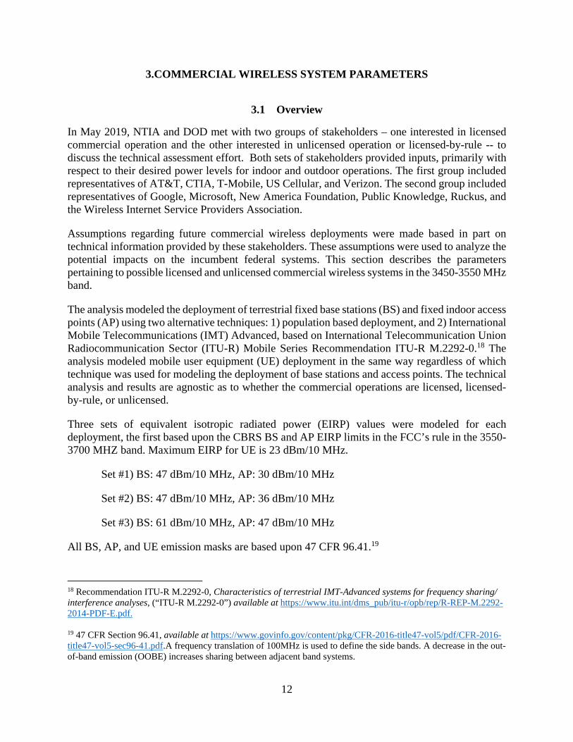
Three sets of equivalent isotropic radiated power (EIRP) values were modeled for each deployment, the first based upon the CBRS BS and AP EIRP limits in the FCC’s rule in the 3550-3700 MHZ band. Maximum EIRP for UE is 23 dBm/10 MHz.
Set #1) BS: 47 dBm/10 MHz, AP: 30 dBm/10 MHz
Set #2) BS: 47 dBm/10 MHz, AP: 36 dBm/10 MHz
Set #3) BS: 61 dBm/10 MHz, AP: 47 dBm/10 MHz
All BS, AP, and UE emission masks are based upon 47 CFR 96.41.19
18 Recommendation ITU-R M.2292-0, Characteristics of terrestrial IMT-Advanced systems for frequency sharing/ interference analyses, (“ITU-R M.2292-0”) available at https://www.itu.int/dms_pub/itu-r/opb/rep/R-REP-M.2292-2014-PDF-E.pdf. 19 47 CFR Section 96.41, available at https://www.govinfo.gov/content/pkg/CFR-2016-title47-vol5/pdf/CFR-2016-title47-vol5-sec96-41.pdf.A frequency translation of 100MHz is used to define the side bands. A decrease in the out-of-band emission (OOBE) increases sharing between adjacent band systems.

13
3.2 Population Based Deployment
Geographic Information System (GIS) 2011 National Land Cover Database (NLCD) data20 and 2010 U.S. Census population data were used to distribute terrestrial mobile systems.21 For each census tract, the NLCD area classification codes were collected for the entire area of the census tract, and then the census tract was classified by the highest occurring count of NLCD codes: dense urban (24), urban (23), suburban (22), and rural (21).
Assuming a mature deployment phase, a service penetration factor of 20 percent was assumed.22 To account for distribution of users across ten available 10 MHz channels in the 3450-3550 MHz band, a scaling factor of 10 percent was used to determine the number of effective users in each 10 MHz channel. For dense urban and urban census tracts, a daytime commuter factor of 1.31 was used. For suburban and rural census tracts, a daytime commuter factor of 1 was used, resulting in no increase or decrease in the population. The numbers of indoor AP and outdoor BS were calculated for each census tract, rounding up to the nearest whole number. Table 11 provides the population deployment parameters for indoor AP and outdoor BS. Equation 3 and Equation 4 are used to calculate the number of BSs and APs per census tract.
Table 11. Terrestrial Mobile Population Deployment Parameters
Area Type
Percent Users Served by Users per AP/BS
Indoor APs Outdoor BSs Indoor APs Outdoor BSs
Urban 80% 20% 50 200
Suburban 60% 40% 20 200
Rural 40% 60% 3 500
𝐵𝑆 𝑐𝑒𝑖𝑙𝑖𝑛𝑔
(3)
𝐴𝑃 𝑐𝑒𝑖𝑙𝑖𝑛𝑔𝑃𝑜𝑝 𝐶𝑆 𝐶𝐹 𝑆𝑃 𝑃𝑈𝑆
𝑈𝑠𝑒𝑟𝑠 (4)
20Multi-Resolution Land Characteristics (MRLC) Consortium, available at https://www.mrlc.gov/index.php. 21 United States Census Bureau, available at https://www.census.gov/geo/maps-data/data/tiger.html. 22 Service Penetration in this band takes the following assumptions into account: -A market penetration of 100% is assumed. -It is assumed that 2 of the 4 operators will use this band, and that each operator has equal market share. -It is assumed that each device and operator in this band typically supports other bands and may use this band 80% at a given time instance or for 80% of users at a given time instance.
𝑆𝑒𝑟𝑣𝑖𝑐𝑒𝑃𝑒𝑛𝑒𝑡𝑟𝑎𝑡𝑖𝑜𝑛2 𝑀𝑎𝑟𝑘𝑒𝑡𝑃𝑒𝑛𝑒𝑡𝑟𝑎𝑡𝑖𝑜𝑛
4 𝑇𝑜𝑡𝑎𝑙 𝑂𝑝𝑒𝑟𝑎𝑡𝑜𝑟𝑠𝑃𝑒𝑟𝑐𝑒𝑛𝑡𝑎𝑔𝑒𝑈𝑠𝑒𝑟

14
where:
𝑃𝑜𝑝 : the population of the census tract;
𝐶𝑆: channel scaling;
𝐶𝐹: commuter factor;
𝑆𝑃: service penetration;
𝑃𝑈𝑆: percentage of users served;
𝑈𝑠𝑒𝑟𝑠 : users served per base station;
𝑈𝑠𝑒𝑟𝑠 : users served per access point;
𝐵𝑆 : base stations per census tract;
𝐴𝑃 : access points per census tract.
The locations of the AP and BS were uniformly distributed within the census tract. Table 12 and Table 13 provides the terrestrial mobile parameters for the indoor AP and outdoor BS. For each AP and BS, the antenna height was uniformly distributed based upon the census tract NLCD classification. To account for BS/AP transmissions of a 50% duty cycle, a 3 dB reduction is applied to EIRP. Each BS uses three sectors with an azimuthal spacing of 120 degrees at each site.
Table 12. Indoor AP Parameters Parameter Dense Urban Urban Suburban Rural
Antenna Height [m]
50%: 3-15m 25%: 18-30m 25%: 33-60m
50%: 3m 50%: 6-18m
70%: 3m 30%: 6-12m
80%: 3m 20%: 6m
Sectorization 1 Sector Downtilt 0 degrees
Antenna Pattern Recommendation ITU-R F.1336 omni23 See Figure 1 for the Antenna Patterns
23 See Recommendation ITU-R F.1336-5, Reference radiation patterns of omnidirectional, sectoral and other antennas for the fixed and mobile service for use in sharing studies in the frequency range from 400 MHz to about 70 GHz, available at https://www.itu.int/dms_pubrec/itu-r/rec/f/R-REC-F.1336-5-201901-I!!PDF-E.pdf.

15
Figure 1. Access Point Antenna Gain Patterns
Table 13. Outdoor BS Parameters Parameter Dense Urban Urban Suburban Rural Antenna Height [m]
6-30 m 6-100 m
Sectorization 3 Sectors Downtilt 10 degrees 6 degrees
Antenna Pattern
Recommendation ITU-R F.133624 ka = 0.7 kp = 0.7 kh = 0.7 kv = 0.3 k = 0.7 Horizontal 3 dB beamwidth: 65 degrees Vertical 3 dB beamwidth: determined from the horizontal beamwidth by equations in Recommendation ITU-R F.1336. See Figure 2 and Figure 3 for the Antenna Patterns
24 ITU-R F.1336-5 Recommends using 3.1.

16
Macro Urban—Vertical Macro Urban—Vertical
Figure 2. Urban and Suburban Vertical Antenna Gain Pattern (showing downtilt)
Figure 3. Urban and Suburban Horizontal Antenna Gain Pattern

17
Figure 4 shows an example of population based deployment for the contiguous United States (CONUS).25 There are 423,730 indoor AP (red) and 74,004 outdoor BS (blue).26
Figure 4. Example population based deployment for the contiguous United States.
25 See https://www.census.gov/geo/maps-data/data/tiger.html for geographic data. 26 From the 74,002 census tracts, 72,539 are in CONUS. Of those 72,539 census tracts, 496 have zero population, resulting in 72,043 census tracts in the CONUS that have a population greater than zero.

18
3.3 IMT Advanced Deployment
Terrestrial IMT-Advanced BS and AP systems were generated according to Recommendation ITU-R M.2292-0. Figure 5 illustrates the geometry for a 3-sector deployment, and defines the parameters cell radius (A) and inter-site distance (B). Each cell (also referred to as a sector) is shown as a hexagon, and in this figure there are three cells/sectors per BS site. BS use three sectors with an azimuthal spacing of 120 degrees at each site. AP locations are randomized within the cell.
Figure 5. Geometry for 3-sector deployment
Figure 6. Example Macro layout of 19 cells

19
The following guidance related to deployments is provided in Recommendation ITU-R M.2292-0.
“Sharing studies using cell radii corresponding to urban and suburban deployment should take into account that those are only deployed in limited areas, central areas of large cities and suburban areas. Furthermore, rural deployments often do not cover all areas in a country/region, as coverage may be provided by other frequency bands, therefore assuming that rural cells which have complete coverage will overestimate interference in most of the cases.”27
Figure 7 shows the IMT Advanced deployment with a hex-grid pattern across the contiguous United States, within the designated Census Urban Areas28 with 409,994 BS and 1,096,946 AP. For each Census Urban Area, the NLCD area classification codes were collected for the entire area. Each Census Urban Area was designated by the highest occurring count of NLCD codes: urban (23 and 24) and suburban (21 and 22).
Figure 7. Example IMT Advanced BS deployment for the contiguous United States.
27 ITU-R M.2292-0, at page 5. 28 The 2010 United States Census data is available at https://www.census.gov/geo/maps-data/data/cbf/cbf_ua.html. The Census Bureau defines an urban area as any incorporated place that contains at least 2,500 people within its boundaries. A total of 3,601 urban areas are defined for the 2010 Census. The urban areas of the United States for the 2010 census represents 80.7% of the population. Additional information on Census Urban Areas is available at https://www.census.gov/geo/reference/ua/uafaq.html.

20
ITU-R M.2292 lists the deployment-related parameters for bands between 3 and 6 GHz. Table 14 shows the relevant information used in the feasibility study.
Table 14. ITU-R M.2292 Deployment-related parameters for bands between 3 and 6 GHz
Parameter Macro Suburban (BS)
Macro Urban (BS)
Indoor Urban (AP)
Cell Radius (Typical value to be used in sharing studies)
0.6 km 0.3 km 1 per suburban macro site 1 per urban macro sector
Antenna Height 25 m 20 m 3 m
Sectorization 3 Sectors 3 Sectors 1 Sector
Downtilt 6 degrees 10 degrees 0 degrees
Frequency reuse 1 1 1
Average Activity 50% 50% 50%
Antenna Pattern
Recommendation ITU-R F.133629 ka = 0.7 kp = 0.7 kh = 0.7 kv = 0.3 k = 0.7 Horizontal 3 dB beamwidth: 65 degrees Vertical 3 dB beamwidth: determined from the horizontal beamwidth by equations in Recommendation ITU-R F.1336. See Figure 2 and Figure 3 for the Antenna Patterns
ITU-R F.1336 omni See Figure 1 for the Antenna Patterns
29 ITU-R F.1336-5 at 4.

21
3.4 User Equipment Deployment
The UE deployment for the population based and IMT-Advanced deployments are the same. Assuming a Physical Downlink Control Channel (PDCCH), the number of simultaneously transmitting UE are 6 per sector for a 10 MHz channel. The location of the UEs are randomized within the sector/cell for each BS/AP. Table 15 shows the UE characteristics, which were based upon ITU-R M.2292-0.30 To account for UE transmissions of a 50% duty cycle, a 3 dB reduction is applied to the UE EIRP.
Table 15. ITU-R M.2292 UE Deployment-related parameters for bands between 3 and 6 GHz
Maximum UE Output Power
23 dBm
Typical Antenna Gain for UE
-4 dBi
Maximum UE EIRP 16 dBm /10MHz
Body Loss 4 dB
Antenna Height 1.5 m
30 ITU-R M.2292-0 at page 13.

22
4. ENGINEERING MODELS
4.1 Overview
This section describes the engineering models used in this feasibility study, including each of the losses for basic transmission, clutter, building penetration, and frequency dependent rejection (FDR).
4.2 Basic Transmission Loss
For the shipborne and ground-based radars, the Irregular Terrain Model (ITM) point-to-point mode was used to calculate the propagation loss using a 1 arc-second terrain database.31 The reliability was uniformly randomized from 0.1%-99.9%. Additional ITM parameters include:
- Polarization: Vertical - Dielectric constant: 25 - Conductivity: 0.02 S/m - Confidence: 50% - Mode of Variability: 13 (broadcast point-to-point) - Surface Refractivity: value varies by location and was derived by the methods and
associated data files in Recommendation ITU-R P.452.32 - Climate: value varies by location and was derived by the methods and associated
data files in Recommendation ITU-R P.617.33
For airborne radars, ITU-R P.528 was used to calculate the propagation loss for 50% of the time.34
31 See NTIA Report 82-100, A Guide to the Use of the ITS Irregular Terrain Model in the Area Prediction Mode (Apr. 1982), available at https://www.ntia.doc.gov/report/1982/guide-use-its-irregular-terrain-model-area-prediction-mode. 32 Recommendation ITU-R P.452-16, Prediction procedure for the evaluation of interference between stations on the surface of the Earth at frequencies above about 0.1 GHz (2015), available at https://www.itu.int/dms_pubrec/itu-r/rec/p/R-REC-P.452-16-201507-I!!PDF-E.pdf. 33 Recommendation ITU-R P.617-4 Propagation prediction techniques and data required for the design of trans-horizon radio-relay systems (2017), available at https://www.itu.int/dms_pubrec/itu-r/rec/p/R-REC-P.617-4-201712-I!!PDF-E.pdf. 34 Recommendation ITU-R P.528-3 Propagation curves for aeronautical mobile and radionavigation services using the VHF, UHF and SHF bands (2012), available at https://www.itu.int/dms_pubrec/itu-r/rec/p/R-REC-P.528-3-201202-I!!PDF-E.pdf. NTIA Institute for Telecommunication Sciences open sources P.528 software implementation is available at https://www.its.bldrdoc.gov/about-its/archive/2019/its-open-sources-p528-reference-software-implementation.aspx.

23
4.3 Clutter Loss
For the shipborne, airborne, and ground-based radars, clutter loss, 𝐿 , was calculated based upon a combination of Recommendation ITU-R P.210835 and Recommendation ITU-R P.452,36 which takes into consideration the height of the transmitter, the elevation angle between the transmitter and receiver, and the NLCD classification of the transmitter as a determination of the nominal height of the clutter.
To account for the relationship between the height of the transmitter and the nominal height of the clutter, Recommendation ITU-R P.452, Section 4.5 is used. Equation 5 is used to calculate the additional loss 𝐴 .
𝐴 10.25𝐹 ∙ 𝑒 1 𝑡𝑎𝑛ℎ 6ℎℎ
0.625 0.33 (5)
𝐹 0.25 0.375 1 𝑡𝑎𝑛ℎ 7.5 𝑓 0.5 (6)
Where 𝑑 is the distance (km) from nominal clutter point to the antenna, ℎ is the antenna height (m) of the transmitter above the local ground level, ℎ is the nominal clutter height (m) above the local ground level, and 𝑓 is the transmitter frequency (GHz). Table 16 has the values for ℎ and 𝑑 that were used in the feasibility study and provided by ITU-R P.452.
Table 16. ITU-R P.452 (Table 4) NLCD
Classification/Clutter Category
Nominal height 𝒉𝒂 (m) Nominal distance 𝒅𝒌
(km)
Rural 4 0.1 Suburban 9 0.025
Urban 20 0.02 Dense Urban 25 0.02
Figure 8 shows the calculated clutter loss as a function of transmitter height, at 3450 MHz for the four NLCD types.
35 Recommendation ITU-R P.2108-0 Prediction of clutter loss (06/2017) (“ITU-R P.2108”), available at https://www.itu.int/dms_pubrec/itu-r/rec/p/R-REC-P.2108-0-201706-I!!PDF-E.pdf. 36 ITU-R P. 452-16.

24
Figure 8. Example calculated clutter loss as a function of transmitter antenna height.
To expand the model to include ground-to-air clutter loss, the mathematical structure of Recommendation ITU-R P.2108, Section 3.3 was applied. As the elevation angle increases from 0 to 90 degrees, clutter goes to 0 dB. The curve-fitting constant in Equation 7 is then normalized to 1 in Equation 8.37
𝑐𝑢𝑟𝑣𝑒 𝑐𝑜𝑡 0.05 1𝜃
90𝜋𝜃
180 (7)
𝑛𝑜𝑟𝑚 𝑐𝑢𝑟𝑣𝑒 𝑚𝑖𝑛 𝑐𝑢𝑟𝑣𝑒
𝑚𝑎𝑥 𝑐𝑢𝑟𝑣𝑒 𝑚𝑖𝑛 𝑐𝑢𝑟𝑣𝑒
(8)
Figure 9 shows the normalized clutter loss as a function of elevation angle.
37 Report ITU-R P.2402-0, A method to predict the statistics of clutter loss for earth-space and aeronautical paths (2017), available at https://www.itu.int/dms_pub/itu-r/opb/rep/R-REP-P.2402-2017-PDF-E.pdf. The cotangent expression recognizes the dominance of specular reflection in the clutter loss, but instead of cot[πθ/180], which would give infinite loss at zero elevation angle, this is modified to cot[A1(1 – θ/90) + πθ/180], to give high loss at zero elevation angle, but a similar result to cot[πθ/180] at high θ. Thus A1 controls the loss at low θ, relatively independently of high θ, and a low value such as A1 = 0.05 is suggested.

25
Figure 9. Normalized Clutter Loss Constant
Equation 9 was used to calculate the clutter loss that includes the elevation angle from the transmitter to receiver.
𝐿 𝐴 𝑛𝑜𝑟𝑚 𝑑𝐵 (9)
4.4 Building Loss
A building penetration loss of 15 dB was applied to indoor APs only.38
4.5 Frequency Dependent Rejection
Frequency dependent rejection (FDR) accounts for the fact that not all of the transmitted energy from the BS, AP, or UE devices at the radar will reach the radar receiver’s detector or signal processor. FDR is a calculation of the amount of transmitter energy that is rejected by a victim receiver due to the intermediate frequency (IF) filtering in the radar receiver. This FDR attenuation is composed of two parts: on-tune rejection (OTR) and off-frequency rejection (OFR). The OTR is the rejection provided by a receiver’s 3 dB bandwidth to a co-tuned transmitter’s 3 dB bandwidth
38 Report ITU-R P.2109-1, Prediction of building entry loss (08/2019), available at https://www.itu.int/dms_pubrec/itu-r/rec/p/R-REC-P.2109-1-201908-I!!PDF-E.pdf.

26
and the OFR is calculated by using the receiver’s IF selectivity and the transmitters emission spectra. The radar receiver IF selectively and 3 dB bandwidth data for the federal systems was obtained from the agencies. A detailed description of how to compute FDR can be found in Recommendation ITU-R SM.337-4.39
39 Recommendation ITU-R SM.337-4, Frequency and Distance Separations, available at https://www.itu.int/dms_pubrec/itu-r/rec/sm/R-REC-SM.337-4-199710-S!!PDF-E.pdf.

27
5. SHARING WITH AIRBORNE SYSTEMS
5.1 Overview
This section shows how the aggregate interference from BSs, APs, and UEs operating in a co-channel or an adjacent-channel band to the airborne systems was computed. To mitigate the aggregate interference to the nationwide systems (Airborne Systems 1 and 2), the maximum BS EIRP was calculated, i.e., the EIRP that would not cause aggregate interference to exceed the IPC. To mitigate the aggregate interference to the more localized operations of Airborne System 3, static exclusion zones and dynamic coordination zones were analyzed.
5.2 Base Station EIRP Limit for Airborne System 1 and 2
This section calculates the maximum allowable BS EIRP, keeping the AP and UE EIRP constant, that would not cause aggregate interference to exceed the protection criteria of Airborne System 1 and Airborne System 2. The three AP EIRP levels from Section 3.1 were used, 30 dBm/10 MHz, 36 dBm/10 MHz, and 47 dBm/10 MHz.
5.2.1 BS EIRP Limit Methodology
The following steps were used to calculate the maximum BS EIRP that would not cause aggregate interference to the receiver to exceed the S/I interference protection criteria when the aircraft is at altitudes of 500 ft., 1,000 ft., 2,000 ft., 3,000 ft., and 4,000 ft. above ground level (AGL).
Step 1: A layout of outdoor BSs, indoor APs, and associated UEs was generated across the entire CONUS and the elevation above mean sea level was determined for each one.40
Step 2: Simulation points were generated across CONUS for aircraft at altitudes of 500 ft., 1,000 ft., 2,000 ft., 3,000 ft., and 4,000 ft. AGL.
Step 3: The aggregate interference power level at each simulation point was calculated, incrementing the EIRP of all outdoor BS from 20 dBm/10 MHz to 61 dBm/10 MHz and keeping the AP and UE EIRP constant.
The aggregate interference power level at a single simulation point for a single aircraft altitude was calculated using the following steps:
Step 3a: The BSs, APs, and associated UEs within 600 km of the simulation point, at ground level, were determined.
Step 3b: For each BS/AP/UE, the slant range, azimuth, and elevation angle between the transmitter antenna and the airborne system antenna, in a spherical system (e.g., not assuming flat earth), was calculated.
40 See https://www.census.gov/geo/maps-data/data/tiger.html for geographic data.

28
Step 3c: The BS/AP/UE antenna loss in the direction (azimuth and elevation) of the airborne system was calculated.
Step 3d: The path loss, Equation 10, from the BS/AP/UE to the airborne system receiver using Recommendation ITU-R P.528 was calculated. Clutter loss and building loss were added when applicable.41
𝐿 𝐿 𝐿 𝐿 (10)
where:
𝐿 : path loss calculated from ITU-R P.528;
𝐿 : calculated clutter loss (See Equation 9); and
𝐿 : 15dB of building loss.
Step 3e: Using Equation 11, the received power at the input of an airborne system receiver from a single BS/AP/UE was calculated.
𝑃 𝐸𝐼𝑅𝑃 𝐿 𝐺𝑎𝑖𝑛 𝐿𝑜𝑠𝑠 𝐹𝐷𝑅 (11)
where:
𝑃 : received power at the receiver (dBm/10 MHz);
𝐸𝐼𝑅𝑃: equivalent isotropic radiated power of the BS/AP/UE (dBm/10 MHz), including antenna gain;
𝐺𝑎𝑖𝑛 : gain of the airborne system antenna in the direction (azimuth and elevation) of the transmitter (dBi);
𝐿𝑜𝑠𝑠 : loss of the BS/AP/UE antenna in the direction (azimuth and elevation) of the transmitter (dBi); see Figure 1, Figure 2, and Figure 3 for the antenna patterns;
𝐹𝐷𝑅 : Co-channel FDR (Section 4.5) was set to 0 dB. Adjacent-channel FDR was calculated using the frequency separation between the airborne system and the BS/AP/UE, the airborne system receiver selectivity, and the BS/AP/UE transmission mask.
Step 3f: Separately calculate the aggregate interference to the omni-directional and directional antenna for each airborne system, with 1 degree position increments for the directional antenna.
41 See ITU-R P.528-3.

29
Step 4: For all simulation points for a single aircraft altitude, the 99th percentile BS EIRP that does not cause interference to the airborne system was calculated.
5.2.2 BS EIRP Limit Results
Table 17 and Table 18 show the maximum BS EIRP for which the aggregate interference would not exceed the interference protection criterion for each airborne system channel at an altitude from 500 ft. to 4,000 ft. AGL, based on the aggregate power of all BS being set to that EIRP. For example in Table 17, the BS operating frequencies would be 3520-3550 MHz. If the BS has an EIRP of 61 dBm/10MHz, Airborne Channels 1, 2, and 3 would not have interference. Airborne Channel 4 could experience interference in some geographic regions, primarily those with high population centers. Appendix A provides additional results.
5.2.2.1 30 Megahertz Sharing Option
5.2.2.1.1 IMT-Advanced
Table 17. BS EIRP Limit, 30 Megahertz Sharing Option AP EIRP
dBm/10MHz Airborne Channel 1
Airborne Channel 2
Airborne Channel 3
Airborne Channel 4
30 61dBm/10MHz 61 dBm/10MHz 61 dBm/10MHz 41 dBm/10MHz 36 61dBm/10MHz 61 dBm/10MHz 61 dBm/10MHz 41 dBm/10MHz 47 61dBm/10MHz 61 dBm/10MHz 61 dBm/10MHz 40 dBm/10MHz
5.2.2.2 100 Megahertz Sharing Option
5.2.2.2.1 IMT-Advanced
Table 18. BS EIRP Limit, 100 Megahertz Sharing Option AP EIRP
dBm/10MHz Airborne Channel 1
Airborne Channel 2
Airborne Channel 3
Airborne Channel 4
30 61 dBm/10MHz 61 dBm/10MHz 33 dBm/10MHz 33 dBm/10MHz 36 61 dBm/10MHz 61 dBm/10MHz 32 dBm/10MHz 32 dBm/10MHz 47 61 dBm/10MHz 61 dBm/10MHz N/A+ N/A+
+ There does not exist a BS EIRP that would not cause interference to Airborne Channels 3 and 4. Additionally, with just the AP transmitting at an EIRP of 47dBm/10MHz, there is interference to Airborne Channels 3 and 4.

30
5.3 Static Exclusion Zones for Airborne System 3
This section shows the calculation of static exclusion zones to protect the Airborne System 3 from aggregate interference.
5.3.1 Static Exclusion Zones Analysis Methodology
The following steps were used to calculate the static exclusion zone for the Airborne System 3. A single simulation was defined as one terrestrial deployment. A total of 1,000 deployments with outdoor BS, indoor AP, and UE placement were run to calculate a single exclusion zone.
Step 1: A layout of BSs/APs/UEs was generated around the area, projected onto the ground, of the airspace, 600 km for BS and AP, and associated UEs for each BS and AP.
Step 2: Simulation points were generated throughout the volume of the airspace, with a separation distance of 1 km on the horizontal plane, and at intervals of 500 ft. in altitude of the airspace.
Step 3: For all simulation points, the BS and AP, and their associated UEs were turned off until the aggregate interference was below the airborne system threshold. The airborne antenna parameters (Section 2.6) were taken into consideration for the calculation. Co-channel FDR (Section 4.5) was set to 0 dB, because the bandwidth of the receiver is greater than the bandwidth of the transmitter.
At each simulation point, the following method was used to calculate the aggregate interference. For each BS/AP/UE, the slant range, azimuth, and elevation angle between the transmitter antenna and airborne antenna, in a spherical system (i.e., not assuming flat earth) was calculated. The BS/AP/UE antenna loss in the direction (azimuth and elevation) of the airborne antenna was calculated. The path loss, Equation 12, from each BS/AP/UE to the airborne radar receiver using Recommendation ITU-R P.528 was calculated. Clutter loss and building loss were added when applicable. 42
𝐿 𝐿 𝐿 𝐿 (12) where:
𝐿 : path loss calculated from ITU-R P.528;
𝐿 : calculated clutter loss (See Equation 9); and
𝐿 : 15dB of building loss.
Using Equation 13 the received power at the input of the airborne system receiver from a single BS/AP/UE was calculated.
𝑃 𝐸𝐼𝑅𝑃 𝐿 𝐺𝑎𝑖𝑛 𝐿𝑜𝑠𝑠 (13)
42 ITU-R P.528-3.

31
where:
𝑃 : received power at the receiver (dBm/10 MHz);
𝐸𝐼𝑅𝑃: equivalent isotropic radiated power of the BS/AP/UE (dBm/10 MHz), including antenna gain;
𝐺𝑎𝑖𝑛 : gain of the airborne system antenna in the direction (azimuth and elevation) of the transmitter (dBi);
𝐿𝑜𝑠𝑠 : loss of the BS/AP/UE antenna in the direction (azimuth and elevation) of the transmitter (dBi); see Figure 1, Figure 2, and Figure 3 for the antenna patterns.
The aggregate interference was calculated by converting each 𝑃 into 𝑃 , using Equation 14 and then adding the 𝑃 from each BS/AP/UE, using Equation 15, where n is the number of BS/AP/UE transmitters, and converting the aggregate power receiver, 𝑃 , to
dBm/10MHz, using Equation 16.
𝑃 10 (14)
𝑃 𝑃 (15)
𝑃 𝑙𝑜𝑔 𝑃 30 (16)
Step 4: Calculate the BS turn off list and AP turn off list for all Airborne System 3 positions/orientations, in which the aggregate interference will not cause interference in the receiver.
Step 5: Create the union for the BS turn off list and for the AP turn off list for all simulation points.
Step 6: Step 1 through Step 4 was calculated 1,000 times and then compiled with the BS/AP turned off from each simulation. 1,000 simulations represent 1,000 randomized BS/AP deployments.
Step 7: The separation distance from the boundary of the airspace, projected onto the ground, to each individual BS and AP that was turned off. The 95th percentile turn off distance for the BS and for the AP was then calculated.

32
Step 8: The exclusion zone, projected onto the ground, is the area around all BS/AP that were turned off and are within the 95th percentile turn off distance, adding an additional 1 km buffer, ensuring a minimum 1 km exclusion zone.
5.3.2 Results
For the Airborne System 3, the 30 Megahertz and 100 Megahertz sharing analysis options produce the same results because the Airborne System 3 and commercial deployment were co-channel. For each frequency sharing option and set of EIRPs, the plots show the airborne system exclusion zones (BS and AP) plotted for all airborne system locations (in the contiguous United States). The population impact figures are provided in Appendix A.

33
5.3.2.1 Population Based Deployment
Figure 10. Airborne 3 Exclusion Zone: BS EIRP: 47 dBm/10 MHz, AP EIRP: 30 dBm/10 MHz
100 Megahertz Sharing Option and Population Deployment

34
Figure 11. Airborne 3 Exclusion Zone: BS EIRP: 47 dBm/10 MHz, AP EIRP: 36 dBm/10 MHz
100 Megahertz Sharing Option and Population Deployment

35
Figure 12. Airborne 3 Exclusion Zone: BS EIRP: 61 dBm/10 MHz, AP EIRP: 47 dBm/10 MHz
100 Megahertz Sharing Option and Population Deployment

36
5.3.2.2 ITM-Advanced Deployment
Figure 13. Airborne 3 Exclusion Zone: BS EIRP: 47 dBm/10 MHz, AP EIRP: 30 dBm/10 MHz
100 Megahertz Sharing Option and IMT-Advanced Deployment

37
Figure 14. Airborne 3 Exclusion Zone: BS EIRP: 47 dBm/10 MHz, AP EIRP: 36 dBm/10 MHz
100 Megahertz Sharing Option and IMT-Advanced Deployment

38
Figure 15. Airborne 3 Exclusion Zone: BS EIRP: 61 dBm/10 MHz, AP EIRP: 47 dBm/10 MHz
100 Megahertz Sharing Option and IMT-Advanced Deployment

39
5.4 Dynamic Coordination Zones for Airborne System 3
This section describes how the dynamic coordination zones would be used to protect the Airborne System 3 from aggregate interference. A dynamic coordination zone would be a pre-defined protection area that would be used to protect the federal incumbent while providing flexibility for commercial operations. A geographic area would define the boundaries of the dynamic coordination zone as coordinates of a polygon or as a single point. An activated dynamic coordination zone would be protected from the aggregate interference from outdoor BSs, indoor APs, and UEs based on specified protection criteria for the dynamic coordination zone.
A dynamic coordination zone would be activated by multiple mechanisms. Three possible mechanisms include:
- an always activated dynamic coordination zone, - an activated dynamic coordination zone by the means of a spectrum sensing device, - an activated dynamic coordination zone by the means of an incumbent informing (e.g.,
scheduling) system.
The dynamic coordination zone neighborhood would be defined as the area around which the commercial deployment of the BS and AP is taken into consideration when calculating which devices must not use the impacted frequencies to protect the federal incumbent using these frequencies. The dynamic coordination zone neighborhood should be calculated using the actual AP and BS commercial deployment (that information would be assumed to be available).
5.4.1 Dynamic Coordination Zone Neighborhood Methodology
The following steps were used to calculate the dynamic coordination zone neighborhoods.
Step 1: A deployment of outdoor BS and indoor AP, and associated UEs, was generated within 600 km distance of each dynamic coordination zone.
Step 2: Protection points were generated throughout the volume of the airspace, with a separation distance of 1 km on the horizontal plane, and at intervals of 500 ft. in altitude of the airspace.
Step 3: Keeping the AP neighborhood distance constant, the BS neighborhood distance was varied until the minimum sufficient BS neighborhood distance was calculated. A sufficient nieghborhood distance was defined as the consideration area for which the aggregate interference is less than or equal to the airborne system interference threshold.
For example, keeping the AP neighborhod distance at 600 km and a BS the same, at each protection point for each BS and AP in the BS/AP area, the aggregate interference was calculated using Equation 12 to Equation 16. Clutter loss (Section 4.3) and building loss (Section 4.4) were added where applicable. BS and AP, and their associated UEs were turned off until the aggregate interference was below the airborne system interference protection threshold. The airborne antenna parameters (Section 2.6) were taken into consideration for the calculation. Co-channel FDR (Section 4.5) was set to 0 dB.

40
The union of the turn off lists for all protection points was created. The BSs and APs, and their associated UEs were turned off if they were in the union of the turn off lists. If the aggregate interference at each protection point was less than the airborne system threshold, then the BS neighborhood radius was decreased; otherwise the BS neighborhood radius was increased.
Step 4: Keeping the BS neighborhood distance constant, the AP neighborhood distance was varied until the minimum sufficient AP neighborhood distance was calculated. A sufficient neighborhood distance was defined as the consideration area for which the 95th percentile aggregate interference was less than or equal to the airborne system interference threshold.
5.4.2 Results
For the Airborne System 3, the 30 MHz and 100 MHz sharing analysis options produce the same results because the Airborne System 3 and commercial deployment would be co-channel. For each frequency sharing option and set of EIRPs, the dynamic coordination zone neighborhoods (BS and AP) were plotted for all Airborne System 3 locations (in the contiguous United States). The estimated population impact figures are provided in Appendix A.

41
5.4.2.1 Population Deployment
Figure 16. Airborne 3 Dynamic Coordination Zone Neighborhood: BS EIRP: 47 dBm/10 MHz, AP EIRP: 30 dBm/10 MHz,
100 Megahertz Sharing Option and Population Deployment

42
Figure 17. Airborne 3 Dynamic Coordination Zone Neighborhood: BS EIRP: 47 dBm/10 MHz, AP EIRP: 36 dBm/10 MHz,
100 Megahertz Sharing Option and Population Deployment

43
Figure 18. Airborne 3 Dynamic Coordination Zone Neighborhood: BS EIRP: 61 dBm/10 MHz, AP EIRP: 47 dBm/10 MHz,
100 Megahertz Sharing Option and Population Deployment

44
5.4.2.2 IMT-Advanced
Figure 19. Airborne 3 Dynamic Coordination Zone Neighborhood: BS EIRP: 47 dBm/10 MHz, AP EIRP: 30 dBm/10 MHz,
100 Megahertz Sharing Option and IMT-Advanced Deployment

45
Figure 20. Airborne 3 Dynamic Coordination Zone Neighborhood: BS EIRP: 47 dBm/10 MHz, AP EIRP: 36 dBm/10 MHz,
100 Megahertz Sharing Option and IMT-Advanced Deployment

46
Figure 21. Airborne 3 Dynamic Coordination Zone Neighborhood: BS EIRP: 61 dBm/10 MHz, AP EIRP: 47 dBm/10 MHz, 100 Megahertz Sharing Option and IMT-Advanced Deployment

47
6. SHARING WITH GROUND-BASED RADARS
6.1 Overview
This section shows how the aggregate interference power from BSs, APs, and UEs, operating in a co-channel or an adjacent-channel band to ground-based radars, was calculated and how it would be mitigated using static exclusion zones and dynamic coordination zones, as illustrated on the maps below.
6.2 Static Exclusion Zones
This section shows how the static exclusion zones that would protect the ground-based radars from aggregate interference were calculated.
6.2.1 Static Exclusion Zones Analysis Methodology
The following steps were used to calculate the static exclusion zones for a ground-based radar. A single simulation is defined as one terrestrial deployment. A total of 1,000 deployments with outdoor BS, indoor AP, and UE placements were simulated to calculate a single exclusion zone.
Step 1: A commercial deployment was generated around the military installation, within 600 km for BSs and their associated UEs, and within 250 km for APs and their associated UEs. Figure 22 shows an example of the commercial deployment area for the military base Naval Air Station (NAS) Oceana.
Figure 22. Example Commercial Deployment Area

48
Step 2: Protection points were generated around the outer edge of the military installation with a separation distance of 0.5 km. Figure 23 shows example protection points (red points) for the military base NAS Oceana (black line).
Figure 23. Example protection points for NAS Oceana
Step 3: At each protection point, 2,000 Monte Carlo path loss iterations were generated for each BS/AP/UE using ITM with its reliability setting uniformly randomized from 0.1%-99.9% (Section 4.2). Clutter loss (Section 4.3) and building loss (Section 4.4) were added when applicable. BS, AP, and their associated UEs were turned off until the 95th percentile aggregate interference of the Monte Carlo iterations is below the ground-based radar threshold. The ground-based radar antenna parameters (Section 2.6) were taken into consideration for the calculation. Co-channel FDR (Section 4.5) is set to 0 dB. Adjacent-channel FDR is calculated using the frequency separation between the ground-based radar receiver and the BS/AP/UE transmitter, the ground-based radar receiver IF selectivity, and the BS/AP/UE transmission mask. Equation 17 through Equation 21 provide details about the link budget to calculate the aggregate interference. The BS/AP/UE turn off algorithm was based upon Working Document WINNF-TS-0112.43
43 Wireless Innovation Forum (WInnForum) Requirements for Commercial Operation in the U.S. 3550-3700 MHz Citizens Broadband Radio Service Band, Working Document WINNF-TS-0112 Version V1.4.1 (Jan. 16 2018), WInnForum Working Document, available at https://workspace.winnforum.org/higherlogic/ws/public/download/5116/WINNF-TS-0112-V1.4.1%20CBRS%20Operational%20and%20Functional%20Requirements.pdf.

49
𝐿 𝐿 𝐿 𝐿 (17) where:
𝐿 : path loss calculated from ITM; (See Section 4.2)
𝐿 : calculated clutter loss (See Equation 9); and
𝐿 : 15dB of building loss.
Using Equation 18, the received power at the input of a radar receiver from a single BS/AP/UE was calculated.
𝑃 𝐸𝐼𝑅𝑃 𝐿 𝐺𝑎𝑖𝑛 𝐿𝑜𝑠𝑠 𝐹𝐷𝑅 (18) where:
𝑃 : received power at the receiver (dBm/10 MHz);
𝐸𝐼𝑅𝑃: equivalent isotropic radiated power of the BS/AP/UE (dBm/10 MHz), including antenna gain;
𝐺𝑎𝑖𝑛 : gain of the radar antenna in the direction (azimuth and elevation) of the transmitter (dBi);
𝐿𝑜𝑠𝑠 : loss of the BS/AP/UE antenna in the direction (azimuth and elevation) of the transmitter (dBi); see Figure 1, Figure 2, and Figure 3 for the antenna patterns.
𝐹𝐷𝑅 : Co-channel FDR (Section 4.5) is set to 0 dB. Adjacent-channel FDR was calculated using the frequency separation between the radar receiver and the BS/AP/UE transmitter, the radar receiver IF selectivity, and the BS/AP transmission mask.
The aggregate interference was calculated by converting each 𝑃 into 𝑃 , using Equation 19, and then adding the 𝑃 from each BS/AP/UE, using Equation 20, and converting the aggregate power receiver, 𝑃 , to dBm/10MHz, using Equation 21.
𝑃 10 (19)
𝑃 𝑃 (20)
𝑃 𝑙𝑜𝑔 𝑃 30 (21)

50
Step 4: The union for the BS turn off list and for the AP turn off list for all simulation points was calculated.
Step 5: Step 1 through Step 4 was calculated 1,000 times and then compiled with the BS/AP turned off from each simulation. 1,000 simulations represent 1,000 randomized BS/AP deployments.
Step 6: The separation distance from the boundary of the military installation to each individual BS/AP was calculated and the 95th percentile turn off distance for the BS and for the AP was calculated.
Step 7: The exclusion zone consists of the area around which all BSs/APs that were turned off and are within the 95th percentile turn off distance, adding an additional 1 km buffer, ensuring a minimum 1 km exclusion zone was drawn.
6.2.2 Results
For each frequency sharing option and set of EIRPs, the plots in Figure 24 through Figure 35 show the ground-based exclusion zones (BS and AP) plotted for all ground-based radars (in the contiguous United States). The population impact figures are provided in Appendix B.

51
6.2.2.1 30 Megahertz Sharing Analysis Option
6.2.2.1.1 Population Deployment
Figure 24. Ground Based Exclusion Zone: BS EIRP: 47 dBm/10 MHz, AP EIRP: 30 dBm/10 MHz
30 Megahertz Sharing Option and Population Deployment

52
Figure 25. Ground Based Exclusion Zone: BS EIRP: 47 dBm/10 MHz, AP EIRP: 36 dBm/10 MHz
30 Megahertz Sharing Option and Population Deployment

53
Figure 26. Ground Based Exclusion Zone: BS EIRP: 61 dBm/10 MHz, AP EIRP: 47 dBm/10 MHz
30 Megahertz Sharing Option and Population Deployment

54
6.2.2.1.2 IMT-Advanced
Figure 27. Ground Based Exclusion Zone: BS EIRP: 47 dBm/10 MHz, AP EIRP: 30 dBm/10 MHz
30 Megahertz Sharing Option and IMT-Advanced Deployment

55
Figure 28. Ground Based Exclusion Zone: BS EIRP: 47 dBm/10 MHz, AP EIRP: 36 dBm/10 MHz
30 Megahertz Sharing Option and IMT-Advanced Deployment

56
Figure 29. Ground Based Exclusion Zone: BS EIRP: 61 dBm/10 MHz, AP EIRP: 47 dBm/10 MHz
30 Megahertz Sharing Option and IMT-Advanced Deployment

57
6.2.2.2 100 Megahertz Sharing Analysis Option
6.2.2.2.1 Population Deployment
Figure 30. Ground Based Exclusion Zone: BS EIRP: 47 dBm/10 MHz, AP EIRP: 30 dBm/10 MHz
100 Megahertz Sharing Option and Population Deployment

58
Figure 31. Ground Based Exclusion Zone: BS EIRP: 47 dBm/10 MHz, AP EIRP: 36 dBm/10 MHz
100 Megahertz Sharing Option and Population Deployment

59
Figure 32. Ground Based Exclusion Zone: BS EIRP: 61 dBm/10 MHz, AP EIRP: 47 dBm/10 MHz
100 Megahertz Sharing Option and Population Deployment

60
6.2.2.2.2 IMT-Advanced
Figure 33. Ground Based Exclusion Zone: BS EIRP: 47 dBm/10 MHz, AP EIRP: 30 dBm/10 MHz
100 Megahertz Sharing Option and IMT-Advanced Deployment

61
Figure 34. Ground Based Exclusion Zone: BS EIRP: 47 dBm/10 MHz, AP EIRP: 36 dBm/10 MHz
100 Megahertz Sharing Option and IMT-Advanced Deployment

62
Figure 35. Ground Based Exclusion Zone: BS EIRP: 61 dBm/10 MHz, AP EIRP: 47 dBm/10 MHz
100 Megahertz Sharing Option and IMT-Advanced Deployment

63
6.3 Dynamic Coordination Zone Neighborhood
This section describes how the dynamic coordination zones would be used to protect the ground-based radars from aggregate interference. A dynamic coordination zone would be a pre-defined protection area that can be used to protect the federal incumbent, providing flexibility for commercial operations. The boundaries of the dynamic coordination zone are defined as a list of coordinates comprising of an enclosed polygon or a single point. An activated dynamic coordination zone would be protected from aggregate interference from outdoor BSs, indoor APs, and UEs based on specified protection criteria to the dynamic coordination zone.
A dynamic coordination zone could be activated by multiple mechanisms. Three possible mechanisms include:
- an always activated dynamic coordination zone, - an activated dynamic coordination zone by the means of a spectrum sensing device, - an activated dynamic coordination zone by the means of an incumbent-informing (e.g.,
scheduling) system.
When a dynamic coordination zone is activated, the associated neighborhood contains the commercial deployment of the BS and AP, which is to be taken into consideration when calculating which devices need to be turned off to protect the federal incumbent from aggregate interference. The aggregate interference throughout dynamic coordination zones will be calculated using the actual AP and BS commercial deployment when that information is available.
6.3.1 Dynamic Coordination Zone Neighborhood Methodology
The following steps were used to calculate the dynamic coordination zone neighborhoods.
Step 1: For each dynamic coordination zone, a deployment of outdoor BSs was generated within 600 km and indoor APs within 250 km, and UEs for each BS and AP. Figure 36 shows an example of the commercial deployment area for the military base NAS Oceana.

64
Figure 36. Example Commercial Deployment Area
Step 2: Protection points were generated around the outer edge of the military installation with a separation distance of 0.5 km. Figure 37 shows example protection points (red points) for the military base NAS Oceana (black line).

65
Figure 37. Example protection points for NAS Oceana
Step 3: Keeping the AP area constant, the BS area was varied until the minimum sufficient BS area distance was calculated. A sufficient area distance was defined as the consideration area for which the 95th percentile aggregate interference was less than or equal to the radar interference threshold.
For example, keeping the AP neighborhood distance at 250 km and a BS neighborhood distance at 600 km, the 95th percentile aggregate interference is calculated using 2,000 Monte Carlo trials at each protection point (Figure 37). For each BS/AP/UE, the ITM reliability was uniformly randomized from 0.1%-99.9% (Section 4.2). Clutter loss (Section 4.3) and building loss (Section 4.4) were added when applicable. Equation 17 through Equation 21 provide details about the link budget to calculate the aggregate interference. The BS/AP/UE turn off algorithm was based on Working Document WINNF-TS-0112.
BSs and APs, and their associated UEs were turned off until the aggregate interference was below the ground-based radar threshold. The ground-based radar antenna parameters (Section 2.6) were taken into consideration for the calculation. Co-channel FDR (Section 4.5) was set to 0 dB. Adjacent-channel FDR was calculated using the frequency separation between the ground-based radar and the BS/AP/UE, the ground-based radar receiver selectivity, and the BS/AP/UE transmission mask.

66
The union of the turn off list for all protection points was created. The BSs and APs, and their associated UEs were turned off if they were in the union of the turn off list. The aggregate interference was calculated at each protection point, using a protection Monte Carlo percentile of 95% with a minimum of 2,000 trials, in which the ITM reliability was uniformly randomized from 0.1%-99.9%. Clutter loss and building loss were added when applicable. The ground-based radar antenna parameters were taken into consideration for the calculation. If the aggregate interference at each protection point was less than the ground-based radar threshold, then the BS neighborhood distance was decreased; otherwise, the BS neighborhood distance was increased.
Step 4: Keeping the BS neighborhood distance constant, the AP neighborhood distance was varied until the minimum sufficient AP neighborhood distance was calculated. A sufficient neighborhood distance is defined as the consideration area for which the 95th percentile aggregate interference is less than or equal to the radar interference threshold.
6.3.2 Results
For each frequency sharing option (i.e., 30 megahertz and 100 megahertz) and set of EIRPs, the plots in Figure 38 through Figure 49 show the dynamic coordination zone areas (BS and AP) plotted for all ground-based radars (in the contiguous United States). The population impact figures are provided in Appendix B.

67
6.3.2.1 30 Megahertz Sharing Analysis Option
6.3.2.1.1 Population Deployment
Figure 38. Ground Based Dynamic Coordination Zone Neighborhood: BS EIRP: 47 dBm/10 MHz, AP EIRP: 30 dBm/10 MHz
30 Megahertz Sharing Option and Population Deployment

68
Figure 39. Ground Based Dynamic Coordination Zone Neighborhood: BS EIRP: 47 dBm/10 MHz, AP EIRP: 36 dBm/10 MHz
30 Megahertz Sharing Option and Population Deployment

69
Figure 40. Ground Based Dynamic Coordination Zone Neighborhood: BS EIRP: 61 dBm/10 MHz, AP EIRP: 47 dBm/10 MHz
30 Megahertz Sharing Option and Population Deployment

70
6.3.2.1.2 MT-Advanced
Figure 41. Ground Based Dynamic Coordination Zone Neighborhood: BS EIRP: 47 dBm/10 MHz, AP EIRP: 30 dBm/10 MHz
30 Megahertz Sharing Option and IMT-Advanced Deployment

71
Figure 42. Ground Based Dynamic Coordination Zone Neighborhood: BS EIRP: 47 dBm/10 MHz, AP EIRP: 36 dBm/10 MHz
30 Megahertz Sharing Option and IMT-Advanced Deployment

72
Figure 43. Ground Based Dynamic Coordination Zone Neighborhood: BS EIRP: 61 dBm/10 MHz, AP EIRP: 47 dBm/10 MHz
30 Megahertz Sharing Option and IMT-Advanced Deployment

73
6.3.2.2 100 Megahertz Sharing Analysis Option
6.3.2.2.1 Population Deployment
Figure 44. Ground Based Dynamic Coordination Zone Neighborhood: BS EIRP: 47 dBm/10 MHz, AP EIRP: 30 dBm/10 MHz
100 Megahertz Sharing Option and Population Deployment

74
Figure 45. Ground Based Dynamic Coordination Zone Neighborhood: BS EIRP: 47 dBm/10 MHz, AP EIRP: 36 dBm/10 MHz
100 Megahertz Sharing Option and Population Deployment

75
Figure 46. Ground Based Dynamic Coordination Zone Neighborhood: BS EIRP: 61 dBm/10 MHz, AP EIRP: 47 dBm/10 MHz
100 Megahertz Sharing Option and Population Deployment

76
6.3.2.2.2 IMT-Advanced
Figure 47. Ground Based Dynamic Coordination Zone Neighborhood: BS EIRP: 47 dBm/10 MHz, AP EIRP: 30 dBm/10 MHz
100 Megahertz Sharing Option and IMT-Advanced Deployment

77
Figure 48. Ground Based Dynamic Coordination Zone Neighborhood: BS EIRP: 47 dBm/10 MHz, AP EIRP: 36 dBm/10 MHz
100 Megahertz Sharing Option and IMT-Advanced Deployment

78
Figure 49. Ground Based Dynamic Coordination Zone Neighborhood: BS EIRP: 61 dBm/10 MHz, AP EIRP: 47 dBm/10 MHz
100 Megahertz Sharing Option and IMT-Advanced Deployment

79
7. SHARING WITH SHIPBORNE RADARS
7.1 Overview
This section shows how the aggregate power from BS, AP, and UE operating in a co-channel band to the shipborne radar was calculated. To mitigate aggregate interference to the federal incumbent, static exclusion zones and dynamic coordination zones were analyzed.
7.2 Static Exclusion Zones
This section shows how static exclusion zones were calculated to protect the shipborne radars from aggregate interference.
7.2.1 Static Exclusion Zone Analysis Methodology
The following steps were used to calculate the exclusion zone for a shipborne radar. A single simulation is defined as one terrestrial deployment. A total of 1,000 deployments with outdoor BS and indoor AP placement and associated UEs were run to calculate a single exclusion zone.
Step 1: Simulation points were chosen based upon the operational parameters of the shipborne radar. Simulation points were chosen at Navy ports and 10 km off the east, west, and gulf coast.
Step 2: For each simulation point, a deployment of outdoor BSs was generated within 600 km, indoor APs within 250 km, and UEs for each BS and AP. At each simulation point, 2,000 Monte Carlo path loss iterations were generated for each BS/AP/UE, in which ITM reliability was uniformly randomized from 0.1%-99.9% (Section 4.2). Clutter loss (Section 4.3) and building loss (Section 4.4) were added when applicable. BSs, APs, and their associated UEs were turned off until the 95th percentile aggregate interference of the Monte Carlo iterations was below the shipborne radar threshold. The shipborne radar antenna parameters (Section 2.6) were taken into consideration for the calculation. Co-channel FDR (Section 4.5) was set to 0 dB. Equation 22 through Equation 26 provide the link budget details to calculate the aggregate interference. The BS/AP turn off algorithm was based on Working Document WINNF-TS-0112.
𝐿 𝐿 𝐿 𝐿 (22) where:
𝐿 : path loss calculated from ITM; (See Section 4.2)
𝐿 : calculated clutter loss (See Equation 9); and
𝐿 : 15dB of building loss.
Using Equation 23, the received power at the input of a radar receiver from a single BS/AP/UE was calculated.
𝑃 𝐸𝐼𝑅𝑃 𝐿 𝐺𝑎𝑖𝑛 𝐿𝑜𝑠𝑠 𝐹𝐷𝑅 (23)

80
where:
𝑃 : received power at the receiver (dBm/10 MHz);
𝐸𝐼𝑅𝑃: equivalent isotropically radiated power of the BS/AP/UE (dBm/10 MHz), including antenna gain;
𝐺𝑎𝑖𝑛 : gain of the radar antenna in the direction (azimuth and elevation) of the transmitter (dBi);
𝐿𝑜𝑠𝑠 : loss of the BS/AP/UE antenna in the direction (azimuth and elevation) of the transmitter (dBi); see Figure 1, Figure 2, and Figure 3 for the antenna patterns;
𝐹𝐷𝑅 : Co-channel FDR (Section 4.5) is set to 0 dB. Adjacent-channel FDR is calculated using the frequency separation between the radar receiver and the BS/AP transmitter, the radar receiver IF selectivity, and the BS/AP transmission mask.
The aggregate interference was calculated by converting each 𝑃 into 𝑃 , using Equation 24, and then adding the 𝑃 from each BS/AP/UE, using Equation 25, where n is the number of BS/AP/UE transmitters, and converting the aggregate power receiver, 𝑃 , to
dBm/10MHz, using Equation 26.
𝑃 10 (24)
𝑃 𝑃 (25)
𝑃 𝑙𝑜𝑔 𝑃 30 (26)
Step 3: Step 2 was repeated 1,000 times and the BS turn off list and the AP turn off list was found for all the simulations. 1,000 simulations represent 1,000 randomized BS/AP deployments.
Step 4: The turn off distance was calculated from the shipborne operational area to the BS and the AP that were turned off. Then 95th percentile turn off distance was then calculated for the BS and for the AP.
Step 5: An exclusion zone was drawn around all BS and AP that were turned off and are within the 95th percentile turn off distance, with an additional 1 km buffer, ensuring a minimum 1 km exclusion zone.

81
Step 6: Step 2 – Step 5 was repeated for each simulation point.
7.2.2 Results
The results were the same for both frequency sharing options because the federal incumbents and commercial deployment would be co-channel. For each set of EIRPs, Figure 50 through Figure 55 shows the shipborne exclusion zones (BS and AP) plotted for all shipborne radars (in the contiguous United States). The population impact figures are provided in Appendix C.

82
7.2.2.1.1 Population Deployment
Figure 50. Shipborne Exclusion Zone: BS EIRP: 47 dBm/10 MHz, AP EIRP: 30 dBm/10 MHz
Population Deployment

83
Figure 51. Shipborne Exclusion Zone: BS EIRP: 47 dBm/10 MHz, AP EIRP: 36 dBm/10 MHz
Population Deployment

84
Figure 52. Shipborne Exclusion Zone: BS EIRP: 61 dBm/10 MHz, AP EIRP: 47 dBm/10 MHz
Population Deployment

85
7.2.2.1.2 IMT-Advanced
Figure 53. Shipborne Exclusion Zone: BS EIRP: 47 dBm/10 MHz, AP EIRP: 30 dBm/10 MHz
IMT-Advanced Deployment

86
Figure 54. Shipborne Exclusion Zone: BS EIRP: 47 dBm/10 MHz, AP EIRP: 36 dBm/10 MHz
IMT-Advanced Deployment

87
Figure 55. Shipborne Exclusion Zone: BS EIRP: 61 dBm/10 MHz, AP EIRP: 47 dBm/10 MHz
IMT-Advanced Deployment

88
7.3 Dynamic Coordination Zones
This section shows how to calculate and use dynamic coordination zones to protect the shipborne radars from aggregate interference. A dynamic coordination zone can be used in conjunction with either an electromagnetic sensor device that can detect the radar or an incumbent informing mechanism to protect the federal incumbent, providing flexibility for commercial operations. Three areas were studied concerning dynamic coordination zones: 1) electromagnetic sensor threshold, 2) dynamic coordination zone geography, and 3) dynamic coordination zone neighborhoods.44
7.3.1 Electromagnetic Sensor Threshold
The electromagnetic sensor threshold is defined as the minimum received power by which a sensor must detect the shipborne radar signal, which is the point at which the radar will experience interference from the commercial deployment. The following analysis describes how the sensor threshold was calculated.
7.3.1.1 Methodology
Step 1: Perpendicular lines, spaced approximately 10 km along the coast, were drawn from the coast of the United States. Each line starts 10 km off shore, and extends 1024 km out to the ocean. For example, Figure 56 shows the perpendicular (red) lines off the coast of Maryland/Virginia/North Carolina, extending out to Bermuda.
Figure 56. Example East Coast perpendicular lines.
44 Similar to WinnForum Neighborhood Areas

89
Step 2: A commercial deployment of outdoor BSs and UEs was generated within 600 km and indoor APs and UEs was generated within 250 km to the closest simulation point to the shore for each perpendicular line.
Step 3: For multiple simulation points along each line, the aggregate interference power was calculated at the radar with all BS, AP, and UEs transmitting. At each simulation point, 2,000 Monte Carlo path loss iterations were generated for each BS/AP/UE, in which ITM reliability was uniformly randomized from 0.1%-99.9% (Section 4.2). Clutter loss (Section 4.3) and building loss (Section 4.4) were added when applicable. The 95th percentile aggregate interference was calculated. The shipborne radar antenna parameters (Section 2.6) were taken into consideration for the calculation. Co-channel FDR (Section 4.5) was set to 0 dB.
Step 4: Step 3 was repeated for 1,000 simulations, representing 1,000 randomized BS/AP deployments.
Step 5: For each line, the minimum distance from the shore where the received 95th percentile aggregate interference is less than or equal to the radar interference threshold was determined.
Step 6: For each line, the 95th percentile of 1,000 minimum distances was calculated, which defines a 95th percentile point (latitude and longitude) for each line.
Step 7: For the 95th percentile point for each line, the received radar signal at the coastal sensor locations was calculated, taking the maximum received radar power from all sensors. 45
Step 8: All sensor detection thresholds were compiled (East Coast, Gulf Coast, and West Coast) and the 99th percentile of all sensor detection thresholds was calculated.
45 The simulated sensor locations are from two sources: 1) the 3.55 GHz ESC threshold simulated sensor locations, and 2) the current 3.55 GHz ESC locations at the time of the simulation.

90
7.3.1.2 Results
Table 19 provides the sensor threshold results for each deployment and EIRP set.
Table 19. Sensor Detection Threshold Results46 BS/AP EIRP 47/30dBm 47/36dBm 61/47dBm Population Deployment
-88dBm/1MHz -88dBm/1MHz -102.4dBm/1MHz
IMT-Advanced Deployment
-92.8dBm/1MHz -92.9dBm/1MHz -107.5dBm/1MHz
Additional results are provided in Appendix C.
7.3.2 Dynamic Coordination Zone Geometry
This section describes the method to define the area of the dynamic coordination zones.
7.3.2.1 Methodology
The following guidelines were used when drawing the dynamic coordination zones.
Dynamic coordination zones are at least 65 nautical miles wide to ensure operational security. Dynamic coordination zones start 10 km off the coast and extend to the minimum distance line calculated in Section 7.3.1. Dynamic coordination zone width may vary based on shoreline. Dynamic coordination zones will not overlap.
7.3.2.2 Results
Figure 57 through Figure 59 show the shipborne radar dynamic coordination zones.
46 The average-detected atomic-electron thermal (Boltzmann) noise at room temperature is -114 dBm/1MHz. Radar pulses require peak detection, adding 10 dB to the noise level, resulting in a noise level of -104 dBm/1MHz. A receiver will have a non-zero noise figure and RF front-end line loss. For example, if a receiver had a combined noise figure and line loss of 5 dB, then the inherent peak-detected noise limit of that receiver at room temperature would be -99 dBm/1MHz. Reliable single-event detection of radar pulses typically require a signal-to-noise ratio of at least 10 dB, i.e., the required 3.55-3.65 GHz ESC detection threshold is -89 dBm/1MHz.

91
Figure 57. Shipborne Radar Dynamic coordination zones for the Eastern Coast of the
United States

92
Figure 58. Shipborne Radar Dynamic coordination zones for the Gulf Coast of the United
States

93
Figure 59. Shipborne Radar Dynamic coordination zones for the Western Coast of the
United States

94
7.3.3 Dynamic Coordination Zone Neighborhoods
The dynamic coordination zone neighborhood is defined as the area around a dynamic coordination zone that should be taken into consideration when calculating which BS and AP to suspend operation or relocate to protect the federal incumbent.
7.3.3.1 Methodology
The following steps were used to compute the dynamic coordination zone neighborhoods shown below:
Step 1: For and from each dynamic coordination zone, a commercial deployment of outdoor BSs was generated within 600 km and indoor APs within 250 km.
Step 2: Keeping the AP area constant, the BS area was varied while doing Step 3 through Step 5 until the minimum sufficient BS area distance was calculated. A sufficient area distance is defined as the consideration area for which the 95th percentile aggregate interference, calculated in Step 5, is less than or equal to the radar interference threshold.
Step 3: Protection points were generated along the inner edge and the two side edges of the dynamic coordination zone. For each protection point of a dynamic coordination zone, the BS and AP that must be turned off to protect the shipborne radars was determined. At each protection point, 2,000 Monte Carlo path loss iterations were generated for each BS/AP, in which ITM reliability was uniformly randomized from 0.1%-99.9%. Clutter loss (section 4.3) and building loss (section 4.4) were added when applicable. BS/AP were turned off until the 95th percentile aggregate interference of the Monte Carlo iterations was below the shipborne radar interference threshold. Equation 22 through Equation 26 provide the link budget details to calculate the aggregate interference. The BS/AP turn off algorithm was based on Working Document WINNF-TS-0112.
Step 4: The union of the turn off list for all protection points was calculated.
Step 5: The 95th percentile aggregate interference at each protection point from the BS and AP that are transmitting was calculated.
Step 6: Keeping the BS area constant, the AP area was varied while doing Step 3 through Step 5 until a sufficient AP area distance was calculated.
7.3.3.2 Results
The results are the same for both frequency-sharing options. For each set of EIRPs, the plots in Figure 60 through Figure 65 show the shipborne dynamic coordination zone areas (BS and AP) for all shipborne radars (in the contiguous United States). The population impact figures are provided in Appendix C.

95
7.3.3.2.1 Population Deployment
Figure 60. Shipborne Dynamic Coordination Zone Neighborhood: BS EIRP: 47 dBm/10 MHz, AP EIRP: 30 dBm/10 MHz
Population Deployment

96
Figure 61. Shipborne Dynamic Coordination Zone Neighborhood: BS EIRP: 47 dBm/10 MHz, AP EIRP: 36 dBm/10 MHz
Population Deployment

97
Figure 62. Shipborne Dynamic Coordination Zone Neighborhood: BS EIRP: 61 dBm/10 MHz, AP EIRP: 47 dBm/10 MHz
Population Deployment

98
7.3.3.2.2 IMT-Advanced
Figure 63. Shipborne Dynamic Coordination Zone Neighborhood: BS EIRP: 47 dBm/10 MHz, AP EIRP: 30 dBm/10 MHz
IMT-Advanced Deployment

99
Figure 64. Shipborne Dynamic Coordination Zone Neighborhood: BS EIRP: 47 dBm/10 MHz, AP EIRP: 36 dBm/10 MHz
IMT-Advanced Deployment

100
Figure 65. Shipborne Dynamic Coordination Zone Neighborhood: BS EIRP: 61 dBm/10 MHz, AP EIRP: 47 dBm/10 MHz
IMT-Advanced Deployment

101
8. SUMMARY
8.1 Overview
As a technical matter, spectrum sharing can occur in one or more of three domains:
• The frequency domain—with sufficient frequency separation between the incumbent federal operations and terrestrial commercial systems.
• The space domain—with sufficient separation distance between the incumbent federal operations and terrestrial commercial systems or by limiting the transmission power of the terrestrial commercial systems.
• The time domain—by avoiding simultaneous operation of the incumbent federal operations and terrestrial commercial systems (in the same geographical area).
The assessment addressed the following areas. Section 2 described the operations of federal government stations authorized to use the frequencies in the 3350-3550 MHz band.47 Section 5, 6, and 7 gave a detailed assessment, associated with each federal system type, for the criteria that may be necessary to ensure shared licensed or unlicensed services would not cause harmful interference to federal users operating in the 3450-3550 MHz band. Two frequency options, 3520-3550 MHz (i.e., 30 megahertz) and 3450-3550 MHz (i.e., 100 megahertz), were studied for sharing with commercial wireless services.
The assessment analyzed the possible aggregate interference to the incumbent federal operations from outdoor BS, indoor AP, and mobile UE, using two different hypothetical commercial deployments. The analysis assumed a 10 megahertz channel bandwidth, with the option to include channel aggregation. The analysis used information provided by industry concerning the characteristics of their likely operations and their deployment. Two outdoor BS EIRP levels were analyzed: 47 dBm/10 MHz and 61 dBm/10 MHz. Three indoor AP EIRP levels were analyzed: 30 dBm/10 MHz, 36 dBm/10 MHz, and 47 dBm/10 MHz. Due to their nationwide operation, Airborne System 1 and Airborne System 2 would only be protected from interference by limiting the power of the outdoor BS. All other federal systems could be protected from interference by using static exclusion zones and dynamic coordination zones.
Section 9 describes further studies that would need to be conducted to improve frequency and time domain sharing in the 3450-3550 MHz band and possibly accommodate higher power levels for commercial wireless services.
47 The adjacent bands to the 3450-3550 MHz band are considered in this report as the 150 Megahertz on both sides, 3300-3450 MHz and 3550-3700 MHz. The 3550-3700 MHz adjacent band was not studied in this feasibility report.

102
8.2 Sharing Options for Airborne System 1 and-2
The Airborne System 1 and Airborne System 2 sharing mechanism would limit the EIRP of outdoor BSs to protect the federal incumbent. Table 20 and Table 21 provide the maximum allowable BS EIRP that does not cause interference to the Airborne System 1 and Airborne System 2 for each specific Airborne Channel (1-4).
8.2.1 30 Megahertz Sharing Option
Table 20. BS EIRP Limit, 30 Megahertz Sharing Option AP EIRP
dBm/10MHz Airborne Channel 1
Airborne Channel 2
Airborne Channel 3
Airborne Channel 4
30 61dBm/10MHz 61 dBm/10MHz 61 dBm/10MHz 41 dBm/10MHz 36 61dBm/10MHz 61 dBm/10MHz 61 dBm/10MHz 41 dBm/10MHz 47 61dBm/10MHz 61 dBm/10MHz 61 dBm/10MHz 40 dBm/10MHz
8.2.2 100 Megahertz Sharing Option
Table 21. BS EIRP Limit, 100 Megahertz Sharing Option AP EIRP
dBm/10MHz Airborne Channel 1
Airborne Channel 2
Airborne Channel 3
Airborne Channel 4
30 61 dBm/10MHz 61 dBm/10MHz 33 dBm/10MHz 33 dBm/10MHz 36 61 dBm/10MHz 61 dBm/10MHz 32 dBm/10MHz 32 dBm/10MHz 47 61 dBm/10MHz 61 dBm/10MHz N/A+ N/A+
N/A+ indicates there does not exist a BS EIRP that does not cause interference to Airborne Channels 3 and 4. Additionally, with just the APs transmitting at 47 dBm/10MHz, there is interference to Airborne Channels 3 and 4.

103
8.3 Sharing Options for Ground-Based Radars, Shipborne Radars, and Airborne System 3
The incumbent federal operations span the entire globe as well as the US&P. They currently include airborne systems, over one hundred unique ground-based radar locations, over twenty ship ports, and the Atlantic, Pacific, and Gulf coasts. New incumbent federal operations, with new systems and locations, are continually being deployed in the 3100-3650 MHz band. Spectrum sharing is possible in some areas with a lower-power terrestrial commercial system, such as an indoor AP. However, to facilitate spectrum sharing with higher-power outdoor BSs, a sharing mechanism would need to be developed, in which the commercial terrestrial systems are notified of where and when there are active incumbent federal operations.
The federal incumbent ground-based radars, shipborne radars, and Airborne System 3 were analyzed to be protected by static exclusion zones or dynamic coordination zones. The population impact is similar with each method, with the main difference being that dynamic coordination zones could permit co-frequency sharing of the spectrum in the time domain. The following tables provide the percentage of population that could be served by outdoor BS and indoor AP. Figure 66 through Figure 75 show the BS and AP shipborne and ground-based radar exclusion zone population impact based on the FCC Partial Economic Areas (PEA) for the 30 Megahertz Sharing Option.48 Each PEA is shaded according to the percentage of population that would be able to access the spectrum.
8.3.1 30 Megahertz Sharing Option
Table 22 summarizes the percentage of population accessibility for the 30 Megahertz Sharing Option.
Table 22. Population Accessibility per EIRP and Deployment set
Deployment EIRP: 47/30 dBm/10MHz
EIRP: 47/36 dBm/10MHz
EIRP: 61/47 dBm/10MHz
Population Based BS:51% AP:74%
BS:51% AP:71%
BS:40% AP:63%
IMT-Advanced BS:47% AP:78%
BS:47% AP:76%
BS:36% AP:71%
48 https://www.fcc.gov/oet/maps/areas

104
Figure 66. Population Based Deployment Accessibility: BS EIRP: 47 dBm/10 MHz
30 Megahertz Sharing Option

105
Figure 67. Population Based Deployment Accessibility: BS EIRP: 61 dBm/10 MHz
30 Megahertz Sharing Option

106
Figure 68. Population Based Deployment Accessibility: AP EIRP: 30 dBm/10 MHz
30 Megahertz Sharing Option

107
Figure 69. Population Based Deployment Accessibility: AP EIRP: 36 dBm/10 MHz
30 Megahertz Sharing Option

108
Figure 70. Population Based Deployment Accessibility: AP EIRP: 47 dBm/10 MHz
30 Megahertz Sharing Option

109
Figure 71. IMT-Advanced Deployment Accessibility: BS EIRP: 47 dBm/10 MHz
30 Megahertz Sharing Option

110
Figure 72. IMT-Advanced Deployment Accessibility: BS EIRP: 61 dBm/10 MHz
30 Megahertz Sharing Option

111
Figure 73. IMT-Advanced Deployment Accessibility: AP EIRP: 30 dBm/10 MHz
30 Megahertz Sharing Option

112
Figure 74. IMT-Advanced Deployment Accessibility: AP EIRP: 36 dBm/10 MHz
30 Megahertz Sharing Option

113
Figure 75. IMT-Advanced Deployment Accessibility: AP EIRP: 47 dBm/10 MHz
30 Megahertz Sharing Option

114
8.3.2 100 Megahertz Sharing Option
Table 23 summarizes the percentage of population accessibility for the 100 Megahertz Sharing Option.
Table 23. Population Accessibility per EIRP and Deployment set
Deployment EIRP: 47/30 dBm/10MHz
EIRP: 47/36 dBm/10MHz
EIRP: 61/47 dBm/10MHz
Population Based BS:28% AP:61%
BS:28% AP:58%
BS:9% AP:48%
IMT-Advanced BS:22% AP:69%
BS:22% AP:66%
BS:7% AP:59%
Figure 76 through Figure 85 show the BS and AP ground-based radar, shipborne radar, and Airborne System 3 exclusion zone population impact based on the FCC PEAs for the 100 Megahertz Sharing Option.

115
Figure 76. Population Based Deployment Accessibility: BS EIRP: 47 dBm/10 MHz
100 Megahertz Sharing Option

116
Figure 77. Population Based Deployment Accessibility: BS EIRP: 61 dBm/10 MHz
100 Megahertz Sharing Option

117
Figure 78. Population Based Deployment Accessibility: AP EIRP: 30 dBm/10 MHz
100 Megahertz Sharing Option

118
Figure 79. Population Based Deployment Accessibility: AP EIRP: 36 dBm/10 MHz
100 Megahertz Sharing Option

119
Figure 80. Population Based Deployment Accessibility: AP EIRP: 47 dBm/10 MHz
100 Megahertz Sharing Option

120
Figure 81. IMT-Advanced Deployment Accessibility: BS EIRP: 47 dBm/10 MHz
100 Megahertz Sharing Option

121
Figure 82. IMT-Advanced Deployment Accessibility: BS EIRP: 61 dBm/10 MHz
100 Megahertz Sharing Option

122
Figure 83. IMT-Advanced Deployment Accessibility: AP EIRP: 30 dBm/10 MHz
100 Megahertz Sharing Option

123
Figure 84. IMT-Advanced Deployment Accessibility: AP EIRP: 36 dBm/10 MHz
100 Megahertz Sharing Option

124
Figure 85. IMT-Advanced Deployment Accessibility: AP EIRP: 47 dBm/10 MHz
100 Megahertz Sharing Option

125
9. FURTHER STUDIES
9.1 Summary
It is critical that incumbent federal agencies maintain primary access to the entire 2700-3650 MHz domestic “S-band” spectrum to support national defense as well as national emergencies. However, with further study it may be possible for agencies to enable more sharing operations above 3450 MHz and allow for improved commercial wireless access. The key objective of further studies would be to determine where and when commercial wireless users can utilize the spectrum near essential military operations.
Because the current incumbent federal operations encompass large geographic areas, it will be difficult to share geographically in the space domain with higher-power outdoor BSs. This suggests focusing the further studies on the frequency and time domain. To increase spectrum sharing in the frequency domain, in 3450-3550 MHz, a further spectrum sharing study focusing on frequency optimization would assess the feasibility of DOD limiting operations in the 3450-3550 MHz band. To increase spectrum sharing in the time domain, with an eye towards the 3100-3650 MHz band, the application of a federal incumbent-informing mechanism should be studied for all federal systems.
9.2 Further Studies
Potential further studies can be divided into three groups: 1) frequency domain sharing, 2) time domain sharing, and 3) other agency-wide solutions.
9.2.1 Frequency Domain Sharing
A spectrum usage optimization study should be performed to determine whether the incumbent systems could operate below all or portions of the 3450-3550 MHz band without impacting mission need and capabilities. This assessment should include:
- the mission impact for compressing multiple incumbent systems below 3450 MHz; - whether affected federal incumbent systems can be restricted from operating above
3450 MHz, without system modifications; and - the impact to system performance for each system type, from limiting spectrum access
to below 3450 MHz.
Limiting available spectrum could degrade radar performance to a point where federal systems are no longer effective. This is due to the increased potential for interference between incumbent federal systems operating in the same geographic area while having less spectrum available to de-conflict frequency usage by the federal systems i.e., congestion occurs in geography and in spectrum. There may be systems that require access to their entire operational spectrum, even in peacetime operations; therefore, the sharing study would need to understand methods of addressing these systems, including periodicity of operation, typical locations, and estimated impacted areas where commercial wireless operations would not be available.

126
In addition to frequency optimization, the following outlines further frequency domain assessments for each affected system type.
9.2.1.1 Airborne Systems
As part of the above-mentioned performance impact assessment, further studies would analyze the ability of the nationwide systems to operate on assigned frequencies below the 3450 MHz. This will require evaluation of associated system modifications to support the mission needs. This study would determine whether the airborne systems could vacate all 100 Megahertz of the band.
Existing analysis indicates out-of-band emissions from commercial operations can affect the size of dynamic coordination zones. Further study would include an evaluation of the electromagnetic footprint of all airborne systems operating adjacent to (below) 3450 MHz and factor commercial out-of-band emissions into the operational impact of such a sharing plan.
9.2.1.2 Ground-Based Radars
In support of the above-mentioned performance impact study, an analysis should be performed to quantify the impact of wireless services operating in-band and out-of-band on radar performance against various size targets at various ranges (up to threshold and objective ranges), including impacts to the probability of false detection. This would likely result in increased sharing by enabling less conservative interference mitigation approaches to be used when determining proximity limitations between the ground-based radars and the wireless devices.
9.2.1.3 Shipborne Radars
Along coastlines, commercial access would be dependent on the occurrence of naval ships transitioning in and around these areas. A ship density study should be conducted to determine how often and for what duration naval operations would impact commercial access.
Further studies would identify methods to mitigate interference and potentially expand shared spectrum access. For example, a shipborne radar operating outside of the 3450-3550 MHz band may provide insight into the functionality required to improve sharing.
9.2.1.4 Test and Training Range Capabilities
Range capabilities could be included in the spectrum optimization study to address impacts to airspaces and instrumentation at DOD test and training ranges and ways to maintain current testing and training capabilities. Occasional test and training events in the 3450-3550 MHz band are required to ensure the DOD can accomplish its objectives during a national emergency or contingency. These test and training events could also incorporate testing the of sharing rules that would cause the commercial wireless services not to use the band during these events.

127
9.2.2 Time Domain Sharing
To implement time-domain sharing, additional information on federal incumbent usage would be needed to determine accessibility of the spectrum for use by commercial operations. For each federal incumbent, the daily time of usage could be logged throughout a year. The study would analyze the time-of-use data to estimate the accessibility of the spectrum for the incumbent system at a specific geographic location. A study of implementing an appropriate informing spectrum sharing mechanism would include evaluation of inherent challenges posed to the operation security, continuity of operations, and cyber security postures of federal incumbents. If such a system is found to be possible, it could be developed to support federal systems operating in the 3450-3550 MHz band, and be considered for expansion to federal systems that operate in the 3100--3650 MHz band.
9.2.3 Other Agency-wide Solutions
The susceptibility of incumbent receivers in the presence of commercial waveforms could be investigated to confirm or modify interference protection criteria. More detail on, and possible refinements to, operational scenarios could be investigated by the respective federal agencies; this effort may result in changes to the relationship of victim receivers and the interference environment. The results of these follow-on efforts can refine recommendations on the feasibility of sharing prior to the initiation of regulatory activities to implement sharing.
Before licensed or unlicensed commercial wireless users can operate in the 3450-3550 MHz band, there will need to be regulatory actions/service rules that protect federal incumbent operations and provide flexibility for commercial wireless use. A key enabler and precursor for developing these service rules will be better radio propagation models that are more accurate. The development of enhanced radio propagation models that consider the unique characteristics of the mid-band spectrum will require a systematic program of radio propagation measurement campaigns and improved modeling, simulation, and analysis techniques that leverage higher resolution datasets for terrain and natural and man-made clutter environments.
Additionally, a sharing study should be performed to determine the ability to conduct open air electronic warfare and live fire test, training, and large force exercises on Major Range and Test Facility Base ranges in the presence of co-channel or adjacent channel commercial wireless services. The purpose of this sharing study would be to identify gaps and shortfalls that would either hinder or prevent the sharing of the band.

A-1
APPENDIX A: ADDITIONAL RESULTS FOR AIRBORNE SYSTEM FEASIBILITY OF SHARING ANALYSIS
A.1 Base Station Emission Limits Results
Each subsection in this appendix contains four graphs that describe how each of the values in each table (for Airborne Channel 4) are derived:
1) For each simulated base station (BS) equivalent isotropically radiated power (EIRP),
the interference margin (in dB), defined as the maximum contiguous United States (CONUS) aggregate interference minus the airborne system threshold, is plotted. Any value greater than 0 dB indicates the interference threshold of the airborne system 1 and 2 is exceeded. The maximum allowable BS EIRP is determined from this graph. The analysis considered multiple aircraft altitudes specified in terms of above ground level (AGL).
2) The probability distribution function (PDF) of the interference margin is plotted for the maximum allowable BS EIRP. Two PDFs are plotted, representing the aggregate interference to the directional and omni-directional antenna for Airborne System 1 and Airborne System 2 (Airborne 1-2).
3) The cumulative distribution function (CDF) of the interference margin is plotted for the maximum allowable BS EIRP. Two CDFs are plotted, representing the aggregate interference to the directional and omni-directional antenna.
4) The maximum allowable BS EIRP interference margin is represented geographically for CONUS. The colorbar on the right represents the distribution of the interference margin, which is similar to the PDF graph (described in number 2 above).
A.1.1 30 Megahertz Sharing Option
A.1.1.1 IMT-Advanced Deployment
Table 1. BS EIRP Limit [dBm/10MHz] AP EIRP 30 dBm/10MHz
Altitude (AGL) Airborne Channel 1
Airborne Channel 2
Airborne Channel 3
Airborne Channel 4
4,000 ft. 61 61 61 44 3,000 ft. 61 61 61 44 2,000 ft. 61 61 61 43 1,000 ft. 61 61 61 42 500 ft. 61 61 61 41

A-2
Table 2. BS EIRP Limit [dBm/10MHz] AP EIRP 36 dBm/10MHz
Altitude (AGL) Airborne Channel 1
Airborne Channel 2
Airborne Channel 3
Airborne Channel 4
4,000 ft 61 61 61 44 3,000 ft 61 61 61 44 2,000 ft 61 61 61 43 1,000 ft 61 61 61 42 500 ft 61 61 61 41
Table 3. BS EIRP Limit [dBm/10MHz] AP EIRP 47 dBm/10MHz
Altitude (AGL) Airborne Channel 1
Airborne Channel 2
Airborne Channel 3
Airborne Channel 4
4,000 ft 61 61 61 43 3,000 ft 61 61 61 42 2,000 ft 61 61 61 42 1,000 ft 61 61 61 42 500 ft 61 61 61 40

A-3
Figure 1. Airborne 1-2: Maximum Allowable EIRP
30 Megahertz Sharing Option, 500 ft (AGL) Altitude
Figure 2. Airborne 1-2: Probability Distribution Function of the Interference Margin
30 Megahertz Sharing Option, 500 ft (AGL) Altitude

A-4
Figure 3. Airborne 1-2: Cumulative Distribution Function of the Interference Margin
30 Megahertz Sharing Option, 500 ft (AGL) Altitude
Figure 4. Airborne 1-2: Geographical Interference Margin
30 Megahertz Sharing Option, 500 ft (AGL) Altitude

A-5
Figure 5. Airborne 1-2: Maximum Allowable EIRP
30 Megahertz Sharing Option, 1,000 ft (AGL) Altitude
Figure 6. Airborne 1-2: Probability Distribution Function of the Interference Margin
30 Megahertz Sharing Option, 1,000ft (AGL) Altitude

A-6
Figure 7. Airborne 1-2: Cumulative Distribution Function of the Interference Margin
30 Megahertz Sharing Option, 1,000ft (AGL) Altitude
Figure 8. Airborne 1-2: Geographical Interference Margin
30 Megahertz Sharing Option, 1,000ft (AGL) Altitude

A-7
Figure 9. Airborne 1-2: Maximum Allowable EIRP
30 Megahertz Sharing Option, 2,000 ft (AGL) Altitude
Figure 10. Airborne 1-2: Probability Distribution Function of the Interference Margin
30 Megahertz Sharing Option, 2,000ft (AGL) Altitude

A-8
Figure 11. Airborne 1-2: Cumulative Distribution Function of the Interference Margin
30 Megahertz Sharing Option, 2,000ft (AGL) Altitude
Figure 12. Airborne 1-2: Geographical Interference Margin
30 Megahertz Sharing Option, 2,000ft (AGL) Altitude

A-9
Figure 13. Airborne 1-2: Maximum Allowable EIRP
30 Megahertz Sharing Option, 3,000 ft (AGL) Altitude
Figure 14. Airborne 1-2: Probability Distribution Function of the Interference Margin
30 Megahertz Sharing Option, 3,000ft (AGL) Altitude

A-10
Figure 15. Airborne 1-2: Cumulative Distribution Function of the Interference Margin
30 Megahertz Sharing Option, 3,000ft (AGL) Altitude
Figure 16. Airborne 1-2: Geographical Interference Margin
30 Megahertz Sharing Option, 3,000ft (AGL) Altitude

A-11
Figure 17. Airborne 1-2: Maximum Allowable EIRP
30 Megahertz Sharing Option, 4,000 ft (AGL) Altitude
Figure 18. Airborne 1-2: Probability Distribution Function of the Interference Margin
30 Megahertz Sharing Option, 4,000ft (AGL) Altitude

A-12
Figure 19. Airborne 1-2: Cumulative Distribution Function of the Interference Margin
30 Megahertz Sharing Option, 4,000ft (AGL) Altitude
Figure 20. Airborne 1-2: Geographical Interference Margin
30 Megahertz Sharing Option, 4,000ft (AGL) Altitude

A-13
A.1.2 100 Megahertz Sharing Option
A.1.2.1 IMT-Advanced Deployment
Table 4. BS EIRP Limit [dBm/10MHz] AP EIRP 30 dBm/10MHz
Altitude (AGL) Airborne Channel 1
Airborne Channel 2
Airborne Channel 3
Airborne Channel 4
4,000 ft 61 61 35 35 3,000 ft 61 61 33 33 2,000 ft 61 61 34 34 1,000 ft 61 61 34 34 500 ft 61 61 34 34
Table 5. BS EIRP Limit [dBm/10MHz] AP EIRP 36 dBm/10MHz
Altitude (AGL) Airborne Channel 1
Airborne Channel 2
Airborne Channel 3
Airborne Channel 4
4,000 ft 61 61 34 34 3,000 ft 61 61 32 32 2,000 ft 61 61 33 33 1,000 ft 61 61 34 34 500 ft 61 61 34 34
Table 6. BS EIRP Limit [dBm/10MHz] AP EIRP 47 dBm/10MHz
Altitude (AGL) Airborne Channel 1
Airborne Channel 2
Airborne Channel 3
Airborne Channel 4
4,000 ft 61 61 N/A+ N/A+ 3,000 ft 61 61 N/A+ N/A+ 2,000 ft 61 61 N/A+ N/A+ 1,000 ft 61 61 N/A+ N/A+ 500 ft 61 61 30 30
+ There does not exist a BS EIRP that does not cause interference to Airborne Channels 3 and 4. Additionally, with just the APs transmitting at an EIRP of 47dBm/10MHz, there is interference to Airborne Channels 3 and 4.

A-14
Figure 21. Airborne 1-2: Maximum Allowable EIRP
100 Megahertz Sharing Option, 500 ft (AGL) Altitude
Figure 22. Airborne 1-2: Probability Distribution Function of the Interference Margin
100 Megahertz Sharing Option, 500 ft (AGL) Altitude

A-15
Figure 23. Airborne 1-2: Cumulative Distribution Function of the Interference Margin
100 Megahertz Sharing Option, 500 ft (AGL) Altitude
Figure 24. Airborne 1-2: Geographical Interference Margin
100 Megahertz Sharing Option, 500 ft (AGL) Altitude

A-16
Figure 25. Airborne 1-2: Maximum Allowable EIRP
100 Megahertz Sharing Option, 1,000 ft (AGL) Altitude
Figure 26. Airborne 1-2: Probability Distribution Function of the Interference Margin
100 Megahertz Sharing Option, 1,000ft (AGL) Altitude

A-17
Figure 27. Airborne 1-2: Cumulative Distribution Function of the Interference Margin
100 Megahertz Sharing Option, 1,000ft (AGL) Altitude
Figure 28. Airborne 1-2: Geographical Interference Margin
100 Megahertz Sharing Option, 1,000ft (AGL) Altitude

A-18
Figure 29. Airborne 1-2: Maximum Allowable EIRP
100 Megahertz Sharing Option, 2,000 ft (AGL) Altitude
Figure 30. Airborne 1-2: Probability Distribution Function of the Interference Margin
100 Megahertz Sharing Option, 2,000ft (AGL) Altitude

A-19
Figure 31. Airborne 1-2: Cumulative Distribution Function of the Interference Margin
100 Megahertz Sharing Option, 2,000ft (AGL) Altitude
Figure 32. Airborne 1-2: Geographical Interference Margin
100 Megahertz Sharing Option, 2,000ft (AGL) Altitude

A-20
Figure 33. Airborne 1-2: Maximum Allowable EIRP
100 Megahertz Sharing Option, 3,000 ft (AGL) Altitude
Figure 34. Airborne 1-2: Probability Distribution Function of the Interference Margin
100 Megahertz Sharing Option, 3,000ft (AGL) Altitude

A-21
Figure 35. Airborne 1-2: Cumulative Distribution Function of the Interference Margin
100 Megahertz Sharing Option, 3,000ft (AGL) Altitude
Figure 36. Airborne 1-2: Geographical Interference Margin
100 Megahertz Sharing Option, 3,000ft (AGL) Altitude

A-22
Figure 37. Airborne 1-2: Maximum Allowable EIRP
100 Megahertz Sharing Option, 4,000 ft (AGL) Altitude
Figure 38. Airborne 1-2: Probability Distribution Function of the Interference Margin
100 Megahertz Sharing Option, 4,000ft (AGL) Altitude

A-23
Figure 39. Airborne 1-2: Cumulative Distribution Function of the Interference Margin
100 Megahertz Sharing Option, 4,000ft (AGL) Altitude
Figure 40. Airborne 1-2: Geographical Interference Margin
100 Megahertz Sharing Option, 4,000ft (AGL) Altitude

A-24
A.2 Airborne System 3 Static Exclusion Zone Results
For each Airborne System 3, the two frequency sharing options have the same results, therefore the results are only presented for the 100 megahertz sharing option. For each set of Base Station (BS) and Access Point (AP) equivalent isotropically radiated power (EIRP) levels, and deployment techniques, the individual Airborne System 3 static exclusion zone area and the population availability is provided. The two plots show the BS and AP exclusion zone population impact based on the FCC Partial Economic Areas (PEA)1. Each PEA is shaded according to the percentage of population that is available to use the spectrum.
A.2.1 100 Megahertz Sharing Option
Table 7 summarizes the percentage of population availability for the 100 Megahertz Sharing Option.
Table 7. Population Availability per EIRP and Deployment set
Deployment EIRP: 47/30 dBm/10MHz
EIRP: 47/36 dBm/10MHz
EIRP: 61/47 dBm/10MHz
Population Based BS:80% AP:99%
BS:80% AP:97%
BS:77% AP:84%
IMT-Advanced BS:80% AP:99%
BS:78% AP:99%
BS:76% AP:99%
1 https://www.fcc.gov/oet/maps/areas

A-25
A.2.1.1 Population Deployment
Figure 41. BS Airborne System 3 Exclusion Zone Population Availability
BS EIRP: 47 dBm/10 MHz, AP EIRP: 30 dBm/10 MHz 100 Megahertz Sharing Option, Population Deployment

A-26
Figure 42. AP Airborne System 3 Exclusion Zone Population Availability
BS EIRP: 47 dBm/10 MHz, AP EIRP: 30 dBm/10 MHz 100 Megahertz Sharing Option, Population Deployment

A-27
Figure 43. BS Airborne System 3 Exclusion Zone Population Availability
BS EIRP: 47 dBm/10 MHz, AP EIRP: 36 dBm/10 MHz 100 Megahertz Sharing Option, Population Deployment

A-28
Figure 44. AP Airborne System 3 Exclusion Zone Population Availability
BS EIRP: 47 dBm/10 MHz, AP EIRP: 36 dBm/10 MHz 100 Megahertz Sharing Option, Population Deployment
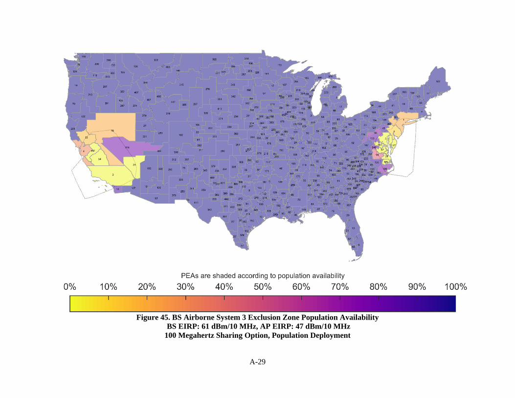
A-29
Figure 45. BS Airborne System 3 Exclusion Zone Population Availability
BS EIRP: 61 dBm/10 MHz, AP EIRP: 47 dBm/10 MHz 100 Megahertz Sharing Option, Population Deployment

A-30
Figure 46. AP Airborne System 3 Exclusion Zone Population Availability
BS EIRP: 61 dBm/10 MHz, AP EIRP: 47 dBm/10 MHz 100 Megahertz Sharing Option, Population Deployment

A-31
A.2.1.2 IMT-Advanced Deployment
Figure 47. BS Airborne System 3 Exclusion Zone Population Availability
BS EIRP: 47 dBm/10 MHz, AP EIRP: 30 dBm/10 MHz 100 Megahertz Sharing Option, IMT-Advanced Deployment

A-32
Figure 48. AP Airborne System 3 Exclusion Zone Population Availability
BS EIRP: 47 dBm/10 MHz, AP EIRP: 30 dBm/10 MHz 100 Megahertz Sharing Option, IMT-Advanced Deployment

A-33
Figure 49. BS Airborne System 3 Exclusion Zone Population Availability
BS EIRP: 47 dBm/10 MHz, AP EIRP: 36 dBm/10 MHz 100 Megahertz Sharing Option, IMT-Advanced Deployment

A-34
Figure 50. AP Airborne System 3 Exclusion Zone Population Availability
BS EIRP: 47 dBm/10 MHz, AP EIRP: 36 dBm/10 MHz 100 Megahertz Sharing Option, IMT-Advance Deployment

A-35
Figure 51. BS Airborne System 3 Exclusion Zone Population Availability
BS EIRP: 61 dBm/10 MHz, AP EIRP: 47 dBm/10 MHz 100 Megahertz Sharing Option, IMT-Advanced Deployment

A-36
Figure 52. AP Airborne System 3 Exclusion Zone Population Availability
BS EIRP: 61 dBm/10 MHz, AP EIRP: 47 dBm/10 MHz 100 Megahertz Sharing Option, IMT-Advanced Deployment

A-37
A.3 Airborne System 3 Dynamic Coordination Zone Neighborhood Results
For each Airborne System 3, the two frequency sharing options have the same results, therefore only the results for the 100 megahertz sharing option are provided. For each set of BS and AP EIRP levels, and deployment techniques, the individual Airborne System 3 dynamic coordination zone neighborhood and the population coverage is provided. The coordination zone neighborhood is not an exclusion zone, but defines the area around which the BS and AP are taken into account when determining which devices need to be turned off to protect the federal incumbent. The two plots show the BS and AP ground-based dynamic coordination zone neighborhood population impact based on the FCC Partial Economic Areas (PEA).2 Each PEA is shaded according to the percentage of population that is available to use the spectrum.
A.3.1 100 Megahertz Sharing Option
Table 8 summarizes the percentage of population availability for the 100 Megahertz Sharing Option.
Table 8. Population Availability per EIRP and Deployment set
Deployment EIRP: 47/30 dBm/10MHz
EIRP: 47/36 dBm/10MHz
EIRP: 61/47 dBm/10MHz
Population Based BS:77% AP:99%
BS:77% AP:99%
BS:73% AP:99%
IMT-Advanced BS:75% AP:99%
BS:75% AP:99%
BS:74% AP:99%
2 https://www.fcc.gov/oet/maps/areas

A-38
A.3.1.1 Population Deployment
Figure 53. BS Dynamic Coordination Zone Neighborhood Population Availability
BS EIRP: 47 dBm/10 MHz, AP EIRP: 30 dBm/10 MHz 100 Megahertz Sharing Option, Population Deployment

A-39
Figure 54. AP Dynamic Coordination Zone Neighborhood Population Availability
BS EIRP: 47 dBm/10 MHz, AP EIRP: 30 dBm/10 MHz 100 Megahertz Sharing Option, Population Deployment

A-40
Figure 55. BS Dynamic Coordination Zone Neighborhood Population Availability
BS EIRP: 47 dBm/10 MHz, AP EIRP: 36 dBm/10 MHz 100 Megahertz Sharing Option, Population Deployment

A-41
Figure 56. AP Dynamic Coordination Zone Neighborhood Population Availability
BS EIRP: 47 dBm/10 MHz, AP EIRP: 36 dBm/10 MHz 100 Megahertz Sharing Option, Population Deployment

A-42
Figure 57. BS Dynamic Coordination Zone Neighborhood Population Availability
BS EIRP: 61 dBm/10 MHz, AP EIRP: 47 dBm/10 MHz 100 Megahertz Sharing Option, Population Deployment

A-43
Figure 58. AP Dynamic Coordination Zone Neighborhood Population Availability
BS EIRP: 61 dBm/10 MHz, AP EIRP: 47 dBm/10 MHz 100 Megahertz Sharing Option, Population Deployment

A-44
A.3.1.2 IMT-Advanced Deployment
Figure 59. BS Dynamic Coordination Zone Neighborhood Population Availability
BS EIRP: 47 dBm/10 MHz, AP EIRP: 30 dBm/10 MHz 100 Megahertz Sharing Option, IMT-Advanced Deployment

A-45
Figure 60. AP Dynamic Coordination Zone Neighborhood Population Availability
BS EIRP: 47 dBm/10 MHz, AP EIRP: 30 dBm/10 MHz 100 Megahertz Sharing Option, IMT-Advanced Deployment

A-46
Figure 61. BS Dynamic Coordination Zone Neighborhood Population Availability
BS EIRP: 47 dBm/10 MHz, AP EIRP: 36 dBm/10 MHz 100 Megahertz Sharing Option, IMT-Advanced Deployment

A-47
Figure 62. AP Dynamic Coordination Zone Neighborhood Population Availability
BS EIRP: 47 dBm/10 MHz, AP EIRP: 36 dBm/10 MHz 100 Megahertz Sharing Option, IMT-Advanced Deployment

A-48
Figure 63. BS Dynamic Coordination Zone Neighborhood Population Availability
BS EIRP: 61 dBm/10 MHz, AP EIRP: 47 dBm/10 MHz 100 Megahertz Sharing Option, IMT-Advanced Deployment

A-49
Figure 64. AP Dynamic Coordination Zone Neighborhood Population Availability
BS EIRP: 61 dBm/10 MHz, AP EIRP: 47 dBm/10 MHz 100 Megahertz Sharing Option, IMT-Advanced Deployment

B-1
APPENDIX B. ADDITIONAL RESULTS FOR GROUND-BASED RADAR FEASIBILITY OF SHARING ANALYSIS
B.1 Static Exclusion Zone Results
For each frequency sharing option and for each set of base station (BS) and access point (AP) equivalent isotropically radiated power (EIRP) levels, and deployment techniques, the individual ground-based radar static exclusion zone area and the population availability is provided. The two plots show the BS and AP ground based exclusion zone population impact based on the FCC Partial Economic Areas (PEA)3. Each PEA is shaded according to the percentage of population that is available to use the spectrum.
B.1.1 30 Megahertz Sharing Option
Table 9 summarizes the percentage of population availability for the 30 Megahertz Sharing Option.
Table 9. Population Availability per EIRP and Deployment set
Deployment EIRP: 47/30 dBm/10MHz
EIRP: 47/36 dBm/10MHz
EIRP: 61/47 dBm/10MHz
Population Based BS:92% AP:99%
BS:92% AP:99%
BS:84% AP:99%
IMT-Advanced BS:93% AP:99%
BS:93% AP:99%
BS:87% AP:99%
3 https://www.fcc.gov/oet/maps/areas

B-2
B.1.1.1 Population Deployment
Figure 65. BS Ground Based Exclusion Zone Population Availability
BS EIRP: 47 dBm/10 MHz, AP EIRP: 30 dBm/10 MHz 30 Megahertz Sharing Option, Population Deployment

B-3
Figure 66. AP Ground Based Exclusion Zone Population Availability.
BS EIRP: 47 dBm/10 MHz, AP EIRP: 30 dBm/10 MHz 30 Megahertz Sharing Option, Population Deployment

B-4
Figure 67. BS Ground Based Exclusion Zone Population Availability
BS EIRP: 47 dBm/10 MHz, AP EIRP: 36 dBm/10 MHz 30 Megahertz Sharing Option, Population Deployment

B-5
Figure 68. AP Ground Based Exclusion Zone Population Availability BS EIRP: 47 dBm/10 MHz, AP EIRP: 36 dBm/10 MHz 30 Megahertz Sharing Option, Population Deployment

B-6
Figure 69. BS Ground Based Exclusion Zone Population Availability
BS EIRP: 61 dBm/10 MHz, AP EIRP: 47 dBm/10 MHz 30 Megahertz Sharing Option, Population Deployment

B-7
Figure 70. AP Ground Based Exclusion Zone Population Availability
BS EIRP: 61 dBm/10 MHz, AP EIRP: 47 dBm/10 MHz 30 Megahertz Sharing Option, Population Deployment

B-8
B.1.1.2 IMT-Advanced Deployment
Figure 71. BS Ground Based Exclusion Zone Population Availability
BS EIRP: 47 dBm/10 MHz, AP EIRP: 30 dBm/10 MHz 30 Megahertz Sharing Option, IMT-Advanced Deployment

B-9
Figure 72. AP Ground Based Exclusion Zone Population Availability
BS EIRP: 47 dBm/10 MHz, AP EIRP: 30 dBm/10 MHz 30 Megahertz Sharing Option, IMT-Advanced Deployment

B-10
Figure 73. BS Ground Based Exclusion Zone Population Availability:
BS EIRP: 47 dBm/10 MHz, AP EIRP: 36 dBm/10 MHz 30 Megahertz Sharing Option, IMT-Advanced Deployment

B-11
Figure 74. AP Ground Based Exclusion Zone Population Availability
BS EIRP: 47 dBm/10 MHz, AP EIRP: 36 dBm/10 MHz 30 Megahertz Sharing Option, IMT-Advanced Deployment

B-12
Figure 75. BS Ground Based Exclusion Zone Population Availability BS EIRP: 61 dBm/10 MHz, AP EIRP: 47 dBm/10 MHz
30 Megahertz Sharing Option, IMT-Advanced Deployment

B-13
Figure 76. AP Ground Based Exclusion Zone Population Availability
BS EIRP: 61 dBm/10 MHz, AP EIRP: 47 dBm/10 MHz 30 Megahertz Sharing Option, IMT-Advanced Deployment

B-14
B.1.2 100 Megahertz Sharing Option
Table 10 summarizes the percentage of population availability for the 100 Megahertz Sharing Option.
Table 10. Population Availability per EIRP and Deployment set
Deployment EIRP: 47/30 dBm/10MHz
EIRP: 47/36 dBm/10MHz
EIRP: 61/47 dBm/10MHz
Population Based BS:33% AP:74%
BS:33% AP:71%
BS:13% AP:63%
IMT-Advanced BS:27% AP:83%
BS:28% AP:79%
BS:10% AP:73%

B-15
B.1.2.1 Population Deployment
Figure 77. BS Ground Based Exclusion Zone Population Impact
BS EIRP: 47 dBm/10 MHz, AP EIRP: 30 dBm/10 MHz 100 Megahertz Sharing Option, Population Deployment

B-16
Figure 78. AP Ground Based Exclusion Zone Population Impact
BS EIRP: 47 dBm/10 MHz, AP EIRP: 30 dBm/10 MHz 100 Megahertz Sharing Option, Population Deployment

B-17
Figure 79. BS Ground Based Exclusion Zone Population Impact
BS EIRP: 47 dBm/10 MHz, AP EIRP: 36 dBm/10 MHz 100 Megahertz Sharing Option, Population Deployment

B-18
Figure 80. AP Ground Based Exclusion Zone Population Impact: BS EIRP: 47 dBm/10 MHz, AP EIRP: 36 dBm/10 MHz
100 Megahertz Sharing Option, Population Deployment

B-19
Figure 81. BS Ground Based Exclusion Zone Population Availability: BS EIRP: 61 dBm/10 MHz, AP EIRP: 47 dBm/10 MHz
100 Megahertz Sharing Option, Population Deployment

B-20
Figure 82. AP Ground Based Exclusion Zone Population Availability: BS EIRP: 61 dBm/10 MHz, AP EIRP: 47 dBm/10 MHz
100 Megahertz Sharing Option, Population Deployment

B-21
B.1.2.2 IMT-Advanced Deployment
Figure 83. BS Ground Based Exclusion Zone Population Availability: BS EIRP: 47 dBm/10 MHz, AP EIRP: 30 dBm/10 MHz
100 Megahertz Sharing Option, IMT-Advanced Deployment

B-22
Figure 84. AP Ground Based Exclusion Zone Population Availability: BS EIRP: 47 dBm/10 MHz, AP EIRP: 30 dBm/10 MHz
100 Megahertz Sharing Option, IMT-Advanced Deployment

B-23
Figure 85. BS Ground Based Exclusion Zone Population Availability: BS EIRP: 47 dBm/10 MHz, AP EIRP: 36 dBm/10 MHz
100 Megahertz Sharing Option, IMT-Advanced Deployment

B-24
Figure 86. AP Ground Based Exclusion Zone Population Availability: BS EIRP: 47 dBm/10 MHz, AP EIRP: 36 dBm/10 MHz
100 Megahertz Sharing Option, IMT-Advanced Deployment

B-25
Figure 87. BS Ground Based Exclusion Zone Population Availability: BS EIRP: 61 dBm/10 MHz, AP EIRP: 47 dBm/10 MHz
100 Megahertz Sharing Option, IMT-Advanced Deployment

B-26
Figure 88. AP Ground Based Exclusion Zone Population Availability: BS EIRP: 61 dBm/10 MHz, AP EIRP: 47 dBm/10 MHz
100 Megahertz Sharing Option, IMT-Advanced Deployment

B-27
B.2 Dynamic Coordination Zone Neighborhood Results
For each frequency sharing option and for each set of BS and AP EIRP levels and deployment techniques, the individual ground-based radar dynamic coordination zone neighborhood and the population coverage is provided. The coordination zone neighborhood is not an exclusion zone, but defines the area around which the BS and AP are taken into account when determining which devices need to be turned off to protect the federal incumbent. The two plots show the BS and AP ground-based dynamic coordination zone neighborhood population impact based on the FCC Partial Economic Areas (PEA).4 Each PEA is shaded according to the percentage of population that is available to use the spectrum.
B.2.1 30 Megahertz Sharing Option
Table 11 summarizes the percentage of population availability for the 30 Megahertz Sharing Option.
Table 11. Population Availability per EIRP and Deployment set
Deployment EIRP: 47/30 dBm/10MHz
EIRP: 47/36 dBm/10MHz
EIRP: 61/47 dBm/10MHz
Population Based BS:86% AP:99%
BS:88% AP:99%
BS:74% AP:97%
IMT-Advanced BS:83% AP:99%
BS:83% AP:99%
BS:73% AP:99%
4 https://www.fcc.gov/oet/maps/areas

B-28
B.2.1.1 Population Deployment
Figure 89. BS Dynamic Coordination Zone Neighborhood Population Availability
BS EIRP: 47 dBm/10 MHz, AP EIRP: 30 dBm/10 MHz 30 Megahertz Sharing Option, Population Deployment

B-29
Figure 90. AP Dynamic Coordination Zone Neighborhood Population Availability
BS EIRP: 47 dBm/10 MHz, AP EIRP: 30 dBm/10 MHz 30 Megahertz Sharing Option, Population Deployment

B-30
Figure 91. BS Dynamic Coordination Zone Neighborhood Population Availability: BS EIRP: 47 dBm/10 MHz, AP EIRP: 36
dBm/10 MHz 30 Megahertz Sharing Option, Population Deployment

B-31
Figure 92. AP Dynamic Coordination Zone Neighborhood Population Availability: BS EIRP: 47 dBm/10 MHz, AP EIRP: 36
dBm/10 MHz 30 Megahertz Sharing Option, Population Deployment

B-32
Figure 93. BS Dynamic Coordination Zone Neighborhood Population Availability: BS EIRP: 61 dBm/10 MHz, AP EIRP: 47
dBm/10 MHz 30 Megahertz Sharing Option, Population Deployment

B-33
Figure 94. AP Dynamic Coordination Zone Neighborhood Population Availability: BS EIRP: 61 dBm/10 MHz, AP EIRP: 47
dBm/10 MHz 30 Megahertz Sharing Option, Population Deployment

B-34
B.2.1.2 IMT-Advanced Deployment
Figure 95. BS Dynamic Coordination Zone Neighborhood Population Availability: BS EIRP: 47 dBm/10 MHz, AP EIRP: 30
dBm/10 MHz 30 Megahertz Sharing Option, IMT-Advanced Deployment

B-35
Figure 96. AP Dynamic Coordination Zone Neighborhood Population Availability: BS EIRP: 47 dBm/10 MHz, AP EIRP: 30
dBm/10 MHz 30 Megahertz Sharing Option, IMT-Advanced Deployment

B-36
Figure 97. BS Dynamic Coordination Zone Neighborhood Population Availability: BS EIRP: 47 dBm/10 MHz, AP EIRP: 36
dBm/10 MHz 30 Megahertz Sharing Option, IMT-Advanced Deployment

B-37
Figure 98. AP Dynamic Coordination Zone Neighborhood Population Availability: BS EIRP: 47 dBm/10 MHz, AP EIRP: 36
dBm/10 MHz 30 Megahertz Sharing Option, IMT-Advanced Deployment

B-38
Figure 99. BS Dynamic Coordination Zone Neighborhood Population Availability: BS EIRP: 61 dBm/10 MHz, AP EIRP: 47
dBm/10 MHz 30 Megahertz Sharing Option, IMT-Advanced Deployment

B-39
Figure 100. AP Dynamic Coordination Zone Neighborhood Population Availability: BS EIRP: 61 dBm/10 MHz, AP EIRP: 47
dBm/10 MHz 30 Megahertz Sharing Option, IMT-Advanced Deployment

B-40
B.2.2 100 Megahertz Sharing Option
Table 12 summarizes the percentage of population availability for the 100 Megahertz Sharing Option.
Table 12. Population Availability per EIRP and Deployment set
Deployment EIRP: 47/30 dBm/10MHz
EIRP: 47/36 dBm/10MHz
EIRP: 61/47 dBm/10MHz
Population Based BS:21% AP:64%
BS:26% AP:61%
BS:9% AP:52%
IMT-Advanced BS:16% AP:76%
BS:17% AP:73%
BS:5% AP:66%

B-41
B.2.2.1 Population Deployment
Figure 101. BS Dynamic Coordination Zone Neighborhood Population Availability BS EIRP: 47 dBm/10 MHz, AP EIRP: 30 dBm/10 MHz 100 Megahertz Sharing Option, Population Deployment

B-42
Figure 102. AP Dynamic Coordination Zone Neighborhood Population Availability
BS EIRP: 47 dBm/10 MHz, AP EIRP: 30 dBm/10 MHz 100 Megahertz Sharing Option, Population Deployment

B-43
Figure 103. BS Dynamic Coordination Zone Neighborhood Population Availability
BS EIRP: 47 dBm/10 MHz, AP EIRP: 36 dBm/10 MHz 100 Megahertz Sharing Option, Population Deployment

B-44
Figure 104. AP Dynamic Coordination Zone Neighborhood Population Availability
BS EIRP: 47 dBm/10 MHz, AP EIRP: 36 dBm/10MHz 100 Megahertz Sharing Option, Population Deployment

B-45
Figure 105. BS Dynamic Coordination Zone Neighborhood Population Availability
BS EIRP: 61 dBm/10 MHz, AP EIRP: 47 dBm/10 MHz 100 Megahertz Sharing Option, Population Deployment

B-46
Figure 106. AP Dynamic Coordination Zone Neighborhood Population Availability
BS EIRP: 61 dBm/10 MHz, AP EIRP: 47 dBm/10MHz 100 Megahertz Sharing Option, Population Deployment

B-47
B.2.2.2 IMT-Advanced Deployment
Figure 107. BS Dynamic Coordination Zone Neighborhood Population Availability
BS EIRP: 47 dBm/10 MHz, AP EIRP: 30 dBm/10 MHz 100 Megahertz Sharing Option, IMT-Advanced Deployment

B-48
Figure 108. AP Dynamic Coordination Zone Neighborhood Population Availability
BS EIRP: 47 dBm/10 MHz, AP EIRP: 30 dBm/10 MHz 100 Megahertz Sharing Option, IMT-Advanced Deployment

B-49
Figure 109. BS Dynamic Coordination Zone Neighborhood Population Availability BS EIRP: 47 dBm/10 MHz, AP EIRP: 36 dBm/10 MHz
100 Megahertz Sharing Option, IMT-Advanced Deployment

B-50
Figure 110. AP Dynamic Coordination Zone Neighborhood Population Availability: BS EIRP: 47 dBm/10 MHz, AP EIRP: 36
dBm/10MHz 100 Megahertz Sharing Option, IMT-Advanced Deployment

B-51
Figure 111. BS Dynamic Coordination Zone Neighborhood Population Availability: BS EIRP: 61 dBm/10 MHz, AP EIRP: 47
dBm/10 MHz 100 Megahertz Sharing Option, IMT-Advanced Deployment

B-52
Figure 112. AP Dynamic Coordination Zone Neighborhood Population Availability: BS EIRP: 61 dBm/10 MHz, AP EIRP: 47
dBm/10MHz 100 Megahertz Sharing Option, IMT-Advanced Deployment

C-1
APPENDIX C. ADDITIONAL RESULTS FOR SHIPBORNE RADAR FEASIBILITY OF SHARING ANALYSIS
C.1 Static Exclusion Zone Results
For each set of base station (BS) and access point (AP) EIRP levels and deployment techniques, the individual shipborne radar static exclusion zone area and the population availability is provided. For the shipborne radar, the results for the 30 megahertz and 100 megahertz sharing option analysis were the same, therefore, the results for the 100 megahertz sharing option is provided. The two plots show the BS and AP shipborne exclusion zone population impact based on the FCC Partial Economic Areas (PEA).5 Each PEA is shaded according to the percentage of population that is available to use the spectrum.
Table 13 summarizes the percentage of population availability for the 100 Megahertz Sharing Option.
Table 13. Population Availability per EIRP and Deployment set
Deployment EIRP: 47/30 dBm/10MHz
EIRP: 47/36 dBm/10MHz
EIRP: 61/47 dBm/10MHz
Population Based BS:52% AP:74%
BS:52% AP:72%
BS:43% AP:63%
IMT-Advanced BS:48% AP:78%
BS:48% AP:77%
BS:39% AP:72%
5 https://www.fcc.gov/oet/maps/areas.

C-2
C.1.1 Population Deployment
Figure 113. BS Shipborne Exclusion Zone Population Availability
BS EIRP: 47 dBm/10 MHz, AP EIRP: 30 dBm/10 MHz

C-3
Population Deployment
Figure 114. AP Shipborne Exclusion Zone Population Availability: BS EIRP: 47 dBm/10 MHz, AP EIRP: 30 dBm/10 MHz
Population Deployment

C-4
Figure 115. BS Shipborne Exclusion Zone Population Availability: BS EIRP: 47 dBm/10 MHz, AP EIRP: 36 dBm/10 MHz
Population Deployment

C-5
Figure 116. AP Shipborne Exclusion Zone Population Availability: BS EIRP: 47 dBm/10 MHz, AP EIRP: 36 dBm/10 MHz
Population Deployment

C-6
Figure 117. BS Shipborne Exclusion Zone Population Availability: BS EIRP: 61 dBm/10 MHz, AP EIRP: 47 dBm/10 MHz
Population Deployment

C-7
Figure 118. AP Shipborne Exclusion Zone Population Availability: BS EIRP: 61 dBm/10 MHz, AP EIRP: 47 dBm/10 MHz
Population Deployment

C-8
C.1.2 IMT-Advanced Deployment
Figure 119. BS Shipborne Exclusion Zone Population Availability: BS EIRP: 47 dBm/10 MHz, AP EIRP: 30 dBm/10 MHz
IMT-Advanced Deployment

C-9
Figure 120. AP Shipborne Exclusion Zone Population Availability: BS EIRP: 47 dBm/10 MHz, AP EIRP: 30 dBm/10 MHz
IMT-Advanced Deployment

C-10
Figure 121. BS Shipborne Exclusion Zone Population Availability: BS EIRP: 47 dBm/10 MHz, AP EIRP: 36 dBm/10 MHz
IMT-Advanced Deployment

C-11
Figure 122. AP Shipborne Exclusion Zone Population Availability: BS EIRP: 47 dBm/10 MHz, AP EIRP: 36 dBm/10 MHz
IMT-Advanced Deployment

C-12
Figure 123. BS Shipborne Exclusion Zone Population Availability: BS EIRP: 61 dBm/10 MHz, AP EIRP: 47 dBm/10 MHz
IMT-Advanced Deployment

C-13
Figure 124. AP Shipborne Exclusion Zone Population Availability: BS EIRP: 61 dBm/10 MHz, AP EIRP: 47 dBm/10 MHz
IMT-Advanced Deployment

C-14
C.2 Dynamic Coordination Zone Results
For each deployment technique and BS and AP EIRP set, three graphs show the results of sensor threshold simulations. The results are for Shipborne Radar 3 (SB3). The first plot shows the minimum distance from the shore for the shipborne radar, with a (vertical) histogram showing the distribution of distances for the East Coast, Gulf Coast, and West Coast. For example, Figure 125 shows the minimum distance being 146 km to 401 km with a BS EIRP of 47 dBm/10 MHz and AP EIRP of 30 dBm/10 MHz. The distance from the coast is depicted by the color of the line. The histogram on the right shows the probability of occurrence for each minimum distance. For example, the highest occurring minimum distance is 230 km.
The second plot shows the sensor thresholds for all minimum distances and calculates the 99th percentile. For example, Figure 127 shows the received radar signal at the coastal sensor locations with the 99th percentile calculated at -88 dBm/10 MHz (redline on figure).

C-15
C.2.1 Population Deployment
Figure 125. Minimum Distance: BS EIRP: 47 dBm/10 MHz, AP EIRP: 30 dBm/10 MHz
Population Deployment

C-16
Figure 126. Minimum Distance Distribution: BS EIRP: 47 dBm/10 MHz, AP EIRP: 30 dBm/10 MHz
Population Deployment

C-17
Figure 127. Sensor Detection Threshold
BS EIRP: 47 dBm/10 MHz, AP EIRP: 30 dBm/10 MHz Population Deployment

C-18
Figure 128. Minimum Distance: BS EIRP: 47 dBm/10 MHz, AP EIRP: 36 dBm/10 MHz
Population Deployment

C-19
Figure 129. Minimum Distance Distribution: BS EIRP: 47 dBm/10 MHz, AP EIRP: 36 dBm/10 MHz
Population Deployment

C-20
Figure 130. Sensor Detection Threshold BS EIRP: 47 dBm/10 MHz, AP EIRP: 36 dBm/10 MHz
Population Deployment

C-21
Figure 131. Minimum Distance: BS EIRP: 61 dBm/10 MHz, AP EIRP: 47 dBm/10 MHz
Population Deployment

C-22
Figure 132. Minimum Distance Distribution: BS EIRP: 61 dBm/10 MHz, AP EIRP: 47 dBm/10 MHz
Population Deployment

C-23
Figure 133. Sensor Detection Threshold BS EIRP: 61 dBm/10 MHz, AP EIRP: 47 dBm/10 MHz
Population Deployment

C-24
C.2.1.1 IMT-Advanced
Figure 134. Minimum Distance: BS EIRP: 47 dBm/10 MHz, AP EIRP: 30 dBm/10 MHz
IMT-Advanced Deployment

C-25
Figure 135. Minimum Distance Distribution: BS EIRP: 47 dBm/10 MHz, AP EIRP: 30 dBm/10 MHz
IMT-Advanced Deployment

C-26
Figure 136. Sensor Detection Threshold
BS EIRP: 47 dBm/10 MHz, AP EIRP: 30 dBm/10 MHz IMT-Advanced Deployment

C-27
Figure 137. Minimum Distance: BS EIRP: 47 dBm/10 MHz, AP EIRP: 36 dBm/10 MHz
IMT-Advanced Deployment

C-28
Figure 138. Minimum Distance Distribution: BS EIRP: 47 dBm/10 MHz, AP EIRP: 36 dBm/10 MHz
IMT-Advanced Deployment

C-29
Figure 139. Sensor Detection Threshold BS EIRP: 47 dBm/10 MHz, AP EIRP: 36 dBm/10 MHz
IMT-Advanced Deployment

C-30
Figure 140. Minimum Distance: BS EIRP: 61 dBm/10 MHz, AP EIRP: 47 dBm/10 MHz
IMT-Advanced Deployment

C-31
Figure 141. Minimum Distance Distribution: BS EIRP: 61 dBm/10 MHz, AP EIRP: 47 dBm/10 MHz
IMT-Advanced Deployment

C-32
Figure 142. Sensor Detection Threshold BS EIRP: 61 dBm/10 MHz, AP EIRP: 47 dBm/10 MHz
IMT-Advanced Deployment

C-33
C.2.1.2 Dynamic Coordination Zone Area
For each frequency sharing option and set of EIRPs, the individual shipborne radar dynamic coordination zone area and the population coverage is provided. The two plots show the BS and AP ground based dynamic coordination zone area population impact to the FCC Partial Economic Areas (PEA)6. Each PEA is shaded according to the percentage of population that is available to use the spectrum. The dotted gray lines plot the BS and AP shipborne dynamic coordination zone area.
Table 14 summarizes the percentage of population availability for the 100 Megahertz Sharing Option.
Table 14. Population Availability per EIRP and Deployment set
Deployment EIRP: 47/30 dBm/10MHz
EIRP: 47/36 dBm/10MHz
EIRP: 61/47 dBm/10MHz
Population Based BS:45% AP:70%
BS:45% AP:67%
BS:40% AP:59%
IMT-Advanced BS:43% AP:74%
BS:43% AP:71%
BS:36% AP:66%
6 https://www.fcc.gov/oet/maps/areas

C-34
C.2.2 Population Deployment
Figure 143. BS Dynamic Coordination Zone Neighborhood Population Availability: BS EIRP: 47 dBm/10 MHz, AP EIRP: 30
dBm/10 MHz Population Deployment

C-35
Figure 144. AP Dynamic Coordination Zone Neighborhood Population Availability: BS EIRP:47 dBm/10 MHz, AP EIRP: 30
dBm/10 MHz Population Deployment

C-36
Figure 145. BS Dynamic Coordination Zone Neighborhood Population Availability
BS EIRP: 47 dBm/10 MHz, AP EIRP: 36 dBm/10 MHz Population Deployment

C-37
Figure 146. AP Dynamic Coordination Zone Neighborhood Population Availability: BS EIRP: 47 dBm/10 MHz, AP EIRP: 36
dBm/10MHz Population Deployment

C-38
Figure 147. BS Dynamic Coordination Zone Neighborhood Population Availability: BS EIRP: 61 dBm/10 MHz, AP EIRP: 47
dBm/10 MHz Population Deployment

C-39
Figure 148. AP Dynamic Coordination Zone Neighborhood Population Availability: BS EIRP: 61 dBm/10 MHz, AP EIRP: 47
dBm/10MHz Population Deployment

C-40
C.2.3 IMT-Advance Deployment
Figure 149. BS Dynamic Coordination Zone Neighborhood Population Availability: BS EIRP: 47 dBm/10 MHz, AP EIRP: 30
dBm/10 MHz IMT-Advanced Deployment

C-41
Figure 150. AP Dynamic Coordination Zone Neighborhood Population Availability: BS EIRP:47 dBm/10 MHz, AP EIRP: 30
dBm/10 MHz IMT-Advanced Deployment

C-42
Figure 151. BS Dynamic Coordination Zone Neighborhood Population Availability: BS EIRP: 47 dBm/10 MHz, AP EIRP: 36
dBm/10 MHz IMT-Advanced Deployment

C-43
Figure 152. AP Dynamic Coordination Zone Neighborhood Population Availability: BS EIRP:47 dBm/10 MHz, AP EIRP: 36
dBm/10 MHz IMT-Advanced Deployment

C-44
Figure 153. BS Dynamic Coordination Zone Neighborhood Population Availability: BS EIRP: 61 dBm/10 MHz, AP EIRP: 47
dBm/10 MHz IMT-Advanced Deployment

C-45
Figure 154. AP Dynamic Coordination Zone Neighborhood Population Availability: BS EIRP: 61 dBm/10 MHz, AP EIRP: 47
dBm/10MHz IMT-Advanced Deployment