Just for sharing ^_^

Susskind

and Hrabovsky

Th

e T

he

or

et

ic

al

Min

im

um

Author of The Black Hole Warleonard susskind

A world-class physicist and a

citizen scientist combine forces

to teach Physics 101—the DIY way.

The Theoretical Minimum is a book for anyone who has

ever regretted not taking physics in college—or

who simply wants to know how to think like a

physicist. In this unconventional introduction, physicist Leonard

Susskind and amateur scientist George Hrabovsky offer a first

course in physics and associated math for the ardent amateur.

Unlike most popular physics books—which give readers a taste

of what physicists know but shy away from equations or math—

Susskind and Hrabovsky actually teach the skills you need to do

physics, beginning with classical mechanics, yourself. Based on

Susskind’s enormously popular Stanford University-based (and

YouTube-featured) continuing-education course, the authors

cover the minimum—the theoretical minimum of the title—that

readers need to master to study more advanced topics.

An alternative to the conventional go-to-college method, The

Theoretical Minimum provides a tool kit for amateur scientists to learn

physics at their own pace.

$26 .99 US / $30 .00 CANScience

Advance Praise For

The Theoretical Minimum

$26.99 US / $30.00CAN

ISBN 978-0-465-02811-5

9 7 8 0 4 6 5 0 2 8 1 1 5

5 2 7 9 9

A Member of the Perseus Books Group

www.basicbooks.com

“What a wonderful and unique resource. For anyone who is

determined to learn physics for real, looking beyond conventional

popularizations, this is the ideal place to start. It gets directly to the

important points, with nuggets of deep insight scattered along the

way. I’m going to be recommending this book right and left.”

—Sean Carroll, physicist, California Institute of Technology,

and author of The Particle at the End of the Universe

Leonard Susskind has been the Felix Bloch Professor

in Theoretical Physics at Stanford University since 1978. The

author of The Black Hole War and The Cosmic Landscape, he lives in Palo

Alto, California.

George Hrabovsky is the president of Madison

Area Science and Technology (MAST), a nonprofit organization

dedicated to scientific and technological research and education.

He lives in Madison, Wisconsin.

©A

nne

War

ren

©D

iann

a H

rabo

vsky

Jacket design by Nicole Caputo

Jacket image © Rick Schwab

1/13

5 5/8” x 8 1/2”S: 0.8900”B: 0.7650”

BASICHC

4/C

FINISH:Gritty Matte

THE

THEORETICAL

MINIMUM

THE THEORETICAL

MINIMUM

WHAT YOU NEED to KNOW

to START DOING PHYSICS

LEONARD SUSSKIND

and

GEORGE HRABOVSKY

A Member of the Perseus Books GroupNew York

Copyright © 2013 by Leonard Susskind and George Hrabovsky

Published by Basic Books,A Member of the Perseus Books Group

All rights reserved. Printed in the United States of America. No part of this book maybe reproduced in any manner whatsoever without written permission except in thecase of brief quotations embodied in critical articles and reviews. For information, address Basic Books, 250 West 57th Street, 15th Floor, New York, NY 10107-1307.

Books published by Basic Books are available at special discounts for bulk purchases in the United States by corporations, institutions, and other organiza-tions. For more information, please contact the Special Markets Department at thePerseus Books Group, 2300 Chestnut Street, Suite 200, Philadelphia, PA 19103, orcall (800) 810-4145, ext. 5000, or e-mail [email protected].

LCCN: 2012953679

ISBN 978-0-465-02811-5 (hardcover)ISBN 978-0-465-03174-0 (e-book)

10 9 8 7 6 5 4 3 2 1

To our spouses—those who have chosen to put up with us,and to the students of Professor Susskind’s

Continuing Education Courses

CONTENTS

Preface ix

lecture 1 The Nature of Classical Physics 1Interlude 1 Spaces, Trigonometry, and Vectors 15

lecture 2 Motion 29Interlude 2 Integral Calculus 47

lecture 3 Dynamics 58Interlude 3 Partial Differentiation 74

lecture 4 Systems of More Than One Particle 85

lecture 5 Energy 95

lecture 6 The Principle of Least Action 105

lecture 7 Symmetries and Conservation Laws 128

lecture 8 Hamiltonian Mechanics and Time-Translation Invariance 145

lecture 9 The Phase Space Fluid and the Gibbs-Liouville Theorem 162

lecture 10 Poisson Brackets, Angular Momentum, and Symmetries 174

lecture 11 Electric and Magnetic Forces 190

Appendix 1 Central Forces and Planetary Orbits 212

Index 229

PrefaceI’ve always enjoyed explaining physics. For me it’s much morethan teaching: It’s a way of thinking. Even when I’m at my deskdoing research, there’s a dialog going on in my head. Figuring outthe best way to explain something is almost always the best wayto understand it yourself.

About ten years ago someone asked me if I would teach acourse for the public. As it happens, the Stanford area has a lot ofpeople who once wanted to study physics, but life got in the way.They had had all kinds of careers but never forgot their one-timeinfatuation with the laws of the universe. Now, after a career ortwo, they wanted to get back into it, at least at a casual level.

Unfortunately there was not much opportunity for suchfolks to take courses. As a rule, Stanford and other universitiesdon’t allow outsiders into classes, and, for most of these grown-ups, going back to school as a full-time student is not a realisticoption. That bothered me. There ought to be a way for people todevelop their interest by interacting with active scientists, butthere didn’t seem to be one.

That’s when I first found out about Stanford’sContinuing Studies program. This program offers courses forpeople in the local nonacademic community. So I thought that itmight just serve my purposes in finding someone to explainphysics to, as well as their purposes, and it might also be fun toteach a course on modern physics. For one academic quarteranyhow.

It was fun. And it was very satisfying in a way thatteaching undergraduate and graduate students was sometimesnot. These students were there for only one reason: Not to getcredit, not to get a degree, and not to be tested, but just to learnand indulge their curiosity. Also, having been “around the block”a few times, they were not at all afraid to ask questions, so theclass had a lively vibrancy that academic classes often lack. Idecided to do it again. And again.

What became clear after a couple of quarters is that thestudents were not completely satisfied with the layperson’scourses I was teaching. They wanted more than the ScientificAmerican experience. A lot of them had a bit of background, a bitof physics, a rusty but not dead knowledge of calculus, and someexperience at solving technical problems. They were ready to trytheir hand at learning the real thing—with equations. The resultwas a sequence of courses intended to bring these students to theforefront of modern physics and cosmology.

Fortunately, someone (not I) had the bright idea to video-record the classes. They are out on the Internet, and it seems thatthey are tremendously popular: Stanford is not the only placewith people hungry to learn physics. From all over the world I getthousands of e-mail messages. One of the main inquiries iswhether I will ever convert the lectures into books? The TheoreticalMinimum is the answer.

The term theoretical minimum was not my own invention. Itoriginated with the great Russian physicist Lev Landau. The TMin Russia meant everything a student needed to know to workunder Landau himself. Landau was a very demanding man: Histheoretical minimum meant just about everything he knew, whichof course no one else could possibly know.

I use the term differently. For me, the theoreticalminimum means just what you need to know in order to proceedto the next level. It means not fat encyclopedic textbooks thatexplain everything, but thin books that explain everythingimportant. The books closely follow the Internet courses that youwill find on the Web.

Welcome, then, to The Theoretical Miniumum—ClassicalMechanics, and good luck!Leonard SusskindStanford, California, July 2012

I’ve always enjoyed explaining physics. For me it’s much morethan teaching: It’s a way of thinking. Even when I’m at my deskdoing research, there’s a dialog going on in my head. Figuring outthe best way to explain something is almost always the best wayto understand it yourself.










x The Theoretical Minimum

I’ve always enjoyed explaining physics. For me it’s much morethan teaching: It’s a way of thinking. Even when I’m at my deskdoing research, there’s a dialog going on in my head. Figuring outthe best way to explain something is almost always the best wayto understand it yourself.










I started to teach myself math and physics when I was eleven.That was forty years ago. A lot of things have happened sincethen—I am one of those individuals who got sidetracked by life.Still, I have learned a lot of math and physics. Despite the factthat people pay me to do research for them, I never pursued adegree.

For me, this book began with an e-mail. After watchingthe lectures that form the basis for the book, I wrote an e-mail toLeonard Susskind asking if he wanted to turn the lectures into abook. One thing led to another, and here we are.

We could not fit everything we wanted into this book, orit wouldn’t be The Theoretical Minimum—Classical Mechanics, itwould be A-Big-Fat-Mechanics-Book. That is what the Internet isfor: Taking up large quantities of bandwidth to display stuff thatdoesn’t fit elsewhere! You can find extra material at the websitewww.madscitech.org/tm. This material will include answers tothe problems, demonstrations, and additional material that wecouldn’t put in the book.

I hope you enjoy reading this book as much as weenjoyed writing it.George HrabovskyMadison, Wisconsin, July 2012

Preface xi

Lecture 1: The Nature of Classical Physics

Somewhere in Steinbeck country two tired men sit down at theside of the road. Lenny combs his beard with his fingers and says,“Tell me about the laws of physics, George.” George looks downfor a moment, then peers at Lenny over the tops of his glasses.“Okay, Lenny, but just the minimum.”

What Is Classical Physics?

The term classical physics refers to physics before the advent ofquantum mechanics. Classical physics includes Newton’sequations for the motion of particles, the Maxwell-Faraday theoryof electromagnetic fields, and Einstein’s general theory ofrelativity. But it is more than just specific theories of specificphenomena; it is a set of principles and rules—an underlyinglogic—that governs all phenomena for which quantumuncertainty is not important. Those general rules are calledclassical mechanics.

The job of classical mechanics is to predict the future.The great eighteenth-century physicist Pierre-Simon Laplace laidit out in a famous quote:

We may regard the present state of the universe as the effect of its pastand the cause of its future. An intellect which at a certain momentwould know all forces that set nature in motion, and all positionsof all items of which nature is composed, if this intellect were also vastenough to submit these data to analysis, it would embrace in a singleformula the movements of the greatest bodies of the universe and thoseof the tiniest atom; for such an intellect nothing would be uncertainand the future just like the past would be present before its eyes.

We may regard the present state of the universe as the effect of its pastand the cause of its future. An intellect which at a certain momentwould know all forces that set nature in motion, and all positionsof all items of which nature is composed, if this intellect were also vastenough to submit these data to analysis, it would embrace in a singleformula the movements of the greatest bodies of the universe and thoseof the tiniest atom; for such an intellect nothing would be uncertainand the future just like the past would be present before its eyes.

In classical physics, if you know everything about a system atsome instant of time, and you also know the equations thatgovern how the system changes, then you can predict the future.That’s what we mean when we say that the classical laws ofphysics are deterministic. If we can say the same thing, but with thepast and future reversed, then the same equations tell youeverything about the past. Such a system is called reversible.

Simple Dynamical Systems and the Space of States

A collection of objects—particles, fields, waves, or whatever—iscalled a system. A system that is either the entire universe or is soisolated from everything else that it behaves as if nothing elseexists is a closed system.

Exercise 1: Since the notion is so important totheoretical physics, think about what a closed system isand speculate on whether closed systems can actuallyexist. What assumptions are implicit in establishing aclosed system? What is an open system?

To get an idea of what deterministic and reversible mean,we are going to begin with some extremely simple closed systems.They are much simpler than the things we usually study inphysics, but they satisfy rules that are rudimentary versions of thelaws of classical mechanics. We begin with an example that is sosimple it is trivial. Imagine an abstract object that has only onestate. We could think of it as a coin glued to the table—forevershowing heads. In physics jargon, the collection of all statesoccupied by a system is its space of states, or, more simply, itsstate-space. The state-space is not ordinary space; it’s amathematical set whose elements label the possible states of thesystem. Here the state-space consists of a single point—namelyHeads (or just H)—because the system has only one state.Predicting the future of this system is extremely simple: Nothingever happens and the outcome of any observation is always H.

The next simplest system has a state-space consisting oftwo points; in this case we have one abstract object and twopossible states. Imagine a coin that can be either Heads or Tails(H or T). See Figure 1.

2 The Theoretical Minimum

To get an idea of what deterministic and reversible mean,we are going to begin with some extremely simple closed systems.They are much simpler than the things we usually study inphysics, but they satisfy rules that are rudimentary versions of thelaws of classical mechanics. We begin with an example that is sosimple it is trivial. Imagine an abstract object that has only onestate. We could think of it as a coin glued to the table—forevershowing heads. In physics jargon, the collection of all statesoccupied by a system is its space of states, or, more simply, itsstate-space. The state-space is not ordinary space; it’s amathematical set whose elements label the possible states of thesystem. Here the state-space consists of a single point—namelyHeads (or just H)—because the system has only one state.Predicting the future of this system is extremely simple: Nothingever happens and the outcome of any observation is always H.

The next simplest system has a state-space consisting oftwo points; in this case we have one abstract object and twopossible states. Imagine a coin that can be either Heads or Tails(H or T). See Figure 1.

T

H

Figure 1: The space of two states.

In classical mechanics we assume that systems evolvesmoothly, without any jumps or interruptions. Such behavior issaid to be continuous. Obviously you cannot move between Headsand Tails smoothly. Moving, in this case, necessarily occurs indiscrete jumps. So let’s assume that time comes in discrete stepslabeled by integers. A world whose evolution is discrete could becalled stroboscopic.

A system that changes with time is called adynamical system. A dynamical system consists of more than a spaceof states. It also entails a law of motion, or dynamical law. Thedynamical law is a rule that tells us the next state given thecurrent state.

The Nature of Classical Physics 3

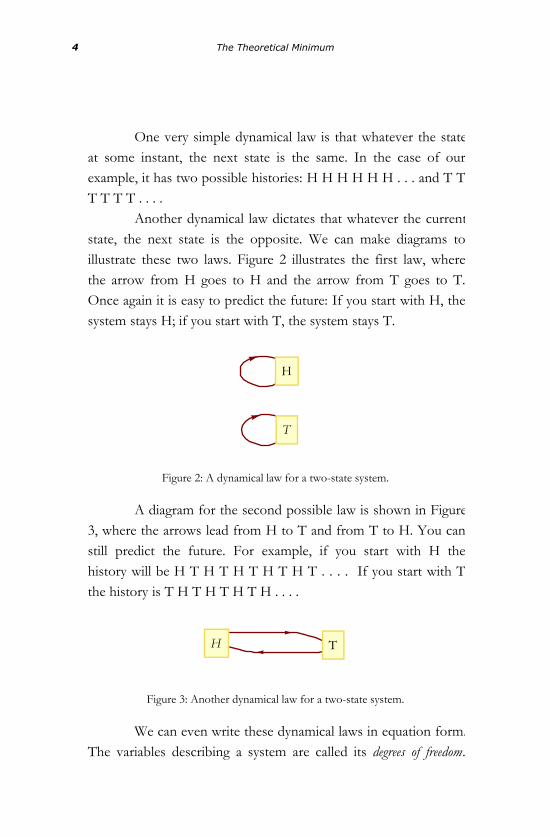
One very simple dynamical law is that whatever the stateat some instant, the next state is the same. In the case of ourexample, it has two possible histories: H H H H H H . . . and T TT T T T . . . .

Another dynamical law dictates that whatever the currentstate, the next state is the opposite. We can make diagrams toillustrate these two laws. Figure 2 illustrates the first law, wherethe arrow from H goes to H and the arrow from T goes to T.Once again it is easy to predict the future: If you start with H, thesystem stays H; if you start with T, the system stays T.

T

H

Figure 2: A dynamical law for a two-state system.

A diagram for the second possible law is shown in Figure3, where the arrows lead from H to T and from T to H. You canstill predict the future. For example, if you start with H thehistory will be H T H T H T H T H T . . . . If you start with Tthe history is T H T H T H T H . . . .

TH

Figure 3: Another dynamical law for a two-state system.

We can even write these dynamical laws in equation form.The variables describing a system are called its degrees of freedom.Our coin has one degree of freedom, which we can denote by thegreek letter sigma, Σ. Sigma has only two possible values; Σ = 1and Σ = -1, respectively, for H and T. We also use a symbol tokeep track of the time. When we are considering a continuousevolution in time, we can symbolize it with t . Here we have adiscrete evolution and will use n. The state at time n is describedby the symbol ΣHnL, which stands for Σ at n.

Let’s write equations of evolution for the two laws. Thefirst law says that no change takes place. In equation form,


We can even write these dynamical laws in equation form.The variables describing a system are called its degrees of freedom.Our coin has one degree of freedom, which we can denote by thegreek letter sigma, Σ. Sigma has only two possible values; Σ = 1and Σ = -1, respectively, for H and T. We also use a symbol tokeep track of the time. When we are considering a continuousevolution in time, we can symbolize it with t . Here we have adiscrete evolution and will use n. The state at time n is describedby the symbol ΣHnL, which stands for Σ at n.

Let’s write equations of evolution for the two laws. Thefirst law says that no change takes place. In equation form,

Σ Hn + 1L = Σ HnL .

In other words, whatever the value of Σ at the nth step, it willhave the same value at the next step.

The second equation of evolution has the form

Σ Hn + 1L = -Σ HnL,implying that the state flips during each step.

Because in each case the future behavior is completelydetermined by the initial state, such laws are deterministic. All thebasic laws of classical mechanics are deterministic.

To make things more interesting, let’s generalize thesystem by increasing the number of states. Instead of a coin, wecould use a six-sided die, where we have six possible states (seeFigure 4).

Now there are a great many possible laws, and they arenot so easy to describe in words—or even in equations. Thesimplest way is to stick to diagrams such as Figure 5. Figure 5says that given the numerical state of the die at time n, weincrease the state one unit at the next instant n + 1. That worksfine until we get to 6, at which point the diagram tells you to goback to 1 and repeat the pattern. Such a pattern that is repeatedendlessly is called a cycle. For example, if we start with 3 then thehistory is 3, 4, 5, 6, 1, 2, 3, 4, 5, 6, 1, 2, . . . . We’ll call this patternDynamical Law 1.


implying that the state flips during each step.Because in each case the future behavior is completely

determined by the initial state, such laws are deterministic. All thebasic laws of classical mechanics are deterministic.

To make things more interesting, let’s generalize thesystem by increasing the number of states. Instead of a coin, wecould use a six-sided die, where we have six possible states (seeFigure 4).

Now there are a great many possible laws, and they arenot so easy to describe in words—or even in equations. Thesimplest way is to stick to diagrams such as Figure 5. Figure 5says that given the numerical state of the die at time n, weincrease the state one unit at the next instant n + 1. That worksfine until we get to 6, at which point the diagram tells you to goback to 1 and repeat the pattern. Such a pattern that is repeatedendlessly is called a cycle. For example, if we start with 3 then thehistory is 3, 4, 5, 6, 1, 2, 3, 4, 5, 6, 1, 2, . . . . We’ll call this patternDynamical Law 1.

1

2

3

4

5

6

Figure 4: A six-state system.

1

2

3

4

5

6

Figure 5: Dynamical Law 1.

Figure 6 shows another law, Dynamical Law 2. It looks alittle messier than the last case, but it’s logically identical—in eachcase the system endlessly cycles through the six possibilities. Ifwe relabel the states, Dynamical Law 2 becomes identical toDynamical Law 1.

Not all laws are logically the same. Consider, for example,the law shown in Figure 7. Dynamical Law 3 has two cycles. Ifyou start on one of them, you can’t get to the other.Nevertheless, this law is completely deterministic. Wherever youstart, the future is determined. For example, if you start at 2, thehistory will be 2, 6, 1, 2, 6, 1, . . . and you will never get to 5. Ifyou start at 5 the history is 5, 3, 4, 5, 3, 4, . . . and you will neverget to 6.


Figure 6 shows another law, Dynamical Law 2. It looks alittle messier than the last case, but it’s logically identical—in eachcase the system endlessly cycles through the six possibilities. Ifwe relabel the states, Dynamical Law 2 becomes identical toDynamical Law 1.

Not all laws are logically the same. Consider, for example,the law shown in Figure 7. Dynamical Law 3 has two cycles. Ifyou start on one of them, you can’t get to the other.Nevertheless, this law is completely deterministic. Wherever youstart, the future is determined. For example, if you start at 2, thehistory will be 2, 6, 1, 2, 6, 1, . . . and you will never get to 5. Ifyou start at 5 the history is 5, 3, 4, 5, 3, 4, . . . and you will neverget to 6.

1

3

26

45


1

26

3

4

5


Figure 8 shows Dynamical Law 4 with three cycles.

1

2

3

45

6



It would take a long time to write out all of the possibledynamical laws for a six-state system.

Exercise 2: Can you think of a general way to classify thelaws that are possible for a six-state system?

Rules That Are Not Allowed: The Minus-First Law

According to the rules of classical physics, not all laws are legal.It’s not enough for a dynamical law to be deterministic; it mustalso be reversible.

The meaning of reversible—in the context of physics—canbe described a few different ways. The most concise descriptionis to say that if you reverse all the arrows, the resulting law is stilldeterministic. Another way, is to say the laws are deterministic into thepast as well as the future. Recall Laplace’s remark, “for such anintellect nothing would be uncertain and the future just like thepast would be present before its eyes.” Can one conceive of lawsthat are deterministic into the future, but not into the past? Inother words, can we formulate irreversible laws? Indeed we can.Consider Figure 9.

1

2

3

Figure 9: A system that is irreversible.

The law of Figure 9 does tell you, wherever you are, where to gonext. If you are at 1, go to 2. If at 2, go to 3. If at 3, go to 2.There is no ambiguity about the future. But the past is a differentmatter. Suppose you are at 2. Where were you just before that?You could have come from 3 or from 1. The diagram just doesnot tell you. Even worse, in terms of reversibility, there is no statethat leads to 1; state 1 has no past. The law of Figure 9 isirreversible. It illustrates just the kind of situation that is prohibitedby the principles of classical physics.

Notice that if you reverse the arrows in Figure 9 to giveFigure 10, the corresponding law fails to tell you where to go inthe future.


The law of Figure 9 does tell you, wherever you are, where to gonext. If you are at 1, go to 2. If at 2, go to 3. If at 3, go to 2.There is no ambiguity about the future. But the past is a differentmatter. Suppose you are at 2. Where were you just before that?You could have come from 3 or from 1. The diagram just doesnot tell you. Even worse, in terms of reversibility, there is no statethat leads to 1; state 1 has no past. The law of Figure 9 isirreversible. It illustrates just the kind of situation that is prohibitedby the principles of classical physics.

Notice that if you reverse the arrows in Figure 9 to giveFigure 10, the corresponding law fails to tell you where to go inthe future.

1

2

3

Figure 10: A system that is not deterministic into the future.

There is a very simple rule to tell when a diagramrepresents a deterministic reversible law. If every state has asingle unique arrow leading into it, and a single arrow leading outof it, then it is a legal deterministic reversible law. Here is aslogan: There must be one arrow to tell you where you’re going and one totell you where you came from.

The rule that dynamical laws must be deterministic andreversible is so central to classical physics that we sometimesforget to mention it when teaching the subject. In fact, it doesn'teven have a name. We could call it the first law, but unfortunatelythere are already two first laws—Newton's and the first law ofthermodynamics. There is evan a zeroth law of thermodynamics.So we have to go back to a minus-first law to gain priority for whatis undoubtedly the most fundamental of all physical laws—theconservation of information. The conservation of information issimply the rule that every state has one arrow in and one arrowout. It ensures that you never lose track of where you started.

The conservation of information is not a conventionalconservation law. We will return to conservation laws after adigression into systems with infinitely many states.


There is a very simple rule to tell when a diagramrepresents a deterministic reversible law. If every state has asingle unique arrow leading into it, and a single arrow leading outof it, then it is a legal deterministic reversible law. Here is aslogan: There must be one arrow to tell you where you’re going and one totell you where you came from.

The rule that dynamical laws must be deterministic andreversible is so central to classical physics that we sometimesforget to mention it when teaching the subject. In fact, it doesn'teven have a name. We could call it the first law, but unfortunatelythere are already two first laws—Newton's and the first law ofthermodynamics. There is evan a zeroth law of thermodynamics.So we have to go back to a minus-first law to gain priority for whatis undoubtedly the most fundamental of all physical laws—theconservation of information. The conservation of information issimply the rule that every state has one arrow in and one arrowout. It ensures that you never lose track of where you started.

The conservation of information is not a conventionalconservation law. We will return to conservation laws after adigression into systems with infinitely many states.

Dynamical Systems with an Infinite Number of States

So far, all our examples have had state-spaces with only a finitenumber of states. There is no reason why you can’t have adynamical system with an infinite number of states. For example,imagine a line with an infinite number of discrete points alongit—like a train track with an infinite sequence of stations in bothdirections. Suppose that a marker of some sort can jump fromone point to another according to some rule. To describe such asystem, we can label the points along the line by integers thesame way we labeled the discrete instants of time above. Becausewe have already used the notation n for the discrete time steps,let’s use an uppercase N for points on the track. A history of themarker would consist of a function NHnL, telling you the placealong the track N at every time n. A short portion of this state-space is shown in Figure 11.

º -1 0 1 2 3 º

Figure 11: State-space for an infinite system.

A very simple dynamical law for such a system, shown in Figure12, is to shift the marker one unit in the positive direction at eachtime step.


º -1 0 1 2 3 º

Figure 12: A dynamical rule for an infinite system.

This is allowable because each state has one arrow in and onearrow out. We can easily express this rule in the form of anequation.

(1)N Hn + 1L = N HnL + 1

Here are some other possible rules, but not all are allowable.

(2)N Hn + 1L = N HnL - 1

(3)N Hn + 1L = N HnL + 2

(4)N Hn + 1L = N HnL2

(5)N Hn + 1L = -1N HnL N HnL

Exercise 3: Determine which of the dynamical lawsshown in Eq.s (2) through (5) are allowable.

In Eq. (1), wherever you start, you will eventually get toevery other point by either going to the future or going to thepast. We say that there is a single infinite cycle. With Eq. (3), onthe other hand, if you start at an odd value of N , you will neverget to an even value, and vice versa. Thus we say there are twoinfinite cycles.

We can also add qualitatively different states to thesystem to create more cycles, as shown in Figure 13.


º -1 0 1 2 3 º

BA

Figure 13: Breaking an infinite configuration space into finite and infinite cycles.

If we start with a number, then we just keep proceeding throughthe upper line, as in Figure 12. On the other hand, if we start atA or B, then we cycle between them. Thus we can have mixtureswhere we cycle around in some states, while in others we moveoff to infinity.

Cycles and Conservation Laws

When the state-space is separated into several cycles, the systemremains in whatever cycle it started in. Each cycle has its owndynamical rule, but they are all part of the same state-spacebecause they describe the same dynamical system. Let’s considera system with three cycles. Each of states 1 and 2 belongs to itsown cycle, while 3 and 4 belong to the third (see Figure 14).

1

234

Figure 14: Separating the state-space into cycles.

Whenever a dynamical law divides the state-space intosuch separate cycles, there is a memory of which cycle theystarted in. Such a memory is called a conservation law; it tells us thatsomething is kept intact for all time. To make the conservationlaw quantitative, we give each cycle a numerical value called Q. In

the example in Figure 15 the three cycles are labeled Q = +1,

Q = -1, and Q = 0. Whatever the value of Q, it remains the

same for all time because the dynamical law does not allowjumping from one cycle to another. Simply stated, Q is conserved.


Whenever a dynamical law divides the state-space intosuch separate cycles, there is a memory of which cycle theystarted in. Such a memory is called a conservation law; it tells us thatsomething is kept intact for all time. To make the conservationlaw quantitative, we give each cycle a numerical value called Q. In

the example in Figure 15 the three cycles are labeled Q = +1,

Q = -1, and Q = 0. Whatever the value of Q, it remains the

same for all time because the dynamical law does not allowjumping from one cycle to another. Simply stated, Q is conserved.

-1

+100

Figure 15: Labeling the cycles with specific values of a conserved quantity.

In later chapters we will take up the problem ofcontinuous motion in which both time and the state-space arecontinuous. All of the things that we discussed for simplediscrete systems have their analogs for the more realistic systemsbut it will take several chapters before we see how they all playout.

The Limits of Precision

Laplace may have been overly optimistic about how predictablethe world is, even in classical physics. He certainly would haveagreed that predicting the future would require a perfectknowledge of the dynamical laws governing the world, as well astremendous computing power—what he called an “intellect vastenough to submit these data to analysis.” But there is anotherelement that he may have underestimated: the ability to know theinitial conditions with almost perfect precision. Imagine a diewith a million faces, each of which is labeled with a symbolsimilar in appearance to the usual single-digit integers, but withenough slight differences so that there are a milliondistinguishable labels. If one knew the dynamical law, and if onewere able to recognize the initial label, one could predict thefuture history of the die. However, if Laplace’s vast intellectsuffered from a slight vision impairment, so that he was unable todistinguish among similar labels, his predicting ability would belimited.

In the real world, it’s even worse; the space of states isnot only huge in its number of points—it is continuously infinite.In other words, it is labeled by a collection of real numbers suchas the coordinates of the particles. Real numbers are so densethat every one of them is arbitrarily close in value to an infinitenumber of neighbors. The ability to distinguish the neighboringvalues of these numbers is the “resolving power” of anyexperiment, and for any real observer it is limited. In principle wecannot know the initial conditions with infinite precision. In mostcases the tiniest differences in the initial conditions—the startingstate—leads to large eventual differences in outcomes. Thisphenomenon is called chaos. If a system is chaotic (most are), thenit implies that however good the resolving power may be, thetime over which the system is predictable is limited. Perfectpredictability is not achievable, simply because we are limited inour resolving power.


Laplace may have been overly optimistic about how predictablethe world is, even in classical physics. He certainly would haveagreed that predicting the future would require a perfectknowledge of the dynamical laws governing the world, as well astremendous computing power—what he called an “intellect vastenough to submit these data to analysis.” But there is anotherelement that he may have underestimated: the ability to know theinitial conditions with almost perfect precision. Imagine a diewith a million faces, each of which is labeled with a symbolsimilar in appearance to the usual single-digit integers, but withenough slight differences so that there are a milliondistinguishable labels. If one knew the dynamical law, and if onewere able to recognize the initial label, one could predict thefuture history of the die. However, if Laplace’s vast intellectsuffered from a slight vision impairment, so that he was unable todistinguish among similar labels, his predicting ability would belimited.

In the real world, it’s even worse; the space of states isnot only huge in its number of points—it is continuously infinite.In other words, it is labeled by a collection of real numbers suchas the coordinates of the particles. Real numbers are so densethat every one of them is arbitrarily close in value to an infinitenumber of neighbors. The ability to distinguish the neighboringvalues of these numbers is the “resolving power” of anyexperiment, and for any real observer it is limited. In principle wecannot know the initial conditions with infinite precision. In mostcases the tiniest differences in the initial conditions—the startingstate—leads to large eventual differences in outcomes. Thisphenomenon is called chaos. If a system is chaotic (most are), thenit implies that however good the resolving power may be, thetime over which the system is predictable is limited. Perfectpredictability is not achievable, simply because we are limited inour resolving power.


Interlude 1: Spaces, Trigonometry, and Vectors

“Where are we, George?”

George pulled out his map and spread it out in front ofLenny. “We’re right here Lenny, coordinates 36.60709N,–121.618652W.”

“Huh? What’s a coordinate George?”

Coordinates

To describe points quantitatively, we need to have a coordinatesystem. Constructing a coordinate system begins with choosing apoint of space to be the origin. Sometimes the origin is chosen tomake the equations especially simple. For example, the theory ofthe solar system would look more complicated if we put theorigin anywhere but at the Sun. Strictly speaking, the location ofthe origin is arbitrary—put it anywhere—but once it is chosen,stick with the choice.

The next step is to choose three perpendicular axes.Again, their location is somewhat arbitrary as long as they areperpendicular. The axes are usually called x, y, and z but we can

also call them x1, x2, and x3. Such a system of axes is called aCartesian coordinate system, as in Figure 1.

x

y

z

Figure 1. A three-dimensional Cartesian coordinate system.

We want to describe a certain point in space; call it P. Itcan be located by giving the x, y, z coordinates of the point. In

other words, we identify the point P with the ordered triple ofnumbers Hx, y, zL (see Figure 2).

x

y

z

P

Figure 2. A point in Cartesian space.

The x coordinate represents the perpendicular distance of Pfrom the plane defined by setting x = 0 (see Figure 3). The sameis true for the y and z coordinates. Because the coordinates

represent distances they are measured in units of length, such asmeters.


x

y

z

P

Figure 3: A plane defined by setting x = 0, and the distance to P along the x axis.

When we study motion, we also need to keep track oftime. Again we start with an origin—that is, the zero of time. Wecould pick the Big Bang to be the origin, or the birth of Jesus, orjust the start of an experiment. But once we pick it, we don'tchange it.

Next we need to fix a direction of time. The usualconvention is that positive times are to the future of the originand negative times are to the past. We could do it the other way,but we won’t.

Finally, we need units for time. Seconds are thephysicist’s customary units, but hours, nanoseconds, or years arealso possible. Once having picked the units and the origin, we canlabel any time by a number t .

There are two implicit assumptions about time in classicalmechanics. The first is that time runs uniformly—an interval of 1second has exactly the same meaning at one time as at another.For example, it took the same number of seconds for a weight tofall from the Tower of Pisa in Galileo’s time as it takes in ourtime. One second meant the same thing then as it does now.

The other assumption is that times can be compared atdifferent locations. This means that clocks located in differentplaces can be synchronized. Given these assumptions, the fourcoordinates—x, y, z, t—define a reference frame. Any event in the

reference frame must be assigned a value for each of thecoordinates.

Given the function f HtL = t2, we can plot the points on a

coordinate system. We will use one axis for time, t , and anotherfor the function, f HtL (see Figure 4).

Spaces, Trigonometry, and Vectors 17

When we study motion, we also need to keep track oftime. Again we start with an origin—that is, the zero of time. Wecould pick the Big Bang to be the origin, or the birth of Jesus, orjust the start of an experiment. But once we pick it, we don'tchange it.

Next we need to fix a direction of time. The usualconvention is that positive times are to the future of the originand negative times are to the past. We could do it the other way,but we won’t.

Finally, we need units for time. Seconds are thephysicist’s customary units, but hours, nanoseconds, or years arealso possible. Once having picked the units and the origin, we canlabel any time by a number t .

There are two implicit assumptions about time in classicalmechanics. The first is that time runs uniformly—an interval of 1second has exactly the same meaning at one time as at another.For example, it took the same number of seconds for a weight tofall from the Tower of Pisa in Galileo’s time as it takes in ourtime. One second meant the same thing then as it does now.

The other assumption is that times can be compared atdifferent locations. This means that clocks located in differentplaces can be synchronized. Given these assumptions, the fourcoordinates—x, y, z, t—define a reference frame. Any event in the

reference frame must be assigned a value for each of thecoordinates.

Given the function f HtL = t2, we can plot the points on a

coordinate system. We will use one axis for time, t , and anotherfor the function, f HtL (see Figure 4).

1 2 3 4t

5

10

15

f HtL

Figure 4: Plotting the points of f HtL = t2.

We can also connect the dots with curves to fill in the spacesbetween the points (see Figure 5).

1 2 3 4t

5

10

15

f HtL

Figure 5: Joining the plotted points with curves.


In this way we can visualize functions.

Exercise 1: Using a graphing calculator or a programlike Mathematica, plot each of the following functions.See the next section if you are unfamiliar with thetrigonometric functions.

f HtL = t4 + 3 t3 - 12 t2 + t - 6g HxL = sin x - cos xΘ HΑL = eΑ + Α ln Αx HtL = sin2 x - cos x

Trigonometry

If you have not studied trigonometry, or if you studied it a longtime ago, then this section is for you.

We use trigonometry in physics all the time; it iseverywhere. So you need to be familiar with some of the ideas,symbols, and methods used in trigonometry. To begin with, inphysics we do not generally use the degree as a measure of angle.Instead we use the radian; we say that there are 2 Π radians in360°, or 1 radian = Π 180 °, thus 90 ° = Π 2 radians, and30 ° = Π 6 radians. Thus a radian is about 57° (see Figure 6).

The trigonometric functions are defined in terms ofproperties of right triangles. Figure 7 illustrates the right triangleand its hypotenuse c , base b, and altitude a. The greek letter theta,Θ, is defined to be the angle opposite the altitude, and the greekletter phi, Φ, is defined to be the angle opposite the base.


One radian

Radius

Figure 6: The radian as the angle subtended by an arc equal to the radius of the circle.

c a

bΘ

Φ

Figure 7: A right triangle with segments and angles indicated.

We define the functions sine (sin), cosine (cos), and tangent (tan),as ratios of the various sides according to the followingrelationships:

sin Θ =a

c

cos Θ =b

c

tan Θ =a

b=

sin Θ

cos Θ.

We can graph these functions to see how they vary(see Figures 8 through 10).


We can graph these functions to see how they vary(see Figures 8 through 10).

Π

2Π

3 Π

22 Π

Θ

-1

1sin Θ

Figure 8: Graph of the sine function.

Π

2Π

3 Π

22 Π

Θ

-1

1cos Θ

Figure 9: Graph of the cosine function.

Π

2Π

3 Π

22 Π

Θ

tan Θ

Figure 10: Graph of the tangent function.

There are a couple of useful things to know about thetrigonometric functions. The first is that we can draw a trianglewithin a circle, with the center of the circle located at the originof a Cartesian coordinate system, as in Figure 11.


x

y

Θ

c

b

a

Figure 11: A right triangle drawn in a circle.

Here the line connecting the center of the circle to any pointalong its circumference forms the hypotenuse of a right triangle,and the horizontal and vertical components of the point are thebase and altitude of that triangle. The position of a point can bespecified by two coordinates, x and y, where

x = c cos Θ

and

y = c sin Θ.

This is a very useful relationship between right triangles andcircles.

Suppose a certain angle Θ is the sum or difference of twoother angles using the greek letters alpha, Α, and beta, Β, we canwrite this angle, Θ, as Α ± Β. The trigonometric functions of Α ± Β

can be expressed in terms of the trigonometric functions of Αand Β.


sin HΑ + ΒL = sin Α cos Β + cos Α sin Β

sin HΑ - ΒL = sin Α cos Β - cos Α sin Β

cos HΑ + ΒL = cos Α cos Β - sin Α sin Β

cos HΑ - ΒL = cos Α cos Β + sin Α sin Β.

A final—very useful—identity is

(1)sin2 Θ + cos2 Θ = 1.

(Notice the notation used here: sin2 Θ = sin Θ sin Θ.) This equationis the Pythagorean theorem in disguise. If we choose the radius

of the circle in Figure 11 to be 1, then the sides a and b are thesine and cosine of Θ, and the hypotenuse is 1. Equation (1) isthe familiar relation among the three sides of a right triangle:a2 + b2 = c2.

Vectors

Vector notation is another mathematical subject that we assumeyou have seen before, but—just to level the playing field—let’sreview vector methods in ordinary three-dimensional space.

A vector can be thought of as an object that has both alength (or magnitude) and a direction in space. An example isdisplacement. If an object is moved from some particular startinglocation, it is not enough to know how far it is moved in order toknow where it winds up. One also has to know the direction ofthe displacement. Displacement is the simplest example of avector quantity. Graphically, a vector is depicted as an arrow witha length and direction, as shown in Figure 12.


x

y

z

r®

rxrz

r y

rxrz

r yrx

Figure 12: A vector rÓ in Cartesian coordinates.

Symbolically vectors are represented by placing arrows over

them. Thus the symbol for displacement is r®

. The magnitude, orlength, of a vector is expressed in absolute-value notation. Thus

the length of r®

is denoted ¢ r®¦.

Here are some operations that can be done with vectors.First of all, you can multiply them by ordinary real numbers.When dealing with vectors you will often see such real numbersgiven the special name scalar. Multiplying by a positive numberjust multiplies the length of the vector by that number. But youcan also multiply by a negative number, which reverses the

direction of the vector. For example -2 r®

is the vector that is

twice as long as r®

but points in the opposite direction.

Vectors may be added. To add A®

and B®

, place them asshown in Figure 13 to form a quadrilateral (this way thedirections of the vectors are preserved). The sum of the vectors isthe length and angle of the diagonal.


A®

+ B®

A®

B®

Figure 13: Adding vectors.

If vectors can be added and if they can be multiplied by negativenumbers then they can be subtracted.

Exercise 2: Work out the rule for vector subtraction.

Vectors can also be described in component form. Webegin with three perpendicular axes x, y, z. Next, we define

three unit vectors that lie along these axes and have unit length. Theunit vectors along the coordinate axes are called basis vectors. Thethree basis vectors for Cartesian coordinates are traditionally

called iï

, jï

, and kï

(see Figure 14). More generally, we write e`1, e`2,

and e`3 when we refer to Hx1, x2, x3L, where the symbol ^ (knownas a carat) tells us we are dealing with unit (or basis) vectors. The

basis vectors are useful because any vector V®

can be written interms of them in the following way:

(2)V®

= Vx iï

+ V y jï

+ Vz kï

.


x

y

ziï

jïkï

Figure 14: Basis vectors for a Cartesian coordinate system.

The quantities Vx , V y , and Vz are numerical coefficients that

are needed to add up the basis vectors to give V®

. They are also

called the components of V®

. We can say that Eq. (2) is a linearcombination of basis vectors. This is a fancy way of saying that weadd the basis vectors along with any relevant factors. Vectorcomponents can be positive or negative. We can also write a

vector as a list of its components—in this case IVx , V y , Vz M.The magnitude of a vector can be given in terms of itscomponents by applying the three-dimensional Pythagoreantheorem.

(3)V®

= Vx2 + V y

2 + Vz2

We can multiply a vector V®

by a scalar, Α, in terms ofcomponents by multiplying each component by Α.

Α V®

= IΑ Vx , Α V y , Α Vz MWe can write the sum of two vectors as the sum of thecorresponding components.


We can write the sum of two vectors as the sum of thecorresponding components.

KA®

+ B®O

x= HAx + BxL

KA®

+ B®O

y= IA y + B yM

KA®

+ B®O

z= IAz + Bz M.

Can we multiply vectors? Yes, and there is more than oneway. One type of product—the cross product—gives anothervector. For now, we will not worry about the cross product andonly consider the other method, the dot product. The dot product

of two vectors is an ordinary number, a scalar. For vectors A®

and

B®

it is defined as follows:

A®

× B®

= £A® § £B®§ cos Θ.

Here Θ is the angle between the vectors. In ordinary language, thedot product is the product of the magnitudes of the two vectorsand the cosine of the angle between them.

The dot product can also be defined in terms ofcomponents in the form

A®

× B®

= Ax Bx + A y B y + Az Bz .

This makes it easy to compute dot products given thecomponents of the vectors.

Exercise 3: Show that the magnitude of a vector satisfies

£A® §2 = A®

× A®

.


Exercise 3: Show that the magnitude of a vector satisfies

£A® §2 = A®

× A®

.

Exercise 4: Let HAx = 2, A y = -3, Az = 1M and

IBx = -4, B y = -3,Bz = 2M. Compute the magnitude of

a A®

and B®

, their dot product, and the angle betweenthem.

An important property of the dot product is that it iszero if the vectors are orthogonal (perpendicular). Keep this inmind because we will have occasion to use it to show that vectorsare orthogonal.

Exercise 5: Determine which pair of vectors areorthogonal. (1, 1, 1) (2, -1, 3) (3, 1, 0) (-3, 0, 2 )

Exercise 6: Can you explain why the dot product of twovectors that are orthogonal is 0?


Lecture 2: MotionLenny complained, “George, this jumpy stroboscopic stuff makesme nervous. Is time really so bumpy? I wish things would go alittle more smoothly.”

George thought for a moment, wiping the blackboard,“Okay, Lenny, today let’s study systems that do changesmoothly.”

Mathematical Interlude: Differential Calculus

In this book we will mostly be dealing with how variousquantities change with time. Most of classical mechanics dealswith things that change smoothly—continuously is themathematical term—as time changes continuously. Dynamicallaws that update a state will have to involve such continuouschanges of time, unlike the stroboscopic changes of the firstlecture. Thus we will be interested in functions of theindependent variable t .

To cope, mathematically, with continuous changes, weuse the mathematics of calculus. Calculus is about limits, so let’sget that idea in place. Suppose we have a sequence of numbers,l1, l2, l3, . . . , that get closer and closer to some value L. Here isan example: 0.9, 0.99, 0.999, 0.9999, . . . . The limit of thissequence is 1. None of the entries is equal to 1, but they getcloser and closer to that value. To indicate this we write

limi®¥

li = L.

In words, L is the limit of li as i goes to infinity.

We can apply the same idea to functions. Suppose wehave a function, f HtL, and we want to describe how it varies as t

gets closer and closer to some value, say a. If f HtL gets arbitrarily

close to L as t tends to a, then we say that the limit of f HtL as t

approaches a is the number L . Symbolically,

We can apply the same idea to functions. Suppose wehave a function, f HtL, and we want to describe how it varies as t

gets closer and closer to some value, say a. If f HtL gets arbitrarily

close to L as t tends to a, then we say that the limit of f HtL as t

approaches a is the number L . Symbolically,

limt®a

f HtL = L.

Let f HtL be a function of the variable t . As t varies, so will

f HtL. Differential calculus deals with the rate of change of such

functions. The idea is to start with f HtL at some instant, and then

to change the time by a little bit and see how much f HtL changes.

The rate of change is defined as the ratio of the change in f to

the change in t . We denote the change in a quantity with theuppercase greek letter delta, D. Let the change in t be called Dt .(This is not D t , this is a change in t .) Over the interval Dt , f

changes from f HtL to f Ht + DtL. The change in f , denoted D f , is

then given by

D f = f Ht + DtL - f HtL.To define the rate of change precisely at time t , we must

let Dt shrink to zero. Of course, when we do that D f also shrinks

to zero, but if we divide D f by Dt , the ratio will tend to a limit.

That limit is the derivative of f HtL with respect to t ,

(1)d f HtL

dt= lim

Dt®0

D f

Dt= lim

Dt®0

f Ht + DtL - f HtLDt

.

A rigorous mathematician might frown on the idea that

d f HtLd t

is the ratio of two differentials, but you will rarely make a

mistake this way.Let's calculate a few derivatives. Begin with functions

defined by powers of t . In particular, let's illustrate the method bycalculating the derivative of f HtL = t2. We apply Eq. (1) and begin

by defining f Ht + DtL :


d f HtLd t

is the ratio of two differentials, but you will rarely make a

mistake this way.Let's calculate a few derivatives. Begin with functions

defined by powers of t . In particular, let's illustrate the method bycalculating the derivative of f HtL = t2. We apply Eq. (1) and begin

by defining f Ht + DtL :

f Ht + DtL = Ht + DtL2.

We can calculate Ht + DtL2 by direct multiplication or we can usethe binomial theorem. Either way,

f Ht + DtL = t2 + 2tDt + Dt2.

We now subtract f HtL:f Ht + DtL - f HtL = t2 + 2tDt + Dt2 - t2

= 2tDt + Dt2.

The next step is to divide by Dt :


=2tDt + Dt2

Dt= 2t + Dt .

Now it’s easy to take the limit Dt ® 0. The first term does notdepend on Dt and survives, but the second term tends to zeroand just disappears. This is something to keep in mind: Terms ofhigher order in Dt can be ignored when you calculate derivatives.Thus

limDt®0


= 2t

So the derivative of t2 is

Motion 31

d It2Mdt

= 2t

Next let us consider a general power, f HtL = tn. To

caclulate its derivative, we have to calculate

f Ht + DtL = Ht + DtLn. Here, high school algebra comes in

handy: The result is given by the binomial theorem. Given twonumbers, a and b, we would like to calculate Ha + bLn. Thebinomial theorem gives

Ha + bLn = an + nan-1b +nHn - 1L

2an-2b2 +

nHn - 1LHn - 2L3

an-3b3 +

× × × +bn

How long does the expression go on? If n is an integer, iteventually terminates after n + 1 terms. But the binomial theoremis more general than that; in fact, n can be any real or complexnumber. If n is not an integer, however, the expression neverterminates; it is an infinite series. Happily, for our purposes, onlythe first two terms are important.

To calculate Ht + DtLn, all we have to do is plug in a = tand b = Dt to get

f Ht + DtL = Ht + DtLn

= tn + ntn-1Dt + × × × .

All the terms represented by the dots shrink to zero in the limit,so we ignore them.

Now subtract f HtL (or tn),

D f = f Ht + DtL - f HtL= tn + ntn-1Dt +

+


nHn - 1L2

tn-2Dt2 + × × × - tn

= ntn-1Dt +

nHn - 1L2

tn-2Dt2 + × × × .

Now divide by Dt ,

D f

Dt= ntn-1 +

nHn - 1L2

tn-2Dt + × × × .

and let Dt ® 0. The derivative is then

dHtnLdt

= ntn-1.

One important point is that this relation holds even if n is not aninteger; n can be any real or complex number.

Here are some special cases of derivatives: If n = 0, thenf HtL is just the number 1. The derivative is zero—this is the case

for any function that does’t change. If n = 1, then f HtL = t and

the derivative is 1—this is always true when you take thederivative of something with respect to itself. Here are somederivatives of powers

d It2Mdt

= 2t

d It3Mdt

= 3t2

d It4Mdt

= 4t3

Motion 33

dHtnLdt

= ntn-1 .

For future reference, here are some other derivatives:

(2)

dHsin tLdt

= cos t

dHcos tLdt

= -sint

dHet Ldt

= et

dHlog tLdt

=1

t.

One comment about the third formula in Eq. (2), d Iet M

dt= et . The

meaning of et is pretty clear if t is an integer. For example,e3 = e ´ e ´ e. Its meaning for non-integers is not obvious.Basically, et is defined by the property that its derivative is equalto itself. So the third formula is really a definition.

There are a few useful rules to remember aboutderivatives. You can prove them all if you want a challengingexercise. The first is the fact that the derivative of a constant isalways 0. This makes sense; the derivative is the rate of change,and a constant never changes, so

dc

dt= 0.

The derivative of a constant times a function is theconstant times the derivative of the function:


dHc f Ldt

= cdf

dt.

Suppose we have two functions, f HtL and gHtL. Their sum

is also a function and its derivative is given by

dH f + gLdt

=dH f Ldt

+dH gLdt

.

This is called the sum rule.Their product of two functions is another function, and

its derivative is

dH fgLdt

= f HtL dH gLdt

+ gHtL dH f Ldt

.

Not surprisingly, this is called the product rule.Next, suppose that gHtL is a function of t , and f H gL is a

function of g. That makes f an implicit function of t . If you want to

know what f is for some t , you first compute gHtL. Then,

knowing g, you compute f H gL. It’s easy to calculate the t-

derivative of f :

df

dt=

d f

d g

d g

d t.

This is called the chain rule. This would obviously be true if thederivatives were really ratios; in that case, the d g’s would cancel in

the numerator and denominator. In fact, this is one of thosecases where the naive answer is correct. The important thing toremember about using the chain rule is that you invent anintermediate function, gHtL, to simplify f HtL making it f H gL. For

example, if

Motion 35

f HtL = ln t3

and we need to find d f

d t, then the t3 inside the logarithm might

be a problem. Therefore, we invent the intermediate functiong = t3, so we have f H gL = ln g. We can then apply the chain rule.

df

dt=

d f

d g

d g

d t.

We can use our differentiation formulas to note that d f

d g=

1g

and

d g

d t= 3t2, so

df

dt=

3 t2

g.

We can substitute g = t3, to get

df

dt=

3 t2

t3=

3

t.

That is how to use the chain rule.Using these rules, you can calculate a lot of derivatives.

That’s basically all there is to differential calculus.

Exercise 1: Calculate the derivatives of each of thesefunctions.

f HtL = t4 + 3 t3 - 12 t2 + t - 6g HxL = sin x - cos xΘ HΑL = eΑ + Α ln Α

x HtL = sin2 x - cos x


Exercise 1: Calculate the derivatives of each of thesefunctions.

f HtL = t4 + 3 t3 - 12 t2 + t - 6g HxL = sin x - cos xΘ HΑL = eΑ + Α ln Α

x HtL = sin2 x - cos x

Exercise 2: The derivative of a derivative is called the

second derivative and is written d2 f HtLdt2

. Take the second

derivative of each of the functions listed above.

Exercise 3: Use the chain rule to find the derivatives ofeach of the following functions.

gHtL = sinIt2M - cosIt2MΘHΑL = e3Α + 3ΑlnH3ΑL

xHtL = sin2It2M - cosIt2M

Exercise 4: Prove the sum rule (fairly easy), the productrule (easy if you know the trick), and the chain rule(fairly easy).

Exercise 5: Prove each of the formulas in Eq.s (2). Hint:

Look up trigonometric identities and limit properties in a

reference book.

Motion 37

Particle Motion

The concept of a point particle is an idealization. No object is sosmall that it is a point—not even an electron. But in manysituations we can ignore the extended structure of objects andtreat them as points. For example, the planet Earth is obviouslynot a point, but in calculating its orbit around the Sun, we canignore the size of Earth to a high degree of accuracy.

The position of a particle is specified by giving a value foreach of the three spatial coordinates, and the motion of theparticle is defined by its position at every time. Mathematically,we can specify a position by giving the three spatial coordinatesas functions of t : xHtL, yHtL, zHtL.

The position can also be thought of as a vector r®HtL

whose components are x, y, z at time t . The path of the

particle—its trajectory—is specified by r®HtL. The job of classical

mechanics is to figure out r®HtL from some initial condition and

some dynamical law.Next to its position, the most important thing about a

particle is its velocity. Velocity is also a vector. To define it weneed some calculus. Here is how we do it:

Consider the displacement of the particle between time tand a little bit later at time t + Dt . During that time interval theparticle moves from xHtL, yHtL, zHtL to xHt + DtL, yHt + DtL,zHt + DtL, or, in vector notation, from r

®HtL to r®Ht + DtL. The

displacement is defined as

Dx = xHt + DtL - xHtLD y = yHt + DtL - yHtLDz = zHt + DtL - zHtL


or

D r®

= r®Ht + DtL - r

®HtL.The displacement is the small distance that the particle moves inthe small time Dt . To get the velocity, we divide the displacementby Dt and take the limit as Dt shrinks to zero. For example,

vx = limDt®0

Dx

Dt.

This—of course—is the definition of the derivative of x withrespect to t .

vx =dx

dt= x

×

v y =d y

d t= y

×

vz =dz

dt= z

×.

Placing a dot over a quantity is standard shorthand for taking thetime derivative. This convention can be used to denote the timederivative of anything, not just the position of a particle. Forexample, if T stands for the temperature of a tub of hot water,

then T×

will represent the rate of change of the temperature withtime. It will be used over and over, so get familiar with it.

It gets tiresome to keep writing x, y, z, so we will often

condense the notation. The three coordinates x, y, z are

collectively denoted by xi and the velocity components by vi :

Motion 39

vi =dxi

dt= x

×

i

where i takes the values x, y, z, or, in vector notation

v®

=d r

®

dt= r

®

.

The velocity vector has a magnitude ¢ v®¦,

¢ v®¦2 = vx

2 + v y2 + vz

2,

this represents how fast the particle is moving, without regard to

the direction. The magnitude ¢ v®¦ is called speed.

Acceleration is the quantity that tells you how the velocityis changing. If an object is moving with a constant velocityvector, it experiences no acceleration. A constant velocity vectorimplies not only a constant speed but also a constant direction.You feel acceleration only when your velocity vector changes,either in magnitude or direction. In fact, acceleration is the timederivative of velocity:

ai =dvi

dt= v

×

i

or, in vector notation,

a®

= v®

.

Because vi is the time derivative of xi and ai is the timederivative of vi , it follows that acceleration is the second time-derivative of xi ,


ai =d 2xi

dt2= x

××

i ,

where the double-dot notation means the second time-derivative.

Examples of Motion

Suppose a particle starts to move at time t = 0 according to theequations

xHtL = 0yHtL = 0

zHtL = zH0L + vH0Lt -1

2gt2

The particle evidently has no motion in the x and y directions

but moves along the z axis. The constants zH0L and vH0L represent

the initial values of the position and velocity along the z direction

at t = 0. We also consider g to be a constant.

Let’s calculate the velocity by differentiating with respectto time.

vxHtL = 0v yHtL = 0

vzHtL = vH0L - gt .

The x and y components of velocity are zero at all times. The z

component of velocity starts out at t = 0 being equal to vH0L. Inother words, vH0L is the initial condition for velocity.

As time progresses, the - gt term becomes nonzero.

Eventually, it will overtake the initial value of the velocity, and theparticle will be found moving along in the negative z direction.

Now let's calculate the acceleration by differentiating withrespect to time again.

Motion 41

As time progresses, the - gt term becomes nonzero.

Eventually, it will overtake the initial value of the velocity, and theparticle will be found moving along in the negative z direction.

Now let's calculate the acceleration by differentiating withrespect to time again.

axHtL = 0a yHtL = 0

azHtL = - g.

The acceleration along the z axis is constant and negative. If the z

axis were to represent altitude, the particle would acceleratedownward in just the way a falling object would.

Next let’s consider an oscillating particle that moves backand forth along the x axis. Because there is no motion in theother two directions, we will ignore them. A simple oscillatorymotion uses trigonometric functions:

xHtL = sin Ω t

where the lowercase greek letter omega, Ω, is a constant. Thelarger Ω, the more rapid the oscillation. This kind of motion iscalled simple harmonic motion (see Figure 1).

t

x

Figure 1: Simple harmonic motion.

Let’s compute the velocity and acceleration. To do so, we need todifferentiate xHtL with respect to time. Here is the result of thefirst time-derivative:


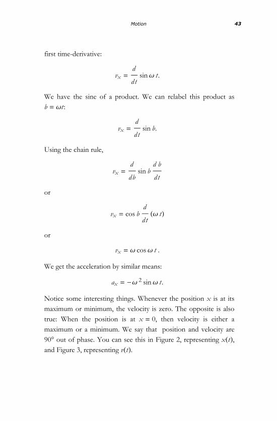
Let’s compute the velocity and acceleration. To do so, we need todifferentiate xHtL with respect to time. Here is the result of thefirst time-derivative:

vx =d

dtsin Ω t .

We have the sine of a product. We can relabel this product asb = Ωt :

vx =d

dtsin b.

Using the chain rule,

vx =d

dbsin b

d b

dt

or

vx = cos bd

dtHΩ tL

or

vx = Ω cos Ω t .

We get the acceleration by similar means:

ax = - Ω 2 sin Ω t .

Notice some interesting things. Whenever the position x is at itsmaximum or minimum, the velocity is zero. The opposite is alsotrue: When the position is at x = 0, then velocity is either amaximum or a minimum. We say that position and velocity are90° out of phase. You can see this in Figure 2, representing xHtL,and Figure 3, representing vHtL.

Motion 43

Π

2Π

3Π

22Π

Θ

-1

1xHtL

Figure 2: Representing position.

Π

2Π

3Π

22Π

Θ

-1

1vHtL

Figure 3: Representing velocity.

The position and acceleration are also related, both beingproportional to sin Ω t . But notice the minus sign in theacceleration. That minus sign says that whenever x is positive(negative), the acceleration is negative (positive). In other words,wherever the particle is, it is being accelerated back toward theorigin. In technical terms, the position and acceleration are 180°out of phase.

Exercise 6: How long does it take for the oscillatingparticle to go through one full cycle of motion?

Next, let’s consider a particle moving with uniformcircular motion about the origin. This means that it is moving in acircle at a constant speed. For this purpose, we can ignore the z

axis and think of the motion in the x, y plane. To describe it we

must have two functions, xHtL and yHtL. To be specific we will

choose the particle to move in the counterclockwise direction.Let the radius of the orbit be R.

It is helpful to visualize the motion by projecting it ontothe two axes. As the particle revolves around the origin, xoscillates between x = -R and x = R. The same is true of the y

coordinate. But the two coordinates are 90° out of phase; when xis maximum y is zero, and vice versa.

The most general (counterclockwise) uniform circularmotion about the origin has the mathematical form


Next, let’s consider a particle moving with uniformcircular motion about the origin. This means that it is moving in acircle at a constant speed. For this purpose, we can ignore the z

axis and think of the motion in the x, y plane. To describe it we

must have two functions, xHtL and yHtL. To be specific we will

choose the particle to move in the counterclockwise direction.Let the radius of the orbit be R.

It is helpful to visualize the motion by projecting it ontothe two axes. As the particle revolves around the origin, xoscillates between x = -R and x = R. The same is true of the y

coordinate. But the two coordinates are 90° out of phase; when xis maximum y is zero, and vice versa.

The most general (counterclockwise) uniform circularmotion about the origin has the mathematical form

x HtL = R cos Ω tyHtL = R sin Ω t .

Here the parameter Ω is called the angular frequency. It is defined asthe number of radians that the angle advances in unit time. It alsohas to do with how long it takes to go one full revolution, theperiod of motion—the same as we found in Exercise 6:

T =2 Π

Ω

Now it is easy to calculate the components of velocity andacceleration by differentiation:

(3)

vx = -R Ω sin Ω tv y = R Ω cos Ω t

ax = -R Ω2 cos Ω ta y = -R Ω2 sin Ω t

This shows an interesting property of circular motion thatNewton used in analyzing the motion of the moon: Theacceleration of a circular orbit is parallel to the position vector,but it is oppositely directed. In other words, the accelerationvector points radially inward toward the origin.

Motion 45

This shows an interesting property of circular motion thatNewton used in analyzing the motion of the moon: Theacceleration of a circular orbit is parallel to the position vector,but it is oppositely directed. In other words, the accelerationvector points radially inward toward the origin.

Exercise 7: Show that the position and velocity vectorsare orthogonal.

Exercise 8: Calculate the velocity, speed, andacceleration for each of the following position vectors. Ifyou have graphing software, plot each position vector,each velocity vector, and each acceleration vector.

r®

= Hcos Ω t , eΩ t Lr®

= Hcos HΩ t - ΦL, sin HΩ t - ΦLLr®

= Ic cos3 t , c sin3 tMr®

= Hc Ht - sin tL, c H1 - cos tLL


Interlude 2: Integral Calculus“George, I really like doing things backward. Can we dodifferentiation backward?”

“Sure we can, Lenny. It’s called integration.”

Integral Calculus

Differential calculus has to do with rates of change. Integralcalculus has to do with sums of many tiny incremental quantities.It’s not immediately obvious that these have anything to do witheach other, but they do.

We begin with the graph of a function f HtL, as in Figure 1.

1 2 3 4 5t

5

10

15

f HtL

Figure 1: The behavior of f HtL.

The central problem of integral calculus is to calculate the areaunder the curve defined by f HtL. To make the problem well

defined, we consider the function between two values that we calllimits of integration, t = a and t = b. The area we want to calculate isthe area of the shaded region in Figure 2.

a b

1 2 3 4 5t

5

10

15

f HtL

Figure 2: The limits of integration.

In order to do this, we break the region into very thin rectanglesand add their areas (see Figure 3).

a b

1 2 3 4 5t

5

10

15

f HtL

Figure 3: An illustration of integration.

Of course this involves an approximation, but it becomesaccurate if we let the width of the rectangles tend to zero. Inorder to carry out this procedure, we first divide the intervalbetween t = a and t = b into a number, N , of subintervals—eachof width D t . Consider the rectangle located at a specific value oft . The width is D t and the height is the local value of f HtL. It

follows that the area of a single rectangle, ∆ A, is

∆ A = f HtL D t .

Now we add up all the areas of the individual rectangles to get anapproximation to the area that we are seeking. The approximateanswer is


Now we add up all the areas of the individual rectangles to get anapproximation to the area that we are seeking. The approximateanswer is

A = âi

f HtiL D t

where the uppercase greek letter sigma, S, indicates a sum ofsuccessive values defined by i. So, if N = 3, then

A = â3

i

f HtiL D t

= f Ht1L D t + f Ht2L D t + f Ht3L D t .

Here ti is the position of the ith rectangle along the t axis.To get the exact answer, we take the limit in which D t

shrinks to zero and the number of rectangles increases to infinity.That defines the definite integral of f HtL between the limits t = a

and t = b. We write this as

A = àa

bf HtL d t = lim

D t®0â

i

f HtiL D t .

The integral sign, called summa, Ù, replaces the summation sign,and—as in differential calculus—D t is replaced by d t . Thefunction f HtL is called the integrand.

Let’s make a notational change and call one of the limitsof integration T . In particular, replace b by T and consider theintegral

àa

Tf HtL d t

where we are going to think of T as a variable instead of as adefinite value of t . In this case, this integral defines a function ofT , which can take on any value of t . The integral is a function ofT because it has a definite value for each value of T .

49Integral Calculus

where we are going to think of T as a variable instead of as adefinite value of t . In this case, this integral defines a function ofT , which can take on any value of t . The integral is a function ofT because it has a definite value for each value of T .

FHT L = àa

Tf HtL d t .

Thus a given function f HtL defines a second function FHT L. We

could also let a vary, but we won’t. The function FHT L is calledthe indefinite integral of f HtL. It is indefinite because instead of

integrating from a fixed value to a fixed value, we integrate to avariable. We usually write such an integral without limits ofintegration,

(1)FHtL = à f HtL d t .

The fundamental theorem of calculus is one of the simplest andmost beautiful results in mathematics. It asserts a deepconnection between integrals and derivatives. What it says is that

if FHT L = Ù f HtL d t , then

f HtL =d FHtL

d t.

To see this, consider a small incremental change in T from T toT + D t . Then we have a new integral,

FHT + D tL = àa

T+D tf HtL d t .

In other words, we have added one more rectangle of width D tat t = T to the area shaded in Figure 3. In fact, the differenceFHT + D tL - FHT L is just the area of that extra rectangle, whichhappens to be f HT L D t , so

FHT + D tL - FHT L = f HT L D t .


Dividing by D t ,

FHT + D tL - FHT LD t

= f HT L

we obtain the fundamental theorem connecting F and f , when

we take the limit where D t ® 0:

d F

d T= lim

D t®0

FHT + D tL - FHT LD t

= f HT L.

We can simplify the notation by ignoring the difference between tand T ,

d F

d t= f HtL.

In other words, the processes of integration and differentiationare reciprocal: The derivative of the integral is the originalintegrand.

Can we completely determine FHtL knowing that itsderivative is f HtL? Almost, but not quite. The problem is that

adding a constant to FHtL does not change its derivative. Given

f HtL, its indefinite integral is ambiguous, but only up to adding a

constant.To see how the fundamental theorem is used, let’s work

out some indefinite integrals. Let’s find the integral of a powerf HtL = tn. Consider,

FHtL = à f HtL d t .

It follows that

51Integral Calculus

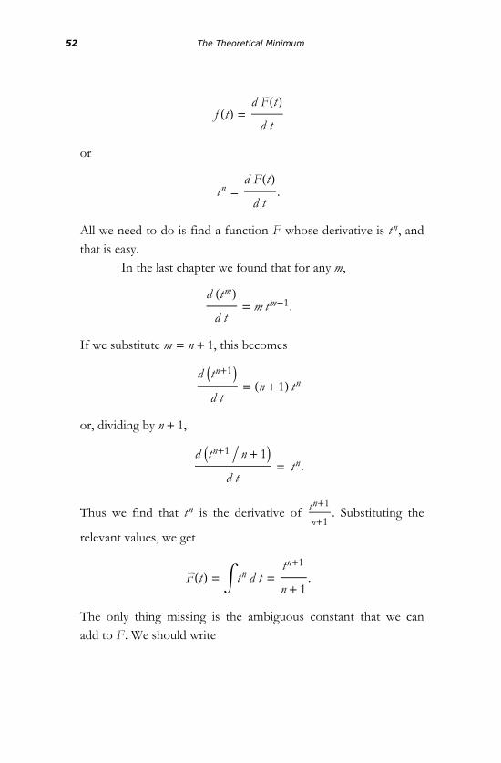
f HtL =d FHtL

d t

or

tn =d FHtL

d t.

All we need to do is find a function F whose derivative is tn, andthat is easy.

In the last chapter we found that for any m,

d HtmLd t

= m tm-1.

If we substitute m = n + 1, this becomes

d Itn+1Md t

= Hn + 1L tn

or, dividing by n + 1,

d Itn+1 n + 1Md t

= tn.

Thus we find that tn is the derivative of tn+1

n+1. Substituting the

relevant values, we get

FHtL = à tn d t =tn+1

n + 1.

The only thing missing is the ambiguous constant that we canadd to F . We should write


à tn d t =tn+1

n + 1+ c

where c is a constant that has to be determined by other means.The ambiguous constant is closely related to the

ambiguity in choosing the other endpoint of integration that weearlier called a. To see how a determines the ambiguous constantc , let’s consider the integral

àa

Tf HtL d t .

in the limit where the two limits of integration come together—that is, T = a. In this case, the integral has to be zero. You canuse that fact to determine c .

In general, the fundamental theorem of calculus is written

(2)àa

bf HtL d t = FHtL

a

b= FHbL - FHaL.

Another way to express the fundamental theorem is by asingle equation:

(3)àd f

d td t = f HtL + c .

In other words, integrating a derivative gives back the originalfunction (up to the usual ambiguous constant). Integration anddifferentiation undo each other.

Here are some integration formulas:

à c d t = c t

53Integral Calculus

à c f HtL d t = c à f HtL d t

à t d t =t2

2+ c

à t 2 d t =t3

3+ c

à t n d t =tn+1

n + 1+ c

à sin t d t = - cos t + c

à cos t d t = sin t + c

à et d t = et

àd t

t= ln t + c

à @ f HtL ± g HtLD d t = à f HtL d t ± à g HtL d t .

Exercise 1: Determine the indefinite integral of each ofthe following expressions by reversing the process ofdifferentiation and adding a constant.

f HtL = t4

f HtL = cos tf HtL = t2 - 2

Exercise 2: Use the fundamental theorem of calculus toevaluate each integral from Exercise 1 with limits ofintegration being t = 0 to t = T .


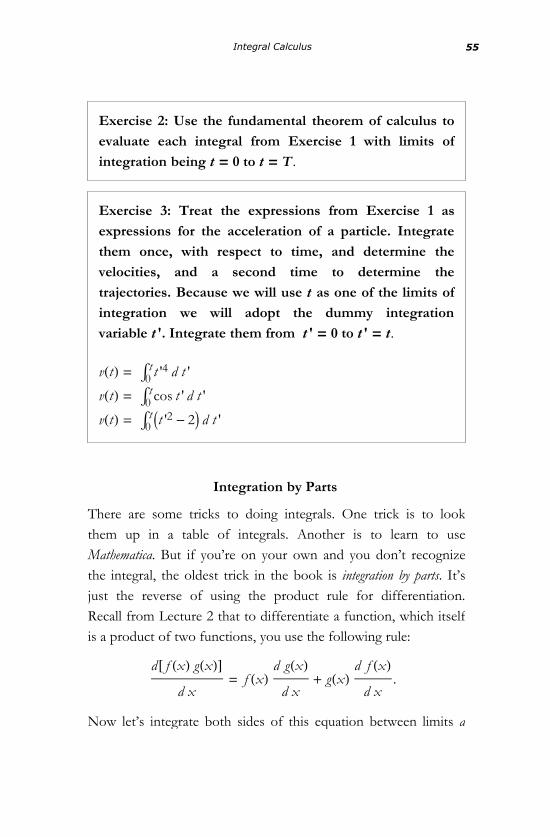
Exercise 2: Use the fundamental theorem of calculus toevaluate each integral from Exercise 1 with limits ofintegration being t = 0 to t = T .

Exercise 3: Treat the expressions from Exercise 1 asexpressions for the acceleration of a particle. Integratethem once, with respect to time, and determine thevelocities, and a second time to determine thetrajectories. Because we will use t as one of the limits ofintegration we will adopt the dummy integrationvariable t '. Integrate them from t ' = 0 to t ' = t.

vHtL = Ù0t t '4 d t '

vHtL = Ù0tcos t ' d t '

vHtL = Ù0t It '2 - 2M d t '

Integration by Parts

There are some tricks to doing integrals. One trick is to lookthem up in a table of integrals. Another is to learn to useMathematica. But if you’re on your own and you don’t recognizethe integral, the oldest trick in the book is integration by parts. It’sjust the reverse of using the product rule for differentiation.Recall from Lecture 2 that to differentiate a function, which itselfis a product of two functions, you use the following rule:

d@ f HxL gHxLDd x

= f HxL d gHxLd x

+ gHxL d f HxLd x

.

Now let’s integrate both sides of this equation between limits aand b.

55Integral Calculus

Now let’s integrate both sides of this equation between limits aand b.

àa

b d@ f HxL gHxLDd x

= àa

bf HxL d gHxL

d x+

àa

bgHxL d f HxL

d x

The left side of the equation is easy. The integral of a derivative(the derivative of f g) is just the function itself. The left side is

f HbL g HbL - f HaL gHaLwhich we often write in the form

f HxL g HxL¤ab .

Now let’s subtract one of the two integrals on the right side andshift it to the left side.

(4)f HxL g HxL¤ab - àa

bf HxL d gHxL

d x= à

a

bgHxL d f HxL

d x.

Suppose we have some integral that we don’t recognize, but wenotice that the integrand happens to be a product of a functionf HxL and the derivative of another function gHxL. In other words,

after some inspection, we see that the integral has the form of theright side of Eq. (4), but we don’t know how to do it. Sometimeswe are lucky and recognize the integral on the left side of theequation.

Let’s do an example. Suppose the integral that we want todo is

à0

Π

2 x cos x d x.


That’s not in our list of integrals. But notice that

cos x =d sin x

d x

so the integral is

à0

Π

2 xd sin x

d xd x.

Equation (4) tells us that this integral is equal to

x sin x¤0Π

2 - à0

Π

2d x

d xsin x d x

or just

Π

2sin

Π

2- à

0

Π

2 sin x d x.

Now it’s easy. The integral Ù sin x d x is on our list: it’s just cos x.

I’ll leave the rest to you.

Exercise 4: Finish evaluating Ù0

Π

2 x cos x d x.

You might wonder how often this trick works. The answer isquite often, but certainly not always. Good luck.

57Integral Calculus

Lecture 3: DynamicsLenny: “What makes things move, George?

George: “Forces do, Lenny.”Lenny: “What makes things stop moving, George?”George: “Forces do, Lenny.”

Aristotle’s Law of Motion

Aristotle lived in a world dominated by friction. To makeanything move—a heavy cart with wooden wheels, for example—you had to push it, you had to apply a force to it. The harder youpushed it, the faster it moved; but if you stopped pushing, thecart very quickly came to rest. Aristotle came to some wrongconclusions because he didn’t understand that friction is a force.But still, it’s worth exploring his ideas in modern language. If hehad known calculus, Aristotle might have proposed the followinglaw of motion:

The velocity of any object is proportional to the total applied force.

Had he known how to write vector equations, his law would havelooked like this:

F®

= m v®

.

F®

is of course the applied force, and the response (according to

Aristotle) would be the velocity vector, v®

. The factor m relatingthe two is some characteristic quantity describing the resistanceof the body to being moved; for a given force, the bigger the m ofthe object, the smaller its velocity. With a little reflection, the oldphilosopher might have identified m with the mass of the object.It would have been obvious that heavier things are harder tomove than lighter things, so somehow the mass of the object hasto be in the equation.

One suspects that Aristotle never went ice skating, or hewould have known that it is just as hard to stop a body as to get itmoving. Aristotle’s law is just plain wrong, but it is neverthelessworth studying as an example of how equations of motion candetermine the future of a system. From now on, let’s call thebody a particle.

Consider one-dimensional motion of a particle along thex axis under the influence of a given force. What I mean by agiven force is simply that we know what the force is at any time.We can call it FHtL (note that vector notation would be a bitredundant in one dimension). Using the fact that the velocity isthe time derivative of position, x, we find that Aristotle’sequation takes the form

F®

is of course the applied force, and the response (according to

Aristotle) would be the velocity vector, v®

. The factor m relatingthe two is some characteristic quantity describing the resistanceof the body to being moved; for a given force, the bigger the m ofthe object, the smaller its velocity. With a little reflection, the oldphilosopher might have identified m with the mass of the object.It would have been obvious that heavier things are harder tomove than lighter things, so somehow the mass of the object hasto be in the equation.

One suspects that Aristotle never went ice skating, or hewould have known that it is just as hard to stop a body as to get itmoving. Aristotle’s law is just plain wrong, but it is neverthelessworth studying as an example of how equations of motion candetermine the future of a system. From now on, let’s call thebody a particle.

Consider one-dimensional motion of a particle along thex axis under the influence of a given force. What I mean by agiven force is simply that we know what the force is at any time.We can call it FHtL (note that vector notation would be a bitredundant in one dimension). Using the fact that the velocity isthe time derivative of position, x, we find that Aristotle’sequation takes the form

dxHtLdt

=FHtLm

.

Before solving the equation, let’s see how it compares to thedeterministic laws of Chapter 1. One obvious difference is thatAristotle’s equation is not stroboscopic—that is neither t nor x isdiscrete. They do not change in sudden stroboscopic steps; theychange continuously. Nevertheless, we can see the similarity if weassume that time is broken up into intervals of size Dt and

replace the derivative by DxDt

. Doing so gives

Dynamics 59

xHt + DtL = xHtL + DtFHtLm

.

In other words, wherever the particle happens to be at time t , atthe next instant its position will have shifted by a definiteamount. For example, if the force is constant and positive, thenin each incremental step the particle moves forward by an

amount Dt FHtLm

. This law is obviously deterministic. Knowing that

the particle was at a point xH0L at time t = 0 (or x0), one caneasily predict where it will be in the future. So by the criteria ofChapter 1, Aristotle did not commit any crime.

Let’s go back to the exact equation of motion:

dxHtLdt

=FHtLm

.

Equations for unknown functions that involve derivatives arecalled differential equations. This one is a first-order differentialequation because it contains only first derivatives. Equations likethis are easy to solve. The trick is to integrate both sides of theequation:

àdxHtL

dtd t = à

FHtLm

dt .

The left side of the equation is the integral of a derivative. That’swhere the fundamental theorem of calculus comes in handy. Theleft side is just xHtL + c .

The right side, on the other hand, is the integral of somespecified function and, apart from a constant, is also determined.For example, if F is constant, then the right side is


àF

mdt =

F

mt + c .

Note that we included an additive constant. Putting an arbitraryconstant on both sides of the equation is redundant. In this case,the equation of motion is satisfied by

xHtL =F

mt + c .

How do you fix the constant c? The answer is by the initialcondition. For example, if we knew that the particle started atx = 1, at time t = 3 we would plug these values in, obtaining

1 =F

m3 + c ,

and solve for c :

c = 1 - 3F

m.

Exercise 1: Given a force that varies with time according

to F = 2t2, and with the initial condition at time zero,xH0L = Π, use Aristotle’s law to find xHtL at all times.

Aristotle’s equations of motion are deterministic, but arethey reversible? In Lecture 1, I explained that reversible means thatif all the arrows were reversed, the resulting new law of motionwould also be deterministic. The analogous procedure toreversing the arrows when time is continuous is very simple.Everywhere you see time in the equations, replace it with minustime. That will have the effect of interchanging the future and thepast. Changing t to - t also includes changing the sign of smalldifferences in time. In other words, every Dt must be replacedwith - Dt . In fact, you can do it right at the level of the

differentials dt . Reversing the arrows means changing the differentialdt to -dt . Let’s go back to Aristotle’s equation

Dynamics 61

Aristotle’s equations of motion are deterministic, but arethey reversible? In Lecture 1, I explained that reversible means thatif all the arrows were reversed, the resulting new law of motionwould also be deterministic. The analogous procedure toreversing the arrows when time is continuous is very simple.Everywhere you see time in the equations, replace it with minustime. That will have the effect of interchanging the future and thepast. Changing t to - t also includes changing the sign of smalldifferences in time. In other words, every Dt must be replacedwith - Dt . In fact, you can do it right at the level of the

differentials dt . Reversing the arrows means changing the differentialdt to -dt . Let’s go back to Aristotle’s equation

FHtL = mdx

dt

and change the sign of time. The result is

FH- tL = -mdx

dt.

The left-hand side of the equation is the force, but the forceevaluated at time - t , not at time t . However, if FHtL is a knownfunction, then so is FH- tL. In the reversed problem, the force isalso a known function of reversed time.

On the right-hand side of the equation we’ve replaced dtwith -dt , thereby changing the sign of the whole expression. Infact, one can shift the minus sign to the left-hand side of theequation:

-FH- tL = mdx

dt.

The implication is simple: The reversed equation of motion isexactly like the original, but with a different rule for the force as afunction of time. The conclusion is clear: If Aristotle’s equationsof motion are deterministic into the future, they are alsodeterministic into the past. The problem with Aristotle’sequations is not that they are inconsistent; they are just the wrongequations.

It is interesting that Aristotle's equations do have anapplication—not as fundamental laws, but as approximations.Frictional forces do exist, and in many cases they are soimportant that Aristotle's intuition—things stop if you stoppushing—is almost correct. Frictional forces are notfundamental. They are a consequence of a body interacting with ahuge number of other tiny bodies—atoms and molecules—thatare too small and too numerous to keep track of. So we averageover all the hidden degrees of freedom. The result is frictionalforces. When frictional forces are very strong such as in a stonemoving through mud—then Aristotle's equation is a very goodapproximation, but with a qualification. It's not the mass thatdetermines the proportionality between force and velocity. It'sthe so-called viscous drag coefficient. But that may be more thanyou want to know.


It is interesting that Aristotle's equations do have anapplication—not as fundamental laws, but as approximations.Frictional forces do exist, and in many cases they are soimportant that Aristotle's intuition—things stop if you stoppushing—is almost correct. Frictional forces are notfundamental. They are a consequence of a body interacting with ahuge number of other tiny bodies—atoms and molecules—thatare too small and too numerous to keep track of. So we averageover all the hidden degrees of freedom. The result is frictionalforces. When frictional forces are very strong such as in a stonemoving through mud—then Aristotle's equation is a very goodapproximation, but with a qualification. It's not the mass thatdetermines the proportionality between force and velocity. It'sthe so-called viscous drag coefficient. But that may be more thanyou want to know.

Mass, Acceleration, and Force

Aristotle’s mistake was to think that a net “applied” force isneeded to keep an object moving. The right idea is that oneforce—the applied force—is needed to overcome anotherforce—the force of friction. An isolated object moving in freespace, with no forces acting on it, requires nothing to keep itmoving. In fact, it needs a force to stop it. This is the law of inertia.What forces do is change the state of motion of a body. If thebody is initially at rest, it takes a force to start it moving. If it’smoving, it takes a force to stop it. If it is moving in a particulardirection, it takes a force to change the direction of motion. Allof these examples involve a change in the velocity of an object,and therefore an acceleration.

From experience we know that some objects have moreinertia than others; it requires a larger force to change theirvelocities. Obvious examples of objects possessing large andsmall inertia are locomotives and Ping-Pong balls, respectively.The quantitative measure of an object's inertia is its mass.

Newton's law of motion involves three quantities:acceleration, mass, and force. Acceleration we studied in Lecture2. By monitoring the position of an object as it moves, a cleverobserver—with a bit of mathematics—can determine itsacceleration. Mass is a new concept that is actually defined interms of force and acceleration. But so far we haven't definedforce. It sounds like we are in a logical circle in which force isdefined by the ability to change the motion of a given mass, andmass is defined by the resistance to that change. To break thatcircle, let's take a closer look at how force is defined andmeasured in practice.

There are very sophisticated devices that can measureforce to great accuracy, but it will suit our purposes best toimagine a very old-fashioned device, namely, a spring balance. Itconsists of a spring and a ruler to measure how much the springis stretched from its natural equilibrium length (see Figure 1).

Dynamics 63

From experience we know that some objects have moreinertia than others; it requires a larger force to change theirvelocities. Obvious examples of objects possessing large andsmall inertia are locomotives and Ping-Pong balls, respectively.The quantitative measure of an object's inertia is its mass.

Newton's law of motion involves three quantities:acceleration, mass, and force. Acceleration we studied in Lecture2. By monitoring the position of an object as it moves, a cleverobserver—with a bit of mathematics—can determine itsacceleration. Mass is a new concept that is actually defined interms of force and acceleration. But so far we haven't definedforce. It sounds like we are in a logical circle in which force isdefined by the ability to change the motion of a given mass, andmass is defined by the resistance to that change. To break thatcircle, let's take a closer look at how force is defined andmeasured in practice.

There are very sophisticated devices that can measureforce to great accuracy, but it will suit our purposes best toimagine a very old-fashioned device, namely, a spring balance. Itconsists of a spring and a ruler to measure how much the springis stretched from its natural equilibrium length (see Figure 1).

A

1 kg

ScalePull

Figure 1: A spring balance.

The spring has two hooks, one to attach to the massive bodywhose mass is being measured, and one to pull on. In fact, whileyou are at it, make several such identical devices.

Let’s define a unit of force by pulling on one hook, whileholding the other hook fixed to some object A, until the pointerregisters one “tick” on the ruler. Thus we are applying a unit offorce to A.

To define two units of force, we could pull just hardenough to stretch the spring to two ticks. But this assumes thatthe spring behaves the same way between one tick and two ticksof stretching. This will lead us back to a vicious circle ofreasoning that we don’t want to get into. Instead, we define twounits of force by attaching two spring balances to A and pullingboth of them with a single unit of force (see Figure 2).

In other words, we pull both hooks so that each pointerrecords a single tick. Three units of force would be defined byusing three springs, and so on.

When we do this experiment in free space, we discoverthe interesting fact that object A accelerates along the direction inwhich we pull the hook. More exactly, the acceleration isproportional to the force—twice as big for two units of force,three times as big for three units, and so on.


The spring has two hooks, one to attach to the massive bodywhose mass is being measured, and one to pull on. In fact, whileyou are at it, make several such identical devices.

Let’s define a unit of force by pulling on one hook, whileholding the other hook fixed to some object A, until the pointerregisters one “tick” on the ruler. Thus we are applying a unit offorce to A.

To define two units of force, we could pull just hardenough to stretch the spring to two ticks. But this assumes thatthe spring behaves the same way between one tick and two ticksof stretching. This will lead us back to a vicious circle ofreasoning that we don’t want to get into. Instead, we define twounits of force by attaching two spring balances to A and pullingboth of them with a single unit of force (see Figure 2).

In other words, we pull both hooks so that each pointerrecords a single tick. Three units of force would be defined byusing three springs, and so on.

When we do this experiment in free space, we discoverthe interesting fact that object A accelerates along the direction inwhich we pull the hook. More exactly, the acceleration isproportional to the force—twice as big for two units of force,three times as big for three units, and so on.

Figure 2: Twice the force.

Let us do something to change the inertia of A. Inparticular, we will double the inertia by hooking together twoidentical versions of object A (see Figure 3).

Dynamics 65

Figure 3: Twice the mass.

What we find is that when we apply a single unit of force (bypulling the whole thing with a single spring stretched to one tick)the acceleration is only half what it was originally. The inertia(mass) is now twice as big as before.

The experiment can obviously be generalized; hook upthree masses, and the acceleration is only a third as big, and so on.

We can do many more experiments in which we hookany number of springs to any number of A’s. The observationsare summarized by a single formula, Newton’s second law ofmotion, which tells us that force equals mass times acceleration,

(1)F®

= m a®

.

This equation can also be written in the form

(2)F®

= md v

®

dt.

In other words, force equals mass times the rate of change ofvelocity: no force—no change in velocity.

Note that these equations are vector equations. Bothforce and acceleration are vectors because they not only havemagnitude but also direction.


An Interlude on Units

A mathematician might be content to say that the length of a linesegment is 3. But a physicist or engineer—or even an ordinaryperson—would want to know, “Three what?” Three inches, threecentimeters, or three light years?

Similarly, it conveys no information to say that the massof an object is 7 or 12. To give the numbers meaning, we mustindicate what units we are using. Let’s begin with length.

Somewhere in Paris rests the defining platinum meterstick. It is kept in a sealed container at a fixed temperature andaway from other conditions that might affect its length.1 From

here on, we will adopt that meter stick as our unit of length.

Thus we write

@xD = @lengthD = meters.

Despite its appearance, this is not an equation in the usual sense.The way to read it is x has units of length and is measured in meters.

Similarly, t has units of time and is measured in seconds.The definition of a second could be given by the amount of timeit takes a certain pendulum to make a single swing:

@tD = @timeD = seconds.

The units meters and seconds are abbreviated as m and s,respectively.

1. There is a more modern definition of the meter in terms of thewavelength of light emitted by atoms jumping from one quantum levelto another. For our purposes the Paris meter stick will do just fine.

Dynamics 67

Once we have units for length and time, we can constructunits for velocity and acceleration. To compute the velocity of anobject, we divide a distance by a time. The result has units oflength per time, or—in our units—meters per second.

@vD =length

time=

m

s.

Similarly, acceleration is the rate of change of velocity, and itsunits are velocity per unit time, or length per unit time per unittime:

@aD =length

time

1

time=

length

time2=

m

s2.

The unit of mass that we will use is the kilogram; it isdefined as the mass of a certain lump of platinum, that is alsokept somewhere in France. Thus

@mD = @massD = kilogram = kg.

Now let’s consider the unit of force. One might define itin terms of some particular spring made of a specific metal,stretched a distance of 0.01 meter, or something like that. But infact, we have no need for a new unit of force. We already haveone—namely the force that it takes to accelerate one kilogram byone meter per second per second. Even better is to use Newton’slaw F = ma. Evidently, force has units of mass times acceleration,

@FD = @forceD= @maD


=mass length

time2

=kg m

s2.

There is a name for this unit of force. One kilogram meter persecond squared is called a Newton, abbreviated N. Newton,himself, being English, probably favored the British unit, namelythe pound. There are about 4.4 N to a pound.

Some Simple Examples of Solving Newton’s Equations

The simplest of all examples is a particle with no forces acting onit. The equation of motion is Eq. (2), but with the force set tozero:

md v

®

dt= 0,

or, using the dot notation for time derivative,

m v®

= 0.

We can drop the factor of mass and write the equation incomponent form as

v×x = 0

v×

y = 0

v×z = 0

Dynamics 69

The solution is simple: The components of velocity are constantand can just be set equal to their initial values,

(3)vxHtL = vxH0L.The same goes for the other two components of velocity. This,incidently, is often referred to as Newton’s first law of motion:

Every object in a state of uniform motion tends to remain in that state ofmotion unless an external force is applied to it.

Equations (1) and (2) are called Newton’s second law of motion,

The relationship between an object’s mass m, its acceleration a, and theapplied force F is

F = ma.

But, as we have seen, the first law is simply a special case of thesecond law when the force is zero.

Recalling that velocity is the derivative of position, wecan express Eq. (3) in the form

x×

= vxH0L.This is the simplest possible differential equation, whose solution(for all components) is

xHtL = x0 + vxH0LtyHtL = y0 + v yH0LtzHtL = z0 + vzH0Lt

or, in vector notation,

r®HtL = r

®

0 + v®

0t .

A more complicated motion results from the applicationof a constant force. Let’s first carry it out for just the z direction.

Dividing by m, the equation of motion is


A more complicated motion results from the applicationof a constant force. Let’s first carry it out for just the z direction.

Dividing by m, the equation of motion is

v×z =

Fz

m.

Exercise 2: Integrate this equation. Hint: Use definite

integrals.

From this result we deduce

vzHtL = vzH0L +Fz

mt ,

or

z× HtL = vzH0L +

Fz

mt .

This is probably the second simplest differential equation. It iseasy to solve:

(4)zHtL = z0 + vzH0Lt +Fz

2mt2.

Exercise 3: Show by differentiation that this satisfies theequation of motion.

This simple case may be familiar. If z represents the height above

the surface of the Earth, and Fz

m is replaced with the acceleration

due to gravity, Fz

m= - g, then Eq. (4) is the equation describing

the motion of an object falling from height z0 with an initial

velocity vzH0L:

Dynamics 71

This simple case may be familiar. If z represents the height above

the surface of the Earth, and Fz

m is replaced with the acceleration

due to gravity, Fz

m= - g, then Eq. (4) is the equation describing

the motion of an object falling from height z0 with an initial

velocity vzH0L:

(5)zHtL = z0 + vzH0Lt -1

2gt2.

Let’s consider the case of the simple harmonic oscillator.This system is best thought of as a particle that moves along thex axis, subject to a force that pulls it toward the origin. The forcelaw is

Fx = -kx.

The negative sign indicates that at whatever the value of x, theforce pulls it back toward x = 0. Thus, when x is positive, theforce is negative, and vice versa. The equation of motion can bewritten in the form

x××

= -k

mx,

or, by defining km

= Ω2,

(6)x××

= - Ω2x.

Exercise 4: Show by differentiation that the general solution to Eq. (6) is given in terms of two constants A and B by

xHtL = A cos Ω t+B sin Ω t.Determine the initial position and velocity at time t = 0 in terms of A and B.

The harmonic oscillator is an enormously importantsystem that occurs in contexts ranging from the motion of apendulum to the oscillations of the electric and magnetic fields ina light wave. It is profitable to study it thoroughly.


The harmonic oscillator is an enormously importantsystem that occurs in contexts ranging from the motion of apendulum to the oscillations of the electric and magnetic fields ina light wave. It is profitable to study it thoroughly.

Dynamics 73

Interlude 3: Partial Differentiation“Look out there, Lenny. Ain’t those hills and valleys pretty?”

“Yeah George. Can we get a place over there when weget some money? Can we?”

George squinted. “Exactly where are you looking Lenny?”Lenny pointed. “Right over there George. That local

minimum.”

Partial Derivatives

The calculus of multivariable functions is a straightforwardgeneralization of single-variable calculus. Instead of a function ofa single variable t , consider a function of several variables. Toillustrate, let’s call the variables x, y, z, although these don’t have

to stand for the coordinates of ordinary space. Moreover, therecan be more or fewer then three. Let us also consider a functionof these variables, V Hx, y, zL. For every value of x, y, z, there is

a unique value of V Hx, y, zL that we assume varies smoothly as

we vary the coordinates.Multivariable differential calculus revolves around the

concept of partial derivatives. Suppose we are examining theneighborhood of a point x, y, z, and we want to know the rate at

which V varies as we change x while keeping y and z fixed. We

can just imagine that y and z are fixed parameters, so the only

variable is x. The derivative of V is then defined by

(1)d V

d x= lim

D x®0

D V

D x

where D V is defined by

(2)D V = V H@x + D xD, y, zL - V Hx, y, zL.Note that in the defininition of D V , only x has been shifted; y

and z are kept fixed.

The derivative defined by Eq. (1) and Eq. (2) is called thepartial derivative of V with respect to x and is denoted

¶V

¶x

or, when we want to emphasize that y and z are kept fixed,

¶V

¶x y,z.

By the same method we can construct the partialderivative with respect to either of the other variables:

¶V

¶ y= lim

D y®0

D V

D y.

A shorthand notation for the partial derivatives of V withrespect to y is

¶V

¶ y= ¶ y V .

Multiple derivatives are also possible. If we think of ¶V¶x

as itself being a function of x, y, z, then it can be differentiated.

Thus we can define the second-order partial derivative withrespect to x:

Partial Differentiation 75

¶2 V

¶x2= ¶x

¶V

¶x= ¶x,x V .

Mixed partial derivatives also make sense. For example, one candifferentiate ¶ y V with respect to x:

¶2 V

¶x ¶ y= ¶x

¶V

¶ y= ¶x, y V .

It’s an interesting and important fact that the mixed derivativesdo not depend on the order in which the derivatives are carriedout. In other words,

¶2 V

¶x ¶ y=

¶2 V

¶ y ¶x.

Exercise 1: Compute all first and second partialderivatives—including mixed derivatives—of thefollowing functions.

x2 + y2 = sin Hx yLxy

ex2+ y2

ex cos y

Stationary Points and Minimizing Functions

Let’s look at a function of y that we will call F (see Figure 1).


y

FH yL

Figure 1: Plot of the function FI yM.

Notice that there are places on the curve where a shift in y in

either direction produces only an upward shift in F . These pointsare called local minima. In Figure 2 we have added dots to indicatethe local minima.

y

FH yL

Figure 2: Local minima.

For each local minimum, when you go in either direction along y,

you begin to rise above the dot in FH yL. Each dot is at the

bottom of a little depression. The global minimum is the lowestpossible place on the curve.

One condition for a local minimum is that the derivativeof the function with respect to the independent variable at thatpoint is zero. This is a necessary condition, but not a sufficientcondition. This condition defines any stationary point,

d

d yFH yL = 0.

The second condition tests to see what the character of thestationary point is by examining its second derivative. If thesecond derivative is larger than 0, then all points nearby will beabove the stationary point, and we have a local minimum:


The second condition tests to see what the character of thestationary point is by examining its second derivative. If thesecond derivative is larger than 0, then all points nearby will beabove the stationary point, and we have a local minimum:

d2

d2 yFH yL > 0.

If the second derivative is less than 0, then all points nearby willbe below the stationary point, and we have a local maximum:

d2

d2 yFH yL < 0.

See Figure 3 for examples of local maxima.

y

FH yL

Figure 3: Local maxima.

If the second derivative is equal to 0, then the derivative changesfrom positive to negative at the stationary point, which we call apoint of inflection:

d2

d2 yFH yL = 0.

See Figure 4 for an example of a point of inflection.


y

FH yL

Figure 4: Point of inflection.

These are collectively the results of a second-derivative test.

Stationary Points in Higher Dimensions

Local maxima, local minima, and other stationary points canhappen for functions of more than one variable. Imagine a hillyterrain. The altitude is a function that depends on the twocoordinates—let’s say latitude and longitude. Call it AHx, yL. The

tops of hills and the bottoms of valleys are local maxima andminima of AHx, yL. But they are not the only places where the

terrain is locally horizontal. Saddle points occur between twohills. You can see some examples in Figure 5.

Figure 5: A function of several variables.

The very tops of hills are places where no matter whichway you move, you soon go down. Valley bottoms are theopposite; all directions lead up. But both are places where theground is level.

There are other places where the ground is level. Betweentwo hills you can find places called saddles. Saddle points are level,

but along one axis the altitude quickly increases in eitherdirection. Along another perpendicular direction the altitudedecreases. All of these are called stationary points.


The very tops of hills are places where no matter whichway you move, you soon go down. Valley bottoms are theopposite; all directions lead up. But both are places where theground is level.

There are other places where the ground is level. Betweentwo hills you can find places called saddles. Saddle points are level,

but along one axis the altitude quickly increases in eitherdirection. Along another perpendicular direction the altitudedecreases. All of these are called stationary points.

Let's take a slice along the x axis through our space sothat the slice passes through a local minimum of A, see Figure 6.

Figure 6: A slice along the x axis.

It’s apparent that at the minimum, the derivative of Awith respect to x vanishes, we write this:

¶ A

¶ x= 0.

On the other hand, the slice could have been oriented along they axis, and we would then conclude that

¶ A

¶ y= 0.

To have a minimum, or for that matter to have any stationarypoint, both derivatives must vanish. If there were more directionsof space in which A could vary, then the condition for astationary point is given by:


(3)¶ A

¶ xi= 0.

for all xi .

There is a shorthand for summarizing these equations.Recall that the change in a function when the point x is varied alittle bit is given by

∆ A = âi

¶ A

¶ xi∆ xi .

The set of Equations (3) are equivalent to the condition that

(4)∆ A = 0

for any small variation of x.Suppose we found such a point. How do we tell whether

it is a maximum, a minimum, or a saddle. The answer is ageneralization of the criterion for a single variable. We look at thesecond derivatives. But there are several second derivatives. Forthe case of two dimensions, we have

¶2 A

¶ x2,

¶2 A

¶ y2,

¶2 A

¶ x ¶ y,

and


¶2 A

¶ y ¶ x,

the last two being the same.These partial derivatives are often arranged into a special

matrix called the Hessian matrix.

H =

¶2A

¶ x2¶2A

¶ x ¶ y

¶2A¶ y ¶ x

¶2A

¶ y2 .

Important quantities, called the determinant and the trace, can bemade out of such a matrix. The determinant is given by

Det H =¶2 A

¶ x2

¶2 A

¶ y2-

¶2 A

¶ y ¶ x

¶2 A

¶ x ¶ y

and the trace is given by

Tr H =¶2 A

¶ x2+

¶2 A

¶ y2.

Matrices, determinants, and traces may not mean muchto you beyond these definitions, but they will if you follow theselectures to the next subject—quantum mechanics. For now, allyou need is the definitions and the following rules.

If the determinant and the trace of the Hessian is positive then the point is alocal minimum.

If the determinant is positive and the trace negative the point is a localmaximum.

If the determinant is negative, then irrespective of the trace, the point is asaddle point.

However: One caveat, these rules specifically apply to functionsof two variables. Beyond that, the rules are more complicated.None of this is obvious for now, but it still enables you to testvarious functions and find their different stationary points. Let’stake an example. Consider


However: One caveat, these rules specifically apply to functionsof two variables. Beyond that, the rules are more complicated.None of this is obvious for now, but it still enables you to testvarious functions and find their different stationary points. Let’stake an example. Consider

FHx, yL = sin x + sin y.

Differentiating, we get

¶ F

¶ x= cos x

¶ F

¶ y= cos y.

Take the point x =Π

2, y =

Π

2. Since cos Π

2= 0, both derivatives

are zero and the point is a stationary point.Now, to find the type of stationary point, compute the

second derivatives. The second derivatives are

¶2 F

¶ x2= -sin x

¶2 F

¶ y2= -sin y

¶2 F

¶ x ¶ y= 0

¶2 F

¶ y ¶ x= 0.

Since sin Π

2= 1 we see that both the determinant and the trace of

the Hessian are positive. The point is therefore a minimum.


Since sin Π

2= 1 we see that both the determinant and the trace of

the Hessian are positive. The point is therefore a minimum.

Exercise 2: Consider the points Jx =Π

2, y = -

Π

2N,

Jx = -Π

2, y =

Π

2N ,

Jx = -Π

2, y = -

Π

2N. Are these points stationary points of

the following functions? Is so, of what type?.

FHx, yL = sin x + sin yFHx, yL = cos x + cos y


Lecture 4: Systems of More Than One Particle

It’s a lazy, warm evening. Lenny and George are lying in the grasslooking up at the sky.

“Tell me about the stars George. Are they particles?”“Kind of, Lenny.”“How come they don't move?”“They do, Lenny. It’s just that they’re very far away.”“There’s an awful lot of them, George. Do you think that

guy Laplace could really figure them all out?”

Systems of Particles

If—as Laplace believed—natural systems are composed ofparticles, then the laws of nature must be the dynamical laws ofmotion that determine the motion of those systems of particles.Again, Laplace: “An intellect which at a certain moment wouldknow all forces . . . and all positions . . . .” What is it thatdetermines the force on a given particle? It is the positions of allthe other particles.

There are many types of forces—such as friction, thedrag force exerted by the wind, and the force exerted by the floorthat keeps you from falling to the basement—that are notfundamental. They originate from the microscopic interactionsbetween atoms and molecules.

The fundamental forces are those that act betweenparticles, like gravity and electric forces. These depend on anumber of things: Gravitational forces between particles areproportional to the product of their masses, and electric forcesare proportional to the product of their electric charges. Chargesand masses are considered to be intrinsic properties of a particle,and specifying them is part of specifying the system itself.

Apart from the intrinsic properties, the forces depend onthe location of the particles. For example, the distance betweenobjects determines the electric and gravitational force that oneparticle exerts on another. Suppose that the locations of all theparticles are described by their coordinates: x1, y1, z1 for the first

particle, x2, y2, z2 for the second particle, x3, y3, z3 for the third

particle, and so on up to the last, or the N th, particle. Then theforce on any one particle is a function of its location as well asthe location of all the others. We can write this in the form

If—as Laplace believed—natural systems are composed ofparticles, then the laws of nature must be the dynamical laws ofmotion that determine the motion of those systems of particles.Again, Laplace: “An intellect which at a certain moment wouldknow all forces . . . and all positions . . . .” What is it thatdetermines the force on a given particle? It is the positions of allthe other particles.

There are many types of forces—such as friction, thedrag force exerted by the wind, and the force exerted by the floorthat keeps you from falling to the basement—that are notfundamental. They originate from the microscopic interactionsbetween atoms and molecules.

The fundamental forces are those that act betweenparticles, like gravity and electric forces. These depend on anumber of things: Gravitational forces between particles areproportional to the product of their masses, and electric forcesare proportional to the product of their electric charges. Chargesand masses are considered to be intrinsic properties of a particle,and specifying them is part of specifying the system itself.

Apart from the intrinsic properties, the forces depend onthe location of the particles. For example, the distance betweenobjects determines the electric and gravitational force that oneparticle exerts on another. Suppose that the locations of all theparticles are described by their coordinates: x1, y1, z1 for the first

particle, x2, y2, z2 for the second particle, x3, y3, z3 for the third

particle, and so on up to the last, or the N th, particle. Then theforce on any one particle is a function of its location as well asthe location of all the others. We can write this in the form

F®

i = F®

i J: r®>N.

What this equation means is that the force on the ith particle is a

function of the positions of all the particles. The symbol : r®>

stands for the collective location of every particle in the system.Another way of saying this is that the symbol represents the setof all position vectors.

Once we know the force on any particle—for example,particle number 1—we can write Newton’s equation of motionfor that particle:

F®

1 J: r®>N = m1 a

®

1,

where m1 and a®

1 are the mass and acceleration of particle 1.When we express the acceleration as the second derivative of theposition, the equation becomes


F®

1 J: r®>N = m1

d2 r®

1

d t2.

In fact, we can write such an equation for each particle:

F®

1 J: r®>N = m1

d2 r®

1

d t2

F®

2 J: r®>N = m2

d2 r®

2

d t2

F®

3 J: r®>N = m3

d2 r®

3

d t2

»

F®

N J: r®>N = mN

d2 r®

N

d t2

or, in condensed form,

F®

i J: r®>N = mi

d2 r®

i

d t2.

We can also write these equations in component form:

(1)

HFxLi H8x<L = mid2 xi

d t2

IF yMi H8 y<L = mid2 yi

d t2

IFz Mi H8z<L = mid2 zi

d t2.

In this set of equations, HFxLi , IF yMi , and IFz Mi mean the x, y, and

z components of the force on the ith particle, and the symbols

8x<, 8 y<, and 8z< represent the sets of all the x coordinates, all the

y coordinates, and all the z coordinates of all the particles.

This last set of equations makes it clear that there is anequation for each coordinate of every particle, which would tellLaplace’s vast intellect how every particle moves if the initialconditions were known. How many equations are there in all?The answer is three for each particle, so if there are N particlesthe grand total is 3N equations.

Systems of More Than One Particle 87

In this set of equations, HFxLi , IF yMi , and IFz Mi mean the x, y, and

z components of the force on the ith particle, and the symbols

8x<, 8 y<, and 8z< represent the sets of all the x coordinates, all the

y coordinates, and all the z coordinates of all the particles.

This last set of equations makes it clear that there is anequation for each coordinate of every particle, which would tellLaplace’s vast intellect how every particle moves if the initialconditions were known. How many equations are there in all?The answer is three for each particle, so if there are N particlesthe grand total is 3N equations.

The Space of States of a System of Particles

The formal meaning of the state of a system is, “Everything youneed to know (with perfect accuracy) to predict its future, giventhe dynamical law.” Recall from Lecture 1, that the space ofstates, or state-space, is the collection of all possible states of thesystem. In the examples of Lecture 1, the state-space was typicallya discrete collection of possibilities: H or T for the coin, 1through 6 for the die, and so forth. In Aristotelian mechanics,assuming that the forces on an object are known, the state isspecified by simply knowing the location of the object. In fact,from Aristotle’s law, the force determines the velocity, and thevelocity tells you where the particle will be at the next instant.

But Newton’s law is different from Aristotle’s: It tells youthe acceleration, not the velocity. This means that to get started,you need to know not only where the particles are but also theirvelocities. Knowing the velocity tells you where the particle willbe at the next instant, and knowing the acceleration tells you whatthe velocity will be.

All of this means that the state of a system of particlesconsists of more than just their current locations; it also includestheir current velocities. For example, if the system is a singleparticle, its state consists of six pieces of data: the threecomponents of its position and the three components of itsvelocity. We may express this by saying that the state is a point ina six-dimensional space of states labeled by axes x, y, z, vx , v y , vz .

Now let’s consider the motion of the particle. At eachinstant of time, the state is specified by the values of the sixvariables xHtL, yHtL, zHtL, vxHtL, v yHtL, vzHtL. The history of the

particle can be pictured as a trajectory through the six-dimensional state-space.

Next, consider the space of states of a system of Nparticles. To specify the state of the system, we need to specifythe state of every particle. This obviously means that the space ofstates is 6N-dimensional: three position components and threevelocity components for each of the N particles. One may evensay that the motion of the system is a trajectory through a 6N-dimensional space.

But wait. If the state-space is 6N-dimensional, why is itthat 3N components in Equations (1) are enough to determinehow the system evolves? Are we missing half the equations? Let’sgo back to a system of a single particle with specified forces andwrite Newton’s equations, using the fact that acceleration is therate of change of velocity:


The formal meaning of the state of a system is, “Everything youneed to know (with perfect accuracy) to predict its future, giventhe dynamical law.” Recall from Lecture 1, that the space ofstates, or state-space, is the collection of all possible states of thesystem. In the examples of Lecture 1, the state-space was typicallya discrete collection of possibilities: H or T for the coin, 1through 6 for the die, and so forth. In Aristotelian mechanics,assuming that the forces on an object are known, the state isspecified by simply knowing the location of the object. In fact,from Aristotle’s law, the force determines the velocity, and thevelocity tells you where the particle will be at the next instant.

But Newton’s law is different from Aristotle’s: It tells youthe acceleration, not the velocity. This means that to get started,you need to know not only where the particles are but also theirvelocities. Knowing the velocity tells you where the particle willbe at the next instant, and knowing the acceleration tells you whatthe velocity will be.

All of this means that the state of a system of particlesconsists of more than just their current locations; it also includestheir current velocities. For example, if the system is a singleparticle, its state consists of six pieces of data: the threecomponents of its position and the three components of itsvelocity. We may express this by saying that the state is a point ina six-dimensional space of states labeled by axes x, y, z, vx , v y , vz .

Now let’s consider the motion of the particle. At eachinstant of time, the state is specified by the values of the sixvariables xHtL, yHtL, zHtL, vxHtL, v yHtL, vzHtL. The history of the

particle can be pictured as a trajectory through the six-dimensional state-space.

Next, consider the space of states of a system of Nparticles. To specify the state of the system, we need to specifythe state of every particle. This obviously means that the space ofstates is 6N-dimensional: three position components and threevelocity components for each of the N particles. One may evensay that the motion of the system is a trajectory through a 6N-dimensional space.

But wait. If the state-space is 6N-dimensional, why is itthat 3N components in Equations (1) are enough to determinehow the system evolves? Are we missing half the equations? Let’sgo back to a system of a single particle with specified forces andwrite Newton’s equations, using the fact that acceleration is therate of change of velocity:

md v

®

d t= F

®

.

Since there is no expression for the velocity here, let’s add to thisanother equation expressing the fact that velocity is the rate ofchange of position:


d r®

d t= v

®.

When we include this second equation, we have a total of sixcomponents that tell us how the six coordinates of the state-space change with time. The same idea, applied to each individualparticle, gives us 6N equations governing the motion through thespace of states:

(2)mi

d vi

d t= Fi

d ri

d t= vi .

Thus, in answer to the question posed above, we were missing halfthe equations.

Wherever you happen to be in the 6N-dimensional spaceof states, Equations (2) tell you where you will be next. They alsotell you where you were an instant ago. Thus, Equations (2) aresuitable dynamical laws. We now have our 6N equations for theN particles.

Momentum and Phase Space

If you are struck by a moving object, the result depends not onlyon the velocity of the object but also on its mass. Obviously, aPing-Pong ball at 30 miles per hour (about 13 meters per second)will have much less of a mechanical effect than a locomotivemoving at the same speed. In fact, the effect is proportional tothe momentum of the object, which for now we shall define as theproduct of the velocity and the mass. Since the velocity is avector, so is the momentum, denoted by the letter p. Thus


If you are struck by a moving object, the result depends not onlyon the velocity of the object but also on its mass. Obviously, aPing-Pong ball at 30 miles per hour (about 13 meters per second)will have much less of a mechanical effect than a locomotivemoving at the same speed. In fact, the effect is proportional tothe momentum of the object, which for now we shall define as theproduct of the velocity and the mass. Since the velocity is avector, so is the momentum, denoted by the letter p. Thus

pi = mi vi

or

p®

= m v®

.

Since velocity and momentum are so closely linked, wecan use momentum and position instead of velocity and positionto label the points of the state-space. When the state-space isdescribed this way, it has a special name—phase space. The phasespace of a particle is a six-dimensional space with coordinates xiand pi (see Figure 1).

x

pHx, pL

Figure 1: A point in phase space.

Why didn’t we call this space configuration space? Whythe new term phase space? The reason is that the termconfiguration space is used for something else, namely, the three-dimensional space of positions: Just the ri ’s. It might have beencalled position space; then we could have said, “Position spaceplus momentum space equals phase space.” In fact, we do saythat, but we also use the term configuration spaceinterchangeably with position space. Therefore the slogan is

Configuration space plus momentum space equals phase space.

You may wonder why we go to the trouble of replacingthe intuitive concept of velocity with the more abstract conceptof momentum in describing the state of a particle. The answershould become clear as we develop the basic framework ofclassical mechanics in later chapters. For now, let’s just reexpressEquations (2) in terms of momentum instead of velocity. To doso, we first note that


You may wonder why we go to the trouble of replacingthe intuitive concept of velocity with the more abstract conceptof momentum in describing the state of a particle. The answershould become clear as we develop the basic framework ofclassical mechanics in later chapters. For now, let’s just reexpressEquations (2) in terms of momentum instead of velocity. To doso, we first note that

md v

®

d t

is nothing but the time rate of change of momentum—that is,

d p®

d t, or in the condensed dot notation,

md v

®

d t= p

®×

.

The full set of equations becomes

(3)pi×

= FiH8ri<Lri×

=pi

m.

This simple, elegant set of equations is exactly what Laplaceimagined the laws of nature to be: For each coordinate of phasespace we have a single equation to tell you how it changes over aninfinitesimal interval of time.

Action, Reaction, and the Conservation of Momentum

The principle of the conservation of momentum is a profoundconsequence of abstract general principles of classical mechanicsthat we have yet to formulate. But it can also be understood at anelementary level from Newton’s third law of motion:


For every action there is an equal and opposite reaction.

The simplest way to think of the third law is to suppose first thatparticles interact in pairs. Each particle j exerts a force on each

other particle i, and the total force on any particle is the sum ofthe forces on it exerted by all the other particles. If we denote the

force on particle i due to particle j by the symbol f ij , then the

total force acting on particle i is

(4)F i = âj

f ij .

The left side represents the total force on particle i, and the rightside is the sum of the forces acting on i due to all the otherparticles.

Newton’s law of action and reaction is about the force

between pairs of particles, f ij . What it says is simple: The force

due to one particle j on another particle i is equal and opposite to

the force due to particle i acting on particle j . As an equation, the

third law says that for every i and j ,

(5)f ij = - f ji .

Let’s rewrite the first of Equations (3), plugging in Eq. (4):

pi

= â

j

f ij .

In other words, the rate of change of the momentum of anyparticle is the sum of the forces due to all the other particles.Now let’s add up all these equations to see how the totalmomentum changes.


âi

pi

= â

iâ

j

f ij

The left-hand side of this equation is the sum of the ratesof change of all the momenta (the plural of momentum). In otherwords, it is the rate of change of the total momentum. The right-hand side of the equation is zero. That’s because when you writeit out, each pair of particles contributes two terms: the force on idue to j , and the force on j due to i. The law of action and

reaction, Eq. (5), ensures that these cancel. Thus we are left withan equation that we can write in the form

d

d tâ

i

pi = 0.

This equation is precisely the mathematical expression of the“conservation” of momentum: The total momentum of anisolated system never changes.

Let's consider the 6N-dimensional space of p’s and x’s.

At every point the entire collection of momenta are specified, soit follows that every point in the phase space is (partially)characterized by a value of the total momentum. We could gothrough the phase space, labeling each point with its totalmomentum. Now imagine starting the system of particles at somepoint. As time evolves, the phase point sweeps out a path inphase space. Every point on that path is labeled with the samevalue of total momentum; the point never jumps from one valueto another. This is entirely similar to the idea of a conservationlaw that we explained in Lecture 1.


Lecture 5: Energy“Old timer, what are you looking for under the locomotive?”

Lenny loved the big steam locomotives, so now andthen, on their days off, George took him down to the train yard.Today, they found a confused old man who looked as if he hadlost something.

“Where’s the horse that pulls this thing?” the old timerasked George.

“We’ll, it don’t need no horse. Here, I’ll show you how itworks. You see this place over here,” he said, pointing. “That’sthe fire box where they burn the coal to get out the chemicalenergy. Then this, right next to it, is the boiler where the heatboils the water to make steam. The steam pressure does workagainst the piston in this here box. Then, the piston pushesagainst these rods, and they make the wheels turn.” The old timergrinned, shook George’s hand, and took his leave.

Lenny had been standing aside while George explainedthe locomotive. Now, with a look of sheer admiration, he cameover to George and said, “George, I loved the way you explainedthings to that guy. And I understood all of it. The fire box, theboiler, the piston. Just one thing I didn’t get.”

“What’s that, Lenny?”“Well, I was just wondering. Where’s the horse?”

Force and Potential Energy

One often learns that there are many forms of energy (kinetic,potential, heat, chemical, nuclear, . . . ) and that the sum total ofall of them is conserved. But when reduced to the motion ofparticles, classical physics really has only two forms of energy:kinetic and potential. The best way to derive the conservation ofenergy is to jump right into the formal mathematical principlesand then step back and see what we have.

The basic principle—call it the potential energy principle—asserts that all forces derive from a potential energy functiondenoted V H8x<L. Recall that 8x< represents the entire set of 3Ncoordinates—the configuration space—of all particles in thesystem. To illustrate the principle, let’s begin with the simplestcase of a single particle moving along the x axis under theinfluence of a force FHxL. According to the potential energyprinciple, the force on the particle is related to the derivative ofthe potential energy, V HxL:

One often learns that there are many forms of energy (kinetic,potential, heat, chemical, nuclear, . . . ) and that the sum total ofall of them is conserved. But when reduced to the motion ofparticles, classical physics really has only two forms of energy:kinetic and potential. The best way to derive the conservation ofenergy is to jump right into the formal mathematical principlesand then step back and see what we have.

The basic principle—call it the potential energy principle—asserts that all forces derive from a potential energy functiondenoted V H8x<L. Recall that 8x< represents the entire set of 3Ncoordinates—the configuration space—of all particles in thesystem. To illustrate the principle, let’s begin with the simplestcase of a single particle moving along the x axis under theinfluence of a force FHxL. According to the potential energyprinciple, the force on the particle is related to the derivative ofthe potential energy, V HxL:

(1)FHxL = -d V HxL

d x.

In the one-dimensional case, the potential energy principle isreally just a definition of V HxL. In fact, the potential energy canbe reconstructed from the force by integrating Eq. (1):

(2)V HxL = -à FHxL d x.

We can think of Eq. (1) in the following way: The force is alwaysdirected in a way that pushes the particle toward lower potentialenergy (note the minus sign). Moreover, the steeper V HxL, thestronger the force. The slogan that captures the idea is Force pushesyou down the hill.

Potential energy by itself is not conserved. As the particlemoves, V HxL varies. What is conserved is the sum of potentialenergy and kinetic energy. Roughly speaking, as the particle rollsdown the hill (in other words, as it moves toward lower potentialenergy), it picks up speed. As it rolls up the hill, it loses speed.Something is conserved.

Kinetic energy is defined in terms of the velocity v andmass m of the particle. It is denoted by T :


We can think of Eq. (1) in the following way: The force is alwaysdirected in a way that pushes the particle toward lower potentialenergy (note the minus sign). Moreover, the steeper V HxL, thestronger the force. The slogan that captures the idea is Force pushesyou down the hill.

Potential energy by itself is not conserved. As the particlemoves, V HxL varies. What is conserved is the sum of potentialenergy and kinetic energy. Roughly speaking, as the particle rollsdown the hill (in other words, as it moves toward lower potentialenergy), it picks up speed. As it rolls up the hill, it loses speed.Something is conserved.

Kinetic energy is defined in terms of the velocity v andmass m of the particle. It is denoted by T :

T =1

2m v2.

The total energy E of the particle is the sum of the kinetic andpotential energies:

E =1

2m v2 + V HxL.

As the particle rolls along the x axis, the two types of energyindividually vary, but always in such a way that the sum isconserved. Let’s prove it by showing that the time derivative of Eis zero.

First let’s calculate the rate of change of the kineticenergy. The mass is assumed constant, but v2 can vary. The timederivative of v2 is

(3)d v2

d t= 2 v

d v

d t= 2 v v

×.

Exercise 1: Prove Eq. (3). Hint: Use the product rule for

differentiation.

It follows that the time derivative of the kinetic energy is

T×

= m v v×

= m v a,

where the time derivative of the velocity has been replaced by theacceleration.

Next, let’s calculate the rate of change of potential energy.The key is to realize that V HxL changes with time because xchanges. Here is the formula that expresses this:

Energy 97

where the time derivative of the velocity has been replaced by theacceleration.

Next, let’s calculate the rate of change of potential energy.The key is to realize that V HxL changes with time because xchanges. Here is the formula that expresses this:

d V

d t=

d V

d x

d x

d t.

(It's okay to think of derivatives as ratios and to cancel the factorsof d x in the numerator and denominator.) Another way to write

this equation is to replace d xd t

with the velocity v:

d V

d t=

d V

d xv.

(Be careful to not confuse V and v.)Now we can calculate the rate of change of the total

energy:

E×

= T×

+ V×

= m v a +d V

d xv .

Note that since both terms contain a factor of v, we can factor itout:

E×

= v m a +d V

d x.

Now look at the expression in parentheses. Use the factthat the derivative of V is related to the force. Recalling theminus sign in Eq. (1), we see that the rate of change of E is givenby


E×

= vHm a - FHxLL .

We now have what we need to prove energy conservation:Newton’s law, F = m a, is exactly the condition that the factor inparentheses vanishes, which in turn tells us that the total energy isconstant.

One point before we go on to many-dimensional motion.We have shown that energy is conserved, but why is it thatmomentum is not conserved in this case? After all, in theprevious chapter we showed that for an isolated system ofparticles, Newton’s third law implies that total momentum doesnot change. The answer is that we have left something out of thesystem—namely, the object that exerts the force on the one-dimensional particle. For example, if the problem has to do witha particle falling in a gravitational field, the gravitational force isexerted by the Earth. When the particle falls, its momentumchanges, but that change is exactly compensated for by a tinychange in the motion of the Earth.

More Than One Dimension

It is a fact that the components of force are derivatives ofpotential energy, but it is not a definition. This is so when there ismore than one x to worry about—because space has more thanone dimension, or because there is more than one particle, orboth. It is quite possible to imagine force laws that do not comefrom differentiating a potential energy function, but nature doesnot make use of such nonconservative forces.

Let’s be a little more abstract than we have so far been.Call the coordinates of configuration space xi (remember,configuration space is the same as position space). For now, thesubscript i will not refer to which particle we are talking about orwhich direction of space. It runs over all these possibilities. Inother words, for a system of N particles there are 3N values of i.Let’s forget where they come from; we are simply considering asystem of abstract coordinates labeled i.

Now let’s write the equations of motion:

Energy 99

It is a fact that the components of force are derivatives ofpotential energy, but it is not a definition. This is so when there ismore than one x to worry about—because space has more thanone dimension, or because there is more than one particle, orboth. It is quite possible to imagine force laws that do not comefrom differentiating a potential energy function, but nature doesnot make use of such nonconservative forces.

Let’s be a little more abstract than we have so far been.Call the coordinates of configuration space xi (remember,configuration space is the same as position space). For now, thesubscript i will not refer to which particle we are talking about orwhich direction of space. It runs over all these possibilities. Inother words, for a system of N particles there are 3N values of i.Let’s forget where they come from; we are simply considering asystem of abstract coordinates labeled i.

Now let’s write the equations of motion:

(4)mi x××

i = FiH8x<L .

For each coordinate, there is a mass mi and a component of forceFi . Each component of force can depend on all positions 8x<.

We have seen in the one-dimensional case that the forceis minus the derivative of the potential energy, as in Eq. (1). Thiswas a definition of V , not a special condition on the force. Butwhen there is more than one dimension, things get morecomplicated. It is generally not true that if you have a set offunctions FiH8x<L, that they can all be derived by differentiating asingle function V H8x<L. It would be a brand-new principle if weasserted that the components of force can be described as(partial) derivatives of a single potential energy function.

Indeed this principle is not hypothetical. It is a basicmathematical expression of one of the most important principlesof physics:

For any system there exists a potential V H8x<L such that

(5)FiH8x<L = -¶V H8x<<

¶xi.

What law of nature does Eq. (5) represent? You may have alreadyguessed that it is the conservation of energy. We’ll see thatshortly, but first let’s try to visualize what it means.

Picture a terrain with the function V H8x<< representingthe height or altitude at each point. First of all, the minus sign inEq. (5) means that the force points in the downhill direction. Italso says that the force is greater along directions where the slopeis steeper. For example, on a contour map, there is no forcepushing along the contour lines. The force vector pointsperpendicular to the contours.

Now let’s come back and derive energy conservation. Todo that, we plug Eq. (5) into the equations of motion (4):


What law of nature does Eq. (5) represent? You may have alreadyguessed that it is the conservation of energy. We’ll see thatshortly, but first let’s try to visualize what it means.

Picture a terrain with the function V H8x<< representingthe height or altitude at each point. First of all, the minus sign inEq. (5) means that the force points in the downhill direction. Italso says that the force is greater along directions where the slopeis steeper. For example, on a contour map, there is no forcepushing along the contour lines. The force vector pointsperpendicular to the contours.

Now let’s come back and derive energy conservation. Todo that, we plug Eq. (5) into the equations of motion (4):

(6)mi x××

i = -¶V H8x<<

¶xi.

The next step is to multiply each of the separate equations in Eq.

(6) by the corresponding velocity x×

i and sum them all,

(7)âi

mi x×

i x××

i = -âi

x×

i¶V H8x<<

¶xi.

Now we have to manipulate both sides of the equation in thesame way that we did in the one-dimensional example. We definethe kinetic energy to be the sum of all the kinetic energies foreach coordinate:

T =1

2â

i

mi x×

i2.

Here is what the two sides of Eq (7) give. First the left-hand side:

âi

mi x×

i x××

i =d T

d t.

Now the right-hand side:

Energy 101

Now the right-hand side:

-âi

x×

i¶V H8x<<

¶xi= -

d V

d t.

Thus we can rewrite Eq. (7) as

(8)d T

d t+

d V

d t= 0.

Precisely as in the one-dimensional case, Eq. (8) says that thetime derivative of the total energy is zero—energy is conserved.

To picture what is going on, imagine that the terrain has africtionless ball rolling on it. Whenever the ball rolls toward alower altitude it picks up speed, and whenever it rolls uphill itloses speed. The calculation tells us this happens in a special waythat conserves the sum of the kinetic and potential energies.

You might wonder why the forces of nature are alwaysgradients (derivatives) of a single function. In the next chapter wewill reformulate classical mechanics using the principle of leastaction. In this formulation, it is “built in” from the verybeginning that there is a potential energy function. But then whythe principle of least action? Ultimately, the answer can be tracedto the laws of quantum mechanics and to the origin of forces infield theory—subjects that, for the moment, are still out of rangefor us. So, why quantum field theory? At some point we have togive up and say that’s just the way it is. Or, not give up and pushon.

Exercise 2: Consider a particle in two dimensions, x andy. The particle has mass m, equal in both directions.

The potential energy is V =1

2kIx2

+ y2M. Work out the

equations of motion. Show that there are circular orbitsand that all orbits have the same period. Prove explicitlythat the total energy is conserved.


Exercise 2: Consider a particle in two dimensions, x andy. The particle has mass m, equal in both directions.

The potential energy is V =1

2kIx2

+ y2M. Work out the

equations of motion. Show that there are circular orbitsand that all orbits have the same period. Prove explicitlythat the total energy is conserved.

Exercise 3: Rework Exercise 2 for the potential

V =k

2 Ix2+ y2M . Are there circular orbits? If so, do they all

have the same period? Is the total energy conserved?

Before moving on to the principle of least action, I wantto list a few of the different kinds of energy that we talk about inphysics, and review how they fit into the picture. Let’s consider

è mechanical energyè heatè chemical energyè atomic/nuclear energyè electrostatic energyè magnetic energyè radiation energy

Some, but not all, of these distinctions are a bit old-fashioned.Mechanical energy usually refers to the kinetic and potential energyof large visible objects such as planets or weights being hoistedby a crane. It often refers to gravitational potential energy.

The heat contained in a gas or other collection ofmolecules is also kinetic and potential energy. The only differenceis that it involves the large and chaotic motion of so manyparticles that we don’t even try to follow it in detail. Chemicalenergy is also a special case: The energy stored in chemical bondsis a combination of the potential energy and kinetic energy of theconstituent particles that make up the molecules. It’s harder tounderstand because quantum mechanics has to replace classicalmechanics, but nonetheless, the energy is the potential andkinetic energy of particles. The same goes for atomic and nuclearenergy.

Electrostatic energy is just another word for the potentialenergy associated with the forces of attraction and repulsionbetween electrically charged particles. In fact, apart fromgravitational energy, it is the primary form of potential energy inthe ordinary, classical world. It is the potential energy betweencharged particles in atoms and molecules.

Magnetic energy is tricky, but the force between the polesof magnets is a form of potential energy. The tricky part comeswhen we think about the forces between magnets and chargedparticles. Magnetic forces on charged particles are a new kind ofbeast called velocity-dependent forces. We will come back to thislater in the book.

Finally, there is the energy stored in electromagneticradiation. It can take the form of heat from the sun, or the energystored in radio waves, laser light, or other forms of radiation. Insome very general sense, it is a combination of kinetic andpotential energy, but it is not the energy of particles (not until weget to quantum field theory, anyway) but, of fields. So we will setelectromagnetic energy aside until a later book.

Energy 103

Some, but not all, of these distinctions are a bit old-fashioned.Mechanical energy usually refers to the kinetic and potential energyof large visible objects such as planets or weights being hoistedby a crane. It often refers to gravitational potential energy.

The heat contained in a gas or other collection ofmolecules is also kinetic and potential energy. The only differenceis that it involves the large and chaotic motion of so manyparticles that we don’t even try to follow it in detail. Chemicalenergy is also a special case: The energy stored in chemical bondsis a combination of the potential energy and kinetic energy of theconstituent particles that make up the molecules. It’s harder tounderstand because quantum mechanics has to replace classicalmechanics, but nonetheless, the energy is the potential andkinetic energy of particles. The same goes for atomic and nuclearenergy.

Electrostatic energy is just another word for the potentialenergy associated with the forces of attraction and repulsionbetween electrically charged particles. In fact, apart fromgravitational energy, it is the primary form of potential energy inthe ordinary, classical world. It is the potential energy betweencharged particles in atoms and molecules.

Magnetic energy is tricky, but the force between the polesof magnets is a form of potential energy. The tricky part comeswhen we think about the forces between magnets and chargedparticles. Magnetic forces on charged particles are a new kind ofbeast called velocity-dependent forces. We will come back to thislater in the book.

Finally, there is the energy stored in electromagneticradiation. It can take the form of heat from the sun, or the energystored in radio waves, laser light, or other forms of radiation. Insome very general sense, it is a combination of kinetic andpotential energy, but it is not the energy of particles (not until weget to quantum field theory, anyway) but, of fields. So we will setelectromagnetic energy aside until a later book.


Lecture 6: The Principle of Least ActionLenny was frustrated—not a good sign considering his size andstrength—and his head hurt. “George, I can’t remember all thisstuff! Forces, masses, Newton’s equations, momentum, energy.You told me that I didn’t need to memorize stuff to do physics.Can’t you make it just one thing to remember?”

“Okay, Lenny. Calm down. I’ll make it simple. All youhave to remember is that the action is always stationary.”

The Transition to Advanced Mechanics

The principle of least action—really the principle of stationaryaction—is the most compact form of the classical laws ofphysics. This simple rule (it can be written in a single line)summarizes everything! Not only the principles of classicalmechanics, but electromagnetism, general relativity, quantummechanics, everything known about chemistry—right down tothe ultimate known constituents of matter, elementary particles.

Let’s begin with a general observation about the basicproblem of classical mechanics, namely this problem is todetermine the trajectories (or orbits) of systems from theirequations of motion. We usually express the problem bypostulating three things: the masses of the particles, a set offorces FH8x<L (or, even better, a formula for the potential energy),and an initial condition. The system begins with some values ofthe coordinates and velocities and then moves, according toNewton’s second law, under the influence of the given forces. Ifthere are a total of N coordinates, Hx1, x2, …, xN L, then the

initial conditions consist of specifying the 2N positions andvelocities. For example, at an initial time t0, we can specify the

positions 8x< and velocities 9x× = and then solve the equations to

find out what the positions and velocities will be at the later timet1. In the process, we will usually determine the whole trajectorybetween t0 and t1 (see Figure 1).

The principle of least action—really the principle of stationaryaction—is the most compact form of the classical laws ofphysics. This simple rule (it can be written in a single line)summarizes everything! Not only the principles of classicalmechanics, but electromagnetism, general relativity, quantummechanics, everything known about chemistry—right down tothe ultimate known constituents of matter, elementary particles.

Let’s begin with a general observation about the basicproblem of classical mechanics, namely this problem is todetermine the trajectories (or orbits) of systems from theirequations of motion. We usually express the problem bypostulating three things: the masses of the particles, a set offorces FH8x<L (or, even better, a formula for the potential energy),and an initial condition. The system begins with some values ofthe coordinates and velocities and then moves, according toNewton’s second law, under the influence of the given forces. Ifthere are a total of N coordinates, Hx1, x2, …, xN L, then the

initial conditions consist of specifying the 2N positions andvelocities. For example, at an initial time t0, we can specify the

positions 8x< and velocities 9x× = and then solve the equations to

find out what the positions and velocities will be at the later timet1. In the process, we will usually determine the whole trajectorybetween t0 and t1 (see Figure 1).

x

t

t0

t1

Figure 1: A trajectory from time t0 to time t1.

But we can formulate the problem of classical mechanicsin another way that also involves specifying 2N items ofinformation. Instead of providing the initial positions andvelocities, we provide the initial and final positions. Here is theway to think about it: Suppose that an outfielder wants to throw abaseball (from x0 at time t0) and he wants it to arrive at secondbase Hx1L after exactly 1.5 seconds Ht1L. How does the ball have tomove in between? Part of the problem in this case will be todetermine what the initial velocity of the ball has to be. The initialvelocity is not part of the input data in this way of posing thequestion; it is part of the solution.

Let’s draw a space-time picture to illustrate the point (seeFigure 2). The horizontal axis shows the position of a particle (orthe baseball), and the vertical axis denotes the time. Thebeginning and end of the trajectory are a pair of points on the

space-time diagram, and the trajectory itself is a curve connectingthe points.


space-time diagram, and the trajectory itself is a curve connectingthe points.

xHt0L

xHt1L

x

t

t0

t1

Figure 2: A trajectory of the baseball.

The two ways of posing the problem of motion areanalogous to two ways of formulating the problem of fixing astraight line in space. One thing we could ask is to construct astraight line from the origin that begins in some particulardirection. That’s like asking for the trajectory given the initialposition and velocity. On the other hand, we could ask toconstruct a straight line that connects two particular points. Thatis like finding the trajectory that begins at one position andarrives at another position after a specified time. In this form, theproblem is similar to asking how we have to aim a line fromsome initial point so that it passes through another point. Theanswer: Find the shortest path between the points. In theproblems of classical mechanics, the answer is to find the path ofstationary action.

Action and the Lagrangian

Formulating the action principle involves exactly the sameparameters as formulating Newton’s equations. You have toknow the masses of the particles, and you have to know thepotential energy. The action for a trajectory is an integral fromthe start of the trajectory at t0 to the end of the trajectory at t1.I’ll just tell you what the integral is—no motivation—and thenwe’ll explore the consequences of minimizing it.1 We’ll end up

with Newton's equations. Once we see how that works, anyfurther motivation will be unnecessary. If it’s equivalent toNewton’s equations, what more motivation do we need?

Before being general, let’s illustrate the idea for a singleparticle moving on a line. The position of the particle at time t is

xHtL, and its velocity is x× HtL. The kinetic and potential energies are

The Principle of Least Action 107

Formulating the action principle involves exactly the sameparameters as formulating Newton’s equations. You have toknow the masses of the particles, and you have to know thepotential energy. The action for a trajectory is an integral fromthe start of the trajectory at t0 to the end of the trajectory at t1.I’ll just tell you what the integral is—no motivation—and thenwe’ll explore the consequences of minimizing it.1 We’ll end up

with Newton's equations. Once we see how that works, anyfurther motivation will be unnecessary. If it’s equivalent toNewton’s equations, what more motivation do we need?

Before being general, let’s illustrate the idea for a singleparticle moving on a line. The position of the particle at time t is

xHtL, and its velocity is x× HtL. The kinetic and potential energies are

T =1

2m x

× 2

V = V HxL,respectively. The action of a trajectory is written

(1)

A = àt0

t1HT - V L d t

= àt0

t1 1

2m x

× 2- V HxL d t .

You might think that there is a typo in Eq. (1). The energy is thesum of T and V , but the integral involves the difference. Whythe difference and not the sum? You can try the derivation withT + V , but you’ll get the wrong answer. The quantity T - V is

1. I use the term minimizing because, to my knowledge, there is no verbto express making a quantity stationary. I tried stationaryizing,stationizing, and a few others, but I eventually gave up and took thepath of least action. But remember, least action really meansstationary action.

called the Lagrangian of the system, and it’s denoted by thesymbol L. The things you need to know to specify L are themass of the particle (for the kinetic energy) and the potentialV HxL. It is, of course, no accident that these are the same thingsyou need to know to write Newton's equation of motion.

Think of the Lagrangian as a function of the position x

and the velocity x×. It's a function of position because the

potential energy depends on x, and it's a function of velocity

because the kinetic energy depends on x×. So we write


called the Lagrangian of the system, and it’s denoted by thesymbol L. The things you need to know to specify L are themass of the particle (for the kinetic energy) and the potentialV HxL. It is, of course, no accident that these are the same thingsyou need to know to write Newton's equation of motion.

Think of the Lagrangian as a function of the position x

and the velocity x×. It's a function of position because the

potential energy depends on x, and it's a function of velocity

because the kinetic energy depends on x×. So we write

L = LIx, x× M.

We can rewrite the action as the integral of the Lagrangian:

(2)A = àt0

t1LIx, x× M d t .

The principle of stationary action is really very remarkable. Italmost seems that the particle must have supernatural powers tofeel out all the possible trajectories and pick the one that makesthe action stationary. Let’s pause to consider what we are doingand where we are going.

The process of minimizing the action is a generalizationof minimizing a function. The action is not an ordinary functionof a few variables. It depends on an infinity of variables: All thecoordinates at every instant of time. Imagine replacing thecontinuous trajectory by a “stroboscopic” trajectory consisting ofa million points. Each point is specified by a coordinate x, butthe whole trajectory is specified only when a million x’s arespecified. The action is a function of the whole trajectory, so it is


The principle of stationary action is really very remarkable. Italmost seems that the particle must have supernatural powers tofeel out all the possible trajectories and pick the one that makesthe action stationary. Let’s pause to consider what we are doingand where we are going.

The process of minimizing the action is a generalizationof minimizing a function. The action is not an ordinary functionof a few variables. It depends on an infinity of variables: All thecoordinates at every instant of time. Imagine replacing thecontinuous trajectory by a “stroboscopic” trajectory consisting ofa million points. Each point is specified by a coordinate x, butthe whole trajectory is specified only when a million x’s arespecified. The action is a function of the whole trajectory, so it is

a function of a million variables. Minimizing the action involves amillion equations.

Time is not really stroboscopic, and a real trajectory is afunction of a continuously infinite number of variables. To put itanother way, the trajectory is specified by a function x HtL, and theaction is a function of a function. A function of a function—aquantity that depends on an entire function—is called a functional.Minimizing a functional is the subject of a branch of mathematicscalled the calculus of variations.

Nevertheless, despite the differences from ordinaryfunctions, the condition for a stationary action strongly resemblesthe condition for a stationary point of a function. In fact, it hasexactly the same form as Eq. (4) in Interlude 3, namely

∆ A = 0.

Now, however, the variations are not just small shifts of a fewcoordinates, but all the possible small variations of a wholetrajectory.

Later in this lecture we will work out the equations forminimizing the action. They are called the Euler-Lagrangeequations. For the case of a single degree of freedom, there is oneequation at each point along the trajectory. In fact, the equationsbecome differential equations that tell the system how to movefrom one instant to the next. Thus the particle does not have tohave supernatural powers to test out all future trajectories—atleast no more so than it needs to follow Newton’s equations ofmotion.

We will derive the Euler-Lagrange equations later in thislecture. To do you a flavor, I will write down their form. If youare the independent type, you can try to plug in the Lagrangianand see if you can derive Newton’s equation of motion. Here,then, is the Euler-Lagrange equation for a single degree offreedom:


Now, however, the variations are not just small shifts of a fewcoordinates, but all the possible small variations of a wholetrajectory.

Later in this lecture we will work out the equations forminimizing the action. They are called the Euler-Lagrangeequations. For the case of a single degree of freedom, there is oneequation at each point along the trajectory. In fact, the equationsbecome differential equations that tell the system how to movefrom one instant to the next. Thus the particle does not have tohave supernatural powers to test out all future trajectories—atleast no more so than it needs to follow Newton’s equations ofmotion.

We will derive the Euler-Lagrange equations later in thislecture. To do you a flavor, I will write down their form. If youare the independent type, you can try to plug in the Lagrangianand see if you can derive Newton’s equation of motion. Here,then, is the Euler-Lagrange equation for a single degree offreedom:

d

d t

¶L

¶x×

-¶L

¶x= 0.

Derivation of the Euler-Lagrange Equation

Let’s see if we can derive the Euler-Lagrange equation for a singledegree of freedom. Start by replacing continuous time withstroboscopic time. The instants can be labeled by integers n. Thetime between neighboring instants is very small. Call it D t . Theaction is an integral, but, as always, an integral is the limit of asum. In this case, we are going to think of the sum as being overthe intervals between successive instants.

Here are the replacements that we do when weapproximate the integral by the sum:

à L d t = â L D t

x×

=xn+1 - xn

D t.

The first replacement is just the usual approximation of replacingthe integral by a discrete sum of terms, each weighted with thesmall time interval D t . The second is also familiar. It replaces the

velocity x× with the difference of neighboring positions divided by

the small time interval.The last replacement is a bit more subtle. Since we are

going to think of the sum as being over the small intervalsbetween neighboring instants, we need an expression for theposition halfway between the instants. That’s easy. Just replacex HtL with the average position between neighboring instants:


The first replacement is just the usual approximation of replacingthe integral by a discrete sum of terms, each weighted with thesmall time interval D t . The second is also familiar. It replaces the

velocity x× with the difference of neighboring positions divided by

the small time interval.The last replacement is a bit more subtle. Since we are

going to think of the sum as being over the small intervalsbetween neighboring instants, we need an expression for theposition halfway between the instants. That’s easy. Just replacex HtL with the average position between neighboring instants:

xHtL =xn + xn+1

2.

Notice that everywhere x× occurred in the Lagrangian I replaced it

with xn+1-xn

D t, and everywhere that x occurred I substituted

xn+xn+12

.

The total action is found by adding up all the incrementalcontributions:

(3)A = ân

Lxn+1 - xn

D t,

xn + xn+1

2D t .

I have very explicitly taken the action apart into its components,almost like writing a computer program to evaluate it.

Now suppose we want to minimize the action by varyingany one of the xn and setting the result equal to zero. Let’s pickone of them, say x8. (Any other one would have been just asgood.) This sounds very complicated, but notice that x8 appearsonly in two of the terms in Eq. (3). The two terms that contain x8are

A = Lx9 - x8

D t,

x8 + x9

2D t +

Lx8 - x7

D t,

x7 + x8

2D t .

Now all we have to do is differentiate with respect to x8. Noticethat x8 appears in two ways in each term. It appears through thevelocity dependence and through the x dependence. Thederivative of A with respect to x8 is


Now all we have to do is differentiate with respect to x8. Noticethat x8 appears in two ways in each term. It appears through thevelocity dependence and through the x dependence. Thederivative of A with respect to x8 is

¶ A

¶x8=

1

D t-

¶L

¶x×

n=9+

¶L

¶x×

n=8+

1

2

¶L

¶x n=8+

¶L

¶x n=9.

The symbol ¤n=8 is an instruction to evaluate the function at thediscrete time n = 8.

To minimize the action with respect to variations of x8,we set d A d x equal to zero. But before we do, let’s see whathappens to d A d x in the limit when D t tends to zero. Startwith the first term,

1

D t-

¶L

¶x×

n=9+

¶L

¶x×

n=8.

This has the form of the difference between a quantity evaluatedat two neighboring times, n = 8 and n = 9, divided by the smallseparation between them. This obviously tends to a derivative,namely

1

D t-

¶L

¶x×

n=9+

¶L

¶x×

n=8-

d

d t

¶L

¶x×

.

The second term,

1

2

¶L

¶x n=8+

¶L

¶x n=9,

also has a simple limit. It is half the sum of ¶L¶x

evaluated at

neighboring times. As the separation between the points shrinks

to zero, we just get ¶L¶x

.

The condition that ¶A¶x8

= 0 becomes the Euler-Lagrange

equation,


also has a simple limit. It is half the sum of ¶L¶x

evaluated at

neighboring times. As the separation between the points shrinks

to zero, we just get ¶L¶x

.

The condition that ¶A¶x8

= 0 becomes the Euler-Lagrange

equation,

(4)d

d t

¶L

¶x×

-¶L

¶x= 0.

Exercise 1: Show that Eq. (4) is just another form ofNewton’s equation of motion F = m a.

The derivation is essentially the same for many degrees offreedom. There is an Euler-Lagrange equation for eachcoordinate xi :

d

d t

¶L

¶x×

i

-¶L

¶xi= 0.

What this derivation shows is that there is no magicinvolved in the ability of the particle to feel out the entire pathbefore deciding which way to go. At each stage along thetrajectory, the particle has only to minimize the action between apoint in time and a neighboring point in time. The principle ofleast action just becomes a differential equation at each instantthat determines the immediate future.

More Particles and More Dimensions

All together, let there be N coordinates that we call xi . Themotion of the system is described by a trajectory, or orbit, throughan N-dimensional space. For an even better description we canadd time, thinking of the orbit as a path through N + 1dimensions. The starting point of the trajectory is the set ofpoints xiHt0L, and the endpoint is another set of points xiHt1L. Theorbit through the HN + 1)-dimensional space is described bygiving all the coordinates as functions of time xiHtL.

The principle of least action for more degrees of freedomis essentially no different than the case with only a single degreeof freedom. The Lagrangian is the kinetic energy minus thepotential energy:


All together, let there be N coordinates that we call xi . Themotion of the system is described by a trajectory, or orbit, throughan N-dimensional space. For an even better description we canadd time, thinking of the orbit as a path through N + 1dimensions. The starting point of the trajectory is the set ofpoints xiHt0L, and the endpoint is another set of points xiHt1L. Theorbit through the HN + 1)-dimensional space is described bygiving all the coordinates as functions of time xiHtL.

The principle of least action for more degrees of freedomis essentially no different than the case with only a single degreeof freedom. The Lagrangian is the kinetic energy minus thepotential energy:

L = âi

1

2mi x

×

i2

- V H8x<L.

The action is also exactly as before, the integral of the Lagrangian,

(5)A = àt0

t1LK8x<, 8x<× O d t ,

and the principle of least (stationary) action is that the trajectoryminimizes this action.

When there are many variables, we can vary the trajectoryin many ways, for example we can vary x1HtL, or x2HtL, and so on.It’s like minimizing a function of many variables: There is anequation for each variable. The same is true for the Euler-Lagrange equations: There is one for each variable xi . Each onehas the same general form as Eq. (4)

(6)d

d t

¶L

¶x×

i

=¶L

¶xi.

Exercise 2: Show that Eq. (6) is just another form of

Newton’s equation of motion Fi = mi x××

i .


What’s Good about Least Action?

There are two primary reasons for using the principle of leastaction. First, it packages everything about a system in a veryconcise way. All the parameters (such as the masses and forces),and all the equations of motion are packaged in a singlefunction—the Lagrangian. Once you know the Lagrangian, theonly thing left to specify is the initial conditions. That’s really anadvance: a single function summarizing the behavior of anynumber of degrees of freedom. In future volumes, we will findthat whole theories—Maxwell’s theory of electrodynamics,Einstein’s theory of gravity, the Standard Model of elementaryparticles—are each described by a Lagrangian.

The second reason for using the principle of least actionis the practical advantage of the Lagrangian formulation ofmechanics. We’ll illustrate it by an example. Suppose we want towrite Newton’s equations in some other coordinates, or in someframe of reference that is moving or accelerating.

Take the case of a particle in one dimension that, fromthe point of view of someone standing at rest, satisfies Newton’slaws. The physicist at rest—call him Lenny—uses the coordinatex to locate the object.

A second physicist—George—is moving relative toLenny, and he wants to know how to describe the object relativeto his own coordinates. First of all, what does it mean to talkabout George’s coordinates? Because George moves relative toLenny, the origin of his coordinate frame moves relative toLenny’s origin. This is easily described by changing coordinatesfrom Lenny's x to George’s coordinate system X .

Here is how we do it. At any time t , Lenny locatesGeorge’s origin at x + f HtL, where f is some function that

describes how George moves relative to Lenny. An event (at timet) that Lenny assigns a coordinate x, George assigns coordinateX where


There are two primary reasons for using the principle of leastaction. First, it packages everything about a system in a veryconcise way. All the parameters (such as the masses and forces),and all the equations of motion are packaged in a singlefunction—the Lagrangian. Once you know the Lagrangian, theonly thing left to specify is the initial conditions. That’s really anadvance: a single function summarizing the behavior of anynumber of degrees of freedom. In future volumes, we will findthat whole theories—Maxwell’s theory of electrodynamics,Einstein’s theory of gravity, the Standard Model of elementaryparticles—are each described by a Lagrangian.

The second reason for using the principle of least actionis the practical advantage of the Lagrangian formulation ofmechanics. We’ll illustrate it by an example. Suppose we want towrite Newton’s equations in some other coordinates, or in someframe of reference that is moving or accelerating.

Take the case of a particle in one dimension that, fromthe point of view of someone standing at rest, satisfies Newton’slaws. The physicist at rest—call him Lenny—uses the coordinatex to locate the object.

A second physicist—George—is moving relative toLenny, and he wants to know how to describe the object relativeto his own coordinates. First of all, what does it mean to talkabout George’s coordinates? Because George moves relative toLenny, the origin of his coordinate frame moves relative toLenny’s origin. This is easily described by changing coordinatesfrom Lenny's x to George’s coordinate system X .

Here is how we do it. At any time t , Lenny locatesGeorge’s origin at x + f HtL, where f is some function that

describes how George moves relative to Lenny. An event (at timet) that Lenny assigns a coordinate x, George assigns coordinateX where

X = x - f HtL.When Lenny sees a particle moving on the trajectory xHtL,George sees the same particle moving on the trajectoryX = xHtL - f HtL. If George does not want to keep asking Lenny

what the trajectory is, then he wants his own laws of motion todescribe the object from his coordinates. The easiest way to dothis is to transform the equations of motion from one coordinatesystem to another is to use the principle of least action, or theEuler-Lagrange equations.

According to Lenny, the action of a trajectory is

(7)A = àt0

t1 1

2m x

× 2- V HxL d t .

But we can also write the action in terms of George’s

coordinates. All we have to do is to express x× in terms of X

×

:

x×

= X×

+ f×

.

So we plug this into Eq. (7) to get

A = àt0

t1 1

2mK X

×

+ f× O2

- V HXL d t .

The potential energy V HXL simply means the potential energythat Lenny would use, evaluated at the object’s location, butexpressed in George’s coordinates—same point, different label.And now we know the Lagrangian in the X frame of reference,


L =1

2mK X

×

+ f× O2

- V HXL,

where we can expand the square:

(8)L =1

2m X

× 2+ 2 X

×

f×

+ f× 2

- V HXL.

What does George do with Eq. (8)? He writes the Euler-Lagrangeequation. Here is what he gets:

m X××

+ m f××

= -d V

d X,

or, with a small rearrangement,

m X××

= -d V

d X- m f

××

.

The result is nothing surprising. George sees an extra, “fictitious”

force on the object equal to -m f××

. What is interesting is the

procedure: Instead of transforming the equation of motion, weworked directly with the Lagrangian.

Let’s do another example. This time George is on arotating carousel. Lenny’s coordinates are x and y. George’s

coordinate frame is X and Y , and it rotates with the carousel.Here is the connection between the two frames:

(9)x = X cos Ω t + Y sin Ω ty = -X sin Ω t + Y cos Ω t .

Both observers see a particle moving in the plane. Let’s assumethat Lenny observes that the particle moves with no forces.

acting on it. He describes the motion using the action principlewith Lagrangian


acting on it. He describes the motion using the action principlewith Lagrangian

(10)L =m

2Jx× 2

+ y× 2N.

What we want to do is express the action in George’srotating frame and then use the Euler-Lagrange equations tofigure out the equations of motion. Since we already know theaction in Lenny’s frame, all we need to do is express the velocityin his frame in terms of George’s variables. Just differentiateEquations (9) with respect to time:

x×

= X×

cos Ω t - Ω X sin Ω t + Y×

sin Ω t

+ Ω Y cos Ω t

y×

= -X×

sin Ω t - Ω X cos Ω t + Y×

cos Ω t

- Ω Y sin Ω t .

After a little bit of algebra using sin2 + cos2 = 1, here is what we

get for x× 2

+ y× 2

(11)x× 2

+ y× 2

= X× 2

+ Y× 2

+ Ω2IX2 + Y 2M +

2 ΩKX×

Y - Y×

XO.

Now all we have to do is plug Eq. (11) into Lenny’s Lagrangian,Eq. (10), to get George’s Lagrangian. It’s the same Lagrangianexcept expressed in George’s coordinates:


(12)L =

m

2X

× 2+ Y

× 2+

m Ω2

2IX2 + Y 2M +

m ΩKX×

Y - Y×

XO.

Let’s examine the various terms. The first term, m2

X× 2

+ Y× 2

, is

familiar—it’s just what George would call the kinetic energy.Notice that if angular velocity were zero, that’s all there would be.

The next term, m Ω2IX2 + Y 2M, is something new due to the

rotation. What it looks like to George is a potential energy,

V = -m Ω2IX2 + Y 2M,which can easily be seen to create an outward force proportionalto the distance from the center of rotation:

F = m Ω2 r®

.

This is nothing but the centrifugal force.The last term in Eq. (12) is a little less familiar. It is called

the Coriolis force. To see how it all works, we can work out theEuler-Lagrange equations. Here is what we get:

m X××

= m Ω2 X - 2 m Ω Y×

m Y××

= m Ω2 Y + 2 m Ω X×

.

This looks exactly like Newton’s equations with centrifugal andCoriolis forces. Notice that there is something new in the form ofthe force law. The components of the Coriolis force,


FX = -2 m Ω Y×

FY = 2 m Ω X×

,

depend not only on the position of the particle but also on itsvelocity. The Coriolis force is a velocity-dependent force.

Exercise 3: Use the Euler-Lagrange equations to derivethe equations of motion from this Lagrangian.

The main point of this exercise was not so much toderive the centrifugal and Coriolis forces as to show you how totransform a mechanics problem from one coordinate system toanother by simply rewriting the Lagrangian in the newcoordinates. This is, by far, the easiest way to do thetransformation—a lot easier than trying to transform Newton’sequations directly.

Another example, which we will leave to you, is totransform George’s equations to polar coordinates:

X = R cos Θ

Y = R sin Θ .

Exercise 4: Work out George’s Lagrangian and Euler-Lagrange equations in polar coordinates.

Generalized Coordinates and Momenta

There is really nothing very general about Cartesian coordinates.There are many coordinate systems that we can choose torepresent any mechanical system. For example, suppose we wantto study the motion of an object moving on a spherical surface—say, the Earth’s surface. In this case, Cartesian coordinates arenot of much use: The natural coordinates are two angles,longitude and latitude. Even more general would be an objectrolling on a general curved surface like a hilly terrain. In such acase, there may not be any special set of coordinates. That’s whyit is important to set up the equations of classical mechanics in ageneral way that applies to any coordinate system.

Consider an abstract problem in which a system isspecified by a general set of coordinates. We usually reserve thenotations xi for Cartesian coordinates. The notation for a generalsystem of coordinates is called qi . The qi could be Cartesian

coordinates, or polar coordinates, or anything else we can thinkof.

We also need to specify the velocities, which in theabstract situation means the time derivatives of the qi generalized

coordinates. An initial condition consists of the set of generalized

coordinates and velocities Iqi , q×

iM.In a general coordinate system, the equations of motion

may be complicated, but the action principle always applies. Allsystems of classical physics—even waves and fields—aredescribed by a Lagrangian. Sometimes the Lagrangian iscalculated from some previous knowledge. An example iscalculating George’s Lagrangian, knowing Lenny’s. Sometimesthe Lagrangian is guessed on the basis of some theoreticalprejudices or principles, and sometimes we deduce it fromexperiments. But however we get it, the Lagrangian neatlysummarizes all the equations of motion in a simple package.

Why are all systems described by action principles andLagrangians? It’s not easy to say, but the reason is very closelyrelated to the quantum origins of classical physics. It is alsoclosely related to the conservation of energy. For now, we aregoing to it take as given that all known systems of classicalphysics can be described in terms of the action principle.

The Lagrangian is always a function of the coordinates

and the velocities, L = LIqi , q×

iM, and the action principle is always














∆A = ∆ àt0

t1LIqi , q×

iM d t = 0.

This means that the equations are of the Euler-Lagrange form.Here, then, is the most general form of classical equations ofmotion. There is an equation for each qi

(13)d

d t

¶L

¶q×

i

=¶L

¶qi.

That’s it, all of classical physics in a nutshell! If you know whatthe qi ’s are, and if you know the Lagrangian, then you have it all.

Let’s look a little closer at the two sides of Eq. (13). Begin

with the expression ¶L

¶q×i. Suppose for a moment that the qi ’s are

the ordinary Cartesian coordinates of a particle and L is the usualkinetic energy minus potential energy. In this case, the Lagrangian

would contain m2

x× 2

and then ¶L

¶q×i

would just be m x×—in other

words, the component of momentum in the x direction. We then

call ¶L

¶q×i

the generalized momentum conjugate to qi or just the conjugate

momentum to qi .

The concept of conjugate momentum transcends thesimple example in which momentum comes out to be mass timesvelocity. Depending on the Lagrangian, the conjugate momentummay not be anything you recognize, but it is always defined by


That’s it, all of classical physics in a nutshell! If you know whatthe qi ’s are, and if you know the Lagrangian, then you have it all.

Let’s look a little closer at the two sides of Eq. (13). Begin

with the expression ¶L

¶q×i. Suppose for a moment that the qi ’s are

the ordinary Cartesian coordinates of a particle and L is the usualkinetic energy minus potential energy. In this case, the Lagrangian

would contain m2

x× 2

and then ¶L

¶q×i

would just be m x×—in other

words, the component of momentum in the x direction. We then

call ¶L

¶q×i

the generalized momentum conjugate to qi or just the conjugate

momentum to qi .

The concept of conjugate momentum transcends thesimple example in which momentum comes out to be mass timesvelocity. Depending on the Lagrangian, the conjugate momentummay not be anything you recognize, but it is always defined by

pi =¶L

¶q×

i

.

The notation for generalized momentum is pi .

With that definition, the Euler-Lagrange equations are

d pi

d t=

¶L

¶qi.

Let’s do a couple of examples starting with a particle in polarcoordinates. In this case the qi ’s are the radius, r , and the angle, Θ.

We can use the result from Exercise 4 to get the Lagrangian:

L =m

2r×2

+ r2 Θ× 2

.

The generalized momentum conjugate to r (the r momentum) is

pr =¶L

¶ r×

= m r×,

and the corresponding equation of motion is

d pr

d t=

¶L

¶ r= m r Θ

× 2.

Using p×

= m r×× and canceling m from both sides, we can write this

equation in the form

r××

= r Θ× 2

.

The equation of motion for the angle Θ is especiallyinteresting. First consider the conjugate momentum to Θ:


pΘ =¶L

¶ Θ×

= m r2 Θ×

.

This quantity should be familiar. It is the angular momentum of theparticle. Angular momentum and pΘ are exactly the same thing.

Now consider the equation of motion for Θ. Since Θ itselfdoes not appear in the Lagrangian, there is no right-hand side,and we have

(14)d pΘ

d t= 0.

In other words, angular momentum is conserved. Another way towrite Eq. (14) is

(15)d

d tKm r2 Θ

× O = 0.

We can see that r2 Θ×

is a constant. That’s why angular velocityincreases as a particle gets closer to the origin.

Exercise 5: Use these results to predict the motion of apendulum of length l.

Cyclic Coordinates

As we’ve just seen, it sometimes happens that some coordinatedoes not appear in the Lagrangian though its velocity does. Suchcoordinates are called cyclic (I don’t know why.)

What we do know is that the Lagrangian does not changewhen you shift the value of a cyclic coordinate. Whenever acoordinate is cyclic, its conjugate momentum is conserved.Angular momentum is one example. Another is ordinary (linear)momentum. Take the case of a single particle with Lagrangian


As we’ve just seen, it sometimes happens that some coordinatedoes not appear in the Lagrangian though its velocity does. Suchcoordinates are called cyclic (I don’t know why.)

What we do know is that the Lagrangian does not changewhen you shift the value of a cyclic coordinate. Whenever acoordinate is cyclic, its conjugate momentum is conserved.Angular momentum is one example. Another is ordinary (linear)momentum. Take the case of a single particle with Lagrangian

L =m

2Jx× 2

+ y× 2

+ z× 2N.

None of the coordinates appear in the Lagrangian, so they are allcyclic. Again, there is nothing particularly cyclic about them—it’sjust a word. Therefore, all of the components of momentum areconserved. This would not be true if there were a potential energythat depended on the coordinates.

Let’s take another case: two particles moving on a linewith a potential energy that depends on the distance betweenthem. For simplicity I’ll take the masses to be equal, but there isnothing special about that case. Let’s call the positions of theparticles x1 and x2. The Lagrangian is

(16)L =m

2Jx× 1

2+ x

×

22N - V Hx1 - x2L.

Now the Lagrangian depends on both x1 and x2, and neither iscyclic. Neither momentum is conserved.

But that’s missing an important point. Let’s make achange of coordinates. Define x+ and x- as

x+ =Hx1 + x2L

2

x- =Hx1 - x2L

2.

We can easily rewrite the Lagrangian. The kinetic energy is

T = mJx× +2

+ x×

-2N.

Exercise 6: Explain how we derived this.


Exercise 6: Explain how we derived this.

The important point is that the potential energy depends only onx -. The Lagrangian is then

L = mJx× +2

+ x×

-2N - V Hx-L.

In other words, there was a hidden cyclic coordinate, namely x+.This means that the conjugate momentum to x+ (call it p+) is

conserved. It is easy to see that p+ is nothing but the total

momentum,

p+ = 2 m x×

+ = m x×

1 + m x×

2.

The real point that we will come to in the next lecture is not somuch about cyclic coordinates but about symmetries.


Lecture 7: Symmetries and Conservation Laws

Lenny had trouble reading maps. It always seemed like whicheverway he was facing must be north. He wondered why he had moretrouble with NSEW than he did with up and down. He couldalmost always get up and down right.

Preliminaries

The relationship between symmetries and conservation laws isone of the big main themes of modern physics. We’re going tobegin by giving some examples of conservation laws for somesimple systems. At first, the fact that certain quantities areconserved will seem somewhat accidental—hardly things of deepprinciple. Our real goal, however, is not to identify accidentalconserved quantities, but to identify a set of principles connectingthem to something deeper.

We’ll begin with the system that we studied at the end ofLecture 6 in Eq. (16), but let’s free it from the interpretation ofparticles moving on a line. It could be any system with twocoordinates: particles, fields, rotating rigid bodies, or whatever.To emphasize the broader context, let’s call the coordinates q

instead of x and write a Lagrangian of similar—but not quiteidentical—form:

(1)L =1

2Jq× 1

2+ q

×

22N - V Hq1 - q2L.

The potential is a function of one combination of variables,namely Hq1 - q2L. Let’s denote the derivative of the potential V

by V '. Here are the equations of motion:

The potential is a function of one combination of variables,namely Hq1 - q2L. Let’s denote the derivative of the potential V

by V '. Here are the equations of motion:

(2)p×

1 = -V ' Hq1 - q2Lp×

2 = +V ' Hq1 - q2L.

Exercise 1: Derive Equations (2) and explain the signdifference.

Now add the two equations together to see that the sum p1 + p2

is conserved.Next, let’s do something slightly more complicated.

Instead of the potential being a function of Hq1 - q2L, let’s have it

be a function of a general linear combination of q1 and q2. Call

the combination Ha q1 - b q2L. The potential then has the form

(3)V Hq1, q2L = V Ha q1 - b q2L.For this case the equations of motion are

p×

1 = -a V ' Ha q1 - b q2Lp×

2 = +b V ' Ha q1 - b q2L.It seems that we’ve lost the conservation law; adding the

two equations does not give the conservation of p1 + p2.

But the conservation law has not been lost; it justchanged a little bit. By multiplying the first equation by b and thesecond by a and then adding them, we can see that b p1 + a p2 is

conserved.

Exercise 2: Explain this conservation.

Symmetries and Conservation Laws 129

Exercise 2: Explain this conservation.

On the other hand, suppose the potential is a function ofsome other, more general combination of the q’s, such as

q1 + q22. Then there is no conserved combination of the p’s. So,

then, what is the principle? What determines whether there areconservation laws and what they are? The answer has beenknown for almost 100 years from the work of the Germanmathematician Emmy Noether.

Examples of Symmetries

Let’s consider a change of coordinates from qi to a new set qi '.

Each qi ' is a function of all of the original q coordinates:

qi ' = qi ' HqiL.There are two ways to think about a change of coordinates. Thefirst way is called passive. You don’t do anything to the system—just relabel the points of the configuration space.

For example, suppose that the x axis is labeled with tickmarks, x = . . . , -1, 0, 1, 2, . . . and there is a particle at x = 1.Now suppose you are told to perform the coordinatetransformation

(4)x ' = x + 1.

According to the passive way of thinking, the transformationconsists of erasing all the labels and replacing them with newones. The point formerly known as x = 0 is now called x ' = 1.The point formerly known as x = 1 is now called x ' = 2, and so.


According to the passive way of thinking, the transformationconsists of erasing all the labels and replacing them with newones. The point formerly known as x = 0 is now called x ' = 1.The point formerly known as x = 1 is now called x ' = 2, and so.

on. But the particle is left where it was (if it was at x = 1, then thenew labeling puts it at x ' = 2); only the label has changed.

In the second way of thinking about coordinatetransformations, which is called active, you don't relabel the pointsat all. The transformation x ' = x + 1 is interpreted as aninstruction: Wherever the particle is, move it one unit to theright. In other words, it is an instruction to actually move thesystem to a new point in the configuration space.

In what follows, we will adopt the active point of view.Whenever I make a change of coordinates, it means that thesystem is actually displaced to the new point in the configurationspace. In general, when we make a transformation, the systemactually changes. If, for example, we move an object, thepotential energy—and therefore the Lagrangian—may change.

Now I can explain what a symmetry means. A symmetry isan active coordinate transformation that does not change thevalue of the Lagrangian. In fact, no matter where the system islocated in the configuration space, such a transformation doesnot change the Lagrangian.

Let’s take the simplest example: a single degree offreedom with Lagrangian

L =1

2q× 2

.

Suppose we make a change in the coordinate q by shifting it an

amount ∆. In other words, any configuration is replaced byanother in which q has been shifted (see Figure 1).


∆

q q + ∆

Figure 1: Shifting the coordinate of a point, q, by ∆.

If the shift ∆ does not depend on time (as we will assume), then

the velocity q×

does not change, and—most important—neither

does the Lagrangian. In other words, under the change

(5)q ® q + ∆,

the change in the Lagrangian is ∆ L = 0.In Eq. (5) the quantity ∆ can be any number. Later, when

we consider transformations by infinitesimal steps, the symbol ∆will be used to represent infinitesimal quantities, but for now itdoesn’t matter.

We could consider a more complicated Lagrangian with apotential energy V HqL. Unless the potential is a constant

independent of q, then the Lagrangian will change as q is shifted.

In that case there is no symmetry. The symmetry of moving asystem in space by adding a constant to the coordinates is calledtranslation symmetry, and we will spend a lot of time discussing it.

Now look at Equations (2). Suppose we shift q1 but not

q2. In that case the Lagrangian will change because the potential

energy changes. But if we shift both coordinates by the sameamount so that q1 - q2 does not change, then the value of the

Lagrangian is unchanged. We say that the Lagrangian is invariantunder the change

(6)q1 ® q1 + ∆

q2 ® q2 + ∆.

We say that the Lagrangian is symmetric with respect to thetransformation in Equations (6). Again this is a case of translationsymmetry, but in this case, to have a symmetry we must translateboth particles so that the distance between them is unchanged.

For the more complicated case of Eq. (3), where thepotential depends on a q1 + b q2, the symmetry is less obvious.

Here is the transformation:


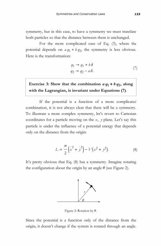
We say that the Lagrangian is symmetric with respect to thetransformation in Equations (6). Again this is a case of translationsymmetry, but in this case, to have a symmetry we must translateboth particles so that the distance between them is unchanged.

For the more complicated case of Eq. (3), where thepotential depends on a q1 + b q2, the symmetry is less obvious.

Here is the transformation:

(7)q1 ® q1 + b ∆

q2 ® q2 - a ∆.

Exercise 3: Show that the combination a q1 + b q2, along

with the Lagrangian, is invariant under Equations (7).

If the potential is a function of a more complicatedcombination, it is not always clear that there will be a symmetry.To illustrate a more complex symmetry, let’s revert to Cartesiancoordinates for a particle moving on the x, y plane. Let’s say this

particle is under the influence of a potential energy that dependsonly on the distance from the origin:

(8)L =m

2Jx× 2

+ y× 2N - V Ix2 + y2M.

It’s pretty obvious that Eq. (8) has a symmetry. Imagine rotatingthe configuration about the origin by an angle Θ (see Figure 2).

r

Θ

Figure 2: Rotation by Θ.

Since the potential is a function only of the distance from theorigin, it doesn’t change if the system is rotated through an angle.Moreover, the kinetic energy is also unchanged by a rotation. Thequestion is how we express such a change. The answer isobvious: Just rotate coordinates


Since the potential is a function only of the distance from theorigin, it doesn’t change if the system is rotated through an angle.Moreover, the kinetic energy is also unchanged by a rotation. Thequestion is how we express such a change. The answer isobvious: Just rotate coordinates

(9)x ® x cos Θ + y sin Θ

y ® -x sin Θ + y cos Θ.

where Θ is any angle.Now we come to an essential point about the

transformations of translation and rotation. You can do them insmall steps—infinitesimal steps. For example, instead of movinga particle from x to x + 1, you can move it from x to x + ∆. NowI am using ∆ to denote an infinitesimal. In fact, you can build upthe original displacement x ® x + 1 by many tiny steps of size ∆.The same is true for rotations: You can rotate through aninfinitesimal angle ∆ and, by repeating the process, eventuallybuild up a finite rotation. Transformations like this are calledcontinuous: They depend on a continuous parameter (the angle ofrotation), and, moreover, you can make the parameterinfinitesimal. This will prove to be a good thing, because we canexplore all the consequences of continuous symmetries byrestricting our attention to the infinitesimal case.

Since finite transformations can be compounded out ofinfinitesimal ones, in studying symmetries it’s enough to considertransformations with very small changes in the coordinates, theso-called infinitesimal transformations. So let’s consider what happensto Equations (9) when the angle Θ is replaced by an infinitesimalangle ∆. To first order in ∆,

cos ∆ = 1sin ∆ = ∆.

(Recall that for small angles, sin ∆ = ∆ and cos ∆ = 1 -12

∆2, so

the first-order shift in the cosine vanishes and the first-order shiftin sine is ∆.)

Then the rotation represented by Equations (9) simplifiesto


(Recall that for small angles, sin ∆ = ∆ and cos ∆ = 1 -12

∆2, so

the first-order shift in the cosine vanishes and the first-order shiftin sine is ∆.)

Then the rotation represented by Equations (9) simplifiesto

(10)x ® x + y ∆

y ® y - x ∆.

You can also see that the velocity components change. Justdifferentiate Equations (10) with respect to time:

(11)x×

® x×

+ y×

∆

y×

® y×

- x×

∆.

Another way to express the effect of the infinitesimaltransformation is to concentrate on the changes in thecoordinates and write

(12)∆ x = y ∆

∆ y = -x ∆.

Now it’s a simple calculus exercise to show that the Lagrangiandoes not change to first order in ∆.

Exercise 4: Show this to be true.

One thing worth noting is that if the potential is not afunction of distance from the origin, then the Lagrangian is notinvariant with respect to the infinitesimal rotations. This veryimportant point should be checked by examining some explicit.

examples. A simple example is a potential that depends only on xand not on y.


examples. A simple example is a potential that depends only on xand not on y.

More General Symmetries

Before we get to the connection between symmetries andconservation laws, let’s generalize our notion of symmetry. Suppose the coordinates of an abstract dynamical system are qi .

The general idea of an infinitesimal transformation is that it is asmall shift of the coordinates, that may itself depend on the valueof the coordinates. The shift is parameterized by an infinitesimalparameter ∆, and it has the form

(13)∆ qi = fiHqL ∆.

In other words, each coordinate shifts by an amount proportionalto ∆, but the proportionality factor depends on where you are inconfiguration space. In the example of Equations (6) the value off1 and of f2 are both 1. In the example of Equations (7) the f -

functions are f1 = a and f2 = -b. But in the more complicated

example of the rotations of Equations (12), the f ’s are not

constant:

fx = yf y = -x.

If we want to know the change in velocities—in order, forexample, to compute the change in the Lagrangian—we needonly to differentiate Eq. (13). A little calculus exercise gives

(14)∆ q×

i =d

d tH∆ qiL.


For example, from Equations (12),

(15)∆ x

×= y

×∆

∆ y×

= -x×

∆.

Now we can re-state the meaning of a symmetry for theinfinitesimal case. A continuous symmetry is an infinitesimaltransformation of the coordinates for which the change in theLagrangian is zero. It is particularly easy to check whether theLagrangian is invariant under a continuous symmetry: All youhave to do is to check whether the first order variation of theLagrangian is zero. If it is, then you have a symmetry.

Now let’s see what the consequences of a symmetry are.

The Consequences of Symmetry

Let’s calculate how much LIq, q× M changes when we do a

transformation that shifts qi by the amount in Eq. (13) and, at the

same time, shifts q×

i by the amount in Eq. (14). All we have to do

is compute the change due to varying the q×’s and add it to the

change due to varying the q’s:

(16)∆ L = âi

¶ L

¶ q×

i

∆ q×

i +¶ L

¶ qi∆ qi .

Now we do a bit of magic. Watch it carefully. First, we remember

that ¶ L

¶ q×i

is the momentum conjugate to qi , which we denote pi .

Thus the first term in Eq. (16) is Úi pi ∆ q×

i . Hold on to that while

.

we study the second term, ¶ L¶ qi

∆ qi . To evaluate terms of this

type, we assume the system is evolving along a trajectory thatsatisfies the Euler-Lagrange equations


we study the second term, ¶ L¶ qi

∆ qi . To evaluate terms of this

type, we assume the system is evolving along a trajectory thatsatisfies the Euler-Lagrange equations

¶ L

¶ qi=

d pi

d t.

Combining the terms, here is what we get for the variation of theLagrangian:

∆ L = âi

J pi ∆ q×

i + p×

i ∆ qiN.

The final piece of magic is to use the product rule for derivatives:

d HF GLd t

= F G×

+ F×

G.

Thus we get the result

∆ L =d

d tâ

i

pi ∆ qi .

What does all of this have to do with symmetry andconservation? First of all, by definition, symmetry means that thevariation of the Lagrangian is zero. So if Eq. (13) is a symmetry,then ∆ L = 0 and

d

d tâ

i

pi ∆ qi = 0.

But now we plug in the form of the symmetry operation, Eq.(13), and get


(17)d

d tâ

i

pi fiHqL = 0.

That’s it: The conservation law is proved. What Eq. (17) states isthat a certain quantity,

(18)Q = âi

pi fiHqL,

does not change with time. In other words, it is conserved. Theargument is both abstract and powerful. It did not depend on thedetails of the system, but only on the general idea of a symmetry.Now let’s turn back to some particular examples in light of thegeneral theory.

Back to Examples

Let’s apply Eq. (18) to the examples we studied earlier. In thefirst example, Eq. (1), the variation of the coordinates inEquations (12) defines both f1 and f2 to be exactly 1. Plugging

f1 = f2 = 1 into Eq. (18) gives exactly what we found earlier:

H p1 + p2L is conserved. But now we can say a far more general

thing: For any system of particles, if the Lagrangian is invariant undersimultaneous translation of the positions of all particles, then momentumis conserved. In fact, this can be applied separately to each spatialcomponent of momentum. If L is invariant under translationsalong the x axis, then the total x component of momentum isconserved. Thus we see that Newton’s third law—action equalsreaction—is the consequence of a deep fact about space: Nothingin the laws of physics changes if everything is simultaneously shifted in space.


Next let’s look at the second example, in which thevariations of Equations (12) imply f1 = b, f2 = -a. Again,

plugging this result into Eq. (18), we find that the conservedquantity is b p1 + a p2.

The last example—rotation—is more interesting. Itinvolves a new conservation law that we haven’t met yet. FromEq. (14) we obtain fx = y, f y = -x. This time the conserved

quantity involves both coordinates and momenta. It is called l , orangular momentum. From Eq. (18) we get

l = y px - x p y .

Again, as in the case of translations, there is a deeper thinginvolved than just the angular momentum of a single particle:

For any system of particles, if the Lagrangian is invariant undersimultaneous rotation of the position of all particles, about the origin, thenangular momentum is conserved.

Exercise 5: Determine the equation of motion for asimple pendulum of length l swinging through an arc inthe x, y plane from an initial angle of Θ.

So far, our examples have been very trivial. TheLagrangian formulation is beautiful, elegant, blah blah, but is itreally good for solving hard problems? Couldn’t you just useF = m a?

Try it. Here is an example: the double pendulum. Apendulum swings in the x, y plane supported at the origin. The

rod of the pendulum is massless, and the bob (weight at the end)is M . To make it simple, let the rod be 1 meter in length and letthe bob be 1 kilogram in mass. Next, take another identicalpendulum, but suspend it from the bob of the first pendulum, asshown in Figure 3. We can study two cases: with and without agravitational field.


So far, our examples have been very trivial. TheLagrangian formulation is beautiful, elegant, blah blah, but is itreally good for solving hard problems? Couldn’t you just useF = m a?

Try it. Here is an example: the double pendulum. Apendulum swings in the x, y plane supported at the origin. The

rod of the pendulum is massless, and the bob (weight at the end)is M . To make it simple, let the rod be 1 meter in length and letthe bob be 1 kilogram in mass. Next, take another identicalpendulum, but suspend it from the bob of the first pendulum, asshown in Figure 3. We can study two cases: with and without agravitational field.

Mr

rM

Figure 3: The double pendulum.

Our goal will not be to solve the equations of motion.That we can always do, even if we have to put them on acomputer and do it numerically. The goal is to find thoseequations. It’s a tricky problem if you try to do it by F = M a.Among other things, you have to worry about the forcestransmitted through the rod. The Lagrangian method is mucheasier. There is a more or less mechanical procedure for doing it.The steps are the following:

1. Choose some coordinates that uniquely specify theconfiguration of the components. You can choose themhowever you like—just make sure that you have justenough to determine the configuration—and keep themas simple as possible.

In the double pendulum example, you need twocoordinates. I will choose the first one to be the angle ofthe first pendulum from the vertical. Call it Θ. Next, I havea choice. Should I choose the second angle (the angle ofthe second rod) also to be measured from the vertical, orshould I measure it relative to the angle of the first rod?The answer is that it does not matter. One choice maymake the equations a little simpler, but either will get you .to the answer. I will choose the angle Α to be measuredrelative to the first rod rather than to the vertical.


to the answer. I will choose the angle Α to be measuredrelative to the first rod rather than to the vertical.

2. Work out the total kinetic energy. In this case it is thekinetic energy of the two bobs.

The easiest way to do this is to refer temporarilyto Cartesian coordinates x, y. Let x1, y1 refer to the firstbob and x2, y2 to the second bob. Here are somerelations among the angles Θ, Α and x, y: For bob 1,

x1 = sin Θ

y1 = cos Θ

and for bob 2,

x2 = sin Θ + sin HΑ + ΘLy2 = cos Θ + cos HΑ + ΘL.

Now, by differentiating with respect to time, you cancompute the Cartesian velocity components in terms ofthe angles and their time derivatives.

Finally, work out the kinetic energy m2

Jx× 2+ y

× 2Nfor each bob and add them. It should take a couple ofminutes. Remember that we have chosen the masses androd lengths to be 1.

Here is the result: The kinetic energy of the firstbob is:

T1 =Θ× 2

2

and the kinetic energy of the second bob is

T2 =

Θ× 2

+ KΘ×

+ Α× O2

2+ Θ

× K Θ×

+ Α× O cos Α.

If there is no gravitational field, then the kineticenergy is the Lagrangian:


If there is no gravitational field, then the kineticenergy is the Lagrangian:

L = T1 + T2 =Θ× 2

2+

Θ× 2

+ KΘ×

+ Α× O2

2+ Θ

× K Θ×

+ Α× O cos Α.

If there is gravity, then we have to calculate thegravitational potential energy. That’s easy: For each bobwe add its altitude times m g. This gives a potential energy

V HΘ, ΑL = - g @2 cos Θ + cos HΘ - ΑLD.3. Work out the Euler-Lagrange equations for each degree

of freedom.4. For later purposes, work out the conjugate momenta for

each coordinate, pi =¶L

¶q×i.

Exercise 6: Work out the Euler-Lagrange equations for Θand Α.

There is more that you may want to do. In particular, youmay want to identify the conserved quantities. Energy is usuallythe first one. The total energy is just T + V . But there may bemore. Finding symmetries is not always a mechanical procedure;you may have to do some pattern recognition. In the doublependulum case without any gravity, there is another conservationlaw. It follows from rotation symmetry. Without a gravitationalfield, if you rotate the whole system about the origin, nothingchanges. This implies conservation of angular momentum, but tofind the form of the angular momentum, you have to go throughthe procedure that we derived. That involves knowing theconjugate momenta.

Exercise 7: Work out the form of the angularmomentum for the double pendulum, and prove that itis conserved when there is no gravitational field.


Exercise 7: Work out the form of the angularmomentum for the double pendulum, and prove that itis conserved when there is no gravitational field.


Lecture 8: Hamiltonian Mechanics and Time-Translation Invariance

Doc was sitting at the bar drinking his usual—a beer milk shake—and reading the paper, when Lenny and George walked in. “Whatare you reading about, Doc?”

Doc looked up at Lenny over his glasses. “I see wherethis guy Einstein says, ‘Insanity is doing the same thing over andover and expecting different results.’ What do you think aboutthat?”

Lenny thought for a minute. “You mean like every time Ieat here I order chili, and then I get a stomachache?”

Doc chuckled, “Yeah, that’s the idea. I see you’rebeginning to understand Einstein.”

Time-Translation Symmetry

You may wonder what happened to energy conservation andwhether it fits the pattern relating symmetries to conservationlaws. Yes, it does, but in a slightly different way than theexamples in Lecture 7. In all of those examples the symmetryinvolved shifting the coordinates qi . For instance, a translation is

a symmetry that simultaneously shifts the Cartesian coordinatesof all the particles in a system by the same amount. Thesymmetry connected with energy conservation involves a shift oftime.

Imagine an experiment involving a closed system farfrom any perturbing influences. The experiment begins at time t0with a certain initial condition, proceeds for a definite period, andresults in some outcome. Next, the experiment is repeated inexactly the same way but at a later time. The initial conditions arethe same as before, and so is the duration of the experiment; theonly difference is the starting time, which is pushed forward tot0 + D t . You might expect that the outcome will be exactly thesame, and that the shift D t would make no difference. Wheneverthis is true, the system is said to be invariant under time translation.

Time-translation invariance does not always apply. Forexample, we live in an expanding universe. The effect of theexpansion on ordinary laboratory experiments is usuallynegligible, but it’s the principle that counts. At some level ofaccuracy, an experiment that begins later will have a slightlydifferent outcome than one which begins earlier.

Here is a more down-to-earth example. Suppose thesystem of interest is a charged particle moving in a magnetic field.If the magnetic field is constant then the motion of the particlewill be time-translation invariant. But if the current that generatesthe field is being slowly increased, then the same initial conditionfor the particle—but starting at different times—will result in adifferent outcome. The description of the particle will not betime-translation invariant.

How is time-translation symmetry, or the lack of it,reflected in the Lagrangian formulation of mechanics? Theanswer is simple. In those cases where there is such symmetry,the Lagrangian has no explicit dependence on time. This is asubtle point: The value of the Lagrangian may vary with time, butonly because the coordinates and velocities vary. Explicit timedependence means that the form of the Lagrangian depends ontime. For example, take the harmonic oscillator with Lagrangian

You may wonder what happened to energy conservation andwhether it fits the pattern relating symmetries to conservationlaws. Yes, it does, but in a slightly different way than theexamples in Lecture 7. In all of those examples the symmetryinvolved shifting the coordinates qi . For instance, a translation is

a symmetry that simultaneously shifts the Cartesian coordinatesof all the particles in a system by the same amount. Thesymmetry connected with energy conservation involves a shift oftime.

Imagine an experiment involving a closed system farfrom any perturbing influences. The experiment begins at time t0with a certain initial condition, proceeds for a definite period, andresults in some outcome. Next, the experiment is repeated inexactly the same way but at a later time. The initial conditions arethe same as before, and so is the duration of the experiment; theonly difference is the starting time, which is pushed forward tot0 + D t . You might expect that the outcome will be exactly thesame, and that the shift D t would make no difference. Wheneverthis is true, the system is said to be invariant under time translation.

Time-translation invariance does not always apply. Forexample, we live in an expanding universe. The effect of theexpansion on ordinary laboratory experiments is usuallynegligible, but it’s the principle that counts. At some level ofaccuracy, an experiment that begins later will have a slightlydifferent outcome than one which begins earlier.

Here is a more down-to-earth example. Suppose thesystem of interest is a charged particle moving in a magnetic field.If the magnetic field is constant then the motion of the particlewill be time-translation invariant. But if the current that generatesthe field is being slowly increased, then the same initial conditionfor the particle—but starting at different times—will result in adifferent outcome. The description of the particle will not betime-translation invariant.

How is time-translation symmetry, or the lack of it,reflected in the Lagrangian formulation of mechanics? Theanswer is simple. In those cases where there is such symmetry,the Lagrangian has no explicit dependence on time. This is asubtle point: The value of the Lagrangian may vary with time, butonly because the coordinates and velocities vary. Explicit timedependence means that the form of the Lagrangian depends ontime. For example, take the harmonic oscillator with Lagrangian


L =1

2Jm x

× 2- k x2N.

If m and k are time-independent then this Lagrangian is time-translation invariant.

But one can easily imagine that the spring constant kmight, for some reason, change with time. For example, if theexperiment took place in a changing magnetic field, this couldhave a subtle effect on the atoms of the spring, which in turncould cause k to vary. In that case, we would have to write

L =1

2Bm x

× 2- kHtL x2F.

This is what we mean by an explicit time dependence. Moregenerally, we can write

(1)L = LIqi , q×

i , tM,where the t dependence is due to the time variation of all theparameters controlling the behavior of the system.

With this idea in hand, we can now give a very succinctmathematical criterion for time-translation symmetry: A system istime-translation invariant if there is no explicit time dependence in itsLagrangian.

Energy Conservation

Let’s consider how the actual value of the Lagrangian, Eq. (1),changes as a system evolves. There are three sources of timedependence of L. The first and second are due to the time

dependence of the coordinates q and the velocities q×. If that were

all, we would write

Hamiltonian Mechanics and Time-Translation Invariance 147

Let’s consider how the actual value of the Lagrangian, Eq. (1),changes as a system evolves. There are three sources of timedependence of L. The first and second are due to the time

dependence of the coordinates q and the velocities q×. If that were

all, we would write

d L

d t= â

i

¶L

¶qiq×

i +¶L

¶q×

i

q××

i .

But if the Lagrangian has explicit time dependence, thenthere is another term:

(2)d L

d t= â

i

¶L

¶qiq×

i +¶L

¶q×

i

q××

i +¶L

¶ t.

Let’s examine the various terms in Eq. (2) using the Euler-

Lagrange equations of motion. The first type of term, ¶L¶qi

q×

i , can

be written

¶L

¶qiq×

i = p×

i q×

i .

The second type of term, ¶L

¶q×i

q××

i , takes the form

¶L

¶q×

i

q××

i = pi q××

i .

If we combine everything, we get

d L

d t= â

i

J p×

i q×

i + pi q××

iN +¶L

¶ t.

The first two terms can be simplified. We use the identity

âi

J p×

i q×

i + pi q××

iN =d

d tâ

i

I pi q×

iM


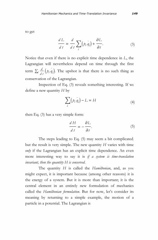
to get

(3)d L

d t=

d

d tâ

i

I pi q×

iM +¶L

¶ t.

Notice that even if there is no explicit time dependence in L, theLagrangian will nevertheless depend on time through the first

term Úid

d tI pi q

×

iM. The upshot is that there is no such thing as

conservation of the Lagrangian.Inspection of Eq. (3) reveals something interesting. If we

define a new quantity H by

(4)âi

I pi q×

iM - L = H

then Eq. (3) has a very simple form:

(5)d H

d t= -

¶L

¶ t.

The steps leading to Eq. (5) may seem a bit complicated,but the result is very simple. The new quantity H varies with timeonly if the Lagrangian has an explicit time dependence. An evenmore interesting way to say it is if a system is time-translationinvariant, then the quantity H is conserved.

The quantity H is called the Hamiltonian, and, as youmight expect, it is important because (among other reasons) it isthe energy of a system. But it is more than important; it is thecentral element in an entirely new formulation of mechanicscalled the Hamiltonian formulation. But for now, let’s consider itsmeaning by returning to a simple example, the motion of aparticle in a potential. The Lagrangian is


(6)L =m

2x× 2

- V HxL,

and the canonical momentum is just the usual momentum

(7)p = m x×.

Let’s plug Eq. (6) and Eq. (7) into Eq. (4), the definition of H :

H = Im x× M x

×-

m

2x× 2

+ V HxL

= m x× 2

-m

2x× 2

+ V HxL

=m

2x× 2

+ V HxL.

Notice what happens: Two terms proportional to m x× 2

combineto give the usual kinetic energy, and the potential term becomes+V HxL. In other words, H just becomes the usual total energy,kinetic plus potential.

This is the general pattern that you can check for anynumber of particles. If the Lagrangian is kinetic energy minuspotential energy, then

H = p q×

- T + V .= T + V .

There are systems for which the Lagrangian has a more intricateform than just T - V . For some of those cases, it is not possibleto identify a clear separation into kinetic and potential energy.Nonetheless, the rule for constructing the Hamiltonian is thesame. The general definition of energy for these systems is


Energy equals Hamiltonian.

Moreover, if there is no explicit time dependence in theLagrangian, then the energy H is conserved.

If, however, the Lagrangian is explicitly time-dependent,then Eq. (5) implies that the Hamiltonian is not conserved. Whathappened to the energy in that case? To understand what is goingon, let's consider an example. Suppose that a charged particle,with unit electric charge, is moving between the plates of acapacitor. The capacitor has a uniform electric field Ε due to thecharges on the plates. (The reason we are using Ε for electric field,instead of the more conventional E, is to avoid confusing it withenergy.) You don’t have to know anything about electricity. Allyou need to know is that the capacitor creates a potential energyequal to Ε x. The Lagrangian is

L =m

2x× 2

- Ε x.

As long as the field is constant, the energy is conserved. Butsuppose the capacitor is being charged up so that Ε is alsoramping up. Then the Lagrangian has an explicit time dependence:

L =m

2x× 2

- ΕHtL x.

Now the energy of the particle is not conserved. Depending onthe momentary location x of the particle, the energy variesaccording to

d H

d t=

d Ε

d tx.

Where did that energy come from? The answer is that itcame from the battery that was charging the capacitor. I won’t gointo details, but the point is that when we defined the system toconsist of just the particle, we narrowed our focus to just a partof a bigger system that includes the capacitor and the battery.These additional items are also made of particles and thereforehave energy.

Consider the entire experiment, including the battery,capacitor, and particle. The experiment begins with an unchargedcapacitor and a particle at rest, somewhere between the plates. Atsome moment we close a circuit, and current flows into thecapacitor. The particle experiences a time-dependent field, and, atthe end of the experiment, the capacitor is charged and theparticle is moving.

What if we did the entire experiment an hour later? Theoutcome, of course, would be the same. In other words, theentire closed system is time-translation invariant, so the entireenergy of all items is conserved. If we treated the entire collectionas a single system, it would be time-translation invariant, and thetotal energy would be conserved.

Nevertheless, it is often useful to divide a system intoparts and to focus on one part. In that case, the energy of part ofthe system will not be conserved if the other parts are varyingwith time.


Where did that energy come from? The answer is that itcame from the battery that was charging the capacitor. I won’t gointo details, but the point is that when we defined the system toconsist of just the particle, we narrowed our focus to just a partof a bigger system that includes the capacitor and the battery.These additional items are also made of particles and thereforehave energy.

Consider the entire experiment, including the battery,capacitor, and particle. The experiment begins with an unchargedcapacitor and a particle at rest, somewhere between the plates. Atsome moment we close a circuit, and current flows into thecapacitor. The particle experiences a time-dependent field, and, atthe end of the experiment, the capacitor is charged and theparticle is moving.

What if we did the entire experiment an hour later? Theoutcome, of course, would be the same. In other words, theentire closed system is time-translation invariant, so the entireenergy of all items is conserved. If we treated the entire collectionas a single system, it would be time-translation invariant, and thetotal energy would be conserved.

Nevertheless, it is often useful to divide a system intoparts and to focus on one part. In that case, the energy of part ofthe system will not be conserved if the other parts are varyingwith time.

Phase Space and Hamilton’s Equations

The Hamiltonian is important because (among other reasons) it isthe energy. But its significance is far deeper: It is the basis for acomplete revamping of classical mechanics, and it is even moreimportant in quantum mechanics.

In the Lagrangian—or action—formulation ofmechanics, the focus is on the trajectory of a system through theconfiguration space. The trajectory is described in terms of thecoordinates qHtL. The equations are second-order differential

equations, so it is not enough to know the initial coordinates; wealso have to know the initial velocities.

In the Hamiltonian formulation, the focus is on phasespace. Phase space is the space of both the coordinates qi and the

conjugate momenta pi . In fact, the q’s and p’s are treated on the

same footing, the motion of a system being described by atrajectory through the phase space. Mathematically, thedescription is through a set of functions qiHtL, piHtL. Notice that

the number of dimensions of phase space is twice that ofconfiguration space.

What do we gain by doubling the number of dimensions?The answer is that the equations of motion become first-orderdifferential equations. In less technical terms, this means that thefuture is laid out if we know only the initial point in phase space.

The first step in constructing the Hamiltonian

formulation is to get rid of the q×'s and replace them with the p's.

The goal is to express the Hamiltonian as a function of q's and

p's. For particles in ordinary Cartesian coordinates, the momenta

and velocities are almost the same thing, differing only by a factorof the mass. As usual, the particle on a line is a good illustration.

We start with the two equations


The Hamiltonian is important because (among other reasons) it isthe energy. But its significance is far deeper: It is the basis for acomplete revamping of classical mechanics, and it is even moreimportant in quantum mechanics.

In the Lagrangian—or action—formulation ofmechanics, the focus is on the trajectory of a system through theconfiguration space. The trajectory is described in terms of thecoordinates qHtL. The equations are second-order differential

equations, so it is not enough to know the initial coordinates; wealso have to know the initial velocities.

In the Hamiltonian formulation, the focus is on phasespace. Phase space is the space of both the coordinates qi and the

conjugate momenta pi . In fact, the q’s and p’s are treated on the

same footing, the motion of a system being described by atrajectory through the phase space. Mathematically, thedescription is through a set of functions qiHtL, piHtL. Notice that

the number of dimensions of phase space is twice that ofconfiguration space.

What do we gain by doubling the number of dimensions?The answer is that the equations of motion become first-orderdifferential equations. In less technical terms, this means that thefuture is laid out if we know only the initial point in phase space.

The first step in constructing the Hamiltonian

formulation is to get rid of the q×'s and replace them with the p's.

The goal is to express the Hamiltonian as a function of q's and

p's. For particles in ordinary Cartesian coordinates, the momenta

and velocities are almost the same thing, differing only by a factorof the mass. As usual, the particle on a line is a good illustration.

We start with the two equations

(8)

p = m x×

H =m x

× 2

2+ V HxL.

When we replace the velocity with p m the Hamiltonian

becomes a function of p and x:


H =p2

2 m+ V HxL.

One last point before we write the equations of motion inHamiltonian form: The partial derivative of H with respect to x

is just d Vd x

, or minus the force. Thus the equation of motion

HF = m aL takes the form

(9)p×

= -¶ H

¶ x.

We noted earlier that in the Hamiltonian formulation, thecoordinates and momenta are on the same footing. From thatyou might guess that there is another equation similar to Eq. (9),with p and x interchanged. That is almost true, but not quite. The

correct equation is

(10)x×

=¶ H

¶ p,

with a plus sign instead of a minus sign.To see why Eq. (10) is true, just differentiate the

expression for H with respect to p. From the second of

Equations (8) we get

¶H

¶ p=

p

m,

which from the first equation is just x×.

So now we see a very simple symmetric packaging of theequations. We have two equations of motion instead of one, buteach is of first-order:


(11)

p×

= -¶ H

¶ x

x×

=¶ H

¶ p.

These are Hamilton’s equations for a particle on a line. Soon wewill derive the general form for any system, but for now I will tellyou what it is. We start with a Hamiltonian that is a function ofall the q’s and p’s:

H = HHqi , piL.We can use this to generalize Equations (11),

(12)

p×

i = -¶ H

¶ qi

q×

i =¶ H

¶ pi.

So we see that for each direction in phase space, there is a singlefirst-order equation.

Let’s stop to consider how these equations are related tothe very first chapter of this book, in which we described howdeterministic laws of physics predict the future. What Equations(12) say is this:

If at any time you know the exact values of all the coordinates and momenta,and you know the form of the Hamiltonian, Hamilton’s equationswill tell you the corresponding quantities an infinitesimal time later. By aprocess of successive updating, you can determine a trajectory through phasespace.


The Harmonic Oscillator Hamiltonian

The harmonic oscillator is by far the most important simplesystem in physics. It describes all sorts of oscillations in whichsome degree of freedom is displaced and then oscillates about anequilibrium position. To see why it is so important, let’s supposea degree of freedom q has a potential energy V HqL that has a

minimum. The minimum describes a stable equilibrium, andwhen the degree of freedom is displaced, it will tend to return tothe equilibrium position. Without any real loss of generality, wecan locate the minimum at q = 0. The generic function that has a

minimum at this point can be approximated by the quadraticfunction

(13)V HqL = V H0L + c q2.

where V H0L and c are constants. The reason why there is no

linear term proportional to q is that the derivative d Vd q

must be

zero at the minimum. We can also drop the term V H0L sinceadding a constant to the potential energy has no effect.

The form of Eq. (13) is not very general; V couldcontain terms of all orders—for example, q3 or q4. But as long as

the system deviates from q = 0 by only a small amount, these

higher-order terms will be negligible compared to the quadraticterm. This reasoning applies to all sorts of systems: springs,pendulums, oscillating sound waves, electromagnetic waves, andon and on.

I will write the Lagrangian in what may seem like a specialform involving a single constant called Ω:


(14)L =1

2 Ωq× 2

-Ω

2q2.

Exercise 1: Start with the Lagrangian m x× 2

2-

k

2x2 and

show that if you make the change in variables

q = Hk mL14 x, the Lagrangian has the form of Eq. (14).

What is the connection among k, m, and Ω?

Exercise 2: Starting with Eq. (14), calculate theHamiltonian in terms of p and q.

The Hamiltonian corresponding to Eq. (14) is verysimple:

(15)H =Ω

2I p2 + q2M.

It was in order to get H into such a simple form that we changedvariables from x to q in Exercise 1.

One of the hallmarks of the Hamiltonian formulation ishow symmetric it is between the q’s and p’s. In the case of the

harmonic oscillator, it is almost completely symmetric. The onlyasymmetry is a minus sign in the first of Equations (12). For asingle degree of freedom, Hamilton’s equations are Equations(11). If we plug our Hamiltonian, Eq. (15), into Equations (12),we get,


(16)p×

i = -Ω q

q×

i = Ω p.

How do these two equations compare with Lagrange’s equationsthat we would derive from Eq. (14)? First of all, there is only oneLagrangian equation:

(17)q××

= -Ω2 q.

Second, this equation is second-order, meaning that it involvessecond time-derivatives. By contrast, the Hamiltonian equationsare each first-order. This somehow means that two first-orderequations are equivalent to one second-order equation. We cansee this by differentiating the second equation in Equations (16)with respect to time,

q××

= Ω p×,

and then using the first equation in Equations (16). This enables

us to replace p×

with -Ω q, which gives us Eq. (17): The Euler-

Lagrange equation of motion.Is one formulation better than the other? Did Lagrange

have the final word or did Hamilton? You can decide foryourself, but wait a while before you do. We still have a couple ofcourses on relativity and quantum mechanics before the realmeanings of the Lagrangian and Hamiltonian become completelyclear.

Let’s return to Equations (16). We usually “think” inconfiguration space. The harmonic oscillator is a system thatmoves back and forth along a single axis. But it is also anexcellent starting point for getting used to “thinking” in phasespace. Phase space (for the oscillator ) is two-dimensional. It iseasy to see that the trajectories of the oscillator in phase space areconcentric circles about the origin. The argument is very simple.Go back to the expression for the Hamiltonian, Eq. (15). TheHamiltonian, being the energy, is conserved. It follows thatq2 + p2 is constant with time. In other words, the distance from

the origin of phase space is constant, and the phase point moveson a circle of fixed radius. In fact Eq. (16) is the equation for apoint moving with constant angular velocity Ω about the origin.Especially interesting is the fact that the angular velocity in phasespace is the same for all orbits, independent of the energy of theoscillator. As the phase point circles the origin, you can projectthe motion onto the horizontal q axis, as shown in Figure 1. It

moves back and forth in an oscillatory motion, exactly asexpected. However, the two-dimensional circular motion throughphase space is a more comprehensive description of the motion.By projecting onto the vertical p axis, we see that the momentum

also oscillates.


and then using the first equation in Equations (16). This enables

us to replace p×

with -Ω q, which gives us Eq. (17): The Euler-

Lagrange equation of motion.Is one formulation better than the other? Did Lagrange

have the final word or did Hamilton? You can decide foryourself, but wait a while before you do. We still have a couple ofcourses on relativity and quantum mechanics before the realmeanings of the Lagrangian and Hamiltonian become completelyclear.

Let’s return to Equations (16). We usually “think” inconfiguration space. The harmonic oscillator is a system thatmoves back and forth along a single axis. But it is also anexcellent starting point for getting used to “thinking” in phasespace. Phase space (for the oscillator ) is two-dimensional. It iseasy to see that the trajectories of the oscillator in phase space areconcentric circles about the origin. The argument is very simple.Go back to the expression for the Hamiltonian, Eq. (15). TheHamiltonian, being the energy, is conserved. It follows thatq2 + p2 is constant with time. In other words, the distance from

the origin of phase space is constant, and the phase point moveson a circle of fixed radius. In fact Eq. (16) is the equation for apoint moving with constant angular velocity Ω about the origin.Especially interesting is the fact that the angular velocity in phasespace is the same for all orbits, independent of the energy of theoscillator. As the phase point circles the origin, you can projectthe motion onto the horizontal q axis, as shown in Figure 1. It

moves back and forth in an oscillatory motion, exactly asexpected. However, the two-dimensional circular motion throughphase space is a more comprehensive description of the motion.By projecting onto the vertical p axis, we see that the momentum

also oscillates.

q

p

Figure 1: The harmonic oscillator in phase space.

The harmonic oscillator is especially simple. In general,the motion of a system through phase space is more complicatedand less symmetric. But the fact that the phase point stays on acontour of constant energy is universal. Later we will discovermore general properties of motion in phase space.


Derivation of Hamilton’s Equations

Let’s complete a piece of business that we left unfinished: thegeneral derivation of Hamilton’s equations. The Lagrangian issome general function of the coordinates and velocities,

L = LI8q<, 9q× =M,and the Hamiltonian is

H = âi

I pi q×

iM - L.

The change in the Hamiltonian is

∆ H = âi

I pi ∆ q×

i + q×

i ∆ piM - ∆ L

= âi

pi ∆ q×

i + q×

i ∆ pi -¶L

¶qi∆ qi -

¶L

¶q×

i

∆ q×

i .

Now if we use the definition of pi , namely pi =¶L

¶q×i, we see that

the first and last terms exactly cancel, leaving

∆ H = âi

q×

i ∆ pi -¶L

¶qi∆ qi .

Let’s compare this with the general rule for a smallchange in a function of several variables:

∆ HH8q<, 8 p<L = âi

¶H

¶ pi∆ pi +

¶H

¶qi∆ qi .


By matching the terms proportional to ∆ qi and ∆ pi , we arrive at

(18)

¶H

¶ pi= q

×

i

¶H

¶qi= -

¶L

¶q×

i

.

There is only one last step, and that is to write Lagrange’sequations in the form

¶L

¶q×

i

= p×

i .

Inserting this in the second of Equations (18) we get Hamilton’sequations,

(19)

¶H

¶ pi= q

×

i

¶H

¶qi= - p

×

i .


Lecture 9: The Phase Space Fluid and the Gibbs-Liouville Theorem

Lenny loved watching the river, especially watching little bits offloating debris making their way downstream. He tried to guesshow they would move between the rocks or get caught in eddys.But the river as a whole—the large-scale current, the volume ofwater, the shear, and the divergence and convergence of the flowwere beyond him.

The Phase Space Fluid

Focusing on a particular initial condition and following it alongits specific trajectory through phase space are very natural thingsto do in classical mechanics. But there is also a bigger picture thatemphasizes the entire collection of trajectories. The biggerpicture involves visualizing all possible starting points and allpossible trajectories. Instead of putting your pencil down at apoint in phase space and then following a single trajectory, try todo something more ambitious. Imagine you had an infinitenumber of pencils and used them to fill phase space uniformlywith dots (by uniformly, I mean that the density of dots in the

q, p space is everywhere the same). Think of the dots as particles

that make up a fictitious phase-space-filling fluid.Then let each dot move according to the Hamiltonian

equations of motion,

(1)

q×

i =¶ H

¶ pi

p×

i = -¶ H

¶ qi,

so that the fluid endlessly flows through the phase space.The harmonic oscillator is a good example to start with.

In Lecture 8 we saw that each dot moves in a circular orbit withuniform angular velocity. (Remember, we are talking about phasespace, not coordinate space. In coordinate space, the oscillatormoves back and forth in one dimension.) The whole fluid movesin a rigid motion, uniformly circulating around the origin ofphase space.

Now let’s return to the general case. If the number ofcoordinates is N , then the phase space, and the fluid, are 2N-dimensional. The fluid flows, but in a very particular way. Thereare features of the flow that are quite special. One of these specialfeatures is that if a point starts with a given value of energy—agiven value of HHq, pL—then it remains with that value of energy.

The surfaces of fixed energy (for example, energy E) are definedby the equation

(2)HHq, pL = E.

For each value of E we have a single equation for 2N phase-space variables, thus defining a surface of dimension 2N - 1. Inother words, there is a surface for each value of E; as you scanover values of E, those surfaces fill up the phase space. You canthink of the phase space, along with the surfaces defined in Eq.(2) as a contour map (see Figure 1), but, instead of representingaltitude, the contours denote the value of the energy. If a point ofthe fluid is on a particular surface, it stays on that surface forever.That’s energy conservation.

The Phase Space Fluid and the Gibbs-Liouville Theorem 163

For each value of E we have a single equation for 2N phase-space variables, thus defining a surface of dimension 2N - 1. Inother words, there is a surface for each value of E; as you scanover values of E, those surfaces fill up the phase space. You canthink of the phase space, along with the surfaces defined in Eq.(2) as a contour map (see Figure 1), but, instead of representingaltitude, the contours denote the value of the energy. If a point ofthe fluid is on a particular surface, it stays on that surface forever.That’s energy conservation.

q

p

Figure 1: Contour plot of energy surfaces of a harmonic oscillator in phase space.

For the harmonic oscillator, the phase space is two-dimensional and the energy surfaces are circles:

(3)Ω

2Iq2 + p2M = E.

For a general mechanical system, the energy surfaces are far toocomplicated to visualize, but the principle is the same: The energysurfaces fill the phase space like layers and the flow moves so that the pointsstay on the surface that they begin on.

A Quick Reminder

We want to stop here and remind you of the very first lecture,where we discussed coins, dice, and the simplest idea of a law ofmotion. We described those laws by a set of arrows connectingdots that represented the states of the system. We also explainedthat there are allowable laws and unallowable laws, the allowablelaws being reversible. What is it that characterizes an allowablelaw? The answer is that every point must have exactly oneincoming arrow and one outgoing arrow. If at any point thenumber of incoming arrows exceeds the number of outgoingarrows (such a situation is called a convergence), then the law isirreversible. The same is true if the number of outgoing arrowsexceeds the number of incoming arrows (such a situation is calleda divergence). Either a convergence or divergence of the arrowsviolates reversibility and is forbidden. So far we have notreturned to that line of reasoning. Now is the time.


We want to stop here and remind you of the very first lecture,where we discussed coins, dice, and the simplest idea of a law ofmotion. We described those laws by a set of arrows connectingdots that represented the states of the system. We also explainedthat there are allowable laws and unallowable laws, the allowablelaws being reversible. What is it that characterizes an allowablelaw? The answer is that every point must have exactly oneincoming arrow and one outgoing arrow. If at any point thenumber of incoming arrows exceeds the number of outgoingarrows (such a situation is called a convergence), then the law isirreversible. The same is true if the number of outgoing arrowsexceeds the number of incoming arrows (such a situation is calleda divergence). Either a convergence or divergence of the arrowsviolates reversibility and is forbidden. So far we have notreturned to that line of reasoning. Now is the time.

Flow and Divergence

Let’s consider some simple examples of fluid flow in ordinaryspace. Forget about phase space for the moment, and justconsider an ordinary fluid moving through regular three-dimensional space labeled by axes x, y, z. The flow can be

described by a velocity field. The velocity field v®Hx, y, zL is defined

by going to each point of space and specifying the velocity vectorat that point (see Figure 2).

x

y

z

Figure 2: Velocity field.


Figure 2: Velocity field.

Or we may describe the velocity field to be the components ofthe velocity: vxHx, y, zL, v yHx, y, zL, vzHx, y, zL. The velocity at a

point might also depend on time, but let’s suppose that it doesn’t.In that case the flow is called stationary.

Now let’s suppose the fluid is incompressible. Thismeans that a given amount of the fluid always occupies the samevolume. It also means that the density of the fluid—the numberof molecules per unit volume—is uniform and stays that wayforever. By the way, the term incompressible also means in-decompressible. In other words, the fluid cannot be stretchedout, or decompressed. Consider a small cubic box defined by

x0 < x < x0 + d xy0 < y < y0 + d yz0 < z < z0 + d z.

Incompressibility implies that the number of fluid points in everysuch box is constant. It also means that the net flow of fluid intothe box (per unit time) must be zero. (As many points flow in asflow out.) Consider the number of molecules per unit timecoming into the box across the face x = x0. It will beproportional to the flow velocity across that face, vxHx0L.

If vx were the same at x0 and at x0 + d x, then theflow into the box at x = x0 would be the same as the flow out ofthe box at x = x0 + d x. However, if vx varies across the box,then the two flows will not balance. Then the net flow into thebox across the two faces will be proportional to

-¶vx

¶xd x d y d z.

Exactly the same reasoning applies to the faces at y0 and

y0 + d y, and also at z0 and z0 + d z. In fact, if you add it all up,

the net flow of molecules into the box (inflow minus outflow) isgiven by


Exactly the same reasoning applies to the faces at y0 and

y0 + d y, and also at z0 and z0 + d z. In fact, if you add it all up,

the net flow of molecules into the box (inflow minus outflow) isgiven by

-¶vx

¶x+

¶v y

¶ y+

¶vz

¶zd x d y d z.

The combination of derivatives in the parentheses has a name: It

is the divergence of the vector field v®HtL and is denoted by

(4)Ñ × v®

=¶vx

¶x+

¶v y

¶ y+

¶vz

¶z.

The divergence is aptly named; it represents a spreading out ofthe molecules, or an increase in the volume occupied by themolecules. If the fluid is incompressible, then the volume mustnot change, and this implies that the divergence must be zero.

One way to think about incompressibility is to imaginethat each of the molecules, or points, of the fluid occupies avolume that cannot be compromised. They cannot be squeezedinto a smaller volume, nor can they disappear or appear fromnowhere. With a little bit of thought, you can see how similarincompressibility is to reversibility. In the examples that weexamined in Lecture 1, the arrows also defined a kind of flow.And in a sense the flow was incompressible, at least if it wasreversible. The obvious question that this raises is whether theflow through phase space is incompressible. The answer is yes, ifthe system satisfies Hamilton’s equations. And the theorem thatexpresses the incompressibility is called Liouville’s theorem.

Liouville’s Theorem

Let’s go back to the fluid flow in phase space and consider thecomponents of the velocity of the fluid at every point of thephase space. Needless to say, the phase-space fluid is not three-dimensional with coordinates x, y, z. Instead it is a 2N-

dimensional fluid with coordinates pi , qi . Therefore, there are

2N components of the velocity field, one for each q and one for

each p. Let’s call them vqi and v pi .

The concept of a divergence in Eq. (4) is easilygeneralized to any number of dimensions. In three dimensions itis the sum of the derivatives of the velocity components in therespective directions. It’s exactly the same in any number ofdimensions. In the case of phase space, the divergence of a flowis the sum of 2N terms:


Let’s go back to the fluid flow in phase space and consider thecomponents of the velocity of the fluid at every point of thephase space. Needless to say, the phase-space fluid is not three-dimensional with coordinates x, y, z. Instead it is a 2N-

dimensional fluid with coordinates pi , qi . Therefore, there are

2N components of the velocity field, one for each q and one for

each p. Let’s call them vqi and v pi .

The concept of a divergence in Eq. (4) is easilygeneralized to any number of dimensions. In three dimensions itis the sum of the derivatives of the velocity components in therespective directions. It’s exactly the same in any number ofdimensions. In the case of phase space, the divergence of a flowis the sum of 2N terms:

(5)Ñ × v®

= âi

¶vqi

¶qi+

¶v pi

¶ pi.

If the fluid is incompressible, then the expression in Eq. (5) mustbe zero. To find out, we need to know the components of thevelocity field—that being nothing but the velocity of a particle ofthe phase space fluid.

The flow vector of a fluid at a given point is identifiedwith the velocity of a fictitious particle at that point. In otherwords,

vqi = q×

i

v pi = p×

i .

Moreover, q×

i and p×

i are exactly the quantities that Hamilton’s

equations, Equations (1), give:


(6)

vqi =¶H

¶ pi

v pi = -¶H

¶qi.

All we have to do is plug Equations (6) into Eq. (5) and see whatwe get:

(7)Ñ × v®

= âi

¶

¶qi

¶H

¶ pi-

¶

¶ pi

¶H

¶qi.

Recalling that a second derivative like ¶

¶qi

¶H¶ pi

does not depend

on the order of differentiation, we see that the terms in Eq. (7)exactly cancel in pairs:

Ñ × v®

= 0.

Thus the phase space fluid is incompressible. In classicalmechanics, the incompressibility of the phase space fluid is calledLiouville’s theorem, even though it had very little to do with theFrench mathematician Joseph Liouville. The great Americanphysicist Josiah Willard Gibbs first published the theorem in1903, and it is also known as the Gibbs-Liouville theorem.

We defined the incompressibity of a fluid by requiringthat the total amount of fluid that enters every small box be zero.There is another definition that is exactly equivalent. Imagine avolume of fluid at a given time. The volume of fluid may haveany shape—a sphere, a cube, a blob, or whatever. Now follow allthe points in that volume as they move. After a time the fluidblob will be at a different place with a different shape. But if thefluid is incompressible, the volume of the blob will remain what itwas at the beginning. Thus we can rephrase Liouville’s theorem:The volume occupied by a blob of phase space fluid is conserved with time.

Let’s take the example of the harmonic oscillator inwhich the fluid moves around the origin in circles. It’s obviousthat a blob maintains its volume since all it does is rigidly rotate.In fact, the shape of the blob stays the same. But this latter fact isspecial to the harmonic oscillator. Let’s take another example.Suppose the Hamiltonian is given by


Thus the phase space fluid is incompressible. In classicalmechanics, the incompressibility of the phase space fluid is calledLiouville’s theorem, even though it had very little to do with theFrench mathematician Joseph Liouville. The great Americanphysicist Josiah Willard Gibbs first published the theorem in1903, and it is also known as the Gibbs-Liouville theorem.

We defined the incompressibity of a fluid by requiringthat the total amount of fluid that enters every small box be zero.There is another definition that is exactly equivalent. Imagine avolume of fluid at a given time. The volume of fluid may haveany shape—a sphere, a cube, a blob, or whatever. Now follow allthe points in that volume as they move. After a time the fluidblob will be at a different place with a different shape. But if thefluid is incompressible, the volume of the blob will remain what itwas at the beginning. Thus we can rephrase Liouville’s theorem:The volume occupied by a blob of phase space fluid is conserved with time.

Let’s take the example of the harmonic oscillator inwhich the fluid moves around the origin in circles. It’s obviousthat a blob maintains its volume since all it does is rigidly rotate.In fact, the shape of the blob stays the same. But this latter fact isspecial to the harmonic oscillator. Let’s take another example.Suppose the Hamiltonian is given by

H = p q.

You probably don’t recognize this Hamiltonian, but it iscompletely legitimate. Let’s work out its equations of motion:

q×

= q

p×

= - p.

What these equations say is that q increases exponentially with

time, and p decreases exponentially at the same rate. In other

words, the flow compresses the fluid along the p axis, while

expanding it by the same amount along the q axis. Every blob

gets stretched along q and squeezed along p. Obviously, the blob

undergoes an extreme distortion of its shape—but its phase spacevolume does not change.

Liouville’s theorem is the closest analogy that we canimagine to the kind of irreversibility we discussed in Lecture 1. Inquantum mechanics, Liouville’s theorem is replaced by aquantum version called unitarity. Unitarity is even more like thediscussion in Lecture 1—but that’s for the next installment of TheTheoretical Minimum.


Poisson Brackets

What were the nineteenth-century French mathematiciansthinking when they invented these extremely beautiful—andextremely formal—mathematical ways of thinking aboutmechanics? (Hamilton himself was an exception—he was Irish.)How did they get the action principle, Lagrange’s equations,Hamiltonians, Liouville’s theorem? Were they solving physicsproblems? Were they just playing with the equations to see howpretty they could make them? Or were they devising principles bywhich to characterize new laws of physics? I think the answer is abit of each, and they were incredibly successful in all these things.But the really astonishing degree of success did not becomeapparent until the twentieth century when quantum mechanicswas discovered. It almost seems as if the earlier generation ofmathematicians were clairvoyant in the way they invented exactparallels of the later quantum concepts.

And we are not finished. There is one more formulationof mechanics that seems to have been very prescient. We owe itto the French mathematician Poisson, whose name means “fish”in French. To motivate the concept of a Poisson bracket, let’sconsider some function of qi and pi . Examples include the kinetic

energy of a system that depends on the p’s, the potential energy

that depends on the q’s, or the angular momentum that depends

on products of p’s and q’s. There are, of course, all sorts of other

quantities that we might be interested in. Without specifying theparticular function, let’s just call it F Hq, pL.

We can think of F Hq, pL in two ways. First of all, it is a

function of position in the phase space. But if we follow anypoint as it moves through the phase space—that is, any actualtrajectory of the system—there will be a value of F that variesalong the trajectory. In other words, the motion of the systemalong a particular trajectory turns F into a function of time. Let’scompute how F varies for a given point as it moves, bycomputing the time derivative of F :


What were the nineteenth-century French mathematiciansthinking when they invented these extremely beautiful—andextremely formal—mathematical ways of thinking aboutmechanics? (Hamilton himself was an exception—he was Irish.)How did they get the action principle, Lagrange’s equations,Hamiltonians, Liouville’s theorem? Were they solving physicsproblems? Were they just playing with the equations to see howpretty they could make them? Or were they devising principles bywhich to characterize new laws of physics? I think the answer is abit of each, and they were incredibly successful in all these things.But the really astonishing degree of success did not becomeapparent until the twentieth century when quantum mechanicswas discovered. It almost seems as if the earlier generation ofmathematicians were clairvoyant in the way they invented exactparallels of the later quantum concepts.

And we are not finished. There is one more formulationof mechanics that seems to have been very prescient. We owe itto the French mathematician Poisson, whose name means “fish”in French. To motivate the concept of a Poisson bracket, let’sconsider some function of qi and pi . Examples include the kinetic

energy of a system that depends on the p’s, the potential energy

that depends on the q’s, or the angular momentum that depends

on products of p’s and q’s. There are, of course, all sorts of other

quantities that we might be interested in. Without specifying theparticular function, let’s just call it F Hq, pL.

We can think of F Hq, pL in two ways. First of all, it is a

function of position in the phase space. But if we follow anypoint as it moves through the phase space—that is, any actualtrajectory of the system—there will be a value of F that variesalong the trajectory. In other words, the motion of the systemalong a particular trajectory turns F into a function of time. Let’scompute how F varies for a given point as it moves, bycomputing the time derivative of F :

F×

= âi

¶F

¶qiq×

i +¶F

¶ pip×

i .

By now the routine should be obvious—we use Hamilton’sequations for the time derivatives of q and p:

(8)F×

= âi

¶F

¶qi

¶H

¶ pi-

¶F

¶ pi

¶H

¶qi.

I don’t know exactly what Poisson was doing when he inventedhis bracket, but I suspect he just got tired of writing the righthand side of Eq. (8) and decided to abbreviate it with a newsymbol. Take any two functions of phase space, G Hq, pL and

F Hq, pL. Don’t worry about their physical meaning or whether

one of them is the Hamiltonian. The Poisson bracket of F and Gis defined as

(9)8F , G< = âi

¶F

¶qi

¶G

¶ pi-

¶F

¶ pi

¶G

¶qi.

Poisson could now save himself the trouble of writing Eq. (8).Instead, he could write

(10)F×

= 8F , H<.The amazing thing about Eq. (10) is that it summarizes so much.The time derivative of anything is given by the Poisson bracket ofthat thing with the Hamiltonian. It even contains Hamilton’s.

equations themselves. To see that, let F Hq, pL just be one of the

q's:


equations themselves. To see that, let F Hq, pL just be one of the

q's:

q×

k = 8qk, H<.Now, if you work out the Poisson bracket of qi and H , you will

discover that it has only one term—namely, the one where you

differentiate qk with respect to itself. Since ¶qk¶qk

= 1, we find that

the Poisson bracket 8qk, H< is just equal to ¶H¶ p

, and we recover

the first of Hamilton’s equations. The second equation is easilyseen to be equivalent to

p×

k = 8 pk, H<.Notice that in this formulation the two equations have the samesign, the sign difference being buried in the definition of thePoisson bracket.

The French obsession with elegance really paid off. ThePoisson bracket turned into one of the most basic quantities ofquantum mechanics: the commutator.


Lecture 10: Poisson Brackets, Angular Momentum, and Symmetries

Lenny asked, “Hey George, can we hang fish on a PoissonBracket?”

George smiled. “Only if they’re theoretical.”

An Axiomatic Formulation of Mechanics

Let’s abstract a set of rules that enable one to manipulate PoissonBrackets (from now on I’ll use the abbreviation PB) without allthe effort of explicitly calculating them. You can check (considerit homework) that the rules really do follow from the definitionof PB’s. Let A, B, and C be functions of the p’s and q’s. In the

last lecture, I defined the PB:

(1)8A, C< = âi

¶ A

¶qi

¶C

¶ pi-

¶ A

¶ pi

¶C

¶qi.

è The first property is antisymmetry: If you interchange thetwo functions in the PB it changes sign:

(2)8A, C< = -8C , A<.In particular, that means that the PB of a function withitself is zero:

(3)8A, A< = 0.

è Next is linearity in either entry. Linearity entails twoproperties. First, if you multiply A (but not C) by aconstant k, the PB gets multiplied by the same constant:

(4)8k A, C< = k 8A, C<.Second if you add A + B and take the PB with C , theresult is additive:

(5)8HA + BL, C< = 8A, C< + 8B, C<.Eq.s (2) and (3) define the linearity property of PB’s.

è Next we consider what happens when we multiply A andB and then take the PB with C . To figure it out, all youneed to do is go back to the definition of the PB andapply the rule for differentiating a product. For example,

¶HA BL¶q

= A¶B

¶q+ B

¶ A

¶q.

The same thing is true for derivatives with respect to p.Here is the rule:

(6)8HA BL, C< = B 8A, C< + A 8B, C<.è Finally, there are some specific PB’s that you need in

order to get started. Begin by noting that any q or any p isa function of the p’s and q’s. Since every PB involvesderivatives with respect to both p’s and q’s, the PB of anyq with any other q is zero. The same is true for the PB oftwo p’s:

(7)9qi , q j = = 0

9 pi , p j = = 0.

But a PB of a q with a p is not zero. The rule is that9qi , p j = is one if i = j and zero otherwise. Using the

Kronecker symbol,

(8)9qi , p j = = ∆ij .

Now we have everything we need to calculate any PB. We canforget the definition and think of Eq.s (2, 3, 4, 5, 6, 7, and 8) as aset of axioms for a formal mathematical system.

Suppose we want to compute

Poisson Brackets, Angular Momentum, and Symmetries 175

Now we have everything we need to calculate any PB. We canforget the definition and think of Eq.s (2, 3, 4, 5, 6, 7, and 8) as aset of axioms for a formal mathematical system.

Suppose we want to compute

(9)8qn, p<,where for simplicity I have assumed a system with just one q and

one p. I will tell you the answer and then prove it. The answer is

(10)8qn, p< = n qHn-1L.

The way to prove this kind of formula is to use mathematicalinduction. That takes two steps. The first step is to assume theanswer for n (assume the induction hypothesis, Eq. (10)) andshow that it follows for n + 1. The second step is to explicitlyshow that the induction hypothesis holds for n = 1.

Thus, replacing n with n + 1, we can write Eq. (9) usingEq. (6):

9qHn+1L, p= = 8q × qn, p<= q 8qn, p< + qn 8q, p<.

Next use Eq. (8), which in this case is just 8q, p< = 1:

9qHn+1L, p= = 8q × qn, p<= q 8qn, p< + qn .

We now use the induction hypothesis—Eq. (10)—and get

(11)

9qHn+1L, p= = 8q × qn, p<= q n qHn-1L + qn

= Hn + 1L qn.

Equation (11) is exactly the induction hypothesis for n + 1.Therefore, all we need to do is show that Eq. (10) holds forn = 1. But all it says is that 8q, p< = 1, which is of course true.

Thus Eq. (10) is true.We can write this example in another way that has far-

reaching consequences. Notice that n qHn-1L is nothing but the

derivative of qn. Thus, for this case,


Equation (11) is exactly the induction hypothesis for n + 1.Therefore, all we need to do is show that Eq. (10) holds forn = 1. But all it says is that 8q, p< = 1, which is of course true.

Thus Eq. (10) is true.We can write this example in another way that has far-

reaching consequences. Notice that n qHn-1L is nothing but the

derivative of qn. Thus, for this case,

(12)8qn, p< =dHqnLd q

.

Now take any polynomial (even an infinite power series) of q. By

applying Eq. (12) to each term in the polynomial and usinglinearity to combine the results, we can prove

(13)8FHqL, p< =d FHqL

d q.

Since any smooth function can be arbitrarily well approximatedby a polynomial, this enables us to prove Eq. (13) for anyfunction of q. In fact, it even goes further. For any function of q

and p, it is easy to prove that

(14)8FHq, pL, pi< =¶FHq, pL

¶qi.

Exercise 1: Prove Eq. (14).

Thus we have discovered a new fact about Poisson Brackets:Taking the PB of any function with pi has the effect of differentiating the

function with respect to qi . We could have proved that directly from

the definition of the PB, but I wanted to show you that it followsfrom the formal axioms.

What about taking the Poisson bracket of F Hq, pL with

qi? You may be able to guess the answer from the symmetric way

in which the p's and q's enter all the rules. By now you may even

guess the sign of the answer:


What about taking the Poisson bracket of F Hq, pL with

qi? You may be able to guess the answer from the symmetric way

in which the p's and q's enter all the rules. By now you may even

guess the sign of the answer:

(15)8FHq, pL, qi< = -¶FHq, pL

¶ pi.

Exercise 2: Hamilton’s equations can be written in the

form q×

= 8q, H< and p×

= 8 p, H<. Assume that the

Hamiltonian has the form H =1

2 mp2

+ V HqL. Using

only the PB axioms, prove Newton’s equations ofmotion.

Angular Momentum

In Lecture 7, I explained the relationship between rotationsymmetry and the conservation of angular momentum. Just toremind you, I will briefly review it for the case of a single particlemoving in the x, y plane. We wrote the formula for an

infinitesimal rotation in the form

(16)∆ x = Ε fx = -Ε y∆ y = Ε f y = Ε x.

Then, assuming that the Lagrangian is invariant, we derived aconserved quantity

Q = px fx + p y f y ;

with a change of sign, we call it the angular momentum L,


(17)L = x p y - y px .

Now I want to go to three-dimensional space, whereangular momentum has the status of a vector. Equation (16) isstill true, but it takes on a new meaning: It becomes the rule forrotating a system about the z axis. In fact, we can fill it out with a

third equation that expresses the fact that z is unchanged by a

rotation about the z axis:

(18)

∆ x = Ε fx = -Ε y∆ y = Ε f y = Ε x

∆ z = 0.

Equation (17) is also unchanged, except that we interpret the left-hand side as the z component of the angular momentum. The

other two components of angular momentum are also easilycomputed, or you can guess them just by cycling the equationx ® y, y ® z, z ® x:

Lz = x p y - y px

Lx = y pz - z p y

L y = z px - x pz .

As you might expect, each component of the vector L®

isconserved if the system is rotationally symmetric about every axis.

Now let’s consider some Poisson Brackets involvingangular momentum. For example, consider the PB’s of x, y, and

z with Lz :


(19)

9x, Lz= = 9x, Ix p y - y pxM=9 y, Lz= = 9 y, Ix p y - y pxM=9z, Lz= = 9z, Ix p y - y pxM=.

You can work out these PB’s using the definition Eq. (1), or youcan use the axioms.

Exercise 3: Using both the definition of PB’s and theaxioms, work out the PB’s in Equations (19). Hint: In

each expression, look for things in the parentheses that have

nonzero Poisson Brackets with the coordinate x, y, or z.

For example, in the first PB, x has a nonzero PB with px.

Here are the results:

9x, Lz= = - y

9 y, Lz= = x

9z, Lz= = 0.

If we compare this with Equations (18) we see a very interestingpattern. By taking the PB’s of the coordinates with Lz we

reproduce (apart from the Ε) the expressions for the infinitesimalrotation about the z axis. In other words,

9x, Lz=~ ∆ x

9 y, Lz=~ ∆ y

9z, Lz=~ ∆ z.

where ~ means “apart from the factor Ε.”The fact that taking a PB with a conserved quantity gives

the transformation behavior of the coordinates under asymmetry—the symmetry related to the conservation law—is notan accident. It is very general and gives us another way to thinkabout the relationship between symmetry and conservation.Before we pursue this relationship further, let’s explore otherPB’s involving angular momentum. First of all, it is easy togeneralize to other components of L. Again, you can do it bycycling x ® y, y ® z, z ® x. You’ll get six more equations, and

you might wonder whether there is a nice way to summarizethem. In fact there is.


where ~ means “apart from the factor Ε.”The fact that taking a PB with a conserved quantity gives

the transformation behavior of the coordinates under asymmetry—the symmetry related to the conservation law—is notan accident. It is very general and gives us another way to thinkabout the relationship between symmetry and conservation.Before we pursue this relationship further, let’s explore otherPB’s involving angular momentum. First of all, it is easy togeneralize to other components of L. Again, you can do it bycycling x ® y, y ® z, z ® x. You’ll get six more equations, and

you might wonder whether there is a nice way to summarizethem. In fact there is.

Mathematical Interlude—The Levi-Civita Symbol

A good notation can be worth a lot of symbols, especially if itappears over and over. An example is the Kronecker deltasymbol ∆ij . In this section I will give you another one, the Levi-

Civita symbol, which is also called the Ε symbol Εijk. As in the

Kronecker case, the indices i, j , k represent the three directions

of space, either x, y, z or 1, 2, 3. The Kronecker symbol takes

on two values: either 1 or 0, depending on whether i = j or

i ¹ j . The Ε symbol takes on one of three values: 0, 1, or –1. The

rules for Εijk are a little more complicated than those for ∆ij .

First of all, Εijk = 0 if any two indices are the same.—for

example, Ε111 and Ε223 are both zero. The only time Εijk is not

zero is when all three indices are different. There are sixpossibilities: Ε123, Ε231, Ε312, Ε213, Ε132, Ε321. The first three havevalue 1, and the second three have value -1.

What is the difference between the two cases? Here isone way to describe it: Arrange the three numbers 1, 2, 3 on acircle, like a clock with only three hours (see Figure 1).


1

23

Figure 1: A circular arrangement of the numbers 1, 2, and 3.

Start at any of the three numbers and go aroundclockwise. You get (123), (231), or (312), depending on whereyou start. If you do the same going counterclockwise, you get(132), (213), or (321). The rule for the Levi-Civita symbol is thatΕijk = 1, for the clockwise sequences, and Εijk = -1 for the

counterclockwise sequences.

Back to Angular Momentum

Now, with the aid of the Ε symbol, we can write the PB’s for all

the coordinates and all the components of L®

:

(20)9xi , L j = = âk

Εijk xk.

For example, suppose that you want to know 8 y, Lx<. Identifying

1, 2, 3 with x, y, z and plugging these into Eq. (20) we get

8x2, L1< = Ε213 x3.

Since 213 is a counterclockwise sequence, Ε213 = -1, so

8x2, L1< = -x3.

Let’s consider another set of PB’s—namely, the PB’s of

pi with the components of L®

. They are easy to work out, and

with the aid of the Ε symbol, we get


Let’s consider another set of PB’s—namely, the PB’s of

pi with the components of L®

. They are easy to work out, and

with the aid of the Ε symbol, we get

9 pi , L j = = Εijk pk.

For example,

9 px , Lz= = - p y .

The thing to notice is that the PB’s of the p’s and L’s have

exactly the same form as those of the x’s and L’s. That isinteresting because the p’s and x’s transform exactly the same

way under a rotation of coordinates. Just as ∆ x ~- y for a

rotation about z, the variation of px is proportional to – p y .

The meaning of this is quite deep. It says that to computethe change in any quantity when the coordinates are rotated, wecompute the Poisson bracket of the quantity with the angularmomentum. For a rotation about the ith axis,

(21)∆ F = 8F , Li<.The angular momentum is the generator of rotations.

We will come back to this theme, and to the intimaterelationship connecting symmetry transformations, PoissonBrackets, and conserved quantities, but first I want to explainhow PB’s can be useful in formulating and solving problems.

Rotors and Precession

One thing we haven’t done yet is to compute the PB’s betweendifferent components of the angular momentum. The PB ofanything with itself is always zero, but the PB of one component

of L®

with another is not zero. Consider


9Lx , L y= = 9I y pz - z p yM, Iz px - x pz M=.Either by using the definition of PB’s or by using the axioms, wewill get

9Lx , L y= = Lz .

Try it.The general relation can be read off by cycling through

x, y, z. Here it is using the Levi-Civita symbol:

(22)9Li , L j = = âk

Εijk Lk.

That’s very pretty, but what can we do with it? To illustrate thepower of relations such as Eq. (22), let’s consider a small, rapidlyspinning ball in outer space. Call it a rotor. At any instant there isan axis of rotation, and the angular momentum is along that axis.If the rotor is isolated from all influences, then its angularmomentum will be conserved, and the axis of rotation will notchange.

Now suppose the rotor has some electric charge. Becausethe rotor is rapidly spinning, it behaves like an electromagnet withits north and south poles along the rotation axis. The strength ofthe dipole is proportional to the rate of rotation—or, better yet—to the angular momentum. This won’t make any difference unless

we put the whole thing in a magnetic field B®

. In that case, there

will be some energy associated with any misalignment between L®

and B®

(see Figure 2).


L®

B®

Figure 2: A rotor aligned at an angle to a magnetic field.

That energy is proportional to the cosine of the anglebetween the two vectors and to the product of their magnitudes.In other words, the alignment energy is proportional to the dotproduct

(23)H ~ B®

× L®

.

I’ve used the notation H for energy because later we will identifyit with the Hamiltonian of the system.

Let’s take the magnetic field to be along the z axis so that

H is proportional to the z component of L®

. Lumping the

magnetic field, the electric charge, the radius of the sphere, andall the other unspecified constants into a single constant Ω, theenergy of alignment takes the form

(24)H = Ω Lz .

Let’s pause for some perspective on what we are doing andwhere we are going. It’s obvious that without the magnetic field,the system is rotationally symmetric in the sense that the energydoes not change if you rotate the axis of the rotor. But with themagnetic field, there is something to rotate relative to. Therefore,the rotational symmetry is ruined. Eq.s (23) and (24) representthe rotational asymmetry. But what is the effect? The answer isobvious: The angular momentum is no longer conserved—nosymmetry, no conservation. That means the direction of the spinwill change with time, but exactly how?

One can try to guess the answer. The rotor is a magnet—like a compass needle—and intuition suggests that the angular

momentum will swing toward the direction of B®

, like apendulum. That’s wrong if the spin is very rapid. What doeshappen is that the angular momentum precesses, exactly like agyroscope, around the magnetic field. (A gyroscope wouldprecess about the gravitational field.) To see that, let’s use thePoisson Bracket formulation of mechanics to work out the

equations of motion for the vector L®

.First, recall that the time derivative of any quantity is the

PB of that quantity with the Hamiltonian. Applying this rule to

the components of L®

gives


Let’s pause for some perspective on what we are doing andwhere we are going. It’s obvious that without the magnetic field,the system is rotationally symmetric in the sense that the energydoes not change if you rotate the axis of the rotor. But with themagnetic field, there is something to rotate relative to. Therefore,the rotational symmetry is ruined. Eq.s (23) and (24) representthe rotational asymmetry. But what is the effect? The answer isobvious: The angular momentum is no longer conserved—nosymmetry, no conservation. That means the direction of the spinwill change with time, but exactly how?

One can try to guess the answer. The rotor is a magnet—like a compass needle—and intuition suggests that the angular

momentum will swing toward the direction of B®

, like apendulum. That’s wrong if the spin is very rapid. What doeshappen is that the angular momentum precesses, exactly like agyroscope, around the magnetic field. (A gyroscope wouldprecess about the gravitational field.) To see that, let’s use thePoisson Bracket formulation of mechanics to work out the

equations of motion for the vector L®

.First, recall that the time derivative of any quantity is the

PB of that quantity with the Hamiltonian. Applying this rule to

the components of L®

gives

L×

z = 9Lz , H=L×

x = 8Lx , H<L×

y = 9L y , H=.or, using Eq. (24)

L×

z = Ω 9Lz , Lz=L×

x = Ω 9Lx , Lz=L×

y = Ω 9L y , Lz=.Now we can see the point. Even if we know nothing about thematerial that the rotor is made of, where the charge resides, orhow many particles are involved, we can solve the problem: We

know the PB’s between all components of L®

. First we take the

equation for L×

z . Since it involves the PB of Lz with itself,


Now we can see the point. Even if we know nothing about thematerial that the rotor is made of, where the charge resides, orhow many particles are involved, we can solve the problem: We

know the PB’s between all components of L®

. First we take the

equation for L×

z . Since it involves the PB of Lz with itself,

L×

z = 0.

The z component of L®

does not change. That immediately

precludes the idea that L®

swings like a pendulum about B®

.

Next we use Eq. (22) to work out L×

x and L×

y :

L×

x = -Ω L y

L×

y = Ω Lx .

This is exactly the equation of a vector in the x, y plane rotating

uniformly about the origin with angular frequency Ω. In other

words, L®

precesses about the magnetic field. The magic ofPoisson Brackets allows us to solve the problem knowing very

little other than that the Hamiltonian is proportional to B®

× L®

.

Symmetry and Conservation

Let’s go back to Eq. (21), the meaning of which is that thevariation of any quantity, under the action of a rotation, isproportional to the PB of that quantity with Li . Moreover, Lihappens to be the quantity that is conserved by virtue ofinvariance with respect to rotation. That’s an interestingconnection, and one wonders how general it is. Let me give acouple of other examples of the same thing. Consider a particleon a line. If there is translation invariance, then the momentum p

is conserved. Now take the PB of any function of x with p:


Let’s go back to Eq. (21), the meaning of which is that thevariation of any quantity, under the action of a rotation, isproportional to the PB of that quantity with Li . Moreover, Lihappens to be the quantity that is conserved by virtue ofinvariance with respect to rotation. That’s an interestingconnection, and one wonders how general it is. Let me give acouple of other examples of the same thing. Consider a particleon a line. If there is translation invariance, then the momentum p

is conserved. Now take the PB of any function of x with p:

8FHxL, p< =d F

d x.

What is the change in F HxL under an infinitesimal translation bydistance Ε? The answer is

∆ F = Εd F

d x,

or

∆ F = Ε 8FHxL, p<.Here’s another example: If a system has time-translationinvariance, then the Hamiltonian is conserved. What is the smallchange in a quantity under a time translation? You guessed it—the time derivative of the PB of the quantity with H .

Let’s see if we can generalize the connection. Let G Hq, pLbe any function of the coordinates and momenta of a system. Iuse the letter G because I am going to call it a generator. What itgenerates is small displacements of the phase space points. Bydefinition, we will shift every point in phase space by the amount∆ qi , ∆ pi , where

(25)∆ qi = 8qi , G<∆ pi = 8 pi , G<.

Equations (25) generate an infinitesimal transformation of phasespace. The transformation generated by G may or may not be asymmetry of the system. What exactly does it mean to say that itis a symmetry? It means that no matter where you start, thetransformation does not change the energy. In other words, if∆ H = 0 under the transformation generated by G, then thetransformation is a symmetry. We can therefore write that thecondition for a symmetry is


Equations (25) generate an infinitesimal transformation of phasespace. The transformation generated by G may or may not be asymmetry of the system. What exactly does it mean to say that itis a symmetry? It means that no matter where you start, thetransformation does not change the energy. In other words, if∆ H = 0 under the transformation generated by G, then thetransformation is a symmetry. We can therefore write that thecondition for a symmetry is

(26)8H , G< = 0.

But Eq. (26) can be read another way. Since interchanging theorder of the two functions in a PB changes only the sign, Eq. (26)may be expressed as

(27)8G, H< = 0.

which is exactly the condition that G is conserved. One can say itthis way: The same Poisson Bracket that tells us how H changesunder the transformation generated by G also tells us how Gchanges with time.


Lecture 11: Electric and Magnetic ForcesHe kept a magnet in his coat pocket. How it attracted nails andother bits of metal was an endless source of fascination, and theway it spun the needle of his compass, round and round theworld. What magic was inside that horseshoe-shaped bit of iron?Whatever it was, Lenny never tired of playing with his favoritetoy. What he didn’t know was that the whole Earth is a magnet.Or that the earth-magnet was a providential force, that protectedhim from deadly solar radiation, bending the paths of chargedparticles into safe orbits. For the moment such things werebeyond Lenny’s imagination.

“Tell me about magnets, George.”

Vector Fields

A field is nothing but a function of space and time that usuallyrepresents some physical quantity that can vary from point topoint and from time to time. Two examples taken frommeteorology are the local temperature and the air pressure. Sincethe temperature can vary, it makes sense to think of it as afunction of space and time, T Hx, y, z, tL, or, more simply,

T Hx, tL. The temperature and air pressure are obviously notvector fields. They have no sense of direction, nor do they havecomponents in different directions. Asking for the y component

of temperature is nonsense. A field that consists of only onenumber at each point of space is called a scalar field. Thetemperature field is a scalar.

There are, however, vector fields such as the local windvelocity. It has a magnitude, a direction, and components. We can

write it as v®Hx, tL, or we can write its components viHx, tL. Other

examples of vector fields are the electric and magnetic fieldscreated by electric charges and currents.

Because such fields vary in space, we can construct newfields by differentiating the original fields. For example, the three

partial derivatives of temperature, ¶T¶x

, ¶T¶ y

, ¶T¶z

, can be considered

to be the components of a vector field called the temperaturegradient. If the temperature increases from north to south then thegradient points toward the south. Let’s spend a little time goingover the tricks used to create new fields from old ones bydifferentiating.

A field is nothing but a function of space and time that usuallyrepresents some physical quantity that can vary from point topoint and from time to time. Two examples taken frommeteorology are the local temperature and the air pressure. Sincethe temperature can vary, it makes sense to think of it as afunction of space and time, T Hx, y, z, tL, or, more simply,

T Hx, tL. The temperature and air pressure are obviously notvector fields. They have no sense of direction, nor do they havecomponents in different directions. Asking for the y component

of temperature is nonsense. A field that consists of only onenumber at each point of space is called a scalar field. Thetemperature field is a scalar.

There are, however, vector fields such as the local windvelocity. It has a magnitude, a direction, and components. We can

write it as v®Hx, tL, or we can write its components viHx, tL. Other

examples of vector fields are the electric and magnetic fieldscreated by electric charges and currents.

Because such fields vary in space, we can construct newfields by differentiating the original fields. For example, the three

partial derivatives of temperature, ¶T¶x

, ¶T¶ y

, ¶T¶z

, can be considered

to be the components of a vector field called the temperaturegradient. If the temperature increases from north to south then thegradient points toward the south. Let’s spend a little time goingover the tricks used to create new fields from old ones bydifferentiating.

Mathematical Interlude: Del

Let’s invent a fake vector called Ñ®

. The verbal name of Ñ is “del,”standing, I suppose, for delta, although an honest delta is written

as D. The components of Ñ®

are not numbers. They are derivativesymbols:

(1)

Ñx º¶

¶x

Ñ y º¶

¶ y

Ñz º¶

¶z

At first sight Equations (1) look like nonsense. The componentsof vectors are numbers, not derivative symbols. And anyway thederivative symbols don’t make sense—derivatives of what? Thepoint is that Ñ never stands alone. Just like the derivative symbol

dd x

, it must act on something—it must have a function of some

sort to differentiate. For example, Ñ can act on a scalar such asthe temperature. The components of Ñ T are

Electric and Magnetic Forces 191

At first sight Equations (1) look like nonsense. The componentsof vectors are numbers, not derivative symbols. And anyway thederivative symbols don’t make sense—derivatives of what? Thepoint is that Ñ never stands alone. Just like the derivative symbol

dd x

, it must act on something—it must have a function of some

sort to differentiate. For example, Ñ can act on a scalar such asthe temperature. The components of Ñ T are

Ñx T º¶T

¶x

Ñ y T º¶T

¶ y

Ñz T º¶T

¶z.

and they indeed form the components of a genuine vector field—the gradient of the temperature. In a similar way, we can form thegradient of any scalar field.

Next, let’s define the divergence of a vector field. Thedivergence is defined in analogy with the dot product of two

vectors V®

× A®

= Vx Ax + V y A y + Vz Az , which, by the

way, is a scalar. The divergence of a vector is also a scalar. Let the

vector field be A®HxL. The divergence of A

® is the dot product of

Ñ®

and A®

—in other words, Ñ®

× A®

. The meaning of this symbol iseasy to guess by analogy with the usual dot product:

(2)Ñ®

× A®

=¶ Ax

¶x+

¶ A y

¶ y+

¶ Az

¶z.

Then consider the cross product of two vectors V®

and A®

which gives another vector. The components of the crossproduct are


Then consider the cross product of two vectors V®

and A®

which gives another vector. The components of the crossproduct are

V®

A®

x= V y Az - Vz A y

V®

A®

y= Vz Ax - Vx Az

V®

A®

z= Vx A y - V y Az .

Here is another way to write them using the Levi-Civita symbol:

(3)V®

A®

i= â

kâ

j

Εijk V j Ak.

Exercise 1: Confirm Eq. (3). Also prove that

Vi A j - V j Ai = Úk Εijk V®

A®

i .

Now let’s substitute the fake vector Ñ®

for V®

in Eq. (3):

Ñ®

A®

i= â

kâ

j

Εijk¶ Ak

¶x j.

More explicitly

Ñ®

A®

x=

¶ Az

¶ y-

¶ A y

¶z

Ñ®

A®

y=

¶ Ax

¶z-

¶ Az

¶x


Ñ®

A®

z=

¶ A y

¶x-

¶ Ax

¶ y.

What we have done is to start with a vector field A®HxL and

generate another vector field Ñ®

A®

by differentiating A in a

particular way. The new vector field Ñ®

A®

is called the curl of A®

.Here is a theorem that takes a few seconds to prove. For

any starting field A®HxL, the curl of A has no divergence,

Ñ®

× Ñ®

A®

= 0.

The theorem actually has a stronger form that is harder to prove.A field has zero divergence if and only if it is the curl of anotherfield.

Here is another theorem that is easy to prove. Let avector field be defined by the gradient of a scalar field:

E®HxL = Ñ

®

V HxL

where V is the scalar. Then it follows that the curl of E®

is zero:

(4)Ñ®

Ñ®

V HxL = 0.

Exercise 2: Prove Eq. (4).

Magnetic Fields

Magnetic fields (called B® HxL) are vector fields, but not just any

vector field can represent a magnetic field. All magnetic fieldshave one characteristic feature: Their divergence is zero. Thus itfollows that any magnetic field can be expressed as a curl of someauxiliary field:


Magnetic fields (called B® HxL) are vector fields, but not just any

vector field can represent a magnetic field. All magnetic fieldshave one characteristic feature: Their divergence is zero. Thus itfollows that any magnetic field can be expressed as a curl of someauxiliary field:

(5)B®

= Ñ®

A®

where A®

is called the vector potential. In component form,

(6)

Bx =¶ Az

¶ y-

¶ A y

¶z

B y =¶ Ax

¶z-

¶ Az

¶x

Bz =¶ A y

¶x-

¶ Ax

¶ y.

The vector potential is a peculiar field. In a sense it does not havethe same reality as magnetic or electric fields. It’s only definitionis that its curl is the magnetic field. A magnetic or electric field issomething that you can detect locally. In other words, if you wantto know whether there is an electric/magnetic field in a smallregion of space, you can do an experiment in that same region tofind out. The experiment usually consists of seeing whether thereare any forces exerted on charged particles in that region. Butvector potentials cannot be detected locally. First of all, they arenot uniquely defined by the magnetic field they are representing.

Suppose B®

is given by a vector potential, as in Eq. (5). We can

always add a gradient to A®

to define a new vector potential

without changing B®

. The reason is that the curl of a gradient isalways zero. Thus if two vector potentials are related by


A '®

= A®

+ Ñ s

for some scalar s, then they produce identical magnetic fields andcannot be distinguished by any experiment.

This is not the first time we have seen an ambiguityhaving to do with one thing being defined by a derivative ofanother. Remember that the force on a system is minus thegradient of the potential energy:

F®HxL = - Ñ UHxL.

The potential energy is not unique: You can always add aconstant without changing the force. This means that you cannever directly measure the potential, but only its derivative. Thesituation is similar with the vector potential; indeed, that’s why itis called a potential.

Let’s consider an example of a magnetic field and itsassociated vector potential. The simplest case is a uniformmagnetic field pointing, say, along the z axis:

(7)

Bx = 0B y = 0

Bz = b,

where b is a number representing the strength of the field. Nowdefine a vector potential by

(8)

Ax = 0A y = b x

Az = 0.

When the curl of A®

is computed, there is only one term, namely.


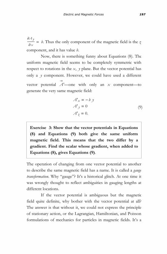
When the curl of A®

is computed, there is only one term, namely.¶A y

¶ x= b. Thus the only component of the magnetic field is the z

component, and it has value b.Now, there is something funny about Equations (8). The

uniform magnetic field seems to be completely symmetric withrespect to rotations in the x, y plane. But the vector potential has

only a y component. However, we could have used a different

vector potential A®

'—one with only an x component—togenerate the very same magnetic field:

(9)

A 'x = -b yA ' y = 0

A 'z = 0.

Exercise 3: Show that the vector potentials in Equations(8) and Equations (9) both give the same uniformmagnetic field. This means that the two differ by agradient. Find the scalar whose gradient, when added toEquations (8), gives Equations (9).

The operation of changing from one vector potential to anotherto describe the same magnetic field has a name. It is called a gaugetransformation. Why “gauge”? It’s a historical glitch. At one time itwas wrongly thought to reflect ambiguities in gauging lengths atdifferent locations.

If the vector potential is ambiguous but the magneticfield quite definite, why bother with the vector potential at all?The answer is that without it, we could not express the principleof stationary action, or the Lagrangian, Hamiltonian, and Poissonformulations of mechanics for particles in magnetic fields. It’s aweird situation: The physical facts are gauge invariant, but theformalism requires us to choose a gauge (a particular choice ofvector potential).


The operation of changing from one vector potential to anotherto describe the same magnetic field has a name. It is called a gaugetransformation. Why “gauge”? It’s a historical glitch. At one time itwas wrongly thought to reflect ambiguities in gauging lengths atdifferent locations.

If the vector potential is ambiguous but the magneticfield quite definite, why bother with the vector potential at all?The answer is that without it, we could not express the principleof stationary action, or the Lagrangian, Hamiltonian, and Poissonformulations of mechanics for particles in magnetic fields. It’s aweird situation: The physical facts are gauge invariant, but theformalism requires us to choose a gauge (a particular choice ofvector potential).

The Force on a Charged Particle

Electrically charged particles are influenced by electric and

magnetic fields E®

and B®

. The force due to the electric field issimple and of the form that we studied in earlier chapters;specifically, it is the gradient of a potential energy. In terms of theelectric field,

F®

= e E®

,

where e is the charge of the particle. It is a rule of electromagnetictheory that a static (not time-dependent) electric field has no curlso it must be a gradient. The usual notation is

E®

= - Ñ®

V ,

so we can write the force as

F®

= - e Ñ®

V .

The potential energy is e Ñ®

V , and everything is completelyconventional.

Magnetic forces on charged particles are different and alittle more complicated. They depend not only on the position ofthe particle through the value of the magnetic field, but also onthe velocity of the particle. They are referred to as velocity-dependentforces. The magnetic force on a charged particle was first writtendown by the great Dutch physicist H. A. Lorentz and is called theLorentz force. It involves the velocity vector of the particle and thespeed of light c :


The potential energy is e Ñ®

V , and everything is completelyconventional.

Magnetic forces on charged particles are different and alittle more complicated. They depend not only on the position ofthe particle through the value of the magnetic field, but also onthe velocity of the particle. They are referred to as velocity-dependentforces. The magnetic force on a charged particle was first writtendown by the great Dutch physicist H. A. Lorentz and is called theLorentz force. It involves the velocity vector of the particle and thespeed of light c :

(10)F®

=e

cv®

B®

.

Notice that the Lorentz force is perpendicular to both thevelocity and the magnetic field. Combining Eq. (10) with

Newton’s F®

= m a®

, we find that the equations of motion for aparticle in a magnetic field are

(11)m a®

=e

cv®

B®

.

The Lorentz force is not the first velocity-dependent force wehave encountered. Recall that in a rotating frame, there are twoso-called fictitious forces: The centrifugal force and (more to thepoint) the Coriolis force. The Coriolis force is given by

(12)F®

= 2 m v®

Ω®

,

where Ω®

is the vector representing the angular velocity of therotating frame. The Coriolis and Lorentz forces are very similar,with the magnetic field and the angular velocity playing the samerole. Of course, not all magnetic fields are uniform, so themagnetic situation can be far more complex than the Corioliscase.

The Lagrangian

All of this raises the question of how to express magnetic forcesin the action, or Lagrangian, form of mechanics. One source ofconfusion is that the symbol for action and the symbol for vectorpotential are both A. In what follows, we will use A for the

action, and A®

, or Ai , as the vector potential. Let’s ignore or setequal to zero the electric field and concentrate on the magnetic,or Lorentz force. Begin with the action for a free particle with noforces:


All of this raises the question of how to express magnetic forcesin the action, or Lagrangian, form of mechanics. One source ofconfusion is that the symbol for action and the symbol for vectorpotential are both A. In what follows, we will use A for the

action, and A®

, or Ai , as the vector potential. Let’s ignore or setequal to zero the electric field and concentrate on the magnetic,or Lorentz force. Begin with the action for a free particle with noforces:

A = àt0

t1LIx, x× M d t

with

L =m

2Ix× iM2.

Here i refers to the direction of space, and the summation signfor summing over x, y, z has been left implicit. Get used to it.

What can we add to the action or to the Lagrangian togive rise to a Lorentz force? The answer is not obvious.However, we know that whatever the additional ingredient is, itshould be proportional to the electric charge, and it should alsoinvolve the magnetic field in some form.

You can experiment around with it and get frustrated.

There is nothing you can do directly involving B®

that will give theLorentz force. The key is the vector potential. The simplest thingwe can do with the vector potential is to dot it into the velocityvector. Remember that the Lagrangian involves only thepositions and the velocities. You might also try dot products of

the position vector with A®

, but that doesn’t work very well. Solet’s try adding to the Lagrangian the term


(13)e

cv®

× A®HxL =

e

câ

i

CHx× i AiHxLG.

The reason for including the speed of light is that itoccurs together with the charge in Lorentz force. Thus we try outthe action:

(14)A = àt0

t1âi

C m

2Ix× iM2

+e

cx×

i × AiHxLG d t .

Now you might object that the equation of motion is notsupposed to involve the vector potential, but only the magneticfield. We know that the vector potential is not unique, so won’twe get another answer if we make a gauge transformation

A®

' = A®

+ Ñ®

s? Let’s see what happens to the action if we do so.The important part of the action is the term arising from

Eq. (13):

AL =e

cà

t0

t1âi

Bx× i AiHxLF d t .

or, more explicitly,

AL =e

cà

t0

t1âi

AiHxL d xi

d td t .

In this equation, AL is the part of the action that we are addingto try to account for the Lorentz force—hence the subscript L.

Suppose we change A®

by adding Ñ®

s. At first sight, it would seemto change AL by adding the term


e

cà

t0

t1âi

¶ s

¶xi

d xi

d td t .

If you look at this carefully, you will see that it all boils down to asimple expression. The d t ’s in the numerator and denominatorcancel:

e

câ

ià

t0

t1 ¶ s

¶xid xi .

And then the whole thing is just the difference between the valueof s at the beginning and its value at the end of the trajectory. Inother words, the gauge transformation added a term s1 - s0 to theaction, where s0 and s1 are the values of s at the initial and finalpositions of the trajectory, respectively. In other words, thechange in the action due to the gauge transformation is

(15)s1 - s0.

Does such a change make any difference to the equations ofmotion? Let’s recall exactly what the action principle actually says.Given any two points in space and time, x0, t0 and x1, t1, thereare many trajectories that connect them, but only one is the truetrajectory taken by a particle. The true trajectory is the one thatminimizes, or makes stationary, the action. So what we do isexplore all trajectories that connect the points until we find thestationary-action solution. From that principle we derived theEuler-Lagrange equations of motion.

As we see in Eq. (15), a gauge transformation changes theaction, but only if we vary the endpoints. If the endpoints arekept fixed, the change in the action has no effect. The stationarypoint has to do only with changing the trajectory without movingthe endpoints. Though the action changes, the equations ofmotion do not, and neither do the solutions. We say that theequations of motion and their solutions are gauge invariant.

One more bit of jargon: Since there are many possiblechoices of vector potentials that describe the same physicalsituation, a specific choice is simply called a gauge. For example,Equations (8) and Equations (9) are two different gaugesdescribing the same uniform magnetic field. The physicalprinciple that the result of any experiment should not depend onthe gauge choice is called gauge invariance.


Does such a change make any difference to the equations ofmotion? Let’s recall exactly what the action principle actually says.Given any two points in space and time, x0, t0 and x1, t1, thereare many trajectories that connect them, but only one is the truetrajectory taken by a particle. The true trajectory is the one thatminimizes, or makes stationary, the action. So what we do isexplore all trajectories that connect the points until we find thestationary-action solution. From that principle we derived theEuler-Lagrange equations of motion.

As we see in Eq. (15), a gauge transformation changes theaction, but only if we vary the endpoints. If the endpoints arekept fixed, the change in the action has no effect. The stationarypoint has to do only with changing the trajectory without movingthe endpoints. Though the action changes, the equations ofmotion do not, and neither do the solutions. We say that theequations of motion and their solutions are gauge invariant.

One more bit of jargon: Since there are many possiblechoices of vector potentials that describe the same physicalsituation, a specific choice is simply called a gauge. For example,Equations (8) and Equations (9) are two different gaugesdescribing the same uniform magnetic field. The physicalprinciple that the result of any experiment should not depend onthe gauge choice is called gauge invariance.

Equations of Motion

Let’s return to the action, Eq. (14). And let’s be very explicitabout the Lagrangian:

(16)L =m

2Jx× 2

+ y× 2

+ z× 2N +

e

cIx× Ax + y

×A y + z

×Az M.

Starting with x, the Lagrange equation of motion is

(17)p×

x =¶L

¶x.

First the canonical momenta: You might think that the momentaare just the usual mass times velocity, but that’s not right. Thecorrect definition is that the momenta are the derivatives of theLagrangian with respect to the components of velocity. This doesgive p = m v with the usual particle Lagrangians, but not with a

magnetic field. From Eq. (16) we get

(18)px = m x×

+e

cAx .

This may worry you. It indicates that the canonicalmomentum is not gauge invariant. This is true, but we are notfinished yet. We have two more things to do. We must computethe time derivative of px and also compute the right-hand side of

Eq. (17). Maybe, if we are lucky, all the gauge-dependent stuff willcancel.

The left-hand side of Eq. (17) is


This may worry you. It indicates that the canonicalmomentum is not gauge invariant. This is true, but we are notfinished yet. We have two more things to do. We must computethe time derivative of px and also compute the right-hand side of

Eq. (17). Maybe, if we are lucky, all the gauge-dependent stuff willcancel.

The left-hand side of Eq. (17) is

p×

x = m ax +e

c

d

d tAx

= m ax +e

c

¶ Ax

¶xx×

+¶ Ax

¶ yy×

+¶ Ax

¶zz×

,

where ax is the x component of acceleration.The right-hand side side of Eq. (17) is:

¶L

¶x=

e

c

¶ Ax

¶xx×

+¶ A y

¶xy×

+¶ Az

¶xz×

.

Now let’s combine the left and right sides:

(19)m ax =e

c

¶ A y

¶x-

¶ Ax

¶ yy×

+e

c

¶ Az

¶x-

¶ Ax

¶zz×.

Equation (19) looks complicated, but note that the combinationsof derivatives

¶ A y

¶x-

¶ Ax

¶ y

and

¶ Az

¶x-

¶ Ax

¶z

are things we saw in Equations (7)—namely, the z and y

components of the magnetic field. We can rewrite Eq. (19) in amuch simpler form:


are things we saw in Equations (7)—namely, the z and y

components of the magnetic field. We can rewrite Eq. (19) in amuch simpler form:

(20)m ax =e

cIBz y

×- B y z

× M.

Take a careful look at Eq. (20). You should be impressed by anumber of things. First of all, the equation is gauge invariant: Onthe right-hand side, the vector potential has completelydisappeared in favor of the magnetic field. The left-hand side isthe mass times the acceleration—that is the left-hand side ofNewton’s equation. In fact, Eq. (20) is nothing but the xcomponent of the Newton-Lorentz equation of motion, Eq. (12).

One might wonder why we bothered introducing thevector potential at all. Why not just write the gauge-invariantNewton-Lorentz equation? The answer is that we can, but thenwe lose any possibility of formulating the equations as an actionprinciple, or as Hamilton’s equations of motion. That might notbe such a tragedy for the classical theory, but it would be adisaster for quantum mechanics.

The Hamiltonian

Before discussing the Hamiltonian of a charged particle in amagnetic field, let’s go back to the definition of the particle’smomentum. You may still find it confusing. The reason is thatthere are two separate concepts: mechanical momentum andcanonical momentum. Mechanical momentum is what you learnabout in elementary mechanics (Momentum equals mass times velocity)and in advanced mechanics (Canonical momentum equals derivative ofthe Lagrangian with respect to velocity). In the simplest situationswhere the Lagrangian is just the difference of kinetic andpotential energy, the two kinds of momentum are the same.

That’s because the only dependence on velocity is 12

m v2.

But once the Lagrangian gets more complicated, the twokinds of momentum may not be the same. In Eq. (18) we seesuch an example. The canonical momentum is the mechanicalmomentum plus a term proportional to the vector potential. Wecan write it in vector notation:


Before discussing the Hamiltonian of a charged particle in amagnetic field, let’s go back to the definition of the particle’smomentum. You may still find it confusing. The reason is thatthere are two separate concepts: mechanical momentum andcanonical momentum. Mechanical momentum is what you learnabout in elementary mechanics (Momentum equals mass times velocity)and in advanced mechanics (Canonical momentum equals derivative ofthe Lagrangian with respect to velocity). In the simplest situationswhere the Lagrangian is just the difference of kinetic andpotential energy, the two kinds of momentum are the same.

That’s because the only dependence on velocity is 12

m v2.

But once the Lagrangian gets more complicated, the twokinds of momentum may not be the same. In Eq. (18) we seesuch an example. The canonical momentum is the mechanicalmomentum plus a term proportional to the vector potential. Wecan write it in vector notation:

(21)p®

= m v®

+e

cA®HxL.

The mechanical momentum is not only familiar; it is gaugeinvariant. It is directly observable, and in that sense it is “real.”The canonical momentum is unfamiliar and less “real”; it changeswhen you make a gauge transformation. But whether or not it isreal, it is necessary if you want to express the mechanics ofcharged particles in Lagrangian and Hamiltonian language.

To pass to the Hamiltonian, we recall the definition

H = âi

I pi q×

iM - L,

which in this case is

(22)H = âi

; pi x×

i - C m

2Ix× iM2

+e

cx×

i × AiHxLG?.

Let’s work it out. First we will need to get rid of the velocities;the Hamiltonian is always thought of as a function of coordinatesand momenta. That’s easy. We just solve Eq. (21) for velocity interms of p:


(23)x×

i =1

mC pi -

e

cAiHxLG.

Now wherever you see a velocity component in Eq. (22),substitute Eq. (23) and then do a little rearranging. Here is whatyou will get:

(24)H = âi

1

2 mC pi -

e

cAiHxLGC pi -

e

cAiHxLG .

Exercise 4: Using the Hamiltonian, Eq. (24), work outHamilton’s equations of motion and show that you justget back the Newton-Lorentz equation of motion.

If you carefully look at Eq. (24), you will see something a little

surprising. The combination B pi -ec

AiHxLF is the mechanical

momentum m vi . The Hamiltonian is nothing but

H =1

2m v2.

In other words, its numerical value is the same as the naivekinetic energy. That proves (among other things) that the energyis gauge invariant. Since it conserved, the naive kinetic energy isalso conserved, as long as the magnetic field does not changewith time. But that does not mean the particle motion does notsense the magnetic field. If you want to use the Hamiltonian tofind the motion, you must express it in terms of the canonicalmomentum, not the velocity, and then use Hamilton’s equations.Alternatively, you can work with velocities and use theLagrangian form of the equations, but in that case the Lagrangianis not the naive kinetic energy. In either case, if you work it allout, you will discover that the charged particle experiences agauge-invariant Lorentz magnetic force.


In other words, its numerical value is the same as the naivekinetic energy. That proves (among other things) that the energyis gauge invariant. Since it conserved, the naive kinetic energy isalso conserved, as long as the magnetic field does not changewith time. But that does not mean the particle motion does notsense the magnetic field. If you want to use the Hamiltonian tofind the motion, you must express it in terms of the canonicalmomentum, not the velocity, and then use Hamilton’s equations.Alternatively, you can work with velocities and use theLagrangian form of the equations, but in that case the Lagrangianis not the naive kinetic energy. In either case, if you work it allout, you will discover that the charged particle experiences agauge-invariant Lorentz magnetic force.

Motion in a Uniform Magnetic Field

Motion in a uniform magnetic field is easy enough to solve, and itillustrates a lot of the principles we have been discussing. Let’stake the field to lie in the z direction and to have magnitude b.

This is the situation described in Equations (6, 7, 8). The choicebetween the vector potentials in Equations (7, 8) is an example ofthe ambiguity associated with gauge transformations. Let’s firstchoose Equations (7) and write the Hamiltonian, Eq. (24), using

HAx = 0, A y = b x, Az = 0M. We get

H =1

2 mCH pxL2 + I pz M2 + K p y -

e

cb xO2G.

As always, the first thing to do is to look for conservation laws.We already know one: energy conservation. As we’ve seen, the

energy is the old-fashioned kinetic energy 12

m v2. It follows that

the magnitude of the velocity is constant.Next, notice that the only coordinate that appears in H is

x. This means that when we work out Hamilton’s equations, wewill find that px is not conserved but that both pz and p y are

conserved. Let’s see what the implications are. First the z

component. Since Az = 0, pz = m vz , and the conservation of

pz tells the familiar story that the z component of velocity is

constant.Next look at the conservation of p y . This time p y is not

equal to m v y but, rather, to m v y +ec

b x. The conservation of p y

then tells us that


As always, the first thing to do is to look for conservation laws.We already know one: energy conservation. As we’ve seen, the

energy is the old-fashioned kinetic energy 12

m v2. It follows that

the magnitude of the velocity is constant.Next, notice that the only coordinate that appears in H is

x. This means that when we work out Hamilton’s equations, wewill find that px is not conserved but that both pz and p y are

conserved. Let’s see what the implications are. First the z

component. Since Az = 0, pz = m vz , and the conservation of

pz tells the familiar story that the z component of velocity is

constant.Next look at the conservation of p y . This time p y is not

equal to m v y but, rather, to m v y +ec

b x. The conservation of p y

then tells us that

m a y +e

cb vx = 0,

or

(25)a y = -e b

m cvx .

Notice that the conservation of p y does not imply that the y

component of velocity is conserved.What about px? It does not seem to be conserved since

H has explicit dependence on x. We could use Hamilton’sequations to determine the x component of acceleration, but I’mgoing to do it another way. Instead of using Equations (8) I’mgoing to change the gauge in midstream and use Equations (7).Remember that the physical phenomena should not change. Thenew Hamiltonian that goes with Equations (7) is,

H =1

2 mCK px +

e

cb yO2

+ I p yM2 + I pz M2G.

Now the Hamiltonian does not depend on x, which implies thatpx is conserved. How can that be? We previously showed the x-

component of momentum px is conserved when we used

Equations (8). The answer is that when we make a gaugetransformation the components of p change. In the two cases, px

does not have the same meaning.Let us see the implication of px conservation in the new

gauge. Using Equations (7) we find that px = m vx -ec

b y. Thus

the conservation of px is expressed as


(26)ax =e b

m cv y .

By now you may have already realized that Eq. (25) and Eq. (26)are familiar. They are the Newton-Lorentz equations for motionin a uniform magnetic field.

Exercise 5: Show that in the x, y plane, the solution to

Eq. (25) and the solution to Eq. (26) are a circular orbitwith the center of the orbit being anywhere on the plane.Find the radius of the orbit in terms of the velocity.

Gauge Invariance

The reason why I left magnetic forces for the last lecture is that Iwant you to remember the lessons when, in future study, wecome to quantum mechanics and field theory. Gauge fields andgauge invariance are not minor artifacts of writing the Lorentzforce in Lagrangian form. They are the central guiding principlesthat underlie everything, from quantum electrodynamics togeneral relativity and beyond. They play a leading role incondensed matter physics—for example, in explaining all sorts oflaboratory phenomena such as superconductivity. I will closethese lectures on classical mechanics by reviewing the meaning ofthe gauge idea, but its real importance will become clear only inlater lectures.

The simplest meaning of a gauge field—the vectorpotential is the most elementary example—is that it is an auxiliarydevice that is introduced to make sure certain constraints are

satisfied. In the case of a magnetic field, not any B®HxL is allowed.

The constraint is that B®HxL should have no divergence:


The reason why I left magnetic forces for the last lecture is that Iwant you to remember the lessons when, in future study, wecome to quantum mechanics and field theory. Gauge fields andgauge invariance are not minor artifacts of writing the Lorentzforce in Lagrangian form. They are the central guiding principlesthat underlie everything, from quantum electrodynamics togeneral relativity and beyond. They play a leading role incondensed matter physics—for example, in explaining all sorts oflaboratory phenomena such as superconductivity. I will closethese lectures on classical mechanics by reviewing the meaning ofthe gauge idea, but its real importance will become clear only inlater lectures.

The simplest meaning of a gauge field—the vectorpotential is the most elementary example—is that it is an auxiliarydevice that is introduced to make sure certain constraints are

satisfied. In the case of a magnetic field, not any B®HxL is allowed.

The constraint is that B®HxL should have no divergence:

Ñ®

× B®

= 0

To ensure that, we write the magnetic field as the curl of

something—A®HxL—because curls automatically have no

divergence. It’s a trick to avoid having to worry explicitly about

the fact that B®HxL is constrained.

But we soon discover that we cannot get along without

A®HxL. There is no way to derive Lorentz’s force law from aLagrangian without the vector potential. That is a pattern: Towrite the equations of modern physics in either Lagrangian orHamiltonian form, auxiliary gauge fields have to be introduced.

But they are also nonintuitive and abstract. Despite theirbeing indispensable, you can change them without changing thephysics. Such changes are called gauge transformations, and the factthat physical phenomenal do not change is called gauge invariance.Gauge fields cannot be “real,” because we can change themwithout disturbing the gauge invariant physics. On the otherhand, we cannot express the laws of physics without them.

I am not about to give you a sudden insight that willresolve this tension. I will just say that’s the way it is: The laws ofphysics involve gauge fields, but objective phenomena are gaugeinvariant.

Good Bye for Now

We are now finished with classical mechanics. If you havefollowed along, you know the Theoretical Minimum—all youneed to know about classical mechanics to move on to the nextthing. See you in Quantum Mechanics!


Appendix 1: Central Forces and Planetary Orbits

Lenny stooped and peered through the eyepiece of the telescope.It was the first time he had ever done that. He saw the rings ofSaturn and whistled at their beauty. “George, have you seen therings?”

George nodded and said, “Yup, I seen ’em.”Lenny looked up and pressed his friend. “Where do they

come from?”George said, “It’s like the Earth goin’ round the Sun.”Lenny nodded. “How does it go around?”

The Central Force of Gravity

A central force field is a force that points toward a center—inother words, toward a point of space (see Figure 1). In addition,for a force to be a central force, the magnitude of the force mustbe the same in every direction.

Figure 1: A central force.

Other than the obvious symmetry—rotational symmetry—thereis nothing very special about central forces from a mathematicalviewpoint. But their role in physics and in the history of physicsis very special. The first problems solved by Newton—theproblems of planetary orbits—were central force problems. Themotion of an electron orbiting a hydrogen nucleus is a centralforce problem. Two atoms orbiting one another to form a simplemolecule can be reduced to a central force problem in which thecenter is the center of mass. Since there was not enough time tocover this subject in the lectures, we’ll add it here as a supplement.

Let’s focus on the motion of the Earth as it orbits themuch heavier Sun. According to Newton’s laws, the force exertedby the Sun on the Earth is equal and opposite to that exerted bythe Earth on the Sun. Moreover, the direction of those forces isalong the line connecting the two bodies. Because the Sun is somuch heavier than the Earth, the motion of the Sun is negligible,and it can be considered to be at a fixed location. We can chooseour coordinates so that the Sun is at the origin, x = y = z = 0.

The Earth, by contrast, moves in an orbit about the origin. Let’s

denote the location of the Earth by the vector r®

withcomponents x, y, z. Since the Sun is located at the origin, the

force on the Earth points toward the origin, as shown in Figure1. Moreover, the magnitude of the force depends only on thedistance r from the origin. A force with these properties—pointing toward the origin and depending only on the distance—is called a central force.

Let’s rewrite the unit vector from Interlude 1:

Other than the obvious symmetry—rotational symmetry—thereis nothing very special about central forces from a mathematicalviewpoint. But their role in physics and in the history of physicsis very special. The first problems solved by Newton—theproblems of planetary orbits—were central force problems. Themotion of an electron orbiting a hydrogen nucleus is a centralforce problem. Two atoms orbiting one another to form a simplemolecule can be reduced to a central force problem in which thecenter is the center of mass. Since there was not enough time tocover this subject in the lectures, we’ll add it here as a supplement.

Let’s focus on the motion of the Earth as it orbits themuch heavier Sun. According to Newton’s laws, the force exertedby the Sun on the Earth is equal and opposite to that exerted bythe Earth on the Sun. Moreover, the direction of those forces isalong the line connecting the two bodies. Because the Sun is somuch heavier than the Earth, the motion of the Sun is negligible,and it can be considered to be at a fixed location. We can chooseour coordinates so that the Sun is at the origin, x = y = z = 0.

The Earth, by contrast, moves in an orbit about the origin. Let’s

denote the location of the Earth by the vector r®

withcomponents x, y, z. Since the Sun is located at the origin, the

force on the Earth points toward the origin, as shown in Figure1. Moreover, the magnitude of the force depends only on thedistance r from the origin. A force with these properties—pointing toward the origin and depending only on the distance—is called a central force.

Let’s rewrite the unit vector from Interlude 1:

rï =r®

r.

In equation form, the definition of a central force is

Appendix—Central Forces and Planetary Orbits 213

F®

= f J r®N rï,

where f J r®N determines two things. First, the magnitude of f J r

®Nis the magnitude of the force when the Earth is at distance r .

Second, the sign of f J r®N determines whether the force is toward

or away from the Sun—in other words, whether the force is

attractive or repulsive. In particular, if f J r®N is positive the force

is away from the Sun (repulsive), and if it is negative the force istoward the Sun (attractive).

The force between the Sun and the Earth is of coursegravitational. According to Newton’s law of gravitation, thegravitational force between two objects of mass m1 and m2 hasthe following properties.

N1: The force is attractive and proportional to the product of theobjects’ masses and a constant called G. Today we refer to G asNewton’s constant. Its value is G » 6.673 m3 kg-1 s-2.

N2: The force is inversely proportional the square of the distancebetween the masses.

To summarize, the force is attractive and has magnitude G m1 m2

r2 .

In other words, the function f J r®N is given by

f J r®N =

G m1 m2

r2,

and


F®

grav = -G m1 m2

r2rï.

For the case of the Earth-Sun system let’s denote the Sun’s massby M and the Earth’s mass by m. The force on the Earth is

F®

grav = -G M m

r2rï.

The equation of motion for the Earth’s orbit is the usual F = m a,or, using the gravitational force,

md2 r

®

d t2= -

G M m

r2rï.

Notice an interesting fact: The mass of the Earth cancels fromboth sides of the equation, so the equation of motion does notdepend on the mass of the Earth:

(1)d2 r

®

d t2= -

G M

r2rï.

An object of very different mass, such as a satellite, could orbitthe Sun in the same orbit as the Earth. One caveat about thisfact: It is true only if the Sun is so massive, compared with theEarth or satellite, that its motion can be ignored.

Gravitational Potential Energy

The gravitational force can be derived from a potential energyfunction. Recall that the force associated with a potential energyis minus the gradient of the potential:


F = -ÑV .

It’s not too hard to guess the form of V for the gravitationalcase. First of all, since the force is proportional to the constantG M m, one expects the potential energy also to have this factor.

Next, because the magnitude of the force only dependson the distance r , one may expect the potential energy V Hr L alsoto depend only on r . Finally, since we have to differentiate V Hr Lto get the force, and since the force is proportional to 1 r2, the

potential energy must be proportional to -1 r . Thus it is naturalto try

V Hr L = -G M m

r.

In fact, this is exactly right.

The Earth Moves in a Plane

Earlier, we mentioned that the central force problem has asymmetry. You probably recognize it as rotational symmetryabout the origin. The implication of the symmetry, explained inLecture 7, is the conservation of angular momentum. Suppose

that at some instant the earth has location r®

and velocity v®

. Wecan place these two vectors and the position of the Sun in aplane—the momentary plane of the Earth’s orbit.

The angular momentum vector L®

is proportional to the

cross product r®

v®

, so it is perpendicular to both r®

and v®

(seeFigure 2). In other words, the angular momentum isperpendicular to the plane of the orbit. This is a powerful factwhen combined with the conservation of angular momentum.

The conservation tells us that the vector L®

never changes. Fromthat we conclude that the orbital plane never changes. To put itsimply, the Earth’s orbit and the Sun permanently lie in a fixedplane that does not vary. Knowing this, we may rotate ourcoordinates so that the orbit is in the x, y plane. The entire

problem is then two-dimensional, the third coordinate z playing

no role.


Earlier, we mentioned that the central force problem has asymmetry. You probably recognize it as rotational symmetryabout the origin. The implication of the symmetry, explained inLecture 7, is the conservation of angular momentum. Suppose

that at some instant the earth has location r®

and velocity v®

. Wecan place these two vectors and the position of the Sun in aplane—the momentary plane of the Earth’s orbit.

The angular momentum vector L®

is proportional to the

cross product r®

v®

, so it is perpendicular to both r®

and v®

(seeFigure 2). In other words, the angular momentum isperpendicular to the plane of the orbit. This is a powerful factwhen combined with the conservation of angular momentum.

The conservation tells us that the vector L®

never changes. Fromthat we conclude that the orbital plane never changes. To put itsimply, the Earth’s orbit and the Sun permanently lie in a fixedplane that does not vary. Knowing this, we may rotate ourcoordinates so that the orbit is in the x, y plane. The entire

problem is then two-dimensional, the third coordinate z playing

no role.

L®

r®

v®

Figure 2: The relationship among the angular momentum

L®

, the position vector r®

, and the velocity v®

.

Polar Coordinates

We could work with the Cartesian coordinates x, y, but central

force problems are much easier to solve in polar coordinates r , Θ:

r = x2 + y2

cos Θ =x

r

In polar coordinates the kinetic energy of the earth is simpleenough:


In polar coordinates the kinetic energy of the earth is simpleenough:

(2)T =m

2r×2

+ r2 Θ× 2

.

The potential energy is even simpler—it does not involve Θ at all:

(3)V Hr L = -G M m

r.

Equations of Motion

As is usually the case, the easiest route to the equations of motionis through the Lagrangian method. Recall that the Lagrangian isthe difference of the kinetic and potential energies, L = T - V .Using Eq. (2) and Eq. (3), the Lagrangian in polar coordinates is

(4)L =m

2r×2

+ r2 Θ× 2

+G M m

r.

The equations of motion,

d

d t

¶L

¶ r×

=¶L

¶ r

d

d t

¶L

¶Θ×

=¶L

¶Θ,

take the explicit form

(5)r××

= r Θ×

-G M

r

and


(6)d

d tKm r2 Θ

× O = 0.

This last equation has the form of a conservation law. Notsurprisingly, it is conservation of angular momentum. (To beprecise, it is the conservation of the z component of angular

momentum.) It is traditional to denote the angular momentum bythe symbol L, but we are using that as the Lagrangian, so we willuse pΘ instead. If we know pΘ at any particular instant, then we

know it for all time. We may write

(7)m r2 Θ×

= pΘ

and just treat pΘ as a known constant.

This enables us to express the angular velocity in terms ofthe distance of the Earth from the Sun. We just solve the

equation for Θ×

:

(8)Θ×

=pΘ

m r2.

We will come back to this relation between angular velocity andradial distance, but first let’s return to the equation for r , namely

(9)m r××

= m r Θ× 2

-G M m

r2.

In Eq. (9) the angular velocity appears, but we can use Eq. (8) toreplace it:

(10)m r××

=pΘ

2

m r3-

G M m

r2.

The equation for r has an interesting interpretation. It looks likethe equation for a single coordinate r under the influence of acombined “effective” force:


The equation for r has an interesting interpretation. It looks likethe equation for a single coordinate r under the influence of acombined “effective” force:

(11)Feffective =pΘ

2

m r3-

G M m

r2.

The term - G M m

r2 is just the gravitational force, but at first sight

the second term may be a surprise. It is, in fact, nothing but thefictitious centrifugal force experienced by any particle that has anangular motion about the origin.

It’s useful to pretend that Eq. (11) really does describe aparticle moving under a total force that includes both the realgravitational force and the centrifugal force. Of course, for eachvalue of the angular momentum, we must readjust pΘ, but since

pΘ is conserved, we may regard it as a fixed number.

Given the effective force, one can also construct aneffective potential energy function that includes the effect ofgravity and the effect of centrifugal force:

(12)Veffective =pΘ

2

2 m r2-

G M m

r.

You can easily check that

Feffective = -d Veffective

d r.

For all practical purposes, we can pretend the r motion isjust that of a particle whose kinetic energy has the usual form,

m r×2

2, whose potential energy is Veffective, and whose Lagrangian

is


For all practical purposes, we can pretend the r motion isjust that of a particle whose kinetic energy has the usual form,

m r×2

2, whose potential energy is Veffective, and whose Lagrangian

is

(13)Leffective =m r

×2

2-

pΘ2

2 m r2+

G M m

r.

Effective Potential Energy Diagrams

In getting a feel for a problem, it is often a good idea to make agraph of the potential energy. For example, the equilibriumpoints (where the system may be at rest) can be identified as thestationary points (minima, maxima) of the potential. Inunderstanding central force motion, we do exactly the same,except that we apply it to the effective potential. Let’s first plotthe two terms in Veffective separately, as shown in Figure 3. Notethat the two terms are of opposite sign; the centrifugal term ispositive and the gravitational term negative. The reason is thatthe gravitational force is attractive, whereas the centrifugal forcepushes the particle away from the origin.

V Hr L =pΘ

2

2 m r2

V Hr L = -G m

r

r

VHrL

Figure 3: The potential energy diagram for the centrifugal and gravitational terms.

Near the origin the centrifugal term is the mostimportant, but at large values of r the gravitational term has thelarger magnitude. When we combine them, we get a graph ofVeffective that looks like Figure 4.


Near the origin the centrifugal term is the mostimportant, but at large values of r the gravitational term has thelarger magnitude. When we combine them, we get a graph ofVeffective that looks like Figure 4.

V Hr L =pΘ

2

2 m r2-

G m

r

r

VHrL

Figure 4: The potential energy diagram for the combination of centrifugal and gravitational terms.

Note that when the two terms are combined, the graph has aminimum. That may seem odd; we don’t expect an equilibriumpoint where the Earth can stand still. But we have to rememberthat we are discussing only the behavior of r and ignoring theangular coordinate Θ. The point is that for each angularmomentum, there are orbits that maintain a constant radialdistance while moving around the Sun. Such orbits are circular.On the graph of Veffective a circular orbit is represented by afictitious particle sitting at rest at the minimum.

Let’s compute the value of r at the minimum. All we haveto do is differentiate Veffective and set the derivative equal tozero. It’s an easy calculation that I will leave to you. The result isthat the minimum occurs at


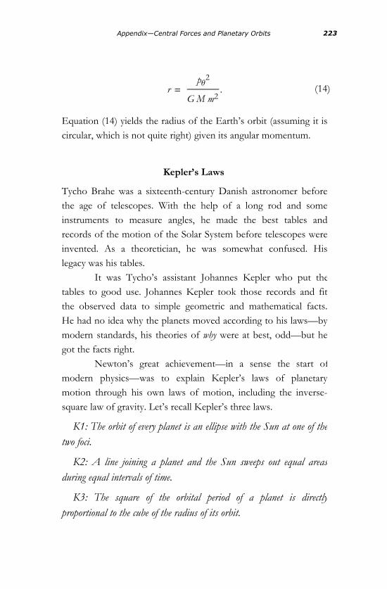
(14)r =pΘ

2

G M m2.

Equation (14) yields the radius of the Earth’s orbit (assuming it iscircular, which is not quite right) given its angular momentum.

Kepler’s Laws

Tycho Brahe was a sixteenth-century Danish astronomer beforethe age of telescopes. With the help of a long rod and someinstruments to measure angles, he made the best tables andrecords of the motion of the Solar System before telescopes wereinvented. As a theoretician, he was somewhat confused. Hislegacy was his tables.

It was Tycho’s assistant Johannes Kepler who put thetables to good use. Johannes Kepler took those records and fitthe observed data to simple geometric and mathematical facts.He had no idea why the planets moved according to his laws—bymodern standards, his theories of why were at best, odd—but hegot the facts right.

Newton’s great achievement—in a sense the start ofmodern physics—was to explain Kepler’s laws of planetarymotion through his own laws of motion, including the inverse-square law of gravity. Let’s recall Kepler’s three laws.

K1: The orbit of every planet is an ellipse with the Sun at one of thetwo foci.

K2: A line joining a planet and the Sun sweeps out equal areasduring equal intervals of time.

K3: The square of the orbital period of a planet is directlyproportional to the cube of the radius of its orbit.


K3: The square of the orbital period of a planet is directlyproportional to the cube of the radius of its orbit.

Begin with K1, the ellipse law. Earlier we explained that circularorbits correspond to being in equilibrium at the minimum of theeffective potential. But there are motions of the effective one-dimensional system in which it oscillates back and forth near, butnot at, the minimum. A motion of this type would have the Earthperiodically getting closer to and farther from the Sun.Meanwhile, because it has angular momentum L, the Earth mustalso be moving around the Sun. In other words the angle Θ isincreasing with time. The resulting trajectory, in which thedistance oscillates and the angular position changes, is elliptical.Figure 5 shows just such an elliptical orbit. If you follow the orbitand keep track only of the radial distance, the position of theEarth periodically moves in and out as if it were oscillating in theeffective potential.

Figure 5: The elliptical orbit of the Earth around the Sun.

To prove the orbit is exactly an ellipse is a bit difficult, and wewill not prove it now.

Let’s take another look at the motion of a particle in theeffective potential. Imagine a particle with so much energy that itwould completely escape from the dip in the potential energy. Insuch an orbit the particle comes in from infinity, bounces off thepotential near r = 0, and goes back out, never to return. Suchorbits certainly exist; they are called unbounded hyperbolic orbits.

Now let’s move on to K2. According to Kepler’s secondlaw, as the radial vector sweeps out the ellipse, the area that itsweeps per unit time is always the same. This sounds like aconservation law, and indeed it is—the conservation of angularmomentum. Go back to Eq. (7) and divide it by the mass m:


To prove the orbit is exactly an ellipse is a bit difficult, and wewill not prove it now.

Let’s take another look at the motion of a particle in theeffective potential. Imagine a particle with so much energy that itwould completely escape from the dip in the potential energy. Insuch an orbit the particle comes in from infinity, bounces off thepotential near r = 0, and goes back out, never to return. Suchorbits certainly exist; they are called unbounded hyperbolic orbits.

Now let’s move on to K2. According to Kepler’s secondlaw, as the radial vector sweeps out the ellipse, the area that itsweeps per unit time is always the same. This sounds like aconservation law, and indeed it is—the conservation of angularmomentum. Go back to Eq. (7) and divide it by the mass m:

(15)r2 Θ×

=pΘ

m.

Imagine the radial line as it sweeps out an area. In a small time∆ t , the area changes by ∆ Θ.

Figure 6: The area swept out by the line connecting the Earth to the Sun in a short time ∆ t .

The small triangle swept out in Figure 6 has area


∆ A =1

2r2 ∆ Θ.

You can check this using the fact that the area of a triangle is one-half the base Hr L times the height Hr ∆ΘL. If we divide by the smalltime interval ∆ t , we get

d A

d t=

r2

2Θ×

.

But now we use angular momentum conservation in the form ofEq. (15), and we get the final equation

(16)d A

d t=

pΘ

2 m.

Since pΘ (and also m) do not vary, we see that the rate of swept-

out area is constant, and, moreover, it is just proportional to theangular momentum of the orbit.

Finally, we come to K3: The square of the orbital period of aplanet is directly proportional to the cube of the radius of its orbit.

Kepler’s formulation was very general, but we will work itout only for circular orbits. There are a number of ways we cando this, but the simplest is just to use Newton's law, F = m a. Theforce on the orbiting Earth is just the gravitational force, whosemagnitude is

F = -G M m

r2.

On the other hand, in Lecture 2 we calculated the accelerationof an object moving in a circular orbit,


(17)a = Ω2 r

where Ω is the angular velocity.

Exercise 1: Show that Eq. (17), above, is a consequenceof Equations (3) from Lecture 2.

Newton's law becomes

G M m

r2= m Ω2 r .

We can easily solve this for Ω2:

Ω2 =G M

r3.

The last step is to note that the period of the orbit—the time tomake one circuit—is simply related to the angular velocity.Denoting the period by the Greek letter tau, Τ, we have

Τ =1

2 ΠΩ.

Traditionally we would use T for the period, but we are alreadyusing T for the kinetic energy. Putting it all together we get

Τ2 =1

4 Π G Mr3.

Indeed, the square of the period is proportional to the cube ofthe radius.


Accelerationof circular orbit, 45–46due to gravity, 71–72mass, force, and, 63–66, 70of particle, 40–41, 42, 43–44,

45–46position and, 44, 46state-space of system of particles

and, 88, 89units of, 68

Action, 108–110, 115reaction and, 92–94, 139total, 112See also Principle of least action

Active change of coordinates, 131Addition, of vectors, 24–25, 26–27Advanced mechanics, 105–107Angle, measure of, 19–20Angular frequency, 45Angular momentum, 124–125

conservation of, 140, 143–144,219, 225–226

Earth’s orbit and, 216–217Poisson brackets and, 178–181,

182–187Angular velocity, radial distance and,

219–221Antisymmetry of Poisson Brackets,

174Aristotle’s (false) law of motion,

58–63Atomic energy, 103, 104Axes, 15–16

Basis vectors, 25–26Binomial theorem, 31, 32Brahe, Tycho, 223

Calculusfundamental theorem of, 50–53of variations, 110See also Differential calculus;

Integral calculusCanonical momentum, 203–204,

205–207Carat, 25Cartesian coordinates, 15–19,

121–122vectors for, 23–24, 25–27

Central forces, 212–215equations of motion and,

218–221gravitational potential energy and,

215–216planetary orbits and, 213–215polar coordinates and, 217–218

Centrifugal force, 120in effective potential energy

diagrams, 221, 222effective potential energy function

and, 220, 221Chain rule, 35–36Chaos, 14Charges, 85–86Chemical energy, 103, 104Circle, right triangle drawn in, 21–22Circular motion, 44–46

Index

Circular orbit, 222–223, 226–227velocity and acceleration of, 45–46

Classical mechanics, 1–2Classical physics

assumptions about time in, 17–18cycles and conservation laws and,

12–13defined, 1–2dynamical systems with infinite

number of states and, 10–12limits of precision and, 13–14minus-first law and, 8–10systems and state-space and, 2–8

Closed systems, 2Commutator, 173Components, of vectors, 26Condensed matter physics, 210Configuration space, 91Conjugate momentum, 123–125,

126–127Conservation, symmetry and,

178–181, 187–189Conservation laws

cycles and, 12–13for simple systems, 128–130symmetry and, 139–144

Conservation of angular momentum,140, 216–217, 219, 225–226

Conservation of energy, 101–103,145–152

Conservation of information, 9–10Conservation of momentum, 92–94,

139–140Constant, derivative of a, 34Continuous evolution, 3Continuous transformations, 134, 137Convergence, 165Coordinates, 15–19

Cartesian, 15–17, 121–122

cyclic, 125–127generalized, 121–125polar, 124, 217–218

Coordinate system, Cartesian, 15–17

Coordinate transformation, 117–120,130–135

Coriolis force, 120–121, 199Cosine (cos), 20, 21, 23Cross product, 27, 193Curl, 193–194Cycles, 5–6

conservation laws and, 12–13Cyclic coordinates, 125–127

Definite integral, 49Degrees of freedom, 4–5

Euler-Lagrange equation for asingle, 110–111

Del, 191–194Delta (Δ), 30Derivatives

calculating, 31–36defined, 30–31of a constant, 34integrals and, 50–53of powers, 32–34rules for, 33–36second, 79, 82, 83–84second-order partial, 76special cases, 33–34time, 38–39

Determinant, 82Deterministic, 2

dynamical laws and, 8–9laws of classical physics and, 5

Differential calculus, 29–37partial derivatives and

multivariable, 74–84

230 Index

Differential equationsfirst-order, 60–63second-order, 69–72

Direction of time, 17Displacement, 23, 38–39Distance

angular velocity and radial, 219–221

coordinates and, 16electric and gravitational forces and,

85–86Divergence, 165

flow and, 165–167of magnetic fields, 195of vector field, 167, 192curl and, 194

Dot product, 27Double pendulum, angular

momentum and, 140–144Drag force, 85Dynamical laws, 3–8

reversible and deterministic, 8–10Dynamical systems, 3

with infinite number of states, 10–12

DynamicsAristotle’s law of motion, 58–63mass, acceleration, and force,

63–66Newton’s equations, 69–73

Earth, angular velocity and distancefrom Sun, 219–220

Earth’s orbit, 224central forces and, 213–215equation of motion for, 215gravitational force and, 214–215as movement in a plane, 216–217radius of, 222–223

Effective potential energy diagrams,221–223

Electric field, 198Electric forces, 85–86Electromagnetic energy, 103–104Electrostatic energy, 103, 104Ellipse law, 223–225Elliptical orbit, 223–225Energy, 95–104

atomic/nuclear, 103, 104chemical energy, 103, 104conservation of (see Energy

conservation)electrostatic, 103, 104heat, 103–104kinetic, 97, 101–102magnetic, 103, 104mechanical, 103multiple dimensions and, 99–102potential, 95–99radiation, 103, 104rate of change of, 97–99total, 97

Energy conservation, 97–99, 147–152motion in uniform magnetic field

and, 208–210phase space fluid and, 162–164symmetry and, 145–152

Equations of motion, 203–205, 218–221

determining trajectories from, 105–108

for Earth’s orbit, 215generalized coordinates and,

121–125Lagrange and the vector potential,

203–205Newton-Lorentz, 204–205, 207, 209Newton’s, 69–73, 86–88

Index 231

Euler-Lagrange equations, 110–114,202

conjugate momentum and, 123–125

derivation of, 111–114use of, 116–121

Fictitious forces, 118, 199Fields

electric, 198gauge, 210–211magnetic (see Magnetic fields)scalar, 190–191, 194vector (see Vector fields)

First-order differential equations, 60–63

Flowdivergence and, 165–167in phase space, 162–164stationary, 166

Forces, 58–59, 96central (see Central forces)centrifugal (see Centrifugal force)on charged particle, 198–199Coriolis, 120–121, 199defining, 63–66electric, 85–86fictitious, 199friction, 58, 63, 85fundamental, 85–86gravitational (see

Gravity/gravitational force)Lorentz, 198–199magnetic (see Magnetic forces)mass, acceleration, and, 63–67, 70nonconservative, 100potential energy and, 95–99types of, 85units of, 68–69

velocity and, 58–60velocity-dependent, 198

Friction, 58, 63, 85Functional, 110Functions

graphing, 18–19implicit, 35minimizing, 76–79trigonometric, 19–23

Fundamental forces, 85–86Fundamental theorem of calculus,

50–53

Gauge, 197, 203Gauge fields, 210–211Gauge invariance, 203, 210–211Gauge invariant, 198, 203–205, 208Gauge transformation, 197, 201, 202,

211Generalized coordinate system,

121–125Generalized coordinates, 121–125Generalized momentum, 123–125Generator, 183, 188Gibbs, Josiah Willard, 169Gibbs-Liouville theorem, 169Global minimum, 77Gradient, 191–192Graph

of functions, 18–19of harmonic oscillator in phase

space, 163–164of integration, 47–48of local maxima, 78of local minima, 77of simple harmonic motion, 42of trigonometric functions, 21of vector, 24of velocity field, 165

232 Index

Gravitational potential energy, 215–216

Gravity/gravitational force, 85–86,212–216

acceleration due to, 71–72in effective potential energy

diagrams, 221–222effective potential energy function

and, 220–222inverse-square law of, 222–223on orbiting Earth, 214–215,

226–227properties of, 214

Gyroscope, 185–187

Hamiltonian, 149–152charged particle in magnetic field

and, 205–208gauge fields and, 210–211harmonic oscillator, 156–159phase space and, 152–155symmetry of, 157

Hamilton’s equations, 153–155derivation of, 160–161Poisson brackets and, 178

Harmonic oscillator, 72–73Liouville’s theorem and, 170phase space fluid and, 162–164time-translation symmetry and,

145–147Harmonic oscillator Hamiltonian,

156–159Heat energy, 103–104Hessian matrix, 82–84

Implicit function, 34Incompressibility of fluid, 166–167

Liouville’s theorem and, 167–170Indefinite integral, 50, 51–54

Inertia, law of, 63Infinitesimal transformations,

134–136, 137Inflection, point of, 78–79Information, conservation of, 9–10Initial conditions, 13–14Integral calculus, 47–57

integration by parts, 55–57Integrals

definite, 49derivatives and, 50–53indefinite, 50, 51–54integration by parts and, 55–57

Integrand, 49Integration

formulas, 53–54graph of, 48by parts, 55–57

Inverse-square law of gravity, 223Irreversible, 8–9

Kepler, Johannes, 223Kepler’s laws, 223–227Kilogram (kg), 68Kinetic energy, 97–98, 101

defined, 97Kronecker delta, 175, 181

Lagrange equation of motion for acharged particle, 203

Lagrangian (L), 107–111cyclic coordinates and, 125–127energy conservation and, 147–152gauge fields and, 210–211in generalized coordinate system,

123–125Hamiltonian and, 149–152Lorentz forces and, 199–203in polar coordinates, 218–219

Index 233

Lagrangian (L), (continued )symmetry and, 130–136, 137–139time-translation symmetry and,

146–147use of, 116–121

Laplace, Pierre-Simon, 1–2, 13, 85Law of inertia, 63Law of motion, 3–10Length, units of, 67Levi-Civita symbol, 181–182,

183–184, 193Limits, 29–30

of integration, 47–48of precision, 13–14

Linear combination, of basis vectors,26

Linearity of Poisson Brackets, 174–175

Liouville, Joseph, 169Liouville’s theorem, 167–170Local maximum(a), 78

Hessian and, 82in higher dimensions, 80, 82

Local minimum(a), 77–78Hessian and, 82in higher dimensions, 80–82

Lorentz, H.A., 198Lorentz forces, 198–199

Lagrangian and, 199–203

Magnetic fields, 194–198equations of motion and, 203–205gauge invariance and, 210–211Hamiltonian of charged particle in,

205–207motion in uniform, 208–210

Magnetic forceson charged particles, 198–199Lagrangian and, 199–203

Magnitude, of vector, 23, 26Mass, acceleration, force, and, 63–66,

70Mathematica, 19, 55Mathematical induction, 176Matrix, Hessian, 82–84Maximum, local. See Local

maximum(a)Mechanical energy, 103Mechanical momentum, 205–206Mechanics, axiomatic formulation of,

174–178Meter (m), 67Meters per second (m/s), 68Minimizing functions, 76–79Minimum

global, 77local (see Local minimum(a))

Minus-first law, 8–10Mixed partial derivatives, 76Momentum(a)

angular (see Angular momentum)canonical, 203–204, 205–207conjugate, 123–125, 126–127conservation of, 92–94, 139–140defined, 90–91generalized, 123–125mechanical, 205–206phase space and, 90–92

Momentum space, 91Motion

Aristotle’s law of, 58–63circular, 44–46examples of, 41–46oscillatory, 41–42particle, 38–41simple harmonic, 42–44in uniform magnetic field, 208–210See Dynamics; Equations of motion

234 Index

Multiplication, of vectors, 24, 27Multivariable differential calculus,

partial derivatives, 74–76

N-dimensional spaceorbit through, 114–115principle of least action and,

114–1156N-dimensional space

conservation of momentum in, 94motion of system through, 90–92

Newton, Isaac, Kepler’s laws and, 223Newton-Lorentz equation of motion,

204–205, 207, 210Newton (N), 69Newton’s equations of motion, 86–88

solving, 69–73Newton’s first law of motion, 63–64,

70Newton’s law of gravitation, 214Newton’s second law of motion, 66,

70Newton’s third law of motion, 92–93,

139Noether, Emmy, 130Nonconservative forces, 99Nuclear energy, 103, 104

Open systems, 2Orbit, 114–115

circular, 222–223, 226–227elliptical, 223–225

Origin, 15Orthogonal vectors, 28Oscillatory motion, 41–42

Partial derivatives, 74–76Hessian matrix and, 82

Partial differentiation

minimizing functions and, 79–84partial derivatives, 74–76stationary points and, 76–84

Particle motion, 38–41examples of, 41–46

Particlesforce on charged, 198–199gravitational force on, 214Hamiltonian of charged, 205–208on a line, Hamilton’s equations for,

155rate of change of momentum of,

93–94See Systems of particles

Passive change of coordinates, 130–131

Period of motion, 45Phase space, 90–92

Hamiltonian and, 152–155harmonic oscillator in, 158–159infinitesimal transformation of, 188

Phase space fluid, 162–164flow and divergence, 165–167Liouville’s theorem and, 167–170

Phi (f), 19Plane

Earth’s orbit in, 216–217Planetary orbits

central forces and, 212–215Kepler’s laws and, 223–227See Earth’s orbit

Plotting points, 18Point(s), 16

of inflection, 78–79plotting, 18stationary, 76–79

Poisson brackets, 171–173angular momentum and, 179–181,

182–187

Index 235

Poisson brackets (continued )rotors and precession and, 183–187rules for, 174–178symmetry and conservation and,

187–189Polar coordinates, 124, 217–218

Euler-Lagrange equations in, 124–125

Lagrangian in, 121, 218–219Position

acceleration and, 44, 46in phase space, momentum and, 91representing, 38velocity as rate of change of, 39–40

Potential energyeffective potential energy diagrams,

221–223force and, 95–99gravitational, 215–216in more than one dimension,

99–103Potential energy principle, 96Pound (lb), 69Powers, derivatives of, 33–34Precession, 183–187Principle of least action, 102,

105–127advanced mechanics, 105–107cyclic coordinates, 125–127derivation of the Euler-Lagrange

equation, 111–114generalized coordinates and

momenta, 121–125Lagrangian and, 107–111N-dimensional space and,

114–115reasons for using, 116–121

Product rule, 35, 138Pythagorean theorem, 23, 26

Radian, 19, 20Radiation energy, 103–104Radius, of planet’s orbit, 222–223,

226–227Rates of change, 30

of momentum of particles, 93–94of potential energy, 98of total energy, 98–99See also Differential calculus

Reaction, action and, 93–94, 139Reference frame, 18Relative motion, 116–121Resolving power of an experiment, 14Reversed time, 61–62Reversible, 2, 8

dynamical laws and, 8–10Right triangle

drawn in circle, 21, 22relation among three sides of, 20trigonometric functions and, 20

Rotationof frames of reference, 118–121transformations of, 134–135

Rotation symmetryabout the origin, 216conservation law and, 139, 140conservation of angular momentum

and, 178–179, 184Rotors, 183–187

Saddle point, 80, 82Hessian and, 82

Scalar, 24, 26Scalar fields, 190–191, 194Second derivatives, 82

stationary points and, 83–84Second-derivative test, 79Second-order partial derivative, 75–76Second (s), 17, 67

236 Index

Sigma (s), 5Sigma (S), 49Simple harmonic motion, 42Sine (sin), 20, 21, 23Speed, 40Spring balance, 64–66State-space

defined, 2–3dynamical systems and, 3–8infinite systems and, 10–12, 14system of particles and, 88–90

Stationary flow, 166Stationary points, 77–79

in higher dimensions, 79–84Stroboscopic, 3Subtraction, of vectors, 25Summa (∫), 49Sum rule, 34Symmetry

antisymmetry of Poisson Brackets,174

consequences of, 137–139conservation and, 178–181,

187–189conservation law and, 139–144defined, 131examples of, 130–136general, 136–137rotation, 136, 140, 143, 178–181,

184–185time-translation, 145–147translation, 132–133

Systems, 2–8closed, 2dynamical, 3, 10–12open, 2

Systems of particles, 85–88action, reaction, and conservation

of momentum and, 92–94

momentum and phase space and,90–92

space of states of, 88–90

Tangent (tan), 20, 21, 23Theta (u), 19Time

Aristotle’s equations of motion and,60–63

assumptions about, 17–18direction of, 17reversed, 62units of, 17, 67

Time derivative, 39–41Time translation, 146Time-translation invariance, 146–147Time-translation symmetry, 145–147Trace, 82Trajectory

determining from equations ofmotion, 105–107

Lagrangians and, 107–111of particle, 38throughN-dimensional space,

114–115through phase space, 155

Transformationscontinuous, 134, 137coordinate, 130–135gauge, 197, 201, 202, 211infinitesimal, 134–136, 137

Translation, transformations of, 134Translation symmetry, 132–133Trigonometric functions, 19–23

oscillatory motion and, 41–42

Unitarity, 170Units

of acceleration, 68

Index 237

Units (continued )of distance, 16of force, 68–69of length, 16, 67of mass, 68of time, 17, 67of velocity, 67

Unit vectors, 25

Vector equations, 66Vector fields, 190–191

divergence of, 167, 192–194magnetic fields and, 194–195

Vector potential, 195–197equation of motion and,

204–205Lagrangian and, 200Lorentz force and, 201

Vectors, 23–28addition of, 24–25, 27basis, 25, 26dot product, 27in component form, 25–26linear combinations, 25–26magnitude, 24multiplication by a scalar, 24, 26orthogonal, 28

subtraction of, 25unit, 25

Velocityacceleration and, 40–41, 42–46of circular orbit, 44–45Coriolis force and, 120force and, 58–60Lagrangian and, 109, 122momentum and, in phase space,

90–92of particle, 38–41, 42–46representing, 39–40state-space of system of particles

and, 88–90units of, 68

Velocity-dependent forces, 198Velocity field, 165–166Viscous drag coefficient, 63

x-axis, 15x-coordinate, 16

y-axis, 15y-coordinate, 16

z-axis, 15z-coordinate, 16

238 Index

Just for sharing ^_^

Documents

Transcript of Just for sharing ^_^