ce-center.be

CIRCULAR ECONOMYPOLICY RESEARCHCENTER

CE CENTER

OVAMWE MAKE

TOMORROWB E AUT I FUL

DEPARTMENT OFECONOMYSCIENCE &INNOVATION

Car-sharing in Flanders

PUB. N°

9

CIRCULAR ECONOMYPOLICY RESEARCHCENTER

CE CENTER

PUB. N°

9

Contact information:

Luc Alaertsmanager Policy Research Center luc@vlaanderen-circulair.be +32 16 324 969

Karel Van Ackerpromoter Policy Research Center karel.vanacker@kuleuven.be +32 16 321 271

Car-sharing in Flanders

Raïsa CarmenSandra RousseauJohan Eyckmans

Center for Economics and Corporate Sustainability (CEDON), KU LeuvenWarmoesberg 26, 1000 Brussel, Belgium

Donald ChapmanKarel Van Acker

Sustainability Assessment of Material Life Cycles, KU LeuvenKasteelpark Arenberg 44, 3001 Leuven, Belgium

Luc Van OotegemKris Bachus

Research Group Sustainable Development, HIVA, KU Leuven Parkstraat 47 bus 5300, 3000 Leuven, Belgium

November 2019

CE Center publication N° 9

Executive Summary

This report details the research conducted by researchers of the SteunpuntCirculaire Economie. The report covers the results of a consumer survey withover 2000 respondents, as well as four interviews with car-sharing companiesand interest groups.

The main aims of this research are to get a better understanding of theposition of car-sharing in Flanders, what people think of car-sharing, in-cluding the barriers people face, and what impact car-sharing is having onbehaviour and the environment. The report concludes with a set of implica-tions and recommendations for policy relating to car-sharing and its place inthe circular economy. These conclusions are summarised below.

On the evidence of this report, car-sharing could help to reduce the en-vironmental impacts associated with mobility, but only under certain condi-tions. There is a danger that car-sharing adds to environmental pressures ifit is used as an additional form of mobility, rather than as a replacement forprivate car ownership. Thus, in order to maximise the environmental benefitsof car-sharing, and to minimise the risk of increasing environmental burdens,car-sharing should only be encouraged at the expense of car ownership.

There is little evidence that reducing the cost of car-sharing for userswill have environmental benefits. Evidence from those who already use car-sharing show that 91% do so because it is cheaper than owning and usinga private car (figure 15). Moreover, of those who are not-sharing, cost wasthe least important barrier (figure 27). Reducing the cost of car-sharing toconsumers will lead to a greater risk of increasing car-use, at the expense ofpublic transport and cycling. Thus, policy should avoid subsidies, both forfirms and consumers, whether in the form of direct cash transfers, refunds,or beneficial tax treatment.

Almost 40% of the respondents (figure 27) said that they might be morewilling to share cars if the city would make it easier to park shared cars.However, the underlying principle expressed earlier means that any ease ofparking restrictions or increase of spaces must be at the expense of privatecars. That is, if parking for shared cars is to be eased, parking for privatecars should be reduced and restricted concurrently.

Car-sharing has ambiguous e↵ects on public transport. In our survey,70% of car-sharing users joined car-sharing because it is faster than publictransport (figure 15). This suggests that for some members, car-sharing couldsubstitute for public transport, a negative outcome for the environment. To

1

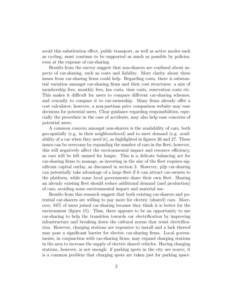
avoid this substitution e↵ect, public transport, as well as active modes suchas cycling, must continue to be supported as much as possible by policies,even at the expense of car-sharing.

Results from the survey suggest that non-sharers are confused about as-pects of car-sharing, such as costs and liability. More clarity about theseissues from car-sharing firms could help. Regarding costs, there is substan-tial variation amongst car-sharing firms and their cost structures: a mix ofmembership fees, monthly fees, km costs, time costs, reservation costs etc.This makes it di�cult for users to compare di↵erent car-sharing schemes,and crucially to compare it to car-ownership. Many firms already o↵er acost calculator; however, a non-partisan price comparison website may easedecisions for potential users. Clear guidance regarding responsibilities, espe-cially the procedure in the case of accidents, may also help ease concerns ofpotential users.

A common concern amongst non-sharers is the availability of cars, bothgeo-spatially (e.g. in their neighbourhood) and to meet demand (e.g. avail-ability of a car when they need it), as highlighted in figures 26 and 27. Theseissues can be overcome by expanding the number of cars in the fleet; however,this will negatively a↵ect the environmental impact and resource e�ciency,as cars will be left unused for longer. This is a delicate balancing act forcar-sharing firms to manage, as investing in the size of the fleet requires sig-nificant capital outlay, as discussed in section 3. However, p2p car-sharingcan potentially take advantage of a large fleet if it can attract car-owners tothe platform, while some local governments share their own fleet. Sharingan already existing fleet should reduce additional demand (and production)of cars, avoiding some environmental impact and material use.

Results from this research suggest that both existing car-sharers and po-tential car-sharers are willing to pay more for electric (shared) cars. More-over, 94% of users joined car-sharing because they think it is better for theenvironment (figure 15). Thus, there appears to be an opportunity to usecar-sharing to help the transition towards car electrification by improvinginfrastructure and breaking down the cultural norms that resist electrifica-tion. However, charging stations are expensive to install and a lack thereofmay pose a significant barrier for electric car-sharing firms. Local govern-ments, in conjunction with car-sharing firms, may expand charging stationsin the area to increase the supply of electric shared vehicles. Having chargingstations, however, is not enough: if parking spots in the city are scarce, itis a common problem that charging spots are taken just for parking space.

2

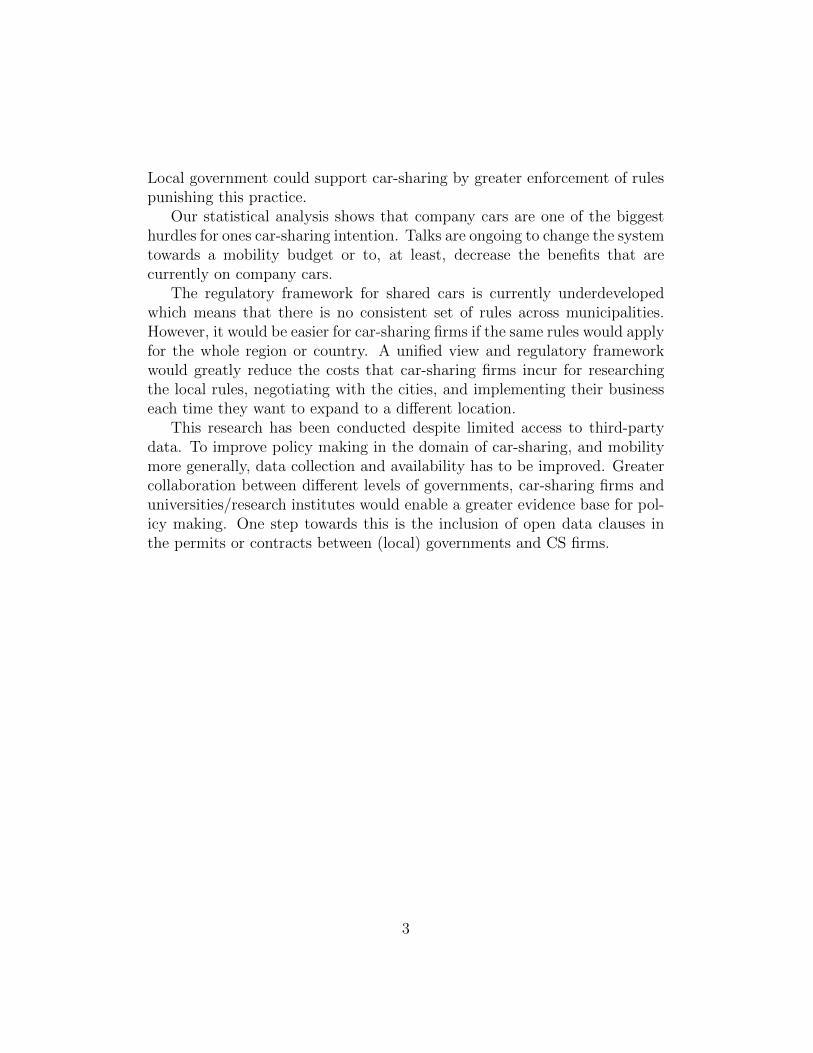
Local government could support car-sharing by greater enforcement of rulespunishing this practice.

Our statistical analysis shows that company cars are one of the biggesthurdles for ones car-sharing intention. Talks are ongoing to change the systemtowards a mobility budget or to, at least, decrease the benefits that arecurrently on company cars.

The regulatory framework for shared cars is currently underdevelopedwhich means that there is no consistent set of rules across municipalities.However, it would be easier for car-sharing firms if the same rules would applyfor the whole region or country. A unified view and regulatory frameworkwould greatly reduce the costs that car-sharing firms incur for researchingthe local rules, negotiating with the cities, and implementing their businesseach time they want to expand to a di↵erent location.

This research has been conducted despite limited access to third-partydata. To improve policy making in the domain of car-sharing, and mobilitymore generally, data collection and availability has to be improved. Greatercollaboration between di↵erent levels of governments, car-sharing firms anduniversities/research institutes would enable a greater evidence base for pol-icy making. One step towards this is the inclusion of open data clauses inthe permits or contracts between (local) governments and CS firms.

3

Nederlandse Samenvatting

Dit rapport zet de details uiteen van het onderzoek van onderzoekers vanhet Steunpunt Circulaire Economie. Het rapport bevat de resultaten vaneen consumentenonderzoek met meer dan 2000 respondenten, evenals vierinterviews met autodeelbedrijven en belangengroepen.

De belangrijkste doelstellingen van dit onderzoek zijn een beter inzicht teverkrijgen in de positie van autodelen in Vlaanderen, wat mensen denken overautodelen, inclusief de barrieres waarmee mensen worden geconfronteerd, enwelke impact autodelen heeft op gedrag en het milieu. Het rapport besluitmet een reeks implicaties en aanbevelingen voor beleid met betrekking totautodelen en de plaats daarvan in de circulaire economie. Deze conclusieszijn hieronder samengevat.

Op basis van dit rapport zou autodelen kunnen helpen om de milieu-e↵ecten gepaard gaand met mobiliteit te verminderen, maar alleen onderbepaalde omstandigheden. Het gevaar bestaat dat autodelen bijdraagt aande milieudruk als het wordt gebruikt als een extra vorm van mobiliteit, inplaats van als vervanging voor particulier autobezit. Om de milieuvoordelenvan autodelen te maximaliseren en het risico op toenemende milieulasten teminimaliseren, moet autodelen daarom alleen worden gestimuleerd ten kostevan het autobezit.

Er zijn weinig aanwijzingen dat het verlagen van de kosten van autode-len voor gebruikers voordelen voor het milieu zal hebben. Uit gegevens vandegenen die al autodelen gebruiken, blijkt dat 91% dit doet omdat het goed-koper is dan het bezit en het gebruik van een prive-auto (figuur 15). Vandegenen die niet delen, was bovendien de kostprijs de minst belangrijke fac-tor (figuur 27). Het verlagen van de kosten van autodelen voor consumentenleidt tot een groter risico op toenemend autogebruik, ten koste van het open-baar vervoer en fietsen. Het beleid moet dus subsidies, zowel voor bedrijvenals voor consumenten, vermijden in de vorm van rechtstreekse overdrachtenin contanten, terugbetalingen of een gunstige fiscale behandeling.

Bijna 40% van de respondenten (figuur 27) gaf aan misschien meer bereidte zijn om auto’s te delen als de stad het gemakkelijker zou maken omgedeelde auto’s te parkeren. Het eerder geformuleerde onderliggende principebetekent echter dat elk gemak van parkeerbeperkingen of toename van hetaantal parkeerplaatsen ten koste moet gaan van prive-auto’s. Dat wil zeggen,als parkeren voor deelauto’s moet worden vereenvoudigd, moet parkeren voorpriveauto’s tegelijkertijd worden verminderd en moeilijker gemaakt.

4

Autodelen heeft ambigue e↵ecten op het openbaar vervoer. In onzeenquete heeft 70% van de autodeelgebruikers zich aangemeld voor autodelenomdat dit sneller is dan het openbaar vervoer (figuur 15). Dit suggereertdat voor sommige leden autodelen in de plaats zou komen van openbaar ver-voer, een negatieve uitkomst voor het milieu. Om dit substitutie-e↵ect tevoorkomen, moeten het openbaar vervoer en actieve vervoerswijzen, zoalsfietsen, zoveel mogelijk door beleid worden ondersteund, zelfs ten koste vanautodelen.

Resultaten van de enquete suggereren dat niet-delers vragen hebben overaspecten van autodelen, zoals kosten en aansprakelijkheid. Meer duideli-jkheid vanuit autoverzekeringsbedrijven over deze kwesties zou kunnen helpen.Wat de kosten betreft, is er een grote variatie tussen autodeelbedrijven enhun kostenstructuren: een combinatie van lidmaatschapskosten, maandeli-jkse kosten, km-kosten, tijdskosten, reserveringskosten, enz. Dit maakt hetmoeilijk voor gebruikers om verschillende autodeelsystemen te vergelijken,en nog meer om te vergelijken met autobezit. Veel bedrijven bieden aleen kostencalculator aan; een onafhankelijke prijsvergelijkingswebsite kanbeslissingen voor potentile gebruikers echter vergemakkelijken. Duidelijkerichtlijnen met betrekking tot verantwoordelijkheden, vooral de procedurebij ongevallen, kunnen ook de bezorgdheden van potentile gebruikers helpenverlichten.

Een veel voorkomende zorg onder niet-delers is de beschikbaarheid vanauto’s, zowel geo-ruimtelijk (bv. in hun buurt) als om aan de vraag te vol-doen (bv. beschikbaarheid van een auto wanneer ze deze nodig hebben), zoalsaangegeven in figuren 26 en 27. Deze problemen kunnen worden opgelostdoor het aantal auto’s in het wagenpark uit te breiden; dit heeft echter eennegatieve invloed op de milieu-impact en de hulpbronnene�cintie, omdatauto’s langer ongebruikt blijven. Dit is een delicate evenwichtsoefening voorautodeelbedrijven om te managen, omdat investeren in de omvang van devloot aanzienlijke kapitaaluitgaven vereist, zoals besproken in hoofdstuk 3.P2p autodelen kan echter potentieel profiteren van een grote vloot als hetauto-eigenaren naar het platform kan trekken, terwijl sommige lokale over-heden hun eigen vloot delen. Het delen van een reeds bestaande vloot zou deextra vraag (en productie) van auto’s moeten verminderen, waardoor enigemilieu-impact en materiaalverbruik wordt vermeden.

Resultaten van dit onderzoek suggereren dat zowel bestaande als potentileautodelers bereid zijn meer te betalen voor elektrische (deel)auto’s. Boven-dien is 94 % van de gebruikers lid geworden van autodelen omdat ze denken

5

dat dit beter is voor het milieu (figuur 15). Er lijkt dus een mogelijkheid tebestaan om autodelen te gebruiken om de overgang naar auto-elektrificatie tehelpen door de infrastructuur te verbeteren en de culturele normen te door-breken die weerstand bieden aan elektrificatie. Laadstations zijn echter duurom te installeren en een gebrek daaraan kan een belangrijke barriere vormenvoor bedrijven die elektrische auto’s delen. Lokale overheden, in samen-werking met autodeelbedrijven, kunnen laadstations in het gebied uitbreidenom het aanbod van elektrische gedeelde voertuigen te vergroten. Laadpalenhebben is echter niet voldoende: als parkeerplaatsen in de stad schaars zijn, ishet een veel voorkomend probleem dat laadpunten louter als parkeerplaatsenworden ingenomen. De lokale overheid zou autodelen kunnen ondersteunendoor een betere handhaving van regels die deze praktijk bestra↵en.

Onze statistische analyse laat zien dat bedrijfswagens een van de grootstehindernissen zijn voor iemands intentie tot autodelen. Er zijn gesprekkengaande om het systeem te veranderen in de richting van een mobiliteitsbudgetof om de voordelen van bedrijfsauto’s te verminderen.

Het regelgevend kader voor deelauto’s is momenteel onderontwikkeld, watbetekent dat er geen consistente set regels bestaat tussen gemeenten. Voorautodeelbedrijven zou het echter eenvoudiger zijn als dezelfde regels voor dehele regio of het hele land zouden gelden. Een uniforme visie en een regel-gevend kader zouden de kosten die autodeelbedrijven met zich meebrengenvoor het uitzoeken van de lokale regels, het onderhandelen met de steden enhet uitvoeren van hun bedrijf elke keer dat ze naar een andere locatie willenuitbreiden aanzienlijk verminderen.

Dit onderzoek is uitgevoerd ondanks beperkte toegang tot gegevens vanderden. Om de beleidsvorming op het gebied van autodelen en mobiliteit inhet algemeen te verbeteren, moeten gegevensverzameling en -beschikbaarheidworden verbeterd. Meer samenwerking tussen verschillende niveaus vanoverheden, autodeelbedrijven en universiteiten/onderzoeksinstituten zou eengrotere bewijsbasis voor beleidsvorming mogelijk maken. Een stap hiertoeis het opnemen van open data-clausules in de vergunningen of contractentussen (lokale) overheden en CS-bedrijven.

6

Contents

1 Introduction 9

1.1 Setting . . . . . . . . . . . . . . . . . . . . . . . . . . . . . . . 91.2 Literature review . . . . . . . . . . . . . . . . . . . . . . . . . 10

1.2.1 Car-sharing profiles, motivations and barriers . . . . . 111.2.2 Car-sharing impacts . . . . . . . . . . . . . . . . . . . 12

2 Methodology 14

2.1 Demographics . . . . . . . . . . . . . . . . . . . . . . . . . . . 142.2 Mobility data . . . . . . . . . . . . . . . . . . . . . . . . . . . 152.3 Car-sharing . . . . . . . . . . . . . . . . . . . . . . . . . . . . 15

2.3.1 Motivations and inhibiting factors for car-sharing . . . 162.4 Attitude/scale questions . . . . . . . . . . . . . . . . . . . . . 162.5 Discrete choice experiment . . . . . . . . . . . . . . . . . . . . 17

2.5.1 DCE-NCS . . . . . . . . . . . . . . . . . . . . . . . . . 172.5.2 DCE-CS . . . . . . . . . . . . . . . . . . . . . . . . . . 19

2.6 Closing questions . . . . . . . . . . . . . . . . . . . . . . . . . 21

3 Company interviews 21

3.1 Local level . . . . . . . . . . . . . . . . . . . . . . . . . . . . . 233.2 Regional (Flemish) level . . . . . . . . . . . . . . . . . . . . . 253.3 Federal level . . . . . . . . . . . . . . . . . . . . . . . . . . . . 253.4 Culture of (car) ownership and a systems thinking view . . . . 263.5 Determinants of shared car use . . . . . . . . . . . . . . . . . 26

4 Exploratory data analysis 27

4.1 Demographics . . . . . . . . . . . . . . . . . . . . . . . . . . . 294.2 Mobility data . . . . . . . . . . . . . . . . . . . . . . . . . . . 364.3 Car-sharing . . . . . . . . . . . . . . . . . . . . . . . . . . . . 414.4 Closing questions . . . . . . . . . . . . . . . . . . . . . . . . . 514.5 Quitting car-sharing . . . . . . . . . . . . . . . . . . . . . . . 55

5 Statistical analyses 56

5.1 Factor analysis . . . . . . . . . . . . . . . . . . . . . . . . . . 575.1.1 Full dataset factor analysis . . . . . . . . . . . . . . . . 585.1.2 Non-car-sharers’ factor analysis . . . . . . . . . . . . . 615.1.3 Car-sharers’ factor analysis . . . . . . . . . . . . . . . . 64

7

5.2 Predicting the car-sharing intention . . . . . . . . . . . . . . . 675.2.1 Multicollinearity check . . . . . . . . . . . . . . . . . . 70

5.3 Non-sharer’s discrete choice experiment . . . . . . . . . . . . . 725.3.1 Non-sharer’s DCE with latent classes . . . . . . . . . . 75

5.4 Sharer’s discrete choice experiment . . . . . . . . . . . . . . . 785.4.1 Sharer’s DCE with latent classes . . . . . . . . . . . . 79

5.5 Conclusion . . . . . . . . . . . . . . . . . . . . . . . . . . . . . 82

6 Environmental Impact 83

6.1 Method . . . . . . . . . . . . . . . . . . . . . . . . . . . . . . 846.1.1 Formation of treatment and control groups . . . . . . . 846.1.2 Decomposition of treatment and control groups . . . . 856.1.3 Beta regressions to estimate e↵ect . . . . . . . . . . . . 87

6.2 Treatment e↵ects . . . . . . . . . . . . . . . . . . . . . . . . . 886.2.1 Model 1: Simulated average treatment e↵ects . . . . . 906.2.2 Model 2: Simulated treatment e↵ects for p2p vs b2c

systems . . . . . . . . . . . . . . . . . . . . . . . . . . 906.2.3 Simulated treatment e↵ects for urban, suburban, and

rural users . . . . . . . . . . . . . . . . . . . . . . . . . 926.3 The environmental impacts of car-sharing in Belgium . . . . . 956.4 Aggregate results under di↵erent scenarios . . . . . . . . . . . 96

6.4.1 Model 1: Average treatment e↵ect . . . . . . . . . . . 976.4.2 Model 2: separate e↵ects for p2p and b2c users . . . . 976.4.3 Model 3: separate e↵ects for user location . . . . . . . 98

6.5 Sensitivity analysis of technical parameters . . . . . . . . . . . 1006.6 Conclusions . . . . . . . . . . . . . . . . . . . . . . . . . . . . 102

7 Policy conclusions 104

8 Acknowledgements 111

Bibliography 113

Appendix 117

8

1. Introduction

Flanders is the Dutch-speaking region in the North of Belgium. Flanders’tra�c is problematic, especially around Belgium’s capital, Brussels. VanBroeck (2018) summarizes a couple of striking numbers. Although Flandersis only 13.522 km2 with about 6.5 million inhabitants, there are 4 million carsthat need approximately 24000 hectares of parking space because, on average,the cars stand still for about 23 out of the 24 hours in a day. Van Broeck(2018) links the parking and mobility problems to bad spatial planning; manylike to live in more rural areas but that means they rely on a car to get towork, shops, and other facilities. Making public transportation availableclose to everyone’s home is also di�cult if houses are spread everywhere.Changing the spatial planning takes a lot of time, and mobility as a service(MAAS) is viewed as a good temporary means to reduce car ownership, carusage, and ultimately resource use and CO2 emissions; car-sharing is part ofMAAS.

1.1. Setting

This article describes the results of a online survey on car-sharing that waslaunched in Dutch in September, 2018. The survey was spread as a clickablelink through several institutions’ mailing lists, social media, and news lettersto reach a broad and varied audience. The study’s target audience wereadults living in the Flanders region, in Belgium. Most of them already hada drivers’ license but we were also interested in respondent who didn’t havea license yet but were planning to get one soon (within 5 years). It has beensaid that younger people consider a car less of a status symbol and are thusless eager to get a drivers’ license (the number of new drivers’ licenses peryear has dropped 18% since 2010, (Cardone 2019)). We wondered whetherthose who still need to get their drivers’ license would be more willing toshare cars once they start driving. Especially since experts believe the mainreasons for postponing or forgoing obtaining a drivers’ license is convenientpublic transportation and the high cost of getting a license (Hjorthol 2016,Le Vine and Polak 2014).

In line with neighboring countries, Belgium has seen a rise in the numberof car-sharing businesses the last years. Table 1 gives and overview of allcar-sharing providers that operate in the Flanders and Brussels region. Allinformation was retrieved from the company websites. For the costs reportedin Table 1, we distinguish three possible fixed costs that do not depend on

9

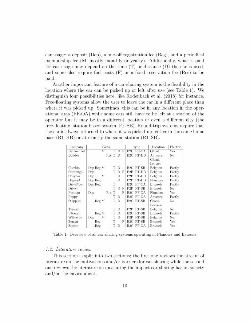
car usage: a deposit (Dep), a one-o↵ registration fee (Reg), and a periodicalmembership fee (M, mostly monthly or yearly). Additionally, what is paidfor car usage may depend on the time (T) or distance (D) the car is used,and some also require fuel costs (F) or a fixed reservation fee (Res) to bepaid.

Another important feature of a car-sharing system is the flexibility in thelocation where the car can be picked up or left after use (see Table 1). Wedistinguish four possibilities here, like Rodenbach et al. (2018) for instance.Free-floating systems allow the user to leave the car in a di↵erent place thanwhere it was picked up. Sometimes, this can be in any location in the oper-ational area (FF-OA) while some cars still have to be left at a station of theoperator but it may be in a di↵erent location or even a di↵erent city (thefree-floating, station based system, FF-SB). Round-trip systems require thatthe car is always returned to where it was picked-up; either in the same homebase (RT-HB) or at exactly the same station (RT-SB).

Company Costs type Location ElectricBattmobiel M T D F B2C FF-OA Ghent YesBolides Res T D B2C RT-HB Antwerp,

Ghent,Leuven

No

Cambio Dep Reg M T D B2C RT-SB Belgium PartlyCaramigo Dep T D F P2P RT-HB Belgium PartlyCozycar Dep M D P2P RT-HB Belgium PartlyDegage! Dep Reg D P2P RT-HB Flanders PartlyDriveNow Dep Reg T B2C FF-OA Brussels PartlyDrivy T D F P2P RT-SB Brussels NoPartago Dep Res T F B2C FF-OA Flanders YesPoppy T D B2C FF-OA Antwerp PartlyStapp.in Reg M T D B2C RT-SB Groot-

BeverenNo

Tapazz T D P2P RT-SB Belgium NoUbeeqo Reg M T D B2C RT-SB Brussels PartlyWibee.be Dep M T D P2P RT-SB Belgium NoZencar Reg T F B2C RT-SB Brussels YesZipcar Reg T D B2C FF-OA Brussels Yes

Table 1: Overview of all car sharing systems operating in Flanders and Brussels

1.2. Literature reviewThis section is split into two sections; the first one reviews the stream of

literature on the motivations and/or barriers for car-sharing while the secondone reviews the literature on measuring the impact car-sharing has on societyand/or the environment.

10

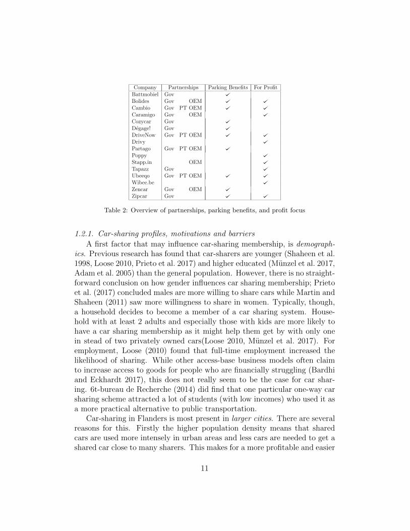
Company Partnerships Parking Benefits For ProfitBattmobiel GovBolides Gov OEMCambio Gov PT OEMCaramigo Gov OEMCozycar GovDegage! GovDriveNow Gov PT OEMDrivyPartago Gov PT OEMPoppyStapp.in OEMTapazz GovUbeeqo Gov PT OEMWibee.beZencar Gov OEMZipcar Gov

Table 2: Overview of partnerships, parking benefits, and profit focus

1.2.1. Car-sharing profiles, motivations and barriersA first factor that may influence car-sharing membership, is demograph-

ics. Previous research has found that car-sharers are younger (Shaheen et al.1998, Loose 2010, Prieto et al. 2017) and higher educated (Munzel et al. 2017,Adam et al. 2005) than the general population. However, there is no straight-forward conclusion on how gender influences car sharing membership; Prietoet al. (2017) concluded males are more willing to share cars while Martin andShaheen (2011) saw more willingness to share in women. Typically, though,a household decides to become a member of a car sharing system. House-hold with at least 2 adults and especially those with kids are more likely tohave a car sharing membership as it might help them get by with only onein stead of two privately owned cars(Loose 2010, Munzel et al. 2017). Foremployment, Loose (2010) found that full-time employment increased thelikelihood of sharing. While other access-base business models often claimto increase access to goods for people who are financially struggling (Bardhiand Eckhardt 2017), this does not really seem to be the case for car shar-ing. 6t-bureau de Recherche (2014) did find that one particular one-way carsharing scheme attracted a lot of students (with low incomes) who used it asa more practical alternative to public transportation.

Car-sharing in Flanders is most present in larger cities. There are severalreasons for this. Firstly the higher population density means that sharedcars are used more intensely in urban areas and less cars are needed to get ashared car close to many sharers. This makes for a more profitable and easier

11

business for car-sharing firms (Munzel et al. 2017). Secondly, research hasshown that people in urban areas are more open to car sharing and sharing ingeneral (Loose 2010). Lastly, an urban environment often has better publictransportation and expensive parking space which makes car-sharing moreinteresting than owning a car (Munzel et al. 2017, Huwer 2004, Adam et al.2005).

When asked about the reason for sharing cars, many car sharers statethat it is cheaper than owning a car (provided the car is used very little).One can save on maintenance costs, purchasing costs, but also parking costs(in Flanders, several communities provide parking benefits for shared cars).It is calculated that a shared car would be cheaper for people who driveless than 10,000 to 12,000 kilometers per year (Loose 2010). However, thebenefit will depend on the car that would have been chosen as a private car;if one would choose a small, fuel e�cient car, the turning point beyond whichsharing is no longer financially beneficial is 6500 kilometers (van Driel andHafkamp 2015).

Most of the articles that are reviewed in this section use consumer studiesto come to their conclusions. However, very few include a choice experimentin their study. Liao et al. (2018) is very similar to our survey consideringthat they designed a choice experiment where the attributes include manysimilar car-sharing system characteristics such as the fuel type of the vehicles,one-o↵ and recurring operating costs, return location and availability andaccess time. Liao et al. (2018) one-o↵, monthly, and operating costs for bothprivate cars and car-sharing systems. We limit the cost parameters to justtwo. Intermediate trials with a test audience reveled that this type of coststructure was too di�cult to comprehend and compare. While they alsoinclude both car sharers and non-carsharers, all respondents are required tomake a choice between buying (or not scrapping) a car and car-sharing. Incontrast, in our DCE, car sharers choose between two car-sharing systemsto get a better estimate of the WTP for car-sharing system attributes fromthose who have used it before.

1.2.2. Car-sharing impactsMeasuring the impact of the sharing economy on the environment is cru-

cial to establish the extent to which it can help the transition to a moresustainable economy. To meet global environmental goals to reduce green-house gas emissions and to reduce material throughput, technological changeis unlikely to be su�cient: there will also need to be a change in behaviour.

12

The purported benefits of car-sharing include a reduction in car productionand car use amongst existing car drivers as a result of behavioural changesCohen and Kietzmann (2014). On the technological side, benefits may bestimulated at other stages of the value chain, such as the development of carswith higher fuel e�ciencies and much longer lifetimes (in terms of distancetravelled) Material Economics (2018). These e↵ects are all interrelated, andthe ultimate e↵ect on the environment is a result of a complex interactionbetween these e↵ects.

Existing car-sharing studies tend to focus on the e↵ects of car-sharing oncar-ownership, often neglecting e↵ects on car-use altogether. In general, car-sharing is associated with a reduction in the number of cars owned, eitherthrough the sale or scrappage of a car, or through cancelling the plannedpurchase of a car. However, in a number of these studies, there are notadequate methods to eliminate reverse causality, i.e. cases where a lack ofcar-ownership causes someone to join car-sharing, rather than vice versa.By ignoring this, results will be positively biased, showing a greater e↵ect ofcar-sharing than is the case in reality.

Moreover, focusing exclusively on car-ownership alone will not revealwhether car-sharing results in a net environmental benefit. Private cars arelikely to be replaced less often than shared cars because of their lower use-intensity. An elementary calculation can thus show that, unless car-sharingreduces car-use or increases car longevity (i.e. the total distance travelled inthe car during its lifetime), then the number of cars produced will not bea↵ected at the aggregate.

It is thus vital to look at the impacts of car-sharing on car-use, whichsome studies have done. In general, car-use appears to fall amongst someusers (e.g. those who get rid of a car), but increases for others (e.g. thosewho did not own a car). Martin and Shaheen (2011) found that the numberof car-sharing users that increased their km travelled by car was greaterthan those that reduced their in car km. However, at the aggregate, car-sharing resulted in fewer km driven by car (and less emissions) due to thesize of the e↵ect: the decrease in km travelled by car per person because ofcar-sharing was much larger than the increase in km travelled for the othergroup without a car. Reductions in car-usage have also have been found by,inter alia, Martin and Shaheen (2016), Cervero et al. (2006), Nijland and vanMeerkerk (2017). However, the methods use to estimate changes in car userely on car-sharing users’ estimate of their own change in behaviour. Thiscan introduce a number of issues, such as self-assessment bias and recall bias,

13

both of which can lead to inaccurate estimates of the e↵ect of car-use.In sum, while there seems evidence of a benefit of car-sharing for the

environment and resource use, there are a number of methodological short-comings that could lead to question this broad conclusions. Moreover, fewstudies examine how or what is responsible for this benefit in car-sharing, orwhich characteristics of users or car-sharing schemes may lead to a benefitof car-sharing. This research aims to fill these gaps by conducting a robustimpact evaluation car-sharing.

2. Methodology

We started with interviewing car-sharing users, car-sharing experts, andthree Belgian car-sharing companies (see Section 3). Based on informationfrom the interviews and a review of the academic literature, a first versionof the survey was designed. This initial survey was then reviewed by atest group with a balanced mix of experienced car-sharers on the one handand people who were completely unfamiliar with car-sharing on the otherhand. After several iterations of review and adjustments, the final surveywas put online September 2018. The survey was made with Qualtrics andstayed online until the end of October, 2018. The survey consists of severalparts. Respondents were asked about their socio-demographic information(Section 2.1) and their current and historic mobility choices and options(Section 2.1). Respondents who are shared cars got some extra questions(Section 2.3). Next, all respondents are asked to make 8 choices betweenfictitious cars to buy or share in a discrete choice experiment (Section 2.5).Lastly, the survey concludes with some closing questions and room for therespondent to leave feedback to the survey (Section 2.6).

2.1. Demographics

Since previous research indicates that many socio-demographics matterin making mobility choices, people are first questioned about the following:

• Age: Shaheen et al. (1998), Loose (2010), Prieto et al. (2017) show thatyounger people are more likely to share cars.

• Gender: Prieto et al. (2017) found men to be more likely to share cars.

• Occupation (and income): Prieto et al. (2017) found that car-sharersare often in the lower income category and a French car-sharing study

14

found most car-sharers had executive jobs although one of the car-sharing system (Autolib’) attracted quite some students (6t-bureau deRecherche 2014).

• education: car-sharing attracts more highly-educated people accordingto (Becker et al. 2017, Prieto et al. 2017, 6t-bureau de Recherche 2014)

• Location (postal code and rural vs urban environment): Loose (2010)found that car-sharers mostly lived in urban environment. This is tobe expected since this is where o↵er of shared car well developed anddiverse.

2.2. Mobility data

Whether or not someone has a car, bike, or public transport subscrip-tion will certainly influence the interest in sharing cars. For many, nothingbeats the convenience of having a private car in the driveway and it is hardto imagine having to reserve a shared car in advance or walking a coupleof minutes to get to the car. Therefor, we asked respondents whether theyhave a drivers’ license, private or company cars, public transport subscrip-tions, bikes, motorcycles, and scooters. For private cars, we obtained thetype/model of the car, age, fuel type, estimated weekly kilometers, and thenumber of passengers that are usually in the car.

6t-bureau de Recherche (2014) noted a decrease in the number of privatecars and the vehicle kilometers travelled for their sample of car-sharers. Totest this, we asked respondent how many kilometers they travel with all trans-portation modes (private car, company car, as a passenger in someone else’scar, shared car, public transportation, by foot, (electric) bike, motorcycle,taxi). We also asked about how they commute to work or school and how farthis commute is. To be able to compare car ownership between car-sharersand non-car-sharers, we ask all respondents how many cars they bought (newor 2nd hand), least, sold, and scrapped in the last 5 years. For the next fiveyears, we ask respondents how likely it is that the obtain another private car.

2.3. Car-sharing

To realistically estimate the environmental impact of car-sharing, a lot ofdata is needed. Some data can be retrieved from industry-level data such asthe number of cars that a car-sharing firm has, the longevity, and the fuele�ciency of these shared cars compared to the average private car. But it

15

is expected that people who start sharing cars will likely alter their mobilityhabits when they start sharing.

We firstly ask car-sharer whether they sold or scrapped a car because theystarted sharing, or whether they did not buy a car because of car-sharing.This allows each car-sharing user to be sub-categorised into di↵erent usertypes, each of which is expected to change their behaviour di↵erently. Wealso ask sharer how they think they changed their mobility habits since theystarted sharing; whether they drive a car, bike, or walk more or less. Wealso ask how often they drive the shared car, for which trips they use it,and which other modes of transport they use in combination with a sharedcar. Looking forward, we ask them how likely it is that, in the next fiveyears, they will buy, sell, scrap or do not replace their current car because ofcar-sharing.

Many of these questions are hypothetical or require people to make anestimate (partly based on possibly subjective feelings). To control for thisuncertainty, responses to these questions were on a scale to represent howconfident respondents’ were in their answers.

2.3.1. Motivations and inhibiting factors for car-sharingNon-sharers were asked why they are not sharing cars and what would

have to change for them to start sharing cars.Sharers, on the other hand, were asked about their motivations to start

sharing and whether they would consider to stop sharing (and, if so, why).There were also some respondents that used to share cars but were not

sharing cars anymore. This is an interesting group of people because theyhave real experience with car-sharing and appeared to be not satisfied.

A recent survey with one-way car-sharing users in France revealed thatonly 6% of the respondents mentions ecological concerns and most use sharedcars because it is more practical than PT (6t-bureau de Recherche 2014).Those who found shared cars more practical than the private car, usuallyattributed this to the parking benefits they had. Some car-sharing businessesalso expect environmental concern to be a motivational factor to few and thuslook for other ways to make car-sharing more appealing (see Section 3).

2.4. Attitude/scale questions

Attitude or scale questions are typically added to surveys to better un-derstand the underlying motivations, attitudes and values that drive people’schoices. Respondents are commonly asked to rate several statements on a

16

five- or seven-point scale from ‘strongly disagree’ to ‘strongly agree’. How-ever, previous experience with online surveys showed that respondent are notalways too eager to fill in these question as they require a lot of careful read-ing and may appear quite boring. Therefor, we limited the set of attitudequestions and spread them over the survey in smaller batches so as not toexhaust the respondent too much with long lists of scale questions.

The statements were mainly based on previous literature on the motiva-tion for car use and sharing. In particular, Steg (2005) investigated instru-mental, symbolic, and a↵ective motives for car use through scale questions.Hawlitschek et al. (2016), on the other hand, examined drivers for sharingand many of their questions were adapted to fit the car-sharing setting. Intotal, there were 46 statements which were used in a factor analysis, as de-scribed in section 5.1.

2.5. Discrete choice experiment

A discrete choice experiment (DCE) is a stated preference technique thatasks respondents to state their preference over di↵erent alternatives. It isespecially suitable for multidimensional problems such as the choice betweenbuying or sharing a car. A baseline alternative, corresponding to the statusquo or opt-out situation is included in each choice set in order to be able tointerpret the results in standard welfare economic terms.

The survey has two DCEs - one for non-carsharers (DCE-NCS) and onefor ca-sharers (DCE-CS). The first lets us explore why non car-sharers preferto buy a car over sharing one and which attributes or specific features of car-sharing systems might entice them to start sharing. The second gives moreinsight into which attributes are most important for people who have actualpractical experience with car-sharing. The attributes were chosen after anexploratory literature review, extensive talks with (non) car-sharers, field ex-perts, and car-sharing companies. We describe each in detail in Section 2.5.1and Section 2.5.1 respectively.

2.5.1. DCE-NCSIn this experiment, respondents are faced with 8 choices between (A)

buying a car, (B) sharing a car or (C) an opt-out option (’neither’) in thefollowing scenario (translated from Dutch).

17

8>><

>>:

Imagine that you (and your family) are in need of a new car.

Imagine you just got your driver’s license and you decide youwant to start driving more often

We will ask you to choose between two options to expandyour mobility options eight times. If neither of the optionsseem attractive to you, you can also indicate this. There areno right or wrong answers, we are only interested in youropinion

If you choose to purchase a car, omnium insurance is in-cluded. The cost per kilometer must be interpreted as theexpected cost for fuel, insurance, taxes, and all maintenancecosts.

A shared car also always includes an omnium insurance.The cars you use can be owned by other individuals who sharetheir personal car on a sharing platform or owned by acar-sharing company. To be a member, you need to pay amonthly subscription fee. Next to that fee, you pay for eachkilometer that you drive with the car. There are no costsother than those that are specified. Some cars need to beleft behind in a dedicated parking spot after you used themwhile other systems are more flexible and the cars can beleft behind anywhere. Reserving can be done online, throughphone or a smartphone app.

The attributes that are involved in buying or sharing a car di↵er, as shownin Table 3. When people buy a car, there are many technical attributes to acar that play a key role (brand, model, price class, maximum speed, numberof seats,...). As we are not interested in the willingness to pay for many ofthese car attributes, we first question the respondent about their preferredcar model (mini; family car (max 5 passengers); family car (more than 5passengers); sports car; SUV; or a self-specified other model), preferred fueltype (diesel; petrol; electric; hybrid; LPG; or other), price class, and whetherthey would buy a new, nearly new, or second hand car. The price class

18

categories go from less than 5000 until more than 50000 euros, in steps of5000 euros. In the experiment, the mid-point of the indicated price classis used as the budget in the attribute levels of the purchasing cost (seeTable 3).

Most attributes in Table 3 are self-explanatory but the flexibility andavailability might require some additional explanations.

The flexibility refers to the options the car-sharer has in the locationwhere he can pick up and drop of a car. The least flexible option is a station-based system with fixed parking spots where the shared car can be picked upand needs to be returned after use. Free floating systems are the most flexibleas the car can be left wherever after use. Free-floating systems usually alsoallows users to locate the shared cars through gps-tracking. An intermediatesystem was also included where the car can be left anywhere within a 2kilometer radius around the pick-up location.

The availability captures the time it typically takes to get from the user’shome to the shared car. If the closest car is not available at the time oneneeds a car, we reasoned that there must be another car further away.

2.5.2. DCE-CScar-sharers choose between two car-sharing systems (A and B) or staying

with their own car-sharing system. For later analysis, it is thus necessary toknow what their current car-sharing system is. We ask respondents for thefollowing information:

• Their primary (i.e. most often used) car-sharing system of which theyare a member. This also gives us information about whether the fleetincludes electric cars or not and whether it’s a B2C or P2P system(Table 1). Some respondents were left out because they indicated aride-sharing system in stead of a car-sharing system or an informalsharing system with friends or family.

• The costs for using the shared cars. Table 1 showed that the cost struc-ture may be quite complicated. Respondents were asked for registrationfees, yearly or monthly fixed costs, costs per kilometer, and costs perhour of driving/usage/parking. If people indicated they did not knowsome of these costs, we used the average costs that peers who did fill inall costs or tried to find the standard pricing scheme of their primarycar-sharing system (for instance, if there were too few peers to get a re-liable average cost). If that did not work, the respondent was excluded

19

Buying a car Sharing a carAttribute Attribute levels Attribute Attribute levels

Purchasingcost

budget -2000budget -1000

budgetbudget+1000budget+2000budget+3000budget+4000budget+5000

Monthlycost

0510152025

Kilometercost

0.150.30.50.7

Kilometercost

0.20.40.60.81

Fueltype

petroldieselelectric

Fueltypes inthe fleet

Diesel and petrolall kinds, including electric

Type ofsystem

B2BP2P

FlexibilityFree floating2km radius

exact same spot

Availability2 minutes5 minutes15 minutes

Reservationtime

10 minutes in advance1-3 hours in advance2 days in advance

Table 3: Attributes and attribute levels (costs in euros)

for further analysis. All of these costs were recalculated to one monthlycost and one kilometer cost to be able to compare it to the chosen at-tributes in the other options. Mmonth = Reg/24 +Mmonth +Myear andDkm = Dkm + 0.6 ⇤ (Thour). If only one of the three hourly costs arefilled in, Thour is equal to this costs. If multiple are filled in, costs forusing or parking get a weight of 20% (if they are filled in) while drivingcosts get a weight of 80 or 60% if one or both of the other hourly costsare filled in respectively. The hourly costs (Thour) are multiplied by0.6 to obtain a kilometer cost as data studies showed that an averagecar-sharing trip took about half an hour while the travel distance wasabout 3km (Habibi et al. 2017).

• The number of minutes, hours, or days it takes to reserve a car.

20

• The time it take to get from their home to the shared car in minutes

2.6. Closing questions

To end the survey, respondents get some text boxes where they can leaveany message they still want to send to the researchers. They are asked tomention any aspect of car-sharing that was overlooked in the survey buthighly influences their decision (not to) share cars. Links were provided tothe website of autodelen.net and the portal of the research unit. Lastly, theywere referred to a separate form where they could leave some contact detailsif they were interested in winning cinema, Fnac, or Win-for-life tickets (witha value of 20).

3. Company interviews

To investigate which levers and/or obstacles Flemish CS firms experienceto expand their business, four interviews of 1.5 to 2 hours were taken withrepresentatives of three CS companies (Van Ootegem 2017d,a,c) and withJe↵rey Matthijs of autodelen.net (Van Ootegem 2017b). Autodelen.net is anumbrella organization for CS firms in Flanders which also informs consumerswith regards to all practicalities that come with becoming a car-sharer. Thethree CS firms were selected based on their size, the type of organization andthe type of CS system they o↵er. Degage is a P2P CS firm that operatesmainly in the city of Ghent. They recently also launched bike sharing andare spreading their CS services to other cities in Flanders. Degage is mostlyled by volunteers. Partago is a B2C initiative with a fully electric fleet. Thecars can be located and unlocked with an app. The system is essentially free-floating but the cars do need to be left at a charging station at the end of theuse. At the time of the survey, they were mainly based in Ghent but, likeDegage, they are quickly spreading to other cities. Cambio is the player withthe most experience and the most members on the Belgian market. Theyhave a station-based, round-trip CS model. This section will summarize themost important conclusions from all four interviews.

The main goal that is achieved by promoting CS is that sustainable mo-bility is facilitated, i.e.:

• reducing the number of cars

• reducing the number of kilometers that are driven with cars

21

• increasing the number of kilometers that are driven with cars

• increasing public transportation use

• increasing biking, walking, and other alternatives

• stimulating alternative fuel cars (eg. electic)

If all of the above benefits are realized, this will firstly lead to moresustainable mobility, but also to many other positive side e↵ects, each alaudable objective with clear social added value:

• Positive environmental e↵ects by reducing the number of cars and thenumber of kilometers that are driven with a car. It is expected thatpeople are less likely to take the car if it is not available in their garageat all times.

• Social cohesion is promoted, especially in P2P CS systems with moresocial interaction. CS may also support and aid in the development ofalternative cohabitation forms and (behavioral) practices

• Cooperative, sustainable, social entrepreneurship with a social purpose.

The interviewees thus agree that there are significant benefits in sharingcars for the environment, sustainable mobility, and from a social viewpoint.What is more, the benefits in each of those areas will likely even reinforceeach other. The only issue on which there was some disagreement betweeninterviewees was whether or not electric vehicles are shared more or less.Cambio stated that “sharing is more important than a forced electrificationbecause sharing, in itself has many environmental advantages”. They fearthat having an only electric fleet might hinder some to start sharing if theydo not feel comfortable with, for instance, the limited driving distance of theelectric car or the limited number of charging stations.

To structure the information, the first three sections describe conclusionsthat are relevant for the local (Section 3.1), regional (Flemish) (Section 3.2),or federal level (Section 3.3). The following section discusses how CS (doesnot) fit into the current Flemish culture from a broader, systems-thinkingview (Section 3.4). Lastly, Section 3.5 describes some determinants of CSsystems that determine customer choices.

We would like to emphasize that Section 3 contains the views of the in-terviewees and not necessarily those of the authors. During the interviews,

22

we took the same standpoint as the interviewee; that CS should be promotedas an alternative to car ownership because it could limit the number of carsand kilometers driven with cars (this proposition is investigated further inSection 6). The main focus for the interviews was defining the most impor-tant levers and obstacles for Flemish CS firms to establish or expand theirbusiness.

3.1. Local level

CS is and remains a mostly local (or urban / city-specific) phenomenon.Therefor, local (city) governments are the first and foremost potential part-ners for CS companies. There are many alternatives for car ownership incities so CS is typically more successful. In a city with trains, trams andbuses, there are plenty alternative for a car and, thus, a car is needed onlysporadically. Owning a car becomes less attractive and sharing is more ap-pealing; it is “no longer sensible to be a car owner” (Van Ootegem 2017a).

Local governments can play an important role by creating levers to makeCS more successful. CS organizations are often looking for partner cities tohelp them establish themselves in the city. Cities are the engine for futuredevelopments in many areas, including mobility, and thus, CS. Several waysin which local governments may stimulate CS were mentioned: they canhelp out with communication, logistics, creating mobihubs (Mobihubs 2019),purchase or cooperation guarantees, and bringing in capital.

Communication is best set up in both a permanent way (e.g. an infor-mation sheet) and a specific/ short term way (e.g. promoting an activity).Local governments and cities have the best communication channels to reachlocal inhabitants, for example, the city’s or village’s newspaper, info sheet,website, or local activities. They can also organize specific event after whichword-of-mouth will follow. Such a bottom-up approach has often proven tobe most successful so starting up a new CS initiative is best done locally.

Local governments are the ideal logistic partners. They can o↵er parkingbenefits to shared cars. Similarly, they can provide reserved parking spacesfor shared cars or add proper signals with the reserved parking spots. Propersignalization and/ or patrolling around the reserved parking spots is requiredto prevent them from being (mis)used by other drivers. All of this is seenas a huge motivation to start sharing, especially if parking space is currentlyscarce or expensive in the city.

Local governments can also install CS hubs or, better yet, mobihubs (Mo-bihubs 2019). Mobihubs are physical centers where (shared) bikes, public

23

transport, shared cars, electric charging stations, taxis, or even shops withpick-up point for package deliveries all come together. There hubs are ex-pected to be very important in rural areas as well where they would representan o✏ine version of Mobility as a Service (MaaS). Accomplishing such a mo-bihub will require a very well-coordinated policy vision and spacial planning.

Local organizations and governments can also establish purchase guaran-tees i.e., a minimum amount that the communal service will use the sharedcars. This may significantly reduce the risk a starting CS business expe-riences. CS organizations may also choose to co-own cars with the localgovernments. Sharing the existing city’s car fleet in a P2P CS system, al-though conceptually attractive, is not straightforward. It is unclear who willclean the cars (Cambio has a norm for cleanliness), maintain the car, andcoordinate the availability of the cars. “CS is more than just making carsavailable. It is a service that does not ‘happen’ by itself. Cities have toolittle experience with it and take it too lightly” (Van Ootegem 2017a).

Capital needs are high for B2C CS companies because they have to pre-finance an entire fleet of cars. What is more, the sharing system will onlyflourish if the service and car availability is high, meaning that plenty carsare needed to be able to attract plenty customers. Whether the cities can(or should) help by incorporating guarantees, buying cooperative shares, orsupporting financial models to gather citizen capital is still an open question.

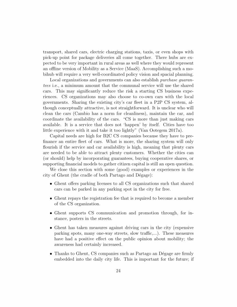
We close this section with some (good) examples or experiences in thecity of Ghent (the cradle of both Partago and Degage):

• Ghent o↵ers parking licenses to all CS organizations such that sharedcars can be parked in any parking spot in the city for free.

• Ghent repays the registration fee that is required to become a memberof the CS organization.

• Ghent supports CS communication and promotion through, for in-stance, posters in the streets.

• Ghent has taken measures against driving cars in the city (expensiveparking spots, many one-way streets, slow tra�c,...). These measureshave had a positive e↵ect on the public opinion about mobility; theawareness had certainly increased.

• Thanks to Ghent, CS companies such as Partago an Degage are firmlyembedded into the daily city life. This is important for the future; if

24

the CS companies are part of daily life, they will be taken into accountin future projects.

3.2. Regional (Flemish) level

The most important obstacles that would need to be addressed at theFlemish level are:

• All cities and communities currently have a di↵erent way of recogniz-ing or deciding to accept a CS firm. A standardized Flemish regulatoryframework would help because this would make it much easier to moveto di↵erent cities if the CS company has been recognized in one. cur-rently, there is a Flemish resolution for CS (De Ridder et al. 2016).

• Widespread promotion and awareness is lacking and the Flemish gov-ernment could promote the CS idea, sector, and good examples.

• As local governments do not always have the manpower to work outa whole policy for a CS firm, Flemish government could support andincentivize them, possibly financially. Examples would be to outlinehow to arrange purchase guarantees, or incentives to share the city’scar fleet.

• Flanders can implement and support ‘testing grounds’ to try out newinitiative such as sharing vehicles for people with physical disabilities,sharing school buses, or other vehicles for special need groups. Thesetesting grounds may also allow to test new business models.

3.3. Federal level

The biggest obstacles and how they at the federal level may be solved arethe following:

• The VAT-rate for CS is currently 21% because it falls in the rentalsector. However, the goals in sharing cars are very di↵erent from thegoals in renting cars. Interviewees stated that the VAT-rate should belowered to 6%.

• In Belgium, company cars are very beneficial from a fiscal point-of-view. Shared cars currently simply cannot compete with company cars.Recently, there have been some suggestions for introducing a mobilitybudget for employees that can be used for any mode of transport to get

25

to work. This new system could make public transportation or sharedcars better competitors against the company car.

• A license plate that clearly distinguishes shared cars from regular carscan make patrolling for parking violations easier.

• Some busy streets have a priority lane, reserved for buses. The intervie-wees suggest that these might also be used by shared cars or creatinga special lane for shared cars only.

3.4. Culture of (car) ownership and a systems thinking view

A general obstacle for CS is materialism; the fact that people like toown things. For cars, people value the convenience of having a car closeby at all times and owning a nice car is considered a status symbol. Formany, their car is almost like an extra private room where they talk, havemeetings, or even eat. And cars are more and more customizable or fittedto the individual. This car culture would have to change for CS to flourishsince this requires that the car they used is also used by others.

Altering the current car culture will require some reflection about thecurrent way of life; it should evolve into a more socially sensitive and en-vironmentally conscious system. Our anthropocentrism is very large (anddisastrous). We must distance ourselves from the idea that everything mustalways be immediately available. We should make more conscious choices todetermine how we want to spend out time.

This change of attitude or way of life will also require more drastic changesin the whole system of mobility and spatial planning. We all have to makebetter choices about where we live, work, shop, relax, and also how we all livetogether. The urban sprawl is costing Flanders a fortune (Vermeiren et al.2019).

3.5. Determinants of shared car use

Although there is consensus that CS is cheaper than owning a car forthose who drive less than 10.000km per year, few actually make the shift toshared cars. In general, the limited success may be explained by the followingdeterminants; ease of use, availability and proximity of the shared car, andprice.

For the price, it is di�cult for users to make a fair comparison betweenthe price of a shared or privately owned car. The actual price of a private

26

car consists of the purchase price, maintenance, vehicle inspection, insurance,fuel costs, etc... . Car owners rarely take into account all of these and tend toconsider only fuel costs while indirect costs are overlooked. This means thatshared system may seem overpriced. It should also be noted that externalcosts (pollution, congestion,...) are significant for the society but neglectedin any price calculation. It is expected that these costs are lower for sharedcars than privately owned cars.

A second important benefit of CS is ease of use but this is often under-rated. One does not have to take care of maintenance of the car (big orsmall), there’s no car insurance, you do not have to look for a replacementwhen it breaks down... One is really carefree if he shares cars.

Thirdly, the availability and proximity of the car is important. Threecriteria play a role: where you want a car, which car you want, and whenyou want it. Starting from those criteria, Cambio o↵ers alternatives to choosefrom when a customer makes a request to come as close to what they wantas possible. As such, 90% of the car requests are fulfilled. Only 10% cannotbe fulfilled, for instance if a large moving truck is needed at a very specifictime and it has been reserved by someone else in advance.

If the perception of people can be shifted toward the idea “that sharedcars should be chosen for convenience”, the group of customers that can beconvinced may be a lot larger since this would not only attract people withenvironmental motives.

4. Exploratory data analysis

In total, 3433 individuals opened the survey online. They were told thatthe survey would take approximately 20 minutes and that they would havea chance for a prize (cinema tickets, lottery tickets, or a 20 gift voucher fora multimedia store.

For further analysis, we only focus on people who filled in, at least the fullDCE experiment. As such, we are left with 2106 respondents (i.e. a responserate of 61.35%). The violin and box-plots in Figure 1 shows the distributionof the time it took respondents to fill in the whole survey. Since car-sharerreceived some additional questions, it took these respondents slightly longerto fill in the survey. It should be noted that the Qualtrics survey platformallows respondent to close their browser and continue their answers later on(up until a week later). Completion times of more than 2 hours are not shownin the Figure to exclude outliers such as those who stopped and continued at

27

a later point in time (140 respondents took more than 2 hours to completethe survey).

N=1815 Response rate=61.73%

N=291 Response rate=59.03%

25

50

75

100

125

Non−car sharers Car sharers

Com

plet

ion

time

in m

inut

es

Figure 1: Distribution of the time it took respondents to fill in the survey.

The Qualtrics software also allows to track the progress of the respon-dents. Figure 2 shows how far respondents got into the survey. As indicatedon the figure, many stopped when we asked them to describe all the privatelyowned cars in their family. This question was quite detailed; we asked for themodel of car, the year it was produced, the fuel type, the average number ofkilometers they drive per week, and how sure they are about their estimatedaverage mileage per week. There is another drop in respondents when we getto the DCE. This requires respondents to really think and compare di↵erentoptions. Some respondents might have underestimated the mental e↵ort thatthe survey required and were not willing to put in the e↵ort. Finally, 60.08%of the non car-sharers and 59.46% of the car-sharers filled in the completesurvey. The P-value of 0.47 for the Logrank test indicates that there’s nostatistical di↵erence between how much the car-sharers and non-car-sharerscompleted the survey.

28

P−value = 0.47

DCE non−carsharersDCE car sharers

Describe private cars

0%

20%

40%

60%

80%

100%

0 20 40 60 80 100Completeness of the survey (%)

Perc

enta

ge o

f the

resp

onde

nts

Non−carsharers Carsharers

Figure 2: Distribution of the time it took respondents to fill in the survey.

4.1. Demographics

Figure 3 shows the distribution of the age and gender of the respondents.Overall, the survey attracted a nice range of ages and gender. There’s a slightpeak in respondent in their mid-twenties. This is likely due to the fact thattwo Masters’ students were asked to spread the survey; they mainly spreadit in their own group of friends through social media.

The mean age of car-sharers appeared to be significantly lower than themean age of the non-car-sharers (mean age of 37.8 vs 41.1 years old, One-WayANOVA p-value < 0.001) but there was no significant di↵erence in gender(Chi-Squared test, p-value of 0.97).

29

Non−carsharer (1815) Carsharer (291)Fem

ale (1306)M

ale (800)

30 50 70 30 50 70

0

10

20

30

40

50

0

10

20

30

40

50

Age

Num

ber o

f res

pond

ents

Figure 3: Distribution of the age and gender of the respondents.

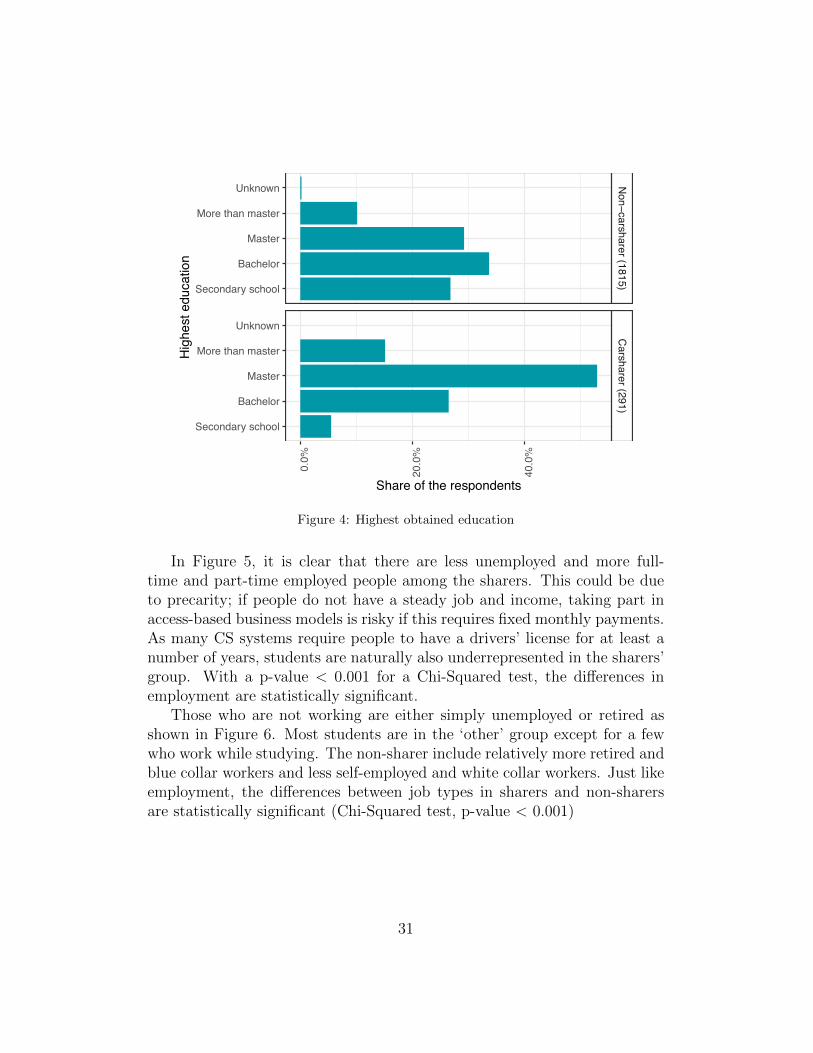
When it comes to education, car-sharers are relatively higher educatedwith more people having a Master degree or higher (Figure 4). Among thenon-sharers, there are far more people whose highest degree was secondaryschool. This di↵erence in education is statistically significant (Chi-Squaredtest, p-value < 0.001).

30

Non−carsharer (1815)

Carsharer (291)

0.0%

20.0

%

40.0

%

Secondary school

Bachelor

Master

More than master

Unknown

Secondary school

Bachelor

Master

More than master

Unknown

Share of the respondents

Hig

hest

edu

catio

n

Figure 4: Highest obtained education

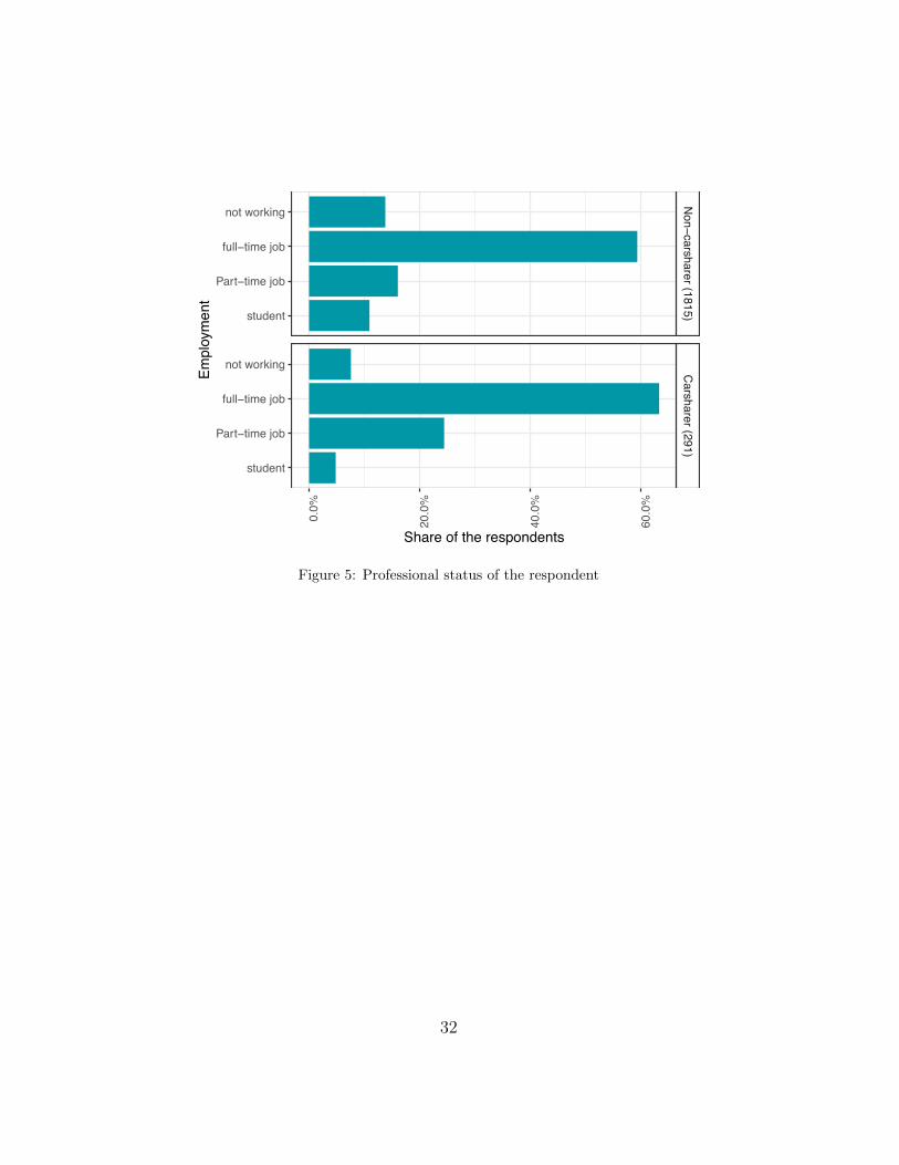
In Figure 5, it is clear that there are less unemployed and more full-time and part-time employed people among the sharers. This could be dueto precarity; if people do not have a steady job and income, taking part inaccess-based business models is risky if this requires fixed monthly payments.As many CS systems require people to have a drivers’ license for at least anumber of years, students are naturally also underrepresented in the sharers’group. With a p-value < 0.001 for a Chi-Squared test, the di↵erences inemployment are statistically significant.

Those who are not working are either simply unemployed or retired asshown in Figure 6. Most students are in the ‘other’ group except for a fewwho work while studying. The non-sharer include relatively more retired andblue collar workers and less self-employed and white collar workers. Just likeemployment, the di↵erences between job types in sharers and non-sharersare statistically significant (Chi-Squared test, p-value < 0.001)

31

Non−carsharer (1815)

Carsharer (291)

0.0%

20.0

%

40.0

%

60.0

%

student

Part−time job

full−time job

not working

student

Part−time job

full−time job

not working

Share of the respondents

Empl

oym

ent

Figure 5: Professional status of the respondent

32

Non−carsharer (1815)

Carsharer (291)

0.0%

20.0

%

40.0

%

60.0

%

Other

Blue collar

White collar

self−employed

retired

Unemployed

Other

Blue collar

White collar

self−employed

retired

Unemployed

Share of the respondents

Jobs

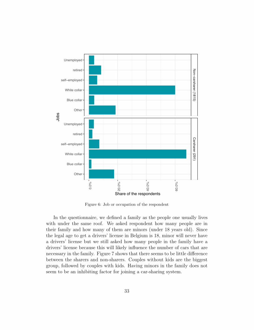
Figure 6: Job or occupation of the respondent

In the questionnaire, we defined a family as the people one usually liveswith under the same roof. We asked respondent how many people are intheir family and how many of them are minors (under 18 years old). Sincethe legal age to get a drivers’ license in Belgium is 18, minor will never havea drivers’ license but we still asked how many people in the family have adrivers’ license because this will likely influence the number of cars that arenecessary in the family. Figure 7 shows that there seems to be little di↵erencebetween the sharers and non-sharers. Couples without kids are the biggestgroup, followed by couples with kids. Having minors in the family does notseem to be an inhibiting factor for joining a car-sharing system.

33

13.7 2.4 1.8 0.5 0.2 0

26.4 9.2 14.7 5.2 1 0.1

8.9 2.6 0.7 0.2 0 0

8.3 1.4 0.2 0 0 0

2.4 0.3 0.1 0 0 0

15.9 3.8 4.8 0.7 0 0

30 9.3 17.2 6.2 0.3 0.7

3.8 1 0 0.7 0 0

3.4 0 0.3 0 0 0

1.4 0 0.3 0 0 0

Non−carsharer (1815) Carsharer (291)

0 1 2 3 4 5 0 1 2 3 4 5

1

2

3

4

5 or more

Number of minors in the family

Num

ber o

f adu

lts in

the

fam

ily

0 10 20 30% of respondents

Figure 7: Family composition. Numbers in the graph show the percentage of (non) sharers’families with a certain family composition.

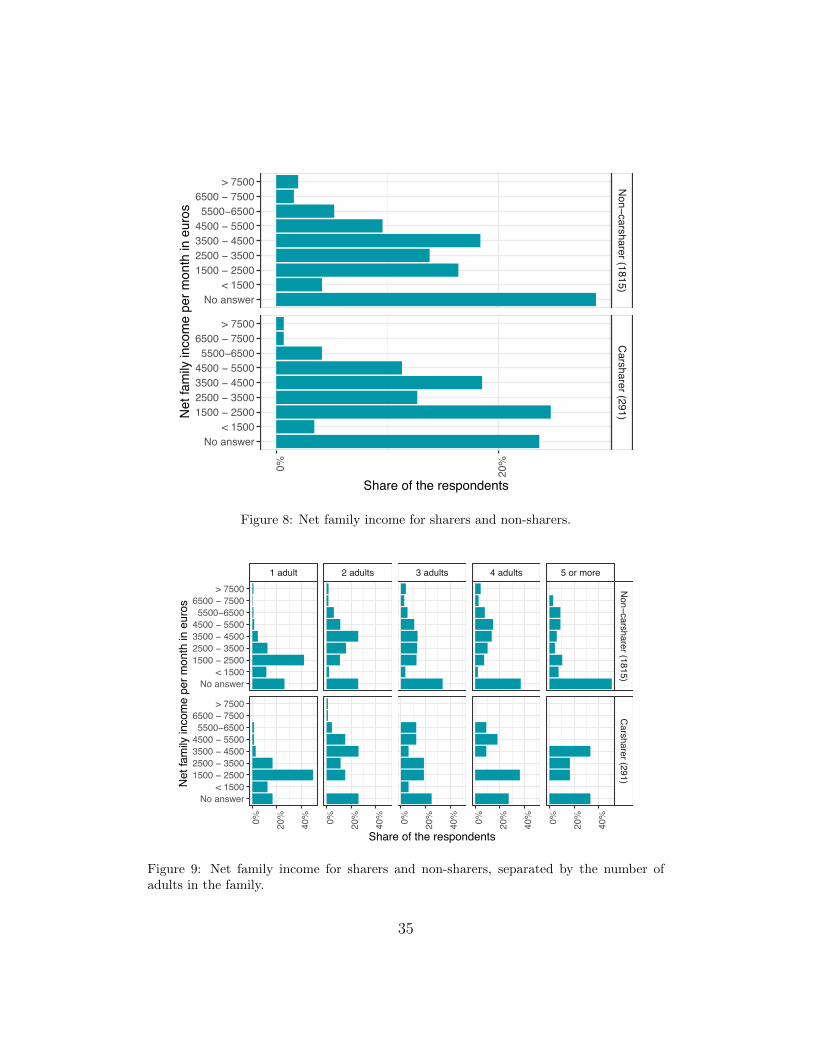
We also asked respondents about their monthly net income for the wholefamily. Many respondents choose not to answer this question. The resultsare shown in Figure 8. At first glance, it seems like there are more sharersin the income scale between 1500 and 2500. We also split up the resultsfor the number of adults in the family since this will likely influence the netfamily income (see Figure 9). Overall, we can conclude that the sharers haverelatively less people in the highest and more people in the lower incomegroups (especially in single-adult families).

34

Non−carsharer (1815)

Carsharer (291)

0% 20%

No answer< 1500

1500 − 25002500 − 35003500 − 45004500 − 55005500−6500

6500 − 7500> 7500

No answer< 1500

1500 − 25002500 − 35003500 − 45004500 − 55005500−6500

6500 − 7500> 7500

Share of the respondents

Net

fam

ily in

com

e pe

r mon

th in

eur

os

Figure 8: Net family income for sharers and non-sharers.

1 adult 2 adults 3 adults 4 adults 5 or more

Non−carsharer (1815)

Carsharer (291)

0% 20%

40% 0% 20%

40% 0% 20%

40% 0% 20%

40% 0% 20%

40%

No answer< 1500

1500 − 25002500 − 35003500 − 45004500 − 55005500−6500

6500 − 7500> 7500

No answer< 1500

1500 − 25002500 − 35003500 − 45004500 − 55005500−6500

6500 − 7500> 7500

Share of the respondents

Net

fam

ily in

com

e pe

r mon

th in

eur

os

Figure 9: Net family income for sharers and non-sharers, separated by the number ofadults in the family.

35

A last demographic that we would like to discuss is the place where peoplelive. We asked people for their postal code and whether they live in an urban,suburban, or rural area. As the survey was available only in Dutch, thereare few respondents from the French-speaking Walloon region and only a fewfrom the Brussels-Capital region. Table 4 shows the province or region of therespondents and the type of environment they live in. One thing that standsout is that many of the car-sharers live in East Flanders. This is becauseDegage actively spread the survey among their members and they operatemainly in Ghent (in East Flanders). Another important thing to notice isthat non-sharers live mostly in rural areas while less than 10 percent of thesharers live in a rural environment.

Variable Levels nNCS %NCS nCS %CS nall %all

Location Brussels 28 1.5 14 4.8 42 2.0Walloon Brabant 0 0.0 0 0.0 0 0.0Flemish Brabant 410 22.6 43 14.8 453 21.5Antwerp 405 22.3 57 19.6 462 21.9Limburg 297 16.4 3 1.0 300 14.2Liege 2 0.1 0 0.0 2 0.1Namur 0 0.0 0 0.0 0 0.0Hainaut 2 0.1 0 0.0 2 0.1Luxembourg 0 0.0 0 0.0 0 0.0West Flanders 196 10.8 11 3.8 207 9.8East Flanders 474 26.1 163 56.0 637 30.3

p = 0.0005 all 1814 100.0 291 100.0 2105 100.0

Environment Rural 756 41.8 27 9.3 783 37.3Suburban 598 33.1 75 25.8 673 32.1Urban 454 25.1 189 65.0 643 30.6

p = 0.0005 all 1808 100.0 291 100.0 2099 100.0

Table 4: Living location and environment of not car sharers (NCS) and car sharers (CS).P-values of Fisher’s exact test added. Missing data is left out.

4.2. Mobility data

To be able to compare the impact of car-sharing on the environment, wehave to know how vehicle ownership, travelled kilometers, and travel modesdi↵er between sharers and non-sharers. Table A.39 in the appendix shows thenumber of cars, bikes and public transportation subscriptions (non) sharershave in their family. It appears that car-sharing families have significantlyless private, company cars, and motorcycles but more public transport sub-scriptions and bikes. There is also a substantial di↵erent in the kilometers

36

that are driven with each of the transportation modes; Figure 10 shows thisgraphically while Table A.38 in the appendix summarizes the raw data forsharers and non-sharers. It can be seen that sharers walk, bike, and usepublic transportation more. 95% and 75% of sharers never drive a companyor private car respectively and if they do, they tend to drive it for shorterdistances.

Figure 10: Weekly kilometers travelled by (non) sharers using di↵erent transportationmodes. Percentages on the left indicate the percentage of respondents that never use thetransportation mode.

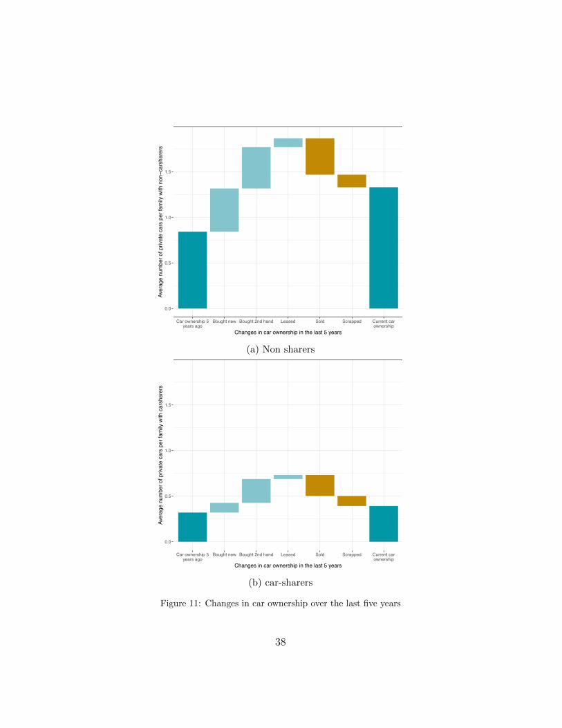
Apart from current private car ownership, we also asked respondents howmany cars they acquired and have gotten rid of in the last 5 years. Figure 11shows waterfall charts for the changes in car ownership of the average nonsharing and sharing family respectively. Firstly, it is clear that the averagesharing family has less private cars than non-sharers. Secondly, non-sharersbought approximately an equal amount of new and second hand car whilesharers seem to opt for second hand a lot more often.

37

0.0

0.5

1.0

1.5

Car ownership 5years ago

Bought new Bought 2nd hand Leased Sold Scrapped Current carownership

Changes in car ownership in the last 5 years

Aver

age

num

ber o

f priv

ate

cars

per

fam

ily w

ith n

on−c

arsh

arer

s

(a) Non sharers

0.0

0.5

1.0

1.5

Car ownership 5years ago

Bought new Bought 2nd hand Leased Sold Scrapped Current carownership

Changes in car ownership in the last 5 years

Aver

age

num

ber o

f priv

ate

cars

per

fam

ily w

ith c

arsh

arer

s

(b) car-sharers

Figure 11: Changes in car ownership over the last five years

38

Looking at the future, Figure 12 shows that there are relatively less peoplein the sharing group that consider it to be (highly) likely that they will buy anew private car in the next 5 years. There is also a minority (52 respondents)that stated they will never buy a new private car. Most of them want to avoidbuying a private car because of environmental reasons, because they prefer towalk or bike, or because they have access to shared cars (Figure 13, multiplereasons could be selected).

Non−carsharer (1812)

Carsharer (291)

0 250 500 750

I / my family willnever buy a private

car

Not likely

Likely

Highly likely

I / my family willnever buy a private

car

Not likely

Likely

Highly likely

Number of respondents

How likely is it that you (your family) buy(s) a car in the next 5 years?

Figure 12: Likelihood of buying a new private car in the next five year. Missing valuesare left out.

39

no drivers' license

do not like driving

other

use company carsonly

prefer PT

too expensive

use shared cars

prefer walking andbiking

bad for environment

0 10 20 30 40Number of times chosen

Why would you never buy a private car?

Figure 13: Reasons for never wanting to buy a car.

When the respondents use the car, they are often alone in the car, asshown in Figure 14. However, it appears that shared cars are used a bit moree�ciently because they are less likely to be driven without any passengers.33% of respondents claim to usually or always have three or more people inthe shared car while this is only 21% for private cars. A possible cause forthis di↵erence, is that shared cars are rarely used for the commute to work;a ride that is often performed solo.

40

10%

16%

43%

66%

35%

21%

24%

49%

35%3 or more person

2 persons

1 person

100 50 0 50 100Percentage

Never Seldom Sometimes Usually Always

(a) Private cars

29%

28%

48%

49%

36%

33%

22%

36%

18%3 or more person

2 persons

1 person

100 50 0 50 100Percentage

Never Seldom Sometimes Usually Always

(b) Shared cars

Figure 14: Number of passengers in a car, including the driver for personal and sharedcars.

To finish this section, we would like to mention that section AppendixA.1 in the appendix briefly touches upon the debate on how much the liv-ing environment influences the the choice of transportation mode and thedistance that people travel.

4.3. Car-sharing

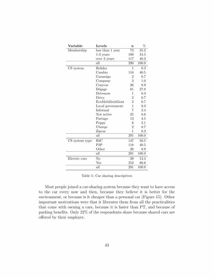
This section describes which car-sharing firms are represented in our sam-ple, how often CS is used, and the motivations for using it. Table 5 shows that40% of respondents have been sharing cars for over 3 years. Cambio is the

41

most common car-sharing system, followed closely by Degage. One respon-dent indicated that he uses the cars that local government makes availablefor their inhabitant outside o�ce hours. 7 respondents informally share carswith friend or families. 25 respondents were classified as ‘not active’ sincethey (almost) never used the shared cars but they did have a membershipwith a car-sharing system. Table 5 only shows the primary car-sharing sys-tem of the respondent, 26 respondents were a member with two providers and4 respondents even had three memberships. The car-sharers are quite evenlydivided between P2P and B2C systems. Respondents that are not active orshared cars of the local government are classified as ‘Other’ systems. It isalso encouraging to see that most car-sharing systems include electric cars intheir fleet.

42

Variable Levels n %Membership less than 1 year 73 25.2

1-3 years 100 34.5over 3 years 117 40.3all 290 100.0

CS system Bolides 1 0.3Cambio 118 40.5Caramigo 2 0.7Company 3 1.0Cozycar 26 8.9Degage 81 27.8Drivenow 1 0.3Drivy 2 0.7EcoMobiliteitGent 2 0.7Local government 1 0.3Informal 7 2.4Not active 25 8.6Partago 13 4.5Poppy 6 2.1Ubeeqo 2 0.7Zipcar 1 0.3all 291 100.0

CS system type B2C 147 50.5P2P 118 40.5Other 26 8.9all 291 100.0

Electric cars No 39 13.4Yes 252 86.6all 291 100.0

Table 5: Car sharing descriptives

Most people joined a car-sharing system because they want to have accessto the car every now and then, because they believe it is better for theenvironment, or because is it cheaper than a personal car (Figure 15). Otherimportant motivations were that it liberates them from all the practicalitiesthat come with owning a cars, because it is faster than PT, and because ofparking benefits. Only 22% of the respondents share because shared cars areo↵ered by their employer.

43

3%

6%

9%

11%

30%

32%

70%

71%

78%

91%

97%

94%

91%

89%

70%

68%

30%

29%

22%

9%It is safer

than publictransportation.

Car sharing isoffered by my

employer.

People around mealready used it.

It is less crowdedthan public

transportation.

I do not haveto worry about a

parking spot.

It is fasterthan public

transportation.

No worries aboutthe practicalities

for owning acar (insurance,

maintenance,...)

It is cheaper than aprivate car.

Car sharing isbetter for theenvironment.

I can use a carevery now and then.

100 50 0 50 100Percentage van de respondenten

Not important Important Very important

Figure 15: Reasons for joining a car-sharing system (multiple could be chosen).

Figure 16 and 17 show that very few people use the shared car daily andthat it is most often used for visiting family and friends, leisure activities,and shopping. It makes sense that the shared car is only used occasionallysince previous research showed that car-sharing only makes economic sensefor users if the car is used less than 10,000 kilometers per year (see, forexample Litman (2000)). Respondents also had the opportunity to fill inany other reason to use the shared car. Here, they mentioned some trips forwhich a larger car is needed (moving house, buying large furniture, bringingstu↵ to recycling center or junk yard) ; this shows that some people reallydo value the flexibility of choosing a car that fits their needs. Some use it tolearn how to drive, going to school, and doctor visits.

44

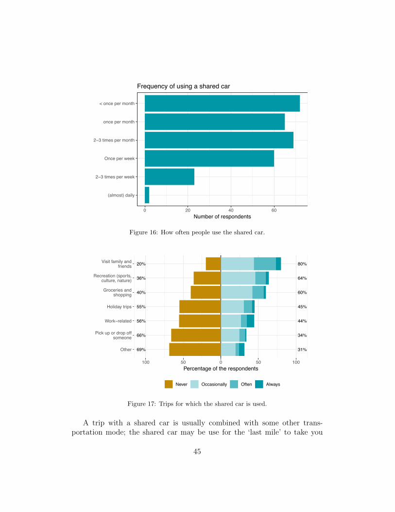
(almost) daily

2−3 times per week

Once per week

2−3 times per month

once per month

< once per month

0 20 40 60Number of respondents

Frequency of using a shared car

Figure 16: How often people use the shared car.

20%

36%

40%

55%

56%

66%

69%

80%

64%

60%

45%

44%

34%

31%Other

Pick up or drop offsomeone

Work−related

Holiday trips

Groceries andshopping

Recreation (sports,culture, nature)

Visit family andfriends

100 50 0 50 100Percentage of the respondents

Never Occasionally Often Always

Figure 17: Trips for which the shared car is used.

A trip with a shared car is usually combined with some other trans-portation mode; the shared car may be use for the ‘last mile’ to take you

45

where public transportation is not available, or the shared car may be lo-cated for from the user’s home. Figure 18 shows that walking and bikingis the preferred transportation mode which is good from an environmentalpoint-of-view. The people who chose ‘Other’ mentioned taxi, metro, electricscooter, carpooling, or ‘none’. Over 30% say they use the train in combina-tion with a shared car. This vouches for Mobihubs close to railway stationsMobihubs (2019).

36%

40%

69%

80%

90%

91%

64%

60%

31%

20%

10%

9%Other

Shared bike

Bus or tram

Train

Own bike

Walking

100 50 0 50 100Percentage of the respondents

Never Occasionally Often Always

Figure 18: Other transportation modes with which the shared car trip is combined.

Section 4.2 already described in detail some di↵erence between sharersand non-sharers with respect to the number of cars that are owned and recentcar purchases or disposal of personal cars (Figure 11). We additionally askedcar-sharers how many cars they bought, leased, sold or scrapped since theystarted sharing (Figure 19). Overall, there is an (almost negligible) increasein the number of cars that are owned by the sharers. But this graph shouldbe nuanced as some may have only just become a member and thus have nothave the chance to get rid of a car. It is encouraging, however, that many saythey bike, walk, and use public transport more in lieu of private cars sincejoining a car-sharing firm (Figure 20).

46

−0.15

−0.10

−0.05

0.00

0.05

0.10

Bought new Bought 2nd hand Leased Sold Scrapped Net cars acquired

Aver

age

num

ber o

f car

s pe

r fam

ilyHow many cars have you ... since sharing?

Figure 19: Changes in car ownership since joining a car-sharing system.

2%

9%

1%

11%

30%

80%

62%

37%

31%

25%

22%

13%

2%

1%Motorcycle orscooter

Private Cars

Carpooling

Bus/tram/metro

Walk

Train

Bike

100 50 0 50 100Percentage of the respondents

never

a lot less

less

the same

more

a lot more

Figure 20: Changes in mobility choices since joining a car-sharing system.

If sharers had gotten rid of a car, they were asked how important the factthat they share cars was in their decision to buy, scrap, or sell a car sincethey started sharing cars. Figure 21 shows that car-sharing was particularly

47

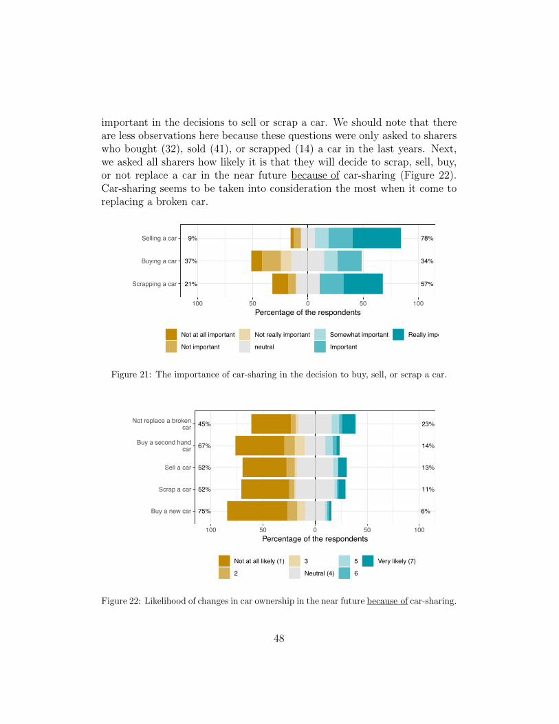
important in the decisions to sell or scrap a car. We should note that thereare less observations here because these questions were only asked to sharerswho bought (32), sold (41), or scrapped (14) a car in the last years. Next,we asked all sharers how likely it is that they will decide to scrap, sell, buy,or not replace a car in the near future because of car-sharing (Figure 22).Car-sharing seems to be taken into consideration the most when it come toreplacing a broken car.

9%

21%

37%

78%

57%

34%

Scrapping a car

Buying a car

Selling a car

100 50 0 50 100Percentage of the respondents

Not at all important

Not important

Not really important

neutral

Somewhat important

Important

Really important

Figure 21: The importance of car-sharing in the decision to buy, sell, or scrap a car.

45%

67%

52%

52%

75%

23%

14%

13%

11%

6%Buy a new car

Scrap a car

Sell a car

Buy a second handcar

Not replace a brokencar

100 50 0 50 100Percentage of the respondents

Not at all likely (1)

2

3

Neutral (4)

5

6

Very likely (7)

Figure 22: Likelihood of changes in car ownership in the near future because of car-sharing.

48

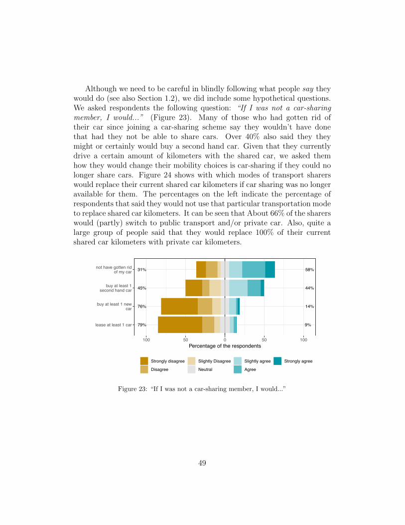
Although we need to be careful in blindly following what people say theywould do (see also Section 1.2), we did include some hypothetical questions.We asked respondents the following question: “If I was not a car-sharingmember, I would...” (Figure 23). Many of those who had gotten rid oftheir car since joining a car-sharing scheme say they wouldn’t have donethat had they not be able to share cars. Over 40% also said they theymight or certainly would buy a second hand car. Given that they currentlydrive a certain amount of kilometers with the shared car, we asked themhow they would change their mobility choices is car-sharing if they could nolonger share cars. Figure 24 shows with which modes of transport sharerswould replace their current shared car kilometers if car sharing was no longeravailable for them. The percentages on the left indicate the percentage ofrespondents that said they would not use that particular transportation modeto replace shared car kilometers. It can be seen that About 66% of the sharerswould (partly) switch to public transport and/or private car. Also, quite alarge group of people said that they would replace 100% of their currentshared car kilometers with private car kilometers.

31%

45%

76%

79%

58%

44%

14%

9%lease at least 1 car

buy at least 1 newcar

buy at least 1second hand car

not have gotten ridof my car

100 50 0 50 100Percentage of the respondents

Strongly disagree

Disagree

Slightly Disagree

Neutral

Slightly agree

Agree

Strongly agree

Figure 23: “If I was not a car-sharing member, I would...”

49

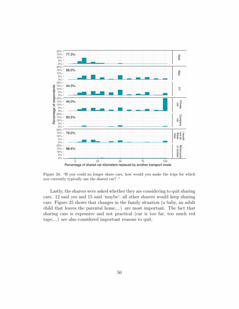
77.3%

56.0%

44.3%

44.0%

93.5%

79.0%

98.6%

Walk

BikePT

Privatecar

Com

panycar

I wouldnot dothesetrips

Motorcycle

or scooter

0 25 50 75 100

0%5%

10%15%20%

0%5%

10%15%20%

0%5%

10%15%20%

0%5%

10%15%20%

0%5%

10%15%20%

0%5%

10%15%20%

0%5%

10%15%20%

Percentage of shared car kilometers replaced by another transport mode

Perc

enta

ge o

f res

pond

ents

Figure 24: “If you could no longer share cars, how would you make the trips for whichyou currently typically use the shared car? “

Lastly, the sharers were asked whether they are considering to quit sharingcars. 12 said yes and 15 said ‘maybe’; all other sharers would keep sharingcars. Figure 25 shows that changes in the family situation (a baby, an adultchild that leaves the parental home,...) are most important. The fact thatsharing cars is expensive and not practical (car is too far, too much redtape,...) are also considered important reasons to quit.

50

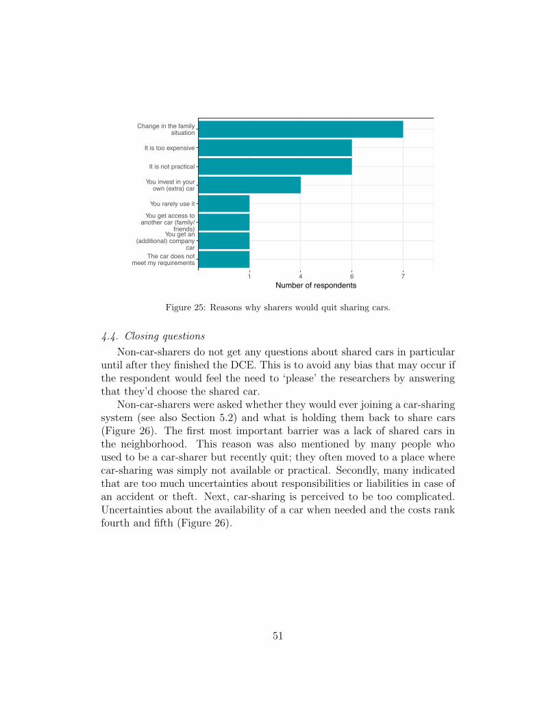
The car does notmeet my requirements

You get an(additional) company

car

You get access toanother car (family/

friends)

You rarely use it

You invest in yourown (extra) car

It is not practical

It is too expensive

Change in the familysituation

1 4 6 7Number of respondents

Figure 25: Reasons why sharers would quit sharing cars.

4.4. Closing questions

Non-car-sharers do not get any questions about shared cars in particularuntil after they finished the DCE. This is to avoid any bias that may occur ifthe respondent would feel the need to ‘please’ the researchers by answeringthat they’d choose the shared car.

Non-car-sharers were asked whether they would ever joining a car-sharingsystem (see also Section 5.2) and what is holding them back to share cars(Figure 26). The first most important barrier was a lack of shared cars inthe neighborhood. This reason was also mentioned by many people whoused to be a car-sharer but recently quit; they often moved to a place wherecar-sharing was simply not available or practical. Secondly, many indicatedthat are too much uncertainties about responsibilities or liabilities in case ofan accident or theft. Next, car-sharing is perceived to be too complicated.Uncertainties about the availability of a car when needed and the costs rankfourth and fifth (Figure 26).

51

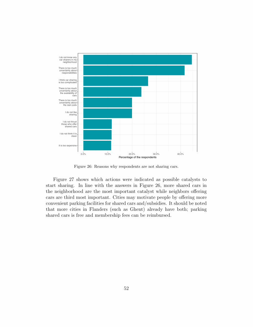
It is too expensive

I do not think it isclean

I do not thrustthose who offer

shared cars

I do not likesharing

There is too muchuncertainty about

the real costs

There is too muchuncertainty aboutthe availability of

cars

I think car sharingis too complicated

There is too muchuncertainty about

responsibilities

I do not know anycar sharers in my

neighborhood

0.0% 10.0% 20.0% 30.0% 40.0%Percentage of the respondents

Figure 26: Reasons why respondents are not sharing cars.

Figure 27 shows which actions were indicated as possible catalysts tostart sharing. In line with the answers in Figure 26, more shared cars inthe neighborhood are the most important catalyst while neighbors o↵eringcars are third most important. Cities may motivate people by o↵ering moreconvenient parking facilities for shared cars and/subsidies. It should be notedthat more cities in Flanders (such as Ghent) already have both; parkingshared cars is free and membership fees can be reimbursed.

52

More info about thecosts of car sharing

Car sharing needs tobe cheaper

More info aboutresponsibilities in

case of an accidentor theft

Subsidies of thecity or community

Neighbors that takeinitiative to share

cars

Initiatives by thecity to allow for

easier parking forshared cars

Shared cars in myneighborhood

0.0% 20.0% 40.0% 60.0%Percentage of the respondents

Figure 27: Actions that might help people to start sharing cars.

We also asked respondents which features were not taken into account inthe DCE. Although we will also use statistical methods to find out whethersome attributes really were insignificant or not considered by the respondents,this might give a rough idea of what people find important. Figure 28 showsthat the majority took all attributes into account; there are only three at-tributes for private cars. For the shared car, there are seven attributes whichmakes it harder to take everything in consideration in making a choice. Theattributes that were overlooked the most, according to the respondents, arewhether it’s a B2C or P2P system, the kilometer cost and the fuel type forthe shared cars. Figure 29 also indicated B2C/P2P and the fuel type asthe attributes that were neglected the most among the car-sharing group ofrespondents. The sharers could not choose a private car in their DCE and,thus, they do not have private car attributes.

53

Purchase cost

Fuel type

Time to get to car

Reservation time

Flexibility

Monthly cost

Kilometer cost

Fuel type

Kilometer cost

I took everythingfor shared cars into

account

B2B/P2P

I took everythingfor private cars

into account

0.0% 20.0% 40.0% 60.0%Percentage of the respondents

Private car Shared car

Figure 28: The attributes that non-sharers did not take into account in the DCE.

Kilometer cost

Monthly cost

Time to get to car

Reservation time

I took everythinginto account

Flexibility

Fuel type

B2B/P2P

0.0% 10.0% 20.0% 30.0% 40.0%Percentage of the respondents

Figure 29: The attributes that sharers did not take into account in the DCE.

54

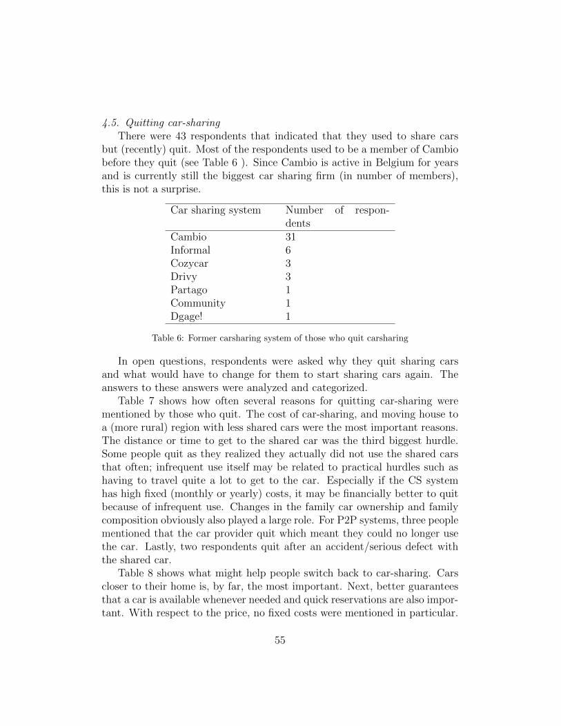
4.5. Quitting car-sharingThere were 43 respondents that indicated that they used to share cars

but (recently) quit. Most of the respondents used to be a member of Cambiobefore they quit (see Table 6 ). Since Cambio is active in Belgium for yearsand is currently still the biggest car sharing firm (in number of members),this is not a surprise.

Car sharing system Number of respon-dents

Cambio 31Informal 6Cozycar 3Drivy 3Partago 1Community 1Dgage! 1

Table 6: Former carsharing system of those who quit carsharing

In open questions, respondents were asked why they quit sharing carsand what would have to change for them to start sharing cars again. Theanswers to these answers were analyzed and categorized.

Table 7 shows how often several reasons for quitting car-sharing werementioned by those who quit. The cost of car-sharing, and moving house toa (more rural) region with less shared cars were the most important reasons.The distance or time to get to the shared car was the third biggest hurdle.Some people quit as they realized they actually did not use the shared carsthat often; infrequent use itself may be related to practical hurdles such ashaving to travel quite a lot to get to the car. Especially if the CS systemhas high fixed (monthly or yearly) costs, it may be financially better to quitbecause of infrequent use. Changes in the family car ownership and familycomposition obviously also played a large role. For P2P systems, three peoplementioned that the car provider quit which meant they could no longer usethe car. Lastly, two respondents quit after an accident/serious defect withthe shared car.

Table 8 shows what might help people switch back to car-sharing. Carscloser to their home is, by far, the most important. Next, better guaranteesthat a car is available whenever needed and quick reservations are also impor-tant. With respect to the price, no fixed costs were mentioned in particular.

55

Reason NumberIt is too expensive 8Moved house 8It is too far 7I used it too little 3I got a company car 3Kids 3I got a new private car 3Peers/car owners quit 3Accidents with the shared car 2

Table 7: Reasons for quitting car sharing

Most people mentioned that they might not replace (one of) their privatecar(s) if it broke down and choose a shared car instead but none would getrid of their car as long as it if still operational.

Motivation NumberCars closer by 13Better availability guarantees and flexible reservation 6It should be cheaper 5Less private cars 4I’d never share cars again 4Others 2Better revenues if I share my car 1A mobility budget at work 1Better public transportation 1

Table 8: ’What could make you share cars again?’

5. Statistical analyses

In this section, we use our data set in statistical models to explore sig-nificant factors that a↵ect the willingness to share cars and that make car-sharing systems more or less attractive. Section 5.1 first describes threefactor analyses; for the full dataset, only the non-sharers, and only the shar-ers. Section 5.2 describes an ordinal model that explains the willingness to

56

share cars. Lastly, Section 5.3 and 5.4 analyze the responses to the DCEs forthe non-sharers and sharers respectively.

5.1. Factor analysis

The survey contains several statements about the environment, cars, driv-ing, and sharing which respondents were asked to rate according to theiragreement on a scale from 1 to 5. There are 46 statements in total thatpeople were asked to rate on a 5 or 7-point scale. 6 of these statements wereonly presented to car-sharers as they were not relevant for non-car-sharers(for instance ‘Thanks to car-sharing, I meet new and interesting people’ ).All of these statements contain valuable information about the ideologies,character, and opinions of the respondent which might also drive the choicesthey made in the DCE. Instead of adding the score to each statement as aseparate variable in further statistical models, we will look for correlationsamong multiple statements and thus reduce the number of variables to justa few underlying explanations, or factors.

First, we test whether a factor analysis is sensible using the Measure ofSampling Adequacy (MSA) for individual statements and the Kaiser-Meyer-Olkin (KMO) Criterion that both rely on the Anti-Image-Correlation Matrix.These are easily obtained in R using the REdaS package.

Next, determining the appropriate number of factors can be tricky andseveral methods exist to make a good choice (see (Horn and Engstrom 1979),for instance). The following methods were considered and they often sug-gested di↵erent numbers of factors to be chosen:

1. Parallel analysis: extracting factors until the eigenvalues of the realdata set are less than the corresponding eigenvalues of a random dataset of the same size (Horn 1965).

2. Using the Very Structured Criterion (VSS) (Revelle and Rocklin 1979)

3. Scree test: a sudden drop in eigenvalues analogous to the change inslope seen when scrambling up the talus slope of a mountain and ap-proaching the rock face (Cattell 1966).

4. Minimum Average Partial (MAP) (Velicer 1976).

5. We check the communalities for each of the variables (statements).These are the sum of the squared loadings for the variable and can beinterpreted as the proportion of variation in that variable explained bythe factors. If they are low for some statements, we might want to addmore factors.

57

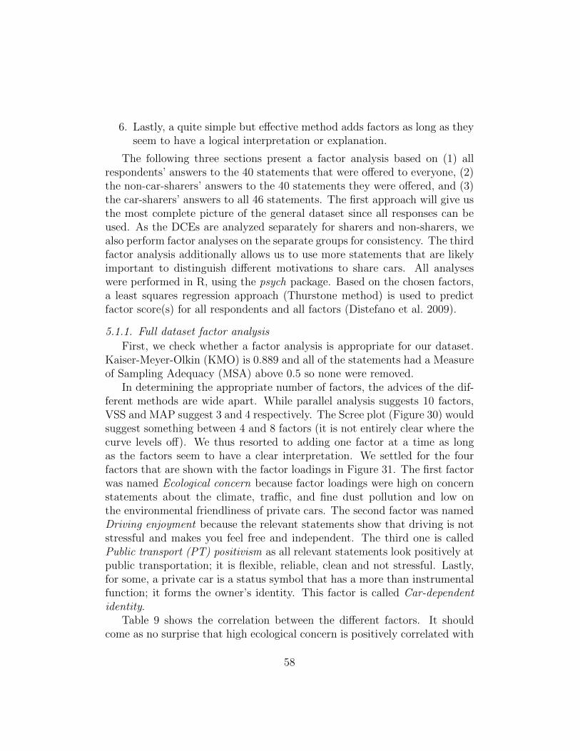
6. Lastly, a quite simple but e↵ective method adds factors as long as theyseem to have a logical interpretation or explanation.

The following three sections present a factor analysis based on (1) allrespondents’ answers to the 40 statements that were o↵ered to everyone, (2)the non-car-sharers’ answers to the 40 statements they were o↵ered, and (3)the car-sharers’ answers to all 46 statements. The first approach will give usthe most complete picture of the general dataset since all responses can beused. As the DCEs are analyzed separately for sharers and non-sharers, wealso perform factor analyses on the separate groups for consistency. The thirdfactor analysis additionally allows us to use more statements that are likelyimportant to distinguish di↵erent motivations to share cars. All analyseswere performed in R, using the psych package. Based on the chosen factors,a least squares regression approach (Thurstone method) is used to predictfactor score(s) for all respondents and all factors (Distefano et al. 2009).

5.1.1. Full dataset factor analysisFirst, we check whether a factor analysis is appropriate for our dataset.

Kaiser-Meyer-Olkin (KMO) is 0.889 and all of the statements had a Measureof Sampling Adequacy (MSA) above 0.5 so none were removed.

In determining the appropriate number of factors, the advices of the dif-ferent methods are wide apart. While parallel analysis suggests 10 factors,VSS and MAP suggest 3 and 4 respectively. The Scree plot (Figure 30) wouldsuggest something between 4 and 8 factors (it is not entirely clear where thecurve levels o↵). We thus resorted to adding one factor at a time as longas the factors seem to have a clear interpretation. We settled for the fourfactors that are shown with the factor loadings in Figure 31. The first factorwas named Ecological concern because factor loadings were high on concernstatements about the climate, tra�c, and fine dust pollution and low onthe environmental friendliness of private cars. The second factor was namedDriving enjoyment because the relevant statements show that driving is notstressful and makes you feel free and independent. The third one is calledPublic transport (PT) positivism as all relevant statements look positively atpublic transportation; it is flexible, reliable, clean and not stressful. Lastly,for some, a private car is a status symbol that has a more than instrumentalfunction; it forms the owner’s identity. This factor is called Car-dependentidentity.

Table 9 shows the correlation between the di↵erent factors. It shouldcome as no surprise that high ecological concern is positively correlated with

58

●

●

●

●

●

●●

●● ● ● ● ● ● ● ● ● ● ● ● ● ● ● ● ● ● ● ● ● ● ● ● ● ● ● ● ● ● ● ●

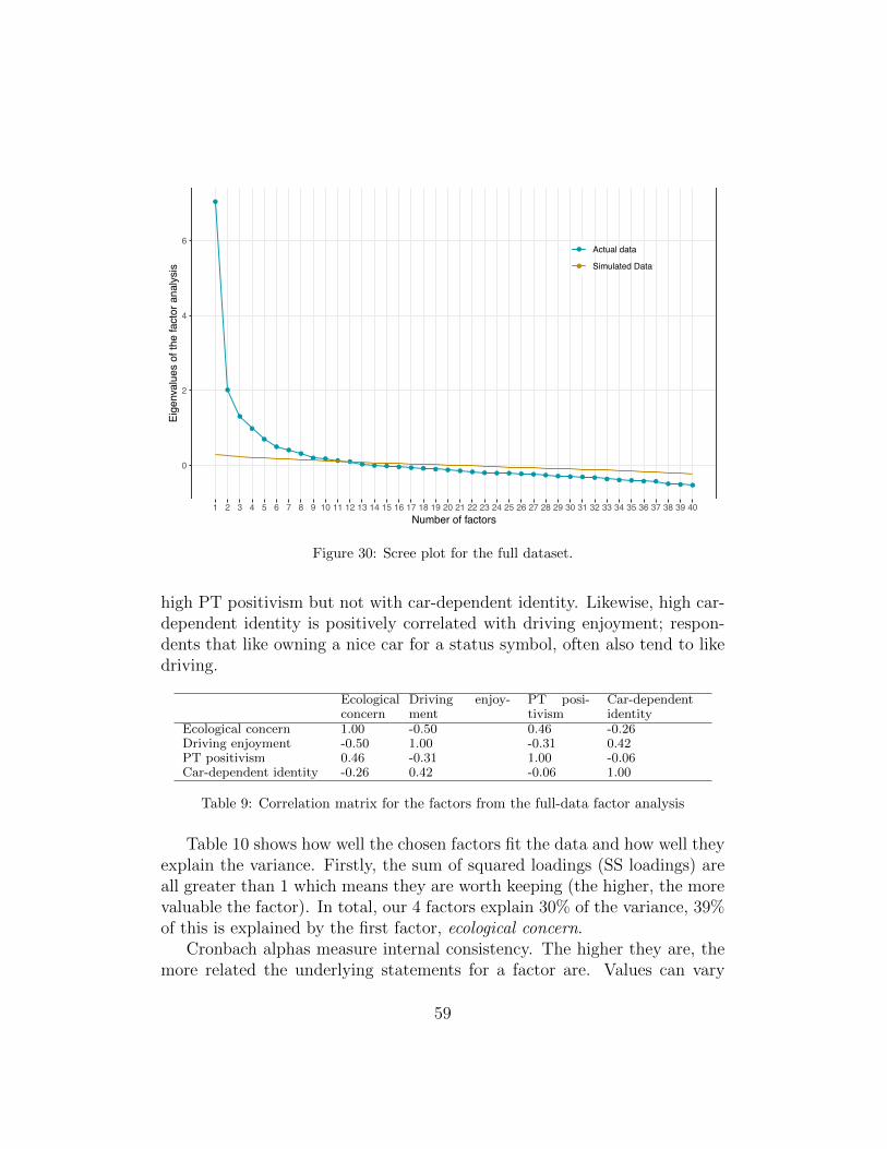
0

2

4

6

1 2 3 4 5 6 7 8 9 10 11 12 13 14 15 16 17 18 19 20 21 22 23 24 25 26 27 28 29 30 31 32 33 34 35 36 37 38 39 40Number of factors

Eige

nval

ues

of th

e fa

ctor

ana

lysi

s

●

●

Actual data

Simulated Data

Figure 30: Scree plot for the full dataset.

high PT positivism but not with car-dependent identity. Likewise, high car-dependent identity is positively correlated with driving enjoyment; respon-dents that like owning a nice car for a status symbol, often also tend to likedriving.

Ecologicalconcern

Driving enjoy-ment

PT posi-tivism

Car-dependentidentity

Ecological concern 1.00 -0.50 0.46 -0.26Driving enjoyment -0.50 1.00 -0.31 0.42PT positivism 0.46 -0.31 1.00 -0.06Car-dependent identity -0.26 0.42 -0.06 1.00

Table 9: Correlation matrix for the factors from the full-data factor analysis

Table 10 shows how well the chosen factors fit the data and how well theyexplain the variance. Firstly, the sum of squared loadings (SS loadings) areall greater than 1 which means they are worth keeping (the higher, the morevaluable the factor). In total, our 4 factors explain 30% of the variance, 39%of this is explained by the first factor, ecological concern.

Cronbach alphas measure internal consistency. The higher they are, themore related the underlying statements for a factor are. Values can vary

59

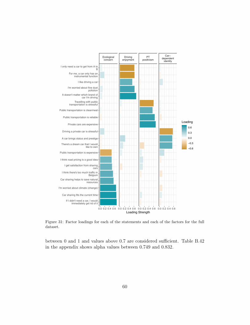
Ecologicalconcern

Drivingenjoyment

PTpositivism

Car−dependent

identity

0.0 0.2 0.4 0.6 0.0 0.2 0.4 0.6 0.0 0.2 0.4 0.6 0.0 0.2 0.4 0.6

If I didn't need a car, I wouldimmediately get rid of it

Car sharing fits the current time

I'm worried about climate (change)

Car sharing helps to save naturalresources

I think there's too much traffic inBelgium

I get satisfaction from sharingcars

I think road pricing is a good idea

Public transportation is expensive

There's a dream car that I wouldlike to own

A car brings status and prestige

Driving a private car is stressful

Private cars are expensive

Public transportation is reliable

Public transportation is clean/neat

Travelling with publictransportation is stressful

It doesn't matter which brand ofcar I'm driving

I'm worried about fine dustpollution

I like driving a car

For me, a car only has aninstrumental function

I only need a car to get from A toB

Loading Strength

−0.6

−0.3

0.0

0.3

0.6

Loading

Figure 31: Factor loadings for each of the statements and each of the factors for the fulldataset.

between 0 and 1 and values above 0.7 are considered su�cient. Table B.42in the appendix shows alpha values between 0.749 and 0.832.

60

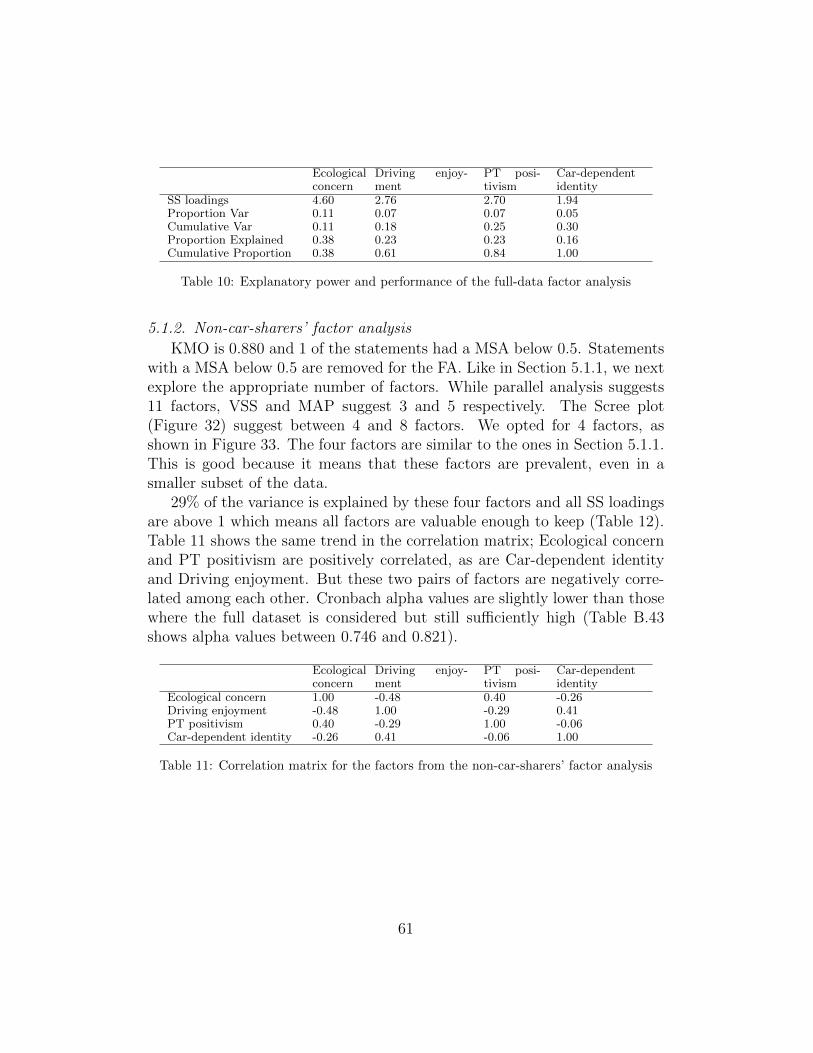
Ecologicalconcern

Driving enjoy-ment

PT posi-tivism

Car-dependentidentity

SS loadings 4.60 2.76 2.70 1.94Proportion Var 0.11 0.07 0.07 0.05Cumulative Var 0.11 0.18 0.25 0.30Proportion Explained 0.38 0.23 0.23 0.16Cumulative Proportion 0.38 0.61 0.84 1.00

Table 10: Explanatory power and performance of the full-data factor analysis

5.1.2. Non-car-sharers’ factor analysisKMO is 0.880 and 1 of the statements had a MSA below 0.5. Statements

with a MSA below 0.5 are removed for the FA. Like in Section 5.1.1, we nextexplore the appropriate number of factors. While parallel analysis suggests11 factors, VSS and MAP suggest 3 and 5 respectively. The Scree plot(Figure 32) suggest between 4 and 8 factors. We opted for 4 factors, asshown in Figure 33. The four factors are similar to the ones in Section 5.1.1.This is good because it means that these factors are prevalent, even in asmaller subset of the data.

29% of the variance is explained by these four factors and all SS loadingsare above 1 which means all factors are valuable enough to keep (Table 12).Table 11 shows the same trend in the correlation matrix; Ecological concernand PT positivism are positively correlated, as are Car-dependent identityand Driving enjoyment. But these two pairs of factors are negatively corre-lated among each other. Cronbach alpha values are slightly lower than thosewhere the full dataset is considered but still su�ciently high (Table B.43shows alpha values between 0.746 and 0.821).

Ecologicalconcern

Driving enjoy-ment

PT posi-tivism

Car-dependentidentity

Ecological concern 1.00 -0.48 0.40 -0.26Driving enjoyment -0.48 1.00 -0.29 0.41PT positivism 0.40 -0.29 1.00 -0.06Car-dependent identity -0.26 0.41 -0.06 1.00

Table 11: Correlation matrix for the factors from the non-car-sharers’ factor analysis

61

●

●

●

●

●

●● ●

● ● ●● ● ● ● ● ● ● ● ● ● ● ● ● ● ● ● ● ● ● ● ● ● ● ● ● ●

● ●

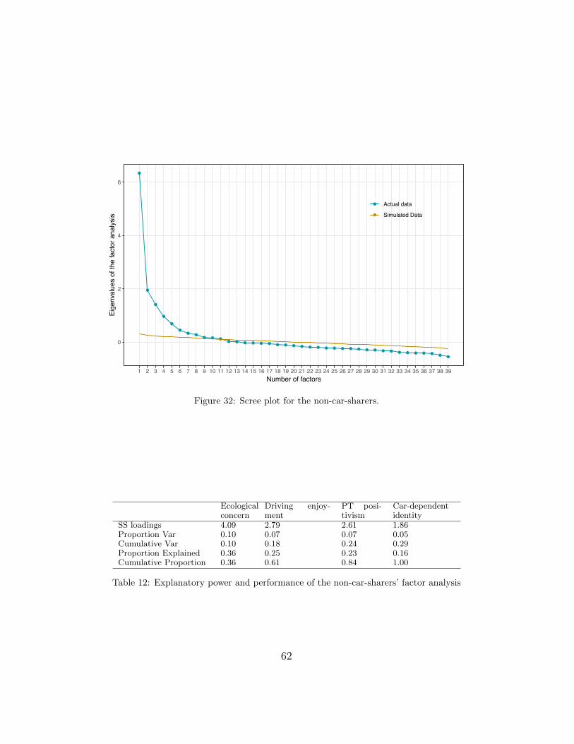
0

2

4

6

1 2 3 4 5 6 7 8 9 10 11 12 13 14 15 16 17 18 19 20 21 22 23 24 25 26 27 28 29 30 31 32 33 34 35 36 37 38 39Number of factors

Eige

nval

ues

of th

e fa

ctor

ana

lysi

s

●

●

Actual data

Simulated Data

Figure 32: Scree plot for the non-car-sharers.

Ecologicalconcern

Driving enjoy-ment

PT posi-tivism

Car-dependentidentity

SS loadings 4.09 2.79 2.61 1.86Proportion Var 0.10 0.07 0.07 0.05Cumulative Var 0.10 0.18 0.24 0.29Proportion Explained 0.36 0.25 0.23 0.16Cumulative Proportion 0.36 0.61 0.84 1.00

Table 12: Explanatory power and performance of the non-car-sharers’ factor analysis

62

Ecologicalconcern

Drivingenjoyment

PTpositivism

Car−dependent

identity

0.0 0.2 0.4 0.6 0.0 0.2 0.4 0.6 0.0 0.2 0.4 0.6 0.0 0.2 0.4 0.6

If I didn't need a car, I wouldimmediately get rid of it

I'm worried about climate (change)

Car sharing fits the current time

Car sharing helps to save naturalresources

I think there's too much traffic inBelgium

I think road pricing is a good idea

I get satisfaction from sharingcars

Public transportation is expensive

A car brings status and prestige

There's a dream car that I wouldlike to own

Driving a private car is stressful

Private cars are expensive

Public transportation is reliable

Public transportation is clean/neat

Travelling with publictransportation is stressful

It doesn't matter which brand ofcar I'm driving

I'm worried about fine dustpollution

I like driving a car

For me, a car only has aninstrumental function

I only need a car to get from A toB

Loading Strength

−0.6

−0.3

0.0

0.3

0.6

Loading

Figure 33: Factor loadings for each of the statements and each of the factors.

63

5.1.3. Car-sharers’ factor analysisThis section focuses on people who currently share cars. This means there

are substantially less respondents than in the previous analyses but there aresome additional statements; 46 in total in stead of 40. KMO is 0.685 and 1of the statements had a MSA below 0.5. Statements with a MSA below 0.5are removed for the FA..

VSS and MAP suggest 8 and 3 factors respectively while parallel anal-ysis and the Scree plot find 6 to be a good number of factors for our data(Figure 34). Figure 33 shows the final choice with, again, 4 factors that havesimilar interpretations as the factors in the previous sections. The correla-tions are in line with what was seen in the previous section (Table 13) andthe factors explain 23% of the variance (Table 14). Some statements thatwere only included in sharers’ surveys also have high factor loadings (for in-stance ‘Thanks to car-sharing, I meet new and interesting people’ and ‘I getsatisfaction from sharing car’, see Figure 35).

The Cronbach alpha values are now slightly lower; between 0.681 and0.769 (see Table B.44). As the dataset is much smaller, we have to acceptthese slightly disappointing alpha values.

●

●

●

●

●

●● ●

● ● ●● ● ● ● ● ● ● ● ● ● ● ● ● ● ● ● ● ● ● ● ● ● ● ● ● ●

● ●

0

2

4

6

1 2 3 4 5 6 7 8 9 10 11 12 13 14 15 16 17 18 19 20 21 22 23 24 25 26 27 28 29 30 31 32 33 34 35 36 37 38 39Number of factors

Eige

nval

ues

of th

e fa

ctor

ana

lysi

s

●

●

Actual data

Simulated Data

Figure 34: Scree plot for the car-sharers.

64

Social& eco-logicalconcern

Shared mobility Drivingenjoyment

Car-dependentidentity

Social & ecological con-cern

1.00 -0.27 -0.04 0.28

Shared mobility -0.27 1.00 0.31 -0.16Driving enjoyment -0.04 0.31 1.00 0.01Car-dependent identity 0.28 -0.16 0.01 1.00

Table 13: Correlation matrix for the factors from the car-sharers’ factor analysis

Social& eco-logicalconcern

Shared mobility Drivingenjoyment

Car-dependentidentity

SS loadings 2.94 2.56 2.34 2.33Proportion Var 0.07 0.06 0.05 0.05Cumulative Var 0.07 0.12 0.18 0.23Proportion Explained 0.29 0.25 0.23 0.23Cumulative Proportion 0.29 0.54 0.77 1.00

Table 14: Explanatory power and performance of the car-sharers’ factor analysis

65

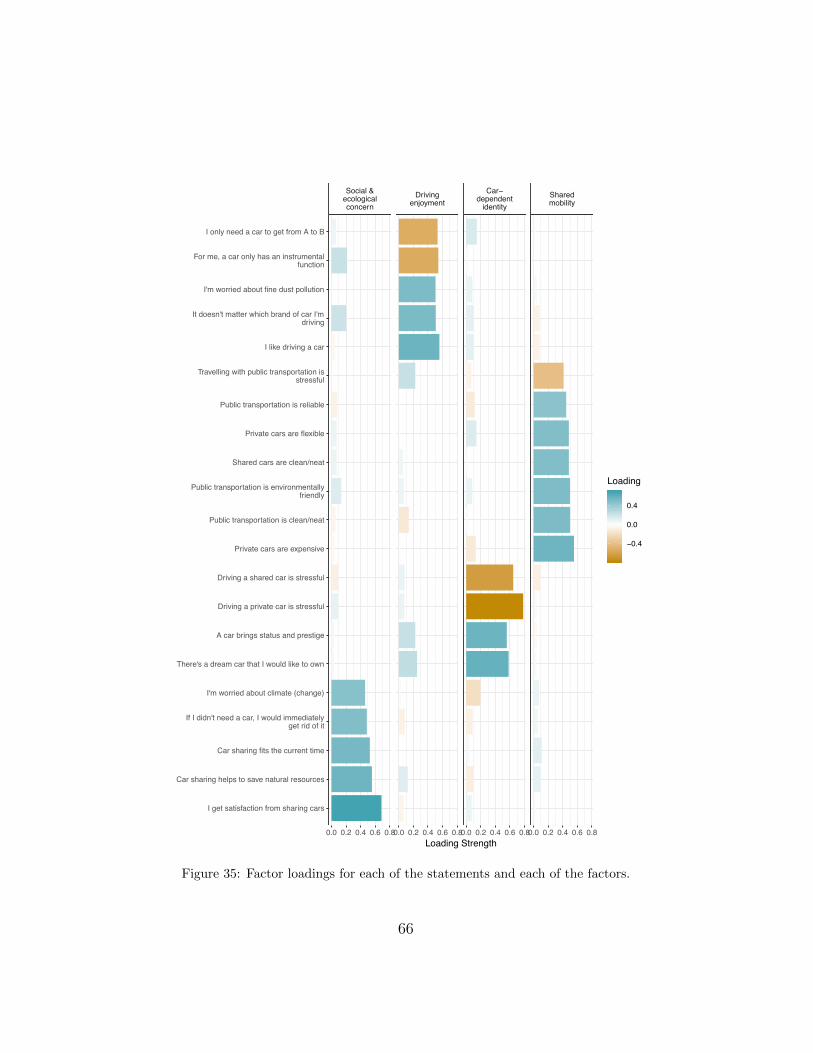
Social &ecologicalconcern

Drivingenjoyment

Car−dependent

identitySharedmobility

0.0 0.2 0.4 0.6 0.80.0 0.2 0.4 0.6 0.80.0 0.2 0.4 0.6 0.80.0 0.2 0.4 0.6 0.8

I get satisfaction from sharing cars

Car sharing helps to save natural resources

Car sharing fits the current time

If I didn't need a car, I would immediatelyget rid of it

I'm worried about climate (change)

There's a dream car that I would like to own

A car brings status and prestige

Driving a private car is stressful

Driving a shared car is stressful

Private cars are expensive

Public transportation is clean/neat

Public transportation is environmentallyfriendly

Shared cars are clean/neat

Private cars are flexible

Public transportation is reliable

Travelling with public transportation isstressful

I like driving a car

It doesn't matter which brand of car I'mdriving

I'm worried about fine dust pollution

For me, a car only has an instrumentalfunction

I only need a car to get from A to B

Loading Strength

−0.4

0.0

0.4

Loading

Figure 35: Factor loadings for each of the statements and each of the factors.

66

5.2. Predicting the car-sharing intention

The sensitivity analyses in section 4 already investigated factors thatmight influence whether a respondent shares cars or not. We also askedrespondents whether they would ever consider becoming a member of a car-sharing system (Figure 36). This not only allows us to look for significant fac-tors that determine current car-sharing membership but also possible mem-bership in the future.

Researchers have previously hypothesized that younger, highly-educatedpeople are more likely to share cars. To investigate these and other hy-potheses, an ordered multinomial regression model was fit on the data1. Theoutcome or dependent variable is the car-sharing intention which is ordered;car-sharing intention is highest for current car-sharers and lowest for thosewho answered ‘No, I would never [share cars]’ (this is category 0). Peo-ple in higher categories (categories 1, 2, 3 and 4) are more likely to sharecars. Therefor, positive coe�cients for independent variables indicate thatthe model would predict a higher probability for higher categories i.e. ahigher car-sharing intention. As explanatory variables, all variables that werefound significant in previous research (see literature review and Section 4)were tested. In addition, we included the factors of section 5.1.1.

The model was fit using the the vglm function from the VGAM packagein R2. The results can be found in Table 15. The table also included oddsratios. For a unit increase in a continuous predictor or when changing levelsof a categorical predictor, the odds for cases in a group that is greater thank versus less than or equal to k are ‘odds times’ larger.

The multinomial logit model shows that:

1. Males are more likely to share cars. This is similar to Prieto et al.(2017). Although this might seem counter-intuitive given that mate-rialism has often been found to be higher for men than women (East-man et al. 1997, Rimple et al. 2015, Segal and Podoshen 2013), oneshould consider that that this model already corrects for these atti-tudes through the four factors from section 5.1.1.

1Respondents that did not know enough about car-sharing or those who indicated thatthey used to be a member were left out.

2other functions exist, such as the polr function from the MASS package, the clmfunction from the ordinal package, the lrm function from the rms package, or the oglmxfunction from the oglmx package. The multinom function from the nnet package fitsregular(not ordered) multinomial regressions

67

Yes, definitely

Yes,perhaps in thefar future

No, I do not thinkso

No, I would never dothis

I do not know enoughabout car sharing to

make this decision

I do not know whata car sharing system

is

I used to be amember of a car

sharing system but Iquit

0 200 400 600Number of respondents

Car

sha

ring

inte

ntio

nWould you ever consider to start sharing cars?

Figure 36: car-sharing intention among all respondents.

2. The factors of section 5.1.1 are good predictors for the car-sharing in-tention. People who enjoy driving have lower car-sharing intention.High scores on any of the other three factors increases car-sharing in-tention. Similar conclusions have been drawn in previous research.Burkhardt and Millard-Ball (2006), Efthymiou and Antoniou (2016)showed that people who are environmentally conscious (this may co-incide with people with high environmental concern in our study) aremore likely to share cars. Efthymiou and Antoniou (2016) also showedthat positive attitude towards public transport and high use of publictransport encourages car-sharing.

3. People that had higher education are more likely to share cars. Ed-ucation is incorporated through four dummy variables. Primary orsecondary education is the baseline. The model shows that, the higherthe education, the higher the car-sharing intention (Bachelor’s educa-tion is higher than secondary, then there’s the Master’s degree, andthose with more than a Master’s degree (>Master) have the highestcar-sharing intention).

4. We have five employment categories in the model. Unemployed (thebaseline), students, part-time workers, full-time workers and retired

68

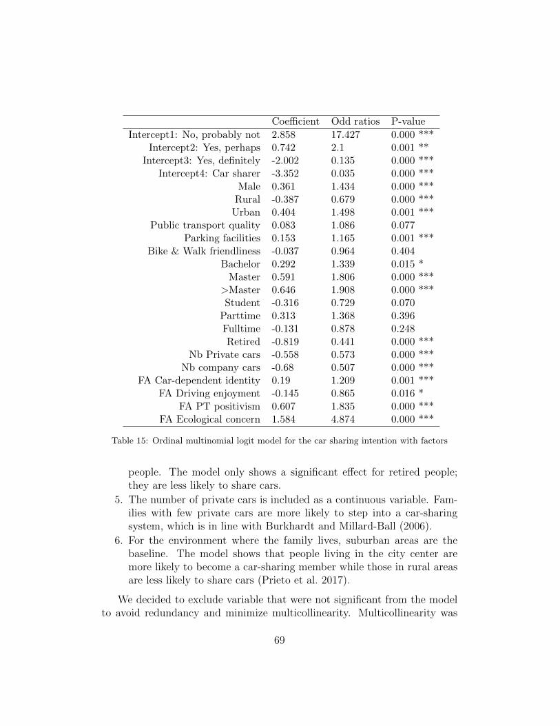
Coe�cient Odd ratios P-valueIntercept1: No, probably not 2.858 17.427 0.000 ***

Intercept2: Yes, perhaps 0.742 2.1 0.001 **Intercept3: Yes, definitely -2.002 0.135 0.000 ***

Intercept4: Car sharer -3.352 0.035 0.000 ***Male 0.361 1.434 0.000 ***Rural -0.387 0.679 0.000 ***Urban 0.404 1.498 0.001 ***

Public transport quality 0.083 1.086 0.077Parking facilities 0.153 1.165 0.001 ***

Bike & Walk friendliness -0.037 0.964 0.404Bachelor 0.292 1.339 0.015 *Master 0.591 1.806 0.000 ***

>Master 0.646 1.908 0.000 ***Student -0.316 0.729 0.070Parttime 0.313 1.368 0.396Fulltime -0.131 0.878 0.248Retired -0.819 0.441 0.000 ***

Nb Private cars -0.558 0.573 0.000 ***Nb company cars -0.68 0.507 0.000 ***

FA Car-dependent identity 0.19 1.209 0.001 ***FA Driving enjoyment -0.145 0.865 0.016 *

FA PT positivism 0.607 1.835 0.000 ***FA Ecological concern 1.584 4.874 0.000 ***

Table 15: Ordinal multinomial logit model for the car sharing intention with factors

people. The model only shows a significant e↵ect for retired people;they are less likely to share cars.

5. The number of private cars is included as a continuous variable. Fam-ilies with few private cars are more likely to step into a car-sharingsystem, which is in line with Burkhardt and Millard-Ball (2006).

6. For the environment where the family lives, suburban areas are thebaseline. The model shows that people living in the city center aremore likely to become a car-sharing member while those in rural areasare less likely to share cars (Prieto et al. 2017).

We decided to exclude variable that were not significant from the modelto avoid redundancy and minimize multicollinearity. Multicollinearity was

69

checked through generalized variance inflation factors and did not seem tobe a problem in the final model as shown in section 5.2.1. Interestingly, theage and the family composition appeared not to be significant in any form,as shown in the extended model in Table B.45 in the appendix

We tried a continuous age variable (linear and quadratic), and categoricalage variables with di↵erent cut-o↵ points. None appeared significant andsince the correlation with ’student’ and ’retired was high, we decided toexclude it from the model. This contrasts with Loose (2010), Shaheen et al.(1998), Prieto et al. (2017), who concluded that being younger increases thelikelihood of sharing cars.

While Efthymiou and Antoniou (2016) showed that households with few(or no) kids are more likely to share cars, we found no significant e↵ects forthe family composition. We tested a continuous variable for the total numberof family members, the total number of kids, or a dummy variable that was1 for families with kids. All attempts failed to deliver any significant e↵ects.It is possible that smaller/younger kids that are still in a car seat pose abigger barrier to start sharing cars but our data did not allow us to test thishypothesis. We only asked for the number of minors (younger than 18) inthe family.

5.2.1. Multicollinearity checkAs the model includes many categorical variables, generalized Variance

Inflation Factors (VIFs) were calculated, displayed in Table 16. The gener-alized VIF is the VIF, corrected by the number of degrees of freedom (Df)

of the predictor variable and may be compared to thresholds of 101

2⇤Df to as-sess collinearity (Fox and Monette 1992). Some variables that are included ashigher-order terms or in interaction terms have high VIF values, as expected.Overall, multicollinearity seems to be of little concern in the model.

70

GVIF Degrees of freedom (Df) GVIF(1/(2⇤Df))

Male 1.16 1 1.08Living area 1.55 3 1.08

Public transport quality 1.36 1 1.17Parking facilities 1.21 1 1.10

Bike & Walk friendliness 1.16 1 1.08Education 1.28 4 1.03

Work 1.37 4 1.04Nb Private cars 1.31 1 1.15

Nb company cars 1.14 1 1.07FA Car-dependent identity 1.30 1 1.14

FA Driving enjoyment 1.61 1 1.27FA PT positivism 1.46 1 1.21

FA Ecological concern 1.80 1 1.34

Table 16: Generalized variance inflation factor (GVIF). The transformationGVIF(1/(2⇤Df)) makes the VIFs comparable across di↵erent number of parameters

The correlation matrix in Figure 37 confirms that collinearity does notappear to be a problem. The highest correlations appear between binarydummy variables that represent categorical variables. High correlations be-tween these variables are to be expected.

71

1 0.02 −0.04 −0.05 0.06 0 0.08 0.05 0.05 −0.1 0.01 −0.16 −0.17 −0.14 −0.13 0.01 −0.17 −0.14 0.03

0.02 1 0.34 −0.28 0.06 0.12 0.01 0.01 0.05 −0.02 −0.02 0.02 0.01 −0.07 0 0.01 −0.01 −0.08 0.01

−0.04 0.34 1 0.17 −0.21 −0.04 0.03 0 0.03 0.02 0.01 −0.05 −0.04 0.1 0.06 0 −0.02 −0.04 −0.04

−0.05 −0.28 0.17 1 −0.07 −0.14 0 0.01 0.02 −0.04 −0.01 −0.02 −0.03 −0.03 −0.02 −0.02 0.04 0.23 0.01

0.06 0.06 −0.21 −0.07 1 −0.23 0.03 0.07 0.08 −0.04 0 0.01 −0.01 0.01 0.01 0.07 −0.01 0.08 0.11

0 0.12 −0.04 −0.14 −0.23 1 0 0.01 −0.01 0.07 −0.01 0 −0.01 −0.03 0.02 0.07 0.02 0.02 −0.06

0.08 0.01 0.03 0 0.03 0 1 0.61 0.47 0.05 0.01 −0.05 0.06 −0.02 −0.05 −0.02 0 0.04 −0.12

0.05 0.01 0 0.01 0.07 0.01 0.61 1 0.5 0.09 0.01 −0.08 0.04 0.01 −0.1 0 0.01 −0.01 −0.15

0.05 0.05 0.03 0.02 0.08 −0.01 0.47 0.5 1 0.05 0.03 −0.11 0.05 −0.06 −0.11 0.04 0.03 0 −0.12

−0.1 −0.02 0.02 −0.04 −0.04 0.07 0.05 0.09 0.05 1 0.14 0.47 0.28 0.27 0.14 −0.11 −0.03 0.02 0.02

0.01 −0.02 0.01 −0.01 0 −0.01 0.01 0.01 0.03 0.14 1 0.2 0.13 0.01 0.01 0.02 −0.02 −0.02 0

−0.16 0.02 −0.05 −0.02 0.01 0 −0.05 −0.08 −0.11 0.47 0.2 1 0.44 0.02 −0.05 −0.09 −0.01 0.04 0.01

−0.17 0.01 −0.04 −0.03 −0.01 −0.01 0.06 0.04 0.05 0.28 0.13 0.44 1 −0.05 0.06 0.01 0.02 −0.09 0.01

−0.14 −0.07 0.1 −0.03 0.01 −0.03 −0.02 0.01 −0.06 0.27 0.01 0.02 −0.05 1 0.22 −0.1 −0.02 0.02 0.06

−0.13 0 0.06 −0.02 0.01 0.02 −0.05 −0.1 −0.11 0.14 0.01 −0.05 0.06 0.22 1 −0.08 −0.03 0 0.02

0.01 0.01 0 −0.02 0.07 0.07 −0.02 0 0.04 −0.11 0.02 −0.09 0.01 −0.1 −0.08 1 −0.34 −0.09 0.11

−0.17 −0.01 −0.02 0.04 −0.01 0.02 0 0.01 0.03 −0.03 −0.02 −0.01 0.02 −0.02 −0.03 −0.34 1 0.14 0.24

−0.14 −0.08 −0.04 0.23 0.08 0.02 0.04 −0.01 0 0.02 −0.02 0.04 −0.09 0.02 0 −0.09 0.14 1 −0.14

0.03 0.01 −0.04 0.01 0.11 −0.06 −0.12 −0.15 −0.12 0.02 0 0.01 0.01 0.06 0.02 0.11 0.24 −0.14 1

Male

Rural

Urban

Public transport quality

Parking facilities

Bike & Walk friendliness

Bachelor

Master

>Master

Student

Parttime

Fulltime

Retired

Nb Private cars

Nb company cars

FA Car−dependent identity

FA Driving enjoyment

FA PT positivism

FA Ecological concern

MaleRura

lUrba

n

Public

trans

port q

uality

Parking

facili

ties

Bike & W

alk fri

endlin

ess

Bache

lor

Master

>Mas

ter

Studen

t

Parttim

e

Fulltim

e

Retired

Nb Priv

ate ca

rs

Nb com

pany

cars

FA Car−

depe

nden

t iden

tity

FA Driv

ing en

joymen

t

FA PT po

sitivis

m

FA Eco

logica

l conc

ern

−1.0

−0.5

0.0

0.5

1.0Corr

Figure 37: Correlation matrix for all explanatory variables that are in the model of Table 15

5.3. Non-sharer’s discrete choice experiment

As described in section 2.5, we asked each of the non-sharers to imaginethat they want to expand their mobility options and let them choose betweeneither buying or sharing a car (or to opt-out). Each respondent was askedto make eight such choices and, in each choice, the attributes that are listedin Table 3 were varied. Random utility theory poses that a choice dependson the utilities associated with all attributed and attribute levels. A respon-dent’s utility function is assumed to consist of a deterministic and randomcomponent (✏i) (Christie et al. 2004) and to take the form of a linear functionof the form (Day et al. 2012, Ryan et al. 2008)

72

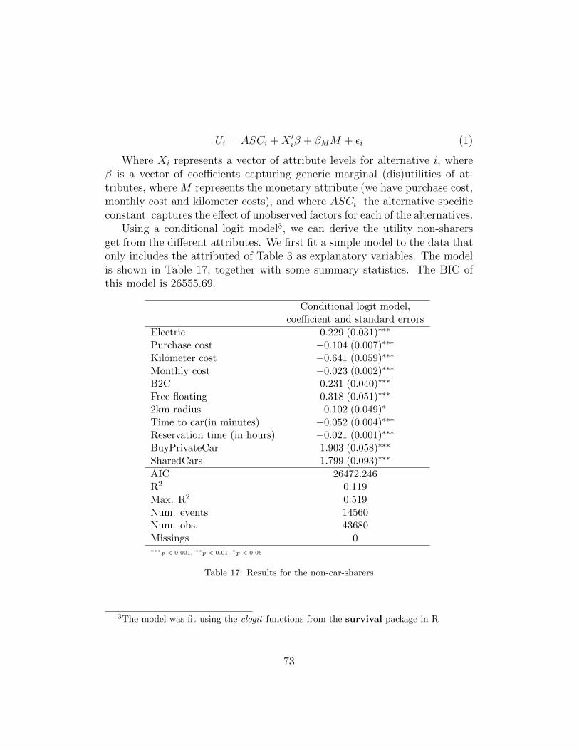
Ui = ASCi +X 0i� + �MM + ✏i (1)

Where Xi represents a vector of attribute levels for alternative i, where� is a vector of coe�cients capturing generic marginal (dis)utilities of at-tributes, where M represents the monetary attribute (we have purchase cost,monthly cost and kilometer costs), and where ASCi the alternative specificconstant captures the e↵ect of unobserved factors for each of the alternatives.

Using a conditional logit model3, we can derive the utility non-sharersget from the di↵erent attributes. We first fit a simple model to the data thatonly includes the attributed of Table 3 as explanatory variables. The modelis shown in Table 17, together with some summary statistics. The BIC ofthis model is 26555.69.

Conditional logit model,coe�cient and standard errors

Electric 0.229 (0.031)⇤⇤⇤

Purchase cost �0.104 (0.007)⇤⇤⇤

Kilometer cost �0.641 (0.059)⇤⇤⇤

Monthly cost �0.023 (0.002)⇤⇤⇤

B2C 0.231 (0.040)⇤⇤⇤

Free floating 0.318 (0.051)⇤⇤⇤

2km radius 0.102 (0.049)⇤

Time to car(in minutes) �0.052 (0.004)⇤⇤⇤

Reservation time (in hours) �0.021 (0.001)⇤⇤⇤

BuyPrivateCar 1.903 (0.058)⇤⇤⇤

SharedCars 1.799 (0.093)⇤⇤⇤

AIC 26472.246R2 0.119Max. R2 0.519Num. events 14560Num. obs. 43680Missings 0⇤⇤⇤p < 0.001, ⇤⇤p < 0.01, ⇤p < 0.05

Table 17: Results for the non-car-sharers

3The model was fit using the clogit functions from the survival package in R

73

It can be seen that all costs have a negative coe�cient. This is logical ashigher costs typically mean a lower utility for consumers. We can also seethat non-sharers get a positive utility from electric cars (over petrol or dieselcars), from a B2C car-sharing organization (as opposed to P2P), and flexiblecar-sharing systems such as a free-floating system or one where the car canbe left behind in a 2km radius (as opposed to systems where the car needs tobe left behind in exactly the same parking spot). The utility of a car-sharingo↵ering for consumers decreases if the time to get to the car increases of ifthe car needs to be reserved a long time in advance.

We can also derive the willingness to pay (WTP) for the di↵erent at-tributes from the model in Table 17. The marginal WTP for a particularchange in one specific attribute level, i.e. the marginal rate of substitution,can be estimated as a ratio of estimated coe�cients:

WTP = �coe�cient of the attribute level

coe�cient of price(2)

As the kilometer cost applies to both the car-sharing and car buyingoption, we used the coe�cient of the kilometer costs to calculate the WTPvalues that are shown in Table 18. It shows, for instance, that people arewilling to pay approximately 50 cents per kilometer more for a free-floatingsystem than a station-based system. For each additional minute longer oneneeds to get to the shared car, people want to pay 8 cents less per kilometer.

WTPElectric 0.36 ***

Purchase Cost -0.16 ***B2C 0.36 ***

Free-floating 0.50 ***2km radius 0.16 *

Time to car (in minutes) -0.08 ***Reservation time (in hours) -0.03 ***

Buy a car 2.97 ***Shared car 2.81 ***

Table 18: Willingness to pay in euros per kilometer

74

5.3.1. Non-sharer’s DCE with latent classesThe model of Table 17 only includes the attributes as explanatory vari-

ables and assumes homogeneity in preferences. However, it is highly likelythat the choices also depend on respondent characteristics. This sectiontherefor explores a latent class model. In a latent class model, we assumethat there are di↵erent classes of respondents who will make di↵erent choicein the DCE. Although class membership is not directly observable, we canderive a lot of information on class membership based on the choices thatwere made and, possibly, also observable respondent characteristics such asdemographics and attitudes. The best BIC value was obtained from a modelwith three class, which is shown in Table 19. Factor scores were used to helpallocate respondents to classes; Table 20 provides some more insights in thetype of people that belong to each of the classes, it shows that:

• Class one is the smallest group because the intercept for the otherclasses is positive

• Respondents with high car-dependent identity are most likely to belongto class 2 and least likely to belong to class 3

• Class 1 enjoys driving the least

• Class 1 has the lowest ecological concern and class three has the highest.

• Class 3 is most positive about PT and class 2 the least.

In the appendix, Table B.46 and Table B.47 show additional summarytables for each of the classes’ demographics.

The first class prefers a B2C system over a P2P system the most and,since the ASC for the shared car is negative, they seem to rather choose theopt-out than the shared car. Summary tables B.46 and B.47 show that thisclass is typically older and expressed low car-sharing intention. Most retiredrespondents are in this first class.

The second class, is the only class that has a negative WTP for electriccars. They consider cars to be status symbols and do not like public trans-portation. Table B.46 shows that this class has the largest group of full-timeworking people.

The third class has, on average, more public transport subscriptions inthe family, owns more bikes and less (company) cars (Table B.47). Theyalso are less likely to live in an urban environment, are higher educated and

75

most of the respondent who used to share cars but stopped are in this class(Table B.46).

76

Tab

le19:Coe�cientestimates,p-values

andW

TP

per

kilometer

foreach

class

Class

1Class

2Class

3

coe�

cientp-value

WTP/k

mcoe�

cient

p-value

WTP/k

mcoe�

cient

p-value

WTP/k

m

Electricfleet

0.196

0.011

0.271

-0.230

0.079

-0.424

0.432

0.000

0.328

Purchasecost

-0.116

0.000

-0.180

0.000

-0.141

0.000

Kilom

eter

costs

-0.723

0.000

-0.542

0.018

-1.317

0.000

Mon

thly

costs

-0.061

0.000

-0.077

0.000

-0.025

0.000

B2C

0.609

0.002

0.842

0.403

0.035

0.742

0.130

0.062

0.099

Free-floating

0.118

0.579

0.163

1.197

0.000

2.208

0.385

0.000

0.292

2km

radius

-0.602

0.022

-0.833

0.177

0.544

0.326

-0.102

0.219

-0.078

Availab

ility(inminutes)

-0.055

0.008

-0.076

-0.120

0.000

-0.221

-0.076

0.000

-0.058

Reservation

time(inhou

rs)

-0.024

0.000

-0.034

-0.022

0.000

-0.041

-0.032

0.000

-0.024

ASC,PurchaseCar

0.510

0.000

0.706

5.392

0.000

9.943

2.317

0.000

1.759

ASC,Shared

car

-0.275

0.392

-0.380

3.390

0.000

6.251

3.960

0.000

3.007

Class

share(%

)22.532

31.698

45.769

77

Class 2 Class 3

coe�cient p-value coe�cient p-value

Class (intercept) 0.341 0.00 0.709 0.00Car-dependent identity 0.402 0 -0.078 0.04Driving enjoyment 0.415 0.00 0.391 0.00Ecological concern 0.140 0.00 1.379 0.00PT positivism -0.144 0.00 0.306 0.00

Table 20: coe�cient estimates and p-values for class assignment

5.4. Sharer’s discrete choice experiment

As discussed in section 2.5, the sharers were asked eight times to choosebetween two fictitious CS systems or staying with their own, current, CS sys-tem. It is particularly interesting to see whether sharers valued the di↵erentattributes in the same way as the non-sharers.

The sharers’ DCE required a bit of extra data cleaning since the thirdoption in each choice is not not just an opt-out, it is the current car-sharingsystem of the respondent. We asked respondents what their primary CSsystem is, how long it takes them to get to the shared car, and the costs theypay. The type of fleet, reservation time, type of system (B2C vs P2P), andflexibility was then derived from the data that is available online for each ofthe CS companies (Table 1 and Table 2). Due to typing mistakes or missingvalues in the costs, we had to adjust some outliers.

As with the non-sharers’ analysis, we first fit a basic conditional logitmodel that only includes the attributes of the DCE. Table 21 shows thecoe�cients, p-values, and the willingness to pay for each attribute. Justlike non-sharers, respondents are willing to pay more for electric cars thanpetrol or diesel cars and free-floating car-sharing systems are considered tobe significantly better than station-based systems. However, there are someinteresting di↵erences with the model of Table 17 (the simple model for thenon-sharers). Firstly, while B2C CS systems were considered to be signifi-cantly more attractive than P2P systems by non-sharers, sharers don’t mindP2P systems at all. This may be partly because many of the sharers in ourdata set were currently in a P2P system (see Section 4). Secondly, the reser-vation time is not significant in the model. This observation may indicatethat sharers already made a mind-switch where they do not mind thinkingahead about when they would like to use a shared car. For non-sharers, it

78

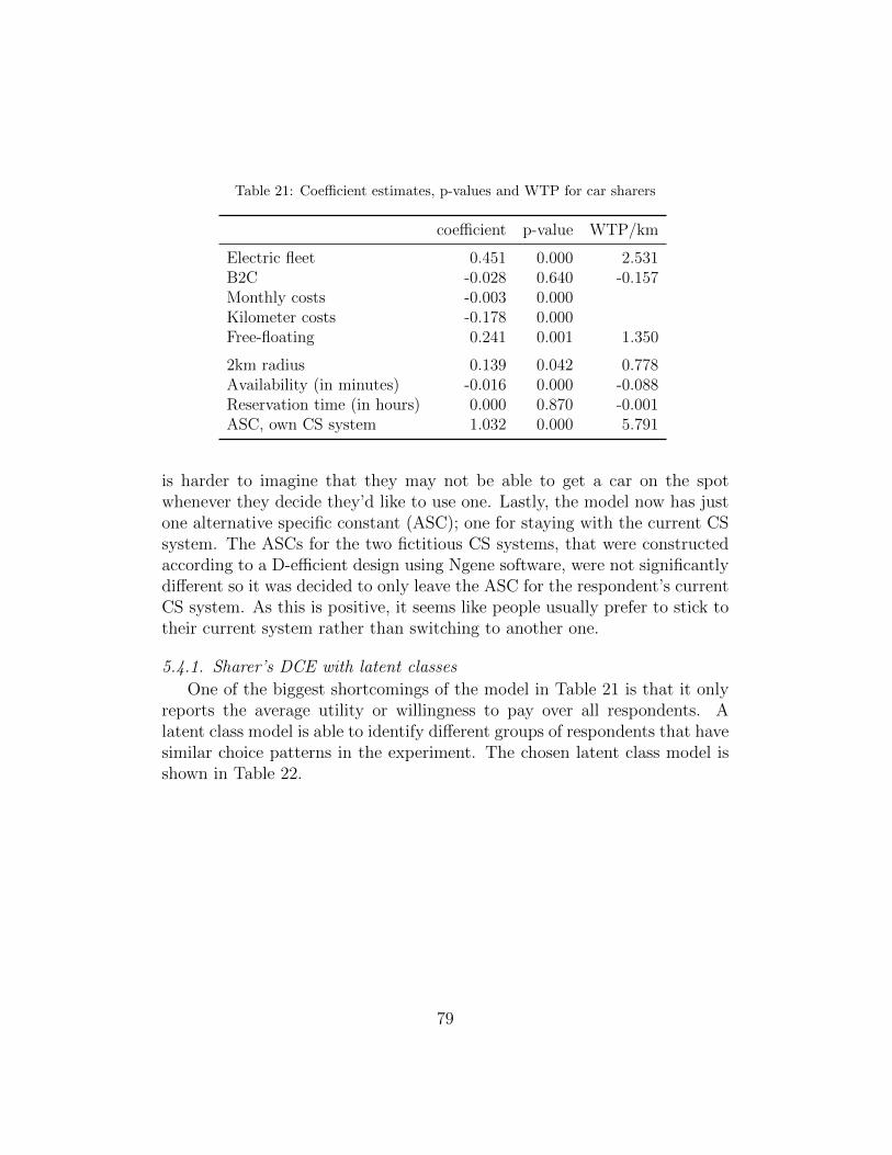
Table 21: Coe�cient estimates, p-values and WTP for car sharers

coe�cient p-value WTP/km

Electric fleet 0.451 0.000 2.531B2C -0.028 0.640 -0.157Monthly costs -0.003 0.000Kilometer costs -0.178 0.000Free-floating 0.241 0.001 1.350

2km radius 0.139 0.042 0.778Availability (in minutes) -0.016 0.000 -0.088Reservation time (in hours) 0.000 0.870 -0.001ASC, own CS system 1.032 0.000 5.791

is harder to imagine that they may not be able to get a car on the spotwhenever they decide they’d like to use one. Lastly, the model now has justone alternative specific constant (ASC); one for staying with the current CSsystem. The ASCs for the two fictitious CS systems, that were constructedaccording to a D-e�cient design using Ngene software, were not significantlydi↵erent so it was decided to only leave the ASC for the respondent’s currentCS system. As this is positive, it seems like people usually prefer to stick totheir current system rather than switching to another one.

5.4.1. Sharer’s DCE with latent classesOne of the biggest shortcomings of the model in Table 21 is that it only

reports the average utility or willingness to pay over all respondents. Alatent class model is able to identify di↵erent groups of respondents that havesimilar choice patterns in the experiment. The chosen latent class model isshown in Table 22.

79

Tab

le22:Coe�cientestimates,p-values

andW

TP

per

kilometer

foreach

class

Class

1Class

2Class

3

coe�

cient

p-value

WTP/k

mcoe�

cient

p-value

WTP/k

mcoe�

cient

p-value

WTP/k

m

Electricfleet

1.358

0.000

0.322

0.488

0.000

0.574

0.567

0.000

0.709

B2C

-0.141

0.447

-0.033

0.472

0.000

0.555

0.373

0.002

0.466

Mon

thly

costs

-0.171

0.000

-0.006

0.000

-0.011

0.063

Kilom

eter

costs

-4.214

0.000

-0.851

0.000

-0.800

0.000

Free-floating

0.167

0.446

0.040

0.026

0.860

0.031

0.270

0.048

0.337

2km

radius

-0.111

0.603

-0.026

-0.258

0.082

-0.304

-0.103

0.445

-0.129

Availab

ility(inminutes)

-0.019

0.001

-0.005

-0.010

0.165

-0.011

-0.034

0.000

-0.042

Reservation

time(inhou

rs)

-0.002

0.056

-0.001

-0.004

0.007

-0.004

-0.010

0.000

-0.013

ASC,ow

nCSsystem

-0.667

0.005

-0.158

3.870

0.000

4.549

-1.438

0.000

-1.798

Class

share(%

)27.920

46.657

25.423

80

We chose three groups, or ‘classes’, of respondents because this modelyielded the lowest BIC value; the model of Table 17 has a BIC of 4468.5, amodel with 2, 3, 4, or 5 latent classes has a BIC value of 3728.859, 3546.28,3667.16, and 3555.109 respectively. We tried adding the factor scores anddemographic information (age, education, employment) as explanatory vari-ables for class membership but none of those variables appeared significantor resulted in a decrease of the BIC value so they were left out.

Despite the fact that demographics or factor score did not appear to haveenough explanatory power to withhold them for the final model, it is stillinteresting to look at the di↵erences in respondent characteristics betweenthe classes. Section Appendix B.4 in the appendix summarizes demographics,factor scores, mobility options, and the current CS systems for the threeclasses.

The most important conclusions for each of the classes are the following:

• 27% of our sharers are in the first class. They are the only class thatdoes not prefer B2C systems over P2P systems which makes sense asover three quarters are P2P users (Table B.50). Furthermore, theydo not seems to care about how flexible the systems is because free-floating, station based and systems where the car can be left in a 2kmradius are all considered equally attractive. Table B.50 in the appendixshows that more than half of these people are currently with Degageand none have a free-floating CS provider.

• The second class is the biggest with 46.7% of the respondents. Just likethe first class, they prefer electric vehicles and the flexibility of the cardrop-o↵ is not important for them. They are the only class that clearlyprefers to stay with their current CS provider; Cambio, Degage, andPartago are the most common with 45%, 20%, and 8% respectively ofthe people in this class. They also do not mind spending some timeto get to the car (availability). As 70% of these respondents live inan urban environment, they are likely used to have everything at closewalking distance.

• The third class has the highest utility for electric cars and free-floatingsystems and they are not very attached to their current CS system.They also have the highest sensitivity for availability and reservationtime. This class appears to be living in a significantly more rural envi-ronment than the other two classes. Over half of these respondents are

81

Cambio members and Cozycar is the second most popular with 13%.The factor scores in Table B.48 show that this class also has the highestcar-dependent identity and the lowest ecological and social concern.

5.5. Conclusion

Cars move people; not just literally but also emotionally. The factoranalysis of section 5.1 shows that a large part of our respondents have verystrong opinions about cars: cars are part of their identity, and driving a carmakes them feel good and happy. Others factors that could be identifiedwere environmental concern and a positive perception of public transporta-tion. The ordinal model of section 5.2 shows that these factors are just as(or even more) valuable predictors for someones car-sharing intention thandemographics.

Knowing which type of person might have a high intention to share carsis important for car-sharing companies to expand their business and for agovernment that wants to stimulate sharing. The ordinal model of section 5.2showed that males, people living in urban areas with a higher educationare significantly more likely to have a high car-sharing intention. Retiredpeople or people with more private or company cars, on the other hand, willhave lower car-sharing intention. However, the explanatory variable with thebiggest positive e↵ect on the car-sharing intention is the factor ‘ecologicalconcern’. Urban environments will therefore not only be more interestingfor car-sharing companies because of the higher population density (whichmakes running a CS business easier) but also because of the mindset ofpeople in the city. Bringing CS to rural areas is a challenge for both CSfirms and local governments. Our results show that it would be a good ideato focus on highly educated people, particularly men, with a high ecologicalconcern. Belgian government might also make company cars or private carsless financially interesting, thus increasing car-sharing intention with many.

While the ordinal model gave some insights in the general CS intention,there are many di↵erent ways of running a CS business and each of those waysmight appeal to a di↵erent audience. The two discrete choice experiments ofsection 5.4 and 5.4 provide new insights in this area. There are two importantdi↵erences between sharers and non-sharers:

1. Non-sharers prefer a B2C system over a P2P system while sharers areindi↵erent. Attracting more people to share cars may thus be easier

82

for B2C systems or if P2P systems are better known/ more familiar.Informing customers about P2P sharing and annihilating insecurities(about liabilities, insurance and costs, for example) might help.

2. Sharers do not mind reserving a car in advance while non-sharers donot like long reservation times. This might mean that the sharers havealready made a mind-switch where they are used to not having the caravailable at all times and jumping in the car whenever they feel likeit. Just like PT, shared cars require a bit more mobility planning thanprivate cars.

Other than those di↵erences, all respondents prefer electric cars, moreflexibility for where to pick up or leave behind the car, and good availabilityof cars close-by.

6. Environmental Impact

The environmental impact of car-sharing works through two channels:technical changes and behavioural changes. Technical changes are the di↵er-ences in the technologies of cars used by car-sharing relative to private carownership. For example, shared cars might be lighter, more fuel e�cient, beused for longer (i.e. increased lifetime kms) or be more likely to be electricor use lower impact fuels. That said, these e↵ects could also work in re-verse: private cars may be used for longer since owners may be more willingto tolerate an older car or a car with small defects than would a user of acar-sharing service.

The other channel through which environmental impacts may work is be-havioural change. As discussed in section 1.2.2, car-sharing induces changesin how people fulfill their mobility needs. Some users may sell a car andreplace their car-use with car-sharing, and in doing so, they reduce theircar use, perhaps due to higher marginal costs or the reduced conveniencerelative to private cars. Others, however, for whom car-sharing does not af-fect car-ownership, may use car-sharing to substitute for public transport orother modes, creating greater environmental impacts compared to withoutcar-sharing.

In this research, the focus is on the behavioural change induced by car-sharing, specifically, changes to car-use and car ownership. Due to a lack ofdata, there is no empirical measurement of di↵erences in technical param-eters, such as fuel e�ciency and vehicle lifetime; however they have beenconsidered in a sensitivity analysis.

83

The environmental impact of car-sharing was calculated by first estimat-ing the impact of car-sharing on users’ behaviour (car-ownership and car-use)based on the survey results, and second, converting this into environmentalimpacts using life-cycle analysis. As discussed in section 1.2.2, estimating theimpact of car-sharing on behaviour is not straightforward. Since car-sharingusers choose to join car-sharing for certain reasons, comparing users to non-users will introduce selection bias and reverse causality, i.e. car-sharing usersmay be systematically di↵erent to non-users, and these di↵erences may alsobe the cause of di↵erent behaviour.

Thus, in order to estimate the treatment e↵ect of car-sharing, all alter-native explanations for a change in behaviour should be eliminated, leavingonly the e↵ect of car-sharing. Specifically, the aim is to remove the influenceof factors that may a↵ect both behaviour and the decision to join car-sharing.To do so, we estimate what the car-use and car-ownership of a car-sharinguser would be if (s)he was not a member of car-sharing. This hypotheticaloutcome is known as the counterfactual.

6.1. Method

This section outlines the approach taken to estimate the counterfactual.First, a control group was formed consisting only of non-users who showedan interest in car-sharing based on the discrete choice experiment. Second,both car-sharing users (treatment group) and non-users were sub-dividedinto di↵erent categories based on car-ownership. Third, any remaining dif-ferences based on observed characteristics between treatment and controlgroups within each category were controlled for through regression analysis.

6.1.1. Formation of treatment and control groupsThe use of treatment and control groups to find impacts of an intervention

is a recognised method in impact evaluation. The aim is to find a controlgroup that is as similar as possible to the treatment group, thereby reducingselection bias, ensuring the comparison between groups is more fair.

In this study, only non-users who said they would be interested in joiningcar-sharing in the near or far future were kept to form the control group.In addition, any non-user who did not choose car-sharing in at least 3 ofthe 8 instances in the discrete choice experiment were removed from thecontrol group. By choosing only those with an interest in car-sharing toform the control group, we remove some selection bias that would otherwisebe unobserved.

84

The treatment group of car-sharing users was trimmed to only includethose who were defined as active (i.e. users who were deemed to have beena↵ected by car-sharing), since there are many users who may be membersof car-sharing but who do not use it, and including these non-active userswould bias results. Active users were defined as those who:

1. Used car-sharing in a typical week; or

2. Sold or scrapped a car because of car-sharing; or

3. Did not purchase a car because of car-sharing

Using this definition of an active user, the sample size of the treatmentgroup is 215. The control group consists of 359 observations.

6.1.2. Decomposition of treatment and control groupsThe impact of car-sharing on car-use is directly related to car-ownership.

Car-sharing changes the way one has access to a car – it either increases ordecreases access, compared to the counterfactual where car-sharing doesn’texist. However, car-ownership may also a↵ect the decision to join car-sharing:someone without a car may join a car-sharing scheme to gain access to a cari.e. a lack of car-ownership causes the decision to join car-sharing, ratherthan car-sharing causing someone to sell a car. If we fail to capture thisreverse causality, then we will overestimate the impact of car-sharing. Toavoid these issues, we directly ask users what they did because of car-sharing,or what they would do in the absence of car-sharing with respect to carownership. Concretely, respondents to the survey were asked:

• How important was car-sharing when deciding to sell or scrap a car?

• If I was not a member of car-sharing, I would buy/lease/not have solda car. Do you agree or disagree?

This is a self-assessed question, and thus is open to bias. However, wejustify the use of this for two reasons: first, we anticipate that users areable to better make a judgement regarding the e↵ect of car-sharing on largedecisions like car-ownership than much smaller decisions such as car-use,data which other studies rely on (e.g. Martin and Shaheen (2011), Firnkornand Muller (2011). Second, this self-assessment is captured with uncertaintyembedded in the question: users are asked the extent to which car-sharing

85

was responsible on a 7 point scale. Thus, we can capture this degree ofuncertainty, and in tandem, account for the size of any bias.

Based on this observation, di↵erent categories of car-sharing users canbe defined based on how car-sharing a↵ected car-ownership in each user’shousehold. Note that it is the household level car-ownership that is used todefine these categories, rather than individual car-ownership, since cars areoften shared among members of a household rather than exclusively drivenby one individual.

Car-sharing users have been sub-divided into the following categories:

• Would-be car-owner (WCO): these users do not own a car or donot have access to one within their household, but have either sold a caror would have bought one had they not been members of car-sharing.Compared to the situation where they owned a car, these users areexpected to reduce their car-use.

• Would-be additional car-owner (WACO): users own, or have ac-cess to, at least one car in the household, but have sold a car orwould have bought an additional car had they not been members ofcar-sharing. They are expected to reduce their car-use, since the userwould have had easier access to a car compared to car-sharing.

• Car-owner (CON): these users own at least one car, or have access toone within the household, but their car-ownership has not been a↵ectedby car-sharing. They are expected to increase their car-use since theynow use car-sharing in addition to their private car-use.

• Non-car-owner (NCO): these users do not own a car or do not haveaccess to one within the household, and would not have bought a carwithout car-sharing. They increase their car-use since they would nothave access to a car without car-sharing. Their increase in car use isdirectly measurable.

The advantage of the discrete choice experiment in the survey is thatwe can identify members of the control group that are the best matches forcar-sharing users. Each respondent who was not a car-sharing member wasasked about the scenario under which they imagined the choice, i.e. werethey imagining the need for an additional car, or a replacement car. Thisallows us to find control users who are most similar to car-sharing users:

86

User category Number of observationsTreatment Control

WCO 110 180WACO 39 108CON 19 32NCO 47 N/A

Table 23: The breakdown of the sample by user category

Threshold WCO WACO CON NCO

Agree a little 110 39 19 47Agree 51 26 28 88

Totally agree 17 4 41 114

Table 24: The number of users in each category depending on the threshold used todetermine e↵ects of car-sharing on car-ownership.

only those who said they considered car-sharing as a replacement vehiclewere compared to would-be car-owners or would-be additional car-owners.

The breakdown of the user categories is shown in table 23. The largesttreatment group is would-be car-owners, followed by non-car-owners.

The distribution in table 23 is based on a looser interpretation of thecausal impact of car-sharing on car-ownership: car-sharing users who indi-cated that they “agree a little” that they sold/scrapped a car because ofcar-sharing are considered as would-be (additional) car-owners. A stricterdefinition of the causal e↵ect of car-sharing on car-ownership changes thedistribution of car-sharing users towards non-car-owners and car-owners. Ta-ble 24 shows how the distribution of users changes depending on the answerto the question; for example, if users that only answer “Agree” and “To-tally agree” are considered to have sold/scrapped/not bought a car, then thenumber of WCO users drops by more than half, while the number of WACOusers drops by a third. This table is the basis for two di↵erent scenarios,covered in section 6.4.

6.1.3. Beta regressions to estimate e↵ectThe final stage of the estimate of the treatment e↵ect is to use regressions

to control for di↵erences in characteristics between treatment and control

87

groups that were recorded in the survey. Such characteristics include: thelocation of the household, the size of the household, the distance the indi-vidual lives from work, etc. Each of these is expected to influence both thedecision to join car-sharing and car-use and car-ownership. Controlling forthese factors in a regression model should further reduce any selection biaspresent between treatment and control groups.

The dependent variable in the regression model (i.e. the e↵ect we areestimating) is the proportion of total km in a typical week travelled by privatecar and additionally, for car-sharing users, shared cars. Since the proportionis bounded between 0 and 1, linear regression methods such as ordinary leastsquares are inappropriate. Thus, a method known as beta regression wasused, allowing for a more accurate calculation of the e↵ect of car-sharing.

Of the four categories of users outlined above, a beta regression was per-formed for three: would-be car-owners, would-be additional car-owners, andcar-owners. A regression is not necessary for non-car-owners since the e↵ectof car-sharing is directly observed (i.e. the km driven by car).

Table 25 lists the control variables used in the models. These were selectedunder the assumption that they a↵ect both car-sharing and car-use, but thatthey themselves are not a↵ected by car-sharing or car-use. For example, ifa two person household lives without children, they may decide that car-sharing is preferable to owning a car since their need for a car is relativelypredictable. Thus, the number of children in a household may a↵ect car-sharing membership. But it is extremely unlikely that the reverse is true, i.e.that being a member of a car-sharing system or the amount one uses a carwill influence the number of children in a household.

Three models were estimated for each user category. In the first model, anaverage treatment e↵ect is calculated. The second model estimates di↵erenttreatment e↵ects for users of b2c and p2p systems. In the third model,we estimate the additional e↵ect of a car-sharing user living in an urban,suburban, or rural area.

6.2. Treatment e↵ects

By using beta regressions, the treatment e↵ect for each user will di↵erdepending on the proportion of km currently travelled by car. In addition,in models 2 and 3, the treatment e↵ects also di↵er depending on the typeof car-sharing and the user location, respectively. To illustrate the e↵ect ofthese parameters, simulated e↵ects have been calculated. The simulations

88

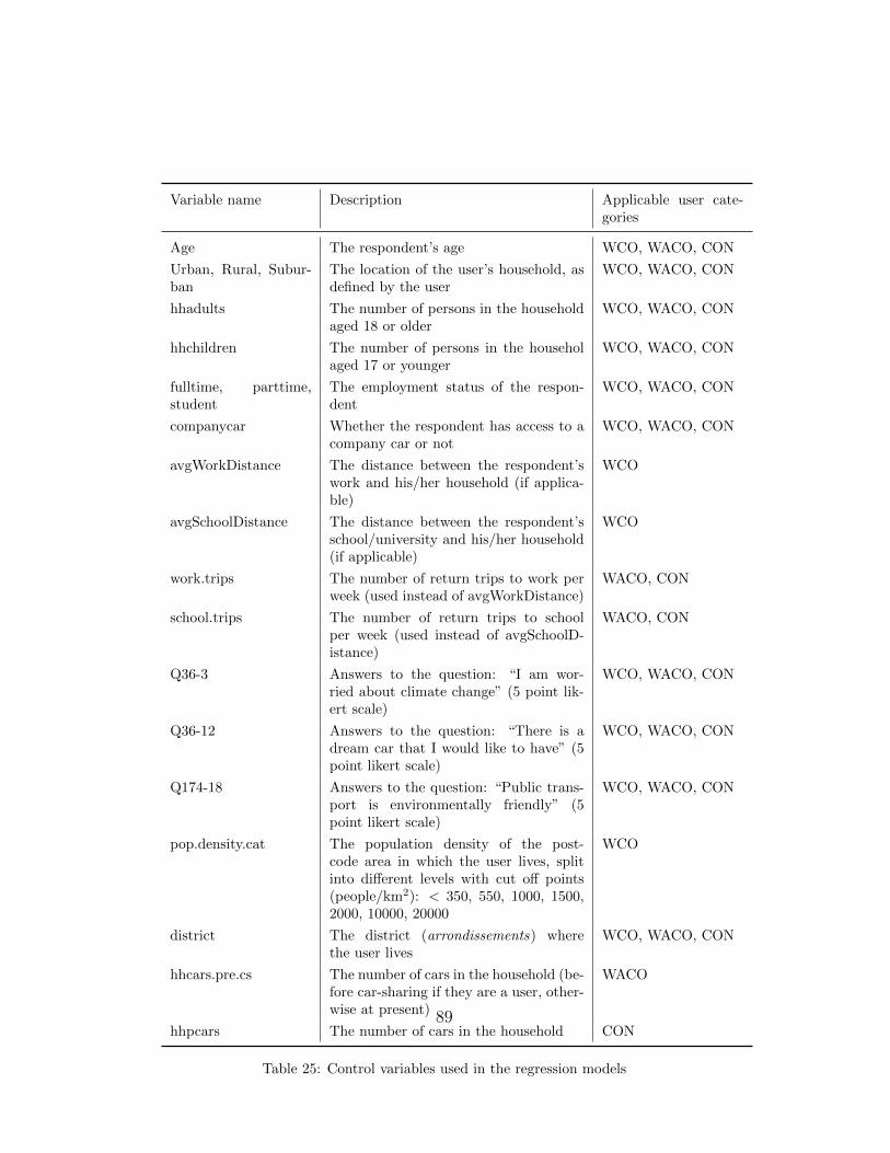
Variable name Description Applicable user cate-gories

Age The respondent’s age WCO, WACO, CON

Urban, Rural, Subur-ban

The location of the user’s household, asdefined by the user

WCO, WACO, CON

hhadults The number of persons in the householdaged 18 or older

WCO, WACO, CON

hhchildren The number of persons in the householaged 17 or younger

WCO, WACO, CON

fulltime, parttime,student

The employment status of the respon-dent

WCO, WACO, CON

companycar Whether the respondent has access to acompany car or not

WCO, WACO, CON

avgWorkDistance The distance between the respondent’swork and his/her household (if applica-ble)

WCO

avgSchoolDistance The distance between the respondent’sschool/university and his/her household(if applicable)

WCO

work.trips The number of return trips to work perweek (used instead of avgWorkDistance)

WACO, CON

school.trips The number of return trips to schoolper week (used instead of avgSchoolD-istance)

WACO, CON

Q36-3 Answers to the question: “I am wor-ried about climate change” (5 point lik-ert scale)

WCO, WACO, CON

Q36-12 Answers to the question: “There is adream car that I would like to have” (5point likert scale)

WCO, WACO, CON

Q174-18 Answers to the question: “Public trans-port is environmentally friendly” (5point likert scale)

WCO, WACO, CON

pop.density.cat The population density of the post-code area in which the user lives, splitinto di↵erent levels with cut o↵ points(people/km2): < 350, 550, 1000, 1500,2000, 10000, 20000

WCO

district The district (arrondissements) wherethe user lives

WCO, WACO, CON

hhcars.pre.cs The number of cars in the household (be-fore car-sharing if they are a user, other-wise at present)

WACO

hhpcars The number of cars in the household CON

Table 25: Control variables used in the regression models

89

are based on 1000 random draws of the treatment e↵ect from a normal distri-bution based on the results of the regression, incorporating the uncertaintyinherent in the model.

The results of the simulations show what the expected proportion of kmdriven by car would be for a user if (s)he was not a member of car-sharing.Each treatment e↵ect is estimated with a margin of error. For some of thetreatment e↵ects, we cannot be certain that it is di↵erent from 0, i.e. thatthere is any e↵ect of car-sharing on behaviour.

6.2.1. Model 1: Simulated average treatment e↵ectsThe results of the simulated average treatment e↵ects are presented in

Table 26. The table should be interpreted as follows: a WCO user whotravels 10% of his/her weekly km by car (both private and shared) would beexpected to drive 22% of his/her weekly by car if they were not a memberof car-sharing, on average. Thus, for a such a user, car-sharing causes areduction of 12% of km driven by car. The mean e↵ect for CON users showsthat car-sharing causes an increase in the amount they use a car, e.g. a CONuser who drives 10% of his/her km by car with car-sharing would be expectedto drive just 3.1% of km by car without car-sharing.

The 95% confidence intervals for all three e↵ects are shown in table 27.For both WCO and WACO users, the lower bound of the 95% confidenceinterval shows that car-sharing is expected to reduce car-use. For CONusers, however, the upper bound of the confidence interval is greater thanthe “With CS” column, meaning that we cannot conclude with certainty thatCON users increase their car-use because of car-sharing. This is due to thelow number of CON users in the sample (see table 24.

6.2.2. Model 2: Simulated treatment e↵ects for p2p vs b2c systemsThe aim of model 2 is to see if the e↵ect of car-sharing on p2p and b2c

car-sharing users di↵ers. The average treatment e↵ects based on di↵erentcar-use proportions for both p2p and b2c systems are given in table 28. Theresults can be interpreted as follows: a p2p WCO who currently drives 10%of his/her km by car would drive 25.2% of his/her km by car if (s)he wasnot a member of car-sharing. Thus, as a result of car-sharing, this user hasreduced his/her car-use by 15.2%. Car-sharing causes a reduction in car-use for both WCO and WACO users. However, for CON users, car-sharingcauses an increase in car-use: a p2p CON user who drives 10% of his/her

90

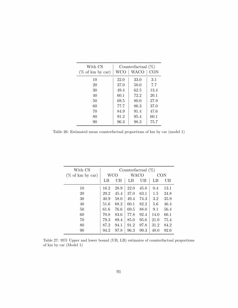
With CS Counterfactual (%)(% of km by car) WCO WACO CON

10 22.0 33.0 3.120 37.0 50.0 7.730 49.4 62.5 13.440 60.1 72.2 20.150 69.5 80.0 27.960 77.7 86.3 37.070 84.9 91.4 47.680 91.2 95.4 60.190 96.3 98.3 75.7

Table 26: Estimated mean counterfactual proportions of km by car (model 1)

With CS Counterfactual (%)(% of km by car) WCO WACO CON

LB UB LB UB LB UB

10 16.2 28.9 22.0 45.8 0.4 13.120 29.2 45.4 37.0 63.1 1.5 24.830 40.9 58.0 49.4 74.3 3.2 35.940 51.6 68.2 60.1 82.2 5.6 46.450 61.6 76.6 69.5 88.0 9.1 56.460 70.8 83.6 77.8 92.4 14.0 66.170 79.3 89.4 85.0 95.6 21.0 75.480 87.2 94.1 91.2 97.8 31.2 84.290 94.2 97.8 96.3 99.3 48.0 92.6

Table 27: 95% Upper and lower bound (UB, LB) estimates of counterfactual proportionsof km by car (Model 1)

91

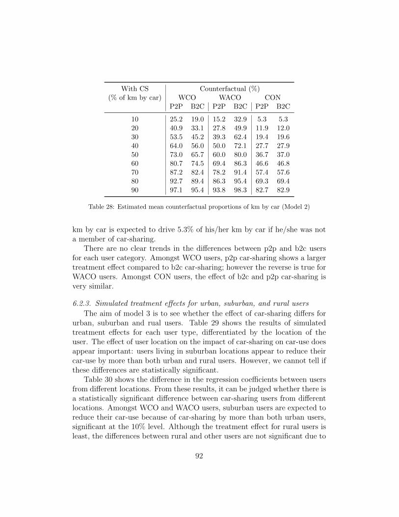
With CS Counterfactual (%)(% of km by car) WCO WACO CON

P2P B2C P2P B2C P2P B2C

10 25.2 19.0 15.2 32.9 5.3 5.320 40.9 33.1 27.8 49.9 11.9 12.030 53.5 45.2 39.3 62.4 19.4 19.640 64.0 56.0 50.0 72.1 27.7 27.950 73.0 65.7 60.0 80.0 36.7 37.060 80.7 74.5 69.4 86.3 46.6 46.870 87.2 82.4 78.2 91.4 57.4 57.680 92.7 89.4 86.3 95.4 69.3 69.490 97.1 95.4 93.8 98.3 82.7 82.9

Table 28: Estimated mean counterfactual proportions of km by car (Model 2)

km by car is expected to drive 5.3% of his/her km by car if he/she was nota member of car-sharing.

There are no clear trends in the di↵erences between p2p and b2c usersfor each user category. Amongst WCO users, p2p car-sharing shows a largertreatment e↵ect compared to b2c car-sharing; however the reverse is true forWACO users. Amongst CON users, the e↵ect of b2c and p2p car-sharing isvery similar.

6.2.3. Simulated treatment e↵ects for urban, suburban, and rural usersThe aim of model 3 is to see whether the e↵ect of car-sharing di↵ers for

urban, suburban and rual users. Table 29 shows the results of simulatedtreatment e↵ects for each user type, di↵erentiated by the location of theuser. The e↵ect of user location on the impact of car-sharing on car-use doesappear important: users living in suburban locations appear to reduce theircar-use by more than both urban and rural users. However, we cannot tell ifthese di↵erences are statistically significant.

Table 30 shows the di↵erence in the regression coe�cients between usersfrom di↵erent locations. From these results, it can be judged whether there isa statistically significant di↵erence between car-sharing users from di↵erentlocations. Amongst WCO and WACO users, suburban users are expected toreduce their car-use because of car-sharing by more than both urban users,significant at the 10% level. Although the treatment e↵ect for rural users isleast, the di↵erences between rural and other users are not significant due to

92

the small number of rural car-sharing users. Amongst CON users, suburbanusers are expected to increase their car-use by most. However, none of thee↵ects for CON users are significant, again due to the small amount of CONusers.

93

WithCS

Cou

nterfactual

(%)

(%of

kmby

car)

WCO

WACO

CON

Urban

Suburban

Rural

Urban

Suburban

Rural

Urban

Suburban

Rural

1018.7

30.6

12.3

37.0

41.7

20.7

7.3

1.7

10.2

2032.7

47.3

23.6

54.3

59.1

35.3

15.5

4.7

20.3

3044.8

59.8

34.3

66.4

70.8

47.6

24.2

8.7

30.4

4055.5

69.8

44.7

75.7

79.4

58.3

33.4

13.8

40.4

5065.3

78.0

54.8

82.9

85.8

67.8

43.1

20.1

50.4

6074.1

84.8

64.6

88.5

90.7

76.3

53.1

28.0

60.4

7082.0

90.3

74.1

93.0

94.5

83.8

63.7

37.7

70.4

8089.1

94.7

83.2

96.3

97.2

90.4

74.7

50.2

80.3

9095.3

98.0

92.0

98.7

99.1

96.0

86.6

67.2

90.2

Tab

le29:Estim

ated

meancounterfactual

proportion

sof

kmby

carby

user’shou

seholdlocation

(Mod

el3)

Usercategory

Suburban

-Urban

p-value(6=

0)Suburban

-Rural

p-value(6=

0)Urban

-Rural

p-value(6=

0)

WCO

�0.38

0.060

�0.65

0.130

�0.27

0.675

WACO

�0.12

0.740

�0.61

0.123

�0.49

0.434

CON

0.66

0.386

0.85

0.361

0.19

0.779

Tab

le30:Di↵erence

inmeanregression

coe�

cients

betweenurban

andsuburban

users

(suburban

-urban

)

94

6.3. The environmental impacts of car-sharing in Belgium

Using the estimate of the change in proportion of km driven by car,the overall impact of car-sharing on the environment for the sample of car-sharing users can be estimated. In this analysis, the impacts considered arecontributions to climate change and resource use.

The impacts are calculated using life-cycle analysis (LCA). The systemmodelled is the manufacture of a generic car, the production of petrol, andthe use of a car. Thus, emissions are generated from three main processes:car production, petrol production, and direct exhaust emissions from thecar. Maintenance and end-of-life processes have not been considered in thisanalysis. Note that the use of other modes of transport, such as publictransport, have not been included, and thus the overall of e↵ect on totalemissions caused by car-sharing cannot be concluded from this data alone.It is likely that emissions due to car-sharing would be slightly larger (butstill negative) if these impacts were included. However, relative comparisonsbetween di↵erent users (based on categories, b2c/p2p or user location) canbe judged.

To complete the LCA, a number of assumptions are made:

1. There is no change in overall km travelled by a car-sharing user

2. Shared cars and private cars have the same weight, fuel e�ciency(0.0621kg petrol per km) and lifetimes (in 250,000 km)

3. Cars are modelled as Euro 5 petrol cars of medium size (1600kg)

4. Inventories for the cars are based on the generic inventories from theEcoInvent database, v3.5

Using assumption 1, above, allows the estimate of the counterfactual kmdriven by car-sharing users to be calculated as detailed in equation 3, where

ˆKmCFi is the counterfactual km travelled by car, ˆPPCF

i is the counterfactualproportion of total km driven by car, and KmTotal/wk,i

is the total numberof km travelled in a typical week.

ˆKmCFi = ˆPPCF

i ·KmTotal/wk,i(3)

The results of the LCA have been calculated based on the di↵erent re-gression models listed above. In each LCA model, the uncertainty in thetreatment e↵ects have been propagated through the model, enabling robust-ness checks for conclusions. However, it should be noted that the models

95

Scenario Threshold WCO WACO CON NCO

Best case Agree a little 110 39 19 47Middle Agree 51 26 28 88

Table 31: The number of users from each category for both scenarios

including separate e↵ects for b2c and p2p users (model 2), and those de-pending on location (model 3) have been modelled assuming each e↵ect isindependent of the other. That is, that the e↵ect for p2p users is not af-fected by the estimated treatment e↵ect for b2c users. However, whetherthese e↵ects are truly independent is debatable. Most obviously, there maybe a systematic bias in the model, meaning that each e↵ect (b2c and p2p, orurban, suburban, and rural) is a↵ected in the same way, i.e. over or under es-timated. Given this possibility, the variance of the results for scenarios 2 and3 may be underestimated. While this a↵ects absolute conclusions regardingwhether car-sharing results in an environmental benefit, it should not a↵ectrelative conclusions, for example when comparing urban to rural users.

In addition to the three models, model 1 has been analysed under twodi↵erent scenarios depending on the number of users in each category. Thefirst scenario includes all users who at least “Agree a little” that they got ridor would have bought a car because of car-sharing as WCO/WACO users.Thus, it can be considered a “best-case” scenario. The second scenario as-sumes that only those who “Agree” or “strongly agree” that car-sharing af-fected their car-ownership are counted as WCO/WACO users. This is calledthe ”middle” scenario.

6.4. Aggregate results under di↵erent scenarios

Comparing the composition of the two scenarios (table 31), there is largerise in NCO users in the “middle” scenario. This increase comes from thosewho were considered WCO users in the best-case scenario.

Table 32 shows the aggregate results of both scenarios, broken down byuser type. In the best-case scenario, the reduction in environmental impact ofWACO and WCO users more than compensates for the increase in environ-mental impact of CON and NCO users, leading to an overall environmentalbenefit in 97.5% of simulations, with a total average reduction of 1064kg ofCO2eq. emissions. In the middle scenario, car-sharing leads to an environ-mental benefit in 30.7% of scenarios. Consulting table 32, this divergence

96

Best-case scenario Middle ScenarioUser category Average standard deviation Average standard deviation

WCO -960.4 225.3 -396.6 139.3WACO -901.9 170.0 -573.5 131.6CON 241.8 153.2 209.7 234.5NCO 556.3 - 998.2 -

Total -1064.3 547.0 237.9 504.7

Table 32: Aggregate change in of Kg CO2eq. emissions per user category per week

between the two scenarios is driven by the concurrent increase and reductionin the impact of NCO and WCO users respectively.

These results show that the environmental impacts of car-sharing are verysensitive to the e↵ect of car-sharing on car-ownership. The impacts of thosewhose car-ownership is not a↵ected by car-sharing (NCO and CON) are largeand may o↵set those who have fewer cars because of car-sharing (WCO andWACO).

6.4.1. Model 1: Average treatment e↵ectModel 1 represents the assumption that car-sharing users in each category

regardless of their location or the type of car-sharing are a↵ected in the samemanner. These are the same e↵ects listed in table 26: the proportion ofkm currently travelled by car a↵ects the estimation of the counterfactualproportion without car-sharing.

The average impact for a user in each category is shown in table 33.The impact of NCO users is not estimated by a model, thus these resultshave no uncertainty attached. The distributions of the three user types showthat the average WACO user has a larger overall reduction in GHG emissionscompared to the average WCO user. The average WACO user reduces his/herCO2eq emissions by more than an average WCO user, and this di↵erence issignificant (p ⇡ 0.00). Car-sharing causes the average CON user to increasetheir emissions, although this is not significant.

6.4.2. Model 2: separate e↵ects for p2p and b2c usersTable 34 shows the break down of the results of the average user by

user category, and figure 38 the distribution. The average p2p WCO usergenerates fewer emissions compared to b2c WCO users, while the reverse is

97

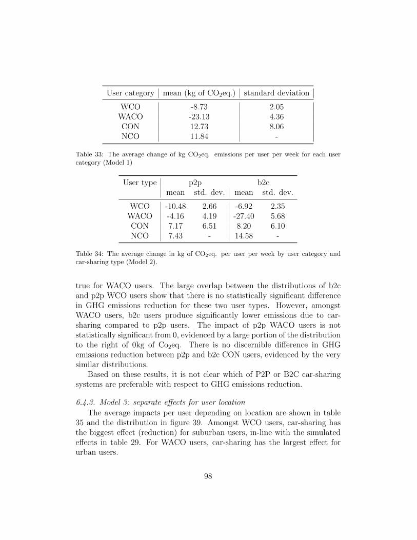
User category mean (kg of CO2eq.) standard deviation

WCO -8.73 2.05WACO -23.13 4.36CON 12.73 8.06NCO 11.84 -

Table 33: The average change of kg CO2eq. emissions per user per week for each usercategory (Model 1)

User type p2p b2cmean std. dev. mean std. dev.

WCO -10.48 2.66 -6.92 2.35WACO -4.16 4.19 -27.40 5.68CON 7.17 6.51 8.20 6.10NCO 7.43 - 14.58 -

Table 34: The average change in kg of CO2eq. per user per week by user category andcar-sharing type (Model 2).

true for WACO users. The large overlap between the distributions of b2cand p2p WCO users show that there is no statistically significant di↵erencein GHG emissions reduction for these two user types. However, amongstWACO users, b2c users produce significantly lower emissions due to car-sharing compared to p2p users. The impact of p2p WACO users is notstatistically significant from 0, evidenced by a large portion of the distributionto the right of 0kg of Co2eq. There is no discernible di↵erence in GHGemissions reduction between p2p and b2c CON users, evidenced by the verysimilar distributions.

Based on these results, it is not clear which of P2P or B2C car-sharingsystems are preferable with respect to GHG emissions reduction.

6.4.3. Model 3: separate e↵ects for user locationThe average impacts per user depending on location are shown in table

35 and the distribution in figure 39. Amongst WCO users, car-sharing hasthe biggest e↵ect (reduction) for suburban users, in-line with the simulatede↵ects in table 29. For WACO users, car-sharing has the largest e↵ect forurban users.

98

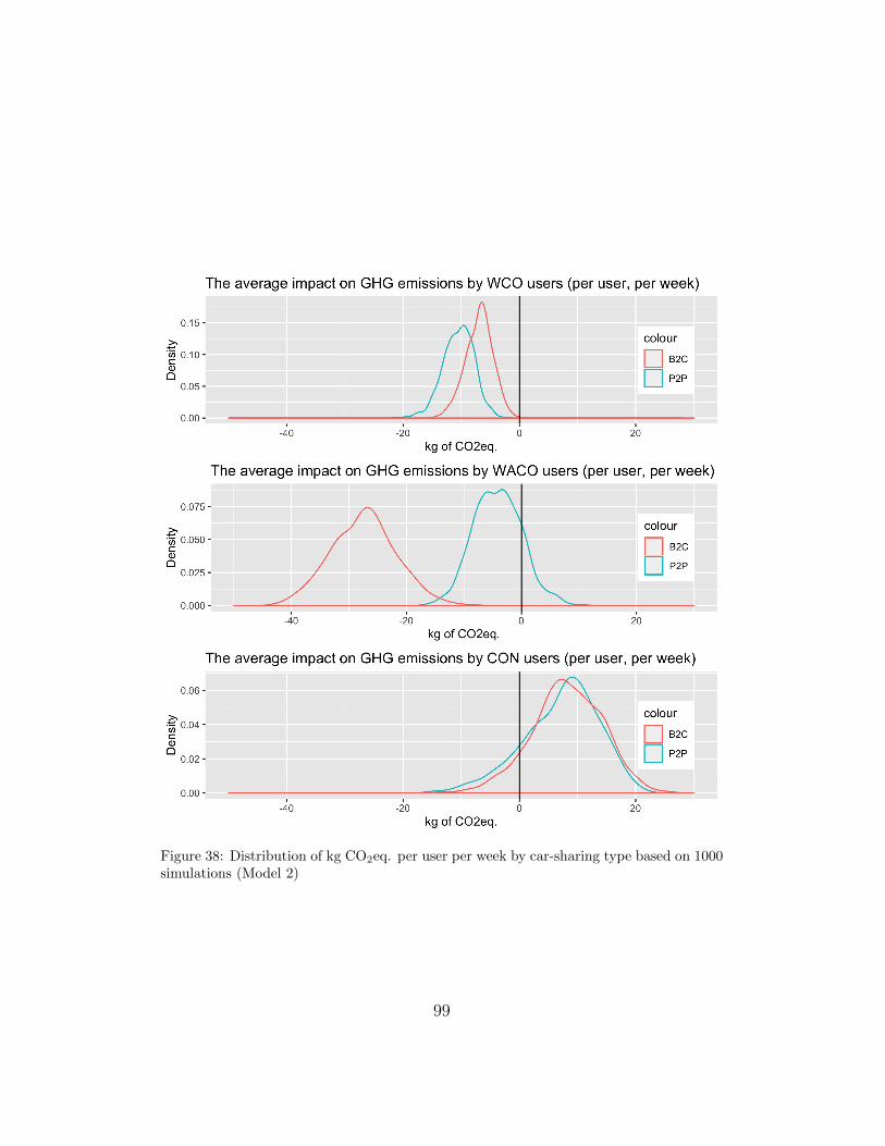
Figure 38: Distribution of kg CO2eq. per user per week by car-sharing type based on 1000simulations (Model 2)

99

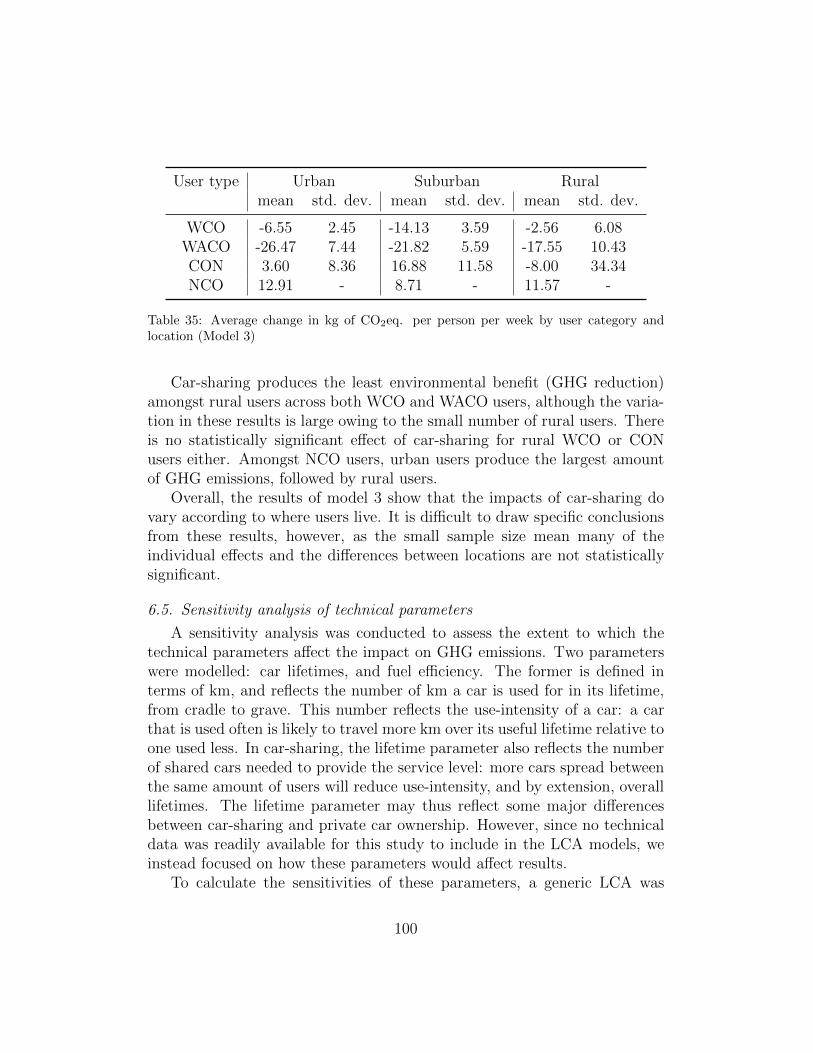
User type Urban Suburban Ruralmean std. dev. mean std. dev. mean std. dev.

WCO -6.55 2.45 -14.13 3.59 -2.56 6.08WACO -26.47 7.44 -21.82 5.59 -17.55 10.43CON 3.60 8.36 16.88 11.58 -8.00 34.34NCO 12.91 - 8.71 - 11.57 -

Table 35: Average change in kg of CO2eq. per person per week by user category andlocation (Model 3)

Car-sharing produces the least environmental benefit (GHG reduction)amongst rural users across both WCO and WACO users, although the varia-tion in these results is large owing to the small number of rural users. Thereis no statistically significant e↵ect of car-sharing for rural WCO or CONusers either. Amongst NCO users, urban users produce the largest amountof GHG emissions, followed by rural users.

Overall, the results of model 3 show that the impacts of car-sharing dovary according to where users live. It is di�cult to draw specific conclusionsfrom these results, however, as the small sample size mean many of theindividual e↵ects and the di↵erences between locations are not statisticallysignificant.

6.5. Sensitivity analysis of technical parameters

A sensitivity analysis was conducted to assess the extent to which thetechnical parameters a↵ect the impact on GHG emissions. Two parameterswere modelled: car lifetimes, and fuel e�ciency. The former is defined interms of km, and reflects the number of km a car is used for in its lifetime,from cradle to grave. This number reflects the use-intensity of a car: a carthat is used often is likely to travel more km over its useful lifetime relative toone used less. In car-sharing, the lifetime parameter also reflects the numberof shared cars needed to provide the service level: more cars spread betweenthe same amount of users will reduce use-intensity, and by extension, overalllifetimes. The lifetime parameter may thus reflect some major di↵erencesbetween car-sharing and private car ownership. However, since no technicaldata was readily available for this study to include in the LCA models, weinstead focused on how these parameters would a↵ect results.

To calculate the sensitivities of these parameters, a generic LCA was

100

Figure 39: Distribution of kg CO2eq. per user per week by user location based on 1000simulations (Model 3)

101

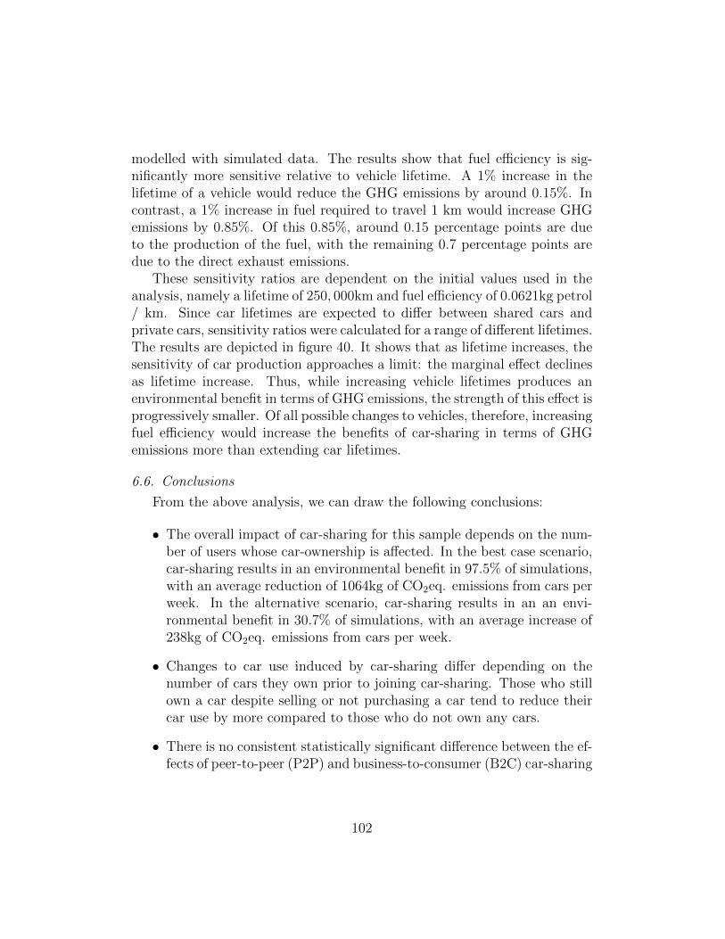
modelled with simulated data. The results show that fuel e�ciency is sig-nificantly more sensitive relative to vehicle lifetime. A 1% increase in thelifetime of a vehicle would reduce the GHG emissions by around 0.15%. Incontrast, a 1% increase in fuel required to travel 1 km would increase GHGemissions by 0.85%. Of this 0.85%, around 0.15 percentage points are dueto the production of the fuel, with the remaining 0.7 percentage points aredue to the direct exhaust emissions.

These sensitivity ratios are dependent on the initial values used in theanalysis, namely a lifetime of 250, 000km and fuel e�ciency of 0.0621kg petrol/ km. Since car lifetimes are expected to di↵er between shared cars andprivate cars, sensitivity ratios were calculated for a range of di↵erent lifetimes.The results are depicted in figure 40. It shows that as lifetime increases, thesensitivity of car production approaches a limit: the marginal e↵ect declinesas lifetime increase. Thus, while increasing vehicle lifetimes produces anenvironmental benefit in terms of GHG emissions, the strength of this e↵ect isprogressively smaller. Of all possible changes to vehicles, therefore, increasingfuel e�ciency would increase the benefits of car-sharing in terms of GHGemissions more than extending car lifetimes.

6.6. Conclusions

From the above analysis, we can draw the following conclusions:

• The overall impact of car-sharing for this sample depends on the num-ber of users whose car-ownership is a↵ected. In the best case scenario,car-sharing results in an environmental benefit in 97.5% of simulations,with an average reduction of 1064kg of CO2eq. emissions from cars perweek. In the alternative scenario, car-sharing results in an an envi-ronmental benefit in 30.7% of simulations, with an average increase of238kg of CO2eq. emissions from cars per week.

• Changes to car use induced by car-sharing di↵er depending on thenumber of cars they own prior to joining car-sharing. Those who stillown a car despite selling or not purchasing a car tend to reduce theircar use by more compared to those who do not own any cars.

• There is no consistent statistically significant di↵erence between the ef-fects of peer-to-peer (P2P) and business-to-consumer (B2C) car-sharing

102

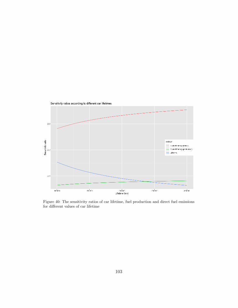
Figure 40: The sensitivity ratios of car lifetime, fuel production and direct fuel emissionsfor di↵erent values of car lifetime

103

on user behaviour or GHG emissions. P2P car-sharing users who be-come car-less reduce their emissions more compared to B2C users; how-ever for those users who retain a car, B2C car-sharing users reduce theirGHG emissions by more.

• Among users who have fewer cars because of car-sharing, suburbanusers are expected to reduce car-use by more compared to both urbanand rural users all else being equal. The environmental benefits ofcar-sharing are greatest for suburban and urban users.

• The production of cars has a progressively smaller relative e↵ect onoverall emissions as a car’s lifetime increases, while the relative e↵ectsof both fuel production and direct vehicle emissions increase as lifetimeincreases.

• Increasing fuel e�ciency of shared cars would have a larger impacton the reduction of GHG emissions compared to increasing lifetimes,regardless of the car’s lifetime.

7. Policy conclusions

The transition to sustainable transport

On the evidence of this report, car-sharing could help to reduce the en-vironmental impacts associated with mobility, but only under certain condi-tions. There is a danger that car-sharing adds to environmental pressures ifit is used as an additional form of mobility, rather than as a replacement forprivate car ownership. Thus, in order to maximise the environmental benefitsof car-sharing, and to minimise the risk of increasing environmental burdens,car-sharing should only be encouraged at the expense of car ownership. Itis important to note that it is replacing private car-ownership that is key,not private car-use. The discussion that follows is based on the premise thatmobility policies a↵ecting car-sharing should aim to reduce environmentalimpact and resource use, policies that promote a sustainable and circulareconomy.

Subsidies and other financial incentives

There is little evidence that reducing the cost of car-sharing for userswill have environmental benefits. Evidence from those who already use car-sharing show that 91% do so because it is cheaper than owning and using

104

a private car (figure 15). Moreover, of those who are not-sharing, cost wasthe least important barrier (figure 27). Evidence from other studies alsoshow that people who drive less than 6000-10000km per year would savemoney by switching to car-sharing (see section 1.2); people who drive morethan this are unlikely to switch to car-sharing anyway. Reducing the costof car-sharing to consumers will lead to a greater risk of increasing car-use,at the expense of public transport and cycling. Thus, policy should avoidsubsidies, both for firms and consumers, whether in the form of direct cashtransfers, refunds, or beneficial tax treatment, unless governments can becertain car-sharing is replacing car ownership (see next paragraph). From anenvironmental perspective, it would make more sense to invest in improvingcycling infrastructure and/or public transport, either to lower its cost orimprove the service, rather than in lowering the cost of car-sharing.

One way to encourage car-sharing as a replacement for car-ownership isthrough incentives when car-owners scrap (one of) their car(s). The Flemishgovernment used to provide benefits for families that get rid of their allpersonal cars. Currently, there are some initiatives at the local (city) level butthe regional benefits have been abolished. Some examples of local initiativescan be found in the city of Gent where people get up to 1000 euros if theyscrap an old/ polluting car 4. The city of Antwerpen pays back 10% of aMaaS subscription (up to 50 euros per month) to people who get rid of theircar 5, while Brussel o↵ers a Cambio subscription for a year and either ayear subscription for all public transportation in the city or a bike subsidy(up to 505 euros)6. Of these, the policy of Brussels and Antwerp would, intheory, be the most e↵ective at preventing a return to car-ownership sincethey o↵er in-kind benefits for cycling, public transport or car-sharing. Gent’scash transfer, instead, may be used to o↵set the cost of a replacement vehicle.Applying the general principle outlined above, any incentives should focus onin-kind cycling or public transport benefits, with in-kind car-sharing benefitslimited to low-cost incentives, such as the refunding of registration fees. Evenin-kind benefits, however, may not prevent former owners from purchasing acar at a later date unless car-ownership is made less attractive.

4https://stad.gent/mobiliteit-openbare-werken/producten/slooppremie5http://www.slimnaarantwerpen.be6http://www.brusselair-premie.be/

105

ParkingMany cities in Flanders have restrict car use in city centres, while park-

ing spaces in the city centre are either extremely limited or very expensive.Almost 40% of the respondents (figure 27) said that they might be morewilling to share cars if the city would make it easier to park shared cars.Some cities such as Gent, Antwerpen and Leuven reserve parking spaces forstation-based systems and / or allow parking permits for shared cars. Theinterviewees also commented that clear demarcation of car-sharing spacestogether with regular patrols around the parking spaces is also necessaryto avoid (mis)use by private car owners. However, the underlying principleexpressed earlier means that any ease of parking restrictions or increase ofspaces must be at the expense of private cars. That is, if parking for sharedcars is to be eased, parking for private cars should be reduced and restrictedconcurrently. Otherwise, car-sharing risks being used as a substitute for pub-lic transport or cycling, for example, by enabling an easier route to reach citycentres relative to public transport/cycling.

Currently, real estate developers in Flanders are required by law to pro-vide 1.2 or even 2 parking spaces per residential unit for a new-build apart-ment. They are required to do so because municipal authorities fear thatresidents will park in the streets in the vicinity of the new building if thereis not enough parking space in the building itself. This not only drives upthe price of these new buildings, but recent research has shown that about1 in 5 of these parking spaces remain empty (Van Neck (2018)). Followingneighbouring countries, municipalities should relax the minimum amount ofparking spaces in new residential projects and could rather consider providingone or more shared cars that can be used by all residents.

Enabling multi-modal lifestyles

Good public transport and extensive cycling infrastructure are key forusers to lead more multi-modal lifestyles. Car-sharing, however, has am-biguous e↵ects on public transport. In our survey, 70% of car-sharing usersjoined car-sharing because it is faster than public transport (figure 15). Thissuggests that for some members, car-sharing could substitute for public trans-port, a negative outcome for the environment.7 Moreover, those who are not

7Further evidence is presented in Figure 24: when car-sharing users were asked howthey would replace car-sharing journeys if they were not members, 56% of users would

106

yet car-sharing members but are interested in joining have positive views ofpublic transport, suggesting they are already or willing to be regular users.Whilst the outcome of these potential members is not known, it cannot be dis-counted that such users would substitute public transport with car-sharing.To avoid this substitution e↵ect, public transport, as well as active modessuch as cycling, must continue to be supported as much as possible by poli-cies, even at the expense of car-sharing. One interviewee suggested in section3 that shared cars should be allowed to use priority lanes currently reservedfor public transport; however, such a policy puts car-sharing and public trans-port on an equal footing, whereas the emphasis should be on making publictransport, as well as cycling, more attractive at the expense of all car-use,including sharing.

The last miles to get to a destination are often hard when one is limitedto public transportation. This hurdle is usually overcome by avoiding publictransport altogether and using a personal car for the whole trip. Mobihubsare one solution to counter this problem, helping the transition to multi-modal lifestyles; they bring public transportation, electric charging stations,shared cars, and shared bikes all in one spot or hub, meaning that sharedcars or bikes can be used for the last mile, complementing public transport.However, careful planning of such systems is necessary so that the hubs areeasily accessible themselves by public transport or bike, so that cars are notnecessary to reach the hub for most users.

Disincentivising car-ownership

The place of car-sharing in sustainable mobility is only as a transitiontool away from car-ownership and towards cycling and public transport. Ane↵ective way of encouraging this transition is to make car-ownership moreunattractive. For example, policies that increase taxes on car-ownership or

replace at least some of their journeys with public transport. Note that this does not meanthat 70% or 56% of users substitute car-sharing for public transport. Rather, it impliesthat for some users, for some journeys, car-sharing may replace public transport. Theoverall, aggregate, e↵ect of car-sharing on public transport cannot be concluded on thebasis of this. It should also be emphasised that car-sharing users who sell or do not buya car (WCO and WACO) will increase their use of public transport, a positive e↵ect forthe environment. Regardless of whether car-sharing ultimately substitutes or complementspublic transport, and/or cycling, investment in public transport and cycling infrastructureis necessary to continue to help car-owners transition away from car-ownership, and car-use(shared or otherwise).

107

congestion charges that target car-use, can benefit car-sharing by proxy. Notethat in this scenario, it would also make sense to subject car-sharing to thecongestion charge, to ensure car-use in general is not incentivised. The e↵ectsof such taxes or charges would probably be regresssive, hitting the pooresthardest; thus, measures to redress the balance should be part of the policymix. This could include discounted public transport passes or (electric) bikesfor those with low incomes.

Information and communication

Results from the survey suggest that non-sharers are confused about as-pects of car-sharing, such as costs and liability. More clarity about theseissues form car-sharing firms could help. Regarding costs, there is substan-tial variation amongst car-sharing firms and their cost structures: a mix ofmembership fees, monthly fees, km costs, time costs, reservation costs etc.This makes it di�cult for users to compare di↵erent car-sharing schemes,and crucially to compare it to car-ownership. Many firms already o↵er acost calculator; however, a non-partisan price comparison website may easedecisions for potential users. Clear guidance regarding responsibilities, espe-cially the procedure in the case of accidents, may also help ease concerns ofpotential users.

One obvious hurdle for people to share cars is unfamiliarity with the con-cept and the existence of alternatives in their neighbourhood. It can thereforegreatly help if local government actively promotes shared cars. Leaflets, fly-ers, or articles on the citys website or in local newspapers are all examplesof how to get the word out. However, simply making the shared cars morevisible in the city with clearly signalized parking spaces for shared cars oreye-catching vehicles can also help to build trust.

A finding from the survey is that those who are most concerned aboutthe environment were also the most interested in car-sharing. Moreover, a94% of car-sharing users joined partly because they believe it is better forthe environment. Thus, if such potential users were more informed aboutthe impacts of car-sharing, particularly that its environmental benefits onlyaccrue when car-sharing replaces car-ownership, then more users may bemore willing to forgo private cars. There is a danger that car-sharing usersfeel they are doing something that benefits the environment, without actu-ally realising those benefits in reality. Clear communication of the principlethat car-sharing should replace ownership could help to realise more pro-environmental behaviour.

108

Car availability and fleet size

A common concern amongst non-sharers is the availability of cars, bothgeo-spatially (e.g. in their neighbourhood) and to meet demand (e.g. avail-ability of a car when they need it), as highlighted in figures 26 and 27. Theseissues can be overcome by expanding the number of cars in the fleet; however,this will negatively a↵ect the environmental impact and resource e�ciency,as cars will be left unused for longer. This is a delicate balancing act forcar-sharing firms to manage, as investing in the size of the fleet requires sig-nificant capital outlay, as discussed in section 3.However, p2p car-sharing canpotentially take advantage of a large fleet if it can attract car-owners to theplatform. In addition, some local governments share their own fleet. Sharingan already existing fleet should reduce additional demand (and production)of cars, avoiding some environmental impact and material use. Another solu-tion is used by Partago, which uses a co-operative model: new users are askedto pay a large up-front cost to become a member, refundable when users de-cide to leave. This may give smaller firms the start-up capital necessary tosecure further financial backing to expand the size of the fleet.

Electrification

The analysis in section 6 showed that increasing fuel e�ciency is moreimportant than lifetime extension when trying to reduce GHG emissions.While electric vehicles are not a panacea, combined with a renewable energymix, they would o↵er greater environmental benefits over fossil-fuel basedcars (both GHG emission and air pollution reduction).

Although the correspondent from Cambio stated that they opt for a mixedfleet because they believe not everyone is open to electrification, results fromthis research suggest that both existing car-sharers and potential car-sharersare willing to pay more for electric (shared) cars. Moreover, 94% of usersjoined car-sharing because they think it is better for the environment (figure15). Thus, there appears to be an opportunity to use car-sharing to help thetransition towards car electrification by improving infrastructure and break-ing down the cultural norms that resist electrification. However, chargingstations are expensive to install and a lack thereof may pose a significantbarrier for electric car-sharing firms. Local governments, in conjunction withcar-sharing firms, may expand charging stations in the area to increase thesupply of electric shared vehicles. Having charging stations, however, is notenough. Having just one parking spot with a charging station means that

109

the charging station can often not be used as long as the parking spot is oc-cupied. If parking spots in the city are scarce, it is a common problem thatcharging spots are taken just for parking space. Local government couldsupport car-sharing by greater enforcement of rules punishing this practice.

Rural areas

It is very di�cult and expensive to provide public transportation closeto inhabitants in rural areas. Many people in rural areas feel like they needa car to go to work, shop for groceries, etc. because the distances are toolarge to travel by bike and public transportation is not (su�ciently) avail-able. Likewise, getting shared cars to rural areas appears to be di�cult (andpossibly not even desirable) because it is less profitable for CS firms andthe car sharing intention is lower. Mobihubs (see above) could be a par-ticularly useful solution in rural areas. However, as discussed in section 6,rural users produce the least environmental benefits, as car-sharing has thelowest substitution for private car use. More research is needed to examinewhether mobihubs could help rural inhabitants switch from a car-dominatedto a more multi-modal lifestyle.

Regulatory framework

Our statistical analysis shows that company cars are one of the biggesthurdles for ones car sharing intention. Talks are ongoing to change the systemtowards a mobility budget or to, at least, decrease the benefits that arecurrently on company cars.

The regulatory framework for shared cars is currently underdevelopedwhich means that there is no consistent set of rules across municipalities.However, it would be easier for car sharing firms if the same rules would applyfor the whole region or country. A unified view and regulatory frameworkwould greatly reduce the costs that car sharing firms incur for researchingthe local rules, negotiating with the cities, and implementing their businesseach time they want to expand to a di↵erent location.

Improving the evidence base: Data needs

This research has been conducted despite limited access to third-partydata. Assessing the environmental impact of car-sharing, or its place in thecircular economy, is di�cult to do without extensive data. To improve policymaking in the domain of car-sharing, and mobility more generally, data col-lection and availability has to be improved. Car-sharing companies currently

110

hold a lot of data about the use of their cars, how often they are used, howoften they break down, etc.; however, it is not easy to tell from this whethercar-sharing is having a positive impact on the environment. Moreover, ac-cess to this data for researchers is restricted. Greater collaboration betweendi↵erent levels of governments, car-sharing firms and universities/researchinstitutes would enable a greater evidence base for policy making. One steptowards this is the inclusion of open data clauses in the permits or contractsbetween (local) governments and CS firms.

The data required to calculate the environmental impact of car-sharingis extensive. As a step towards a better understanding of environmentalimpacts, car-sharing firms could keep track of whether their users have givenup a car because of car-sharing. Whilst not ideal, it could act as an indicatorthat car-sharing is helping to reduce the car hegemony. A better solutionwould be to gather mobility data from the same panel of participants everyyear, both car-sharing users and non-sharers, which would enable researchersto have a much clearer understanding of the impact of car-sharing.

8. Acknowledgements

The authors are very grateful for full financial support received fromthe Flemish administration via the Steunpunt Circulaire Economie (PolicyResearch Centre Circular Economy).

This publication contains the opinions of the authors, not that of theFlemish administration. The Flemish administration will not carry any li-ability with respect to the use that can be made of the produced data orconclusions.

The authors would also like to thank everyone who helped spread thesurvey. In particular, we would like to thank:

• Degage who helped spread the survey and were willing to make timefor an interview.

• Lucie Evers from Partago, Je↵rey Matthijs from autodelen.net, andGeert Gisquire from Cambio Vlaanderen for their valueable insights inthe interviews.

• Julie Poppe from VVSG for bringing us into contact with the mobilitydepartment of all Flemish cities and villages

111

• oraganisations that spread the survey through their newsletters andnetwork: OVAM, Vlaanderen circulair, EWI, Touring, Bond BeterLeefmilieu Vlaanderen

• The cities who actively spread the survey among their inhabitants(Riemst, Gent, Bierbeek, Hulshout, Berlaar, Alveringem, Zottegem,Harelbeke, Beveren, Avelgem, Schoten, Zandhoven, Oudenaarde, Meeuwen-Gruitrode, Roeselare, Deinze, Laakdal, Brecht, Erpe-Mere, Lummen,Menen, Hoeilaart, Zele, Mechelen, Kampenhout, Grimbergen, Ger-aardsbergen, Aalst, Oudenburg, Tervuren, Steenokkerzeel, De Pinte,Oostkamp, Herentals, Ledegem, Temse)

• Our thesis students, Sven Jacques and Ben Verheyen who spread thesurvey mainly on social media

• everyone else who filled in the survey or helped share it.

112

Bibliography

6t-bureau de Recherche (2014). One-way carsharing: Which alternative to privatecar? The case study of Autolib’ in Paris. Technical Report May, 6t-bureaude Recherche.

Adam, M.-b., Murray, G., Ter schure, J., Fox, C., and Burkhardt, J. (2005).Car-Sharing: Where and How It Succeeds. Technical report, TransportationResearch Board.

Bardhi, F. and Eckhardt, G. M. (2017). Liquid consumption. Journal of ConsumerResearch, 44(3):582–597.

Becker, H., Ciari, F., and Axhausen, K. W. (2017). Comparing car-sharing schemesin Switzerland: User groups and usage patterns. Transportation ResearchPart A: Policy and Practice, 97:17–29.

Burkhardt, J. E. and Millard-Ball, A. (2006). Who is Attracted to Carshar-ing? Transportation Research Record: Journal of the Transportation ResearchBoard, 1986(1):98–105.

Cardone, N. (2019). Steeds minder Belgen halen een rijbewijs: Jongeren zien eenauto niet langer als statussymbool.

Cattell, R. B. (1966). The Scree Test For The Number Of Factors. MultivariateBehavioral Research, 1(2):245–276.

Cervero, R., Golub, A., and Nee, B. (2006). San Francisco City CarShare: Longer-Term Travel-Demand and Car Ownership Impacts.

Christie, M., Warren, J., Hanley, N., Murphy, K., Wright, R., Hyde, T., and Lyons,N. (2004). Developing measures for valuing changes in biodiversity.

Cohen, B. and Kietzmann, J. (2014). Ride On! Mobility Business Models for theSharing Economy. Organization & Environment, 27(3):279–296.

Day, B., Bateman, I. J., Carson, R. T., Dupont, D., Louviere, J. J., Morimoto,S., Scarpa, R., and Wang, P. (2012). Ordering e↵ects and choice set aware-ness in repeat-response stated preference studies. Journal of environmentaleconomics and management, 63(1):73–91.

De Ridder, A., De Kort, D., Keulen, M., Jans, L., Brouwers, K., and Van Miert,P. (2016). Voorstel van resolutie betre↵ende het stimuleren van autodelen.Technical report, Vlaams Parlement.

Distefano, C., Zhu, M., and Mındril, D. (2009). Understanding and using fac-tor scores: Considerations for the applied researcher - practical assessment,research & evaluation. 14.

Eastman, J. K., Fredenberger, B., Campbell, D., and Calvert, S. (1997). The Re-lationship between Status Consumption and Materialism: A Cross-Cultural

113

Comparison of Chinese, Mexican, and American Students. Journal of Mar-keting Theory and Practice, 5(1):52–66.

Efthymiou, D. and Antoniou, C. (2016). Modeling the propensity to join carsharingusing hybrid choice models and mixed survey data. Transport Policy, 51:143–149.

Firnkorn, J. and Muller, M. (2011). What will be the environmental e↵ects ofnew free-floating car-sharing systems? The case of car2go in Ulm. EcologicalEconomics, 70(8):1519–1528.

Fox, J. and Monette, G. (1992). Generalized Collinearity Diagnostics GeneralizedCollinearity Diagnostics. Journal of the American Statistical Association,87(417):178–183.

Habibi, S., Voronov, A., Engdahl, H., Wedlin, J., Englund, C., Sprei, F., andPetterson, S. (2017). Comparison of free-floating car sharing services in cities.In ECEEE SUMMER STUDY PROCEEDINGS, pages 771–778.

Hawlitschek, F., Teubner, T., and Gimpel, H. (2016). Understanding the sharingeconomy - Drivers and impediments for participation in peer-to-peer rental.Proceedings of the Annual Hawaii International Conference on System Sci-ences, 2016-March:4782–4791.

Hjorthol, R. (2016). Decreasing popularity of the car? Changes in driving licenceand access to a car among young adults over a 25-year period in Norway.Journal of Transport Geography, 51:140–146.

Horn, J. L. (1965). A rationale and test for the number of factors in factor analysis.Psychometrika, 30(2):179–185.

Horn, J. L. and Engstrom, R. (1979). Cattell’s Scree Test In Relation To Bartlett’sChi-Square Test And Other Observations On The Number Of Factors Prob-lem. Multivariate Behavioral Research, 14(3):283–300.

Huwer, U. (2004). Public transport and car-sharingbenefits and e↵ects of combinedservices. Transport Policy, 11(1):77–87.

Kuzmyak, J. (2012). Land Use and Tra�c Congestion. Technical report, ArizonaDepartment of Transportation, Arizona.

Le Vine, S. and Polak, J. (2014). Factors Associated With Young Adults De-laying and Forgoing Driving Licenses: Results From Britain. Tra�c InjuryPrevention, 15(8):794–800.

Liao, F., Molin, E., Timmermans, H., and Wee, B. V. (2018). Carsharing : theimpact of system characteristics on its potential to replace private car tripsand reduce car ownership. Number 0123456789. Springer US.

Litman, T. (2000). Evaluating carsharing benefits. Transportation ResearchRecord, (1702):31–35.

114

Litman, T. A., Litman, T., and Steele, W. R. (2018). Land Use Impacts onTransport How Land Use Factors A↵ect Travel Behavior. Technical report.

Loose, W. (2010). The state of European Car-Sharing. Technical report, FinalReport D 2.4 Work Package 2 , Bundesverband CarSharing e. V.

Martin, E. and Shaheen, S. (2016). Impacts of car2go on Vehicle Ownership, ModalShift, Vehicle Miles Travelled, and Greenhouse Gas Emissions: An Analysisof Five North American Cities. Technical report.

Martin, E. and Shaheen, S. A. (2011). Greenhouse gas emissions impacts of car-sharing in North America. Transactions on Intelligent Transportation Sys-tems, 12(4):1074–1086.

Material Economics (2018). The Circular Economy, a Powerful Force for ClimateMitigation. Technical report.

Mobihubs (2019). Mobihubs. https://mobihubs.eu/. Accessed: 2019-06-26.

Munzel, K., Boon, W., Frenken, K., and Vaskelainen, T. (2017). Innovation Stud-ies Utrecht ( ISU ) Working Paper Series Carsharing Business Models inGermany : Characteristics , Success and Future Prospects. pages 1–19.

Nijland, H. and van Meerkerk, J. (2017). Mobility and environmental impactsof car sharing in the Netherlands. Environmental Innovation and SocietalTransitions, 23:84–91.

Prieto, M., Baltas, G., and Stan, V. (2017). Car sharing adoption intention inurban areas: What are the key sociodemographic drivers? TransportationResearch Part A: Policy and Practice, 101:218–227.

Revelle, W. and Rocklin, T. (1979). Very Simple Structure: An Alternative Pro-cedure For Estimating The Optimal Number Of Interpretable Factors. Mul-tivariate Behavioral Research, 14(4):403–414.

Rimple, M., Srikant, M., Naseem, A., and Kumar, M. J. (2015). A study ofinteraction of materialism and money attitude and its impact on car purchase.Management & Marketing, 10(3):245 – 269.

Rodenbach, J. A., Mathijs, J. A., Chicco, A. P., Diana, M. P., and Nehrke, G. B.(2018). Car sharing in Europe A multidimensional classification and inven-tory D 2.1. Technical report, STARS - Shared mobility opporTunities Andchallenges foR European citieS.

Ryan, M., Gerard, K., and Amaya-Amaya, M. (2008). Discrete Choice Experi-ments in a Nutshell. pages 13–46. Springer, Dordrecht.

Segal, B. and Podoshen, J. S. (2013). An examination of materialism, conspicu-ous consumption and gender di↵erences. International Journal of ConsumerStudies, 37(2):189–198.

115

Shaheen, S., Sperling, D., and Wagner, C. (1998). Carsharing in Europe and NorthAmerica: Past, Present and Future. Transportation Quarterly, 52(3):35–52.

Steg, L. (2005). Car use: Lust and must. Instrumental, symbolic and a↵ectivemotives for car use. Transportation Research Part A: Policy and Practice,39(2-3 SPEC. ISS.):147–162.

Van Broeck, L. (2018). Parkeren in Vlaanderen: mobiliteit en ruimtelijke ordeningzijn elkaars kinderen — VRT NWS.

van Driel, P. and Hafkamp, W. (2015). De e↵ecten van autodelen op autogebruik.Tijdschrift Vervoerswetenschappen, 51(4):18–37.

Van Neck, J. (2018). De slimme parkeernorm voor de stad van morgen.

Van Ootegem, L. (2017a). Interview with Geert Gisquiere, Cambio.

Van Ootegem, L. (2017b). Interview with Je↵rey Matthijs, Cozycar and Autode-len.net.

Van Ootegem, L. (2017c). Interview with John Wante, Degage.

Van Ootegem, L. (2017d). Interview with Lucy Evers, Partago.

Velicer, W. F. (1976). Determining the number of components from the matrix ofpartial correlations. Psychometrika, 41(3):321–327.

Vermeiren, K., Poelmans, L., Engelen, G., Broekx, S., Beckx, C., De Nocker, L.,and Dyck, K. V. (2019). Monetariseren van de impact van urban sprawl inVlaanderen. Technical report, Departement omgeving.

116

Appendix

Appendix A. Appendices to section 4

Table A.36 shows the di↵erence between sharers and not sharers withrespect to several categorical, demographic variables. Fisher’s exact test wasused as some categories had very few observations.

Variable Levels nNCS %NCS nCS %CS nall %all

Gender Man 688 38.1 112 38.6 800 38.2Woman 1109 61.5 177 61.0 1286 61.4X 7 0.4 1 0.3 8 0.4

p = 0.96 all 1804 100.0 290 100.0 2094 100.0

Education Secundary school 486 26.8 16 5.5 502 23.9Bachelor degree 611 33.7 77 26.5 688 32.7Master degree 530 29.3 154 52.9 684 32.5>Master 184 10.2 44 15.1 228 10.8

p = 0.0005 all 1811 100.0 291 100.0 2102 100.0

Degree of urbanisation Rural 756 41.8 27 9.3 783 37.3Urban 454 25.1 189 65.0 643 30.6Suburban 598 33.1 75 25.8 673 32.1

p = 0.0005 all 1808 100.0 291 100.0 2099 100.0

Profession Other 217 12.0 13 4.5 230 10.9Blue collar worker 67 3.7 5 1.7 72 3.4White collar worker 1054 58.1 191 65.6 1245 59.1Education 119 6.6 38 13.1 157 7.4Self-employed 104 5.7 21 7.2 125 5.9Civil servant 34 1.9 6 2.1 40 1.9Retired 154 8.5 7 2.4 161 7.6Incapacitated 19 1.0 3 1.0 22 1.0Unemployed 28 1.5 6 2.1 34 1.6Stay-at-home (wo)man 19 1.0 1 0.3 20 0.9

p = 0.0005 all 1815 100.0 291 100.0 2106 100.0

Employment Student 198 10.9 14 4.8 212 10.1Part time job 291 16.1 71 24.5 362 17.2Full time job 1076 59.5 184 63.5 1260 60.0Not working 245 13.5 21 7.2 266 12.7

p = 0.0005 all 1810 100.0 290 100.0 2100 100.0

Table A.36: Demographics compared between not car sharers (NCS) and car sharers (CS).p-values of Fisher’s exact test added. Missing data is left out.

Table A.37 summarize several continuous variables for the sharing (CS)and non-sharing (NCS) population. it shows the number of respondents(n), minimum (Min), first quartile (q1), mean (x), third quartile (q3), max-imum (Max), and standard deviation (s). p-values are based on a t-test

117

of Mann-Whitney test if the data cannot be assumed to be normally dis-tributed. The table shows that sharing respondents are significantly youngerthan non-sharing people. Sharing families also tend to have less adults andmore minor in the family. For the factor scores, we see that sharers have sig-nificantly lower scores for driving enjoyment and car dependent enjoymentand significantly higher scores for ecological concern and public transportpositivism.

Variable Levels n Min q1 x q3 Max sAge NCS 1814 18.0 29.0 41.1 52.0 85.0 14.3

CS 291 18.0 30.0 38.4 44.0 73.0 10.2p = 0.03 all 2105 18.0 29.0 40.8 51.0 85.0 13.8Number of adults NCS 1798 1.0 2.0 2.2 2.0 9.0 1.0

CS 290 1.0 1.2 1.9 2.0 6.0 0.8p < 0.0001 all 2088 1.0 2.0 2.2 2.0 9.0 1.0Number of minors NCS 1798 0.0 0.0 0.7 1.0 5.0 1.0

CS 290 0.0 0.0 0.9 2.0 5.0 1.1p = 0.04 all 2088 0.0 0.0 0.8 2.0 5.0 1.0Car dependent identity NCS 1815 -3.2 -0.5 0.0 0.6 2.9 0.8

CS 291 -2.6 -0.9 -0.2 0.5 2.2 1.0p < 0.0001 all 2106 -3.2 -0.5 0.0 0.6 2.9 0.9Ecological concern NCS 1815 -4.4 -0.7 -0.2 0.5 2.2 0.9

CS 291 -1.5 0.6 1.0 1.4 2.2 0.6p < 0.0001 all 2106 -4.4 -0.6 0.0 0.7 2.2 0.9Driving enjoyment NCS 1815 -1.9 -0.6 0.1 0.7 3.1 0.9

CS 291 -1.7 -1.1 -0.4 0.0 2.6 0.8p < 0.0001 all 2106 -1.9 -0.7 0.0 0.6 3.1 0.9PT positivism NCS 1815 -3.2 -0.7 -0.1 0.5 3.1 0.8

CS 291 -1.9 0.3 0.8 1.3 3.1 0.8p < 0.0001 all 2106 -3.2 -0.6 0.0 0.6 3.1 0.9

Table A.37: Age, family composition, and factor scores compared between not car sharers(NCS) and car sharers (CS). Missing data is left out.

Table A.38 shows the average number of kilometers travelled in a week.The ‘informal car’ indicates rides that were travelled with a friends’ or rela-tives’ car without any formal contract or payment. p-values are based on at-test of Mann-Whitney test if the data cannot be assumed to be normallydistributed. The table shows that sharers travel significantly less with privatecars, company cars and significantly more by bike, by public transportation,on foot, and with shared cars.

Table A.39 shows the number of cars, bikes, PT subscriptions, scooters

118

and motorcycles a family owns. Car-sharers appear to own significantly lessprivate and company cars and motorcycles, and slightly less electric bikes. Onthe other hand, they tend to have slightly more regular bikes and significantlymore people in the family had public transportation subscriptions. p-valuesare based on a t-test of Mann-Whitney test if the data cannot be assumedto be normally distributed.

Appendix A.1. Comparing respondents in rural, suburban, and urban envi-ronments

Following a recent report, published by Flanders’ government environ-ment department on the urban sprawl (Vermeiren et al. 2019), we supplementthis report with some summary data that we got from our questionnaire.Vermeiren et al. (2019) discusses how the urban sprawl and the environ-ment people live in influences, among other things, car ownership. Previousresearch indicated that rural areas, longer distances to all facilities, less PToptions and better parking facilities might increase car ownership and overalltravel distance (Kuzmyak 2012, Litman et al. 2018).

TableA.40 seems to support the hypothesis that people that live in lessurban environments travel more with private cars and bike and walk less.

Table A.41 shows that people in rural areas also have more private andcompany cars in the family.

119

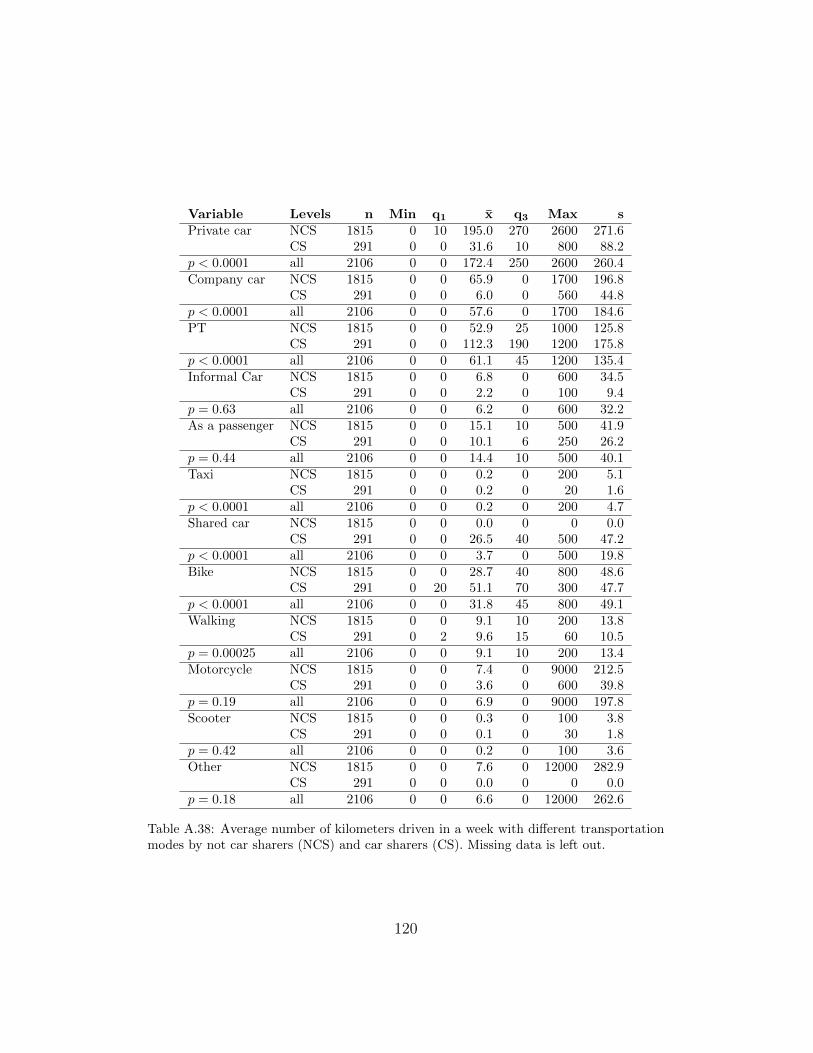
Variable Levels n Min q1 x q3 Max sPrivate car NCS 1815 0 10 195.0 270 2600 271.6

CS 291 0 0 31.6 10 800 88.2p < 0.0001 all 2106 0 0 172.4 250 2600 260.4Company car NCS 1815 0 0 65.9 0 1700 196.8

CS 291 0 0 6.0 0 560 44.8p < 0.0001 all 2106 0 0 57.6 0 1700 184.6PT NCS 1815 0 0 52.9 25 1000 125.8

CS 291 0 0 112.3 190 1200 175.8p < 0.0001 all 2106 0 0 61.1 45 1200 135.4Informal Car NCS 1815 0 0 6.8 0 600 34.5

CS 291 0 0 2.2 0 100 9.4p = 0.63 all 2106 0 0 6.2 0 600 32.2As a passenger NCS 1815 0 0 15.1 10 500 41.9

CS 291 0 0 10.1 6 250 26.2p = 0.44 all 2106 0 0 14.4 10 500 40.1Taxi NCS 1815 0 0 0.2 0 200 5.1

CS 291 0 0 0.2 0 20 1.6p < 0.0001 all 2106 0 0 0.2 0 200 4.7Shared car NCS 1815 0 0 0.0 0 0 0.0

CS 291 0 0 26.5 40 500 47.2p < 0.0001 all 2106 0 0 3.7 0 500 19.8Bike NCS 1815 0 0 28.7 40 800 48.6

CS 291 0 20 51.1 70 300 47.7p < 0.0001 all 2106 0 0 31.8 45 800 49.1Walking NCS 1815 0 0 9.1 10 200 13.8

CS 291 0 2 9.6 15 60 10.5p = 0.00025 all 2106 0 0 9.1 10 200 13.4Motorcycle NCS 1815 0 0 7.4 0 9000 212.5

CS 291 0 0 3.6 0 600 39.8p = 0.19 all 2106 0 0 6.9 0 9000 197.8Scooter NCS 1815 0 0 0.3 0 100 3.8

CS 291 0 0 0.1 0 30 1.8p = 0.42 all 2106 0 0 0.2 0 100 3.6Other NCS 1815 0 0 7.6 0 12000 282.9

CS 291 0 0 0.0 0 0 0.0p = 0.18 all 2106 0 0 6.6 0 12000 262.6

Table A.38: Average number of kilometers driven in a week with di↵erent transportationmodes by not car sharers (NCS) and car sharers (CS). Missing data is left out.

120

Variable Levels n Min q1 x q3 Max sPrivate car NCS 1812 0 1 1.3 2 6 0.9

CS 291 0 0 0.4 1 3 0.6p < 0.0001 all 2103 0 1 1.2 2 6 0.9Company car NCS 1815 0 0 0.4 1 10 0.7

CS 291 0 0 0.1 0 2 0.3p < 0.0001 all 2106 0 0 0.3 1 10 0.7Bike NCS 1815 0 1 2.9 4 34 2.2

CS 291 0 1 3.1 4 16 2.2p = 0.03 all 2106 0 1 2.9 4 34 2.2Electric bike NCS 1815 0 0 0.4 1 7 0.7

CS 291 0 0 0.3 0 5 0.6p = 0.01 all 2106 0 0 0.4 1 7 0.7Bus subscription NCS 1815 0 0 0.4 1 10 0.8

CS 291 0 0 0.7 1 5 1.0p < 0.0001 all 2106 0 0 0.4 1 10 0.8Train subscription NCS 1815 0 0 0.4 1 4 0.6

CS 291 0 0 0.5 1 3 0.6p = 0.0012 all 2106 0 0 0.4 1 4 0.6Scooter NCS 1815 0 0 0.0 0 3 0.2

CS 291 0 0 0.0 0 1 0.1p = 0.43 all 2106 0 0 0.0 0 3 0.2Motorcycle NCS 1815 0 0 0.1 0 5 0.4

CS 291 0 0 0.0 0 2 0.2p = 0.0034 all 2106 0 0 0.1 0 5 0.3

Table A.39: The number of cars, bikes, public transportation subscriptions, scooters andmotorcycles a family owns. Missing data is left out.

121

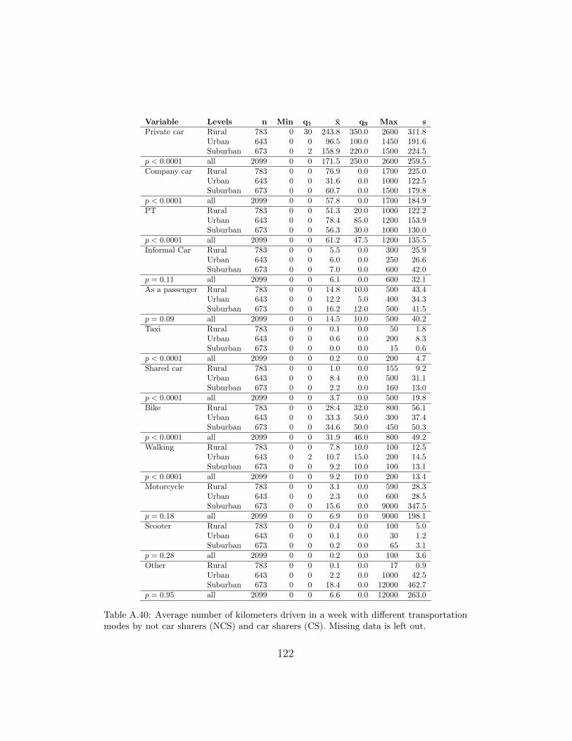
Variable Levels n Min q1 x q3 Max sPrivate car Rural 783 0 30 243.8 350.0 2600 311.8

Urban 643 0 0 96.5 100.0 1450 191.6Suburban 673 0 2 158.9 220.0 1500 224.5

p < 0.0001 all 2099 0 0 171.5 250.0 2600 259.5Company car Rural 783 0 0 76.9 0.0 1700 225.0

Urban 643 0 0 31.6 0.0 1000 122.5Suburban 673 0 0 60.7 0.0 1500 179.8

p < 0.0001 all 2099 0 0 57.8 0.0 1700 184.9PT Rural 783 0 0 51.3 20.0 1000 122.2

Urban 643 0 0 78.4 85.0 1200 153.9Suburban 673 0 0 56.3 30.0 1000 130.0

p < 0.0001 all 2099 0 0 61.2 47.5 1200 135.5Informal Car Rural 783 0 0 5.5 0.0 300 25.9

Urban 643 0 0 6.0 0.0 250 26.6Suburban 673 0 0 7.0 0.0 600 42.0

p = 0.11 all 2099 0 0 6.1 0.0 600 32.1As a passenger Rural 783 0 0 14.8 10.0 500 43.4

Urban 643 0 0 12.2 5.0 400 34.3Suburban 673 0 0 16.2 12.0 500 41.5

p = 0.09 all 2099 0 0 14.5 10.0 500 40.2Taxi Rural 783 0 0 0.1 0.0 50 1.8

Urban 643 0 0 0.6 0.0 200 8.3Suburban 673 0 0 0.0 0.0 15 0.6

p < 0.0001 all 2099 0 0 0.2 0.0 200 4.7Shared car Rural 783 0 0 1.0 0.0 155 9.2

Urban 643 0 0 8.4 0.0 500 31.1Suburban 673 0 0 2.2 0.0 160 13.0

p < 0.0001 all 2099 0 0 3.7 0.0 500 19.8Bike Rural 783 0 0 28.4 32.0 800 56.1

Urban 643 0 0 33.3 50.0 300 37.4Suburban 673 0 0 34.6 50.0 450 50.3

p < 0.0001 all 2099 0 0 31.9 46.0 800 49.2Walking Rural 783 0 0 7.8 10.0 100 12.5

Urban 643 0 2 10.7 15.0 200 14.5Suburban 673 0 0 9.2 10.0 100 13.1

p < 0.0001 all 2099 0 0 9.2 10.0 200 13.4Motorcycle Rural 783 0 0 3.1 0.0 590 28.3

Urban 643 0 0 2.3 0.0 600 28.5Suburban 673 0 0 15.6 0.0 9000 347.5

p = 0.18 all 2099 0 0 6.9 0.0 9000 198.1Scooter Rural 783 0 0 0.4 0.0 100 5.0

Urban 643 0 0 0.1 0.0 30 1.2Suburban 673 0 0 0.2 0.0 65 3.1

p = 0.28 all 2099 0 0 0.2 0.0 100 3.6Other Rural 783 0 0 0.1 0.0 17 0.9

Urban 643 0 0 2.2 0.0 1000 42.5Suburban 673 0 0 18.4 0.0 12000 462.7

p = 0.95 all 2099 0 0 6.6 0.0 12000 263.0

Table A.40: Average number of kilometers driven in a week with di↵erent transportationmodes by not car sharers (NCS) and car sharers (CS). Missing data is left out.

122

Variable Levels n Min q1 x q3 Max sPrivate car Rural 781 0 1 1.5 2 6 0.9

Urban 642 0 0 0.8 1 5 0.8Suburban 673 0 1 1.2 2 6 0.8

p < 0.0001 all 2096 0 1 1.2 2 6 0.9Company car Rural 783 0 0 0.4 1 10 0.8

Urban 643 0 0 0.2 0 4 0.5Suburban 673 0 0 0.3 1 4 0.6

p < 0.0001 all 2099 0 0 0.3 1 10 0.7Bike Rural 783 0 1 3.0 4 12 2.1

Urban 643 0 1 2.6 4 34 2.4Suburban 673 0 1 3.0 4 16 2.2

p < 0.0001 all 2099 0 1 2.9 4 34 2.2Electric bike Rural 783 0 0 0.5 1 7 0.8

Urban 643 0 0 0.2 0 5 0.6Suburban 673 0 0 0.4 1 4 0.7

p < 0.0001 all 2099 0 0 0.4 1 7 0.7Bus subscription Rural 783 0 0 0.4 1 4 0.7

Urban 643 0 0 0.5 1 4 0.8Suburban 673 0 0 0.5 1 10 0.9

p = 0.15 all 2099 0 0 0.4 1 10 0.8Train subscription Rural 783 0 0 0.3 1 4 0.6

Urban 643 0 0 0.4 1 3 0.6Suburban 673 0 0 0.4 1 4 0.7

p = 0.03 all 2099 0 0 0.4 1 4 0.6Scooter Rural 783 0 0 0.0 0 3 0.2

Urban 643 0 0 0.0 0 2 0.2Suburban 673 0 0 0.0 0 1 0.2

p = 0.25 all 2099 0 0 0.0 0 3 0.2Motorcycle Rural 783 0 0 0.1 0 5 0.4

Urban 643 0 0 0.0 0 2 0.2Suburban 673 0 0 0.1 0 2 0.3

p = 0.0024 all 2099 0 0 0.1 0 5 0.3

Table A.41: The number of cars, bikes, public transportation subscriptions, scooters andmotorcycles a family owns. We distinguish families in urban, suburban, and rural envi-ronments. Missing data is left out.

123

Appendix B. Appendices to section 5

Appendix B.1. Factor analysis

The Tables below show, for each factor, the Cronbach alpha which is ameasure of internal consistency, i.e., it indicates how closely a set of itemsare related as a group. Ideally the Cronbach alpha is at least 0.7. TheCronbach alpha’s were calculated using the psych package in R. Each of thethree tables is the result of a factor analysis on a di↵erent set of observations.The first table (Table B.42) shows the factors for the full data set with allrespondents. Table B.43 and Table B.44 show the factors for only the non-sharers or sharers respectively.

Factor Statement Majorfactorloading

Cronbachalpha

Ecological concern If I didn’t need a car, I would immediately getrid of it

0.711 0.833

Car sharing fits the current time 0.698I’m worried about climate (change) 0.686Car sharing helps to save natural resources 0.579I think there’s too much tra�c in Belgium 0.555I get satisfaction from sharing cars 0.514I think road pricing is a good idea 0.498Public transportation is expensive -0.495

Car-dependent identity There’s a dream car that I would like to own 0.545 0.749A car brings status and prestige 0.544Driving a private car is stressful -0.569

PT positivism Private cars are expensive 0.683 0.754Public transportation is reliable 0.641Public transportation is clean/neat 0.549Travelling with public transportation is stressful -0.593

Driving enjoyment It doesn’t matter which brand of car I’m driving 0.698 0.774I’m worried about fine dust pollution 0.628I like driving a car 0.531For me, a car only has an instrumental function -0.626I only need a car to get from A to B -0.619

Table B.42: Overview of factor loadings and internal consistency (Cronbach’s alpha) forthe full dataset

124

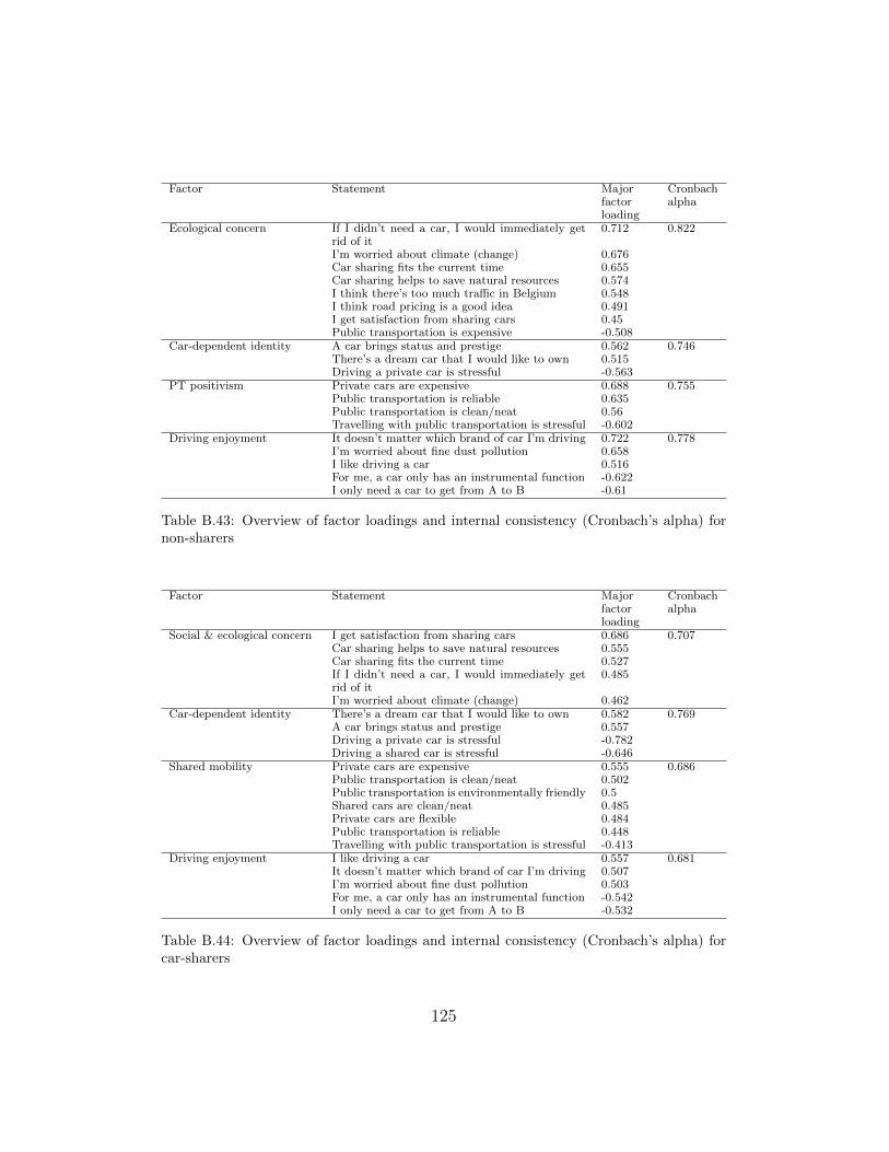
Factor Statement Majorfactorloading

Cronbachalpha

Ecological concern If I didn’t need a car, I would immediately getrid of it

0.712 0.822

I’m worried about climate (change) 0.676Car sharing fits the current time 0.655Car sharing helps to save natural resources 0.574I think there’s too much tra�c in Belgium 0.548I think road pricing is a good idea 0.491I get satisfaction from sharing cars 0.45Public transportation is expensive -0.508

Car-dependent identity A car brings status and prestige 0.562 0.746There’s a dream car that I would like to own 0.515Driving a private car is stressful -0.563

PT positivism Private cars are expensive 0.688 0.755Public transportation is reliable 0.635Public transportation is clean/neat 0.56Travelling with public transportation is stressful -0.602

Driving enjoyment It doesn’t matter which brand of car I’m driving 0.722 0.778I’m worried about fine dust pollution 0.658I like driving a car 0.516For me, a car only has an instrumental function -0.622I only need a car to get from A to B -0.61

Table B.43: Overview of factor loadings and internal consistency (Cronbach’s alpha) fornon-sharers

Factor Statement Majorfactorloading

Cronbachalpha

Social & ecological concern I get satisfaction from sharing cars 0.686 0.707Car sharing helps to save natural resources 0.555Car sharing fits the current time 0.527If I didn’t need a car, I would immediately getrid of it

0.485

I’m worried about climate (change) 0.462Car-dependent identity There’s a dream car that I would like to own 0.582 0.769

A car brings status and prestige 0.557Driving a private car is stressful -0.782Driving a shared car is stressful -0.646

Shared mobility Private cars are expensive 0.555 0.686Public transportation is clean/neat 0.502Public transportation is environmentally friendly 0.5Shared cars are clean/neat 0.485Private cars are flexible 0.484Public transportation is reliable 0.448Travelling with public transportation is stressful -0.413

Driving enjoyment I like driving a car 0.557 0.681It doesn’t matter which brand of car I’m driving 0.507I’m worried about fine dust pollution 0.503For me, a car only has an instrumental function -0.542I only need a car to get from A to B -0.532

Table B.44: Overview of factor loadings and internal consistency (Cronbach’s alpha) forcar-sharers

125

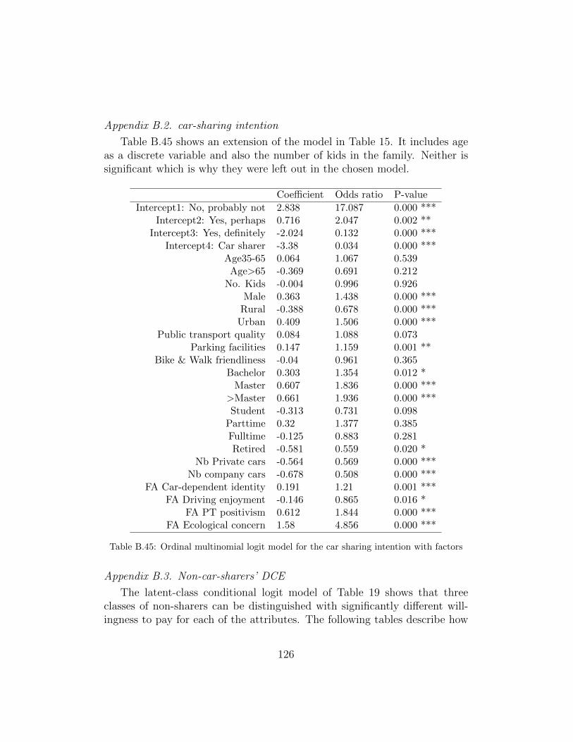
Appendix B.2. car-sharing intention

Table B.45 shows an extension of the model in Table 15. It includes ageas a discrete variable and also the number of kids in the family. Neither issignificant which is why they were left out in the chosen model.

Coe�cient Odds ratio P-valueIntercept1: No, probably not 2.838 17.087 0.000 ***

Intercept2: Yes, perhaps 0.716 2.047 0.002 **Intercept3: Yes, definitely -2.024 0.132 0.000 ***

Intercept4: Car sharer -3.38 0.034 0.000 ***Age35-65 0.064 1.067 0.539Age>65 -0.369 0.691 0.212

No. Kids -0.004 0.996 0.926Male 0.363 1.438 0.000 ***Rural -0.388 0.678 0.000 ***Urban 0.409 1.506 0.000 ***

Public transport quality 0.084 1.088 0.073Parking facilities 0.147 1.159 0.001 **

Bike & Walk friendliness -0.04 0.961 0.365Bachelor 0.303 1.354 0.012 *Master 0.607 1.836 0.000 ***

>Master 0.661 1.936 0.000 ***Student -0.313 0.731 0.098Parttime 0.32 1.377 0.385Fulltime -0.125 0.883 0.281Retired -0.581 0.559 0.020 *

Nb Private cars -0.564 0.569 0.000 ***Nb company cars -0.678 0.508 0.000 ***

FA Car-dependent identity 0.191 1.21 0.001 ***FA Driving enjoyment -0.146 0.865 0.016 *

FA PT positivism 0.612 1.844 0.000 ***FA Ecological concern 1.58 4.856 0.000 ***

Table B.45: Ordinal multinomial logit model for the car sharing intention with factors

Appendix B.3. Non-car-sharers’ DCE

The latent-class conditional logit model of Table 19 shows that threeclasses of non-sharers can be distinguished with significantly di↵erent will-ingness to pay for each of the attributes. The following tables describe how

126

each of the classes di↵er with respect to demographics and mobility optionsthat are available to them.

Variable Levels n1 %1 n2 %2 n3 %3 nall %all

Gender Man 141 37.5 229 39.8 318 37.3 688 38.1Woman 234 62.2 344 59.7 531 62.3 1109 61.5X 1 0.3 3 0.5 3 0.3 7 0.4

p = 0.85 all 376 100.0 576 100.0 852 100.0 1804 100.0

Education Secundary school 144 38.0 170 29.5 172 20.1 486 26.8Bachelor degree 109 28.8 215 37.3 287 33.5 611 33.7Master degree 101 26.6 141 24.5 288 33.6 530 29.3>Master 25 6.6 50 8.7 109 12.7 184 10.2

p = 0.0005 all 379 100.0 576 100.0 856 100.0 1811 100.0

Degree of urbanisation Rural 164 43.2 285 49.5 307 36.0 756 41.8Urban 93 24.5 102 17.7 259 30.4 454 25.1Suburban 123 32.4 189 32.8 286 33.6 598 33.1

p = 0.0005 all 380 100.0 576 100.0 852 100.0 1808 100.0

Profession Other 31 8.2 81 14.0 105 12.2 217 12.0Blue collar worker 21 5.5 25 4.3 21 2.4 67 3.7White collar worker 218 57.4 331 57.3 505 58.9 1054 58.1Education 12 3.2 36 6.2 71 8.3 119 6.6Self-employed 20 5.3 40 6.9 44 5.1 104 5.7Civil servant 7 1.8 10 1.7 17 2.0 34 1.9Retired 59 15.5 34 5.9 61 7.1 154 8.5Incapacitated 4 1.0 8 1.4 7 0.8 19 1.0Unemployed 2 0.5 9 1.6 17 2.0 28 1.5Stay-at-home (wo)man 6 1.6 4 0.7 9 1.0 19 1.0

p = 0.0005 all 380 100.0 578 100.0 857 100.0 1815 100.0

Employment Student 30 7.9 71 12.3 97 11.3 198 10.9Part time job 71 18.7 79 13.7 141 16.5 291 16.1Full time job 205 54.1 362 63.0 509 59.5 1076 59.5Not working 73 19.3 63 11.0 109 12.7 245 13.5

p = 0.0015 all 379 100.0 575 100.0 856 100.0 1810 100.0

Car sharing intention Yes, certainly 20 5.4 10 1.8 228 27.1 258 14.5Yes, perhaps 110 29.9 175 30.8 461 54.7 746 41.9No, probably not 142 38.6 241 42.4 95 11.3 478 26.9No, never 90 24.5 138 24.2 27 3.2 255 14.3Used to be a sharer 6 1.6 5 0.9 32 3.8 43 2.4

p = 0.0005 all 368 100.0 569 100.0 843 100.0 1780 100.0

Table B.46: Demographics compared between latent classes. p-values of Fisher’s exacttest added. Missing data is left out.

127

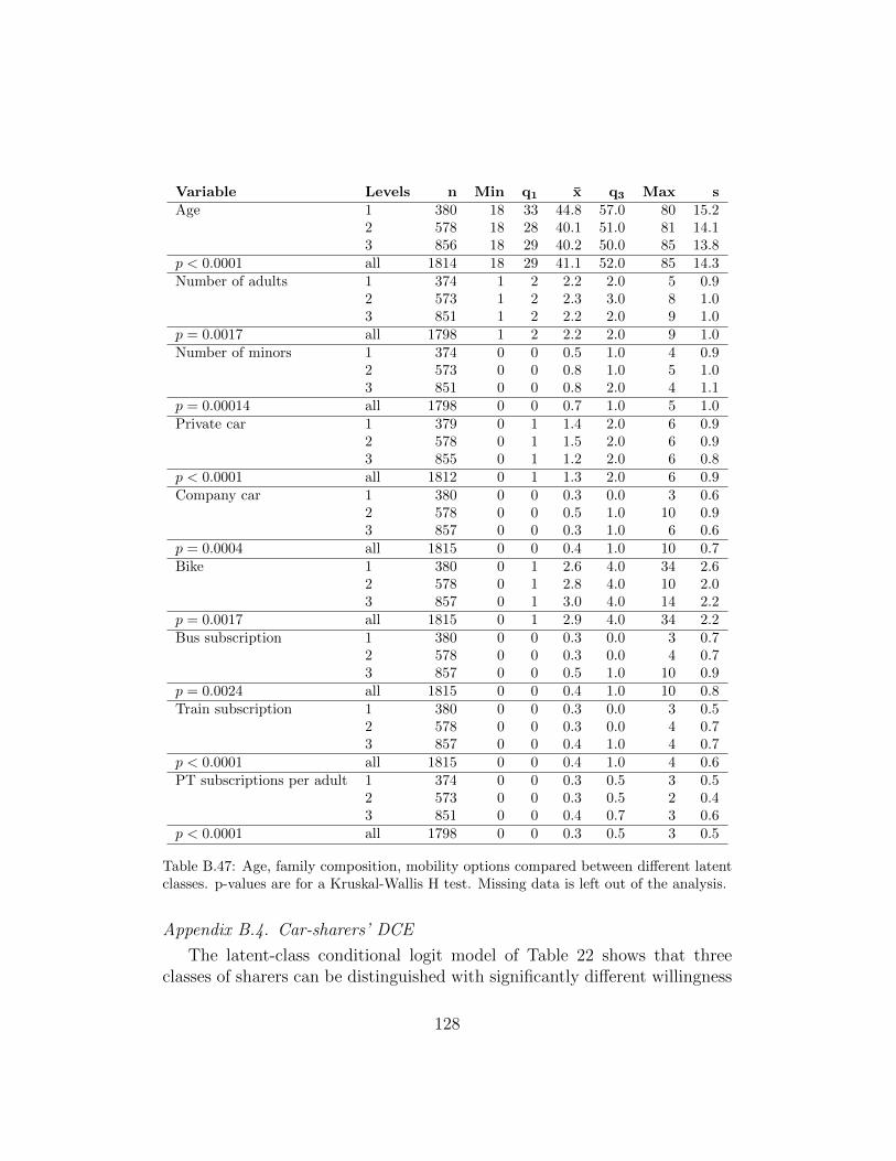
Variable Levels n Min q1 x q3 Max sAge 1 380 18 33 44.8 57.0 80 15.2

2 578 18 28 40.1 51.0 81 14.13 856 18 29 40.2 50.0 85 13.8

p < 0.0001 all 1814 18 29 41.1 52.0 85 14.3Number of adults 1 374 1 2 2.2 2.0 5 0.9

2 573 1 2 2.3 3.0 8 1.03 851 1 2 2.2 2.0 9 1.0

p = 0.0017 all 1798 1 2 2.2 2.0 9 1.0Number of minors 1 374 0 0 0.5 1.0 4 0.9

2 573 0 0 0.8 1.0 5 1.03 851 0 0 0.8 2.0 4 1.1

p = 0.00014 all 1798 0 0 0.7 1.0 5 1.0Private car 1 379 0 1 1.4 2.0 6 0.9

2 578 0 1 1.5 2.0 6 0.93 855 0 1 1.2 2.0 6 0.8

p < 0.0001 all 1812 0 1 1.3 2.0 6 0.9Company car 1 380 0 0 0.3 0.0 3 0.6

2 578 0 0 0.5 1.0 10 0.93 857 0 0 0.3 1.0 6 0.6

p = 0.0004 all 1815 0 0 0.4 1.0 10 0.7Bike 1 380 0 1 2.6 4.0 34 2.6

2 578 0 1 2.8 4.0 10 2.03 857 0 1 3.0 4.0 14 2.2

p = 0.0017 all 1815 0 1 2.9 4.0 34 2.2Bus subscription 1 380 0 0 0.3 0.0 3 0.7

2 578 0 0 0.3 0.0 4 0.73 857 0 0 0.5 1.0 10 0.9

p = 0.0024 all 1815 0 0 0.4 1.0 10 0.8Train subscription 1 380 0 0 0.3 0.0 3 0.5

2 578 0 0 0.3 0.0 4 0.73 857 0 0 0.4 1.0 4 0.7

p < 0.0001 all 1815 0 0 0.4 1.0 4 0.6PT subscriptions per adult 1 374 0 0 0.3 0.5 3 0.5

2 573 0 0 0.3 0.5 2 0.43 851 0 0 0.4 0.7 3 0.6

p < 0.0001 all 1798 0 0 0.3 0.5 3 0.5

Table B.47: Age, family composition, mobility options compared between di↵erent latentclasses. p-values are for a Kruskal-Wallis H test. Missing data is left out of the analysis.

Appendix B.4. Car-sharers’ DCE

The latent-class conditional logit model of Table 22 shows that threeclasses of sharers can be distinguished with significantly di↵erent willingness

128

to pay for each of the attributes. Tables B.48 and B.49 describe how each ofthe classes di↵er with respect to demographics, factor scores, and the mobilityoptions that are available to them. Table B.50 additionally describes thecharacteristics of the current CS system of the respondents.

Variable Levels n1 %1 n2 %2 n3 %3 nall %all

Gender Man 28 33.3 53 40.5 29 42.0 110 38.7Woman 55 65.5 78 59.5 40 58.0 173 60.9X 1 1.2 0 0.0 0 0.0 1 0.3

p = 0.45 all 84 100.0 131 100.0 69 100.0 284 100.0

Education Secundary school 4 4.7 7 5.3 5 7.2 16 5.6Bachelor degree 22 25.9 34 25.9 20 29.0 76 26.7Master degree 47 55.3 67 51.1 36 52.2 150 52.6>Master 12 14.1 23 17.6 8 11.6 43 15.1

p = 0.93 all 85 100.0 131 100.0 69 100.0 285 100.0

Degree of urbanisation Rural 6 7.1 6 4.6 12 17.4 24 8.4Urban 57 67.1 92 70.2 38 55.1 187 65.6Suburban 22 25.9 33 25.2 19 27.5 74 26.0

p = 0.04 all 85 100.0 131 100.0 69 100.0 285 100.0

Profession Other 1 1.2 5 3.8 6 8.7 12 4.2Blue collar worker 1 1.2 1 0.8 3 4.3 5 1.8White collar worker 57 67.1 87 66.4 43 62.3 187 65.6Education 9 10.6 18 13.7 11 15.9 38 13.3Self-employed 10 11.8 7 5.3 3 4.3 20 7.0Civil servant 3 3.5 0 0.0 3 4.3 6 2.1Retired 1 1.2 6 4.6 0 0.0 7 2.5Incapacitated 1 1.2 2 1.5 0 0.0 3 1.0Unemployed 2 2.4 4 3.0 0 0.0 6 2.1Stay-at-home (wo)man 0 0.0 1 0.8 0 0.0 1 0.3

p = 0.05 all 85 100.0 131 100.0 69 100.0 285 100.0

Employment Student 1 1.2 7 5.3 5 7.3 13 4.6Part time job 25 29.4 28 21.4 15 22.1 68 23.9Full time job 54 63.5 82 62.6 46 67.7 182 64.1Not working 5 5.9 14 10.7 2 2.9 21 7.4

p = 0.14 all 85 100.0 131 100.0 68 100.0 284 100.0

Table B.48: Demographics compared between classes of car sharers. p-values of Fisher’sexact test added. Missing data is left out.

129

Variable Levels n Min q1 x q3 Max sAge 1 85 23.0 31.0 38.7 45.0 64.0 9.7

2 131 23.0 30.0 38.8 44.5 73.0 10.43 69 18.0 29.0 37.7 43.0 71.0 10.5

p = 0.76 all 285 18.0 30.0 38.5 44.0 73.0 10.2Number of adults 1 85 1.0 1.0 1.9 2.0 4.0 0.7

2 130 1.0 1.0 1.9 2.0 5.0 0.83 69 1.0 2.0 2.1 2.0 6.0 1.0

p = 0.14 all 284 1.0 1.0 1.9 2.0 6.0 0.8Number of minors 1 85 0.0 0.0 0.9 2.0 4.0 1.0

2 130 0.0 0.0 0.7 1.0 5.0 1.13 69 0.0 0.0 1.1 2.0 5.0 1.1

p = 0.05 all 284 0.0 0.0 0.9 2.0 5.0 1.1FA Car-dependent identity 1 85 -1.5 -0.8 -0.2 0.4 2.1 0.8

2 131 -1.9 -0.7 0.0 0.5 2.8 0.93 69 -1.4 -0.5 0.3 0.9 3.4 1.0

p = 0.02 all 285 -1.9 -0.7 0.0 0.6 3.4 0.9FA Social & ecological concern 1 85 -2.8 -0.2 0.2 0.8 1.6 0.8

2 131 -2.9 -0.4 0.0 0.6 1.5 0.93 69 -3.3 -0.7 -0.3 0.4 1.9 1.0

p = 0.0047 all 285 -3.3 -0.4 0.0 0.6 1.9 0.9FA Shared mobility 1 85 -2.1 -0.7 0.0 0.7 2.5 0.9

2 131 -1.9 -0.6 0.0 0.7 2.0 0.93 69 -2.2 -0.6 -0.1 0.5 1.9 0.9

p = 0.91 all 285 -2.2 -0.6 0.0 0.6 2.5 0.9FA Driving enjoyment 1 85 -3.0 -0.7 -0.1 0.6 2.2 1.0

2 131 -2.1 -0.4 0.1 0.8 2.2 0.83 69 -2.4 -0.4 -0.2 0.3 1.3 0.8

p = 0.05 all 285 -3.0 -0.5 0.0 0.6 2.2 0.9Private car 1 85 0.0 0.0 0.4 1.0 3.0 0.6

2 131 0.0 0.0 0.3 1.0 2.0 0.53 69 0.0 0.0 0.5 1.0 2.0 0.6

p = 0.06 all 285 0.0 0.0 0.4 1.0 3.0 0.6Company car 1 85 0.0 0.0 0.1 0.0 2.0 0.3

2 131 0.0 0.0 0.1 0.0 2.0 0.33 69 0.0 0.0 0.2 0.0 1.0 0.4

p = 0.0042 all 285 0.0 0.0 0.1 0.0 2.0 0.3Bike 1 85 0.0 2.0 3.2 4.0 9.0 2.1

2 131 0.0 1.0 2.8 4.0 10.0 2.13 69 0.0 2.0 3.6 5.0 16.0 2.4

p = 0.05 all 285 0.0 1.0 3.1 4.0 16.0 2.2Bus subscription 1 85 0.0 0.0 0.6 1.0 3.0 0.9

2 131 0.0 0.0 0.7 1.0 4.0 1.03 69 0.0 0.0 0.7 1.0 5.0 1.2

p = 0.31 all 285 0.0 0.0 0.6 1.0 5.0 1.0Train subscription 1 85 0.0 0.0 0.4 1.0 2.0 0.6

2 131 0.0 0.0 0.5 1.0 3.0 0.73 69 0.0 0.0 0.4 1.0 2.0 0.6

p = 0.80 all 285 0.0 0.0 0.5 1.0 3.0 0.7PT subscriptions per adult 1 85 0.0 0.0 0.5 1.0 3.0 0.7

2 130 0.0 0.0 0.7 1.0 4.0 0.83 69 0.0 0.0 0.6 1.0 2.5 0.7

p = 0.32 all 284 0.0 0.0 0.6 1.0 4.0 0.8

Table B.49: Age, family composition, mobility options, and factor scores compared be-tween di↵erent classes of car sharers. p-values are for a Kruskal-Wallis H test. Missingdata is left out of the analysis.

130

Variable Levels n1 %1 n2 %2 n3 %3 nall %all

CS provider Bolides 1 1.2 0 0.0 0 0.0 1 0.3Cambio 16 18.8 59 45.0 40 58.0 115 40.4Caramigo 1 1.2 1 0.8 0 0.0 2 0.7Company 0 0.0 1 0.8 1 1.4 2 0.7Cozycar 11 12.9 6 4.6 9 13.0 26 9.1Degage 45 52.9 27 20.6 7 10.1 79 27.7Drivenow 0 0.0 1 0.8 0 0.0 1 0.3Drivy 2 2.4 0 0.0 0 0.0 2 0.7EcoMobiliteitGent 0 0.0 2 1.5 0 0.0 2 0.7City cars 0 0.0 1 0.8 0 0.0 1 0.3Informal 1 1.2 3 2.3 3 4.3 7 2.5nonActive 6 7.1 14 10.7 5 7.2 25 8.8Partago 2 2.4 11 8.4 0 0.0 13 4.6Poppy 0 0.0 4 3.0 2 2.9 6 2.1Ubeeqo 0 0.0 0 0.0 2 2.9 2 0.7Zipcar 0 0.0 1 0.8 0 0.0 1 0.3

p = 0.0005 all 85 100.0 131 100.0 69 100.0 285 100.0

Type of CS system B2C 19 22.4 79 60.3 45 65.2 143 50.2P2P 66 77.7 52 39.7 24 34.8 142 49.8

p = 0.0005 all 85 100.0 131 100.0 69 100.0 285 100.0

Flexibility Free-floating 0 0.0 8 6.1 2 2.9 10 3.52km radius 60 70.6 45 34.4 16 23.2 121 42.5Station-based 25 29.4 78 59.5 51 73.9 154 54.0

p = 0.0005 all 85 100.0 131 100.0 69 100.0 285 100.0

Use frequency Daily or almost daily 0 0.0 2 1.5 0 0.0 2 0.72-3 times per month 22 25.9 31 23.7 15 21.7 68 23.9once per week 12 14.1 29 22.1 16 23.2 57 20.02 to 3 times per week 8 9.4 11 8.4 4 5.8 23 8.1once per month 25 29.4 27 20.6 12 17.4 64 22.5less than 1 time per month 18 21.2 31 23.7 22 31.9 71 24.9

p = 0.49 all 85 100.0 131 100.0 69 100.0 285 100.0

Table B.50: Characteristics of the current car sharing system. p-values of Fisher’s exacttest added. Missing data is left out.

131

ce-center.be

CIRCULAR ECONOMYPOLICY RESEARCHCENTRE

OVAMWE MAKE

TOMORROWB E AUT I FUL

DEPARTMENT OFECONOMYSCIENCE &INNOVATIONOVAM

WE MAKETOMORROWB E AUT I FUL

DEPARTMENT OFECONOMYSCIENCE &INNOVATION

CIRCULAR ECONOMYPOLICY RESEARCHCENTRE

CE CENTER

Disclaimer:This publication reflects the views only of the author, and the Flemish Government cannot be heldresponsible for any use which may be made of the information contained therein.