Bird-MAC: Energy-Efficient MAC for Quasi-Periodic ... - GitHub Pages
Upload
khangminh22Category
view
0download
0
SEDStudent Experiment Documentation
Document ID: BX26 TUBULAR SEDv5-2 26Apr21
Mission: BEXUS 26
Team Name: TUBULAR
Experiment Title: Alternative to AirCore for Atmospheric Greenhouse Gas Sampling
Team NameStudent Team Leader: Natalie Lawton
Team Members: Nuria Agues PaszkowskyKyriaki BlazakiEmily ChenJordi Coll OrtegaGustav DyrssenErik FagerstromGeorges L. J. LabrechePau Molas RocaEmil NordqvistMuhammad Ansyar Rafi PutraHamad SiddiqiIvan Zankov
University: Lulea University of Technology
Version: Issue Date: Document Type: Valid from
5.2 April 26, 2021 Spec April 26, 2021
Issued by:
The TUBULAR Team
Approved by:
Dr. Thomas Kuhn
BX26 TUBULAR SEDv5-2 26Apr21

- 2 -
CHANGE RECORD
Version Date Changed chapter Remarks0 2017-12-20 New Version1-0 2018-01-15 All PDR1-1 2018-01-25 1.1, 2.2, 2.3, 3.3.3, 3.5, 4.1, 4.4.2,
4.5, 4.6, 4.7, 6.1.5, 6.1.6, 6.2, 6.4,7.3.1
Incorporatingfeedback fromPDR
1-2 2018-03-12 Added: 4.5.1, 4.5.2, 4.5.3, 4.5.4,4.6.1, 4.6.2, 4.6.3, 4.6.4, 4.7.1,4.7.2, 5.2, Appendix: D, E, G, F.Changed: 1.5, 2.1, 2.3, 2.4, 2.5,3.1, 3.2, 3.3, 3.3.2, 3.4, 3.5, 4.1,4.3.1, 4.4, 4.4.2, 4.5, 4.5.1, 4.5.2,4.5.3, 4.5.4, 4.6, 4.6.3, 4.6.4, 4.7,4.7.1, 4.7.2, 4.8, 5.1, 5.2, 6.1,6.1.4, 6.2, 6.3, 6.4, Appendix: BC.
2-0 2018-05-13 Added: 5.3.1, 5.3.2, 6.4.2, 7.1,H.6.1 in Appendix H, Appendix I,Changed: 1.5, 2.2, 2.3, 3.2 3.3.1,3.5, 4.1, 4.3.1, 4.4.2, 4.4.4, 4.5,4.5.1, 4.5.2, 4.5.3, 4.5.4, 4.6, 4.6.3,4.6.6, 4.71, 4.7.2, 4.8.2, 4.9, 5.1,5.2, 5.3, 5.3.1, 6.1, 6.1.4, 6.2,6.4.1, 7.1, 7.4, 7.4.1 Appendix E.3,F
CDR
2-1 2018-05-24 Added: 4.2.2, 4.2.33-0 2018-07-10 Changed: Acknowledgements, Ab-
stract, 1.3, 1.5, 2.1, 2.2, 2.3, 3.1,3.2, 3.3, 3.4, 3.5, 4.1, 4.2, 4.3, 4.4,4.5, 4.6, 4.7, 4.8, 5.1, 5.2, 5.3, 6.1,6.2, 6.3, 7.1, 7.2, Appendix: A, B,C, D, E, F, G, H, I, J, K, L, M, N,O
IPR and appendixreordered.
3-1 2018-07-22 Changed: 2.3, 3.3.1, 3.3.2, 3.5,4.2.1, 4.3, 4.4.5, 4.5.1, 4.5.5, 4.5.6,4.6.3, 5.1, 5.2, 5.3, 6.1.2, App C,App F, App M, App O
pre-IPR feedback
BX26 TUBULAR SEDv5-2 26Apr21

- 3 -
4-0 2018-10-04 Added: 5.3.9, 5.3.10, 5.3.11,5.3.12, 5.3.13, 5.3.14, 5.3.15,5.3.16, 5.3.17, 5.3.18, 5.3.19,5.3.20, 5.3.21 Changed: 2.2, 2.3,3.3.1, 3.3.2, 3.5, 4.1, 4.2, 4.3, 4.4,4.5, 4.6, 4.7, 4.9, 4.9, 5.1, 5.2,5.3.5, 5.3.6, 5.3.7, 5.3.8, 6.1.2,6.1.6, 6.2, 6.3, 6.4, 7.4, App A, AppB, App C, App D, App E, App F,App M, App N, App O
EAR
5-0 2019-01-11 Added: 7.3.2, 7.3.3, 7.3.4, 7.3.5,7.3.6, 7.4 Changed: 1.3, 1.4, 3.1,3.2, 3.3, 3.4, 3.5, 4.1, 4.2, 4.4, 4.5,4.6, 4.7, 4.8, 4.8, 4.9, 5.2, 6.1, 6.2,6.3, 6.4, 7.1, 7.2, 7.3, 7.4, 7.5
Final Report
5-1 2019-07-17 Changed: Preface, Acknowledge-ments, Abbreviations and Refer-ences, 3.3.1, 3.3.2, 4.2.1, 4.7.1,5.1, 5.2.3, 5.3.4, 6.1.2, 6.3, App C,App D, App H, App K, App M, AppO
Editorial updates:SNSB to SNSAand table format-ting with respectto page margins.
5-2 2021-04-26 Changed: 3.5, 7.3.6, 7.3.7, 8.2 Fixed brokenreferences.Resolved am-biguities withtext and plots inResults section.Mentioned andreferenced pub-lished conferencepapers.
BX26 TUBULAR SEDv5-2 26Apr21

- 4 -
Abstract:Carbon dioxide (CO2), methane (CH4), and carbon monoxide (CO) are threemain greenhouse gases emitted by human activities. Developing a better un-derstanding of their contribution to greenhouse effects requires more accessible,flexible, and scalable air sampling mechanisms. A balloon flight is the most cost-effective mechanism to obtain a vertical air profile through continuous samplingbetween the upper troposphere and the lower stratosphere. However, recoverytime constraints due to gas mixture concerns geographically restrict the samplingnear existing research centers where analysis of the recovered samples can takeplace. The TUBULAR experiment is a technology demonstrator for atmosphericresearch supporting an air sampling mechanism that would offer climate changeresearchers access to remote areas by minimizing the effect of gas mixtures withinthe collected samples so that recovery time is no longer a constraint. The exper-iment includes a secondary sampling mechanism that serves as reference againstwhich the proposed sampling mechanism can be validated.
Keywords: Balloon Experiments for University Students, Climate Change, Stratospheric AirSampling, AirCore, Sampling Bags, Greenhouse Gas, Carbon Dioxide (CO2),Methane (CH4), Carbon Monoxide (CO).
BX26 TUBULAR SEDv5-2 26Apr21

- 5 -
Contents
CHANGE RECORD 2
PREFACE 12
1 Introduction 151.1 Scientific Background . . . . . . . . . . . . . . . . . . . . . . . . . . . . . . 151.2 Mission Statement . . . . . . . . . . . . . . . . . . . . . . . . . . . . . . . . 151.3 Experiment Objectives . . . . . . . . . . . . . . . . . . . . . . . . . . . . . . 161.4 Experiment Concept . . . . . . . . . . . . . . . . . . . . . . . . . . . . . . . 161.5 Team Details . . . . . . . . . . . . . . . . . . . . . . . . . . . . . . . . . . . 18
2 Experiment Requirements and Constraints 222.1 Functional Requirements . . . . . . . . . . . . . . . . . . . . . . . . . . . . . 222.2 Performance Requirements . . . . . . . . . . . . . . . . . . . . . . . . . . . . 222.3 Design Requirements . . . . . . . . . . . . . . . . . . . . . . . . . . . . . . . 232.4 Operational Requirements . . . . . . . . . . . . . . . . . . . . . . . . . . . . 242.5 Constraints . . . . . . . . . . . . . . . . . . . . . . . . . . . . . . . . . . . . 24
3 Project Planning 253.1 Work Breakdown Structure . . . . . . . . . . . . . . . . . . . . . . . . . . . 253.2 Schedule . . . . . . . . . . . . . . . . . . . . . . . . . . . . . . . . . . . . . 283.3 Resources . . . . . . . . . . . . . . . . . . . . . . . . . . . . . . . . . . . . 29
3.3.1 Manpower . . . . . . . . . . . . . . . . . . . . . . . . . . . . . . . . 293.3.2 Budget . . . . . . . . . . . . . . . . . . . . . . . . . . . . . . . . . . 323.3.3 External Support . . . . . . . . . . . . . . . . . . . . . . . . . . . . . 33
3.4 Outreach Approach . . . . . . . . . . . . . . . . . . . . . . . . . . . . . . . 343.5 Risk Register . . . . . . . . . . . . . . . . . . . . . . . . . . . . . . . . . . . 35
4 Experiment Design 414.1 Experiment Setup . . . . . . . . . . . . . . . . . . . . . . . . . . . . . . . . 414.2 Experiment Interfaces . . . . . . . . . . . . . . . . . . . . . . . . . . . . . . 50
4.2.1 Mechanical Interfaces . . . . . . . . . . . . . . . . . . . . . . . . . . 504.2.2 Thermal Interfaces . . . . . . . . . . . . . . . . . . . . . . . . . . . . 524.2.3 CAC Interfaces . . . . . . . . . . . . . . . . . . . . . . . . . . . . . . 534.2.4 AAC Interfaces . . . . . . . . . . . . . . . . . . . . . . . . . . . . . . 534.2.5 Electrical Interfaces . . . . . . . . . . . . . . . . . . . . . . . . . . . 54
4.3 Experiment Components . . . . . . . . . . . . . . . . . . . . . . . . . . . . . 564.3.1 Electrical Components . . . . . . . . . . . . . . . . . . . . . . . . . . 564.3.2 Mechanical Components . . . . . . . . . . . . . . . . . . . . . . . . . 614.3.3 Other Components . . . . . . . . . . . . . . . . . . . . . . . . . . . . 66
4.4 Mechanical Design . . . . . . . . . . . . . . . . . . . . . . . . . . . . . . . . 684.4.1 Structure . . . . . . . . . . . . . . . . . . . . . . . . . . . . . . . . . 714.4.2 Walls and Protections . . . . . . . . . . . . . . . . . . . . . . . . . . 724.4.3 CAC Box . . . . . . . . . . . . . . . . . . . . . . . . . . . . . . . . . 734.4.4 AAC Box . . . . . . . . . . . . . . . . . . . . . . . . . . . . . . . . . 754.4.5 Pneumatic Subsystem . . . . . . . . . . . . . . . . . . . . . . . . . . 79
BX26 TUBULAR SEDv5-2 26Apr21

- 6 -
4.5 Electrical Design . . . . . . . . . . . . . . . . . . . . . . . . . . . . . . . . . 814.5.1 Block Diagram . . . . . . . . . . . . . . . . . . . . . . . . . . . . . . 814.5.2 Miniature Diaphragm Air Pump . . . . . . . . . . . . . . . . . . . . . 824.5.3 Electromagnetically Controlled Valves . . . . . . . . . . . . . . . . . . 844.5.4 Switching Circuits . . . . . . . . . . . . . . . . . . . . . . . . . . . . 854.5.5 Schematic . . . . . . . . . . . . . . . . . . . . . . . . . . . . . . . . 864.5.6 PCB Layout . . . . . . . . . . . . . . . . . . . . . . . . . . . . . . . 88
4.6 Thermal Design . . . . . . . . . . . . . . . . . . . . . . . . . . . . . . . . . 914.6.1 Thermal Environment . . . . . . . . . . . . . . . . . . . . . . . . . . 914.6.2 The Critical Stages . . . . . . . . . . . . . . . . . . . . . . . . . . . 914.6.3 Overall Design . . . . . . . . . . . . . . . . . . . . . . . . . . . . . . 924.6.4 Internal Temperature . . . . . . . . . . . . . . . . . . . . . . . . . . 944.6.5 Calculations and Simulation Reports . . . . . . . . . . . . . . . . . . 95
4.7 Power System . . . . . . . . . . . . . . . . . . . . . . . . . . . . . . . . . . 984.7.1 Power System Requirements . . . . . . . . . . . . . . . . . . . . . . . 98
4.8 Software Design . . . . . . . . . . . . . . . . . . . . . . . . . . . . . . . . . 994.8.1 Purpose . . . . . . . . . . . . . . . . . . . . . . . . . . . . . . . . . 994.8.2 Design . . . . . . . . . . . . . . . . . . . . . . . . . . . . . . . . . . 994.8.3 Implementation . . . . . . . . . . . . . . . . . . . . . . . . . . . . . 104
4.9 Ground Support Equipment . . . . . . . . . . . . . . . . . . . . . . . . . . . 105
5 Experiment Verification and Testing 1065.1 Verification Matrix . . . . . . . . . . . . . . . . . . . . . . . . . . . . . . . . 1065.2 Test Plan . . . . . . . . . . . . . . . . . . . . . . . . . . . . . . . . . . . . . 109
5.2.1 Test Priority . . . . . . . . . . . . . . . . . . . . . . . . . . . . . . . 1095.2.2 Planned Tests . . . . . . . . . . . . . . . . . . . . . . . . . . . . . . 1095.2.3 Test Descriptions . . . . . . . . . . . . . . . . . . . . . . . . . . . . 111
5.3 Test Results . . . . . . . . . . . . . . . . . . . . . . . . . . . . . . . . . . . 1235.3.1 Test 28: Pump Operations . . . . . . . . . . . . . . . . . . . . . . . 1235.3.2 Test 18: Pump Low Pressure . . . . . . . . . . . . . . . . . . . . . . 1235.3.3 Test 30: Sampling Bag Bursting . . . . . . . . . . . . . . . . . . . . . 1245.3.4 Test 29: Pump Current under Low Pressure . . . . . . . . . . . . . . 1255.3.5 Test 17: Sampling bags’ holding times and samples’ . . . . . . . . . . 1255.3.6 Test 4: Low Pressure . . . . . . . . . . . . . . . . . . . . . . . . . . 1275.3.7 Test 20: Switching Circuit Testing and Verification . . . . . . . . . . . 1285.3.8 Test 32: Software Failure . . . . . . . . . . . . . . . . . . . . . . . . 1285.3.9 Test 31: Unit Test . . . . . . . . . . . . . . . . . . . . . . . . . . . . 1285.3.10 Test 10: Software and Electronics Operation . . . . . . . . . . . . . . 1285.3.11 Test 14: Ground Station-OBC Parameters Reprogram Test . . . . . . 1295.3.12 Test 24: Software and Electronics Integration . . . . . . . . . . . . . . 1295.3.13 Test 5: Thermal Test . . . . . . . . . . . . . . . . . . . . . . . . . . 1295.3.14 Test 27: Shock test . . . . . . . . . . . . . . . . . . . . . . . . . . . 1295.3.15 Test 9: Vibration test . . . . . . . . . . . . . . . . . . . . . . . . . . 1305.3.16 Test 25: Structure test . . . . . . . . . . . . . . . . . . . . . . . . . 1305.3.17 Test 33: Electrical Component Testing . . . . . . . . . . . . . . . . . 1305.3.18 Test 12: Removal test . . . . . . . . . . . . . . . . . . . . . . . . . . 1305.3.19 Test 2: Data collection test . . . . . . . . . . . . . . . . . . . . . . . 130
BX26 TUBULAR SEDv5-2 26Apr21
- 7 -
5.3.20 Test 7: Bench test . . . . . . . . . . . . . . . . . . . . . . . . . . . . 1315.3.21 Test 16: Sampling test . . . . . . . . . . . . . . . . . . . . . . . . . 131
6 Launch Campaign Preparations 1326.1 Input for the Campaign / Flight Requirements Plans . . . . . . . . . . . . . . 132
6.1.1 Dimensions and Mass . . . . . . . . . . . . . . . . . . . . . . . . . . 1326.1.2 Safety Risks . . . . . . . . . . . . . . . . . . . . . . . . . . . . . . . 1326.1.3 Electrical Interfaces . . . . . . . . . . . . . . . . . . . . . . . . . . . 1336.1.4 Launch Site Requirements . . . . . . . . . . . . . . . . . . . . . . . . 1336.1.5 Flight Requirements . . . . . . . . . . . . . . . . . . . . . . . . . . . 1346.1.6 Accommodation Requirements . . . . . . . . . . . . . . . . . . . . . 135
6.2 Preparation and Test Activities at Esrange . . . . . . . . . . . . . . . . . . . 1366.3 Timeline for Countdown and Flight . . . . . . . . . . . . . . . . . . . . . . . 1396.4 Post Flight Activities . . . . . . . . . . . . . . . . . . . . . . . . . . . . . . . 141
6.4.1 CAC Recovery . . . . . . . . . . . . . . . . . . . . . . . . . . . . . . 1416.4.2 Recovery Checklist . . . . . . . . . . . . . . . . . . . . . . . . . . . . 1416.4.3 Analysis Preparation . . . . . . . . . . . . . . . . . . . . . . . . . . . 142
7 Data Analysis and Results 1437.1 Data Analysis Plan . . . . . . . . . . . . . . . . . . . . . . . . . . . . . . . . 143
7.1.1 Picarro G2401 . . . . . . . . . . . . . . . . . . . . . . . . . . . . . . 1437.1.2 Analysis Strategy . . . . . . . . . . . . . . . . . . . . . . . . . . . . . 146
7.2 Launch Campaign . . . . . . . . . . . . . . . . . . . . . . . . . . . . . . . . 1517.2.1 Flight preparation activities during launch campaign . . . . . . . . . . 1517.2.2 Flight performance . . . . . . . . . . . . . . . . . . . . . . . . . . . . 1517.2.3 Recovery . . . . . . . . . . . . . . . . . . . . . . . . . . . . . . . . . 1527.2.4 Post flight activities . . . . . . . . . . . . . . . . . . . . . . . . . . . 152
7.3 Results . . . . . . . . . . . . . . . . . . . . . . . . . . . . . . . . . . . . . . 1567.3.1 Mechanical Subsystem Performance . . . . . . . . . . . . . . . . . . . 1567.3.2 Electrical Subsystem Performance . . . . . . . . . . . . . . . . . . . . 1587.3.3 Software Subsystem Performance . . . . . . . . . . . . . . . . . . . . 1587.3.4 Thermal Subsystem Performance . . . . . . . . . . . . . . . . . . . . 1597.3.5 Past Results . . . . . . . . . . . . . . . . . . . . . . . . . . . . . . . 1597.3.6 Scientific Results . . . . . . . . . . . . . . . . . . . . . . . . . . . . . 1647.3.7 Future Work . . . . . . . . . . . . . . . . . . . . . . . . . . . . . . . 166
7.4 Failure Analysis . . . . . . . . . . . . . . . . . . . . . . . . . . . . . . . . . 1677.4.1 Post flight analysis . . . . . . . . . . . . . . . . . . . . . . . . . . . . 1677.4.2 Lab analysis . . . . . . . . . . . . . . . . . . . . . . . . . . . . . . . 1687.4.3 Conclusion . . . . . . . . . . . . . . . . . . . . . . . . . . . . . . . . 169
7.5 Lessons Learned . . . . . . . . . . . . . . . . . . . . . . . . . . . . . . . . . 1707.5.1 Management Division . . . . . . . . . . . . . . . . . . . . . . . . . . 1707.5.2 Scientific Division . . . . . . . . . . . . . . . . . . . . . . . . . . . . 1717.5.3 Electrical Division . . . . . . . . . . . . . . . . . . . . . . . . . . . . 1727.5.4 Software Division . . . . . . . . . . . . . . . . . . . . . . . . . . . . 1737.5.5 Mechanical Division . . . . . . . . . . . . . . . . . . . . . . . . . . . 1737.5.6 Thermal Division . . . . . . . . . . . . . . . . . . . . . . . . . . . . . 174
8 Abbreviations and References 175
BX26 TUBULAR SEDv5-2 26Apr21

- 8 -
8.1 Abbreviations . . . . . . . . . . . . . . . . . . . . . . . . . . . . . . . . . . . 1758.2 References . . . . . . . . . . . . . . . . . . . . . . . . . . . . . . . . . . . . 177
A Experiment Reviews 179A.1 Preliminary Design Review (PDR) . . . . . . . . . . . . . . . . . . . . . . . . 179A.2 Critical Design Review (CDR) . . . . . . . . . . . . . . . . . . . . . . . . . . 182A.3 Integration Progress Review (IPR) . . . . . . . . . . . . . . . . . . . . . . . . 186A.4 Experiment Acceptance Review (EAR) . . . . . . . . . . . . . . . . . . . . . 194
B Outreach 201B.1 Outreach on Project Website . . . . . . . . . . . . . . . . . . . . . . . . . . 201B.2 Outreach Timeline . . . . . . . . . . . . . . . . . . . . . . . . . . . . . . . . 206B.3 Social Media Outreach on Facebook . . . . . . . . . . . . . . . . . . . . . . 207B.4 Social Media Outreach on Instagram . . . . . . . . . . . . . . . . . . . . . . 208B.5 Outreach with Open Source Code Hosted on a REXUS/BEXUS GitHub Repos-
itory . . . . . . . . . . . . . . . . . . . . . . . . . . . . . . . . . . . . . . . 209B.6 Outreach with Team Patch . . . . . . . . . . . . . . . . . . . . . . . . . . . 209B.7 Visit by the Canadian Ambassador . . . . . . . . . . . . . . . . . . . . . . . 210B.8 Attendance at Lift Off 2018 . . . . . . . . . . . . . . . . . . . . . . . . . . . 211
C Additional Technical Information 212C.1 Materials Properties . . . . . . . . . . . . . . . . . . . . . . . . . . . . . . . 212C.2 Coiled Tube and Sampling Bag Example . . . . . . . . . . . . . . . . . . . . 213
C.2.1 CAC Coiled Tube . . . . . . . . . . . . . . . . . . . . . . . . . . . . 213C.2.2 Air Sampling Bag . . . . . . . . . . . . . . . . . . . . . . . . . . . . 213
C.3 Dimensions of the sampling bag . . . . . . . . . . . . . . . . . . . . . . . . . 214C.4 List of components in The Brain . . . . . . . . . . . . . . . . . . . . . . . . 214C.5 Pneumatic System Interfaces . . . . . . . . . . . . . . . . . . . . . . . . . . 216
C.5.1 Straight Fittings . . . . . . . . . . . . . . . . . . . . . . . . . . . . . 216C.5.2 90 Degree Fittings . . . . . . . . . . . . . . . . . . . . . . . . . . . . 216C.5.3 Tee Fittings . . . . . . . . . . . . . . . . . . . . . . . . . . . . . . . 216C.5.4 Quick Connectors . . . . . . . . . . . . . . . . . . . . . . . . . . . . 217C.5.5 Reducer and Adapters Fittings . . . . . . . . . . . . . . . . . . . . . 217C.5.6 Port Connections and Ferrule Set . . . . . . . . . . . . . . . . . . . . 217
C.6 Manufacturing Drawings . . . . . . . . . . . . . . . . . . . . . . . . . . . . . 218C.7 Software Sequence Diagram . . . . . . . . . . . . . . . . . . . . . . . . . . . 255
C.7.1 Air Sampling Control Object Sequence diagrams . . . . . . . . . . . . 255C.8 Heating Object Sequence Diagrams . . . . . . . . . . . . . . . . . . . . . . . 258C.9 Sensor Object Sequence Diagrams . . . . . . . . . . . . . . . . . . . . . . . . 261C.10 Software Interface Diagram . . . . . . . . . . . . . . . . . . . . . . . . . . . 264
C.10.1 Sensor Object Interface Diagram . . . . . . . . . . . . . . . . . . . . 264C.10.2 Air Sampling Control Object Interface Diagram . . . . . . . . . . . . . 265C.10.3 Heating Object Interface Diagram . . . . . . . . . . . . . . . . . . . . 266
C.11 PCB Schematics . . . . . . . . . . . . . . . . . . . . . . . . . . . . . . . . . 267C.12 Tube . . . . . . . . . . . . . . . . . . . . . . . . . . . . . . . . . . . . . . . 270C.13 AAC Manifold Valve . . . . . . . . . . . . . . . . . . . . . . . . . . . . . . . 271C.14 AAC Flushing Valve and CAC Valve . . . . . . . . . . . . . . . . . . . . . . . 272C.15 Pump . . . . . . . . . . . . . . . . . . . . . . . . . . . . . . . . . . . . . . . 275
BX26 TUBULAR SEDv5-2 26Apr21
- 9 -
C.16 Airflow Sensor . . . . . . . . . . . . . . . . . . . . . . . . . . . . . . . . . . 276C.17 Static Pressure Sensor . . . . . . . . . . . . . . . . . . . . . . . . . . . . . . 280
D Checklists 283D.1 Pre-Launch Checklist . . . . . . . . . . . . . . . . . . . . . . . . . . . . . . 283D.2 Cleaning Checklist . . . . . . . . . . . . . . . . . . . . . . . . . . . . . . . . 290D.3 Recovery Team Checklist . . . . . . . . . . . . . . . . . . . . . . . . . . . . 291
E Team Availability 295E.1 Team availability from February 2018 to July 2018 . . . . . . . . . . . . . . . 295E.2 Team availability from August 2018 to January 2019 . . . . . . . . . . . . . . 296E.3 Graph Showing Team availability Over Summer . . . . . . . . . . . . . . . . . 297
F Gantt Chart 298F.1 Gantt Chart (1/4) . . . . . . . . . . . . . . . . . . . . . . . . . . . . . . . . 299F.2 Gantt Chart (2/4) . . . . . . . . . . . . . . . . . . . . . . . . . . . . . . . . 300F.3 Gantt Chart (3/4) . . . . . . . . . . . . . . . . . . . . . . . . . . . . . . . . 301F.4 Gantt Chart (4/4) . . . . . . . . . . . . . . . . . . . . . . . . . . . . . . . . 302
G Equipment Loan Agreement 304
H Air Sampling Model for BEXUS Flight 307H.1 Introduction . . . . . . . . . . . . . . . . . . . . . . . . . . . . . . . . . . . 307
H.1.1 Objectives . . . . . . . . . . . . . . . . . . . . . . . . . . . . . . . . 307H.1.2 Justification . . . . . . . . . . . . . . . . . . . . . . . . . . . . . . . 307H.1.3 Methodology . . . . . . . . . . . . . . . . . . . . . . . . . . . . . . . 307
H.2 Scientific and Empirical Background . . . . . . . . . . . . . . . . . . . . . . . 307H.2.1 Study of Previous BEXUS Flights . . . . . . . . . . . . . . . . . . . . 307H.2.2 Trace Gases Distribution . . . . . . . . . . . . . . . . . . . . . . . . . 312
H.3 Sampling Flowrate . . . . . . . . . . . . . . . . . . . . . . . . . . . . . . . . 317H.3.1 Pump Efficiency . . . . . . . . . . . . . . . . . . . . . . . . . . . . . 317
H.4 Discussion of the Results . . . . . . . . . . . . . . . . . . . . . . . . . . . . 318H.4.1 Computational Methods vs. Flight Measurements . . . . . . . . . . . 318H.4.2 Mass Effects in the Descent Curve . . . . . . . . . . . . . . . . . . . 322H.4.3 Discrete Sampling Volumes . . . . . . . . . . . . . . . . . . . . . . . 323H.4.4 Limitations of the Bag Sampling Method . . . . . . . . . . . . . . . . 324
H.5 Conclusions . . . . . . . . . . . . . . . . . . . . . . . . . . . . . . . . . . . . 326H.5.1 Sampling Strategy . . . . . . . . . . . . . . . . . . . . . . . . . . . . 326H.5.2 Discusion of the Results . . . . . . . . . . . . . . . . . . . . . . . . . 326
I Experiment Thermal Analysis 329I.1 Component Temperature Ranges . . . . . . . . . . . . . . . . . . . . . . . . 329I.2 Thermal equations . . . . . . . . . . . . . . . . . . . . . . . . . . . . . . . . 331
I.2.1 Variables and Tables . . . . . . . . . . . . . . . . . . . . . . . . . . . 331I.3 Thermal calculations in MATLAB . . . . . . . . . . . . . . . . . . . . . . . . 332
I.3.1 Solar flux and Albedo . . . . . . . . . . . . . . . . . . . . . . . . . . 332I.3.2 Conduction . . . . . . . . . . . . . . . . . . . . . . . . . . . . . . . . 332I.3.3 Earth IR flux . . . . . . . . . . . . . . . . . . . . . . . . . . . . . . . 332
BX26 TUBULAR SEDv5-2 26Apr21

- 10 -
I.3.4 Radiation . . . . . . . . . . . . . . . . . . . . . . . . . . . . . . . . . 333I.3.5 Convection . . . . . . . . . . . . . . . . . . . . . . . . . . . . . . . . 333I.3.6 Thermal equations . . . . . . . . . . . . . . . . . . . . . . . . . . . . 335I.3.7 Trial run with BEXUS 25 air temperature data for altitudes . . . . . . 336I.3.8 Trial flight for the CAC . . . . . . . . . . . . . . . . . . . . . . . . . 337I.3.9 MATLAB Conclusion . . . . . . . . . . . . . . . . . . . . . . . . . . 338
I.4 Thermal Simulations in ANSYS . . . . . . . . . . . . . . . . . . . . . . . . . 339I.5 ANSYS Result . . . . . . . . . . . . . . . . . . . . . . . . . . . . . . . . . . 340
I.5.1 Including Air With Same Density as Sea Level in the Brain . . . . . . . 340I.5.2 No Air in the Brain . . . . . . . . . . . . . . . . . . . . . . . . . . . 341
I.6 Result . . . . . . . . . . . . . . . . . . . . . . . . . . . . . . . . . . . . . . 342
J Thermal Analysis MATLAB Code 344J.1 Convection MATLAB Code . . . . . . . . . . . . . . . . . . . . . . . . . . . 344J.2 Main Thermal MATLAB Code . . . . . . . . . . . . . . . . . . . . . . . . . . 345
K Budget Allocation and LaTeX Component Table Generator Google ScriptCode 350K.1 Budget Allocation Code . . . . . . . . . . . . . . . . . . . . . . . . . . . . . 350K.2 Latex Component Table Generator . . . . . . . . . . . . . . . . . . . . . . . 353
L Center of Gravity Computation 356L.1 Code . . . . . . . . . . . . . . . . . . . . . . . . . . . . . . . . . . . . . . . 356
M Budget Spreadsheets 361M.1 Structure . . . . . . . . . . . . . . . . . . . . . . . . . . . . . . . . . . . . . 361M.2 Electronics Box . . . . . . . . . . . . . . . . . . . . . . . . . . . . . . . . . . 362M.3 Cables and Sensors . . . . . . . . . . . . . . . . . . . . . . . . . . . . . . . . 363M.4 CAC . . . . . . . . . . . . . . . . . . . . . . . . . . . . . . . . . . . . . . . 364M.5 AAC . . . . . . . . . . . . . . . . . . . . . . . . . . . . . . . . . . . . . . . 365M.6 Tools, Travel, and Other . . . . . . . . . . . . . . . . . . . . . . . . . . . . . 366
N Full List of Requirements 367N.1 Functional Requirements . . . . . . . . . . . . . . . . . . . . . . . . . . . . . 367N.2 Performance Requirements . . . . . . . . . . . . . . . . . . . . . . . . . . . . 368N.3 Design Requirements . . . . . . . . . . . . . . . . . . . . . . . . . . . . . . . 369N.4 Operational Requirements . . . . . . . . . . . . . . . . . . . . . . . . . . . . 371N.5 Constraints . . . . . . . . . . . . . . . . . . . . . . . . . . . . . . . . . . . . 371
O Test Results 372O.1 Test 28: Pump Operations . . . . . . . . . . . . . . . . . . . . . . . . . . . . 372O.2 Test 18: Pump Low Pressure . . . . . . . . . . . . . . . . . . . . . . . . . . 373
O.2.1 Test 30: Sampling Bag Bursting . . . . . . . . . . . . . . . . . . . . . 375O.3 Test 29: Pump Current under Low Pressure . . . . . . . . . . . . . . . . . . 377O.4 Test 17: Sampling bags’ holding times and samples’ condensation verification . 380
O.4.1 Test 4: Low Pressure . . . . . . . . . . . . . . . . . . . . . . . . . . 388O.4.2 Test 24: Software and Electronics Integration . . . . . . . . . . . . . . 393O.4.3 Test 5: Thermal Test . . . . . . . . . . . . . . . . . . . . . . . . . . 394
BX26 TUBULAR SEDv5-2 26Apr21

- 11 -
O.4.4 Test 20: Switching Circuit Testing and Verification . . . . . . . . . . . 398O.4.5 Test 32: Software Failure . . . . . . . . . . . . . . . . . . . . . . . . 399
O.5 Test 33: Electrical Component Testing . . . . . . . . . . . . . . . . . . . . . 400O.5.1 Test results for Electrical component testing . . . . . . . . . . . . . . 401O.5.2 Test Results for PCB Testing . . . . . . . . . . . . . . . . . . . . . . 402O.5.3 Test 27: Shock test . . . . . . . . . . . . . . . . . . . . . . . . . . . 402O.5.4 Test 9: Vibration test . . . . . . . . . . . . . . . . . . . . . . . . . . 402O.5.5 Test 25: Structure test . . . . . . . . . . . . . . . . . . . . . . . . . 402O.5.6 Test 12: Removal test . . . . . . . . . . . . . . . . . . . . . . . . . . 403O.5.7 Test 2: Data collection test . . . . . . . . . . . . . . . . . . . . . . . 404O.5.8 Test 7: Bench test . . . . . . . . . . . . . . . . . . . . . . . . . . . . 404O.5.9 Test 16: Sampling test . . . . . . . . . . . . . . . . . . . . . . . . . 404
BX26 TUBULAR SEDv5-2 26Apr21

- 12 -
PREFACE
The Rocket and Balloon Experiments for University Students (REXUS/BEXUS) programmeis realized under a bilateral Agency Agreement between the German Aerospace Center (DLR)and the Swedish National Space Agency (SNSA). The Swedish share of the payload has beenmade available to students from other European countries through a collaboration with theEuropean Space Agency (ESA).
EuroLaunch, a cooperation between the Esrange Space Center of SSC and the Mobile RocketBase (MORABA) of DLR, is responsible for the campaign management and operations of thelaunch vehicles. Experts from DLR, SSC, ZARM, and ESA provide technical support to thestudent teams throughout the project.
The Student Experiment Documentation (SED) is a continuously updating document re-garding the BEXUS student experiment TUBULAR - Alternative to AirCore for AtmosphericGreenhouse Gas Sampling and will undergo reviews during the preliminary design review, thecritical design review, the integration progress review, and final experiment report.
The TUBULAR Team consists of a diverse and inter-disciplinary group of students from LuleaUniversity of Technology’s Masters programme in Atmospheric Studies, Space Engineering,and Spacecraft Design. The idea for the proposed experiment stems from concerns over therealities of climate change as a result of human activity coupled with the complexity andlimitations in obtaining greenhouse gas profile data to support climate change research.
Based above the Arctic circle in Kiruna, Sweden, the TUBULAR Team is exposed to Arcticscience research with which it has collaborated in order to produce research detailing the airsampling methodology, measurements, analysis, and findings.
BX26 TUBULAR SEDv5-2 26Apr21

- 13 -
Acknowledgements
The TUBULAR Team wishes to acknowledge the invaluable support received by the REXUS/BEXUSorganizers, SNSA, DLR, ESA, SSC, ZARM, Esrange Space Centre, and ESA Education. Inparticular, the team’s gratitude extends to the following project advisers who show specialinterest in our experiment:
• Dr. Rigel Kivi, Senior Scientist at the Finnish Meteorological Institute (FMI). A keyproject partner, Dr. Kivi’s research and experience in Arctic atmospheric studies servesas a knowledge-base reference that ensures proper design of the experiment.
• Mr. Pauli Heikkinen, Scientist at FMI. A key project partner, Dr. Heikkinen’s researchand experience in Arctic atmospheric studies serves as a knowledge-base reference thatensures proper design of the experiment.
• Dr. Uwe Raffalski, Associate Professor at the Swedish Institute of Space physics (IRF)and the project’s endorsing professor. Dr. Raffalski’s research and experience in Arcticatmospheric studies serves as a knowledge-base reference that ensures proper design ofthe experiment.
• Dr. Thomas Kuhn, Associate Professor at Lulea University of Technology (LTU).A project course offered by Dr. Kuhn serves as a merited university module all whileproviding the team with guidance and supervision.
• Mr. Olle Persson, Operations Administrator at Lulea University of Technology (LTU).A former REXUS/BEXUS affiliate, Mr. Persson has been providing guidance based onhis experience.
• Mr. Grzegorz Izworski, Electromechanical Instrumentation Engineer at EuropeanSpace Agency (ESA). Mr. Izworski is the team’s mentor supporting design and devel-opment of the project to ensure launch success.
• Mr. Koen Debeule, Electronic Design Engineer at European Space Agency (ESA).Mr. Debeule is the team’s supporting mentor.
• Mr. Vince Still, LTU alumni and previous BEXUS participant with project EXIST. MrStill assists the team as a thermal consultant.
The TUBULAR Team would also like to acknowledge component sponsorship from the fol-lowing manufacturers and suppliers all of which showed authentic interest in the project andprovided outstanding support:
• Restek develops and manufactures GC and LC columns, reference standards, sampleprep materials, and accessories for the international chromatography industry.
• SMC Pneumatics specializes in pneumatic control engineering to support industrialautomation. SMC develops a broad range of control systems and equipment, such asdirectional control valves, actuators, and air line equipment, to support diverse applica-tions.
• SilcoTek provides coatings solutions that are corrosion resistant, inert, H2S resistant,anti-fouling, and low stick.
BX26 TUBULAR SEDv5-2 26Apr21

- 14 -
• Swagelok designs, manufactures, and delivers an expanding range of fluid system prod-ucts and solutions.
• Teknolab Sorbent provides products such as analysis instruments and accessories withinreference materials, chromatography and separation technology.
• Lagers Masking Consulting specializes in maintenance products and services for in-dustry, construction, and municipal facilities.
• Bosch Rexroth manufactures products and systems associated with the control andmotion of industrial and mobile equipment.
• KNF develops, produces, and distributes high quality diaphragm pumps and systems forgases, vapors, and liquids.
• Eurocircuits are specialist manufacturers of prototype and small batch PCBs.
BX26 TUBULAR SEDv5-2 26Apr21

- 15 -
1 Introduction
1.1 Scientific Background
The ongoing and increasingly rapid melting of the Arctic ice cap has served as a reference tothe global climate change. Researchers have noted that “the Arctic is warming about twiceas fast as the rest of the world” [20] and projecting an ice-free Arctic Ocean as a realisticscenario in future summers similar to the Pliocene Epoch when “global temperature was only2–3°C warmer than today” [4]. Suggestions that additional loss of Arctic sea ice can beavoided by reducing air pollutant and CO2 growth still require confirmation through betterclimate effect measurements of CO2 and non-CO2 forcings [4]. Such measurements bear highcosts, particularly in air sampling for trace gas concentrations in the region between the uppertroposphere and the lower stratosphere which have a significant effect on the Earth’s climate.There is little information on distribution of trace gases at the stratosphere due to the inherentdifficulty of measuring gases above aircraft altitudes.
Trace gases are gases which make up less than 1% of the Earth’s atmosphere. They includeall gasses except Nitrogen, and Oxygen. In terms of climate change, the main concern for thescientific community is that of CO2 and CH4 concentrations which make up less than 0.1% ofthe trace gases and are referred to as Greenhouse gases. Greenhouse gas concentrations aremeasured in parts per million (ppm), and parts per billion (ppb). They are the main offenders ofthe greenhouse effect caused by human activity as they trap heat into the atmosphere. Largeremissions of greenhouse gases lead to higher concentrations of those gases in the atmospherethus contributing to climate change.
1.2 Mission Statement
There is little information on the distribution of trace gases at the stratosphere due to theinherent difficulty and high cost of air sampling above aircraft altitudes [4]. The experimentseeks to contribute to and support climate change research by proposing and validating a low-cost air sampling mechanism that reduces the current complexities and limitations of obtainingdata on stratospheric greenhouse gas distribution.
BX26 TUBULAR SEDv5-2 26Apr21

- 16 -
1.3 Experiment Objectives
Beyond providing knowledge on greenhouse gas distributions, the sampling obtained from theexperiment serves as a reference to validate the robustness and reliability of the proposedsampling system through comparative analysis of results obtained with a reference samplingsystem.
The primary objective of the experiment consisted of validating the proposed sampling systemas a reliable mechanism that enables sampling of stratospheric greenhouse gases in remoteareas. Achieving this objective consisted of developing a cost-effective and re-usable strato-spheric air sampling system (i.e. AAC). Samples collected by the proposed mechanism were tobe compared against samples collected by a proven sampling system (i.e. CAC). The provensampling system is to be part of the experimental payload as a reference that will validate theproof-of-concept air sampling system.
The secondary objective of the experiment was to analyze the samples by both systems in amanner that will contribute to climate change research in the Arctic region. The trace gasprofiles to be analyzed were that of carbon dioxide (CO2), methane (CH4), and carbon oxide(CO)1. The research activities will culminate in a research paper written in collaboration withFMI.
1.4 Experiment Concept
The experiment sought to test the viability and reliability of a proposed cost-effective alterna-tive to the The AirCore Sampling System. The AirCore Sampling System consisted of a longand thin stainless steel tube shaped in the form of a coil which takes advantage of changes inpressure during descent to sample the surrounding atmosphere and preserve a profile (see Fig-ure 83 in Appendix C.2). Sampling during a balloon’s Descent Phase resulted in a profile shapeextending the knowledge of distribution of trace gases for the measured column between theupper troposphere and the lower stratosphere [6]. The experiment consisted of two samplingsubsystems: a conventional implementation of AirCore as described above, henceforth referredto as CAC, and a proposed alternative, henceforth referred to as Alternative to AirCore (AAC).
The proposed AAC system was primarily motivated by the CAC sampling mechanism lackingflexibility in choice of coverage area due to the geographical restriction imposed by the irre-versible process of gas mixing along the air column sampled in its stainless tube. Because ofthis, the sampling region for the CAC system needs to remain within proximity to researchfacilities for post-flight gas analysis. The AAC sampling system is a proposed alternative con-figuration to the CAC sampling system that has been designed to address this limitation allwhile improving cost-effectiveness. The AAC sampling system consists of a series of smallindependent air sampling bags (see Figure 84 in Appendix C.2) rather than the CAC’s singlelong and coiled tube. Each sampling bag was allocated a vertical sampling range capped at500 meters so that mixing of gases becomes a lesser concern.
The use of sampling bags in series rather than a single long tube is meant to tackle limitationsof the CAC by 1) reducing system implementation cost inherent to the production of a long
1The third gas being sampled was changed from N2O to CO. The main reason for changing this was thatthe model of analyzer used was only able to detect CO2, CH4 and CO.
BX26 TUBULAR SEDv5-2 26Apr21

- 17 -
tube and 2) enabling sampling of remote areas by reducing the effect of mixing of gasesin post-analysis. However, the AAC comes with its own limitations as its discrete samplingdoes not allow for a the type of continuous profiling made possible by the CAC coiled tube.Overall design of AAC was be approached with miniaturization, cost-effectiveness, and designfor manufacturability (DFM) in mind with the purpose of enabling ease of replication.
BX26 TUBULAR SEDv5-2 26Apr21

- 18 -
1.5 Team Details
The TUBULAR Team consists of diverse and inter-disciplinary team members all of which arestudying at the Masters level at LTU’s space campus in Kiruna, Sweden.
Natalie Lawton - Management and Electrical Di-vision
Current Education: MSc in Spacecraft Design.
Previous Education: MEng in Aerospace Engineering.Previous experience in UAV avionic systems and emis-sions measurement techniques.
Responsibilities: Acting as Systems Engineer/ProjectManager from the CDR until the end of the project.Previously was acting as deputy to these roles and in theelectrical division. Ensured testing was planned and ex-ecuted. Oversaw manufacture, maintaining coordinationbetween different teams and preventing project creep.Coordinating between different teams, project stakehold-ers, and documentation efforts.
Georges L. J. Labreche - Management Division
Current Education: MSc in Spacecraft Design.
Previous Education: BSc in Software Engineering withexperience in technical leadership and project manage-ment in software development.
Responsibilities: Acting as Systems Engineer / ProjectManager and managing overall implementation of theproject until the Critical Design Review (CDR). Estab-lishing and overseeing product development cycle. Co-ordinating between different teams, project stakeholders,and documentation efforts.
Nuria Agues Paszkowsky - Scientific Division
Current Education: MSc in Earth Atmosphere and theSolar System.
Previous Education: BSc in Aerospace Engineering.
Responsibilities: Defining experiment parameters; dataanalysis; interpreting and documenting measurements;research on previous CAC experiments for comparativeanalysis purposes; contacting researchers or institutionsworking on similar projects; exploring potential partner-ship with researchers and institutions, evaluating the reli-ability of the proposed AAC sampling system; conductingmeasurements of collected samples; documenting andpublishing findings.
BX26 TUBULAR SEDv5-2 26Apr21

- 19 -
Kyriaki Blazaki - Scientific Division
Current Education: MSc in Earth Atmosphere and theSolar System.
Previous Education: BSc in Physics.
Responsibilities: Coordinating between the Scientific Di-vision and the Project Manager; defining experiment pa-rameters; data analysis; interpreting and documentingmeasurements; research on previous CAC experiments forcomparative analysis purposes; evaluating the reliabilityof the proposed AAC sampling system; conducting mea-surements of collected samples; documenting and pub-lishing findings.
Emily Chen - Mechanical Division
Current Education: MSc in Space Engineering (5thYear).
Responsibilities: Mechanical designing and assembly ofCAC subsystem; analyzing the test results and chang-ing the design as needed in collaboration with the teamleader; integrating and assembling final design.
Jordi Coll Ortega - Mechanical Division
Current Education: MSc in Spacecraft Design.
Previous Education: BASc in Aerospace Vehicle Engi-neering.
Responsibilities: Designing or redesigning cost-effectivemechanical devices using analysis and computer-aideddesign; developing and testing prototypes of designed de-vices; analyzing the test results and changing the designas needed in collaboration with the team lead; integrat-ing and assembling final design.
BX26 TUBULAR SEDv5-2 26Apr21

- 20 -
Gustav Dyrssen - Software Division
Current Education: MSc in Space Engineering (5thYear).
Responsibilities: Leading quality assurance and testingefforts; Enforcing software testing best practices such ascontinuous integration testing and regression testing; re-viewing requirements and specifications in order to fore-see potential issues; provide input of functional require-ments; advising on design; formalizing test cases; track-ing defects and ensuring their resolution; facilitating codereview sessions; supporting software implementation ef-forts.
Erik Fagerstrom - Thermal Division
Current Education: MSc in Space Engineering (5thYear).
Responsibilities: Coordinating between the Thermal Di-vision and the Project Manager. Planning project ther-mal analysis and testing strategy. Thermal simulationsof proposed designs and analyze results.
Pau Molas Roca - Mechanical Division
Current Education: MSc in Spacecraft Design.
Previous Education: BSc in Aerospace Technology En-gineering, Mechanical experience.
Responsibilities: Coordinating between the MechanicalDivision and the Project Manager; designing or redesign-ing cost-effective mechanical devices using analysis andcomputer-aided design; producing details of specifica-tions and outline designs; overseeing the manufacturingprocess for the devices; identifying material and compo-nent suppliers; integrating and assembling final design.
Emil Nordqvist - Electrical Division
Current Education: MSc in Space Engineering (5thYear).
Responsibilities: Quality assurance of circuit design andimplementation. Developing, testing, and evaluatingtheoretical designs.
BX26 TUBULAR SEDv5-2 26Apr21

- 21 -
Muhammad Ansyar Rafi Putra - Software Division
Current Education: MSc in Spacecraft Design.
Previous Education: BSc in Aerospace Engineering.
Responsibilities: Coordinating between the Software Di-vision and the Project Manager; gathering software re-quirements; formalizing software specifications; draftingarchitecture design, detailed design; leading software im-plementation efforts.
Hamad Siddiqi - Electrical Division
Current Education: MSc Satellite Engineering.
Previous Education: BSc in Electrical Engineering withexperience in telecommunication industry and electron-ics.
Responsibilities: Coordinating between the ElectricalDivision and the Project Manager; designing and im-plementing cost-effective circuitry using analysis andcomputer-aided design; producing details of specifica-tions and outline designs; developing, testing, and eval-uating theoretical designs; identifying material as well ascomponent suppliers.
Ivan Zankov - Thermal Division
Current Education: MSc in Spacecraft Design.
Previous Education: BEng in Mechanical Engineering.
Responsibilities: Thermal analysis of proposed designsand analysis result based recommendations.
BX26 TUBULAR SEDv5-2 26Apr21
- 22 -
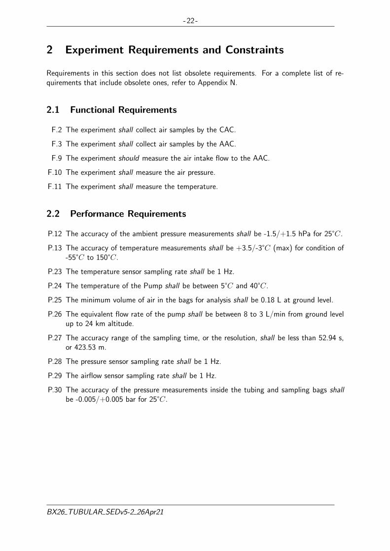
2 Experiment Requirements and Constraints
Requirements in this section does not list obsolete requirements. For a complete list of re-quirements that include obsolete ones, refer to Appendix N.
2.1 Functional Requirements
F.2 The experiment shall collect air samples by the CAC.
F.3 The experiment shall collect air samples by the AAC.
F.9 The experiment should measure the air intake flow to the AAC.
F.10 The experiment shall measure the air pressure.
F.11 The experiment shall measure the temperature.
2.2 Performance Requirements
P.12 The accuracy of the ambient pressure measurements shall be -1.5/+1.5 hPa for 25°C.
P.13 The accuracy of temperature measurements shall be +3.5/-3°C (max) for condition of-55°C to 150°C.
P.23 The temperature sensor sampling rate shall be 1 Hz.
P.24 The temperature of the Pump shall be between 5°C and 40°C.
P.25 The minimum volume of air in the bags for analysis shall be 0.18 L at ground level.
P.26 The equivalent flow rate of the pump shall be between 8 to 3 L/min from ground levelup to 24 km altitude.
P.27 The accuracy range of the sampling time, or the resolution, shall be less than 52.94 s,or 423.53 m.
P.28 The pressure sensor sampling rate shall be 1 Hz.
P.29 The airflow sensor sampling rate shall be 1 Hz.
P.30 The accuracy of the pressure measurements inside the tubing and sampling bags shallbe -0.005/+0.005 bar for 25°C.
BX26 TUBULAR SEDv5-2 26Apr21

- 23 -
2.3 Design Requirements
D.1 The experiment shall operate in the temperature profile of the BEXUS flight[8].
D.2 The experiment shall operate in the vibration profile of the BEXUS flight[8].
D.3 The experiment shall not have sharp edges or loose connections to the gondola that canharm the launch vehicle, other experiments, and people.
D.4 The experiment’s communication system shall be compatible with the gondola’s E-linksystem with the RJF21B connector over UDP for down-link and TCP for up-link.
D.5 The experiment’s power supply shall have a 24v, 12v, 5v and 3.3v power output andbe able to take 28.8v input through the Amphenol PT02E8-4P connector supplied fromthe gondola.
D.7 For the supplied voltage of 28.8 V, the total continuous DC current draw should bebelow 1.8 A.
D.8 The total power consumption should be below 374 Wh.
D.16 The experiment shall be able to autonomously turn itself off just before landing.
D.17 The experiment box shall be placed with at least one face exposed to the outside.
D.18 The experiment shall operate in the pressure profile of the BEXUS flight[8].
D.19 The experiment shall operate in the vertical and horizontal accelerations profile of theBEXUS flight[8].
D.21 The experiment shall be attached to the gondola’s rails.
D.22 The telecommand data rate shall not be over 10 kb/s.
D.23 The air intake rate of the air pump shall be equivalent to a minimum of 3 L/min at 24km altitude.
D.24 The temperature of the Brain2 shall be between -10°C and 25°C.
D.26 The air sampling systems shall filter out all water molecules before filling the samplingbags.
D.27 The total weight of the experiment shall be less than 28 kg.
D.28 The AAC box shall be able to fit at least 6 air sampling bags.
D.29 The CAC box shall take less than 3 minutes to be removed from the gondola withoutremoving the whole experiment.
D.30 The AAC shall be re-usable for future balloon flights.
D.31 The altitude from which a sampling bag will start sampling shall be programmable.
D.32 The altitude from which a sampling bag will stop sampling shall be programmable.
2The Brain is a central command unit which contains Electronic Box and pneumatic sampling system.
BX26 TUBULAR SEDv5-2 26Apr21

- 24 -
2.4 Operational Requirements
O.13 The experiment should function automatically.
O.14 The experiment’s air sampling mechanisms shall have a manual override.
2.5 Constraints
C.1 Constraints specified in the BEXUS User Manual.
BX26 TUBULAR SEDv5-2 26Apr21

- 25 -
3 Project Planning
3.1 Work Breakdown Structure
The team was categorized into different groups of responsibilities with dedicated leaders whoreported to and coordinated with the Project Manager. Leadership was organized on a ro-tational basis when the need arose. The formation of these divisions constituted a workbreakdown structure which is illustrated in Figure 1.
The Management was composed of a Project Manager and a Deputy Project Manager, bothacted as Systems Engineer and managed the overall implementation of the project. The ProjectManager was responsible for establishing and overseeing product development cycle; coordi-nating between different teams, project stakeholders, and documentation efforts; outreach andpublic relations; Fundraising; monitoring and reporting; system integration; and quality assur-ance. Once all subsystems had been assembled, the Project Manager was also responsible foroverseeing the integration processes leading to the final experiment setup and put emphasison leading quality assurance integration testing efforts. The Deputy Project Manager assistedthe Project Manager in all management duties in a manner that ensured replaceability whennecessary.
The Scientific Division was responsible for defining experiment parameters; data analysis;interpreting and documenting measurements; researching previous CAC experiments for com-parative analysis purposes; evaluating the reliability of the proposed AAC sampling system;conducting measurements of collected samples; documenting and publishing findings; defin-ing experiment parameters; contacting researchers or institutions working on similar projects;exploring potential partnership with researchers and institutions; documenting and publishingfindings.
The Mechanical Division was responsible for designing or redesigning cost-effective mechani-cal devices using analysis and computer-aided design; producing details of specifications andoutline designs; overseeing the manufacturing process for the devices; identifying material andcomponent suppliers; developing and testing prototypes of designed devices; analyzing testresults and changing the design as needed; and integrating and assembling final design.
The Electrical Division was responsible for designing and implementing cost-effective circuitryusing analysis and computer-aided design; producing details of specifications and outline de-signs; developing, testing, and evaluating theoretical designs; identifying material as well ascomponent suppliers; reviewing and testing proposed designs; recommending modificationsfollowing prototype test results; and assembling designed circuitry.
The Software Division was responsible for gathering software requirements; formalizing softwarespecifications; drafting architecture design; leading software implementation efforts; leadingquality assurance and testing efforts; enforcing software testing best practices such as con-tinuous integration testing and regression testing; reviewing requirements and specificationsin order to foresee potential issues; providing input for functional requirements; advising ondesign; formalizing test cases; tracking defects and ensuring their resolution; facilitating codereview sessions; and supporting software implementation efforts.
The Thermal Division was responsible for ensuring thermal regulation of the payload as peroperational requirements of all experiment components; evaluating designs against thermal
BX26 TUBULAR SEDv5-2 26Apr21

- 26 -
simulation and propose improvements; managing against mechanical design and electricalpower limitations towards providing passive and active thermal control systems.
BX26 TUBULAR SEDv5-2 26Apr21

-27-
Figure 1: Work Breakdown Structure.
BX
26T
UB
UL
AR
SE
Dv5-2
26Apr21
- 28 -
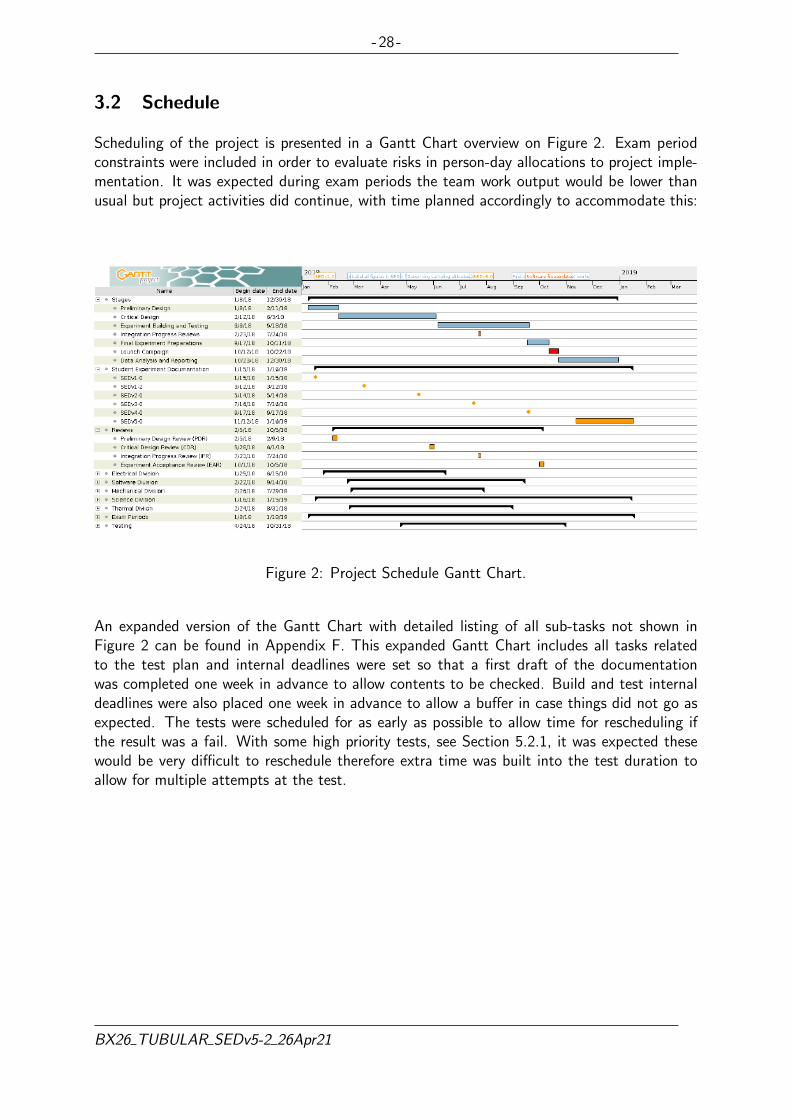
3.2 Schedule
Scheduling of the project is presented in a Gantt Chart overview on Figure 2. Exam periodconstraints were included in order to evaluate risks in person-day allocations to project imple-mentation. It was expected during exam periods the team work output would be lower thanusual but project activities did continue, with time planned accordingly to accommodate this:
Figure 2: Project Schedule Gantt Chart.
An expanded version of the Gantt Chart with detailed listing of all sub-tasks not shown inFigure 2 can be found in Appendix F. This expanded Gantt Chart includes all tasks relatedto the test plan and internal deadlines were set so that a first draft of the documentationwas completed one week in advance to allow contents to be checked. Build and test internaldeadlines were also placed one week in advance to allow a buffer in case things did not go asexpected. The tests were scheduled for as early as possible to allow time for rescheduling ifthe result was a fail. With some high priority tests, see Section 5.2.1, it was expected thesewould be very difficult to reschedule therefore extra time was built into the test duration toallow for multiple attempts at the test.
BX26 TUBULAR SEDv5-2 26Apr21
- 29 -
3.3 Resources
3.3.1 Manpower
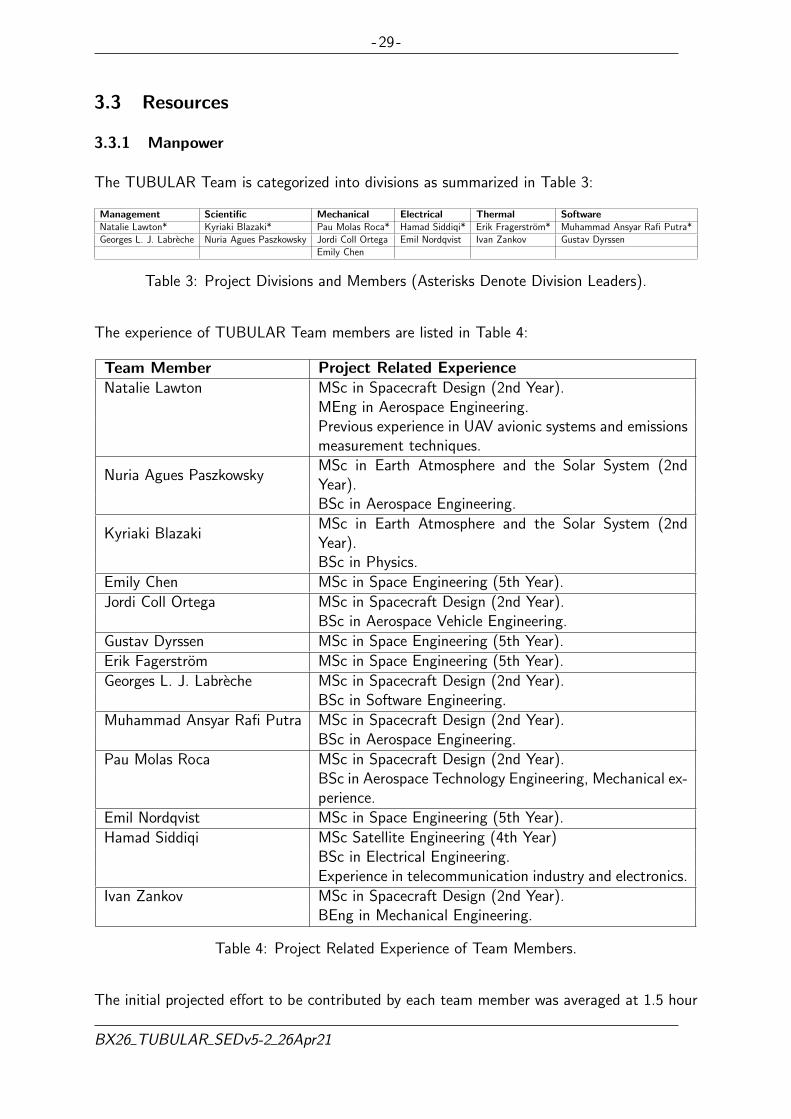
The TUBULAR Team is categorized into divisions as summarized in Table 3:
Management Scientific Mechanical Electrical Thermal SoftwareNatalie Lawton* Kyriaki Blazaki* Pau Molas Roca* Hamad Siddiqi* Erik Fragerstrom* Muhammad Ansyar Rafi Putra*Georges L. J. Labreche Nuria Agues Paszkowsky Jordi Coll Ortega Emil Nordqvist Ivan Zankov Gustav Dyrssen
Emily Chen
Table 3: Project Divisions and Members (Asterisks Denote Division Leaders).
The experience of TUBULAR Team members are listed in Table 4:
Team Member Project Related ExperienceNatalie Lawton MSc in Spacecraft Design (2nd Year).
MEng in Aerospace Engineering.Previous experience in UAV avionic systems and emissionsmeasurement techniques.
Nuria Agues PaszkowskyMSc in Earth Atmosphere and the Solar System (2ndYear).BSc in Aerospace Engineering.
Kyriaki BlazakiMSc in Earth Atmosphere and the Solar System (2ndYear).BSc in Physics.
Emily Chen MSc in Space Engineering (5th Year).Jordi Coll Ortega MSc in Spacecraft Design (2nd Year).
BSc in Aerospace Vehicle Engineering.Gustav Dyrssen MSc in Space Engineering (5th Year).Erik Fagerstrom MSc in Space Engineering (5th Year).Georges L. J. Labreche MSc in Spacecraft Design (2nd Year).
BSc in Software Engineering.Muhammad Ansyar Rafi Putra MSc in Spacecraft Design (2nd Year).
BSc in Aerospace Engineering.Pau Molas Roca MSc in Spacecraft Design (2nd Year).
BSc in Aerospace Technology Engineering, Mechanical ex-perience.
Emil Nordqvist MSc in Space Engineering (5th Year).Hamad Siddiqi MSc Satellite Engineering (4th Year)
BSc in Electrical Engineering.Experience in telecommunication industry and electronics.
Ivan Zankov MSc in Spacecraft Design (2nd Year).BEng in Mechanical Engineering.
Table 4: Project Related Experience of Team Members.
The initial projected effort to be contributed by each team member was averaged at 1.5 hour
BX26 TUBULAR SEDv5-2 26Apr21

- 30 -
per person per day corresponding to a team total of 15 hours per day. Since then, 3 newmembers had been included in the team thus increasing the projected daily effort to 19.5hours per day. During the summer period many team members were away which meant thatthe team hours put in had little significant overall change. The period of these different effortcapacities are listed in Table 5:
From To Capacity (hours/day)08/01/2018 18/03/2018 1519/03/2018 08/04/2018 16.509/04/2018 09/05/2018 1810/05/2018 15/08/2018 19.515/08/2018 22/10/2018 19.523/10/2018 31/01/2019 19.5
Table 5: Projected Daily Team Effort per Period.
Taking into account all team members and the mid-project changes in team size, the efforts/-capacity projected to be allocated to each stages of the project during 2018 are summarizedin Table 6:
StageStartDate
EndDate
Duration(days)
Effort (hours)Capacity Actual Diff. (%)
Preliminary Design 08/01 11/02 35 525 708 +29.68Critical Design 12/02 03/06 112 1,680 2,649 +57.66Experiment Buildingand Testing 04/06 16/09 105 2,048 1,943 -5.40Final ExperimentPreparations 17/09 11/10 25 488 571 +17.00Launch Campaign 12/10 22/10 10 390 777 +99.23Data Analysis andReporting 23/10 30/01 69 1,346 245 -81.78
Total: 356 7,989 6939 -13.14
Table 6: Project Effort Allocation per Project Stages.
It can be seen that it was necessary at some stages to work more than was projected and atother stages less work was required to achieve the aims.
All TUBULAR Team members are based in Kiruna, Sweden, just 40 km from Esrange SpaceCenter. Furthermore, all team members are enrolled in LTU Master programmes in Kiruna andthus remained in LTU during the entire project period. Special attention was made for planningtasks during the summer period where many team members traveled abroad. A timeline ofteam member availability until January 2019 is available in Appendix E. A significant riskwas observed during the summer months from June to August where most members wereonly partially available and some completely unavailable. As such, team member availabilityand work commitments over the summer were negotiated across team members in order toguarantee that at least one member per division was present in Kiruna over the Summerwith the exception of the Software Division which could work remotely. Furthermore, the
BX26 TUBULAR SEDv5-2 26Apr21

- 31 -
Project Manager role was assigned to the Deputy Project Manager due to an extended fulltime unavailability after the CDR.
As part of their respective Master programmes, most TUBULAR Team members are enrolledin a project course at LTU. The TUBULAR project acts as the course’s project for most teammembers from which they will obtain ECTS credits. This course is supervised by Dr. ThomasKuhn, Associate Professor at LTU.
BX26 TUBULAR SEDv5-2 26Apr21
- 32 -
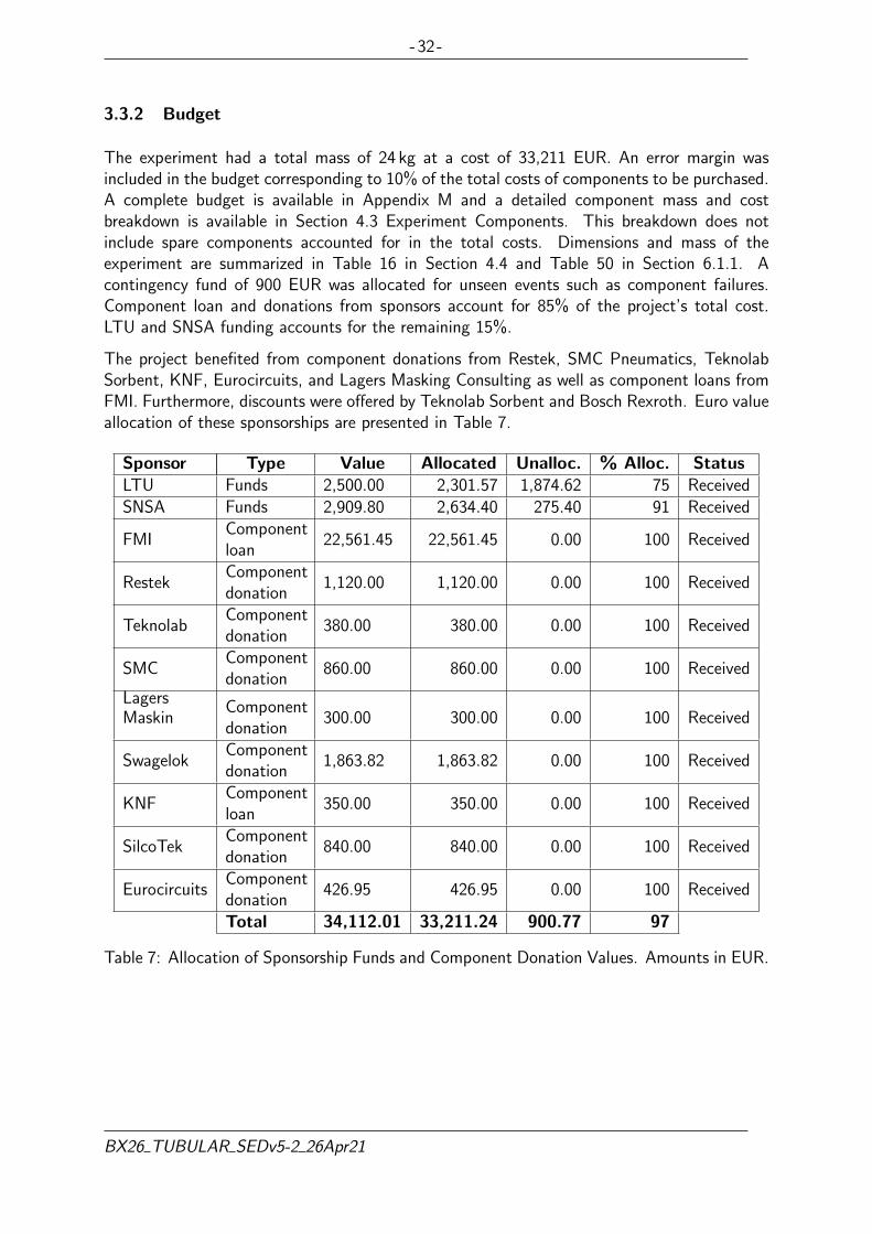
3.3.2 Budget
The experiment had a total mass of 24 kg at a cost of 33,211 EUR. An error margin wasincluded in the budget corresponding to 10% of the total costs of components to be purchased.A complete budget is available in Appendix M and a detailed component mass and costbreakdown is available in Section 4.3 Experiment Components. This breakdown does notinclude spare components accounted for in the total costs. Dimensions and mass of theexperiment are summarized in Table 16 in Section 4.4 and Table 50 in Section 6.1.1. Acontingency fund of 900 EUR was allocated for unseen events such as component failures.Component loan and donations from sponsors account for 85% of the project’s total cost.LTU and SNSA funding accounts for the remaining 15%.
The project benefited from component donations from Restek, SMC Pneumatics, TeknolabSorbent, KNF, Eurocircuits, and Lagers Masking Consulting as well as component loans fromFMI. Furthermore, discounts were offered by Teknolab Sorbent and Bosch Rexroth. Euro valueallocation of these sponsorships are presented in Table 7.
Sponsor Type Value Allocated Unalloc. % Alloc. StatusLTU Funds 2,500.00 2,301.57 1,874.62 75 ReceivedSNSA Funds 2,909.80 2,634.40 275.40 91 Received
FMIComponentloan
22,561.45 22,561.45 0.00 100 Received
RestekComponentdonation
1,120.00 1,120.00 0.00 100 Received
TeknolabComponentdonation
380.00 380.00 0.00 100 Received
SMCComponentdonation
860.00 860.00 0.00 100 Received
LagersMaskin
Componentdonation
300.00 300.00 0.00 100 Received
SwagelokComponentdonation
1,863.82 1,863.82 0.00 100 Received
KNFComponentloan
350.00 350.00 0.00 100 Received
SilcoTekComponentdonation
840.00 840.00 0.00 100 Received
EurocircuitsComponentdonation
426.95 426.95 0.00 100 Received
Total 34,112.01 33,211.24 900.77 97
Table 7: Allocation of Sponsorship Funds and Component Donation Values. Amounts in EUR.
BX26 TUBULAR SEDv5-2 26Apr21

- 33 -
3.3.3 External Support
Partnership with FMI, and IRF has provided the team with technical guidance in implementingthe sampling system. FMI’s experience in implementing past CAC sample systems provideinvaluable lessons learned towards conceptualizing, designing, and implementing the proposedAAC sampling system.
FMI was a key partner in the TUBULAR project, its scientific experts have advised and sup-ported the TUBULAR project by sharing knowledge, experience, and granting accessibility ofequipment. As per the agreement shown in Appendix G, FMI had provided the TUBULARTeam with the AirCore stainless tube component of the CAC subsystem as well as the post-flight gas analyzer. This arrangement required careful considerations on the placement ofthe experiment in order to minimize hardware damage risks. These contributions resulted insignificant cost savings regarding equipment and component procurement.
Daily access to LTU’s Space Campus in Kiruna exposed the team to scientific mentorship andexpert guidance from both professors and researchers involved in the study of greenhouse gasesand climate change. Dr Uwe Raffalski, IRF, Associate professor (Docent) was one of manyresearchers involved in climate study whom mentored the team.
BX26 TUBULAR SEDv5-2 26Apr21

- 34 -
3.4 Outreach Approach
The experiment as well as the REXUS/BEXUS programme and its partners has been bepromoted through the following activities:
• Published research papers co-authored with FMI, detailing the sampling methodology,measurement result, analysis, and findings [3] [11].
• Collected data licensed as open data to be freely available to everyone to use andrepublish as they wish, without restrictions from copyright, patents or other mechanismsof control.
• A website to summarize the experiment and provide regular updates. Backend webanalytics included to gauge interest on the project through number of visitors and theirorigins (See Appendix B).
• Dedicated Facebook page used as publicly accessible logbook detailing challenges, progress,and status of the project. Open for comments and questions (See Figure 77 in AppendixB).
• An Instagram account for short and frequent image and video updates (See Figures 78in Appendix B).
• GitHub account to host all project software code under free and open source license (SeeFigure 79 in Appendix B). Other REXUS/BEXUS teams were invited to host their codein this account.
• “Show and Tell”trips to local high schools and universities. Team members were respon-sible to organize such presentations through any of their travel opportunities abroad.
• Articles and/or blogposts about the project in team members’ alma mater websites.
• In-booth presentation and poster display in the seminars or career events at differentuniversities.
• A thoroughly documented and user-friendly manual on how to build replicate and launchCAC and AAC sampling systems will be produced and published.
BX26 TUBULAR SEDv5-2 26Apr21

- 35 -
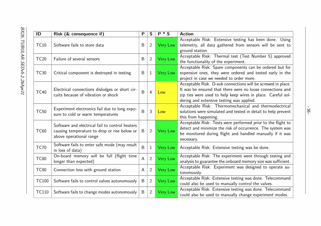
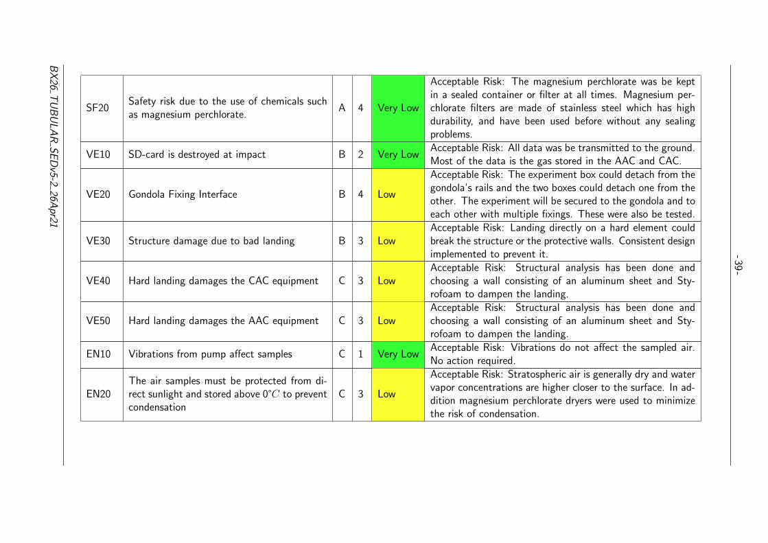
3.5 Risk Register
Risk ID
TC – Technical/Implementation
MS – Mission (operational performance)
SF – Safety
VE – Vehicle
PE – Personnel
EN – Environmental
OR - Outreach
BG - Budget
Adapt these to the experiment and add other categories. Consider risks to the experiment, tothe vehicle and to personnel.
Probability (P)
A Minimum – Almost impossible to occur
B Low – Small chance to occur
C Medium – Reasonable chance to occur
D High – Quite likely to occur
E Maximum – Certain to occur, maybe more than once
Severity (S)
1. Negligible – Minimal or no impact
2. Significant – Leads to reduced experiment performance
3. Major – Leads to failure of subsystem or loss of flight data
4. Critical – Leads to experiment failure or creates minor health hazards
5. Catastrophic – Leads to termination of the REXUS/BEXUS programme, damage to thevehicle or injury to personnel
The rankings for probability (P) and severity (S) were combined to assess the overall riskclassification, ranging from very low to very high and being coloured green, yellow, orange orred according to the SED guidelines.
SED guidelines were used to determine whether a risk was acceptable or unacceptable. Foracceptable risks, details of the mitigation undertaken were included which reduced the risk toan acceptable level.
BX26 TUBULAR SEDv5-2 26Apr21
-36-
ID Risk (& consequence if) P S P * S Action
TC10 Software fails to store data B 2 Very LowAcceptable Risk: Extensive testing has been done. Usingtelemetry, all data gathered from sensors will be sent toground station.
TC20 Failure of several sensors B 2 Very LowAcceptable Risk: Thermal test (Test Number 5) approvedthe functionality of the experiment.
TC30 Critical component is destroyed in testing B 1 Very LowAcceptable Risk: Spare components can be ordered but forexpensive ones, they were ordered and tested early in theproject in case we needed to order more.
TC40Electrical connections dislodges or short cir-cuits because of vibration or shock
B 4 Low
Acceptable Risk. D-sub connections will be screwed in place.It was be ensured that there were no loose connections andzip ties were used to help keep wires in place. Careful sol-dering and extensive testing was applied.
TC50Experiment electronics fail due to long expo-sure to cold or warm temperatures
B 3 LowAcceptable Risk: Thermomechanical and thermoelectricalsolutions were simulated and tested in detail to help preventthis from happening.
TC60Software and electrical fail to control heaterscausing temperature to drop or rise below orabove operational range
B 2 Very Low
Acceptable Risk: Tests were performed prior to the flight todetect and minimize the risk of occurrence. The system wasbe monitored during flight and handled manually if it wasnecessary.
TC70Software fails to enter safe mode (may resultin loss of data)
B 1 Very Low Acceptable Risk: Extensive testing was be done.
TC80On-board memory will be full (flight timelonger than expected)
A 2 Very LowAcceptable Risk: The experiment went through testing andanalysis to guarantee the onboard memory size was sufficient.
TC90 Connection loss with ground station A 2 Very LowAcceptable Risk: Experiment was designed to operate au-tonomously.
TC100 Software fails to control valves autonomously B 2 Very LowAcceptable Risk: Extensive testing was done. Telecommandcould also be used to manually control the valves.
TC110 Software fails to change modes autonomously B 2 Very LowAcceptable Risk: Extensive testing was done. Telecommandcould also be used to manually change experiment modes.
BX
26T
UB
UL
AR
SE
Dv5-2
26Apr21

-37-
TC120 Complete software failure B 4 LowAcceptable Risk: A long duration testing (bench test) wasperformed to catch the failures early.
TC130 Failure of fast recovery system B 2 Very Low
Acceptable Risk: Clear and simple instructions were given tothe recovery team. A test took place before launch to ensuresomeone unfamiliar with the experiment could remove theCAC box. Test number: 12.
TC140The gas analyzer isn’t correctly calibrated andreturns inaccurate results
B 3 Low Acceptable Risk: Gas analyzer was calibrated before use.
TC150Partnership with FMI does not materialize,resulting in loss of access to CAC coiled tube.
B 2 Very LowAcceptable Risk: Signed agreement has been obtained. AACsample analysis results can be validated against available his-torical data from past FMI CAC flights.
MS10 Down link connection is lost prematurely B 2 Very Low Acceptable Risk: Data was also be saved on SD card.
MS20Condensation on experiment PCBs whichcould causes short circuits
A 3 Very LowAcceptable Risk: The Brain was sealed to prevent conden-sation.
MS30Temperature sensitive components that areessential to full the mission objective mightbe below their operating temperature.
C 3 LowAcceptable Risk: Safe mode to prevent the components tooperate out of its operating temperature range.
MS40Experiment lands in water causing electronicsfailure
B 1 Very LowAcceptable Risk: All the necessary data was be downloadedduring the flight.
MS50Interference from other experiments and/orballoon
A 2 Very Low Acceptable Risk: no action.
MS60 Balloon power failure B 2 LowAcceptable Risk: Valves default state was closed so if allpower is lost valves would automatically close preserving allsamples collected up until that point.
MS70 Sampling bags disconnect B 3 Low
Acceptable Risk: The affected bags could not collect sam-ples. The connection between the spout of the bags and theT-union was double checked before flight. The system haspassed vibration testing with no disconnects.
BX
26T
UB
UL
AR
SE
Dv5-2
26Apr21

-38-
MS71 Sampling bags puncture B 3 Low
Acceptable Risk: The affected bags could not collect sam-ples. Inner styrofoam walls have been choosen and no sharpedges were exposed to avoid puncture from external ele-ments.
MS72 Sampling bags’ hold time is typically 48h B 2 Very LowAcceptable risk: Validation studies have demonstrated ac-ceptable stability for up to 48 hours.
MS80 Pump failure B 3 Low
Acceptable Risk: A pump was chosen based on a previoussimilar experiment. The pump has also been tested in alow pressure chamber down to 10hPa and has successfullyturned on and filled a sampling bag. The CAC subsystem isnot reliant on the pump therefore would still operate even inthe event of pump failure.
MS90 Intake pipe blocked by external element C 3 LowAcceptable Risk: The bags would not be filled and thus theAAC system would fail. An air filter was placed in bothintake and outlet of the pipe to prevent this.
MS100 Expansion/Contraction of insulation B 2 Very LowAcceptable Risk: The insulation selected has flown success-fully on similar flights in the past. Test was done to see howit reacts in a low pressure environment.
MS110Sampling bags are over-filled resulting inbursting and loss of collected samples.
B 3 Low
Acceptable Risk: Test was performed at target ambient pres-sure levels to identify how long the pump needs to fill thesampling bags. A static pressure sensor on board monitoredthe in-bag pressure during sampling and no bag would everbe over pressured. In addition an airflow rate sensor moni-tored the flow rate and a timer started when a bag valve isopened. The sampling would stop when either the maximumallowed pressure or maximum allowed time is reached.
SF10Safety risk due to pressurized vessels duringrecovery.
A 1 Very Low
Acceptable Risk: The volume of air in the AAC decreasesduring descent because the pressure inside is lower than out-side. The CAC is sealed at nearly sea level pressure, thereforethere is only a small pressure difference.
BX
26T
UB
UL
AR
SE
Dv5-2
26Apr21
-39-
SF20Safety risk due to the use of chemicals suchas magnesium perchlorate.
A 4 Very Low
Acceptable Risk: The magnesium perchlorate was be keptin a sealed container or filter at all times. Magnesium per-chlorate filters are made of stainless steel which has highdurability, and have been used before without any sealingproblems.
VE10 SD-card is destroyed at impact B 2 Very LowAcceptable Risk: All data was be transmitted to the ground.Most of the data is the gas stored in the AAC and CAC.
VE20 Gondola Fixing Interface B 4 Low
Acceptable Risk: The experiment box could detach from thegondola’s rails and the two boxes could detach one from theother. The experiment will be secured to the gondola and toeach other with multiple fixings. These were also be tested.
VE30 Structure damage due to bad landing B 3 LowAcceptable Risk: Landing directly on a hard element couldbreak the structure or the protective walls. Consistent designimplemented to prevent it.
VE40 Hard landing damages the CAC equipment C 3 LowAcceptable Risk: Structural analysis has been done andchoosing a wall consisting of an aluminum sheet and Sty-rofoam to dampen the landing.
VE50 Hard landing damages the AAC equipment C 3 LowAcceptable Risk: Structural analysis has been done andchoosing a wall consisting of an aluminum sheet and Sty-rofoam to dampen the landing.
EN10 Vibrations from pump affect samples C 1 Very LowAcceptable Risk: Vibrations do not affect the sampled air.No action required.
EN20The air samples must be protected from di-rect sunlight and stored above 0°C to preventcondensation
C 3 Low
Acceptable Risk: Stratospheric air is generally dry and watervapor concentrations are higher closer to the surface. In ad-dition magnesium perchlorate dryers were used to minimizethe risk of condensation.
BX
26T
UB
UL
AR
SE
Dv5-2
26Apr21

-40-
PE10Change in Project Manager after the CDR in-troduces a gap of knowledge in managementresponsibilities.
E 1 Low
Acceptable Risk: A Deputy Project Manager was selectedat an early stage and was progressively handed over projectmanagement tasks and responsibilities until complete han-dover after the CDR. The previous Project Manager re-motely assisted the new Project Manager until the end ofthe project. The Deputy Project Manager was also part ofthe Electrical Division so a new team member has been in-cluded to that division in order compensate for the DeputyProject Manager’s reduced bandwidth to work on ElectricalDivision tasks once she is appointed Project Manager.
PE20Team members from the same division areunavailable during the same period over thesummer.
C 2 LowAcceptable Risk: Summer travel schedules have been coor-dinated among team members so that there is at least onemember from each division available during the summer.
PE30No one from management is available to over-see the work for a reasonable period.
B 2 Very Low
Acceptable Risk: Management summer travel schedules havebeen planned to fit around known deadlines. There wasalways be at least one member from management availablevia phone at all times. All team members were made awareof which members will be available at what times so workcould be planned accordingly.
PE40Miscommunication between team membersresults in work being incomplete or inaccu-rate
B 2 Very LowAcceptable Risk: Whatsapp, Asana and Email were used incombination to ensure that all team members are up to datewith the most current information.
Table 8: Risk Register.
BX
26T
UB
UL
AR
SE
Dv5-2
26Apr21

- 41 -
4 Experiment Design
4.1 Experiment Setup
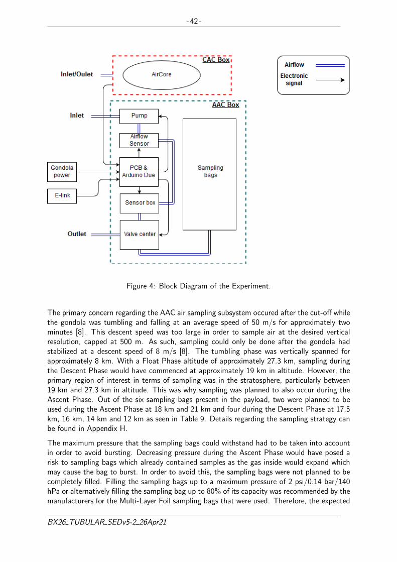
The experiment consisted of the AAC subsystem, with six sampling bags, and the CAC coiledtube subsystem. Shown in Figure 3, the AirCore was fitted into the CAC box, and thealternative sampling system with bags in the AAC box, together with the pneumatic systemand the electronics placed inside the Brain. The principal aim was to validate the AAC samplingmethod. To do so, it was necessary to sample during Descent Phase in order to compare theresults with the ones obtained from the CAC. This was because the CAC collected its air samplepassively by pressure differentials in the descent. Flight speeds mentioned in this section wereobtained from the BEXUS manual as well as through analysis of past flights. Figure 4 showsa generic block diagram of the main subsystems interconnection.
Figure 3: Physical Setup of the Experiment.
BX26 TUBULAR SEDv5-2 26Apr21
- 42 -
Figure 4: Block Diagram of the Experiment.
The primary concern regarding the AAC air sampling subsystem occured after the cut-off whilethe gondola was tumbling and falling at an average speed of 50 m/s for approximately twominutes [8]. This descent speed was too large in order to sample air at the desired verticalresolution, capped at 500 m. As such, sampling could only be done after the gondola hadstabilized at a descent speed of 8 m/s [8]. The tumbling phase was vertically spanned forapproximately 8 km. With a Float Phase altitude of approximately 27.3 km, sampling duringthe Descent Phase would have commenced at approximately 19 km in altitude. However, theprimary region of interest in terms of sampling was in the stratosphere, particularly between19 km and 27.3 km in altitude. This was why sampling was planned to also occur during theAscent Phase. Out of the six sampling bags present in the payload, two were planned to beused during the Ascent Phase at 18 km and 21 km and four during the Descent Phase at 17.5km, 16 km, 14 km and 12 km as seen in Table 9. Details regarding the sampling strategy canbe found in Appendix H.
The maximum pressure that the sampling bags could withstand had to be taken into accountin order to avoid bursting. Decreasing pressure during the Ascent Phase would have posed arisk to sampling bags which already contained samples as the gas inside would expand whichmay cause the bag to burst. In order to avoid this, the sampling bags were not planned to becompletely filled. Filling the sampling bags up to a maximum pressure of 2 psi/0.14 bar/140hPa or alternatively filling the sampling bag up to 80% of its capacity was recommended by themanufacturers for the Multi-Layer Foil sampling bags that were used. Therefore, the expected
BX26 TUBULAR SEDv5-2 26Apr21

- 43 -
maximum pressure inside the bags, that were filled during the Ascent Phase, would be 1.6psi/0.11 bar/110 hPa. The inverse was also true for the Descent Phase where compressionwould occur. As such, the sampling bags had to be fully filled during the Descent Phase inorder to ensure that enough samples were collected for analysis. During the Descent Phase,the expected maximum pressure inside the bags was expected to be 1.98 psi/0.13 bar/130 hPa.Past research had revealed that the selected sampling bags were able to withstand pressuredifference of 310 hPa at 30 km of altitude, which was equivalent to 0.31 bar [5]. Test 16 and18, shown in Table 33 respective Table 35, were conducted in order to confirm the maximumallowable pressure for the bags.
The maximum operating pressure for the tubes, according to the manufacturers, was 2.2psi/0.15 bar/150 hPa. The valve’s leakage rate, given by the manufacturers, was 0.001 l/min.
Due to the difference in pressure between sea level and sampling altitudes, the volume of thesample taken would have been considerably reduced when it reached sea level. This shrinkinghad to be taken into account as the minimum volume that had to be present in the samplingbag at sea level in order to obtain results with the Picarro analyzer. A minimum amount wasrequired for the analyzer to detect concentrations of the targeted trace gases. This minimumamount was 0.18 L at sea level and it had to be specially considered for the samples takenat higher altitudes. The samples taken at lower altitudes were exposed to smaller changes inpressure, therefore their size was not critically reduced. Table 9 shows the minimum volumeof air that was needed to be sampled at different altitudes in order to assure the minimum airsample of 0.18L left at sea level.
This was the worst case scenario, and testing had shown that the higher the volume of the airsample left at sea level, the better the results. This was why the aimed volume of the samples,at sea level was at least 0.6L.
MinimumSampling Volume
SamplingAltitudes
AmbientPressure
AmbientTemperature
Ascent Phase1.8 L 18 km 75.0 hPa 216.7 K2.4 L 21 km 46.8 hPa 217.6 K
Descent Phase
1.7 L 17.5 km 81.2 hPa 216.7 K1.3 L 16 km 102.9 hPa 216.7 K1.0 L 14 km 141.0 hPa 216.7 K0.7 L 12 km 193.3 hPa 216.7 K
Table 9: Sampling Altitudes as well as the Corresponding Ambient Pressures and TemperaturesAccording to the 1976 US Standard Atmosphere and the Minimum Sampling Volume at EachAltitude to Obtain Enough Air to Perform a Proper Analysis (0.18 L at Sea Level), AppendixH.
The AAC needed an air pump for sampling due to low ambient pressure at stratosphericaltitudes. The air pump was also needed in order to assure the intake flow rate and obtain agood resolution. An air pump with an intake rate of at least 3 L/min was used to ensure thatthe vertical resolution of the sampling air remained under 500 m during the Ascent Phase’sascent speed of 5 m/s and the Descent Phase’s descent speed of 8 m/s. A flushing valve (seeFigure 28, No.23) was used to flush the AAC system before each bag would have been filled
BX26 TUBULAR SEDv5-2 26Apr21

- 44 -
and make sure that each bag would have been filled with fresh air from the correspondingaltitude. This filling/flushing procedure was planned to occur twice, the first time during theAscent Phase for the first two sampling bags and the second time during the Descent Phasefor the remaining four sampling bags.
Shortly after the launch, the CAC valve was opened in order to allow the fill gas that wasinside the tube to flush, while the AAC valves were closed until reaching the sampling altitude.Flushing of the CAC tube happened passively through the progressive decrease in air pressureduring the balloon’s Ascent Phase and it was emptied by the time it reached the Float Phase.Filling of the CAC tube also happened passively through the progressive increase in air pressureduring the balloon’s Descent Phase. The CAC valve was planned to remain open at all timeduring the Ascent, Float, and Descent phases. Due to some problems, it was briefly closedand opened again for a few times without really compromising the results. The valve shouldhave been closed just before hitting the ground in order to preserve the sample.
The ambient pressure was measured by three pressure sensors located outside the experimentbox. Only one of them was necessary for AAC and CAC, but using three, redundancy wasprovided. To measure the pressure inside the bag that was currently being filled, one analoguestatic pressure sensor was connected to the pneumatic system. To measure the ambienttemperature in the CAC, three sensors were allocated in the CAC box (in the Styrofoam).Temperature inside the coil was assumed to quickly adjust to the ambient temperature insidethe CAC box, therefore there would not be differentiation in temperature between the air insidethe tube and the air surrounding the tube. For the bags three more temperature sensors wereplaced in the bags’ box (in the Styrofoam). To control the temperature for the pump and thevalves in pneumatic subsystem, one temperature sensor was used for each of them. In total,there were three pressure sensors and eight temperature sensors.
The sampling of the AAC was triggered by the pressure reading from the sensors outside theexperiment box. When the required pressure was reached, as seen in Table 9 the valve insidethe manifold corresponding to the bag that was to be sampled, should have opened and thesampling should have started. The closing of the valve depended on two conditions and itwas triggered when either one of the conditions was true. These conditions were: maximumsampling time or maximum pressure difference between inside/outside the bags. They weredetermined from past research [5]. A first estimation of the maximum sampling time hadalready been made, from Test 18 shown in Table 35. Completed tests, such as Test 14 andTest 18, shown in Table 25 respective Table 35, the maximum pressure condition had beendetermined and the maximum sampling times had been confirmed.
The CAC emptying as well as the AAC and CAC sampling sequence is represented in Figures 5and 6. It should be kept in mind that the different pressures were what should have triggeredthe opening of the valves.
BX26 TUBULAR SEDv5-2 26Apr21

- 45 -
Figure 5: The Emptying and Sampling Sequence-Ascent Phase.
BX26 TUBULAR SEDv5-2 26Apr21

- 46 -
Figure 6: The Emptying and Sampling Sequence-Descent Phase.
In the diagrams, 0 denotes closed/off and 1 denotes opened/on. The horizontal axis denotesthe different pressure levels throughout the flight, with p0 being the sea level pressure and p8
being the pressure during Float Phase.
The ambient pressure dependent timeline of the experiment was planned to be as follow:
Ascent Phase:p0 – p1
• CAC valve shall be closed.
• AAC valves shall be closed.
p1 – p2
• CAC valve shall be opened.
• CAC tube shall start flushing.
p2 – p3
• AAC flushing valve shall be opened, allowing for the system to flush.
BX26 TUBULAR SEDv5-2 26Apr21

- 47 -
• CAC valve should remain open.
p3 – p4
• AAC flushing valve shall be closed.
• Valve 1 shall be opened, allowing for air to enter the first bag.
• CAC valve should remain open.
p4 – p5
• Valve 1 shall be closed.
• AAC flushing valve shall be closed.
• CAC valve should remain open.
p5 - p6
• AAC flushing valve shall be opened, allowing the system to flush.
• CAC valve should remain open.
p6 - p7
• AAC flushing valve shall be closed.
• Valve 2 shall be opened, allowing for air to enter the second bag.
• CAC valve should remain open.
p7 - p8
• Valve 2 shall be closed.
• AAC flushing valve shall be closed.
• CAC shall finish flushing.
Float Phase:No action was taken other than continued telemetry.
Descent Phase:
p9 – p10
• CAC shall start sampling.
• AAC valves shall be closed.
p10 – p11
• AAC flushing valve shall be opened allowing the system to flush.
• CAC valve should remain open.
p11 – p12
• AAC flushing valve shall be closed.
BX26 TUBULAR SEDv5-2 26Apr21

- 48 -
• Valve 3 shall be opened, allowing for air to enter the third bag.
• CAC valve should remain open.
p12 – p13
• Valve 3 shall be closed.
• AAC flushing valve shall be closed.
• CAC valve should remain open.
p13 – p14
• AAC flushing valve shall be opened allowing the system to flush.
• CAC valve should remain open.
p14 – p15
• AAC flushing valve shall be closed.
• Valve 4 shall be opened, allowing for air to enter the fourth bag.
• CAC valve should remain open.
p15 – p16
• Valve 4 shall be closed.
• AAC flushing valve shall be closed.
• CAC valve should remain open.
p16 – p17
• AAC flushing valve shall be opened, allowing the system to flush.
• CAC should remain open.
p17 – p18
• AAC flushing valve shall be closed.
• Valve 5 shall be opened, allowing for air to enter the fifth bag.
• CAC valve should remain open.
p18 – p19
• Valve 5 shall be closed.
• AAC flushing valve shall be closed.
• CAC valve should remain open.
p19 – p20
• AAC flushing valve shall be opened, allowing the system to flush.
• CAC valve should remain open.
p20 – p21
BX26 TUBULAR SEDv5-2 26Apr21
- 49 -
• AAC flushing valve shall be closed.
• Valve 6 shall be opened, allowing for air to enter the sixth bag.
• CAC valve should remain open.
ppre−landing
• Valve 6 shall be closed.
• AAC flushing valve shall be closed.
• CAC valve shall be opened.
p0−landing
• CAC valve shall be closed.
Note: The AAC system’s air pump is only on during sampling into the air sampling bags andflushing of the system.
BX26 TUBULAR SEDv5-2 26Apr21
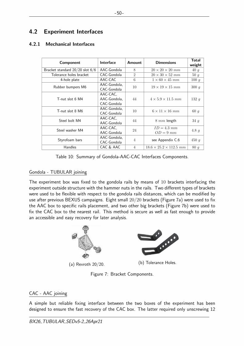
- 50 -
4.2 Experiment Interfaces
4.2.1 Mechanical Interfaces
Component Interface Amount DimensionsTotal
weightBracket standard 20/20 slot 6/6 AAC-Gondola 8 20× 20× 20 mm 40 g
Tolerance holes bracket CAC-Gondola 2 20× 30× 52 mm 50 g4-hole plate AAC-CAC 6 1× 60× 45 mm 100 g
Rubber bumpers M6AAC-Gondola,CAC-Gondola
10 19× 19× 15 mm 300 g
T-nut slot 6 M4AAC-CAC,AAC-Gondola,CAC-Gondola
44 4× 5.9× 11.5 mm 132 g
T-nut slot 8 M6AAC-Gondola,CAC-Gondola
10 6× 11× 16 mm 60 g
Steel bolt M4AAC-CAC,AAC-Gondola
44 8 mm length 34 g
Steel washer M4AAC-CAC,AAC-Gondola
24ID = 4.3 mmOD = 9 mm
4.8 g
Styrofoam barsAAC-Gondola,CAC-Gondola
4 see Appendix C.6 450 g
Handles CAC & AAC 4 18.6× 25.2× 112.5 mm 80 g
Table 10: Summary of Gondola-AAC-CAC Interfaces Components.
Gondola - TUBULAR joining
The experiment box was fixed to the gondola rails by means of 10 brackets interfacing theexperiment outside structure with the hammer nuts in the rails. Two different types of bracketswere used to be flexible with respect to the gondola rails distances, which can be modified byuse after previous BEXUS campaigns. Eight small 20/20 brackets (Figure 7a) were used to fixthe AAC box to specific rails placement, and two other big brackets (Figure 7b) were used tofix the CAC box to the nearest rail. This method is secure as well as fast enough to providean accessible and easy recovery for later analysis.
(a) Rexroth 20/20. (b) Tolerance Holes.
Figure 7: Bracket Components.
CAC - AAC joining
A simple but reliable fixing interface between the two boxes of the experiment has beendesigned to ensure the fast recovery of the CAC box. The latter required only unscrewing 12
BX26 TUBULAR SEDv5-2 26Apr21

- 51 -
bolts as well as unplugging a D-Sub connector marked in RED, see Figure 14. Once the CACbox was detached, the AAC Box still remained fixed in the gondola. Table 10 includes all thecomponents required to fix the experiment to the gondola.
Handles
Four top handles, as shown in Figure 8 were mounted to facilitate the experiment box manip-ulation when moving it in and out of the gondola.
Figure 8: Handling Interfaces.
Inlet/Outlet Pipes
In order to collect reliable air samples, the experiment was required to be mounted with atleast one side exposed to the outside. This reduced the pipe length used to collect clean air.As it can be seen in Figure 3, three pipes were extended from the experiment box face: onefor the CAC sampling and two, input and output, for the AAC sampling.
These pipes were welded/drawn 304 grade stainless steel tubes from RESTEK company, whichwere specially recommended for chromatography applications and gas delivery systems withlow pressures and inert environments. These tubes were sulfinert, which is a required treatmentfor metal components when analyzing for parts-per-billion levels of organo-sulfur compounds.
The tubes, which were the same ones used in the pneumatic system of the Brain (see Section4.4.5), had an outer diameter OD = 6.35 mm (1/4 inches) and an inner diameter ID =4.57 mm (0.18 inches).
Pump vibration
To mitigate the vibrations produced by the pump, an extra piece of styrofoam has been addedbetween the pump’s anchor plate and the surface of the level 1 of the brain, where this keycomponent is fixed.
BX26 TUBULAR SEDv5-2 26Apr21

- 52 -
4.2.2 Thermal Interfaces
Both main structural components and external walls of the two boxes of the experimentwere made by aluminum and steel components. For this reason, since these were conductivematerials, a direct attachment to the gondola creates many heat paths with the internal spaceand subsystems of the experiment. Considering that the temperature gradient between thegondola and the operative requirements of the electronic components can be quite high, thisconductive connections drastically decrease the efficiency of the thermal insulation. Therefore,a system based on rubber bumpers and styrofoam bars (see Figure 10) has been designed toremove heat bridges and minimize temperature leaks from the inside of the experiment to theoutside.
Figure 9 shows a CAD model of the bumper component and how it looks like when attachedto the gondola with the brackets explained in the previous section.
Figure 9: Rubber Bumper.
The styrofoam bars were attached directly to the rails of the experiment structure by M4plastic screws and big washers.
Figure 10: Thermal Interfaces TUBULAR-Gondola.
BX26 TUBULAR SEDv5-2 26Apr21

- 53 -
4.2.3 CAC Interfaces
An uncoupled quick connector, shown in Figure 11, was attached at each end of the coiledtube to seal the opening. It remained tightly sealed until the quick connectors were manuallycoupled.
Figure 11: Swagelok Quick Connector Body.
The interfaces between the other parts in the CAC set up were joined with specific tube fittings,listed in Table 11. All the chosen interfaces were from Swagelok. Using products from thesame manufacture minimizes the risk for leakage or mismatched interfaces in the system.
Component Interface Amount Fitting SizeQuick connector body
SS-QC4-B-200Outlet of coiled tube 1 1/8 in.
Quick connector bodySS-QC4-B-400
Inlet of coiled tube 1 1/4 in.
Quick connector stemSS-QC4-D-400
Inlet of coiled tube - Filter 1 1/4 in.
Male connectorSS-400-1-2
Tube fitting - Solenoid valve 2Tube OD 1/8 in. to
Tube OD 1/4 in.Straight Tube Union
SS-200-6Quick connector 1/8 in. - Tube 1/8 in. 1 1/8 in.
Tube ReducerSS-400-6-2
Tube 1/8 in. - Tube 1/4 in. 1Tube OD 1/8 in. to
Tube OD 1/4 in.Straight Tube Union
SS-400-6Tube 1/4 in. - 90 degree connector 1 1/4 in.
Union 90-degree connectorSS-400-9
Between certain tube fittingsOutlet tube
3 1/4 in.
Tube fittingSS-401-PC
Between certain tube fittingsMagnesium dryer filter
5 1/4 in.
Table 11: Interfaces within CAC Setup.
4.2.4 AAC Interfaces
In the AAC system, the interfaces between various components were a mixture of elevendifferent types of tube fittings from Swagelok. The selected types were straight and elbowunion, T-union, female and male elbows, male and female connectors, tube fittings, and quickcoupling with a certain specifications. Some of them are shown in Figure 12. Informationregarding the fitting’s placement in the AAC and fitting sizes are summarized in Table 12.
BX26 TUBULAR SEDv5-2 26Apr21

- 54 -
Figure 12: From Left to Right: Male Connector, Male Elbow, T-union, Straight Union andFemale Connector.
Component Interface Amount Fitting Size
Male connectorSS-400-1-2
Tube to Manifold - Flushing valveFlushing valve - Outlet tubeManifold valve - Tube to bag
8Male 1/8 in. to
Tube OD 1/4 in.
Male connectorSS-400-1-4
Manifold - Tube to Flushing valve 1Male 1/4 in. to
Tube OD 1/4 in.Male elbowSS-400-2-4
Static pressure sensor - Manifold 1Male 1/4 in. to
Tube OD 1/4 in.Female elbow
SS-400-8-4Pump tube - Airflow sensor
Airflow sensor - Static pressure sensor2
Female 1/4 in. toTube OD 1/4 in. in.
Female connectorSS-4-TA-7-4RG
Static pressure sensor - T-Union 1Female 1/4 in. and
Tube OD 1/4 in. in.Straight union
SS-400-6Filter - Tube filterTube filter - Pump
3 Tube OD 1/4 in.
Elbow unionSS-400-9
Pump tube - Filter tube 1 Tube OD 1/4 in. in.
T-UnionSS-400-3
Static pressure sensor 3 Tube OD 1/4 in.
T-UnionSS-400-3-4TTM
Tube valve - Bag valve - Quick Connector 5Male 1/4 in. and
2 x Tube OD 1/4 in.T-Union
SS-400-3-4TMTTube valve - Bag valve - Quick Connector 1
Male 1/4 in.2 x Tube OD 1/4 in.
T-UnionSS-6M0-3
Pump Inlet and Outlet 2 Tube OD 6mm
Tube FittingSS-401-PC
Filter - Pump 1 Tube OD 1/4in.
Tube Fitting ReducerSS-400-R-6M
Filter - PumpPump - Airflow sensor
2Tube OD 1/4in. to
Tube OD 6mmTube InsertsSS-6M5-4M
Pump Inlet and Outlet 2 OD 6mm - ID 4mm
Tube Fitting FemaleSS-4-TA-7-4RG
Static pressure sensor 1Tube OD 1/4in. to
female 1/4”Quick CouplingSS-QC4-B-4PF
T-Union of bags 6 SS female 1/4”
Tube adapterSS-300-R-4
T-Union - Bag valve 6Tube OD 1/4in. to
Tube OD 3/16”
Table 12: Interface Descriptions Inside AAC System.
4.2.5 Electrical Interfaces
The experiment was connected to the gondola electrically via a 4 pin, male, box mountreceptacle MIL - C-26482P series 1 connector with an 8-4 insert arrangement (MS3112E8-4P)
BX26 TUBULAR SEDv5-2 26Apr21
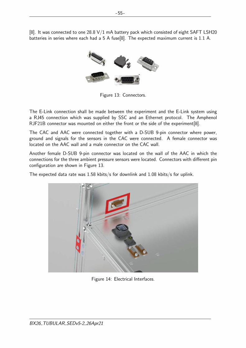
- 55 -
[8]. It was connected to one 28.8 V/1 mA battery pack which consisted of eight SAFT LSH20batteries in series where each had a 5 A fuse[8]. The expected maximum current is 1.1 A.
Figure 13: Connectors.
The E-Link connection shall be made between the experiment and the E-Link system usinga RJ45 connection which was supplied by SSC and an Ethernet protocol. The AmphenolRJF21B connector was mounted on either the front or the side of the experiment[8].
The CAC and AAC were connected together with a D-SUB 9-pin connector where power,ground and signals for the sensors in the CAC were connected. A female connector waslocated on the AAC wall and a male connector on the CAC wall.
Another female D-SUB 9-pin connector was located on the wall of the AAC in which theconnections for the three ambient pressure sensors were located. Connectors with different pinconfiguration are shown in Figure 13.
The expected data rate was 1.58 kbits/s for downlink and 1.08 kbits/s for uplink.
Figure 14: Electrical Interfaces.
BX26 TUBULAR SEDv5-2 26Apr21
-56-
4.3 Experiment Components
Component tables were generated from the project budget spreadsheet in Appendix M using the scripts included in Appendix K.
4.3.1 Electrical Components
Table 13 shows all required electrical components with their total mass and price.
ID Component Name ManufacturerManufacturerCode
QtyTotalMass[g]
TotalCost[EUR]
Note Status
E1Arduino Due with head-ers
Arduino A000062 1 36 35Fast and has many ana-log, and digital pins
Received
E2 Ethernet Shield SEEED Studio SKU 103030021 1 36 28Can be mounted on topof the board
Received
E3Miniature diagphramair pump
KNFNMP 850.1.2KNDC-B
1 430 350 Received
E4 Pressure sensorSENSOR SO-LUTIONS
MS560702BA03-50
4 20 9.2High resolution, largemeasuring range
Received
E5Sampling Valve (inletand outlet 1/8”female)
SMC VDW22UANXB 1 100 45 Received
E6 Airflow sensor Honeywell AWM5102VN 1 60 130 0-10 SLPM Received
E7 Heater Minco HK5160R157L12 4 16 380Easy to mount, com-pact size
Received
E9 Temperature sensorMaxim Inte-grated
DS1631+-ND 8 16 24I2C digital outputinterface, temperaturerange down to -55 °C
Received
BX
26T
UB
UL
AR
SE
Dv5-2
26Apr21

-57-
E10 DC/DC converter 24 V Traco Power S24SP24003PDFA 2 92 98Provides required out-put voltage and power,93% efficiency
Received
E12 MicroSDKingston Tech-nology
SDCIT/16GB 1 0.5 20Small, good tempera-ture range, sufficientstorage
Received
E13 Logic CAT5E Network Valueline VLCT85000Y30 1 90 7For testing and groundstation
Received
E14 Resistors n/a n/a 25 25 0 Received
E15Capacitors (0.1 uF,5uF, 10 uF, 100uF)
n/a n/a 7 7 0 Received
E16Mosfet for current con-trol
IR IRLB8748PBF 11 22 7.7Cheap, good tempera-ture range
Received
E17Diodes for DCDC con-verters
Diotec Semi-conductor
1N5059 4 1.6 0.4Cheap, good tempera-ture range
Received
E18 LED 3.3 VWurth Elek-tronik
151034GS03000 16 6.4 8.3 For monitoring, testing Received
E1915-pin D-SUB Femaleconnector with pins
RND Connect RND 205-00779 2 22 1.5For connecting dis-tributed components
Received
E209-pin D-SUB Femaleconnector with pins
RND Connect RND 205-00777 3 26 2For connecting dis-tributed components
Received
E219 pin D-SUB Femaleconnector with solder-ing cups
RND Connect RND 205-00704 3 27 1.7For connecting dis-tributed components
Received
E229 pin D-SUB Male con-nector with solderingcups
RND Connect RND 205-00700 6 54 2.9For connecting dis-tributed components
Received
E2315-pin D-SUB Maleconnector with solder-ing cups
RND Connect RND 205-00701 2 22 1.2For connecting dis-tributed components
Received
BX
26T
UB
UL
AR
SE
Dv5-2
26Apr21

-58-
E24 9-pin D-SUB backing EnchitechMHDTZK-9-BK-K
6 240 17For connecting dis-tributed components
Received
E25 15-pin D-SUB backing EnchitechMHDTZK-15-BK-K
2 130 6.1For connecting dis-tributed components
Received
E26 Wall mounting bolts RND Connect RND 205-00786 3 7.5 3.1For connecting dis-tributed components
Received
E28 3.3 V Zener diodeRND Compo-nents
RND 1N746A 15 7.5 1.1Regulate indicationLED voltage
Received
E29 Male connector on PCB Binder Serie 768 1 5 8.5 Received
E30Female connector fromwall
Binder Serie 768 1 11 12 Received
E31 Grounding contact Vogt DIN 46234 4 2.3 8.6 1 pack of 100 pcs Received
E32Logic CAT5 E-link forinside box 0.5m
Valueline VLCP85121E05 1 20 1.3To connect from wall toArduino shield
Received
E33 Signal wire Alpha Wire 5854/7 YL005 1 120 34Roll of 30 m. Half willbe used approximately
Received
E34Flushing valve (inletand outlet 1/8”female)
SMC VDW22UANXB 1 100 45 Received
E35Valves manifold (outlet1/8” female)
SMC VDW23-5G-1-H-Q 6 600 240 Received
E36 Power wire - Back Alpha Wire 5856 BK005 1 73 46Roll of 30 m. A fifthwill be used approxi-mately
Received
E37Electrical Tape formarking wires - White
Hellerman Ty-ton
HTAPE-FLEX15WH-15X10
1 14 0.82Roll of 10 m. A forthwill be used approxi-mately
Received
E38Electrical Tape formarking wires - Black
Hellerman Ty-ton
HTAPE-FLEX15BK-15X10
1 13 0.82Roll of 10 m. A forthwill be used approxi-mately
Received
BX
26T
UB
UL
AR
SE
Dv5-2
26Apr21

-59-
E39Electrical Tape formarking wires - Green
Hellerman Ty-ton
HTAPE-FLEX15GN-15X10
1 14 0.82Roll of 10 m. A forthwill be used approxi-mately
Received
E40Electrical Tape formarking wires - Violet
Hellerman Ty-ton
HTAPE-FLEX15VT-15X10
1 14 0.82Roll of 10 m. A forthwill be used approxi-mately
Received
E41Electrical Tape formarking wires - Gray
Hellerman Ty-ton
HTAPE-FLEX15GY-15X10
1 14 0.82Roll of 10 m. A forthwill be used approxi-mately
Received
E42Electrical Tape formarking wires - Brown
Hellerman Ty-ton
HTAPE-FLEX15BN-15X10
1 14 0.82Roll of 10 m. A forthwill be used approxi-mately
Received
E43Electrical Tape formarking wires - Blue
Hellerman Ty-ton
HTAPE-FLEX15BU-15X10
1 14 1.9Roll of 10 m. A forthwill be used approxi-mately
Received
E48 Power wire - Red Alpha Wire 5856 RD005 1 73 46Roll of 30 m. A fifthwill be used approxi-mately
Received
E506-pin male double rowheader
RND Connect RND 205-00634 2 2 0.44 Received
E518-pin male single rowheader
RND Connect RND 205-00629 5 5 1.4 Received
E5210-pin male single rowheader
ProstarSD-2X5-T1-7/3MM
1 1 0.26 Received
E5336-pin male double rowheader
Wurth Elek-tronik
61303621121 1 2 1.7 Received
E54 DC/DC converter 12 V Delta R-7812-0.5 2 40 6812V,1.67A, 20WDCDC
Received
E55Potentiometer 50kOhm
Bourns 3296Y-1-503LF 10 10 18 Received
BX
26T
UB
UL
AR
SE
Dv5-2
26Apr21

-60-
E56 Static Pressure SensorGems Sensorsand Controls
3500S0001A05E000 1 53 120 Received
E57Connector for theStatic Pressure Sensor
Schneider Elec-tric
XZCPV1141L2 1 14 14-25 to 80 celcius, fe-male 4 pin M12 connec-tor with 2 meter wire
Received
E58 PCB board Eurocircuits n/a 1 100 180 Will be custom-made ReceivedE59 Pressure sensor PCB Eurocircuits n/a 3 75 42 Will be custom-made Received
E60Arduino Due withoutheaders
Arduino 2 1 36 34 Received
Table 13: Electrical Components Table
BX
26T
UB
UL
AR
SE
Dv5-2
26Apr21
-61-
4.3.2 Mechanical Components
Table 14 shows all required mechanical components with their total mass and price.
ID Component Name ManufacturerManufacturerCode
QtyTotalMass[g]
TotalCost[EUR]
Note Status
M1Strut profile 20x20M6/M6, length: 460mm
Bosch - Rexroth 3842993231 16 2900 93Railed geometry, Struc-tural element
Received
M2Strut profile 20x20M6/M6, length: 360mm
Bosch - Rexroth 3842993231 4 580 22Railed geometry, Struc-tural element
Received
M3Strut profile 20x20M6/M6, length: 190mm
Bosch - Rexroth 3842993231 4 300 21Railed geometry, Struc-tural element
Received
M4 T-nut N6 M4 Bosch - Rexroth 3842536599 100 300 74Wall, Protective ele-ment
Received
M5 Sliding block N6 M4 Bosch - Rexroth 3842523140 100 300 90Wall, Protective ele-ment
Received
M6Bracket standard 20x20N6/6
Bosch - Rexroth 3842523508 100 500 52Wall, Protective ele-ment
Received
M7Variofix block S N620x20
Bosch - Rexroth 3842548836 100 500 62Wall, Protective ele-ment
Received
M8Cubic connector 20/3N6
Bosch - Rexroth 3842523872 16 160 39 Received
M9 Strap-shaped handle Bosch - Rexroth 3842518738 4 80 19 ReceivedM10 Retainer ring M4 Bosch - Rexroth 3842542328 100 50 5.4 ReceivedM11 DIN 7984 M4x8 bolts n/a n/a 150 150 0 ReceivedM12 M6x16 bolts Bossard 79850616 48 240 6.2 Received
BX
26T
UB
UL
AR
SE
Dv5-2
26Apr21

-62-
M13 ISO 4762 bolts n/a n/a 8 16 0 ReceivedM14 Washers n/a n/a 20 4 0 ReceivedM15 Aluminum sheets - 204599 1 2500 25 ReceivedM16 Styrofoam 250 SL-A-N Isover 3542005000 1 1800 97 ReceivedM17 Fixing bar for the bags Maskindelen n/a 2 26 6 Received
M18Flat plate interface forfixing bar
Alfer n/a 4 130 0The cost is included inM20
Received
M19CAC-AAC interface 6-hole plate
Alfer n/a 4 65.6 0The cost is included inM20
Received
M20Steel sheet500x250x0.75 mm
Alfer n/a 3 0 17.6 Used for M18 and M19 Received
M22 DIN 7984 M4x8 bolts n/a n/a 26 26 0 ReceivedM23 DIN 7984 M4x30 bolts n/a n/a 16 32 0 ReceivedM24 Nut M4 n/a n/a 42 42 0 Received
M2615mm M3 Standoff/S-pacer for PCB
Keystone Elec-tronics
24339 10 20 7.8 Received
M27Lock nut M3 (DIN985)for PCB
n/a n/a 5 5 0 Received
M28M3 Cheese HeadScrews 6mm
n/a n/a 5 4 0 Received
M32 Coiled tube FMI n/a 1 6200 22000 - Received
M34Interface tube-screwmale (OD 1/4” - ID5/32” to male 1/8”)
Swagelok SS-400-1-2 2 26 20 Received
M36Interface attached tothe coiled tube outlet,quick connector
Swagelok SS-QC4-B-200 1 91 65 Received
M37Interface attached tothe coiled tube inlet,quick connector
Swagelok SS-QC4-B-400 1 68 50 Received
BX
26T
UB
UL
AR
SE
Dv5-2
26Apr21

-63-
M38Interface quick connec-tor stem with valve
Swagelok SS-QC4-D-400 1 58 40 Received
M43Gas Sampling Bag,Multi-Layer Foil, 3L,10”x10”, 5pk
Restek 22951 6 30 120 Received
M44Manifold (inlet andoutlet 1/8” female)
SMCVV2DW2-H0601N-F-Q
1 440 140 Received
M45Interface tube-screwmale (OD 1/4” - ID5/32” to male 1/8”)
Swagelok SS-400-1-2 8 100 110 Received
M46
Interface tube-screwmale 90 degree(OD1/4”- ID 5/32”to male1/8”)
Swagelok SS-400-2-2 3 39 48 Received
M47Male 90-degree connec-tor (OD 1/4”- ID 5/32”to male 1/4”)
Swagelok SS-400-2-4 1 16 14 Received
M49Interface T-Union(male 1/4”)
Swagelok SS-400-3 1 71 33 Received
M51
Tubing, Sulfinert304SS Welded/Drawn50ft (OD 1/4” - ID0.21”)
SilcoTek 29255 1 600 840 Received
M52Quick Coupling female1/4”
Swagelok SS-QC4-B-4PF 6 270 300 Received
M53 90 degree elbow 1/4” Swagelok SS-400-9 1 55 19 Received
M54
Interface female 90-degree connector (OD1/4” - ID 5/32” to fe-male 1/4”)
Swagelok SS-400-8-4 2 120 47 Received
BX
26T
UB
UL
AR
SE
Dv5-2
26Apr21

-64-
M55Female tube adapter(Tube OD 1/4” to fe-male 1/4” ISO)
Swagelok SS-4-TA-7-4RG 1 46 20 Received
M56Tube Fitting Reducer(OD 3/16 in. to 1/4 in.Tube OD)
Swagelok SS-300-R-4 6 120 72 Received
M57 Tube plug 1/4 in. Swagelok SS-400-C 4 0 27Will only be used beforeand after flight
Received
M58Magnesium filter tubewith interface
FMI n/a 1 65 150 Received
M59T-Union 6 mm TubeOD
Swagelok SS-6M0-3 2 100 54 Received
M60Tube Fitting Reducer(1/4 in. to 6 mm TubeOD)
Swagelok SS-400-R-6M 2 60 25 Received
M61Tubing Insert, 6 mmOD x 4 mm ID
Swagelok SS-6M5-4M 4 40 11 Received
M62Male Branch Tee (OD1/4” - 1/4” Male NPT)
Swagelok SS-400-3-4TTM 5 320 92 Received
M63Male Branch Tee (OD1/4” - 1/4” Male NPT)
Swagelok SS-400-3-4TMT 1 63 63 Received
M64Male connector (OD1/4” - 1/4” Male NPT)
Swagelok SS-400-1-4 1 30 8.6 Received
M65Straight tube union(OD 1/4” - ID 5/32”)
Swagelok SS-400-6 1 30 13 Received
M66Straight reducing tubeunion (OD 1/4” to OD1/8”)
Swagelok SS-400-6-2 1 25 17 Received
M67 90 degree elbow 1/4” Swagelok SS-400-9 3 170 58 Received
BX
26T
UB
UL
AR
SE
Dv5-2
26Apr21

-65-
M68Port Connector, 1/4 in.Tube OD
Swagelok SS-401-PC 5 25 32 Received
M69Magnesium filter withinterface
FMI n/a 1 65 150 Received
M70 Aluminum sheets n/a 204599 1 100 1 Received
M71Styrofoam (bulk - 1piece from 1.16)
Isover 3542005000 1 110 0The cost is included inM16
Received
M72Strut profile 20x20M6/M6, length: 360mm
Bosch - Rexroth 3842992888 2 290 6 Received
M73Strut profile 20x20M6/M6, length: 170mm
Bosch - Rexroth 3842992888 2 140 4.5 Received
M74Strut profile 20x20M6/M6, length: 263mm
Bosch - Rexroth 3842993230 1 110 4.2 Received
M75 Sliding block N8 M6 Bosch - Rexroth 3842547815 10 30 11 Received
M76Straight tube union(OD 1/8” - ID 5/32”)
Swagelok SS-200-6 1 30 13 Received
M77 Rubber bumper n/a n/a 10 355 0 Received
Table 14: Mechanical Components Table
BX
26T
UB
UL
AR
SE
Dv5-2
26Apr21

-66-
4.3.3 Other Components
Table 15 shows other components which contribute to the mass and/or price.
ID Component Name ManufacturerManufacturerCode
QtyTotalMass[g]
TotalCost[EUR]
Note Status
O1Hand Tube Bender 1/4in
Swagelok MS-HTB-4T 1 - 250 Received
O2Tube Cutter (4 mm to25 mm)
Swagelok MS-TC-308 1 - 35 Received
O3 Tubing Reamer Swagelok MS-TDT-24 1 - 26 Received
O4Travel to FMI for sam-ple bag testing
n/a n/a 1 - 250 Completed
O5Travel to FMI for inte-gration testing
n/a n/a 1 - 250 Completed
O6 Shipping costs n/a n/a n/a - 430 n/aO7 Error margin n/a n/a n/a 2400 220 n/a
O8PTFE Tape ThreadSealant, 1/4”
Swagelok MS-STR-4 1 - 1.9 Received
O9Double-Sided AdhesiveTape
3M 180-89-682 8 - 78 Received
O10 PTFE Tape, 32.9 m 3M 60-1”X36YD 1 - 68 ReceivedO11 Microfibre cloth n/a 180-63-478 1 - 9.4 Received
O12IPA Cleaner Spray, 400ml
RND Lab RND 605-00129 3 - 12 Received
O13IPA Cleaner fluid, 1000ml
Electrolube EIPA01L 2 - 35 Received
O14 Disposable gloves L Eurostat 51-675-0032 1 - 12 Received
BX
26T
UB
UL
AR
SE
Dv5-2
26Apr21
-67-
O15Electronic Leak Detec-tor
Restek 22655-R 1 - 1000 Received
O16 Thermal AdhesiveFischer Elek-tonik
WLK 10 1 - 18 Received
O17Flushing process (nitro-gen or dry calibratedgas)
n/a n/a 2 - 200 - Received
Table 15: Other Components Table
BX
26T
UB
UL
AR
SE
Dv5-2
26Apr21

- 68 -
4.4 Mechanical Design
The experiment consisted of two rectangular boxes, one stacked next to the other, shown inFigure 16. The higher but narrower box (CAC box) allocated the heaviest element, the CAC.The main box (AAC box) contained the pneumatic system with six sampling bags and thecentral command unit: The Brain. The Brain contained the general Electronic box (EB) aswell as the pneumatic sampling system.
The two-box design allowed ease of access and manipulation of both the CAC and AACsubsystems. In addition, the AAC sampling system is designed to be re-usable for futurehandover to the FMI, as such, it can be mounted on any standard balloon flight without havingto introduce major design changes. The experiment would only require its own batteries asa power unit. In order to help balance the AAC box center of mass, they would be allocatedin the corner opposite to the Brain, see Figure 15. This also maintains the space for 6 bagsinside the AAC box.
Figure 15: Layout Including a Battery (in Red).
BX26 TUBULAR SEDv5-2 26Apr21

- 69 -
Since the CAC was the heaviest component in the whole experiment its positioning and ori-entation inside the gondola directly affected the stress analysis of the structure. In the worstcase scenario, without a proper study of the aforesaid interface, shear in the screws could beproduced after a violent landing stress or unexpected shaking. The larger the distance to thefixed points, the bigger the momentum produced by the component. For this reason, the CACbox was securely attached to the AAC box by means of six anchor points with four screwseach. This fixing interface can be seen in red in Figure 16 to help the fast recovery. Takinginto account also the two extra anchor points to the gondola, the fast recovery of CAC thenonly required unscrewing 16 screws and unplugging a D-Sub connector.
Figure 16: General Dimensions of the Experiment.
The main mechanical characteristics of the experiment are summarized in Table 16, wherethe values are based on the reference axis shown in Figure 17. The Center Of Gravity forthe whole experiment was determined to be located just on the plate of the third level ofthe Brain, which coincides with the location of the electronics PCB. This outcome was quiteadvantageous in terms of stability for one of the most sensitive subsystems of the experimentin terms of shakes and loads.
CAC AAC TOTALExperiment mass [kg] 11.95 12.21 24.16
Experiment dimensions [m] 0.23× 0.5× 0.5 0.5× 0.5× 0.4 0.73× 0.5× 0.5Experiment footprint area [m2] 0.115 0.25 0.365
Experiment volume [m3] 0.0575 0.1 0.1575
Experiment expected COG positionX = 23.51 cmY = 10 cmZ = 22.57 cm
X = 29.04 cmY = 16.63 cmZ = 16.2 cm
X = 26.31 cmY = 24.99 cmZ = 19.35 cm
Table 16: Experiment Summary Table.
BX26 TUBULAR SEDv5-2 26Apr21

- 70 -
Figure 17: Reference Axis for the Total Center of Gravity.
BX26 TUBULAR SEDv5-2 26Apr21

- 71 -
4.4.1 Structure
The main purpose of the experiment box structure was to provide overall mechanical integrityand maintain the system geometry. It was able to carry the loads of all the phases of the flightand ensure that all the components and subsystems could withstand them. Test 9 in Table 29helped to confirm the frame could withstand these vibrations.
Moreover, other considerations such as electrical and, especially, thermal conductivity werealso a concern since the experiment flown up to 25 km in the Polar Circle and many criticalsubsystems had tight operative ranges values.
Figure 18: Structure Overview.
For this purpose, two boxes built with straight frames were chosen as the best option asshown in Figure 18. The frame of these boxes were strut profiles made of aluminum, witha characteristic cross-section of 20 × 20 mm, and with M6 thread at each side. The railsallowed an easy interface between bars and other elements. In turn, these profiles were joinedtogether in each corner with aluminum cubic connectors of 20× 20 mm (see Figure 19b) andM6 × 16 bolts aligned with the bars axis. At the same time, these nodes were reinforced bythree 20/20 brackets (see Figure 19a), each was fixed to the frames with M4 × 8 bolts andthe corresponding M4 T-nut. All these components were manufactured by Bosch Rexroth.
BX26 TUBULAR SEDv5-2 26Apr21

- 72 -
(a) Brackets Reinforcement. (b) Cubic Connector.
Figure 19: Strut Profiles Connections.
Table 17 shows the main mechanical properties of the Bosch Rexroth 20/20 strut profiles usedin the structure. For further details see Table 59.
Section surface MassMoment of Inertia(Ix = Iy)
Moment of resistance(Wx = Wy)
1.6 cm2 0.4 kg/m 0.7 cm4 0.7 cm3
Table 17: Intrinsic Characteristics of the Strut Profiles.
4.4.2 Walls and Protections
Since the experiment was placed close to the outside of the gondola, it was very exposed toboth external elements impacts and also possible broken parts from other experiments in thegondola due to unexpected rapid movements, and a probable hard landing impact. Therefore,the experiment box was shielded with removable aluminum walls along with a thick layer ofStyrofoam attached to each wall. This thickness varied from two to three centimeters in theAAC box, and five centimeters to protect the AirCore. Besides protection, the thickness ofthe styrofoam was also motivated by thermal control issues.
To mount the experiment a combination of three different elements were used, as shown inFigure 20. The walls were screwed to the Variofix blocks by means of M4 × 8 bolts. Inbetween the aluminum walls and the bolts, a M4 retainer ring was placed to improve thefixation of each spot. Eight fixation points for each wall were considered sufficient to keep theexperiment safe from any impact.
The styrofoam sheets were attached to the aluminum walls with double sided tape.
Tables 60 and 61 show the main properties of the materials used to build the walls of theboxes.
BX26 TUBULAR SEDv5-2 26Apr21

- 73 -
Figure 20: Exploit View of the Attachment of the Walls.
4.4.3 CAC Box
The CAC subsystem was designed to fit a 300 m stainless steel coiled tube, a solenoid valveprovided by SMC controlling it, tube fittings manufactured by Swagelok, an air filter and threetemperature sensors. A schematic of this subsystem can be seen in Figure 22. The CACconsisted of a combination of a 200 m coiled tube of 1/8 inches diameter and a 100 m coiledtube of 1/4 inches diameter. The outlet of the CAC was sealed with a quick connector providedby FMI. The inlet was sealed the same way but it could be opened by another interface pluggedinto the quick connector. A custom made filter by FMI was placed between this orifice and thesolenoid valve. The filter contained magnesium perchlorate powder with stone wool at bothends of the tube. It ensured that no moisture entered the coil during any testing or sampling.A piece of stainless steel tube, manufactured by Silcotek, was attached to the solenoid valvethat goes outside the box, thus having a direct outside outlet and inlet for the whole CACsystem, as seen in Figure 21.
A D-sub cable was used to connect the electrical components to the control unit in the AACbox. Both boxes had their own D-sub connector, which was located on one of the box’s walls.
Figure 21: 3D Model of the Aircore and its pneumatic fittings. The Numbers Correspond tothe main components in Figure. 22.
BX26 TUBULAR SEDv5-2 26Apr21

-74-
Figure 22: Schematic of CAC.
BX
26T
UB
UL
AR
SE
Dv5-2
26Apr21

- 75 -
4.4.4 AAC Box
The AAC box has been designed and manufactured to be as compact as possible. An analysisregarding the variation of the bags dimensions to different sampled volume, was made and issummarized in Appendix C.3. From these results it was shown that the AAC subsystem wasable to fit six 3 L sampling bags, provided by RESTEK, together with The Brain that includedthe pneumatic system and the electronic box. Each bag had a dedicated valve in the ValveCenter (VC) to allow emptying and filling processes as well as to close the bag when needed.The bags hung from a bar that was attached to the structure frame by two anchor points onthe top. The distribution layout can be seen in Figures 23a and 23b. To ensure a properlybuilt pneumatic system with the minimal leakage risk, all tubes manufactured by Silcotek inthe system were exclusively connected to tube fittings which were provided by Swagelok.
(a) Isometric View of the AAC Box. (b) Lateral View of the AAC Box.
Figure 23: Distribution Inside the AAC Box.
The tubes going from the valve centre to the bags were sized as short as possible followingscience concerns regarding length.
BX26 TUBULAR SEDv5-2 26Apr21
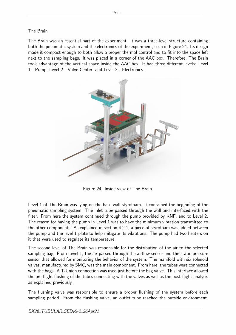
- 76 -
The Brain
The Brain was an essential part of the experiment. It was a three-level structure containingboth the pneumatic system and the electronics of the experiment, seen in Figure 24. Its designmade it compact enough to both allow a proper thermal control and to fit into the space leftnext to the sampling bags. It was placed in a corner of the AAC box. Therefore, The Braintook advantage of the vertical space inside the AAC box. It had three different levels: Level1 - Pump, Level 2 - Valve Center, and Level 3 - Electronics.
Figure 24: Inside view of The Brain.
Level 1 of The Brain was lying on the base wall styrofoam. It contained the beginning of thepneumatic sampling system. The inlet tube passed through the wall and interfaced with thefilter. From here the system continued through the pump provided by KNF, and to Level 2.The reason for having the pump in Level 1 was to have the minimum vibration transmitted tothe other components. As explained in section 4.2.1, a piece of styrofoam was added betweenthe pump and the level 1 plate to help mitigate its vibrations. The pump had two heaters onit that were used to regulate its temperature.
The second level of The Brain was responsible for the distribution of the air to the selectedsampling bag. From Level 1, the air passed through the airflow sensor and the static pressuresensor that allowed for monitoring the behavior of the system. The manifold with six solenoidvalves, manufactured by SMC, was the main component. From here, the tubes were connectedwith the bags. A T-Union connection was used just before the bag valve. This interface allowedthe pre-flight flushing of the tubes connecting with the valves as well as the post-flight analysisas explained previously.
The flushing valve was responsible to ensure a proper flushing of the system before eachsampling period. From the flushing valve, an outlet tube reached the outside environment.
BX26 TUBULAR SEDv5-2 26Apr21

- 77 -
This can be seen in Figure 25b.
The OBC and its external elements were allocated in the third level of The Brain. The PCBwas fixed to the aluminum plate by means of 10 standoffs. As shown in Figure 25c, it had ahole, as well as the level plate, to collect all the wires connecting with levels 1 and 2. Thislevel had its own outside top wall which contained the electrical interfaces. The latter allowedthe wall to be opened without having to remove all the sockets attached with screws and afemale in the inside of the wall. The styrofoam shielding of The Brain had a hole on top toallow the temperature sensors wires to reach the inside of the AAC Box.
A more detailed content of the components for each level is summarized in Appendix C.4.
(a) Isometric View of Level 1. (b) Isometric View of Level 2. (c) Isometric View of Level 3.
Figure 25: Distribution in Each Level.
This distribution allowed easy access to the PCB from the top and provided the physical desiredseparation between electronics and pneumatic circuit.
The structure of The Brain provided versatility in terms of implementation and construction.It was made out of strut profiles: four bars placed vertically and four bars placed horizontally.The railed bars allowed the possibility to fix all the pieces together and to provide the anchorpoints for the lateral and top styrofoam shield as well as to fix the whole unit to the boxstructure bars.
The bulk dimensions of The Brain were 260 mm long, 150mm wide and 290 mm high. If theshielding styrofoam walls were taken into account, the dimensions were 290 mm long, 180 mmwide and 300 mm high. Therefore, accounting for the space the column bars took, each platehad a surface of 258 mm x 158 mm. The distance between levels was variable depending onthe components dimensions. Level 1 had a height of 7 cm, Level 2 had a height of 9 cm andLevel 3 had 8 cm to the top styrofoam shielding. The Brain with styrofoam shielding can beseen in Figure 26.
BX26 TUBULAR SEDv5-2 26Apr21
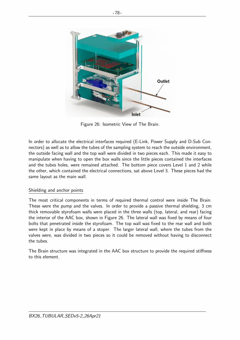
- 78 -
Figure 26: Isometric View of The Brain.
In order to allocate the electrical interfaces required (E-Link, Power Supply and D-Sub Con-nectors) as well as to allow the tubes of the sampling system to reach the outside environment,the outside facing wall and the top wall were divided in two pieces each. This made it easy tomanipulate when having to open the box walls since the little pieces contained the interfacesand the tubes holes, were remained attached. The bottom piece covers Level 1 and 2 whilethe other, which contained the electrical connections, sat above Level 3. These pieces had thesame layout as the main wall.
Shielding and anchor points
The most critical components in terms of required thermal control were inside The Brain.These were the pump and the valves. In order to provide a passive thermal shielding, 3 cmthick removable styrofoam walls were placed in the three walls (top, lateral, and rear) facingthe interior of the AAC box, shown in Figure 26. The lateral wall was fixed by means of fourbolts that penetrated inside the styrofoam. The top wall was fixed to the rear wall and bothwere kept in place by means of a stoper. The larger lateral wall, where the tubes from thevalves were, was divided in two pieces so it could be removed without having to disconnectthe tubes.
The Brain structure was integrated in the AAC box structure to provide the required stiffnessto this element.
BX26 TUBULAR SEDv5-2 26Apr21

- 79 -
4.4.5 Pneumatic Subsystem
In order to be able to collect separated samples of air, a pneumatic subsystem was developedand implemented. The schematics and components of this can be seen in Figure 28. Thesystem was formed by almost 100 components located inside The Brain and the AAC Box.
In between these components, the same Sulfinert-treated stainless steel tubing as the onesused for the Inlet/Outlet pipes explained in Section 4.2.1 were chosen.
The schematic for the pneumatic system can be seen in Figure 28. The air was sucked fromthe outside through the inlet tube (No.1), the lower tube in Figure 27, and it went through thefilter (No.2) inside the pump (No.9). From here, and changing to Level 2, it passed throughthe airflow sensor (No.15), which allowed the airflow rate to be monitored. Thereafter the airpassed through the static pressure sensor (No.20) before getting to the six station manifold(No.23). It was in here where the air was directed to the desired bag (No.36) thanks to itsdedicated solenoid valve (No.30).
When flushing the pneumatic system before each sampling period, the flushing valve (No.27)was opened so that the outlet of the system was open and new air ran through the main partof the pneumatic system.
Figure 27: Pneumatic System Top View.
BX26 TUBULAR SEDv5-2 26Apr21

-80-
Figure 28: AAC Pneumatic System Diagram and Components.
BX
26T
UB
UL
AR
SE
Dv5-2
26Apr21

- 81 -
4.5 Electrical Design
4.5.1 Block Diagram
The electronics design can be seen in Figure 29 which shows the connections, grounding,voltages, and signals.
Figure 29: Block Diagram for all Electronic Components Showing the Connection, Signal andPower Connections.
Most of the electronics were located in the Brain inside the AAC box. However, there weresix distinct areas:
1. The Brain level 3, where the PCB is located with the Arudino and shield, two 24 VDC-DC, two 12 V DC-DC, 11 MOSFETs and 16 LEDs.
2. The Brain level 2, where the valve manifolds with six sampling valves, the flushingvalve, two heaters, airflow sensor, static pressure sensor and one temperature sensorwere located.
3. The Brain level 1, where the pump, two heaters and one temperature sensor were located.
BX26 TUBULAR SEDv5-2 26Apr21
- 82 -
4. The AAC box, where 3 ambient temperature sensors were located.
5. The CAC box, where the CAC valve and 3 ambient temperature sensors were located.
6. Outside of the experiment box, where 3 ambient pressure sensors were located.
From the PCB, on level 3, five D-sub connectors were used to connect to the other five areas.Fifteen pin connectors were used for level 1 and level 2. For the CAC box, AAC box samplingbags area, and the external pressure sensors, nine pin connectors were used. In addition therewas a connection to the gondola power and gondola E-link.
All of the power distribution was done through the PCB using two 24 V DC-DC and two 12V DC-DC converters in parallel with a forwarding diode.
• 28.8V =⇒ 24V By DC-DC converters
• 28.8V =⇒ 12V By DC-DC converters
The heaters did not require the voltage to be stepped down and so were powered directly fromthe gondola battery.
The Arduino was used to control all of the sensors, valves, heaters and the pump from thePCB. Sensors were directly connected to the Arduino. The valves, heaters and the pump wereconnected via a switching circuit.
The LEDs were used as visual indicators that displayed whether different parts of the circuitare active or not. They gave indications on the status of the valves, pump, heaters, DC-DCconverters and Arduino.
Grounding was done following a distributed single point grounding, with all ground connectionsmeeting at a single star point ensuring there were no floating grounds. As not all componentswere connected via DC-DC converters the experiment was not isolated from the gondola powersupply therefore there was a connection between the star point and the gondola ground. Thestar point was located on the main PCB board which was then grounded to the experimentbox. The grounding can be seen in Figure 29 where it is indicated by dashed lines labeledGND. The analog sensors that were used on level 1 in the brain used a separate groundingwire(AGND) onto the main PCB where there was a separate trace connecting to the groundpins on the Arduino board. Furthermore the upper and lower level of the main PCB boardwere making use of the common grounding plane where possible.
4.5.2 Miniature Diaphragm Air Pump
The pump which was selected was the 850.1.2. KNDC B, Figure 30, which is manufacturedby KNF. One of the reasons this pump was selected is that it was successfully flown on asimilar flight in the past where it managed to pump enough air at 25 km altitude to have 180mL remaining at sea level [5]. However, to ensure the pump will operate as intended, severaltests were carried out. These tests — 4, 5, 18, 28 and 29, can be seen in Tables 25, 26, 35,41, and 42.
At sea level conditions the pump was tested and found to have a flow rate of 8.0 L/min and acurrent draw of 250 mA. The peak current draw was recorded as 600 mA which lasts for lessthan one second and occurs when the pump is switched on.
BX26 TUBULAR SEDv5-2 26Apr21

- 83 -
From the results of Test 18, in Section 7.3.5, the flow rate was shown to be around 3.36 L/minat the lowest pressure that will be seen in flight. This was in line with requirement D23. Theresults found in Test 28, in Section O.1, appeared to be inline with the information given bythe manufacturer, seen in Figure 31. The highest continuous current draw expected from thepump was 185 mA when the experiment is at 12 km altitude and was expected to decrease aswe increase in altitude. While it appeared that the pump increased in current draw at around6 km there was no plan to sample below 12 km therefore the highest current draw was takenfrom 12 km. As the pump had a peak current of 600 mA when it switches on, the mosfet andDC-DC power have been chosen to be able to withstand this demand.
Figure 30: KNF 850.1.2. KNDC B Miniature Diaphragm Pump.
BX26 TUBULAR SEDv5-2 26Apr21

- 84 -
Figure 31: KNF 850.1.2. KNDC B Flow Rate and Current Draw to Pressure Graph.
4.5.3 Electromagnetically Controlled Valves
Filling the sampling bags was controlled by solenoid valves. The solenoid valves selectedwere model VDW23-5G-1-H-Q, seen in Figure 32, manufactured by SMC. These valves werenormally closed through out the experiment with zero power consumption and opened, whengiven power, to fill up the sampling bags at specific altitudes. In addition one valve was onthe CAC, in order to seal the coil at the end of the flight and another at the end of the AACtubing, flushing valve, in order to flush the system. The valves selected for these are modelVDW22UANXB, Figure 32. The CAC valve was opened shortly after take off and remainedopen the whole flight. This valve was closed shortly before landing. The flushing valve wasopened before sampling in order to ensure the air in the tubes was from the correct altitude.
BX26 TUBULAR SEDv5-2 26Apr21
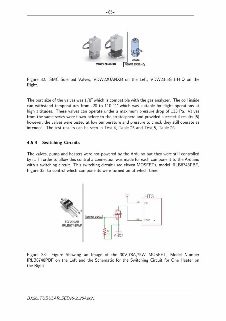
- 85 -
Figure 32: SMC Solenoid Valves, VDW22UANXB on the Left, VDW23-5G-1-H-Q on theRight.
The port size of the valves was 1/8”which is compatible with the gas analyzer. The coil insidecan withstand temperatures from -20 to 110 °C which was suitable for flight operations athigh altitudes. These valves can operate under a maximum pressure drop of 133 Pa. Valvesfrom the same series were flown before to the stratosphere and provided successful results [5]however, the valves were tested at low temperature and pressure to check they still operate asintended. The test results can be seen in Test 4, Table 25 and Test 5, Table 26.
4.5.4 Switching Circuits
The valves, pump and heaters were not powered by the Arduino but they were still controlledby it. In order to allow this control a connection was made for each component to the Arduinowith a switching circuit. This switching circuit used eleven MOSFETs, model IRLB8748PBF,Figure 33, to control which components were turned on at which time.
Figure 33: Figure Showing an Image of the 30V,78A,75W MOSFET, Model NumberIRLB8748PBF on the Left and the Schematic for the Switching Circuit for One Heater onthe Right.
BX26 TUBULAR SEDv5-2 26Apr21

- 86 -
4.5.5 Schematic
The schematics show all the components and how they are connected, the full schematics canbe seen in Figure 34. There are four requirements for the the power distribution given below:
• 28.8V for the heaters.
• 28.8V =⇒ 24V for the pump and valves.
• 28.8V =⇒ 12V for the airflow sensor, static pressure sensor and Arduino due.
• 3.3V for the temperature and pressure sensors.
The voltage available from gondola power is 28.8 V, therefore the heaters were connecteddirectly to the main power supply. For the rest of the components, two 24 V and two 12V DC-DCs in parallel were used to make sure if one of them fails then the other can takeover. The circuitry can be seen in Figure 35. All the valves and the pump were then poweredthrough the 24 V DC-DCs. To step down the voltage from 28.8 V to 12 V to power theairflow sensor, static pressure sensor and the Arduino, two 12 V DC-DCs in parallel were usedfor redundancy purposes. Finally, to power the temperature and external pressure sensors, 3.3V is required which is supplied by the Arduino board.
To meet the requirements of the pneumatic subsystem, a static pressure sensor was chosen tomeasure the pressure inside the tubes and bags. This analogue pressure sensor operated on12 V so could share the same power line as the airflow sensor and Arduino.
BX26 TUBULAR SEDv5-2 26Apr21

- 87 -
Figure 34: Schematic for All of the Electronics on Board TUBULAR. This can also be Foundat https://rexusbexus.github.io/tubular/img/electrical-design-schematics.png
BX26 TUBULAR SEDv5-2 26Apr21

- 88 -
Figure 35: Schematic Showing the DC-DC Redundancy of Both 24 V and the 12 V DC-DCConverters.
4.5.6 PCB Layout
All electronic control circuits were gathered on a single PCB on level 3 of the Brain. ThePCB contained the Arduino due, switching circuits, indication LEDs, a temperature sensor,the power system and all necessary connectors. The connectors were divided so that eachconnector’s wires goes to the same level of the Brain to improve cable management. Due tothe relocation of components there are some components on level 2, Static pressure sensorand the airflow sensor, which were connected to the level 1 connector. Although this didnot produce major problems since both those components have separate connectors on the
BX26 TUBULAR SEDv5-2 26Apr21

- 89 -
cable going down to level 1 and does not share any connections with any components on level1. Thus you could still unplug each level separately since the wires to these two componentscould just be broken of from the cable loom at the appropriate point. To further improve cablemanagement the shared pins for I2C and SPI were connected to a single pin on each respectiveD-SUB connector and split up on the respective level. The PCB’s components layout can beseen in Figure 36
The PCB was made using Eagle software and fully sponsored by the Eurocircuits for manufac-turing. The traces had a width designed to fit the IPC-2221 standards[14] with extra widthadded. The PCB layout with traces can be seen in in Appendix C.11. On the main PCB thetraces were 1.4mm wide for the nets containing components that consumes higher amountsof current and the ones with lower current requirements had a trace width of 0.3mm. On thepressure sensor PCB all traces were 0.5mm wide.
BX26 TUBULAR SEDv5-2 26Apr21

- 90 -
Figure 36: PCB Components Layout
BX26 TUBULAR SEDv5-2 26Apr21

- 91 -
4.6 Thermal Design
4.6.1 Thermal Environment
The experiment experienced a wide temperature range during the flight and it was able tocontinue operating despite these changes due to the incorporated thermal design. As seenin Figure 37, the coldest point of the flight was between 10 km and 15 km where the airtemperature can drop to −70°C outside. During the flight the coldest recorded temperatureon the gondola was −54°C during the Ascent and Descent. In addition, launching fromKiruna in late October meant the temperature on the ground could be as low as −10°C butthe temperature at the time for launch ended up being around 0°C. As the component withthe warmest lower limit operating temperature had to be kept at a minimum of 5°C (E3 inTable73), this required the heaters to be switched on while the experiment was still on theground.
Figure 37: Diagram Showing the Temperature Profile of the Atmosphere [15].
4.6.2 The Critical Stages
The flight had the following critical stages:
• Launch pad
• Early ascent
• Sampling ascent
• Float
• Descent before sampling
BX26 TUBULAR SEDv5-2 26Apr21
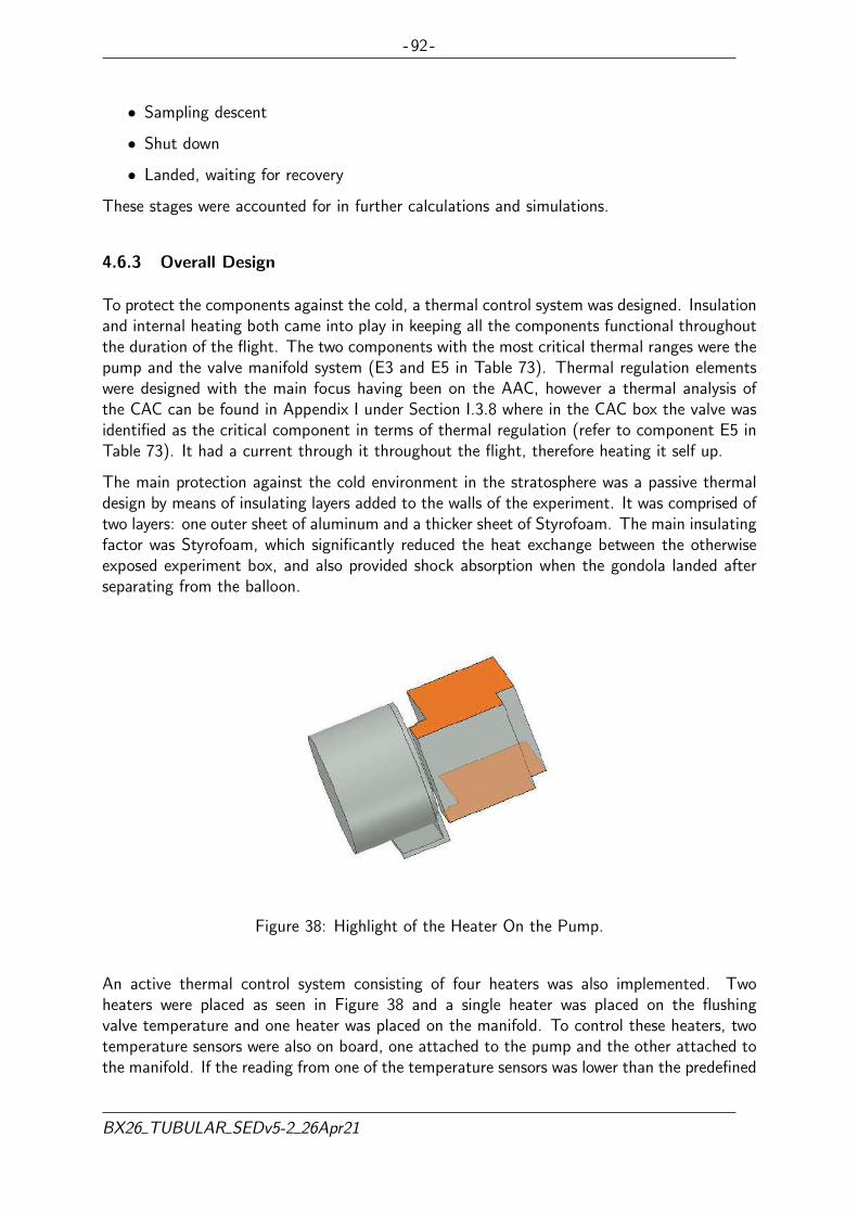
- 92 -
• Sampling descent
• Shut down
• Landed, waiting for recovery
These stages were accounted for in further calculations and simulations.
4.6.3 Overall Design
To protect the components against the cold, a thermal control system was designed. Insulationand internal heating both came into play in keeping all the components functional throughoutthe duration of the flight. The two components with the most critical thermal ranges were thepump and the valve manifold system (E3 and E5 in Table 73). Thermal regulation elementswere designed with the main focus having been on the AAC, however a thermal analysis ofthe CAC can be found in Appendix I under Section I.3.8 where in the CAC box the valve wasidentified as the critical component in terms of thermal regulation (refer to component E5 inTable 73). It had a current through it throughout the flight, therefore heating it self up.
The main protection against the cold environment in the stratosphere was a passive thermaldesign by means of insulating layers added to the walls of the experiment. It was comprised oftwo layers: one outer sheet of aluminum and a thicker sheet of Styrofoam. The main insulatingfactor was Styrofoam, which significantly reduced the heat exchange between the otherwiseexposed experiment box, and also provided shock absorption when the gondola landed afterseparating from the balloon.
Figure 38: Highlight of the Heater On the Pump.
An active thermal control system consisting of four heaters was also implemented. Twoheaters were placed as seen in Figure 38 and a single heater was placed on the flushingvalve temperature and one heater was placed on the manifold. To control these heaters, twotemperature sensors were also on board, one attached to the pump and the other attached tothe manifold. If the reading from one of the temperature sensors was lower than the predefined
BX26 TUBULAR SEDv5-2 26Apr21

- 93 -
threshold, then the heater turned on and warmed the component. If it was above the higherthreshold the heater turned off.
Simulations in MATLAB (code can be found in Appendix J) were used to determine the averageuniform heat inside the experiment. The ANSYS thermal modelling platform was used to thesimulate the thermal conditions inside the Brain.
Table 18, below, covers the thermal ranges of the components crucial to the experiment flightfrom those listed in Section 4.3:
ID ComponentsOperating (°C) Survivable (°C) Expected (°C)Min. Max. Min. Max. Min. Max.
E1 Arduino Due -40 85 -60 150 -15.7 54.0E2 Ethernet Shield -40 85 -65 150 -15.7 54.0
E3Miniature di-aphragm air pump
5 40 -10 40 10 34.9
E4 Pressure Sensor -40 85 -40 125 -15.7 54.0
E5Sampling Valve (in-let and outlet 1/8””female)
-20 68 -203 683 -15 20
E6Airflow sensorAWM43300V
-20 70 -203 703 -8.8 34.9
E7Heater (12.7 ×50.8mm)
-200 200 -2003 2003 -20 36
E9 Temperature Sensor -55 125 -65 150 -19.7 43E10 DCDC 24 V -40 85 -55 125 -15.7 54.0E12 Micro SD -25 85 -2003 2003 -15.7 54.0
E16MOSFET for cur-rent control
-55 175 -55 175 -15.7 54.0
E17Diodes for DCDCconverters
-65 175 -653 1753 -15.7 54.0
E18 3.3V LED -40 85 -403 853 -15.7 54.0E28 3.3 Zener diode -65 175 -653 1753 -15.7 54.0
E32Logic CAT5 E-linkfor inside box
-55 60 -553 603 -34 15
E34Flushing valve (inletand outlet 1/8”” fe-male)
-20 68 -203 68 -7.4 25.8
E35Valves manifold(outlet 1/8”” fe-male)
-10 50 -103 503 3 18
E58 PCB -50 110 -503 1103 -15.7 54.0
E59Pressure SensorPCB
-50 110 -503 1103 -50 39
Table 18: Table of Component Temperature Ranges.
3If survivable temperatures were not given, operating temperatures were used as survivable limits.
BX26 TUBULAR SEDv5-2 26Apr21

- 94 -
A complete table of component temperature ranges, which includes static entities (such aswires and connectors) can be found in Appendix I.
4.6.4 Internal Temperature
An enclosed partition of the experiment model was reserved in the corner of the AAC section.This partition took the shape of a rectangular section and was to house all of the electroniccomponents not required to be situated in specified locations throughout the experimentsetting, such as the Arduino boards and some of the sensors.
The pump had the most critical temperature range as it was the only component in theexperiment that could not operate below freezing temperatures. Failure of the pump meantfailure of the entire AAC system. It’s data sheet stated that it must always start above 5°C,or the EPDM diaphragm may be too stiff to start. However, as this type of pump was usedsuccessfully on previous high altitude flights, [5], tests were conducted on the pump to find itstrue performance at lower temperatures and in a low vacuum environment. The AAC valveswere also crucial to the experiment’s function, as they enabled each and every sampling bagon board to be used. For this reason, while the valves could operate down to −20°C, it wasdesirable to be keep them above this limit whenever in use. The manifold valves in the brainhad a minimum operating temperature of only −10°C, but simulations proved they would bekept above 0°C.
As the most temperature-sensitive equipment was all housed within the Brain, it was importantto know what heat would be lost through the different heat transfer mechanisms as this wouldaffect the amount of time the heaters had to be active. This was addressed through calculationsand simulations to find required insulation. All calculations concerning heat transfer can befound in Appendix I. As a worst-case scenario for heat distribution, it was assumed that all ofthe power dissipated through resistance in the electrical components would reach the markedboundaries of the experiment’s walls.
Aluminum sheeting was used as the outer layer of insulation for the experiment and Styrofoamwas the inner layer. Aluminum may have among the highest of thermal conductivities, but itsarrangement around the Styrofoam, creating one large heat bridge with the inner layer, provideda useful thermoregulatory mechanism [23]. The high ratio between the absorptivity (0.3) andemissivity (0.09) of the material was used to its advantage [23]. Because the ratio for polishedaluminum is higher than 1.0, the element would get hotter as it got exposed to the radiationfrom the sun and the power-dissipating components [16]. The low emissivity coefficient forthe aluminum cover meant it would not get significantly hotter than the surrounding ambienttemperature, but its increased temperature may have negated some of the heat being lostfrom the experiment’s interior via some of the heat from the aluminum propagating into theexperiment, reducing the net heat loss by a small amount. As conservation of power wasimperative, the heaters were used sparingly, and instead methods like the use of aluminum forshielding were employed as passive heating. The aluminum layer was be 0.5 mm in thickness,while the Styrofoam layer beneath it span 20 to 30 mm in thickness. The Styrofoam, incontrast to the aluminum had a low thermal conductivity even when compared to similarpolymer structures [23]. The Styrofoam handled the bulk of the thermal resistance in keepingthe experiment from losing the heat it would have obtained prior to being moved to thelaunchpad. The aluminum came into play as the experiment rose into colder altitudes and
BX26 TUBULAR SEDv5-2 26Apr21

- 95 -
encounters increased sun exposure. While the warmed aluminum had little impact on theexperiment’s heat loss, this also meant that the experiment’s internal temperatures would beprevented from rising to the upper allowed operating limit of the experiment made possiblebecause of the aluminum’s low absorptivity of sunlight.
Another heat bridge that was needed was the fastening of the experiment to the gondola. Thealuminum frame of the gondola would be colder than the experiment and with normal screwsthere would be a lot of heat transfer. In this case rubber bumper screws, suggested at CDR,were used to fasten the experiment to the gondola and reduced the heat transfer between theexperiment and the gondola.
4.6.5 Calculations and Simulation Reports
The temperature ranges could vary for the different stages but the most critical moment wasduring the Ascent Phase. According to the thermal analysis, the heaters would not be requiredduring float and descent. During the flight the heaters were still operating for some intervalsduring the Ascent and Float Phases. All simulation equations and their details can be seen inAppendix I.
An estimate of the temperature in the Brain at the sampling times during the Ascent Phaseis visualized in Figure 39. The higher temperature was in the lower right corner where thepump is located. A cooler area exists around the middle of the left edge where no heaters areapplied. The legend in the Figure shows the temperature in Celsius.
Figure 39: Cross Section of the Air in the Brain at the Time to Start Sample During Ascent.
In Figure 40 the average temperature of the pump with data from ANSYS is presented. Onewas simulated with no air in the Brain and the other has air with the same density as sea level.In between the vertical dotted line is when the experiment is above 15km. At 4h in the figurethe experiment is launched. It can be seen that the pump should have an average temperatureover 5 degrees during the flight.
BX26 TUBULAR SEDv5-2 26Apr21
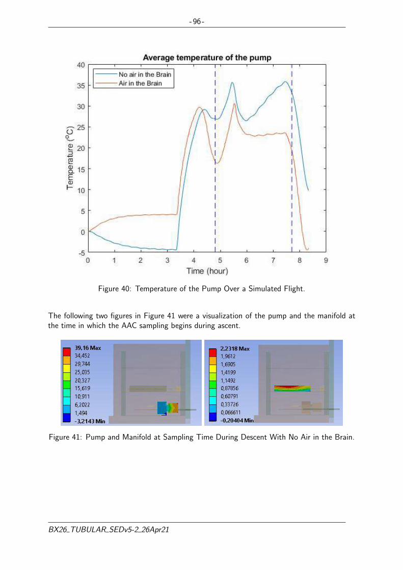
- 96 -
Figure 40: Temperature of the Pump Over a Simulated Flight.
The following two figures in Figure 41 were a visualization of the pump and the manifold atthe time in which the AAC sampling begins during ascent.
Figure 41: Pump and Manifold at Sampling Time During Descent With No Air in the Brain.
BX26 TUBULAR SEDv5-2 26Apr21

- 97 -
Figure 42: Flushing Valve Prior to Sampling Commencing With No Air in the Brain.
During a worst case simulation that is shown in Figure 41, the four heaters were used for 26.66Wh in total together over the course of the simulation the figures are from. Only the pumpheaters required more time if the outside were colder there was 80 Wh in the power budgettable dedicated to thermal control (shown in Table 19). There was therefore an incentive tokeep the pump heaters on for a longer time if needed.
Based on the calculations and thermal simulations, it was concluded that the thermal designedpassive and active thermal control mechanisms detailed in this section would ensure that theAAC’s pump and manifold were in their operating temperature during the entire flight flight. Ithas been shown that the CAC has a sufficiently adequate thermal design to operate throughoutthe whole flight.
Thermal testing (Test 5, section 5.3.13) showed that the heaters and the subsequent internaltemperature responded as expected from simulations and work as required when heating thecritical components. A full 4h test at −50°C was done after the temperature sensor issue hadbeen resolved and it concluded that the experiment would be able to operate thermal wiseduring the whole flight.
BX26 TUBULAR SEDv5-2 26Apr21
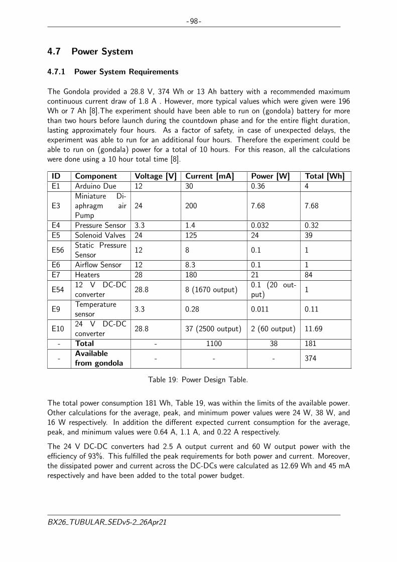
- 98 -
4.7 Power System
4.7.1 Power System Requirements
The Gondola provided a 28.8 V, 374 Wh or 13 Ah battery with a recommended maximumcontinuous current draw of 1.8 A . However, more typical values which were given were 196Wh or 7 Ah [8].The experiment should have been able to run on (gondola) battery for morethan two hours before launch during the countdown phase and for the entire flight duration,lasting approximately four hours. As a factor of safety, in case of unexpected delays, theexperiment was able to run for an additional four hours. Therefore the experiment could beable to run on (gondala) power for a total of 10 hours. For this reason, all the calculationswere done using a 10 hour total time [8].
ID Component Voltage [V] Current [mA] Power [W] Total [Wh]E1 Arduino Due 12 30 0.36 4
E3Miniature Di-aphragm airPump
24 200 7.68 7.68
E4 Pressure Sensor 3.3 1.4 0.032 0.32E5 Solenoid Valves 24 125 24 39
E56Static PressureSensor
12 8 0.1 1
E6 Airflow Sensor 12 8.3 0.1 1E7 Heaters 28 180 21 84
E5412 V DC-DCconverter
28.8 8 (1670 output)0.1 (20 out-put)
1
E9Temperaturesensor
3.3 0.28 0.011 0.11
E1024 V DC-DCconverter
28.8 37 (2500 output) 2 (60 output) 11.69
- Total - 1100 38 181
-Availablefrom gondola
- - - 374
Table 19: Power Design Table.
The total power consumption 181 Wh, Table 19, was within the limits of the available power.Other calculations for the average, peak, and minimum power values were 24 W, 38 W, and16 W respectively. In addition the different expected current consumption for the average,peak, and minimum values were 0.64 A, 1.1 A, and 0.22 A respectively.
The 24 V DC-DC converters had 2.5 A output current and 60 W output power with theefficiency of 93%. This fulfilled the peak requirements for both power and current. Moreover,the dissipated power and current across the DC-DCs were calculated as 12.69 Wh and 45 mArespectively and have been added to the total power budget.
BX26 TUBULAR SEDv5-2 26Apr21

- 99 -
4.8 Software Design
4.8.1 Purpose
The purpose of the software was to automate control of the valves so that they will beopened/closed at the target altitude. Moreover, the software stored housekeeping data fromsensors, pump, and valves states to the on-board memory storage device. Logging sensor datawas necessary in order to determine a vertical profile of the analyzed samples:
In order to determine the vertical profiles of CO2, CH4, and CO from the analysisof sampled air, measurements of several atmospheric parameters were needed [...].The two most important parameters were the ambient pressure and the meancoil temperature. These parameters were be recorded by the AirCore-HR (HighResolution) electronic data package. Mean coil temperature was obtained bytaking the mean of three temperatures recorded by independent probes located atdifferent positions along the AirCore-HR.[17]
Both the ambient pressure and the sampling container temperature were also essential for AACsampling bags. The temperature data was collected by the sensors near the sampling bags.
The software shall also transmit data to the ground so that the team can monitor the conditionsof the experiment in real time. Telecommand was also needed to overwrite pre-programmedsampling scheduled in case of automation failure or to mitigate unexpected changes in theflight path and reached altitudes. It was used to test the system, especially valves and heaters.
4.8.2 Design
(a) Process OverviewThe software which ran on the Arduino read from the sensors through the analog, I2C,and SPI interfaces. The sensors provided temperature, pressure and airflow data. Theacquired data was time-stamped and stored in the on-board SD card and transmittedvia the E-Link System to the ground station. Then according to the pressure/altitude,the software controlled the valves which allowed the air to be pumped inside the bags.Figure 43 visually explain the process flow.
BX26 TUBULAR SEDv5-2 26Apr21

- 100 -
Figure 43: The Process Overview of the Experiment.
(b) General and Safety related conceptsThe watchdog timer, which was an electronic countdown timer that causes an interruptwhen it reaches 0, was used to avoid failure because of a possible freezing problem in thesoftware. During normal operations, the software set flags when done with their task.When all the flags had been set the watchdog got reset. If any task fails to set the theirflag before the watchdog elapses, the system resets. Telecommand was also be used asbackup in case the automation fails or otherwise become unresponsive. Telemetry wasutilized to transmit housekeeping data and the state of the valves to get confirmationof operation. Rigorous testing was performed during the development of the projectand before the launch phase to insure that that the software was capable to control theexperiment.
(c) InterfacesTable 20 demonstrates how the components interacted with the onboard computer(OBC). Components that used SPI, shared MISO, MOSI, and CLK pins on the Ar-duino board. Each of them was also connected to general pins input output (GPIO) forslave select. Furthermore, components using I2C protocol, shared Serial Data pin (SDA)and Serial Clock pin (SCL).
BX26 TUBULAR SEDv5-2 26Apr21

- 101 -
Components interacting Communication protocol InterfacePressure sensors-OBC SPI Arduino SPI and Digital PinsTemperature sensors-OBC I2C Arduino I2CAirflow sensor-OBC Analog Arduino analog pinHeaters-OBC Digital GPIO pinsAir pump-OBC Digital GPIO pinsValve-OBC Digital GPIO pinsOBC-microSD Storage SPI Arduino Ethernet shieldOBC - E-Link Ethernet Ethernet port
Table 20: Communication and Interface Protocols.
Every transmission to/from the ground utilized the E-link connection. The data packetwhich was used was an Ethernet Packet with a header containing the address of desti-nation, followed by the data, and at the end there was a frame check sequence (FCS).The up-linked data packet had the same structure, with header followed by commandsand ended with FCS.
The protocol that had been chosen was UDP for telemetry and TCP for telecommand.The UDP was used to prevent software getting stuck waiting for handshake from theground if the connection was temporarily lost.
The telecommand contained the following services:
• Changing instrument modes
• Manually control valves, pump, and heaters
• Change sampling schedule
Furthermore, telemetry contained the services below:
• Data from temperature, pressure and airflow sensor
• Current instrument modes
• Instrument housekeeping data (valve, pump, and heater states)
(d) Data Acquisition and StorageData was stored on the SD memory card on the Arduino Ethernet Shield using theFAT16 and FAT32 file systems. To minimize data loss in the event of a reset, the samefile was written only in a set amount of time before closing it and opened a new file.It was estimated that for the entire flight, all the sensors produced less than 5 MB ofdata. The sampling rate was fixed at 1 sampling per second.
The data was collected and presented as a matrix, where the first column was thetime frame, the following columns were the sensors data. After the sensors data, therewas also housekeeping data, that kept track of the valves, and heaters states. However,the size of the housekeeping data was not expected to surpass 20 bits per sampling.
Data was continuously down-linked two times per second and the total telemetry size
BX26 TUBULAR SEDv5-2 26Apr21
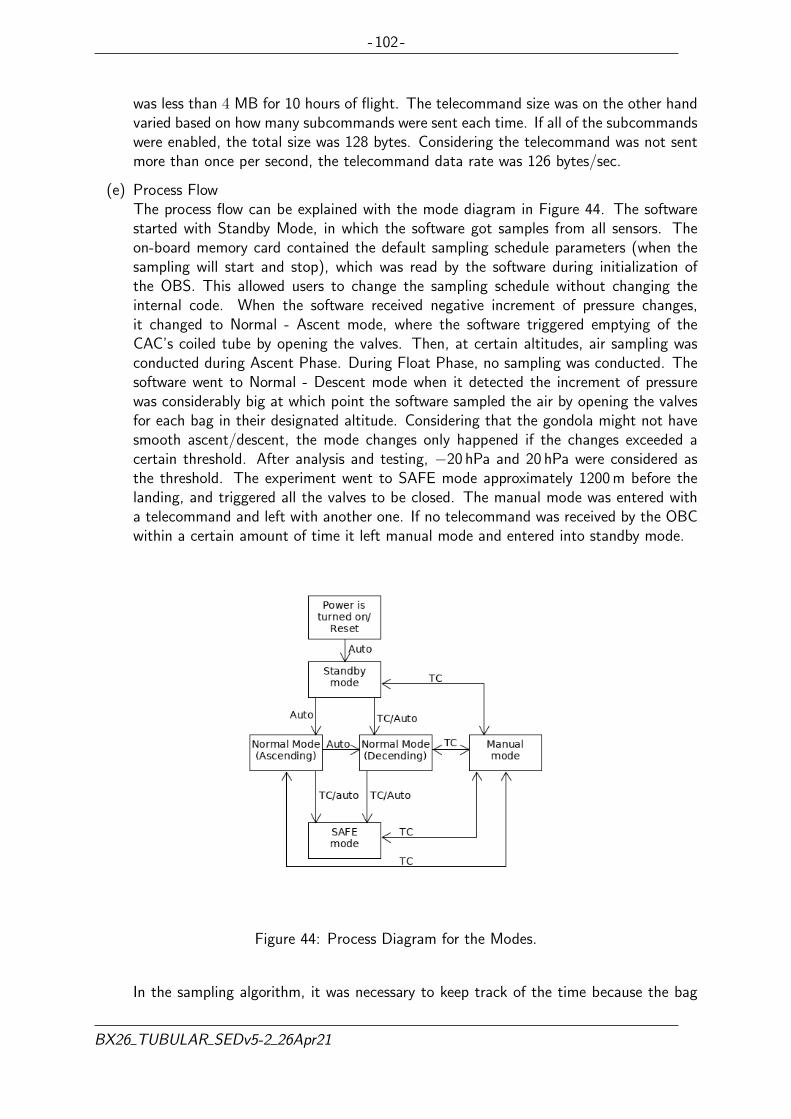
- 102 -
was less than 4 MB for 10 hours of flight. The telecommand size was on the other handvaried based on how many subcommands were sent each time. If all of the subcommandswere enabled, the total size was 128 bytes. Considering the telecommand was not sentmore than once per second, the telecommand data rate was 126 bytes/sec.
(e) Process FlowThe process flow can be explained with the mode diagram in Figure 44. The softwarestarted with Standby Mode, in which the software got samples from all sensors. Theon-board memory card contained the default sampling schedule parameters (when thesampling will start and stop), which was read by the software during initialization ofthe OBS. This allowed users to change the sampling schedule without changing theinternal code. When the software received negative increment of pressure changes,it changed to Normal - Ascent mode, where the software triggered emptying of theCAC’s coiled tube by opening the valves. Then, at certain altitudes, air sampling wasconducted during Ascent Phase. During Float Phase, no sampling was conducted. Thesoftware went to Normal - Descent mode when it detected the increment of pressurewas considerably big at which point the software sampled the air by opening the valvesfor each bag in their designated altitude. Considering that the gondola might not havesmooth ascent/descent, the mode changes only happened if the changes exceeded acertain threshold. After analysis and testing, −20 hPa and 20 hPa were considered asthe threshold. The experiment went to SAFE mode approximately 1200 m before thelanding, and triggered all the valves to be closed. The manual mode was entered witha telecommand and left with another one. If no telecommand was received by the OBCwithin a certain amount of time it left manual mode and entered into standby mode.
Figure 44: Process Diagram for the Modes.
In the sampling algorithm, it was necessary to keep track of the time because the bag
BX26 TUBULAR SEDv5-2 26Apr21

- 103 -
could not be filled fully (it might burst). A simple library was used to keep track of thetime from the start of the experiment.
(f) Modularization and Pseudo Code
Figure 45: Onboard Software Design Tree.
The software design was produced by using object oriented approach. The functionalityof the experiment was divided into several objects and their children. The design tree isshown in Figure 45.
The Telemetry object was responsible to format the sensor/housekeeping data, andto transmit it. MODE was responsible for controlling the five modes of software. INITinitialized the necessary software. COMMANDS read the telecommands and executedtheir commands. The AIR SAMPLING CONTROL object had the four children objects.The first child was responsible for controlling the pump. The second child contained theparameters for the valves and pump. The third child read the data from the sensors, afourth child was responsible for manipulating the valves.
The SENSOR object had two children objects. One for sampling the sensors and anotherfor recording and storing the housekeeping data. The HEATER object had three childrenobjects. One for reading the temperature sensor data, another for deciding if the heatersshould be turn on/off. And the third child for turning it on/off.
The MONITOR object utilized a watchdog timer that caused an interrupt when itreaches 0. The watchdog did not get fed directly from by the end of the differenttasks. Instead the tasks set a flag, if all the flags were set the watchdog got reset andthe countdown started from the beginning. If the watchdog timed out before all theflags were set the monitor object reset the board.
Each of the objects interacted with each others fulfilling mutually exclusive interaction.It meant that any shared variables could only be accessed by one object at time. Thiswas important considering the program was fully automatic and to prevent unnecessary
BX26 TUBULAR SEDv5-2 26Apr21

- 104 -
data lost. The objects interface diagrams and their sequence diagrams can be found inAppendix C.7 and C.10.
4.8.3 Implementation
The C/C++ programming language was used when programming the platform. Instead ofArduino IDE, PlatformIO IDE was used, other software was used if necessary. The softwarewas functioning autonomously using a real-time operating system. FreeRTOS was chosen asthe real-time operating system, which provided a feature to split functionality into severalmutual exclusive tasks. These tasks were
• The Sampler task (periodic)
• The Reading task (periodic)
• heaterTask task (periodic)
• telecommand task (sporadic)
Several libraries that were used:
• FreeRTOS ARM.h (FreeRTOS specially port for ARM microprocessor like Due)
• ArduinoSTL.h (allows standard C++ functionality)
• RTCDue.h (keeps track of the time from the software start)
• Necessary Arduino libraries.
• DS1631.h (self made library)
• MS5607.h (self made library)
• Sensors libraries.
BX26 TUBULAR SEDv5-2 26Apr21

- 105 -
4.9 Ground Support Equipment
The purpose of the ground station was to monitor in real-time the experiment and providemanual override capability in case the experiment failed functioning autonomously. The manualoverride was able to control all the valves, pump, and heaters. It also provided a service tochange the sampling schedule while in flight.
One personal computer was used to connect to the E-Link through the Ethernet port. AGUI was created to display the sensors data and valves, pump states during the experiment.MATLAB GUIDE was used for the development.
The design of the ground station was responsible for receiving and transmitting data over theprovided Ethernet connection. Using GUIDE to create a GUI and respective functions as askeleton, the necessary functionality to receive, transmit and display were built accordingly.The functions were defined for each GUI element.
Figure 46: GUI Design for Ground Station Version 2.
Figure 46 shows the design of ground station GUI. Telemetry data was shown in several tablesbased on the data type. The data was recorded and stored on the computer. The experimentstatus panel represented the real-time status of the experiments, the red indicator changed togreen if the pump or valves were open later on. On the bottom side, the telecommand controlpanel provided command generation for the experiment. On its right side, the connectioncontrol panel had full control of the connections.
BX26 TUBULAR SEDv5-2 26Apr21

- 106 -
5 Experiment Verification and Testing
5.1 Verification Matrix
The verification matrix was made following the standard of ECSS-E-10-02A. [21]. This sectiondoes not list obsolete requirements. For a complete list of requirements that include obsoleteones, refer to Appendix N.
There are four established verification methods:A - Verification by analysis or similarityI - Verification by inspectionR - Verification by review-of-designT - Verification by testing
ID Written requirement VerificationTestnumber
Status
F.2The experiment shall collect air samples bythe CAC.
A, R - Pass
F.3The experiment shall collect air samples bythe AAC.
A, T 2, 16 Pass
F.9The experiment should collect data on the airintake flow to the AAC.
A, T24, 31,32
Pass 4
F.10The experiment shall collect data on the airpressure.
A, T24, 31,32
Pass 4
F.11The experiment shall collect data on the tem-perature.
A, T24, 31,32
Pass 4
P.12The accuracy of the ambient pressure mea-surements shall be -1.5/+1.5 hPa for 25°C.
R - Pass
P.13The accuracy of the temperature measure-ments shall be +3.5/-3°C(max) for conditionof -55°C to 150°C.
R - Pass
P.23The sampling rate of the temperature sensorshall be 1 Hz.
A,T 10 Pass
P.24The temperature of the Pump shall be be-tween 5°C and 40°C.
A, T 5 Pass
P.25The minimum volume of air in the samplingbags for analysis shall be 0.18 L at groundlevel.
A, T 16, 17 Pass
P.26The equivalent flow rate of the pump shall bebetween 8 to 3 L/min from ground level upto 24 km altitude.
T 18 Pass
P.27The accuracy range of the sampling time, orthe resolution, shall be less than 52.94 s, or423.53 m.
T 16 Pass
4sensor libraries are available online and used by many users
BX26 TUBULAR SEDv5-2 26Apr21
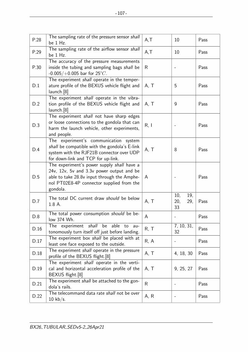
- 107 -
P.28The sampling rate of the pressure sensor shallbe 1 Hz.
A,T 10 Pass
P.29The sampling rate of the airflow sensor shallbe 1 Hz.
A,T 10 Pass
P.30The accuracy of the pressure measurementsinside the tubing and sampling bags shall be-0.005/+0.005 bar for 25°C.
R - Pass
D.1The experiment shall operate in the temper-ature profile of the BEXUS vehicle flight andlaunch.[8]
A, T 5 Pass
D.2The experiment shall operate in the vibra-tion profile of the BEXUS vehicle flight andlaunch.[8]
A, T 9 Pass
D.3
The experiment shall not have sharp edgesor loose connections to the gondola that canharm the launch vehicle, other experiments,and people.
R, I - Pass
D.4
The experiment’s communication systemshall be compatible with the gondola’s E-linksystem with the RJF21B connector over UDPfor down-link and TCP for up-link.
A, T 8 Pass
D.5
The experiment’s power supply shall have a24v, 12v, 5v and 3.3v power output and beable to take 28.8v input through the Amphe-nol PT02E8-4P connector supplied from thegondola.
A - Pass
D.7The total DC current draw should be below1.8 A.
A, T10, 19,20, 29,33
Pass
D.8The total power consumption should be be-low 374 Wh.
A - Pass
D.16The experiment shall be able to au-tonomously turn itself off just before landing.
R, T7, 10, 31,32
Pass
D.17The experiment box shall be placed with atleast one face exposed to the outside.
R, A - Pass
D.18The experiment shall operate in the pressureprofile of the BEXUS flight.[8]
A, T 4, 18, 30 Pass
D.19The experiment shall operate in the verti-cal and horizontal acceleration profile of theBEXUS flight.[8]
A, T 9, 25, 27 Pass
D.21The experiment shall be attached to the gon-dola’s rails.
R - Pass
D.22The telecommand data rate shall not be over10 kb/s.
A, R - Pass
BX26 TUBULAR SEDv5-2 26Apr21

- 108 -
D.23The air intake rate of the air pump shall beequivalent to a minimum of 3 L/min at 24km altitude.
A, T 4, 18 Pass
D.24The temperature of the Brain shall be be-tween -10°C and 25°C.
A, T 5 Pass
D.26The AAC air sampling shall filter out all watermolecules before filling the sampling bags.
A, T 17 Pass
D.27The total weight of the experiment shall beless than 28 kg.
R, T 3 Pass
D.28The AAC box shall be able to fit at least 6air sampling bags.
R - Pass
D.29The CAC box shall take less than 3 minutesto be removed from the gondola without re-moving the whole experiment.
R, T 12 Pass
D.30The AAC shall be re-usable for future balloonflights.
R, T 7, 16 Pass
D.31The altitude from which a sampling bag willstart sampling shall be programmable.
A,T 10, 14 Pass
D.32The altitude from which a sampling bag willstop sampling shall be programmable.
A,T 10 Pass
O.13The experiment should function automati-cally.
R, T 7, 8, 10 Pass
O.14The experiment’s air sampling mechanismsshall have a manual override.
R, T 8, 10 Pass
C.1Constraints specified in the BEXUS UserManual.
I - Pass
Table 21: Verification Matrix.
BX26 TUBULAR SEDv5-2 26Apr21

- 109 -
5.2 Test Plan
5.2.1 Test Priority
As shown in Table 22, tests were split into three different levels of priority, low, medium andhigh. The priority given to each test was dependent on several factors including complexity,amount of external help required and time taken.
PriorityLevel
TestNumber
Classification
High 4, 5, 7,10, 17
• Requires the use of external facilities which must be bookedin advance and could have limited availability.
• If a re-test is required the wait time could be on the orderof weeks or months.
• Testing could potentially break a non-spare component witha long re-order time.
Medium 2, 8, 9,12, 16,18, 24,27, 29,30
• Requires internal cooperation or multiple parts of the exper-iment completed to a minimum standard.
• If a re-test is required the wait time could be on the orderof days.
• Testing could potentially break a critical component thatwould require re-ordering or replacing.
Low 3, 13,14, 15,19, 20,25, 28,31, 32
• Can be performed by a single department.• If a re-test is required the wait time could be on the order
of hours.• Have low or no risk of breaking components.
Table 22: Table Showing the Classification of the Tests.
5.2.2 Planned Tests
The planned tests were as follows:
1. Valves test.5
2. Data collection test in Table 23.
3. Weight verification in Table 24.
4. Low pressure test in Table 25.
5. Thermal test in Table 26.
5Was combined with Tests 4, 5 and 24.
BX26 TUBULAR SEDv5-2 26Apr21

- 110 -
6. Experiment assembly and disassembly test.6
7. Bench test in Table 27.
8. E-Link test in Table 28.
9. Vibration test in Table 29.
10. Software operation test in Table 30.
11. Power systems test.7
12. Experiment removal test in Table 31.
13. Ground station - OBC connection test 7
14. Ground station - OBC parameters reprogram test in Table 32
15. Ground station invalid commands test6
16. Sampling test in Table 33.
17. Samples’ condensation test in Table 34.
18. Pump low pressure test in Table 35.
19. PCB operations test in Table 36.
20. Switching circuit testing and verification in Table 37.
21. Arduino sensor operation test.8
22. Arduino, pump and valves operation test.8
23. Pump thermal test.9
24. Software and electronics integration testing in Table 38.
25. Mechanical structural testing in Table 39.
26. Insulating foam low pressure test.10
27. Shock test in Table 40.
28. Pump operation test in Table 41.
29. Pump current in low pressure test in Table 42.
30. Sampling bag bursting test in Table 43.
31. On-board software unit test in Table 44.
32. Software failure test in Table 45.
33. Electrical component test in Table 46
6Unnecessary test.7Was combined with Test 10.8Was combined with Test 24.9Was combined with Test 5.10Was combined with Test 4.
BX26 TUBULAR SEDv5-2 26Apr21

- 111 -
5.2.3 Test Descriptions
If a non-destructive test was not proceeding as expected and it was thought there was arisk to components it would have been aborted. If a test was aborted for this reason aninvestigation must have been completed to discover why it did not proceed as expected andthe issue resolved before a re-test could occur.
Tests took place on the flight model due to budget and time restrictions which prevented a testmodel from being created. However, if a component was broken during testing spares wereavailable. Tests 4 and 5 did not use the entire model due to size restrictions in the chambers.Instead only critical components were tested.
Test Number 2Test Type SoftwareTest Facility LTU, KirunaTested Item Arduino, sensors, valves and pump
Test Level/ Procedureand Duration
Test procedure: Run software for full flight duration andensure data collection proceeds as expected. Particularlywatch for error handling and stack overflow.Test duration: 5 hours. Based on previous BEXUS flightdurations.
Test Campaign Duration 2 days (1 day build-up, 1 day testing)Test Campaign Date AugustTest Completed YES
Table 23: Test 2: Data Collection Test Description.
Test Number 3Test Type Weight VerificationTest Facility LTU, KirunaTested Item The entire experiment
Test Level/ Procedureand Duration
Test procedure: Use scales to measure the weight of theentire experiment.Test duration: 1 minute
Test Campaign Duration 1 dayTest Campaign Date OctoberTest Completed YES
Table 24: Test 3: Weight Verification Description.
BX26 TUBULAR SEDv5-2 26Apr21

- 112 -
Test Number 4Test Type VacuumTest Facility IRF, KirunaTested Item Sampling System
Test Level/ Procedureand Duration
Test procedure: Take sampling system down to 5 hPa andverify all systems work. If the size of the vacuum cham-ber is restrictive testing just the pump with the airflow andpressure sensors, one valve and one bag will suffice. En-sure valves and pump still perform as expected by checkingthe flow rate with the airflow sensor and visually observingthe bag inflating. In addition the insulating foam will bechecked to ensure it does not deform when exposed to lowpressures.Test duration: 5 hours
Test Campaign Duration 3 weeksTest Campaign Date 18th July, 20th July, August, SeptemberTest Completed YES
Table 25: Test 4: Low Pressure Test Description.
Test Number 5Test Type ThermalTest Facility FMI, Finland, Esrange, KirunaTested Item The entire experiment
Test Level/ Procedureand Duration
Test procedure: Place experiment in thermal chamber andtake the temperature down to at least −40°C but preferably−80°C and verify all systems still work. Make sure that theBrain stays between −10°C and 25°C.Test duration: 5 hours
Test Campaign Duration 1 weekTest Campaign Date 3rd-7th September, 29th September, 5th OctoberTest Completed YES
Table 26: Test 5: Thermal Test Description.
BX26 TUBULAR SEDv5-2 26Apr21
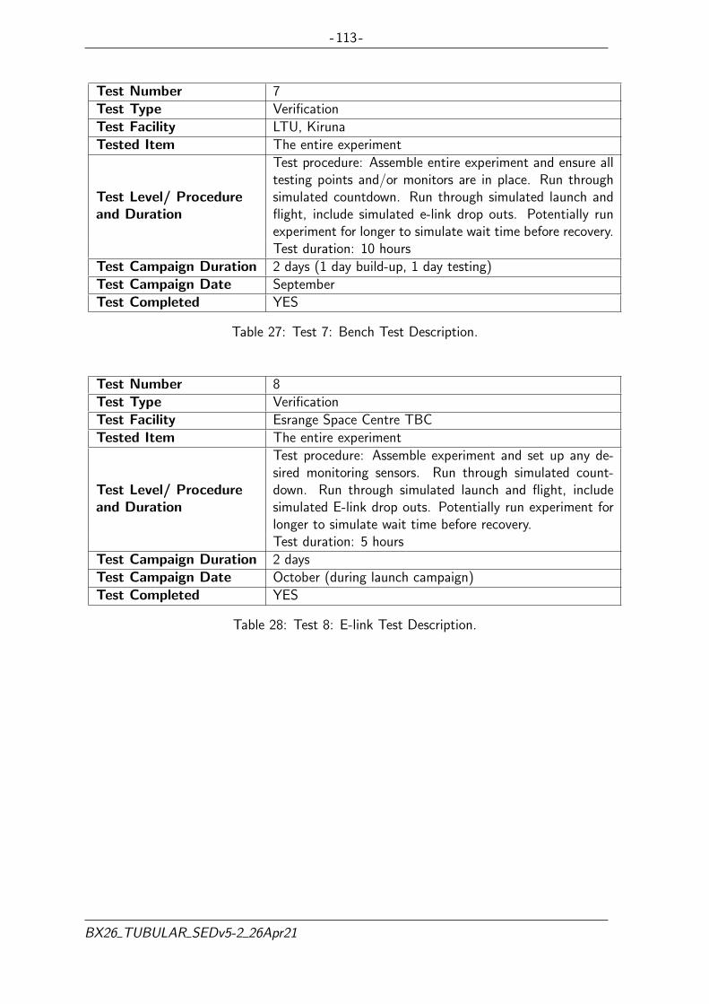
- 113 -
Test Number 7Test Type VerificationTest Facility LTU, KirunaTested Item The entire experiment
Test Level/ Procedureand Duration
Test procedure: Assemble entire experiment and ensure alltesting points and/or monitors are in place. Run throughsimulated countdown. Run through simulated launch andflight, include simulated e-link drop outs. Potentially runexperiment for longer to simulate wait time before recovery.Test duration: 10 hours
Test Campaign Duration 2 days (1 day build-up, 1 day testing)Test Campaign Date SeptemberTest Completed YES
Table 27: Test 7: Bench Test Description.
Test Number 8Test Type VerificationTest Facility Esrange Space Centre TBCTested Item The entire experiment
Test Level/ Procedureand Duration
Test procedure: Assemble experiment and set up any de-sired monitoring sensors. Run through simulated count-down. Run through simulated launch and flight, includesimulated E-link drop outs. Potentially run experiment forlonger to simulate wait time before recovery.Test duration: 5 hours
Test Campaign Duration 2 daysTest Campaign Date October (during launch campaign)Test Completed YES
Table 28: Test 8: E-link Test Description.
BX26 TUBULAR SEDv5-2 26Apr21

- 114 -
Test Number 9Test Type VibrationTest Facility IRF/LTU, KirunaTested Item Entire experiment
Test Level/ Procedureand Duration
Test procedure: Mount the experiment on the back of acar/trailer in the same way it will be mounted on the gon-dola and drive over a bumpy or rough terrain. Afterwards,check the experiment for functionality and structural in-tegrity.Test duration: 2 hours
Test Campaign Duration 1 weekTest Campaign Date 3rd - 7th SeptemberTest Completed YES
Table 29: Test 9: Vibration Test Description.
Test Number 10Test Type Software and ElectronicsTest Facility LTU, KirunaTested Item Electronics and sampling systems
Test Level/ Procedureand Duration
Test procedure: First ensure communication betweenground station and OBC work. Ensure software and elec-tronics responds well to all possible commands for all phasesof the flight. Check the electronic currents, voltages at thedifferent stages. Ensure experiment can be shut down man-ually. Perform simulated flight using previous BEXUS flightdata.Test duration: 10 hours
Test Campaign Duration 2 days (1 day build up, 1 day test)Test Campaign Date AugustTest Completed YES
Table 30: Test 10: Software and Electronics Operation Test Description.
BX26 TUBULAR SEDv5-2 26Apr21

- 115 -
Test Number 12Test Type VerificationTest Facility LTU, KirunaTested Item Entire experiment
Test Level/ Procedureand Duration
Test procedure: Mount the experiment as it would bemounted in the gondola. Using only the instructions thatwill be given to the recovery team a volunteer from outsideof the team will remove the CAC box. A timer will be run tocheck how long it takes, this time should not exceed threeminutes. The procedure should be simple and fast and theinstructions clear.Test duration: 5 minutes
Test Campaign Duration 1 hourTest Campaign Date SeptemberTest Completed YES
Table 31: Test 12: Experiment Removal Test Description.
Test Number 14Test Type SoftwareTest Facility LTU, KirunaTested Item Ardunio, ground station
Test Level/ Procedureand Duration
Test procedure: Ensure ground station can reprogram someparameters on OBC. Perform parameter changes.Test duration: 15 minutes
Test Campaign Duration 1 dayTest Campaign Date 25th AugustTest Completed YES
Table 32: Test 14: Ground Station-OBC Parameters Reprogram Test Description.
BX26 TUBULAR SEDv5-2 26Apr21
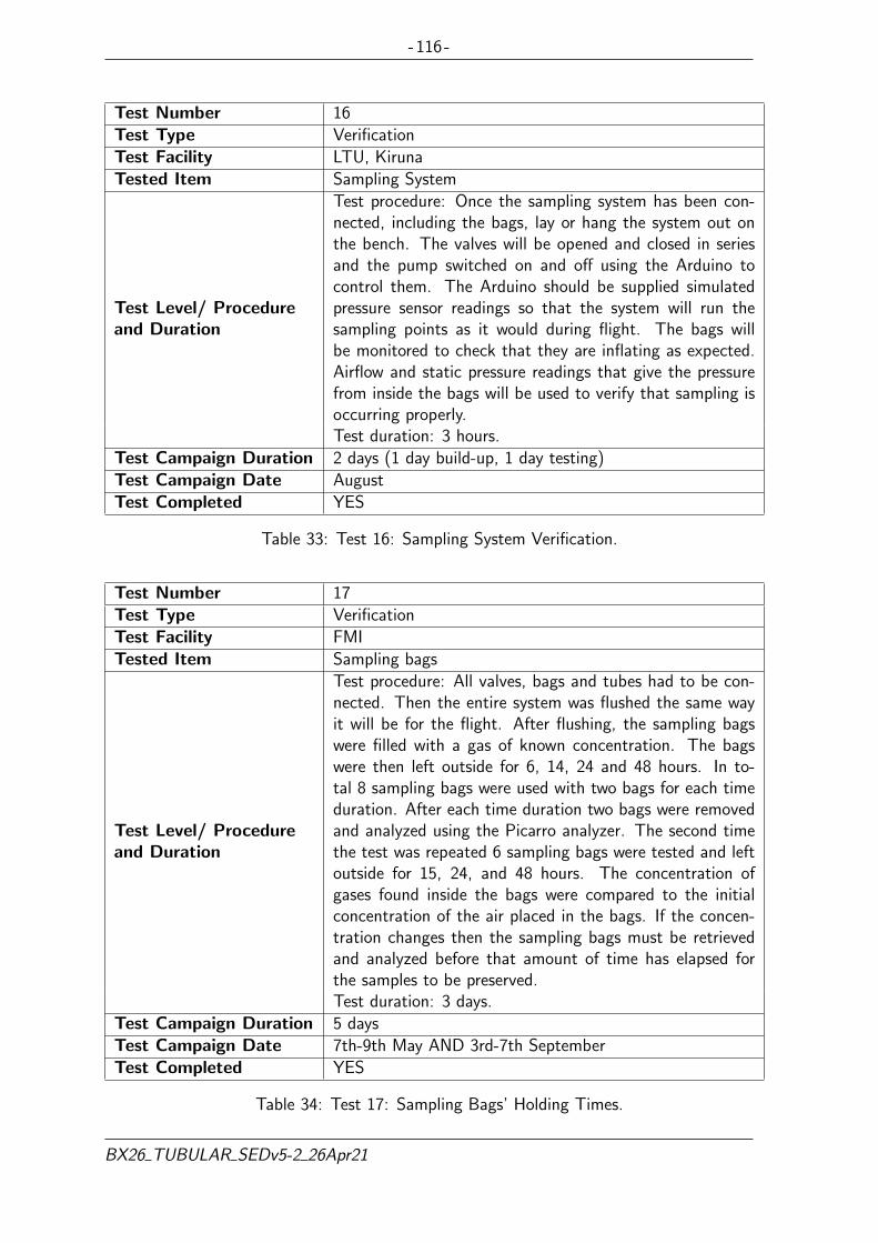
- 116 -
Test Number 16Test Type VerificationTest Facility LTU, KirunaTested Item Sampling System
Test Level/ Procedureand Duration
Test procedure: Once the sampling system has been con-nected, including the bags, lay or hang the system out onthe bench. The valves will be opened and closed in seriesand the pump switched on and off using the Arduino tocontrol them. The Arduino should be supplied simulatedpressure sensor readings so that the system will run thesampling points as it would during flight. The bags willbe monitored to check that they are inflating as expected.Airflow and static pressure readings that give the pressurefrom inside the bags will be used to verify that sampling isoccurring properly.Test duration: 3 hours.
Test Campaign Duration 2 days (1 day build-up, 1 day testing)Test Campaign Date AugustTest Completed YES
Table 33: Test 16: Sampling System Verification.
Test Number 17Test Type VerificationTest Facility FMITested Item Sampling bags
Test Level/ Procedureand Duration
Test procedure: All valves, bags and tubes had to be con-nected. Then the entire system was flushed the same wayit will be for the flight. After flushing, the sampling bagswere filled with a gas of known concentration. The bagswere then left outside for 6, 14, 24 and 48 hours. In to-tal 8 sampling bags were used with two bags for each timeduration. After each time duration two bags were removedand analyzed using the Picarro analyzer. The second timethe test was repeated 6 sampling bags were tested and leftoutside for 15, 24, and 48 hours. The concentration ofgases found inside the bags were compared to the initialconcentration of the air placed in the bags. If the concen-tration changes then the sampling bags must be retrievedand analyzed before that amount of time has elapsed forthe samples to be preserved.Test duration: 3 days.
Test Campaign Duration 5 daysTest Campaign Date 7th-9th May AND 3rd-7th SeptemberTest Completed YES
Table 34: Test 17: Sampling Bags’ Holding Times.
BX26 TUBULAR SEDv5-2 26Apr21

- 117 -
Test Number 18Test Type VacuumTest Facility IRF, KirunaTested Item Pump
Test Level/ Procedureand Duration
Test procedure: Pump shall be placed in a low pressuretesting chamber and a bag with a known volume attached toits output. The pump shall then be run at several differentpressures that will be encountered during flight. The timetaken to fill the bag will be recorded and the flow rateextrapolated.Test duration: 1 day
Test Campaign Duration 2 days (1 day build-up, 1 day testing)Test Campaign Date 1st - 2nd MayTest Completed YES
Table 35: Test 18: Pump Low Pressure Test.
Test Number 19Test Type ElectronicsTest Facility LTU, KirunaTested Item Electronics PCB
Test Level/ Procedureand Duration
Test procedure: As PCB board is soldered check using amultimeter for shorts. Check that the circuit operates as in-tended by checking the voltages and currents at test pointsusing a multimeter.Test duration: 1 hour
Test Campaign Duration RecurrentTest Campaign Date JulyTest Completed YES
Table 36: Test 19: PCB Board Operations Check.
BX26 TUBULAR SEDv5-2 26Apr21

- 118 -
Test Number 20Test Type ElectronicsTest Facility LTU, KirunaTested Item Valves, Arduino, Switching Circuit
Test Level/ Procedureand Duration
Test procedure: Beginning on a bread board the switch-ing circuit will be set up connecting one end to a 3.3 Vsupply and another to a 24 V supply. It will be checkedthat turning the 3.3 V supply on and off also turns thevalve/heater/pump on and off. The current draws duringswitching will also be monitored to check that they are inline with what the DC-DC/gondola power that can be pro-vided. Once the circuit is working in this configuration the3.3V supply will be switched for the Arduino and the 24 Vsupply to the DC-DC and the test repeated. When the cir-cuit is working on bread board it can then be soldered ontothe PCB. As it is soldered onto the PCB each switch shouldbe checked. Finally once all switches are soldered onto thePCB a check should be made on the whole switching systemthat it turns on and off all components on command.Test duration: Recurrent
Test Campaign Duration 2 monthsTest Campaign Date July and AugustTest Completed YES
Table 37: Test 20: Switching Circuit Testing and Verification.
BX26 TUBULAR SEDv5-2 26Apr21

- 119 -
Test Number 24Test Type Verification and integrationTest Facility LTU, KirunaTested Item All electronics, ground station and Arduino
Test Level/ Procedureand Duration
Test procedure: Once the electronics is at minimum in abreadboard state it will be tested with the software. Thiswill begin with sensor checks. The Arduino will be con-nected to the sensors and performance checked. Oncethe switching circuits have been completed for the valves,pump, and heaters the software which controls how thesecomponents turn on and off will be tested. If any of theresponses from the electronics are not what was expectedfrom the input from the software then the electronic con-nections will be checked and the software refined and thetest will repeat. These tests will begin on bread board elec-tronics and continue as the electronics are fixed into theirfinal positions. In addition as the software will continue tobe developed until 15th September these tests will repeatto ensure that performance continues to be as expected.Test duration: Recurrent
Test Campaign Duration Until 15th SeptemberTest Campaign Date RecurrentTest Completed YES
Table 38: Test 24: Software and Electronics Integration Testing.
Test Number 25Test Type VerificationTest Facility LTU, KirunaTested Item Mechanical box structure
Test Level/ Procedureand Duration
Test procedure: The mechanical structure will be testedunder different loads to ensure it can withstand the expectedstresses and strains during flight regarding different g-loads.This test will consist in a non-destructive static stress testwith progressive loads located at the top of the CAC andAAC boxes.Test duration: 2 days
Test Campaign Duration 1 weeksTest Campaign Date AugustTest Completed YES
Table 39: Test 25: Structural Test.
BX26 TUBULAR SEDv5-2 26Apr21

- 120 -
Test Number 27Test Type MechanicalTest Facility LTU, KirunaTested Item Mechanical interfaces
Test Level/ Procedureand Duration
Test procedure: The mechanical interfaces will be testedunder different loads to ensure they can withstand the ex-pected stresses and strains during flight. This is done bydropping the whole box from a certain height with a mat-tress or soft surface underneath it. Maximum height 1 m.Test duration: 2 hours
Test Campaign Duration 1 dayTest Campaign Date 20th SeptemberTest Completed YES
Table 40: Test 27: Shock Test.
Test Number 28Test Type ElectricalTest Facility LTU, KirunaTested Item Pump
Test Level/ Procedureand Duration
Test procedure: The pump will be tested to check its cur-rent draw under normal, turn on, entrance covered and exitcovered conditions.Test duration: 1 hour
Test Campaign Duration 1 dayTest Campaign Date 24th AprilTest Completed YES
Table 41: Test 28: Pump Operation Test.
Test Number 29Test Type ElectricalTest Facility IRF, KirunaTested Item Pump
Test Level/ Procedureand Duration
Test procedure: The pump will be tested to check its cur-rent draw as the outside air pressure is changed.Test duration: 2 hours
Test Campaign Duration 1 dayTest Campaign Date 4th MayTest Completed YES
Table 42: Test 29: Pump Current in Low Pressure Test.
BX26 TUBULAR SEDv5-2 26Apr21
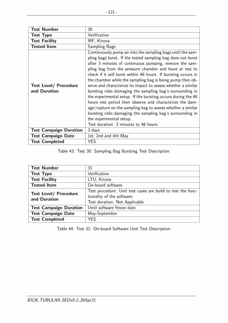
- 121 -
Test Number 30Test Type VerificationTest Facility IRF, KirunaTested Item Sampling Bags
Test Level/ Procedureand Duration
Continuously pump air into the sampling bags until the sam-pling bags burst. If the tested sampling bag does not burstafter 3 minutes of continuous pumping, remove the sam-pling bag from the pressure chamber and leave at rest tocheck if it will burst within 48 hours. If bursting occurs inthe chamber while the sampling bag is being pump then ob-serve and characterize its impact to assess whether a similarbursting risks damaging the sampling bag’s surrounding inthe experimental setup. If the bursting occurs during the 48hours rest period then observe and characterize the dam-age/rupture on the sampling bag to assess whether a similarbursting risks damaging the sampling bag’s surrounding inthe experimental setup.Test duration: 3 minutes to 48 hours.
Test Campaign Duration 3 daysTest Campaign Date 1st, 2nd and 4th MayTest Completed YES
Table 43: Test 30: Sampling Bag Bursting Test Description.
Test Number 31Test Type VerificationTest Facility LTU, KirunaTested Item On-board software
Test Level/ Procedureand Duration
Test procedure: Unit test cases are build to test the func-tionality of the software.Test duration: Not Applicable.
Test Campaign Duration Until software freeze date.Test Campaign Date May-SeptemberTest Completed YES
Table 44: Test 31: On-board Software Unit Test Description.
BX26 TUBULAR SEDv5-2 26Apr21

- 122 -
Test Number 32Test Type SoftwareTest Facility LTU, KirunaTested Item On-board software and Arduino
Test Level/ Procedureand Duration
Test procedure: Test failure possibilities in the software.Micro-controller re-sets during auto-mode. Communicationloss at inconvenient moments such as when changing mode,when sending a command, when receiving data whilst sam-pling. Simulate loss of SD card during flight.Test duration: 1 hour
Test Campaign Duration RecurrentTest Campaign Date July and AugustTest Completed YES
Table 45: Test 32: Software Failure Test
Test Number 33Test Type ElectricalTest Facility LTU, KirunaTested Item Electrical Components
Test Level/ Procedureand Duration
Test procedure: Connect components on breadboard as partof the schematic and test them partwise. Check the resis-tances requiredTest duration: 3 hour
Test Campaign Duration 2 weeksTest Campaign Date 21st-22nd July and 4th-5th AugustTest Completed YES
Table 46: Test 33: Electrical Component Testing.
BX26 TUBULAR SEDv5-2 26Apr21

- 123 -
5.3 Test Results
The results shown here provide the key information obtained from testing. A full report foreach test can be found in Appendix O.
5.3.1 Test 28: Pump Operations
It was found that when the power supply was switched on the current went up to 600 mAfor less than one second. It then settled to 250 mA. By covering the air intake, simulatingair intake from a lower pressure, the current drops to 200 mA. By covering the air output,simulating pushing air into a higher pressure, the current rises to 400 mA.
Therefore the power for each of these conditions was 14.4 W at turn on, 6 W in normal use,4.8 W when sucking from low pressure, 9.6 W when pushing to high pressure.
5.3.2 Test 18: Pump Low Pressure
The pump was tested at low pressure using a small vacuum chamber down to 10 hPa. Flowrates were recorded from 75 hPa, the expected highest sampling altitude.
The results can also be seen in Table 47 and Figure 47.
Sampling Altitudes Ambient Pressure Actual Flow rate
Ascent Phase18 km 75.0 hPa ∼3.78 L/min21 km 46.8 hPa ∼3.36 L/min
Descent Phase
17.5 km 81.2 hPa ∼3.77 L/min16 km 102.9 hPa ∼3.99 L/min14 km 141.0 hPa ∼4.18 L/min12 km 193.3 hPa ∼4.71 L/min
Table 47: Sampling Altitudes as well as the Corresponding Ambient Pressures According tothe 1976 US Standard Atmosphere and the Normal Flow Rates at Each Altitude.
BX26 TUBULAR SEDv5-2 26Apr21

- 124 -
Figure 47: Obtained Pump Performance at Low Pressure.
5.3.3 Test 30: Sampling Bag Bursting
A sampling bag was placed in a small vacuum chamber connected to the pump and the pumpwas run for 3 minutes with a full bag to see how the bag reacted.
It was found that there are two potential failure modes. The first is a slow leakage caused bydamage to the bag seal and the second is a rapid failure of the bag seal leading to total lossof the sample.
It was concluded that, as long as the bags are well secured to the valves at the bottom andthrough the metal ring at the top, bag bursting during flight would not cause damage to anyother components on board. Even during the more energetic burst that occurs from continuouspumping the bag remained fixed to the valve connection and experienced no fragmentation.The consequences of a single bag burst would be limited to loss of data and a disturbance toaudio frequencies.
BX26 TUBULAR SEDv5-2 26Apr21

- 125 -
5.3.4 Test 29: Pump Current under Low Pressure
In general it was found that decreasing the pressure, or increasing the altitude, lead to adecrease in pump current draw. The full results can be seen in Table 79.
Altitude (km) Pressure (hPa)Into Bag Current(mA)
Into Seal Current(mA)
20 57 140 13818 68 150 14116 100 161 14612 190 185 1759 300 - 2006 500 - 2420 1013 - 218
Table 48: Table Showing How the Current Draw of the Pump Changed With Outside AirPressure for Two Different Conditions. The First Pumping Into a Sampling Bag and theSecond Pumping Into a Sealed Tube.
From the table it can be seen that the current draw is higher during the bag filling than duringthe sealed case. As the experiment will sample between 11 km and 24 km it can be concludedthat the highest current draw will occur during the 11 km altitude sample and can be expectedto be around 200 mA.
5.3.5 Test 17: Sampling bags’ holding times and samples’
The main objective of this test was to flush eight 1 L sampling bags with nitrogen, the sameway it will be done for the flight. After the flushing was done, filled them with a dry gas andplaced them outside for 6, 14, 24 and 48 hours. Then analyzed two sampling bags after eachtime duration and saw if the concentration of gases inside has changed.
The test was done twice as the first test did not give conclusive results.
The general outcome of this test the first time was that the team realized that the flushingof the sampling bags is a very delicate process. This test was also useful to decide that theflushing of the sampling bags should be done with dry gas instead of nitrogen in order tominimize the effects of the nitrogen diluting in the samples.
This test had to and was repeated, using the set-up described in Section 4, with some dif-ferences. This time 3L bags were flushed with dry gas and left outside for 15, 24, 48 hours.After the flushing was done, two bags for each time were filled with 0.5 L and 1L of dry gasand left outside. Then they were analyzed and checked if the sample concentrations were thesame or close enough with the reference values of the filled dry gas.
The obtained results are shown in Figure 168. The blue points represent the sampling bags withthe 0.5L sample, while the red points show the sampling bags with the 1L sample. SamplingBag No1 with the sampling bag No4 were analyzed after 15 hours. The pair of sampling bags
BX26 TUBULAR SEDv5-2 26Apr21
- 126 -
No2 and No5 were analyzed after 24 hours and the last pair of sampling bags, No4 and No6after 48 hours.
Figure 48: Obtained Variation in Concentration for (a) CO2 in ppm, (b) CO in ppb, (c) CH4
in ppb and (d) H2O in %.
The results were very good in general with the CO2 concentration differences not higher than2 ppm. The bags with the 0.5L sample gave bigger CO2 concentration differences and higherhumidity for all the tested times. For the bags that analyzed after 48 hours, the humiditywas two times higher for the 0.5L sample compared to the 1L sample. If water goes throughthe walls of the bags at the same rate for both bags then it is normal that sampling bagswith larger amounts of sampled air have lower humidity concentrations. Therefore, for betterresults, the air left in the sampling bags at sea level pressure must be the maximum possible.
Efficiency of the flushing procedure.
While testing the holding times of the sampling bags, some other relevant tests were per-formed. A sampling bag was flushed the way it will be flushed before flight, and then analyzedimmediately. The Picarro readings were very close with the reference values, which meansthat the flushing procedure is sufficient. From the results obtained when flushing in May, itwas also decided to use dry gas for flushing and not nitrogen which has now been confirmedto work better.
The humidity levels inside the AAC system were also tested and found to be acceptable.
BX26 TUBULAR SEDv5-2 26Apr21

- 127 -
Flushing over night.
In addition to the tests performed for the holding times, it was also tested if flushing a samplingbag the night before and sampling it the next day was affecting the samples. A sampling bagwas flushed following the same procedure as before and left sealed over night. The next day itwas sampled and left outside for almost four hours. Then it was analyzed and the results werecompared with a sampling bag that was being flushed and then immediately sampled. Theresults were good enough with CO2 concentrations being higher in the sampling bag whichwas flushed the night before. A reasonable result since the CO2 concentration inside a roomis higher than outside. Therefore, the team has decided that the flushing of the bags shall bedone as late as possible moment before the flight.
5.3.6 Test 4: Low Pressure
Styrofoam
The same vacuum chamber was used as in Tests 18 and 29. The Styrofoam was measuredon each side before it was placed in the chamber. It was then taken down to 5 hPa and heldthere for 75 minutes. It was then removed and the sides were measured again. It was foundthat there was no significant change in dimensions. The results can be seen in Table 49.
Side Before (cm) After (cm)A 9.610 9.580B 9.555 9.550C 9.560 9.565D 9.615 9.610E 9.615 9.615F 9.555 9.550G 9.605 9.605H 5.020 5.020I 5.025 5.025J 5.015 5.015K 5.020 5.025
Table 49: Styrofoam Size Before and After Vacuum.
Airflow
After the first airflow in vacuum test failed due to datalogging errors the airflow test wasrepeated. In this repeated test all of the Brain was placed into the vacuum chamber and onebag attached. It was not possible to attach more than one bag due to space restrictions.
The flow rate seemed to be too low for the rate the bag was inflating in the chamber. It wasconcluded that the airflow rate displayed is the equivalent airflow at sea level.
Software
With the same set-up as the airflow low pressure testing the software was tested to verify if itwas operating as intended and that the conditions for stopping sampling were working.
BX26 TUBULAR SEDv5-2 26Apr21

- 128 -
The software was found to be operating as intended and the stoppers were working.
Temperatures
As it is not possible to complete a thermal vacuum test in addition to the thermal testingtemperatures were also monitored inside the vacuum chamber.
The temperature of the CAC flushing valve, pressure sensor, PCB, Pump and Manifold wasalso monitored with continuous use. After one hour and 48 minutes during the same test asthe valve temperature the CAC flushing valve was found to reach 68°C and the pressure sensorwas found to reach 39°C. After one hour and 24 minutes during the flow rate monitoring testwhere the sensors, pump, and one manifold valve were on continuously the PCB temperaturesensor was at 43°C, the pump at 42°C and the manifold at 33°C. As the pump will never beon for more than a few minutes at a time there is not any concern that this temperature willever be reached during flight.
5.3.7 Test 20: Switching Circuit Testing and Verification
The switching circuit has been continuously tested from breadboard to PCB and verified towork at each different step. All valves, heaters and pump can be controlled both manuallyand automatically by the Arduino. For further details on this test see Appendix O.5.
5.3.8 Test 32: Software Failure
it was found that losing the SD card does not interrupt ground station data, it just means nodata will be written to the SD card. However, if you reconnect the SD after removing it willnot connect back to the SD card and it as if the SD card has been permanently lost.
The second failure test is how the software handles unexpected reset. The most concerningproblem is which bag that will be sampled after the reset. It has been tested that the softwarecould read the current sampling status from SD card and continue where it left off.
5.3.9 Test 31: Unit Test
Unit test was used to test several software non-hardware dependent functionality e.g. translat-ing telecommand, storing measurements data to buffer. The functions were tested for severalexpected cases and a few bugs were discovered and fixed.
5.3.10 Test 10: Software and Electronics Operation
OBS transmits data to ground station continuously. If connection is lost and later re-establishedthe ground station will continue to receive data from the onboard computer. To send atelecommand after a drop in connection requires a restart to the TCP connection.
BX26 TUBULAR SEDv5-2 26Apr21

- 129 -
5.3.11 Test 14: Ground Station-OBC Parameters Reprogram Test
After the scheduler, a command to change the sampling parameters, is implemented, thescheduler was tested and can change the sampling schedule from ascent to descent. Theprevious parameters were 56.8 and 36.8. They were successfully changed to 30 and 70.However, the user needs to be careful and has to do the correct calculation for the newparameters.
5.3.12 Test 24: Software and Electronics Integration
The different type of sensors were integrated one at time with the Arduino. The result was allthe sensors working without interfering with each other.
5.3.13 Test 5: Thermal Test
A AAC test box out of Styrofoam were put into a freezer at Esrange. Only the bag area werereduced in order to fit. The test were on for 4h and 40min. For 3h 30min the temperature were−50°C. During that span it were tested if the heating system worked between the thresholds,flush, sample and try run the pump and let it fall bellow zero while operating. From Figure 49it can be seen that the pump (pink) and the valve (black) is heating and in their thresholds.It were concluded that everything worked as it should. After 3h 30min the freezer were slowlyput to go down to −60°C to try the experiments heating system more.
Figure 49: Thermal Chamber Test.
5.3.14 Test 27: Shock test
The entire pneumatic system and electrical system was mounted in the AAC box along withthe walls and Styrofoam attached. It was then dropped from a height of approximately one
BX26 TUBULAR SEDv5-2 26Apr21

- 130 -
meter three times. Nothing came loose or was damaged after this drop test. All electronicswere verified to still work.
5.3.15 Test 9: Vibration test
The entire experiment was placed in the tailgate of a car, while the test was carried out ona 18 km long rough terrain. An emergency brake was also implemented during the test. Theexperiment’s functionality and structural integrity were capable of handling the vibrations andthe stopping force. No damages or issues were detected after this test.
5.3.16 Test 25: Structure test
A team member was placed on top of each box’s structure. Both the CAC and AAC box wasable to fully support the member’s weight without showing any instability or deflections. Nodamages or issues were detected after this test.
5.3.17 Test 33: Electrical Component Testing
The components were tested separately, one by one to double check and determine their powerconsumption and their functionality. Some tests were also run to determine specific resistanceson voltage bridges and pull down resistors for LEDs running at different voltages. These testsgave further insight to the PCB design and the power design. The test results were accordingto expectations and the design and assembly could continue as planned. There were also sometest run for the PCB, which showed that some connections were not done in the way thatwas planned due to design issues. Theses were solved by adding wires to the PCB instead ofredesigning the PCB and order a new one due to time and budget limitations. For furtherdetails on these tests see Section O.5.
5.3.18 Test 12: Removal test
For a non team member to perform the removal of the CAC box based on the given instructions,it took that person 6 min and 25 sec. This time is expected to be lower for the recovery teamas the items to be unscrewed were not yet clearly marked. One problem that occurred duringthis test was that the person had problems to distinguishing the CAC from the AAC box. Toresolve this the boxes now have clear labels on them.
5.3.19 Test 2: Data collection test
The full software was run in auto mode to check everything operated as expected over a fulltest flight. At the end of the simulated flight the experiment was to shutdown automatically.This was tested both on the bench and in the vacuum chamber. In the vacuum chamber tests,see Section 5.3.6, the bench test, see Appendix O.5.8 and the thermal test, see Appendix O.4.3data collection was also monitored. It was found that the physical samples were being collectedproperly and all the sensors were returning expected data.
BX26 TUBULAR SEDv5-2 26Apr21
- 131 -
5.3.20 Test 7: Bench test
The experiment was run for 5 hours simulating 1 hour on ground, 1.5 hours in ascent, 2 hoursin float and 0.5 hours in descent. The experiment was found to be operating as intended atall points. Additionally the temperature sensors have been tested at ambient conditions forover 6 hours and the pressure sensors for over 8 hours. No problems were found with thetemperature sensors or pressure sensors on the bench.
5.3.21 Test 16: Sampling test
The system was tested while already mounted as this test was pushed back due to the latearrival of the static pressure sensor.
The Arduino successfully controlled all valves and the pump and through the static pressureand airflow sensor readings alone it could be confirmed if a bag was sampling.
BX26 TUBULAR SEDv5-2 26Apr21

- 132 -
6 Launch Campaign Preparations
6.1 Input for the Campaign / Flight Requirements Plans
The TUBULAR experiment consisted of two boxes with one air sampling system inside eachof them. It was positioned with at least one side exposed to the outside.
6.1.1 Dimensions and Mass
The data shown in Table 50 below was based on the design presented in Section 4.4.
CAC AAC TOTALExperiment mass [kg] 11.95 12.21 24.16
Experiment dimensions [m] 0.23 x 0.5 x 0.5 0.5 x 0.5 x 0.4 0.73 x 0.5 x 0.5Experiment footprint area [m2] 0.115 0.25 0.365
Experiment volume [m3] 0.0575 0.1 0.1575
Experiment COG positionX = 23.51 cmY = 10 cmZ = 22.57 cm
X = 29.04 cmY = 16.63 cmZ = 16.2 cm
X = 26.31 cmY = 24.99 cmZ = 19.35 cm
Table 50: Experiment Summary Table.
6.1.2 Safety Risks
Table 51 contains the risks of all stages of the whole campaign and project.
Risk Key Characteristics MitigationFlammablesubstances
Styrofoam Brand Foam is oil basedand is highly flammable11
Extensive testing will be performed tomake sure there is no heat/fire source
Sharp orcuttingedges
Edges along the experimentFile down edges and cover them withtape
Chemicalsubstances
Chemicals could be exposed after ahard landing
Magnesium Perchlorate filter mecha-nism is sealed and has been used be-fore without any problem. In case ofexposure after a hard impact, use pro-tective goggles and gloves to avoidcontact with the eyes and skin. Thesmall quantities used for the experi-ment will not be a threat for the en-vironment. Magnesium Perchloratealone is not flammable but may causeor intensify fire in case of contact withcombustible material. Therefore, thefilter is made of stainless steel, whichhas high durability.
11Styrofoam has been found to only pose a flammable hazard when heated to at least 346°C.[2]
BX26 TUBULAR SEDv5-2 26Apr21
- 133 -
PressureVessels
Compressed fluid containers canpose a risk of exploding if damaged
Pressurised gas will be used to flushthe system before flight and to cali-brate the sensors before analysing oursamples after landing. NO pressurisedvessels will fly. Three gas cylinderswill be brought to Esrange by FMI.The cylinders will contain compresseddry air:Flush gas for the bag sampler: 20L at140 barCalibration gas for Picarro: 14L at130 barFlush/fill gas for AirCore: 26.8L at110 bar (there will be 13 ppm CO inthe cylinder)
Table 51: Experiment Safety Risks.
6.1.3 Electrical Interfaces
Please refer to Table 52 for details on the electrical interfaces with the gondola.
BEXUS Electrical InterfacesE-link Interface: Yes
Number of E-link interfaces 1Data rate - Downlink 1.58 kbps
Data rate - Uplink 1.08 kbpsInterface type (RS232, Ethernet) Ethernet
Power system: Gondola power required? YesPeak power (or current) consumption: 38 W
Average power (or current consumption) 24 WPower system: Experiment includes batteries? No
Table 52: Electrical Interface Table.
6.1.4 Launch Site Requirements
The experiment needed some preparations before the flight. For that reason, the team neededa room with a big table to place the Picarro analyzer, with some extra space for all theinterfaces between the analyzer and the CAC system, as well as the AAC system. A laptopPC was used to monitor the experiment. Therefore, a desk and a chair were needed for thisstation. A total of 16 chairs need to be rented: 13 chairs for all members of the TUBULARTeam and an additional three for visiting collaborators from FMI. One power outlet and oneEthernet cable for E-link connection were also essential for the laptop PC.
BX26 TUBULAR SEDv5-2 26Apr21
- 134 -
6.1.5 Flight Requirements
Floating altitude was desired to be as high as possible in order to sample air from the strato-sphere both in ascent and Decent Phase. The duration of the Float Phase was not relevantfor the experiment performance.
No conditions for visibility were required for this experiment.
With respect to a swift recovery and transport for fast data analysis, a launch time in the earlymorning hours was favorable.
BX26 TUBULAR SEDv5-2 26Apr21

- 135 -
6.1.6 Accommodation Requirements
The experiment involved two rectangular boxes inside the gondola environment. The onlyrequirement was to allocate the box with at least one face exposed to the outside. The latteralso facilitated the fast experiment recovery for the later analysis of the collected samples. Thedesign allowed full adaptability regarding the interface with the gondola’s rails, for more detailssee Section 4.4. The current location of the experiment in Figure 50 is the one arranged withREXUS/BEXUS Coordinators during the Training Week in Esrange.
Figure 50: Example of Experiment Box Accommodation Inside the Gondola.
BX26 TUBULAR SEDv5-2 26Apr21

- 136 -
6.2 Preparation and Test Activities at Esrange
The ground station laptop PC was put in place and set up so it was operational. The com-munication through E-link with the experiment was tested. The air sampling schedule on theSD card was checked before flight.
In the preparation phase magnesium filters were prepared. These were short (7 cm) lengthsof stainless steel tubing that were filled with 2 mg of fresh magnesium perchlorate powder[6]. One was attached to the inlet of the CAC tubing, to ensure that no moisture entered thetubing during testing or sampling. The magnesium perchlorate powder was loosely packed tomake sure that the air flow was not blocked. Stone wool was placed at both ends of the tubeto prevent the powder escaping from the filter.
The same set-up was used for the AAC. As stratospheric air is dry the risk of moisture enteringthe system during sampling was very low, however, the team decided to use one to reduce therisk of condensation in the samples after landing.
A few days before the flight while in Finland, the CAC was left inside an oven at 110 °C for 5hours. At the same time, nitrogen was running through the CAC at a flow rate of 110 ml/min.This was necessary, in order to remove humidity sufficiently through evaporation. Due to thehigh temperature of the oven and having nitrogen running through the system, it was madesure to remove the humidity from the coil.
Two days before the flight, the CAC went through some preparations. At 19:44 on Sunday14 of October, the flushing of the coiled tube with fill gas started. A fill gas is air with aspike of a known gas, for example CO. During the flushing process the coiled tube, solenoidvalve, the exit tube as well as the magnesium perchlorate filter were flushed separately. In theflushing process the quick connectors at outlet and inlet were connected to the fill gas bottleand Picarro analyzer respectively. The fill gas with a flow rate of 2 L/min was then flownthrough the coiled tube all the way to the Picarro for 10 minutes. Then, it was left flushingover night at a flow rate of 40.8 ml/min to ensure unknown gases inside the tube would beremoved.
After approximately 11 hours, the flushing of the CAC was over at 07:03 on Monday 15 ofOctober. When the flushing procedure was over, Picarro was disconnected while the fill gasremained connected in order to over-pressure the CAC. This ensured that when the otherparts were connected ambient air would not enter the system, as the fill gas would be exiting.Leaving the CAC over-pressured also ensured that if the quick connectors were leaking it wouldbe fill gas leaking our and not ambient air leaking in. This was important as there were twodays in between flushing and flight. Meanwhile on other hand the solenoid valve and the exittube were flushed manually for approximately 5 minutes at a flow rate of 2L/min. As a laststep, the outlet and inlet were sealed while the gas was still running through the CAC andtherefore the CAC was filled and over-pressured. Thereafter it was attached to the remainingcomponents such as the magnesium perchlorate filter, solenoid valve and exit tube. At thisstage the CAC was ready for the flight.
A pre-launch checklist in Appendix D.1, was made to assure that the flight preparations willbe done thoroughly. This includes a step by step flushing procedure.
For the AAC system, the manifold was cleaned by flushing it with a dry gas as soon as all thepre-flight testing was done. The dry gas is extracted from the fill gas and has slightly different
BX26 TUBULAR SEDv5-2 26Apr21

- 137 -
concentrations from the fill gas. The dry gas bottle, the vacuum pump and the AAC system,were all connected as a system to the central valve. The pump and the valves of the AACsystem were cleaned by this procedure. The night of the flight, Tuesday 16 of October at23:00, the flushing of the AAC started. The plugs from the inlet and outlet tubes of the AACwere unscrewed and a male thread quick connector was screwed in to the inlet tube. The drygas, vacuum pump, and central valve system were then connected to the inlet tube. Flushingstarted when the central valve was open to dry gas, and dry gas started flowing into the AACmanifold while the flushing valve was open with the rest of the valves closed. The flow ratewas at 2L/min and the flushing procedure was going on for approximately 15 minutes. Whenthe central valve was closed, and dry gas stopped flowing into the AAC, the flushing valve wasclosed. The dry gas bottle, the vacuum pump, and the central valve system were disconnectedfrom the inlet tube. The plug was screwed in to the inlet tube.
In a second phase, using the AAC valves this time, the bags and consequently the tubesbetween the bags and the manifold, were flushed, again after the pre-flight testing was done.Only one bag was flushed at a time, using the central valve, the flushing valve, and the solenoidvalve that matched the bag to control which bag was being flushed. The flushing had to bedone three times for each bag to ensure the bags were properly cleaned. It was also importantto flush the manifold again, between the flushing of each bag. The dry gas, the vacuumpump, and the central valve system were connected to the outlet tube, while the inlet tubewas sealed. Next, the bags manual valves were opened. The flushing valve was kept openduring the whole procedure. Only one solenoid valve that matched the bag which was beingflushed was opened at a time.
Flushing started when the central valve was open to dry gas, and dry gas started flowingthrough the AAC manifold, tubes, into the bag. The flow rate was set at 2 L/min. It took1.5 minutes to fill each bag with 3L of dry gas. Then, the central valve was turned open tothe vacuum allowing the bag to empty, for approximately 4.5 minutes. This procedure wasrepeated for all six bags. After the flushing of one bag was completed, the dry gas, vacuumpump, and central valve system was disconnected from the outlet tube and connected tothe inlet tube, allowing the manifold to be flushed, before flushing the next bag, as describedabove. Then the dry gas, vacuum pump, and central valve system were connected to the outlettube again, and the next bag was flushed. The whole flushing procedure took approximately3 hours. After the end of the flushing, when the bags were empty again, the flushing valvewas closed. The dry gas, vacuum pump, and central valve system was disconnected from theoutlet tube and the plug was screwed in. At this point, the AAC was ready for flight.
The pre-launch checklist in Appendix D.1 was again made sure that all the steps were donecorrectly and in the right order.
In a laboratory phase, tests under monitored conditions were done to evaluate the overallconsistency of the CAC and the AAC. In particular, the CAC and the AAC were tested forleaks at the junctions and at the valves.
Furthermore, the team decided to clean the rest of the experiment’s components, such asthe Brain, as well as the structure. Doing so, any unwanted particles released during theexperiment’s construction, was removed avoiding these particles to enter the pneumatic systemand thus contaminating the collected samples.
The system was cleaned manually with a dust cloth, using gloves and IPA, given that this
BX26 TUBULAR SEDv5-2 26Apr21

- 138 -
cleaning procedure is not of high need as the cleaning of the coil or the bags. Consideringthat the building of the experiment took place in a lab, which was a clean environment, thisaction was done once before the flight. This procedure was done just after EAR.
BX26 TUBULAR SEDv5-2 26Apr21

- 139 -
6.3 Timeline for Countdown and Flight
Table 53 was the estimated timeline during countdown and flight.
The desired altitudes in which air samples were to be collected with the sampling bags wasassociated with specific air pressure values. Thus, the valve operations to sample air duringthe balloon Ascent and Descent Phases were to be triggered by readings from the ambientpressure sensor. The time values presented in Table 53 merely served as an indicative estimateof when the sampling will take place as sampling was not programmed based on flight time.
Time Altitude EventsT-1/2DAYS 0 Start flushing the CAC system overnight for 8H
T-7H 0 Start flushing the AAC system for 3HT-3H 0 Experiment is switched on external powerT-3H 0 Experiment goes to Standby modeT-1H 0 Experiment switches to internal powerT=0 0 Lift-offT+1s ∼5 meter Experiment goes to Normal - Ascent mode
T+15 min 1 km Experiment starts to empty the CAC’s tubeT+∼1H ∼18 km Take air samples with AAC until ∼24 km
T+∼1.5H ∼25 km Float PhaseT+∼2.5H ∼25 km Cut-offT+∼2.6H ∼25 km Experiment goes to Normal - Descent modeT+∼2.75H ∼20 km Parachute is deployed
T+∼2.8H ∼19 kmTake air samples with AAC and CAC until 10 km aboveground
T+3.5H ∼10 km Experiment goes to SAFE mode (all valves are closed)
Table 53: Countdown and Flight Estimated Timeline.
Table 54 shows the actual timeline which occurred during flight. The in-flight pump startupfailure that occurred is shown together with the relevant actions taken during the in flightanalysis of what the problem might have been. The procedure of differential pressure differenceis also shown. After attempting to start the pump several times the team recognised alreadythat a likely cause of failure was related to the pump getting enough current, therefore severaldifferent procedures were attempted to start the pump. The first was attempting to turn thepump on when everything other than the Arduino was switched off. The second was heatingthe pump up until the temperature readings showed that the pump was near the top of itsoperating range and then attempting to turn it on, still with all other components except theArduino turned off. Neither of these attempts worked. A third idea was to try and start it bycreating a pressure difference during the descent, however this was not attempted as it riskedthe CAC sample. Instead during descent the valves were opened to attempt passive samplingof the bags. However due to the lack of pressure difference between the bag and the ambientpressure this had a low probability of success.
BX26 TUBULAR SEDv5-2 26Apr21

- 140 -
Time Altitude EventT-03:54 0 Go to manual mode for 6 seconds then back to standbyT-03:07 0 Restart Ground StationT-03:02 0 Groundstation Back Online and reciving dataT-00:00 0 Liftoff and automatic Accent modeT+00:31 10.1-10.3 km Pump heater on 12 minutes
T+00:58 18.8-19.1 kmFirst flushing was suposed to start, instead the Arduinoresets and resulting in CAC valve closing
T+00:58 18.8-19.1 km Enter Manual ModeT+01:01 19.7-20 km Flushing Valve opens for 20 secondsT+01:05 20.9-21.2 km CAC Valve ReopenedT+01:06 21.2-21.6 km Pump Heater is on for 6 minutesT+01:11 22.8-23.1 km Board Resets Due to attempting to start pumpT+01:12 23.1-23.5 km Pump Heater is on for 4 minutes
T+01:17 24.4-24.5 kmBoard resets due to attempt to start pump and openflushing Valve
T+01:20 24.4-24.4 kmFlush Valve and Valve 1 is turned on to check if it wouldinduce an error
T+01:21 24.4-24.5 km Float Phase Entered
T+01:32 24.5-24.5 kmChange scheduler to 1 - 2 mbar for all bags as an atemptto make sure the system would not attempt to automat-icaly sample
T+01:36 24.4-24.4 km Pump and Valve Heater onT+02:10 24.3-24.4 km Pump and Valve Heater offT+02:10 24.3-24.4 km Attempt to start Pump, fails and resets boardT+02:12 24.3-24.3 km CAC Valve opens and prepare for decentT+02:55 24.1-24.1 km Decent Phase Entered
T+03:04 14.9-14.1 kmValve 2 is opened in an attempt to fill bags with ambientpressure difference
T+03:09 11.0-10.4 km Valve 2 is closed
T+03:10 10.4-9.8 kmValve 3 is opened in an attempt to fill bags with ambientpressure difference
T+03:14 7.9-7.3 km Valve 3 i closed
T+03:15 7.3-6.7 kmValve 4 i opened in an attempt to fill bags with ambientpressure difference
T+03:16 6.7-6.2 km Valve 4 is closedT+03:16 6.7-6.2 km Accidental closing of CAC valve to earlyT+03:17 6.2-5.7 km CAC Valve accidentally reopens for 1 second.
Table 54: TUBULAR BEXUS 26 Launch Timeline
BX26 TUBULAR SEDv5-2 26Apr21

- 141 -
6.4 Post Flight Activities
6.4.1 CAC Recovery
It was important that the CAC was recovered as quickly as possible. The experiment hadbeen designed so that the recovery team could easily remove the AirCore in the CAC box fromthe gondola without having to remove the entire experiment. This was to facilitate possibletransportation back to Esrange via helicopter.
This quick recovery was important to minimize the length of time in which mixing of the gasoccured in the collected CAC sample. The sample should be analyzed within five to six hoursafter the experiment lands. At PDR it was discussed that the CAC box could be brought backto Esrange on the helicopter instead of the truck. This situation was preferable for TUBULARTeam.
The FMI team arrived at Esrange on the 12th of October with all the necessary equipment forpre-flight flushing and post-flight analysis. Having the FMI team at Esrange gave additionaltime for them to install and calibrate their lab equipment and also allowed them to proceedfaster with the analysis process as soon as the CAC was returned to Esrange.
Detailed instructions were provided on how to remove the CAC box. In addition, instructionswere provided to ensure that the system was completely shut down and the valves secured.Shutdown was automated, however, a manual shutdown mechanism was included should theautomation fail.
6.4.2 Recovery Checklist
FAST RECOVERY OF CAC
• Check no damage exists to outer structure and no white paste seen in inlet tubes, thisconfirms no leak and chemicals are SAFE.
• Screw on the three metal plugs provided to the inlet and outlet tubes.
• Unplug the gondola power cord from the AAC box. Circled with RED paint.
• Unplug the E-Link connection from the AAC box. Circled with RED paint.
• Unplug the D-Sub connector from the CAC Box. Circled with RED paint.
• Unscrew 6 screws in the outside face of the experiment. Painted in RED.
• Unscrew 6 screws in the inside face of the experiment. Painted in RED.
• Unscrew 2 gondola attachment points from the CAC
• Remove the CAC Box from the gondola. Handles located at the top of the box.
The regular recovery of the AAC and the non nominal recovery of the experiment is listed inSection D.3 of Appendix D.
BX26 TUBULAR SEDv5-2 26Apr21

- 142 -
6.4.3 Analysis Preparation
In order to efficiently remove ambient air moisture from the analyzer, a calibration gas hadto run through the Picarro analyzer, after the gondola cut-off phase until the CAC analysis.The reason this was done was because it was necessary that the readings of the calibratinggas stabilized before starting the analysis and the presence of moisture would have made thisstabilization slower. Having the analyzer running for a few hours before the CAC recovery,saved precious time as it made it possible to start the analysis as soon as the CAC wasrecovered.
BX26 TUBULAR SEDv5-2 26Apr21

- 143 -
7 Data Analysis and Results
7.1 Data Analysis Plan
7.1.1 Picarro G2401
The analyzer that was used is the model Picarro G2401. It uses near-infrared Cavity RingDown Spectroscopy (CRDS) technology and is capable of measuring four atmospheric tracegases simultaneously and continuously (CO,CO2, CH4, H2O).
The CRDS technique’s basic principle is shown in Figure 51. Light from a semiconductor diodelaser is used. There is an optical cavity filled with the gas that has to be analyzed and theaim is to determine the decay time of the diode laser light. As it can be seen in Figure 51,the sample gas is introduced in a cavity with three high-reflectivity mirrors. When the laseris shut off, the light that was circulating in the cavity decays with a characteristic time whichis measured. If the wavelength of the injected light does not match any absorption feature ofany gas in the cavity, the decay time is dominated by mirror loss and it is very long. On theother side, when the wavelength of the injected light is resonant with an absorption feature ofa species in the cavity, the decay time is short and decreases as the reciprocal of the speciesconcentration.
Figure 51: Schematics of CRDS Analyzer Showing Optical Cavity and Sample Gas Flow [19].
Figure 52 shows the back of the analyzer with gas supply, electrical and computer connections.The analyzer can be configured to deliver data in different formats: digital or analogue. Whenthe main power is turned on the analyzer automatically starts, including the Graphical UserInterface (GUI).
BX26 TUBULAR SEDv5-2 26Apr21

- 144 -
Figure 52: Back of Picarro G2401 Analyzer Showing Gas Supply, Electrical and ComputerConnections [12].
Before the Picarro analyzer was ready for analysis, it was necessary to run a calibrating gasthrough it in order to remove moisture inside and to have stable measurements to comparewith. Figure 53 shows the Picarro set up in Esrange. A three way valve controlled whichwas the gas flowing into the analyzer. The tube labelled as ”AIRCORE” was the one to beconnected to the sample, either sampling bags or CAC. The tube labelled as ”PICARRO” wasthe one that was going to the Picarro’s inlet and the third tube, without a label, was connectedto the calibrating gas bottle.This set up allowed easy changing between the samples, dry gasand fill gas with the calibrating gas without getting moisture inside.
BX26 TUBULAR SEDv5-2 26Apr21

- 145 -
Figure 53: Picarro Set-up Connections at FMI in Sodankyla.
Figure 54 shows the Picarro GUI during analysis. From top to bottom: CO2 ppm, CO ppm,CH4 ppm and cavity pressure. These options could be changed during analysis as it onlymeans that those were the ones being displayed. Figure 54 was taken minutes after a changebetween calibrating gas-sample had been done so a change in the concentrations of CO2 and
BX26 TUBULAR SEDv5-2 26Apr21

- 146 -
CH4 can be easily appreciated. The Picarro analyzer did not only give information about thedisplayed parameters, all the data was saved in a .dat file to be analyzed afterwards. Themost relevant logged parameters were time, date, ambient pressure, cavity pressure, cavitytemperature, CO concentration, CO2, CH4 and H2O normal and dry concentration.
Figure 54: Picarro Graphical User Interface. From Top to Bottom: CO2 ppm, CO ppm, CH4
ppm and Cavity Pressure.
7.1.2 Analysis Strategy
Approximately one month after the CAC analysis, the Picarro raw data files were available andthe analysis could start. Figure 55 shows some of the Picarro’s raw data.
BX26 TUBULAR SEDv5-2 26Apr21

- 147 -
Figure 55: Picarro Raw Data Showing the Concentrations of CO, CO2, and CH4 all in ppm.
For the analysis purposes, the program MATLAB was used. Several steps were required toaccurately place the Picarro measurements on a vertical scale in order to retrieve the verticalprofiles. The dry mole fractions of CO2 and CH4 provided by the Picarro were used. Thereason behind that was because they were automatically corrected by the instrument for acombined effect of dilution and line broadening caused by water vapor.
Figure 56: Picarro Analysis of the CAC sample from the BEXUS 26 flight. Left: CO2 MixingRatios as a Function of the Analysis Time in Seconds; Right: CH4 Mixing Ratios as a Functionof the Analysis Time in Seconds.
Figure 56 shows an example of CO2 and CH4 mixing ratios measured by the Picarro instrumentduring the BEXUS 26 campaign. In order to extract the measurements corresponding to thesampled air, the top and the bottom of the profiles needed to be defined. The top of theCAC sample was considered to be at midpoint of the transition in concentration between the
BX26 TUBULAR SEDv5-2 26Apr21

- 148 -
push gas and the remaining fill gas. This point is marked with a green star in Figure 56. Thebottom of the profile was defined at midpoint on the transition of concentration between pushgas and sampled air. It is marked with a red star in Figure 56.
Figure 57: CO Mixing Ratios as a Function of the Analysis Time in Seconds.
The beginning and end of the sample analysis was detected due to changes in concentrations,at the beginning between calibrating gas/sample, and at the end, between sample/fill gas.The remaining fill gas in the coil had high concentration of CO, while the stratosphere hadconsiderably lower CO concentrations. Figure 57 , was used to define the sample. Again, thetop of the profile is marked with a green star and the bottom of the profile with a red star.
It is assumed that the air entering the tube equilibrates the sample with ambient pressureand adjusts very quickly with the mean coil temperature. As the characteristics of the CAC(length, diameter) do not change, ambient pressure and mean coil temperature are the twomain factors that regulate the number of moles in the CAC. Using the ideal gas law, it ispossible to calculate the number of moles captured in the tube all along the trajectory.
PV = nRT <=> n =PV
RT(1)
where P was the ambient pressure, V was the inner volume of the CAC, n the fraction ofmoles, R was the universal gas constant in J K−1 mol−1 and T the ambient temperature inKelvin, [17]. A constant unit of pressure in the atmosphere was represented by a unit of lengthin the CAC tube, due to the method that the CAC sampled the ambient air. With measuredtime series of pressure (Pi) and temperature (Ti), it was possible to relate the number of air
BX26 TUBULAR SEDv5-2 26Apr21

- 149 -
moles in the tube (ni) to the atmospheric pressure at any given time during the flight:
ni =PiV
RTi, (2)
and this number was maximum when the CAC reached the surface,
nmax =PsV
RTs, (3)
where Ps and Ts corresponded to the surface pressure and to the temperature of the CACwhen landed at the surface.
The flow rate during the analysis was kept constant at 40.8 cm3/min, which ensured that thenumber of moles that went through the analyzer increased linearly with time. So, the numberof moles at any time during the analysis was
ni = nmax ti∆t
(4)
where ∆t was the total time duration of the analysis between the top and bottom of the CACsample.
At the next step, Equations 2, and 4 were used to associate every pressure point with everyPicarro measurement of the sample to retrieve the vertical profiles. In order to do that, it wasimportant that the data points of the sample from the Picarro, matched the data points forpressure and temperature from the ground station. This was not the case, because the Picarrodata had by far more. For that reason, the ground station data for pressure and temperaturewere interpolated to match the ones from the Picarro.
Finally, the CO, CO2, and CH4 vertical profiles were plotted against the pressure. The resultedvertical profiles as well as discussion of the results can be seen in Section 7.3.6.
The AAC sampling system was planned to be analyzed, in the same manner as the CAC, usingthe same Picarro gas analyzer. In the same way as for the CAC, the calibrating gas wouldneeded to be flowing through the analyzer until the moisture was minimum and the readingsin concentrations were stable. Then a sampling bag system would have been connected to theanalyzer and a dry gas bottle, in a similar way as it was done in Test 17. The tubes connectingthe sampling bags would have been flushed with dry gas and when the concentrations givenby the Picarro analyzer were stable, the air inside the sampling bags would go through theanalyzer followed again by dry gas.
Watching at the Picarro GUI, it was easily recognizable when a sampling bag was beinganalyzed due to the difference in concentrations between its air and the dry gas. Again, asfor the CAC, equations 1 and 4 were going to be used to relate a specific pressure point withevery Picarro measurement of the sample.
The basic working principle used by the chromatographer to obtain the concentrations was asfollows:
• Have calibrating gas - sample - calibrating gas flowing through the analyzer. (It couldalso be the case: calibrating gas - dry gas - sample - dry gas - calibrating gas but theprinciple was the same).
BX26 TUBULAR SEDv5-2 26Apr21

- 150 -
• Identify in the GUI readings the different gases easily seen by sudden variations in theconcentrations.
• Compare the calibrating gas reading with the known real value. Do this before and afterthe sample. This difference corresponds to the drift given by the Picarro.
• Interpolate the values of drift from before and after the sample to obtain the drift duringthe sample.
• Correct the readings given by the Picarro analyzer due to drift and that is the realconcentration value.
NOTE: A calibrating gas was a gas that has been flowing through the Picarro analyzer multipletimes and its concentration were known with accuracy. A calibrating gas had to flow beforeand after the samples in order to compare the readings given by the analyzer with the realvalue and obtain a corrected value for the samples.
BX26 TUBULAR SEDv5-2 26Apr21

- 151 -
7.2 Launch Campaign
7.2.1 Flight preparation activities during launch campaign
The scientific and pneumatic flight preparations can be found in Section 6.2.
On the first day of the campaign the experiment boxes were mounted into the gondola for thefirst time to check where the gondola fixation points should be. Once this was checked thebox was dismounted again for final preparations. Styrofoam was fixed onto the bottom of thegondola to act as extra support for the boxes. It was fixed with the same double sided tapeas was used to fix the Styrofoam to the walls of the experiment boxes.
Once the CAC box was fully integrated with the AirCore it was discovered that one temperaturesensor required re soldering.
During preparations for the E-link test it was discovered that the The Amphenol RJF21Bconnector was built in the incorrect configuration and it had to be dismantled and rebuiltbefore E-link testing could be completed.
During the Flight Compatibility Test (FCT) it was discovered that the experiment was sensitiveto the Radio Frequencies (RF) emitted from the VHF radios used. If the VHF radios wereused within a 10-15m radius of the experiment box errors would appear in the sensor data. Inthe most extreme case this caused a complete failure of the software and no more data wasreceived until a power cycle was completed. Following this discovery a radio silence area wasset around the experiment to prevent these errors from occurring again. It is thought that thisphenomenon was caused by two factors, the first being that the boxes housing the experimenthave very large surface areas which are completed covered in aluminum and are grounding theelectronics. Therefore when the experiment was on if RF interfered with the floating groundpoint in the boxes surface this can affect the grounding voltage. The second factor was the factthat the I2C connection was spread across very long wires making them more susceptible tointerference. This also gave some background to the sensor issues experienced during thermaltesting.
Just before mounting the box onto the gondola for the final time all sides of the box weretaped with kapton tap to cover any small gaps in between the walls and the structural bars.
7.2.2 Flight performance
The flight began nominally with data being down linked as expected. There were somecommunication losses before takeoff but these were to be expected from the gondola antennabeing too close to the ground.
Thermal systems were observed from the ground station to be operating nominally.
After takeoff the software successfully entered ascent mode and the CAC successfully opened.Thermal control continued nominally.
At the first sampling point for the AAC subsystem the software operated as it should attemptingto turn on the pump however the pump failed to switch on and caused a full reset of the board.After the board reset the software could correctly re-identify the mode and reopen the CAC
BX26 TUBULAR SEDv5-2 26Apr21

- 152 -
valve. However manual control was taken in an attempt the remedy the pump. Unfortunatelyall attempts to start the pump were unsuccessful during ascent and float phases.
During the descent phase in order to preserve the samples in the CAC no further attemptswere made to start the pump as if the CAC valve closed and reopened it would compromisethe samples within it.
From takeoff until the landing there were no sensor errors as had been observed during testing.It is thought that the sensor errors during testing may have been due to RF from mobile phonesand other on ground emitters. This would explain why there were errors on ground but notduring flight.
Upon recovery it was noted that all mechanical systems operated nominally.
7.2.3 Recovery
The recovery checklist, in Section 6.4.2, was given to the recovery team to collect the CAC.Due to low cloud cover it was not possible to make a recovery by helicopter. Instead therecovery team drove out to the landing site before hiking through several kilometers of forest.They found the gondola had landed onto the air inlet and outlet tubes however no damagewas observed. It is thought that the gondola came down slowly due to the trees and tilted atthe last moment. Dirt and forest debris was inside all three tubes.
The CAC was then returned to Esrange at around 1am the same night. It was immediatelyhooked up to the analyzers which were previously prepared.
The AAC returned the following night at around 2am and was also immediately investigatedto see if any samples had been collected.
Both systems were returned before the gases inside the tubes and bags would have been toomixed. The TUBULAR Team is very grateful to all who made this recovery happen so fastgiven the conditions.
7.2.4 Post flight activities
The CAC system was recovered and brought back to Esrange approximately 13 hours afterthe gondola landed, and was immediately hooked up to the gas analyzer. The CAC analysissystem can be seen in Figure 58.
BX26 TUBULAR SEDv5-2 26Apr21

- 153 -
Figure 58: Schematics of CAC Analysis System [10].
For the analysis purposes, parts 10 to 17, shown in Figure 22 were removed. The magnesiumperchlorate filter was also removed and wrapped in plastic foil for sealing reasons, and wastaken by the FMI people. The fill gas was connected to the quick connector body (9), seen inFigure 22, and since the CAC valve closed at 6 km of altitude, one would expect a pressuredecrease. In that case it would be necessary to fill the coil with fill gas, and bring it to ambientpressure, before connecting it to the analyzer. But no pressure change was seen. This couldonly mean two things: either there was a leak and ambient air entered the coil or the CACvalve never worked and the fill gas from the flushing procedure was still there. Next, thePicarro analyzer was connected to the quick connector body (1) as seen in Figure 22. As ithas been mentioned in Section 7.1, during the flight, calibrating gas was flowing through thePicarro G2401. As soon as the values measured with the continuous analyzer were stabilizedto the expected values for the calibration gas, the analysis of the air captured in the coil couldstart. As soon as this connection was done, both CAC ends were opened simultaneously, andthe valve shown in Figure 53 was switched from calibrating gas to ”AIRCORE” position. Fewmoments later, Picarro read the sample and the first readings showed up in the screen, seen inFigure 59. The air was pulled from one end into the continuous analyzer and low-concentrationfill gas was pulled through the other end. The top of the profile with the remaining fill gaswas pulled first into the analyzer.
The fill gas was a high-concentration standard in order to have a noticeable difference betweenthe remained fill gas in the coil and the stratospheric air sample at the top of the profile. The
BX26 TUBULAR SEDv5-2 26Apr21

- 154 -
low-concentration calibration standard was chosen to be used as push gas to have a noticeabledifference of the mixing ratios compared with the expected values of CO2 and CH4 at thesurface.
Figure 59: First Readings of the CAC. From top to bottom: CO2 ppm, CO ppm, CH4 ppmand cavity pressure.
As seen in Figure 59 there was a sudden increase in the concentrations and this was the fillgas that had remained, as expected, in the coil. After a while, there was a sudden decrease inthe concentrations, and that was the start of the actual sample. The whole CAC profile canbe seen in Figure 60
BX26 TUBULAR SEDv5-2 26Apr21
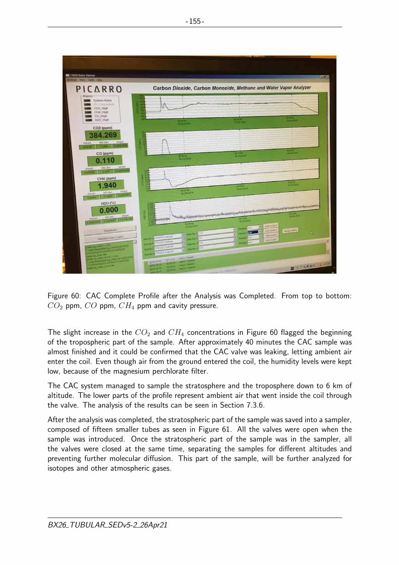
- 155 -
Figure 60: CAC Complete Profile after the Analysis was Completed. From top to bottom:CO2 ppm, CO ppm, CH4 ppm and cavity pressure.
The slight increase in the CO2 and CH4 concentrations in Figure 60 flagged the beginningof the tropospheric part of the sample. After approximately 40 minutes the CAC sample wasalmost finished and it could be confirmed that the CAC valve was leaking, letting ambient airenter the coil. Even though air from the ground entered the coil, the humidity levels were keptlow, because of the magnesium perchlorate filter.
The CAC system managed to sample the stratosphere and the troposphere down to 6 km ofaltitude. The lower parts of the profile represent ambient air that went inside the coil throughthe valve. The analysis of the results can be seen in Section 7.3.6.
After the analysis was completed, the stratospheric part of the sample was saved into a sampler,composed of fifteen smaller tubes as seen in Figure 61. All the valves were open when thesample was introduced. Once the stratospheric part of the sample was in the sampler, allthe valves were closed at the same time, separating the samples for different altitudes andpreventing further molecular diffusion. This part of the sample, will be further analyzed forisotopes and other atmospheric gases.
BX26 TUBULAR SEDv5-2 26Apr21

- 156 -
Figure 61: CAC Sampler with 15 Different Stages.
For the AAC unfortunately due to the pump failure no data was collected. A post flight failureanalysis was carried out on the pump and this can be seen in Section 7.4.
Data received by the ground station was also analyzed to find the pressure and temperatureprofiles during the flight. This was completed on MATLAB and was shown during the postflight briefing at campaign.
7.3 Results
The results gained from the TUBULAR flight can be broken down into the various subsystemsas follows
7.3.1 Mechanical Subsystem Performance
Structural Performance
The frame structure and the aluminum walls withstood all the flight phases providing therequired protection to all the components inside both boxes.
Regarding the frame, the most critical load that it had to face was during landing. The gondolalanded on the side where the boxes where allocated, thus they experienced a high load. Thanks
BX26 TUBULAR SEDv5-2 26Apr21

- 157 -
to the use of bumpers as anchors of the boxes to the gondola rails and the styrofoam as asitting surface, the force was damped, see Figures 62 and 63. Consequently the boxes did notmove from its original place.
Figure 62: Position of the bumpers after landing.
Figure 63: Sytrofoam below the boxes after landing.
The walls did not suffer any remarkable damage apart from the dirt that stuck to them as acause of the sideways landing and some scratches from trees during landing.
BX26 TUBULAR SEDv5-2 26Apr21

- 158 -
Pneumatic circuit Performance
The experiment had two separate pneumatic circuits, on each box.
The air sampling with the CAC system was nominal. The valve opened and closed upon bothautomated and manual commands. This allowed to empty the 300-meter coiled tube duringascent and filling with stratospheric air during the descent phase.
On the other hand, the large pneumatic system of the AAC system experienced a failure inthe pump which lead to the failure of the this alternative sampling system. Although the bagscould not be filled with stratospheric air for later analysis, data of both airflow and pressuresensor was received as expected and all the valves worked nominally (manifold and flushing).
The failure analysis of the pump can be found in Section 7.4.
7.3.2 Electrical Subsystem Performance
Throughout the flight, none of the previous sensor dropouts that had been experienced wereseen. This is thought to be due to the absence of larger electromagnetic interference’s.
All other electrical parts worked as intended.
For details on the full failure analysis of the pump see Section 7.4.
7.3.3 Software Subsystem Performance
The software managed to control the experiment through the majority of the phases of themission. The software worked even with frequent telemetry connection cutoff before thetakeoff, during take-off it switched to Ascent mode successfully. When the failure with thepump occurred it successfully reset and put itself in the correct mode. Since sampling causeda reset it was decided that the software would be kept in Manual mode for the remainder ofthe flight.
An unforeseen behavior was observed during descent when the choice was made to changethe mode from Manual mode to Normal-Descent mode. Directly after this change a lossof communication happened before it reestablished itself a few seconds later, with all valvesclosed and the experiment in Standby mode. This is was indicative of a reset. Why it resetitself was most likely brought on by the fact the experiment passed several sampling points inManual mode. Manual mode was thought to only be used for a short while and not to skipa sampling point. Incapable of taking a sample in Manual mode it is believed that the ASCperformed a sampling when the software had the authority to do so, in which the pump wasinvolved and therefor a reset happened. After the reset the software successfully went intoNormal-Descent mode without taking a sample using the AAC. The choice was the made totake it into Safe mode which closed every valve successfully.
During the flight the only intermission of telemetry was during the reboot of the software aftera reset. A permanent loss of telemetry happened at a low altitude due to limitations withline-of-sight. The on board software continued to record sensor data for several hours afterlanding.
BX26 TUBULAR SEDv5-2 26Apr21

- 159 -
7.3.4 Thermal Subsystem Performance
Figure 64: The Temperature for the Different Sensors During Whole Fight.
The thermal result for the flight are as seen in Figure 64. Both the critical components didnot go lower than the operating threshold. The heaters operated as expected and kept thepump and manifold in their respective threshold limits. During the float phase a test weredone to see if the pump issue were thermal related. The pump were then heated up to theupper limit and tried to start but did not work. It could then be concluded that the issuewith pump during the flight were not thermal related. The simulations estimated the heaterswould use 26.66Wh and during flight (calculated from Figure 64) 27.667Wh were used so thesimulations were a good estimation.
7.3.5 Past Results
After the analysis of the samples, the expected results were the vertical profiles of CO, CO2,and CH4. The profiles presented a similar pattern to that of Figure 65 which was found inan experiment by Karion et al (AirCore: An Innovative Atmospheric Sampling System) [6].The continuous profile (dashed line) belongs to the CAC while the discrete values (black dots)belongs to the AAC ([6]). Both profiles are showing a decrease in concentration of CH2 andCH4 with increasing altitude.
BX26 TUBULAR SEDv5-2 26Apr21

- 160 -
Figure 65: Pressure Profiles for (Left) CO2 and (Right) CH4 by Three Different Methods [6].
This experiment’s goal was to achieve the highest vertical resolution possible. Since the verticalresolution was determined by the length and the diameter of the tube [17], a 300 m long tubewas used, consisting of 2 smaller tubes. One of 200 m length with 3× 10⁻³ m outside diameterand 1.3× 10⁻⁴ m wall thickness, and another one of 100 m length with 6× 10⁻³ m outsidediameter and 1.3× 10⁻⁴ m wall thickness. For achieving higher stratospheric resolution, thetube with the smaller diameter was used to sample the higher altitudes and the one with thebigger diameter for the lower ones. Figure 66 by Olivier Membrive [17] compares the verticalresolution that can be expected with three different AirCores.
BX26 TUBULAR SEDv5-2 26Apr21

- 161 -
Figure 66: Comparison of the Vertical Resolutions That can be Expected with Different Air-Cores, After 3h Storage Time Before Analysis [17].
The High-Resolution AirCore-HR (red line),[17], is a combination of two tubes. One of 200m and one of 100 m.
The NOAA ’original’ CAC, [6], (black line) is a 152 m long tube and the AirCore-GUF (designedand developed at Goethe University Frankfurt), (blue line) is a combination of three tubes,100 m long in total.
The longer AirCore, AirCore-HR, achieved a higher resolution throughout the whole sampledair.
In addition, the vertical resolution depends on the the mixing inside the tube.
This experiment took into account two types of mixing. Molecular diffusion and the shear flowdiffusion, known as Taylor dispersion. The effect of molecular diffusion was described by theroot-mean-square of the distance of molecular travel,
Xrms =√
2Dt (5)
where, D was the molecular diffusivity of the molecule in the surrounding gas, and t was thetime over which travel occurs, [6]. For the tubing dimension that were used in this experiment,the flow of air through the CAC, was laminar. In such a flow, a parabolic velocity profile existedinside the tube, causing longitudinal mixing (Taylor dispersion).
BX26 TUBULAR SEDv5-2 26Apr21

- 162 -
Before their experiment was recovered, only molecular diffusion affected the sample, but duringanalysis both molecular diffusion and Taylor dispersion affected the sample. Combining bothof them, an effective diffusion coefficient was calculated as,
Deff = D +a2V 2
48D(6)
where D was the molecular diffusivity, a was the tube’s inner radius, and V was the averagevelocity [17]. The first term translated into the longitudinal direction, while the second onewas the Taylor dispersion.
After completing Test 4 and Test 18 as seen in Tables 25, and 35 respectively, the teammanaged to get the standard flow rate readings for the different altitudes. Standard flow rateis the volumetric flow rate of a gas corrected to standarized conditions of temperature andpressure. In this case the logged flow rates correspond to sea level conditions. Table 55 showsthe standard flow rates at the sampling altitudes.
Sampling Altitudes Ambient Pressure Standard Flow rate
Ascent Phase18 km 75.0 hPa ∼0.38 L/min21 km 46.8 hPa ∼0.21 L/min
Descent Phase
17.5 km 81.2 hPa ∼0.41 L/min16 km 102.9 hPa ∼0.55 L/min14 km 141.0 hPa ∼0.79 L/min12 km 193.3 hPa ∼1.22 L/min
Table 55: Sampling Altitudes as well as the Corresponding Ambient Pressures According tothe 1976 US Standard Atmosphere and the Standard Flow Rates at Each Altitude.
It was necessary to also calculate the actual flow rates at the different altitudes. The conversion
was done using the equation [1]: V olumetricflow = (Standardflowrate) ·(
Talt
Tstd
)·(
Pstd
Palt
)where,Pstd = 1013hPa was the standard pressure.Tstd = 294.25K was the standard temperature.Talt was the temperature at the different altitudes.Palt was the pressure at the different altitudes.
Table 56, shows the actual flow rates at the sampling altitudes.
Sampling Altitudes Ambient Pressure Actual Flow rate
Ascent Phase18 km 75.0 hPa ∼3.78 L/min21 km 46.8 hPa ∼3.36 L/min
Descent Phase
17.5 km 81.2 hPa ∼3.77 L/min16 km 102.9 hPa ∼3.99 L/min14 km 141.0 hPa ∼4.18 L/min12 km 193.3 hPa ∼4.71 L/min
Table 56: Sampling Altitudes as well as the Corresponding Ambient Pressures According tothe 1976 US Standard Atmosphere and the Normal Flow Rates at Each Altitude.
BX26 TUBULAR SEDv5-2 26Apr21

- 163 -
Finally, storage time, that was the time from the moment the tube was sealed until the endof the analysis, was a key factor that affected the experiment’s results in terms of resolution.
Figure 67 shows the effect of time delay between landing and analysis, on the expected verticalresolution.
Figure 67: Expected Vertical Resolution of AirCore-HR, for a Storage Time of 3h (Black), 6h(Blue), 12h (Green), 24h (Orange) and 1 Week (Red) [17].
It is clear that the sooner the samples were analyzed, the better the results for the verticalresolution of the CAC sample. At an altitude of 20 km the resolution decreased significantlyfrom 300 m to 500 m for 6h and 12h of delay, respectively, [17]. But even after a week ofstorage, a vertical profile could still be achieved with lower resolution.
Based on past BEXUS projects, the time to experiment recovery was estimated at 12 to 24hours, if not multiple days. As such, it was expected that the desired vertical resolution ofgas analysis favoured AAC configuration over that of CAC due to mixing of gases in the latterconfiguration, resulting in poorer vertical resolution.
The vertical resolution for the AAC was expected to be approximately 500 m. This wouldhave been achieved assuring the airflow intake rate. For Ascent Phase, a nominal speed of 5m/s was considered, which meant that it would take 28.57 seconds to fill a sampling bag with1.8L of air while ascending 142.85 m, and an actual airflow intake rate of approximately 3.78L/min at 18 km of altitude. For Descent Phase, the nominal speed was assumed to be 8 m/s.While descending 156.4 m a sampling bag would be filled in 19.55 seconds, with 1.3 L of air
BX26 TUBULAR SEDv5-2 26Apr21

- 164 -
and an actual airflow intake rate of 3.99 L/min at 16 km of altitude. However, taking intoaccount that the volume of the samples, at sea level, would have been lower, the samplingtime would have been longer and the vertical resolution closer to 500m.
For a 500 m of vertical displacement, the horizontal resolution of the AAC was approximatedbased on past BEXUS flights data obtained from the BEXUS manual [8]. The average hori-zontal resolution obtained for Ascent Phase was 588m and for Descent Phase was 186.5 m.This meant that the square area covered by the sample would have been 500 m x 588 m and500 m x 186.5 m for ascent and Descent Phases respectively.
7.3.6 Scientific Results
From the ambient temperature profile, seen in Figure 68, the tropopause was estimated tobe at 165.2 hPa. The AirCore onboard the CAC system operated nominally resulting in highresolution profiles for CO, CO2, and CH4. These profiles are presented in Figure 69. The datafrom 400 hPa down to 1000 hPa were deleted. During those measurements the CAC valve wasclosed and the gases were leaking inside the coil with some unknown delay, and from insidethe box (not from the troposphere).
Figure 68: Ambient Temperature in °C Over Ambient Pressure in hPa.
Trace gas concentrations are measured in parts per million (ppm) and parts per billion (ppb).A decreasing concentration trend is observed for CO2, CH4, and CO as the altitude increases.The maximum values are approximately 407 ppm for CO2, 1.9 ppm for CH4, and close to 89ppb for CO.
BX26 TUBULAR SEDv5-2 26Apr21

- 165 -
Figure 69: AirCore profiles for CO, CO2, and CH4 (in black) with their respective forecasts (ingrey). The red line denotes the tropopause boundary between the troposphere and the strato-sphere. The red asterisk denotes a reference point for 1,000 hPa surface level concentrationsmeasured at 20 km from the landing site.
A sharp decrease of CO2 can be observed in the first layers above the tropopause. Tropopausealtitude was at 274 hPa, about 9.8 km. In the stratosphere, values are lower since the exchangebetween the upper troposphere and lower stratosphere takes several years [17]. Variability ishigher near the ground, which agrees with the idea that CO2 may have negative and positiveanomalies at the surface that are mainly associated with vegetation uptake and anthropogenicemissions [17].
The mixing ratios of CH4 have a small variability in the troposphere. A strong decrease in thestratosphere is easy to spot with a value of 1.85 ppm near the tropopause and 1.33 ppm at 15.2km (118 hPa). Variability is higher in the mid-to-upper troposphere and in the stratosphere,which is mostly due to positive anomalies coming from the surface and negative anomaliescoming from the stratosphere [17].
It is difficult to draw any conclusions based on measurements extracted from a single samplingflight. Variations of greenhouse gas concentrations would have to be observed through timewith data collected over numerous reflights.
BX26 TUBULAR SEDv5-2 26Apr21

- 166 -
7.3.7 Future Work
It was expected that the AAC would serve as model enabling a cost-effective large scaledeployment scheme for regular high altitude greenhouse gas measurement. Unlike CAC, thedesign of AAC would have not imposed experimental restrictions based on the proximity ofinfrastructure for shipping and analysis. As such, a successful proof of concept of AAC samplingsystem would have served as a basis to enable reliable cost-effective measurements in remoteareas.
Despite the end of the BEXUS 26 programme, future flights can still be designed that willresolve the problems discovered during the campaign. Notably, using a different or dedicatedbattery set for the TUBULAR experiment.
The TUBULAR Team has presented its findings in two conferences and published experiment’sresults in proceeding for the 24th ESA Symposium on European Rocket Balloon Programmesand Related Research [3] and the 3rd Symposium on Space Educational Activities [11]. Thesepublications can serve as references for future work.
BX26 TUBULAR SEDv5-2 26Apr21

- 167 -
7.4 Failure Analysis
During the flight the experiment experienced unexpected errors. This section will go into theprocedures and results of the failure analysis. In general there was two stages of analysis,firstly the post flight analysis that was made as soon as the experiment was retrieved duringcampaign and, secondly the lab analysis that was made in the lab some time after launchcampaign.
7.4.1 Post flight analysis
Shortly after the conclusion of failure on the AAC system an investigation plan was created tomake sure that the team did not destroy any potential evidence. Deducted from the behaviourduring flight, a list of potential problems was made and can be seen in Table 57. Most possiblecauses were unlikely due to the extensive testing made before flight.
1 Shorted output pin on Arduino2 Pump elastic diaphragm broke3 Pump too cold4 Short circuit in pump5 Pump MOSFET broken6 Pump current draw too high7 Pump drive shaft blocked8 Pump tubing blocked
Table 57: List of Potential Failure Causes
Shortly after the experiment was retrieved a structured post flight investigation was made toinvestigate the possible causes of the in flight failure. The experiment walls were removedone at a time and there was no unexpected smells when opening the walls of the experimentthat might have indicated burning of components. After the main PCB board was accessible,resistance measurements were taken on the MOSFET’s. Which all were the same, indicatingthat the MOSFET’s were not damaged. There were no shorts anywhere on the PCB either.The forward resistance of the pump was measured and compared to the forward resistanceof a spare pump. The resistances were similar and deemed not to be suspicious. There wasno discontinuities on the PCB where they were not expected. No problems were found fromelectrical measurements and visual inspection.
Thus the next step in the procedure was to try to start the system from a power supply andcheck functionality. The power supply was set to 28.8V and a current limit of 1.8A. Thesystem was turned on and data was feed out nominally as it did during flight as well. Afterinspecting basic functionality of the experiment the pump and the flushing valve were turnedon and opened to see if the same issue occurred as during flight. The pump turned on andthe valve opened nominally and pumped air through the system. Since the pipes going outwere dismounted at this point and one of the concerns was that the pump might have beenblocked, the inlet of the pump was blocked and the procedure repeated. The pump turned onagain, although without blowing air, as expected.
BX26 TUBULAR SEDv5-2 26Apr21
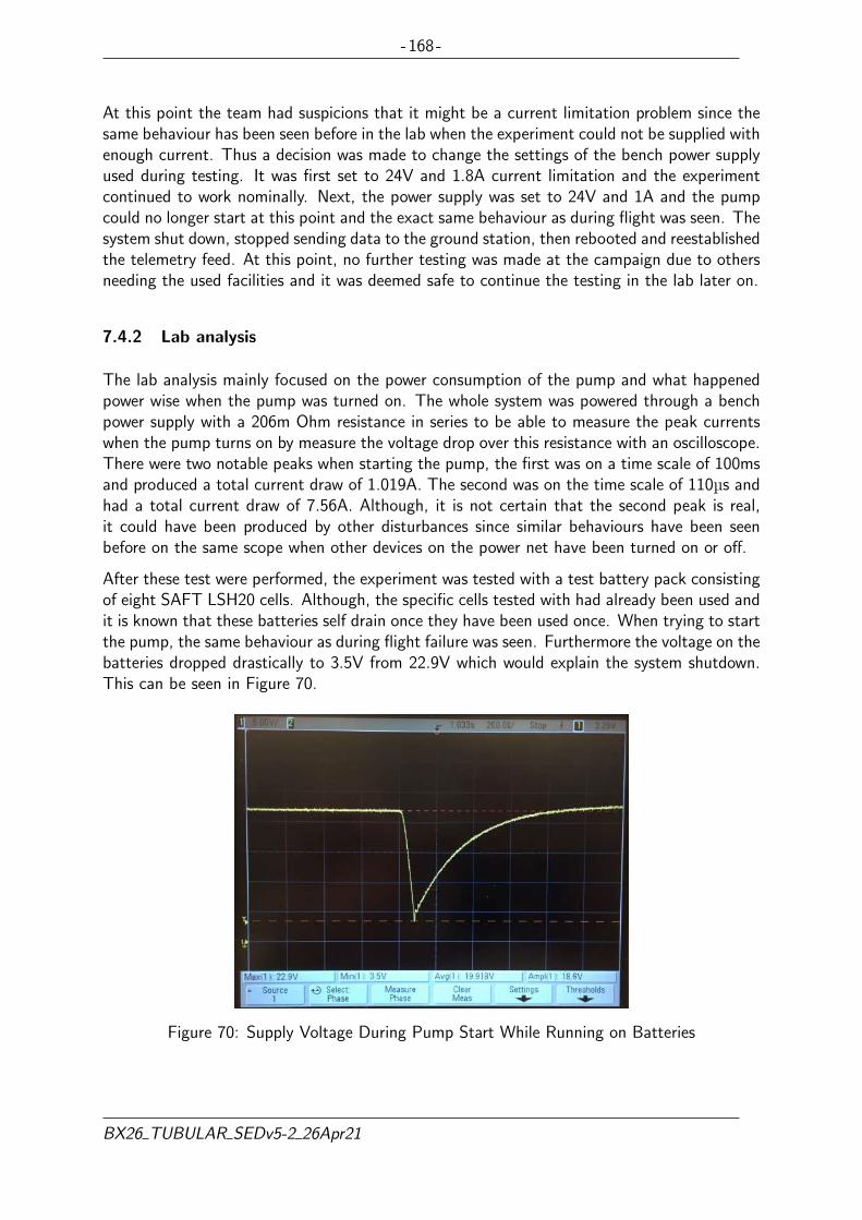
- 168 -
At this point the team had suspicions that it might be a current limitation problem since thesame behaviour has been seen before in the lab when the experiment could not be supplied withenough current. Thus a decision was made to change the settings of the bench power supplyused during testing. It was first set to 24V and 1.8A current limitation and the experimentcontinued to work nominally. Next, the power supply was set to 24V and 1A and the pumpcould no longer start at this point and the exact same behaviour as during flight was seen. Thesystem shut down, stopped sending data to the ground station, then rebooted and reestablishedthe telemetry feed. At this point, no further testing was made at the campaign due to othersneeding the used facilities and it was deemed safe to continue the testing in the lab later on.
7.4.2 Lab analysis
The lab analysis mainly focused on the power consumption of the pump and what happenedpower wise when the pump was turned on. The whole system was powered through a benchpower supply with a 206m Ohm resistance in series to be able to measure the peak currentswhen the pump turns on by measure the voltage drop over this resistance with an oscilloscope.There were two notable peaks when starting the pump, the first was on a time scale of 100msand produced a total current draw of 1.019A. The second was on the time scale of 110µs andhad a total current draw of 7.56A. Although, it is not certain that the second peak is real,it could have been produced by other disturbances since similar behaviours have been seenbefore on the same scope when other devices on the power net have been turned on or off.
After these test were performed, the experiment was tested with a test battery pack consistingof eight SAFT LSH20 cells. Although, the specific cells tested with had already been used andit is known that these batteries self drain once they have been used once. When trying to startthe pump, the same behaviour as during flight failure was seen. Furthermore the voltage on thebatteries dropped drastically to 3.5V from 22.9V which would explain the system shutdown.This can be seen in Figure 70.
Figure 70: Supply Voltage During Pump Start While Running on Batteries
BX26 TUBULAR SEDv5-2 26Apr21

- 169 -
7.4.3 Conclusion
The experiment works within the current specifications of a single SAFT LSH20 cell. Although,the supplier has not specified the single cell behaviour for short peaks such as 100µs. Theeffects on current specifications when using these cells in series is also unknown. Although, itis known that lithium-thionyl chloride batteries have a relatively large internal resistance whichmight affect the performance. Thus the conclusion is that the experiment was current limitedand thus reset itself, but the source of limitation is still unknown.
Since it was not possible to start the pump during the pre-flight readiness review as a resultof the flushing already being made, starting the pump while running on batteries should havebeen tested before. Either in the Lab, or before the system was flushed at launch campaign.Then the issue might have been discovered before the flight.
BX26 TUBULAR SEDv5-2 26Apr21

- 170 -
7.5 Lessons Learned
At the end of the project, the TUBULAR Team has learned many important lessons regardingdocument creation as well as learning how to build an idea into a project, integrating it, testingit, flying it and analysisng the data afterwards.
The TUBULAR Team found that the REXUS/BEXUS programme was rewarding in termsof experience regarding balloon craft design and development, with real deadlines, publisheddocuments, and team work.
7.5.1 Management Division
• Coordination between multiple project stakeholders.
• Task definition, estimation, and management.
• Task integration.
• Conflict management and resolution.
• Communication flows.
• Funding research and outreach.
• Identifying team member strengths as well as weaknesses and assigning responsibilitiesaccordingly without neglecting the opportunities to improve on weaknesses.
• Do not assume cross-division communication will take place without organizing/planningit.
• Reviewing progress of assigned task should be continuous rather than waiting for theirdue dates.
• Agree on and clearly communicate to the team definition of “Done” when referring totasks being completed.
• Agree on and clearly communicate to the team the definition of “Final Version” whenreferring to schematics, diagrams, and component lists.
• The lessons learned section of previous BEXUS SEDs is an invaluable resource thatanswers many BEXUS related recurring questions.
• If changes in management are required it is important that there is a sufficiently longchange over period to allow a transfer of knowledge.
• Tasks that are not completed on time or were simply not worked on during the assignedtime will impact projected deadlines and these situations must be planned for and mit-igated against. An early red flag for this is if the reported team working hours tend tobe lower than expected at which point one can expect to have to make up those hoursup before a deadline. These concerns must continuously be communicated to the team.
• The REXUS/BEXUS programme is a significant investment in time and resources fromall programme partners and as such the unique opportunity is not limited to participatingstudents but to component manufacturers and suppliers as well. With this in mind,
BX26 TUBULAR SEDv5-2 26Apr21

- 171 -
the team should not shy away from aggressively seeking funds or sponsorships fromcomponent manufacturers and suppliers as they stand to benefit from such a partnershipto show case the robustness of their products.
• Testing will always take longer than expected and so time must be planned to accountfor this.
• When working with many remote team members extra time must be allowed for tasksto be completed as the communication is slower. Internal earlier deadlines help a lot.
• During manufacture and test having many smaller deadlines has proven useful in ensuringthings stick to the time plan.
• When things don’t go to plan during flight it is essential to keep a cool head and thinkthings through calmly. It might be hard to make final decisions on things but it isimportant to ensure appropriate actions are taken in a timely and sensible fashion.
• You can never do too much testing!
7.5.2 Scientific Division
After an extended research in trace gases and climate change, as well as in atmosphericsampling methods, the science team has gained so far:
• General knowledge in climate change.
• General knowledge in the different sampling methods of the atmosphere; its character-istics and applications.
• Study scientific papers in detail.
• Outreach to scientific community.
• Translating scientific concepts to technical teams.
• Knowledge of how to design the scientific requirements in such a way that are in thepermitted limits of the budget while the technical requirements are fulfilled.
• How to sufficiently distribute the tasks within the science team and keep good commu-nication with the other departments.
• Experience, that writing down the tasks that need to be done, and keep tracking onthem is better rather than having them as goals.
• Experience in producing a presentation only with the key points of a project and pre-senting it in front of other people.
• Work as a group from different locations.
• How to prepare and plan a test, under the real environment of the experiment.
• The importance of testing, and how to sufficiently deal with problems that come upunexpectedly.
• How to perform a failure analysis, documenting every step.
BX26 TUBULAR SEDv5-2 26Apr21

- 172 -
• Knowledge in data analysis procedure and how to extract the desired results from rawdata.
• Using MATLAB to obtain the vertical profiles of the CO2, CH4, and CO gasses.
7.5.3 Electrical Division
The electrical team has enhanced its understanding of the electronics design as well as gainedconfidence in selecting appropriate components as per requirements. Some of the points teamimproved as their general understanding are listed below:
• Gained confidence in designing electronics circuitry.
• Familiarized with the selection of the electrical components.
• By reading through large number of data sheets, team is now able to easily extract andunderstand technical details.
• Learned and developed power calculation skills.
• Got experience of using the Eagle software and how to find and make the libraries,footprints, and schematics for the required components.
• How to test the components in the vacuum chamber.
• Learned about the different connectors, wires and how to place the components on thePCB so the actual design can fit into the experiment box.
• Discovered the cascading consequences of changing one component.
• Finding how having big sheets with a lot of information can be preferable to severalsheets with less specification.
• While designing PCB’s with Eagle it’s a good idea to draw the traces manually ratherthan using autotracer. Since it allows you double check your schematics while pullingthe traces.
• When using netnaming to design schematics for later PCB designs in Eagle it’s veryimportant to triple check the net names since they sometimes change in unexpectedways.
• Got practical experience of soldering the different types of sensors, wires and connectors.
• Learned how to solder SMD miniature pressure sensors onto the PCB.
• Familiarized with using work shop tools and machinery.
• Got experience how to work around spontaneous problems arise due to design changesby the other departments and the testings.
• Learned how to conduct failure analysis; it’s basic methodology and rules required inorder to avoid destruction of any evidence for the post-flight analysis.
• Learned how important electrical housekeeping data could be during a in-flight errors.
BX26 TUBULAR SEDv5-2 26Apr21
- 173 -
• Learned how to come up with and assess compromises during launch campaign to ac-commodate to eventual changes.
7.5.4 Software Division
• Learned more about version control in the form of Git.
• Learned how to implement an RTOS on Arduino.
• Learned how to translate experiment requirements to a software design.
• Learned how to split functionality into several testable functions.
• Gained experience on software unit testing.
• Learned how to design and create GUI using MATLAB GUIDE.
• Learned how to use Git, a version control system for tracking changes in computer filesand coordinating work on those files among multiple people.
• Learned how to implement TCP/IP and UDP on ethernet connection.
• Learned how to make telecommand and telemetry.
• Learned how the I2C and SPI protocols work and operate.
• Learned how to efficiently debug software.
• Learned that when suppressing the output of a system, it would also be good to notignore it.
• Learned that using a sequence based system is not optimal when said system is wishedto not be operated non sequentially.
• Learned that the expected cases one designs around, may not be the actual cases whichencountered in real life.
7.5.5 Mechanical Division
• Come up with real design solutions starting from conceptual problems.
• Make a proper use of both space and mass.
• Learn mechanical tricks when designing.
• Adapt the design to components availability and characteristics.
• Select and contact with vendors.
• Implement a real pneumatic system.
• Compute structural analysis.
• Team collaboration with other departments, i.e. Electrical, Science, and Thermal.
• Design is trickier when it comes to implementation.
BX26 TUBULAR SEDv5-2 26Apr21

- 174 -
• Always document specific department knowledge. If who designed a certain part of theexperiment is not available for the manufacture phase, whoever works on it should beable to figure out most of the solutions by themselves.
• Manufacturing and integration of the different subsystems of the experiment takes longerthan expected during design phase.
• The design is never frozen until everything is built and working properly.
• Good planning when designing and manufacturing allows to avoid last minute tricksduring Launch Campaign.
• After flying the experiment and thinking of what could be changed to improve it, severalideas arise.
7.5.6 Thermal Division
• Learned how to do Steady-State and Transient thermal analysis in ANSYS.
• Coordinate between other division to find a solution that works for everyone.
• Do a thermal plan and structure up what needs to be done for a long period of time.
• How to improve and be more efficient when adjusting to sudden changes in design.
• How to balance details in simulations.
• How to do thermal test, analyze the result and make improvement of the results.
• How to work with Styrofoam.
• How temperatures inside component operating ranges can impact component perfor-mances.
• How the real flight actually is different from test and simulations and it is hard to do aperfect test and simulations beforehand.
BX26 TUBULAR SEDv5-2 26Apr21

- 175 -
8 Abbreviations and References
8.1 Abbreviations
AAC Alternative to the Air CoilASC Air Sampling ControlANSYS ANalysis SYStemBEXUS Balloon Experiment for University StudentsCAC Conventional Air CoilCAD Computer Aided DesignCDR Critical Design ReviewCFD Computational Fluid DynamicsCH4 MethaneCLK Serial ClockCO Carbon MonoxideCO2 Carbon DioxideCOG Center of GravityCRDS Cavity Ring Down SpectrometerDC Direct CurrentDFM Design for ManufacturabilityDLR Deutsches Zentrum fur Luft- und RaumfahrtEB Electronic BoxEBASS Esrange BAlloon Service SystemECTS European Credit Transfer SystemEPDM Ethylene Propylene Diene MonomerESA European Space AgencyFCS Frame Check SequenceFEA Finite Element AnalysisFMI Finnish Meteorological InstituteGC Ground Control StationGPIO General Pins Input OutputGPS Global Positioning SystemGUI Graphical User InterfaceH20 WaterHOOD Hierarchic Object-Oriented DesignI2C Inter-Integrated CircuitIDE Integrated Software EnvironmentI/O Input/OutputIR Infra-RedIRF Institutet for rymdfysik (Swedish Institute for Space
Physics)LED Light Emitting DiodeLTU Lulea University of TechnologyMATLAB MATrix LABoratoryMB Mega ByteMISO Master Input Slave OutputMORABA Mobile Rocket Base
BX26 TUBULAR SEDv5-2 26Apr21

- 176 -
MOSFET Metal Oxide Semiconductor Field Effect TransistorMOSI Master Output Slave InputMSc Master of ScienceNOAA National Oceanographic and Atmospheric Adminis-
trationOBC Onboard Computerppb parts per billionppm parts per millionPCB Printed Circuit BoardPDR Preliminary Design ReviewREXUS Rocket Experiment for University StudentsRJ45 Registered Jack 45RTOS Real-time operating systemSAFT Societe des Accumulateurs Fixes et de TractionSCP Serial Clock PinSD Secure Digital (Storage)SDP Serial Data PinSED Student Experiment DocumentationSNSA Swedish National Space AgencySPI Serial Peripheral InterfaceSSC Swedish Space CorporationSTP Standard Temperature PressureTBC To Be ConfirmedTBD To Be DeterminedTCP Transmission Control ProtocolTT&C Telemetry, Tracking, and CommandUDP User Datagram ProtocolVC Valve CenterZARM Zentrum fur angewandte Raumfahrttechnologie und
Mikrogravitation
BX26 TUBULAR SEDv5-2 26Apr21

- 177 -
8.2 References
[1] Standard flow rate vs volumetric flow rate. http://www.tsi.com/uploadedFiles/_Site_Root/Products/Literature/Application_Notes/GenPurp-Standard_vs_Volumetric.pdf. Accessed: 2018-10-03.
[2] Dow Sverige AB. Sakerhetsdatablad. Dow Sverige AB, Dow Sverige AB, Box 783, 60117 Norrkoping, Sweden, Oct 2010.
[3] Fagerstrom E, Lawton N, Labreche G, et al. Project TUBULAR: Use of multi-layer foilsampling bags and a 200 meter AirCore for greenhouse gas sampling on-board the BEXUS26 stratospheric balloon flight. 24th ESA Symposium on European Rocket BalloonProgrammes and Related Research, 2019.
[4] Hansen James et al. Climate Change and Trace Gases. The Royal Society Publishing,2007.
[5] Hooghiem Joram J.D. et al. LISA: a lightweight stratospheric air sampler. AtmosphericMeasurement Techniques, Pending, 26th January 2018.
[6] Karion et al. AirCore: An innovative atmospheric sampling system. 2010.
[7] M.Diallo et al. Global distribution of CO2 in the upper troposphere and stratosphere.2017.
[8] EuroLaunch. BEXUS User Manual. Version 7.2. 31 Nov 2017.
[9] Rodger E. Farley. BalloonAscent: 3-D simulation tool for the ascent and floatof high-altitude balloons. https://ntrs.nasa.gov/archive/nasa/casi.ntrs.nasa.gov/20050243623.pdf Accessed: 2018-04-15.
[10] FMI. AirCore flights at Sodankyla. https://www.gruan.org/gruan/editor/documents/meetings/icm-9/pres/pres_0719_Kivi_Aircore.pdf. air-core.
[11] Labreche GLJ, Molas-Roca P, Lawton N, et al. Stratospheric balloon flight of cost-effective sampling bags and high resolution AirCore to measure arctic greenhouse gasconcentrations of CO2 and CH4. 3rd Symposium on Space Educational Activities, 2020.
[12] Picarro Inc. PICARRO G2401 Analyzer for CO2/CO/CH4/H2O User’s Guide. PicarroInc, 480 Oakmead Parkway, Sunnyvale, California, CA 94085, USA., 2010.
[13] Texas Instruments. HDC2010 Low Power Humidity and Temperature Digital Sensors.Texas Instruments, Texas Instruments, Post Office Box 655303, Dallas, Texas 75265, Jul2017.
[14] IPC. IPC-2221B, generic standards on printed board design. http://www.pcb-factory.net/Upload/DownLoad/PCBdesign%20principle_16030316524806.pdf. Accessed: 2018-05-26.
BX26 TUBULAR SEDv5-2 26Apr21

- 178 -
[15] Daniel J. Jacob. Atmospheric Chemistry, chapter 2.3. Princeton University Press, 1999.
[16] Duane Johnson. Heliostat design concepts. http://www.redrok.com/concept.htm#emissivity. Accessed: 2018-02-26.
[17] Olivier Membrive, Cyril Crevoisier, Colm Sweeney, Francois Danis, Albert Hertzog, An-dreas Engel, Harald Bonisch, and Laurence Picon. AirCore-HR: a high-resolution columnsampling to enhance the vertical description of CH4 and CO2. Atmospheric MeasurementTechniques, 10(6):2163–2181, 2017.
[18] NOAA. Global distribution. https://www.esrl.noaa.gov/gmd/ccgg/gallery/figures/. Accessed: 2018-04-17.
[19] Aaron Van Pelt. Real-time atmospheric monitoring of stable isotopes and trace greenhousegases. International Environmental Technology, 2008.
[20] Sid Perkins. Arctic warming twice as fast as rest of world. ScienceShot, 2013.
[21] ECSS Secretariat. Space Engineering: Verification. ESA-ESTEC, Requirements & Stan-dards Division, ESTEC, P.O. Box 299, 2200 AG Noordwijk, The Netherlands, Nov 1998.
[22] Engineering Toolbox. Standard atmosphere air properties. https://www.engineeringtoolbox.com/standard-atmosphere-d_604.html. Ac-cessed: 2018-06-24.
[23] Engineering Toolbox. Thermal conductivity of common materials and gases. https://www.engineeringtoolbox.com/thermal-conductivity-d_429.html.Accessed: 2018-02-25.
BX26 TUBULAR SEDv5-2 26Apr21

RXBX_PDR Report_TUBULAR_V1-2_06Feb18
Flight: BEXUS 26 Payload Manager: TBC Experiment: TUBULAR Location: SSC, Esrange Space Center, Sweden Date: 6th Feb. 2018 1. Review Board members
Stefan Kramer, SSC (chair) Veronica Botti (minutes) Giorgio Parzianello, ESA Koen Debeule, ESA Simon Mawn, ZARM Dieter Bischoff, ZARM
Katharina Schuettauf, DLR MORABA Maria Holmström, SSC Klas Nehrman, SSC Jörgen Blomberg, SSC Juha Keinström, SSC Jianning, Li SSC
2. Experiment Team members Gustav Dyrssen Jordi Coll Ortega Natalie Lawton Nuria Agües Paszkowsky Hamad Siddiqi Muhammad Ansyar Rafi Putra Pau Molas Roca 3. General Comments Presentation
- The presentation was clear and well done.
SED - In general, the SED was well done and appreciated by the panel. - The team should clarify better the objectives. - In general, the team should include more labelled diagrams instead of long pages of text.
4. Panel Comments and Recommendations Requirements and constraints (SED chapter 2)
- There are too many functional requirements. The team should reduce them. - The requirements F16 to F27 do not need to be listed. - The team shall add a performance requirement about the volume of air to analyse. - The requirements P16 to P22 are all design requirements. - For the requirement P16 the team should specify the altitude. - The design requirement D8 is fine, but the team should remember that that 374Wh is the
capacity of the battery at nominal temperature and with a current draw of 0.1A. A more typical capacity of 7Ah (196 Wh).
- Regarding the design requirement D13 the team might expect the experiment environment to be below -30C.
- The constraints listed in the SED are not real constraints.
REXUS / BEXUS Experiment Preliminary Design Review
- 179 -
Appendix A Experiment Reviews
A.1 Preliminary Design Review (PDR)
BX26 TUBULAR SEDv5-2 26Apr21

RXBX_PDR Report_TUBULAR_V1-2_06Feb18
Mechanics
- The team should consider also the locations and accessibility of the external electronic interface.
- The team should think about a solution to access the experiment without taking it off from the gondola.
- The set-up of the box needs to be re-discussed. - The team should consider a thermal insulation for the experiment since the experiment is
drawing cold air from the environment. - The team should check the capability of the pump is enough to suck the required amount of
air.
Electronics and data management (SED chapter 4.2.2, 4.2.3, 4.5, 4.7, 4.9) - A consumption of 1 mA is underestimated. - The team should check how to connect the device to the microcontroller and choose a
possible interface. - To reduce the voltage to that required the team shall use a DC/DC converter.
Thermal (SED chapter 4.2.4 & 4.6)
- The team should perform a thermal analysis of the experiment, especially considering that the experiment will suck very cold air from the external environment.
- The team should finish to list the temperature ranges of the components. - The team should clarify which temperature they need inside the box. - The team should find an alternative solution to access the experiment in order to prevent
unwanted openings of the box.
Software (SED chapter 4.8) - The software design was well done. - The team should consider to perform some manual actions on the experiment. The
experiment does not need to be all automatized. - If the team wants to keep the triggered watchdog, all the events should be activated from the
beginning of the countdown. Maybe it’s better to remove the watchdog. Verification and testing (SED chapter 5) - The verification matrix must be reviewed. - In general, not everything can be verified by test. Test is often proceeded by an analysis or
review. - The team should make sure that the test really covers the requirement. M - any requirements point to the same test so a detailed test plan will be needed to ensure the
test specifically addresses that requirement. - In some cases, it might be better to split out separate tests. - The team should add a test to verify the functioning of the pumping system. - The team should verify that the pump is able to produce the required velocity with such a small
delta-p. - It’s very important for the team to test the opening and closing of the valves.
Safety and risk analysis (SED chapter 3.5)
- The team, in general, should review the risk register. - In general, the risks are underestimated. - The team should foresee some managerial risks, such as the risk of someone leaving the
team. - The team should consider as a major risk the partnership with the Finnish. - The team should consider as a major risk also the use of the single pump. This should be
ordered early and tested and maybe it would be better to order at least two pumps.
Launch and operations (SED chapter 6)
- The chapter was well done, however the team should add more information about the recovery, since it is a critical part of the experiment.
- The team should clarify where did they get the data about balloon descent rate. - The team should specify why they cannot flush on the ground. - The team should clarify whether the valve operation is linked to time or altitude.
- 180 -
BX26 TUBULAR SEDv5-2 26Apr21

RXBX_PDR Report_TUBULAR_V1-2_06Feb18
Organisation, project planning & outreach (SED chapters 3.1, 3.2, 3.3 & 3.4) - The team should clarify the work packages and specific tasks of each team member in the
WBS. - The Gantt chart is too basic and should be refined. - There is no mapping of team availability over the project period to the work required. - The team should clarify whether the project is part of a course. - The budget description is too basic. The team should describe all the costs and clarify bet ter
what is already covered and what needs to be covered. - The outreach plan is good but not implemented yet. The team should create soon a webpage
and a page in different social media.
5. Internal Panel Discussion Summary of main actions for the experiment team
- The team should verify that the bags and the pump work properly before the CDR. - The team should review the Requirements and Constraints section. - The team should further develop and document their electronics design. - The team should provide a more defined thermal analysis. - The team should improve the management section.
PDR Result: conditional pass Next SED version due: v1-2, 12th March 2018
- 181 -
BX26 TUBULAR SEDv5-2 26Apr21

RXBX11_TUBULAR_CDR REPORT_V1-1_31MAY18
Flight: BEXUS 26 Payload Manager: TBC Experiment: TUBULAR Location: ESA, ESTEC, Noordwijk, The Netherlands Date: 31 May 2018 1. Review Board members
- Michael Becker (DLR) - Kristine Dannenberg (SNSB) - Alexander Kinnaird (ESA) - Veronica Botti (ESA) –Minutes - Stefan Krämer (SSC) – Chair - Maria Snäll (SSC)
- Koen DeBeule (ESA) - Piotr Skrzypek (ESA) - Grzegorz Izworski (ESA) - Katharina Schüttauf (DLR MORABA) - Dieter Bischoff (ZARM) - Simon Mawn (ZARM)
2. Experiment Team members
- Natalie Lawton - Erik Fagerström - Pau Molas Roca - Gustav Dryssen
3. General Comments Presentation - The presentation was very clear and complete and the panel appreciated the approach of the team
in analysing and finding a solution to possible issues.
SED - The team may read the SEDs of BX_COSPA or BX_A5UNIBO for more information about similar
pumps and experiment principles. - The team should be consistent with thousand markers (,) and decimal markers (.) (e.g. in the
budget). - The team should keep the appendices as indicated in the SED Guidelines (in particular A for the
review reports and B for outreach) but, in general, there are some excellent additional information. - The document is going to end up very long. This is not a problem, but the team must try to be
succinct using diagrams and summary tables where possible and not including unnecessary ‘discussion’.
- The team should keep images compressed without reducing the readability. - The team should describe what the “Brain” is the first time they mention it in the document.
4. Panel Comments and Recommendations Requirements and constraints (SED chapter 2) - Since the team deleted a lot of requirements and the document is getting very big, maybe it would
be better to rewrite the updated requirements and put the old ones in the appendix. - The team should add a note in the introduction and in the objectives to explain the reasons for
changing, the type of gas that will be detected during the flight (i.e. from N2O to CO). - Req. F6-F7: they are software requirements. The team should be aware that it’s difficult to justify
them in system level functional requirements. If they really want to keep them for verification it’s ok,
BEXUS Experiment Critical Design Review
- 182 -
A.2 Critical Design Review (CDR)
BX26 TUBULAR SEDv5-2 26Apr21

RXBX11_TUBULAR_CDR REPORT_V1-1_31MAY18
but in that case it would be better to put them in the design requirements or re-word them and put them in operational requirements..
- Req. F10 to F12: instead of saying “shall collect data”, the team should say “shall measure”. - There are still some performance requirements missing, such as: amount of air, range accuracy
and frequency of the flow rate, pressure measurements, temperature measurements and humidity. These requirements should be separate in different performance requirements.
- Req. D3: The requirement “shall not disturb the launch vehicle” should not be deleted but rather reworded such that is unambiguous and verifiable.
- Req. D4: the team should be more specific and define the type of connector, protocol, etc. - Req. D5: the team should be more specific and define the type of connector, voltage, ripple,
grounding, etc. - Req. D7: the requirement only makes sense with the reference voltage. The team should add it. - Deleting the duplicated temperature requirements does make sense, but the team shouldn’t delete
those ranges. The team is advised to put them in the verification plan now. - When stating “profiles of flight” the team should either state the specifics and/or reference the
section manual. Mechanics (SED chapter 4.2.1 & 4.4) - The rack built out of strut profiles is a good choice because of flexibility in fixating the components
inside and stiffness properties. The team should consider the attachment to the gondola which does not allow tolerances of the rails and which functions as lot of heat bridges.
- The team should consider how to absorb vibrations/shocks of the pumps? (“Bismat” clamps could be a solution).
- The team should specify how they plan to activate the valves. The team should be aware that they will heat up after a while and that there are valves with a high activation power but a lower holding power.
- The team should specify what kind of tubes and connectors are used and consider how to perform a leakage test, how to access any connection and how to seal any connection (it could be easy just raising the torque a little more, but could be difficult as well in case that an O-ring or sealing has to be changed).
- The team should avoid sharp corners, especially at racks with lower space and fulfilled with equipment (such as the “brain”.).
- Inline pressure sensor from ”FESTO” could be good. - Mechanical pressure sensors based on pitot tubes may also be an option. - The team should clarify what is the expected maximum pressure inside the bags and tubes. The
team is advised to check the datasheet of the valves regarding leakage rate or perform tests with different pressure on both sides to ensure proper function.
- The team should make sure to define and use the right procedure to clean pumps and valves.
Electronics and data management (SED chapter 4.2.2, 4.2.3, 4.5, 4.7, 4.9) - The team should consider the connector location carefully. It is very good to have easy access but
it’s not good to have the cables/connector pointing out of the gondola, because the turn may protrude outside and increase the risk of damage during launch/landing. This issue can be discussed with payload manager during accommodation session.
- In general, the accessibility of the connector panel is pretty good but without any protection. The team should move this panel upwards to the top cover (access from above).
Thermal (SED chapter 4.2.4 & 4.6) - Regarding the EPS extruded Styrofoam, the team should ensure that this material is suitable for
low pressure environment. Many foams expand when the pressure decreases but do not restore completely when back in normal pressure which would cause open gaps of the insulation cover.
- From a thermal point of view the team is suggested to install big heat bridges with this attachment. It would be better to use a flat material or another strut profile fixated with thermal spacers and attached to the gondola with the help of rubber bumpers.
- The team should investigate any hot spots of the setup and try to spread the heat with heat sinks to serve better conditions for the surrounding components.
- In general, there are too many heat bridges in the experiment setup. - To raise the conditions at the beginning the team could insert chemical heater(s) like hand
warmers during late access. - The team could colour the strut profiles with black paint to count on the effect by heating up by the
sun while the setup faces into it.
- 183 -
BX26 TUBULAR SEDv5-2 26Apr21
RXBX11_TUBULAR_CDR REPORT_V1-1_31MAY18
- The team should be aware that the expected lowest temperature on a BEXUS launch in October (day flight) is around -55°C.
- The team should specify how will the implementation of the insulation material looks. - An internal temperature around +5°C is low. The team should consider that the performance
decreases at lower temperatures.
Software (SED chapter 4.8) - The team is suggested to implement hysteresis for automatic mode change and to filter the sensors. - Regarding the process diagram in figure 44, there is no way out from the manual mode. The team
should specify what are they planning to do if the connection to the ground station is lost. - The team should clarify if/how they are planning to keep track of the time. - A list of telecommands and supported telemetries is missing. The team should not forget to insert a
command to query the storage status, general system status, update automatic timeline, update time and perhaps reinitialise/clean up the storage.
- The team should specify which is the file system used on the SD card. FAT is not recommended. - The team should clarify the concept of mode switching based on the pressure sensors. - It’s a good choice to use three tasks for Arduino but in the Software design section the identification
of these three tasks is missing. The team should add it. Verification and testing (SED chapter 5) - Only positive software testing is currently foreseen. The team should explore failure scenarios: resets
of the microcontroller (during auto mode), loss of communication at inconvenient times, multiple loss of communication, loss of SD card (unplug, broken filesystem, etc.).
- Req. P12 to P14: the requirement should be verified by Review of Design and not by Inspection (you review a data sheet you inspect a model/build).
- The team should be careful that where items are already verified by analysis, the analysis remains valid if/when the design changes/evolves.
- The team should state within the test plan whether the testing item is flight, prototype or another kind of model; they should also state within the test plan which requirements will be verified and then write the plan to make sure it will clearly verify those requirements.
- The team should insert all these tests in the Gantt Chart and have a global test plan which would lays them out logically.
- The team should consider what happens if a test fails and a change is needed and understand how far to come back in the test plan.
- Doing a vibration test on a shaker is good learning experience for the team, but the team should pay attention to which spectrum(s) are applied to the experiment, as there are none specified for BEXUS.
- There is no need to remove the walls during the test. The team should engage a good test engineer to understand the process.
- The team should include a summary of one or two paragraphs (maybe with figure where relevant) for each test, and then make a separate complete report in the appendix.
- The team should specify for which reasons there are no concerns about bag burst.
Safety and risk analysis (SED chapter 3.5) - Risk TC40: the severity is too low. - The team, in general, should avoid the word “proper” when defining an action to mitigate any risks. - EN10: the team should better clarify which is the risk and which is the foreseen action. “Vibration”
does not mean anything. - The team should consider some management risks, in particular regarding time availability . - The team should also consider some operational risks. - The team should check again the severity of some risks. In general, it is too high. - In general there are many risk with the same code (same probability and severity) that are considered
sometimes acceptable and sometimes unacceptable and an action is always foreseen. This is confusing. The team should clarify what is an acceptable risk for them and what is unacceptable and, based on that, they should think of an action or accept the risk.
Launch and operations (SED chapter 6) - The team should add any safety risks associated with pressurised vessels during recovery. - It is very good that there is already a checklist. The team should check it with SSC to confirm it is all
possible before flight after the final ECTs. - The team should use this checklist during the systems tests and update them, including photos, and
making sure that the person doing the final version is the person who did it before.
- 184 -
BX26 TUBULAR SEDv5-2 26Apr21

RXBX11_TUBULAR_CDR REPORT_V1-1_31MAY18
- The team should add any launch site requirements, such as a room, a laboratory for preparations or testing on ground.
- The team should add risk connected to the use of chemicals. - The team should think of what could happen in case of hard landing and exposed gas or liquid. - The team should insert in the launch and operation chapter (or link to the appendix) the cleaning
procedure of the pump and valves. - The team should use the checklist during the tests. - The team should be aware that from T -3h to T- 1h the experiment will work on external power. Organisation, project planning & outreach (SED chapters 3.1, 3.2, 3.3 & 3.4) - In the Resources section, under Table 6, it is written that all the team members are currently enrolled
in LTU master programmes. However, according to the team details, most of the students are bachelor students. The team should clarify.
- The team should be aware that, during the last months they will need to allocate more resources to the experiment.
- In the outreach section is written “a website WILL be launched…”. If it has already been done the verb should be at the past, not at the future.
- The team should clarify who is responsible once the subsystems are assembled (i.e. system level AIT and launch/operations).
- The team should try to trace the critical path to know where to focus their efforts. - The team should better clarify if the exam period is really blocked out. - It is very good to have some internal deadlines. - It seems that there is a very little margin at the moment (testing completed at the start of October);
the team should not forget to plan some buffer time and, in case of late testing, the team should think about the associated risks and how to mitigate them (e.g. good analysis).
- The team should relate their resource availability to the Gantt chart and clarify how the impact of any delays on the project planning.
- Regarding the budget, the team should specify if they have considered any contingency for unexpected events.
- It would be great to have a dedicated outreach timeline/media plan to see when these events are happening; they could be used to punctuate the project (a nice break or celebration for you) and/or to build excitement around certain events.
- The team should add a picture of the experiment on the website. - In the “Project” Section, in the website, the first word is “Problem”. The team should change it with
something like “objective”, or something similar. - The team should add a headline in the website to capture the attention of the reader. Something like
“we launch an experiment to the edge of space….” could be a good starting point. - The team should look again at the relative logo sizing (SNSA is too small) in the website. - The website loads very slowly, especially large header photos. The team should consider optimising
this and check its compatibility for mobile devices. - In the Facebook page the team should expand the “about” section to include mention of the
REXUS/BEXUS programme. 5. Internal Panel Discussion Summary of main actions for the experiment team
- Update the mechanical design as per the recommendations. - Make the design decision regarding inlet pressure and humidity measurement (contact their
mentor for further advice). CDR Result: Pass
Next SED version due: SED_v3-0, due 3 weeks before IPR. Date TBD
- 185 -
BX26 TUBULAR SEDv5-2 26Apr21

Page 1
BEXUS
Experiment Integration Progress Review
1. REVIEW
Flight: BEXUS 26
Experiment: TUBULAR
Review location: IRF Kiruna / Sweden
Date: 23 / 24 July 2018
Review Board Members
1. Stefan Krämer (SSC)
2. Grzegorz Izworski (ESA)
Experiment Team Members
Natalie Lawton Emily Chen
Hamad Siddiqi Emil Nordqvist
Gustav Dyrssen Erik Fagerström
2. GENERAL COMMENTS
2.1. Presentation
Good Presentation. Good status update.
2.2. SED
No comments
2.3. Hardware
Mechanics
o Almost components are in house.
o The Outer Structure made of BOSCH Profiles is mounted
o Some parts of the insulation are cut and assembled
o Pneumatic system not yet assembled since parts just arrived at the day of IPR.
Electronics
o PCB order has been send out to Manufacturer.
o Breadboard finalised and working
Running Pump via Ground Station
Switching valves ((LED as place holders for Valves)
Heaters
- 186 -
A.3 Integration Progress Review (IPR)
BX26 TUBULAR SEDv5-2 26Apr21

Page 2
BEXUS
Experiment Integration Progress Review
Power supply
3. PHOTOGRAPHS
Picture 1: Pump and Temperature sensors on breadboard
- 187 -
BX26 TUBULAR SEDv5-2 26Apr21

Page 3
BEXUS
Experiment Integration Progress Review
Picture 2: Frame for Air Coil including insulation material
Picture 3: Power Supply for two voltage levels on breadboard and heaters mounted to alumium block heat sink.
- 188 -
BX26 TUBULAR SEDv5-2 26Apr21

Page 4
BEXUS
Experiment Integration Progress Review
Picture 4: LED as placeholders for valves
Picture 5: DCDC converters on breadboard
4. REVIEW BOARD COMMENTS AND RECOMMENDATIONS
- 189 -
BX26 TUBULAR SEDv5-2 26Apr21

Page 5
BEXUS
Experiment Integration Progress Review
4.1. Science
Check for suitable cleaning procedures. Cleanliness is highest priority when you manufacture and
o Clean your tools with IPA before use
o Clean your workspace (IPA, Aceton) thoroughly!
o Use Gloves (powderfree !)
o Check, if you can use the pressured air in your lab or if the system is oiled.
Un case of doubts, use Dried Air or Nitrogen from the bottles
Implement a filter on the low pressure side to avoid contamination of particles from the bottle.
o Use standard cleanroom wipes
o Keep the working area free from other people
o Keep the tubes close with Kapton tape and away (boxed) from access of other people. As long the system is still open, use gloves and wipe off the ends and parts before assembly.
o Consider flushing the system with IPA / Aceton after assembly. Leave the fluid inside the system for some hours to resolve the residual grease or oil.
4.2. Requirements and constraints (SED chapter 2)
No comments
4.3. Mechanics (SED chapter 4.2.1 & 4.4)
All components are in house except of:
o Some fittings (Swagelok) for sample bags
o Double sided tape
o Sheet metal
o Rail nuts
o Pressure Sensor (ordered)
All Tubing and fittings, valves have arrived
Start assembling pneumatic system as soon as possible
o Take your time for bending and fit checking. Avoid stress on tubing and fittings, it might introduce leaks!
o Use contraction loops in straight tubes.
4.4. Electronics and data management (SED chapter 4.2.2, 4.2.3, 4.5 & 4.7)
PCB order has been send out to Manufacturer.
- 190 -
BX26 TUBULAR SEDv5-2 26Apr21

Page 6
BEXUS
Experiment Integration Progress Review
Have at least one or two spare boards ready
Interface cable between AAC and CAC: Use self-made cable with PTFE insulation and D-Sub connector.
Check if you have the opportunity to crimp the D-Sub connectors
Solder according to the course you got at ESTEC.
Test the full setup on your breadboard including all valves while you wait for the PCBs
o Check each component on its own in the circuit and document it
o Measure the current for the different modes
4.5. Thermal (SED chapter 4.2.4 & 4.6)
Thermal setup with passive insulation looks ok. Will be verified by test and eventually improved
4.6. Software (SED chapter 4.8)
Ground Station is running and the breadboard is fully operated via Ethernet
The I2C and SPI I/F have to be verified
All functions of Ground Station Operational mode and Manual mode work and have been verified
The reconnection after communication loss is verified
Status of valves and components are reflected on GS GUI
Revise your S/W before uploading and mark your OBC with S/W version
Team decided to continue with FAT 32 File system. Test this in a dedicated test and try to generate errors by e.g. power loss. Repeat the test many times!
Calibrate your sensors, Temp and pressure. Calibrate all hardware spares and have the baseline measurements saved.
Label your components
4.7. Verification and testing (SED chapter 5)
Calibrate your sensors, Temp and pressure. Calibrate all hardware spares and have the baseline measurements saved.
Testing Schedule and progress is reasonable. Document the results well.
4.8. Safety and risk analysis (SED chapter 3.4)
Consider the risk of contamination during the different stages of the project
o Manufacturing
o Testing
o Transport
- 191 -
BX26 TUBULAR SEDv5-2 26Apr21

Page 7
BEXUS
Experiment Integration Progress Review
o campaign
4.9. Launch and operations (SED chapter 6)
Have Swagelok caps as RBF on your tubes for CD and later provided to Recovery crew.
4.10. Organisation, project planning & outreac h (SED chapters 3.1, 3.2 & 3.3)
Plan for implementation and testing is reasonable and achievable. Nevertheless, stay ahead of your planning.
Deadline for finished and tested experiment is the first week in September for the testing campaign at FMI in Finland.
Distribute small work packages to get stuff done
4.11. End-to-end Test
Breadboard test with all functions and Ground Station was successfully performed
o Placeholder LEDs instead of valves verifying the function of electronics and software
o Pump function verified
o Communication to ground station verified
o Read out of I2C and SPI communication based temperature sensors not yet possible
o Pressure sensor is to be delivered and verification of function pending
o Heater function verified
5. FINAL REMARKS
5.1. Summary of main actions for the experiment team
Look into the I2C and SPI libraries for sensor communication and make them work
5.2. Summary of main actions for the organisers
Have frequent tele conference between Mentor and team.
5.3. IPR Result: pass / conditional pass / fail
Pass
5.4. Next SED version due
SED_v4-0: 4th October 2018
- 192 -
BX26 TUBULAR SEDv5-2 26Apr21

Page 8
BEXUS
Experiment Integration Progress Review
6. INTEGRATION PROGRESS REVIEW – IPR
Experiment documentation must be submitted at least five working days (the exact date will be announced) before the review (SED version 3). The input for the Campaign / Flight Requirement Plans should be updated if applicable. The IPR will generally take place at the location of the students’ university, normally with the visit of one expert.
The experiment should have reached a certain status before performing the IPR:
The experiment design should be completely frozen
The majority of the hardware should have been fabricated
Flight models of any PCB should have been produced or should be in production
The majority of the software should be functional
The majority of the verification and testing phase should have been completed
The experiment should be ready for service system simulator testing (requiring experiment hardware, electronics, software and ground segment to be at development level as minimum)
Content of IPR:
General assessment of experiment status
Photographic documentation of experiment integration status, with comments were necessary
Discussion of any open design decisions if applicable
Discussion of review items still to be closed
Discussion of potential or newly identified review item discrepancies
Discussion of components or material still to be ordered or received by the team
Clarification of any technical queries directed towards the visiting expert
Communication and functional testing (Service system simulator testing and E-link testing for REXUS and BEXUS respectively)
- 193 -
BX26 TUBULAR SEDv5-2 26Apr21

Page 1
RXBX11_TUBULAR_EAR Report_V1-0_10Oct18
BEXUS
Experiment Acceptance Review
1. REVIEW
Flight: BEXUS 26
Experiment: TUBULAR
Review location: LTU Kiruna / Sweden
Date: 10th October 2018
Review Board Members
Stefan Krämer (SSC, Science Services, Payloads)
Experiment Team Members
Natalie Lawton Núria Agües Paszkowsky
Kyriaki Blazaki
Emily Chen Jordi Coll Ortega
2. GENERAL COMMENTS
2.1. Review Summary
The Team presented a fully integrated Experiment and the functions were proven within a End to End test. The quality of manufacturing is very good and all functions were verified. The testing phase is finished and was performed successfully.
The Aircoil will be integrated at the campaign. The Experiment has been testes togher with the aircoil and fit checked.
2.2. Mechanics
Net Mass (measured) n/a kg
Gross Mass (measured) 24.17kg
CAC: 11.95kg
AAC: 12.22kg
kg
The Mechanical integration is finished. The experiment looks is well mounted, safe and sturdy
The separation level to the detachable CAC Box is clearly marked for recovery purpose
Only a few sharp edges need rework
2.3. Electronics
Low Battery Voltage 24 1.17A
- 194 -
A.4 Experiment Acceptance Review (EAR)
BX26 TUBULAR SEDv5-2 26Apr21

Page 2
RXBX11_TUBULAR_EAR Report_V1-0_10Oct18
BEXUS
Experiment Acceptance Review
Average Battery Voltage 28.87V 0.750A / 1.25A
High Battery Voltage 31.64 1.5A
The Electronics is finalised and fully tested
The manufacturing quality is good
The cables are harnessed
2.4. Software
Uplink n/a
Downlink 162bytes/s
Ground Station
o Ground Station SW is finished and is looks good. All functions are visible.
o Experiment status is clearly verifiable
o The SW has a high level of complexity and information
Experiment
o SW design frozen since 13 Sept.
o All functions are tested on durability
o Communication verified
2.5. Verification and testing
Pre campaign Testing phase is finished. All necessary tests were successfully accomplished.
2.6. End-to-end Test
The End to End test in a accelerated test mode was successful.
All functions are verified.
Valves open and close in sequence and depending on sensor input
Bags are filled in sequence with air samples by the use of the pump
2.7. Launch Site requirements
The team requires access to the gondola after FCT for flushing the system until Pick up of the gondola
The procedure has been discussed and seems feasible. It will be discussed during the campaign with OPS and REC.
- 195 -
BX26 TUBULAR SEDv5-2 26Apr21
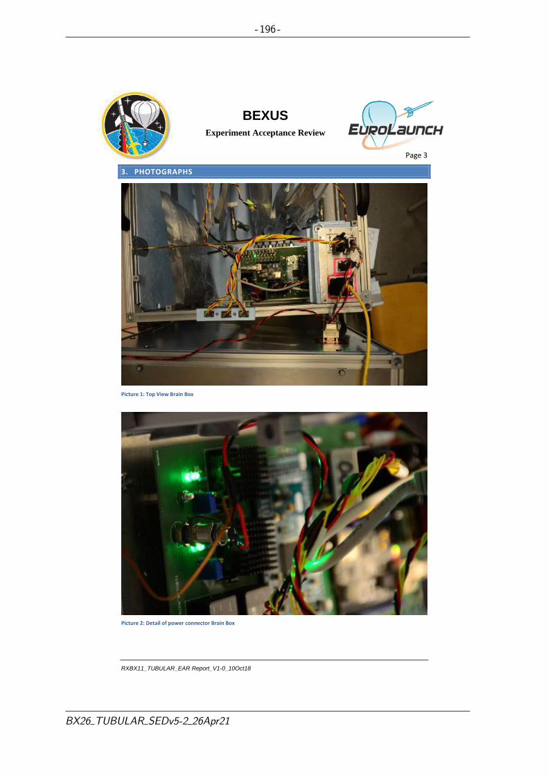
Page 3
RXBX11_TUBULAR_EAR Report_V1-0_10Oct18
BEXUS
Experiment Acceptance Review
3. PHOTOGRAPHS
Picture 1: Top View Brain Box
Picture 2: Detail of power connector Brain Box
- 196 -
BX26 TUBULAR SEDv5-2 26Apr21

Page 4
RXBX11_TUBULAR_EAR Report_V1-0_10Oct18
BEXUS
Experiment Acceptance Review
Picture 3: Screenshot Ground Station GUI
Picture 4:Experiment Setup during End-to End Test with inflated bags
- 197 -
BX26 TUBULAR SEDv5-2 26Apr21
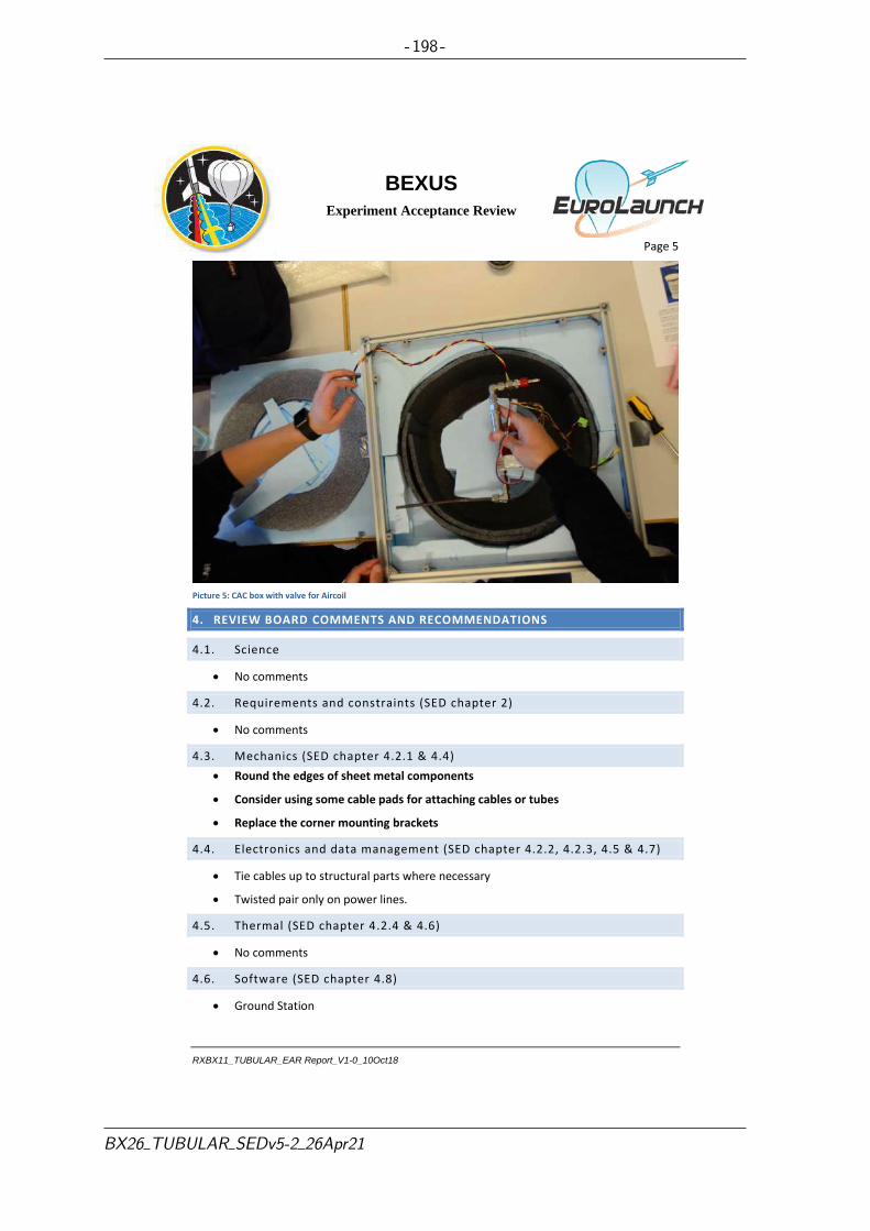
Page 5
RXBX11_TUBULAR_EAR Report_V1-0_10Oct18
BEXUS
Experiment Acceptance Review
Picture 5: CAC box with valve for Aircoil
4. REVIEW BOARD COMMENTS AND RECOMMENDATIONS
4.1. Science
No comments
4.2. Requirements and constraints (SED chapter 2)
No comments
4.3. Mechanics (SED chapter 4.2.1 & 4.4)
Round the edges of sheet metal components
Consider using some cable pads for attaching cables or tubes
Replace the corner mounting brackets
4.4. Electronics and data management (SED chapter 4.2.2, 4.2.3, 4.5 & 4.7)
Tie cables up to structural parts where necessary
Twisted pair only on power lines.
4.5. Thermal (SED chapter 4.2.4 & 4.6)
No comments
4.6. Software (SED chapter 4.8)
Ground Station
- 198 -
BX26 TUBULAR SEDv5-2 26Apr21

Page 6
RXBX11_TUBULAR_EAR Report_V1-0_10Oct18
BEXUS
Experiment Acceptance Review
o No comments
Experiment
o No comments
4.7. Verification and testing (SED chapter 5)
No comments
4.8. Safety and risk analysis (SED chapter 3.4)
No comments
4.9. Organisation, project planning & outreach (SED chapters 3.1, 3.2 & 3.3 )
No comments
4.10. End-to-end Test
No comments
5. FINAL REMARKS
5.1. Summary of main actions for the experiment team
Bring the Experiment to Esrange and fly it.
5.2. Summary of main actions for the organisers
No actions
5.3. EAR Result: pass / conditional pass / fail
Pass
5.4. Next SED version due
- 199 -
BX26 TUBULAR SEDv5-2 26Apr21

Page 7
RXBX11_TUBULAR_EAR Report_V1-0_10Oct18
BEXUS
Experiment Acceptance Review
6. EXPERIMENT ACCEPTANCE REVIEW – EAR
Experiment documentation must be submitted at least five working days (the exact date will be announced) before the review (SED version 4) This will take place upon delivery of the completed experiment to EuroLaunch. The review may take place at either the location of the students’ university, or a DLR, SSC or ESA institute.
Content of EAR:
Team presentation of project status
Follow-up of IPR action items
Review of schedule status with respect to REXUS program timeline and upcoming activities
Demonstration of the fully integrated experiment
Experiment mass properties determination/discussion
Mechanical and electrical interface checkout
Electrical Interface Test (REXUS service system simulator test or BEXUS E-link functionality test)
Flight Simulation Test (FST) – including a full end to end system demonstration
Experiment acceptance decision: Passed/conditional pass/failed. If a conditional pass is elected, the immediate action items should be discussed, along with an appropriate deadline(s)
- 200 -
BX26 TUBULAR SEDv5-2 26Apr21

- 201 -
Appendix B Outreach
B.1 Outreach on Project Website
To increase the projects out reach the TUBULAR Team created a project website. On thewebsite there are descriptions of the project, a link to download the latest SED, information onthe TUBULAR Team members and sponsors and a contact link. In addition the microbloggingcarried out by the TUBULAR Team is also displayed on the website.
Figure 71: The Home Page of TUBULAR’s Website.
BX26 TUBULAR SEDv5-2 26Apr21

- 202 -
Figure 72: The Daily Microblogging Displayed on the Website.
BX26 TUBULAR SEDv5-2 26Apr21
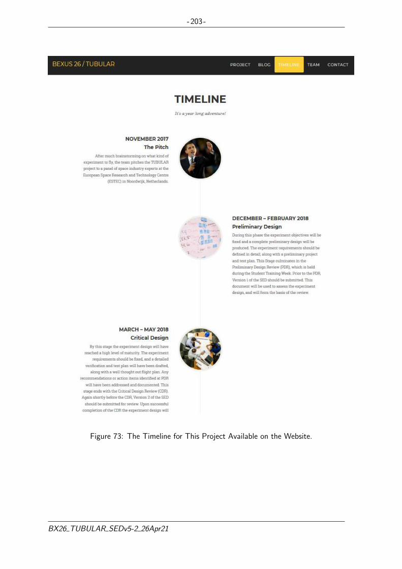
- 203 -
Figure 73: The Timeline for This Project Available on the Website.
BX26 TUBULAR SEDv5-2 26Apr21

- 204 -
Figure 74: The Information of the Tubular’s Team Members Available on the Website.
BX26 TUBULAR SEDv5-2 26Apr21

- 205 -
Figure 75: The Sponsors In This Project Available on the Website.
BX26 TUBULAR SEDv5-2 26Apr21
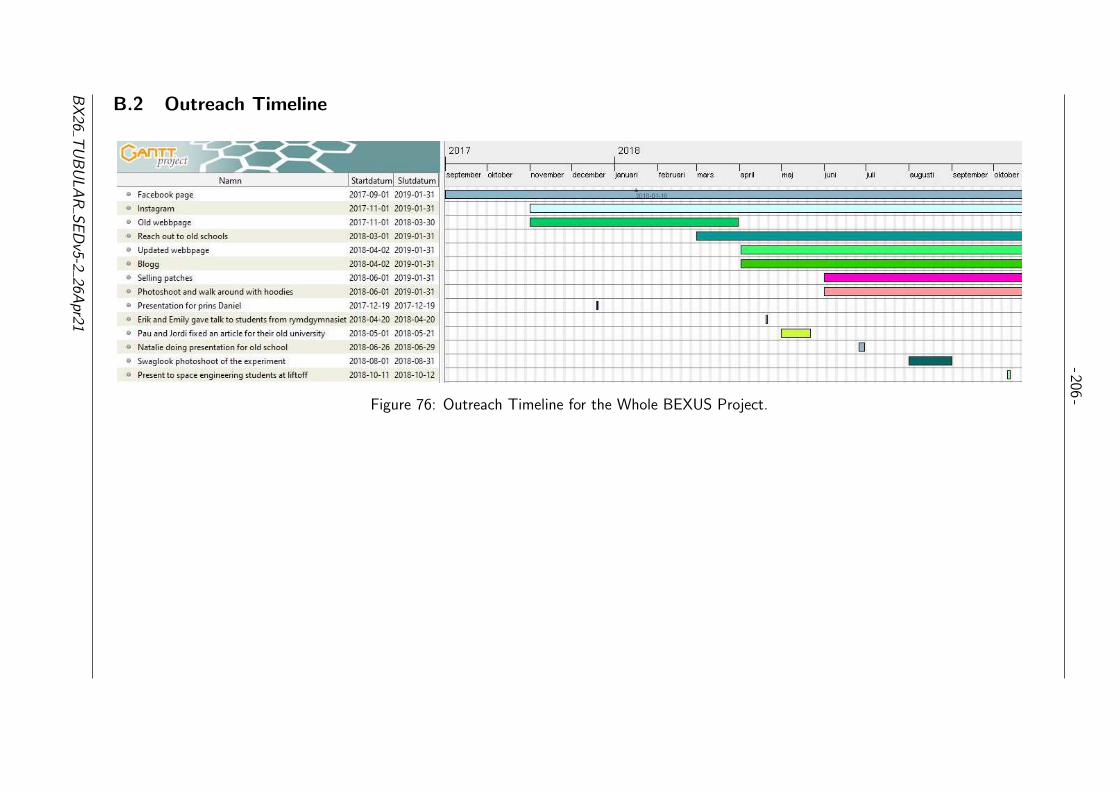
-206-
B.2 Outreach Timeline
Figure 76: Outreach Timeline for the Whole BEXUS Project.
BX
26T
UB
UL
AR
SE
Dv5-2
26Apr21

- 207 -
B.3 Social Media Outreach on Facebook
Another outreach avenue is Facebook. On Facebook the TUBULAR Team posts photos, shorttext updates and links to our blog posts.
Figure 77: Photos from Social Media Outreach on Facebook.
BX26 TUBULAR SEDv5-2 26Apr21

- 208 -
B.4 Social Media Outreach on Instagram
On Instagram the TUBULAR Team posts regularly with updates on the project progress andwhat the TUBULAR Team has been up to.
Figure 78: Some of the Social Media Outreach on Instagram.
BX26 TUBULAR SEDv5-2 26Apr21

- 209 -
B.5 Outreach with Open Source Code Hosted on a REXUS/BEXUSGitHub Repository
The TUBULAR Team has opened a GitHub Repository to share all the code used in theTUBULAR project. It was created with an open invite to all other REXUS/BEXUS teams toview, use and contribute to.
Figure 79: The Open Source Code Hosted on a REXUS/BEXUS GitHub Repository.
B.6 Outreach with Team Patch
The team also had patches made of the TUBULAR logo and 150 patches have been ordered.Around 70 of these have already been bought by the team for themselves and to give to friendsand family. It is intended that the remaining 80 will be sold for a small profit at university.
Figure 80: A Photo of the Patch in Production Sent by the Company Making it.
BX26 TUBULAR SEDv5-2 26Apr21

- 210 -
B.7 Visit by the Canadian Ambassador
During Canadian Ambassador Heather Grant’s visit at the Swedish Institute of Space Physics,the team got the honor to do a brief presentation of the TUBULAR project. It also includeda short explanation regarding one of the electrical tests in the vacuum chamber. This is nowdisplayed on the universities website with a link to the TUBULAR website.
Figure 81: Picture taken by Ella Carlsson which is shown on the LTU Website.
BX26 TUBULAR SEDv5-2 26Apr21

- 211 -
Figure 82: The Text Accomopanying the Image on the LTU Webpage.
B.8 Attendance at Lift Off 2018
The team will attend Lift Off 2018 event and present the TUBULAR project for students,companies and organizations. The guests will have a chance to have a peek at the wholeexperiment and find out more about the REXUS/BEXUS programme.
BX26 TUBULAR SEDv5-2 26Apr21

- 212 -
Appendix C Additional Technical Information
C.1 Materials Properties
Material DensityTensilestrength
0.2%Proofstress
Ductileyield A5
Modulusof elastic-ity
Brinellhardness
EN AW- AlMgSi6060
2.7 g/cm3 245 MPa195MPa 10% 70GPa 75 HB
Table 59: Mechanical Properties of the Bosch Rexroth Strut Profiles.
Material DensityTensilestrength
YieldStrength
Modulusof elastic-ity
Brinellhardness
Aluminum5754
2.67 g/cm3 190 MPa 80 MPa 70 GPa 77 HB
Table 60: Mechanical Properties of the Aluminum Panels.
Material DensityTensilestrength
MaximumTemperature
Styrofoam250 SL-AN
28 kg/m3 90 kPa 75 C
Table 61: Mechanical Properties of the Styrofoam Insulation/Protection.
BX26 TUBULAR SEDv5-2 26Apr21

- 213 -
C.2 Coiled Tube and Sampling Bag Example
C.2.1 CAC Coiled Tube
Figure 83: CAC Coiled Tube.
C.2.2 Air Sampling Bag
Figure 84: Air Sampling Bag.
BX26 TUBULAR SEDv5-2 26Apr21

- 214 -
C.3 Dimensions of the sampling bag
Table 62 shows how the dimensions of the bags change according to the sampled volume.This data has been obtained by testing and has been taken into account in order to determinethe maximum number of bags that can be filled inside the box.
Volume Length (horizontal) Height (vertical) WidthEmpty 26.4 cm 28 cm 0.5 cm0.5 L 26.4 cm 27.5 cm 1.5 cm1 L 26 cm 27.5 cm 2 cm
1.5 L 25.5 cm 26.5 cm 4.5 cm2 L 25 cm 25 cm 5.5 cm
2.5 L 24.5 cm 23 cm 7.5 cm3 L 24 cm 22 cm 10.5 cm
Table 62: Dimensions of the Bags When Filled with Different Air Sample Volumes.
C.4 List of components in The Brain
Level 1 - PumpList of components of Level 1:
A. 1 Magnesium filter
B. 1 Pump
C. 1 Temperature sensor
D. 2 Heaters
E. 3 Tubes
F. 8 interfaces
Level 2 - Valve CenterList of components of Level 2:
A. 1 Airflow sensor
B. 1 Static pressure sensor
C. 1 Temperature sensor
D. 2 Heater
E. 1 Manifold
F. 6 Sampling valves
G. 1 Flushing valve
H. 11 Tubes
I. 14 interfaces
BX26 TUBULAR SEDv5-2 26Apr21

- 215 -
Level 3 - ElectronicsList of components of Level 3:
A. 1 PCB
B. 5 D-Sub female connectors
C. 1 E-link socket
D. 1 Power socket
All the electrical components connected to the PCB in Level 3 are summarized in Tables 63and 64.
CACArea Electrical component #
Solenoid valve 1CAC
Temperature sensor 3
Table 63: Connections to CAC Box.
AACArea Electrical component #
Pump 1Heater 2
Level 1
Temperature sensor 1Static Pressure sensor 1Airflow sensor 1Solenoid valves 7Heater 2
Level 2
Temperature sensor 1Sampling bags center Temperature sensor 3Outside Pressure sensor 3
Table 64: Connections to AAC System.
BX26 TUBULAR SEDv5-2 26Apr21

- 216 -
C.5 Pneumatic System Interfaces
All the fittings in the AAC and CAC subsystem were sponsored and manufactured by Swagelok.
C.5.1 Straight Fittings
(a) SS-200-6 (b) SS-400-1-2
Figure 85: Straight Tube and Male Fittings.
C.5.2 90 Degree Fittings
(a) SS-400-9 (b) SS-400-2-2 (c) SS-400-8-4
Figure 86: Various Kinds of 90 Degree Fittings
C.5.3 Tee Fittings
(a) SS-400-3 (b) SS-400-3-4TTM (c) SS-400-3-8TMT
Figure 87: Various Kinds of Tee Fittings
BX26 TUBULAR SEDv5-2 26Apr21

- 217 -
C.5.4 Quick Connectors
(a) SS-QC4-B-4PF (b) SS-QC4-B-200 (c) SS-QC4-D-400
Figure 88: Quick Connect Body and Quick Connect Stem With Valve
C.5.5 Reducer and Adapters Fittings
(a) SS-400-6-2 (b) SS-4-TA-7-4RG (c) SS-300-R-4
Figure 89: Various Kinds of Reducer and Adapters Fittings
C.5.6 Port Connections and Ferrule Set
(a) SS-401-PC (b) SS-400-C (c) SS-400-SET (d) SS-6M5-4M
Figure 90: Various Kinds of Port Connections and Ferrule Set
BX26 TUBULAR SEDv5-2 26Apr21

- 218 -
C.6 Manufacturing Drawings
The following drafts are to be used to manufacture the mechanical components of the exper-iment.
BX26 TUBULAR SEDv5-2 26Apr21


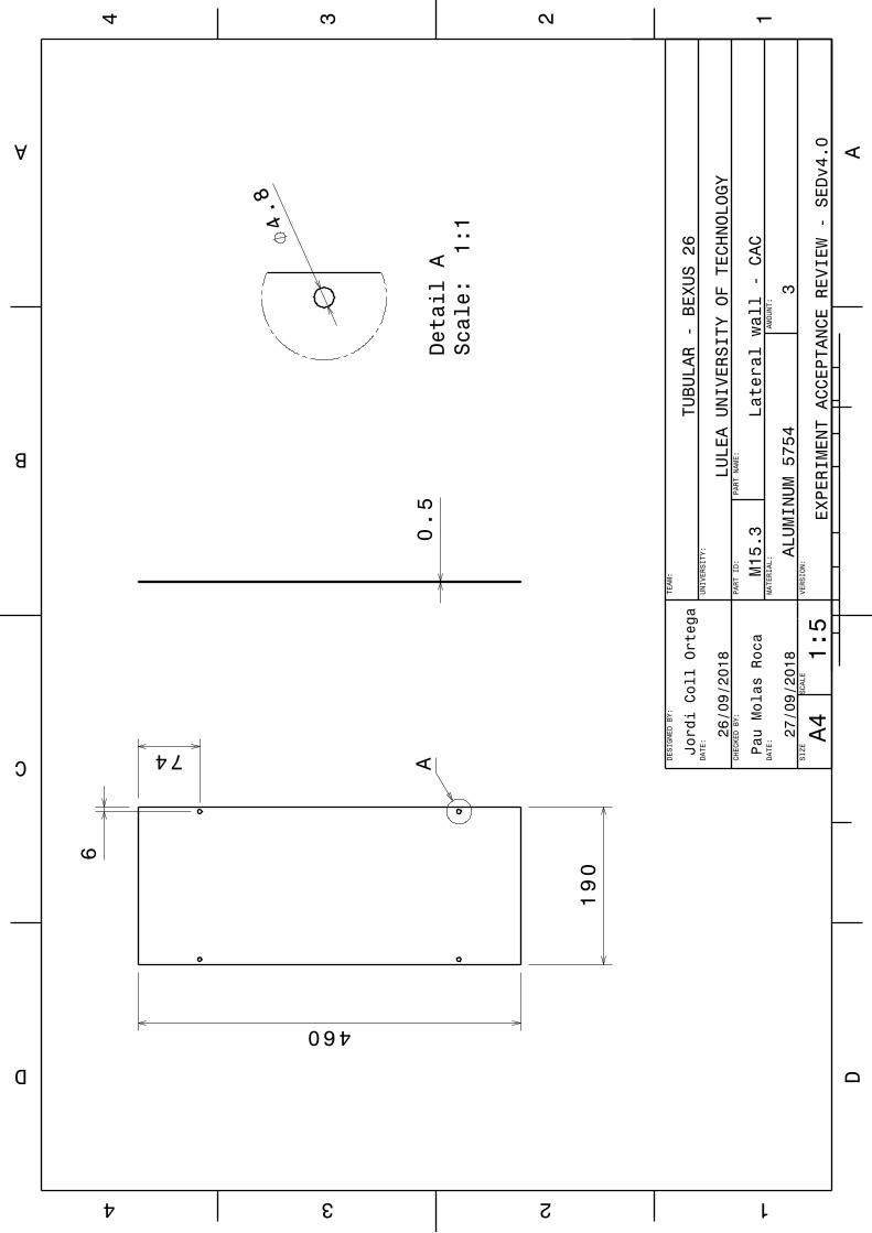


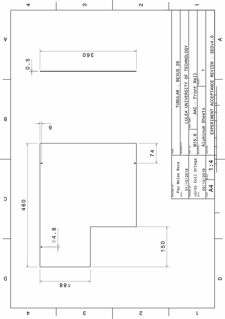


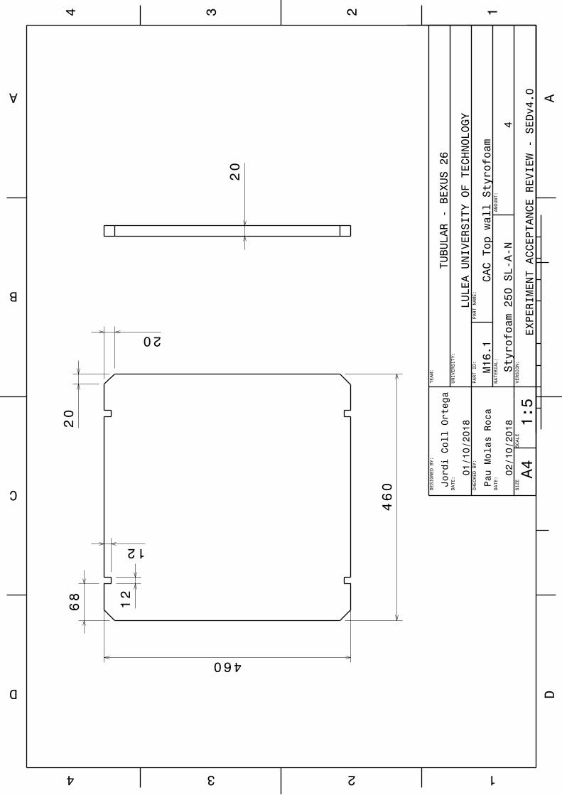


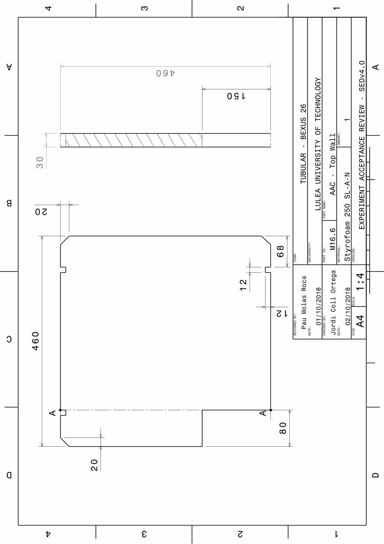


-255-
C.7 Software Sequence Diagram
C.7.1 Air Sampling Control Object Sequence diagrams
Figure 91: ASC Object in Normal Mode - Ascent.
BX
26T
UB
UL
AR
SE
Dv5-2
26Apr21

-256-
Figure 92: ASC Object in Normal Mode - Descent.
BX
26T
UB
UL
AR
SE
Dv5-2
26Apr21

-257-
Figure 93: ASC Object in Standby Mode.
BX
26T
UB
UL
AR
SE
Dv5-2
26Apr21

-258-
C.8 Heating Object Sequence Diagrams
Figure 94: Heating Object in Standby Mode.
BX
26T
UB
UL
AR
SE
Dv5-2
26Apr21

-259-
Figure 95: Heating Object in Normal Mode - Ascent.
BX
26T
UB
UL
AR
SE
Dv5-2
26Apr21

-260-
Figure 96: Heating Object in Normal Mode - Descent.
BX
26T
UB
UL
AR
SE
Dv5-2
26Apr21

-261-
C.9 Sensor Object Sequence Diagrams
Figure 97: Sensor Object in Standby Mode.
BX
26T
UB
UL
AR
SE
Dv5-2
26Apr21
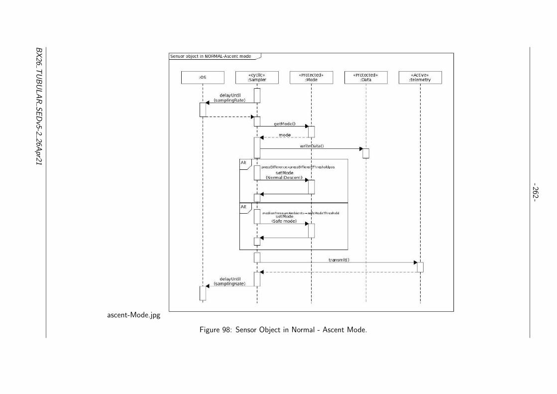
-262-
ascent-Mode.jpg
Figure 98: Sensor Object in Normal - Ascent Mode.
BX
26T
UB
UL
AR
SE
Dv5-2
26Apr21

-263-
Figure 99: Sensor Object in Normal - Descent Mode.
BX
26T
UB
UL
AR
SE
Dv5-2
26Apr21

- 264 -
C.10 Software Interface Diagram
C.10.1 Sensor Object Interface Diagram
Figure 100: Sensor Object Interface Diagram.
BX26 TUBULAR SEDv5-2 26Apr21

- 265 -
C.10.2 Air Sampling Control Object Interface Diagram
Figure 101: Air Sampling Control Object Interface Diagram.
BX26 TUBULAR SEDv5-2 26Apr21

- 266 -
C.10.3 Heating Object Interface Diagram
Figure 102: Heating Object Interface Diagram.
BX26 TUBULAR SEDv5-2 26Apr21

- 267 -
C.11 PCB Schematics
Red is traces pulled on the top layer and blue are the traces on the bottom layer.
Figure 103: Main PCB Top layer Layout in Eagle.
BX26 TUBULAR SEDv5-2 26Apr21

- 268 -
Figure 104: Main PCB bottom layer Layout in Eagle.
BX26 TUBULAR SEDv5-2 26Apr21
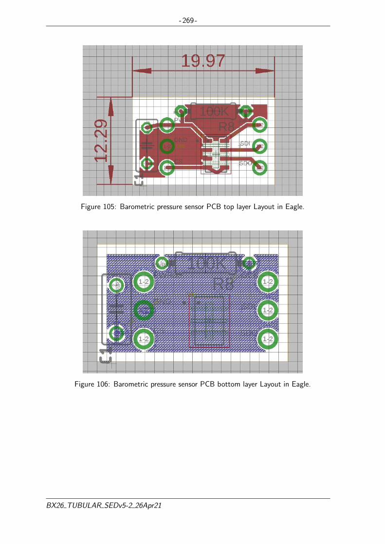
- 269 -
Figure 105: Barometric pressure sensor PCB top layer Layout in Eagle.
Figure 106: Barometric pressure sensor PCB bottom layer Layout in Eagle.
BX26 TUBULAR SEDv5-2 26Apr21

314 www.restek.com
GCACCESSORIES| GAS MANAGEMENT
Tubing
*The availability of long lengths is subject to inventory constraints. Lead times may vary depending on the continuous length needed. Please inquire before ordering. Maximum continuous lengths are: 200** ft (cat.# 29201, 29209), 2,000 ft (cat.# 29217, 29225, 29233, 29241), 1,150 ft (cat.# 29249), and 750 ft (cat.# 29257). Pricing for lengths of 101 ft or more is on a per foot basis.**Contact us if longer length is needed for cat.# 29201 or 29209.
Treated Welded/Drawn 304 Grade Stainless Steel TubingOur most popular grade of tubing. Recommended for:• Chromatography applications.• Gas delivery systems.• Lower pressures.• Inert applications. Maximum temperature of 450 °C in an inert atmosphere.
An extra charge is applied for cutting Sulfinert® or Silcosteel®-CR tubing. The charge is calculated from the total number of pieces produced for each line item.
ordering noteRequired length in meters x 3.2808 = length in feet.
*The availability of long lengths is subject to inventory constraints. Lead times may vary depending on the continuous length needed. Please inquire before ordering. 1/8" OD: 1,500 ft in one continuous coil; 1/4" OD: 750 ft in one continuous coil; 3/8" OD: 250 ft in one continuous coil. Longer lengths will be more than one coil. Pricing for lengths of 101 ft or more is on a per foot basis.
Treated Seamless 316L Grade Stainless Steel TubingHigh durability tubing. Recommended for:• Inert applications.• High temperatures.• High pressures.• Corrosive environments. • Zero bleed. Length Wall 6 Feet 10 Feet 15 Feet 20 Feet 25 Feet 50 Feet 100 Feet >100 FeetID OD Thickness cat.# cat.# cat.# cat.# cat.# cat.# cat.# cat.#*Silcosteel®-CR Treated (Coiled) 0.055" (1.40 mm) 1/8" (3.18 mm) 0.035" 29091 29092 29093 29094 29095 29096 29097 29098 0.180" (4.57 mm) 1/4" (6.35 mm) 0.035" 29099 29100 29101 29102 29103 29104 29105 29106 0.277" (7.04 mm) 3/8" (9.52 mm) 0.049" 29107 29108 29109 29110 29111 29112 29113 29114 Sulfinert® Treated (Coiled) 0.055" (1.40 mm) 1/8" (3.18 mm) 0.035" 29067 29068 29069 29070 29071 29072 29073 29074 0.180" (4.57 mm) 1/4" (6.35 mm) 0.035" 29075 29076 29077 29078 29079 29080 29081 29082 0.277" (7.04 mm) 3/8" (9.52 mm) 0.049" 29083 29084 29085 29086 29087 29088 29089 29090
Length Wall 6 Feet 10 Feet 15 Feet 20 Feet 25 Feet 50 Feet 100 Feet >100 Feet
ID OD Thickness cat.# cat.# cat.# cat.# cat.# cat.# cat.# cat.#*Sulfinert® Treated (Coiled)
0.011" (0.28 mm) 0.022" (0.56 mm) 29194 29195 29196 29197 29198 29199 29200 29201
0.021" (0.53 mm) 0.029" (0.74 mm) 29202 29203 29204 29205 29206 29207 29208 29209
0.010" (0.25 mm) 1/16" (1.59 mm) 29210 29211 29212 29213 29214 29215 29216 29217
0.020" (0.51 mm) 1/16" (1.59 mm) 29218 29219 29220 29221 29222 29223 29224 29225
0.030" (0.76 mm) 1/16" (1.59 mm) 29226 29227 29228 29229 29230 29231 29232 29233
0.040" (1.02 mm) 1/16" (1.59 mm) 29234 29235 29236 29237 29238 29239 29240 29241
0.085" (2.16 mm) 1/8" (3.18 mm) 0.020" 29242 29243 29244 29245 29246 29247 29248 29249
0.210" (5.33 mm) 1/4" (6.35 mm) 0.020" 29250 29251 29252 29253 29254 29255 29256 29257
- 270 -
C.12 Tube
BX26 TUBULAR SEDv5-2 26Apr21

Configuration symbol
Port sizeSizeOrifice
diameter[mmø]
Model
Maximum operatingpressure differential [MPa]
0.7
0.4
0.2
80
1.6
2.3
3.2
M5, 1/82
C [dm3/(s·bar)] b
0.07
0.18
0.30
0.45
0.45
0.38
0.30
0.58
1.10
Cv
Flow-rate characteristics
Normally Closed (N.C.)Aluminium Body Type
VDW20
Resin Body Type (Built-in One-touch Fittings)
Model/Valve Specifications
N.C.
Weight[g]
Port sizeSizeOrifice
diameter[mmø]
ModelMaximum operating
pressure differential [MPa]
0.9
0.4
0.7
0.4
0.2
1.0
1.6
1.6
2.3
3.2
M5ø3.2 One-touch fittingø4 One-touch fitting
M5ø4 One-touch fittingø6 One-touch fitting
1
2
C [dm3/(s·bar)] b Pressurized port 1
Pressurized port 1
0.04
0.07
0.07
0.18
0.30
0.40
0.25
0.45
0.45
0.38
0.14
0.30
0.30
0.58
1.10
Cv
Flow-rate characteristics
VDW10
VDW20
Weight[g]
Refer to “Glossary of Terms” on page 11 for details on the maximum operating pressure differential.
Fluid and Ambient Temperature
Note) Dew point temperature: –10°C or less
Note) The configuration symbol shows ports 1 and 2 as blocked, but there is actually a limit to the blocking capability when the pressure of port 2 is greater than the pressure of port 1. Please contact SMC when low leakage performance is required.
−10 to 50
Ambient temperature [°C]Fluid temperature [°C]
−10 Note) to 50
Valve LeakageInternal Leakage
Note) Leakage is the value at ambient temperature 20°C.
External Leakage
NBR
Seal material Leakage rate (Air) Note)
1 cm3/min or less (AIuminium body type)
15 cm3/min or less (Resin body type)
NBR
Seal material Leakage rate (Air) Note)
1 cm3/min or less (AIuminium body type)
15 cm3/min or less (Resin body type)
45
80
21
Single UnitFor Air
Series VDW
2
- 271 -
C.13 AAC Manifold Valve
BX26 TUBULAR SEDv5-2 26Apr21

5
VDW20 15A 1
Bracket assembly part no.• Series 20
VCW20 12 01A• Series 30
VDW21-F VDW31-F
0.8
936.5
17.5
8.5
(6.3
)
0.8
929.6
14.3
8
*-***-*-*VDW31-*F-
36 (27.6)
10.5
55.8
(for grounding)M3.5
12.8
2 x M4 x 6
14
6.35
40
30
34 25
4-ø5SMC
66 (
62.5
)
28
6
1 (IN) port1/8, 1/4
2 (OUT) port
1/8, 1/4
*-***-*-*VDW21-*F-
22
46.2
6.7
(for grounding)M3.5
11.46.
35
27
27
20
20
(Bracket mounting hole)2 x ø3.5
56
20.5
5
2 (OUT) port
M5, 1/8
1 (IN) portM5, 1/8
15
2 x M3 x 5
Dimensions
Series VDW10/20/30Compact Direct Operated2 Port Solenoid Valve For Water and Air
Series VDW10/20/30 2-port type has been remodeled to new compact and lightweight series.For details about new series, refer to New VDW for VDW10/20 and to Series VX21 for VDW30, respectively.
- 272 -
C.14 AAC Flushing Valve and CAC Valve
BX26 TUBULAR SEDv5-2 26Apr21
6
How to Order Manifold
VV2DW 2 05 01 How to Order Manifold Assembly
Enter the mounting valve and option part numbers under the manifold base part number.
<Ordering example>VV2DW2-0501 ········
∗VDW23-5G-2 ·········
1 set
5 sets
Manifold part no.
Valve part no.(Stations 1 to 5)
123
102030
Series
123
102030
Series
3 N.C. for manifold
Valve type
-FN
RcG
NPT
Thread type
Symbol
M50102
Port size
M51/8 (6A)1/4 (8A)
10––
Series20–
30–
OUT port size
VVDW 0 3A2
VDW 2 3 5 2G
12123234
SymbolOrifice diameter
(mmø)11.61.62.33.2234
10
20
30
Series
Orifice size
Blanking plate assembly
MaterialSymbol
-ABGHJ
Manifold material
Brass (C37)
Stainlesssteel
Seal materialNBRFKM
EPDMNBRFKM
EPDM
• Series 10, 20
VVCW20 3A• Series 30
1
D side
2
3
4
5U side
Symbol-ABGHJ
L Note)
Body material
Brass (C37)
Stainlesssteel
Seal materialNBRFKM
EPDMNBRFKM
EPDMFKM
Coil insulation
Material and insulation type
Class B
02
10
2 stations
10 stations
Stations
-F
NoneWith bracket
Option
Note) Series 30 is available with bracket only.
Note) IN port sizes are as follows.10: 1/8 (6A)20: 1/4 (8A)30: 3/8 (10A)
Enter together in order, counting from station 1 on the D side.
How to Order Valves (For manifold)
Manifold Options
12
1020
Series
∗ Plate material is stainless steel only.
MaterialSymbol
GHJ
Plate material
Stainless steel
Seal materialNBRFKM
EPDM
MaterialSymbol
GHJ
Plate material
Stainless steel
Seal materialNBRFKM
EPDM
GFW
Grommet / Tape windingFastonTM terminal / MoldedGrommet / Molded
Coil type Note)
123456VSR
VoltageSymbol
100 VAC (50/60 Hz)200 VAC (50/60 Hz)110 VAC (50/60 Hz)220 VAC (50/60 Hz) 24 VDC 12 VDC 6 VDC 5 VDC 3 VDC
Grommet /Tape
winding
FastonTM
terminal,Molded
Grommet /Molded
Voltage
∗ Please consult with SMC regarding other voltages.
Note) For series and coil type combinations, refer to page 1.
Note) For deionized water: the armature assembly is a corrosion resistant construction.
“∗” is the symbol for assembly. Add an “∗” in front of the part numbers to have solenoid valves, etc. mounted on the manifold.
Q
Q
Series VDW10/20/30

7
Dimensions
VV2DW1
4 x M3
8.1
n x M5(OUT port)
L1
L3
L2
13.4
3.4
1R1.7
16.3
2 x ∗1/8 (IN port)(∗: Thread type)
16
VDW13-*G-* VDW13-*G-* VDW13-*G-* VDW13-*G-*
8.8 P = 17.5 8.8
(19.
6)
11.5
7.7
(16.
3)
5
7.7
11.5
61
7.7 P = 17.5 1.5
13 19.6
24.4
2.8
22.5 40 7.5
26.5
(2.8
)
34
(4.4
)
9.4
≈ 30
0
30
(1.5)
2
35
45
52
2 stns. x 1
Dimension
L1
L2
L3
L Dimension
3
52.5
62.5
69.5
3 stns. x 1
4
70
80
87
2 stns. x 2
5
87.5
97.5
104.5
2 stns. + 3 stns.
6
105
115
122
3 stns. x 2
7
122.5
132.5
139.5
2 stns. x 2 + 3 stns.
8
140
150
157
2 stns. + 3 stns. x 2
9
157.5
167.5
174.5
3 stns. x 3
10
175
185
192
2 stns. x 2 + 3 stns. x 2
(mm)
n (stations)
Manifold composition
1StationsD side 2 3 4 5 n U side
∗ When w/o bracket, M3 threads at both ends (4 locations) can be used for other purposes.
Note) The manifold base consists of a junction of 2 and 3 station bases. Refer to page 10 and 11 regarding manifold additions.
Series VDW10/20/30Compact Direct Operated2 Port Solenoid Valve For Water and Air

NMP850K_DC-B NMP850.1.2KPDC-B
NMP850KPDC-B
NMP850KTDC-B NMP850.1.2KPDC-B
PERFORMANCE DATA
Type KNF DC motor,
brushless
(V)
Delivery
at atm. pressure
(l/min)1)
Max. operating
pressure
(bar)
Ultimate
vacuum
(mbar abs.)
NMP850KPDC-B 12 4.2 1.5 230
NMP850KTDC-B 12 3.5 1.5 300
NMP850KPDC-B 24 4.2 1.5 230
NMP850KTDC-B 24 3.5 1.5 300
1) Liter at STP
PUMP MATERIAL
Type Pump head Diaphragm Valves
NMP850KPDC-B PPS EPDM EPDM
Chemically resistant version
NMP850KTDC-B PPS PTFE-coated FFPM
PERFORMANCE DATA
Type KNF DC motor,
brushless
(V)
Delivery
at atm. pressure
(l/min)1)
Max. operating
pressure
(bar)
Ultimate
vacuum
(mbar abs.)
NMP850.1.2KPDC-B 12 8.0 1.5 230
NMP850.1.2KPDC-B 24 8.0 1.5 230
PUMP MATERIAL
Type Pump head Diaphragm Valves
NMP850.1.2KPDC-B PPS EPDM EPDM
barmbar
Vacuum atm. pressure pressure
Flo
w c
ap
acit
y l
/min
(Liter
at
ST
P)
0 200 400 600 800
4.5
4.0
3.5
3.0
2.5
2.0
1.5
1.0
0.5
00 0.5 1.0 1.5 2.0
barmbar
Vacuum atm. pressure pressure
Flo
w c
ap
acit
y l
/min
(Liter
at
ST
P)
0 200 400 600 800
4.5
4.0
3.5
3.0
2.5
2.0
1.5
1.0
0.5
0
0 0.5 1.0 1.5 2.0
barmbar
Vacuum atm. pressure pressure
Flo
w c
ap
acit
y l
/min
(Liter
at
ST
P)
0 200 400 600 800
10.0
9.0
8.0
7.0
6.0
5.0
4.0
3.0
2.0
1.0
00 0.5 1.0 1.5 2.0
- - - - for short periods only
- - - - for short periods only- - - - for short periods only
- 275 -
C.15 Pump
BX26 TUBULAR SEDv5-2 26Apr21
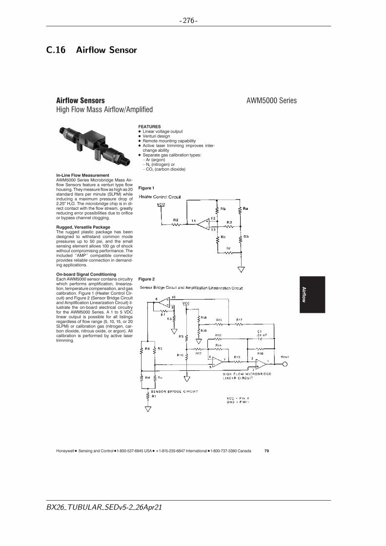
Airflow Sensors AWM5000 SeriesHigh Flow Mass Airflow/Amplified
Honeywell 1 Sensing and Control 1 1-800-537-6945 USA 1 F1-815-235-6847 International 1 1-800-737-3360 Canada 79
In-Line Flow MeasurementAWM5000 Series Microbridge Mass Air-flow Sensors feature a venturi type flowhousing. They measure flow as high as 20standard liters per minute (SLPM) whileinducing a maximum pressure drop of2.25N H2O. The microbridge chip is in di-rect contact with the flow stream, greatlyreducing error possibilities due to orificeor bypass channel clogging.
Rugged, Versatile PackageThe rugged plastic package has beendesigned to withstand common modepressures up to 50 psi, and the smallsensing element allows 100 gs of shockwithout compromising performance. Theincluded ‘‘AMP’’ compatible connectorprovides reliable connection in demand-ing applications.
On-board Signal ConditioningEach AWM5000 sensor contains circuitrywhich performs amplification, lineariza-tion, temperature compensation, and gascalibration. Figure 1 (Heater Control Cir-cuit) and Figure 2 (Sensor Bridge Circuitand Amplification Linearization Circuit) il-lustrate the on-board electrical circuitryfor the AWM5000 Series. A 1 to 5 VDClinear output is possible for all listingsregardless of flow range (5, 10, 15, or 20SLPM) or calibration gas (nitrogen, car-bon dioxide, nitrous oxide, or argon). Allcalibration is performed by active lasertrimming.
FEATURES1 Linear voltage output1 Venturi design1 Remote mounting capability1 Active laser trimming improves inter-
change ability1 Separate gas calibration types:
– Ar (argon)– N2 (nitrogen) or– CO2 (carbon dioxide)
Figure 1
Figure 2
Airflo
w
- 276 -
C.16 Airflow Sensor
BX26 TUBULAR SEDv5-2 26Apr21
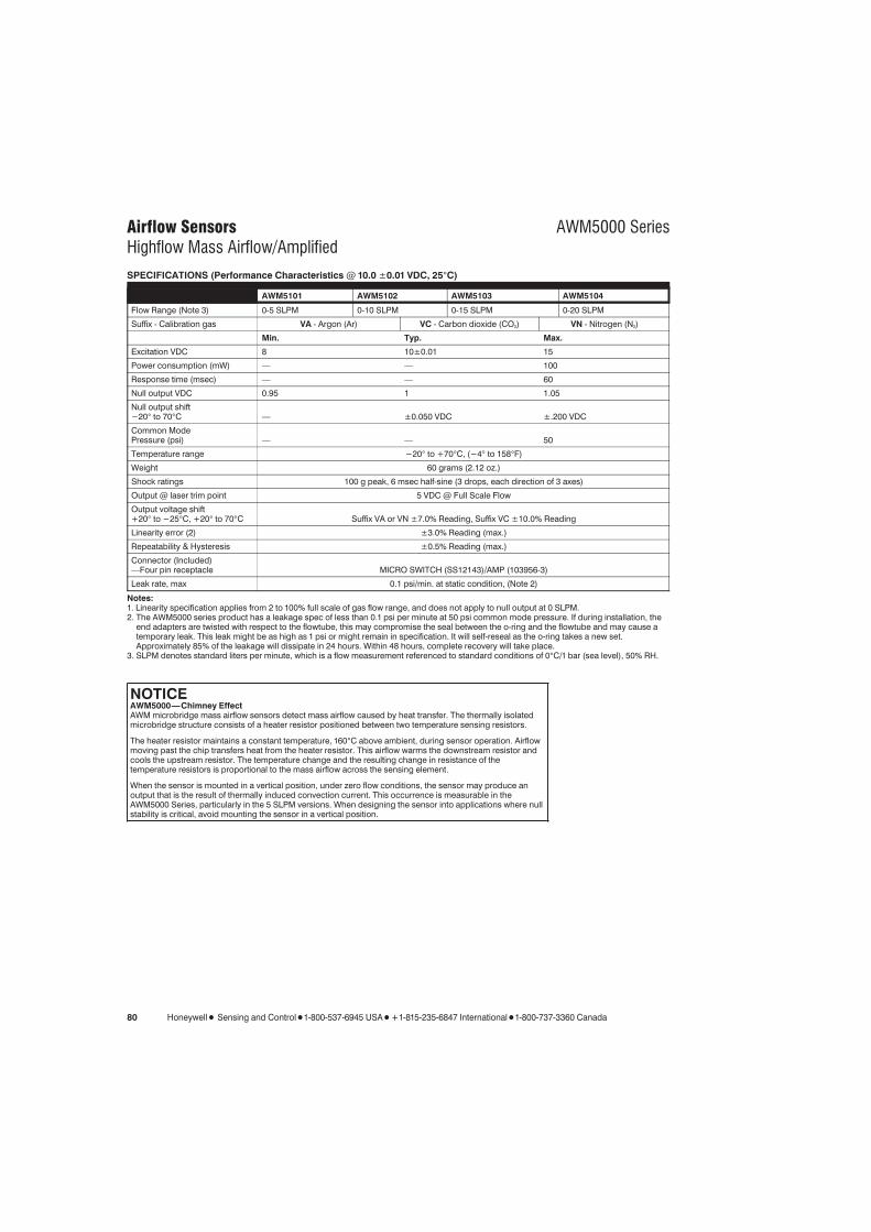
Airflow Sensors AWM5000 SeriesHighflow Mass Airflow/Amplified
80 Honeywell 1 Sensing and Control 1 1-800-537-6945 USA 1 F1-815-235-6847 International 1 1-800-737-3360 Canada
SPECIFICATIONS (Performance Characteristics @ 10.0 ±0.01 VDC, 25°C)
AWM5101 AWM5102 AWM5103 AWM5104
Flow Range (Note 3) 0-5 SLPM 0-10 SLPM 0-15 SLPM 0-20 SLPM
Suffix - Calibration gas VA - Argon (Ar) VC - Carbon dioxide (CO2) VN - Nitrogen (N2)
Min. Typ. Max.
Excitation VDC 8 10±0.01 15
Power consumption (mW) — — 100
Response time (msec) — — 60
Null output VDC 0.95 1 1.05
Null output shift−20° to 70°C — ±0.050 VDC ±.200 VDC
Common ModePressure (psi) — — 50
Temperature range −20° to +70°C, (−4° to 158°F)
Weight 60 grams (2.12 oz.)
Shock ratings 100 g peak, 6 msec half-sine (3 drops, each direction of 3 axes)
Output @ laser trim point 5 VDC @ Full Scale Flow
Output voltage shift+20° to −25°C, +20° to 70°C Suffix VA or VN ±7.0% Reading, Suffix VC ±10.0% Reading
Linearity error (2) ±3.0% Reading (max.)
Repeatability & Hysteresis ±0.5% Reading (max.)
Connector (Included)—Four pin receptacle MICRO SWITCH (SS12143)/AMP (103956-3)
Leak rate, max 0.1 psi/min. at static condition, (Note 2)
Notes:1. Linearity specification applies from 2 to 100% full scale of gas flow range, and does not apply to null output at 0 SLPM.2. The AWM5000 series product has a leakage spec of less than 0.1 psi per minute at 50 psi common mode pressure. If during installation, the
end adapters are twisted with respect to the flowtube, this may compromise the seal between the o-ring and the flowtube and may cause atemporary leak. This leak might be as high as 1 psi or might remain in specification. It will self-reseal as the o-ring takes a new set.Approximately 85% of the leakage will dissipate in 24 hours. Within 48 hours, complete recovery will take place.
3. SLPM denotes standard liters per minute, which is a flow measurement referenced to standard conditions of 0°C/1 bar (sea level), 50% RH.
NOTICEAWM5000—Chimney EffectAWM microbridge mass airflow sensors detect mass airflow caused by heat transfer. The thermally isolatedmicrobridge structure consists of a heater resistor positioned between two temperature sensing resistors.
The heater resistor maintains a constant temperature, 160°C above ambient, during sensor operation. Airflowmoving past the chip transfers heat from the heater resistor. This airflow warms the downstream resistor andcools the upstream resistor. The temperature change and the resulting change in resistance of thetemperature resistors is proportional to the mass airflow across the sensing element.
When the sensor is mounted in a vertical position, under zero flow conditions, the sensor may produce anoutput that is the result of thermally induced convection current. This occurrence is measurable in theAWM5000 Series, particularly in the 5 SLPM versions. When designing the sensor into applications where nullstability is critical, avoid mounting the sensor in a vertical position.

Airflow Sensors AWM5000 SeriesHigh Flow Mass Airflow/Amplified
Honeywell 1 Sensing and Control 1 1-800-537-6945 USA 1 F1-815-235-6847 International 1 1-800-737-3360 Canada 81
OUTPUT CURVES (Performance Characteristics @ 10.0 ±0.01 VDC, 25°C)
Airflo
w

Airflow Sensors AWM5000 SeriesHighflow Mass Airflow/Amplified
82 Honeywell 1 Sensing and Control 1 1-800-537-6945 USA 1 F1-815-235-6847 International 1 1-800-737-3360 Canada
AWM5000 ORDER GUIDE
Catalog Listing Flow Range
AWM5101VA 5 SLPM, Argon calibration
AWM5101VC 5 SLPM, CO2 calibration (2)
AWM5101VN 5 SLPM, N2 calibration (1)
AWM5102VA 10 SLPM, Argon calibration
AWM5102VC 10 SLPM, CO2 calibration (2)
AWM5102VN 10 SLPM, N2 calibration (1)
AWM5103VA 15 SLPM, Argon calibration
AWM5103VC 15 SLPM, CO2 calibration (2)
AWM5103VN 15 SLPM, N2 calibration (1)
AWM5104VA 20 SLPM, Argon calibration
AWM5104VC 20 SLPM, CO2 calibration (2)
AWM5104VN 20 SLPM, N2 calibration (1)
CONNECTOR ORDER GUIDE
Catalog Listing Description
SS12143 Four pin Electrical connectorConnectors use Amp 103956-3
Note: All listings have 1 - 5 VDC linear output with 10 VDC supply over given flow range for aspecific calibration gas.1. N2 calibration is identical to 02 and air calibration.2. CO2 calibration is identical to N2O calibration.3. For additional gas correction factors, see Application Note 3.
OUTPUT CONNECTIONSPin 1 + Supply voltagePin 2 GroundPin 3 No connectionPin 4 Output voltageArrow on bottom of housing indicates direction of flow.
MOUNTING DIMENSIONS (for reference only)

H-76
PR
ESSUR
E TRA
NSD
UCER
S
Visit www.GemsSensors.com for most current information. 3500 Series / p1of4 / 14-JUL-15
GEMS COMPLIANT®
Ro HS
GEMS COMPLIANT®
Ro HS
3500 SeriesCompact Low Pressure OEM Pressure Transmitters 5 to 600 psi pressure ranges (0.35 to 40 bar) Choice of outputs, electrical connections and pressure ports Operating temperature up to 257°F (125°C)
For OEMs that need consistent high levels of performance, reliability and stability the 3500 Series units offer a small package size with all stainless steel wetted parts at an unbeatable price performance ratio. A wide choice of electrical outputs as well as both electrical and pressure connections means the unit is suitable for most applications without modification. The compact construction of the 3500 Series makes it ideal for installation where space is at a premium.
SpecificationsInput
Pressure Range 5-600 psi (0.35-40 bar)Proof Pressure 2xBurst Pressure 3X
PerformanceLong Term Drift <0.2% FS/YR
Accuracy 0.25% FSThermal Error, Max. ±1% / 176°F (80°C)Compensated Temperatures -4°F to +212°F (-20°C to +100°C)Operating Temperatures -40°F to +257°F (-40°C to +125°C)Zero Tolerance, Max. ±0.5% of spanSpan Tolerance, Max. ±0.5% of spanFatigue Life Designed for more than 100 M cycles
Mechanical ConfigurationPressure Port See under “How to Order,” last pageWetted Parts 316L Stainless SteelElectrical Connection See under “How to Order,” last page
Enclosure IP67 Vibration BSEN 60068-2-6 (FC)
BSEN 60068-2-64 (FH) Shock BSEN 60068-2-27 (Ea) Approvals CE, RoHS Weight 1.23 to 1.9 ounces (35-53 grams). Configuration dependant
Individual SpecificationsVoltage Output 0V min. to 10V max.
See under “How to Order,” last pageSupply Voltage (Vs) 2 Volts above full scale to 30 Vdc
(24 Vdc, max. above 230°F (110°C) applications)Source and Sinks 8 mA
Current Output 4-20 mA
Supply Voltage (Vs) 10-30 Vdc (24 Vdc, max. above 230°F (110°C) applications)Maximum Load Resistance (Supply Voltage -10) x 50ohms
Ratiometric Output 0.5 to 4.5V
Supply Voltage (Vs) 5 Vdc ±10%
EMC SpecificationsEmissions Tests: EN61326-1:2006 and EN61326-2-3:2006EN55011:2009 + A1 Radiated Emissions
Immunity Tests: EN61326-1:2006 and EN61326-2-3:2006EN61000-4-2:2009 Electrostatic DischargeEN61000-4-3:2006 + A2 Radiated ImmunityEN61000-4-4:2012 Fast Burst TransientsEN61000-4-6:2009 Conducted RF Immunity
- 280 -
C.17 Static Pressure Sensor
BX26 TUBULAR SEDv5-2 26Apr21

H-77
PR
ESSU
RE
TRA
NSD
UCE
RS
Visit www.GemsSensors.com for most current information.3500 Series / p2of4 / 14-JUL-15
MMS TYPE
BSP & Metric
G1/8˝ External G1/4˝-19 External w/O-Ring
G1/4˝-19 A Integral Face Seal M12 x 1.5 w/O-Ring
Dimensions in MM
Fitting Code OS 01 05 OL
Torque 22-25 NM 30-35 NM 30-35 NM 28-30 NM
* NPT Threads 2-3 turns from finger tight. Wrench tighten 2-3 turns.
General Notes:1. The diameter of all cans is 19 mm (0.748˝)2. Hex is 22 mm (0.886˝) Across Flats (A/F) for deep socket mounting
Pressure PortsSAE
1/8˝-27 NPT 1/4˝-18 NPT 7/16˝-20 UNF with 37° Flare 7/16˝-20 UNF 1/8˝-27 NPTF
Dimensions in Inches
Fitting Code 08 02 04 1J 4D
Torque 2-3 TFFT* 2-3 TFFT* 15-16 NM 18-20 NM 2-3 TFFT*
G1/4˝ External
01
11.0
13.1
G1/8˝ External
OS
11.0
13.1
G1/4"A Integral Face Seal
05
12.5 11.0
13.1
OL
ISO 6149-2:M12 x 1.5
11.0
13.1
1/8"-27 NPT
08
0.52
0.39
1/4"-18 NPT
02
0.57
0.52
Wiring Diagram
POWER SUPPLY
READOUT
(-) (+)
(-) (+) IN (+)
COMMON
OUT(+)
VOLTAGEOUTPUT
TRANSDUCER
POWER SUPPLY
READOUT
(-) (+)
(-) (+)CURRENTOUTPUT
TRANSDUCER
+
(-)
7/16” -20 UNF
3500 1J
0.43
0.52
0.5
1/8”-27 NPTF
3500 4D
0.37
0.52
7/16”-20 UNF with 37° Flare
3500 04
0.55
0.52

H-78
PR
ESSUR
E TRA
NSD
UCER
S
Visit www.GemsSensors.com for most current information. 3500 Series / p3of4 / 14-JUL-15
inch(mm)
DIN 9.4 mm M12 x 1P Deutsch DT04-4P DIN 43650A Packard MetriPack
Code B Code K Code E Code 8 Code G Code 9
Pin#
VoltageMode
CurrentMode
VoltageMode
CurrentMode
VoltageMode
CurrentMode
VoltageMode
CurrentMode
VoltageMode
CurrentMode
PinID
VoltageMode Note
1 Vout(pressure)
NoConnect Vsupply Supply Vsupply Supply Ground Return Vsupply Supply C Vout
(pressure)MetriPack connectors
may be used with 0.5-4.5V
Ratiometric and 4-20 mA only.
2 Vsupply Supply Ground Return Vout (pressure)
NoConnect Vsupply Supply Ground Return A Ground
3 No Connect
NoConnect
Vout NoConnect Ground Return No
ConnectNo
ConnectVout No
Connect B Vsupply
4 Ground Return No Connect
NoConnect
NoConnect
NoConnect
Vout (pressure)
NoConnect
No Connect
NoConnect — —
2
3
4
1
POLARIZINGWIDE CONTACT
0.86(21.9)
1
3
42
0.4(10.1)
0.72(18.3)
KEY
4
1
3
2
1.538.1
0.071.9
Electrical Connector
AB
C
1.52(38.6)
Mating Connectors
Part Number Description For Use on Elect. Code #
557230 MINI DIN Connector, Strain Relief (with drive screw & gasket) B and K557254 Large DIN 43650A G557703-01M0 M12 Cord Set – 1 Meter (Red 1, Green 2, Blue 3, Yellow 4) E557703-03M0 M12 Cord Set – 3 Meters (Red 1, Green 2, Blue 3, Yellow 4) E557703-04M0 M12 Cord Set – 4 Meters (Red 1, Green 2, Blue 3, Yellow 4) E557703-05M0 M12 Cord Set – 5 Meters (Red 1, Green 2, Blue 3, Yellow 4) E
Recommended Mating Parts (Deutsch p/n: Housing Plug DT064S-P012; Wedge W4S-P012; Sockets 4X 0462-201-1631) 8224153 Deutsch Cord Set 3´ Long (18 AWG PVC Cable – Black 1, Red 2, Green 3, White 4) 8
Recommended Mating Parts (Delphi Packard MetriPack p/n: Body 12065286; Seal 12052893. Consult Delphi for Contacts) 9218760 Packard Mate Kit 9223974 Packard Cord Set 3´ Long (24 AWG PVC Cable – White 1, Black 2, Red 3) 9223975 Packard Cord Set 6´ Long (24 AWG PVC Cable – White 1, Black 2, Red 3) 9227987 Packard Cord Set 14.75' Long (22 AWG PVC Cable - White 1, Black 2, Red 3) 9220492 Packard Mate - 12˝ Flying Leads – 3 Conductor PVC 18 AWG 9222976 Packard Mate - 18˝ Flying Leads – 3 Conductor PVC 18 AWG 9220797 Packard Mate - 24˝ Flying Leads – 3 Conductor PVC 18 AWG 9
3
E
2 1
1.57(40.0)
Ø0.84(21.3)

- 283 -
Appendix D Checklists
The Pre-Launch Checklist will be taken care of by two team members. One of them will beresponsible of reading out loud each item and marking them when they are done. The otherone will be responsible for performing the stated actions. At the same time, the one readingwill check that the actions are properly conducted.
For three key actions (M5, M9 and M13), a third team member will be responsible of askingand, when possible, checking, that they have been properly conducted.
D.1 Pre-Launch Checklist
ID ITEM CHECKSCIENCE
CAC
S1Remove the CAC wall with the D-SUB connector, if it’s not re-moved already.
S2 Connect picarro to quick connector stem at No 10.
S3Attach the fill gas bottle’s quick connector stem to quick connectorbody No 1.
S4 Let the fill gas run through the AirCore at a flow rate of 40ml/min.S5 Leave it flushing over night.S6 Detach quick connector stem at No 1.S7 Detach the quick connector stem at No 10.S8 Disconnect the picarro analyser.S9 Connect the dryer tube No 14 to No 13.S10 Connect parts 11 to 21.S11 Check all connections are tighten.S12 Close the CAC’s solenoid valve No 17.S13 Connect quick connector stem No 10 to No 9.S14 Connect No 10 with No 11.S15 Check all connections are tighten.S16 Put the CAC wall with the D-SUB connector back.
AAC/MANIFOLDS17 Unscrew the plug from the inlet (1) and outlet tube (29).S18 Screw in the male threaded quick connector to the inlet tube (1).
S19Connect the vacuum pump and the dry gas bottle through a cen-tral valve to the AAC’s inlet tube (1).
S20 Open flushing valve (27).S21 Turn central valve on so that is open to dry gas.S22 Let the dry gas run through the AAC’s manifold for 10 minutes.S23 Close flushing valve (27)S24 Turn central valve off so that is close to dry gas.
S25Disconnect the vacuum pump and the dry gas bottle through acentral valve from the AAC’s inlet tube (1).
BX26 TUBULAR SEDv5-2 26Apr21

- 284 -
S26 Screw in the plug to the AAC inlet tube (1).AAC/TUBES/BAGS
S27Connect the vacuum pump and the dry gas bottle through a cen-tral valve to the AAC’s outlet tube (29).
S28 Make sure the AAC’s inlet tube (1) is shielded.S29 Open 1st bag’s manual valve.S30 Open flushing valve (27).S31 Open 1st bag’s solenoid valve in the manifold (23)S32 Open central valve so that is open to dry gas.
S33Start filling the bag with 3L of dry gas with a flow rate of 2L/minfor 1.5 minutes.
S34After 1.5 mins, when the bag is full, turn the central valve opento the vacuum , allowing the bag to empty.
S35Empty the bag with controlled vacuum only 1-2 mbar below am-bient pressure.
S36 Turn the central valve open to dry gas.
S37Start filling the bag with 3L of dry gas with a flow rate of 2L/minfor 1.5 minutes.
S38After 1.5 mins, when the bag is full, turn the central valve opento the vacuum , allowing the bag to empty.
S39Empty the bag with controlled vacuum only 1-2 mbar below am-bient pressure.
S40 Repeat steps S36 to S39 one more time.S41 Close 1st bag’s solenoid valve in the manifold (23).
S42Disconnect the vacuum pump and the dry gas bottle through acentral valve from the AAC’s outlet tube (29).
S43 Unscrew the plug from the AAC inlet tube (1).
S44Connect the vacuum pump and the dry gas bottle through a cen-tral valve to the AAC’s inlet tube (1).
S45 Turn central valve on so that is open to dry gas.S46 Let the dry gas run through the AAC’s manifold for 2 minutes.S47 Close flushing valve (27)S48 Turn central valve off so that is close to dry gas.
S49Disconnect the vacuum pump and the dry gas bottle through acentral valve from the AAC’s inlet tube (1).
S50 Screw in the plug to the AAC inlet tube (1).
S51Connect the vacuum pump and the dry gas bottle through a cen-tral valve to the AAC’s outlet tube (29).
S52 Make sure the AAC’s inlet tube (1) is shielded.S53 Open 2nd bag’s manual valve.S54 Open flushing valve (27).S55 Open 2nd bag’s solenoid valve in the manifold (23)S56 Open central valve so that is open to dry gas.
S57Start filling the bag with 3L of dry gas with a flow rate of 2L/minfor 1.5 minutes.
BX26 TUBULAR SEDv5-2 26Apr21

- 285 -
S58After 1.5 mins, when the bag is full, turn the central valve opento the vacuum , allowing the bag to empty.
S59Empty the bag with controlled vacuum only 1-2 mbar below am-bient pressure.
S60 Turn the central valve open to dry gas.
S61Start filling the bag with 3L of dry gas with a flow rate of 2L/minfor 1.5 minutes.
S62After 1.5 mins, when the bag is full, turn the central valve opento the vacuum , allowing the bag to empty.
S63Empty the bag with controlled vacuum only 1-2 mbar below am-bient pressure.
S64 Repeat steps S60 to S63 one more time.S65 Close 2nd bag’s solenoid valve in the manifold (23).
S66Disconnect the vacuum pump and the dry gas bottle through acentral valve from the AAC’s outlet tube (29).
S67 Unscrew the plug from the AAC inlet tube (1).
S68Connect the vacuum pump and the dry gas bottle through a cen-tral valve to the AAC’s inlet tube (1).
S69 Turn central valve on so that is open to dry gas.S70 Let the dry gas run through the AAC’s manifold for 2 minutes.S71 Close flushing valve (27)S72 Turn central valve off so that is close to dry gas.
S73Disconnect the vacuum pump and the dry gas bottle through acentral valve from the AAC’s inlet tube (1).
S74 Screw in the plug to the AAC inlet tube (1).
S75Connect the vacuum pump and the dry gas bottle through a cen-tral valve to the AAC’s outlet tube (29).
S76 Make sure the AAC’s inlet tube (1) is shielded.S77 Open 3rd bag’s manual valve.S78 Open flushing valve (27).S79 Open 3rd bag’s solenoid valve in the manifold (23)S80 Open central valve so that is open to dry gas.
S81Start filling the bag with 3L of dry gas with a flow rate of 2L/minfor 1.5 minutes.
S82After 1.5 mins, when the bag is full, turn the central valve opento the vacuum , allowing the bag to empty.
S83Empty the bag with controlled vacuum only 1-2 mbar below am-bient pressure.
S84 Turn the central valve open to dry gas.
S85Start filling the bag with 3L of dry gas with a flow rate of 2L/minfor 1.5 minutes.
S86After 1.5 mins, when the bag is full, turn the central valve opento the vacuum , allowing the bag to empty.
S87Empty the bag with controlled vacuum only 1-2 mbar below am-bient pressure.
BX26 TUBULAR SEDv5-2 26Apr21

- 286 -
S88 Repeat steps S84 to S87 one more time.S89 Close 3rd bag’s solenoid valve in the manifold (23).
S90Disconnect the vacuum pump and the dry gas bottle through acentral valve from the AAC’s outlet tube (29).
S91 Unscrew the plug from the AAC inlet tube (1).
S92Connect the vacuum pump and the dry gas bottle through a cen-tral valve to the AAC’s inlet tube (1).
S93 Turn central valve on so that is open to dry gas.S94 Let the dry gas run through the AAC’s manifold for 2 minutes.S95 Close flushing valve (27)S96 Turn central valve off so that is close to dry gas.
S97Disconnect the vacuum pump and the dry gas bottle through acentral valve from the AAC’s inlet tube (1).
S98 Screw in the plug to the AAC inlet tube (1).
S99Connect the vacuum pump and the dry gas bottle through a cen-tral valve to the AAC’s outlet tube (29).
S100 Make sure the AAC’s inlet tube (1) is shielded.S101 Open 4th bag’s manual valve.S102 Open flushing valve (27).S103 Open 4th bag’s solenoid valve in the manifold (23)S104 Open central valve so that is open to dry gas.
S105Start filling the bag with 3L of dry gas with a flow rate of 2L/minfor 1.5 minutes.
S106After 1.5 mins, when the bag is full, turn the central valve opento the vacuum , allowing the bag to empty.
S107Empty the bag with controlled vacuum only 1-2 mbar below am-bient pressure.
S108 Turn the central valve open to dry gas.
S109Start filling the bag with 3L of dry gas with a flow rate of 2L/minfor 1.5 minutes.
S110After 1.5 mins, when the bag is full, turn the central valve opento the vacuum , allowing the bag to empty.
S111Empty the bag with controlled vacuum only 1-2 mbar below am-bient pressure.
S112 Repeat steps S108 to S111 one more time.S113 Close 4th bag’s solenoid valve in the manifold (23).
S114Disconnect the vacuum pump and the dry gas bottle through acentral valve from the AAC’s outlet tube (29).
S115 Unscrew the plug from the AAC inlet tube (1).
S116Connect the vacuum pump and the dry gas bottle through a cen-tral valve to the AAC’s inlet tube (1).
S117 Turn central valve on so that is open to dry gas.S118 Let the dry gas run through the AAC’s manifold for 2 minutes.S119 Close flushing valve (27)S120 Turn central valve off so that is close to dry gas.
BX26 TUBULAR SEDv5-2 26Apr21

- 287 -
S121Disconnect the vacuum pump and the dry gas bottle through acentral valve from the AAC’s inlet tube (1).
S122 Screw in the plug to the AAC inlet tube (1).
S123Connect the vacuum pump and the dry gas bottle through a cen-tral valve to the AAC’s outlet tube (29).
S124 Make sure the AAC’s inlet tube (1) is shielded.S125 Open 5th bag’s manual valve.S126 Open flushing valve (27).S127 Open 5th bag’s solenoid valve in the manifold (23)S128 Open central valve so that is open to dry gas.
S129Start filling the bag with 3L of dry gas with a flow rate of 2L/minfor 1.5 minutes.
S130After 1.5 mins, when the bag is full, turn the central valve opento the vacuum , allowing the bag to empty.
S131Empty the bag with controlled vacuum only 1-2 mbar below am-bient pressure.
S132 Turn the central valve open to dry gas.
S133Start filling the bag with 3L of dry gas with a flow rate of 2L/minfor 1.5 minutes.
S134After 1.5 mins, when the bag is full, turn the central valve opento the vacuum , allowing the bag to empty.
S135Empty the bag with controlled vacuum only 1-2 mbar below am-bient pressure.
S136 Repeat steps S132 to S135 one more time.S137 Close 5th bag’s solenoid valve in the manifold (23).
S138Disconnect the vacuum pump and the dry gas bottle through acentral valve from the AAC’s outlet tube (29).
S139 Unscrew the plug from the AAC inlet tube (1).
S140Connect the vacuum pump and the dry gas bottle through a cen-tral valve to the AAC’s inlet tube (1).
S141 Turn central valve on so that is open to dry gas.S142 Let the dry gas run through the AAC’s manifold for 2 minutes.S143 Close flushing valve (27)S144 Turn central valve off so that is close to dry gas.
S145Disconnect the vacuum pump and the dry gas bottle through acentral valve from the AAC’s inlet tube (1).
S146 Screw in the plug to the AAC inlet tube (1).
S147Connect the vacuum pump and the dry gas bottle through a cen-tral valve to the AAC’s outlet tube (29).
S148 Make sure the AAC’s inlet tube (1) is shielded.S149 Open 6th bag’s manual valve.S150 Open flushing valve (27).S151 Open 6th bag’s solenoid valve in the manifold (23)S152 Open central valve so that is open to dry gas.
BX26 TUBULAR SEDv5-2 26Apr21

- 288 -
S153Start filling the bag with 3L of dry gas with a flow rate of 2L/minfor 1.5 minutes.
S154After 1.5 mins, when the bag is full, turn the central valve opento the vacuum , allowing the bag to empty.
S155Empty the bag with controlled vacuum only 1-2 mbar below am-bient pressure.
S156 Turn the central valve open to dry gas.
S157Start filling the bag with 3L of dry gas with a flow rate of 2L/minfor 1.5 minutes.
S158After 1.5 mins, when the bag is full, turn the central valve opento the vacuum , allowing the bag to empty.
S159Empty the bag with controlled vacuum only 1-2 mbar below am-bient pressure.
S160 Repeat steps S156 to S159 one more time.S161 Close 6th bag’s solenoid valve in the manifold (23).
S162Disconnect the vacuum pump and the dry gas bottle through acentral valve from the AAC’s outlet tube (29).
S163 Unscrew the plug from the AAC inlet tube (1).
S164Connect the vacuum pump and the dry gas bottle through a cen-tral valve to the AAC’s inlet tube (1).
S165 Turn central valve on so that is open to dry gas.S166 Let the dry gas run through the AAC’s manifold for 2 minutes.S167 Close flushing valve (27)S168 Turn central valve off so that is close to dry gas.
S169Disconnect the vacuum pump and the dry gas bottle through acentral valve from the AAC’s inlet tube (1).
S170 Screw in the plug to the AAC inlet tube (1).ELECTRICAL
E1Check that all (3 9-Pin, Bags, Out, CAC, and 2 15-pin, Level 1and 2) D-subs are connected and screwed in on the PCB (handtight, DO NOT TIGHTEN TO HARD).
E2Check that plastic 28.8V power is connected to level 1 and 2connectors (Red wire, plastic connector, Male on wires going toeach level, female is underneath the PCB.).
E3Check that the plastic 28.8V power cable from the PCB is securedwith zip tie to one of the standoffs.
E4 Check that power is plugged in on the PCB.
E5Check that Ethernet is connected form PCB to wall. (should hearclick)
E6Check that outside pressure sensors are connected to the outsideupper (furthest from frame) 9-pin D-sub wall connector (handtight, DO NOT TIGHTEN TO HARD).
E7Check that CAC is connected on the outside lower (closestto frame) 9-pin D-sub wall connector (hand tight, DO NOTTIGHTEN TOO HARD).
BX26 TUBULAR SEDv5-2 26Apr21

- 289 -
E8 Check that power is connected on the outside wall.
E9Check that the Ethernet is connected on the outside wall (shouldhear click).
E10Check main PCB board is secure (Locking nuts where possible andno nut for the rest).
E11Check that pressure sensors are secure on the outside (Bolted downwith locking nuts).
E12Check output voltage from DCDC’s and make sure they are usedequally (after diode).
E13 Verify sensors give data to ground station.
E14Verify that all valves open and close as expected (listen and checkPCB lights).
E15Verify that heaters get warm when they are turned on (Checktemp data, feel, and check lights)
SOFTWARE
SW1The ground station laptop PC will need to be put in place andoperational.
SW2The correct version of the onboard software have been uploadedto the OBC.
SW3The communication through E-link with the experiment shall betested.
SW4 Verify that the data from sensors are realistic.SW5 The air sampling itinerary is checked.SW6 SD card contents are checked.MECHANICALM1 Check that the frame structure is properly fixed.M2 Check that the handles of both boxes are properly fixed.
AAC BOX
M3Check that The Brain is properly attached to the structure of theAAC Box.
M4Check that all the pneumatic connections are set (interfaces,valves, bags): use the manufactured tool for this matter.
M5 Check that the bags valve are open.M6 Check that the bags are properly fixed with the circular bar.
M7Check that the electronic interfaces panel is properly fixed to thetop wall.
M8Close all the open walls and check that they are all properly fixedand closed.
M9 Unscrew the plugs from the inlet and the outlet tube.CAC BOX
M10 Check that the AirCore is properly placed.
M11Check that all the pneumatic connections are set (interfaces,valves)
M12Close all the open walls and check that they are all properly fixedand closed.
BX26 TUBULAR SEDv5-2 26Apr21
- 290 -
M13 Unscrew the plug from the inlet/outlet tube.GONDOLA
M14 Attach both boxes one to the other.M15 Introduce both boxes inside the gondola.
M16Check that the experiment box is fixed to the gondola rails (10anchor points).
M17Check that the electronic connectors are properly fixed to bothelectronic panels (D-sub, power, E-link)
D.2 Cleaning Checklist
Why Cleaning is ImportantGrease on pipe and fittings will outgas and contaminate samplesDust increases the risk of condensation which destroys samplesOrganic material can outgas and contaminate samples
DO NOTBlow into tubes or fittingsHandle the pneumatic system without glovesLeave clean items unsealed on the bench
Before you beginWorkspace clear of debrisSignage up that this area is clean so no touchingWearing glovesWorkspace cleaned with IPATools cleaned with IPATupperware storage cleaned with IPA
Working ProcedureCuttingUse pipe cutterEnsure debris does not fall onto workspaceCut one piece at a timeReemingUse the reeming toolReemer must be lower than pipeEnsure debris does not fall onto workspaceMinimise debris falling further into pipeUse oil free compressed air to clear pipe of debrisDO NOT BLOW INTO PIPEBending
BX26 TUBULAR SEDv5-2 26Apr21

- 291 -
Use the bending toolClamp one end of bending tool to bench if possibleBend slowlyBend slightly further (1 or 2 degrees) more than the targetCheck bend with protractor BEFORE removing itIf bend not correct rebendIf bend correct remove pipeCleaning afterPlace Kapton tape (or equivalent) over both pipe endsPlace pipe into clean tupperware boxPlace tools into clean tupperware boxFittingsUse IPA to clean vigorously before attachmentAVOID touching with bare handsAlways follow correct Swagelok procedure when attaching
Table 69: Table Containing the Cleaning Checklist for use During Manufacture.
D.3 Recovery Team Checklist
FAST RECOVERY OF CAC
• Check no damage exists to outer structure and no white paste seen in inlet tubes, thisconfirms no leak and chemicals are SAFE.
• Screw on the three metal plugs provided to the inlet and outlet tubes.
• Unplug the gondola power cord from the AAC box. Circled with RED paint. See Figure107.
• Unplug the E-Link connection from the AAC box. Circled with RED paint. See Figure107.
• Unplug the D-Sub connector from the CAC Box. Circled with RED paint. See Figure107.
• Unscrew 6 screws vertically aligned in the CAC frame in the outside face of the experi-ment. Painted in RED. Allen key #3. See Figure 108.
• Unscrew 6 screws vertically aligned in the CAC frame in the inside face of the experiment(opposite to outside). Painted in RED. Allen key #3.
• Unscrew 2 gondola attachment points from the CAC, L-shape anchor, 4 screws in total.Allen key #3. See Figure 109.
• Loosen the gondola’s safety wire (on the CAC side), use a thick Allen key (i.e. Allenkey #5) and a clamp.
• Remove the CAC Box from the gondola from the lateral side. Handles located at thetop of the box. First lift it up, then drag it out. Take care with the outlet tube not tohit the gondola structure.
BX26 TUBULAR SEDv5-2 26Apr21

- 292 -
• Tighten the gondola’s safety wire (on the CAC side), use a thick Allen key (i.e. Allenkey #5) and a clamp.
Figure 107: Electrical Interfaces detail.
BX26 TUBULAR SEDv5-2 26Apr21

- 293 -
Figure 108: Fast Recovery Interfaces detail, boxes attachment.
Figure 109: Fast Recovery Interfaces detail.
REGULAR RECOVERY OF AAC
• Unscrew 8 gondola attachment points from the AAC.
• Remove the AAC Box from the gondola. Handles located at the top of the box.
If the recovery is not nominal the following instructions should be followed. It should be notedthat the chemical on-board, magnesium perchlorate, has the appearance of white powderystones when dry and a white paste when wet.
BX26 TUBULAR SEDv5-2 26Apr21
- 294 -
• If outer structure is damaged or white paste is seen in inlet tubes put on provided glovesbefore proceeding. Assume possibility chemicals are UNSAFE.
• If white paste is seen wipe with provided cloth and seal the end of tube with the providedplugs. Put any contaminated items into a bag which is then sealed.
• In event magnesium perchlorate comes into contact with skin wash immediately withwater (following the MSDS procedure).
• In the event magnesium perchlorate comes into contact with clothes remove clothes assoon as possible and wash before wearing again.
• Even if no contact was made with the magnesium perchlorate it is recommended towash hands after as a preventative measure.
• In the event that magnesium perchlorate is seen on the ground or inside the gondola,the appearance is a white paste or white stone, it should be recovered with gloves andwiped and placed into a sealed bag.
Provided material
• Gloves
• Piece of cloth
• Plastic bag
• Three plugs
• Allen key set (at least #3 and #5)
• Clamp
BX26 TUBULAR SEDv5-2 26Apr21

-295-
Appendix E Team Availability
E.1 Team availability from February 2018 to July 2018
Figure 110: Team Availability From February 2018 to July 2018.
BX
26T
UB
UL
AR
SE
Dv5-2
26Apr21

-296-
E.2 Team availability from August 2018 to January 2019
Figure 111: Team Availability From August 2018 to January 2019.
BX
26T
UB
UL
AR
SE
Dv5-2
26Apr21

-297-
E.3 Graph Showing Team availability Over Summer
Green squares with question marks indicate uncertainty over whether someone will be available in Kiruna at that time.
Figure 112: Graph Showing Team Avaliability Over the Summer Period.
BX
26T
UB
UL
AR
SE
Dv5-2
26Apr21

-298-
Appendix F Gantt Chart
The current critical path starts with ordering and receiving parts, until this is done building cannot take place. The key components are thepump, valves, tubing, fittings and Arduino. Once orders have been received building can take place and then testing can begin. All remainingtests require some degree of building to be completed. Certain tests such as Test 17 in Table 34 require the entire pneumatic system to becompleted and others such as Test 2 in Table 23 require just the electronics and software.
BX
26T
UB
UL
AR
SE
Dv5-2
26Apr21

-299-
F.1 Gantt Chart (1/4)
Figure 113: Gantt Chart (1/4).
BX
26T
UB
UL
AR
SE
Dv5-2
26Apr21
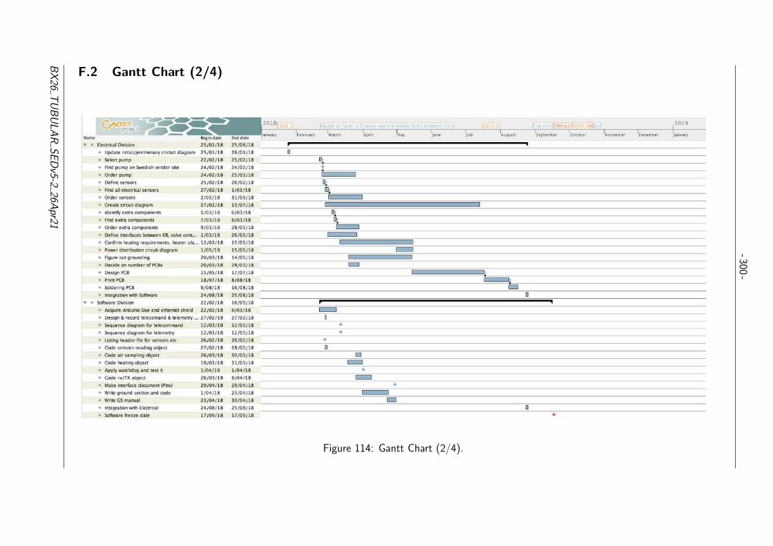
-300-
F.2 Gantt Chart (2/4)
Figure 114: Gantt Chart (2/4).
BX
26T
UB
UL
AR
SE
Dv5-2
26Apr21

-301-
F.3 Gantt Chart (3/4)
Figure 115: Gantt Chart (3/4).
BX
26T
UB
UL
AR
SE
Dv5-2
26Apr21

-302-
F.4 Gantt Chart (4/4)
Figure 116: Gantt Chart (4/4).
BX
26T
UB
UL
AR
SE
Dv5-2
26Apr21
-303-
By comparing the team availability in Appendix E to the Gantt chart it can be seen that across the summer there is lower team availability. Inthis time frame there are two periods with particularly low team availability; The early summer and early August. The work has been plannedso that the critical work will be completed in the periods with higher availability. In the event that the work takes longer than expected thequestion marks can become green.
BX
26T
UB
UL
AR
SE
Dv5-2
26Apr21

1
Equipment Loan Agreement
I. Lender Information
Institution: Finnish Meteorological Institute (FMI)
Address: Tähteläntie 62, 99600 Sodankylä, Finland
Representative: Dr. Rigel Kivi
E-Mail: [email protected]
Telephone Number: +358 405 424 543
Hereinafter referred to as “the Lender.”
II. Borrower Information
Group: Team TUBULAR (BEXUS 26/27)
Address: Luleå University of Technology, Rymdcampus, 981 28, Kiruna, Sweden.
Representative: Georges L. J. Labrèche
E-Mail: [email protected]
Telephone Number: +4670 577 23 87
Hereinafter referred to as “the Borrower.”
III. Equipment Information
The borrowed Equipment, hereinafter referred to as “the Equipment,” is a coiled 300 meters long stainless
steel tube. The tube is coated and has wall thickness of 0.005 inches. The coil can be damaged if not
packed properly, using some kind of shock absorbing material, for example soft styrofoam material. The
Borrower is to use the Equipment as part of an AirCore experimental setup that will collect air samples
during a high altitude balloon flight under the REXUS/BEXUS programme[1] scheduled to launch in
October, 2018. After the payload landing and gas analysis the Equipment will be returned to the Lender.
[1]
REXUS/BEXUS – Rocket and Balloon Experiments for University Students, http://rexusbexus.net/.
- 304 -
Appendix G Equipment Loan Agreement
BX26 TUBULAR SEDv5-2 26Apr21

2
IV. Borrower Responsibilities
This Agreement and the responsibilities as outlined hereunder are not transferable without the written
approval of the Lender. By executing this Agreement, the Borrower agrees to comply with the terms set
forth below:
1. Use/Disclaimer
1.1. The Borrower is responsible for the proper use and deployment of the Equipment.
1.2. The Borrower is responsible for training anyone using the Equipment on the proper use
of the Equipment in accordance with any Equipment use procedures.
1.3. The Borrower agrees to use the Equipment for academic or research use only and not for
any commercial use of application.
1.4. If the Equipment is lost, stolen, or damaged, the Borrower agrees to promptly notify the
Lender Representative designated above.
2. Proper Care and Protection
2.1. The Borrower is responsible for proper care, maintenance, and protection of the
Equipment.
2.2. The Borrower is responsible for designing experiments using the Equipment with
protection of the Equipment as the primary requirement.
2.3. The Borrower is responsible for testing the designed Equipment protection measures.
2.4. The Borrower is responsible for communicating the Equipment protection test results to
the Lender Representative designated above.
2.5. The Borrower is not responsible for Equipment damage related to hard landings.
Nominally, the landing is gentle with no damage to the experiments however, on rare
occasions, landing shocks up to 35g have been recorded when landing in rocky terrain.
2.6. The Borrower is not responsible for Equipment damage related to the unlikely event of a
water landing since the experiment gondola is not watertight.
3. Delivery and Return
3.1. Title to the Equipment is to remain with the Lender.
3.2. The Borrower is responsible for the safe packaging, proper import, export, and receiving
of the Equipment.
3.3. The Equipment is to be returned within a reasonable amount of time after the Loan
Period end date agreed between the Lender and the Borrower.
3.4. The Equipment shall be returned to the Lender in as good a condition as when received
by the Borrower.
4. Indemnification
4.1. In consideration for the Equipment loan, the Borrower agrees to indemnify, defend, and
hold Lender harmless from any and all damages, losses, claims, causes of actions,
expenses, and liability of any nature whatsoever associated with its use of the Equipment
while under care, custody, and control of the Borrower unless due to the negligence of
Lender.

3
5. Amendment/Modification
5.1. This Agreement cannot be amended or modified except by an instrument in writing
signed by both parties. Any attempt to do so except in accordance with this paragraph
shall be void.
6. Force Majeure
6.1. The Borrower is not responsible to Lender for any loss, damage, or failure to perform if
occasioned by fire, flood, explosion, windstorm, riot, war, transportation difficulty, or
any other cause beyond the reasonable control of the Borrower.
In witness whereof, the parties have executed this Agreement effective as of the date of the last party to
sign this Agreement below.
Authorized Borrower Representative Authorized Lender Representative
Signature: Signature:
Name: Georges L. J. Labrèche Name: Dr. Rigel Kivi
Title: Project Manager (Team TUBULAR) Title: Senior Scientist
Date: Date: March 12, 2018
3/12/2018

- 307 -
Appendix H Air Sampling Model for BEXUS Flight
H.1 Introduction
H.1.1 Objectives
The purpose of this is to theoretically simulate the experiment; its preparation, the samplingmethodology, and the expected results.
H.1.2 Justification
This theoretical model will give an estimation of the time needed to fill the bags in order toachieve the best resolution, the required volume of the samples at the different altitudes, tomake sure that there is enough sample left for analysis, the sampling altitudes and the numberof the bags.
H.1.3 Methodology
For this purpose, a mathematical model was created using MATLAB. In order to make surethat this model is reliable, it is going to be tested for the atmospheric conditions in the Arctic,and then compared with the 1976 US Standard atmosphere model that is used for this region.What is more, the model will be compared with past BEXUS flight data. The goal of themodel is to be as close as possible with these past data. After the tests, and making surethat the mathematical model is accurate, it will be adjusted with the TUBULAR’s experimentrequirements. In this way, the TUBULAR Team will get a general picture of the experiment’slayout. Hence, the results of the experiment will be more or less expected, and in the caseof complications, the mathematical model will be used as a reference of understanding whatwent wrong.
H.2 Scientific and Empirical Background
H.2.1 Study of Previous BEXUS Flights
This section has been elaborated based on the flight data files located in the previous BEXUSflights folders in the REXUS/BEXUS teamsite. This data was recorded by the Esrange BalloonService System (EBASS).
This unit is responsible of the piloting of the balloon is done by Esrange. It provides thecommunication link between the gondola and the ground station. The EBASS airborne unit,receives the data from the on board sensors, and then it sends them to the EBASS groundunit. It is also responsible for the payload control, providing functions like the altitude control,by valve and ballast release or the flight termination. What is more, EBASS keeps track ofthe filght trajectory with an on-board GPS system.
BX26 TUBULAR SEDv5-2 26Apr21

- 308 -
Tables 70 and 71 below gather some general information before and after the BEXUS flights.The pre-flight and the post-flight data are more or less in agreement in estimating for example,the ascent/descent time, the cut-off altitude and the float time. Knowing those informationand that the estimations are close enough to the real data, will help the TUBULAR Team todefine the experiment’s parameters with higher accuracy.
It is worth mentioning that the ascent speed in Table 71 is lower than the predicted 5 ∼ 6m/swhich is mentioned in the BEXUS manual. That is because it is the average velocity value ofall the data points.
BEXUS 20 BEXUS 21 BEXUS 22 BEXUS 23 BEXUS 24 BEXUS 25Main Balloon Zodiac 12SF Zodiac 12SF Zodiac 35SF Zodiac 35SF Zodiac 12SF Zodiac 12SF
Balloon mass [kg] 101.4 101.4 - - 101.4 101.4Parachute [m2] 80 80 80 80 80 80
Vehicle massLaunch [kg] 256.8 287.8 - - 300.6 321.15Vehicle massDescent [kg] 155.4 186.4 189.58 181.5 199.2 219.75
Float altitudeestimation [km] 28.2 27.5 - - 27 26.6Float pressureestimation [hPa] 15.38 17.11 - - 18.5 19.6
Float temperatureestimation [°C] - 48 - 48 - - - 49.5 - 49.9
Estimatedascent time 1h 33min 1h 31min - - 1h 29min 1h 27min
Table 70: Pre-flight Information Available in Previous BEXUS Campaigns.
BEXUS 20 BEXUS 21 BEXUS 22 BEXUS 23 BEXUS 24 BEXUS 25Ascent time 1h 37min 1h 37min 1h 51min 1h 51min 1h 55min 3h 45min
Average ascent speed [m/s] 4.78 4.59 4.52 4.79 3.79 1.86Floating altitude [km] 28 27 32 32 26.5 25.8
Floating time 2h 10min 1h 46min 2h 34min 2h 42min 2h 9min 2h 36minCut-off altitude [km] 27.7 20.5 28 32 25.7 25.2Ending altitude [m] 648 723 3380 1630 1050 -
Descent time 36 min 31 min 29 min 31 min 30 min -
Table 71: Post-flight Information Regarding the Flight Profile for Previous BEXUS Campaings.
In order to find out how many bags it is possible to sample during Ascent and Descent Phaseit is important to know the time duration of each phase i.e Ascent, Floating and Descent.For that reason, Figure 117 provides some sights on how previous BEXUS flights perform andwhat we can expect from BEXUS 26.
BX26 TUBULAR SEDv5-2 26Apr21
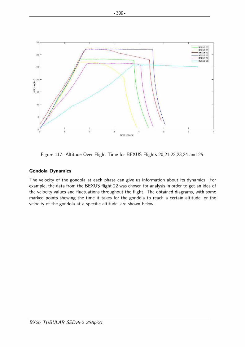
- 309 -
Figure 117: Altitude Over Flight Time for BEXUS Flights 20,21,22,23,24 and 25.
Gondola Dynamics
The velocity of the gondola at each phase can give us information about its dynamics. Forexample, the data from the BEXUS flight 22 was chosen for analysis in order to get an idea ofthe velocity values and fluctuations throughout the flight. The obtained diagrams, with somemarked points showing the time it takes for the gondola to reach a certain altitude, or thevelocity of the gondola at a specific altitude, are shown below.
BX26 TUBULAR SEDv5-2 26Apr21

- 310 -
Figure 118: Altitude Profile [Up] and Vertical Velocity Profile [Down] Over the Flight TimeDuring BEXUS 22 Flight.
Figure 119 below, illustrates the velocity changes throughout the different phases.It workslike a combination of both graphics form previous Figure 118, however it provides a betterrepresentation of the velocity values at each phase. Especially during the Descent Phase,which is the most determinant for the air sampling process.
For each altitude, there are two velocity values, one for the Ascent and one for the DescentPhase. Constant and positive velocities indicate the Ascent Phase. During Ascent Phase thevelocity is 6 m/s and almost constant, in agreement with the ascent speed value in the BEXUSmanual. A zero velocity value indicates the Float Phase. Then the velocity becomes negativewhich indicates the Descent Phase. Once again, the velocity value close to the ground is 8m/s as mentioned in the BEXUS manual[8].
BX26 TUBULAR SEDv5-2 26Apr21

- 311 -
Figure 119: Vertical Velocity of the Gondola Over the Altitude During BEXUS 22 Flight.
Atmospheric Conditions
In order to see how the atmospheric conditions change during a BEXUS flight, the data fromthe BEXUS flight 22 was chosen for analysis. Figure 120 below shows which kind of informationis available for different parameters such as the temperature, the pressure and the air densitywith altitude.
Figure 120: Variations in Temperature, Pressure and Air Density During the Ascent andDescent Phase for BEXUS Flight 22.
BX26 TUBULAR SEDv5-2 26Apr21

- 312 -
H.2.2 Trace Gases Distribution
Atmospheric greenhouse gases are mostly concentrated in the upper troposphere and lowerstratosphere. The Arctic region is of significant importance since there is where the maximumconcentration of greenhouse gases is found due to meridional circulation (temperature differ-ences) that pushes the gases from the equatorial to higher latitudes. Figures 121 and 122 areshowing the concentration over latitude of two of the main greenhouse gases, CO2 and CH4
respectively.
Figure 121: Global Distribution of Atmospheric Carbon Dioxide[18].
BX26 TUBULAR SEDv5-2 26Apr21

- 313 -
Figure 122: Global Distribution of Atmospheric Methane[18].
The same applies for the vertical distribution of atmospheric greenhouse gases. The favouredaltitudes for higher concentrations are the upper troposphere and the lower stratosphere dueto gravity waves and the vertical wind, which carry the trace gases at higher altitudes. Whatis more, CO2 has longer lifetime in the troposphere and stratosphere, where it has essentiallyno sources or sinks since it is basically chemically inert in the free troposphere.
Figure 123 shows the global distribution of carbon dioxide in the upper troposphere-stratosphere,at 50-60°N for the time period 2000-2010.
Figure 124 shows the global distribution of the seasonal cycle of the monthly mean CO2 (inppmv) in the upper troposphere and the lower stratosphere for the even months of 2010 andthe altitude range from 5-45 Km.
BX26 TUBULAR SEDv5-2 26Apr21

- 314 -
Figure 123: Global Distribution of CO2 in the Upper Troposphere-Stratosphere[7].
BX26 TUBULAR SEDv5-2 26Apr21

- 315 -
Figure 124: Global Distribution of the Seasonal Cycle of the Monthly Mean CO2 (in ppm) inthe Upper Troposphere and the Lower Stratosphere for the Even Months of 2010[7].
Figures 123, and 124, indicate that the higher CO2 concentrations are found between 5 and25 km with peaks around 10 to 15 km (figure 123) and 20 km for October (figure 124).
Figures 125 and 126 focus more on the region near the Arctic Circle. These figures representvertical profiles distribution of CO, CO2 and CH4 extracted from past research papers [5][17]. The range of altitudes that will be compared is the one between 10 and 25 km. SinceFigure 125 vertical axis is in pressure, the equivalent pressures for these altitudes will be fromapproximately 200 hPa to 20 hPa.
• CH4 distribution: There is a good agreement between both researches that the con-centration around 10 km of altitude is about 1800 ppb and then it starts decreasinggradually with altitude. This decrease seems to be faster above 17 km ( 70 hPa) whichwould make this the region of major interest.
• CO2 distribution: The concentration around 10 km is approximately 390-400 ppm inboth researches. The biggest variation in concentration can be found between 10-17km. The concentration of CO2 seems to have an increase and then decrease again sothis would be the most interesting range to sample.
• CO distribution: Only one research with CO profiles has been presented here so it cannotbe compared with other researches. Analysing the only CO profile, it seems that the
BX26 TUBULAR SEDv5-2 26Apr21

- 316 -
largest variation lays on the range 10-15 km, which should be the area of interest.
Based on the vertical distribution profiles obtained from past researches, seems that our ex-periment should focus on sampling between 10-15 km for CO and CO2 but above 17 km forCH4.
Figure 125: Vertical Profiles in Black for CO2 and CH4. The Green Lines are High ResolutionForecasts [17].
BX26 TUBULAR SEDv5-2 26Apr21

- 317 -
Figure 126: Vertical Profiles Comparison of AirCore and LISA Measurements of CO2, CH4
and CO Mole Fractions[5].
H.3 Sampling Flowrate
H.3.1 Pump Efficiency
For the air sampling process, the micro diaphragm gas pum 850 1.2 KNDC B from KNFcompany will be used.
The TUBULAR Team has tested this pump in vacuum conditions in IRF facilities in Kiruna.Table 72 shows the obtained results. It has been proved that the pump is operative down to20 hPa.
BX26 TUBULAR SEDv5-2 26Apr21

- 318 -
Altitude PressureDatasheetFlowrate
DatasheetEfficiency
EmpiricalFlowrate
EmpiricalEfficiency
0 km 1013 hPa 8 L/min 100 % 4.35 L/min 54.4 %0.5 km 925 hPa 7 L/min 87.5 % 4.26 L/min 63.25 %1.5 km 850 hPa 6 L/min 75 % 4.16 L/min 52 %2.3 km 760 hPa 5 L/min 62.5 % 3.88 L/min 48.5 %3.1 km 680 hPa 4 L/min 50 % 3.61 L/min 45 %4.6 km 560 hPa 3 L/min 37.5 % 3.11 L/min 38.9 %6.4 km 450 hPa 2 L/min 25 % 2.61 L/min 32.6 %8.3 km 320 hPa 1 L/min 12.5 % 2.12 L/min 26.5 %
10.7 km 230 hPa 0 L/min 0 % 1.50 L/min 18.8 %12 km 194 hPa 0 L/min 0 % 1.22 L/min 15.3 %17 km 88 hPa 0 L/min 0 % 0.47 L/min 5.9 %20 km 55.29 hPa 0 L/min 0 % 0.27 L/min 3.4 %24 km 30 hPa 0 L/min 0 % 0.13 L/min 1.6 %30 km 11.97 hPa 0 L/min 0 % 0.07 L/min 0.9 %
Table 72: Pump Flowrate/Efficiency According to the Datasheet and Tests.
H.4 Discussion of the Results
H.4.1 Computational Methods vs. Flight Measurements
Atmospheric Model
In this section, the data from the past BEXUS flights is compared with the 1976 US StandardAtmosphere, for validation reasons. Figure 127 compares the changes in pressure over altitudefor the BEXUS flights with the atmospheric model. It can be seen that the flights data-setsare in good agreement with the atmospheric model.
BX26 TUBULAR SEDv5-2 26Apr21

- 319 -
Figure 127: Comparative of Pressure Variation Over the Altitude During Different BEXUSFlights with the US Standard Atmosphere (1976).
Figure 128 below shows the changes in temperature over altitude, for all the BEXUS flights withthe atmospheric model. It can be seen that there is a quite large deviation of the temperatureabove 20km of altitude between the BEXUS flights and the US Standard Atmosphere 1976model. This is not arbitrary since it appears in all flights. But it is not surprising either,because most of the atmospheric models fail to precisely predict the temperatures at higheraltitudes.
BX26 TUBULAR SEDv5-2 26Apr21

- 320 -
Figure 128: Comparative of Temperature Variation Over the Altitude During Different BEXUSFlights with the US Standard Atmosphere (1976).
Descent Curve
Again, in this section, the trajectories of past BEXUS flights, were compared with the math-ematical model for validation reasons as shown in Figure 129. Overall, BEXUS flights 20, 23and 24 are in good agreement with the mathematical model. Some deviations exist betweenthe mathematical model and the BEXUS flights 21 and 22 mostly in the last 5km of the flight.
BX26 TUBULAR SEDv5-2 26Apr21
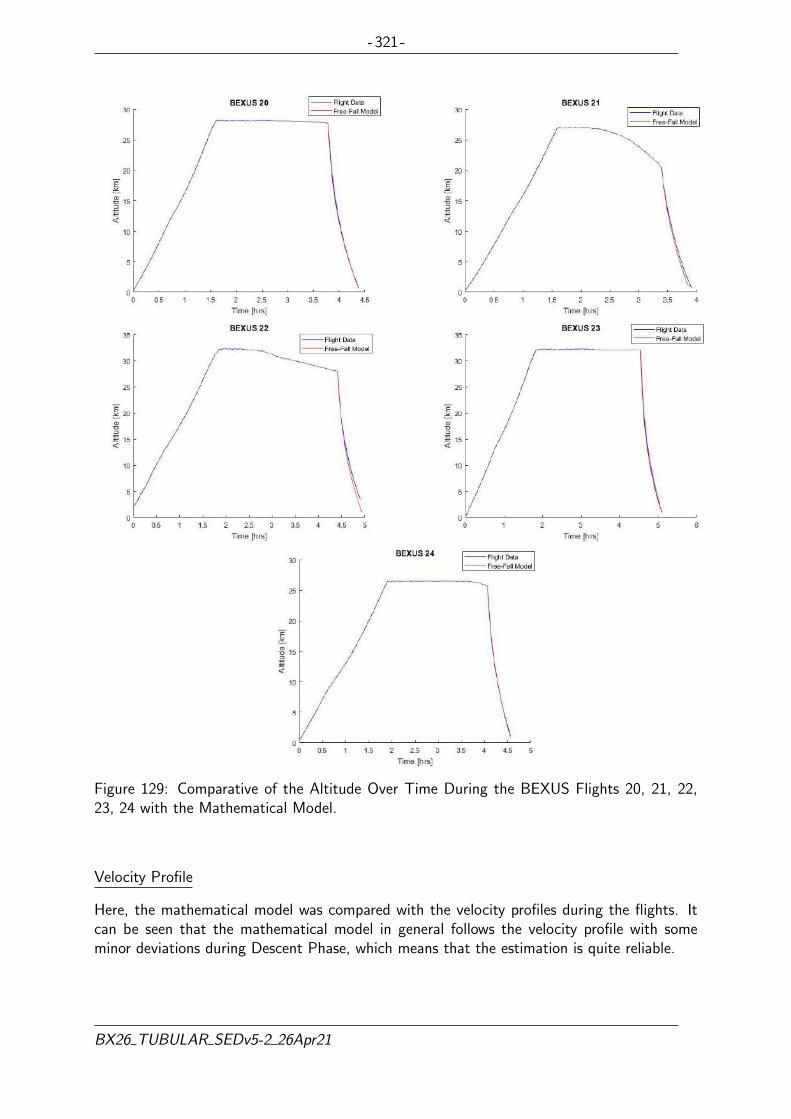
- 321 -
Figure 129: Comparative of the Altitude Over Time During the BEXUS Flights 20, 21, 22,23, 24 with the Mathematical Model.
Velocity Profile
Here, the mathematical model was compared with the velocity profiles during the flights. Itcan be seen that the mathematical model in general follows the velocity profile with someminor deviations during Descent Phase, which means that the estimation is quite reliable.
BX26 TUBULAR SEDv5-2 26Apr21

- 322 -
Figure 130: Comparative of the Velocity Over Altitude During the BEXUS Flights 20, 21, 22,23, 24 with the Mathematical Model.
H.4.2 Mass Effects in the Descent Curve
Figure 131, shows how the descent time changes with different gondola mass values, after thecut-off phase. The heavier the payload, the sooner it will land. For example, if the gondolaweights 250kg, it will land in approximately 25 minutes after the cutoff, while it would takeapproximately 40 minutes to land if it weights 100kg.
BX26 TUBULAR SEDv5-2 26Apr21
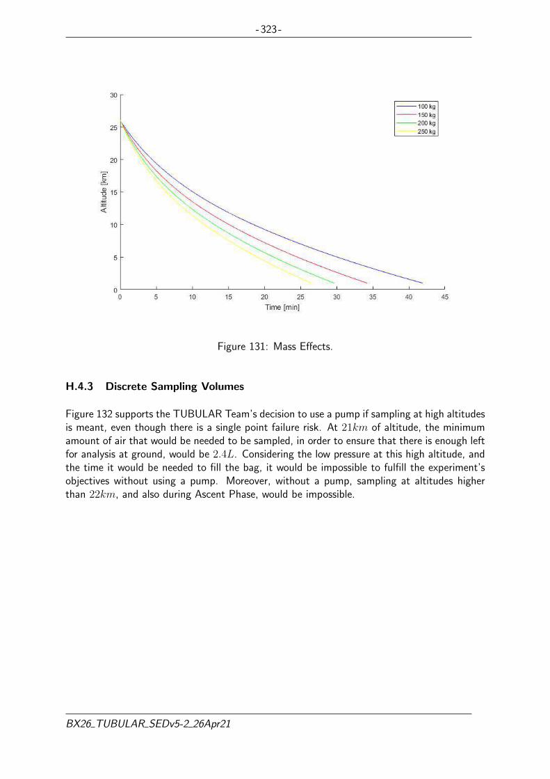
- 323 -
Figure 131: Mass Effects.
H.4.3 Discrete Sampling Volumes
Figure 132 supports the TUBULAR Team’s decision to use a pump if sampling at high altitudesis meant, even though there is a single point failure risk. At 21km of altitude, the minimumamount of air that would be needed to be sampled, in order to ensure that there is enough leftfor analysis at ground, would be 2.4L. Considering the low pressure at this high altitude, andthe time it would be needed to fill the bag, it would be impossible to fulfill the experiment’sobjectives without using a pump. Moreover, without a pump, sampling at altitudes higherthan 22km, and also during Ascent Phase, would be impossible.
BX26 TUBULAR SEDv5-2 26Apr21

- 324 -
Figure 132: Minimum Sampling Volume at Each Altitude to Obtain Enough Air to Perform aProper Analysis (180 mL at Sea Level).
H.4.4 Limitations of the Bag Sampling Method
Roof Altitude Effect
For a hypothetical study case, an ideal and continuous flow rate was used (1L/min). Theobtained diagrams below, show that even if the sampling starts at 26km, or at 30km, orat 40km, the number of filled bags would still be the same. This happens, due to the lowpressure conditions at such altitudes which not allow a faster filling of a bag, and specially thelow air density which forces to sample much more volume of air. Of course, the number ofbags that can be filled, depends on the pump’s efficiency at high altitudes. So, the altitude ofthe gondola’s cut-off over about 26km would not affect the experiment’s outcome.
BX26 TUBULAR SEDv5-2 26Apr21

- 325 -
(a) Starting of Sampling at 26 km. (b) Starting of Sampling at 30 km.
(c) Starting of Sampling at 40 km.
Figure 133: Bag’s Sampling System Limitations.
One Single Pump
Since the experiment uses a single pump, it is not possible to sample more than one bags atthe same time. For the above hypothetical case, the maximum number of filled bags was five,considering continuous sampling. However, this is not the case when it comes to real life.Before sampling a bag, the system has to be flushed. Then, the sampling of a bag begins.After filling one bag, the system has to be flushed again before starting sampling a secondbag. In that case, filling five bags, according to the hypothetical scenario, would be practicallyimpossible.
BX26 TUBULAR SEDv5-2 26Apr21

- 326 -
H.5 Conclusions
H.5.1 Sampling Strategy
After testing the pump at low pressure environment, an overall idea about the performanceof the pump at high altitudes is now known and an approximation of the sampling strategy ispossible. The total weight of the BEXUS 26 gondola is approximated to be 266.55 kg, and theballoon is expected to reach 25.8 km altitude, following almost the trajectory of the BEXUS 24flight as shown in figure 129. This serves the objectives of the TUBULAR experiment since, asindicated in Section H.2.2 the altitudes with higher differences in trace gases concentrations,are between 10 and 25 km. These are the altitudes where the sampling will be done. Samplingsix bags in total, is enough to fulfil the objectives of the experiment and it is also feasible.Two bags will be sampled during Ascent Phase and four during Descent Phase. The ascentspeed of the gondola, as shown in Figure 118, is estimated to be 5 m/s. A velocity of thisrate, makes sampling of two bags possible while achieving a good resolution. It is important tomention here that the pressure inside the two bags that will be sampled during Ascent Phaseshall not exceed 140 hPa since their volume will increase with decreasing pressure and theycould burst. On the other hand, during Descent Phase the four remaining bags shall be filledwith the full 3 L. This is because their volume will decrease with increasing pressure and it hasto be made sure that there will be enough sample left for analysis.
The sampling of the first bag will start at 18 km of altitude. The minimum sampling time isestimated to be 29s with an achieved resolution of 143m. The second bag will be sampledat 21 km of altitude, and it will take 43 s to fill the minimum desired volume of air, with aresolution of 214 m. Before sampling, flushing of the AAC system for one minute is taken intoaccount. During that, the gondola will cover a distance of 300 m.
During Descent Phase and considering a descent speed of 8 m/s, the sampling of the thirdbag will start from 17.5 km. The minimum sampling time is estimated to be 27 sec with aresolution of 216.5 m. The fourth bag will be sampled at 16 km for at least 20 s and resolutionof 156 m. The fifth bag will be sampled at 14 km for 14.3 s minimum and resolution of 115m. The sample of the last bag will start at 12 km for 9 s minimum sampling time and 71 mresolution. Again, one minute of flushing is taken into account, in between the sampling ofeach bag.
The flow rates of the pump, at each sampling altitude were taken from Table 56.
H.5.2 Discusion of the Results
Overall, the mathematical model is in good agreement with the data from the past BEXUSflights as well as, with the atmospheric model used for the Arctic region. Making this docu-ment, helped the TUBULAR Team to cross-check some theoretical values, important for thelayout and the planning of the experiment. Tables 70 and 71 show that the estimated databefore each flight are pretty close with the real data obtained by the flights which helped theTUBULAR Team to define the experiment’s parameters with higher accuracy. In order tomake a sampling plan, it is important to know the duration time of each phase. Figure 117,shows the trajectories of the different BEXUS flights, giving the TUBULAR Team a general
BX26 TUBULAR SEDv5-2 26Apr21

- 327 -
idea of what the trajectory of the flight can look like and how the duration of each phasechanges regarding the maximum altitude that the gondola reaches.
The velocity profile, Figure 119, is of high importance since the velocity during Ascent andDescent Phase, will determine the resolution of the samples. In general, the velocity valuesare in agreement with the BEXUS manual, with an ascent speed of 5 m/s and a descentspeed, fluctuating after cutoff, before stabilizing at 8 m/s at the last kilometers of the flight.Another important thing that has to be mentioned here, is the TUBULAR Team’s decision tosample during Ascent Phase too and not only during Descent Phase. As seen in figure 119 thegondola is turbulent after the cutoff with velocities up to 83 m/s, and needs more or less 6km before stabilizing its velocity as figure 118 indicates. Hence, the altitudes that the gondolawill be turbulent, will be covered by sampling during Ascent Phase. This will not affect thecomparison with the CAC that will be sampled during Descent Phase only, since the horizontaldisplacement of the gondola is much smaller than the vertical.
Atmospheric conditions play a crucial role for the TUBULAR experiment. The TUBULARTeam should know, the different pressures at each altitude, since the pressure is the parameterthat will trigger the sampling of the bags. What is more, the pressure will determine theperformance of the pump and it is crucial to know under what pressures the pump needs to betested depending on the sample altitude. The temperature is of high importance too and thetrickier to predict especially at high altitudes. The TUBULAR Team should be able to keepthe temperature of the pump within its working temperature range in order to assure that thepump will start working. To do so, the air temperature must be known at each altitude whichwill help the TUBULAR Team to come up with a good thermal plan.
The sampling altitude range will not be chosen randomly. The idea is to find the altituderange, where the trace gases show the bigger differences in concentration. In Section H.2.2,were presented some theoretical trace gases concentration values as well as, some results frompast research papers. According to them, the more interesting area to sample is between 10and 25 km of altitude. The TUBULAR Team, plans to sample between 17 and 22 km duringAscent Phase and 17 to 10 km during Descent Phase.
Additionally, the sampling software revealed some limitations of the sampling system and alsowhich parameters should be taken into account for the experiment’s layout and which not.The weight of the gondola, will affect the maximum altitude that the balloon will reach, andthe time needed for the gondola to land, but it doesn’t contribute to the decision of how manybags will be used.
The decision of the TUBULAR Team to use a pump was questioned at the beginning, asa single point failure risk. However, this decision is justified by the need of sampling duringAscent Phase, ohterwise the sampling would not be possible. Figure 132, supports the use of apump because without a pump, sampling at 22 km of altitude, would be impossible consideringthe low pressure and the time it would take to fill a bag.
Note that even with the pump, some limitations still exist. The sampling of the bags cannotbe continuous since the system has to be flushed before sampling a bag. Furthermore, theflow rate of the pump will be lower at high altitudes than it is on the ground, due to pressuredifferences. Figure 133 points out that even with an ideal flow rate of 1 L/min and samplingcontinuously, it is not possible to sample more than five bags, because it takes a lot of timeto sample a bag at high altitude atmospheric conditions. Additionally, it makes clear why
BX26 TUBULAR SEDv5-2 26Apr21

- 328 -
the maximum altitude that the gondola will reach, does not affect the experiment’s outcome.As the gondola ascents, the pressure gets lower and takes more time to sample a bag. So,sampling more bags would not be possible even if the balloon reaches a higher altitude. Thesame applies for the Descent Phase and the cutoff altitude.
Concluding, whilst at the beginning, the idea was to sample a total of sixteen bags in order tohave more samples to compare with the continuous vertical profile obtained by the CAC, thisdocument justifies that this is not feasible. Taking into account all the different parameters,it made clear which of them are important and which are not. Parameters like the gondola’svelocity, the pressure at different altitudes, and the pump’s flow rate, will determine theoutcome of the TUBULAR experiment, the number of the bags that will be used, as well asthe sampling altitudes. Parameters like the gondola’s weight or the maximum altitude thatthe balloon will reach, does not affect the experiment’s outcome and have a secondary role.
BX26 TUBULAR SEDv5-2 26Apr21

- 329 -
Appendix I Experiment Thermal Analysis
I.1 Component Temperature Ranges
Table 73, below covers the thermal ranges of all components included in the experiment’sflight stage as listed in Section 4.3:
ID ComponentsOperating (°C) Survivable (°C) Expected (°C)Min. Max. Min. Max. Min. Max.
E1 Arduino Due -40 85 -60 150 -15.7 54.0E2 Ethernet Shield -40 85 -65 150 -15.7 54.0
E3Miniature di-aphragm air pump
5 40 -10 40 10 34.9
E4 Pressure Sensor -40 85 -40 125 -15.7 54.0
E5Sampling Valve (in-let and outlet 1/8””female)
-20 68 -203 683 -15 20
E6Airflow sensorAWM43300V
-20 70 -203 703 -8.8 34.9
E7Heater (12.7 ×50.8mm)
-200 200 -2003 2003 -20 36
E9 Temperature Sensor -55 125 -65 150 -19.7 43E10 DCDC 24 V -40 85 -55 125 -15.7 54.0E12 Micro SD -25 85 -2003 2003 -15.7 54.0E13 Logic CAT5E -55 60 -553 603 -34 15
E16MOSFET for cur-rent control
-55 175 -55 175 -15.7 54.0
E17Diodes for DCDCconverters
-65 175 -653 1753 -15.7 54.0
E18 3.3V LED -40 85 -403 853 -15.7 54.0
E1915-pin D-SUB Fe-male connector withpins
-55 120 -2003 2003 -15.7 54.0
E209-pin D-SUB Femaleconnector with pins
-55 120 -2003 2003 -15.7 54.0
E219-pin D-SUB Femaleconnector with sol-dering cups
-55 105 -553 1053 -15.7 54.0
E229-pin D-SUB Maleconnector with sol-dering cups
-55 105 -553 1053 -15.7 54.0
E2315-pin D-SUB Maleconnector with sol-dering cups
-55 105 -553 1053 -15.7 54.0
E249-pin D-SUB back-ing
-40 120 -403 120 -15.7 54.0
BX26 TUBULAR SEDv5-2 26Apr21

- 330 -
E2515-pin D-SUB back-ing
-40 120 -403 120 -15.7 54.0
E28 3.3 Zener diode -65 175 -653 1753 -15.7 54.0
E29Male connector onPCB
-40 85 -403 85 -15.7 54.0
E30Female connectorfrom wall
-40 85 -403 85 -50.7 15
E31 Grounding contact -55 125 -553 1253 -50.7 15
E32Logic CAT5 E-linkfor inside box
-55 60 -553 603 -34 15
E33 Signal Wires -60 200 -603 2003 -34 15
E34Flushing valve (inletand outlet 1/8”” fe-male)
-20 68 -203 68 -7.4 25.8
E35Valves manifold(outlet 1/8”” fe-male)
-10 50 -103 503 3 18
E36 Power wire black -60 200 -603 2003 -34 15E48 Power wire red -60 200 -603 200 3 -34 15E50 6-pin male -55 105 -553 1053 -8.8 24.0
E518-pin male singlerow header
-40 105 -403 1053 -8.8 24.0
E5210-pin male singlerow header
-55 105 -553 1053 -8.8 24.0
E5336-pin male doublerow header
-40 105 -40 125 -8.8 24.0
E5412 V DC/DC con-verter
-40 85 -55 125 -15.7 54.0
E5550 kΩ Potentiome-ter
-55 125 -553 1253 -15.7 54.0
E56Static pressure sen-sor
-40 120 -403 1203 -8.8 34.9
E57Connector for staticpressure sensor
-25 80 -253 803 -8.8 34.9
E58 PCB -50 110 -503 1103 -15.7 54.0
E59Pressure SensorPCB
-50 110 -503 1103 -50 39
Table 73: Table of Component Temperature Ranges.
BX26 TUBULAR SEDv5-2 26Apr21
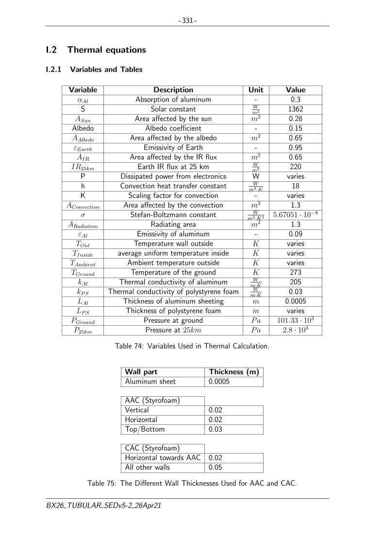
- 331 -
I.2 Thermal equations
I.2.1 Variables and Tables
Variable Description Unit ValueαAl Absorption of aluminum - 0.3S Solar constant W
m2 1362ASun Area affected by the sun m2 0.28
Albedo Albedo coefficient - 0.15AAlbedo Area affected by the albedo m2 0.65εEarth Emissivity of Earth - 0.95AIR Area affected by the IR flux m2 0.65
IR25km Earth IR flux at 25 km Wm2 220
P Dissipated power from electronics W variesh Convection heat transfer constant W
m2·K 18K Scaling factor for convection - varies
AConvection Area affected by the convection m2 1.3σ Stefan-Boltzmann constant W
m2·K4 5.67051 · 10−8
ARadiation Radiating area m2 1.3εAl Emissivity of aluminum - 0.09TOut Temperature wall outside K variesTInside average uniform temperature inside K variesTAmbient Ambient temperature outside K variesTGround Temperature of the ground K 273kAl Thermal conductivity of aluminum W
m·K 205kPS Thermal conductivity of polystyrene foam W
m·K 0.03LAl Thickness of aluminum sheeting m 0.0005LPS Thickness of polystyrene foam m varies
PGround Pressure at ground Pa 101.33 · 103
P25km Pressure at 25km Pa 2.8 · 103
Table 74: Variables Used in Thermal Calculation.
Wall part Thickness (m)Aluminum sheet 0.0005
AAC (Styrofoam)Vertical 0.02Horizontal 0.02Top/Bottom 0.03
CAC (Styrofoam)Horizontal towards AAC 0.02All other walls 0.05
Table 75: The Different Wall Thicknesses Used for AAC and CAC.
BX26 TUBULAR SEDv5-2 26Apr21

- 332 -
I.3 Thermal calculations in MATLAB
For the MATLAB calculations, a few assumptions were made. They were as follows:
• Taking the average of MATLAB calculations for calculations with or without sunlight.
• Calculating the average temperature on the outside wall of the experiment.
• Assuming the inner temperature at the bags section is uniform.
• Ignoring the pipes letting cold air into the experiment.
• Assuming no interference between the two experiment boxes.
• All conduction was uniform from the inside.
• Assume steady flow through the walls from conduction.
• Assume radiation and convection from/on 6 walls not 5.
I.3.1 Solar flux and Albedo
The albedo is the reflected solar flux from earth so it was put into the same equation as thesolar flux. It was assumed that the sun hit two sides of the experiment at a 45° angle at alltimes while over 10 km altitude. In the middle of October at the time of launch the sun wasexpected to hit the experiment with a maximum inclination of 15° from the horizon.
QSun+Albedo = αAl · S · cos(15) · (ASun · cos(45) + Albedo · AAlbedo)
I.3.2 Conduction
For calculating the outer walls temperature, the assumption of steady flow through walls wasused.
QConduction = [Steady flow through wall] = Dissipated power = P
I.3.3 Earth IR flux
The earth IR flux is the flux that comes from earth as a black body radiating. It was calculatedfrom the determined IR flux at ground level then scaled to the altitude the experiment wouldreach. The following equations were found from [9]:
IRGround = εearth · σ · T 4ground
τatmIR = 1.716− 0.5 ·
[e−0.65
P25kmPground + e
−0.95P25km
Pground
]IR25km = τatmIR · IRGround
After the IR was calculated for the floating altitude it was put into the following equation.
QIR = εearth · AIR · IR25km
BX26 TUBULAR SEDv5-2 26Apr21

- 333 -
I.3.4 Radiation
It was assumed that the experiment would experience radiation from all 6 sides. In reality itwould experience radiation from 5 sides because the CAC box will be in contact with one ofthe AAC box’s sides. It was decided to leave the simulation with input from the 6 sides forthe calculations in order to compensate for having no holes to let cold air in to the pump.
QRadiation = σ · εAl · ARadiation · (T 4Out − T 4
Ambient)
I.3.5 Convection
At an altitude of 25 km there is far lower air density than at sea level. This therefore gavea scaling factor K that had to be taken into account when calculating the convection and Kcan be seen in Table 76 for different altitudes.
QConvection = h ·K · AConvection · (TOut − TAmbient)
The equation for approximating the heat transfer coefficient for air was outlined as:
h = 10.45− v + 10 ·√v
Where v is the velocity of the fluid medium.
As the balloon was expected to rise at approximately 5m/s for the duration of the AscentPhase, the starting value for the convective heat transfer coefficient h was expected to be27.811, assuming negligible wind currents perpendicular to the direction of ascent.
The equations used to obtain the value of K are listed below:
F (Tsea, Talt) =( kaltksea
)1−n ×[( βaltβsea
)×(µsea
µalt
)×( cp−alt
cp−sea
)×( ρ(Talt)
ρ(Tsea)
)2]nWhere:
• n is an exponent value dependent on the turbulence of the fluid medium (14
for laminarflow and 1
3for turbulent flow)
• k is the thermal conductivity of the air
• β is the thermal expansion coefficient for air
• µ is the dynamic viscosity of the air
• cp is the specific heat capacity of the air at constant pressure
• ρ(T ) is the density of the air as a function of only temperature difference (i.e. forconstant pressure)
• ”sea” denotes the current variable is represented by its value found at sea level
• ”alt”denotes the current variable is represented by its value found at a specified altitude
BX26 TUBULAR SEDv5-2 26Apr21

- 334 -
The values for F from this equation were then applied to its respective position in the followingequation to determine the ratio between the convective heat transfer coefficient h at sea level(assumed to have negligible differences for Esrange ground level) and the same coefficient ata specified altitude:
K =( ρ(Palt)
ρ(Psea)
)2n×(∆Tair
∆Tsea
)n× F (Tsea, Talt)
Where:
• ρ(T ) is the density of the air as a function of only temperature difference (i.e. forconstant pressure)
• δT is the difference between the temperature of the ambient air and the surface inquestion
Table 76 combines the previously listed convection and radiation formulae integrated into theMATLAB scripts to determine the convective and radiative heat loss in the worst case for(highest) power dissipation during each stage of the experiment. Additional information onthe thermodynamics of the atmosphere was obtained from Engineering Toolbox [23]
Altitude Case Tamb K halt Tout Qconv Qrad
Hangar(Preparations)
Cold 283 1 10.45 20.3 139.409 6.516Expected 288 1 10.45 25.2 139.081 6.844Warm 293 1 10.45 30.2 138.743 7.182
Ground(Stationary)
Cold 263 1 18 -0.8 215.705 4.690Expected 273 1 18 9.2 215.171 5.222Warm 283 1 18 19.2 214.600 5.790
Ground(Launched)
Cold 263 1 28.945 -4.2 217.528 2.884Expected 273 1 28.945 5.8 217.195 3.217Warm 283 1 28.945 15.8 216.837 3.573
5 kmCold 228 0.7868 22.774 -37.6 217.979 2.430Expected 263 0.8468 24.511 -3.2 216.990 3.417Warm 273 0.8507 24.624 6.3 216.615 3.792
10 kmCold 193 0.4882 14.131 -68.1 217.916 2.480Expected 223 0.5286 15.300 -39.1 216.940 3.453Warm 238 0.5421 15.691 -24.4 216.336 4.055
15 kmCold 193 0.3300 9.552 -61.9 224.325 3.961Expected 233 0.3680 10.652 -23.9 222.309 5.972Warm 253 0.3825 11.071 -4.6 221.050 7.226
20 kmCold 213 0.2401 6.950 -35.6 220.777 7.430Expected 243 0.2563 7.419 -7.4 218.297 9.899Warm 268 0.2687 7.778 16.4 215.906 12.282
25 kmCold 223 0.1683 4.871 -16.0 215.482 12.549Expected 253 0.1792 5.187 11.4 211.791 16.226Warm 273 0.1847 5.346 30.1 208.893 19.112
FloatPhase
Cold 223 0.1683 3.029 -1.7 190.087 19.521Expected 253 0.1792 3.226 24.1 185.077 24.530
BX26 TUBULAR SEDv5-2 26Apr21
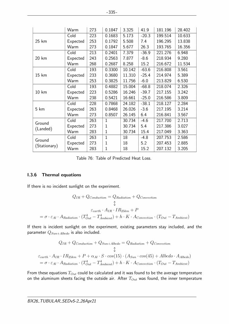
- 335 -
Warm 273 0.1847 3.325 41.9 181.196 28.402
25 kmCold 223 0.1683 5.173 -20.3 199.514 10.633Expected 253 0.1792 5.508 7.4 196.295 13.838Warm 273 0.1847 5.677 26.3 193.765 16.356
20 kmCold 213 0.2401 7.379 -36.9 221.276 6.948Expected 243 0.2563 7.877 -8.6 218.934 9.280Warm 268 0.2687 8.258 15.2 216.672 11.534
15 kmCold 193 0.3300 10.142 -63.6 216.808 3.561Expected 233 0.3680 11.310 -25.4 214.974 5.389Warm 253 0.3825 11.756 -6.0 213.829 6.530
10 kmCold 193 0.4882 15.004 -68.8 218.074 2.326Expected 223 0.5286 16.246 -39.7 217.155 3.242Warm 238 0.5421 16.661 -25.0 216.586 3.809
5 kmCold 228 0.7868 24.182 -38.1 218.127 2.284Expected 263 0.8468 26.026 -3.6 217.195 3.214Warm 273 0.8507 26.145 6.4 216.841 3.567
Ground(Landed)
Cold 263 1 30.734 -4.6 217.700 2.713Expected 273 1 30.734 5.4 217.386 3.027Warm 283 1 30.734 15.4 217.049 3.363
Ground(Stationary)
Cold 263 1 18 -4.8 207.753 2.586Expected 273 1 18 5.2 207.453 2.885Warm 283 1 18 15.2 207.132 3.205
Table 76: Table of Predicted Heat Loss.
I.3.6 Thermal equations
If there is no incident sunlight on the experiment.
QIR +QConduction = QRadiation +QConvection
lεearth · AIR · IR25km + P
= σ · εAl · ARadiation · (T 4Out − T 4
Ambient) + h ·K · AConvection · (TOut − TAmbient)
If there is incident sunlight on the experiment, existing parameters stay included, and theparameter QSun+Albedo is also included.
QIR +QConduction +QSun+Albedo = QRadiation +QConvection
lεearth · AIR · IR25km + P + αAl · S · cos(15) · (ASun · cos(45) + Albedo · AAlbedo)
= σ · εAl · ARadiation · (T 4Out − T 4
Ambient) + h ·K · AConvection · (TOut − TAmbient)
From these equations TOut could be calculated and it was found to be the average temperatureon the aluminum sheets facing the outside air. After TOut was found, the inner temperature
BX26 TUBULAR SEDv5-2 26Apr21

- 336 -
could be calculated by determining the heat transfer through the wall.
P =TInside − TOutside
A · (LAl
kAl+ LPS
kPS)
l
TInside = P · A · (LAl
kAl
+LPS
kPS
) + TOutside
TInside was then assumed to be the uniform air temperature in the experiment.
I.3.7 Trial run with BEXUS 25 air temperature data for altitudes
The air temperature data varying over altitude from previous BEXUS flights could be foundon the REXUS/BEXUS website. To do a simulated test flight for the calculations done inMATLAB (with the intention of seeing how the temperature profile would appear for a realflight), it was calculated and plotted in with data from BEXUS 25 flight. Because of itoriginally having approximately 42000 data points, the profile had to be scaled down. Onlyevery 25th data point was used to reduce processing time and this resulted in little detailloss. In Figure 134, the TUBULAR test flight is the uniform temperature on the inside with ainsulation consisting as specified in Table 75.
BX26 TUBULAR SEDv5-2 26Apr21

- 337 -
Figure 134: Simulated Test Flight of TUBULAR AAC Box with Data From BEXUS 25.
When the data was found it was checked in ANSYS to determine and add heaters to controlthe most critical parts of the model.
I.3.8 Trial flight for the CAC
The CAC box did not require as much thermal design as the AAC box. The only part to beconsidered was the valve, which had a lower limit of the operating temperature of −10°C.It would not be a problem because the valve would open just prior launch and have currentrunning through it throughout the whole flight — heating it self up. If the thermal analysiswas proven wrong by a test, showing that it was not sufficient to use only self-heating, a heatercould be applied at a later date. The passive thermal design for the CAC box would consistof aluminum sheets and Styrofoam as specified in 75.
BX26 TUBULAR SEDv5-2 26Apr21
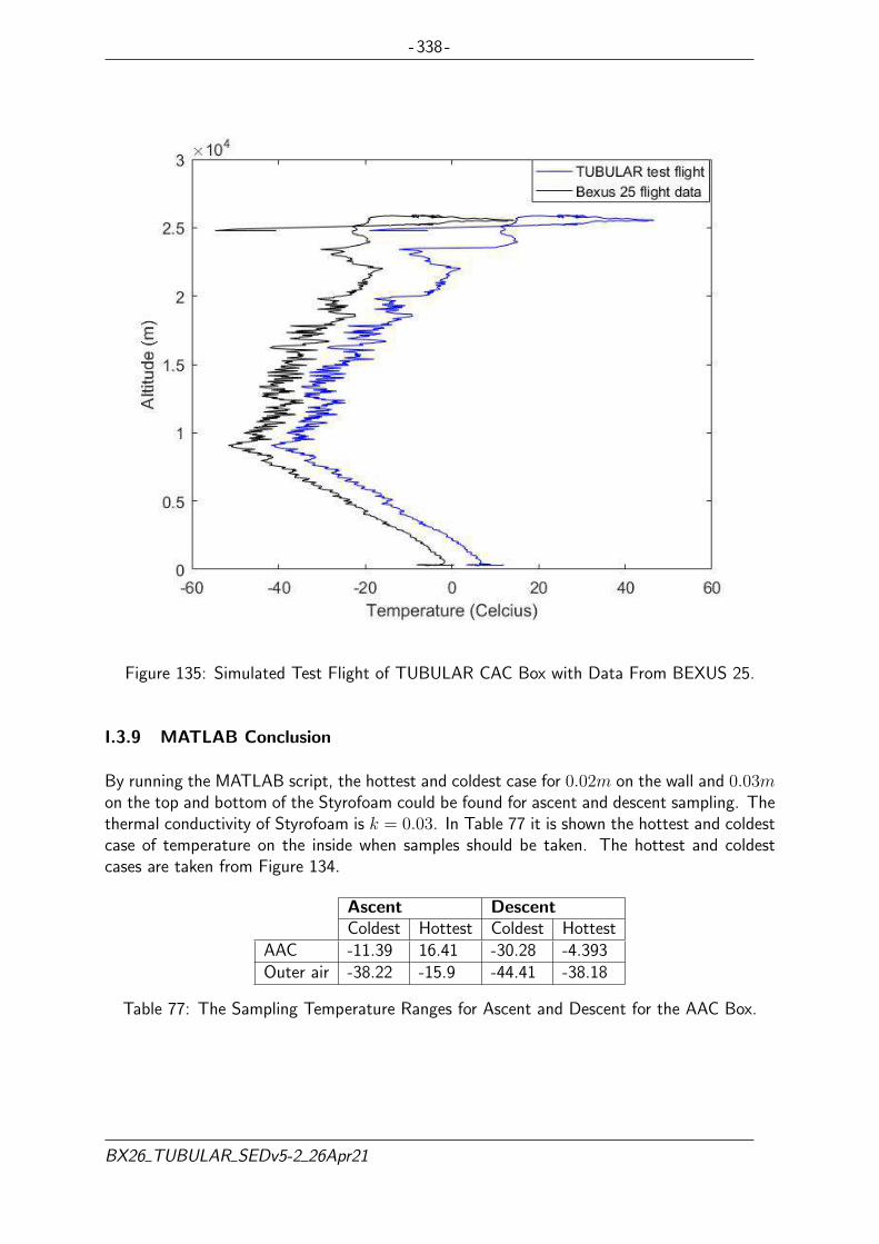
- 338 -
Figure 135: Simulated Test Flight of TUBULAR CAC Box with Data From BEXUS 25.
I.3.9 MATLAB Conclusion
By running the MATLAB script, the hottest and coldest case for 0.02m on the wall and 0.03mon the top and bottom of the Styrofoam could be found for ascent and descent sampling. Thethermal conductivity of Styrofoam is k = 0.03. In Table 77 it is shown the hottest and coldestcase of temperature on the inside when samples should be taken. The hottest and coldestcases are taken from Figure 134.
Ascent DescentColdest Hottest Coldest Hottest
AAC -11.39 16.41 -30.28 -4.393Outer air -38.22 -15.9 -44.41 -38.18
Table 77: The Sampling Temperature Ranges for Ascent and Descent for the AAC Box.
BX26 TUBULAR SEDv5-2 26Apr21

- 339 -
I.4 Thermal Simulations in ANSYS
The CAD model used is seen in the figure 136. The side exterior walls were 0.02m in height,the interior walls of the Brain to the bags were 0.03m in length and the top and bottom wallconsisted of 0.03m long Styrofoam as well. The outer parts of the pipes were set to stainlesssteel with a constant temperature (the same as the ambient outside). The tubes closest tothe pump and the one leading from the pump to the manifold were set to include air to beable to vary during the simulation depending on the temperature outside of the experimentand the pump heating up from the heater.
Figure 136: The CAD Model Used for ANSYS Simulations
In ANSYS, FEA simulations were done using both Steady-State Thermal and Transient Ther-mal analysis. Because of the limitations in ANSYS student license, a simplified model wasused, which can be seen in Figure 137. It was focused on the corner region of the experimenthousing the Brain and had three walls to the sampling bags and assumed the air was uniformlyheated on the inside. The uniform inside air could be taken from the data from the testflight in Figure (134). These simulations were done to find what temperature the pump andmanifolds would reach, as they were the most critical components in the experiment.
A transient thermal analysis was also performed by simulating a test flight with data fromBEXUS 25 using results from MATLAB. It was performed so the thickness of the wall couldbe verified to see if it was good enough and whether adding heaters was required. Through theaddition of, correct placement, adequate assigned power, and activation time for the heaters,it was possible to enable the pump and the manifold to operate in their required temperatureranges.
BX26 TUBULAR SEDv5-2 26Apr21

- 340 -
I.5 ANSYS Result
I.5.1 Including Air With Same Density as Sea Level in the Brain
Figure 137: Cross Section of the Air in the Brain at the Time to Sample During Ascent.
Figure 138: The Pump at the Time to Sample During Ascent (left) and Descent (right).
Figure 139: The manifold at the Time to Sample During Ascent (left) and Descent (right).
BX26 TUBULAR SEDv5-2 26Apr21

- 341 -
Figure 140: Pump and Manifold at the Coldest Part of Ascent.
Figure 141: Flushing Valve a Little Before Sampling Shall Start.
I.5.2 No Air in the Brain
Figure 142: The Pump at the Time to Sample During Ascent (left) and Descent (right).
BX26 TUBULAR SEDv5-2 26Apr21

- 342 -
Figure 143: The manifold at the Time to Sample During Ascent (left) and Descent (right).
Figure 144: The Structure of the Brain at the Time to Sample During Ascent (left) andDescent (right).
Figure 145: Flushing Valve a Little Before Sampling Shall Start.
I.6 Result
The main objective from first performing the MATLAB calculations and then the ANSYSsimulations was to find the wall thickness of Styrofoam between the Brain and the inside ofthe AAC box and make updated iterations of the result. The next objective was to iteratethe design by adding heaters to find the required amount and find approximately how long
BX26 TUBULAR SEDv5-2 26Apr21

- 343 -
they need to run. By running a transient thermal analysis for the test flight it was possible tosimulate heaters that will be on and off to determine how strong they need to be.
The results from the ANSYS simulations assumed a worst case scenario. It was to be expectedthat the results were not fully accurate, and instead were slightly warmer in reality. The worstcase was with air inside the experiment at normal density. In reality when it was time to sample(at 17km), the air density would be less then 15% of the air density at sea level [22]. Thismeant that there would be less heat loss from components to the air inside the brain thanpredicted. Figures 138 and 139 show that the temperature of the pump was above 5°C andthe manifold was above −10°C. It was only during a portion of the Ascent Phase, just prior tothe start of sampling that the heater would need to be on in order for the pump to be above5°C, and it would only need to be on during this Phase. By having a heater on the flushingvalve and the manifold it was possible to get all the valves to the operating temperature. Theflushing tube that led out to the open air outside would cool down the flushing valve, so aheater there to compensate for the heat loss would be required. It would then be time to flushright before sample can be seen in Figure 145. The manifold would still need a heater becauseit will be affected by the cold outer air and help heat up all the components.
The insulation for the AAC used is specified in Table 75. For the three inner walls betweenthe Brain and the bags there was a 0.03m long wall of Styrofoam. Two 5W heaters for thepump (one on top and one on bottom side), a 5 W heater for the flushing valve and onefor the manifold were used. The thermal simulations predicted that they would be within theoperating limits with a satisfactory margin. For the heater controller, it would be set such thatif the pump fell below 15°C, it would turn on. As for the flushing valve, the heater would beset to turn on if the flushing valve and manifold fell below −5°C.
BX26 TUBULAR SEDv5-2 26Apr21

- 344 -
Appendix J Thermal Analysis MATLAB Code
J.1 Convection MATLAB Code
1 %% Reynolds Number for Forced Convection2
3 Re_v = 6;4 Re_D = 0.4;5 Re_rho = 1.225;6 Re_mu = 1.764e5;7
8 Re = (Re_v * Re_D * Re_rho)/Re_mu;9
10 if Re < 230011 n = 0.2512 else13 n = 0.33333314 end15
16
17 %% Forced Convection18
19 n = 0.25;20 rho_sea = 1.225;21 rho_alt = 0.0400; %At 25 km22 k_alt = 0.02281;23 k_sea = 0.02436;24 beta_sea = 0.00369;25 mu_sea = 1.710e-05;26 mu_alt = 1.610e-05;27 cp_alt = 1006.0;28 cp_sea = 1003.7;29 T_sea_cold = 263;30 T_sea_exp = 273;31 T_sea_hot = 283;32 T_5_cold = 228;33 T_5_exp = 263;34 T_5_hot = 273;35 T_10_cold = 193;36 T_10_exp = 223;37 T_10_hot = 238;38 T_15_cold = 193;39 T_15_exp = 233;40 T_15_hot = 253;41 T_20_cold = 213;42 T_20_exp = 243;43 T_20_hot = 268;44 T_alt_cold = 223; % 25 km45 T_alt_exp = 253;46 T_alt_hot = 273;47
48 F = ((k_alt/k_sea)^(1-n)) * ((beta_alt/beta_sea)*(mu_sea/mu_alt)*(cp_alt/cp_sea)*(((T_alt_exp)/(T_sea_exp))^2))^n
49
50 P_sea = 101300;51 deltaT_sea = 10;
BX26 TUBULAR SEDv5-2 26Apr21

- 345 -
52 P_alt = 2549; %at 25 km53 P_5 = 54050;54 P_10 = 26500;55 P_15 = 12110;56 P_20 = 5529;57 deltaT_alt = 20; % Assumed from surface temperature at 25000 km from
previous main Thermal script.58
59 h_ratio = (((P_alt)/(P_sea))^(2*n)) * ((deltaT_alt/deltaT_sea)^n) * F
The resulting h− ratio is then applied to the value of K in the main script written below:
J.2 Main Thermal MATLAB Code
1 %Erik test earlier version2 clear all3
4 %Trial v1.2 ,Erik5 %Variables:6 Area_outside=2*0.5*0.4 + 2*0.5*0.5 + 2*0.5*0.4;7 Area_inside=2*(0.5-0.04)*(0.4-0.04) + 2*(0.5-0.06)*(0.5-0.06) +
2*(0.5-0.04)*(0.4-0.04);8 alpha_al = 0.3; %Absorbity of aluminium9 S = 1362*cosd(15); %Solar constant
10 A_sun = (0.5*0.4+0.4*0.49)*cosd(45); %Area affectd by the sun11 Albedo = 0.15; %The albedo coefficient of earth12 A_albedo = Area_outside/2; %Area affected by the alebedo
reflection13 e_earth = 0.95; %Emissivity of earth14 IR = 220; %Earth IR15 A_IR = Area_outside/2; %Area affected by the IR16 P = 11.499; %Worst Disapated power17 P2 = 8.993; %Average Disapated power18 h = 27.811*0.3392; %Convection heat transfere constant19 %h=18 ground h=27.811 ascent h
=30.33 descent20 A_convect = Area_outside; %Area affected by convection21 K = 1; %Factor which decrease convection
at high altitude22 %TO = ; %Temperature wall outside23 %TI = ; %Temperature wall inside24 Ta = 223; %Ambient temperature outside25 sigma = 5.67051*10^-8; %Stefan-Boltzmann constant26 A_tot = Area_outside; %Whole outer area27 e_Al = 0.09; %Emissivity of aluminium28
29 %Scaling factors IR flux Tground=10C30 Qir=e_earth*sigma*273^4;31 tau=1.716-0.5*(exp(-0.65*(2.8/101.33))+exp(-0.95*(2.8/101.33)));32 Qir_25k=tau*Qir;33
34 %Equations that are used:35 %36 Q_sun_Albedo = alpha_al*S*(A_sun+Albedo*A_albedo);37 Q_conduction = P; %Assumed steady heat flow through wall38 Q_IR = e_earth*A_IR*IR;
BX26 TUBULAR SEDv5-2 26Apr21

- 346 -
39 Q_radiation = sigma*e_AL*A_tot*(TO^4 - Ta^4);40 Q_convection = (h*A_convect*(TO-Ta))/K;41 %42
43 %%%%44 %For the Worst dissipated power45 %%%%46 %Sides with no sun47 syms x positive48 outside_temperature = P + e_earth*IR*A_IR == e_Al*sigma*A_tot*((x^4)-(Ta^4)
) + (h*A_convect*(x-Ta))/K;49 solx = solve(outside_temperature, x);50 T_no_sun = vpa(solx);51
52 %Solving TO53 syms x positive54 outside_temperature = P + e_earth*IR*A_IR + alpha_al*S*(A_sun+Albedo*
A_albedo) == e_Al*sigma*A_tot*((x^4)-(Ta^4)) + (h*A_convect*(x-Ta))/K;55 solx = solve(outside_temperature, x);56 TO = vpa(solx);57
58 %Solving TI59 %Assume TI is a uniform temperature inside60 Lal = 0.002; %thicknes aluminium61 Lps = 0.02; %thicknes polystyrene foam62 Lpe = 0.00; %thicknes polyethylene foam63
64 kal = 205; %thermal conductivity aluminium65 kps = 0.03; %thermal conductivity polystyrene foam66 kpe = 0.47; %thermal conductivity polyethylene foam67
68 TI = P*((Lal/(kal*Area_inside))+(Lps/(kps*Area_inside))+(Lpe/(kpe*Area_inside))) + TO;
69 TI_no_sun = P*((Lal/(kal*Area_inside))+(Lps/(kps*Area_inside))+(Lpe/(kpe*Area_inside))) + T_no_sun;
70
71 %%%%72 %For the Average dissipated power73 %%%%74 %Sides with no sun75 syms x positive76 outside_temperature = P2 + e_earth*IR*A_IR == e_Al*sigma*A_tot*((x^4)-(Ta
^4)) + (h*A_convect*(x-Ta))/K;77 solx = solve(outside_temperature, x);78 T_no_sun2 = vpa(solx);79
80 %Solving TO81 syms x positive82 outside_temperature = P2 + e_earth*IR*A_IR + alpha_al*S*(A_sun+Albedo*
A_albedo) == e_Al*sigma*A_tot*((x^4)-(Ta^4)) + (h*A_convect*(x-Ta))/K;83 solx = solve(outside_temperature, x);84 TO2 = vpa(solx);85
86 TI2 = P2*((Lal/(kal*Area_inside))+(Lps/(kps*Area_inside))+(Lpe/(kpe*Area_inside))) + TO2;
87 TI_no_sun2 = P2*((Lal/(kal*Area_inside))+(Lps/(kps*Area_inside))+(Lpe/(kpe*Area_inside))) + T_no_sun2;
BX26 TUBULAR SEDv5-2 26Apr21

- 347 -
88
89 %Results90 TO=TO-273;91 TI=TI-273;92 Ta=Ta-273;93 T_no_sun=T_no_sun-273;94 TI_no_sun=TI_no_sun-273;95
96 TO2=TO2-273;97 TI2=TI2-273;98 T_no_sun2=T_no_sun2-273;99 TI_no_sun2=TI_no_sun2-273;
100 %only use if it is Launch pad, Early ascent, shutdown descent, landed101 T_wall_average2=(T_no_sun2+TO2)/2;102 T_in_average2=(TI_no_sun2+TI2)/2;103 T_wall_average=(T_no_sun+TO)/2;104 T_in_average=(TI_no_sun+TI)/2;105
106 Results = [Ta T_wall_average T_in_average ; Ta T_wall_average2T_in_average2] %TO TI T_no_sun TI_no_sun
107
108 %%%%109 %The part to run if a test run with BEXUS 25 data wants to be used.110 %%%%111 %Testing bexus 25 flight data, Erik112 Area_inside=2*(0.5-0.04)*(0.4-0.04) + 2*(0.5-0.06)*(0.5-0.06) +
2*(0.5-0.04)*(0.4-0.04);113
114 % test CAC115 %116 Area_outside=4*0.5*0.25+2*0.5*0.5;117 Area_inside=4*(0.5-0.1)*(0.25-0.1)+2*(0.5-0.04)*(0.5-0.1);118 A_convect = Area_outside;119 A_sun = (0.5*0.5+0.5*0.25)*cosd(45);120 A_IR = Area_outside/2;121 A_albedo=A_IR;122 %123 Allti=’Alltitude.txt’;124 Alltitude=csvread(Allti);125 for i=2:1:length(Alltitude)126 if Alltitude(i) < 20127 Alltitude(i)=Alltitude(i-1);128 elseif Alltitude(i) > 30000129 Alltitude(i)=Alltitude(i-1);130 end131 end132 Alltitude(41948)=Alltitude(41947);133 Alltitude(41949)=Alltitude(41947);134 Alltitude(41950)=Alltitude(41947);135
136 M=’test.txt’;137 T1=csvread(M);138
139 T1(41948)=T1(41947);140 T1(41949)=T1(41947);141 T1(41950)=T1(41947);142
BX26 TUBULAR SEDv5-2 26Apr21

- 348 -
143 j=length(T1)/25144 ty=1;145 for r=25:25:length(T1)146 T12(ty)=T1(r);147 Alltitude2(ty)=Alltitude(r);148 ty=ty+1;149 end150
151 for i=1:1:length(T12)152 h=18;153 if Alltitude2(i) < 400154 h=18*1;155 P=0.075+10;156 elseif Alltitude2(i) > 400 && Alltitude2(i) < 5000157 h=27.811*1;158 P=0.075+10;159 elseif Alltitude2(i) > 5000 && Alltitude2(i) < 10000160 h=27.811*0.7962;161 P=0.075+10;162 elseif Alltitude2(i) > 10000 && Alltitude2(i) < 15000163 h=27.811*0.5134;164 P=0.075+10;165 elseif Alltitude2(i) > 15000 && Alltitude2(i) < 20000166 h=27.811*0.3392;167 P=7.5+10+5;168 elseif Alltitude2(i) > 20000 && Alltitude2(i) < 23500169 h=27.811*0.2292;170 P=7.5+10+5;171 elseif Alltitude2(i) > 23500172 h=18*0.1592;173 P=0.075;174 end175
176
177 %Solving TO178 syms x positive179 outside_temperature = P + e_earth*IR*A_IR + alpha_al*S*(A_sun+Albedo*
A_albedo) == e_Al*sigma*A_tot*((x^4)-(T12(i)^4)) + (h*A_convect*(x-T12(i)))/K;
180 solx = solve(outside_temperature, x);181 TO(i) = vpa(solx);182
183 %Solving TI184 %Assume TI is a uniform temperature inside185 Lal = 0.002; %thicknes aluminium186 Lps = 0.02; %thicknes polystyrene foam187 Lpe = 0.00; %thicknes polyethylene foam188
189 kal = 205; %thermal conductivity aluminium190 kps = 0.03; %thermal conductivity polystyrene foam191 kpe = 0.47; %%thermal conductivity polyethylene foam192
193 TI(i) = P*((Lal/(kal*Area_inside))+(Lps/(kps*Area_inside))+(Lpe/(kpe*Area_inside))) + TO(i);
194
195 syms x positive196 outside_temperature = P + e_earth*IR*A_IR == e_Al*sigma*A_tot*((x^4)-(T12(i
BX26 TUBULAR SEDv5-2 26Apr21

- 349 -
)^4)) + (h*A_convect*(x-T12(i)))/K;197 sol = solve(outside_temperature, x);198 TO2(i) = vpa(sol);199
200 TI2(i) = P*((Lal/(kal*Area_inside))+(Lps/(kps*Area_inside))+(Lpe/(kpe*Area_inside))) + TO2(i);
201
202 TI(i)=TI(i)-273;203 T12(i)=T12(i)-273;204 TI2(i)=TI2(i)-273;205 if Alltitude2(i) < 10000206 Tmid(i)=(TI(i)+TI2(i))/2;207 else208 Tmid(i)=TI2(i);209 end210 i211 end212 %213 figure(1)214 plot(TI,Alltitude2,’b’,T12,Alltitude2,’k’,TI2,Alltitude2,’g’)215 xlabel(’Temperature (Kelvin)’);216 ylabel(’Altitude (m)’)217 legend(’Sun all the way’,’Bexus 25 flight data’,’No sun all the way’)218 figure(2)219 plot(TI,Alltitude2,’b’,T12,Alltitude2,’k’,TI2,Alltitude2,’g’)220 xlabel(’Temperature (Celcius)’);221 ylabel(’Altitude (m)’)222 legend(’Sun all the way’,’Bexus 25 flight data’,’No sun all the way’)223 %224 figure(3)225 plot(Tmid,Alltitude2,’b’,T12,Alltitude2,’k’)226 xlabel(’Temperature (Celcius)’);227 ylabel(’Altitude (m)’)228 legend(’TUBULAR test flight’,’Bexus 25 flight data’)229 %
BX26 TUBULAR SEDv5-2 26Apr21

- 350 -
Appendix K Budget Allocation and LaTeX ComponentTable Generator Google Script Code
K.1 Budget Allocation Code
1 // Define constants for range and cell locations.2 var COLUMN_RANGE_SPONSOR = ’K5:K221’;3 var COLUMN_RANGE_COST = ’J5:J221’;4
5 var CELL_SHIPPING_COST = ’J224’;6 var CELL_ERROR_MARGIN_COST = ’J225’;7
8 var CELL_SPONSOR_SHIPPING = ’K224’;9 var CELL_SPONSOR_ERROR_MARGIN = ’K225’;
10
11 var CELL_SHIPPING_COST_PERCENTAGE = ’F233’;12 var CELL_ERROR_MARGIN_PERCENTAGE = ’F234’;13
14
15 // Mapping between sponsors and the total allocated funds cell16 var SPONSORS_TOTAL_ALLOCATION_CELL_DICT = 17 ’LTU’: ’G239’,18 ’SNSA’: ’G240’,19 ’FMI’: ’G241’,20 ’RESTEK’: ’G242’,21 ’TEKNOLAB’: ’G243’,22 ’SMC’: ’G244’,23 ’PARKER’: ’G245’,24 ’SWAGELOK’: ’G246’,25 ’KNF’: ’G247’,26 ’SILCOTEK’: ’G248’,27 ’EUROCIRCUITS’: ’G249’28 ;29
30 // Sheet and ranges.31 var sheet = SpreadsheetApp.getActiveSpreadsheet();32 var rangeSponsor = sheet.getRange(COLUMN_RANGE_SPONSOR);33 var rangeCost = sheet.getRange(COLUMN_RANGE_COST);34
35 /**36 * Iterator through all the item/coponent rows in the budget table37 * and sum to total cost sponsored by a given sponser.38 */39 function calculateSponsorBudgetAllocation_(sponsor) 40
41 var numRows = rangeSponsor.getNumRows();42 var totalAmountSponsored = 0;43
44 for (var i = 1; i <= numRows; i++) 45 var componentSponsor = rangeSponsor.getCell(i,1).getValue();46 if(componentSponsor == sponsor)47 var amountSponsored = rangeCost.getCell(i,1).getValue();48 totalAmountSponsored = totalAmountSponsored + amountSponsored;49 50
BX26 TUBULAR SEDv5-2 26Apr21

- 351 -
51
52 var cell = sheet.getRange(SPONSORS_TOTAL_ALLOCATION_CELL_DICT[sponsor]);53 cell.setValue(totalAmountSponsored);54
55 return totalAmountSponsored;56 57
58
59 /**60 * Allocate shipping cost to a given sponsor.61 */62 function allocateShippingCostToSponsor_(shippingCost, sponsor)63 var cell = sheet.getRange(CELL_SPONSOR_SHIPPING);64 cell.setValue(sponsor);65
66 allocateExtraCostToSponsor_(shippingCost, sponsor)67 68
69 /**70 * Allocate error margin cost to a given sponsor.71 */72 function allocateErrorMarginCostToSponsor_(errorMarginCost, sponsor)73 var cell = sheet.getRange(CELL_SPONSOR_ERROR_MARGIN);74 cell.setValue(sponsor);75
76 allocateExtraCostToSponsor_(errorMarginCost, sponsor)77 78
79 /**80 * Allocate extra cost to a given sponsor.81 */82 function allocateExtraCostToSponsor_(extraCost, sponsor)83 var costAllocatedToSponsorCell = sheet.getRange(
SPONSORS_TOTAL_ALLOCATION_CELL_DICT[sponsor]);84 costAllocatedToSponsorCell.setValue(costAllocatedToSponsorCell.getValue()
+ extraCost);85 86
87
88 /**89 * Calculate sponsorship allocation of funds for all sponsors.90 */91 function calculateAllSponsorBudgetAllocations()92 var amountLTU = calculateSponsorBudgetAllocation_(’LTU’);93 var amountSNSA = calculateSponsorBudgetAllocation_(’SNSA’);94 var amountFMI = calculateSponsorBudgetAllocation_(’FMI’);95 var amountRESTEK = calculateSponsorBudgetAllocation_(’RESTEK’);96 var amountTEKNOLAB = calculateSponsorBudgetAllocation_(’TEKNOLAB’);97 var amountSMC = calculateSponsorBudgetAllocation_(’SMC’);98 var amountPARKER = calculateSponsorBudgetAllocation_(’PARKER’);99 var amountSWAGELOK = calculateSponsorBudgetAllocation_(’SWAGELOK’);
100 var amountKNF = calculateSponsorBudgetAllocation_(’KNF’);101 var amountSILCOTEK = calculateSponsorBudgetAllocation_(’SILCOTEK’);102 var amountEUROCIRCUITS = calculateSponsorBudgetAllocation_(’EUROCIRCUITS’
);103
104 // Calculate error margin.
BX26 TUBULAR SEDv5-2 26Apr21

- 352 -
105 // Error margin only applies to components purchased with LTU and SNSAfunds.
106 // This is because other sponsorships are not based on funds but oncomponents donated.
107 var errorMarginPercentage = sheet.getRange(CELL_ERROR_MARGIN_PERCENTAGE).getValue();
108 var errorMarginCost = errorMarginPercentage * (amountLTU + amountSNSA);109 var cell = sheet.getRange(CELL_ERROR_MARGIN_COST);110 cell.setValue(errorMarginCost);111
112 // Calculate shipping cost.113 // Treat the shipping cost the same way as error margin.114 // only applies to components purchased with LTU and SNSA funds.115 var shippingCostPercentage = sheet.getRange(CELL_SHIPPING_COST_PERCENTAGE
).getValue();116 var shippingCost = shippingCostPercentage * (amountLTU + amountSNSA);117 var cell = sheet.getRange(CELL_SHIPPING_COST);118 cell.setValue(shippingCost);119
120 // Allocate shipping and error costs to specific sponsor.121 allocateShippingCostToSponsor_(shippingCost, ’SNSA’);122 allocateErrorMarginCostToSponsor_(errorMarginCost, ’SNSA’);123
BX26 TUBULAR SEDv5-2 26Apr21

- 353 -
K.2 Latex Component Table Generator
1 RANGE_TABLE = ’B5:P226’;2
3 var sheet = SpreadsheetApp.getActiveSpreadsheet();4 var tableRange = sheet.getRange(RANGE_TABLE);5
6 /**7 * Generate all component tables.8 */9 function generateAllComponentTables()
10 generateTable_(’M’, ’Mechanical Components Table’, ’tab:components-table-mechanical’, ’E300’);
11 generateTable_(’E’, ’Electrical Components Table’, ’tab:components-table-electrical’, ’E302’);
12 generateTable_(’O’, ’Other Components Table’, ’tab:component-table-other’, ’E304’);
13 14
15 /**16 * Generate speficic component table based on provided arguments.17 */18 function generateTable_(divisionCode, caption, label, outputCell) 19
20 var header = ’\\ beginlongtable ’ +21 ’|m0.05\\ textwidth|m0.25\\ textwidth|m0.15\\ textwidth|m0.2\\
textwidth|m0.05\\ textwidth|m0.07\\ textwidth|m0.07\\ textwidth|m0.25\\ textwidth|m0.11\\ textwidth| ’ +
22 ’\\ hline ’ +23 ’\\ textbfID & \\ textbfComponent Name & \\ textbfManufacturer & \\
textbfManufacturer Code & \\ textbfQty & \\ textbfTotal Mass [g] & \\ textbfTotal Cost [Eur] & \\ textbfNote & \\ textbfStatus \\\\ \\ hline ’;
24
25 var footer = ’\\ caption’ + caption + ’ ’ +26 ’\\ label’ + label + ’ ’ +27 ’\\ endlongtable ’ +28 ’\\ raggedbottom’;29
30 var rowArray = new Array();31
32 var numRows = tableRange.getNumRows();33 var numCols = tableRange.getNumColumns();34
35 for (var i = 1; i <= numRows; i++) 36 var id = tableRange.getCell(i, 13).getValue();37
38 if(id.toString().indexOf(divisionCode) == 0)39
40 var itemNumber = tableRange.getCell(i, 1).getValue();41 var itemSubNumber = ’’;42 var component = tableRange.getCell(i, 2).getValue();43
44 if(itemNumber == ’’)45 itemSubNumber = tableRange.getCell(i, 2).getValue();46 component = tableRange.getCell(i, 3).getValue();47
BX26 TUBULAR SEDv5-2 26Apr21
- 354 -
48
49 var manufacturerCode = tableRange.getCell(i, 4).getValue();50 var quantity = tableRange.getCell(i, 5).getValue();51
52 var unitMass = tableRange.getCell(i, 6).getValue();53 if (unitMass != ’n/a’ && totalMass != ’’ && totalMass != ’-’)54 unitMass = significantFigure_(unitMass, 2);55 56
57 var unitCost = tableRange.getCell(i, 7).getValue();58 if (unitCost != ’n/a’ && unitCost != ’’ && unitCost != ’-’)59 unitCost = significantFigure_(unitCost, 2);60 61
62 var totalMass = tableRange.getCell(i, 8).getValue();63 if (totalMass != ’n/a’ && totalMass != ’’ && totalMass != ’-’)64 totalMass = significantFigure_(totalMass, 2);65 66
67 var totalCost = tableRange.getCell(i, 9).getValue();68 if (totalCost != ’n/a’ && totalCost != ’’ && totalCost != ’-’)69 totalCost = significantFigure_(totalCost, 2);70 71
72 var sponsor = tableRange.getCell(i, 10).getValue();73 var manufacturer = tableRange.getCell(i, 12).getValue();74 var status = tableRange.getCell(i, 14).getValue();75 var note = tableRange.getCell(i, 15).getValue();76
77 var key = padStart_(id.substr(1), 2, "0")78 rowArray[key] = ’’ + id + ’ & ’ + component + ’ & ’ + manufacturer +
’ & ’ + manufacturerCode + ’ & ’ + quantity + ’ & ’ + totalMass +’ & ’ + totalCost + ’ & ’ + note + ’ & ’ + status + ’ \\\\ \\
hline ’;79
80 81
82 83
84 // Make sure that rows are sorted by their Component IDs.85 var rowBuffer = ’’;86 var sortedComponentIds = keys_(rowArray, true);87 for (var i = 0; i < sortedComponentIds.length; i++) 88 rowBuffer = rowBuffer + rowArray[sortedComponentIds[i]];89 90
91 // Building LaTeX string for the entire component table.92 var completeTable = header + rowBuffer + footer;93 completeTable = completeTable.replace(/\\ /g, ’\\’);94
95 // Output to spreadsheet so it can be copy and pasted into SED.96 var cell = sheet.getRange(outputCell);97 cell.setValue(completeTable);98
99 return completeTable100 101
BX26 TUBULAR SEDv5-2 26Apr21
- 355 -
102 /**103 * Get keys of an array104 */105 function keys_(obj, sorted)106 var keys = [];107 for(var key in obj)108 if(obj.hasOwnProperty(key))109 keys.push(key);110 111 112
113 if(sorted)114 return keys.sort();115
116 else117 return keys;118 119 120
121 /**122 * Format numbers123 */124 function significantFigure_(n, sig) 125 var mult = Math.pow(10, sig - Math.floor(Math.log(n) / Math.LN10) - 1);126 return Math.round(n * mult) / mult;127 128
129 /**130 * The padStart() method pads the current string with another string (
repeated, if needed)131 * so that the resulting string reaches the given length. The padding is
applied from132 * the start (left) of the current string.133 *134 * Source code taken from here:135 * https://developer.mozilla.org/en-US/docs/Web/JavaScript/Reference/
Global_Objects/String/padStart136 */137 function padStart_(str, targetLength, padString) 138 targetLength = targetLength >> 0; // truncate if number or convert non-
number to 0;139 padString = String((typeof padString !== ’undefined’ ? padString : ’ ’));140
141 if (str.length > targetLength)142 return String(str);143
144 else 145
146 targetLength = targetLength - str.length;147 if (targetLength > padString.length) 148 //append to original to ensure we are longer than needed149 padString += padString.repeat(targetLength/padString.length);150 151
152 return padString.slice(0, targetLength) + String(str);153 154
BX26 TUBULAR SEDv5-2 26Apr21

- 356 -
Appendix L Center of Gravity Computation
The Center of Gravity of the experiment has been calculated considering all the components’mass listed in Section 4.3.
L.1 Code
1 %%-------------------------------------------------------------------------2 % TUBULAR COG (Center Of Gravity)3 %%-------------------------------------------------------------------------4 % Date: May 20185 %%-------------------------------------------------------------------------6
7 clear all8 close all9 clc
10
11 %% Data12 m_CAC_valves = 850; %[g]13 m_cub = 10; %[g]14 m_aircoil = 5049; %[g]15 m_profile = 4; %[g/cm]16 m_Tunion = 71; %[g]17 d_styro = 0.028; %[g/cm3]18 d_al = 2.67; %[g/cm3]19 m_brain1 = 687; %[g]20 m_brain2 = 1522; %[g]21 m_brain3 = 285; %[g]22
23 %% CAC24 % X-axis25 m1_CAC = 2*m_cub+m_profile*19;26 m2_CAC = m1_CAC;27 m3_CAC = m1_CAC;28 m4_CAC = m1_CAC;29 m5_CAC = m_profile*46;30 m6_CAC = m5_CAC;31 m7_CAC = m5_CAC;32 m8_CAC = m5_CAC;33 m9_CAC = m_aircoil;34 m10_CAC = (22*pi*25^2-15*pi*20^2)*d_styro;35 m11_CAC = m_CAC_valves;36 mT_CAC = m1_CAC+m2_CAC+m3_CAC+m4_CAC+m5_CAC+m6_CAC+m7_CAC+m8_CAC+m9_CAC+
m10_CAC+m11_CAC;37
38 X1_CAC = 1;39 X2_CAC = 49;40 X3_CAC = 1;41 X4_CAC = 49;42 X5_CAC = 25;43 X6_CAC = 1;44 X7_CAC = 49;45 X8_CAC = 25;46 X9_CAC = 25;
BX26 TUBULAR SEDv5-2 26Apr21

- 357 -
47 X10_CAC = 25;48 X11_CAC = 11.5;49
50 XG_CAC = (m1_CAC*X1_CAC+m2_CAC*X2_CAC+m3_CAC*X3_CAC+m4_CAC*X4_CAC+m5_CAC*X5_CAC+m6_CAC*X6_CAC+m7_CAC*X7_CAC+m8_CAC*X8_CAC+m9_CAC*X9_CAC+m10_CAC*X10_CAC+m11_CAC*X11_CAC)/mT_CAC;
51
52 % Y-axis53 m1_CAC = 2*m_cub+m_profile*46;54 m2_CAC = m1_CAC;55 m3_CAC = m1_CAC;56 m4_CAC = m1_CAC;57 m5_CAC = m_profile*19;58 m6_CAC = m5_CAC;59 m7_CAC = m5_CAC;60 m8_CAC = m5_CAC;61 m9_CAC = m_aircoil;62 m10_CAC = (22*pi*25^2-15*pi*20^2)*d_styro;63 m11_CAC = m_CAC_valves;64 mT_CAC = m1_CAC+m2_CAC+m3_CAC+m4_CAC+m5_CAC+m6_CAC+m7_CAC+m8_CAC+m9_CAC+
m10_CAC+m11_CAC;65
66 Y1_CAC = 22;67 Y2_CAC = 1;68 Y3_CAC = 22;69 Y4_CAC = 1;70 Y5_CAC = 11.5;71 Y6_CAC = 22;72 Y7_CAC = 1;73 Y8_CAC = 11.5;74 Y9_CAC = 9.5;75 Y10_CAC = 20;76 Y11_CAC = 3;77
78 YG_CAC = (m1_CAC*Y1_CAC+m2_CAC*Y2_CAC+m3_CAC*Y3_CAC+m4_CAC*Y4_CAC+m5_CAC*Y5_CAC+m6_CAC*Y6_CAC+m7_CAC*Y7_CAC+m8_CAC*Y8_CAC+m9_CAC*Y9_CAC+m10_CAC*Y10_CAC+m11_CAC*Y11_CAC)/mT_CAC;
79
80 % % Z-axis81 m1_CAC = 2*m_cub+m_profile*19;82 m2_CAC = m1_CAC;83 m3_CAC = m1_CAC;84 m4_CAC = m1_CAC;85 m5_CAC = m_profile*46;86 m6_CAC = m5_CAC;87 m7_CAC = m5_CAC;88 m8_CAC = m5_CAC;89 m9_CAC = m_aircoil;90 m10_CAC = (22*pi*25^2-15*pi*20^2)*d_styro;91 m11_CAC = m_CAC_valves;92 mT_CAC = m1_CAC+m2_CAC+m3_CAC+m4_CAC+m5_CAC+m6_CAC+m7_CAC+m8_CAC+m9_CAC+
m10_CAC+m11_CAC;93
94 Z1_CAC = 49;95 Z2_CAC = 49;96 Z3_CAC = 1;97 Z4_CAC = 1;
BX26 TUBULAR SEDv5-2 26Apr21

- 358 -
98 Z5_CAC = 49;99 Z6_CAC = 25;
100 Z7_CAC = 25;101 Z8_CAC = 1;102 Z9_CAC = 25;103 Z10_CAC = 25;104 Z11_CAC = 3;105
106 ZG_CAC = (m1_CAC*Z1_CAC+m2_CAC*Z2_CAC+m3_CAC*Z3_CAC+m4_CAC*Z4_CAC+m5_CAC*Z5_CAC+m6_CAC*Z6_CAC+m7_CAC*Z7_CAC+m8_CAC*Z8_CAC+m9_CAC*Z9_CAC+m10_CAC*Z10_CAC+m11_CAC*Z11_CAC)/mT_CAC;
107
108
109 %% AAC110 % X-axis111 m1_AAC = 2*m_cub+m_profile*46;112 m2_AAC = m1_AAC;113 m3_AAC = m1_AAC;114 m4_AAC = m1_AAC;115 m5_AAC = m_profile*46 +3*46*46*d_styro;116 m6_AAC = m_profile*36 +3*36*46*d_styro;117 m7_AAC = m6_AAC;118 m8_AAC = m5_AAC;119 m9_AAC = m_brain3;120 m10_AAC = m_brain2;121 m11_AAC = m_brain1;122 m12_AAC = m_Tunion;123 m13_AAC = m12_AAC;124 m14_AAC = m12_AAC;125 m15_AAC = m12_AAC;126 m16_AAC = m12_AAC;127 m17_AAC = m12_AAC;128
129 mT_AAC = m1_AAC+m2_AAC+m3_AAC+m4_AAC+m5_AAC+m6_AAC+m7_AAC+m8_AAC+m9_AAC+m10_AAC+m11_AAC+m12_AAC+m13_AAC+m14_AAC+m15_AAC+m16_AAC+m17_AAC;
130
131 X1_AAC = 1;132 X2_AAC = 49;133 X3_AAC = 1;134 X4_AAC = 49;135 X5_AAC = 25;136 X6_AAC = 1;137 X7_AAC = 49;138 X8_AAC = 25;139 X9_AAC = 33.5;140 X10_AAC = 33.5;141 X11_AAC = 33.5;142 X12_AAC = 41.67;143 X13_AAC = 12.5;144 X14_AAC = 33.33;145 X15_AAC = 25;146 X16_AAC = 16.67;147 X17_AAC = 8.33;148
149 XG_AAC = (m1_AAC*X1_AAC+m2_AAC*X2_AAC+m3_AAC*X3_AAC+m4_AAC*X4_AAC+m5_AAC*X5_AAC+m6_AAC*X6_AAC+m7_AAC*X7_AAC+m8_AAC*X8_AAC+m9_AAC*X9_AAC+m10_AAC*X10_AAC+m11_AAC*X11_AAC+m12_AAC*X12_AAC+m13_AAC*X13_AAC+m14_AAC*X14_AAC+
BX26 TUBULAR SEDv5-2 26Apr21

- 359 -
m15_AAC*X15_AAC+m16_AAC*X16_AAC+m17_AAC*X17_AAC)/mT_AAC;150
151 % Y-axis152 m1_AAC = 2*m_cub+m_profile*46;153 m2_AAC = m1_AAC;154 m3_AAC = m1_AAC;155 m4_AAC = m1_AAC;156 m5_AAC = m_profile*46 +3*46*46*d_styro;157 m6_AAC = m_profile*36 +3*36*46*d_styro;158 m7_AAC = m6_AAC;159 m8_AAC = m5_AAC;160 m9_AAC = m_brain3;161 m10_AAC = m_brain2;162 m11_AAC = m_brain1;163 m12_AAC = 5*m_Tunion;164 m13_AAC = m_Tunion;165
166 mT_AAC = m1_AAC+m2_AAC+m3_AAC+m4_AAC+m5_AAC+m6_AAC+m7_AAC+m8_AAC+m9_AAC+m10_AAC+m11_AAC+m12_AAC+m13_AAC;
167
168 Y1_AAC = 1;169 Y2_AAC = 49;170 Y3_AAC = 1;171 Y4_AAC = 49;172 Y5_AAC = 25;173 Y6_AAC = 1;174 Y7_AAC = 49;175 Y8_AAC = 25;176 Y9_AAC = 7.5;177 Y10_AAC = 7.5;178 Y11_AAC = 7.5;179 Y12_AAC = 31;180 Y13_AAC = 17;181
182 YG_AAC = (m1_AAC*Y1_AAC+m2_AAC*Y2_AAC+m3_AAC*Y3_AAC+m4_AAC*Y4_AAC+m5_AAC*Y5_AAC+m6_AAC*Y6_AAC+m7_AAC*Y7_AAC+m8_AAC*Y8_AAC+m9_AAC*Y9_AAC+m10_AAC*Y10_AAC+m11_AAC*Y11_AAC+m12_AAC*Y12_AAC+m13_AAC*Y13_AAC)/mT_AAC;
183
184 % Z-axis185 m1_AAC = 2*m_cub+m_profile*46;186 m2_AAC = m1_AAC;187 m3_AAC = m1_AAC;188 m4_AAC = m1_AAC;189 m5_AAC = m_profile*46 +3*46*46*d_styro;190 m6_AAC = m_profile*36 +3*36*46*d_styro;191 m7_AAC = m6_AAC;192 m8_AAC = m5_AAC;193 m9_AAC = m_brain3;194 m10_AAC = m_brain2;195 m11_AAC = m_brain1;196 m12_AAC = 5*m_Tunion;197 m13_AAC = m_Tunion;198
199 mT_AAC = m1_AAC+m2_AAC+m3_AAC+m4_AAC+m5_AAC+m6_AAC+m7_AAC+m8_AAC+m9_AAC+m10_AAC+m11_AAC+m12_AAC+m13_AAC;
200
201 Z1_AAC = 39;
BX26 TUBULAR SEDv5-2 26Apr21

- 360 -
202 Z2_AAC = 39;203 Z3_AAC = 1;204 Z4_AAC = 1;205 Z5_AAC = 39;206 Z6_AAC = 20;207 Z7_AAC = 20;208 Z8_AAC = 1;209 Z9_AAC = 24.5;210 Z10_AAC = 15.5;211 Z11_AAC = 6.5;212 Z12_AAC = 10;213 Z13_AAC = Z12_AAC;214
215 ZG_AAC = (m1_AAC*Z1_AAC+m2_AAC*Z2_AAC+m3_AAC*Z3_AAC+m4_AAC*Z4_AAC+m5_AAC*Z5_AAC+m6_AAC*Z6_AAC+m7_AAC*Z7_AAC+m8_AAC*Z8_AAC+m9_AAC*Z9_AAC+m10_AAC*Z10_AAC+m11_AAC*Z11_AAC+m12_AAC*Z12_AAC+m13_AAC*Z13_AAC)/mT_AAC;
216
217 %% TOTAL218 m_AAC= 12370;219 m_CAC= 12080;220 mT_TOTAL= m_AAC+m_CAC;221
222 % X-axis223 XG_TOTAL = (m_AAC*XG_AAC+m_CAC*XG_CAC)/mT_TOTAL;224 % Y-axis225 YG_TOTAL = (m_AAC*(YG_AAC+23)+m_CAC*YG_CAC)/mT_TOTAL;226 % Z-axis227 ZG_TOTAL = (m_AAC*ZG_AAC+m_CAC*ZG_CAC)/mT_TOTAL;
BX26 TUBULAR SEDv5-2 26Apr21

-361-
Appendix M Budget Spreadsheets
M.1 Structure
Figure 146: Budget Table for Structure Components.
BX
26T
UB
UL
AR
SE
Dv5-2
26Apr21

-362-
M.2 Electronics Box
Figure 147: Budget Table for Electronics Box Components.
BX
26T
UB
UL
AR
SE
Dv5-2
26Apr21

- 363 -
M.3 Cables and Sensors
Figure 148: Budget Table for Cables and Sensors Components.
BX26 TUBULAR SEDv5-2 26Apr21

-364-
M.4 CAC
Figure 149: Budget Table for CAC Components.
BX
26T
UB
UL
AR
SE
Dv5-2
26Apr21

-365-
M.5 AAC
Figure 150: Budget Table for AAC Components.
BX
26T
UB
UL
AR
SE
Dv5-2
26Apr21
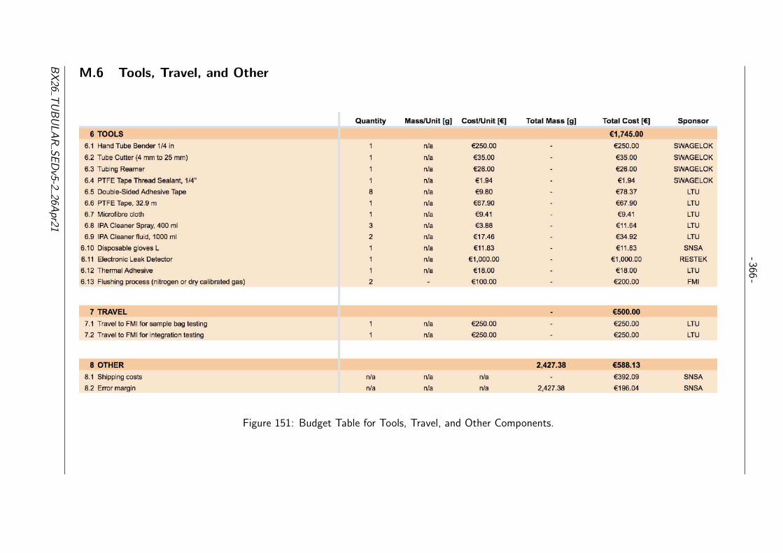
-366-
M.6 Tools, Travel, and Other
Figure 151: Budget Table for Tools, Travel, and Other Components.
BX
26T
UB
UL
AR
SE
Dv5-2
26Apr21

- 367 -
Appendix N Full List of Requirements
N.1 Functional Requirements
F.1 The experiment shall collect air samples.12
F.2 The experiment shall collect air samples by the CAC.
F.3 The experiment shall collect air samples by the AAC.
F.4 The experiment’s AAC System shall be able to collect air samples during the AscentPhase.12
F.5 The experiment’s AAC System shall be able to collect air samples during the DescentPhase.12
F.6 The altitude from which a sampling bag will start sampling shall be programmable. 13
F.7 The altitude from which a sampling bag will stop sampling shall be programmable.13
F.8 The experiment shall pump air into the AAC Sampling Bags.12
F.9 The experiment should measure the air intake flow to the AAC.
F.10 The experiment shall measure the air pressure.
F.11 The experiment shall measure the temperature.
F.12 The experiment shall collect data on the humidity. 12
F.13 The experiment shall measure the temperature inside the AAC Valve Box.12
F.14 The experiment should measure the humidity inside the AAC Valve Box.12
F.15 The experiment shall collect data on the time.14
F.16 The experiment shall accept telecommand instructions to program AAC sampling alti-tudes for each sampling bag.12
F.17 The experiment shall accept telecommand instructions to open designated valves.12
F.18 The experiment shall accept telecommand instructions to close designated valves.12
F.19 The experiment may accept telecommand instructions to change the sampling rate ofthe ambient pressure sensor.12
F.20 The experiment may accept telecommand instructions to change the sampling rate ofthe ambient temperature sensor.12
F.21 The experiment may accept telecommand instructions to change the sampling rate ofthe AAC Valve Box temperature sensor.12
F.22 The experiment may accept telecommand instructions to turn on the air pump.12
12Unnecessary requirement that has been removed.13Moved to design requirements.14Unverifiable requirement that has been removed.
BX26 TUBULAR SEDv5-2 26Apr21
- 368 -
F.23 The experiment may accept telecommand instructions to turn off the air pump.12
F.24 The experiment may accept telecommand instructions to turn on the Valve Heater.12
F.25 The experiment may accept telecommand instructions to turn off the Valve Heater.12
F.26 The experiment may accept telecommand instructions to turn on the Electronics BoxHeater.12
F.27 The experiment may accept telecommand instructions to turn off the Electronics BoxHeater.12
N.2 Performance Requirements
P.1 The telecommand data rate shall be 10 Kb/s.13
P.2 The default sampling rate of the ambient pressure sensor during Standby mode shall be0.1 Hz.15
P.3 The default sampling rate of the ambient pressure sensor during Normal operation-ascentmode shall be 0.2 Hz.15
P.4 The default sampling rate of the ambient pressure sensor during Normal operation-de-scent mode shall be 10 Hz.15
P.5 The default sampling rate of the AAC Valve Box temperature sensor shall be 1 Hz.15
P.6 The programmable sampling rate of the ambient pressure sensor shall not be lesser than0.1 Hz.15
P.7 The programmable sampling rate of the ambient pressure sensor shall not be greaterthan 100 Hz.15
P.8 The programmable sampling rate of the Electronics Box temperature sensor shall notbe lesser than 1 Hz.15
P.9 The programmable sampling rate of the Electronics Box temperature sensor shall notbe greater than 7 Hz.15
P.10 The programmable sampling rate of the AAC Valve Box temperature sensor shall notbe lesser than 1 Hz.15
P.11 The programmable sampling rate of the AAC Valve Box temperature sensor shall notbe greater than 7 Hz.15
P.12 The accuracy of the ambient pressure measurements shall be -1.5/+1.5 hPa for 25°C.
P.13 The accuracy of temperature measurements shall be +3.5/-3°C (max) for condition of-55°C to 150°C.
P.14 The accuracy of the ambient humidity measurements shall be ±3% . [13]12
P.15 The accuracy of the AAC Valve Box temperature measurements shall be +3.5/-2°C(max).16
15Replaced by P.2316Combined with P13
BX26 TUBULAR SEDv5-2 26Apr21

- 369 -
P.16 The air intake rate of the air pump shall be minimum 3 L/min.13
P.17 The temperature of the Electronics Box shall be between 0°C and 25°C. 13
P.18 The temperature of the Electronics Box shall not exceed 25°C.17
P.19 The temperature of the AAC Valve Box shall be between 0°C and 25°C.13
P.20 The temperature of the AAC Valve Box shall not exceed 25°C.18
P.21 The air sampling systems shall filter out all water molecules before filling the samplingcontainers. 13
P.22 The CAC air sampling shall filter out all water molecules before filling the tube.19
P.23 The sensors sampling rate shall be 1 Hz.
P.24 The temperature of the Pump shall be between 5°C and 40°C.
P.25 The minimum volume of air in the bags for analysis shall be 0.18 L at ground level.
P.26 The equivalent flow rate of the pump shall be between 8 to 3 L/min from ground levelup to 24 km altitude.
P.27 The accuracy range of the sampling time, or the resolution, shall be less than 52.94 s,or 423.53 m.
P.28 The sampling rate of the pressure sensor shall be 1 Hz.
P.29 The sampling rate of the airflow sensor shall be 1 Hz.
P.30 The accuracy of the pressure measurements inside the tubing and sampling bags shallbe -0.005/+0.005 bar for 25°C.
N.3 Design Requirements
D.1 The experiment shall operate in the temperature profile of the BEXUS flight[8].
D.2 The experiment shall operate in the vibration profile of the BEXUS flight[8].
D.3 The experiment shall not have sharp edges that can harm the launch vehicle, otherexperiments, and people.
D.4 The experiment’s communication system shall be compatible with the gondola’s E-linksystem.
D.5 The experiment’s power supply shall be compatible with the gondola’s provided power.
D.6 The experiment shall not disturb other experiments on the gondola.12
D.7 The total DC current draw should be below 1.8 A.
D.8 The total power consumption should be below 374 Wh.
17Combined with P17 and moved to design requirements.18Combined with P19 and moved to design requirements.19Combined with P21 and moved to design requirements.
BX26 TUBULAR SEDv5-2 26Apr21

- 370 -
D.9 The experiment shall be able to operate in low pressure conditions (10-15 hPa) up to30 km altitude.20
D.10 The components of the experiment shall operate within their temperature ranges.12
D.11 The OBC shall be able to autonomously control the heaters.12
D.12 The ground station GC shall be able to display some of the received data.12
D.13 The experiment shall be able to survive and operate between -30°C and 60°C.12
D.14 The external components that are directly exposed to the outside environment shall beable to operate at -70°C.12
D.15 The watchdog should be able to reset the system.12
D.16 The experiment shall be able to autonomously turn itself off just before landing.
D.17 The experiment box shall be placed with at least one face exposed to the outside.
D.18 The experiment shall operate in the pressure profile of the BEXUS flight[8].
D.19 The experiment shall operate in the vertical and horizontal accelerations profile of theBEXUS flight[8].
D.20 The experiment shall operate in the horizontal accelerations profile of the BEXUS flight.[8] 21
D.21 The experiment shall be attached to the gondola’s rails.
D.22 The telecommand data rate shall not be over 10 kb/s.
D.23 The air intake rate of the air pump shall be equivalent to a minimum of 3 L/min at 24km altitude.
D.24 The temperature of the Brain shall be between -10°C and 25°C.
D.25 The temperature of the Brain level 2 shall be between 0°C and 25°C. 22
D.26 The air sampling systems shall filter out all water molecules before filling the samplingbags.
D.27 The total weight of the experiment shall be less than 28 kg.
D.28 The AAC box shall be able to fit at least 6 air sampling bags.
D.29 The CAC box shall take less than 3 minutes to be removed from the gondola withoutremoving the whole experiment.
D.30 The AAC shall be re-usable for future balloon flights.
D.31 The altitude from which a sampling bag will start sampling shall be programmable.
D.32 The altitude from which a sampling bag will stop sampling shall be programmable.
20Repeated in D1821Combined with D1922Combined with D24
BX26 TUBULAR SEDv5-2 26Apr21

- 371 -
N.4 Operational Requirements
O.1 The TUBULAR Team shall send telecommands from the ground station to the experi-ment before and during the flight.12
O.2 The TUBULAR Team shall receive telemetry from the experiment during the flight.12
O.3 The experiment shall change modes autonomously.12
O.4 The heating mechanism shall work autonomously.12
O.5 The experiment shall store data autonomously.12
O.6 The Air sampling control system shall work autonomously.12
O.7 The valves in air sampling control system should be controllable from the ground sta-tion.12
O.8 The experiment should be able to handle a timeout or drop in the network connection.12
O.9 The heaters should be controllable from the ground station.12
O.10 The watchdog23 should be able to reset the system.12
O.11 The system should be able to be reset with a command from the ground station.12
O.12 The experiment should enter different modes with a telecommand from the groundstation.12
O.13 The experiment should function automatically.
O.14 The experiment’s air sampling mechanisms shall have a manual override.
N.5 Constraints
C.1 Constraints specified in the BEXUS User Manual.
C.2 The person-hours allocated to project implementation is limited by university relatedfactors such as exams, assignments, and lectures.12
C.3 Budget limited to TBD.12
C.4 The dimensions show a minimum print area of 50 x 50 cm and 65 cm height experimentbox.12
23Explained in subsection 4.8. Software Design
BX26 TUBULAR SEDv5-2 26Apr21

- 372 -
Appendix O Test Results
O.1 Test 28: Pump Operations
The pump was connected via crocodile connections to a power supply set to 24 V. The powersupply was then switched on and the current was read off. This set-up can be seen in Figure152.
It was found that when the power supply was switched on the current went up to 600 mAfor less than one second. It then settled to 250 mA. By covering the air intake, simulatingair intake from a lower pressure, the current drops to 200 mA. By covering the air output,simulating pushing air into a higher pressure, the current rises to 400 mA.
Therefore the power for each of these conditions is 14.4 W at turn on, 6 W in normal use, 4.8W when sucking from low pressure, 9.6 W when pushing to high pressure.
Figure 152: Photo Showing the Set-up for the Pump Testing in the Laboratory.
BX26 TUBULAR SEDv5-2 26Apr21
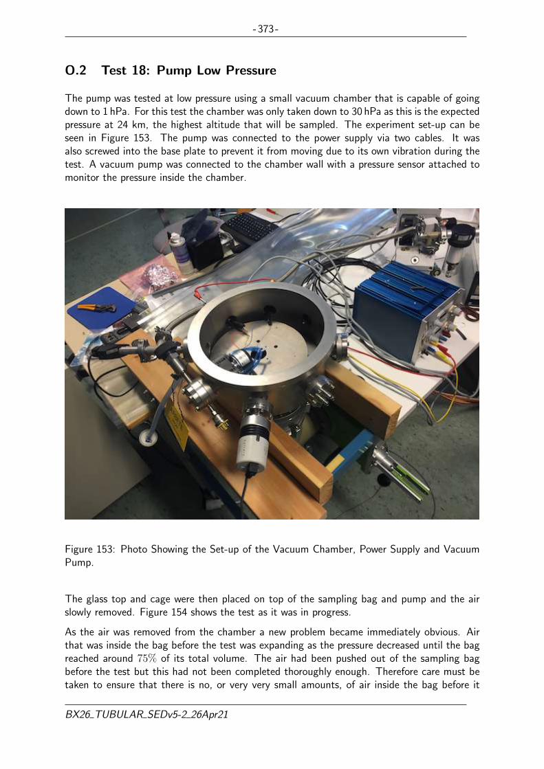
- 373 -
O.2 Test 18: Pump Low Pressure
The pump was tested at low pressure using a small vacuum chamber that is capable of goingdown to 1 hPa. For this test the chamber was only taken down to 30 hPa as this is the expectedpressure at 24 km, the highest altitude that will be sampled. The experiment set-up can beseen in Figure 153. The pump was connected to the power supply via two cables. It wasalso screwed into the base plate to prevent it from moving due to its own vibration during thetest. A vacuum pump was connected to the chamber wall with a pressure sensor attached tomonitor the pressure inside the chamber.
Figure 153: Photo Showing the Set-up of the Vacuum Chamber, Power Supply and VacuumPump.
The glass top and cage were then placed on top of the sampling bag and pump and the airslowly removed. Figure 154 shows the test as it was in progress.
As the air was removed from the chamber a new problem became immediately obvious. Airthat was inside the bag before the test was expanding as the pressure decreased until the bagreached around 75% of its total volume. The air had been pushed out of the sampling bagbefore the test but this had not been completed thoroughly enough. Therefore care must betaken to ensure that there is no, or very very small amounts, of air inside the bag before it
BX26 TUBULAR SEDv5-2 26Apr21

- 374 -
enters a low pressure environment. For subsequent tests the pump was used in reverse to suckany remaining air out of the bags.
Figure 154: Photo Showing the Pump and Sampling Bag in the Vacuum Chamber During theTest.
Repeating the test and using the pump to suck out excess air from the bags the chamber wastaken to around 30 hPa. Once the chamber was at this pressure the pump was switched onand a stopwatch began. Once the bag stopped inflating the stopwatch was stopped. Duringthis test there was also a drop in pressure to 28 hPa and during a repeat there was a drop to25 hPa. This also occurred in later tests. This is not seen as a significant problem as duringthe flight this is exactly what will happen when testing during ascent. In addition the flow rateincreases with increasing outside pressure therefore this is showing our worst case flow rate. Itwas found that the pump was able to successfully switch on and fill the bag at this altitudewith a flow rate of approximately 3 L/min.
The test was repeated again at 88 hPa, representing 17 km altitude and 220 hPa, representing11 km altitude. Here the flow rates were found to be 3.4 L/min and 4.9 L/min respectively.The results can also be seen in Table 78 and Figure 155.
As this test could only provide and approximation due to the lack of equipment such as flow-meters that would have made this test more precise it was later repeated. In the repeat ofthis test the flow rates were found to be within the same magnitude. The full results can beseen in Section 7.3.5 in Table 56.
BX26 TUBULAR SEDv5-2 26Apr21

- 375 -
Altitude
(km)
Pressure
Start (hPa)
Pressure
End (hPa)Time (sec)
Flow Rate
(L/min)
24 30 23 60 317 87 80 53 3.411 220 190 37 4.9
Table 78: Table Showing the Time Taken Until the 3 L Bag Stopped Expanding at VariousDifferent Pressures.
Figure 155: Obtained Pump Performance at Low Pressure.
O.2.1 Test 30: Sampling Bag Bursting
A sampling bag was placed in a small vacuum chamber connected to the pump with the sameset up as in Test 18, see Figures 153 and 154. The pump was run for 3 minutes with a fullbag to see how the bag reacted. No changes were observed in the bag and no leaks appearedwhilst it was in the testing chamber. Upon returning it to atmospheric levels it also appearedto be able to withstand the over pressure. The bag was then left, with the valve closed, on atable where it was handled a little during this time. Approximately 30 minutes after the testthe bag made an audible popping noise and air leaked out. The damage that occurred to thebag during the burst can be seen in Figure 156 for the front of the bag and Figure 157 for theback of the bag.
BX26 TUBULAR SEDv5-2 26Apr21

- 376 -
Figure 156: Photo Showing the Extent of Damage on the Front of the Bag Due to Bursting.
Figure 157: Photo Showing the Extent of Damage on the Back of the Bag Due to Bursting.
This kind of bag failure could occur if bags are overfilled, particularly during ascent.
Next the system was set-up in the same way with a new bag. This time the pump wascontinuously run until failure occurred. This took around 6 minutes. The bag failed alongthe lower seam close to the valve and also at the valve connection. At the valve connectionthe bag ripped just above the valve. This time the burst was more energetic with the bottomof the bag moving outwards. Upon inspection the bottom of the bag was completely openand the part of the bag connected to the valve partially ripped open. In addition at the topof the bag small failures similar to those seen in Figure 156 were seen again. It is thereforethought that the bag was starting to fail at both the top and the bottom of the bag and butthe bottom failed first.
The damage can be seen in Figures 158 and 159. It should be noted that the white bag valvewas pulled off after the test and before photos were taken.
BX26 TUBULAR SEDv5-2 26Apr21
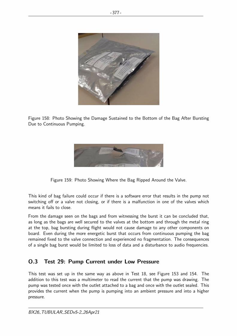
- 377 -
Figure 158: Photo Showing the Damage Sustained to the Bottom of the Bag After BurstingDue to Continuous Pumping.
Figure 159: Photo Showing Where the Bag Ripped Around the Valve.
This kind of bag failure could occur if there is a software error that results in the pump notswitching off or a valve not closing, or if there is a malfunction in one of the valves whichmeans it fails to close.
From the damage seen on the bags and from witnessing the burst it can be concluded that,as long as the bags are well secured to the valves at the bottom and through the metal ringat the top, bag bursting during flight would not cause damage to any other components onboard. Even during the more energetic burst that occurs from continuous pumping the bagremained fixed to the valve connection and experienced no fragmentation. The consequencesof a single bag burst would be limited to loss of data and a disturbance to audio frequencies.
O.3 Test 29: Pump Current under Low Pressure
This test was set up in the same way as above in Test 18, see Figure 153 and 154. Theaddition to this test was a multimeter to read the current that the pump was drawing. Thepump was tested once with the outlet attached to a bag and once with the outlet sealed. Thisprovides the current when the pump is pumping into an ambient pressure and into a higherpressure.
BX26 TUBULAR SEDv5-2 26Apr21

- 378 -
In general it was found for both cases that decreasing the pressure, or increasing the altitude,lead to a decrease in pump current draw. It was noted that there was an increase in currentdraw in between sea level conditions and 11 km altitude conditions. However as the lowestsampling point it intended to be at 11 km this should not be a problem for the experiment.The full results can be seen in Table 79.
Altitude (km) Pressure (hPa)Into Bag Current(mA)
Into Seal Current(mA)
20 57 140 13818 68 150 14116 100 161 14612 190 185 1759 300 - 2006 500 - 2420 1013 - 218
Table 79: Table Showing How the Current Draw of the Pump Changed With Outside AirPressure for Two Different Conditions. The First Pumping Into a Sampling Bag and theSecond Pumping Into a Sealed Tube.
A graphical representation of these results are shown in Figures 160 and 161. From the tableand figures it can be seen that the current draw is higher during the bag filling than duringthe sealed case. As the experiment will sample between 11 km and 24 km it can be concludedthat the highest current draw will occur during the 11 km altitude sample and can be expectedto be around 200 mA.
BX26 TUBULAR SEDv5-2 26Apr21

- 379 -
Figure 160: Graph Showing the Expected Current Values When the Pump is Pumping Air Intoa Bag Based Upon the Results Obtained.
BX26 TUBULAR SEDv5-2 26Apr21

- 380 -
Figure 161: Graph Showing the Expected Current Values When the Pump is Pumping Air Intoa Sealed Outlet Based Upon the Results Obtained and the Data Shown In Figure 31.
By looking at the data from both Test 18 and Test 29 a relationship can be seen between theoutside air pressure, the flow rate of the pump and the current draw of the pump.
O.4 Test 17: Sampling bags’ holding times and samples’ condensa-tion verification
The main objective of this test was to flush eight 1 L sampling bags with nitrogen, the sameway it will be done for the flight. After the flushing is done, fill them with a dry gas and leavethem outside for 6, 14, 24 and 48 hours. Then analyze two sampling bags after each timeduration and see if the concentration of gases inside has changed.
A dry gas is a gas of high concentration of CO and low H2O and its exact concentrationcan be known by comparison to the calibrating gas in the Picarro analyzer. Therefore, theconcentration when sampling the bags is known and it can be compared with the concentrationafter analysis. If the sampling bags can hold the samples for 48 hours then when analyzing,the concentration of gases should not change. If condensation occurs that will be seen as anincrease in water vapour concentration.
Note that the size of the sampling bags was not the same as the size that will be usedduring the experiment. The reasons were availability of 1 L sampling bags at FMI and a firstassumption that the size would not affect the results. The sampling bags were exactly thesame model/material.
BX26 TUBULAR SEDv5-2 26Apr21

- 381 -
This test was realized at FMI in Sodankyla. Eight Multi-Layer Foil bags of 1 L volume wereconnected to SMC valves as shown in Figure 162 and all together connected in series withstainless steel tubes as can be seen in Figure 163.
Figure 162: 1 L Sampling Bag With SMC Valve Attached to It. The Valve is at One of theEnds of the System so a Quick Connector is Connecting it to the Tube That Goes to theNitrogen Bottle/Vacuum Pump.
BX26 TUBULAR SEDv5-2 26Apr21

- 382 -
Figure 163: Sampling Bags System Connected in Series.
BX26 TUBULAR SEDv5-2 26Apr21
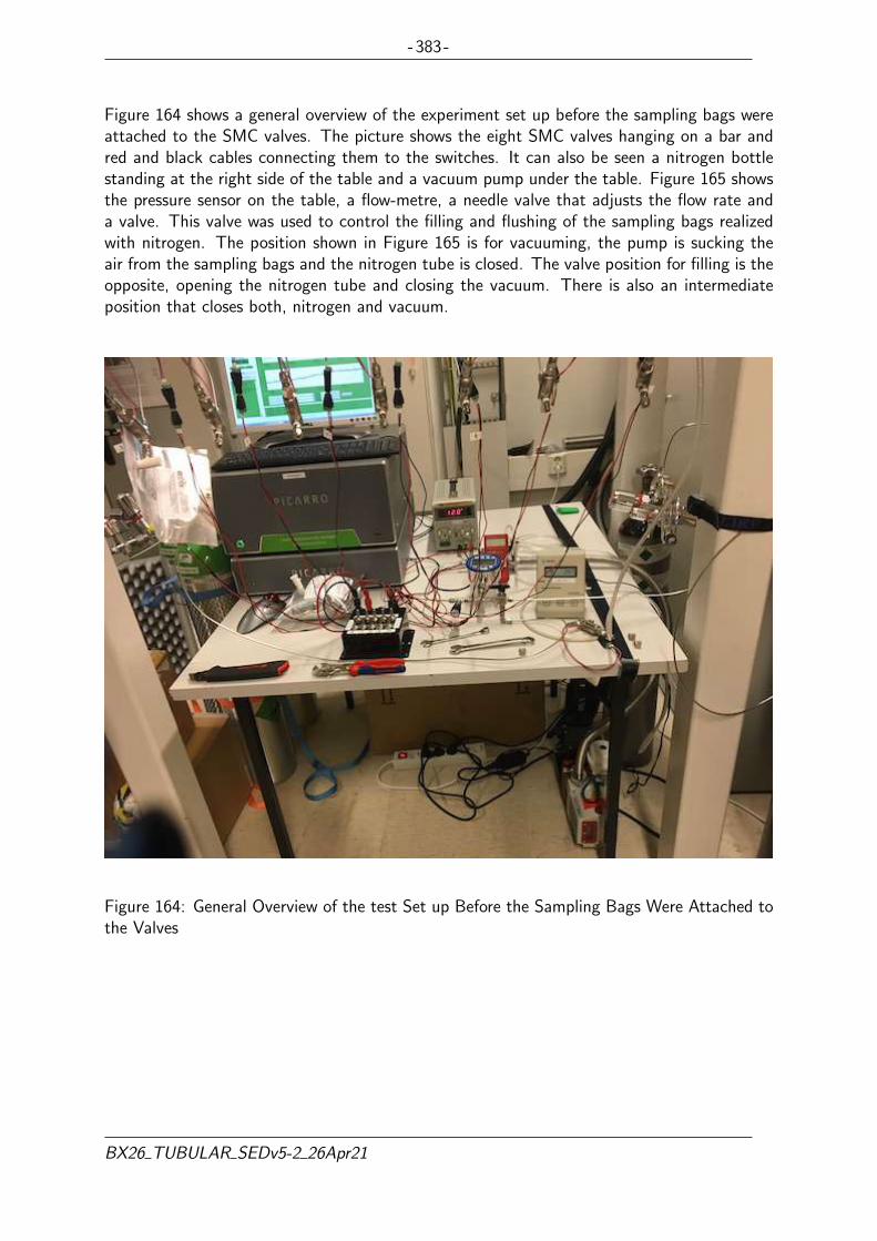
- 383 -
Figure 164 shows a general overview of the experiment set up before the sampling bags wereattached to the SMC valves. The picture shows the eight SMC valves hanging on a bar andred and black cables connecting them to the switches. It can also be seen a nitrogen bottlestanding at the right side of the table and a vacuum pump under the table. Figure 165 showsthe pressure sensor on the table, a flow-metre, a needle valve that adjusts the flow rate anda valve. This valve was used to control the filling and flushing of the sampling bags realizedwith nitrogen. The position shown in Figure 165 is for vacuuming, the pump is sucking theair from the sampling bags and the nitrogen tube is closed. The valve position for filling is theopposite, opening the nitrogen tube and closing the vacuum. There is also an intermediateposition that closes both, nitrogen and vacuum.
Figure 164: General Overview of the test Set up Before the Sampling Bags Were Attached tothe Valves
BX26 TUBULAR SEDv5-2 26Apr21

- 384 -
Figure 165: Valve that Controls Filling/Vacuum in of the Sampling Bags. Pressure Sensor,Flow-metre and Needle Valve.
The procedure during the test was as follows:
• Set up all the connections between pump, nitrogen bottle, valves system in series.
• Attach the sampling bags to the SMC valves.
• Start flushing the tubes with nitrogen. For this all the sampling bags’ valves are closed.
• Adjust the flow rate of nitrogen at 500 ml/min.
• Open sampling bags’ manual valves (not to be confused with the SMC valves which arestill all closed).
BX26 TUBULAR SEDv5-2 26Apr21

- 385 -
• Turn on valve 1. Fill sampling bag number 1 for 2 minutes. Turn off valve 1. Repeat itfor the seven sampling bags left.
• Change the valve seen in Figure 165 to vacuum position and empty the bags.
• Flush the tubes after all the sampling bags have been emptied. This is to remove asmuch air as possible that could be left inside the sampling bags.
• Repeat the flushing for two more times.
• Change the nitrogen bottle for the dry gas bottle.
• Flush the tubes with nitrogen.
• Fill the eight sampling bags one by one.
• Take the sampling bags outside as shown in Figure 166 to simulate the conditions atwhich they will be exposed after landing.
Figure 166: Sampling Bags Left Outside Waiting to be Analyzed.
After each of the mentioned times, 6, 14, 24 and 48 hours, two sampling bags were takeninside the laboratory to be analyzed. The procedure to analyze was:
• Have the dry gas flowing through the Picarro analyzer for at least one hour before theanalysis. This is to avoid having moisture inside the tubes and have stable measurementsof concentrations.
• Flush the tubes in between the two sampling bags with dry gas. For that the dry gas hasto be disconnected from the analyzer and moisture would get into the Picarro. To avoidthis, calibrating gas is flowing through the analyzer while the tubes are being flushed.
• Connect the system formed by two sampling bags with one end to the dry gas bottleand the other to the Picarro inlet.
BX26 TUBULAR SEDv5-2 26Apr21

- 386 -
• Wait for one hour until the readings of dry gas concentrations are stable.
• Open the valve of the first sampling bag.
• Right after the first sampling bag is empty, close its valve and open the valve for thenext one.
• Keep the dry gas flowing for one more hour after analysis.
After analyzing the sampling bags the obtained results are presented in Figure 167.
Figure 167: Obtained Variation in Concentration for (a) CO2 in ppm, (b) CO in ppb, (c)CH4 in ppb and (d) H2O in ppb.
It should be mentioned that the results were not at all what was expected. If the samplingbags held the gases for 48 hours, the analyzed concentration should have been the same asthe dry gas used to fill them or the variation should have been smaller.
A possible explanation for this results could be that the emptying of the sampling bags wasnot done rigorously enough and that some air/nitrogen was left inside which diluted in the drygas and changed the concentrations. This effect is even increased due to the smaller size ofthe used sampling bags (1 L instead of 3 L). This would also explain why the results don’tfollow any pattern.
The general outcome of this test was that the team realized that the flushing of the samplingbags is a very delicate process. This test was also useful to decide that the flushing of the
BX26 TUBULAR SEDv5-2 26Apr21

- 387 -
sampling bags should be done with dry gas instead of nitrogen in order to minimize the effectsof the nitrogen diluting in the samples.
This test had to and was repeated, using the set-up described in Section 4, with some dif-ferences. This time 3L bags were flushed with dry gas and left outside for 15, 24, 48 hours.After the flushing was done, two bags for each time were filled with 0.5 L and 1L of dry gasand left outside. Then they were analyzed and checked if the sample concentrations were thesame or close enough with the reference values of the filled dry gas.
The obtained results are shown in Figure 168. The blue points represent the sampling bags withthe 0.5L sample, while the red points show the sampling bags with the 1L sample. SamplingBag No1 with the sampling bag No4 were analyzed after 15 hours. The pair of sampling bagsNo2 and No5 were analyzed after 24 hours and the last pair of sampling bags, No4 and No6after 48 hours.
Figure 168: Obtained Variation in Concentration for (a) CO2 in ppm, (b) CO in ppb, (c)CH4 in ppb and (d) H2O in %.
The results were very good in general with the CO2 concentration differences not higher than2 ppm. The bags with the 0.5L sample gave bigger CO2 concentration differences and higherhumidity for all the tested times. For the bags that analyzed after 48 hours, the humiditywas two times higher for the 0.5L sample compared to the 1L sample. If water goes throughthe walls of the bags at the same rate for both bags then it is normal that sampling bags
BX26 TUBULAR SEDv5-2 26Apr21

- 388 -
with larger amounts of sampled air have lower humidity concentrations. Therefore, for betterresults, the air left in the sampling bags at sea level pressure must be the maximum possible.
O.4.1 Test 4: Low Pressure
Styrofoam
The same vacuum chamber was used as in Tests 18 and 29. The Styrofoam was measuredon each side before it was placed in the chamber. It was then taken down to 5 hPa and heldthere for 75 minutes. It was then removed and the sides were measured again. It was foundthat there was no significant change in dimensions. The results can be seen in Table 80.
Side Before (cm) After (cm)A 9.610 9.580B 9.555 9.550C 9.560 9.565D 9.615 9.610E 9.615 9.615F 9.555 9.550G 9.605 9.605H 5.020 5.020I 5.025 5.025J 5.015 5.015K 5.020 5.025
Table 80: Styrofoam Size Before and After Vacuum.
As some sides are measured slightly bigger after and some slightly smaller it is thought this isdue to the measuring technique and not due to changes in the Styrofoam. It is thought theresult from side A could be due to deforming the Styrofoam with calipers or a misread originallength.
Figure 169: Picture Showing how the Styrofoam was Labeled for the Test.
BX26 TUBULAR SEDv5-2 26Apr21

- 389 -
Airflow
After the first airflow in vacuum test failed due to datalogging errors the airflow test wasrepeated. In this repeated test all of the Brain was placed into the vacuum chamber and onebag attached. It was not possible to attach more than one bag due to space restrictions. Aview inside the vacuum chamber can be seen in Figure 170.
Figure 170: Picture Showing inside of the Vacuum Chamber During the Test.
To confirm the airflow rates the vacuum chamber was then taken down to from 400 hPa to 5hPa in steps and the airflow rate logged. The results can be seen in Figure 171.
BX26 TUBULAR SEDv5-2 26Apr21

- 390 -
Figure 171: Graph Showing how the Airflow Rate is Changing with Ambient Pressure.
Sampling will take place between 200 hPa and 22 hPa, this area is seen in greater detail inFigure 172. From this graph it can be seen that the airflow rate is varying from 1.2 LPM to0.1 LPM.
BX26 TUBULAR SEDv5-2 26Apr21
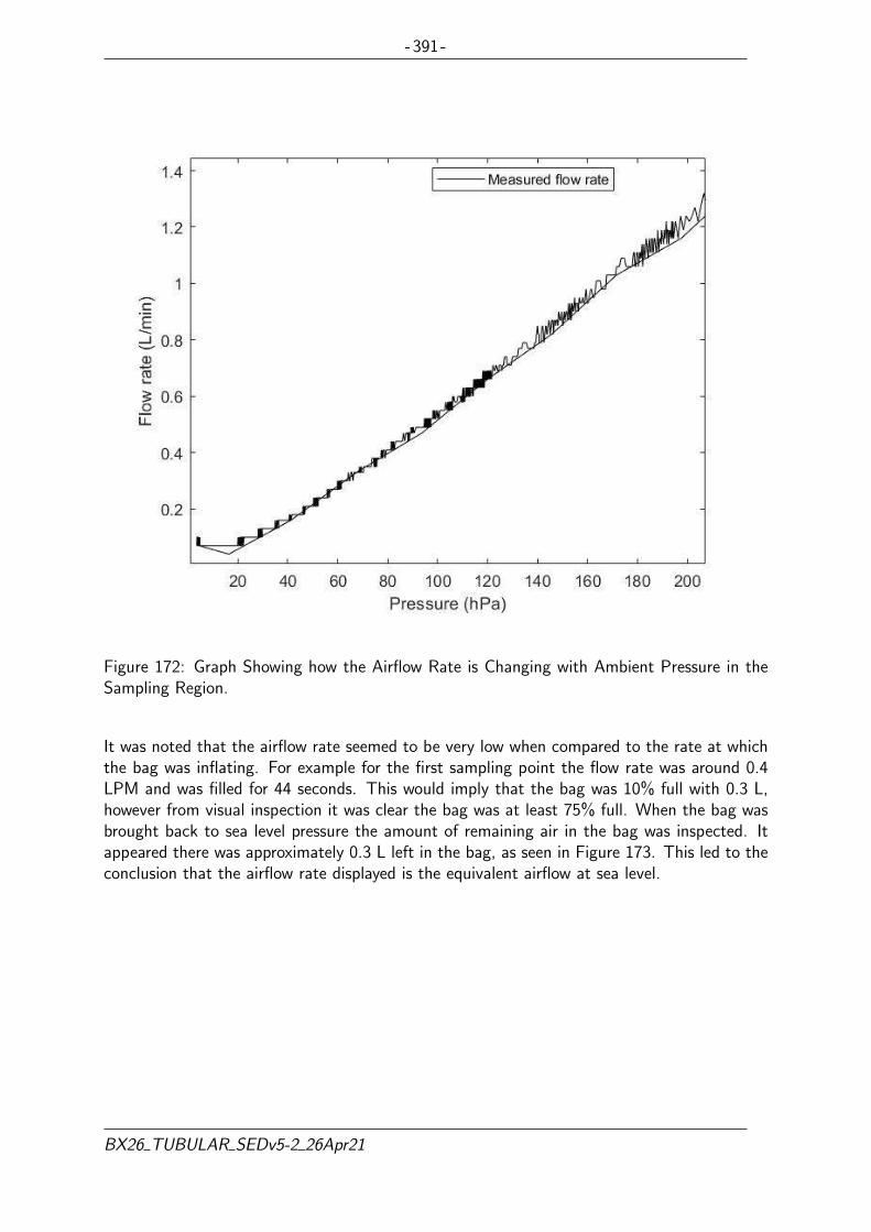
- 391 -
Figure 172: Graph Showing how the Airflow Rate is Changing with Ambient Pressure in theSampling Region.
It was noted that the airflow rate seemed to be very low when compared to the rate at whichthe bag was inflating. For example for the first sampling point the flow rate was around 0.4LPM and was filled for 44 seconds. This would imply that the bag was 10% full with 0.3 L,however from visual inspection it was clear the bag was at least 75% full. When the bag wasbrought back to sea level pressure the amount of remaining air in the bag was inspected. Itappeared there was approximately 0.3 L left in the bag, as seen in Figure 173. This led to theconclusion that the airflow rate displayed is the equivalent airflow at sea level.
BX26 TUBULAR SEDv5-2 26Apr21

- 392 -
Figure 173: Picture Showing the Air Remaining in the Bag After Returning to Sea LevelPressure.
Software
With the same set-up as the airflow low pressure testing the software was tested to verify if itwas operating as intended and that the conditions for stopping sampling were working.
First the software was run as it will be during flight. As the pressure inside the chamber wasdropped it was possible to see through the LEDs on board the PCB the system going throughthe flight actions. When the first sampling altitude was reached the lights came on for theflushing valve and pump indicating the system was flushing. After one minute these lightswent out and the first valve opened. For the first sampling point it was possible to see thebag inflate providing extra visual confirmation that the system is operating as intended.
The next check was to see if our conditions for stopping sampling were working. Testing withthe initial sampling schedule meant that the time stopper always occurred first and workedwell. The pressure threshold stopper also worked well with the system stopping sampling ifthe defined pressure range was left. Our third stopper is based on pressure and compares thepressure inside the bag to the ambient pressure to ensure we do not overpressure the bags.Interestingly it was found that this pressure was not being reached even after filling the bagscontinuously for three minutes, three times our time limit.
This shows that the maximum allowed pressure for the bags is not the pressure when the bagis 3L full but when the air in the bag has been compressed. This reduces the risk of bagsbursting significantly.
Temperatures
As it is not possible to complete a thermal vacuum test in addition to the thermal testingtemperatures were also monitored inside the vacuum chamber. Particular attention was paidto the CAC valve which will be on for the entire flight. From Figure 174 it can be seen thatafter 2 hours the temperature is leveling off at around 68°C. This is still well within theoperating temperature range of the valve. In addition this was also held at 5 hPa which is a
BX26 TUBULAR SEDv5-2 26Apr21
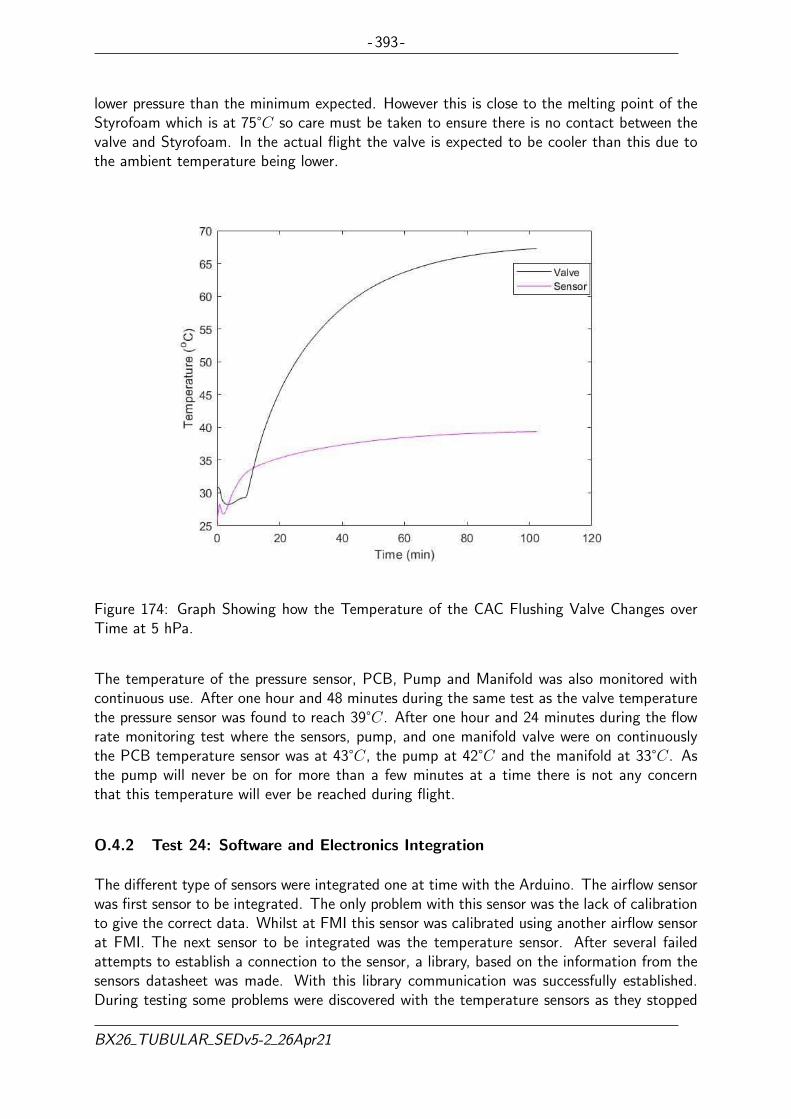
- 393 -
lower pressure than the minimum expected. However this is close to the melting point of theStyrofoam which is at 75°C so care must be taken to ensure there is no contact between thevalve and Styrofoam. In the actual flight the valve is expected to be cooler than this due tothe ambient temperature being lower.
Figure 174: Graph Showing how the Temperature of the CAC Flushing Valve Changes overTime at 5 hPa.
The temperature of the pressure sensor, PCB, Pump and Manifold was also monitored withcontinuous use. After one hour and 48 minutes during the same test as the valve temperaturethe pressure sensor was found to reach 39°C. After one hour and 24 minutes during the flowrate monitoring test where the sensors, pump, and one manifold valve were on continuouslythe PCB temperature sensor was at 43°C, the pump at 42°C and the manifold at 33°C. Asthe pump will never be on for more than a few minutes at a time there is not any concernthat this temperature will ever be reached during flight.
O.4.2 Test 24: Software and Electronics Integration
The different type of sensors were integrated one at time with the Arduino. The airflow sensorwas first sensor to be integrated. The only problem with this sensor was the lack of calibrationto give the correct data. Whilst at FMI this sensor was calibrated using another airflow sensorat FMI. The next sensor to be integrated was the temperature sensor. After several failedattempts to establish a connection to the sensor, a library, based on the information from thesensors datasheet was made. With this library communication was successfully established.During testing some problems were discovered with the temperature sensors as they stopped
BX26 TUBULAR SEDv5-2 26Apr21
- 394 -
giving data back when exposed to colder temperatures. This was fixed by implementing a newpiece of software code. Before the integration of the pressure sensor it had been expected theneed of a self made library, despite this several changes was needed to the library to make thesensor responsive.
It was discovered that the pressure sensor on board the PCB wouldn’t function while the otherpressure sensors when connected to the SPI bus. Parasitic capacitance was suggested to be theculprit when looking on the SPI bus with an oscilloscope. During an telephone conference withour mentors another more reasonable theory was put forwards. Since the SPI was designedto function for short distances only the long cables connecting the outside pressure sensorscaused reflections in the bus. The solution was to disregard the pressure sensor on the PCBsince it was not a critical sensor.
When all the sensors had been integrated the sensors where tested together. The result wasall the sensors, exept the PCB pressure sensor, working without interfering with each other.
O.4.3 Test 5: Thermal Test
The thermal chamber used was the one at FMI and Esrange. At FMI it could go down tobetween −40°C and −90°C and at Esrange it were tested down to −60°C. A few longrun tests were done slowly going down to a temperature and stabilizing before lowering thetemperature again to safely test that everything worked when it was below −20°C outsideand if it would handle a 4h −40°C test. The long run test for −40°C still needs to be done,because the temperature sensors gave an error and stopped showing data meaning the testwas interrupted. With no temperature data the heaters could not be operated properly andthe risk for damage was high enough to stop the testing to make sure no components wereharmed.
To start with, only the AAC was put into the freezer. In the following Figures the verticaldotted line indicates where the sensor started to throw the error. The first test slowly wentdown to −20°C before it stabilized, then it went down to −30°C and then the communicationreceived an error after a while as seen in Figure 175.
BX26 TUBULAR SEDv5-2 26Apr21

- 395 -
Figure 175: First Thermal Chamber Test.
The second test went straight down to −30°C and stabilized there to try long run test. Aftera while the communication got error again. The test can be seen in Figure 176.
Figure 176: Second Thermal Chamber Test.
The third test went down to −40°C and was left to stabilize. After approximately half an hourthe communication error happened again as seen in Figure 177.
BX26 TUBULAR SEDv5-2 26Apr21

- 396 -
Figure 177: Third Thermal Chamber Test.
The fourth test was a repeat of the third test with −40°C and left to stabilize and survivedapproximately 50min as seen in Figure 178.
Figure 178: Fourth Thermal Chamber Test.
A separate test was completed afterwards with only the CAC inside the freezer and the AACoutside with cables going to the CAC. The freezer was at −26°C and the communication erroroccurred as seen in Figure 179.
BX26 TUBULAR SEDv5-2 26Apr21

- 397 -
Figure 179: CAC Thermal Chamber Test.
The conclusion of the test is that the heating regulations for the pump and the manifold areworking as they should keeping the critical components operating. It was concluded that thePCB is not the issue for the temperature sensors to give back error. The communicationerror was solved and a 8h freezer test were done at IRF to see if it could work in −20°Ctemperature. At the same time three different resistors were put for the outside pressuresensors. The resistors produced 0.1W, 0.5W and 1W to the pressure sensors to determine thetemperature difference from ambient temperature. In Figure 180 the temperatures is shownover time.
Figure 180: Freezer Test for 8h at IRF.
The average temperature difference between the pressure sensor and the ambient temperaturewas as can be seen in table 81.
BX26 TUBULAR SEDv5-2 26Apr21

- 398 -
Watt from resistor (W) 0.1 0.5 1Temperature difference (°C) 14.0488 31.336 56.9809
Table 81: Temperature Difference on Pressure Sensor from Ambient.
A final thermal test were done at Esrange. The test were 3h and 30min at −50°C where allfunctions were tested and then went down to −60°C to try the experiment a little more. Inthe end the test lasted 4h 40min.
As seen in Figure 181 the temperature of the pump (pink) and the valve (black) have theirheating cycles fully working. After a little more then an hour the flushing were tested. Thensoon after the pump and it can be seen that the temperature of the pump drop bellow zero. Itwere confirmed then if the pump is operating it can drop bellow zero and keep going. It werefound out that when it were −55°C and colder the valve heater could not keep up fully andstarted to drop in temperature when the valves were not operating. Even while the temperaturewere dropping it were so slow and that it will not drop bellow operating temperature duringflight and if the valves are operating they generate some heat as well.
Figure 181: Thermal Chamber Test.
In Figure 181 it can be seen a lot of spikes and it is when the software returns an error value.It is not an issue because the error rate is so low and goes back to working directly after so itdoes not affect the heating system.
O.4.4 Test 20: Switching Circuit Testing and Verification
This has begun on breadboards with LEDs replacing the valves until the valves arrive.
So far DC-DCs have been set up and tested. Sensors have been connected electronically andthe next step is to get them to communicate with the Arduino.
BX26 TUBULAR SEDv5-2 26Apr21

- 399 -
Mosfets connecting to the pump and the heaters have been tested for switching on and offwith good results.
O.4.5 Test 32: Software Failure
So far testing has revealed that losing the SD card does not interrupt ground station data, itjust means no data will be written to the SD card. However, if you reconnect the SD afterremoving it currently it will not connect back to the SD card and it as if the SD card has beenpermanently lost.
BX26 TUBULAR SEDv5-2 26Apr21

- 400 -
O.5 Test 33: Electrical Component Testing
The components were separately tested and later on tested together inside the full system. Theseparate component testing can be seen in Table 82. The results of these tests can be seen inSection O.5.1. There was also a full assembly off all components on the bench connected ona breadboard. This test was carried out with nominal results. Furthermore there were somePCB tests which can be seen in Table 83. The results of these tests can be seen in O.5.2
Complete Test # Test Description
YES 1Test Voltage di-vider (Airflow +Pressure sensor)
Test the airflow sense with voltage dividerand check the voltage output with dividervs without to control that signal does notget interfered
YES 2 Test MOSFETTest the MOSFETS by applying 3.3v tothe gate from something else than Arduino
YES 3Test LED Configu-ration
Test the resistance and zener diode con-figuration
YES 4Test Valves withMOSFET
Test to open and close valves through theMOSFETS without Arduino 3.3v
YES 5Test Pump +MOSFET
Same as valves but for pump
YES 6Test DCDCs inparallel with LED
Test that the parallel configuration of thedcdc converters with the indication lightsand make sure it works as expected
YES 7Test interface con-nections
Test the dsub and power cables that willbe inside the brain by checking for connec-tivity and wire resistances.
YES 8Test Potentiome-ter trimming forDCDC
Test the DCDC trimming by using the po-tentiometers
YES 9Test ground-ing for analogcomponents
Test the grounding configuration for theanalog components and compare it withnon isolated ground wile turning on otherpower hungry components
YES 10 Heater testingSupply 28.8v to the heaters in paralel andsee if they work outside their limits de-scribed in the datasheet.
Table 82: Electrical Component Testing Detailed Descriptions
Complete Test # Test Description
YES 12 Check conectionsCheck that all soldering points are con-nected to the right parts of the board
YES 13 AssemblySolder everything in it’s places and turnthe board on and chech that everything isworking nominaly
Table 83: PCB Tests with Detailed Descriptions
BX26 TUBULAR SEDv5-2 26Apr21

- 401 -
.
O.5.1 Test results for Electrical component testing
• Test 1: The max output from the airflow sensor was not 10V as advertised, it wasinstead 10.82V. The resistors in the voltage divider will be changed accordingly to takecare of this problem and not to damage the Arduino. There will be 240k Ohms on theupper part of the voltage divider and 100k on the bottom. This will limit the max outputto approximately 3.2V which will be safe for the Arduino. Pressure sensor max outputwas approximately 9.54V at ground level. The sensor is sensitive to the voltage divider.It seems that a larger resistance lowers the output compared to an open circuit. Aftertesting with three resistors at 330k, 100k, 33k and 3.3k Ohm resistor it was seen thatusing 330k Ohm the output was measured to 7V over the whole bridge. With the 3.3kOhm voltage divider the output was measured to be 9.52V which is 0.2% below opencircuit which is smaller than the measurement error of the sensor itself. Furthermore theoutput had a lot of very small spikes which gave a voltage ripple of 300-400mV, addinga 0.47uF capacitance in parallel to the output and ground decreased the ripple to 60-70mV. Larger capacitors did not lower the ripple although smaller capacitors increasedthe ripple. Furthermore the start up spikes of the senor has to be rectified, therefore a1uF capacitor will be added to the sensor output on the wiring since there is no spacededicated for this on the main PCB. Furthermore, huge spikes of upwards to 30V peakto peak was discovered on turn on on the Vin on the pressure sensor. Therefore a 100uFelectrolytic capacitor will be added in parallel to the 12 system
• Test 2: Using the MOSFET as a grounding switch and supplying 3.2V to the gate theresulting drain to source voltage was below 0.3V for components using 24V or 28V
• Test 3: 1k Ohm on 12V 3.9k Ohm for 24V as pull-up resistors
• Test 4: The circuit worked as expected. The circuit pulled 127mA at 24V 3.048W forone manifold valve. The valves on the tubing gave the same results
• Test 5: Supplying 3.2V to the gate on the MOSFET started the pump as expected.
• Test 6: The circuit functioned as expected. The indications are indicating each DCDCindividually
• Test 7: All interface connections have been checked with good result by using thecontinuity measurement on a multimeter
• Test 8: Trimming works, extra resistors had to be added in series with the potentiometerto get the resistance required for the voltage output that was required. 26+390k Ohmfor 24V. 15 + 32k Ohm for 12V
• Test 9: The proposed way of grounding analog sensors works. Although, if there is afaulty grounding somewhere else, the Arduino sits at risk since all the grounding currentgoes through the Arduino and might burn the Arduino
• Test 10: Using the heaters in parallel at 28.8V worked fine as long as they had somematerial to dissipate the heat into. Otherwise they are overheating. This is true at28V as well which is the specified max voltage. Supplying 28.8V will not be a problem.
BX26 TUBULAR SEDv5-2 26Apr21

- 402 -
The heaters did use a little extra power. The specific power draws were: 28.62V anddepending on the temperature the power draw was 0.37-0.36A. This results in a powerdraw of 10.59W which is 0.59W or 5.9% more than expected.
O.5.2 Test Results for PCB Testing
• Test 12: All connections were checked and it was discovered that some connections werenot connected and some were faulty connected. There was one MOSFET gate pin thatwas not connected. The 28.8V power that goes to the heaters was connected to the 24Vpower. And the 24V power was not connected to the dc-dc. This was solved by addinga separate wire to connect the 24V power to one of the pins 24V pins on the D-Subs,since the D-Subs were connected together. The 28.8V power was solved by removingthe cable from the d-sub and adding a separate connector that goes to 28.8V power.The MOSFET gate problem was solved by adding a wire from the correct Arduino pinto the corresponding MOSFET gate pin.
• Test 13: After the connections was checked and the problems resolved, the board wasturned on. The functionality was checked and everything worked nominally.
O.5.3 Test 27: Shock test
The entire pneumatic system and electrical system was mounted in the AAC box along withthe walls and styrofoam attached. It was then dropped from a height of approximately onemeter three times. Nothing came loose or was damaged after this drop test. All electronicswere verified to still work.
O.5.4 Test 9: Vibration test
The entire experiment was placed in the tailgate of a car, while the test was carried out ona 18 km long rough terrain. An emergency brake was also implemented during the test. Theexperiment’s functionality and structural integrity were capable of handling the vibrations andthe stopping force. No damages or issues were detected after this test.
O.5.5 Test 25: Structure test
A team member was placed on top of each box’s structure, see Figure 183. Both the CACand AAC box was able to fully support the member’s weight without showing any instabilityor deflections. No damages or issues were detected after this test.
BX26 TUBULAR SEDv5-2 26Apr21

- 403 -
Figure 182: Structure Test for AAC Box
O.5.6 Test 12: Removal test
For a non team member to perform the removal of the CAC box based on the given instructions,it took that person 6 min and 25 sec. One problem that occurred during this test was thatthe person had problems to distinguishing the CAC from the AAC box. To resolve this theboxes will now have clear labels on them. The set up for this test can be seen in Figure ??.
Figure 183: Picture Showing how the Experiment was Mounted on the Bench.
There were additional confusions during the test due to the fact the experiment was not actuallyfixed to the gondola and it had to be explained what was meant by gondola attachment points.The items to be unscrewed were also not yet clearly marked which also added time to the test.It is expected that the time will be lower for the recovery team due to this. Therefore theteam finds this time to be satisfactory.
BX26 TUBULAR SEDv5-2 26Apr21

- 404 -
O.5.7 Test 2: Data collection test
The full software was run in auto mode to check everything operated as expected over a fulltest flight. At the end of the simulated flight the experiment was to shutdown automatically.This was tested both on the bench and in the vacuum chamber. In the vacuum chamber tests,see Section 5.3.6, the bench test, see Appendix O.5.8 and the thermal test, see Appendix O.4.3data collection was also monitored. It was found that the physical samples were being collectedproperly and all the sensors were returning good data.
O.5.8 Test 7: Bench test
The experiment was run for 5 hours simulating 1 hour on ground, 1.5 hours in ascent, 2 hoursin float and 0.5 hours in descent. The experiment was found to be operating as intended atall points. Additionally, the temperature sensors have been tested at ambient conditions forover 6 hours. No problems were found with the temperature sensors on the bench.
O.5.9 Test 16: Sampling test
The system was tested while already mounted as this test was pushed back due to the latearrival of the static pressure sensor.
The Arduino successfully controlled all valves and the pump and through the static pressureand airflow sensor readings alone it could be confirmed if a bag was sampling.
BX26 TUBULAR SEDv5-2 26Apr21
Copyright © 2022 FDOKUMEN