
Linear Systems - GitHub Pages
283
Linear Systems Professor Yi Ma Professor Claire Tomlin GSI: Somil Bansal Scribe: Chih-Yuan Chiu Department of Electrical Engineering and Computer Sciences University of California, Berkeley Berkeley, CA, U.S.A. May 22, 2019
-
Upload
khangminh22 -
Category
Documents
-
view
1 -
download
0
Transcript of Linear Systems - GitHub Pages

Linear Systems
Professor Yi MaProfessor Claire Tomlin
GSI: Somil BansalScribe: Chih-Yuan Chiu
Department of Electrical Engineering and Computer SciencesUniversity of California, Berkeley
Berkeley, CA, U.S.A.
May 22, 2019

2

Contents
Preface 5
Notation 7
1 Introduction 91.1 Lecture 1 . . . . . . . . . . . . . . . . . . . . . . . . . . . . . . . . . . . . . . . 9
2 Linear Algebra Review 152.1 Lecture 2 . . . . . . . . . . . . . . . . . . . . . . . . . . . . . . . . . . . . . . . 152.2 Lecture 3 . . . . . . . . . . . . . . . . . . . . . . . . . . . . . . . . . . . . . . . 222.3 Lecture 3 Discussion . . . . . . . . . . . . . . . . . . . . . . . . . . . . . . . . . 282.4 Lecture 4 . . . . . . . . . . . . . . . . . . . . . . . . . . . . . . . . . . . . . . . 302.5 Lecture 4 Discussion . . . . . . . . . . . . . . . . . . . . . . . . . . . . . . . . . 352.6 Lecture 5 . . . . . . . . . . . . . . . . . . . . . . . . . . . . . . . . . . . . . . . 372.7 Lecture 6 . . . . . . . . . . . . . . . . . . . . . . . . . . . . . . . . . . . . . . . 42
3 Dynamical Systems 453.1 Lecture 7 . . . . . . . . . . . . . . . . . . . . . . . . . . . . . . . . . . . . . . . 453.2 Lecture 7 Discussion . . . . . . . . . . . . . . . . . . . . . . . . . . . . . . . . . 513.3 Lecture 8 . . . . . . . . . . . . . . . . . . . . . . . . . . . . . . . . . . . . . . . 553.4 Lecture 8 Discussion . . . . . . . . . . . . . . . . . . . . . . . . . . . . . . . . . 603.5 Lecture 9 . . . . . . . . . . . . . . . . . . . . . . . . . . . . . . . . . . . . . . . 613.6 Lecture 9 Discussion . . . . . . . . . . . . . . . . . . . . . . . . . . . . . . . . . 673.7 Lecture 10 . . . . . . . . . . . . . . . . . . . . . . . . . . . . . . . . . . . . . . . 723.8 Lecture 10 Discussion . . . . . . . . . . . . . . . . . . . . . . . . . . . . . . . . . 86
4 System Stability 914.1 Lecture 12 . . . . . . . . . . . . . . . . . . . . . . . . . . . . . . . . . . . . . . . 914.2 Lecture 12 Discussion . . . . . . . . . . . . . . . . . . . . . . . . . . . . . . . . . 1014.3 Lecture 13 . . . . . . . . . . . . . . . . . . . . . . . . . . . . . . . . . . . . . . . 1064.4 Lecture 13 Discussion . . . . . . . . . . . . . . . . . . . . . . . . . . . . . . . . . 1174.5 Lecture 14 . . . . . . . . . . . . . . . . . . . . . . . . . . . . . . . . . . . . . . . 1204.6 Lecture 14 Discussion . . . . . . . . . . . . . . . . . . . . . . . . . . . . . . . . . 1264.7 Lecture 15 . . . . . . . . . . . . . . . . . . . . . . . . . . . . . . . . . . . . . . . 127
3

4 CONTENTS
4.8 Lecture 15 Discussion . . . . . . . . . . . . . . . . . . . . . . . . . . . . . . . . . 148
5 Controllability and Observability 1575.1 Lecture 16 . . . . . . . . . . . . . . . . . . . . . . . . . . . . . . . . . . . . . . . 1575.2 Lecture 17 . . . . . . . . . . . . . . . . . . . . . . . . . . . . . . . . . . . . . . . 1635.3 Lectures 16, 17 Discussion . . . . . . . . . . . . . . . . . . . . . . . . . . . . . . 1765.4 Lecture 18 . . . . . . . . . . . . . . . . . . . . . . . . . . . . . . . . . . . . . . . 1825.5 Lecture 19 . . . . . . . . . . . . . . . . . . . . . . . . . . . . . . . . . . . . . . . 1855.6 Lecture 20 . . . . . . . . . . . . . . . . . . . . . . . . . . . . . . . . . . . . . . . 1945.7 Lectures 18, 19, 20 Discussion . . . . . . . . . . . . . . . . . . . . . . . . . . . . 2115.8 Lecture 21 . . . . . . . . . . . . . . . . . . . . . . . . . . . . . . . . . . . . . . . 2165.9 Lecture 22 . . . . . . . . . . . . . . . . . . . . . . . . . . . . . . . . . . . . . . . 222
6 Additional Topics 2336.1 Lecture 11 . . . . . . . . . . . . . . . . . . . . . . . . . . . . . . . . . . . . . . . 2336.2 Hamilton-Jacobi-Bellman Equation . . . . . . . . . . . . . . . . . . . . . . . . . 254
A Appendix to Lecture 12 259A.1 Cayley-Hamilton Theorem: Alternative Proof 1 . . . . . . . . . . . . . . . . . . 259A.2 Cayley-Hamilton Theorem: Alternative Proof 2 . . . . . . . . . . . . . . . . . . 262
B Appendix to Lecture 15 265B.1 Rate of Decay . . . . . . . . . . . . . . . . . . . . . . . . . . . . . . . . . . . . . 265B.2 Basic Lyapunov Theorems: . . . . . . . . . . . . . . . . . . . . . . . . . . . . . . 267B.3 Exponential Stability Theorem: . . . . . . . . . . . . . . . . . . . . . . . . . . . 270B.4 Lyapunov Equation: Uniqueness of Solution . . . . . . . . . . . . . . . . . . . . 273B.5 Indirect Lyapunov’s Method . . . . . . . . . . . . . . . . . . . . . . . . . . . . . 280

Preface
The Fall 2018 graduate-level EE221A Linear Systems Theory course, offered by Professor Yi Main the Department of Electrical Engineering and Computer Sciences (EECS) at the Universityof California, Berkeley, included content largely drawn from the following sources:
• Tomlin, Claire. Lecture Notes on Linear Systems Theory [10].
• Ma, Yi. Lectures Notes on Linear System Theory [7].
• Callier, Frank and Desoer, Charles. Linear System Theory [4].
• Sastry, Shankar. Nonlinear Systems: Stability, Analysis, and Control [9]
• Liberzon, Daniel. Calculus of Variations and Optimal Control, A Concise Introduction[6]
• Yung, Chee-Fai. Linear Algebra, 3rd Edition. [11]
• Yung, Chee-Fai. Lecture Notes on Mathematical Control Theory. [12]
The following collection of notes represents my attempt to organize this ensemble oflinear systems-related material into a friendly introduction to the subject of linear systems. Thechapters contain collections of lectures in Professor Claire Tomlin’s Lecture Notes on LinearSystems Theory [10], presented in roughly the same order, with the exception of Lecture 11(Linear Quadratic Regulator), which has been relocated to the end of the text. Chapter 1contains content from Lecture 1, which gives an introduction to linear systems. Chapter 2includes material from Lectures 2-6, and primarily reviews concepts in linear algebra, such asfields, vector spaces, linear independence and dependence, linear maps and matrix representations,norms, orthogonality, inner product spaces, adjoint maps, projection, least squares optimization,and the singular value decomposition. Chapter 3 was organized from Lectures 7-10, andformally introduces dynamical systems and their properties, beginning with the FundamentalTheorem of Differential Equations, particular classes of dynamical systems (linear, non-linear,time-invariant, time-varying), and concluding with properties of the matrix exponential and aninverted pendulum example. Chapter 4, compiled from material in Lectures 12-15, discussesnotions of stability, as well as necessary and sufficient conditions for these different definitionsof stability. Chapter 5, which spans Lectures 16-22, defines controllability, observability,stabilizability, and detectability, and explores different criteria that different types of systems
5

6 CONTENTS
must satisfy in order to be controllable, observable, stabilizable, and/or detectable. Chapter 6discusses the Linear Quadratic Regulator, the subject of Lecture 11, as well as the Hamilton-Jacobi-Bellman Equation, as discussed in Chapter 2 of [6]. Finally, appendices including theBasic Lypaunov Theorem and other stability theorems for non-linear systems, among othermaterial, have been added, partly for completeness, and partly to interest readers in moreadvanced topics in control theory. This material originates largely from Chapter 5 of [9].
These notes have several possible shortcomings. To minimize the reader’s confusion, Ihave attempted to unify the notation used in the references cited above, and correct most of thetypos in the text. Nevertheless, it is inevitable that minor errors or inconsistencies in notationremain scattered throughout the notes (Readers have discovered such mistakes are welcome tocontact me at chihyuan [email protected]). Regarding the material itself, Professors Yi Maand Claire Tomlin often gave useful remarks in their lectures that were not included in theirwritten notes. Although I have added as many of these comments into the notes as possible, it iscertain that I have missed many others. Moreover, some supplementary material from the Fall2017 EE221 Linear Systems Theory course were omitted, since I found the material to be similarto content already included. (e.g. Somil Bansal’s ”Special Lecture on the Linear QuadraticRegulator,” which discusses dynamic programming solutions to the finite LQR problem, andDr. Jerry Ding’s ”Alternative Derivation of Linear Quadratic Regulator,” which describes howthe Pontryagin Minimum Principle can be applied to solve the linear quadratic optimizationproblem.) My inexperience with the subject of linear systems may also have contributed towardserrors in the notes. Nonetheless, it is my hope that the text remains a useful, introductoryreference to readers studying linear systems theory for the first time.
It is an honor for me to dedicate these notes to the following individuals. Naturally,without the carefully prepared lectures and handouts given by Professor Yi Ma, and thepainstakingly detailed notes and figures organized by Professor Claire Tomlin, this work wouldnot exist. I would also like to acknowledge Professors Shankar Sastry, author of ”NonlinearSystems: Stability, Analysis, and Control” [9], and Professor Daniel Liberzon, author of”Calculus of Variations and Optimal Control, A Concise Introduction” [6], for their time andeffort into compiling these works, which serve as the foundation of most of the material in thelast chapter and appendix. Somil Bansal, the Graduate Student Instructor for this course inthe Fall semester of 2018, deserves gratitude not only for meticulously preparing the discussionnotes included in this text, but also for taking the extra effort to arrange office hours, andorganize midterm and final discussion sessions. My appreciation extends to Professor Chee-FaiYung, who first sparked my interest in control theory, and who graciously allowed me to usesections of his lectures notes in this work. I would also like to acknowledge my fellow classmatesin this course, many of whom provided helpful suggestions throughout the semester. Lastly, Iwould like to thank my parents for their unending support and encouragement.
Chih-Yuan ChiuUniversity of California, Berkeley
Department of Electrical Engineering and Computer SciencesDecember 2018

Notation
The following notation will be employed throughout this text:N : Set of all positive integersZ : Set of all integers’Q : Set of all rational numbersR : Set of all real numbers, i.e. the real lineC : Set of all complex numbersC− : Set of all complex numbers with a (strictly) negative real partC− : Set of all complex numbers with a non-positive real partC0 : Set of all purely imaginary numbersC+ : Set of all complex numbers with a (strictly) positive real partC+ : Set of all complex numbers with a non-negative real part∈: Is an element of (Is contained in)∀: For each (for all)∃: There exists∃!: There exists a unique∃?: Does there exist3: Such thatA⇒ B: A implies BB ⇐ A: B implies AA⇔ B: A and B are equivalentIn: Identity matrix of dimension n× nOn: Zero matrix of dimension n× n: Composition of Functions1X : Identity map from X to XS1 ⊂ S2: The set S1 is a subset of the set S2
W ≤ V : The vector space W is a subspace of the vector space VW ⊕ V : The direct sum of W and V .
W⊥⊕ V : The orthogonal direct sum of W and V .
| · |: Norm of a vector‖ · ‖: Norm of a matrix or operatorX(s): Unilateral Laplace transform of x(t)
(If the time-domain argument is capitalized, e.g. X(t), a hat is used, e.g. X(s)).ust(t): Unit step function
7

8 CONTENTS
LTI: Linear time-invariantLTV: Linear time-variantSISO: Single-input-single-outputMIMO: Multiple-input-multiple-output

Chapter 1
Introduction
1.1 Lecture 1
Goals of Lecture 1:
1. An introduction to the broad concepts of modeling and analysis of engineering systems—Modeling, Analysis and control, Verification, Simulation, Validation
2. An overview of the course
The difference between science and engineering is sometimes expressed in terms of interactionwith a physical phenomenon. Physical sciences study the phenomenon, while the engineeringdisciplines design, manipulate, and control the phenomenon. Simply put, scientists describewhile engineers control.
The main purpose of control is to choose an input u(t) to a system such that somepre-defined reward or cost is optimized.
9

10 CHAPTER 1. INTRODUCTION
1. Modeling:
The same physical system may have different models, the best choice depends on theproblem at hand:
• MEMS Device:
• Hubble Space Telescope:
Which model makes the most sense to use to move the telescope from one altitudeto another?
The utility of a model is in its predictive power: the ability to use it to forecast whatthe system will do. For example, if, while modeling a system, you notice that input uiproduces output yi for each i = 1, · · · ,m, then a model will be judged by what it predictsthe outcome will be when the input is other than u1, · · · , un.
A basic tenet of science and engineering is that it is of value to find compact, abstractprinciples which serve as models rather than an exhaustive listing of rules. The principleis that abstraction saves time and effort. Models can then be analyzed, starting fromabstract representations.
In the current age of artificial intelligence (AI) and machine learning (ML), it has becomepossible to construct more complicated models, and extend (generalize) models to accommodatean infinite number of possible inputs.
In general, dynamical systems can be categorized by their temporal evolution, linearity,and time invariance.

1.1. LECTURE 1 11
(a) Temporal Evolution:
t is a ”privileged” variable representing the progression of time. The reason tis ”privileged” is for its uni-directionality of evolution. However, there are manymodels for the evolution of time.
• Continuous time:t ∈ R
• Discrete time, synchronous:
t ∈ nT |n ∈ Z• Discrete time, asynchronous:
t ∈ ti|i ∈ N, or t ∈ Z,i.e. ei represents events in a processor when it receives packets from a bus:
(b) Linear models, Nonlinear models:
Suppose the system can be in a finite number of ”states.” When this ”statespace” is finite, the system is usually modeled by a finite state automation:
Here, it is understood that u causes the system to transition from state q1 to state q2,and so on.
Example. A packet transmitting node transmits a packet and then waits for up to Tseconds (timeout) before responding. If an acknowledgement is received, it sends anotherpacket if one is available.

12 CHAPTER 1. INTRODUCTION
Here, there is no notion of linearity or nonlinearity explicitly (though we can havefinite state spaces which have linear structure). When the state space has a vector spacestructure, we can talk about linearity or non-linearity.
Analysis of linear models is much easier than that of nonlinear models (see EECS 222,Spring Semester).
2. Analysis and Control:
Control, broadly speaking, is pervasive; consider the following list of applications:
• Autopilots on aircraft and spacecraft
• Air Traffic Control
• Chemical Process Control
• Mechatronic:
Control of ELectromechanical devices, e.g. robots, MEMS, spacecraft, disk drives
• Power Systems—Generators, turbines, power networks
• Communication Networks:
Control of queues, flow control at the network level (congestion management)

1.1. LECTURE 1 13
• Quantum Chemistry:
Bond-selective chemistry, e.g. breaking strong bonds and retaining weak bonds
• Biological motor control:
How we organize control of our musculo-skeletal systems
• Telepresence:
Projecting your influence to a remote location
• Computational biology:
Understanding developmental biology
Indeed, some factors that have contributed to a renaissance in control techniques include:
• Cheap processing ability
• CAD tools for inexpensive prototyping new controller designs
• The need to take systems—designed in an era in which suboptimal operation wasadequate—to a level of greater performance, e.g. power systems, highways, air traffic,and even the Internet
3. Verification:
Here, one applies control laws or analysis techniques to a possibly more detailed modelof the system than the one it was based on to see if one can analytically verify or provethat the control law does what is advertised. For example, if you want to regulate somesystem variables, you shoudl try to prove stability of the system. If you know that acertain region of the state space is unsafe, you need to prove that you can keep thetrajectory out of that region.
4. Simulation:
Sometimes, one does not have a clear sense of how all the different parts of the systembehave when one focuses on simplified models and objectives. Simulation helps one toget an overall sense of the system design, as well as a sense of how the controller behaveson a model closer to the true system.
5. Validation:
Validation, usually through extensive testing, refers to the act of trying out a designon teh true system and testing if requirements (safety, performance) are met. Sincethe true system is different from the model, which has gone through several levels ofsimplification, it is important that the design be robust, i.e. its performance degradescontinuously (”gently”) with changes in the model. A major difficulty lies in the fact thatin simulations, only a finite number of states can be sampled at any given time.
In particular, in the field of adaptive control, controllers are designed to adapt to acontrol system with parameters that vary.

14 CHAPTER 1. INTRODUCTION

Chapter 2
Linear Algebra Review
Note. In the following, aside from Professor Claire Tomlin’s notes [10], we will also make useof definitions, theorems, and examples from Professor Chee-Fai Yung’s text on linear algebra[11].
2.1 Lecture 2
Goals of Lecture 2:Review of Linear Algebra
1. Functions:
Injective, surjective, bijective, left inverse, right inverse
2. Field, ring
3. Vector space, subspace
4. Linear independence and dependence
5. Basis, coordinates
Note (Reference). Callier and Desoer (C;D), Appendix A (A.1 - A.3)
The purpose of abstraction is to describe mathematical, scientific, or engineering conceptsthat share properties with familiar mathematical objects (Z,R,, etc.)
The following chart describes how linear algebraic concepts are used in the descriptionand analysis of linear systems:
1. Linear (vector) space:
State space, input space, output space
2. Linear maps:
Reachability map Lr, Observability map Lo
15

16 CHAPTER 2. LINEAR ALGEBRA REVIEW
3. Normed spaces:
Stability analysis
4. Inner product, Adjoint:
”Adjoint” linear systems, controllability Grammians, observability Grammians
Recall the notations used for the complex numbers, real numbers, and their subsets(N,Z,Q,R,C), the set of quantifiers (∈, 6∈, ∀, ∃,∃!,∃?,3), and implications (=⇒,⇐=,⇐⇒)
Definition 2.1 (Cartesian Product). Given two sets X and Y, the Cartesian product X ×Yis the set of all ordered pairs (x, y) such that x ∈ X and y ∈ Y:
X × Y ≡ (x, y)|x ∈ X , y ∈ Y
The set of all ordered n-tuples of real (complex) numbers is denoted by Rn (Cn).
Definition 2.2 (Functions). Given two sets X and Y, by f : X → Y, we mean that for eachx ∈ X , we assign a unique f(x) ∈ Y. In this case, we say that f maps the domain X intothe codomain (or image domain) Y, and we say that:
f(X ) = f(x)|x ∈ X
is the range of f .
Definition 2.3 (Injective Function). A function f : X → Y is called injective (or one-to-one, or 1-1) if f(x1) = f(x2) for any x1, x2 ∈ X , then x1 = x2. In other words:
f is injective⇐⇒ f(x1) = f(x2)⇒ x1 = x2
⇐⇒ x1 6= x2 ⇒ f(x1) 6= f(x2)
Definition 2.4 (Surjective Function]). A function f : X → Y is called surjective if, foreach y ∈ Y, there exists some x ∈ X such that y = f(x); in other words:
f is surjective⇐⇒ ∀y ∈ Y ,∃x ∈ X 3 y = f(x)
⇐⇒ f(X ) = Y

2.1. LECTURE 2 17
Definition 2.5 (Bijective Function, Bijection). A function f : X → Y is called bijective,or a bijection, if it is both injective and surjective; in other words:
f is bijective⇐⇒ ∀y ∈ Y ,∃!x ∈ X 3 y = f(x)
Definition 2.6 (Left and Right Inverse). Consider f : X → Y, and let 1X be the identitymap on X . We define the left inverse of f , if it exists, as the map gL : Y → X such that
gL f = 1X ,
where gL f : X → X , the composition of gL and f , is defined by (gL f)(x) ≡ gL(f(x)).Similarly, we define the right inverse of f as the map gR : Y → X such that fgR = 1Y .If X = Y, and the left and right inverses of f : X → X exist, then they are identical
(Exercise). This mapping is called the inverse of f and is denoted as f−1.
Theorem 2.7. A function f : X → Y has a left inverse gL ⇐⇒ f is injective.
Proof.
”⇐ ” If f is injective, then for each distinct x1, x2 ∈ X , we have f(x1) 6= f(x2). Constructa function gL : f(X ) → X such that gL(f(x)) = x for each x ∈ X . (This is a well-definedfunction, due to the injectivity of f). By definition:
∵ (gL f)(x) = gL(f(x)) = x, ∀x ∈ X∴gL f = 1X
If f has a left inverse g′L, then by definition of left inverse, g′L(f(x)) = x for each x ∈ X , sog′L = gL. This demonstrates the uniqueness of the left inverse.
” ⇒ ” Suppose f : X → Y has a left inverse gL, and let x1, x2 ∈ X be given such thatf(x1) = f(x2). Then:
x1 = gL(f(x1)) = gL(f(x2)) = x2
Exercise. Prove that f : X → Y has a right inverse gR ⇐⇒ f is surjective.

18 CHAPTER 2. LINEAR ALGEBRA REVIEW
Definition 2.8 (Field). A field is a composed of a set F of scalars (numbers), on which thetwo operations addition ” + ” and multiplication ” · ” are defined. These two operations satisfythe properties below:
1. Closure of +, · —For each a, b ∈ F, a+ b ∈ F, and a · b (often simplified as ab) ∈ F
2. Commutativity over +, ·—For each a, b ∈ F, a+ b = b+ a and ab = ba.
3. Associativity—For each a, b, c ∈ F, (a+ b) + c = a+ (b+ c) and (ab)c = a(bc).
4. Distributivity—For each a, b, c ∈ F, a(b+ c) = ab+ ac.
5. Unit Elements—There exist scalars 0, 1 ∈ F, where 0 6= 1, such that for each a ∈ F,a+ 0 = 0 + a = a and 1 · a = a · 1 = a. (It is possible to prove that 0 and 1 are unique).
6. Additive Inverse—For each a ∈ F, there exists a scalar b ∈ F such that a+b = b+a = 0.(It is not difficult to show that b is unique. b is said to be the additive inverse of a, andis often denoted as −a).
7. Multiplicative Inverse—For each a ∈ F, where a 6= 0, there exists some c ∈ F such thatac = ca = 1. (It is possible to prove that c is unique. c is said to be the multiplicativeinverse of a, and is often denoted as 1/a or a−1).
Remark. A motivation for not allowing the additive identity 0 to have a multiplicative inverseis to render the additive and multiplicative identities distinct. In other words, if 0 has amultiplicative inverse, then 0 = 1.
Example. Recall that R,C are the set of real and complex numbers, respectively. Define:
R(s) ≡ the set of rational functions in swith coefficients in RC(s) ≡ the set of rational functions in swith coefficients in CR[s] ≡ the set of polynomials in swith coefficients in R
Rp,o(s) ≡ the set of strictly proper rational functions
Note that R,C,R(s),C(s) are fields, while R[s],Rp,o(s) are not (Not all elements in the lattertwo sets have multiplicative inverses).
Furthermore, the subtraction of two scalars a, b ∈ F (i.e. a− b) is defined as the additionof a to the additive inverse of b, i.e. −b. Similarly, the division of two scalars a, b ∈ F (i.e. a
b),
where b 6= 0, is defined as the multiplication of a to the multiplicative inverse of b, i.e. b−1.Below, we introduce several categories of algebraic structures which share properties
with the field. The last of these, the vector space, is the most important.
Definition 2.9 (Ring, Commutative Ring). A ring is a set that shares all characteristicsof a field, except:
1. It may not be commutative under ·

2.1. LECTURE 2 19
2. It may not have an inverse under · for non-zero elements.
Rings that are commutative under · are known as commutative rings; rings that are not arecalled non-commutative rings.
Example. Examples of commutative rings include:
Z,R[s],C[s],Rp,o(s),Rp(s)
Examples of non-commutative rings include:
Rn×n,Cn×n,Rn×n[s],Cn×n[s],Rn×n(s),Cn×n(s),Rn×np (s)
Definition 2.10 (Vector Space). Let there be a set V and a field F. If there exist twooperations, vector addition + : V × V → V and scalar multiplication · : F× V → V (Fora ∈ F, x ∈ V, a · x is often written as ax) that satisfy the following axioms, V is said to be avector space over the field F:
1. For each x,y ∈ V, x + y = y + x.
2. For each x,y, z ∈ V, (x + y) + z = x + (y + z).
3. There exists an element 0 ∈ V such that for each x ∈ V, x + 0 = 0 + x = x.
4. For each x ∈ V, there exists a y ∈ V such that x + y = y + x = 0 (y is called theadditive inverse of x).
5. For each x ∈ V and a, b ∈ F, a(bx) = (ab)x.
6. For each x, y ∈ V and a ∈ F, a(x + y) = ax + by
7. For each x ∈ V and a, b ∈ F, (a+ b)x = ax + bx
8. For each x ∈ V, 1 · x = x.
A vector space V defined over the field F is often denoted as (V ,F), or simply FV ; it isalso common to remove the ”F” and simply say that V is a vector space. The elements of Vare known as vectors, while the elements of F are known as scalars. When F = R (or C), V issaid to be a real vector space (or respectively, complex vector space).
The definition of the operator + : V × V → V indicates that V must be closed undervector addition, that is, for each x, y ∈ V , x + y ∈ V . Similarly, the definition of the operator· : F × V → V indicates that V must be closed under scalar multiplication, that is, for eachx ∈ V and a ∈ F, ax ∈ V . The first four axioms in Definition 2.5 are related to vectoraddition, while the latter four are related to scalar multiplication. The first and second axiomsrespectively describe the commutative and associative properties of vector addition. Similarly,the fifth axiom describes the associative property of scalar multiplication. The third axiomexplains that each vector space consists of at least one vector—the zero vector. The fourthaxiom declares that an additive inverse exists for each vector in a vector space. The sixth andseventh axioms describe the distributive properties of scalar multiplication. The eighth and lastaxiom (identity), may appear trivial at first glance, but will later be revealed to have greatsignificance.

20 CHAPTER 2. LINEAR ALGEBRA REVIEW
Example. Examples of vector spaces include:
1. (Fn,F): The space of n-tuples in F over the field F. Common examples include (Rn,R)and (Cn,C).
2. Consider the function space F (D, V ) of all functions which map D to V , where (V, F ) isa vector space, D is a set (e.g. R,Rn, etc.), and each f, g ∈ F (D, V ), d ∈ D satisfy:
(a) Addition— (f + g)(d) = f(d) + g(d)
(b) Scalar multiplication— (αf)d = αf(d).
Then (F(D, V ),F) is a vector space.
Examples include:
1. (C ([t0, t1],Rn),R)— The set of all continuous functions on [t0, t1]→ Rn
2. (C k([t0, t1],Rn),R)— The set of all k-times differentiable functions on [t0, t1]→ Rn
Definition 2.11 (Subspace). Let (V ,F) be a vector space, and let W be a subset of V. Applythe vector addition and scalar multiplication operations of V are applied to W. If W thenbecomes a vector space itself, then W is said to be a subspace of V.
How can one determine whether or not a subset of V is a subspace? The theorem belowdescribes a simple method for determining the basic properties of a subspace.
Theorem 2.12. Let (V ,F) be a vector space, and let W be a subset of V. Then (W ,F) is avector subspace of (V ,F) if and only if:
1. 0 ∈ W
2. For each x, y ∈ W, x + y ∈ W
3. For each x ∈ W and a ∈ F, ax ∈ W
where 0 is the zero vector of V.
Proof.
Necessity: Suppose W is a subspace of V . From the closure of vector addition andscalar multiplication, conditions 2 and 3 must be true. Since W is a vector space, the thirdaxiom of vector spaces implies that there exists in W a zero vector 0′ ∈ W ⊂ V , such that foreach x ∈ W , x + 0’ = 0’ + x = x. But for each x ∈ V , x + 0 = 0 + x = x, so x + 0’ =x + 0 . From the Cancellation Law of Vector Addition, 0′ = 0. In other words, the zero vector0’ ∈ W and the zero vector 0 ∈ V are the same.
Sufficiency: Suppose W is some subset of V satisfying the above three conditions. Acareful observation of the axioms of the vector field reveals that besides Axiom 4, all axiomsthat are valid in V will naturally also be true in W . In fact, Axiom 4 is also valid in W: Foreach x ∈ W , its additive inverse in V is −x = (−1)· x ∈ W .

2.1. LECTURE 2 21
Definition 2.13 (Linear Dependence and Linear Independence). Let (V ,F) be a vectorspace, and let S be a subset of V. Then:
1. If there exist a finite number of vectors x1,x2, · · · ,xn, and corresponding scalars a1, a2, · · · an ∈F, not all zero, such that:
a1x1 + · · ·+ anxn = 0
then S is said to be a linearly dependent subset of S (or simply, S is linearlydependent). Likewise, the elements of S are said to be linearly dependent.
2. If S is not linearly dependent, it is said to be a linearly independent subset of V (orsimply, S is linearly independent). Likewise, the elements of S are said to be linearlyindependent.
From the above definition, it is clear that S is linearly independent if and only if, foreach finite subset of arbitrary vectors x1, · · · ,xn in S:
a1x1 + · · ·+ anxn = 0
implies a1 = a2 = · · · = an = 0. Equivalently, S is linearly independent if and only if the onlylinear combination of elements of S that generates the zero vector 0 is:
0 = 0x1 + · · ·+ 0xn
Definition 2.14 (Basis). Let V be a vector space, and let B be a subset of V. If:
1. B is a linearly independent subset,
2. B is a spanning subset,
then B is said to be a basis for V.
Theorem 2.15. Let V be a vector space, and let B be a subset of V. Then B is a basis for Vif and only if each element of V can be expressed as a unique linear combination of elements ofB.
The unique linear combination of a vector x with respect to B is called the set ofcoordinates of x with respect to B. The coordinate transformation of x from the basis Bto a different basis B′, is left as an exercise.

22 CHAPTER 2. LINEAR ALGEBRA REVIEW
2.2 Lecture 3
This lecture concerns a review of linear transformations and linear operators.
Definition 2.16 (Linear Transformation). Let (U ,F) and (V ,F) be two vector spaces. If amapping L: U → V satisfies the following two conditions:
1. For each x, y ∈ U, L(x + y) = Lx + Ly.
2. For each x ∈ U and each a ∈ F, L(ax) = aLx.
then L is said to be a linear map or linear transformation. If U = V, the lineartransformation is also called a linear operator.
In the following text, the field F is often omitted when it is clear that I and V areconstructed from the same field.
This property can clearly be extended to any number of coefficients, i.e. for any lineartransformation L : U → V given α1, · · · , αn ∈ F and v1, · · · , vn ∈ (V ,F), we have:
L
(∑i=1
αivi
)=
n∑i=1
αiL(vi)
Example. Consider the mapping:
L : as2 + bs+ c −→∫ s
0
(bt+ a)dt
Then, with respect to the basis B = s2, s, 1, the representation of the mapping can bedescribed as follows:
(a, b, c) −→(
1
2b, a, 0
)Clearly, L is linear.
Example. If we modify the linear mapping shown above to:
L′ : as2 + bs+ c −→∫ s
0
(bt+ a)dt+ 5
Then this is no longer a linear map, since the zero vector 0 is no longer mapped to itself.However, since L′ − 5 is a linear map, L′ can be considered the composition of a linear mapand a translation. Such maps are known as affine maps.

2.2. LECTURE 3 23
Definition 2.17 (Range, Null Space). Let a linear map L : U → V be given.
1. The range, or image, of L is the subspace defined by:
R(L) = v|v = L(u), u ∈ U ≤ V
2. The null space, or kernel, of L is the subspace defined by:
N(L) = u|L(u) = 0 ≤ U
It is not immediately obvious from their definitions that the range and null spaces of alinear map are subspaces; this must be explicitly proved.
The range and null space are critical in the analysis of the injectivity and surjectivity ofa linear map. Given a system of linear equations characterized by:
Lu = b,
where b ∈ V is given, the solution exists if L is surjective and is unique if L is both injectiveand surjective (i.e. if L is bijective).
Theorem 2.18 (Dimension Theorem). Let U ,V be vector spaces, where where dimU = n <∞, and let L ∈ L(U ,V). Then:
nullity(L) + rank(L) = dimU . (2.1)
Proof. Exercise.
Below, we discuss the matrix representations of linear mappings. Let U ,V be finite-dimensional vector spaces, and let a linear mapping L : U → V be given. Let BU = ujnj=1 andBV = vimi=1 be bases for U and V , respectively. In affect, the task of finding the image, underL, of an infinite number of elements in U can be reduced to find the image of each element inthe finite set ujnj=1. First, we associate U with V as follows:
L(uj) =m∑i=1
aijvi
Then, given any linear combination of ujnj=1, e.g. x =∑n
j=1 ξjuj, we have:
L(x) =n∑j=1
ξjL(uj) =n∑j=1
ξj
m∑i=1
aijvi
=m∑i=1
(n∑j=1
aijξj
)vi =
m∑i=1
ηivi
where we have defined ηi ≡∑n
j=1 aijξj. In other words:
η = Aξ

24 CHAPTER 2. LINEAR ALGEBRA REVIEW
where η = (η1, · · · , ηm), ξ = (ξ1, · · · , ξn), and A = [aij]m×n, i.e.:
a11 a12 · · · a1n
a21 a22 · · · a2n
......
. . ....
am1 am2 · · · amn
We conclude that the linear map is uniquely defined by the matrix A. We say that A is thematrix representation of L with respect to U and V ; this is denoted by:
A = [L]VU
The following is useful to remember—The jth column of the matrix A contains the coordinatesof the vector A(uj) ∈ V expressed with respect to vimi=1.
Suppose, given some linear operator L : Rn → Rn, there exists a b ∈ Rn such that:
BV = b, Lb, · · · , Ln−1b
forms a basis for V . Then, since Lnb ∈ V , one can find coordinates α1, · · · , αn such that:
Lnb = −αnb− αn−1Lb− · · · − α1Ln−1b
In this case, the coordinate representation of b and the matrix representation A of L, both withrespect to BV , are:
b =
10...0
, A =
0 0 0 · · · 0 −αn1 0 0 · · · 0 −αn−1
0 1 0 · · · 0 −αn−2
......
.... . .
......
0 0 0 · · · 0 −α2
0 0 0 · · · 1 −α1
This is often helpful in the analysis of linear systems (e.g. characterized by the form x =Ax + Bu), in which the entire state space can be decomposed into subspaces with matrixrepresentation of the above form.
Below, we consider the relationship between two matrix representations of the samelinear map L : U → V . Let BU = ujnj=1 and BU = ujnj=1 be bases for U , and let BV = vimi=1
and BV = vimi=1 be bases for V . Let A,A be the matrix representations of L with respect toBU ,BV and BU ,BV , respectively.

2.2. LECTURE 3 25
Now, let x ∈ U be given, and suppose:
x =m∑i=1
ξiui =m∑i=1
ξiui
⇒x =[u1 u2 · · · un
]ξ1
ξ2
...ξn
=[u1 u2 · · · un
]ξ1
ξ2
...
ξn
⇒
ξ1
ξ2
...ξn
=[u1 u2 · · · un
]−1 [u1 u2 · · · un
]︸ ︷︷ ︸≡P
ξ1
ξ2
...
ξn
= P
ξ1
ξ2
...
ξn
Similarly, for Lx ∈ V , we have:
Lx =m∑i=1
ηivi =m∑i=1
ηivi
⇒x =[v1 v2 · · · vn
]η1
η2
...ηn
=[v1 v2 · · · vn
]η1
η2
...ηn
⇒
η1
η2
...ηn
=[v1 v2 · · · vn
]−1 [v1 v2 · · · vn
]︸ ︷︷ ︸≡Q
η1
η2
...ηn
= Q
η1
η2
...ηn
Now, if we define A ≡ [L]VU , then:
∵ η = Aξ
∴ η = Q−1η = Q−1Aξ = Q−1APξ,
where:
[L]BVBU≡ A = Q−1AP
is the matrix representation of A with respect to BUui,BVvj.

26 CHAPTER 2. LINEAR ALGEBRA REVIEW
Essentially, a change in basis is equivalent to a change in matrix or vector representation.
Definition 2.19 (Rank, Nullity). Given a linear mapping L : U −→ V, define:
1. rank(L) = dim(R(L)).
2. nullity(L) = dim(N(L)).
We conclude our discussion on linear transformations with a corollary that summarizesthe important relationships between injectivity, surjectivity, and the existence of right and leftinverses.
Theorem 2.20. Let V,W be vector spaces, with dimensions m,n and bases BV ,mathcalBW ,respectively. Let L : V → W be a mapping from V to W , with associated matrix representationA ≡ LBWBV ∈ Rm×n. Then:
1. The following statements are equivalent:
• L is injective.
• L is left invertible.
• N(L) = 0V .
• A has full column rank.
2. The following statements are equivalent:
• L is surjective.
• L is right invertible.

2.2. LECTURE 3 27
• R(L) = W .
• A has full row rank.
Proof.
1. ”(1) ⇒ (2)” : Suppose L is injective. Then, by definition, for each w ∈ R(L), onecan identify a unique v ∈ V such that Lv = w. The left inverse of L can thus be definedas the mapping that associates each w ∈ R(L) with the unique v ∈ V such that Lv = w.
”(2)⇒ (3)” : Suppose there exists some left inverse L−1 of L, and let v ∈ N(L) bearbitrarily given, i.e. Lv = 0. Then, applying L−1 to the left on both sides, we have:
v = L−10 = 0
”(3) ⇒ (4)” : Suppose N(L) = 0V . Then N(A) = 0Rn . This implies that, if Aidenotes the i-th column of A, for each i = 1, · · · , n, and a vector a ≡ (a1, · · · , an)T ∈ Rn
were given such that:0 = Av = a1A1 + · · ·+ anAn,
then a1 = · · · = an = 0. This implies that A1, · · · , An are linearly independent, i.e Ahas full column rank.
”(4) ⇒ (1)” : We will demonstrate that (4) ⇒ (3) ⇒ (1). By reversing theabove argument, we see that if A has full column rank, i.e. if its columns are linearlyindependent, then 0Rn is the only vector contained in N(A), i.e. N(A) = 0Rn, and (3)immediately follows.
Now, suppose there exist some v1, v2 ∈ V and w ∈ W such that:
Lv1 = Lv2 = w.
Then L(v1− v2) = 0, and since N(L) = 0V , we have v1− v2 = 0V , or v1 = v2. This showsthat for each w ∈ W , there exists a most one v ∈ V such that L(v) = w (specifically, ifw 6∈ R(L), no such v exists; if w ∈ R(L), then one unique v exists). This establishes (1).
We have thus shown that (1) ⇒ (2) ⇒ (3) ⇒ (4) ⇒ (1), i.e. (1), (2), (3), (4) areequivalent.
2. Simply take the transpose of the above arguments; the desired results follow from thesimple fact that, if a matrix has full row rank, its transpose matrix must have full columnrank.
Corollary 2.21.

28 CHAPTER 2. LINEAR ALGEBRA REVIEW
2.3 Lecture 3 Discussion
Example (Discussion 6, Problem 5). Let B = e1, e2, e3 be the standard ordered basis inR3, and let C be the ordered basis given by:
C = c1, c2, c3 ≡
1
10
,0
11
,1
01
Let A : (R3,R)→ (R3,R) be a linear map, with:
A(e1) =
2−10
, A(e2) =
000
, A(e3) =
042
.Find the following:
1. [A]CB, i.e. the matrix representation of A with respect to basis B for domain and basis Cfor codomain.
2. [A]CC, i.e. the matrix representation of A with respect to basis C for both domain andcodomain.
Solution :
1. Let A ≡ [A]BB, the matrix representation of A given with respect to the standard basis.The problem gives us:
A =[Ae1 Ae2 Ae3
]=
2 0 0−2 0 40 0 2
By definition of change of basis, for each i ∈ 1, 2, 3 the elements of the vector [A]CBeiare the coefficients, in the same ordering, of Aei when expressed as a linear combinationof basis vectors in C. In other words, if [A]CB ei = (a1i, a2i, a3i), then:
Aei = a1ib1 + a2ib2 + a3ib3
We thus have: [c1 c2 c3
][A]CB = A
[e1 e2 e3
]⇒ [A]CB =
[c1 c2 c3
]−1A[e1 e2 e3
]=
1 0 11 1 00 1 1
−1 2 0 0−2 0 40 0 2
1 0 00 1 00 0 1
=
1
2
1 0 2−3 0 63 0 −2

2.3. LECTURE 3 DISCUSSION 29
2. Repeating the above process, we have:
[A]CC =[c1 c2 c3
]−1A[c1 c2 c3
]=
1 0 11 1 00 1 1
−1 2 0 0−2 0 40 0 2
1 0 11 1 00 1 1
=
1
2
1 2 3−3 6 33 −2 1

30 CHAPTER 2. LINEAR ALGEBRA REVIEW
2.4 Lecture 4
Definition 2.22 (Normed Linear Spaces). Let the field F be R or C. A linear space (V ,F)is said to be a normed linear space if there exists a map:
‖ · ‖ : V −→ R+
satisfying the following axioms, for each v1, v2 ∈ V:
1. ‖v1 + v2‖ ≤ ‖v1‖+ ‖v2‖
2. ‖αv‖ ≤ |α| · ‖v‖
3. ‖v‖ = 0 if and only if v = 0.
Example. Common norms for the Euclidean space Rn are, for each x = (x1, · · · , xn):
1. Two-norm:
‖x‖2 =
(∞∑i=1
|xi|2) 1
2
2. One-norm:
‖x‖1 =∞∑i=1
|xi|
3. p-norm:
‖x‖p =
(∞∑i=1
|xi|p) 1
p
4. ∞-norm:‖x‖∞ = max
i|xi| = lim
p→∞‖x‖p
The following is not a norm, but is still sometimes referred to as the ”l0-norm”
limp→0‖x‖p = number of non-zero entries in x
Definition 2.23 (Equivalent Norms). Two norms ‖ · ‖a and ‖ · ‖b are called equivalent ifthere exist α, β ∈ R+ such that, for each v ∈ V:
ml‖v‖a ≤ ‖v‖b ≤ mu‖v‖a
In other words, ‖·‖a and ‖·‖b are topologically equivalent, in that qualitative comparisonsof norms of different vectors hold in any norm. It can be shown that any two norms on a finite-dimensional vector space are equivalent.
Example. Common norms for the function space C([t0, t1],Rn) are, for each f ∈ C([t0, t1],Rn):

2.4. LECTURE 4 31
1. Two-norm:
‖f‖2 =
[∫ t1
t0
‖f(t)‖2
] 12
2. ∞-norm:
‖f‖∞ = max‖f(t)‖∞, t ∈ [t0, t1]
Definition 2.24 (Induced Norms). Let L : (U ,F) −→ (V ,F) be a continuous linear operator,and suppose U ,V are endowed with the norms ‖ · ‖U and ‖ · ‖V , respectively. Then the inducednorms of L is defined by:
‖A‖i = supu6=0
‖Au‖V‖u‖U
Theorem 2.25 (Facts about Induced Norms). Let (U , ‖ · ‖U), (V , ‖ · ‖V), (W , ‖ · ‖W) benormed linear spaces, and define L, L : V → W and M : U → V. Then, for each v ∈ V andα ∈ R:
1. ‖Lv‖W ≤ ‖L‖i · ‖v‖V
2. ‖αL‖ = |α| · ‖L‖
3. ‖L+ L‖i ≤ ‖L‖i + ‖L‖i
4. ‖L‖i = 0 if and only if L = 0.
5. ‖LM‖i ≤ ‖L‖i · ‖M‖i.
This definition leads naturally to the concept of sensitiviity—A measure of how thesolution x to Ax = b changes as A and b are perturbed. Let A : Fn → Fn, with b ∈ Fn. If A−1
exists, the solution x = A−1b is unique, and is denoted as the nominal solution:
x0 ≡ A−1b
Now, suppose A and b undergo the following perturbations:
A −→ A+ δA
b −→ b+ δb

32 CHAPTER 2. LINEAR ALGEBRA REVIEW
and the solution x0 undergoes a perturbation x0 → x0 + δx. Then:
(A+ δ)(x0 + δx) = b+ δb
⇒Ax0 + Aδx+ δAx0 ≈ b+ δb
⇒Aδx+ δAx0 = δb
⇒δx = A−1[−δA · x+ δb]
⇒|δx| ≤ ‖A−1‖i ·[‖δA‖i · |x|+ |δb|
],
⇒ |δx||x0|≤ ‖A−1‖i ·
[‖δA‖i +
|δb||x0|
],
≤ ‖A−1‖i · ‖A‖ ·[‖δA‖i‖A‖
+|δb|‖A‖|x0|
],
≤ ‖A−1‖i · ‖A‖ ·[‖δA‖i‖A‖
+|δb||b|
],
since Ax0 = b implies ‖A‖ · |x0| ≥ |b|.The quantity:
κ(A) ≡ ‖A−1‖i · ‖A‖ ≥ 1
is defined as the condition number of A. If κ(A) 1, then small changes in δb and δA caninduce large changes in δx. In other words, the larger the conditional number of A is, the moredifficult the system is to stabilize.
Definition 2.26 (Inner Product Space). Let the field F be R or C, and consider the linearspace (H,F). The function:
〈·, ·〉 : H ×H −→ RC
is called an inner product if, for each x, y, z ∈ H and α ∈ F:
1. 〈x, y + z〉 = 〈x, y〉+ 〈x, z〉.
2. 〈x, αy〉 = α〈x, y〉
3. |x|2 ≡ 〈x, x〉 > 0 iff x 6= 0H .
4. 〈x, y〉 = 〈y, x〉.
A complete inner product space is known as a Hilbert space. Here, completeness refersto the fact that every Cauchy sequence in the space must converge.
A vector v ∈ H that satisfies |v| = 〈v, v〉 = 1 is said to be a unit vector.
Example.

2.4. LECTURE 4 33
1. (Fn,F, 〈·, ·〉) is a Hilbert space under the inner product:
〈x, y〉 ≡n∑i=1
xiyi = x?y
for each x, y ∈ Fn.
2. L2([t0, t1],Fn), the space of square integrable Fn-valued functions on [t0, t1], is a Hilbertspace under the inner product:
〈f, g〉 ≡∫ t1
t0
f(t)?g(t)dt
for each f, g ∈ L2([t0, t1],Fn).
Inner products allow us to define orthogonality of vectors and discuss angles betweenvectors. Henceforth, we will abbreviate (H,F, 〈·, ·〉) as H.
Definition 2.27 (Orthogonality). If H is an inner product space space, then x, y ∈ H aresaid to be orthogonal if 〈x, y〉 = 0, and x ∈ H is said to be orthogonal to a subset S ⊂ H if〈x, s〉 = 0 for each s ∈ S.
Definition 2.28 (Orthogonal Complement). If (H,F, 〈·, ·〉) is an inner product space, andM ⊂ H, then:
M⊥ ≡ y ∈ H : 〈x, y〉 = 0, ∀x ∈M ≤ H
is a subspace of H, and is called the orthogonal complement of M .
Theorem 2.29. Given a Hilbert space H and some M ⊂ H:
1. M ∩M⊥ = 0.
2. (M⊥)⊥ = span(M).
Proof.
1. Let x ∈ H be given such that x ∈ M ∩M⊥. Then, since x ∈ M and x ∈ M⊥, we have〈x, x〉 = 0. This implies that x = 0H .
2. Exercise.
Given a Hilbert space H and some subset M ⊂ H, then H = M ⊕M⊥, where ”⊕”
denotes the direct sum. (In fact, H = M⊥⊕ M⊥, where ”⊕” denotes the orthogonal direct
sum.)

34 CHAPTER 2. LINEAR ALGEBRA REVIEW
Definition 2.30 (Adjoint). Let F = R or C, and let (U, F, 〈·, ·〉u) and (V, F, 〈·, ·〉u) be innnerproduct spaces. Let A : U → V be continuous and linear. Then the adjoint of A, denoted asA?, is the (unique) map A? : V → U such that:
〈v,Au〉V = 〈A?v, u〉U
Example (From an old prelim). Let f(·), g(·) ∈ C ([t0, t1],Rn) and define a linear map A :C ([t0, t1],Rn)→ R by:
A(f(·)) = 〈g(·), f(·)〉
for any f(·), g(·) ∈ C ([t0, t1],Rn). Find the adjoint map of A.
Solution :
By definition of adjoint, A? must satisfy, for any x ∈ R, f, g ∈ C ([t0, t1], Rn):
〈A?x, f(·)〉 = 〈Af(·), x〉R = x · 〈g(·), f(·)〉
In other words, the mapping is characterized by:
A?x = x · g(·)

2.5. LECTURE 4 DISCUSSION 35
2.5 Lecture 4 Discussion
Example (Discussion 8, Problem 2). Let M,N be two subspaces of V . Suppose BM ≡m1, · · · ,mp and BNn1, · · · , nq form bases forM andN , respectively. Show that V = M⊕Nif and only if B = m1, · · · ,mp, n1, · · · , nq is a basis of V .
Solution:
” ⇒ ” Suppose V = M ⊕N . To verify that B is a basis of V , we need to show that thevectors in B (1) are linearly independent, and (2) generate V .
1. Let v ∈ V = M ⊕ N be given arbitrarily. Then there exists some (unique) m ∈ M andn ∈ N such that v = m+n. Since BM and BN are bases for M and N , respectively, thereexist some (unique) scalars α1, · · · , αp, β1, · · · , βq such that:
m = α1m1 + · · ·+ αpmp
n = β1n1 + · · ·+ βqnq
Thus, we have:
v = m+ n
= α1m1 + · · ·+ αpmp + β1n1 + · · ·+ βqnq,
so B ≡ m1, · · · ,mp, n1, · · · , nq spans V .
2. To demonstrate linear independence, let scalars α1, · · · , αp, β1, · · · , βq be given such that:
α1m1 + · · ·αpmp︸ ︷︷ ︸∈M
+ β1n1 + · · ·+ βqnq︸ ︷︷ ︸∈N
= 0V .
Since 0V ∈M ∪N , we also have:
0V︸︷︷︸∈M
+ 0V︸︷︷︸∈N
= 0V .
But V = M ⊕ N , so by definition the decomposition of 0V as the sum of a vector in Mand a vector in N must be unique. It follows that:
α1 = · · · = αp = 0
β1 = · · · = βq = 0,
which establishes the linear independence of B ≡ m1, · · · ,mp, n1, · · · , nq.

36 CHAPTER 2. LINEAR ALGEBRA REVIEW
” ⇐ ” For the other direction of the proof, we essentially reverse the above argument.Suppose β = m1, · · · ,mp, n1, · · · , nq form a basis for V . Fix an arbitrary v ∈ V . Then thereexists (unique) scalars α1, · · · , αp, β1, · · · , βq such that:
v = α1m1 + · · ·αpmp︸ ︷︷ ︸unique, ∈N
+ β1n1 + · · ·+ βqnq︸ ︷︷ ︸unique, ∈N
This establishes our desired conclusion, V = M ⊕N .
Remark. The above result can be extended to yield the following immediate corollary—SupposeM1,M2, · · · ,Mn ≤ V , and that, for each i = 1, · · · , n, the set Bi forms a basis for Mi. Then:
V = M1 ⊕ · · · ⊕Mn
if and only if:B ≡ B1 ∪ · · · ∪ Bn
forms a basis for V .

2.6. LECTURE 5 37
2.6 Lecture 5
The definitions given in the previous lecture lead naturally to the concept of orthogonalprojections. For instance, suppose b ∈ R2 is a unit vector, i.e. |b| = 〈b, b〉 = 1. Givenany nonzero v ∈ R2 (the case v = 0 is trivial), define:
u? = 〈v, b〉b
Then v − u? ⊥ b, since:
〈v − u?, b〉 = 〈v − 〈v, b〉, b〉= 〈v, b〉 − 〈v, b〉〈b, b〉 = 0
This observation is officially recorded as the theorem below.
Theorem 2.31 (Projection Theorem). Let V be a finite-dimensional inner product spacewith dim(V) = n, and let S ≤ V. Fix v ∈ V and consider the problem of finding:
infs∈S|v − s| (2.2)
It is not always true that there exists a solution to the above equation.
1. Suppose the optimization problem (2.31) is solvable, with solution s. Then s is optimal ifand only if:
(v − s) ⊥ S
Furthermore, the optimal vector s is unique.
2. Suppose S is complete, then (2.31) is solvable.
3. Suppose S is finite-dimensional. Let B = b1, · · · , bn be a basis for S, and define thematrix M ∈ Cn×n be defined by:
M = [〈bi, bj〉]n×n
Then M is non-singular, and (2.31) is solvable by the unique solution:
s =n∑i=1
αibi
where: α1
...αn
= M−1
〈b1, v〉...
〈bn, v〉
Proof.

38 CHAPTER 2. LINEAR ALGEBRA REVIEW
1. ” ⇒ ” Let s be optimal. Suppose by contradiction that (v − s) ⊥ S is false. Thenthere exists some s1 ∈ S and α 6= 0 such that:
〈s1, v − s〉 = α 6= 0
Clearly, s1 6= 0V . Define β = α/|s1|2 6= 0, and vnew = s+ βs1 ∈ S. Then:
|v − snew|2 = |v − s− βs1|2
= |v − s|2 + ‖βs1‖2 − 〈v − s, βs1〉 − 〈βs1, v − s〉= |v − s|2 + |β|2|s1|2 − βα− αβ= |v − s|2 + |α|2|s1|4 − 2|α|2|s1|4
= |v − s|2 − |α|2|s1|4
< |v − s|2
which indicates that s is not optimal, a contradiction.
”⇐ ” To show the converse, let v be any vector satisfying (v − s) ⊥ S. Then:
|v − s|2 = |(v − s) + (s− s)|2
= |v − s|2 + |s− s|2 + 2Re(〈v − s, s− s〉)= |v − s|2 + |s− s|2
≥ |v − s|2
since the fact that v − s ⊥ S and s− s ∈ S implies 〈v − s, s− s〉 = 0. This shows that sis optimal.
Finally, we show that, given v ∈ V , the condition (v − s) ⊥ S uniquely determines s.Suppose there exists some s′ ∈ S such that (v − s′) ⊥ S. Then:
|s′ − s|2 = 〈s′ − s, s′ − s〉= 〈(v − s)− (v − s′), s′ − s〉= 〈v − s, s′ − s〉 − 〈v − s′, s′ − s〉= 0.
since v − s ⊥ S, v − s′ ⊥ S, and s− s′ ∈ S.
2. Define γ ≡ infs∈S |v − s|. By definition of infimum, there exists a sequence of vectorssk∞k=1 in S such that:
limk→∞|v − sk| = γ
Let ε > 0 be given. Then there exists some N0 ∈ N such that |v − sk| < 12ε for each
k ≥ N0. Now, let k1, k2 ≥ N0 be given. Using the triangle inequality, we have:
|sk1 − sk2| ≤ |v − sk1|+ |v − sk2| < ε
This shows that sk∞k=1 is a Cauchy sequence in S; since S is complete, this sequenceconverges, say, to some s0, completing the proof.

2.6. LECTURE 5 39
3. Since M?j,i = 〈bj, bi〉 = 〈bi, bj〉 = Mi,j, the matrix M is Hermitian. That it is nonsingular
can thus be demonstrated by showing that it is, in fact, positive definite. Let a nonzeron-tuple of scalars a = (a1, · · · , an) ∈ Cn\0 be arbitrarily given. Then:
a?Ma =n∑i=1
n∑j=1
a?i 〈bi, bj〉aj =
⟨n∑i=1
aibi,
n∑j=1
ajbj
⟩
=
∣∣∣∣∣n∑i=1
aibi
∣∣∣∣∣2
≥ 0
since the fact that B forms a basis for S indicates that∑n
i=1 aibi = 0 if and only if ai = 0for each i = 1, · · · , n, contradicting the fact that a is nonzero.
Since S is finite-dimensional, it must be complete. Part b) then implies that (2.31) issolvable, while Part a) offers a method for finding the solution. In particular, let theoptimal solution be of the form:
s =n∑j=1
αjbj
By Part a), (v − s) ⊥ S, so for each i = 1, · · · , n:
0 = 〈bi, v − s〉 =
⟨bi, v −
n∑j=1
αjbj
⟩
= 〈bi, v〉 −n∑j=1
αj〈bi, bj〉
⇒ 〈bi, v〉 =n∑j=1
αj〈bi, bj〉 =n∑j=1
Mijαj.
In other words:
M
α1
...αn
=
〈b1, v〉...
〈bn, v〉
,completing the proof.
Orthogonal projection finds uses in filtering (de-noising), which is used to eliminatecomponents of noise ”orthogonal” to the true output of a system (e.g. Consider an output ofthe form y = Ax+ n, where n ⊥ R(A)).
To simplify the form of the matrix M , we usually wish to obtain an orthonormal basisfrom a given basis. This is because, if the basis under consideration is orthonormal, M becomes

40 CHAPTER 2. LINEAR ALGEBRA REVIEW
the identity matrix, and we thus have:α1
...αn
=
〈b1, v〉...
〈bn, v〉
The proof of the following theorem provides an algorithm for doing so.
Theorem 2.32 (Gram-Schmidt Process for Orthonormalization). Each finite-dimensionalinner product space has an orthonormal basis.
Proof. This theorem can be proved by directly constructing an orthonormal basis for anarbitrarily given finite-dimensional inner product space V . If V = 0, then the empty setφ is an orthonormal basis for V . Suppose V 6= 0, and v1, · · · ,vn is a basis for V . Definesubspaces Wj of V , for each i = 1, 2, · · · , n as:
Wj = spanv1,v2, · · · ,vjEvidently, W1 ⊂ W2 ⊂ · · · ⊂ Wn ⊂ V .
To construct a basis for W1 = spanv1, let:
u1 =v1
‖v1‖Since u1 is a unit vector, u1 is an orthonormal basis for W . Suppose an orthonormal basisu1, · · ·uk forWk has been defined, for some k = 1, 2, · · · , n−1. Define PWk
as the orthogonalprojection onto Wk, and let:
uk+1 =vk+1 −PWk
(vk+1)
‖vk+1 −PWk(vk+1)‖
By induction, an orthonormal basis u1, · · · ,un for Wn = V can be found.
A numerical example of the Gram-Schmidt orthonormalization process is given below.
Example. Consider the following set in R3:
B =
1
23
,2
34
,3
45
≡ v1, v2, v3
Suppose we wish to obtain an orthonormal basis B′ = v′1, v′2, v′3 with the same span as B.First, note that v1 − 2v2 + v3 = 0, so it suffices to restrict our attention to v1, v2.
Applying the Gram-Schmidt orthonormalization procedure, we have:
v′1 ∝v1
|v1|=
1√14
123
v′2 ∝ v2 −
〈v2, v1〉〈v1, v1〉
v1 =
234
− 20
14
123
=1
7
41−2

2.6. LECTURE 5 41
Normalizing the above orthogonal vectors, we have:
v′1 =1√14
123
v′2 =
1√21
41−2

42 CHAPTER 2. LINEAR ALGEBRA REVIEW
2.7 Lecture 6
Definition 2.33 (Self-Adjoint Maps). Given an inner product space (H,F, 〈·, ·〉H), let A :H → H be a continuous linear map with adjoint A? : H → H. The map A is said to beself-adjoint if A = A?, i.e. for each x, y ∈ H:
〈x,Ay〉H = 〈Ax, y〉H
Example (Hermitian Matrices). Let the linear map A : Fn → Fn be represented by a matrixA = (aij)i,j∈1,··· ,m ∈ Fn×n. Then A is self-adjoint if and only if the matrix A is Hermitian.Equivalently, A = A?, meaning aij = aji for each i, j ∈ 1, · · · , n, or that A is equal to itscomplex conjugate transpose.
Definition 2.34 (Unitary Matrix, Orthogonal Matrix). A matrix U ∈ Fn×n is called aunitary matrix if:
U? = U−1.
Equivalently, U is a unitary matrix if and only if the n columsn and n rows of U formorthonormal bases for Fn. If F = R, such a matrix is said to be orthogonal.
Below, we present an important theorem often used in mathematical optimization.
Theorem 2.35. Let V and U be finite-dimensional inner product spaces over C or R, withdimensions n and m, respectively. Let L ∈ L(U ,V) be given, and define r = rank(L). Thenthere exist ordered, orthonormal bases BU = u1, · · · ,ur,ur+1, · · · ,un, for U , and BV =v1, · · · ,vr,vr+1, · · · ,vm, for V, such that:
1. u1, · · · ,ur is an ordered, orthonormal basis for Ker(L)⊥ = Im(L†).
2. ur+1, · · · ,um is an ordered, orthonormal basis for Ker(L) = Im(L†)⊥.
3. v1, · · · ,vr is an ordered, orthonormal basis for Im(L) = Ker(L†)⊥.
4. vr+1, · · · ,vm is an ordered, orthonormal basis for Im(L)⊥ = Ker(L†).
5. Lui = σivi, Lvi = σiui, where σi ≥ 0, for each i = 1, · · · , r.
In particular, σ1, · · · , σr are said to be the singular values of L, u1, · · · ,ur are said to bethe right singular vectors of L, while v1, · · · ,vr are said to be the left singular vectorsof L.
Proof. To demonstrate Part 2 of this theorem, consider the positive operator L†L ∈ L(U). Sincer = rank(L) = rank(L†L), there exists an ordered, orthonormal basis BU = u1, · · · ,ur,ur+1, · · · ,unconsisting of eigenvectors of L†L, with corresponding eigenvalues satisfying:
λ1 ≥ · · · ≥ λr > 0 = λr+1 = · · ·+ λn.
For each i = r + 1, · · · , n:
‖Lui‖2 = 〈Lui,Lui〉 = 〈L†Lui,ui〉 = λi‖ui‖2 = 0,

2.7. LECTURE 6 43
so Lui = 0. Thus, span(ur+1, · · · ,un) ⊂ Ker(L). Conversely, suppose v =∑n
i=1 auui ∈Ker(L). Then:
0 = 〈Lv,Lv〉 =
⟨n∑i=1
aiLui,n∑j=1
ajLuj
⟩=
n∑i=1
n∑j=1
aia?j〈Lui,Luj〉
=n∑i=1
n∑j=1
aia?j〈L†Lui,uj〉 =
n∑i=1
n∑j=1
aia?jλi〈ui,uj〉 =
n∑i=1
n∑j=1
aia?jλiδij
=r∑i=1
|ai|2λ2i ,
Thus,ai = 0 for each i = 1, 2, · · · , r, so v ∈ span(ur+1, · · · ,un), which implies Ker(L) ⊂span(ur+1, · · · ,un). This establishes Part 2, i.e. Ker(L) ⊂ span(ur+1, · · · ,un). Sinceu1, · · · ,ur,ur+1, · · · ,un is orthonormal, u1, · · · ,ur is thus an ordered, orthonormal basisfor Im(L) = Ker(L†), which confirms Part 1.
To prove Part 5, define σi =√λi for each i = 1, 2, · · · , n. Then:
L†Lui = λui = σ2i ui
In particular, σi = 0 for each i = r + 1, · · · , n. Define vi = (1/σi)Lui. Then:
Lui =
σivi, i = 1, 2, · · · r,0, i ≤ r,
L†vi =
σiui, i = 1, 2, · · · r,0, i ≤ r.
This establishes Part 5.To prove Part 3, for each i, j = 1, · · · , r:
〈vi,vj〉 =1
σiσj〈Lui,Luj〉 =
1
σiσj〈L†Lui,uj〉 =
σiσj
= δij,
so v1, · · · ,vr is an ordered, orthonormal basis for Im(L) = Ker(L†)⊥. Using the ExtensionTheorem (Alternate Proof for Theorem 2.84) and the Gram-Schmidt Process (Theorem 6.31),choose normalized vectors vr+1, · · · ,vn such that v1, · · · ,vr, · · · ,vr+1, · · · ,vm such that BVis an ordered, orthonormal basis for V . Evidently, vr+1, · · · ,vm is an ordered, orthonormalbasis for Ker(L†), which verifies Part 4. It is not difficult to observe that:
LL†vi = σiLui = σ2i vi,
so v1, · · · ,vr are eigenvalues of LL† corresponding to λ1(= σ21), · · · , λr(= σ2
r).
The singular value decomposition can also be presented as shown below.

44 CHAPTER 2. LINEAR ALGEBRA REVIEW
Theorem 2.36 (Singular Value Decomposition for Matrices). Let M ∈ Cm×n withrank(M) = r. Then there exist unitary matrices U ∈ Cm×m and V ∈ Cn×n such that:
M = UΣV = U
[Σ1 00 0
]V ?
where:
Σ1 =
σ1 0 · · · 00 σ2 · · · 0...
.... . .
...0 0 · · · 0
,where σ1 ≥ σ2 ≥ · · · ≥ σr > 0 are called the singular values of M , and the representationabove is called the singular-value decomposition of M .
Theorem 2.37. Let M ∈ Cm×n with rank(M) = r, and let M = UΣV ? be the singular-valuedecomposition of M . Partition U and V as:
U =[U1 U2
], V =
[V1, V2
],
where U1, V1 ∈ Cr×r. Then:
1. The columns of U1 and U2 form orthonormal bases for R(M) and N(M?), respectively.(Note—these are subspaces of Cm.
2. The columns of V1 and V2 form orthonormal bases for R(M)? and N(M), respectively.(Note—these are subspaces of Cn.

Chapter 3
Dynamical Systems
3.1 Lecture 7
In this section, we investigate properties of differential equations. In particular, given adifferential equation:
x = f(x, t), x(t0) = x0
where x(t) ∈ Rn, f(x, t) : Rn × R+ → Rn, we are interested in the conditions under which:
1. A solution exists, i.e. there exists some x(t), defined for all t ≥ t0, satisfying the givendifferential equation.
2. The solution is unique.
Definition 3.1 (Piecewise Continuity). The function f(x, t) : Rn × R+ → Rn is said tobe piecewise continuous in t if, in any compact interval, f(x, ·) : R+ → Rn is continuousexcept at a finite number of points.
Definition 3.2 (Lipschitz Continuity). The function f(x, t) : Rn × R+ → Rn is said tobe Lipschitz continuous in x if, for each t, there exists a piecewise continuous functionκ(·) : R+ → R+ such that:
|f(x, t)− f(y, t)| ≤ κ(t) · |x− y|for each x, y ∈ Rn, and t ∈ R+. This inequality is called the Lipschitz condition.
We wish to present a theorem for the existence of a unique solution to a differentialequation with certain continuity restrictions. However, before presenting the theorem, we firstexamine the following lemma.
Lemma 3.3 (Bellman-Gronwall Lemma). Let u(·), k(·) be real-valued, piecewise continuousfunctions on R+, and assume that u(t), k(t) > 0 on R+. If, for some differentiable, non-decreasing function c(t):
u(t) ≤ c(t) +
∫ t
t0
k(τ)u(τ)dτ ≡ Z(t) (3.1)
then:u(t) ≤ c(t)e
∫ tt0k(τ) dτ
45

46 CHAPTER 3. DYNAMICAL SYSTEMS
Proof. Without loss of generality, suppose t > t0. Define:
Z(t) = c(t) +
∫ t
t0
k(τ)u(τ)dτ,
then u(t) ≤ Z(t). In differential form:
d
dtZ(t) = c′(t) + k(t)u(t)
Z(t0) = c(t0)
Multiplying both sides of (3.1) by the non-negative function:
k(t)e−
∫ tt0k(τ) dτ ≥ 0
we find:
0 ≥[u(t)− Z(t)
]· k(t)e
−∫ tt0k(τ) dτ
≥(d
dtZ(t)− c′(t)− Z(t)k(t)
)· e−
∫ tt0k(τ) dτ
=
(d
dtZ(t)− Z(t)k(t)
)· e−
∫ tt0k(τ) dτ − c′(t) e
−∫ tt0k(τ) dτ︸ ︷︷ ︸
≤1, since k(t)≥0
≥(d
dtZ(t)− Z(t)k(t)
)· e−
∫ tt0k(τ) dτ − c′(t)
=d
dt
(Z(t) · e−
∫ tt0k(τ) dτ − c(t)
)Thus, the function Z(t) · e−
∫ tt0k(τ) dτ − c(t) is decreasing, and must at any time t be less than
its value at t0:
Z(t) · e−∫ tt0k(τ) dτ − c(t) ≤ Z(t0)− c(t0) = 0
⇒u(t) ≤ Z(t) ≤ c(t) · e∫ tt0k(τ) dτ
Theorem 3.4 (Fundamental Theorem of Differential Equations). Consider the differentialequation:
x = f(x, t), x(t0) = x0
where f(x, t) : Rn×R+ → Rn is piecewise continuous in t and Lipschitz continuous in x. Thenthere exists a unique function of time φ(·) : R+ → Rn that is continuously differentiable almosteverywhere, and satisfies:
φ(t0) = x0
φ(t, 0) = f(φ(t), t),
for each t ∈ [t0, t1]\D, where D denotes the set of discontinuity points of f as a function of t.

3.1. LECTURE 7 47
Proof. Construct a sequence of continuous functions:
xm+1(t) ≡ x0 +
∫ t
t0
f(xm(τ), τ)dτ, m = 0, 1, 2, · · ·
where x0(t0) = t0. The idea is to show that
1. The sequence of continuous functions:
xm(·)∞0
converges to: a continuous function φ(·) : R+ → Rn,
2. φ(·) is a solution of the given ODE, i.e.:
φ = f(φ, t), φ(t0) = x0.
3. φ(·) is the unique solution. This technique is known as the ”construction of a solution byiteration.”
We proceed to prove each of the above claims.
1. To show that φ(·) is a continuous function, we first demonstrate that xm(·)∞0 is a Cauchysequence in the Banach space (C([t1, t2],Rn),R, ‖ · ‖∞), where t0, t ∈ [t1, t2]:
‖xm+1(t)− xm(t)| ≡∥∥∥∥∫ t
t0
[f(xm(τ), τ)− f(xm−1(τ), τ)
]dτ
∥∥∥∥≤∫ t
t0
‖f(xm(τ), τ)− f(xm−1(τ), τ)‖ dτ
≤∫ t
t0
κ(τ) · ‖xm(τ)− xm−1(τ)‖dτ
≤ κ ·∫ t
t0
‖xm(τ)− xm−1(τ)‖dτ
where κ(t) is a piecewise continuous function arising from the fact that f(x, t) is Lipschitzcontinuous in x, and where we have defined κ = sup
t∈[t1,t2]
κ(t). By the definition of xm(·)∞0 :
x1(t) ≡ x0 +
∫ t
t0
f(x0, τ)dτ, t ∈ [t1, t2]
∴ ‖x1(t)− x0‖ ≤∫ t
t0
‖f(x0, τ)‖dτ ≤∫ t2
t1
‖f(x0, τ)‖dτ ≡M
Since x0 is specified, M is known.

48 CHAPTER 3. DYNAMICAL SYSTEMS
Thus, if we define T = |t− t0| and apply the recursive bound derived above, we have:
‖x2(t)− x1(t)‖ ≤Mκ|t− t0| = MκT
‖x3(t)− x2(t)‖ ≤ 1
2Mκ2T 2
...
‖x2(t)− x1(t)‖ ≤ 1
m!MκmTm
Next, recall that ‖f(·)‖∞ = max |f(t)|, t ∈ [t1, t2]. To see that xm(·)∞m=0 is a Cauchysequence in (C ([t1, t2],Rn),R, ‖ · ‖∞), observe that for any m, p ∈ N, we have:
‖xm+p(·)− xm(·)‖∞ =
∥∥∥∥∥p−1∑k=0
[xm+k+1(·)− xm+k(·)
]∥∥∥∥∥∞
≤p−1∑k=0
∥∥[xm+k+1(·)− xm+k(·)]∥∥∞
≤M ·p−1∑k=0
(κT )m+k
(m+ k)!
≤M(κT )m
m!·p−1∑k=0
(κT )k
k!
≤M(κT )m
m!eκT
Thus, given any ε > 0, we can always choose a sufficiently large m ∈ N such that, foreach p ∈ N:
‖xm+p(·)− xm(·)‖∞ < ε
By definition, xm(·)∞m=0 is Cauchy.
2. Next, we must show that φ(·) is a solution of the given differential equation, i.e. φ =f(φ, t), φ(t0) = x0. It is sufficient to show that:
φ(t) = x0 +
∫ t
t0
f(φ(τ), τ)dτ,
since the differential equation would follow by differentiating with respect to t on bothsides, while the initial condition can be obtained substituting t = t0 on both sides.
By construction, we already have:
xm+1(t) = x0 +
∫ t
t0
f(xm(τ), τ)dτ

3.1. LECTURE 7 49
Moreover, by the proof in Part 1, xm(·)→ φ(·) on [t1, t2] as m→∞. It remains to verifythat: ∫ t
t0
f(xm(τ), τ)dτ −→∫ t
t0
f(φ(τ), τ)dτ
as m→∞. This can be done straightforwardly, by once again observing the convergenceof xm(t)∞m=1 (with respect to the infinity norm) derived in (1):∣∣∣∣∫ t
t0
[f(xm(τ), τ)− f(φ(τ), τ)
]dτ
∣∣∣∣=
∫ t
t0
∣∣f(xm(τ), τ)− f(φ(τ), τ)∣∣dτ
≤∫ t
t0
κ(τ) · |xm(τ)− φ(τ)|dτ
≤ κ · ‖xm(·)− φ(·)‖∞ · T
≤κ ·MeκT · (κT )m
m!· T,
which approaches 0 as m→∞.
3. Finally, uniqueness can be demonstrated using the Bellman-Gronwell Lemma. Supposeψ(t) is a solution satisfying:
˙ψ(t) = f(ψ(t), t), ψ(t0) = x0
Then:
|ψ(t)− φ(t)| =∣∣∣∣∫ t
t0
[f(ψ(τ), τ))− f(φ(τ), τ))
]dτ
∣∣∣∣≤∫ t
t0
|f(ψ(τ), τ)− f(φ(τ), τ)| dτ
≤∫ t
t0
κ(t) · |ψ(τ)− φ(τ)| dτ
By the Bellman-Gronwell Lemma (here, c1 = 0), we have |ψ(t)−φ(t)| = 0, i.e. ψ(t) = φ(t)for each t ∈ [t1, t2].
Example. Consider the time-variant system:x(t) = A(t)x(t) +B(t)u(t),
x(t0) = x0
Show that the solution to this ODE is unique.

50 CHAPTER 3. DYNAMICAL SYSTEMS
Solution :Suppose φ(t) and ψ(t) are two solutions to the given ODE. Then φ(t0) = ψ(t0) = x0,
and:
φ(t) = A(t)φ(t) +B(t)u(t)
ψ(t) = A(t)ψ(t) +B(t)u(t)
Then:
|ψ(t)− φ(t)| =∣∣∣∣∫ t
t0
[ψ(t)− φ(t)
]dτ
∣∣∣∣≤∫ t
t0
|A(τ)| · |ψ(τ)− φ(τ)|dτ
≤ ‖A(t)‖∞ ·∫ t
t0
|ψ(τ)− φ(τ)|dτ
where the infinity norm of A(t) was taken over the interval [t0, t1]. By the Bellman-GronwellLemma, |ψ(t)− φ(t)| = 0, so ψ(t) = φ(t) for each t ≥ 0. The proof is done.
Example (Reverse-Time Differential Equation). Consider again the differential equation:
x = f(x, t), x(t0) = x0
Suppose f(x, t) satisfies the hypotheses of the Fundamental Theorem, so that the solution existsand is unique for t ≥ t0.
Now, consider τ ∈ (0, t0), i.e. τ = t0 − t for some t ∈ (0, t0). Show that there exists atrajectory z(τ) such that z(τ) = x(t).
Solution :The proof can be done by constructing a differential equation for z(τ) that satisfies the
constraints imposed in the Fundamental Theorem:
d
dτz(τ) = − d
dtx(t) = −f(x(t), t) = −f(z(τ), t0 − τ)
≡ f(z(τ), τ)
Since f(x, t) is piecewise continuous in t and Lipschitz continuous in x, we see that f(z, τ) ispiecewise continuous in τ and Lipschitz continuous in z. This is because, given any z1(τ), z2(τ),if we define z1(τ) ≡ z1(t0 − τ) = z1(t) and z2(τ) ≡ z2(t0 − τ) = z2(t):
‖f(z2(τ), τ)− f(z1(τ), τ)‖ = ‖f(z2(τ), t0 − τ)− f(z1(τ), t0 − τ)‖= ‖f(z2(t), t)− f(z1(t), t)‖
Thus, given the relation between f and f , f(x, t) is Lipschitz in x if and only if f(z, τ) isLipschitz in z. The hypotheses of the Fundamental Theorem are thus satisfied, so f is Lipschitzin z.

3.2. LECTURE 7 DISCUSSION 51
3.2 Lecture 7 Discussion
Definition 3.5 (Locally Lipschitz). A system of differential equations is said to be locallyLipschitz in Rn if, for each r > 0, there exists some Lr > 0 such that:
|f(x)− f(y)| ≤ Lr · |x− y|
for each x, y ∈ Br(0), where Br(0) is the n-dimensional ball of radius r centered at 0.
Theorem 3.6 (Mean-Value Theorem in Rn). Suppose S is an open subset of Rn, andassume that f : S → Rm is differentiable at each point of S. Let x, y ∈ S be given such thatλx+ (1− λ)y ∈ S for each λ ∈ [0, 1]. Then there exists some λ ∈ (0, 1) such that:
|f(y)− f(x)| ≤ |f ′(z)| · |y − x|
where z = λx+ (1− λ)y. Here, f ′(z) denotes the Jacobian of f at z.
Note. The above version of the Mean-Value Theorem follows directly from Apostol [1], Theorem12.9, pg. 355.
Example (Discussion 4, Problem 1). Consider the following system of differential equations.
x1 = x21 + x2
2
x2 = x21 − x2
2
As in Lecture 7, f(x1, x2) = (x1, x2) = (x21 + x2
2, x21 − x2
2). Prove that f is locally Lipschitz butnot (globally) Lipschitz.
Solution :
1. To show that the system is locally Lipschitz, we apply the n-dimensional Mean-ValueTheorem. Fix r > 0, and let x, y ∈ Br(0) be given. Since f is continuously differentiablethroughout R2, we can calculate its Jacobian at any point (z1, z2) ∈ Br(0) as:
f ′(z1, z2) =
∥∥∥∥∥∥[∂f1
∂x1
∂f1
∂x2∂f2
∂x1
∂f2
∂x2
](z1,z2)
∥∥∥∥∥∥F
=
∥∥∥∥[2z1 2z2
2z1 −2z2
]∥∥∥∥F
<√
8r
where the subscript F denotes the Frobenius norm. (Since all norms are equivalent onR2, norms can be arbitrarily chosen so long as their use is consistent). Note that, since(z1, z2) ∈ Br(0), we have z2
1 + z21 < r. Since this holds for any (z1, z2) ∈ Br(0), which is
convex, we can apply the Mean-Value Theorem to get:
|f(x)− f(y)| ≤ 8r · |x− y|
as desired.

52 CHAPTER 3. DYNAMICAL SYSTEMS
2. Suppose by contradiction that there exists some L > 0 such that:
|f(x)− f(y)|1 ≤ L · |x− y|1
where the subscript ”∞” denotes the one-norm, defined on R2 by:∣∣∣∣[v1
v2
]∣∣∣∣ = |v1|+ |v2|
The local Lipschitz property of f , as demonstrated above, implies that that thisinequality may in fact hold if x, y are constrained to be within a sufficiently small ballcentered at the origin (0, 0). Thus, to achieve a contradiction, we must take x, y ∈ R2 tobe sufficiently large, e.g.:
x ≡[2L0
], y =
[L0
]In this case:
|f(x)− f(y)|1 =
∣∣∣∣[4L2
0
]−[L2
0
]∣∣∣∣ = 3L2
L · |x− y|1 = L ·∣∣∣∣[2L0
]−[L0
]∣∣∣∣ = L2
Clearly, |f(x)− f(y)|1 ≤ L · |x− y|1 does not hold in this case, a contradiction.
Example (Discussion 4, Problem 2). Consider the following linear system:
x = A(t)x(t) +B(t)u(t)
x(t0) = x0
Provide a sufficient condition for the linear system to have a unique solution.
Solution:By the Fundamental Theorem, f should be:
• Piecewise continuous in t, for any given x, and
• Lipschitz continuous in x, for any given t, with the Lipschitz constant piecewise continuousin time.
Thus, if we:
1. Fix x —A(t), B(t), u(t) are piecewise continuous in t.
2. Fix t —Observe that:
|f(x1, t)− f(x2, t)| ≤ ‖A(t)‖i · |x1(t)− x2(t)|
Thus, it suffices to show that A(t) is bounded and piecewise continuous.

3.2. LECTURE 7 DISCUSSION 53
Example. Consider the following linear system:
x = Ax(t)
x(0) = x0
where A ∈ Rn×n is nonzero. Now, suppose the initial state x0 undergoes a variation x0 tobecome x(0) = x0 + x0. Then the system evolves according to:
˙x = Ax(t)
x(0) = x0
By subtracting each corresponding equation in the above system, we arrive at a third systemfor the error of the system:
˙x = Ax(t)
x(0) = x0
Use the Bellman-Gronwell Lemma to show that, as |x0| → 0, we have |x(t)| → 0 for anyt ∈ [0, T ].
Solution:The problem can be solved by appropriately bounding the error of the state at time t.
Rewriting the system for x(t) as an integral equation, we have:
x(t) = x0 +
∫ t
0
Ax(t)dt
⇒ |x(t)| ≤ |x0|+∫ ∞
0
‖A‖ · |x(t)|dt
where the Cauchy-Schwarz Inequality has been applied. Since |x0| is constant and ‖A‖ > 0, wecan apply Bellman-Gronwell lemma to find:
|x(t)| ≤ |x0| · e∫∞0 ‖A‖ dt = |x0| · e‖A‖ t
Remark. Essentially, the problem statement claims that the error in the state x(t) at any giventime t can be made arbitrarily small by adequately reducing the error in the initial state x0.The solution reveals that although this is true, the bound increases exponentially with t.
Example (Differential Version). Let x(t) be a non-negative, continuously differentiable functionon [0, T ], satisfying:
x(t) ≤ A(t)x(t) +B(t)
for each t ∈ [0, T ], where A,B are non-negative integrable functions on [0, T ], and vectors onthe two side of the inequality are compared term by term. Show that:
x(t) ≤ exp
(∫ t
0
A(τ)dτ
)·[x(0) +
∫ t
0
B(τ)dτ
]for each t ∈ [0, T ].

54 CHAPTER 3. DYNAMICAL SYSTEMS
Solution:We proceed by rewriting the inequality describing x(t) in integral form, and applying
the Bellman-Gronwell Lemma:
x(t) ≤ A(t)x(t) +B(t)
⇒ x(t) ≤ x(0) +
∫ t
0
[A(τ)x(τ) +B(τ)] dτ
=
[x(0) +
∫ t
0
B(τ)dτ
]+
∫ t
0
A(τ)x(τ)dτ
⇒ x(t) ≤[x(0) +
∫ t
0
B(τ)dτ
]· exp
(∫ t
0
A(τ)dτ
)since the term in the square brackets is non-decreasing:
d
dt
[x(0) +
∫ t
0
B(τ)dτ
]= B(t) ≥ 0
Example (Discussion 4, Problem 4). Suppose that the dynamical system:
x(t) = A(t)x(t) +B(t)u(t)
y(t) = C(t)x(t) +D(t)u(t)
x(t0) = x0
admits the unique solution:
x(t) = Φ(t, t0)x0 +
∫ t
t0
Φ(t, t0)B(τ)u(τ)dτ,
for each t ∈ [t0,∞). Identify the state transition function, the output read-out map, and theresponse function.
Solution:The state transition function s(t, t0, x0, u[t0, t]) is:
x(t) = Φ(t, t0)x0 +
∫ t
t0
Φ(t, t0)B(τ)u(τ)dτ
the output read-out map is:y(t) = C(t)x(t) +D(t)u(t)
while the response function is:
y(t) = C(t)Φ(t, t0)x0 + C(t) ·∫ t
t0
Φ(t, t0)B(τ)u(τ)dτ +D(t)u(t)

3.3. LECTURE 8 55
3.3 Lecture 8
A system representation is a mathematical model of an input-output system. Consider, forexample, the representation in Lecture 7:
x = f(x, u, t), f : Rn × Rni × R+ → Rn
y = h(x, u, t), h : Rn × Rni × R+ → Rn0
with initial condition x(t0) = x0.Another example is the discrete-time representation:
xk+1 = f(xk, uk, k)
yk = h(xk, uk, k)
To motivate the following abstract description of a dynamical system, consider first theconcrete example of a passive electrical circuit.
Example (Electrical Circuit). As an example, consider the following electrical circuit:
where:
1. φ1, φ2, q: Fluxes φ1, φ2 and capacitor charge q, considered here to be state variables.
2. u: Voltage source, considered here to be the input
3. y: Voltage across R2, considered here to be the output
Then, by KCL and KVL, we have:
q =1
L1
φ1 −1
L2
φ2
φ1 =1
Cq − R1
L1
φ1 − u
φ2 =1
Cq − R2
L2
φ2
y =R1
L2
φ2

56 CHAPTER 3. DYNAMICAL SYSTEMS
In system representation: qφ1
φ2
=
0 1L1
− 1L2
1C−R1
L10
1C
0 −R2
L2
qφ1
φ2
+
0−10
u⇒y =
[0 0 R2
L2
] qφ1
φ2
The above description can be generalized into a formal definition of a dynamical system
Definition 3.7 (Dynamical System). Let time T be a variable defined on T = (∞,∞) or[0,∞) (continuous-time case) or nT, n ∈ Z (discrete-time case). A dynamical system isa 5-tuple:
(U ,Σ,Y , s, r)defined on T , where:
1. Input space: (U)
U is the set of input functions from T → U :
u(t) = u(t), T → U
Typically, U = Rni.
2. Output space: (Y)
Y is the set of output functions from T → Y
u(t) = y(t), T → Y
Typically, Y = Rno.
3. States: (Σ)
Σ is a set, called the state space, that contains all state trajectories
Σ = x(t), t ∈ T
Typically, Σ = Rn.
4. State transition map: (s)
The state transition map:
s : T × T × Σ× U → Σ
is a mapping from a given pair of initial and final times (t0, t1), an initial state (x0), andan input functions (u[t0, t1]), to a final state (x(t1)):
x(t1) = s(t1, t0, x0, u)

3.3. LECTURE 8 57
By convention, the third element in s(·, ·, ·, ·) refers to the location of the trajectory x(t) atthe time given by the second element in s(·, ·, ·, ·). For instance, writing x(t) = s(t, τ, x′, u)indicates that the initial condition under consideration is x′ = x(τ).
5. Output Read-out Map: (r)
The output readout function:
r : T × Σ× U → Y
is a mapping from a given point in time t, and the state and output at time t, to theoutput y(t) at time t:
y(t) = r(t, x(t), u(t))
Remark (Difference between u[t0, t1] and u(t)). All state transition maps s take into accountthe action of u on the state trajectory x(t) at all times in T . When considering state transitionsbetween different points in time (given an initial state), it is usually insufficient to merelyconsider the effect of u at any specific point in time between [t0, t1]. On the other hand, in ourmodel of dynamical systems, we assume that the output y(t) at any point in time t′ dependsonly on the state and input at time t′ (i.e. x(t′), u(t′), respectively. Thus, when calculatingy(t′), it is enough to know x(t′) and u(t′); we do not need to know u[t0, t1].
Definition 3.8. For any given dynamical system, the state transition map s is required tosatisfy the following two axioms:
1. State Transition Axiom:
Let t0, t1 ∈ T be given, with t0 ≤ t1. The state transition axiom states that ifu(t), u(t) ∈ U satisfy:
u(t) = u(t), ∀ t ∈ [t0, t1] ∩ T
for each interval [t0, t1] ∩ T , then:
s(t1, t0, x0, u) = s(t1, t0, x0, u)
2. Semi-Group Axiom:
Let t0, t1, t2 ∈ T be given, with t0 ≤ t1 ≤ t2. The semi-group axiom states that ifu(t), u(t) ∈ U satisfy:
s(t2, t1, x(t1), u) = s(t2, t1, s(t1, t0, x0, u), u)
= s(t2, t0, x0, u)
for each initial state x0 ∈ Σ and input function u ∈ U .
Remark (Interpretations of the State Transition Axioms).

58 CHAPTER 3. DYNAMICAL SYSTEMS
1. State Transition Axiom:
Only the input between the initial and final points of time will affect the statetrajectory. This property is suggested by writing:
x(t1) = s(t, t0, x0, u[t0, t1])
2. Semi-Group Axiom:
In other words, the concatenated effects of applying the same input u throughout thetime intervals [t0, t1] and [t1, t2] is the same as the effect of applying u throughout thetotal time interval [t0, t2], assuming all initial conditions are aligned.
Below, we define two important classes of dynamical systems—time-invariant systemsand linear dynamical systems.
Definition 3.9 (Shift Operator). Define the shift operator Tτ : U → U as:
(Tτu)(t) = u(t− τ)
(Similar notations are used for Tτ : Y → Y.)
Definition 3.10 (Time-Invariant Dynamical System). A dynamical system is said to betime-invariant if:
1. U is closed under Tτ , for each τ .
2. For each t0, t, τ ∈ T , where t0 ≤ t1, and each x0 ∈ Σ, u ∈ U , we have:
s(t1, t0, x0, u) = s(t1 + τ, t0 + τ, x0, Tτu)
Definition 3.11 (Linear Dynamical Systems). A dynamical system is said to be linear if:
1. U ,Σ,Y are linear spaces over the same field F.
2. For each t0, t ∈ T , with t0 ≤ t, the response map ρ is linear in Σ × U , i.e. for anyx1, x2 ∈ Σ and α1, α2 ∈ F:
ρ(t, t0, α1x1 + α2x2, α1u1 + α2u2)
=α1 · ρ(t, t0, x1, u1) + α2 · ρ(t, t0, x2, u2)
Remark. The above axioms in the definition of linearity for dynamical systems basically statethat, in order for a dynamical system to be considered linear, the parameters and mappingsassociated with its definition must satisfy the following properties:
1. Any two states, or their linear combinations, can be added together. So can any twoinputs or any two outputs.

3.3. LECTURE 8 59
2. For any given initial time t0 and final (time of response) time t, the (output) response ofthe dynamical system to a linear combination of 2-tuples of (initial state, input), i.e.:
α1(x01, u1) + · · ·+ αn(x0n, un)
is the linear combination of the responses of the system to any particular 2-tuple (xn1, un),with the same coefficients α1, · · · , αn.
Definition 3.12 (Zero-State Response, Zero-Input Response). Given a linear dynamicalsystem (U ,Σ,Y , r, s), suppose θΣ and θU are the zero elements of Σ and U , respectively. Then:
(x0, u) = (θΣ, u) + (x0, θU)
⇒ ρ(t, t0, x0, u) = ρ(t, t0, θΣ, u) + ρ(t, t0, x0, θU)
Define:
ρ(t, t0, θΣ, u) ≡ zero-state response
ρ(t, t0, x0, θU) ≡ zero-input response
We have thus shown that the response map of any linear dynamical system can be written as thesum of a zero-state response and a zero-input response. The linearity of each can be establishedby observing that both θΣ and θU can be written as linear combinations of itself:
ρ(t, t0, θΣ, α1u1 + α2u2)
=α1 · ρ(t, t0, θΣ, u1) + α2 · ρ(t, t0, θΣ, u2)
ρ(t, t0, α1x01 + α2x02, θU)
=α1 · ρ(t, t0, x01, θU) + α2 · ρ(t, t0, x02, θU)
Finally, we establish the concept of equivalent states and equivalent representations fortwo dynamical systems.
Definition 3.13 (Equivalent States). Let D = (U ,Σ,Y , s, r) and D = (U , Σ,Y , s, r) be twodynamical systems with the same input and output spaces (U and Y, respectively). We say thatan initial state x0 ∈ Σ of D and an initial state x0 ∈ Σ of D are equivalent if, for each t ≥ t0:
ρ(t, t0, x0, u[t0, t]) = ρ(t, t0, x0, u[t0, t])
In other words, stating that x0 ∈ Σ and x ∈ Σ are equivalent states is the same asstating the following—If at time t0, the systems D and D are initialized at state x0 and x0,respectively, and are subject to the same input u[t0, t] during the interval [t0, t], then they musthave the same response ρ at t.
Definition 3.14 (Equivalent Representations). Two dynamical systems D and D are saidto be equivalent if and only if, for each t0 ∈ T, x ∈ D, there exists at least one state x ∈ D thatis equivalent to x at t0. Thus, equivalent system representaitons have the same input-outputpairs.

60 CHAPTER 3. DYNAMICAL SYSTEMS
3.4 Lecture 8 Discussion
Example (Discussion 4, Problem 4). Suppose that the dynamical system:
x(t) = A(t)x(t) +B(t)u(t)
y(t) = C(t)x(t) +D(t)u(t)
x(t0) = x0
admits the unique solution:
x(t) = Φ(t, t0)x0 +
∫ t
t0
Φ(t, t0)B(τ)u(τ)dτ,
for each t ∈ [t0,∞). Identify the state transition function, the output read-out map, and theresponse function.
Solution:The state transition function s(t, t0, x0, u[t0, t]) is:
x(t) = Φ(t, t0)x0 +
∫ t
t0
Φ(t, t0)B(τ)u(τ)dτ
the output read-out map is:y(t) = C(t)x(t) +D(t)u(t)
while the response function is:
y(t) = C(t)Φ(t, t0)x0 + C(t) ·∫ t
t0
Φ(t, t0)B(τ)u(τ)dτ +D(t)u(t)

3.5. LECTURE 9 61
3.5 Lecture 9
In Sections 7 and 8, we considered the system to be evolving according the differentialequation x = f(x, t), where f can be of any form, so long as it guarantees the existence of aunique solution. Here, we restrict our attention to specific forms for f(x, t), as well as specificforms for writing the output in terms of the states and inputs. This will allow us to define amapping Φ(t, t0), called the state transition matrix, that concisely describes the state trajectoryx(t).
Definition 3.15 (System Representation). The system representation R = [A(·), B(·), C(·), D(·)]stands for the dynamical system:
x(t) = A(t)x(t) +B(t)u(t), x(t0) = x0 (3.2)
y(t) = C(t)x(t) +D(t)u(t) (3.3)
where we have:
u(t) ∈ Rni
y(t) ∈ Rn0
x(t) ∈ Rn,
with matrix-valued piecewise continuous functions:
A(t) ∈ Rn×n
B(t) ∈ Rn×ni
C(t) ∈ Rno×n
D(t) ∈ Rno×ni
The input u(t) ∈ U , where U is the set of piecewise continuous functions from R+ → Rni .We wish to show that (3.2) and (3.3) satisfy the conditions of the existence and uniqueness
theorem for differential equations; this would imply that x(t) and y(t) ∈ Rn0 is well-defined forall t ≥ t0. Rewrite (3.2) as:
x(t) = A(t)x(t) +B(t)u(t)
≡ p(x(t), t)
Observe that for each x, the function p(x, t) is piecewise continuous in t, sinceA(t), B(t), u(t)are piecewise continuous in t. Also, for each fixed t, p(x, t) is globally Lipschitz in x (withLipschitz constant ‖A(t)‖i piecewise continuous in t), as shown below:
|p(x1, t)− p(x2, t)| = |A(t)(x1 − x2)
≤ ‖A(t)‖i|x1 − x2|

62 CHAPTER 3. DYNAMICAL SYSTEMS
The solution x(t) can be represented in terms of the state transition map s, while theoutput can be represented by the response map ρ:
x(t) = s(t, t0, x0, u[t0, t])
y(t) = ρ(t, t0, x0, u[t0, t])
Example (Linearization). One of the reasons for adopting a system representation of theform (3.2), (3.3), is that state perturbations in non-linear systems can be characterized vialinearization. Consider a general non-linear system with dynamics of the form:
x = f(x, u, t), x(t0) = x0
y = h(x, u, t)
and suppose that a small perturbation is applied to the state (x) and input (u) of the system,thus inducing a slight change in the output (y):
x −→ x+ δx
x(t0) −→ x0 + δx0
u −→ u+ δu
y −→ y + δy
Then, Taylor expansion gives us:
x+ δx = f(x+ δx, u+ δu, t)
= f(x, u, t) +∂
∂xf(x, u, t)
∣∣∣∣∣x,u︸ ︷︷ ︸
≡A(t)∈Rn×n
δx+∂
∂uf(x, u, t)
∣∣∣∣∣x,u︸ ︷︷ ︸
≡B(t)∈Rn×ni
δu
⇒ δx = A(t) · δx+B(t) · δu
Similarly, we have:
y + δy = h(x+ δx, u+ δu, t)
= h(x, u, t) +∂
∂xh(x, u, t)
∣∣∣∣∣x,u︸ ︷︷ ︸
≡C(t)∈Rno×n
δx+∂
∂uf(x, u, t)
∣∣∣∣∣x,u︸ ︷︷ ︸
≡D(t)∈Rno×ni
δu
⇒ δy = C(t) · δx+D(t) · δu
In summary, we have:
δx = A(t) · δx+B(t) · δuδy = C(t) · δx+D(t) · δu

3.5. LECTURE 9 63
Below, we define the state transition matrix for dynamical systems with system representationof the form (3.2) and (3.3), and demonstrate its relationship to the state x(t).
Definition 3.16 (State Transition Matrix). Consider a dynamical system (U ,Σ,Y , s, r)with system representation given as in (3.2), (3.3). The state transition matrix Φ(t, t0)of the system is defined as the unique solution to the following differential equation, whereX(t) ∈ Rn×n for each t ∈ R:
X = A(t)X, X(t0) = X0 (3.4)
Proposition 3.17. Consider a dynamical system (U ,Σ,Y , s, r) with system representationgiven as in (3.2), (3.3), and state transition matrix Φ(t, t0). Then:
1. The (unique) solution to the differential equation:
x = A(t)x, x(t0) = x0
is given by:x(t) ≡ s(t, t0, x0) = Φ(t, t0)x0
Moreover, for each t, t0, t1 ∈ R+, we have:
2. Φ(t, t0) = Φ(t, t1) · Φ(t1, t0).
3. [Φ(t, t0)]−1 = Φ(t0, t)
4. det(t, t0) = exp(∫ t
t0tr(A(τ))dτ
)Proof.
1. By the Fundamental Theorem, we only have to show that the given expression satisfiesthe given differential equation and initial conditions. For the differential equation, wehave:
d
dt
[Φ(t, t0)x0
]=
[d
dtΦ(t, t0)
]x0 = A(t)x0
At t = t0, we have:x(t0) = Φ(t0, t0)x0 = x0
The proof is done.
2. Here, we will show that the expression on the right-hand side satisfies the matrix differentialequation that defines Φ(t, t0), as well as the given initial condition:
d
dt
[Φ(t, t1) · Φ(t1, t0)
]=[A(t) · Φ(t, t1)
]· Φ(t1, t0),

64 CHAPTER 3. DYNAMICAL SYSTEMS
since, by definition, Φ(t, t1) is the unique solution to the matrix equation:
X = A(t)X, X(t1) = I
For the initial condition, we have at t1:
Φ(t1, t1)Φ(t1, t0) = Φ(t1, t0)
3. Observe that:
I = Φ(t0, t0) = Φ(t0, t) · Φ(t, t0)
I = Φ(t, t) = Φ(t, t0) · Φ(t0, t),
so Φ(t0, t)−1 = Φ(t, t0).
4. The given equation can be rewritten in its differential form, as follows:
d
dtΦ(t, t0) = tr(A) · det
(Φ(t, t0)
)This can be shown by observing that:
Φ(t, t0) = Φ(t, t0) + A(t)Φ(t0, t)dt+O(dt2)
= (I + A(t)dt)Φ(t, t0) +O(dt2)
⇒ det(Φ(t+ dt, t0)
)=
[1 +
n∑i=1
aiidt+O(dt2)
]· det
(Φ(t, t0)
)+O(dt2)
= [1 + tr(A) · dt] · detΦ(t, t0) +O(dt2)
⇒ d
dtdetΦ(t, t0) = lim
t→0
detΦ(t+ dt, t0)− detΦ(t, t0)
dt= tr(A) · det(Φ(t, t0))
Now, we wish to demonstrate what happens when a nonzero input function u(t) issuperimposed onto the system. Consider an input u(t) imposed onto the system during theinfinitesimal time period [t′, t′ + dt], where:
t0 t′ < t′ + dt′ t
as shown in the figure below.

3.5. LECTURE 9 65
Analyzing the trajectory x(t) at times t′, t′ + dt and t, we find:
x(t′) = Φ(t′, t0)x0
⇒ x(t′ + dt′) = x(t′) +[A(t′)x(t′) +B(t′)u(t′)
]dt′
⇒ x(t) = Φ(t, t′ + dt′)x(t′ + dt′)
= Φ(t, t′ + dt′)[x(t′) +
[A(t′)x(t′) +B(t′)u(t′)
]dt′]
= Φ(t, t′ + dt′)[I + A(t′)dt′
]x(t′) + Φ(t, t′ + dt′)B(t′)u(t′)dt′
≈ Φ(t, t′ + dt′)Φ(t′ + dt′)
where ddt
Φ(t, t0) = A(t)Φ(t, t0):
A(t)Φ(t, t0) =d
dtΦ(t, t0)
≈ Φ(t′ + dt′, t′)− Φ(t′, t′)
dt′
=Φ(t′ + dt′, t′)− I
dt′
⇒ Φ(t′ + dt′, t′) ≈ I + A(t)Φ(t, t0)dt′
Theorem 3.18. The state transition and response maps for a dynamical system with systemrepresentation (3.2), (3.3) are:
s(t, t0, x0, u[t0, t]) = Φ(t, t0)x0 +
∫ t
t0
Φ(t, t′)B(t′)u(t′)dt′, (3.5)
ρ(t, t0, x0, u[t0, t]) = C(t)Φ(t, t0)x0 + C(t)
∫ t
t0
Φ(t, t′)B(t′)u(t′)dt′ +D(t)u(t), (3.6)
respectively.
Proof. To verify (3.5), we must demonstrate that the expression on its right-hand side satisfiesthe differential equation (3.2). By taking the derivative of s with respect to time, we have:
d
dts(t, t0, x0, u[t0, t]) =
[d
dtΦ(t, t0)
]x0 + Φ(t, t)B(t)u(t)
= [A(t)Φ(t, t0)]x0 +B(t)u(t)
= A(t)x(t) +B(t)u(t)
It remains to show that the initial condition is satisfied:
x(t0) = Φ(t, t0)x0 + 0 = x0
Finally, (3.6) follows when (3.5) is substituted as x(t) into (3.3). This completes the proof.

66 CHAPTER 3. DYNAMICAL SYSTEMS
Theorem 3.19. The state transition function (3.5) satisfies the state transition axiom and thesemi-group axiom.
Proof.
1. State Transition Axiom:
Let inputs u(·) and u(·) be given such that they take identical values in the timeinterval τ ∈ [t0, t]. Then we have:
s(t, t0, x0, u[t0, t]) = Φ(t, t0)x0 +
∫ t
t0
Φ(t, t′)B(t′)u(t′)dt′
= Φ(t, t0)x0 +
∫ t
t0
Φ(t, t′)B(t′)u(t′)dt′
= s(t, t0, x0, u[t0, t])
2. Semi-Group Axiom:
To check the semi-group axiom, we must compare s(t2, t1, s(t1, t0, x0, u[t0, t1], u[t1, t2]))and s(t2, t0, x0, u[t0, t2]):
s(t2, t1, s(t1, t0, x0, u[t0, t1], u[t1, t2]))
=Φ(t2, t1) ·(
Φ(t1, t0)x0 +
∫ t1
t0
Φ(t1, τ)B(τ)u(τ)dτ
)+
∫ t2
t1
Φ(t2, τ)B(τ)u(τ)dτ
=Φ(t2, t0)x0 +
∫ t1
t0
Φ(t2, τ)B(τ)u(τ)dτ +
∫ t2
t1
Φ(t2, τ)B(τ)u(τ)dτ
=Φ(t2, t0)x0 +
∫ t2
t0
Φ(t2, τ)B(τ)u(τ)dτ

3.6. LECTURE 9 DISCUSSION 67
3.6 Lecture 9 Discussion
Example (Discussion 5, Problem 5, Fall 2009, 2015 Midterms). For a non-singularM(t) ∈ Rn×n, determine an expression for:
d
dt
[M−1(t)
]in terms of M(t) and M−1(t).
Solution :The desired result can be derived by applying the definition for the inverse of a matrix
and the product rule for differentiation:
I = M(t) ·M−1(t)
⇒O =
[d
dtM(t)
]M−1(t) +M(t)
[d
dtM−1(t)
]⇒ d
dtM−1(t) = −M−1(t)
[d
dtM(t)
]M−1(t)
Example (Discussion 5, Problems 6, 7, Fall 2014 Midterm). Given a system of the form(3.2) and (3.3), with state transition matrix Φ(t, t0)
1. Find an expression for:d
dτΦ(t, τ)
in terms of Φ(t, t0) and A(t).
2. Prove that Φ(t0, t) is the unique solution to the matrix differential equation:
d
dtX(t) = −X(t)A(t), A(t0) = I
Solution:
1. We repeat the solution process of the above example for Φ(t, τ):
I = Φ(t, t) = Φ(t, τ)Φ(τ, t)
⇒O =
[d
dτΦ(t, τ)
]Φ(t, τ) + Φ(t, τ)
[d
dτΦ(τ, t)
]⇒ d
dτΦ(t.τ) = −Φ(t, τ)
[d
dtΦ(τ, t)
]Φ(t, τ)
= −Φ(t, τ)[A(τ)Φ(τ, t)
]= −Φ(t, τ)A(τ)

68 CHAPTER 3. DYNAMICAL SYSTEMS
where Φ(τ, t) is the unique solution:
d
dτX = A(τ)X, X(τ) = I.
2. First, we verify that Φ(t0, t) satisfies the given differential equation. This follows directlyfrom the results derived above (simply replace t and τ with t0 and t, respectively:
∵d
dτΦ(t.τ) = −Φ(t, τ)A(τ)
⇒ d
dtΦ(t0, t) = −Φ(t0, t)A(t)
Remark. Any uniqueness issues in the definition of Φ(t, t0) can be circumvented by noting that,when A(t) is piecewise continuous in t, the differential equation d
dtX(t) = A(t)X(t) satisfies the
Fundamental Theorem (which extends to matrix differential equations).
Example (Discussion 5, Problem 8). Calculate the state transition matrix for the differentialequation x(t) = A(t)x(t), where:
A(t) =
[t 20 −1
]Solution-1:
Since A(t) ∈ R2×2 for each t ∈ R, the state space Σ is 2-dimensional, i.e. x(t) =(x1(t), x2(t))T . Let the initial conditions be x1(t0) = a and x2(t0) = b, and rewrite thedifferential equation as:
x1 = tx1 + 2x2
x2 = −x2
The second equation implies that x2(t) = be−(t−t0). Substituting this result into the firstequation, we have:
x1 = tx1 + 2be−(t−t0)
The solution to x1(t) can then be found via the integrating factor method:
x1 = tx1 + 2be−t
⇒e−12t2x1 − te−
12t2x1 = 2be−t−
12t2
⇒ d
dt
(e−
12t2x1
)= 2be−t−
12t2
⇒e−12t2x1 − e−
12t20 · a = 2
∫ t
t0
e−τ−12τ2
dτ · b,

3.6. LECTURE 9 DISCUSSION 69
where, in the final step, we have integrated from t0 to t on both sides of the equality. Insummary, we have for x1(t) and x2(t):
x1(t) = e12
(t2−t20) · a+ 2e−12t20
∫ t
t0
e−τ−12τ2
dτ · b
x2(t) = e−(t−t0) · b
Since the state transition matrix uniquely satisfies x(t) = Φ(t, t0)x0, we find that:
Φ(t, t0) =
[e
12
(t2−t20) 2e−12
(t2−t0)∫ tt0e−τ−
12τ2dτ
0 e−(t−t0)
]Solution-2:
Another method is to solve for Φ(t, t0) directly, from its definition as the unique solutionto the differential equation:
X(t) = A(t)X(t), X(t0) = I
Define the components of Φ(t, t0) as:
Φ(t, t0) ≡[Φ11(t, t0) Φ12(t, t0)Φ21(t, t0) Φ22(t, t0)
]Then the differential equation uniquely satisfied by Φ(t, t0) becomes:[
Φ11(t, t0) Φ12(t, t0)
Φ21(t, t0) Φ22(t, t0)
]=
[A11(t) A12(t)A21(t) A22(t)
] [Φ11(t, t0) Φ12(t, t0)Φ21(t, t0) Φ22(t, t0)
]=
[t 20 −1
] [Φ11(t, t0) Φ12(t, t0)Φ21(t, t0) Φ22(t, t0)
]This can be expressed as four differential equations, one each for Φ11(t, t0), Φ12(t, t0), Φ21(t, t0),and Φ22(t, t0):
Φ11 = tΦ11 + 2Φ21
Φ11 = tΦ11 + 2Φ22
Φ21 = −Φ21
Φ22 = −Φ22
with initial conditions:
Φ11(t0, t0) = 1
Φ12(t0, t0) = 0
Φ21(t0, t0) = 0
Φ22(t0, t0) = 1

70 CHAPTER 3. DYNAMICAL SYSTEMS
From the differential equations for Φ21 and Φ22, we immediately conclude that Φ21(t, t0) = 0and Φ22(t, t0) = e−(t−t0). Substituting into the differential equations for Φ11 and Φ12, we have:
Φ11 = tΦ11 + 2e−(t−t0)
Φ12 = tΦ12
Using the initial conditions Φ11(t0, t0) = 1 and Φ12(t0, t0) = 0, we have:
Φ11(t, t0) = e12
(t2−t20)
Φ12(t, t0) = 2e−12
(t2−t0)
∫ t
t0
e−τ−12τ2
dτ,
in agreement with the solution presented above.
Example (Discussion 5, Problem 10). Determine whether the dynamical system describedby the following equations is linear:[
x1
x2
]=
[sin(x2)
sin(t)x2(0)
]+
[01
]u(t)
y(t) =[0 0
]x(t)
Assume that u(t) is piecewise continuous in t.
Solution:The system is linear since the response map, which is identically 0, is linear with respect
to any tuple of initial state and control, (x0, u[t0, t]). This problem emphasizes the fact that,even if the dynamics of the system appear non-linear, the system itself is linear by definition ifits response map is linear.
Example (Discussion 5, Problem 11). Find a mathematical representation for the systempresented below, and determine whether it is a dynamical system. Is it linear?
Solution:
1. Since multiplying by 1/s in the frequency domain is equivalent to an integrator in thetime domain, we have:
x = −2x+ u
y = x

3.6. LECTURE 9 DISCUSSION 71
2. Applying (3.9) to the given differential equation, with the initial condition x(t0) = x0, wefind:
x(t) = e−2(t−t0)x0 +
∫ t
t0
u(τ) · e−2(t−τ)dτ
To verify that the above trajectory is that of a dynamical system, we must verify that itsatisfies the state transition axiom and the semi-group axiom:
• State Transition Axiom:
Let u and u′ be input functions taking identical values at each point in [t0, t].Since the given state trajectory only depends on values of u in the time interval[t0, t], it satisfies state transition axiom.
• Semi-Group Axiom:
We have:
s(t2, t1, s(t1, t0, x0, u[t0, t1]), u[t1, t2]
)=e−2(t2−t1)
(e−2(t−t0)x0 +
∫ t1
t0
u(τ) · e−2(t1−τ)dτ
)+
∫ t2
t1
u(τ) · e−2(t2−τ)dτ
=e−2(t2−t0)x0 +
∫ t1
t0
u(τ) · e−2(t1−τ)dτ +
∫ t2
t1
u(τ) · e−2(t1−τ)dτ
=e−2(t2−t0)x0 +
∫ t2
t0
u(τ) · e−2(t1−τ)dτ
=s(t1, t0, x0, u[t0, t2])

72 CHAPTER 3. DYNAMICAL SYSTEMS
3.7 Lecture 10
It will become apparent that the solution to the differential equations (3.2), (3.2) involves thematrix exponential etA. Thus, we devote the first half of this section towards understandingthis expression.
The following material, which establishes the convergence of etA for eachsquare matrix A and each t ∈ R, is not included in the Lecture 10 Notes. Itoriginates from Professor Chee-Fai Yung’s Lecture Notes on Mathematical ControlTheory [12].
Below, we extend (3.5) and (3.6) to the special case where A(t), B(t), C(t), D(t) are fixedmatrices whose values are independent of time. However, we first require a result for theconvergence of a particular sequence of matrix polynomials.
Definition 3.20 (Convergence of a Series of Matrices). Let c(k) be a sequence of m×nmatrices. We say that
∑k ck converges if each series
∑k c
(k)ij converges, where:
ck = [c(k)ij ]m×n
If∑
k c(k)ij converges for each i, j, then we define:
[bij] ≡∑k
ck
Theorem 3.21. If∑
k ‖ck‖ converges, then∑
k ck converges.
Proof. Without loss of generality, take the Frobenius norm. Since |c(k)ij | ≤ ‖ck‖ for each i, j,
and∑
k ‖ck‖ converges, the series∑
k |cij(k) converges for each i, j. In other words,
∑k c
(k)ij
converges (absolutely), for each i, j, so∑
k ck converges by Theorem 3.20.
Theorem 3.22. For each square matrix A, the infinite sum:
∞∑k=0
Ak
k!
converges.
Proof. For each k = 0, 1, 2, · · · : ∥∥∥∥Ak
k!
∥∥∥∥ =‖Ak‖k!≤ ‖A‖
k
k!
⇒∞∑k=0
∥∥∥∥Ak
k!
∥∥∥∥ ≤ ∞∑k=0
‖A‖k
k!= e‖A‖
The right-hand side converges, by the Comparison Test. Thus, by Theorem 3.21, so does∑∞k=0
Ak
k!.

3.7. LECTURE 10 73
With the above results, we can now simplify (3.5) and (3.6) for the case where A(t), B(t),C(t), D(t) are all constant.
Lecture 10 Notes begin here
Corollary 3.23. Let D be a dynamical system with system representation (3.2) and (3.3), withA(t), B(t), C(t), D(t) all constant (i.e. time-independent). Then the state transition matrixΦ(t, t0) for D is:
Φ(t, t0) = e(t−t0)A (3.7)
As a result, the state transition and response maps for a dynamical system with system representation(3.2), (3.3), when A(t), B(t), C(t), D(t) are all constant, are:
x(t) = e(t−t0)Ax0 +
∫ t
t0
e(t−τ)ABu(τ)dτ (3.8)
y(t) = C(t)e(t−t0)Ax0 + C(t)
∫ t
t0
e(t−τ)ABu(τ)dτ +Du(t) (3.9)
Proof. To show (3.7), we must show that e(t−t0)A satisfies (3.4):
d
dte(t−t0)A =
d
dt
[∞∑k=0
tkAk
k!
]=
d
dt
[∞∑k=0
tkAk
k!
]=∞∑k=0
[d
dt
(tkAk
k!
)]=∞∑k=0
tk−1Ak
(k − 1)!=∞∑k=1
tkAk+1
k!
= AetA = etAA
The exchange of the infinite sum and the differentiation in the third equality relies on the factthat the convergence of
(k!
tkAk, k ≥ 0
)to etA is uniformly continuous in t (see Rudin [8]). (3.5)
and (3.9) then follow by substituting (3.7) into (3.5) and (3.6). (Observe that the norm of A,a constant matrix, offers a natural choice for the Lipschitz constant. Thus, if u(t) is piecewisecontinuous, all the conditions of the Fundamental Theorem are then satisfied.)
Other properties regarding the matrix exponential etA are discussed below.
Theorem 3.24 (Properties of the Matrix Exponential).
1. eO = I.
2. e(t+s)A = etA · esA = esA · etA.
3. If (and only when) AB = BA, we have et(A+B) = etA · etB
4. (etA)−1 = e−tA
5. If A = PBP−1, then etA = PetBP−1.

74 CHAPTER 3. DYNAMICAL SYSTEMS
Proof.
1. By definition of the matrix exponential:
eO = I + I +O +O + · · · = I
2. By expanding the left-hand side of the given expression, we have:
e(t+s)A =∞∑n=0
(t+ s)nAn
n!=∞∑n=0
n∑k=0
(n
k
)tksn−k · A
n
n!
=∞∑k=0
∞∑n=k
n!
k!(n− k)!tksn−k · A
n
n!
=∞∑k=0
∞∑n=0
1
k!n!tksn · A(n+k)
= etA · esA
= esA · etA
3. ”⇒ ” By expanding the left-hand side of the given expression, we have:
et(A+B) =∞∑n=0
tn(A+B)n
n!=∞∑n=0
n∑k=0
(n
k
)AkBn−k · t
n
n!
=∞∑k=0
∞∑n=k
n!
k!(n− k)!AkBn−k · t
n
n!
=∞∑k=0
∞∑n=0
1
k!n!AkBn · t(n+k)
= etA · etB
= etB · etA
where the fact that AB = BA has been used, in conjunction with the binomial theorem,to separate the A and B terms in the expression (A+B)n.
” ⇐ ” Conversely, suppose et(A+B) = etAetB. Differentiating both sides twice andtaking t = 0, we have:
et(A+B) = etA · etB
⇒ (A+B)et(A+B) = etA(A+B)etB
⇒ (A+B)2 et(A+B) = etA(A(A+B) + (A+B)B
)etB
⇒A2 + AB +BA+B2 = A2 + 2AB +B2
⇒AB = BA

3.7. LECTURE 10 75
4. Since A and −A clearly commute, we have from the above derivation:
I = eO = et(A+(−A)) = etA · e−tA = e−tA · etA
5. By definition of the matrix exponential:
PetBP−1 = P
(∞∑k=0
tkBk
k!
)P−1 =
∞∑k=0
tkPBkP−1
k!
=∞∑k=0
tk(PBP−1)k
k!=∞∑k=0
tkAk
k!= etA
Methods for calculating etA, when A is independent of t, include:
1. Direct Expansion
2. Laplace Transform
3. Cayley-Hamilton Theorem
4. Diagonalization or Jordan Canonical Form
However, if A = A(t) is time-dependent, the differential equation must be directly solved(either for x(t), or for Φ(t)). The process is rather time-consuming. Examples are furnished inthe discussion problems following this lecture.
For very simple matrices, etA can be directly calculated. In general, the results of theabove theorem allow etA to be calculated via diagonalization or Jordan decomposition. Othermethods for calculating etA, as listed above, are demonstrated in examples in Discussion Notesfollowing this chapter.
Example. Suppose:
A =
[0 10 0
]Find etA using the definition of the matrix polynomial.
Solution 1 : (Direct Calculation)Since A2 = O, we have An = O for any n = 2, 3, · · · . Thus:
etA = I + tA =
[1 t0 1
]For more difficult examples, the Laplace transform can be used to find the matrix
polynomial. Consider again the matrix differential equation X = AX,X(0) = In. By takingthe Laplace transform on both sides, we have:

76 CHAPTER 3. DYNAMICAL SYSTEMS
X = AX
⇒sX(s)−X(0) = AX(s)
⇒ (sI − A)X(s) = I
⇒X(s) = (sI − A)−1
⇒x(t) = L−1(sI − A)−1
where the adjugate matrix adj(sI − A) of A is the transpose of the cofactor matrix Cof A, as shown below. We define Aij as the matrix obtained by deleting the i-th row and j-thcolumn of A:
Cij(A) = (−1)i+jdet(Aij)
adj(A) =[C(A)
]TSolution 2 : (Laplace Transform)
From above, we know that etA = L−1(sI − A), so:
sI − A =
[s −10 s
]⇒ (sI − A)−1 =
1
s2
[s 10 s
]=
[1s
1s2
0 1s
]⇒etA = L(sI − A)−1 = L−1
[1s
1s2
0 1s
]=
[1 t0 1
]
Below, we revisit the derivation of the solution to the linear time-invariant system:
x(t) = Ax(t) +Bu(t), x(t0) = x0
y(t) = C x(t) +Du(t)
The solution is given by (3.8) and (3.9), as reproduced below:
x(t) = e(t−t0)Ax0 +
∫ t
t0
e(t−τ)ABu(τ)dτ
y(t) = C(t)e(t−t0)Ax0 + C(t)
∫ t
t0
e(t−τ)ABu(τ)dτ +Du(t)
Below, we show that these formulas can be derived via Laplace transform and inverse Laplacetransform. Consider the Laplace transform of the linear time-invariant system:

3.7. LECTURE 10 77
sX(s)− x0 = AX(s) +B U(s)
sY (s) = C X(s) +DU(s)
⇒
X(s) = (sI − A)−1x0 + (sI − A)−1B U(s)
Y (s) = C(sI − A)−1x0 +D(sI − A)−1B U(s)
⇒
x(t) = L−1(sI − A)−1x0 + L−1(sI − A)−1 ? (Bu)(t)
= e(t−t0)Ax0 +∫ tt0e(t−τ)ABu(τ)dτ
y(t) = CL−1(sI − A)−1x0 +DL−1(sI − A)−1 ? (Bu)(t)
= Ce(t−t0)Ax0 +D∫ tt0e(t−τ)ABu(τ)dτ
Example (Inverted Pendulum). Consider the inverted pendulum described by the differentialequation and figure provided below:
ml2θ −mgl sin θ = τ
Analyze its dynamics.
Figure 10.1
Solution:The given dynamics can be rewritten as:
θ = Ω2θ + u
y = θ
where we have defined:Ω2 =
g
l, u(t) =
τ
ml2
By taking the Laplace transform on both sides, we have for the transfer function G(s):
G(s) ≡ Y (s)
U(s)=
1
s2 − Ω2=
1
(s+ Ω)(s− Ω)
The zero-state response of the system can thus be represented by the figure below. This systemhas an unstable pole at s = Ω.
Figure 10.2

78 CHAPTER 3. DYNAMICAL SYSTEMS
Closed-Loop Solution:
Suppose we try to cancel this pole by passing the input through another controller withtransfer function and applying some sort of closed-loop feedback:
K(s) =s− Ω
s
such that the original transfer function, G(s) becomes (see accompanying figure):
H(s) ≡ K(s) ·G(s) =1
s(s+ Ω)
Figure 10.3
Now, suppose we close the loop:
Figure 10.4
If we apply a step function for the input R(t), the resulting closed-loop step response isas follows (the MATLAB code used to generate figures in this example is provided at the endof the section):
Figure 10.5

3.7. LECTURE 10 79
Now, Consider the original dynamics as:
x1 = x2
x2 = Ω2x1 + u
We wish to replace u with as the overall input of the composite system. This can be done byintroducing a third state variable, x3, from the relationship between u and u:
u =
(s− Ω
s
)u
⇒ u = ˙u− Ωu
A good candidate for x3 is thus x3 ≡ u− u, which yields x3 = Ωu. The state space equationsfor the above (open loop) system are (see accompanying figure):
x1 = x2
x2 = Ω2x1 + u
x3 = Ωu
Figure 10.6

80 CHAPTER 3. DYNAMICAL SYSTEMS
MATLAB Simulations for Closed-Loop Step Response and Initial State Response:
For the remainder of this example, we will suppose Ω = 1 for simplicity. If so, the aboveequations can be rewritten in matrix form as follows:
x =
0 1 01 0 −10 0 0
︸ ︷︷ ︸
≡A
x+
011
︸︷︷︸≡B
u
y =[1 0 0
]︸ ︷︷ ︸≡C
x
Now, consider the closed-loop system obtained by using as our input u the differencebetween a desired output r and the output y(t) (via feedback), as shown below. Here, we take:
u(t) = c0 · ust(t)
where ust(t) denotes the unit-step function.The dynamics of the closed-loop system can be analyzed in the frequency domain as
follows (see accompanying figure):
u(t) = e(t) = r(t)− y(t)
⇒H(s) · [R(s)− Y (s)] = Y (s)
⇒Y (s) =H(s)
1 +H(s)R(s) =
1
s(s+ Ω) + 1· c0
s
Figure 10.8
As a sanity check, we can use the Final-Value Theorem to verify that the steady-stateresponse of the system is stable:
limt→∞
y(t) = lims→0+
sY (s) = c0

3.7. LECTURE 10 81
Back in the state space representation, the closed-loop system becomes:
x = (A−BC)x+BR (3.10)
y = Cx
Consider the following two types of system response simulated and plotted using MATLAB:
1. Closed-Loop Step Response:
Figure 10.9
2. Closed-Loop Initial-State Response:
Figure 10.10

82 CHAPTER 3. DYNAMICAL SYSTEMS
Qualitative Analysis to Explain Instability:
The above simulation results illustrate that, although pole cancellation modifies thepoles in the transfer function, which connects the input and output of a system, it cannoteliminate sources of instability within the system itself. Thus, when the system may becomeunstable when initialized at particular states, even in the absence of external inputs. Below,we qualitatively analyze the state space model to gain more insight into this phenomenon.
By (3.5), the solution to (3.10) is:
x(t) = et(A−BC)x0 +
∫ t
0
e(t−τ)(A−BC)BR(τ)dτ,
where et(A−BC) can be calculated via the inverse Laplace transform:
et(A−BC) = L−1(sI − A)−1 = L−1
s −1 0
0 s 11 0 s
−1= L−1
1
s3 − 1
s2 s −11 s2 −s−s −1 s2
−1Note that (sI − (A − BC))−1 can be evaluated via Gauss-Jordan elimination, use of
the adjunct (classical adjoint) matrix, or any other method for evaluating the inverse of aninvertible matrix. In particular, Gauss-Jordan elimination provides an straightforward methodfor evaluating (sI−(A−BC))−1, while the adjunct matrix method reveals that (sI−(A−BC))−1

3.7. LECTURE 10 83
is a rational function with polynomials of degrees n−1 and n in the numerator and denominator,respectively.
Recall that we wish to understand why the closed-loop step response of the system isstable, while the initial state response, with x(t) = (1, 0, 0)T is not (to be more precise, it isthe first term in the response, which is a 3D vector, that is unstable). We do so explicitlybelow. This time, consider from a qualitative viewpoint the response y(t) under the two typesof responses simulated earlier:
1. Closed-Loop Step Response—R(t) = 0, and x0 = (1, 0, 0)T :
Similarly, only certain components of et(A−BC) are necessary in the evaluation of y(t)in this case:
y(t) =[1 0 0
]x(t)
=[1 0 0
] [∫ t
0
e(t−τ)ABdτ
]
=
∫ t
0
[1 0 0] [e(t−τ)A
] 011
dτ
=
∫ t
0
L−1
s
s3 − 1− 1
s3 − 1
dτ
=
∫ t
0
L−1
1
s2 + s+ 1
dτ
=
∫ t
0
e−0.5(t−τ) cos(0.866(t− τ)
)dτ
which is stable, since the poles in this case, s = −0.5 ± j 0.866 are all on the left half ofthe complex plane.
2. Closed-Loop Initial-State Response—R(t) = 0, and x0 = (1, 0, 0)T :
It is, in fact, unnecessary to evaluate each term in et(A−BC); the figures given aboveimply we only have to show that certain parts of the response converge:
y(t) =[1 0 0
]x(t)
=[1 0 0
]et(A−BC)
100
= L−1
s2
s3 − 1

84 CHAPTER 3. DYNAMICAL SYSTEMS
Since s3 − 1 includes s = 1 as a pole, the resulting y(t) is a linear combination ofexponential and sinusoidal terms, one of which is et. This demonstrates that y(t) hasan unstable mode due to the pole at s = 1.
For this purpose, it is actually unnecessary to evaluate every term in et(A−BC); we onlyneed to obtain the (1, 1) entry.
This result can be interpreted by comparing A and A−BC:
A =
0 1 01 0 −10 0 0
A−BC =
0 1 00 0 −11 0 0
We can straightforwardly compute the eigenvalues of A and A−BC as follows:
σ(A) = 1,−1, 0
σ(A−BC) =
1,
1
2± j 0.87
Note that the unstable eigenvalue at s = 1 is still present, even after the control is applied.
Note. The MATLAB code used to generate the figures in this example is as follows:
Figure 10.7

3.7. LECTURE 10 85

86 CHAPTER 3. DYNAMICAL SYSTEMS
3.8 Lecture 10 Discussion
Example (Discussion 6, Problem 3). Compute etA for the following matrix:[−1 1−2 −3
]Below, we compute etA in three different ways—(1) Laplace Transform, (2) Cayley-
Hamilton Theorem, (2) Diagonalization.
Solution 1 : (Laplace Transform)We have:
etA = L−1(sI − A)−1
= L−1
[s+ 1 −1
2 s+ 3
]−1
= L−1
1
(s+ 1)(s+ 3) + 2
[s+ 3 2
1 s+ 1
]= L−1
1
(s+ 2)2 + 1
[s+ 3 2
1 s+ 1
]=
[e−2t(cos t+ sin t) e−2t sin t−2e−2t sin t e−2t(cos t− sin t)
]Solution 2 : (Cayley-Hamilton Theorem)
To invoke the Cayley-Hamilton Theorem. which roughly states that all square matricessatisfy their own characteristic equation, we must find the characteristic function of A:
χλ(A) = (λ+ 1)(λ+ 3) + 2 = λ2 + 4λ+ 5
The roots of χλ(A), i.e. the eigenvalues of A, are −2± i.Thus, the Cayley-Hamilton Theorem implies that A2 + 4A + 5 = 0. Now, consider the
function etλ, which we will treat as an infinite polynomial of λ, with coefficients dependent on t.We hope to express etλ in such a way that allows us to easily compute etA by replacing λ withA. To that end, consider the long division of etλ over χλ(A). By the Polynomial RemainderTheorem, there must exist polynomials q(λ), r(λ), with the degree of r(λ) less than 2 (thedegree of χλ(A), such that:
etλ = q(λ) · (λ2 + 4λ+ 5) + (c1λ+ c0)︸ ︷︷ ︸≡ r(λ)
.
The coefficients c0, c1 ∈ C can be readily computed by taking λ to be the eigenvalues of A,since they are the roots of the polynomial λ2 + 4λ+ 5:
et(−2+i)= c1(−2 + i) + c0
et(−2−i) = c1(−2− i) + c0

3.8. LECTURE 10 DISCUSSION 87
Solving for c0, c1, we have:
c1 =1
i2(eit − e−it) = e−2t sin t
c2 = e−2t(eit − sin t(−2 + i)) = e−2t(cos t+ 2 sin t)
Substituting back into etx, we have:
etλ = q(λ) · (λ2 + 4λ+ 5) + (e−2t sin t)λ+ e−2t(cos t+ 2 sin t)
Finally, replacing λ with A, we have:
etA = q(A) · (A2 + 4A+ 5) + (e−2t sin t)A+ e−2t(cos t+ 2 sin t)I2
= (e−2t sin t)A+ e−2t(cos t+ 2 sin t)I2
=
[e−2t(cos t+ sin t) e−2t sin t−2e−2t sin t e−2t(cos t− sin t)
]Solution 3 : (Diagonalization)
Finally, etA can also be computed by diagonalizing A, since, if A = PDP−1, where P isinvertible and D is diagnol, then etA = PetDP−1.
From above, we find that the characteristic equation of A is χλ(A) = λ2 + 4λ+ 5, withroots at −2± i. Using this fact, we find that the following serves as possible values for P andD:
P =
[1 1
−1 + i −1− i
], D =
[−2 + i 0
0 −2− i
], P−1 =
1
2
[1− i −i1 + i i
]Thus, we have:
etA = PetDP−1
=
[1 1
−1 + i −1− i
] [e−2t(cos t+ i sin t) 0
0 e−2t(cos t− i sin t)
]· 1
2
[1− i −i1 + i i
]=
[e−2t(cos t+ sin t) e−2t sin t−2e−2t sin t e−2t(cos t− sin t)
]The last equality can be verified by rearranging terms.
Example (Discussion 6, Problem 6). Calculate the state transition matrix for x(t) = A(t)x(t),where:
A(t) =
[t t0 −1
]Let x(t0) = (a, b)T , and rewrite the differential equations as:
x1 = tx1 + tx2, x1(t0) = a,
x2 = −x2, x2(t0) = b,

88 CHAPTER 3. DYNAMICAL SYSTEMS
The second differential equation, which only concerns x2, yields the solution x2(t) = b · e−(t−t0).Thus, the first equation becomes:
x1 − tx1 = bte−(t−t0), x1(t0) = a
⇒ d
dt
(e−
12t2x1
)= bte−
12t2−t+t0
⇒e−12t2x1 − e−
12t20a = b · et0
∫ t
t0
τe−12τ2−τ
⇒x1(t) = a · e−12
(t2−t20) + b · e12t2+t0
∫ t
t0
τe−12τ2−τ
where the integrating factor was calculated as I(t) = e∫−τdτ = e−
12t2 Thus, we have:
x(t) =
[a · e− 1
2(t2−t20) + b · e 1
2t2+t0
∫ tt0τe−
12τ2−τ
b · e−(t−t0)
]≡ Φ(t, t0)x(t0)
⇒Φ(t, t0) =
[e
12
(t2−t20) e12t2+t0
∫ tt0τe−
12τ2−τ
0 e−(t−t0)
]Alternatively, Φ(t, t0) could have been derived by directly solving the differential equation:
Φ(t, t0) = A(t)Φ(t, t0), Φ(t0, t0) = I2
and evaluating differential equations for each of the four elements in Φ(t, t0) ∈ R2×2. (The sameprocedure is outlined as an alternate solution in Discussion 5, Problem 8). This is left to thereader as an exercise. In particular, Φ12(t) (which, as the above derivation shows, is the most”complicated” element in Φ(t, t0)) satisfies the differential equation:
Φ12 = tΦ12 + te−(t−t0), Φ12(t0) = 0
Example (Discussion 6, Problem 7). Compute etA1 and etA2 , where:
A1 =
[9 1−4 −5
], A2 =
5 −3 215 −9 610 −6 4
Solution :
1. We will solve this problem using Laplace transform and the Cayley-Hamilton Theorem.Note that diagonalizing A1 (or finding its Jordan canonical form) involves finding theeigenvectors (and/or generalized eigenvectors) of A, which is a time-consuming process.)
(a) Laplace Transform:
Using Laplace transform and inverse Laplace transform, we have:

3.8. LECTURE 10 DISCUSSION 89
etA1 = L−1(sI − A)−1
= L−1
[s+ 9 −1
4 s+ 5
]= L−1
1
(s+ 9)(s+ 5) + 4
[s+ 5 1−4 s+ 9
]= L−1
1
(s+ 7)2
[s+ 5 1−4 s+ 9
]=
[(1− 2t)e−7t te−7t
−4te−7t (1 + 2t)e−7t
](b) Cayley-Hamilton Theorem:
The characteristic equation of A1 is:
χA(λ) = (λ+ 9)(λ+ 5) + 4 = (λ+ 7)2
Let q(λ) and c1, c0 ∈ R be given such that:
etλ = q(λ) · (λ+ 7)−1 + c1λ+ c0
tetλ = q′(λ) · (λ+ 7)2 −+2q(λ) · (λ+ 7) + c1,
where the second equality follows by taking the derivative with respect to λ. Substitutingλ = 7 into the above equation, we have:
e−7t = −7c1 + c0
te−7t = c1,
so (c1, c0) = (te−7t, (1 + 7t)e−7t). Substituting back into etλ, and replacing λ with A,we find:
etλ = q(λ) · (λ+ 7)2 + te−7t · λ+ (1 + 7t)e−7t
etA = q(A) · (A+ 7I2)2 + te−7t · A+ (1 + 7t)e−7tI2
= te−7t · A+ (1 + 7t)e−7tI2
=
[(1− 2t)e−7t te−7t
−4te−7t (1 + 2t)e−7t
]2. We will solve this problem using Jordan decomposition and the Cayley-Hamilton Theorem.
As we will see below, the Jordan decomposition approach actually allows us to findetA without actually finding the eigenvectors and generalized eigenvectors of A. SinceA ∈ R3×3, Laplace transform in fact becomes a more time-consuming approach for thisparticular problem.
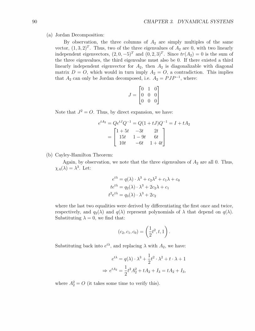
90 CHAPTER 3. DYNAMICAL SYSTEMS
(a) Jordan Decomposition:
By observation, the three columns of A2 are simply multiples of the samevector, (1, 3, 2)T . Thus, two of the three eigenvalues of A2 are 0, with two linearlyindependent eigenvectors, (2, 0,−5)T and (0, 2, 3)T . Since tr(A2) = 0 is the sum ofthe three eigenvalues, the third eigenvalue must also be 0. If there existed a thirdlinearly independent eigenvector for A2, then A2 is diagonalizable with diagonalmatrix D = O, which would in turn imply A2 = O, a contradiction. This impliesthat A2 can only be Jordan decomposed, i.e. A2 = PJP−1, where:
J =
0 1 00 0 00 0 0
Note that J2 = O. Thus, by direct expansion, we have:
etA2 = QetJQ−1 = Q(1 + tJ)Q−1 = I + tA2
=
1 + 5t −3t 2t15t 1− 9t 6t10t −6t 1 + 4t
(b) Cayley-Hamilton Theorem:
Again, by observation, we note that the three eigenvalues of A2 are all 0. Thus,χA(λ) = λ3. Let:
etλ = q(λ) · λ3 + c2λ2 + c1λ+ c0
tetλ = q2(λ) · λ3 + 2c2λ+ c1
t2etλ = q3(λ) · λ3 + 2c2
where the last two equalities were derived by differentiating the first once and twice,respectively, and q2(λ) and q(λ) represent polynomials of λ that depend on q(λ).Substituting λ = 0, we find that:
(c2, c1, c0) =
(1
2t2, t, 1
).
Substituting back into etλ, and replacing λ with A2, we have:
etλ = q(λ) · λ3 +1
2t2 · λ2 + t · λ+ 1
⇒ etA2 =1
2t2A2
2 + tA2 + I3 = tA2 + I3,
where A22 = O (it takes some time to verify this).

Chapter 4
System Stability
4.1 Lecture 12
Consider the time-invariant dynamical system:
x(t) = A(t)x(t), x(0) = x0
which, as shown in Lecture 10, has the state transition matrix:
Φ(t, 0) = etA
The Laplace Transform method of evaluating the matrix polynomial etA is provided below.
Φ(t, 0) = etA = L−1(sI − A)−1.
The expression:
(sI − A)−1 =adj(sI − A)
det(sI − A),
where det(sI −A) and adj(sI −A) (classical adjoint) are n-dimensional and n− 1-dimensionalmatrices, respectively, can be used to evaluate (sI − A)−1. Alternatively, (sI − A)−1 can alsobe evaluated via Gauss-Jordan elimination.
Below, we introduce a very important property of the characteristic equation of a squarematrix. However, before doing so, we must introduce the concept of a matrix function.
Theorem 4.1 (Cayley-Hamilton Theorem). Let A ∈ Rn×n, and suppose its characteristicpolynomial has the form:
χA(s) ≡ det(sI − A) = sn + d1sn−1 + · · ·+ dn−1s+ dn
Then:χA(A) = An + d1A
n−1 + · · ·+ dn−1A+ dnI = O
Remark. In the statement of the Cayley-Hamilton Theorem, we have overloaded the notationχA(·) to describe polynomials of either scalar or square matrix inputs with the same coefficientsas the characteristic polynomial of A.
91

92 CHAPTER 4. SYSTEM STABILITY
Proof. Consider the inverse of (sI − A), computed using the classical adjoint of A:
(sI − A)−1 =adj(sI − A)
det(sI − A)
⇒ (sI − A) · adj(sI − A) = det(sI − A) · I
Let adj(A), which is of degree n− 1, have the following form:
adj(A) = B0sn−1 +B1s
n−2 + · · ·+Bn−2s+Bn−1
Then the above equation becomes:
(sI − A)(B0sn−1 +B1s
n−2 + · · ·+Bn−2s+Bn−1)
=(sn + d1sn−1 + · · ·+ dn−1s+ dn)I
By comparing coefficients on both sides of the equation, we have:
B0 = I
Bk = ABk−1 + dkI, ∀k = 1, · · · , n− 1
O = ABn−1 + dnI
We claim that, for each k ∈ 1, · · · , n:
O = AkBn−k + Ak−1dn−k+1 + · · ·+ dn−1A+ dn
This can be done via induction, by working backwards from n − 1. When k = 1, we haveO = ABn−1 + dn−1I. Suppose the claim holds for some k ∈ 1, · · · , n− 1. Then:
O = AkBn−k + Ak−1dn−k+1 + · · ·+ dn−1A+ dn
= Ak(ABn−k−1 + dn−k) + Ak−1dn−k+1 + · · ·+ dn−1A+ dn
= Ak+1Bn−k−1 + Akdn−k + Ak−1Bn−k+1 + · · ·+ dn−1A+ dn
By induction, the claim holds. Taking k = n− 1 completes the proof.
The Cayley-Hamilton Theorem is both of significant theoretical interest in linear andabstract algebra, and useful as a computational tool for evaluating functions of square matrices.Alternative proofs for the Cayley-Hamilton (some of which may appear less ad hoc than theone presented above) are provided in the appendix.
Now, consider a polynomial p(s) of degree m ≥ n (where m may be infinite), andsuppose we wish to evaluate the matrix p(A). By the Polynomial Remainder Theorem, thereexists polynomials q(s) and r(s) such that:
p(s) = q(s) · χA(s) + r(s),
where the degree of q(s) is m− n, if m is finite, and infinite otherwise, and the degree of r(s)is less than n. By the Cayley-Hamilton Theorem, χA(A) = 0, so:
p(A) = q(A) · χA(A) + r(A) = r(A)

4.1. LECTURE 12 93
We have thus reduced the problem of evaluating a matrix polynomial of ≥ n (and possiblyinfinite) degree to one of solving a matrix polynomial of < n degree. This is particularly usefulwhen n = ∞, i.e. when p(s) is an infinite polynomial, as is the case when p(s) represents theTaylor expansion of a continuously differentiable, non-polynomial function (i.e. sin s, cos s, es,etc.) Examples are given in the Discussion notes following this lecture.
Dyadic Expansion:
We devote the next part of this section to a discussion of dyadic expansion. Let A ∈ Rn×n
be a diagonalizable matrix with n distinct eigenvalues λ1, λ2 · · · , λn, and corresponding right(column) eigenvectors e1, e2 · · · , en. Define:
P ≡[e1 e2 · · · en
],
D ≡
λ1 0 · · · 00 λ2 · · · 0...
.... . .
...0 0 · · · λn
.Then we have:
A[e1 e2 · · · en
]︸ ︷︷ ︸≡P
=[λ1e1 λ2e2 · · · λnen
]
=[e1 e2 · · · en
]︸ ︷︷ ︸≡P
λ1 0 · · · 00 λ2 · · · 0...
.... . .
...0 0 · · · λn
︸ ︷︷ ︸
≡D
⇒A = PDP−1
The above process is known as the diagonalization of A.Now, let vT1 , v
T2 , · · · , vTn be the rows of P−1. Then:
A = PDP−1 = (P−1)−1DP
=
vT1vT2...vTn
−1
λ1 0 · · · 00 λ2 · · · 0...
.... . .
...0 0 · · · λn
vT1vT2...vTn
⇒
vT1vT2...vTn
A =
vT1vT2...vTn
λ1 0 · · · 00 λ2 · · · 0...
.... . .
...0 0 · · · λn
=
λ1v
T1
λ2vT2...
λnvTn

94 CHAPTER 4. SYSTEM STABILITY
It follows that vTi A = λivTi , for each i = 1, · · · , k. We call vT1 , · · · , vTn the left (row)
eigenvectors of A.Now, let us return to the expression A = PDP−1, and rewrite P and P−1 as a collection
of the column and row eigenvectors of A, respectively:
A = PDP−1
=[e1 e2 · · · en
]λ1 0 · · · 00 λ2 · · · 0...
.... . .
...0 0 · · · λn
vT1vT2...vTn
=
n∑i=1
λieivTi ,
where each eivTi is a rank-1 matrix called a dyad.
Observe that:
I = PP−1 =[e1 e2 · · · en
]vT1vT2...vTn
=n∑i=1
eivTi
I = P−1P =
vT1vT2...vTn
[e1 e2 · · · en]
=
vT1 e1 vT1 e2 · · · vT1 envT2 e1 vT2 e2 · · · vT2 en...
.... . .
...vTn e1 vTn e2 · · · vTn en
The first equality states that the dyads of A sum to the identity matrix, while the secondimplies that:
vTi ej = δij,
where δij, called the Kronecker delta, is 1 if i = j and 0 otherwise.
Example. Find the minimal polynomial of:
A =
2 1 00 2 00 0 2
Solution :
Since σ(A) = 2, the characteristic polynomial of A is:
χA(s) = (s− 2)3
However, in fact, we have:(A− 2I)2 = 0
This demonstrates that the characteristic polynomial is not always the minimal polynomial.

4.1. LECTURE 12 95
Theorem 4.2. If A ∈ Cn×n has n distinct eigenvalues λ1, · · · , λn ∈ C, with correspondingeigenvectors v1, · · · , vn, then v1, · · · , vn forms a basis for Cn×n.
Proof. Suppose by contradiction that v1, · · · , vn are not linearly independent. Then thereexist α1, · · · , αn ∈ C, not all zero, such that:
α1v1 + · · ·+ αnvn = 0.
Without loss of generality, suppose α1 6= 0. Applying (L− λ2I)(L− λ3I) · · · (L− λnI) on bothsides, we have:
0 = (L− λ2I)(L− λ3I) · · · (L− λnI)(α1v1 + · · ·+ αnvn)
= α1(L− λ2I)(L− λ3I) · · · (L− λnI)v1 + 0
= α1(λ1 − λ2)(λ1 − λ3) · · · (λ1 − λn)v1
6= 0,
a contradiction. The above equalities follow from the facts that (1) The (L− λiI) terms in theproduct (L− λ2I)(L− λ3I) · · · (L− λnI) all commute, since they are all functions of the samemapping L, and (2) (L− λiI)vi = 0 for each i = 1, · · · , n.
Alternatively, this theorem can be proved via induction, as demonstrated below.
Proof. The lemma can be proven using by induction. When k = 1, we have Lv1 = λ1v1, wherev1 6= 0, so v1 is a linearly independent subset. Suppose the lemma is valid for some k − 1,where k ∈ 2, 3, · · · . Let:
a1v1 + a2v2 + · · ·+ akvk = 0
Then:
0 = (L− λkI)(a1v1 + a2v2 + · · ·+ akvk)
= a1(λ1 − λk)v1 + a2(λ2 − λk)v2 + · · ·+ ak−1(λk−1 − λk)vk−1 + ak(λk − λk)vk︸ ︷︷ ︸=0
By the induction hypothesis, v1, v2, · · · , vk−1 is linearly independent, so:
a1(λ1 − λk) = a2(λ2 − λk) = · · · = ak−1(λk−1 − λk) = 0
Since λi 6= λk for each i 6= k:
a1 = a2 = · · · = ak−1 = 0
So Equation (4.1) becomes akvk = 0. Since vk 6= 0, we have ak = 0, which indicates thatv1, v2, · · · , vk is a linearly independent subset. The proof follows by induction.

96 CHAPTER 4. SYSTEM STABILITY
This theorem can be applied to the solving process of a matrix differential equationx = Ax. Recall that its solution is:
x(t) = etAx0
If A has n distinct eigenvalues λ1, · · · , λn ∈ C, with corresponding eigenvalues v1, · · · , vn, thenby the above theorem, we can write:
x0 =∞∑i=1
ηi(0)vi,
which allows us to simplify the given expression for x(t):
x(t) = etAx0 =∞∑i=1
ηi(0)etAvi
=∞∑i=1
ηi(0)etλivi
Note that λ1, · · · , λn may contain real values and/or complex conjugate pairs. In general,a complex eigenvalue λir + iλic would correspond to either an exponentially growing mode (ifλir > 0) or an exponentially decaying mode (if λir < 0), oscillating at angular frequency |λic|.
Modal Decomposition
Recall that, given a change of coordinates in the system state x = Tx, the equivalentsystem representation of an LTI system R : (A,B,C,D) is R : (TAT−1, TB,CT−1, D), i.e.:
x = Ax+Bu,
y = Cx+Du,⇒
x = TAT−1x+ TBu,
y = CT−1x+Du,
Equivalent systems have the same transfer function, since:
CT−1(sI − TAT−1)−1TB
=CT−1(T (sI − A)−1T−1
)TB
=C(sI − A)−1B
Let an LTI system R : (A,B,C,D) be given, and suppose A is diagonalizable. Definethe rows of B and the columns of C by:
B =[b1 b2 · · · bni
], C =
cT1cT2...cTno

4.1. LECTURE 12 97
Let T−1 be an invertible matrix whose columns are linearly independent right eigenvectorsof A. (Equivalently, the rows of T are the corresponding linearly independent left eigenvectorsof A). Then we can diagonalize A as shown below:
TAT−1 =
λ1 0 · · · 00 λ2 · · · 0...
.... . .
...0 0 · · · λn
Then, if we define:
TB =
vT1vT2...vTn
[b1 b2 · · · bni]
=
vT1 b1 vT1 b2 · · · vT1 bnivT2 b1 vT2 b2 · · · vT2 bni...
.... . .
...vTn b1 vTn b2 · · · vTn bni
≡B1
B2
...
Bn
,
CT−1 =
cT1cT2...cTno
[e1 e2 · · · en]
=
cT1 e1 cT1 e2 · · · cT1 encT2 e1 cT2 e2 · · · cT2 en...
.... . .
...cTnoe1 cTnoe2 · · · cTnoen
≡ [C1 C2 · · · Cn].
where, as before, e1, · · · , en and vT1 , · · · , vTn are the left (column) eigenvectors and correspondingleft (row) eigenvectors of A, respectively. The transfer function of the system then becomes:
H(s) = CT−1(sI − TAT−1)−1TB
=[C1 C2 · · · Cn
]
1s−λ1
0 · · · 0
0 1s−λ2
· · · 0...
.... . .
...0 0 · · · 1
s−λn
B1
B2
...
Bn
If the system were single-input-single-output (SISO), i.e. B ∈ Rn×1, C ∈ R1×n, theneach Bi and each Ci is a scalar. The transfer function then has the simple form:
H(s) =n∑i=1
CiBi
s− λi
This is called modal decomposition. Notice that, if Bi = 0 or Ci = 0, the transferfunction C(sI −A)−1B does not contain the corresponding term 1/(s− λi), and thus does notcontain the corresponding pole λi. A block diagram is given below.

98 CHAPTER 4. SYSTEM STABILITY
If the system were multiple-input multiple-output (MIMO), the same analysis follows—If, for some i = 1, · · · , n, we have:
Bi =[vTi b1 vTi b2 · · · vTi bn
]= 0, or
Ci =
cT1 eicT2 ei...
cTnei
= 0,
then the pole λi does not appear in C(sI − A)−1B.
Forced Response
The discussion above implies that, for a given LTI system R : (A,B,C), and arbitraryinitial state x0 and input u(·), exponential functions of the form eλit, where λi ∈ σ(A), wouldarise in the resulting trajectory x(t). We now wish to ask whether there exist specific initialstates from which, if the system were excited by an input u(t) = u0e
λt, λ 6∈ σ(A), the resultingtrajectory would only contain terms of the form eλt. The theorem below answers this in theaffirmative.
Theorem 4.3. Given an LTI system R : (A,B,C), and an input u(t) = u0eλt, with λ 6∈ σ(A)
and some arbitrary u0 ∈ Rni, the resulting trajectory is of the form:
y(t) = y0eλt
if and only if the initial condition satisfies:
x0 = (λI − A)−1Bu0

4.1. LECTURE 12 99
Proof. Using (3.9) :
∵ y(t) = CetAx0 +
∫ t
0
Ce(t−τ)ABu(τ)dτ
= CetAx0 +
∫ t
0
Ce(t−τ)ABu0eλτ dτ
⇒ Y (s) = C(sI − A)−1x0 + C(sI − A)−1B · u0
s− λwhere we have used the fact that the Laplace transform of the convolution of two functionsequals the product of the Laplace transform of the individual functions.
Now, we wish to isolate the effect of (sI −A)−1 and (s− λ)−1 on u0, in order to isolatea term in Y (s) that depends only on (s − λ)−1. This can be done by rewriting (sI − A)−1 interms of (λi − A)−1 and (s− λ)−1. In particular, observe that:
(sI − A)− (λI − A) = (s− λ)I,
⇒ (λI − A)−1 − (sI − A)−1 = (s− λ)(sI − A)−1(λI − A)−1,
⇒ (sI − A)−1 =[I − (s− λ)(sI − A)−1
](λI − A)−1
Substituting into the above expression, we have:
Y (s) = C(sI − A)−1x0 + C(sI − A)−1B · u0
s− λ= C(sI − A)−1x0 + C
[I − (s− λ)(sI − A)−1
](λI − A)−1B · u0
s− λ= C(sI − A)−1
[x0 − (λI − A)−1Bu0
]+ C(λI − A)−1B · u0
s− λ,
⇒ y(t) = CetA[x0 − (λI − A)−1Bu0
]+ C(λI − A)−1Bu0e
λt
Thus, y(t) is proportional to eλt if and only if x0 = (λI − A)−1Bu0, in which case:
y(t) = C(λI − A)−1Bu0eλt = H(λ) · u0e
λt,
where H(s) = C(sI − A)−1B is the transfer function of the system.
Remark. If the system is stabilizable, then etA → O as t → ∞, so y(t) → H(λ) · u0eλt as
t → ∞. In other words, even though y(t) may initially not be directly proportional to eλt,it will eventually asymptotically approach a function proportional to eλt as its steady-stateresponse.
We end our discussion by connecting the above concepts to that of the ”zeros” of atransfer function.
Definition 4.4 (Zero (of a transfer function)). Let R : (A,B,C) be a ”square” system, inthe sense that ni = n0. Then z ∈ C is said to be a zero of the system if the transfer functionevaluated at z:
H(z) = C(zI − A)−1B
is singular.

100 CHAPTER 4. SYSTEM STABILITY
For ”square” LTI systems with zeros, particular choices of initial state and input functionscan be chosen such that the output is identically zero. Specifically, if H(z) is singular for somez ∈ C, then there must exist some u0 ∈ Rni such that H(z)u0 = 0. Now, let:
u(t) = u0ezt,
x0 = (zI − A)−1Bu0
The analysis above shows that y(t) = 0.

4.2. LECTURE 12 DISCUSSION 101
4.2 Lecture 12 Discussion
Example (Discussion 7, Problem 1). Let:
A =
[1 10 2
]Is I2, A,A
2 linearly dependent or independent in R2×2?
Solution :The characteristic equation of A is:
χA(λ) = (λ− 1)(λ− 2) = λ2 − 3λ+ 2
The Cayley-Hamilton Theorem thus implies that:
O = χA(A) = (A− I2)(A− 2I) = A2 − 3A+ 2I2
This shows that I, A,A2 is linearly dependent.
Remark. The solution to this problem can actually be generalized to show that I, A, · · · , Anis linearly dependent for each A ∈ Rn×n.
Example (Discussion 7, Problems 2, 3, 6, 7). Let:
A =
[1 01 2
]Consider the following questions:
1. Find A3.
2. Find etA via dyadic expansion.
3. Find sin(eA).
4. Find 2A4 − 3A3 − 3A2 + 4I2.
Solution :The characteristic equation of A is:
χA(λ) = (λ− 1)(λ− 2) = λ2 − 3λ+ 2
The Cayley-Hamilton Theorem thus implies that:
O = χA(A) = (A− I2)(A− 2I) = A2 − 3A+ 2I2
The three given functions of A can thus be solved via long-division.

102 CHAPTER 4. SYSTEM STABILITY
1. By long division:
A3 = (A2 − 3A+ 2I2)(A+ 3I2) + (7A− 6I2) = 7A− 6I2 =
[1 07 8
]2. Since we have already computed σ(A) = 2, 1 to be the eigenvalues ofA, the diagonalization
of A can be readily found:
A =
[0 11 −1
] [2 00 1
] [1 11 0
]where the vertical and horizontal lines are used to emphasize the placement of the (right)column and (left) eigenvectors of A in its diagonalization.
Thus, the dyadic expansion of A is:
A = 2 ·[01
] [1 1
]+ 1 ·
[1−1
] [1 0
]Since the eigenvalues of etA are simply etλi, where λi are the eigenvalues of A, withthe same corresponding eigenvectors, the dyadic expansion of etA is simply that of A witheach eigenvalue λ replaced with etA:
A = e2t ·[01
] [1 1
]+ et ·
[1−1
] [1 0
]= e2t ·
[0 01 1
]+ et ·
[1 0−1 0
]=
[et 0
e2t − et e2t
]3. Let c1, c0 be time-dependent coefficients such that:
sin(eλ) = q(λ) · (λ2 − 3λ+ 2) + c1λ+ c0
Taking λ = 1 and λ = 2, we have:
sin(e) = c1 + c0
sin(e2) = 2c1 + c0
Thus, c1 = sin(e2)− sin(e) and c0 = − sin(e2) + 2 sin(e), so:
sin(eλ) = q(λ) · (λ2 − 3λ+ 2) + (sin(e2)− sin(e))λ+ (− sin(e2) + 2 sin(e))
⇒ sin(eA) = q(A) · (A2 − 3A+ 2I2) + (sin(e2)− sin(e))A+ (− sin(e2) + 2 sin(e))I2
= (sin(e2)− sin(e))A+ (− sin(e2) + 2 sin(e))I2
=
[sin(e) 0
sin(e2)− sin(e) sin(e2)
]

4.2. LECTURE 12 DISCUSSION 103
4. By long division:
2A4 − 3A3 − 3A2 + 4I2 = (A2 − 3A+ 2I2)(2A2 + 3A+ 2I2) = O
i.e. f(x) = 2x4 − 3x3 − 3x2 + 4 annihilates A.
Example (Discussion 7, Problem 4, 9). Consider:
x = Ax, x(0) = vi
where A ∈ Rn×n has n linearly independent eigenvectors v1, · · · , vn with corresponding realeigenvalues λ1, · · · , λn (not necessarily distinct). Find x(t) in terms of the eigenvalues andeigenvectors of A, and give a geometric interpretation of the result when x0 = vi for somei = 1, · · · , n.
Solution :Since v1, · · · , vn is linearly independent, it must be a basis for Rn. Thus, there exist
scalars a1, · · · , an such that:x0 = a1v1 + · · ·+ anvn
Substituting into (3.8), we have:
x(t) = etAx0
= etA(a1v1 + · · ·+ anvn)
= a1eλ1tv1 + · · ·+ ane
tλntvn
In particular, x0 = vi corresponds to the case that aj = δij, where the Kronecker delta δijequals 1 if i = j and equals 0 otherwise. In this case, the above equation becomes:
x(t) = vieλit
Thus, the trajectory diverges if <λi > 0, and converges otherwise.
Example (Discussion 7, Problem 5). Suppose A ∈ R2×2 has eigenvalues λ, λ ∈ C, where λdenotes the complex conjugate of λ. Let v ∈ Cn be the (complex) eigenvector ofA correspondingto the eigenvalue λ, and suppose:
λ = σ + jω
v = v1 + jv2,
where σ, ω ∈ R and v1, v2 ∈ Rn.Now, consider:
x = Ax, x(0) =1
2(v + v),
where v denotes the (term-wise) complex conjugate of v. Find an expression for the trajectoryx(t) in terms of v1, v2, σ, ω, t, and give a geometric interpretation of x(t).

104 CHAPTER 4. SYSTEM STABILITY
Solution :Using (3.8), we have:
x(t) = etAx0 = etA · 1
2(v + v) =
1
2etAv +
1
2etAv
=1
2etλv +
1
2etλv
=1
2e(σ+jω)t(v1 + jv2) +
1
2e(σ−jω)t(v1 − jv2)
=1
2eσt(ejωtv1 + e−jωtv1 + jejωtv2 − je−jωtv2
= eσt(cos(ωt)v1 + sin(ωt)v2)
Example (Discussion 7, Problem 10). Given:
A =
[−3 10 −2
]Answer the following questions.
1. Find the characteristic polynomial of A.
2. Express A4 as the lowest order polynomial in A.
3. Find etA by the Cayley-Hamilton Theorem; that is, show that etA = a0(t)I2 + a1(t)A.
Solution :
1. We have:χA(λ) = (λ+ 3)(λ+ 2)
2. The Cayley-Hamilton Theorem implies that:
O = χA(A) = (A+ 3I2)(A+ 2I2) = A2 + 5A+ 6I2
Using long division, we have:
A4 = (A2 + 5A+ 6I2)(A2 − 5A+ 19I2) + (−65A− 114I2)
= −65A− 114I2
3. Note that there exist t-dependent coefficients a0(t), a1(t) such that:
etλ = q(λ) · (λ+ 3)(λ+ 2) + a1(t)λ+ a0(t)

4.2. LECTURE 12 DISCUSSION 105
Setting λ = −3 and λ = −2, we have:
e−3t = 3a1(t) + a0(t)
e−2t = 2a1(t) + a0(t),
which yields a1(t) = e−2t − e−3t and a2(t) = 3e−2t − 2e−3t.
Substituting λ with A, we have:
etA = a1(t)A+ a0I2
= (e−2t − e−3t)
[s− 3 1
0 −2
]+ (3e−2t − 2e−3t)
[1 00 1
]=
[e−3t e−3t − e−2t
0 e−2t
]

106 CHAPTER 4. SYSTEM STABILITY
4.3 Lecture 13
If a given square matrix A ∈ Rn×n is diagonalizable, then each of its eigenvectors vi, i =1, · · · , n will remain invariant with respect to their original one-dimensional subspaces, i.e.:
Avi ∈ spanvi
for each i = 1, · · · , k. However, this does not hold in general for non-diagonalizable squarematrices. This motivates the following definition.
Definition 4.5 (Subspace Invariance). Given a vector space V and a linear operator A :V → V , a subsspace M ≤ V is invariant under A, or A-invariant if, for each x ∈ M , wehave Ax ∈M .
It can be easily checked that the null space and range space of any linear operator A areA-invariant. This is detailed in the lemma below. The proofs are left as exercises to the reader.
Lemma 4.6. Let A be a linear operator. If λ ∈ σ(A), and p(s) is any polynomial, the followingsubspaces are A-invariant:
1. N(A)
2. R(A)
3. N(A− λI)
4. N(p(A))
Theorem 4.7. If M1,M2 ∈ V are A-invariant, so are M1 +M2 and M1 ∪M2.
Definition 4.8 (Direct Sum). Let V be a vector space, and let M1, · · · ,Mk ≤ V . Then V issaid to be the direct sum of M1, · · · ,Mk, if, for each i = 1, · · · , k, denoted by:
V = M1 ⊕M2 ⊕ · · · ⊕Mk,
if, for each x ∈ V , there exists a unique xi ∈Mi for each i = 1, · · · , k such that:
x = x1 + · · ·+ xk
Theorem 4.9 (Equivalent Definition for Direct Sum of Subspaces). Let V be a vectorspace, and let M1, · · · ,Mk ≤ V . Then V = M1 ⊕ · · · ⊕Mk if and only if:
1. V = M1 + · · ·+Mk, and
2. M1
⋂· · ·⋂Mk = 0.

4.3. LECTURE 13 107
The above definitions for subspace invariance and direct sum to make the followingobservation. Let V be a vector space, and let A be a linear operator on V . If V is the directsum of a sequence of A-invariant subspaces M1, · · · ,Mk, then there exists a choice of basis B forV , constructed by taking the union of bases for each Mi, such that the matrix representationof A with respect to B is block diagonal.
For example, for the k = 2 case, if b1, · · · , bk is a basis for M1, and bk+1, · · · , bn isa basis for M2, then:
b1, · · · , bk, bk+1, · · · , bn
A version of the above result is discussed below.
Theorem 4.10 (2nd Representation Theorem). Let V = M1⊕M2 be a finite-dimensionalvector space. If M1 is A-invariant, then there exists a basis B of V such that the matrixrepresentation of A with respect to B has the form:
[A]B =
[A11 A12
O A22
]∈ Fn×n,
where A11 ∈ Fk×k, A12 ∈ Fk×(n−k), and A22 ∈ F(n−k)×(n−k). In other words, the first k columnsof A have zeros in the last (n− k) rows.
Proof. Essentially, we wish to show that([A]B
)ji
= 0 for each i = 1, · · · , k and j = k+1, · · · , n.
Let b1, · · · , bk and bk+1, · · · , bn be bases for M1 and M2, respectively. Then B ≡b1, · · · , bn forms a basis for V . Then, for each bi, i = 1, · · · , k, we have the following equalityfrom the definition of matrix representations:
Abi =n∑j=1
([A]B
)jibj
where ei denotes the i-th standard vector in Fn. Since M1 is A-invariant, we have Abi ∈ A, andsince vector representations with respect to a given basis are unique, we must have:
Abi =k∑j=1
([A]B
)jibj
This implies that, for each i = 1, · · · , k:
n∑j=k+1
([A]B
)jibj = 0
Since bj, j = k + 1, · · · , n forms a basis for M2, we have([A]B
)ji
= 0 for each i = 1, · · · , kand j = k + 1, · · · , n. This completes the proof.

108 CHAPTER 4. SYSTEM STABILITY
If M1,M2 were both A-invariant, then the above argument can be repeated to show thatA12 = 0, so:
[A]B =
[A11 00 A22
]∈ Fn×n,
where A11 ∈ Fk×k and A22 ∈ F(n−k)×(n−k), as before. This is simply the observation describedabove.
Corollary 4.11. Given a diagonalizable matrix A ∈ Rn×n with n distinct eigenvalues λ1, · · · , λn:
Cn = N(A− λ1I)⊕N(A− λ2I)⊕ · · · ⊕N(A− λnI)
In general, suppose A ∈ Rn×n, not necessarily diagonalizable, has a characteristicequation of the form:
χA(s) = (s− λ1)d1(s− λ2)d2 · · · · · (s− λσ)d1
=σ∏i=1
(s− λi)di
where di is the algebraic multiplicity of λi, we have d1 + · · · dk = n, and σ is the number ofdistinct eigenvalues of A (clearly, σ ≤ n.
Definition 4.12 (Annihilating Polynomial). Given a linear operator A, an annihilatingpolynomial of A is a finite-dimensional polynomial f(s) such that:
f(A) = 0
Definition 4.13 (Minimal Polynomial). Given a linear operator A, a minimal polynomialψA(s) of A is a non-zero polynomial of the least degree, with leading coefficient 1, that annihilatesA, i.e. it is a polynomial of the last degree such that:
ψA(s) = On×n
Below, we show that the minimal polynomial must be a factor of any annihilating factor.This can be sued to show that the minimal polynomial is unique.
Theorem 4.14. Let A be a linear operator. If p(A) is an annihilating polynomial of A, andψA(s) is a minimal polynomial of A, then ψA(s) divides p(A).
Proof. Since pA(s) annihilatesA, it must have higher (or the same) degree as χA(s), a polynomialof least degree that annihilates A. Thus, there exist matrix polynomials q(s), r(s), withdeg(r(s)) ≤ deg(ψA(s)), such that:
pA(s) = ψA(s)q(s) + r(s)
⇒ pA(A) = ψA(A)q(A) + r(A).
Since pA(A) = ψA(A) = 0, we have r(A) = 0. If r(s) is non-zero, then it is a non-zeropolynomial of degree less than degψA(s) that annihilates A, a contradiction. Thus, r(s) = 0,so pA(A) = ψA(A)q(A). The proof is done.

4.3. LECTURE 13 109
Corollary 4.15. The minimal polynomial ψA(s) of any linear operator A is unique.
Proof. Suppose ψA,1(s) and ψA,2(s) are both minimal polynomials of A. Then, by the aboveargument, there exist polynomials q1(s), q2(s) such that:
ψA,1(s) = q1(s) · ψA,2(s)
ψA,2(s) = q2(s) · ψA,1(s)
⇒ψA,1(s) = q1(s) · ψA,2(s)
= q1(s)q2(s) · ψA,1(s)
⇒q1(s)q2(s) = 1
Since ψA,1(s) and ψA,2(s) both have leading coefficient 1, so must q1(s) and q2(s). The fact thatq1(s)q2(s) = 1 implies that q1(s) and q2(s) are both constant. Combining these two facts, wehave:
q1(s) = q2(s) = 1,
and so ψA,1(s) = ψA,2(s).
The corollary below shows that χA(s) and ψA(s) must have the same roots.
Corollary 4.16. Let A ∈ Cn×n be a linear operator with distinct eigenvalues λ1, · · · , λσ, whereσ ≤ n. Then the minimal polynomial χA(s) of A has the form:
ψA(s) = (s− λ1)m1 · (s− λ2)m2 · · · · · (s− λσ)mσ ,
where 1 ≤ mi ≤ ai for each i = 1, · · · , σ.
Proof. Taking p(s) = χA(s) (the characteristic polynomial of A) in the above theorem, we findthat χA(s) is a factor of p(s). Since χA(s) has the form:
χA(s) = (s− λ1)a1 · · · · · (s− λσ)aσ
the minimal polynomial p(s) must have the form:
χA(s) = (s− λ1)m1 · · · · · (s− λσ)mσ
where 0 ≤ mi ≤ ai for each i = 1, · · · , σ.It remains to show that mi ≥ 1 for each i = 1, · · · , σ, i.e. that each λi is a root of ψA(s).
Let vi be an eigenvector of A with corresponding eigenvalue λi. Then, since ψA(A) = 0, wehave:
0 = ψA(A)vi = ψA(λi)vi,
where the replacement of A with λi in the second equality follows from the observation thatAkvi = λki vi for each k ∈ N. Since vi 6= 0, we have ψA(λi) = 0, which shows that λi is a root ofψA(s). The proof is done.

110 CHAPTER 4. SYSTEM STABILITY
Theorem 4.17. Given any matrix A ∈ Rn×n with σ ≤ n distinct eigenvalues λ1, · · · , λσ:
Cn = N(A− λ1I)m1 ⊕N(A− λ2I)m2 ⊕ · · · ⊕N(A− λnI)mn
Proof. Fix x ∈ Cn, and observe that:
ψA(s) = (s− λ1)m1 · (s− λ2)m2 · · · · · (s− λσ)mσ
⇒ 1
ψA(s)=
1
(s− λ1)m1 · (s− λ2)m2 · · · · · (s− λσ)mσ
=n1(s)
(s− λ1)m1+
n2(s)
(s− λ2)m2+ · · ·+ nσ(s)
(s− λσ)mσ
⇒I =1
ψA(A)· ψA(A)
= n1(A) · ψA(A)
(A− λ1I)m1+ · · ·+ nσ(A) · ψA(A)
(A− λσI)mσ
⇒x = n1(A)ψA(A)
(A− λ1I)m1x+ · · ·+ nσ(A)
ψA(A)
(A− λσI)mσx
where n1(s), · · · , nσ(s) are functions of s with degree less than m1, · · · ,mσ, respectively. Foreach i = 1, · · · , n:
(A− λiI)mi(ni(A)
ψA(A)
(A− λiI)mσx
)= ni(A)ψA(A)x = 0,
since ψA(A) = 0. Thus, x is written as a linear combination of elements in N(A− λiI)mi , i.e.:
Cn = N(A− λ1I)m1 +N(A− λ2I)m2 + · · ·+N(A− λnI)mn
To complete the proof, it remains to show that N(A− λiI)⋂N(A− λjI) = 0 for each i, j ∈
1, · · · , σ. Fix one such pair of i, j, and suppose without loss of generality that 1 ≤ mi ≤ mj.Let v ∈ N(A− λi)mi , and define:
mi = minm|v ∈ N(A− λi)m
The definition of m shows that m|v ∈ N(A − λi)m is bounded above by mi, so mi exists.Now:
0 = (A− λiI)miv = (A− λiI)(A− λiI)mi−1v
⇒A(A− λiI)mi−1v = λi(A− λiI)mi−1v
In other words, (A − λiI)mi−1 is an eigenvector of A with corresponding eigenvalue λi (Bydefinition of mi, we have (A− λiI)mi−1 6= 0). We thus have:
(A− λjI)m2v = (A− λjI)m2−m1+1 (A− λjI)m1−1v
= (λi − λj)m2−m1+1(A− λjI)m1−1v 6= 0
since (λi − λj)m2−m1+1 6= 0 and (A− λjI)m1−1v 6= 0.

4.3. LECTURE 13 111
Definition 4.18 (Algebraic and Geometric Multiplicities, Grade). Let A ∈ Rn×n begiven, and suppose A has characteristic polynomial given by:
χA(λ) = (λ− λ1)d1 · · · · (λ− λσ)aσ
where λ1, · · · , λσ are the distinct eigenvalues of A, i.e. σ(A) = λ1, · · · , λσ and minimalpolynomial given by:
ψA(λ) = (λ− λ1)m1 · · · · (λ− λσ)mσ
Then, we have the following definitions:
1. Algebraic Multiplicity:
di is called the algebraic multiplicity of λi. Note that∑σ
i=1 di = 1
2. Geometric Multiplicity:
qi ≡ dim(N(A − λi)) is called the geometric multiplicity of λi, and describes themaximum number of linearly independent eigenvectors corresponding to the eigenvalue λi.
3. Grade:
mi ≡ dim(N(A− λi)) is called the grade of λi. It describes the largest Jordan blockof A corresponding to λi, since it takes mi multiplications of (A − λi) to annihilate theblocks.
Example. Consider the algebraic multiplicities, geometric multiplicities, and grades of thefollowing square matrices (observe that they are already in Jordan form), with λ ∈ C arbitrarilygiven:
A1 =
λ 1 0 00 λ 0 00 0 λ 10 0 0 λ
, A2 =
λ 1 0 00 λ 1 00 0 λ 00 0 0 λ
By observation, we can compile the following table. The algebraic multiplicity of λ is 4 for bothA1 and A2, since they are both 4× 4 matrices with whose only eigenvalue is λ. The geometricmultiplicity of λ is 2 for both A1 and A2 since they both have two Jordan blocks. Finally, thegrades of λ for A1 and A2 are 2 and 3, respectively, since the maximum size of the Jordanblocks corresponding to λ in A1 and A2 are 2× 2 and 3× 3, respectively.
Parameter A1 A2
Algebraic Multiplicity 4 4Geometric Multiplicity 2 2
Grade of λ 2 3
Theorem 4.19 (Spectral Mapping Theorem). Given a square matrix A ∈ Rn×n, and apolynomial f(λ), we have:
σ(f(A)) = f(σ(A)),
i.e. the spectrum of f(A) is the set of f(λ) for each eigenvalue λ of A.

112 CHAPTER 4. SYSTEM STABILITY
Proof. Explicitly express f as:
f(x) = anxn + an−1x
n−1 + · · ·+ a1x+ a0
Let λ ∈ σ(A). Then there exists some eigenvector v of A such that Av = λv. Thus:
f(A)v = (anAn + an−1A
n−1 + · · ·+ a1A+ a0I)v
= (anλn + an−1λ
n−1 + · · ·+ a1λ+ a0)v
= f(λ)v
This establishes the theorem.
Remark. This result can be extended to all analytic functions (not just polynomials), via Taylorexpansion.
Consider the following simple example of a 2× 2 matrix. Suppose:
J =
[λ 10 λ
].
It can be verified that:
Jn =
[λn nλn−1
0 λn
]Then, for the matrix exponential etJ , we have
etJ = I + tJ +(tJ)2
2!+ · · ·+ (tJ)n
n!+ · · ·
=
[eλt b0 eλt
],
where b ∈ R can be determined by using the formula above for Jn:
b = t+ 2λt2
2!+ · · ·+ nλn−1 · t
n
n!+ · · ·
= teλt
Thus:
etJ =
[eλt teλt
0 eλt
]In general, we can show that, if J ∈ Rn×n is given by:
J =
λ 1 0 · · · 0 00 λ 1 · · · 0 00 0 λ · · · 0 0...
......
. . ....
...0 0 0 · · · λ 10 0 0 · · · 0 λ

4.3. LECTURE 13 113
Then, we have (by induction):
etJ =
etλ tetλ t2
2!etλ · · · tn−2
(n−2)!f (n−2)(λ) tn−1
(n−1)!f (n−1)(λ)
0 etλ tetλ · · · tn−3
(n−3)!f (n−3)(λ) tn−2
(n−2)!f (n−2)(λ)
0 0 etλ · · · tn−4
(n−4)!f (n−4)(λ) tn−3
(n−3)!f (n−3)(λ)
......
.... . .
......
0 0 0 · · · etλ tetλ
0 0 0 · · · 0 etλ
The above generalized result can be proven by the following theorems.
Lemma 4.20. Let A ∈ Rn×n be a square matrix, with minimal polynomial:
ψA(s) = (s− λ1)m1 · · · · · (s− λσ)mσ
Let n =∑σ
i=1 di = n, and let h(s) be an (n− 1)-th order polynomial. Then f(A) = h(A) if andonly if:
f (k)(λi) = h(k)(λi), ∀k = 0, 1, · · · ,mi − 1, i = 1, · · ·σ,
where f (k)(λi) and h(k)(λi) respectively denote the k-th derivative of f and g, evaluated at λi.
Proof. The proof follows by Taylor expansion at each λi ∈ σ(A).
Theorem 4.21 (Functions of a Matrix). Consider an n× n Jordan block given by:
J =
λ 1 0 · · · 0 00 λ 1 · · · 0 00 0 λ · · · 0 0...
......
. . ....
...0 0 0 · · · λ 10 0 0 · · · 0 λ
Then:
f(J) =
f(λ) f ′(λ) 12!f ′′(λ) · · · 1
(n−2)!f (n−2)(λ) 1
(n−1)!f (n−1)(λ)
0 f(λ) f ′(λ) · · · 1(n−3)!
f (n−3)(λ) 1(n−2)!
f (n−2)(λ)
0 0 f(λ) · · · 1(n−4)!
f (n−4)(λ) 1(n−3)!
f (n−3)(λ)...
......
. . ....
...0 0 0 · · · f(λ) f ′(λ)0 0 0 · · · 0 f(λ)
Proof. From the above lemma, we have:
f(J) =n−1∑k=0
f (k)(λ) · 1
k!(x− λ)k

114 CHAPTER 4. SYSTEM STABILITY
Thus, by substituting x with J , we find:
f(J) =∞∑k=0
f (k)(λ) · 1
k!(J − λI)k
The proof is completed by observing that, for each m = 1, · · · , n, we have:
[(J − λI)m]ij = δi,j−m
Note that the Jordan form J = P−1AP is unique only up to permutations of the Jordanblocks. This can be seen by interchanging the order in which different Jordan chains (i.e. setscontaining a single eigenvector and generalized eigenvectors associated with that eigenvector)appear in P .
Example (From an Old Prelim).
1. A matrix A has minimal polynomial (s− λ1)2(s− λ2)3. Find cos(eA) as a polynomial inA.
2. Now, assume further that A has characteristic polynomial (s− λ1)2(s− λ2)3, and that ithas four linearly independent eigenvectors. Write down the Jordan form J of this matrix,and write down cos(eA) explicitly.
Solution:
1. Since the minimal polynomial, by definition, is the (unique) polynomial of the lowestdegree with leading coefficient 1 that annihilatesA. To that end, let a (infinite) polynomialq(λ) and constants c4, c3, c2, c1, c0 be given such that:
cos(eλ) = q(λ) · (λ− λ1)2(λ− λ2)3 + c4λ4 + c3λ
3 + c2λ2 + c1λ+ c0
The five constants can be found by differentiating cos(eλ) with respect to λ twice times,and substituting λ = λ1 to cos(eλ) and its first derivative, and substituting λ = λ2 tocos(eλ) and its first and second derivatives. The derivatives of cos(eλ) are:
d
dλcos(eλ) = −eλ sin(eλ)
d2
dλ2cos(eλ) = −eλ sin(eλ)− e2λ cos(eλ)
So, substituting λ = λ1 and λ = λ2 in the relevant equations, we have:
cos(eλ1) = c4λ41 + c3λ
31 + c2λ
21 + c1λ1 + c0
cos(eλ2) = c4λ42 + c3λ
32 + c2λ
22 + c1λ2 + c0
−eλ1 sin(eλ1) = 4c4λ31 + 3c3λ
21 + 2c2λ1 + c1
−eλ2 sin(eλ2) = 4c4λ32 + 3c3λ
22 + 2c2λ2 + c1
−eλ2 sin(eλ2)− e2λ2 cos(eλ2) = 12c4λ22 + 6c3λ2 + 2c2

4.3. LECTURE 13 115
Thus, c4, c3, c2, c1, c0 can be solved as functions of t. We thus have:
A = c4A4 + c3A
3 + c2A2 + c1A+ c0I
2. Note that the exponent of each term in minimal polynomials gives the size of the largestJordan block corresponding to each eigenvalue; in this case, m1 = 2 and m2 = 3. Sinceeach linearly independent eigenvector of A gives rise to one Jordan block, the total numberof Jordan blocks in the Jordan form of A is 4 (In other words, they occupy a 4×4 matrixin the Jordan form of A). On the other hand, the algebraic multiplicities corresponding toeach eigenvalue of A is the total size of all Jordan blocks corresponding to that eigenvalue.
In the context of this problem, the above information implies that:
• For λ1, the largest Jordan block is of size 2, and the sum of the sizes of the Jordanblocks is 5.
• For λ1, the largest Jordan block is of size 3, and the sum of the sizes of the Jordanblocks is 3.
• In the Jordan form of A, the eigenvalues λ1 and λ2 have a total of four Jordan blocks.
The second fact in the above list indicates that there exists only one (3× 3) Jordan blockcorresponding to λ2. Thus, there exist three Jordan blocks corresponding to λ1. Theseblocks have maximum size 2 and total size 5, so there must be two blocks of size 2 andone block of size 1. In short, the Jordan form of A looks as follows:
J =
λ1 0 0 0 0 0 0 00 λ1 1 0 0 0 0 00 0 λ1 0 0 0 0 00 0 0 λ1 1 0 0 00 0 0 0 λ1 0 0 00 0 0 0 0 λ2 1 00 0 0 0 0 0 λ2 10 0 0 0 0 0 0 λ2
By Theorem 4.21, for any analytic function f(·), we have:
f(J) =
f(λ1) 0 0 0 0 0 0 00 f(λ1) f ′(λ1) 0 0 0 0 00 0 f(λ1) 0 0 0 0 00 0 0 f(λ1) f ′(λ1) 0 0 00 0 0 0 f(λ1) 0 0 00 0 0 0 0 f(λ2) f ′(λ2) 1
2f ′′(λ2)
0 0 0 0 0 0 f(λ2) f ′(λ2)0 0 0 0 0 0 0 f(λ2)
The solution is completed by substituting f(x) = cos(ex) and its first and second derivativesinto the expression above. The resulting matrix is a similarity transform away from

116 CHAPTER 4. SYSTEM STABILITY
f(A), with respect to the same invertible matrix P (with columns/rows consisting of thecolumn/row eigenvectors of A) that connects A to J via the similarity transformation:
A = PJP−1
More examples are furnished in the Discussion questions listed below.
Corollary 4.22. For any A ∈ Rn×n, the characteristic and minimal polynomials of A and AT
are the same.
Proof. First, since the determinant is invariant with respect to taking the transpose of thematrix:
χA(λ) = det(A− λI) = det(AT − λI) = χAT (λ)
Next, suppose the minimal polynomial of A is of the form:
mA(λ) = (λ− λ1)m1 · · · · (λ− λσ)mσ = 0,
The Cayley-Hamilton Theorem implies that mA(A) = On, so:
On =(mA(A)
)T=((A− λ1In)m1 · · · · (A− λσIn)mσ
)T= (AT − λσIn)mσ · · · · · (AT − λ1In)m1
= (AT − λ1In)m1 · · · · (AT − λσIn)mσ
= mA(AT )
It follows that mA(λ) annihilates AT . But by definition of minimal polynomial, mAT (λ) is thepolynomial of least degree that annihilates AT . Thus:
deg(mA(λ)) ≤ mAT (λ)
By symmetry (or, by replacing A with AT ), we have deg(mA(λ)) ≥ mAT (λ). We conclude thatdeg(mA(λ)) = mAT (λ). Since, by definition of minimal polynomial, both mA(λ) and mAT (λ)have leading coefficient 1, they must be equal:
mAT (λ) = mA(λ)
It follows that A and AT have identical Jordan forms, up to a permutation of the Jordanblocks.

4.4. LECTURE 13 DISCUSSION 117
4.4 Lecture 13 Discussion
Example (Discussion 8, Problems 1, 8, 10). Consider the matrix A given below:
A =
3 −2 00 1 00 −1 2
Consider the following subspaces of R3:
M1 = span
0
10
, M2 = span
1
00
,0
01
Answer the following questions:
1. Determine whether or not M1 and M2 are A-invariant.
2. Using M1 and M2, find a basis representation for A based on the 2nd RepresentationTheorem, i.e. with an block upper triangular form.
Solution:
1. Since [0, 1, 0]T ∈M1, but:
A
010
=
3 −2 00 1 00 −1 2
010
=
−21−1
6∈M1,
we conclude that M1 is not an A-invariant subspace of R3.
On the other hand, any vector in M2 must have the form (a, 0, b)T , and:
A
a0b
=
3 −2 00 1 00 −1 2
a0b
=
3a02b
∈M2
we conclude that M1 is not an A-invariant subspace of R3.
2. Technically, A is already in block upper triangular form: 3 −2 00 1 00 −1 2
This is due to the fact that, not only is M2 an A-invariant subspace, so are the twosubspaces spanned by the two linearly independent vectors used in the definition of M2,namely (1, 0, 0)T and (0, 0, 1)T . In particular, the block upper triangular form of A results

118 CHAPTER 4. SYSTEM STABILITY
from the A-invariance of (1, 0, 0)T . However, an (actual, not just block) upper triangularmatrix representation of A can be derived by shuffling the vectors that generate M1 andM2 such that the two A-invariant vectors are placed first:
A =
3 −2 00 1 00 −1 2
=
1 0 00 0 10 1 0
3 0 −20 2 −10 0 1
1 0 00 0 10 1 0
−1
Example (Discussion 8, Problems 4, 5).
1. Find the characteristic polynomial and minimal polynomial of the following matrix:
A =
3 0 01 3 00 0 3
2. Verify that:
dim(N(A− λiI)mi
)= di
Solution:
1. Since AT is in Jordan form, with a largest Jordan block of size 2, we have:
χA(λ) = χAT (λ) = (λ− 3)3
ψA(λ) = ψAT (λ) = (λ− 3)2
2. With regard to the left-hand side of the given equality, since λi = 3 and mi = 2, we have,by the Cayley-Hamilton Theorem:
(A− λiI)mi = (A− 3I3)2 = O3
⇒dim(N(A− λiI)
)= dim
(N(O3)
)= dim(R3) = 3
Example (Discussion 8, Problem 6). A square matrix A has the following characteristic andminimal polynomials:
χA(λ) = (λ− 1)4(λ− 2)2
ψA(λ) = (λ− 1)2(λ− 2)
Answer the following questions:
1. What is the size of A?
2. Find the possible Jordan forms J of A, up to a permutation of the Jordan blocks.
3. Repeat the above question, this time with the additional constraint that A has 5 linearlyindependent eigenvectors.

4.4. LECTURE 13 DISCUSSION 119
Solution :
1. A square matrix A has dimension n×n if and only if its characteristic polynomial χA(λ)is of degree n. Here, deg(χA(λ)) = 6, so A ∈ R6×6.
2. From χA(λ) and ψA(λ), we have:
d1 = 4, d2 = 2
m1 = 2, m2 = 1
It follows that the Jordan blocks corresponding to λ = 1 have maximum size 2 and totalsize 4, while the Jordan blocks corresponding to λ = 2 have maximum size 1 and totalsize 2. Thus, for λ1, there could be two Jordan blocks of size 2, or one Jordan block ofsize 2 and two Jordan blocks of size 1. However, for λ2, there can only be two Jordanblocks of size 1. The possibilities are as follows: (with the Jordan blocks correspondingto each eigenvalue placed in decreasing order of size along the diagnol):
J =
1 1 0 0 0 00 1 0 0 0 00 0 1 1 0 00 0 0 1 0 00 0 0 0 2 00 0 0 0 0 2
or J =
1 1 0 0 0 00 1 0 0 0 00 0 1 0 0 00 0 0 1 0 00 0 0 0 2 00 0 0 0 0 2
3. The number of linearly independent eigenvectors corresponding to each eigenvalue corresponds
to the total number of Jordan blocks associated with that eigenvalue, as each eigenvectorgenerates exactly one Jordan block. Thus, that A has 5 linearly independent eigenvectorscorresponds to the presence of 5 Jordan blocks in J . This corresponds to the secondmatrix J written above.

120 CHAPTER 4. SYSTEM STABILITY
4.5 Lecture 14
Below, we discuss input-output stability. Recall that, given a dynamical system described byequations of the form (3.2) and (3.3), we have:
y(t) =
∫ t
0
C(t)Φ(t, τ)B(τ)u(τ)dτ +D(t)u(t)
Thus, in general, the relationship between the input and output of a system can beelucidated by rewriting the y(t) and u(t) as follows:
y(t) =
∫ t
−∞H(t, τ)u(τ)dτ (4.1)
Definition 4.23 (Norms). In the ensuing discussion, the following norms will be used:
1. ‖x‖∞ = maxi |xi|.
2. ‖A‖i,∞ = max1≤i≤m∑n
j=1 |aij|
3. ‖u(·)‖∞ = supt∈R ‖u(t)‖∞ = supt∈Rmax1≤j≤ni |uj(t)|
4. ‖y(·)‖∞ = supt∈R ‖y(t)‖∞ = supt∈Rmax1≤j≤ni |yj(t)|
5. Lni∞ = u(·)|‖u(·)‖∞ <∞
6. Lno∞ = y(·)|‖y(·)‖∞ <∞
Note in particular that the matrix norm induced by the infinity norm is simply the maxrow sum.
Definition 4.24 (Bounded Input, Bounded Output (BIBO) Stability). A system isbounded-input, bounded-output (BIBO) stable if there exists some k ≥ 0 such that, foreach u(·) ∈ Lni∞, and each t ≥ 0:
‖y(·)‖∞ ≤ ‖u(·)‖∞ (4.2)
Remark.
1. (4.2) is BIBO stable if all bounded inputs produce bounded outputs. In fact, one canthink of (4.2) as a linear operator L : Lni∞ → Ln0
∞ such that:
(Lu(·)
)(t) ≡= y(t) =
∫ t
−∞H(t, τ)u(τ)dτ
2. Note that (4.2) specifies a linear relationship between y and u. Thus, as with inducednorms, one can equivalently define a system to be BIBO stable if there exists some k > 0such that, for each input u(·) with unit norm:
‖y(·)‖∞ ≤ k

4.5. LECTURE 14 121
3. A system is not BIBO stable if no k > 0 exists to satisfy (4.2), i.e. if there exists asequence of unit-norm inputs uk(·) ∈ Lni∞, where k = 1, 2, · · · , such that:
‖yk(·) ≡ (Luk(·))‖ > k
for each k = 1, · · · , n.
4. On any finite-dimensional space, all norms are equivalent; thus, the inequality in thedefinition of BIBO stability can be given with respect to any norm without changing thedefinition.
Our main theorem involving BIBO stability will require the following lemma.
Lemma 4.25. Given a matrix H(t, τ) = [hij(t, τ)]n0,ni dependent on two time instances, wehave:
supt∈R
∫ t
−∞‖H(t, τ)‖i,∞dτ
<∞
⇐⇒ supt∈R
∫ t
−∞|hij(t, τ)|i,∞dτ
<∞,
for each i = 1, · · · , no and j = 1, · · · , ni.
Proof. The lemma follows straightforwardly from the fact that the induced matrix sup norm isin fact the maximum row sum, which implies:
|hij(t, τ)| ≤ ‖H(t, τ)‖i,∞ ≤n0∑i=1
ni∑j=1
|hij(t, τ)|.
Theorem 4.26. The system given by (4.1) is BIBO stable if and only if:
supt∈R
∫ t
−∞‖H(t, τ)‖i,∞dτ
<∞
Equivalently, by the above lemma, (4.2) is BIBO stable if and only if:
supt∈R
∫ t
−∞|hij(t, τ)|i,∞dτ
<∞
for each i = 1, · · · , n0 and j = 1, · · · , ni.

122 CHAPTER 4. SYSTEM STABILITY
Proof.”⇒ ” Notice that:
‖y(t)‖∞ =
∥∥∥∥∫ t
−∞H(t, τ)u(τ)dτ
∥∥∥∥∞
≤∫ t
−∞‖H(t, τ)u(τ)‖∞ dτ
≤∫ t
−∞‖H(t, τ)‖i,∞ · ‖u(τ)‖∞ dτ
=
∫ t
−∞‖H(t, τ)‖i,∞ dτ · ‖u(·)‖∞
≤ supt∈R
∫ t
−∞‖H(t, τ)‖i,∞dτ
· ‖u(·)‖∞
”⇐ ” Suppose by contradiction that:
supt∈R
∫ t
−∞‖H(t, τ)‖i,∞dτ
=∞
The above lemma implies that this is equivalent to assuming the existence of some α ∈1, · · · , no and β ∈ 1, · · · , ni such that:
supt∈R
∫ t
−∞||hα,β(t, τ)||dτ
In other words, there exists a sequence of times tk∞k=1 such that:∫ tk
−∞‖hα,β(t, τ)‖i,∞dτ > k
for each k = 1, · · · ,∞.We now have to demonstrate the existence of a sequence of unit-norm inputs uk(t)
such that the corresponding outputs have norms diverging to +∞. We do so by exploiting thedivergence of the integral of |hαβ|. For each k = 1, · · · , n, such that:
uk,i(t) =
sgn(hαβ(tk, t)
)· δi,β, t ≤ tk
0, t > tk,
where uk,i denotes the i-th component of uk, while δi,β is the Kronecker delta. Notice that‖uk(·‖∞ = 1 for each k ∈ N, and that this definition allows us to have:
yk,α(tk) =
∫ tk
−∞
ni∑i=1
hα,i(t, τ) · uk,i(τ)dτ
=
∫ tk
−∞
ni∑i=1
‖hαβ(tk, t)‖ · δi,β dτ > k

4.5. LECTURE 14 123
By definition of ‖yk(·)‖ as the maximum row sum of yk(·):
‖yk(·)‖ ≥ |yk,α(tk)| =∫ tk
−∞|hα,β(tk, τ)|dτ > k
Corollary 4.27. A linear time-varying system described by (3.2) and (3.3), with boundedA(·), B(·), C(·), D(·), is BIBO stable if and only if:
supt≥0
∫ t
0
‖C(t)Φ(t, τ)B(τ)‖dτ<∞
Proof. Simply note that:
y(t) =
∫ t
−∞H(t, τ)u(τ)dτ +D(t)u(t),
where H(t, τ) is taken here to be:
H(t, τ) =
C(t)Φ(t, τ)B(τ), τ ≥ 0,
0, τ < 0
The corollary thus follows from the above theorem.
In particular, for linear time-invariant systems:
supt≥0
∫ t
0
‖Ce(t−τ)AB‖dτ<∞
⇔∫ ∞
0
‖CeAτB‖dτ <∞
Theorem 4.28. Consider the following transfer function:
H(s) = C(sI − A)−1B +D ∈ Rni×no(s)
Then the following is equivalent:
1. The system is BIBO stable.
2.∫∞
0‖CetAB‖dt <∞.
3. Poles(H(s)) ∈ Co.

124 CHAPTER 4. SYSTEM STABILITY
Proof.”⇐ ” Let G(t) ≡ CetAB = L−1H(s) −D. Then:∫ ∞
0
‖CetAB‖dt <∞
⇐⇒∫ ∞
0
|gij(t)|dt <∞,
Moreover, since the poles of G(s) are the union of those of gij(s):
Poles(H(s)) ⊂ C−
⇐⇒Poles(Gij(s)) ⊂ C−
for each i ∈ 1, · · · , no, j ∈ 1, · · · , niWe thus need to show that: ∫ ∞
0
|gij(t)|dt <∞
=⇒Poles(Gij(s)) ⊂ C−.
This can be shown by observing that:
sups∈C+
|Gij(s)| ≤∫ ∞
0
sups∈C+
|gij(t)e−st|dt
≤∫ ∞
0
|gij(t)|dt
<∞
Thus, |Gij(s)| is bounded above in C+ by a positive constant throughout C+. This demonstratesthat no pole of Gij lies in C+; therefore, all its poles must be in Co.
” ⇒ ” If poles(G(s)) ≡ λ1, · · · , λl ∈ Co, then poles(gij(t)) ∈ Co. Thus, there existpolynomials π1(t), · · · , πl(t):
gij(t) =l∑
k=1
πk(t)eλkt,
For each ε > 0, since each πk(t) is polynomial in t, it must grow at a slower rate than eεt. Thus,there exists polynomials m1(ε), · · · ,ml(ε) > 0 such that:
|πk(t)| ≤ mk(ε) · eεt
Now, define:
µ ≡ mink−Re(λk) > 0
ε ≡ 1
2µ
m(ε) ≡l∑
k=1
mk(ε)

4.5. LECTURE 14 125
Thus, we have:
⇒ |gij(t)| =
∣∣∣∣∣l∑
k=1
πk(t) · eλkt∣∣∣∣∣
≤l∑
k=1
|πk(t)| · eλkt
≤l∑
k=1
mk(ε)eεt · e−µt
= m(ε) · e−(µ−ε)t
⇒∫ ∞
0
|gij(t)|dt ≤m(ε)
µ− ε<∞
Since g(t) = CetAB, we have:‖G(t)‖ ≤ m(ε)e−(µ−ε)t

126 CHAPTER 4. SYSTEM STABILITY
4.6 Lecture 14 Discussion
Example (Discussion 9, Problem 2). Consider the linear time-varying system:
x(t) = A(t)x(t) +B(t)u(t)
y(t) = C(t)x(t) +D(t)u(t).
Assume that the equilibrium 0 of x(t) = A(t)x(t) is exponentially stable. Let B(·), C(·), D(·)be bounded. Show that the system is BIBO stable.
Solution:Since B(·), C(·), D(·) are bounded, there exist k1, k2, k3 ∈ R+ such that:
‖B(·)‖ ≤ k1
‖C(·)‖ ≤ k2
‖D(·)‖ ≤ k3
and since x(t) = A(t)x(t) is exponentially stable, there exists some M > 0 such that:
‖Φ(t, t0)‖ ≤M · e−α(t−t0)
Given an input u(t), the output y(t) is:
y(t) = C(t) ·∫ t
0
Φ(t, t0) ·B(τ)u(τ)dτ +D(t)u(t)
= ·∫ t
0
[C(t)Φ(t, t0)B(τ) +D(t) · δ(t− τ)
]︸ ︷︷ ︸≡H(t,τ)
u(τ)dτ +D(t)u(t)
⇒ ‖H(t, τ)‖ ≤ k1k2M
∫ t
−∞e−α(t−t0) dτ + k3
= k1k2M ·∫ ∞
0
e−αtdt
=k1k2M
α

4.7. LECTURE 15 127
4.7 Lecture 15
Below, we describe state-space notions of stability (e.g. asymptotic stability, exponentialstability), and compare these with BIBO stability. We conclude this section with Lyapunov’sLemma, which poses. This lecture draws largely from Professor Shankar Sastry’s text ”NonlinearSystems: Analysis, Stability, and Control” [9]. In this lecture, the origin of each theorem,lemma, or definition originating from this text will be provided in parentheses as a convenienceto the reader.
We begin our discussion with different definitions for internal stability.
Notions of Internal StabilityBelow, we concern ourselves with state trajectories following the dynamics:
x = f(x, t), x(t0) = x0 (4.3)
Definition 4.29 (Equilibrium Point (Definition 5.2, pg. 184)). A state x? ∈ Σ is called anequilibrium point if f(x?, t) = 0 for all t ≥ 0.
Definition 4.30 (Stable in the sense of Lyapunov (Definition 5.4, pg. 185)).
1. The state xe ≡ 0 is called stable (in the sense of Lyapunov) if, for each x0 ∈ Rn
and t0 ∈ R, the mapping:x(t) = Φ(t, t0)x0
is bounded by some positive function of t0.
2. The equilibrium point x = 0 is called a stable equilibrium point of the system (4.3) if,for any t0 ≥ 0 and ε > 0, there exists some δ(t0, ε) such that:
|x0| < δ(t0, ε) ⇒ |x(t)| < ε, ∀ t ≥ t0,
where x(t) is the solution to (4.3), starting from x(t0) = x0.
Definition 4.31 (Uniformly Stable (Definition 5.5, pg. 185)).
1. The state xe ≡ 0 is called uniformly stable if, for each x0 ∈ Rn and t0 ∈ R, themapping:
x(t) = Φ(t, t0)x0
is bounded by some positive constant.
2. The equilibrium point x = 0 is called a uniformly stable equilibrium point of thesystem if it achieves the criterion for stable equilibrium points, with some δ(ε) that isindependent of t0.
In essence, a stable (in the sense of Lyapunov) equilibrium point is uniformly stable ifthe associated upper bounds δ(t0, ε) for its norms never approach 0, i.e.:
inft0∈R
δ(t0, ε) > 0

128 CHAPTER 4. SYSTEM STABILITY
Definition 4.32 (Asymptotically Stable (Definition 5.6, pg. 185-186)). The state xe ≡ 0is called asymptotically stable if:
1. xe ≡ 0 is a stable equilibrium point of (4.3), and
2. x(t) converges to 0, i.e. limt→∞
Φ(t, t0) = 0. If this condition is met, x = 0 is said to be
attractive.
The reader may question whether it is necessary to specify the first condition ”xe ≡ 0is a stable equilibrium point of (4.3)” if the second statement ” lim
t→∞Φ(t, t0) = 0” already holds
true. The following example answers this question in the affirmative.
Example. Consider the dynamical system given by:
x1 = x21 − x2
2
x2 = 2x1x2.
The phase portrait of this system indicates that, although all trajectories following this systemtends to x = 0 as t → ∞, those particularly close to the x-axis will initially move far awayfrom the origin before returning. In fact, one can choose a sequence of trajectories, increasinglycloser to being parallel to the x-axis, such that the maximum distance (in time) between eachtrajectory and the origin increases as the sequence progresses. In this sense, x = 0 is not stable,even though it is attractive.
Definition 4.33 (Uniformly Asymptotically Stable (Definition 5.7, pg. 186-187)). Thestate xe ≡ 0 is called uniformly asymptotically stable if:
1. xe ≡ 0 is a uniform stable equilibrium point of (4.3), and
2. x(t) converges uniformly to 0, i.e. ∃δ > 0, and γ(τ, x0) : R+ × Rn → R+ such that,whenever |x0| < δ:
‖φ(t, t0)‖ ≤ γ(t− t0, x0)
limτ→∞
γ(τ, x0) = 0
Let φ(t, x0, t0) denotes the trajectory of the system x = f(x, t), x(t0) = t0, starting fromx0 at time t0. Then the second condition above is equivalent to the following statement—∃δ and some non-decreasing function T : R+ → R+ such that, whenever |x0| < δ:
|φ(t1 + t, x0, t1)| < ε
for each t1 ≥ t0.
The definitions of asymptotic stability do not quantify the speed of convergence oftrajectories to the origin, e.g. 1/t, 1/
√t, etc. However, there is a particularly strong form
of stability that demands an exponential rate of convergence.

4.7. LECTURE 15 129
Definition 4.34 (Exponentially Stable, Rate of Convergence (Definition 5.10, pg. 187)).The state xe ≡ 0 is called exponentially stable if xe ≡ 0 is stable, and ∃M,α > 0 such that:
‖x(t)‖ ≤Me−α(t−t0) · |x0|
We will later show that, for linear systems (whether time-invariant or time-varying),uniform asymptotic stability implies exponential stability. However, we first examine a fewbasic results regarding asymptotic stability.
Theorem 4.35 (Asymptotic Stability (Theorem 5.33, pg. 209)). For a time-invariantsystem, x = 0 is asymptoptically stable if and only if, for each t0 ∈ R:
limt→∞
Φ(t, 0) = O
Remark. Since t → Φ(t, 0) is continuous, that limt→∞ φ(t, 0) → 0 implies the boundedness ofΦ(t, t0) in t, for each t0 ∈ R.
Proof.
” ⇒ ” The proof is most readily established by contradiction. Suppose that Φ(t, 0) doesnot approach 0 as t→∞. Then there must exist some i, j ∈ 1, · · · , n such that:
φi,j(t, 0) 6→ O
as t → ∞. Now, choose x0 to be the j-th standard vector in Rn, i.e. with one for the j-thelement and zero for all other elements. Then the i-th component of x(t) = φ(t, 0)x0 will notapproach 0 as t→∞, contradicting the fact that x = 0 is asymptotically stable.
” ⇐ ” The proof can be completed by establishing bounds on φ(t, 0) and x(t). Fix someinitial state x0 and some initial time t0, and let ε > 0. Since φ(t, 0)→ O as t→∞, there existssome tM ∈ R+ such that:
‖Φ(t, 0)‖ < ε
|x0| · ‖Φ(0, t0)
whenever t > tM . Then, when t > tM :
|x(t)| = |φ(t, 0)x0| ≤ ‖Φ(t, 0)‖ · Φ(0, t0) · |x0| < ε
This establishes the asymptotic stability of x = 0.
Lemma 4.36 (Exponential Stability of x = Ax). The system x = Ax is exponentiallystable if and only if:
σ(A) ⊂ C−

130 CHAPTER 4. SYSTEM STABILITY
Proof. Applying the Jordan form of A and the Cayley-Hamilton Theorem, there exist aninvertible matrix P , and polynomials π1(t), · · · , πn(t), of order less than n (constructed fromthe elements of P ) such that:
eAt = PetJP−1 =n∑k=1
πk(t) · eλkt,
where J is the Jordan form of A.
” ⇒ ” Again, the proof is most readily established by contradiction. If at least one of theeigenvalues of A is not in C−, then eAt =
∑nk=1 πk(t) · eλkt does not tend to 0 as t→∞. Thus,
x = Ax is not exponentially stable.
”⇐ ” Since σ(A) = λk|k = 1, · · · , n ∈ C− by hypothesis, and the behavior of exponentialfunctions dominate that of polynomial functions over time, it follows that x = Ax is exponentiallystable.
The following theorem summarizes the relationship between the internal stability of thesystem x = Ax and the Jordan decomposition of A.
Theorem 4.37. Let A ∈ Rn be given, and let σ(A) denote the set of all eigenvalues of A,i.e. the spectrum of A. Then the system x = Ax is internally stable if and only if both of thefollowing conditions hold:
1. σ(A) ⊂ C−
2. The Jordan blocks for each λ ∈ σ(A) ∩ Co are all of size 1.
Proof. We provide a succinct, though not completely mathematically rigorous, explanation.Let σ(A) = λ1, · · · , λk, where k ≤ n. Let ai, gi andmi denote the algebraic multiplicity,
geometric multiplicity, and index for each i = 1, · · · , k. Let:
A = PJP−1
be the Jordan decomposition of A. Recall that the stability of the solution, x(t) = etAx(0),depends on the time dependence of the matrix exponential etA.
First, since the Jordan decomposition of A is block-diagnol, Rn can be written as thedirect sum of a collection of subspaces, each of which is spanned by a particular Jordan chainconsisting of an eigenvector of A and generalized eigenvectors derived from that eigenvector.More precisely, by recalling that the geometric multiplicity of each eigenvalue gives the numberof Jordan blocks associated with that eigenvalue:
Rn = (Vλ1,1 ⊕ · · · ⊕ Vλ1,g1)⊕ · · · ⊕ (Vλk,1 ⊕ · · · ⊕ Vλk,gk)⇒ J = diagJλ1,1, · · · , Jλ1,g1 , · · · , Jλk,1, · · · , Jλk,gσ

4.7. LECTURE 15 131
Clearly, x(t) = etAx(0) is stable if and only if etA contains only constant or exponentiallydecaying terms; this, in turn, is true for etA if and only if it is true for each etJλi,j , wherei = 1, · · · , σ, j = 1, · · · , gi. If σ(A) ⊂ C−, this is always true; if there exists some eigenvalue onthe imaginary axis, i.e. ∃λ ∈ σ(A)∩Co, then we require that eigenvalue to have Jordan blocksof size 1. This is because Jordan blocks of sizes larger than 1 would involve polynomial termsin t, which, for eigenvalues of real part 0, would result in divergence in off-diagonal terms ofthe Jordan block as t→∞.
Theorem 4.38 (Exponential and Uniform Asymptotic Stability (Theorem 5.33, pg.209)). Consider a linear, time-varying system of the form:
x = A(t)x, , x(t0) = x0,
where A(t) is piecewise continuous and bounded. Then the following statements are equivalent:
1. x = 0 is a uniform asymptotic stable equilibrium point of this system.
2. x = 0 is an exponentially stable equilibrium point of this system.
Remark. The ”if” direction is trivial. Our strategy for the ”only if” direction will be to showthat, for any fixed t0, as t increase in time, the norm of the state transition matrix Φ(t, t0) mustdecay in a geometric series, whenever t increases by some T .
Proof. By definition, exponential stability implies uniform asymptotic stability. For the converse,suppose the system is uniformly asymptotically stable. Fix some t0 ≥ 0; then, for each t1 ≥ 0,there exists some m0 > 0 such that:
‖Φ(t, t1)‖ ≤ m0, t ≥ t1
Next, the uniform convergence of Φ(t, t0), (which follows from the uniform asymptotic stabilityof x = 0) implies that there exists some T > 0 for which:
‖Φ(t, t1)‖ < 1
2,
whenever t− t1 > T . Now, fix t > t0, and let k ∈ 0, 1, 2, · · · , be given such that:
t0 + (k − 1)T ≤ t ≤ t0 + kT
Then, we have:
‖Φ(t, t0)‖ =
∣∣∣∣∣Φ(t, t0 + kT ) ·k∏j=1
Φ(t0 + jT, t0 + (j − 1)T
)∣∣∣∣∣≤ ‖Φ(t, t0 + kT )‖ ·
k∏j=1
‖Φ(t0 + jT, t0 + (j − 1)T
)‖
≤ m0 · 2−k
≤ m0 · 2−t−t0T ,
since k ≥ t−t0T
. This establishes the exponential decay of ‖Φ(t, t0)‖ towards 0 as t→∞.

132 CHAPTER 4. SYSTEM STABILITY
The following theorem provides a method of determining whether the eigenvalues of Aall lie in the left half plane that is computationally more efficient than explicitly solving for then roots of the n-degree polynomial χA(s).
Theorem 4.39 (Routh-Hurwitz Criterion for Matrix Stability). Let A ∈ Rn×n, andsuppose the characteristic polynomial of A is:
χA(s) = sn + an−1sn−1 + · · ·+ a1s+ a0,
where a0, · · · , an−1 ∈ R. Consider the matrices:
D1 = an−1,
D2 =
[an−1 an−3
an an−2
],
D3 =
an−1 an−3 an−5
an an−2 an−4
0 an−1 an−3
...
Dn =
an−1 an−3 an−5 · · · · · · 0an an−2 an−4 · · · · · · 00 an−1 an−3 · · · · · · 00 an an−2 · · · · · · 0...
......
.... . .
...0 0 · · · · · · a1 00 0 · · · · · · a2 a0
Then σ(A) ⊂ C− if and only if det(Di) > 0 for each i = 1, · · · , n. This is known as theHurwitz criterion.
Example. Using the Hurwitz condition, find the conditions for α under which the systemgoverned by:
y + 2αy + y = 0
is stable.
We conclude this section by noting that, although exponential stability in linear systemsimplies BIBO stability, the converse is, in general, not true.
Theorem 4.40. Consider the linear system:
x(t) = A(t)x+B(t)u
y(t) = C(t)x+D(t)u
If x = 0 be an exponentially stable point of this system, and B(·), C(·), D(·) are bounded, thesystem is BIBO stable.

4.7. LECTURE 15 133
Proof. Since B(·), C(·), D(·) are bounded, there exist k1, k2, k3 > 0 such that:
‖C(·)‖ ≤ k1,
‖B(·)‖ ≤ k2,
‖D(·)‖ ≤ k3
The zero-state response of the system is:
y(t) =
∫ t
0
C(t)Φ(t, τ)B(τ)u(τ)dτ +D(t)u(t)
Thus, we need to show that:
supt∈R
∫ t
−∞‖C(t)Φ(t, τ)B(τ) +D(t)δ(t− τ)‖dτ
≤ supt∈R
∫ t
−∞‖C(t)‖ · ‖Φ(t, τ)‖ · ‖B(τ)‖dτ + ‖D(t)‖
≤ supt∈R
∫ t
−∞k1 ·me−µ(t−τ) · k2 dτ
=mk1k2
µ<∞
This establishes the BIBO stability of the given system.
BIBO vs. Internal Stability, Stability in Time-Variant Systems
The converse to the above theorem is not true, i.e. BIBO-stable linear systems are notnecessarily exponentially stable, or even internally stable. It is not true even for time-invariantsystems. This is because the ”output matrix” C and ”control matrix” C may be chosen suchthat the internal instability of the system, characterized by eigenvalues of A in C+ (or possibly,on Co), does not appear in the transfer function:
H(s) = C(sI − A)−1B +D
If this occurs for some choice of C, the unstable modes of the system are said to be unobservable;if this occurs for some choice ofB, the unstable modes of the system are said to be uncontrollable.This is illustrated by the inverted pendulum example following Lecture 10, and in the followingexamples.
This concept can be explained in a slightly different manner. In bygone eras of controltheory, engineers may be given a transfer function H(s) that models some system, and asked todesign a linear system to implement H(s). Mathematically speaking, the task at hand wouldbe to find suitable state and input vectors, x(t) and u(t), respectively, and matrices A,B,C,Dsuch that the system:
x(t) = A(t)x(t) +B(t)u(t)
y(t) = C(t)x(t) +D(t)u(t)

134 CHAPTER 4. SYSTEM STABILITY
has the transfer function H(s). If the system can be made time-invariant, the latter task boilsdown to finding A,B,C,D such that:
H(s) = C(sI − A)−1B +D
Choices of A,B,C,D that implement the transfer function H(s) are called realizations of H(s).
It is easy to see that realizations for a given transfer function are not unique. Given arealization, one could, for example, multiply each entry of C by 2 and divide each entry of Dby 2 without changing H(s). One could also choose B,C such that certain poles of A do notappear in the transfer function H(s) = C(sI−A)−1B+D. Of particular interest are choices ofx(t), u(t), and A,B,C,D such that all the modes of A are controllable and observable; such arealization is said to be minimal. Minimal realizations force all the eigenvalues of A to appear asmodes in the transfer function H(s), and thus eliminates the asymmetry between BIBO stabilityand exponential stability. In other words, for a minimally realized linear time-invariant systemS, the following are equivalent:
• Poles(H(s)) = σ(A) ⊂ C−
• S is exponentially stable.
• S is BIBO stable.
As the following examples illustrate that this equivalence does not hold for realizations ingeneral.
The figure on the next page summarizes the relationship between BIBO and internalstability.
Example (Lecture 15, pg. 8, Example 1). Consider the linear dynamical system:x = Ax+Bu
y = Cx,
where:
A =
−1 0 00 −3 00 0 −6
, B =
1/10−1/61/15
, C =[1 1 1
]Discuss the internal and BIBO stability of this system.
Solution:
Since σ(A) = −1,−3,−6 ⊂ C−, the given system is internally stable. Thus, thetransfer function G(s) = C(sI − A)−1B can only have roots at s = −1,−3,−6. As such,the given system is also BIBO stable.

4.7. LECTURE 15 135

136 CHAPTER 4. SYSTEM STABILITY
More explicitly, we have for the transfer function:
G(s) = C(sI − A)−1B
=[1 1 1
] 1s+1
0 0
0 1s+3
0
0 0 1s+6
1/100
1/15
=
1
10· 1
s+ 1− 1
6· 1
s+ 3+
1
15· 1
s+ 6
=1
(s+ 1)(s+ 3)(s+ 6)
Thus, the given system is BIBO stable.
Example (Lecture 15, pg. 8, Example 2). Consider the linear dynamical system:x = Ax+Bu
y = Cx,
where:
A =
−1 0 00 3 00 0 −6
, B =
1/100
1/15
, C =[1 1 1
]Discuss the internal and BIBO stability of this system.
Solution:Since σ(A) = −1, 3,−6 6⊂ C−, the given system is not internally stable.To consider the BIBO stability of the system, consider the transfer function:
G(s) = C(sI − A)−1B
=[1 1 1
] 1s+1
0 0
0 1s−3
0
0 0 1s+6
1/100
1/15
=
1
10· 1
s+ 1− 1
6· 1
s+ 3+
1
15· 1
s+ 6
=1
6· s+ 4
(s+ 1)(s+ 6)
Thus, the given system is BIBO stable, despite not being internally stable. This is because,the mode λ = 3 is uncontrollable from u, i.e. the corresponding pole disappears during thederivation of the transfer function when (sI − A)−1 is multiplied to the right by B.
Example (Lecture 15, pg. 11, Example 3). Consider the linear dynamical system:x = Ax+Bu
y = Cx,

4.7. LECTURE 15 137
where:
A =
−1 0 00 3 00 0 −6
, B =
1/10−1/61/15
, C =[1 0 1
]Discuss the internal and BIBO stability of this system.
Solution:Since σ(A) = −1, 3,−6 6⊂ C−, the given system is not internally stable.To consider the BIBO stability of the system, consider the transfer function:
G(s) = C(sI − A)−1B
=[1 0 1
] 1s+1
0 0
0 1s−3
0
0 0 1s+6
1/10−1/61/15
=
1
10· 1
s+ 1− 1
6· 1
s+ 3+
1
15· 1
s+ 6
=1
6· s+ 4
(s+ 1)(s+ 6)
Thus, the given system is BIBO stable, despite not being internally stable. This is because,the mode λ = 3 is unobservable from y, i.e. the corresponding pole disappears during thederivation of the transfer function when (sI − A)−1 is multiplied to the left by C.
For time-varying system, there exists no connection between the eigenvalues of A(t) andstability. Even if σ(A(t)) = −1 ∈ C−, the matrix A(t) may contain time-varying terms thatcause the state x(t) to become unbounded as t → ∞. As an example, consider the systemshown below.
Example. Consider the system characterized by:[x1
x2
]=
[−1 e2t
0 −1
] [x1
x2
], x0 =
[01
]Solving the above differential equations, we have:
x2 = e−t
⇒ x1 = −x1 + e2t · x2
= −x1 + et
⇒ x1(t) =1
2(et − e−t).
In short, due to the off-diagonal term e2t in A(t), we have x1(t) → ∞ as t → ∞, despite thefact that σ(A(t)) = −1 ∈ C−.
However, there are in fact two notable cases when the eigenvalues of A(t) reveal asignificant amount of information regarding the stability of a system.
The first case arises when A(t) = AT (t) (i.e. when A is symmetric).

138 CHAPTER 4. SYSTEM STABILITY
Theorem 4.41. If A(t) is symmetric, and there exists some µ > 0 such that each eigenvalueof A(t) is no greater than −µ, then 0 is exponentially stable.
Proof. Given the system x = Ax, and any initial point x(0), consider a simple energy functionon the corresponding trajectory:
xTx = |x|2
(Energy functions of more complex forms will be given in subsequent subsections of this lecture).Then:
d
dt(|x|2) = xTx+ xT x
= xTAT (t)x+ xTA(t)x
= 2xTA(t)x
≤ −2µxTx
⇒ |x(t)|2 ≤ |x(0)|2 · e−2µt
This shows that |x(t)| ≤ ‖x(0)‖ ·e−µt, which establishes the exponential stability of the system.
Theorem 4.42. If there exist some λ > 0 and some sufficiently small ε > 0 such that A(t)satisfies:
Re(A(t)) ≤ −λ < 0
for each t ∈ R, and ‖A(t)‖ ≤ ε, then the system is stable.
Proof. (Beyond the scope of this course).
Stability and Energy Functions:
The Basic Stability Theorem of Lyapunov, presented below, illustrates that the differentdefinitions of stability mentioned above can be directly characterized by an energy functionV (x, t) that describes the system. This energy function is often upper and/or lower boundedby a set of continuous functions with particular properties. We first present definitions of broadclasses of functions that satisfy these properties.
Definition 4.43 (Classes of Functions, Part 1 (Definition 5.12, pg. 188)).
1. A function α(·) : R+ → R+ belongs to class K, denoted by α(·) ∈ K, if it is continuous,strictly increasing, and α(0) = 0.
2. A function α(·) : R+ → R+ belongs to class KR, denoted by α(·) ∈ K, if α ∈ K andα(p)→∞ as p→∞.

4.7. LECTURE 15 139
Below, we characterize functions that behave locally and globally ”like an energy function,”in the sense that they increase in the direction away from the origin (which can, in the contextof these definitions, be intuitively thought of as an attractive equilibrium point).
Definition 4.44 (Classes of Functions, Part 2 (Definitions 5.12, 5.13, 5.14, pg. 188)).
1. A function v(x, t) : Rn × R+ → R+ is called locally positive definite (l.p.d.) if it iscontinuous, and there exists some h > 0 and some function α(·) ∈ K such that:
v(0, t) = 0,
v(x, t) ≥ α(|x|), ∀x ∈ Bh, t ≥ 0
2. A function v(x, t) : Rn × R+ → R+ is called (globally) positive definite (p.d.) if itis continuous, and there exists some function α(·) ∈ KR such that:
v(0, t) = 0,
v(x, t) ≥ α(|x|), ∀x ∈ Rn, t ≥ 0
3. A function v(x, t) → Rn × R+ → R+ is called decrescent if it is continuous, and thereexists some function β(·) ∈ K such that:
v(x, t) ≤ β(|x|), ∀x ∈ Bh, t ≥ 0
Remark. If v(x, t) does not explicitly depend on the time t, it must be decrescent. This isbecause it is either bounded above by a function of class K, or unbounded above, in whichcase it is bounded by itself. In addition, if v(x, t) is decrescent, then v(0, t) ≤ β(0) = 0. (Theequality follows from β(·) ∈ K).
Examples are given below for each of the above types of functions.
Example (Examples of l.p.d., p.d., and decrescent functions (Example 5.15, pgs. 188-189)).Here are some examples of energy-like functions and their membership in the various classesintroduced above. It is an interesting exercise to check the appropriate functions of class Kand KR that can to be used to verify these properties.
For the examples below, P is positive definite, whereas Q is not. No other informationis assumed about P or Q.
Table 4.1: Classification of Value Functions
v(x, t) l.p.d.f. p.d.f. Decrescent(1) |x2| Yes Yes Yes(2) xTPx Yes Yes Yes(3) (t+ 1)|x|2 Yes Yes No(4) e−t|x|2 No No Yes(5) sin2(|x|2) Yes No Yes(6) etxTQx No No No

140 CHAPTER 4. SYSTEM STABILITY
The theorem below illustrates how imposing an increasingly strict set of conditions onthe value function v(x, t) and its time derivative v(x, t), defined along the trajectory of thesystem’s state, allows us to make increasingly stronger claims regarding the stability of thesystem. In particular, we define v(x, t) as:
dv
dt(x, t)
∣∣∣∣∣ x=f(x,t)
x(t0)=x0
=∂v
∂t(x, t) +
∂v
∂x(x, t)
dx
dt
=∂v
∂t(x, t) +
∂v
∂x(x, t)f(x, t)
This is called the Lie derivative of v(x, t) along f(x, t).
Theorem 4.45 (Basic Lyapunov Theorems (Theorem 5.16, pg. 189)). Sets of conditionson v(x, t) and v(x, t) are associated with notions of internal stability as given in the followingtable. Without loss of generality, we have placed the equilibrium point at the origin.
Table 4.1
Table 4.2: Basic Lyapunov Theorems
Conditions on Conditions on Conclusionsv(x, t) −v(x, t)
1 l.p.d.f. ≥ 0 locally stable2 l.p.d.f., decrescent ≥ 0 locally unif. stable3 l.p.d.f., decrescent l.p.d.f. unif. asymp. stable4 p.d.f., decrescent p.d.f. globally unif. asymp. stable
Proof. (see Appendix)
Next, we wish to examine the stability of exponential functions.
Theorem 4.46 (Exponential Stability Theorem (Theorem 5.17, pg. 195)). Supposef(x, t) : Rn×R+ → Rn has continuous first partial derivatives in x, and is piecewise continuousin t. Then the following two statements are equivalent:
1. x = 0 is a locally exponentially stable equilibrium point of x = f(x, t):, i.e. there existssome h,m, α > 0 such that for each x ∈ Bh:
|Φ(t, t0)| ≤ me−α(t−t0)
2. There exists a function v(x, t) and some h, α1, α2, α3, α4 > 0 such that:
α1|x|2 ≤ v(x, t) ≤ α2|x|2
dv
dt(x, t)
∣∣∣ x=f(x,t)
x(t0)=x0
≤ −α3|x|2∣∣∣∣∂v∂x(x, t)
∣∣∣∣ ≤ α4|x|

4.7. LECTURE 15 141
Proof.”(1)⇒ (2)” : (see Appendix).
”(2)⇒ (1)” : This direction is straightforward. Note that:
v(x, t) ≤ −α3
α2
v(x, t),
⇒v(x(t), t) ≤ v(x(t0), t0) · e−α3α2
(t−t0)
⇒α1|x(t)|2 ≤ v(x(t), t) ≤ v(x(t0), t0) · e−α3α2
(t−t0) ≤ α2|x(t0)|2e−α3α2
(t−t0)
⇒|x(t) ≤√α2
α1
|x(t0)| · e−α3α2
(t−t0)
Lyapunov Equations:
Below, we motivate the definition of Lyapunov equations. Consider the time-varyingsystem:
x = A(t)x
and suppose this system is associated with some notion of stability that is characterized by apotential function:
V (x, t) ≡ x?P (t)x
Intuitively, if the system is stable, then the potential decreases in time, i.e.:
0 ≥ dV
dt= x?P (t)x+ x?P (t)x+ x?P (t)x
= (x?A(t)?)P (t)x+ x?P (t)(A(t)x) + x?P (t)x
= x?(A(t)?P (t) + P (t)A?(t) + P (t)︸ ︷︷ ︸≡−Q(t)
)x
In other words, we want:
A(t)?P (t) + P (t)A?(t) + P (t) = −Q(t)
with Q(t) positive definite.The above concepts leads to Lyapunov’s Lemma, presented below. However, we first
present the following lemma to illustrate the connection between the Lyapunov equation andexponential stability. In a way, this is a more generalized version of Lyapunov’s Lemma.
Lemma 4.47 (Time-Varying Lyapunov Lemma (Claim 5.38, Theorem 5.40, pgs. 212-213)).Given a system x = A(t)x with state transition matrix Φ(t, t0), the following statements areequivalent:

142 CHAPTER 4. SYSTEM STABILITY
1. The system x = A(t)x is exponentially stable.
2. There exist constants α, β, µ > 0, and some positive definite Q(t) such that the followingtwo conditions hold:
• Q(t) ≥ µI, and:
• The Lypaunov equation P + A?P + PA = −Q has a solution P (t):
P (t) =
∫ ∞t
Φ?(τ, t)Q(τ)Φ(τ, t)dτ
satisfying αI ≤ P (t) ≤ βI.
Proof. For both sides of the proof, we must establish that the function:
P (t) =
∫ ∞t
Φ?(τ, t)Q(τ)Φ(τ, t)dτ
solves the Lyapunov equation P +A?P +PA = −Q. To begin with, it is uncertain whether ornot P (t), as given by the above improper integral, is even well-defined; that would depend onproperties of Φ(τ, t), to be verified in the ”(1) ⇒ (2)” portion of the proof. If, however, P (t)is indeed well defined, we can directly differentiate P (t) via differentiation under the integralsign:
d
dt
(∫ ∞t
Φ?(τ, t)Q(τ)Q(τ, t)dτ
)= −Q(t) +
∫ ∞t
[A?(t)Φ?(τ, t)Q(τ)Q(τ, t) + Φ?(τ, t)Q(τ)Q(τ, t)A(t)
]dτ
= −Q(t) + A?(t)P (t) + P (t)A(t)
Thus, if P (t) is well-defined, it satisfies the Lyapunov equation P + A?P + PA = −Q.
”(2)⇒ (1)” : By the Basic Lyapunov Theorems, it suffices to show the following:
• v(x, t) ≡ x?P (t)x is bounded above and below by locally positive definite functions of x(criteria referred to as decrescence and positive definiteness, respectively.
• −v(x, t) is bounded below by some locally positive definite function. (Roughly speaking,v(x, t) must be changing with respect to time at an increasing rate.)
The Basic Lyapunov Theorem implies that, if these conditions hold, then x = 0 isuniformly asymptotically stable, and is thus exponentially stable (by the equivalence of thesetwo notions of stability for linear systems).
Fortunately, by hypothesis, we have:
αI ≤ P (t) ≤ βI
⇒α|x|2 ≤ x?P (t)x︸ ︷︷ ︸≡ v(x,t)
≤ β|x|2

4.7. LECTURE 15 143
where we have left multiplied each term by x? and right multiplied each term by x to obtainthe second expression.
In addition, we have:
v(x, t) = x?P (t)x+ x?P (t)x+ x?P (t)x
= x?(P (t) + A?(t)P (t) + P (t)A(t))x
= −x?Q(t)x
≤ −α|x|2
The proof is done.
”(1)⇒ (2)” : (see Appendix) This portion of the proof, which requires Lyapunov’s Lemma,is placed in the Appendix.
The time-varying Lyapunov Lemma, as presented above, can be used to demonstratethe boundedness of P (t) if the given system is time-invariant. However, we will directlydemonstrate this below, since we presented an incomplete version of the proof for the time-varying Lyapunov Lemma.
Lemma 4.48. Consider the system x = Ax, where A ∈ Rn×n and σ(A) ∈ C−. Then the uniquesolution to Lyapunov’s Equation, A?P + PA = −Q, where Q > 0, is given by:
P =
∫ ∞0
eA?tQeAt dt
In particular, the above integral is well-defined.
Proof. Define the time-dependent matrix:
S(t) ≡∫ ?
0
eA?τQeAτ dτ
=
∫ ?
0
eA?(t−τ)QeA(t−τ) dτ
Differentiating S(t) with respect to t (by again applying differentiation under the integral sign),we have:
S(t) = A?S + SA+Q.
Since σ(A) ∈ C−, the terms eA?(t−τ) and eA(t−τ) are bounded above by exponential terms, so:
P ≡ S(∞) =
∫ ∞0
eA?τQeAτ dτ
is well-defined. The existence (convergence) of P implies that:
A?P + PA+Q = limt→∞
S(t) = 0.

144 CHAPTER 4. SYSTEM STABILITY
It remains to demonstrate the uniqueness of P . Consider the linear mapping L : Rn×n → Rn×n,defined by:
L(X) = A?X +XA.
Let M ∈ Rn×n. Repeating the above procedure, we find that:
X ≡∫ ∞
0
eτA?
(−M)eτA dτ
satisfies L(X) = M . Thus, L is surjective. Since the domain and codomain of the linearmapping L have the same dimension, this implies that L is injective. This establishes theuniqueness of P .
Remark. See the appendix for a more direct, but also more mathematically intensive, proof ofthe uniqueness of P .
Theorem 4.49 (Lyapunov Lemma (Theorem 5.36, pgs. 211-212)). Let A,P,Q ∈ Rn×n, withQ > 0, and consider the matrix equation:
A?P + PA = −Q. (4.4)
The following statements are equivalent:
1. x = Ax is exponentially stable.
2. σ(A) ⊂ C−.
3. There exists some Q > 0 such that:
A?P + PA = −Q
admits a unique solution P > 0.
4. For each Q > 0:A?P + PA = −Q
admits a unique solution P > 0.
Proof. We have already established that (1) ⇔ (2), and it is trivial that (4) ⇒ (3). Lemma ??establishes (3) ⇒ (1). It remains to show that (2) ⇒ (4).
The lemma above implies that, for linear, time-invariant systems, the solution is of theform:
P =
∫ ∞0
eA?tQeAt dt
It is clear that P ≥ 0. To show that P > 0, first note that since Q > 0, there exists somenon-singular M such that Q = M?M . Now, let x 6= 0 be arbitrarily given such that:
0 = x?Px =
∫ ∞0
x?eA?tQeAtxdt =
∫ ∞0
|MeAtx|2 dt
Thus, MeAtx. Since M and eAt are non-singular, we have x = 0. This verifies that P > 0.

4.7. LECTURE 15 145
Alternative proof to Lyapunov’s Theorem, ”(4) ⇒ (2)”:
Proof. Consider the value function V : Rn → R given by:
V (x, t) = x?Px
Given Q > 0, let P > 0 be the solution to Lyapunov’s Equation, A?P + PA = −Q. As derivedabove, we have:
V (x, t) = −x?Qx.We proceed to bound V (x, t) by V (x, t) to establish an exponential limit for V (x), and, in turn,|x|. Since, P,Q > 0:
λmin(P ) · |x|2 ≤ x?Px︸ ︷︷ ︸≡V (x,t)
≤ λmax(P ) · |x|2
λmin(Q) · |x|2 ≤ x?Qx︸ ︷︷ ︸≡ V (x,t)
≤ λmax(Q) · |x|2
We thus have:
V (x) = −x?Qx ≤ −λmin(Q) · |x|2 ≤ − λmin(Q)
λmax(P )︸ ︷︷ ︸≡ k1
·V (x)
⇒ V (x) ≤ V (x0) · e−kt
where we have defined k1 ≡ λmin(Q)/λmax(P ). But V (x) = x?Px, so V (x0) = x?0Px0, and thusthe above equation implies:
λmin(P ) · |x|2 ≤ V (x) ≤ V (x0) · e−kt ≤ λmax(P ) · |x0|2e−kt
Taking k2 = λmax(P )/λmin(P ), we have:
|x(t)| ≤√k2e− 1
2k1t
Thus, x = Ax is exponentially stable.
Numerical computation using Part 4 of the above lemma, which essentially involvessolving an n× n system of linear equations, is more efficient than Part 2 of the above lemma,which involves finding the roots of an n-degree polynomial.
We conclude this section by stating without proof a generalization of the Lyapunovlemma, called the Taussky Lemma. It is useful when σ(A) 6⊂ C−.
Theorem 4.50 (Taussky Lemma Lemma 5.37, pg. 212). Let A,Q ∈ Rn×n such that Q > 0.If A has no eigenvalues on the imaginary axis, then the unique symmetric solution P to theLyapunov Equation:
A?P + PA = −Qhas as many positive eigenvalues as the number of eigenvalues of A in C−, and as many negativeeigenvalues as the number of eigenvalues of A in C+.

146 CHAPTER 4. SYSTEM STABILITY
Proof. See ”O. Taussky. A remark on a theorem of Lyapunov. Journal of MathematicalAnalysis and Applications. 2: 015-107, 1961.
Instability Theorem:
The Basic Lyapunov Theorem tells us that, if the value function v(x, t) satisfies certainconstraints, then the system satisfies certain notions of stability. A partial converse is stated inthe following theorem, i.e. if the valued function v(x, t) is ”sufficiently ill-behaved” in a certainsense, the system is guaranteed to be unstable. This theorem will be used again to prove theinstability of non-linear systems that can be approximated as unstable linear systems, via theindirect method of Lyapunov (see Appendix).
Theorem 4.51 (Basic Instability Theorem (Theorem 5.29, pg. 206)). If there exists avalue function v(x, t) satisfying each of the conditions below:
1. v(x, t) is decrescent,
2. v(x, t) is locally positive definite,
3. There exist points x arbitrarily close to 0 such that v(x, t0) > 0,
then the equilibrium point 0 is unstable at time t0.
Proof. Since v(x, t) is decrescent and v(x, t) is locally positive definite, there exist r, s > 0 andα, β ∈ K such that:
v(x, t) ≤ β(|x|), x ∈ Br,
v(x, t) ≥ α(|x|), x ∈ Bs.
To show that 0 is an unstable equilibrium point, we must prove there exists some ε > 0 suchthat, for every δ > 0, there exists some x0 ∈ Bδ and some corresponding time Tδ ≥ t0 such thatif |x0| < δ, then x(Tδ) ≥ ε.
Choose ε = minr, s, and fix δ > 0 arbitrarily. By the third condition on v(x, t), thereexists some x0 ∈ Bδ such that v(x0, t0) > 0. If |x0| ≥ ε, the proof is completed by takingTδ = t0. Otherwise, x0 ∈ Bε = Br ∩Bs. Now, suppose by contradiction that x(t) ∈ Bε for eacht ≥ t0. Then we have:
v(x(t), t) ≥ 0,
⇒v(x(t), t) ≥ v(x0, t0) > 0.
Since v(x, t) is decrescent, and therefore continuous, there must exist some δ′ > 0 such that|x(t)| < δ′ implies v(x(t), t) < v(x0, t0). The above inequality states that v(x(t), t) ≥ v(x0, t0),so we must have |x(t)| ≥ δ′. Thus:
v(x, t) ≥ α(|x|) ≥ α(δ′) > 0,
⇒ v(x(t), t)) = v(x0, t0) +
∫ t
t0
v(x(τ), τ)dτ
≥ v(x0, t0) + α(δ′) · (t− t0).

4.7. LECTURE 15 147
In particular, when:
t = t0 +ε− v(x0, t0)
α(δ′)
we have v(x(t), t) ≥ ε, a contradiction. The proof is done.
Indirect Lyapunov’s Method:
If a system is only slightly non-linear, in the sense that there exists some A(t) such that:
x = A(t)x+ f1(x, t), with :
lim|x|→0
supt≥0
|f1(x, t)||x|
= 0,
then local uniform asymptotic stability can be determined by examining the global uniformasymptotic stability of the linear system:
z = A(t)z
Roughly speaking, we derive a slightly weaker sense of stability for a slightly non-linear systemfrom the stability of the linear system that it resembles. This is rigorously justified by thefollowing theorem, which also establishes a partial converse—If a slightly non-linear system canbe approximated as an unstable linear system, then that slightly non-linear system must alsobe unstable.
Theorem 4.52 (Indirect Lyapunov’s Method (Theorems 5.41, 5.42, pgs. 215-217)).Suppose the non-linear system x = f(x, t), x(t0) = x0 has the linear approximation:
x = f(x, t) = A(t)x+ f1(x, t), with
lim|x|→0
supt≥0
|f1(x, t)||x|
= 0.
Then the following statements hold:
1. If ∂f(x,·)∂x
∣∣x=0
is bounded in time, and 0 is a uniformly asymptotically stable equilibriumpoint of the linearized system:
z(t) =∂f1(x, t)
∂x
∣∣∣∣∣x=0
z(t),
then 0 is also a locally uniformly asymptotically stable equilibrium point of the originalnon-linear system x = f(x, t), x(t0) = x0.
2. If ∂f(x,·)∂x
∣∣x=0
is constant in time, and has at least one eigenvalue in C+, then 0 is anunstable equilibrium point of the original nonlinear system x = f(x, t), x(t0) = x0.
Proof. (See Appendix).

148 CHAPTER 4. SYSTEM STABILITY
4.8 Lecture 15 Discussion
Example (Discussion 10, Problem 2). Show that, if A(t) = −A(t)T , then x(t) = A(t)x(t) isinternally stable.
Solution:We directly evaluate the time derivative of the square of the norm of the state:
d
dt|x|2 = xTx+ xT x = xTATx+ xTAx
= xT (AT + A)x = 0.
Thus, |x| is constant with respect to time, so the system is stable.
Example (Discussion 10, pg. 6, Fall 2009 Prelims, Prof. Arcak). Consider the LTIsystem:
x = Ax+Bu,
y = Cx.
1. Suppose there exists some P > 0 and a constant α such that:
ATP + PA < αP (4.5)
(a) Which region in the complex plane do the eigenvalues of A lie in?
(b) Suppose (4.5) holds with α = 0, and in addition, PB = CT . Show that the givensystem is asymptotically stable for any feedback u = −ky, where k ≥ 0.
2. Suppose, instead of (4.5), P > 0 satisfies the equality:
ATP + PA = O
(a) Which region in the complex plane do the eigenvalues of A lie in?
(b) Does the above equality guarantee asymptotic stability for the feedback u = −ky,with a positive gain k > 0? If not, what additional conditions would you need?
Solution:
1. (a) Let λ ∈ σ(A); then there exists some v 6= 0 such that Av = λv. Substituting into(4.5), we have:
0 > v?(A?P + PA− αP )v = (2Re(λ)− α)v?Pv
⇒Reλ <1
2α.

4.8. LECTURE 15 DISCUSSION 149
(b) Substituting u = −ky = −kCx into the given system, we have:
x = (A− kBC)x
Since (4.5) holds with α = 0, we have:
A?P + PA < 0,
⇒ (A− kBC)?P + P (A− kBC) + k(C?B?P + PBC) < 0,
⇒ (A− kBC)?P + P (A− kBC) + 2kC?C < 0,
⇒ (A− kBC)?P + P (A− kBC) < 0,
since C?C ≥ 0. The above result thus implies that, for each λ ∈ σ(A − kBC),we have Re λ < 1
2α = 0. Thus, the given feedback renders the system asymptotic
stable.
2. (a) Our solution for 1 a) implies that Re λ = 0 for each λ ∈ σ(A). In other words, theeigenvalues of A lie on the imaginary axis.
(b) Our solution for 1 b) implies that:
(A− kBC)?P + P (A− kBC) + 2kC?C = O
To achieve asymptotic stability, we require
(A− kBC)?P + P (A− kBC) < 0,
i.e. C?C > 0. This occurs if and only if C has full column rank.
Example (Discussion 10, pg. 7, Fall 2015 Prelims, Prof. Carmena).
1. Is the network shown in the figure BIBO stable? If not, find a bounded input that willexcite an unbounded output.
2. Is the homogeneous state equation shown below asymptotically stable? Marginally stable?
x =
−1 0 10 0 00 0 0
x

150 CHAPTER 4. SYSTEM STABILITY
3. Is the following state equation controllable? Observable? If not, reduce it to a controllableand observable form.
Solution :
1. Let i1 and i2 be the current flowing through the 1H inductor and the 1F capacitor,respectively, both in the downward direction. By Kirchhoff’s Circuit Law (KCL) andKirchhoff’s Voltage Law (KVL), we have:
y = Ldi1dt
=1
C
∫ t
0
i2 dt,
u = i1 + i2
Define the states of the systems to be x1 = i1, x2 = i1. Then:
x1 = x2,
x2 =1
Ly =
1
LC(u− i1) = − 1
LCx1 +
1
LCu,
y = Li1 = Lx2.
In matrix form, we have: [x1
x2
]=
[0 1− 1LC
0
]︸ ︷︷ ︸
≡A
[x1
x2
]+
[01LC
]︸ ︷︷ ︸≡B
u
y =[0 L
]︸ ︷︷ ︸≡C
[x1
x2
]
The transfer function of the system is:
H(s) = B(sI − A)−1C
=[0 L
] [ s −11LC
s
]−1 [01LC
]=
1
C· s
s2 + 1LC
,
with poles at ±i1/√LC, both of which are on the imaginary axis. Thus, the system is
not BIBO stable. Since its poles are at ±i1/√LC, an example of a bounded input that
would excite an unbounded output would be a sinuosidal function with angular frequency1√LC
.
2. Observe that:
A ≡
−1 0 10 0 00 0 0

4.8. LECTURE 15 DISCUSSION 151
Then x = Ax.
Since A is upper triangular, its eigenvalues can be read off the diagonal—σ(A) = −1, 0.The eigenvalue 0 is repeated twice, but each is associated with a Jordan block of size 1.Thus, the system is stable (although not asymptotically stable).
3. By inspection, when s = λ1, the third row of the controllability matrix pencil[sI − A B
]is a zero row, and the first column of
[sI − AC
]is a zero column. Thus,
[sI − A B
]and[
sI − AC
]lack full row rank and full column rank, respectively, when s = λ1; as a result,
the given state equation is neither controllable nor observable.
Example (Discussion 10, pg. 8, Spring 2017 Prelims, Prof. El Ghaoui). Consider acontinuous-time LTI system x(t) = Ax(t), t ≥ 0, with no input (such a system is said to beautonomous), and output y(t) = Cx. We wish to evaluate the energy contained in the system’soutput, as measured by the index:
J(x0) ≡∫ ∞
0
y(t)Ty(t)dt =
∫ ∞0
x(t)TQx(t)dt
where Q ≡ CTC 0.
1. Show that if the system is stable, then J(x0) < ∞ for any given x0. Hint : Show that‖y(t)‖2 ≤ c‖x0‖2e
σmaxt, where σmax is the maximum real part of the eigenvalues λi of A,and c > 0 is some constant.
2. Show that if the system is stable and there exists a matrix P 0 such that:
ATP + PA+Q 0,
then it holds that J(x0) ≤ xT0 Px0. Hint : Consider the quadratic form V (x(t)) =x(t)TPx(t), and evaluate its derivative with respect to time.
3. Explain how to compute a minimal upper bound on the state energy, for the given initialconditions.
Remark. Here, we interpret ”stable” as ”asymptotically stable.”
Solutions :We also assume that A ∈ Rn×n, C ∈ Rp×n, and that, in general, p 6= n.
1. Observe that:
y(t) = Cx(t) = CetAx0,
⇒ J(x0) =
∫ ∞0
y(t)Ty(t)dt =
∫ ∞0
‖CetAx0‖2dt

152 CHAPTER 4. SYSTEM STABILITY
Now, since the system is stable, there exists some σmax > 0 such that all eigenvalues ofetA decay exponentially at a rate faster than σmax. Thus, since each term in CetAx0 isa linear combination of eλit, where σ(A) = λi|i = 1, · · · , n, it follows that the infiniteintegral J(x0) converges.
2. Following the hint, we have:
∵d
dt(xTPx) = xTPx+ xTPx = xT (ATP + PA)x ≤ −xTQx,
⇒J(x0) =
∫ ∞0
xTQxdt ≤∫ ∞
0
− d
dt(xTPx)dt = xT0 Px0
3. Let x0 = Px0, where P is an invertible matrix whose columns are the eigenvectors (orgeneralized eigenvectors) of A, in a correct order i.e. A = P−1JP for some square matrixJ in Jordan form. For convenience, we choose to focus on the 1-norm of the state energy,defined by: ∫ ∞
0
|x(t)|21 dt =
∫ ∞0
∣∣etAx0
∣∣21dt =
∫ ∞0
|P−1etJPx0|21 dt
≤ ‖P−1‖1 ·∫ ∞
0
‖etJ‖21 dt · |Px0|21
≤ ‖P−1‖1 ·∫ ∞
0
(n−1∑k=0
σkmaxtk
k!
)2
e−2σmaxt dt · |Px0|21
where, in the worst case, J may contain a single Jordan block of size n, and the maximum
column sum of etJ thus contains n non-zero elements of the form σkmaxtk
k!, for each k =
0, 1, · · · , n− 1.
Example (Discussion 10, pg. 9, Fall 2013 Prelims, Prof. Arcak).
1. Consider the linear system x = Ax, where:
A =
[α β−β α
],
with α, β ∈ R. For which values of α, β is the system stable, asymptotically stable, andunstable?
2. Suppose α = 0. If we fix some T > 0 and take samples of the trajectories every T unitsof time, we obtain:
x[n] ≡ x(nT )
for each n = 0, 1, 2, · · · .

4.8. LECTURE 15 DISCUSSION 153
(a) Find the matrix Ad for the discrete-time model x[n+ 1] = Adx[n] as a function of βand T .
(b) For which values of β and T are the solutions x[n] periodic in n?
Solution:
1. The characteristic function of A is:
χA(s) ≡ det(sI − A) = (s− α)2 + β2
We thus have σ(A) = α ± βi. If α < 0, the system is asymptotically stable; if α > 0,the system is unstable. If α = 0, and β 6= 0, then the system state oscillates sinusoidally;if α = β = 0, then A = 0, so x(t) remains constant. In summary, the system is stable,asymptotically stable, and unstable when α = 0, α < 0, and α > 0, respectively.
2. Since the original system is x = Ax, we have x(t) = e(t−t0)Ax(t0).
(a) Taking t0 = nT and t = (n+ 1)T , we have:
x[n+ 1] = x((n+ 1)T ) = eTAx[n]
Thus, Ad = eTA. We can evaluate this matrix exponential using the Cayley-HamiltonTheorem; notice that, with α = 0, the characteristic equation becomes χA(s) =s2 + β2. Let q(s) and a1, a0 ∈ C be given such that:
eTs = (s2 + β2) · q(s) + α1s+ α0,
Substituting s = ±iβ, we have:
eiβT = iα1β + α0
e−iβT = −iα1β + α0
We thus have α1 = 1β
sin βT and α2 = cos βT , so
eTA =
(1
βsin βT
)A+ (cos βT ) I =
[cos βT 1
βsin βT
1β
sin βT cos βT
](b) If x[n] is periodic in n, there must exist some positive integer N ∈ N for which
x[n+N ] = x[n] for each n = 0, 1, 2, · · · . Since x[n+N ] = eNTA · x[n], we must haveeNTA = I.
Repeating the above procedure, we find that eNTA can be found by simply replacingT with NT in the expression for eTA, i.e.:
eNTA =
[cosNβT 1
βsinNβT
1β
sinNβT cosNβT
]Setting eNβT = I, we find that βT = 2π
N. In other words, x[n] is periodic in n if and
only if βT is a positive rational multiple of 2π.

154 CHAPTER 4. SYSTEM STABILITY
Example (Discussion 10, pg. 10, Spring 2017 Prelims, Prof. Fearing).
1. Given an LTI system x = Ax, and a matrix M > 0 such that V ≡ xTMx satisfies V < 0for any trajectory, determine the possible range of eigenvalues for A.
2. Consider the continuous-time linear system defined by:[x1
x2
]=
[−1 00 −2
] [x1
x2
]+
[12
]u
(a) For u(t) = 0, determine the state trajectory with:
xa(t = 0) =
[21
], xb(t = 0) =
[12
].
(b) For u(t) = 1 for t ≥ 0, determine the state trajectory with:
xa(t = 0) =
[21
], xb(t = 0) =
[12
].
(c) Given an initial condition x0, explain how you would find a u(t) such that x(t)asymptotically approaches a finite fixed value, say for:
x0 =
[21
], xf =
[20
].
(d) Given an initial condition x0, explain whether it is possible to find a u(t) such thatx(t) asymptotically approaches a finite fixed value, say for:
x0 =
[21
], xf =
[20
],
with fixed x1(t) = 2 for t ≥ 0?
Solution:
1. Differentiating V with respect to time, we have:
0 > V = xTMx+ xTMx = xT (AM +MA)x,
where x ∈ Rn is arbitrary. Let λ ∈ σ(A), and let v be a corresponding eigenvector. Then:
0 > vT (AM +MA)v = vT (2λM)v.
Since vTMv > 0, we have λ < 0.

4.8. LECTURE 15 DISCUSSION 155
2. (a) If u = 0, then:
x1 = −x1,
x2 = −2x2,
Thus, we have:
x1(t) = x1(0)e−t
x2(t) = x2(0)e−2t
(b) If u = 1, then:
x1 = −x1 + 1,
x2 = −2x2 + 2,
Thus, we have:
x1(t) = x1(0)e−t + t
x2(t) = x2(0)e−2t + 2t
(c) Suppose by contradiction that there exists a function u(·) that drives the system
from x0 =[2 1
]Tto xf =
[2 0
]TThen:
x1 = −x1 + u(t),
x2 = −2x2 + 2u(t),
Rearranging terms and taking t→∞, the above two equations become contradictory:
limt→∞
u(t) = limt→∞
x1(t) + limt→∞
x1(t) = 0 + 2 = 2,
limt→∞
u(t) =1
2· limt→∞
x2(t) + limt→∞
x2(t) = 0 + 0 = 0.
Thus, there exists no input driving x(t) from x0 to xf asymptotically.
(d) The answer to c implies that there exist no such u(·). However, even without theanswer to c, we can show this to be true.
Suppose by contradiction that such an input u exists. Since:
x1 = −x1 + u,
and we want x1(t) = 2, x1(t) = 0 at each time t, we must apply u = 2, with theresult that:
x2 = −2x2 + 4
Since x2(0) = 1, we thus have:
x2(t) = e−2t + 4t
as the unique solution to x2(t). Thus, x2(t) → ∞ as t → ∞, contradicting the fact
that x(t) is supposed to asymptotically approach xf =[2 0
]T.

156 CHAPTER 4. SYSTEM STABILITY

Chapter 5
Controllability and Observability
5.1 Lecture 16
In this lecture, we wish to understand how, given a dynamical system, we can design an inputu(t) such that the system produces a desirable output y(t). Notice that u(t) affects y(t) throughx(t).
Note. Below, uτ will denote the function u in the time interval τ . Notice that τ is often anopen, closed, or half-open-half-closed interval, e.g. (t0, t), [t0, t], or [t0, t).
Definition 5.1 (Steering). Let (U,Σ,Y , s, r) be a dynamical system representation, and lett0, t1 be given with t0 < t1. The input u[t0,t1](·) steers (x0, t0) to (x1, t1) if:
x1 = s(t1, t0, x0, u[t0,t1])
Definition 5.2 ((Complete) Controllability on [t0, t1]). The system representation D is(completely) controllable on [t0, t1] if, for each x0, x1 ∈ Σ, there exists some u[t0,t1] ∈ Uthat steers x0 at t0 to x1 at t1.
Proposition 5.3. Given a dynamical system D = (U,Σ,Y , s, r), the following are equivalent:
1. D is controllable on [t0, t1].
2. For each x0 ∈ Σ, the map:
x(·) = s(t1, t0, x0, u[t0,t1](·)) : U → Σ
is surjective.
Memoryless Feedback and Controllability:
In general, the input u(·) may be an output feedback, i.e. u(y, t), or a state feedback,i.e. u(x, t). Consider two memoryless maps:
FS : Σ→ UFO : Y → U
157

158 CHAPTER 5. CONTROLLABILITY AND OBSERVABILITY
and the following block diagrams, which represent state feedback and output feedback, respectively:
Figure 5.1: State Feedback
Figure 5.2: Output Feedback
In the top and bottom figures, the input u(·) corresponds to the state and outputfeedback, respectively, whereas v(·) is known as the auxilliary input. This simply means thatv(·) is the input we apply to the closed-loop system:
u(x, t) = v(t)− FS(x(t))
u(y, t) = v(t)− FO(y(t))
Below, we introduce several equivalent definitions for the controllability of a state.We first discuss an important concept, known as the well-posedness assumption, on which
the validity of many of these results depend.
Definition 5.4 (Well-Posed). Let D = (U ,Σ,Y , s, r) be a dynamical system representation,and let DS and DO be memoryless feedback systems constructed from D, as given above. D issaid to be well-posed if, for each initial state x0, initial time t0, and overall input v(·), thesystems DS and DO have unique inputs and outputs.
If a system is not well-posed, it is said to be ill-posed.

5.1. LECTURE 16 159
The well-posedness assumption captures the intuitive notion that, for the closed feedbackloop to make sense, there should be some delay about the feedback loop. For example, if therewere no delay in the closed state feedback loop, the input u at some time t would produce astate x, at the same time t, and then this state would be fed back to affect u, again at the sametime t. This results in circular (and thus contradictory) logic.
Example (An Ill-Posed System). Suppose by contradiction that the following linear dynamicalsystem:
x = 0,
y = u,
with Fs(·) = Fo(·) = −1, is well-posed. Then y = v+ u, a contradiction to the fact that y = u,and v is arbitrary.
Theorem 5.5. Let D = (U ,Σ,Y , s, r) be a dynamical system representation, and let DS and DO
be well-posed memoryless feedback systems constructed from D. Then the following statementsare equivalent:
1. D is controllable on [t0, t1].
2. DS is controllable on [t0, t1].
3. DO is controllable on [t0, t1].
Proof.”(1)⇔ (2)” :
We will first establish that (1)⇒ (2). Fix x0, x1 ∈ Σ. Since D is controllable on [t0, t1],there exists some u[t0,t1](·) that steers x0 at t0 to x1 at t1. To demonstrate the controllability ofDS, we must show that there exists some input v(t) to DS that steers (x0, t0) to (x1, t1). Thiscan be done by defining:
v(t) = u(t) + FS(x(t))
= u(t) + FS(s(t, t0, x0, u[t0,t]))
Conversely, if DS were controllable, then for each x0, x1 ∈ Σ, there exists some controlv[t0,t1] that steers (x0, t0) to (x1, t1) on DS. Thus, the input u(t) generated internally by DS
steers (x0, t0) to (x1, t1) on DS, so D is controllable.
”(1)⇔ (3)” :The proof here is similar to the proof for ”(1)⇔ (2)”; simply replace the state feedback
FS with the output feedback FO, and the state transition map s(t, t0, x0, u[t0,t1]) with theresponse map ρ(t, t0, x0, u[t0,t1]).

160 CHAPTER 5. CONTROLLABILITY AND OBSERVABILITY
Now consider the case where the state feedback, instead of being a function mapping xto some control signal FS(x(t)), is in fact a dynamical system FS with representation:
FS = (Σ,Σ1,U , sF , rF )
Contrast this with the original system D = (U ,Σ,Y , s, r). In short, FS takes states x ∈ Σ of Das inputs, and produce inputs u ∈ U of D as outputs. We denote FS’s own state space by Σ1.
In fact, the above theorem holds even when the feedback loop is itself a dynamicalsystem.
Theorem 5.6. Let D = (U ,Σ,Y , s, r) be a dynamical system representation, and let DS be adynamical feedback system constructed from D. Then the following statements are equivalent:
1. D is controllable on [t0, t1].
2. DS is controllable on [t0, t1].
Definition 5.7 ((Complete) Observability on [t0, t1]). The dynamical system D = (U,Σ,Y , s, r)is said to be (completely) observable on [t0, t1] if, for each u[t0,t1](·) ∈ U and each y[t0,t1](·) ∈Y, the initial state x0 ≡ x(t0) is uniquely determined by u(·) and y(·).
Proposition 5.8. The dynamical system D = (U,Σ,Y , s, r) is observable on [t0, t1] if and onlyif the response map:
y(·) = ρ(·, t0, x0, u[t0,t1](·)) : Σ→ Y
is injective.
Intuitively, this means that, given any output in a given time interval [t0, t1], the statecan be uniquely determined.
Memoryless Feedback and Memoryless Feedforward
Just as the output y can be connected to the input u via the feedback loop Fo(·), theinput u can be ”fed forward” to the output y via a feedforward loop, as shown below.

5.1. LECTURE 16 161
Figure 5.3: Memoryless Output Feedback and Memoryless Feedforward
It is a curious fact that neither memoryless output feedback nor memoryless feedfowardalters the observability of the system.
Theorem 5.9. Let D = (U ,Σ,Y , s, r) be a dynamical system representation, and let Do andDf be well-posed memoryless output feedback and input feedforward systems constructed fromD. Then the following statements are equivalent:
1. Do is observable on [t0, t1].
2. Df is observable on [t0, t1].
However, state feedback may affect observability. For instance, it is possible to transforma completely observable system D into a closed-loop state feedback system DS that is notcompletely observable. Here, D and DS are defined as given above:
Figure 5.4: State Feedback

162 CHAPTER 5. CONTROLLABILITY AND OBSERVABILITY
The reason is that the connection between the auxiliary input v(·) (i.e. the input to theclosed-loop state feedback system DS) and the actual input u(·) (i.e. the input into the originalsystem D) is related via the system state x, which remains unknown to the observer.
Consider the counterexample below, which makes use of a state feedback chosen to placethe state into the null space of the output matrix C.
Example (State Feedback Changes Observability). Consider the time-invariant system:
x =
[0 01 0
]︸ ︷︷ ︸≡A
x+
[21
]︸︷︷︸≡B
u,
y =[0 1
]︸ ︷︷ ︸≡C
x,
u =[1 0
]︸ ︷︷ ︸≡Fs
x
Since the auxiliary input v(·) is given by:
v = u− Fsx
the dynamics of D can be rewritten as:
x =
[0 01 0
]x+
[21
](v −
[1 0
]x)
=
[−2 00 0
]︸ ︷︷ ︸≡A−BFs
x+
[21
]︸︷︷︸≡B
v,
y =[0 1
]x,
Using observability tests described in the next lecture, we can show that the original system Dis completely observable, but the closed-loop system DS is not.

5.2. LECTURE 17 163
5.2 Lecture 17
For a time-varying system R = [A(·), B(·), C(·), D(·)], recall that the state transition andresponse maps as:
x(t) = Φ(t, t0)x0 +
∫ t1
t0
Φ(t, τ)B(τ)u(τ)dτ
y(t) = C(t)Φ(t, t0)x0 +
∫ t1
t0
C(t)Φ(t, τ)B(τ)u(τ)dτ +D(t)u(t)
Define the mappings:
Lc : U[t0,t1] → Rn
Lo : Rn → Y[t0,t1]
as follows. For each t ≥ 0, we have:
Lc(u[t0,t1]) =
∫ t1
t0
Φ(t, τ)B(τ)u(τ)dτ
(Lox0)(·) = C(·)Φ(·, t0)x0
= y(·)−∫ ·t0
C(·)Φ(·, t0)B(τ)u(τ)dτ −D(t)u(t)
Intuitively, Lc captures the notion that inputs u(t) can be chosen to alter (”control”) the statex(t), whereas y(t) can be obtained (”observed”) through the state x(t). In mathematical terms,R(Lc) is the subspace of all states that can be controlled, while N(Lo) is the subspace of allstates that cannot be observed. This intuition suggests that R(Lc) and N(Lo) are relatedto the controllability and observability of the system, respectively. In particular, if Lc issurjective, and Lo is injective (i.e. R(Lc) = Rn and N(Lo) = 0), then the system is completelycontrollable and completely observable, respectively. However, from a practical point of view,the surjectiveness of Lc and injectiveness of Lo are difficult to verify, since R(Lc) and N(Lo)are infinite-dimensional spaces.
Fortunately, from linear algebra, we know that:
R(Lc) = R(LcL?c)
N(Lo) = N(L?oLo)
Thus, instead of evaluating the dimensions of R(Lc) and N(Lo), we can instead attempt toevaluate R(LcL
?c) and N(L?oLo). This is easier, since LcL
?c and L?oLo are simply n × n (semi-
positive definite) matrices. We call Wc ≡ LcL?c and W0 ≡ L?oLo the Controllability Grammian
and the Observability Grammian, respectively.To evaluate Wc and Wo, we need to find suitable expressions for L?c and L?o. These can
be found using the original definition of the Hermitian adjoint of a vector. Let Hu denote theHilbert space inhabited by inputs in the range [t0, t1], and let u[t0,t1] ∈ Hu and v ∈ Rn bearbitrarily given. Then:

164 CHAPTER 5. CONTROLLABILITY AND OBSERVABILITY
〈L?cv, u[t0,t]〉Hu = 〈v, Lcu[t0,t]〉Rn
= v?∫ t
t0
Φ(t, τ)B(τ)u(τ)dτ
=
∫ t
t0
(B(τ)?Φ(t, τ)?v)?u(τ)dτ
=⟨B(·)?Φ(t, ·)?v, u[t0,t]
⟩H
⇒ (L?cv)(·) = B(·)?Φ(t, ·)?v
Similarly, let Hy denote the Hilbert space inhabited by inputs in the range [t0, t1], andlet y[t0,t1] ∈ Hy and v ∈ Rn be arbitrarily given. Then:
〈L?o y[t0,t1], v〉Rn = 〈y[t0,t1], Lov〉Hy
=
∫ t
t0
y(τ)?(Lov)(τ)
=
∫ t
t0
y(τ)?C(τ)Φ(τ, t0)v dτ
=
(∫ t1
t0
Φ(τ, t0)?C(τ)?y(τ)
)?v
=
⟨∫ t1
t0
Φ(τ, t0)?C(τ)?y(τ)dτ, v
⟩Rn
⇒ L?0 y[t0,t1] =
∫ t1
t0
Φ(τ, t0)?C(τ)?y(τ)dτ
We thus have the following definitions.
Definition 5.10 (Controllability Grammian, Observability Grammian). For a time-varying system R = [A(·), B(·), C(·), D(·)], recall that the state transition and response mapsas:
x(t) = Φ(t, t0)x0 +
∫ t
t0
Φ(t, τ)B(τ)u(τ)dτ
y(t) = C(t)Φ(t, t0)x0 +
∫ t
t0
C(t)Φ(t, τ)B(τ)u(τ)dτ +D(t)u(t)
Define the Controllability Grammian, denoted by Wc(t0, t1) : Rn → Rn and the ObservabilityGrammian, denoted by Wo(t0, t1) : Rn → Rn as:
Wc(t0, t) ≡ LcL?c =
∫ t
t0
Φ(t, τ)B(τ)B?(τ)Φ?(t, τ)dτ
Wo(t0, t) ≡ L?oLo =
∫ t
t0
Φ?(τ, t0)C?(τ)C(τ)Φ(τ, t0)dτ

5.2. LECTURE 17 165
respectively.
Remark. By definition, Wc(t0, t1) = LcL?c and Wo(t0, t1) = LoL
?o, so Wc(t0, t1) and Wo(t0, t1)
are both semi-positive definite.
Theorem 5.11 (Controllability of Linear Time-Variant Systems). For a time-varyingsystem R = [A(·), B(·), C(·), D(·)], the following statements are equivalent:
1. R is completely controllable (c.c.) on [t0, t1].
2. For each x0 ∈ Rn, there exists some input u[t0,t1] that steers (x0, t0) to (0, t1).
3. For each x1 ∈ Rn, there exists some input u[t0,t1] that steers (0, t0) to (x1, t1).
4. The mapping Lc : U[t0,t1] → Rn is surjective, i.e.:
R(Lc) = Rn
5. The Controllability Grammian Wc(t0, t1) is invertible for each t, i.e.:
rank(Wc(t0, t1)) = n
for each t. In fact, Wc(t0, t1) > 0.
Proof.Fix t1, t0 such that t1 ≥ t0 ≥ 0, and arbitrarily x0, x1 ∈ Σ. Note that, if x1 = x(t), then:
x1 = Φ(t, t0)x0 +
∫ t
t0
Φ(t, τ)B(τ)u(τ)dτ (5.1)
(1)⇔ (2)⇔ (3):
Note that the following are equivalent:
x1 = Φ(t, t0)x0 + Lcu(·)0 = Φ(t, t0)
(x0 − Φ−1(t, t0)x0
)+ Lcu(·)
x1 − Φ(t, t0)x0 = Lcu(·)
Since x0, x1 can be any state in Σ, this demonstrates the equivalence of 1, 2, and 3.
(1)⇔ (4):
Since the state x0, x1 ∈ Σ in (5.1) are arbitrarily chosen, a necessary condition forcomplete controllability is the surjectivity of R(Lc):
R(Lc) = Rn

166 CHAPTER 5. CONTROLLABILITY AND OBSERVABILITY
Intuitively, this is required for complete controllability, since x0, x1 ∈ Σ can be any vector inRn.
However, this is also sufficient, since if x1 and x0 are given at t1 and t0, respectively,then there exists some y[t0,t1] such that:
x1 − Φ(t, t0)x0 = Lcu
A rearrangement of terms gives us (5.1).
(4)⇔ (5):
From linear algebra, R(LcL?c) = R(Wc), which establishes the equivalence of (4) and (5).
For linear time-invariant systems, we can provide an even more computationally efficientmethod of determining the controllability and observability of a system. This involves definingthe observability matrix and controllability matrix of a system, as shown below.
Definition 5.12 (Controllability Matrix, Observability Matrix). Let a linear time-invariant system D = (A,B,C,D) be given. Define the Controllability Matrix, denotedby ΣC : Rn×nni and the Observability Matrix, denoted by ΣO : Rnno×n, as follows:
ΣC =[B AB · · · ABn−1
]ΣO =
CCA...
CAn−1
Remark. Notice that:
R(ΣC) ≡ R( [B AB · · · An−1B
] )= R(B) +R(AB) + · · ·+R(An−1B)
N(ΣO) ≡ N
CCA...
CAn−1
= N(C) ∩N(CA) ∩ · · · ∩N(CAn−1)
We are now ready to state a stronger version of the above theorem regarding controllability,as it pertains to linear time-invariant systems.
Theorem 5.13 (Controllability of Linear Time-Invariant Systems). For a time-invariantsystem R : x = Ax+Bu, the following statements are equivalent:

5.2. LECTURE 17 167
1. R is completely controllable (c.c.) on [t0, t1].
2. For each x0 ∈ Rn, there exists some input u[t0,t1] that steers (x0, t0) to (0, t1).
3. For each x1 ∈ Rn, there exists some input u[t0,t1] that steers (0, t0) to (x1, t1).
4. The mapping Lc : U[t0,t1] → Rn is surjective, i.e.:
R(Lc) = Rn
5. The Controllability Grammian Wc(t0, t1) ∈ Rn×n is invertible for each t, i.e.:
rank(Wc(t0, t1)) = n
for each t. In fact, Wc(t0, t1) > 0.
6. Wc(t0, t1) > 0, and, if σ(A) ∈ C−, then Wc(t0, t1) is the unique solution to the Lyapunovequation:
AWc +WcA? = −BB?
7. The Controllability matrix ΣC ∈ Rn×nni is of full row rank:
rank(ΣC) = rank( [B AB · · · An−1B
] )= n.
8. For each s ∈ C, the matrix[sI − A B
], known as the Controllability Matrix Pencil
of (A,B), has full row rank, i.e.
rank( [sI − A B
] )= n.
This is known as the Popov-Belovich-Hautus (PBH) test for controllability.Since sI − A lacks full row rank if and only if s ∈ σ(A), the condition ”for each s ∈ C”can be replaced by the condition ”for each s ∈ σ(A)” without any loss in generality.
9. For any polynomial p(s) of degree n, there exists some F ∈ Rni×n such that:
χA+BF (s) = p(s)
Proof.
(1)⇔ (2)⇔ (3)⇔ (4)⇔ (5):
See the proofs given for Theorem 5.11.
(5)⇔ (6)

168 CHAPTER 5. CONTROLLABILITY AND OBSERVABILITY
If (5) holds, then AWc + WcAT = −BBT , with rank(Wc(t0, t1)) = n, so Wc(t0, t1) > 0.
Moreover, by the lemma preceding the Time-Varying Lyapunov Lemma (Lemma 4.48), Wc isthe unique solution to AWc +WcA
T = −BBT .Conversely, if Wc(t0, t1) > 0, then rank(Wc(t0, t1)) = n.
(5)⇔ (7)
For time invariant systems, Φ(t1, τ) = e(t1−τ)A, so the Controllability Grammian becomes:
Wc(t0, t1) =
∫ t1
t0
e(t1−τ)ABB?e(t1−τ)A? dt
Now, observe the equivalence of the following statements, which establishes the desired resultby contradiction. Since Wc(t0, t1) ≥ 0:
Wc(t0, t1) =
∫ t1
t0
e(t1−τ)ABB?e(t1−τ)A? dτ > 0 is false,
⇐⇒∃x 6= 0 3 x?Wc(t0, t1)x =
∫ t1
t0
|x?e(t1−τ)AB|2 dτ = 0,
⇐⇒∃x 6= 0 3 x?eτAB = 0,∀τ ∈ [0, t1 − t0], (5.2)
⇐⇒∃x 6= 0 3 x?AkB = 0,∀k = 1, · · · , n− 1,
⇐⇒∃x 6= 0 3 x? ∈ LN([B AB · · · An−1B
]︸ ︷︷ ︸≡ΣC
)
⇐⇒ rank([B AB · · · An−1B
]︸ ︷︷ ︸≡ΣC
) < n, (5.3)
Since ΣC ∈ Rn×nni , we have ΣC ≤ n; this implies that exactly one of the statements”rank(ΣC) < n” and ”rank(ΣC) = n” are true. The equivalence of the above statements thusforms a proof by contradiction for the claim ”(5)⇔ (7)”.
(7)⇔ (8)
(7)⇒ (8) can be straightforwardly demonstrated via proof by contradiction. If (8) failsto hold, then there exists some λ ∈ σ(A), with corresponding left eigenvector v? 6= 0, such thatv?B = 0. This implies that, for each k = 1, · · · , n− 1, we have:
v?AkB = λk(v?B) = 0
and thus:v?ΣC = v?
[B AB · · · An−1B
]= 0,
contradicting (7).

5.2. LECTURE 17 169
(8)⇒ (7) can also be shown via proof by contradiction, although not as straightforwardly.Suppose that (7) fails to hold, i.e.:
rank(ΣC) = rank([B AB · · · An−1B
]) < n
We wish to establish that (8) fails to hold, by considering a matrix representation of theControllability Matrix Pencil
[sI − A B
], that separates the controllable and uncontrollable
subspaces of A. Notice that since (5) fails to hold, there exist collections of vectors:
βΣC ≡ v1, · · · , vkβ′ ≡ vk+1, · · · , vnβ ≡ βΣC ∪ β′
= v1, · · · , vk, vk+1, · · · , vnwhere k < n, and βΣC and β form ordered bases for R(ΣC) and Rn, respectively. To completethe picture, let V ≡ span(β′). We thus have:
Rn = R(ΣC)⊕ V1
(Recall that ⊕ means direct sum.)Now, notice that:
R(ΣC) = R(B) +R(AB) + · · ·+R(An−1B)
is an A-invariant subspace containing R(B). This allows us to simultaneously transform A intoa block-upper-triangular form, while reducing several rows of B to 0. In particular, if we let Tbe the invertible square matrix whose columns are the vectors in the ordered basis B (placedin the same order as they appear in B, then:
A ≡ T−1AT =
[A11 A12
O A22
],
B ≡ T−1B =
[B1
O
],
In particular, the zero matrix block in A arises from the invariance of R(B) = span(ΣC),whereas the zero matrix block in B arises from the fact that, with respect to the ordered basisB = BΣC ∪ B, only the first k coordinates of elements in R(B) can be nonzero.
Now, notice that:
rank( [sI − A B
] )=rank
(T[sI − A B
] [T−1 OO I
])=rank
( [sI − A B
] )=rank
([sI − A11 −A12 B
O sI − A22 O
])

170 CHAPTER 5. CONTROLLABILITY AND OBSERVABILITY
This shows that[sI − A B
]lacks full row rank (at least) whenever s ∈ σ(A22), i.e. (7) does
not hold.
(5)⇔ (9)
(See Lecture 20)
An analogous theorem exists for the equivalence of conditions that determine the observabilityof the system.
Theorem 5.14 (Observability of Linear Time-Invariant Systems). For a time-invariantsystem R : x = Ax, y = Cx, the following statements are equivalent:
1. R is completely observable (c.o.) on [t0, t1].
2. The mapping Lo : U[t0,t1] → Rn is injective, i.e.:
N(Lc) = 0
3. The Observability Grammian Wo(t0, t1) = (L?oLo)(t0, t1) ∈ Rn×n is invertible for each t,i.e.:
rank(Wo(t0, t1)) = n
for each t. In fact, Wo(t0, t1) > 0.
4. Wo(t0, t1) > 0, and, if σ(A) ∈ C−, then Wo(t0, t1) is the unique solution to the Lyapunovequation:
A?Wo +WoA = −C?C.
5. The Observability matrix ΣO ∈ Rnno×n is of full column rank:
rank(ΣO) = rank
CCA...
CAn−1
= n.
6. For each s ∈ C, the matrix
[sI − AC
], known as the Observability Matrix Pencil of
(A,B), has full column rank, i.e.
rank
([sI − AC
])= n.
This is known as the Popov-Belovich-Hautus (PBH) test for observability. SincesI −A lacks full column rank if and only if s ∈ σ(A), the condition ”for each s ∈ C” canbe replaced by the condition ”for each s ∈ σ(A)” without any loss in generality.

5.2. LECTURE 17 171
7. For any polynomial p(s) of degree n, there exists some L ∈ Rn×no such that:
χA+LC(s) = p(s)
Proof. The proof of this theorem can be demonstrated in a manner analogous to the proofof Theorem 5.13. However, the results can also follow by observing the duality betweencontrollabiity and observability, a concept captured by the following theorem.
Definition 5.15 (Adjoint System (Dual System)). The adjoint system (or dual system)of the linear time-varying system:
Σ :
x(t) = A(t)x(t) +B(t)u(t)
y(t) = C(t)x(t) +D(t)u(t)
is defined as:
Σ :
x(t) = −A?(t)x(t)− C?(t)u(t)
y(t) = B?(t)x(t) +D?(t)u(t)
Note. Given a system S, the dual system of its dual system is S itself with a change of sign forthe state ([4], Chapter 2, Comment 125, pg. 27):
− ˙x(t) = A(t)(− x(t)
)+B)(t)u(t),
y(t) = C(t)(− x(t)
)+D(t)u(t)
Theorem 5.16 (Properties of Adjoint Systems). Let Σ and Σ? be dual linear time-varyingsystems. Define Φ(t, t0), Lc(t, t0), and Lo(t, t0) to be the state transition matrix, ControllabilityGrammian, and Observability Grammian, of Σ, respectively, and define Φ(t, t0), Lc(t, t0), andLo(t, t0) similarly for Σ. Then:
1. Φ(t, t0) = Φ?(t0, t).
2. Lc(t0, t) = Φ?(t0, t)Lo(t0, t)Φ(t0, t).
3. Lo(t, t0) = Φ(t0, t)Lc(t0, t)Φ?(t0, t).
It follows that Σ : (A,B,C,D) is observable if and only if Σ : (−A?,−C?, B?, D?) iscontrollable.
Proof.
1. Recall that Φ(t, t0) and Φ(t, t0) are the unique time-dependent matrices satisfying:
d
dtΦ(t, t0) = A(t)Φ(t, t0), Φ(t0, t0) = I
d
dtΦ(t, t0) = −A?(t)Φ(t, t0), Φ(t0, t0) = I

172 CHAPTER 5. CONTROLLABILITY AND OBSERVABILITY
Thus, to show that Φ(t, t0) = Φ?(t0, t), we must show that Φ?(t0, t) satisfies the seconddifferential equation and initial condition. We already know that Φ?(t0, t) = I; for thedifferential equation, we retrace the solution to Discussion 5, Problem 6, as follows:
∵ I = Φ(t, t0)Φ(t0, t),
⇒ O =d
dtΦ(t, t0)Φ(t0, t) + Φ(t, t0)
d
dtΦ(t0, t)
= A(t)Φ(t0, t)Φ(t0, t) + Φ(t, t0)d
dtΦ(t0, t)
= A(t) + Φ(t, t0)d
dtΦ(t0, t).
Rearranging terms, we have:
d
dtΦ(t0, t) = −Φ(t0, t)A(t),
⇒ d
dtΦ?(t0, t) = −A?(t)Φ?(t0, t).
where we have used the fact Φ(t, t0)−1 = Φ(t0, t) in the last step.
2. We have:
Lc(t0, t) =
∫ t
t0
Φ(t, τ)(− C?(τ)
)(− C?(τ)
)?Φ ?(t, τ)dτ
=
∫ t
t0
Φ?(τ, t)C?(τ)C(τ)Φ(τ, t)dτ
= Φ?(t0, t)
(∫ t
t0
Φ?(τ, t0)C?(τ)C(τ)Φ(τ, t0)dτ
)Φ(t0, t)
= Φ?(t0, t)Lo(t0, t)Φ(t0, t)
3. We have:
Lo(t, t0) =
∫ t
t0
Φ ?(τ, t0)(B?(τ)
)?B?(τ)Φ(τ, t0)dτ
=
∫ t
t0
Φ(t0, τ)B(τ)B?(τ) Φ?(t0, τ)dτ
= Φ(t0, t)
(∫ t
t0
Φ(t, τ)B(τ)B?(τ) Φ?(t, τ)dτ
)Φ?(t0, t)
= Φ(t0, t)Lc(t0, t)Φ?(t0, t)

5.2. LECTURE 17 173
Since Φ(t0, t)Φ(t, t0) = I, Φ(t0, t) is invertible. Thus, Lc(t0, t) is of full rank if and onlyif Lo(t0, t) is of full rank, and Lo(t0, t) is of full rank if and only if Lc(t0, t) is of full rank.Part 5 of Theorem 5.13 therefore implies that Σ : (A,B,C,D) is observable if and only ifΣ : (−A?,−C?, B?, D?) is controllable..
This result allows us to intuitively (and, with a little work, rigorously) demonstratethe equivalence of Theorem 5.13 and Theorem 5.14. The corollary itself establishes Part 3 ofTheorem 5.14, which states that a LTI system is observable if and only if its ObseravabilityGrammian has full rank. Part 6 of Theorem 5.14, which states the PBH test for observabilityalso follows from the above corollary, by observing that the observability matrix pencil of anLTI system (A,B,C): [
sI − AC
]is of full column rank, for each s ∈ C, if and only if the controllability matrix pencil of itsadjoint system (−A?,−C?, B?): [
sI + A? −C?],
for each s ∈ C (here, we take D = D? = O in the definition of the adjoint system). Part 5 ofTheorem 5.14, which concerns the column rank of the observability matrix, follows similarlyfrom the above corollary.
Finally, in the event that the system is not completely controllable or completely observable,it is reasonable to ask whether or not a subset of the entire state space is controllable orobservable. The following theorems address this concept (see Lecture 11 in Professor Tomlin’soriginal notes).
Theorem 5.17. For a time-invariant system R : x = Ax + Bu, and each fixed t0, t1 witht0 < t1:
R(Wc[t0, t1]) = R(ΣC)
Proof. Since, for any linear map A : V → W , we have R(A) ⊕ N(A?) = V , we can insteadverify that N(W ?
c [t0, t1]) = N(ΣO?).
Observe that, for each v ∈ Rn, the following statements are equivalent (i.e. for eachv ∈ Rn, they are either all true or all false):
v?Wc[t1, t0] = 0,
⇐⇒v?[∫ t1
t0
e(t1−τ)ABB?e(t1−τ)A? dτ
]v = 0,
⇐⇒∫ t1
t0
|v?e(t1−τ)AB|2 dτ = 0,
⇐⇒v?e(t1−τ)AB = 0, ∀ t ∈ [t0, t1],
⇐⇒v?[B,AB, · · · , An−1B
]= 0.

174 CHAPTER 5. CONTROLLABILITY AND OBSERVABILITY
The logic used in the forward direction of the above implications is straightforward; that ofthe backward direction involves the Cayley-Hamilton Theorem and the fact that Wc[t0, t1] ispositive semidefinite.
An analogous result holds for the observability of a system’s output.
Theorem 5.18. For each system R : x = Ax, y = Cx, we have N(W0(t0, t1)) = N(ΣO).
The following theorem illustrates how R(ΣC) (= R(Wc[t0, t1])) can be used to find statesthat are controllable in a system that is not completely controllable.
Theorem 5.19. For a time-invariant system R : x = Ax + Bu, if x1, x2 ∈ ΣC, then thereexists an input u[t0,t1] that steers x = Ax+Bu from (x0, t0) to (x1, t1).
Proof. Since x0, x1 ∈ R(Wc[t0, t1]) = R(Lc[t0, t1]), and R(Wc[t0, t1]) = R(ΣO) is A-invariant,there exists some u[t0,t1], defined on [t0, t1], such that:
Lcu(·) = x1 − e(t−t0)Ax0,
⇒x1 = e(t−t0)Ax0 + Lcu(·)
= e(t−t0)Ax0 +
∫ t1
t0
e(t−τ)ABu(τ)dτ,
i.e. u[t0,t1] steers x = Ax+Bu from (x0, t0) to (x1, t1).
Finally, we discuss the controllability of a system over different time intervals.
Theorem 5.20. Let R : x = Ax+Bu be a time-invariant system, and suppose t0 ≤ t′0 < t′1 ≤ t1.Then, if R is completely controllable on [t′0, t
′1], it is completely controllable on [t0, t1].
Proof. Suppose R is completely controllable on [t′0, t′1]. Let x0, x1 be arbitrarily given. We will
show that a suitable input can be achieved by using zero input in the intervals [t0, t′0] and [t′1, t1],
i.e.:u[t0,t′0] = u[t′1,t1] = 0
Solving the differential equation R : x = Ax+Bu in the intervals [t0, t′0] and [t′1, t1], subject to
the boundary conditions x(t0) = x0, x(t1) = x1, we have:
x = Ax+Bu = Ax
⇒ x(t) =
e(t−t0)Ax0, t ∈ [t0, t
′0],
e(t−t1)Ax1, t ∈ [t′1, t1]
Now, since R is completely controllable on [t′0, t′1], there exists an input u[t′0,t
′1] that steers the
system from (e(t−t0)Ax0, t′0) to (e(t′1−t1)Ax1, t
′1). In summary, we have thus demonstrated a
sequence of three controls that steer the system as follows:
(x0, t0) −→ (e(t−t0)Ax0, t′0) −→ (e(t′1−t1)Ax1, t
′1) −→ (x1, t1)

5.2. LECTURE 17 175
Remark. The converse is not always true, i.e. a time-varying system that is controllable on atime interval may not necessarily be controllable on a strict subset of that time interval.
Consider, as a counterexample, the time-varying (but ”piecewise time-invariant”) system:
x = A(t)x+B(t)u, x(0) = x0.
where A(t) and B(t) are given by:
A(t) = 0, ∀ t ≥ 0,
B(t) =
0, t ∈ [0, 1),
1, t ≥ 1.
It is straightforward to see that, when t ≥ 0:
x(t) =
x0, t ∈ [0, 1),
x0 +∫ t
1u(τ)dτ, t ≥ 1,
Then, for each t ≥ 1, and arbitrarily fixed final state xf , the constant control:
u ≡ xf − x0
t− 1
will drive the system from (0, x0) to (t, xf ). Thus, the system is controllable on [0, t] for anyt > 1.
However, the system is clearly not controllable on the smaller interval [0, 1], since x =x(0) regardless of our choice of input during that period of time.

176 CHAPTER 5. CONTROLLABILITY AND OBSERVABILITY
5.3 Lectures 16, 17 Discussion
Example (Discussion 11, Problem 2). Show that, for any linear map A : U → V , we have:
R(A?A) = R(A?)
Solution :Below, we directly show that R(A?A) ⊂ R(A?) and R(A?) ⊂ R(A?A). Alternatively,
one can also show that N(AA?) = N(A?), and then invoke the fact that V = R(A)⊥⊕ N(A?)
and U = R(A?)⊥⊕ N(A), and demonstrate that the orthogonal complement subspace of any
fixed subspace is unique.” ⊂ ” : Suppose u ∈ R(A?A) ⊂ U . Then there exists some u′ ∈ U such that
A?Au′ = u. This implies that u is the image of Au′ through A?, so u ∈ R(A?).
” ⊃ ” : Suppose u ∈ R(A?). Then there exists some v ∈ V such that u = A?v.
Since V = R(A)⊥⊕N(A?), there exists some v1 ∈ R(A) and v2 ∈ N(A?) such that v = v1 + v2.
Moreover, since v1 ∈ R(A), there must exist some u′ ∈ U such that v1 = Au′. Combining thesefacts, we have:
u = A?v = A?(v1 + v2) = A?Au′ + A?v2 = A?Au′.
Thus, u ∈ R(A?A).
Example (Discussion 11, Problem 3). Consider the controllability and observability GrammiansWc,Wo of a linear time-invariant system (A,B,C) over the time period [0, T ]. Prove that theσ(WcW0) is invariant with respect to the similarity transformation:
(A,B,C) → (TAT−1, TB,CT−1),
where T is non-singular.
Solution:We have, for the Controllability Grammian of the transformed system:
Wc[0, t] =
∫ t
0
eTAT−1(t−τ) · TB · (TB)? · e(TAT−1)?(t−τ) dτ
= T
(∫ t
0
eA(t−τ)T−1 · TB ·B?T ? · (T ?)−1eA?(t−τ) dτ
)T ?
= T
(∫ t
0
eA(t−τ)BB?eA?(t−τ) dτ
)T ?
= T ·Wc[0, t] · T ?
Similarly, we can show that:
Wo[0, t] = (T ?)−1 ·Wc[0, t] · T−1
Thus, we have:WcWo = T (WcWo)
−1T−1,
so σ(WcWo = σ(WcWo).

5.3. LECTURES 16, 17 DISCUSSION 177
Example (Discussion 11, Problem 4). A system (A,B) is one with dynamics of the form:
x = Ax+Bu
For each of the following statements, provide either a proof or a counterexample.
1. Suppose the system (A,B) is controllable. Is the system (A2, B) controllable?
2. Suppose the system (A2, B) is controllable. Is the system (A,B) controllable?
Solution :
1. No. As a counterexample, let:
A2 =
[0 10 0
], B =
[0 1
]Using the PBH test for controllability, we have:[
sI − A B]
=
[s −1 00 s 1
][sI − A2 B
]=
[s 0 00 s 1
]For each s ∈ C, the controllability matrix pencil
[sI − A B
]has full row rank; however,
when s = 0, the matrix pencil[sI − A2 B
]drops rank. We have thus established a
counterexample such that (A,B) is controllable, but (A2, B) is not.
2. The statement is true. To see this, observe that if (A2, B) is controllable, then:
rank([B A2B · · · A2(n−1)B
]) = n.
However, by the Cayley-Hamilton Theorem, for each k ∈ N, the matrix Ak can beexpressed as a linear combination of I, A, · · · , An−1B, so:
R([B A2B · · · A2(n−1)B
]) ⊂ R(
[B AB · · · An−1B
]),
⇒ n = rank([B A2B · · · A2(n−1)B
]) ≤ rank(
[B AB · · · An−1B
])
But[B AB · · · An−1B
]∈ Rn×nni , so its rank is at most n; the above inequality thus
implies that its rank is in fact n. Thus, it has full row rank, and so (A,B) is controllable.
Example (Discussion 11, Problem 5). Let L1 = (A1, b1, cT1 ) and L2 = (A2, b2, c
T2 be completely
controllable and completely observable single-input-single-output (SISO) systems. Discuss thecontrollability and observability of the systems:
L3 = (A3, B3, C3) =
([A1 00 A2
],
[b1
b2
],[cT1 cT2
]),
L4 = (A4, B4, C4) =
([A1 00 A2
],
[b1 00 b2
],
[cT1 00 cT2
])for the following two cases:

178 CHAPTER 5. CONTROLLABILITY AND OBSERVABILITY
1. A1, A2 have no common eigenvalues.
2. A1, A2 have at least one common eigenvalues.
Solution :We apply the PBH test for controllability and observability to both L3 and L4. Here,
we assume A1 ∈ Rn1×n1 and A2 ∈ Rn2×n2 :
L3 :[sI − A B3
]=
[sI − A1 0 b1
0 sI − A2 b2
],
[sIC3
]=
sI − A1 00 sI − A2
cT1 cT2
,L4 :
[sI − A B4
]=
[sI − A1 0 b1 0
0 sI − A2 0 b2
],
[sIC4
]=
sI − A1 0
0 sI − A2
cT1 00 cT2
,Solution :
We discuss only the controllability of L3 and L4. Analogous results that hold forobservability can be found through duality.
1. L3:
Observe the equivalence of the following statements:
L3 is not controllable
⇔∃s ∈ C, αT = (α1, · · · , αn1), βT = (β1, · · · , βn), not both 0, such that:
0 =[αT βT
] [sI − A B
]=[αT (sI − A1) βT (sI − A2) αT b1 + βT b2
]If α = 0 or β = 0, the other vector must be 0; in this case, the first inequality can bereduced to rank(
[sI − A b1
]) < n, or rank(
[sI − A b2
]) < n, contradicting the fact
that L1 and L2 are both controllable. Thus, α 6= 0 and β 6= 0.
In summary, L3 is uncontrollable if and only if there exist nonzero vectors α ∈ Rn1 andβ ∈ Rn2 such that:
αT (sI − A1) = 0,
βT (sI − A2) = 0,
αT b1 + βT b2 = 0.
This, in turn occurs if and only if σ(A1)∩ σ(A2) 6= φ. Observe that, if this holds, we canalways scale αT and βT to ensure the third equality holds.
This result implies that, despite the complete controllability of L1 and L2, it is possiblefor L3 to not be completely controllable, as long as A1, A2, b1, b2 satisfy certain criteria.

5.3. LECTURES 16, 17 DISCUSSION 179
These criteria can be used to explicitly used to construct a counterexample; for instance,we could consider the rather trivial case:
A1 = A2 = 0, b1 = b2 = 1
where n1 = n2 = 1.
2. Repeating the above procedure, we arrive at the following four equalities instead:
αT (sI − A1) = 0,
βT (sI − A2) = 0,
αT b1 = 0,
βT b2 = 0,
where α and β cannot both be 0. Again, the above logic can be used to argue that αand β, in fact, must both be nonzero. The first and third statements in the above list ofequalities thus imply that L1 is uncontrollable, while the second and fourth imply that L2
is uncontrollable; both of these conclusions are contradictions to the assumptions givenin the problem.
It follows that if L1 and L2 are completely controllable, the same must be true for L4.
Example (Discussion 11, Problem 6). Consider the control system:[x1
x2
]=
[−2 10 −1
] [x1
x2
]+
[01
]u(t)
Find some input u : [0, 1] → R that takes the zero-state to (1, 1) at time 1. (Hint: Tryu(t) = a1e
t + a2e2t.
Solution:
Taking the (single-sided) Laplace transform of the two differential equations, we have:
X1(s) =X2(s)
(s+ 2)
U(s)
(s+ 1)(s+ 2),
X2(s) =U(s)
(s+ 1).
where X1(s), X2(s), U(s) represent the Laplace transform of x1(t), x2(t), u(t) respectively. Sinceu(t) is a linear combination of et and e2t, its Laplace transform must be of the form:
U(s) =a1s+ a0
(s− 1)(s− 2)

180 CHAPTER 5. CONTROLLABILITY AND OBSERVABILITY
Substituting into the given differential equations, and applying Heaviside’s method of partialfraction decomposition, we have:
X1(s) =a1s+ a0
(s+ 1)(s− 1)(s− 2)
=−1
6a1 + 1
6a0
s+ 1+−1
2a1 − 1
2a0
s− 1+
23a1 + 1
3a0
s− 2
X2(s) =a1s+ a0
(s+ 1)(s+ 2)(s− 1)(s− 2)
=−1
6a1 + 1
6a0
s+ 1+
16a1 − 1
12a0
s+ 2+−1
6a1 − 1
6a0
s− 1+
16a1 + 1
12a0
s− 2
Taking the inverse Laplace transform, we have:
x1(t) =
(−1
6a1 +
1
6a0
)e−t +
(−1
2a1 −
1
2a0
)et +
(2
3a1 +
1
3a0
)e2t
x2(t) =
(−1
6a1 +
1
6a0
)e−t +
(1
6a1 −
1
12a0
)e−2t +
(1
6a1 −
1
6a0
)et +
(1
6a1 +
1
12a0
)e2t
Substituting t = 1 and collecting terms, we have:
1 =
(−1
6e−1 − 1
2e+
2
3e2
)a1 +
(1
6e−1 − 1
2e+
1
3e2
)a0
≈ 3.506a1 + 1.165a0,
1 =
(−1
6e−1 +
1
6e−2 +
1
6e+
1
6e2
)a1 +
(1
6e−1 − 1
12e−2 − 1
6e+
1
12e2
)a0
≈ 1.646a1 + 0.213a0.
Rewriting the above equations in a matrix form, we find that:[a1
a0
]≈[3.506 1.1651.646 0.213
]−1 [11
]=
[−0.182 0.9951.406 −2.995
] [11
]=
[0.813−1.589
]Substituting back to U(s), we have:
U(s) =a1s+ a0
(s− 1)(s− 2)=−a1 − a0
s− 1+
2a1 + a0
s− 2=
0.776
s− 1+
0.038
s− 2,
⇒u(t) = 0.776et + 0.038e2t
Remark.
1. The initial conditions (x1, x2)(0) = (0, 0) and final conditions (x1, x2)(1) = (1, 1) technicallyimply that we need to solve a system of four linear equations. However, by taking the(single-sided) Laplace transform, we automatically take into account the initial conditions,leaving us with the final conditions. This is the reason we only required two variables,a1, and a2.

5.3. LECTURES 16, 17 DISCUSSION 181
2. In fact, other inputs, such as those of the form u(t) = a1t+ a0 or u(t) = a1et + a2t would
also suffice.

182 CHAPTER 5. CONTROLLABILITY AND OBSERVABILITY
5.4 Lecture 18
In this section, we will discuss observers and least L2-norm inputs.
Observers:
Consider the following linear time-variant system without inputs:
x = A(t)x,
y = C(t)x,
In the following discussion, we assume that W0[t0, t1] is completely observable, i.e. W−10 [t0, t1] is
well-defined. In the case that this is not true, we can simply replace W−10 [t0, t1] with W †
0 [t0, t1],the pseudo-inverse of W0[t0, t1] (see, for instance [5], Section 6.7, pgs. 413-417 for details).
By the definition of the observability map:
y(·) = L0x0 = C(·)Φ(·, t0)x0.
The minimum least-square estimate of x0 from y0 is thus:
x0 =(L?0[·, t0] · L0[·, t0]
)−1L?0[·, t0])y(·)
= W−10 [t0, t] ·
∫ t
t0
Φ?(τ, t0)C?(τ)y(τ)dτ
Define x(t) to be the optimal estimate of x(t) based on y(τ) : t0 ≤ τ ≤ t. Then:
x(t0) = W−10 [t, t0]L?0[t, t0]y(·)
⇒ x(t) = Φ(t, t0)W−10 [t, t0]L?0[t, t0]y(·)
Below, we wish to establish a recursive relation for x(t), to characterize the difference betweenthe time evolution of the system state x(t) and that of the optimal estimate x(t). Applying the

5.4. LECTURE 18 183
product rule for differentiation, we have:
d
dtx(t) = A(t)Φ(t, t0)W−1
0 [t, t0] · L?0[t, t0]y(·)
+ Φ(t, t0)
(d
dtW−1
0
)[t, t0] · L?0[t, t0]y(·)
+ Φ(t, t0)W−10 [t, t0]Φ?(t, t0)C?(t)y(t)
= A(t)x(t)
+ Φ(t, t0)(−W−1
0 W0W−10
)[t, t0] · L?0[t, t0]y(·)
+ Φ(t, t0)W−10 [t, t0]Φ?(t, t0)C?(t)y(t)
= A(t)x(t)
− Φ(t, t0)(W−10 [t, t0] · Φ?(t, t0)C?(t)C(t) Φ(t, t0) ·W−1
0 [t, t0]) · L?0[t, t0]y(·)︸ ︷︷ ︸= x(t)
+ Φ(t, t0)W−10 [t, t0]Φ?(t, t0)C?(t)y(t)
= A(t)x(t) + Φ(t, t0)W−10 [t, t0]Φ?(t, t0)︸ ︷︷ ︸
P (t): Kalman Filter gain
C?(t)(y(t)− C(t)x(t)
)︸ ︷︷ ︸observed error
In other words, the optimal state estimate evolves with a rate of change differing from that of theoriginal system by an amount proportional to the state estimation error. This proportionalityis described by the Kalman Filter gain P (t), a positive semi-definite matrix.
The evolution of P (t) can be characterized as follows:
P (t) = A(t)P (t) + P (t)A?(t)
− Φ(t, t0)W−10 [t, t0]Φ?(t, t0)C?(t)C(t)Φ(t, t0)W−1
0 [t, t0]Φ?(t, t0)
= A(t)P (t) + P (t)A?(t)− P (t)C?(t)C?(t)C(t)P (t)
Notice that since W0[t, t0] = 0, the Kalman filter gain is, in fact, not well-defined at t = 0.Thus, instead of directly observing the evolution of P (t), we instead observe the evolution ofQ(t) ≡ P−1(t):
Q(t) = −Q(t)A(t)− A?(t)Q(t) + C?(t)C(t)
where Q(0) = 0, since W0[t, t0] = 0.If there are inputs to the linear system, we simply subtract the effect of the input on the
system from the total observation:
y(t) = C(t)Φ(t, t0)x0 +
∫ t
t0
C(t)Φ(t, τ)B(τ)u(τ)dτ +D(t)u(t)
⇒ z(t) ≡ y(t)−∫ t
t0
C(t)Φ(t, τ)B(τ)u(τ)dτ −D(t)u(t)
= C(t)Φ(t, t0)x0

184 CHAPTER 5. CONTROLLABILITY AND OBSERVABILITY
The above analysis follows; we simply replace each (total observation) y(t) with (observationcharacterizing the evolution of x(t)) z(t).
Least L2 norm input to steer from x0 to x1:
Consider the linear time-variant dynamical system:
x(t) = A(t)x+B(t)u,
y(t) = C(t)x+D(t)u.
We wish to solve for the optimal control, in the least L2-norm sense, that drives the systemfrom (x0, t0) to (x1, t1):
x(t1) = Φ(t1, t0)x(t0) +
∫ t1
t0
Φ(t1, τ)B(τ)u(τ)dτ
= Φ(t1, t0)x(t0) + Lc[t, t0]u(·)⇒ Lc[t, t0]u(·) = x1 − Φ(t1, t0)x0
In the event that Lc is not invertible, the (unique) optimal solution for u(·) must lie in N(Lc)⊥ =
R(L?c), i.e. there must exist some w ∈ Rn such that L?c [t, t0]w = u(·). We thus have:
(LcL?c)[t, t0]w0 = x1 − Φ(t1, t0)x0
⇒w0 =(LcL
?c
)−1[t, t0]
(x1 − Φ(t1, t0)x0
)⇒u(·) = L?c [t, t0]
(LcL
?c
)−1[t, t0]
(x1 − Φ(t1, t0)x0
)

5.5. LECTURE 19 185
5.5 Lecture 19
In Lecture 17, we established that a linear time-invariant system (A,B,C,D), with n-dimensionalstate space Σ, is completely controllable if and only if:
R(ΣC) ≡ R([B AB · · · An−1B
]) = Rn
and completely observable if and only if:
N(ΣO) ≡ N
CCA...
CAn−1
= 0
We now wish to quantitatively investigate whether a linear time-invariant system (A,B,C,D)can be partially controllable or observable if it is not completely so.
In the most general case, it is possible that (A,B,C,D) is neither completely controllablenor completely observable. In this case, we wish to categorize states as either ”controllable,””observable,” both, or neither. To that end, consider the definitions below.
Definition 5.21 (Reachable from 0, Reachable, Unobservable, IndistinguishableStates).
1. Given an initial time and state (x0, t0), the state x1 is reachable from 0 on [t0, t1] arethose for which there exists some input u(·)[t0,t1] such that:
x1 = Lc[t0, t1]u(·),
i.e. x1 ∈ R(ΣC).
2. Given an initial time and state (x0, t0), the state x1 is reachable on [t0, t1] are those forwhich there exists some initial state x0 and input u(·)[t0,t1] such that:
x1 = Lc[t0, t1]u(·) + e(t−t0)Ax0,
i.e. x1 ∈ R(ΣC) + e(t−t0)Ax0.
3. Given initial and final times t0, t1, respectively, the state x0 is said to be unobservableat t1 from (x0, t0) if the corresponding zero input response is 0, i.e.:
L0[t0, t1]x0 = 0
i.e. x0 ∈ N(ΣO).
4. Given initial and final times t0, t1, respectively, the states x01 and x02 are said to beindistinguishable at t1 from (x0, t0) if the corresponding zero input responses are thesame, i.e.:
L0[t0, t1]x01 = L0[t0, t1]x02,
i.e. x02 ∈ N(ΣO) + x01.

186 CHAPTER 5. CONTROLLABILITY AND OBSERVABILITY
Next, we wish to establish certain properties of controllable and observable subspaces—namely, the fact that they are A-invariant.
Theorem 5.22. Given a linear time-invariant dynamical system (A,B,C,D):
1. R(ΣC) is the smallest A-invariant subspace of Σ that contains R(B).
2. N(ΣO) is the largest A-invariant subspace of Σ that contains N(C).
Proof.
1. There are four claims to verify:
• R(ΣC) is a subspace of Σ.
• R(ΣC) contains R(B).
• R(ΣC) is A-invariant.
• R(ΣC) is the smallest subspace of Σ that satisfies the above two properties, i.e. anyother subspace satisfying the above properties contains R(ΣC).
The first two claim are true by the definition R(ΣC = R(B)+R(AB)+· · ·+R(An−1B).
To verify the third claim, let us adopt the following notation, for any mapping A :V → W and subset S ⊂ V :
A(S) ≡ Ax|x ∈ S = R(A|S)
The third claim essentially states that A(R(ΣC)) ⊂ R(ΣC). This follows from the factthat:
A(R(B)) ≡ R(AΣC)
=[R(AB) R(A2B) · · · R(AnB)
]⊂[R(B) R(AB) · · · R(An−1B)
](5.4)
⊂[R(B) R(AB) R(A2B) · · · R(An−1B)
](5.5)
= R(B),
where (5.5) follows from Cayley-Hamilton Theorem, which implies that An is a linearcombination of I, B, · · · , An−1B. This in turn implies that:
R(AnB) ⊂[R(B) R(AB) R(A2B) · · · R(An−1B)
]= R(B)
It remains to demonstrate the fourth statement. Let V be any A-invariant subspace of Σthat contains R(B). Then, since V is A-invariant, it must also contain:
Ak(R(B)) = R(Ak(B))
for any k ∈ N. It thus contains:
R(ΣC) = R( [B AB · · · An−1B
] ),
completing the proof.

5.5. LECTURE 19 187
2. Again, we have four statements to verify:
• N(ΣO) is a subspace of Σ.
• N(ΣO) contains N(C).
• N(ΣO) is A-invariant.
• N(ΣO) is the largest subspace of Σ that satisfies the above two properties, i.e. anyother subspace satisfying the above properties must be contained in N(ΣO).
Again, the first two claims follows from the definition of N(ΣO):
N(ΣO) = N(C) ∩N(CA) ∩ · · · ∩N(CAn−1)
To show that the third claim holds, suppose x ∈ N(ΣO). Then:
Cx = CAx = · · · = CAn−1x = 0,
⇒C(Ax) = C(A2x) = · · · = CAnx = 0,
i.e. Ax ∈ N(ΣO), since, by the Cayley-Hamilton Theorem, An is a linear combination ofI, A, · · · , An−1. This shows that A(N(ΣO)) ⊂ N(ΣO), i.e. N(ΣO) is A-invariant.
To verify the fourth claim, let W be any A-invariant subspace of Σ that containsN(C). Thus, C(W ) = 0, and since W is A-invariant, i.e. Ak(W ) ⊂ W for each k ∈ N,we have:
C(AkW ) ⊂ C(W ) = 0,
i.e. W ⊂ N(CAk) for each k ∈ N. Thus:
W ⊂ N(A) ∩N(CA) ∩ · · · ∩N(CAn−1 = N(ΣO),
completing the proof.
The above proof allows us to decompose the state space Σ according to whether thestates are reachable from 0, controllable, both, or neither. Now, let us define:
ΣC ≡ R(ΣC)
ΣO′ ≡ N(ΣO)
we have ΣC 6= Rn and ΣO′ 6= 0, so there exist non-zero subspaces of the state space Σ,denoted as ΣC′ ,ΣO (not unique), such that:
Σ = ΣC + ΣC′ = ΣO′ + ΣO,
Intuitively speaking, ΣC ,ΣC′ ,ΣO′ ,ΣO correspond to the controllable, uncontrollable, observable,and unobservable subspaces of the state space, respectively.

188 CHAPTER 5. CONTROLLABILITY AND OBSERVABILITY
Although the state subspaces ΣC ≡ R(O) and ΣO′ ≡ N(ΣO) are uniquely given by thesystem parameters A,B,C,D, the state subspaces ΣC′ and ΣO are not. This is because, whileit is indeed true that any state in ΣC ,ΣC′ ,ΣO′ ,ΣO would be controllable from 0, uncontrollablefrom 0, observable, and unobservable on [t0, t1], respectively, it is not true that states uncontrollablefrom 0 are restricted to ΣC′ , nor is it true that the observable states are restricted to ΣO. This,in turn, is because the sum of a controllable-from-0 and an uncontrollable-from-0 state is astate that is not controllable from 0; similarly, the sum of an unobservable and an observablestate gives an observable state (as can be verified by substituting into the above definitions).
Now, we divide the state space Σ into subspaces based on controllability and observability:
ΣCO = ΣC ∩ ΣO,
ΣCO′ = ΣC ∩ ΣO′ ,
ΣC′O = ΣC′ ∩ ΣO,
ΣC′O′ = ΣC′ ∩ ΣO′ ,
where the subscripts C,O,C ′, O′ indicate that the subspace is controllable, observable, uncontrollable,or unobservable, respectively. Among these four subspaces, however, only ΣCO′ = ΣC ∩ ΣO′ isuniquely defined. However, regardless of our choice of ΣCO,ΣC′O, and ΣC′O′ , we always have:
Σ = ΣCO ⊕ ΣCO′ ⊕ ΣC′O ⊕ ΣC′O′
Below, we find suitable matrix representations for the parameters of the systems dynamics,A,B,C,D, to illuminate the controllability and observability of the system.
Kalman Decomposition Theorem
Let BCO,BCO′ ,BC′O,BC′O′ be ordered bases for ΣCO,ΣCO′ , ΣC′O,ΣC′O′ , respectively.Then:
BC ≡ BCO ∪ BCO′ ,BO′ ≡ BCO′ ∪ BC′O′ ,B ≡ BCO ∪ BCO′ ∪ BC′O ∪ BC′O′ ,
with the union taken in that order, are ordered bases for ΣC , ΣO′ , and Σ, respectively.Let [A]B, [B]B, and [C]B be the matrix representations of A,B,C, respectively, with
respect to the ordered basis B. Since ΣC ≡ R(ΣC) is A-invariant, the 2nd RepresentationTheorem (Theorem 4.10) implies that these matrix representations are of the form:
[A]B =
A11 A12 A13 A14
A21 A22 A23 A24
O O A33 A34
O O A43 A44
, [B]B =
B1
B2
OO
,[C]B =
[C1 C2 C3 C4
],

5.5. LECTURE 19 189
Similarly, since ΣO′ ≡ N(ΣO) is A-invariant, these matrix representations must also be of theform:
[A]B =
A11 O A13 OA21 A22 A23 A24
A31 O A33 OA41 A42 A43 A44
, [B]B =
B1
B2
B3
B4
,[C]B =
[C1 O C3 O
],
Combining the above two facts, we have:
[A]B =
A11 O A13 OA21 A22 A23 A24
O O A33 OO O A43 A44
, [B]B =
B1
B2
OO
,[C]B =
[C1 O C3 O
],
The controllability and observability of these four subspaces can be expressed using thefollowing diagrams:

190 CHAPTER 5. CONTROLLABILITY AND OBSERVABILITY
Finally, we will show that the transfer function of a system only depends on the subspaceof the state space that is both observable and controllable. However, to do so, we must firstestablish the following formula regarding the inverse of block-upper-triangular matrices. Weinvoke a simplified case of Schur Decomposition.
Lemma 5.23 (Schur Complement, Simplified Form). Consider A,B ∈ R(n+k)×(n+k):
A =
[A11 A12
O A22
], B =
[B11 OB21 B22
],
where A11, B11 ∈ Rn×n, A12 ∈ Rn×k, B21 ∈ Rk×n, and A22, B22 ∈ Rk×k. If A11 and A12 areinvertible, then so is A, and:
A−1 =
[A−1
11 −A−111 A12A
−122
0 A−122
], B−1 =
[B−1
11 O−B−1
22 B21B−111 B−1
22
](5.6)
Proof. We can straightforwardly verify that (5.6) gives the correct expression for the left inverseof A, as shown below:[
A−111 −A−1
11 A12A−122
0 A−122
] [A11 A12
O A22
]=
[In OO Ik
]= In+k.
Since A is a square matrix, the existence of its left inverse implies that its right inverse mustalso exist, and equal its left inverse.
For B, we simply take the transpose of A, the apply the equation derived for A−1.
We are now ready to show that the transfer function of a system only depends on thesubspace of the state space that is both observable and controllable.

5.5. LECTURE 19 191
Theorem 5.24. Consider an LTI system (A,B,C) with dynamics:
x = Ax+Bu,
y = Cx
and Kalman decomposition:
[A]B =
A11 O A13 OA21 A22 A23 A24
O O A33 OO O A43 A44
, [B]B =
B1
B2
OO
,[C]B =
[C1 O C3 O
],
Then the transfer function of (A,B,C) is:
H(s) ≡ C(sI − A)−1B = C1(sI − A11)−1B1
Proof. First, we observe that change of coordinates does not affect the controllability, observability,or transfer function of a system. Thus, it suffices to verify that
[C]B(sI − [A]B)−1[B]B = C1(sI − A11)−1B1
Define K(s) = (sI−[A]B)−1. Since Schur Decomposition implies that the inverse of an invertibleblock-upper-triangular (respectively, block-lower-triangular) matrix must also be block-upper-triangular (respectively, block-lower-triangular), K must have a form similar to A, i.e.:
K =
K11 O K13 K14
K21 K22 K23 K24
O O K33 OO O K43 K44
Thus, we have:
H(s) = [C]B(sI − [A]B)−1[B]B = [C]BK(s)[B]B
=[C1 O C3 O
] K11 O K13 K14
K21 K22 K23 K24
O O K33 OO O K43 K44
(s)
B1
B2
OO
= C1(sI − A11)−1B1
where we have again used the Schur Complement to show that K11(s) = (sI − A11)−1.
We conclude our discussion by pointing out several important properties of the Kalmancanonical form.

192 CHAPTER 5. CONTROLLABILITY AND OBSERVABILITY
Theorem 5.25.
1. Suppose a system R : x = Ax + Bu has controllability matrix ΣC with rank nc < n, andKalman decomposition of the form:
[A]B =
[A11 A12
O A22
], [B]B =
[B1
O
]where B is an ordered basis for Rn, the first nc columns of which form a basis for ΣC.Then (A11, B1) is completely controllable.
2. Suppose a system R : x = Ax, y = Cx has observability matrix ΣO with rank no < n, andKalman decomposition of the form:
[A]B =
[A11 OA21 A22
], [C]B =
[C1 O
]where B is an ordered basis for Rn, the last no columns of which form a basis for ΣO.Then (A11, C1) is completely observable.
Proof.
1. Let T ∈ Rn be the (invertible) matrix consisting of the columns of B in the same order.Then:
[A]B = V −1AV, [B]B = V −1B
Now, observe the following sequence of equalities:
rank( [B1 A11B1 · · · Anc−1
11 B1
] )= rank
( [B1 A11B1 · · · Anc−1
11 B1 Anc11B1 · · · An−111 B1
] )= rank
([B1 A11B1 · · · Anc−1
11 B1 Anc11B1 · · · An−111 B1
O O · · · O O · · · O
])= rank
( [[B]B [A]B[B]B · · · [A]n−1
B [B]B] )
= rank(V[[B]B [A]B[B]B · · · [A]n−1
B [B]B] )
= rank( [B AB · · · An−1B
] )= nc
The first equality follows from the Cayley-Hamilton theorem; since A11 ∈ nc × nc, thecolumns of Anc11B, · · · , An−1
11 B are all linear combinations of the columns of B,AB, · · · , Anc−1B.Thus, adding these additional columns will not affect the (overall) column rank. Thesecond equality follows from the fact that the row rank of a matrix remains the same ifextra rows of zero row vectors are added. The second-to-last equality follows from thefact that multiplication with an invertible matrix does not change rank.

5.5. LECTURE 19 193
2. This portion of the proof can be demonstrated similarly, or shown by considering theadjoint system of R.
Corollary 5.26.
1. Here, we use the same notation used in Part a) of the previous theorem. Then thecontrollability matrix pencil: [
sI − A B]
lacks full row rank if and only if s ∈ σ(A22). For this reason, the eigenvalues in A22 arethus called the uncontrollable modes of the system.
2. Here, we use the same notation used in Part b) of the previous theorem. Then theobservability matrix pencil: [
sI − AC
]lacks full column rank if and only if s ∈ σ(A22). For this reason, t The eigenvalues in A22
are thus called the unobservable modes of the system.
Proof.
1. By retracing the proof of the above theorem, we have:
rank( [sI − A B
] )= rank
(V[sI − [A]B [B]B
] )= rank
( [sI − [A]B [B]B
] )= rank
([sI − A11 −A12 B1
O sI − A22 O
])Since (A11, B1) is completely controllable,
[sI − A11 B1
]has full row rank for each s ∈ C,
and thus so does[sI − A11 −A12 B1
], since adding additional elements to each row of[
sI − A11 B1
]does not change their linear independence (so long as these extra elements
are added in the same relative positions, which, in this case, they are). Thus,[sI − A B
]loses row rank if and only if sI − A22 loses row rank, i.e. if and only if s ∈ σ(A22).
2. This portion of the proof can be demonstrated similarly, or shown by considering theadjoint system of R.

194 CHAPTER 5. CONTROLLABILITY AND OBSERVABILITY
5.6 Lecture 20
Definition 5.27 (Stabilizable). The linear time-invariant system (A,B) is called stabilizableif all uncontrollable modes are already stable, i.e. if all unstable modes are controllable. Mathematically,we have:
rank( [sI − A B
] )for each s ∈ σ(A) ∩ C+.
Definition 5.28 (Detectable). The linear time-invariant system (A,C) is called detectable ifall unobservable modes are already stable, i.e. if all unstable modes are observable. Mathematically,we have:
rank
([sI − AC
])for each s ∈ σ(A) ∩ C+.
Definition 5.29. Two systems R and R, with states represented by x and x, respectively, aresaid to be equivalent if there exists some:
R :
x = T−1ATx+ T−1Bu,
y = CTx+Du,,
R :
x = Ax+Bu,
y = Cx+Du,.
The systems R and R′ can be considered the same system, subject to the change of basis x = Txin the state space.
Proposition 5.30 (Eigenvalue Placement by State Feedback). Consider the system R :(A,B), given by:
x = Ax+ bu
where A ∈ Rn×n, b ∈ Rn and uinR, i.e. this is a single-input-single output (SISO) system.Then the following statements are equivalent:
1. (A, b) is completely controllable.
2. There exists a matrix representation of A in the controllable canonical form, i.e. thereexists some invertible T ∈ Rn×n such that:
A = T−1AT =
0 1 0 · · · 00 0 1 · · · 00 0 0 · · · 0...
......
. . ....
0 0 0 · · · 1−αn −αn−1 −αn−2 · · · −α1
, b = T−1b =
000...01
,

5.6. LECTURE 20 195
where α1, α2, · · · , αn are coefficients that appear in the characteristic polynomial of A and A,i.e.:
χA(s) = sn + α1sn−1 + · · ·+ αn−1s+ αn
Proof.
” ⇒ ” : Suppose (A, b) is completely controllable. We will demonstrate the existenceof T by implicit construction, i.e. we will explore the form that T must satisfy, in terms of Aand b, if it exists.
From the controllable canonical form of A, and A = T−1AT , b = Ten, we have:
Aen = en−1 − α1en,
Aen−1 = en−2 − α2en,...
Ae2 = e1 − αn−1en,
T b = b
⇒
Ab = Ten−1 − α1b,
ATen−1 = Ten−2 − α2b,...
ATe2 = Te1 − αn−1b,
Ten = b
⇒
Ten = b,
Ten−1 = (A+ α1I)b,
Ten−2 = ATen−1 + α2b = A2b+ α1Ab+ α2b,...
T e1 = ATe2 + αn−1b = An−1b+ α1An−2b+ · · ·+ αn−1b,
⇒T =[b Ab · · · An−1b
]︸ ︷︷ ︸≡ΣC
αn−1 αn−2 · · · α2 α1 1αn−2 αn−3 · · · α1 1 0αn−3 αn−4 · · · 1 0 0...
... . .. ...
......
α1 1 · · · 0 0 01 0 · · · 0 0 0
Since (A,B) is completely controllable, ΣC is invertible, and thus if we define T to be
as shown above, it must also be invertible (the other matrix is upper left diagonal, and is thusalways invertible).
”⇐ ” : Conversely, suppose we have:
A = T−1AT =
0 1 0 · · · 00 0 1 · · · 00 0 0 · · · 0...
......
. . ....
0 0 0 · · · 1−αn −αn−1 −αn−2 · · · −α1
, b = T−1b =
000...01
.

196 CHAPTER 5. CONTROLLABILITY AND OBSERVABILITY
Then we find that:
b =
00...001
Ab =
00...01−α1
, A2b =
00...1−α1
α2 + α21
In short, for each i = 0, · · · , n− 1, the first n− i− 1 elements of the vector Aib are 0, and the(n− i)-th element is 1. It follows that:
ΣC =[b Ab · · · An−1b
]is lower right triangular with 1 as its (i, n − i)-th entry, for each i; thus, it has full rank, so(A, b) is controllable.
Finally, notice that since A and A are related via a similarity transform, we have:
χA(s) = χA(s) = sn + α1sn−1 + · · ·+ αn−1s+ αn,
as can be verified via induction on the matrix blocks composing A.
Theorem 5.31. Let (A, b) be completely controllable, where A ∈ Rn×n and b ∈ Rn, and let π(s)be any monic polynomial of degree n with real coefficients. Then there exists a unique feedbackfT ∈ R1×n such that:
χA+bfT (s) = π(s)
Moreover, f is given by:
fT = −eTnΣ−1C π(A)
Proof. Let π1, · · · , πn ∈ R be given such that:
π(s) = sn + π1sn−1 + · · ·+ πn−1s+ πn.
Again, we demonstrate the existence of fT via explicit construction. First, notice that:
χA+bfT (s) = χT−1(A+bfT )T = χA+bfT
where, in addition to A = T−1AT, b = T−1b, as defined in the previous theorem, we have alsodefined:
fT ≡ fTT =[fn · · · f1
]

5.6. LECTURE 20 197
We wish to determine the identity of f1, · · · , fn, as doing so would determine fT and thus(using the formula for T in the above theorem) f . To that end, observe that:
∵ A+ bfT =
0 1 0 · · · 00 0 1 · · · 00 0 0 · · · 0...
......
. . ....
0 0 0 · · · 1−αn + fn −αn−1 + fn−1 −αn−2 + fn−2 · · · −α1 + f1
It thus follows that:
χA+bfT = sn + (α1 − f1)sn−1 + · · ·+ (αn−1 − fn−2)s+ (αn − fn)
Since we want:χA+bfT = π(s) = sn + π1s
n−1 + · · ·+ πn−1s+ πn
We thus must take fi = αi − πi for each i = 1, · · · , n, i.e. we want:
fT = fTT =[αn − πn · · · α1 − π1
]Since T is invertible, we have thus found an explicit, achievable (from a design point of view)formula for fT .
Remark. In particular, the state feedback that achieves the χA+bfT (s) = π(s) is:
fT = −[0 · · · 0 1
] [b Ab · · · An−1b
]−1π(A)
(assuming, naturally, that (A, b) is controllable). This can be shown as follows. Observe that:
eT1 A = eT2 ,
eT1 A2 = eT2 A = eT3 ,
...
eT1 An = eT2 A
n−1 = · · · = eTn−1A =[−αn · · · −α1
]Thus, we want:
fT = fTT =[αn − πn · · · α1 − π1
]= −πneT1 − πn−1e
T2 − · · · − π2e
Tn−1 − π1e
Tn −
[−αn · · · −α1
]= −πneT1 − πn−1e
T1 A− · · · − π2e
T1 A
n−2 − π1eT1 A
n−1 − eT1 An
= −eT1[πn + πn−1A+ · · ·+ π1A
n−1 + An]
= −eT1 π(A)

198 CHAPTER 5. CONTROLLABILITY AND OBSERVABILITY
Multiplying on the right by T−1, we have:
fT = −eT1 π(A)T−1 = −eT1 π(T−1AT )T−1 = −eT1 T−1π(A)
= −eT1
αn−1 αn−2 · · · α2 α1 1αn−2 αn−3 · · · α1 1 0αn−3 αn−4 · · · 1 0 0...
... . .. ...
......
α1 1 · · · 0 0 01 0 · · · 0 0 0
−1
[b Ab · · · An−1b
]−1π(A)
= −eTnΣ−1C π(A)
since the first row of the inverse of the left upper triangular matrix whose elements consist of1, α1, · · · , αn−1 is eTn .
Remark. We considered negative state feedback (u = −Fx) above; for the rest of this lecture,we will use positive state feedback (u = Fx). To avoid confusion, readers should keep thisdistinction in mind, though using either gives the same results for controllability and stabilizability.
Note (Notation). Below, we will use the notation ΣC(A,B) ≡[B AB · · · An−1B
].
Theorem 5.32 (State Feedback and Controllability). Consider an LTI system (A,B)with state feedback:
x = Ax+Bu,
u = Kx+ v.
Then R(ΣC(A,B)
)= R
(ΣC(A+BK,B)
). In particular, (A+BK,B) is completely controllable
if and only if (A,B) is.
Proof. First, for each i = 1, · · · , n− 2, the expression (A+BK)iB can be expanded as follows:
(A+BK)iB = AiB + Ai−1BMi,i−1 + · · ·+BMi,0,
⇐⇒AiB = (A+BK)iB + Ai−1B(−Mi,i−1) + · · ·+B(−Mi,0),
for some matrices Mi,0,Mi,1, · · · ,Mi,i−1 ∈ Rni×ni , where we have labeled the second subscriptof each M to match the corresponding power of A in each term. We thus have:
R((A+BK)iB
)⊂ R(AiB) +R(Ai−1B) + · · ·+R(B),
R(AiB) ⊂ R((A+BK)iB
)+R(Ai−1B) + · · ·+R(B),
Replacing i with j = 0, · · · , i − 1 in the second statement, and substituting the resultingrelations back into the second statement itself, we have:
R((A+BK)iB
)⊂ R(AiB) +R(Ai−1B) + · · ·+R(B),
R(AiB) ⊂ R((A+BK)iB
)+R
((A+BK)i−1B
)+ · · ·+R(B),

5.6. LECTURE 20 199
Thus:
R(ΣC(A+BK,B) = R((A+BK)n−1B
)+ · · ·+R
((A+BK)B
)+R(B)
= R(An−1B) + · · ·+R(AB) +R(B)
= R(ΣC(A,B)),
concluding the proof.
Remark. Alternatively, we could have demonstrated the equivalence of the controllability of(A + BK,B) with that of (A,B) (a weaker claim than R
(ΣC(A + BK,B)
)= R
(ΣC(A,B)
))
by applying the PBH test. For each s ∈ C, we have:[sI − (A+BK), B
]=[sI − A,B
] [In×n 0−K Ini×ni
].
Since the matrix
[In×n 0−K Ini×ni
]is invertible, it follows that
[sI − (A+BK), B
]is of full row
rank if and only if[sI − A,B
]is of full row rank. The PBH test thus gives the desired result.
Theorem 5.33 (Output Feedback and Controllability). Consider the LTI system withoutput feedback:
x = Ax+Bu,
u = Ly + v.
The following statements hold:
1. R(ΣC(A+BLC,B)
)= R
(ΣC(A,B)
).
2. N(ΣO(A+BLC,C)
)= N
(ΣO(A,C)
).
Thus, (A+BLC,C) is completely controllable or completely observable if and only if (A,B) is.
Proof.
1. This follows from Theorem 5.32; take K = LC.
2. We use a similar strategy as the one used to prove Theorem 5.32. By expanding C(A +BLC)i, we find that:
C(A+BLC)i = CAi +Mi,i−1CAi−1 + · · ·+Mi,0C
⇔ CAi = C(A+BLC)i + (−Mi,i−1)CAi−1 + · · ·+ (−Mi,0)C
for some Mi,i−1, · · · ,Mi,0 ∈ Rno×no . This implies that:
N(CAi) ∩N(CAi−1) ∩ · · · ∩N(C) ⊂ N(C(A+BLC)i
),
N(C(A+BLC)i
)∩N(CAi−1) ∩ · · · ∩N(C) ⊂ N(CAi).

200 CHAPTER 5. CONTROLLABILITY AND OBSERVABILITY
Replacing i with j for each j = 0, · · · , i−1 in the second statement above, and substitutingthe resulting relations back into the second statement itself, we find that:
N(CAi) ∩N(CAi−1) ∩ · · · ∩N(C) ⊂ N(C(A+BLC)i
),
N(C(A+BLC)i
)∩N
(C(A+BLC)i−1
)∩ · · · ∩N(C) ⊂ N(CAi).
which shows that:
N(ΣO(A+BLC,C)
)= N
(C(A+BLC)n−1
)∩ · · · ∩N
(C(A+BLC)
)∩N(C)
= N(CAn−1) ∩ · · · ∩N(CA) ∩N(C)
= N(ΣO(A,C)
),
completing the proof.
Example (Lecture 20, pg. 7). Consider the system:[x1
x2
]=
[−1 a3 −2
] [x1
x2
]+
[01
]u
For which values of a are we able to place the poles of the closed loop system in any desiredlocation? In particular, try to design a state feedback that relocates the poles of the system toλ = −2,−3.
Solution :We apply state feedback, as shown in the figure below:
Let the feedback be given by u = −Fx, where F =[f1 f2
]. We have x = (A− BF )x,
where:
A−BF =
[−1 a3 −2
]−[01
] [f1 f2
]=
[−1 a
3− f1 −2− f2
]⇒ χA−BF (s) = det
([s+ 1 −af1 − 3 s+ 2 + f2
])= s2 + (3 + f2)s+
(2 + f2 + a(f1 − 3)
)

5.6. LECTURE 20 201
We want the characteristic function to assume the form:
(s+ 2)(s+ 3) = s2 + 5s+ 6,
If a 6= 0, we can take:
F =[f1 f2
]=[
2a
+ 3 2]
Thus, the state feedback control law is:
u = −Fx =[f1 f2
] [x1
x2
]= −f1x1 − f2x2
= −(
2
a+ 3
)x1 − 2x2
Note that this result depends on the condition a 6= 0. On the other hand, if a = 0, we have:
χA−BF (s) = s2 + (3 + f2)s+ (2 + f2)
= (s+ 1)(s+ (2 + f2)
)Thus, regardless of our choice of f1, f2, we cannot move the pole at s = −1. However, we canstill relocate the pole at s = −2 to an arbitrary location, say, s = λ, by taking f2 = −λ− 2.
In summary, if a = 0, the pole originally at λ = −1 is fixed, while the pole at λ = 2can be relocated to an arbitrary location via state feedback. On the other hand, if a 6= 0, thenboth poles can be moved to arbitrary locations.
Example (Lecture 20, pg. 10). Consider the following system:
x1 = 2x1 + 3x2 + 2x3 + x4 + u,
x2 = −2x1 − 3x2 − 2u,
x3 = −2x1 − 2x2 − 4x3 + 2u,
x4 = −2x1 − 2x2 − 2x3 − 5x4 − u,y = 7x1 + 6x2 + 4x3 + 2x4,
as shown in the figure below. Find its transfer function, and interpret the result.

202 CHAPTER 5. CONTROLLABILITY AND OBSERVABILITY
Solution :
The given dynamics can be expressed in matrix form, as shown below:
x1
x2
x3
x4
=
2 3 2 1−2 −3 0 0−2 −2 −4 0−2 −2 −2 −5
︸ ︷︷ ︸
≡A
x1
x2
x3
x4
+
1−22−1
︸ ︷︷ ︸≡B
u,
y =[7 6 4 2
]︸ ︷︷ ︸≡C
x1
x2
x3
x4
Rather than solve for the transfer function by directly taking the Laplace transform of
the complicated-looking matrices above, we will first try to find a similarity transform for thesystem by diagonalizing A. Recall that the equivalent system representation for an LTI systemΣ : (A,B,C,D), with state transformation x = Px, is Σ : (PAP−1, PB,CP−1, D). In this

5.6. LECTURE 20 203
case, we wish to associate P with the matrix transformation from x to x, i.e.:
A =
2 3 2 1−2 −3 0 0−2 −2 −4 0−2 −2 −2 −5
=
1 −1 0 0−1 2 −1 00 −1 2 −10 0 −1 2
︸ ︷︷ ︸
≡P−1
−1 0 0 00 −2 0 00 0 −3 00 0 0 −4
︸ ︷︷ ︸
≡A
4 3 2 13 3 2 12 2 2 11 1 1 1
︸ ︷︷ ︸
≡P
⇒ A = PAP−1 =
−1 0 0 00 −2 0 00 0 −3 00 0 0 −4
,
B = PB =
1010
,C = CP−1 =
[1 1 0 0
]Since equivalent systems have the same transfer functions, we have:
H(s) = C(sI − A)−1B =1
s+ 1
In other words, since x = Ax+Bu, y = Cx, we have:
x1 = −x1 + u,
x2 = −2x2,
x3 = −3x3 + u,
x4 = −4x4,
y = x1 + x2
We interpret the above results as follows.
x1 : Affected by the input, Visible in the output,
x2 : Not affected by the input, Visible in the output,
x3 : Affected by the input, Not visible in the output,
x4 : Not affected by the input, Not visible in the output,

204 CHAPTER 5. CONTROLLABILITY AND OBSERVABILITY
The figure below demonstrates the relationship between x1, x2, x3, and x4:
In some cases, the controllability of a system can be explicitly associated with, orinterpreted by, physical characteristics of the system we are describing. Consider, for instance,the next example.
Example (Lecture 20, pg. 13). Consider the following system, which is physically uncontrollable.This is because the only forces and torques (”inputs”) are internal to the system, and Newton’sThird Law—every action has an equal and opposite reaction—implies that the center of massof a closed system cannot be changed by internal forces or torques.

5.6. LECTURE 20 205
Let x1, x2 be the center of masses of m1,m2, respectively, as shown above, and letx3 ≡ x1, x4 ≡ x2 denote their respective velocities. The dynamics of the system can then bemodeled as:
x1 = x3,
x2 = x4,
x3 = − k
m1
(x1 − x2)− f
m1
,
x4 = − k
m2
(x2 − x1) +f
m2
.
Check the controllability of the system, and interpret your results.
Solution:Rewriting the above equations in matrix form, we have:
x1
x2
x3
x4
=
0 0 1 00 0 0 1− km1
km1
0 0km2
− km1
0 0
︸ ︷︷ ︸
≡A
x1
x2
x3
x4
+
00− 1m11m2
︸ ︷︷ ︸≡B
u.
We can check the controllability of the system by finding the rank of the controllability matrix:
ΣC ≡[B AB A2B A3B
]
=
0 − 1
m10 k
m1
(1m1
+ 1m2
)0 1
m20 − k
m2
(1m1
+ 1m2
)− 1m1
0 km1
(1m1
+ 1m2
)0
1m2
0 − km2
(1m1
+ 1m2
)0
Since the second and fourth rows are −m1/m2 times the first and third rows, respectively, ΣC
is of rank 2, and thus lacks full row rank. The system is thus uncontrollable.

206 CHAPTER 5. CONTROLLABILITY AND OBSERVABILITY
We can interpret this result by, once again, applying a similarity transform to the originaldynamics. This time, we wish to transform the system into an equivalent representation whosefirst two states x1, x2, measure the center of mass of the system:
x1 =m1x1 +m2x2
m1 +m2
and the displacement between the two masses:
x2 = x1 − x2
Analogous to our original system, we will define x3, x4, to be the rate of change of x1, x2.Mathematically, this requires us to consider the transformation:
x1
x2
x3
x4
=
m1
m1+m2
m2
m1+m20 0
1 −1 0 00 0 m1
m1+m2
m2
m1+m2
0 0 1 −1
︸ ︷︷ ︸
≡P
x1
x2
x3
x4
As stated in the above example, the equivalent system representation for an LTI systemΣ : (A,B,C,D), with state transformation x = Px, is Σ : (PAP−1, PB,CP−1, D). After somealgebra, we have:
A = PAP−1 =
0 0 1 00 0 0 10 0 0 0
0 0 0 −k(
1m1
+ 1m2
) ,
B = PB =
000
−(
1m1
+ 1m2
)
Notice that only the fourth element in B is nonzero; this implies that the internal forces, whichconstitute the only input to this system, can only affect:
x4 = x3 − x4 =d
dt(x1 − x2)
That is, although the internal forces will change the relative positions of x1 and x2, the centerof mass of the entire system, x1, remains completely unaffected. To control x1, an externalforce is needed.
Example (Lecture 20, pg. 16). Consider the system:
x =
[−1 00 −3
]︸ ︷︷ ︸
≡A
+
[11
]︸︷︷︸≡B
u

5.6. LECTURE 20 207
1. Is the given system controllable?
2. If the given system is controllable, determine the negative state feedback gain matrixF =
[f1 f2
]that relocates the poles to s = −2,−2.
Solution :
1. The controllability matrix of the given system is:
ΣC =[B AB
]=
[1 −11 −3
],
which has full row rank. Thus, the system is completely controllable.
2. We have:
A− bfT =
[−1− f1 −f2
−f1 −3− f2
]⇒ χA−bfT (s) = det
([s+ (1 + f1) f2
f1 s+ (3 + f2)
])= s2 + (4 + f1 + f2) + (3f1 + f2 + 3)
We want the characteristic function to be:
(s+ 2)2 = s2 + 4s+ 4
Thus, we should take f1, f2 such that:
f1 + f2 = 0
3f1 + f2 = 1,
i.e. F =[f1 f2
]=[
12−1
2
].
Remark. Part b) of the above problem can also be directly solved by transforming A,B totheir control canonical form. As verified in Theorem 5.31, we have: (Note that the sign of Fis inverted, because the theorem considers positive feedback, while here we consider negativefeedback)
F = eT2 Σ−1C π(A)
=[0 1
] [1 −11 −3
]−1
(A2 + 4A+ 4I)
= −1
2
[0 1
] [−3 1−1 1
] [1 00 1
]=[
12−1
2
]

208 CHAPTER 5. CONTROLLABILITY AND OBSERVABILITY
Example (Lecture 20, pg. 20). An approximate linear model of the longitudinal dynamics ofcertain aircraft, for a particular set of conditions, has the linearized state and control vectors:
x =
prβφ
, u =
[δµ
]
where the variables given above have the following physical interpretations:
States: p — incremental roll rate,
r — incremental yaw rate,
β — incremental sideslip angle,
φ — incremental roll angle
Inputs: δa — aileron angle
δr — rudder angle
The state space equation for this model is x = Ax+Bu, where:
A =
−10 0 −10 0
0 −0.7 9 00 −1 −0.7 01 0 0 0
, B =
20 2.80 −3.130 00 0
1. Suppose a malfunction prevents manipulation of the input δr. Is it possible to completely
control the aircraft using only δa?
2. If you had your choice of only one of the following sensors, which would you use? Explain.
• A rate gyro which measures the roll rate p.
• A bank indicator which measures φ.
A figure for the aircraft is provided below:

5.6. LECTURE 20 209
Solution :
1. We can analyze the controllability of the given system in the case where we are onlyallowed to control δa by considering the controllability matrices for the system in thiscase.
LetB1, B2 denote the first and second columns ofB, respectively. Then the controllabilitymatrices under the assumption that we can control on only δa would be:
ΣC1 =[B1 AB1 A2B1 A3B1
]=
20 −200 2000 −200000 0 0 00 0 0 00 20 −200 2000
,respectively. Since ΣC1 has rank 2, and thus lacks full row rank, the system is uncontrollable.
2. Similarly, we can analyze the observability of the given system in the case where we areonly allowed to observe q or θ by considering the observability matrices for the systemunder the above two cases.
First, note that ”only observing p” and ”only observing θ” correspond to the followingmatrices for C:
C1 =[1 0 0 0
],
C2 =[0 0 1 0
],
respectively. In this case, the observability matrices under the assumption that we cancontrol on only δ and only µ are:
ΣC1 =
C1
C1AC1A
2
C1A3
=
1 0 0 0−10 0 −10 0100 10 107 0−1000 −114 −984.9 0
,
ΣC2 =
C2
C2AC2A
2
C2A3
=
0 0 0 11 0 0 0−10 0 −10 0100 10 107 0
Since ΣO1 lacks full row rank (it has rank 3), while ΣO2 has full row rank, we concludethat only having a bank indicator which measures φ is preferable to only having a rategyro which measures the roll rate p.
Remark. The above example, taken from Bryson’s text on aircraft dynamics, describes thelateral dynamics of a conventional take-off and landing (CTOL) aircraft, which simply meansthat the aircraft takes off and lands on a runway (as opposed to vertical take-off and landingaircrafts). These aircraft are designed such that the longitudinal dynamics (e.g. pitch, up-and-down motion) with its lateral motion. For instance, BOEING has designed such aircraft such

210 CHAPTER 5. CONTROLLABILITY AND OBSERVABILITY
that the lateral and longitudinal dynamics can be controlled independently. This is not thecase for sophisticated military aircraft.
The roll rate p in this example is the rate at which the plane rotates about the axispassing through its front (nose) and end (tail). The yaw rate r, meanwhile, describes rotationabout a vertical axis passing through the midsection of the plane, i.e. ”turning side to side.”The sideslip angle β describes the difference between the direction in which the aircraft ispointing and the direction in which the aircraft is currently headed. The aileron angle δais associated with the flaps at the aircraft’s tail that move up and down, while the rudderangle δr is associated with the flaps at the aircraft’s tail that move up and down. The rollangle (or bank angle) φ is the angle associated with, and changing at a rate equal to, the rollrate p. In particular, the roll rate p and roll angle φ are of interest because they provide thefirst indication that an aircraft will very soon be turning. This is attributed to the actualcoupling between the longitudinal and lateral movement of the aircraft, a coupling ignored inthe aforementioned model in which the lateral and longitudinal dynamics were assumed to becompletely independent.
More details can be found in Professor Claire Tomlin’s Video Lecture 31 (30:30—41:22),in which she explains the terminology and concepts associated with this exercise.

5.7. LECTURES 18, 19, 20 DISCUSSION 211
5.7 Lectures 18, 19, 20 Discussion
Example (Discussion 12, Problem 1). Consider the LTI system given by:
x =
[0 1−1 −1
]+
[01
]u,
y =
[1 00 0
]x
1. Is the system controllable? Is it observable?
2. Can the closed loop poles of the system be placed at λ1 = −2, λ2 = −2 using outputfeedback alone?
Now, consider the same plant with an additional state measurement state such that:
y =
[1 00 1
]x
3. Is the system still controllable and observable?
4. Can the closed loop poles of the system be placed at λ1 = −2, λ2 = −2?
5. Explain how the closed loop poles of the system could be placed at λ1 = −2, λ2 = −2using only a single sensor, i.e., using only a one-dimensional output.
Solution :
1. The controllability and observability matrices are, respectively:
ΣC =[B AB
]=
[0 11 −1
],
ΣO =
[CCA
]=
1 00 00 10 0
Since ΣC has full row rank and ΣO has full column rank, the system is both controllableand observable.
2. This problem can be solved by considering the properties that must be satisfied by anoutput feedback that places the poles of the resulting closed-loop system at λ1 = −2, λ2 =−2, if it exists.
Formally, consider an arbitrary output feedback u = Fy, where F =[f1 f2
]∈ R1×2.
The dynamics of the closed-loop system is thus:
x = Ax+Bu = Ax+B(Fy) = (A+BFC)y,

212 CHAPTER 5. CONTROLLABILITY AND OBSERVABILITY
where:
A+BFC =
[0 1−1 −1
]+
[01
] [f1 f2
] [1 00 0
]=
[0 1
−1 + f1 −1
],
χA+BFC(s) = s(s+ 1) + (f1 + 1)
= s2 + s+ (f1 + 1).
However, we want λ1 = −2, λ2 = −2, or equivalently, the characteristic equation of theoutput feedback loop must be s2 + 4s + 4. Clearly, this cannot be achieved with anychoice of f1, since the coefficient of s in χA+BFC(s) remains 1 regardless of our choice.
3. The given change in C does not affect ΣC , but it does affect ΣO, which becomes:
ΣO =
[CCA
]=
1 00 10 11 −1
Since ΣC still have full row rank and ΣO has full column rank, the system is still bothcontrollable and observable.
4. Unlike the case in sub-problem 2, we can place the poles at λ1 = −2, λ2 = −2 via ouptutfeedback. This is because the controllability of ΣA implies that state feedback can beused to place the resulting closed loop poles anywhere in the complex plane. Now, sinceC = I2, the output y is in fact identically equal to the state x; thus, for this problem,output and state feedback are synonymous.
The particular state feedback required to relocate the poles can be found in a mannersimilar to that shown in the above sub-problems. Suppose F =
[f1 f2
]is the desired
output feedback. Since the resulting system is x = (A+BFC)x, where:
A+BFC =
[0 1−1 −1
]+
[01
] [f1 f2
] [1 00 1
]=
[0 1
−1 + f1 −1 + f2
],
χA+BFC(s) = s(s− f2 + 1) + (−f1 + 1)
= s2 + s(−f2 + 1) + (−f1 + 1).
we require that F =[f1 f2
]=[−3 −3
]to allow χA+BFC(s) = s2 + 4s + 4 = (s + 2)2,
a result equivalent to pole placement at λ1 = −2, λ2 = −2.
5. If the output is one-dimensional, then the matrix C, which maps states to outputs, musthave dimensions 1× 2, while the output feedback matrix, which maps outputs to inputs,

5.7. LECTURES 18, 19, 20 DISCUSSION 213
must be scalar. Thus, in general, we have:
C =[c1 c2
],
F =[f]
for some c1, c2, f . This problem essentially asks us to find a suitable combination of c1, c2, fsuch that the characteristic function of the resulting closed-loop system is χA+BFC(s) =(s+ 2)2 = s2 + 4s+ 4. To that end, let us calculate A+BFC:
A+BFC =
[0 1−1 −1
]+
[01
] [f] [c1 c2
]=
[0 1
−1 + fc1 −1 + fc2
],
χA+BFC(s) = s(s− fc2 + 1) + (−fc1 + 1)
= s2 + s(−fc2 + 1) + (−fc1 + 1).
Thus, we need to choose c1, c2, f such that fc1 = fc2 = −3. We can choose, for instance,c1 = 1, c2 = 1, f = −3.
Example (Discussion 12, Problem 2). An approximate linear model of the longitudinaldynamics of certain aircraft, for a particular set of conditions, has the linearized state andcontrol vectors:
x =
vαθq
, u =
[δµ
]
where the variables given above have the following physical interpretations:
States: v — change in forward velocity,
α — change in angle of attack,
θ — change in pitch angle,
q — change in pitch rate
Inputs: δ — deflection of the elevators
µ — throttle position
The state space equation for this model is x = Ax+Bu, where:
A =
−0.045 0.036 −32 −2−0.4 −3 −0.3 250
0 0 0 10.002 −0.04 0.001 −3.2
, B =
0 0.1−03 0
0 0−10 0

214 CHAPTER 5. CONTROLLABILITY AND OBSERVABILITY
1. Suppose a malfunction prevents manipulation of the input δ. Is it possible to completelycontrol the aircraft using only µ? What if only δ is available?
2. If you had your choice of only one of the following sensors, which would you use? Wouldit make a difference? Explain.
• A rate gyro which measures the pitch rate q.
• A pitch indicator which measures θ.
Solution :
1. We can analyze the controllability of the given system in the case where we are onlyallowed to control µ or δ by considering the controllability matrices for the system underthe above two cases.
LetB1, B2 denote the first and second columns ofB, respectively. Then the controllabilitymatrices under the assumption that we can control on only δ and only µ are:
ΣC1 =[B1 AB1 A2B1 A3B1
]=
0 18.92 166 −491.33−30 −2410 15525 −49106
0 −10 33.2 −9.81−10 33.2 −9.81 −589.25
,
ΣC2 =[B1 AB2 A2B2 A3B2
]=
0.1 0 0 00 −0.04 0.1718 −0.2770 0 0 0.0010 0 0.001 −0.01
respectively. Whereas ΣC1 is non-singular, ΣC2 is very close to losing rank on two of itsrows. A conservative answer would be that complete control is theoretically possible withonly δ or only µ, but doing so would be extremely difficult using µ.
2. Similarly, we can analyze the observability of the given system in the case where we areonly allowed to observe q or θ by considering the observability matrices for the systemunder the above two cases.
First, note that ”only observing q” and ”only observing θ” correspond to the followingmatrices for C:
C1 =[0 0 0 1
],
C2 =[0 0 1 0
],
respectively. In this case, the observability matrices under the assumption that we can

5.7. LECTURES 18, 19, 20 DISCUSSION 215
control on only δ and only µ are:
ΣC1 =
C1
C1AC1A
2
C1A3
=
0 0 0 1
0.002 −0.04 0.001 −3.20.001 0.248 −0.055 0.237−0.099 −0.753 −0.379 61.185
,
ΣC2 =
C2
C2AC2A
2
C2A3
=
0 0 1 00 0 0 1
0.002 −0.040 0.001 −3.20.010 0.248 −0.055 0.237
Notice that C2A = C1, which then implies that C2A
n+1 = C1An for each n ∈ N. This
implies that:
N(ΣO2) =n−1⋂i=0
N(C2Ai) =
n⋂i=0
N(C2Ai) = N(C2)
⋂(n⋂i=1
N(C2Ai)
)
= N(C2)⋂(
n−1⋂i=0
N(C1Ai)
)= N(C2)
⋂N(ΣO1)
⊂ N(ΣO1)
where we have used the Cayley-Hamilton theorem to assert that⋂ni=1N(C2A
i−1) ⊂N(C2A
n) to justify the second equality.
In plain English, compared to the case where we only observe q (corresponding tothe larger N(ΣO1)), we obtain a strictly smaller set of completely unobservable sets if weobserve only θ (corresponding to the smaller N(ΣO2)). In that sense, it is better to onlymeasure θ than to only measure q.
However, if we are only considering the observability of the two systems by askingwhether ΣC1 and ΣC2 have full column rank, it makes no difference.

216 CHAPTER 5. CONTROLLABILITY AND OBSERVABILITY
5.8 Lecture 21
Lemma 5.34 (Heymann Lemma). Let (A,B) be completely controllable, with B =[b1, · · · , bni
],
and suppose B has full rank. Then there exists a linear state feedback u = kx+ v such that theresulting closed-loop system
x = (A+BK)x+Bv,
is controllable via b1v1, i.e. (A+BK, b1) is completely controllable.
Proof. We offer a proof of construction. Define:
z1 = b,
zi+1 = Azi + bvi,
where, for each i ≥ 1, we choose vi such that z1, · · · , zi, zi+1 is linearly independent.We claim that the induction continues until i = n. This is because, if the induction
continues up to some i ∈ 1, · · · , n, we have for each vi ∈ Rni :
Azi +Bvi ∈ spanz1, · · · , zi︸ ︷︷ ︸≡M
⊂ Σ,
Observe the following facts:
1. M is a subspace of Σ; this follows from its definition as the span of a set of vectors.
2. M is A-invariant, since if we take vi = 0, we find Azi ∈M .
3. R(B) ∈ M . This is because, if not, then there exists some vi ∈ Rni such that Bzi 6∈ M .But then zi+1 = Azi +Bzi 6∈M , in contradiction to our hypothesis.
By Theorem 5.22, R(ΣC) is the smallest A-invariant subspace of Σ that contains R(B).This implies that R(ΣC) ⊂M , and so i = rank(M) ≥ rank(ΣC) = n, where the final equalityfollows from the complete controllability of (A,B). However, since M is a subspace of Σ, clearlyi ≤ n. We thus have i = n, as desired.
Now, since M = Σ, we find that z1, · · · , zn are linearly independent. Thus, fix somearbitrary v ∈ Σ, and define:
F ≡[z1 · · · zn−1 zn
]−1 [v1 · · · vn−1 v
]⇒[z1 · · · zn−1 zn
]F =
[v1 · · · vn−1 v
]As a result, we have:
z1 = b,
z2 = Az1 +Bv1 = (A+BF )b,
z3 = Az2 +Bv2 = (A+BF )v2 = (A+BF )2b,
...
zn = Azn−1 +Bvn−1 = (A+BF )zn−1 = (A+BF )n−1b

5.8. LECTURE 21 217
This can be rearranged as: [b (A+BF )b · · · (A+BF )n−1
],
=[z1 z2 · · · zn
]In other words, the controllability matrix pencil for (A+BF, b) has rank n, i.e. full row rank.We conclude that (A+BF, b) is completely controllable.
Remark. The above lemma tells that, if (A,B) is completely controllable and b ∈ R(B), thenwe can find a suitable state feedback F that moves the eigenvalues of A to wherever we want.
Formally, given A ∈ Rn×n, B ∈ Rn×ni , and any monic polynomials π(s) with realcoefficients, choose b ∈ R(B) arbitrarily, and let v be given such that b = Bv. Then thereexists some F1 ∈ Rni×n such that (A+BF1, b) is completely controllable.
Now, by the remark following Theorem 5.31, choose:
fT2 = eTn[b (A+BF1)b · · · (A+BF )n−1b
]−1π(A+BF1).
Then, observe that:σ(A+BF1 + bfT2 ) = σ(A+B(F1 + vfT2 ))
consist of the roots of π(s); in other words, F = F1 + vfT2 places the closed loop eigenvalues ofthe system at π(s).
Lemma 5.35. Given an LTI system R : x = Ax+Bu, if (A,B) is not completely controllable,then for each state feedback F ∈ Rni×n, the resulting closed-loop dynamics contain all uncontrollablemodes, i.e. if λ ∈ σ(A), with rank
( [λI − A B
] )< n, then λ ∈ σ(A + BF ) for each
F ∈ Rni×n.
Proof. Suppose rank( [sI − A B
] )< n for some s ∈ C. Then there exists some v 6= 0 such
that:
vT[sI − A B
]= 0,
⇒vT[sI − (A+BK) B
]= vT
[sI − A B
] [ I O−K I
]= 0,
so rank( [sI − (A+BK) B
] )< n as well. This implies that s ∈ σ(A+BK), since sI − (A+
BK) can only have rank less than n when s ∈ σ(A+BK).
Theorem 5.36 (PBH Test for Stabilizability). Given an LTI system (A,B), the followingtwo statements are equivalent (the first is simply the definition of stabilizability):
1. rank([sI − A B
])= n, ∀s ∈ C+.
2. ∃F ∈ Rni×n such that σ(A+BK) ⊂ C−.

218 CHAPTER 5. CONTROLLABILITY AND OBSERVABILITY
Proof.
”⇐ ” : Suppose by contradiction that there exists some λ ∈ C+ such that rank(λI−A,B)< n. Then, by the above lemma, λ ∈ σ(A+BF ), contradicting the fact that σ(A+BK) ∈ C−.
”⇒ ” :Now, suppose rank
( [sI − A B
] )= n for each s ∈ C+. The theory of Kalman
decomposition, we can find an invertible matrix T whose columns consist of basis vectors formedfrom bases vectors of the controllable and uncontrollable subspaces, in that order. Thus, thematrix representations of A and B with respect to T are then of the form:
[A] =
[A11 A12
O A22
], [B] =
[B1
0
],
with A11 ∈ Rnc×nc , A12 ∈ Rnc×(n−nc), A22 ∈ R(n−nc)×(n−nc) and B1 ∈ Rnc×ni , where nc ∈1, · · · , n is the dimension of the controllable subspace. By hypothesis, all of the uncontrollablemodes are in the left half complex plane, so σ(A22) ∈ C−, and (A11, B1) is completely controllable.Thus, there exists some F1 ∈ Rni×nc such that σ(A11 + B1F1) ∈ C−. Fix some arbitraryF2 ∈ Rni×(n−nc), and choose F ≡
[F1 F2
]. Then:
A+BF =
[A11 +B1F1 A12 +B1F2
O A22
]with σ(A+BF ) = σ(A11 +B1F1) ∪ σ(A22) ∈ C−.
Theorem 5.37 (PBH Test for Detectability). Given an LTI system (A,C), the followingtwo statements are equivalent (the first is simply the definition of detectability):
1. rank
([sI − AC
])= n, ∀s ∈ C+.
2. ∃L ∈ Rn×no such that σ(A+ LC) ⊂ C−.
Proof.
” ⇐ ” : Again, the proof follows by contradiction. If there exists some s ∈ C+ such
that
[sI − AC
]lacks full column rank, then there exists some v 6= 0 such that, for this s ∈ C+,
and any L ∈ Rn×no : [sI − AC
]v = 0
⇒[I −LO I
] [sI − AC
]v = 0
⇒[sI − (A+ LC)
C
]v = 0,

5.8. LECTURE 21 219
i.e. rank
([sI − (A+ LC)
C
])< n. This implies s ∈ σ(A + LC), since sI − A only have rank
less than n when s ∈ σ(A+ LC). To summarize, there exists some s ∈ C+ such that, for eachL ∈ Rn×no , we have s ∈ σ(A+ LC). This is the exact opposite of the statement ”∃L ∈ Rn×no
such that σ(A+ LC) ⊂ C−”, so we are done.
”⇒ ” : Suppose rank
([sI − AC
])= n for each s ∈ C+. Then, by Kalman decomposition,
we can find an invertible matrix T whose columns consist of basis vectors formed from basesvectors of the observable and unobservable subspaces, in that order. The matrix representationsof A and C with respect to T are then of the form:
[A] =
[A11 OA21 A22
], [C] =
[C1 O
],
where σ(A22) ∈ C−, with A11 ∈ Rnobs×nobs , A12 ∈ Rnobs×(n−nobs), A22 ∈ R(n−nobs)×(n−nobs), andC1 ∈ Rno×nobs , where nobs ∈ 1, · · · , n is the dimension of the observable subspace, and no, asusual, is the dimension of the output. By hypothesis, all of the observable modes are in the lefthalf complex plane, so σ(A22) ∈ C−, and (A11, C1) is completely observable. Then there existssome L1 ∈ Rnobs×no such that σ(A11 +L1C1) ∈ C−. Fix some L2 ∈ R(n−nobs)×no arbitrarily, and
define L ≡[L1 L2
]T. Then:
A+ LC =
[A11 + L1C1 OA21 + L2C1 A22
],
with σ(A+ LC) = σ(A11 + L1C1) ∪ σ(A22) ∈ C−.
Theorem 5.38. An LTI system (A,C) is detectable if and only if its adjoint system (A?, C?)is stabilizable.
Proof. Note the equivalence of the following statements:
(A,C) is detectable,
⇐⇒∀s ∈ C+, rank
([sI − AC
])= n,
⇐⇒∀s ∈ C+, rank([s?I − A? C?
])= n,
⇐⇒∀s ∈ C+, rank([sI − A? C?
])= n,
where complex conjugation is a surjection when defined on the left half complex plane.
Theorem 5.39. Consider the LTI system (A, b, cT ), i.e.:
x = Ax+ bu,
y = cTx

220 CHAPTER 5. CONTROLLABILITY AND OBSERVABILITY
where A, b, cT are given by:
A =
0 1 0 · · · 0 00 0 1 · · · 0 00 0 0 · · · 0 0...
......
. . ....
...0 0 0 · · · 0 1−a0 −a1 −a2 · · · −an−2 −an−1
, b =
000...01
,
cT =[c0 c1 c2 · · · cn−2 cn−1
]
Then the transfer function of (A, b, cT ) is:
H(s) = cT (sI − A)−1b
=cn−1s
n−1 + · · ·+ c1s+ c0
sn + an−1sn−1 + · · ·+ a1s+ a0
Proof. Observe that (sI − A)−1b is simply the n-th column of (sI − A)−1. Let its entries bedenoted by x1, · · · , xn. Then, we have:
s −1 0 · · · 0 00 s −1 · · · 0 00 0 s · · · 0 0...
......
. . ....
...0 0 0 · · · s −1a0 a1 a2 · · · an−2 s+ an−1
︸ ︷︷ ︸
= sI−A
·
· · · · · · · · · · · · · · · x1
· · · · · · · · · · · · · · · x2
· · · · · · · · · · · · · · · x3
· · · · · · · · · · · · · · ·...
· · · · · · · · · · · · · · · xn−1
· · · · · · · · · · · · · · · xn
︸ ︷︷ ︸
= (sI−A)−1
= I
⇒
s −1 0 · · · 0 00 s −1 · · · 0 00 0 s · · · 0 0...
......
. . ....
...0 0 0 · · · s −1a0 a1 a2 · · · an−2 s+ an−1
·
x1
x2
x3
...xn−1
xn
=
000...01

5.8. LECTURE 21 221
Thus, we have the following system of linear equations:
sx1 − x2 = 0,
sx2 − x3 = 0,...
sxn−1 − xn = 0,
a0x1 + a1x2 + · · · an−2xn−1 + (s+ an−1)xn = 1
,
⇒
x2 = sx1,
x3 = sx2 = s2x1,...
xn = sxn−1 = · · · sn−1x1,
a0x1 + a1x2 + · · · an−2xn−1 + (s+ an−1)xn
= (a0 + a1s+ · · ·+ an−1sn−1 + sn)x1 = 1
,
⇒xi =si−1
sn + an−1sn−1 + · · ·+ a1s+ a0
, i = 1, · · · , n
Substituting back into our expression for H(s), we find that:
H(s) = cT (sI − A)−1b
=[c0 c1 · · · cn−1
]x1
x2
...xn
=[c0 c1 · · · cn−1
]· 1
sn + an−1sn−1 + · · ·+ a1s+ a0
1s...
sn−1
=
cn−1sn−1 + · · ·+ c1s+ c0
sn + an−1sn−1 + · · ·+ a1s+ a0
Remark. The transfer function does not necessarily reveal all the eigenvalues of A (and thusdoes not necessarily reveal all uncontrollable / unobservable modes), since pole-zero cancellationmay have occurred.

222 CHAPTER 5. CONTROLLABILITY AND OBSERVABILITY
5.9 Lecture 22
Observer Design:
In previous sections, we discussed how controllable (or stabilizable) LTI systems canbe steered from one point in space and time to another via state feedback (e.g. u = Fx), asshown below:
Often, the state itself is inaccessible for direct measurement, and must be somehowestimated. In this section, we discuss how a signal reconstruction device, called an observer,can be designed to estimate these inaccessible states. Moreover, we show that if the LTI systemis observable, the observer can be designed such that its state estimation error asymptoticallyapproaches 0 as t→∞.
Consider an LTI plant R : (A,B,C), with dynamics as shown below:
x = Ax+Bu,
y = Cx,

5.9. LECTURE 22 223
where, as before, u, x, y denote the input, state, and output, respectively. We can then constructa full-order observer (i.e. an observer with states of the same dimensions as those in theoriginal system). The observer takes as its input the inputs and outputs of the original system,and attempts to evolve its states in such a way that the difference (”error”) between theobserver state and system state vanishes asymptotically. Mathematically, we wish to choosethe observer’s dynamics:
˙z = Mz +Nu+ Ty,
where M ∈ Rn×n, N ∈ Rn×ni , T ∈ Rn×no , such that the error :
e ≡ z − x
approaches 0 asymptotically as t→∞.
Observer with State Feedback—The Separation Theorem:
To see what choice of M,N, T would allow this to occur, we consider the system andobserver dynamics together, as follows:[
x˙z
]=
[A OTC M
] [xz
]+
[BN
]u
Now, suppose we apply a negative feedback based on the observer estimate, i.e. u = −F z + r,where v is known as the reference or auxiliary input. Applying this input, and using the changeof variables e ≡ z − x, we have:
∵
[x˙z
]=
[A −BFTC M −NF
] [xz
]+
[BN
]v, and
[xz
]=
[I 0I I
] [xe
],
⇒[xe
]=
[I 0I I
]−1 [A −BFTC M −NF
] [I 0I I
] [xe
]+
[I 0I I
]−1 [BN
]v
=
[I 0−I I
] [A−BF −BF
TC +M −NF M −NF
] [xe
]+
[B
−B +N
]v
=
[A−BF −BF
−(A− TC) +M + (B −N)F M + (B −N)F
] [xe
]+
[B
−B +N
]v
Since we want the error to decay exponentially regardless of the state or input, set:
−(A− TC) +M + (B −N)F = O,
−B +N = O,
σ(M + (B −N)F
)⊂ C−
Rearranging terms, we have:
M = A− TC,N = B,
σ(A− TC) ⊂ C−

224 CHAPTER 5. CONTROLLABILITY AND OBSERVABILITY
Notice that the final requirement can be achieved if (A,C) is observable. In that case, bysubstituting back the above choices of M,N, T , we find that our desired full-order observermust evolve according to the dynamics:
˙z = (A− TC)z +Bu+ TCx
= Az +Bu+ T (y − Cz),
⇒[xe
]=
[A−BF −BF
O A− TC
] [xe
]+
[BO
]v,
which can be physically implemented by feeding the difference between the outputs of thesystem and observer back into the observer as an input; a figure is provided below.

5.9. LECTURE 22 225
The above derivation shows that the set of eigenvalues of the composite system is simply:
σ(A−BF ) ∪ σ(A− TC).
Thus, the problem of arbitrarily assigning the closed-loop poles of a system using feedback canbe ”separated” into two parts:
1. Designing an observer to provide a set of asymptotically-accurate state estimates, bydesigning the observer (estimation) poles σ(A− TC), and
2. Designing a pole-assigning state feedback matrix as though the true states were availablefor direct measurement, by designing theclosed loop poles σ(A−BF ).
Notice that σ(A−TC) = σ((A−TC)T ) = σ(AT−CTT T ) whenever A is a square matrix,and C, T are of appropriate dimension. Thus, the pole placement algorithm for observer designis identical to the pole placement algorithm for state feedback design, with A,B, F replaced byAT , CT , T T , respectively. For this reason, the standard observer configuration is said to be thedual of the state feedback configuration.
Remark (Guidelines for Pole Placement). The following guidelines are useful for decidingwhere the closed-loop poles, σ(A−BF ) and the closed-loop (estimator poles) σ(A−TC) shouldbe placed:
1. Closed-loop (Estimator) Poles:
• The larger the gain, the larger the control input—this is because u = −Fx, i.e. thecontrol input u is proportional to the gain matrix F .
• The more the poles are moved from open-loop systems (with ”A”) to closed-loopsystems (with ”A − BF”), the larger the gain matrix F . This arises from the factthat the following is a sequence of continuous mappings:
Elements in square matrix A
−→ The characteristic polynomial of A, i.e. χA(s)
−→ The roots of χA(s), i.e. the eigenvalues of A
2. Estimator Poles:
• Estimator poles are generally chosen to be to the left (on the complex plane, i.e. witha more negative real part) than the controller poles. This is because we wish theestimator error to have a faster rate of decay compared with the desired dynamics.
• In practice, however, it is often a bad idea to move estimator poles too far to theloeft, since this increases the bandwidth of the estimator, causing more sensor noiseto pass on to the control actuator.

226 CHAPTER 5. CONTROLLABILITY AND OBSERVABILITY
Example (Inverted Pendulum with Disturbance). Consider a slightly modified version ofthe inverted pendulum example given in Lecture 10, where θ is the angle of deviation of thependulum from its vertical (pointing upwards) position, α denotes some constant disturbance,and the states are defined as:
(x1, x2, x3) = (θ, θ, d),
with dynamics given by:
x1 = x2,
x2 = Ω2x1 − αx2 + x3 + u,
x3 = 0.
y = x1
In matrix form, we have: x1
x2
x3
=
0 1 0Ω2 −α 10 0 0
︸ ︷︷ ︸
=A
x1
x2
x3
+
010
︸︷︷︸=B
u,
y =[1 0 0
]︸ ︷︷ ︸=C
x1
x2
x3
Thus, if we design the observer dynamics with T =
[T1 T2 T3
]T, we have:
˙z = Az +Bu+ T (y − Cz) = (A− TC)z +Bu+ Ty
=
−T1 1 0Ω2 − T2 −α 1−T3 0 0
z +
010
u+
T1
T2
T3
yExample. Consider the following system:
x =
0 0 01 0 00 1 −1
x+
100
u,y =
[0 0 1
]x
1. Design an observer with poles at −4 and −4± j2.
2. Design a state feedback so that the closed loop poles are located at −2 and −2± j2.
Solution:

5.9. LECTURE 22 227
1. The poles of the observer the eigenvalues of A−TC, which, if T =[T1 T2 T3
]T ∈ R1×3,equals:
A− TC =
0 0 01 0 00 1 −1
−T1
T2
T3
[0 0 1]
=
0 0 −T1
1 0 −T2
0 1 −1− T3
with characteristic polynomial:
χA−TC(s) = det
s 0 T1
−1 s T2
0 −1 s+ 1 + T3
= s(s(s+ 1 + T3) + T2
)+ T1
= s3 + (1 + T3)s2 + T2s+ T1
Now, to place the poles at −4 and −4± 2, we want this characteristic polynomial to be:
(s+ 4)(s− (−4 + j2))(s− (−4− j2))
=(s+ 4)((s+ 4)2 + 4) = (s+ 4)(s2 + 8s+ 20)
=s3 + 12s2 + 52s+ 80
Comparing the two polynomials, we see that we should set:
T =
T1
T2
T3
=
805211
2. The closed-loop poles the eigenvalues of A − BF , which, if F =
[F1 F2 F3
]∈ R3,
equals:
A−BF =
0 0 01 0 00 1 −1
−1
00
[F1 F2 F3
]
=
−F1 −F2 −F3
1 0 00 1 −1
with characteristic polynomial:
χA−BF (s) = det
s+ F1 F2 F3
−1 s 00 −1 s+ 1
= (s+ F1)s(s+ 1) + F2(s+ 1) + F3
= s3 + (F1 + 1)s2 + (F1 + F2)s+ (F2 + F3)

228 CHAPTER 5. CONTROLLABILITY AND OBSERVABILITY
Now, to place the poles at − and −4± 2, we want this characteristic polynomial to be:
(s+ 2)(s− (−2 + j2))(s− (−2− j2))
=(s+ 2)((s+ 2)2 + 4) = (s+ 2)(s2 + 4s+ 8)
=s3 + 6s2 + 16s+ 16
Comparing the two polynomials, we see that we should set:
F =[F1 F2 F3
]=[5 11 5
]
Reduced Order Observer Design:
In the above analysis, we constructed full-order observers for LTI systems, i.e. observerswith states of the same dimension as the states in the original LTI system. However, this maybe needlessly complicated, especially if several of the states are directly measured in y.
To be more specific, since y = Cx, where C ∈ Rp×n we can derive rank(C) linearlyindependent relations among the different dimensions of the state x at any given time. We canassume C has full row rank, i.e. rank(C) = p, since if not, we can simply remove redundantoutputs from our system representation via Gaussian elimination. Now, instead of designinga full-order observer with n states, we can instead design a reduced-order observer with n −rank(C) = n − p states, which, together with the direct observations y = Cx, allow us toreconstruct an estimate of the system state with asymptotically decaying error. The generalidea is to design an observer some T = R(n−p)×n such that:[
TC
]∈ Rn×n
is invertible. Note that the matrix T ∈ R(n−p)×p here maps the output of the partial stateobserver to the estimate of the state, as shown in the figure below. It is not the outputfeedback used in the full observer case; for the partial state observe, we use ”L” instead, asdescribed below.

5.9. LECTURE 22 229
As with the full observer case, we consider the estimator dynamics to be of the form:
˙z = Mz +Nu+ Ly
for some M ∈ Rp×p, N ∈ Rp×ni , L ∈ Rp×no . (Note that, since the estimator state z and systemstate x now have different dimensions, M is no longer n× n.) We wish to choose M,N,L suchthat the error :
e ≡ z − Tx
asymptotically approaches 0 as t→∞. To do so, we retrace the steps taken in the derivationof the full-state observer. Since:
x = Ax+Bu,
y = Cx,
˙z = Mz +Nu+ Ly,
and e = z − Tx, we have:
∵
[x˙z
]=
[A OLC M
] [xz
]+
[BN
]u, and
[xz
]=
[I OT I
] [xe
],
⇒[xe
]=
[I 0T I
]−1 [A OLC M
] [I 0T I
] [xe
]+
[I 0T I
]−1 [BN
]u
=
[I 0−T I
] [A O
LC +MT M
] [xe
]+
[I 0−T I
] [BN
]u
=
[A O
MT − TA+ LC M
] [xe
]+
[B
−TB +N
]u
In other words:
x = Ax+Bu,
e = (MT − TA+ LC)x+Me+ (N − TB)u.
Since we wish to design M,N,L such that e → 0 as t → ∞, the above dynamics suggestschoosing M,N,L such that e = Me, with M to be asymptotically stable (i.e. with σ(M) ∈ C−).In other words, we want:
1. N = TB.
2. MT − TA+ LC = O.
3. σ(M) ∈ C−
The following design steps provide one method of achieving the above objectives:
1. Choose M such that σ(M) ∈ C−.

230 CHAPTER 5. CONTROLLABILITY AND OBSERVABILITY
2. Choose L.
3. Solve for T from MT − TA+ LC = O.
4. Solve for N in N = TB.
5. Check that
[TC
]is invertible, e.g. by showing that:
det
([TC
])6= 0.
While this design procedure may appear reasonable for simple systems, it is not recommended
in general, since it gives the designer no control over the matrix
[TC
]. Thus, if
[TC
]is close to
being singular, its inverse would result in a huge gain in the backward loop.
Consider instead the following design.
Reduced Order Observer Design—Algorithm:
1. Find an equivalent representation for the plant as follows; as before, we assume C to beof full column rank (i.e. rank(C) = p):
Σ :
x = Ax+Bu,
y = Cx,
x = Ax+Bu,
y = Cx
where x = Sx and:
A = S−1AS ≡[A11 A12
A21 A22
]B = S−1B =
[B1
B2
]C = CS =
[C1 O
]for some invertible S ∈ Rn×n, and invertible C1 ∈ Rp×p. That C = CS =
[C1 O
],
with C1 invertible, can always be achieved by choosing the invertible S ∈ Rn×n, whenmultiplied to the right of C, to rearrange the columns of C in such a way that the firstp columns become linearly independent, and the remaining columns are annihilated. (Inlinear algebra, we call this the column echelon form of C). By construction, A11 ∈Rp×p, B1 ∈ Rp×m, C1 ∈ Rp×p
2. Choose T,M :

5.9. LECTURE 22 231
Design an observer for x, i.e. construct a state estimate z such that z → xasymptotically as t → ∞. Specifically, we choose T =
[T1 I
]for some T1 ∈ R(n−p)×p.
This is done to force
[TC
]to assume the form:
[TC
]=
[−T1 IC1 O
],
which would then always be invertible, as I and C1 both have full row rank. It remainsto solve for T1, which we can do using the criterion MT − TA+ LC = O:
O = MT − TA+ LC
= M[−T1 I
]−[−T1 I
] [A11 A12
A21 A22
]+ L
[C1 O
]=[−MT1 + T1A11 − A21 + LC1 M + T1A12 − A22
]In particular, M = A22−T1A12, and we wish for M to have eigenvalues strictly on the lefthalf complex plane. Notice that this is simply a standard pole placement problem; thatis, if (A22, A12) is observable, then there exists some T1 such that σ(M) = σ(A22−T1A12)can be placed wherever we want.
We conclude our analysis by showing that, if (A,C) is observable, then (A22, A12) isindeed observable. This is because, for each s ∈ C:
n = rank
sI − A11 −A12
−A21 sI − A22
C1 O
= rank
O −A12
O sI − A22
I O
= p+ rank
([−A12
sI − A22
])= p+ rank
([sI − A22
A12
])⇒ rank
([sI − A22
A12
])= n− p,
as applying elementary row operations to a matrix does not affect its rank. Thus,[sI − A22
A12
]has full column rank.

232 CHAPTER 5. CONTROLLABILITY AND OBSERVABILITY
3. Solve for L:
From the above derivation, we have:
−MT1 + T1A11 − A21 + LC1 = O,
⇒L = (MT1 − T1A11 + A21)C−11
4. Solve for N :
Finally, we have:
N = TB =[−T1 O
] [B1
B2
]= −T1B1 +B2
Example. Design a reduced order observer for the system:
x =
[0 1−2 0
]+
[01
]u,
y =[1 0
]x
Solution :Observe that n = 2, p = 1, and C is already in column echelon form.
1. Since C is already in column echelon form with p = 1, we have C1 = 1.
2. Let T =[−T1 1
], and observe that:
A =
[A11 A12
A21 A22
]=
[0 1−2 0
]Thus, if we choose a particular stable M , e.g. M = −1, we can solve for T1 as follows:
1 = M = A22 − T1A12 = 0− t1 · 1 = −t1,⇒ T1 = 1.
3. Solve for L:
L = (MT1 − T1A11 + A21)C−1
= (−1 · 1− 1 · 0 + (−2)) · 1−1
= −3.
4. Solve for N :
N = −T1B1 +B2 = −1 · 0 + 1 = 1.

Chapter 6
Additional Topics
6.1 Lecture 11
In this final lecture, we combine everything we have learned in previous lectures and examine aclassical problem in control theory—the linear quadratic regulator (LQR). This lecture drawslargely from Professor Daniel Liberzon’s text ”Calculus of Variations and Optimal Control, AConcise Introduction” [6].
Note. We will assume t0 = 0, and positive state feedback, throughout the following derivations.
Finite-Horizon LQR Problem—Riccati Differential Equation Method
Definition 6.1 (Finite-Horizon LQR Problem). The finite-horizon linear quadraticoptimal control problem is defined as follows—Given the system:
x = Ax+Bu, x(0) = x0,
y = Cx,
evolving in the time interval [0, t1] with x ∈ Rn, u ∈ Rni, and (A,B) controllable, (A,C)observable, find the input function u(·) : [0, t1] that minimizes a quadratic cost functional:
J(u(·)
)=
∫ t1
0
[x?Qx+ u?Ru
]dt+ x(t1)?Sx(t1)
satisfying Q ≡ C?C ≥ 0, R > 0 for each t ∈ [0, t1], and S ≥ 0. (The argument t is abbreviatedin the integrand, for ease of notation).
Just as the Lyapunov equation can be motivated by a quadratic value function, here weattempt to rewrite the final cost x(t1)TSx(t1) in terms of some initial cost, plus an integratedterm. In particular, consider the following theorem.
233

234 CHAPTER 6. ADDITIONAL TOPICS
Theorem 6.2 (Finite-Horizon LQR Solution: RDE Method). Let P (t) ∈ Rn×n be thesolution to the final state Riccati differential equation (RDE):
P + A?P + PA− PBR−1B?P +Q = 0, P (t1) = S.
Then the optimal control to the finite-horizon LQR problem is the linear time-varying control:
uopt(t) = −R−1B?Px(t)
where the argument t is hidden in R,B, P , for convenience of notation. The correspondingoptimal cost is:
J(uopt,[0,t]) = x?0P (0)x0
Proof. By directly expanding the cost function, we have:
J(u[0,t1]) =
∫ t1
0
(x?Qx+ u?Ru)dt+ x(t1)?Sx(t1)
=
∫ t1
0
(x?Qx+ u?Ru)dt+ x(0)?P (0)x(0) +
∫ t1
0
d
dt(x?Px)dt
=
∫ t1
0
(x?Qx+ u?Ru)dt+ x(0)?P (0)x(0)
+
∫ t1
0
[(Ax+Bu)?Px+ x?P (Ax+Bu) + x?P x
]dt
=
∫ t1
0
(x?Qx+ u?Ru)dt+ x(0)?P (0)x(0)
+
∫ t1
0
[x?A?Px+ x?PAx+ u?B?Px+ x?PBu+ x?P x
]dt
= x(0)?P (0)x(0) +
∫ t1
0
x?(P + A?P + PA+Q− PBR−1B?P
)xdt
+
∫ t1
0
[(u+R−1B?Px)?R(u+R−1B?Px)
]dt
= x(0)?P (0)x(0) +
∫ t1
0
[(u+R−1B?Px)?R(u+R−1B?Px)
]dt
where, in the second-to-last step, we have completed the square inside the second integral, toforce the integrand into a quadratic form.
The optimal control and cost are thus:
uopt ≡ arg minu[t0,t1]
J(u[t0,t1]) = −R−1B?Px,
⇒ J(uopt) = minu[t0,t1]
J(u[t0,t1]) = x?0Px0
Since J(u[t0,t1]) ≥ 0 for any arbitrary x0, we have P0 ≥ 0.

6.1. LECTURE 11 235
Remark. In general, Riccati differential equations are mathematically defined as the first-orderdifferential equations that are quadratic, i.e. of the form:
x(t) = p0(t) + p1(t)x(t) + p2(t)x2(t),
where p2(t) is a non-zero function. However, here, for the purposes of solving the LQR problem,we will restrict ourselves the particular matrix form of the RDE shown above.
Infinite-Horizon LQR Problem
Below, we state the infinite-horizon analogue of the finite-horizon LQR problem.
Definition 6.3 (Infinite-Horizon LQR Problem). The infinite-horizon linear quadraticoptimal control problem is defined as follows—Given the system:
x = Ax+Bu, x(0) = x0,
y = Cx,
evolving in the time interval [0,∞) with x ∈ Rn, u ∈ Rni, and (A,B) controllable, (A,C)observable, find the input function u[0,∞) that minimizes the quadratic cost:
J(u(·)
)=
∫ ∞0
[x?Qx+ u?Ru
]dt
satisfying Q ≡ C?C ≥ 0, R > 0 for each t ∈ [0,∞). (Again, the argument t is abbreviated inthe integrand, for ease of notation).
Remark. The infinite-horizon LQR problem is simply its finite-horizon LQR counterpart witht1 → ∞ and S = 0. The reason we set S = 0 is because, in general, for the infinite-horizonquadratic cost to be finite, we require the state and input to converge to 0.
Our strategy to solving the infinite-horizon LQR problem will be to observe its similaritieswith its finite-horizon LQR problem. In particular, since we wish to take t1 →∞ in the infinite-horizon variant of the problem, let us regard t1 as a parameter to be varied, rather than fixed (asthe was case for the finite-horizon LQR). In particular, we will denote by P (t, t1) the solutionat time t of the RDE:
P + A?P + PA− PBR−1B?P +Q = 0,
P (t1) = 0.
and let the corresponding finite-horizon LQR optimal control and minimum cost be:
ut1opt(t) = −R−1B?P (t, t1)x(t), ∀ t ∈ [0, t1],
J t1(ut1opt,[0,t1]) = x?0P (t, t1)x0.

236 CHAPTER 6. ADDITIONAL TOPICS
It is natural to conjecture that the infinite-horizon optimal cost and optimal control canbe obtained by simply applying the limit t1 →∞ to the above finite-horizon solutions:
u∞opt(t) = −R−1B?
(limt1→∞
P (t, t1)
)x(t), ∀ t ∈ [0,∞)
J∞(u∞opt,[0,∞)) = x?0
(limt1→∞
P (t, t1)
)x0.
The next theorem indicates that this conjecture is correct. To do so, we must establishseveral facts, such as the existence and positive-definiteness of the limit limt1→∞ P (t, t1).
Theorem 6.4 (Infinite-Horizon LQR Solution). Suppose we are given the LTI systemdescribed in the infinite-horizon LQR problem.
1. Consider the Riccati Differential Equation and the Algebraic Riccati Equation given below:
P = −PA− A?P −Q+ PBR−1B?P, P (t1) = 0, (6.1)
PA+ A?P +Q− PBR−1B?P = O. (6.2)
Let P (0, t1) be the solution of (6.1) at time 0. Then:
P ≡ limt1→∞
P (0, t1)
exists and is a positive definite solution of (6.2).
2. The optimal cost is:
J(uopt) = xT0 Px0,
which equals the t1 →∞ limit of the finite-horizon optimal cost xT0 P (0, t1)x0. An optimalcontrol that achieves this optimal cost is the linear time-invariant state feedback:
uopt(t) = −R−1B?Px(t),
which is the limit as t1 →∞ of the finite-horizon optimal feedback ut1(t) = −R−1B?P (t, t1)x(t)derived in the above section on the finite-horizon LQR problem.
3. The corresponding closed-loop system ˙xopt = (A−BR−1B?P )xopt is exponentially stable.
4. P is the unique positive definite solution to (6.2).
Proof.
1. We divide the proof for this portion of the theorem into four parts. First, we observethe behavior of P (0, t1) as t1 →∞. Then, we show that lim
t→∞P (0, t1) exists, and satisfies
(6.2).

6.1. LECTURE 11 237
• Monotonicity of x?0P (0, t1)x0 with respect to t1:
The finite-horizon optimal cost x?0P (0, t1)x0 is a monotonically non-decreasingfunction of the final time t1, since, if t2 > t1:
x?0P (0, t2)x0 =
∫ t2
0
[x?Qx+ u?Ru
]dt ≥
∫ t1
0
[x?Qx+ u?Ru
]dt
= x?0P (0, t1)x0
Note that the trajectory x(t) in the above two integrands is the same non-negativevalue, since we apply the same control in the interval [t0, t1], and Q ≥ 0, R > 0.
• Boundedness of x?0P (t0, t1)x0, given (A,B) controllable:
Since (A,B) is controllable, there exists some time T and a control u′[0,T ]
that steers the LTI system from (x0, 0) to (0, T ). Let u′[0,∞) denote the control that
equalsu′[0,T ] on the interval [0, T ], and 0 afterwards. If we apply u′[0,∞), we obtain a
state trajectory that is identically zero for all t ≥ T . Now, since x?0P (0, t1)x0 is theoptimal finite-horizon cost for any t1 ≥ 0, we have for each t1 ≥ T :
x?0P (0, t1)x0 ≤∫ ∞
0
[x?Qx+ u′?Ru′
]dt =
∫ T
0
[x?Qx+ u′?Ru′
]dt <∞
This establishes the boundedness of x?0P (0, t1)x0 with respect to t1.
• Existence and Positive Definiteness of P ≡ limt1→∞ P (0, t1):
The two claims above, combined with the Monotonic Sequence ConvergenceTheorem in analysis (see [8], Theorem 3.14), indicate that lim
t1→∞x?0P (0, t1)x0 exist
for any choice of x0. Here, we wish to show that, in fact, the matrix limt1→∞
P (0, t1) is
also well-defined. To see this, let ei, ej ∈ Rn be any two distinct standard vectors inRn. Then:
e?iP (0, t1)ei = Pii(0, t1),
e?jP (0, t1)ej = Pjj(0, t1),
(ei + ej)?P (0, t1)(ei + ej) = Pii(0, t1) + 2Pij(0, t1) + Pjj(0, t1).
where Pkl[0, t1] denotes the (k, l)-th element of P (0, t1), for any k, l ∈ 1, · · · , n.Since the left-hand side of each of the above equalities converges as t1 →∞, so doesthe right-hand side. Thus, limt1→∞ Pij(0, t1) exists for any i, j ∈ 1, · · · , n, and itautomatically follows that so does:
P ≡ limt1→∞
P (0, t1).

238 CHAPTER 6. ADDITIONAL TOPICS
One can think of the above limit as the matrix obtained by starting from the zeromatrix at some very negative initial time t0 → −∞, then propagating forward totime 0 along the RDE (6.1).
Observe that P is positive semi-definite, since P (0, t1) is positive semi-definitefor each t1 ≥ 0, and P (t, t1) is continuous in t1 (see Fundamental Theorem ofDifferential Equations, i.e. Theorem 3.4).
• P ≡ limt1→∞ P (0, t1) satisfies (6.2):
Applying t1 →∞ to both sides of the RDE (6.1), we find that limt1→∞ P (0, t1) mustalso exist, and equal the zero matrix. Thus, P satisfies the ARE (6.2).
2. Observe that, for any control u[0,∞) over the infinite time horizon, we have:
J(u[0,∞)) =
∫ ∞0
[x?Qx+ u?Ru
]dt ≥
∫ t1
0
[x?Qx+ u?Ru
]dt
≥ x?0P (0, t1)x0.
for any t1 ≥ 0. Taking t1 →∞ on both sides, we have:
J(u[0,∞)) ≥ x?0Px0.
Thus, the infinite-horizon cost must be at least x?0Px0.
Meanwhile, if we take the input to be uopt(t) ≡ −R−1B?Px(t), we have thetrajectory:
x = Ax+Bu = (A−BR−1B?P )x
Thus, over any finite horizon [0, t):
J t1(uopt) =
∫ t1
0
[x?Qx+ u?optRuopt
]dt =
∫ t1
0
x?(Q+ PBR−1B?P )xdt
≤∫ t1
0
x?(PA+ A?P − 2PBR−1B?P )xdt
≤ −∫ t1
0
[x?(A−BR−1B?P )?Px+ x?P (A−BR−1B?P )x
]dt
≤ −∫ t1
0
[x?Px+ x?Px
]dt
= −∫ t1
0
d
dt(x?Px)dt
≤ x?0Px0 − x(t1)?Px(t1)
≤ x?0Px0

6.1. LECTURE 11 239
Taking t1 →∞ on both sides, we have:
J(uopt) ≤ x?0Px0.
In summary, the infinite-horizon cost J(u) must be at least x?0Px0, while the optimalinfinite-horizon cost J(uopt) is at most x?0Px0. It follows that:
J(uopt) = x?0Px0.
3. Since the system is LTI, it suffices to show that σ(A − BR−1B?P ) ∈ C−. Let λ ∈σ(A−BR−1B?P ) be arbitrarily given, with corresponding eigenvector v 6= 0. Then, fromthe ARE (6.2):
0 = v?[PA+ A?P +Q− PBR−1B?P
]v
= v?[P (A−BR−1B?P ) + (A−BR−1B?P )?P +Q+ PBR−1B?P
]v
= 2Re(λ) · v?Pv + v?(Q+ PBR−1B?P )v
Since P ≥ 0, Q > 0, and R ≥ 0, we have Re(λ) ≤ 0.
Now, suppose by contradiction that Re(λ) = 0. Then, from the above chain of equalities,we have:
v?(Q+ PBR−1B?P )v = 0
. Recall that v was originally defined as an eigenvector of (A−BR−1B?P ), with correspondingeigenvalue λ, and that Q = C?C ≥ 0 and R > 0. Thus:
(A−BR−1B?P )v = λv,
Cv = 0,
B?Pv = 0
⇒
Av = λv,
Cv = 0,
⇒[λI − AC
]v = 0
Since (A,C) is observable, we have v = 0 by the PBH test, in contradiction of the factthat v 6= 0 from its definition as an eigenvector of (A−BR−1B?P ).
4. Again, we separate the proof into two claims.
• P > 0:
We have already established that P ≥ 0. Now, let an initial state x0 ∈ Rn begiven such that x?0Px0 = 0. By the above statements in this theorem, x?0Px0 is, infact, the infinite-horizon optimal cost, so this implies that:
0 = J(uopt) =
∫ ∞0
[x?C?Cx+ u?optRuopt
]dt = 0,
⇒y = Cx = 0, uopt = 0,

240 CHAPTER 6. ADDITIONAL TOPICS
since R > 0. In other words, if the observable system (A,B) is propagated fromthe initial state x0 with no control, its output is identically 0, at all times t ≥ 0.This implies that the state x(t) itself must be identically 0, at all times t ≥ 0. Inparticular, x0 = 0. This establishes P > 0, as desired.
• P is the unique positive semi-definite solution to the ARE (6.2)
Suppose there exists another P ′ ≥ 0 satisfying the ARE (6.2). Fix any initialstate x0, and consider the new finite-horizon cost function:
J ′t1(u[0,t1]) ≡∫ t1
0
[x?Qx+ u?Ru
]dt+ x?(t1)Px(t1)
From the solution to the finite-horizon LQR problem, we know that the optimal costwith respect to the above cost function is x?0P (0;P , t1)x0, where P (0;P , t1) denotesa positive semi-definite satisfying the RDE:
P = −PA− A?P −Q+ PBR−1B?P, P (t1) = P .
However, by definition, P itself satisfies the ARE:
0 = −PA− A?P −Q+ PBR−1B?P
Thus, P (0;P , t1) = P , and so the optimal cost is x?0Px0. Since this holds for anyarbitrary t1, we conclude that this is also the infinite-horizon optimal cost.
On the other hand, we can directly calculate an expression for the infinite-horizon cost, as follows:
∵J ′t1(u[0,t1]) ≡∫ t1
0
[x?Qx+ u?Ru
]dt+ x?(t1)Px(t1),
⇒J ′∞(u[0,∞)) =
∫ ∞0
[x?Qx+ u?Ru
]dt+ lim
t1→∞x?(t1)Px(t1)
=
∫ ∞0
[x?Qx+ u?Ru
]dt ≥
∫ ∞0
[x?Qx+ u?optRuopt
]dt
= J∞(uopt) = x?0Px0
where the last two equalities follow from the fact that ˙xopt = (A − BR−1B?P )xoptis exponentially stable, and so x(t1) → 0 as t1 → ∞. Now, equality holds when wetake the control u to be uopt = −R−1B?Px. The corresponding optimal cost is thusx?0Px0.
In summary, the infinite-horizon optimal cost is x?0Px0 = x0Px0 for any initialstate x0. Taking x0 to be ei, ej, ei + ej, and repeating the logic used to prove theboundedness of x?0P (0, t1)x0 for any x0 and t1 ≥ 0, we find that P = P .

6.1. LECTURE 11 241
Remark.
1. If (A,B) were not controllable, the finite-horizon optimal cost x?0P (0, t1)x0 may be unboundedabove as t1 → ∞. For example, if x = ax, where a > 0, then x(t) = eat is clearlyunbounded above, and so is the infinite-horizon optimal cost:
J(u[0,t1]) =
∫ t1
0
[x?Qx+ u?Ru
]dt
regardless of our choice of input (since B = 0 in this case). We reiterate that the reasonfor this phenomenon is that (A,B) is uncontrollable.
2. In fact, the optimal control uopt(t) = −R−1B?P (t, t1)x(t) given above is unique. Theproof of this statement follows by applying the Hamilton-Jacobi-Bellman equation (seeAppendix).
Examples
Example (Finite-Horizon Optimal Cost). Consider the scalar integrator and associated cost:
x = u, x(0) = x0,
J(u) =
∫ t1
0
[x2 + u2
]dt
for any t1 ≥ 0. Suppose we wish to minimize the cost for some fixed t1. From the aboveequations, we have A = 0, B = 1, Q = 1, R = 1,M = 0. Substituting into the RDE (6.1) andsolving for P , we have:
P = P 2 − 1, P (t1) = 0,
⇒∫ P (t1)
P (t)
1
P 2 − 1dP =
∫ t1
t
dτ,
⇒ − tanh−1(P (t1)) + tanh−1(P (t)) = t1 − t,⇒P (t) = tanh(t1 − t),
since P (t1) = 0. Substituting back into our expression for u(t), we have:
u(t) = − tanh(t1 − t)x(t)
as the optimal control.
Remark. It is interesting to observe that, if we had defined R = −1 instead, the RDE (6.1)
P = −P 2 − 1, P (t1) = 0,
⇒ P (t) = tan(t− t1),

242 CHAPTER 6. ADDITIONAL TOPICS
with corresponding solution:
and control u(t) = − tan(t − t1)x, which is not well-defined when t − t1 is an odd multiple ofπ/2.
This illustrates the importance of postulating that R ≥ 0.
The next example uses a simple, scalar system to illustrate that, without assuming(A,C) observable, we cannot guarantee that the input achieving the infinite-horizon optimalcost is stabilizing.
Example (Infinite-Horizon Optimal Cost). Consider the following system and associatedcost:
x = x+ u, x(0) = x0,
J(u) =
∫ ∞0
u2(t)dt
Suppose we to calculate the finite-horizon optimal control and cost for the system. From theabove equations, we have A = 1, B = 1, Q = 0, R = 1. Substituting into the ARE (6.2), wehave:
∵PA+ A?P +Q− PBR−1B?P = O,
⇒2P − P 2 = O.
Thus, P = 0 or 2. Let us consider the cost associated with each case:
• If P = 0, the corresponding control, closed-loop dynamics, and cost are:
uopt = 0,
˙xopt = xopt,
J(uopt) = 0.
respectively. Thus, the corresponding control optimizes the infinite-horizon cost, but failsto create a stable closed-loop system.
• If P = 2, the corresponding control and cost are:
uopt = −2xopt,
˙xopt = −xopt,J(uopt) = 4x2
0.
respectively. Thus, the corresponding control generates an stable closed-loop system, butfails to optimize the infinite-horizon cost.

6.1. LECTURE 11 243
Finite-Horizon LQR Problem—Hamiltonian Method
Below, we present an alternative, but equivalent, formulation of the solution to the LQRproblem. This method can be found on Lecture 11, pgs. 1-12 of Professor Claire Tomlin’sLecture Notes, as well as Chapter 2, pgs. 29-37 of the Callier & Desoer text desoer1. First, wedefine a slightly more specific version of the LQR optimal control problem.
Definition 6.5 (Finite-Horizon LQR Problem (Modified version)). The finite-horizonlinear quadratic optimal control problem (discussed in this subseciton) is defined asfollows—Given the system:
x = Ax+Bu, x(0) = x0,
y = x,
evolving in the time interval [0, t1] with x ∈ Rn, u ∈ Rni, and (A,B) controllable, (A,C)observable, find the input function u(·) : [0, t1] that minimizes a quadratic cost functional:
J(u(·)
)=
∫ t1
0
[x?C?Cx+ u?u
]dt+ x(t1)?Sx(t1) (6.3)
where C(·) : R+ → Rn0 is a piecewise continuous function, S ≥ 0, and J(·) maps a continuousfunction with domain [0, t1] and codomain Rni (namely, u[0,t1] into R. (As with before, theargument t is abbreviated in the integrand, for ease of notation).
Before continuing, we will review our definition of the adjoint system (or dual system),as given by (5.15), reproduced below.
Definition 6.6 (Adjoint System (Dual System)). The adjoint system (or dual system) ofthe linear time-varying system:
Σ :
x(t) = A(t)x(t) +B(t)u(t)
y(t) = C(t)x(t) +D(t)u(t)
is defined as:
Σ :
x(t) = −A?(t)x(t)− C?(t)u(t)
y(t) = B?(t)x(t) +D?(t)u(t)
The following useful lemma follows. Its proof can be found on pg. 36 of the Callier &Desoer text [4].
Lemma 6.7 (Pairing Lemma). Let Σ be the dual system of Σ, with notations for inputs,states, and outputs given as defined above. Then:
〈x(t), x(t)〉+
∫ t
0
〈u(τ), y(τ)〉dτ = 〈x(0), x(0)〉+
∫ t
0
〈y(τ), u(τ)〉dτ
for any t, t0 ∈ R+, x(t0), x(t) ∈ Rn, u(·) ∈ U , and u(·) ∈ U .

244 CHAPTER 6. ADDITIONAL TOPICS
Remark. The remarkable versatility of the Pairing Lemma lies in the fact that at it holdsregardless of our choice of u(·), u(·), x(0), x(0), and thus grants us the ability to freely definethese parameters.
Proof. By duality, we have:
x = −A?x− C?u,
y = B?x+D?u.
Rearranging terms and combining the above inequalities, we have:
0 = 〈x+ A?x+ C?u, x〉+ 〈−y +B?x+D?u, u〉= 〈x, x〉+ 〈x,Ax〉+ 〈u,Cx〉 − 〈y, u〉+ 〈x,Bu〉+ 〈u,Du〉= 〈x, x〉+ 〈x,Ax+Bu〉+ 〈u,Cx+Du〉 − 〈y, u〉= 〈x, x〉+ 〈x, x〉+ 〈u, y〉 − 〈y, u〉
=d
dt〈x, x〉+ 〈u, y〉 − 〈y, u〉
We recover the desired result by rearranging terms and integrating from 0 to t.
In this alternative solution method, instead of deriving of the optimal input u[0,t1] andcost J(u[0,t1]) directly and invoking properties of the Riccati differential equation, we will insteadobserve what happens to the cost functional J(u(·)) when the input function u is perturbed byan infinitesimal amount, i.e. u→ u+ δu.
Definition 6.8 (Global Minimizer of the Cost Functional). Given a cost functionalJ(uopt(·)), a global minimizer of J(u(·)) is an input function uopt such that, for each ε > 0and piecewise continuous δu : [0, t1]→ Rni:
J(uopt + εδu) ≥ J(uopt)
Proposition 6.9. Consider the expansion of J(u+ εδu) (with ε > 0) about ε = 0, as expressedin the following form:
J(u+ εδu) = J(u) + ε · δJ(δu) + o(ε)
Then, for a piecewise continuous input u0,t1] to be a global minimizer of the cost functional J ,it is necessary and sufficient that, for any piecewise continuous input perturbation δu[0,t1]:
δJ(δu) = 0
in the expansion of J(u) about uopt.
Proof. Expanding J(u+ εδu), we have:
J(u+ εδu) =
∫ t1
0
[‖u+ εδu‖2 + ‖C(x+ εδx)‖2
]dt+ (x+ εδx)?(t1)S(x+ εδx)(t1)
= J(u) + ε ·[2
∫ t1
0
(〈u, δu〉+ 〈Cx,Cδx〉
)dt+ 〈Sx(t1), δx(t1)
]+ ε2 · J(δu)
≡ J(u) + ε · δJ(δu) + ε2 · J(δu) (6.4)

6.1. LECTURE 11 245
where we have defined:
δJ(δu) = 2
∫ t1
0
(〈u, δu〉+ 〈Cx,Cδx〉
)dt+ 〈Sx(t1), δx(t1). (6.5)
Observe that ε2 · J(δu) can also be expressed as o(ε).”⇒ ” : If u[0,t1] is a global minimizer, then, for each ε ∈ R, we have:
0 ≤ J(u+ εδu)− J(u) = ε
[δJ(δu) +
o(ε)
ε
]Thus, for ε → 0+, we have δJ(δu) ≥ 0; for ε → 0−, we have δJ(δu) ≤ 0. We conclude thatδJ(δu) = 0.
”⇐ ” : Suppose δJ(δu) = 0. Then, from (6.4), we have:
J(uopt + εδu) = J(uopt) + ε2 · J(δu) ≥ J(u),
i.e. uopt is minimizing.
Theorem 6.10 (Finite-Horizon LQR Solution: Hamiltonian Method). Consider the2n-dimensional two point boundary value problem, given by:[
xx
]=
[A −BB?
−C?C −A?] [xx
], (6.6)
x(0) = x0,
x(t1) = Sx(t1),
with corresponding matrix equation:[X
X
]=
[A −BB?
−C?C −A?] [XX
], (6.7)
X(0) = I,
X(t1) = S.
where the argument t is hidden in A,B,C,X,X, for convenience of notation. Then X(t) isinvertible for each t ∈ [0, t1], and the optimal control to the finite-horizon LQR problem is thelinear time-varying control:
uopt(t) = −B?x(t) (6.8)
= −B?XX−1x(t) (6.9)
with corresponding optimal cost:
J(uopt(·)) = 〈x0, x0〉 (6.10)
= 〈X(0)X−1(0)x0, x0〉 (6.11)

246 CHAPTER 6. ADDITIONAL TOPICS
Proof. We will divide the proof of this theorem into the following three components.
• uopt(t) = −B?x(t) is the optimal control, with corresponding optimal cost J(uopt(·)) .
• X(t) is invertible for each t ∈ [0, t1].
• x(t) = XX−1x(t).
Notice that the first claim establishes (6.8) and (6.10), whereas the second and thirdestablish (6.9) and (6.11). We begin the proof below.
• uopt(t) = −B?x(t) is the optimal control, with corresponding optimal cost J(uopt(·)):If a perturbation δu in the input u results in a perturbation δx in the resulting
trajectory x, the resulting trajectory is x+ δx = A(x+ δx) +B(u+ δu). Thus, the errorsystem is:
δx = Aδx+Bδu, x(0) = x0. (6.12)
δ y = δ x
By the definition of dual system (Theorem 5.15), the dual system of (6.12) is as follows:
x = −A?x− u, x(t1) = x1 (6.13)
y = B?x
Recall that this holds for any choice of x1 and u(t).
Applying the Pairing Lemma (Lemma 6.7) to (6.12), (6.13), we have:
〈x1, δx(t1)〉+
∫ t1
0
〈u, δx〉dt =
∫ t1
0
〈B?x, δu〉dt
Meanwhile, (6.5) gives the expression for the cost perturbation δJ(δu). Combining thiswith the above equation from the Pairing Lemma, we have:
δJ(δu) =
∫ t1
0
〈u, δu〉+ 〈C?Cx, δx〉dt+ 〈Sx(t1), δx(t1)〉
=
∫ t1
0
〈u+B?x, δu〉+ 〈C?Cx− u, δx〉dt+ 〈Sx(t1)− x1, δx(t1)〉
Again, this holds for any choice of x1 and u(t). Now, Proposition 6.9 impliess that, tominimize δJ(δu), we wish to find a choice of u such that δJ(δu) = 0. The form of theabove equation implies that this is easiest when we choose:
u = C?Cx,
x1 = S x(t1),

6.1. LECTURE 11 247
which rids us of the second and third terms (those unrelated to δu). With this choice,δJ(δu) now becomes:
δJ(δu) =
∫ t1
0
〈u+B?x, δu〉+ 〈C?Cx− u, δx〉dt
To ensure that this value stays 0 for any choice of δu, we must choose:
uopt = −B?x
for our control. This verifies that the optimal control is given by (6.8). The correspondingoptimal cost is thus:
J(uopt) ≡∫ t1
0
[〈u, u〉+ 〈Cx,Cx〉
]dt+ x?(t1)S x(t1)
=
∫ t1
0
[〈−B?x, u〉2 + 〈u, x〉
]dt+ x?(t1)S x(t1)
= 〈x0, x0〉
where the final equality follows from the Pairing Lemma. This verifies (6.9).
• X(t) is invertible for each t ∈ [0, t1]:
Consider (6.7). Suppose by contradiction that there exists some τ ∈ [0, t1) suchthat X(τ) is singular (since X(t1) = I, we have τ 6= t1). This implies there exists somek 6= 0 such that X(τ)k = 0. Now, observe that:[
x(t)x(t)
]=
[X(t)X(t)
]k
solves the differential equations in (6.6) for each t ∈ [τ, t1], with boundary conditionschanged to:
x(τ) = X(τ)k = 0,
x(t1) = X(t1)k = Sk.
Substituting into (6.9), we have:
0 = 〈x(τ), x(τ)〉 = J(u[τ,t1])
=
∫ t1
τ
[‖u‖2 + ‖Cx‖2
]dt+ x?(t1)Sx(t1).
Since S > 0, each of the above terms in the final integral must be zero, i.e. x(t1) = 0,and u(t) = 0, Cx(t) = 0 for each t ∈ [τ, t1]. Thus, the original dynamics become:
x(t) = Ax(t) +Bu(t) = Ax(t), x(τ) = 0,
which implies x(t1) = 0, contradicting the fact that, since X(t1) is invertible and k 6= 0:
x(t1) = X(t1)k
is nonzero. The claim follows by contradiction.

248 CHAPTER 6. ADDITIONAL TOPICS
• x(t) = XX−1x(t):
Our goal is to associate x(t) to x(t). Now, observe that:[x(t)x(t)
]=
[X(t)X(t)
]k
satisfy (6.7). The Fundamental Theorem of Differential Equations (Theorem 3.4) thusimplies that they must be the unique solution to (6.7). Moreover, since X(t) is non-singular for each t ∈ [0, t1], we have:
x(t) = X(t)X−1(t)x(t),
as claimed. Equations (6.10) and (6.11) thus follow. The proof is done.
Remark (Comparison of the Two Approaches ([4], Chapter 2, pg. 38)). It is interesting tocompare the two approaches to the finite-horizon LQR problem. For the variant of the problemdescribed in (6.5), the Riccati Differential Equation (RDE) approach gives the optimal controlas:
uopt(t) = −B?Px(t),
for each t ∈ [0, t1], with P (t) as the unique positive definite solution to the (quadratic) RDEP + PA + A?P − PBB?P + C?C = 0, P (t1) = S, whereas the Hamiltonian method gives theoptimal control as:
uopt(t) = −B?XXx(t),
for each t ∈ [0, t1], with the tuple X,X satisfying the (linear) differential equations given by(6.7).
These two formulations are, in fact, equivalent, as can be seen by ”establishing abijection” between the solution to the RRDE (modified for this variant of the problem, asgiven above), and the solution to the Hamiltonian approach given by (6.6).
• Hamiltonian Approach → RDE:
Let X(t), X(t) be the solution to the Hamiltonian formulation (6.7), and defineP1 ≡ XX−1. Then, from (6.7), we have:
P1 = XX−1 −XX−1XX−1
= (−C?CX − A?X)X−1 − P1(AX −BB?X)X−1
= −C?C − A?P1 − P1A+ P1BB?P1,
with P1(t1) = X(t1)X−1(t1) = S. Thus, P1 ≡ XX−1 is the unique solution to the RDEP + PA+ A?P − PBB?P + C?C = 0.

6.1. LECTURE 11 249
Now, since P1(t1) = S is positive definite, and therefore Hermitian, so is P1. Thus,P1(t) is Hermitian for each [0, t1]. Meanwhile, from (6.11), we have:
x?0P (t0)x0 = x?0X(t0)X−1(t0)x0 = 〈x(t0), x(t0)〉?
= J(uopt,[t0,t]])? ≥ 0,
for any choice of initial time t0, which implies that each P (t) is positive semidefinite.Since RDEs yield unique positive semidefinite solutions, P (t) must the unique positivedefinite solution to P + PA+ A?P − PBB?P + C?C = 0, P (t1) = S.
• RDE → Hamiltonian Approach:
Conversely, suppose P is the unique positive definite solution to the RDE P+PA+A?P − PBB?P + C?C = 0, P (t1) = S. Following the RDE formulation, we know thatthe optimal control is u(t) = −B?Px(t). Thus, we have:[
X˙(PX)
]=
[X
PX + PX
]=
[(A−BB?P )X
(−PA− A?P + PBB?P − C?C)X + P (A−BB?P )X
]=
[(A−BB?P )X
(−A?P − C?C)X
]=
[A −BB?
−C?C −A?] [
XPX
].
Thus, the tuple (X,PX) satisfies the Hamiltonian formulation (6.7). Uniqueness followsfrom the Fundamental Theorem (Theorem 3.4).
Although the two approaches are equivalent, it is interesting to contemplate their differences.The RDE P +PA+A?P −PBB?P +C?C = 0, P (t1) = S is a quadratic differential equation,whereas in the Hamiltonian formulation, (6.7) gives a system of two linear differential equations.In effect, the Hamiltonian approach swaps the quadratic RDE for two linear ODEs, at the costof solving two variables (X,X) instead of one (P ).
Finally, we conclude this section with a specific example of an optimal control problemfor a non-linear system.
Example. Consider the non-linear system:
x = f(x, u, t), x(0) = x0.
Given a cost functional J(u(·)) that depends only on the final state, i.e. of the form:
J(u(·)) = g(x(t1))
= g(s(t1, 0, x0, u(·)),
find the optimal piecewise continuous control that minimizes J(u(·)).

250 CHAPTER 6. ADDITIONAL TOPICS
Solution : In general, there is no closed-form solution. However, in practice, wecan start from a reasonable guess, and try to improve on it. Let ui(·), xi(·) be an initial guess,and perturb it as follows:
ui(·)→ ui(·) + δu(·),xi(·)→ xi(·) + δx(·).
The problem is now to find a perturbation δu(·) to decrease the cost, i.e. such that:
g(xi(t1) + δx(t1)
)< g(xi(t1))
Since x = f(x, u, t), the dynamics of the perturbation are:
δx = D1f(xi, ui, t)︸ ︷︷ ︸≡A(t)
δx+D2f(xi, ui, t)︸ ︷︷ ︸≡B(t)
δu, δx(0) = 0,
Consider the adjoint system given by:
x = −A?(t)x(t), x(t1) = Dx1g∣∣∣xi(t1)
,
(which holds if we set y = 0 for the original system). Let Φ(t, τ) be the state transition matrixdescribing the perturbation dynamics. Then x(t) = Φ?(t, t1)x(t1) = Φ?(t, t1)Dx1g|?xi(t1), and:
δg(t1) = Dx1g|xi(t1) · δx(t1)
=
∫ t1
0
Dx1g|xi(t1) Φ(t, τ)B(τ)δu(τ)dτ
=
∫ t1
0
x(τ)?B(τ)δu(τ)dτ.
Observe that the input perturbation:
δu(t) ≡ −αB?x(t) = −αB?XX−1x(t)
= −αB?Px(t)
always renders the cost perturbation δg(t1) non-positive. However, Proposition 6.9 implies that,to optimize the cost, it is necessary and sufficient to choose a control ui(·) such that δg(t1) = 0for any input perturbation δu. Thus, we must require:
B?(t)P (t) = 0
as a necesary condition for reaching a local optimum. In other words, a necessary condition forreaching a local optimum is:
xi = f(xi, ui, t), xi(0) = x0,
x = −(D1f)(xi, ui, t)x, x(t1) = D1g|xi(t1)
with (D2f)(xi, ui, t)x(t) = 0.

6.1. LECTURE 11 251
Remark (Hamilton’s Equations). Alternatively, if we define the Hamiltonian as:
H(x, u, x, t) = x?f(x, u, t),
the necessary conditions described above can be rephrased as follows—Choose a control inputui such that ∂H
∂u
∣∣ui
= 0, and set:
x =
(∂H
∂x
)?, x(0) = x0,
x = −(∂H
∂x
)?, x(t1) = (D1g)?(x(t1)).
These are known as Hamilton’s Equations. More details can be found in Chapter 2 of [6].
Example (Optimal Control of a Single-Axis Satellite Altitude). Suppose a given single-axis satellite, as shown below, can be approximately described by the time-invariant system:
x = Ax+Bu,
y = x
where A and B are given by:
A ≡[0 10 0
], B ≡
[01
]

252 CHAPTER 6. ADDITIONAL TOPICS
Here, we wish to choose P ≥ 0, R > 0 to minimize the infinite-horizon cost given by:
J ≡∫ ∞
0
(x?Qx+ u?Ru)dt
The figure on the next page shows MATLAB solutions with parameters set at:
Q =
[1 00 0
], and
R = 10, 1, 0.01,
respectively.

6.1. LECTURE 11 253

254 CHAPTER 6. ADDITIONAL TOPICS
6.2 Hamilton-Jacobi-Bellman Equation
Dynamic Programming:
To motivate subsequent discussions regarding the Hamilton-Jacobi-Bellman Equation,we first explain the principles of dynamic programming as they apply to a finite-time, discretesystem with a finite number of states and a finite number of control input choices at eachstate. For example, suppose the state space X and input space U consist of n and ni elements,respectively, and that the dynamics of the system evolve according to:
xk+1 = f(xk, uk), k = 0, 1, · · · , T − 1
where T ∈ N, and xk ∈ X, uk ∈ U for each k = 0, 1, · · · , T. Suppose we wish to minimizesome cost function:
J(x0, u0, u1, · · · , uT−1) +K(xT ),
where J : X × UT → R and K : X → R are the running cost and terminal cost, respectively.The most straightforward method is to enumerate all possible state trajectories going
forward from (x0, t0), and compare the resulting costs. An alternative, and more efficient,approach to the problem is to apply dynamic programming, in the form of backwards induction.At time T , the terminal cost is known for each state xk. Now, at time T − 1, find a state andcontrol pair uT−1 that minimizes the cost-to-go, i.e. the sum of the one-step running costfrom T − 1 to T , and the terminal cost at time T . Take note of the corresponding one-steptrajectories, and repeat this process for times T − 2, T − 3, · · · , 1, 0, by working backwardsusing the computed costs-to-go as the terminal cost for each step. We claim that, at the endof this procedure, we will have obtained an optimal trajectory. This is because the backwardinduction process eliminates all locally sub-optimal paths, which cannot be a part of any optimaltrajectory.
Let us compare the computational complexity of each approach. For the straightforwardapproach, T additions are required to compute the cost for each of roughly nTi possible trajectories,resulting in a computational cost of approximately O(nTi T ). For the dynamic programmingapproach, there are T points in time, each of which requires a backward induction step ofchoosing one of n possible states and one of ni inputs, corresponding to a computational costof approximately O(nTi T ). Thus, for a fixed number of states and inputs (i.e. fixed n, ni), it isclear that dynamic programming is far more efficient than the forward search. This is becausedynamic programming allows us to eliminate large subsets of trajectories that are globally sub-optimal in each unit time interval, by rejecting fragments of these sub-optimal paths at eachpoint in time. A brute-force forward search algorithm cannot accomplish this, since a locallysub-optimal path fragment may be part of a globally optimal trajectory, and vice versa.
The advantages of using dynamic programming actually extend beyond ensuring highercomputational efficiency. In fact, the backwards induction process identifies an optimal controlfor each initial state x0. In other words, dynamic programming generates an optimal control inthe form of a state feedback. Thus, this approach realizes the following quote given by RichardE. Bellman, who first introduced dynamic programming in 1953: ”In place of determining the

6.2. HAMILTON-JACOBI-BELLMAN EQUATION 255
optimal sequence of decisions from a fixed state of the system, we wish to determine the optimaldecision to be made at any state of the system. Only if we know the latter, do we understandthe intrinsic structure of the solution.” [3]
Remark (Curse of Dimensionality). If n and ni are large, the number of operations requiredto find the optimal trajectory will still grow rapidly, regardless of whether one applies thestraightforward method or dynamic programming. This is known as ”the curse of dimensionality,”a somewhat nebulous description. As Professor Alessandro Astolfi likes to quip: ”At whatdimension does the problem become cursed?”
Principle of Optimality in Optimal Control:
Below, we apply dynamic programming to solve a class of optimal control problem thatis more general than the LQR problem. In particular, given a continuous time system:
x = f(x, u, t),
with x ∈ Rn, u ∈ U ⊂ Rni , t ≥ 0, and some well-behaved function f : Rn × U × [0,∞) → Rn,we wish to minimize the global cost functional:
J(x0, u) =
∫ t1
0
L(τ, x(τ), u(τ)
)dτ +K(x(t1)),
where L : R × Rn × U and K : R × Rn → R are called the running cost (or Lagrangian) andterminal cost, respectively.
Dynamic programming suggests that we should consider the cost-to-go at each t ∈ [t0, t1]:
J(t, x(t), u[t,t1]) =
∫ t1
t
L(τ, x(τ), u(τ)
)dτ +K(x(t1)).
Our objective is to find the global minimum of this quantity:
V (t, x(t)) ≡ infu[t0,t1]
J(t, x(t), u[t,t1])
= infu[t0,t1]
∫ t1
t
L(τ, x(τ), u(τ)
)dτ +K(x(t1))
Below, we apply the principle of dynamic programming to V (t, x(t)).
Proposition 6.11 (Principle of Optimality in Optimal Control). For every x ∈ Rn, andevery t,∆t such that 0 ≤ t < t+ ∆t < t1, the value function V (t, x(t)) defined above satisfies:
V (t, x(t)) = infu[t,t+∆t]
∫ t+∆t
t
L(τ, x(τ), u(τ)
)dτ + V (t+ ∆t, x(t+ ∆t))
(6.14)
where x(·) on the right-hand side denotes the state trajectory, starting at x(t) = x, thatcorresponds to the control u[t,t+∆t].

256 CHAPTER 6. ADDITIONAL TOPICS
Proof. Let V (t, x(t)) be the expression defined on the right-hand side, i.e.:
V (t, x(t)) = infu[t,t+∆t]
∫ t+∆t
t
L(τ, x(τ), u(τ)
)dτ + V (t+ ∆t, x(t+ ∆t))
Below, we aim to show that, for any ε > 0:
V (t, x(t)) < V (t, x(t)) + ε,
V (t, x(t)) < V (t, x) + ε,
which establishes V (t, x(t)) = V (t, x(t)).Let ε > 0. By definition of V (t, x(t)), there exists some control uε,[t,t1], with corresponding
trajectory xε,[t,t1], such that:∫ t1
t
L(τ, xε(τ), uε(τ)
)dτ +K(x(t1)) < V (t, x(t)) + ε
Then, by definition of V (t, x(t)) and V (t+ ∆t, xε(t+ ∆t), we have:
V (t, x(t)) ≤∫ t1
t
L(τ, xε(τ), uε(τ)
)dτ + V (t+ ∆t, xε(t+ ∆t))
≤∫ t+∆t
t
L(τ, xε(τ), uε(τ)
)dτ +
∫ t1
t+∆t
L(τ, xε(τ), uε(τ)
)dτ
+ V (t+ ∆t, xε(t+ ∆t))
≤∫ t1
t
L(τ, xε(τ), uε(τ)
)dτ +K(x(t1))
< V (t, x(t)) + ε
Similarly, there must exist controls uε1,[t,t+∆t] and uε2,[t+∆t,t1] such that:∫ t+∆t
t
L(τ, x(τ), uε1(τ)
)+ V (t+ ∆t, x(t+ ∆t)) < V (t, x(t)) +
1
2ε,∫ t1
t+∆t
L(τ, x(τ), uε2(τ)
)+K(x(t1)) < V (t+ ∆t, x(t+ ∆t)) +
1
2ε.
Let uε,[t,t1] be defined such that uε,[t,t1](τ) = uε1,[t,t+∆t](τ) when τ ∈ [t, t+ ∆t), and uε,[t,t1](τ) =uε2,[t+∆t,t1](τ) when τ ∈ [t+ ∆t, t1). Thus:
V (t, x) ≤∫ t1
t
L(τ, x(τ), uε(τ)
)dτ +K(x(t1))
≤∫ t+∆t
t
L(τ, x(τ), uε1(τ)
)dτ +
∫ t1
t+∆t
L(τ, x(τ), uε2(τ)
)dτ +K(x(t1))
<
∫ t+∆t
t
L(τ, x(τ), uε(τ)
)dτ + V (t+ ∆t, x(t+ ∆t)) +
1
2ε
< V (t, x) + ε

6.2. HAMILTON-JACOBI-BELLMAN EQUATION 257
In summary, we have V (t, x) < V (t, x) + ε and V (t, x) < V (t, x) + ε, so V (t, x) = V (t, x), asclaimed. The proof is done.
Remark. In the previous section, we have essentially described the principle of optimality in thecontext of controlling a n-state, ni-input, finite-horizon discrete-time system. In the definitiondirectly above, the context became the optimal control of continuous systems. However,Bellman originally defined the principle of optimality as follows, to cover a much broaderscope of problems— ”An optimal policy has the property that whatever the initial state andinitial decision are, the remaining decisions must constitute an optimal policy with regard tothe state resulting from the first decision.” [3]
Hamilton-Jacobi-Bellman Equation:
The Hamilton-Jacobi-Bellman (HJB) Equation can be thought of as the differentialanalogue of the principle of optimality. That is, whereas the principle of optimality encapsulatesthe spirit of dynamic programming in a difference equation, the HJB Equation describes theessence of dynamic programming using a differential equation. It is derived by taking ∆t→ 0in the principle of optimality.
Theorem 6.12 (Hamilton-Jacobi-Bellman Equation (HJB)). For each x ∈ Rn and t ∈[t0, t1), the Hamilton-Jacobi-Bellman (HJB) Equation:
− ∂V
∂t(t, x(t)) = inf
u∈U
L(t, x(t), u(t)) +
⟨∂V
∂x(t, x(t)), f(t, x, u)
⟩(6.15)
holds. It is the differential analogue of the principle of optimality.
Proof. The principle of optimality, (6.14), states that:
V (t, x(t)) = infu[t,t+∆t]
∫ t+∆t
t
L(τ, x(τ), u(τ)
)dτ + V (t+ ∆t, x(t+ ∆t))
.
When ∆t→ 0, the two terms on the right-hand side of the above expression become:∫ t+∆t
t
L(τ, x(τ), u(τ)
)dτ = L
(t, x(t), u(t)
)∆t+ o(∆t)
and:
V (t+ ∆t, x(t+ ∆t))
=V (t, x(t)) +∂V
∂t(t, x(t))∆t+
⟨∂V
∂x(t, x(t)) · f(t, x, u)
⟩∆t+ o(∆t)
where V (t+ ∆t, x(t+ ∆t)) has been expanded using the Chain Rule:
dV
dt=∂V
∂t+∂V
∂x· dxdt
=∂V
∂t+∂V
∂x· f(t, x, u)

258 CHAPTER 6. ADDITIONAL TOPICS
After substituting back into the principle of optimality, (6.14), canceling out the term V (t, x(t))on both sides, and dividing by ∆t, we have:
V (t, x(t)) = infu[t,t+∆t]
L(t, x(t), u(t)
)∆t+ V (t, x(t)) +
∂V
∂t(t, x(t))∆t+
⟨∂V
∂x(t, x(t)) · f(t, x, u)
⟩∆t
⇒ − ∂V
∂t(t, x(t)) = inf
u[t,t+∆t]
L(t, x(t), u(t)
)+
⟨∂V
∂x(t, x(t)) · f(t, x, u)
⟩,
which is the HJB equation. Notice that V (x(t), t) and ∂V∂t
(x(t), t) can be moved outside of theinfimum, since they are independent of the control u[t,t+∆t].
Remark. The HJB equation is often solved numerically, since analytic solutions may be difficultor impossible to find.

Appendix A
Appendix to Lecture 12
Below, we present two alternative proofs for the Cayley-Hamilton Theorem. These proofs revealhow the theorem naturally arises from the algebraic and geometric structure of linear operators.
A.1 Cayley-Hamilton Theorem: Alternative Proof 1
For the first alternative proof, we begin by examining Schur’s Theorem, which states that, forevery finite-dimensional vector space V over an Euclidean space, and linear operator L : V → V ,there exists an orthonormal basis B of V for which the matrix representation of L with respectto B is upper triangular. Below, we present the matrix version.
Theorem A.1 (Schur’s Theorem ([5], Theorem 6.14, pg. 370)). For any n ∈ N and A ∈Rn×n, there exists an orthonormal basis B for Rn such that [A]B is upper triangular.
Proof. The proof follows by induction on n. When n = 1, the matrix A is in fact a scalar, so weare done. Suppose the theorem holds for any square matrix in Rk×k, where k ∈ 1, · · · , n− 1.Then the desired result would follow if we can show that there exists an orthonormal basisB = v1, · · · , vn for Rn such that:
[A]B =
[B w1:n−1
0 wn
],
for some B ∈ R(n−1)×(n−1), w1:n−1 ≡[w1 · · · wn−1
]T ∈ Rn−1, and vn ∈ R. This is because
we could then apply the induction hypothesis to B ∈ R(n−1)×(n−1), to generate a suitableorthonormal basis for span(v1, · · · , vn−1) = vn⊥), for which the corresponding matrixrepresentation of B is upper triangular, thus completing the proof. (We use the notationvn⊥ ≡ w|〈w, vn〉 = 0; notice that this is a vector space). This is equivalent to postulatingthe existence of a vector vn ∈ Rn such that vn⊥ is A-invariant. (If so, then it makes sense todefine the restriction of A on vn⊥. This is, in fact, the matrix B).
We claim that a suitable choice of ”vn,” as defined above is any eigenvector of A?
corresponding to any eigenvalue λ ∈ σ(A?). In other words, we claim that for such a choice
259

260 APPENDIX A. APPENDIX TO LECTURE 12
of vn, the (n − 1)-dimensional subspace vn⊥ is A-invariant. This is because, for any x ∈span(w)⊥, we have:
〈Ax,w〉 = 〈x,A?w〉 = λ〈x,w〉 = 0.
The proof is done.
Remark. The statement of the theorem given in [5], Theorem 6.14, pg. 370, concerns anarbitrary linear operator L on an arbitrary finite-dimensional vector space V , with no assumptionson the field F over which V is defined. In that case, it is unclear whether the characteristicpolynomial of L has n roots (where n ∈ N is the dimension of V), since the FundamentalTheorem of Algebra only applies to real and complex fields. This is addressed by imposing theadditional condition that the characteristic polynomial of L splits, i.e. it yields n roots.
Theorem A.2 (Cayley-Hamilton Theorem). Let A ∈ Rn×n, and suppose its characteristicpolynomial has the form:
χA(s) ≡ det(sI − A) = sn + d1sn−1 + · · ·+ dn−1s+ dn
Then:
χA(A) = An + d1An−1 + · · ·+ dn−1A+ dnI = O
Proof. As demonstrated above, Schur’s Theorem shows that each square matrix A can berelated to at least one upper triangular matrix via a similarity transformation (specifically, viaan orthogonal transformation). Since similarity transformations do not change the characteristicequation, we merely have to prove the Cayley-Hamilton Theorem for the case where A ∈ Rn×n
is upper triangular.
Now, let aij denote the (i, j)-th element of A. Since A is upper triangular, aij = 0whenever i > j, and:
χA(s) =n∏k=1
(s− akk)
We wish to show that χA(A) = O. This is equivalent to showing that, we have χA(A)v = 0 foreach v ∈ Rn, which is in turn follows by showing that:
χA(A)ei =i∏
k=1
(A− akkI)ei = 0, (A.1)
for each i = 1, · · · , n, where ei denotes the i-th standard vector in Rn.
Below, we verify (A.1) via induction on i. When i = 1, since A is upper-triangular,we have (A − a11I)e1 = 0, (A.1) holds. Now, suppose for some i > 1, (A.1) holds for each

A.1. CAYLEY-HAMILTON THEOREM: ALTERNATIVE PROOF 1 261
j = 1, · · · , i− 1. Again, since A is upper-triangular, we have:
ei =i∑
j=1
ajiej,
(A− aiiI)ei =i−1∑j=1
ajiej,
⇒i∏
k=1
(A− akkI)ei =i−1∏k=1
(A− akkI)
(i−1∑j=1
ajiej
)=
i−1∑j=1
aji
(i−1∏k=1
(A− akkI)ej
)= 0,
since, by applying (A.1) to each j = 1, · · · , i− 1, we have∏j
k=1(A− akkI)ej = 0. Thus, (A.1)holds for i, and by induction, we are done.

262 APPENDIX A. APPENDIX TO LECTURE 12
A.2 Cayley-Hamilton Theorem: Alternative Proof 2
Our second alternative proof to the Cayley-Hamilton Theorem demonstrates that, for a fixedA ∈ Rn×n, each v ∈ Rn can be associated with a particular polynomial factor of χA(I) thatannihilates it. Specifically, this polynomial is the characteristic polynomial of A restricted onthe cyclic subspace generated by v, a concept defined below.
Theorem A.3. Let A : Rn → Rn be a linear operator, and let v ∈ Rn be arbitrarily given.Then CA(v), the A-cyclic subspace generated by v:
CA(v) ≡ span(Akv |k = 0, 1, 2, · · · )
is the smallest A-invariant subspace of V that contains v.
Note. The span of an infinite set of vectors is defined here as the finite linear combination ofits elements, to prevent situations in which the resulting subspace is not closed under infinitelinear combinations.
Proof. We have four claims to verify:
• CA(v) is a subspace of Rn.
• CA(v) contains v.
• CA(v) is A-invariant.
• CA(v) is the smallest subspace of Rn that satisfies the above two properties, i.e. any othersubspace of Rn that satisfies the above properties contains CA(v).
The first two claims follow from the definition of CA(v) as the span of a collection ofvectors that includes v.
To verify the third claim, let u ∈ CA(v) be arbitrarily given. Then there exists m ∈ N,and scalars a0, a1, · · · , an−1 such that:
u = a0v + a1Av + · · ·+ amAmv
⇒ Au = a0Av + a1A2v + · · ·+ am+1A
m+1v ∈ CA(v),
so CA(v) is A-invariant.To verify the fourth claim, let W be an arbitrary A-invariant subspace, and let v ∈ W
be arbitrarily given. We will prove by induction that CA(v) ⊂ W . By definition, A0v = v ∈ W. Now, suppose Ak−1v ∈ W for some k ∈ N. Since W is a A-invariant subspace, Akv =A(Ak−1v) ∈ W . By induction, Akv ∈ W for each k = 0, 1, 2, · · · , so CA(v) ⊂ W .
Theorem A.4. Let V be a vector space. Using the same terminology as used in the abovetheorem, we have:
1. dimCA(v) is also finite-dimensional, and dimCA(v) ≤ dim V.

A.2. CAYLEY-HAMILTON THEOREM: ALTERNATIVE PROOF 2 263
2. Define k ≡ dimCA(v) ≤ n. Then B = v, Av, · · · , Ak−1v is an ordered basis for CA(v).Let scalars b0, b1, · · · , bk−1 be given such that:
Akv = b0v + b1Av + · · ·+ bk−1Ak−1v
Then:
[A|CA(v)]B =
0 0 · · · 0 b0
1 0 · · · 0 b1
0 1 · · · 0 b2
......
. . ....
...0 0 · · · 1 bk−1
(A.2)
In particular,
χA|CA(v)(λ) = λk − bk−1λ
k−1 − · · · − b1λ− b0
Proof.
1. Since CA(v) is a subspace of V , it is finite-dimensional, with dimension no greater thandimV .
2. Let m be the greatest positive integer such that S ≡ Ak−1, · · · , Av, v is a linearlyindependent subset (since k < ∞, such an m must exist). Define W = span(S); thenS is an ordered basis for W . By definition of m, Amv ∪ S is linearly dependent, soAmv ∈ W . Then, for each w ∈ W , there exist scalars a0, a1, · · · , am−1 ∈ F such that:
w = a0v + a1Av + · · ·+ am−1Am−1v
Lw = a0Av + a1A2v + · · ·+ am−2A
m−1v + am−1Amv
Since v ∈ W , this implies that W is an A-invariant subspace of V that contains v. ButCA(v) is the smallest A-invariant subspace of V that contains v, so W ∈ CA(v). On theother hand, W ⊂ CA(v) by definition, so W = CA(v). This implies that S is an orderedbasis for CA(v), so k = m, i.e. S = B. Also:
A(Ak−1v) = Akv = bk−1Ak−1v + · · ·+ b1Av + b0v
and A(Ajv) = Aj+1v for each j = 0, 1, 2, · · · , k − 2. So (A.2) holds.
It is straightforward to verify that:
χA|CA(v)(λ) = λk − bk−1λ
k−1 − · · · − b1λ− b0
via induction on (A.2) (a procedure also seen in the derivation of the controllable canonicalform).

264 APPENDIX A. APPENDIX TO LECTURE 12
The following lemma, a direct consequence of the Second Representation Theorem(Theorem 4.10), bridges the gap between the theory of cyclic subspaces and the Cayley-Hamilton Theorem.
Lemma A.5. Let A : Rn → Rn be a linear operator. If V1 and V2 are A-invariant subspacesof Rn, and Rn = V1 ⊕ V2, then:
χA(λ) = χA|V1(λ) · χA|V2
(λ)
Proof. Since V1 and V2 are A-invariant, and Rn = V1⊕V2 the Second Representation Theorem(Theorem 4.10) tells us that there exist ordered bases B1,B2, and B, of V1,V2, and Rn,respectively, with B = B1 ∪ B2 (in that order), such that:
[A]B =
[A1 OO A2
],
where A1 = A|V1 and A2 = A|V2 are the restrictions of A on V1 and V2, respectively. Thelemma follows by observing that:
χA(λ) = det(λI − [A]B)
= det(λI − [A]V1) · det(λI − [A]V2)
= χA|V1(λ) · χA|V2
(λ)
Theorem A.6 (Cayley-Hamilton Theorem). Let A ∈ Rn×n, and suppose its characteristicpolynomial has the form:
χA(s) ≡ det(sI − A) = sn + d1sn−1 + · · ·+ dn−1s+ dn
Then:χA(A) = An + d1A
n−1 + · · ·+ dn−1A+ dnI = O
Proof. If n = 0, then A = 0, and the result is evident. Suppose n ≥ 1, and fix any nonzerov ∈ Rn. Let A = A|CA(v) and k = dimCA(v) ≤ n. Let scalars b0, b1, · · · , bk−1 be given such that
Akv = bk−1Ak−1v + · · ·+ b0v, and [A]B is as expressed in (5.1). We thus have:
χA(λ) = λk − bk−1λk−1 − · · · − b1λ− b0
⇒ χA(A)v = Akv − bk−1Ak−1v − · · · − b0v
Since v is an arbitrary nonzero vector, and χA(A)0 = 0, then χA(A)v = 0 for each v ∈ Rn. Bythe corollary above, χA(λ) is a factor of χA(λ), χA(λ) = g(λ)χA(λ) for some polynomial g(λ).We thus have:
χA(A)v = g(A)χA(A)v = 0,
so χA(A) = O.

Appendix B
Appendix to Lecture 15
Note (Notation). In the mathematical statements below, Br will be used to denote an openball of radius r centered at the origin of the vector space under consideration (usually Rn).
B.1 Rate of Decay
Proposition B.1 (Rate of Decay, [9], Proposition 5.3, pg. 184). Suppose x = 0 is anequilibrium point of the system:
x = f(x, t), x(t0) = x0.
where f is locally Lipschitz with respect to x in some ball Bh, with Lipschitz constant k, andpiecewise continuous with respect to t. Then:
|x0|e−k(t−t0) ≤ |x(t)| ≤ |x0|ek(t−t0)
Proof. Observe that: ∣∣∣∣ ddt |x|2∣∣∣∣ = 2|x|
∣∣∣∣d|x|dt∣∣∣∣ ,∣∣∣∣ ddt |x|2
∣∣∣∣ =
∣∣∣∣ ddtxTx∣∣∣∣ = 2
∣∣∣∣xT dxdt∣∣∣∣ ≤ 2|x|
∣∣∣∣dxdt∣∣∣∣ ,
⇒∣∣∣∣d|x|dt
∣∣∣∣ ≤ ∣∣∣∣dxdt∣∣∣∣
Since f(x, t) is Lipschitz continuous, and f(x, 0) = 0, it follows that:
−k|x| ≤ d
dt|x| ≤ k|x|
The desired result follows by applying the Bellman-Gronwell lemma to each of the aboveinequlities, provided the trajectory stays in the ball Bh in which the Lipschitz conditionholds.
265

266 APPENDIX B. APPENDIX TO LECTURE 15
Remark. The above proposition tells us that a trajectory starting inside Bh will stay insideBh for a finite amount of time. If f(x, t) is, in fact, globally Lipschitz, it will always stayinside Bh. The proposition also tells us that the rate of convergence of trajectories is at mostexponentially.

B.2. BASIC LYAPUNOV THEOREMS: 267
B.2 Basic Lyapunov Theorems:
Theorem B.2 (Basic Stability Theorems of Lyapunov, [9], pgs. 189-192)). The followingtable associates different notions of internal stability with different conditions on v(x, t) andv(x, t). Without loss of generality, the equilibrium point has been placed the origin.
Table B.1: Basic Lyapunov Theorems
Conditions on Conditions on Conclusionsv(x, t) −v(x, t)
1 l.p.d.f. ≥ 0 locally stable2 l.p.d.f., decrescent ≥ 0 locally unif. stable3 l.p.d.f., decrescent l.p.d.f. unif. asymp. stable4 p.d.f., decrescent p.d.f. globally unif. asymp. stable
Proof.
1. Since v(x, t) is locally positive definite and v(x, t) ≤ 0 locally, there exists some s, r > 0and α(·) ∈ K such that:
v(x, t) ≥ α(|x|), ∀x ∈ Bs, (B.1)
v(x, t) ≤ 0, ∀x ∈ Br, ∀ t ≥ 0. (B.2)
Fix ε > 0, and let ε ≡ minε, r, s. Since v(0, t0) = 0, and v is continuous (by virtue of itbeing locally positive definite), there exists some δ > 0 such that:
β(t0, δ) ≡ sup|x|<δ
v(x, t0) < α(ε1) (B.3)
Combining (B.1) with (B.3), we have:
α(|x(t0)|) ≤ v(x(t0), t0) < α(ε1). (B.4)
Since α(·) ∈ K, it follows that |x(t0)| < ε1.
We now prove that |x(t0)| ≤ δ implies |x(t)| < ε1, ∀ t ≥ t0, which establishesthe desired result. Suppose by contradiction that there exists some t1 > t0 such that|x(t) ≥ ε1. (Without loss of generality, we may assume that t1 is the earliest timesatisfying this requirement). Then, from (B.1) and (B.4), we have:
v(x(t0), t0) ≤ α(ε1) ≤ α(|x(t1)|) ≤ v(x(t1), t1), (B.5)
contradiction the fact that v(x, t) ≤ 0 for all |x| < ε1. Thus:
|x(t)| < ε1,∀ t ≥ t0,
establishing the desired claim.

268 APPENDIX B. APPENDIX TO LECTURE 15
2. Since v is decrescent, the function:
β(δ) ≡ sup|x|<δ
supt≥t0
v(x, t)
is non-decreasing; moreover, there exists some β′ ∈ K such that, for each d > 0:
β(δ) ≤ β′(d), ∀δ ∈ (0, d)
Now, choose δ such that β(δ) < α(ε1) (Such a choice can always be made, since βis continuous and v(0, t0) = 0). Applying (B.1), we obtain:
α(|x|) ≤ v(x, t) ≤ β(δ) < α(ε1), ∀|x| < δ, ∀ t ≥ t0.
Since α(·) ∈ K, we have |x| < ε1, as desired.
3. Since −v(x, t) is locally positive definite, it satisfies the conditions in the above proof, so0 is a uniformly stable equilibrium point. We wish to show the existence of some δ1 > 0and non-decreasing function T : R+ → R+, such that for each ε > 0, whenever |x0| < δ1
and t > T (ε):
|φ(t1 + t, x0, t1)| < ε.
(Recall that φ(t, x0, t0) denotes the trajectory of the system x = f(x, t), x(t0) = t0,starting from x0 at time t0.)
By hypothesis, v(x, t) is locally positive definite and decrescent, and −v(x, t) islocally positive definite, so there exist functions α(·), β(·), γ(·) such that, whenever t ≥ t0and |x| < r:
α(|x|) ≤ v(x, t) ≤ β(|x|), (B.6)
v(x, t) ≤ −γ(|x|). (B.7)
(B.8)
Now, fix ε > 0, and define δ1, δ2, T such that:
β(δ1) < α(r), (B.9)
β(δ2) < minα(ε), β(δ1), (B.10)
T =α(r)
γ(δ2)(B.11)
(For a pictoral explanation, see [9], Figure 5.3, pg. 191.)
We now claim that there exists some t2 ∈ [t1, t1 + T ] such that |φ(t2, x0, t1)| < δ2.By contradiction, if:
|φ(t, x0, t1)| ≥ δ2, ∀ t ∈ [t1, t1 + T ], (B.12)

B.2. BASIC LYAPUNOV THEOREMS: 269
we would have:
0 ≤ α(δ2) ≤ v(s(t1 + T, x0, t1), t1 + T )
= v(x0, t1) +
∫ t1+T
t1
v(φ(τ, x0, t1)
)dτ
≤ β(δ1)− Tγ(δ2)
≤ β(δ1)− Tα(r)
< 0,
a contradiction. The first line follows from (B.6) and (B.12), the second from the definitionof v(x, t) as the time derivative of v(x, t), the third from (B.7) and (B.12), the fourth from(B.11), and the fifth from (B.9).
Now, take t2 as given in the above claim, and observe that:
α(|φ(t, x0, t1|) ≤ v(φ(t, x0, t1), t) ≤ v(φ(t2, x0, t1), t2)
≤ β(|φ(t2, x0, t1)|) ≤ β(δ2)
≤ α(ε),
The first line follows from (B.6), the second from the fact that t ≥ t1 +T ≥ t2), the thirdfrom (B.6), the fourth from the definition of t2 as satisfying |φ(t2, x0, t1)| < δ2, and thefifth from (B.10).
Since α(·) ∈ K, it follows that |φ(t, x0, t1)| < ε for each t ≥ t1 + T . Because t1 ≥ 0was arbitrarily chosen, we are done.
4. Here, we restrict v(x, t) and −v(x, t) to be positive definite (not just locally positivedefinite). As a result, we can reapply the above proof, with r, δ → ∞, and arrive at thedesired conclusion.

270 APPENDIX B. APPENDIX TO LECTURE 15
B.3 Exponential Stability Theorem:
Theorem B.3 (Exponential Stability Theorem (Theorem 5.17, pg. 195)). Suppose f(x, t) :R+ × Rn → Rn has continuous first partial derivatives in x, and is piecewise continuous in t.Then the following two statements are equivalent:
1. x = 0 is a locally exponentially stable equilibrium point of x = f(x, t):, i.e. there existssome h,m, α > 0 such that for each x ∈ Bh:
|Φ(t, t0)| ≤ me−α(t−t0)
2. There exists a function v(x, t) and some h, α1, α2, α3, α4 > 0 such that:
α1|x|2 ≤ v(x, t) ≤ α2|x|2 (B.13)
dv
dt(x, t)
∣∣∣ x=f(x,t)
x(t0)=x0
≤ −α3|x|2 (B.14)∣∣∣∣∂v∂x(x, t)
∣∣∣∣ ≤ α4|x| (B.15)
Proof.
”(1) ⇒ (2)” : Below, we verify each of the above three inequalities, i.e. (B.13), (B.14),and (B.15), in turn. We start by defining a suitable value function v(x, t) that exploits theexponentially decaying nature of the state:
v(x, t) ≡∫ t+T
t
|φ(τ, x, t)|2 dτ,
where T > (2/α) lnm. (Recall that φ(t, x0, t0) denotes the trajectory of the system x =f(x, t), x(t0) = t0, starting from x0 at time t0).
1. (B.13):
First, observe that since f(x, t) has continuous first partial derivatives with respectto x, the function f(x, t) must be Lipschitz continuous with respect to x. Let k denotethe Lipschitz constant. Since the system is exponentially stable with rate α, TheoremB.1 implies there exists some h > 0 such that:
|x|ek(τ−t) ≤ |φ(τ, x, t)| ≤ m|x|e−α(τ−t)
Substituting into the definition of v(x, t) and integrating, we obtain:
1− e−2/T
2k|x|2 ≤ v(x, t) ≤ (1− e−2/T )m2
2α|x|2
which establishes (B.13), with:
α1 ≡1− e−2/T
2k, α2 ≡
(1− e−2/T )m2
2α

B.3. EXPONENTIAL STABILITY THEOREM: 271
2. (B.14):
Differentiating v(x, t) with respect to t, we have:
dv
dt(x, t) = |φ(t+ T, x, t)|2 − |φ(t, x, t)|2 +
∫ t+T
t
d
dt
(|φ(τ, x(t, t)|2
)dτ
≤ m2e−2αT |x|2 − |x|2 + 0
≤ −(1−m2e−2αT )|x|2
which, by definition of T , satisfies (B.15), with:
α4 ≡ 1−m2e−2αT
3. (B.15):
Differentiating v(x, t) with respect to each component of the state xi, we have:
∂v
∂xi(x, t) = 2
∫ t+T
t
n∑j=1
φj(τ, x, t)∂φj∂xi
(τ, x, t)dτ. (B.16)
Observe that, since φ(τ, x) is smooth and ”well-behaved” in general:
d
dτ
(∂φi∂xj
(τ, x, t)
)=
∂
∂xj
(∂φi∂τ
(τ, x, t)
)=
n∑k=1
∂
∂xk
(∂φi∂τ
(τ, x, t)
)· ∂φk∂xj
(τ, x, t)
=n∑k=1
∂fi∂xk
(τ, x, t) · ∂φk∂xj
(τ, x, t),
along the trajectory satisfying x = f(x, t), x(t0) = x0. If we define:
Qij(τ, x, t) ≡∂φi∂xj
(τ, x, t), Aij(x, t) ≡∂fi∂xj
(x, t)
we find that the above equations can be rewritten in the compact form:
d
dτQ(τ, x, t) = A(φ(τ, x, t), t) ·Q(τ, x, t)
In other words, Q(τ, x, t) is the state transition matrix associated withA(φ(τ, x, t), t).Since we assume that the partials of f with respect to x, it follows that there exists somek > 0 such that:
|A(·, ·)| ≤ k,
⇒ |Q(τ, x, t)| ≤ ek(τ−t).

272 APPENDIX B. APPENDIX TO LECTURE 15
Using this and (B.16), we have:∣∣∣∣∂v∂x(x, t)
∣∣∣∣ ≤ 2
∫ t+T
t
m|x|e(k−α)(τ−t) dτ
which satisfies (B.15) with:
α4 ≡2m(e(k−α)T − 1
k − α
”(2)⇒ (1)” : This direction is straightforward. From (B.13), (B.14), (B.15), we have:
v(x, t) ≤ −α3
α2
v(x, t),
⇒v(x(t), t) ≤ v(x(t0), t0) · e−α3α2
(t−t0)
⇒α1|x(t)|2 ≤ v(x(t), t) ≤ v(x(t0), t0) · e−α3α2
(t−t0) ≤ α2|x(t0)|2e−α3α2
(t−t0)
⇒|x(t) ≤√α2
α1
|x(t0)| · e−α3α2
(t−t0)

B.4. LYAPUNOV EQUATION: UNIQUENESS OF SOLUTION 273
B.4 Lyapunov Equation: Uniqueness of Solution
Our alternative proof of Lemma 4.48 will involve properties of the Krnoecker product ofmatrices, as derived and explained in detail in Professor Chee-Fai Yung’s Lecture Notes onMathematical Control Theory [12]. We begin with its definition below.
Definition B.4 (Kronecker Product). Given A = [aij]m×n ∈ Cm×n and B = [bij]p×q ∈ Cp×q,the Kronecker product of A and B is defined as:
A⊗B ≡
a11B a11B · · · a1nBa21B a22B · · · a2nB...
.... . .
...an1B an2B · · · annB
mp×nq
Example. If A ∈ R2×2 and B ∈ R2×3 are given as:
A =
[1 23 4
], B =
[2 4 60 −1 2,
]then the Kronecker product of A and B is defined as:
A⊗B =
2 4 6 4 8 120 −1 2 0 −2 46 12 18 8 16 240 −3 6 0 −4 7
∈ R4×6
Note. Usually, we denote the i-th row, j-th column element of a matrix A ∈ Rm×n by ”Aij.”For tensor products, we will use a slightly modified version of this standard notation. GivenA ∈ Cm×n and B ∈ Cp×q, define:
(A⊗B)ii′,jj′ ≡ (A⊗B)p(i−1)+i′,q(j−1)+j′ ,
where:
i = 1, · · · ,m,j = 1, · · · , n,i′ = 1, · · · , p,j′ = 1, · · · , q,
and the right-hand side of the above expression uses standard notation. In other words, (A⊗B)ii′,jj′ denotes the (i′, j′) in the (i, j) matrix block. This modified notation will be useful insubsequent proofs, where it is convenient to perform matrix multiplications one block matrixat a time. Sometimes, we will mix the two notations:
(A⊗B)ii′,k ≡ (A⊗B)i(p−1)+i′,k,
(A⊗B)k,jj′ ≡ (A⊗B)k,j(q−1)+j′
Again, the right-hand side uses standard notation.

274 APPENDIX B. APPENDIX TO LECTURE 15
Some basic properties of Kronecker products are presented below.
Proposition B.5 (Properties of the Kronecker Product). For any complex scalars a andcomplex matrices A,B,C,D:
1. (aA)⊗B = A⊗ (aB) = a(A⊗B).
2. (A⊗B)T = AT ⊗BT .
3. (A⊗B)? = A? ⊗B?.
4. (A⊗B)⊗ C = A⊗ (B ⊗ C).
5. A⊗ (B + C) = A⊗B + A⊗ C.
6. (B + C)⊗ A = B ⊗ A+ C ⊗ A.
7. A⊗B = O if and only if A = O or B = O.
8. If A,B are both symmetric or both Hermitian, then so is A⊗B.
9. If A,B are both upper triangular or both lower triangular, so is A⊗B.
10. (A⊗B)(C ⊗D) = (AC)⊗ (BD).
11. (A⊗B)−1 = A−1 ⊗B−1.
(Clearly, the tenth statement only holds when the dimensions of A,B,C,D are compatible, andthe eleventh statement only holds when A,B are invertible).
Proof. Part 1 to Part 9 follow from the definition of the Kronecker product, and in some cases,brute expansion.
For Part 10, observe that:
∵[(A⊗B)(C ⊗D
]ii′,jj′
=∑k”
(A⊗B)ii′,k”(C ⊗D)k,jj”
=∑k,k′
aikbi′k′ckjdk′j′ =
[∑k
aikckj
]· [bi′k′dk′j′ ]
= (AC)ij ⊗ (BD)i′j′ =[(AC)⊗ (BD)
]ii′,jj′
,
⇒ (A⊗B)(C ⊗D) = (AC)⊗ (BD)
For Part 11, we apply Part 10:
(A⊗B)(A−1 ⊗B−1) = (AA−1)⊗ (BB−1) = I ⊗ I = I

B.4. LYAPUNOV EQUATION: UNIQUENESS OF SOLUTION 275
Next, we extend the definition of a complex polynomial of two variables to the matrixcase, using the definition of the Kronecker product.
Definition B.6 (Polynomial of Two Square Matrices). Given a polynomial of x, y ∈ C:
p(x, y) =n∑
i,j=0
pijxi · yj
and two square matrices A,B of arbitrary (possibly different) dimensions, define:
p(A,B) =n∑
i,j=0
pijAi ⊗Bj
The following theorem describes the relationship between σ(p(A,B)) and σ(A), σ(B).
Theorem B.7. Let p(x, y) be a polynomial of x, y ∈ C, and let A,B be square matrices ofarbitrary (possibly different) dimensions. Then:
σ(p(A,B)) = p(λi, µj)|λi ∈ σ(A), µj ∈ σ(B).
Proof. Let A,B be square matrices of arbitrary (possibly different) dimensions. Since p(A,B)is essentially a linear combination of Kronecker products of different powers A and B, we beginby proving the result for Ai⊗Bj, for arbitrary i, j. To that end, let P,Q be invertible matricessuch that:
JA ≡ P−1AP,
JB ≡ Q−1BQ
are the Jordan forms of A,B, respectively. Then, by Part 10 and Part 11 of the aboveproposition, we have:
JkA ⊗ J lB = (P−1AP )k ⊗ (Q−1BQ)l = (PAkP−1)⊗ (Q−1BlQ)
= (P−1 ⊗Q−1)(Ak ⊗Bl)(P ⊗Q) = (P ⊗Q)−1(Ak ⊗Bl)(P ⊗Q)
Thus, J iA ⊗ J jB and Ai ⊗ Bj are similar, and thus share the same eigenvalues. By Part 9 ofthe above proposition, since JA and JB are both upper triangular (by definition of the Jordanform), so is J iA ⊗ J
jB; its eigenvalues can thus be read off its diagonal, as follows:
σ(Ai ⊗Bj) = σ(J iA ⊗ JjB) = λki µlj|λi ∈ σ(A), µj ∈ σ(B)
Now, let p(x, y) =∑
k,l pklAkBl be given. Then:
p(JA, JB) =∑k,l
pklJkA ⊗ J lB
= (P ⊗Q)−1
(∑k,l
pklAk ⊗Bl
)(P ⊗Q)
= (P ⊗Q)−1p(A,B)(P ⊗Q)−1

276 APPENDIX B. APPENDIX TO LECTURE 15
Thus, p(JA, JB) and p(A,B) are similar, so:
σ(p(A,B)) = σ(p(JA, JB)) = p(λi, µj)|λi ∈ σ(A), µj ∈ σ(B)
Corollary B.8. Let A ∈ Cn×n and B ∈ Cm×m, with:
σ(A) = λi|i = 1, · · · , n,σ(B) = µj|j = 1, · · · ,m.
Then, we have:
1. σ(A⊗B) = λiµj|λi ∈ σ(A), µj ∈ σ(B),
2. σ(A⊗ Im + In ⊗B) = λi + µj|λi ∈ σ(A), µj ∈ σ(B).
Proof. Both results follow from the above theorem, by taking
1. p1(x, y) = xy, i.e. p1(A,B) = A⊗B, and
2. p2(x, y) = x+ y = x1y0 + x0y1, i.e. p2(A,B) = A⊗ Im + In ⊗B.
Remark. Given A ∈ Cn×n and B ∈ Cm×m, the expression σ(A ⊗ Im + In ⊗ B) is sometimescalled the Kronecker sum of A and B.
Definition B.9 (Stacking Operator). Let A ∈ Cm×n be arbitrarily given, and let ai denotethe i-th column of A, i.e.:
A =[a1 a2 · · · an
]Define the stacking operator vec: Cm×n → Cmn by:
vec(A) =
a1
a2
...an
.In other words, the stacking operator takes any matrix input and ”stacks” up its columns tocreate a long output vector.
Remark. Observe that vec is linear, i.e. for any A,B ∈ Cm×n and a, b ∈, we have:
vec(aA+ bB) = avec(A) + bvec(B)
It is also bijective, since it simply ”stacks up” the columns of a matrix into a long columnvector without changing any of its elements.

B.4. LYAPUNOV EQUATION: UNIQUENESS OF SOLUTION 277
The following theorem presents an interesting relationship between the Kronecker productand the vec operator.
Theorem B.10. Let A ∈ Cm×n, B ∈ Cp×q, and X ∈ Cn×p be arbitrarily given. Then:
vec(AXB) = (BT ⊗ A)vec(X)
Proof. The proof follows via brute-force expansion. For each i = 1, · · · ,m, j = 1, · · · , q:(vec(AXB)
)m(j−1)+i
= (AXB)ij =n∑k=1
q∑k′=1
AikXkk′Bk′j
=
q∑k′=1
n∑k=1
BTjk′AikXkk′
=
q∑k′=1
n∑k=1
(BT ⊗ A)ji,k′k(vec(X)
)n(k′−1)+k
=
np∑l=1
(BT ⊗ A)ji,l(vec(X)
)l
=((BT ⊗ A)vec(X)
)m(j−1)+i
,
where we have used the modified notation defined earlier. The desired result follows.
Remark. The above theorem allows us to reformulate linear matrix equations. Consider:
N∑i=1
AiXBi = C,
where Ai ∈ Cm×n, Bi ∈ Cp×q for each i = 1, · · · , N , and X ∈ Cn×p. Applying the vec operatorto the above equation and swapping the left- and right-hand sides, we have:
vec(C) =N∑i=1
vec(AiXBi) =
[N∑i=1
(BTi ⊗ Ai)
]vec(X)
which resembles the familiar form of the matrix equation ”Ax = b.” We will use a similartechnique below.
Definition B.11 (Sylvester Equation). The Sylvester Equation is of the form:
AX −XB = −C, (B.17)
where A,B,C ∈ Cn×n are known, while X ∈ Cn×n is unknown.
Remark. The Sylvester Equation, which works out to be a system of linear equations, is usedin output regulation. It includes the Lyapunov Equation as a special case; indeed, we recoverthe Lyapunov Equation from the Sylvester Equation by replacing A,B,C with A?,−A?, Q,respectively, then swap A for A?:
A?X +XA+Q.

278 APPENDIX B. APPENDIX TO LECTURE 15
The next theorem uses properties of the Kronecker product and stacking operator(specifically, Theorem B.10 and Corollary B.8), to establish a necessary and sufficient conditionunder which the Sylvester Equation has a unique solution.
Theorem B.12. The Sylvester Equation has a unique solution if and only if A,B share nocommon eigenvalue, i.e.:
σ(A) ∩ σ(B) = φ.
Proof. Applying the vec operator on both sides of the Sylvester Equation, and applying TheoremB.10, we have the following equivalent (because vec is bijective) equation:
(In ⊗ A−BT ⊗ In)vec(X) = −vec(C).
Thus, the Sylvester Equation has a unique solution if and only if (In⊗A−BT⊗In) is invertible,i.e. if 0 is not one of its eigenvalues (given by Corollary B.8:
σ((In ⊗ A−BT ⊗ In) = µj − λi|λi ∈ σ(A), µj ∈ σ(B).
Thus, the following statements are equivalent:
The Sylvester Equation has a unique solution
⇐⇒σ((In ⊗ A−BT ⊗ In) does not contain 0
⇐⇒µj 6= λi, ∀λi ∈ σ(A), µj ∈ σ(B)
⇐⇒ A,B have distinct eigenvalues.
This establishes the theorem.
Lemma B.13. Consider the system x = Ax, where A ∈ Rn×n and σ(A) ∈ C−. Then theunique solution to Lyapunov’s Equation, A?P + PA = −Q, is given by:
P =
∫ ∞0
eAT tQeAt dt (B.18)
In particular, the above integral is well-defined.
Proof. We can verify that (4.4) solves the Lyapunov Equation by substituting it into theLyapunov Equation:
A?X +XA =
∫ ∞0
(A?eA
?tQeAt + eA?tQeAtA
)=
∫ ∞0
d
dt
(eA
?tQeAt)dt = eA
?tQeAt∣∣∣∞0
= −Q,
where the exponential stability of A implies that σ(A) ∈ C−, so:
limt→∞
eAt = limt→∞
eA?t = O.

B.4. LYAPUNOV EQUATION: UNIQUENESS OF SOLUTION 279
It remains to show that (4.4) uniquely solves the Lyapunov Equation. As remarkedabove, the Lypaunov Equation is a special case of the Sylvester Equation, as can be seen bytaking B = −A?. Since A is exponentially stable:
σ(A) ∈ C−,σ(B) = σ(−A?) = −λ?|λ ∈ σ(A) ∈ C+,
⇒σ(A) ∩ σ(B) = φ.
By Theorem B.12, the solution (4.4) is unique.

280 APPENDIX B. APPENDIX TO LECTURE 15
B.5 Indirect Lyapunov’s Method
Theorem B.14 (Indirect Lyapunov’s Method (Theorems 5.41, 5.42, pgs. 215-217)).Suppose the non-linear system x = f(x, t), x(t0) = x0 has the linear approximation:
x = f(x, t) = A(t)x+ f1(x, t), with (B.19)
lim|x|→0
supt≥0
|f1(x, t)||x|
= 0.
Then the following statements hold:
1. If ∂f(x,·)∂x
∣∣x=0
is bounded in time, and 0 is a uniformly asymptotically stable equilibriumpoint of the linearized system:
z(t) =∂f1(x, t)
∂x
∣∣∣∣∣x=0
z(t), (B.20)
then 0 is also a locally uniformly asymptotically stable equilibrium point of the originalnon-linear system x = f(x, t), x(t0) = x0.
2. If ∂f(x,·)∂x
∣∣x=0
is constant in time, and has at least one eigenvalue in C+, then 0 is anunstable equilibrium point of the original nonlinear system x = f(x, t), x(t0) = x0.
Proof.
1. Since A(·) ≡ ∂f(x,·)∂x
∣∣x=0
is bounded, and 0 is a uniformly asymptotically stable equilibriumpoint of (B.20), the Time-Varying Lyapunov Lemma (Lemma ??) states that:
P (t) =
∫ ∞t
Φ?(τ, t)Φ(τ, t)dτ
is bounded above and below, i.e. ∃α, β > 0 such that:
α|x|2 ≤ x?P (t)x ≤ β|x|2.
In other words, v(x, t) ≡ x?P (t)x is locally positive definite and decrescent. Observe thatP (t) is simply as defined in Time-Varying Lyapunov Lemma (Lemma 4.47), except withQ = I.
Meanwhile, by Time-Varying Lemma also implies that P (t) is uniformly boundedin time, i.e. supt≥0 ‖P (t)‖ <∞. Then (B.19) implies there exists r > 0 such that:
|f1(x, t)| ≤ 1
3 supt≥0 ‖P (t)‖|x|, ∀x ∈ Br, ∀ t ≥ 0,

B.5. INDIRECT LYAPUNOV’S METHOD 281
Now, we put together the above two facts, and consider the Lie derivative of v(x, t)along f(x, t). or each x ∈ Br:
v(x, t) =[Ax+ f1(x, t)
]?P (t)x+ x?P (t)x+ x?P (t)
[Ax+ f1(x, t)
]= x?
[P (t) + P (t)A+ A?(t)P (t)
]x+ 2x?P (t)f1(x, t)
= −x?Ix+ 2x?P (t)f1(x, t)
≤ −|x|2 + 2|x| · ‖P (t)‖ · |f1(x, t)|
≤ −|x|2 +2
3· |x|2
≤ −1
3|x|2,
Thus, −v(x, t) is locally positive definite, so 0 is a locally uniformly asymptotically stableequilibrium point of x = f(x, t), x(t0) = x0.
2. From the theorem statement, we know that:
A0 ≡∂f(x, ·)∂x
∣∣∣∣∣x=0
is independent of time. Now, consider the Lyapunov equation:
A?0P + PA0 = I.
If σ(A0) ∩ C0 = φ, then the Taussky Lemma implies that the Lyapunov equation has aunique solution; moreover, since A0 has at least one eigenvalue in C+, the unique solutionP ahs at least one positive eigenvalue. Then v(x, t) = x?Px has positive values arbitrarilyclose to the origin, and is decrescent (since v(x, t) ≤ ‖P‖ · |x|2).
Now, from (B.19), we know there exists some r > 0 such that:
|f1(x, t)| ≤ 1
3‖P‖|x|, ∀x ∈ Br, ∀ t ≥ 0,
Thus, from the proof of the first part of this theorem:
v(x, t) = x?[PA+ A?0P
]x+ 2x?Pf1(x, t)
= x?Ix+ 2x?Pf1(x, t)
≥ |x|2 − 2|x| · ‖P‖ · |f1(x, t)|
≥ 1
3|x|2.
Thus, v(x, t) is decrescent. By the Basic Instability Theorem (Theorem 4.51), the givensystem is unstable.
If A0 has at least one eigenvalue in C−, and at least another on C0, the desiredresult follows by continuity.

282 APPENDIX B. APPENDIX TO LECTURE 15

Bibliography
[1] Apostol, Tom M. Mathematical Analysis. Addison-Wesley Publishing Company, Inc.,Reading, Massachusetts 2nd Edition, 1974.
[2] Bansal, Somil. Discussion Notes on Linear Systems Theory. University of California,Berkeley, Fall 2018.
[3] Bellman, Richard E. Dynamic Programming. Princeton University Press, 41 WilliamStreet, New Jersey, 08540, 1957.
[4] Desoer, Charles and Callier, Frank. Linear System Theory. Springer Science+BusinessMedia, New York, 1991.
[5] Friedberg, Stephen H., Insel, Arnold J., and Spence, Lawrence E. Linear Algebra. PearsonEducation, Upper Saddle River, New Jersey, 07458, 4th Edition, 2003.
[6] Liberzon, Daniel. Calculus of Variations and Optimal Control, A Concise Introduction.Princeton University Press, 41 William Street, New Jersey, 08540, 2012.
[7] Ma, Yi. Lecture Notes on Linear Systems Theory. University of Illinois at Urbana-Champaign, Fall 2000.
[8] Rudin, Walter. Introduction to Mathematical Analysis. McGraw-Hill, Inc., 3rd Edition,1976.
[9] Sastry, Shankar. Nonlinear Systems, Analysis, Stability and Control, Springer Verlag,1999.
[10] Tomlin, Claire. Lecture Notes on Linear Systems Theory. University of California,Berkeley, Fall 2017.
[11] Yung, Chee-Fai. Linear Algebra. Wunan, Taiwan, Second Edition (Chinese Edition), 2012.
[12] Yung, Chee-Fai. Lecture Notes on Mathematical Control Theory. National TaiwanUniversity, Taipei, Taiwan, 2013-2014.
283